Plant communities

along elevational and temporal gradients

at the GLORIA sites in the Dolomites

Nils Bertol

A thesis submitted to reach the degree of

Master of Science

at the Department of Botany, University of Innsbruck

January 2021

supervised by Univ.-Prof. Dr. Brigitta Erschbamer and Lena Nicklas, MSc

Table of ContentsAbstract.................................................................................................................................................3Zusammenfassung................................................................................................................................4Introduction..........................................................................................................................................5Material and methods...........................................................................................................................8

Study area........................................................................................................................................8Geology............................................................................................................................................8Climate.............................................................................................................................................9Grazing...........................................................................................................................................12Field work......................................................................................................................................12Data preparation.............................................................................................................................13Statistical analyses.........................................................................................................................14

Transect data set (2019)............................................................................................................15Combined data set (2001, 2015, 2019).....................................................................................15Changes at the summits (2001, 2015).......................................................................................16Statistical test............................................................................................................................16Graphs.......................................................................................................................................16

Results................................................................................................................................................17Transect data set (2019).................................................................................................................17

TWINSPAN..............................................................................................................................17Synsystematic allocation...........................................................................................................18Ordinations................................................................................................................................19Ecological indicator values and competitive strategies............................................................22

Phytosociological connection between transects and summits......................................................23TWINSPAN..............................................................................................................................23Ordination.................................................................................................................................24Ecological indicator values and competitive strategy...............................................................25

Changes at the summits between 2001 and 2015..........................................................................27Ecological indicators and competitive strategies......................................................................27

Discussion...........................................................................................................................................29Plant communities on the south-facing slopes...............................................................................29Phytosociological and ecological connection between slopes and summits.................................30Thermophilisation at the summits..................................................................................................31Future development.......................................................................................................................32

Acknowledgements............................................................................................................................33References..........................................................................................................................................34Appendix I - GPS coordinates (2019 data set)...................................................................................40Appendix II - Survey form.................................................................................................................41Appendix III - Plant species list with GLORIA code and ecological values.....................................42Appendix IV - R-scripts for TWINSPAN...........................................................................................47Appendix V - R-scripts for Ordinations.............................................................................................48Appendix VI - R-scripts for ecological and competition type analyses.............................................53Appendix VII - Community table of the transects (2019 data set).....................................................71Appendix VIII - Community table of the transects and summits (2001, 2015 and 2019 data sets)...72Appendix IX - Linear model of the transect and summit comparison...............................................73

1

2

Abstract

High elevation species in the Alps are considered to be particularly sensitive to climate change: up to 50%are expected to go extinct by the end of the 21st century due to competitive displacement by newly invadinglow elevation species. This master thesis continued the monitoring of the GLORIA (Global ObservationResearch Initiative in Alpine Environments, www.gloria.ac.at) sites in the Dolomites (IT_ADO), started in2001, and analysed the plant communities on the southern slopes below the GLORIA summits. According toprevious GLORIA studies, south-facing slopes are those with the most notable changes. In order tounderstand migration patterns and future developments it is important to investigate the slopes below thesummits and determine the local species pool.The vegetation on the southern slopes of the three IT_ADO summits PNL, RNK and MTS was recordedfrom the actual treeline up to the 10 m contour lines of the summits. The transects included clusters of 3 x 3meters every 50 m of elevation. After a phytosociological analysis performed with TWINSPAN as well asDCA and NMDS ordinations, the plant communites of the slopes were compared with the ones found at thesummits during the surveys of 2001 and 2015. Community weighted means of Landolt's ecological indicatorvalues and of competition type were used to obtain a functional overview about the plant communitiesoccurring on the slopes. Furthermore, changes in the mean proportion of thermophilic, nitrophilous andcompetitive species between the first and the last survey were analysed.Four plant communities were identified on the south-facing slopes. Three of them were grasslands, whilescree vegetation was only found on the higher MTS plots. On lower elevations the grassland associationsFestuca nigrescens community and Seslerio-Caricetum sempervirentis were found. On higher elevations atRNK the pioneer grassland Festucetum pumilae was identified, while the Saxifragetum sedoidis was foundon the sparsely vegetated Mesules plateau on MTS. The occurrence of the communities along these slopesreflected the elevational gradient as well as the ecological differences. The three grassland communitiesshowed a considerably higher proportion of thermophilic and competitive species than the scree communitySaxifragetum sedoidis. For the Seslerio-Caricetum sempervirentis and the Festuca nigrescens community theshare of thermophilic species was even higher than 50%.At the summits this study detected two more pioneer grassland communities: Caricetum firmae on PNL andCaricetum rupestris on RNK. Only on RNK the phytosociological as well as the ecological analyses showeda connection between transect and southern summit side. On PNL and MTS the analyses showed remarkabledifferences between southern slopes and summits. This can be explained by the existing topographicalbarrier between their southern slopes and summits.This study gives further evidences of an ongoing thermophilisation at the three analysed GLORIA summitsin the Dolomites as the proportion of thermophilic species increased significantly or nearly significantlybetween 2001 and 2015. The increase of the mean temperature value as well as the increment of theproportion of meso- and nitrophilous species on all investigated summits from 2001 to 2015 was visible,though not significant, probably due to the short span of the analysed period and the low number of relevés.The same applies for the decrease of competitive species on PNL and RNK between 2001 and 2015.The mean temperature, nutrient and competition values of the summit plots had generally the highest valueson the southern plots. Therefore, the southern summit plots seem to be those where the immigration of newspecies will be more likely. From our results it seems that on RNK changes in the plant communities aremore likely to happen in the near future. On PNL and MTS the topographical barrier should preventimminent changes.This study underlines the suggestions from other researchers that the potential newcomers occur already onthe slopes below the summits. As the future development of the vegetation on summits is strongly linked tothe vegetation on the slopes below them, these slopes should ideally be included in future studies andpredictions.

3

Zusammenfassung

In den Alpen werden Arten aus höheren Lagen als besonders empfindlich gegenüber dem Klimawandelangesehen: bis zu 50% von ihnen werden laut verschiedenen Studien bis zum Ende des 21. Jahrhunderts vonkonkurrierenden Arten aus niedrigeren Lagen verdrängt werden. Diese Masterarbeit führte das 2001begonnene Monitoring der GLORIA-Standorte (Global Observation Research Initiative in AlpineEnvironments, www.gloria.ac.at) in den Dolomiten weiter und analysierte die an den Südhängenvorkommenden Pflanzengesellschaften von der Baumgrenze bis zu den permanenten GLORIA-Flächen aufden Gipfeln. Gemäß vorhergehender GLORIA-Untersuchungen sind die Südseiten jene, wo am meistenVeränderungen beobachtet wurden. Um Migrationsmuster und zukünftige Entwicklungen zu verstehen, sinddie Erforschung der Hänge unterhalb der Gipfel und die Bestimmung des lokalen Artenpools wichtig.Die Vegetation an den Südhängen der drei IT_ADO-Gipfel PNL, RNK und MTS wurde von der aktuellenBaumgrenze bis 10 Höhenmeter unterhalb des höchsten Gipfelpunktes aufgenommen. Die Transektebeinhalteten Cluster von 3 x 3 m je 50 Höhenmeter. Nach einer, mit TWINSPAN und DCA- sowie NMDS-Ordinationen durchgeführten pflanzensoziologischen Analyse, wurden die Pflanzengesellschaften derSüdhänge mit den Gesellschaften der Gipfel aus den Untersuchungen von 2001 und 2015 verglichen. Umeine funktionelle Übersicht über die an den Hängen vorkommenden Pflanzengesellschaften zu erhalten,wurden gewichtete Mittelwerte von Landolt's ökologischen Indikatorwerten und Konkurrenztypeneingesetzt. Außerdem wurden die Unterschiede dieser ökologischen Indikatorwerte zwischen der ersten undletzten Untersuchung der Gipfel analysiert.Vier Pflanzengesellschaften wurden an den Südhängen abgegrenzt. Drei davon sind Rasengesellschaften undeine ist eine Schuttgesellschaft, die nur in den höheren Flächen auf MTS gefunden wurde. In niederenHöhenlagen wurden die Rasengesellschaften als Festuca nigrescens-Gesellschaft und Seslerio-Caricetumsempervirentis identifiziert. In höheren Lagen wurde die Pionierrasengesellschaft Festucetum pumilae amRNK erkannt, sowie das Saxifragetum sedoidis an der Mesules-Hochfläche am MTS. Das Vorkommen derGesellschaften entlang der Südhänge spiegelte sowohl den Höhengradienten als auch die ökologischenUnterschiede wider. Die drei Rasengesellschaften hatten einen bedeutend höheren Anteil von thermophilenund konkurrenzstarken Arten als die Schuttgesellschaft. Für das Seslerio-Caricetum sempervirentis und dieFestuca nigrescens-Gesellschaft betrug der Anteil von thermophilen Arten sogar mehr als 50%.Auf den Gipfeln fand diese Arbeit zwei weitere Pionierrasengesellschaften: Caricetum firmae am PNL undCaricetum rupestris am RNK. Nur am RNK zeigte sowohl die pflanzensoziologische als auch dieökologische Analyse eine Ähnlichkeit zwischen dem Südhang und der Südseite des Gipfels. Am PNL undam MTS ergaben sich beträchtliche Unterschiede zwischen Südhang und Gipfel. Dies kann durch die dortvorkommenden topographischen Hindernisse erklärt werden.Diese Studie bringt weitere Hinweise über die laufende Thermophilisierung der drei untersuchten GLORIA-Gipfel in den Dolomiten, da der Anteil an thermophilen Arten zwischen 2001 und 2015 signifikant odernahezu signifikant gestiegen ist. Eine Zunahme des durchschnittlichen Temperaturwertes sowie der meso-und nitrophilen Arten von 2001 bis 2015 war ebenfalls auf allen Gipfeln zu verzeichnen, die Veränderungenwaren allerdings nicht signifikant. Dies liegt vermutlich am kurzen Zeitraum der Untersuchung und an derniedrigen Zahl an Aufnahmen. Dasselbe gilt auch für die Abnahme von konkurrenzstarken Arten am PNLund RNK zwischen 2001 und 2015.Der mittlere Temperatur-, Nährstoff- und Konkurrenzwert war fast auf allen Gipfelflächen bei den Südseitenam höchsten. Deshalb erscheint es, dass auf den südlichen Gipfelflächen die Einwanderung neuer Arten amwahrscheinlichsten ist. Nach unseren Ergebnissen könnten am RNK Änderungen in denPflanzengesellschaften schon in naher Zukunft passieren. Am PNL und am MTS sollten die topographischenHindernisse die Veränderungen noch hinauszögern.Diese Studie verstärkt die Annahme verschiedener Forscher*innen, dass die potentiellen Neuankömmlingeschon an den Südhängen unterhalb der Gipfel vorkommen. Da die zukünftige Entwicklung der Vegetationauf den Gipfeln stark mit der Vegetation der Hänge unterhalb verbunden ist, sollten diese Hänge inzukünftigen Untersuchungen und Prognosen einbezogen werden.

4

Introduction

Mountains harbour a rich biodiversity of vascular plants including several endemic species due tothe high number of different habitats available (Barthlott et al. 1996; Virtanen et al. 2003).However, the future of alpine biodiversity is raising concern as mountain ranges like the EuropeanAlps are strongly affected by climate warming (Gritsch et al. 2016; Lamprecht et al. 2018) andhigh-elevation areas show faster warming trends than lowland areas (Marty & Meister 2012;Mountain Research Initiative EDW Working Group 2015). For the Alpine region an averagewarming of 1.5°C is expected for the first half of the 21st century, while for the second half thewarming could accelerate up to +3.3°C (Gobiet et al. 2014). Further consequences of climatechange are alterations in precipitation as well as smaller snow quantity and shorter snowpackperiods (Jiménez Cisneros et al. 2014). The suitable area for high alpine plant species is thereforecontinuously decreasing: projections show an average range size reduction of 44-50% for highmountain plants until the end of the 21st century (Dullinger et al. 2012). Further predictions expect aloss of 80% of their habitat in some European mountains by the end of this century for up to 55% ofthe alpine species studied (Engler et al. 2011).In addition, high altitude species are considered to be particularly sensitive to climate change(Grabherr et al. 1994; Lamprecht et al. 2018; Steinbauer et al. 2018; Rogora et al. 2018), becausethey are adapted to special conditions like low temperatures and short growing seasons (Körner &Larcher 1988). Biotic factors such as competition among species (Callaway et al. 2002) and humanimpacts decline with elevation (Theurillat & Guisan 2001) and have less importance than climaticfactors on high mountain plant species (Lamprecht et al. 2018). The changes happening in highalpine ecosystems and especially in the occurence of plant species and plant communities aretherefore important indicators of the impact of climate change on wildlife (Theurillat & Guisan2001; Grabherr et al. 2010).Although most alpine and subnival plants are slow growing as well as long lived and, therefore,their response to climate change should be visible only in long term observations (Lamprecht et al.2018), first signs of changes in alpine vegetation due to climate change have already been observed(Gottfried et al. 2012; Gritsch et al. 2016; Steinbauer et al. 2018). Various authors showed thatspecies from lower altitudes are moving upwards due to rising temperatures, increasing the speciesnumber on mountain summits (Gottfried et al. 2012; Wipf et al. 2013; Unterluggauer et al. 2016).The predicted decline of the more cold-adapted species on mountain tops is occurring at themoment at a slow rate, but this could change soon favouring a period of accelerated speciesdecrease (Lamprecht et al. 2018; Steinbauer et al. 2018). Until the end of this century up to half ofthe investigated alpine species are at risk of being displaced by the invading low-altitude species(Engler et al. 2011; Dullinger et al. 2012; Alexander et al. 2015). However, local topography andheterogeneity on mountain summits can mitigate the beforementioned habitat loss and specificniches could function as refugium for specialised high alpine plant species (Scherrer & Körner2011; Lenoir et al. 2013; Opedal et al. 2015; Kulonen et al. 2018).Despite numerous studies being carried out on these issues, it is still difficult to give a realisticprediction for the future development of mountain ecosystems and which high alpine plant speciesare threatened by extinction in the future (Kulonen et al. 2018). Long term research projects such asGLORIA (Global Observation Research Initiative in Alpine Environments, www.gloria.ac.at) aretherefore important to determine amount and direction of biodiversity changes and the fate ofspecies across elevation and habitats (Gottfried et al. 2012; Pauli et al. 2012). The worldwide

5

project is carried out on summits of 130 mountain ranges on six continents and shows already anincrease in the total number of species on the summits of the European Alps (Gottfried et al. 2012;Pauli et al. 2012). The increase of species occurs mainly on the southern and eastern slopes due tothe availability of climatically favoured microsites (Winkler et al. 2016). The potential newcomersat higher elevations should be already present on the slopes below the summits or at the sameelevation on other mountains of the same region (Gottfried et al. 1998; Kammer et al. 2007; Gritschet al. 2016). As the colonization of species seems to be more frequent on the warmer sides oftemperate mountain peaks (Winkler et al. 2016), the southern slopes should give more indicationsabout species migration caused by climate warming.One of the regions with the highest biodiversity of the European mountain ranges are the Dolomitesin the southeastern Alps (Erschbamer et al. 2003). Within the European GLORIA project, foursummits in the Western Dolomites were selected in 2001 and sampled after 5, 7 and 14 years,detecting already several species groups reacting to climate warming (Unterluggauer et al. 2016):increasing species, decreasing species and ubiquitous species (occurring at all sites and persistingeverywhere). These changes are going to reshape the structure of alpine plant communities in thelong term, depending on the available species pool, dispersal properties andcompetition/coexistence abilities of the species. As thermophilic species are increasing on Europeanmountains and cold-adapted species are declining (Gottfried et al. 2012), inducing a so-calledthermophilisation of mountain plant communities (Gottfried et al. 2012; Lamprecht et al. 2018), thetemperature value of plant species is a good indicator for the ongoing climate change in alpineenvironments (Gritsch et al. 2016).Landolt indicator values (Landolt et al. 2010) have been a reliable tool for analysing local-scaleenvironmental conditions in many studies (e.g. Diekmann 2003; Lenoir et al. 2013). They aresimilar to Ellenberg indicator values (Ellenberg et al. 1991) but represent the ecological andbiological parameters specifically for plant species occurring in Switzerland and the Alps. In thisstudy, Landolt's ecological indicator values temperature and soil nutrients are used together withplant strategy types. Grime (1979) defined three principal strategies for plant species: competitive (c), stress tolerant (s),ruderal (r). Competitive species are at their best in relatively stable and productive habitats, whilestress tolerant species are adapted to shifting conditions and resource-poor environments (Pierce etal. 2017). Ruderal species have adjusted to disturbances by investing mainly in their propagules(Pierce et al. 2017). Landolt et al. (2010) followed this strategy scheme and determined for everyplant species its strategy type following the CSR theory, considering also intermediate strategytypes. As the CSR strategies have already been applied successfully within community analysis(Zanzottera et al. 2020), this study uses the competitive ability of the occurring plant species inorder to determine changes in the composition of the plant communities from a functional point ofview.In order to understand migration patterns and future developments, the investigation of the slopesbelow the summits and the determination of the local species pool is important. Therefore, thisstudy analyses the vegetation of the south-facing slopes below the GLORIA-summits of theDolomites (Trentino-South Tyrol, Northern Italy) and follows a similar investigation performed atthe Texel Group in 2018 (Trenkwalder 2019). After a phytosociological analysis, the plantcommunities of the slopes are compared with those found at the summits at the surveys of 2001 and2015. In order to get a functional overview about the plant species occurring on the slopes,Landolt's ecological indicator values temperature and soil nutrients are used together with plant

6

strategy types. Furthermore, differences of these ecological indicator values between the first andthe last survey at the summits are analysed.

The research questions of this master thesis are:

1. Which plant communities occur along the south-facing slopes below the GLORIA-summitsin the Western Dolomites? Are the communities characterised by different ecologicalindicator values (temperature, soil nutrients) and plant strategy types?

2. Are the plant communities of the summits phytosociologically connected to thecommunities on the south-facing slopes? Do the ecological indicator values (temperature,soil nutrients) and the plant strategy types show a relation between the south-facing slopesand the summits?

3. How did the ecological indicator values (temperature, soil nutrients) and the plant strategytypes change between the first and the last survey at the summits? Are there anythermophilisation tendencies?

4. Is it possible to predict the future development of the summit vegetation?

7

Material and methods

Study area

The investigated target region is part of the project GLORIA (Global Observation ResearchInitiative in Alpine Environments, www.gloria.ac.at) and called IT_ADO. Four summits wereselected in 2001 in the Western Dolomites (Trentino-South Tyrol region, Northern Italy, Fig. 1)according to the GLORIA protocol (Pauli et al. 2015). Three of these summits are located in theLatemar group (N46°19‘-N46°23‘, E11°33‘), while the fourth and highest summit lies in the Sellagroup (N46°31‘, E11°49‘). As almost no official names for the summits were available, fictionalnames were given: ‚Grasmugl‘ (GRM 2199 m a.s.l.), ‚Do Peniola‘ (official name, PNL 2463 ma.s.l.), ‚Ragnaroek‘ (RNK 2757 m a.s.l.) and ‚Monte Schutto‘ (MTS 2893 m a.s.l., Erschbamer et al.2003). Due to the proximity of GRM to the tree line, no records were made at this summit duringthis study and no data from this summit was used in the analyses.

Fig. 1: Geological overview of the study area including pictures of the three summits investigated in this study.RNK: Ragnaroek; PNL: Do Peniola; MTS: Monte Schutto. Blue represents sedimentary rocks and pink vulcanicrocks. The geological map is modified from Keim et al. (2017). Summit pictures from GLORIA database

Geology

PNL and RNK consist of Latemar limestone with characteristic intrusions of volcanic rocks, mainlyaugite-porphyry (Bosellini 1998; Stingl & Mair 2005). The south-facing slopes below thesesummits are medium to very steep and covered by grassland, scree and rocks (Fig. 2).

8

L. Keim, V. Mair & C. Morelli (2017)The compilation of this map is based on published and unpublished result of the CARG and the Basiskarte projects, the Italian geological map 1:100.000, the Structural Model of Italy 1:500.000 (ed. 1990), the geological map of the Geologische Bundesanstalt (Wien) and the Geological Overview map of Tirol (Brandner, 1980).

Fig. 2: Partial view of the south-facing slopes of PNL (right) and RNK (middle). Picture by Lena Nicklas2019

MTS is made of dolomitic rocks (Hauptdolomit, Bosellini 1998). The summit lies on the Mesulesplateau which presents a moon-like appearance with scarce vegetation (Fig. 3a). This plateau

Fig. 3a: Part of the Mesules plateau with the verticalwall separating it from the Val Lasties. Picture byLena Nicklas 2019

Fig. 3b: Val Lasties, a typical valley formed byglacier in the last glacial periods. Picture by LenaNicklas 2019

is separated by a vertical wall from the Val Lasties underneath where scree, pioneer vegetation andmore developed sward can be found (Fig. 3b). The transect follows this valley up to the verticalwall and continues from the top of the wall on the plateau.

Climate

The climate of the area studied in this project is of continental type for its pluviometric regime andhumid regarding its ombrotype (Pedrotti 2018). At the weather station Karerpass (1616 m a.s.l.), in

9

the proximity of PNL and RNK the annual mean temperature for the period 1981 - 2010 was 3.6°C,with the hottest month being July (monthly mean temperature 19.9°C) and the coldest months beingDecember and January (0.1°C and 0°C respectively; Fig. 4, 3PClim). The months with the highest

Fig. 4: Annual evolution of temperature at the Karerpass weather station, period1.1.1981 - 31.12.2010 (3PClim).

Fig. 5: Accumulated monthly precipitation at the Karerpass weather station, period1.1.1981 - 31.12.2010 (3PClim).

precipitation were May to August as well as October with a monthly average of more than 130 mmper month and the month with the lowest precipitation was February with a monthly average of 29.5mm, while the annual mean precipitation between 1981 and 2010 was 1198 mm (Fig. 5, 3PClim). At the weather station Passo Pordoi (2155 m a.s.l.), in the proximity of MTS, the annual meantemperature for the period 1981 - 2010 was 1.8°C, with the hottest month being July (monthly meantemperature 10.3°C) and the coldest months being January and February (-5.7°C and -5.9°Crespectively; Fig. 6, 3PClim). The months with the highest precipitation were June to August with amonthly average of more than 130 mm per month and the months with the lowest precipitation were

10

January and February with a monthly average of slightly less than 30 mm, while the annual meanprecipitation between 1981 and 2010 was 1029 mm (Fig. 7, 3PClim).

Fig. 6: Annual evolution of temperature at the Passo Pordoi weather station, period1.1.1981 - 31.12.2010 (3PClim)

Fig. 7: Accumulated monthly precipitation at the Passo Pordoi weather station,period 1.1.1981 - 31.12.2010 (3PClim).

Downscaled satellite climate data for every summit showed a steady increase of mean annualtemperature values (Fig. 8), with a rise of the annual mean temperature on the three summitsbetween 1980 and 2017 of 0.41°C per decade (P < 0.001; linear regression considering serialautocorrelation with NeweyWest standard errors (Newey & West 1987); climate data downscaled to100 m resolution, source: unpublished data by Moser et al., University of Vienna; Chelsa

11

(http://chelsa-climate.org/) combined with CRU TS v. 4.03 (Climate research unit,https://crudata.uea.ac.uk/cru/data/hrg/; Harris et al. 2020).

Fig. 8: Annual mean temperature from 1980 to 2017 of the three ADO summits PNL, RNK and MTS (red, orange,purple); blue line with grey band represents a 15 year moving average +/- confidence interval. Climate data downscaledto 100 m resolution, source: unpublished data by Moser et al., University of Vienna; Chelsa (http://chelsa-climate.org/)combined with CRU TS v. 4.03 (Climate research unit, https://crudata.uea.ac.uk/cru/data/hrg/; Harris et al. 2020).Moving averages were generated by the function smooth of the R package ggplot2 (Wickham 2016).

Grazing

All areas in the Dolomites suitable for grazing have been used for pasturing herds of livestock forhundreds of years. One of the few areas never used for pasturing is the Val Lasties (oral informationfrom local people) which is part of the south-facing transect on MTS analysed in this study. Hereonly wild animals such as ibex and chamois graze. These animals were affected by mange at thebeginning of this century causing a dramatic population decline by 80 to 90%. While the chamoishave reached the same number as before the disease outbreak, the ibex population has not recoveredyet and still counts only few individuals (Information by Stefano Coter, forest warden in Canazei,Trentino).The number of pasturing animals on the slopes of PNL and RNK has already been decreasing forsome decades (oral information from a local shepherd) and nowadays only around 100 sheep areenjoying this area as pasture land. The same applies generally for badly accessible regions all overthe Alps (Tasser et al. 2007).

Field work

For this study, the vegetation on the southern slopes of the three IT_ADO summits PNL, RNK andMTS was recorded from the actual treeline up to the 10 m contour lines of the summits. Thetransects included clusters of 3 x 3 meters every 50 m of elevation (Fig. 9). The position of thetransects, with a width of 20 m, and of the plots was determined prior to field work by Lena Nicklas(see Appendix I for the GPS-coordinates). The clusters were then positioned in the field in order to

12

avoid as much as possible any loss of vegetation caused by rocks or scree. Due to the inaccessibleterrain the transects needed to be partially deviated from the exact southern orientation. Within

Fig. 9: Field work setup. The vegetation was recorded every 50 m of elevation from the actual treeline tothe GLORIA-summits. Percentage cover and Braun-Blanquet abundance values were estimated for everyoccurring vascular plant species in the filled squares. Credits to Iris Trenkwalder

each of the four corner squares every occurring species was recorded (according to the permanentplots in the GLORIA – multi summit approach, Pauli et al. 2015) and their cover was estimated inpercentage as well as using the Braun-Blanquet scale (Reichelt & Wilmanns 1973). Furthermore,the percentage cover of vascular plants, lichens on soil, bryophytes on soil, litter, bare ground, screeand solid rock were recorded as environmental factors (see Appendix II for the sampling form(Pauli et al. 2015)).For every 3 x 3 m cluster, elevation ([m a.s.l.], Garmin GPSMAP 64s), aspect ([°], Recta Type DP10), slope ([°], Suunto PM-5/360 PC Clinometer), latitude and longitude ([°], Garmin GPSMAP64s) were estimated.

Data preparation

The collected data was digitalised using MS EXCEL (2016) and LibreOffice Calc 6.2, following thenomenclature of Fischer et al. (2008; exception Achillea millefolium agg. and Alchemilla vulgarisagg.). Species codes from the GLORIA project were used for the analyses (see Appendix III), whileaggregates were employed for species that were impossible to determine (Achillea millefolium agg.,Alchemilla vulgaris agg., Euphrasia minima agg., Erigeron alpinus agg., Hieracium murorum agg.,Ranunculus montanus agg.). Laserpitium siler includes also Lasperpitium peucedanoides due todetermination problems. Hieracium cf. lactucella and Salix cf. waldsteiniana could not bedetermined with complete certitude. Lichens and mosses were excluded from the table. Theenvironmental factors aspect, slope as well as the percentage cover of vascular plants, solid rock,scree, lichens on soil, bryophytes on soil, bare ground and litter were also included in the table.

13

The summit data collected during the GLORIA field work of 2001 and 2015 were added to the tableof the transect data of 2019. Therefore, for this study two data sets were used: the transect data from2019 (transect data set from now on) and the combined data including the transect survey (2019)and the two summit surveys from 2001 and 2015 (combined data set from now on).For further environmental analyses the following indicator values were extracted from FloraIndicativa (Landolt et al. 2010): temperature, continentality, light, moisture, soil nutrients, soilreaction value. The classification of the CSR-strategy types was also included. The competitionvalue for every plant species of this study was defined as the number of "c" in the KS (competitionstrategy) value from Flora Indicativa (Landolt et al. 2010). The competition strategy was defined byLandolt et al. (2010) with a combination of the three letters ‘c’, ‘r’ and ‘s’, e.g. ‘ccc’ which standsfor a competitive strategy, ‘rrr’ means a ruderal strategy (pioneer species) and ‘sss’ a stress-tolerantstrategy (specialist species). The combination of two of these letters, like ‘ccr’ or ‘crr’, represents anintermediate strategy between these two, and ‘crs’ means an intermediate strategy between all threeof them. The competition value used in this study has therefore a range between 0 and 3. ForHieracium pilosum and Dactylorhiza sp. no data could be found in Landolt et al. (2010), while forRhododendron x intermedium the arithmetic mean of R. ferrugineum and R. hirsutum was used. ForTaraxacum sp. the values of T. alpinum s.l. were chosen. For the aggregates the arithmetic mean ofthe value of different species was calculated. These species were chosen according to their possiblepresence in the area reported on FloraFaunaSüdtirol (www.florafauna.it):

• Achillea millefolium agg.: A. distans, A. millefolium, A. pratensis and A. sudetica;• Alchemilla vulgaris agg.: A. fissa agg. (A. fallax, A. fissa, A. incisa, A. othmarii, A.

venosula), A. hybrida agg. (A. acutata, A. colorata, A. exigua, A. flabellata, A. glaucescens,A. plicata), A. vulgaris agg. (A. acrodon, A. acutiloba, A. cataractarum, A. compta, A.connivens, A. coriacea, A. crinita, A. cymatophylla, A. decumbens, A. diversiloba, A. effusa,A. filicaulis, A. glabra, A. impexa, A. lineata, A. longana, A. lunaria, A. micans, A.monticola, A. obtusa, A. propinqua, A. reniformis, A. rubristipula, A. straminea, A.strigosula, A. subcrenata, A. subglobosa, A. tenuis, A. tirolensis, A. undulata, A. versipila, A.xantochlora);

• Euphrasia minima agg.: E. minima, E. salisburgensis• Ranunuculus montanus agg.: R. carinthiacus, R. montanus, R. oreophilus, R. villarsii;• Hieracium murorum agg.: H. caesium, H. lachenalii, H. murorum.

According to Landolt et al. (2010), Deschampsia cespitosa and Picea abies don't have a preferencein soil reaction. However, to allow a statistic analysis they were classified with the value '3'(meaning slightly acidic soils, pH 4.5-7.5). Finally, aritmethic means of the cover estimates, indicator values and competition strategy werecalculated per cluster (of the four 1 m²). All following statistical analyses were done with thesemean values.

Statistical analyses

All statistical analyses were done in R 3.6.3 (R Core Team 2020). Data sets and R-scripts are storedwith the GLORIA data by Lena Nicklas (Appendix IV-VI, Research group Population Biology andVegetation Ecology, Department of Botany, University of Innsbruck).

14

Transect data set (2019)

The twinspanR-package (Zeleny et al. 2016) was used for the classification of the samples by meansof Two Way Indicator SPecies Analysis (TWINSPAN). Firstly, TWINSPAN was performed with thetransect data set only. The nine cut levels were set as 0, 1, 2, 3, 4, 8, 18, 38, 68. In the communitytable (Appendix VII), the numbers of the plant species in every plot represent the nine cut levels:'-': not present, 1: species with an abundance of > 0 - 1% in this plot, 2: > 1 - 2%, 3: > 2 - 3%, 4: > 3- 4%, 5: > 4 - 8%, 6: > 8 - 18%, 7: > 18 - 38%, 8: > 38 - 68%, 9: > 68 - 100%. With theTWINSPAN result a constancy table was calculated containing the percentage share of theoccurrence of each species for each community. Six constancy classes were used ('-': 0%, I: speciespresent in > 0 - 20% of the samples, II: > 20 - 40%, III: > 40 - 60%, IV: > 60 - 80%, V: > 80 -100%).Ordinations were performed with the R-packages vegan (Oksanen et al. 2019) and tidyverse(Wickham et al. 2019). Detrended Correspondence Analysis (DCA) and NonmetricMultiDimensional Scaling (NMDS) with fitted environmental factors were carried out. The groupsobtained by the TWINSPAN analyses were implemented in the graphs. The environmental variableswere fitted to the plot using the envfit-function in vegan (Oksanen et al. 2019).To compare the ecological factors temperature and soil nutrients as well as the competitive abilityof the plant species, these indicators were respectively classified into two groups (Tab. 1). The meanproportion of these classes was then calculated for each plant community of the transect. Thedefinition of cryophilic and thermophilic species was taken from Evangelista et al. (2016).

Tab. 1: Classification of the environmental factors temperature and soil nutrients as well as competition values for thestatistical analyses of research question 3.

Factor Description

Temperature [1 = nival to 5 = colline)

Cryophilic species temperature values 1 and 1.5

Thermophilic species temperature values 2 and higher

Soil nutrients [1 = oligophil to 4 = nitrophil]

Oligophilous species nutrient values 1 and 2

Meso- to nitrophilous species nutrient values 3 and 4

Competition

Competitive species including competitive CSR strategies: ccc, ccs, ccr

Not competitive species All other CSR strategies

Combined data set (2001, 2015, 2019)

Another TWINSPAN and NMDS ordination were performed with the combined data set followingthe same procedure like described above for the transect dataset.To compare ecological indicator values and competitive strategy of the plant communities occurringalong the transect and on the summit, community weighted means of the ecological indicator values(temperature, soil nutrients; Landolt et al. 2010) and of the competition strategy were calculated perplot as follows (Evangelista et al. 2016):

15

∑i=1

n

(cij∗x

i)

∑i=n

n

(cij)

where cij is the percentage cover of the species i in cluster j and xi is the Landolt indicator value forthe species i.

Changes at the summits (2001, 2015)

To compare the ecological factors temperature and soil nutrients as well as the competitive abilityof the plant species found at the summit survey of 2001 and 2015, these indicators wererespectively classified into two groups (Tab. 1). The mean proportion of these classes was thencalculated for each summit.

Statistical test

Normality and heteroskedasticity of the data were tested by a Kolmogorov-Smirnov test and aBreusch-Pagan test respectively.Due to heteroskedasticity, linear models for the transect data set and the comparison between thesummit surveys were performed with robust standard errors using the function vcovHC fromsandwich-package (Zeileis et al. 2019) in combination with the function coeftest from packagelmtest (Hothorn et al. 2019).Analyses of variance (ANOVA) were performed to compare the ecological indicator values(temperature, soil nutrients) and competition types between the plant communities of the transectsand to test the change over time on each summit.Community weighted means of the combined data set were analysed by linear regression modelswith a subsequent ANOVA of these models.Futhermore, to compare the significance of the changes in ecological indicator values andcompetition types at the summits between 2001 and 2015 a paired t-test was used.

Graphs

The ordination scatterplots were produced with the generic function plot from the package graphics(Murrell 2019), while all other graphs were made with ggplot from the package ggplot2 (Wickham2016). To prevent the overlapping of labels in the ggplot graphs the package ggrepel (Slowikowskiet al. 2020) was used.

16

Results

Transect data set (2019)

TWINSPAN

The first division (eigenvalue: 0.6) obtained by TWINSPAN divided the grasslands from the screevegetation (Fig. 10, community table: Appendix VII). Campanula scheuchzeri was defined asindicator species by TWINSPAN characterising the grassland species. This species was never foundat the scree sites.The second division (eigenvalue: 0.35) separated the clusters recorded on RNK from 2400 m a.s.l.to 2700 m a.s.l., including MTS 2450 m a.s.l., from the other grasslands. TWINSPAN indicatorspecies were Draba aizoides and Minuartia sedoides for the higher RNK sites.The third division (eigenvalue: 0.55) split the MTS 2700 m a.s.l. site from the other clustersgrouped in the scree vegetation with Arabis stellulata as indicator species for the single site. Thisseparation was not highlighted in the community table (Appendix VII).The fourth division (eigenvalue: 0.37) divided the lower grasslands in two groups. The sites fromthe lowest elevations from PNL and RNK were grouped together with Crocus albiflorus as indicatorspecies.

Fig. 10: TWINSPAN results including eigenvalues and indicator species

Three different alpine grassland communities and one scree vegetation community were obtained.The species Poa alpina and Persicaria vivipara were present in all four communities. The alpinegrasslands included the following species with a high constancy in all three communities (AppendixVII): Carex sempervirens, Sesleria caerulea, Festuca norica, Campanula scheuchzeri, Galiumanisophyllon, Ranunculus montanus agg., Scabiosa lucida, Soldanella alpina and Thymus praecoxssp. polytrichus. Further species occurring with a lower constancy in the three grasslandcommunities were: Gentiana verna, Horminum pyrenaicum, Bartsia alpina, Hieracium villosum,Pulsatilla vernalis and Leontodon hispidus.

17

Eigenvalue 0.6

Eigenvalue 0.55

Scree vegetationGrasslandsCampanula scheuchzeri

PNL 2100 RNK 2050-2100, 2200-2250

Crocus albiflorus

MTS 2150-2400PNL 2150-2400

RNK 2150, 2300-2350

MTS 2450RNK 2400-2700

Draba aizoides, Minuartia sedoides

MTS 2700Arabis stellulata

MTS 2500, 2750-2850

Eigenvalue 0.35

Eigenvalue 0.37

Synsystematic allocation

The Festuca nigrescens community was found on PNL and RNK ranging from 2050 to 2250 andwas characterized by a high presence of acidophilic and nitrophilous species. These grasslandsshowed an average cover of vascular plants of 75.6% ± 8.5 (mean ± standard deviation) and anaverage species number of 32 ± 3.5. Frequent species were Carex sempervirens, Sesleria caeruleaand Festuca norica, occurring with high covers in all plots. Species that distinguish this communityfrom the Seslerio-Caricetum sempervirentis were Festuca nigrescens, Anthoxanthum alpinum,Carex ornithopoda, Crocus albiflorus, Lotus corniculatus and Potentilla crantzii, which occurredwith a constancy of V (community table: Appendix VII), while other grassland species such asCarlina acaulis, Coeloglossum viride, Daphne striata, Hippocrepis comosa, Scorzoneroideshelvetica, Nigritella rhellicani, Trifolium pratense ssp. nivale and Trollius europaeus had a slightlylower constancy. Festuca varia and Nardus stricta had only a constancy of II but, if they occurred,they had a high cover.

Fig. 11: RNK at 2250 m a.s.l., in the foreground Seslerio-Caricetum sempervirentis and further behind theFestuca nigrescens community with Festuca varia, identifiable by the darker tussocks. Picture by LenaNicklas 2019

The Seslerio-Caricetum sempervirentis Berger 1922 em. Br.-Bl. 1926 (Seslerietum from now on) onMTS and PNL from 2150 to 2400 m a.s.l. and on RNK on 2150, 2300 and 2350 m a.s.l. showed anaverage vascular plant cover of 63% ± 8.6 and an average species number of 27 ± 3.9. Species withhigh constancy and characteristic for this association were Carex sempervirens, Sesleria caeruleaand Festuca norica (community table: Appendix VII). Regularly co-occurring species in thesegrasslands were Biscutella laevigata, Gentiana clusii, Ranunculus hybridus and Euphrasia minimaagg. Species only present in the Festuca nigrescens community and in the Seslerietum were:Avenula praeusta, Coeloglossum viride, Daphne striata, Nigritella rhellicani, Ranunculus hybridusand Polygala chamaebuxus.

18

The Festucetum pumilae Gams 1927 on RNK between 2400 and 2700 m a.s.l. and on MTS 2450 ma.s.l. had an average vascular plant cover of 55.8% ± 4.7 and their average species number was 30 ±3.7. Characteristic species with a high constancy were Festuca pumila, Minuartia sedoides, Drabaaizoides, Kobresia myosuroides, Salix serpyllifolia, Silene acaulis agg., Anemone baldensis,Gentiana brachyphylla, Homogyne alpina and Carex ornithopodioides.Species that had a high constancy in the Seslerietum and in the Festucetum pumilae were:Gentianella anisodonta, Helianthemum alpestre, Agrostis alpina, Anthyllis vulneraria ssp. alpicola,Achillea clavennae and Festuca pumila. Bellidiastrum michelii, Dryas octopetala and Selaginellaselaginoides also occurred in both communities but with a lower constancy.The Saxifragetum sedoidis Pign. E. et S. 1995 was found on the Mesules plateau on MTS between2700 and 2850 m a.s.l. and just before the vertical wall separating Val Lasties and the plateau on2500 m a.s.l. These records had an average vascular plant cover of 5.5% ± 4.4 and an averagespecies number of 8 ± 4.4. Species with a high constancy were Saxifraga sedoides, Carexparviflora, Cerastium uniflorum and Hornungia alpina. Occurring in the Festucetum pumilae aswell as in the Saxifragetum sedoidis were Achillea oxyloba, Draba hoppeana and Solidagovirgaurea.According to TWINSPAN, MTS 2700 m a.s.l. is an isolated relevé. However, due to the presence ofSaxifraga sedoides and several scree species the relevé was grouped to the Saxifragetum sedoidis.

Fig. 12: MTS 2800 m a.s.l. showing the plant association Saxifragetum sedoidis within the 3 x 3 mcluster. Picture by Martin Mallaun 2019

Ordinations

The DCA scatterplot reflected perfectly the divisions obtained by TWINSPAN (Fig. 13).Eigenvalues and axis lengths are shown in Tab. 2. The polygons highlight the plots belonging to theplant communities according to the TWINSPAN result. The MTS-plots were clearly separated from

19

the grassland communities. Similarly, also the NMDS scatterplot (Fig. 14) showed this divergence.The very different species composition compared to the grassland communities was responsible forthis distinct pattern. The solitary position of MTS 2700 m a.s.l. in the DCA scatterplot confirmed itssingularity compared to the other plots on the Mesules plateau already seen at the TWINSPANanalysis. MTS 2350 m a.s.l. was a good visible outlier of the Seslerietum due to the high abundanceof Carex firma and Dryas octopetala.

Tab. 2: DCA eigenvalues and axis lengths (2019 data set)

DCA1 DCA2 DCA3 DC4

Eigenvalues 0.592 0.366 0.186 0.179

Axis lengths 7.294 3.736 2.266 2.451

The TWINSPAN divisions were also reflected in the NMDS scatterplot (Fig. 14). The final stresswas 0.091. The environmental factors elevation, aspect, total cover, latitude, longitude, light,temperature, continentality, moisture and soil nutrients proved to have a significant effect on thestructure of the data and were fitted to the plot (Tab. 3). Scree, continentality, litter and moisturewere closely related to the first NMDS-axis, while temperature, light, competition and soil nutrientswere related to the second axis.

20

Fig. 13: DCA scatterplot of the 2019 transect sampling; Seslerietum: Seslerio-Caricetum sempervierentis; M: MTS, P:PNL, R: RNK; the numbers after the letter denote the elevation of the plot.

Tab. 3: The environmental variables, their relation to the axes (NMDS1 and NMDS2), the squared correlationcoefficient (R2) and the significance regarding their influence on the structure of the data (P) in the 2019 data set ('***' P< 0.001). Variables with a significant impact (P ≤ 0.05) were fitted to the plot (Fig. 13).

NMDS1 NMDS2 R2 P

Elevation 0.616 -0.787 0.7377 0.001 ***

Slope -0.886 0.463 0.1128 0.174

Vascular_plants_cover -0.780 0.625 0.8175 0.001 ***

Solid_rock 0.666 -0.745 0.5288 0.001 ***

Scree 0.947 -0.320 0.6836 0.001 ***

Total_crypto 0.360 -0.933 0.0636 0.368

Bare_ground -0.144 -0.990 0.1263 0.120

Litter -0.855 0.519 0.5661 0.001 ***

Species_nr -0.772 0.636 0.6799 0.001 ***

Temperature -0.494 0.869 0.8996 0.001 ***

Continentality -0.806 -0.592 0.8928 0.001 ***

Light 0.511 -0.860 0.8294 0.001 ***

Moisture 0.874 0.485 0.8350 0.001 ***

Competition -0.525 0.851 0.8007 0.001 ***

Soil nutrients -0.132 0.991 0.6587 0.001 ***

Soil reaction 0.192 -0.981 0.1051 0.171

Elevation, light as well as scree and solid rock cover were negatively correlated to temperature,competition, vascular plants' cover, species number, litter and soil nutrients. The communities at

21

Fig. 14: NMDS scatterplot with fitted environmental variables of the 2019 transect sampling; Seslerietum: Seslerio-Caricetum sempervierentis; M: MTS, P: PNL, R: RNK; the numbers after the letter denote the elevation of the plot.

higher elevations showed a lower species number, less competitive species and a lower vascularplants cover but, on the other hand, had more light-demanding species and a higher cover of screeand solid rock. Furthermore, moisture was negatively correlated to continentality. The plots of theSeslerietum had the highest continentality value, while the Festuca nigrescens community had thehighest temperature and nutrients values as well as the highest amount of competitive species.

Ecological indicator values and competitive strategies

The four communities were significantly different regarding the proportion of thermophilic, meso-to nitrophilous and competitive species (Tab. 4). The heteroskedasticity was mitigated with thecalculation of robust standard errors and their corresponding t values (P < 0.001).

Tab. 4: Results of the analyses of variance ('***' P < 0.001)

Source df Sum of squares Mean square F P

Thermophilic

Community 4 42,658 10,664.5 227.43 < 2.2e-16 ***

Residuals 127 5955 46.9

Meso- to nitrophilous

Community 4 8617.8 2154.45 89.807 < 2.2e-16 ***

Residuals 127 3046.7 23.99

Competitive

Community 4 9685.0 2421.26 140.16 < 2.2e-16 ***

Residuals 127 2193.9 17.27

The communities occurring on lower elevations (Festuca nigrescens community and Seslerietum)showed a higher proportion of thermophilic, meso- to nitrophilous and competitive species than thecommunities occurring on higher elevations (Festucetum pumilae and Saxifragetum sedoidis, Fig.15). The Festuca nigrescens community and the Seslerietum had 63% and 59% thermophilic

Fig. 15: Comparison between the plant communities occurring along the south-facing slopes. The bars show theproportion of thermophilic (red), meso- to nitrophilous (green) and competitive (orange) species for each community.Fn: Festuca nigrescens community, SC: Seslerio-Caricetum sempervirentis, Fp: Festucetum pumilae, Ss: Saxifragetumsedoidis. The proportion of thermophilic, meso- to nitrophilous and competitive species differed significantly betweencommunities (P < 0.001, see Tab. 4).

22

Fn SC Fp Ss Fn SC Fp Ss Fn SC Fp Ss

Thermophilic species Meso- to nitrophilous species Competitive species

species respectively, while the percentage at the Festucetum pumilae was 31.4%. A considerabledifference of the proportion of thermophilic and competitive species was visible betweenSaxifragetum sedoidis and the other communities of the transects. Only few thermophilic specieswere growing at the plots of this community, such as Cystopteris fragilis, Minuartia gerardii andSalix cf. waldsteiniana. Among all species occurring in the Saxifragetum sedoidis only Salix cf.waldsteiniana has a competitive strategy.

Phytosociological connection between transects and summits

TWINSPAN

The TWINSPAN analysis with the combined data set partly reflected the classification of thetransect data set adding two plant communities (community table: Appendix VIII): Caricetumfirmae on PNL and Caricetum rupestris on RNK. Furthermore, the plots on RNK at 2400 m and2450 m a.s.l. were placed in the Seslerietum group, while they had been identified as Festucetumpumilae at the classification of the transects.The Festucetum nigrescens community and the Seslerietum were found only on the lower parts ofthe transects with the Seslerietum reaching the highest plot on RNK on 2450 m a.s.l. Biscutellalaevigata ssp. laevigata, Avenula praeusta and Ranunculus hybridus were abundant in bothcommunities and not found in the other communities.The southern summit plot on RNK from the 2001 survey was placed as borderline in the Caricetumrupestris but, due to its species composition, it was moved to the Festucetum pumilae. Therefore,the Festucetum pumilae was found at the southern summit plots on RNK at both surveys (2001,2015) and represented the same community found on its southern slope.The summit clusters of PNL introduced a community not present on the southern slopes. They wererepresented as Caricetum firmae Br.-Bl. 1926 subassociation with Dryas octopetala (Grabherr et al.1993; Pignatti & Pignatti 2014a). This community had an average vascular plant cover of 21.4% ±7.3 and an average species number of 16 ± 1.2. Species with a high constancy and abundance wereCarex firma, Euphrasia minima, Potentilla nitida, Oxytropis montana, Phyteuma sieberi, Saxifragacaesia, Festuca pumila and Helianthemum alpestre. Dryas octopetala was not present in all plotsbut, where it occurred, it had a high cover. MTS 2350 m a.s.l. was a borderline plot for this groupand confirmed its special status, already seen in the ordinations of the transect data set (Fig. 13 andFig. 14). However, based on its species composition it was still placed in the Seslerietum.Species that occurred in the Caricetum firmae as well as in the Seslerietum and Festucetum pumilaewere: Carex firma, Euphrasia minima agg., Anthyllis vulneraria ssp. alpicola and Dryas octopetala.The MTS 2700 site which was singled out in the TWINSPAN analysis of the 2019 data set is placedtogether with all plots from the RNK summit, with the exception of the western plots, to a groupwhich was named as Caricetum rupestris Pign. E. et S. 1985 (Grabherr 1993; Pignatti & Pignatti2014b). These records had an average vascular plant cover of 12.6% ± 6.6 and an average speciesnumber of 15 ± 5.7. While Saxifraga sedoides had a high constancy in this group, the presence ofCarex rupestris and the higher abundance of Draba aizoides, Salix serpyllifolia, Sesleriaspaerocephala and Silene acaulis agg., differentiated it from the Saxifragetum sedoidis group.Species that occurred in the Caricetum rupestris as well as in the Festucetum pumilae were: Drabaaizoides, Silene acaulis agg., Salix serpyllifolia, Erigeron uniflorus and Carex rupestris. Arenaria

23

ciliata was found not only in these two communities, but also in the Caricetum firmae with aconstancy of V.All summit plots of MTS as well as the western summit plots of RNK were grouped with theSaxifragetum sedoidis association obtained by the TWINSPAN analysis of the 2019 data set. Thefollowing species occurred in the Saxifragetum sedoidis as well as in the Caricetum rupestris and inthe Festucetum pumilae: Minuartia sedoides and Saxifraga oppositifolia. Saxifraga sedoides,Cerastium uniflorum and Hornungia alpina had a high constancy in the Caricetum rupestris as wellas in the Saxifragetum sedoidis.

Ordination

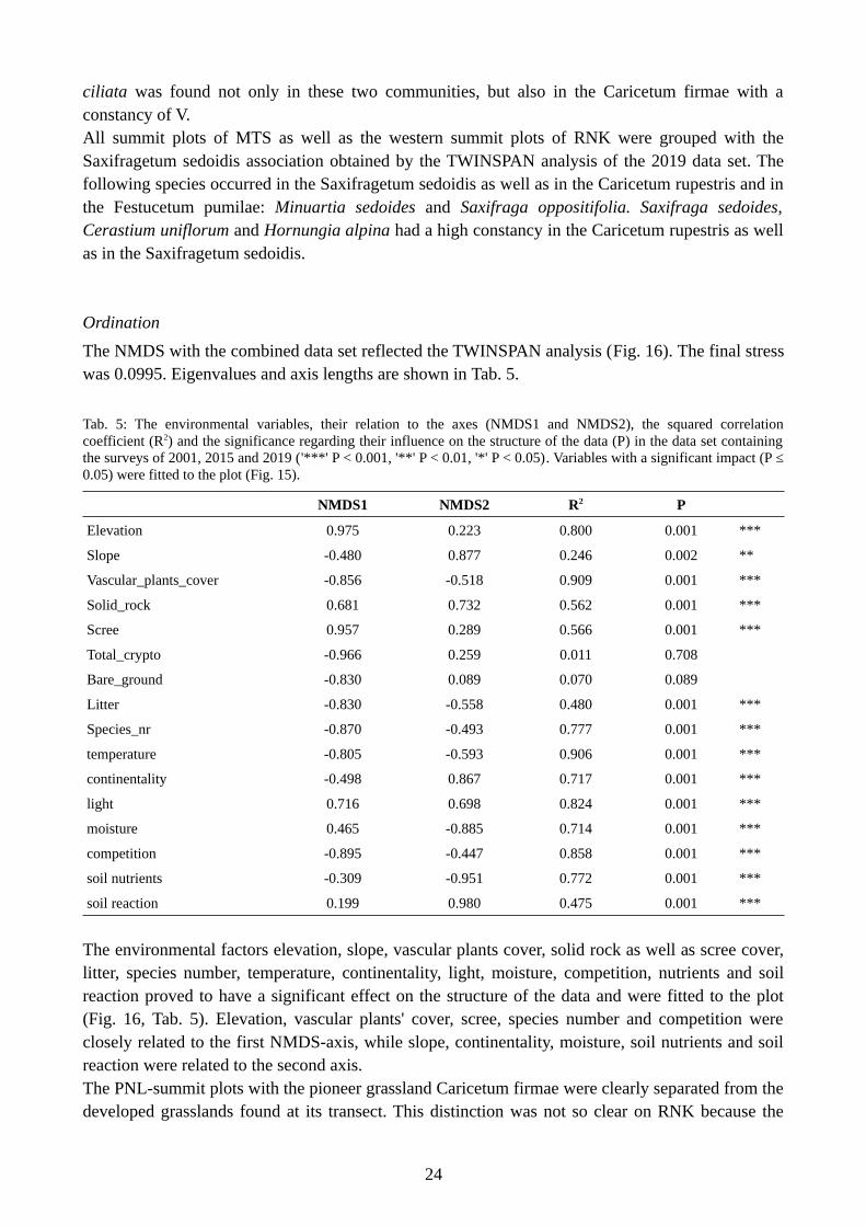
The NMDS with the combined data set reflected the TWINSPAN analysis (Fig. 16). The final stresswas 0.0995. Eigenvalues and axis lengths are shown in Tab. 5.

Tab. 5: The environmental variables, their relation to the axes (NMDS1 and NMDS2), the squared correlationcoefficient (R2) and the significance regarding their influence on the structure of the data (P) in the data set containingthe surveys of 2001, 2015 and 2019 ('***' P < 0.001, '**' P < 0.01, '*' P < 0.05). Variables with a significant impact (P ≤0.05) were fitted to the plot (Fig. 15).

NMDS1 NMDS2 R2 P

Elevation 0.975 0.223 0.800 0.001 ***

Slope -0.480 0.877 0.246 0.002 **

Vascular_plants_cover -0.856 -0.518 0.909 0.001 ***

Solid_rock 0.681 0.732 0.562 0.001 ***

Scree 0.957 0.289 0.566 0.001 ***

Total_crypto -0.966 0.259 0.011 0.708

Bare_ground -0.830 0.089 0.070 0.089

Litter -0.830 -0.558 0.480 0.001 ***

Species_nr -0.870 -0.493 0.777 0.001 ***

temperature -0.805 -0.593 0.906 0.001 ***

continentality -0.498 0.867 0.717 0.001 ***

light 0.716 0.698 0.824 0.001 ***

moisture 0.465 -0.885 0.714 0.001 ***

competition -0.895 -0.447 0.858 0.001 ***

soil nutrients -0.309 -0.951 0.772 0.001 ***

soil reaction 0.199 0.980 0.475 0.001 ***

The environmental factors elevation, slope, vascular plants cover, solid rock as well as scree cover,litter, species number, temperature, continentality, light, moisture, competition, nutrients and soilreaction proved to have a significant effect on the structure of the data and were fitted to the plot(Fig. 16, Tab. 5). Elevation, vascular plants' cover, scree, species number and competition wereclosely related to the first NMDS-axis, while slope, continentality, moisture, soil nutrients and soilreaction were related to the second axis.The PNL-summit plots with the pioneer grassland Caricetum firmae were clearly separated from thedeveloped grasslands found at its transect. This distinction was not so clear on RNK because the

24

southern summit plots were placed midway between the Festucetum pumilae group and theCaricetum rupestris group. Furthermore, the Caricetum rupestris group was not that far away fromthe scree vegetation found at the western summit plots on RNK. The MTS-plots from the Mesulesplateau were clearly separated from the grassland communities found at the Val Lasties.

Fig. 16: NMDS scatterplot with fitted environmental variables (arrows) with data from 2001, 2015 and 2019. Thepolygons represent the plant communities found at the TWINSPAN analysis. Seslerietum: Seslerio-Caricetumsempervierentis; M: MTS, P: PNL, R: RNK; for the transect plots (squares) the numbers after the letter denote theelevation of the plot; the summit plots (triangles) include the first letter of the summit with the orientation of the plotand the chronological number of the survey (1 = 2001, blue; 4 = 2015, red).

The scatterplot showed a clear segregation of the plant communities along the elevational gradient.The differentiation of communities of the same elevation was given by the slope and by the Landoltindicator values continentality, moisture and nutrients. Slope and continentality were negativelycorrelated to moisture. Lower sites had higher species numbers as well as a higher cover of vascularplants. Furthermore, on these sites the percentage of litter was larger and more competitive speciesas well as species with a higher temperature value were present. For plots at higher elevations thepercentage of the area covered by solid rock and scree increased as well as the number of specieswith higher light values. The plots with the highest soil reaction value, i.e. with more basiphilicspecies, were the summit plots of PNL. The plots with the lowest soil reaction value were the onesincluded in the Festuca nigrescens community.

Ecological indicator values and competitive strategy

The investigated ecological values (temperature, soil nutrients) and the competitive behaviourdecreased significantly along the elevational gradient (Fig. 17, P < 0.001, Tab. 6).The mean temperature value decreased along the elevational gradient at all summits, with thesteepest slope found on PNL and RNK. The mean nutrients value declined strongly along theelevational gradient on PNL, while on RNK and MTS it showed a slight decrease from the lower tothe higher plots. The mean competition value decreased along the elevational gradient at allsummits with the steepest slope found on PNL and MTS.

25

Fig. 17: Mean temperature, nutrients and competition value (calculated as community weighted mean from Landolt etal. (2010) indicator values, see methods) along the elevational gradient of the investigated south-facing slopes to thesummits. The label colors represent the plant community. The label name consists of the first letter of the summit (P:PNL, R: RNK, M: MTS) with the elevation of the slope plots, while for the summit plots the first letter of the summitwith the orientation of the plot and the chronological number of the survey is shown (4 = 2015). The black linerepresents the smoothed regression line fitting a linear model with +/- confidence interval.

26

Tab. 6: Results of the analyses of variance of the linear models ('***' P < 0.001, '**' P < 0.01, '*' P < 0.05, '°' P < 0.1, forresults of the linear models see Appendix IX)

Mean temperature value Mean nutrients value Mean competitive value

P P P

Summit 2.637e-06 *** 0.030 * 0.0001 ***

Elevation < 2.2e-16 *** 0.0243 * 1.988e-11 ***

Summit:Elevation 0.042 * 0.057 ° 0.110

Changes at the summits between 2001 and 2015

Ecological indicators and competitive strategies

The analysis of the first and the last survey of the summits by means of ecological indicator valuesand competitive strategy has shown that only the increase of thermophilic species was significant(P < 0.05, Tab. 7). The interaction effect of summit and year was not significant and thereforeomitted from the table and model. The proportion of thermophilic species increased on all threesummits (Fig. 18). Only on PNL, however, was this increment significant with a P-value lower than0.05, while on RNK and MTS it was slightly significant (P < 0.1, Tab. 8).

Tab. 7: Results of the analyses of variance of the proportion of thermophilic, nitrophilous and competitive speciesbetween summits and years ('***' P < 0.001, '**' P < 0.01, '*' P < 0.05)

Source df Sum of squares Mean square F P

Thermophilic

Summit 2 784.4 392.2 22.43 1.16e-08 ***

Year 1 220.2 220.2 12.59 0.0006 ***

Residuals 92 1,608.8 17.5

Nitrophilous

Summit 2 210.6 105.32 3.873 0.0243 *

Year 1 8.5 8.46 0.311 0.5785

Residuals 92 2502.0 27.20

Competitive

Summit 2 4466 2233.0 156.059 <2e-16 ***

Year 1 37 37.1 2.591 0.111

Residuals 92 1316 14.3

Tab. 8: Mean proportion of thermophilic species and its difference between 2001 and 2015; P-values from paired t-test('***' P < 0.001, '**' P < 0.01, '*' P < 0.05, '°' P < 0.1)

Summit SurveyMean proportion of

thermophilic species [%]Standard deviation Difference 2001-2015 [%] P

PNL 2001 12.799 3.133

PNL 2015 16.999 6.087 4.200 0.014 *

RNK 2001 9.464 2.914

RNK 2015 10.658 2.267 1.194 0.056 °

MTS 2001 6.250 6.455

MTS 2015 9.943 1.525 3.693 0.066 °

27

Fig. 18: Proportion of thermophilic, meso- to nitrophilous and competitive species at three summits from the surveys of2001 and 2015. ‘*’ denotes P < 0.05 and ‘°’ denotes P < 0.1 significance of the differences between 2001 and 2015between the proportion of classified species based on paired t-test (Tab. 8).

Overall, the proportion of thermophilic species increased by 3.3%. The increase was quite similaron PNL (+4.2%) and MTS (+3.7%), while on RNK it was lower (+1.2%). While the results fornutrient-demanding and competitive species were not significant, they showed trends. Meso- tonitrophilous species slightly increased on all summits. On PNL and RNK competitive speciesdecreased. On MTS no competitive species were found either in 2001 or in 2015.The mean temperature value increased on all summits between 2001 and 2015 (PNL: +0.025; RNK:+0.047; MTS: +0.055; Fig. 19), but these increments were not significant (P > 0.1 on every summitfrom paired t-test).

Fig. 19: Mean temperature values (community weightedmeans per plot) at the three ADO summits between 2001(blue) and 2015 (red). The points of the boxplots representthe median. Differences between 2001 and 2015 were notsignificant at any summit based on paired t-test.

28

* ° °

Discussion

Plant communities on the south-facing slopes

This study analysed the vegetation of the south-facing slopes below three GLORIA summits of theDolomites and as a result four plant communities were identified. Three of them are grasslands,while one is a scree vegetation found only on the higher plots of MTS. The grassland associationsFestuca nigrescens community and Seslerietum were observed on lower elevations (Fig. 14). Thepioneer grassland Festucetum pumilae was found on higher elevations at RNK, while theSaxifragetum sedoidis was identified on the sparsely vegetated Mesules plateau on MTS.The two grassland associations Festuca nigrescens community and Seslerietum grow next to eachother, but the first is characterised by the presence of acidophilic and nitrophilous species such asFestuca nigrescens, Anthoxanthum alpinum, Crocus albiflorus, Festuca varia and Nardus stricta.This can be explained by the existence of deeper soils.The Seslerietum is the typical grassland growing on sunny slopes at the foot of the rock walls onlimestone and dolomite at an elevation of 2000 m to 2500 m a.s.l., and represents some of the areaswith the highest biodiversity of the Dolomites (Pignatti & Pignatti 2014a). According to Grabherr etal. (1993) the Seslerietum of the southeastern Alps should be called Ranunculo hybridi-Caricetumsempervirentis due to the separation made by Feoli Chiapella & Poldini (1993). However, forPignatti & Pignatti (2016) one single, highly polymorphic association which includes allSeslerietum associations from both northern and southeastern Alps denotes better the reality andgives a unitary vision for both sides of the Alps. This community is included in the Natura 2000habitat lists with the code 6170 - Alpine and subalpine calcareous grasslands (Lasen & Wilhalm,2004). Some red-listed plant species (Fig. 20) were found in this association as well as in theFestuca nigrescens community during the survey: Dianthus superbus, Nigritella dolomitensis andN. rhellicani, Traunsteinera globosa.

Fig. 20: Dianthus superbus, Nigritella dolomitensis and Traunsteinera globosa, red-listed species(Wilhalm & Hilpold 2006) found in the Festuca nigrescens community and in the Seslerio-Caricetumsempervirentis on PNL and RNK. Pictures by Lena Nicklas 2019

The Festucetum pumilae was found on higher elevations on RNK and MTS. This community ispresent in different areas of the eastern Alps on ridges where rocks and scree are found (Grabherr et

29

al. 1993). Due to the high constancy and abundance of Carex sempervirens, Sesleria caerulea andFestuca norica it seems to be a transitional stage tending towards a Seslerietum. This transitionalstage is also underlined by the low dominance of Festuca pumila in these plots.The scree vegetation was specified as Saxifragetum sedoidis and found mainly on the Mesulesplateau on MTS. On these plots dwarf chamaephytes such as Saxifraga sedoides, Cerastiumuniflorum and Hornungia alpina together with Carex parviflora and Achillea oxyloba could befound between the scree, in contact with rocky, overhanging walls and growing only in patcheswhich cover small parts of the surface (see also Pignatti & Pignatti 2014b). This associationdevelops where S. sedoides grows optimally (Pignatti & Pignatti 2014b). It is included in the Natura2000 habitat lists with the code 8120 - Calcareous and calcshist screes of the montane to alpinelevels (Thlaspietea rotundifolii, Lasen & Wilhalm 2004).The occurrence of the communities along these slopes reflected the elevational gradient as well asthe ecological differences (Fig. 15). The three grassland communities showed a considerable higherproportion of thermophilic and competitive species than the scree community Saxifragetumsedoidis. For the Seslerietum and the Festuca nigrescens community the share of thermophilicspecies was even higher than 50%. The Saxifragetum sedoidis community grows only in patches inspecial habitat niches (Pignatti & Pignatti 2014b) and includes hardly any thermophilic andcompetitive species.

Phytosociological and ecological connection between slopes and summits

The joint phytosociological analysis of transects and summits showed that the Festuca nigrescenscommunity and the Seslerietum were only found on the lower transect plots. Their presence isrelated to deeper soils with humus and fine earth (Pignatti & Pignatti 2014a). However, some of thecharacteristic species of these communities, such as Carex sempervirens, Sesleria caerulea andFestuca norica, were also found with a high constancy and abundance in the Festucetum pumilaeon higher elevations.At the summits less soil and harsher climatic conditions affect the plant life and consequentlypioneer grasslands can thrive in these areas (Grabherr et al. 1993). This study detected two pioneergrassland communities at the summits (Fig. 16): Caricetum firmae on PNL and Caricetum rupestrison RNK. Depending on the summit, they showed more or less similarities with the communities onthe slopes below.On PNL, the NMDS scatterplot as well as the analysis of the mean temperature value along thetransect to the summit showed a remarkable difference between southern slope and summit (Fig. 16,Fig. 17). Furthermore, the Caricetum firmae at the summit plots included only few species from thecommunities found on the southern slope. This could be explained by the secondary summitseparating the southern slope from the real summit and acting as topographical barrier.On RNK, the Festucetum pumilae reached the southern summit plots indicating a phytosociologicalconnection between transect and southern summit side. Also the analysis of the ecologicalindicators along the south-facing slope to the summit showed a smooth transition between transectand summit on RNK (Fig. 17). These results reflect the observations made by Winkler et al. (2016)indicating that on the southern sides the colonization of species seems to be more frequent and,therefore, more similarities between slopes and summits should be observable.

30

On MTS, two very different plant communities were mainly found: the Seslerietum as developedgrassland and the Saxifragetum sedoidis as scree vegetation. The reason therefore, could be the highwall separating the Val Lasties with the developed grasslands from the moon-like Mesules plateauwith scree vegetation (Fig. 3a and 3b). On the Mesules plateau, the plots below the summit and thesummit plots are placed in the same community and their mean temperature and competition valuesare in the same range (Fig. 17). The very similar geomorphological and ecological conditions on theMesules plateau, should explain this strong relation.

Thermophilisation at the summits

This study gives further evidences of an ongoing thermophilisation on the three analysed GLORIAsummits in the Dolomites as the proportion of thermophilic species increased significantly between2001 and 2015 (Fig. 18, Unterluggauer et al. 2016). Previous studies of vegetation changes in thelast decades on alpine summits showed that the frequency of thermophilic species is increasing andthe abundance of cryophilic species is declining (Gottfried et al. 2012; Wipf et al. 2013). Theexpansion of thermophilic species on European mountains was already related to the effects ofclimate warming (Engler et al. 2011; Gottfried et al. 2012; Fernández Calzado & Mesa 2013).The increase of the mean temperature value in this study was visible on all three summits (Fig. 19).However, it was not statistically significant probably due to the short period analysed and the lownumber of relevés. The temperature indicator value has been used in studies performed on Europeanmountain ranges (Evangelista et al. 2016; Lamprecht et al. 2018), underlining the ongoing climatewarming, and should be analysed with future survey data for the four ADO summits.Further causes for changes in plant composition of high-mountain habitats can be related to theincrease in soil nutrients produced by higher decomposition rates caused by global warming(Gavazov 2010; Gong et al. 2015) and the increment of atmospheric nitrogen deposition(Hättenschwiler & Körner 1997; Schaap et al. 2017; Rumpf et al. 2018). While the increase of theproportion of meso- and nitrophilous species observed on all investigated summits from 2001 to2015 was not significant, future studies of the area should also analyse this ecological indicator.Studies in the Western Alps (Theurillat & Guisan 2001) and in the Apennines (Evangelista et al.2016) revealed consistent changes in the composition and the structure of vegetation, due to shiftstowards mesic conditions. The increase of nutrients could, consequently, be another factorreinforcing the changes caused by global warming (Huber et al. 2007; Engler et al. 2011).The decrease of competitive species on PNL and RNK between 2001 and 2015 was surprisingbecause competitive species should benefit from more favourable climatic conditions (Alexander etal. 2018). Generally, studies showed that in alpine zones the competitive ability loses influence withelevation (Callaway et al. 2002; Caccianiga et al. 2006). Ruderal species thrive as pioneers atglacier forelands, while late succession stages are dominated by stress-tolerant plant species(Caccianiga et al. 2006). The succession trajectory was similar on scree, reaching stability with asiliceous alpine grassland with long-living and tough perennials (Pierce et al. 2017). However,subsequent grazing changed this community to more ruderal and competitive characteristics (Pierceet al. 2017). The influence of disturbances such as grazing had already been observed in earlierstudies with a resulting increase of species richness and the presence of more competitive species(Pierce et al. 2007). Other studies have shown that global warming may increase the importance of

31

competitive interactions in seminatural grasslands and the consequent advantages for competitivespecies over subordinated species (Olsen et al. 2016).The dominant species on PNL as well as on RNK were mainly stress-tolerant or had an intermediatestrategy ('css', 'sss' or 'crs' (Landolt et al. 2010), Appendix III): Carex firma, Potentilla nitida,Phyteuma sieberi, Saxifraga caesia, Arenaria ciliata and Dryas octopetala on PNL; Scorzoneroideshelvetica, Thymus praecox ssp. polytrichus, Carex sempervirens, Festuca pumila, Silene acaulisagg. and Salix serpyllifolia on RNK. However, while on PNL the more competitive species wererare and had a low cover, on RNK some competitive species (Potentilla crantzii, Ranunculusmontanus, Helianthemum alpestre, Kobresia myosuroides and Sesleria caerulea) were wellestablished. CSR-strategies together with plant traits could help to predict changes in plantcommunities caused by climate warming or land use change (Pierce et al. 2017) but furtherinvestigations on this topic are still necessary. The results were not significant for this study andmay be explained by the short period which has been analysed. Furthermore, the avalability ofdiverse microhabitats and the wide range of soil types available on summits offer suitable niches fora large number of different species (Matteodo et al. 2013). Consequently, the plant strategy conceptmight not be appropriate to analyse colonization processes on summits in the short term. Theecological values of the species such as temperature and nutrient values seem to be moreinformative for the ongoing processes.

Future development

The development of the environmental factors at the summits between 2001 and 2015, visible at theNMDS scatterplot (Fig. 16), confirmed the changes detected on various European mountain rangesand related to the ongoing climate warming (Gottfried et al. 2012; Pauli et al. 2012; Wipf et al.2013; Steinbauer et al. 2018): increase of vascular plants cover, increment of the number of plantspecies as well as the evolution towards communities typical of lower elevations and highertemperature values.The mean temperature, nutrient and competition values of the summit plots showed generally thehighest values on the southern plots. The southern summit plots appear, therefore, those where theimmigration of new species will be more likely and this reinforces the assumption that speciesmigration caused by climate warming occurs mainly on the southern slopes (Winkler et al. 2016).Also Unterluggauer et al. (2016) found that at the same summits the new species were mostfrequent on the southern aspects of PNL and RNK and their altitudinal ranks exceeded the ranks ofthe resident species.On RNK, the temperature and competition values of the highest plots of the transect were similar tothe summit plots (Fig. 17). As the Festucetum pumilae was found on the southern slope as well as atthe southern summit plot in 2001 and in 2015 (Fig. 16), we could also find similarities at aphytosociological level. Furthermore, various characteristic species from the developed grasslandsbelow, such as Carex sempervirens, Sesleria caerulea and Festuca norica, were already abundant inthe Festucetum pumilae plots. It appears, therefore, that the summit of RNK, especially the southernside, is developing towards more developed grasslands. While the total species number on thesummit may increase due to these changes (Pauli et al. 2012), the increase in species richness couldbe only a temporary effect (Winkler et al. 2019). In the long-term, specialists such as Saxifragasedoides, Cerastium uniflorum, Hornungia alpina, Carex parviflora and Noccaea rotundifolia

32

(Landolt et al. 2010) could lose their present habitat due to the arrival of new competitors and theymay survive only in special niches or even disappear.The phytosociological as well as the ecological analyses on PNL showed an important distinctionbetween south-facing slope and summit (Fig. 16, Fig. 17) and it is difficult to identify future trendsfor this summit from the available data. However, due to the ongoing climate warming this low-growing community might be at risk due to the immigration of taller-growing species adapted towarmer conditions as observed on four mountain ranges of the northeastern Austrian Alps (Gritschet al. 2016).The high wall of Hauptdolomit on MTS separating the Mesules plateau from the valley underneathcould help to prevent the invasion by plant species from lower elevations, although the comparisonbetween the surveys of 2001 and 2015 showed that the proportion of thermophilic plant species andthe mean temperature values have already increased (Fig. 18, Fig. 19). Besides, Unterluggauer et al.(2016) detected a strong increase in species richness on this summit between 2001 and 2015.Newcomers from lower elevations could outcompete the specialised species occurring on thisplateau. Currently, the availability of empty niches is still high and these species shouldconsequently be able to find a refugium so that their extinction on MTS should not happen in thenear future.Finally, this study underlines the suggestions from other researchers (Gottfried et al. 1998; Kammeret al. 2007; Engler et al. 2011; Gritsch et al. 2016), that the potential newcomers are alreadyoccurring on the slopes below the summits. As the future development of the vegetation on summitsis strongly linked to the vegetation on the slopes below them, these slopes should ideally beincluded in future studies and predictions.

33

Acknowledgements

I would like to express my gratitude to my supervisors, Brigitta Erschbamer and Lena Nicklas, fortheir support and useful suggestions throughout this research work.I wish to thank also Martin Mallaun for his help at the vegetation surveys.Thanks are due also to Alexandra Nicklas and Klaus Egger, who have helped us to carry our stuffup to the campsite on PNL and RNK.I want to thank also Annelise and Tomaso Ochrymowicz for their useful help about style andgrammar.Financial support has been provided by the Knoll-Widmung (Austrian Academy of Sciences) andthe University of Innsbruck.

34

Fig. 21: Lena Nicklas, Nils Bertol, Martin Mallaun and Brigitta Erschbamer at MTS, June 2020 (from left to right).Picture by Lena Nicklas 2019

References

3PClim. 2020. Past, Present and Perspective Climate of Tirol, Südtirol-Alto Adige and Veneto.http://www.alpenklima.eu.

Alexander, J.M., Chalmandrier, L., Lenoir, J., Burgess, T.I., Essl, F., Haider, S., Kueffer, C.,McDougall, K., Milbau, A., Nuñez, M.A., Pauchard, A., Rabitsch, W., Rew, L.J., Sanders,N.J., & Pellissier, L. 2018. Lags in the response of mountain plant communities to climatechange. Global Change Biology 24: 563–579.

Alexander, J.M., Diez, J.M., & Levine, J.M. 2015. Novel competitors shape species’ responses toclimate change. Nature 525: 515–518.

Barthlott, W., Lauer, W., & Placke, A. 1996. Global Distribution of Species Diversity in VascularPlants: Towards a World Map of Phytodiversity (Globale Verteilung der ArtenvielfaltHöherer Pflanzen: Vorarbeiten zu einer Weltkarte der Phytodiversität). Erdkunde 50: 317–327.

Bosellini, A. 1998. Geologie der Dolomiten. Verl.-Anst. Athesia, Bozen.Caccianiga, M., Luzzaro, A., Pierce, S., Ceriani, R.M., & Cerabolini, B. 2006. The functional basis

of a primary succession resolved by CSR classification. Oikos 112: 10–20.Callaway, R.M., Brooker, R.W., Choler, P., Kikvidze, Z., Lortie, C.J., Michalet, R., Paolini, L.,

Pugnaire, F.I., Newingham, B., Aschehoug, E.T., Armas, C., Kikodze, D., & Cook, B.J.2002. Positive interactions among alpine plants increase with stress. Nature 417: 844–848.

Diekmann, M. 2003. Species indicator values as an important tool in applied plant ecology – areview. Basic and Applied Ecology 4: 493–506.

Dullinger, S., Gattringer, A., Thuiller, W., Moser, D., Zimmermann, N.E., Guisan, A., Willner, W.,Plutzar, C., Leitner, M., Mang, T., Caccianiga, M., Dirnböck, T., Ertl, S., Fischer, A., Lenoir,J., Svenning, J.-C., Psomas, A., Schmatz, D.R., Silc, U., Vittoz, P., & Hülber, K. 2012.Extinction debt of high-mountain plants under twenty-first-century climate change. NatureClimate Change 2: 619–622.

Ellenberg, H., Weber, H., Düll, R., Wirth, V., Werner, W., & Paulissen, D. 1991. Zeigerwerte vonPflanzen in Mitteleuropa. Scripta Geobotanica 18: 9–166.

Engler, R., Randin, C.F., Thuiller, W., Dullinger, S., Zimmermann, N.E., Araújo, M.B., Pearman,P.B., Lay, G.L., Piedallu, C., Albert, C.H., Choler, P., Coldea, G., Lamo, X.D., Dirnböck, T.,Gégout, J.-C., Gómez‐García, D., Grytnes, J.-A., Heegaard, E., Høistad, F., Nogués‐Bravo,D., Normand, S., Puşcaş, M., Sebastià, M.-T., Stanisci, A., Theurillat, J.-P., Trivedi, M.R.,Vittoz, P., & Guisan, A. 2011. 21st century climate change threatens mountain floraunequally across Europe. Global Change Biology 17: 2330–2341.

Erschbamer, B., Mallaun, M., & Unterluggauer, P. 2003. Die Dolomiten – hot spots derArtenvielfalt. Gredleriana 3: 361–376.

Evangelista, A., Frate, L., Carranza, M.L., Attorre, F., Pelino, G., & Stanisci, A. 2016. Changes incomposition, ecology and structure of high-mountain vegetation: a re-visitation study over42 years. AoB PLANTS 8: 1–11.

Feoli Chiapella, L., & Poldini, L. 1993. Prati e pascoli del Friuli su substrati basici. StudiaGeobotanica 13: 3–140.

Fernández Calzado, M., & Mesa, J. 2013. Changes in the summit flora of a Mediterranean mountain(Sierra Nevada, Spain) as a possible effect of climate change. Lazaroa 34: 65–75.

Fischer, M., Oswald, K., & Adler, W. 2008. Exkursionsflora für Österreich, Liechtenstein undSüdtirol. 3. Auflage.

FloraFaunaSüdtirol. Das Portal zur Verbreitung von Tier- und Pflanzenarten in Südtirol,Naturmuseum Südtirol, Bozen. www.florafauna.it (10.03.2020).

Gavazov, K.S. 2010. Dynamics of alpine plant litter decomposition in a changing climate. Plantand Soil 337: 19–32.

35

Gobiet, A., Kotlarski, S., Beniston, M., Heinrich, G., Rajczak, J., & Stoffel, M. 2014. 21st centuryclimate change in the European Alps—A review. Science of The Total Environment 493:1138–1151.

Gong, S., Guo, R., Zhang, T., & Guo, J. 2015. Warming and Nitrogen Addition Increase LitterDecomposition in a Temperate Meadow Ecosystem. PLOS ONE 10: e0116013.

Gottfried, M., Pauli, H., Futschik, A., Akhalkatsi, M., Barančok, P., Alonso, J.L.B., Coldea, G.,Dick, J., Erschbamer, B., Calzado, M.R.F., Kazakis, G., Krajči, J., Larsson, P., Mallaun, M.,Michelsen, O., Moiseev, D., Moiseev, P., Molau, U., Merzouki, A., Nagy, L.,Nakhutsrishvili, G., Pedersen, B., Pelino, G., Puscas, M., Rossi, G., Stanisci, A., Theurillat,J.-P., Tomaselli, M., Villar, L., Vittoz, P., Vogiatzakis, I., & Grabherr, G. 2012. Continent-wide response of mountain vegetation to climate change. Nature Climate Change 2: 111–115.

Gottfried, M., Pauli, H., & Grabherr, G. 1998. Prediction of Vegetation Patterns at the Limits ofPlant Life: A New View of the Alpine-Nival Ecotone. Arctic and Alpine Research 30: 207–221.

Grabherr, G. 1993. Carici rupestris-Kobresietea bellardii. In Grabherr, G. & Mucina, L. (eds.), DiePflanzengesellschaften Österreichs. Teil II, pp. 373–381. Fischer, Jena.

Grabherr, G., Gottfried, M., & Pauli, H. 2010. Climate Change Impacts in Alpine Environments.Geography Compass 4: 1133–1153.

Grabherr, G., Gottfried, M., & Pauli, H. 1994. Climate effects on mountain plants. Nature 369: 448–448.

Grabherr, G., Mucina, L., & Greimler, J. 1993. Seslerietea albicantis. In Grabherr, G. & Mucina, L.(eds.), Die Pflanzengesellschaften Österreichs. Teil II, pp. 402–446. Fischer, Jena.

Grime, J.P. 1979. Plant strategies and vegetation processes. Wiley, Chichester.Gritsch, A., Dirnböck, T., & Dullinger, S. 2016. Recent changes in alpine vegetation differ among

plant communities. Journal of Vegetation Science 27: 1177–1186.Harris, I., Osborn, T.J., Jones, P., & Lister, D. 2020. Version 4 of the CRU TS monthly high-

resolution gridded multivariate climate dataset. Scientific Data 7: 109.Hättenschwiler, S., & Körner, C. 1997. Annual CO2 budget of spruce model ecosystems in the third

year of exposure to elevated CO2. Acta Oecologica 18: 319–325.Hothorn, T., Zeileis, A., Farebrother (pan.f), R.W., Cummins (pan.f), C., Millo, G., & Mitchell, D.

2019. lmtest: Testing Linear Regression Models. https://CRAN.R-project.org/package=lmtest

Huber, E., Wanek, W., Gottfried, M., Pauli, H., Schweiger, P., Arndt, S.K., Reiter, K., & Richter, A.2007. Shift in soil–plant nitrogen dynamics of an alpine–nival ecotone. Plant and Soil 301:65–76.

Jiménez Cisneros, Blanca E., Oki, Taikan, Arnell, Nigel W., D., Benito, Gerardo, Cogley, J.Graham, Döll, Petra, Jiang, Tong, & Mwakalila, Shadrack S. 2014. Freshwater Resources. InIn: Field CB, Barros VR, Dokken DJ, Mach KJ, Mastrandrea MD, Bilir TE, Chatterjee M,Ebi KL, Estrada YO, Genova RC et al., eds. Climate Change 2014: impacts, adaptation,and vulnerability. Part A: Global and sectoral aspects. Contribution of Working Group II tothe Fifth Assessment Report of the Intergovernmental Panel on Climate Change., pp. 229–269. Cambridge University Press, Cambridge, United Kingdom and New York, NY, USA.

Kammer, P.M., Schöb, C., & Choler, P. 2007. Increasing species richness on mountain summits:Upward migration due to anthropogenic climate change or re-colonisation? Journal ofVegetation Science 18: 301–306.

Keim, L., Mair, V., & Morelli, C. 2017. General Geologic Map - Geotirol. Körner, C., & Larcher, W. 1988. Plant life in cold climates. Symposia of the Society for

Experimental Biology 42: 25–57.

36

Kulonen, A., Imboden, R.A., Rixen, C., Maier, S.B., & Wipf, S. 2018. Enough space in a warmerworld? Microhabitat diversity and small-scale distribution of alpine plants on mountainsummits. Diversity and Distributions 24: 252–261.

Lamprecht, A., Semenchuk, P.R., Steinbauer, K., Winkler, M., & Pauli, H. 2018. Climate changeleads to accelerated transformation of high-elevation vegetation in the central Alps. NewPhytologist 220: 447–459.

Landolt, E., Bäumler, B., Ehrhardt, A., Hegg, O., Klötzli, F., Lämmler, W., Nobis, M., Rudmann-Maurer, K., Schweingruber, F.H., & Theurillat, J.-P. 2010. Flora indicativa: ÖkologischeZeigerwerte und biologische Kennzeichen zur Flora der Schweiz und der Alpen. Haupt,Bern.

Lasen, C., & Wilhalm, T. 2004. Natura 2000: Lebensräume in Südtirol. Autonome Provinz Bozen-Südtirol, Abteilung Natur und Landschaft, Bozen.

Lenoir, J., Graae, B.J., Aarrestad, P.A., Alsos, I.G., Armbruster, W.S., Austrheim, G., Bergendorff,C., Birks, H.J.B., Bråthen, K.A., Brunet, J., Bruun, H.H., Dahlberg, C.J., Decocq, G.,Diekmann, M., Dynesius, M., Ejrnæs, R., Grytnes, J.-A., Hylander, K., Klanderud, K.,Luoto, M., Milbau, A., Moora, M., Nygaard, B., Odland, A., Ravolainen, V.T., Reinhardt, S.,Sandvik, S.M., Schei, F.H., Speed, J.D.M., Tveraabak, L.U., Vandvik, V., Velle, L.G.,Virtanen, R., Zobel, M., & Svenning, J.-C. 2013. Local temperatures inferred from plantcommunities suggest strong spatial buffering of climate warming across Northern Europe.Global Change Biology 19: 1470–1481.

Marty, C., & Meister, R. 2012. Long-term snow and weather observations at Weissfluhjoch and itsrelation to other high-altitude observatories in the Alps. Theoretical and AppliedClimatology 110: 573–583.

Matteodo, M., Wipf, S., Stöckli, V., Rixen, C., & Vittoz, P. 2013. Elevation gradient of successfulplant traits for colonizing alpine summits under climate change. Environmental ResearchLetters 8: 024043.

Mountain Research Initiative EDW Working Group. 2015. Elevation-dependent warming inmountain regions of the world. Nature Climate Change 5: 424–430.

Murrell, P. 2019. R Graphics (3rd Edition). Chapman & Hall/CRC, Boca Raton.Newey, W., & West, K. 1987. A Simple, Positive Semi-definite, Heteroskedasticity and

Autocorrelation Consistent Covariance Matrix. Econometrica 55: 703–08.Oksanen, J., Blanchet, F.G., Friendly, M., Kindt, R., Legendre, P., McGlinn, D., Minchin, P.R.,

O’Hara, R.B., Simpson, G.L., Solymos, P., Stevens, M.H.H., Szoecs, E., & Wagner, H.2019. vegan: Community Ecology Package. https://CRAN.R-project.org/package=vegan

Olsen, S.L., Töpper, J.P., Skarpaas, O., Vandvik, V., & Klanderud, K. 2016. From facilitation tocompetition: temperature-driven shift in dominant plant interactions affects populationdynamics in seminatural grasslands. Global Change Biology 22: 1915–1926.

Opedal, Ø.H., Armbruster, W.S., & Graae, B.J. 2015. Linking small-scale topography withmicroclimate, plant species diversity and intra-specific trait variation in an alpine landscape.Plant Ecology & Diversity 8: 305–315.

Pauli, H., Gottfried, M., Dullinger, S., Abdaladze, O., Akhalkatsi, M., Alonso, J.L.B., Coldea, G.,Dick, J., Erschbamer, B., Calzado, R.F., Ghosn, D., Holten, J.I., Kanka, R., Kazakis, G.,Kollár, J., Larsson, P., Moiseev, P., Moiseev, D., Molau, U., Mesa, J.M., Nagy, L., Pelino,G., Puşcaş, M., Rossi, G., Stanisci, A., Syverhuset, A.O., Theurillat, J.-P., Tomaselli, M.,Unterluggauer, P., Villar, L., Vittoz, P., & Grabherr, G. 2012. Recent Plant DiversityChanges on Europe’s Mountain Summits. Science 336: 353–355.

Pauli, H., Gottfried, M., Lamprecht, A., Niessner, S., Rumpf, S., Winkler, M., Steinbauer, K., &Grabherr, G. 2015. The GLORIA field manual – standard Multi-Summit approach,supplementary methods and extra approaches. GLORIA-Coordination, Austrian Academyof Sciences & University of Natural Resources and Life Sciences, Vienna.

37

Pedrotti, F. 2018. Vegetation Series Along Climatic Gradients in the Central Southern Alps(Trentino- Alto Adige Region). In Pedrotti, F. (ed.), Climate Gradients and Biodiversity inMountains of Italy, pp. 51–81. Geobotany Studies. Springer International Publishing, Cham.

Pierce, S., Luzzaro, A., Caccianiga, M., Ceriani, R.M., & Cerabolini, B. 2007. Disturbance is thePrincipal a-scale Filter Determining Niche Differentiation, Coexistence and Biodiversity inan Alpine Community. Journal of Ecology 95: 698–706.

Pierce, S., Negreiros, D., Cerabolini, B.E.L., Kattge, J., Díaz, S., Kleyer, M., Shipley, B., Wright,S.J., Soudzilovskaia, N.A., Onipchenko, V.G., Bodegom, P.M. van, Frenette‐Dussault, C.,Weiher, E., Pinho, B.X., Cornelissen, J.H.C., Grime, J.P., Thompson, K., Hunt, R., Wilson,P.J., Buffa, G., Nyakunga, O.C., Reich, P.B., Caccianiga, M., Mangili, F., Ceriani, R.M.,Luzzaro, A., Brusa, G., Siefert, A., Barbosa, N.P.U., Chapin, F.S., Cornwell, W.K., Fang, J.,Fernandes, G.W., Garnier, E., Stradic, S.L., Peñuelas, J., Melo, F.P.L., Slaviero, A.,Tabarelli, M., & Tampucci, D. 2017. A global method for calculating plant CSR ecologicalstrategies applied across biomes world-wide. Functional Ecology 31: 444–457.

Pignatti, E., & Pignatti, S. 2014a. Alpine Grasslands on Limestones and Dolomites. In Pignatti, E.& Pignatti, S. (eds.), Plant Life of the Dolomites: Vegetation Structure and Ecology, pp.381–434. Springer, Berlin, Heidelberg.

Pignatti, E., & Pignatti, S. 2014b. Plant Life on Dolomitic and Calcareous Scree. In Pignatti, E. &Pignatti, S. (eds.), Plant Life of the Dolomites: Vegetation Structure and Ecology, pp. 319–378. Springer, Berlin, Heidelberg.

Pignatti, E., & Pignatti, S. 2016. Syntaxonomy of the Seslerio-Caricetum sempervirentis. InPignatti, E. & Pignatti, S. (eds.), Plant Life of the Dolomites: Vegetation Tables, pp. 7–15.Springer, Berlin, Heidelberg.

R Core Team. 2020. R: A Language and Environment for Statistical Computing. https://www.R-project.org/

Reichelt, G., & Wilmanns, O. 1973. Vegetationsgeographie. Georg Westermann Verlag,Braunschweig.

Rogora, M., Frate, L., Carranza, M.L., Freppaz, M., Stanisci, A., Bertani, I., Bottarin, R., Brambilla,A., Canullo, R., Carbognani, M., Cerrato, C., Chelli, S., Cremonese, E., Cutini, M., DiMusciano, M., Erschbamer, B., Godone, D., Iocchi, M., Isabellon, M., Magnani, A.,Mazzola, L., Morra di Cella, U., Pauli, H., Petey, M., Petriccione, B., Porro, F., Psenner, R.,Rossetti, G., Scotti, A., Sommaruga, R., Tappeiner, U., Theurillat, J.-P., Tomaselli, M.,Viglietti, D., Viterbi, R., Vittoz, P., Winkler, M., & Matteucci, G. 2018. Assessment ofclimate change effects on mountain ecosystems through a cross-site analysis in the Alps andApennines. Science of The Total Environment 624: 1429–1442.

Rumpf, S.B., Hülber, K., Klonner, G., Moser, D., Schütz, M., Wessely, J., Willner, W.,Zimmermann, N.E., & Dullinger, S. 2018. Range dynamics of mountain plants decreasewith elevation. Proceedings of the National Academy of Sciences 115: 1848–1853.

Schaap, M., Banzhaf, S., Scheuschner, T., Geupel, M., Hendriks, C., Kranenburg, R., Nagel, H.-D.,Segers, A.J., von Schlutow, A., Wichink Kruit, R., & Builtjes, P.J.H. 2017. Atmosphericnitrogen deposition to terrestrial ecosystems across Germany. Biogeosciences Discussions,in review.

Scherrer, D., & Körner, C. 2011. Topographically controlled thermal-habitat differentiation buffersalpine plant diversity against climate warming. Journal of Biogeography 38: 406–416.

Slowikowski, K., Schep, A., Hughes, S., Lukauskas, S., Irisson, J.-O., Kamvar, Z.N., Ryan, T.,Christophe, D., Hiroaki, Y., & Gramme, P. 2020. ggrepel: Automatically Position Non-Overlapping Text Labels with “ggplot2.” https://rdrr.io/cran/ggrepel/

Steinbauer, M.J., Grytnes, J.-A., Jurasinski, G., Kulonen, A., Lenoir, J., Pauli, H., Rixen, C.,Winkler, M., Bardy-Durchhalter, M., Barni, E., Bjorkman, A.D., Breiner, F.T., Burg, S.,Czortek, P., Dawes, M.A., Delimat, A., Dullinger, S., Erschbamer, B., Felde, V.A.,Fernández-Arberas, O., Fossheim, K.F., Gómez-García, D., Georges, D., Grindrud, E.T.,

38

Haider, S., Haugum, S.V., Henriksen, H., Herreros, M.J., Jaroszewicz, B., Jaroszynska, F.,Kanka, R., Kapfer, J., Klanderud, K., Kühn, I., Lamprecht, A., Matteodo, M., Cella, U.M. di,Normand, S., Odland, A., Olsen, S.L., Palacio, S., Petey, M., Piscová, V., Sedlakova, B.,Steinbauer, K., Stöckli, V., Svenning, J.-C., Teppa, G., Theurillat, J.-P., Vittoz, P., Woodin,S.J., Zimmermann, N.E., & Wipf, S. 2018. Accelerated increase in plant species richness onmountain summits is linked to warming. Nature 556: 231–234.

Stingl, V., & Mair, V. 2005. Einführung in die Geologie Südtirols. Autonome Provinz Bozen-Südtirol, Amt für Baustoffprüfung und Geologie, Bozen.

Tasser, E., Walde, J., Tappeiner, U., Teutsch, A., & Noggler, W. 2007. Land-use changes and naturalreforestation in the Eastern Central Alps. Agriculture, Ecosystems & Environment 118: 115–129.

Theurillat, J.-P., & Guisan, A. 2001. Potential Impact of Climate Change on Vegetation in theEuropean Alps: A Review. Climatic Change 50: 77–109.

Trenkwalder, I. 2019. The plant associations of the Texel Group and their change with elevationand over time. Master thesis. University of Innsbruck.

Unterluggauer, P., Mallaun, M., & Erschbamer, B. 2016. The higher the summit, the higher thediversity changes - Results of a long‐term monitoring project in the Dolomites. Gredleriana16: 5–34.

Virtanen, R., Dirnböck, T., Dullinger, S., Grabherr, G., Pauli, H., Staudinger, M., & Villar, L. 2003.Patterns in the Plant Species Richness of European High Mountain Vegetation. In Nagy, L.,Grabherr, G., Körner, C., & Thompson, D.B.A. (eds.), Alpine Biodiversity in Europe, pp.149–172. Ecological Studies. Springer, Berlin, Heidelberg.

Wickham, H. 2016. ggplot2: Elegant Graphics for Data Analysis. Springer-Verlag, New York.Wickham, H., Averick, M., Bryan, J., Chang, W., McGowan, L., François, R., Grolemund, G.,

Hayes, A., Henry, L., Hester, J., Kuhn, M., Pedersen, T., Miller, E., Bache, S., Müller, K.,Ooms, J., Robinson, D., Seidel, D., Spinu, V., Takahashi, K., Vaughan, D., Wilke, C., Woo,K., & Yutani, H. 2019. Welcome to the Tidyverse. Journal of Open Source Software 4: 1686.

Wilhalm, T., & Hilpold, A. 2006. Rote Liste der gefährdeten Gefäßpflanzen Südtirols. Gredleriana6: 115–198.

Winkler, M., Lamprecht, A., Steinbauer, K., Hülber, K., Theurillat, J.-P., Breiner, F., Choler, P., Ertl,S., Girón, A.G., Rossi, G., Vittoz, P., Akhalkatsi, M., Bay, C., Alonso, J.-L.B., Bergström, T.,Carranza, M.L., Corcket, E., Dick, J., Erschbamer, B., Calzado, R.F., Fosaa, A.M., Gavilán,R.G., Ghosn, D., Gigauri, K., Huber, D., Kanka, R., Kazakis, G., Klipp, M., Kollar, J.,Kudernatsch, T., Larsson, P., Mallaun, M., Michelsen, O., Moiseev, P., Moiseev, D., Molau,U., Mesa, J.M., Cella, U.M. di, Nagy, L., Petey, M., Pușcaș, M., Rixen, C., Stanisci, A.,Suen, M., Syverhuset, A.O., Tomaselli, M., Unterluggauer, P., Ursu, T., Villar, L., Gottfried,M., & Pauli, H. 2016. The rich sides of mountain summits – a pan-European view on aspectpreferences of alpine plants. Journal of Biogeography 43: 2261–2273.

Winkler, D.E., Lubetkin, K., & Carrell, A.A. 2019. Chapter 12 - Responses of alpine plantcommunities to climate warming. Elsevier,San Diego,California,United States of America.

Wipf, S., Stöckli, V., Herz, K., & Rixen, C. 2013. The oldest monitoring site of the Alps revisited:accelerated increase in plant species richness on Piz Linard summit since 1835. PlantEcology & Diversity 6: 447–455.

Zanzottera, M., Dalle Fratte, M., Caccianiga, M., Pierce, S., & Cerabolini, B.E.L. 2020.Community-level variation in plant functional traits and ecological strategies shapes habitatstructure along succession gradients in alpine environment. Community Ecology 21: 55–65.

Zeileis, A., Lumley, T., Berger, S., & Graham, N. 2019. sandwich: Robust Covariance MatrixEstimators. http://sandwich.r-forge.r-project.org/

39

Appendix I - GPS coordinates (2019 data set)

Average GPS coordinates (WGS 84) of every elevational step of the three investigated slopes

Latitude [°] Longitude [°]

PNL2100 11.6061152 46.3763453

PNL2150 11.6061190 46.3773448

PNL2200 11.6061310 46.3779200

PNL2250 11.6061908 46.3785047

PNL2300 11.6062093 46.3790700

PNL2350 11.6062002 46.3797047

PNL2400 11.6062182 46.3803983

RNK2050 11.6048150 46.3750140

RNK2100 11.6037870 46.3758430

RNK2150 11.6028903 46.3764157

RNK2200 11.6023963 46.3768307

RNK2250 11.6014053 46.3774095

RNK2300 11.6005080 46.3779375

RNK2350 11.5999673 46.3783475

RNK2400 11.5986075 46.3793598

RNK2450 11.5974732 46.3801955

RNK2500 11.5967420 46.3806257

RNK2550 11.5959417 46.3812327

RNK2600 11.5950585 46.3818228

RNK2650 11.5942118 46.3825167

RNK2700 11.5931908 46.3831800

MTS2150 11.7997245 46.5073143

MTS2200 11.8005440 46.5077743

MTS2250 11.8012482 46.5081310

MTS2300 11.8028115 46.5089705

MTS2350 11.8067770 46.5111027

MTS2400 11.8086082 46.5123827

MTS2450 11.8096350 46.5129908

MTS2500 11.8142250 46.5160000

MTS2700 11.8154340 46.5170710

MTS2750 11.8164358 46.5176632

MTS2800 11.8178542 46.5185680

MTS2850 11.8173002 46.5226255

40

Appendix II - Survey form

41

Appendix III - Plant species list with GLORIA code and ecological values

List of the plant species found at the transect (2019) and at the summits (2001, 2015) including theGLORIA code, the ecological indicator values and the classification of the CSR-strategy (T =temperature, K = continentality, L = light, F = moisture, R = soil reaction, N = soil nutrients, KS =plant strategy type, Landolt et al. 2010).

GLORIA code Species name T K L F R N KS

ACHICLAV Achillea clavennae 1.5 4 5 2 5 2 css

ACHIMILL Achillea millefolium 3 3.5 3.75 2.75 3 3 crs

ACHIOXOX Achillea oxyloba 1.5 3 5 3 5 2 css

ACINALAL Clinopodium alpinum 2 4 4 2 3 2 crs

AGROALPI Agrostis alpina 1.5 4 5 2 4 2 crs

AJUGPYRA Ajuga pyramidalis 2 3 4 3 2 2 crs

ALCHVUVU Alchemilla vulgaris agg. 2 2.51 3.44 3.3 3 3 ccs

ANDROBTU Androsace obtusifolia 1.5 3 4 2.5 2 2 css

ANEMBALD Anemone baldensis 1.5 3 4 2 4 2 crs

ANTECARP Antennaria carpatica 1.5 4 4 2.5 3 2 crs

ANTEDIOI Antennaria dioica 2 3 4 2 2 2 crs

ANTHODAL Anthoxanthum alpinum 1.5 3 4 3 3 2 crs

ANTHVUAL Anthyllis vulneraria ssp. alpicola 1.5 4 5 2 5 2 crs

ARABALAL Arabis alpina ssp. alpina 2 3 4 3 5 2 crs

ARABCAER Arabis caerulea 1 2 5 4 4 2 rss

ARABPUST Arabis stellulata 1.5 3 5 1.5 5 2 rss

ARCTALPI Arctostaphylos alpinus 1.5 2 3 3.5 3 2 ccs

ARENCICI Arenaria ciliata 1 3 5 3 4 2 crs

ARMEALPI Armeria alpina 1 4 5 2 2 2 css

ARNIMONT Arnica montana 2 3 4 3.5 2 2 crs

ASPLRUMU Asplenium ruta-muraria 2.5 4 4 2 5 2 rss

ASPLTRIC Asplenium trichomanes 3 3 3 2 2 2 rrs

ASPLVIRI Asplenium viride 2 2 2 3.5 5 2 rrs

ASTEALPI Aster alpinus 2 4 5 2 3 2 crs

ASTEBELL Bellidiastrum michelii 2 3 3 3.5 4 2 crs

ASTRAUST Astragalus australis 1.5 4 4 3 4 2 ccs

ATHACRET Athamanta cretensis 2 4 5 2 5 2 css

AVENPRAE Avenula praeusta 2.5 4 4 2 4 2 css

AVENVERS Avenula versicolor 1.5 3 4 2 2 2 css

BARTALPI Bartsia alpina 2 3 4 4 3 3 rss

BISCLALA Biscutella  laevigata ssp. laevigata 2 3 4 2.5 4 2 crs

BOTRLUNA Botrychium lunaria 2 3 4 3 3 2 crs

BRIZMEDI Briza media 3 4 4 2 4 2 crs

CALAVARI Calamagrostis varia 3 3 3 3.5 4 2 ccs

CAMPBARB Campanula barbata 2 3 4 3 2 2 crs

CAMPCOCH Campanula cochlearifolia 2 3 4 3.5 5 2 css

CAMPSCHE Campanula scheuchzeri 1.5 3 4 2.5 3 3 crs

CARDDEFL Carduus defloratus 2.5 4 4 2 4 3 crs

CAREATAT Carex atrata 1.5 2 4 3.5 3 2 crs

CARECAPI Carex capillaris 1.5 4 4 3.5 4 1 css

CARECURO Carex curvula ssp. rosae 1 4 5 2 4 2 css

CAREERIC Carex ericetorum 3 5 4 2 3 1 crs

CAREFIRM Carex firma 1.5 5 5 2 5 1 css

CAREHUMI Carex humilis 3.5 4 3 1.5 5 2 css

42

CAREMOMO Carex montana 3 4 3 2.5 4 2 ccs

CAREMUCR Carex mucronata 2.5 4 5 1.5 5 2 css

CAREORO1 Carex ornithopoda 3.5 3 3 2.5 4 2 crs

CAREOROR Carex ornithopoides 1 3 5 3 4 2 css

CAREPARV Carex parviflora 1 3 5 3.5 5 2 crs

CARERUPE Carex rupestris 1.5 4 5 2 4 1 css

CARESEMP Carex sempervirens 1.5 4 4 2 3 2 css

CARLACAU Carlina acaulis 3 4 4 2.5 2 2 crs

CENTTRIU Centaurea triumfetti 3 4 3 2.5 4 3 ccs

CERAFOFO Cerastium fontanum 1.5 3 4 3 2 4 crs

CERAHOLO Cerastium holosteoides 3.5 3 4 3 3 4 crs

CERAUNIF Cerastium uniflorum 1 3 5 3 2 2 crs

CHAMALPI Chamorchis alpina 1.5 4 5 2 5 1 css

CIRSSPIN Cirsium spinosissimum 1.5 3 4 3.5 3 4 ccs

CLEMALAL Clematis alpina 2 3 3 3 4 2 ccs

COELVIRI Coeloglossum viride 2 3 4 3 3 2 crs

CREPFRFR Crepis froelichiana ssp. froelichiana 3.5 4 3 2.5 5 2 css

CREPJAKE Crepis jacquinii ssp. kerneri 1.5 4 5 3 5 2 css

CROCVEAL Crocus albiflorus 2.5 3 4 3 4 4 css

CYSTFRAG Cystopteris fragilis 3 2 3 3.5 4 2 rss

DAPHSTRI Daphne striata 1.5 3 3 2.5 4 2 ccs

DESCCESP Deschampsia cespitosa 3 3 3 4 3 3 ccs

DESCFLEX Avenella flexuosa 3 3 2 2.5 1 2 css

DIANSYLV Dianthus sylvestris 3 4 5 1 3 2 crs

DRABAIZO Draba aizoides 1.5 3 4 2 5 2 css

DRABDOLO Draba dolomitica 1 3 4 2.5 5 2 css

DRABDUBI Draba dubia 1 4 5 2 3 1 css

DRABHOPP Draba hoppeana 1 3 5 3 3 2 css

DRABTOME Draba tomentosa 1 4 5 2 5 1 css

DRYAOCTO Dryas octopetala 1.5 3 5 2.5 5 2 crs

ERICHERB Erica carnea 2 4 3 2 4 2 ccs

ERIGUNIF Erigeron uniflorus 1 4 5 2.5 3 2 css

EUPHMIMI Euphrasia minima 2 3.5 4.5 2.25 3.5 2 rrs

FESTALPI Festuca alpina 1 4 5 1.5 5 1 ccs

FESTHAHA Festuca halleri 1.5 4 5 2 2 2 ccs

FESTINTE Festuca intercedens 1 4 5 1 2 2 ccs

FESTNINI Festuca nigrescens 2.5 2 3 2.5 2 3 crs

FESTNORI Festuca norica 1.5 4 5 3 5 3 ccs

FESTPULC Festuca pulchella 1.5 2 4 3.5 4 2 css

FESTQUAD Festuca pumila 1 4 5 2.5 5 2 css

FESTVARI Festuca varia 1.5 4 5 2 2 2 ccs

GALIANIS Galium anisophyllon 2 3 4 2.5 3 2 ccs

GENTACAU Gentiana acaulis 1.5 3 4 2.5 2 2 css

GENTANIS Gentianella anisodonta 1.5 3 4 2 3 2 crs

GENTBRBR Gentiana brachyphylla 1 4 5 3 2 2 css

GENTBRFA Gentiana orbicularis 1 4 5 3 4 2 css

GENTCLUS Gentiana clusii 1.5 3 5 2.5 5 2 css

GENTTENE Comastoma tenellum 1 3 4 3 3 4 crs

GENTTETE Gentiana terglouensis 1 4 5 2 5 2 css

GENTVEVE Gentiana verna 2.5 3 4 3 4 2 crs

GERASYLV Geranium sylvaticum 2.5 3 3 3.5 3 4 ccs

GEUMMONT Geum montanum 1.5 3 4 3 2 2 ccs

GEUMREPT Geum reptans 1 2 5 3 2 2 ccs

GLOBCORD Globularia cordifolia 2.5 4 5 2 5 2 css

43

GNAPHOPP Gnaphalium hoppeanum 1.5 2 4 3.5 4 2 css

GYMNCONO Gymnadenia conopsea 3.5 3 4 3 4 2 crs

GYMNODOR Gymnadenia odoratissima 3 4 4 2.5 5 2 crs

GYPSREPE Gypsophila repens 2 3 5 3.5 5 2 crs

HEDYHEDY Hedysarum hedysaroides 1.5 3 4 3 4 3 ccs

HELINUGR Helianthemum nummularium ssp. grandliflorum 1.5 4 4 2 3 2 ccs

HELIOEAL Helianthemum alpestre 1.5 4 5 2 5 2 ccs

HIERBIFI Hieracium bifidum agg. 2 4 4 2.5 4 2 crs

HIERGLAC Hieracium angustifolium 1.5 4 5 2 2 2 crs

HIERLACT Hieracium cf. lactucella 3 3 4 3 2 2 crs

HIERMUMU Hieracium murorum agg. 3 3.33 3 2.33 3 3 crs

HIERPILO Hieracium pilosella 3 4 4 2 3 2 crs

HIERPILU Hieracium pilosum

HIERVILL Hieracium villosum 2 4 4 3 5 2 css

HIPPCOMO Hippocrepis comosa 3 4 4 2 5 2 crs

HOMOALPI Homogyne alpina 2 3 3 3.5 2 2 crs

HORMPYRE Horminum pyrenaicum 2 4 4 3 5 2 css

HUPESESE Huperzia selago 2 3 3 3 2 1 css

HYPOUNIF Hypochaeris uniflora 2 3 4 3 2 2 crs

JUNCMONA Juncus monanthos 1.5 3 5 2 5 2 css

JUNCTRTR Juncus trifidus 1.5 4 5 2 1 2 css

JUNICOAL Juniperus communis ssp. nana 1.5 4 4 2 3 2 ccs

KNAULONG Knautia longifolia 2.5 2 3 3.5 4 3 ccs

KOBRMYOS Kobresia myosuroides 1.5 4 5 2 3 1 ccs

LARIDECI Larix decidua 2 4 4 3 2 2 ccc

LASESILE Laserpitium siler 3.5 4 4 2 4 2 ccs

LEONALAL Leontopodium alpinum 1.5 4 4 2 4 2 ccs

LEONHISP Leontodon hispidus 3 3 4 2.5 4 3 crs

LEONPYHE Scorzoneroides helvetica 1.5 3 4 3 2 2 crs

LEONMOMO Scorzoneroides montana 1 2 5 3.5 5 2 crs

LIGUMUTE Pachypleurum mutellinoides 1 4 5 3 3 2 crs

LILIMART Lilium martagon 3 3 3 3 4 3 crs

LINAALPI Linaria alpina ssp. alpina 1.5 4 5 3.5 4 2 rss

LOTUCORN Lotus corniculatus 3 3 4 2.5 3 3 crs

LUZULUTE Luzula lutea 1.5 3 4 2 2 2 css

LUZULUZU Luzula luzuloides 3.5 3 3 2.5 2 2 crs

LUZUMULT Luzula multiflora 3 3 3 2.5 1 2 crs

LUZUSPIC Luzula spicata 1.5 3 5 2.5 2 1 crs

LUZUSYLV Luzula sylvatica 3 2 2 3.5 2 2 ccs

MINUCHCH Minuartia cherleroides ssp. cherleroides 1 3 5 2 5 1 css

MINUSEDO Minuartia sedoides 1 4 5 2.5 3 1 css

MINUVEVE Minuartia gerardii 2 4 5 2 4 1 rss

MUTEADON Mutellina adonidifolia 1.5 2 4 3.5 2 3 ccs

MYOSALPE Myosotis alpestris 1.5 3 4 3 4 3 crs

NARDSTRI Nardus stricta 2.5 3 4 3 2 2 css

NIGRNINI Nigritella rhellicani 2 3 4 2.5 3 2 crs

OXYTCACA Oxytropis campestris 1.5 3 4 2 4 2 ccs

OXYTJACQ Oxytropis montana 1.5 3 5 2 5 2 ccs

PAEDBONA Paederota bonarota 2 4 4 2 5 2 css

PAPAALRH Papaver alpinum ssp. rhaeticum 1.5 3 5 3 4 2 sss

PARNPALU Parnassia palustris 2 3 4 4 4 2 css

PEDIELON Pedicularis elongata 1.5 3 4 2.5 5 2 css

PEDIRORO Pedicularis rosea 1.5 4 5 2 5 2 css

PEDIROST Pedicularis rostratocapitata 1.5 4 4 2 5 2 css

44

PEDITUBE Pedicularis tuberosa 1.5 3 4 2.5 2 2 css

PEDIVERT Pedicularis verticillata 1.5 3 4 3.5 4 2 css

PHLERHAE Phleum rhaeticum 2 3 4 3.5 3 4 ccs

PHYTHEHE Phyteuma hemisphaericum 1.5 3 4 2.5 1 2 css

PHYTORBI Phyteuma orbiculare 2.5 3 4 3 4 2 css

PHYTSIEB Phyteuma sieberi 1.5 4 4 2 5 2 css

PINGALPI Pinguicula alpina 2 3 4 4 4 2 sss

PINUCEMB Pinus cembra 2 4 3 3 2 2 ccc

POAALPIX Poa alpina 1.5 3 4 3.5 3 4 crs

POAMINOX Poa minor 1 2 5 3.5 5 2 css

POLYALPE Polygala alpestris 2 3 4 3 4 2 ccs

POLYCHAM Polygala chamaebuxus 2.5 3 3 2 4 2 ccs

POLYVERT Polygonatum verticillatum 2.5 2 2 3.5 3 3 crs

POLYVIVI Persicaria vivipara 1.5 3 4 3 3 2 crs

POTEAUAU Potentilla aurea 1.5 3 4 2.5 2 2 ccs

POTECRAN Potentilla crantzii 1.5 4 4 2.5 4 2 ccs

POTENITI Potentilla nitida 1.5 3 5 2 5 2 css

PRIMAURI Primula auricula 1.5 3 4 3.5 5 2 css

PRIMELAT Primula elatior 3 2 2 3.5 4 3 ccs

PRIMHALL Primula halleri 1.5 4 5 2 4 1 css

PRITALAL Hornungia alpina 1 2 5 3.5 4 2 rss

PULMANGU Pulmonaria angustifolia 3.5 4 3 2.5 3 2 ccs

PULSALAP Pulsatilla alpina ssp. apiifolia 2 3 3 3 2 3 crs

PULSVERN Pulsatilla vernalis 2 4 4 2.5 2 2 crs

RANUHYBR Ranunculus hybridus 1.5 4 5 2 4 2 css

RANUMONT Ranunculus montanus agg. 2 3 3.5 3 4 3 ccs

RANUSESE Ranunculus seguieri 1.5 4 5 3 5 2 css

RHODFERR Rhododendron ferrugineum 2 2 3 3 2 2 ccs

RHODHIRS Rhododendron hirsutum 2 2 3 3 4 2 ccs

ROSAPEND Rosa pendulina 2.5 3 3 3.5 4 3 ccc

RUBUSAXA Rubus saxatilis 3 3 2 3 4 2 css

SAGISASA Sagina saginoides 1.5 2 4 3.5 3 2 css

SALIALPI Salix alpina 2 3 4 3 5 2 ccs

SALIBREV Salix breviserrata 1.5 3 4 3.5 4 2 ccs

SALIRETI Salix reticulata 1.5 2 4 3 5 2 css

SALIRETU Salix retusa 1.5 2 5 3 4 2 css

SALISERP Salix serpyllifolia 1 4 5 2.5 4 2 css

SALIWALD Salix cf. waldsteiniana 2 2 4 4 3 2 ccc

SAUSALPI Saussurea alpina 1.5 4 5 2.5 3 2 css

SAXIAIZO Saxifraga aizoides 2 2 4 4 4 2 css

SAXIANDR Saxifraga androsacea 1 2 4 3.5 4 2 sss

SAXICAES Saxifraga caesia 1.5 4 5 2 5 1 sss

SAXIEXMO Saxifraga moschata 1 4 5 3 4 1 sss

SAXIFACC Saxifraga facchinii 1 3 4 2.5 5 1 sss

SAXIOPOP Saxifraga oppositifolia 1 4 5 3.5 4 2 css

SAXIPANI Saxifraga paniculata 2 3 5 2 4 2 sss

SAXISESE Saxifraga sedoides 1.5 2 5 3.5 5 2 css

SAXISQUA Saxifraga squarrosa 2 4 5 2 5 1 sss

SCABLUCI Scabiosa lucida 1.5 4 4 2 4 2 crs

SCORARIS Scorzonera aristata 2 4 4 2.5 4 3 crs

SEDUATRA Sedum atratum 1.5 3 5 3 5 1 rss

SELASELA Selaginella selaginoides 2 3 3 3.5 4 2 css

SENEABRO Senecio abrotanifolius 2 4 4 2 4 3 css

SENEDORO Senecio doronicum 1.5 4 4 2.5 4 2 css

45

SESLALBI Sesleria caerulea 2 4 4 2 4 2 ccs

SESLSPHA Sesleria sphaerocephala 1.5 4 5 2 5 1 css

SILEACAC Silene acaulis agg. 1 3 5 2.5 3 1 css

SILERUPE Atocion rupestre 2.5 4 4 1.5 2 2 css

SILEUNGL Silene vulgaris ssp. glareosa 1.5 4 5 2.5 4 2 css

SILEVUVU Silene vulgaris ssp. vulgaris 3 4 4 2.5 3 2 crs

SOLDALPI Soldanella alpina 2 2 4 4 3 3 css

SOLDMINI Soldanella minima 1.5 1 5 4 5 2 sss

SOLIVIRG Solidago virgaurea 3.5 3 2 2.5 3 3 crs

TARANN00 Taraxacum sp. in ADO 1.5 3 4 3.5 3 4 crs

THESALPI Thesium alpinum 2 3 4 3 3 2 css

THLARORO Noccaea rotundifolia ssp. rotundifolia 1.5 3 5 3 5 2 css

THYMPRPO Thymus praecox ssp. polytrichus 2 4 4 2 4 2 css

TRAUGLOB Traunsteinera globosa 2 3 4 3.5 4 3 crs

TRIFPRNI Trifolium pratense ssp. nivale 1.5 3 4 3 3 3 crs

TRIFREPE Trifolium repens 3 3 4 3 3 4 crs

TROLEURO Trollius europaeus 2.5 3 4 4 3 3 ccs

VACCMYRT Vaccinium myrtillus 2.5 3 2 3 1 2 ccs

VACCULMI Vaccinium gaultherioides 1.5 3 3 3.5 1 2 ccs

VACCVIVI Vaccinium vitis-idaea 2.5 3 3 2.5 1 2 css

VALEMONT Valeriana montana 2 3 3 3.5 5 2 css

VALESUPI Valeriana supina 1 3 5 3 5 2 css

VEROALPI Veronica alpina 1.5 2 4 4 2 2 css

VEROAPHY Veronica aphylla 1.5 4 4 3 5 2 css

VEROCHAM Veronica chamaedrys 3 3 3 2.5 4 3 crs

VEROFRUT Veronica fruticans 1.5 4 4 2 3 2 css

VIOLBIFL Viola biflora 2 3 2 4 3 4 css

46

Appendix IV - R-scripts for TWINSPAN

# install.packages("devtools")# devtools::install_github("nsj3/riojaExtra")# devtools::install_github("zdealveindy/twinspanR")

library(tidyverse)library(twinspanR)

# TWINSPAN with averages of 2019

ado2019.data <- read_csv("I:/masterarbeit/r/ADO_Data_2019_avg.csv") %>% pivot_longer(-Species, names_to = "names", values_to = "values") %>% pivot_wider(names_from = Species, values_from = values) %>% column_to_rownames("names") %>% as.matrix()

ado2019.twin <- twinspan(ado2019.data, cut.levels = c(0,1,2,3,4,8,18,38,68), show.output.on.console = F, quiet = T, diagram = 1, max.no.sp.table = 300)

write.csv(ado2019.twin$twi,file='I:/masterarbeit/r/ado2019.output.csv', row.names = F, quote=F)

# TWINSPAN with averages of 2019-2015-2001

ado2019_2015_2001.data <- read_csv("I:/masterarbeit/r/ADO_Data_2019_2015_2001_avg.csv") %>% pivot_longer(-Species, names_to = "names", values_to = "values") %>% pivot_wider(names_from = Species, values_from = values) %>% column_to_rownames("names") %>% as.matrix()

ado2019_2015_2001.twin <- twinspan(ado2019_2015_2001.data, cut.levels = c(0,1,2,3,4,8,18,38,68), show.output.on.console = F, quiet = T, diagram = 1,

max.no.sp.table = 300)

write.csv(ado2019_2015_2001.twin$twi,file='ado2019_2015_2001.output.csv', row.names = F, quote=F)

47

Appendix V - R-scripts for Ordinations

library(vegan)library(tidyverse)

flora_indicativa <- read.csv("Flora_indicativa_ado2019.csv", skip= 1, header=TRUE) %>% select(-(starts_with("x"))) %>% rename(WORKCODE = Species.name..short.) %>% select(WORKCODE, Taxon, T, N, R, K, L, F, KS) %>% # here you can select the traits you want to analyse mutate(F = as.numeric(F)) %>% mutate(CType = as.numeric(ifelse(KS=="ccc", 3, #create Ctype via definition unique(flora_indicativa$KS) ifelse (KS =="css", 1, ifelse (KS=="crs", 1, ifelse (KS=="ccs", 2, ifelse (KS=="rss", 0, ifelse (KS=="rrs", 0, ifelse (KS=="ccr", 2, ifelse (KS=="sss", 0, NA )))))))))) %>% # create variable for strategy type select(-KS) #%>%

# load altitudinal ranks:altiranks_gloria_ADO <- read_csv("AR_GLORIA_ADO_TRA.csv")

altiranks_gloria_ADO <-altiranks_gloria_ADO %>% rename(WORKCODE = `Species name (short)`)

# join with other trait data and prefix TRTflora_indicativa_alti <- left_join(flora_indicativa, altiranks_gloria_ADO, by ="WORKCODE") %>% select(-`Species name (full)`) %>% # attention Species name (full) and Taxon are not always the same you can check rename_all(list(~paste0("TRT",. ))) %>% rename(WORKCODE = TRTWORKCODE, Taxon = TRTTaxon)

ado_QUAD_tran_sum_cross <- read.csv("ADO_Data_2019_2015_2001_avg.csv") %>% rename(WORKCODE = Species) %>% rename_all(list(~paste0("QUD",. ))) %>% rename(WORKCODE = QUDWORKCODE)

ado_QUAD_tran_sum_cross <- read.csv("ADO_Data_2019_2015_2001_avg.csv") %>% rename(WORKCODE = Species) %>% rename_all(list(~paste0("QUD",. ))) %>% rename(WORKCODE = QUDWORKCODE)

# two species are missing in the Landolt table:

ADO_TRAIT_QUAD <- left_join(ado_QUAD_tran_sum_cross, flora_indicativa_alti, by ="WORKCODE")ADO_TRAIT_QUAD_01 <- ADO_TRAIT_QUAD %>% column_to_rownames("WORKCODE")ADO_TRAIT_QUAD_01 <- decostand(x = ADO_TRAIT_QUAD %>% select(starts_with("QUD")), method = "pa")

rownames(ado_QUAD_tran_sum_cross) <- ado_QUAD_tran_sum_cross$WORKCODE

48

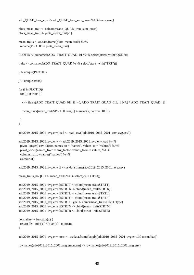
ado_QUAD_tran_sum <- ado_QUAD_tran_sum_cross %>% transpose()

plots_mean_trait <- colnames(ado_QUAD_tran_sum_cross)plots_mean_trait <- plots_mean_trait[-1]

mean_traits <- as.data.frame(plots_mean_trait) %>% rename(PLOTID = plots_mean_trait)

PLOTID <- colnames(ADO_TRAIT_QUAD_01 %>% select(starts_with("QUD")))

traits <- colnames(ADO_TRAIT_QUAD %>% select(starts_with("TRT")))

i <- unique(PLOTID)

j <- unique(traits)

for (i in PLOTID){ for ( j in traits ){ x <- ifelse(ADO_TRAIT_QUAD_01[, i] > 0, ADO_TRAIT_QUAD_01[, i], NA) * ADO_TRAIT_QUAD[, j] mean_traits[mean_traits$PLOTID==i, j] <- mean(x, na.rm=TRUE) }}

ado2019_2015_2001_avg.env.load <- read_csv("ado2019_2015_2001_env_avg.csv")

ado2019_2015_2001_avg.env <- ado2019_2015_2001_avg.env.load %>% pivot_longer(-env_factor, names_to = "names", values_to = "values") %>% pivot_wider(names_from = env_factor, values_from = values) %>% column_to_rownames("names") %>% as.matrix()

ado2019_2015_2001_avg.env.df <- as.data.frame(ado2019_2015_2001_avg.env)

mean_traits_noQUD <- mean_traits %>% select(-c(PLOTID))

ado2019_2015_2001_avg.env.df$TRTT <- cbind(mean_traits$TRTT)ado2019_2015_2001_avg.env.df$TRTK <- cbind(mean_traits$TRTK)ado2019_2015_2001_avg.env.df$TRTL <- cbind(mean_traits$TRTL)ado2019_2015_2001_avg.env.df$TRTF <- cbind(mean_traits$TRTF)ado2019_2015_2001_avg.env.df$TRTCType <- cbind(mean_traits$TRTCType)ado2019_2015_2001_avg.env.df$TRTN <- cbind(mean_traits$TRTN)ado2019_2015_2001_avg.env.df$TRTR <- cbind(mean_traits$TRTR)

normalize <- function(x) { return ((x - min(x)) / (max(x) - min(x)))}

ado2019_2015_2001_avg.env.norm <- as.data.frame(lapply(ado2019_2015_2001_avg.env.df, normalize))

rownames(ado2019_2015_2001_avg.env.norm) <- rownames(ado2019_2015_2001_avg.env)

49

colnames(ado2019_2015_2001_avg.env.norm)[c(10)] <- c("temperature")colnames(ado2019_2015_2001_avg.env.norm)[c(11)] <- c("continentality")colnames(ado2019_2015_2001_avg.env.norm)[c(12)] <- c("light")colnames(ado2019_2015_2001_avg.env.norm)[c(13)] <- c("moisture")colnames(ado2019_2015_2001_avg.env.norm)[c(14)] <- c("competition")colnames(ado2019_2015_2001_avg.env.norm)[c(15)] <- c("nutrients")colnames(ado2019_2015_2001_avg.env.norm)[c(16)] <- c("soil_reaction")

ado2019_2015_2001_avg.env_fact <- ado2019_2015_2001_avg.env.norm[,1:9]head(ado2019_2015_2001_avg.env_fact)

ado2019_2015_2001_avg.landolt <- ado2019_2015_2001_avg.env.norm[,10:16]head(ado2019_2015_2001_avg.landolt)

# environmental factors for ADO 2019ado2019_avg.env_fact <- ado2019_2015_2001_avg.env_fact[1:33, ]ado2019_avg.landolt <- ado2019_2015_2001_avg.landolt[1:33, ]ado2019_avg_env.norm <- ado2019_2015_2001_avg.env.norm[1:33, ] # env_factors + Landolt values

# Ordinations with averages of 2019

ado2019_avg.data <- read_csv("ADO_Data_2019_avg.csv") %>% pivot_longer(-Species, names_to = "names", values_to = "values") %>% pivot_wider(names_from = Species, values_from = values) %>% column_to_rownames("names") %>% as.matrix()

ado2019_groups <- read.csv('ado2019_groups.csv', header = F)group.vector <- as.integer(ado2019_groups[,1])

## DCA with averages ADO 2019---------------------------

ado2019_avg.dca <- decorana(ado2019_avg.data)windows()plot (ado2019_avg.dca,display='sites',type='n', xlab='DCA1 (eigenvalue: 0.592)', ylab='DCA2 (eigenvalue: 0.366)')axis(1,at=(-2:4))points(ado2019_avg.dca,col='grey30')text(ado2019_avg.dca,dis='sites',pos=3,offset=0.2,cex=0.6)ordihull(ado2019_avg.dca, groups = group.vector, col=c('red','darkgreen', 'blue', 'orange'))legend(x=2.5, y=-0.5, legend=c(expression(paste(italic('Festuca nigrescens '), 'community')), expression('Seslerietum'), expression('Festucetum pumilae'), expression('Saxifragetum sedoidis')), lty=1, col=c('darkgreen','blue','orange','red'), cex=1.2, bty='n', y.intersp = 0.4)

ado2019_avg.dca

## NMDS with averages ADO 2019 -----------------------

ado2019_avg.nmds <- metaMDS(ado2019_avg.data, trace=T)

50

windows()plot(ado2019_avg.nmds, ylim = c(-2, 1.5), display='sites', type='n')points(ado2019_avg.nmds, display = "sites", col = c(rep("grey30", 33), rep("grey10", 7), rep("grey50", 14)), pch = c(rep(15, 12), rep(18, 7), rep(16, 14)))text(ado2019_avg.nmds, dis = 'sites', pos = 3, offset = 0.3, col = c(rep("grey30", 33), rep("grey10", 7), rep("grey50", 14)), cex = 0.7)ordihull(ado2019_avg.nmds, groups = group.vector, col=c('red', 'darkgreen', 'blue', 'orange'))lines(c(0,0,-10,10),c(-10,10,0,0),lty=3)legend(x=(1.6), y=(-1.2), legend=c(expression(paste(italic('Festuca nigrescens '), 'community')), expression('Seslerietum'), expression('Festucetum pumilae'), expression('Saxifragetum sedoidis')), lty=1,col=c('darkgreen','blue','orange','red'), cex=1.2, bty='n', y.intersp = 0.4)

ado2019_avg.env.nmds <- envfit(ado2019_avg.nmds, ado2019_avg_env.norm)plot(ado2019_avg.env.nmds, p.max=0.05, cex=0.8, col='black')

ado2019_avg.nmdsado2019_avg.env.nmds

# NMDS with averages 2019-2015-2001

ado2019_2015_2001_avg.data <- read_csv("ADO_Data_2019_2015_2001_avg.csv") %>% pivot_longer(-Species, names_to = "names", values_to = "values") %>% pivot_wider(names_from = Species, values_from = values) %>% column_to_rownames("names") %>% as.matrix()

ado2019_2015_2001.groups <- read.csv('ado_2019_2015_2001_groups.csv', header = F)group.vector2 <- as.integer(ado2019_2015_2001.groups[,1])

ado2019_2015_2001_avg.nmds <- metaMDS(ado2019_2015_2001_avg.data, trace=T)

windows()plot (ado2019_2015_2001_avg.nmds, display='sites', type='n')axis(1, at=(-2:2))points(ado2019_2015_2001_avg.nmds, display = "sites", col = c(rep("grey30", 33), rep("blue", 16), rep("red", 16)), pch = c(rep(15, 33), rep(17, 16), rep(17, 16)))text(ado2019_2015_2001_avg.nmds, dis = 'sites', pos = 1, offset = 0.22, col = c(rep("grey30", 33), rep("blue", 16), rep("red", 16)), cex = 0.7)ordihull(ado2019_2015_2001_avg.nmds, groups = group.vector2, col=c('darkgreen','blue','purple','brown', 'red', 'orange'))legend(x=(1.8), y=(1.5),legend=c( expression(paste(italic('Festuca nigrescens '), 'community')), expression('Seslerietum'), expression('Festucetum pumilae'), expression('Caricetum firmae'),

51

expression('Caricetum rupestris'), expression('Saxifragetum sedoides')),lty = 1, col=c('darkgreen','blue','orange','purple', 'brown', 'red'), cex=1.1, bty='n', y.intersp = 0.4, x.intersp = 0.3)lines(c(0,0,-10,10),c(-10,10,0,0),lty=3)

ado2019_2015_2001_avg.env.nmds <- envfit(ado2019_2015_2001_avg.nmds, ado2019_2015_2001_avg.env.norm)plot(ado2019_2015_2001_avg.env.nmds, p.max=0.05, cex=0.8, col = c('black'))

ado2019_2015_2001_avg.env.nmdsado2019_2015_2001_avg.nmds

52

Appendix VI - R-scripts for ecological and competition type analyses

# Plant communities of the transects - ecological indicator values and competition types

library(vegan)library(tidyverse)library(ggrepel)library(lmtest)library(sandwich)

# load data

ado2019_2015_2001_avg.data <- read_csv("ADO_Data_2019_2015_2001_avg.csv") #%>%

head(ado2019_2015_2001_avg.data)

ado2019_2015_2001_avg.data.list <- ado2019_2015_2001_avg.data %>% pivot_longer(-Species, names_to = "PlotID", values_to = "Cover") %>% filter(Cover > 0)

# 1) join species table and trait table--------------------------

flora_indicativa <- read.csv("Flora_indicativa_ado2019.csv", skip= 1, header=TRUE) %>% select(-(starts_with("x"))) %>% rename(Species = Species.name..short.) %>% select(Species, T, N, KS) %>% mutate(C_value = as.numeric(ifelse(KS=="ccc", 3,

ifelse (KS =="css", 1, ifelse (KS=="crs", 1,

ifelse (KS=="ccs", 2, ifelse (KS=="rss", 0,

ifelse (KS=="rrs", 0, ifelse (KS=="ccr", 2,

ifelse (KS=="sss", 0, NA)))))))))) %>%select(-KS)

ADO_TRAIT_PLOT <- left_join(ado2019_2015_2001_avg.data.list, flora_indicativa, by ="Species") %>% group_by(PlotID, Species) %>% mutate(TRC = "ADO",TYP = ifelse((str_count(PlotID) == 5) , "TRA", "SUM"),SUC = (substr(PlotID, 1 , 1)), SUC = ifelse(SUC== "M", "MTS", # here we overwrite the letter with the full summit code

ifelse(SUC== "G", "GRM", ifelse(SUC== "P", "PNL",

ifelse(SUC=="R", "RNK", NA)))),ELEV = ifelse(TYP == "TRA", (substr(PlotID, 2, 5)), ifelse(SUC == "GRM", "2199",

ifelse(SUC == "PNL", "2463", ifelse(SUC == "RNK", "2757", "2893"))))) %>%

mutate(Ttype = ifelse(T < 1.6, "Tcryo", "Ttherm")) %>% mutate(Ntype = ifelse(N < 2.1, "Nolig", "Nmeso")) %>% mutate(Ctype = ifelse(C_value > 1.9, "competitive", "not competitive"))

53

ADO_TRAIT_PLOT <- na.omit(ADO_TRAIT_PLOT)

ADO_avg_comm <- read_csv("ADO_2019_2015_2001_avg_community.csv")

ADO_TRAIT_PLOT <- left_join(ADO_TRAIT_PLOT, ADO_avg_comm, by = "PlotID")

ADO_TRAIT_TRA <- ADO_TRAIT_PLOT %>% filter(TYP == "TRA") # only transects, no summit data

# Proportion of bioindicators per community---------------# TemperatureADO_TRAIT_TRA_propT <- ADO_TRAIT_TRA %>% ungroup() %>%

select(PlotID, Ttype) %>% group_by(PlotID, Ttype) %>% summarize(Tn = n()) %>%mutate(propTtype = (Tn/sum(Tn)*100)) %>%ungroup() %>% complete(PlotID, Ttype, fill = list(propTtype = 0, Tn = 0 ))

# NutrientsADO_TRAIT_TRA_propN <- ADO_TRAIT_TRA %>% ungroup() %>%

select(PlotID, Ntype) %>%group_by(PlotID, Ntype) %>% summarize(Nn = n()) %>%mutate(propNtype = (Nn/sum(Nn)*100)) %>%ungroup() %>% complete(PlotID, Ntype, fill = list(propNtype = 0, Nn = 0 ))

# C-valueADO_TRAIT_TRA_propC <- ADO_TRAIT_TRA %>% ungroup() %>%

select(PlotID, Ctype) %>% group_by(PlotID, Ctype) %>% summarize(Cn = n()) %>%mutate(propCtype = (Cn/sum(Cn)*100)) %>%ungroup() %>% complete(PlotID, Ctype, fill = list(propCtype = 0, Cn = 0 ))

ADO_TRAIT_TRA_plot <- ADO_TRAIT_TRA %>% ungroup() %>% select(PlotID, TYP, SUC, Community) %>%distinct(PlotID, .keep_all = TRUE)

ADO_TRAIT_TRA_propT_info <- left_join (ADO_TRAIT_TRA_plot, ADO_TRAIT_TRA_propT, by = "PlotID")

ADO_TRAIT_TRA_propT_N <- left_join (ADO_TRAIT_TRA_propT_info, ADO_TRAIT_TRA_propN, by = "PlotID")

ADO_TRAIT_TRA_prop <- left_join (ADO_TRAIT_TRA_propT_N, ADO_TRAIT_TRA_propC, by = "PlotID")

ADO_TRAIT_TRA_prop$Community <- as.factor(ADO_TRAIT_TRA_prop$Community)

ADO_TRAIT_TRA_prop$Community <- fct_relevel(ADO_TRAIT_TRA_prop$Community, "Festuca nigrescens community", "Seslerietum", "Festucetum pumilae", "Saxifragetum sedoidis")

54

ADO_TRAIT_TRA_prop$Ttype <- as.factor(ADO_TRAIT_TRA_prop$Ttype)

ADO_TRAIT_TRA_prop$Ttype <- fct_relevel(ADO_TRAIT_TRA_prop$Ttype, "Ttherm", "Tcryo")

# boxplots with all dataADO_TRAIT_TRA_prop %>% filter(Community != "Caricetum rupestris") %>%

ggplot(aes(x = Ttype, y = propTtype, fill = Ttype)) + geom_boxplot() +facet_wrap(.~Community)

# violinplots with all dataADO_TRAIT_TRA_prop %>% filter(Community != "Caricetum rupestris") %>%

ggplot(aes(x = Ttype, y = propTtype, fill = Ttype)) + geom_violin() +facet_wrap(.~Community)

# Statistical test## Analysis of variance## overall not possibleaov_Ttype <- lm(propTtype ~ Community, data = ADO_TRAIT_TRA_prop)summary(aov_Ttype)

# Thermophilic speciesaov_therm <- aov(propTtype ~ Community, data = (ADO_TRAIT_TRA_prop %>%

filter(Ttype=="Ttherm")))summary(aov_therm)anova(aov_therm)coeftest(aov_therm, vcov = vcovHC(aov_therm)) par(mfrow=c(2,2))plot(aov_therm)

# Meso- to nitrophilous speciesaov_meso <- aov(propNtype ~ Community, data = (ADO_TRAIT_TRA_prop %>%

filter(Ntype != "Nolig")))summary(aov_meso)anova(aov_meso)coeftest(aov_meso, vcov = vcovHC(aov_meso)) par(mfrow=c(2,2))plot(aov_meso)

# Competitive speciesaov_compet <- aov(propCtype ~ Community, data = (ADO_TRAIT_TRA_prop %>%

filter(Ctype == "competitive")))summary(aov_compet)anova(aov_compet)coeftest(aov_compet, vcov = vcovHC(aov_compet)) par(mfrow=c(2,2))plot(aov_compet)

# Model criticism## Normality of residuals - Kolmogorov-Smirnov test### Thermophilic speciesfitted_values_Ttherm <- aov_therm$fitted.valuesresiduals_Ttherm <- aov_therm$residuals

(T_norm <- tibble(

55

fitted_value = fitted_values_Ttherm,residual = residuals_Ttherm

))

ggplot(T_norm, aes(residual)) + geom_histogram()

ggplot(T_norm, aes(sample = residual)) + stat_qq() + stat_qq() + stat_qq_line()

ks.test(residuals_Ttherm, "pnorm", mean = mean(residuals_Ttherm), sd = sd(residuals_Ttherm))

### Meso- to nitrophilous speciesfitted_values_Nmeso <- aov_meso$fitted.valuesresiduals_ Nmeso <- aov_meso$residuals

(N_norm <- tibble(fitted_value = fitted_values_ Nmeso,residual = residuals_ Nmeso

))

ggplot(N_norm, aes(residual)) + geom_histogram()

ggplot(N_norm, aes(sample = residual)) + stat_qq() + stat_qq() + stat_qq_line()

ks.test(residuals_Nmeso, "pnorm", mean = mean(residuals_Nmeso), sd = sd(residuals_Nmeso))

### Competitive speciesfitted_values_Compet <- aov_compet$fitted.valuesresiduals_Compet <- aov_compet$residuals

(C_norm <- tibble(fitted_value = fitted_values_Compet,residual = residuals_Compet

))

ggplot(C_norm, aes(residual)) + geom_histogram()

ggplot(C_norm, aes(sample = residual)) + stat_qq() + stat_qq() + stat_qq_line()

ks.test(residuals_Compet, "pnorm", mean = mean(residuals_Compet), sd = sd(residuals_Compet))

## Breusch-Pagan test

# Thermophilic speciesADO_TRAIT_PLOT_Ttherm <- ADO_TRAIT_TRA_prop %>% filter(Ttype == "Ttherm")bptest(ADO_TRAIT_PLOT_Ttherm$propTtype ~ ADO_TRAIT_PLOT_Ttherm$Community)

# NoligADO_TRAIT_PLOT_Nmeso <- ADO_TRAIT_TRA_prop %>% filter(Ntype == "Nmeso")bptest(ADO_TRAIT_PLOT_Nmeso$propNtype ~ ADO_TRAIT_PLOT_Nmeso$Community)

# CompetitiveADO_TRAIT_PLOT_Compet <- ADO_TRAIT_TRA_prop %>% filter(Ctype == "competitive")bptest(ADO_TRAIT_PLOT_Compet$propCtype ~ ADO_TRAIT_PLOT_Compet$Community)

56

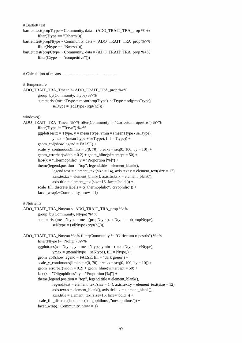
# Bartlett testbartlett.test(propTtype ~ Community, data = (ADO_TRAIT_TRA_prop %>%

filter(Ttype == "Ttherm")))bartlett.test(propNtype ~ Community, data = (ADO_TRAIT_TRA_prop %>%

filter(Ntype == "Nmeso")))bartlett.test(propCtype ~ Community, data = (ADO_TRAIT_TRA_prop %>%

filter(Ctype == "competitive")))

# Calculation of means-----------------------------------------

# TemperatureADO_TRAIT_TRA_Tmean <- ADO_TRAIT_TRA_prop %>%

group_by(Community, Ttype) %>% summarise(meanTtype = mean(propTtype), sdTtype = sd(propTtype),

seTtype = (sdTtype / sqrt(n())))

windows()ADO_TRAIT_TRA_Tmean %>% filter(Community != "Caricetum rupestris") %>%

filter(Ttype != "Tcryo") %>% ggplot(aes(x = Ttype, y = meanTtype, ymin = (meanTtype - seTtype),

ymax = (meanTtype + seTtype), fill = Ttype)) + geom_col(show.legend = FALSE) + scale_y_continuous(limits = c(0, 70), breaks = seq(0, 100, by = 10)) + geom_errorbar(width = 0.2) + geom_hline(yintercept = 50) + labs(x = "Thermophilic", y = "Proportion [%]") +theme(legend.position = "top", legend.title = element_blank(),

legend.text = element_text(size = 14), axis.text.y = element_text(size = 12), axis.text.x = element_blank(), axis.ticks.x = element_blank(), axis.title = element_text(size=16, face="bold")) +

scale_fill_discrete(labels = c("thermophilic","cryophilic")) +facet_wrap(.~Community, nrow = 1)

# NutrientsADO_TRAIT_TRA_Nmean <- ADO_TRAIT_TRA_prop %>%

group_by(Community, Ntype) %>% summarise(meanNtype = mean(propNtype), sdNtype = sd(propNtype),

seNtype = (sdNtype / sqrt(n())))

ADO_TRAIT_TRA_Nmean %>% filter(Community != "Caricetum rupestris") %>% filter(Ntype != "Nolig") %>% ggplot(aes(x = Ntype, y = meanNtype, ymin = (meanNtype - seNtype),

ymax = (meanNtype + seNtype), fill = Ntype)) + geom_col(show.legend = FALSE, fill = "dark green") + scale_y_continuous(limits = c(0, 70), breaks = seq(0, 100, by = 10)) + geom_errorbar(width = 0.2) + geom_hline(yintercept = 50) + labs(x = "Oligophilous", y = "Proportion [%]") +theme(legend.position = "top", legend.title = element_blank(),

legend.text = element_text(size = 14), axis.text.y = element_text(size = 12), axis.text.x = element_blank(), axis.ticks.x = element_blank(), axis.title = element_text(size=16, face="bold")) +

scale_fill_discrete(labels = c("oligophilous","mesophilous")) +facet_wrap(.~Community, nrow = 1)

57

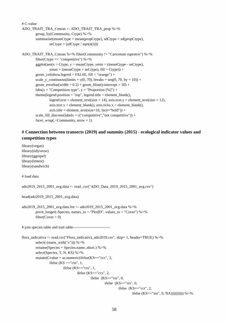
# C-valueADO_TRAIT_TRA_Cmean <- ADO_TRAIT_TRA_prop %>%

group_by(Community, Ctype) %>% summarise(meanCtype = mean(propCtype), sdCtype = sd(propCtype),

seCtype = (sdCtype / sqrt(n())))

ADO_TRAIT_TRA_Cmean %>% filter(Community != "Caricetum rupestris") %>% filter(Ctype == "competitive") %>% ggplot(aes(x = Ctype, y = meanCtype, ymin = (meanCtype - seCtype),

ymax = (meanCtype + seCtype), fill = Ctype)) + geom_col(show.legend = FALSE, fill = "orange") + scale_y_continuous(limits = c(0, 70), breaks = seq(0, 70, by = 10)) + geom_errorbar(width = 0.2) + geom_hline(yintercept = 50) + labs(x = "Competition type", y = "Proportion [%]") +theme(legend.position = "top", legend.title = element_blank(),

legend.text = element_text(size = 14), axis.text.y = element_text(size = 12),axis.text.x = element_blank(), axis.ticks.x = element_blank(),axis.title = element_text(size=16, face="bold")) +

scale_fill_discrete(labels = c("competitive","not competitive")) +facet_wrap(.~Community, nrow = 1)

# Connection between transects (2019) and summits (2015) - ecological indicator values and competition types

library(vegan)library(tidyverse)library(ggrepel)library(lmtest)library(sandwich)

# load data

ado2019_2015_2001_avg.data <- read_csv("ADO_Data_2019_2015_2001_avg.csv")

head(ado2019_2015_2001_avg.data)

ado2019_2015_2001_avg.data.list <- ado2019_2015_2001_avg.data %>% pivot_longer(-Species, names_to = "PlotID", values_to = "Cover") %>% filter(Cover > 0)

# join species table and trait table-----------------------------

flora_indicativa <- read.csv("Flora_indicativa_ado2019.csv", skip= 1, header=TRUE) %>% select(-(starts_with("x"))) %>% rename(Species = Species.name..short.) %>% select(Species, T, N, KS) %>%mutate(Cvalue = as.numeric(ifelse(KS=="ccc", 3,

ifelse (KS =="css", 1, ifelse (KS=="crs", 1,

ifelse (KS=="ccs", 2, ifelse (KS=="rss", 0,

ifelse (KS=="rrs", 0, ifelse (KS=="ccr", 2,

ifelse (KS=="sss", 0, NA)))))))))) %>%

58

select(-KS) #%>%

ADO_TRAIT_PLOT_avg <- left_join(ado2019_2015_2001_avg.data.list, flora_indicativa, by ="Species") %>% group_by(PlotID, Species) %>% mutate(TRC = "ADO",TYP = ifelse((str_count(PlotID) == 5) , "TRA", "SUM"), SUC = (substr(PlotID, 1 , 1)),SUC = ifelse(SUC== "M", "MTS",

ifelse(SUC== "G", "GRM", ifelse(SUC== "P", "PNL",

ifelse(SUC=="R", "RNK", NA)))),ELEV = ifelse(TYP == "TRA", (substr(PlotID, 2, 5)), ifelse(SUC == "GRM", "2199",

ifelse(SUC == "PNL", "2463", ifelse(SUC == "RNK", "2757", "2893")))))

ADO_TRAIT_PLOT_avg <- na.omit(ADO_TRAIT_PLOT_avg)

ADO_avg_comm <- read_csv("ADO_2019_2015_2001_avg_community.csv")

ADO_TRAIT_PLOT_avg <- left_join(ADO_TRAIT_PLOT_avg, ADO_avg_comm, by = "PlotID")

# Calculate weighted mean of indicator values and plant strategy type

ADO_TRAIT_PLOT_SPEC_mean <- ADO_TRAIT_PLOT_avg %>% group_by(PlotID) %>% mutate(SPn = n(),

T_mean= weighted.mean((as.numeric(T)), Cover, na.rm= TRUE),N_mean= weighted.mean((as.numeric(N)), Cover, na.rm= TRUE),Cvalue_mean= weighted.mean((as.numeric(Cvalue)), Cover, na.rm= TRUE))

# Create a summarized data set without the species:ADO_TRAIT_PLOT_mean <- ADO_TRAIT_PLOT_SPEC_mean %>%

select(-Species, - Cover) %>% group_by(PlotID, T) %>% filter(T>0) %>% summarise_each(funs(first))

ADO_TRAIT_PLOT_noGRM <- ADO_TRAIT_PLOT_mean %>% filter(SUC != "GRM") %>% select(PlotID, TYP, SUC, ELEV, Community, T_mean, N_mean, Cvalue_mean) %>% distinct(T_mean, .keep_all = TRUE)

ADO_TRAIT_PLOT_2019_2015 <- ADO_TRAIT_PLOT_noGRM %>% filter(PlotID != "ME1", PlotID != "MN1", PlotID != "MS1",

PlotID != "MW1",PlotID != "PE1", PlotID != "PN1", PlotID != "PS1", PlotID != "PW1", PlotID != "RE1", PlotID != "RN1", PlotID != "RS1", PlotID != "RW1" )

ADO_TRAIT_PLOT_2019_2015$SUC <- as.factor(ADO_TRAIT_PLOT_2019_2015$SUC)

ADO_TRAIT_PLOT_2019_2015$SUC <- fct_relevel(ADO_TRAIT_PLOT_2019_2015$SUC, "PNL", "RNK", "MTS")

59

# Statistical test---------------------------------------------------

## Temperature valuelm_Tmean <- lm(T_mean ~ ELEV, data = ADO_TRAIT_PLOT_2019_2015)summary(lm_Tmean)fitted_values_Tmean <- lm_Tmean$fitted.valuesresiduals_Tmean <- lm_Tmean$residuals

(T_norm <- tibble( observed = ADO_TRAIT_PLOT_2019_2015$T_mean, fitted_value = fitted_values_Tmean, residual = residuals_Tmean))

ggplot(T_norm, aes(residuals_Tmean)) + geom_histogram()

ggplot(T_norm, aes(sample = residuals_Tmean)) + stat_qq() + stat_qq_line()

ks.test(residuals_Tmean, "pnorm", mean = mean(residuals_Tmean), sd = sd(residuals_Tmean))

bptest(ADO_TRAIT_PLOT_2019_2015$T_mean ~ ADO_TRAIT_PLOT_2019_2015$ELEV)

## Nutrient value

lm_Nmean <- lm(N_mean ~ ELEV, data = ADO_TRAIT_PLOT_2019_2015)fitted_values_Nmean <- lm_Nmean$fitted.valuesresiduals_Nmean <- lm_Nmean$residuals

(N_norm <- tibble( observed = ADO_TRAIT_PLOT_2019_2015$N_mean, fitted_value = fitted_values_Nmean, residual = residuals_Nmean))

ggplot(N_norm, aes(residuals_Nmean)) + geom_histogram()

ggplot(N_norm, aes(sample = residuals_Nmean)) + stat_qq() + stat_qq_line()

ks.test(residuals_Nmean, "pnorm", mean = mean(residuals_Nmean), sd = sd(residuals_Nmean))

bptest(ADO_TRAIT_PLOT_2019_2015$N_mean ~ ADO_TRAIT_PLOT_2019_2015$ELEV)

## Competition valuelm_Cvalue_mean <- lm(Cvalue_mean ~ ELEV, data = ADO_TRAIT_PLOT_2019_2015)fitted_values_Cvalue_mean <- lm_Cvalue_mean$fitted.valuesresiduals_Cvalue_mean <- lm_Cvalue_mean$residuals

(T_norm <- tibble( observed = ADO_TRAIT_PLOT_2019_2015$Cvalue_mean, fitted_value = fitted_values_Cvalue_mean, residual = residuals_Cvalue_mean))

60

ggplot(T_norm, aes(residuals_Cvalue_mean)) + geom_histogram()

ggplot(T_norm, aes(sample = residuals_Cvalue_mean)) + stat_qq() + stat_qq_line()

ks.test(residuals_Cvalue_mean, "pnorm", mean = mean(residuals_Cvalue_mean), sd = sd(residuals_Cvalue_mean))

bptest(ADO_TRAIT_PLOT_2019_2015$Cvalue_mean ~ ADO_TRAIT_PLOT_2019_2015$ELEV)

## Bartlett testbartlett.test(T_mean ~ SUC, data = ADO_TRAIT_PLOT_2019_2015)bartlett.test(N_mean ~ SUC, data = ADO_TRAIT_PLOT_2019_2015)bartlett.test(Cvalue_mean ~ SUC, data = ADO_TRAIT_PLOT_2019_2015)

bartlett.test(T_mean ~ ELEV, data = ADO_TRAIT_PLOT_2019_2015)

# All transects in one plot--------------------------------------------------------------------

# Mean temperature value

windows()ggplot(data = ADO_TRAIT_PLOT_2019_2015, aes(x= as.numeric(ELEV),

y= T_mean, col = Community)) + geom_point(show.legend = FALSE) + geom_smooth(method = lm, col = "grey30") +geom_text_repel(aes(label = PlotID)) + labs(x = "Elevation [m a.s.l]", y = "Mean Temperature value", title = NULL) +theme(legend.justification=c(1, 1), legend.position=c(1, 1),

axis.text = element_text(size=12), axis.title = element_text(size=20, face="bold"),title = element_text(size = 20, face = "bold"), legend.text = element_text(size = 12), strip.text.x = element_text(size = 18)) +

scale_x_continuous(breaks = seq(2100, 2900, by = 100), limits = c(2050, 2900)) + scale_y_continuous(breaks = seq(0.2, 3, by = 0.2), limits = c(1, 2.2)) + scale_color_manual(name = NULL,

breaks = c("Festuca nigrescens community", "Seslerietum", "Festucetum pumilae","Caricetum firmae", "Caricetum rupestris", "Saxifragetum sedoidis"), values = c("darkgreen", "blue", "orange","purple", "brown", "red")) +

facet_wrap(.~SUC)

# Mean nutrients value

ggplot(data = ADO_TRAIT_PLOT_2019_2015, aes(x= as.numeric(ELEV), y= N_mean, col = Community)) + geom_point() + geom_smooth(method = lm, col = "grey30") + geom_text_repel(aes(label = PlotID)) + labs(x = "Elevation [m a.s.l]", y = "Mean Nutrient value", title = NULL) +theme(legend.justification=c(1, 0), legend.position="", axis.text = element_text(size=12),

axis.title = element_text(size=20, face="bold"), title = element_text(size = 20, face = "bold"),strip.text.x = element_text(size = 18), legend.text = element_text(size = 12)) +

scale_x_continuous(breaks = seq(2100, 2900, by = 100), limits = c(2050, 2900)) + scale_y_continuous(breaks = seq(0.2, 3, by = 0.2), limits = c(1, 3)) + scale_color_manual(name = NULL, breaks = c("Festuca nigrescens community",

"Seslerietum", "Festucetum pumilae", "Caricetum firmae", "Caricetum rupestris",

61

"Saxifragetum sedoidis"), values = c("darkgreen", "blue" , "orange", "purple", "brown", "red")) +

facet_wrap(.~SUC)

# Mean competition value

ggplot(data = ADO_TRAIT_PLOT_2019_2015, aes(x= as.numeric(ELEV), y= Cvalue_mean, col = Community)) + geom_point() + geom_smooth(method = lm, col = "grey30") + geom_text_repel(aes(label = PlotID)) + labs(x = "Elevation [m a.s.l]", y = "Mean Competition value", title = NULL) +theme(legend.justification=c(1, 0), legend.position= "", axis.text = element_text(size=12),

axis.title = element_text(size=20, face="bold"), title = element_text(size = 20, face = "bold"),strip.text.x = element_text(size = 0), legend.text = element_text(size = 12)) +

scale_x_continuous(breaks = seq(2100, 2900, by = 100), limits = c(2050, 2900)) + scale_y_continuous(breaks = seq(0.2, 3, by = 0.2), limits = c(0.4, 1.8)) + scale_color_manual(name = NULL, breaks = c("Festuca nigrescens community",

"Seslerietum", "Festucetum pumilae", "Caricetum firmae", "Caricetum rupestris","Saxifragetum sedoidis"), values = c("darkgreen", "blue", "orange", "purple", "brown", "red")) +

facet_wrap(.~SUC)

# Summit comparison (2001, 2015) - ecological indicators and competition types

library(vegan)library(tidyverse)library(ggrepel)library(lmtest)library(betareg)library(sandwich)

# load data

ado2019_2015_2001_avg.data <- read_csv("ADO_Data_2019_2015_2001_avg.csv")

head(ado2019_2015_2001_avg.data)

ado2019_2015_2001_avg.data.list <- ado2019_2015_2001_avg.data %>% pivot_longer(-Species, names_to = "PlotID", values_to = "Cover") %>% ilter(Cover > 0)

#Join species table and trait table------------------------------

flora_indicativa <- read.csv("Flora_indicativa_ado2019.csv", skip= 1, header=TRUE) %>% select(-(starts_with("x"))) %>% rename(Species = Species.name..short.) %>% select(Species, T, N, KS) %>% mutate(C_value = as.numeric(ifelse(KS=="ccc", 3,

ifelse (KS =="css", 1, ifelse (KS=="crs", 1,

ifelse (KS=="ccs", 2, ifelse (KS=="rss", 0,

ifelse (KS=="rrs", 0,

62

ifelse (KS=="ccr", 2,ifelse (KS=="sss", 0, NA)))))))))) %>%

select(-KS)

ADO_TRAIT_PLOT <- left_join(ado2019_2015_2001_avg.data.list, flora_indicativa,by ="Species") %>% group_by(PlotID, Species) %>% mutate(TRC = "ADO",TYP = ifelse((str_count(PlotID) == 5) , "TRA", "SUM"),SUC = (substr(PlotID, 1 , 1)),SUC = ifelse(SUC== "M", "MTS"

ifelse(SUC == "P", "PNL", ifelse(SUC == "R", "RNK", NA))),

ELEV = ifelse(TYP == "TRA", (substr(PlotID, 2, 5)), ifelse(SUC == "GRM", "2199", ifelse(SUC == "PNL", "2463",

ifelse(SUC == "RNK", "2757", "2893")))),YEAR = ifelse((str_count(PlotID) == 5), 2019, ifelse((substr(PlotID, 3, 3) == 1),

2001, 2015))) %>% mutate(Ttype = ifelse(T < 1.6, "cryophilic", "thermophilic")) %>% mutate(Ntype = ifelse(N < 2.1, "oligophilous", "meso- to nitrophilous")) %>% mutate(Ctype = ifelse(C_value > 1.9, "competitive", "not competitive"))

ADO_TRAIT_PLOT <- na.omit(ADO_TRAIT_PLOT)

ADO_avg_comm <- read_csv("ADO_2019_2015_2001_avg_community.csv")

ADO_TRAIT_PLOT <- left_join(ADO_TRAIT_PLOT, ADO_avg_comm, by = "PlotID")

ADO_TRAIT_PLOT_SUM <- ADO_TRAIT_PLOT %>% filter(TYP == "SUM")

# Proportion of indicator value per community--------------## TemperatureADO_TRAIT_SUM_propT <- ADO_TRAIT_PLOT_SUM %>% ungroup() %>%

select(PlotID, Ttype) %>% group_by(PlotID, Ttype) %>% summarize(Tn = n()) %>%mutate(propTtype = (Tn/sum(Tn)*100)) %>%ungroup() %>% complete(PlotID, Ttype, fill = list(propTtype = 0, Tn = 0 ))

# NutrientsADO_TRAIT_SUM_propN <- ADO_TRAIT_PLOT_SUM %>% ungroup() %>%

select(PlotID, Ntype) %>% group_by(PlotID, Ntype) %>% summarize(Nn = n()) %>%mutate(propNtype = (Nn/sum(Nn)*100)) %>%ungroup() %>% complete(PlotID, Ntype, fill = list(propNtype = 0, Nn = 0 ))

# Competition valueADO_TRAIT_SUM_propC <- ADO_TRAIT_PLOT_SUM %>% ungroup() %>%

select(PlotID, Ctype) %>% group_by(PlotID, Ctype) %>% summarize(Cn = n()) %>%

63

mutate(propCtype = (Cn/sum(Cn)*100)) %>%ungroup() %>% complete(PlotID, Ctype, fill = list(propCtype = 0, Cn = 0 ))

ADO_TRAIT_SUM_plot <- ADO_TRAIT_PLOT_SUM %>% ungroup() %>% select(PlotID, YEAR, TYP, SUC) %>% distinct(PlotID, .keep_all = TRUE)

ADO_TRAIT_SUM_propT_info <- left_join (ADO_TRAIT_SUM_plot, ADO_TRAIT_SUM_propT, by = "PlotID")

ADO_TRAIT_SUM_propT_N <- left_join (ADO_TRAIT_SUM_propT_info, ADO_TRAIT_SUM_propN, by ="PlotID")

ADO_TRAIT_SUM_prop <- left_join (ADO_TRAIT_SUM_propT_N,ADO_TRAIT_SUM_propC, by = "PlotID")

ADO_TRAIT_SUM_prop$YEAR <- as.character(ADO_TRAIT_SUM_prop$YEAR)

ADO_TRAIT_SUM_prop$SUC <- as.factor(ADO_TRAIT_SUM_prop$SUC)

ADO_TRAIT_SUM_prop$SUC <- fct_relevel(ADO_TRAIT_SUM_prop$SUC, "PNL", "RNK", "MTS")

ADO_TRAIT_SUM_prop$Ttype <- as.factor(ADO_TRAIT_SUM_prop$Ttype)

ADO_TRAIT_SUM_prop$Ttype <- fct_relevel(ADO_TRAIT_SUM_prop$Ttype, "thermophilic", "cryophilic")

# Boxplots with all dataADO_TRAIT_SUM_prop %>% #group_by(SUC, YEAR) %>%

ggplot(aes(x = Ttype, y = propTtype, fill = YEAR)) + geom_boxplot() +facet_wrap(.~SUC)

# Violinplots with all dataADO_TRAIT_SUM_prop %>% #group_by(SUC, YEAR) %>%

ggplot(aes(x = Ttype, y = propTtype, fill = YEAR)) + geom_violin() +facet_wrap(.~SUC)

# Statistical test## Analysis of variance## Overall not possibleaov_Ttype <- lm(propTtype ~ SUC + YEAR + Ttype, data = ADO_TRAIT_SUM_prop)summary(aov_Ttype)anova(aov_Ttype)par(mfrow=c(2,2))plot(aov_Ttype)

aov_Ttype <- lm(propTtype ~ SUC * YEAR, data = ADO_TRAIT_SUM_prop)summary(aov_Ttype)

## Thermophilic speciesaov_therm <- aov(propTtype ~ SUC + YEAR, data = (ADO_TRAIT_SUM_prop %>% filter(Ttype=="thermophilic")))summary(aov_therm)

64

### Linear modellm_therm <- lm(propTtype ~ SUC + YEAR, data = (ADO_TRAIT_SUM_prop %>%

filter(Ttype == "thermophilic")))summary(lm_therm)anova(lm_therm)plot(lm_therm)coef(lm_therm)

### Robust standard errorscoeftest(aov_therm, vcov = vcovHC(aov_therm))

# Meso- to nitrophilous speciesaov_meso <- aov(propNtype ~ SUC + YEAR, data = (ADO_TRAIT_SUM_prop %>% filter(Ntype != "oligophilous")))summary(aov_meso)

# Competitive speciesaov_compet <- aov(propCtype ~ SUC + YEAR, data = (ADO_TRAIT_SUM_prop %>% filter(Ctype =="competitive")))summary(aov_compet)

# Model criticism## Normality of residuals - Kolmogorov-Smirnov test### Tcryofitted_values_Ttherm <- aov_therm$fitted.valuesresiduals_Ttherm <- aov_therm$residuals

(T_norm <- tibble(fitted_value = fitted_values_Ttherm,residual = residuals_Ttherm

))

ggplot(T_norm, aes(residual)) + geom_histogram()

ggplot(T_norm, aes(sample = residual)) + stat_qq() + stat_qq() + stat_qq_line()

ks.test(residuals_Ttherm, "pnorm", mean = mean(residuals_Ttherm), sd = sd(residuals_Ttherm))

# Meso- to nitrophilous speciesfitted_values_Nmeso <- aov_meso$fitted.valuesresiduals_ Nmeso <- aov_meso$residuals

(N_norm <- tibble( fitted_value = fitted_values_Nmeso, residual = residuals_ Nmeso))

ggplot(N_norm, aes(residual)) + geom_histogram()

ggplot(N_norm, aes(sample = residual)) + stat_qq() + stat_qq() + stat_qq_line()

ks.test(residuals_Nmeso, "pnorm", mean = mean(residuals_Nmeso), sd = sd(residuals_Nmeso))

# Competitive species

65

fitted_values_Compet <- aov_compet$fitted.valuesresiduals_Compet <- aov_compet$residuals

(C_norm <- tibble(fitted_value = fitted_values_Compet,residual = residuals_Compet

))

ggplot(C_norm, aes(residual)) + geom_histogram()

ggplot(C_norm, aes(sample = residual)) + stat_qq() + stat_qq() + stat_qq_line()

ks.test(residuals_Compet, "pnorm", mean = mean(residuals_Compet), sd = sd(residuals_Compet))

## Breusch-Pagan test### Thermophilic speciesADO_TRAIT_SUM_Ttherm <- ADO_TRAIT_SUM_prop %>% filter(Ttype == "thermophilic")bptest(ADO_TRAIT_SUM_Ttherm$propTtype ~

ADO_TRAIT_SUM_Ttherm$SUC * ADO_TRAIT_SUM_Ttherm$YEAR)

### Meso- to nitrophilous speciesADO_TRAIT_SUM_Nmeso <- ADO_TRAIT_SUM_prop %>% filter(Ntype != "oligophilous")bptest(ADO_TRAIT_SUM_Nolig$propNtype ~

ADO_TRAIT_SUM_Nmeso$SUC * ADO_TRAIT_SUM_Nmeso$YEAR)

### Competitive speciesADO_TRAIT_SUM_Compet <- ADO_TRAIT_SUM_prop %>% filter(Ctype == "competitive")bptest(ADO_TRAIT_SUM_Compet$propCtype ~

ADO_TRAIT_SUM_Compet$SUC * ADO_TRAIT_SUM_Compet$YEAR)

## F-Testvar.test(propTtype ~ YEAR, (data = ADO_TRAIT_SUM_prop %>% filter(SUC == "PNL")))var.test(propTtype ~ YEAR, (data = ADO_TRAIT_SUM_prop %>% filter(SUC == "RNK")))var.test(propTtype ~ YEAR, (data = ADO_TRAIT_SUM_prop %>% filter(SUC == "MTS")))

## t-testt.test(propTtype ~ YEAR, (data = ADO_TRAIT_SUM_prop %>%

filter(SUC == "PNL", Ttype == "thermophilic")), paired = T)t.test(propTtype ~ YEAR, (data = ADO_TRAIT_SUM_prop %>%

filter(SUC == "RNK", Ttype == "thermophilic")), paired = T)t.test(propTtype ~ YEAR, (data = ADO_TRAIT_SUM_prop %>%

filter(SUC == "MTS", Ttype == "thermophilic")), paired = T)

t.test(propTtype ~ YEAR, (data = ADO_TRAIT_SUM_prop %>% filter(SUC == "PNL", Ntype == "meso- to nitrophilous")), paired = T)

# Calculation of mean, standard deviation and standard error for each summit and year---------## TemperatureADO_TRAIT_SUM_Tmean <- ADO_TRAIT_SUM_prop %>%

group_by(SUC, YEAR, Ttype) %>% summarise(meanTtype = mean(propTtype), sdTtype = sd(propTtype),

seTtype = (sdTtype / sqrt(n())))## NutrientsADO_TRAIT_SUM_Nmean <- ADO_TRAIT_SUM_prop %>%

66

group_by(SUC, YEAR, Ntype) %>% summarise(meanNtype = mean(propNtype), sdNtype = sd(propNtype),

seNtype = (sdNtype / sqrt(n())))# Competition valueADO_TRAIT_SUM_Cmean <- ADO_TRAIT_SUM_prop %>%

group_by(SUC, YEAR, Ctype) %>% summarise(meanCtype = mean(propCtype), sdCtype = sd(propCtype),

seCtype = (sdCtype / sqrt(n())))

## Plotswindows()### TemperatureADO_TRAIT_SUM_Tmean %>% filter(Ttype == "thermophilic") %>%

ggplot(aes(x = YEAR, y = meanTtype, ymin = (meanTtype - seTtype), ymax = (meanTtype + seTtype), fill = YEAR)) +

geom_col() + scale_y_continuous(limits = c(0, 20), breaks = seq(0, 20, by = 5)) + geom_errorbar(width = 0.2) +labs(x = "", y = "Proportion [%]") +scale_fill_manual(values = c("blue", "red")) +theme(legend.position = "", legend.title = element_blank(),

legend.text = element_text(size = 14), axis.text = element_text(size = 12), axis.title = element_text(size=16, face="bold"), strip.text.x = element_text(size = 14)) +

facet_wrap(.~SUC + Ttype, nrow = 1)

## Nutrients

ADO_TRAIT_SUM_Nmean %>% filter(Ntype == "meso- to nitrophilous") %>% ggplot(aes(x = YEAR, y = meanNtype, ymin = (meanNtype - seNtype),

ymax = (meanNtype + seNtype), fill = YEAR)) + geom_col() +scale_y_continuous(limits = c(0, 20), breaks = seq(0, 20, by = 5)) +geom_errorbar(width = 0.2) +labs(x = "", y = "") +scale_fill_manual(values = c("blue", "red")) +theme(legend.position = "", legend.title = element_blank(),

legend.text = element_text(size = 14), axis.text = element_text(size = 12), axis.title = element_text(size=16, face="bold"), strip.text.x = element_text(size = 14)) +

facet_wrap(.~SUC + Ntype, nrow = 1)

## Competition value

ADO_TRAIT_SUM_Cmean %>% filter(Ctype == "competitive") %>% ggplot(aes(x = YEAR, y = meanCtype, ymin = (meanCtype - seCtype),

ymax = (meanCtype + seCtype), fill = YEAR)) + geom_col() + scale_y_continuous(limits = c(0, 20), breaks = seq(0, 20, by = 5)) +geom_errorbar(width = 0.2) +labs(x = "", y = "") +scale_fill_manual(values = c("blue", "red")) +theme(legend.position = "", legend.title = element_blank(),

legend.text = element_text(size = 14), axis.text = element_text(size = 12),axis.title = element_text(size=16, face="bold"), strip.text.x = element_text(size = 14)) +facet_wrap(.~SUC + Ctype, nrow = 1)

67

# Summit comparison (2001, 2015) - mean temperature value

library(vegan)library(tidyverse)library(ggrepel)library(lmtest)library(ggpubr)

# load data

ado2019_2015_2001_avg.data <- read_csv("ADO_Data_2019_2015_2001_avg.csv")

head(ado2019_2015_2001_avg.data)

ado2019_2015_2001_avg.data.list <- ado2019_2015_2001_avg.data %>% pivot_longer(-Species, names_to = "PlotID", values_to = "Cover") %>% filter(Cover > 0)

# Join species table and trait table-----------------------------

flora_indicativa <- read.csv("Flora_indicativa_ado2019.csv", skip= 1, header=TRUE) %>% select(-(starts_with("x"))) %>% rename(Species = Species.name..short.) %>% select(Species, T, N, KS) %>% mutate(CType = as.numeric(ifelse(KS=="ccc", 3,

ifelse (KS =="css", 1, ifelse (KS=="crs", 1,

ifelse (KS=="ccs", 2, ifelse (KS=="rss", 0,

ifelse (KS=="rrs", 0, ifelse (KS=="ccr", 2,

ifelse (KS=="sss", 0, NA)))))))))) %>% select(-KS)

ADO_TRAIT_PLOT_avg <- left_join(ado2019_2015_2001_avg.data.list, flora_indicativa, by ="Species") %>%

group_by(PlotID, Species) %>% mutate(TRC = "ADO",TYP = ifelse((str_count(PlotID) == 5) , "TRA", "SUM"),SUC = (substr(PlotID, 1 , 1)), # substr takes the first digit of plotID where we have theSUC = ifelse(SUC== "M", "MTS", # here we overwrite the letter with the full summit code

ifelse(SUC== "G", "GRM", ifelse(SUC== "P", "PNL",

ifelse(SUC=="R", "RNK", NA)))),ELEV = ifelse(TYP == "TRA", (substr(PlotID, 2, 5)), ifelse(SUC == "GRM", "2199",

ifelse(SUC == "PNL", "2463", ifelse(SUC == "RNK", "2757", "2893")))))

ADO_TRAIT_PLOT_summit_avg <- ADO_TRAIT_PLOT_avg %>% filter(TYP == "SUM") %>% mutate(YEAR = (substr(PlotID, 3, 3)), YEAR = ifelse(YEAR == 1, "2001", "2015")) %>% group_by(PlotID) %>% mutate(T_weighted = weighted.mean((as.numeric(T)), Cover, na.rm= TRUE)) %>%

68

na.omit(ADO_TRAIT_PLOT_avg) %>% distinct(PlotID, .keep_all = TRUE)

ADO_TRAIT_PLOT_summit_avg$SUC <- as.factor(ADO_TRAIT_PLOT_summit_avg$SUC)

ADO_TRAIT_PLOT_summit_avg$SUC <- fct_relevel(ADO_TRAIT_PLOT_summit_avg$SUC, "PNL", "RNK", "MTS")

ADO_TRAIT_PLOT_summit_avg %>%ggplot(aes(x = YEAR, y = T_weighted, fill = YEAR)) + geom_boxplot() +theme(legend.position = "") +facet_wrap(.~SUC)

ADO_TRAIT_PLOT_summit_avg %>%ggplot(aes(x = YEAR, y = T_weighted, fill = YEAR)) + geom_violin() +theme(legend.position = "") +facet_wrap(.~SUC)

# Statistical analysis## Linear modellm_temp <- lm(T_weighted ~ SUC + YEAR, data = ADO_TRAIT_PLOT_summit_avg)summary(lm_temp)aov_temp <- aov(T_weighted ~ SUC + YEAR, data = ADO_TRAIT_PLOT_summit_avg)summary(aov_temp)anova(aov_temp)par(mfrow=c(2,2))plot(aov_temp)

# Model criticism## Normality of residuals - Kolmogorov-Smirnov test

fitted_values_Tmean <- aov_temp$fitted.valuesresiduals_Tmean <- aov_temp$residuals

(T_norm <- tibble(fitted_value = fitted_values_Tmean,residual = residuals_Tmean

))

ggplot(T_norm, aes(residual)) + geom_histogram()

ggplot(T_norm, aes(sample = residual)) + stat_qq() + stat_qq() + stat_qq_line()

ks.test(residuals_Tmean, "pnorm", mean = mean(residuals_Tmean), sd = sd(residuals_Tmean))

## Breusch-Pagan test

bptest(T_weighted ~ SUC + YEAR, data = ADO_TRAIT_PLOT_summit_avg)

# F-Testvar.test(T_weighted ~ YEAR, (data = ADO_TRAIT_PLOT_summit_avg %>%

filter(SUC == "PNL")))var.test(T_weighted ~ YEAR, (data = ADO_TRAIT_PLOT_summit_avg %>%

filter(SUC == "RNK")))

69

var.test(T_weighted ~ YEAR, (data = ADO_TRAIT_PLOT_summit_avg %>% filter(SUC == "MTS")))

# t-testt.test(T_weighted ~ YEAR, (data = ADO_TRAIT_PLOT_summit_avg %>%

filter(SUC == "PNL")), paired = T)t.test(T_weighted ~ YEAR, (data = ADO_TRAIT_PLOT_summit_avg %>%

filter(SUC == "RNK")), paired = T)t.test(T_weighted ~ YEAR, (data = ADO_TRAIT_PLOT_summit_avg %>%

filter(SUC == "MTS")), paired = T)

compare_means(T_weighted ~ YEAR, data = ADO_TRAIT_PLOT_summit_avg, group_by = "SUC", method ="t.test", paired = T)

# Calculation of meansADO_TRAIT_SUM_Tmean_avg <- ADO_TRAIT_PLOT_summit_avg %>% group_by(SUC, YEAR) %>%summarise(meanTemp = sum(T_weighted)/4, sdTemp = sd(T_weighted),

seTemp = (sdTemp / sqrt(4)))

# Point plotwindows()ADO_TRAIT_SUM_Tmean_avg %>%

ggplot(aes(x = YEAR, y = meanTemp, ymin = (meanTemp - (1.96*seTemp)), ymax = (meanTemp + (1.96*seTemp)), color = YEAR)) +

geom_point(size = 4) +scale_y_continuous(limits = c(0.9, 1.6), breaks = seq(0, 1.6, by = 0.2)) +geom_errorbar(width = 0.5) +scale_color_manual(values = c("blue", "red")) +labs(x = "", y = "Mean temperature value") +theme(legend.position = "", legend.title = element_blank(),

legend.text = element_text(size = 14), axis.text.y = element_text(size = 12), axis.text.x = element_text(size = 12), strip.text.x = element_text(size = 18),axis.title = element_text(size=16, face="bold")) +

facet_wrap(.~SUC, nrow = 1)

70

Appendix VII - Community table of the transects (2019 data set)

TWINSPAN division 1 was between grasslands and scree vegetation (R2700 and M2700), division2 was between grasslands and Festucetum pumilae (M2350 and R2400), division 3 between M2700and other scree plots was not considered in this table, division 4 was between the two grasslands oflower elevations (R2250 and P2150).

M: MTS, P: PNL, R: RNK; the numbers after the letter denote the elevation of the plot.

The numbers of the plant species in every plot represent the nine cut levels: '-': not present, 1:species with an abundance of > 0 - 1% in this plot, 2: > 1 - 2%, 3: > 2 - 3%, 4: > 3 - 4%, 5: > 4 -8%, 6: > 8 - 18%, 7: > 18 - 38%, 8: > 38 - 68%, 9: > 68 - 100%.

Six constancy classes were used: '-': 0%, I: species present in > 0 - 20% of the samples, II: > 20 -40%, III: > 40 - 60%, IV: > 60 - 80%, V: > 80 - 100%.

71

Appendix VIII - Community table of the transects and summits (2001, 2015 and 2019 data sets)

TWINSPAN division 1 was between grasslands and scree vegetation together with the Caricetumrupestris (RS1 and RS4, but RS4 was a borderline plot and due to its species composition wasmoved to the Festucetum pumilae). Division 2 separated the pioneer grasslands at PNL summitplots from the othre grasslands (PS4 and R2100), while division 3 isolated the scree vegetation fromthe Caricetum rupestris (RN4 and M2500). Division 4 was not considered and division 5 wasbetween the more developed grasslands of lower elevations and the pioneer grassland Caricetumrupestris on higher elevations (M2350 and R2500). Division 10 was also considered in this table,because it separated the twograsslands from lower elevations (R2250 and P2400).

M: MTS, P: PNL, R: RNK; for the transect plots the numbers after the letter denote the elevation ofthe plot; the summit plots include the first letter of the summit with the orientation of the plot andthe chronological number of the survey (1 = 2001, 4 = 2015).

The numbers of the plant species in every plot represent the nine cut levels: '-': not present, 1:species with an abundance of > 0 - 1% in this plot, 2: > 1 - 2%, 3: > 2 - 3%, 4: > 3 - 4%, 5: > 4 -8%, 6: > 8 - 18%, 7: > 18 - 38%, 8: > 38 - 68%, 9: > 68 - 100%.

Six constancy classes were used: '-': 0%, I: species present in > 0 - 20% of the samples, II: > 20 -40%, III: > 40 - 60%, IV: > 60 - 80%, V: > 80 - 100%.

72

Appendix IX - Linear model of the transect and summit comparison

Mean temperature value

Estimate Standard Error t value Pr(>t) P

(Intercept) 4.861 0.560 8.681 1.2e-10 ***

Summit RNK -0.557 0.614 -0.907 0.370

Summit MTS -1.299 0.612 -2.122 0.040 *

Elevation -0.001 0.0002 -5.593 1.9e-06 ***

Summit RNK: Elevation 0.0003 0.0003 0.976 0.335

Summit MTS: Elevation 0.0005 0.0003 2.096 0.043 *

Residual standard error: 0.1035 on 39 degrees of freedomMultiple R-squared: 0.866, Adjusted R-squared: 0.8488 F-statistic: 50.39 on 5 and 39 DF, p-value: 5.55e-16

Mean nutrient value

Estimate Standard Error t value Pr(>t) P

(Intercept) 6.013 1.360 4.421 7.64e-05 ***

Summit RNK -3.394 1.493 -2.274 0.029 *

Summit MTS -3.299 1.487 -2.219 0.032 *

Elevation -0.002 0.0006 -3.020 0.004 **

Summit RNK: Elevation 0.002 0.0006 2.456 0.019 *

Summit MTS: Elevation 0.001 0.0006 2.304 0.027 *

Residual standard error: 0.2513 on 39 degrees of freedomMultiple R-squared: 0.3317, Adjusted R-squared: 0.246 F-statistic: 3.872 on 5 and 39 DF, p-value: 0.006051

Mean competitive value

Estimate Standard Error t value Pr(>t) P

(Intercept) 4.020 0.775 5.190 6.86e-06 ***

Summit RNK -1.193 0.850 -1.403 0.168

Summit MTS -0.366 0.847 -0.432 0.668

Elevation -0.001 0.0003 -3.540 0.001 **

Summit RNK: Elevation 0.0005 0.0004 1.501 0.141

Summit MTS: Elevation 0.0002 0.0004 0.479 0.634

Residual standard error: 0.1431 on 39 degrees of freedomMultiple R-squared: 0.7441, Adjusted R-squared: 0.7113 F-statistic: 22.68 on 5 and 39 DF, p-value: 1.34e-10

73