Elements of regional beetle faunas: faunal variation and compositional breakpoints along climate,...

Elements of regional beetle faunas: faunal variation

and compositional breakpoints along climate, land

cover and geographical gradients

Jani Heino1* and Janne Alahuhta2

1Finnish Environment Institute, Natural Environment Centre, Biodiversity, PO Box 413, FI-90014 Oulu, Finland; and2Department of Geography, University of Oulu, PO Box 3000, FI-90014 Oulu, Finland

Summary

1. Regional faunas are structured by historical, spatial and environmental factors. We studied

large-scale variation in four ecologically different beetle groups (Coleoptera: Dytiscidae, Cara-

bidae, Hydrophiloidea, Cerambycidae) along climate, land cover and geographical gradients,

examined faunal breakpoints in relation to environmental variables, and investigated the best

fit pattern of assemblage variation (i.e. randomness, checkerboards, nestedness, evenly spaced,

Gleasonian, Clementsian). We applied statistical methods typically used in the analysis of

local ecological communities to provide novel insights into faunal compositional patterns at

large spatial grain and geographical extent.

2. We found that spatially structured variation in climate and land cover accounted for most

variation in each beetle group in partial redundancy analyses, whereas the individual effect of

each explanatory variable group was generally much less important in accounting for varia-

tion in provincial species composition.

3. We also found that climate variables were most strongly associated with faunal break-

points, with temperature-related variables alone accounting for about 20% of variation at the

first node of multivariate regression tree for each beetle group. The existence of faunal break-

points was also shown by the ‘elements of faunal structure’ analyses, which suggested Clem-

entsian gradients across the provinces, that is, that there were two or more clear groups of

species responding similarly to the underlying ecological gradients.

4. The four beetle groups showed highly similar biogeographical patterns across our study

area. The fact that temperature was related to faunal breakpoints in the species composition

of each beetle group suggests that climate sets a strong filter to the distributions of species at

this combination of spatial grain and spatial extent. This finding held true despite the ecologi-

cal differences among the four beetle groups, ranging from fully aquatic to fully terrestrial

and from herbivorous to predaceous species.

5. The existence of Clementsian gradients may be a common phenomenon at large scales,

and it is likely to be caused by crossing multiple species pools determined by climatic and his-

torical factors on the distributions of species.

Key-words: assemblage composition, compositional gradients, environmental gradients,

idealized models, multivariate regression trees, partial redundancy analysis, regionalisation

Introduction

Regional biotas develop under the influences of evolution-

ary, historical and environmental factors. These factors

can be understood as a spatiotemporal continuum, with

evolutionary factors largely driving differences in species

composition among broad geographic regions over long

time periods, historical factors such as the most recent ice

age causing variation among smaller regions, and environ-

mental factors being important not only at large spatial

scales but also within smaller regions (Brown & Lomolino

1998; Mittelbach 2012). Examining the relative impor-

tance of these factors for faunal composition in different*Correspondence author. E-mail: [email protected]

© 2014 The Authors. Journal of Animal Ecology © 2014 British Ecological Society

Journal of Animal Ecology 2014 doi: 10.1111/1365-2656.12287

regions is a prerequisite for understanding the interactions

between regional species pools and local communities

(e.g. Cornell 2013), delineating regions for environmental

assessment and conservation (e.g. Bailey 2010), and pre-

dicting the effects of global change on species distribu-

tions at large spatial scales (e.g. Elith & Leathwick 2009).

New insights into those biogeographical patterns can be

attained by applying analytical methods that have been

more typically applied in the analysis of local ecological

communities.

Regional faunas show multiple patterns of interest to

ecologists. These include variations in species richness,

endemism, rarity and composition, all of which may show

various patterns in space and time (Brown & Lomolino

1998; Gaston 2000). Elements of faunal composition can

also be evaluated with regard to which idealized assem-

blage pattern they fit best. Leibold & Mikkelson (2002)

devised an approach to examine such assemblage patterns,

whereby random distributions of species are contrasted

with five idealized models. These idealized models include

checkerboards (e.g. Gotelli & McCabe 2002), nestedness

(e.g. Patterson & Atmar 1986), evenly spaced gradients

(e.g. Tilman 1982), Gleasonian gradients (e.g. Gleason

1926) and Clementsian gradients (e.g. Clements 1916).

Although this approach of ‘elements of metacommunity

structure’ (EMS) was originally aimed at separating dif-

ferent patterns across a set of local communities (Leibold

& Mikkelson 2002), the same approach can be adapted to

examine distribution patterns and faunal structure at large

biogeographical scales, across regions or across sets of

islands (Presley & Willig 2010; Meynard et al. 2013).

The five idealized spatial patterns and randomness

should be tested simultaneously with the same data set

(Leibold & Mikkelson 2002; Dallas & Presley 2014),

although most previous studies have tested different pat-

terns in isolation. For example, checkerboards and nested-

ness are examples of such patterns typically examined in

isolation. Checkerboards refer to a situation where species

pairs have mutually exclusive distributions, whereby two

species replace each other across a set of sites (Diamond

1975; Gotelli & Graves 1996). While most studies have

examined checkerboards across a set of islands or patchy

mainland habitats (Gotelli & McCabe 2002; G€otzenberger

et al. 2012), there is no reason not to examine checker-

boards across large spatial scales on continents. For

example, Gotelli, Graves & Rahbek (2010) examined

checkerboard distributions of birds based on large grain

sizes at a regional extent and found that some species

pairs occurred together less often than expected by chance

expectations. Hence, checkerboards may also occur at

large grain sizes and large geographical extents, although

the mechanisms underlying such patterns should differ

between large-scale biogeographical studies and smaller-

scale studies encompassing local communities.

The nested subset pattern has also been studied exten-

sively in various systems, ranging from islands through

habitat patches to continental habitats (Wright et al.

1998). A perfectly nested pattern occurs when species

poor faunas comprise subsets of those in progressively

richer faunas, and when the species with the broadest

range include those of species with progressively smaller

ranges (Patterson & Atmar 1986). Nestedness has been

examined at large biogeographic scales, too, and these

studies have often found a significantly nested pattern

(Baselga 2008). However, very few studies have tried to

compare such biogeographical variation with other idea-

lised patterns, which have been studied more extensively

across local communities along habitat gradients.

The remaining spatial patterns can be divided between

three main idealized models. Evenly spaced gradients

describe a situation, where species range boundaries are

hyperdispersed along the underlying environmental gradi-

ent (Tilman 1982), indicating maximal differences among

species in environmental tolerances (Presley & Willig

2010). Based on the idea of Clementsian gradients, com-

munities are tight collections of two or more species

groups, responding similarly to environmental gradients

and hence showing discrete community boundaries (Cle-

ments 1916). In contrast, based on the idea of Gleasonian

gradients, each species responds to the environmental gra-

dients individualistically and communities are mere collec-

tions of species, whose ranges happen to overlap in space

and time (Gleason 1926). While the debate over commu-

nity gradients has been ongoing for almost a century,

most attention has been devoted to terrestrial plants and

examinations of local communities (Allen & Hoekstra

1992; McIntosh 1995; Hoagland & Collins 1997). It is

thus important to test the fit of these idealised models in

various other organismal groups, ecological systems and

spatial scales (Henriques-Silva, Lindo & Peres-Neto 2013;

Meynard et al. 2013).

The EMS approach is mainly a descriptive, pattern-based

approach and it does not tell us much about the underlying

mechanisms responsible for the patterns detected. There

has hence been recent interest in accounting for variation in

community composition using spatial and environmental

predictors (Cottenie 2005; Meynard et al. 2013). While

most studies have taken a continuum perspective, whereby

community composition has been examined using direct

gradient analysis methods, such as redundancy analysis

(RDA; Dray et al. 2012; Meynard et al. 2013), recently

developed constrained clustering methods, such as multi-

variate regression trees, allow not only description and pre-

diction of variation in community composition, but also

provide a means to find breakpoints of variation in assem-

blage composition (De’ath 2002; Borcard, Gillet & Legen-

dre 2011). Such breakpoints may occur when there is a

clear change in assemblage composition that is typically

associated with a clear change in environmental conditions.

Surprisingly, very few studies have assessed both continu-

ous variation and breakpoints of community composition

in the same study, and these studies have mainly considered

local habitat gradients within a small region (Davidson

et al. 2010; Sahuquillo & Miracle 2013; Heino, Ilmonen &

© 2014 The Authors. Journal of Animal Ecology © 2014 British Ecological Society, Journal of Animal Ecology

2 J. Heino & J. Alahuhta

Paasivirta 2014). However, it is at large spatial grain sizes

and geographical extents where the occurrence of break-

points in faunal compositions should be most easily dis-

cernible, because studies spanning large spatial scales are

likely to cross multiple regional species pools determined

by the effects of historical factors and climatic constraints

on the distributions of species (Brown & Lomolino 1998;

Heino 2011). Hence, those breakpoints should also be

examined using large-scale biotic, climatic and land cover

data. Such examinations are also valuable owing to the fact

that they provide important information about biogeo-

graphic regionalisation for environmental assessment and

biodiversity conservation (Bailey 2010; Rueda, Rodriguez

& Hawkins 2010).

We examined geographical variation and breakpoints in

the regional faunal composition of four beetle groups

(Coleoptera: Carabidae, Dytiscidae, Hydrophiloidea,

Cerambycidae), showing a wide variety of habitats (both

aquatic and terrestrial groups) and trophic modes (rang-

ing from predators through omnivores to herbivores).

Our study region comprised the whole Fennoscandia and

Denmark, where large gradients in climatic conditions

(i.e. from temperate to arctic regions), land cover (i.e.

from deciduous forest to tundra landscapes) and land use

(i.e. heavily anthropogenically modified to near-pristine

regions) occur in a relatively small geographical area. We

specifically examined the following questions: (i) What are

the contributions of climatic, land cover and spatial vari-

ables to variation in faunal composition? (ii) What envi-

ronmental factors best determine the breakpoints in

faunal composition if such breakpoints exist? (iii) Which

idealized model best fits the empirical data of the four

beetle families? (iv) Are there differences in these patterns

among aquatic (Dytiscidae, Hydrophiloidea) and terres-

trial (Carabidae, Cerambycidae) beetles? Based on evi-

dence from previous studies, we expected that the aquatic

and terrestrial groups would respond relatively similarly

to climatic gradients (V€ais€anen, Heli€ovaara & Immonen

1992; Heino 2001), but show different responses to land

cover gradients due to different habitat requirements.

Materials and methods

study area

We analysed biological and environmental data from the 101

biogeographic provinces belonging to Denmark, Sweden, Norway

and Finland (V€ais€anen, Heli€ovaara & Immonen 1992; V€ais€anen

& Heli€ovaara 1994). Prior to the analyses, we merged small

coastal provinces in Norway to provide a better and more accu-

rate representation of species ranges. We also omitted a single

small Swedish island province (Gotska Sand€o), as it was a clear

outlier in preliminary ordination analyses. After these modifica-

tions, the number of provinces to be analysed decreased from 101

to 79. Each province has typical characteristics of climate and

land cover, thereby ‘province’ being a relatively homogeneous

study unit. The insect faunas in the study area are relatively well

known, offering good data for insect groups used infrequently in

biogeographical analyses (V€ais€anen, Heli€ovaara & Immonen

1992). Thus, although most insect biodiversity studies are affected

by variation in detection of species, we are confident that these

data adequately characterize provincial assemblages and are rep-

resentative of true ecological patterns. Furthermore, there are

actually certain benefits of using biogeographical province as

sampling units rather than using equal area map grids. First, any

change in the spatial grain of the grid system has strong impacts

on the final outcomes. Secondly, in case of fragmented data, most

of such grid cells tend to appear empty, although they are very

likely to be occupied by the target species. Use of more natural

geographical units may hence be superior to grid systems, espe-

cially when distributional data are fragmented, as is the case of

most insect groups. We hence used the 79 provinces as sampling

units (i.e. grain size) and, hence, the species recorded from each

province were pooled to represent a single assemblage.

the study organisms and species data

We analysed the literature data for four beetle groups, including

ground beetles (Carabidae; Lindroth 1985, 1986), diving beetles

(Dytiscidae; Nilsson & Holmen 1995), longhorn beetles (Ceram-

bycidae; Bily & Mehl 1989) and water scavenger beetles (Hydro-

philoidea; Holmen 1987). Ground beetles comprise a large family

of mainly terrestrial beetles, which are predatory, omnivorous,

granivorous or herbivorous species as adults and mostly preda-

ceous as larvae (Lindroth 1985). Diving beetles occur in fresh

waters and, in some cases, brackish water environments, and they

are mostly predaceous as larvae and predators or scavengers as

adults (Nilsson & Holmen 1995). Longhorn beetles are primarily

forest insects that live in timber as larvae and feed on various

types of plant material as adults (Bily & Mehl 1989). Water scav-

enger beetles are mainly predaceous, scavenging or herbivorous

as adults and predaceous as larvae. They occur chiefly in fresh-

water or semi-aquatic environments (Holmen 1987). These four

groups thus comprise main life styles and habitats amongst bee-

tles, allowing us to analyse variation in ecologically highly differ-

ent, yet phylogenetically relatively closely related organisms.

The diversity of these four beetle groups is considerable across

the 79 provinces considered in this study. The most diverse group is

Carabidae (total number of species = 388; mean = 159, SD =

56�9), followed by Dytiscidae (total number of species = 155;

mean = 78�9, SD = 19�3), Cerambycidae (total number of species =

118; mean = 46�5, SD = 17�6) and Hydrophiloidea (total number

of species = 116; mean = 52�4, SD = 22�6).

climate variables

Climate variables included average annual temperature (°C),

maximum temperature of the warmest month (°C), minimum

temperature of the coldest month (°C), precipitation of the wet-

test month (mm) and precipitation of the driest month (mm).

The climate variables were average values for each biogeographi-

cal province and were derived from WORLDCLIM with

0�93 km 9 0�93 km resolution (Hijmans et al. 2005).

land cover variables

Land cover and land use variables consisted of percentages of

fresh water, forests, open areas, wetlands, agricultural areas and

urban development. Land cover and land use variables were


Elements of regional beetle faunas 3

obtained from European CORINE with 100 m resolution.

Although European CORINE data are temporally overlapping,

yet of recent origin, in comparison to the insect data that have

accumulated within a longer time period, we considered our data

to represent well provincial differences in land use. This is

because the southernmost provinces (i.e. which are most heavily

burdened by human land use nowadays) have differed from the

northernmost provinces (i.e. which are very little modified even

nowadays) in land use for a long time. For example, major

deforestation had already began in Denmark 3000 years ago

(Bradshaw 2005), whereas widespread human presence was not

evidenced in the nature of northern Scandinavia until 500 years

ago (van der Linden et al. 2008). We also used distance to the

sea as a variable representing marine influence on the insect

fauna. The starting point for the distance measurement was the

midpoint of a province, which is located at the centre of gravity

(i.e. centroid) of the polygon (i.e. true centroid of the province).

Finally, average elevation and elevation range within the province

were also included as land cover variables, as these variables are

related to the range of habitat types along elevation gradients.

Elevation variables were obtained from 3D Digital Elevation

Model over Europe with 25 m resolution.

province area

We considered province area (km2) as a separate group of predic-

tor variables, because at this scale, it is not clearly mechanisti-

cally associated with the environmental variables we considered.

Province area may also be considered as a proxy for sampling

effects (i.e. a larger province is likely to sample more species than

a smaller province), although sampling effects should be less

important for overall faunal structure (i.e. our focus in this study)

than for species richness.

spatial variables

We used an eigenfunction spatial analysis by means of the family

of Moran’s eigenvector maps to model spatial structures among

the provinces (Dray, Legendre & Peres-Neto 2006; Griffith &

Peres-Neto 2006). To do this, we ran principal coordinates of

neighbour matrix analyses (PCNM) based on Euclidean distance

among the provinces as input (Borcard & Legendre 2002; Bor-

card, Gillet & Legendre 2011). We retained the PCNM eigenvec-

tors with positive eigenvalues as explanatory variables in further

analyses (see below). Basically, the first PCNMs with large eigen-

values describe broadscale spatial structures, whereas those

PCNMs with small eigenvalues describe fine-scale spatial varia-

tion (Peres-Neto & Legendre 2010). The PCNMs are mutually

orthogonal and linearly unrelated spatial variables and can be

used to model spatial variation in provincial species composition

in this study. Significant spatial variation as related to PCNMs

may be a consequence of environmental autocorrelation, dispersal

limitation or historical effects on provincial species composition

(Dray et al. 2012; Peres-Neto, Leibold & Dray 2012). PCNM

analysis was conducted using the R package PCNM (Legendre

et al. 2013).

statist ical methods

We first examined variation in species composition as opposed to

turnover in species composition (for definitions, see Anderson

et al. 2011) across the provinces, and therefore, we chose to use

constrained ordination and constrained clustering methods as our

main statistical tools (Legendre & Legendre 2012). Our main sta-

tistical method was canonical RDA that analyses variation in

species composition in relation to explanatory variables (Rao

1964). Prior to the RDAs, species data of each beetle group were

Hellinger-transformed to account for numerous zero values and

making the data analysable using linear methods (Legendre &

Gallagher 2001). We first selected variables in the final RDA

models of each set of variables (i.e. land cover, climate, spatial)

based on the forward selection method proposed by Blanchet,

Legendre & Borcard (2008). We next used partial redundancy

analysis (pRDA) to decompose variation in the provincial species

composition of each beetle group among climate, land cover, spa-

tial variables and province area following the protocols explained

in detail elsewhere (Borcard, Legendre & Drapeau 1992; Ander-

son & Gribble 1998; Legendre & Legendre 2012). Variation parti-

tioning among four sets of predictor variables results in

individual climate, individual land cover, individual spatial and

province area fractions, as well as their shared effects and unex-

plained variance. Adjusted coefficient of determination (adj. R2)

was reported in all variation partitioning analyses, because they

are unbiased measures of explained variation (Peres-Neto et al.

2006). RDAs and variation partitioning were conducted using the

R package vegan (Oksanen et al. 2013).

We constructed Mantel correlograms (Sokal & Oden 1978) for

each beetle group to examine spatial autocorrelation in faunal

composition across the provinces. Mantel correlograms are a

multivariate version of univariate Moran I correlograms and

have been shown to be effective in portraying spatial patterns

(Borcard & Legendre 2012). We used Hellinger-transformed spe-

cies data as the basis of Mantel correlograms. In these analyses,

the number of distance classes was based on Sturge’s rule (Bor-

card, Gillet & Legendre 2011), and the significance of Mantel

correlations at each distance class was based on Holm correction

(Holm 1979). Mantel correlograms were done using the R pack-

age vegan (Oksanen et al. 2013).

We examined breakpoints of faunal variation along climatic and

land cover gradients using multivariate regression tree analysis

(MRT; De’ath 2002). We used MRT based on Euclidean distance

of Hellinger-transformed multivariate species data (response vari-

ables) and province area, climate and land cover variables as

explanatory variables. We also ran trial analyses with latitude and

longitude included among the explanatory variables, but their

inclusion did not lead to clearly better MRT models. MRT forms

clusters of sites by repeatedly splitting the data, each split is defined

by a simple rule based on the values of explanatory variables, and

the splits are chosen to minimize the dissimilarity of sites within

clusters (De’ath 2002; Borcard, Gillet & Legendre 2011). MRT

results in a tree whose terminal site groups or ‘leaves’ are composed

of subsets of sites that are chosen to minimize the within-group

sums of squares. Each successive partitioning of data is defined by

a threshold value of one of the explanatory variables. This method

retains a solution with the greatest predictive power and can handle

a wide variety of situations, including a situation where assem-

blage–environment relationships are nonlinear (Borcard, Gillet &

Legendre 2011; Legendre & Legendre 2012). In brief, the computa-

tion of MRTs consists of (i) constrained partitioning of the data

and (ii) cross-validation of the results (De’ath 2002). In this study,

we chose the ‘best’ tree with the minimum cross-validated error

(CVRE). MRTs were constructed using the R package MVPART-

wrap (Ouellette & Legendre 2013).



We also examined elements of provincial faunal structure based

on the original EMS approach and the ‘range perspective’ in our

analyses (Leibold & Mikkelson 2002). The analysis of the ele-

ments of faunal structure was based on three metrics: (i) coher-

ence, (ii) turnover and (iii) boundary clumping. Prior to

calculating these three metrics, provinces-by-species presence–

absence matrix is ordinated through reciprocal averaging (i.e. cor-

respondence analysis; Gauch 1982). Correspondence analysis

defines a latent gradient, ordering sites and species along that

gradient (Leibold & Mikkelson 2002; Presley & Willig 2010). The

first metric that we evaluated is coherence. It is based on calculat-

ing the number of embedded absences in the ordinated matrix

and, subsequently, comparing the observed value to a null distri-

bution of embedded absences from randomizations. An embed-

ded absence means that there is a gap in a species range (Leibold

& Mikkelson 2002; Presley & Willig 2010). A small number of

embedded absences lead to positive coherence, while a large num-

ber of embedded absences mean negative coherence. Significantly

negative coherence thus provides support to a checkerboard dis-

tribution of species, non-significant coherence to randomness,

and significantly positive coherence to nestedness, evenly spaced

gradients, Gleasonian gradients or Clementsian gradients (Lei-

bold & Mikkelson 2002). A second metric is called turnover. This

metric is evaluated if coherence is positive, and it is used for

deciding which gradient model best fits the data. Species turnover

is measured as the number of times one species replaces another

between two sites in an ordinated matrix (Presley & Willig 2010).

Significantly negative turnover is related to nestedness, whereas

non-significant (i.e. moderately positive) or significantly positive

turnover points to evenly spaced, Gleasonian or Clementsian gra-

dients (Leibold & Mikkelson 2002; Henriques-Silva, Lindo &

Peres-Neto 2013). These last three types of gradients can be sepa-

rated based on evaluation of boundary clumping (Leibold &

Mikkelson 2002; Presley, Higgins & Willig 2010). Boundary

clumping is analysed using Morisita’s index and a chi-square test

comparing observed and expected distributions of range bound-

ary locations. Values of this index that are not different from 1

indicate randomly distributed range boundaries (i.e. Gleasonian

gradients), values significantly larger than 1 indicate clumped

range boundaries (i.e. Clementsian gradients) and values signifi-

cantly < 1 indicate hyperdispersed range boundaries (i.e. evenly

spaced gradients). The significance of the index values for coher-

ence and turnover was tested using the fixed-equiprobable null

model (Gotelli 2000), where the species richness of each site was

maintained (i.e. row sums are fixed), but species occurrences were

assumed to be equiprobable (i.e. column sums are not fixed).

Because species richness typically varies along environmental gra-

dients, this null model makes sense ecologically (Presley et al.

2009). We also used a strict and conservative fixed–fixed null

model to find out if the null model used affected the results. In

the fixed–fixed null model, the species richness of each site was

maintained (i.e. row sums are fixed) and species occurrences were

the same as species frequencies of occupancy (i.e. column sums

are fixed). We used 999 simulations to provide random matrices

for testing coherence and turnover. Elements of faunal structure

were evaluated for each beetle group along primary (axis 1) cor-

respondence analysis axis based on each null model. Elements of

faunal structure were analysed using the R package metacom

(Dallas 2013) in the R environment (version 3.0.1, R Core Team

2013).

Although the original EMS approach (Leibold & Mikkelson

2002) has been criticized by some authors on the basis that a

data set may simultaneously show different significant patterns

(Ulrich & Gotelli 2013), other researchers have recently shown

that it is a good means to indicate ‘the best fit’ of an empirical

data set with one of the idealized patterns (Meynard et al. 2013;

Dallas & Presley 2014; de la Sancha et al. 2014). Furthermore,

one major difference between the EMS approach and the tradi-

tional nestedness and co-occurrence analyses is that the former

approach examines different patterns along a single major gradi-

ent in the data, while the latter two analyses examine a given pat-

tern in the whole sites-by-species matrix simultaneously (Presley,

Higgins & Willig 2010; Presley & Willig 2010).

We used a combination of k-means partitioning, chi-square

tests and correspondence analysis to assess the robustness of the

MRT results and to associate the findings from the MRT and

EMS analyses regarding faunal breakpoints. We hence used

k-means partitioning to cluster the provinces based on the number

of groups corresponding those from the MRTs at the first node

and based on the number of final MRT leaves. K-means parti-

tioning works by forming groups through identifying high-density

regions in the data and, contrary to other clustering methods, it

is based on a pre-determined number of final groups (Borcard,

Gillet & Legendre 2011). We used either Hellinger-transformed

or chi-square-transformed data as the input matrix in k-means

partitioning (for the transformations, see Legendre & Gallagher

2001). The Hellinger transformation connected the Hellinger-

based RDAs and MRTs and the chi-square transformation

connected the findings with correspondence analysis that is based

on chi-square distance (Gauch 1982). We compared the matches

between the MRT and k-means clusters using chi-square tests

(Borcard, Gillet & Legendre 2011). We also compared the

matches between the four beetle groups using chi-square tests.

K-means clustering was done using the R package Rcmdr (Fox

2005) and chi-square tests with permutation using the R package

coin (Hothorn et al. 2008). Finally, we plotted the province and

species scores of each beetle group on correspondence analysis

ordination plots to show that the MRT breakpoints at the first

node were associated with breaks in species distributions and pro-

vincial species composition detected in the EMS analysis.

Results

Eigenfunction spatial analysis produced 28 eigenvectors

with positive eigenvalues. These ranged from those

describing large-scale spatial trends (i.e. those with large

eigenvalues) to those related to small-scale spatial rela-

tionships among sites (i.e. those with small eigenvalues).

These spatial variables were subsequently used to describe

variation in the provincial species composition of each

beetle group. The spatial models in the RDAs included

the following numbers of significant spatial variables: div-

ing beetles 16 spatial variables, ground beetles 20 spatial

variables, water scavenger beetles 17 spatial variables and

longhorn beetles 13 spatial variables (Appendix S1, Sup-

porting information). In general, the spatial eigenvector

variables (SEVs) with the largest eigenvalues (SEV1 and

SEV2) were selected first for each beetle group, followed

by a variable combination of intermediate and small-scale

spatial variables depending on the beetle group.

Highly similar sets of significant climate and land cover

variables were selected in the final RDA models of each



beetle group (Appendix S1, Supporting information). Var-

iation in the provincial species composition of diving bee-

tles was significantly accounted for by (in order of

importance) mean annual temperature, maximum temper-

ature, precipitation of the wettest month and minimum

temperature, as well as by agriculture, forests, wetlands,

altitude range and open area. For ground beetles, the

selected climate variables were the same as for diving bee-

tles, but the set of land cover variables included agricul-

ture, forests, wetland, altitude range, open area and water

systems area. For longhorn beetles, minimum tempera-

ture, maximum temperature, mean annual temperature

and precipitation of the wettest month were significant cli-

mate variables, whereas agriculture, forests, wetland, alti-

tude range, open area, urban area and water systems area

were significant land cover variables. The provincial spe-

cies composition of water scavenger beetles was closely

associated with mean annual temperature, maximum tem-

perature, precipitation of the wettest month and minimum

temperature, as well as significantly related to agriculture,

forests, wetlands, altitude range, open area and water sys-

tems area.

Variation partitioning based on pRDAs showed that

the three main groups of predictor variables and province

area accounted for variation in the species composition of

each beetle group highly similarly (Table 1). Thus, the

contributions of climate, land cover and spatial variables

were very high, accounting for 31–51% of variation in

provincial species composition. Of the individual effects

of the explanatory variable groups (Table 1), spatial vari-

ables were clearly the most important ones (variation

accounted for: 7�5–11�6%), followed by the minor individ-

ual effects of climate (0�7–2�7%) and land cover variables

(0�9–1�8%). There was also joint variation among two of

the variable groups, and even these joint effects typically

slightly overcame the individual effects of climate and

land cover variables (Table 1). Province area had clearly

weaker effects on provincial species composition than any

Table 1. Results of variation partitioning of species composition in each beetle group among four predictor variable groups (land cover,

climate, spatial and province area). Shown are total, individual and joint fractions of variation. Province area was not considered an

environmental variable, but was included to account for the species–area relationship. Significant individual fractions are in bold

Diving beetles Ground beetles Scavenger beetles Longhorn beetles

d.f. Adj. R2 d.f. Adj. R2 d.f. Adj. R2 d.f. Adj. R2

Fractions

Land cover = L 5 0�376 6 0�364 6 0�332 7 0�314Climate = C 4 0�424 4 0�398 4 0�343 4 0�342Spatial = S 16 0�462 20 0�513 17 0�419 13 0�398Area = A 1 0�188 1 0�192 1 0�139 1 0�157L+C 9 0�459 10 0�443 10 0�400 11 0�397L+S 21 0�509 26 0�543 23 0�466 20 0�441L+A 6 0�403 7 0�388 7 0�351 8 0�344C+S 20 0�526 24 0�546 21 0�456 17 0�450C+A 5 0�426 5 0�403 5 0�347 5 0�348S+A 17 0�465 21 0�52 18 0�425 14 0�407L+C+S 25 0�534 30 0�559 27 0�475 24 0�473L+C+A 10 0�462 11 0�449 11 0�404 12 0�402L+S+A 22 0�518 27 0�549 24 0�475 21 0�451C+S+A 21 0�528 25 0�554 22 0�466 18 0�459L+C+S+A 26 0�537 31 0�564 28 0�482 25 0�477

Individual fractions

L| C+S+A 5 0�009 6 0�010 6 0�015 7 0�018C| L+S+A 4 0�019 4 0�016 4 0�007 4 0�027S| L+C+A 16 0�075 20 0�116 17 0�077 13 0�076A| L+C+S 1 0�003 1 0�006 1 0�007 1 0�005

Joint fractions

L∩C 0 0�045 0 0�018 0 0�034 0 0�025C∩S 0 0�040 0 0�044 0 0�047 0 0�031L∩S 0 0�027 0 0�035 0 0�042 0 0�035L∩A 0 0�000 0 0�002 0 0�004 0 0�004C∩A 0 0�006 0 0�000 0 0�002 0 0�005S∩A 0 0�000 0 0�000 0 �0�002 0 0�000L∩C∩A 0 �0�006 0 0�000 0 �0�007 0 �0�005L∩C∩S 0 0�134 0 0�133 0 0�120 0 0�109C∩S∩A 0 0�017 0 0�019 0 0�013 0 0�020L∩S∩A 0 �0�001 0 0�000 0 �0�003 0 �0�002C∩L∩S∩A 0 0�169 0 0�168 0 0�127 0 0�131

Residuals 0 0�463 0 0�436 0 0�518 0 0�522



of the three main predictor variable groups (Table 1). The

total amounts of variation attributable to the four explan-

atory variable groups were relatively high, ranging from

47�7% for longhorn beetles to 56�4% for ground beetles.

The Mantel correlograms were highly similar among

the beetle groups (Appendix S2, Supporting information).

There was significant positive autocorrelation at the small-

est distance classes, no significant autocorrelation at the

middle classes and significant negative autocorrelation at

the largest distance classes.

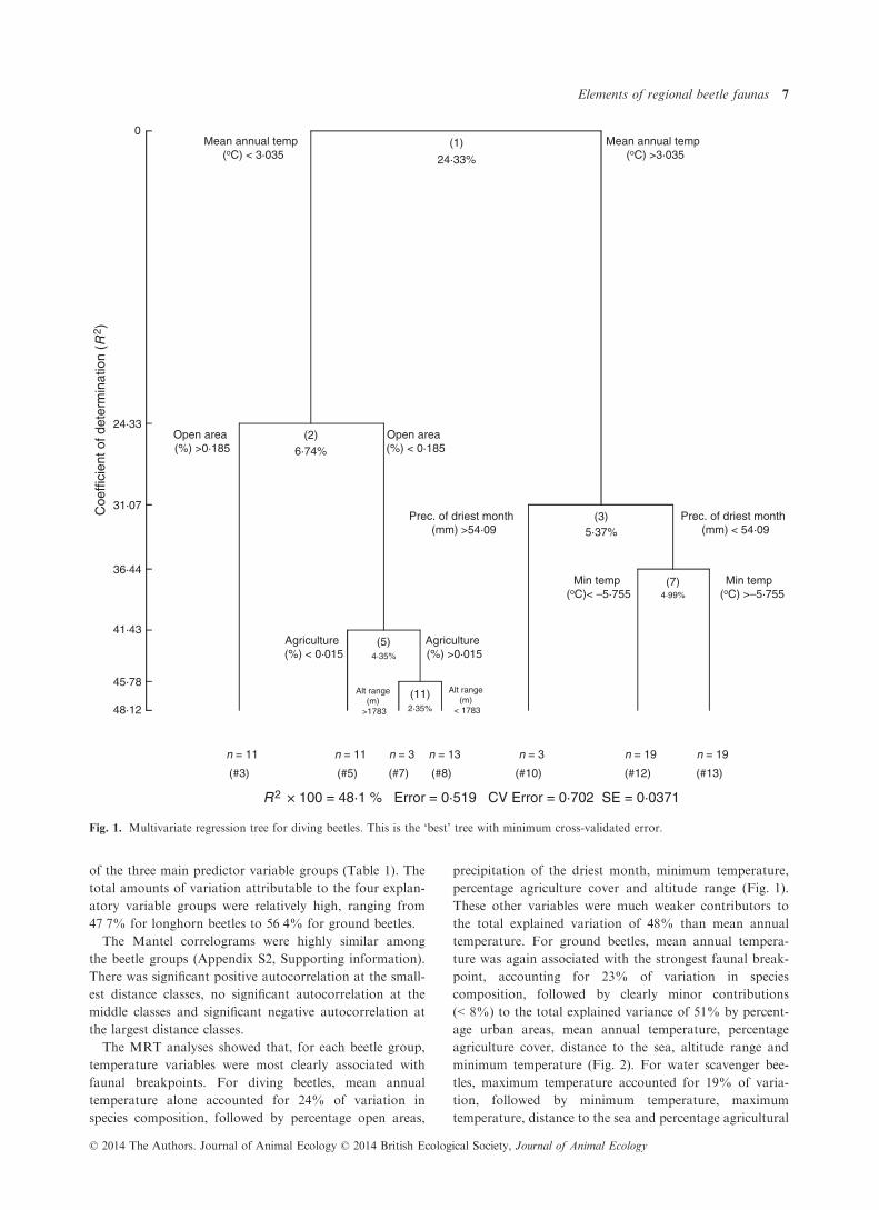
The MRT analyses showed that, for each beetle group,

temperature variables were most clearly associated with

faunal breakpoints. For diving beetles, mean annual

temperature alone accounted for 24% of variation in

species composition, followed by percentage open areas,

precipitation of the driest month, minimum temperature,

percentage agriculture cover and altitude range (Fig. 1).

These other variables were much weaker contributors to

the total explained variation of 48% than mean annual

temperature. For ground beetles, mean annual tempera-

ture was again associated with the strongest faunal break-

point, accounting for 23% of variation in species

composition, followed by clearly minor contributions

(< 8%) to the total explained variance of 51% by percent-

age urban areas, mean annual temperature, percentage

agriculture cover, distance to the sea, altitude range and

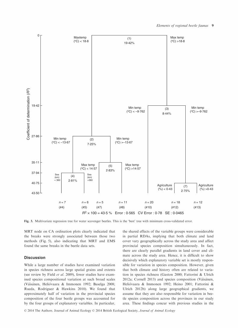
minimum temperature (Fig. 2). For water scavenger bee-

tles, maximum temperature accounted for 19% of varia-

tion, followed by minimum temperature, maximum

temperature, distance to the sea and percentage agricultural

Coe

ffici

ent o

f det

erm

inat

ion

(R2 )

48·12

45·78

41·43

36·44

31·07

24·33

0(1)

24·33%

Mean annual temp (oC) < 3·035

Mean annual temp (oC) >3·035

(2)6·74%

Open area (%) >0·185

Open area(%) < 0·185

n = 11

(#3)

(5)4·35%

Agriculture(%) < 0·015

Agriculture(%) >0·015

n = 11

(#5)

(11)2·35%

Alt range(m)

>1783

Alt range(m)

< 1783

n = 3

(#7)

n = 13

(#8)

(3)5·37%

Prec. of driest month (mm) >54·09

Prec. of driest month(mm) < 54·09

n = 3

(#10)

(7)4·99%

Min temp(oC)< –5·755

Min temp(oC) >–5·755

n = 19

(#12)

n = 19

(#13)

R2 × 100 = 48·1 % Error = 0·519 CV Error = 0·702 SE = 0·0371

Fig. 1. Multivariate regression tree for diving beetles. This is the ‘best’ tree with minimum cross-validated error.



cover (Fig. 3). These variables explained 43% of variation

in species composition. For longhorn beetles, minimum

temperature alone accounted for 21% of variation in spe-

cies composition, followed by percentage forest cover, per-

centage urban land cover, maximum temperature and

distance to the sea (Fig. 4). These variables accounted for a

total of 41% of variation in species composition. The

results of the MRT analyses remained largely the same

when latitude and longitude were included in the set of the

explanatory variables. Their inclusion did not significantly

increase the explanatory power of the MRTs, and they

appeared only in the lower nodes of the trees (results not

shown).

The EMS analysis indicated that each beetle group

showed (i) positive coherence (i.e. the number of embed-

ded absences was lower than expected by chance), (ii)

more turnover than expected by chance (i.e. the number

of replacements was higher than expected by chance) and

(iii) significantly higher boundary clumping than 1 (i.e.

based on Morisita’s I) (Table 2). The same result held

true for both fixed-equiprobable and fixed–fixed null mod-

els. These findings indicated that the beetle faunas fitted

best with Clementsian gradients along the primary axis of

variation in provincial species composition.

The groupings based on the MRTs and k-means parti-

tioning were very similar, and significant chi-square tests

strengthened this conclusion (Table 3). This result held

with both distance transformations of species data that

were used as the basis of k-means partitioning. Chi-square

tests also indicated that the breakpoints at the first MRT

node were highly similar between the beetle groups

(Table 4; see also Appendices S3 and S4, Supporting

information), and the same was true for k-means clusters

(Table 4). Finally, plotting the two groups of the first

Coe

ffici

ent o

f det

erm

inat

ion

(R2 )

51·61

49·71

47·29

44·39

41·25

37·71

31·4

23·61

0(1)

23·61%

Mean annual temp(oC)< 3·395

Mean annual temp(oC) >3·395

(2)

7·79%

Urban(%) < 0·005

Urban(%) >0·005

(4)3·54%



n = 3

(#7)

(8)3·14%

Sea(km)

< 334·5

Sea(km)

>334·5

n = 8

(#5)

n = 10

(#6)

(5)2·90%

Altrange(m) < 938·2

Altrange(m) >938·2

n = 12

(#9)

n = 7

(#10)

(3)

6·31%

Mean annual temp(oC) < 7·015

Mean annual temp(oC) >7·015

n = 16

(#17)

(6)2·42%

Altrange(m) >1099

Altrange(m) < 1099

n = 3

(#13)

(13)1·90%

Min temp (C)< –8·668

Mintemp (C) >–8·668

n = 8

(#15)

n = 12

(#16)

R 2 × 100 = 51·6 % Error = 0·484 CV Error = 0·716 SE = 0·0338

Fig. 2. Multivariate regression tree for ground beetles. This is the ‘best’ tree with minimum cross-validated error.



MRT node on CA ordination plots clearly indicated that

the breaks were strongly associated between those two

methods (Fig. 5), also indicating that MRT and EMS

found the same breaks in the beetle data sets.

Discussion

While a large number of studies have examined variation

in species richness across large spatial grains and extents

(see review by Field et al. 2009), fewer studies have exam-

ined species compositional variation at such broad scales

(V€ais€anen, Heli€ovaara & Immonen 1992; Baselga 2008;

Rueda, Rodriguez & Hawkins 2010). We found that

approximately half of variation in the provincial species

composition of the four beetle groups was accounted for

by the four groups of explanatory variables. In particular,

the shared effects of the variable groups were considerable

in partial RDAs, implying that both climate and land

cover vary geographically across the study area and affect

provincial species composition simultaneously. In fact,

there are clearly parallel gradients in land cover and cli-

mate across the study area. Hence, it is difficult to show

decisively which explanatory variable set is mostly respon-

sible for variation in species composition. However, given

that both climate and history often are related to varia-

tion in species richness (Gaston 2000; Fattorini & Ulrich

2012a; Cornell 2013) and species composition (V€ais€anen,

Heli€ovaara & Immonen 1992; Heino 2001; Fattorini &

Ulrich 2012b) along large geographical gradients, we

assume that they are also responsible for variation in bee-

tle species composition across the provinces in our study

area. These findings concur with previous studies in the

Coe

ffici

ent o

f det

erm

inat

ion

(R2 )

43·50

40·75

37·94

35·11

27·86

19·42

0(1)

19·42%

Maxtemp (oC) < 18·8

Max temp(oC) >18·8

(2)

7·25%

Min temp (oC) < –13·67

Min temp (oC) >–13·67

(4)

2·81%

Sea (km) < 360

Sea (km)>360

n = 7

(#4)

n = 6

(#5)

(5)

2·83%

Max temp(oC) < 14·57

Max temp(oC) >14·57

n = 5

(#7)

n = 11

(#8)

(3)

8·44%

Min temp (oC) < –9·762

Min temp (oC) >–9·762

n = 20

(#10)

(7)

2·75%



n = 18

(#12)

n = 12

(#13)

R2 × 100 = 43·5 % Error : 0·565 CV Error : 0·78 SE : 0·0465

Fig. 3. Multivariate regression tree for water scavenger beetles. This is the ‘best’ tree with minimum cross-validated error.



same area, which have suggested the influences of climate

on the regionalisation of various animal and plant groups

(Lahti, Kurtto & V€ais€anen 1988; V€ais€anen, Heli€ovaara &

Immonen 1992; Heino 2001). Our findings are also similar

to those at a broader spatial scale across Europe, where

climatic and historical factors were important in determin-

ing species richness, endemism and composition of regio-

nal faunas of longhorn beetles (Baselga 2008) and

darkling beetles (Fattorini & Baselga 2012). In contrast,

the degree to which land cover affected species composi-

tion is more difficult to infer. We could expect that if land

cover was important, we would have seen differences in

the particular land cover variables between aquatic and

terrestrial beetles. This was not the case, however, and

generally the same land cover variables appeared in the

final constrained ordination models.

There was significant positive autocorrelation at the

smallest distance classes and significant negative autocor-

relation at the largest distance classes in all beetle groups.

This finding suggests (i) that contiguous provinces have

similar species composition, as a consequence of the fact

that that neighbouring provinces share similar environ-

mental conditions and (ii) that provinces far from each

other have increasingly dissimilar faunas, suggesting that

climatic differences between provinces increase faunal dif-

ferences. Thus, it can be assumed that due to their cli-

matic similarities or differences, significant spatial

autocorrelation results from climate forcing on species

41·49

38·38

34·12

27·73

21·06

0(1)

21·06%

Min temp(oC) < –8·59

Min temp(oC) >–8·59

(2)

6·39%

Urban(%) < 0·005

Urban(%) >0·005

n = 26

(#6)

(4)

3·11%

Sea (km)

< 334·5

Sea(km)

>334·5

n = 9

(#4)

n = 10

(#5)

(3)

6·66%

Forests(%) < 0·12

Forests(%) >0·12

n = 11

(#8)

(7)

4·25%

Max temp(oC) < 15·64

Max temp(oC) >15·64

n = 5

(#10)

n = 18

(#11)

R2 × 100 = 41·5 % Error : 0·585 CV Error : 0·762 SE : 0·0379

Coe

ffici

ent o

f det

erm

inat

ion

(R2 )

Fig. 4. Multivariate regression tree for longhorn beetles. This is the ‘best’ tree with minimum cross-validated error.



ranges. However, significant negative autocorrelation may

also suggest that provinces that are geographically far

from each other are differently affected by historical fac-

tors (Brown & Lomolino 1998; Baselga 2008). For exam-

ple, most of our study region was covered by ice sheets

until about 10 000 years ago, and biotas have hence colo-

nized this region relatively recently (V€ais€anen, Heli€ovaara

& Immonen 1992; Heino 2001). Thus, it is possible that

(i) different species have colonized the region using differ-

ent dispersal routes, (ii) this region is still under coloniza-

tion, and (iii) climate change or land use alteration leads

to increasing ranges of some species, reduces the ranges of

some others and perhaps will lead to new faunal associa-

tions. Historical and climatic factors may not only lead to

continuous variation in faunal composition, but also con-

tribute to more abrupt changes in faunal characteristics.

Breakpoints in faunal composition were most strongly

related to climate. This finding was evidenced by the fact

that the first division of the faunal composition of each bee-

tle group was always related to temperature variables even

when latitude and longitude were included in the set of con-

straining variables. The temperature variables accounted

for about half of the total variation explained by the multi-

variate regression trees for each beetle group, whereas the

remaining land cover and climate variables alone accounted

for considerably less variation in faunal composition. These

findings suggest that if faunal breakpoints exist at large spa-

tial scales, they are first and foremost determined by cli-

matic conditions. Whether or not climatic factors vary

continuously or show clear breakpoints themselves across

Table 3. Comparisons between the multivariate regression tree

(MRT) and k-means classifications for each beetle group. Shown

are the results of v2-tests of the match between two MRT groups at

the first node and two k-means groups. Also shown are the results

of v2-tests of the match between MRT final leaves and k-means

partitioning based on the corresponding number of groups. K-

means partitioning was based on data transformed using either

Hellinger transformation or chi-square transformation

No.

groups

K-means with transformed species

data

Hellinger Chi-square

v2 P v2 P

MRT first node

Diving beetles 2 13�70 < 0�001 60�26 < 0�001Ground beetles 2 48�57 < 0�001 48�57 < 0�001Scavenger beetles 2 53�52 < 0�001 53�52 < 0�001Longhorn beetles 2 71�05 < 0�001 71�05 < 0�001

MRT final leaves

Diving beetles 7 246�46 < 0�001 289�57 < 0�001Ground beetles 9 363�04 < 0�001 358�93 < 0�001Scavenger beetles 7 283�37 < 0�001 205�40 < 0�001Longhorn beetles 6 229�09 < 0�001 196�74 < 0�001

Table 2. Results of the ‘elements of metacommunity structure’ analysis of patterns in provincial species composition. All analyses on the

first correspondence analysis axis based on each null model point strongly towards Clementsian gradients

Null model

Coherence Turnover Boundary clumping

Abs Z-value P-value

Sim

mean

Sim

SD Rep Z-value P-value

Sim

mean

Sim

SD Index P-value d.f.

Fixed-Equiprobable

Diving beetles 3234 �26�71 0�001 5475 83 746 882 69�67 0�001 26 020 10 346 2�45 <0�001 152

Ground beetles 8438 �31�21 0�001 16 406 255 4 282 211 65�50 0�001 168 758 62 794 2�85 <0�001 385

Scavenger beetles 2224 �21�85 0�001 4405 99 343 100 24�87 0�001 30 648 12 560 8�28 <0�001 113

Longhorn beetles 2875 �15�55 0�001 4833 125 420 386 19�34 0�001 49 674 19 159 4�43 <0�001 115

Fixed–FixedDiving beetles 3234 �18�43 0�001 5102 101 746 882 55�24 0�001 12 671 13 290 2�45 <0�001 152

Ground beetles 8438 �22�31 0�001 14 113 254 4 282 211 50�38 0�001 92 286 83 159 2�85 <0�001 385

Scavenger beetles 2224 �8�89 0�001 3262 116 343 100 69�20 0�001 1451 4936 8�28 <0�001 113

Longhorn beetles 2875 �8�20 0�001 3989 135 420 386 20�73 0�001 13 346 19 633 4�43 <0�001 115

Z-value, (Observed index value-Simulated mean)/Simulated SD; Abs, number of embedded absences; Rep, number of replacements; Sim

mean, average of simulated index values; Sim SD, standard deviation of simulated index values.

Table 4. Comparisons of the match of classifications between the

beetle groups at the first node of multivariate regression tree (a)

and between the beetle groups for the two k-means clusters based

on Hellinger (b) or chi-square (c) transformation of species data.

The v2 values are shown below the diagonal, and the P-values

are above the diagonal

Diving

beetles

Ground

beetles

Scavenger

beetles

Longhorn

beetles

(a) v2 or PDiving beetles – <0�001 <0�001 <0�001Ground beetles 67�49 – <0�001 <0�001Scavenger beetles 31�69 24�88 – 0�005Longhorn beetles 36�89 39�25 9�33 –

(b) v2 or PDiving beetles – <0�001 <0�001 0�012Ground beetles 13�54 – <0�001 <0�001Scavenger beetles 13�52 56�42 – <0�001Longhorn beetles 7�27 24�86 12�27 –

(c) v2 Or P

Diving beetles – <0�001 <0�001 <0�001Ground beetles 61�06 – <0�001 <0�001Scavenger beetles 60�47 56�42 – <0�001Longhorn beetles 20�42 24�86 12�27 –



large spatial scales is open to debate, but maps show clear

temperature variation across the study area (Appendix S3,

Supporting information). It has to be highlighted, however,

that multivariate regression trees indicate the existence of a

breakpoint even in continuous data (De’ath 2002; Borcard,

Gillet & Legendre 2011), emphasizing the need to supple-

ment ecological inferences by means of other data analyses.

The breakpoints in faunal variation are also supported

by the distributions of single species of beetles across the

study area. There are some northern species, occurring

north of approximately 65°N in Finland, Sweden and Nor-

way, and larger numbers of southern species, occurring

south of approximately 58°N in Denmark and southern-

most Sweden (Lindroth 1985; Holmen 1987; Bily & Mehl

1989; Nilsson & Holmen 1995). Thus, despite the fact that

the ranges of most species in the study area are inclined

towards south and that there is a latitudinal gradient in

species richness (Lindroth 1985; V€ais€anen & Heli€ovaara

1994), the compositional gradients of beetles are more com-

plex than a clear latitudinal cline often detected in species

richness (Baselga 2008; Fattorini & Ulrich 2012b). Such

compositional gradients may again be caused by certain

sets of species responding to climatic conditions in a similar

manner or that there are groups of species that have colo-

nized the study area using the same dispersal routes.

The finding that patterns of faunal composition best fit-

ted Clementsian gradients also suggested clear breakpoints

in species composition. This finding is intuitive, given that

there are these southern and northern faunal elements in

the study area. The idea of Clementsian gradients suggests

that there are two or more groups of species showing simi-

lar responses to the environment and that the responses dif-

fer among the groups (Clements 1916; Allen & Hoekstra

1992). Most studies testing this idea have considered local

CA1 (EV = 0·284)

CA

2 (E

V =

0·1

20)

+

++

+

+++

+

++

+

++++

+

+

+++

+

+

+

++

+

+

++ ++++++

+

+

+

+

+++

+

+

+ +++

+

+

+++

+

+

++

+

+

+

+

++ +

+

+

+

+

++

+

+

+

+

+++

+

+

++

++

+

+

+

+

+++

+

+

+

++

++

+

+

+

+

+

+

++

+

+

+

+

+

+

+ +

++

+

++

CA1 (EV = 0·248)

CA

2 (E

V =

0·1

01)

++

+

+

+

+

+

+

+

++

+++

++

++

+

++

+

+

++

+

+

+++ +

+

+++

+

+

+

+

++

+

+

+ +

++

+

++

+

+

+

++ ++++ +++

+++ ++

++ + ++ +++

+

++

+++

+ ++

+

+ +

+

+

++

+

++++

+

+

+

++

++

+

++ +++

++

++++

+

+

CA

2 (E

V =

0·1

24) + +

++

+ ++

+

+

+

++

+

+++

+

+

+++

+

+

++

+

+ ++

+

++ ++

+

+

++

++

++

+

+ ++

+

+

+++++

+

+

+

+

++

+

+

+

+

++

+

+

+

+

++

+

++

++

+

+++

++ +

+

+++

+

+

+

+

+

+

+ ++

+ +

+

+

+

+

++

+

+

+ +

++

+

+

+

+

+

+

+

+

+

+

+

+

+

+++

+

+

++

+

++

+

+

++

+

+

+

+

+

+

+++

+

+

+

+

+

+

+

+

+

+

+

+

+

+

+ +

+

+

+

+

+

+

+

++

+

+

+

+

+

+++

+

+++

++

+++

+

+

++

++

+

+

+

++

+

++ ++++

+

+

+

+

++

+

+

++++

+

+

++ ++++

+

+

+

++

+ ++

+

+

+ +

+

+

++ +

+

+

++

+

+

+

+

+

+

+

++

+

+ +++

+

++ +

++

+

+

+

+

+

+

++

+

+

+

+

++

+

+

+

+

++

+

+

++

++

+

+

++ +

+++

+

+

++++

+

++

++

+

+

+

++

+

++ +

+

++

+

+

+

+

+

+

+

+

+

+

+

+

+

+

+

+

++

+

+++

+

+

+

+

+

+

+

+

+

+

+

+++

+

+

+

+

+

++

+

+

++

++

+

+

+ ++

+

+

+

++

+

++ +

–3 –2 –1 0 1 2 3

–2–1

01

23

–2 0 2 4 6

–5–4

–3–2

–10

1

–3 –2 –1 0 1 2

–3–2

–10

1

–2 –1 0 1 2

–2–1

01

CA1 (EV = 0·263) CA1 (EV = 0·302)

CA

2 (E

V =

0·0

79)

+

+

+

+

+

+

+

+ + ++

+

+

+

++

++

+

+

+++ +

+++

+

+

+

+

+

++

++

++

+

++

+++

+

+++

+

+

++

+

+

++

+

+

+++

+

+

+

+

+

++

+

+

+

+

+

+

+

+

+

+++ +

+

+

+

+

+

+

+

+

+

++

+

+

+

+

+

+

++

+

+

+

+

+

++

+

+

++

+

++++

+ +

+++

+

+

++

+++

+

+

+

+

+++

+

+++

+

+

+

+

++ ++

++

++

+

+

++

(a) (b)

(c) (d)

Mean oC < 3·03

Mean oC > 3·03

Mean oC < 3·39

Mean oC > 3·39

Max oC < 18·80

Max oC > 18·80

Min oC < –8·59

Min oC > –8·59

Fig. 5. Ordination plots from correspondence analysis (CA) of each beetle group, showing the scores of the provinces (open or filled cir-

cles) and species (crosses) along the first two CA axes. Particular attention should be given to CA axis 1. The values of environmental

variables associated with the breakpoints at the first node of the multivariate regression trees are shown in inserts. Shown are CA plots

for (a) diving beetles, (b) ground beetles, (c) water scavenger beetles and (d) longhorn beetles.



communities across landscapes or relatively small regions,

where environmental control typically accounts for such

species compositional gradients (Presley et al. 2009; Presley

& Willig 2010). However, at large grain sizes and spatial

extents, local environmental gradients are unlikely to

account for Clementsian gradients, but rather climate or

historical factors are more likely candidates for explaining

abrupt changes in faunal composition (L�opez-Gonz�alez

et al. 2012). Such abrupt changes may result from the fact

that large-scale studies cross multiple species pools that are

formed by either historical forces or climatic constraints or,

more likely, their joint effects on species ranges. Such

abrupt changes in faunal composition are even more likely

at broader spatial scales than that of our study, and the

very foundations of biogeographical regionalisation indeed

rest on the assumption of clearly definable geographical

areas harbouring species typical to each region in various

taxonomic groups (Brown & Lomolino 1998; Heikinheimo

et al. 2007; Rueda, Rodriguez & Hawkins 2010).

Geographical patterns in faunal composition were very

similar among ecologically disparate beetle taxa, as evi-

denced by RDA, spatial correlograms and multivariate

regression trees. Climate gradients, particularly those

related to temperature, also accounted for major faunal

breakpoints of beetles in the study area, suggesting that cli-

mate determines species broadscale distributions and leads

to clear groups of species responding similarly to environ-

mental gradients. The finding that the best idealized model

describing faunal variation across the provinces was ‘Clem-

entsian gradients’ also lent support for the existence of

groups of species having similar environmental relation-

ships. Given such close associations between faunal varia-

tion, faunal breakpoints and environmental conditions,

broadscale environmental factors and environmental diver-

sity (Faith 2003) may be used for preliminary regionalisa-

tion in the context of environmental assessment and

biodiversity studies in the present study area (Lahti, Kurtto

& V€ais€anen 1988; V€ais€anen, Heli€ovaara & Immonen 1992)

and possibly in other regions (Heikinheimo et al. 2007;

Rueda, Rodriguez & Hawkins 2010). The methodological

approaches we used in this study could hence be widely

applied in attempts to find abiotic proxy variables for

faunal and floral patterns. Such proxies for biogeographic

regionalisation may also be highly promising and cost-

effective means in regions where no appropriate data on

species distributions exist.

Acknowledgements

We thank the associate editor, two anonymous reviewers and Simone

Fattorini for excellent comments that greatly improved this paper. We also

thank Maija Lantto for keyboard work when compiling the biological

data. This study was supported by grants from the Academy of Finland.

Data accessibility

The biological data we used can be found entirely in the literature (Lind-

roth 1985, 1986; Holmen 1987; Bily & Mehl 1989; Nilsson & Holmen

1995), and the climate and land cover data are downloadable in the Inter-

net (Climate data: http://www.worldclim.org/; Land cover data: http://

www.eea.europa.eu/publications/COR0-landcover).

References

Allen, T.F.H. & Hoekstra, T.W. (1992) Toward a Unified Ecology. Colum-

bia University Press, New York.

Anderson, M.J. & Gribble, N.A. (1998) Partitioning the variation among

spatial, temporal and environmental components in a multivariate data

set. Australian Journal of Ecology, 23, 158–167.Anderson, M.J., Crist, T.O., Chase, J.M., Vellend, M., Inouye, B.D., Free-

stone, A.L. et al. (2011) Navigating the multiple meanings of b diver-

sity: a roadmap for the practicing ecologist. Ecology Letters, 14, 19–28.Bailey, R.G. (2010) Ecosystem Geography. From Ecoregions to Sites.

Springer, New York.

Baselga, A. (2008) Determinants of species richness, endemism and turn-

over in European longhorn beetles. Ecography, 31, 263–271.Bily, S. & Mehl, O. (1989) Longhorn beetles (Coleoptera, Cerambycidae) of

Fennoscandia and Denmark. Fauna Entomologica Scandinavica, 22, 1–203.Blanchet, F.G., Legendre, P. & Borcard, D. (2008) Forward selection of

explanatory variables. Ecology, 89, 2623–2632.Borcard, D., Gillet, F. & Legendre, P. (2011) Numerical Ecology with R.

Springer, New York.

Borcard, D. & Legendre, P. (2002) All-scale spatial analysis of ecological

data by means of principal coordinates of neighbour matrices. Ecologi-

cal Modelling, 153, 51–68.Borcard, D. & Legendre, P. (2012) Is the Mantel correlogram powerful

enough to be useful in ecological analysis? A simulation study. Ecology,

93, 1473–1481.Borcard, D., Legendre, P. & Drapeau, P. (1992) Partialling out the spatial

component of ecological variation. Ecology, 73, 1045–1055.Bradshaw, E.M. (2005) Mid-to late-Holocene land-use change and lake

development at Dallund S0, Denmark: synthesis of multiproxy data,

linking land and lake. The Holocene, 15, 1152–1162.Brown, J.H. & Lomolino, M.V. (1998) Biogeography, 2nd edn. Sinauer,

Sunderland, Massachusetts, USA.

Clements, F.E. (1916) Plant Succession. An Analysis of the Development of

Vegetation. Carnegie Institution, Washington, DC.

Cornell, H.V. (2013) Is regional species diversity bounded or unbounded?

Biological Reviews, 88, 140–165.Cottenie, K. (2005) Integrating environmental and spatial processes in

ecological community dynamics. Ecology Letters, 8, 1175–1182.Dallas, T. (2013) metacom: Analysis of the “elements of metacommunity

structure”. R package version 1.2. http://CRAN.R-project.org/pack-

age=metacom

Dallas, T. & Presley, S.J. (2014) Relative importance of host environment,

transmission potential and host phylogeny to the structure of parasite

metacommunities. Oikos, 123, 866–874.Davidson, T.A., Sayer, C.D., Perrow, M., Bramm, M. & Jeppesen, E.

(2010) The simultaneous inference of zooplanktivorous fish and macro-

phyte density from sub-fossil cladoceran assemblages: a multivariate

regression tree approach. Freshwater Biology, 55, 546–564.De’ath, G. (2002) Multivariate regression trees: a new technique for

modelling species-environment relationships. Ecology, 83, 1105–1111.Diamond, J.M. (1975) Assembly of species communities. Ecology and Evo-

lution of Communities (eds M.L. Cody & J.M. Diamond), pp. 342–444.Harvard University Press, Cambridge.

Dray, S., Legendre, P. & Peres-Neto, P.R. (2006) Spatial modelling: a

comprehensive framework for principal coordinate analysis of neigh-

bour matrices (PCNM). Ecological Modelling, 196, 483–493.Dray, S., P�elissier, R., Couteron, P., Fortin, M.J., Legendre, P., Peres--

Neto, P.R. et al. (2012) Community ecology in the age of multivariate

multiscale spatial analysis. Ecological Monographs, 82, 257–275.Elith, J. & Leathwick, J.R. (2009) Species Distribution Models: ecological

explanation and prediction across space and time. Annual Review of

Ecology, Evolution, and Systematics, 40, 677–697.Faith, D.P. (2003) Environmental diversity (ED) as surrogate information

for species-level biodiversity. Ecography, 26, 374–379.Fattorini, S. & Baselga, A. (2012) Species richness and turnover patterns

in European tenebrionid beetles. Insect Conservation and Diversity, 5,

331–345.Fattorini, S. & Ulrich, W. (2012a) Drivers of species richness in European

Tenebrionidae (Coleoptera). Acta Oecologica, 43, 22–28.



Fattorini, S. & Ulrich, W. (2012b) Spatial distributions of European Tene-

brionidae point to multiple postglacial colonization trajectories. Biologi-

cal Journal of the Linnean Society, 105, 318–329.Field, R., Hawkins, B.A., Cornell, H.V., Currie, D.J., Diniz-Filho, J.A.F.,

Guegan, J.-F. et al. (2009) Spatial species-richness gradients across

scales: a meta-analysis. Journal of Biogeography, 36, 132–147.Fox, J. (2005) The r commander: a basic statistics graphical user interface

to R. Journal of Statistical Software, 14, 1–42.Gaston, K.J. (2000) Global patterns in biodiversity. Nature, 405, 220–227.Gauch, H.G. (1982) Multivariate Analysis in Community Ecology. Cam-

bridge University Press, Cambridge.

Gleason, H.A. (1926) The individualistic concept of the plant association.

Bulletin of the Torrey Botanical Club, 53, 7–26.Gotelli, N.J. (2000) Null model analysis of species co-occurrence patterns.

Ecology, 81, 2606–2621.Gotelli, N.J. & Graves, G.R. (1996) Null Models in Ecology. Smithsonian

Institute Press, Washington.

Gotelli, N.J., Graves, G.R. & Rahbek, C. (2010) Macroecological signals

of species interactions in the Danish avifauna. Proceedings of the

National Academy of Sciences, 107, 530–535.Gotelli, N.J. & McCabe, D.J. (2002) Species coexistence: a meta-analysis

of J. M. Diamond’s assembly rules model. Ecology, 83, 2091–2096.G€otzenberger, L., de Bello, F., Br�athen, K.A., Davison, J., Dubuis, A.,

Guisan, A. et al. (2012) Ecological assembly rules in plant communities:

approaches, patterns and prospects. Biological Reviews, 87, 111–127.Griffith, D.A. & Peres-Neto, P.R. (2006) Spatial modeling in ecology: the

flexibility of eigenfunction spatial analyses. Ecology, 87, 2603–2613.Heikinheimo, H., Fortelius, M., Eronen, J. & Mannila, H. (2007) Biogeog-

raphy of European land mammals shows environmentally distinct and

spatially coherent clusters. Journal of Biogeography, 34, 1053–1064.Heino, J. (2001) Regional gradient analysis of freshwater biota: do similar

biogeographic patterns exist among multiple taxonomic groups? Journal

of Biogeography, 28, 69–77.Heino, J. (2011) A macroecological perspective of diversity patterns in the

freshwater realm. Freshwater Biology, 56, 1703–1722.Heino, J., Ilmonen, J. & Paasivirta, L. (2014) Continuous variation of

macroinvertebrate communities along environmental gradients in north-

ern streams. Boreal Environment Research, 19, 21–38.Henriques-Silva, R., Lindo, Z. & Peres-Neto, P.R. (2013) A community of

metacommunities: exploring pattern in species distributions across large

geographical scales. Ecology, 94, 627–639.Hijmans, R.J., Cameron, S.E., Parra, J.L., Jones, P.G. & Jarvis, A. (2005)

Very high resolution interpolated climate surfaces for global land areas.

International Journal of Climatology, 25, 1965–1978.Hoagland, B.W. & Collins, S.L. (1997) Gradient models, gradient analysis,

and hierarchical structure in plant communities. Oikos, 78, 23–30.Holm, S. (1979) A simple sequentially rejective multiple test procedure.

Scandinavian Journal of Statistics, 6, 65–70.Holmen, M. (1987) The Hydrophiloidea (Coleoptera) of Fennoscandia

and Denmark. Fauna Entomologica Scandinavica, 18, 1–254.Hothorn, T., Hornik, K., van de Wiel, M.A. & Zeileis, A. (2008) Imple-

menting a class of permutation tests: the coin package. Journal of

Statistical Software, 28, 1–23.Lahti, T., Kurtto, A. & V€ais€anen, R.A. (1988) Floristic composition and

regional species richness of vascular plants in Finland. Annales Botanici

Fennici, 25, 281–291.Legendre, P. & Gallagher, E.D. (2001) Ecologically meaningful transfor-

mations for ordination of species data. Oecologia, 129, 271–280.Legendre, P. & Legendre, L. (2012) Numerical Ecology, 3rd edn. Elsevier,

Amsterdam.

Legendre, P., Borcard, D., Blanchet, F.G. & Dray, S. (2013) PCNM:

MEM spatial eigenfunction and principal coordinate analyses. R pack-

age version 2.1-2/r109. http://R-Forge.R-project.org/projects/sedar/

Leibold, M.A. & Mikkelson, G.M. (2002) Coherence, species turnover,

and boundary clumping: elements of metacommunity structure. Oikos,

97, 237–250.van der Linden, M., Barke, J., Vickery, E., Charman, D.J. & van Geel, B.

(2008) Late Holocene human impact and climate change recorded in a

North Swedish peat deposit. Palaeogeography, Palaeoclimatology, Palae-

oecology, 258, 1–27.Lindroth, C.H. (1985) The Carabidae (Coleoptera) of Fennoscandia and

Denmark. Fauna Entomologica Scandinavica, 15, 1–225.Lindroth, C.H. (1986) The Carabidae (Coleoptera) of Fennoscandia and

Denmark. Fauna Entomologica Scandinavica, 15, 226–497.

McIntosh, R.P. (1995) H. A. Gleason’s “individualistic community

concept” and theory of animal communities: a continuing controversy.

Biological Reviews, 70, 317–357.Meynard, C.N., Lavergen, S., Boulangeat, I., Garraud, L., Van Es, J.,

Mouquet, N. et al. (2013) Disentangling the drivers of metacommuni-

ty structure across spatial scales. Journal of Biogeography, 40, 1560–1571.

Mittelbach, G.G. (2012) Community Ecology. Sinauer, Sunderland, Massa-

chusetts, USA.

Nilsson, A.N. & Holmen, M. (1995) The aquatic adephaga of Fennoscan-

dia and Denmark 2, Dytiscidae. Fauna Entomologica Scandinavica, 32,

1–188.Oksanen, J., Blanchet, F.G., Kindt, R., Legendre, P., Minchin, P.R.,

O’Hara, R.B. et al. (2013) vegan: Community Ecology Package. R

package version 2.0-9. http://CRAN.R-project.org/package=vegan.

Ouellette, M.-H. & Legendre, P. (2013) MVPARTwrap: Additional func-

tionalities for package mvpart. R package version 0.1-9.2. http://

CRAN.Rproject.org/package=MVPARTwrap.

Patterson, B.D. & Atmar, W. (1986) Nested subsets and the structure of

insular mammal faunas and archipelagos. Biological Journal of the Lin-

nean Society, 28, 65–82.Peres-Neto, P.R. & Legendre, P. (2010) Estimating and controlling for

spatial structure in the study of ecological communities. Global Ecology

and Biogeography, 19, 174–184.Peres-Neto, P.R., Leibold, M.A. & Dray, S. (2012) Assessing the effects of

spatial contingency and environmental filtering on metacommunity phy-

logenetics. Ecology, 93, 14–30.Peres-Neto, P.R., Legendre, P., Dray, S. & Borcard, D. (2006) Variation

partitioning of species data matrices: estimation and comparison of frac-

tions. Ecology, 87, 2614–2625.Presley, S.J., Higgins, C.L. & Willig, M.R. (2010) A comprehensive frame-

work for the evaluation for metacommunity structure. Oikos, 119,

908–917.Presley, S.J. & Willig, M.R. (2010) Bat metacommunity structure on

Caribbean islands and the role of endemics. Global Ecology and Bioge-

ography, 19, 185–199.Presley, S.J., Higgins, C.L., L�opez-Gonz�alex, C. & Stevens, R.D. (2009)

Elements of metacommunity structure of Paraguayan bats: multiple

gradients require analysis of multiple ordination axes. Oecologia, 160,

781–793.R Core Team (2013) R: A Language and Environment for Statistical Com-

puting. R Foundation for Statistical Computing, Vienna. http://www.

R-project.org/.

Rao, C.R. (1964) The use and interpretation of principal component

analysis in applied research. Sankhy�a: The Indian Journal of Statistics,

Series A, 26, 329–358.Rueda, M., Rodriguez, M.A. & Hawkins, B.A. (2010) Towards a biogeo-

graphic regionalization of the European biota. Journal of Biogeography,

37, 2067–2076.Sahuquillo, M. & Miracle, M.R. (2013) The role of historic and climatic

factors in the distribution of crustacean communities in Iberian Medi-

terranean ponds. Freshwater Biology, 58, 1251–1266.de la Sancha, N., Higgins, C.L., Presley, S.J. & Strauss, R.E. (2014) Meta-

community structure in a highly fragmented forest: has deforestation in

the Atlantic Forest altered historic biogeographic patterns? Diversity

and Distributions, 20, 1058–1070.Sokal, R.R. & Oden, N.L. (1978) Spatial autocorrelation in biology. 1.

Methodology. Biological Journal of the Linnean Society, 10, 199–228.Tilman, D. (1982) Resource Competition and Community Structure. Prince-

ton University Press, Princeton, New Jersey, USA.

Ulrich, W. & Gotelli, N.J. (2013) Pattern detection in null model analysis.

Oikos, 122, 2–18.V€ais€anen, R. & Heli€ovaara, K. (1994) Hot-spots of insect diversity in

northern Europe. Annales Zoologici Fennici, 31, 71–81.V€ais€anen, R., Heli€ovaara, K. & Immonen, A. (1992) Biogeography of

northern European insects: province records in multivariate analysis

(Saltatoria, Lepidoptera: Sesiidae; Coleoptera: Bubrestidae, Cerambyci-

dae). Annales Zoologici Fennici, 28, 57–81.Wright, D.H., Patterson, B.D., Mikkelson, G.M., Cutler, A. & Atmar, W.

(1998) A comparative analysis of nested subset patterns of species com-

position. Oecologia, 113, 1–20.

Received 2 May 2014; accepted 30 August 2014

Handling Editor: Frank Johansson



Supporting Information

Additional Supporting Information may be found in the online version

of this article.

Appendix S1. The predictor variables selected in the forward

selection of each variable group for each beetle group.

Appendix S2. A Mantel correlogram for each beetle group.

Appendix S3. Temperature maps of northern Europe.

Appendix S4. Province groupings for each beetle group based on

the multivariate regression trees (MRT) analysis.



Elements of regional beetle faunas: faunal variation and compositional breakpoints along climate,...

Documents

Transcript of Elements of regional beetle faunas: faunal variation and compositional breakpoints along climate,...