Estimating Peer Effects Using Partial Network Data

Estimating Peer Effects Using Partial Network Data

Vincent Boucher∗ and Aristide Houndetoungan†

April 2020

Abstract

We study the estimation of peer effects through social networks when researchers do not observethe network structure. Instead, we assume that researchers know (have a consistent estimate of)the distribution of the network. We show that this assumption is sufficient for the estimation ofpeer effects using a linear-in-means model. We present and discuss important examples whereour methodology can be applied. In particular, we provide an empirical application to the studyof peer effects on students’ academic achievement.

JEL Codes: C31, C36, C51Keywords: Social networks, Peer effects, Missing variables, Measurement errors

∗Corresponding author. Department of Economics, Université Laval, CRREP and CREATE;email: [email protected]†Department of Economics, Université Laval, CRREP; email: [email protected]

We would like to thank Bernard Fortin for his helpful comments and insights, as always. We wouldalso like to thank Eric Auerbach, Yann Bramoullé, Arnaud Dufays, Stephen Gordon, Chih-Sheng Hsieh,Arthur Lewbel, Tyler McCormick, Angelo Mele, Onur Özgür, Eleonora Patacchini, Xun Tang, and YvesZenou for helpful comments and discussions. Thank you also to the participants of the Applied/CDESseminar at Monash University, the Economic seminar at the Melbourne Business School, the Econo-metric workshop at the Chinese University of Hong Kong, and the Centre of Research in the Economicsof Development workshop at the Université de Namur.

This research uses data from Add Health, a program directed by Kathleen Mullan Harris and designedby J. Richard Udry, Peter S. Bearman, and Kathleen Mullan Harris at the University of North Carolinaat Chapel Hill, and funded by Grant P01-HD31921 from the Eunice Kennedy Shriver National Instituteof Child Health and Human Development, with cooperative funding from 23 other federal agenciesand foundations. Special acknowledgment is given to Ronald R. Rindfuss and Barbara Entwisle forassistance in the original design. Information on how to obtain Add Health data files is available onthe Add Health website (http://www.cpc.unc.edu/addhealth). No direct support was received fromGrant P01-HD31921 for this research.

http://www.cpc.unc.edu/addhealth

1 Introduction

There is a large and growing literature on the impact of peer effects in social networks.1 However

eliciting network data is expensive (Breza et al., 2017), and since networks must be sampled

completely (Chandrasekhar and Lewis, 2011), there are few existing data sets that contain

detailed network information.

In this paper, we explore the estimation of the widely used linear-in-means model (e.g.

Manski (1993), Bramoullé et al. (2009)) when the researcher does not observe the entire network

structure. Specifically, we assume that the researcher knows the distribution of the network but

not necessarily the network itself. An important example is when a researcher is able to estimate

a network formation model using some partial information about the network structure (e.g.

Breza et al. (2017)). Other examples are when the researcher observes the network with noise

(e.g. Hardy et al. (2019)) or only observes a subsample of the network (e.g. Chandrasekhar and

Lewis (2011)).

We present an instrumental variable estimator and show that we can adapt the strategy

proposed by Bramoullé et al. (2009), which uses instruments constructed using the powers of

the interaction matrix. Specifically, we use two different draws from the distribution of the

network. One draw is used to approximate the endogenous explanatory variable, while the

other is used to construct the instruments.

We show that since the true networks and the two approximations are drawn from the same

distribution, the instruments are uncorrelated with the approximation error and are therefore

valid. We explore the properties of the estimator using Monte Carlo simulations. We show that

the method performs well, even when the distribution of the network is diffuse and when we

allow for group-level fixed effects.

We also present a Bayesian estimator. The estimator imposes more structure but allows cover

cases for which the instrumental variable strategy fails.2 Our estimator is general enough that it

can be applied to many peer-effect models having misspecified networks (e.g. Chandrasekhar and

Lewis (2011), Hardy et al. (2019), or Griffith (2019)). The approach relies on data augmentation

(Tanner and Wong, 1987). The assumed distribution for the network acts as a prior distribution,

and the inferred network structure is updated through the Markov chain Monte Carlo (MCMC)

algorithm.1For recent reviews, see Boucher and Fortin (2016), Bramoullé et al. (2019), Breza (2016), and De Paula

(2017).2We also provide a classical version of the estimator (using an expectation maximization algorithm) in Ap-

pendix 9.6, which is similar to the strategies used by Griffith (2018) and Hardy et al. (2019).

1

We present numerous examples of settings in which our estimators are implementable. In

particular, we present an implementation of our instrumental variable estimator using the net-

work formation model developed by Breza et al. (2017). We show that the method performs

very well. We also show that the recent estimator proposed by Alidaee et al. (2020) works well

but is less precise.

We also present an empirical application. We explore the impact of errors in the observed

networks using data on adolescents’ friendship networks. We show that the widely used Add

Health database features many missing links: only 70% of the total number of links are observed.

We estimate a model of peer effects on students’ academic achievement. We show that our

Bayesian estimator reconstructs these missing links and obtains a valid estimate of peer effects.

In particular, we show that disregarding missing links underestimates the endogenous peer effect

on academic achievement.

This paper contributes to the recent literature on the estimation of peer effects when the

network is either not entirely observed or observed with noise. Chandrasekhar and Lewis (2011)

show that models estimated using sampled networks are generally biased. They propose an

analytical correction as well as a two-step general method of moment (GMM) estimator. Liu

(2013) shows that when the interaction matrix is not row-normalized, instrumental variable

estimators based on an out-degree distribution are valid, even with sampled networks. Relatedly,

Hsieh et al. (2018) focus on a regression model that depends on global network statistics. They

propose analytical corrections to account for non-random sampling of the network (see also Chen

et al. (2013)).

Hardy et al. (2019) look at the estimation of (discrete) treatment effects when the network

is observed noisily. Specifically, they assume that observed links are affected by iid errors and

present an expectation maximization (EM) algorithm that allows for a consistent estimate of

the treatment effect. Griffith (2018) also presents an EM algorithm to impute missing network

data. Griffith (2019) explores the impact of imposing an upper bound to the number of links

when eliciting network data. He shows, analytically and through simulations, that these bounds

may bias the estimates significantly.

Relatedly, some papers derive conditions under which peer effects can be identified even

without any network data. De Paula et al. (2018a) and Manresa (2016) use panel data and

present models of peer effect having an unknown network structure. Both approaches require

observing a large number of periods and some degree of sparsity for the interaction network.

De Paula et al. (2018a) prove a global identification result and estimate their model using an

2

adaptive elastic net estimator, while Manresa (2016) uses a lasso estimator, while assuming no

endogenous effect and deriving its explicit asymptotic properties.

Souza (2014) studies the estimation of a linear-in-means model when the network is not

known. He presents a pseudo-likelihood model in which the true (unobserved) network is re-

placed by its expected value, given a parametric network formation model. He formally derives

the identified set and applies his methodology to study the spillover effects of a randomized

intervention.

Thirkettle (2019) focuses on the estimation of a given network statistic (e.g. some centrality

measure), assuming that the researcher only observes a random sample of links. Using a struc-

tural network formation model, he derives bounds on the identified set for both the network

formation model and the network statistic of interest. Lewbel et al. (2019) use a similar strat-

egy but focus on the estimation of a linear-in-means model and assume a network formation

model having conditionally independent linking probabilities. They show that their estimator

is point-identified given some exclusion restrictions.

We contribute to the literature by proposing two estimators for the linear-in-means model,

in a cross-sectional setting, when the econometrician does not know the true social network but

rather knows the distribution of true network. Our estimators are both simple to implement and

flexible. In particular, they can be used when network formation models can be estimated given

only limited network information (e.g. Breza et al. (2017) or Graham (2017)) or when networks

are observed imperfectly (e.g. Chandrasekhar and Lewis (2011), Griffith (2019), or Hardy et al.

(2019)). We show that having partial information about network structure (as opposed to no

information) allows the development of flexible and easily implementable estimators. Finally,

we also present an easy-to-use R package—named PartialNetwork—for implementing our es-

timators and examples, including the estimator proposed by Breza et al. (2017). The package

is available online at: https://github.com/ahoundetoungan/PartialNetwork.

The remainder of the paper is organized as follows. In Section 2, we present the econometric

model as well as the main assumptions. In Section 3, we present an instrumental variable

estimator. In Section 4, we present our Bayesian estimation strategy. In Section 5, we present

important economic contexts in which our method is implementable. In Section 6, we present

an empirical application in which the network is only partly observed. Section 7 concludes with

a discussion of the main results, limits, and challenges for future research.

3

https://github.com/ahoundetoungan/PartialNetwork

2 The Linear-in-Means Model

Let A represent the N × N adjacency matrix of the network. We assume a directed network:

aij ∈ 0, 1, where aij = 1 if i is linked to j. We normalize aii = 0 for all i and let ni =∑j

aij

denote the number of links of i. Let G = f(A), the N ×N interaction matrix for some function

f . Unless otherwise stated, we assume that G is a row-normalization of the adjacency matrix

A.3 Our results extend to alternative specifications of f .

We focus on the following model:

y = c1 + Xβ + αGy + GXγ + ε, (1)

where y is a vector of an outcome of interest (e.g. academic achievement), c is a constant,

X is a matrix of observable characteristics (e.g. age, gender...), and ε is a vector of errors.

The parameter α therefore captures the impact of the average outcome of one’s peers on their

behaviour (the endogenous effect). The parameter β captures the impact of one’s characteristics

on their behaviour (the individual effects). The parameter γ captures the impact of the average

characteristics of one’s peers on their behaviour (the contextual effects).

This linear-in-means model (Manski, 1993) is perhaps the most widely used model for study-

ing peer effects in networks (see Bramoullé et al. (2019) for a recent review). In this paper, we

contrast with the literature by assuming that the researcher does not know the interaction

matrix G. Specifically, we assume instead that the researcher knows the distribution of the

interaction matrix.

The next assumption summarizes our set-up.

Assumption 1. We maintain the following assumptions:

(1.1) |α| < 1/‖G‖ for some submultiplicative norm ‖ · ‖.

(1.2) The distribution P (A) of the true network A (which potentially depends on X) is known.

(1.3) The population is partitioned inM > 1 groups, where the size Nr of each group r = 1, ...,Mis bounded. The probability of a link between individuals of different groups is equal to 0.

(1.4) For each group, the outcome and individual characteristics are observed, i.e. (yr,Xr),r = 1, ...,M , are observed.

(1.5) The network is exogenous in the sense that E[ε|X,G] = 0.

Assumption 1.1 ensures that the model is coherent and that there exists a unique vector y

compatible with (1). When G is row-normalized, |α| < 1 is sufficient.3In such a case, gij = aij/ni whenever ni > 0, while gij = 0 otherwise.

4

Assumption 1.2 states that the researcher knows the distribution of the true network A. Of

course, knowledge of P (A) is sufficient for P (G), since G = f(A) for some known function f .

Assumption 1.2 is weaker than assuming that the econometrician observes the entire network

structure. In Section 5, we discuss some important examples where Assumption 1.2 is reasonable

for important economic contexts. In particular, we present examples from the literature on

network formation models that allow for a consistent estimation of P (A) using only partial

network information.

As will be made clear, our estimation strategy requires that the econometrician be able

to draw iid samples from P (A). As such, and for the sake of simplicity, all of our examples

will be based on network distributions that are conditionally independent across links (i.e.

P (aij |A−ij) = P (aij)), although this is not formally required.4

Assumption 1.3 is by no means necessary; however, it simplifies the exposition and ensures

a law of large numbers (LLN) in our context. We refer the reader to Lee (2004) and Lee et al.

(2010) for more general, alternative sufficient conditions.

Assumption 1.4 implies that the data is composed of a subset of fully sampled groups.5 A

similar assumption is made by Breza et al. (2017). Note that we assume that the network is

exogenous (Assumption 1.5) mostly to clarify the presentation of the estimators. In Section 7,

we discuss how recent advances for the estimation of peer effects in endogenous networks can

be adapted to our context.

Finally, note that Assumption 1 does not imply that one can simply proxy G in (1) using a

draw G from P (G). The reason is that for any vector w, Gw generally does not converge to

Gw as N goes to infinity. In other words, knowledge of P (G) and w is not sufficient to obtain

a consistent estimate of Gw. We discuss some exceptions in Section 7.

3 Estimation Using Instrumental Variables

As discussed in the introduction, we show that it is possible to estimate (1) given only partial

information on network structure. To understand the intuition, note that it is not necessary to

observe the complete network structure to observe y, X, GX, and Gy. For example, one could

simply obtain Gy from survey data: “What is the average value of your friends’ y?”

However, the observation of y, X, GX, and Gy is not sufficient for the estimation of (1).4A prime example of a network distribution that is not conditionally independent is the distribution for an

exponential random graph model (ERGM), e.g. Mele (2017). See also our discussion in Section 7.5Contrary to Liu et al. (2017) or Wang and Lee (2013), for example.

5

The reason is that Gy is endogenous; thus, a simple linear regression would produce biased

estimates. (e.g. Manski (1993), Bramoullé et al. (2009)).

The typical instrumental approach to deal with this endogeneity is to use instruments based

on the structural model, i.e. instruments constructed using second-degree peers (e.g. G2X, see

Bramoullé et al. (2009)). These are less likely to be found in survey data. Indeed, we could

doubt the informativeness of questions such as: “What is the average value of your friends’

average value of their friends’ x?”

Under the assumption that the network is observed, the literature has focused mostly on

efficiency: that is, how to construct the optimal set of instruments (e.g. Kelejian and Prucha

(1998) or Lee et al. (2010)). Here, we are interested in a different question. We would like to

understand how much information on the network structure is needed to construct relatively

“good” instruments for Gy? As we will discuss, it turns out that even very imprecise estimates

of G allow for constructing valid instruments.

We present valid instruments in Proposition 1 and Proposition 2 below. We also study the

properties of the implied estimators using Monte Carlo simulations. Unless otherwise stated,

these simulations are performed as follows: we simulate 100 groups of 50 individuals each.

Within each group, each link (i, j) is drawn from a Bernoulli distribution with probability:

pij =expcij/λ

1 + expcij/λ, (2)

where cij ∼ N(0, 1), and λ > 0.

This approach is convenient since it allows for some heterogeneity among linking probabil-

ities. Moreover, λ can easily control the spread of the distribution, and hence the quality of

the approximation of the true network.6 Indeed, when λ→ 0, pij → 1 whenever cij > 0, while

pij → 0 whenever cij < 0. Similarly, as λ → ∞, pij → 1/2. Then, simulations are very precise

for λ→ 0 and very imprecise (and homogeneous) for λ→∞.

We also let X = [1,x1,x2], where x1i ∼ N(0, 52) and x2i ∼ Poisson(6). We set the true value

of the parameters to: α = 0.4, β0 = 2, β1 = 1, β2 = 1.5, γ1 = 5, and γ2 = −3. Finally, we let

εi ∼ N(0, 1).

We now present our formal results. To clearly expose the argument, we first start by dis-

cussing the special case where there are no contextual effects: γ = 0. The model in (1) can6The true network and the approximations are drawn from the same distribution.

6

therefore be rewritten as:

y = c1 + Xβ + αGy + ε.

The following proposition holds.

Proposition 1. Assume that γ = 0. There are two cases:

1. Suppose that Gy is observed and let H be an interaction matrix, correlated with G, and

such that E[ε|X,H] = 0. Then, HX, H2X,... are valid instruments.

2. Suppose that Gy is not observed and let G and G be two draws from the distribution

P (G). Then, GX, G2X,... are valid instruments when Gy is used as a proxy for Gy.

First, suppose that Gy is observed directly from the data; then, any instrument correlated

with the usual instruments GX,G2X,... while being exogenous are valid. Note that a special

case of the first part of Proposition 1 is when H is drawn from P (G). However, the instrument

remains valid if the researcher uses the wrong distribution P (G).7 A similar strategy is used by

Kelejian and Piras (2014) and Lee et al. (2020) in a different context. An example, presented

in Section 5.2, is when P (G) is estimated imprecisely in small samples.

Of course, the specification error on P (G) must be independent of ε. Note also that if the

specification error is too large, the correlation between Gy and HX will likely be weak. It is

also worth noting that the first part of Proposition 1 does not depend on the assumption that

groups are entirely sampled (i.e. Assumption 1.4).

When Gy is not observed directly, however, specification errors typically produce invalid

instruments. Note also that the estimation requires two draws from P (G) instead of just one.

To see why, let us rewrite the model as:

y = c1 + Xβ + αGy + [η + ε],

where η = α[Gy − Gy] is the approximation error for Gy. Suppose also that GX is used as

an instrument for Gy.

The validity of the instrument therefore requires E[η + ε|X, GX] = 0, and in particular:

E[Gy|X, GX] = E[Gy|X, GX],

which is true since G and G are drawn from the same distribution.7We would like to thank Chih-Sheng Hsieh and Arthur Lewbel for discussions on this important point.

7

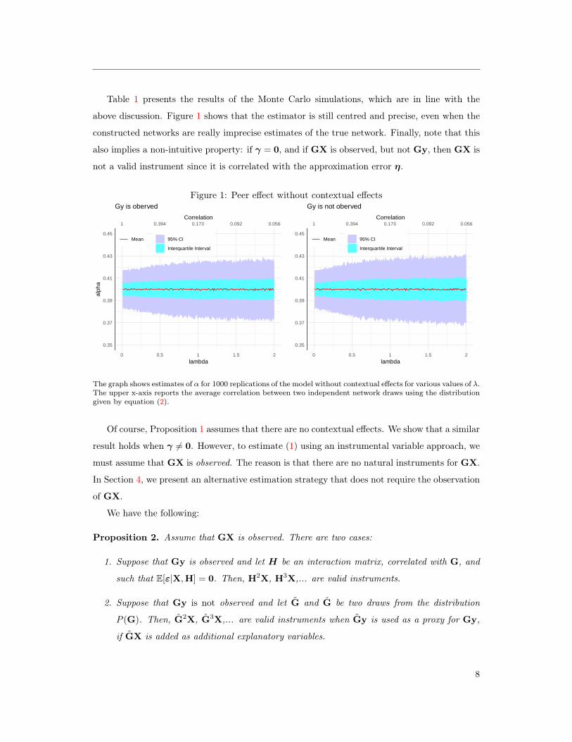
Table 1 presents the results of the Monte Carlo simulations, which are in line with the

above discussion. Figure 1 shows that the estimator is still centred and precise, even when the

constructed networks are really imprecise estimates of the true network. Finally, note that this

also implies a non-intuitive property: if γ = 0, and if GX is observed, but not Gy, then GX is

not a valid instrument since it is correlated with the approximation error η.

Figure 1: Peer effect without contextual effects

1 0.394 0.173 0.092 0.056

0.35

0.37

0.39

0.41

0.43

0.45

0 0.5 1 1.5 2

Correlation

lambda

alph

a

Mean 95% CI

Interquartile Interval

Gy is oberved

1 0.394 0.173 0.092 0.056

0.35

0.37

0.39

0.41

0.43

0.45

0 0.5 1 1.5 2

Correlation

lambda

Mean 95% CI


Gy is not oberved

The graph shows estimates of α for 1000 replications of the model without contextual effects for various values of λ.The upper x-axis reports the average correlation between two independent network draws using the distributiongiven by equation (2).

Of course, Proposition 1 assumes that there are no contextual effects. We show that a similar

result holds when γ 6= 0. However, to estimate (1) using an instrumental variable approach, we

must assume that GX is observed. The reason is that there are no natural instruments for GX.

In Section 4, we present an alternative estimation strategy that does not require the observation

of GX.

We have the following:

Proposition 2. Assume that GX is observed. There are two cases:

1. Suppose that Gy is observed and let H be an interaction matrix, correlated with G, and

such that E[ε|X,H] = 0. Then, H2X, H3X,... are valid instruments.

2. Suppose that Gy is not observed and let G and G be two draws from the distribution

P (G). Then, G2X, G3X,... are valid instruments when Gy is used as a proxy for Gy,

if GX is added as additional explanatory variables.

8

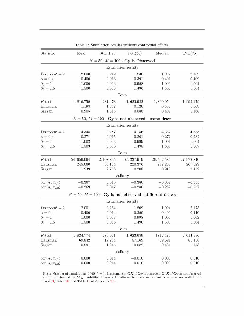
Table 1: Simulation results without contextual effects.

Statistic Mean Std. Dev. Pctl(25) Median Pctl(75)

N = 50, M = 100 - Gy is Observed

Estimation results

Intercept = 2 2.000 0.242 1.830 1.992 2.162α = 0.4 0.400 0.013 0.391 0.401 0.409β1 = 1 1.000 0.003 0.998 1.000 1.002β2 = 1.5 1.500 0.006 1.496 1.500 1.504

Tests

F -test 1, 816.759 281.478 1, 623.922 1, 800.054 1, 995.179Hausman 1.198 1.607 0.120 0.566 1.669Sargan 0.905 1.315 0.088 0.402 1.168

N = 50, M = 100 - Gy is not observed - same draw

Estimation results

Intercept = 2 4.348 0.287 4.156 4.332 4.535α = 0.4 0.271 0.015 0.261 0.272 0.282β1 = 1 1.002 0.003 0.999 1.001 1.004β2 = 1.5 1.503 0.006 1.498 1.503 1.507

Tests

F -test 26, 656.064 2, 108.805 25, 237.919 26, 492.586 27, 972.810Hausman 245.060 36.134 220.376 242.230 267.029Sargan 1.939 2.768 0.208 0.910 2.452

Validity

cor(ηi, xi,1) −0.367 0.018 −0.380 −0.367 −0.355cor(ηi, xi,2) −0.269 0.017 −0.280 −0.269 −0.257

N = 50, M = 100 - Gy is not observed - different draws

Estimation results

Intercept = 2 2.001 0.264 1.809 1.994 2.175α = 0.4 0.400 0.014 0.390 0.400 0.410β1 = 1 1.000 0.003 0.998 1.000 1.002β2 = 1.5 1.500 0.006 1.496 1.500 1.504

Tests

F -test 1, 824.774 280.901 1, 623.689 1812.479 2, 014.936Hausman 69.842 17.204 57.169 69.691 81.438Sargan 0.891 1.245 0.082 0.431 1.143

Validity

cor(ηi, xi,1) 0.000 0.014 −0.010 0.000 0.010cor(ηi, xi,2) 0.000 0.014 −0.010 0.000 0.010

Note: Number of simulations: 1000, λ = 1. Instruments: GX if Gy is observed, GcX if Gy is not observedand approximated by Gcy. Additional results for alternative instruments and λ = +∞ are available inTable 9, Table 10, and Table 11 of Appendix 9.1.

9

The first part of Proposition 2 is a simple extension of the first part of Proposition 1. The

second part of Proposition 2 requires more discussion. Essentially, it states that G2X, G3X, ...

are valid instruments when the following expanded model is estimated:

y = c1 + Xβ + αGy + GXγ + GXγ + η + ε, (3)

where the true value of γ is 0.

To understand why the introduction of GXγ is needed, recall that the constructed instru-

ment must be uncorrelated with the approximation error η. This correlation is conditional on

the explanatory variables, that contain G. In particular, it implies that generically,

E[Gy|X,GX, G2X] 6= E[Gy|X,GX, G2X].

It turns out that adding the auxiliary variable GX as a covariate is sufficient to restore the

result, i.e.

E[Gy|X,GX, G2X, GX] = E[Gy|X,GX, G2X, GX].

Table 2 presents the simulations’ results. We see that most of the estimated parameters are

not biased. However, we also see that estimating the expanded model, instead of the true one,

comes at a cost. Due to multicollinearity, the estimation of γ is contaminated by GX, and the

parameters are biased. Figure 3 also shows that the estimation of α remains precise, even as

the value of λ increases.

Proposition 1 and Proposition 2 therefore show that the estimation of (1) is possible, even

with very limited information about the network structure. We conclude this section by dis-

cussing how one can adapt this estimation strategy while allowing for group-level unobservables.

3.1 Group-Level Unobservables

A common assumption is that each group in the population is affected by a common shock,

unobserved by the econometrician (e.g. Bramoullé et al. (2009)). As such, for each group

r = 1, ...,M , we have:

yr = cr1r + Xrβ + αGryr + GrXrγ + εr,

10

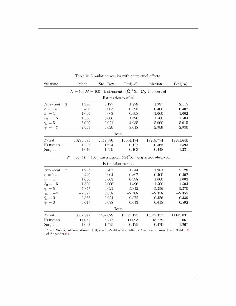
Table 2: Simulation results with contextual effects.


N = 50, M = 100 - Instrument: (G)2X - Gy is observed

Estimation results

Intercept = 2 1.996 0.177 1.879 1.997 2.115α = 0.4 0.400 0.003 0.398 0.400 0.402β1 = 1 1.000 0.003 0.998 1.000 1.002β2 = 1.5 1.500 0.006 1.496 1.500 1.504γ1 = 5 5.000 0.021 4.985 5.000 5.015γ2 = −3 −2.999 0.029 −3.018 −2.999 −2.980

Tests

F -test 18295.381 2049.380 16864.174 18258.774 19581.640Hausman 1.202 1.624 0.127 0.568 1.593Sargan 1.046 1.559 0.103 0.448 1.321

N = 50, M = 100 - Instrument: (G)2X - Gy is not observed

Estimation results

Intercept = 2 1.987 0.207 1.844 1.983 2.128α = 0.4 0.400 0.004 0.397 0.400 0.402β1 = 1 1.000 0.003 0.998 1.000 1.002β2 = 1.5 1.500 0.006 1.496 1.500 1.504γ1 = 5 5.357 0.021 5.342 5.356 5.370γ2 = −3 −2.381 0.038 −2.408 −2.378 −2.355γ1 = 0 −0.356 0.024 −0.372 −0.356 −0.339γ2 = 0 −0.617 0.038 −0.643 −0.618 −0.592

Tests


Note: Number of simulations: 1000, λ = 1. Additional results for λ = +∞ are available in Table 12of Appendix 9.1.

11

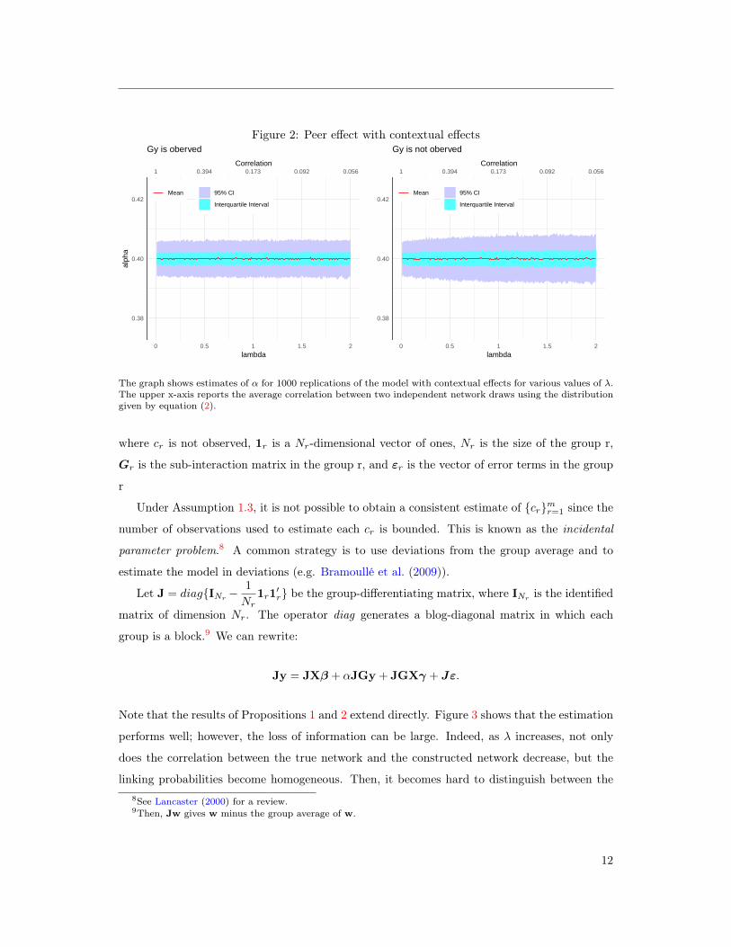
Figure 2: Peer effect with contextual effects

1 0.394 0.173 0.092 0.056

0.38

0.40

0.42

0 0.5 1 1.5 2

Correlation

lambda

alph

a

Mean 95% CI


Gy is oberved

1 0.394 0.173 0.092 0.056

0.38

0.40

0.42

0 0.5 1 1.5 2

Correlation

lambda

Mean 95% CI


Gy is not oberved

The graph shows estimates of α for 1000 replications of the model with contextual effects for various values of λ.The upper x-axis reports the average correlation between two independent network draws using the distributiongiven by equation (2).

where cr is not observed, 1r is a Nr-dimensional vector of ones, Nr is the size of the group r,

Gr is the sub-interaction matrix in the group r, and εr is the vector of error terms in the group

r

Under Assumption 1.3, it is not possible to obtain a consistent estimate of crmr=1 since the

number of observations used to estimate each cr is bounded. This is known as the incidental

parameter problem.8 A common strategy is to use deviations from the group average and to

estimate the model in deviations (e.g. Bramoullé et al. (2009)).

Let J = diagINr− 1

Nr1r1′r be the group-differentiating matrix, where INr

is the identified

matrix of dimension Nr. The operator diag generates a blog-diagonal matrix in which each

group is a block.9 We can rewrite:

Jy = JXβ + αJGy + JGXγ + Jε.

Note that the results of Propositions 1 and 2 extend directly. Figure 3 shows that the estimation

performs well; however, the loss of information can be large. Indeed, as λ increases, not only

does the correlation between the true network and the constructed network decrease, but the

linking probabilities become homogeneous. Then, it becomes hard to distinguish between the8See Lancaster (2000) for a review.9Then, Jw gives w minus the group average of w.

12

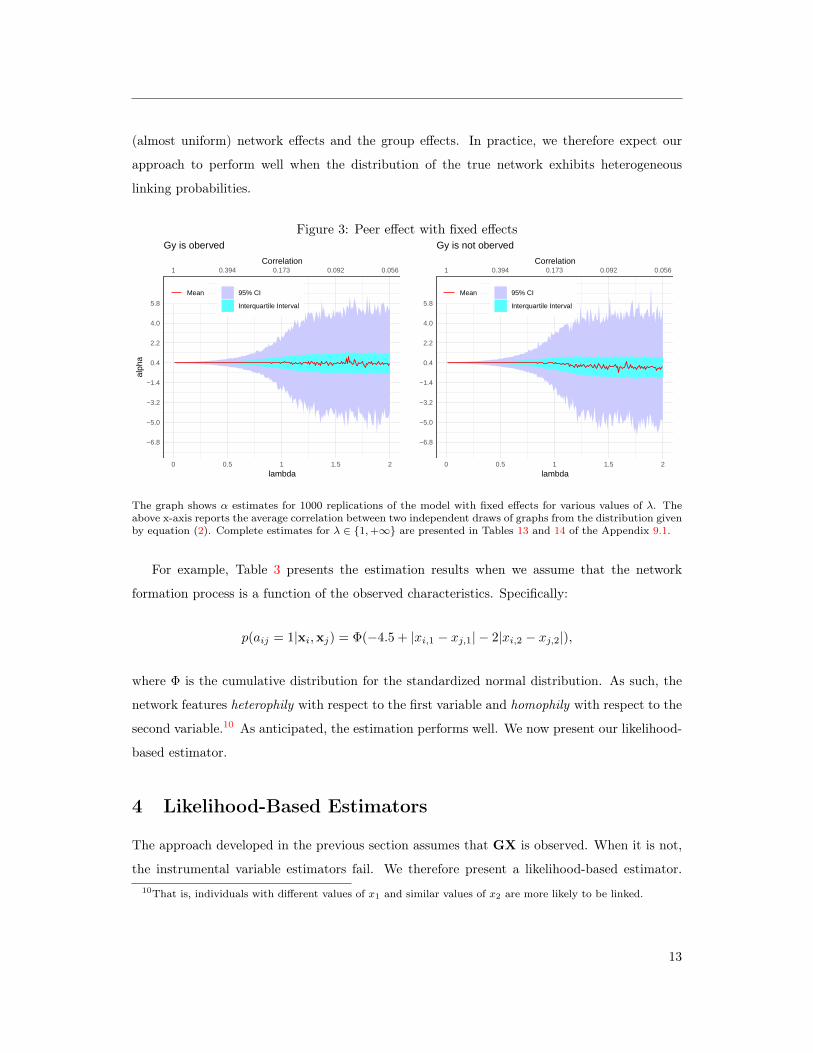
(almost uniform) network effects and the group effects. In practice, we therefore expect our

approach to perform well when the distribution of the true network exhibits heterogeneous

linking probabilities.

Figure 3: Peer effect with fixed effects

1 0.394 0.173 0.092 0.056

−6.8

−5.0

−3.2

−1.4

0.4

2.2

4.0

5.8

0 0.5 1 1.5 2

Correlation

lambda

alph

a

Mean 95% CI


Gy is oberved

1 0.394 0.173 0.092 0.056

−6.8

−5.0

−3.2

−1.4

0.4

2.2

4.0

5.8

0 0.5 1 1.5 2

Correlation

lambda

Mean 95% CI


Gy is not oberved

The graph shows α estimates for 1000 replications of the model with fixed effects for various values of λ. Theabove x-axis reports the average correlation between two independent draws of graphs from the distribution givenby equation (2). Complete estimates for λ ∈ 1,+∞ are presented in Tables 13 and 14 of the Appendix 9.1.

For example, Table 3 presents the estimation results when we assume that the network

formation process is a function of the observed characteristics. Specifically:

p(aij = 1|xi,xj) = Φ(−4.5 + |xi,1 − xj,1| − 2|xi,2 − xj,2|),

where Φ is the cumulative distribution for the standardized normal distribution. As such, the

network features heterophily with respect to the first variable and homophily with respect to the

second variable.10 As anticipated, the estimation performs well. We now present our likelihood-

based estimator.

4 Likelihood-Based Estimators

The approach developed in the previous section assumes that GX is observed. When it is not,

the instrumental variable estimators fail. We therefore present a likelihood-based estimator.10That is, individuals with different values of x1 and similar values of x2 are more likely to be linked.

13

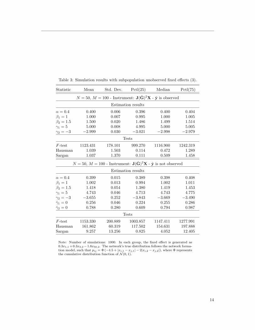
Table 3: Simulation results with subpopulation unobserved fixed effects (3).


N = 50, M = 100 - Instrument: J(G)2X - y is observed

Estimation results

α = 0.4 0.400 0.006 0.396 0.400 0.404β1 = 1 1.000 0.007 0.995 1.000 1.005β2 = 1.5 1.500 0.020 1.486 1.499 1.514γ1 = 5 5.000 0.008 4.995 5.000 5.005γ2 = −3 −2.999 0.030 −3.021 −2.998 −2.979

Tests


N = 50, M = 100 - Instrument: J(G)2X - y is not observed

Estimation results

α = 0.4 0.399 0.015 0.389 0.398 0.408β1 = 1 1.002 0.013 0.994 1.002 1.011β2 = 1.5 1.418 0.054 1.380 1.419 1.453γ1 = 5 4.743 0.046 4.713 4.743 4.775γ2 = −3 −3.655 0.252 −3.843 −3.669 −3.490γ1 = 0 0.256 0.046 0.224 0.255 0.286γ2 = 0 0.788 0.280 0.609 0.794 0.987

Tests


Note: Number of simulations: 1000. In each group, the fixed effect is generated as0.3x1,1 + 0.3x3,2−1.8x50,2. The network’s true distribution follows the network forma-tion model, such that pij = Φ (−4.5 + |xi,1 − xj,1| − 2|xi,2 − xj,2|), where Φ representsthe cumulative distribution function of N (0, 1).

14

Accordingly, more structure must be imposed on the errors ε.11

To clarify the exposition, we will focus on the network adjacency matrix A instead of the

interaction matrix G. Of course, this is without any loss of generality. Given parametric

assumptions for ε, one can write the log-likelihood of the outcome as:12

lnP(y|A,θ), (4)

where θ = [α,β′,γ′,σ′]′, σ are unknown parameters from the distribution of ε. Note that

y = (IN − αG)−1(c1 + Xβ + GXγ + ε) and (IN − αG)−1 exist under our Assumption 1.1.

If the adjacency matrix A was observed, then (4) could be estimated using a simple maximum

likelihood estimator (as in Lee et al. (2010)) or using Bayesian inference (as in Goldsmith-

Pinkham and Imbens (2013)).

Since A is not observed, an alternative would be to focus on the unconditional likelihood,

i.e.

lnP(y|θ) = ln∑A

P(y|A,θ)P (A).

A similar strategy is proposed by Chandrasekhar and Lewis (2011) using a GMM estimator.

One particular issue with estimating lnP(y|θ) is that the summation is not tractable. In-

deed, the sum is over the set of possible adjacency matrices, which contain 2N(N−1) elements.

Then, simply simulating networks from P (A) and taking the average is likely to lead to poor

approximations.13 A classical way to address this issue is to use an EM algorithm (Dempster

et al., 1977). The interested reader can consult Appendix 9.6 for a presentation of such an

estimator. Although valid, we found that the Bayesian estimator proposed in this section is less

restrictive and numerically outperforms its classical counterpart.

For concreteness, we will assume that ε ∼ N (0, σ2IN ); however, it should be noted that our11Lee (2004) presents a quasi maximum-likelihood estimator that does not require such a specific assumption

for the distribution of the error term. His estimator could be used alternatively. As well, as will be made clear,our approach can be used for a large class of extremum estimators, following Chernozhukov and Hong (2003),and in particular for GMM estimators, as in Chandrasekhar and Lewis (2011).

12Note that under Assumption 1.3, the likelihood can be factorized across groups.

13That is: lnP(y|,θ) ≈ ln1

S

S∑s=1

P(y|As,θ), where As is drawn from P (A). This is the approximation

suggested by Chandrasekhar and Lewis (2011) (see their Section 4.3). In their case, they only need to integrateover the m < N(N − 1) pairs that are not sampled. Still, the number of compatible adjacency matrices is 2m.As such, the approach is likely to produce bad approximations.

15

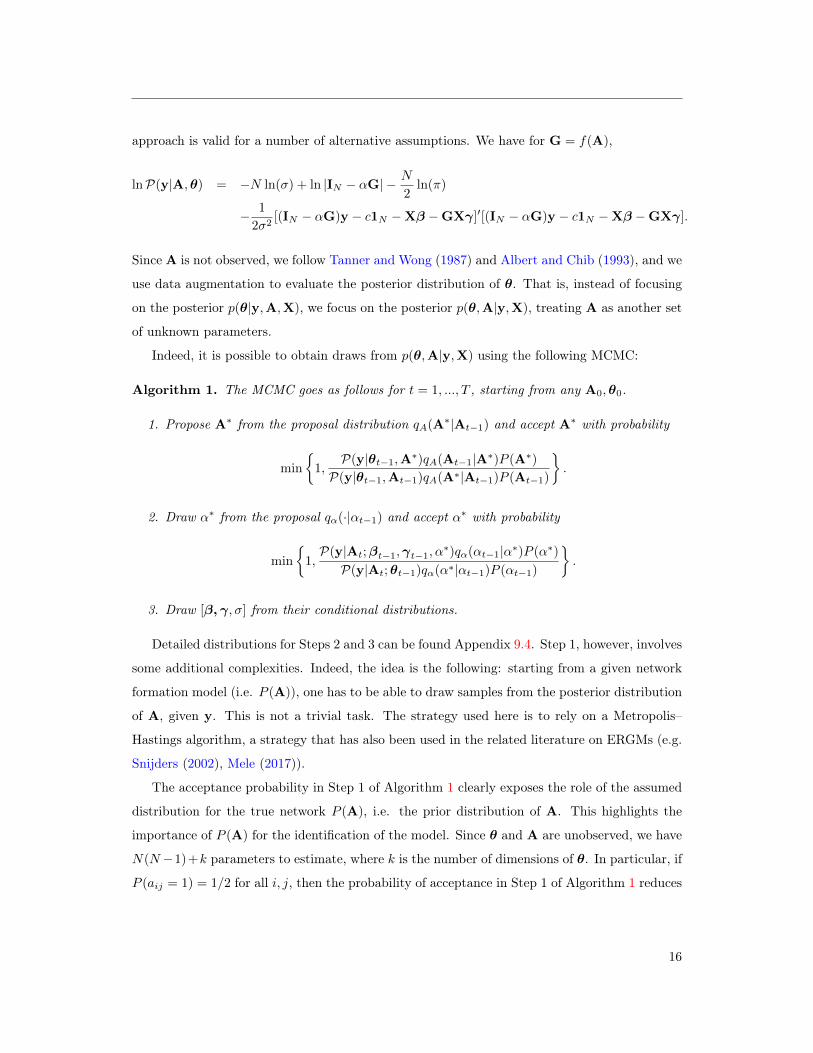
approach is valid for a number of alternative assumptions. We have for G = f(A),

lnP(y|A,θ) = −N ln(σ) + ln |IN − αG| − N

2ln(π)

− 1

2σ2[(IN − αG)y − c1N −Xβ −GXγ]′[(IN − αG)y − c1N −Xβ −GXγ].

Since A is not observed, we follow Tanner and Wong (1987) and Albert and Chib (1993), and we

use data augmentation to evaluate the posterior distribution of θ. That is, instead of focusing

on the posterior p(θ|y,A,X), we focus on the posterior p(θ,A|y,X), treating A as another set

of unknown parameters.

Indeed, it is possible to obtain draws from p(θ,A|y,X) using the following MCMC:

Algorithm 1. The MCMC goes as follows for t = 1, ..., T , starting from any A0,θ0.

1. Propose A∗ from the proposal distribution qA(A∗|At−1) and accept A∗ with probability

min

1,P(y|θt−1,A∗)qA(At−1|A∗)P (A∗)

P(y|θt−1,At−1)qA(A∗|At−1)P (At−1)

.

2. Draw α∗ from the proposal qα(·|αt−1) and accept α∗ with probability

min

1,P(y|At;βt−1,γt−1, α

∗)qα(αt−1|α∗)P (α∗)

P(y|At;θt−1)qα(α∗|αt−1)P (αt−1)

.

3. Draw [β, γ, σ] from their conditional distributions.

Detailed distributions for Steps 2 and 3 can be found Appendix 9.4. Step 1, however, involves

some additional complexities. Indeed, the idea is the following: starting from a given network

formation model (i.e. P (A)), one has to be able to draw samples from the posterior distribution

of A, given y. This is not a trivial task. The strategy used here is to rely on a Metropolis–

Hastings algorithm, a strategy that has also been used in the related literature on ERGMs (e.g.

Snijders (2002), Mele (2017)).

The acceptance probability in Step 1 of Algorithm 1 clearly exposes the role of the assumed

distribution for the true network P (A), i.e. the prior distribution of A. This highlights the

importance of P (A) for the identification of the model. Since θ and A are unobserved, we have

N(N−1)+k parameters to estimate, where k is the number of dimensions of θ. In particular, if

P (aij = 1) = 1/2 for all i, j, then the probability of acceptance in Step 1 of Algorithm 1 reduces

16

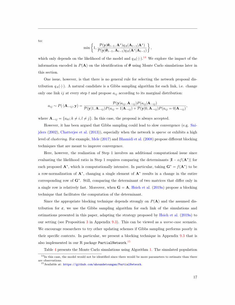
to:

min

1,P(y|θt−1,A∗)qA(At−1|A∗)P(y|θt−1,At−1)qA(A∗|At−1)

,

which only depends on the likelihood of the model and qA(·|·).14 We explore the impact of the

information encoded in P (A) on the identification of θ using Monte Carlo simulations later in

this section.

One issue, however, is that there is no general rule for selecting the network proposal dis-

tribution qA(·|·). A natural candidate is a Gibbs sampling algorithm for each link, i.e. change

only one link ij at every step t and propose aij according to its marginal distribution:

aij ∼ P (·|A−ij ,y) =P(y|aij ,A−ij)P (aij |A−ij)

P(y|1,A−ij)P (aij = 1|A−ij) + P(y|0,A−ij)P (aij = 0|A−ij),

where A−ij = akl; k 6= i, l 6= j. In this case, the proposal is always accepted.

However, it has been argued that Gibbs sampling could lead to slow convergence (e.g. Sni-

jders (2002), Chatterjee et al. (2013)), especially when the network is sparse or exhibits a high

level of clustering. For example, Mele (2017) and Bhamidi et al. (2008) propose different blocking

techniques that are meant to improve convergence.

Here, however, the realization of Step 1 involves an additional computational issue since

evaluating the likelihood ratio in Step 1 requires comparing the determinants |I − αf(A∗)| for

each proposed A∗, which is computationally intensive. In particular, taking G∗ = f(A∗) to be

a row-normalization of A∗, changing a single element of A∗ results in a change in the entire

corresponding row of G∗. Still, comparing the determinant of two matrices that differ only in

a single row is relatively fast. Moreover, when G = A, Hsieh et al. (2019a) propose a blocking

technique that facilitates the computation of the determinant.

Since the appropriate blocking technique depends strongly on P (A) and the assumed dis-

tribution for ε, we use the Gibbs sampling algorithm for each link of the simulations and

estimations presented in this paper, adapting the strategy proposed by Hsieh et al. (2019a) to

our setting (see Proposition 3 in Appendix 9.3). This can be viewed as a worse-case scenario.

We encourage researchers to try other updating schemes if Gibbs sampling performs poorly in

their specific contexts. In particular, we present a blocking technique in Appendix 9.3 that is

also implemented in our R package PartialNetwork.15

Table 4 presents the Monte Carlo simulations using Algorithm 1. The simulated population14In this case, the model would not be identified since there would be more parameters to estimate than there

are observations.15Available at: https://github.com/ahoundetoungan/PartialNetwork.

17

https://github.com/ahoundetoungan/PartialNetwork

is the same as in Section 3; however, for computational reasons, we limit ourselves to M = 50

groups of N = 30 individuals each. As expected, the average of the means of the posterior

distributions are centred relatively on the parameters’ true values. Note, however, that due to

the smaller number of groups and the fact that we performed only 200 simulations, the results

in Table 4 may exhibit small sample as well as simulation biases.

Table 4: Simulation results with a Bayesian method.


N = 30, M = 50

Estimation results

Intercept = 2 1.873 0.893 1.312 1.815 2.486α = 0.4 0.398 0.025 0.383 0.398 0.414β1 = 1 1.003 0.027 0.982 1.002 1.019β2 = 1.5 1.500 0.019 1.489 1.501 1.512γ1 = 5 5.011 0.167 4.909 5.009 5.117γ2 = −3 −2.987 0.135 −3.084 −2.983 −2.887

σ2 = 1 1.018 0.113 0.946 1.016 1.089

Note: Simulation results for 200 replications of the model with unobserved exogenouseffects estimated by a Bayesian method where the graph precision parameter λ is setto 1.

5 Network Formation Models

Our main assumption (Assumption 1.2) is that the researcher has access to the true distribution

of the observed network. An important special case is when the researcher has access to a

consistent estimate of this distribution. For concreteness, in this section we assume that links

are generated as follows:

P(aij = 1) ∝ expQ(θ,wij), (5)

where Q is some known function, wij is a vector of (not necessarily observed) characteristics for

the pair ij, and θ is a vector of parameters to be estimated.

An important feature of such models is that their estimation may not necessarily require

the observation of the entire network structure. To understand the intuition, assume a simple

18

logistic regression framework:

P(aij = 1) =expxijθ

1 + expxijθ,

where xij is a vector of observed characteristics of the pair ij. Here, note that s =∑ij

aijxij is

a vector of sufficient statistics. In practice, this therefore means that the estimation of θ only

requires the observation of such sufficient statistics.

To clarify this point, consider a simple example where individuals are only characterized by

their gender and age. Specifically, assume that xij = [1,1genderi = genderj, |agei − agej |].

Then, the set of sufficient statistics is resumed by (1) the number of links, (2) the number of

same-gender links, and (3) average age difference between linked individuals.

Note that these statistics are much easier (and cheaper) to obtain than the entire network

structure; however, they nonetheless allow for estimating the distribution of the true network.

Of course, in general, the simple logistic regression above might be unrealistically simple as

the probability of linking might depend on unobserved variables.

In this section, we discuss some examples of network formation models that can be estimated

using only partial information about the network. We subdivide such models into two categories:

models that can be estimated using sampled network data and latent surface models.

5.1 Sampled Network

As discussed in Chandrasekhar and Lewis (2011), sampled data can be used to estimate a

network formation model under the assumptions that (1) the sampling is exogenous and (2)

links are conditionally independent, i.e. P (aij |A−ij) = P (aij), as in (5).

Indeed, if the sampling was done, for example, as a function of the network structure, the

estimation of the network formation model would likely be biased. Also, if the network formation

model is such that links are not conditionally independent, then consistent estimation usually

requires the observation of the entire network structure.16

An excellent illustration of a compatible sampling scheme is presented in Conley and Udry

(2010). Rather than collecting the entire network structure, the authors asked the respondents

about their relationship with a random sample of the other respondents: “Have you ever gone

to ____ for advice about your farm?” If the answer is “Yes,” then a link is assumed between16Or at least requires additional network summary statistics, such as individual degree or clustering coefficients;

see Boucher and Mourifié (2017) or Mele (2017).

19

the respondents.

Since the pairs of respondents for which the “Yes/No” question is asked are random, the

estimation of a network formation model with conditionally independent links gives consistent

estimates. If, in addition, the individual characteristics of the sampled pair of respondents

cover the set of observable characteristics for the entire set of respondents, one can compute the

predicted probability that any two respondents are linked.

For concreteness, consider the simple model presented above, such that:

P(aij = 1) =expxijθ

1 + expxijθ,

where xij = [1,1genderi = genderj, |agei − agej |].

Then, as long as the random sample of pairs for which the “Yes/No” question is asked includes

both men and women and includes individuals of different ages, then these sampled pairs allow

for a consistent estimation of θ. As such, for any two respondents the (predicted) probability

of a link is given by pij = expxij θ/(1 + expxij θ), where θ is a consistent estimator of θ.

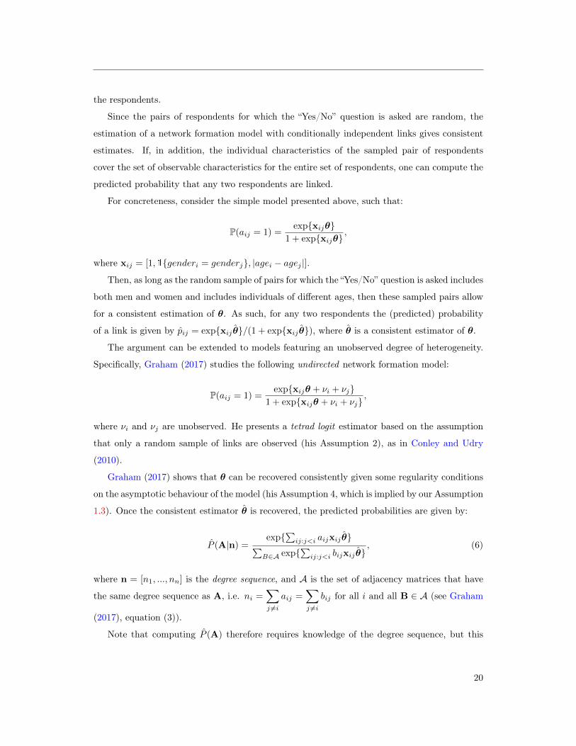
The argument can be extended to models featuring an unobserved degree of heterogeneity.

Specifically, Graham (2017) studies the following undirected network formation model:

P(aij = 1) =expxijθ + νi + νj

1 + expxijθ + νi + νj,

where νi and νj are unobserved. He presents a tetrad logit estimator based on the assumption

that only a random sample of links are observed (his Assumption 2), as in Conley and Udry

(2010).

Graham (2017) shows that θ can be recovered consistently given some regularity conditions

on the asymptotic behaviour of the model (his Assumption 4, which is implied by our Assumption

1.3). Once the consistent estimator θ is recovered, the predicted probabilities are given by:

P (A|n) =exp

∑ij:j<i aijxij θ∑

B∈A exp∑ij:j<i bijxij θ

, (6)

where n = [n1, ..., nn] is the degree sequence, and A is the set of adjacency matrices that have

the same degree sequence as A, i.e. ni =∑j 6=i

aij =∑j 6=i

bij for all i and all B ∈ A (see Graham

(2017), equation (3)).

Note that computing P (A) therefore requires knowledge of the degree sequence, but this

20

information can easily be incorporated as a survey question: “How many people have you gone

to for advice about your farm?” Also, as noted by Graham (2017), the computation of the

normalizing term in (6) is not tractable for networks of moderate size. As such, the predicted

probabilities cannot be computed directly and must be simulated, for example using the sequen-

tial importance sampling algorithm proposed by Blitzstein and Diaconis (2011).

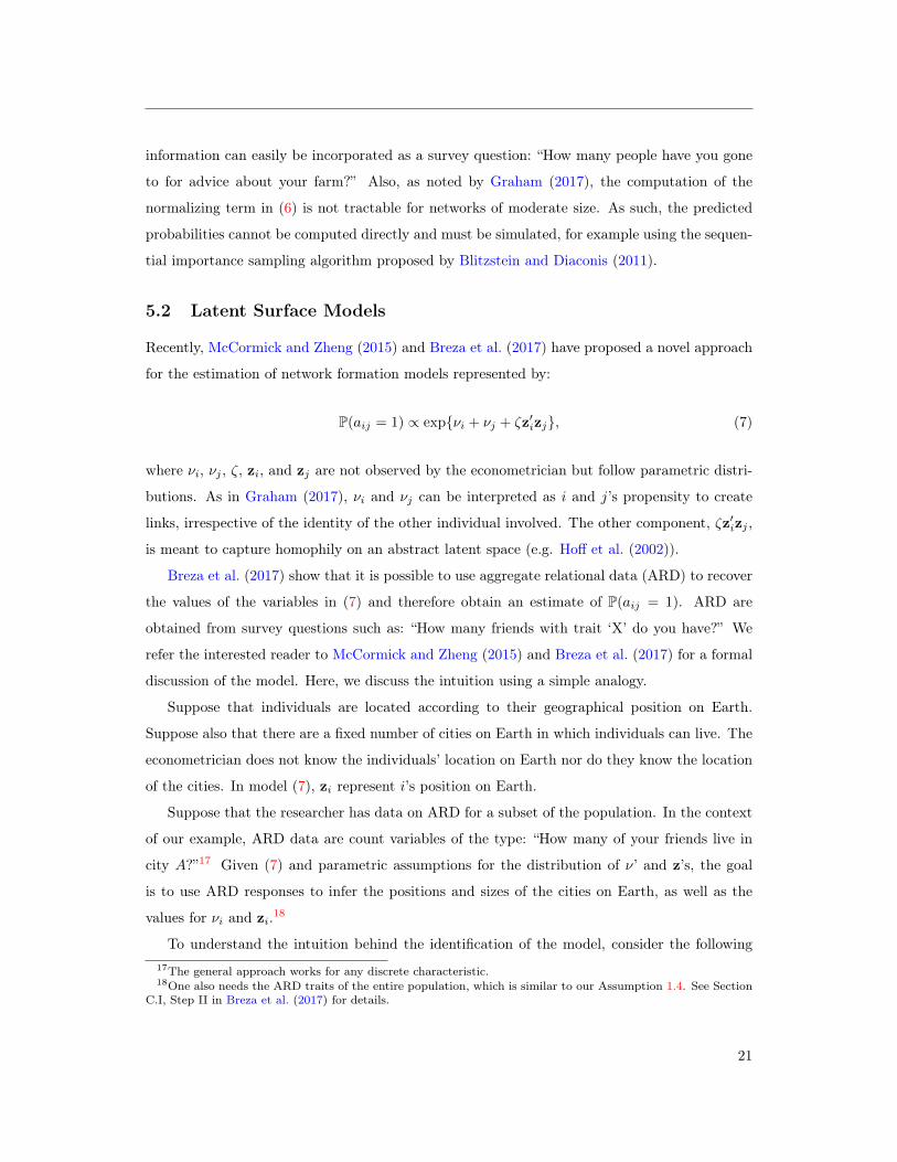
5.2 Latent Surface Models

Recently, McCormick and Zheng (2015) and Breza et al. (2017) have proposed a novel approach

for the estimation of network formation models represented by:

P(aij = 1) ∝ expνi + νj + ζz′izj, (7)

where νi, νj , ζ, zi, and zj are not observed by the econometrician but follow parametric distri-

butions. As in Graham (2017), νi and νj can be interpreted as i and j’s propensity to create

links, irrespective of the identity of the other individual involved. The other component, ζz′izj ,

is meant to capture homophily on an abstract latent space (e.g. Hoff et al. (2002)).

Breza et al. (2017) show that it is possible to use aggregate relational data (ARD) to recover

the values of the variables in (7) and therefore obtain an estimate of P(aij = 1). ARD are

obtained from survey questions such as: “How many friends with trait ‘X’ do you have?” We

refer the interested reader to McCormick and Zheng (2015) and Breza et al. (2017) for a formal

discussion of the model. Here, we discuss the intuition using a simple analogy.

Suppose that individuals are located according to their geographical position on Earth.

Suppose also that there are a fixed number of cities on Earth in which individuals can live. The

econometrician does not know the individuals’ location on Earth nor do they know the location

of the cities. In model (7), zi represent i’s position on Earth.

Suppose that the researcher has data on ARD for a subset of the population. In the context

of our example, ARD data are count variables of the type: “How many of your friends live in

city A?”17 Given (7) and parametric assumptions for the distribution of ν’ and z’s, the goal

is to use ARD responses to infer the positions and sizes of the cities on Earth, as well as the

values for νi and zi.18

To understand the intuition behind the identification of the model, consider the following17The general approach works for any discrete characteristic.18One also needs the ARD traits of the entire population, which is similar to our Assumption 1.4. See Section

C.I, Step II in Breza et al. (2017) for details.

21

example: suppose that individual i has many friends living in city A. Then, city A is likely

located close to i’s location. Similarly, if many individuals have many friends living in city A,

then city A is likely a large city. Finally, if i has many friends from many cities, i likely has a

large νi.

As mentioned above, we refer the interested reader to McCormick and Zheng (2015) and

Breza et al. (2017) for a formal description of the method as well as formal identification con-

ditions. Here, we provide Monte Carlo simulations for the estimators developed in Section 3,

assuming that the true network follows (7). The details of the Monte Carlo simulations can be

found in Appendix 9.2.

We simulate 20 groups of 250 individuals each. Within each subpopulation, we simulate the

ARD responses as well as a series of observable characteristics (e.g. cities). We then estimate

the model in (7) and compute the implied probabilities, P(aij = 1), which we used as the

distribution of our true network.19 We estimate peer effects using the instrumental variable

strategy presented in Section 3. Results are presented in Tables 5 and 6.

Results show that the method performs relatively well when Gy is observed but slightly less

well when Gy is not observed and when the model allows for group-level unobservables. Note,

however, that one potential issue with this specific network formation model is that it is based

on a single population setting (i.e. there is only one Earth). The researcher should keep in mind

that the method should only be used on medium- to large-sized groups.

If the method proposed by Breza et al. (2017) performs well, note that our instrumental

variable estimator does not require the identification of the structural parameters in (7). Indeed,

the procedure only requires a consistent estimate of the linking probabilities.

As such, we could alternatively use the approach recently proposed by Alidaee et al. (2020).

They present an alternative estimation procedure for models with ARD that does not rely on

the parametric assumption in equation (7). They propose a penalized regression based on a

low-rank assumption. One main advantage of their estimator is that it allows for a wider class

of model and ensures that the estimation is fast and easily implementable.20

As for most penalized regressions, the estimation requires the user to select a tuning param-

eter, which effectively controls the weight of the penalty. We found that the value recommended

by the authors is too large in the context of (7), using our simulated values. Since the choice

of this tuning parameter is obviously context dependent, we recommend choosing it using a

cross-validation procedure.19We fix ζ = 1.5 (i.e. ζ is not estimated) to mitigate part of the small sample bias. See our discussion below.20The authors developed user-friendly packages in R and Python. See their paper for links and details.

22

To explore the properties of their estimator in our context, we do the following. First, we

simulate data using (7), using the same specification as for Tables 5 and 6. Second, we estimate

the linking probabilities using their penalized regression under different tuning parameters, in-

cluding the optimal (obtained through cross-validation) and the recommended parameter (taken

from Alidaee et al. (2020)). Third, we estimate the peer-effect model using our instrumental

variable estimator.

Table 16 of Appendix 9.1 presents the results under alternative tuning parameters when Gy

is observed and γ = 0. We see that the procedure performs well but is less precise than when

using the parametric estimation procedure. This is intuitive since the estimation procedure

in Breza et al. (2017) imposes more structure (and is specified correctly in our context). The

procedure proposed by Alidaee et al. (2020) is valid for a large class of models but is less precise.

Tables 17 and 18 also exemplify the results of Propositions 1 and 2. When Gy is observed, the

estimation is precise, even if the network formation model is not estimated precisely. However,

when Gy is not observed, small sample bias strongly affects the performance of the estimator.

Results from this section imply that, when Gy is observed, the estimator proposed by Alidaee

et al. (2020) is the most attractive since it is less likely to be misspecified (and correlated with ε).

However, when Gy is not observed, the estimator from Breza et al. (2017) should be privileged.

Of course, in the latter case, the validity of the results are based on the assumption that (7) is

correctly specified.

6 Imperfectly Measured Networks

In this section, we assume that the econometrician has access to network data but that the data

may contain errors. For example, Hardy et al. (2019) assume that some links are missing with

some probability, while others are included falsely with some other probability.

To show how our method can be used to address these issues, we consider a simple example

where we are interested in estimating peer effects on adolescents’ academic achievements. We

assume that we observe the network but that some links are missing.

To estimate this model, we use the AddHealth database. Specifically, we focus on a subset

of schools from the “In School” sample that each have less than 200 students. Table 7 displays

the summary statistics.

Most of the papers estimating peer effects that use this particular database have taken the

network structure as given. One notable exception is Griffith (2019), looking at the issue of

23

Table 5: Simulation results using ARD with contextual effects (1000 replications).



Estimation results

Intercept = 2 1.991 0.222 1.845 1.992 2.141α = 0.4 0.400 0.006 0.396 0.400 0.404β1 = 1 1.000 0.003 0.998 1.000 1.002β2 = 1.5 1.500 0.005 1.496 1.500 1.504γ1 = 5 5.000 0.020 4.986 4.999 5.013γ2 = −3 −2.999 0.032 −3.020 −2.998 −2.977

Tests




Tests

F -test 4790.020 1407.596 3760.700 4682.825 5686.841Hausman 70.940 19.503 57.143 70.430 82.175Sargan 1.167 1.615 0.103 0.523 1.534F -test 3, 867.077 1, 093.165 3, 037.776 3, 855.692 4, 588.458Hausman 228.290 49.002 194.110 227.981 261.617Sargan 26.953 13.515 17.184 25.380 34.583

Note: Results without contextual effects are presented in Table 15 of Appendix 9.1.

24

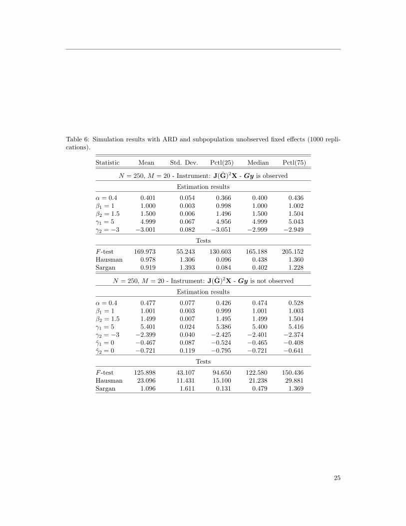
Table 6: Simulation results with ARD and subpopulation unobserved fixed effects (1000 repli-cations).


N = 250, M = 20 - Instrument: J(G)2X - Gy is observed

Estimation results

α = 0.4 0.401 0.054 0.366 0.400 0.436β1 = 1 1.000 0.003 0.998 1.000 1.002β2 = 1.5 1.500 0.006 1.496 1.500 1.504γ1 = 5 4.999 0.067 4.956 4.999 5.043γ2 = −3 −3.001 0.082 −3.051 −2.999 −2.949

Tests


N = 250, M = 20 - Instrument: J(G)2X - Gy is not observed

Estimation results

α = 0.4 0.477 0.077 0.426 0.474 0.528β1 = 1 1.001 0.003 0.999 1.001 1.003β2 = 1.5 1.499 0.007 1.495 1.499 1.504γ1 = 5 5.401 0.024 5.386 5.400 5.416γ2 = −3 −2.399 0.040 −2.425 −2.401 −2.374γ1 = 0 −0.467 0.087 −0.524 −0.465 −0.408γ2 = 0 −0.721 0.119 −0.795 −0.721 −0.641

Tests


25

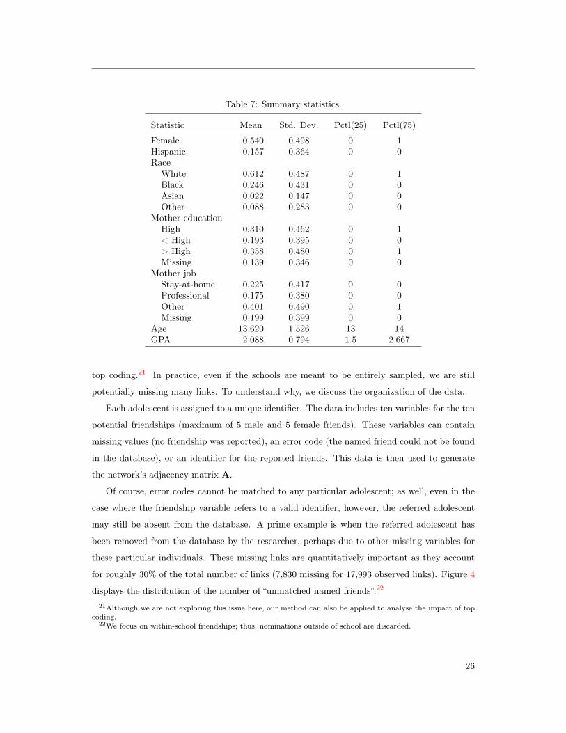
Table 7: Summary statistics.

Statistic Mean Std. Dev. Pctl(25) Pctl(75)

Female 0.540 0.498 0 1Hispanic 0.157 0.364 0 0Race

White 0.612 0.487 0 1Black 0.246 0.431 0 0Asian 0.022 0.147 0 0Other 0.088 0.283 0 0

Mother educationHigh 0.310 0.462 0 1< High 0.193 0.395 0 0> High 0.358 0.480 0 1Missing 0.139 0.346 0 0

Mother jobStay-at-home 0.225 0.417 0 0Professional 0.175 0.380 0 0Other 0.401 0.490 0 1Missing 0.199 0.399 0 0

Age 13.620 1.526 13 14GPA 2.088 0.794 1.5 2.667

top coding.21 In practice, even if the schools are meant to be entirely sampled, we are still

potentially missing many links. To understand why, we discuss the organization of the data.

Each adolescent is assigned to a unique identifier. The data includes ten variables for the ten

potential friendships (maximum of 5 male and 5 female friends). These variables can contain

missing values (no friendship was reported), an error code (the named friend could not be found

in the database), or an identifier for the reported friends. This data is then used to generate

the network’s adjacency matrix A.

Of course, error codes cannot be matched to any particular adolescent; as well, even in the

case where the friendship variable refers to a valid identifier, however, the referred adolescent

may still be absent from the database. A prime example is when the referred adolescent has

been removed from the database by the researcher, perhaps due to other missing variables for

these particular individuals. These missing links are quantitatively important as they account

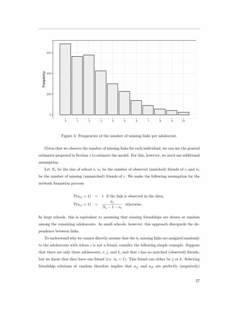
for roughly 30% of the total number of links (7,830 missing for 17,993 observed links). Figure 4

displays the distribution of the number of “unmatched named friends”.22

21Although we are not exploring this issue here, our method can also be applied to analyse the impact of topcoding.

22We focus on within-school friendships; thus, nominations outside of school are discarded.

26

0

200

400

600

0 1 2 3 4 5 6 7 8 9 10

Fre

quen

cy

Figure 4: Frequencies of the number of missing links per adolescent.

Given that we observe the number of missing links for each individual, we can use the general

estimator proposed in Section 4 to estimate the model. For this, however, we need one additional

assumption.

Let Ns be the size of school s, ni be the number of observed (matched) friends of i, and ni

be the number of missing (unmatched) friends of i. We make the following assumption for the

network formation process:

P(aij = 1) = 1 if the link is observed in the data,

P(aij = 1) =ni

Ns − 1− niotherwise.

In large schools, this is equivalent to assuming that missing friendships are drawn at random

among the remaining adolescents. In small schools, however, this approach disregards the de-

pendence between links.

To understand why we cannot directly assume that the ni missing links are assigned randomly

to the adolescents with whom i is not a friend, consider the following simple example. Suppose

that there are only three adolescents, i, j, and k, and that i has no matched (observed) friends,

but we know that they have one friend (i.e. ni = 1). This friend can either be j or k. Selecting

friendship relations at random therefore implies that aij and aik are perfectly (negatively)

27

correlated. This will lead many Metropolis–Hastings algorithms to fail. In particular, this

is the case of the Gibbs sampling procedure.23

Assuming P(aij = 1) = P(aik = 1) =ni

Ns − 1− ni= 1/2 for unobserved links circumvents

this issue. Moreover, since this assumption only affects the prior distribution of our Bayesian

inference procedure, it need not have important consequences on the posterior distribution.

Table 8 presents the estimation results.24 Importantly, we see that the estimated value for

α is significantly larger when the network is reconstructed. Also notable is the fact that the

reconstructed network captures an additional contextual peer effect: having a larger fraction of

Hispanic friends significantly reduces academic achievement.25 The remainder of the estimated

parameters are roughly the same for both specifications.

7 Discussions

In this paper, we proposed two types of estimators that can estimate peer effects given that the

researcher only has access to the distribution of the true network. In doing so, we abstracted

from many important considerations. In this section, we discuss some limits, some areas for

future research, and some general implications of our results.

7.1 Endogenous Networks

In this paper, we assumed away any endogeneity of the network structure (Assumption 1.5). As

discussed in Section 2, this is done for the purposes of presentation. Indeed, there are mulitple

ways to introduce, and correct for, endogenous networks, which lead to many possible models.

In this section, we discuss how existing endogenous network corrections can be adapted to our

setting. Specifically, we assume that there exists some unobserved variable correlated with both

the network A and the outcome y. This violates Assumption 1.5.

A first remark is that our ability to accommodate such an unobserved variable depends on

the flexibility of the used network formation model. Indeed, some models can obtain estimates

of the unobserved heterogeneity (e.g. Breza et al. (2017) or Graham (2017)). In such cases, one

could simply include the estimated unobserved variables as additional explanatory variables.

Johnsson and Moon (2015) discuss this approach as well as other control-function approaches23This issue could be solved by updating an entire line of A for each step of the algorithm. However, this

proves to be computationally intensive for networks of moderate size.24Trace plots and posterior distributions are presented in Figures 5, 6, and 7 of Appendix 9.5.25Note that one has to be careful in discussing the structural interpretation of the contextual effects. See

Boucher and Fortin (2016) for a discussion.

28

Table 8: Posterior distribution.

Observed network Reconstructed networkStatistic Mean Std. Dev. t-stat Mean Std. Dev. t-stat

Peer effect 0.350∗∗∗ 0.022 15.519 0.526∗∗∗ 0.036 14.468Intercept 1.196∗∗∗ 0.132 9.086 1.153∗∗∗ 0.139 8.293

Own effects

Female −0.144∗∗∗ 0.029 −5.013 −0.131∗∗∗ 0.028 −4.690Hispanic 0.084∗∗ 0.042 1.999 0.122∗∗∗ 0.044 2.745Race

Black 0.231∗∗∗ 0.045 5.084 0.233∗∗∗ 0.047 4.913Asian 0.090 0.090 1.008 0.106 0.087 1.212Other −0.056 0.051 −1.085 −0.044 0.052 −0.862

Mother education< High 0.122∗∗∗ 0.039 3.125 0.120∗∗∗ 0.038 3.136> High −0.139∗∗∗ 0.033 −4.165 −0.111∗∗∗ 0.034 −3.317Missing 0.060 0.051 1.179 0.058 0.052 1.131

Mother jobProfessional −0.081∗ 0.044 −1.833 −0.068 0.044 −1.551Other −0.003 0.035 −0.078 0.009 0.034 0.253Missing 0.066 0.047 1.411 0.067 0.047 1.426

Age 0.073∗∗∗ 0.009 7.749 0.076∗∗∗ 0.010 7.824

Contextual effects

Female −0.012 0.049 −0.234 −0.048 0.071 −0.679Hispanic −0.061 0.069 −0.876 −0.275∗∗∗ 0.091 −3.042Race

Black −0.051 0.058 −0.868 −0.097 0.065 −1.478Asian −0.212 0.184 −1.150 −0.131 0.324 −0.404Other 0.138 0.090 1.539 0.154 0.140 1.099

Mother education< High 0.269∗∗∗ 0.072 3.733 0.337∗∗∗ 0.109 3.093> High −0.071 0.060 −1.196 −0.118 0.086 −1.377Missing 0.078 0.094 0.828 0.013 0.146 0.089

Mother jobProfessional 0.109 0.081 1.352 0.060 0.115 0.519Other 0.101∗ 0.060 1.684 0.057 0.088 0.647Missing 0.093 0.087 1.080 0.055 0.136 0.400

Age −0.066∗∗∗ 0.006 −11.583 −0.087∗∗∗ 0.008 −11.178

SE2 0.523 0.493

Note: N = 3,126. Observed links = 17,993. Missing links = 7,830. Significance levels: ∗∗∗ = 1%, ∗∗ = 5%,∗ = 10%.

29

in detail. Since their instrumental variable estimator is based on the higher-order link relations

(i.e. G2X,G3X, ...), it is also valid for the instrumental variable estimator proposed in Section

3.26

However, this is not entirely satisfying since it assumes that the network formation is esti-

mated consistently, independent of the peer-effect model.27 The Bayesian estimator presented

in Section 4 allows for more flexibility. Indeed, one could expand Algorithm 1 and perform the

estimation of the network formation model jointly with the peer-effect model, as has been done,

for instance, by Goldsmith-Pinkham and Imbens (2013), Hsieh and Van Kippersluis (2018), and

Hsieh et al. (2019b)) in contexts where the network is observed. Essentially, instead of relying

on the known distribution P (A), one would need to rely on P (A|S,κ, z), where S is a matrix

(possibly a vector) of observed statistics about A (e.g. a sample, a vector of summary statistics,

or ARD), z is an unobserved latent variable (correlated with ε), and κ is a vector of parameters

to be estimated.

This contrasts, for example, with the network formation model presented in Section 5.2

where S (i.e. ARD) is sufficient for the estimation of all of the models’ parameters. Here, the

estimation of z and κ also requires knowledge about the likelihood of y. The exploration of

such models (especially their identification) goes far beyond the scope of the current paper and

is left for future (exciting) research.

7.2 Large Populations and Partial Sampling

In this section, we discuss the estimation of (1) when the population cannot be partitioned into

groups of bounded sizes (i.e. when Assumption 1.3 does not hold). Note that doing so will

also most likely violate Assumption 1.4. Indeed, in large populations (e.g. cities, countries...),

assuming that the individuals’ characteristics (y,X) are observed for the entire population is

unrealistic (that is, except for census data). This implies that strategies such as the one presented

in Section 4 would also be unfeasible, irrespective of the network formation model.28

One would therefore have to rely on an instrumental strategy, such as the one presented in

Section 3. In this section, we discuss the properties of the estimator in Section 3 in the context

of a single, large sample.

To fix the discussion, assume for now that xi = xi has only one dimension and only takes26Note that estimated unobserved variables can also be added as explanatory variables in the context of the

estimator presented in Section 4.27See, for example, Assumption 1 and Assumptions 6–11 in Johnsson and Moon (2015).28Also, in terms of computational cost, the estimator presented in Section 4 is likely to be very costly for very

large populations.

30

on a finite number of distinct values. Assume also that for any two i, j, P (aij = 1) = φ(xi, xj)

for some known function φ. We have:

(Gx)i =

N∑j=1

gijxj ,

which we can rewrite as:

N∑j=1

gijxj =

∑x x(nx/N) 1

nx

∑j:xj=x

aij∑x(nx/N) 1

nx

∑j:xj=x

aij,

where nx is the number of individuals having the trait x. Note that since we assumed that the

support of x only takes a finite number of values, nx goes to infinity with N . We therefore have

(by a strong law of large numbers):

1

nx

∑j:xj=x

aij → φ(xi, x), (8)

and nx/N → p(x), where p(x) is the fraction of individuals with trait x in the population. We

therefore have:

(Gx)i →∑x xp(x)φ(xi, x)∑x p(x)φ(xi, x)

≡ x(xi).

For example, for an Erdös–Rényi network (i.e. φ(x, x′) = φ for all x, x′), we have x(xi) = Ex.

This means that the knowledge of φ(·, ·) is sufficient to construct a consistent estimate of

Gx. Note also that a similar argument allows constructing a consistent estimate for Gy or

G2X. As such, the instrumental variable strategy proposed in Section 3 can be applied even if

GX is not observed.

Unfortunately, this approach relies on the (perhaps unrealistic) assumption that P (aij =

1) = φ(xi, xj), which here implies that individuals form an (asymptotically) infinite number of

links.29 When the number of links is bounded (e.g. De Paula et al. (2018b)), the average in (8)

does not converge for each i. Note, however, that the first part of Proposition 2 still applies: if

Gy and GX are observed, then the constructed (biased) instrument H2X drawn from a network

formation model with bounded degrees is valid.

Finally, note that the argument presented here can be generalized. In particular, Parise and

Ozdaglar (2019) recently proposed a means of approximating games on large networks using

graphon games, i.e. games played directly on the network formation model. If the approach29A special case, when the network is complete, is presented in Brock and Durlauf (2001).

31

is promising, its implications for the estimation of peer effects go far beyond the scope of this

paper and are left for future research.

7.3 Survey Design

As discussed in Section 3, instrumental variable estimators are only valid if the researcher

observes GX. Also, Breza et al. (2017) and Alidaee et al. (2020) propose using ARD to estimate

network formation models. Importantly, although ARD responses and GX are similar, they are

not equivalent. For example, consider a binary variable (e.g. gender). One can obtain GX by

asking questions such as “What fraction of your friends are female?” For ARD, the question

would be “How many of your friends are female?” This suggests asking two questions. One

related to the number of female friends and one related to the number of friends.30

For continuous variables (e.g. age), this creates additional issues. One can obtain GX by

asking about the average age of one’s friends, but ARD questions must be discrete: “How many

of your friends are in the same age group as you?” Then, in practice, an approach could be to

ask individuals about the number of friends they have, as well as the number of friends they

have from multiple age groups: “How many of your friends are between X and Y years old?”

Using this strategy allows construction of both the ARD and GX.

Finally, an implication of Propositions 1 and 2 is that asking directly for Gy in the survey

leads to a more robust estimation strategy. Indeed, the constructed instruments are valid even

if the network formation model is misspecified.

7.4 Next Steps

In this paper, we proposed two estimators where peer effects can be estimated without having

knowledge of the entire network structure. We found that, perhaps surprisingly, even very

partial information on network structure is sufficient. However, there remains many important

challenges, in particular with respect to the study of compatible models of network formation.

30Breza et al. (2017) do not require information on the number of friends, although this significantly helps theestimation.

32

References

Albert, J. H. and S. Chib (1993): “Bayesian analysis of binary and polychotomous response

data,” Journal of the American Statistical Association, 88, 669–679.

Alidaee, H., E. Auerbach, and M. P. Leung (2020): “Recovering Network Structure from

Aggregated Relational Data using Penalized Regression,” arXiv preprint arXiv:2001.06052.

Atchadé, Y. F. and J. S. Rosenthal (2005): “On adaptive markov chain monte carlo

algorithms,” Bernoulli, 11, 815–828.

Bhamidi, S., G. Bresler, and A. Sly (2008): “Mixing time of exponential random graphs,”

in 2008 49th Annual IEEE Symposium on Foundations of Computer Science, IEEE, 803–812.

Blitzstein, J. and P. Diaconis (2011): “A sequential importance sampling algorithm for

generating random graphs with prescribed degrees,” Internet mathematics, 6, 489–522.

Boucher, V. and B. Fortin (2016): “Some challenges in the empirics of the effects of net-

works,” The Oxford Handbook on the Economics of Networks, 277–302.

Boucher, V. and I. Mourifié (2017): “My friend far, far away: a random field approach to

exponential random graph models,” The econometrics journal, 20, S14–S46.

Bramoullé, Y., H. Djebbari, and B. Fortin (2009): “Identification of peer effects through

social networks,” Journal of econometrics, 150, 41–55.

——— (2019): “Peer Effects in Networks: A Survey,” Annual Review of Economics, forthcoming.

Breza, E. (2016): “Field Experiments, Social Networks, and Development,” The Oxford Hand-

book on the Economics of Networks, 412–439.

Breza, E., A. G. Chandrasekhar, T. H. McCormick, and M. Pan (2017): “Using

Aggregated Relational Data to feasibly identify network structure without network data,”

Tech. rep., National Bureau of Economic Research.

Brock, W. A. and S. N. Durlauf (2001): “Discrete choice with social interactions,” The

Review of Economic Studies, 68, 235–260.

Chandrasekhar, A. and R. Lewis (2011): “Econometrics of sampled networks,” Unpublished

manuscript, MIT.[422].

33

Chatterjee, S., P. Diaconis, et al. (2013): “Estimating and understanding exponential

random graph models,” The Annals of Statistics, 41, 2428–2461.

Chen, X., Y. Chen, and P. Xiao (2013): “The impact of sampling and network topology on

the estimation of social intercorrelations,” Journal of Marketing Research, 50, 95–110.

Chernozhukov, V. and H. Hong (2003): “An MCMC approach to classical estimation,”

Journal of Econometrics, 115, 293–346.

Chib, S. and S. Ramamurthy (2010): “Tailored randomized block MCMC methods with

application to DSGE models,” Journal of Econometrics, 155, 19–38.

Conley, T. G. and C. R. Udry (2010): “Learning about a new technology: Pineapple in

Ghana,” American economic review, 100, 35–69.

De Paula, A. (2017): “Econometrics of network models,” in Advances in Economics and

Econometrics: Theory and Applications: Eleventh World Congress (Econometric Society

Monographs, ed. by M. P. B. Honore, A. Pakes and L. Samuelson, Cambridge: Cambridge

University Press, 268–323.

De Paula, Á., I. Rasul, and P. Souza (2018a): “Recovering social networks from panel

data: identification, simulations and an application,” LACEA Working Paper Series.

De Paula, Á., S. Richards-Shubik, and E. Tamer (2018b): “Identifying preferences in

networks with bounded degree,” Econometrica, 86, 263–288.

Dempster, A. P., N. M. Laird, and D. B. Rubin (1977): “Maximum likelihood from

incomplete data via the EM algorithm,” Journal of the Royal Statistical Society: Series B

(Methodological), 39, 1–22.

Goldsmith-Pinkham, P. and G. W. Imbens (2013): “Social networks and the identification

of peer effects,” Journal of Business & Economic Statistics, 31, 253–264.

Graham, B. S. (2017): “An econometric model of network formation with degree heterogene-

ity,” Econometrica, 85, 1033–1063.

Griffith, A. (2018): “Random assignment with non-random peers: A structural approach to

counterfactual treatment assessment,” Working Paper.

——— (2019): “Name Your Friends, but Only Five? The Importance of Censoring in Peer

Effects Estimates using Social Network Data,” Working Paper.

34

Hardy, M., R. M. Heath, W. Lee, and T. H. McCormick (2019): “Estimating spillovers

using imprecisely measured networks,” arXiv preprint arXiv:1904.00136.

Hoff, P. D., A. E. Raftery, and M. S. Handcock (2002): “Latent space approaches to

social network analysis,” Journal of the American Statistical Association, 97, 1090–1098.

Hsieh, C.-S., S. I. Ko, J. Kovářík, and T. Logan (2018): “Non-Randomly Sampled Net-

works: Biases and Corrections,” Tech. rep., National Bureau of Economic Research.

Hsieh, C.-S., M. D. König, and X. Liu (2019a): “A Structural Model for the Coevolution

of Networks and Behavior,” CEPR Discussion Paper No. DP13911.

Hsieh, C.-S., L.-F. Lee, and V. Boucher (2019b): “Specification and estimation of network

formation and network interaction models with the exponential probability distribution,” .

Hsieh, C.-S. and H. Van Kippersluis (2018): “Smoking initiation: Peers and personality,”

Quantitative Economics, 9, 825–863.

Johnson, C. R. and R. A. Horn (1985): Matrix analysis, Cambridge University Press Cam-

bridge.

Johnsson, I. and H. R. Moon (2015): “Estimation of peer effects in endogenous social

networks: control function approach,” Review of Economics and Statistics, 1–51.

Kelejian, H. H. and G. Piras (2014): “Estimation of spatial models with endogenous weight-

ing matrices, and an application to a demand model for cigarettes,” Regional Science and

Urban Economics, 46, 140–149.

Kelejian, H. H. and I. R. Prucha (1998): “A generalized spatial two-stage least squares

procedure for estimating a spatial autoregressive model with autoregressive disturbances,”

The Journal of Real Estate Finance and Economics, 17, 99–121.

Lancaster, T. (2000): “The incidental parameter problem since 1948,” Journal of economet-

rics, 95, 391–413.

Lee, L.-F. (2004): “Asymptotic distributions of quasi-maximum likelihood estimators for spatial

autoregressive models,” Econometrica, 72, 1899–1925.

Lee, L.-f., X. Liu, and X. Lin (2010): “Specification and estimation of social interaction

models with network structures,” The Econometrics Journal, 13, 145–176.

35

Lee, L.-f., X. Liu, E. Patacchini, and Y. Zenou (2020): “Who is the key player? A network

analysis of juvenile delinquency,” ournal of Business and Economic Statistics, forthcoming.

Lewbel, A., X. Qu, and X. Tang (2019): “Social networks with misclassified or unobserved

links,” Working Paper.

Liu, X. (2013): “Estimation of a local-aggregate network model with sampled networks,” Eco-

nomics Letters, 118, 243–246.

Liu, X., E. Patacchini, and E. Rainone (2017): “Peer effects in bedtime decisions among

adolescents: a social network model with sampled data,” The econometrics journal, 20, S103–

S125.

Manresa, E. (2016): “Estimating the Structure of Social Interactions Using Panel Data,”

Working paper.

Manski, C. F. (1993): “Identification of endogenous social effects: The reflection problem,”

Review of Economic Studies, 60, 531–542.

McCormick, T. H. and T. Zheng (2015): “Latent surface models for networks using Aggre-

gated Relational Data,” Journal of the American Statistical Association, 110, 1684–1695.

Mele, A. (2017): “A structural model of Dense Network Formation,” Econometrica, 85, 825–

850.

Parise, F. and A. E. Ozdaglar (2019): “Graphon Games: A Statistical Framework for

Network Games and Interventions,” Available at SSRN 3437293.

Snijders, T. A. (2002): “Markov chain Monte Carlo estimation of exponential random graph

models,” Journal of Social Structure, 3, 1–40.

Souza, P. (2014): “Estimating network effects without network data,” PUC-Rio Working Paper.

Tanner, M. A. and W. H. Wong (1987): “The calculation of posterior distributions by data

augmentation,” Journal of the American statistical Association, 82, 528–540.

Thirkettle, M. (2019): “Identification and Estimation of Network Statistics with Missing

Link Data,” Working Paper.

Wang, W. and L.-F. Lee (2013): “Estimation of spatial autoregressive models with randomly

missing data in the dependent variable,” The Econometrics Journal, 16, 73–102.

36

8 Appendix – Proofs

8.1 Proof of Proposition 1

The model can be written as:

y = [I− αG]−1[Xβ + ε].

Or, using the geometric expansion:

y =

∞∑k=0

αkGkXβ +

∞∑k=0

αkGkε

or

Gy =

∞∑k=0

αkGk+1Xβ +

∞∑k=0

αkGk+1ε.

As such, any variable correlated with GX, G2X,... is also correlated with Gy, conditional on

X. It remains to show that such variables are valid. For the first part of Proposition 1, we need:

E[ε|X,HX,H2X, ...] = 0,

which is true by assumption. For the second part of Proposition 1, we need:

E[ε+ η|X, GX, G2X, ...] = 0.

By Assumption 1.5, this is equivalent to:

E[η|X, GX, G2X, ...] = 0,

which is equivalent to:

E[Gy|X, GX, G2X, ...] = E[Gy|X, GX, G2X, ...].

Using iterated expectations:

EyE[Gy|X, GX, G2X, ...,y]|X, GX, G2X, ... = E[G|X, GX, G2X, ...]E[y|X, GX, G2X, ...],

and so E[Gy|X, GX, G2X, ...] = E[Gy|X, GX, G2X, ...] follows since G G and G are iid, which

implies that E[G|X, GX, G2X, ...] = E[G|X, GX, G2X, ...].

37

8.2 Proof of Proposition 2

The model can be written as:

y = [I− αG]−1[Xβ + GXγ + ε].

Or, using the geometric expansion:

y =

∞∑k=0

αkGkXβ +

∞∑k=0

αkGk + GXγ

∞∑k=0

αkGkε

or

Gy =

∞∑k=0

αkGk+1Xβ +

∞∑k=0

αkGk+2Xγ +

∞∑k=0

αkGk+1ε.

As such, any variable correlated with G2X, G3X,... is also correlated with Gy, conditional on

X and GX. It remains to show that such variables are valid. For the first part of Proposition

2, we need:

E[ε|X,GX,H2X,H3X, ...] = 0,

which is true by assumption. For the second part of Proposition 1, we need:

E[ε+ η|X,GX, GX, G2X, G3X, ...] = 0.

By Assumption 1.5, this is equivalent to:

E[η|X,GX, GX, G2X, G3X, ...] = 0,

which is equivalent to:

E[Gy|X,GX, GX, G2X, G3X, ...] = E[Gy|X,GX, GX, G2X, G3X, ...].

Using iterated expectations:

EyE[Gy|X,GX, GX, G2X, G3X, ...,y]|X,GX, GX, G2X, G3X, ...

= E[G|X,GX, GX, G2X, G3X, ...]E[y|X,GX, GX, G2X, G3X, ...],

38

and so E[Gy|X,GX, GX, G2X, G3X, ...] = E[Gy|X,GX, GX, G2X, G3X, ...] follows since G

G and G are iid, which implies that E[G|X,GX, GX, G2X, G3X, ...] = E[G|X,GX, GX, G2X, G3X, ...].

9 Appendix – Supplementary Material

9.1 Additional Monte-Carlo Results

39

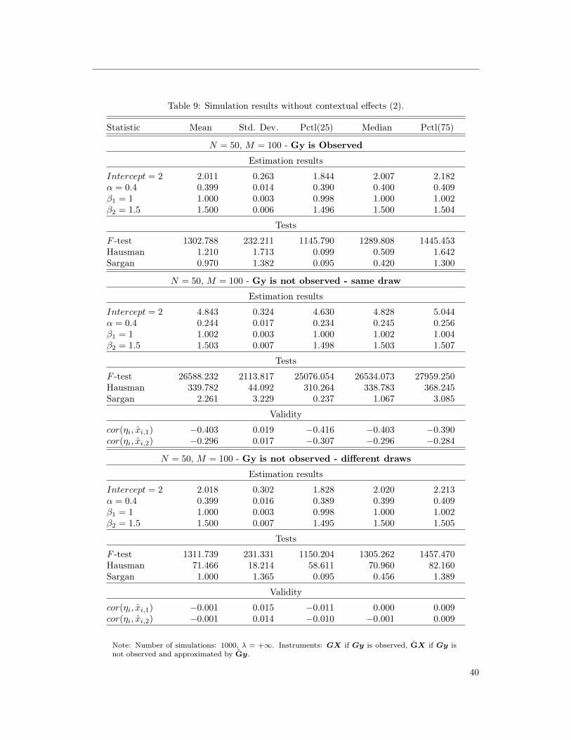
Table 9: Simulation results without contextual effects (2).



Estimation results

Intercept = 2 2.011 0.263 1.844 2.007 2.182α = 0.4 0.399 0.014 0.390 0.400 0.409β1 = 1 1.000 0.003 0.998 1.000 1.002β2 = 1.5 1.500 0.006 1.496 1.500 1.504

Tests



Estimation results

Intercept = 2 4.843 0.324 4.630 4.828 5.044α = 0.4 0.244 0.017 0.234 0.245 0.256β1 = 1 1.002 0.003 1.000 1.002 1.004β2 = 1.5 1.503 0.007 1.498 1.503 1.507

Tests


Validity

cor(ηi, xi,1) −0.403 0.019 −0.416 −0.403 −0.390cor(ηi, xi,2) −0.296 0.017 −0.307 −0.296 −0.284


Estimation results

Intercept = 2 2.018 0.302 1.828 2.020 2.213α = 0.4 0.399 0.016 0.389 0.399 0.409β1 = 1 1.000 0.003 0.998 1.000 1.002β2 = 1.5 1.500 0.007 1.495 1.500 1.505

Tests


Validity

cor(ηi, xi,1) −0.001 0.015 −0.011 0.000 0.009cor(ηi, xi,2) −0.001 0.014 −0.010 −0.001 0.009

Note: Number of simulations: 1000, λ = +∞. Instruments: GX if Gy is observed, GX if Gy isnot observed and approximated by Gy.

40

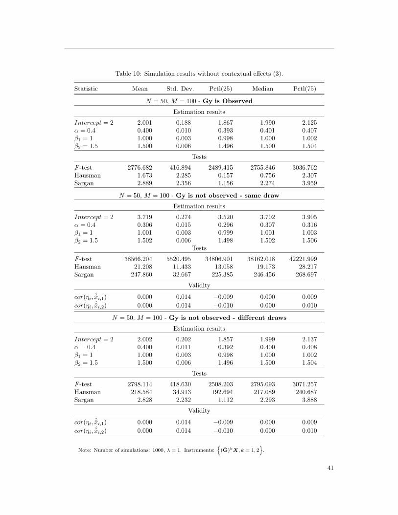
Table 10: Simulation results without contextual effects (3).



Estimation results

Intercept = 2 2.001 0.188 1.867 1.990 2.125α = 0.4 0.400 0.010 0.393 0.401 0.407β1 = 1 1.000 0.003 0.998 1.000 1.002β2 = 1.5 1.500 0.006 1.496 1.500 1.504

Tests



Estimation results

Intercept = 2 3.719 0.274 3.520 3.702 3.905α = 0.4 0.306 0.015 0.296 0.307 0.316β1 = 1 1.001 0.003 0.999 1.001 1.003β2 = 1.5 1.502 0.006 1.498 1.502 1.506

Tests


Validity

cor(ηi, ˆxi,1) 0.000 0.014 −0.009 0.000 0.009

cor(ηi, ˆxi,2) 0.000 0.014 −0.010 0.000 0.010


Estimation results

Intercept = 2 2.002 0.202 1.857 1.999 2.137α = 0.4 0.400 0.011 0.392 0.400 0.408β1 = 1 1.000 0.003 0.998 1.000 1.002β2 = 1.5 1.500 0.006 1.496 1.500 1.504

Tests


Validity

cor(ηi, ˆxi,1) 0.000 0.014 −0.009 0.000 0.009

cor(ηi, ˆxi,2) 0.000 0.014 −0.010 0.000 0.010

Note: Number of simulations: 1000, λ = 1. Instruments:

(G)kX, k = 1, 2.

41

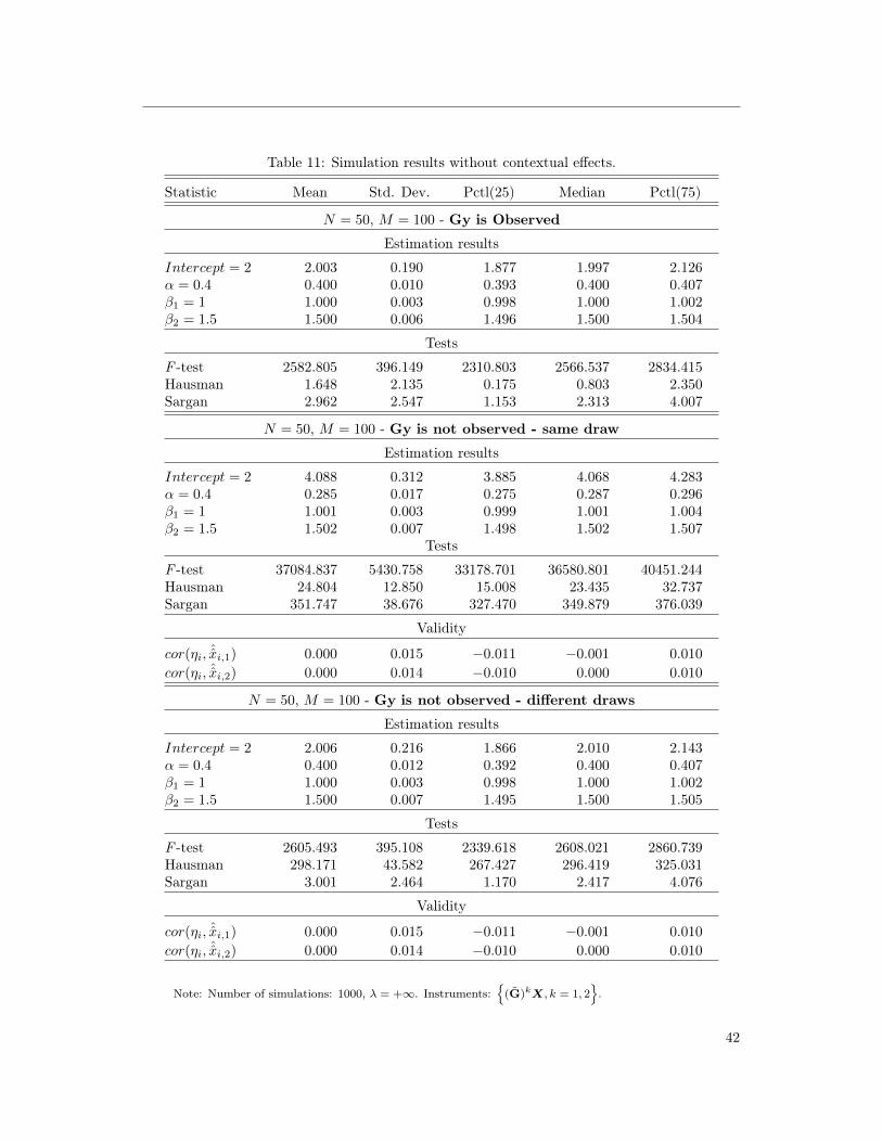
Table 11: Simulation results without contextual effects.



Estimation results

Intercept = 2 2.003 0.190 1.877 1.997 2.126α = 0.4 0.400 0.010 0.393 0.400 0.407β1 = 1 1.000 0.003 0.998 1.000 1.002β2 = 1.5 1.500 0.006 1.496 1.500 1.504

Tests



Estimation results

Intercept = 2 4.088 0.312 3.885 4.068 4.283α = 0.4 0.285 0.017 0.275 0.287 0.296β1 = 1 1.001 0.003 0.999 1.001 1.004β2 = 1.5 1.502 0.007 1.498 1.502 1.507

Tests


Validity

cor(ηi, ˆxi,1) 0.000 0.015 −0.011 −0.001 0.010

cor(ηi, ˆxi,2) 0.000 0.014 −0.010 0.000 0.010


Estimation results

Intercept = 2 2.006 0.216 1.866 2.010 2.143α = 0.4 0.400 0.012 0.392 0.400 0.407β1 = 1 1.000 0.003 0.998 1.000 1.002β2 = 1.5 1.500 0.007 1.495 1.500 1.505

Tests


Validity

cor(ηi, ˆxi,1) 0.000 0.015 −0.011 −0.001 0.010

cor(ηi, ˆxi,2) 0.000 0.014 −0.010 0.000 0.010

Note: Number of simulations: 1000, λ = +∞. Instruments:

(G)kX, k = 1, 2.

42

Table 12: Simulation results with contextual effects (2).



Estimation results

Intercept = 2 2.004 0.181 1.880 2.007 2.126α = 0.4 0.400 0.003 0.398 0.400 0.402β1 = 1 1.000 0.003 0.998 1.000 1.002β2 = 1.5 1.500 0.006 1.496 1.500 1.504γ1 = 5 5.001 0.021 4.987 5.001 5.015γ2 = −3 −3.001 0.029 −3.020 −3.001 −2.981

Tests



Estimation results


Tests


Note: Number of simulations: 1000, λ = +∞.

43

Table 13: Simulation results with subpopulation unobserved fixed effects.



Estimation results

α = 0.4 0.379 1.703 −0.122 0.398 0.938β1 = 1 1.000 0.005 0.997 1.000 1.003β2 = 1.5 1.500 0.009 1.496 1.500 1.505γ1 = 5 5.018 1.318 4.584 5.001 5.415

4.970 1.372 4.565 4.992 5.421γ2 = −3 −2.967 2.710 −3.861 −2.998 −2.156

Tests



Estimation results

α = 0.4 0.345 1.609 −0.246 0.265 0.869β1 = 1 1.000 0.005 0.997 1.000 1.002β2 = 1.5 1.500 0.008 1.495 1.500 1.505γ1 = 5 5.351 0.170 5.284 5.343 5.408γ2 = −3 −2.378 0.123 −2.416 −2.373 −2.331γ1 = 0 −0.307 1.442 −0.769 −0.236 0.237γ2 = 0 −0.534 2.490 −1.346 −0.407 0.398

Tests


Note: Number of simulations: 1000, λ = 1. In each group, the fixed effect is generatedas 0.3x1,1 + 0.3x3,2 − 1.8x50,2.

44

Table 14: Simulation results with subpopulation unobserved fixed effects (2).



Estimation results

α = 0.4 0.623 4.670 −0.475 0.341 1.345β1 = 1 1.001 0.015 0.997 1.000 1.003β2 = 1.5 1.499 0.019 1.494 1.500 1.504γ1 = 5 4.826 3.644 4.263 5.042 5.688γ2 = −3 −3.357 7.485 −4.491 −2.913 −1.572

Tests



Estimation results

α = 0.4 −0.071 3.561 −0.949 −0.047 0.876β1 = 1 0.999 0.010 0.996 0.999 1.002β2 = 1.5 1.500 0.018 1.495 1.501 1.506γ1 = 5 5.305 0.377 5.208 5.306 5.406γ2 = −3 −2.364 0.192 −2.411 −2.355 −2.306γ1 = 0 0.062 3.183 −0.777 0.051 0.846γ2 = 0 0.117 5.512 −1.360 0.062 1.459

Tests


Note: Number of simulations: 1000, λ = +∞. In each group, the fixed effect isgenerated as 0.3x1,1 + 0.3x3,2 − 1.8x50,2.

45

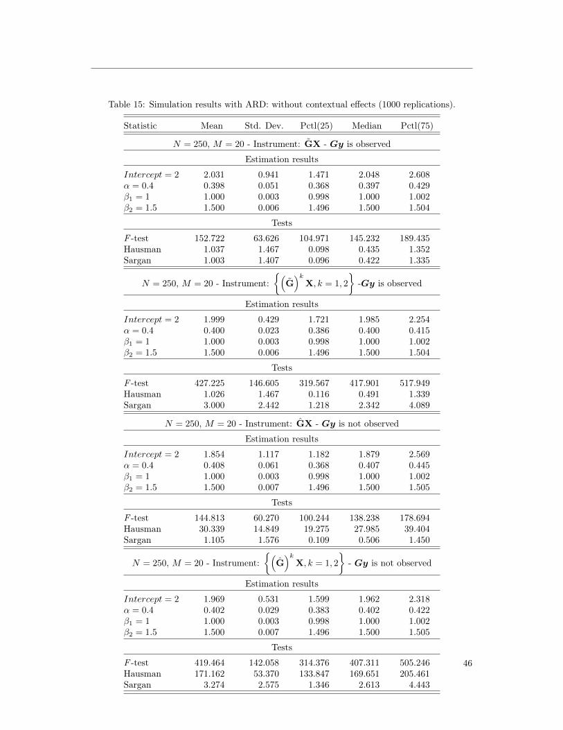
Table 15: Simulation results with ARD: without contextual effects (1000 replications).


N = 250, M = 20 - Instrument: GX - Gy is observed

Estimation results

Intercept = 2 2.031 0.941 1.471 2.048 2.608α = 0.4 0.398 0.051 0.368 0.397 0.429β1 = 1 1.000 0.003 0.998 1.000 1.002β2 = 1.5 1.500 0.006 1.496 1.500 1.504

Tests


N = 250, M = 20 - Instrument:(

G)k

X, k = 1, 2

-Gy is observed

Estimation results

Intercept = 2 1.999 0.429 1.721 1.985 2.254α = 0.4 0.400 0.023 0.386 0.400 0.415β1 = 1 1.000 0.003 0.998 1.000 1.002β2 = 1.5 1.500 0.006 1.496 1.500 1.504

Tests


N = 250, M = 20 - Instrument: GX - Gy is not observed

Estimation results

Intercept = 2 1.854 1.117 1.182 1.879 2.569α = 0.4 0.408 0.061 0.368 0.407 0.445β1 = 1 1.000 0.003 0.998 1.000 1.002β2 = 1.5 1.500 0.007 1.496 1.500 1.505

Tests



G)k

X, k = 1, 2

- Gy is not observed

Estimation results

Intercept = 2 1.969 0.531 1.599 1.962 2.318α = 0.4 0.402 0.029 0.383 0.402 0.422β1 = 1 1.000 0.003 0.998 1.000 1.002β2 = 1.5 1.500 0.007 1.496 1.500 1.505

Tests


46

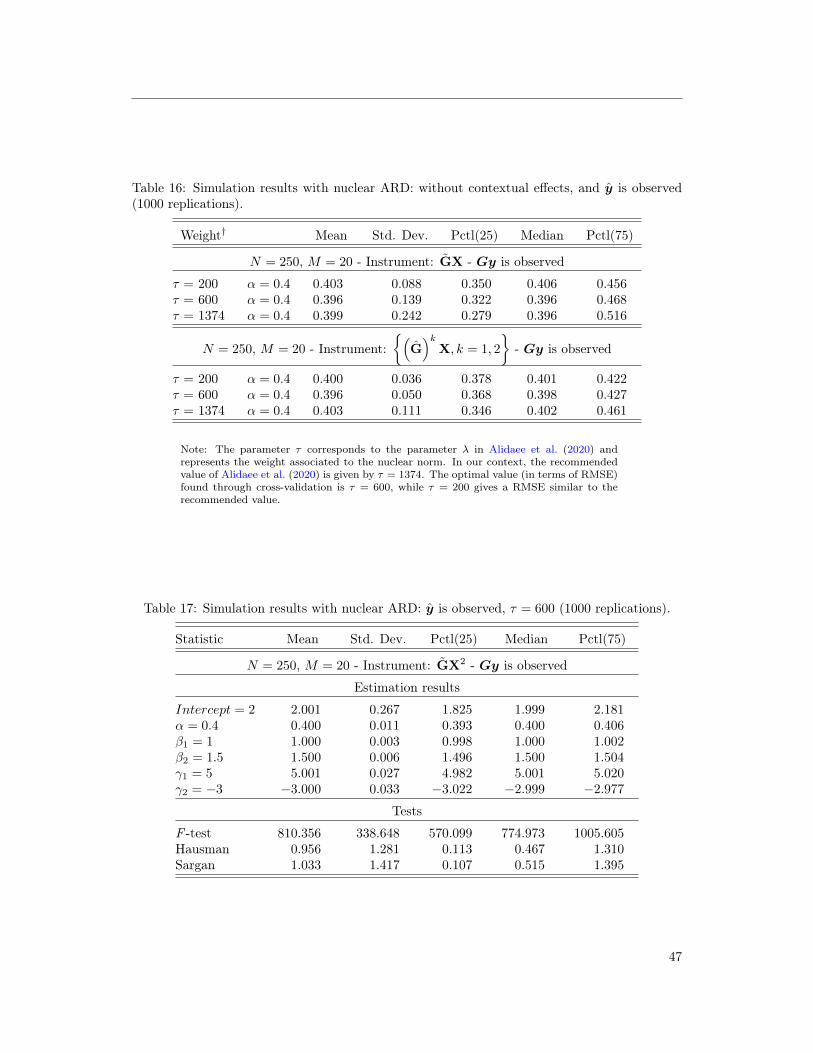
Table 16: Simulation results with nuclear ARD: without contextual effects, and y is observed(1000 replications).

Weight† Mean Std. Dev. Pctl(25) Median Pctl(75)

N = 250, M = 20 - Instrument: GX - Gy is observed

τ = 200 α = 0.4 0.403 0.088 0.350 0.406 0.456τ = 600 α = 0.4 0.396 0.139 0.322 0.396 0.468τ = 1374 α = 0.4 0.399 0.242 0.279 0.396 0.516


G)k

X, k = 1, 2

- Gy is observed

τ = 200 α = 0.4 0.400 0.036 0.378 0.401 0.422τ = 600 α = 0.4 0.396 0.050 0.368 0.398 0.427τ = 1374 α = 0.4 0.403 0.111 0.346 0.402 0.461

Note: The parameter τ corresponds to the parameter λ in Alidaee et al. (2020) andrepresents the weight associated to the nuclear norm. In our context, the recommendedvalue of Alidaee et al. (2020) is given by τ = 1374. The optimal value (in terms of RMSE)found through cross-validation is τ = 600, while τ = 200 gives a RMSE similar to therecommended value.

Table 17: Simulation results with nuclear ARD: y is observed, τ = 600 (1000 replications).


N = 250, M = 20 - Instrument: GX2 - Gy is observed

Estimation results

Intercept = 2 2.001 0.267 1.825 1.999 2.181α = 0.4 0.400 0.011 0.393 0.400 0.406β1 = 1 1.000 0.003 0.998 1.000 1.002β2 = 1.5 1.500 0.006 1.496 1.500 1.504γ1 = 5 5.001 0.027 4.982 5.001 5.020γ2 = −3 −3.000 0.033 −3.022 −2.999 −2.977

Tests


47

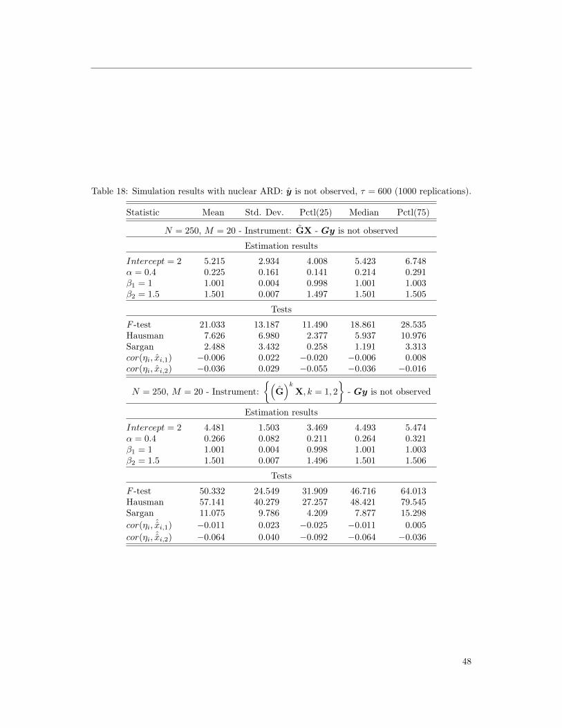
Table 18: Simulation results with nuclear ARD: y is not observed, τ = 600 (1000 replications).


N = 250, M = 20 - Instrument: GX - Gy is not observed

Estimation results

Intercept = 2 5.215 2.934 4.008 5.423 6.748α = 0.4 0.225 0.161 0.141 0.214 0.291β1 = 1 1.001 0.004 0.998 1.001 1.003β2 = 1.5 1.501 0.007 1.497 1.501 1.505

Tests

F -test 21.033 13.187 11.490 18.861 28.535Hausman 7.626 6.980 2.377 5.937 10.976Sargan 2.488 3.432 0.258 1.191 3.313cor(ηi, xi,1) −0.006 0.022 −0.020 −0.006 0.008cor(ηi, xi,2) −0.036 0.029 −0.055 −0.036 −0.016


G)k

X, k = 1, 2

- Gy is not observed

Estimation results

Intercept = 2 4.481 1.503 3.469 4.493 5.474α = 0.4 0.266 0.082 0.211 0.264 0.321β1 = 1 1.001 0.004 0.998 1.001 1.003β2 = 1.5 1.501 0.007 1.496 1.501 1.506

Tests


cor(ηi, ˆxi,1) −0.011 0.023 −0.025 −0.011 0.005

cor(ηi, ˆxi,2) −0.064 0.040 −0.092 −0.064 −0.036

48

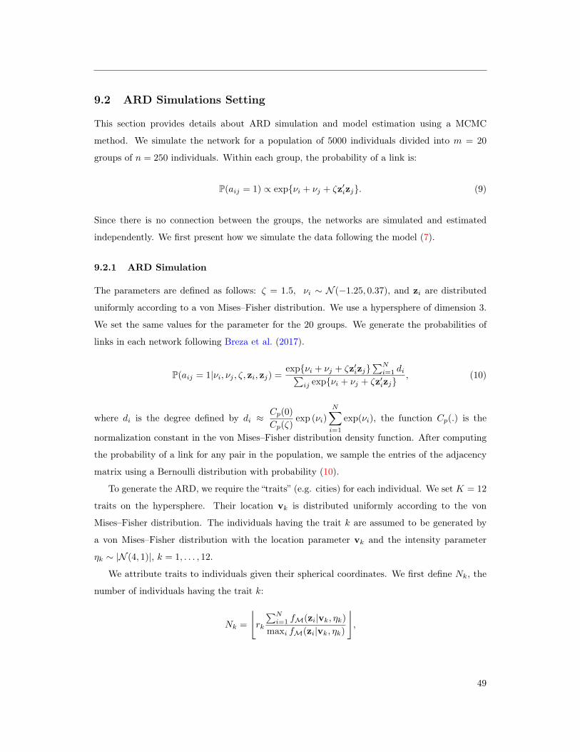
9.2 ARD Simulations Setting

This section provides details about ARD simulation and model estimation using a MCMC

method. We simulate the network for a population of 5000 individuals divided into m = 20

groups of n = 250 individuals. Within each group, the probability of a link is:

P(aij = 1) ∝ expνi + νj + ζz′izj. (9)

Since there is no connection between the groups, the networks are simulated and estimated

independently. We first present how we simulate the data following the model (7).

9.2.1 ARD Simulation

The parameters are defined as follows: ζ = 1.5, νi ∼ N (−1.25, 0.37), and zi are distributed

uniformly according to a von Mises–Fisher distribution. We use a hypersphere of dimension 3.

We set the same values for the parameter for the 20 groups. We generate the probabilities of

links in each network following Breza et al. (2017).

P(aij = 1|νi, νj , ζ, zi, zj) =expνi + νj + ζz′izj

∑Ni=1 di∑

ij expνi + νj + ζz′izj, (10)

where di is the degree defined by di ≈Cp(0)

Cp(ζ)exp (νi)

N∑i=1

exp(νi), the function Cp(.) is the

normalization constant in the von Mises–Fisher distribution density function. After computing

the probability of a link for any pair in the population, we sample the entries of the adjacency

matrix using a Bernoulli distribution with probability (10).

To generate the ARD, we require the “traits” (e.g. cities) for each individual. We set K = 12

traits on the hypersphere. Their location vk is distributed uniformly according to the von

Mises–Fisher distribution. The individuals having the trait k are assumed to be generated by

a von Mises–Fisher distribution with the location parameter vk and the intensity parameter

ηk ∼ |N (4, 1)|, k = 1, . . . , 12.

We attribute traits to individuals given their spherical coordinates. We first define Nk, the

number of individuals having the trait k:

Nk =

⌊rk

∑Ni=1 fM(zi|vk, ηk)

maxi fM(zi|vk, ηk)

⌋,

49

where bxc stands for the greatest integer less than or equal to x, rk is a random number

uniformly distributed over (0.8; 0.95), and fM(zi|vk, ηk) is the von Mises–Fisher distribution

density function evaluated at zi with the location parameter vk and the intensity parameter ηk.

The intuition behind this definition for Nk is that when many zi are close to vk, many

individuals should have the trait k.

We can finally attribute trait k to individual i by sampling a Bernoulli distribution with the

probability fik given by:

fik = NkfM(zi|vk, ηk)∑Ni=1 fM(zi|vk, ηk)

.

The probability of having a trait depends on the proximity of the individuals to the trait’s

location on the hypersphere.

Once the traits for each individual and the network are generated, we can build the ARD.

9.2.2 Model Estimation

In practice, we only have the ARD and the traits for each individual. McCormick and Zheng

(2015) propose a MCMC approach to infer the parameters in model (9).

However, the spherical coordinates and the degrees in this model are not identified. The

authors solve this issue by fixing some vk and use the fixed positions to rotate the latent surface

back to a common orientation at each iteration of the MCMC using a Procrustes transformation.

In addition, the total size of a subset bk is constrained in the MCMC.

As discussed by McCormick and Zheng (2015), the numbers of vk and bk to be set as fixed

depends on the dimension of hypersphere. In our simulations, v1, v2, . . . , v5 are set as fixed to

rotate back the latent space. When simulating the data, we let v1 = (1, 0, 0), v2 = (0, 1, 0), and

v3 = (0, 0, 1). This ensures that the fixed positions on the hypersphere are spaced, as suggested

by the authors, to use as much of the space as possible, maximizing the distance between the

estimated positions. We also constrain b3 to its true value. The results do not change when we

constrain a larger set of bk

Following Breza et al. (2017), we estimate the link probabilities using the parameters’ pos-

terior distributions. The gregariousness parameters are computed from the degrees di and the

parameter ζ using the following equation:

νi = log(di)− log( N∑i=1

di

)+

1

2log(Cp(ζ)

Cp(0)

).

50

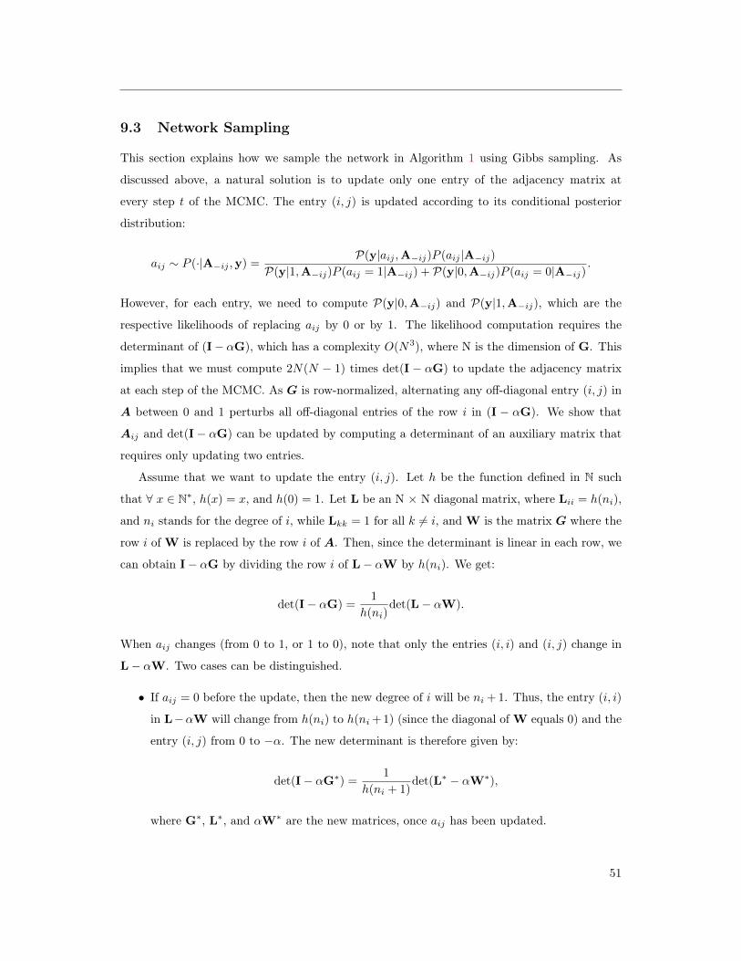
9.3 Network Sampling

This section explains how we sample the network in Algorithm 1 using Gibbs sampling. As

discussed above, a natural solution is to update only one entry of the adjacency matrix at

every step t of the MCMC. The entry (i, j) is updated according to its conditional posterior

distribution:

aij ∼ P (·|A−ij ,y) =P(y|aij ,A−ij)P (aij |A−ij)

P(y|1,A−ij)P (aij = 1|A−ij) + P(y|0,A−ij)P (aij = 0|A−ij).

However, for each entry, we need to compute P(y|0,A−ij) and P(y|1,A−ij), which are the

respective likelihoods of replacing aij by 0 or by 1. The likelihood computation requires the

determinant of (I− αG), which has a complexity O(N3), where N is the dimension of G. This

implies that we must compute 2N(N − 1) times det(I − αG) to update the adjacency matrix

at each step of the MCMC. As G is row-normalized, alternating any off-diagonal entry (i, j) in

A between 0 and 1 perturbs all off-diagonal entries of the row i in (I − αG). We show that

Aij and det(I − αG) can be updated by computing a determinant of an auxiliary matrix that

requires only updating two entries.

Assume that we want to update the entry (i, j). Let h be the function defined in N such

that ∀ x ∈ N∗, h(x) = x, and h(0) = 1. Let L be an N × N diagonal matrix, where Lii = h(ni),

and ni stands for the degree of i, while Lkk = 1 for all k 6= i, and W is the matrix G where the

row i of W is replaced by the row i of A. Then, since the determinant is linear in each row, we

can obtain I− αG by dividing the row i of L− αW by h(ni). We get:

det(I− αG) =1

h(ni)det(L− αW).

When aij changes (from 0 to 1, or 1 to 0), note that only the entries (i, i) and (i, j) change in

L− αW. Two cases can be distinguished.

• If aij = 0 before the update, then the new degree of i will be ni + 1. Thus, the entry (i, i)

in L−αW will change from h(ni) to h(ni + 1) (since the diagonal of W equals 0) and the

entry (i, j) from 0 to −α. The new determinant is therefore given by:

det(I− αG∗) =1

h(ni + 1)det(L∗ − αW∗),

where G∗, L∗, and αW∗ are the new matrices, once aij has been updated.

51

• If aij = 1 before the update, then the new degree of k will be ni − 1. Thus the entry (i, i)

in L − αW will change from h(ni) to h(ni − 1) and the entry (i, j) from −α to 0. The

new determinant is therefore given by:

det(I− αG∗) =1

h(ni − 1)det(L∗ − αW∗).

Then, to update det(L−αW) when only the entries (i, i) and (i, j) change, we adapt the Lemma

1 in Hsieh et al. (2019a) as follows:

Proposition 3. Let ei be the i’th unit basis vector in RN . Let M denote an N × N matrix and

Bij(Q, ε) an N × N matrix as function of an N × N matrix Q and a real value ε, such that:

Bij(Q, ε) =Qeie

′jQ

1 + εe′jQei. (11)

Adding a perturbation ε1 in the (i, i)th position and a perturbation ε2 in the (i, j)th position to

the matrix M can be written as M = M + ε1eie′i + ε2eie

′j.

(a) The inverse of the perturbed matrix can be written as:

M−1 = M−1 − ε1Bii(M−1, ε1)− ε2Bij

(M−1 − ε1Bii(M

−1, ε1), ε2).

(b) The determinant of the perturbed matrix can be written as:

det(M)

=(1 + ε2e

′j

(M−1 − ε1Bii(M

−1, ε1)ei))

(1 + ε1e′iM−1ei)det (M) .

Proof. (a) By the Sherman–Morrison formula (Mele, 2017), we have:

(M + εeie

′j

)−1= M−1 − ε

M−1eie′jM−1

1 + εe′jM−1ei

= M−1 − εBij(M, ε).

Thus,

M−1 =((M + ε1eie

′i) + ε2eie

′j

)−1,

M−1 = (M + ε1eie′i)−1 − ε2Bij((M + ε1eie

′i)−1, ε2),

M−1 = M−1 − ε1Bii(M−1, ε1)− ε2Bij

(M−1 − ε1Bii(M

−1, ε1), ε2).

52

(b) By the matrix determinant lemma (Johnson and Horn, 1985), we have:

det(M + εeie

′j

)= (1 + εe′jM

−1ei)det (M) .

It follows that:

det(M)

= det((M + ε1eie

′i) + ε2eie

′j

),

det(M)

= (1 + ε2e′j(M + ε1eie

′i)−1ei)det (M + ε1eie

′i) ,

det(M)

=(1 + ε2e

′j

(M−1 − ε1Bii(M

−1, ε1)ei))

(1 + ε1e′iM−1ei)det (M) .

The method proposed above becomes computationally intensive when many entries must be

updated simultaneously. We also propose an alternative method that allows updating the block

for entries in A. Let D = (I− αG); we can write:

det(D) =

N∑j=1

(−1)i+jDijδij, (12)

where i denotes any row of D and δij the minor31 associated with the entry (i, j). The minors of

row i do not depend on the values of entries in row i. To update any block in row i, we therefore

compute the N minors associated to i and use this minor within the row. We can then update

many entries simultaneously without increasing the number of times that we compute det(D).

One possibility is to update multiple links simultaneously by randomly choosing the number

of entries to consider and their position in the row. As suggested by Chib and Ramamurthy

(2010), this method would help the Gibbs to converge more quickly. We can summarize how we

update the row i as follows:

(a) Compute the N minors δi1, . . . , δin .

(b) Let ΩG be the entries to update in the row i, and nG = |ΩG| the number of entries in ΩG.

(b.1) Choose r, the size of the block to update, as a random integer number such that

1 ≤ r ≤ nG. In practice, we choose r ≤ min(5, nG) since the number of possibilities

of links to consider grows exponentially with r.31The determinant of the submatrix of M by removing row i and column j.

53

(b.2) Choose the r random entries from ΩG. These entries define the block to update.

(b.3) Compute the posterior probabilities of all possibilities of links inside the block and

update the block (there are 2r possibilities). Use the minors calculated at (a) and

the formula (12) to quickly compute det(D).

(b.4) Remove the r drawn positions from ΩG and let nG = nG − r. Replicate (b.1), (b.2),

and (b.3) until nG = 0.

9.4 Posterior Distributions for Algorithm 1.

To compute the posterior distributions, we set prior distributions on α, Λ, and σ2, where

α = log(α

1− α) and Λ = [β,γ]. In Algorithm 1, we therefore sample α and compute α, such

that α =exp(α)

1 + exp(α). Using this functional form for computing α ensures that α ∈ (0, 1). The

prior distributions are set as follows:

α ∼ N (µα, σ2α),

Λ|σ2 ∼ N (µΛ, σ2ΣΛ),

σ2 ∼ IG(a

2,b

2).

For the simulations and estimations in this paper, we set: µα = −1, σ−2α = 2, µΛ = 0,

ΣΛ−1 =

1

100IK , a = 4 and b = 4, where IK is the identity matrix of dimension K and

K = dim(Λ).

Following Algorithm 1, α is updated at each iteration t of the MCMC by drawing α∗ from the

proposal N (αt−1, ξt), where the jumping scale ξt is also updated at each t following Atchadé and

Rosenthal (2005) for an acceptance rate of a∗ targeted at 0.44. As the proposal is symmetrical,

α∗ =exp(α∗)

1 + exp(α∗)is accepted with the probability:

min

1,P(y|At,Λt−1, α

∗)P (α∗)

P(y|At,θt−1)P (αt)

.

54

The parameters Λt = [βt, γt] and σ2t are drawn from their posterior conditional distributions,

given as follows:

Λt|y,At, αt, σ2t−1 ∼ N (µΛt

, σ2t−1ΣΛt),

σ2t |y,At,θt ∼ IG

(at2,bt2

),

where,

Σ−1Λt

= V′tVt + Σ−1Λ ,

µΛt= ΣΛt

(V′t(y − αtGty) + Σ−1Λ µΛ

),

at = a+N,

bt = b+ (Λt − µΛ)′Σ−1Λ (Λt − µΛ) + (y − αtGty −VtΛt)′(y − αtGty −VtΛt),

Vt = [1, X, GtX].

9.5 Empirical Application

55

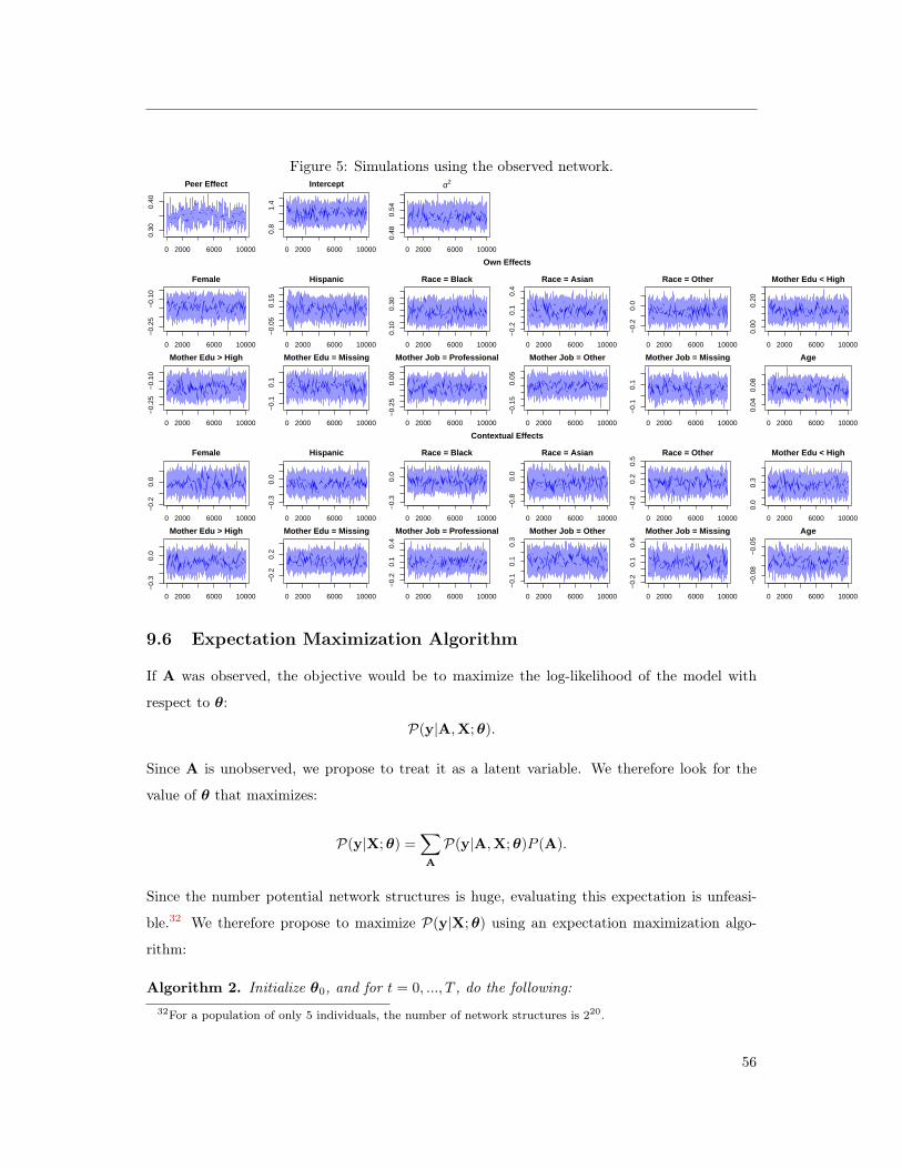
Figure 5: Simulations using the observed network.

0 2000 6000 10000

0.30

0.40

Peer Effect

0 2000 6000 10000

0.8

1.4

Intercept

0 2000 6000 10000

0.48

0.54

σ2

0 2000 6000 10000

−0.

25−

0.10

Female

0 2000 6000 10000

−0.

050.

15Hispanic

0 2000 6000 10000

0.10

0.30

Race = Black

0 2000 6000 10000

−0.

20.

10.

4

Race = Asian

0 2000 6000 10000

−0.

20.

0

Race = Other

0 2000 6000 10000

0.00

0.20

Mother Edu < High

0 2000 6000 10000

−0.

25−

0.10

Mother Edu > High

0 2000 6000 10000

−0.

10.

1

Mother Edu = Missing

0 2000 6000 10000

−0.

250.

00

Mother Job = Professional

0 2000 6000 10000

−0.

150.

05

Mother Job = Other

0 2000 6000 10000

−0.

10.

1

Mother Job = Missing

0 2000 6000 10000

0.04

0.08

Age

0 2000 6000 10000

−0.

20.

0

Female

0 2000 6000 10000

−0.

30.

0

Hispanic

0 2000 6000 10000

−0.

30.

0

Race = Black

0 2000 6000 10000−

0.8

0.0

Race = Asian

0 2000 6000 10000

−0.

20.

20.

5

Race = Other

0 2000 6000 10000

0.0

0.3

Mother Edu < High

0 2000 6000 10000

−0.

30.

0

Mother Edu > High

0 2000 6000 10000

−0.

20.

2


0 2000 6000 10000

−0.

20.

10.

4


0 2000 6000 10000

−0.

10.

10.

3

Mother Job = Other

0 2000 6000 10000

−0.

20.

10.

4


0 2000 6000 10000

−0.

08−

0.05

Age

Own Effects

Index

Contextual Effects

Index

9.6 Expectation Maximization Algorithm

If A was observed, the objective would be to maximize the log-likelihood of the model with

respect to θ:

P(y|A,X;θ).

Since A is unobserved, we propose to treat it as a latent variable. We therefore look for the

value of θ that maximizes:

P(y|X;θ) =∑A

P(y|A,X;θ)P (A).

Since the number potential network structures is huge, evaluating this expectation is unfeasi-

ble.32 We therefore propose to maximize P(y|X;θ) using an expectation maximization algo-

rithm:

Algorithm 2. Initialize θ0, and for t = 0, ..., T , do the following:32For a population of only 5 individuals, the number of network structures is 220.

56

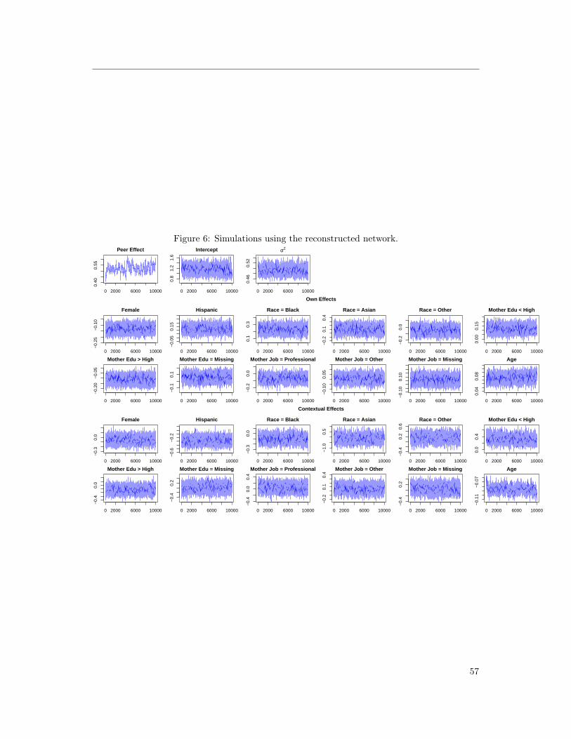
Figure 6: Simulations using the reconstructed network.

0 2000 6000 10000

0.40

0.55

Peer Effect

0 2000 6000 10000

0.8

1.2

1.6

Intercept

0 2000 6000 10000

0.46

0.52

σ2

0 2000 6000 10000

−0.

25−

0.10

Female

0 2000 6000 10000

−0.

050.

15

Hispanic

0 2000 6000 10000

0.1

0.3

Race = Black

0 2000 6000 10000

−0.

20.

10.

4

Race = Asian

0 2000 6000 10000

−0.

20.

0

Race = Other

0 2000 6000 10000

0.00

0.15

Mother Edu < High

0 2000 6000 10000

−0.

20−

0.05

Mother Edu > High

0 2000 6000 10000

−0.

10.

1


0 2000 6000 10000

−0.

20.

0


0 2000 6000 10000

−0.

100.

05

Mother Job = Other

0 2000 6000 10000−

0.10

0.10


0 2000 6000 10000

0.04

0.08

Age

0 2000 6000 10000

−0.

30.

0

Female

0 2000 6000 10000

−0.

6−

0.2

Hispanic

0 2000 6000 10000

−0.

30.

0

Race = Black

0 2000 6000 10000

−1.

00.

5

Race = Asian

0 2000 6000 10000

−0.

40.

20.

6

Race = Other

0 2000 6000 10000

0.0

0.4

Mother Edu < High

0 2000 6000 10000

−0.

40.

0

Mother Edu > High

0 2000 6000 10000

−0.

40.

2


0 2000 6000 10000

−0.

40.

00.

4


0 2000 6000 10000

−0.

20.

10.

4

Mother Job = Other

0 2000 6000 10000

−0.

40.

2


0 2000 6000 10000

−0.

11−

0.07

Age

Own Effects

Index

Contextual Effects

Index

57

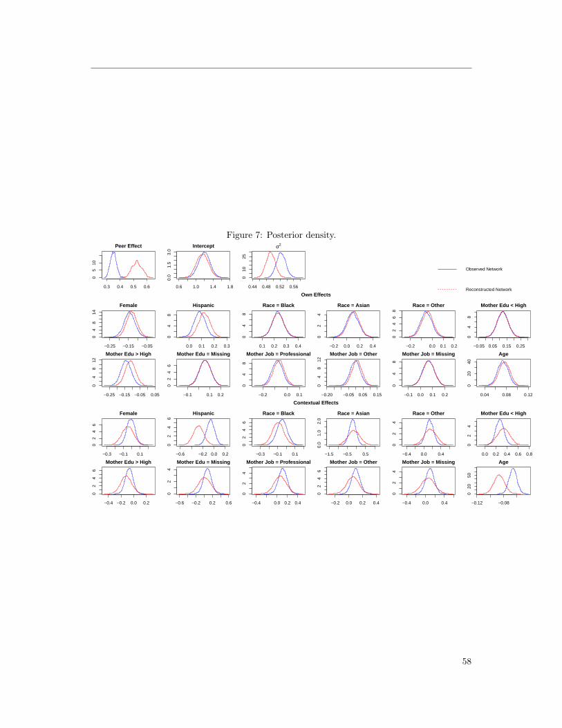
Figure 7: Posterior density.

0.3 0.4 0.5 0.6

05

10

Peer Effect

0.6 1.0 1.4 1.8

0.0

1.5

3.0

Intercept

0.44 0.48 0.52 0.56

010

25σ2

−0.25 −0.15 −0.05

04

814

Female

0.0 0.1 0.2 0.3

04

8

Hispanic

0.1 0.2 0.3 0.4

04

8

Race = Black

−0.2 0.0 0.2 0.4

02

4

Race = Asian

−0.2 0.0 0.1 0.2

02

46

8

Race = Other

−0.05 0.05 0.15 0.25

04

8

Mother Edu < High

−0.25 −0.15 −0.05 0.05

04

812

Mother Edu > High

−0.1 0.1 0.2

02

46


−0.2 0.0 0.1

04

8


−0.20 −0.05 0.05 0.15

04

812

Mother Job = Other

−0.1 0.0 0.1 0.20

48


0.04 0.08 0.12

020

40

Age

−0.3 −0.1 0.1

02

46

Female

−0.6 −0.2 0.0 0.2

02

46

Hispanic

−0.3 −0.1 0.1

02

46

Race = Black

−1.5 −0.5 0.5

0.0

1.0

2.0

Race = Asian

−0.4 0.0 0.4

02

4

Race = Other

0.0 0.2 0.4 0.6 0.8

02

4

Mother Edu < High

−0.4 −0.2 0.0 0.2

02

46

Mother Edu > High

−0.6 −0.2 0.2 0.6

02

4


−0.4 0.0 0.2 0.4

02

4


−0.2 0.0 0.2 0.4

02

46

Mother Job = Other

−0.4 0.0 0.4

02

4


−0.12 −0.08

020

50

Age

0

0

Observed Network

Reconstructed NetworkOwn Effects

Index

Contextual Effects

Index

58

1. Use a Metropolis–Hastings algorithm (see Algorithm 1) to obtain the draws (A1, ...,AR)

from P (A|y,θt).

2. Evaluate

Qt(θ) ≈R∑r=1

P(y|Ar,X;θt).

3. Set θt+1 = arg maxQt(θ).

59

Estimating Peer Effects Using Partial Network Data

Documents

Transcript of Estimating Peer Effects Using Partial Network Data