Fluid Limits Applied toPeer to Peer Network Analysis

Laura AspirotUniversidad de la Republica

Montevideo, Uruguayaspirot@fing.edu.uy

Ernesto MordeckiUniversidad de la Republica

Montevideo, Uruguaymordecki@cmat.edu.uy

Gerardo RubinoINRIA Rennes - Bretagne Atlantique

Rennes, Francegerardo.rubino@inria.fr

Abstract—The objective of several techniques including fluidlimits and mean field approximations is to analyze a stochasticcomplex system (e.g. Markovian) studying a simplified model(deterministic, represented by ordinary differential equations(ODEs)). In this paper, we explore models proposed for theanalysis of BitTorrent P2P systems and we provide the argumentsto justify the passage from the stochastic process, under adequatescaling, to a fluid approximation driven by an ODE. We also makethe link between the stationary regime of the stochastic modelsand the fixed points of the associated ODEs. Finally, we analyzethe asymptotic distribution of the scaled process.

Index Terms—fluid limits, mean fields, BitTorrent

I. I NTRODUCTION

There are several examples of complex stochastic systemsfor which analytical expressions cannot be derived, or thatare even difficult to simulate. However, in many cases theycan be studied much more easily by analyzing deterministicsystems, obtained as asymptotic approximations of the originalones. The complexity of the system may be due to its size,its dependence structure, etc. There are many such systems,as for instance TCP connections, wireless systems, or peerto peer networks. In the case of TCP connections sharing abottleneck, wireless users sharing a channel, or in the peertopeer case, there is a common resource and many individuals.The behavior of each one depends on the state of the wholesystem, introducing dependence between all the individuals.

Starting from a stochastic model the objective is to finda deterministic approximation for the original process. Thisintroduces the problem of finding the suitable scale for thisapproximation. For example, classical results in queuing the-ory consider a sequence of stochastic processes indexed byan integerN , where some key state variable appears dividedby N , and the time variable is multiplied (“accelerated”) bythe same factor, obtaining a deterministic limit whenN goesto infinity. In addition, in other areas such as in biology,or in the analysis of epidemic phenomena, a typical scalingconsists in dividing byN , and in considering transition ratesincreasing withN (jumps are of order1/N and transition ratesof orderN , that means that the product remains “constant” asN increases). For a survey about this topic see [1], and fora more general reference about limits of stochastic processeswe suggest [2]. In this paper we follow mostly the approachof [2] and [3].

Let us describe another way to approximate complexstochastic systems by deterministic ones. This approach iscalled mean field approximations. This technique comes fromphysics, where it is used to study systems with a large numberof interacting particles. When the number of particles increaseseach particle behaves as if it were under the action of a globalforce (the mean field). Applications to telecommunicationsappeared in the literature and were widely developed in thelast decade. There are many works, considering different typesof phenomena and different types of models (discrete orcontinuous time, discrete or continuous state space, etc.). Forinstance [4], [5], [6], [7] and the references therein coverawide range of techniques and applications. More recently meanfield methods have been applied to game theory and optimalcontrol (see for example [8], [9] and references therein).

In mean field approximations we can distinguish two steps:the first one is focused on the occupation measure limit (i.e.the asymptotic proportion of individuals in each state) andthe second one is focused on the decoupling assumption(asymptotically the state of each individual is independentfrom the others). A very frequent approach to the first stepconsists in proving the limit with the same techniques as inthe fluid limits case. The proof of the asymptotic independencerelies in different tools.

One of the main results, both in the case of fluid limitsor mean fields, when a stochastic system is approximated byone modeled by an ODE, is that in some cases the stationaryregime of the former can be analyzed by studying the ODE’sfixed points. There are many issues on this topic discussed in[4], [5], [10].

Our object of study is the use of fluid limits for modelingpeer to peer systems. In the literature we can find works onpeer to peer systems using stochastic models [11], fluid models[12], [13] and fluid limits or mean field approximations [14],[15], [16]).

In this work we consider a fluid limit model for a BitTorrentnetwork based on [12], [13]. In both papers the deterministicmodel is the starting point of the analysis. We, on the otherhand, start from a stochastic one and justify the passage fromone to the other.

The contributions of this work consist first in the mathe-matical justification that the deterministic fluid models in[12]and [13] are fluid limits of stochastic models, that we present.

En each case we define a stochastic model and construct asequence of stochastic processes such that, under adequatescaling, converges to a deterministic model driven by an ODE.The second contribution is that we prove the existence of astationary regime for each process in the sequence and thenwe prove that the sequence of processes in stationary regimeconverges to the ODE’s fixed point. We finally describe theasymptotic distribution of the stochastic process. We prove thatthe difference between the scaled process and the deterministicone can be approximated by a gaussian process.

The remainder of the paper is structured as follows. InSection II first we present some well known models andthen we describe our model. In Section III we provide ourresults about the approximation by a deterministic process,the existence and convergence of stationary regime and theasymptotic distribution. In Section IV we conclude this work.

II. M ODEL

In this section we give a brief description of BitTorrent.Then we consider three BitTorrent models from the literature:a stochastic model in [11], and two fluid models in [12] and[13], in subsection II-A. At the end we state our stochasticmodels in subsection II-B.

BitTorrent is a peer to peer protocol, for file sharingover a network. BitTorrent divides the target file into smallfiles (chunks). Each peer connects to others and downloadssimultaneously different chunks. There are two types of peers:leechersandseeds. Leechers download parts of the file fromother peers and upload parts of the file for other leechers.Seeds have all the file and only remain in the system to helpleechers to get missing file parts (they arealtruist nodes).We do not detail here the peer selection policy (see forexample [12]) and other features that help in understandingthe behavior, for example based on traffic measures (see [17],[18], [19]).

A. Stochastic and fluid models for BitTorrent in the literature

We first describe the stochastic model proposed by Yang andde Veciana in [11], that is the motivation for the fluid modelin [12]. In [11] the BitTorrent network is described using abranching process for the transient regime and a Markov modelfor the stationary regime. For the Markov model, the followingparameters are considered:

• X(t): number of leechers at timet,• Y (t): number of seeds at timet,• λ: arrival rate (Poisson) of peers,• µ: uploading rate for each peer,• γ: leaving rate for seeds;

with the following transition rates:

• q((x, y), (x + 1, y)) = λ (arrival of a new peer),• q((x, y), (x−1, y+1)) = µ(x+y) (a leecher successfully

finishes downloading the file),• q((x, y), (x, y − 1)) = γy (a seed leaves the network).

For (0, y) there is no possible transition in the directionq((x, y), (x − 1, y + 1) and the remaining rates are the same

as before. In [11] the stationary distribution is computednumerically.

Now we describe the fluid model proposed by Qiu andSrikant in [12]. A BitTorrent system is analyzed, using dif-ferent tools. One of the approaches is the fluid descriptionbased on the stochastic model of [11]. The fluid model alsoconsiders two aspects that are not discussed in [11]: the firstone is that leechers may leave the system before finishingtheir download and the second one is that capacity restriction,related to the time needed to finish a download, may be inthe uploading capacity of peers (as in [11]) but also in thedownloading capacity. The fluid model is stated as follows:

• x(t): number of leechers at timet,• y(t): number of seeds at timet,• λ: arrival rate (Poisson) of peers,• µ: uploading rate for each peer,• c: downloading rate for each peer,• θ: leaving rate for leechers,• γ: leaving rate for seeds,• η ∈ [0, 1]: efficiency factor, that takes into account the

efficiency of the file sharing mechanism ([12] provides adetailed analysis ofη),

The maximal total uploading rate isµ(ηx+y), the maximaltotal downloading rate iscx, and the restriction may be in theupload or in the download. The effective downloading rateis thusmin (cx, µ(ηx + y)). The evolution of the number ofleechers and seeds is described by the following ODE:

{x′ = λ−min(cx, µ(ηx + y))− θx,y′ = min(cx, µ(ηx + y))− γy.

(1)

There is a liney = (c/µ− η)x where the behavior ofthe system changes because of the termmin(cx, µ(ηx + y)),dividing the state space in two zones. The authors state thatthe average number of leechers and seeds in stationary regimeare the values of the ODE’s fixed point(x∗, y∗) and derive theaverage downloading time from an approximation of Little’slaw. They also show a good fitting with simulations of theBitTorrent protocol and with real traces, specially when thearrival rateλ is high.

Based on [12], Rivero and Rubino in [13] consider a fluidmodel for a BitTorrent network with different classes of peers.There are two classes of leechers: high tolerance leechers andlow tolerance ones. The parameters are the following:

• xa(t): number of high tolerance leechers at timet,• xb(t): number of low tolerance leechers at timet,• y(t): number of seeds at timet,• λa: arrival rate of high tolerance leechers,• λb: arrival rate of low tolerance leechers,• µ: uploading rate for each peer,• c: downloading rate for each peer,• θa: leaving rate for high tolerance leechers,• θb: leaving rate for low tolerance leechers, withθb > θa,• γ: leaving rate for seeds,• the efficiency factor isη = 1,

The fluid model for this system is:

x′a = λa − θaxa − ua,

x′b = λb − θbxb − ub,

y′ = ua + ub − γy,(2)

where

ua = min(cxa, µ(xa + xb + y)

xa

x

),

ub = min(cxb, µ(xa + xb + y)

xb

x

).

From this equation there are also two different zones, dividedby a plane, again due to the restriction in uploading anddownloading capacity. A strategy to improve performance bygiving priority to peers that will probably stay more time inthe system as seeds, specially in bad resource conditions, isstudied. In order to define the policy, the space is dividedby planes in three zones, according to the capacity. Foreach zone a server policy is defined (giving priority for hightolerance leechers when capacity is not enough). A fluid modelconsidering the different policies in each zone is stated. Thestudy of fixed points allows to analyze the priority policy,compared with the non priority one.

In this paper we consider stochastic and fluid models thatallow to analyze the number of peers in the system. Anotherapproach to study BitTorrent systems is to consider the numberand type of chunks that each peer possesses [14], [15], [16].In particular they study the asymptotic behavior of a Markovprocess that converges to the solution of an ODE. In the threeworks the authors consider different asymptotic regimes, bothin the number of peers and in the number of chunks. Forinstance, the authors of [16] study what they callcouponreplication system, that models a file sharing BitTorrent-like mechanism. Their model consider many users, each oneaiming to complete a collection of coupons. At each time twousers meet and obtain one missing coupon from the otherby replication (if they do not have the same coupons). Themodel is motivated by the BitTorrent mechanism, where eachchunk is a coupon. Results from [2] are used to prove theapproximation by an asymptotic deterministic model for thenumber of coupons hold by each user, when the number ofcoupons goes to infinity. However, a closed form formula isobtained only for some particular cases.

B. Stochastic models

In this subsection we introduce our stochastic models thatdescribe the number of leechers and seeds for the systemsstudied in [12], [13]. From these microscopic descriptionsofthe models in [12], [13] we construct a sequence of processesthat converges to deterministic limits. We consider a two-dimensional continuous time Markov chain for the numberof leechers and seeds, so we describe the whole system.However, our model is motivated by a detailed descriptionfor the behavior of each peer. In Section III we prove thatthese limits verify equations (1) and (2) respectively, whichare the starting points in [12], [13].

0 5 100

0.1

0.2

0.3

0.4

0.5

0.6

0.7

Time (s)

Pee

rs (

10−

2 )

LeechersSeeds

0 0.1 0.2 0.3 0.4−0.1

0

0.1

0.2

0.3

0.4

0.5

0.6

0.7

Leechers (10−2)

See

ds (

10−

2 )

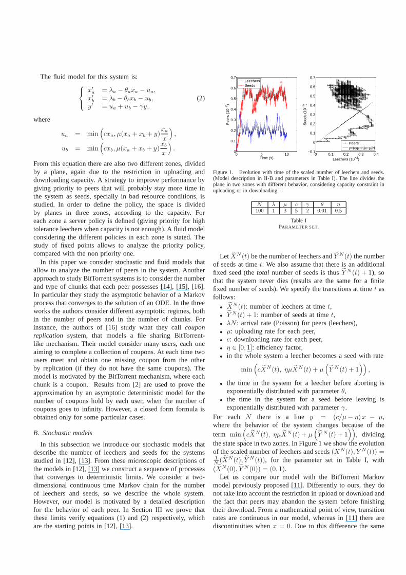
Peersy=(c/µ−η)x−µ/N

Figure 1. Evolution with time of the scaled number of leechers and seeds.(Model description in II-B and parameters in Table I). The line divides theplane in two zones with different behavior, considering capacity constraint inuploading or in downloading .

N λ µ c γ θ η

100 1 3 5 2 0.01 0.5

Table IPARAMETER SET.

Let XN(t) be the number of leechers andY N (t) the numberof seeds at timet. We also assume that there is an additionalfixed seed (thetotal number of seeds is thusY N (t) + 1), sothat the system never dies (results are the same for a finitefixed number of seeds). We specify the transitions at timet asfollows:

• XN(t): number of leechers at timet,• Y N (t) + 1: number of seeds at timet,• λN : arrival rate (Poisson) for peers (leechers),• µ: uploading rate for each peer,• c: downloading rate for each peer,• η ∈ [0, 1]: efficiency factor,• in the whole system a leecher becomes a seed with rate

min(cXN(t), ηµXN(t) + µ

(Y N (t) + 1

)),

• the time in the system for a leecher before aborting isexponentially distributed with parameterθ,

• the time in the system for a seed before leaving isexponentially distributed with parameterγ.

For each N there is a line y = (c/µ− η)x − µ,where the behavior of the system changes because of theterm min

(cXN(t), ηµXN (t) + µ

(Y N (t) + 1

)), dividing

the state space in two zones. In Figure 1 we show the evolutionof the scaled number of leechers and seeds(XN(t), Y N (t)) =1N(XN(t), Y N (t)), for the parameter set in Table I, with

(XN(0), Y N (0)) = (0, 1).Let us compare our model with the BitTorrent Markov

model previously proposed [11]. Differently to ours, they donot take into account the restriction in upload or download andthe fact that peers may abandon the system before finishingtheir download. From a mathematical point of view, transitionrates are continuous in our model, whereas in [11] there arediscontinuities whenx = 0. Due to this difference the same

0 5 100

0.1

0.2

0.3

0.4

0.5

0.6

0.7

Time (s)

Pee

rs (

10−

2 )

LeechersSeeds

0 0.05 0.1 0.150

0.1

0.2

0.3

0.4

0.5

0.6

0.7

Leechers (10−2)

See

ds (

10−

2 )

Peers

Figure 2. Evolution with time of the scaled number of leechers and seedsfor the model in [11] (parameters in Table I).

techniques cannot be used to analyze them. To get someintuition on both models we compare them in Figure 1 and 2,where we show the evolution for the model in [11], when thearrival rate isλN , the scaled number of leechers and seeds.Note that there is a refracting barrier inx = 0 in Figure 2.

Now describe a stochastic microscopic model associated tothe fluid model in [13]. Consider two classes of leechers. LetXN

a (t) be the number of leechers of typea, XNb (t) the number

of leechers of typeb, andY N (t) the number of seeds at timet. The total number of seeds isY N (t) + 1, so that the systemnever dies. We specify the transitions at timet as follows:

• λaN , λbN : arrival rate (Poisson) for peers (leechers) oftype a andb respectively,

• a leecher of typea becomes a seed with rate

min

(cXN

a (t), µXNa (t) + µ(Y N (t) + 1)

XNa (t)

XN(t)

),

and the same holds for a leecher of typeb with rate

min

(cXN

b (t), µXNb (t) + µ(Y N (t) + 1)

XNb (t)

XN(t)

),

• the time in the system for a leecher before aborting itsdownload is exponentially distributed with parameterθafor leechers of typea and with parameterθb for leechersof type b, with θb > θa,

• the time in the system for a seed before leaving isexponentially distributed with parameterγ.

Regarding our model we have considered a Poisson arrivalprocess and exponentially distributed times. There are refer-ences in the literature where this assumption is discussed andcontrasted with real measurements [17], [19]. This point willbe addressed in future work.

III. R ESULTS

In this section we present results about deterministic ap-proximations for the model in II-B. Convergence to an ODE,existence of stationary regime and convergence of the station-ary regime are studied in III-A. A Central Limit Theorem isdiscussed in III-B.

A. Deterministic approximation

We justify the fluid approximation of our model stated inII-B, obtaining equation (1) as the limit when the arrival ratefor peers goes to infinity. We also prove the existence of astationary regime and the convergence in this regime to theODE’s fixed point. These issues are discussed in [12], [13],[16] without proofs and the whole system is directly analyzedfrom the study of ODE’s fixed points.

Proposition 1. Consider

(XN (t), Y N (t)

)=

1

N

(XN(t), Y N (t)

)

and (x, y) the solution to equation(1) with initial condition(x(0), y(0)). If

limN→∞

(XN (0), Y N (0)) = (x(0), y(0))

then, for allT > 0,

limN→∞

supt∈[0,T ]

∥∥(XN (t), Y N (t))− (x(t), y(t))

∥∥ = 0 a.s.,

where a.s. means almost sure convergence.

Proof: The possible transitions in theN -th model, fromstate(XN (t), Y N (t)) are the following:

• a leecher arrives with rateNλ,• a leecher becomes seed with rate

N min(cXN(t), µ

(ηXN(t) + Y N (t) + 1

)),

• a leecher aborts before downloading with rateNθXN (t),• a seed leaves the system with rateNγY N (t).

(XN(t), Y N (t)) is a jump Markov process with transitionrates of the form

Nβl

[(XN(t), Y N (t)

)+O

(1

N

)]

for l ∈ Z2 (l represents a possible transition). Asβl is bounded

and Lipschitz on compact subsets, result follows directly fromKurtz’s Theorem (Theorem 2.1, p. 456) in [2].

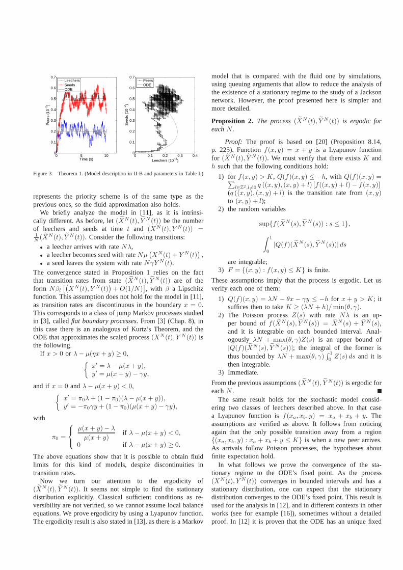
The previous proposition is illustrated in Figure 3. In theleft we show the simulation of one trajectory of the scaledMarkov chain (number of leechers and seeds) for largeN andthe trajectory of the ODE. In the right we show for the samesimulation the evolution on the plane of the Markov chainand the ODE. We can see from that picture that, for largetime values, the number of leechers is around the ODE’s fixedpoint. We analyze this in Theorem 1.

The proof of Kurtz’s Theorem relies on a characterizationon the process(XN , Y N ) as a sum of independent Poissonprocesses (one for each direction of possible transitions)evaluated in a random time change. Under this characterizationthe theorem follows from Gronwall’s inequality and the lawof large numbers for the Poisson process.

The result of Proposition 1 is also valid for the stochasticmodel associated with the system in [13], as it verifies thesame hypotheses and it is also valid for the priority schemeproposed in the same paper [13]. The Markov chain that

0 5 100

0.1

0.2

0.3

0.4

0.5

0.6

0.7

Time (s)

Pee

rs (

10−

2 )

LeechersSeedsODE

0 0.1 0.2 0.3 0.40

0.1

0.2

0.3

0.4

0.5

0.6

0.7

Leechers (10−2)

See

ds (

10−

2 )

PeersODE

Figure 3. Theorem 1. (Model description in II-B and parameters in Table I.)

represents the priority scheme is of the same type as theprevious ones, so the fluid approximation also holds.

We briefly analyze the model in [11], as it is intrinsi-cally different. As before, let(XN (t), Y N (t)) be the numberof leechers and seeds at timet and (XN(t), Y N (t)) =1N(XN(t), Y N (t)). Consider the following transitions:

• a leecher arrives with rateNλ,• a leecher becomes seed with rateNµ

(XN(t) + Y N (t)

),

• a seed leaves the system with rateNγY N (t).

The convergence stated in Proposition 1 relies on the factthat transition rates from state(XN (t), Y N (t)) are of theform Nβl

[(XN(t), Y N (t)

)+O(1/N)

], with β a Lipschitz

function. This assumption does not hold for the model in [11],as transition rates are discontinuous in the boundaryx = 0.This corresponds to a class of jump Markov processes studiedin [3], called flat boundary processes. From [3] (Chap. 8), inthis case there is an analogous of Kurtz’s Theorem, and theODE that approximates the scaled process(XN(t), Y N (t)) isthe following.

If x > 0 or λ− µ(ηx + y) ≥ 0,{

x′ = λ− µ(x+ y),y′ = µ(x+ y)− γy,

and if x = 0 andλ− µ(x+ y) < 0,{

x′ = π0λ+ (1 − π0)(λ − µ(x+ y)),y′ = −π0γy + (1− π0)(µ(x + y)− γy),

with

π0 =

µ(x + y)− λ

µ(x + y)if λ− µ(x+ y) < 0,

0 if λ− µ(x+ y) ≥ 0.

The above equations show that it is possible to obtain fluidlimits for this kind of models, despite discontinuities intransition rates.

Now we turn our attention to the ergodicity of(XN (t), Y N (t)). It seems not simple to find the stationarydistribution explicitly. Classical sufficient conditionsas re-versibility are not verified, so we cannot assume local balanceequations. We prove ergodicity by using a Lyapunov function.The ergodicity result is also stated in [13], as there is a Markov

model that is compared with the fluid one by simulations,using queuing arguments that allow to reduce the analysis ofthe existence of a stationary regime to the study of a Jacksonnetwork. However, the proof presented here is simpler andmore detailed.

Proposition 2. The process(XN (t), Y N (t)) is ergodic foreachN .

Proof: The proof is based on [20] (Proposition 8.14,p. 225). Functionf(x, y) = x + y is a Lyapunov functionfor (XN (t), Y N (t)). We must verify that there existsK andh such that the following conditions hold:

1) for f(x, y) > K, Q(f)(x, y) ≤ −h, with Q(f)(x, y) =∑l∈Z2,l 6=0 q ((x, y), (x, y) + l) [f((x, y) + l)− f(x, y)]

(q ((x, y), (x, y) + l) is the transition rate from(x, y)to (x, y) + l);

2) the random variables

sup{f(XN(s), Y N (s)) : s ≤ 1},∫ 1

0

|Q(f)(XN(s), Y N (s))| ds

are integrable;3) F = {(x, y) : f(x, y) ≤ K} is finite.

These assumptions imply that the process is ergodic. Let usverify each one of them:

1) Q(f)(x, y) = λN − θx − γy ≤ −h for x + y > K; itsuffices then to takeK ≥ (λN + h)/min(θ, γ).

2) The Poisson processZ(s) with rate Nλ is an up-per bound off(XN (s), Y N (s)) = XN(s) + Y N (s),and it is integrable on each bounded interval. Anal-ogously λN + max(θ, γ)Z(s) is an upper bound of|Q(f)(XN(s), Y N (s))|; the integral of the former isthus bounded byλN + max(θ, γ)

∫ 1

0Z(s) ds and it is

then integrable.3) Immediate.

From the previous assumptions(XN (t), Y N (t)) is ergodic foreachN .

The same result holds for the stochastic model consid-ering two classes of leechers described above. In that casea Lyapunov function isf(xa, xb, y) = xa + xb + y. Theassumptions are verified as above. It follows from noticingagain that the only possible transition away from a region{(xa, xb, y) : xa + xb + y ≤ K} is when a new peer arrives.As arrivals follow Poisson processes, the hypotheses aboutfinite expectation hold.

In what follows we prove the convergence of the sta-tionary regime to the ODE’s fixed point. As the process(XN(t), Y N (t)) converges in bounded intervals and has astationary distribution, one can expect that the stationarydistribution converges to the ODE’s fixed point. This resultisused for the analysis in [12], and in different contexts in otherworks (see for example [16]), sometimes without a detailedproof. In [12] it is proven that the ODE has an unique fixed

0 0.1 0.2 0.3 0.4 0.5 0.6 0.70

0.2

0.4

0.6

0.8

1

Leechers (10−2)

See

ds (

10−

2 )

Figure 4. Vector field for equation (1) (parameter set in Table I.).

point

(x∗, y∗) =

λ

β(1 + θ

β

) , λ

γ(1 + θ

β

)

,

with1

β= max

{1

c,1

µ− 1

γ

}.

and that the system is locally stable. The work from Qiu andSang [21] is devoted to the analysis of equation (1), and theyprove that the unique fixed point is a global attractor. We showin Figure 4 the vector field associated with equation (1).

Theorem 1. Let(XN(∞), Y N (∞)

)be the scaled number of

leechers and seeds in stationary regime. Let(x∗, y∗) be thefixed point in(1). Then

limN→∞

(XN(∞), Y N (∞)

)= (x∗, y∗)

in probability.

Proof: Let µN (t) be the distribution of(XN(t), Y N (t)

)

and letπN (∞) be the stationary distribution of the process (weknow from Proposition 2 that there exists a unique stationarydistribution for eachN ). We will use for our proof Theorem6.89, p. 165 in [3]. This theorem assures that under a set ofhypotheses that will be verified, if(x∗, y∗) is a global attractorthen limN→∞

∫Bε(q)

dπN (∞) = 1, with (x∗, y∗) = q andBε(q) =

{y ∈ R

2 : ‖y − q‖ < ε}

, which implies that

limN→∞

(XN(∞), Y N (∞)

)= (x∗, y∗)

in probability. To apply the result we must verify that:

1) the jumps of the Markov process take integer values ineach direction,

2) the ratesβl are uniformly Lipschitz continuous in aneighborhood of(x∗, y∗),

3) the process is positive recurrent,4) if τε(N) = inf

{t :∥∥(XN (t), Y N (t)

)− (x∗, y∗)

∥∥ < ε}

,then for eachK, ε and for allN , there exists a constantCε,M (that depends onε andM ) such that

sup‖p−q‖≤M

Ep [τε(N)] ≤ Cε,M < ∞,

with p = (x(0), y(0)) andEp the expected value startingfrom p.

The first three assumptions are immediately verified (the thirdone arises from Proposition 2). So, we focus on fourth as-sumption. Also from [3] (Lemma 6.32 p. 143) the distributionof τε(N) has geometric tails for largeN , that is, there is aT (ε) < ∞ and a constantC0(ε) such that

Pp(τε(N) > kT ) ≤ e−NC0(ε)k.

This implies the bound forEp [τε(N)] and thus completes theproof.

The convergence for the stationary distribution to the ODE’sfixed points is a widely discussed topic. The authors of [4]prove this convergence in the case of the occupation measureof a system withN individuals and a finite state space. Ourproblem differs from that situation because of the compactnessof the state space. However, our proof and the proof in [4]rely in large deviations results. The proof in [4] is basedon [22], where a very general result (considering the casewith multiple invariant distributions and a much more complexasymptotic behavior for the ODE) is proven using large devia-tions arguments together with dynamical systems ones. In [4]it is also discussed why the existence of a unique fixed pointdoes not guarantee the convergence of a sequence of invariantdistributions. It shows examples where there is only one fixedpoint but the support of accumulation points of invariantdistributions lies on set that is a limit cycle for the ODE. Inorder to avoid the problem of proving asymptotic stability,[10]presents a very general result of convergence for the stationarydistribution when there is a unique fixed point in case ofreversible processes, a strong assumption that is not validinour model. The convergence for the stationary distributionofthe occupation measure is also discussed in [23], in a moregeneral framework (denumerable state spaces). The proof thereis strongly related with the mean field decoupling assumption(the asymptotic independence and the convergence of thestationary distributions are proved together).

For the model in [13] we do not have a proof of globalstability of ODE’s fixed point, so we cannot yet extendthe previous theorem for that case. It is only observed insimulations in [13] that the stationary regime converges tothe fixed point of the associated ODEs, both in the priorityand non priority schemes.

B. Gaussian approximation

Here we derive a Gaussian approximation for the distribu-tion of the difference between the stochastic and the determin-istic processes. This approximation describes in a precisewaythe system behavior for large values ofN simultaneously forall t providing confidence intervals for the number of leechersand seeds.

Theorem 2. Consider(XN(t), Y N (t)

)and let (x, y) be the

solution to equation(1) with initial condition (x(0), y(0)). If

limN→∞

√N[(XN (0), Y N (0))− (x(0), y(0))

]= V (0)

−2 0 20

10

20

30Leechers (N=10)

−2 0 20

5

10

15

20Seeds (N=10)

−2 0 20

10

20

30Leechers (N=50)

−2 0 20

10

20

30Seeds (N=50)

−2 0 20

10

20

30Leechers (N=100)

−2 0 20

10

20

30Seeds (N=100)

−2 0 20

10

20

30Leechers (N=500)

−2 0 20

10

20

30Seeds (N=500)

Figure 5. Histograms of 100 independent samples of√

N(

XN (1) − x(1))

and√

N(

Y N (1) − y(1))

for different values ofN .

in probability, withV (0) deterministic, then,√N[(XN(t), Y N (t)

)− (x(t), y(t))

]⇒N V (t),

where⇒ means convergence in distribution.V (t) is a Gaus-sian process with covariance matrix

Cov (V (t), V (r))

= eM(t)t+M(r)T r

∫ t∧r

0

e−(M(t)+M(r)T)sG(s) ds,

G(s) = λ+ θx(s) + γy(s) + 2min(cx(s), µ(ηx(s) + y(s))

),

M(t) =

(−(c+ θ) 0

c −γ

)if cx(t) < µ(ηx(t) + y(t)),

M(t) =

(−(µη + θ) −µ

µη µ− γ

)if cx(t) > µ(ηx(t)+y(t)),

M(t)T denote the transposed ofM(t).

Proof: Result follows as a consequence of Kurtz’s The-orem (see Theorem 2.3, p.458, in [2]). We use the explicitform of the covariance matrix provided there. The proof ofthat theorem relies on a representation ofV N (t) and V (t)by an integral involving the differentialdF (x(t), y(t)), so theoriginal theorem assumes that the transition ratesβl(x, y) areC1 functions. This assumption is not valid in our case, butthere is only onet whereβl(x(t), y(t)) is not differentiable(that is whencx(t) = µ(ηx(t) + y(t))). As this happensat only one point, it does not affect the integral represen-tation. The justification that there is only onet for whichcx(t) = µ(ηx(t) + y(t)) follows from the fact that the fixedpoint is a global attractor, so the trajectories(x(t), y(t)) hit{(x, y) : cx = µ(ηx+ y)} only a finite number of times (thisis sufficient for the validity of the integral representation ofV N (t) as in Theorem 2.3, p. 458, [2]). In Figure 4 it can beseen that there is at most one hitting point in our case.

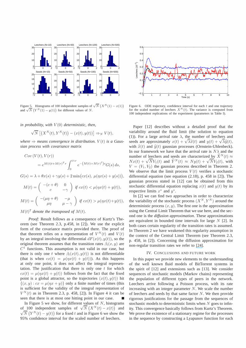
In Figure 5 we show, for different values ofN , histogramsof 100 independent samples of

√N(XN(t)− x(t)

)and√

N(Y N (t)− y(t)

)for a fixedt and in Figure 6 we show the

95% confidence interval for the scaled number of leechers.

0 1 2 3 4 5 6 7 8 9 10−0.1

0

0.1

0.2

0.3

0.4

0.5

0.6

Time (s)

Leec

hers

(10

−2 )

Figure 6. ODE trajectory, confidence interval for eacht and one trajectoryfor the scaled number of leechersXN (t). The variance is computed from100 independent replications of the experiment (parameters in Table I).

Paper [12] describes without a detailed proof that thevariability around the fluid limit (the solution to equation(1)). For a large arrival rateλ, the number of leechers andseeds are approximatelyx(t) +

√λx(t) and y(t) +

√λy(t),

with x(t) and y(t) gaussian processes (Ornstein-Uhlenbeck).In our framework we have that the arrival rate isNλ and thenumber of leechers and seeds are characterized byXN(t) ≈Nx(t) +

√NV1(t) and Y N (t) ≈ Ny(t) +

√NV2(t), with

V = (V1, V2) the gaussian process described in Theorem 2.We observe that the limit processV (t) verifies a stochasticdifferential equation (see equation (2.18), p. 458 in [2]).Thegaussian process stated in [12] can be obtained from thisstochastic differential equation replacingx(t) andy(t) by itsrespective limitsx∗ andy∗.

In [2] we can find two approaches in order to characterizethe variability of the stochastic process(XN , Y N ) around thedeterministic process(x, y). The first one is the approximationusing the Central Limit Theorem that we use here, and the sec-ond one is thediffusion approximation. These approximationsare equivalent in bounded time intervals for largeN [2]. Inboth cases certain regularity of the transition rates is assumed.In Theorem 2 we have weakened this regularity assumption inthe context of the Central Limit Theorem (see Theorem 2.3,p. 458, in [2]). Concerning the diffusion approximation fornon-regular transition rates we refer to [24].

IV. CONCLUSIONS AND FUTURE WORK

In this paper we provide new elements to the understandingof the well known fluid models of BitTorrent systems inthe spirit of [12] and extensions such as [13]. We considersequences of stochastic models (Markov chains) representingthe population of different types of peers in the network.Leechers arrive following a Poisson process, with its rateincreasing with an integer parameterN . We scale the numberof leechers and seeds by that same factorN . We then providerigorous justifications for the passage from the sequences ofstochastic models to deterministic limits whenN goes to infin-ity. This convergence basically follows from Kurtz’s Theorem.We prove the existence of a stationary regime for the processesin the sequence by constructing a Lyapunov function for each

one of them and the convergence of the stationary distributionto the ODE’s fixed point. This result involves some argumentsfrom large deviations’ theory. We also prove, as a consequenceof Kurtz’s Theorem, that asymptotically the scaled numberof leechers and seeds follows a gaussian process. These aretopics to be further analyzed in future work, together withsome stability issues. We will also analyze the assumptionsabout Poisson arrivals and exponentially distributed times, inorder to consider more general models.

ACKNOWLEDGEMENTS

This paper was partially supported by the French ResearchANR Project ViPeer. The authors would like to thank PabloBelzarena and Federico Larroca for helpful discussions on thetopics of the paper.

REFERENCES

[1] R. W. R. Darling and J. R. Norris, “Differential equationapproximationsfor Markov chains,”Probab. Surv., vol. 5, pp. 37–79, 2008.

[2] S. N. Ethier and T. G. Kurtz,Markov processes: Characterization andconvergence, ser. Wiley Series in Probability and Statistics. New York:John Wiley & Sons Inc., 1986.

[3] A. Shwartz and A. Weiss,Large deviations for performance analysis,ser. Stochastic Modeling Series. London: Chapman & Hall, 1995,queues, communications, and computing, With an appendix byRobertJ. Vanderbei.

[4] M. Benaım and J.-Y. Le Boudec, “A class of mean field interactionmodels for computer and communication systems,”Perform. Eval.,vol. 65, no. 11-12, pp. 823–838, 2008.

[5] C. Bordenave, D. McDonald, and A. Proutiere, “A particlesystem ininteraction with a rapidly varying environment: Mean field limits andapplications,” Networks and Heterogeneous Media, vol. 5, no. 1, pp.31–62, 2010.

[6] A. Chaintreau, J.-Y. Le Boudec, and N. Ristanovic, “The age of gossip:Spatial mean-field regime,” inACM Sigmetrics, , Ed., ACM Sigmetrics,2009, best paper award.

[7] J.-Y. Le Boudec, D. McDonald, and J. Mundinger, “A generic meanfield convergence result for systems of interacting objects,” in QEST’07, Proceedings of the Fourth International Conference onQuantitativeEvaluation of Systems. Washington, DC, USA: IEEE Computer Society,2007, pp. 3–18.

[8] N. Gast, B. Gaujal, and J.-Y. Le Boudec, “Mean field for MarkovDecision Processes: from Discrete to Continuous Optimization,” Tech.Rep., 2010.

[9] H. Tembine, J.-Y. Le Boudec, R. El-Azouzi, and E. Altman,“MeanField Asymptotic of Markov Decision Evolutionary Games andTeams,”in Gamenets 2009, 2009, invited Paper.

[10] J.-Y. Le Boudec, “The Stationary Behaviour of Fluid Limits of Re-versible Processes is Concentrated on Stationary Points,”Tech. Rep.,2010.

[11] X. Yang and G. de Veciana, “Service capacity of peer to peernetworks,” in IEEE INFOCOM, 2004, pp. 1–11. [Online]. Available:citeseer.ist.psu.edu/yang04service.html

[12] D. Qiu and R. Srikant, “Modeling and performance analysis ofbittorrent-like peer-to-peer networks,” inSIGCOMM ’04: Proceedingsof the 2004 conference on Applications, technologies, architectures, andprotocols for computer communications. New York, NY, USA: ACM,2004, pp. 367–378.

[13] M. E. Rivero-Angeles and G. Rubino, “Priority-based scheme for filedistribution in peer-to-peer networks,” inIEEE International Conferenceon Communications (ICC), 2010, 2010, pp. 1–6.

[14] G. Kesidis, T. Konstantopoulos, and P. Sousi, “Modeling file-sharingwith bittorrent-like incentives,” inIEEE International Conference onAcoustics, Speech and Signal Processing, ICASSP 2007, vol. 4, apr.2007, pp. IV–1333 –IV–1336.

[15] ——, “A stochastic epidemiological model and a deterministic limit forbittorrent-like peer-to-peer file-sharing networks,” inNetwork Controland Optimization, ser. Lecture Notes in Computer Science, E. Altmanand A. Chaintreau, Eds. Springer Berlin / Heidelberg, vol. 5425, pp.26–36.

[16] L. Massoulie and M. Vojnovic, “Coupon replication systems,”SIGMET-RICS Perform. Eval. Rev., vol. 33, no. 1, pp. 2–13, 2005.

[17] L. Guo, S. Chen, Z. Xiao, E. Tan, X. Ding, and X. Zhang, “Mea-surements, analysis, and modeling of bittorrent-like systems,” in IMC’05: Proceedings of the 5th ACM SIGCOMM conference on InternetMeasurement. Berkeley, CA, USA: USENIX Association, 2005, pp.4–4.

[18] M. Izal, G. Urvoy-Keller, E. W. Biersack, P. Felber, A. A. Hamra,and L. Garces-Erice, “Dissecting bittorrent: Five monthsin a torrent’slifetime,” in PAM, 2004, pp. 1–11.

[19] J. A. Pouwelse, P. Garbacki, D. H. J. Epema, and H. J. Sips, “Thebittorrent p2p file-sharing system: Measurements and analysis,” inIPTPS, 2005, pp. 205–216.

[20] P. Robert,Stochastic Networks and Queues, ser. Stochastic Modellingand Applied Probability Series. New York: Springer-Verlag, 2003.

[21] D. Qiu and W. Sang, “Global stability of peer-to-peer file sharingsystems,”Comput. Commun., vol. 31, no. 2, pp. 212–219, 2008.

[22] M. Benaım, “Dynamics of stochastic approximation algorithms,” inSeminaire de Probabilites, XXXIII, ser. Lecture Notes in Math. Berlin:Springer, 1999, vol. 1709, pp. 1–68.

[23] C. Bordenave, D. McDonald, and A. Proutiere, “Performance of randommedium access control, an asymptotic approach,” inSIGMETRICS ’08:Proceedings of the 2008 ACM SIGMETRICS international conferenceon Measurement and modeling of computer systems. New York, NY,USA: ACM, 2008, pp. 1–12.

[24] R. Hayden and J. T. Bradley, “A functional central limittheorem forPEPA,” in 8th Workshop on Process Algebra and Stochastically TimedActivities, August 2009, pp. 13–23.