Hydrol. Earth Syst. Sci., 15, 2679–2692, 2011www.hydrol-earth-syst-sci.net/15/2679/2011/doi:10.5194/hess-15-2679-2011© Author(s) 2011. CC Attribution 3.0 License.

Hydrology andEarth System

Sciences

Estimating flooded area and mean water level using active andpassive microwaves: the example of Parana River Delta floodplain

M. Salvia1, F. Grings1, P. Ferrazzoli2, V. Barraza1, V. Douna1, P. Perna1, C. Bruscantini1, and H. Karszenbaum1

1Instituto de Astronomıa y Fısica del Espacio (IAFE, CONICET-UBA), Ciudad Universitaria, Pabellon IAFE,Buenos Aires, Argentina2Tor Vergata University, Ingegneria, DISP, 00133 Rome, Italy

Received: 27 December 2010 – Published in Hydrol. Earth Syst. Sci. Discuss.: 21 March 2011Revised: 12 July 2011 – Accepted: 8 August 2011 – Published: 26 August 2011

Abstract. This paper describes a procedure to estimate boththe fraction of flooded area and the mean water level in veg-etated river floodplains by using a synergy of active and pas-sive microwave signatures. In particular, C band EnvisatASAR in Wide Swath mode and AMSR-E at X, Ku andKa band, are used. The method, which is an extension ofpreviously developed algorithms based on passive data, ex-ploits also model simulations of vegetation emissivity. Theprocedure is applied to a long flood event which occurred inthe Parana River Delta from December 2009 to April 2010.Obtained results are consistent with in situ measurements ofriver water level.

1 Introduction

Over the past decade, several flood monitoring/forecastingmethodologies, based on remote sensing data, have been pro-posed. Among them, the ones based on microwave observa-tions are the most successful, since large flood events andintense cloud covers are often encountered simultaneously.Furthermore, since flood events are dynamic processes, hightemporal and spatial resolutions are usually required. How-ever, due to orbital and technical constraints, both require-ments are generally not achievable.

In this context, several microwave based flood monitoringtechniques were developed. Among them, it is worth men-tioning direct measuring techniques based on scatterometerdata (Prigent et al., 2007), interferometric techniques (Als-dorf et al., 2007) and the fusion of remote sensing-derived

Correspondence to:F. Grings(verderis@iafe.uba.ar)

flood boundaries with topographic data (Pappenberger et al.,2007; Matgen et al., 2007; Zwenzner and Voigt, 2009, allbased on SAR data) and the estimation of flooded areas withpassive microwave signatures (Sippel et al., 1994).

Active microwave techniques, particularly interferomet-ric ones, can provide accurate results. However, the rela-tively low temporal resolution and the small spatial extentlimit their applicability. In general, these techniques are con-strained to small areas and low temporal resolutions. Fur-thermore, active microwave methods have further limitations(e.g. interferometry needs suitable interferometric pairs, andfusion techniques require accurate DEMs of the area). Onthe other hand, passive microwave techniques, characterizedby low spatial resolution and high temporal resolution, canprovide rough estimates of flooded fraction in certain flood-plain regions with virtually no ancillary data (Sippel et al.,1994). Therefore, passive microwaves are often exploited.This is particularly true in large river basins, where extremeflood events compromise thousands of square kilometers in afew days.

From a physical point of view, the sensitivity of mi-crowave measurements to soil and vegetation properties wasproved by several theoretical and experimental investigations(Ulaby et al., 1986). In many cases, passive microwave in-vestigations adopt the absolute difference between the ver-tically and horizontally polarized brightness temperatures1T = (Tbv − Tbh) (Choudhury, 1989) as a useful index tomonitor soil and vegetation conditions. In other cases, thesame difference is normalized to the average value (Polariza-tion Index, PI= 2∗1T/(Tbv +Tbh)) (Paloscia et al., 1993)with the advantage to reduce, or eliminate, the dependenceon surface temperature. For angles higher than 30◦–40◦, itwas proved that both1T and PI are high for wet, flat andbare soils, while their values are reduced if the soil is dry,

Published by Copernicus Publications on behalf of the European Geosciences Union.

2680 M. Salvia et al.: The example of Parana River Delta floodplain

and in presence of roughness and/or vegetation cover (Ulabyet al., 1986; Choudhury, 1989; Kerr and Njoku, 1990; Palos-cia et al., 1993; Jackson and Schmugge, 1991; Paloscia andPampaloni, 1988; Ferrazzoli et al., 1992). All the effects pro-duced by flooding contribute to an increase of1T and PI.

In particular, flooding increases the moisture of the surfaceand decreases its roughness. For higher water levels, and inpresence of vegetation cover, flooding also reduces the heightof the emerged vegetation. In extreme cases, water level sub-merges vegetation. Therefore, the polarization indexes havethe potential to detect the fraction of inundated area and tomonitor the increase of water level. Finally, it is importantto mention that these effects are present at all microwave fre-quencies. Lower frequencies show a better dynamics, but arecharacterized by worse spatial resolution.

Also the influence of surface variables on radar signatureswas investigated extensively for various environments, suchas crops, forests, natural low vegetation, and urban areas.For the active microwave case in natural areas, the overallbackscattering coefficient is essentially influenced by threeprocesses: surface direct contribution, vegetation contribu-tion and surface-vegetation double bounce. At lower fre-quencies (L, C and X band) and angles higher than about 30◦,the three contributions behave and interact in a complex way.Surface backscattering increases with moisture and rough-ness. Vegetation attenuates surface backscattering and pro-duces its own contribution, as well as double bounce. Flood-ing reduces the surface contribution, due to the decrease ofroughness, and increases the double bounce effect in veg-etated areas. At C band, the overall effect produced by amoderate flooding in vegetated areas is an increase of thebackscattering coefficient due to an increase of the doublebounce contribution. However, if the increase of water levelsubmerges most of the vegetation cover, the overall effect isa decrease of backscattering coefficient. Therefore, the trendof the backscattering coefficient as a function of water levelis not monotonic. These properties have been investigatedfor some cases of agricultural and natural vegetation, mostlyat C and X band, also with the aid of models (Le Toan et al.,1989; Caizzone et al., 2009; Grings et al., 2005). In vege-tated areas, the increase of the backscattering coefficient dur-ing flooding related to double bounce was detected also inforest areas, using L band signatures (Wang et al., 1995).

The above mentioned properties make microwave remotesensing a good candidate for flood monitoring of large riverbasins. Some algorithms were designed to integrate both ac-tive and passive information in order to estimate flood con-ditions. A global study about flood dynamics was carriedout using SSM/I signatures in synergy with data collectedby AVHRR and ERS scatterometer (Prigent et al., 2007).However, most of the operational algorithms still use onlypassive or active data. Several authors proposed methodolo-gies to estimate flooded area as a function of brightness tem-perature (or derived indexes) and ancillary information. InChoudhury(1989) the sensitivity of the polarization differ-

ence (1T ) measured at Ka band to flood events was investi-gated. Nimbus 7 data was used to monitor the Amazon River,and a strong seasonal pattern partially correlated to river wa-ter level was found.

An operational algorithm based on passive microwave datawhich estimates the fraction of flooded area was developedby Sippel et al.(1994) and further developed inSippel et al.(1998) andHamilton et al.(2002). Using physical hypothe-ses about the emissivity of water and vegetation, this algo-rithm estimates the fraction of flooded area of a pixel as afunction of the absolute polarization difference (1T ) at agiven frequency. The fractional flooded area is estimatedusing linear mixing models that account for the microwaveemission of the major land covers within the subregion (Sip-pel et al., 1994). This algorithm was tested using Ka bandof SSM/I system. It assumes that the temperature differenceof flooded land,1Tf , has a constant value for all the floodedvegetation types present in the area. This assumption is crit-ical, since1Tf can present large variations as reported bySippel et al.(1994, 1998) andHamilton et al.(2002). In part,these variations are simply related to the statistical inhomo-geneity of vegetation cover in the dimension of the space-borne radiometer pixel, which is of the order of hundredsof km2. However, they are also physically related to varia-tions of water level in vegetated areas, as previously observedin Sippel et al.(1998) and Hamilton et al.(2002). More-over, this dependency on water level is related to vegetationstructure; in fact, for wetland marshes an increase in waterlevel corresponds to a proportional decrease in the emergedbiomass, with severe effects on the vegetation emissivity. Onthe contrary, in arboreous vegetation an increase in waterlevel is related to a decrease in trunk height, a componentof the vegetation that has negligible emission properties forfrequencies= 6.9 GHz.

The objective of this paper is to estimate both the fractionof inundated area and the mean water level inside a wetland.The Parana River Delta is selected as test site. The workadopts techniques of previous papers, such as the formulasof Sippel et al.(1994) and an emission model (Ferrazzoli andGuerriero, 1996a) that is able to simulate the vegetation po-larization difference as a function of water level. The generalapproach is based on the use of both active and passive signa-tures, collected almost simultaneously. First of all, the frac-tion of inundated area is evaluated by applying a thresholdtechnique to Envisat ASAR signatures collected in the WideSwath (WS) mode. Then, AMSR-E signatures are used andformulas ofSippel et al.(1994) are inverted, in order to es-timate1Tf . Finally, the average water level is estimated byinverting the results of model simulations. In this procedurethree AMSR-E channels, i.e. X, Ku and Ka band, are tested.C band is not considered, due to its poor spatial resolution.Some empirical corrections are used to remove the effects ofthe continental area.

Hydrol. Earth Syst. Sci., 15, 2679–2692, 2011 www.hydrol-earth-syst-sci.net/15/2679/2011/

M. Salvia et al.: The example of Parana River Delta floodplain 2681

Section2 gives details about the study area and the usedsatellite signatures. Moreover, it describes all the details ofthe adopted procedure. The obtained results are shown andcommented in Sect.3.

2 Materials and methods

2.1 Description of the site and available maps

The Parana River Delta (PRD) region stretches through thefinal 300 km of the Parana basin. It covers approximately17 500 km2, close to Buenos Aires city in Argentina. Aland cover map is shown in Fig.1, in which the locationsof the five water level stations considered in this paper areindicated.

The Parana River drains an approximate area of2 310 000 km2 and, according to its length, basin size, andwater discharge, is considered the second most importantone in South America after the Amazonas. Among the largerivers of the world, it is the only one that flows from tropi-cal to temperate latitudes, where it joins the Uruguay Riverending in the Del Plata estuary.

The landscape patterns of this region are subordinated toa flooding regime characterized by different sources of wa-ter with different properties, such as local precipitation andlarge rivers, whose specific flooding patterns affect particu-lar areas. Sometimes these sources add together provokingstrong flooding events, with main peaks in late summer andin winter.

The combination of local topographic gradients and a re-gional flooding regime constitutes the primary factor that de-termines the emergent natural vegetation, mainly consistingof marshes growing in lowlands where the substrate is sat-urated permanently or semi permanently (Parmuchi et al.,2002). In the specific area of the Delta under study, there arefour ecosystems that account for more than 95 % of the land-cover: junco marsh, cortadera marsh, grassland and prairieof aquatic herbaceous vegetation. All these ecosystems arecomposed by herbaceous vegetation, which presents an av-erage height of 2 m. Some of them (Cortadera marsh, grass-land) are mainly composed by leafy vegetation with nearlyuniform density and an average LAI of∼ 5. The otherones (junco marsh, praire) are composed by nearly verti-cal long stems, with an average density of∼ 90 plants m−2.The selected area is indicated as a rectangle in Fig.1. Itincludes a significant fraction of the Delta. For opera-tional reasons, which will be explained later, also a conti-nental part is considered, but its contribution will be sub-tracted. Therefore, the part of the Delta where the frac-tion of flooded area and the mean water level as a func-tion of time will be evaluated is dominated by two marshspecies: Junco (Schoenoplectus californicus), and Cortadera(Scirpus giganteus) (Salvia et al., 2009).

2.2 Available data

To estimate the hydrological condition of this area, we usedboth active and passive microwave signatures, as well asancillary data. In particular, we used Wide Swath EnvisatASAR data and brightness temperature AMSR-E data. De-tails about product characteristics are given in Table1.

Seven acquisition dates were available for ASAR data.They are, in Julian days starting from 1 January 2009: 161,231, 264, 336, 353, 371 and 476. The first date, which cor-responds to non flooded conditions, was selected as a refer-ence. A change detection algorithm was applied to the subse-quent six acquisitions. The corresponding six AMSR-E dateswere selected in order to be as close as possible to ASARones, with the further condition to be separated by multiplesof 16 days, which corresponds to the repeat orbit. Followingthese criteria, the selected AMSR-E Julian dates are: 232,264, 328, 344, 376 and 472.

AMSR-E is a microwave radiometer operating at six fre-quency bands: 6.925 GHz (C), 10.65 GHz (X), 18.7 GHz(Ku), 23.8 GHz, 36.5 GHz (Ka), and 89.0 GHz (Kawanishiet al., 2003) (Parkinson, 2003). A conical scanning is usedto observe the terrestrial surface with a local angle of 55◦.The Instantaneous Field of View (IFOV) is dependent on fre-quency. In order to compare among different bands, in thiswork we used products with the resolution of X band, i.e.AMSR-E Res-2, 29× 51 km, for all channels. For the higherfrequencies (Ku and Ka band) we used data resampled tothis resolution. The data are stored in Hierarchical Data For-mat (HDF), which is compatible with NASA HDF-EOS stan-dard. In this study, we used L1b data, which contains valuesof brightness temperature, at vertical (V) and horizontal (H)polarization, geometrically corrected and calibrated. Eachfile is 80 Mb, contains brightness temperature values alonga 1450 km strip. The data was downloaded from NASA site(https://wist.echo.nasa.gov/api/).

Even when using 16-days repeat orbit data, the centers ofAMSR-E image pixels are not coincident. This is due toAMSR-E conical scanning acquisition strategy (Kawanishiet al., 2003). Therefore, it is not possible to perform a pixelto pixel comparison between two images, even if they arefrom the same orbit. Instead, a drop-in-the-bucket methodis usually preferred in time series analysis of AMSR-E data(Kawanishi et al., 2003). This method estimates the meanvalue of the brightness temperature of an area as the aver-age of all the observations whose pixel centers are containedin this area. However, it is important to remark that thisestimate includes brightness temperature observations fromoutside the area of interest. This error can be neglectedwhen the study area is large and homogeneous, but is criticalwhen comparing multitemporal data corresponding to rela-tively small area (i.e. a narrow river floodplain).

www.hydrol-earth-syst-sci.net/15/2679/2011/ Hydrol. Earth Syst. Sci., 15, 2679–2692, 2011

2682 M. Salvia et al.: The example of Parana River Delta floodplain

la Plata

River

LegendCortadera marshForestGrasslandJunco marshPrairie of aquatic herbaceousWater bodies

Bolivia

Atlan

tic O

cean

Pacif

ic Oc

ean Argentina

RiversStudy areaBoundary of the region

Cartographic signsLocation

Rivers

58°0'W60°0'W

32°0'S

34°0'S

R.O del Uruguay

Entre Ríos

Santa Fe

Buenos Aires

59° W60° W61° W

33° S

34° S

±

R.O del Uruguay

0 40 80 12020Kilometers

Santa Fe

Buenos Aires

Entre Rios

San Pedro !

Baradero !

San Lorenzo

!

Ramallo !

Rosario!

!

!

!

!

Fig. 1. Landcover map of Parana River Delta. Main vegetation patterns mapped using SAC-C MMRS system (Salvia et al., 2009) are shown.The rectangular box indicates the area selected in this study.

Table 1. Summary of used data.

Envisat ASAR, Wide Swath Mode AMSR-E

Pixel size 75 x 75 m 29 x 51 kmOperational Frequency C band X, Ku and Ka bandAvailable polarizations HH H and VAcquisition dates Non flooded: 10 Jun 2009 Flooded: 19 Aug 2009 21 Sep 2009 20 Aug 2009, 21 Sep 2009, 24 Nov 2009

2 Dec 2009, 19 Dec 2009, 6 Jan 2010, 21 Apr 2010 10 Dec 2009, 11 Jan 2010, 17 Apr 2010

Furthermore, these errors are proportional to the sum ofthe fractions of footprint areas that are outside the study area.In our case, since the area is narrow and the polarization dif-ference of the wetland is large compared to the one of thecontinent, the overall effect is a reduction of the observedpolarization difference.

In order to deal with this issue, we developed an ad hocstrategy to minimize the effects of this kind of errors in smallareas. We extracted AMSR-E data from the rectangular boxindicated in Fig.1, which is larger than the specific study arealimited by the Delta, since it includes a fraction of the con-tinent. Then, we developed a methodology to estimate thepolarization differences specifically contributed by the Deltaarea. To this aim, we used the polarization difference valuesaveraged over the whole box of Fig. 1 and over some sampleareas taken within the continent.

Multitemporal images of the observed polarization dif-ference1Tobs at X band are shown in Fig.2. An evi-dent increase of the polarization difference is observed afterDecember 2009.

As far as active microwave signatures are concerned, thiswork uses Envisat ASAR medium resolution image productsin Wide Swath image mode (ESA, 2007). For each date,there is a multilook ground range digital image. For thisparticular application, we selected HH polarization, consid-ering the well known dynamic range of HH to changes inflood condition (Grings et al., 2005). Sample images of thearea are shown in Fig.3. The first image was collected on10 June 2009, corresponding to a non-flooded condition, andwas used as a reference. An evident change of the backscat-tering coefficient is observed in the subsequent two images.It is an increase for moderate flooding, and a decrease forintense flooding, as discussed inGrings et al.(2006).

Hydrol. Earth Syst. Sci., 15, 2679–2692, 2011 www.hydrol-earth-syst-sci.net/15/2679/2011/

M. Salvia et al.: The example of Parana River Delta floodplain 2683

±

LegendΔT

70

5

0 130 26065 Kilometers

08-20-2009 (232 JD) 09-21-2009 (264 JD) 11-24-2009 ( 328 JD)

12-10-2009 ( 344 JD) 01-11-2010 ( 376 JD) 04-17-2010 (472 JD)

±

±

±

±

±

RiversBoundary of the regionCartographic signs

Study area

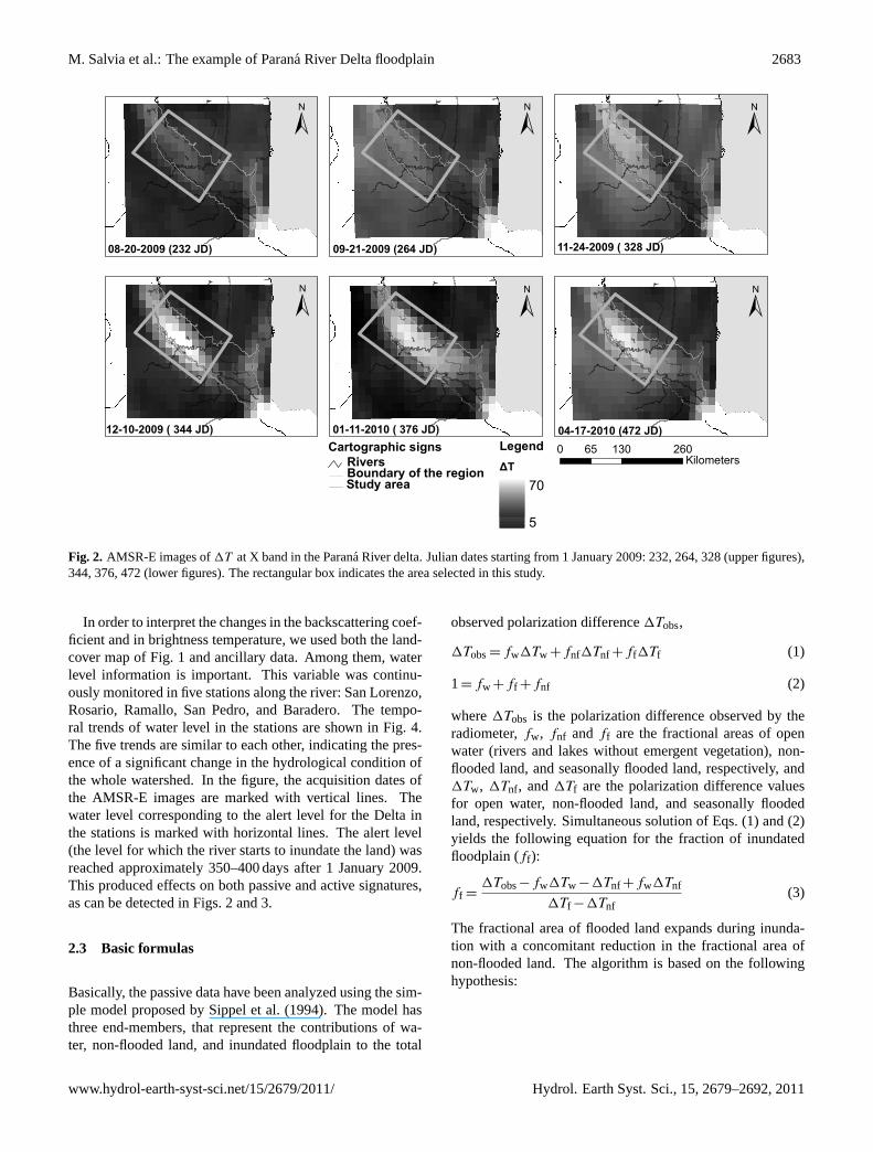
Fig. 2. AMSR-E images of1T at X band in the Parana River delta. Julian dates starting from 1 January 2009: 232, 264, 328 (upper figures),344, 376, 472 (lower figures). The rectangular box indicates the area selected in this study.

In order to interpret the changes in the backscattering coef-ficient and in brightness temperature, we used both the land-cover map of Fig.1 and ancillary data. Among them, waterlevel information is important. This variable was continu-ously monitored in five stations along the river: San Lorenzo,Rosario, Ramallo, San Pedro, and Baradero. The tempo-ral trends of water level in the stations are shown in Fig.4.The five trends are similar to each other, indicating the pres-ence of a significant change in the hydrological condition ofthe whole watershed. In the figure, the acquisition dates ofthe AMSR-E images are marked with vertical lines. Thewater level corresponding to the alert level for the Delta inthe stations is marked with horizontal lines. The alert level(the level for which the river starts to inundate the land) wasreached approximately 350–400 days after 1 January 2009.This produced effects on both passive and active signatures,as can be detected in Figs. 2 and 3.

2.3 Basic formulas

Basically, the passive data have been analyzed using the sim-ple model proposed bySippel et al.(1994). The model hasthree end-members, that represent the contributions of wa-ter, non-flooded land, and inundated floodplain to the total

observed polarization difference1Tobs,

1Tobs= fw1Tw +fnf1Tnf +ff1Tf (1)

1= fw +ff +fnf (2)

where1Tobs is the polarization difference observed by theradiometer,fw, fnf andff are the fractional areas of openwater (rivers and lakes without emergent vegetation), non-flooded land, and seasonally flooded land, respectively, and1Tw, 1Tnf, and1Tf are the polarization difference valuesfor open water, non-flooded land, and seasonally floodedland, respectively. Simultaneous solution of Eqs. (1) and (2)yields the following equation for the fraction of inundatedfloodplain (ff):

ff =1Tobs−fw1Tw −1Tnf +fw1Tnf

1Tf −1Tnf(3)

The fractional area of flooded land expands during inunda-tion with a concomitant reduction in the fractional area ofnon-flooded land. The algorithm is based on the followinghypothesis:

www.hydrol-earth-syst-sci.net/15/2679/2011/ Hydrol. Earth Syst. Sci., 15, 2679–2692, 2011

2684 M. Salvia et al.: The example of Parana River Delta floodplain

LegendDB

0

-18

0 90 18045Kilometers

06-10-2009 (161 JD) 12-02-2009 ( 336 JD)

01-06-2010 ( 371 JD)

RiversBoundary of the regionCartographic signs

Study area

±

±±

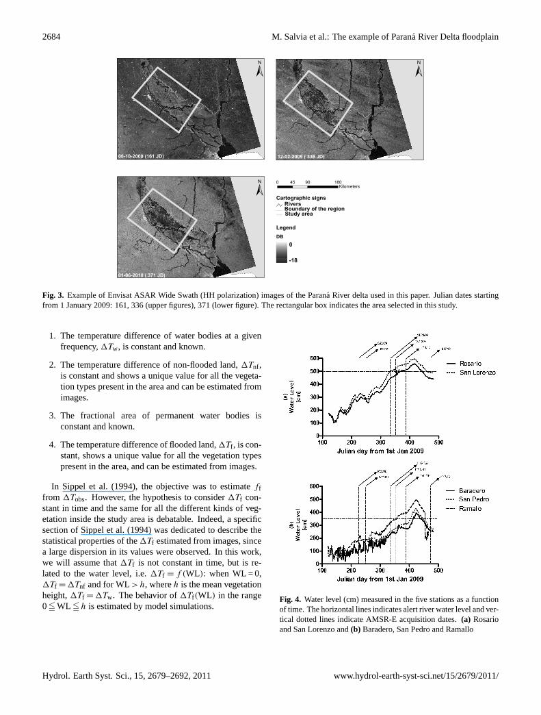
Fig. 3. Example of Envisat ASAR Wide Swath (HH polarization) images of the Parana River delta used in this paper. Julian dates startingfrom 1 January 2009: 161, 336 (upper figures), 371 (lower figure). The rectangular box indicates the area selected in this study.

1. The temperature difference of water bodies at a givenfrequency,1Tw, is constant and known.

2. The temperature difference of non-flooded land,1Tnf,is constant and shows a unique value for all the vegeta-tion types present in the area and can be estimated fromimages.

3. The fractional area of permanent water bodies isconstant and known.

4. The temperature difference of flooded land,1Tf , is con-stant, shows a unique value for all the vegetation typespresent in the area, and can be estimated from images.

In Sippel et al.(1994), the objective was to estimatefffrom 1Tobs. However, the hypothesis to consider1Tf con-stant in time and the same for all the different kinds of veg-etation inside the study area is debatable. Indeed, a specificsection ofSippel et al.(1994) was dedicated to describe thestatistical properties of the1Tf estimated from images, sincea large dispersion in its values were observed. In this work,we will assume that1Tf is not constant in time, but is re-lated to the water level, i.e.1Tf = f (WL): when WL = 0,1Tf = 1Tnf and for WL> h, whereh is the mean vegetationheight,1Tf = 1Tw. The behavior of1Tf(WL) in the range05 WL 5h is estimated by model simulations.

6 Salvia, M., et. al.:

Fig. 4. Water level (cm) measured in the five stations as a functionof time. The horizontal lines indicates alert river water level andvertical dotted lines indicate AMSR-E acquisition dates. (a) Rosarioand San Lorenzo and (b) Baradero, San Pedro and Ramallo

types present in the area, and can be estimated from im-ages.

In Sippel et al. (1994), the objective was to estimate ff

from ∆Tobs. However, the hypothesis to consider ∆Tf con-stant in time and the same for all the different kinds of vegeta-tion inside the study area is debatable. Indeed, a specific sec-tion of Sippel et al. (1994) was dedicated to describe the sta-tistical properties of the ∆Tf estimated from images, sincea large dispersion in its values were observed. In this work,we will assume that ∆Tf is not constant in time, but is re-lated to the water level, i.e. ∆Tf = f(WL): when WL= 0,∆Tf = ∆Tnf and for WL>h, where h is the mean vegeta-tion height, ∆Tf = ∆Tw. The behavior of ∆Tf (WL) in therange 0 5WL5h is estimated by model simulations.

2.4 Model simulations

As it will be outlined in 2.5.6, we use a look-up table whichassociates ∆Tf to water level (WL), for all the consideredAMSR-E channels. The look-up table is obtained by modelsimulations. We used the vegetation model developed at TorVergata University. It is a discrete model based on the ra-diative transfer theory, including multiple scattering effects.The model is able to compute both the emissivity and the

backscattering coefficient, and was adapted to several typesof vegetation.

The modeling process is subdivided into various steps.First of all, the geometry of vegetation elements is selected.Stems are represented as dielectric cylinders, while leaves arerepresented as dielectric discs. The permittivity of elementsis computed as a function of their moisture. Using electro-magnetic approximations available in the literature, such as”Infinite Length” for cylinders and Physical Optics for discs,the extinction, absorption, and bistatic scattering cross sec-tions of single elements are computed. Using a matrix algo-rithm which includes multiple scattering effects, the singlecontributions are combined, the bistatic scattering coefficientof the whole medium is computed, and the emissivity is ob-tained by using the energy conservation law. Details of thepassive version of the model are available in Ferrazzoli andGuerriero (1996a) and Ferrazzoli and Guerriero (1996b). Inthe study area, the main vegetation is herbaceous, and themain species are junco and cortadera. For this type of veg-etation, we adopted the vegetation dielectric and geometriccharacteristics already used in Grings et al. (2006) to simu-late the changes in the backscattering coefficient of the herba-ceous vegetation due to changes in the flood condition. Thesoil is represented as a half-space with rough interface. Forinundated marshes, the soil has the permittivity of water anda low roughness. For junco marshes, vegetation elementsare stems, represented as vertical dielectric cylinders. Theirheight is equal to the height of the emerged vegetation, whileother variables are given on the basis of previous measure-ments ((Grings et al., 2006), (Grings et al., 2008)). For cor-tadera marshes, which are essentially made of long leaves,vegetation elements are represented as dielectric discs. Themaximum leaf area index in absence of flooding is equal to5. While the water level increases, the leaf area index is as-sumed to be reduced following a linear trend, consistent withthe uniform distribution of biomass observed experimentally.The other variables are also assigned on the basis of previousmeasurements (Grings et al., 2006). The input variables tothe model are given in Table 2.

2.5 Methodology

In order to deal with drop-in-the-bucket inherent errors as-sociated to small areas already mentioned in Section 2.2, wedeveloped a methodology to extract the polarization differ-ence values of Parana River delta area from a known largerarea. This methodology is necessary, since it is not possibleto have the same pixel centers at all dates, even using repeatpass orbit images. Moreover, the included area of continentvaries from image to image and introduces several artifactsthat degrade the quality of the estimation of the flooded frac-tion. In fact, the averaging is affected by the contribution ofborder pixels mainly dominated by crops, which present alow polarization difference.

Fig. 4. Water level (cm) measured in the five stations as a functionof time. The horizontal lines indicates alert river water level and ver-tical dotted lines indicate AMSR-E acquisition dates.(a) Rosarioand San Lorenzo and(b) Baradero, San Pedro and Ramallo

Hydrol. Earth Syst. Sci., 15, 2679–2692, 2011 www.hydrol-earth-syst-sci.net/15/2679/2011/

M. Salvia et al.: The example of Parana River Delta floodplain 2685

Table 2. Input parameters to the interaction model.

Parameter Value Observations

General Frequency 10.8 GHz, 18.7 GHz, 36.6 GHz AMSR-E, X band, Ku band, Ka bandIncidence angle 55◦ AMSR-E

Soil parameters Soil moisture 1.0 cm3 cm−3 Flooded soilRMS height 0.04 cm Flooded soilCorrelation length 10 cm Flooded soil

Vegetation parameters Vegetation height 200 cm Cortadera marshMaximum emerged Leaf Area Index 5 Mean LAI of cortadera marshLeaf width 2.5 cm Cortadera marshLeaf thickness 0.02 cm Cortadera marshLeaf gravimetric moisture 0.7 g g−1 Cortadera marshMaximum emerged stem height 180 cm Junco marshStem radius 0.45 cm Junco marshPlant density 90 plants m−2 Junco marshStem gravimetric moisture 0.7 g g−1 Junco marsh

8 Salvia, M., et. al.:

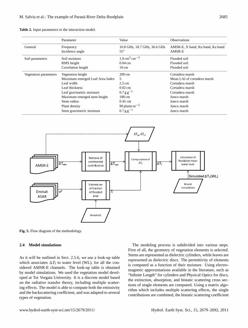
Fig. 5. Flow diagram of the methodology

Of course, higher thresholds correspond to more severecriteria. As it will be shown in the following, they lead tohigher values of water level in the pixels labeled as ”flooded”.

2.5.2 Computation of the overall polarization difference∆Tobs

For the three selected AMSR-E channels, and for all thelisted dates the polarization difference ∆Tobs, was computedby averaging among all the pixels whose centers are insidethe rectangular box of Figure 1. These values resulted froma complex combination of various contributions: floodedmarsh, non flooded marsh, water body and continental areas.

2.5.3 Removal of the continent part and estimation ofthe polarization difference of the wetland ∆Twet

We estimated the polarization differences of the wetland,∆Twet, from the polarization differences of the original box,∆Tobs. In order to remove the effect of the continent contri-bution, we estimated the polarization difference of the conti-nental part, ∆Tc, considering samples from both the North-east and Southwest side of the river floodplain. Using thisresult, we estimated the polarization difference values of thewetland, ∆Twet, as:

∆Twet =∆Tobs−fc∆Tc

1−fc(4)

where fc is the fraction of continent in the rectangularstudy area of Figure 1. In order to estimate fc, we subtractedthe Parana River Delta area to the total area (see Figure 1).Using this procedure, we found fc = 0.51.

2.5.4 Estimation of non-flooded area (∆Tnf ) and water(∆Tw) polarization differences

As stated before, the temperature difference of non-floodedland, ∆Tnf was considered constant for each frequency. Inorder to estimate this parameter, we applied two differentmethods: i) we considered ∼20 AMSR-E measured values

extracted in the drought period for nearly homogeneous veg-etated pixels; and ii) we used model simulations for the non-flooded case. Both estimates are reported in Table 3. For themeasured values the standard deviation is also given. Simu-lated and measured values are in agreement.

It is well established that the polarization difference ofcalm water, ∆Tw, depends on frequency, observation angleand surface roughness (Ulaby et al., 1986). We estimated thisvalue for each frequency using the same AMSR-E images.Tothis end, we considered samples from a large permanent en-dorheic lake (Laguna de Mar Chiquita), located at a distanceof about 300 Km from the study site. The obtained valuesof ∆Tw are also given in Table 3.

2.5.5 Computation of the polarization difference inflooded marsh (∆Tf )

As we discussed before, we assumed that the polarizationdifferences of the flooded marshes, ∆Tf , cannot be consid-ered constant for all dates and are in fact function of waterlevel. Therefore, the formulas of Sippel et al. (1994) wereused inversely, in order to estimate ∆Tf as a function of∆Twet. Then, equation (1) was rewritten as:

∆Tf =∆Twet−fw∆Tw−∆Tnf +fw∆Tnf

ff+∆Tnf (5)

In summary, we estimated ∆Tf , using

– The polarization differences of the wetland measured byAMSR-E (∆Twet);

– The flooded fraction of the wetland derived from En-visat ASAR data (ff );

– The fraction of permanent water bodies derived fromSAC-C data (fw) (Salvia et al., 2009)

– The polarization difference of water (∆Tw) and that ofnon-flooded vegetation (∆Tnf ) which are given in Ta-ble 3.

Fig. 5. Flow diagram of the methodology.

2.4 Model simulations

As it will be outlined in Sect.2.5.6, we use a look-up tablewhich associates1Tf to water level (WL), for all the con-sidered AMSR-E channels. The look-up table is obtainedby model simulations. We used the vegetation model devel-oped at Tor Vergata University. It is a discrete model basedon the radiative transfer theory, including multiple scatter-ing effects. The model is able to compute both the emissivityand the backscattering coefficient, and was adapted to severaltypes of vegetation.

The modeling process is subdivided into various steps.First of all, the geometry of vegetation elements is selected.Stems are represented as dielectric cylinders, while leaves arerepresented as dielectric discs. The permittivity of elementsis computed as a function of their moisture. Using electro-magnetic approximations available in the literature, such as“Infinite Length” for cylinders and Physical Optics for discs,the extinction, absorption, and bistatic scattering cross sec-tions of single elements are computed. Using a matrix algo-rithm which includes multiple scattering effects, the singlecontributions are combined, the bistatic scattering coefficient

www.hydrol-earth-syst-sci.net/15/2679/2011/ Hydrol. Earth Syst. Sci., 15, 2679–2692, 2011

2686 M. Salvia et al.: The example of Parana River Delta floodplain

Table 3. Parameters of the water level retrieval algorithm.

1Tnf 1Tnf(from model (from

1Tw [K] simulations) [K] images) [K]

X band 97.0±3.2 8.0 8.1±0.8Ku band 92.8±1.8 4.0 5.2±0.4Ka band 88.2±4.2 2.0 2.2±0.2

of the whole medium is computed, and the emissivity is ob-tained by using the energy conservation law. Details of thepassive version of the model are available inFerrazzoli andGuerriero(1996a) andFerrazzoli and Guerriero(1996b). Inthe study area, the main vegetation is herbaceous, and themain species are junco and cortadera. For this type of veg-etation, we adopted the vegetation dielectric and geometriccharacteristics already used inGrings et al.(2006) to simu-late the changes in the backscattering coefficient of the herba-ceous vegetation due to changes in the flood condition. Thesoil is represented as a half-space with rough interface. Forinundated marshes, the soil has the permittivity of water anda low roughness. For junco marshes, vegetation elementsare stems, represented as vertical dielectric cylinders. Theirheight is equal to the height of the emerged vegetation, whileother variables are given on the basis of previous measure-ments (Grings et al., 2006, 2008). For cortadera marshes,which are essentially made of long leaves, vegetation ele-ments are represented as dielectric discs. The maximum leafarea index in absence of flooding is equal to 5. While thewater level increases, the leaf area index is assumed to be re-duced following a linear trend, consistent with the uniformdistribution of biomass observed experimentally. The othervariables are also assigned on the basis of previous measure-ments (Grings et al., 2006). The input variables to the modelare given in Table2.

2.5 Methodology

In order to deal with drop-in-the-bucket inherent errors as-sociated to small areas already mentioned in Sect.2.2, wedeveloped a methodology to extract the polarization differ-ence values of Parana River delta area from a known largerarea. This methodology is necessary, since it is not possibleto have the same pixel centers at all dates, even using repeatpass orbit images. Moreover, the included area of continentvaries from image to image and introduces several artifactsthat degrade the quality of the estimation of the flooded frac-tion. In fact, the averaging is affected by the contribution ofborder pixels mainly dominated by crops, which present alow polarization difference.

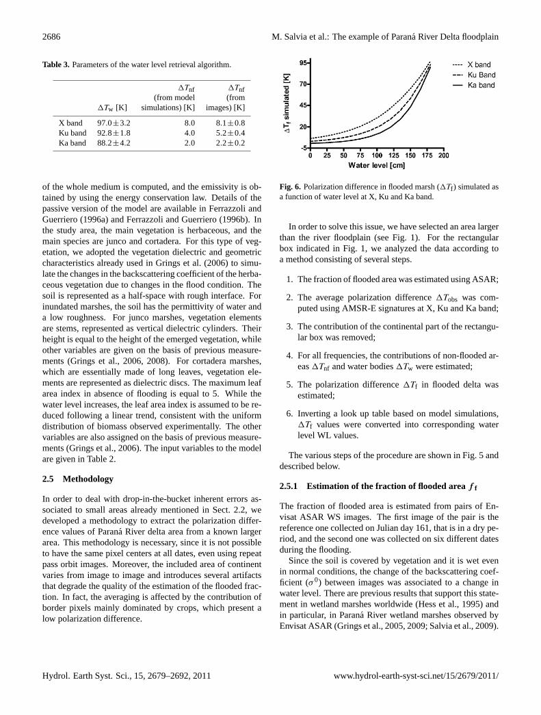
Fig. 6. Polarization difference in flooded marsh (1Tf ) simulated asa function of water level at X, Ku and Ka band.

In order to solve this issue, we have selected an area largerthan the river floodplain (see Fig.1). For the rectangularbox indicated in Fig.1, we analyzed the data according toa method consisting of several steps.

1. The fraction of flooded area was estimated using ASAR;

2. The average polarization difference1Tobs was com-puted using AMSR-E signatures at X, Ku and Ka band;

3. The contribution of the continental part of the rectangu-lar box was removed;

4. For all frequencies, the contributions of non-flooded ar-eas1Tnf and water bodies1Tw were estimated;

5. The polarization difference1Tf in flooded delta wasestimated;

6. Inverting a look up table based on model simulations,1Tf values were converted into corresponding waterlevel WL values.

The various steps of the procedure are shown in Fig.5 anddescribed below.

2.5.1 Estimation of the fraction of flooded areaf f

The fraction of flooded area is estimated from pairs of En-visat ASAR WS images. The first image of the pair is thereference one collected on Julian day 161, that is in a dry pe-riod, and the second one was collected on six different datesduring the flooding.

Since the soil is covered by vegetation and it is wet evenin normal conditions, the change of the backscattering coef-ficient (σ 0) between images was associated to a change inwater level. There are previous results that support this state-ment in wetland marshes worldwide (Hess et al., 1995) andin particular, in Parana River wetland marshes observed byEnvisat ASAR (Grings et al., 2005, 2009; Salvia et al., 2009).

Hydrol. Earth Syst. Sci., 15, 2679–2692, 2011 www.hydrol-earth-syst-sci.net/15/2679/2011/

M. Salvia et al.: The example of Parana River Delta floodplain 2687

Since the complete flood event we are analyzing lasted9 months, we compared images from different seasons.Therefore, one important hypothesis is that C bandσ 0 ofthe studied vegetation does not depends strongly on sea-son; therefore, the changes in C bandσ 0 can be unequivo-cally interpreted as changes in the flood condition. For theParana River Delta marshes, that are perennial, there is ex-perimental evidence that the C bandσ 0 of the vegetationmeasured with Envisat ASAR does not change significantlybetween seasons (Pratolongo, 2005).

According to previous works, in predominantly verticalwetland marshes observed at C band, a change in the floodcondition can produce either an increase or a decrease inthe overallσ 0 of the area (Grings et al., 2008). This is dueto a complex interaction between vegetation bistatic scatter-ing and vegetation attenuation (Grings et al., 2006). In fact,flooding reduces the surface contribution, due to the decreaseof roughness, but increases the double bounce. Overall, mod-erate flooding produces an increase of backscattering coef-ficient, due to the increase of double bounce. However, ifthe increase of water level submerges most of vegetation, theoverall effect is a decrease of backscattering coefficient.

We exploited these properties in order to identify the pixelsaffected by flooding. We considered three different thresh-olds in σ 0 variation with respect to the image of day 161,taken as reference. A pixel was assumed to be flooded forvariations higher than:

– 1.0 dB increase or 1.0 dB decrease,

– 1.5 dB increase or 1.5 dB decrease,

– 2.0 dB increase or 2.0 dB decrease.

Of course, higher thresholds correspond to more severecriteria. As it will be shown in the following, they lead tohigher values of water level in the pixels labeled as “flooded”.

2.5.2 Computation of the overall polarization difference1Tobs

For the three selected AMSR-E channels, and for all thelisted dates the polarization difference1Tobs, was computedby averaging among all the pixels whose centers are insidethe rectangular box of Fig.1. These values resulted froma complex combination of various contributions: floodedmarsh, non flooded marsh, water body and continental areas.

2.5.3 Removal of the continent part and estimation ofthe polarization difference of the wetland1Twet

We estimated the polarization differences of the wetland,1Twet, from the polarization differences of the original box,1Tobs. In order to remove the effect of the continent contri-bution, we estimated the polarization difference of the conti-nental part,1Tc, considering samples from both the North-east and Southwest side of the river floodplain. Using this

result, we estimated the polarization difference values of thewetland,1Twet, as:

1Twet=1Tobs−fc1Tc

1−fc(4)

wherefc is the fraction of continent in the rectangular studyarea of Fig.1. In order to estimatefc, we subtracted theParana River Delta area to the total area (see Fig.1). Usingthis procedure, we foundfc = 0.51.

2.5.4 Estimation of non-flooded area (1Tnf) and water(1Tw) polarization differences

As stated before, the temperature difference of non-floodedland, 1Tnf was considered constant for each frequency. Inorder to estimate this parameter, we applied two differentmethods: (i) we considered∼20 AMSR-E measured valuesextracted in the drought period for nearly homogeneous veg-etated pixels; and (ii) we used model simulations for the non-flooded case. Both estimates are reported in Table3. For themeasured values the standard deviation is also given. Simu-lated and measured values are in agreement.

It is well established that the polarization difference ofcalm water,1Tw, depends on frequency, observation angleand surface roughness (Ulaby et al., 1986). We estimated thisvalue for each frequency using the same AMSR-E images.Tothis end, we considered samples from a large permanent en-dorheic lake (Laguna de Mar Chiquita), located at a distanceof about 300 km from the study site. The obtained values of1Tw are also given in Table3.

2.5.5 Computation of the polarization difference inflooded marsh (1Tf)

As we discussed before, we assumed that the polarizationdifferences of the flooded marshes,1Tf , cannot be consid-ered constant for all dates and are in fact function of wa-ter level. Therefore, the formulas ofSippel et al.(1994)were used inversely, in order to estimate1Tf as a functionof 1Twet. Then, Eq. (1) was rewritten as:

1Tf =1Twet−fw1Tw −1Tnf +fw1Tnf

ff+1Tnf (5)

In summary, we estimated1Tf , using

– The polarization differences of the wetland measured byAMSR-E (1Twet);

– The flooded fraction of the wetland derived from En-visat ASAR data (ff);

– The fraction of permanent water bodies derived fromSAC-C data (fw) (Salvia et al., 2009)

– The polarization difference of water (1Tw) and thatof non-flooded vegetation (1Tnf) which are given inTable3.

www.hydrol-earth-syst-sci.net/15/2679/2011/ Hydrol. Earth Syst. Sci., 15, 2679–2692, 2011

2688 M. Salvia et al.: The example of Parana River Delta floodplain

±

LegendDecrease ( <-1.5 dB)Increase ( >1.5 dB)No changeWater Bodies

0 90 18045Kilometers

08-19-2009 (231 JD) 09-21-2009 ( 264 JD) 12-02-2009 ( 336 JD)

12-19-2009 ( 353 JD) 01-06-2010 (371JD) 04-21-2010 ( 476 JD)

±

±

±

±

±

RiversBoundary of the regionCartographic signs

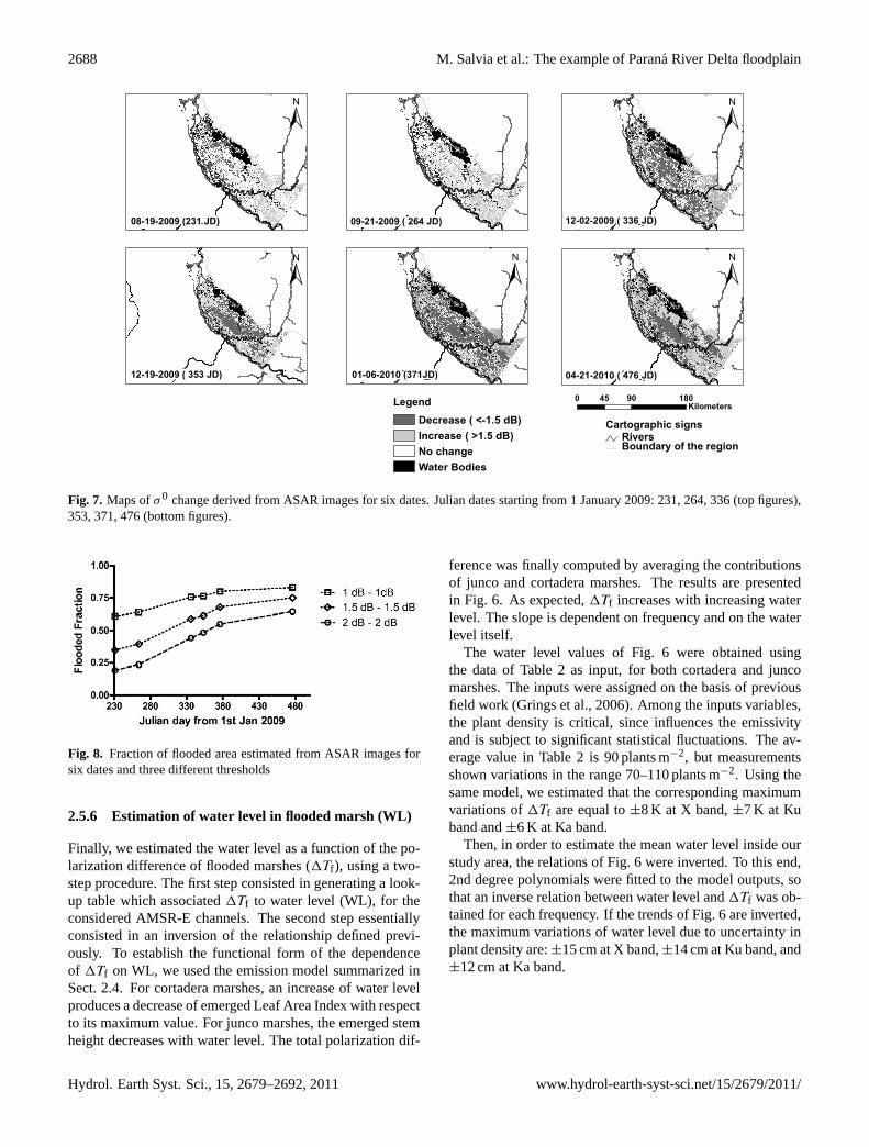
Fig. 7. Maps ofσ0 change derived from ASAR images for six dates. Julian dates starting from 1 January 2009: 231, 264, 336 (top figures),353, 371, 476 (bottom figures).

Fig. 8. Fraction of flooded area estimated from ASAR images forsix dates and three different thresholds

2.5.6 Estimation of water level in flooded marsh (WL)

Finally, we estimated the water level as a function of the po-larization difference of flooded marshes (1Tf), using a two-step procedure. The first step consisted in generating a look-up table which associated1Tf to water level (WL), for theconsidered AMSR-E channels. The second step essentiallyconsisted in an inversion of the relationship defined previ-ously. To establish the functional form of the dependenceof 1Tf on WL, we used the emission model summarized inSect.2.4. For cortadera marshes, an increase of water levelproduces a decrease of emerged Leaf Area Index with respectto its maximum value. For junco marshes, the emerged stemheight decreases with water level. The total polarization dif-

ference was finally computed by averaging the contributionsof junco and cortadera marshes. The results are presentedin Fig. 6. As expected,1Tf increases with increasing waterlevel. The slope is dependent on frequency and on the waterlevel itself.

The water level values of Fig.6 were obtained usingthe data of Table2 as input, for both cortadera and juncomarshes. The inputs were assigned on the basis of previousfield work (Grings et al., 2006). Among the inputs variables,the plant density is critical, since influences the emissivityand is subject to significant statistical fluctuations. The av-erage value in Table2 is 90 plants m−2, but measurementsshown variations in the range 70–110 plants m−2. Using thesame model, we estimated that the corresponding maximumvariations of1Tf are equal to±8 K at X band,±7 K at Kuband and±6 K at Ka band.

Then, in order to estimate the mean water level inside ourstudy area, the relations of Fig.6 were inverted. To this end,2nd degree polynomials were fitted to the model outputs, sothat an inverse relation between water level and1Tf was ob-tained for each frequency. If the trends of Fig.6 are inverted,the maximum variations of water level due to uncertainty inplant density are:±15 cm at X band,±14 cm at Ku band, and±12 cm at Ka band.

Hydrol. Earth Syst. Sci., 15, 2679–2692, 2011 www.hydrol-earth-syst-sci.net/15/2679/2011/

M. Salvia et al.: The example of Parana River Delta floodplain 2689Salvia, M., et. al.: 11

Fig. 9. Polarization differences as a function of time for the threeAMSR-E considered bands. (a): Overall measured ∆Tobs (b): con-tinent ∆Tc . (c): wetland ∆Twet.

tion models, the mean water level of the wetland area wasobtained.

This methodology makes use of ancillary data, such as alandcover map that characterizes the main vegetation typespresent in the area, and exploits an interaction model thatsimulates the polarization difference of the vegetation at var-ious frequencies and for different water levels.

A complete validation of the results over the whole area isnot feasible. However, a comparison with in situ data of riverwater level measured at five stations is consistent. During thetime in which the in situ measured water level increases, thefraction of flooded area increases regularly, while the waterlevel estimated in the marshes increases slightly, with a stepincrement occurring in the Julian days from 328 to 344, whenthe river reached the alert level. Moreover, the algorithm was

Fig. 10. ∆Tf as a function of time for the three frequencies and forthree different thresholds. (a) 1 dB, (b) 1.5 dB and (c) 2 dB

applied using three different AMSR-E frequencies showingvery close values of mean water level. Although the behaviorof ∆Tf at X band differs from the other two, the trends ofWL are similar.

The use of both active and passive data allows us to es-timate also the water level in flooded vegetation, but limitsthe temporal resolution. As a future development, we plan touse the water level estimated using both passive and activesignatures as an initial value in the algorithm of Sippel et al.(1994) that uses passive data only. This can allow us to ex-ploit the temporal resolution of passive data with a periodicadjournment (using both passive and active data) of waterlevel information.

Acknowledgements. The authors specially thank the EuropeanSpace Agency (ESA) for the continuous support through AO 667supported project, the National Commission for Space Activities

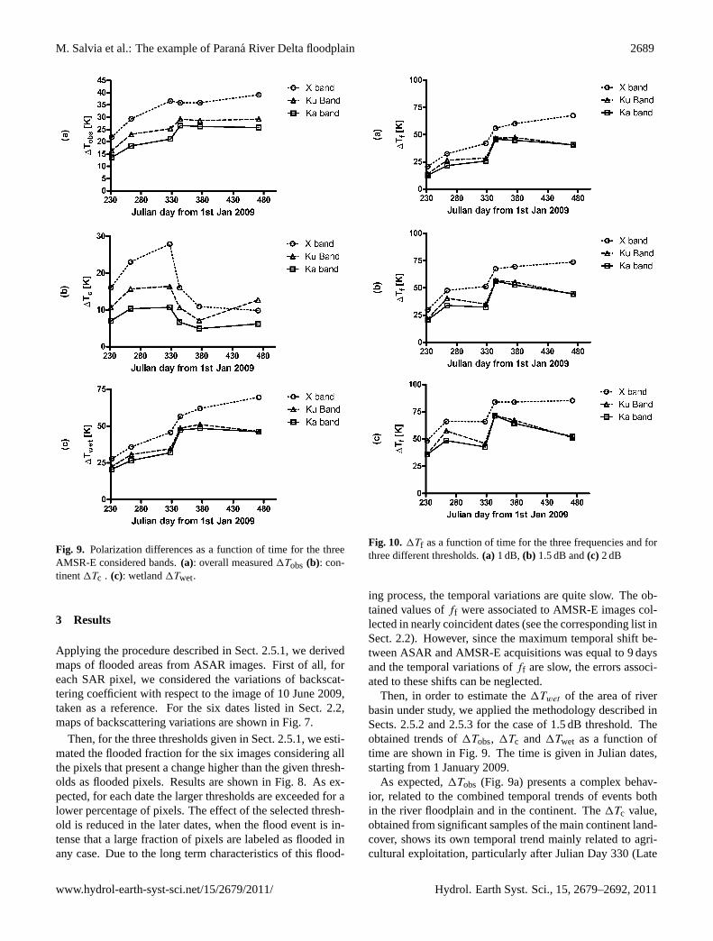
Fig. 9. Polarization differences as a function of time for the threeAMSR-E considered bands.(a): overall measured1Tobs (b): con-tinent1Tc . (c): wetland1Twet.

3 Results

Applying the procedure described in Sect.2.5.1, we derivedmaps of flooded areas from ASAR images. First of all, foreach SAR pixel, we considered the variations of backscat-tering coefficient with respect to the image of 10 June 2009,taken as a reference. For the six dates listed in Sect.2.2,maps of backscattering variations are shown in Fig.7.

Then, for the three thresholds given in Sect.2.5.1, we esti-mated the flooded fraction for the six images considering allthe pixels that present a change higher than the given thresh-olds as flooded pixels. Results are shown in Fig.8. As ex-pected, for each date the larger thresholds are exceeded for alower percentage of pixels. The effect of the selected thresh-old is reduced in the later dates, when the flood event is in-tense that a large fraction of pixels are labeled as flooded inany case. Due to the long term characteristics of this flood-

Salvia, M., et. al.: 11

Fig. 9. Polarization differences as a function of time for the threeAMSR-E considered bands. (a): Overall measured ∆Tobs (b): con-tinent ∆Tc . (c): wetland ∆Twet.

tion models, the mean water level of the wetland area wasobtained.

This methodology makes use of ancillary data, such as alandcover map that characterizes the main vegetation typespresent in the area, and exploits an interaction model thatsimulates the polarization difference of the vegetation at var-ious frequencies and for different water levels.

A complete validation of the results over the whole area isnot feasible. However, a comparison with in situ data of riverwater level measured at five stations is consistent. During thetime in which the in situ measured water level increases, thefraction of flooded area increases regularly, while the waterlevel estimated in the marshes increases slightly, with a stepincrement occurring in the Julian days from 328 to 344, whenthe river reached the alert level. Moreover, the algorithm was

Fig. 10. ∆Tf as a function of time for the three frequencies and forthree different thresholds. (a) 1 dB, (b) 1.5 dB and (c) 2 dB

applied using three different AMSR-E frequencies showingvery close values of mean water level. Although the behaviorof ∆Tf at X band differs from the other two, the trends ofWL are similar.

The use of both active and passive data allows us to es-timate also the water level in flooded vegetation, but limitsthe temporal resolution. As a future development, we plan touse the water level estimated using both passive and activesignatures as an initial value in the algorithm of Sippel et al.(1994) that uses passive data only. This can allow us to ex-ploit the temporal resolution of passive data with a periodicadjournment (using both passive and active data) of waterlevel information.

Acknowledgements. The authors specially thank the EuropeanSpace Agency (ESA) for the continuous support through AO 667supported project, the National Commission for Space Activities

Fig. 10. 1Tf as a function of time for the three frequencies and forthree different thresholds.(a) 1 dB, (b) 1.5 dB and(c) 2 dB

ing process, the temporal variations are quite slow. The ob-tained values offf were associated to AMSR-E images col-lected in nearly coincident dates (see the corresponding list inSect.2.2). However, since the maximum temporal shift be-tween ASAR and AMSR-E acquisitions was equal to 9 daysand the temporal variations offf are slow, the errors associ-ated to these shifts can be neglected.

Then, in order to estimate the1Twet of the area of riverbasin under study, we applied the methodology described inSects.2.5.2and2.5.3for the case of 1.5 dB threshold. Theobtained trends of1Tobs, 1Tc and1Twet as a function oftime are shown in Fig.9. The time is given in Julian dates,starting from 1 January 2009.

As expected,1Tobs (Fig. 9a) presents a complex behav-ior, related to the combined temporal trends of events bothin the river floodplain and in the continent. The1Tc value,obtained from significant samples of the main continent land-cover, shows its own temporal trend mainly related to agri-cultural exploitation, particularly after Julian Day 330 (Late

www.hydrol-earth-syst-sci.net/15/2679/2011/ Hydrol. Earth Syst. Sci., 15, 2679–2692, 2011

2690 M. Salvia et al.: The example of Parana River Delta floodplain12 Salvia, M., et. al.:

Fig. 11. Mean water level within the studied floodplain area as afunction of time, estimated using ∆T f values (Figure 10) and modelsimulations (Figure 6) for three different thresholds. (a) 1 dB, (b)1.5 dB and (c) 2 dB

(CONAE) for the optical data, the National Water Institute (INA)and the National Hydrologic Service (SHN) for providing us riverwater levels and precipitation data. This work was funded by theAgencia Nacional de Promocion Cientifica y Tecnologica (AN-PCyT) (PICT 1203) and MinCyT-CONAE-CONICET project 12.

References

Alsdorf, D. E., Rodrguez, E., and Lettenmaier, D. P.: Measur-ing surface water from space, Rev. Geophys., 34, doi:10.1029/2006RG000197, 2007.

Caizzone, S., Ferrazzoli, P., Guerriero, L., and Pierdicca, N.: Mod-eling backscattering variations due to flooding over vegetatedsurfaces, Italian Journal of Remote Sensing, 3, 25–37, 2009.

Choudhury, B. J.: Monitoring global land surface using Nimbus-7 37 GHz data Theory and examples, International Journal ofRemote Sensing, 10, 1579–1605, 1989.

ESA: ASAR product handbook, Tech. rep., European SpaceAgency (ESA), 2007.

Ferrazzoli, P. and Guerriero, L.: Passive microwave remote sens-ing of forests: a model investigation, Geoscience and RemoteSensing, IEEE Transactions on, 34, 433–443, doi:10.1109/36.485121, 1996a.

Ferrazzoli, P. and Guerriero, L.: Emissivity of vegetation: theoryand computational aspects, Journal of Electromagnetic Wavesand Applications, 1996b.

Ferrazzoli, P., Guerriero, L., Paloscia, S., Pampaloni, P., and Soli-mini, D.: Modeling polarization properties of emission from soilcovered with vegetation, Geoscience and Remote Sensing, IEEETransactions on, 30, 157–165, doi:10.1109/36.124226, 1992.

Grings, F., Ferrazzoli, P., Karszenbaum, H., Tiffenberg, J., Kan-dus, P., Guerriero, L., and Jacobo-Berrles, J.: Modeling tem-poral evolution of junco marshes radar signatures, Geoscienceand Remote Sensing, IEEE Transactions on, 43, 2238–2245, doi:10.1109/TGRS.2005.855067, 2005.

Grings, F., Ferrazzoli, P., Jacobo-Berlles, J., Karszenbaum, H., Tiff-enberg, J., Pratolongo, P., and Kandus, P.: Monitoring flood con-dition in marshes using EM models and Envisat ASAR observa-tions, Geoscience and Remote Sensing, IEEE Transactions on,44, 936–942, doi:10.1109/TGRS.2005.863482, 2006.

Grings, F., Ferrazzoli, P., Karszenbaum, H., Salvia, M., Kandus, P.,Jacobo-Berlles, J., and Perna, P.: Model investigation about thepotential of C band SAR in herbaceous wetlands flood monitor-ing, Int. J. Remote Sens., 2008.

Grings, F., Salvia, M., Karszenbaum, H., Ferrazzoli, P., Kandus,P., and Perna, P.: Advances in radar remote sensing of wetlandecosystems: Combination of satellite observations, field data andem Models, Journal of environmental management, pp. 2189–2198, 2009.

Hamilton, S., Sippel, S. J., and Melack, J. M.: Comparison of in-undation patterns among major South American floodplains, J.Geophys. Research, 107, 2002.

Hess, L., Melack, J., Filoso, S., and Wang, Y.: Delineation of inun-dated area and vegetation along the Amazon floodplain with theSIR-C synthetic aperture radar, Geoscience and Remote Sensing,IEEE Transactions on, 33, 896–904, doi:10.1109/36.406675,1995.

Jackson, T. J. and Schmugge, T. J.: Vegetation effects on the mi-crowave emission from soils, Remote Sens. Environ., 36, 203–212, 1991.

Kawanishi, T., Sezai, T., Ito, Y., Imaoka, K., Takeshima, T., Ishido,Y., Shibata, A., Miura, M., Inahata, H., and Spencer, R.: TheAdvanced Microwave Scanning Radiometer for the Earth Ob-serving System (AMSR-E), NASDA’s contribution to the EOSfor global energy and water cycle studies, Geoscience and Re-mote Sensing, IEEE Transactions on, 41, 184–194, doi:10.1109/TGRS.2002.808331, 2003.

Kerr, Y. and Njoku, E.: A semiempirical model for interpretingmicrowave emission from semiarid land surfaces as seen fromspace, Geoscience and Remote Sensing, IEEE Transactions on,28, 384–393, doi:10.1109/36.54364, 1990.

Le Toan, T., Laur, H., Mougin, E., and Lopes, A.: Multitempo-ral and dual-polarization observations of agricultural vegetation

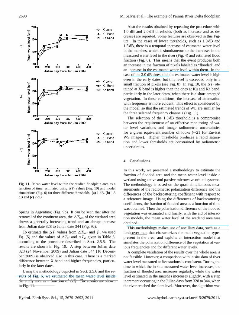
Fig. 11. Mean water level within the studied floodplain area as afunction of time, estimated using1Tf values (Fig.10) and modelsimulations (Fig.6) for three different thresholds.(a) 1 dB, (b) 1.5dB and(c) 2 dB

Spring in Argentina) (Fig. 9b). It can be seen that after theremoval of the continent area, the1Twet of the wetland areashows a generally increasing trend and an abrupt increasefrom Julian date 328 to Julian date 344 (Fig. 9c).

To estimate the1Tf values from1Twet andff , we usedEq. (5) and the values of1Tnf and1Tw given in Table3,according to the procedure described in Sect.2.5.5. Theresults are shown in Fig.10. A step between Julian date328 (24 November 2009) and Julian date 344 (10 Decem-ber 2009) is observed also in this case. There is a markeddifference between X band and higher frequencies, particu-larly in the later dates.

Using the methodology depicted in Sect.2.5.6and the re-sults of Fig.6, we estimated the mean water level insidethe study area as a function of1Tf . The results are shownin Fig. 11.

Also the results obtained by repeating the procedure with1.0 dB and 2.0 dB thresholds (both as increase and as de-crease) are reported. Some features are observed in this Fig-ure. In the cases of lower thresholds, such as 1.0 dB and1.5 dB, there is a temporal increase of estimated water levelin the marshes, which is simultaneous to the increases in themeasured water level in the river (Fig.4) and estimated floodfraction (Fig.8). This means that the event produces bothan increase in the fraction of pixels labeled as “flooded” andan increase in the estimated water level within them. In thecase of the 2.0 dB threshold, the estimated water level is higheven in the early dates, but this level is exceeded only in asmall fraction of pixels (see Fig.8). In Fig. 10, the1Tf ob-tained at X band is higher than the ones at Ku and Ka band.particularly in the later dates, when there is a short emergedvegetation. In these conditions, the increase of attenuationwith frequency is more evident. This effect is considered bythe model, so that the estimated trends of WL are similar forthe three selected frequency channels (Fig.11).

The selection of the 1.5 dB threshold is a compromisebetween the requirement of an effective monitoring of wa-ter level variations and image radiometric uncertaintiesfor a given equivalent number of looks (∼21 for EnvisatWS images). Higher thresholds produces a rapid satura-tion and lower thresholds are constrained by radiometricuncertainties.

4 Conclusions

In this work, we presented a methodology to estimate thefraction of flooded area and the mean water level inside awetland using active and passive microwave orbital systems.The methodology is based on the quasi-simultaneous mea-surements of the radiometric polarization difference and thedifferences of the backscattering coefficient with respect toa reference image. Using the differences of backscatteringcoefficients, the fraction of flooded area as a function of timewas obtained. Then the polarization difference of the floodedvegetation was estimated and finally, with the aid of interac-tion models, the mean water level of the wetland area wasobtained.

This methodology makes use of ancillary data, such as alandcover map that characterizes the main vegetation typespresent in the area, and exploits an interaction model thatsimulates the polarization difference of the vegetation at var-ious frequencies and for different water levels.

A complete validation of the results over the whole area isnot feasible. However, a comparison with in situ data of riverwater level measured at five stations is consistent. During thetime in which the in situ measured water level increases, thefraction of flooded area increases regularly, while the waterlevel estimated in the marshes increases slightly, with a stepincrement occurring in the Julian days from 328 to 344, whenthe river reached the alert level. Moreover, the algorithm was

Hydrol. Earth Syst. Sci., 15, 2679–2692, 2011 www.hydrol-earth-syst-sci.net/15/2679/2011/

M. Salvia et al.: The example of Parana River Delta floodplain 2691

applied using three different AMSR-E frequencies showingvery close values of mean water level. Although the behaviorof 1Tf at X band differs from the other two, the trends of WLare similar.

The use of both active and passive data allows us to es-timate also the water level in flooded vegetation, but limitsthe temporal resolution. As a future development, we plan touse the water level estimated using both passive and activesignatures as an initial value in the algorithm ofSippel et al.(1994) that uses passive data only. This can allow us to ex-ploit the temporal resolution of passive data with a periodicadjournment (using both passive and active data) of waterlevel information.

Acknowledgements.The authors specially thank the EuropeanSpace Agency (ESA) for the continuous support through AO 667supported project, the National Commission for Space Activities(CONAE) for the optical data, the National Water Institute (INA)and the National Hydrologic Service (SHN) for providing us riverwater levels and precipitation data. This work was funded by theAgencia Nacional de Promocion Cientifica y Tecnologica (AN-PCyT) (PICT 1203) and MinCyT-CONAE-CONICET project 12.

Edited by: N. Verhoest

References

Alsdorf, D. E., Rodrıguez, E., and Lettenmaier, D. P.: Mea-suring surface water from space, Rev. Geophys., 34, 1–24,doi:10.1029/2006RG000197, 2007.

Caizzone, S., Ferrazzoli, P., Guerriero, L., and Pierdicca, N.: Mod-eling backscattering variations due to flooding over vegetatedsurfaces, Italian J. Remote Sens., 3, 25–37, 2009.

Choudhury, B. J.: Monitoring global land surface using Nimbus-7 37 GHz data Theory and examples, Int. J. Remote Sens., 10,1579–1605, 1989.

ESA: ASAR product handbook, Tech. rep., European SpaceAgency (ESA), 2007.

Ferrazzoli, P. and Guerriero, L.: Passive microwave remote sensingof forests: a model investigation,, IEEE T. Geosci. Remote Sens.,34, 433–443,doi:10.1109/36.485121, 1996a.

Ferrazzoli, P. and Guerriero, L.: Emissivity of vegetation: theoryand computational aspects, J. Electromagnet. Wave., 10, 609–628,doi:10.1163/156939396X00559, 1996b.

Ferrazzoli, P., Guerriero, L., Paloscia, S., Pampaloni, P., and Solim-ini, D.: Modeling polarization properties of emission from soilcovered with vegetation,, IEEE T. Geosci. Remote Sens., 30,157–165,doi:10.1109/36.124226, 1992.

Grings, F., Ferrazzoli, P., Karszenbaum, H., Tiffenberg, J., Kan-dus, P., Guerriero, L., and Jacobo-Berrles, J.: Modeling tempo-ral evolution of junco marshes radar signatures,, IEEE T. Geosci.Remote Sens., 43, 2238–2245,doi:10.1109/TGRS.2005.855067,2005.

Grings, F., Ferrazzoli, P., Jacobo-Berlles, J., Karszenbaum, H., Tiff-enberg, J., Pratolongo, P., and Kandus, P.: Monitoring floodcondition in marshes using EM models and Envisat ASARobservations,, IEEE T. Geosci. Remote Sens., 44, 936–942,doi:10.1109/TGRS.2005.863482, 2006.

Grings, F., Ferrazzoli, P., Karszenbaum, H., Salvia, M., Kan-dus, P., Jacobo-Berlles, J., and Perna, P.: Model investiga-tion about the potential of C band SAR in herbaceous wet-lands flood monitoring, Int. J. Remote Sens., 29, 5361–5372,doi:10.1080/01431160802036409, 2008.

Grings, F., Salvia, M., Karszenbaum, H., Ferrazzoli, P., Kandus,P., and Perna, P.: Advances in radar remote sensing of wetlandecosystems: Combination of satellite observations, field data andem Models, J. Environ. Manage., 90, 2189–2198, 2009.

Hamilton, S., Sippel, S. J., and Melack, J. M.: Comparison of in-undation patterns among major South American floodplains, J.Geophys. Res., 107, 1–14,doi:10.1029/2000jd000306, 2002.

Hess, L., Melack, J., Filoso, S., and Wang, Y.: Delineation of inun-dated area and vegetation along the Amazon floodplain with theSIR-C synthetic aperture radar,, IEEE T. Geosci. Remote Sens.,33, 896–904,doi:10.1109/36.406675, 1995.

Jackson, T. J. and Schmugge, T. J.: Vegetation effects on the mi-crowave emission from soils, Remote Sens. Environ., 36, 203–212, 1991.

Kawanishi, T., Sezai, T., Ito, Y., Imaoka, K., Takeshima, T., Ishido,Y., Shibata, A., Miura, M., Inahata, H., and Spencer, R.: The Ad-vanced Microwave Scanning Radiometer for the Earth ObservingSystem (AMSR-E), NASDA’s contribution to the EOS for globalenergy and water cycle studies, IEEE T. Geosci. Remote Sens.,41, 184–194,doi:10.1109/TGRS.2002.808331, 2003.

Kerr, Y. and Njoku, E.: A semiempirical model for interpret-ing microwave emission from semiarid land surfaces as seenfrom space, IEEE T. Geosci. Remote Sens., 28, 384–393,doi:10.1109/36.54364, 1990.

Le Toan, T., Laur, H., Mougin, E., and Lopes, A.: Multitempo-ral and dual-polarization observations of agricultural vegetationcovers by X-band SAR images, IEEE T. Geosci. Remote Sens.,27, 709–718,doi:10.1109/TGRS.1989.1398243, 1989.

Matgen, P., Schumann, G., Henry, J., Hoffmann, L., and Pfister, L.:Integration of SAR derived river inundation areas, high-precisiontopographic data and flood propagation models: a step towardseffective, near real-time flood management, Int. J. Appl. EarthObs., 9(3), 247–263,doi:10.1016/j.jag.2006.03.003, 2007.

Paloscia, S. and Pampaloni, P.: Microwave polarization index formonitoring vegetation growth, IEEE T. Geosci. Remote Sens.,26, 617–621,doi:10.1109/36.7687, 1988.

Paloscia, S., Pampaloni, P., Chiarantini, L., Coppo, P., Gagliani, S.,and Luzi, G.: Multifrequency passive microwave remote sensingof soil misture and roughness, Int. J. Remote Sens., 14, 467–483,1993.

Pappenberger, F., Frodsham, K., Beven, K., Romanowicz, R., andMatgen, P.: Fuzzy set approach to calibrating distributed floodinundation models using remote sensing observations, Hydrol.Earth Syst. Sci., 11, 739–752,doi:10.5194/hess-11-739-2007,2007.

Parkinson, C.: Aqua: an Earth-Observing Satellite mission to exam-ine water and other climate variables, IEEE T. Geosci. RemoteSens., 41, 173–183,doi:10.1109/TGRS.2002.808319, 2003.

Parmuchi, G., Karszenbaum, H., and Kandus, P.: Map-ping the Parana River delta wetland using multitemporalRADARSAT/SAR data and a decision based classifier, Can. J.Remote Sens., 28, 175–186, 2002.

Pratolongo, P.: Dinamica de comunidades herbaceas del bajo deltadel rıo parana sujetas a diferentes regımenes hidrologicos y su

www.hydrol-earth-syst-sci.net/15/2679/2011/ Hydrol. Earth Syst. Sci., 15, 2679–2692, 2011

2692 M. Salvia et al.: The example of Parana River Delta floodplain

monitoreo mediante sensores remotos, Ph.D. thesis, Departa-mento de Ecologıa Genetica y Evolucion Facultad de CienciasExactas y Naturales Universidad de Buenos Aires, 2005.

Prigent, C., Papa, F., Aires, F., Rossow, W. B., and Matthews, E.:Global inundation dynamics inferred from multiple satellite ob-servations, 1993–2000, J. Geophys. Res., 112, 113–129, 2007.

Salvia, M., Kandus, P., Karszenbaum, H., and Grings, F.: Opti-cal and radar satellital data for mapping and monitoring wetlandmacrosystems, Revista Espanola de Teledeteccion, 31, 35–51,2009.

Sippel, S. J., Hamilton, S., Melack, J. M., and Choudhury, B.: De-termination of inundation area in the Amazon River floodplainusing the SMMR 37 GHz polarization difference, Remote Sens.Environ., 48, 70–76, 1994.

Sippel S. J., Hamilton, S. K., Melack, J. M., and Novo, E.: Passivemicrowave observations of inundation area and the area/stage re-lation in the Amazon River floodplain, Int. J. Remote Sens., 19,3055–3074, 1998.

Ulaby, F. T., Moore, R. K., and Fung, A.: Microwave Remote Sens-ing: Active and Passive, Vol. III – Volume Scattering and Emis-sion Theory, Advanced Systems and Applications, Addison-Wesley, 1986.

Wang, Y., Hess, L., Filoso, S., and Melack, J.: Understanding theRadar Backscattering from Flooded and Nonflooded AmazonianForests: Results from Canopy Backscatter Modeling, RemoteSens. Environ., 54, 324–332, 1995.

Zwenzner, H. and Voigt, S.: Improved estimation of flood parame-ters by combining space based SAR data with very high resolu-tion digital elevation data, Hydrol. Earth Syst. Sci., 13, 567–576,doi:10.5194/hess-13-567-2009, 2009.

Hydrol. Earth Syst. Sci., 15, 2679–2692, 2011 www.hydrol-earth-syst-sci.net/15/2679/2011/