ESSAYS ON HUMAN CAPITAL & DEVELOPMENT

IN INDIA

A Dissertation

Presented to the Faculty of the Graduate School

of Cornell University

in Partial Fulfillment of the Requirements for the Degree of

Doctor of Philosophy

by

Tanvi Rao

August 2017

c© 2017 Tanvi Rao

ALL RIGHTS RESERVED

ESSAYS ON HUMAN CAPITAL & DEVELOPMENT

IN INDIA

Tanvi Rao, Ph.D.

Cornell University 2017

This dissertation consists of three independent research papers, tied under a broad

research agenda of “human capital” in India. Chapters 1 and 2 are closely related

and both utilize a self-collected, primary dataset on the subjective beliefs, of a sample

of 12th grade students, regarding factors that may influence their decision to invest

in post-secondary education. Chapter 3 examines a different dimension of human

capital and investigates the role of agriculture in improving the nutritional status of

rural, Indian women.

In the first paper, I examine the inaccuracy of students’ beliefs regarding the labor

market returns (i.e. wage earnings) associated with post-secondary (college) educa-

tion. Towards this end, I randomize information on measured population wages to a

sample of 12th grade students, drawn from schools affiliated with a large public state

university in India, who at the time were roughly six months away from making a

decision regarding college attendance and college track (technical, academic, voca-

tional) conditional on attendance. I find that, at baseline, students beliefs about pop-

ulation earnings deviate substantially from true earnings in the population. Upon the

receipt of potentially new information, students revise beliefs regarding own-wages

in the direction of the information, though the average extent of updating is small

and masks substantial sub-group heterogeneity. Additionally, subsequent changes in

enrollment intentions and intentions to borrow for higher education are in line with

both the extent and direction of wage belief updating. A portion of the heterogeneity

in wage belief updating can be explained by initial misperceptions regarding popu-

lation earnings, and baseline relevance of earnings to enrollment intentions. Yet a

large portion remains unexplained, consistent with wide heterogeneity in updating

heuristics, at the individual level. From a policy standpoint, these findings point to

the limited capacity of information campaigns based on population-level aggregates

to induce, on average, large changes in individual priors and help to rationalize a

number of recent papers that find heterogeneous impacts of information provision on

education outcomes.

In my second paper, I draw descriptive insights about the extent and implications of

the same sample of 12th grade students’ misperceptions about post-secondary (col-

lege) expenses, elicited 5-9 months prior to them completing high school. Students’

subjective beliefs about post-secondary expenses are compared to a reference distri-

bution of actual expenses incurred by students of post-secondary education. Stu-

dents overestimate expenses for two out of three tracks. I estimate that if students

perceived expenses more accurately, then their perceived affordability for technical

tracks and general tracks would increase by 10 percentage points and 55 percentage

points, respectively. Students’ have relatively more accurate beliefs about the ex-

penses associated with their utility maximizing track or their most preferred track,

which I estimate using a flexible model of track-choice. Nevertheless, I show that

purging cost beliefs of errors, also increases the perceived affordability of students’

preferred tracks by an economically and statistically large magnitude.

My third paper is co-authored with Dr. Prabhu Pingali. In this paper, we estab-

lish a statistically important relationship between household agricultural income and

maternal BMI using a five-year panel dataset of agricultural households drawn from

18 villages across five Indian states. Using within household variation over time, we

estimate both, the extent to which short-term changes in agricultural income are

associated with short-term changes in BMI, and the effect of agricultural income

growth on BMI growth over a longer term. Over the longer term, and for the group

of households that regularly farm, we find a 10 pp. agriculture income growth to

be associated with a 0.15 pp. growth in BMI. Consistent with the literature, this

effect is economically modest, but important considering that we do not find a cor-

responding effect for growth in non-agricultural income. We present evidence to

suggest that the own-production of food is not an important pathway for nutritional

improvements, but the agricultural income effect is likely operational through pur-

chase of food, specifically of protein rich pulses. Effects of agricultural income are

stronger for younger women, in the age-group 15-25 years, who face a particularly

strong nutritional disadvantage in India.

BIOGRAPHICAL SKETCH

Tanvi Rao was born in Hyderabad, India, and grew up in the bustling metropolis

and national capital of New Delhi. She was schooled at Sardar Patel Vidyalaya

(SPV), where she studied for 14 years, from nursery up until the 12th grade. Despite

attending other excellent institutes thereafter, she considers her formative years spent

at SPV, to have had the strongest and most profound impact on her. In many

different but reinforcing ways, SPV emphasized the importance of being thoughtful,

compassionate and emotionally intelligent, in addition to thinking creatively and

critically in all subjects of educational pursuit. While other competing high-schools

in the city pushed students into the hard sciences or business post 10th grade, SPV

encouraged students into humanities and had an excellent humanities department.

It was here, in the final years of high-school, that Tanvi’s interest in economics,

specifically development economics, was fostered. Tanvi then attended the Shri Ram

College of Commerce (SRCC), part of Delhi University, for an undergraduate degree

in economics. Here, she studied among the nation’s highest scoring students, and

learnt the basics of economics and statistics. A short stint at the London School of

Economics (LSE), during undergrad, introduced Tanvi to econometrics, which today

aides her in all of her academic inquiries. Tanvi was introduced to the demands and

delights of academic research in economics only once she started her M.S. program in

the department of Applied Economics and Management (AEM) at Cornell University,

which she joined in the fall of 2010, the same year she completed her undergraduate

education. Cornell and Ithaca soon became home and a two year masters degree, led

to her staying on for an additional five years of doctoral training in the department.

iii

Even though seven years of graduate school may seem like a long time, each year

brought with it a unique set of challenges, learning, getting to a milestone or start-

ing over, and the years passed by, in what today feels, to her, like a blink of an eye.

While most aspects of doing research are rewarding and fulfilling, enriched further by

interaction with outstanding peers and professors, Tanvi particularly enjoyed spend-

ing a year in the field, collecting primary data for her dissertation, from high school

students in Jharkhand, India, about their beliefs and intentions regarding further

education. The defining role of Tanvi’s own educational experiences in shaping the

course of her life thus far, affirmed her academic interests in studying the education

decisions of other, more resource constrained, Indian students. During field work,

time spent outside of the four walls of the university strengthened learning within

them, making for a more complete and satisfying graduate school experience.

iv

For my anchors, cheerleaders & role models: Sunil Tadepalli & Shalini Rajaram

v

ACKNOWLEDGEMENTS

First and foremost, I would like to acknowledge the outstanding contribution of my

Ph.D. committee, Professors Ravi Kanbur, Prabhu Pingali, Jim Berry and David

Just, towards my dissertation work. I thank them for their attention, availability,

patience and guidance, every step of the way and at all times I needed help. Apart

from your guidance, your own scholarship helped me become a better researcher.

I am extremely grateful to the TATA-Cornell Institute for Agriculture and Nutrition

(TCi) for support in numerable ways throughout the course of my Ph.D. Firstly,

I thank TCi for generous funding, to collect the primary dataset that forms the

basis of inquiry for the majority of my dissertation. Apart from funding, I also

received incredible institutional support, both from TCi support staff in India and

TCi administrative staff (particularly Mary Catherine French) at Cornell, which

ensured the smooth completion of my data collection work. I am also thankful

for the opportunity to work as a research assistant with TCi director Dr. Prabhu

Pingali for multiple summers and semesters at Cornell, during which time I worked

on research which forms a part of my dissertation, and other research which is either

published or in line for publication. In TCi, I also found many incredibly supportive

peers, a research group to call home, and several opportunities for personal and

professional growth.

Several individuals in India made my field work an enjoyable and invaluable experi-

ence. Here, I would first like to thank the program manager of my field-project, Mr.

Thangkhanlal Thangsing (Lal), whose incredible commitment to the project helped

navigate several difficult situations on ground and kept the project on track. I also

vi

thank my team of enumerators, Sunila, Suprit, Kamil, Vijay and Prakash, for their

great work. I appreciate the entire leadership and administration of Ranchi Uni-

versity, who facilitated and supported my research within their institutes. I thank

the TATA-Institute of Social Sciences (TISS) for additional institutional support,

particularly, Dr. Bhaskar Mittra and Ms. Maya Nair. I will forever be thankful to

my flatmates in Ranchi and friends, Maysoon, Guneet, Sarah and Richa, from whom

I received much emotional and moral support, during the entire field-work process.

At Cornell, the list of people to thank, is perhaps endless. Nevertheless, it would

be remiss of me to not mention the excellent interactions I have had with several

professors across departments at the university. Particularly, for advice and support,

I thank Professors Victoria Prowse, Nancy Chau, Arnab Basu and David Lee. I also

thank the entire Dyson community–several supportive administrative staff (partic-

ularly Linda Sanderson) and encouraging and inspiring peers and colleagues with

whom I have shared many insightful seminars, workshops, study sessions at the be-

ginning and job-market practice sessions towards the end.

I made several good friends at Cornell, with whom I hope to share many more life

experiences. I am particularly grateful for my closest friend circle–Vidhya, Leah,

Shouvik, and Maysoon, who cheered me on at every step of the PhD journey. Along

with my incredibly supportive and loving parents, I also thank my entire family (in

the U.S. and in India) for always lending me a ear and a hand. Lastly, I thank Cornell

for Oleg and Oleg for (the) Cornell (experience)–in the five years that passed between

being friends and becoming spouses–you made me a better researcher, thinker, and

person.

vii

TABLE OF CONTENTS

Biographical Sketch . . . . . . . . . . . . . . . . . . . . . . . . . . . . . . . iiiDedication . . . . . . . . . . . . . . . . . . . . . . . . . . . . . . . . . . . . vAcknowledgements . . . . . . . . . . . . . . . . . . . . . . . . . . . . . . . viTable of Contents . . . . . . . . . . . . . . . . . . . . . . . . . . . . . . . . viiiList of Figures . . . . . . . . . . . . . . . . . . . . . . . . . . . . . . . . . . xList of Tables . . . . . . . . . . . . . . . . . . . . . . . . . . . . . . . . . . xii

1 Information, Heterogeneous Updating & Higher Education Deci-sions: Experimental Evidence from India 11.1 Introduction . . . . . . . . . . . . . . . . . . . . . . . . . . . . . . . . 11.2 Post-Secondary Education in India . . . . . . . . . . . . . . . . . . . 91.3 Conceptual Framework . . . . . . . . . . . . . . . . . . . . . . . . . . 121.4 Data & Experiment Details . . . . . . . . . . . . . . . . . . . . . . . 15

1.4.1 Data collection & Timing . . . . . . . . . . . . . . . . . . . . 151.4.2 Survey Questionnaire & Information Treatment . . . . . . . . 17

1.5 Results . . . . . . . . . . . . . . . . . . . . . . . . . . . . . . . . . . . 201.5.1 Covariate Balance . . . . . . . . . . . . . . . . . . . . . . . . . 201.5.2 Correlates of Current Stream of Study . . . . . . . . . . . . . 221.5.3 Baseline Relationship Between Expected Earnings & Enroll-

ment Intentions . . . . . . . . . . . . . . . . . . . . . . . . . . 241.5.4 Baseline Beliefs Regarding Population Earnings . . . . . . . . 251.5.5 Impact on Own-Wage Beliefs . . . . . . . . . . . . . . . . . . 281.5.6 Impact on Enrollment Intentions . . . . . . . . . . . . . . . . 341.5.7 Impact on Borrowing . . . . . . . . . . . . . . . . . . . . . . . 39

1.6 Can Heterogeneity in Updating be Explained? . . . . . . . . . . . . . 401.7 Conclusion . . . . . . . . . . . . . . . . . . . . . . . . . . . . . . . . . 44References for Chapter 1 . . . . . . . . . . . . . . . . . . . . . . . . . . . . 49Figures & Tables for Chapter 1 . . . . . . . . . . . . . . . . . . . . . . . . 53

Appendices 681.A Survey Details . . . . . . . . . . . . . . . . . . . . . . . . . . . . . . . 691.B Balance of Baseline Variables & Correlates of Stream of Study . . . . 771.C Further Results . . . . . . . . . . . . . . . . . . . . . . . . . . . . . . 82

viii

2 Do Students Overestimate Post-Secondary Education Expenses?Insights from Subjective & Measured Indian Data 842.1 Introduction . . . . . . . . . . . . . . . . . . . . . . . . . . . . . . . . 842.2 Background . . . . . . . . . . . . . . . . . . . . . . . . . . . . . . . . 902.3 Data . . . . . . . . . . . . . . . . . . . . . . . . . . . . . . . . . . . . 92

2.3.1 The Survey Sample . . . . . . . . . . . . . . . . . . . . . . . . 932.3.2 NSS Data . . . . . . . . . . . . . . . . . . . . . . . . . . . . . 96

2.4 Estimation . . . . . . . . . . . . . . . . . . . . . . . . . . . . . . . . . 992.4.1 Estimating Students’ Utility Maximizing Track . . . . . . . . 992.4.2 Predicting Expenses from NSS Data . . . . . . . . . . . . . . 103

2.5 Results . . . . . . . . . . . . . . . . . . . . . . . . . . . . . . . . . . . 1052.5.1 Perceived vs. Measured Expenses: A First Take . . . . . . . . 1052.5.2 Students’ Utility Maximizing Tracks . . . . . . . . . . . . . . 1092.5.3 Overestimation of Education Expenses: Extent & Implications 110

2.6 Conclusion . . . . . . . . . . . . . . . . . . . . . . . . . . . . . . . . . 114References for Chapter 2 . . . . . . . . . . . . . . . . . . . . . . . . . . . . 116Figures & Tables for Chapter 2 . . . . . . . . . . . . . . . . . . . . . . . . 120

3 The Role of Agriculture in Women’s Nutrition: Empirical Evidencefrom India 1353.1 Introduction . . . . . . . . . . . . . . . . . . . . . . . . . . . . . . . . 1353.2 Data & Summary Statistics . . . . . . . . . . . . . . . . . . . . . . . 1403.3 Empirical Specification . . . . . . . . . . . . . . . . . . . . . . . . . . 1423.4 Results . . . . . . . . . . . . . . . . . . . . . . . . . . . . . . . . . . . 146

3.4.1 Do Agricultural Incomes Impact Womens Nutritional Status? 1463.4.2 Empirical Insights on Agriculture-Nutrition Pathways . . . . . 153

3.5 Concluding Remarks . . . . . . . . . . . . . . . . . . . . . . . . . . . 154References for Chapter 3 . . . . . . . . . . . . . . . . . . . . . . . . . . . . 157Figures & Tables for Chapter 3 . . . . . . . . . . . . . . . . . . . . . . . . 161

ix

LIST OF FIGURES

1.1 Log Population Wage Beliefs by Gender . . . . . . . . . . . . . . . . 531.2 Log Population Wage Beliefs by Current Stream of Study . . . . . . 541.3 Scatter Plot of Baseline Population Errors Relative to True Wage

(Zero-Error Line) . . . . . . . . . . . . . . . . . . . . . . . . . . . . . 551.4 Pre and Post Distributions of Own Wage Beliefs for Technical Track;

Range 1-99 Percentile . . . . . . . . . . . . . . . . . . . . . . . . . . 561.5 Pre and Post Distributions of Own Wage Beliefs for General Track;

Range 1-99 Percentile . . . . . . . . . . . . . . . . . . . . . . . . . . 561.6 Pre and Post Distributions of Own Wage Beliefs for Vocational Track;

Range 1-99 Percentile . . . . . . . . . . . . . . . . . . . . . . . . . . 571.7 Pre and Post Distributions of Own Wage Beliefs for Non-Attendance

Track; Range 1-99 Percentile . . . . . . . . . . . . . . . . . . . . . . 571.A.1 Survey Structure & Experimental Design . . . . . . . . . . . . . . . 691.A.2 Image of Information Sheet Accompanying Script . . . . . . . . . . . 741.A.3 Loan Card . . . . . . . . . . . . . . . . . . . . . . . . . . . . . . . . 76

2.1 Proportion of Indians Attending Post-Secondary Education byWealth Quintile . . . . . . . . . . . . . . . . . . . . . . . . . . . . . 120

2.2 CDF Plots of Perceived and Measured Annual Education Expensesusing All-India and Jharkhand only NSS data for the Technical track 121

2.3 CDF Plots of Perceived and Measured Annual Education Expensesusing All-India and Jharkhand only NSS data for the General track . 122

2.4 CDF Plots of Perceived and Measured Annual Education Expensesusing All-India and Jharkhand only NSS data for the Vocational track123

2.5 Kernel Density of Measured Expenses for Technical Track. Distribu-tion trimmed at 1st and 99th percentile, value of untrimmed mean isRs. 73,158.41 . . . . . . . . . . . . . . . . . . . . . . . . . . . . . . . 124

2.6 Kernel Density of Measured Expenses for General Track. Distributiontrimmed at 1st and 99th percentile, value of untrimmed mean is Rs.14,525.24 . . . . . . . . . . . . . . . . . . . . . . . . . . . . . . . . . 125

2.7 Kernel Density of Measured Expenses for Vocational Track. Distri-bution trimmed at 1st and 99th percentile, value of untrimmed meanis Rs. 49,057.62 . . . . . . . . . . . . . . . . . . . . . . . . . . . . . . 126

3.1 BMI Distribution of Sample Women (A), and BMI distribution byAge (B) . . . . . . . . . . . . . . . . . . . . . . . . . . . . . . . . . . 161

3.2 Distribution of Yearly Deviations from Woman-Specific BMI Means . 162

x

3.3 Sectoral Composition of Household Incomes from Different Sources,by Year . . . . . . . . . . . . . . . . . . . . . . . . . . . . . . . . . . 163

3.4 Proportion of Income Accruing to Women and Men from Non-Ag.Sector & Farming . . . . . . . . . . . . . . . . . . . . . . . . . . . . 164

3.5 Household-Level Food Group Expenditure Share by Year . . . . . . . 1653.6 Sources of Food Procurement by Year (A), and

Food Group (B) . . . . . . . . . . . . . . . . . . . . . . . . . . . . . 166

xi

LIST OF TABLES

1.1 % of Students Who Overestimate Earnings at Baseline . . . . . . . . 581.2 Impact of the Information Treatment on Own Wage Beliefs for Full

Sample . . . . . . . . . . . . . . . . . . . . . . . . . . . . . . . . . . 591.3 Impact of the Information Treatment on Own Wage Beliefs by Base-

line Error . . . . . . . . . . . . . . . . . . . . . . . . . . . . . . . . . 601.4 Impact of the Information Treatment on Own Wage Beliefs by Stream 611.5 Differential Impact of Information on Own Wage Beliefs for Females

(By Current Stream of Study) . . . . . . . . . . . . . . . . . . . . . 621.6 Differential Impact of Information on Own Wage Beliefs by Gender

(For Over-estimators in Commerce & Science) . . . . . . . . . . . . . 631.7 Revision in Own-Wage Beliefs as a Continuous Function of Baseline

Error . . . . . . . . . . . . . . . . . . . . . . . . . . . . . . . . . . . 641.8 Impact of the Information Treatment on Enrollment for Full Sample 651.9 Impact of the Information Treatment on Enrollment (By Current

Stream of Study) . . . . . . . . . . . . . . . . . . . . . . . . . . . . . 661.10 Impact of the Information Treatment on Enrollment (By Current

Stream of Study; Effects by Gender) . . . . . . . . . . . . . . . . . . 671.11 Impact of the Information Treatment on Borrowing Probability . . . 681.B.1 Balance of Baseline Variables . . . . . . . . . . . . . . . . . . . . . . 771.B.2 Balance of Baseline Variables by Stream . . . . . . . . . . . . . . . . 781.B.3 Balance of Baseline Variables using the F-test Approach . . . . . . . 791.B.4 Correlates of Students’ Current Stream of Study . . . . . . . . . . . 801.B.5 Baseline Relationship between Enrollment Intentions & Own Wage

Beliefs . . . . . . . . . . . . . . . . . . . . . . . . . . . . . . . . . . . 811.C.6 OLS & Quantile Regressions of Baseline Error on Stream of Study . 821.C.7 Probability of Non-Attendance by Stream . . . . . . . . . . . . . . . 831.C.8 Effect of the Treatment on Own-Wage Belief Updating (by Baseline

Enrollment Probability) . . . . . . . . . . . . . . . . . . . . . . . . . 83

2.1 Summary statistics of relevant variables from NSS data . . . . . . . . 1272.2 Testing for Equality of Perceived & Measured Expenses Distributions

using Kolmogorov-Smirnov Tests . . . . . . . . . . . . . . . . . . . . 1282.3 Change in Track-wise Affordability (when perceived expenses are re-

placed with median of measured expenses) . . . . . . . . . . . . . . . 1292.4 Parameter estimates of Track-Choice Model . . . . . . . . . . . . . . 1302.5 Predicted Enrollment Probabilities & Distribution

of Utility Maximizing Tracks . . . . . . . . . . . . . . . . . . . . . . 131

xii

2.6 Parameters of SES Variables that ExplainVariation in Measured Costs . . . . . . . . . . . . . . . . . . . . . . 132

2.7 Change in Track-wise Affordability(Median regression used for predicting person-specificmeasured costs) . . . . . . . . . . . . . . . . . . . . . . . . . . . . . 133

2.8 Percentage-Point Change in Affordability of Utility Maximizing Track(Median regression used for predicting person-specific measured costs) 134

3.1 Descriptive Statistics of Main Variables used in Statistical Analysis . 1673.2 Relationship between Agricultural Income

& Women’s BMI (Baseline Specification) . . . . . . . . . . . . . . . . 1683.3 Changes in Effect-Size of GVA/acre due to Removal of Outliers . . . 1693.4 Relationship between Agricultural Productivity and

Women’s BMI (Pooled Cross-Section Results) . . . . . . . . . . . . . 1703.5 Relationship between Agricultural Income and Women’s BMI with

Sequential Addition of Controls (Panel-Data Results) . . . . . . . . . 1713.6 Relationship between Agricultural Productivity and Women’s BMI

with Income Quartiles as Controls . . . . . . . . . . . . . . . . . . . 1723.7 Relationship between Agricultural Income Growth and BMI growth . 1733.8 Relationship between Agricultural Income and

Women’s BMI- by Age . . . . . . . . . . . . . . . . . . . . . . . . . . 1743.9 Own Production of Different Food Groups and Women’s BMI . . . . 1753.10 Food Purchases of Different Food Groups and Women’s BMI . . . . 1763.11 Relationship between Child’s Weight-for-

Height & Mother’s BMI . . . . . . . . . . . . . . . . . . . . . . . . . 177

xiii

CHAPTER 1

INFORMATION, HETEROGENEOUS UPDATING & HIGHER

EDUCATION DECISIONS: EXPERIMENTAL EVIDENCE FROM

INDIA

1.1 Introduction

Providing information on the returns to education in the labor market is generally

seen as a powerful demand-side tool to encourage human capital accumulation. The

hypothesis that parents and their children might underestimate sizeable returns to

education in the labor market, and hence under invest in education, makes infor-

mation provision a compelling and cost-effective intervention. Encouraging results

from Nguyen (2008) & Jensen (2010), who find that randomizing information to a

sample of students increased average schooling attainment and school attendance at

a basic level of schooling, have spurred a significant literature examining information

interventions in education. A substantial focus of the recent literature (Oreopoulos

and Dunn (2013); Wiswall and Zafar (2015b); Hastings, Neilson and Zimmerman

(2015); Pekkala Kerr et al. (2015)) has been in the context of post-secondary educa-

tion, where premiums vary dramatically by degree and institution, and the focus of

policy-makers has been to minimize the extent to which misinformation may lead to

sub-optimal decisions, which includes enrollment on account of over estimating the

net-returns to certain degree-college tracks vis-a-vis others.

1

By and large, the emergent literature on information interventions in education has

been equivocal in it’s findings. While some studies do find information to be effective

on average1, others document only a subset of the overall sample responding to the

information in some manner, or not at all (Fryer Jr (2013); Loyalka et al. (2013);

Avitabile and De Hoyos Navarro (2015); Pekkala Kerr et al. (2015); Bonilla, Bottan

and Ham (2016)). Low average effectiveness of information interventions have mostly

been explained by examining why certain groups of individuals may not be able to

act on newly acquired information. For instance, Fryer Jr (2013) suggests that in-

formation on returns may have increased students intrinsic effort to do better but

not real outcomes like test-scores because students may not know how to translate

effort into output. In the context of a similar model, Avitabile and De Hoyos Navarro

(2015) also find better learning outcomes among high-income individuals, on account

of being exposed to information, as these individuals are plausibly in a better posi-

tion to translate effort into output. Affordability/credit constraints have also been

suggested to be binding in Bonilla, Bottan and Ham (2016) who find only a response

on the intensive margin of enrollment (towards more selective tracks), driven by the

relatively richer sub-group.

In this paper, I offer another explanation for why the provision of population-level

information on returns may lead to highly heterogeneous (final) outcomes, by exam-

1For instance Oreopoulos and Dunn (2013) find that providing information on mean earningsdifferences between those who complete high school and those who have college degrees along withaccess to a financial aid calculator, leads students to revise upwards the expected earnings fromcollege relative to high school and makes them more likely to state college attendance. Hastings,Neilson and Zimmerman (2015) provide highly customized degree and institution specific informa-tion to individuals, adapted to their individual enrollment intentions, and find low SES individualsto enroll in degrees with higher net earnings.

2

ining in detail the first-link in the causal chain that links population-level information

to education outcomes, that is, the extent to which individuals update own-earnings

beliefs in response to receiving information about population-level averages. Hetero-

geneity in this case depends on (a) the extent to which individuals are misinformed

about population earnings to begin with and (b) the degree to which new informa-

tion on population earnings is relevant to individual’s own earnings beliefs. By and

large papers in the literature either do not systematically collect information on the

impact of information on own belief updating (Fryer Jr (2013);Pekkala Kerr et al.

(2015)) or do not establish heterogeneous outcomes between sub-groups over and

above homogeneous updating in own-beliefs (Loyalka et al. (2013); Avitabile and

De Hoyos Navarro (2015); Bonilla, Bottan and Ham (2016)).

In a framed field experiment (Harrison and List (2004)), I study the role of informa-

tion provision on own-earnings beliefs, stated enrollment and borrowing intentions,

in a setting which abstracts away from both affordability and eligibility constraints.

More specifically, I examine the impact of an experiment that provides information

to high-school students on the distribution of post-secondary, track-specific popu-

lation earnings. The impact of the experiment is measured by students updating

of own wage beliefs contingent on pursuing each post-secondary track, and their

stated probability of enrollment across tracks. Borrowing intentions are measured for

higher-education attendance and are not elicited as a track-specific decision. Wage

beliefs and enrollment intentions were elicited for (potentially) hypothetical choice-

sets where all tracks were available to all individuals. Surveyed students were 5-9

3

months away from making an actual post-secondary education enrollment decision

and were therefore likely to be thinking more actively about their post-secondary

education status. The experiment was carried out with 12th grade students drawn

from constituent schools of a large, public, state university in India and provided

earnings information conditional on three post-secondary tracks- technical, general,

vocational- and information conditional on not pursuing post-secondary education.

Students in this sample have substantially biased beliefs about population earnings at

baseline2. Moreover, at baseline, earnings are a statistically important determinant

of enrollment intentions. Despite this the average impact of information provision

is small. This is the case even when commonly cited binding constraints like credit

availability and eligibility for enrollment are not directly constraining students. In

the current setting, the small average impact of information on own-wage belief up-

dating and hence subsequent decisions, stems from highly heterogeneous updating

of own-wage beliefs. Heterogeneity is examined by students’ current subject stream

of study, an important predictor of post-secondary education in the Indian context

and also the dimension along which the survey sample was stratified. For one group

of students (students in Arts/Humanities) own-wage belief updating, changes in en-

rollment intentions and treatment-control differences in borrowing intentions are all

statistically insignificant. The second group of students (students in the Commerce

stream), revise own-earnings beliefs for attendance tracks, relative to non-attendance,

2While I do not examine the formation of earnings expectations here, Maertens (2011) indicatesthat in her sample from rural India, individuals’ information sets regarding earnings are positivelyinfluenced by the frequency with which information is received via media outlets and from schools,on the number of educated people known and on the respondent’s own education.

4

downwards by a large and highly statistically significant magnitude. This is driven by

a large, downward revisions for wage-beliefs conditional on attendance tracks and no

statistically significant revision for beliefs conditional on the non-attendance track.

This group of students state lower likelihood of enrollment relative to non-enrollment

and treatment individuals are not any more likely to borrow than control ones. The

final group of students (students in the Science stream), revise own-earnings beliefs

for attendance tracks, relative to non-attendance, upwards, and this is driven by a

large, downward revision for the non-attendance track and no statistically discernible

updating for the attendance tracks. This group of students state higher likelihood

of enrollment relative to non-enrollment and treatment individuals are much more

likely to borrow than control ones. Therefore, two sub-groups of students, Commerce

and Science, update attendance earnings, relative to non-attendance, in opposite di-

rections. These patterns are indicative of systematic updating behavior because

enrollment and borrowing intentions for the two sub-groups are in line with the di-

rection of wage belief updating. Moreover, within these sub-groups, the same set

of individuals seem to be driving both wage belief updating and revisions regarding

enrollment intentions.

What explains this differential updating on account of the receipt of the same in-

formation? Arts students have at baseline a small and statistically insignificant

elasticity of enrollment to wage beliefs. At baseline they also make smaller errors, on

average, with regards to beliefs about population earnings. However, these factors

do not explain differential updating on the part of Commerce & Science students.

5

Ex-ante, these students have a statistically important and similar in magnitude elas-

ticity of enrollment to wage beliefs- therefore earnings likely play an important role in

their decisions for future education. Importantly, I establish that differential updat-

ing for these two groups of students cannot be established on account of differences

in baseline errors, regarding population wages, between the groups. Both groups of

students have statistically identical baseline errors for all four tracks. This indicates

that at the individual level heuristics relating beliefs regarding population earnings

to own-earnings are highly varied and undermine the extent to which information

campaigns based on population aggregates might be effective on average. Consistent

with predictions of belief-based models of Bayesian updating, I find some suggestive

evidence to support that individuals with stronger likelihoods to pursue a track are

less likely to update earnings beliefs for that track, compared to individuals with

weaker likelihoods at baseline. However, in the absence of data on individuals’ vari-

ance of their prior beliefs, I cannot rule out that a portion of the non-response to

information may also be non-Bayesian in nature. However, some insights from the

literature indicate that this is a possibility. Wiswall and Zafar (2015b), examine

the extent to which individual-level updating of beliefs deviates from the Bayesian

benchmark. Given each individual’s prior belief and variance of their prior belief,

they construct a Bayesian benchmark for every individual and then use data on

their actual posteriors to classify deviants from the benchmark. They document a

wide range of updating heuristics among respondents; nearly a fifth of their sample

comprises of “Non-Updaters”, in the non-Bayesian sense. Among those who update,

while the most common heuristic is within the band of Bayesian updating, a sub-

6

stantial portion of the sample is more Conservative in their updating and up to 12-19

percent of the respondents update in the Opposite (“Contrary”) direction.

To summarize, in this paper, I establish that heterogeneity in the updating of own-

wage beliefs in response to population-level information is important and drives sig-

nificant differences in decision-making between sub-groups in the sample. A large

part of this updating is unexplained by initial differences in misperceptions regard-

ing population earnings. Some suggestive evidence indicates that this differential

behavior is consistent with predictions of the Bayesian model, but we cannot rule

the extent to which non-Bayesian behavior may account for these findings. However

the literature suggests that the latter is likely to play an important role and merits

further investigation. In this paper, reference to differential updating heuristics indi-

cates both variation in updating consistent with the Bayesian model (i.e. on account

differential variance of prior beliefs) and non-Bayesian updating.

Campaigns designed to provide earnings information based on population level ag-

gregates are attractive to policy-makers. For instance, based on Jensen (2010)’s

influential study, the Mexican Secretariat of Public Education implemented an in-

tervention to provide students entering 10th grade with information about the returns

to high-school and tertiary education, with an aim to improve on-time graduation

and learning outcomes (Avitabile and De Hoyos Navarro (2015)). A major appeal

to information interventions are also their potential for being cost-effective3. For

3Cost-effectiveness analysis accessed on J-PAL’s website at:https://www.povertyactionlab.org/policy-lessons/education/improving-student-participationshow that information provision is more cost-effective than merit scholarships and cash transfers.

7

a policy-maker looking to implement an information campaign to encourage more

optimal education decision making, these findings are not encouraging because they

highlight that the heterogeneity by which individuals apply population-level infor-

mation as relevant to themselves is important. Therefore, even if a policy-maker

has accurate knowledge about the direction and magnitude of baseline errors re-

garding population wages, for a particular group, they may not be able to induce

large changes, on average, in individual’s beliefs about themselves. More detailed

data on earnings conditional on different types of education (as is available in Chile

(Hastings, Neilson and Zimmerman (2015)), Finland (Pekkala Kerr et al. (2015)) &

Colombia (Bonilla, Bottan and Ham (2016)) and for different groups of individuals

(like the National Survey of College Graduates in the U.S.) may help in the design of

more specific information interventions which may provide more informative signals

to different groups of individuals. However, currently, in most developing countries,

such information is not systematically collected.

The primary contribution of this study is to the literature that evaluates the poten-

tial of information policies and campaigns to influence education decision-making.

However, it’s findings can also throw light in other areas of economics where ag-

gregate information is used to influence individual decision-making. Some exam-

ples include the use of information in impacting occupation choice (Osman (2014)),

sexual-behaviors (Dupas (2011)) and migration decisions (Shrestha (2016)). The

results on the demand for borrowing as a result of information provision in this

paper, speak to an important strand in the large literature on higher education ac-

However, only one study on information provision is used as reference

8

cess, which focuses on borrowing constraints (Stinebrickner and Stinebrickner (2008);

Delavande and Zafar (2014); Kaufmann (2014)). In principal, individuals who would

like to borrow at the going interest-rate but are unable to gain credit are classified to

be credit-constrained. However, being credit-constrained depends on each individu-

als net-return calculation from education, which itself may suffer from information

gaps. In my study, the fraction of the sample which revises expected earnings from

post-secondary attendance, relative to non-attendance, upwards is also more likely

to state an increased intentions to borrow. Therefore, to the extent that the link be-

tween information provision and own-wage beliefs is present, information can affect

behavior to lift more binding barriers to education access.

The rest of the paper is organized as follows: section 1.2 briefly discusses aspects of

post-secondary education in India, section 1.3 outlines a conceptual framework to

motivate sources of heterogeneity in own-wage belief updating, section 1.4 discusses

data and experimental details, section 1.5 is devoted to results, section 1.6 entails a

discussion on factors that explain (or fail to) heterogeneous updating in the sample

and the final section concludes.

1.2 Post-Secondary Education in India

I study the decision-making of students between three post-secondary tracks and the

non-attendance alternative. After the completion of high school, students choose

whether or not to attend post-secondary education and what type of post-secondary

9

education to enroll in. I classify post-secondary education into three “attendance

tracks”- technical/professional degrees, general academic degrees and vocational

diploma or certificate courses. This is also how the Government of India classi-

fies higher education tracks in its collection of post-secondary education data as part

of the National Sample Surveys (NSS) and this is the lowest level of aggregation at

which nationally representative earnings data is available in India.

Each higher education track studied in this paper lies at distinct points of the net-

return spectrum from post-secondary education in India. The three attendance

track are also distinct in the type of educational content they impart and have

distinct labor-market implications. Technical degree courses include professional de-

grees in fields like medicine, engineering and architecture as well as job-oriented de-

grees like Bachelors of Computer Application, Business Administration, Information-

Technology (IT), Pharmacy or Hotel Management. These courses are offered both

by government and private institutions and are regulated by the All-India Council

for Technical Education (AICTE). General degree courses are non-technical and

award a bachelors degree in either the arts, sciences or commerce, further catego-

rized according to subject. Mostly, these are offered by the government via central

or state level universities and colleges. Vocational courses are not academic and

focus on imparting a set of skills (rather than broader academic knowledge) tar-

geted towards employment in a specific sector. They are offered by both government

and private institutes. Under the government, these courses are offered either by

Industrial Training Institutes/Centers (ITI/ITC) or by Polytechnics.

10

Recent reports of the NSS 71st round on education expenses, estimates the aver-

age yearly costs for technical/professional degrees to be a little over 60,000 rupees

(approx. 1,000 dollars) with the expenditure on private institutions being 1.5-2.5

times the cost of government institutes. Average yearly expenses for a general ed-

ucation, in contrast, were found to be around 10,000 rupees (approx. 150 dollars)

and for vocational courses, around 30,000 rupees (approximately 450 dollars). Mea-

sured wage premiums for technical degrees are more than a 100% of the wages of

those who complete high school. Despite the fact that vocational training is more

expensive than general degree courses, wage premiums for vocational courses (42%

of high-school wage) are around 8 percentage points lower than the wage premiums

for general courses.

Another feature of higher education in India is that students study in a specific

subject-stream during 11th and 12th grades. This is the case in the current sam-

ple and is also true nationally. Typically, there are three subject streams: (1)

Arts/Humanities, (2) Commerce and (3) Science. As is discussed subsequently, stu-

dents’ current stream of study is expected to be strongly correlated with future

post-secondary education choice on account of preferences, with regards to eligibility

for specific courses or degrees within tracks and also, and also on account of ability

(measured by test-scores) and socio-economic status (SES). In this paper, we discuss

heterogeneity in the impact of the treatment, by students’ current stream of study,

because a-priori, we expect that students from different streams would have different

baseline intentions of pursuing different tracks. In section 1.5.2, we further discuss

11

correlates of students current stream of study to frame our findings.

1.3 Conceptual Framework

I discuss here a simple model of belief updating proposed in Wiswall and Zafar

(2015b) which is useful to frame the set-up, analysis and findings of this paper.

The model highlights that students update beliefs about their own-earnings, upon

receiving information about population earnings if (1) they are misinformed about

populations earnings and (2) their beliefs about their own earnings are linked to their

beliefs about population earnings. Additionally, the function that links population

earnings beliefs to own earnings beliefs, known as the updating function, varies at

the level of the individual, and matters in determining both the direction and extent

to which individuals update beliefs.

Let Xit be individual i′s expectation at time t about her own earnings at some future

date, denoted X and let Ωit denote i′s information set at time t. Prior to receiving

information, in the pre-stage, respondent i reports her beliefs about self earnings as:

Xit = E(X|Ωit) =

∫XdGi(X|Ωit) = fi(Ωit) (1.1)

where Gi(X|Ωit) is individual i′s belief about the distribution of future earnings

conditional on the information Ωit. fi(.) is the updating function that provides the

12

mapping between the individual’s information set to beliefs about own-earnings at

some future date.

An individual’s information set has two parts: Ωit = Iit, Bit. Here, let Iit be

individual i′s current belief about the information we provide in our treatment-

average track-specific post-secondary education earnings in the Indian population.

Bit contains all other elements of an individual’s information set which includes

both other population-level information and private information available only to

the individual like her perceived ability to succeed in a particular track. After the

provision of information, in the post-stage, the individual’s information set is Ωit+1.

At this stage, we also elicit her beliefs about her own-earnings at a future Xit+1,

again.

Two conditions are necessary for an individual to update their beliefs about their

own earnings and for Xit 6= Xit+1:

1. Iit 6= Iit+1 and the individual should not already know the information that we

provide. Therefore the information should be new and also accepted by the

individual as credible.

2. fi(Ωit) 6= fi(Ωit+1) and the individual should consider the population-level

information as relevant to themselves.

If we observe that individuals at baseline have beliefs about population earnings

that are substantially different from the information we provide, then condition 1 is

13

met and the information provided is likely “new” to the individuals in the sample.

If individuals do not update own-earnings beliefs, despite the information being new,

i.e. ∂fi(Ωit+1)∂Iit

= 0, then the general rules stated above imply that the new information

was not relevant to them. A more specific model of the process of belief updating

discussed above is Bayesian updating, the benchmark model for analyzing belief up-

dating, which imposes specific restrictions on the fi(.) function in Equation 1.1. In

our case, a modification of Bayesian updating applies because individuals receive

information over one variable (population earnings) and update beliefs regarding

a separate variable (own earnings). In this Quasi-Bayesian case, updated earnings

(XBit+1) are a linear combination of an individual’s prior beliefs (Xit) and new in-

formation about population earnings (Iit+1), wherein the relative weight placed on

the new information is the variance of the prior belief V (Xit) divided by the vari-

ance of the new information V (Iit+1), i.e. V (Xit)V (Iit+1)

. Therefore, a core prediction of

the Bayesian model of updating is that individuals are more responsive to informa-

tion regarding a quantity that they have weaker priors about (i.e. higher V (Xit))

(DellaVigna and Gentzkow (2010)).

In this paper, we utilize the core prediction of the Bayesian model to rationalize dif-

ferential updating between individuals with identical information sets. V (Iit+1) is the

same for all individuals as the same track-specific information is provided to every-

one, and therefore, variation in responsiveness to information stems from differences

in the variance of prior beliefs. However, this evidence is suggestive because we do

not directly measure individuals’ variance of baseline priors and a body of literature

14

in economics and psychology documents deviations in individual updating compared

to what the Bayesian model would predict (Kahneman and Tversky (1972); Wiswall

and Zafar (2015b)). Therefore, while we cannot fully explain the nature of differential

updating, we do establish that the direction and magnitude of baseline population

errors cannot explain a significant portion of own-belief updating. In other words,

the heterogeneity in individual-level updating is important. We show that this is

the case by highlighting differential updating of own-earnings beliefs for sub-groups

with statistically identical baseline-errors. The documented differential updating of

own-earnings beliefs also has important consequence for the manner in which these

sub-groups update enrollment probabilities and borrowing intentions- decisions that

take updated own-earnings beliefs as inputs. This points to the limited potential for

an information campaign to induce updating of individual beliefs despite accurate

knowledge of information gaps in a particular population.

1.4 Data & Experiment Details

1.4.1 Data collection & Timing

The data for this study was collected from a sample of 1525 students across nine

public schools in the East Indian state of Jharkhand. All nine schools are con-

stituent units of a large state university and the students, at the time of the survey,

15

were studying in in their 12th grade.4 Four of the nine schools are situated in the

capital city of Ranchi, one in a rural block of Ranchi district and four others are

in surrounding rural districts. The survey was conducted between October 2014

and February 2015, five-nine months prior to the time when students make actual

decisions regarding enrollment in post-secondary education.

Figure 1.A.1 highlights the structure of the survey. Half of the complete sample

was randomly assigned to the information treatment group and the other half to

the control group. The sample was also stratified by gender and current stream

of study to ensure equal representation of the two sets of groups across treatment

and control (Duflo, Glennerster and Kremer (2007)). We drew, approximately, an

equal number of students from each school. Further, within each school, students

were randomly assigned to survey-sessions of 15 students each. Survey sessions were

either a control session or a treatment session, with the latter differing only on

account of the feature that it included an approximately 20 minute long information

session, at the end of the collection of baseline data and disbursal of loan cards. For a

given survey-session, round 2 of data collection was conducted the day after the first

round.5 In every school, both rounds of all control sessions were conducted before the

4Specifically, these students were studying in the final year of their “intermediate degree” inwhat are known as “intermediate colleges”. After completing 10th grade, students chose betweenattending either an intermediate college, for two years of higher-secondary schooling, or attendinga high school which offers 11th and 12th grades. Public intermediate colleges, like the ones surveyedhere, are often co-located with public colleges offering undergraduate degrees. Since intermediateeducation is equivalent to higher secondary education, I refer to these students as being in 12th

grade, throughout the paper, to avoid confusing terminology as most people think of colleges asreferring to only post-secondary education.

5The short time-period between round 1 and round 2 of the survey follows from the researchdesigns of Wiswall and Zafar (2015a) and Osman (2014). The short-time span between roundsallows one to be sure that all other factors in an individuals utility function that are correlated

16

treatment survey-sessions, in order to prevent students from the treatment group to

share information with students in the control group, in a manner that can influence

the results of this paper. Both sets of students answered exactly the same round

1 and round 2 questions. Survey sessions were conducted in classrooms within the

students school and were led by a team of two enumerators. Students answered the

questions, posed by the enumerators, on android tablets. The questionnaires were

fielded using Open Data Kit (ODK) software.

1.4.2 Survey Questionnaire & Information Treatment

Round 1 of the survey consisted of questions on (i) socio-economic details including

gender, caste, religion, a household assets module, parental education and occupa-

tion, older sibling gender and education, scores on previous centralized board exam-

inations and history of grade repetition and (ii) baseline beliefs contingent on each

higher education alternative i.e. technical/professional degrees, general degrees, vo-

cational diplomas/certificate courses and the fourth alternative of not attending fur-

ther education after 12th grade. While the three post-secondary education tracks were

constructed to maintain consistency with education data collected by the country’s

National Sample Survey (NSS), the categories are broad and encompass a variety of

courses of study. Therefore, data collection was preceded by a detailed explanation

with earnings beliefs remain invariant and also limits the time that students in the control grouphave to acquire information from other sources, over time. The drawback is that I cannot commenton the process of expectations formation over the long term or on the persistence of the effectsof information provision. However, Wiswall and Zafar (2015a), who collect revised beliefs bothinstantaneously and over the long term, find the effects of information provision to be stronglypersistent two years after the provision of information.

17

of possible courses/degrees that are part of every category. Since a majority of the

beliefs questions were either probabilistic in nature or required students to express

responses on a scale of 0-100, the baseline beliefs module was also preceded by a

discussion (with examples) on answering probabilistic questions6.

In the baseline beliefs module, stated probabilities of enrollment were elicited for (i)

all four higher-education alternatives7 and (ii) only for higher education alternatives

that comprise an individual’s affordable choice-set. Next, individuals were asked

about certain non-pecuniary and pecuniary beliefs conditional on each education al-

ternative. Pecuniary beliefs included data on expected probability of employment

and expected average monthly earnings. These pecuniary beliefs were collected both

for individuals perceptions regarding their own expected labor market outcomes and

outcomes they believe apply to an average individual in the population8. Non-

pecuniary beliefs included questions regarding enjoyment of coursework, parental

6We ensured that answers to all probabilistic questions sum to 100 by placing the total asa constraint in the questionnaire, without fulfilling which, the survey would not proceed to thesubsequent question.

7The exact wording of the question used to elicit enrollment probabilities for potentially hypo-thetically choice sets of individuals was: “Think ahead to next year when you have completed (sic)intermediate. Imagine that you have passed your (sic) intermediate examinations and are able tosecure admission in one degree/course belonging to each of the options 1, 2 and 3. Option 4 isalso available to you. Suppose that you are provided with financial aid such that all your expenses(tuition, boarding, room, etc.) are paid for at a private/government institute for a course belongingto each options 1, 2 and 3. State the percent chance that you would enroll in each of the following?”This statement was followed by the four education options among which students had to allocateprobabilities.

8For e.g. the question used to elicit own earnings beliefs was: Consider the situation where yougraduate from a degree belonging to the alternative insert track. Look ahead to when you will be30 years old. Think about the types of jobs associated with degree/course. How much do you thinkYOU would earn per MONTH on AVERAGE, if you completed a degree of this type? “You” wasreplaced with the phrasing “Typical person” to elicit beliefs about earnings of an average personin the population.

18

approval of education track and likelihood of graduation. In this paper, we are in-

terested in disentangling the effect of information-gaps in one particular aspect of

individuals’ information sets- their knowledge about the distribution of population

(public) earnings by post-secondary track. Therefore, the only belief our experiment

manipulates (and which we collect post-treatment data on) are individuals’ beliefs

regarding track-specific expected average monthly earnings. We utilize beliefs about

expected average monthly earnings in this paper, and the other aforementioned be-

lief variables are not analyzed in detail here. Secondly, since the focus of this paper

is on recovering the elasticity of enrollment intentions to earnings beliefs, we utilize

data on all four higher education alternatives hypothetically “available” to an indi-

vidual. Restricting estimation to only affordable alternatives biases our parameter

of interest, as individuals constrained by costs might appear falsely unresponsive to

the information intervention.

Another part of the data-collection focused on measuring the demand for higher-

education loans in our sample. Therefore, additionally, at the end of round 1, all

students were given a loan-card which had two questions related to borrowing for

higher education which they had to think about at home and discuss with their

family members. The two questions were- a) whether the individual would like to

accept a loan, offered at a fair interest rate, for attending higher education, to be

repaid only after completion of their studies- yes or no b) If yes, keeping in mind

the length of their desired degree, how much would they like to borrow on a yearly

basis?

19

The 20 minute information session discussed the average and the 25th and 75th per-

centile of the monthly earnings distribution of men and women who have completed

each higher education alternative. This data was calculated from two latest rounds of

National Sample Survey (NSS) data9. Individuals part of the information treatment

group also took home a sheet of paper with a graph and some statistics that sum-

marized the contents of the information session that they were part of. The script of

the information-session is reproduced in section 1.A and the information sheet taken

home by the students is given in Figure 1.A.2. The loan card taken home by the

students is given in Figure 1.A.3, along with the accompanying loan script.

The next day, for round 2, students were (i) re-asked about their stated enrollment

probabilities for all four higher education alternatives, (ii) expected average monthly

earnings for each higher education alternative. In addition, their response to the

questions posed in the loan card were also recorded.

1.5 Results

1.5.1 Covariate Balance

Table 1.B.1 in section 1.B summarizes the key background variables of sample indi-

viduals and checks for balance in these characteristics across control and treatment

9Refers to two latest rounds of employment-unemployment data; i.e. - NSS 66th round (2009-10)and NSS 68th round (2011-12)

20

groups, for the full sample. Control and treatment individuals do not differ statis-

tically on account of almost all relevant socio-economic and demographic character-

istics, at baseline. However, we see that control individuals are more likely to own

land (p-value=0.04) and individuals in the treatment group have a slightly higher in-

dex of household assets (p-value=0.10). Nevertheless, one other variable that is also

indicative of the individuals households well-being, namely the HH Facility Index,

does not statistically differ between control and treatment groups. More importantly,

baseline differences in land ownership and household assets, do not manifest in sta-

tistically different baseline enrollment probabilities. Figure 1.4-Figure 1.7 also show

that there are no pre-existing differences between the two groups in the distributions

of track-specific own-wage beliefs.

Table 1.B.2 breaks down the sample by current stream of study. Here, the Arts and

the Science streams seem to be balanced on baseline variables, but there are some

imbalances in the commerce stream (5 out of 20 variables). However, some of the

variables go in opposite directions. For instance, treatment group individuals have

a higher asset index but are less likely to own land. Therefore, in Table 1.B.3, I

complement Table 1.B.1 & Table 1.B.2 by using the F-test approach to testing for

balance. Here, for the commerce stream, the p-value for the F-test that all coefficients

are zero is around 0.30.

21

1.5.2 Correlates of Current Stream of Study

Sub-group heterogeneity in this paper is examined by students’ current stream of

study, a dimension along which the survey sample was stratified. Typically, higher-

secondary education in India (grades 11th and 12th) entails students to be enrolled

in one of three streams of study- (1) Arts (humanities), (2) Commerce or (3) Sci-

ence.10 Students’ current stream of study is strongly correlated with their future

post-secondary education choices, in part because it often determines eligibility for

future study. That is, which particular degrees/courses a student could potentially

study within the three attendance tracks discussed in this paper, is to a large ex-

tent determined by their stream of study at the higher-secondary level. Accordingly,

students’ preferences for post-secondary study and eventual occupations are taken

into account by them when they choose their stream of study in 11th grade. Hence,

a-priori, the impact of track-specific information is expected to differ according to

students’ current educational stream. Students belonging to a particular stream take

classes together and hence can also be expected to have correlated information sets

at baseline and to further develop common proclivities towards type of future study.

Current stream of study is correlated with expected post-secondary enrollment. This

can be seen in the last four rows of Table 1.B.4. Students in the Science stream are

nearly 18 percentage points (pp.) more likely to want to enroll in technical tracks

10The arts stream includes subjects like history, political science, psychology, sociology, languages;the commerce stream includes the study of accounts, business, business mathematics and the sciencestream includes subjects such as physics, chemistry, computer science and mathematics. Economicscan typically be studies across the three streams.

22

as compared to Arts students and 12 pp. more likely as compared to Commerce

students. Arts and Commerce students are more likely than Science students to

enroll in general tracks. Arts students state the highest non-attendance probabilities,

followed by Commerce and then Science students.

For the sample under study the selection of stream in 11th grade was not purely

based on preferences but followed a cut-off system where students apply to study

in a given stream, and admission is based on points scored in the 10th grade board

examination. The highest cut-offs were for Science, followed by Commerce and then

Arts. Table 1.B.4 confirms that students in the Science stream scored, on average,

nearly 11 pp. more than students in the Arts stream and roughly 6 pp. more than

students in the Commerce stream, in the 10th grade. The Science group also has

more males- almost 22 pp. more males than Arts and 16.5 pp. more males than

Commerce. Other correlates are as expected. Students in the Science stream have

the highest Asset/Household facility indices, are least likely to be lower caste (i.e.

Scheduled Tribe), most likely to belong to the majority religion (Hinduism), and have

the most educated parents and older siblings. These measures are least favorable to

students in the Arts stream and Commerce students are in the middle.

23

1.5.3 Baseline Relationship Between Expected Earnings &

Enrollment Intentions

The experiment in this paper follows from the premise that college enrollment de-

cisions are based on perceived net benefits from college (Manski (1993)) and that

subjective expectations of future earnings are important determinants of current ed-

ucation decisions (Arcidiacono, Hotz and Kang (2012);Wiswall and Zafar (2015a)).

In Table 1.B.5 I provide prima facie evidence on the relationship between expected

earnings and enrollment intentions, at baseline, in my sample. Here, I regress the

probability of enrollment of individual i for track j, on individual and track-specific

non-pecuniary and pecuniary beliefs. I control for individual (student) fixed effects

and exploit only within-individual variation in beliefs and enrollment intentions, to

estimate the importance of earnings as a determinant of intended enrollment. Nev-

ertheless, these estimates are only suggestive and not causal because unobserved

track-specific beliefs that are correlated with earnings beliefs, and predict intented

enrollment, are not accounted for.

Consistent with previous literature (Delavande and Zafar (2014); Zafar (2013)) these

estimates imply that expected earnings are small but statistically significant deter-

minants of enrollment intentions and that non-pecuniary factors are generally more

important in the decision-making process of students. The regression function un-

derlying these results is linear-log in wages, therefore a 1% increase in wage beliefs

regarding track j imply an increase of 0.023% increase in probability of enrolling in

24

track j (col. 1 of Table 1.B.5). Beliefs regarding expected enjoyment of coursework is

the most important correlate of enrollment intentions (also the case in Zafar (2013)),

with a 1% increase in the probability of enjoying coursework being associated with

a 0.45% increase in the probability of enrolling in track j11.

Additionally, it is relevant to note that the coefficient on “log own wage” is more

than an order of magnitude smaller for Arts students as compared to the other two

groups and statistically insignificant (col. 2 and 6 of Table 1.B.5). To the extent

that it is costlier for individuals to process or pay attention to information not

relevant to their decision-making process (Hanna, Mullainathan and Schwartzstein

(2014);Sims (2003)), we might expect these students to not update their own-earnings

beliefs in response to information provision. If the baseline elasticity of enrollment to

earnings is strongly correlated with the experimental elasticity, we might expect these

students to not update enrollment intentions/borrowing decisions despite updating

own earnings beliefs.

1.5.4 Baseline Beliefs Regarding Population Earnings

Figure 1.1 plots the distribution of logged wage beliefs held by males and females in

the sample, for an average person in the population. In Indian Rupee (U.S. Dollar)

11If I estimate this relationship using a log-odds specification, comparable to the reduced formmodel of Wiswall and Zafar (2015a) estimated with cross-sectional data, then my estimates implythat a 1% increase in beliefs about own-earnings in a track (relative to own-earnings for non-attendance) increase the log-odds of enrolling in that track by 0.2%. This estimate is much smallerthan their estimated elasticity of 1.6%.

25

terms, the “true” (measured from nationally representative data) average monthly

earnings for working age individuals having completed a technical education track is

Rs. 22,071 (328 USD) per month for males and Rs. 16,453 (245 USD) per month for

females. Average monthly earnings for having completed a general education track

is Rs. 15,280 (227 USD) per month for males and Rs. 12,750 (190 USD) per month

for females and average monthly for having completed a vocational education track

is Rs. 14,495 (216 USD) per month for males and Rs. 12,210 (182 USD) per month

for females. Average monthly earnings of those who don’t pursue post-secondary is

Rs. 9,973 (148 USD) per month for males and Rs. 8,907 (132 USD) per month for

females. Thus, measured college premiums for completing post-secondary education

are high and range from around 121 (85) percent for technical tracks to 45 (37)

percent for vocational tracks, for males (females).

Figure 1.1 indicates that a majority of males seem to substantially over-estimate pop-

ulation wages for the three attendance tracks and for the non-attendance alternative.

A majority of females also seem to over-estimate population wages12. However, for

the three attendance tracks, the proportion of over-estimators is smaller for females

as compared to males and for the non-attendance alternative the proportion of over-

estimators is smaller as compared to the attendance tracks. In investigating the role

of information gaps with regards to college attendance, we are interested in the er-

rors that individuals make for the attendance tracks, relative to the non-attendance

12Interestingly, Bonilla, Bottan and Ham (2016) and Gamboa and Rodrıguez Lesmes (2014) alsofind that their respective samples of high school students substantially overestimate the wages ofcollege graduates in Colombia. Therefore, even within low-income populations, among the demo-graphic of high school students, underestimation of college earnings does not seem to be a seriousimpediment to individuals under-investing in college-level education.

26

alternative. In this regard, males can be said to have more accurate beliefs at base-

line as compared to females. Table 1.1 tabulates the percentage of students who

over-estimate earnings in all four tracks. The “Full Sample” panel of Table 1.1 in-

dicates that 70% of males overestimate population earnings for the non-attendance

alternative. This proportion is higher by 2, 4 and 13 percentage points for technical,

general and vocational tracks, respectively. In contrast, 49% of females overestimate

population earnings for the non-attendance alternative. For girls, this proportion

is higher by 21, 13 and 17 percentage points for technical, general and vocational

tracks, respectively.

Figure 1.2 plots the distribution of logged wage beliefs, for an average person in the

population, broken down by students’ current stream of study. Three facts are ap-

parent in these figures. One, for all tracks, the extent of over-estimation is higher for

students in the Commerce and Science streams, as compared to students in the Arts

(Humanities) stream; two, the distributions of population-beliefs for Commerce and

Science students closely overlay each other; three at least for students in the Com-

merce & Science streams, the extent of over-estimation is higher for the three atten-

dance tracks as compared to the non-attendance alternative. Stream-specific panels

in Table 1.1 further illustrate these points. While for students in the Arts stream

there is no dominant direction in which baseline errors prevail (especially when at-

tendance tracks are compared to the non-attendance alternative), for Commerce and

Science students a majority of students (1) overestimate earnings for all tracks and

(2) overestimate attendance earnings to a larger extent than non-attendance earn-

27

ings. In addition, for both of these streams, a much larger proportion of females,

as compared to males, over-estimate attendance earnings relative to the proportion

that over-estimates non-attendance earnings.

Figure 1.3 gives an idea of the relative magnitude of overestimation versus under-

estimation in the sample. It is a scatter plot of the percentile mean of baseline

population errors where “error” is defined as (perceived population wages)ij-(true

population wages)ij for individual i and track j, and measured in true-wage units.

Looking at errors on either side of the zero-error line, and with added focus on errors

within 1 true-wage unit of zero-error, we see that for the three attendance tracks

there are substantially more individuals one-unit above the true wage than there

are below, though, within this range, individuals are more evenly distributed for the

non-attendance track.

1.5.5 Impact on Own-Wage Beliefs

The impact of the treatment on own-wage beliefs is measured first for each track sep-

arately (Equation 1.2) and then for each attendance track relative to non-attendance

(Equation 1.3):

log(Wijt) = α + β1Post+ β2T + β3(Post× T ) + θXit=1 + uijt (1.2)

28

log(Wijt)− log(WiJt) = α + β1Post+ β2T + β3(Post× T ) + θXit=1 + uijt (1.3)

Where log(Wijt) is the log of own-wage belief of individual i, conditional on enroll-

ment in track j, at either t = 1 (pre-treatment) or t = 2 (post-treatment). Post is

a dummy variable which equals 1 for post-treatment data, T is a dummy variable

which equals 1 for individuals in the treatment group. β3, our coefficient of interest,

measures the average effect of the treatment on updating of own-wage beliefs. Xit=1

denotes baseline controls and uijt is a mean zero error term. log(WiJt) is the log of

own-wage beliefs of individual i for the non-attendance track.

The latter specification is important because we analyze enrollment decisions in a

log-odds framework and interpret attendance log-odds relative to a base-case of non-

attendance.

1.5.5.1 Full Sample

Figure 1.4-Figure 1.7 plot pre and post treatment distributions of own-wage beliefs

for control and treatment groups, by track. To focus on the bulk of the distribution

and to avoid stretching out the densities to the extremes, I plot densities in the

1-99 percentile range of the data. The presented Kolmogorov-Smirnov p-values for

equality of distributions are however based on the full data. For all four tracks,

29

there are no baseline differences in the respective distributions. Post-treatment, the

distribution for the three attendance tracks shifts leftward (a downward revision)

and this shift is statistically significant. The shift is perceptibly larger for general

and vocational tracks. There is no statistically discernible shift in the distribution

of non-attendance earnings.

Table 1.2 examines the effect of the information treatment on updating of own-

wage beliefs in a regression. Panel A looks at each track separately and Panel B

presents updating for each of the three attendance tracks relative to updating for

the non-attendance alternative. For all four tracks, the treatment is associated with

a downward revision in own-wage beliefs, but the revision is statistically significant

for only one track (vocational). Relative to non-attendance, the overall effect of the

treatment on updating of attendance-track wage beliefs for all three tracks is not

statistically significant. The effect-sizes imply an upward revision of earnings-beliefs

of around 6% (technical track) and downward revisions ranging from around 3 to 7.3

percent (general and vocational tracks).

1.5.5.2 By Baseline Error

Table 1.3 examines the effect of the treatment on own wage-belief updating, sepa-

rately for those who under and over estimate track-specific population wage beliefs at

baseline13. Panels A and C look at updating for all four tracks separately, for under

13Baseline under estimators are those for whom (perceived population wages)ij-(true populationwages)ij < 0. Over-estimators are conversely defined.

30

and over-estimators, respectively. Panels B and D present updating relative to the

non-attendance track. In this case baseline under (over) estimators are also defined

as those who under (over) estimate attendance-track population earnings relative to

non-attendance14.

Focusing on Panels A and C, in general, under-estimators seem to revise wage be-

liefs upwards and over-estimators seem to revise wage beliefs downwards (3 out of

4 tracks in each case). Wage beliefs revisions for baseline under-estimators are rel-

atively smaller and statistically indistinguishable from zero as compared to wage

belief revisions for over-estimators. This can partly be explained by differences in

the extent of baseline errors between the two-groups, shown in Figure 1.3. Overall,

there are fewer under-estimators than over-estimators (20-30% of the full sample, de-

pending on track), and over-estimators are farther away from the zero error line than

are under-estimators. This is true, even if we restrict our attention to 1 true-wage

unit below and above zero. Among over-estimators, individuals revise wage-beliefs

downwards for all four tracks, with the magnitudes being largest (and statistically

significant) for the general and vocational tracks. However, the magnitude of down-

ward revision for the non-attendance track is also quite large. As can be seen in

Panel D it is not possible to reject the hypothesis that wage-revisions, relative to

non-attendance, on account of the treatment are zero. The same holds for baseline

under-estimators in Panel B.

14Therefore, for this specification, baseline under estimators are those for whom[(perceived population wages)ij-(true population wages)ij]-[(perceived population wages)iJ-(truepopulation wages)iJ] < 0

31

1.5.5.3 By Current Stream of Study

Table 1.4 examines the effect of the treatment on own wage-belief updating, by

students’ current stream of study, an important determinant of post-secondary ed-

ucation decisions. For each of the three streams- Arts/Humanities, Commerce and

Science I first examine updating for all four tracks (Panels A, C, and E) and then

updating for the three attendance tracks relative to non-attendance (Panels B, D,

and F). For students in the Arts stream, the impact of the information treatment on

own wage revisions is statistically insignificant. Individuals revise own-wage beliefs

downwards by similar magnitudes for general, vocational and non-attendance tracks,

implying small (1.5-2.2 percent) downward revisions for general and vocational tracks

relative to non-attendance.

In contrast, wage belief updating for attendance tracks relative to the non-attendance

alternative (Panels D & F), are large and statistically significant for Commerce and

Science students, but run in opposite directions. Students in the Commerce stream,

strongly revise own-wage beliefs downward for all three attendance tracks, relative

to the non-attendance alternative (Panel D). Here, the magnitudes of wage belief

updating indicate downward revisions of the magnitude 20-30 percent in treatment

relative to control groups15. This is driven by large downward revisions for the

attendance tracks (specifically general and vocational tracks) and no statistically

discernible (but upward) updating for the non-attendance track (Panel C).

15I use the formula prescribed in Kennedy et al. (1981) to interpret interaction terms as theestimating equation is of log-linear form and the independent variables for interest are dummyvariables.

32

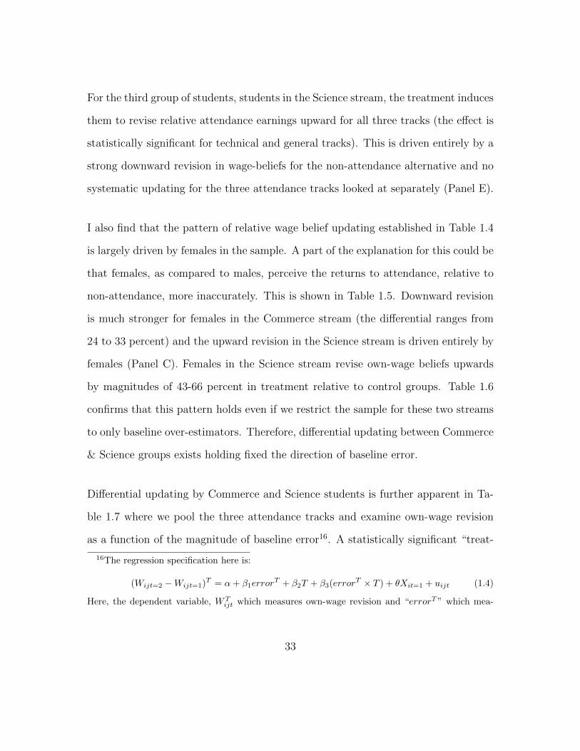
For the third group of students, students in the Science stream, the treatment induces

them to revise relative attendance earnings upward for all three tracks (the effect is

statistically significant for technical and general tracks). This is driven entirely by a

strong downward revision in wage-beliefs for the non-attendance alternative and no

systematic updating for the three attendance tracks looked at separately (Panel E).

I also find that the pattern of relative wage belief updating established in Table 1.4

is largely driven by females in the sample. A part of the explanation for this could be

that females, as compared to males, perceive the returns to attendance, relative to

non-attendance, more inaccurately. This is shown in Table 1.5. Downward revision

is much stronger for females in the Commerce stream (the differential ranges from

24 to 33 percent) and the upward revision in the Science stream is driven entirely by

females (Panel C). Females in the Science stream revise own-wage beliefs upwards

by magnitudes of 43-66 percent in treatment relative to control groups. Table 1.6

confirms that this pattern holds even if we restrict the sample for these two streams

to only baseline over-estimators. Therefore, differential updating between Commerce

& Science groups exists holding fixed the direction of baseline error.

Differential updating by Commerce and Science students is further apparent in Ta-

ble 1.7 where we pool the three attendance tracks and examine own-wage revision

as a function of the magnitude of baseline error16. A statistically significant “treat-

16The regression specification here is:

(Wijt=2 −Wijt=1)T = α+ β1errorT + β2T + β3(errorT × T ) + θXit=1 + uijt (1.4)

Here, the dependent variable, WTijt which measures own-wage revision and “errorT ” which mea-

33

ment x error” coefficient implies that own-wage revisions are a systematic function

of baseline error. A negative coefficient on the interaction term implies that larger

amounts of baseline under-estimation are associated with larger upward revisions in

treatment relative to control group. Focusing on columns (4)-(6), which include the

full set the baseline controls, we see that Commerce students systematically respond

to information presented for the attendance-tracks and Science students respond to

information presented for the non-attendance alternative.

Track by stream regressions in which wage-revisions cannot be systematically estab-

lished as a consequence of the treatment indicate that the track-specific information

provided was not relevant to the individuals of a given stream. In section 1.6, I

discuss that differences in updating between Commerce and Science students is not

a mechanical consequence of sub-group differences in baseline errors. I also provide

some evidence that non-updating is consistent with the Bayesian model but cannot

rule out the extent to which non-Bayesian updating constitute these findings.

1.5.6 Impact on Enrollment Intentions

Next, I examine whether updating of own-wage beliefs in response to information

on public earnings leads to updating of track-specific enrollment intentions among

the sample of students. I examine the impact of the treatment on enrollment in a

sures the difference between perceived and true population wage beliefs, can both take on negativeor positive values. Therefore, both variables are transformed using an inverse hyperbolic sincetransformation, which behaves and is interpreted like a log-transformation, but allows keeping zeroand negative values Bellemare, Barrett and Just (2013).

34

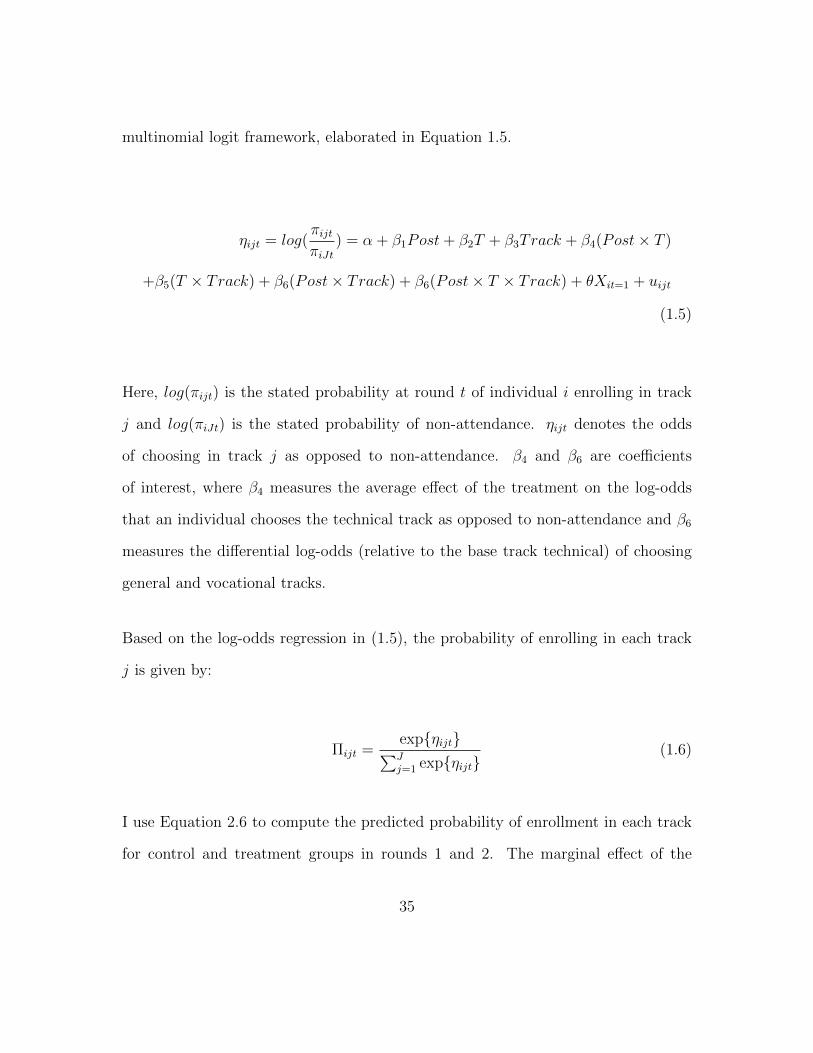
multinomial logit framework, elaborated in Equation 1.5.

ηijt = log(πijtπiJt

) = α + β1Post+ β2T + β3Track + β4(Post× T )

+β5(T × Track) + β6(Post× Track) + β6(Post× T × Track) + θXit=1 + uijt

(1.5)

Here, log(πijt) is the stated probability at round t of individual i enrolling in track

j and log(πiJt) is the stated probability of non-attendance. ηijt denotes the odds

of choosing in track j as opposed to non-attendance. β4 and β6 are coefficients

of interest, where β4 measures the average effect of the treatment on the log-odds

that an individual chooses the technical track as opposed to non-attendance and β6

measures the differential log-odds (relative to the base track technical) of choosing

general and vocational tracks.

Based on the log-odds regression in (1.5), the probability of enrolling in each track

j is given by:

Πijt =expηijt∑Jj=1 expηijt

(1.6)

I use Equation 2.6 to compute the predicted probability of enrollment in each track

for control and treatment groups in rounds 1 and 2. The marginal effect of the

35

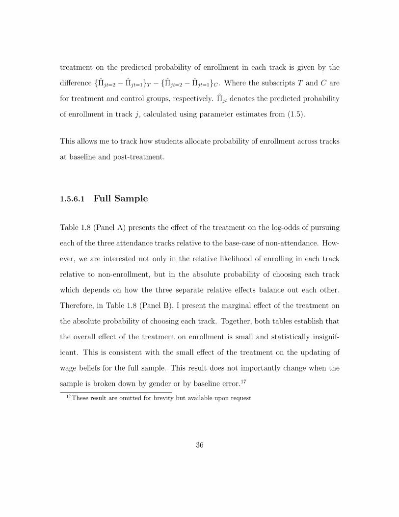
treatment on the predicted probability of enrollment in each track is given by the

difference Πjt=2 − Πjt=1T − Πjt=2 − Πjt=1C . Where the subscripts T and C are

for treatment and control groups, respectively. Πjt denotes the predicted probability

of enrollment in track j, calculated using parameter estimates from (1.5).

This allows me to track how students allocate probability of enrollment across tracks

at baseline and post-treatment.

1.5.6.1 Full Sample

Table 1.8 (Panel A) presents the effect of the treatment on the log-odds of pursuing

each of the three attendance tracks relative to the base-case of non-attendance. How-

ever, we are interested not only in the relative likelihood of enrolling in each track

relative to non-enrollment, but in the absolute probability of choosing each track

which depends on how the three separate relative effects balance out each other.

Therefore, in Table 1.8 (Panel B), I present the marginal effect of the treatment on

the absolute probability of choosing each track. Together, both tables establish that

the overall effect of the treatment on enrollment is small and statistically insignif-

icant. This is consistent with the small effect of the treatment on the updating of

wage beliefs for the full sample. This result does not importantly change when the

sample is broken down by gender or by baseline error.17

17These result are omitted for brevity but available upon request

36

1.5.6.2 By Current Stream of Study

In Table 1.9 (Panel A), I examine the effect of the treatment on the log-odds of pur-

suing each of the three attendance tracks relative to the base-case of non-attendance,

by current stream of study. In Table 1.10, I present these log-odds separately for

males and females.

For students in Arts/Humanities, the effect of the treatment on enrollment log-odds

is small, and statistically insignificant and the marginal effect of the treatment on the

predicted probability of enrollment is also small Table 1.9 (Panel B). As can be seen

in Table 1.10, for both males and females in this stream, we cannot reject the null that

the effect of the treatment on enrollment log-odds, relative to non-enrollment, for

each track is zero. This is consistent with the impact of the treatment on own-wage

belief updating for these students.

For students belonging to the Commerce stream, there is a decrease in enrollment log-

odds relative to non-attendance for technical and general streams (Table 1.9 (Panel

A)), and this effect is entirely driven by females (compare panel B to A of Table 1.10),

for whom there is a decrease in enrollment log-odds for all three attendance tracks

relative to non-attendance. This is consistent with the fact that for this group of

students, the overall effect of the treatment was a downward revision in own-wage

beliefs for each of the three attendance tracks, relative to non-attendance. As can

be seen in Table Table 1.9 (Panel B), which takes into account the relative size of

track-specific treatment effects from Table 1.9 (Panel A), for Commerce students,

37

there is a decrease the probability of enrollment in technical tracks by around 4.7

pp. and increase probability of enrollment in general tracks (1.45 pp.), vocational

tracks (2.77 pp.) and for non-attendance (0.477 pp.).

For students belonging to the Science stream, there is an increase in enrollment

log-odds relative to non-enrollment for all three attendance tracks Table 1.9 (Panel

A). A comparison of panel B to panel A in Table 1.10 shows that this effect of the

treatment on enrollment log-odds is driven by females. This too is consistent with

the fact that for this group of students, the overall effect of the treatment was an

upward revision in own-wage beliefs for each of the three attendance tracks, relative

to non-attendance. As can be seen in Table 1.9 (Panel B), for Science students there

is an increase the probability of enrollment in technical tracks by around 3.45 pp.

and decrease probability of enrollment in general tracks (0.505 pp.), vocational tracks

(2.28 pp.) and for non-attendance (0.668 pp.).

For both Science and Commerce students, and specifically for females, the direc-

tion of updating of enrollment intentions for each attendance track relative to non-

attendance, is broadly consistent with the direction of updating of wage beliefs for

each attendance track relative to non-attendance. However, the overall effect of

the treatment for Commerce students is to induce a movement away from technical

tracks and towards other tracks (more so vocational tracks) and on the contrary the

effect of the treatment for Science students is to induce a movement towards techni-

cal tracks and away from other tracks (more so vocational tracks). This fact cannot

be explained by the difference in magnitude of wage-belief revision between atten-

38

dance tracks, which do not statistically differ from each other, within the groups of

Commerce and Science students18.

1.5.7 Impact on Borrowing

Recall that borrowing intentions for higher education were measured only post-

treatment. Also, unlike stated enrollment intentions, the intent to borrow was not

elicited as a track-specific decision. The average impact of the information treatment

on borrowing intentions is given by β1 in Equation 1.7 below:

Yit=2 = α + β1T + θXit=1 + uit (1.7)

Where Y is a binary variable measuring whether or not the individual would like to

accept a loan offer towards higher education enrollment. We may be concerned that

the answer to this survey question might not be reflective of what would happen if

a loan were actually made available, because individuals might not fully internalize

the costs of borrowing while answering this question. While it is not possible to

fully allay such concerns in this setting, it should be noted that the control group

mean of the fraction of individuals wanting to borrow is only around 56 percent.

This is despite the fact that on average only 1.04 tracks (out of 3) are thought to

18I refer here to panels D & F of Table 1.4. In a variant of these regressions, when tracks areincluded as an interaction term, I confirm that the magnitude of wage-belief updating for eachattendance track does not statistically differ from the magnitude of updating for the other twotracks.

39

be affordable by individuals. The number of tracks affordable to individuals who do

not want to borrow is 1 and this number is 1.08 tracks for individuals who do want

to borrow.

Table 1.11 presents results on the impact of the information treatment on borrowing

intentions, which was the only other primary outcome that we measured in our

survey. Overall, treated individuals state a higher probability of intent to borrow,

which is higher by 6.7 pp. By stream, this effect is largest and statistically significant

only for students in the Science stream who have roughly a 15 pp. higher probability

of wanting to borrow when compared with students in the control group. This

represents a 25 percent increase in demand for borrowing, relative to the control

group mean. This result is further consistent with an upward revision for this group of

students in wage beliefs for attendance tracks relative to non-attendance. Conditional

on loan acceptance, the amount of that individuals would like to borrow does not

statistically differ on account of the treatment.

1.6 Can Heterogeneity in Updating be Explained?

In this section I discuss that while the wage belief updating of Arts students vis-a-vis

the other two streams can be attributable to two observed patterns in the data, the

differential updating between Science & Commerce students remains unexplained.

This points to the existence of substantial heterogeneity in updating heuristics in

the sample.

40

In section 1.5.3, and with reference to Table 1.B.5, we already established that ex-

ante, we might expect Arts students to be less responsive to the information treat-

ment and that is indeed what we find. This ex-ante prediction is based on the

finding that for these students, at baseline, the enrollment elasticity of earnings be-

liefs is close to zero and statistically insignificant. Therefore, to the extent that it is

costlier for individuals to process or pay attention to information not relevant to their

decision-making process, we might expect these students to not update their own-

earnings beliefs in response to information provision. Across tracks, the updating of

own wage beliefs for Arts students, on account of the treatment, is statistically in-

significant and we cannot reject the null that it is zero (first two panels of Table 1.3).

The same analysis indicates that earnings beliefs seem to be important predictors

of enrollment intentions for both Commerce & Science students, and the coefficient

on log wages for both streams is of roughly equal magnitude. Experimentally, these

students update relative own-earnings and also enrollment and borrowing intentions,

in a manner consistent with the updating of own-wage beliefs. Therefore differences

in the baseline relevance of earnings provide us with one explanation for why we may

see differential updating for Arts as compared to Commerce & Science students. It

cannot explain why the two sets of students, Commerce & Science, respond to differ-

ent pieces of information and hence update relative earnings in opposite directions.

Therefore, next I examine whether differential updating can be rationalized on ac-

count of differences in baseline errors, regarding population earnings, between sub-

groups.

41

In Figure 1.2 we had established that the distributions of population wage beliefs for

Commerce and Science students closely overlay each other. On the other hand, on

average, Arts students seem to make smaller errors for all four tracks. This is further

evident in Table 1.C.6. Here, we look at differences in baseline errors19 between the

three sub-groups in a regression framework, using OLS (col. 1) and quantile regres-

sions (col. 2-6). Focusing our attention on col.1, it is evident that for all tracks, for

students in the Arts stream, mean error is statistically significantly smaller (closer

to zero error) than for students in the Science stream. However, the mean error

for Commerce students does not statistically differ from that of Science students,

for any track. Quantile regression results (col. 2-6) also consistently point to the

fact that for several points along the distribution of baseline errors, Arts students

differ consistently in their perceptions about population earnings when compared

to Science students, while Commerce students do not. Therefore, while we cannot

rule out the possibility that Arts students update own-earnings differently than stu-

dents from the other two streams on an additional account of initial differences in

perceptions regarding population earnings, this cannot explain differential updating

between Commerce & Science streams. Therefore, it is evident that a substantial

amount of updating heterogeneity in the sample is, most likely, not a mechanical

consequence of differences in baseline errors regarding population earnings.

Next, I test whether the differential updating between Commerce & Science students

can be explained by a core prediction of the Bayesian model. That is, I test whether

individuals in the sample are more responsive to information regarding a track that

19Measured, as described in footnote 14, using an inverse hyperbolic sine transformation.

42

they are less likely to enroll in (DellaVigna and Gentzkow (2010); Oreopoulos and

Dunn (2013)), and hence have weaker priors about. In Table 1.C.7, I establish

that Commerce students have higher baseline likelihoods of non-attendance. This

is the case both when all four tracks are in an individual’s choice set, regardless of

affordability (unconstrained choice set), and when only affordable tracks enter an

individual’s choice set (constrained choice set)20. In the unconstrained case, Com-

merce students state 1.4-2 pp. higher likelihoods of non-attendance compared to

the reference category of Science students (who state about a 5.3% likelihood of non-

attendance). It is apparent that when the cost constraint is removed and all tracks are

hypothetically made available to all individuals, students state generally small prob-

abilities of non-attendance. With regards to data on individuals constrained choice

sets, wherein unaffordable options are assigned zero probability of attendance, Com-

merce students are about 6.6-9.2 pp. more likely to not-attend compared to Science

students whose probability of non-attendance is about 50%.

In Table 1.C.8 I test whether individuals with a higher baseline probability of en-

rolling in a track are less likely to update earnings beliefs in response to the infor-

mation treatment. I regress the absolute value of wage belief revision on levels and

an interaction of the treatment dummy with the baseline probability of enrollment.

While the effect of the treatment does not vary with the baseline probability of enroll-

ment for the unconstrained case, the “treatment x baseline enrollment probability”

interaction term is negative and significant (at the 5% level) when affordability of

tracks is taken into account. Therefore, the fact that Commerce students are less

20In this case tracks unaffordable to an individual are assigned a zero probability of attendance.

43

likely to attend and more responsive to information on attendance tracks and Science

students are more likely to attendance and less responsive to information on atten-

dance tracks, is consistent with the core prediction of Bayesian updating bearing

out in the data. Previous work in the literature leads us to believe that a portion of

non-updating may also be non-Bayesian in nature (i.e. not explained by the variance

of priors), but unfortunately in the absence of further data, I cannot comment on

the extent to which that may be the case in this sample.

1.7 Conclusion

In this paper I present results from an information experiment, which randomized

information on population earnings, for three post-secondary education tracks- tech-

nical, general, vocational and the final alternative of not pursuing post-secondary

education. The experiment was carried out with 1525 12th grade students, across

nine affiliated schools of a large, non-selective public state university in the Indian

state of Jharkhand.

The impact of information provision is measured by students updating of own wage

beliefs contingent on pursuing each post-secondary track, their stated probability of

enrollment across tracks and borrowing intentions for higher education enrollment.

Average impact of the treatment on the updating of own-wage beliefs and subsequent

changes in enrollment intentions is small, though the impact on borrowing intentions

is positive and statistically important. Average results mask considerable sub-group

44

heterogeneity, defined by the current subject stream of students. For two out of

three sub-groups of students, the impact of the treatment on relative own-earnings

beliefs, is statistically important. For these two sub-groups, own-wage belief updat-

ing is stronger for females, a pattern which may partly be on account of the fact

that females perceive relative returns to attendance more inaccurately than males,

at baseline. However, I also find that females are more responsive to the informa-

tion treatment controlling for the size of baseline error (result omitted for brevity).

Interestingly, Wiswall and Zafar (2015b) also find this to be the case in their sample

of New York University (NYU) students. Within sub-group, the odds of enrollment,

relative to non-enrollment, is consistent with direction of wage belief updating and is,

reassuringly, stronger for the group (females) with larger wage belief updating. The

effect of the treatment on borrowing intentions is also in line it’s effect on wage-belief

updating.

For the two sub-groups (Commerce & Science) for whom the impact of the treatment

on wage beliefs for attendance tracks, relative to non-attendance, is statistically

important, the updating takes place in opposite directions. This pattern is on account

of the fact that individuals in the groups systematically respond to different pieces of

track-specific information. Students in the Commerce sub-group revise wage beliefs

downwards for attendance tracks only, and this pattern carries over to a downward

revision in earnings beliefs for attendance tracks, relative to non-attendance. Science

students revise wage beliefs downwards for the non-attendance track only, which

translates into attendance earnings being relatively more attractive for this group,

45

post-treatment.

A combination of factors may explain why we see the first sub-group, students in

the Arts stream, not revise wage beliefs in response to the treatment. Ex-ante, these

students have a low elasticity of enrollment to wage beliefs and at baseline they

make smaller errors, on average, with regards to beliefs about population earnings.

However, these factors do not explain differential updating on the part of Science

& Commerce students. Ex-ante, these students have a statistically important and

similar in magnitude elasticity of enrollment to wage beliefs- therefore earnings likely

play an important role in their decisions for future education. These students also

make nearly identical errors with regards to population wage beliefs at baseline.

As discussed in the conceptual framework section of the paper, non-updating in

response to “new” information implies that the piece of information provided was

not relevant to individuals. Differential relevance of track-specific information to

different sub-groups of individuals in the sample drives the heterogeneous impacts of

information provision on own-wage belief updating. Sub-groups of individuals with

equally biased information sets vary in their response to information significantly,

depending on the extent to which their beliefs about population earnings are linked

to their beliefs about their own. Track-specific non-updating can be Bayesian or

“rational” or Non-Bayesian. Suggestive evidence implies that variation in updating

may be attributable to the variance of individuals’ priors (consistent with Bayesian

updating), but without further data on individual-level distributions of own-wage

beliefs, we cannot quantify the extent to which non-updating is Bayesian. However,

46

recent evidence (Wiswall and Zafar (2015b)) establishes that individuals do indeed

deviate significantly from the Bayesian benchmark.

Recent papers in the literature which find information provision to have small aver-

age impacts on outcomes like test-scores or enrollment decisions state the presence of

other binding constraints like credit constraints or lack of knowledge of the education

production function as explanations. This paper offers another explanation for why

the provision of population-level information on returns may lead to highly hetero-

geneous outcomes, by examining in detail the first-link in the causal chain that links

population-level information to education outcomes, which is, the extent to which

individuals update own-earnings beliefs in response to receiving information about

population-level averages.

My study is a framed field experiment wherein participants deal with a subject of

interest outside the experiment (their own education) but not in an environment

where they would naturally undertake the task of thinking about their long term

plans. Stakes for the participants were also low with no costs to paying less atten-

tion to the information provided. Therefore, the study was not designed to provide

a model for scaling information provision at a national level, but to examine in more

detail mechanisms (updating of beliefs and intentions) critical to the success of in-

formation interventions. For a policy-maker looking to implement an information

campaign to induce more optimal education decision making, these findings imply,

all else constant, a limited potential for an information campaign to induce, on aver-

age, updating of beliefs regarding oneself, of a particular magnitude and in a given

47

direction, despite accurate knowledge of information gaps in a particular population.

48

REFERENCES FOR CHAPTER 1

Arcidiacono, Peter, V Joseph Hotz, and Songman Kang. 2012. “Modeling

college major choices using elicited measures of expectations and counterfactuals.”

Journal of Econometrics, 166(1): 3–16.

Avitabile, Ciro, and Rafael E De Hoyos Navarro. 2015. “The Heterogeneous

effect of information on student performance: evidence from a randomized control

trial in Mexico.” World Bank Policy Research Working Paper, , (7422).

Bellemare, Marc F, Christopher B Barrett, and David R Just. 2013. “The

welfare impacts of commodity price volatility: evidence from rural Ethiopia.”

American Journal of Agricultural Economics, 95(4): 877–899.

Bonilla, Leonardo, Nicolas L Bottan, and Andres Ham. 2016. “Information

Policies and Higher Education Choices Experimental Evidence from Colombia.”

Delavande, Adeline, and Basit Zafar. 2014. “University choice: the role of

expected earnings, non-pecuniary outcomes, and financial constraints.” FRB of

New York Staff Report, , (683).

DellaVigna, Stefano, and Matthew Gentzkow. 2010. “Persuasion: Empirical

Evidence.” Annual Review of Economics, 2(1): 643–669.

Duflo, Esther, Rachel Glennerster, and Michael Kremer. 2007. “Using ran-

domization in development economics research: A toolkit.” Handbook of develop-

ment economics, 4: 3895–3962.

49

Dupas, Pascaline. 2011. “Do teenagers respond to HIV risk information? Evi-

dence from a field experiment in Kenya.” American Economic Journal: Applied

Economics, 3(1): 1–34.

Fryer Jr, Roland G. 2013. “Information and student achievement: evidence from

a cellular phone experiment.” National Bureau of Economic Research.

Gamboa, Luis, and Paul Rodrıguez Lesmes. 2014. “Do Colombian students

underestimate higher education returns?” UNIVERSIDAD DEL ROSARIO.

Hanna, Rema, Sendhil Mullainathan, and Joshua Schwartzstein. 2014.

“Learning through noticing: Theory and evidence from a field experiment.” The

Quarterly Journal of Economics, 129(3): 1311–1353.

Harrison, Glenn W, and John A List. 2004. “Field experiments.” Journal of

Economic literature, 42(4): 1009–1055.

Hastings, Justine, Christopher A Neilson, and Seth D Zimmerman. 2015.

“The effects of earnings disclosure on college enrollment decisions.” National Bu-

reau of Economic Research.

Jensen, Robert. 2010. “The (perceived) returns to education and the demand for

schooling.” Quarterly Journal of Economics, 125(2).

Kahneman, Daniel, and Amos Tversky. 1972. “Subjective probability: A judg-

ment of representativeness.” Cognitive psychology, 3(3): 430–454.

50

Kaufmann, Katja Maria. 2014. “Understanding the income gradient in college

attendance in Mexico: The role of heterogeneity in expected returns.” Quantitative

Economics, 5(3): 583–630.

Kennedy, Peter E, et al. 1981. “Estimation with correctly interpreted dummy

variables in semilogarithmic equations [the interpretation of dummy variables in

semilogarithmic equations].” American Economic Review, 71(4).

Loyalka, Prashant, Chengfang Liu, Yingquan Song, Hongmei Yi, Xiaot-

ing Huang, Jianguo Wei, Linxiu Zhang, Yaojiang Shi, James Chu, and

Scott Rozelle. 2013. “Can information and counseling help students from poor

rural areas go to high school? Evidence from China.” Journal of Comparative

Economics, 41(4): 1012–1025.

Maertens, Annemie. 2011. “Does education pay off? Subjective expectations on

education in rural India.” Economic & Political Weekly, 46(09): 58–63.

Manski, Charles F. 1993. “Adolescent econometricians: How do youth infer the

returns to schooling?” In Studies of supply and demand in higher education. 43–60.

University of Chicago Press.

Nguyen, Trang. 2008. “Information, role models and perceived returns to educa-

tion: Experimental evidence from Madagascar.” Unpublished manuscript, 6.

Oreopoulos, Philip, and Ryan Dunn. 2013. “Information and college access:

Evidence from a randomized field experiment.” The Scandinavian Journal of Eco-

nomics, 115(1): 3–26.

51

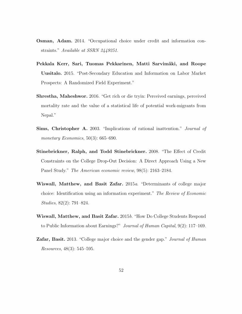
Osman, Adam. 2014. “Occupational choice under credit and information con-

straints.” Available at SSRN 2449251.

Pekkala Kerr, Sari, Tuomas Pekkarinen, Matti Sarvimaki, and Roope

Uusitalo. 2015. “Post-Secondary Education and Information on Labor Market

Prospects: A Randomized Field Experiment.”

Shrestha, Maheshwor. 2016. “Get rich or die tryin: Perceived earnings, perceived

mortality rate and the value of a statistical life of potential work-migrants from

Nepal.”

Sims, Christopher A. 2003. “Implications of rational inattention.” Journal of

monetary Economics, 50(3): 665–690.

Stinebrickner, Ralph, and Todd Stinebrickner. 2008. “The Effect of Credit

Constraints on the College Drop-Out Decision: A Direct Approach Using a New

Panel Study.” The American economic review, 98(5): 2163–2184.

Wiswall, Matthew, and Basit Zafar. 2015a. “Determinants of college major

choice: Identification using an information experiment.” The Review of Economic

Studies, 82(2): 791–824.

Wiswall, Matthew, and Basit Zafar. 2015b. “How Do College Students Respond

to Public Information about Earnings?” Journal of Human Capital, 9(2): 117–169.

Zafar, Basit. 2013. “College major choice and the gender gap.” Journal of Human

Resources, 48(3): 545–595.

52

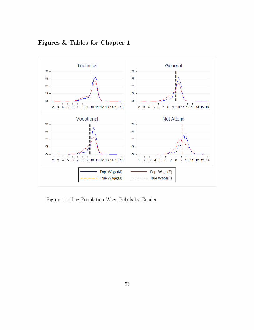
Figures & Tables for Chapter 1

Figure 1.1: Log Population Wage Beliefs by Gender

53

Figure 1.2: Log Population Wage Beliefs by Current Stream of Study

54

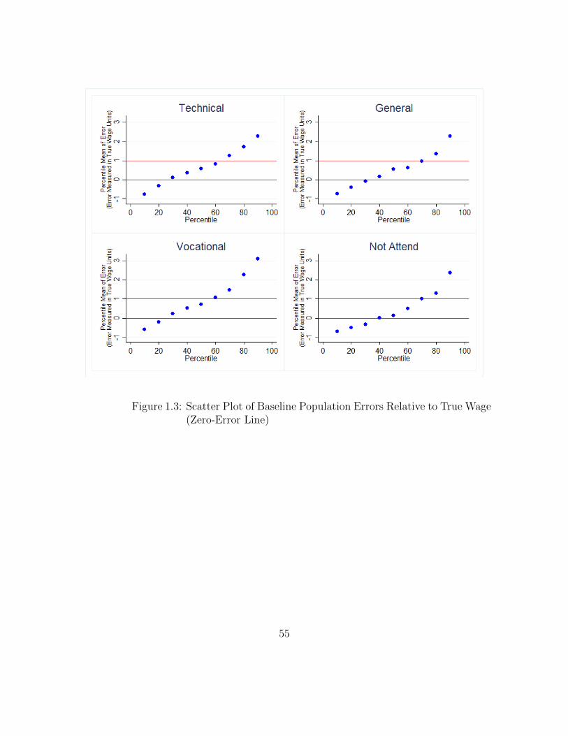
Figure 1.3: Scatter Plot of Baseline Population Errors Relative to True Wage(Zero-Error Line)

55

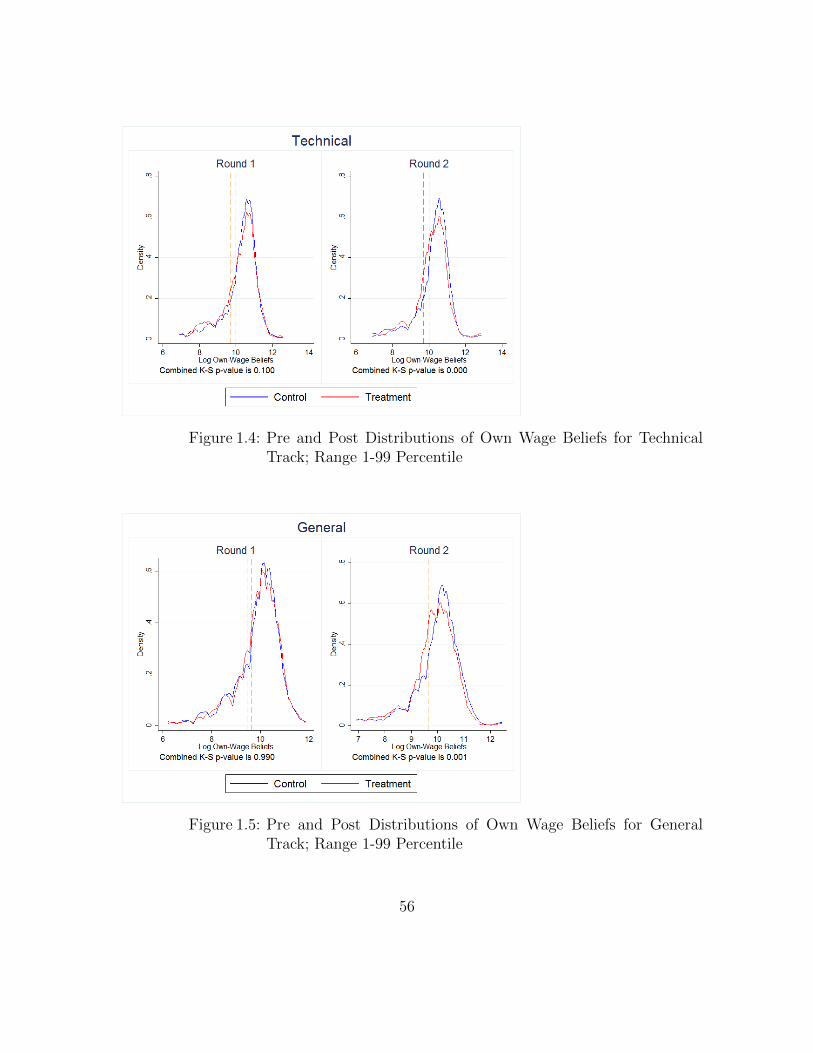
Figure 1.4: Pre and Post Distributions of Own Wage Beliefs for TechnicalTrack; Range 1-99 Percentile

Figure 1.5: Pre and Post Distributions of Own Wage Beliefs for GeneralTrack; Range 1-99 Percentile

56

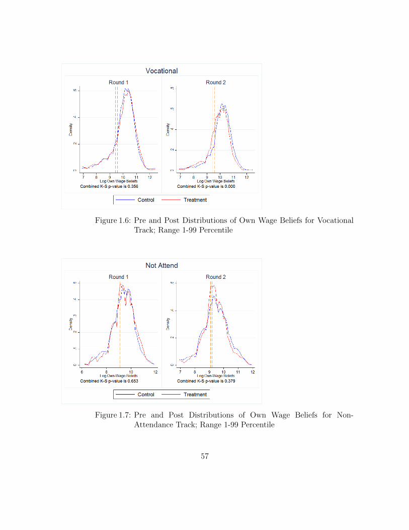
Figure 1.6: Pre and Post Distributions of Own Wage Beliefs for VocationalTrack; Range 1-99 Percentile

Figure 1.7: Pre and Post Distributions of Own Wage Beliefs for Non-Attendance Track; Range 1-99 Percentile

57

Table 1.1: % of Students Who Overestimate Earnings at Baseline

Full Sample:

Overall Males FemalesTechnical 71.41% 72.24% 70.43%General 64.13% 66.06% 61.86%Vocational 75.34% 83.39% 65.86%Not Attend 60.79% 70.55% 49.29%

Arts:

Overall Males FemalesTechnical 55.49% 53.22% 57.34%General 49.52% 49.79% 49.30%Vocational 61.08% 71.24% 52.80%Not Attend 53.18% 63.09% 45.10%

Commerce:

Overall Males FemalesTechnical 77.19% 73.19% 81.20%General 73.35% 74.47% 72.22%Vocational 82.52% 87.23% 77.78%Not Attend 62.47% 72.34% 52.56%

Science:

Overall Males FemalesTechnical 81.72% 84.03% 77.09%General 70.34% 71.15% 68.72%Vocational 82.84% 88.80% 70.95%Not Attend 66.79% 74.23% 51.96%

58

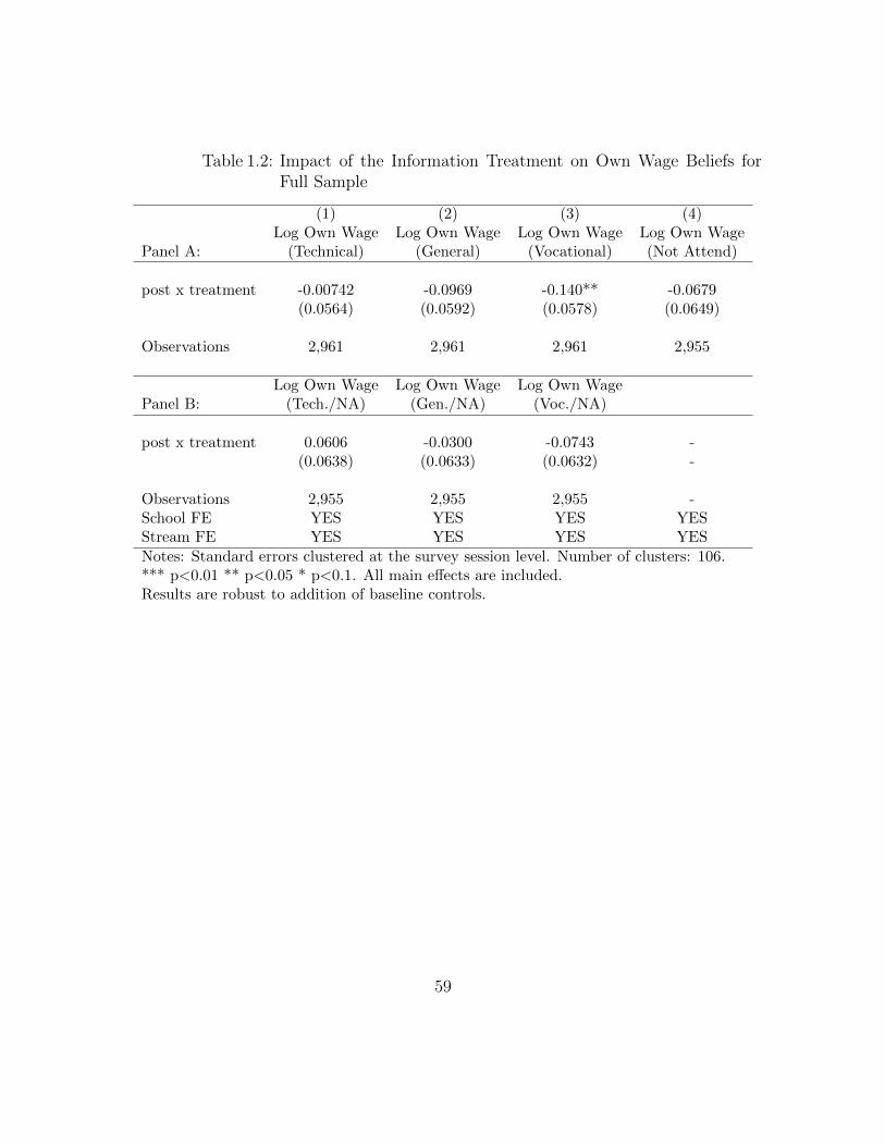
Table 1.2: Impact of the Information Treatment on Own Wage Beliefs forFull Sample

(1) (2) (3) (4)Log Own Wage Log Own Wage Log Own Wage Log Own Wage

Panel A: (Technical) (General) (Vocational) (Not Attend)

post x treatment -0.00742 -0.0969 -0.140** -0.0679(0.0564) (0.0592) (0.0578) (0.0649)

Observations 2,961 2,961 2,961 2,955

Log Own Wage Log Own Wage Log Own WagePanel B: (Tech./NA) (Gen./NA) (Voc./NA)

post x treatment 0.0606 -0.0300 -0.0743 -(0.0638) (0.0633) (0.0632) -

Observations 2,955 2,955 2,955 -School FE YES YES YES YESStream FE YES YES YES YES

Notes: Standard errors clustered at the survey session level. Number of clusters: 106.*** p<0.01 ** p<0.05 * p<0.1. All main effects are included.Results are robust to addition of baseline controls.

59

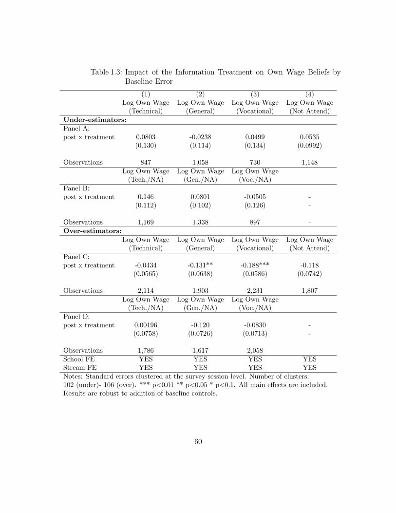
Table 1.3: Impact of the Information Treatment on Own Wage Beliefs byBaseline Error

(1) (2) (3) (4)Log Own Wage Log Own Wage Log Own Wage Log Own Wage

(Technical) (General) (Vocational) (Not Attend)

Under-estimators:

Panel A:post x treatment 0.0803 -0.0238 0.0499 0.0535

(0.130) (0.114) (0.134) (0.0992)

Observations 847 1,058 730 1,148

Log Own Wage Log Own Wage Log Own Wage(Tech./NA) (Gen./NA) (Voc./NA)

Panel B:post x treatment 0.146 0.0801 -0.0505 -

(0.112) (0.102) (0.126) -

Observations 1,169 1,338 897 -

Over-estimators:

Log Own Wage Log Own Wage Log Own Wage Log Own Wage(Technical) (General) (Vocational) (Not Attend)

Panel C:post x treatment -0.0434 -0.131** -0.188*** -0.118

(0.0565) (0.0638) (0.0586) (0.0742)

Observations 2,114 1,903 2,231 1,807

Log Own Wage Log Own Wage Log Own Wage(Tech./NA) (Gen./NA) (Voc./NA)

Panel D:post x treatment 0.00196 -0.120 -0.0830 -

(0.0758) (0.0726) (0.0713) -

Observations 1,786 1,617 2,058 -

School FE YES YES YES YESStream FE YES YES YES YES

Notes: Standard errors clustered at the survey session level. Number of clusters:102 (under)- 106 (over). *** p<0.01 ** p<0.05 * p<0.1. All main effects are included.Results are robust to addition of baseline controls.

60

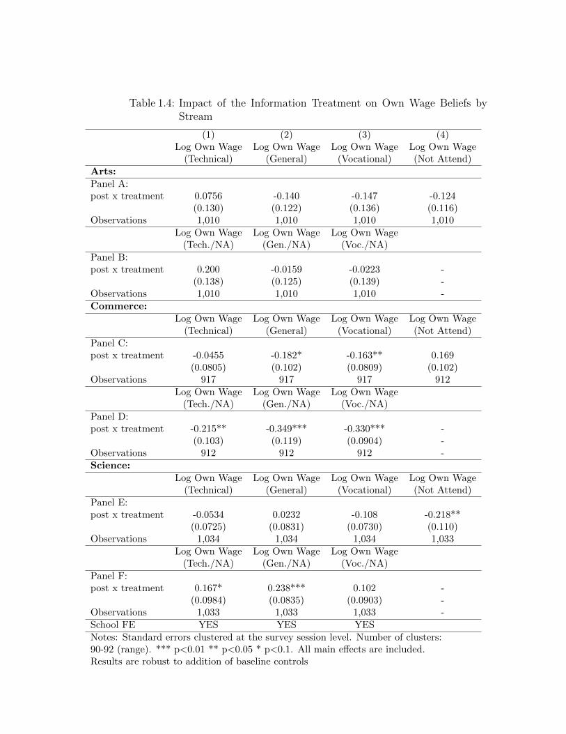
Table 1.4: Impact of the Information Treatment on Own Wage Beliefs byStream

(1) (2) (3) (4)Log Own Wage Log Own Wage Log Own Wage Log Own Wage

(Technical) (General) (Vocational) (Not Attend)

Arts:

Panel A:post x treatment 0.0756 -0.140 -0.147 -0.124

(0.130) (0.122) (0.136) (0.116)Observations 1,010 1,010 1,010 1,010

Log Own Wage Log Own Wage Log Own Wage(Tech./NA) (Gen./NA) (Voc./NA)

Panel B:post x treatment 0.200 -0.0159 -0.0223 -

(0.138) (0.125) (0.139) -Observations 1,010 1,010 1,010 -

Commerce:

Log Own Wage Log Own Wage Log Own Wage Log Own Wage(Technical) (General) (Vocational) (Not Attend)

Panel C:post x treatment -0.0455 -0.182* -0.163** 0.169

(0.0805) (0.102) (0.0809) (0.102)Observations 917 917 917 912

Log Own Wage Log Own Wage Log Own Wage(Tech./NA) (Gen./NA) (Voc./NA)

Panel D:post x treatment -0.215** -0.349*** -0.330*** -

(0.103) (0.119) (0.0904) -Observations 912 912 912 -

Science:

Log Own Wage Log Own Wage Log Own Wage Log Own Wage(Technical) (General) (Vocational) (Not Attend)

Panel E:post x treatment -0.0534 0.0232 -0.108 -0.218**

(0.0725) (0.0831) (0.0730) (0.110)Observations 1,034 1,034 1,034 1,033

Log Own Wage Log Own Wage Log Own Wage(Tech./NA) (Gen./NA) (Voc./NA)

Panel F:post x treatment 0.167* 0.238*** 0.102 -

(0.0984) (0.0835) (0.0903) -Observations 1,033 1,033 1,033 -

School FE YES YES YES

Notes: Standard errors clustered at the survey session level. Number of clusters:90-92 (range). *** p<0.01 ** p<0.05 * p<0.1. All main effects are included.Results are robust to addition of baseline controls

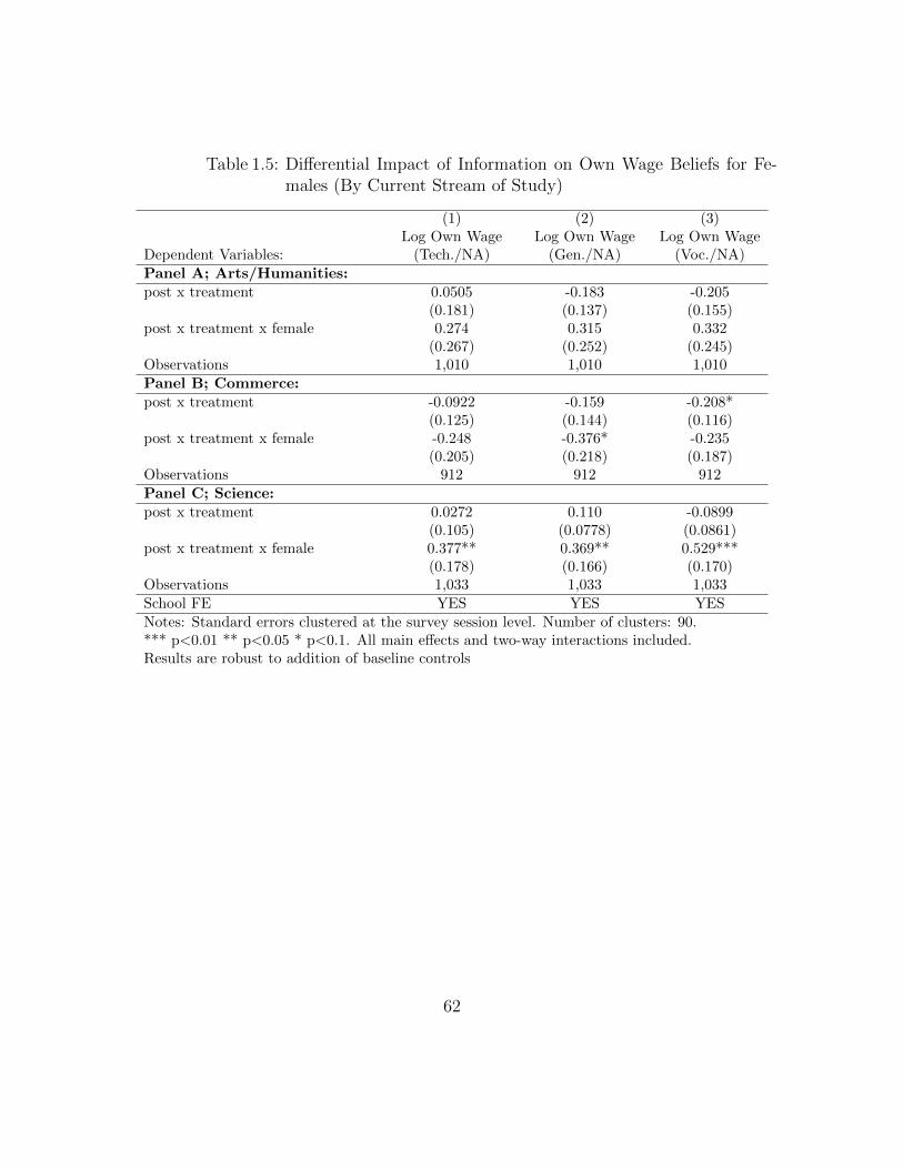
Table 1.5: Differential Impact of Information on Own Wage Beliefs for Fe-males (By Current Stream of Study)

(1) (2) (3)Log Own Wage Log Own Wage Log Own Wage

Dependent Variables: (Tech./NA) (Gen./NA) (Voc./NA)

Panel A; Arts/Humanities:

post x treatment 0.0505 -0.183 -0.205(0.181) (0.137) (0.155)

post x treatment x female 0.274 0.315 0.332(0.267) (0.252) (0.245)

Observations 1,010 1,010 1,010

Panel B; Commerce:

post x treatment -0.0922 -0.159 -0.208*(0.125) (0.144) (0.116)

post x treatment x female -0.248 -0.376* -0.235(0.205) (0.218) (0.187)

Observations 912 912 912

Panel C; Science:

post x treatment 0.0272 0.110 -0.0899(0.105) (0.0778) (0.0861)

post x treatment x female 0.377** 0.369** 0.529***(0.178) (0.166) (0.170)

Observations 1,033 1,033 1,033

School FE YES YES YES

Notes: Standard errors clustered at the survey session level. Number of clusters: 90.*** p<0.01 ** p<0.05 * p<0.1. All main effects and two-way interactions included.Results are robust to addition of baseline controls

62

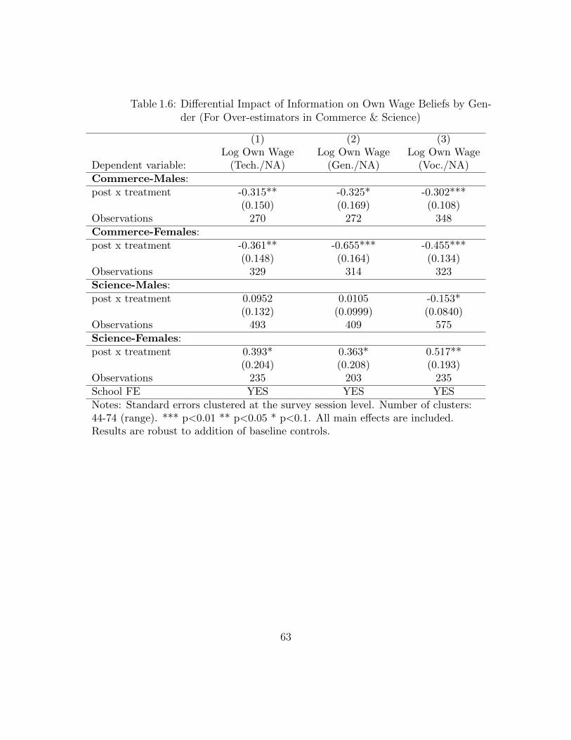
Table 1.6: Differential Impact of Information on Own Wage Beliefs by Gen-der (For Over-estimators in Commerce & Science)

(1) (2) (3)Log Own Wage Log Own Wage Log Own Wage

Dependent variable: (Tech./NA) (Gen./NA) (Voc./NA)

Commerce-Males:

post x treatment -0.315** -0.325* -0.302***(0.150) (0.169) (0.108)

Observations 270 272 348

Commerce-Females:

post x treatment -0.361** -0.655*** -0.455***(0.148) (0.164) (0.134)

Observations 329 314 323

Science-Males:

post x treatment 0.0952 0.0105 -0.153*(0.132) (0.0999) (0.0840)

Observations 493 409 575

Science-Females:

post x treatment 0.393* 0.363* 0.517**(0.204) (0.208) (0.193)

Observations 235 203 235

School FE YES YES YES

Notes: Standard errors clustered at the survey session level. Number of clusters:44-74 (range). *** p<0.01 ** p<0.05 * p<0.1. All main effects are included.Results are robust to addition of baseline controls.

63

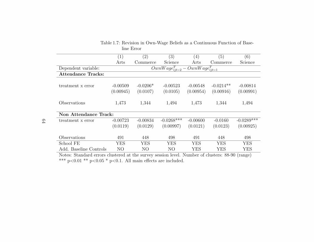
Table 1.7: Revision in Own-Wage Beliefs as a Continuous Function of Base-line Error

(1) (2) (3) (4) (5) (6)Arts Commerce Science Arts Commerce Science

Dependent variable: OwnWageTijt=2 −OwnWageTijt=1

Attendance Tracks:

treatment x error -0.00509 -0.0206* -0.00523 -0.00548 -0.0214** -0.00814(0.00945) (0.0107) (0.0105) (0.00954) (0.00916) (0.00991)

Observations 1,473 1,344 1,494 1,473 1,344 1,494

Non Attendance Track:treatment x error -0.00723 -0.00834 -0.0268*** -0.00600 -0.0160 -0.0289***

(0.0119) (0.0129) (0.00997) (0.0121) (0.0123) (0.00925)

Observations 491 448 498 491 448 498School FE YES YES YES YES YES YESAdd. Baseline Controls NO NO NO YES YES YESNotes: Standard errors clustered at the survey session level. Number of clusters: 88-90 (range)*** p<0.01 ** p<0.05 * p<0.1. All main effects are included.

64

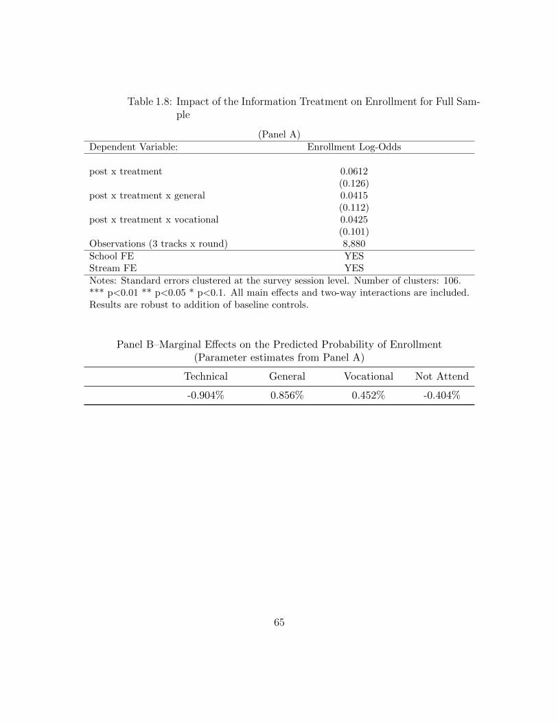
Table 1.8: Impact of the Information Treatment on Enrollment for Full Sam-ple

(Panel A)

Dependent Variable: Enrollment Log-Odds

post x treatment 0.0612(0.126)

post x treatment x general 0.0415(0.112)

post x treatment x vocational 0.0425(0.101)

Observations (3 tracks x round) 8,880

School FE YESStream FE YES

Notes: Standard errors clustered at the survey session level. Number of clusters: 106.*** p<0.01 ** p<0.05 * p<0.1. All main effects and two-way interactions are included.Results are robust to addition of baseline controls.

Panel B–Marginal Effects on the Predicted Probability of Enrollment(Parameter estimates from Panel A)

Technical General Vocational Not Attend

-0.904% 0.856% 0.452% -0.404%

65

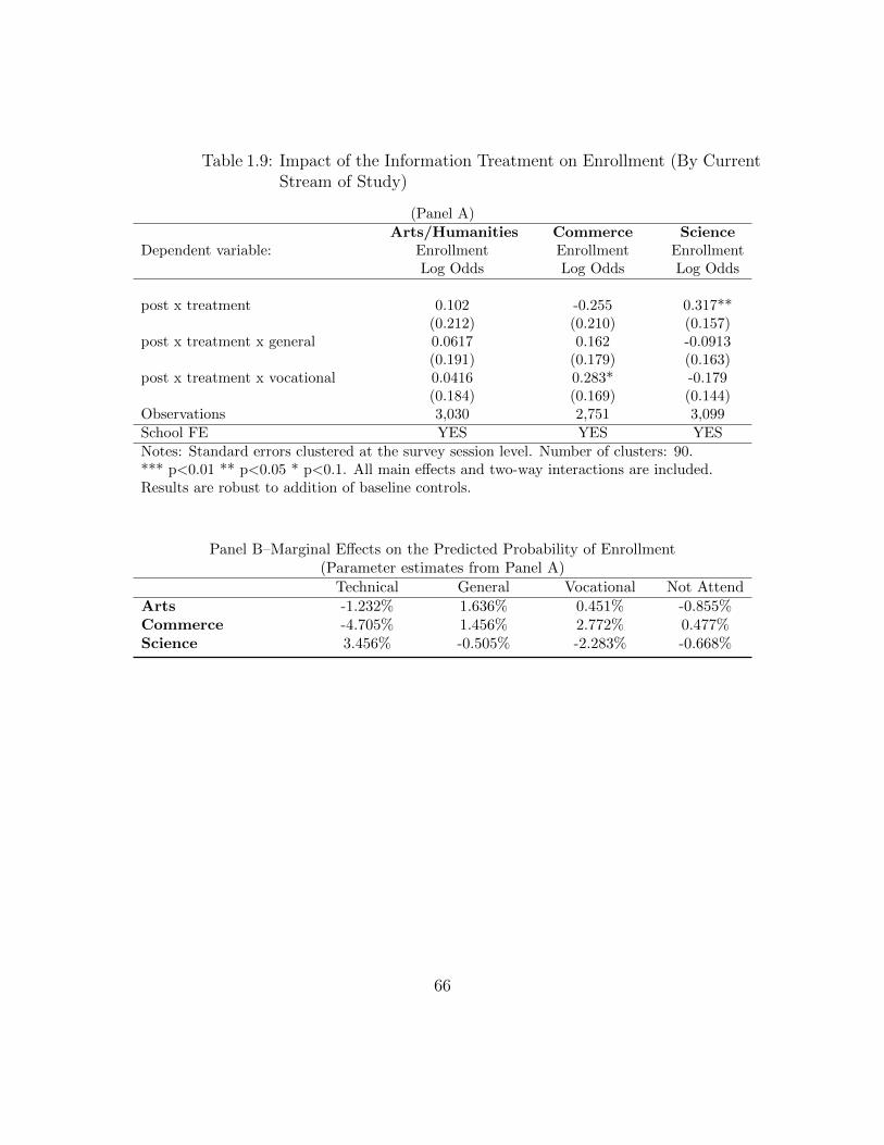
Table 1.9: Impact of the Information Treatment on Enrollment (By CurrentStream of Study)

(Panel A)

Arts/Humanities Commerce ScienceDependent variable: Enrollment Enrollment Enrollment

Log Odds Log Odds Log Odds

post x treatment 0.102 -0.255 0.317**(0.212) (0.210) (0.157)

post x treatment x general 0.0617 0.162 -0.0913(0.191) (0.179) (0.163)

post x treatment x vocational 0.0416 0.283* -0.179(0.184) (0.169) (0.144)

Observations 3,030 2,751 3,099

School FE YES YES YES

Notes: Standard errors clustered at the survey session level. Number of clusters: 90.*** p<0.01 ** p<0.05 * p<0.1. All main effects and two-way interactions are included.Results are robust to addition of baseline controls.

Panel B–Marginal Effects on the Predicted Probability of Enrollment(Parameter estimates from Panel A)

Technical General Vocational Not Attend

Arts -1.232% 1.636% 0.451% -0.855%Commerce -4.705% 1.456% 2.772% 0.477%Science 3.456% -0.505% -2.283% -0.668%

66

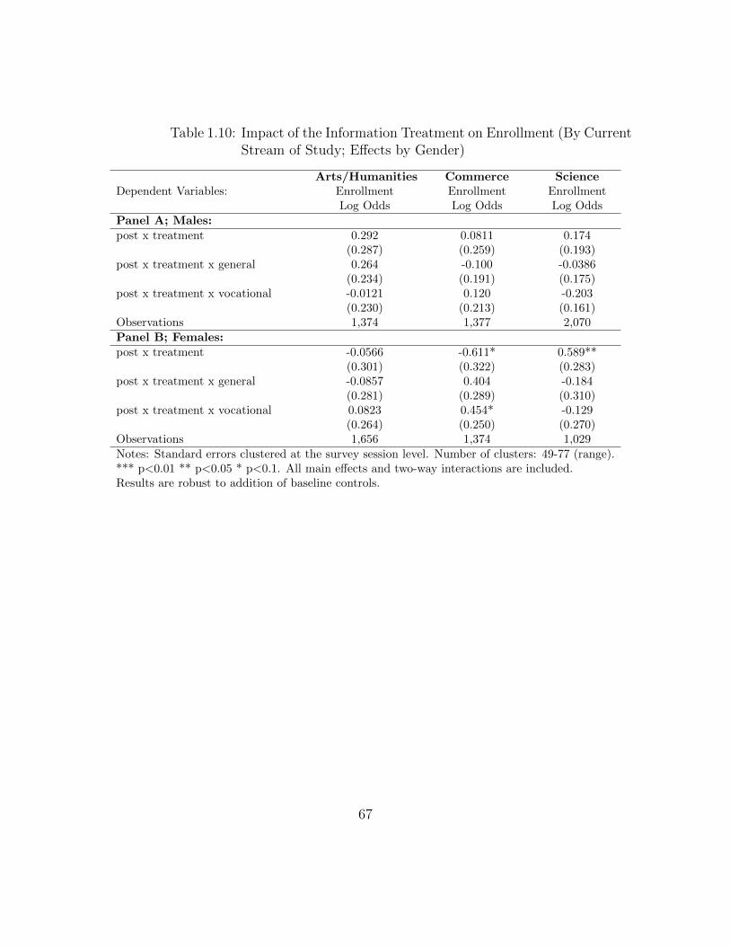
Table 1.10: Impact of the Information Treatment on Enrollment (By CurrentStream of Study; Effects by Gender)

Arts/Humanities Commerce ScienceDependent Variables: Enrollment Enrollment Enrollment

Log Odds Log Odds Log Odds

Panel A; Males:

post x treatment 0.292 0.0811 0.174(0.287) (0.259) (0.193)

post x treatment x general 0.264 -0.100 -0.0386(0.234) (0.191) (0.175)

post x treatment x vocational -0.0121 0.120 -0.203(0.230) (0.213) (0.161)

Observations 1,374 1,377 2,070

Panel B; Females:

post x treatment -0.0566 -0.611* 0.589**(0.301) (0.322) (0.283)

post x treatment x general -0.0857 0.404 -0.184(0.281) (0.289) (0.310)

post x treatment x vocational 0.0823 0.454* -0.129(0.264) (0.250) (0.270)

Observations 1,656 1,374 1,029

Notes: Standard errors clustered at the survey session level. Number of clusters: 49-77 (range).*** p<0.01 ** p<0.05 * p<0.1. All main effects and two-way interactions are included.Results are robust to addition of baseline controls.

67

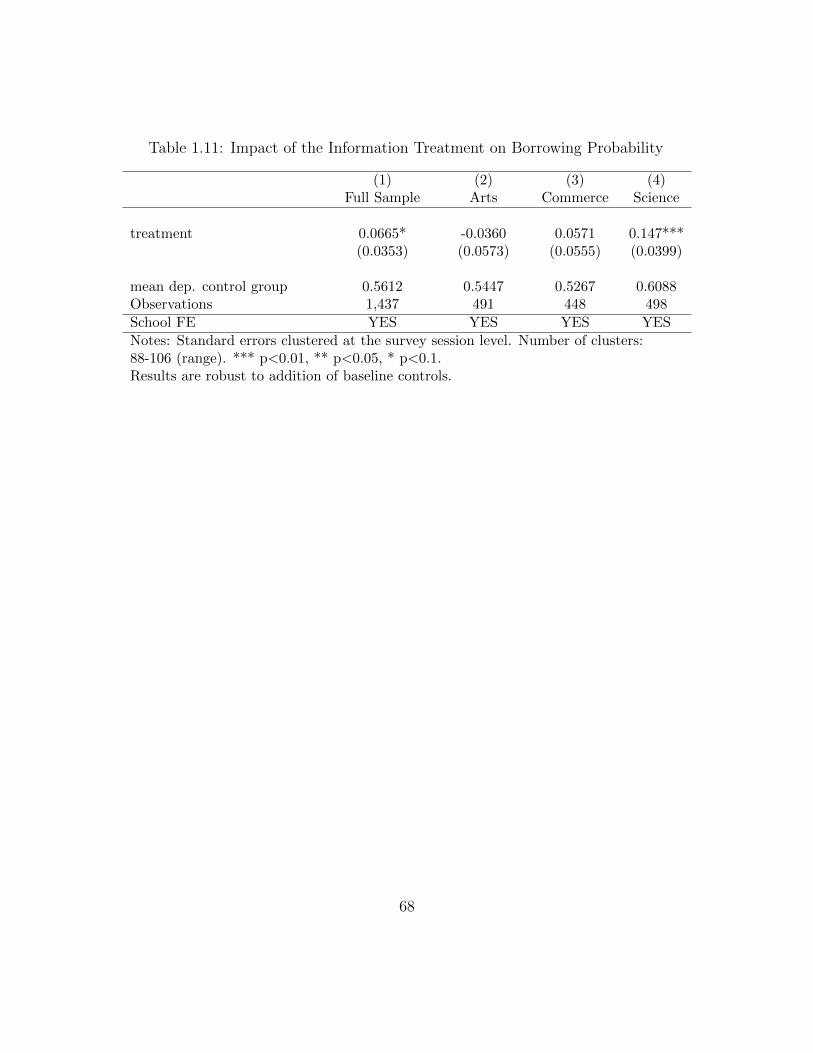
Table 1.11: Impact of the Information Treatment on Borrowing Probability

(1) (2) (3) (4)Full Sample Arts Commerce Science

treatment 0.0665* -0.0360 0.0571 0.147***(0.0353) (0.0573) (0.0555) (0.0399)

mean dep. control group 0.5612 0.5447 0.5267 0.6088Observations 1,437 491 448 498

School FE YES YES YES YES

Notes: Standard errors clustered at the survey session level. Number of clusters:88-106 (range). *** p<0.01, ** p<0.05, * p<0.1.Results are robust to addition of baseline controls.

68

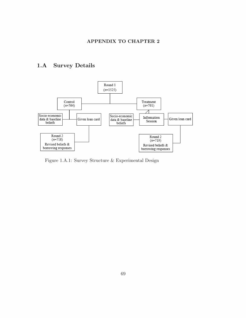
APPENDIX TO CHAPTER 2

1.A Survey Details

Figure 1.A.1: Survey Structure & Experimental Design

69

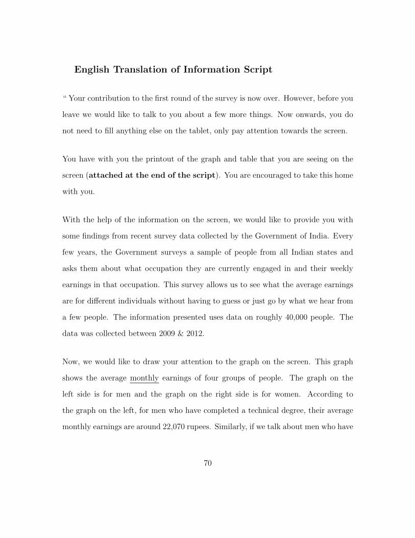
English Translation of Information Script

“ Your contribution to the first round of the survey is now over. However, before you

leave we would like to talk to you about a few more things. Now onwards, you do

not need to fill anything else on the tablet, only pay attention towards the screen.

You have with you the printout of the graph and table that you are seeing on the

screen (attached at the end of the script). You are encouraged to take this home

with you.

With the help of the information on the screen, we would like to provide you with

some findings from recent survey data collected by the Government of India. Every

few years, the Government surveys a sample of people from all Indian states and

asks them about what occupation they are currently engaged in and their weekly

earnings in that occupation. This survey allows us to see what the average earnings

are for different individuals without having to guess or just go by what we hear from

a few people. The information presented uses data on roughly 40,000 people. The

data was collected between 2009 & 2012.

Now, we would like to draw your attention to the graph on the screen. This graph

shows the average monthly earnings of four groups of people. The graph on the

left side is for men and the graph on the right side is for women. According to

the graph on the left, for men who have completed a technical degree, their average

monthly earnings are around 22,070 rupees. Similarly, if we talk about men who have

70

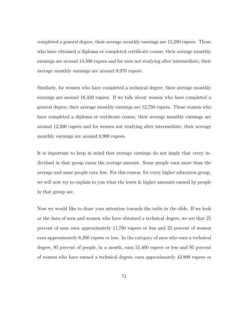
completed a general degree, their average monthly earnings are 15,280 rupees. Those

who have obtained a diploma or completed certificate course, their average monthly

earnings are around 14,500 rupees and for men not studying after intermediate, their

average monthly earnings are around 9,970 rupees.

Similarly, for women who have completed a technical degree, their average monthly

earnings are around 16,450 rupees. If we talk about women who have completed a

general degree, their average monthly earnings are 12,750 rupees. Those women who

have completed a diploma or certificate course, their average monthly earnings are

around 12,200 rupees and for women not studying after intermediate, their average

monthly earnings are around 8,900 rupees.

It is important to keep in mind that average earnings do not imply that every in-

dividual in that group earns the average amount. Some people earn more than the

average and some people earn less. For this reason, for every higher education group,

we will now try to explain to you what the lower & higher amounts earned by people

in that group are.

Now we would like to draw your attention towards the table in the slide. If we look

at the data of men and women who have obtained a technical degree, we see that 25

percent of men earn approximately 11,780 rupees or less and 25 percent of women

earn approximately 6,200 rupees or less. In the category of men who earn a technical

degree, 95 percent of people, in a month, earn 51,400 rupees or less and 95 percent

of women who have earned a technical degree, earn approximately 42,800 rupees or

71

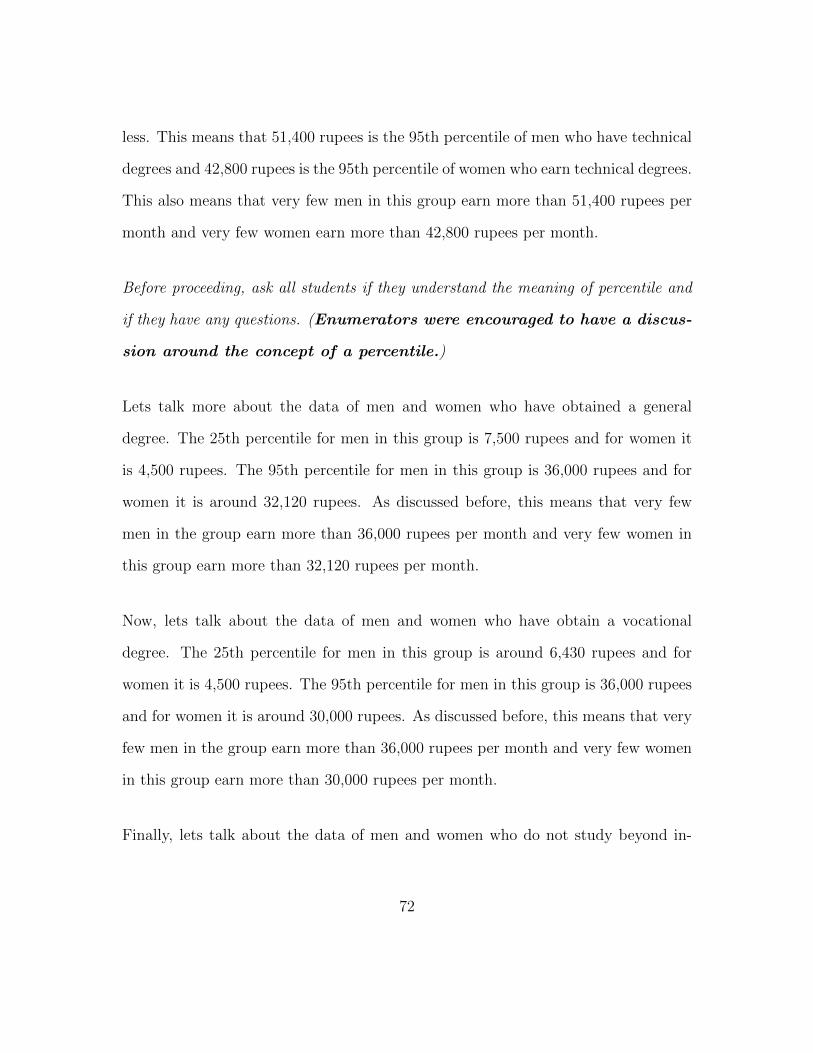
less. This means that 51,400 rupees is the 95th percentile of men who have technical

degrees and 42,800 rupees is the 95th percentile of women who earn technical degrees.

This also means that very few men in this group earn more than 51,400 rupees per

month and very few women earn more than 42,800 rupees per month.

Before proceeding, ask all students if they understand the meaning of percentile and

if they have any questions. (Enumerators were encouraged to have a discus-

sion around the concept of a percentile.)

Lets talk more about the data of men and women who have obtained a general

degree. The 25th percentile for men in this group is 7,500 rupees and for women it

is 4,500 rupees. The 95th percentile for men in this group is 36,000 rupees and for

women it is around 32,120 rupees. As discussed before, this means that very few

men in the group earn more than 36,000 rupees per month and very few women in

this group earn more than 32,120 rupees per month.

Now, lets talk about the data of men and women who have obtain a vocational

degree. The 25th percentile for men in this group is around 6,430 rupees and for

women it is 4,500 rupees. The 95th percentile for men in this group is 36,000 rupees

and for women it is around 30,000 rupees. As discussed before, this means that very

few men in the group earn more than 36,000 rupees per month and very few women

in this group earn more than 30,000 rupees per month.

Finally, lets talk about the data of men and women who do not study beyond in-

72

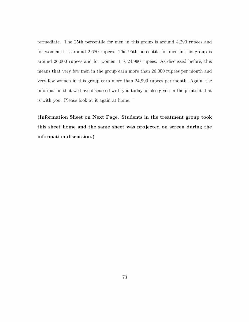
termediate. The 25th percentile for men in this group is around 4,290 rupees and

for women it is around 2,680 rupees. The 95th percentile for men in this group is

around 26,000 rupees and for women it is 24,990 rupees. As discussed before, this

means that very few men in the group earn more than 26,000 rupees per month and

very few women in this group earn more than 24,990 rupees per month. Again, the

information that we have discussed with you today, is also given in the printout that

is with you. Please look at it again at home. ”

(Information Sheet on Next Page. Students in the treatment group took

this sheet home and the same sheet was projected on screen during the

information discussion.)

73

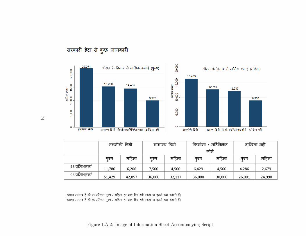
तकनीकी डिगरी सामानय डिगरी डिपलोमा / सरटिफिकट कोसि

दाखिला नह ी

परष मरहला परष मरहला परष मरहला परष मरहला 25 परततशतक1

11,786 6,206 7,500 4,500 6,429 4,500 4,286 2,679

95 परततशतक2 51,429 42,857 36,000 32,117 36,000 30,000 26,001 24,990

1 इसका मतलब ह की 25 परततशत परष / मरहला हर माह रदए गय रकम या इसस कम कमात ह|

2 इसका मतलब ह की 95 परततशत परष / मरहला हर माह रदए गय रकम या इसस कम कमात ह|

Figure 1.A.2: Image of Information Sheet Accompanying Script

74

English Translation of Loan Script

“We want to place in front of you, one other hypothetical situation, for you to think

at home about. Not all students are able to continue their studies after intermediate.

Often, their household income is not enough for them to continue their studies or for

them to enroll in a higher education program of their choice. In some such situations,

bank or non-bank institutions are able to offer higher education loans, at fair interest

rates, which you have to repay after completing your higher education.

Some of you must be wondering what is meant by the term interest rate. Suppose

you take a loan of 100 rupees on which there is a 10% interest rate. When repaying

this loan, you have to return 110 rupees. This additional 10 rupees that you pay is

your interest. Fair interest rate means a rate that is neither too low or neither too

high.

Please read out the questions on the loan card given to the students.

75

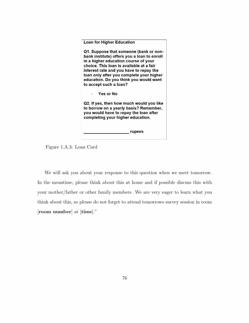
Figure 1.A.3: Loan Card

We will ask you about your response to this question when we meet tomorrow.

In the meantime, please think about this at home and if possible discuss this with

your mother/father or other family members. We are very eager to learn what you

think about this, so please do not forget to attend tomorrows survey session in room

[room number] at [time].”

76

1.B Balance of Baseline Variables & Correlates of Stream of

Study

Table 1.B.1: Balance of Baseline Variables

(1) (2) (3)Control Treatment p-value

Age 17.24 17.30 0.19% Male 0.53 0.55 0.45% Scheduled Tribe 0.33 0.34 0.70% Hindu 0.65 0.63 0.39Asset Index 7.52 7.82 0.10HH Facility Index 2.62 2.63 0.87% Own Land 0.74 0.69 0.04Board Exam Score 61.16 61.17 0.98% Grades Repeated 0.14 0.15 0.69% Father in Contact 0.91 0.92 0.48% Father High School 0.18 0.20 0.22% Father Family Business 0.11 0.14 0.11% Father Salaried Job 0.21 0.21 0.88% Mother High School 0.08 0.09 0.91% Mother Housewife 0.60 0.61 0.51Average Older Sibling Edu. 5.27 5.20 0.45Enroll Probability (Tech) 36.96 35.27 0.24Enroll Probability (Gen) 32.89 32.05 0.47Enroll Probability (Voc) 22.50 24.16 0.15Enroll Probability (NA) 7.65 8.53 0.23% Arts Stream 0.34 0.34 0.84% Commerce Stream 0.31 0.31 0.99% Science Stream 0.35 0.35 0.86

Columns (1) and (2) show sample meansColumn (3) shows p-values of OLS regressions on a treatment group dummy.

77

Table 1.B.2: Balance of Baseline Variables by Stream

Arts Commerce Science

(1) (2) (3) (4) (5) (6) (7) (8) (9)Control Treatment p-value Control Treatment p-value Control Treatment p-value

Age 17.41 17.35 0.60 17.20 17.42 0.02 17.09 17.16 0.43% Male 0.48 0.42 0.19 0.48 0.53 0.29 0.63 0.70 0.11% Scheduled Tribe 0.42 0.47 0.21 0.34 0.26 0.07 0.22 0.27 0.25% Hindu 0.56 0.47 0.05 0.63 0.65 0.66 0.75 0.75 0.96Asset Index 6.40 6.37 0.94 7.75 8.34 0.09 8.43 8.76 0.24HH Facility Index 2.14 2.04 0.52 2.64 2.87 0.19 3.06 2.99 0.66% Own Land 0.74 0.73 0.74 0.66 0.58 0.07 0.79 0.75 0.20Board Exam Score 55.74 56.09 0.69 60.77 60.41 0.72 66.82 66.70 0.91% Grades Repeated 0.18 0.19 0.74 0.14 0.15 0.88 0.10 0.11 0.80% Father in Contact 0.87 0.90 0.24 0.91 0.93 0.40 0.95 0.93 0.30% Father High School 0.13 0.18 0.22 0.18 0.18 0.34 0.23 0.22 0.89% Father Family Business 0.09 0.10 0.79 0.12 0.18 0.09 0.13 0.15 0.47% Father Salaried Job 0.16 0.16 0.99 0.23 0.21 0.52 0.24 0.27 0.43% Mother High School 0.04 0.05 0.62 0.05 0.09 0.11 0.16 0.12 0.22% Mother Housewife 0.52 0.51 0.93 0.63 0.67 0.37 0.65 0.66 0.76Average Older Sibling Edu. 4.88 4.75 0.49 5.23 5.08 0.43 5.75 5.80 0.77Enroll Probability (Tech) 29.75 26.30 0.11 33.95 33.56 0.98 46.67 45.31 0.53Enroll Probability (Gen) 33.85 34.46 0.77 39.72 37.70 0.34 25.93 24.83 0.58Enroll Probability (Voc) 25.78 26.96 0.58 19.70 20.26 0.79 21.76 24.88 0.10Enroll Probability (NA) 10.62 12.28 0.31 6.63 8.48 0.12 5.64 4.98 0.47

Notes: p-values are from OLS regressions on a treatment group dummy.

78

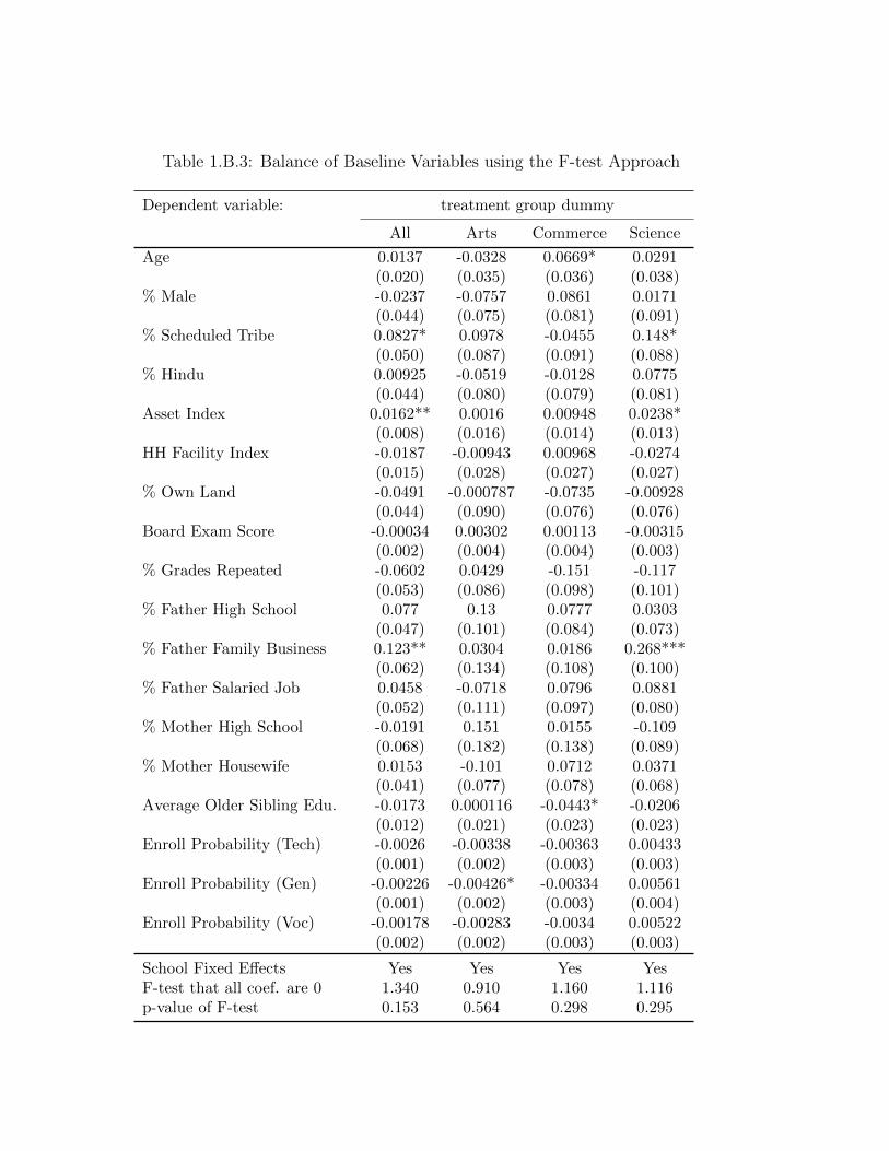
Table 1.B.3: Balance of Baseline Variables using the F-test Approach

Dependent variable: treatment group dummy

All Arts Commerce Science

Age 0.0137 -0.0328 0.0669* 0.0291(0.020) (0.035) (0.036) (0.038)

% Male -0.0237 -0.0757 0.0861 0.0171(0.044) (0.075) (0.081) (0.091)

% Scheduled Tribe 0.0827* 0.0978 -0.0455 0.148*(0.050) (0.087) (0.091) (0.088)

% Hindu 0.00925 -0.0519 -0.0128 0.0775(0.044) (0.080) (0.079) (0.081)

Asset Index 0.0162** 0.0016 0.00948 0.0238*(0.008) (0.016) (0.014) (0.013)

HH Facility Index -0.0187 -0.00943 0.00968 -0.0274(0.015) (0.028) (0.027) (0.027)

% Own Land -0.0491 -0.000787 -0.0735 -0.00928(0.044) (0.090) (0.076) (0.076)

Board Exam Score -0.00034 0.00302 0.00113 -0.00315(0.002) (0.004) (0.004) (0.003)

% Grades Repeated -0.0602 0.0429 -0.151 -0.117(0.053) (0.086) (0.098) (0.101)

% Father High School 0.077 0.13 0.0777 0.0303(0.047) (0.101) (0.084) (0.073)

% Father Family Business 0.123** 0.0304 0.0186 0.268***(0.062) (0.134) (0.108) (0.100)

% Father Salaried Job 0.0458 -0.0718 0.0796 0.0881(0.052) (0.111) (0.097) (0.080)

% Mother High School -0.0191 0.151 0.0155 -0.109(0.068) (0.182) (0.138) (0.089)

% Mother Housewife 0.0153 -0.101 0.0712 0.0371(0.041) (0.077) (0.078) (0.068)

Average Older Sibling Edu. -0.0173 0.000116 -0.0443* -0.0206(0.012) (0.021) (0.023) (0.023)

Enroll Probability (Tech) -0.0026 -0.00338 -0.00363 0.00433(0.001) (0.002) (0.003) (0.003)

Enroll Probability (Gen) -0.00226 -0.00426* -0.00334 0.00561(0.001) (0.002) (0.003) (0.004)

Enroll Probability (Voc) -0.00178 -0.00283 -0.0034 0.00522(0.002) (0.002) (0.003) (0.003)

School Fixed Effects Yes Yes Yes YesF-test that all coef. are 0 1.340 0.910 1.160 1.116p-value of F-test 0.153 0.564 0.298 0.295

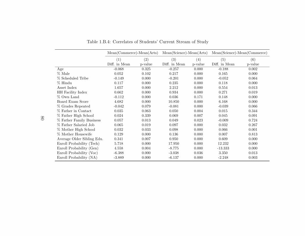
Table 1.B.4: Correlates of Students’ Current Stream of Study

Mean(Commerce)-Mean(Arts) Mean(Science)-Mean(Arts) Mean(Science)-Mean(Commerce)

(1) (2) (3) (4) (5) (6)Diff. in Mean p-value Diff. in Mean p-value Diff. in Mean p-value

Age -0.068 0.325 -0.257 0.000 -0.188 0.002% Male 0.052 0.102 0.217 0.000 0.165 0.000% Scheduled Tribe -0.149 0.000 -0.201 0.000 -0.052 0.064% Hindu 0.117 0.000 0.235 0.000 0.118 0.000Asset Index 1.657 0.000 2.212 0.000 0.554 0.013HH Facility Index 0.662 0.000 0.934 0.000 0.271 0.019% Own Land -0.112 0.000 0.036 0.171 0.148 0.000Board Exam Score 4.682 0.000 10.850 0.000 6.168 0.000% Grades Repeated -0.042 0.079 -0.081 0.000 -0.039 0.066% Father in Contact 0.035 0.063 0.050 0.004 0.015 0.344% Father High School 0.024 0.339 0.069 0.007 0.045 0.091% Father Family Business 0.057 0.013 0.049 0.023 -0.009 0.724% Father Salaried Job 0.065 0.019 0.097 0.000 0.032 0.267% Mother High School 0.032 0.033 0.098 0.000 0.066 0.001% Mother Housewife 0.129 0.000 0.136 0.000 0.007 0.813Average Older Sibling Edu. 0.341 0.007 0.950 0.000 0.609 0.000Enroll Probability (Tech) 5.718 0.000 17.950 0.000 12.232 0.000Enroll Probability (Gen) 4.558 0.004 -8.775 0.000 -13.333 0.000Enroll Probability (Voc) -6.388 0.000 -3.038 0.036 3.350 0.013Enroll Probability (NA) -3.889 0.000 -6.137 0.000 -2.248 0.003

80

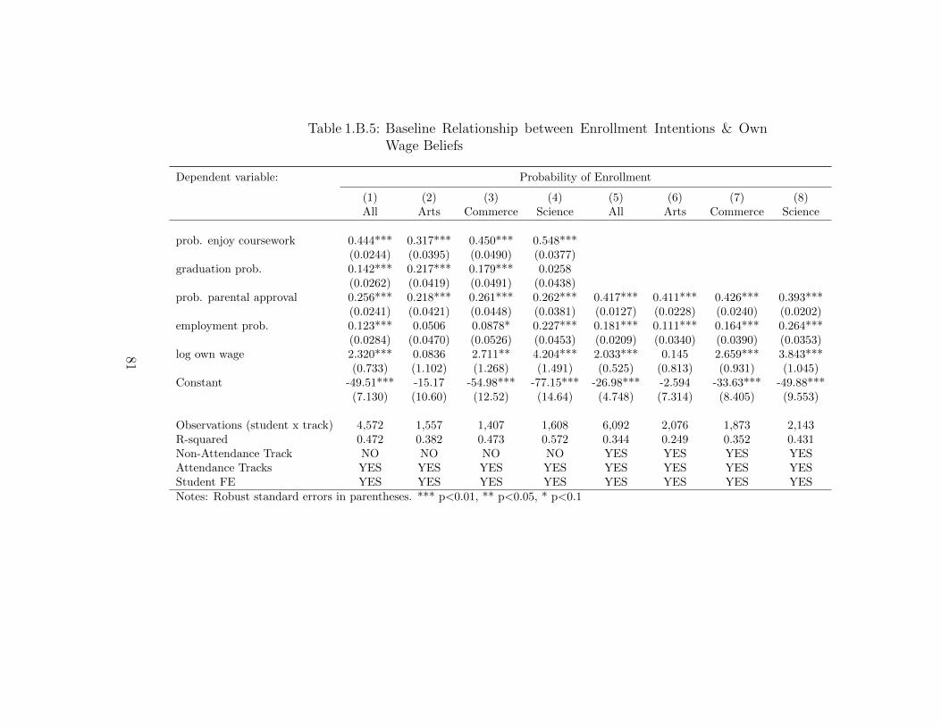
Table 1.B.5: Baseline Relationship between Enrollment Intentions & OwnWage Beliefs

Dependent variable: Probability of Enrollment

(1) (2) (3) (4) (5) (6) (7) (8)All Arts Commerce Science All Arts Commerce Science

prob. enjoy coursework 0.444*** 0.317*** 0.450*** 0.548***(0.0244) (0.0395) (0.0490) (0.0377)

graduation prob. 0.142*** 0.217*** 0.179*** 0.0258(0.0262) (0.0419) (0.0491) (0.0438)

prob. parental approval 0.256*** 0.218*** 0.261*** 0.262*** 0.417*** 0.411*** 0.426*** 0.393***(0.0241) (0.0421) (0.0448) (0.0381) (0.0127) (0.0228) (0.0240) (0.0202)

employment prob. 0.123*** 0.0506 0.0878* 0.227*** 0.181*** 0.111*** 0.164*** 0.264***(0.0284) (0.0470) (0.0526) (0.0453) (0.0209) (0.0340) (0.0390) (0.0353)

log own wage 2.320*** 0.0836 2.711** 4.204*** 2.033*** 0.145 2.659*** 3.843***(0.733) (1.102) (1.268) (1.491) (0.525) (0.813) (0.931) (1.045)

Constant -49.51*** -15.17 -54.98*** -77.15*** -26.98*** -2.594 -33.63*** -49.88***(7.130) (10.60) (12.52) (14.64) (4.748) (7.314) (8.405) (9.553)

Observations (student x track) 4,572 1,557 1,407 1,608 6,092 2,076 1,873 2,143R-squared 0.472 0.382 0.473 0.572 0.344 0.249 0.352 0.431Non-Attendance Track NO NO NO NO YES YES YES YESAttendance Tracks YES YES YES YES YES YES YES YESStudent FE YES YES YES YES YES YES YES YES

Notes: Robust standard errors in parentheses. *** p<0.01, ** p<0.05, * p<0.1

81

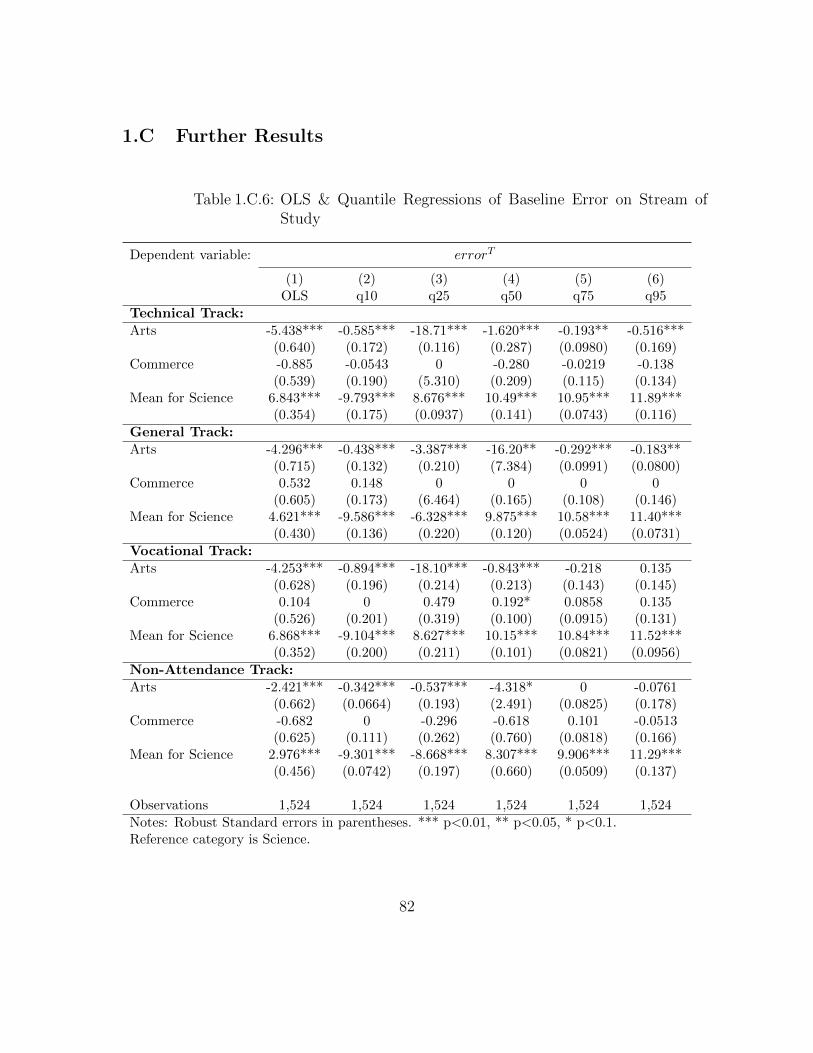
1.C Further Results

Table 1.C.6: OLS & Quantile Regressions of Baseline Error on Stream ofStudy

Dependent variable: errorT

(1) (2) (3) (4) (5) (6)OLS q10 q25 q50 q75 q95

Technical Track:

Arts -5.438*** -0.585*** -18.71*** -1.620*** -0.193** -0.516***(0.640) (0.172) (0.116) (0.287) (0.0980) (0.169)

Commerce -0.885 -0.0543 0 -0.280 -0.0219 -0.138(0.539) (0.190) (5.310) (0.209) (0.115) (0.134)

Mean for Science 6.843*** -9.793*** 8.676*** 10.49*** 10.95*** 11.89***(0.354) (0.175) (0.0937) (0.141) (0.0743) (0.116)

General Track:

Arts -4.296*** -0.438*** -3.387*** -16.20** -0.292*** -0.183**(0.715) (0.132) (0.210) (7.384) (0.0991) (0.0800)

Commerce 0.532 0.148 0 0 0 0(0.605) (0.173) (6.464) (0.165) (0.108) (0.146)

Mean for Science 4.621*** -9.586*** -6.328*** 9.875*** 10.58*** 11.40***(0.430) (0.136) (0.220) (0.120) (0.0524) (0.0731)

Vocational Track:

Arts -4.253*** -0.894*** -18.10*** -0.843*** -0.218 0.135(0.628) (0.196) (0.214) (0.213) (0.143) (0.145)

Commerce 0.104 0 0.479 0.192* 0.0858 0.135(0.526) (0.201) (0.319) (0.100) (0.0915) (0.131)

Mean for Science 6.868*** -9.104*** 8.627*** 10.15*** 10.84*** 11.52***(0.352) (0.200) (0.211) (0.101) (0.0821) (0.0956)

Non-Attendance Track:

Arts -2.421*** -0.342*** -0.537*** -4.318* 0 -0.0761(0.662) (0.0664) (0.193) (2.491) (0.0825) (0.178)

Commerce -0.682 0 -0.296 -0.618 0.101 -0.0513(0.625) (0.111) (0.262) (0.760) (0.0818) (0.166)

Mean for Science 2.976*** -9.301*** -8.668*** 8.307*** 9.906*** 11.29***(0.456) (0.0742) (0.197) (0.660) (0.0509) (0.137)

Observations 1,524 1,524 1,524 1,524 1,524 1,524

Notes: Robust Standard errors in parentheses. *** p<0.01, ** p<0.05, * p<0.1.Reference category is Science.

82

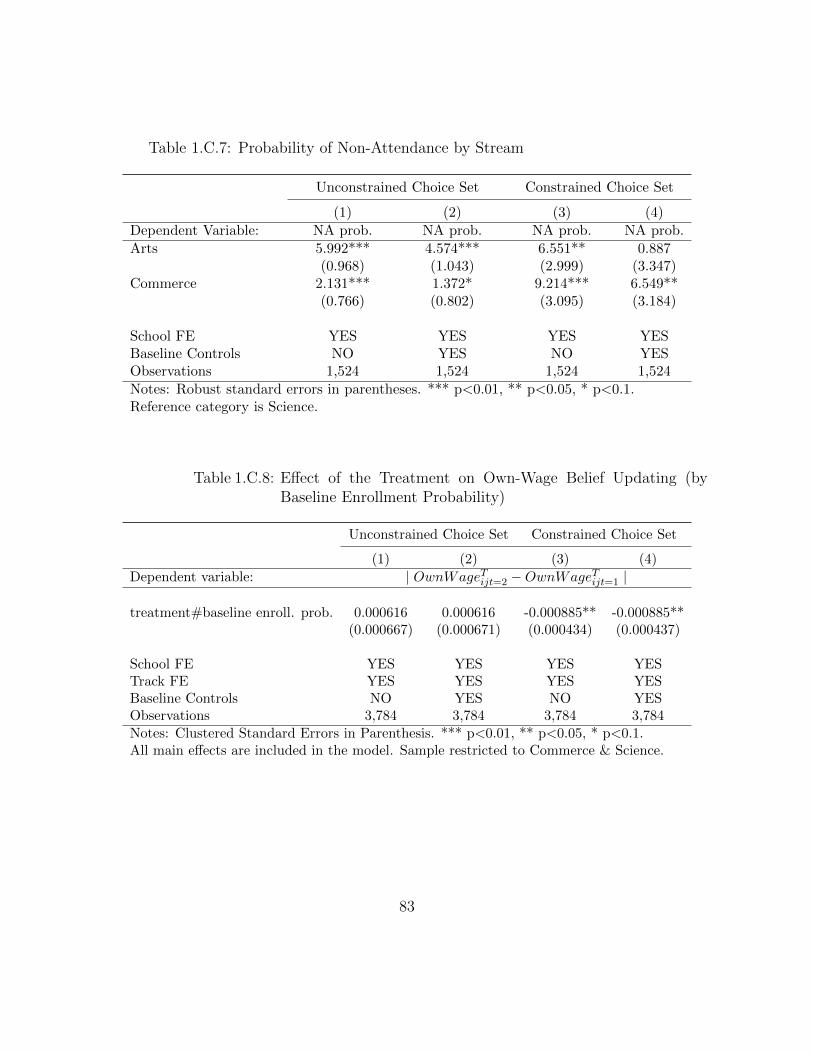
Table 1.C.7: Probability of Non-Attendance by Stream

Unconstrained Choice Set Constrained Choice Set

(1) (2) (3) (4)

Dependent Variable: NA prob. NA prob. NA prob. NA prob.

Arts 5.992*** 4.574*** 6.551** 0.887(0.968) (1.043) (2.999) (3.347)

Commerce 2.131*** 1.372* 9.214*** 6.549**(0.766) (0.802) (3.095) (3.184)

School FE YES YES YES YESBaseline Controls NO YES NO YESObservations 1,524 1,524 1,524 1,524

Notes: Robust standard errors in parentheses. *** p<0.01, ** p<0.05, * p<0.1.Reference category is Science.

Table 1.C.8: Effect of the Treatment on Own-Wage Belief Updating (byBaseline Enrollment Probability)

Unconstrained Choice Set Constrained Choice Set

(1) (2) (3) (4)

Dependent variable: | OwnWageTijt=2 −OwnWageTijt=1 |

treatment#baseline enroll. prob. 0.000616 0.000616 -0.000885** -0.000885**(0.000667) (0.000671) (0.000434) (0.000437)

School FE YES YES YES YESTrack FE YES YES YES YESBaseline Controls NO YES NO YESObservations 3,784 3,784 3,784 3,784

Notes: Clustered Standard Errors in Parenthesis. *** p<0.01, ** p<0.05, * p<0.1.All main effects are included in the model. Sample restricted to Commerce & Science.

83

CHAPTER 2

DO STUDENTS OVERESTIMATE POST-SECONDARY

EDUCATION EXPENSES? INSIGHTS FROM SUBJECTIVE &

MEASURED INDIAN DATA

2.1 Introduction

An increasing amount of recent economics literature is interested in analyzing beliefs

about the benefits and costs of education, that students’ subjectively perceive, prior

to the point of making a critical investment in human capital. One use of eliciting

such subjective beliefs is to estimate standard education choice models, wherein in-

dividuals decide on entering a given level of education by weighing benefits against

costs1, using subjective expectations data rather than actual choice data (Manski

(2004), Wiswall and Zafar (2015), Delavande and Zafar (2014)). Here, the use of

subjective expectations, on all alternatives in an individuals’ choice-set, helps cir-

cumvent assumptions about expectation formation and does not assume a mapping

between revealed elements of education utility to beliefs about these elements at

the time the decision was made. Another point of interest in data about subjective

beliefs, which is perhaps more directly amenable to policy intervention, is analyzing

the accuracy of beliefs. Given that individuals’ subjective beliefs are conditioned on

their information sets, imperfect information about some aspect of the benefit or cost

of education is seen as a barrier to education access (Jensen (2010), Oreopoulos and

1See Willis and Rosen (1979) & Altonji (1993) for more traditional approaches using revealedpreference data.

84

Dunn (2013) Dinkelman and Martınez (2014), Hastings, Neilson and Zimmerman

(2015)).

The accuracy of students’ beliefs about the costs associated with post-secondary ed-

ucation is of primary interest in this paper. The recent literature on analyzing the

accuracy of subjective beliefs regarding education is concentrated more heavily on

the side of studying beliefs about the subjective benefits of education, more specifi-

cally, expected labor market benefits. This includes earlier inquiries by Betts (1996),

and more recent experimental investigations that examine changes in education in-

vestments upon randomizing information on population earnings (Nguyen (2008),

Jensen (2010), Fryer Jr (2013), Loyalka et al. (2013), Oreopoulos and Dunn (2013),

Pekkala Kerr et al. (2015)). The literature on the accuracy about beliefs regarding

other elements of an individual’s education utility function, including beliefs about

costs, is relatively scarce2.

In this paper I combine two datasets to draw insights about the extent and im-

plications of overestimating post-secondary expenses. The first is a self-collected

dataset on high school students’ beliefs regarding post-secondary expenses, condi-

tional on track, elicited 5-9 months before students make an actual decision about

post-secondary enrollment. This data was collected from students studying in schools

located in the east Indian state of Jharkhand. The second is a nationally representa-

2Some research indicates the importance of providing information about financial aid opportu-nities and eligibility for financial aid (Dinkelman and Martınez (2014)) as well as simplifying theprocess of applying for aid in the U.S. (Bettinger et al. (2009)) in reducing high-school absenteeismand increasing college-enrollment, respectively.

85

tive dataset on post-secondary expenses incurred by students studying in the same

tracks. Fortuitously, both datasets were collected during the same year. I use the

nationally representative dataset on measured expenses as a reference distribution

to determine the accuracy of students’ cost beliefs. Naive comparisons indicate that

students’ perceived costs are considerably higher than measured costs, especially

for general academic degrees, which are substantially cheaper than the other two

tracks–technical and vocational. However, comparing every individual’s perceived

costs to an overall distribution of measured expenses disregards the possibility that

some people may rationally expect costs to be lower or higher for them, given their

personal characteristics. To address this, I assign to every individual a measured

cost, from the nationally representative data, of a person most similar in “type to

them, using a set of SES characteristics that overlap both datasets. Using naive and

person-specific predictions of measured costs, for every individual, along with their

cost perceptions and budget for education expenses, I describe the implications of

students’ cost beliefs in determining their perceived affordability for each type of

post-secondary education. Given that students may acquire more information about

tracks most preferred by them, I also estimate a flexible model of track-choice to

estimate each student’s utility maximizing track. With this, I draw implications

of students’ errors regarding post-secondary costs, in determining their perceived

affordability, for their most preferred or utility maximizing track.

This paper uniquely combines three pieces of subjective beliefs data–students’ be-

liefs regarding the cost of education, students’ beliefs about their capacity to pay

86

for this type of education and students’ beliefs about out of pocket expenses net of

scholarships/stipends. This helps us draw insights that add to the limited literature

analyzing subjective cost beliefs. Two papers are of notable interest here. Bleemer

and Zafar (2015) randomize information about the average annual net cost of at-

tending a 4-year public university and that of a 4 year nonprofit private university,

in 2014, in the United States. They find that, on average, U.S. household heads

overestimate the costs associated with public colleges and revise beliefs about their

child’s college costs as a result of the cost information, but do not revise expecta-

tions regarding college enrollment. The paper cannot comment on misperceptions

regarding cost beliefs relative to household’s budget and ability to pay for college,

which might be one reason for why the authors do not see an increase in expected

college enrollment. Hastings et al. (2015) provide descriptive insights on the link

between overestimation of college costs and matriculation in a degree program in

Chile3. They show that those who overestimate costs by at least 25% are 5.5 per-

centage points less likely to matriculate in a degree program, as compared to those

who perceive costs accurately. However, because they cannot rule out that other

determinants of matriculation may be correlated with cost overestimates, it is not

clear whether students who did not matriculate did so because they believed that

college was unaffordable or because those who overestimated costs were also limited

in their ability to matriculate in other ways. While the approach adopted in this

paper is also descriptive, it addresses more directly the link between overestimation

3Hastings, Neilson and Zimmerman (2015) also have an experimental paper, a companion tothe descriptive piece, which randomizes information on earnings and costs together, and does notaddress imperfect information about costs separately.

87

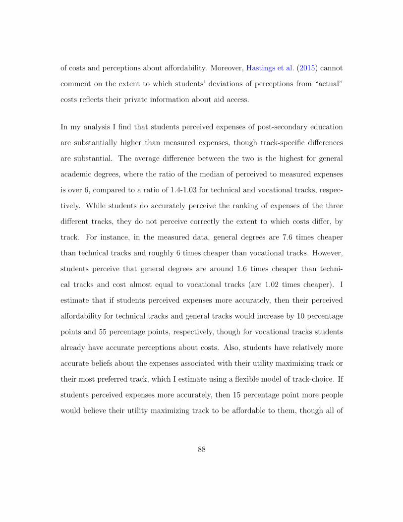
of costs and perceptions about affordability. Moreover, Hastings et al. (2015) cannot

comment on the extent to which students’ deviations of perceptions from “actual”

costs reflects their private information about aid access.

In my analysis I find that students perceived expenses of post-secondary education

are substantially higher than measured expenses, though track-specific differences

are substantial. The average difference between the two is the highest for general

academic degrees, where the ratio of the median of perceived to measured expenses

is over 6, compared to a ratio of 1.4-1.03 for technical and vocational tracks, respec-

tively. While students do accurately perceive the ranking of expenses of the three

different tracks, they do not perceive correctly the extent to which costs differ, by

track. For instance, in the measured data, general degrees are 7.6 times cheaper

than technical tracks and roughly 6 times cheaper than vocational tracks. However,

students perceive that general degrees are around 1.6 times cheaper than techni-

cal tracks and cost almost equal to vocational tracks (are 1.02 times cheaper). I

estimate that if students perceived expenses more accurately, then their perceived

affordability for technical tracks and general tracks would increase by 10 percentage

points and 55 percentage points, respectively, though for vocational tracks students

already have accurate perceptions about costs. Also, students have relatively more

accurate beliefs about the expenses associated with their utility maximizing track or

their most preferred track, which I estimate using a flexible model of track-choice. If

students perceived expenses more accurately, then 15 percentage point more people

would believe their utility maximizing track to be affordable to them, though all of

88

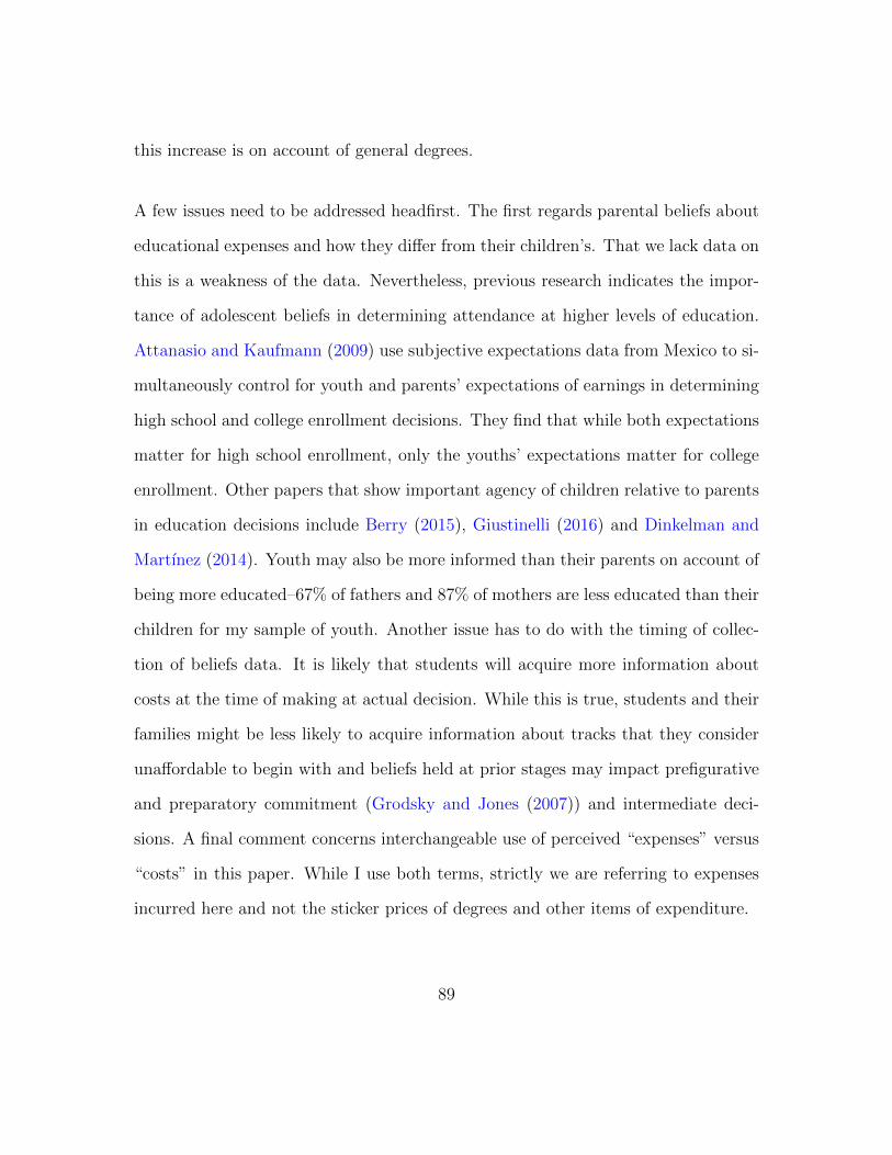
this increase is on account of general degrees.

A few issues need to be addressed headfirst. The first regards parental beliefs about

educational expenses and how they differ from their children’s. That we lack data on

this is a weakness of the data. Nevertheless, previous research indicates the impor-

tance of adolescent beliefs in determining attendance at higher levels of education.

Attanasio and Kaufmann (2009) use subjective expectations data from Mexico to si-

multaneously control for youth and parents’ expectations of earnings in determining

high school and college enrollment decisions. They find that while both expectations

matter for high school enrollment, only the youths’ expectations matter for college

enrollment. Other papers that show important agency of children relative to parents

in education decisions include Berry (2015), Giustinelli (2016) and Dinkelman and

Martınez (2014). Youth may also be more informed than their parents on account of

being more educated–67% of fathers and 87% of mothers are less educated than their

children for my sample of youth. Another issue has to do with the timing of collec-

tion of beliefs data. It is likely that students will acquire more information about

costs at the time of making at actual decision. While this is true, students and their

families might be less likely to acquire information about tracks that they consider

unaffordable to begin with and beliefs held at prior stages may impact prefigurative

and preparatory commitment (Grodsky and Jones (2007)) and intermediate deci-

sions. A final comment concerns interchangeable use of perceived “expenses” versus

“costs” in this paper. While I use both terms, strictly we are referring to expenses

incurred here and not the sticker prices of degrees and other items of expenditure.

89

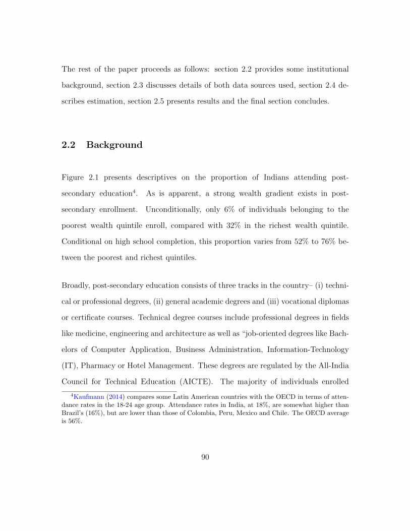
The rest of the paper proceeds as follows: section 2.2 provides some institutional

background, section 2.3 discusses details of both data sources used, section 2.4 de-

scribes estimation, section 2.5 presents results and the final section concludes.

2.2 Background

Figure 2.1 presents descriptives on the proportion of Indians attending post-

secondary education4. As is apparent, a strong wealth gradient exists in post-

secondary enrollment. Unconditionally, only 6% of individuals belonging to the

poorest wealth quintile enroll, compared with 32% in the richest wealth quintile.

Conditional on high school completion, this proportion varies from 52% to 76% be-

tween the poorest and richest quintiles.

Broadly, post-secondary education consists of three tracks in the country– (i) techni-

cal or professional degrees, (ii) general academic degrees and (iii) vocational diplomas

or certificate courses. Technical degree courses include professional degrees in fields

like medicine, engineering and architecture as well as “job-oriented degrees like Bach-

elors of Computer Application, Business Administration, Information-Technology

(IT), Pharmacy or Hotel Management. These degrees are regulated by the All-India

Council for Technical Education (AICTE). The majority of individuals enrolled

4Kaufmann (2014) compares some Latin American countries with the OECD in terms of atten-dance rates in the 18-24 age group. Attendance rates in India, at 18%, are somewhat higher thanBrazil’s (16%), but are lower than those of Colombia, Peru, Mexico and Chile. The OECD averageis 56%.

90

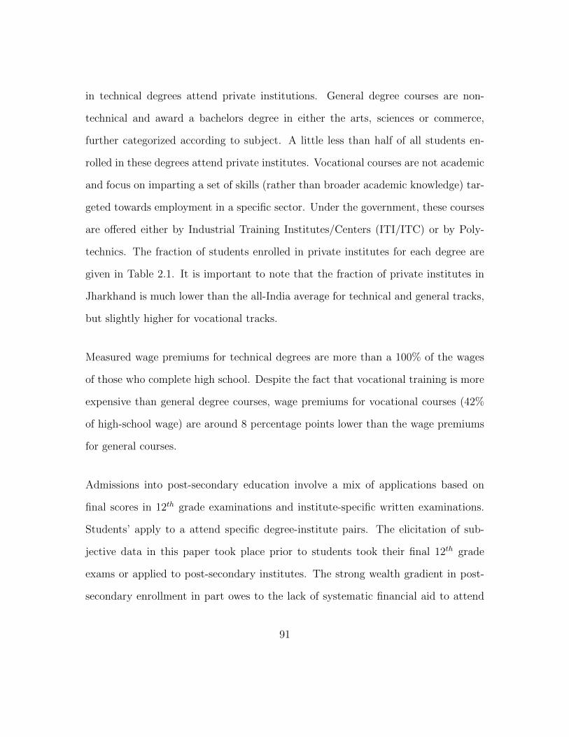
in technical degrees attend private institutions. General degree courses are non-

technical and award a bachelors degree in either the arts, sciences or commerce,

further categorized according to subject. A little less than half of all students en-

rolled in these degrees attend private institutes. Vocational courses are not academic

and focus on imparting a set of skills (rather than broader academic knowledge) tar-

geted towards employment in a specific sector. Under the government, these courses

are offered either by Industrial Training Institutes/Centers (ITI/ITC) or by Poly-

technics. The fraction of students enrolled in private institutes for each degree are

given in Table 2.1. It is important to note that the fraction of private institutes in

Jharkhand is much lower than the all-India average for technical and general tracks,

but slightly higher for vocational tracks.

Measured wage premiums for technical degrees are more than a 100% of the wages

of those who complete high school. Despite the fact that vocational training is more

expensive than general degree courses, wage premiums for vocational courses (42%

of high-school wage) are around 8 percentage points lower than the wage premiums

for general courses.

Admissions into post-secondary education involve a mix of applications based on

final scores in 12th grade examinations and institute-specific written examinations.

Students’ apply to a attend specific degree-institute pairs. The elicitation of sub-

jective data in this paper took place prior to students took their final 12th grade

exams or applied to post-secondary institutes. The strong wealth gradient in post-

secondary enrollment in part owes to the lack of systematic financial aid to attend

91

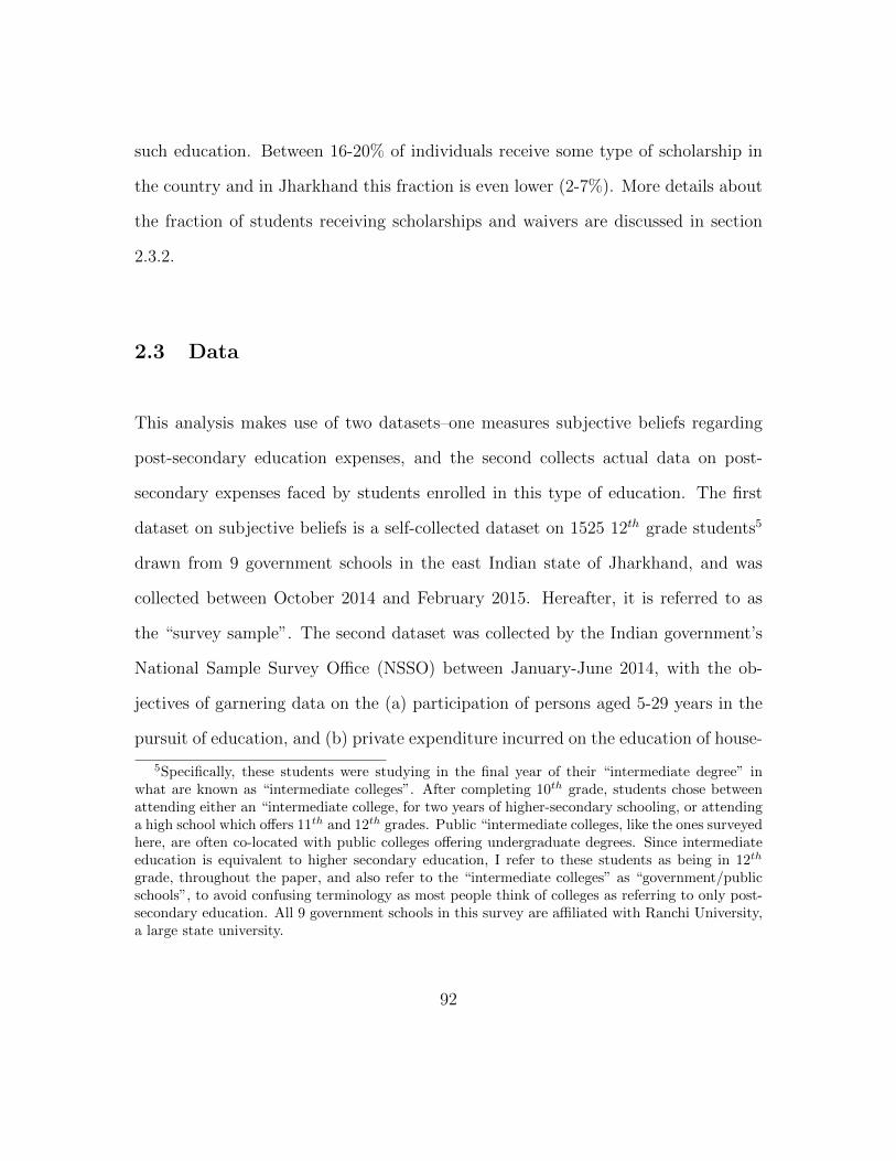
such education. Between 16-20% of individuals receive some type of scholarship in

the country and in Jharkhand this fraction is even lower (2-7%). More details about

the fraction of students receiving scholarships and waivers are discussed in section

2.3.2.

2.3 Data

This analysis makes use of two datasets–one measures subjective beliefs regarding

post-secondary education expenses, and the second collects actual data on post-

secondary expenses faced by students enrolled in this type of education. The first

dataset on subjective beliefs is a self-collected dataset on 1525 12th grade students5

drawn from 9 government schools in the east Indian state of Jharkhand, and was

collected between October 2014 and February 2015. Hereafter, it is referred to as

the “survey sample”. The second dataset was collected by the Indian government’s

National Sample Survey Office (NSSO) between January-June 2014, with the ob-

jectives of garnering data on the (a) participation of persons aged 5-29 years in the

pursuit of education, and (b) private expenditure incurred on the education of house-

5Specifically, these students were studying in the final year of their “intermediate degree” inwhat are known as “intermediate colleges”. After completing 10th grade, students chose betweenattending either an “intermediate college, for two years of higher-secondary schooling, or attendinga high school which offers 11th and 12th grades. Public “intermediate colleges, like the ones surveyedhere, are often co-located with public colleges offering undergraduate degrees. Since intermediateeducation is equivalent to higher secondary education, I refer to these students as being in 12th

grade, throughout the paper, and also refer to the “intermediate colleges” as “government/publicschools”, to avoid confusing terminology as most people think of colleges as referring to only post-secondary education. All 9 government schools in this survey are affiliated with Ranchi University,a large state university.

92

hold members. This NSSO dataset is also referred to as the 71st NSS round, here

we simply refer to it as the “NSS dataset”. The close overlap in the timing of the

collection of the two datasets is fortuitous–nationally representative data on educa-

tion expenses is rarely collected in the country (it was last collected a decade ago in

2007-08) and more regularly collected datasets on overall consumption expenditures,

would be unsuitable for the current analysis. Firstly, they do not contain detailed

measures of education expenses and, secondly, they do not follow a sampling frame

that yields sufficient observations on post-secondary students in the country.

2.3.1 The Survey Sample

The first dataset, the survey sample, was collected with the explicit intention of ex-

amining in detail subjective beliefs regarding post-secondary education, of 12th grade

students, 5-9 months (depending on survey date) before graduating from high-school

and making an actual decision regarding enrollment in post-secondary education. A

total of nine schools participated in the survey. Four of the nine schools are situ-

ated in the capital city of Ranchi, one in a rural block of Ranchi district and four

others are in surrounding rural districts. We drew, approximately, an equal number

of students from each school. Further, within each school, students were randomly

assigned to survey-sessions of 15 students each. An information experiment was em-

bedded in the survey, with survey-sessions being assigned to either a control session

or a treatment session. However, the current analysis, makes use only of the baseline

93

data, which was collected identically across both groups. Details of the experiment

are in a separate paper, here we focus on baseline variables most relevant to the

current analysis.

The baseline survey consisted of two main modules- the first module was focused on

collecting socio-economic details of the students and the second was focused on belief

elicitation about different aspects of post-secondary education. Among the socio-

economic variables, we collected data on student gender, caste, religion, a household

assets and facilities module, parental education and occupation, older sibling gen-

der and education, scores on previous centralized board examinations and history of

grade repetition. In the second part, belief elicitation was contingent on each post-

secondary alternative i.e. technical/professional degrees, general degrees, vocational

diplomas/certificate courses and the fourth alternative of not attending further edu-

cation after 12th grade. The three post-secondary education tracks were constructed

to maintain consistency with classifications maintained by National Sample Survey

Office. Nevertheless, for elicitation purposes, the categories are broad and encompass

a variety of courses of study. Therefore, data collection was preceded by a detailed

explanation of possible courses/degrees that are part of every category. Since a ma-

jority of the beliefs questions were either probabilistic in nature or required students

to express responses on a scale of 0-100, the baseline beliefs module was also preceded

by a discussion (with examples) on answering probabilistic questions.6

6We ensured that answers to all probabilistic questions sum to 100 by placing the total asa constraint in the questionnaire, without fulfilling which, the survey would not proceed to thesubsequent question.

94

In the baseline beliefs module, stated probabilities of enrollment were elicited by

specifying all three post-secondary alternatives as being in all individuals’ feasible

choice-set.7 Next, individuals were asked about certain non-pecuniary and pecu-

niary beliefs conditional on hypothetical enrollment in each alternative. Pecuniary

beliefs included data on expected probability of employment and expected average

monthly earnings at age 30.8 Non-pecuniary beliefs included questions regarding

likelihood of enjoyment of coursework (0-100 scale), likelihood of parental approval

of education track (0-100 scale) and likelihood of being able to pass (graduate from)

the course/degree (0-100 scale). I use this data to estimate each individual’s utility

maximizing track, as described in section 2.4.1.

Finally, the two most important survey questions from the point of view of this

analysis concern the elicitation of beliefs regarding post-secondary expenses and be-

liefs regarding students’ budgets for post-secondary study. The elicitation of beliefs

regarding expected post-secondary expenses, by track, stressed that students must

express beliefs about yearly out-of-pocket expenses, including course fee and other

miscellaneous costs. The exact wording was:

7The exact wording of the question used to elicit enrollment probabilities for potentially hypo-thetically choice sets of individuals was: “Think ahead to next year when you have completed (sic)intermediate. Imagine that you have passed your (sic) intermediate examinations and are able tosecure admission in one degree/course belonging to each of the options 1, 2 and 3. Option 4 isalso available to you. Suppose that you are provided with financial aid such that all your expenses(tuition, boarding, room, etc.) are paid for at a private/government institute for a course belongingto each options 1, 2 and 3. State the percent chance that you would enroll in each of the following?”This statement was followed by the four education options among which students had to allocateprobabilities.

8For e.g. the question used to elicit own earnings beliefs was: Consider the situation where yougraduate from a degree belonging to the alternative insert track. Look ahead to when you will be30 years old. Think about the types of jobs associated with degree/course. How much do you thinkYOU would earn per MONTH on AVERAGE, if you completed a degree of this type?

95

[1] “Think about the yearly expenses (including fees, hostel and other expenses asso-

ciated with a degree/course belonging to each of the three alternatives listed below.

If you are enrolled in a degree/course belonging to each alternative (in an insti-

tute/college of your choosing), then how much do you think that you and your family

would have to spend on a yearly basis? If scholarships/loans are possible, please

subtract the amount you are likely to receive: 1. Technical/Professional degree 2.

General degree 3. Vocational diploma/certificate course.”

To elicit beliefs about students’ yearly budget or maximum feasible amount that

they expect to be able to pay for post-secondary education, the following question

was posed:

[2] “What is the maximum yearly amount (including fees, hostel and other expenses)

that you and your family would be able to pay, for you to be enrolled in a degree/course

after intermediate, without taking any loan?”

2.3.2 NSS Data

The NSS dataset provides us with estimates of actual expenses incurred by indi-

viduals pursuing post-secondary education in the country, and serves as a reference

distribution for comparison with high-school students’ perceptions about expenses

from the survey sample. The survey collects expenditure data from 5-29 year old

96

individuals currently attending education at the primary level and above.9 As listed

in Table 2.1, total expenditure for a year is collected as a sum of item-wise expenses

on (i) course fee10, (ii) books, stationery and uniform, (iii) transport, (iv) private

coaching and (v) other expenses. The “other expenses” category includes miscella-

neous expenses such as payment for a study tour or a compulsory “donation” (often a

bribe) paid for which no valid receipt was provided. Though the elicitation of subjec-

tive beliefs in the survey-sample emphasized that students report their perceptions

about total yearly expenses, the item-wise break-down of expenses collected in the

NSS data is more detailed than in the survey sample. This difference in format works

against us being able to establish over-estimation of education expenses on the part

of students in the survey sample. 97% of all courses are full-time courses, and 94%

of courses have a minimum duration of 12 months. The NSS data, for the purposes

of calculating yearly expenses, is limited to this sample.

Table 2.1 provides summary statistics on item-wise and total yearly expenses. Total

expenditure on the general track is several folds lower than on technical degrees and

vocational diplomas. Median yearly expenses incurred in pursuing a general degree

are 6 times lower than expenses associated with technical degrees, and 3 times lower

than expenses on vocational diplomas. The difference in course fees for the general

track, as compared to the other two tracks, is even starker. Median course fees for

the technical track are over 12 times higher than for the general track and the median

9Data is collected for one “basic course” per individual, defined by a list of criteria to circumventambiguity. For instance, If an individual is pursuing more than one course, then the course whichis at the highest level is considered to be the basic course.

10includes tuition fee, examination fee, development fee and other compulsory payments

97

course fee for vocational tracks are 6 times higher than for the general track. In line

with the all-India numbers, pursuing a general degree in Jharkhand is much cheaper

than technical and vocational tracks–the former is almost 7.5 times more expenses

and the latter over 6 times. For technical and vocational tracks, course fees form the

highest item of expenditure followed by money paid for private tuition. Expenses on

private coaching are even higher than regular course fee for those in general tracks.

To maintain comparability with the elicitation of out-of-pocket expenses in the survey

sample, expenses net of scholarships, stipends and reimbursements are calculated.

The fraction of students receiving scholarships is 16.5%-20% at the all-India level,

but relatively small (2%-7%) in Jharkhand (Table 2.1). However, for those who re-

ceive scholarships, the amount received is relatively large–on average about a third

of total yearly expenses. A small fraction of students also receive some amount of tu-

ition waivers and subsidies for textbooks. The expenses recorded in the NSS data are

amounts actually incurred by households. Another piece of useful data in the NSS

regards whether students attend government or private institutes, which constitutes

an important source of variation in total expenses incurred. While students’ beliefs

about expenses are not elicited separately for government and private institutes, I use

this piece of information from the NSS dataset to compare students’ perceived belief

distributions to two separate distributions of actual expenses, government and pri-

vate, providing illustrative extremes around the extent of overestimation of expenses

on the part of students.

The NSS dataset also collects a rich set of variables on household characteristics,

98

including measurement of socio-economic status (SES). I include in my analysis,

SES variables that overlap with those collected in the survey sample. This includes

student gender, caste, religion, parental education and household occupation, as well

as state of residence. These SES variables are used to make out of sample predictions

of measured costs from the NSS data to students in the survey sample, as described

in further detail in section 2.4.2.

2.4 Estimation

2.4.1 Estimating Students’ Utility Maximizing Track

While we collect data on every students’ beliefs regarding post-secondary expenses

for each of the three tracks, it is additionally informative to investigate the extent

to which students’ beliefs about expenses impacts their perceptions about the af-

fordability of the track that they would most prefer to pursue. Towards this end,

I estimate students’ utility maximizing track using data on their stated enrollment

probabilities across track, track-specific beliefs about pecuniary factors (expected

earnings at age 30 and likelihood of finding employment) and non-pecuniary fac-

tors (likelihood of enjoying associated coursework, of being able to graduate and of

parental approval), as well as student-specific co-variate controls.

The estimating equation is derived from a model of utility maximizing behavior and

99

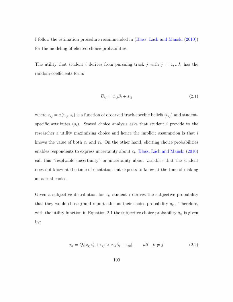
I follow the estimation procedure recommended in (Blass, Lach and Manski (2010))

for the modeling of elicited choice-probabilities.

The utility that student i derives from pursuing track j with j = 1, ..J , has the

random-coefficients form:

Uij = xijβi + εij (2.1)

where xij = x(vij, si) is a function of observed track-specific beliefs (vij) and student-

specific attributes (si). Stated choice analysis asks that student i provide to the

researcher a utility maximizing choice and hence the implicit assumption is that i

knows the value of both xi and εi. On the other hand, eliciting choice probabilities

enables respondents to express uncertainty about εi. Blass, Lach and Manski (2010)

call this “resolvable uncertainty” or uncertainty about variables that the student

does not know at the time of elicitation but expects to know at the time of making

an actual choice.

Given a subjective distribution for εi, student i derives the subjective probability

that they would chose j and reports this as their choice probability qij. Therefore,

with the utility function in Equation 2.1 the subjective choice probability qij is given

by:

qij = Qi[xijβi + εij > xikβi + εik], all k 6= j] (2.2)

100

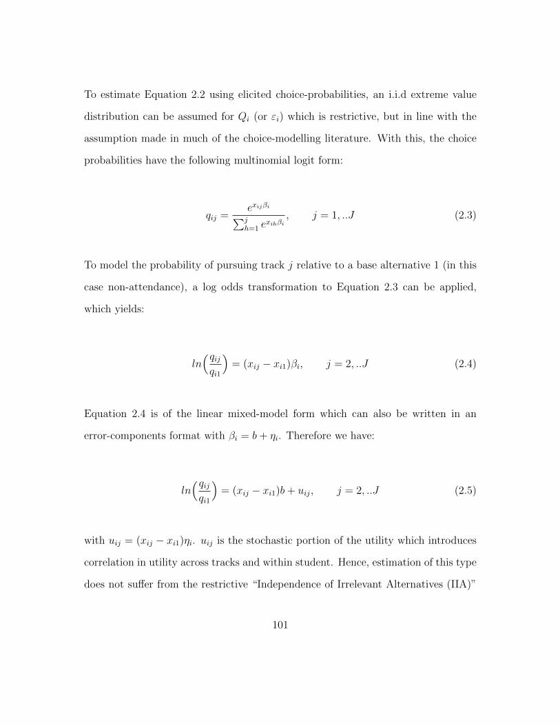
To estimate Equation 2.2 using elicited choice-probabilities, an i.i.d extreme value

distribution can be assumed for Qi (or εi) which is restrictive, but in line with the

assumption made in much of the choice-modelling literature. With this, the choice

probabilities have the following multinomial logit form:

qij =exijβi∑jh=1 e

xihβi, j = 1, ..J (2.3)

To model the probability of pursuing track j relative to a base alternative 1 (in this

case non-attendance), a log odds transformation to Equation 2.3 can be applied,

which yields:

ln(qijqi1

)= (xij − xi1)βi, j = 2, ..J (2.4)

Equation 2.4 is of the linear mixed-model form which can also be written in an

error-components format with βi = b+ ηi. Therefore we have:

ln(qijqi1

)= (xij − xi1)b+ uij, j = 2, ..J (2.5)

with uij = (xij − xi1)ηi. uij is the stochastic portion of the utility which introduces

correlation in utility across tracks and within student. Hence, estimation of this type

does not suffer from the restrictive “Independence of Irrelevant Alternatives (IIA)”

101

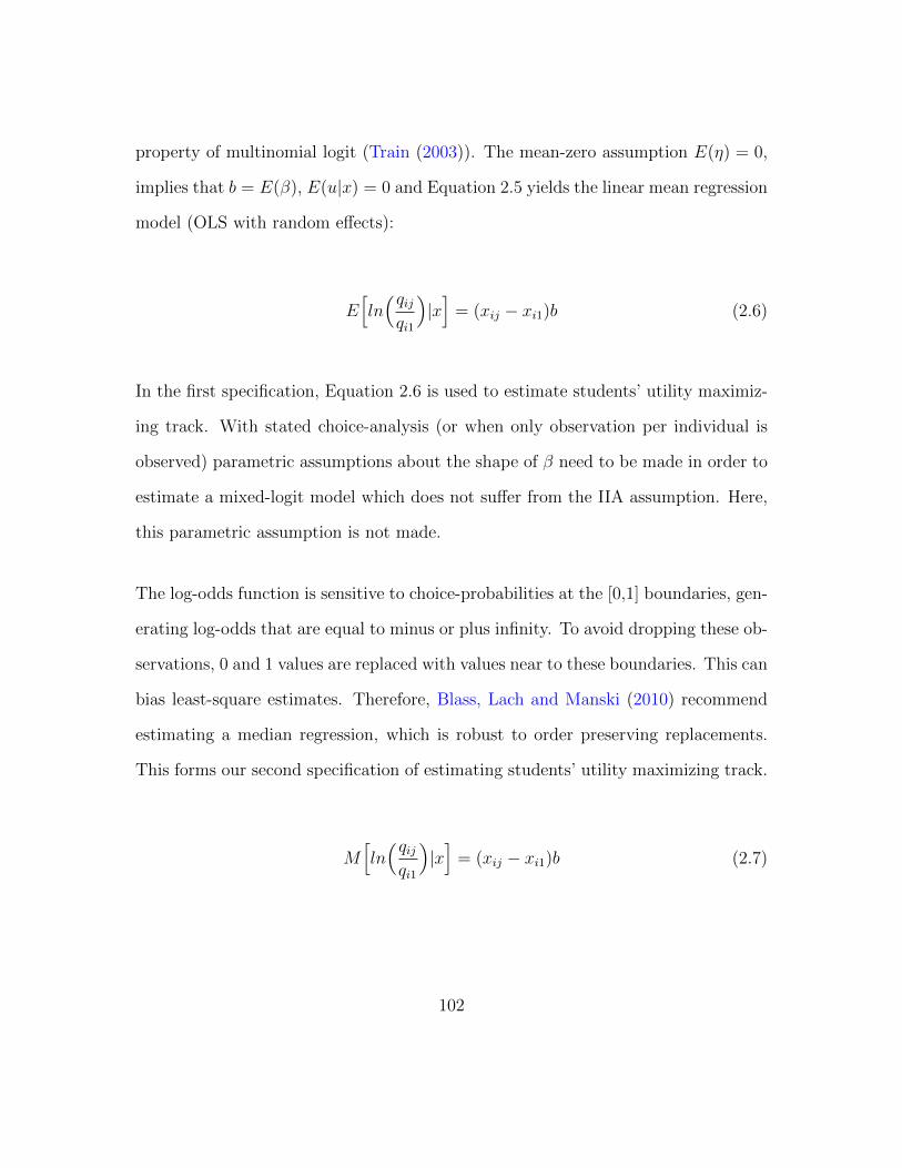
property of multinomial logit (Train (2003)). The mean-zero assumption E(η) = 0,

implies that b = E(β), E(u|x) = 0 and Equation 2.5 yields the linear mean regression

model (OLS with random effects):

E[ln(qijqi1

)|x]

= (xij − xi1)b (2.6)

In the first specification, Equation 2.6 is used to estimate students’ utility maximiz-

ing track. With stated choice-analysis (or when only observation per individual is

observed) parametric assumptions about the shape of β need to be made in order to

estimate a mixed-logit model which does not suffer from the IIA assumption. Here,

this parametric assumption is not made.

The log-odds function is sensitive to choice-probabilities at the [0,1] boundaries, gen-

erating log-odds that are equal to minus or plus infinity. To avoid dropping these ob-

servations, 0 and 1 values are replaced with values near to these boundaries. This can

bias least-square estimates. Therefore, Blass, Lach and Manski (2010) recommend

estimating a median regression, which is robust to order preserving replacements.

This forms our second specification of estimating students’ utility maximizing track.

M[ln(qijqi1

)|x]

= (xij − xi1)b (2.7)

102

2.4.2 Predicting Expenses from NSS Data

The second piece of econometric analysis that requires some explanation is the out of

sample prediction of expenses from the NSS dataset, to the survey sample of students

from Jharkhand. The basic idea is to assign to each individual a value of “measured

expenses”, which most closely approximates the expenses faced by students of their

“type”. This is to facilitate a comparison of more relevant “measured expenses”

with the students’ “perceived expenses”. For example, out-of-pocket post-secondary

expenses likely differ by caste in India, because the Indian government sometimes11

provides scholarships or stipends to students from socially disadvantaged castes.

Hence, it makes sense to compare perceived expenses of a student from a certain

caste to the expenses faced by students of the same caste.

Even though some scholarships are available, the extent of financial aid for post-

secondary education is relatively small. While nationally around 18% of students

in post-secondary education get some scholarships, this figure is only around 5%

in Jharkhand. In the presence of significant out-of-pocket expenses and variation

in costs on account of specific course within track, and institute (e.g. government

versus private) attended, a more important source of variation in measured costs is

likely on account of the fact that richer students may attend higher quality courses

and colleges/institutes.

11According to the NSS dataset 18.69% of all students in post-secondary education received somescholarship and 80% of all those who receive scholarships do so on account of their caste status.Around 94% of all scholarships are provided by the government.

103

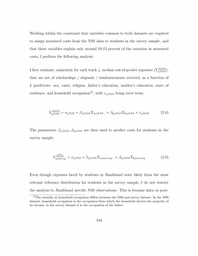
Working within the constraint that variables common to both datasets are required

to assign measured costs from the NSS data to students in the survey sample, and

that these variables explain only around 10-13 percent of the variation in measured

costs, I perform the following analysis:

I first estimate, separately for each track j, median out-of-pocket expenses (Y MEDijNSS),

that are net of scholarships / stipends / reimbursements received, as a function of

k predictors– sex, caste, religion, father’s education, mother’s education, state of

residence, and household occupation12, with εijNSS being error term:

Y MEDijNSS = αjNSS + β1jNSSX1ijNSS..+ βkjNSSXkijNSS + εijNSS (2.8)

The parameters β1jNSS..βkjNSS are then used to predict costs for students in the

survey sample:

Y MEDijsurvey = αjNSS + β1jNSSX1ijsurvey..+ βkjNSSXkijsurvey (2.9)

Even though expenses faced by students in Jharkhand state likely form the most

relevant reference distribution for students in the survey sample, I do not restrict

the analysis to Jharkhand specific NSS observations. This is because data on post-

12The variable on household occupation differs between the NSS and survey dataset. In the NSSdataset, household occupation is the occupation from which the household derives the majority ofits income, in the survey dataset it is the occupation of the father.

104

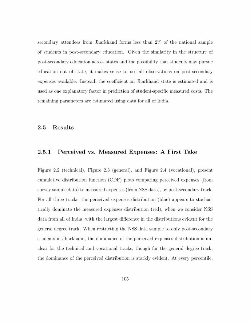
secondary attendees from Jharkhand forms less than 2% of the national sample

of students in post-secondary education. Given the similarity in the structure of

post-secondary education across states and the possibility that students may pursue

education out of state, it makes sense to use all observations on post-secondary

expenses available. Instead, the coefficient on Jharkhand state is estimated and is

used as one explanatory factor in prediction of student-specific measured costs. The

remaining parameters are estimated using data for all of India.

2.5 Results

2.5.1 Perceived vs. Measured Expenses: A First Take

Figure 2.2 (technical), Figure 2.3 (general), and Figure 2.4 (vocational), present

cumulative distribution function (CDF) plots comparing perceived expenses (from

survey sample data) to measured expenses (from NSS data), by post-secondary track.

For all three tracks, the perceived expenses distribution (blue) appears to stochas-

tically dominate the measured expenses distribution (red), when we consider NSS

data from all of India, with the largest difference in the distributions evident for the

general degree track. When restricting the NSS data sample to only post-secondary

students in Jharkhand, the dominance of the perceived expenses distribution is un-

clear for the technical and vocational tracks, though for the general degree track,

the dominance of the perceived distribution is starkly evident. At every percentile,

105

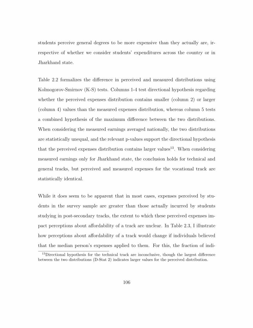
students perceive general degrees to be more expensive than they actually are, ir-

respective of whether we consider students’ expenditures across the country or in

Jharkhand state.

Table 2.2 formalizes the difference in perceived and measured distributions using

Kolmogorov-Smirnov (K-S) tests. Columns 1-4 test directional hypothesis regarding

whether the perceived expenses distribution contains smaller (column 2) or larger

(column 4) values than the measured expenses distribution, whereas column 5 tests

a combined hypothesis of the maximum difference between the two distributions.

When considering the measured earnings averaged nationally, the two distributions

are statistically unequal, and the relevant p-values support the directional hypothesis

that the perceived expenses distribution contains larger values13. When considering

measured earnings only for Jharkhand state, the conclusion holds for technical and

general tracks, but perceived and measured expenses for the vocational track are

statistically identical.

While it does seem to be apparent that in most cases, expenses perceived by stu-

dents in the survey sample are greater than those actually incurred by students

studying in post-secondary tracks, the extent to which these perceived expenses im-

pact perceptions about affordability of a track are unclear. In Table 2.3, I illustrate

how perceptions about affordability of a track would change if individuals believed

that the median person’s expenses applied to them. For this, the fraction of indi-

13Directional hypothesis for the technical track are inconclusive, though the largest differencebetween the two distributions (D-Stat 2) indicates larger values for the perceived distribution.

106

viduals who perceive each track as affordable is computed, first using data on cost

perceptions of students, and then by replacing cost perceptions with the median of

measured costs, for each student.14 I do this for an overall distribution averaged

across institute type and separately for expenses incurred by those studying in gov-

ernment and private institutes. While perception about expenses are not collected

conditional on institute type, and the survey-sample likely contains a mix of individ-

uals intending to pursue government and private degrees, I perform this exercise to

provide an illustrative extreme around the extent of overestimation. In other words,

how would affordability of a track change under one extreme assumption of everyone

anchoring perceptions on attending government institutes? How would affordabil-

ity of a track change under the other extreme of everyone anchoring perceptions on

attending private institutes?

Change in perceived affordability on account of replacing cost perceptions with me-

dian measured costs is the highest for the general track, which would be affordable

to 52 percent points more individuals, had individuals perceived their expenses as

equal to the median person’s. This increase is less dramatic for the vocational track

(19 percentage points) and more so for the technical track (6 percentage points) (col-

umn 1, Table 2.3). Under the extreme possibility that all students report perceived

expenses by anchoring their beliefs on attending private institutes, there is still an in-

crease in affordability when individuals’ cost perceptions are replaced with measured

expenses of those who attend only private institutes. Affordability for the general

14A track is affordable if (max. amount families can pay)-(perceived/measured cost of track) ≥0

107

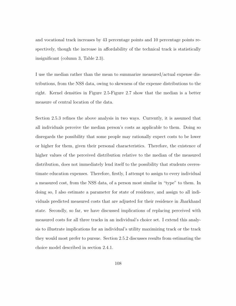
and vocational track increases by 43 percentage points and 10 percentage points re-

spectively, though the increase in affordability of the technical track is statistically

insignificant (column 3, Table 2.3).

I use the median rather than the mean to summarize measured/actual expense dis-

tributions, from the NSS data, owing to skewness of the expense distributions to the

right. Kernel densities in Figure 2.5-Figure 2.7 show that the median is a better

measure of central location of the data.

Section 2.5.3 refines the above analysis in two ways. Currently, it is assumed that

all individuals perceive the median person’s costs as applicable to them. Doing so

disregards the possibility that some people may rationally expect costs to be lower

or higher for them, given their personal characteristics. Therefore, the existence of

higher values of the perceived distribution relative to the median of the measured

distribution, does not immediately lend itself to the possibility that students overes-

timate education expenses. Therefore, firstly, I attempt to assign to every individual

a measured cost, from the NSS data, of a person most similar in “type” to them. In

doing so, I also estimate a parameter for state of residence, and assign to all indi-

viduals predicted measured costs that are adjusted for their residence in Jharkhand

state. Secondly, so far, we have discussed implications of replacing perceived with

measured costs for all three tracks in an individual’s choice set. I extend this analy-

sis to illustrate implications for an individual’s utility maximizing track or the track

they would most prefer to pursue. Section 2.5.2 discusses results from estimating the

choice model described in section 2.4.1.

108

2.5.2 Students’ Utility Maximizing Tracks

Parameters of the choice-model, resultant from estimating Equation 2.6, are tabled

in column 1, Table 2.4. Results from the alternative model in Equation 2.7, are

tabled in column 2, Table 2.4. While the qualitative significance of coefficients in

Table 2.4 are both hard to interpret (owing to the log-odds specification) and not

of central importance in this paper (we are more interested in the distribution of

utility maximizing tracks), it is nevertheless useful to provide some interpretation.

All three track-specific non-pecuniary beliefs are expressed on a probability scale

(0-100). Interpreting coefficients from column 2, Table 2.4, the perceived likelihood

of being able to pass all examinations in order to graduate, is not a statistically

significant predictor of stated enrollment. Among non-pecuniary factors, parental

approval is important–a 10 percentage points increase in the probability of parental

approval for a track (relative to non-enrollment) increases the log-odds of stated

enrollment by 0.19%, whereas the increase for a commensurate change in perceived

enjoyment of coursework is 0.14%. Relative to non-pecuniary beliefs, the beliefs

regarding employment probability (also 0-100 scale), bear a still smaller association

with intended enrollment. A 10 percentage points increase in the probability of

employment for a track (relative to non-enrollment) increases the log-odds of stated

enrollment by 0.06%. Individuals are sensitive to expected age-30 earnings: a 1%

increase in expected monthly earnings is associated with a 0.9% increase in the log-

odds of stated enrollment.

I use the parameter estimates in Table 2.4 to derive the predicted probability of en-

109

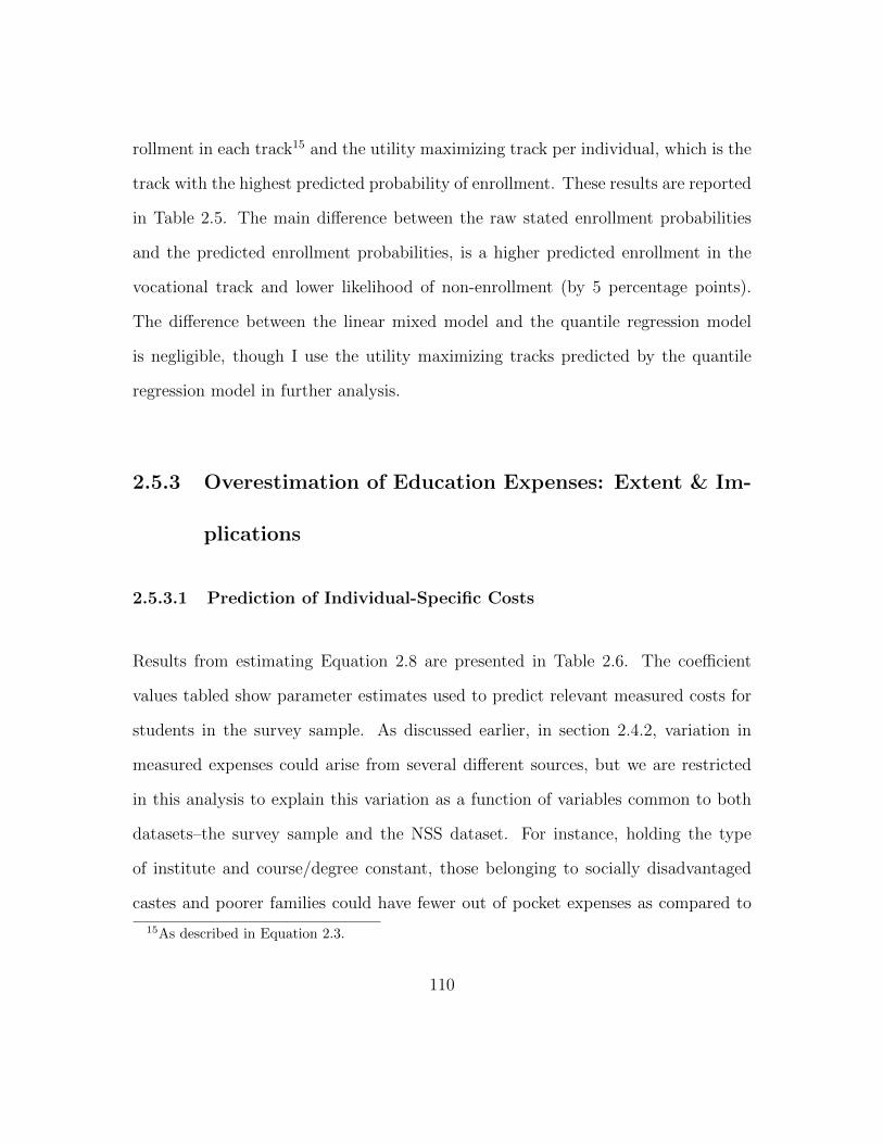
rollment in each track15 and the utility maximizing track per individual, which is the

track with the highest predicted probability of enrollment. These results are reported

in Table 2.5. The main difference between the raw stated enrollment probabilities

and the predicted enrollment probabilities, is a higher predicted enrollment in the

vocational track and lower likelihood of non-enrollment (by 5 percentage points).

The difference between the linear mixed model and the quantile regression model

is negligible, though I use the utility maximizing tracks predicted by the quantile

regression model in further analysis.

2.5.3 Overestimation of Education Expenses: Extent & Im-

plications

2.5.3.1 Prediction of Individual-Specific Costs

Results from estimating Equation 2.8 are presented in Table 2.6. The coefficient

values tabled show parameter estimates used to predict relevant measured costs for

students in the survey sample. As discussed earlier, in section 2.4.2, variation in

measured expenses could arise from several different sources, but we are restricted

in this analysis to explain this variation as a function of variables common to both

datasets–the survey sample and the NSS dataset. For instance, holding the type

of institute and course/degree constant, those belonging to socially disadvantaged

castes and poorer families could have fewer out of pocket expenses as compared to

15As described in Equation 2.3.

110

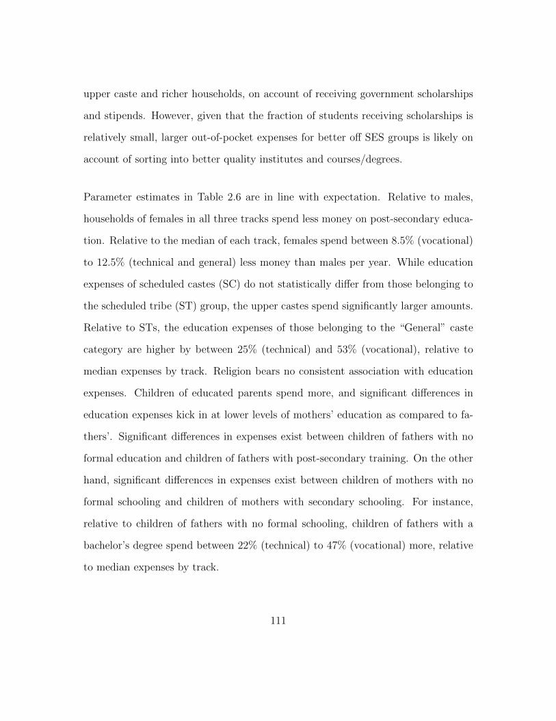
upper caste and richer households, on account of receiving government scholarships

and stipends. However, given that the fraction of students receiving scholarships is

relatively small, larger out-of-pocket expenses for better off SES groups is likely on

account of sorting into better quality institutes and courses/degrees.

Parameter estimates in Table 2.6 are in line with expectation. Relative to males,

households of females in all three tracks spend less money on post-secondary educa-

tion. Relative to the median of each track, females spend between 8.5% (vocational)

to 12.5% (technical and general) less money than males per year. While education

expenses of scheduled castes (SC) do not statistically differ from those belonging to

the scheduled tribe (ST) group, the upper castes spend significantly larger amounts.

Relative to STs, the education expenses of those belonging to the “General” caste

category are higher by between 25% (technical) and 53% (vocational), relative to

median expenses by track. Religion bears no consistent association with education

expenses. Children of educated parents spend more, and significant differences in

education expenses kick in at lower levels of mothers’ education as compared to fa-

thers’. Significant differences in expenses exist between children of fathers with no

formal education and children of fathers with post-secondary training. On the other

hand, significant differences in expenses exist between children of mothers with no

formal schooling and children of mothers with secondary schooling. For instance,

relative to children of fathers with no formal schooling, children of fathers with a

bachelor’s degree spend between 22% (technical) to 47% (vocational) more, relative

to median expenses by track.

111

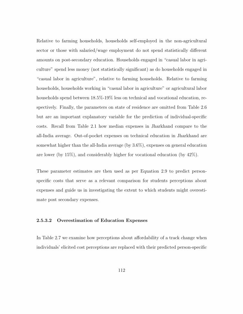
Relative to farming households, households self-employed in the non-agricultural

sector or those with salaried/wage employment do not spend statistically different

amounts on post-secondary education. Households engaged in “casual labor in agri-

culture” spend less money (not statistically significant) as do households engaged in

“casual labor in agriculture”, relative to farming households. Relative to farming

households, households working in “casual labor in agriculture” or agricultural labor

households spend between 18.5%-19% less on technical and vocational education, re-

spectively. Finally, the parameters on state of residence are omitted from Table 2.6

but are an important explanatory variable for the prediction of individual-specific

costs. Recall from Table 2.1 how median expenses in Jharkhand compare to the

all-India average. Out-of-pocket expenses on technical education in Jharkhand are

somewhat higher than the all-India average (by 3.6%), expenses on general education

are lower (by 15%), and considerably higher for vocational education (by 42%).

These parameter estimates are then used as per Equation 2.9 to predict person-

specific costs that serve as a relevant comparison for students perceptions about

expenses and guide us in investigating the extent to which students might overesti-

mate post secondary expenses.

2.5.3.2 Overestimation of Education Expenses

In Table 2.7 we examine how perceptions about affordability of a track change when

individuals’ elicited cost perceptions are replaced with their predicted person-specific

112

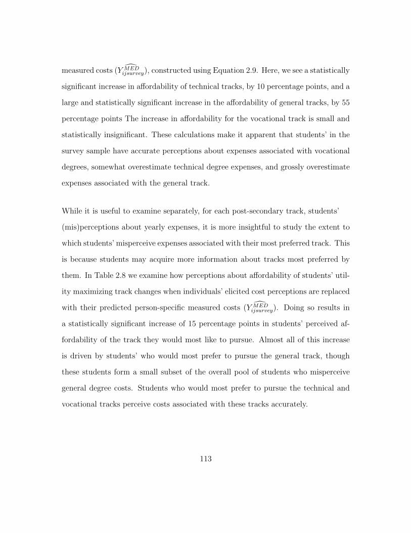
measured costs ( Y MEDijsurvey), constructed using Equation 2.9. Here, we see a statistically

significant increase in affordability of technical tracks, by 10 percentage points, and a

large and statistically significant increase in the affordability of general tracks, by 55

percentage points The increase in affordability for the vocational track is small and

statistically insignificant. These calculations make it apparent that students’ in the

survey sample have accurate perceptions about expenses associated with vocational

degrees, somewhat overestimate technical degree expenses, and grossly overestimate

expenses associated with the general track.

While it is useful to examine separately, for each post-secondary track, students’

(mis)perceptions about yearly expenses, it is more insightful to study the extent to

which students’ misperceive expenses associated with their most preferred track. This

is because students may acquire more information about tracks most preferred by

them. In Table 2.8 we examine how perceptions about affordability of students’ util-

ity maximizing track changes when individuals’ elicited cost perceptions are replaced

with their predicted person-specific measured costs ( Y MEDijsurvey). Doing so results in

a statistically significant increase of 15 percentage points in students’ perceived af-

fordability of the track they would most like to pursue. Almost all of this increase

is driven by students’ who would most prefer to pursue the general track, though

these students form a small subset of the overall pool of students who misperceive

general degree costs. Students who would most prefer to pursue the technical and

vocational tracks perceive costs associated with these tracks accurately.

113

2.6 Conclusion

This paper describes the subjective beliefs of a sample of Indian high school students

about expenses associated with post-secondary education in the country. The paper

describes the extent to which students’ seem to overestimate expenses, relative to

a reference distribution of students currently attending post-secondary education.

Together with data of students’ subjective beliefs about their capacity to pay for

education, the paper describes the implications of overestimating costs on students’

beliefs about their financially feasible choice-sets and affordability of their most pre-

ferred track. Students’ subjective perceptions about their likelihood of receiving

scholarships is also taken into account to compare perceptions about out-of-pocket

expenses with out-of-pocket measured expenses.

In my analysis I find that the extent of students’ inaccuracy of cost beliefs differs

importantly by post-secondary track. More specifically, students make the largest

errors for the general degree track, and fail to perceive that these type of degrees are

substantially cheaper to enroll in as compared to technical and vocational degrees.

I estimate that if students perceived expenses more accurately, then their perceived

affordability for technical tracks and general tracks would increase by 10 percentage

points and 55 percentage points, respectively, though for vocational tracks students

have accurate perceptions about costs at the outset. In addition, I estimate students’

utility maximizing tracks using a flexible model of track-choice. I used the methodol-

ogy proposed by Blass, Lach and Manski (2010) to model stated probabilities, which

114

is simple to estimate, allows unstructured correlations between alternatives “within”

individual and allows individuals to express uncertainty about a decision they will

be making in the future. Students have relatively more accurate beliefs about the

expenses associated with their most preferred track. If students perceived expenses

more accurately, then 15 percentage points more people would believe their utility

maximizing track to be affordable to them. To use as reference a measure of actual

costs more relevant to an individual than an overall distribution of costs, I assign

to every individual a predicted value of measured costs using the set of SES charac-

teristics that overlap both datasets–the survey sample of subjective beliefs and the

NSS dataset on measured expenses.

While the paper goes beyond the existing literature in discussing the overestimation

of expenses in concurrence with its implications for perceived affordability of edu-

cation, the main drawback of the analysis is that it stops short of linking perceived

unaffordability with real enrollment decisions of students.

115

REFERENCES FOR CHAPTER 2

Altonji, Joseph G. 1993. “The demand for and return to education when education

outcomes are uncertain.” Journal of Labor Economics, 11(1, Part 1): 48–83.

Attanasio, Orazio, and Katja Kaufmann. 2009. “Educational choices, subjec-

tive expectations, and credit constraints.” National Bureau of Economic Research.

Berry, James. 2015. “Child Control in Education Decisions An Evaluation of Tar-

geted Incentives to Learn in India.” Journal of Human Resources, 50(4): 1051–

1080.

Bettinger, Eric P, Bridget Terry Long, Philip Oreopoulos, and Lisa San-

bonmatsu. 2009. “The role of simplification and information in college decisions:

Results from the H&R Block FAFSA experiment.” National Bureau of Economic

Research.

Betts, Julian R. 1996. “What do students know about wages? Evidence from a

survey of undergraduates.” Journal of human resources, 27–56.

Blass, Asher A, Saul Lach, and Charles F Manski. 2010. “Using elicited

choice probabilities to estimate random utility models: Preferences for electricity

reliability.” International Economic Review, 51(2): 421–440.

Bleemer, Zachary, and Basit Zafar. 2015. “Intended college attendance: evi-

dence from an experiment on college returns and costs.”

Delavande, Adeline, and Basit Zafar. 2014. “University choice: the role of

expected earnings, non-pecuniary outcomes, and financial constraints.”

116

Dinkelman, Taryn, and Claudia Martınez. 2014. “Investing in schooling in

Chile: The role of information about financial aid for higher education.” Review

of Economics and Statistics, 96(2): 244–257.

Fryer Jr, Roland G. 2013. “Information and student achievement: Evidence from

a cellular phone experiment.” National Bureau of Economic Research.

Giustinelli, Pamela. 2016. “Group decision making with uncertain outcomes: Un-

packing child–parent choice of the high school track.” International Economic Re-

view, 57(2): 573–602.

Grodsky, Eric, and Melanie T Jones. 2007. “Real and imagined barriers to

college entry: Perceptions of cost.” Social Science Research, 36(2): 745–766.

Hastings, Justine, Christopher A Neilson, and Seth D Zimmerman. 2015.

“The effects of earnings disclosure on college enrollment decisions.” National Bu-

reau of Economic Research.

Hastings, Justine S, Christopher A Neilson, Anely Ramirez, and Seth D

Zimmerman. 2015. “(Un) Informed College and Major Choice: Evidence from

Linked Survey and Administrative Data.” National Bureau of Economic Research.

Jensen, Robert. 2010. “The (perceived) returns to education and the demand for

schooling.” The Quarterly Journal of Economics, 125(2): 515–548.

Kaufmann, Katja Maria. 2014. “Understanding the income gradient in college

attendance in Mexico: The role of heterogeneity in expected returns.” Quantitative

Economics, 5(3): 583–630.

117

Loyalka, Prashant, Chengfang Liu, Yingquan Song, Hongmei Yi, Xiaot-

ing Huang, Jianguo Wei, Linxiu Zhang, Yaojiang Shi, James Chu, and

Scott Rozelle. 2013. “Can information and counseling help students from poor

rural areas go to high school? Evidence from China.” Journal of Comparative

Economics, 41(4): 1012–1025.

Manski, Charles F. 2004. “Measuring expectations.” Econometrica, 72(5): 1329–

1376.

Nguyen, Trang. 2008. “Information, role models and perceived returns to educa-

tion: Experimental evidence from Madagascar.” Unpublished manuscript, 6.

Oreopoulos, Philip, and Ryan Dunn. 2013. “Information and college access:

Evidence from a randomized field experiment.” The Scandinavian Journal of Eco-

nomics, 115(1): 3–26.

Pekkala Kerr, Sari, Tuomas Pekkarinen, Matti Sarvimaki, and Roope

Uusitalo. 2015. “Post-secondary education and information on labor market

prospects: a randomized field experiment.”

Train, Kenneth. 2003. Discrete choice methods with simulation. Cambridge uni-

versity press.

Willis, Robert J, and Sherwin Rosen. 1979. “Education and self-selection.”

Journal of political Economy, 87(5, Part 2): S7–S36.

118

Wiswall, Matthew, and Basit Zafar. 2015. “Determinants of college major

choice: Identification using an information experiment.” The Review of Economic

Studies, 82(2): 791–824.

119

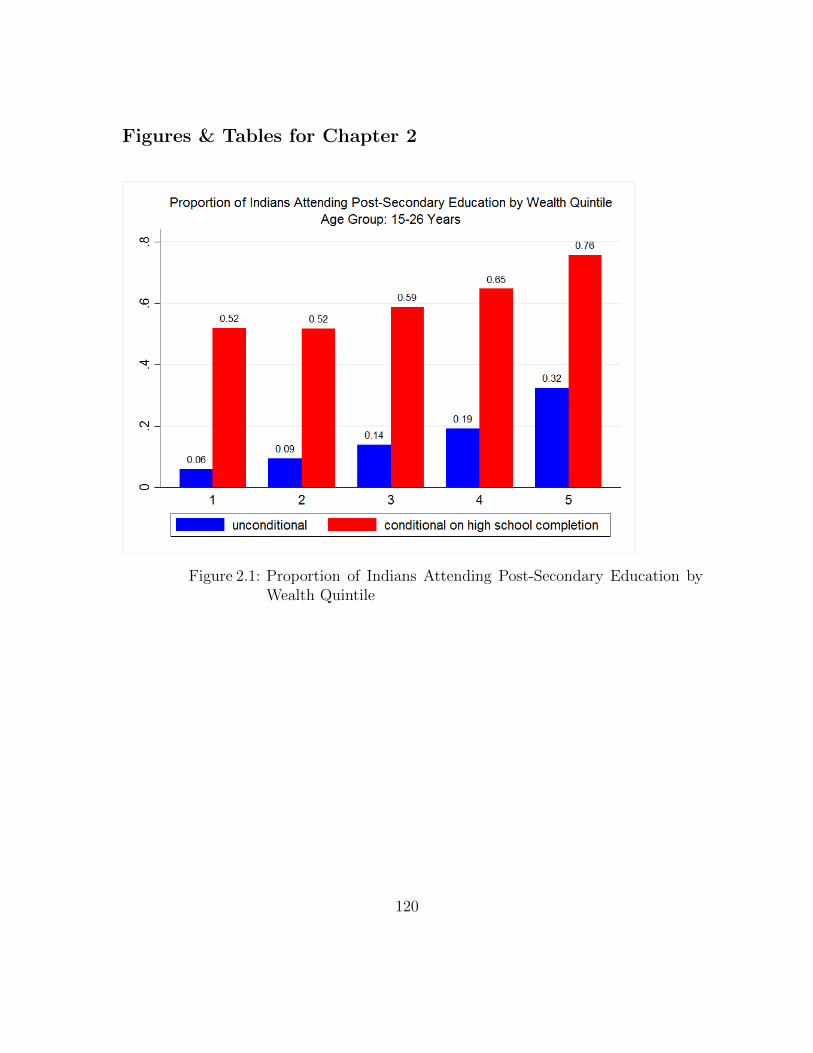
Figures & Tables for Chapter 2

Figure 2.1: Proportion of Indians Attending Post-Secondary Education byWealth Quintile

120

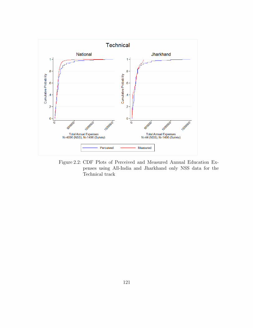
Figure 2.2: CDF Plots of Perceived and Measured Annual Education Ex-penses using All-India and Jharkhand only NSS data for theTechnical track

121

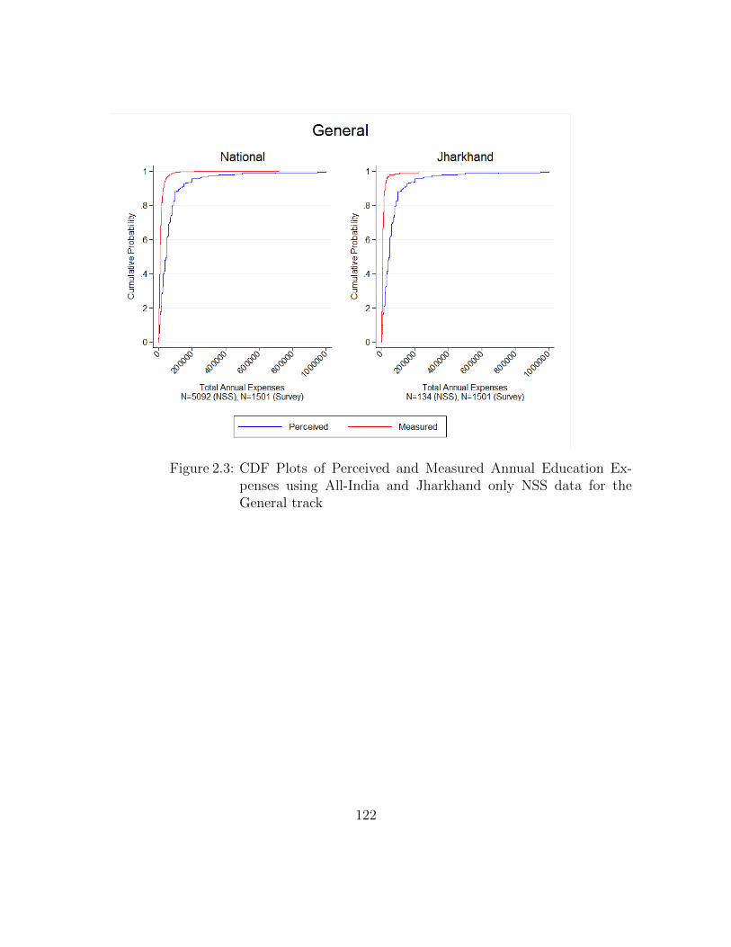
Figure 2.3: CDF Plots of Perceived and Measured Annual Education Ex-penses using All-India and Jharkhand only NSS data for theGeneral track

122

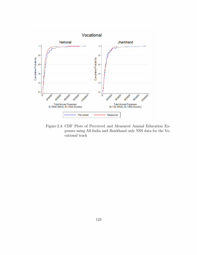
Figure 2.4: CDF Plots of Perceived and Measured Annual Education Ex-penses using All-India and Jharkhand only NSS data for the Vo-cational track

123

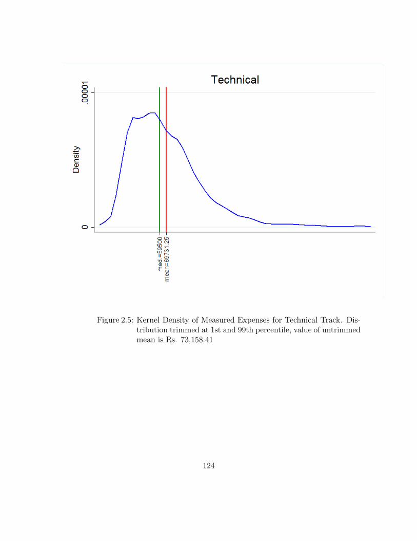
Figure 2.5: Kernel Density of Measured Expenses for Technical Track. Dis-tribution trimmed at 1st and 99th percentile, value of untrimmedmean is Rs. 73,158.41

124

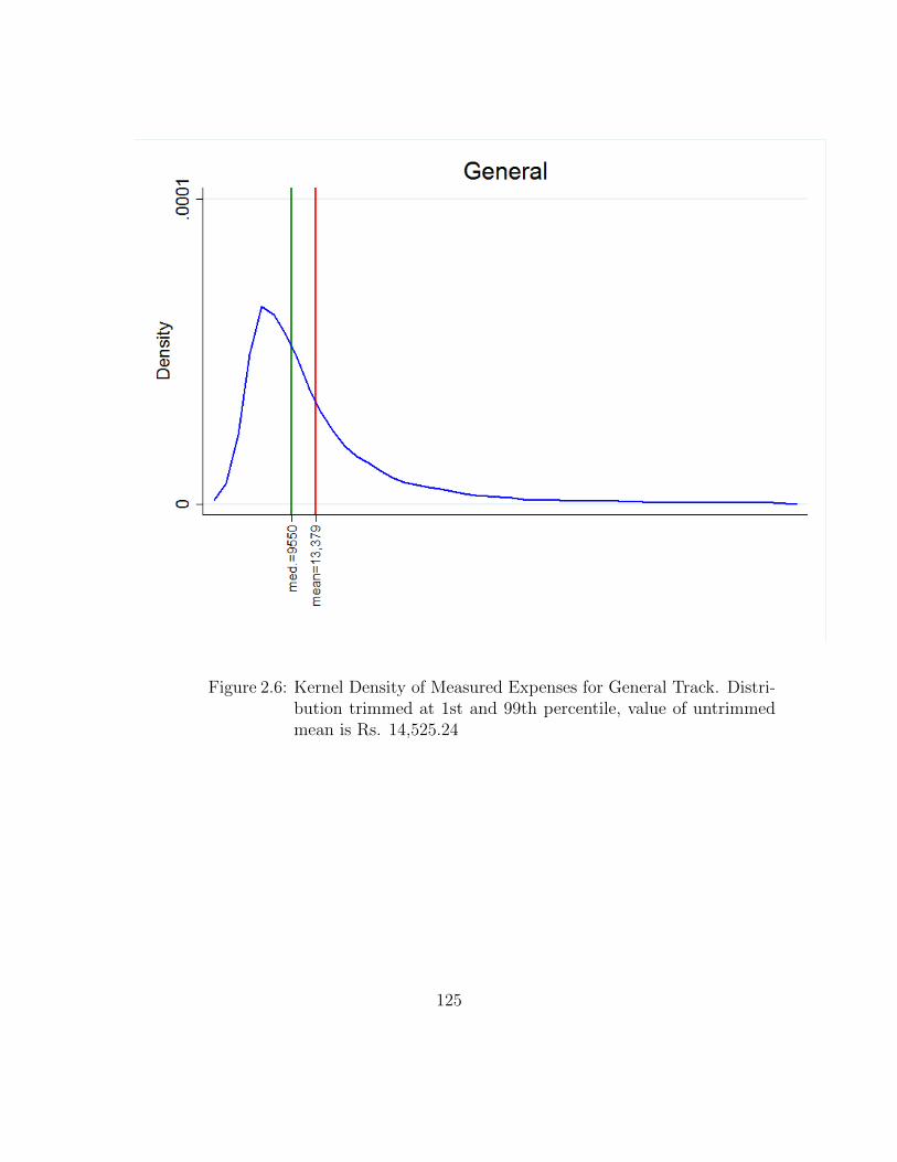
Figure 2.6: Kernel Density of Measured Expenses for General Track. Distri-bution trimmed at 1st and 99th percentile, value of untrimmedmean is Rs. 14,525.24

125

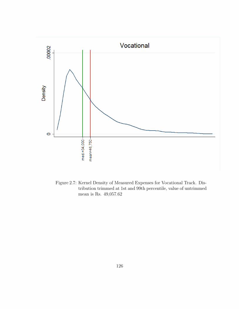
Figure 2.7: Kernel Density of Measured Expenses for Vocational Track. Dis-tribution trimmed at 1st and 99th percentile, value of untrimmedmean is Rs. 49,057.62

126

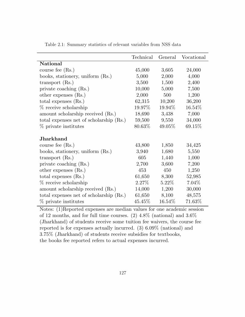
Table 2.1: Summary statistics of relevant variables from NSS data

Technical General Vocational

Nationalcourse fee (Rs.) 45,000 3,605 24,000books, stationery, uniform (Rs.) 5,000 2,000 4,000transport (Rs.) 3,500 1,500 2,400private coaching (Rs.) 10,000 5,000 7,500other expenses (Rs.) 2,000 500 1,200total expenses (Rs.) 62,315 10,200 36,200% receive scholarship 19.97% 19.94% 16.54%amount scholarship received (Rs.) 18,690 3,438 7,000total expenses net of scholarship (Rs.) 59,500 9,550 34,000% private institutes 80.63% 49.05% 69.15%

Jharkhandcourse fee (Rs.) 43,800 1,850 34,425books, stationery, uniform (Rs.) 3,940 1,680 5,550transport (Rs.) 605 1,440 1,000private coaching (Rs.) 2,700 3,600 7,200other expenses (Rs.) 453 450 1,250total expenses (Rs.) 61,650 8,300 52,985% receive scholarship 2.27% 5.22% 7.04%amount scholarship received (Rs.) 14,000 1,200 30,000total expenses net of scholarship (Rs.) 61,650 8,100 48,575% private institutes 45.45% 16.54% 71.63%

Notes: (1)Reported expenses are median values for one academic sessionof 12 months, and for full time courses. (2) 4.8% (national) and 3.6%(Jharkhand) of students receive some tuition fee waivers, the course feereported is for expenses actually incurred. (3) 6.09% (national) and3.75% (Jharkhand) of students receive subsidies for textbooks,the books fee reported refers to actual expenses incurred.

127

Table 2.2: Testing for Equality of Perceived & Measured Expenses Distribu-tions using Kolmogorov-Smirnov Tests

(1) (2) (3) (4) (5)D-stat 1 P-value (col 1) D-stat 2 P-value (col 3) P-value (comb.)

NationalTechnical 0.0539 0.002 -0.1707 0.000 0.000General 0.0011 0.997 -0.588 0.000 0.000Vocational 0.0142 0.621 -0.2091 0.000 0.000

JharkhandTechnical 0.0642 0.703 -0.243 0.006 0.008General 0.0133 0.957 -0.6762 0.000 0.000Vocational 0.0869 0.141 -0.0819 0.176 0.246

Notes: (1) tests the hypothesis that “perceived” expense distribution contains smallervalues than “measured” expense distribution. (2) tests the hypothesisthat “perceived” expense distribution contains larger values than the “measured”expense distribution. P-value for the combined hypothesis tests for the max.of the two directional hypothesis. Obs. in the NSS data for all-India: 4096 (tech.),5902 (gen.), 5846 (voc.). Obs. in the NSS data for Jharkhand: 44 (tech.),134 (gen.) & 142 (voc.). Approx. 1500 obs. in Survey dataset for all 3 tracks.

128

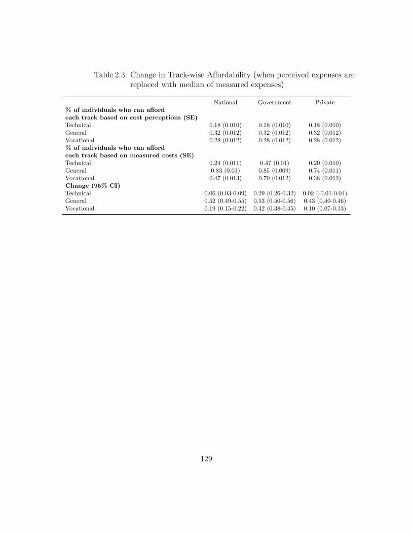
Table 2.3: Change in Track-wise Affordability (when perceived expenses arereplaced with median of measured expenses)

National Government Private% of individuals who can affordeach track based on cost perceptions (SE)Technical 0.18 (0.010) 0.18 (0.010) 0.18 (0.010)General 0.32 (0.012) 0.32 (0.012) 0.32 (0.012)Vocational 0.28 (0.012) 0.28 (0.012) 0.28 (0.012)% of individuals who can affordeach track based on measured costs (SE)Technical 0.24 (0.011) 0.47 (0.01) 0.20 (0.010)General 0.83 (0.01) 0.85 (0.009) 0.74 (0.011)Vocational 0.47 (0.013) 0.70 (0.012) 0.38 (0.012)Change (95% CI)Technical 0.06 (0.03-0.09) 0.29 (0.26-0.32) 0.02 (-0.01-0.04)General 0.52 (0.49-0.55) 0.53 (0.50-0.56) 0.43 (0.40-0.46)Vocational 0.19 (0.15-0.22) 0.42 (0.38-0.45) 0.10 (0.07-0.13)

129

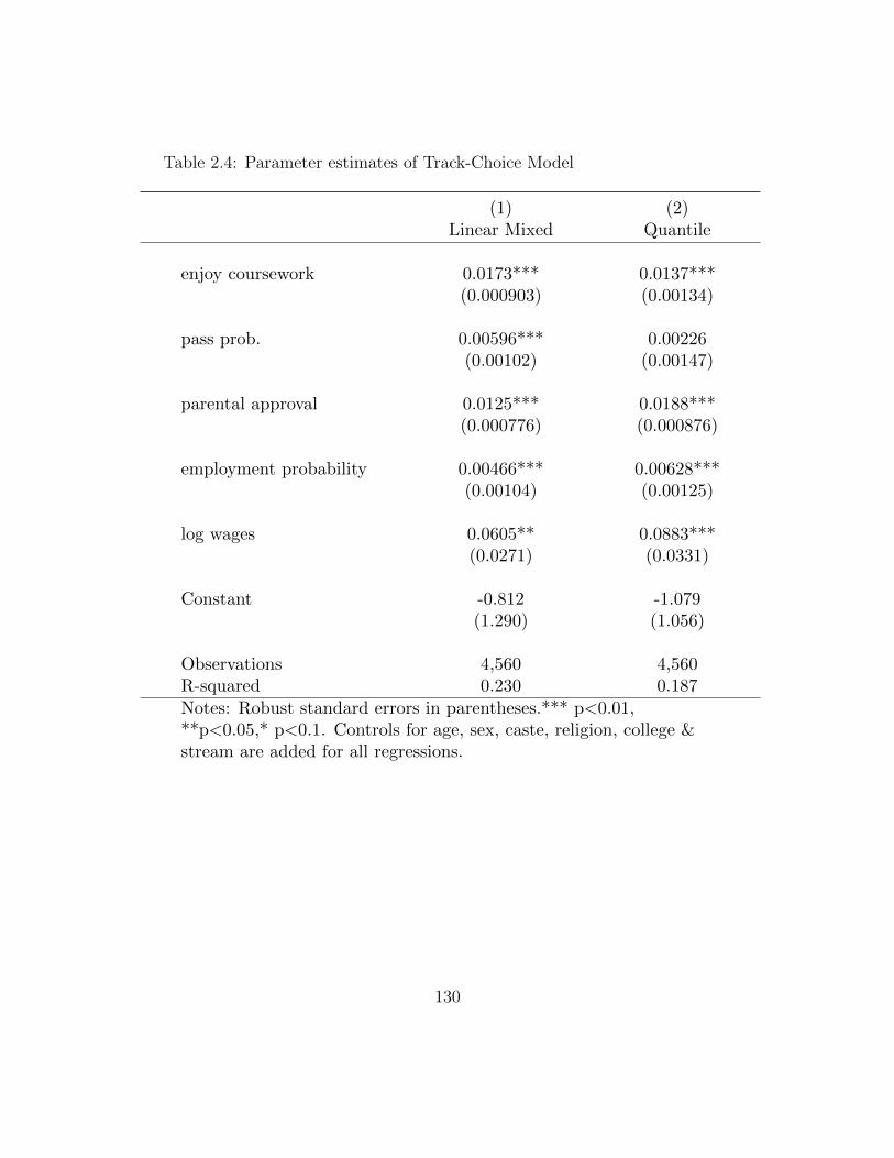
Table 2.4: Parameter estimates of Track-Choice Model

(1) (2)Linear Mixed Quantile

enjoy coursework 0.0173*** 0.0137***(0.000903) (0.00134)

pass prob. 0.00596*** 0.00226(0.00102) (0.00147)

parental approval 0.0125*** 0.0188***(0.000776) (0.000876)

employment probability 0.00466*** 0.00628***(0.00104) (0.00125)

log wages 0.0605** 0.0883***(0.0271) (0.0331)

Constant -0.812 -1.079(1.290) (1.056)

Observations 4,560 4,560R-squared 0.230 0.187

Notes: Robust standard errors in parentheses.*** p<0.01,**p<0.05,* p<0.1. Controls for age, sex, caste, religion, college &stream are added for all regressions.

130

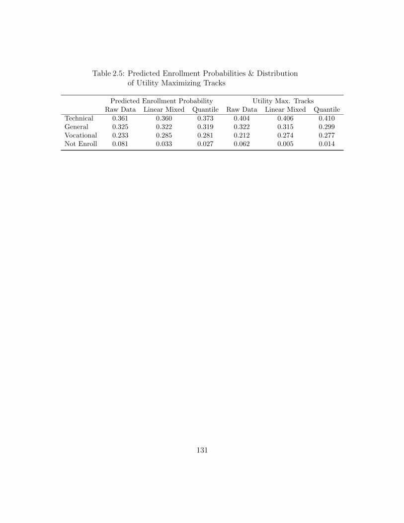
Table 2.5: Predicted Enrollment Probabilities & Distributionof Utility Maximizing Tracks

Predicted Enrollment Probability Utility Max. TracksRaw Data Linear Mixed Quantile Raw Data Linear Mixed Quantile

Technical 0.361 0.360 0.373 0.404 0.406 0.410General 0.325 0.322 0.319 0.322 0.315 0.299Vocational 0.233 0.285 0.281 0.212 0.274 0.277Not Enroll 0.081 0.033 0.027 0.062 0.005 0.014

131

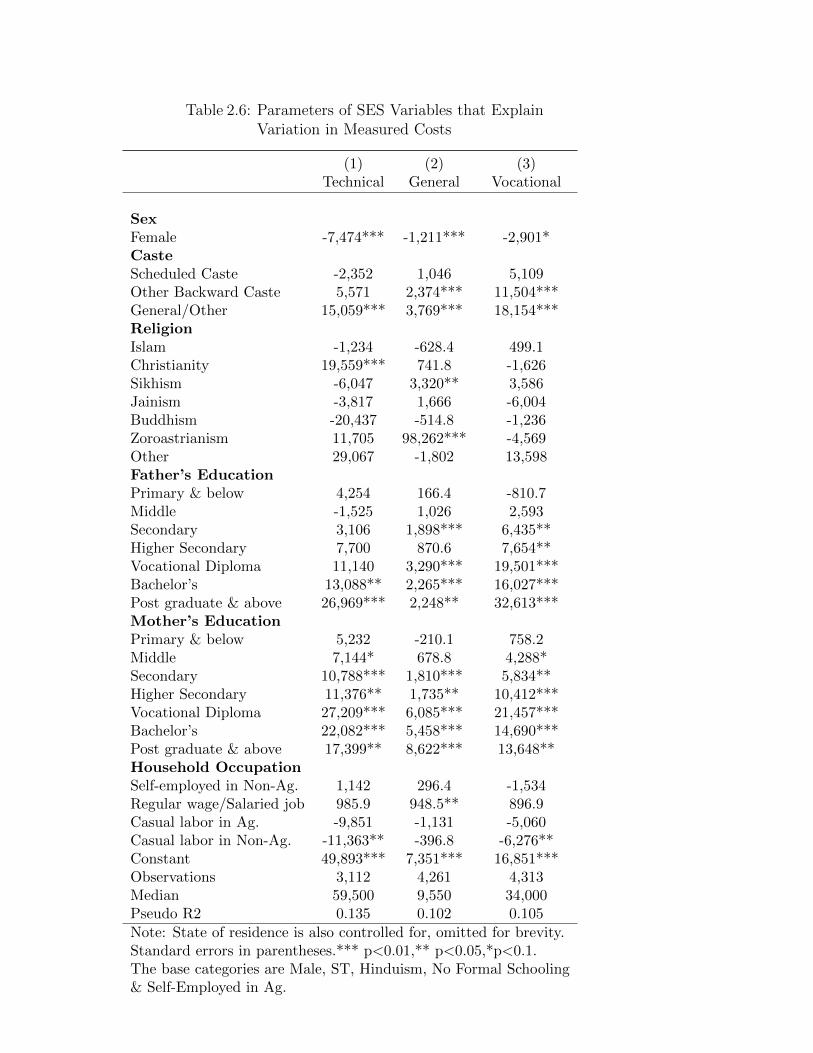
Table 2.6: Parameters of SES Variables that ExplainVariation in Measured Costs

(1) (2) (3)Technical General Vocational

SexFemale -7,474*** -1,211*** -2,901*CasteScheduled Caste -2,352 1,046 5,109Other Backward Caste 5,571 2,374*** 11,504***General/Other 15,059*** 3,769*** 18,154***ReligionIslam -1,234 -628.4 499.1Christianity 19,559*** 741.8 -1,626Sikhism -6,047 3,320** 3,586Jainism -3,817 1,666 -6,004Buddhism -20,437 -514.8 -1,236Zoroastrianism 11,705 98,262*** -4,569Other 29,067 -1,802 13,598Father’s EducationPrimary & below 4,254 166.4 -810.7Middle -1,525 1,026 2,593Secondary 3,106 1,898*** 6,435**Higher Secondary 7,700 870.6 7,654**Vocational Diploma 11,140 3,290*** 19,501***Bachelor’s 13,088** 2,265*** 16,027***Post graduate & above 26,969*** 2,248** 32,613***Mother’s EducationPrimary & below 5,232 -210.1 758.2Middle 7,144* 678.8 4,288*Secondary 10,788*** 1,810*** 5,834**Higher Secondary 11,376** 1,735** 10,412***Vocational Diploma 27,209*** 6,085*** 21,457***Bachelor’s 22,082*** 5,458*** 14,690***Post graduate & above 17,399** 8,622*** 13,648**Household OccupationSelf-employed in Non-Ag. 1,142 296.4 -1,534Regular wage/Salaried job 985.9 948.5** 896.9Casual labor in Ag. -9,851 -1,131 -5,060Casual labor in Non-Ag. -11,363** -396.8 -6,276**Constant 49,893*** 7,351*** 16,851***Observations 3,112 4,261 4,313Median 59,500 9,550 34,000Pseudo R2 0.135 0.102 0.105

Note: State of residence is also controlled for, omitted for brevity.Standard errors in parentheses.*** p<0.01,** p<0.05,*p<0.1.The base categories are Male, ST, Hinduism, No Formal Schooling& Self-Employed in Ag.

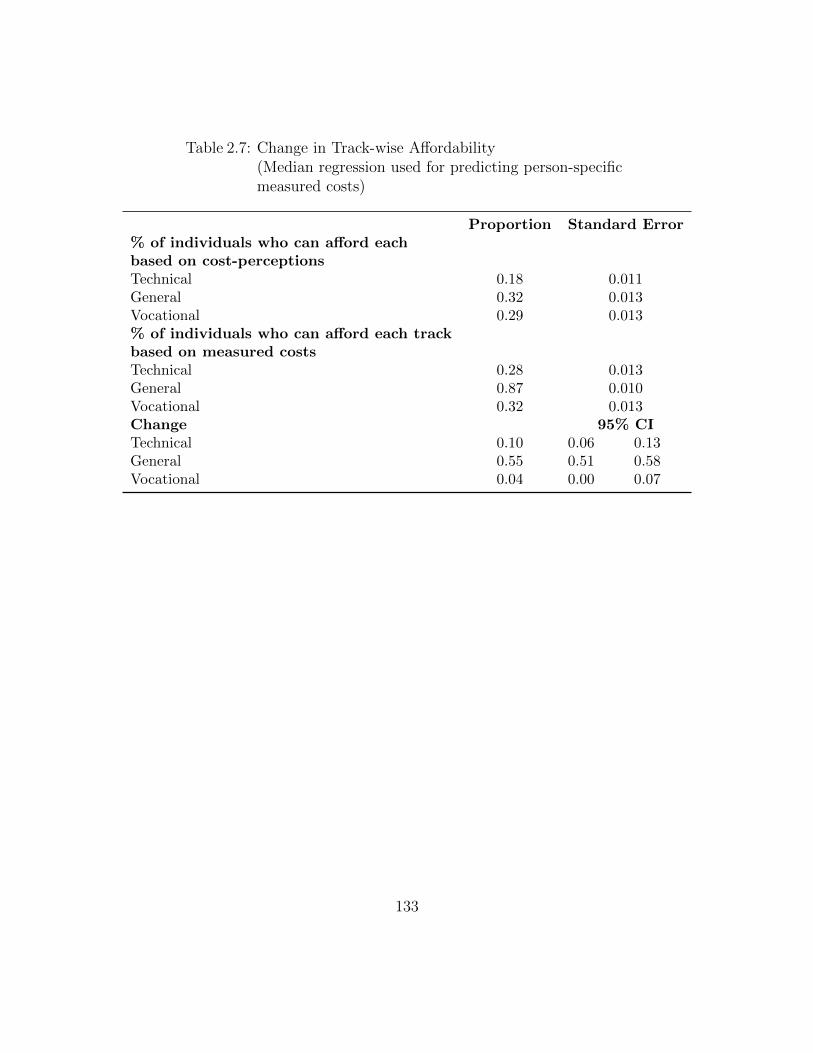
Table 2.7: Change in Track-wise Affordability(Median regression used for predicting person-specificmeasured costs)

Proportion Standard Error% of individuals who can afford eachbased on cost-perceptionsTechnical 0.18 0.011General 0.32 0.013Vocational 0.29 0.013% of individuals who can afford each trackbased on measured costsTechnical 0.28 0.013General 0.87 0.010Vocational 0.32 0.013Change 95% CITechnical 0.10 0.06 0.13General 0.55 0.51 0.58Vocational 0.04 0.00 0.07

133

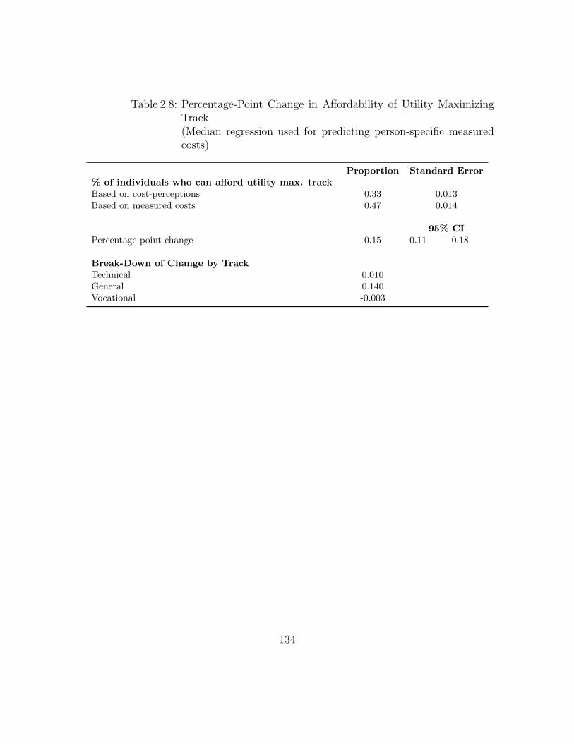
Table 2.8: Percentage-Point Change in Affordability of Utility MaximizingTrack(Median regression used for predicting person-specific measuredcosts)

Proportion Standard Error% of individuals who can afford utility max. trackBased on cost-perceptions 0.33 0.013Based on measured costs 0.47 0.014

95% CIPercentage-point change 0.15 0.11 0.18

Break-Down of Change by TrackTechnical 0.010General 0.140Vocational -0.003

134

CHAPTER 3

THE ROLE OF AGRICULTURE IN WOMEN’S NUTRITION:

EMPIRICAL EVIDENCE FROM INDIA

3.1 Introduction

Low body-mass index (BMI) among women of childbearing age (15-49 years), indica-

tive of maternal undernutrition, is a grave public health concern because its implica-

tions extend well beyond the individual herself. Maternal undernutrition contributes

to fetal growth restriction, which increases the risk of neonatal deaths and, for sur-

viving children, of stunting (Black et al. (2013)). Indian women are particularly at

risk of being too thin. Adjusting for the characteristics1 of pregnant women, it is es-

timated that approximately 42.2% of pre-pregnant women in India are underweight

(Coffey (2015)). In yet another stark manifestation of the Asian Enigma (Vulimiri,

Urban and Jon (1996)), in Sub-Saharan Africa, only 16.5% of pre-pregnant women

are estimated to be underweight, even though they are much poorer.

Among the reasons advanced for the poor nutritional status of Indian women, an en-

during explanation relates to the intra-household status of women. Several indicators

of womens status in the literature consistently rank women in the countries of South

Asia as lower in comparison to their counterparts in Asia, Africa, Latin America

1In India, fertility is concentrated among women in their early twenties as opposed to Sub-Saharan Africa where childbearing is more spread out between the ages of 17-35 years. Indianwomen in their early twenties are almost 15 pp. more likely to be underweight than 40 year oldwomen (Coffey (2015)).

135

and the Caribbean (Haddad (1999)). The Indian case is particularly unique whereby

features of familial structure and cultural norms that designate inter-personal hierar-

chies foster low social-status among women with perpetuating consequences for her

own and her childs health (Coffey, Khera and Spears (2013)). Worryingly, recent

numbers emerging from the Rapid Survey on Children (RSOC) conducted by the

Union Ministry of Women and Child Development and UNICEF2 show that while

India has seen encouraging progress on metrics of child malnutrition since 2005, the

situation for adolescent girls aged 15-19 years has barely budged with close to 45% of

girls in the age-group having BMI of less than 18.5. With this context in mind, pol-

icy interventions that have the potential to increase the bargaining power of women,

hold particular promise in addressing the problem of maternal malnutrition in the

country.

Recent, academic and policy interest in leveraging the agricultural sector in devel-

oping countries to combat the scourge of malnutrition, is motivated, in part, by the

fact that agriculture is not only a major employer overall in these countries, but is

a major employer of women in particular (Harris, Kadiyala et al. (2012), Pingali,

Ricketts and Sahn (2015), Ruel et al. (2013)). Therefore, one important pathway

by which agriculture is linked to nutrition is by way of being a source of income for

women, which in turn can influence the intra-household allocation of food and other

nutrition-enhancing complements (Hoddinott and Haddad (1995), Bobonis (2009)).

At the same time, heavy agricultural workloads and exposure to toxins and disease

2Rapid Survey on Children (provisional report) by the Ministry of Women and Child Develop-ment and the UNICEF accessed on 12.12.2015 from http://wcd.nic.in/issnip/National Fact%

20sheet RSOC%20 02-07-2015.pdf.

136

through agricultural activities can deleteriously affect women’s health and nutri-

tion and also have negative consequences for lactation and child-care (Jones et al.

(2012),Hoddinott (2012)). Therefore, the net implications of agricultural work for

womens nutrition require empirical investigation. Other pathways by which agricul-

ture and nutrition are posited to be linked include, production for own-consumption

(particularly relevant in the face of high transaction costs and missing markets for

nutritious foods), overall income effects for net-sellers of food and price-effects for

net-buyers (Kadiyala et al. (2014), Carletto et al. (2015)).

In a narrative synthesis of the existing malnutrition literature in India (Pingali and

Rao (2017)), find less than ten papers in peer-reviewed journals that empirically ex-

amine different determinants of women’s nutrition, as measured by anthropometric

outcomes (also see (Kadiyala et al. (2014)) for a related and relevant review). More-

over, all of these studies use cross-sectional data, and most of them do not extensively

control for confounding effects. Therefore, while the potential of the agricultural sec-

tor to address problems of malnutrition is promising, at the household-level, there is

little empirical evidence for whether income growth in agriculture is particularly ben-

eficial for improved nutritional outcomes and in particular, anthropometrics. One

constraint in the Indian context is the availability of anthropometric data, which

is strikingly lacking. Periodic National Family and Health Surveys (NFHS) which

collect nationally representative anthropometric data on children and adults, do not

collect detailed income and agriculture data and, moreover, havent released any unit

data in over a decade3. In this paper, we respond to this gap, by using five years

3The NFHS-4 released aggregated health reports for 13 states in 2015-16. However, the survey

137

of household-level panel data, from 18 villages across 5 Indian states, collected by

the International Crops Research Institute for the Semi-Arid Tropics (ICRISAT) as

part of the Village Dynamics in South Asia (VDSA) program, to establish the link

between household agricultural income and womens nutritional status, and explore

the pathways by which agricultural incomes may affect nutrition.

Some existing findings, on agricultural output and malnutrition, in the literature pro-

vide context and aid in the interpretation of our results. The effect of agricultural

production on malnutrition at the state-level is inconclusive in the Indian context.

For instance, (Gulati et al. (2012)) find a modest effect of state-level agricultural

production on both child and adult malnutrition metrics but use cross-sectional data

with few controls. On the other hand, (Headey (2013)), finds the effect of state level

agricultural growth on childhood stunting, with state fixed effects, to be particularly

weak for Indian states. In a household fixed-effects study, using Tanzanian data,

(Slavchevska (2015)), establishes a statistically important, positive (inelastic) effect

of household harvest value of crops on height-for-age z-scores of children under 5.

However, the author does not find any effects of the same for adults. Partly, this

could be because, adult underweight is not a substantial problem in their context,

with only about 9 percent of the adult sample being underweight. Using methods

comparable to ours and of (Slavchevska (2015)), (Kirk et al. (2015)) use three years

of data to examine effects of sector-specific incomes in Uganda. They do not find

agricultural incomes to play a crucial role in improving measures of child malnutri-

tion, but caution that their results are heavily context specific to the agricultural

is still in the field for the remaining states and unit data for all states is yet to be released.

138

and dietary profile of Uganda.

Some recent studies also throw light on specific pathways by which agriculture may

affect nutrition. For instance, (Hirvonen and Hoddinott (2016)), find that there

is a link between household-level production diversity and diversity of diets among

pre-school children in rural Ethiopia, but it breaks down for households that have

market access to food. The potential of two agricultural pathways, production for

own-consumption (measured by production diversity) and income effects (measured

by agricultural revenue), on household dietary diversity has been looked at in the

Nigerian context (Dillon, McGee and Oseni (2015)). The authors find both pathways

to have statistically significant but relatively inelastic effects on household dietary

diversity. Our findings strengthen the existing literature in multiple ways. Firstly, we

show that there is a statistically significant relationship between household agricul-

tural income and individual nutrition. We do so, both, by utilizing within household,

year to year, variation in household agricultural income and by associating growth

in agricultural income with growth in BMI over the longer term. Here, we con-

tribute to the limited pool of estimates, across countries, which provide a measure

for the agricultural income elasticity of anthropometrics. Further, we establish that

production for self-consumption plays only a limited role in producing nutritional

improvements in our data, but the role of food purchases and hence household in-

come is important. Finally, we establish heterogeneous effects by women’s age and

show significantly higher impact of agricultural income on the nutritional status of

younger women.

139

3.2 Data & Summary Statistics

This paper uses five years (2009-2013) of publicly available household and individual

level panel data collected by ICRISAT as part of the VDSA program. The data are

drawn from 18 villages across 5 Indian states Andhra Pradesh/Telangana, Gujarat,

Karnataka, Maharashtra and Madhya Pradesh. The total number of individuals with

valid BMI data in the sample varies from year to year; and ranges between 791-992

individuals. Rainfall data is from the University of Delaware Air Temperature and

Precipitation database.

Table 3.1 lists the key variables we use in our analysis along with their means and

standard deviations. Anthropometric data is collected annually, at the beginning of

the survey cycle, and income and consumption data are collected monthly, in subse-

quent months. In view of this feature of the survey design, we lag all our explanatory

variable by a year, to predict the following years BMI, our outcome variable of in-

terest. Thus, BMI data used in the study applies to years 2010-20134 and data from

2009-2012 are used for the explanatory variables. This ensures that BMI data in

every year is measured after income and expenditure data for the year. Figure 3.1

plots the cross-sectional distribution of the BMI of sample women5. Among all

4Anthropometric data collection in VDSA villages, from the five states, started in 2010.5BMI data that is likely measurement error is excluded from the analysis. For all individuals

having BMI less than 11 and greater than 40, and for individuals with individual-level BMI devia-tions smaller than the 1st percentile and larger than the 99th percentile, we consider observations ofthe individual for all years, on a case-by-case basis, to classify the BMI observation as measurementerror or not. This is done, primarily, based on consistency of height values recorded in other yearsfor the individual. In all, only 0.42% of all BMI observations are excluded on account of beingmeasurement error.

140

women of child-bearing age, between 15-49 years, 33% of women are underweight

with BMI<18.5. This number is worryingly high, and shows little progress since the

DHS national average of 35% underweight women in 2005. Moreover, the incidence

of underweight for younger women (15-25 y), among whom fertility is primarily con-

centrated, is higher by more than 13 percentage points, with the BMI distribution

for this age-group having a larger mass of observations in the low BMI ranges. Fig-

ure 3.2 plots the distribution of the deviations of women’s year-specific BMI from

their mean BMI. As is to be expected, within-individual variation in BMI, which

we will be utilizing for our panel data analysis, is more limited, but nevertheless

sufficient to yield meaningful insights. The average yearly deviation from individual-

specific BMI means is 0.65 points and for 95 percent of the women in our sample

BMI varies within a band of +/- 2 BMI points. Even though we explicitly check for

and exclude BMI observations that are undoubtedly measurement-error (primarily

based on older individuals for whom a lower height was recorded in a subsequent

year), there are some still observations with large absolute deviations in BMI, owing

to wide fluctuations in the weight of the individual over the span of four-years. We

examine how our results are affected by the presence of such outlier individuals in

subsequent analysis.

141

3.3 Empirical Specification

We set-up our econometric framework to (a) quantify the effect of agricultural income

on womens BMI over the short-term by modelling year-wise deviations in BMI from

person-specific means as a function of deviations in household agricultural income;

(b) estimate the growth in womens BMI, over a span of four years, as a function of

the growth in her households agricultural income. The growth specification averages

out positive and negative yearly fluctuations in income and helps to estimate the

cumulative effect of income from agriculture, over time. We examine the effect of

agricultural income on individual nutritional status over the short-term (one year)

using the regression specification in (Equation 3.1):

BMIihvt = αihvt + β1f(GV Ahvt) + β2Ahvt + β3Phvt + β4Xhvt + γih + εihvt (3.1)

As an indicator of individual nutritional status, we are interested in the BMI of

women of child-bearing age, which is measured as a continuous variable. As our

measure of agricultural income, we are interested in the effect of “Gross Value Added

(GVA)” per acre which is measured, at the household level, in monetary terms using

household-level sale prices of crop output. The function f(.) is an inverse hyperbolic

sine (IHS), a transformation which works akin to a log transformation in terms

of reducing the weight attached to extreme observations, but is defined for zero-

142

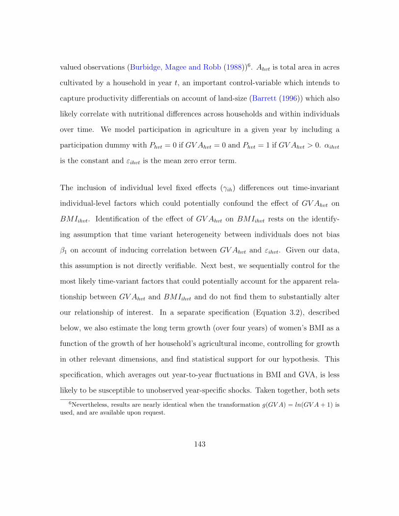
valued observations (Burbidge, Magee and Robb (1988))6. Ahvt is total area in acres

cultivated by a household in year t, an important control-variable which intends to

capture productivity differentials on account of land-size (Barrett (1996)) which also

likely correlate with nutritional differences across households and within individuals

over time. We model participation in agriculture in a given year by including a

participation dummy with Phvt = 0 if GV Ahvt = 0 and Phvt = 1 if GV Ahvt > 0. αihvt

is the constant and εihvt is the mean zero error term.

The inclusion of individual level fixed effects (γih) differences out time-invariant

individual-level factors which could potentially confound the effect of GV Ahvt on

BMIihvt. Identification of the effect of GV Ahvt on BMIihvt rests on the identify-

ing assumption that time variant heterogeneity between individuals does not bias

β1 on account of inducing correlation between GV Ahvt and εihvt. Given our data,

this assumption is not directly verifiable. Next best, we sequentially control for the

most likely time-variant factors that could potentially account for the apparent rela-

tionship between GV Ahvt and BMIihvt and do not find them to substantially alter

our relationship of interest. In a separate specification (Equation 3.2), described

below, we also estimate the long term growth (over four years) of women’s BMI as a

function of the growth of her household’s agricultural income, controlling for growth

in other relevant dimensions, and find statistical support for our hypothesis. This

specification, which averages out year-to-year fluctuations in BMI and GVA, is less

likely to be susceptible to unobserved year-specific shocks. Taken together, both sets

6Nevertheless, results are nearly identical when the transformation g(GV A) = ln(GV A + 1) isused, and are available upon request.

143

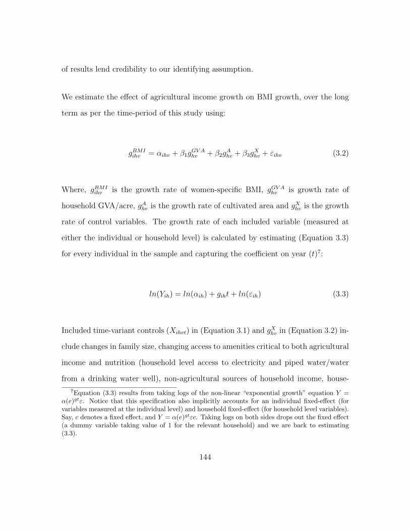
of results lend credibility to our identifying assumption.

We estimate the effect of agricultural income growth on BMI growth, over the long

term as per the time-period of this study using:

gBMIihv = αihv + β1g

GV Ahv + β2g

Ahv + β3g

Xhv + εihv (3.2)

Where, gBMIihv is the growth rate of women-specific BMI, gGV Ahv is growth rate of

household GVA/acre, gAhv is the growth rate of cultivated area and gXhv is the growth

rate of control variables. The growth rate of each included variable (measured at

either the individual or household level) is calculated by estimating (Equation 3.3)

for every individual in the sample and capturing the coefficient on year (t)7:

ln(Yih) = ln(αih) + giht+ ln(εih) (3.3)

Included time-variant controls (Xihvt) in (Equation 3.1) and gXhv in (Equation 3.2) in-

clude changes in family size, changing access to amenities critical to both agricultural

income and nutrition (household level access to electricity and piped water/water

from a drinking water well), non-agricultural sources of household income, house-

7Equation (3.3) results from taking logs of the non-linear “exponential growth” equation Y =α(e)gtε. Notice that this specification also implicitly accounts for an individual fixed-effect (forvariables measured at the individual level) and household fixed-effect (for household level variables).Say, c denotes a fixed effect, and Y = α(e)gtεc. Taking logs on both sides drops out the fixed effect(a dummy variable taking value of 1 for the relevant household) and we are back to estimating(3.3).

144

hold medical expenditure and village-level rainfall. One of the major strengths of

the ICRISAT data are the detailed manner in which household income is tracked- not

based on recall as is typical in surveys of this kind, but through monthly visitations to

households. We include four major categories of non-agricultural income as controls-

livestock income, income from non-agriculture, unearned income and income from

agriculture labor8. In the absence of detailed health data, household medical ex-

penditure is used as a proxy for year-specific health shocks which could both effect

agricultural income through the capacity to work on farm and directly affect BMI.

Village-level rainfall, undoubtedly affects agricultural productivity and also likely

affects nutrition outcomes via altering the individuals disease environment9.

Finally, to account for unobserved aggregate shocks, we cluster our standard errors

8Income from non-agriculture includes income from salaried jobs, income from caste occupations,business income, other non-farm income and income from non-farm migratory work. Unearnedincome includes gifts and remittances, savings and deposits and rental income. Agricultural laborincome includes income from both working in the village labor market and migratory labor income.

9A different strategy to address concerns of correlation between GV Ahvt and εihvt would be toinstrument GV Ahvt with a variable correlated with agricultural income but not with individualnutrition. However, our dataset does not offer suitable instruments to pursue this strategy. Bothsoil quality and irrigation, instruments suggested in the literature (Slavchevska (2015)) to addressendogeneity concerns, lack within individual variation over time, necessary for identification inour model. For instance, the median yearly deviation of “cultivated area under irrigation”, fromindividual-specific means is 0. Another identification concern relevant in this context is one ofreverse causality. This is the idea that better nourished individuals may be able to apply theirlabor more intensively in the agricultural production process and may hence enjoy higher output.Even though, clearly, BMI in our data is recorded after data on agricultural output for a yearwas collected, temporal persistence in BMI data could potentially invalidate our results. To checkwhether this is a concern in our context, we include lagged BMI (by a year) in our final specificationas an explanatory variable. The inclusion of lagged BMI, has no effect on the estimated effect sizeof GV Ahvt, in fact the effect is somewhat strengthened. However, by including lagged BMI welose close to 40 percent of our observations, which nearly doubles our standard errors, makingour inference imprecise. Since anthropometric data collection started only in 2010, by includingin lagged BMI, we lose all of our 2010 observations (BMI missing for 2009) and some additionalobservations for which BMI in the previous year was missing. These results have been omitted forbrevity but are available upon request.

145

at the village level. Because we have a small number of villages (n=18), we boot-

strap standard errors on our coefficients of interest using Wild cluster bootstrapping

(Cameron and Miller (2015)). This addresses concerns that with a small number of

clusters standard asymptotic theory cannot be used to make inference and the use of

standard distributional assumptions yield confidence intervals that are “too narrow”.

To address concerns regarding serially correlated errors, we also alternatively clus-

ter at the individual level, but in most cases these standard errors are smaller and

therefore have been omitted for the sake of brevity, but are available upon request.

3.4 Results

3.4.1 Do Agricultural Incomes Impact Womens Nutritional

Status?

The extent to which the agricultural sector can influence individuals’ nutritional

status, is a function of the size of the sector and its economic importance at the

household-level. In the context of diversifying rural economic activity and the grow-

ing importance of the rural non-farm sector, the role of agriculture in poverty reduc-

tion and nutritional improvements, is not immediately obvious and requires detailed

consideration. In Figure 3.3 we look at the sectoral composition of household in-

comes, to investigate the relative economic significance of farming activity. Income

from farming (i.e. crop income) is the largest source of income for households in

146

our sample and, on average, accounts for around a third of all income. In com-

parison, the share of earned non-agricultural income, while on an upward trend, is

still small, relative to farming. The “unearned income category comprises of rental

income (including rent from land), income from gifts and remittances and savings

and deposits.

Thus, the break-down of the sectoral composition of household incomes posits an

important role of crop incomes as a source of income for purchases and production of

food for self-consumption. We also find descriptive evidence to support that the rela-

tive efficacy of crop incomes versus non-agricultural incomes, in improving nutrition,

could be operating via the gender pathway. Across both the non-agricultural sector

and farming, a majority of income earned accrues to males. However, as can be seen

in Figure 3.4, the proportion of income accruing to women, is nearly two times as

large in farming as it is in non-agriculture. To the extent that women spend more

time working in farming than in non-agriculture, increases in agricultural output can

plausibly afford women control over a larger share of household economic production

and hence greater bargaining power over the allocation of household resources.

Table 3.2 presents results, from our baseline specification (without secondary con-

trols), of the effect of agricultural income on womens BMI. For single crop estimates,

“yield” (i.e. quantity of output per acre) is often used as a simple measure of out-

put. GVA is a comparable measure, except it is in monetary terms and allows us to

aggregate across crops. Aggregation across crops is necessary in our sample because

of the wide variety of crops that households grow. Column (1) includes village fixed

147

effects and column (2) includes individual fixed effects. Therefore, in column (1), we

compare women’s BMI across households with differing agricultural incomes, within

village and year. These estimates utilize cross-sectional variation across households

and compared to the estimates in column (2) are demonstrably biased upwards. In

column (2), we estimate individual-level deviations in BMI (from their person-specific

means) as a function of year-wise deviations in household GVA/acre and, hence, uti-

lize within-individual variation in estimating the effect of agricultural incomes. These

estimates are not confounded by observed and unobserved time-invariant differences

between individuals that weaken the validity of cross-sectional estimates.

In Figure 3.2 we see some individuals with very large BMI changes (<-4/>+4)

over the time-period under consideration. Heights for these individuals were in-

deed recorded consistently, and large BMI changes are purely attributable to large

changes in weight, a metric for which it is considerably harder to discern between

actual changes versus measurement error. In column (3), we explore how sensitive

our estimates are to the exclusion of outliers. In particular, we exclude 15 smallest

and 15 largest individual-level BMI deviations to find that the point estimate on

GVA/acre reduces somewhat. The results however become more precise. In a subse-

quent section, we analyze the implications of our findings for the range of effect-sizes

implied by our treatment of outlier observations. In Table 3.2 and in subsequent ta-

bles, for robustness, we present results first with no outliers dropped and next with

15 smallest and 15 largest observations dropped10.

10To justify why we exclude 15 smallest and 15 largest observations, in Table 3.3 we report howthe effect-size changes when 5, 10 and 15 smallest and largest observations are dropped from thesample. Dropping the 5 smallest and 5 largest observations has the largest impact on our estimate

148

Cross-sectional/within village estimates are presented in Table 3.4 for comparison

with subsequent results that include individual fixed effects (Table 3.5). From the

cross-sectional results in Table 3.4 it is apparent that once we account for other

differences between households and individuals by including relevant controls, no

independent statistically significant effect of agricultural income on BMI can be es-

tablished. Table 3.5 presents results from the short term specification (Equation 1)

and sequentially adds in household-level controls (col. 1), village-level rainfall (col.

2), removes BMI outliers (col. 3), and presents a final set of results with the full set

of controls and without outliers (col. 4). Here, once we account for individual fixed

effects, the effect of agricultural income on women’s BMI is robust to the inclusion

of household level controls shown in column (1). This points to the importance of

household and individual level panel data in establishing the result on the effect of

agricultural income on nutritional status. In column (2), we control for village-level

annual rainfall, which only somewhat moderates the effect of GVA/acre on BMI.

Dropping the 15 smallest and 15 largest BMI changes, results in a somewhat smaller

but more precise effect-size (columns 3 & 4).

The sign of the coefficient on household level access to electricity in columns (3,4)

is not in line with intuition. However, given high average levels of electrification

in the sample villages (93-96 percent in 2010-2013), it is possible that households

electrified during the time-period in our study, that is households electrified last,

of GVA/acre (point estimate drops by around 19 percent), but dropping subsequent observationshave a much smaller impact on our point estimate of interest. Moreover, after dropping 15 smallestand 15 largest observations, the next 5 observations on either tail range from 10-14 kilos of weightchange over the time period in our sample, which are plausible weight changes, especially consideringthat given that our panel is not a balanced one.

149

were the worst off households where no year-on-year improvements in maternal BMI

were seen. Nevertheless, as a first order concern, electricity at the household level

is not correlated with household agricultural output, which is re-assuring. Notice,

that in all specifications the sign on the coefficient on the indicator for agricultural

sector participation is consistently negative. Therefore, households that farm have,

on average, lower BMI than households that do not, which could partly indicate

high energy expenditure on account of agricultural work. Thus, the positive sign

on agricultural income is conditional on agricultural-sector participation, with 77

percent of the sample households participating in the sector.

One concern may be that the income variables included are not statistically signif-

icant and hence may not be serving as effective controls on account of being insuf-

ficiently correlated with BMI. In Table 3.6, we re-estimate Table 3.5 with the four

non-agricultural income variables being included as quartiles. As can be seen, higher

quartiles of non-agricultural income, unearned income and agricultural labor income

are indeed significantly correlated with better BMI outcomes. However, accounting

for these controls does not substantially alter the effect of GVA/acre.

The linear-log relationship between BMI and household agricultural income, as mod-

eled in Equation 1 implies a 10 percent increase in GVA/acre is associated with a

BMI increase of 0.0088-0.0117 points, which is a 0.04-0.06 percent increase relative

to mean BMI. To further give a sense of the economic implication of our results,

we use the parameter-estimate obtained on the GVA/acre coefficient from different

specifications of our individual fixed-effects model, to compare predicted BMI at

150

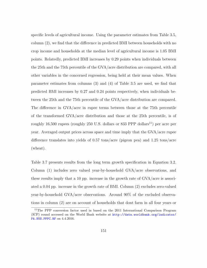
specific levels of agricultural income. Using the parameter estimates from Table 3.5,

column (2), we find that the difference in predicted BMI between households with no

crop income and households at the median level of agricultural income is 1.05 BMI

points. Relatedly, predicted BMI increases by 0.29 points when individuals between

the 25th and the 75th percentile of the GVA/acre distribution are compared, with all

other variables in the concerned regression, being held at their mean values. When

parameter estimates from columns (3) and (4) of Table 3.5 are used, we find that

predicted BMI increases by 0.27 and 0.24 points respectively, when individuals be-

tween the 25th and the 75th percentile of the GVA/acre distribution are compared.

The difference in GVA/acre in rupee terms between those at the 75th percentile

of the transformed GVA/acre distribution and those at the 25th percentile, is of

roughly 16,500 rupees (roughly 250 U.S. dollars or 833 PPP dollars11) per acre per

year. Averaged output prices across space and time imply that the GVA/acre rupee

difference translates into yields of 0.57 tons/acre (pigeon pea) and 1.25 tons/acre

(wheat).

Table 3.7 presents results from the long term growth specification in Equation 3.2.

Column (1) includes zero valued year-by-household GVA/acre observations, and

these results imply that a 10 pp. increase in the growth rate of GVA/acre is associ-

ated a 0.04 pp. increase in the growth rate of BMI. Column (2) excludes zero-valued

year-by-household GVA/acre observations. Around 90% of the excluded observa-

tions in column (2) are on account of households that dont farm in all four years or

11The PPP conversion factor used in based on the 2011 International Comparison Program(ICP) round accessed on the World Bank website at http://data.worldbank.org/indicator/

PA.NUS.PPPC.RF on 4.4.2016.

151

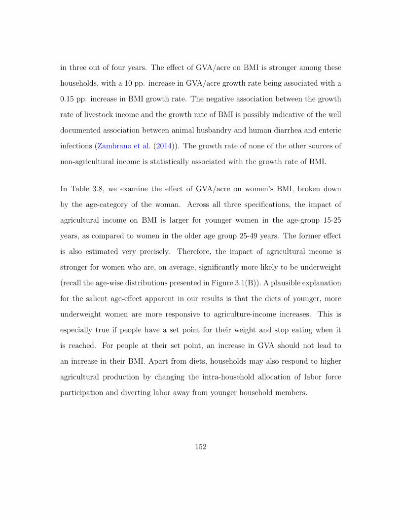
in three out of four years. The effect of GVA/acre on BMI is stronger among these

households, with a 10 pp. increase in GVA/acre growth rate being associated with a

0.15 pp. increase in BMI growth rate. The negative association between the growth

rate of livestock income and the growth rate of BMI is possibly indicative of the well

documented association between animal husbandry and human diarrhea and enteric

infections (Zambrano et al. (2014)). The growth rate of none of the other sources of

non-agricultural income is statistically associated with the growth rate of BMI.

In Table 3.8, we examine the effect of GVA/acre on women’s BMI, broken down

by the age-category of the woman. Across all three specifications, the impact of

agricultural income on BMI is larger for younger women in the age-group 15-25

years, as compared to women in the older age group 25-49 years. The former effect

is also estimated very precisely. Therefore, the impact of agricultural income is

stronger for women who are, on average, significantly more likely to be underweight

(recall the age-wise distributions presented in Figure 3.1(B)). A plausible explanation

for the salient age-effect apparent in our results is that the diets of younger, more

underweight women are more responsive to agriculture-income increases. This is

especially true if people have a set point for their weight and stop eating when it

is reached. For people at their set point, an increase in GVA should not lead to

an increase in their BMI. Apart from diets, households may also respond to higher

agricultural production by changing the intra-household allocation of labor force

participation and diverting labor away from younger household members.

152

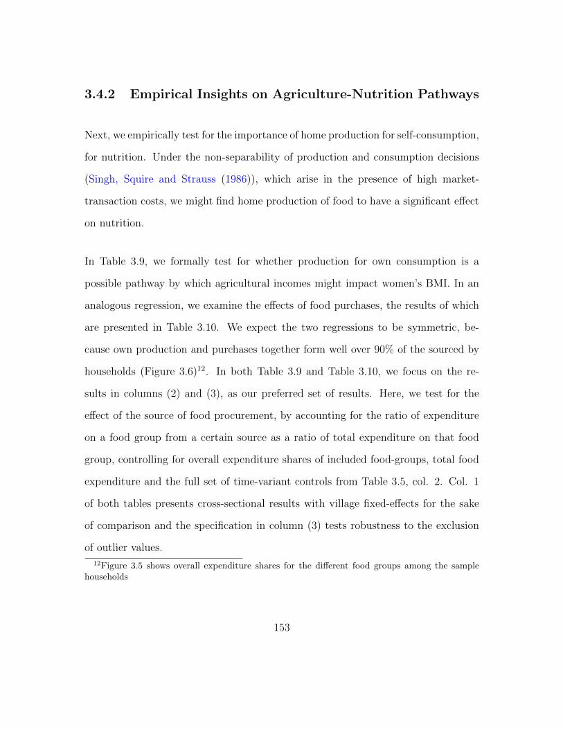
3.4.2 Empirical Insights on Agriculture-Nutrition Pathways

Next, we empirically test for the importance of home production for self-consumption,

for nutrition. Under the non-separability of production and consumption decisions

(Singh, Squire and Strauss (1986)), which arise in the presence of high market-

transaction costs, we might find home production of food to have a significant effect

on nutrition.

In Table 3.9, we formally test for whether production for own consumption is a

possible pathway by which agricultural incomes might impact women’s BMI. In an

analogous regression, we examine the effects of food purchases, the results of which

are presented in Table 3.10. We expect the two regressions to be symmetric, be-

cause own production and purchases together form well over 90% of the sourced by

households (Figure 3.6)12. In both Table 3.9 and Table 3.10, we focus on the re-

sults in columns (2) and (3), as our preferred set of results. Here, we test for the

effect of the source of food procurement, by accounting for the ratio of expenditure

on a food group from a certain source as a ratio of total expenditure on that food

group, controlling for overall expenditure shares of included food-groups, total food

expenditure and the full set of time-variant controls from Table 3.5, col. 2. Col. 1

of both tables presents cross-sectional results with village fixed-effects for the sake

of comparison and the specification in column (3) tests robustness to the exclusion

of outlier values.

12Figure 3.5 shows overall expenditure shares for the different food groups among the samplehouseholds

153

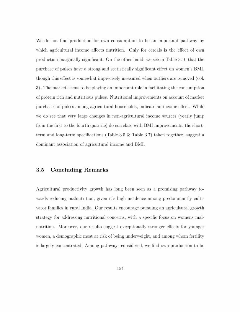
We do not find production for own consumption to be an important pathway by

which agricultural income affects nutrition. Only for cereals is the effect of own

production marginally significant. On the other hand, we see in Table 3.10 that the

purchase of pulses have a strong and statistically significant effect on women’s BMI,

though this effect is somewhat imprecisely measured when outliers are removed (col.

3). The market seems to be playing an important role in facilitating the consumption

of protein rich and nutritious pulses. Nutritional improvements on account of market

purchases of pulses among agricultural households, indicate an income effect. While

we do see that very large changes in non-agricultural income sources (yearly jump

from the first to the fourth quartile) do correlate with BMI improvements, the short-

term and long-term specifications (Table 3.5 & Table 3.7) taken together, suggest a

dominant association of agricultural income and BMI.

3.5 Concluding Remarks

Agricultural productivity growth has long been seen as a promising pathway to-

wards reducing malnutrition, given it’s high incidence among predominantly culti-

vator families in rural India. Our results encourage pursuing an agricultural growth

strategy for addressing nutritional concerns, with a specific focus on womens mal-

nutrition. Moreover, our results suggest exceptionally stronger effects for younger

women, a demographic most at risk of being underweight, and among whom fertility

is largely concentrated. Among pathways considered, we find own-production to be

154

only weakly associated with BMI increases but individual nutrition benefits from

market purchases, especially of protein-rich pulses, to a larger extent. Given the

relative strength of rural markets in India, as compared to countries in sub-Saharan

Africa, we provide an important context to evaluate the income-nutrition pathway via

market access to food. That increasing agricultural incomes also empowers women

within households to allocate expenses towards more nutritious purchases is a hy-

pothesis that requires more detailed consideration, but is consistent with the patterns

in our data. While our results recommend a role for agricultural income increases

to influence nutrition outcomes among the group of households that cultivate, they

also show a trade-off between participation in own farm labor and nutritional gains.

Therefore, investment in labor-saving agricultural technologies can have significant

positive benefits in terms of improved personal health and nutrition.

Lastly, we also find a strong cross-sectional relationship between women’s BMI and

that of her children, as measured by weight-for-height z-scores of children under 5

(Table 3.11). Controlling for a set of village, household, mother and child level vari-

ables, mother’s BMI is a very strong predictor of her child’s weight-for-height z-score

(p-value=0.005). This effect exists net of differences in household socio-economics,

and suggests a more direct link between maternal health and empowerment with

child weight. This effect is likely operational through multiple channels including,

nutritionally, through breast-feeding, or more generally via mothers caring capacity.

This result, in conjunction with recent literature examining the effect of womens

empowerment on child nutrition (Coffey, Khera and Spears (2013)), (Imai et al.

155

(2014)), suggest, additionally, strong inter-generational nutritional benefits of agri-

cultural productivity increases.

156

REFERENCES FOR CHAPTER 3

Barrett, Christopher B. 1996. “On price risk and the inverse farm size-

productivity relationship.” Journal of Development Economics, 51(2): 193–215.

Black, Robert E, Cesar G Victora, Susan P Walker, Zulfiqar A Bhutta,

Parul Christian, Mercedes De Onis, Majid Ezzati, Sally Grantham-

McGregor, Joanne Katz, Reynaldo Martorell, et al. 2013. “Maternal and

child undernutrition and overweight in low-income and middle-income countries.”

The lancet, 382(9890): 427–451.

Bobonis, Gustavo J. 2009. “Is the allocation of resources within the household

efficient? New evidence from a randomized experiment.” Journal of political Econ-

omy, 117(3): 453–503.

Burbidge, John B, Lonnie Magee, and A Leslie Robb. 1988. “Alternative

transformations to handle extreme values of the dependent variable.” Journal of

the American Statistical Association, 83(401): 123–127.

Cameron, A Colin, and Douglas L Miller. 2015. “A practitioners guide to

cluster-robust inference.” Journal of Human Resources, 50(2): 317–372.

Carletto, Gero, Marie Ruel, Paul Winters, and Alberto Zezza. 2015. “Farm-

level pathways to improved nutritional status: introduction to the special issue.”

The Journal of Development Studies.

157

Coffey, Diane. 2015. “Prepregnancy body mass and weight gain during pregnancy

in India and sub-Saharan Africa.” Proceedings of the National Academy of Sci-

ences, 112(11): 3302–3307.

Coffey, Diane, Reetika Khera, and Dean Spears. 2013. “Womens status and

childrens height in India: Evidence from joint rural households.”

Dillon, Andrew, Kevin McGee, and Gbemisola Oseni. 2015. “Agricultural

production, dietary diversity and climate variability.” The Journal of Development

Studies, 51(8): 976–995.

Gulati, Ashok, A Ganesh Kumar, Ganga Shreedhar, and T Nandaku-

mar. 2012. “Agriculture and malnutrition in India.” Food and nutrition bulletin,

33(1): 74–86.

Haddad, Lawrence. 1999. “Womens status: levels, determinants, consequences for

malnutrition, interventions, and policy.”

Harris, Jody, Suneetha Kadiyala, et al. 2012. “The Agriculture-Nutrition Dis-

connect in India: What Do We Know?”

Headey, Derek D. 2013. “Developmental drivers of nutritional change: a cross-

country analysis.” World Development, 42: 76–88.

Hirvonen, Kalle, and John Hoddinott. 2016. “Agricultural production and chil-

dren’s diets: Evidence from rural Ethiopia.” Agricultural Economics.

Hoddinott, John. 2012. “Agriculture, health, and nutrition: toward conceptualiz-

ing the linkages.” Edited by Shenggen Fan and Rajul Pandya-Lorch, 13.

158

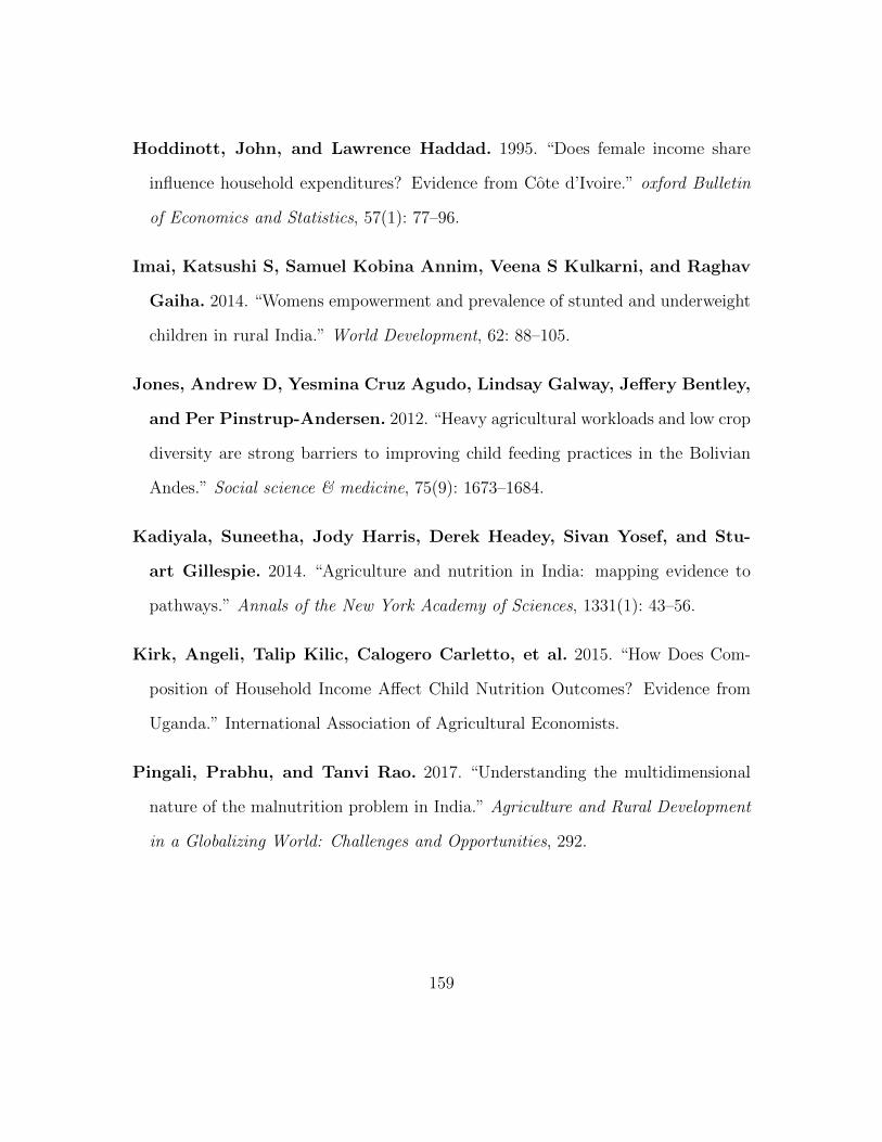
Hoddinott, John, and Lawrence Haddad. 1995. “Does female income share

influence household expenditures? Evidence from Cote d’Ivoire.” oxford Bulletin

of Economics and Statistics, 57(1): 77–96.

Imai, Katsushi S, Samuel Kobina Annim, Veena S Kulkarni, and Raghav

Gaiha. 2014. “Womens empowerment and prevalence of stunted and underweight

children in rural India.” World Development, 62: 88–105.

Jones, Andrew D, Yesmina Cruz Agudo, Lindsay Galway, Jeffery Bentley,

and Per Pinstrup-Andersen. 2012. “Heavy agricultural workloads and low crop

diversity are strong barriers to improving child feeding practices in the Bolivian

Andes.” Social science & medicine, 75(9): 1673–1684.

Kadiyala, Suneetha, Jody Harris, Derek Headey, Sivan Yosef, and Stu-

art Gillespie. 2014. “Agriculture and nutrition in India: mapping evidence to

pathways.” Annals of the New York Academy of Sciences, 1331(1): 43–56.

Kirk, Angeli, Talip Kilic, Calogero Carletto, et al. 2015. “How Does Com-

position of Household Income Affect Child Nutrition Outcomes? Evidence from

Uganda.” International Association of Agricultural Economists.

Pingali, Prabhu, and Tanvi Rao. 2017. “Understanding the multidimensional

nature of the malnutrition problem in India.” Agriculture and Rural Development

in a Globalizing World: Challenges and Opportunities, 292.

159

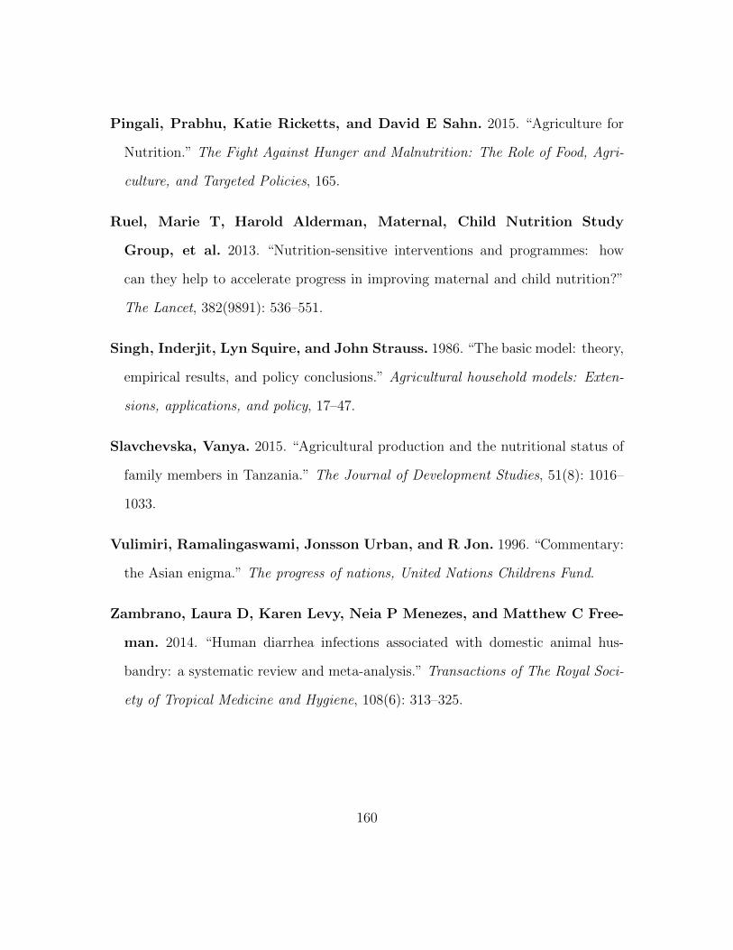
Pingali, Prabhu, Katie Ricketts, and David E Sahn. 2015. “Agriculture for

Nutrition.” The Fight Against Hunger and Malnutrition: The Role of Food, Agri-

culture, and Targeted Policies, 165.

Ruel, Marie T, Harold Alderman, Maternal, Child Nutrition Study

Group, et al. 2013. “Nutrition-sensitive interventions and programmes: how

can they help to accelerate progress in improving maternal and child nutrition?”

The Lancet, 382(9891): 536–551.

Singh, Inderjit, Lyn Squire, and John Strauss. 1986. “The basic model: theory,

empirical results, and policy conclusions.” Agricultural household models: Exten-

sions, applications, and policy, 17–47.

Slavchevska, Vanya. 2015. “Agricultural production and the nutritional status of

family members in Tanzania.” The Journal of Development Studies, 51(8): 1016–

1033.

Vulimiri, Ramalingaswami, Jonsson Urban, and R Jon. 1996. “Commentary:

the Asian enigma.” The progress of nations, United Nations Childrens Fund.

Zambrano, Laura D, Karen Levy, Neia P Menezes, and Matthew C Free-

man. 2014. “Human diarrhea infections associated with domestic animal hus-

bandry: a systematic review and meta-analysis.” Transactions of The Royal Soci-

ety of Tropical Medicine and Hygiene, 108(6): 313–325.

160

Figures & Tables for Chapter 3

Figure 3.1: BMI Distribution of Sample Women (A), and BMI distributionby Age (B)

161

Figure 3.2: Distribution of Yearly Deviations from Woman-Specific BMIMeans

162

Figure 3.3: Sectoral Composition of Household Incomes from DifferentSources, by Year

163

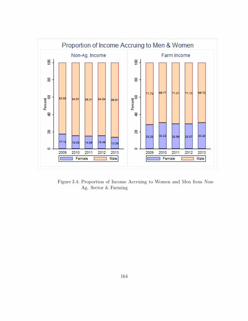
Figure 3.4: Proportion of Income Accruing to Women and Men from Non-Ag. Sector & Farming

164

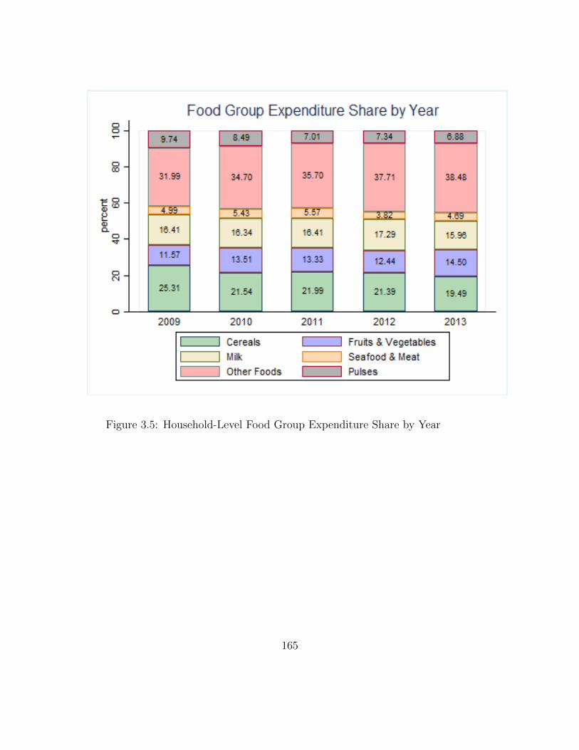
Figure 3.5: Household-Level Food Group Expenditure Share by Year

165

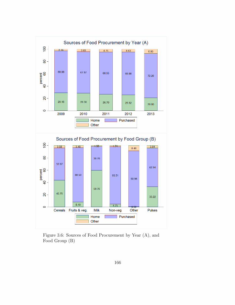
Figure 3.6: Sources of Food Procurement by Year (A), andFood Group (B)

166

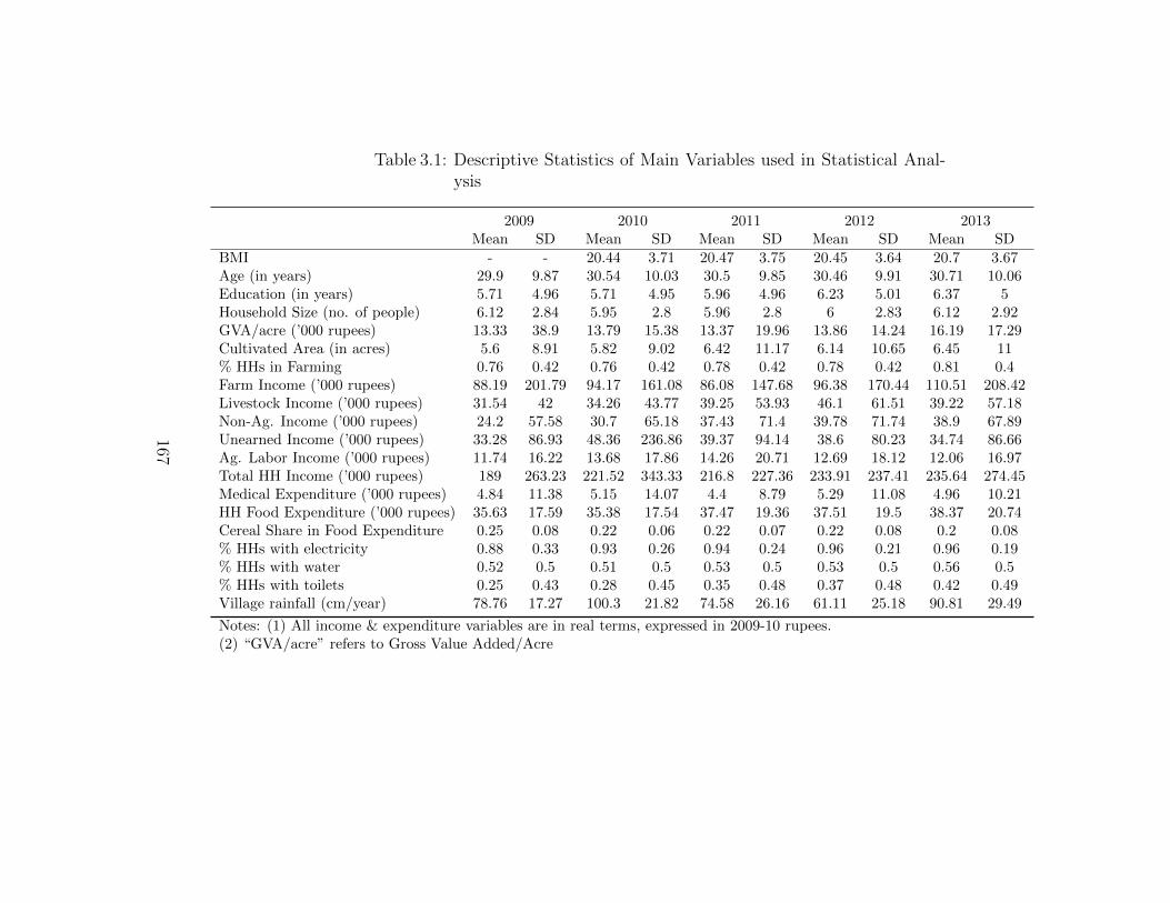
Table 3.1: Descriptive Statistics of Main Variables used in Statistical Anal-ysis

2009 2010 2011 2012 2013Mean SD Mean SD Mean SD Mean SD Mean SD

BMI - - 20.44 3.71 20.47 3.75 20.45 3.64 20.7 3.67Age (in years) 29.9 9.87 30.54 10.03 30.5 9.85 30.46 9.91 30.71 10.06Education (in years) 5.71 4.96 5.71 4.95 5.96 4.96 6.23 5.01 6.37 5Household Size (no. of people) 6.12 2.84 5.95 2.8 5.96 2.8 6 2.83 6.12 2.92GVA/acre (’000 rupees) 13.33 38.9 13.79 15.38 13.37 19.96 13.86 14.24 16.19 17.29Cultivated Area (in acres) 5.6 8.91 5.82 9.02 6.42 11.17 6.14 10.65 6.45 11% HHs in Farming 0.76 0.42 0.76 0.42 0.78 0.42 0.78 0.42 0.81 0.4Farm Income (’000 rupees) 88.19 201.79 94.17 161.08 86.08 147.68 96.38 170.44 110.51 208.42Livestock Income (’000 rupees) 31.54 42 34.26 43.77 39.25 53.93 46.1 61.51 39.22 57.18Non-Ag. Income (’000 rupees) 24.2 57.58 30.7 65.18 37.43 71.4 39.78 71.74 38.9 67.89Unearned Income (’000 rupees) 33.28 86.93 48.36 236.86 39.37 94.14 38.6 80.23 34.74 86.66Ag. Labor Income (’000 rupees) 11.74 16.22 13.68 17.86 14.26 20.71 12.69 18.12 12.06 16.97Total HH Income (’000 rupees) 189 263.23 221.52 343.33 216.8 227.36 233.91 237.41 235.64 274.45Medical Expenditure (’000 rupees) 4.84 11.38 5.15 14.07 4.4 8.79 5.29 11.08 4.96 10.21HH Food Expenditure (’000 rupees) 35.63 17.59 35.38 17.54 37.47 19.36 37.51 19.5 38.37 20.74Cereal Share in Food Expenditure 0.25 0.08 0.22 0.06 0.22 0.07 0.22 0.08 0.2 0.08% HHs with electricity 0.88 0.33 0.93 0.26 0.94 0.24 0.96 0.21 0.96 0.19% HHs with water 0.52 0.5 0.51 0.5 0.53 0.5 0.53 0.5 0.56 0.5% HHs with toilets 0.25 0.43 0.28 0.45 0.35 0.48 0.37 0.48 0.42 0.49Village rainfall (cm/year) 78.76 17.27 100.3 21.82 74.58 26.16 61.11 25.18 90.81 29.49

Notes: (1) All income & expenditure variables are in real terms, expressed in 2009-10 rupees.(2) “GVA/acre” refers to Gross Value Added/Acre

167

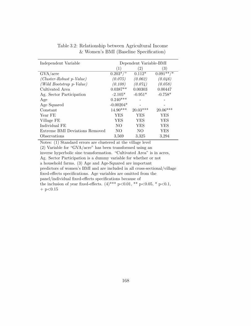
Table 3.2: Relationship between Agricultural Income& Women’s BMI (Baseline Specification)

Independent Variable Dependent Variable-BMI(1) (2) (3)

GVA/acre 0.203*/+ 0.112* 0.091**/*(Cluster-Robust p-Value) (0.075) (0.062) (0.046)(Wild Bootstrap p-Value) (0.108) (0.074) (0.058)Cultivated Area 0.0387** 0.00303 0.00447Ag. Sector Participation -2.105* -0.951* -0.758*Age 0.240*** - -Age Squared -0.00204* - -Constant 14.90*** 20.03*** 20.06***Year FE YES YES YESVillage FE YES YES YESIndividual FE NO YES YESExtreme BMI Deviations Removed NO NO YESObservations 3,569 3,325 3,294

Notes: (1) Standard errors are clustered at the village level(2) Variable for “GVA/acre” has been transformed using aninverse hyperbolic sine transformation. “Cultivated Area” is in acres,Ag. Sector Participation is a dummy variable for whether or nota household farms. (3) Age and Age-Squared are importantpredictors of women’s BMI and are included in all cross-sectional/villagefixed-effects specifications. Age variables are omitted from thepanel/individual fixed-effects specifications because ofthe inclusion of year fixed-effects. (4)*** p<0.01, ** p<0.05, * p<0.1,+ p<0.15

168

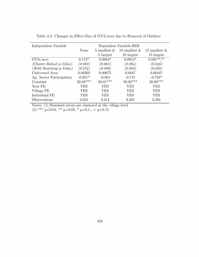
Table 3.3: Changes in Effect-Size of GVA/acre due to Removal of Outliers

Independent Variable Dependent Variable-BMINone 5 smallest & 10 smallest & 15 smallest &

5 largest 10 largest 15 largest

GVA/acre 0.112* 0.0984* 0.0914* 0.091**/*(Cluster-Robust p-Value) (0.062) (0.063) (0.064) (0.046)(Wild Bootstrap p-Value) (0.074) (0.086) (0.080) (0.058)Cultivated Area 0.00303 0.00675 0.0047 0.00447Ag. Sector Participation -0.951* -0.804 -0.715 -0.758*Constant 20.03*** 20.01*** 20.02*** 20.06***Year FE YES YES YES YESVillage FE YES YES YES YESIndividual FE YES YES YES YESObservations 3,325 3,314 3,305 3,294

Notes: (1) Standard errors are clustered at the village level(2) *** p<0.01, ** p<0.05, * p<0.1., + p<0.15

169

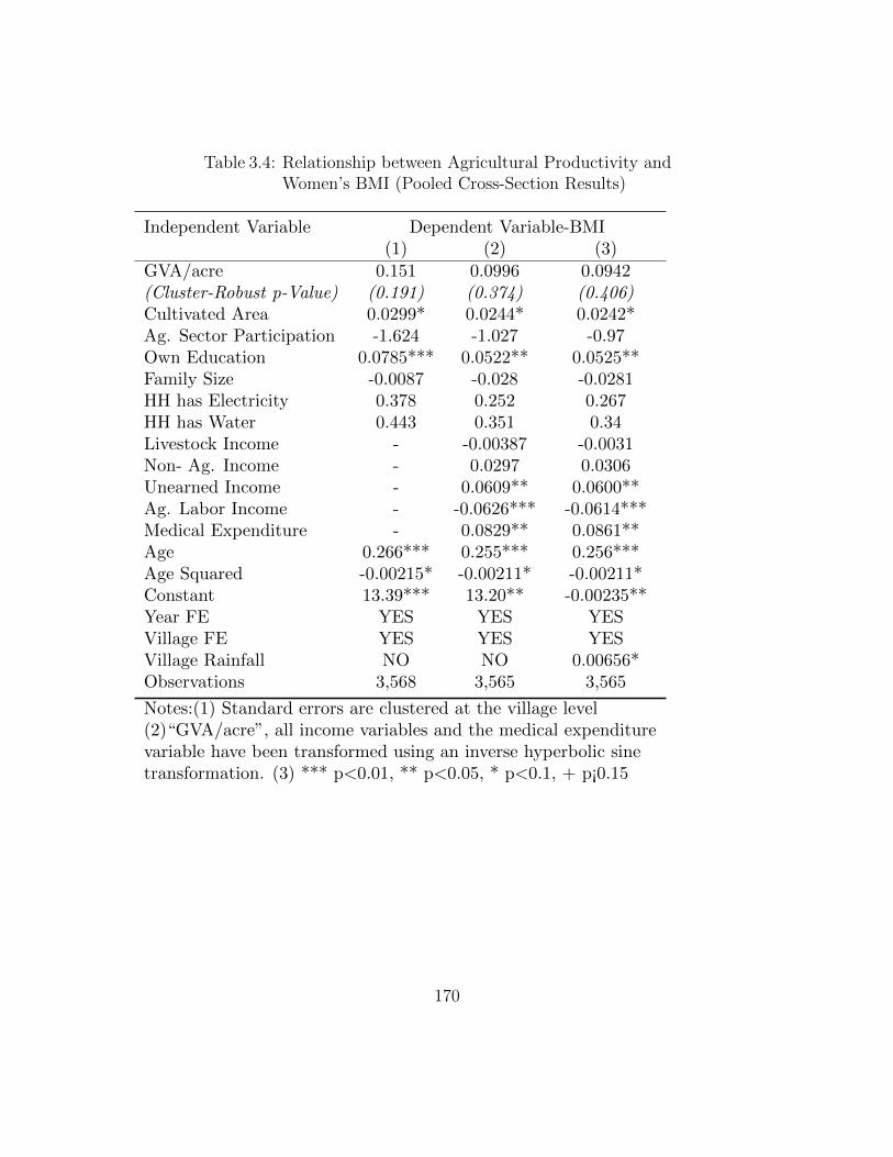
Table 3.4: Relationship between Agricultural Productivity andWomen’s BMI (Pooled Cross-Section Results)

Independent Variable Dependent Variable-BMI(1) (2) (3)

GVA/acre 0.151 0.0996 0.0942(Cluster-Robust p-Value) (0.191) (0.374) (0.406)Cultivated Area 0.0299* 0.0244* 0.0242*Ag. Sector Participation -1.624 -1.027 -0.97Own Education 0.0785*** 0.0522** 0.0525**Family Size -0.0087 -0.028 -0.0281HH has Electricity 0.378 0.252 0.267HH has Water 0.443 0.351 0.34Livestock Income - -0.00387 -0.0031Non- Ag. Income - 0.0297 0.0306Unearned Income - 0.0609** 0.0600**Ag. Labor Income - -0.0626*** -0.0614***Medical Expenditure - 0.0829** 0.0861**Age 0.266*** 0.255*** 0.256***Age Squared -0.00215* -0.00211* -0.00211*Constant 13.39*** 13.20** -0.00235**Year FE YES YES YESVillage FE YES YES YESVillage Rainfall NO NO 0.00656*Observations 3,568 3,565 3,565

Notes:(1) Standard errors are clustered at the village level(2)“GVA/acre”, all income variables and the medical expenditurevariable have been transformed using an inverse hyperbolic sinetransformation. (3) *** p<0.01, ** p<0.05, * p<0.1, + p¡0.15

170

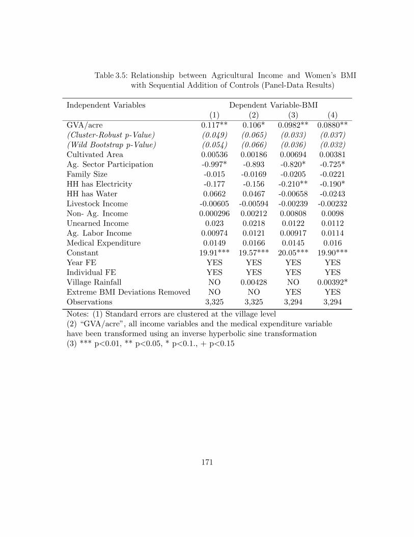
Table 3.5: Relationship between Agricultural Income and Women’s BMIwith Sequential Addition of Controls (Panel-Data Results)

Independent Variables Dependent Variable-BMI(1) (2) (3) (4)

GVA/acre 0.117** 0.106* 0.0982** 0.0880**(Cluster-Robust p-Value) (0.049) (0.065) (0.033) (0.037)(Wild Bootstrap p-Value) (0.054) (0.066) (0.036) (0.032)Cultivated Area 0.00536 0.00186 0.00694 0.00381Ag. Sector Participation -0.997* -0.893 -0.820* -0.725*Family Size -0.015 -0.0169 -0.0205 -0.0221HH has Electricity -0.177 -0.156 -0.210** -0.190*HH has Water 0.0662 0.0467 -0.00658 -0.0243Livestock Income -0.00605 -0.00594 -0.00239 -0.00232Non- Ag. Income 0.000296 0.00212 0.00808 0.0098Unearned Income 0.023 0.0218 0.0122 0.0112Ag. Labor Income 0.00974 0.0121 0.00917 0.0114Medical Expenditure 0.0149 0.0166 0.0145 0.016Constant 19.91*** 19.57*** 20.05*** 19.90***Year FE YES YES YES YESIndividual FE YES YES YES YESVillage Rainfall NO 0.00428 NO 0.00392*Extreme BMI Deviations Removed NO NO YES YESObservations 3,325 3,325 3,294 3,294

Notes: (1) Standard errors are clustered at the village level(2) “GVA/acre”, all income variables and the medical expenditure variablehave been transformed using an inverse hyperbolic sine transformation(3) *** p<0.01, ** p<0.05, * p<0.1., + p<0.15

171

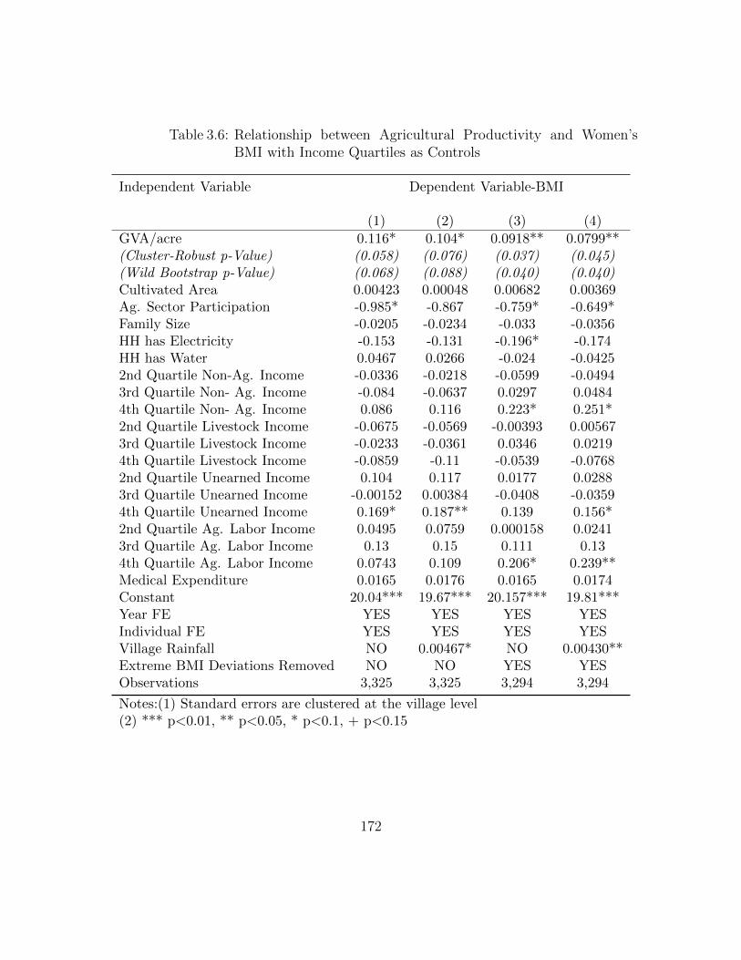
Table 3.6: Relationship between Agricultural Productivity and Women’sBMI with Income Quartiles as Controls

Independent Variable Dependent Variable-BMI

(1) (2) (3) (4)

GVA/acre 0.116* 0.104* 0.0918** 0.0799**(Cluster-Robust p-Value) (0.058) (0.076) (0.037) (0.045)(Wild Bootstrap p-Value) (0.068) (0.088) (0.040) (0.040)Cultivated Area 0.00423 0.00048 0.00682 0.00369Ag. Sector Participation -0.985* -0.867 -0.759* -0.649*Family Size -0.0205 -0.0234 -0.033 -0.0356HH has Electricity -0.153 -0.131 -0.196* -0.174HH has Water 0.0467 0.0266 -0.024 -0.04252nd Quartile Non-Ag. Income -0.0336 -0.0218 -0.0599 -0.04943rd Quartile Non- Ag. Income -0.084 -0.0637 0.0297 0.04844th Quartile Non- Ag. Income 0.086 0.116 0.223* 0.251*2nd Quartile Livestock Income -0.0675 -0.0569 -0.00393 0.005673rd Quartile Livestock Income -0.0233 -0.0361 0.0346 0.02194th Quartile Livestock Income -0.0859 -0.11 -0.0539 -0.07682nd Quartile Unearned Income 0.104 0.117 0.0177 0.02883rd Quartile Unearned Income -0.00152 0.00384 -0.0408 -0.03594th Quartile Unearned Income 0.169* 0.187** 0.139 0.156*2nd Quartile Ag. Labor Income 0.0495 0.0759 0.000158 0.02413rd Quartile Ag. Labor Income 0.13 0.15 0.111 0.134th Quartile Ag. Labor Income 0.0743 0.109 0.206* 0.239**Medical Expenditure 0.0165 0.0176 0.0165 0.0174Constant 20.04*** 19.67*** 20.157*** 19.81***Year FE YES YES YES YESIndividual FE YES YES YES YESVillage Rainfall NO 0.00467* NO 0.00430**Extreme BMI Deviations Removed NO NO YES YESObservations 3,325 3,325 3,294 3,294

Notes:(1) Standard errors are clustered at the village level(2) *** p<0.01, ** p<0.05, * p<0.1, + p<0.15

172

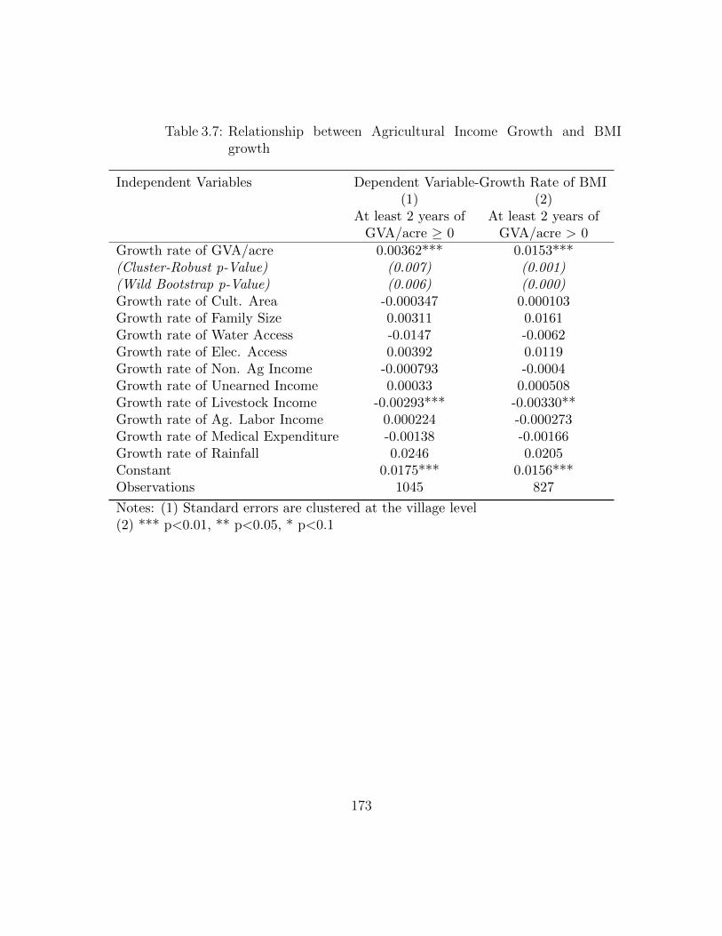
Table 3.7: Relationship between Agricultural Income Growth and BMIgrowth

Independent Variables Dependent Variable-Growth Rate of BMI(1) (2)

At least 2 years of At least 2 years ofGVA/acre ≥ 0 GVA/acre > 0

Growth rate of GVA/acre 0.00362*** 0.0153***(Cluster-Robust p-Value) (0.007) (0.001)(Wild Bootstrap p-Value) (0.006) (0.000)Growth rate of Cult. Area -0.000347 0.000103Growth rate of Family Size 0.00311 0.0161Growth rate of Water Access -0.0147 -0.0062Growth rate of Elec. Access 0.00392 0.0119Growth rate of Non. Ag Income -0.000793 -0.0004Growth rate of Unearned Income 0.00033 0.000508Growth rate of Livestock Income -0.00293*** -0.00330**Growth rate of Ag. Labor Income 0.000224 -0.000273Growth rate of Medical Expenditure -0.00138 -0.00166Growth rate of Rainfall 0.0246 0.0205Constant 0.0175*** 0.0156***Observations 1045 827

Notes: (1) Standard errors are clustered at the village level(2) *** p<0.01, ** p<0.05, * p<0.1

173

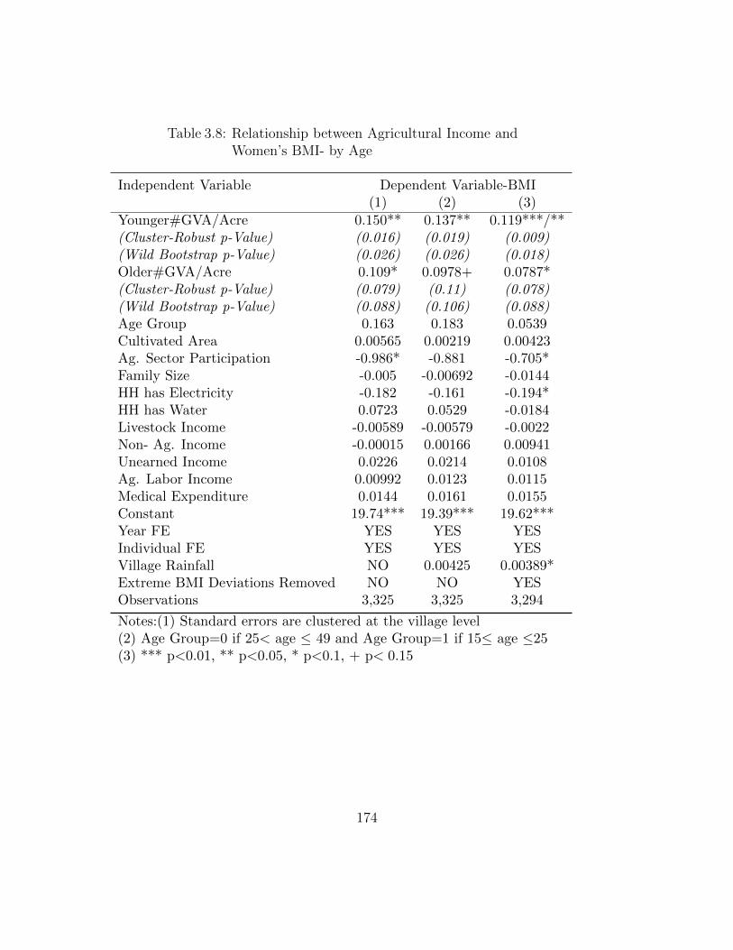
Table 3.8: Relationship between Agricultural Income andWomen’s BMI- by Age

Independent Variable Dependent Variable-BMI(1) (2) (3)

Younger#GVA/Acre 0.150** 0.137** 0.119***/**(Cluster-Robust p-Value) (0.016) (0.019) (0.009)(Wild Bootstrap p-Value) (0.026) (0.026) (0.018)Older#GVA/Acre 0.109* 0.0978+ 0.0787*(Cluster-Robust p-Value) (0.079) (0.11) (0.078)(Wild Bootstrap p-Value) (0.088) (0.106) (0.088)Age Group 0.163 0.183 0.0539Cultivated Area 0.00565 0.00219 0.00423Ag. Sector Participation -0.986* -0.881 -0.705*Family Size -0.005 -0.00692 -0.0144HH has Electricity -0.182 -0.161 -0.194*HH has Water 0.0723 0.0529 -0.0184Livestock Income -0.00589 -0.00579 -0.0022Non- Ag. Income -0.00015 0.00166 0.00941Unearned Income 0.0226 0.0214 0.0108Ag. Labor Income 0.00992 0.0123 0.0115Medical Expenditure 0.0144 0.0161 0.0155Constant 19.74*** 19.39*** 19.62***Year FE YES YES YESIndividual FE YES YES YESVillage Rainfall NO 0.00425 0.00389*Extreme BMI Deviations Removed NO NO YESObservations 3,325 3,325 3,294

Notes:(1) Standard errors are clustered at the village level(2) Age Group=0 if 25< age ≤ 49 and Age Group=1 if 15≤ age ≤25(3) *** p<0.01, ** p<0.05, * p<0.1, + p< 0.15

174

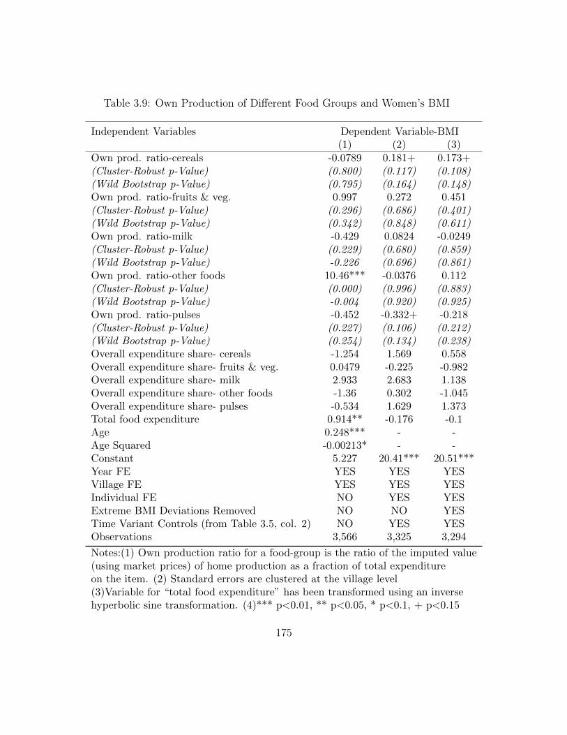
Table 3.9: Own Production of Different Food Groups and Women’s BMI

Independent Variables Dependent Variable-BMI(1) (2) (3)

Own prod. ratio-cereals -0.0789 0.181+ 0.173+(Cluster-Robust p-Value) (0.800) (0.117) (0.108)(Wild Bootstrap p-Value) (0.795) (0.164) (0.148)Own prod. ratio-fruits & veg. 0.997 0.272 0.451(Cluster-Robust p-Value) (0.296) (0.686) (0.401)(Wild Bootstrap p-Value) (0.342) (0.848) (0.611)Own prod. ratio-milk -0.429 0.0824 -0.0249(Cluster-Robust p-Value) (0.229) (0.680) (0.859)(Wild Bootstrap p-Value) -0.226 (0.696) (0.861)Own prod. ratio-other foods 10.46*** -0.0376 0.112(Cluster-Robust p-Value) (0.000) (0.996) (0.883)(Wild Bootstrap p-Value) -0.004 (0.920) (0.925)Own prod. ratio-pulses -0.452 -0.332+ -0.218(Cluster-Robust p-Value) (0.227) (0.106) (0.212)(Wild Bootstrap p-Value) (0.254) (0.134) (0.238)Overall expenditure share- cereals -1.254 1.569 0.558Overall expenditure share- fruits & veg. 0.0479 -0.225 -0.982Overall expenditure share- milk 2.933 2.683 1.138Overall expenditure share- other foods -1.36 0.302 -1.045Overall expenditure share- pulses -0.534 1.629 1.373Total food expenditure 0.914** -0.176 -0.1Age 0.248*** - -Age Squared -0.00213* - -Constant 5.227 20.41*** 20.51***Year FE YES YES YESVillage FE YES YES YESIndividual FE NO YES YESExtreme BMI Deviations Removed NO NO YESTime Variant Controls (from Table 3.5, col. 2) NO YES YESObservations 3,566 3,325 3,294

Notes:(1) Own production ratio for a food-group is the ratio of the imputed value(using market prices) of home production as a fraction of total expenditureon the item. (2) Standard errors are clustered at the village level(3)Variable for “total food expenditure” has been transformed using an inversehyperbolic sine transformation. (4)*** p<0.01, ** p<0.05, * p<0.1, + p<0.15

175

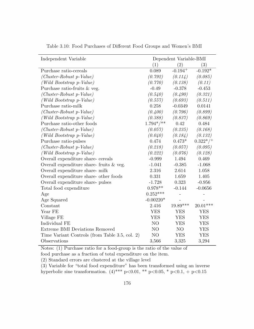
Table 3.10: Food Purchases of Different Food Groups and Women’s BMI

Independent Variable Dependent Variable-BMI(1) (2) (3)

Purchase ratio-cereals 0.089 -0.194+ -0.192*(Cluster-Robust p-Value) (0.792) (0.114) (0.085)(Wild Bootstrap p-Value) (0.770) (0.138) (0.11)Purchase ratio-fruits & veg. -0.49 -0.378 -0.453(Cluster-Robust p-Value) (0.540) (0.490) (0.321)(Wild Bootstrap p-Value) (0.557) (0.693) (0.511)Purchase ratio-milk 0.258 -0.0349 0.0141(Cluster-Robust p-Value) (0.400) (0.796) (0.899)(Wild Bootstrap p-Value) (0.388) (0.837) (0.869)Purchase ratio-other foods 1.794*/** 0.42 0.484(Cluster-Robust p-Value) (0.057) (0.235) (0.168)(Wild Bootstrap p-Value) (0.040) (0.184) (0.132)Purchase ratio-pulses 0.474 0.473* 0.322*/+

(Cluster-Robust p-Value) (0.218) (0.057) (0.095)(Wild Bootstrap p-Value) (0.222) (0.076) (0.128)Overall expenditure share- cereals -0.999 1.494 0.469Overall expenditure share- fruits & veg. -1.041 -0.385 -1.068Overall expenditure share- milk 2.316 2.614 1.058Overall expenditure share- other foods 0.331 1.659 1.405Overall expenditure share- pulses -1.728 0.323 -0.956Total food expenditure 0.978** -0.144 -0.0656Age 0.252*** - -Age Squared -0.00220* - -Constant 2.416 19.89*** 20.01***Year FE YES YES YESVillage FE YES YES YESIndividual FE NO YES YESExtreme BMI Deviations Removed NO NO YESTime Variant Controls (from Table 3.5, col. 2) NO YES YESObservations 3,566 3,325 3,294

Notes: (1) Purchase ratio for a food-group is the ratio of the value offood purchase as a fraction of total expenditure on the item.(2) Standard errors are clustered at the village level(3) Variable for “total food expenditure” has been transformed using an inversehyperbolic sine transformation. (4)*** p<0.01, ** p<0.05, * p<0.1, + p<0.15

176

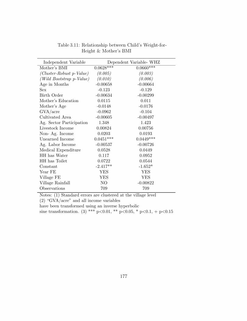
Table 3.11: Relationship between Child’s Weight-for-Height & Mother’s BMI

Independent Variable Dependent Variable- WHZ

Mother’s BMI 0.0628*** 0.0660***(Cluster-Robust p-Value) (0.005) (0.003)(Wild Bootstrap p-Value) (0.010) (0.006)Age in Months -0.00658 -0.00664Sex -0.123 -0.129Birth Order -0.00634 -0.00299Mother’s Education 0.0115 0.011Mother’s Age -0.0148 -0.0176GVA/acre -0.0962 -0.104Cultivated Area -0.00605 -0.00497Ag. Sector Participation 1.348 1.423Livestock Income 0.00824 0.00756Non- Ag. Income 0.0203 0.0193Unearned Income 0.0451*** 0.0449***Ag. Labor Income -0.00537 -0.00726Medical Expenditure 0.0528 0.0449HH has Water 0.117 0.0952HH has Toilet 0.0722 0.0544Constant -2.417** -1.652*Year FE YES YESVillage FE YES YESVillage Rainfall NO -0.00822Observations 709 709

Notes: (1) Standard errors are clustered at the village level(2) “GVA/acre” and all income variableshave been transformed using an inverse hyperbolicsine transformation. (3) *** p<0.01, ** p<0.05, * p<0.1, + p<0.15

177