Accounting Horizons PCAOB Inspections and Large Accounting Firms
Upload
khangminh22Category
view
2download
0


Human Capital in DevelopmentAccounting and Other Essays inEconomics
Hannes Malmberg

ii
© Hannes Malmberg, Stockholms universitet 2017
ISBN 978-91-7649-829-3ISBN 978-91-7649-830-9ISSN 0346-6892
Cover Picture: Graduation photo, Kalmar Teaching College, 1941. Private photo. Author’sgrandmother second to the right in front – the first in her family to obtain an educationbeyond primary level.
Universitetsservice US-AB, Stockholm 2017
Distributor: Institute for International Economic Studies

iii
Doctoral DissertationDepartment of EconomicsStockholm University
Abstracts
Human Capital and Development Accounting Revisited. Iquantify the effects on development accounting of allowing for imper-fectly substitutable labor services. To estimate the degree of substi-tutability between skilled and unskilled labor services in a cross-countrysetting, it is sufficient to estimate the relative price of skilled labor ser-vices, and I develop a novel method for estimating this relative price usinginternational trade data. My method exploits the negative relationshipbetween relative prices of skilled labor services and relative export valuesin skill-intensive industries. I find an approximately constant elasticityof substitution with a value of about 1.3. When integrating my resultsinto a development accounting exercise, I find that efficiency differencesin skilled labor are more important than uniform efficiency differences inexplaining world income differences. Under the traditional developmentaccounting assumption of neutral technology differences, the skilled la-bor efficiency differences reflect human capital quality differences, andhuman capital differences can explain a majority of world income diff-erences. Relaxing the assumption of neutral technology differences, analternative explanation is that there are large skill-biased technologydifferences between rich and poor countries.
Price Level Determination When Tax Payments Are Re-quired in Money. We formalize the idea that the price level can bedetermined by a requirement that taxes be paid in money. We show thatif households have to pay a money tax of a fixed real value and themoney supply is constant, there is a unique stationary price level, and acontinuum of non-stationary deflationary equilibria. The non-stationaryequilibria can be excluded if we introduce an arbitrarily lax borrow-ing constraint. Thus, in the basic model, tax requirements can uniquely

iv
determine the price level. When money has liquidity value, tax require-ments can exclude self-fulfilling hyperinflations.
Swedish Unemployment Dynamics. We decompose the sourcesof unemployment variations into contributions from variations in differ-ent labor market flows. We develop a decomposition method that allowsfor a distinction between permanent and temporary employment and aslow convergence to the steady state, and we apply the method to theSwedish labor market for the period 1987-2012. Variations in unemploy-ment are driven to an approximately equal degree by variations in (i)flows from unemployment to employment, (ii) flows from employmentto unemployment, and (iii) flows in and out of the labor force. Flowsinvolving temporary contracts account for 44% of the variation in un-employment, even though temporary workers only constitute 13% of theworking-age population. Neglecting out-of-steady-state dynamics leadsto an overestimation of the importance of flows involving permanentcontracts.
Supply Chain Risk and the Pattern of Trade. This paper an-alyzes the interaction of supply chain risk and trade patterns. We con-struct a model where an industry’s risk sensitivity is determined by thenumber of customized components that it uses, and countries with a lowsupply chain risk specialize in risk-sensitive goods. Based on our theory,we construct an empirical measure of risk sensitivity from input-outputtables and customization measures. Using industry-level trade data anda variety of risk proxies, we show that countries with a low supply chainrisk disproportionately export risk-sensitive goods.

v
Till Henrietta och min familj.

vi

vii
The men of experiment are like the ant, they only collect and use; the rea-soners resemble spiders, who make cobwebs out of their own substance.But the bee takes a middle course: it gathers its material from the flow-ers of the garden and of the field, but transforms and digests it by apower of its own. Not unlike this is the true business of philosophy; forit neither relies solely or chiefly on the powers of the mind, nor doesit take the matter which it gathers from natural history and mechanicalexperiments and lay it up in the memory whole, as it finds it, but laysit up in the understanding altered and digested. Therefore from a closerand purer league between these two faculties, the experimental and therational...much may be hoped.
Francis Bacon, Novum Organum, 1620

viii

ix
Acknowledgments
It feels special to stand at the end of this long journey. Despite hardwork and occasional despair, doing a PhD in economics has been themost intellectually exciting undertaking of my life, and it has changedmy outlook on the world beyond recognition. Here, I would like to thanksome of the many people who have been part of this journey.
I first want to thank my main advisor, Per Krusell, for all his supportduring these years. Throughout my thesis work, Per has given me thefreedom to explore my own more or less realistic research ideas, alwaysbeing liberal with content and methodology, but dogmatic on qualityand relevance. Moreover, at critical moments, he has provided small, butdecisive, nudges that have moved my projects in the right direction. Forexample, after I had presented early-stage work on what later becamethe main chapter of my thesis, Per noted in passing that, maybe, it couldbe worth thinking about what my results on human capital meant fordevelopment accounting. The title and the main chapter of my thesistestify to the result of exploring this 10 second comment, and this ex-perience was not unique during my thesis writing. I am also extremelygrateful for Per’s consistent support during the stressful job market ex-perience.
Another piece of helpful advice from Per was that I should talk moreto Timo Boppart. This piece of advice led to many exciting discussionsbetween me and Timo on economics, and Timo eventually became myco-advisor. I am grateful for his careful reading and insightful commentsthat have considerably improved my research, and I am constantly im-pressed by his open-mindedness, passion for economics, and sound sci-entific judgment.
I also want to thank the two other members of my job marketcommittee: Torsten Persson and John Hassler. Torsten has beena fantastic source of support. He has always taken the time topatiently deal with the anxieties of a novice researcher, gently

x
steering me away from patently unproductive research paths,and, more than once, he has helped me situate a collection ofunstructured thoughts in the broader framework of our discipline.John has commented extensively on my research, especially onmy earlier projects, and with his experience from practical policy-making, he has often helped me think about the relevance of my research.
I started my economics career at the Department of Economics. Inthe fall of 2010, I did a number of intermediate-level courses, after whichAnna Seim and Yves Zenou made me a fantastic service by encouragingme and helping me to apply to the PhD program.
However, over the last five years, the IIES has been my academichome. Its intense intellectual environment with seminars, kitchen dis-cussions, research meetings, and dinners has been truly inspiring. Itsequally intense social environment has made me feel at home, and hasbeen the foundation of my intellectual work. I am grateful to all fac-ulty, graduate students, and administrative staff who sustain this greatinstitution.
In addition to my job market committee, I particularly want to thankIngvild Almås, Timo Boppart, and Konrad Burchardi for inviting me tojoin their Söderberg project, Philippe Aghion for extensive commentson my work, Assar Lindbeck for consistently providing a historical per-spective on our discipline, Kurt Mitman for a brief, but extremely use-ful, how-to-guide on doing research in quantitative macroeconomics, andDavid Strömberg for many interesting discussions on methodology, aswell as for providing support on the econometric aspects of my job mar-ket paper.
I have also enjoyed discussions in the macro group with TobiasBroer, Sebastian Koehne, Alexander Kohlhas, and Kathrin Schlafmann,as well as discussions with Tessa Bold, Tom Cunningham, Arash Nekoei,Peter Nilsson, Robert Östling, Jon de Quidt, Anna Sandberg, and JakobSvensson. The administrative staff at the IIES has been the source ofexceptional support and many fun kitchen discussions over the years. I

xi
am especially grateful to Christina Lönnblad for her efficiency and herpatience, and for her excellent editorial support during my thesis writing.
Along the way, I have also been fortunate to form a number of veryclose friendships. In my first year, I met Erik Öberg, and Per quicklydubbed us the young Chip an’ Dale (Piff och Puff ) of the IIES (John andPer being the less young versions). We have shared coursework, travels,authorship, office, and many hours of conversations together. Later, I alsobefriended Niels-Jakob Harbo Hansen and Karl Harmenberg. Together,these three friends kept me pleasantly distracted at work through theirreadiness to engage in intellectual discussions on every conceivable topic,and we all became close friends in private as well. Their friendship hasbrought much joy and intellectual excitement to my PhD days.
I am also very grateful for having been part of the broader graduatestudent community of the IIES and the greater Stockholm area. At theIIES, I would especially like to thank Saman Darougheh, Sirus Dehdari,and Jósef Sigurdsson for many fun (and occasionally frustrating) lunchdiscussions, walks, and after-works. I also want to thank the macro group,especially Richard Foltyn, Matilda Kilström, and Jonna Olsson. Further-more, I have had interesting discussions with, among others, Anna Ae-varsdottir, Agneta Berge, Mathias Iwanowsky, Mounir Karadja, ShuheiKitamura, Nathan Lane, Benedetta Lerva, Georg Marthin, Erik Prawitz,Riikka Savolainen, Abdulaziz Shifa, and Miri Stryjan.
Space does not permit me to mention everyone that I have enjoyedtalking to in the greater Stockholm area, but I want to especially thankAdam Altmejd, Niklas Amberg, Julia Boguslaw, Evelina Bonnier, AxelCronert, Montasser Ghachem, Johan Grip, Johannes Hagen, KarinHederos, Magnus Irie, Siri Isaksson, Dany Kessel, Gustaf Lundgren,Elin Molin, Arieda Muco, Paula Roth, Bengt Söderberg, and AndualemMengistu for many exciting discussions over the years.
Going beyond Stockholm, I want to thank Axel Gottfries at the Uni-versity of Cambridge. He has been one of my absolutely closest friendssince high school, and I am constantly inspired and challenged by his

xii
warmth, his sharp eye and mind, his strong ethical views, and his deepknowledge of economic theory. I also want to thank David Bloom atHarvard School of Public Health for receiving me on an exchange visit,and to Maximilian Eber and Kinley Salmon at Harvard University forfruitful collaboration and for many exciting conversations. I have alsobenefited from discussions with Xavier Jaravel at Harvard University.
Economics is but one of many academic disciplines, and academicknowledge is but one of many ways of understanding the world. Through-out my PhD studies, I have drawn intellectual nourishment from exten-sive work and discussions with people outside of economics, and outsideof academia altogether.
The Department of Mathematics at Stockholm University has en-abled me to pursue a part-time PhD in mathematical statistics in par-allel with my studies in economics, and my advisors Ola Hössjer andDmitri Silvestrov have been very generous with their time in supportingmy mathematical research.
I would also like to thank Zihan Hans Liu, who was my roommatewhen I was studying at Cambridge, and who transformed myunderstanding of mathematics. In addition, I’ve benefited greatly fromlong discussions with Arvid Ågren on evolutionary biology, AndreasBjördal on modern management, Hanna Björklund on religious history,Paul Igor Costea on microbiology, Johannes Danielsson on Swedishdomestic and foreign policy, Emma Holten on literature and modernsocial theory, Adam Hurst on biotechnology, Jonathan Illicki onmedicine, Christian Johansson on mathematics, Oskar Lilja on datasciences, Karin Öberg on astronomy and theology, Philip Pärnamets oncognitive psychology and philosophy, Caroline Walerud on technologicalinnovation, Oliver Vikbladh on neuroscience, and Henrik Widmark onurban history and sociology. Without the willingness of these friends todiscuss their perspectives on the world, my outlook on the world wouldhave been much poorer.
Throughout life, my family has been a source of support, inspiration,

xiii
and love. My parents, Bo Malmberg and Lena Sommestad, are bothsocial scientists, and, by osmosis, I came to share their interests. Hour-long discussions around the kitchen table taught me the pleasures ofacademic conversation. For all support, knowledge, and love that I havereceived from them, I am extremely grateful.
My brother Olof and my sister Anna mean the world to me. Olofhas always been my close companion and intellectual sparring partner:often brilliant, sometimes frustrating, but always creative. Anna bringsso much joy to my life through her genuine curiosity and openness; Ienjoy few things more than discussing with Anna what she has learntfrom the world over the last few weeks.
Finally, I want to thank Henrietta for sharing your life with me. Wewalk through this life together, through big things and small. Your love,excitement, humor, warmth, and humanity provide the backdrop againstwhich things make sense and are valuable. You constantly expand how Isee the world, by directing my gaze outwards, away from the sometimesnumbing complexities of the internal world, and towards the richness ofthe lives, feelings, and thoughts of others. For this, and for everythingelse, I am eternally grateful. You are my greatest support and joy, and Ilove you.
Hannes Malmberg, Stockholm, May 2017

xiv
Contents
Introduction 1
1 Human Capital and Development Accounting Revisited 171.1 Introduction . . . . . . . . . . . . . . . . . . . . . . . . . . 171.2 Estimating the relative price of skilled services . . . . . . . 261.3 Development accounting . . . . . . . . . . . . . . . . . . . 381.4 Interpretation of mechanism . . . . . . . . . . . . . . . . . 501.5 Relationship to B Jones (2014) . . . . . . . . . . . . . . . 541.6 Robustness and consistency checks . . . . . . . . . . . . . 561.7 Concluding remarks . . . . . . . . . . . . . . . . . . . . . 66References . . . . . . . . . . . . . . . . . . . . . . . . . . . . . . 69Appendices . . . . . . . . . . . . . . . . . . . . . . . . . . . . . 751.A Environment . . . . . . . . . . . . . . . . . . . . . . . . . 751.B Development accounting . . . . . . . . . . . . . . . . . . . 841.C Estimating the relative price of skilled services . . . . . . . 901.D Mechanisms . . . . . . . . . . . . . . . . . . . . . . . . . . 1041.E Robustness . . . . . . . . . . . . . . . . . . . . . . . . . . 117
2 Price Level Determination When Tax Payments Are Re-quired in Money 1232.1 Introduction . . . . . . . . . . . . . . . . . . . . . . . . . . 1232.2 The model . . . . . . . . . . . . . . . . . . . . . . . . . . . 1282.3 Relationship to the fiscal theory of the price level . . . . . 1342.4 Excluding hyperinflations . . . . . . . . . . . . . . . . . . 136
xv
xvi CONTENTS
2.5 Price level determination under a balanced budget rule . . 1442.6 Discussion . . . . . . . . . . . . . . . . . . . . . . . . . . . 147References . . . . . . . . . . . . . . . . . . . . . . . . . . . . . . 149Appendices . . . . . . . . . . . . . . . . . . . . . . . . . . . . . 151
3 Swedish Unemployment Dynamics 1653.1 Introduction . . . . . . . . . . . . . . . . . . . . . . . . . . 1653.2 Data . . . . . . . . . . . . . . . . . . . . . . . . . . . . . . 1683.3 Method . . . . . . . . . . . . . . . . . . . . . . . . . . . . 1713.4 Estimation and discretization . . . . . . . . . . . . . . . . 1803.5 Results . . . . . . . . . . . . . . . . . . . . . . . . . . . . . 1843.6 Comparison to Elsby et al. (2015) . . . . . . . . . . . . . . 1863.7 Conclusion . . . . . . . . . . . . . . . . . . . . . . . . . . . 188References . . . . . . . . . . . . . . . . . . . . . . . . . . . . . . 188Figures and Tables . . . . . . . . . . . . . . . . . . . . . . . . . 190Appendices . . . . . . . . . . . . . . . . . . . . . . . . . . . . . 206
4 Supply Chain Risk and the Pattern of Trade 2114.1 Introduction . . . . . . . . . . . . . . . . . . . . . . . . . . 2114.2 Literature . . . . . . . . . . . . . . . . . . . . . . . . . . . 2154.3 Model . . . . . . . . . . . . . . . . . . . . . . . . . . . . . 2174.4 Empirical evidence . . . . . . . . . . . . . . . . . . . . . . 2294.5 Conclusion . . . . . . . . . . . . . . . . . . . . . . . . . . . 244References . . . . . . . . . . . . . . . . . . . . . . . . . . . . . . 246Additional results . . . . . . . . . . . . . . . . . . . . . . . . . . 249Appendices . . . . . . . . . . . . . . . . . . . . . . . . . . . . . 251
Sammanfattning 263

Introduction
This thesis consists of four independent chapters on issues in macro-economics, development economics, and trade. While the chapters treatdifferent topics, they jointly reflect my interest in exploring different waysof approaching economic questions. The message of the thesis is one ofmethodological pluralism: economics is well-served when we use multipleways of engaging with its subject matter.
In this introduction, I discuss the thesis with a focus on metho-dology. After briefly summarizing the contents of each chapter, I discussthe methodological approaches that they embody, and the main lessonslearnt from each chapter. I conclude with a discussion of how the thesiswork has shaped my methodological views. The first chapter of the thesisis its main chapter, but my discussion will reflect the chronology of thewriting of the chapters, and will start with Chapters II-IV, and concludewith Chapter I.
Chapter summaries
Chapter II, Price Level Determination When Tax Payments AreRequired in Money, is joint work with Erik Öberg, and explores therole of tax requirements in determining the value of money.
The value of money has proved difficult to model in economics. Thechallenge to theory development is that money is intrinsically useless,which means that standard consumption theory predicts that it shouldhave no value. One of the most widely held theoretical views is that the
1
2 INTRODUCTION
value of money depends on its conventional use as a medium of exchange:I accept your money as payment, because I expect that others will acceptmy money in turn. The value of money is sustained by expectations.While such liquidity-based theories of money are plausible, they do notexplain why expectations should converge on using government money,and why government money rarely, if ever, has suffered a collapse of valuemerely due to a collapse of expectations.
These facts suggest that the value of money is somehow connectedto government power, which raises a question about the nature of thisconnection. This chapter shows that one way in which the governmentcan determine the value of money is by requiring that households paytheir taxes with government-issued money. The idea that the value ofmoney is connected to tax requirements is old, going back to AdamSmith. In our paper, we model this idea, and show conditions under whichthe government can enforce a unique equilibrium of the price level byregulating the money supply and requiring that taxes should be paid withmoney. In cases where money is also valued for its liquidity properties,tax requirements do not necessarily determine the exact value of money,but exclude the possibility that money loses its value through a collapseof expectations.
Chapter III, Swedish Unemployment Dynamics: New Meth-ods and Results, is joint work with Niels-Jakob Harbo Hansen andstudies the statistical properties of unemployment dynamics. This chap-ter belongs to a literature which is motivated by the basic observationthat an increase in unemployment can either be driven by workers losingtheir jobs at a higher rate or by unemployed people taking more timeto find new jobs. Thus, to understand the nature of any given changein unemployment, we need to analyze the underlying flows of the labormarket .
Chapter III develops a new method for decomposing fluctuations inunemployment in the context of a dual labor market featuring a slowconvergence to the steady state. The standard assumption in the lit-erature has been that the current level of unemployment can be well
INTRODUCTION 3
approximated by the steady-state unemployment rate associated withthe current flow rates observed in the data. However, it is also knownthat this approximation works well in a U.S. context, where labor marketgross flows are high, but is problematic in a European context, where theflows are much smaller.
At the same time, many European labor markets are dual, with a rolefor both temporary and permanent contracts. Since the flow propertiesare likely to differ markedly across these two forms of employment, itcan be important to have a method that allows for a distinction betweenpermanent and temporary jobs. To address these issues, we develop adecomposition method which allows for both (i) a slow convergence tothe steady state and (ii) an arbitrary number of labor market states.We apply our method to a new Swedish data set on labor market flowscovering the period 1987-2012.1
Our method is well suited for this application. Indeed, the Swedishlabor market is dual, with temporary contracts accounting for 13% ofthe working-age population, and characterized by relatively low grossflows and a low rate of convergence to the steady state. We find thatvariations in unemployment are driven to an approximately equal degreeby variations in (i) flows from unemployment to employment, (ii) flowsfrom employment to unemployment, and (iii) flows in and out of thelabor force.
We find that flows involving temporary contracts account for 44%of the variation in unemployment, while flows involving permanent con-tracts account for approximately 33% of the variation. The former num-ber is large given the relatively few workers who are employed on tempo-rary contracts. We also show that it is important to account for out-of-steady state dynamics. If we use the decomposition method which relieson approximating the actual state with the steady state, the share ofvariation attributed to flows involving permanent contracts rises from33% to 44%. These results are of broader interest in the study of Eu-
1The most similar method to ours is that of Elsby et al. (2015), which is discussedin the main text.

4 INTRODUCTION
ropean labor markets, since they suggest that decompositions based onthe steady-state assumption are unlikely to be suitable in dual labormarkets.
Chapter IV, Supply Chain Risk and the Pattern of Trade,is joint work with Maximilian Eber. We explore whether countries thatoffer reliable supply chains specialize in goods that are sensitive to supplychain risk. We formalize this hypothesis by constructing a trade modelwith multiple sectors and risky supply chains. Each sector produces agood using a range of intermediate inputs, and the delivery of each inputis subject to a failure risk.
The effect of a delivery failure depends on the nature of the input.Some inputs are standardized, which means that delivery risks are pooledthrough a law of large numbers, and downstream buyers are protectedfrom disruptions. Other inputs are customized, which means that thefailure of a supplier disrupts downstream production. As each customizedinput represents a potential source of failure, an industry’s sensitivityto risk depends on its number of customized inputs. We incorporate oursector production model into a trade model, and show that countries withreliable supply chains will specialize in products with many customizedinputs.
We test the prediction by regressing industry export flows on fixedeffects and an interaction term between proxies of country supply chainreliability and industry risk-sensitivity. This is a method proposed inRomalis (2004) and Nunn (2007). We show that the interaction termis positive and that the result is robust to a wide range of robustnesschecks.
As previously mentioned, Chapter I, Human Capital andDevelopment Accounting Revisited, is the main chapter of thethesis. The chapter analyzes the importance of differences in humancapital in accounting for world income differences.
It is an old and prominent idea that differences in human capitalare important for understanding world income differences. However, aninfluential view in economics is that human capital differences play a lim-

INTRODUCTION 5
ited role in explaining income differences, since microeconomic returns tohuman capital are relatively small. Rich countries have approximately 8years more of schooling than poor countries, and the returns to educationare approximately 10% per year of schooling. Aggregating microeconomicreturns yields a doubling of incomes, which is small as compared to the30-40 times differences in GDP per worker levels across rich and poorcountries.
This argument has been formalized in the literature on developmentaccounting (Hall and C Jones 1999), which shows that human capitaldifferences can only account for a small share of world income differ-ences. Instead, most income differences are accounted for by differencesin technology. Here, technology is broadly construed, and refers to any-thing other than factor inputs that shifts productivity. This result hasbeen influential in development economics, and has led to a focus in theliterature on explaining the sources of technology differences. Humancapital differences have been presumed to be of second-order importance.
The heart of the argument in traditional development accountingis that given observed skilled wage premia, skilled workers seem to beinsufficiently productive for human capital differences to be important.However, an alternative view is that skilled workers are very productivein rich countries, but that the high supply of skilled workers in richcountries pushes down their relative wage. This argument is based onimperfect substitutability between labor services and was proposed byJones (2014).
Even if it is recognized that imperfect substitutability can lead toan underestimation of the role of human capital, there is less agree-ment on the quantitative importance of this mechanism. To estimate itsquantitative importance, we need to measure how much lower efficiency-adjusted prices of skilled labor services are in rich countries. In thischapter, I bring in new quantitative evidence from international trade toanswer this question. I use the fact that the skill intensity of a country’sexport composition contains implicit information about the relative priceof skilled to unskilled labor services.

6 INTRODUCTION
My results suggest that the relative price of skilled to unskilled laborservices is much lower in rich countries as compared to poor countries.As this low relative price of skilled labor services is not reflected in lowskilled wage premia, this suggests that skilled workers in rich countriesare more efficient than skilled workers in poor countries. Here, efficiencyrefers to the number of labor services delivered per worker, and a lowefficiency of skilled workers increases the price of skilled labor servicesfor a given skilled wage premium.
When I follow traditional development accounting and positneutral technology differences, these efficiency differences suggest largedifferences in the quality of skilled labor human capital, and thathuman capital can explain a majority of the world income differences.If I relax the assumption of neutral technology differences, I cannotexclude technology-based explanations of world income differences.However, in contrast to traditional development accounting, thesetechnology differences will specifically augment the efficiency of skilledlabor, and technology-based explanations of world income differenceswould have to account for the interaction between the economicenvironment in rich countries, and the efficiency of skilled workers.
Methodological discussion of chapters
In this section, each chapter is discussed from a methodological point ofview, with a focus on the main lessons learnt from writing each chapter.
Chapter II on money and taxes is the most theoretical chapter of mythesis. It is only connected to empirics via stylized facts, for example thatmoney usually has a positive stable value and is connected to governmentpower. The lessons from this paper relate to the nature of economictheorizing.
The first lesson was the value of simplification when developing eco-nomic theory. Our initial model was complicated, featuring multiplegoods, labor in both the government and the private sector, and theprice level being set via an arbitrage condition in the labor market. A

INTRODUCTION 7
monetary economist asked us critically whether all aspects were actuallyvital to our point. This led us to considerably simplify the model, andthe final version consisted of only one good, a money supply rule, and atax rule. This process of simplification taught me how to better interpretsimple models throughout economics, as I could see how to reverse thesimplification process to create realistic versions of the models.
The second lesson was the discovery of what I came to dub the"Frankenstein moment" of modeling. This is the moment when you havecontinually fed assumptions into a model, and the model suddenly startsto return results that you did not expect, but that nevertheless con-tain insights. These moments taught me in what ways purely theoreticalmodels contribute to our intuitive understanding of the world.
Chapter III is primarily an empirical chapter. Its aim is to decomposethe sources of Swedish unemployment variations. Economic theory is amotivation for studying the topic, but the core of the chapter concernsthe application of probability theory to economic data.
The main lesson from this chapter was the value of clearly connect-ing empirical objects to mathematical objects when conducting measure-ment. Even if the paper used little economic theory, we used stochasticprocess theory to express labor market transitions as a matrix exponen-tial of an integral of instantaneous flow matrices. With this formulation,it was easy to formulate a consistent treatment of all issues involved inthe decomposition exercise.
The connection between theory and measurement is, of course, notunique to our setting; many standard economic measures such as priceindices have strong theoretical underpinnings. However, using stochasticprocess theory for a pure measurement problem in labor economics madethe theoretical dimension of measurement salient, which has made memore attentive to the theoretical dimension of measurement in othersettings.
Chapter IV is the first chapter in which I more explicitly connectedeconomic theory with data. We used a theoretical model to derive theempirical predictions, and the theory guided measurement as it suggested

8 INTRODUCTION
that the supply chain sensitivity of an industry should be measured bythe number of customized inputs.
However, even though the chapter connected theory and empirics, itsuffered from not using an empirical method that allowed for a quanti-tative assessment of the underlying production model. The trade patternsin Chapter IV were driven by variations in relative unit costs across in-dustries, but lacking a trade elasticity, it was not possible to gauge thesize of these relative unit cost deviations. This meant that it was not pos-sible to say anything about the size of productivity damages stemmingfrom supply chain unreliability. In Chapter I, I returned to the questionof trade patterns and economic development, with a model that allowedfor quantification.2
In developing Chapter IV, I also learnt how to build a research ideamore from the bottom up, starting with anecdotes, moving to morestructured qualitative data, and finishing with a formal model testedon quantitative data. The background to Chapter IV was an interestin understanding why Africa had not become a manufacturing hub likeEast Asia. Anecdotal evidence suggested that one reason was that theSub-Saharan African business environment was unreliable, which meantthat one could not trust that one would get one’s inputs on time.
To explore this hypothesis, I decided to first develop my contextualknowledge. I had long been interested in the opportunities afforded toeconomics by interviews, case studies, professional knowledge, and cross-fertilizations with other disciplines. Thus, in preparing for the paper, Iread books on supply chain management from operations research andmanagement science. Through a research grant from PEDL, I also got theopportunity to travel to Ethiopia together with Kinley Salmon. KinleySalmon had previous experience from working as a consultant in AddisAbaba, and we conducted an interview study where we talked to NGOs,
2A second shortcoming of the model in Chapter IV is that the measurement ofrisk sensitivity was derived from an I/O-table. This meant that the measure capturedhow many customized industries an industry used for inputs, rather than how manycustomized inputs any given plant used.

INTRODUCTION 9
officials, manufacturers, and business facilitators about the role of supplychain risk in nascent manufacturing.
I enjoyed thinking through a familiar topic such as comparative ad-vantage through the unfamiliar lens of supply chain theory and narrativesfrom Ethiopian practitioners. The process of reading and interviewingyielded many different perspectives on supply chain risk. In the end, wemanaged to integrate some, but not all, of these aspects in our model.Some aspects that were not integrated are potential directions of futurework. I also work on a follow-up paper with Kinley Salmon where weseek to interpret the interview results from Ethiopia in light of economictheory.
Chapter I is the main chapter of the thesis, and the one with theclosest interaction between data and theory. I analyzed the data throughthe lens of a gravity model which allowed me to back out quantitativelyrelevant parameters from my data analysis. In contrast to Chapter IV,this allowed me to make quantitative statements about the importanceof economic mechanisms.
It was both an exciting and a humbling experience to use theoryfor quantitative purposes. The exciting part was that it forced me tothink more carefully about the mapping between theory and data, and Ilearnt a lot of economics by thinking through how different measurementchoices would affect my conclusions.
The humbling part consisted of the difficulty in performing quantifi-cation based on theory. The world offers us limited sources of variations,and doing quantitative analysis through the lens of theory forces us toplace theoretical structure on the data to identify parameters. A largepart of Chapter I consisted of checking the robustness to various theoret-ical modifications, but it is challenging in any setting to state with anygenerality how dependent any particular conclusion is on the theoreticalstructure used in the estimation.
Looking ahead, despite the challenges of doing quantitative work,I think that it is important to perform a quantification of theoreticalmodels. Whenever we claim that a model is useful in explaining a phe-

10 INTRODUCTION
Data Interpretation
Everyday data Informal theory
Mathematical modelsQuantitative measurements
MathematicalNon-mathematical
Figure 1: Stylized representation of data vs interpretation, and math-metical vs non-mathematical knowledge
nomenon, we are committing to a particular quantification of its para-meters, explicitly or implicitly. The identification problem does not dis-appear because it is less explicit. This does not necessarily mean that toymodels should be fully calibrated - but whenever we use a model to ex-plain a quantitative phenomenon, we should think about how observablephenomena could inform us about the values of its parameters.
Taking stock
In this section, I take stock of how my methodological thinking hasevolved throughout the work on this thesis. The chapters of the the-sis tackle different questions using different approaches, and to explainthe evolution of my views, I have found it helpful to use a stylized rep-resentation of two dimensions of economic knowledge.
The result is in Figure 1 and the figure focuses on two conceptualrelationships that I have wrestled with during the writing of this thesis:the relationship between data and interpretation of data, and therelationship between non-mathematical and mathematical approachesto economics. Below, I explain the terms in the figure, before discussinghow my views on these relationships have evolved.
The left-hand column in Figure 1 represents different forms of data,

INTRODUCTION 11
and aims at capturing the distinction between mathematical and non-mathematical forms of data. I call non-mathematical data "everydaydata" to indicate that this term describes all the standard ways in whichwe obtain information about the world: e.g. through newspapers, conver-sations, interviews, books, and direct observation. Quantitative measure-ments represent the idealization of everyday data into a mathematicalform, and include measurements of GDP, price indices, and income dis-tribution measures.
On the right-hand side, I try to capture a similar distinction betweenmathematical and non-mathematical approaches to interpretation.Most interpretive knowledge of the world is informal, and consists ofthe myriad of theories that people use to navigate their environments.This is "informal theory" in the lower right-hand corner, and I includeeconomists’ informal intuitions and ideas in this category. Formalmathematical models represent an alternative way of interpreting theworld, and mathematical models often represent a formalization andidealization of the informal knowledge base.3
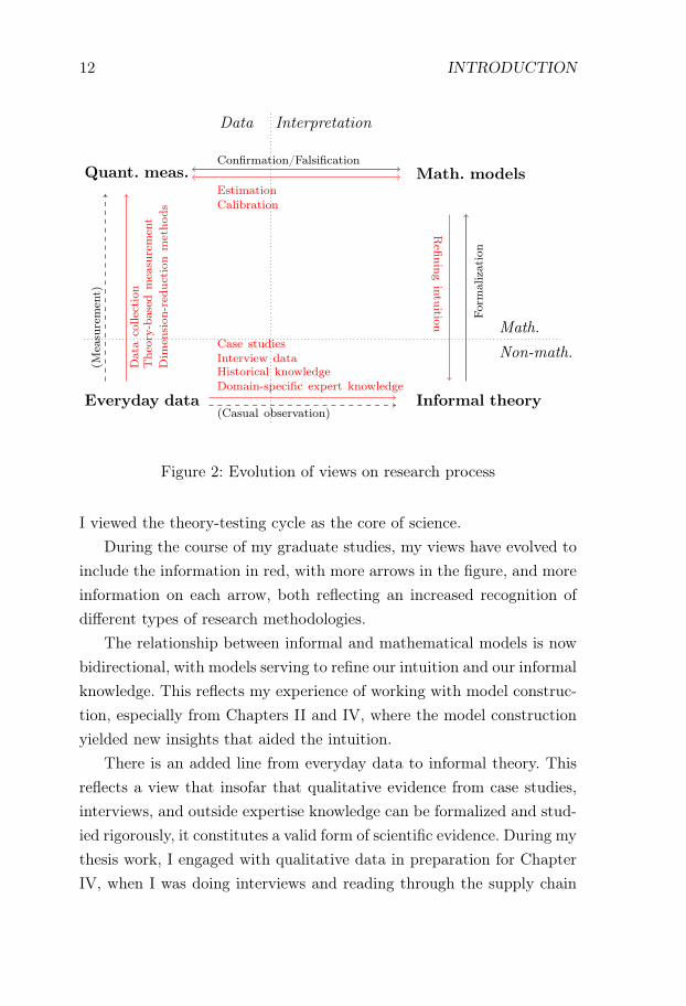
With these concepts, my evolving views on economic methodologycan be summarized in Figure 2, where the information in black representsmy initial views, and the information in red represents the views that Ihave developed during my graduate studies.
When I started graduate school, my view was, somewhat simplified,that a research project started with some informal ideas about poten-tial economic mechanisms. These informal ideas were formalized into amathematical model, which could be used to generate testable predic-tions, which were then tested using some form of quantitative data. Iwas aware of the potential importance of exploiting qualitative data tobuild intuition, and of the challenges of quantitative measurement, but
3Thomas Sargent has, for example, described economics as organized commonsense. The idea of treating the mathematical representation of data and theory asan idealization of everyday phenomena bears some resemblance to Edmund Husserl’scharacterization of the development of modern natural science in his book The Crisisof European Sciences (Husserl, 1970).
12 INTRODUCTION
Data Interpretation
Everyday data Informal theory
Math. modelsQuant. meas.
Math.Non-math.
Refining
intuition
Confirmation/Falsification
EstimationCalibration
Dat
aco
llect
ion
The
ory-
base
dm
easu
rem
ent
Dim
ensi
on-r
educ
tion
met
hods
Case studiesInterview dataHistorical knowledgeDomain-specific expert knowledge
Form
aliz
atio
n
(Mea
sure
men
t)
(Casual observation)
Figure 2: Evolution of views on research process
I viewed the theory-testing cycle as the core of science.During the course of my graduate studies, my views have evolved to
include the information in red, with more arrows in the figure, and moreinformation on each arrow, both reflecting an increased recognition ofdifferent types of research methodologies.
The relationship between informal and mathematical models is nowbidirectional, with models serving to refine our intuition and our informalknowledge. This reflects my experience of working with model construc-tion, especially from Chapters II and IV, where the model constructionyielded new insights that aided the intuition.
There is an added line from everyday data to informal theory. Thisreflects a view that insofar that qualitative evidence from case studies,interviews, and outside expertise knowledge can be formalized and stud-ied rigorously, it constitutes a valid form of scientific evidence. During mythesis work, I engaged with qualitative data in preparation for ChapterIV, when I was doing interviews and reading through the supply chain

INTRODUCTION 13
literature.Furthermore, the measurement arrow is augmented to capture
a richer view of measurement, reflecting that measurement involvesan active construction of facts based on data collection, economictheory, and dimension reduction methods. During my thesis work, themeasurement exercise from Chapter III illustrated the ways in whichdata were not just given, but constructed in an interaction betweenobservations and theory.
Finally, I have added estimation and calibration to the ways inwhich quantitative measurements and mathematical theories interact,reflecting the importance and challenge of using data to quantifyeconomic theory. In my thesis work, this primarily reflects work done onChapter I, where I used data not just to confirm or falsify a hypothesis,but to estimate the parameters of a model.4
Looking back, I can also see that my personal views did not evolve in avacuum, but were connected to a number of broader developments withinthe discipline. Over the last 20 years, some of the more exciting researchprograms in economics have been related to the integration of qualitativeevidence, to new facts from careful quantitative measurements, and to acloser interaction between theory and data.
The field experiment movement has highlighted that qualitative andcontextual evidence is not just anecdotal, but an important componentin research design and in the interpretation of results; the institutionaland historical turn in macroeconomic development has further increasedthe importance of qualitative evidence. Newly available register datasets and analysis tools have generated influential facts regardinginequality, wage dynamics, firm dynamics, productivity dispersion,
4There is an argument to be made for more lines in Figure 2. For example, onecould draw a line from quantitative measurements to informal theory to reflect theuse of statistics in the building of intuition. The choice of having a limited set of linesreflects that the diagram does not aim at being a complete description of the processof scientific work, but merely a vehicle for explaining some specific methodologicaldevelopments.
14 INTRODUCTION
management quality, and international learning outcomes, to name buta few examples. The heterogeneous agent revolution in macroeconomicshas made it possible to connect general equilibrium theory to richmicro data sets, allowing for a closer interaction between data and theory.
In writing my thesis, I have come to appreciate in what ways differentapproaches to economics – theoretical and empirical, formal and informal– are all distinct, and are all relevant to economic research. This hasmade me more aware of the values of methodological pluralism, andthe advantages and disadvantages of different ways of doing economicresearch. I hope that writing this thesis has improved my ability to findthe right strategy for the right question, and brought me at least a bitcloser to the ideal of approaching economic issues with an open, yetcritical, mind.
References
Elsby, M. W., Hobijn, B., and Şahin, A. (2015). On the importanceof the participation margin for labor market fluctuations. Journal ofMonetary Economics, 72:64–82.
Hall, R. E. and Jones, C. I. (1999). Why do Some Countries Produce SoMuch More Output Per Worker than Others? The Quarterly Journalof Economics, 114(1):83–116.
Husserl, E. (1970). The crisis of European sciences and transcenden-tal phenomenology: An introduction to phenomenological philosophy.Northwestern University Press.
Jones, B. F. (2014). The Human Capital Stock: A Generalized Approach.American Economic Review, 104(11):3752–3777.
Nunn, N. (2007). Relationship-Specificity, Incomplete Contracts, and thePattern of Trade. The Quarterly Journal of Economics, 122(2):569–600.

REFERENCES 15
Romalis, J. (2004). Factor Proportions and the Structure of CommodityTrade. American Economic Review, 94(1):67–97.

16 INTRODUCTION

Chapter 1
Human Capital andDevelopment AccountingRevisited∗
1.1 Introduction
Development accounting uses neo-classical production theory in conjunc-tion with price and quantity data to decompose world income differencesinto contributions from capital-output ratios, human capital stocks anduniform labor efficiency (TFP) differences (Klenow and Rodriguez-Clare,1997; Hall and C Jones 1999). A key component of development ac-counting has been to measure the human capital stock by aggregatingmicroeconomic returns to human capital. To aggregate human capital,it has traditionally been assumed that different labor services are per-fectly substitutable and that technology differences are neutral acrosscountries, which means that skilled wage premia can be used to con-
∗I am grateful to Timo Boppart, Axel Gottfries, John Hassler, Karl Harmenberg,Per Krusell, Erik Öberg, and Torsten Persson for extensive comments on the project.Moreover, I am grateful for helpful discussions with Ingvild Almås, Konrad Burchardi,Saman Darougheh, Niels-Jakob Harbo Hansen, Bo Malmberg, Kurt Mitman, Jon deQuidt, Jósef Sigurdsson, Lena Sommestad, and David Strömberg, as well as for helpfulsuggestions during interviews, meetings, and seminars during my job market.
17

18 HUMAN CAPITAL IN DEVELOPMENT ACCOUNTING
vert skilled workers into unskilled equivalent labor units. By assumingthat unskilled labor has a similar level of human capital across countries(or by separately modeling/measuring the quality of unskilled labor), hu-man capital stock differences can be estimated. The key finding has beenthat variations in human capital stocks are much smaller than variationsin labor efficiency, which suggests that large uniform TFP differencesare needed to explain world income differences. This view has had aconsiderable influence on the macroeconomic growth and developmentliterature.2
However, it is known that the results of traditional development ac-counting might be sensitive to relaxing the assumption of perfectly sub-stitutable labor services (Caselli and Coleman, 2006; B Jones 2014a;Caselli 2015). In particular, if labor services are not perfect substitutes,traditional development accounting might underestimate the efficiencyof skilled workers in rich countries, and overstate the importance of uni-form labor efficiency differences. This is due to traditional developmentaccounting equating the skilled wage premium to the relative efficiencyof skilled workers. With imperfect substitutability, this is not true, as therelative abundance of skilled services in rich countries pushes down therelative price of skilled labor services. This means that the relative effi-ciency of skilled labor in rich countries is higher than what is suggestedby skilled wage premia.
If skilled labor efficiency differences are more important than uniformTFP differences, this suggests a different set of interpretations of worldincome differences. If we retain the assumption of skill-neutral technolo-
2Early contributions to development accounting are Klenow and Rodriguez-Clare(1997) and Hall and C Jones (1999). There has been an ongoing debate about the ro-bustness of development accounting. See, for example, Acemoglu and Zilibotti (2001),Erosa et al. (2010), Schoellman (2011), B Jones (2014a), B Jones (2014b), Manuelliand Seshadri (2014), and Schoellman and Hendricks (2016). There is also a largeliterature seeking to explain TFP differences. E.g. Parente and Prescott (1999) andAcemoglu et al. (2007) discuss the role of technology diffusion barriers in explainingTFP differences, and Restuccia and Rogerson (2008), Hsieh and Klenow (2009), andMidrigan and Xu (2014) are a few contributions to the large literature that seeks toexplain TFP differences by misallocation.

INTRODUCTION 19
gies from the traditional development accounting literature, a high effi-ciency of skilled workers in rich countries suggests that skilled workershave a high human capital in rich countries, and that human capital ex-plains a much larger share of world income differences than in traditionaldevelopment accounting. If we relax the assumption of neutral technol-ogy differences, a high efficiency of skilled workers in rich countries canalso indicate large skill-augmenting technology differences. This inter-pretation suggests that technology-based theories of income differencesshould focus on why differences in the economic environment of rich andpoor countries disproportionately affect the efficiency of skilled workers.Thus, imperfect substitutability opens up for a larger role for human cap-ital, and always suggests that the efficiency of skilled labor is relativelymore important as compared to uniform technology differences.3
Even if it is recognized that imperfect substitutability mightbe important for development accounting, there is less agreementon its quantitative importance, and how it should be modeled ina cross-country setting. Early contributions in the developmentaccounting literature assumed that labor services were perfectsubstitutes (Klenow and Rodriguez-Clare, 1997; Hall and C Jones,1999). Recent contributions have made different assumptions. Caselliand Ciccone (2013) take a non-parametric approach where humancapital is aggregated by an arbitrary CRS, concave aggregator. Caselliand Coleman (2006), Jones (2014a), and Caselli (2015) assumethat skilled and unskilled labor services are aggregated using aCES-aggregator, where the elasticity of substitution is assumed to
3The literature on development accounting under imperfect substitutability hasmade different interpretations of the source of skilled labor efficiency differences. Jones(2014a) interprets skilled labor efficiency differences as reflecting human capital qual-ity differences of skilled workers, whereas Caselli and Coleman (2006) and Caselli(2015) interpret skilled labor efficiency differences as reflecting skill-biased technol-ogy differences. The two interpretations are isomorphic in macroeconomic price andquantity data, and this ambiguity has led to conflicting interpretations of the effectsof imperfect substitutability on development accounting, with Jones (2014a) find-ing that imperfect substitutability makes human capital more important, and Caselliand Coleman (2006) and Caselli (2015) finding that imperfect substitutability makeshuman capital less important.
20 HUMAN CAPITAL IN DEVELOPMENT ACCOUNTING
be in line with US time series and panel estimates.4 A number ofrecent contributions in the development accounting literature havealso retained the assumption of perfectly substitutable labor services(Erosa et al., 2010; Manuelli and Seshadri, 2014; Schoellman andHendricks, 2016), as has the recent handbook chapter by C Jones (2015).
In this paper, I bring in new quantitative evidence from internationaltrade data to measure the degree of substitutability between skilled andunskilled workers in a cross-country setting. I use the fact that the skillintensity of a country’s export composition contains implicit informa-tion about the relative price of skilled and unskilled labor services, andthat variations in the relative price of skilled and unskilled labor servicescan be used to estimate a human capital aggregator. My results suggestthat skilled and unskilled labor services are imperfect substitutes, thatthe cross-country relevant human capital aggregator features an approx-imately constant elasticity of substitution, and that this elasticity is inthe same range as that found in US time series panel studies. Thus, myresults provide support for the modeling choices made in Caselli andColeman (2006), Jones (2014a), and Caselli (2015). When I integratemy findings into development accounting, I find a much smaller role foruniform TFP differences than does traditional development accounting.Instead, I find that income differences are primarily driven by skilledlabor efficiency differences.
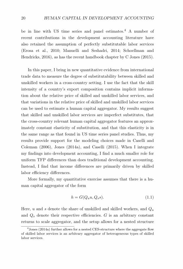
More formally, my quantitative exercise assumes that there is a hu-man capital aggregator of the form
h = G(Quu,Qss). (1.1)
Here, u and s denote the share of unskilled and skilled workers, and Qu
and Qs denote their respective efficiencies. G is an arbitrary constantreturns to scale aggregator, and the setup allows for a nested structure
4Jones (2014a) further allows for a nested CES-structure where the aggregate flowof skilled labor services is an arbitrary aggregator of heterogeneous types of skilledlabor services.
INTRODUCTION 21
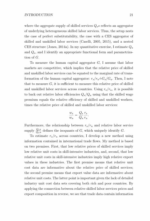
where the aggregate supply of skilled services Qss reflects an aggregatorof underlying heterogeneous skilled labor services. Thus, the setup neststhe case of perfect substitutability, the case with a CES aggregator ofskilled and unskilled labor services (Caselli, 2005, 2015), and a nestedCES structure (Jones, 2014a). In my quantitative exercise, I estimate Qu
and Qs, and I identify an appropriate functional form and parametriza-tion of G.
To measure the human capital aggregator G, I assume that labormarkets are competitive, which implies that the relative price of skilledand unskilled labor services can be equated to the marginal rate of trans-formation of the human capital aggregator: rs/ru=Gs/Gu. Then, I notethat to measure G, it is sufficient to measure this relative price of skilledand unskilled labor services across countries. Using rs/ru, it is possibleto back out relative labor efficiencies Qs/Qu using that the skilled wagepremium equals the relative efficiency of skilled and unskilled workers,times the relative price of skilled and unskilled labor services:
ws
wu=
Qs
Qu
rsru
.
Furthermore, the relationship between rs/ru and relative labor servicesupply Qss
Quudefines the isoquants of G, which uniquely identify G.
To estimate rs/ru across countries, I develop a new method usinginformation contained in international trade flows. My method is basedon two premises. First, that low relative prices of skilled services implylow relative unit costs in skill-intensive industries, and, second, that lowrelative unit costs in skill-intensive industries imply high relative exportvalues in these industries. The first premise means that relative unitcost data are informative about the relative price of skilled services;the second premise means that export value data are informative aboutrelative unit costs. The latter point is important given the lack of detailedindustry unit cost data sets covering both rich and poor countries. Byapplying the connection between relative skilled labor services prices andexport composition in reverse, we see that trade data contain information
22 HUMAN CAPITAL IN DEVELOPMENT ACCOUNTING
about relative skilled labor service prices. For quantification, I use agravity trade model, and I derive a regression specification that combinesa trade elasticity estimate with data on export values and industry factorshares.
My trade data analysis suggests that there is a strong negativerelationship between country income levels and the relative prices ofskilled services. Given that there is also a strong positive relationshipbetween country income levels and relative supplies of skilled labor,this suggests that skilled and unskilled labor services are imperfectlysubstitutable. Furthermore, I find that the human capital aggregatorG can be well approximated by a CES function, and in my baselinespecification, the estimated elasticity of substitution is 1.27.
In the next step, I incorporate this finding into the development ac-counting setting of Hall and C Jones (1999). I posit an aggregate pro-duction function
Y
L=
(K
Y
) α1−α
Ah,
where Y is output, L is the size of the workforce, K is physical capital,A is a uniform TFP-shifter, and h is a human capital aggregator of theform in equation (1.1).5 When I constrain the human capital aggregatorG to be additive, I find that variations in the value of G can only explain12% of world income differences. This is in line with the role attributedto human capital in traditional development accounting. When I allowfor imperfect substitutability, the share of income differences explainedby differences in the value of G increases to 65%. The importance ofTFP-differences decreases correspondingly, and the estimated differencein log TFP between rich and poor countries falls by 66%.
5The equation expresses output per worker as a function of the capital-output ra-tio rather than the capital-labor ratio. This follows Hall and C Jones 1999 and takesinto account the indirect effect of TFP and human capital on capital accumulation.To separate between TFP and unskilled labor quality Qu, my baseline analysis fol-lows Hall and C Jones 1999 and assumes that unschooled workers are similar acrosscountries. If Qu is higher in rich countries, this would further reduce the differencesin A across rich and poor countries.

INTRODUCTION 23
The results are driven by large rich-poor differences in the efficiencyof skilled workers. In my estimation, these efficiency differences are dueto combining moderate rich-poor differences in the skilled wage premiumwith large rich-poor differences in the relative price of skilled services.The trade data estimates suggest that rich countries have 4-5 lower logrelative prices of skilled services. This difference can either be explainedby rich countries having low skilled wage premia, or by rich countrieshaving relatively efficient skilled labor. Wage data suggest that skilledwage premia are indeed lower in rich countries, but not more than ap-proximately one log point lower. Thus, I impute a 3-4 log-point differencein the relative efficiency of skilled labor between rich and poor countries.Intuitively, the German skill premium is not sufficiently low to rationalizehigh exports of engineering products from Germany, and thus I imputea relatively high efficiency of German skilled labor.
Finally, I discuss the interpretation of the results. I show thatthe interpretation depends on the source of skilled labor efficiencydifferences. If I retain the traditional development accountingassumption of skill-neutral technology differences, I find largedifferences in the human capital of skilled workers, and that humancapital explains a majority of world income differences. If I relaxthe assumption of skill-neutral technology differences, an alternativeexplanation is that skilled labor efficiency differences reflect skill-biasedtechnology differences. With this interpretation, theories of incomedifferences should still be theories of technology differences, but theyshould focus more on the interaction between the economic environmentand the efficiency of skilled workers. In Section 1.4, I discuss thesedifferent interpretations, and potential roads forward in discriminatingbetween different sources of skilled labor efficiency differences.
The outline of the paper is as follows. Section 1.2 develops theestimation strategy for the relative price of skilled labor services rs/ru.Section 1.3 presents the development accounting results. Section 1.4discusses the alternative economic interpretations of my results,

24 HUMAN CAPITAL IN DEVELOPMENT ACCOUNTING
focusing on the interpretation of skilled labor efficiency differences asdepending on human capital or skill-augmenting technology differences.Section 1.5 discusses in greater detail the relationship between mypaper and B Jones (2014a) who also studies development accountingwith imperfectly substitutable labor services. Section 1.6 performs alarge number of robustness checks on the baseline results, and Section1.7 concludes the paper.
Related literature. My paper is part of the development accountingliterature, going back to Klenow and Rodriguez-Clare (1997) and Halland C Jones (1999). This literature is surveyed in Caselli (2005), Hsiehand Klenow (2010a), and C Jones (2015). There has been a numberof papers revisiting the contribution of human capital in developmentaccounting, most often in a framework featuring perfect substitutabilitybetween different types of labor services. These papers include Hendricks(2002), Erosa et al. (2010), Schoellman (2011), Manuelli and Seshadri(2014), and Hendricks and Schoellman (2016).
A few papers have analyzed development accounting with imperfectlysubstitutable labor services. These papers include Caselli and Coleman(2006), Caselli and Ciccone (2013), Jones (2014a), and Caselli (2015).
Beyond development accounting, my paper builds on the gravitytrade literature to estimate the relative prices of skilled services (Tin-bergen, 1962; Anderson et al., 1979; Eaton and Kortum, 2002; Andersonand van Wincoop, 2003; Redding and Venables, 2004; Costinot et al.,2011; Head and Mayer, 2014). A number of papers have used trade datato obtain information about productivities, including Trefler (1993) andLevchenko and Zhang (2016). Morrow and Trefler (2017) is a more re-cent contribution that integrates trade into development accounting. Mypaper also relates to the literature that uses industry data to obtain infor-mation about economic development, which includes Rajan and Zingales(1998) and Ciccone and Papaioannou (2009). In the context of trade,papers that analyze the relationship between country variables and theindustrial structure of trade include Romalis (2004), Nunn (2007), Chor

INTRODUCTION 25
(2010), Cuñat and Melitz (2012), and Manova (2013). This literature isreviewed in Nunn and Trefler (2015).
26 HUMAN CAPITAL IN DEVELOPMENT ACCOUNTING
1.2 Estimating the relative price of skilled ser-vices
The aim of this section is to estimate how the relative price of effectiveskilled and unskilled labor services rs/ru varies across countries. For thispurpose, I construct a method for estimating relative factor service pricesin general.
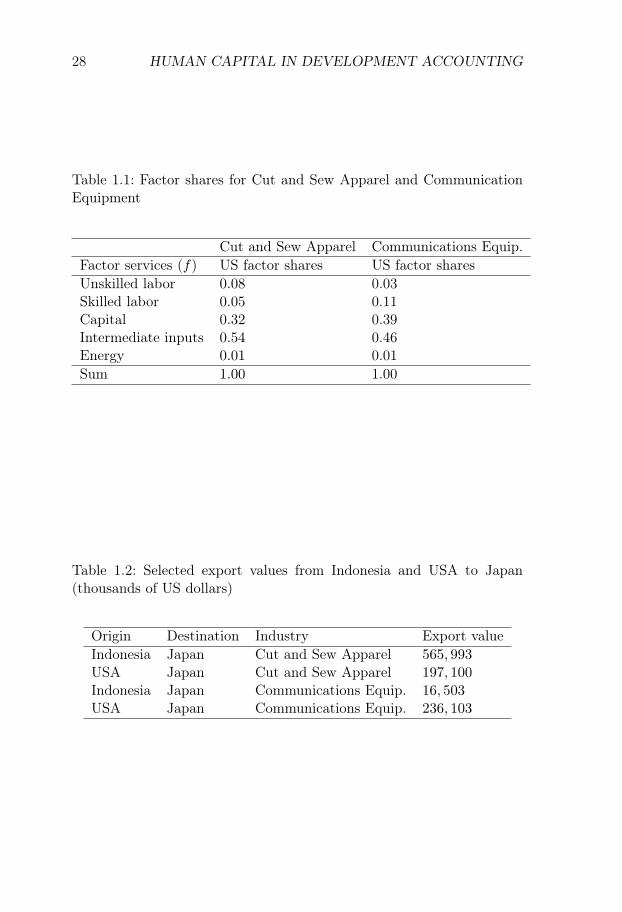
My estimation strategy is based on two premises. The first premise isthat relative factor service prices influence relative unit production costs.To illustrate this, we can consider a case with two industries. ConsiderTable 1.1, which shows the factor shares for “Cut and Sew Apparel"(NAICS code 3152) and “Communications Equipment" (NAICS code3342). Production of Communications Equipment is more skill intensivethan production of Cut and Sew Apparel. If the relative price of skilledservices rises, we can expect a rise in the relative unit production costof Communications Equipment as compared to that of Cut and SewApparel.6
The second premise is that relative unit production costs affect rela-tive export flows, which is a version of the principle of comparative ad-vantage. For example, consider Table 1.2, which presents a number of USand Indonesian export values to Japan. Relative Indonesian-US exportsare much higher in Cut and Sew Apparel as compared to Communica-tions Equipment. Applying the principle of comparative advantage, thisevidence suggests that Indonesia has a high relative unit production costof Communications Equipment.
In combination, my two premises suggest that trade data containinformation about relative factor service prices. For example, the tradedata in Table 1.2 suggest that Indonesia has a high relative unit produc-tion cost of Communications Equipment. Furthermore, factor shares in
6The cost shares are defined as shares of gross output. In Appendix 1.C.3, Idescribe an alternative method where I decompose the non-tradable component ofthe intermediate input cost share into cost shares of other inputs using an input-output table. The final results are not affected by whether I use the basic cost sharesor perform such a decomposition.

ESTIMATING SKILLED SERVICE PRICES 27
Table 1.1 suggest that Communications Equipment production is moreskill intensive than Cut and Sew Apparel production. These two factstogether suggest that Indonesia has a high relative price of skilled ser-vices.
My estimation strategy formalizes and generalizes this method ofobtaining information about relative factor service prices using relativeexport values conditional on trade destination. For this purpose, I relyon a gravity trade model. My main result is that using a version of agravity trade model, it is possible to identify relative factor service pricesusing:
1. Industry factor shares
2. Bilateral industry trade data
3. The price elasticity of export flows
One particular feature of my estimation strategy is that relative unitcosts are estimated from trade data. This estimation choice reflects thelack of a data set that provides detailed cross-country comparable in-dustry unit cost data, which cover both rich and poor countries. Thebest available data set comes from the Groningen Growth and Develop-ment Center, which has done important work in constructing a data setof industry unit costs for cross-country comparisons (Inklaar and Tim-mer, 2008). However, their data set only covers 35 industries in 42 coun-tries, with a limited coverage of poor countries. In contrast, trade dataare recorded at a highly detailed industry level in both rich and poorcountries. This makes trade data an attractive source of information fordevelopment accounting. In Section 1.6.3, I show that for countries wherewe have both unit cost data and trade data, analyses using unit cost dataand trade data yield similar results.
1.2.1 Setup
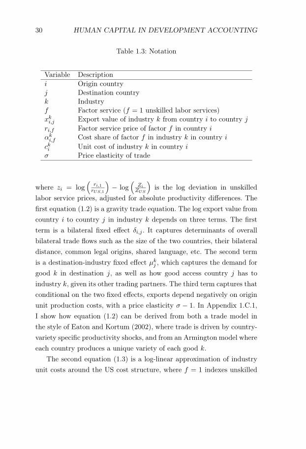
This section describes the setup of my estimation exercise. The notationis summarized in Table 1.3.
28 HUMAN CAPITAL IN DEVELOPMENT ACCOUNTING
Table 1.1: Factor shares for Cut and Sew Apparel and CommunicationEquipment
Cut and Sew Apparel Communications Equip.Factor services (f) US factor shares US factor sharesUnskilled labor 0.08 0.03Skilled labor 0.05 0.11Capital 0.32 0.39Intermediate inputs 0.54 0.46Energy 0.01 0.01Sum 1.00 1.00
Table 1.2: Selected export values from Indonesia and USA to Japan(thousands of US dollars)
Origin Destination Industry Export valueIndonesia Japan Cut and Sew Apparel 565, 993USA Japan Cut and Sew Apparel 197, 100Indonesia Japan Communications Equip. 16, 503USA Japan Communications Equip. 236, 103
ESTIMATING SKILLED SERVICE PRICES 29
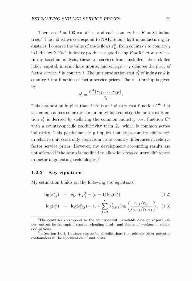
There are I = 103 countries, and each country has K = 84 indus-tries.7 The industries correspond to NAICS four-digit manufacturing in-dustries. I observe the value of trade flows xki,j from country i to country j
in industry k. Each industry produces a good using F = 5 factor services.In my baseline analysis, these are services from unskilled labor, skilledlabor, capital, intermediate inputs, and energy. ri,f denotes the price offactor service f in country i. The unit production cost cki of industry k incountry i is a function of factor service prices. The relationship is givenby
cki =Ck(ri,1, . . . , ri,F )
Zi.
This assumption implies that there is an industry cost function Ck thatis common across countries. In an individual country, the unit cost func-tion cki is derived by deflating the common industry cost function Ck
with a country-specific productivity term Zi, which is common acrossindustries. This particular setup implies that cross-country differencesin relative unit costs only stem from cross-country differences in relativefactor service prices. However, my development accounting results arenot affected if the setup is modified to allow for cross-country differencesin factor augmenting technologies.8
1.2.2 Key equations
My estimation builds on the following two equations:
log(xki,j) = δi,j + μkj − (σ − 1) log(cki ) (1.2)
log(cki ) = log(ckUS) + zi +
F∑f=2
αkUS,f log
(ri,f/ri,1
rUS,f/rUS,1
), (1.3)
7The countries correspond to the countries with available data on export val-ues, output levels, capital stocks, schooling levels, and shares of workers in skilledoccupations.
8In Section 1.6.1, I discuss regression specifications that address other potentialconfounders in the specification of unit costs.
30 HUMAN CAPITAL IN DEVELOPMENT ACCOUNTING
Table 1.3: Notation
Variable Descriptioni Origin countryj Destination countryk Industryf Factor service (f = 1 unskilled labor services)xki,j Export value of industry k from country i to country j
ri,f Factor service price of factor f in country iαki,f Cost share of factor f in industry k in country i
cki Unit cost of industry k in country iσ Price elasticity of trade
where zi = log(
ri,1rUS,1
)− log
(ZiZUS
)is the log deviation in unskilled
labor service prices, adjusted for absolute productivity differences. Thefirst equation (1.2) is a gravity trade equation. The log export value fromcountry i to country j in industry k depends on three terms. The firstterm is a bilateral fixed effect δi,j . It captures determinants of overallbilateral trade flows such as the size of the two countries, their bilateraldistance, common legal origins, shared language, etc. The second termis a destination-industry fixed effect μk
j , which captures the demand forgood k in destination j, as well as how good access country j has toindustry k, given its other trading partners. The third term captures thatconditional on the two fixed effects, exports depend negatively on originunit production costs, with a price elasticity σ − 1. In Appendix 1.C.1,I show how equation (1.2) can be derived from both a trade model inthe style of Eaton and Kortum (2002), where trade is driven by country-variety specific productivity shocks, and from an Armington model whereeach country produces a unique variety of each good k.
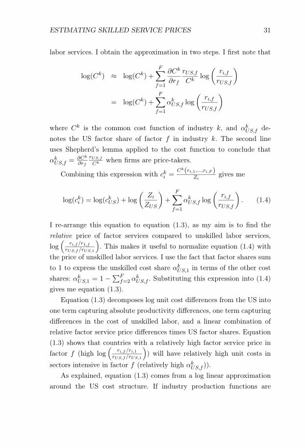
The second equation (1.3) is a log-linear approximation of industryunit costs around the US cost structure, where f = 1 indexes unskilled
ESTIMATING SKILLED SERVICE PRICES 31
labor services. I obtain the approximation in two steps. I first note that
log(Ck) ≈ log(Ck) +
F∑f=1
∂Ck
∂rf
rUS,f
Cklog
(ri,frUS,f
)
= log(Ck) +F∑
f=1
αkUS,f log
(ri,frUS,f
)
where Ck is the common cost function of industry k, and αkUS,f de-
notes the US factor share of factor f in industry k. The second lineuses Shepherd’s lemma applied to the cost function to conclude thatαkUS,f = ∂Ck
∂rf
rUS,f
Ck when firms are price-takers.
Combining this expression with cki =Ck(ri,1,...,ri,F )
Zigives me
log(cki ) = log(ckUS) + log
(Zi
ZUS
)+
F∑f=1
αkUS,f log
(ri,frUS,f
). (1.4)
I re-arrange this equation to equation (1.3), as my aim is to find therelative price of factor services compared to unskilled labor services,log(
ri,f/r1,frUS,f/rUS,1
). This makes it useful to normalize equation (1.4) with
the price of unskilled labor services. I use the fact that factor shares sumto 1 to express the unskilled cost share αk
US,1 in terms of the other costshares: αk
US,1 = 1 −∑Ff=2 α
kUS,f . Substituting this expression into (1.4)
gives me equation (1.3).Equation (1.3) decomposes log unit cost differences from the US into
one term capturing absolute productivity differences, one term capturingdifferences in the cost of unskilled labor, and a linear combination ofrelative factor service price differences times US factor shares. Equation(1.3) shows that countries with a relatively high factor service price infactor f (high log
(ri,f/ri,1
rUS,f/rUS,1
)) will have relatively high unit costs in
sectors intensive in factor f (relatively high αkUS,f )).
As explained, equation (1.3) comes from a log linear approximationaround the US cost structure. If industry production functions are
32 HUMAN CAPITAL IN DEVELOPMENT ACCOUNTING
Cobb-Douglas, this approximation is exact. If industry productionfunctions are not Cobb-Douglas, there is a second-order bias. In Section1.6.1, I analyze the effect of relaxing the Cobb-Douglas assumption.
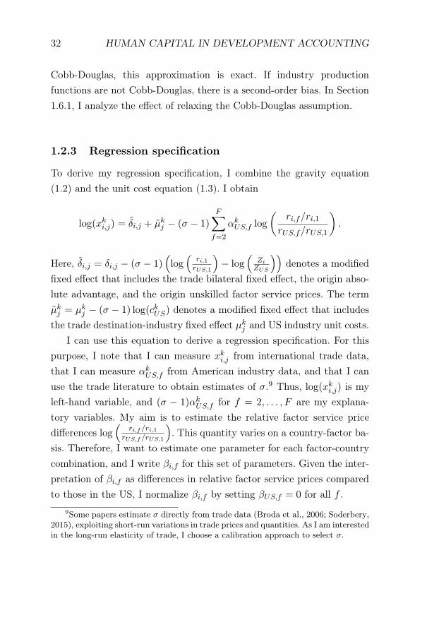
1.2.3 Regression specification
To derive my regression specification, I combine the gravity equation(1.2) and the unit cost equation (1.3). I obtain
log(xki,j) = δi,j + μkj − (σ − 1)
F∑f=2
αkUS,f log
(ri,f/ri,1
rUS,f/rUS,1
).
Here, δi,j = δi,j − (σ − 1)(log(
ri,1rUS,1
)− log
(ZiZUS
))denotes a modified
fixed effect that includes the trade bilateral fixed effect, the origin abso-lute advantage, and the origin unskilled factor service prices. The termμkj = μk
j − (σ − 1) log(ckUS) denotes a modified fixed effect that includesthe trade destination-industry fixed effect μk
j and US industry unit costs.I can use this equation to derive a regression specification. For this
purpose, I note that I can measure xki,j from international trade data,that I can measure αk
US,f from American industry data, and that I canuse the trade literature to obtain estimates of σ.9 Thus, log(xki,j) is myleft-hand variable, and (σ − 1)αk
US,f for f = 2, . . . , F are my explana-tory variables. My aim is to estimate the relative factor service pricedifferences log
(ri,f/ri,1
rUS,f/rUS,1
). This quantity varies on a country-factor ba-
sis. Therefore, I want to estimate one parameter for each factor-countrycombination, and I write βi,f for this set of parameters. Given the inter-pretation of βi,f as differences in relative factor service prices comparedto those in the US, I normalize βi,f by setting βUS,f = 0 for all f .
9Some papers estimate σ directly from trade data (Broda et al., 2006; Soderbery,2015), exploiting short-run variations in trade prices and quantities. As I am interestedin the long-run elasticity of trade, I choose a calibration approach to select σ.
ESTIMATING SKILLED SERVICE PRICES 33
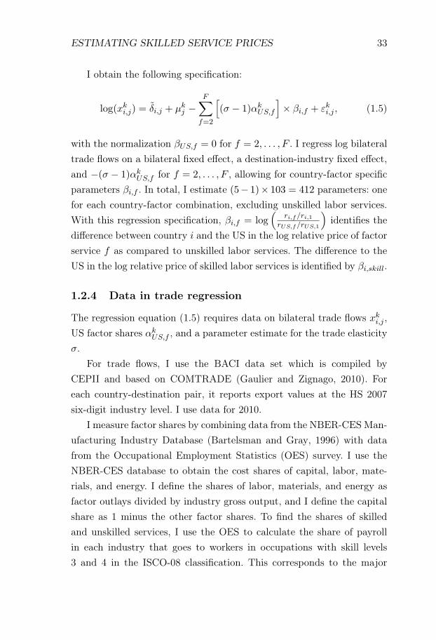
I obtain the following specification:
log(xki,j) = δi,j + μkj −
F∑f=2
[(σ − 1)αk
US,f
]× βi,f + εki,j , (1.5)
with the normalization βUS,f = 0 for f = 2, . . . , F . I regress log bilateraltrade flows on a bilateral fixed effect, a destination-industry fixed effect,and −(σ − 1)αk
US,f for f = 2, . . . , F , allowing for country-factor specificparameters βi,f . In total, I estimate (5− 1)× 103 = 412 parameters: onefor each country-factor combination, excluding unskilled labor services.With this regression specification, βi,f = log
(ri,f/ri,1
rUS,f/rUS,1
)identifies the
difference between country i and the US in the log relative price of factorservice f as compared to unskilled labor services. The difference to theUS in the log relative price of skilled labor services is identified by βi,skill.
1.2.4 Data in trade regression
The regression equation (1.5) requires data on bilateral trade flows xki,j ,US factor shares αk
US,f , and a parameter estimate for the trade elasticityσ.
For trade flows, I use the BACI data set which is compiled byCEPII and based on COMTRADE (Gaulier and Zignago, 2010). Foreach country-destination pair, it reports export values at the HS 2007six-digit industry level. I use data for 2010.
I measure factor shares by combining data from the NBER-CES Man-ufacturing Industry Database (Bartelsman and Gray, 1996) with datafrom the Occupational Employment Statistics (OES) survey. I use theNBER-CES database to obtain the cost shares of capital, labor, mate-rials, and energy. I define the shares of labor, materials, and energy asfactor outlays divided by industry gross output, and I define the capitalshare as 1 minus the other factor shares. To find the shares of skilledand unskilled services, I use the OES to calculate the share of payrollin each industry that goes to workers in occupations with skill levels3 and 4 in the ISCO-08 classification. This corresponds to the major

34 HUMAN CAPITAL IN DEVELOPMENT ACCOUNTING
occupational groups "Managers", "Professionals", and "Technicians andAssociate Professionals". I calculate the skill share as the labor sharefrom the NBER CES times the share of payroll going to skilled workers,and the unskilled share as the labor share times the share of payroll goingto unskilled workers. Note that in my regression, I include the materialsand energy shares in the regression. Appendix 1.C.3 provides a more de-tailed discussion of different choices of intermediate input measurementand their effects.
The regression is performed using NAICS four-digit coding, which isthe coding scheme of the OES industry data. The trade data are recordedusing HS6 codes and the NBER-CES data are recorded using NAICS six-digit codes. The OES occupational data are recorded according to SOC,and they are converted to ISCO-08 to calculate the share of payroll goingto skilled workers.
I take my value of the trade elasticity σ from the literature. I look foran estimate of the long-run elasticity between different foreign varietiesin the same industry. This choice reflects the nature of my regression.The regression is run between countries in different parts of the world-income distribution, and aims at capturing persistent cross-country diff-erences. Furthermore, the regression explains a source country’s exportsconditioned on the total industry imports of a destination country. Thus,the relevant elasticity is the long-run elasticity between different foreignvarieties.
I select σ = 10 as my baseline elasticity. This is a reasonably high es-timate of trade elasticity and reflects a conservative choice for estimatingthe importance of human capital. A higher σ shrinks the importance ofhuman capital since it reduces the estimated differences between coun-tries: differences in relative trade flows translate into smaller unit costdifferences. Even though Eaton and Kortum (2002) open up for esti-mates as high as σ = 14, my estimate is higher than σ = 5 found inSimonovska and Waugh (2014), σ = 7.2 found in Costinot et al. (2011),and the baseline σ = 9.2 found in Eaton and Kortum (2002).10
10Note that the trade elasticity θ in Eaton and Kortum-style models represents
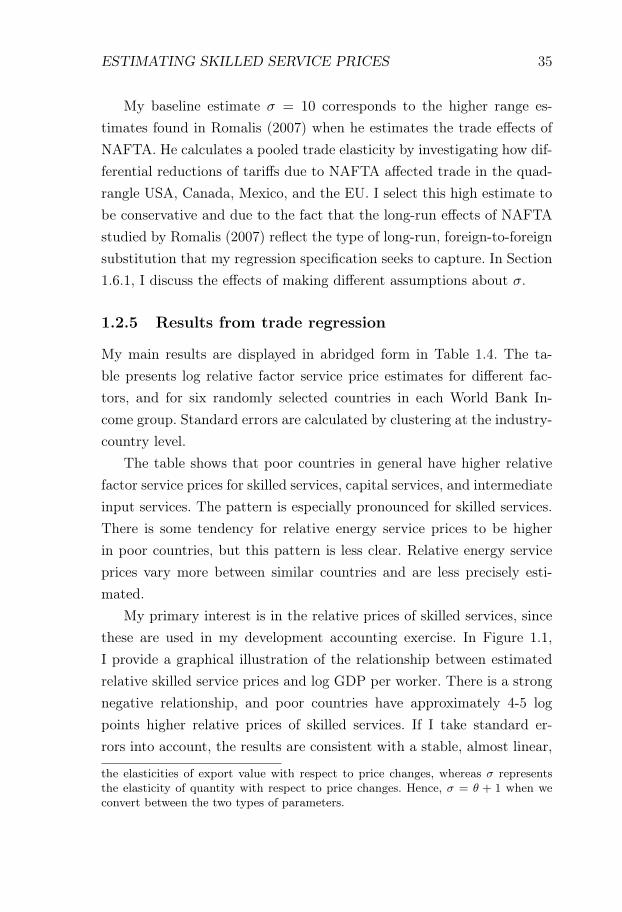
ESTIMATING SKILLED SERVICE PRICES 35
My baseline estimate σ = 10 corresponds to the higher range es-timates found in Romalis (2007) when he estimates the trade effects ofNAFTA. He calculates a pooled trade elasticity by investigating how dif-ferential reductions of tariffs due to NAFTA affected trade in the quad-rangle USA, Canada, Mexico, and the EU. I select this high estimate tobe conservative and due to the fact that the long-run effects of NAFTAstudied by Romalis (2007) reflect the type of long-run, foreign-to-foreignsubstitution that my regression specification seeks to capture. In Section1.6.1, I discuss the effects of making different assumptions about σ.
1.2.5 Results from trade regression
My main results are displayed in abridged form in Table 1.4. The ta-ble presents log relative factor service price estimates for different fac-tors, and for six randomly selected countries in each World Bank In-come group. Standard errors are calculated by clustering at the industry-country level.
The table shows that poor countries in general have higher relativefactor service prices for skilled services, capital services, and intermediateinput services. The pattern is especially pronounced for skilled services.There is some tendency for relative energy service prices to be higherin poor countries, but this pattern is less clear. Relative energy serviceprices vary more between similar countries and are less precisely esti-mated.
My primary interest is in the relative prices of skilled services, sincethese are used in my development accounting exercise. In Figure 1.1,I provide a graphical illustration of the relationship between estimatedrelative skilled service prices and log GDP per worker. There is a strongnegative relationship, and poor countries have approximately 4-5 logpoints higher relative prices of skilled services. If I take standard er-rors into account, the results are consistent with a stable, almost linear,
the elasticities of export value with respect to price changes, whereas σ representsthe elasticity of quantity with respect to price changes. Hence, σ = θ + 1 when weconvert between the two types of parameters.
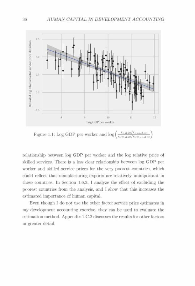
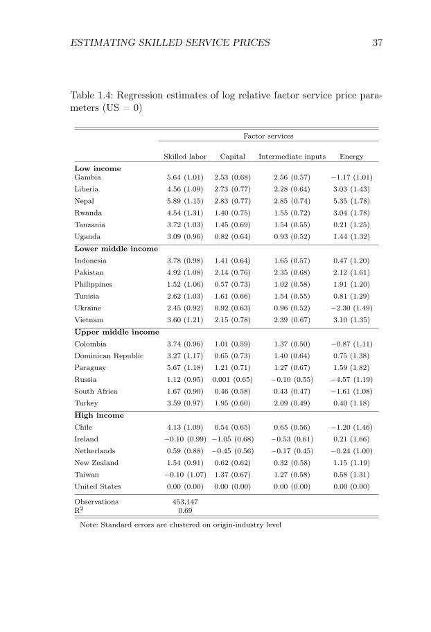
ESTIMATING SKILLED SERVICE PRICES 37
Table 1.4: Regression estimates of log relative factor service price para-meters (US = 0)
Factor services
Skilled labor Capital Intermediate inputs Energy
Low incomeGambia 5.64 (1.01) 2.53 (0.68) 2.56 (0.57) −1.17 (1.01)
Liberia 4.56 (1.09) 2.73 (0.77) 2.28 (0.64) 3.03 (1.43)
Nepal 5.89 (1.15) 2.83 (0.77) 2.85 (0.74) 5.35 (1.78)
Rwanda 4.54 (1.31) 1.40 (0.75) 1.55 (0.72) 3.04 (1.78)
Tanzania 3.72 (1.03) 1.45 (0.69) 1.54 (0.55) 0.21 (1.25)
Uganda 3.09 (0.96) 0.82 (0.64) 0.93 (0.52) 1.44 (1.32)
Lower middle incomeIndonesia 3.78 (0.98) 1.41 (0.64) 1.65 (0.57) 0.47 (1.20)
Pakistan 4.92 (1.08) 2.14 (0.76) 2.35 (0.68) 2.12 (1.61)
Philippines 1.52 (1.06) 0.57 (0.73) 1.02 (0.58) 1.91 (1.20)
Tunisia 2.62 (1.03) 1.61 (0.66) 1.54 (0.55) 0.81 (1.29)
Ukraine 2.45 (0.92) 0.92 (0.63) 0.96 (0.52) −2.30 (1.49)
Vietnam 3.60 (1.21) 2.15 (0.78) 2.39 (0.67) 3.10 (1.35)
Upper middle incomeColombia 3.74 (0.96) 1.01 (0.59) 1.37 (0.50) −0.87 (1.11)
Dominican Republic 3.27 (1.17) 0.65 (0.73) 1.40 (0.64) 0.75 (1.38)
Paraguay 5.67 (1.18) 1.21 (0.71) 1.27 (0.67) 1.59 (1.82)
Russia 1.12 (0.95) 0.001 (0.65) −0.10 (0.55) −4.57 (1.19)
South Africa 1.67 (0.90) 0.46 (0.58) 0.43 (0.47) −1.61 (1.08)
Turkey 3.59 (0.97) 1.95 (0.60) 2.09 (0.49) 0.40 (1.18)
High incomeChile 4.13 (1.09) 0.54 (0.65) 0.65 (0.56) −1.20 (1.46)
Ireland −0.10 (0.99) −1.05 (0.68) −0.53 (0.61) 0.21 (1.66)
Netherlands 0.59 (0.88) −0.45 (0.56) −0.17 (0.45) −0.24 (1.00)
New Zealand 1.54 (0.91) 0.62 (0.62) 0.32 (0.58) 1.15 (1.19)
Taiwan −0.10 (1.07) 1.37 (0.67) 1.27 (0.58) 0.58 (1.31)
United States 0.00 (0.00) 0.00 (0.00) 0.00 (0.00) 0.00 (0.00)
Observations 453,147R2 0.69
Note: Standard errors are clustered on origin-industry level
38 HUMAN CAPITAL IN DEVELOPMENT ACCOUNTING
1.3 Development accounting
In this section, I want to use the estimates from Section 1.2 to perform adevelopment accounting exercise. The aim is to decompose the variancein GDP per worker into contributions from differences in capital-outputratios, uniform labor productivity shifters and differences in human cap-ital aggregators.
1.3.1 Aggregate production function
Performing development accounting requires me to put more theoreticalstructure on the aggregate economy. In Section 1.2, the key assumptionwas that trade flows followed a gravity relationship. This assumption isconsistent with a range of models for the aggregate economy. In con-trast, for development accounting, I need an aggregate production func-tion that summarizes both substitution possibilities within and betweenindustries and substitution possibilities between domestic and foreignproduction.
It can be shown that standard trade models admit a constant re-turns to scale aggregate production function under relatively mild as-sumptions (see Appendix 1.A.2), but there is no general result on thefunctional form of such an aggregate production function. In general,the aggregation of capital, skilled labor, and unskilled labor depends ontrade elasticities, the input-output structure, the relative factor sharesof traded and non-traded goods, and how traded and non-traded goodsare aggregated.
In my baseline specification, I follow the development accounting lit-erature by making the assumption that the aggregate production func-tion can be well approximated by a Cobb-Douglas composite of laborand capital. Moreover, I assume that average human capital is an arbi-trary constant returns to scale function of the number and efficiencies ofskilled and unskilled workers. This assumption allows me to focus on howlabor input aggregation changes the development accounting exercise.
1.3. DEVELOPMENT ACCOUNTING 39
Thus, I posit an aggregate production function:
Y = Kα(ALh)1−α, (1.6)
where Y is total output, K is the physical capital stock, A is a labor-augmenting technology term, L is the size of the labor force, and h
captures the average human capital of the labor force. I allow for a flexiblespecification of h
h = G(Quu,Qss).
Here, G is a constant returns to scale aggregator, u and s are the sharesof unskilled and skilled workers, and Qu and Qs are the amount of un-skilled/skilled services delivered by each unskilled/skilled worker. I willrefer to Qu and Qs efficiencies of unskilled and skilled labor.
The human capital term h has two potential interpretations. Oneinterpretation of the aggregator is that there are two homogenous skilltypes, with the respective efficiencies Qu and Qs. A second interpre-tation is that there are two aggregators Hu = Quu and Hs = Qss,which combine heterogeneous types of services into an aggregate flowof unskilled and skilled services. With this interpretation, Qu and Qs
represent the average flow of unskilled/skilled labor services per unit ofunskilled/skilled labor, and ws and wu are the average wages of skilledand unskilled workers.
The interpretation with two types of labor services is easier to dis-cuss, whereas the aggregator interpretation is more realistic. I will derivemy results in the language of the interpretation with two labor types. Iwill refer to u and s as the share of unskilled and skilled workers, andto Qu and Qs as the (average) efficiencies of unskilled and skilled labor.When I analyze economic mechanisms, I will leverage the mathematicalequivalence to interpret my results in light of the aggregator interpreta-tion.
40 HUMAN CAPITAL IN DEVELOPMENT ACCOUNTING
1.3.2 Estimating terms of aggregate production function
To perform development accounting, we need to measure Y , L, α and h.Data on real output Y , labor force size L, and physical capital stock
K are from the Penn World Table Version 8.1. I use data from 2010, andI set the capital share α to 1/3.
To measure h = G(Quu,Qss), I use data from ILO to measure theshare of skilled workers s. I define the share of skilled workers as the shareof workers having an occupation requiring skill level 3 or 4. According toILO, occupations require skill level 3 or 4 when they "typically involvethe performance of [...] tasks that require an extensive body of [...] knowl-edge in a specialized field". In the International Standard Classificationof Occupations 2008 (ISCO-08), these are "Managers", "Professionals",and "Technicians and Associate Professionals". Figure 1.2 shows the re-lationship between the share of skilled workers and log GDP per worker.There is a strong positive relationship, and a linear regression of theskill share on log GDP per worker has an R2-value of 0.75. My skill def-inition differs from the literature in being occupation-based instead ofschooling-based. I discuss this choice in Appendix 1.B.1.
I calibrate the quality of unskilled labor Qu using data on schoolinglevels and Mincerian returns. I define
Qu = eφ(Su), (1.7)
where Su is the average schooling years of unskilled workers, and φ is aMincerian return function capturing the relationship between schoolingand wages. I measure Su using the Barro-Lee schooling data for 2010. Iassume that there is perfect positive sorting between years of schoolingand working in a skilled profession, which means that unskilled workerscorrespond to the 1− s share of the workforce with the least schooling. Iassume that Su is the average number of school years in this group.11 Itake the Mincerian return function φ(S) from Caselli (2005) and define
11See Appendix 1.B.2 for details on how I calculate the average schooling of un-skilled labor.
1.3. DEVELOPMENT ACCOUNTING 41
it as a piecewise linear function with slope 0.13 for S < 4, slope 0.1 forS ∈ [4, 8), and slope 0.08 for S ≥ 8. This specification was introducedin the literature as a reduced form way of capturing that poor countrieshave higher Mincerian returns.
To measure the relative efficiency of skilled workers Qs/Qu, I assumethat labor markets are competitive. This means that the relative wageof skilled and unskilled workers is
ws
wu=
Qs
Qu
rsru
,
wherersru
=fsfu
.
I measure the relative efficiency of skilled and unskilled labor usingthe equation
ws
wu=
Qs
Qu
rsru
⇐⇒ Qs
Qu=
ws/wu
rs/ru. (1.8)
The skilled wage premium ws/wu is observable, and the relative price ofskilled services rs
ruwas estimated in Section 1.2.12 This equation states
that the skill premium equals the relative amount of services provided byskilled and unskilled workers, times the relative price of those services.Re-arranging the equation shows that there will be a high estimate ofrelative skilled labor efficiency if either a) the skill premium is high giventhe price of skilled services, since this reflects a large amount of servicesbeing delivered, or b) if observed skilled service prices are low given theskill premium, since this reflects a high efficiency of skilled labor, thusbringing down the efficiency adjusted price.
I use ILO data to measure the skilled wage premium ws/wu. ILOsummarizes wage data from multiple sources, and I restrict attention to
12In Section 1.2, I estimated rs/rurUS,s/rUS,u
. To find rs/ru, I need rUS,s/rUS,u. I findthis by normalizing US skilled labor efficiency to QUS,s = 1. This implies:
rUS,s
rUS,u=
(1
QUS,u
)−1wUS,s
wUS,u.
42 HUMAN CAPITAL IN DEVELOPMENT ACCOUNTING
countries where data are available from administrative records, a labor-focused establishment survey, and/or a labor force survey. I use the mea-sure of mean nominal monthly earnings of employees. I combine data onwages and employment across occupations, and I calculate the relativeaverage wage between workers with skill levels 3 or 4 and workers withskill levels 1 or 2. Figure 1.3 shows the relationship between log skilledwage premia and log GDP per worker. Apart from two outliers (Vietnamand Qatar), there is a strong negative relationship. The ILO data onlycover a limited set of countries, and there are large variations betweencountries with similar levels of log GDP per worker. In my developmentaccounting exercise, I want to use a large set of countries, and I am inter-ested in systematic differences between rich and poor countries. Thus, toassign values of the skilled wage premium, I regress the log skilled pre-mium on log GDP per worker (excluding outliers). I assign each countrya skilled premium using the fitted value of this regression. This allowsme to extend the country coverage beyond the limited set of countriescovered in the ILO data, while capturing the systematic changes of theskilled wage premium across the GDP per worker distribution. In Sec-tion 1.6.3, I consider how changes in the measurement of the skilled wagepremium change my results.
With estimates of rs/ru, Qs/Qu, and s/u, it is possible to estimatethe functional form and parameters of the human capital aggregator G.As G has constant returns to scale, it is characterized up to a constantby the relationship between the marginal rate of transformation fs/fu
and the relative effective labor supplies QssQuu
. In particular, a linear rela-
tionship between log(
fsfu
)and log
(QssQuu
)suggests that G has a constant
elasticity of substitution.Using the estimates of rs/ru from Section 1.2, we can plot the re-
lationship between the (log) marginal rate of transformation and (log)relative effective labor supplies. However, we need to be cautious in in-terpreting this relationship when relative qualities Qs/Qu are derivedusing equation (1.8). The reason is that relative supplies are calculated
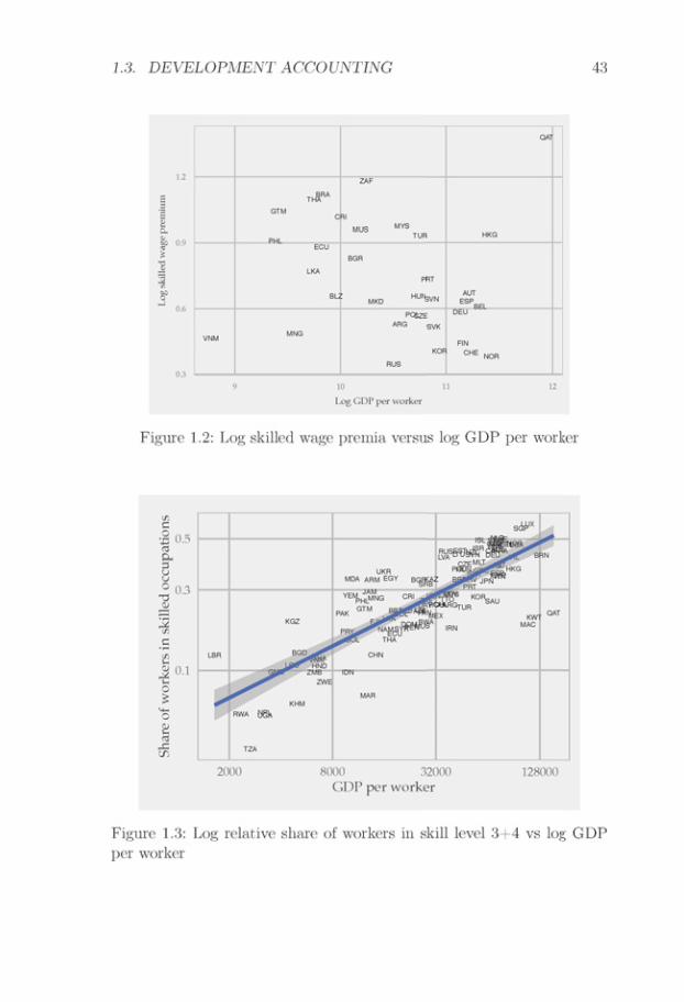
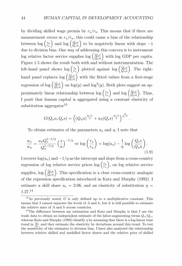
44 HUMAN CAPITAL IN DEVELOPMENT ACCOUNTING
by dividing skilled wage premia by rs/ru. This means that if there aremeasurement errors in rs/ru, this could cause a bias of the relationshipbetween log
(rsru
)and log
(QssQuu
)to be negatively linear with slope −1
due to division bias. One way of addressing this concern is to instrumentlog relative factor service supplies log
(QssQuu
)with log GDP per capita.
Figure 1.5 shows the result both with and without instrumentation. Theleft-hand panel shows log
(rsru
)plotted against log
(QssQuu
). The right-
hand panel replaces log(
QssQuu
)with the fitted values from a first-stage
regression of log(
QssQuu
)on log(y) and log2(y). Both plots suggest an ap-
proximately linear relationship between log(
rsru
)and log
(QssQuu
). Thus,
I posit that human capital is aggregated using a constant elasticity ofsubstitution aggregator13
G(Quu,Qss) =((Quu)
η−1η + aS(Qss)
η−1η
) ηη−1
.
To obtain estimates of the parameters as and η, I note that
ws
wu=
aSQ1−1/ηs
Q1−1/ηu
( su
)−1/η ⇔ log
(rsru
)= log(as)− 1
ηlog
(Qss
Quu
).
(1.9)I recover log(as) and −1/η as the intercept and slope from a cross-countryregression of log relative service prices log
(rsru
), on log relative service
supplies, log(
QssQuu
). This specification is a close cross-country analogue
of the regression specification introduced in Katz and Murphy (1992). Iestimate a skill share as = 2.06, and an elasticity of substitution η =
1.27.14
13As previously noted, G is only defined up to a multiplicative constant. Thismeans that I cannot separate the levels of A and h, but it is still possible to estimatethe relative sizes of A and h across countries.
14The difference between my estimation and Katz and Murphy is that I use thetrade data to obtain an independent estimate of the labor-augmenting terms Qs/Qu,whereas Katz and Murphy (1992) identify η by assuming that there is a log-linear timetrend in Qs
Quand they estimate the elasticity by deviations around this trend. To test
the sensitivity of the estimates to division bias, I have also analyzed the relationshipbetween relative skilled and unskilled factor shares and the relative price of skilled
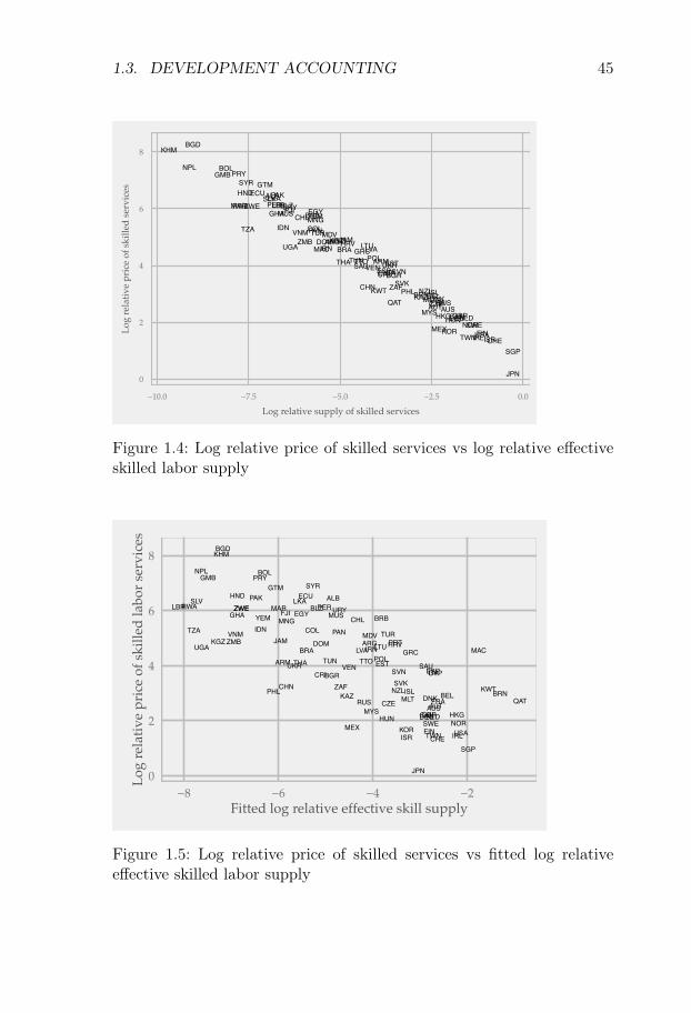
1.3. DEVELOPMENT ACCOUNTING 45
ALB
ARG
ARM
AUSAUT
BEL
BGD
BGR
BLZ
BOL
BRA
BRB
BRN
CAN
CHE
CHL
CHN
COL
CRICYP
CZE
DEU
DNK
DOM
ECU
EGY
ESPEST
FIN
FJI
FRA
GBR
GHA
GMB
GRC
GTM
HKG
HND
HRV
HUN
IDN
IRL
IRN
ISL
ISR
ITA
JAM
JPN
KAZ
KGZ
KHM
KOR
KWT
LBRLKA
LTULVAMAC
MAR
MDV
MEX
MLT
MNGMUS
MYSNLDNOR
NPL
NZL
PAK
PAN
PER
PHL
POL
PRT
PRY
QAT RUS
RWA
SAU
SGP
SLV
SWE
SVK
SVN
SYR
THA TTOTUN
TUR
TWN
TZA
UGA
UKR
URY
USA
VEN
VNM
YEM
ZAF
ZMB
ZWE
0
2
4
6
8
−10.0 −7.5 −5.0 −2.5 0.0
Log relative supply of skilled services
Log
rel
ativ
e pr
ice
of s
kille
d s
ervi
ces
Figure 1.4: Log relative price of skilled services vs log relative effectiveskilled labor supply
ALB
ARG
ARM
AUSAUT
BEL
BGD
BGR
BLZ
BOL
BRA
BRB
BRN
CAN
CHE
CHL
CHN
COL
CRI CYP
CZE
DEU
DNK
DOM
ECU
EGY
ESPEST
FIN
FJI
FRA
GBR
GHA
GMB
GRC
GTM
HKG
HND
HRV
HUN
IDN
IRL
IRN
ISL
ISR
ITA
JAM
JPN
KAZ
KGZ
KHM
KOR
KWT
LBRLKA
LTULVA MAC
MAR
MDV
MEX
MLT
MNGMUS
MYSNLD
NOR
NPL
NZL
PAK
PAN
PER
PHL
POL
PRT
PRY
QATRUS
RWA
SAU
SGP
SLV
SVK
SVN
SWE
SYR
THA TTOTUN
TUR
TWN
TZA
UGA
UKR
URY
USA
VEN
VNM
YEM
ZAF
ZMB
ZWEZWE
0
2
4
6
8
−8 −6 −4 −2Fitted log relative effective skill supply
Log
rel
ativ
e pr
ice
of s
kille
d la
bor
serv
ices
Figure 1.5: Log relative price of skilled services vs fitted log relativeeffective skilled labor supply

46 HUMAN CAPITAL IN DEVELOPMENT ACCOUNTING
1.3.3 Results
In this section, I perform development accounting. My main outcomevariables are the shares of world income differences accounted for byphysical capital, the human capital aggregator G, and TFP differences.To evaluate how my human capital measurement method affects develop-ment accounting, I compare my results to those obtained when the hu-man capital aggregator is additive in line with traditional developmentaccounting methods.
To decompose income differences into contributions from factors andtechnology, I re-arrange the aggregate production function (1.6) into
y=Y
L=
(K
Y
) α1−α
Ah.
With this re-arrangement, aggregate output is expressed as a functionof the capital-output ratio. This approach follows Hall and Jones (1999)and Hsieh and Klenow (2010b), and takes into account the steady-stateeffects of human capital and technology differences on capital accumula-tion.
The aggregate production function admits a linear decomposition oflog output per worker:
log(y) ≡ log
(Y
L
)=
α
1− αlog
(K
Y
)+ log(h) + log(A).
Using this decomposition, I define the shares of income differences at-
and unskilled services. As the relative factor shares can be measured independentlyof rs/ru, this specification does not feature any division bias. I similarly find anapproximate linear relationship, and similar results for the share of income differencesexplained by different values of the human capital aggregator G.
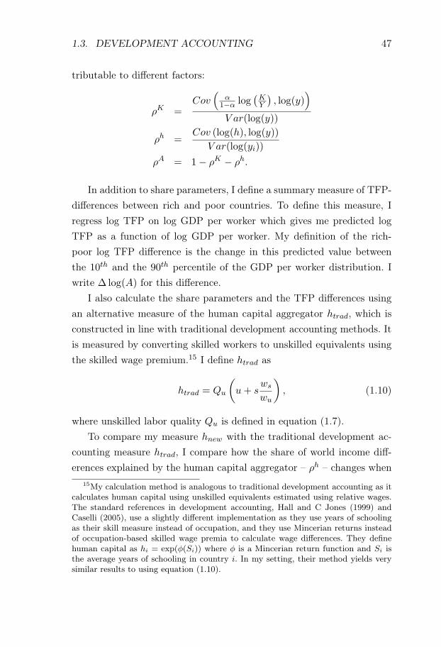
1.3. DEVELOPMENT ACCOUNTING 47
tributable to different factors:
ρK =Cov
(α
1−α log(KY
), log(y)
)V ar(log(y))
ρh =Cov (log(h), log(y))
V ar(log(yi))
ρA = 1− ρK − ρh.
In addition to share parameters, I define a summary measure of TFP-differences between rich and poor countries. To define this measure, Iregress log TFP on log GDP per worker which gives me predicted logTFP as a function of log GDP per worker. My definition of the rich-poor log TFP difference is the change in this predicted value betweenthe 10th and the 90th percentile of the GDP per worker distribution. Iwrite Δ log(A) for this difference.
I also calculate the share parameters and the TFP differences usingan alternative measure of the human capital aggregator htrad, which isconstructed in line with traditional development accounting methods. Itis measured by converting skilled workers to unskilled equivalents usingthe skilled wage premium.15 I define htrad as
htrad = Qu
(u+ s
ws
wu
), (1.10)
where unskilled labor quality Qu is defined in equation (1.7).To compare my measure hnew with the traditional development ac-
counting measure htrad, I compare how the share of world income diff-erences explained by the human capital aggregator – ρh – changes when
15My calculation method is analogous to traditional development accounting as itcalculates human capital using unskilled equivalents estimated using relative wages.The standard references in development accounting, Hall and C Jones (1999) andCaselli (2005), use a slightly different implementation as they use years of schoolingas their skill measure instead of occupation, and they use Mincerian returns insteadof occupation-based skilled wage premia to calculate wage differences. They definehuman capital as hi = exp(φ(Si)) where φ is a Mincerian return function and Si isthe average years of schooling in country i. In my setting, their method yields verysimilar results to using equation (1.10).
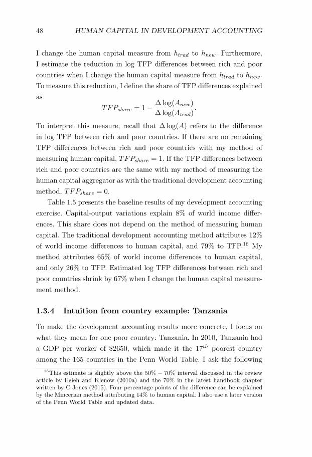
48 HUMAN CAPITAL IN DEVELOPMENT ACCOUNTING
I change the human capital measure from htrad to hnew. Furthermore,I estimate the reduction in log TFP differences between rich and poorcountries when I change the human capital measure from htrad to hnew.To measure this reduction, I define the share of TFP differences explainedas
TFPshare = 1− Δ log(Anew)
Δ log(Atrad).
To interpret this measure, recall that Δ log(A) refers to the differencein log TFP between rich and poor countries. If there are no remainingTFP differences between rich and poor countries with my method ofmeasuring human capital, TFPshare = 1. If the TFP differences betweenrich and poor countries are the same with my method of measuring thehuman capital aggregator as with the traditional development accountingmethod, TFPshare = 0.
Table 1.5 presents the baseline results of my development accountingexercise. Capital-output variations explain 8% of world income differ-ences. This share does not depend on the method of measuring humancapital. The traditional development accounting method attributes 12%
of world income differences to human capital, and 79% to TFP.16 Mymethod attributes 65% of world income differences to human capital,and only 26% to TFP. Estimated log TFP differences between rich andpoor countries shrink by 67% when I change the human capital measure-ment method.
1.3.4 Intuition from country example: Tanzania
To make the development accounting results more concrete, I focus onwhat they mean for one poor country: Tanzania. In 2010, Tanzania hada GDP per worker of $2650, which made it the 17th poorest countryamong the 165 countries in the Penn World Table. I ask the following
16This estimate is slightly above the 50% − 70% interval discussed in the reviewarticle by Hsieh and Klenow (2010a) and the 70% in the latest handbook chapterwritten by C Jones (2015). Four percentage points of the difference can be explainedby the Mincerian method attributing 14% to human capital. I also use a later versionof the Penn World Table and updated data.
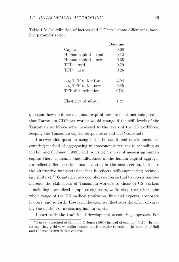
1.3. DEVELOPMENT ACCOUNTING 49
Table 1.5: Contribution of factors and TFP to income differences: base-line parametrization
BaselineCapital 0.08Human capital – trad. 0.12Human capital – new 0.65TFP – trad. 0.79TFP – new 0.26
Log TFP diff. – trad. 2.54Log TFP diff. – new 0.85TFP-diff. reduction 67%
Elasticity of subst. η 1.27
question: how do different human capital measurement methods predictthat Tanzanian GDP per worker would change if the skill levels of theTanzanian workforce were increased to the levels of the US workforce,keeping the Tanzanian capital-output ratio and TFP constant?
I answer this question using both the traditional development ac-counting method of aggregating microeconomic returns to schooling asin Hall and C Jones (1999), and by using my way of measuring humancapital (here, I assume that differences in the human capital aggrega-tor reflect differences in human capital; in the next section, I discussthe alternative interpretation that it reflects skill-augmenting technol-ogy shifters).17 Granted, it is a complex counterfactual to ceteris paribusincrease the skill levels of Tanzanian workers to those of US workers– including specialized computer engineers, world-class researchers, thewhole range of the US medical profession, financial experts, corporatelawyers, and so forth. However, the exercise illustrates the effect of vary-ing the method of measuring human capital.
I start with the traditional development accounting approach. For17I use the method of Hall and C Jones (1999) instead of equation (1.10). In this
setting, they yield very similar results, but it is easier to explain the method of Halland C Jones (1999) in this context.
50 HUMAN CAPITAL IN DEVELOPMENT ACCOUNTING
2010, the Barro-Lee data estimates Tanzanian average schooling levelsto be 5.81 years, and US average schooling levels to be 13.18 years, a dif-ference of approximately 7.5 years. Using the Mincerian return functionfrom Hall and C Jones (1999) and Caselli (2005), these schooling differ-ences translate into an approximately 0.6 log point difference in humancapital. Using the aggregate production function (1.6), log TanzanianGDP per worker increases by the same amount.
This example illustrates that traditional development accountingdoes not attribute a dominant role to human capital in explainingworld income differences. Even if Tanzania increases the skill levelsof its workforce all the way to US skill levels, GDP per worker onlyincreases by 0.6 log points, or to $4675. After this change in skill levels,Tanzanian income levels would not move higher than somewherebetween Senegal and Bangladesh.
In contrast, my method estimates that there is an approximate 2.6log point difference in human capital between the US and Tanzania. Af-ter increasing the skill levels of the Tanzanian workforce, Tanzania wouldhave a GDP per worker of approximately $36, 000, making it approxi-mately as rich as Russia. The lower TFP of Tanzania would still make itsubstantially poorer than the US (with a GDP per worker of $93, 000),but the change in its skill levels would make it an upper middle incomecountry.
1.4 Interpretation of mechanism: High efficiencyof skilled labor
1.4.1 Mechanism
Section 1.3.3 showed that my method of aggregating human capitalattributes a much smaller share of world income differences to TFP-differences than traditional development accounting did. The key mech-anism driving this result is that my method estimates a high efficiencyof skilled labor in rich countries. Figure 1.6 shows the relationship be-
INTERPRETATION OF MECHANISM 51
tween log GDP per worker and the efficiency of skilled labor accordingto the traditional development accounting method which equates rela-tive skilled labor efficiency with the skilled wage premium and the samerelationship according to my method, which also allows for differencesin the relative price of skilled services (in both cases, I normalize log USskilled labor efficiency to 0). The figure shows that traditional develop-ment accounting actually estimates that poor countries have a somewhathigher efficiency of skilled labor than rich countries. This reflects higherskilled wage premia in poor countries. My method paints a different pic-ture. With my method, the efficiency of skilled labor is about four and ahalf log points lower in poor countries as compared to rich countries. Mylarge estimated efficiency differences reflect large estimated differencesin relative skilled service prices. The relative price of skilled services andthe relative efficiency of skilled labor are related through
ws
wu=
Qs
Qu
rsru
,
where wswu
is the skilled wage premium. My trade data estimates suggestthat the relative price of skilled services rs
ruis 4-5 log points lower in
rich countries. Skilled wage premia are also lower in rich countries, butonly approximately one log point lower. This means that the relativeefficiency of skilled labor is 3-4 log points higher in rich countries. Myresults follow from combining this finding with the 0.5 rich-poor logdifference in the quality of unskilled labor. Intuitively, large efficiencydifferences are needed to reconcile moderate differences in skilled wagepremia with large differences in trade patterns.
Large skilled labor efficiency differences lead me to attribute more im-portance to differences in the value of the human capital aggregator G
than does traditional development accounting, and correspondingly lessimportance to uniform TFP-differences. Indeed, traditional developmentaccounting will in general overestimate the importance of uniform effi-ciency differences when rich countries have a higher efficiency of skilledlabor. The reason is that traditional development accounting relies on

INTERPRETATION OF MECHANISM 53
If I retain the assumption from traditional development accountingthat technology differences across countries are skill neutral, then thelarge efficiency differences reflect that skilled workers in rich countrieshave higher human capital. Under this interpretation, a majority of worldincome differences are explained by human capital differences. This isthe interpretation made in Jones (2014a), and it is further elaboratedin an unpublished manuscript (Jones, 2014b), where it is discussed thathuman capital differences among skilled workers can arise as a result ofmore extensive specialization in rich countries.
If we relax the assumption of neutral technology differences, an al-ternative explanation is that skilled labor efficiency differences reflectskill-augmenting technology differences. This is the interpretation madein Caselli and Coleman (2006) and Caselli (2015). Under this interpreta-tion, technology differences are still more important than human capitaldifferences, but it is a different form of technology differences than theTFP differences found in traditional development accounting. As thetechnology shifters are skill-specific, the results suggest that under thisinterpretation, theories of technology differences should explain how eco-nomic environments interact with the efficiency of skilled workers.
With a flexible specification of variation in technology and skilledlabor human capital across countries, it is not possible to distinguish thetechnology and human capital explanations using only price and quantitydata. Indeed, human capital quality and factor augmenting technologyterms appear in the same way in production functions. Thus, they havethe same implications for quantity and price data. Intuitively, price andquantity data alone cannot tell whether a worker is good at hammering,or has a good hammer.
To discriminate between the interpretations, more theoretical struc-ture or other sources of evidence are needed. In the Appendix, I dis-cuss some attempts to distinguish between the two interpretations. InAppendix 1.D.1, I discuss how migration results can be used to shedsome light on the respective roles of technology and human capital. Theconclusion is that imperfect substitutability makes it more complicated
54 HUMAN CAPITAL IN DEVELOPMENT ACCOUNTING
to interpret what wage changes at migration implies for human capitalmeasurement, as there is no longer a simple mapping between humancapital and pre- and post-migration wages with imperfect substitutabil-ity. In Appendix 1.D.2, I also analyze human capital versus technologyin the case when technology bias is constrained to be endogenous to fac-tor prices (as in, for example, Caselli and Coleman (2006) or Acemoglu(2007)). In this case, I show that large differences in human capital qual-ity are still needed to reconcile differences in Qs across countries.
Looking ahead, an important task is to analyze the sources of Qs
differences. Promising approaches are likely to involve more detailed dataon skilled wages in poor countries, and theoretical specifications thatallow us to use migration data and overcome the problems outlined inAppendix 1.D.1.
1.5 Relationship to B Jones (2014)
The paper most closely related to mine is B Jones (2014a), whichconstructs a theory of development accounting under imperfectsubstitutability. His key claim is that with a general human capitalaggregator, you have to scale traditional development accountingresults with the marginal product of unskilled labor to obtain the fullvalue of the human capital aggregator. A general aggregator satisfies
G(H1, . . . , HN ) = G1 ×(H1 +
N∑i=2
Gi
G1Hi
)
= G1 ×(H1 +
N∑i=2
wi
w1Hi
)
where Gi =∂G∂Hi
, and where the second line uses a competitive marketassumption. The terms in brackets on the second line represent the tra-ditional development accounting aggregator, which has to be scaled upby the marginal product of unskilled labor G1.
Although using a different formulation than in my paper, Jones also

1.5. RELATIONSHIP TO B JONES (2014) 55
highlights that traditional development accounting misses quality im-provements in skilled labor. In my formulation, traditional developmentaccounting underestimates improvements in the quality of skilled laboras an increased abundance of skilled services depresses the relative priceof skilled services. In Jones’ formulation, an improvement in the qualityof skilled labor increases the marginal product of unskilled labor, whichincreases the appropriate scaling on the results of traditional develop-ment accounting.
Furthermore, Jones recognizes that the quality of skilled labor canbe interpreted as resulting from an aggregation of heterogeneous skilledservices, which opens up for large quality differences. He emphasizesspecialization which is more fully developed in an unpublished paper(Jones, 2014b). As discussed in Section 1.4, other potential mechanismsthat can lead to large quality differences include strong complementar-ities between different skill types (C Jones, 2011), in particular O-ringeffects (Kremer, 1993).
However, Jones’ positive argument for large quality differences is lessstrong than his conceptual points. His quantitative argument relies onapplying rich country time-series and panel estimates of the elasticity ofsubstitution η to cross-country data. If this elasticity is globally valid, thelow supply of skilled labor in poor countries must imply a very high priceof skilled services. As these high skilled service prices are not observedin skilled wage premia, the quality of skilled labor must be very low inpoor countries.
The challenge to this argument is that most estimates of the elas-ticity of substitution are medium-run estimates from time series datafrom rich countries.19 We do not know a priori whether existing esti-
19One of few papers that take a long-run perspective is Ciccone and Peri (2005),which estimates long-run elasticities using compulsory schooling reforms and US cross-state data on a decadal level. The estimation method is closer to my desired parameteras it is a long-run estimate, and it uses an instrument to deal with the endogeneityof state-level supply of skilled labor. Their preferred estimate is 1.5 with a standarderror of 0.44. The study is unfortunately somewhat limited by weak instruments(the first-stage using the most credibly exogenous instrument has an F-value of 2.56with 6 instruments). Furthermore, there are five observations for every state and the

56 HUMAN CAPITAL IN DEVELOPMENT ACCOUNTING
mates are the relevant long-run cross-country elasticity estimates to beused in development accounting, or whether it is appropriate to assumea constant elasticity of substitution when analyzing cross-country data.Furthermore, the estimated importance of human capital is sensitive tothis elasticity parameter. Using my definition of the share of skilled work-ers, an elasticity of substitution η = 2 using Jones’ method would bringdown the share of world income differences accounted for by human cap-ital to approximately 25% of the world income differences, whereas anelasticity of substitution of approximately η = 1.2 would mean that allworld income differences would be explained by human capital.
Thus, Jones’ quantitative argument is difficult to evaluate if we donot have independent estimates of relative skilled service prices in poorcountries. My trade data method provides such estimates, and I findthat the relative prices of skilled services are indeed very high in poorcountries. My estimated elasticity of substitution η is 1.27. In Appendix1.A.3, I also provide suggestive evidence that a constant elasticity ofsubstitution is appropriate to model cross-country data. My paper thusprovides quantitative backing to Jones’ conceptual points.
1.6 Robustness and consistency checks
Here, I present various robustness and consistency checks of my results.In Section 1.6.1, I analyze how sensitive my estimates of relative skilledservice prices are to varying underlying assumptions and parameters. InSection 1.6.2, I test whether my estimates of relative skilled service pricesare consistent with estimates based on unit production cost data whensuch data are available. In Section 1.6.3, I analyze how my developmentaccounting exercise is affected when I change the measurement of skilledwage premia, and how it is affected when I exclude very poor countriesand oil producing countries from the analysis. The discussion of eachrobustness check is brief, and Appendix 1.E provides more detailed de-
standard errors are not clustered at the state level, which opens up for larger standarderrors.
1.6. ROBUSTNESS AND CONSISTENCY CHECKS 57
scriptions and discussions of the robustness checks.Across a wide range of specifications and parameter values, the con-
clusion holds that the role of human capital is considerably expanded ascompared to findings based on traditional development accounting meth-ods. Furthermore, for countries where both trade data and unit cost dataare available, the two types of analyses give similar results. Excludingthe poorest countries and oil producing countries increases the estimatedimportance of human capital.
1.6.1 Sensitivity of relative skilled service price estimates
I estimate the relative price of skilled services using the regression spec-ification (1.5). In this section, I test the sensitivity of my relative priceestimates to variations in the price elasticity of trade, the set of con-trol variables, the functional form of the underlying industry productionfunctions, and the presence of zero trade flows.
Table 1.6 shows how my development accounting results change whenI change the elasticity of trade σ. Variations in σ are quantitatively im-portant, and a larger σ means a lower importance of human capital. Theintuition is that a larger σ means that less relative unit cost differencesare needed to explain the trade data. This reduces the estimated differ-ences in relative skilled service prices which, in turn, imply a reductionin the estimated quality differences of skilled labor. Even though a largerσ implies a smaller role for human capital, the estimated importance ofhuman capital for σ = 15 is still 4.5 times as large as that found usingtraditional development accounting methods. When the trade elasticityis σ = 5, human capital explains more than 100% of world income differ-ences. In Appendix 1.E.1, I discuss the effect of allowing trade elasticitiesto be different across industries.
A second potential problem in regression (1.5) is omitted variables inthe specification of unit costs. The regression specification assumes thatvariations in relative unit costs are only driven by variations in relativefactor service prices. If there are other determinants of unit costs corre-

58 HUMAN CAPITAL IN DEVELOPMENT ACCOUNTING
lated with relative factor service prices, there will be an omitted variablebias. I test for the importance of an omitted variable bias by controllingfor potential determinants of unit costs apart from relative factor serviceprices. In particular, I allow there to be a country-specific penalty onexternal financing and/or contracting. These penalties increase the logunit cost of an industry in proportion to the financial dependence and/orcontracting dependence of the industry. To measure financial dependenceand contracting dependence at an industry level, I use measures similarto those developed by Rajan and Zingales (1998) and Nunn (2007), re-spectively. The results are presented in Table 1.7. Including a term forcontracting sensitivity does not affect the importance of human capital,and including a term for financial sensitivity decreases the importance ofhuman capital from 65% to 51%. In Appendix 1.E.2, I describe the def-inition of industry financial and contracting sensitivities, and how theyare included in my regression.
A third potential problem in regression (1.5) is a second-order bias inthe log-linearization of unit costs. The regression specification is basedon log-linearizing unit costs around the US cost structure. This log-linearization is exact if the industry production functions are Cobb-Douglas. If the industry production functions are not Cobb-Douglas,there will be a second-order bias as industry factor shares vary with rel-ative factor service prices. I analyze how my results change if industryproduction functions are CES with a common elasticity of substitutionξ = 1. I test for this bias by creating model generated unit costs from amodel where industry production functions are CES. I run my regressionspecification (1.5) on the model generated data and look for the pricedifferences in the model such that my regressions yield similar results onactual and model generated data. This procedure allows me to gauge thebias in my baseline estimates. Table 1.8 shows the development account-ing results for different assumed values of ξ. Appendix 1.D.3 explainsthe environment, the estimation method, the results, and the economicintuition in greater detail.
A fourth potential problem in regression (1.5) is zero trade flows.
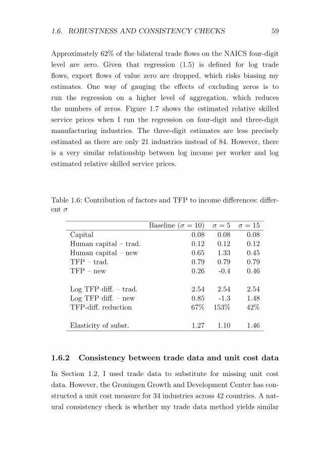
1.6. ROBUSTNESS AND CONSISTENCY CHECKS 59
Approximately 62% of the bilateral trade flows on the NAICS four-digitlevel are zero. Given that regression (1.5) is defined for log tradeflows, export flows of value zero are dropped, which risks biasing myestimates. One way of gauging the effects of excluding zeros is torun the regression on a higher level of aggregation, which reducesthe numbers of zeros. Figure 1.7 shows the estimated relative skilledservice prices when I run the regression on four-digit and three-digitmanufacturing industries. The three-digit estimates are less preciselyestimated as there are only 21 industries instead of 84. However, thereis a very similar relationship between log income per worker and logestimated relative skilled service prices.
Table 1.6: Contribution of factors and TFP to income differences: differ-ent σ
Baseline (σ = 10) σ = 5 σ = 15
Capital 0.08 0.08 0.08Human capital – trad. 0.12 0.12 0.12Human capital – new 0.65 1.33 0.45TFP – trad. 0.79 0.79 0.79TFP – new 0.26 -0.4 0.46
Log TFP diff. – trad. 2.54 2.54 2.54Log TFP diff. – new 0.85 -1.3 1.48TFP-diff. reduction 67% 153% 42%
Elasticity of subst. 1.27 1.10 1.46
1.6.2 Consistency between trade data and unit cost data
In Section 1.2, I used trade data to substitute for missing unit costdata. However, the Groningen Growth and Development Center has con-structed a unit cost measure for 34 industries across 42 countries. A nat-ural consistency check is whether my trade data method yields similar
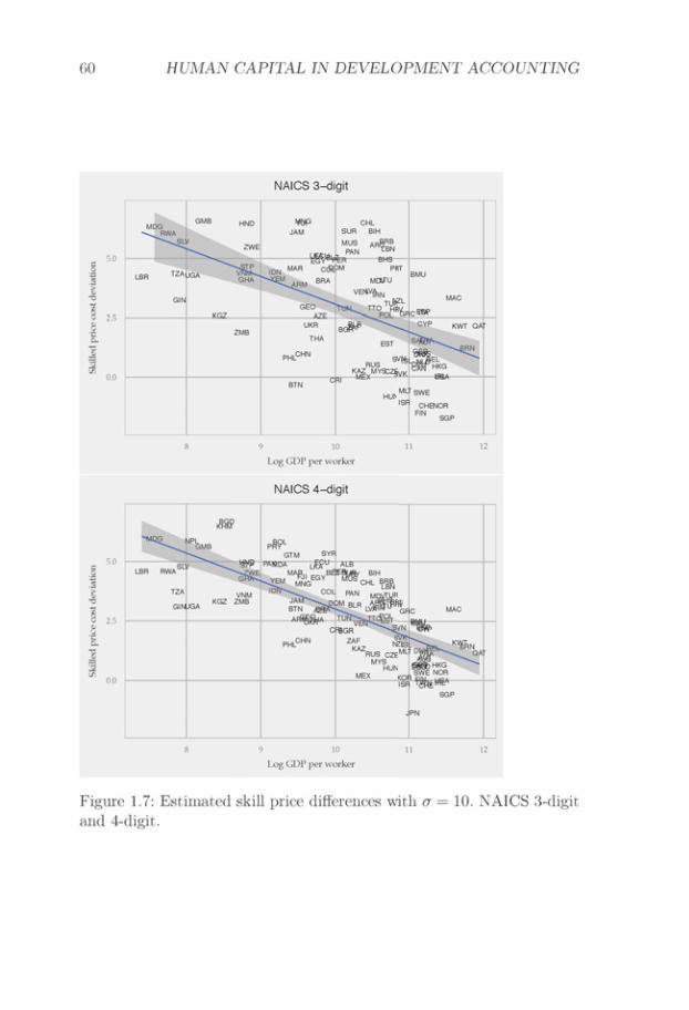
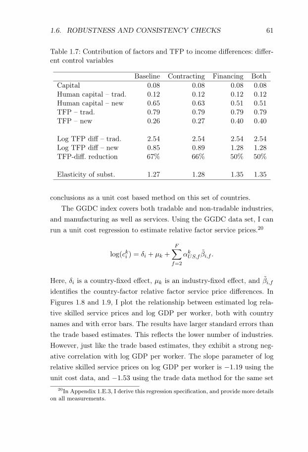
1.6. ROBUSTNESS AND CONSISTENCY CHECKS 61
Table 1.7: Contribution of factors and TFP to income differences: differ-ent control variables
Baseline Contracting Financing BothCapital 0.08 0.08 0.08 0.08Human capital – trad. 0.12 0.12 0.12 0.12Human capital – new 0.65 0.63 0.51 0.51TFP – trad. 0.79 0.79 0.79 0.79TFP – new 0.26 0.27 0.40 0.40
Log TFP diff – trad. 2.54 2.54 2.54 2.54Log TFP diff – new 0.85 0.89 1.28 1.28TFP-diff. reduction 67% 66% 50% 50%
Elasticity of subst. 1.27 1.28 1.35 1.35
conclusions as a unit cost based method on this set of countries.The GGDC index covers both tradable and non-tradable industries,
and manufacturing as well as services. Using the GGDC data set, I canrun a unit cost regression to estimate relative factor service prices.20
log(cki ) = δi + μk +F∑
f=2
αkUS,f βi,f .
Here, δi is a country-fixed effect, μk is an industry-fixed effect, and βi,f
identifies the country-factor relative factor service price differences. InFigures 1.8 and 1.9, I plot the relationship between estimated log rela-tive skilled service prices and log GDP per worker, both with countrynames and with error bars. The results have larger standard errors thanthe trade based estimates. This reflects the lower number of industries.However, just like the trade based estimates, they exhibit a strong neg-ative correlation with log GDP per worker. The slope parameter of logrelative skilled service prices on log GDP per worker is −1.19 using theunit cost data, and −1.53 using the trade data method for the same set
20In Appendix 1.E.3, I derive this regression specification, and provide more detailson all measurements.
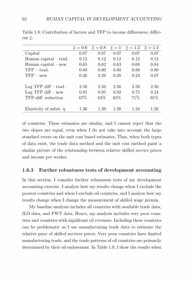
62 HUMAN CAPITAL IN DEVELOPMENT ACCOUNTING
Table 1.8: Contribution of factors and TFP to income differences: differ-ent ξ.
ξ = 0.6 ξ = 0.8 ξ = 1 ξ = 1.2 ξ = 1.4
Capital 0.07 0.07 0.07 0.07 0.07Human capital – trad. 0.12 0.12 0.12 0.12 0.12Human capital – new 0.65 0.62 0.63 0.68 0.84TFP – trad. 0.80 0.80 0.80 0.80 0.80TFP – new 0.26 0.29 0.28 0.23 0.07
Log TFP diff – trad. 2.56 2.56 2.56 2.56 2.56Log TFP diff – new 0.85 0.95 0.92 0.75 0.24TFP-diff. reduction 67% 63% 65% 71% 91%
Elasticity of subst. η 1.36 1.39 1.38 1.34 1.26
of countries. These estimates are similar, and I cannot reject that thetwo slopes are equal, even when I do not take into account the largestandard errors on the unit cost based estimates. Thus, when both typesof data exist, the trade data method and the unit cost method paint asimilar picture of the relationship between relative skilled service pricesand income per worker.
1.6.3 Further robustness tests of development accounting
In this section, I consider further robustness tests of my developmentaccounting exercise. I analyze how my results change when I exclude thepoorest countries and when I exclude oil countries, and I analyze how myresults change when I change the measurement of skilled wage premia.
My baseline analysis includes all countries with available trade data,ILO data, and PWT data. Hence, my analysis includes very poor coun-tries and countries with significant oil revenues. Including these countriescan be problematic as I use manufacturing trade data to estimate therelative price of skilled services prices. Very poor countries have limitedmanufacturing trade, and the trade patterns of oil countries are primarilydetermined by their oil endowment. In Table 1.9, I show the results when
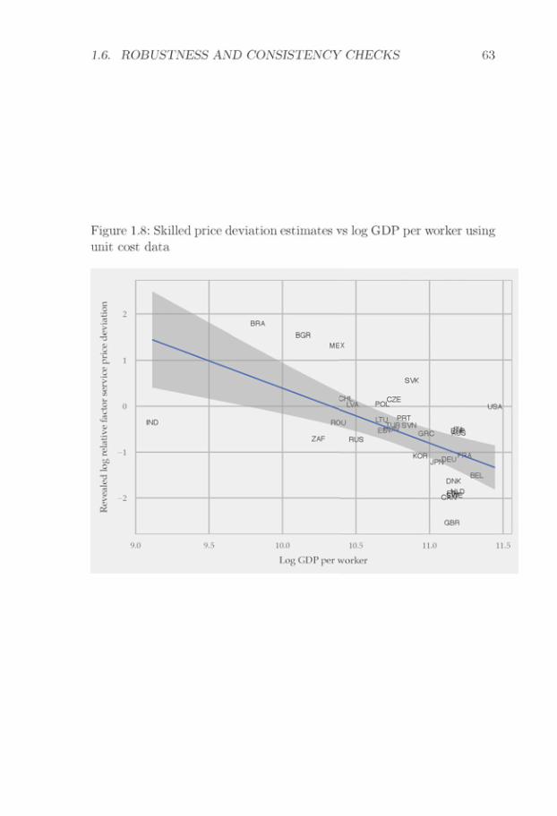
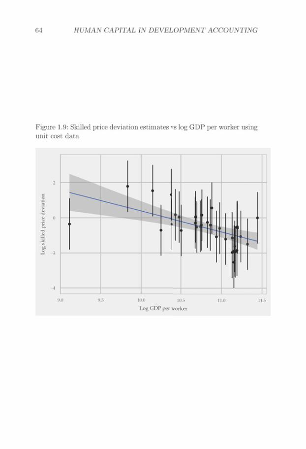

1.6. ROBUSTNESS AND CONSISTENCY CHECKS 65
I exclude oil countries and countries with a log GDP per worker of lessthan 9 in 2010 (corresponding approximately to Ghanaian income lev-els). Excluding these countries considerably expands the role of humancapital, and when both sets of countries are excluded, no TFP differ-ences are needed to explain the income differences among the remainingcountries.
I also analyze the robustness of my results to different measurementsof skilled wage premia. My skilled wage premia measures are based onlimited ILO data, and I want my estimates to be robust to systematicerrors in the data on skilled wage premia in poor countries. I am particu-larly concerned that my measures understate skilled wage premia in poorcountries due to the difficulty in measuring the wages of self-employedworkers and subsistence farmers. My skilled wage premia measures arebased on using a linear relation between log GDP per worker and logskilled wage premia. To test how my results depend on skill premia,I consider how my results change if I allow for a steeper relation be-tween country income and log skilled wage premia keeping rich countryskilled wage premia constant. I redo my analysis for different values ofthe income-skill premia slope γ ≤ 0. The results are presented in Table1.10.
Variations in the posited slope between skilled wage premia and coun-try income have little effect on the estimated importance of human cap-ital. The reason is that two effects counteract each other. Higher skilledwage premia in poor countries reduce the estimated skill-biased qual-ity differences, but they simultaneously reduce the estimated elasticityof substitution between skilled and unskilled workers. These two effectshave opposite consequences for the importance of human capital, andthey approximately offset each other. Intuitively, there are two cases.If skilled wage premia are very high in poor countries, it suggests thatskilled services are difficult to replace, and poor countries are poor be-cause they have few skilled services. If skilled premia are very low inpoor countries, large quality differences in human capital are needed tofit the trade data. Once more, the conclusion is that human capital is
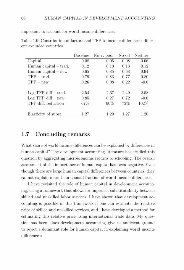
66 HUMAN CAPITAL IN DEVELOPMENT ACCOUNTING
important to account for world income differences.
Table 1.9: Contribution of factors and TFP to income differences: differ-ent excluded countries
Baseline No v. poor No oil NeitherCapital 0.08 0.05 0.08 0.06Human capital – trad. 0.12 0.10 0.13 0.12Human capital – new 0.65 0.85 0.68 0.94TFP – trad. 0.79 0.83 0.77 0.80TFP – new 0.26 0.08 0.22 -0.0
Log TFP diff – trad. 2.54 2.67 2.49 2.58Log TFP diff – new 0.85 0.27 0.72 -0.0TFP-diff. reduction 67% 90% 72% 102%
Elasticity of subst. 1.27 1.20 1.27 1.20
1.7 Concluding remarks
What share of world income differences can be explained by differences inhuman capital? The development accounting literature has studied thisquestion by aggregating microeconomic returns to schooling. The overallassessment of the importance of human capital has been negative. Eventhough there are large human capital differences between countries, theycannot explain more than a small fraction of world income differences.
I have revisited the role of human capital in development account-ing, using a framework that allows for imperfect substitutability betweenskilled and unskilled labor services. I have shown that development ac-counting is possible in this framework if one can estimate the relativeprice of skilled and unskilled services, and I have developed a method forestimating this relative price using international trade data. My ques-tion has been: does development accounting give us sufficient groundto reject a dominant role for human capital in explaining world incomedifferences?
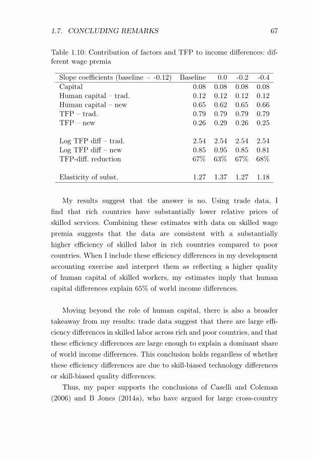
1.7. CONCLUDING REMARKS 67
Table 1.10: Contribution of factors and TFP to income differences: dif-ferent wage premia
Slope coefficients (baseline = -0.12) Baseline 0.0 -0.2 -0.4Capital 0.08 0.08 0.08 0.08Human capital – trad. 0.12 0.12 0.12 0.12Human capital – new 0.65 0.62 0.65 0.66TFP – trad. 0.79 0.79 0.79 0.79TFP – new 0.26 0.29 0.26 0.25
Log TFP diff – trad. 2.54 2.54 2.54 2.54Log TFP diff – new 0.85 0.95 0.85 0.81TFP-diff. reduction 67% 63% 67% 68%
Elasticity of subst. 1.27 1.37 1.27 1.18
My results suggest that the answer is no. Using trade data, Ifind that rich countries have substantially lower relative prices ofskilled services. Combining these estimates with data on skilled wagepremia suggests that the data are consistent with a substantiallyhigher efficiency of skilled labor in rich countries compared to poorcountries. When I include these efficiency differences in my developmentaccounting exercise and interpret them as reflecting a higher qualityof human capital of skilled workers, my estimates imply that humancapital differences explain 65% of world income differences.
Moving beyond the role of human capital, there is also a broadertakeaway from my results: trade data suggest that there are large effi-ciency differences in skilled labor across rich and poor countries, and thatthese efficiency differences are large enough to explain a dominant shareof world income differences. This conclusion holds regardless of whetherthese efficiency differences are due to skill-biased technology differencesor skill-biased quality differences.
Thus, my paper supports the conclusions of Caselli and Coleman(2006) and B Jones (2014a), who have argued for large cross-country

68 HUMAN CAPITAL IN DEVELOPMENT ACCOUNTING
differences in skilled labor efficiency. Their results build on a differentmethod than my results. They note that even though skill premia aresomewhat higher in poor countries, skill premia are not as high as theyshould be, given the low relative supply of skilled labor in poor coun-tries, at least not if the elasticity of substitution between skilled andunskilled labor is in line with rich country estimates. Both their pa-pers explain this observation by positing that skilled labor efficiency isrelatively low in poor countries. Even though they differ in their inter-pretation of these efficiency differences – Caselli and Coleman argue thatthey reflect skill-biased technology differences and B Jones argues thatthey reflect skill-biased human capital differences – they agree on theimportance of efficiency differences in skilled labor.
My findings suggest that their results are not just an artifact of as-suming that rich country estimates of substitution elasticities are glob-ally valid. When I analyze trade data, a similar pattern emerges. Rela-tive skilled service prices diverge more sharply between countries thanskilled wage premia, suggesting large differences in the relative efficiencyof skilled labor. Furthermore, the estimated efficiencies of skilled workersare strongly and positively correlated with GDP per worker. Quantita-tively, efficiency differences among skilled workers account for a substan-tial share of the variation in per capita output. By combining my resultswith the observations made by Caselli and Coleman (2006) and B Jones(2014), we see how skilled labor efficiency differences can provide a uni-fied perspective of the relationship between country income levels, tradepatterns, skilled labor supply, and skilled wage premia.
If output differences are primarily driven by efficiency differencesin skilled labor, this can influence the research agenda of growth anddevelopment economics. First, it means that skilled labor human capitaldifferences can drive a large share of output difference which, in turn,warrants a greater focus on theories of skill acquisition. Potentially in-teresting areas include the quality of higher education and the incentivesand efficiency of on-the-job learning. Second, if the efficiency of skilledlabor is driven by skill-specific technology shifters, our technology ex-
REFERENCES 69
planations should put a larger emphasis on why technology differencesselectively make skilled labor more productive. This suggests a shift awayfrom general TFP explanations toward more specific theories of technol-ogy differences. For example, when we study misallocation, it might bewarranted to focus more on how the efficiency of skilled labor is harmedby misallocation – potentially by looking at intersectoral patterns of mis-allocation. Similarly, when studying technology diffusion, it is warrantedto study whether barriers to technology diffusion specifically prevent thediffusion of technologies that are complementary to skilled workers.
References
Acemoglu, D. (2007). Equilibrium Bias of Technology. Econometrica,75(5):1371–1409.
Acemoglu, D., Antràs, P., and Helpman, E. (2007). Contracts and Tech-nology Adoption. American Economic Review, 97(3):916–943.
Acemoglu, D. and Autor, D. (2011). Chapter 12 – Skills, Tasks andTechnologies: Implications for Employment and Earnings. In Handbookof Labor Economics, volume 4, pages 1043–1171.
Acemoglu, D. and Ventura, J. (2002). The World Income Distribution.The Quarterly Journal of Economics, 117(2):659–694.
Acemoglu, D. and Zilibotti, F. (2001). Productivity Differences. TheQuarterly Journal of Economics, 116(2):563–606.
Anderson, J. E., Anderson, and James (1979). A Theoretical Foundationfor the Gravity Equation. American Economic Review, 69(1):106–16.
Anderson, J. E. and van Wincoop, E. (2003). Gravity with Gravitas: ASolution to the Border Puzzle. American Economic Review, 93(1):170–192.

70 HUMAN CAPITAL IN DEVELOPMENT ACCOUNTING
Barro, R. J. and Lee, J. W. (2013). A new data set of educational at-tainment in the world, 1950–2010. Journal of Development Economics,104:184–198.
Bartelsman, E. J. and Gray, W. (1996). The NBER Manufacturing Pro-ductivity Database.
Broda, C., Weinstein, D., Broda, C., and Weinstein, D. (2006). Global-ization and the Gains from Variety. Quarterly Journal of Economics,121:541–585.
Caselli, F. (2005). Chapter 9 Accounting for Cross-Country Income Diff-erences. Handbook of Economic Growth, 1:679–741.
Caselli, F. (2015). Technology Differences Over Space and Time.
Caselli, F. and Ciccone, A. (2013). The contribution of schooling indevelopment accounting: Results from a nonparametric upper bound.Journal of Development Economics, 104:199–211.
Caselli, F. and Coleman, W. J. (2006). The World Technology Frontier.American Economic Review, 96(3):499–522.
Chor, D. (2010). Unpacking sources of comparative advantage: A quanti-tative approach. Journal of International Economics, 82(2):152–167.
Ciccone, A. and Papaioannou, E. (2009). Human Capital, the Struc-ture of Production, and Growth. Review of Economics and Statistics,91(1):66–82.
Ciccone, A. and Peri, G. (2005). Long-Run Substitutability Be-tween More and Less Educated Workers: Evidence from U.S. States,1950–1990. Review of Economics and Statistics, 87(4):652–663.
Costinot, A., Donaldson, D., and Komunjer, I. (2011). What Goods DoCountries Trade? A Quantitative Exploration of Ricardo’s Ideas. TheReview of Economic Studies, 79(2):581–608.
REFERENCES 71
Cuñat, A. and Melitz, M. J. (2012). Volatility, Labor Market Flexibility,and the Pattern of Comparative Advantage. Journal of the EuropeanEconomic Association, 10(2):225–254.
Eaton, J. and Kortum, S. (2002). Technology, Geography, and Trade.Econometrica, 70(5):1741–1779.
Erosa, A., Koreshkova, T., and Restuccia, D. (2010). How Important IsHuman Capital? A Quantitative Theory Assessment of World IncomeInequality. Review of Economic Studies, 77(4):1421–1449.
Gaulier, G. and Zignago, S. (2010). BACI: International Trade Databaseat the Product-Level (the 1994-2007 Version). SSRN Electronic Jour-nal.
Gollin, D. (2002). Getting Income Shares Right. Journal of PoliticalEconomy, 110(2):458–474.
Hall, R. E. and Jones, C. I. (1999). Why do Some Countries Produce SoMuch More Output Per Worker than Others? The Quarterly Journalof Economics, 114(1):83–116.
Head, K. and Mayer, T. (2014). Gravity Equations: Workhorse,Toolkit,and Cookbook. In Handbook of International Economics, volume 4,pages 131–195. Elsevier B.V.
Hendricks, L. (2002). How Important Is Human Capital for Develop-ment? Evidence from Immigrant Earnings. American Economic Re-view, 92(1):198–219.
Hendricks, L. and Schoellman, T. (2016). Human Capital and Develop-ment Accounting: New Evidence from Wage Gains at Migration.
Hsieh, C.-T. and Klenow, P. J. (2009). Misallocation and Manufac-turing TFP in China and India *. Quarterly Journal of Economics,124(4):1403–1448.

72 HUMAN CAPITAL IN DEVELOPMENT ACCOUNTING
Hsieh, C.-T. and Klenow, P. J. (2010a). Development Accounting. Amer-ican Economic Journal: Macroeconomics, 2(1):207–23.
Hsieh, C.-T. and Klenow, P. J. (2010b). Development Accounting. Amer-ican Economic Journal: Macroeconomics, 2(1):207–223.
Inklaar, R. and Timmer, M. P. (2008). GGDC Productivity LevelDatabase: International Comparisons of Output, Inputs and Produc-tivity at the Industry Level. GGDC Research Memorandum.
Jones, B. F. (2014a). The Human Capital Stock: A Generalized Ap-proach. American Economic Review, 104(11):3752–3777.
Jones, B. F. (2014b). The Knowledge Trap: Human Capital and Develop-ment Reconsidered.
Jones, C. (2015). The Facts of Economic Growth. Technical report,National Bureau of Economic Research, Cambridge, MA.
Jones, C. I. (2011). Intermediate Goods and Weak Links in the The-ory of Economic Development. American Economic Journal: Macro-economics, 3(2):1–28.
Katz, L. F. and Murphy, K. M. (1992). Changes in Relative Wages,1963-1987: Supply and Demand Factors. The Quarterly Journal ofEconomics, 107(1):35–78.
Klenow, P. and Rodriguez-Clare, A. (1997). The Neoclassical Revival inGrowth Economics: Has It Gone Too Far? Technical report.
Kremer, M. (1993). The O-Ring Theory of Economic Development. TheQuarterly Journal of Economics, 108(3):551–75.
Krugman, P. (1988). Differences In Income Elasticities and Trends inReal Exchange Rates. Technical report, National Bureau of EconomicResearch, Cambridge, MA.
REFERENCES 73
Lagakos, D., Moll, B., Porzio, T., Qian, N., and Schoellman, T. (2016).Life-Cycle Human Capital Accumulation Across Countries: LessonsFrom U.S. Immigrants.
Levchenko, A. A. and Zhang, J. (2016). The evolution of comparative ad-vantage: Measurement and welfare implications. Journal of MonetaryEconomics, 78:96–111.
Manova, K. (2013). Credit Constraints, Heterogeneous Firms, and In-ternational Trade. The Review of Economic Studies, 80(2):711–744.
Manuelli, R. E. and Seshadri, A. (2014). Human Capital and the Wealthof Nations †. American Economic Review, 104(9):2736–2762.
Mattsson, L.-G., Weibull, J. W., and Lindberg, P. O. (2014). Extremevalues, invariance and choice probabilities. Transportation ResearchPart B: Methodological, 59:81–95.
Midrigan, V. and Xu, D. Y. (2014). Finance and Misallocation: Evidencefrom Plant-Level Data †. American Economic Review, 104(2):422–458.
Morrow, P. and Trefler, D. (2017). Endowments, Factor Prices, and Skill-Biased Technology: Importing Development Accounting into HOV.
Nunn, N. (2007). Relationship-Specificity, Incomplete Contracts, and thePattern of Trade. The Quarterly Journal of Economics, 122(2):569–600.
Nunn, N. and Trefler, D. (2015). Chapter 5: Domestic Institutions asa Source of Comparative Advantage. In Handbook of InternationalEconomics, volume 4, pages 263–315.
Oberfield, E. and Raval, D. (2014). Micro Data and Macro Technology.Technical report, National Bureau of Economic Research, Cambridge,MA.
Parente, S. L. and Prescott, E. C. (1999). Monopoly Rights: A Barrierto Riches. American Economic Review, 89(5):1216–1233.
74 HUMAN CAPITAL IN DEVELOPMENT ACCOUNTING
Rajan, R. G. and Zingales, L. (1998). Financial Dependence and Growth.American Economic Review, 88(3):559–86.
Rauch, J. E. (1999). Networks versus markets in international trade.Journal of International Economics, 48(1):7–35.
Redding, S. and Venables, A. J. (2004). Economic geography and inter-national inequality. Journal of International Economics, 62(1):53–82.
Restuccia, D. and Rogerson, R. (2008). Policy distortions and aggregateproductivity with heterogeneous establishments. Review of EconomicDynamics, 11(4):707–720.
Romalis, J. (2004). Factor Proportions and the Structure of CommodityTrade. American Economic Review, 94(1):67–97.
Romalis, J. (2007). NAFTA’s and CUSFTA’s Impact on InternationalTrade. http://dx.doi.org/10.1162/rest.89.3.416.
Schoellman, T. (2011). Education Quality and Development Accounting.The Review of Economic Studies, 79(1):388–417.
Schoellman, T. and Hendricks, L. (2016). Human Capital and Develop-ment Accounting: New Evidence from Wage Gains at Migration. 2016Meeting Papers.
Simonovska, I. and Waugh, M. E. (2014). The elasticity of trade: Esti-mates and evidence. Journal of International Economics, 92(1):34–50.
Soderbery, A. (2015). Estimating import supply and demand elastici-ties: Analysis and implications. Journal of International Economics,96(1):1–17.
Tinbergen, J. (1962). Shaping the World Economy; Suggestions for anInternational Economic Policy. Books (Jan Tinbergen).
Trefler, D. (1993). International Factor Price Differences: Leontief wasRight! Journal of Political Economy, 101(6):961–987.
APPENDIX 75
Appendix
1.A Environment
1.A.1 Heterogeneous skill type aggregator interpretationof Qu and Qs
Here, I show that my estimation of the relative quality Qs/Qu is con-sistent with a nested structure where the quality terms Qu and Qs arisefrom aggregation of heterogeneous unskilled and skilled services.
My human capital aggregator is
h =((Quu)
η−1η + as(Qss)
η−1η
) ηη−1
.
Before proving the result, I will provide a formal statement of whatequivalence means in this context. Assume that the true human capitalaggregator is
h =((Hu)
η−1η + as(H
s)η−1η
) ηη−1
,
where Hu and Hs are arbitrary constant returns to scale aggregatorsof heterogeneous unskilled and skilled services. I say that my relativequality estimation is consistent with an aggregator interpretation if thefollowing holds. Given the definition of quality
Qu ≡ Hs
s
Qs ≡ Hu
u,
the relative quality of skilled and unskilled labor Qs/Qu satisfies theequation
ws
wu=
Qs
Qu
rsru
, (1.11)
where wswu
is the relative average wage of skilled and unskilled workers,
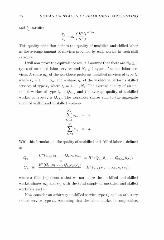
76 HUMAN CAPITAL IN DEVELOPMENT ACCOUNTING
and rsru
satisfiesrsru
= as
(Hs
Hu
)−1/η
.
This quality definition defines the quality of unskilled and skilled laboras the average amount of services provided by each worker in each skillcategory.
I will now prove the equivalence result. I assume that there are Nu ≥ 1
types of unskilled labor services and Ns ≥ 1 types of skilled labor ser-vices. A share utu of the workforce performs unskilled services of type tu
where tu = 1, . . . , Nu, and a share sts of the workforce performs skilledservices of type ts where ts = 1, . . . , Ns. The average quality of an un-skilled worker of type tu is Qu,tu and the average quality of a skilledworker of type ts is Qs,ts . The workforce shares sum to the aggregateshare of skilled and unskilled workers
Nu∑tu=1
utu = u
Ns∑ts=1
sts = s.
With this formulation, the quality of unskilled and skilled labor is definedas
Qu ≡ Hu(Qu,1u1, . . . , Qu,NuuNu)
u= Hu (Qu,1u1, . . . , Qu,Nu uNu)
Qs ≡ Hs(Qs,1s1, . . . , Qs,NusNu)
s= Hs (Qs,1s1, . . . , Qs,Ns sNs) ,
where a tilde (∼) denotes that we normalize the unskilled and skilledworker shares utu and sts with the total supply of unskilled and skilledworkers s and u.
Now consider an arbitrary unskilled service type tu and an arbitraryskilled service type ts. Assuming that the labor market is competitive,
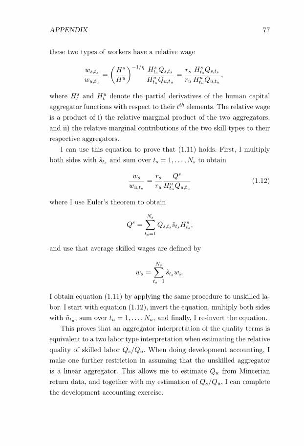
APPENDIX 77
these two types of workers have a relative wage
ws,ts
wu,tu
=
(Hs
Hu
)−1/η HstsQs,ts
HutuQu,tu
=rsru
HstsQs,ts
HutuQu,tu
,
where Hst and Hu
t denote the partial derivatives of the human capitalaggregator functions with respect to their tth elements. The relative wageis a product of i) the relative marginal product of the two aggregators,and ii) the relative marginal contributions of the two skill types to theirrespective aggregators.
I can use this equation to prove that (1.11) holds. First, I multiplyboth sides with sts and sum over ts = 1, . . . , Ns to obtain
ws
wu,tu
=rsru
Qs
HutuQu,tu
(1.12)
where I use Euler’s theorem to obtain
Qs =
Ns∑ts=1
Qs,ts stsHsts ,
and use that average skilled wages are defined by
ws =
Ns∑ts=1
stsws.
I obtain equation (1.11) by applying the same procedure to unskilled la-bor. I start with equation (1.12), invert the equation, multiply both sideswith utu , sum over tu = 1, . . . , Nu, and finally, I re-invert the equation.
This proves that an aggregator interpretation of the quality terms isequivalent to a two labor type interpretation when estimating the relativequality of skilled labor Qs/Qu. When doing development accounting, Imake one further restriction in assuming that the unskilled aggregatoris a linear aggregator. This allows me to estimate Qu from Mincerianreturn data, and together with my estimation of Qs/Qu, I can completethe development accounting exercise.
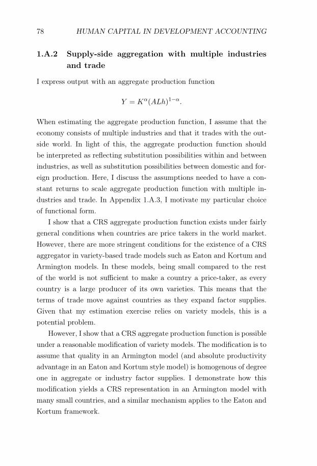
78 HUMAN CAPITAL IN DEVELOPMENT ACCOUNTING
1.A.2 Supply-side aggregation with multiple industriesand trade
I express output with an aggregate production function
Y = Kα(ALh)1−α.
When estimating the aggregate production function, I assume that theeconomy consists of multiple industries and that it trades with the out-side world. In light of this, the aggregate production function shouldbe interpreted as reflecting substitution possibilities within and betweenindustries, as well as substitution possibilities between domestic and for-eign production. Here, I discuss the assumptions needed to have a con-stant returns to scale aggregate production function with multiple in-dustries and trade. In Appendix 1.A.3, I motivate my particular choiceof functional form.
I show that a CRS aggregate production function exists under fairlygeneral conditions when countries are price takers in the world market.However, there are more stringent conditions for the existence of a CRSaggregator in variety-based trade models such as Eaton and Kortum andArmington models. In these models, being small compared to the restof the world is not sufficient to make a country a price-taker, as everycountry is a large producer of its own varieties. This means that theterms of trade move against countries as they expand factor supplies.Given that my estimation exercise relies on variety models, this is apotential problem.
However, I show that a CRS aggregate production function is possibleunder a reasonable modification of variety models. The modification is toassume that quality in an Armington model (and absolute productivityadvantage in an Eaton and Kortum style model) is homogenous of degreeone in aggregate or industry factor supplies. I demonstrate how thismodification yields a CRS representation in an Armington model withmany small countries, and a similar mechanism applies to the Eaton andKortum framework.
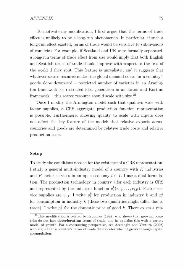
APPENDIX 79
To motivate my modification, I first argue that the terms of tradeeffect is unlikely to be a long-run phenomenon. In particular, if such along-run effect existed, terms of trade would be sensitive to subdivisionsof countries. For example, if Scotland and UK were formally separated,a long-run terms of trade effect from size would imply that both Englishand Scottish terms of trade should improve with respect to the rest ofthe world if they split. This feature is unrealistic, and it suggests thatwhatever scarce resource makes the global demand curve for a country’sgoods slope downward – restricted number of varieties in an Arming-ton framework, or restricted idea generation in an Eaton and Kortumframework – this scarce resource should scale with size.21
Once I modify the Armington model such that qualities scale withfactor supplies, a CRS aggregate production function representationis possible. Furthermore, allowing quality to scale with inputs doesnot affect the key feature of the model: that relative exports acrosscountries and goods are determined by relative trade costs and relativeproduction costs.
Setup
To study the conditions needed for the existence of a CRS representation,I study a general multi-industry model of a country with K industriesand F factor services in an open economy i ∈ I. I use a dual formula-tion. The production technology in country i for each industry is CRSand represented by the unit cost function cki (ri,1, . . . , ri,F ). Factor ser-vice supplies are vi,f . I write yki for production in industry k and xkifor consumption in industry k (these two quantities might differ due totrade). I write pki for the domestic price of good k. There exists a rep-
21This modification is related to Krugman (1988) who shows that growing coun-tries do not face deteriorating terms of trade, and he explains this with a varietymodel of growth. For a contrasting perspective, see Acemoglu and Ventura (2002)who argue that a country’s terms of trade deteriorates when it grows through capitalaccumulation.
80 HUMAN CAPITAL IN DEVELOPMENT ACCOUNTING
resentative consumer whose preferences are defined by an expenditurefunction e(pi, ui). I assume that these preferences are homothetic, whichmeans that there exists a utility representation of preferences such thatthe expenditure function can be written
e(pi, ui) = e(pi)ui
for some function e. Throughout this section, I assume that preferencesare homothetic and I will write e without a tilde going forward.
A CRS aggregator representation exists if prices are unchanged andoutput and consumption scale linearly when we scale factor inputs. For-mally, I say that a CRS aggregator representation exists if the follow-ing condition holds. Let xki , y
ki , ui, ri,f , p
ki , c
ki be an arbitrary equilibrium
given factor supplies vi,f . A CRS representation exists if for each suchequilibrium, a factor supply λvi,f implies that λxki , λy
ki , λui, ri,f , p
ki , c
ki is
an equilibrium.I first consider a model where each country is a price-taker in the
world market. In this case, the equilibrium conditions can be written as:
K∑k=1
∂cki∂ri,f
yki = vi,f f = 1, . . . , F
∂e
∂pkiui = xki k = 1, . . . ,K
cki ≥ pki = 0 if yki > 0
e(pi)ui =F∑
f=1
ri,fvi,f
The first equation gives clearing conditions for the factor markets, wherethe left-hand side uses Shepherd’s lemma applied to the unit cost func-tion to derive factor demands for each factor f and for industry k.The second equation expresses consumer demand, applying Shepherd’slemma to the expenditure function. The third equation is a zero-profitcondition, where the inequality constraint reflects that I allow for zero
APPENDIX 81
production. The fourth equation is the budget constraint for the repre-sentative consumer.
By inspection, this system of equations allows for a CRS aggregatorrepresentation. If there exists a set of prices such that yki , x
ki , ui, vi,f solve
the system, then any scaling λyki , λxki , λui, λvi,f for λ > 0 solves the
system for the same set of prices.To study the Armington case, I retain the assumption that the coun-
try is small in the aggregate world economy. However, the country islarge in its own varieties. I represent this with an Armington model witha continuum of countries and K goods. I write i ∈ [0, 1] for the countryon which I focus.
There are K final goods. Each final good is assembled domesticallyusing a composite of country-industry specific intermediate varieties thatare traded between countries. To produce good k, one needs an inputvariety from each country in the world. I assume that there are no tradecosts so that the unit cost Ck
i of assembling final good k in country i isthe same in every country and equal to
Cki ≡ Ck =
(∫ 1
0akj (c
kj )
1−σdj
) 11−σ
σ > 1.
I normalize akj so that the unit production costs are ckj = 1 for all coun-tries j = i (our unit of analysis). This means that
Ck = 1 k = 1, . . . ,K.
Write qki,j for the amount of input to industry k that is produced incountry i for use in country j. As there are no trading costs and countriesare symmetric, qki,j does not depend on destination j. Furthermore, usingShepherd’s lemma,
qki,j =∂Ck
∂ckixkj ,
where xkj is the country j consumption of final goods in industry k.
82 HUMAN CAPITAL IN DEVELOPMENT ACCOUNTING
I can now write down the equilibrium definition.
qki,j = aki (cki )
−σxkj
pi,k = ci,k
xki =∂e(1, . . . , 1)
∂P kui
F∑f=1
ri,fvi,f = e(1, . . . , 1)ui
K∑k=1
∫ 1
0qki,j
∂cki∂ri,f
= vi,f
The first equation gives country j’s demand for industry k goods pro-duced in country i. The formulation uses that the price index P k
j =
Ckj = 1 for all j. The second equation is a non-profit condition for pro-
duction in country i. There is no inequality constraint, reflecting thatwith a CES specification of production technology from intermediates,production of each variety is always positive. The third equation appliesShepherd’s lemma to the consumer’s expenditure function. It is evaluatedat (1, . . . , 1) as all prices P k = 1. The fourth and fifth equations give theconsumer budget constraints and the factor market clearing condition.
By inspection, there does not exist a CRS aggregator representationof this system. In the first equation, we see that scaling output willchange prices, violating the assumption that there exist scaled equilibriawith the same prices. This reflects a terms of trade effect whereby scalingoutput depresses the terms of trade.
However, there exists a simple modification of the system to obtain aCRS aggregator. If I define aki = Φk
i (vki,1, . . . , v
ki,F ) for some CRS aggre-
gator Φki , there exists a CRS representation of the equilibrium. Allowing
the quality term aki to scale linearly with factor supply captures theintuition that subdivision of observation units should not affect tradepatterns with third parties. Even with this modification, relative tradepatterns across industries are still shaped by relative costs, and if we
APPENDIX 83
were to add trade costs, then trade costs would affect the distributionbetween domestic uses and exports, and trade costs would also affectrelative exports to different countries.
1.A.3 Functional form of aggregate production function
My aggregate production function has the form
Y = Kα(ALh)1−α.
As discussed in Appendix 1.A.2, this represents an aggregation takinginto account the existence of multiple industries and opportunities forinternational trade. In this section, I discuss my choice of functional form.
I choose a Cobb-Douglas aggregator between capital and labor ser-vices. This is standard in the development accounting literature, andcan be motivated by there being constant labor shares across countries(Gollin, 2002).22
For the human capital aggregator, I use a CES aggregator of skilledand unskilled labor services, which is standard in the labor economicsliterature (Acemoglu and Autor, 2011). Ideally, I should have a skillaggregator that was formally aggregated from production functions onthe industry level together with a trade model. Unfortunately, there is nostraightforward aggregation to a CES representation from industries withheterogeneous factor shares. Thus, the constant elasticity assumptionshould be interpreted as an approximation to a more freely specifiedunderlying aggregator.
One way of testing my assumption of constant elasticity of substi-tution is by plotting the cross-country relationship between log relativefactor service prices and log relative factor supplies. Theoretically, these
22Recent studies cast doubt on the Cobb-Douglas assumption (Oberfield andRaval, 2014), and Caselli (2005) suggests that the elasticity of substitution betweencapital and labor can be a crucial parameter in development accounting. I do not pur-sue this line of inquiry further here, but it is an interesting avenue of future research.The Cobb-Douglas specification of labor and capital also precludes capital-labor com-plementarities.

84 HUMAN CAPITAL IN DEVELOPMENT ACCOUNTING
should be related by
log
(rsru
)= log(as)− 1
ηlog
(Qss
Quu
).
If the CES assumption is true, the relationship should be linear. Thetest is not ideal, as my estimated relative quality log
(Qs
Qu
)is implicitly
present in the relative price of factor services, and thus it appears on bothsides of the equation, which biases the relationship towards being linear.However, if the log relative supply of skilled and unskilled workers log
(su
)was not linearly related to the relative quality log
(Qs
Qu
), the relationship
would not be linear. Thus, testing the linearity of this relationship offersan opportunity to falsify the CES assumption. The results are plotted inFigure 1.A.1, which suggests that the linearity assumption is appropriate.
Looking ahead, potential extensions include modifying the functionalform to allow for capital-skill complementarities and non-unitary elastic-ity of substitution between labor and capital.
1.B Development accounting
1.B.1 Occupational vs schooling based skill cutoff
I define the share of unskilled and skilled workers u and s as the sharesof people working in an unskilled and skilled occupation, respectively.This contrasts to the approach taken in Caselli and Coleman (2006), BJones (2014a), and Caselli (2015) who define the share of skilled workersas the share of individuals having an educational attainment above apre-specified threshold (for example, primary education and above, highschool and above, or college and above).
The distinction between the share of workers with a skilled occu-pation and the share of workers with a certain educational level doesnot matter if all countries have the same mapping between educationalattainment and occupational skill level. However, there is no a priorireason to believe that this mapping should be the same across countries.
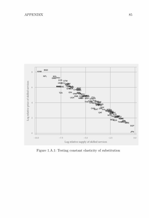
APPENDIX 85
ALB
ARG
ARM
AUSAUT
BEL
BGD
BGR
BLZ
BOL
BRA
BRB
BRN
CAN
CHE
CHL
CHN
COL
CRICYP
CZE
DEU
DNK
DOM
ECU
EGY
ESPEST
FIN
FJI
FRA
GBR
GHA
GMB
GRC
GTM
HKG
HND
HRV
HUN
IDN
IRL
IRN
ISL
ISR
ITA
JAM
JPN
KAZ
KGZ
KHM
KOR
KWT
LBRLKA
LTULVAMAC
MAR
MDV
MEX
MLT
MNGMUS
MYSNLDNOR
NPL
NZL
PAK
PAN
PER
PHL
POL
PRT
PRY
QAT RUS
RWA
SAU
SGP
SLV
SWE
SVK
SVN
SYR
THA TTOTUN
TUR
TWN
TZA
UGA
UKR
URY
USA
VEN
VNM
YEM
ZAF
ZMB
ZWE
0
2
4
6
8
−10.0 −7.5 −5.0 −2.5 0.0
Log relative supply of skilled services
Log
rel
ativ
e pr
ice
of s
kille
d s
ervi
ces
Figure 1.A.1: Testing constant elasticity of substitution

86 HUMAN CAPITAL IN DEVELOPMENT ACCOUNTING
Acemoglu and Autor (2011) have highlighted the importance of distin-guishing between educational attainment and tasks when analyzing UStime series data as the allocation of skills to tasks is an equilibrium out-come. Their point is more relevant when analyzing differences betweencountries with very large differences in educational systems. When ed-ucational attainment does not map to occupational skill content in thesame way across countries, this modeling choice matters.
I choose an occupational definition for two reasons. First, there aremultiple ways of acquiring skills, and education is only one of them.Many people learn skilled occupations outside the educational system,and poor quality of schooling increases the risk that schooling does notfully reflect skill acquisition. When skills are not equal to educationalattainment, the complexity of the occupation is a proxy for skill. Indeed,as long as there is a positive skilled wage premium, barring compensatingdifferential concerns, people will work in the most complex occupationsthat they can perform. Second, occupation is closer to the definitionsused for skill shares in my trade data exercise, where I define the skillshare as the share of gross output that goes to the payroll of workers incertain occupations.
Thus, I measure the share of skilled workers in line with the ILO’sISCO-08 definitions of skill requirements and major occupational groups.The ILO defines 10 major occupational groups and four skill levels. Theoccupational groups and their respective skill levels are presented in Fig-ure 1.B.1. I use the ILOSTAT database to obtain s as the share of thelabor force working as managers, professionals, or technicians and asso-ciated technicians, i.e. skill categories 3 and 4 (I define the armed forcesas primarily unskilled). I define the unskilled share as u ≡ 1− s.
Figure 1.B.2 compares the results from an education based and oc-cupation based definition of the skill share. Figure 1.B.2 shows that forpoor countries, the share of high school educated workers and the shareof skilled workers approximately coincide. For rich countries, there aremuch more high school educated workers than skilled workers. This is ev-idence that the mapping between educational attainment and skill level

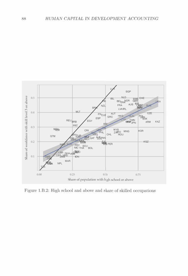

APPENDIX 89
1.B.2 Measurement of unskilled labor quality Qu
I define the quality of unskilled labor Qu using a Mincerian definition.The quality of unskilled labor is defined as
Qu = exp(φ(Su)).
Here, Su is defined as the average years of schooling of unskilled workers.φ is a function capturing the Mincerian returns to education. I use afunctional form from Hall and C Jones (1999) and Caselli (2005) whereφ(S) is a piecewise linear function with slope 0.13 for S < 4, a slope 0.1
for S ∈ [4, 8), and a slope 0.08 for S ≥ 8.I measure Su by using the data from Barro and Lee (2013). I assume
that there is positive sorting between education and skill levels in occupa-tion, and that Su represents the average years of schooling of the share u
of the population working in unskilled occupations. The Barro-Lee datadoes unfortunately not record the cumulative distribution of years ofschooling, but only total schooling attainment within different levels ofschooling. It records the number of schooling years at the primary level,the secondary level, and the higher level.
To calculate Su, I first note that in the vast majority of countries,the cutoff between skilled and unskilled workers goes below the collegelevel, and I attribute none of the schooling years in higher education tounskilled workers. To calculate the years of schooling in primary and sec-ondary school that should be attributed to low skilled workers, I subtract7 times the share of skilled workers from both primary and secondaryschool years, using the approximation that all skilled workers have fin-ished high school and that primary and secondary school both are both7 years. The results are not sensitive to details in this specification. Afterthis subtraction, I divide the remaining primary and secondary schoolyears with the share of unskilled workers to obtain Su.
90 HUMAN CAPITAL IN DEVELOPMENT ACCOUNTING
1.C Estimating the relative price of skilled ser-vices
1.C.1 Theoretical derivation of gravity equation
In this section, I show how my gravity specification can be derivedfrom theoretical trade models. I first derive the specification from anArmington style trade model, and then from an Eaton and Kortumstyle trade model.
Armington model
There are K industries and I countries, indexed i for source countriesand j for destination countries. Each country admits a representativehousehold with preferences
Uj =
(I∑
i=1
K∑k=1
(akj )1/σ(qki,j)
σ−1σ
) σσ−1
j = 1, . . . , I; σ > 1 (1.13)
where qki,j are goods from industry k produced in country i and consumedin country j, σ captures the elasticity of substitution between differentvarieties, and akj is a country-specific taste term. The taste term is areduced form way of capturing differences in tastes across countries, in-cluding potential non-homotheticities in preferences. The representativeconsumer maximizes (1.13) subject to a constraint
I∑i=1
K∑k=1
P ki,jq
ki,j ≤ Yj
where P ki,j is the price of good k produced in country i and bought in
country j. Yj is income in country j.Each variety is produced using a constant returns to scale production
APPENDIX 91
function with the unit cost function
cki = Ck (ri,1, . . . , ri,F ) (1.14)
where ri,f is the price of factor service f in country i.Trade costs take an iceberg form and to consume one unit of a good
from country i, a country j consumer has to buy di,j ≥ 1 goods fromcountry i. The cost term di,j satisfies
di,j ≥ 1
di,i = 1 ∀i = 1, . . . , I
di,jdj,l ≥ di,l.
Output markets are competitive, which implies that prices satisfy
P ki,j = cki di,j . (1.15)
Each country has a supply of factor service flows
ej,f ≥ 0 i = 1, . . . , I; f = 1, . . . , F,
and country income is given by
Yj =F∑
f=1
rj,fej,f (1.16)
An equilibrium is a set of consumption quantities qki,j , production quan-tities Qk
i , factor service prices ri,f , unit costs cki , output prices P ki,j , and
incomes Yj such that:
1. {qki,j} solves the consumer problem given output prices and in-comes.
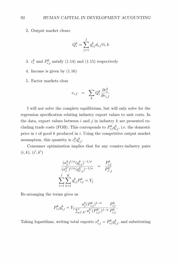
92 HUMAN CAPITAL IN DEVELOPMENT ACCOUNTING
2. Output market clears
Qki =
I∑j=1
qki,jdi,j∀i, k
3. cki and P ki,j satisfy (1.14) and (1.15) respectively
4. Income is given by (1.16)
5. Factor markets clear
ei,f =∑k
Qki
∂cki∂ri,f
I will not solve the complete equilibrium, but will only solve for theregression specification relating industry export values to unit costs. Inthe data, export values between i and j in industry k are presented ex-cluding trade costs (FOB). This corresponds to P k
i,iqki,j , i.e. the domestic
price in i of good k produced in i. Using the competitive output marketassumption, this quantity is cki q
ki,j .
Consumer optimization implies that for any country-industry pairs(i, k), (i′, k′)
(akj )1/σ(qki,j)
−1/σ
(ak′
j )1/σ(qk
′i′,j)
−1/σ=
P ki,j
P k′i′,j
I∑i=1
K∑k=1
qki,jPki,j = Yj
Re-arranging the terms gives us
P ki,iq
ki,j = Yj
akj (Pki,j)
1−σ∑j′,k′ a
k′j (P
k′i,j′)
1−σ
P ki,i
P ki,j
.
Taking logarithms, writing total exports xki,j = P ki,iq
ki,j , and substituting
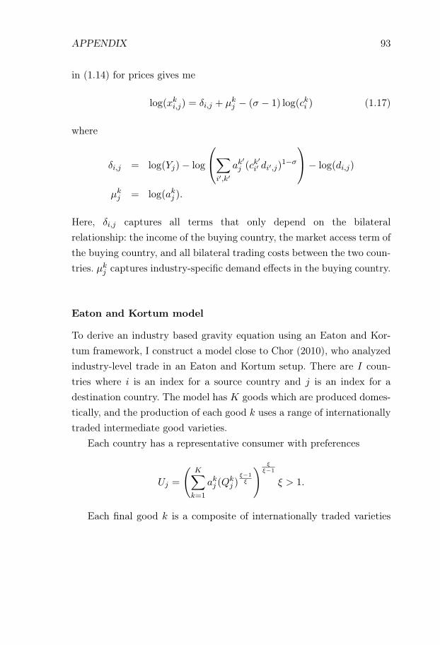
APPENDIX 93
in (1.14) for prices gives me
log(xki,j) = δi,j + μkj − (σ − 1) log(cki ) (1.17)
where
δi,j = log(Yj)− log
⎛⎝∑i′,k′
ak′
j (ck′i′ di′,j)
1−σ
⎞⎠− log(di,j)
μkj = log(akj ).
Here, δi,j captures all terms that only depend on the bilateralrelationship: the income of the buying country, the market access term ofthe buying country, and all bilateral trading costs between the two coun-tries. μk
j captures industry-specific demand effects in the buying country.
Eaton and Kortum model
To derive an industry based gravity equation using an Eaton and Kor-tum framework, I construct a model close to Chor (2010), who analyzedindustry-level trade in an Eaton and Kortum setup. There are I coun-tries where i is an index for a source country and j is an index for adestination country. The model has K goods which are produced domes-tically, and the production of each good k uses a range of internationallytraded intermediate good varieties.
Each country has a representative consumer with preferences
Uj =
(K∑k=1
akj (Qkj )
ξ−1ξ
) ξξ−1
ξ > 1.
Each final good k is a composite of internationally traded varieties
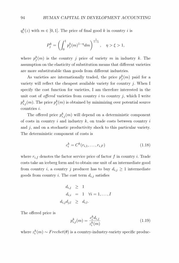
94 HUMAN CAPITAL IN DEVELOPMENT ACCOUNTING
qki (z) with m ∈ [0, 1]. The price of final good k in country i is
P kj =
(∫ 1
0pkj (m)1−ηdm
) 11−η
, η > ξ > 1,
where pkj (m) is the country j price of variety m in industry k. Theassumption on the elasticity of substitution means that different varietiesare more substitutable than goods from different industries.
As varieties are internationally traded, the price pkj (m) paid for avariety will reflect the cheapest available variety for country j. When Ispecify the cost function for varieties, I am therefore interested in theunit cost of offered varieties from country i to country j, which I writepki,j(m). The price pkj (m) is obtained by minimizing over potential sourcecountries i.
The offered price pki,j(m) will depend on a deterministic componentof costs in country i and industry k, on trade costs between country i
and j, and on a stochastic productivity shock to this particular variety.The deterministic component of costs is
cki = Ck(ri,1, . . . , ri,F ) (1.18)
where ri,f denotes the factor service price of factor f in country i. Tradecosts take an iceberg form and to obtain one unit of an intermediate goodfrom country i, a country j producer has to buy di,j ≥ 1 intermediategoods from country i. The cost term di,j satisfies
di,j ≥ 1
di,i = 1 ∀i = 1, . . . , I
di,jdj,l ≥ di,l.
The offered price is
pki,j(m) =cki di,j
zki (m)(1.19)
where zki (m) ∼ Frechet(θ) is a country-industry-variety specific produc-
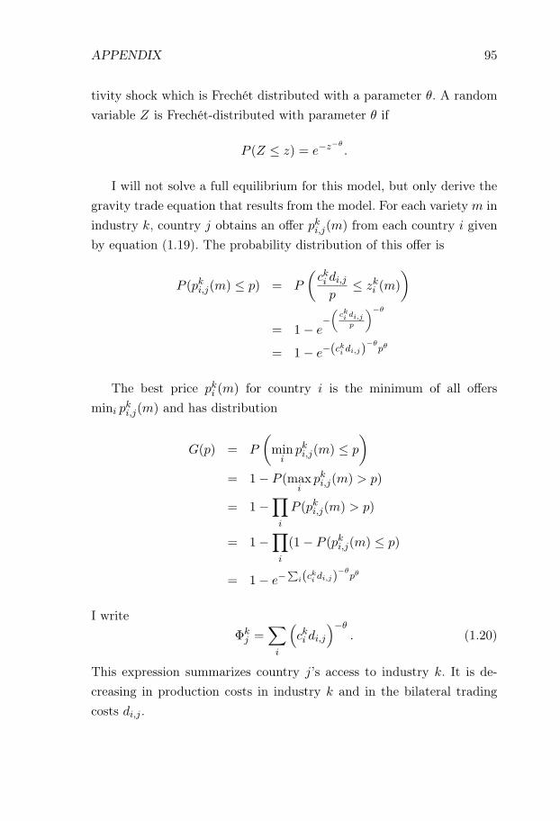
APPENDIX 95
tivity shock which is Frechét distributed with a parameter θ. A randomvariable Z is Frechét-distributed with parameter θ if
P (Z ≤ z) = e−z−θ.
I will not solve a full equilibrium for this model, but only derive thegravity trade equation that results from the model. For each variety m inindustry k, country j obtains an offer pki,j(m) from each country i givenby equation (1.19). The probability distribution of this offer is
P (pki,j(m) ≤ p) = P
(cki di,jp
≤ zki (m)
)
= 1− e−(
cki di,jp
)−θ
= 1− e−(cki di,j)
−θpθ
The best price pki (m) for country i is the minimum of all offersmini p
ki,j(m) and has distribution
G(p) = P
(mini
pki,j(m) ≤ p
)= 1− P (max
ipki,j(m) > p)
= 1−∏i
P (pki,j(m) > p)
= 1−∏i
(1− P (pki,j(m) ≤ p)
= 1− e−∑
i(cki di,j)−θ
pθ
I writeΦkj =
∑i
(cki di,j
)−θ. (1.20)
This expression summarizes country j’s access to industry k. It is de-creasing in production costs in industry k and in the bilateral tradingcosts di,j .
96 HUMAN CAPITAL IN DEVELOPMENT ACCOUNTING
Country j chooses to buy a variety from the country with the lowestprice. The probability that country i offers the lowest price is
πki,j ≡ P (pki,j(z) ≤ min
ipki,j(z))
=(cki di,j)
−θ
Φkj
.
If xkj is the total amount of intermediate inputs bought by country j inindustry k, the trade flow matrix is
xki,j = πki,jx
kj =
(cki di,j)−θ
Φkj
xkj (1.21)
Equation (1.21) requires that the share of import value coming fromcountry i only depends on the share of inputs for which i is the supplier.This property holds as the Frechet distribution has a desirable propertycalled max-stability, which ensures that the best offered price pi,k(z) tocountry i is independent of the source of the best offer (see Eaton andKortum (2002) for a derivation in this particular case, and Mattssonet al. (2014) for a more general discussion of this property of randomvariables) . This means that the total expenditure on imports from onecountry will be fully determined by the share of varieties πk
n,i bought fromthat country. The reason is that all countries offer identical distributionsof variety prices conditioned on them offering the best prices.
Taking the logarithm of both sides of equation (1.21) gives me
log(xki,j) = δi,j + μkj − θ log(cki )
where δi,j = −θ log(di,j) and μkj = log(Xk
j ) − log(Φkj ). Thus, the model
implies a gravity equation of the right form. Note that when using Eatonand Kortum elasticity estimates θ, there needs to be added a 1 to convertthem to the corresponding Armington elasticity estimates σ.
APPENDIX 97
1.C.2 Results for other factors than skilled labor
In Section 1.2, I estimated regression (1.5) to obtain estimates of rela-tive factor service prices across countries. My main interest was in therelative price of skilled services, as this relative price is used directly indevelopment accounting. However, my estimation procedure also yieldsrelative factor service price estimates for capital, intermediate inputs,and energy. Even though I do not use these directly in my developmentaccounting exercising, they are useful to check the plausibility of myfactor service price estimation method.
In particular, as capital, intermediate inputs, and energy are partlytradable, we should expect the relative price of these factors compared tounskilled labor to fall with GDP per worker. The reason is that tradableservices should have similar prices across countries, whereas we expectthe price of unskilled labor services to rise with GDP per worker.
It is possible to quantify how much unskilled service prices shouldfall with GDP. If we assume that the labor share of output is constantat 1− α, the unskilled wage satisfies equation
wu =wu
wuu+ wss× (wuu+ wss)
=1
u+ wswu
s(1− α)y
where y in the second line denotes output per worker. Using that theprice of unskilled labor services is ru = wu/Qu where Qu is the qualityof unskilled workers, I obtain
log(ru) = log(1− α) + log(y)− log(htrad)
where log(htrad) = log(Qu) + log(u + wswu
s) is human capital accordingto traditional development accounting methods, as defined in equation(1.10). Letting rt be the price of any tradable input service, its relative
98 HUMAN CAPITAL IN DEVELOPMENT ACCOUNTING
price compared to unskilled labor services will be
log
(rtru
)= log(rt)− log(1− α)− log(y) + log(htrad).
If log(rt) is constant across countries, we can make the following obser-vation: constant log(htrad) across countries implies that relative tradablefactor prices decrease one-to-one with GDP per capita. If log(htrad) ispositively correlated with GDP, relative tradable factor service prices willfall slower than one-for-one. And even though it is not explicitly modeledin the equation, we can also note that a non-tradable component of t willalso make the relative price/GDP-slope less negative.
In my data, log(htrad) increases at approximately 0.15−0.2 with GDPper capita. Thus, if capital, intermediate inputs, and energy services arefully tradable, they should have a negative slope of between 0.8 and0.85 with respect to GDP per worker. If they are not fully tradable,the negative relationship should be weaker. The results are presentedin Figures 1.C.1-1.C.3. The negative relationship between capital andintermediate input service prices and log GDP per worker is similar at−0.6, which is close to what is predicted by my previous reasoning. Theconclusions are less stable for energy prices. Here, there is also a negativerelationship, but the data is less precise. This is due to energy havinga very small factor share in most industries, and the results for energyare more driven by outliers. Reassuringly, large energy producers such asSaudi Arabia, Kuwait, Russia, and Iran have low revealed energy serviceprices.
1.C.3 Treatment of intermediate inputs
In my main specification, I include the cost share of intermediate inputsαkUS,int. The corresponding estimate βi,int identifies log
(ri,int/ri,1
rUS,int/rUS,1
).
This estimate gives the difference between the US and country i in therelative cost of intermediate input and unskilled labor services.
In my interpretation of this parameter, I assume that intermediate
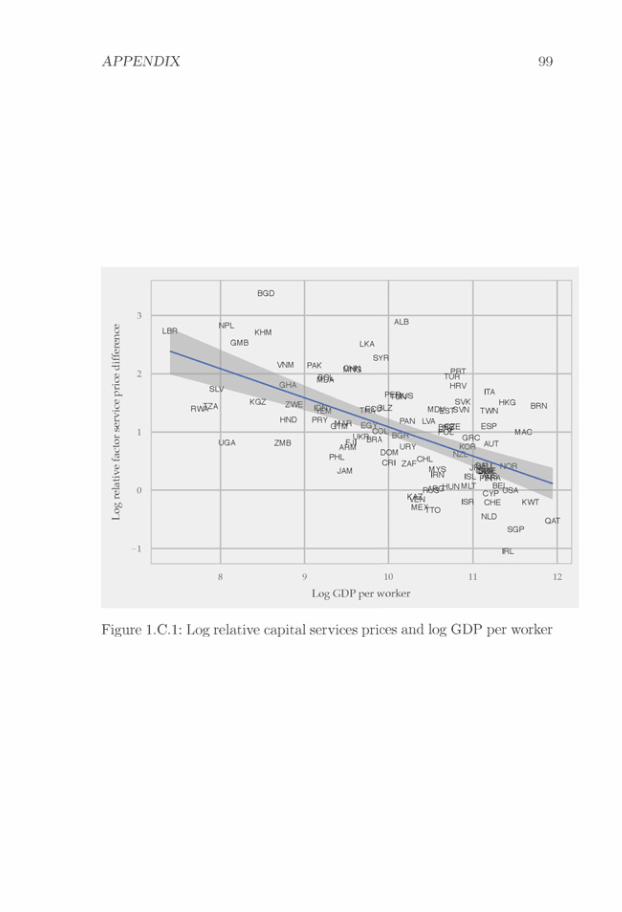
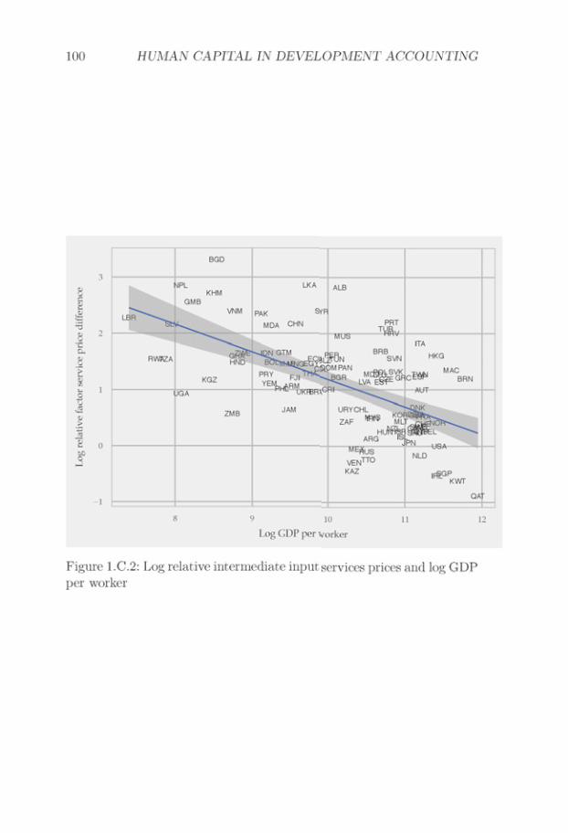
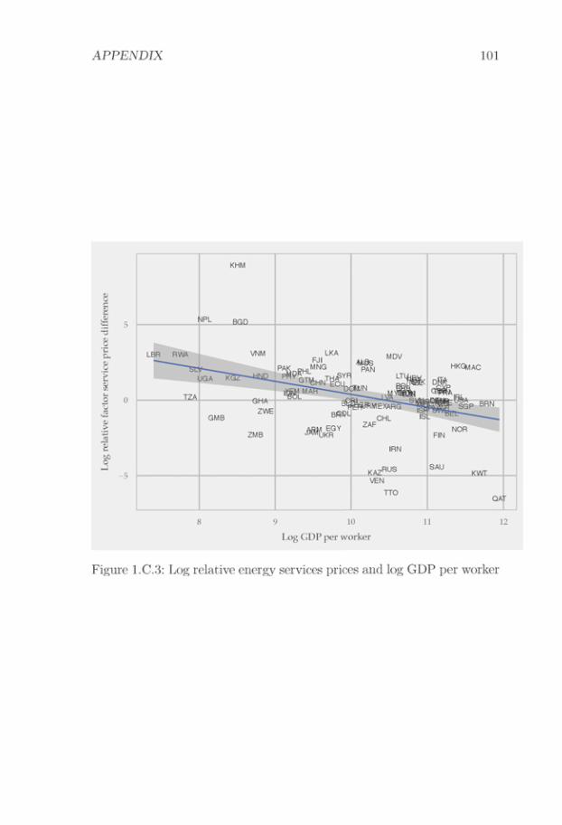
102 HUMAN CAPITAL IN DEVELOPMENT ACCOUNTING
inputs are traded. I interpret ri,int as a product of an international priceof intermediate inputs rint, which is constant across countries, and acountry-specific barrier to international intermediate input markets τi,which varies across countries.
With this interpretation,
βi,int = log(τi/τUS)− log
(ri,1rUS,1
).
βi,int varies across countries for two reasons. First, countries differin their access to international intermediate goods markets τi. Badaccess to international markets (high τi) gives a high revealed price ofintermediate input services (high βi,int). Second, countries differ in theirprices of unskilled labor services log
(ri,1rUS,1
). Countries with a low price
of unskilled services have a high revealed price of intermediate inputservices. This has an intuitive interpretation: relatively inexpensiveunskilled labor services make internationally traded intermediate inputsrelatively expensive.
If intermediate inputs are not traded and the aim is to identify factorservice price differences, a different approach is called for. In this case,there is an indirect effect of factor service price differences via inputprices. To reflect this, the intermediate input share in an industry k
should be resolved into contributions from different factor services, usingthe input-output structure to determine the factor shares of industry k’sintermediate inputs.
To check the robustness of my baseline specification, I develop an ap-proach that allows for both traded and non-traded intermediate inputs.To implement my approach, I use the US input-output table and assumethat services are non-traded and that other goods are traded.23 I use theEU-KLEMS data together with Occupational Employment Survey data
23There is moderate trade in some services such as entertainment, financial ser-vices, and transportation, but the distinction captures the large differences in tradedshares between services and other goods in the US input-output table.
APPENDIX 103
to obtain factor shares in service sectors.I write NT for the number of traded goods and NNT for the number
of non-traded goods. The input-output table Lis an (NT +NNT )×(NT +
NNT ) matrix. For each good k = 1, . . . , NT +NNT , I measure its factorshares including its intermediate input share, and I use these measuredfactor shares to define the first-stage factor shares αk
f . This is the sameas normal factor shares with one difference. For intermediate inputs, wedefine αk
f as the share of inputs that come from non-tradeable interme-diates. In the first stage, I am interested in the cost shares of differentfactors and of tradable inputs. For each industry, 1−∑F
f=1 αkf gives the
share of costs in industry k going to nontraded factor inputs. These first-stage factor shares are the building blocks of the factor shares αk
f thatwill be obtained by resolving the cost share of nontraded intermediateinputs into conventional factors and tradable inputs.
I find the factor shares αkf of tradable goods recursively by first finding
the factor shares of nontradable goods. I define two matrices LT and LNT
where LT is an NT × NNT matrix giving the input uses of nontradedintermediate inputs in the traded sector, and LNT is an NNT × NNT
matrix giving the cost shares from nontraded inputs in the nontradedsector.
I solve the system recursively. The factor shares of nontraded goodsare
αNT = αNT + (LNT )αNT ⇐⇒ αNT = (I − LNT )−1αNT
where αNT is an NNT × F matrix, αNT is an NNT × F matrix, andLNT is an NNT × NNT matrix. The final matrix αNT gives the factorshares of nontraded services in terms of standard factor shares and tradedinput shares. All nontraded input shares have been resolved into theseconstituent parts. Having solved for the factor shares of nontraded goods,the factor shares of traded goods are
αT = αT + (LT )αNT .
Using this modified definition of factor shares, I can re-estimate my
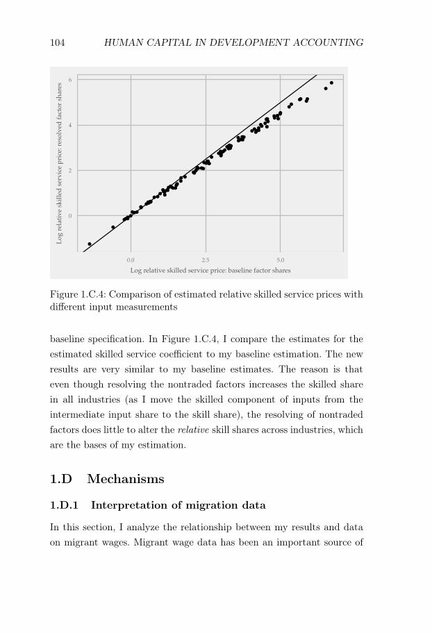
104 HUMAN CAPITAL IN DEVELOPMENT ACCOUNTING
�
�
�
��
�
�
�
�
�
�
�
�
�
�
�
�
�
��
�
�
�
�
�
�
��
�
�
�
�
�
�
�
�
�
�
�
�
�
�
�
�
�
�
�
�
�
�
�
�
�
� �
���
�
�
�
�
� �
��
�
�
�
�
�
�
�
�
�
�
��
�
�
�
�
�
�
�
�
���
�
�
�
�
�
�
�
�
�
�
�
�
�
0
2
4
6
0.0 2.5 5.0
Log relative skilled service price: baseline factor shares
Log
rel
ativ
e sk
illed
ser
vice
pri
ce: r
esol
ved
fact
or s
hare
s
Figure 1.C.4: Comparison of estimated relative skilled service prices withdifferent input measurements
baseline specification. In Figure 1.C.4, I compare the estimates for theestimated skilled service coefficient to my baseline estimation. The newresults are very similar to my baseline estimates. The reason is thateven though resolving the nontraded factors increases the skilled sharein all industries (as I move the skilled component of inputs from theintermediate input share to the skill share), the resolving of nontradedfactors does little to alter the relative skill shares across industries, whichare the bases of my estimation.
1.D Mechanisms
1.D.1 Interpretation of migration data
In this section, I analyze the relationship between my results and dataon migrant wages. Migrant wage data has been an important source of

APPENDIX 105
information in development accounting since Hendricks (2002).24 Ideally,migration provides a natural experiment to distinguish between humancapital based and technology based explanations of world income diff-erences. If selection issues are appropriately addressed, migration dataallows us to compare similar workers in two different environments. Hu-man capital is kept constant, and wage differences have to be attributedto some other factor in the environment. Under some conditions, thisother factor can be interpreted as technology.
In particular, migrant wage data has been used to argue against adominant role for human capital in accounting for world income differ-ences. This was the main argument in Hendricks (2002). He showed thatmigrants from poor countries in the US had dramatically higher wagesthan workers in their native countries. He argued that this was inconsis-tent with human capital differences being large enough to explain worldincome differences. Even though later contributions have tempered thisconclusion by using individual data to account for selection (Hendricksand Schoellman, 2016), it remains important for human capital basedexplanations of world income differences to be consistent with migrantwage data.
Given that I argue that human capital might play a dominant rolein explaining world income differences, it is natural to ask how my re-sults relate to migrant wage data. In this section, I show that my resultsare not inconsistent with existing evidence from migrant wage data. Thekey difference between my analysis and that of Hendricks (2002) is thatI relax the assumption of perfect substitutability and allow for imperfectsubstitutability between labor services. This leads to a different inter-pretation of migrant wage data. In particular, imperfectly substitutablelabor services imply that human capital is multidimensional and thatthere is no longer a simple mapping from human capital to pre- andpost-migration wages. A worker’s wage is the product of the amount oflabor services that the worker provides, and the price of those labor ser-
24In addition to Hendricks (2002), papers that use migrant data include Schoellman(2011), Lagakos et al. (2016), and Hendricks and Schoellman (2016).

106 HUMAN CAPITAL IN DEVELOPMENT ACCOUNTING
vices. Even though wage changes at migration can be due to technologydifferences, they can also be due to labor service price differences.
I analyze the implications of my results for migrant wage data, andI discuss the implications both for unskilled and skilled migrants. Whenmigrants are unskilled workers, my development accounting results implythat there are limited human capital quality differences between richand poor countries. I am interested in whether these limited qualitydifferences are consistent with large wage gains for unskilled migrantsgoing from poor to rich countries. When migrants are skilled workers,my development accounting results suggest that there are substantialquality differences between rich and poor countries. In this situation, I aminterested in whether these large estimated quality differences necessarilymean that skilled migrants going from rich to poor countries should havemuch higher wages than local workers, and conversely if skilled migrantsgoing from poor to rich countries necessarily should have much lowerwages than local workers.
Starting with unskilled migrants, I note that it is consistent with myresults that unskilled workers going from poor to rich countries expe-rience large wage gains. The mechanism is that in rich countries, thehigh relative supply and quality of skilled workers increase the relativeprice of unskilled labor services. This relative scarcity of unskilled laborservices in rich countries makes unskilled wages higher. Wage gains forunskilled migrants are thus consistent with similar quality of unskilledlabor across rich and poor countries, and these wage gains do not relyon large cross-country differences in technology.
For skilled migrants, I begin by analyzing skilled migrants going fromrich to poor countries. According to my estimates, these skilled migrantshave a much higher quality of human capital than their local counter-parts. Does this imply that they will necessarily get much higher wagesthan local skilled workers? The answer is no. The reason is that highUS quality of skilled labor is the result of an aggregation of heteroge-neous skilled services. To make sharp predictions of how wages change atmigration for a worker with particular skills, we need to know the com-

APPENDIX 107
plementarity and substitutability patterns implicit in the aggregator ofskilled services. More concretely, the question is not whether a standardUS engineer migrating to Tanzania gets a much higher salary than theaverage Tanzanian engineer, but whether a US hydraulic engineer spe-cializing in sediment transportation migrating to Tanzania gets a muchhigher salary than an average Tanzanian engineer. The latter question isnot possible to answer without knowing the details of the skilled serviceaggregator.25
Conversely, we can analyze what my results predict about skilledmigrants going from poor to rich countries. According to my results,poor countries have a substantially lower quality of skilled labor thanrich countries. Do my results predict that a skilled migrant going froma poor country to a rich country necessarily should have a muchlower salary than local skilled workers? The answer again is no. Tobegin with, the argument about complementarity and substitutabilitypatterns that I made concerning skilled workers migrating from rich topoor countries still applies to this situation. Furthermore, even if weneglect potential heterogeneity among skilled and unskilled services, myexplanation is still consistent with skilled migrants to rich countriesnot having dramatically lower wages than local counterparts. Thereason is that there is potential for occupational switching at migration.Indeed, note that my results suggest that the relative price of skilledservices is lower in rich countries than in poor countries. Thus, aworker that has a comparative advantage in a skilled occupation ina poor country might have a comparative advantage in a low skill
25Here, I use a low-dimensional representation of labor force heterogeneity to an-alyze cross-country differences, and a high-dimensional representation of labor forceheterogeneity to analyze migration data. This procedure is analogous to the treat-ment of capital in aggregative growth models. The Solow model and the neoclassicalgrowth models use a one-dimensional representation of capital, and these models areappropriate for capturing broad patterns of growth, output and marginal returns tocapital. However, capital aggregation hides an underlying heterogeneity. This meansthat model predictions from these models are commonly not tested by comparingcross-country differences in rental prices of specialized pieces of equipment. Suchcomparisons are outside the domain of validity of the aggregate model setup. Thesame applies to my setup.

108 HUMAN CAPITAL IN DEVELOPMENT ACCOUNTING
occupation in a rich country. For example, a moderately competentcomputer programmer from a poor country might find it profitable towork in an unskilled profession in the US. If the scarcity of unskilledservices in the US has driven up unskilled wages, this is consistent withskilled migrants to rich countries only having moderately lower wagesthan their local skilled counterparts, compared to the large estimatedquality differences in skilled labor. Even though B Jones (2014b)discusses the potential importance of occupational switching formigrant wage data, there has not been any full empirical examinationof this mechanism. However, B Jones (2014a) and Hendricksand Schoellman (2016) provide suggestive evidence that occu-pational downgrading is more common for migrants from poor countries.
In conclusion, it is not directly inconsistent with migrant wage datathat human capital might play an important role in explaining world in-come differences. This consistency is not due to migrant wage data con-firming sharp predictions derived from my results. Apart from predictingwage gains for unskilled migrants going to rich countries, my results putweak restrictions on migrant wage data. Given the natural experimentaspect of migration that makes migrant wage data an attractive sourceof information about human capital differences, an important avenue offuture work is to place restrictions on my setup to derive sharper predic-tions for migrant wage data.26
1.D.2 Endogenous skill-biased technology differences andhuman capital quality
Even though SBTD and quality differences are observationally equiva-lent with respect to price and quantity data, they are not equivalent in
26In an unpublished paper, B Jones (2014b) discusses migrant wage data withimperfect substitutability. He also argues for the importance of relative scarcity inaccounting for the wages of unskilled migrants, and for occupational switching inaccounting for the wages of skilled migrants. The points about complementarity andsubstitutability patterns are to my knowledge original to this paper.

APPENDIX 109
general. If quality differences in skilled labor explain why countries arerich, development theory needs to explain why countries differ in theirquality of skilled labor. If SBTD explain why countries are rich, develop-ment theory needs to explain how similar qualities of skilled labor canresult in very different levels of skilled labor productivity.
Thus, I try to move beyond price and quantity data to gauge therelative merits of SBTD and quality difference interpretations of my es-timates.27 To this end, I examine whether SBTD reduce estimated qual-ity differences when I put theoretical structure on how technology variesacross countries. In particular, I analyze a standard mechanism from theliterature where SBTD arise endogenously in response to relative factorservice price differences (Caselli and Coleman, 2006; Acemoglu, 2007;Caselli, 2015). In Appendix 1.D.3, I test in general for estimation errorsarising from second order errors and endogenous technology differences.There, I provide a detailed description of the environment, my measure-ment procedure, and my results. Below is a summary.
I set up a simple model of endogenous technological choice in line withCaselli and Coleman (2006) and Acemoglu et al. (2007). Technologicalbias varies on an industry-country level as a function of factor serviceprices. For each set of relative factor service prices, I generate unit costdata from the model and run my baseline regression specification onthe model generated data. I find the relative factor service prices suchthat my regression specification gives the same results when applied tomodel data as when applied to actual data. This gives me the relativeservice factor prices that are consistent with my regression estimatesgiven that there is endogenous SBTD. By comparing these relative factorservice prices with those found under my baseline assumptions, I can testwhether my results in Section 1.2 overstates rich-poor quality differencesin skilled labor.
The results are mixed but there is no overall tendency for the en-dogenous SBTD based model to imply lower quality difference than my
27In Section 1.4.2 I did this by discussing circumstantial evidence for quality diff-erences and economic mechanisms that could make them large.

110 HUMAN CAPITAL IN DEVELOPMENT ACCOUNTING
baseline setup. In many cases, estimated quality differences are actuallyhigher when I allow for SBTD. The exact results depend on parametersand the effects are non-monotone in the size of relative skilled serviceprice differences.
These results can be viewed as somewhat surprising: if there areSBTD, a reasonable expectation is that they would lower the need forprice differences in skilled labor services to explain the trade data. Onemechanism that helps explain my findings is that there are to two op-posing tendencies. SBTD reduce the need for quality differences as theyincrease the relative productivity of skilled labor. However, when SBTDare endogenous, they also increase the effective elasticity of substitutionbetween skilled and unskilled labor services. In the context of my esti-mation procedure, this can sometimes mean that there are larger qualitydifferences to explain away. The net effect is ambiguous.
Thus, accounting for SBTD becomes complex when SBTD are en-dogenous. I have not resolved all issues, and a more thorough investi-gation of endogenous SBTD in my context is an important avenue forfuture research. However, in the case when SBTD arise endogenouslyfrom relative factor service price differences, they do not unambiguouslyobviate the need for large quality differences to explain my estimates.
1.D.3 Robustness to industry function specification andendogenous technology bias
My baseline estimates relied on the assumption that it was possible toapproximate unit cost differences from the US by log-linearizing aroundthe US cost structure. In terms of assumptions on industry productionfunctions, this assumption amounts to assuming that industry produc-tion functions are Cobb-Douglas. Furthermore, to interpret estimatesrs/ru in terms of human capital, I needed to assume that there were noskill-biased technology differences between countries. This section teststhe robustness of my results to deviations from these two assumptions.
The section has three subsections. In Appendix 1.D.3, I describe an
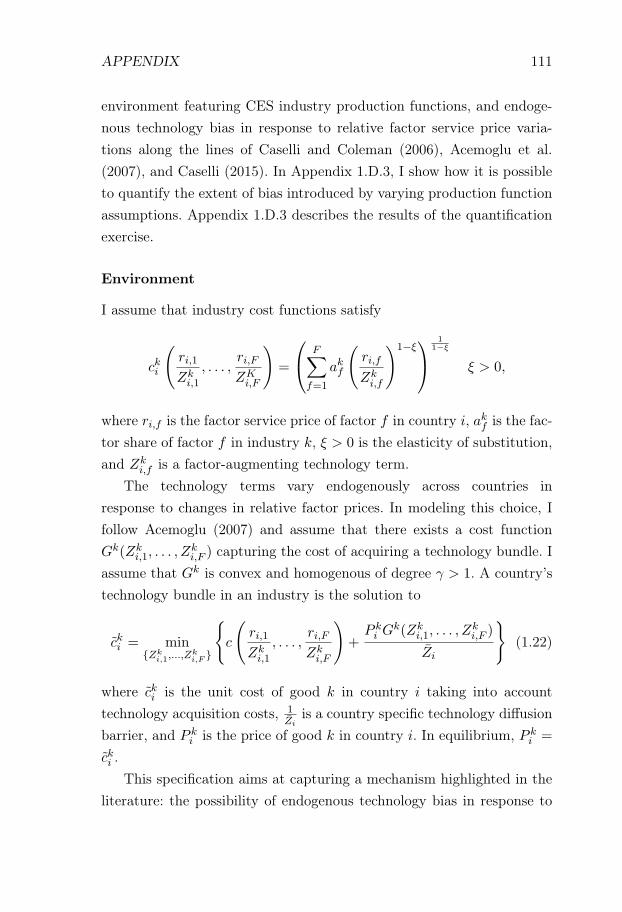
APPENDIX 111
environment featuring CES industry production functions, and endoge-nous technology bias in response to relative factor service price varia-tions along the lines of Caselli and Coleman (2006), Acemoglu et al.(2007), and Caselli (2015). In Appendix 1.D.3, I show how it is possibleto quantify the extent of bias introduced by varying production functionassumptions. Appendix 1.D.3 describes the results of the quantificationexercise.
Environment
I assume that industry cost functions satisfy
cki
(ri,1
Zki,1
, . . . ,ri,F
ZKi,F
)=
⎛⎝ F∑f=1
akf
(ri,f
Zki,f
)1−ξ⎞⎠ 1
1−ξ
ξ > 0,
where ri,f is the factor service price of factor f in country i, akf is the fac-tor share of factor f in industry k, ξ > 0 is the elasticity of substitution,and Zk
i,f is a factor-augmenting technology term.The technology terms vary endogenously across countries in
response to changes in relative factor prices. In modeling this choice, Ifollow Acemoglu (2007) and assume that there exists a cost functionGk(Zk
i,1, . . . , Zki,F ) capturing the cost of acquiring a technology bundle. I
assume that Gk is convex and homogenous of degree γ > 1. A country’stechnology bundle in an industry is the solution to
cki = min{Zk
i,1,...,Zki,F }
{c
(ri,1
Zki,1
, . . . ,ri,F
Zki,F
)+
P ki G
k(Zki,1, . . . , Z
ki,F )
Zi
}(1.22)
where cki is the unit cost of good k in country i taking into accounttechnology acquisition costs, 1
Ziis a country specific technology diffusion
barrier, and P ki is the price of good k in country i. In equilibrium, P k
i =
cki .This specification aims at capturing a mechanism highlighted in the
literature: the possibility of endogenous technology bias in response to
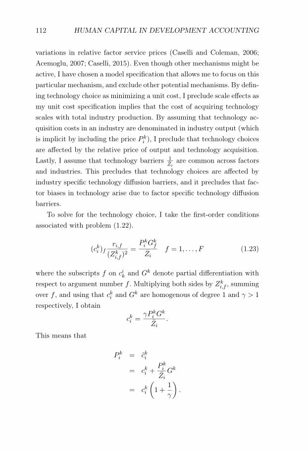
112 HUMAN CAPITAL IN DEVELOPMENT ACCOUNTING
variations in relative factor service prices (Caselli and Coleman, 2006;Acemoglu, 2007; Caselli, 2015). Even though other mechanisms might beactive, I have chosen a model specification that allows me to focus on thisparticular mechanism, and exclude other potential mechanisms. By defin-ing technology choice as minimizing a unit cost, I preclude scale effects asmy unit cost specification implies that the cost of acquiring technologyscales with total industry production. By assuming that technology ac-quisition costs in an industry are denominated in industry output (whichis implicit by including the price P k
i ), I preclude that technology choicesare affected by the relative price of output and technology acquisition.Lastly, I assume that technology barriers 1
Ziare common across factors
and industries. This precludes that technology choices are affected byindustry specific technology diffusion barriers, and it precludes that fac-tor biases in technology arise due to factor specific technology diffusionbarriers.
To solve for the technology choice, I take the first-order conditionsassociated with problem (1.22).
(cki )fri,f
(Zki,f )
2=
P ki G
kf
Zif = 1, . . . , F (1.23)
where the subscripts f on cik and Gk denote partial differentiation withrespect to argument number f . Multiplying both sides by Zk
i,f , summingover f , and using that cki and Gk are homogenous of degree 1 and γ > 1
respectively, I obtain
cki =γP k
i Gk
Zi.
This means that
P ki = cki
= cki +P ki
ZiGk
= cki
(1 +
1
γ
).
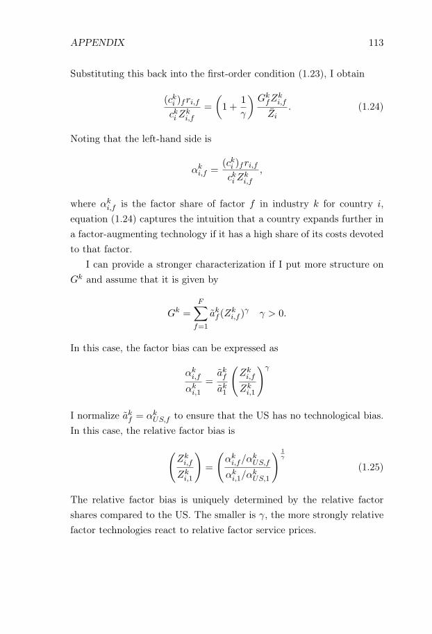
APPENDIX 113
Substituting this back into the first-order condition (1.23), I obtain
(cki )fri,f
cki Zki,f
=
(1 +
1
γ
)Gk
fZki,f
Zi. (1.24)
Noting that the left-hand side is
αki,f =
(cki )fri,f
cki Zki,f
,
where αki,f is the factor share of factor f in industry k for country i,
equation (1.24) captures the intuition that a country expands further ina factor-augmenting technology if it has a high share of its costs devotedto that factor.
I can provide a stronger characterization if I put more structure onGk and assume that it is given by
Gk =
F∑f=1
akf (Zki,f )
γ γ > 0.
In this case, the factor bias can be expressed as
αki,f
αki,1
=akf
ak1
(Zki,f
Zki,1
)γ
I normalize akf = αkUS,f to ensure that the US has no technological bias.
In this case, the relative factor bias is
(Zki,f
Zki,1
)=
(αki,f/α
kUS,f
αki,1/α
kUS,1
) 1γ
(1.25)
The relative factor bias is uniquely determined by the relative factorshares compared to the US. The smaller is γ, the more strongly relativefactor technologies react to relative factor service prices.
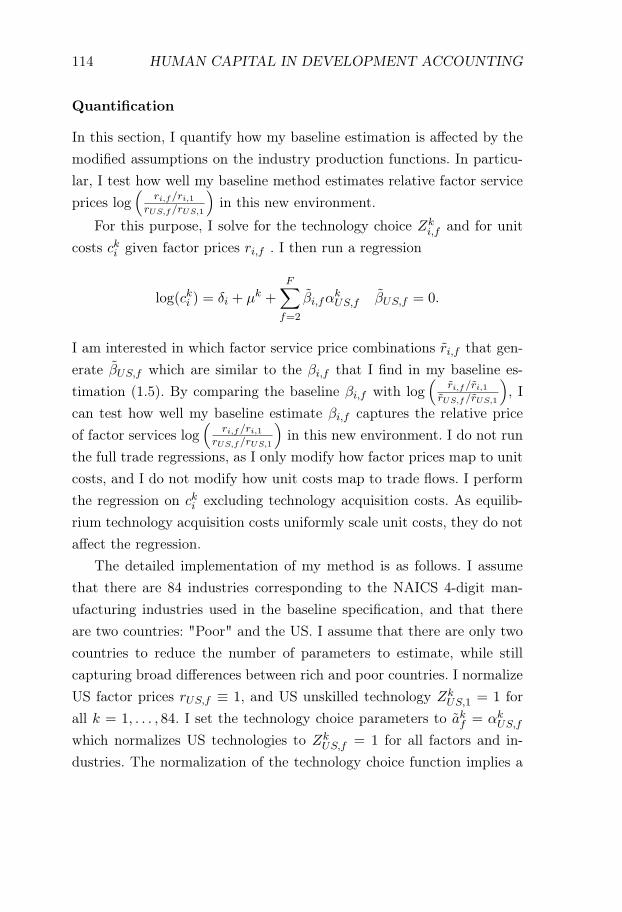
114 HUMAN CAPITAL IN DEVELOPMENT ACCOUNTING
Quantification
In this section, I quantify how my baseline estimation is affected by themodified assumptions on the industry production functions. In particu-lar, I test how well my baseline method estimates relative factor serviceprices log
(ri,f/ri,1
rUS,f/rUS,1
)in this new environment.
For this purpose, I solve for the technology choice Zki,f and for unit
costs cki given factor prices ri,f . I then run a regression
log(cki ) = δi + μk +
F∑f=2
βi,fαkUS,f βUS,f = 0.
I am interested in which factor service price combinations ri,f that gen-erate βUS,f which are similar to the βi,f that I find in my baseline es-timation (1.5). By comparing the baseline βi,f with log
(ri,f/ri,1
rUS,f/rUS,1
), I
can test how well my baseline estimate βi,f captures the relative priceof factor services log
(ri,f/ri,1
rUS,f/rUS,1
)in this new environment. I do not run
the full trade regressions, as I only modify how factor prices map to unitcosts, and I do not modify how unit costs map to trade flows. I performthe regression on cki excluding technology acquisition costs. As equilib-rium technology acquisition costs uniformly scale unit costs, they do notaffect the regression.
The detailed implementation of my method is as follows. I assumethat there are 84 industries corresponding to the NAICS 4-digit man-ufacturing industries used in the baseline specification, and that thereare two countries: "Poor" and the US. I assume that there are only twocountries to reduce the number of parameters to estimate, while stillcapturing broad differences between rich and poor countries. I normalizeUS factor prices rUS,f ≡ 1, and US unskilled technology Zk
US,1 = 1 forall k = 1, . . . , 84. I set the technology choice parameters to akf = αk
US,f
which normalizes US technologies to ZkUS,f = 1 for all factors and in-
dustries. The normalization of the technology choice function implies a
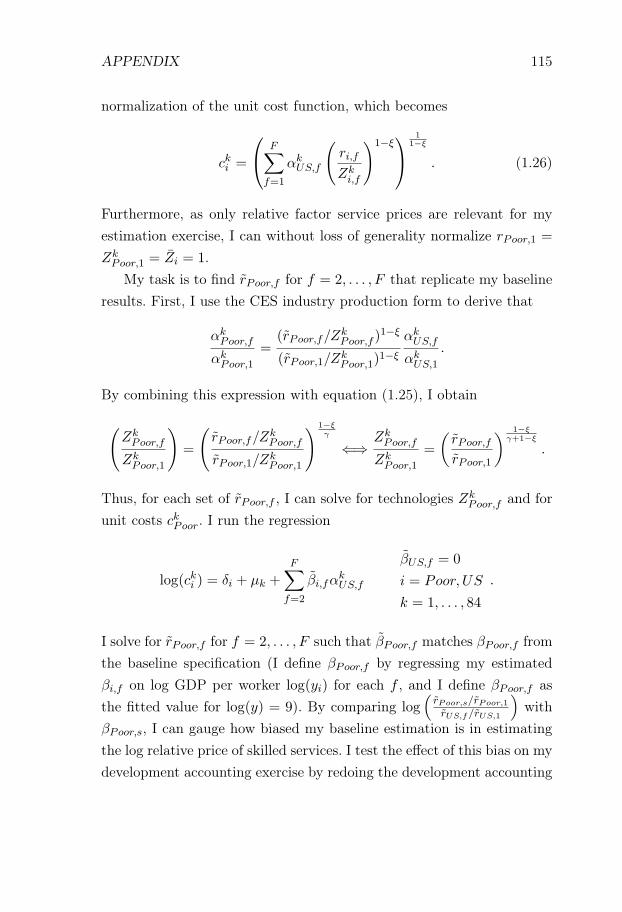
APPENDIX 115
normalization of the unit cost function, which becomes
cki =
⎛⎝ F∑f=1
αkUS,f
(ri,f
Zki,f
)1−ξ⎞⎠ 1
1−ξ
. (1.26)
Furthermore, as only relative factor service prices are relevant for myestimation exercise, I can without loss of generality normalize rPoor,1 =
ZkPoor,1 = Zi = 1.
My task is to find rPoor,f for f = 2, . . . , F that replicate my baselineresults. First, I use the CES industry production form to derive that
αkPoor,f
αkPoor,1
=(rPoor,f/Z
kPoor,f )
1−ξ
(rPoor,1/ZkPoor,1)
1−ξ
αkUS,f
αkUS,1
.
By combining this expression with equation (1.25), I obtain
(ZkPoor,f
ZkPoor,1
)=
(rPoor,f/Z
kPoor,f
rPoor,1/ZkPoor,1
) 1−ξγ
⇐⇒ ZkPoor,f
ZkPoor,1
=
(rPoor,f
rPoor,1
) 1−ξγ+1−ξ
.
Thus, for each set of rPoor,f , I can solve for technologies ZkPoor,f and for
unit costs ckPoor. I run the regression
log(cki ) = δi + μk +F∑
f=2
βi,fαkUS,f
βUS,f = 0
i = Poor, US
k = 1, . . . , 84
.
I solve for rPoor,f for f = 2, . . . , F such that βPoor,f matches βPoor,f fromthe baseline specification (I define βPoor,f by regressing my estimatedβi,f on log GDP per worker log(yi) for each f , and I define βPoor,f asthe fitted value for log(y) = 9). By comparing log
(rPoor,s/rPoor,1
rUS,f/rUS,1
)with
βPoor,s, I can gauge how biased my baseline estimation is in estimatingthe log relative price of skilled services. I test the effect of this bias on mydevelopment accounting exercise by redoing the development accounting
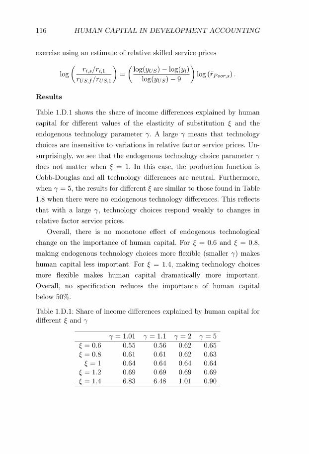
116 HUMAN CAPITAL IN DEVELOPMENT ACCOUNTING
exercise using an estimate of relative skilled service prices
log
(ri,s/ri,1
rUS,f/rUS,1
)=
(log(yUS)− log(yi)
log(yUS)− 9
)log (rPoor,s) .
Results
Table 1.D.1 shows the share of income differences explained by humancapital for different values of the elasticity of substitution ξ and theendogenous technology parameter γ. A large γ means that technologychoices are insensitive to variations in relative factor service prices. Un-surprisingly, we see that the endogenous technology choice parameter γ
does not matter when ξ = 1. In this case, the production function isCobb-Douglas and all technology differences are neutral. Furthermore,when γ = 5, the results for different ξ are similar to those found in Table1.8 when there were no endogenous technology differences. This reflectsthat with a large γ, technology choices respond weakly to changes inrelative factor service prices.
Overall, there is no monotone effect of endogenous technologicalchange on the importance of human capital. For ξ = 0.6 and ξ = 0.8,making endogenous technology choices more flexible (smaller γ) makeshuman capital less important. For ξ = 1.4, making technology choicesmore flexible makes human capital dramatically more important.Overall, no specification reduces the importance of human capitalbelow 50%.
Table 1.D.1: Share of income differences explained by human capital fordifferent ξ and γ
γ = 1.01 γ = 1.1 γ = 2 γ = 5
ξ = 0.6 0.55 0.56 0.62 0.65ξ = 0.8 0.61 0.61 0.62 0.63ξ = 1 0.64 0.64 0.64 0.64
ξ = 1.2 0.69 0.69 0.69 0.69ξ = 1.4 6.83 6.48 1.01 0.90

1.E. ROBUSTNESS 117
1.E Robustness
1.E.1 Discussion: Industry-dependent trade elasticities
In my estimates, I assume that the elasticity of trade σ is common acrossindustries. A number of papers in the trade literature has argued for σ
varying at an industry level (Broda et al., 2006; Soderbery, 2015). I writeσk to denote such an industry-varying trade elasticity. Looking ahead, animportant extension of my paper is to redo the estimates with a serioustreatment of industry-varying σ. However, I have performed a simplerobustness check, and tested a number of ways of solving the problem.Here, I also outline which approaches to this that look relatively morepromising.
First, I note that it is possible to use residual plots to detect evidencefor industry-varying σk. If σk is higher than average in an industry, aplot of fitted values and residuals will have a positive slope. Indeed, ifa country has high fitted trade values in an industry, it suggests thatit has low relative costs. If I use an elasticity for that industry whichis too low, the fitted value will be low compared to the actual value.The opposite is true when an industry has a low fitted value of trade.If I have underestimated the trade elasticity, actual values will be evenlower than fitted values. These effects mean that an underestimated σk
leads to a positive relationship between fitted values and residuals onan industry level. Conversely, if I have overestimated σk, there will be anegative relationship between fitted values and residual values.
By considering industry-by-industry plots of residuals on fitted val-ues, I can obtain information about industry-specific elasticities. I usethis method to perform a simple robustness check by excluding all in-dustries with an absolute value of the residual-fitted plot of more than 1
and I find similar results for this restricted set of industries.I also run the regression specification
log(xki,j) = δi,j + μkj −
F∑f=2
[(σk − 1)αkUS,f ]βi,f + εki,j βUS,f ≡ 0

118 HUMAN CAPITAL IN DEVELOPMENT ACCOUNTING
and use different estimates of σk across industries. I first use the esti-mates of industry-specific trade elasticities in Broda et al. (2006). To testwhether these help resolve the problem with varying trade elasticities, Ianalyze whether there is less evidence for industry-varying trade elastici-ties in the fitted-residual plots when I use the industry-specific estimatesσk from Broda et al. (2006) compared to when I run the regression witha common elasticity of trade corresponding to their median estimate.
I find that using the industry-specific estimates of trade elasticity donot resolve the problem of correlation between fitted values and resid-uals on the industry level. If anything, using industry-specific elasticityestimates makes the problem worse.
In addition to using the estimates from Broda et al. (2006), I also tryan iterative procedure to more directly bring the fitted-residual plots inline. I run the regression with a common σk ≡ σ. I iterate and increasethe σk whenever the fitted-residual slope in industry k is positive, anddecrease σk whenever the fitted-residual slope in industry k is negative.Unfortunately, the procedure does not converge.
Using estimates from Broda et al. (2006) and the iterative proceduredid not solve the problem with varying trade elasticities. One potentialreason for this failure is that it is not theoretically correct to modifyregression specification (1.5) by just changing σk. If trade elasticities varyacross industries, they also interact with trade cost terms that are nowincluded in the bilateral fixed effect δi,j . Thus, this will partly dependon industry k, which means that a standard gravity specification withbilateral fixed effects will not work in this context.
Thus, looking ahead, a proper treatment of varying σk will require away of jointly estimating σk across industries and modify the structuraltrade model to generate a regression specification that fully incorporatesvarying trade elasticities.

APPENDIX: ROBUSTNESS 119
1.E.2 Specification with confounding variables
In Section 1.6.1, I discuss the effects of an omitted variable bias in myspecification of unit costs. Here, I explain how I measure and includepotential confounders in my regression specification.
I analyze two confounding variables: external financing sensitivityand contracting sensitivity. I assume that there are country-specific con-tracting and external financing penalties τcont and τfin which capturethe general quality of a country’s judicial and financial systems. Indus-tries are characterized by a contracting intensity αk
US,con and a exter-nal financing intensity αk
US,fin. Country-level contracting and financialpenalties change log unit costs of industries with τcont × αk
US,con andτfin × αk
US,fin, respectively. That is, contracting and financing penal-ties increase the unit costs of industries in proportion to their respectivecontracting and external financing intensities.
I define an industry’s external financing intensity αkUS,fin as the share
of investment expenditure not covered by external financing (external fi-nancing share of investments) times the share of gross output devotedto investments. I take the external financing share from Rajan and Zin-gales (1998), and I measure the investment share of total output usingNBER CES data. My definition differs from that in Rajan and Zingales(1998) as I multiply the external financing share of investments withthe investment share. The reason is that I interpret the country financialpenalty τfin as a markup on external financing needs. A financing penaltyincreases the unit costs of an industry in proportion to its external fi-nancing needs as a share of gross output. To obtain external financingneeds as a share of gross output, I multiply the external financing shareof investments with the investment share.
I define an industry’s contracting intensity by multiplying two terms.The first term is the share of intermediate inputs expenditure that issensitive to contracting. To measure this term, I follow Nunn (2007) anduse the IO table to calculate the share of intermediate good expendi-tures that are spent on customized inputs, where I define an input as
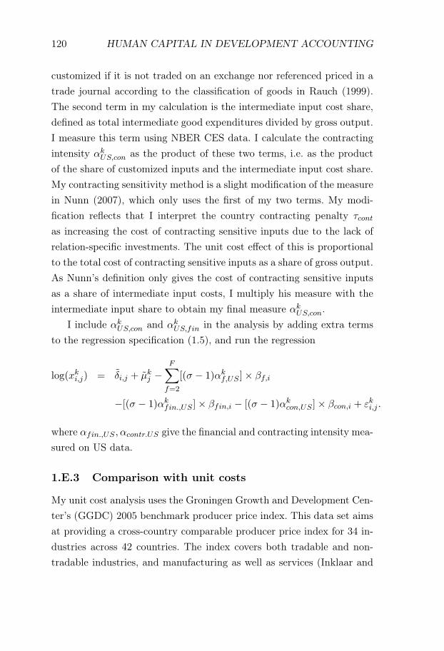
120 HUMAN CAPITAL IN DEVELOPMENT ACCOUNTING
customized if it is not traded on an exchange nor referenced priced in atrade journal according to the classification of goods in Rauch (1999).The second term in my calculation is the intermediate input cost share,defined as total intermediate good expenditures divided by gross output.I measure this term using NBER CES data. I calculate the contractingintensity αk
US,con as the product of these two terms, i.e. as the productof the share of customized inputs and the intermediate input cost share.My contracting sensitivity method is a slight modification of the measurein Nunn (2007), which only uses the first of my two terms. My modi-fication reflects that I interpret the country contracting penalty τcont
as increasing the cost of contracting sensitive inputs due to the lack ofrelation-specific investments. The unit cost effect of this is proportionalto the total cost of contracting sensitive inputs as a share of gross output.As Nunn’s definition only gives the cost of contracting sensitive inputsas a share of intermediate input costs, I multiply his measure with theintermediate input share to obtain my final measure αk
US,con.I include αk
US,con and αkUS,fin in the analysis by adding extra terms
to the regression specification (1.5), and run the regression
log(xki,j) = δi,j + μkj −
F∑f=2
[(σ − 1)αkf,US ]× βf,i
−[(σ − 1)αkfin.,US ]× βfin,i − [(σ − 1)αk
con,US ]× βcon,i + εki,j .
where αfin.,US , αcontr.US give the financial and contracting intensity mea-sured on US data.
1.E.3 Comparison with unit costs
My unit cost analysis uses the Groningen Growth and Development Cen-ter’s (GGDC) 2005 benchmark producer price index. This data set aimsat providing a cross-country comparable producer price index for 34 in-dustries across 42 countries. The index covers both tradable and non-tradable industries, and manufacturing as well as services (Inklaar and
APPENDIX: ROBUSTNESS 121
Timmer, 2008).Following recommendations from a creator of the data set, I exclude
financial services, business services, real estate, government, health ser-vices and education. For these industries, it is difficult to obtain data onoutput quantities which makes it difficult to make cross-country com-parisons in unit costs. I also exclude "private households with employedpersons" as this variable is missing for a large number of countries. Aftermy exclusions, I am left with a total of 27 industries and 35 countrieswith a complete set of observations.
To obtain factor shares, I use the EU KLEMS data set for the US(as my analysis includes non-manufacturing industries, I cannot use theNBER CES database to obtain factor shares). For the US, EU KLEMSprovides data on industry level gross output, labor compensation, andintermediate good compensation. I define the labor share as the laborcompensation over gross output, and the intermediate share as the inter-mediate good compensation over gross output. I calculate the skill shareby multiplying the labor share with the share of payroll going to skilledworkers with an occupational skill level of 3 or 4. I define the capitalshare as one minus the other factor shares.
I run the regression
log(cki ) = δi + μk +
F∑f=2
αkUS,f βi,f + εki
where βi,f = log(
ri,f/ri,1rUS,f/rUS,1
)captures the deviation of relative prices
compared to the US.I compare the results from the unit cost analysis with the trade data
analysis by comparing the relationship between GDP per worker andβi,f with the relationship between GDP per worker and βi,f , where βi,f
comes from the trade data analysis.28
28An alternative way to compare the outcomes would be to regress βi,f on βi,f andtest how close the results are to a 45 degree line. I have chosen my method as I aminterested in broad correlations between skilled service prices and GDP per capita,and given the estimation errors in the skill price estimates, regressing them on each

122 HUMAN CAPITAL IN DEVELOPMENT ACCOUNTING
In Figures 1.8 and 1.9, I plot the results from the unit cost dataanalysis. The slope parameter of log relative skilled service prices on logGDP per worker is −1.19 using the unit cost data, and −1.53 using thetrade data method for the same set of countries. I cannot reject thatthe two coefficients are equal, even without taking into account the largestandard errors on the unit costs based parameters βi,f . Thus, when bothtypes of data exist, the trade data method and the unit cost method painta similar picture of the relationship between relative skilled service pricesand GDP per worker.
1.E.4 Differences in unskilled human capital quality Qu
In the current setup, I estimate the quality of unskilled labor Qu by as-suming that unschooled labor is of equal quality and that improvementsare reflected in Mincerian returns:
QU,i = exp(φ(SU,i))
where φ is a Mincerian return function and SU,i is the average schoolingtime of unskilled labor.
A number of papers on human capital and development accountinghave stressed that there might be uniform quality differences in humancapital (Caselli, 2005; Manuelli and Seshadri, 2014). These quality differ-ences might reflect differences in nutrition, health, or the quality of earlyschooling.
As my paper estimates Qu and Qs/Qu any uniform increase in Qu
will also increase Qs proportionally.
other biases the results down due to measurement error. Regressing βi,f on βi,f andregressing βi,f on βi,f both yield a regression coefficient of less than one.

Chapter 2
Price Level DeterminationWhen Tax Payments AreRequired in Money∗
2.1 Introduction
“A prince who should enact that a certain proportion of histaxes should be paid in a paper money of a certain kindmight thereby give a certain value to this paper money” –Smith (1776)
“The modern state can make anything it chooses generallyacceptable as money and thus establish its value quite apartfrom any connection, even of the most formal kind, with goldor with backing of any kind.... if the state is willing to acceptthe proposed money in payment of taxes and other obliga-tions to itself the trick is done” – Lerner (1947)
∗This chapter has been jointly written with Erik Öberg. We thank Per Krusell forcontinuous support in writing this paper. We are also grateful for helpful commentsfrom Marco Bassetto, David Domeij, Emmanuel Fahri, John Hassler, José-VictorRíos-Rull, David Strömberg, Lars EO Svensson, Randall Wright, and seminar partic-ipants at the IIES internal seminar, the Riksbank, UCL, and SUDSWEC.
123

124 PRICE LEVEL DETERMINATION
“The fiscal theory of the price level recognizes that nominaldebt, including the monetary base, is a residual claim to gov-ernment primary surpluses, just as Microsoft stock is a resid-ual claim to Microsoft’s earnings. [...] An equivalent view isthat money is valued because the government accepts it fortax payments – the ’public’ part of ’This note is legal tenderfor all debts, public and private.’ If the government requiresmoney for tax payments at the end of the day, money will bevalued in trade during the day.” – Cochrane (2005)
“...paper currencies have value because they’re backed by thepower of the state, which defines them as legal tender andaccepts them as payment for taxes.” – Krugman (2013)
From the 18th century to this date, economists have conjectured thatthe value of government issued money is connected to the requirementthat taxes be paid in this money. As indicated by the quotes, the ideasabout the nature of this connection differ. One idea is that tax require-ments exclude equilibria in which money has no value, another is thattax requirements support the general acceptance of money as a mediumof exchange, and another still is that tax requirements provide a mech-anism of price level determination that is equivalent to the fiscal theoryof the price level.
Recent monetary events highlight the practical importance of under-standing the connection between the value of money and tax require-ments. The aim of developing bitcoin was explicitly to create a fiat cur-rency with positive value without any government backing. On the otherhand, the Greek contingency plan for leaving the euro in the summer of2015 explicitly relied on tax requirements to sustain the value of a newspecies of money. The former finance minister Varoufakis (2015) claimedthat they planned to make tax credits electronically transferable, andthat tax credits would temporarily become the main means of paymentsin the country.
In this paper, we perform a theoretical analysis of the relationship
INTRODUCTION 125
between tax requirements in money and the price level. We provide condi-tions for when tax requirements in money together with a money supplyrule uniquely determine the price level.
More specifically, we study an infinite-horizon endowment economywith the added constraint that households have to pay their tax liabilitieswith their money holdings. We show that when the money supply M
and the real value of taxes τ are constant, there is a unique stationaryequilibrium. The price level is Pt = M/τ . There is also a continuumof non-stationary equilibria where the price level Pt is less than M/τ
and falling over time. Tax requirements in themselves provide an upperbound for the price level, but do not uniquely determine the price level.However, we show that all non-stationary equilibria can be excluded ifhouseholds face some arbitrarily lax borrowing constraint.
What is the intuition? To find the unique stationary equilibrium,we note that if Pt > M/τ , the money supply M is not sufficient tocover the tax liability τPt and there is excess demand for money. IfPt < M/τ , the tax constraint is lax, and a strictly positive amount ofmoney Mt = M−τPt > 0 is carried into the next period. Households onlycarry money between periods if money earns a return equal to the realinterest rate, which means that the price level must fall. Thus, Pt = M/τ
is the unique stationary equilibrium.To find the non-stationary equilibria, we note that for each initial
price level P0 < M/τ , the economy starts on a deflationary path wherethe real value of money holdings increases faster than the real interestrate. Even if the value of money holdings grow faster than the real in-terest rate, the household’s transversality condition can be satisfied ifthe positive money holdings are matched by negative bond holdings ofequal size. We show that for each P0 < M/τ , there exists an equilibriumwhere this happens. This means that there is a continuum of deflationaryequilibria.
This construction also suggests how non-stationary equilibria can beexcluded. In all non-stationary equilibria, the real value of bond holdingstends to minus infinity. This means that we can exclude these equilibria
126 PRICE LEVEL DETERMINATION
if we impose an arbitrarily lax borrowing constraint, which in our viewis a mild assumption.
Motivated by the previously mentioned quote in Cochrane (2005), wealso clarify the relationship between our model and the fiscal theory of theprice level (FTPL). We introduce initial government debt B−1 = B > 0
in our baseline model and show that the key difference between our modeland the FTPL is how the government can select its surplus sequence. Inthe FTPL, the government can freely commit to a surplus sequence andthe price level adjusts to equate B/P0 to the present value of the surplussequence. In our model, the price level P = M/τ is determined by themoney supply and the tax level, and the price level P , in turn, constrainsthe government’s choice of surplus sequence. Indeed, the existence of anequilibrium requires that the government selects a surplus sequence withthe present value B/(M/τ). Thus, our model is different from the FTPL.Our model also introduces novel fiscal-monetary interactions as taxesaffect money demand. It is an interesting avenue of future research tofully map out the fiscal-monetary interactions in our model.
We make two extensions to our model to address two issues regardingprice level indeterminacy previously discussed in the literature. First, weaugment the baseline model with a liquidity motive for holding money inorder to analyze the issue of speculative hyperinflations. These hyperin-flationary equilibria are a generic feature of models where money has liq-uidity value; they arise in money-in-the-utility models (Obstfeld and Ro-goff, 1983), in the OLG model of money (Woodford, 1984), and in search-and-matching models of money (Williamson and Wright, 2010). Second,we analyze the issue of price level indeterminacy under a balanced budgetrule, previously treated in Schmitt-Grohé and Uribe (2000).
We show that tax requirements can exclude hyperinflationary equi-libria in a money-in-the-utility model. The reason is that these equilibriadepend on a self-fulfilling belief in an ever increasing price level. Since taxrequirements place an upper bound on the price level, these equilibriaare excluded and the stationary equilibrium is unique.
Price level determinacy under a balanced budget rule is more in-
INTRODUCTION 127
volved. In this setting, the government has to print money in proportionto the price level if it wants to keep government consumption constant.To avoid equilibrium multiplicity, taxes have to be conditioned on theprice level such that taxes increase more than proportionally with theprice level. This ensures that there is excess demand (supply) for moneywhen the price level is above (below) some target price level P , whichbecomes the unique equilibrium price level. The analysis suggests that abalanced budget rule makes it more challenging, but not impossible, toachieve price level determinacy.
We conclude the paper with a section where we discuss the potentialimplications of our theory for the conduct of monetary policy. We conjec-ture that tax requirements will change little if the central bank follows aninterest rate rule. However, money supply rules become more attractivewith tax requirements, since the government can control money demand.
As seen in the introductory quotes, it is not a new idea to connect thevalue of money to tax requirements. Apart from verbal expositions, twotheoretical contributions are Starr (1974) and Goldberg (2012). Starranalyzes how tax requirements need to be structured in order to givemoney a positive value in a static environment, but he never extendshis analysis to a dynamic setting. Goldberg studies a dynamic search-matching model of money where there is a probability of meeting a taxcollector who requires money payments, and provides conditions underwhich non-monetary equilibria are excluded. To our knowledge, ours isthe first paper to study tax requirements in a standard infinite horizonendowment economy.
Throughout the paper, we sketch the proofs to our propositions inthe main text, and provide the complete proofs in the Appendix.
128 PRICE LEVEL DETERMINATION
2.2 The model
2.2.1 Environment and equilibrium definition
We study a discrete-time infinite horizon endowment economy. There isa representative household which consumes a single good. The house-hold has a per-period utility function u which is concave, increasing andsatisfies the Inada conditions. Money holdings do not enter the utilityfunction, and money plays no special role in private transactions.
The household enters each period with money holdings Mt−1, receivesbond payouts Bt−1 in money, and receives an endowment of y goods. Thehousehold then trades for consumption goods ct at price Pt, for money Mt
at a normalized price of unity and for nominal government bonds Bt atprice Qt. After trading, the household uses its acquired money holdingsMt to pay nominal taxes Tt. Any remaining money Mt = Mt − Tt ≥ 0 iscarried over to the next period. We denote Mt within-period money andMt between-period money.
With this timing and setup, the household solves:
max{ct,Bt,Mt,Mt}
∞∑t=0
βtu(ct)
subject to the following per-period budget constraints
ct +Mt
Pt+
QtBt
Pt≤ yt +
Bt−1
Pt+
Mt−1
Pt(2.1)
and initial conditions
M−1 = B−1 = 0. (2.2)
The tax requirements are modeled by the two per-period constraints
Mt + Tt ≤ Mt (2.3)
0 ≤ Mt. (2.4)
THE MODEL 129
The constraint (2.3) states that money is used to pay taxes and to pur-chase between-period money Mt. Constraints (2.3) and(2.4) jointly implythat the household needs to buy enough money to cover its tax liability,i.e. Mt ≥ Tt. Lastly, the household faces a no-Ponzi constraint
limT→∞
(∏T−1t=0 Qt
)(MT +BT )
P0≥ 0. (2.5)
The government issues money Mt − (Mt−1 +Bt−1) and bonds Bt toacquire goods gt. This formulation of money issuance guarantees thatthere is always Mt money available for the household to pay its taxes.Trading takes place before taxes are levied, and the per-period govern-ment budget constraint is
gtPt = Mt − (Mt−1 +Bt−1) +QtBt. (2.6)
After trading, the government levies taxes Tt. A feasible governmentpolicy is a sequence {gt,Mt, Tt, Bt}, such that (2.6) holds for all{Pt, Qt, Mt−1}.
Definition 1. A competitive equilibrium under a feasible governmentpolicy {gt,Mt, Tt, Bt} is a sequence {ct, Mt, Pt, Qt} such that
• {ct, Bt,Mt, Mt} solves the household problem given {Tt, Qt, Pt}.
• The markets for goods and money clear:
ct + gt = yt (2.7)
Mt + Tt = Mt. (2.8)
2.2.2 Equilibrium characterization
To derive the household’s optimality conditions, we use that the per-period budget constraint (2.1) and the tax constraint (2.3) always bind.
130 PRICE LEVEL DETERMINATION
We substitute the tax constraint into the budget constraint and obtain:
ct +Tt
Pt+
(1−Qt)Mt
Pt+
Qt
Pt
(Mt +Bt
)= yt +
1
Pt
(Mt−1 +Bt−1
).
(2.9)
This expression shows that equilibrium requires a no arbitrage conditionon interest rates
Qt ≤ 1, (2.10)
as the household could otherwise obtain unbounded consumption by in-creasing Mt.
The first-order conditions of the household problem with respect toMt, Bt, and ct give us
u′(ct) = βPt
QtPt+1u′(ct+1) (2.11)
(1−Qt)Mt = 0. (2.12)
Equation (2.11) is the Euler equation and equation (2.12) states thatmoney is never held between two periods if the nominal interest rate ispositive. Optimality also requires that the solution satisfies a transver-sality condition, and if we combine this transversality condition with theno-Ponzi constraint (2.5), we obtain an equation for asymptotic wealthholdings:
limT→∞
(∏T−1s=0 Qs
)(MT +BT )
P0= 0. (2.13)
The initial condition (2.2), the non-negativity constraint on money (2.4),and equations (2.9)-(2.13) jointly characterize the solution for Mt, Bt,and ct given Qt, Pt, and Tt. Using the fact that the constraint (2.3)binds at the optimum, we can also solve for Mt.
An equilibrium is fully characterized by the market clearing condi-tions (2.7)-(2.8), the zero lower bound (2.10) and the household optimal-ity conditions (2.2),(2.4), (2.9)-(2.13).
THE MODEL 131
2.2.3 Existence and uniqueness of a stationary equilib-rium
We are interested in the existence and uniqueness of a stationary equilib-rium. We focus on a parametrization where money supply, the real valueof taxes, and government consumption are constant: Mt = M , Tt = τPt,and gt = τ . The bond sequence follows from the government per-periodbudget constraint (2.6), and is given by Bt =
τPt−M+(Mt−1+Bt−1)Qt
.In Proposition 1, we show that there exists a unique stationary equi-
librium, but also a continuum of non-stationary equilibria with Pt → 0.In Proposition 2 we show that the non-stationary equilibria can be ex-cluded if we impose an arbitrarily lax borrowing constraint on the house-hold.
Proposition 1. Suppose that the government policy is given by Mt = M ,Tt = τPt, gt = τ , and Bt = τPt−M+(Mt−1+Bt−1)
Qtfor all t. Then, there
exists a unique stationary equilibrium, with Pt = Mτ . There also exists
an infinite number of non-stationary equilibria with Pt ≤ M/τ for all tand Pt → 0.
Proof. See Appendix.
The key to Proposition 1 is that any stationary equilibrium featuresa positive nominal interest rate. This means that the household carriesno money between periods, i.e. Mt = 0. The constraint (2.3) then impliesτPt = M , i.e. Pt =
Mτ is the unique stationary equilibrium.
We construct a continuum of non-stationary equilibria by showingthat an equilibrium exists for any P0 < P = M/τ (there can never be anequilibrium with a price level larger than M/τ , as the joint constraints(2.3)-(2.4) would be violated with such a price level). If P0 < M/τ , theconstraint (2.4) is slack, which means that M0 > 0 and the householdcarries between-period money. When the household voluntarily carriesbetween-period money, the nominal interest rate must be zero (i.e. Q0 =
1), as seen from equation (2.12). The Euler equation (2.11) then impliesP1 = βP0. As P1 < M/τ , the tax constraint is also slack for t = 1, and
132 PRICE LEVEL DETERMINATION
iterating on t we obtainPt = βtP0. (2.14)
Intuitively, money has to to earn a real return 1/β, and the price levelfalls over time. Between-period money holdings Mt−1 will approach M
as the nominal value of tax payments tends to zero
limt→∞Tt = lim
t→∞ τPt = 0 (2.15)
limt→∞ Mt−1 = lim
t→∞M − τPt−1 = M. (2.16)
To test whether the transversality condition holds, we are interestedin the limiting behavior of household wealth. Here, we note that the realvalue of money holdings grows faster than the real interest rate. Indeed,if we consider the growth rate of real money holdings
Mt−1/Pt
Mt−2/Pt−1
=M − τPt−1
M − τPt−2× Pt−1
Pt,
we note that there are two sources of growth. First, the nominal amountof money holdings increases as τPt−1 shrinks. Second, the value of nom-inal money increases with Pt−1/Pt, which equals the real interest rate.Therefore, the growth rate of the real value of money holdings is higherthan the real interest rate.
How can the fact that money holdings increase faster than the realinterest rate be consistent with the household’s transversality condition?The reason is that the household simultaneously decreases its real bondwealth Bt−1
Pt. More precisely, if we substitute the tax policy Tt = τPt
and the market clearing condition ct + τ = y into the household budgetconstraint (2.9), we obtain a law of motion for nominal wealth
Qt(Bt + Mt) = Bt−1 + Mt−1. (2.17)
Using the initial condition B−1 = M−1 = 0, (2.17) shows that nominalwealth is zero in all periods. The transversality condition trivially holds.
THE MODEL 133
Although the assumptions in Proposition 1 do not give a unique equi-librium, the above argument suggests an easy way of achieving unique-ness. In any non-stationary equilibrium, between-period money holdingsMt−1 converge to M as nominal taxes tend to zero. As total nominalwealth Bt−1 + Mt−1 is zero, bond wealth Bt−1 converges to −M . As theprice level tends to zero, this means that the real value of bond wealthconverges to minus infinity. If the household faces a borrowing constraint−Bt
Pt< b for any finite b > 0, unlimited indebtedness is excluded, and
so are all deflationary price paths associated with the non-stationaryequilibria.
Proposition 2. Assume that the government policy is the same as inProposition 1, and that in addition to constraints (2.1)-(2.5), the house-hold faces a borrowing constraint
−Bt
Pt< b (2.18)
where b > 0. Then, there exists a unique equilibrium, which has Pt =Mτ
for all t.Proof. See Appendix.
To summarize, we have established that there exists a unique station-ary equilibrium if the government policy is stationary. We have furthershown that all non-stationary equilibria can be excluded with an arbi-trarily lax borrowing constraint.
It is not surprising that there is a stationary equilibrium Pt =Mτ . As
soon as the nominal interest rate is positive, the tax constraint binds,and the price level is proportional to the money supply. The mechanismresembles price level determination in a model where there is a moneysupply rule together with a cash-in-advance (CIA) constraint, which alsoposits that some expenditure items must be transacted with money.
It might be more surprising that the equilibrium is not unique. Thisis in contrast with the unique equilibrium obtained in a perfect foresightmodel with fixed money supply and a standard CIA constraint. The dif-
134 PRICE LEVEL DETERMINATION
ference arises because the money supply rules in the two models havedifferent implications for government income. If you keep money supplyconstant in a CIA environment, there is no seigniorage income. A fall inthe price level then leads to an increase in household wealth, which cre-ates excess demand. In our model, a constant money supply requires thatthe government prints money in every period, since money is withdrawnfrom the economy via tax payments. In period t, the government needsto issue τPt−1 money to compensate for the money withdrawn from theeconomy in period t− 1. The real value of newly issued money is
τPt−1
Pt,
and if the price level is falling, this value increases. Given its higher in-come, the government satisfies its per-period budget constraint by lend-ing to the household. The increase in household debt perfectly matchesthe increased value of household money holdings. A deflationary pathdoes not create any excess demand and cannot be excluded.
Although this means that a unique equilibrium is not solely obtainedby tax requirements, we have also shown that there exists an easy mech-anism to obtain uniqueness. It is sufficient to impose an arbitrarily laxborrowing constraint, which in our view is a mild assumption.
2.3 Relationship to the fiscal theory of the pricelevel
Fiscal factors influence the price level in our model, which raises thequestion of how our model is related to the fiscal theory of the price level(FTPL) as introduced by Leeper (1991), Sims (1994), and Woodford(1995). As seen in the introductory quote of the paper, Cochrane (2005)actually claims that the FTPL is equivalent to the view that money isvalued due to tax requirements in money. In this section, we comparethe FTPL to our mechanism of price level determination, and show howthe two differ.
RELATIONSHIP TO THE FTPL 135
In the FTPL, the price level is determined by equating the valueof nominal government liabilities to the present value of future primarysurpluses. More precisely, the theory assumes that there is an initial stockof nominal liabilities B−1, and that the government commits to a surplussequence τt − gt. Restricting attention to stationary parameterizationsτt = τ, gt = g, the price level at time 0 is determined by the governmentintertemporal budget constraint:
B−1
P0=∑t≥0
βt(τ − g).
To compare the FTPL with our model, we introduce an initial stockof government debt to the model in Section 2.2. Formally, we changeB−1 = 0 to B−1 = B > 0 in equation (2.2). We prove the followingproposition:
Proposition 3. Suppose that B−1 = B > 0, Mt = M , τt = τ , andgt = g in the model in Section 2.2. Suppose further that households facea real borrowing constraint −Bt/Pt < b. Then, an equilibrium exists ifand only if τ and g satisfy
B
M/τ=∑t≥0
βt(τ − g). (2.19)
Under these assumptions, the equilibrium is unique and the price level isgiven by P = M/τ .
Proof. See Appendix.
Proposition 3 shows the key difference between our model and theFTPL. In our model, an equilibrium must have Pt = P = M
τ . More-over, this equilibrium exists if and only if the surplus sequence has apresent value B/P . In the FTPL, any surplus sequence with a positivepresent value can be selected, and the price level adjusts to equate thegovernment intertemporal budget constraint.
136 PRICE LEVEL DETERMINATION
To gain more intuition, it is instructive to consider the two cases
τ − g
1− β≶ B
M/τ. (2.20)
The left-hand side of (2.20) is the discounted value of the surplus se-quence at time 0. The right-hand side is the real value of governmentdebt under the price level P0 =
Mτ . When τ−g
1−β < BM/τ and the surplus is
too small according to the proposition, the FTPL posits that the pricelevel adjusts to P0 > M/τ to equate the value of surpluses to initial gov-ernment debt. In our model, the intertemporal budget constraint alsorequires P0 > M/τ . However, this price level is inconsistent with the taxrequirement, and our model has no equilibrium when τ−g
1−β < BM/τ .
Conversely, if τ−g1−β > B
M/τ and the surplus is too large according to theproposition, the FTPL posits that the price level adjusts to P0 < M/τ toequate the value of surpluses to initial government debt. In our model,P0 < M/τ implies that the tax constraint is slack and the householdhas to carry between-period money M0 > 0. By an identical reasoningto that in Section 2.2, this means that the nominal interest rate is zero,there is deflation at the rate of the real interest rate, and the householdaccumulates debt of infinite real value. Since these paths are excludedby the borrowing constraint, our model has no equilibrium when τ−g
1−β >B
M/τ .The mechanism of price level determination in our framework is thus
different from the FTPL. Our model also provides novel fiscal-monetaryinteractions as the tax policy affects money demand. It is an interestingavenue of future research to fully map out the fiscal-monetary interac-tions in our framework.
2.4 Excluding hyperinflations
Up to this point, we have assumed that the household only holds moneyto pay taxes. In this section, we extend our analysis to show the effectsof tax requirements when the household also holds money for liquidity
EXCLUDING HYPERINFLATIONS 137
reasons.The purpose of this exercise is to address the issue of speculative hy-
perinflations. Speculative hyperinflations are a generic feature in modelsthat are designed to capture the liquidity value of money; they arisewhen money is included in the utility function (Obstfeld and Rogoff,1983), in OLG models of money (Woodford, 1984), and in search-and-matching models of money (Williamson and Wright, 2010). Under sta-tionary parameterizations, all these models feature one stationary equi-librium where money is not valued, one stationary equilibrium where thevalue of money is positive, and an infinite number of equilibria where thevalue of money tends to zero.
We extend the model in Section 2.2 by adding money holdings asan argument in the utility function. The model then becomes similar tothat used in the analysis of speculative hyperinflations in Obstfeld andRogoff (1983). The difference between the models is that our model hastax requirements, and that our model features government bonds butno capital. We first show how speculative hyperinflations arise withouttax requirements, and then we show how tax requirements exclude thesespeculative hyperinflations.
2.4.1 A model with money in the utility function
We start with the baseline model in Section 2.2 and add money as an ar-gument in the utility function. The utility gain from money is separablefrom consumption and given by the function v(·). v is non-decreasing,concave and satisfies the Inada conditions. Money holdings have a sat-uration point, so v(m) is constant for large m. Furthermore, we assumethat lim
m→0v(m) > −∞ and v′′′ > 0.1 We follow the timing assumption
of Obstfeld and Rogoff (1983) and assume that Mt gives a utility flow1The assumption lim
m→0v(m) > −∞ is introduced in Obstfeld and Rogoff (1983).
This assumption is important for the existence of hyperinflationary equilibria, butalso plausible. Indeed, there are substitutes for money in trade which means that aninfinitely negative utility of zero money holdings seems unreasonable. The assumptionof v′′′ > 0 is not made by Obstfeld and Rogoff (1983) and they incorrectly claim thatthe concavity of v implies convexity of the function A(·) in (2.30). The assumption
138 PRICE LEVEL DETERMINATION
in period t. An alternative and arguably more appropriate timing as-sumption is that households receive utility from ingoing money Mt−1.This alternative timing assumption, however, is mathematically muchless tractable. We also include an arbitrarily lax borrowing constraint.Proposition 2 then guarantees that there is a unique equilibrium with-out money-in-the-utility. We include a borrowing constraint as we areinterested in how adding liquidity value to money might give rise toother non-stationary equilibria than those already discussed in Section2.2. The household solves
max{ct,Bt,Mt,Mt}
∞∑t=0
βt
(u(ct) + v
(Mt
Pt
))
s.t. ct +Mt
Pt+
QtBt
Pt≤ yt +
Bt−1
Pt+
Mt−1
Pt(2.21)
Mt + Tt ≤ Mt (2.22)
0 ≤ Mt (2.23)
−Bt
Pt< b (2.24)
M−1 = 0 (2.25)
B−1 = B > 0. (2.26)
The government per-period budget constraint is the same as in Section2.2 and is given by (2.6). One difference from Section 2.2 is that we havean initial stock of government debt B. We add this to compensate forseigniorage profits. Indeed, if government consumption equals the realvalue of taxes in each period, the government takes in too much taxeswhen the household holds between-period money. To compensate for thiseffect, we let the household start with a positive holding of governmentbonds. We say that an allocation and a price vector together form anequilibrium if there exists some initial government debt level B suchthat the allocation and price vector together with B form an equilibriumaccording to Definition 1. For the purpose of analyzing speculative hy-
v′′′ > 0 ensures the convexity of A(·).
EXCLUDING HYPERINFLATIONS 139
perinflations, we consider a stationary parameterization, and set yt = y,Tt = τPt, gt = τ , and Mt = M .
The equilibrium conditions are identical to those in Section 2.2 exceptthat we must replace the optimality condition for money holdings (2.12)with
u′(ct)Pt
=
[v′ (Mt/Pt)
Pt
]+ β
u′(ct+1)
Pt+1+ μt (2.27)
where μt is the Lagrange multiplier on the non-negativity constrainton money holdings (2.23). With money in the utility function, the in-tertemporal tradeoff in the household choice of money holdings does notonly capture forgone consumption and the shadow value of relaxing thenon-negativity constraint, but also the flow utility of holding money. Tosee the equilibrium implications of this condition, we substitute in themarket clearing condition for goods (2.7) and money (2.8):
u′(y − τ)
Pt=
[v′ (M/Pt)
Pt
]+ β
u′(y − τ)
Pt+1+ μt. (2.28)
For reasons that will be clear shortly, a useful manipulation of (2.28) isto multiply both sides by the money supply M and write the equationin terms of real money balances mt =
MPt
:
mt+1 =1
βmt
(1− v′(mt)
u′(y − τ)
)− μtM
β. (2.29)
Now, define A(m) = 1βm(1− v′(m)
u′(y−τ)
). Since the tax constraint binds
if and only if mt = τ , an equilibrium to this model is characterized by(2.2), (2.4), (2.7)-(2.11), (2.13) and
mt+1 ∈ Ψ(mt) (2.30)
where Ψ(·) is the correspondence
Ψ(m) =
{A(m) if m > τ
(−∞, A(m)] if m = τ .
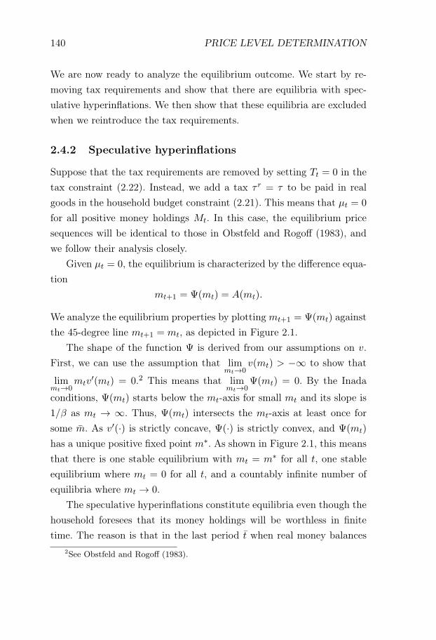
140 PRICE LEVEL DETERMINATION
We are now ready to analyze the equilibrium outcome. We start by re-moving tax requirements and show that there are equilibria with spec-ulative hyperinflations. We then show that these equilibria are excludedwhen we reintroduce the tax requirements.
2.4.2 Speculative hyperinflations
Suppose that the tax requirements are removed by setting Tt = 0 in thetax constraint (2.22). Instead, we add a tax τ r = τ to be paid in realgoods in the household budget constraint (2.21). This means that μt = 0
for all positive money holdings Mt. In this case, the equilibrium pricesequences will be identical to those in Obstfeld and Rogoff (1983), andwe follow their analysis closely.
Given μt = 0, the equilibrium is characterized by the difference equa-tion
mt+1 = Ψ(mt) = A(mt).
We analyze the equilibrium properties by plotting mt+1 = Ψ(mt) againstthe 45-degree line mt+1 = mt, as depicted in Figure 2.1.
The shape of the function Ψ is derived from our assumptions on v.First, we can use the assumption that lim
mt→0v(mt) > −∞ to show that
limmt→0
mtv′(mt) = 0.2 This means that lim
mt→0Ψ(mt) = 0. By the Inada
conditions, Ψ(mt) starts below the mt-axis for small mt and its slope is1/β as mt → ∞. Thus, Ψ(mt) intersects the mt-axis at least once forsome m. As v′(·) is strictly concave, Ψ(·) is strictly convex, and Ψ(mt)
has a unique positive fixed point m∗. As shown in Figure 2.1, this meansthat there is one stable equilibrium with mt = m∗ for all t, one stableequilibrium where mt = 0 for all t, and a countably infinite number ofequilibria where mt → 0.
The speculative hyperinflations constitute equilibria even though thehousehold foresees that its money holdings will be worthless in finitetime. The reason is that in the last period t when real money balances
2See Obstfeld and Rogoff (1983).
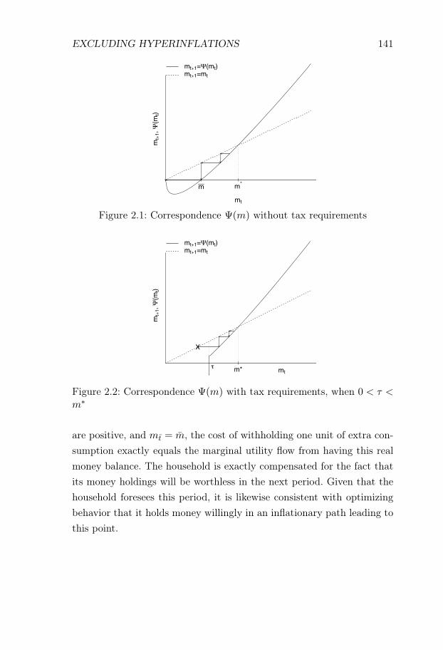
EXCLUDING HYPERINFLATIONS 141
mt
mt+
1, Ψ
(mt)
m*m
mt+1=Ψ(mt)mt+1=mt
Figure 2.1: Correspondence Ψ(m) without tax requirements
mt
mt+
1, Ψ
(mt)
m*τ
X
mt+1=Ψ(mt)mt+1=mt
Figure 2.2: Correspondence Ψ(m) with tax requirements, when 0 < τ <m∗
are positive, and mt = m, the cost of withholding one unit of extra con-sumption exactly equals the marginal utility flow from having this realmoney balance. The household is exactly compensated for the fact thatits money holdings will be worthless in the next period. Given that thehousehold foresees this period, it is likewise consistent with optimizingbehavior that it holds money willingly in an inflationary path leading tothis point.
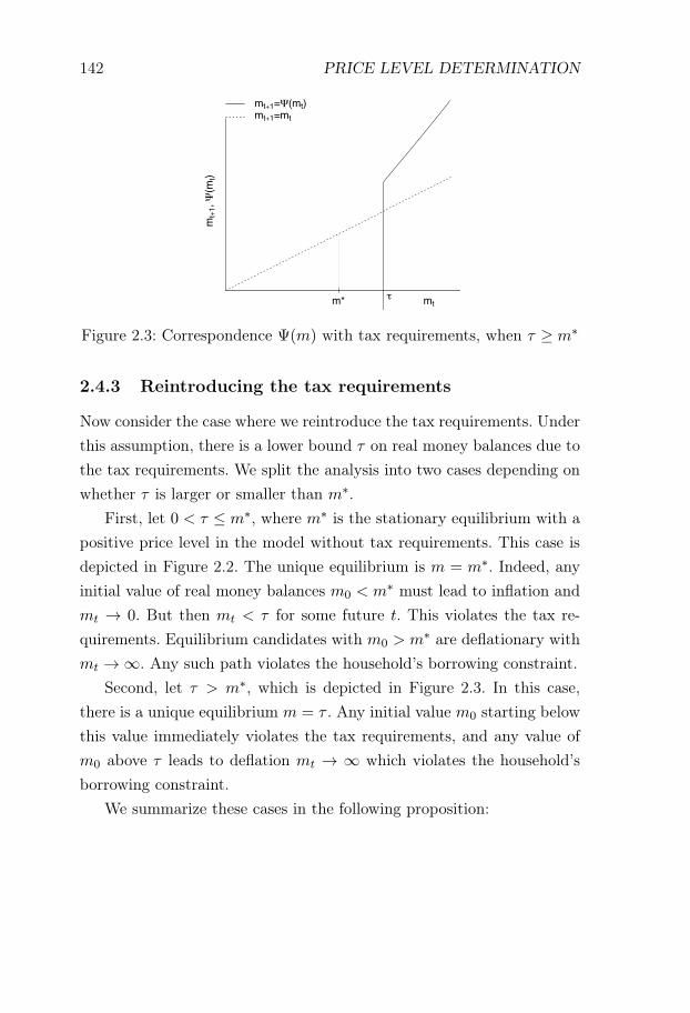
142 PRICE LEVEL DETERMINATION
mt
mt+
1, Ψ
(mt)
m* τ
mt+1=Ψ(mt)mt+1=mt
Figure 2.3: Correspondence Ψ(m) with tax requirements, when τ ≥ m∗
2.4.3 Reintroducing the tax requirements
Now consider the case where we reintroduce the tax requirements. Underthis assumption, there is a lower bound τ on real money balances due tothe tax requirements. We split the analysis into two cases depending onwhether τ is larger or smaller than m∗.
First, let 0 < τ ≤ m∗, where m∗ is the stationary equilibrium with apositive price level in the model without tax requirements. This case isdepicted in Figure 2.2. The unique equilibrium is m = m∗. Indeed, anyinitial value of real money balances m0 < m∗ must lead to inflation andmt → 0. But then mt < τ for some future t. This violates the tax re-quirements. Equilibrium candidates with m0 > m∗ are deflationary withmt → ∞. Any such path violates the household’s borrowing constraint.
Second, let τ > m∗, which is depicted in Figure 2.3. In this case,there is a unique equilibrium m = τ . Any initial value m0 starting belowthis value immediately violates the tax requirements, and any value ofm0 above τ leads to deflation mt → ∞ which violates the household’sborrowing constraint.
We summarize these cases in the following proposition:
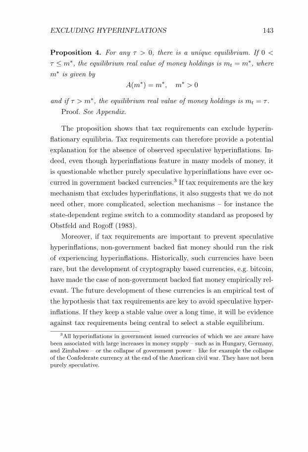
EXCLUDING HYPERINFLATIONS 143
Proposition 4. For any τ > 0, there is a unique equilibrium. If 0 <
τ ≤ m∗, the equilibrium real value of money holdings is mt = m∗, wherem∗ is given by
A(m∗) = m∗, m∗ > 0
and if τ > m∗, the equilibrium real value of money holdings is mt = τ .Proof. See Appendix.
The proposition shows that tax requirements can exclude hyperin-flationary equilibria. Tax requirements can therefore provide a potentialexplanation for the absence of observed speculative hyperinflations. In-deed, even though hyperinflations feature in many models of money, itis questionable whether purely speculative hyperinflations have ever oc-curred in government backed currencies.3 If tax requirements are the keymechanism that excludes hyperinflations, it also suggests that we do notneed other, more complicated, selection mechanisms – for instance thestate-dependent regime switch to a commodity standard as proposed byObstfeld and Rogoff (1983).
Moreover, if tax requirements are important to prevent speculativehyperinflations, non-government backed fiat money should run the riskof experiencing hyperinflations. Historically, such currencies have beenrare, but the development of cryptography based currencies, e.g. bitcoin,have made the case of non-government backed fiat money empirically rel-evant. The future development of these currencies is an empirical test ofthe hypothesis that tax requirements are key to avoid speculative hyper-inflations. If they keep a stable value over a long time, it will be evidenceagainst tax requirements being central to select a stable equilibrium.
3All hyperinflations in government issued currencies of which we are aware havebeen associated with large increases in money supply – such as in Hungary, Germany,and Zimbabwe – or the collapse of government power – like for example the collapseof the Confederate currency at the end of the American civil war. They have not beenpurely speculative.

144 PRICE LEVEL DETERMINATION
2.5 Price level determination under a balancedbudget rule
In Section 2.2, we assumed that government consumption g, money sup-ply M , and the real value of taxes τ were constant and that bond is-suance Bt varied residually to satisfy the government per-period budgetconstraint (2.6). Even though Bt = 0 in the stationary equilibrium, wedid not constrain the government to run a balanced budget out of equi-librium.
This observation raises the question if we can obtain a unique pricelevel under a balanced budget rule. The potential implications of bal-anced budget rules on price level determinacy has previously been high-lighted by Schmitt-Grohé and Uribe (2000). The question is relevantbecause of the importance of balanced budget rules in practical policymaking.4 This is especially true for countries that might be forced intomonetary reform while simultaneously losing access to international fi-nancial markets, as exemplified by the possibility of Greece deciding toleave the euro in the summer of 2015.
In this section, we show that when the bond supply is constrained tobe zero, the tax policy from Section 2.2 fails to ensure a unique equilib-rium price level. This points to a difficulty of price level control under abalanced budget rule. However, there exists a modified tax policy whichrestores uniqueness. More specifically, for each P , there exists a tax func-tion Tt(Pt), which respects the constraint Bt = 0 and which produces aunique equilibrium Pt = P .
To construct such a tax policy, we first note that when the bondsupply is zero, the money supply rule has to keep real proceeds from
4A second reason to study balanced budget rules is obtained from the analysis ofBassetto (2002). In a game-theoretic analysis of the fiscal theory of the price level,he shows that equilibrium indeterminacy can arise if the government tries but fails toissue government bonds. This problem is avoided if the government runs a balancedbudget.
A BALANCED BUDGET RULE 145
money sales Mt−Mt−1
Ptconstant and equal to expenditure gt = τ
Mt = τPt + Mt−1. (2.31)
Equation (2.31) differs from the constant money supply function Mt = M
from Section 2.2. Importantly, with the money supply function (2.31),the proportional tax function Tt = τPt from Section 2.2 does not giveus a unique equilibrium. In fact under Tt = τPt, the constant pricesequence Pt = P is an equilibrium for any P > 0. To see this, note thata constant price level implies a positive nominal interest rate Qt < 1,and zero between-period money holdings Mt = 0. Then Mt = τP = Tt
and the tax requirement is satisfied. This is true for all P . Hence, thereis a continuum of stationary equilibria when we have a balanced budgetrule and the same tax function as in Section 2.2.
Uniqueness fails because price level deviations do not generate excessdemand/supply for money. This differs from the equilibrating mechanismin Section 2.2. In Section 2.2, a price level above the stationary equilib-rium price level P = M/τ implied that the money supply did not sufficeto pay taxes, and a price level below P implied a slack tax constraint andthat households accumulated money holdings and took on debt, whicheventually violated their borrowing constraint.
However, we can modify the tax function to obtain a unique equilib-rium in this setting. The tax function needs to generate excess demandfor money when the price level is too high, and excess supply of moneywhen the price level is too low. The key observation is that with ournew money supply rule (2.31), money supply increases proportionallywith the price level. To ensure a unique equilibrium, we need that taxesincrease more than proportionally with the price level. Therefore, wepropose a tax function
Tt(Pt) = τPt +Π(Pt) (2.32)
with Π(P ) = 0, Π′ > 0 and where Π′ is uniformly bounded away from
146 PRICE LEVEL DETERMINATION
zero. Under this policy, we can prove the following proposition.
Proposition 5. Suppose that the government policy is Bt = 0, gt = τ ,Mt = τPt + Mt−1 and Tt(Pt) = τPt + Π(Pt) with Π(P ) = 0 for someP > 0 and ∂Π
∂Pt> ε for some ε > 0. Then, there exists an equilibrium
with Pt = P , and this equilibrium is unique.
Proof. See Appendix.We sketch the intuition for the proof here. There are three cases:
1. Pt = P
2. Pt > P
3. Pt < P
We can see that Case 1 is an equilibrium. Indeed, if Pt = P , the taxfunction gives us nominal taxes Tt = τP and the money supply isMt = M = τP . This is the same parameters as in Section 2.2 andby Proposition 1, this is an equilibrium. Case 2 is not an equilibriumsince Pt > P implies that the level of taxes exceeds the level of moneyissuance τPt, and the household will violate the tax requirements. Case3 is not an equilibrium. Pt < P implies that money issuance τPt exceedsthe tax requirements, which means that the price level path decreaseswith the real interest rate and the value of household money holdingsincreases faster than the real interest rate. Since Bt = 0 for all t, thisviolates the household’s transversality condition.
The tax function (2.32) is not as simple as the tax system in Section2.2. However, such a tax policy could be constructed in practice by com-bining a tax requirement Tt = τPt, which is fixed in real terms, with anominal lump-sum transfer/tax. These results suggest that it is possible,but more challenging, to use tax requirements to achieve a determinateprice level under a balanced budget rule.
2.6. DISCUSSION 147
2.6 Discussion
In this paper, we have constructed a sequence of models to analyze howtax requirements affect price level determination. In this section, we dis-cuss potential implications of our theory for the conduct of monetarypolicy.
We conjecture that tax requirements are unlikely to affect monetarypolicy when monetary authorities use interest rate rules. We can see thisby considering how an interest rate rule would operate in our environ-ment. Under an interest rate rule, given a path of real consumption, theexpected inflation rate is determined by the Euler equation. Restrictingourselves to the case where nominal interest rates are positive, the taxconstraint binds. The path of money supply is determined by the equa-tion Mt = τPt, and money supply responds passively to any changesin the price level. This outcome is essentially identical to that with aninterest rate rule in a one-good economy with a cash-in-advance con-straint. Apart from sunspot equilibria (Sargent and Wallace, 1975), theequilibrium is unique up to a scaling factor in the initial money supplyand price level.
However, the analysis suggests that tax requirements might makemoney supply rules a more attractive policy instrument. The reason isthat tax requirements address a key dilemma with money supply rules:The difficulty of selecting a monetary aggregate for which there is astable demand, and which is simultaneously possible to control. If themonetary authorities select a narrow monetary aggregate, demand mightbe unstable as financial innovation can generate close substitutes. Theaggregate for which we can expect a reasonably stable demand wouldbe the total amount of all liquid assets. However, the supply of thisaggregate is difficult to control for the monetary authorities.
With tax requirements, government tax policy controls the demandfor the monetary aggregate required for tax payments. This monetaryaggregate can be chosen to be M0, which also gives the governmentcontrol over its supply. In this situation, the government controls both

148 PRICE LEVEL DETERMINATION
the demand and the supply curve of money, and can use this to determinethe price level. In light of recent events, where central banks have failedto control the inflation rate using interest rates alone, it is interestingto explore money supply based alternatives. However, more research isneeded to exactly clarify how a policy based on tax requirements couldbe expected to work, and how it could be implemented.
REFERENCES 149
References
Bassetto, M. (2002). A Game-Theoretic View of the Fiscal Theory ofthe Price Level. Econometrica, 70(6):2167–2195.
Cochrane, J. H. (2005). Money as stock. Journal of Monetary Economics,52(3):501–528.
Goldberg, D. (2012). The tax-foundation theory of fiat money. EconomicTheory, 50(2):489–497.
Krugman, P. (2013). The Antisocial Network. The New York Times,available from ’http://www.nytimes.com/’, published April 14 [August6 2015].
Leeper, E. M. (1991). Equilibria under ‘active’ and ‘passive’ monetaryand fiscal policies. Journal of Monetary Economics, 27(1):129–147.
Lerner, A. P. (1947). Money as a Creature of the State. The AmericanEconomic Review, 37:312–317.
Obstfeld, M. and Rogoff, K. (1983). Speculative Hyperinflations in Max-imizing Models: Can We Rule Them Out? Journal of Political Econ-omy, 91(4):675.
Sargent, T. J. and Wallace, N. (1975). "Rational" Expectations, theOptimal Monetary Instrument, and the Optimal Money Supply Rule.Journal of Political Economy, 83(2):241.
Schmitt-Grohé, S. and Uribe, M. (2000). Price level determinacy andmonetary policy under a balanced-budget requirement. Journal ofMonetary Economics, 45(1):211–246.
Sims, C. A. (1994). A simple model for study of the determination of theprice level and the interaction of monetary and fiscal policy. EconomicTheory, 4(3):381–399.
150 PRICE LEVEL DETERMINATION
Smith, A. (1776). An inquiry into the nature and causes of the wealth ofnations. George Routledge and Sons, London, Untited Kingdom.
Starr, R. M. (1974). The Price of Money in a Pure Exchange MonetaryEconomy with Taxation. Econometrica, 42(1):45–54.
Varoufakis, Y. (2015). Something is rotten in the eurozone kingdom.Financial Times, available from ’http://www.ft.com/’, published July28 [August 10 2015].
Williamson, S. and Wright, R. (2010). New monetarist economics: Mod-els. In Handbook of Monetary Economics 3, pages 25–96.
Woodford, M. (1984). Indeterminacy of equilibrium in the overlappinggenerations model: A survey. mimeo.
Woodford, M. (1995). Price-level determinacy without control of a mon-etary aggregate. Carnegie-Rochester Conference Series on Public Pol-icy, 43:1–46.
PROOFS 151
Appendix
Proofs to Section 2.2
Proof of Proposition 1. To prove the proposition, we proceed in threesteps. First, we establish that the proposed stationary equilibrium exists.Second, we show that there are no other stationary equilibria. Finally,we show that there is an infinite number of non-stationary equilibria.
We guess that an equilibrium is formed by
ct ≡ y − τ Mt = 0
Pt ≡ M
τQt =
1
β
Recall from the proposition statement that Mt ≡ M and Tt = τPt, andthat given the values of other variables, we have Bt = 0.
The guess is an equilibrium if it satisfies the market clearing condi-tions (2.7)-(2.8), the consumer optimality conditions (2.2), (2.4), (2.9)-(2.13) and the zero lower bound on interest rates (2.10). We check theseconditions one by one.
The non-negativity constraint on money (2.4), the initial conditionson money and bonds (2.2), and the non-negativity constraint on nomi-nal interest rates (2.10) are directly satisfied by assumption. The goodsmarket clears since ct = y − τ . The money market clearing condition(2.8) holds as
Tt + Mt = Ptτ = M = Mt

152 PRICE LEVEL DETERMINATION
The household per-period budget constraint (2.9) holds since
ct +Tt
Pt+
(1−Qt)Mt
Pt+
Qt
Pt
(Mt +Bt
)= (y − τ) + τ + (1−Qt)× 0 +Qt(0 + 0)
= y
= y +1
Pt
(Mt−1 +Bt−1
).
The Euler equation (2.11) holds as the consumption and price level areconstant and Qt =
1β . The constraint that between-period money hold-
ings are zero if Qt < 1 (2.12) holds as Mt ≡ 0. The transversality/no-Ponzi condition (2.13) trivially holds since Bt = Mt = 0. The guess istherefore an equilibrium.
To show that the guess is the unique stationary equilibrium, we do aproof by contradiction and show that there is no equilibrium such thatPt = P for all t and P = M
τ .Assume that there is a stationary equilibrium with Pt >
Mτ for some
t. Then Mt < 0 by the money market clearing condition (2.8). This con-tradicts the non-negativity constraint on between-period money holdings(2.4).
Assume that there is a stationary equilibrium with Pt <Mτ for some
t. Then Mt > 0 by the money market clearing condition (2.8). The opti-mality condition for money holdings (2.12) then requires that Qt = 1. Inthat case, the Euler equation (2.11) yields Pt+1 = βPt < Pt, contradict-ing that the price level is constant. Therefore, the proposed stationaryequilibrium is the unique stationary equilibrium.
We now want to show that there is a continuum of non-stationaryequilibria. This is done by constructing an equilibrium for an arbitraryP0 < M/τ (there are no equilibria with P0 > M/τ as this would meanthat the tax constraint was violated). If P0 < M/τ , we know that M0 > 0
by money market clearing, and optimal choice of money holdings implies
PROOFS 153
that Qt = 1. The Euler equation, in turn, implies that P1 = βP0. Thismeans that the tax constraint is lax for t = 1 as well, and by iteratingforward on t, we obtain
Pt = βtP0.
We now propose an equilibrium with B−1 = M−1 = 0 and for t ≥ 0
ct ≡ y − τ Mt = M − τPt
Pt ≡ P0βt Qt = 1
We can confirm that under this equilibrium, Bt = −Mt.It is clear that the initial conditions (2.2) and the non-negativity
constraint on money holdings (2.4) hold. Market clearing for goods andmoney (2.7)-(2.8) both hold. The household per-period budget constraintholds as
ct +Tt
Pt+
(1−Qt)Mt
Pt+
Qt
Pt
(Mt +Bt
)= (y − τ) + τ + 0× Mt +
1
Pt× (Mt − Mt)
= y
= y +1
Pt
(Mt−1 +Bt−1
)
The Euler equation (2.11) holds as we derived the price level path underthe assumption that it did, and the money optimality equation (2.12)holds as Qt ≡ 1. The transversality/no-Ponzi condition (2.13) holds astotal nominal wealth is zero in all periods, and the zero lower bound oninterest rates (2.10) holds by assumption.
Proof of Proposition 2. We know that the stationary equilibrium pro-posed in the proof of Proposition 1 is also an equilibrium under the con-ditions in the current proposition, since Bt = 0 clearly does not violatethe new borrowing constraint. To show that the stationary equilibrium
154 PRICE LEVEL DETERMINATION
from Proposition 1 is the unique equilibrium, we do a proof by contra-diction and show that there is no equilibrium featuring Pt = M
τ .Assume that there is an equilibrium with Pt >
Mτ for some t. Then
Mt < 0 by the money market clearing condition (2.8). This is inconsistentwith the non-negativity constraint on between-period money (2.4).
Assume that there is an equilibrium with Pt <Mτ for some t. Then,
Mt > 0 by the money market clearing condition (2.8). This means thatQt = 1 from the money optimality condition (2.12). Then the Eulerequation (2.11) with constant consumption y − τ gives us Pt+1 = βPt.Hence, Pt+1 <
Mτ and the tax constraint is slack and thus Mt+1 > 0. By
successive iteration, we have that Pt+s = βsPt. Thus, Pt+s → 0. Moneymarket clearing then implies that
Mt+s = M − Pt+sτ → M.
Furthermore, if we substitute Tt = τPt, c = y − τ and (1 − Qt)Mt = 0
(the last from optimality condition (2.12)) into the consumer per-periodbudget constraint (2.9), we obtain a law of motion for nominal wealth
Qt(Bt + Mt) = Bt−1 +Mt−1.
Using the initial condition M−1 = B−1 = 0, the law of motion impliesthat Bt + Mt = 0 for all t. Therefore, if Mt → M , this means thatBt → −M < 0, and together with Pt → 0 we get B
Pt→ −∞. This
violates the borrowing constraint (2.18).
Proofs in Section 2.3
Proof of Proposition 3. We first derive the equilibrium relationship be-tween the price level and the government’s surplus sequence. Supposethat we have an equilibrium price sequence Pt. In an equilibrium, house-hold consumption is c = y− τ by goods market clearing. We can iterate
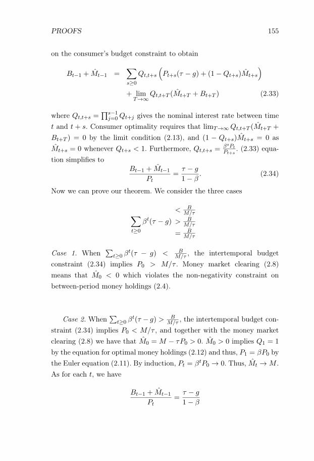
PROOFS 155
on the consumer’s budget constraint to obtain
Bt−1 + Mt−1 =∑s≥0
Qt,t+s
(Pt+s(τ − g) + (1−Qt+s)Mt+s
)+ lim
T→∞Qt,t+T (Mt+T +Bt+T ) (2.33)
where Qt,t+s =∏s−1
j=0Qt+j gives the nominal interest rate between timet and t + s. Consumer optimality requires that limT→∞Qt,t+T (Mt+T +
Bt+T ) = 0 by the limit condition (2.13), and (1 − Qt+s)Mt+s = 0 asMt+s = 0 whenever Qt+s < 1. Furthermore, Qt,t+s =
βsPt
Pt+s. (2.33) equa-
tion simplifies toBt−1 + Mt−1
Pt=
τ − g
1− β. (2.34)
Now we can prove our theorem. We consider the three cases
∑t≥0
βt(τ − g)
< BM/τ
> BM/τ
= BM/τ
Case 1. When∑
t≥0 βt(τ − g) < B
M/τ , the intertemporal budgetconstraint (2.34) implies P0 > M/τ . Money market clearing (2.8)means that M0 < 0 which violates the non-negativity constraint onbetween-period money holdings (2.4).
Case 2. When∑
t≥0 βt(τ − g) > B
M/τ , the intertemporal budget con-straint (2.34) implies P0 < M/τ , and together with the money marketclearing (2.8) we have that M0 = M − τP0 > 0. M0 > 0 implies Q1 = 1
by the equation for optimal money holdings (2.12) and thus, P1 = βP0 bythe Euler equation (2.11). By induction, Pt = βtP0 → 0. Thus, Mt → M .As for each t, we have
Bt−1 + Mt−1
Pt=
τ − g
1− β
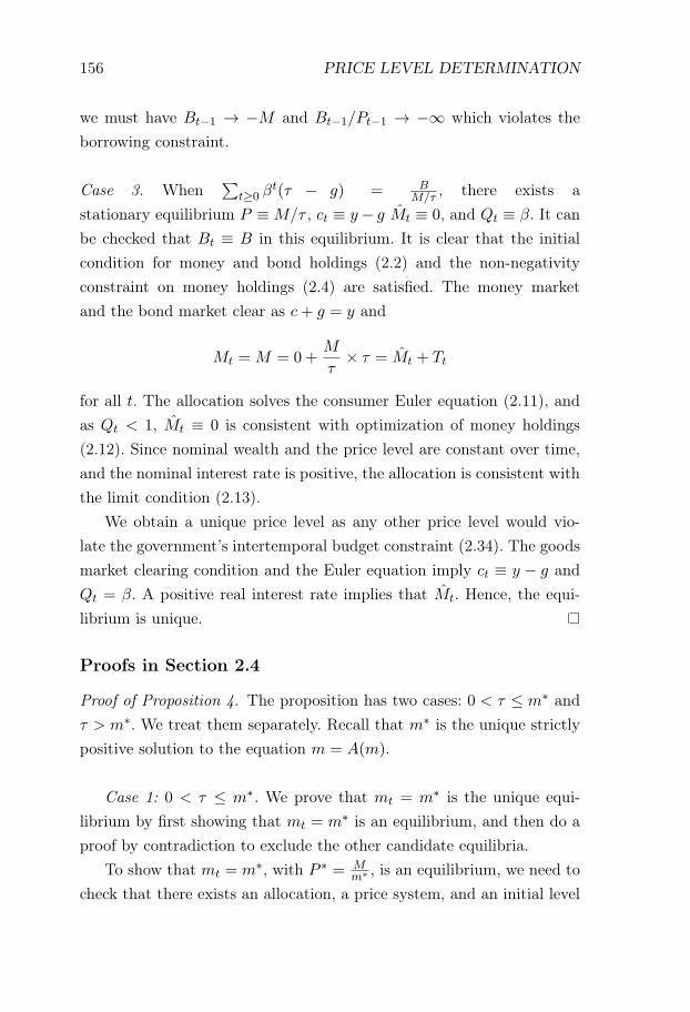
156 PRICE LEVEL DETERMINATION
we must have Bt−1 → −M and Bt−1/Pt−1 → −∞ which violates theborrowing constraint.
Case 3. When∑
t≥0 βt(τ − g) = B
M/τ , there exists astationary equilibrium P ≡ M/τ , ct ≡ y− g Mt ≡ 0, and Qt ≡ β. It canbe checked that Bt ≡ B in this equilibrium. It is clear that the initialcondition for money and bond holdings (2.2) and the non-negativityconstraint on money holdings (2.4) are satisfied. The money marketand the bond market clear as c+ g = y and
Mt = M = 0 +M
τ× τ = Mt + Tt
for all t. The allocation solves the consumer Euler equation (2.11), andas Qt < 1, Mt ≡ 0 is consistent with optimization of money holdings(2.12). Since nominal wealth and the price level are constant over time,and the nominal interest rate is positive, the allocation is consistent withthe limit condition (2.13).
We obtain a unique price level as any other price level would vio-late the government’s intertemporal budget constraint (2.34). The goodsmarket clearing condition and the Euler equation imply ct ≡ y − g andQt = β. A positive real interest rate implies that Mt. Hence, the equi-librium is unique.
Proofs in Section 2.4
Proof of Proposition 4. The proposition has two cases: 0 < τ ≤ m∗ andτ > m∗. We treat them separately. Recall that m∗ is the unique strictlypositive solution to the equation m = A(m).
Case 1: 0 < τ ≤ m∗. We prove that mt = m∗ is the unique equi-librium by first showing that mt = m∗ is an equilibrium, and then do aproof by contradiction to exclude the other candidate equilibria.
To show that mt = m∗, with P ∗ = Mm∗ , is an equilibrium, we need to
check that there exists an allocation, a price system, and an initial level

PROOFS 157
of government debt consistent with (2.2),(2.4), (2.7)-(2.11), (2.13) and(2.30). We propose the allocation ct = y−τ, Mt = M−τP ∗, Bt = 0 withthe initial condition M−1 = 0, B−1 = Mt and the bond price Qt = β.
The initial condition (2.2) is satisfied by assumption. Thenon-negativity constraint on money holdings (2.4) is satisfied sinceMt = M − τP ∗ = M − τ M
m∗ = M(1 − τm∗ ) ≥ 0. The goods market
clearing condition (2.7) and the money market clearing condition (2.8)are satisfied by assumption. The zero lower bound on interest rates(2.10) is satisfied since Qt = β < 1. The per-period household budgetconstraint (2.9) is satisfied in period 0 since
ct +M0
P0+
Q0B0
P0= (y − τ) + τ +
M0
P0+ 0
= y +M0
P0
= y +B−1 + M−1
P0.
Note that we use B−1 = M0. The household budget constraint is satisfiedin period t ≥ 1 since
ct +Mt
Pt+
QtBt
Pt= (y − τ) + τ +
Mt
Pt+ 0
= y +Mt
Pt
= y +Bt−1 + Mt−1
P0.
Here we use Mt = Mt−1 for t ≥ 1. The Euler equation (2.11) holds sinceQt = β and Pt = P ∗ for all t. The transversality/no-Ponzi condition(2.13) holds as Bt = 0 and Mt is constant for all t. Equation (2.30)governing the evolution of mt holds by assumption as m∗ = M/P ∗ is thefixed point of A.
This shows that there exists an equilibrium with mt = m∗. To showthat it is the unique equilibrium, we do a proof by contradiction.
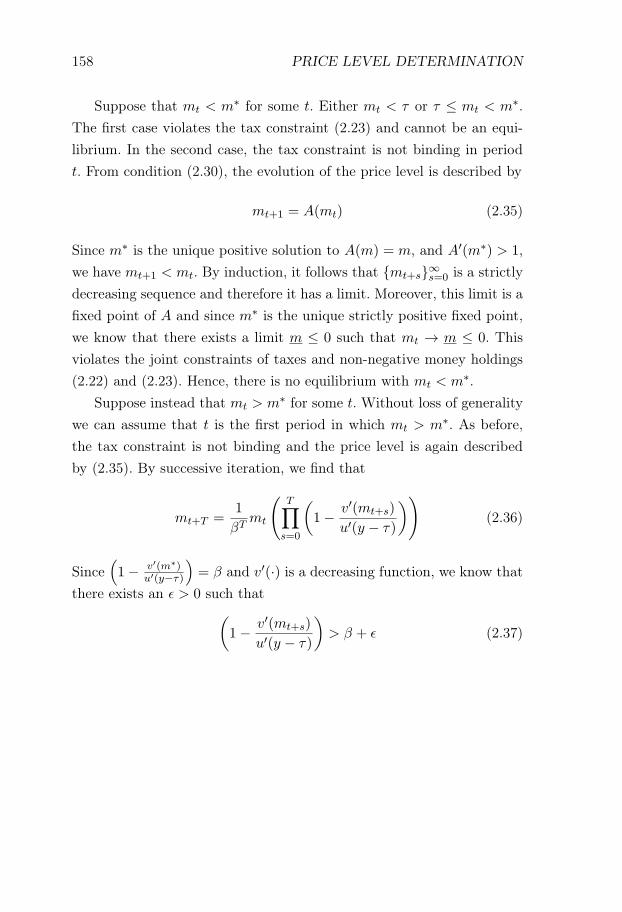
158 PRICE LEVEL DETERMINATION
Suppose that mt < m∗ for some t. Either mt < τ or τ ≤ mt < m∗.The first case violates the tax constraint (2.23) and cannot be an equi-librium. In the second case, the tax constraint is not binding in periodt. From condition (2.30), the evolution of the price level is described by
mt+1 = A(mt) (2.35)
Since m∗ is the unique positive solution to A(m) = m, and A′(m∗) > 1,we have mt+1 < mt. By induction, it follows that {mt+s}∞s=0 is a strictlydecreasing sequence and therefore it has a limit. Moreover, this limit is afixed point of A and since m∗ is the unique strictly positive fixed point,we know that there exists a limit m ≤ 0 such that mt → m ≤ 0. Thisviolates the joint constraints of taxes and non-negative money holdings(2.22) and (2.23). Hence, there is no equilibrium with mt < m∗.
Suppose instead that mt > m∗ for some t. Without loss of generalitywe can assume that t is the first period in which mt > m∗. As before,the tax constraint is not binding and the price level is again describedby (2.35). By successive iteration, we find that
mt+T =1
βTmt
(T∏
s=0
(1− v′(mt+s)
u′(y − τ)
))(2.36)
Since(1− v′(m∗)
u′(y−τ)
)= β and v′(·) is a decreasing function, we know that
there exists an ε > 0 such that(1− v′(mt+s)
u′(y − τ)
)> β + ε (2.37)
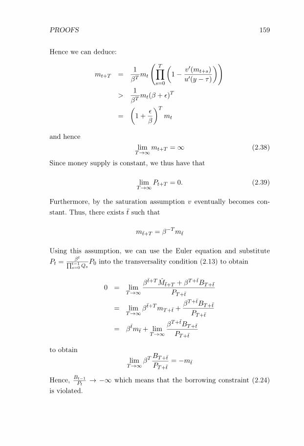
PROOFS 159
Hence we can deduce:
mt+T =1
βTmt
(T∏
s=0
(1− v′(mt+s)
u′(y − τ)
))
>1
βTmt(β + ε)T
=
(1 +
ε
β
)T
mt
and hencelimT→∞
mt+T = ∞ (2.38)
Since money supply is constant, we thus have that
limT→∞
Pt+T = 0. (2.39)
Furthermore, by the saturation assumption v eventually becomes con-stant. Thus, there exists t such that
mt+T = β−Tmt
Using this assumption, we can use the Euler equation and substitutePt =
βt∏t−1s=0 Qs
P0 into the transversality condition (2.13) to obtain
0 = limT→∞
β t+T Mt+T + βT+tBT+t
PT+t
= limT→∞
β t+TmT+t +βT+tBT+t
PT+t
= β tmt + limT→∞
βT+tBT+t
PT+t
to obtainlimT→∞
βT BT+t
PT+t= −mt
Hence, Bt−1
Pt→ −∞ which means that the borrowing constraint (2.24)
is violated.
160 PRICE LEVEL DETERMINATION
Case 2: τ ≥ m∗. We will prove that mt = τ is the unique equilibriumby first showing that it is an equilibrium, and then exclude all other casesby contradiction.
To show that mt = τ , with P = Mτ , is an equilibrium, we need
to check that there exists an allocation and a price system consistentwith (2.2),(2.4), (2.7)-(2.11), (2.13) and (2.30). We propose the allocationct = y − τ, Mt = 0, Bt = 0 with the initial condition B−1 = M−1 = 0
and the bond price Qt = β.(2.2) is satisfied by assumption. (2.4) is satisfied since Mt = 0. (2.7) is
satisfied by assumption. (2.8) is satisfied by assumption. (2.10) is satisfiedsince Qt = β < 1. (2.9) is satisfied since
(1−Qt)M − τPt
Pt+
Qt
Pt(M − τPt +Bt) =
1
Pt(M − τPt−1 +Bt−1)
⇔Bt =1
Qtτ(Pt − Pt−1) +
1
QtBt−1
⇔Bt =1
QtBt−1
which together with the initial conditions imply that Bt = 0 for all t.(2.11) holds since Qt = β and Pt = P for all t. (2.13) holds as Bt = M =
0 for all t. (2.30) holds by assumption.This shows that there is an equilibrium with mt = τ . To show that
it is the unique equilibrium, we proceed by contradiction.Suppose mt < τ in some period t. This violates the tax constraint
(2.23) and cannot be an equilibrium.Suppose mt > τ in some period t. Then we are in the same hyperde-
flationary situation in Case 1, and analogous to that case, the solutionpath will feature a violation of the borrowing constraint as t → ∞.
PROOFS 161
Proofs to Section 2.5
Proof of Proposition 5. For existence, we guess that an equilibrium isformed by
ct ≡ y − τ Bt = 0 Mt = 0 (2.40)
Pt ≡ M
τQt =
1
β(2.41)
The guess is an equilibrium if it satisfies the market clearing conditions(2.7)-(2.8), the consumer optimality conditions (2.4), (2.2) (2.9)-(2.13)and the zero lower bound on interest rates (2.10). We check these con-ditions one by one.
The non-negativity constraint on money (2.4), the initial conditionson money and bonds (2.2), and the non-negativity constraint on nomi-nal interest rates (2.10) are directly satisfied by assumption. The goodsmarket clears since ct = y − τ . The money market clearing condition(2.8) holds as
Tt(P ) + Mt = P τ +Π(P ) + 0
= P τ
= Mt(P )
for all t. The Euler equation (2.11) holds as the consumption and pricelevel are constant and Qt = β. The constraint (2.12) holds as Mt ≡ 0.(2.13) trivially holds since Bt = Mt = 0. The guess is therefore anequilibrium.
For uniqueness, we do a proof by contradiction.Case 1: Pt > P . Assume that there is an equilibrium with Ps > P
in some period s. Then, by the well-ordering principle, there exists asmallest t = t such that Pt > P . Assume that the tax constraint is notviolated. From this assumption together with the money market clearing
162 PRICE LEVEL DETERMINATION
condition (2.8), we derive
Tt(Pt) + Mt = Mt(Pt) = Ptτt + Mt−1
As Tt(Pt) > Ptτt whenever Pt > P and Mt ≥ 0, we have that Mt−1 > 0.That is, as the level of taxes exceeds money issuance, the only way thatthe money market clearing condition can be satisfied is if the householdcarried money from a previous period. Now, either t = 0 which would vi-olate the initial condition Mt−1 = 0, or t ≥ 1 in which case the optimalitycondition for money holdings (2.12) implies Qt−1 = 1. From the Eulerequation (2.11), we then have that Pt = βPt−1 and so Pt−1 > Pt > P ,which violates the minimality of t.
Case 2: Pt < P . Assume that there is an equilibrium with Pt < P
for some t. ThenMt = Mt(Pt)− Tt(Pt) > 0
Mt > 0 is consistent with household optimality conditions (2.12) in pe-riod t only if Qt = 1. From the Euler equation (2.11), we then havethat Pt+1
Pt= β. As such, Pt+1 < Pt < P . By induction, Pt+k = βkPt,
Qt+k = 1, Mt+k > 0. However, this means that the transversality condi-tion is violated. To see this, note that
Mt = Mt−1 + Ptτ − Tt(Pt) = Mt−1 −Π(Pt)
and Π(Pt) < 0 for Pt < P . Using that Qs = 1, Bs = 0 for all s ≥ t, wefind that
limT→∞
(∏T−1s=0 Qs
)(BT + MT )
P0=
(∏T−1s=0 Qs
)P0
limT→∞
MT
=
(∏T−1s=0 Qs
)P0
(Mt + lim
T→∞
T∑s=t+1
−Π(Ps)
)>0
Therefore, the transversality condition is violated and there does not

PROOFS 163
exist an equilibrium with Pt < P for any t. Thus, Pt ≡ P is the uniqueequilibrium price sequence.

164 PRICE LEVEL DETERMINATION
Chapter 3
Swedish UnemploymentDynamics∗
3.1 Introduction
An important question in labor market economics is how important dif-ferent labor market flows are in driving business cycle fluctuations inunemployment. The standard estimation method in the literature buildson Shimer (2012). He notes that actual U.S. unemployment is close tothe steady state implied by the prevailing flow rates and uses this obser-vation to decompose unemployment variations into contributions fromunemployment inflows and outflows.
The steady-state assumption can be problematic when working withEuropean data. First, gross flows are much smaller in European coun-tries than in the U.S., which makes the steady-state unemployment rateless likely to be a good approximation of the actual unemployment rate(Elsby et al., 2013). Second, many European labor markets are dual andthere are potentially large differences in labor market dynamics between
∗This is joint work with Niels-Jakob Harbo Hansen. We are grateful for helpfulcomments from Tobias Broer, Saman Darougheh, Karl Harmenberg, John Hassler,Georg Marthin, Per Krusell, Alexander Kohlhas, Kurt Mitman, Erik Öberg, TorstenPersson, Hans Henrik Sievertsen, David Strömberg as well as seminar participants atthe IIES, Copenhagen University and the National Institute of Economic Research.
165
166 SWEDISH UNEMPLOYMENT DYNAMICS
permanent and temporary jobs. Duality motivates a distinction betweenpermanent and temporary jobs in the decomposition analysis.
We develop a new method for decomposing the sources of labor mar-ket fluctuations that jointly allows for (i) a slow convergence to steadystate and (ii) an arbitrary number of labor market states. The methoduses continuous time Markov chain theory to express the transition prob-ability matrix between different labor market states as the matrix expo-nential of the integral of instantaneous flow matrices. Our formulationcaptures the dependence of the current state on the whole history ofinstantaneous flow rates for an arbitrary number of states, and it alsoprovides a mapping between observed transition rates and underlyinginstantaneous flow rates. We use the matrix exponential formulation toperform a joint treatment of estimation, time-aggregation, detrending,log-linearization, and variance decomposition of trend-deviations intocontributions from different flow rates. The method also allows us tocalculate the convergence rate to steady state.
We apply our methodology to a new data set covering Swedish la-bor market flows through the period 1987-2011. Sweden has a dual labormarket with a strong legal distinction between permanent and temporaryworkers. Temporary workers account for about 13% of the working-agepopulation (and closer to 20% of employment), and experience substan-tially larger flow rates than permanently employed workers. The labormarket is also characterized by a slow convergence to steady state, witha half life of deviations from steady state of approximately two years.
We find that variation in unemployment is driven to an approxi-mately equal degree by variations in (i) flows from unemployment to em-ployment, (ii) flows from employment to unemployment, and (iii) flowsin and out of the labor force. Focusing on flows in and out of the la-bor force, the most important source of variation is changes in the flowfrom inactivity to unemployment. We find that flows involving tempo-rary contracts account for 44% of the variation in unemployment, whileflows involving permanent contracts account for approximately 33% ofthe variation. The former is sizeable given that workers on temporary
INTRODUCTION 167
contracts on average only account for 13% of the working-age popula-tion during the period.
We also show that it is important to account for out-of-steady-statedynamics. If we use the decomposition method which relies on approxi-mating the actual state with the steady state, the share of variation at-tributed to flows involving permanent contracts rises from 33% to 44%.The intuition is that small variations in flow rates involving permanentemployment have large effects on the implied steady-state employmentrate. However, for permanent workers, gross flows are small as comparedto population size, which means that the convergence rate to steady stateis slow. Hence, variations in the steady state due to changes in flows in-volving permanent workers are larger than variations in the actual state.
These results are of broader interest in the study of European labormarkets. Indeed, they suggest that decompositions based on the steady-state assumption are unlikely to be suitable in dual labor markets. Inparticular, our results indicate that there is a risk that existing studieson France and Spain (Silva and Vazquez-Grenno, 2013; Hairault et al.,2015) have overestimated the share of variation stemming from flowsinvolving permanently employed workers.
In Section 3.2, we describe our data on the Swedish labor market.Section 3.3 describes our new decomposition method in continuous timeand contrasts with a method based on a steady-state approximation. InSection 3.4, we discretize the method and estimate the parameters usingthe Swedish survey data. In Section 3.5, we use our parametrizationto decompose labor market flows using both our new method and themethod based on a steady-state assumption. The most closely relatedpaper to ours methodologically is Elsby et al. (2015). We discuss ourrelationship to this paper in Section 3.6. Section 3.7 concludes the paper.
168 SWEDISH UNEMPLOYMENT DYNAMICS
3.2 Data
3.2.1 Data description
Our data are from the Swedish Labor Force Survey (LFS) and cover theperiod 1987-2012 (Statistics Sweden, 2011, 2012). During this period, thesurvey samples 17 000-29 500 individuals each month. The survey beganalready in 1961, but micro data are only available for 1987 and onwards.The survey samples individuals from a register which aims at containingthe entire population in Sweden (RTB). Up to 2001 the sample includesall ages 16-64, but from 2001, the age interval was expanded to 15-74. Forconsistency, we confine our sample to ages 16-64 throughout the entireperiod.
The survey sample is rotating (Figure 3.1). Specifically, a participat-ing individual is interviewed about his or her employment status at agiven week every third month for two years. Each month, eight groupsof individuals are interviewed. Seven of these eight groups have been in-terviewed previously, while one group is being interviewed for the firsttime.
The surveyed population is divided into three categories (i) employed,(ii) unemployed, and (iii) outside the labor force (Figure 3.1).
• An individual is defined as employed if she worked at least one hourduring the reference week as (a) self-employed (including helpingspouse), (b) on a permanent contract (tillsvidareanställning), or (c)on a time-limited contract.1 An individual who has a job but wasabsent from work due to illness, leave, vacation, military service, aconflict or similar is also counted as employed, as is an individualin a labor market program if she receives some remuneration fromher employer.
• An individual is defined as unemployed if she is not employed, but1An alternative term for a permanent contract is that it is open-ended. Time-
limited contracts are dominated by temps, object jobs (objektanställningar) and“called as needed” (kallas vid behov), but also include workers in trial employment,on vacation, and in seasonal employment (Statistics Sweden, 2005)
DATA 169
has been applying for work within the last four weeks and is able tostart work within the reference week or in the two following weeks.An individual is also defined as unemployed if she is set to starta job within the next three months, provided that the individualwould be ready to start already in the reference week or during thefollowing two weeks.
• An individual is defined as outside the labor force if she is notcovered by the above definitions. This includes individuals whowould and could be able to work, but did not actively seek jobs(latent unemployment). This group includes, inter alia, pensioners,people engaged in home production, and conscripted soldiers.
The treatment of students deserves a discussion. Up to 2007, full-timestudents were always defined as belonging to outside the labor force. How-ever, in October 2007 the definition was altered such that non-employedstudents who have been applying for work within the last four weeksand are ready to start work within three weeks, are defined as beingunemployed. This change was made in order to comply with guidelinesfrom the International Labour Organization (ILO) and the EuropeanUnion (EU). For consistency, we use the pre-2007 definition throughoutthe entire period.
3.2.2 Data selection
We use the definition from the Labor Force Survey to construct fourcategories. We classify an individual as being (i) employed on a perma-nent contract, (ii) employed on a temporary contract, (iii) unemployed,or (iv) outside the labor force. We define self-employed workers as beingemployed on permanent contracts.
To compute labor market transition probabilities P (t, t + 1) in aquarter t, we restrict the sample to individuals for whom we also have anobservation in the next quarter t+1. We define 16 indicator variables foreach of these observations: It,i,s1,s2 for s1, s2 ∈ [1, 4]. Here It,i,s1=j,s2=k =
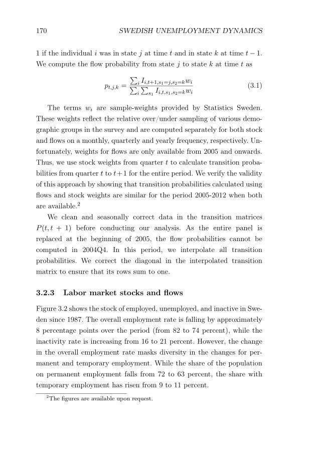
170 SWEDISH UNEMPLOYMENT DYNAMICS
1 if the individual i was in state j at time t and in state k at time t− 1.We compute the flow probability from state j to state k at time t as
pt,j,k =
∑i Ii,t+1,s1=j,s2=kwi∑i
∑s1Ii,t,s1,s2=kwi
(3.1)
The terms wi are sample-weights provided by Statistics Sweden.These weights reflect the relative over/under sampling of various demo-graphic groups in the survey and are computed separately for both stockand flows on a monthly, quarterly and yearly frequency, respectively. Un-fortunately, weights for flows are only available from 2005 and onwards.Thus, we use stock weights from quarter t to calculate transition proba-bilities from quarter t to t+1 for the entire period. We verify the validityof this approach by showing that transition probabilities calculated usingflows and stock weights are similar for the period 2005-2012 when bothare available.2
We clean and seasonally correct data in the transition matricesP (t, t + 1) before conducting our analysis. As the entire panel isreplaced at the beginning of 2005, the flow probabilities cannot becomputed in 2004Q4. In this period, we interpolate all transitionprobabilities. We correct the diagonal in the interpolated transitionmatrix to ensure that its rows sum to one.
3.2.3 Labor market stocks and flows
Figure 3.2 shows the stock of employed, unemployed, and inactive in Swe-den since 1987. The overall employment rate is falling by approximately8 percentage points over the period (from 82 to 74 percent), while theinactivity rate is increasing from 16 to 21 percent. However, the changein the overall employment rate masks diversity in the changes for per-manent and temporary employment. While the share of the populationon permanent employment falls from 72 to 63 percent, the share withtemporary employment has risen from 9 to 11 percent.
2The figures are available upon request.
3.3. METHOD 171
Figures 3.3-3.4 show the flows moving between the four groups com-puted as quarterly hazard rates. In Section 3.4, we explain the compu-tation method. Two trends are visible from these figures. First, all flowrates into permanent and temporary employment have decreased. Thistrend is particularly clear for the flow from unemployment into perma-nent employment. Second, there has been an increase in the probabilityof flowing from employment into unemployment. There is no clear trendin the hazard rates for movements into inactivity.
3.2.4 The cyclicality of flow rates
Table 3.2 illustrates the sensitivity of labor market transition rates tothe business cycle. We measure the cyclicality by regressing the relevanttransition rate (logged) on the unemployment rate and a linear trend.Table 3.2 reports the coefficient on the unemployment rate from thisregression. A positive (negative) value in Table 3.2 indicates that thecorrelation between the relevant transition rate and unemployment ispositive (negative). Since unemployment correlates negatively with thebusiness cycle, this means that a negative (positive) value implies a pro-cyclical (counter-cyclical) transition rate. Thus, from Table 3.2 we seethat all transition rates into permanent and temporary employment arepro-cyclical, while all rates into unemployment are countercyclical. Thetransition rate from permanent and temporary employment to inactivityis a-cyclical, while the transition rate from unemployment to inactivityis counter-cyclical.
3.3 Method
In this section, we outline our method for decomposing fluctuations in un-employment into contributions from the underlying labor market flows.Our method simultaneously addresses three issues.
First, it addresses the well-known time aggregation problem. Thetime aggregation problem arises when individuals can change labor mar-
172 SWEDISH UNEMPLOYMENT DYNAMICS
ket states several times within a measurement interval. In particular, anindividual who is coded as being employed for two consecutive quartersmight have experienced a spell of unemployment in-between. As pointedout by Shimer (2012), this can lead to an underestimation of the impor-tance of the job finding rate for business cycle dynamics, as a decrease inthe job-finding rate mechanically leads to an increase in the measured jobloss rate. In a manner similar to that used in Shimer (2012), we addressthis problem by using a continuous time formulation of the problem.
Our second contribution is to devise a method that can handle a slowconvergence rate towards the steady state. A common method in the lit-erature is to assume that steady-state unemployment is a good approx-imation of actual unemployment and therefore measure how variationsin labor market flows contribute to variations in steady-state unemploy-ment. This assumption seems appropriate in the U.S. where a large labormarket churn ensures a quick convergence to steady state, but it is morequestionable in Europe where both the job-finding and separation ratesare lower. Indeed, Elsby et al. (2013) find an average monthly job-findingrate of 13 percent in Europe as compared to 57 percent in the UnitedStates and a monthly separation rate of 0.8 percent in Europe as com-pared to 3.6 percent in the United States.3 The steady-state assumptionis even more questionable when one includes a distinction between per-manent and temporary jobs since the flows in and out of permanentemployment are low.
Third, our method allows for an arbitrary number of labor marketstates. By using flow matrices and matrix exponentials to characterizelabor market dynamics, we can derive a compact expression for decom-posing flows with an arbitrary number of states.
In this section, we first introduce our notation and describe how weuse a matrix formulation of continuous time Markov chains to express thecurrent labor market distribution as a matrix exponential of a sequence
3For Europe, the numbers are simple averages for the countries France, Germany,Ireland, Italy, Norway, Portugal, Spain, and Sweden. The sample start varies from1968 to 1986.
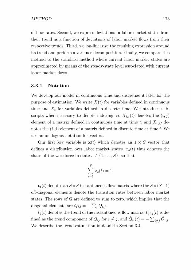
METHOD 173
of flow rates. Second, we express deviations in labor market states fromtheir trend as a function of deviations of labor market flows from theirrespective trends. Third, we log-linearize the resulting expression aroundits trend and perform a variance decomposition. Finally, we compare thismethod to the standard method where current labor market states areapproximated by means of the steady-state level associated with currentlabor market flows.
3.3.1 Notation
We develop our model in continuous time and discretize it later for thepurpose of estimation. We write X(t) for variables defined in continuoustime and Xt for variables defined in discrete time. We introduce sub-scripts when necessary to denote indexing, so Xi,j(t) denotes the (i, j)
element of a matrix defined in continuous time at time t, and Xi,j,t de-notes the (i, j) element of a matrix defined in discrete time at time t. Weuse an analogous notation for vectors.
Our first key variable is x(t) which denotes an 1 × S vector thatdefines a distribution over labor market states. xs(t) thus denotes theshare of the workforce in state s ∈ {1, . . . , S}, so that
S∑s=1
xs(t) = 1.
Q(t) denotes an S×S instantaneous flow matrix where the S×(S−1)
off-diagonal elements denote the transition rates between labor marketstates. The rows of Q are defined to sum to zero, which implies that thediagonal elements are Qi,i = −∑j Qi,j .
Q(t) denotes the trend of the instantaneous flow matrix. Qi,j(t) is de-fined as the trend component of Qij for i = j, and Qii(t) = −∑i �=j Qi,j .We describe the trend estimation in detail in Section 3.4.
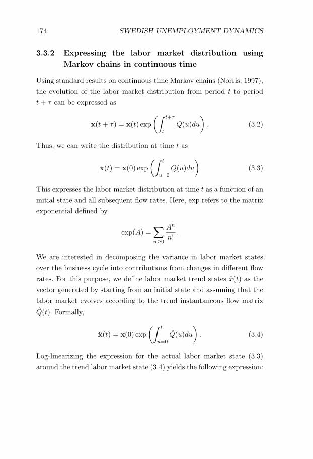
174 SWEDISH UNEMPLOYMENT DYNAMICS
3.3.2 Expressing the labor market distribution usingMarkov chains in continuous time
Using standard results on continuous time Markov chains (Norris, 1997),the evolution of the labor market distribution from period t to periodt+ τ can be expressed as
x(t+ τ) = x(t) exp
(∫ t+τ
tQ(u)du
). (3.2)
Thus, we can write the distribution at time t as
x(t) = x(0) exp
(∫ t
u=0Q(u)du
)(3.3)
This expresses the labor market distribution at time t as a function of aninitial state and all subsequent flow rates. Here, exp refers to the matrixexponential defined by
exp(A) =∑n≥0
An
n!.
We are interested in decomposing the variance in labor market statesover the business cycle into contributions from changes in different flowrates. For this purpose, we define labor market trend states x(t) as thevector generated by starting from an initial state and assuming that thelabor market evolves according to the trend instantaneous flow matrixQ(t). Formally,
x(t) = x(0) exp
(∫ t
u=0Q(u)du
). (3.4)
Log-linearizing the expression for the actual labor market state (3.3)around the trend labor market state (3.4) yields the following expression:
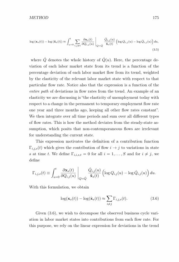
METHOD 175
log (xs(t))− log (xs(t)) ≈∫ t
u=0
∑i,j �=i
∂xs(t)
∂Qi,j(u)
∣∣∣∣∣Q=Q
Qi,j(u)
xs(t)
(logQi,j(u)− log Qi,j(u)
)du,
(3.5)
where Q denotes the whole history of Q(u). Here, the percentage de-viation of each labor market state from its trend is a function of thepercentage deviation of each labor market flow from its trend, weightedby the elasticity of the relevant labor market state with respect to thatparticular flow rate. Notice also that the expression is a function of theentire path of deviations in flow rates from the trend. An example of anelasticity we are discussing is “the elasticity of unemployment today withrespect to a change in the permanent to temporary employment flow rateone year and three months ago, keeping all other flow rates constant”.We then integrate over all time periods and sum over all different typesof flow rates. This is how the method deviates from the steady-state as-sumption, which posits that non-contemporaneous flows are irrelevantfor understanding the current state.
This expression motivates the definition of a contribution functionΓi,j,s(t) which gives the contribution of flow i → j to variations in states at time t. We define Γi,i,s,t = 0 for all i = 1, . . . , S and for i = j, wedefine
Γi,j,s(t) ≡∫ t
u=0
∂xs(t)
∂Qi,j(u)
∣∣∣∣∣Q=Q
Qi,j(u)
xs(t)
(logQi,j(u)− log Qi,j(u)
)du.
With this formulation, we obtain
log(xs(t))− log(xs(t)) ≈∑i �=j
Γi,j,s(t). (3.6)
Given (3.6), we wish to decompose the observed business cycle vari-ation in labor market states into contributions from each flow rate. Forthis purpose, we rely on the linear expression for deviations in the trend
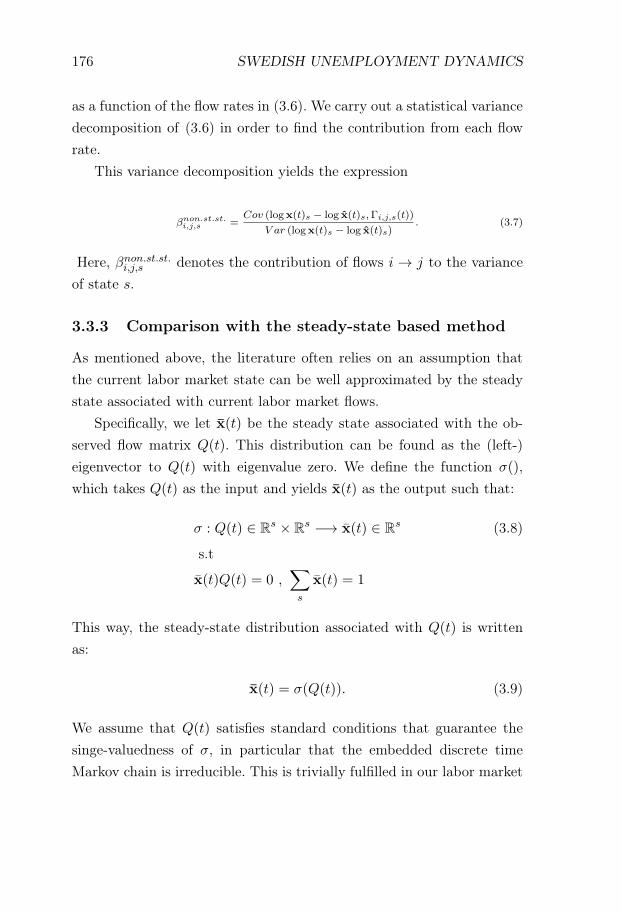
176 SWEDISH UNEMPLOYMENT DYNAMICS
as a function of the flow rates in (3.6). We carry out a statistical variancedecomposition of (3.6) in order to find the contribution from each flowrate.
This variance decomposition yields the expression
βnon.st.st.i,j,s =
Cov (logx(t)s − log x(t)s,Γi,j,s(t))
V ar (logx(t)s − log x(t)s). (3.7)
Here, βnon.st.st.i,j,s denotes the contribution of flows i → j to the variance
of state s.
3.3.3 Comparison with the steady-state based method
As mentioned above, the literature often relies on an assumption thatthe current labor market state can be well approximated by the steadystate associated with current labor market flows.
Specifically, we let x(t) be the steady state associated with the ob-served flow matrix Q(t). This distribution can be found as the (left-)eigenvector to Q(t) with eigenvalue zero. We define the function σ(),which takes Q(t) as the input and yields x(t) as the output such that:
σ : Q(t) ∈ Rs × R
s −→ x(t) ∈ Rs (3.8)
s.t
x(t)Q(t) = 0 ,∑s
x(t) = 1
This way, the steady-state distribution associated with Q(t) is writtenas:
x(t) = σ(Q(t)). (3.9)
We assume that Q(t) satisfies standard conditions that guarantee thesinge-valuedness of σ, in particular that the embedded discrete timeMarkov chain is irreducible. This is trivially fulfilled in our labor market
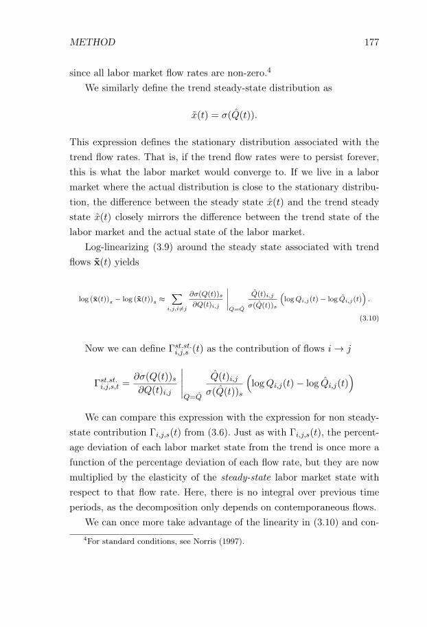
METHOD 177
since all labor market flow rates are non-zero.4
We similarly define the trend steady-state distribution as
x(t) = σ(Q(t)).
This expression defines the stationary distribution associated with thetrend flow rates. That is, if the trend flow rates were to persist forever,this is what the labor market would converge to. If we live in a labormarket where the actual distribution is close to the stationary distribu-tion, the difference between the steady state x(t) and the trend steadystate x(t) closely mirrors the difference between the trend state of thelabor market and the actual state of the labor market.
Log-linearizing (3.9) around the steady state associated with trendflows x(t) yields
log (x(t))s − log (x(t))s ≈∑
i,j,i �=j
∂σ(Q(t))s
∂Q(t)i,j
∣∣∣∣∣Q=Q
Q(t)i,j
σ(Q(t))s
(logQi,j(t)− log Qi,j(t)
).
(3.10)
Now we can define Γst.st.i,j,s (t) as the contribution of flows i → j
Γst.st.i,j,s,t =
∂σ(Q(t))s∂Q(t)i,j
∣∣∣∣∣Q=Q
Q(t)i,j
σ(Q(t))s
(logQi,j(t)− log Qi,j(t)
)We can compare this expression with the expression for non steady-
state contribution Γi,j,s(t) from (3.6). Just as with Γi,j,s(t), the percent-age deviation of each labor market state from the trend is once more afunction of the percentage deviation of each flow rate, but they are nowmultiplied by the elasticity of the steady-state labor market state withrespect to that flow rate. Here, there is no integral over previous timeperiods, as the decomposition only depends on contemporaneous flows.
We can once more take advantage of the linearity in (3.10) and con-4For standard conditions, see Norris (1997).
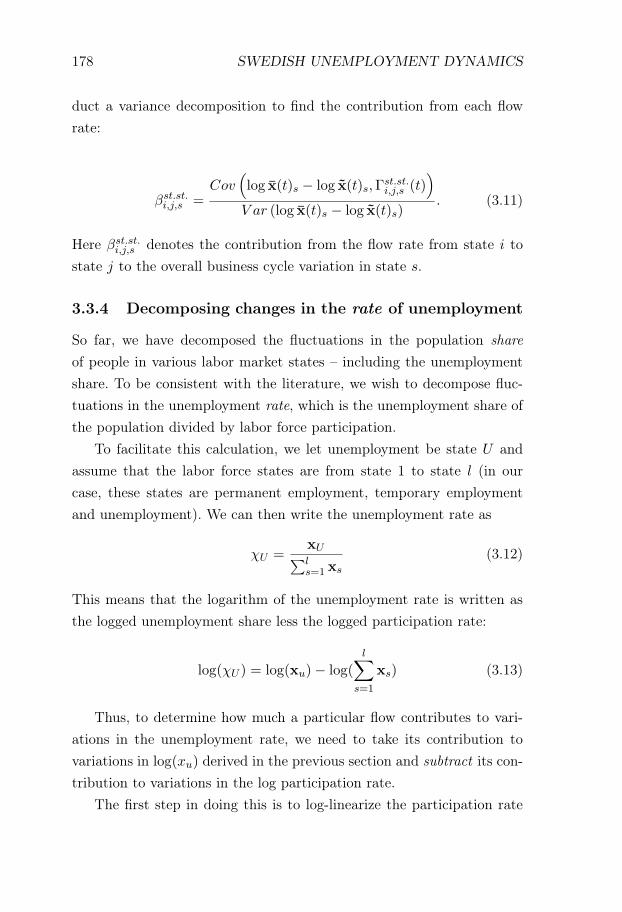
178 SWEDISH UNEMPLOYMENT DYNAMICS
duct a variance decomposition to find the contribution from each flowrate:
βst.st.i,j,s =
Cov(log x(t)s − log x(t)s,Γ
st.st.i,j,s (t)
)V ar (log x(t)s − log x(t)s)
. (3.11)
Here βst.st.i,j,s denotes the contribution from the flow rate from state i to
state j to the overall business cycle variation in state s.
3.3.4 Decomposing changes in the rate of unemployment
So far, we have decomposed the fluctuations in the population shareof people in various labor market states – including the unemploymentshare. To be consistent with the literature, we wish to decompose fluc-tuations in the unemployment rate, which is the unemployment share ofthe population divided by labor force participation.
To facilitate this calculation, we let unemployment be state U andassume that the labor force states are from state 1 to state l (in ourcase, these states are permanent employment, temporary employmentand unemployment). We can then write the unemployment rate as
χU =xU∑ls=1 xs
(3.12)
This means that the logarithm of the unemployment rate is written asthe logged unemployment share less the logged participation rate:
log(χU ) = log(xu)− log(
l∑s=1
xs) (3.13)
Thus, to determine how much a particular flow contributes to vari-ations in the unemployment rate, we need to take its contribution tovariations in log(xu) derived in the previous section and subtract its con-tribution to variations in the log participation rate.
The first step in doing this is to log-linearize the participation rate
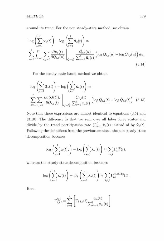
METHOD 179
around its trend. For the non steady-state method, we obtain
log
(l∑
s=1
xs(t)
)− log
(l∑
s=1
xs(t)
)≈
l∑s=1
∫ t
u=0
∑i,j �=i
∂xs(t)
∂Qi,j(u)
∣∣∣∣∣Q=Q
Qi,j(u)∑ls=1 xs(t)
(logQi,j(u)− log Qi,j(u)
)du.
(3.14)
For the steady-state based method we obtain
log
(l∑
s=1
xs(t)
)− log
(l∑
s=1
xs(t)
)≈
l∑s=1
∑i,j �=i
∂σ(Q(t))s∂Qi,j(t)
∣∣∣∣∣Q=Q
Qi,j(t)∑ls=1 xs(t)
(logQi,j(t)− log Qi,j(t)
)(3.15)
Note that these expressions are almost identical to equations (3.5) and(3.10). The difference is that we sum over all labor force states anddivide by the trend participation rate
∑ls=1 xs(t) instead of by xs(t).
Following the definitions from the previous sections, the non steady-statedecomposition becomes
log
(l∑
s=1
x(t)s
)− log
(l∑
s=1
xs(t)
)≈∑i �=j
Γlfpi,j (t),
whereas the steady-state decomposition becomes
log
(l∑
s=1
xs(t)
)− log
(l∑
s=1
xs(t)
)≈∑i �=j
Γst.st,lfpi,j (t).
Here
Γlfpi,j,t =
l∑s=1
[Γi,j,s(t)
xs(t)∑ls′=1 xs′(t)
]
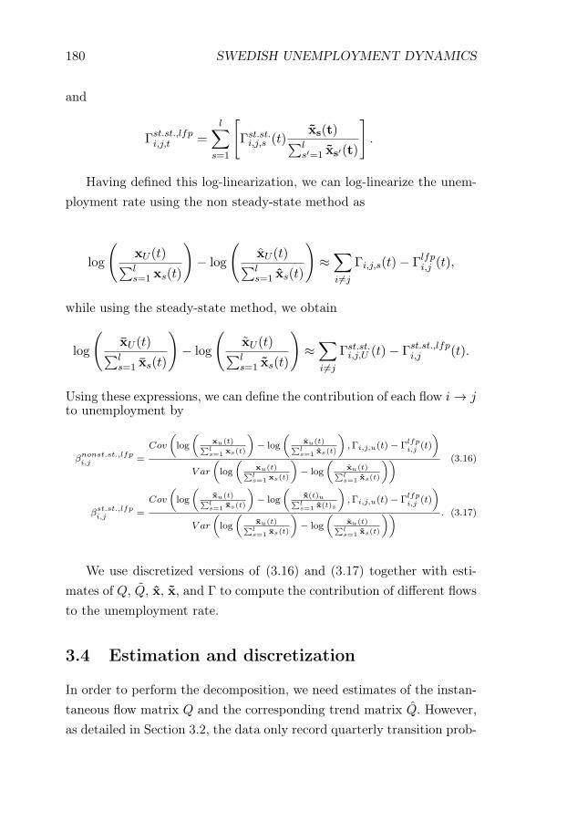
180 SWEDISH UNEMPLOYMENT DYNAMICS
and
Γst.st.,lfpi,j,t =
l∑s=1
[Γst.st.i,j,s (t)
xs(t)∑ls′=1 xs′(t)
].
Having defined this log-linearization, we can log-linearize the unem-ployment rate using the non steady-state method as
log
(xU (t)∑ls=1 xs(t)
)− log
(xU (t)∑ls=1 xs(t)
)≈∑i �=j
Γi,j,s(t)− Γlfpi,j (t),
while using the steady-state method, we obtain
log
(xU (t)∑ls=1 xs(t)
)− log
(xU (t)∑ls=1 xs(t)
)≈∑i �=j
Γst.st.i,j,U (t)− Γst.st.,lfp
i,j (t).
Using these expressions, we can define the contribution of each flow i → jto unemployment by
βnonst.st.,lfpi,j =
Cov
(log
(xu(t)
∑ls=1 xs(t)
)− log
(xu(t)
∑ls=1 xs(t)
),Γi,j,u(t)− Γlfp
i,j (t)
)
V ar
(log
(xu(t)
∑ls=1 xs(t)
)− log
(xu(t)
∑ls=1 xs(t)
)) (3.16)
βst.st.,lfpi,j =
Cov
(log
(xu(t)
∑ls=1 xs(t)
)− log
(x(t)u∑l
s=1 x(t)s
),Γi,j,u(t)− Γlfp
i,j (t)
)
V ar
(log
(xu(t)
∑ls=1 xs(t)
)− log
(xu(t)
∑ls=1 xs(t)
)) . (3.17)
We use discretized versions of (3.16) and (3.17) together with esti-mates of Q, Q, x, x, and Γ to compute the contribution of different flowsto the unemployment rate.
3.4 Estimation and discretization
In order to perform the decomposition, we need estimates of the instan-taneous flow matrix Q and the corresponding trend matrix Q. However,as detailed in Section 3.2, the data only record quarterly transition prob-
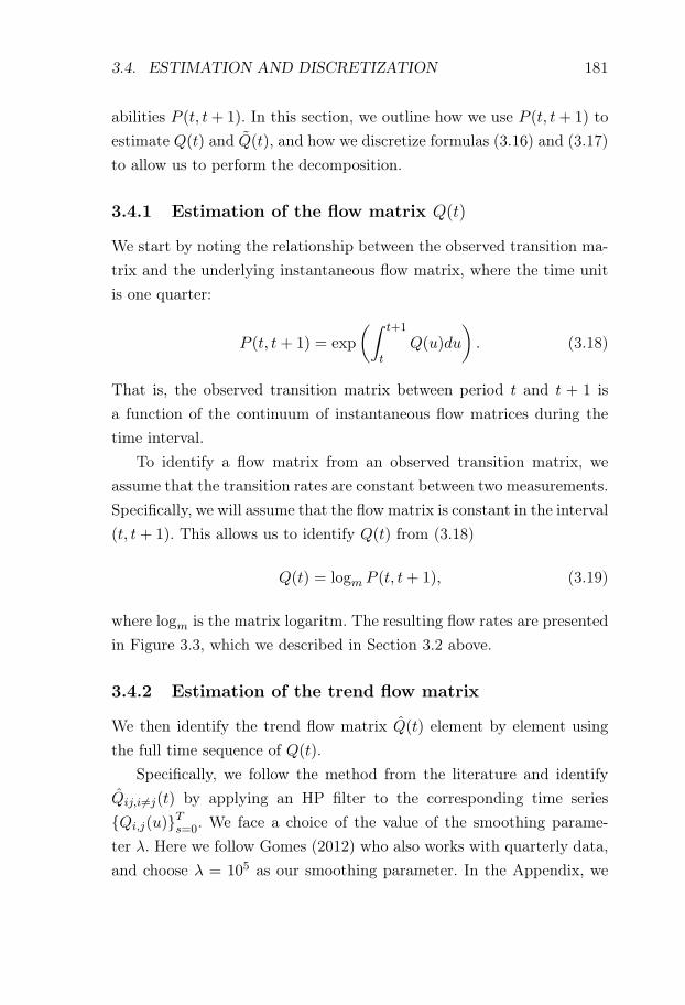
3.4. ESTIMATION AND DISCRETIZATION 181
abilities P (t, t+ 1). In this section, we outline how we use P (t, t+ 1) toestimate Q(t) and Q(t), and how we discretize formulas (3.16) and (3.17)to allow us to perform the decomposition.
3.4.1 Estimation of the flow matrix Q(t)
We start by noting the relationship between the observed transition ma-trix and the underlying instantaneous flow matrix, where the time unitis one quarter:
P (t, t+ 1) = exp
(∫ t+1
tQ(u)du
). (3.18)
That is, the observed transition matrix between period t and t + 1 isa function of the continuum of instantaneous flow matrices during thetime interval.
To identify a flow matrix from an observed transition matrix, weassume that the transition rates are constant between two measurements.Specifically, we will assume that the flow matrix is constant in the interval(t, t+ 1). This allows us to identify Q(t) from (3.18)
Q(t) = logm P (t, t+ 1), (3.19)
where logm is the matrix logaritm. The resulting flow rates are presentedin Figure 3.3, which we described in Section 3.2 above.
3.4.2 Estimation of the trend flow matrix
We then identify the trend flow matrix Q(t) element by element usingthe full time sequence of Q(t).
Specifically, we follow the method from the literature and identifyQij,i �=j(t) by applying an HP filter to the corresponding time series{Qi,j(u)}Ts=0. We face a choice of the value of the smoothing parame-ter λ. Here we follow Gomes (2012) who also works with quarterly data,and choose λ = 105 as our smoothing parameter. In the Appendix, we
182 SWEDISH UNEMPLOYMENT DYNAMICS
vary λ to check the robustness. The diagonal elements, Qi,i(t), are com-puted as residuals such that each row in Q(t) sums to 0. The resultingtrend flow rates are depicted in Figure 3.5.
3.4.3 Discretization
When we have estimated the discrete versions of Q(t) and Q(t), we candefine Qt and Qt as the values they take on the intervals [t, t + 1). Wecan now write the labor market evolution in discrete form as
xt = x0 exp
(t−1∑u=0
Qu
).
With this expression, we can re-express the contribution function Γi,j,s(t)
in a discrete version Γi,j,s,t as
Γi,j,s,t =
t−1∑u=0
∂xs,t
∂Qi,j,u
Qi,j,u
xs,t
(log(Qi,j,u)− log(Qi,j,u)
)
and with the concomitant change to Γlfpi,j,t. With this discrete approx-
imation, we define the contribution of a flow i → j to variations inunemployment as
βnonst.st.i,j =
Cov(log(
xU,t∑ls=1 xs,t
)− log
(xU,t∑ls=1 xs,t
),Γi,j,U,t − Γlfp
i,j,t
)V ar
(log(
xU,t∑ls=1 xs,t
)− log
(xU,t∑ls=1 xs,t
))where Cov and V ar denote sample covariances and variances. This isthe estimation method we take to the data.
Panel A in Table 3.3 shows the decomposition of the variation inthe unemployment rate using our preferred non steady-state methoddescribed in Section 3.3. The table suggests that we can dividecontributions to unemployment variations into three types of flows ofroughly equal sizes. Flows from unemployment to employment explain35% (=13%+22%), flows from employment to unemployment explain

3.4. ESTIMATION AND DISCRETIZATION 183
32% (=15%+17 %), and flows involving non-participation explain 32%of the variation in unemployment.
Panel A in Table 3.3 also tells us how variations in flow rates concern-ing temporary and permanent contracts contribute to the total variationin unemployment. In particular, we see that variations in flows involvingtemporary employment account for 44% of the variation in unemploy-ment, while flows concerning permanent employment account for 33%.The former are sizable, as workers on temporary contracts on average(during 1987-2012) only account for 13% of the population aged 16-64,while workers on permanent contracts account for 66%.5
The results also suggest that the convergence to steady state is slow.This convergence rate can be calculated using the second largest eigen-value to the transition matrix, Q(t). The largest eigenvalue is 0 so thesecond largest eigenvalue is a negative number λ < 0. Deviations fromsteady state decay at the rate −λ. As the second largest eigenvalue isapproximately −0.09, the halving time of a deviation from the steadystate is approximately 70/9 ≈ 8 quarters ≈ 2 years.6
To evaluate the importance of out-of-steady-state dynamics, we cal-culate the variance decomposition using the steady-state assumption.The results are reported in Panel B of Table 3.3. The main differencecompared to the non steady-state method is that flows involving perma-nent workers are attributed a larger role. The share explained by flowsinvolving permanent employment rises from 33% to 44% (30+14).
Why are the contributions stemming from permanent employmentoverestimated under the steady-state assumption? A likely reason isthat the stock of individuals in permanent employment is sizable. Con-sequently, small swings in the in- and outflow rates from this state willhave a large impact on the steady-state level of unemployment. However,as the flows in and out of permanent employment are low, it takes a longtime to reach the new steady state. Consequently, short-lived swings in
5Recall from Section 3.2 that we have characterized self-employed workers as beingon permanent contracts.
6For reference, see Norris (1997).
184 SWEDISH UNEMPLOYMENT DYNAMICS
the transition in and out of regular employment will cause large varia-tions in the steady state but small ones in the actual distribution.
Taken together, our results suggest that properly accounting for out-of-steady-state dynamics is important when analyzing a dual labor mar-ket. In a Swedish context, failing to do so leads to an overestimation ofthe variation from permanent employment. We think that this point ispotentially also important in a broader European context, where labormarkets have a substantial share of temporary contracts. When analyz-ing labor market duality in France and Spain, existing studies (Hairaultet al., 2015; Silva and Vazquez-Grenno, 2013) have not accounted for theout-of-steady-state dynamics.
In Table 3.4 - Table 3.9 we check the robustness of our results inthree dimensions. First, we redo the decomposition using non seasonallyadjusted data (Table 3.4). Second, we vary the value of the smoothingparameter we utilize to compute the path of trend flow rates, Q(t). This isdone in Table 3.5 - Table 3.6. Third, we vary the time period. We do thisto (i) exclude the latest recession (Table 3.7), (ii) exclude the recession inthe early 1990s (Table 3.8) and (iii) exclude both these recessions (Table3.9). None of these modifications change our results considerably.
3.5 Results
Panel A in Table 3.3 shows the decomposition of the variation in the un-employment rate using our preferred non steady-state method describedin Section 3.3. The table suggests that we can divide contributions tounemployment variations into three types of flows of roughly equal sizes.Flows from unemployment to employment explain 35% (=13%+22%),flows from employment to unemployment explain 32% (=15%+17 %),and flows involving non-participation explain 32% of the variation inunemployment.
Panel A in Table 3.3 also tells us how variations in flow rates concern-ing temporary and permanent contracts contribute to the total variationin unemployment. In particular, we see that variations in flows involving
RESULTS 185
temporary employment account for 44% of the variation in unemploy-ment, while flows concerning permanent employment account for 33%.The former are sizable, as workers on temporary contracts on average(during 1987-2012) only account for 13% of the population aged 16-64,while workers on permanent contracts account for 66%.7
The results also suggest that the convergence to steady state is slow.This convergence rate can be calculated using the second largest eigen-value to the transition matrix, Q(t). The largest eigenvalue is 0 so thesecond largest eigenvalue is a negative number λ < 0. Deviations fromsteady state decay at the rate −λ. As the second largest eigenvalue isapproximately −0.09, the halving time of a deviation from the steadystate is approximately 70/9 ≈ 8 quarters ≈ 2 years.8
To evaluate the importance of out-of-steady-state dynamics, we cal-culate the variance decomposition using the steady-state assumption.The results are reported in Panel B of Table 3.3. The main differencecompared to the non steady-state method is that flows involving perma-nent workers are attributed a larger role. The share explained by flowsinvolving permanent employment rises from 33% to 44% (30+14).
Why are the contributions stemming from permanent employmentoverestimated under the steady-state assumption? A likely reason isthat the stock of individuals in permanent employment is sizable. Con-sequently, small swings in the in- and outflow rates from this state willhave a large impact on the steady-state level of unemployment. However,as the flows in and out of permanent employment are low, it takes a longtime to reach the new steady state. Consequently, short-lived swings inthe transition in and out of regular employment will cause large varia-tions in the steady state but small ones in the actual distribution.
Taken together, our results suggest that properly accounting for out-of-steady-state dynamics is important when analyzing a dual labor mar-ket. In a Swedish context, failing to do so leads to an overestimation of
7Recall from Section 3.2 that we have characterized self-employed workers as beingon permanent contracts.
8For reference, see Norris (1997).
186 SWEDISH UNEMPLOYMENT DYNAMICS
the variation from permanent employment. We think that this point ispotentially also important in a broader European context, where labormarkets have a substantial share of temporary contracts. When analyz-ing labor market duality in France and Spain, existing studies (Hairaultet al., 2015; Silva and Vazquez-Grenno, 2013) have not accounted for theout-of-steady-state dynamics.
In Table 3.4 - Table 3.9 we check the robustness of our results inthree dimensions. First, we redo the decomposition using non seasonallyadjusted data (Table 3.4). Second, we vary the value of the smoothingparameter we utilize to compute the path of trend flow rates, Q(t). This isdone in Table 3.5 - Table 3.6. Third, we vary the time period. We do thisto (i) exclude the latest recession (Table 3.7), (ii) exclude the recession inthe early 1990s (Table 3.8) and (iii) exclude both these recessions (Table3.9). None of these modifications change our results considerably.
3.6 Comparison to Elsby et al. (2015)
Methodologically, the most similar paper to ours is Elsby et al. (2015),which seeks to estimate the importance of the participation margin forlabor market fluctuations in the US. To compare their paper to ours, notethat the key to our methodology is to formulate labor market changesin terms of the matrix exponential of instantaneous flow rates:
x(t+ τ) = x(t) exp
(∫ t+τ
tQ(s)ds
). (3.20)
This formulation allows us to (i) derive the (average) instantaneous flowrate in a period as the matrix logarithm of the observed transition proba-bility matrix, and (ii) log-linearize changes in labor market states aroundany path of flow matrices.
Elsby et al. (2015) do not use the matrix formulation in equation(3.20), but they develop a method to perform variance decomposition,taking into account the history of flow rates in the case when lineariza-tion is performed around lagged flow rates. To derive flow rates from
COMPARISON TO ELSBY ET AL. (2015) 187
observed transition probability matrices, they derive our matrix loga-rithm formulation from first principles. They note that if flow rates Q
are constant between t and t+ 1, the labor market flows are given by
x(t) = x(t)Q, (3.21)
which is a linear differential equation with the solution
x(t+ 1) = x(t)V ΓV −1,
where V is a matrix of eigenvectors of Q and Γ is a diagonal matrixwith diagonal elements eλi where λi are the eigenvalues of Q. If P is thetransition matrix between t and t + 1, this implies P = V ΓV −1 and Q
can be derived from P by
Q = V log(V −1PV )V −1, (3.22)
where log(·) denotes an element-wise logarithm. By noting that the gen-eral solution of equation (3.21) is x(t+ 1) = x(t) exp
(∫ t+1t Q(s)ds
), we
see that (3.22) estimates the average flow rate Qt over a given time pe-riod. It can also be shown that the right-hand side of (3.22) gives thematrix logarithm of P .
To perform a variance decomposition, their paper linearizes Δx(t)
around lagged flow rates ΔQ(t). Under this linearization, one does notneed to directly use equation (3.20) since it is possible to express Δx(t) asa function of the history of Δx(t)’s, where x(t) denotes the implied steadystate given Q(t). Thus, given that they are interested in Δx(t), they areable to fully express the effects of lagged flow rates as a function of theireffects on the implied steady-state distribution. The method differs fromthe standard steady-state approximation since it takes into account thefull history of changes in steady-state distributions.
188 SWEDISH UNEMPLOYMENT DYNAMICS
3.7 Conclusion
This paper decomposes the total variation in unemployment in Sweden,where the labor market is dual and the convergence to steady state isslow. In doing so, we make two methodological contribution to the liter-ature. First, we extend existing decomposition methods in the literatureby allowing for an arbitrary number of labor market states. This is help-ful in order to analyze the Swedish labor market, where both temporaryand permanent contracts exist. Second, in this setting we allow for nonsteady state dynamics. This is important in a Swedish context, due tolow flows between states and consequently a slow rate of convergencetowards the steady state.
Using this setup we show that the contribution to unemploymentvariability from in- and outflow from unemployment is roughly 60/30.We furthermore show that flows involving temporary contrasts accountfor 44% of the total variation, while flows involving permanent contractsaccount for 33%. The former is substantial given that on average only13% of the working-age population is on temporary contracts.
We also show that properly accounting for out of steady state dynam-ics is important. Indeed, applying the standard decomposition from theliterature, which relies on an assumption of fast convergence to steadystate, leads to overestimating the contribution from permanent con-tracts and underestimating the contribution from temporary contracts.We think this point is relevant for existing studies that decompose thevariability in unemployment in a European context (Silva and Vazquez-Grenno, 2013; Hairault et al., 2015).
References
Elsby, M. W., Hobijn, B., and Şahin, A. (2015). On the importanceof the participation margin for labor market fluctuations. Journal ofMonetary Economics, 72:64–82.
Elsby, M. W. L., Hobijn, B., and Şahin, A. (2013). Unemployment Dy-
REFERENCES 189
namics in the OECD. Review of Economics and Statistics, 95(2):530–548.
Gomes, P. (2012). Labour market flows: Facts from the United Kingdom.Labour Economics, 19(2):165–175.
Hairault, J. O., Le Barbanchon, T., and Sopraseuth, T. (2015). Thecyclicality of the separation and job finding rates in France. EuropeanEconomic Review, 76:60–84.
Norris, J. (1997). Markov Chains. Cambridge University Press, Cam-bridge, United Kingdom.
Shimer, R. (2012). Reassessing the Ins and Outs of Unemployment.Review of Economic Dynamics, 15(2):127–148.
Silva, J. I. and Vazquez-Grenno, J. (2013). The Ins and Outs of Unem-ployment in a Two-Tier Labor Market. Labour Economics, 24:161–169.
Statistics Sweden (2005). Flödesstatistik från AKU.
Statistics Sweden (2011). Basic Principles for Labour Force Surveys(LFS) and Labour Market Statistics.
Statistics Sweden (2012). Arbetskraftsundersökningarna.
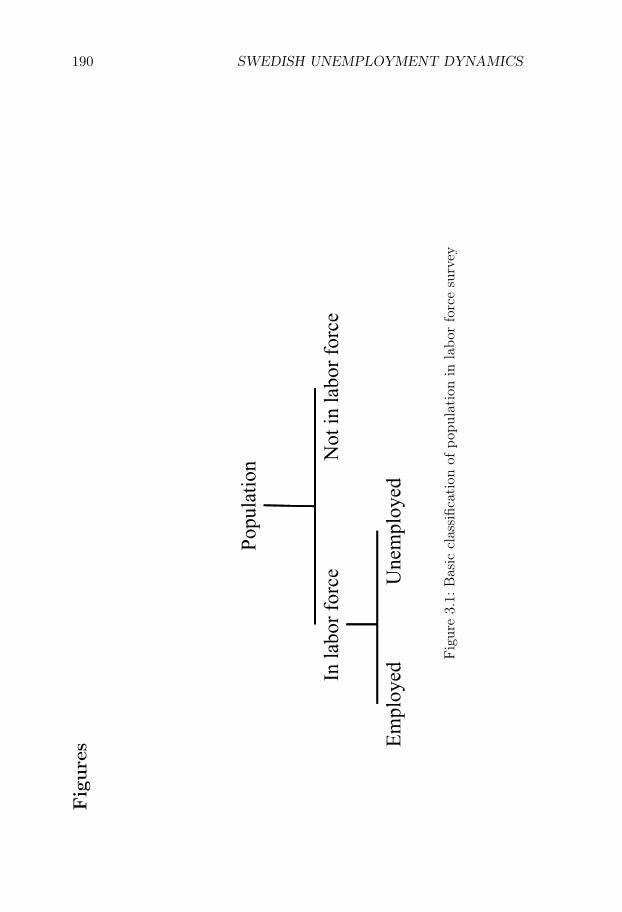
190 SWEDISH UNEMPLOYMENT DYNAMICSFig
ures
Popu
latio
n
In la
bor f
orce
Not
in la
bor f
orce
Empl
oyed
Une
mpl
oyed
Fig
ure
3.1:
Bas
iccl
assi
ficat
ion
ofpo
pula
tion
inla
bor
forc
esu
rvey
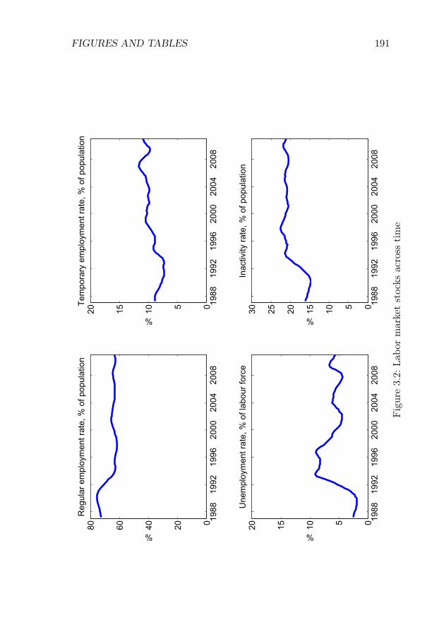
FIGURES AND TABLES 191
1988
1992
1996
2000
2004
2008
020406080R
egul
ar e
mpl
oym
ent r
ate,
% o
f pop
ulat
ion
%
1988
1992
1996
2000
2004
2008
05101520Te
mpo
rary
em
ploy
men
t rat
e, %
of p
opul
atio
n
%
1988
1992
1996
2000
2004
2008
05101520U
nem
ploy
men
t rat
e, %
of l
abou
r for
ce
%
1988
1992
1996
2000
2004
2008
051015202530In
activ
ity ra
te, %
of p
opul
atio
n
%
Fig
ure
3.2:
Labo
rm
arke
tst
ocks
acro
ssti
me
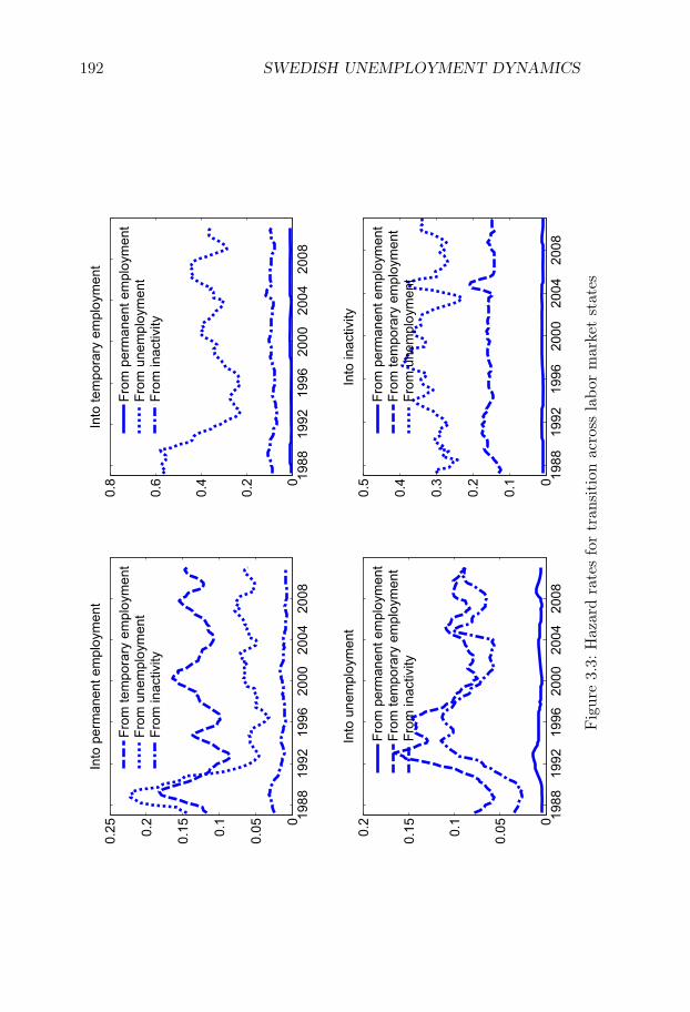
192 SWEDISH UNEMPLOYMENT DYNAMICS
1988
1992
1996
2000
2004
2008
0
0.050.
1
0.150.
2
0.25
Into
per
man
ent e
mpl
oym
ent
Fr
om te
mpo
rary
em
ploy
men
tFr
om u
nem
ploy
men
tFr
om in
activ
ity
1988
1992
1996
2000
2004
2008
0
0.2
0.4
0.6
0.8
Into
tem
pora
ry e
mpl
oym
ent
Fr
om p
erm
anen
t em
ploy
men
tFr
om u
nem
ploy
men
tFr
om in
activ
ity
1988
1992
1996
2000
2004
2008
0
0.050.
1
0.150.
2In
to u
nem
ploy
men
t
Fr
om p
erm
anen
t em
ploy
men
tFr
om te
mpo
rary
em
ploy
men
tFr
om in
activ
ity
1988
1992
1996
2000
2004
2008
0
0.1
0.2
0.3
0.4
0.5
Into
inac
tivity
Fr
om p
erm
anen
t em
ploy
men
tFr
om te
mpo
rary
em
ploy
men
tFr
om u
nem
ploy
men
t
Fig
ure
3.3:
Haz
ard
rate
sfo
rtr
ansi
tion
acro
ssla
bor
mar
ket
stat
es
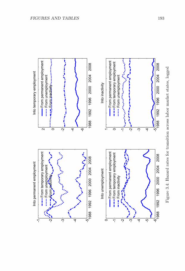
FIGURES AND TABLES 193
1988
1992
1996
2000
2004
2008
-5-4-3-2-1In
to p
erm
anen
t em
ploy
men
t
Fr
om te
mpo
rary
em
ploy
men
tFr
om u
nem
ploy
men
tFr
om in
activ
ity
1988
1992
1996
2000
2004
2008
-6-4-202
Into
tem
pora
ry e
mpl
oym
ent
Fr
om p
erm
anen
t em
ploy
men
tFr
om u
nem
ploy
men
tFr
om in
activ
ity
1988
1992
1996
2000
2004
2008
-6-5-4-3-2-10In
to u
nem
ploy
men
t
Fr
om p
erm
anen
t em
ploy
men
tFr
om te
mpo
rary
em
ploy
men
tFr
om in
activ
ity
1988
1992
1996
2000
2004
2008
-5-4-3-2-101In
to in
activ
ity
Fr
om p
erm
anen
t em
ploy
men
tFr
om te
mpo
rary
em
ploy
men
tFr
om u
nem
ploy
men
t
Fig
ure
3.4:
Haz
ard
rate
sfo
rtr
ansi
tion
acro
ssla
bor
mar
ket
stat
es,l
ogge
d
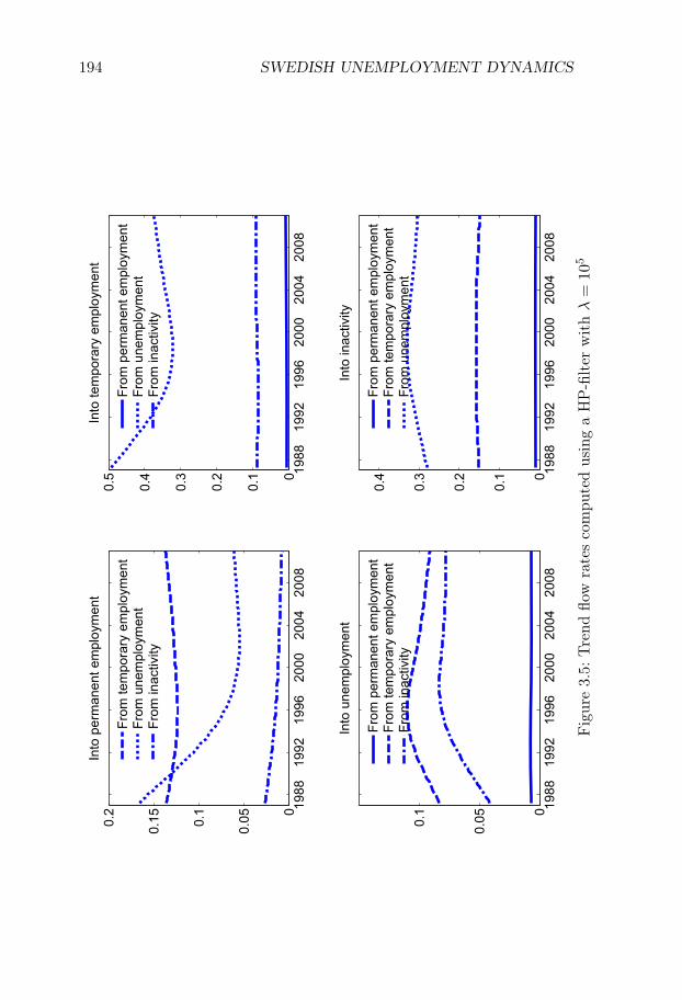
194 SWEDISH UNEMPLOYMENT DYNAMICS
1988
1992
1996
2000
2004
2008
0
0.050.
1
0.150.
2In
to p
erm
anen
t em
ploy
men
t
Fr
om te
mpo
rary
em
ploy
men
tFr
om u
nem
ploy
men
tFr
om in
activ
ity
1988
1992
1996
2000
2004
2008
0
0.1
0.2
0.3
0.4
0.5
Into
tem
pora
ry e
mpl
oym
ent
Fr
om p
erm
anen
t em
ploy
men
tFr
om u
nem
ploy
men
tFr
om in
activ
ity
1988
1992
1996
2000
2004
2008
0
0.050.
1
Into
une
mpl
oym
ent
Fr
om p
erm
anen
t em
ploy
men
tFr
om te
mpo
rary
em
ploy
men
tFr
om in
activ
ity
1988
1992
1996
2000
2004
2008
0
0.1
0.2
0.3
0.4
Into
inac
tivity
Fr
om p
erm
anen
t em
ploy
men
tFr
om te
mpo
rary
em
ploy
men
tFr
om u
nem
ploy
men
t
Fig
ure
3.5:
Tre
ndflo
wra
tes
com
pute
dus
ing
aH
P-fi
lter
wit
hλ=
105
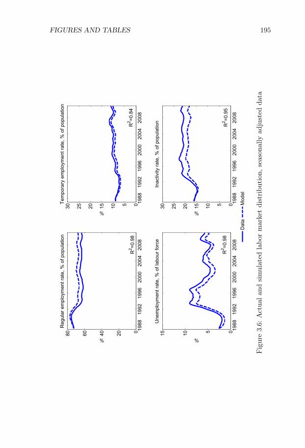
FIGURES AND TABLES 195
1988
1992
1996
2000
2004
2008
020406080R
egul
ar e
mpl
oym
ent r
ate,
% o
f pop
ulat
ion
%
R2 =0
.98
1988
1992
1996
2000
2004
2008
051015202530Te
mpo
rary
em
ploy
men
t rat
e, %
of p
opul
atio
n
%
R2 =0
.84
1988
1992
1996
2000
2004
2008
051015U
nem
ploy
men
t rat
e, %
of l
abou
r for
ce
%
R2 =0
.98
1988
1992
1996
2000
2004
2008
051015202530In
activ
ity ra
te, %
of p
opul
atio
n
%R
2 =0.9
5
Dat
aM
odel
Fig
ure
3.6:
Act
uala
ndsi
mul
ated
labo
rm
arke
tdi
stri
buti
on,s
easo
nally
adju
sted
data
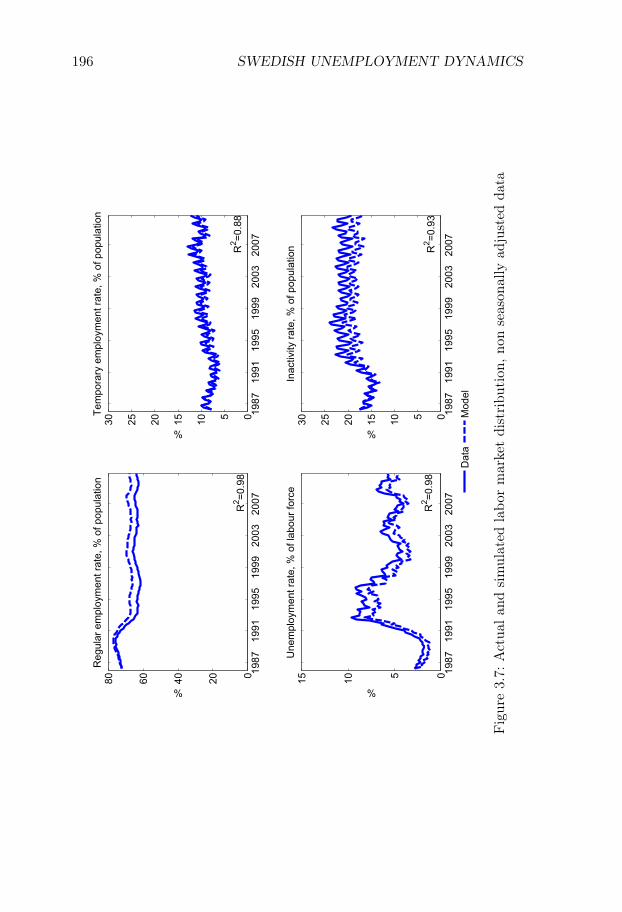
196 SWEDISH UNEMPLOYMENT DYNAMICS
1987
1991
1995
1999
2003
2007
020406080R
egul
ar e
mpl
oym
ent r
ate,
% o
f pop
ulat
ion
%
R2 =0
.98
1987
1991
1995
1999
2003
2007
051015202530Te
mpo
rary
em
ploy
men
t rat
e, %
of p
opul
atio
n
%
R2 =0
.88
1987
1991
1995
1999
2003
2007
051015U
nem
ploy
men
t rat
e, %
of l
abou
r for
ce
%
R2 =0
.98
1987
1991
1995
1999
2003
2007
051015202530In
activ
ity ra
te, %
of p
opul
atio
n
%
R2 =0
.93
Dat
aM
odel
Fig
ure
3.7:
Act
uala
ndsi
mul
ated
labo
rm
arke
tdi
stri
buti
on,n
onse
ason
ally
adju
sted
data
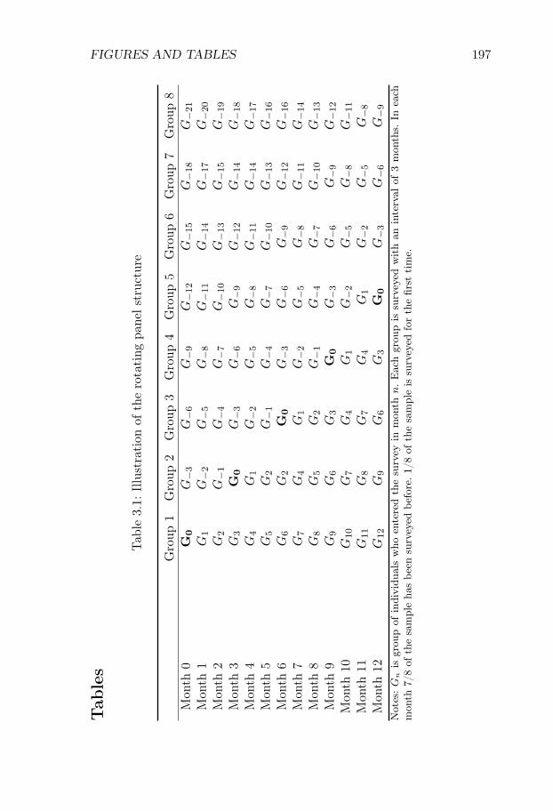
FIGURES AND TABLES 197
Tab
les
Tab
le3.
1:Illu
stra
tion
ofth
ero
tati
ngpa
nels
truc
ture
Gro
up1
Gro
up2
Gro
up3
Gro
up4
Gro
up5
Gro
up6
Gro
up7
Gro
up8
Mon
th0
G0
G−3
G−6
G−9
G−1
2G
−15
G−1
8G
−21
Mon
th1
G1
G−2
G−5
G−8
G−1
1G
−14
G−1
7G
−20
Mon
th2
G2
G−1
G−4
G−7
G−1
0G
−13
G−1
5G
−19
Mon
th3
G3
G0
G−3
G−6
G−9
G−1
2G
−14
G−1
8
Mon
th4
G4
G1
G−2
G−5
G−8
G−1
1G
−14
G−1
7
Mon
th5
G5
G2
G−1
G−4
G−7
G−1
0G
−13
G−1
6
Mon
th6
G6
G2
G0
G−3
G−6
G−9
G−1
2G
−16
Mon
th7
G7
G4
G1
G−2
G−5
G−8
G−1
1G
−14
Mon
th8
G8
G5
G2
G−1
G−4
G−7
G−1
0G
−13
Mon
th9
G9
G6
G3
G0
G−3
G−6
G−9
G−1
2
Mon
th10
G10
G7
G4
G1
G−2
G−5
G−8
G−1
1
Mon
th11
G11
G8
G7
G4
G1
G−2
G−5
G−8
Mon
th12
G12
G9
G6
G3
G0
G−3
G−6
G−9
Not
es:G
nis
grou
pof
indi
vidu
als
who
ente
red
the
surv
eyin
mon
thn.E
ach
grou
pis
surv
eyed
wit
han
inte
rval
of3
mon
ths.
Inea
chm
onth
7/8
ofth
esa
mpl
eha
sbe
ensu
rvey
edbe
fore
.1/8
ofth
esa
mpl
eis
surv
eyed
for
the
first
tim
e.
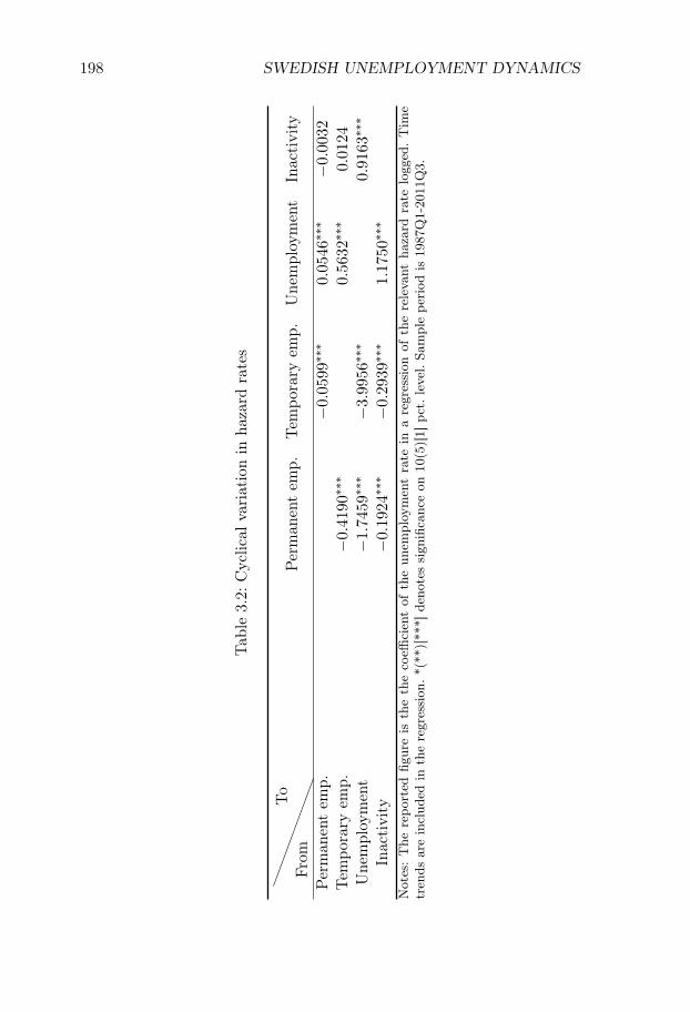
198 SWEDISH UNEMPLOYMENT DYNAMICS
Tab
le3.
2:C
yclic
alva
riat
ion
inha
zard
rate
s
From
To
Per
man
ent
emp.
Tem
pora
ryem
p.U
nem
ploy
men
tIn
acti
vity
Per
man
ent
emp.
−0.0599∗
∗∗0.0546
∗∗∗
−0.0032
Tem
pora
ryem
p.−0
.4190∗∗
∗0.5632
∗∗∗
0.0124
Une
mpl
oym
ent
−1.7459∗∗
∗−3
.9956∗∗
∗0.9163∗
∗∗
Inac
tivi
ty−0
.1924∗
∗∗−0
.2939∗∗
∗1.1750
∗∗∗
Not
es:
The
repo
rted
figur
eis
the
the
coeffi
cien
tof
the
unem
ploy
men
tra
tein
are
gres
sion
ofth
ere
leva
ntha
zard
rate
logg
ed.
Tim
etr
ends
are
incl
uded
inth
ere
gres
sion
.*(*
*)[*
**]d
enot
essi
gnifi
canc
eon
10(5
)[1]
pct.
leve
l.Sa
mpl
epe
riod
is19
87Q
1-20
11Q
3.
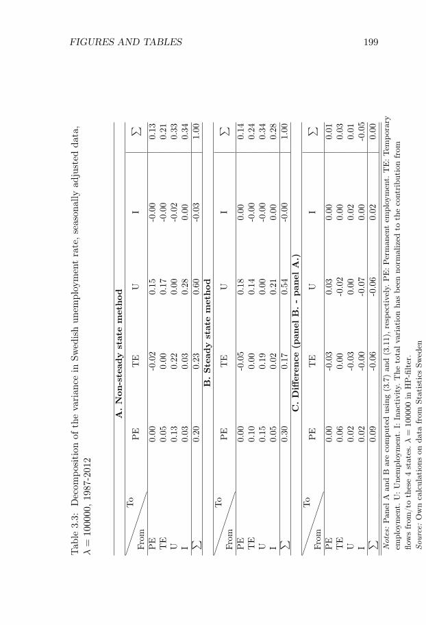
FIGURES AND TABLES 199
Tab
le3.
3:D
ecom
posi
tion
ofth
eva
rian
cein
Swed
ish
unem
ploy
men
tra
te,s
easo
nally
adju
sted
data
,λ=
100000
,198
7-20
12
A.N
on-s
tead
yst
ate
met
hod
From
To
PE
TE
UI
∑P
E0.
00-0
.02
0.15
-0.0
00.
13T
E0.
050.
000.
17-0
.00
0.21
U0.
130.
220.
00-0
.02
0.33
I0.
030.
030.
280.
000.
34∑
0.20
0.23
0.60
-0.0
31.
00B
.Ste
ady
stat
em
ethod
From
To
PE
TE
UI
∑P
E0.
00-0
.05
0.18
0.00
0.14
TE
0.10
0.00
0.14
-0.0
00.
24U
0.15
0.19
0.00
-0.0
00.
34I
0.05
0.02
0.21
0.00
0.28
∑0.
300.
170.
54-0
.00
1.00
C.D
iffer
ence
(pan
elB
.-
pan
elA
.)
From
To
PE
TE
UI
∑P
E0.
00-0
.03
0.03
0.00
0.01
TE
0.06
0.00
-0.0
20.
000.
03U
0.02
-0.0
30.
000.
020.
01I
0.02
-0.0
0-0
.07
0.00
-0.0
5∑
0.09
-0.0
6-0
.06
0.02
0.00
Not
es:
Pan
elA
and
Bar
eco
mpu
ted
usin
g(3
.7)
and
(3.1
1),r
espe
ctiv
ely.
PE
:Per
man
ent
empl
oym
ent.
TE
:Tem
pora
ryem
ploy
men
t.U
:Une
mpl
oym
ent.
I:In
acti
vity
.The
tota
lvar
iati
onha
sbe
enno
rmal
ized
toth
eco
ntri
buti
onfr
omflo
ws
from
/to
thes
e4
stat
es.λ
=100000
inH
P-fi
lter
.So
urce
:O
wn
calc
ulat
ions
onda
tafr
omSt
atis
tics
Swed
en
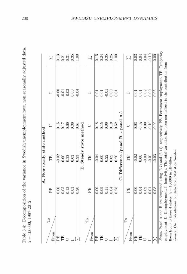
200 SWEDISH UNEMPLOYMENT DYNAMICSTab
le3.
4:D
ecom
posi
tion
ofth
eva
rian
cein
Swed
ish
unem
ploy
men
tra
te,n
onse
ason
ally
adju
sted
data
,λ=
100000
,198
7-20
12
A.N
on-s
tead
yst
ate
met
hod
From
To
PE
TE
UI
∑P
E0.
00-0
.02
0.15
-0.0
00.
13T
E0.
050.
000.
17-0
.01
0.21
U0.
130.
220.
00-0
.03
0.31
I0.
030.
030.
300.
000.
35∑
0.20
0.23
0.61
-0.0
41.
00B
.Ste
ady
stat
em
ethod
From
To
PE
TE
UI
∑P
E0.
00-0
.04
0.18
0.01
0.15
TE
0.09
0.00
0.15
0.01
0.24
U0.
150.
220.
00-0
.01
0.35
I0.
040.
020.
190.
000.
25∑
0.28
0.20
0.52
0.01
1.00
C.D
iffer
ence
(pan
elB
.-
pan
elA
.)
From
To
PE
TE
UI
∑P
E0.
00-0
.02
0.03
0.01
0.03
TE
0.04
0.00
-0.0
20.
010.
04U
0.02
-0.0
00.
000.
020.
04I
0.01
-0.0
1-0
.10
0.00
-0.1
0∑
0.08
-0.0
3-0
.09
0.05
0.00
Not
es:
Pan
elA
and
Bar
eco
mpu
ted
usin
g(3
.7)
and
(3.1
1),r
espe
ctiv
ely.
PE
:Per
man
ent
empl
oym
ent.
TE
:Tem
pora
ryem
ploy
men
t.U
:Une
mpl
oym
ent.
I:In
acti
vity
.The
tota
lvar
iati
onha
sbe
enno
rmal
ized
toth
eco
ntri
buti
onfr
omflo
ws
from
/to
thes
e4
stat
es.λ
=100000
inH
P-fi
lter
.So
urce
:O
wn
calc
ulat
ions
onda
tafr
omSt
atis
tics
Swed
en
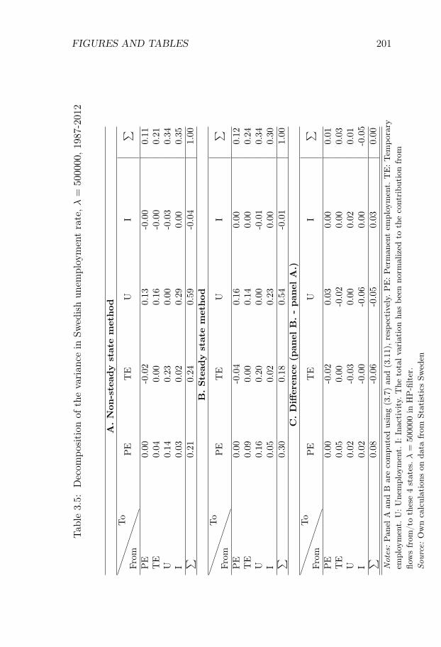
FIGURES AND TABLES 201
Tab
le3.
5:D
ecom
posi
tion
ofth
eva
rian
cein
Swed
ish
unem
ploy
men
tra
te,λ
=500000
,198
7-20
12
A.N
on-s
tead
yst
ate
met
hod
From
To
PE
TE
UI
∑P
E0.
00-0
.02
0.13
-0.0
00.
11T
E0.
040.
000.
16-0
.00
0.21
U0.
140.
230.
00-0
.03
0.34
I0.
030.
020.
290.
000.
35∑
0.21
0.24
0.59
-0.0
41.
00B
.Ste
ady
stat
em
ethod
From
To
PE
TE
UI
∑P
E0.
00-0
.04
0.16
0.00
0.12
TE
0.09
0.00
0.14
0.00
0.24
U0.
160.
200.
00-0
.01
0.34
I0.
050.
020.
230.
000.
30∑
0.30
0.18
0.54
-0.0
11.
00C
.D
iffer
ence
(pan
elB
.-
pan
elA
.)
From
To
PE
TE
UI
∑P
E0.
00-0
.02
0.03
0.00
0.01
TE
0.05
0.00
-0.0
20.
000.
03U
0.02
-0.0
30.
000.
020.
01I
0.02
-0.0
0-0
.06
0.00
-0.0
5∑
0.08
-0.0
6-0
.05
0.03
0.00
Not
es:
Pan
elA
and
Bar
eco
mpu
ted
usin
g(3
.7)
and
(3.1
1),r
espe
ctiv
ely.
PE
:Per
man
ent
empl
oym
ent.
TE
:Tem
pora
ryem
ploy
men
t.U
:Une
mpl
oym
ent.
I:In
acti
vity
.The
tota
lvar
iati
onha
sbe
enno
rmal
ized
toth
eco
ntri
buti
onfr
omflo
ws
from
/to
thes
e4
stat
es.λ
=500000
inH
P-fi
lter
.So
urce
:O
wn
calc
ulat
ions
onda
tafr
omSt
atis
tics
Swed
en
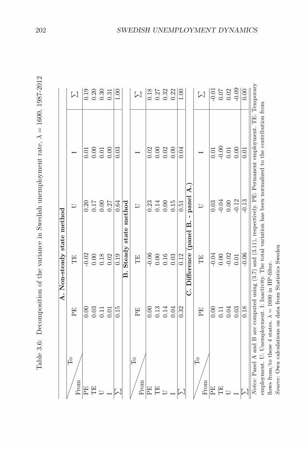
202 SWEDISH UNEMPLOYMENT DYNAMICSTab
le3.
6:D
ecom
posi
tion
ofth
eva
rian
cein
Swed
ish
unem
ploy
men
tra
te,λ
=1600
,198
7-20
12
A.N
on-s
tead
yst
ate
met
hod
From
To
PE
TE
UI
∑P
E0.
00-0
.02
0.20
0.01
0.19
TE
0.03
0.00
0.17
0.00
0.20
U0.
110.
180.
000.
010.
30I
0.01
0.02
0.27
0.00
0.31
∑0.
150.
190.
640.
031.
00B
.Ste
ady
stat
em
ethod
From
To
PE
TE
UI
∑P
E0.
00-0
.06
0.23
0.02
0.18
TE
0.13
0.00
0.14
0.00
0.27
U0.
140.
160.
000.
020.
32I
0.04
0.03
0.15
0.00
0.22
∑0.
320.
120.
510.
041.
00C
.D
iffer
ence
(pan
elB
.-
pan
elA
.)
From
To
PE
TE
UI
∑P
E0.
00-0
.04
0.03
0.01
-0.0
1T
E0.
110.
00-0
.04
-0.0
00.
07U
0.04
-0.0
20.
000.
010.
02I
0.03
0.01
-0.1
20.
00-0
.09
∑0.
18-0
.06
-0.1
30.
010.
00N
otes
:Pan
elA
and
Bar
eco
mpu
ted
usin
g(3
.7)
and
(3.1
1),r
espe
ctiv
ely.
PE
:Per
man
ent
empl
oym
ent.
TE
:Tem
pora
ryem
ploy
men
t.U
:Une
mpl
oym
ent.
I:In
acti
vity
.The
tota
lvar
iati
onha
sbe
enno
rmal
ized
toth
eco
ntri
buti
onfr
omflo
ws
from
/to
thes
e4
stat
es.λ
=1600
inH
P-fi
lter
.So
urce
:O
wn
calc
ulat
ions
onda
tafr
omSt
atis
tics
Swed
en

FIGURES AND TABLES 203
Tab
le3.
7:D
ecom
posi
tion
ofth
eva
rian
cein
Swed
ish
unem
ploy
men
tra
te,λ
=100000
,198
7-20
07
A.N
on-s
tead
yst
ate
met
hod
From
To
PE
TE
UI
∑P
E0.
00-0
.02
0.15
-0.0
00.
13T
E0.
050.
000.
17-0
.00
0.21
U0.
130.
220.
00-0
.02
0.33
I0.
030.
020.
280.
000.
33∑
0.20
0.22
0.60
-0.0
31.
00B
.Ste
ady
stat
em
ethod
From
To
PE
TE
UI
∑P
E0.
00-0
.05
0.18
-0.0
00.
13T
E0.
100.
000.
15-0
.00
0.25
U0.
150.
190.
00-0
.01
0.34
I0.
050.
020.
220.
000.
29∑
0.30
0.17
0.54
-0.0
11.
00C
.D
iffer
ence
(pan
elB
.-
pan
elA
.)
From
To
PE
TE
UI
∑P
E0.
00-0
.03
0.03
-0.0
0-0
.00
TE
0.06
0.00
-0.0
20.
000.
04U
0.02
-0.0
30.
000.
020.
01I
0.02
-0.0
0-0
.06
0.00
-0.0
5∑
0.10
-0.0
6-0
.06
0.02
0.00
Not
es:
Pan
elA
and
Bar
eco
mpu
ted
usin
g(3
.7)
and
(3.1
1),r
espe
ctiv
ely.
PE
:Per
man
ent
empl
oym
ent.
TE
:Tem
pora
ryem
ploy
men
t.U
:Une
mpl
oym
ent.
I:In
acti
vity
.The
tota
lvar
iati
onha
sbe
enno
rmal
ized
toth
eco
ntri
buti
onfr
omflo
ws
from
/to
thes
e4
stat
es.λ
=100000
inH
P-fi
lter
.So
urce
:O
wn
calc
ulat
ions
onda
tafr
omSt
atis
tics
Swed
en

204 SWEDISH UNEMPLOYMENT DYNAMICSTab
le3.
8:D
ecom
posi
tion
ofth
eva
rian
cein
Swed
ish
unem
ploy
men
tra
te,λ
=100000
,199
2-20
12
A.N
on-s
tead
yst
ate
met
hod
From
To
PE
TE
UI
∑P
E0.
00-0
.02
0.14
-0.0
10.
11T
E0.
050.
000.
16-0
.01
0.20
U0.
130.
260.
00-0
.03
0.36
I0.
030.
030.
270.
000.
33∑
0.21
0.28
0.56
-0.0
51.
00B
.Ste
ady
stat
em
ethod
From
To
PE
TE
UI
∑P
E0.
00-0
.05
0.16
-0.0
00.
11T
E0.
120.
000.
13-0
.00
0.25
U0.
150.
220.
00-0
.00
0.37
I0.
050.
030.
190.
000.
27∑
0.32
0.20
0.48
-0.0
11.
00C
.D
iffer
ence
(pan
elB
.-
pan
elA
.)
From
To
PE
TE
UI
∑P
E0.
00-0
.03
0.02
0.00
0.00
TE
0.06
0.00
-0.0
20.
010.
05U
0.03
-0.0
40.
000.
030.
01I
0.02
-0.0
0-0
.09
0.00
-0.0
6∑
0.11
-0.0
7-0
.08
0.04
0.00
Not
es:
Pan
elA
and
Bar
eco
mpu
ted
usin
g(3
.7)
and
(3.1
1),r
espe
ctiv
ely.
PE
:Per
man
ent
empl
oym
ent.
TE
:Tem
pora
ryem
ploy
men
t.U
:Une
mpl
oym
ent.
I:In
acti
vity
.The
tota
lvar
iati
onha
sbe
enno
rmal
ized
toth
eco
ntri
buti
onfr
omflo
ws
from
/to
thes
e4
stat
es.λ
=100000
inH
P-fi
lter
.So
urce
:O
wn
calc
ulat
ions
onda
tafr
omSt
atis
tics
Swed
en

FIGURES AND TABLES 205
Tab
le3.
9:D
ecom
posi
tion
ofth
eva
rian
cein
Swed
ish
unem
ploy
men
tra
te,λ
=100000
,199
2-20
07
A.N
on-s
tead
yst
ate
met
hod
From
To
PE
TE
UI
∑P
E0.
00-0
.02
0.14
-0.0
10.
11T
E0.
050.
000.
16-0
.01
0.20
U0.
130.
260.
00-0
.03
0.36
I0.
030.
030.
270.
000.
33∑
0.20
0.27
0.57
-0.0
51.
00B
.Ste
ady
stat
em
ethod
From
To
PE
TE
UI
∑P
E0.
00-0
.05
0.15
-0.0
10.
10T
E0.
120.
000.
14-0
.00
0.25
U0.
160.
220.
00-0
.00
0.37
I0.
050.
030.
190.
000.
28∑
0.33
0.20
0.49
-0.0
11.
00C
.D
iffer
ence
(pan
elB
.-
pan
elA
.)
From
To
PE
TE
UI
∑P
E0.
00-0
.03
0.02
0.00
-0.0
1T
E0.
070.
00-0
.02
0.01
0.05
U0.
03-0
.04
0.00
0.03
0.02
I0.
02-0
.00
-0.0
80.
00-0
.05
∑0.
12-0
.07
-0.0
80.
040.
00N
otes
:Pan
elA
and
Bar
eco
mpu
ted
usin
g(3
.7)
and
(3.1
1),r
espe
ctiv
ely.
PE
:Per
man
ent
empl
oym
ent.
TE
:Tem
pora
ryem
ploy
men
t.U
:Une
mpl
oym
ent.
I:In
acti
vity
.The
tota
lvar
iati
onha
sbe
enno
rmal
ized
toth
eco
ntri
buti
onfr
omflo
ws
from
/to
thes
e4
stat
es.λ
=100000
inH
P-fi
lter
.So
urce
:O
wn
calc
ulat
ions
onda
tafr
omSt
atis
tics
Swed
en
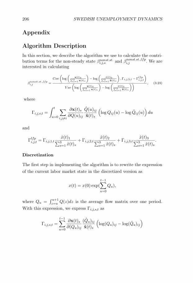
206 SWEDISH UNEMPLOYMENT DYNAMICS
Appendix
Algorithm Description
In this section, we describe the algorithm we use to calculate the contri-bution terms for the non-steady state βnonst.st.
i,j,s and βnonst.st.,lfpi,j . We are
interested in calculating
βnonst.st.,lfpi,j =
Cov
(log
(x(t)3∑3
s=1 x(t)s
)− log
(x(t)3∑3
s=1 x(t)s
),Γi,j,3,t − Γlfp
i,j,t
)
V ar
(log
(x(t)3∑3
s=1 x(t)s
)− log
(x(t)3∑3
s=1 x(t)s
)) , (3.23)
where
Γi,j,s,t =
∫ t
u=0
∑i,j �=i
∂x(t)s∂Q(u)ij
Q(u)ijx(t)s
(logQij(u)− log Qij(u)
)du
and
Γlfpi,j,t = Γi,j,1,t
x(t)1∑3s=1 x(t)s
+ Γi,j,2,tx(t)2∑3s=1 x(t)s
+ Γi,j,3,tx(t)3∑3s=1 x(t)s
.
Discretization
The first step in implementing the algorithm is to rewrite the expressionof the current labor market state in the discretized version as
x(t) = x(0) exp(t−1∑u=0
Qu),
where Qu =∫ u+1z=u Q(z)dz is the average flow matrix over one period.
With this expression, we express Γi,j,s,t as
Γi,j,s,t =
t−1∑u=0
∂x(t)s∂(Qu)ij
(Qu)ijx(t)s
(log(Qu)ij − log(Qu)ij
)
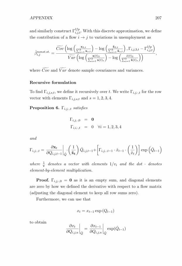
APPENDIX 207
and similarly construct Γlfpi,j,t. With this discrete approximation, we define
the contribution of a flow i → j to variations in unemployment as
βnonst.st.i,j =
Cov(log(
x3,t∑3s=1 xs,t
)− log
(x3,t∑3s=1 xs,t
),Γi,j,3,t − Γlfp
i,j,t
)V ar
(log(
x(t)3∑3s=1 x(t)s
)− log
(x(t)3∑3s=1 x(t)s
)) ,
where Cov and V ar denote sample covariances and variances.
Recursive formulation
To find Γi,j,s,t, we define it recursively over t. We write Γi,j,·,t for the rowvector with elements Γi,j,s,t and s = 1, 2, 3, 4.
Proposition 6. Γi,j,·,t satisfies
Γi,j,·,0 = 0
Γi,i,·,t = 0 ∀i = 1, 2, 3, 4
and
Γi,j,·,t =∂xt
∂Qi,j,t−1
∣∣∣∣Q
·(
1
xt
)Qi,j,t−1+
[Γi,j,·,t−1 · xt−1 ·
(1
xt
)]exp(Qt−1
)where 1
v denotes a vector with elements 1/vi and the dot · denoteselement-by-element multiplication.
Proof. Γi,j,·,0 = 0 as it is an empty sum, and diagonal elementsare zero by how we defined the derivative with respect to a flow matrix(adjusting the diagonal element to keep all row sums zero).
Furthermore, we can use that
xt = xt−1 exp (Qt−1)
to obtain∂xt
∂Qi,j,u
∣∣∣∣Q
=∂xt−1
∂Qi,j,u
∣∣∣∣Q
exp(Qt−1)

208 SWEDISH UNEMPLOYMENT DYNAMICS
whenever u < t − 1. Using this expression, we obtain that wheneveru < t− 1, we have
∂xt
∂Qi,j,u·(
1
xt
)Qi,j,u
(log(Qi,j,u − log(Qi,j,u
)=
∂xt−1
∂Qi,j,uexp(Qt) ·
(1
xt
)Qi,j,u
(log(Qi,j,u)− log(Qi,j,u)
)=[(
∂xt−1
∂Qi,j,u·(
1
xt−1
)Qi,j,u
(log(Qi,j,u)− log(Qi,j,u)
))· xt−1
]· exp(Qt−1) ·
(1
xt
).
We can use this expression to calculate
Γi,j,·,t =
t−1∑u=0
∂xt
∂Qi,j,uQi,j,u ·
(1
xt
)(log(Qi,j,u)− log(Qi,j,u)
)
=∂xt
∂Qi,j,t−1Qi,j,t−1 ·
(1
xt
)(log(Qi,j,t−1)− log(Qi,j,t−1)
)
+
t−2∑u=0
∂xt
∂Qi,j,uQi,j,u ·
(1
xt
)(log(Qi,j,u)− log(Qi,j,u)
)
=∂xt
∂Qi,j,t−1Qi,j,t−1 ·
(1
xt
)(log(Qi,j,t−1)− log(Qi,j,t−1)
)
+
[(t−2∑u=0
∂xt−1
∂Qi,j,u·(
1
xt−1
)Qi,j,u
(log(Qi,j,u)− log(Qi,j,u)
))· xt−1
]exp(Qt−1) ·
(1
xt
)
=∂xt
∂Qi,j,t−1Qi,j,t−1 ·
(1
xt
)(log(Qi,j,t−1)− log(Qi,j,t−1)
)
+ (Γi,j,·,t−1 · xt−1) · exp(Qt−1) ·(
1
xt
),
which completes the proof.
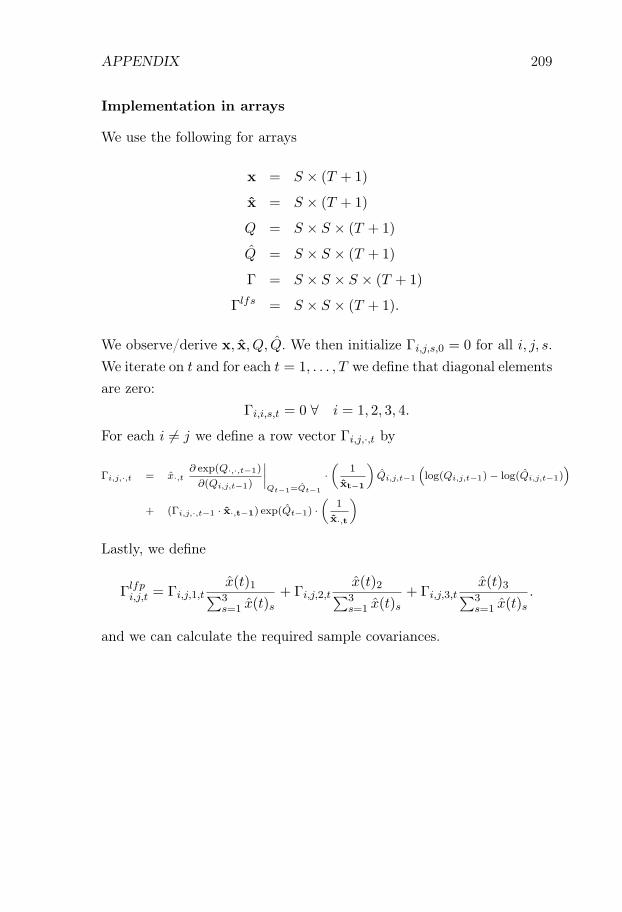
APPENDIX 209
Implementation in arrays
We use the following for arrays
x = S × (T + 1)
x = S × (T + 1)
Q = S × S × (T + 1)
Q = S × S × (T + 1)
Γ = S × S × S × (T + 1)
Γlfs = S × S × (T + 1).
We observe/derive x, x, Q, Q. We then initialize Γi,j,s,0 = 0 for all i, j, s.We iterate on t and for each t = 1, . . . , T we define that diagonal elementsare zero:
Γi,i,s,t = 0 ∀ i = 1, 2, 3, 4.
For each i = j we define a row vector Γi,j,·,t by
Γi,j,·,t = x·,t∂ exp(Q·,·,t−1)
∂(Qi,j,t−1)
∣∣∣∣Qt−1=Qt−1
·(
1
xt−1
)Qi,j,t−1
(log(Qi,j,t−1)− log(Qi,j,t−1)
)
+ (Γi,j,·,t−1 · x·,t−1) exp(Qt−1) ·(
1
x·,t
)
Lastly, we define
Γlfpi,j,t = Γi,j,1,t
x(t)1∑3s=1 x(t)s
+ Γi,j,2,tx(t)2∑3s=1 x(t)s
+ Γi,j,3,tx(t)3∑3s=1 x(t)s
.
and we can calculate the required sample covariances.

210 SWEDISH UNEMPLOYMENT DYNAMICS
Chapter 4
Supply Chain Risk and thePattern of Trade∗
4.1 Introduction
This paper is motivated by a growing concern in the policy and businesscommunity over supply chain risk. The 2011 tsunami in Japan illustrateshow important reliability is for modern production. For example, GeneralMotors had to close a factory in Louisiana due to a lack of Japanese-made parts.1 The Inter-American Development Bank notes that “firmsfragmenting production internationally are likely to look for locationswith adequate transport and logistics infrastructure to reduce disrup-tions in the supply chain” (Blyde, 2014). Similarly, the US Departmentof Commerce argues that “Expected gains from offshoring can often be
∗This is joint work with Maximilian Eber. We thank Pol Antras, Kerem Cosar,Elhanan Helpman, and Xavier Jaravel for helpful feedback. We also thank KinleySalmon for collaboration on a preparatory field study, and to Ethiopian academics,policymakers, and business people who were generous with their time and their in-sights, as well as being patient with our questions. This project was supported bya Private Enterprise Development for Low-Income Countries (PEDL) exploratoryresearch grant.
1Source: http://www.nytimes.com/2011/03/20/business/20supply.html (last ac-cessed Nov 17th, 2015)
211
212 SUPPLY CHAIN RISK
erased by [...] unexpected delays.”2 In this paper, we study the relation-ship between supply chain risk and observed trade patterns.
Countries vary in the degree of supply chain risk. Some countries offerhigh-quality infrastructure and predictable, quick bureaucratic services.In other countries, poor logistics systems and low government effective-ness increase supply chain risk: components get stuck in the port; roadsrain away; land rights are not transparent; import permits are delayed,and foreign currency availability is uncertain.
Variation in country-level supply chain risk induces comparative ad-vantage when goods vary in their risk sensitivity. Consider two industries,plain t-shirt production and cars. For t-shirts, there are few separate in-termediate inputs used in production. In this case, a risky supply chainis not too problematic. On the other hand, a modern car factory basedon lean production principles requires a continuous flow of hundreds—ifnot thousands—of customized components. In car manufacturing, supplychain reliability is crucial. If a country’s infrastructure and its institu-tions create severe supply chain risk, the country can be expected tohave a comparative advantage in t-shirt production, and a comparativedisadvantage in modern car production.
We formalize this intuition by constructing a model in which eachsector produces a final good using intermediate inputs. Intermediate in-put production is subject to disruption risk, which means that produc-tion (including delivery) fails with some positive probability. Proximatecauses of production failures are infrastructure problems, strikes, politi-cal instability, and unpredictable bureaucratic procedures.
Some inputs are pre-committed before uncertainty is resolved, andthese inputs are lost if complementary inputs are not delivered. In thisway, upstream supply disruptions damage downstream productivity. It isan important assumption that some inputs are pre-committed. Indeed,without precommitment, upstream idiosyncratic supply chain disrup-tions would not have downstream consequences as inputs could be real-
2http://www.esa.doc.gov/economic-briefings/assess-costs-everywhere-shipping(last accessed Nov 17th, 2015)
INTRODUCTION 213
located to production units which had not experienced supply chain dis-ruptions. The combination between supply chain risk and pre-committedinputs damages productivity.
A key feature of the model is that the effect of disruption risk dependson whether intermediate goods are standardized or customized. Stan-dardized inputs are homogenous and traded on centralized exchanges,whereas customized inputs are delivered directly from input producersto final goods producers. For standardized inputs, the centralized ex-change insulates producers from disruption risk through a law of largenumbers. There will be a steady supply of goods even if some suppliersfail for idiosyncratic reasons. This is not the case for customized inputs,and upstream disruptions in customized input production are transmit-ted to dowstream producers.
We derive a novel aggregation result that makes the model highlytractable. We show that aggregate supply and demand of a sector canbe characterized by a representative firm with deterministic production,even though the underlying firms experience stochastic shocks. Sup-ply chain risk enters the sectoral production function as a productivitypenalty. As all customized intermediate inputs are essential for produc-tion, this productivity penalty grows exponentially with the number ofcustomized intermediate inputs used in production.3 The theory alsosuggests a measure of industry risk sensitivity. Because each customizedintermediate good represents an independent source of error, the risk sen-sitivity of a product depends on the number of customized componentsused in production.
We embed this sectoral production structure in a simple trade model.In the model, we let goods vary in their number of customized inputs m,and let countries vary in the disruption risk π. We show that productivityis log-submodular in π and m. Thus, we can use the insight from Costinot(2009a) to show that there will be negative sorting between π and m.In other words, risky countries (high π) will produce goods with few
3We assume that input disruption shocks are independent.
214 SUPPLY CHAIN RISK
customized intermediate inputs (low m).In the empirical part of the paper, we test this hypothesis in trade
data using the methodology in Romalis (2004). In a first step, we useinput-output tables and the definition of customized goods developedby Rauch (1999) to construct a measure of how many customized in-termediate inputs each industry uses. To proxy for disruption risk, weuse the World Governance Indicator (WGI) for government effectivenessand the World Bank’s Logistics Performance Index (LPI). We then testwhether countries with more effective government and logistics systemsexport relatively more goods with a large number of customized compo-nents. We show that this effect exists and is statistically and economicallymeaningful. The effect is present in a wide range of specifications, evenwhen we (over-) control for country income levels.
The effects we find are somewhat smaller but of a similar order ofmagnitude as other institutional determinants of trade patterns, for ex-ample contracting quality (Nunn, 2007). However, our theory builds ona different mechanism. Nunn (2007) emphasizes that a bad contractingenvironment leads to a higher cost of customized intermediate inputsvia lower levels of relation-specific investments. Therefore, he measuresthe proportion in value terms of inputs that comes from customized in-termediate inputs. Our paper focuses on disruption risk and thereforeconsiders the number of customized intermediate inputs.
Different perspectives on the sources of comparative advantage alsoimply different policy levers. Many countries are actively trying to attract“sophisticated” industries such as advanced electronics manufacturing. Ifrelationship-specific investments are key—as implied by models such asAntràs (2003) and measured by Nunn (2007)—then the main task forgovernments is to improve the quality of the contracting environmentand the rule of law. If supply chain risk matters—as suggested by ourresults—then it is also important for governments to improve the reliabil-ity of the business environment through, for example, more predictablebureaucracy and infrastructure.
Our theory also has implications for the measurement of the quality

4.2. LITERATURE 215
of the business environment. Few existing indicators focus on uncertaintyand risk. For example, the World Bank’s Doing Business Indicators havebeen used widely to illustrate the challenges for businesses in poor coun-tries. It measures the de jure time and cost to complete a wide rangeof functions such as the time to export, import, receive electricity, andopen a business. However, for most tasks, the indicator only provides asingle estimate per country of the time required for a given task, andit contains little information about the variability of its implementa-tion. We stress the importance of risk and uncertainty in the businessenvironment. Our findings suggest that characterizations of the businessenvironment should include measures of risk. For example, surveys wouldbenefit from reporting not only the average time to obtain a permit, butalso the variance associated with the time to obtain such a permit andthe risk of not obtaining a permit at all.
We discuss related literature in Section 4.2. Section 4.3 provides themodel. We bring the model to the data in Section 4.4. Section 4.5 con-cludes the paper.
4.2 Literature
The paper connects to a number of different literatures. The produc-tion structure in which all components are vital for production relates toKremer’s O-Ring theory of production (Kremer, 1993). Furthermore, weanalyze how institutional features interact with risk to shape countries’trade patterns. Therefore, the paper also adds to the literature on institu-tional sources of comparative advantage. Lastly, it contributes to a newliterature analyzing the role of supply chain disruptions in productionnetworks.
O-Ring theory and sequential production Our production processfeatures a number of vital inputs that are necessary for production. Thus,the most closely related model is the O-Ring Theory proposed by Kremer(1993). He analyzes a production process where all tasks have to be

216 SUPPLY CHAIN RISK
performed succesfully for production to be succesful. In his analysis, lowhuman capital plays a similar role as supply chain unreliability plays inour setting.
A paper that applies an O-Ring like mechanisms to trade is Costinot(2009b). He proposes a model of comparative advantage where firmstrade off the value of specialization against the risk of disruption whenthey select team sizes. Disruption comes from poorly enforced contracts.As the gains from specialization stems from economizing on fixed trainingcosts, his definition of sensitivity is the total training cost for workers inan industry. In contrast, we have a different source of disruption risk,and therefore focus on the number of specialized inputs as the measureof risk sensitivity.
More generally, production processes in which all components arevital are related to sequential production, in which goods have to passthrough a number of pre-defined steps. Economists have long noted thepotential implications of sequential production, and also analyzed tradepatterns in the context of sequential production models. Dixit and Gross-man (1982) is an early attempt of analyzing the role of sequential pro-duction in shaping trade patterns. More recently, Costinot et al. (2013)and Antràs and Chor (2013) have proposed novel models of sequentialproduction and used them to interpret sorting along global supply chains.
Institutional sources of comparative advantage We analyze howvariations in government effectiveness and logistics systems quality shapetrade patterns. This connects the paper to the growing literature on in-stitutional determinants of comparative advantage. Existing work on theinstitutional determinants of comparative advantage focuses on the roleof technological differences Eaton and Kortum (2002), factor endowments(Romalis, 2004), contracting quality (Nunn, 2007; Antràs, 2003; Antrasand Helpman, 2004), financial development (Manova, 2013), or labormarket institutions (Cuñat and Melitz, 2012). Nunn and Trefler (2014)provide a recent survey of the literature.
In particular, Levchenko (2007) treats institutional quality as a source
4.3. MODEL 217
of comparative advantage. In the model, he focuses on imperfect contractenforcement in the spirit of Grossman and Hart (1986). A contrast toour model is that we posit that institutions determine the amount ofrisk that firms face, which in turn shapes comparative advantage. Blydeand Molina (2015) provides evidence that foreign direct investment isrelated to logistics infrastructure. Similar to our paper, he stresses thatproduction of complex goods is challenging when the environment isrisky.
Disruptions in production networks A number of recent papershave analyzed the effect of disruption in production networks. Carvalhoet al. (2016) analyze the production network consequences of the 2011Great East Japanese Earthquake. Barrot and Sauvagnat (2016) provideevidence for a key assumption in our paper, namely that upstream dis-ruption shocks are particularly damaging when upstream producers pro-duce specialized goods.
4.3 Model
We construct a trade model where intermediate input production is risky.Countries vary in their degree of supply chain risk and goods vary in theirrisk sensitivity. This generates specialization across countries accordingto comparative advantage. We first develop a parsimonius characteriza-tion of production with risky inputs. For each sector, we derive a sectorlevel aggregate production function, which summarizes how supply chainrisk and industry characteristics interact to determine sector level pro-ductivity. We then use these sectoral production functions in a trademodel to characterize how supply chains shape trade patterns.
A sector s consists of a continuum of final goods producers whichproduce a good using labor and multiple intermediate inputs. The finalgoods producers combine intermediate inputs using a CES aggregatorwhere inputs are gross complements. Therefore, every input is essentialfor production. Intermediate inputs are produced using labor, and the
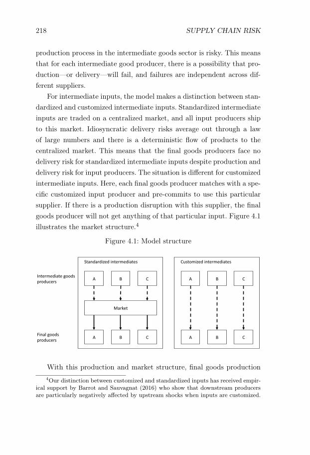
218 SUPPLY CHAIN RISK
production process in the intermediate goods sector is risky. This meansthat for each intermediate good producer, there is a possibility that pro-duction—or delivery—will fail, and failures are independent across dif-ferent suppliers.
For intermediate inputs, the model makes a distinction between stan-dardized and customized intermediate inputs. Standardized intermediateinputs are traded on a centralized market, and all input producers shipto this market. Idiosyncratic delivery risks average out through a lawof large numbers and there is a deterministic flow of products to thecentralized market. This means that the final goods producers face nodelivery risk for standardized intermediate inputs despite production anddelivery risk for input producers. The situation is different for customizedintermediate inputs. Here, each final goods producer matches with a spe-cific customized input producer and pre-commits to use this particularsupplier. If there is a production disruption with this supplier, the finalgoods producer will not get anything of that particular input. Figure 4.1illustrates the market structure.4
Figure 4.1: Model structure
�� �� ��
�����
�� �� ��
�� �� ��
�� �� ��
� �����������������������
�� ������������������
��� ��������� ��������� ����������� ���������
With this production and market structure, final goods production4Our distinction between customized and standardized inputs has received empir-
ical support by Barrot and Sauvagnat (2016) who show that downstream producersare particularly negatively affected by upstream shocks when inputs are customized.
MODEL 219
succeeds only when all customized intermediate inputs are succesfullydelivered. We define the failure probability π and assume that failuresare independent. Then, production succeeds with probability (1 − π)ms
where ms is the number of customized intermediate inputs in sectors. We assume that labor supply and other customized input suppliesare pre-committed before the resolution of production risk. Hence whenproduction fails, those inputs are wasted. One insight in the model isthat there need to be pre-committed costs to generate large costs ofsupply chain disruptions. If costs were not pre-committed, productionfactors would be re-allocated to firms which did not suffer supply chaindisruptions, which would limit the negative consequences of supply chaindisruptions.
Even though the model features idiosyncratic risk, we show thataggregate output and aggregate labor demand of every sector can besummarized by an optimizing representative firm. This representativefirm has a deterministic production function which is linear in labor.The supply chain risk appears as a productivity penalty proportional to(1 − π)ms(1−γ)+γ . where γ is the cost share of standardized intermedi-ate goods. The interpretation of the productivity penalty is that supplychain risk confers a (1 − π)ms penalty on the productivity of labor andcustomized intermediate inputs, as they are pre-commited but only uti-lized when production succeeds. There is a 1−π productivity penalty onstandardized intermediate inputs due to production and delivery risk,but the centralized market means that this effect is not amplified bydownstream effects in the production chain. Combining these two penal-ties using the factor shares yields the aggregate productivity penalty.
Once we have characterized each sector using a representative firm,we can build a trade model that incorporates supply chain risk. We createa world economy in which sectors vary in their number of intermediateinputs ms and countries vary in their degree of supply chain risk πc. Werepresent the production technology of each country-sector pair usingthe previously derived representative firm. This gives us a trade modelwith country-industry-specific productivity penalties (1− πc)
ms(1−γ)+γ .
220 SUPPLY CHAIN RISK
We note that these productivity terms are log-submodular in πc andms. It is well-known in trade theory that there is a a close connectionbetween log-submodularity in productivity and negative sorting, and weprove that our model indeed features negative sorting between πc andms. Countries with high supply chain risk will specialize in goods witha low number of customized inputs.
We abstract from risk mitigation in this model. In practice, firmscan mitigate supply chain risk by holding inventory, having redundancyin the supply chain, and by making costly investment in speeding updelayed processes. However, even if firms could mitigate supply chainrisks, the trade pattern consequences would be similar if there is a fixedcost associated with mitigation per input: for example, if there is a fixedcosts of contracting with an extra supplier to have redundancy, or insetting up an inventory for a particular input. The functional form of therelation between productivity, number of customized inputs, and supplychain risk would change if there were mitigation possibilities, but thesorting prediction only depends on a positive interaction between costsof supply chain disruptions and the number of customized inputs.
In Section 4.3.1, we set up the production environment for a sectorand derive a representative firm to characterize the sector’s aggregatebehavior. In Section 4.3.2, we insert these sectors into a trade model andderive the pattern of specialization.
4.3.1 Sector level supply function
A sector s features a unit interval of final goods producers j ∈ [0, 1] (wewill suppress this subscript when we talk about firm behavior). Finalgoods production requires labor, a composite of customized intermediateinputs X, and a composite of standardized intermediate inputs Z forproduction.
It will be important to distinguish between variables that are de-termined before and after the resolution of production and delivery un-certainty. In particular, the realized intermediate input supplies will be
MODEL 221
stochastic as they depend on the realization of a collection of productionand delivery shocks. We will use the convention to put a tilde (∼) on topof variables to denote stochastic variables that are determined after theresolution of uncertainty. The production function is given by
y = κlαXβZγ , α+ β + γ = 1
We introduce the normalization κ = α−αβ−βγ−γ(1 − γπ)mβ
1−ηnγ
1−η fornotational convenience. The composite intermediate goods are producedaccording to
X =
(m∑i=1
xiη−1η
) ηη−1
Z =
(n∑
i=1
ziη−1η
) ηη−1
.
Timing matters as firm decisions can take place before or after the res-olution of uncertainty. In our model, firms decide on labor use and cus-tomized input orders before the resolution of uncertainty. They decideon standardized input purchases after the resolution of uncertainty. Ourchoice of timing is motivated by considering the possibility of reallocat-ing inputs in case of input delivery failure. We think it is reasonable thatlabor is difficult to reallocate quickly, and customized goods orders in-volve pre-commitment as the producer needs to specialize a productionbatch to a particular buyer. In contrast, for standardized inputs withdeep markets, it is reasonable that inputs can be reallocated from firmswith disruptions to those without disruptions relatively easily. Hence,the firm first decides on labor input l and customized input orders xfi .This particular assumption is not crucial for our conclusions regardingtrade patterns, but it is important that some costs are pre-committed assupply chain disruption otherwise would not create costs for downstreambuyers.
From the point of view of a firm, labor has a pre-determined wage w
222 SUPPLY CHAIN RISK
and the firm gives a take it or leave it offer to customized intermediateinput producers to pay pxi x
fi in case of successful delivery.5 After the
resolution of uncertainty, the final goods firm decides how much of thestandardized intermediate inputs to buy. We denote this quantity zfito emphasize that it is a stochastic choice variable depending on therealization of production disruption shocks. The firm pays pzi per unit ofstandardized goods.6 We assume that firms behave competitively in thestandardized input market and that they can buy an arbitrary amountof goods at the prevailing price pzi . There is no delivery uncertainty, andin equilibrium pzi will adjust to clear the market. Taken together, thefirm solves
maxl,xi,zi
E (P y − wl −∑mi=1 p
xi xi −
∑mi=1 p
zi zi) s.t. y = κlαXβZγ ,
and subject to the customized input supplier accepting the offer.We simplify this expression in steps to clarify the optimization prob-
lem. We first note that the randomness can be reduced to two cases:either all customized inputs arrive or at least one is missing. When acustomized input is missing, production will fail (y = 0) regardless ofthe purchased amount of standardized inputs. Clearly, the firm will thenchoose not to buy any standardized inputs. Thus, there is only one stateof the world in which the firm buys standardized inputs: when all custu-mized input goods arrive. We write zi without a tilde (∼) to denote thepurchased amount of standardized inputs in this case. As all failures of
5We place all the bargaining strength on the buyer side and we do not introduceany contracting frictions. These assumptions can be relaxed to analyze the interactionbetween contracting frictions and production uncertainty. It is a non-consequentialassumption that firms only pay when delivery is successful as firms are risk neutral,but if firms were risk averse, the pricing scheme would embody some form of risk-sharing. This notion could be useful to analyze the selection of payment terms ininternational trade. The choice of writing total payment as pi(j)x
fi (j) is only an
inconsequential reparametrization of total payments Ti(j).6In a general version we would write pzi to denote that the price of standardized
inputs is determined after the realization of production shocks, but in this case thereare no aggregate production shocks, and the price will be independent of the realizedshocks with probability one.
MODEL 223
customized goods are independent and happen with probability π, theprobability that all deliveries will suceed is (1−π)m. We can rewrite theoptimization problem as
maxlf ,xi,zi
(1− π)mPy − wl −m∑i=1
pxi (1− π)xi −n∑
i=1
(1− π)mpzi zi,
subject to production being given by y = κlαXβZγ . Here, (1 − π) inthe xi-terms stems from our assumption that firms only pay customizedgoods suppliers upon succesful delivery, and X,Z are the values taken byX, Z when there are no disruptions. With this formulation, we can derivethe relative demand for different factors using standard methods. We cannote that the presence of supply chain risks bias firms to have relativelymore standardized inputs versus customized inputs than implied by theirprice ratio pzi /p
xi . The intuition is that supply chain risks bias firms away
from pre-commited inputs, as these are wasted in case of supply chaindisruptions.
xil
=β
α
1
m(1− π)
w
pxizil
=γ
α
1
n(1− π)mw
pzi
The customized intermediate input sector has a linear production func-tion in labor. When they employ labor lxi , they produce output lxi withprobability 1− π and zero output with probability π. The firms obtainsan order xi for which it is paid pxi xi upon delivery and 0 otherwise. Con-ditional on producing, it is always optimal for the firm to employ xi unitsof labor to fill the order exactly. Firms can also choose not to produceat all. Thus, they choose between accepting or not accepting an order.They solve
maxx′i∈{0,xi}
x′i ((1− π)pxi − w) .
Just as customized intermediate input producers, standardized interme-
224 SUPPLY CHAIN RISK
diate input producers have linear production functions in labor and pro-duction is risky. Thus, they employ lzi workers and produce lzi goods withprobability 1− π and 0 goods with probability π. When successful, theysell their output to the centralized market at price pzi . Producers chooselzi ≥ 0 to maximize their expected profit
Πzi = p(1− π)lzi − wlzi (4.1)
We analyze a single sector which will be inserted into a trade model.Therefore, our primary interest is how the sector’s aggregate labor de-mand and aggregate output vary with prices. That is, we are interestedin
Y =
∫ 1
0y(j)dj
L =
∫ 1
0l(j)dj +
m∑i=1
∫ 1
0lxi (j)dj +
n∑i=1
∫ 1
0lzi (j)dj
and how they depend on the final goods price P and wages w. Ourmain result is that the sector’s aggregate behavior can be described bya representative firm where supply chain risk enters as a productivityterm. We first define the aggregate net supply of the sector Ssto(P,w)
as the set of sector outputs and labor demands that are consistent withprofit maximization for some intermediate good prices. More formally,a pair of output and labor demand (Y,L) belongs to the net supplycorrespondence Ssto if we can find some intermediate input prices, orderquantities, and labor demands such that:
• The quantities and labor demands are optimal for both final goodsproducers and intermediate goods producers given intermediateintermediate input prices and aggregate prices P and w
• Total production of final goods is Y
Y =
∫ 1
0yjdj = (1− π)my a.s.
MODEL 225
• Total labor demand from final and intermediate good producers isL ∫ 1
0
(l(j) +
m∑i=1
lxi (j) +
n∑i=1
lzi (j)
)dj = L a.s.
• Standardized goods markets clear almost surely∫ 1
0zi(j)dj =
∫ 1
0lzi (j)I (successi(j) = 1) dj a.s. i = 1, . . . , n.
Here successi(j) is an indicator variable taking value 1 if there is no dis-ruption for firm j in standardized intermediate input sector i. Exploitingthe fact all firms behave symmetrically, we can write the labor demandequation and the market clearing equation for standardized inputs as
l +
m∑i=1
lxi +
n∑i=1
lzi = L a.s.
(1− π)mzi = (1− π)lzi a.s. (4.2)
The market clearing condition in the standardized input markets (4.2)is non-standard. The left-hand side reflects that only a fraction (1−π)m
of firms demands standardized input goods, whereas the right-hand sidereflects that only a fraction (1−π) of all standardized input producers aresuccessful in their production. In all equilibrium equations, we use theformulation almost surely (a.s.) because the statement is probabilistic.There do exist events where the market does not clear, but due to a lawof large numbers, these events have probability zero.
Now we want to show that this sector aggregate supply correspon-dence Ssto is identical to the aggregate supply correspondence of a rep-resentative firm with a linear deterministic production function
Y = (1− π)m(1−γ)+γL (4.3)
The intuition behind this representative firm is that there is a (1− π)m
probability that a firm will produce. For customized inputs and labor
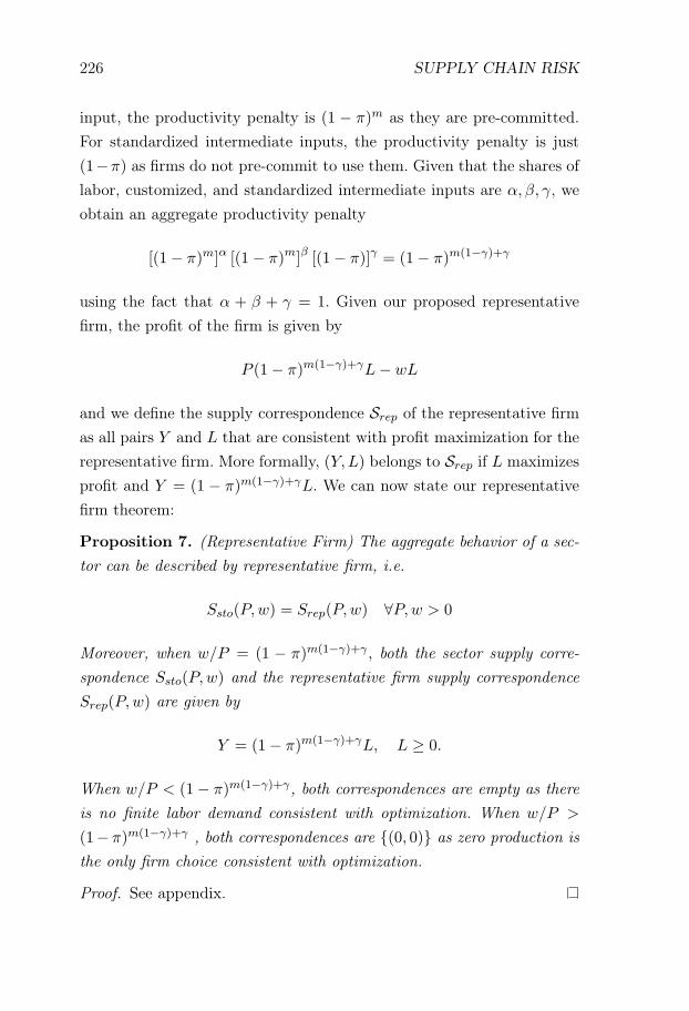
226 SUPPLY CHAIN RISK
input, the productivity penalty is (1 − π)m as they are pre-committed.For standardized intermediate inputs, the productivity penalty is just(1−π) as firms do not pre-commit to use them. Given that the shares oflabor, customized, and standardized intermediate inputs are α, β, γ, weobtain an aggregate productivity penalty
[(1− π)m]α [(1− π)m]β [(1− π)]γ = (1− π)m(1−γ)+γ
using the fact that α + β + γ = 1. Given our proposed representativefirm, the profit of the firm is given by
P (1− π)m(1−γ)+γL− wL
and we define the supply correspondence Srep of the representative firmas all pairs Y and L that are consistent with profit maximization for therepresentative firm. More formally, (Y, L) belongs to Srep if L maximizesprofit and Y = (1 − π)m(1−γ)+γL. We can now state our representativefirm theorem:
Proposition 7. (Representative Firm) The aggregate behavior of a sec-tor can be described by representative firm, i.e.
Ssto(P,w) = Srep(P,w) ∀P,w > 0
Moreover, when w/P = (1 − π)m(1−γ)+γ , both the sector supply corre-spondence Ssto(P,w) and the representative firm supply correspondenceSrep(P,w) are given by
Y = (1− π)m(1−γ)+γL, L ≥ 0.
When w/P < (1− π)m(1−γ)+γ, both correspondences are empty as thereis no finite labor demand consistent with optimization. When w/P >
(1− π)m(1−γ)+γ , both correspondences are {(0, 0)} as zero production isthe only firm choice consistent with optimization.
Proof. See appendix.
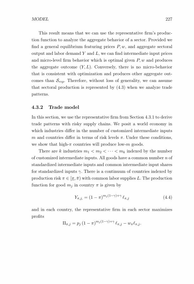
MODEL 227
This result means that we can use the representative firm’s produc-tion function to analyze the aggregate behavior of a sector. Provided wefind a general equilibrium featuring prices P,w, and aggregate sectoraloutput and labor demand Y and L, we can find intermediate input pricesand micro-level firm behavior which is optimal given P,w and producesthe aggregate outcome (Y, L). Conversely, there is no micro-behaviorthat is consistent with optimization and produces other aggregate out-comes than Srep. Therefore, without loss of generality, we can assumethat sectoral production is represented by (4.3) when we analyze tradepatterns.
4.3.2 Trade model
In this section, we use the representative firm from Section 4.3.1 to derivetrade patterns with risky supply chains. We posit a world economy inwhich industries differ in the number of customized intermediate inputsm and countries differ in terms of risk levels π. Under these conditions,we show that high-π countries will produce low-m goods.
There are k industries m1 < m2 < · · · < mk indexed by the numberof customized intermediate inputs. All goods have a common number n ofstandardized intermediate inputs and common intermediate input sharesfor standardized inputs γ. There is a continuum of countries indexed byproduction risk π ∈ [π, π) with common labor supplies L. The productionfunction for good mj in country π is given by
Yπ,j, = (1− π)mj(1−γ)+γ �π,j (4.4)
and in each country, the representative firm in each sector maximizesprofits
Ππ,j = pj (1− π)mj(1−γ)+γ �π,j − wπ�π,j .
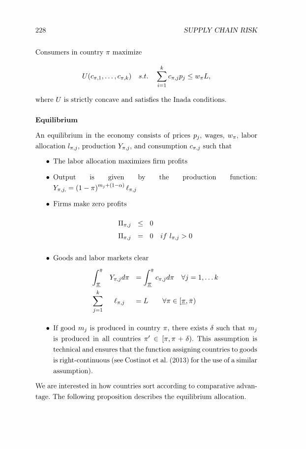
228 SUPPLY CHAIN RISK
Consumers in country π maximize
U(cπ,1, . . . , cπ,k) s.t.
k∑i=1
cπ,jpj ≤ wπL,
where U is strictly concave and satisfies the Inada conditions.
Equilibrium
An equilibrium in the economy consists of prices pj , wages, wπ, laborallocation lπ,j , production Yπ,j , and consumption cπ,j such that
• The labor allocation maximizes firm profits
• Output is given by the production function:Yπ,j, = (1− π)mj+(1−α) �π,j
• Firms make zero profits
Ππ,j ≤ 0
Ππ,j = 0 if lπ,j > 0
• Goods and labor markets clear∫ π
πYπ,jdπ =
∫ π
πcπ,jdπ ∀j = 1, . . . k
k∑j=1
�π,j = L ∀π ∈ [π, π)
• If good mj is produced in country π, there exists δ such that mj
is produced in all countries π′ ∈ [π, π + δ). This assumption istechnical and ensures that the function assigning countries to goodsis right-continuous (see Costinot et al. (2013) for the use of a similarassumption).
We are interested in how countries sort according to comparative advan-tage. The following proposition describes the equilibrium allocation.
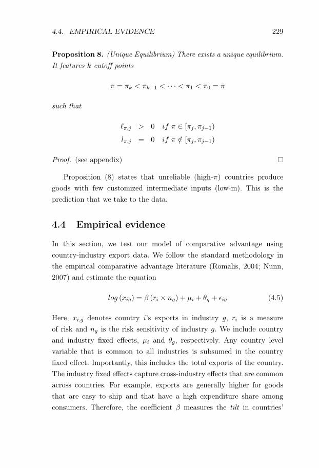
4.4. EMPIRICAL EVIDENCE 229
Proposition 8. (Unique Equilibrium) There exists a unique equilibrium.It features k cutoff points
π = πk < πk−1 < · · · < π1 < π0 = π
such that
�π,j > 0 if π ∈ [πj , πj−1)
lπ,j = 0 if π /∈ [πj , πj−1)
Proof. (see appendix)
Proposition (8) states that unreliable (high-π) countries producegoods with few customized intermediate inputs (low-m). This is theprediction that we take to the data.
4.4 Empirical evidence
In this section, we test our model of comparative advantage usingcountry-industry export data. We follow the standard methodology inthe empirical comparative advantage literature (Romalis, 2004; Nunn,2007) and estimate the equation
log (xig) = β (ri × ng) + μi + θg + εig (4.5)
Here, xi,g denotes country i’s exports in industry g, ri is a measureof risk and ng is the risk sensitivity of industry g. We include countryand industry fixed effects, μi and θg, respectively. Any country levelvariable that is common to all industries is subsumed in the countryfixed effect. Importantly, this includes the total exports of the country.The industry fixed effects capture cross-industry effects that are commonacross countries. For example, exports are generally higher for goodsthat are easy to ship and that have a high expenditure share amongconsumers. Therefore, the coefficient β measures the tilt in countries’
230 SUPPLY CHAIN RISK
trade pattern towards certain industries depending on country-industrycharacteristics. The interpretation is the same as in Romalis (2004).
The logic of the specification can be illustrated with an example. Sup-pose, for the sake of argument, that there are two industries, electronicsand cement production. The former is highly sensitive to disruptionswhile the latter is relatively robust. Assume further that there are twocountries, a large safe and a small risky country. First, we might expectthe large country to have higher exports in both industries. The coun-try fixed effect takes this into account. Second, we might assume thatelectronics are generally more traded than cement. The industry fixedeffect takes this into account. Any remaining effect then ideally reflectsthe interaction of industry and country variables. The safe country isexpected to export more electronics than cement, since electronics arerisk-sensitive. This is the effect that the coefficient β aims to captures.
We adopt the convention that high values of ri correspond to highreliability (low risk), and our theoretical prediction is therefore β > 0:countries with high scores on reliability measures specialize in industriesthat are sensitive to risk.
4.4.1 Data Sources and Concordances
To measure trade flows, we use the BACI dataset which is compiledby CEPII and based on the COMTRADE data (Gaulier and Zignago,2010). We use total value of exports for each country in each HS 2007six digit level industry. We use data for 2012. To categorize inputs asspecialized vs customized we use Rauch’s classification into goods whichare traded on exchange, goods which are referenced in a trade journal,and goods which are neither (Rauch, 1999). For measurement of govern-ment properties, we use the World Banks’ World Governance Indicators(WGI) (Kaufmann et al., 2011). The logistics quality is measured bythe World Bank’s Logistics Performance Index (Arvis, 2010). GDP andcountry factor endowments are obtained for 2011 data in the Penn WorldTable 8.1 (Feenstra et al., 2015). For GDP, we use expenditure-side real
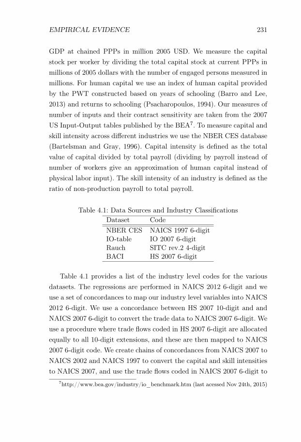
EMPIRICAL EVIDENCE 231
GDP at chained PPPs in million 2005 USD. We measure the capitalstock per worker by dividing the total capital stock at current PPPs inmillions of 2005 dollars with the number of engaged persons measured inmillions. For human capital we use an index of human capital providedby the PWT constructed based on years of schooling (Barro and Lee,2013) and returns to schooling (Psacharopoulos, 1994). Our measures ofnumber of inputs and their contract sensitivity are taken from the 2007US Input-Output tables published by the BEA7. To measure capital andskill intensity across different industries we use the NBER CES database(Bartelsman and Gray, 1996). Capital intensity is defined as the totalvalue of capital divided by total payroll (dividing by payroll instead ofnumber of workers give an approximation of human capital instead ofphysical labor input). The skill intensity of an industry is defined as theratio of non-production payroll to total payroll.
Table 4.1: Data Sources and Industry ClassificationsDataset CodeNBER CES NAICS 1997 6-digitIO-table IO 2007 6-digitRauch SITC rev.2 4-digitBACI HS 2007 6-digit
Table 4.1 provides a list of the industry level codes for the variousdatasets. The regressions are performed in NAICS 2012 6-digit and weuse a set of concordances to map our industry level variables into NAICS2012 6-digit. We use a concordance between HS 2007 10-digit and andNAICS 2007 6-digit to convert the trade data to NAICS 2007 6-digit. Weuse a procedure where trade flows coded in HS 2007 6-digit are allocatedequally to all 10-digit extensions, and these are then mapped to NAICS2007 6-digit code. We create chains of concordances from NAICS 2007 toNAICS 2002 and NAICS 1997 to convert the capital and skill intensitiesto NAICS 2007, and use the trade flows coded in NAICS 2007 6-digit to
7http://www.bea.gov/industry/io_benchmark.htm (last acessed Nov 24th, 2015)

232 SUPPLY CHAIN RISK
create the weights used in these concordances. We create a concordancefrom NAICS 2007 to NAICS 2012 to convert all data into NAICS 2012.
For the customization variable, we use a concordance between SITCrev.2. 4-digit and HS 2007 6-digit to convert the variable into HS 20076-digit. Again we use the trade data now in HS 2007 6-digit to createthe weighting scheme. We then map to IO 2007 via NAICS 2007 6-digit as we use the Rauch data in the IO-table to calculate industrycharacteristics. The IO-data together with the Rauch variables are thenmapped to NAICS 2012 via NAICS 2007.
In the Appendix, we describe in detail which sources we use for theconcordances, how concordances are weighted, and how the weights areused in the transformations.
4.4.2 Measuring Products’ Sensitivity to Unreliability
Motivated by our theory, we propose a novel measure of industries’ risksensitivity. In the model, we distinguish between standardized and cus-tomized components. Standardized components are traded in liquid mar-kets. As a consequence, final goods producers are not materially affectedby idiosyncratic supply failures. By contrast, customized componentscannot be replaced easily and, therefore, the final goods producers isexposed to the risk that an component cannot be sourced. This couldbe due to outright failure of a supplier or the failure of a port author-ity, bad infrastructure, and so forth. Furthermore, as all components aregross complements, a non-zero amount of each components is essentialto production. Hence, the number of customized components that anindustry uses is an appropriate measure of risk sensitivity.8
We classify components as customized using the methodology devel-oped by Rauch (1999). For each industry, he records if a good is tradedon an exchange or reference-priced in a trade journal. We define a com-ponent as customized if it belongs to an industry which Rauch records
8Our model does not feature mitigation of supply chain risk. A similar resultobtains if there is a fixed cost of mitigation per distinct input.
EMPIRICAL EVIDENCE 233
as neither traded on an exchange nor reference-priced. Using the USinput-tables, we look up the list of other industries that a given industrybuys from and count the number of those industries that are customizedaccording to Rauch. Tables 4.1 and 4.2 list the top and bottom thirtyindustries sorted by the number of customized components. Our risksensitivity measure leads to an intuitive classification of most industries.Motor vehicle components and semiconductor production, for example,are classified as sensitive to risk, whereas farming and cement manufac-turing are not. Industry-level variables are visualized in Figure 4.1b.
We infer the number of inputs used from industry level data. To theextent that firms are heterogeneous, this introduces a problem of aggre-gation. Consider two firms in the same industry that use 50 inputs each.If the firms’ business models are not exactly identical, only 30 out of 50might be the same for the two firms. On aggregate, however, we wouldobserve the industry using 70 inputs, despite each firm using only 50.To protect us against the extreme case when a very small fraction offirms in an industry uses a particular input, we re-estimate the main re-gression excluding input industries which contributes less than 0.1% and0.01% of total intermediate input value. The results are robust againstthis modification. Moreover, as long as this shortcoming is similar acrossindustries it will not affect our results, which is based on the ranking ofindustries.9
Our measure of sensitivity to unreliability can justifiably be calledcomplexity as it denotes how many specialized components a productuses. Thus, we can contrast it with our proposed measures of complex-ity in the literature. Nunn (2007) develops one such measure. He alsouses the Rauch (1999) measure of product differentiation. He measuresan industry’s sensitivity to contract quality as the share of total input
9Further problem that we have not addressed is firstly that an industry can usemultiple components from a single industry. This would lead to an underestimationof the number of inputs. Lastly, there can be a problem in that the fineness of theIO-table classification is endogenous to the US production structure, which mightmean that there is a bias in that US-concentrated industries appear to have moreinputs because of how the IO-table is subdivided.

234 SUPPLY CHAIN RISK
value that comes from customized inputs. The motivation behind hismeasure is that cost-saving investments in specialized goods productionare relation specific, and will be provided less if contract protection ispoor. In light of this, it is reasonable to use the proportion of componentcosts as lack of relation-specific investments can plausibly be expectedto increase costs proportionally. While it is theoretically motivated toweigh the customized intermediate good content by value in the contextof his study, our model suggests an independent role for the number ofcomponents that are customized.
Another measure that has been used to capture complexity is oneminus the Herfindahl index of input suppliers. The Herfindahl index isa concentration index of an industry’s input suppliers. It is high if anindustry’s intermediate good demand is skewed towards few industries.This measure of complexity is used in Blanchard and Kremer (1997)and Levchenko (2007). Levchenko (2007) explicitly discusses why theychoose to use the Herfindahl index instead of the number of intermediateinputs: “If intermediate input use is dominated by one or two inputs(high concentration), and all the other intermediates are used very little,then what really matters to the final good producer is the relationship ithas with the largest one or two suppliers.” Our theory suggests that allsuppliers of customized inputs might matter independent of size. FormerApple executive Tony Fadell illustrated this point well when the Japanesetsunami threatened to disrupt global supply chains: “lacking some part,even if it costs just dimes or a few dollars, can mean shutting down afactory”.10
In Figure 4.1a, we compare our measure to the measure proposedin Nunn (2007). Generally, the correlation is strong and positive.Both measures classify Automobile Manufacturing as risk-sensitiveand contract-intensive. On the other end of the spectrum, SoybeanFarming is classified as neither risk-sensitive and nor contract intensive.However, there are some differences as well. Classification differs for the
10http://www.nytimes.com/2011/03/20/business/20supply.html?pagewanted=2&_r=0(last accessed: November 19th, 2015)
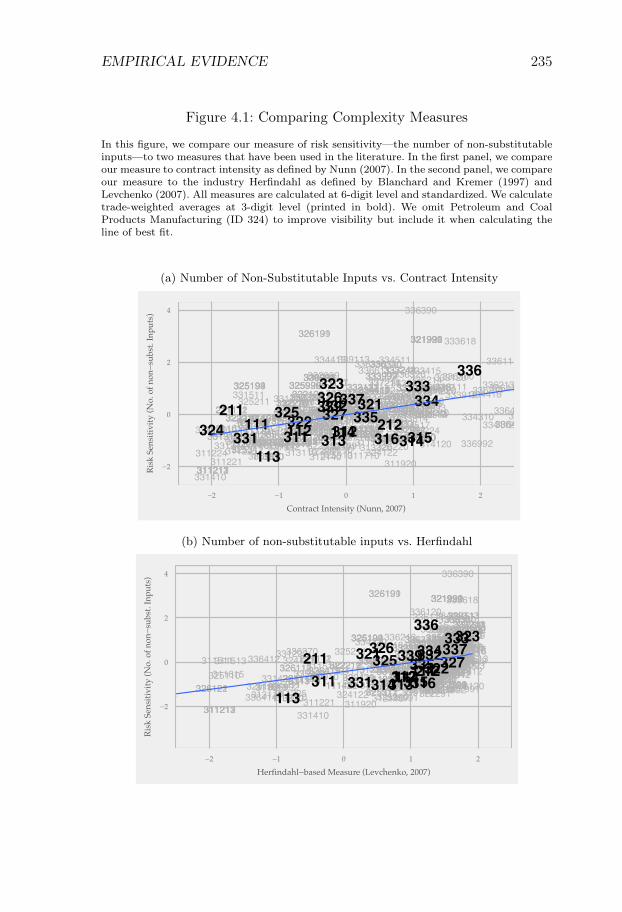
EMPIRICAL EVIDENCE 235
Figure 4.1: Comparing Complexity Measures
In this figure, we compare our measure of risk sensitivity—the number of non-substitutableinputs—to two measures that have been used in the literature. In the first panel, we compareour measure to contract intensity as defined by Nunn (2007). In the second panel, we compareour measure to the industry Herfindahl as defined by Blanchard and Kremer (1997) andLevchenko (2007). All measures are calculated at 6-digit level and standardized. We calculatetrade-weighted averages at 3-digit level (printed in bold). We omit Petroleum and CoalProducts Manufacturing (ID 324) to improve visibility but include it when calculating theline of best fit.
(a) Number of Non-Substitutable Inputs vs. Contract Intensity
111110111120111140111150111160111199
111219111335111339111421111422
111910111920111930111940111991111992111998112410112420112920112930
113210113310
114111114112114119
211111211112 212112212113
212210212221212222
212231212234
212291212311212319212322212325212391212392212393212399 311111311119
311211311212311213311221
311224311225
311230
311340311351311411
311421311422311423311511 311513
311514 311520
311611311613
311615
311710
311824 311911311919
311920
311930311941311942
311999
312111312112312113312120
312130
312140
312230
313110
313210313220313230313240313320
314110314120314910314994314999315220315240315280315990316110316210316992316998321113321114
321211321212321213321214321219
321911321918
321920321991321992321999
322110
322121322122
322130322211322212322219
322220322230
322291322299
323111323117
323120324110
324121
324122
325110 325120
325130
325180
325193325194325199
325211
325212325220325311325312
325411
325412325414
325510325520
325611325612325613
325620
325910
325920325992325998
326112326113
326121326122326160
326191326199
326211326212
326220
326299327110327120327211327212327213327215
327310327320
327331327390
327410327420
327910327991327992
327993327999
331110331222
331313331314
331315331318
331410
331420331491331492
331511
332119
332215332216332311332312
332321332322332323
332410332420
332431332439
332510
332613332618332722332911332912
332913
332919
332991332992332994
332999333111333120
333131333132
333241
333242
333243333244333249
333314
333316333318333413
333414
333415
333511333514
333515333517333519333611
333612333613
333618
333911333912
333913
333921333922333923333924
333991
333992
333993
333994
333995333996
333997333999
3334112
334118
334210
334220
334290 334310
334412
334413
334416334417 334418334419334510
334511
334512
334513 334514334515334516
334517334519
335110
335121335129335210335221335222
335224
335228335311
335312
335313
335314
335911 335912335921335929
335931335932
335991
335999
336111
336211336212 336213336214336320336330336340336350
336360
336370
336390
33641
3364336413
33643364
336510
336611
336612
336991 336992
337110337121
337124337127
337211337214337215
337910337920
339112
339113
339114339115339910
339920
339930339940
339950
339991339992339993339994339999
111 112
113
114211
212311 312
313 314315316
321322
323
324325
326327
331
332333334
335
336
337339
−2
0
2
4
−2 −1 0 1 2
Contract Intensity (Nunn, 2007)
Ris
k Se
nsit
ivit
y (N
o. o
f non
−su
bst.
Inpu
ts)
(b) Number of non-substitutable inputs vs. Herfindahl
111110111120111140111150111160111199
111219111335111339111421111422
111910111920111930111940111991111992111998112410112420112920112930
113210113310
114111114112114119
211111211112 212112212113
212210212221212222212231212234
212291212311212319212322212325212391212392212393212399311111311119
311211311212311213311221
4 311225
311230
311340311351311411
311421311422311423311511311513 311514 311520
311611311613311615
311710
311824311911311919
311920
311930311941311942311999
312111312112312113312120
312130
312140
312230
313110
313210313220313230313240313320
314110314120 314910314994314999315220315240315280315990316110316210316992316998321113321114
321211321212321213321214321219
321911321918
321920321991321992321999
322110
322121322122
322130322211322212322219
322220322230
322291322299
323111323117
323120
324121
324122
325110 325120325130
325180
325193325194325199325211
325212325220325311325312
325411325412
325414325510325520
325611325612325613
325620
325910
325920325992325998
326112326113
326121326122 326160
326191326199
326211326212
326220
326299327110327120327211327212327213327215327310327320
327331327390
327410327420
327910327991327992
327993327999
331110331222
331313331314
331315331318
331410
331420331491331492
331511
332119
332215332216332311332312
332321332322332323
332410332420
332431332439
332510
332613332618332722
332911332912
332913
332919332991
332992332994
332999333111
333120333131333132
333241
333242
333243333244333249
333314
333316333318333413
333414
333415
333511333514333515333517333519333611
333612333613
333618
333911333912
333913333921333922333923333924
333991
333992
333993
333994
333995333996
333997333999
334111334112
334118
334210
334220
334290334310
334412
334413
334416334417334418 334419334510
334511
334512334513334514334515334516
334517334519
335110
335121335129335210335221335222
335224335228
335311
335312
335313
335314
335911 335912335921335929
335931335932
335991
335999
336111336120
336211336212336213 336214336320336330336340336350
336360
336370
336390
336411
336412336413
336414
336415336419
336510
336611
336612
336991336992
337110337121
337124337127
337211337214337215
337910337920339112
339113
339114339115339910
339920339930
339940
339950
339991339992339993339994339999
111112113
114211
212311 312313314 315316
321322
323
325326
327331
332333
334335
336
337339
−2
0
2
4
−2 −1 0 1 2
Herfindahl−based Measure (Levchenko, 2007)
Ris
k Se
nsit
ivit
y (N
o. o
f non
−su
bst.
Inpu
ts)
236 SUPPLY CHAIN RISK
textile-related industries . Nunn’s 2007 measure classifies textile-relatedindustries (NAICS 313, 314, 315, and 316; see bottom-right area in thegraph) as complex, whereas our measure categorizes textile-relatedindustries as non-complex.
In Figure 4.1b, we compare our measure to the Herfindahl measureused in Blanchard and Kremer (1997) and Levchenko (2007). The twomeasures are strongly correlated and tend to classify broad industries insimilar ways. A notable exception is the transportation sector (NAICS336), which our measure tends to classify as more risk-sensitive thanthan the measure based on the Herfindahl Index.
4.4.3 Measuring Countries’ Reliability
We are interested in measuring disruption risk in different countries. Inthis context, we need to take a stand on likely causes of production anddelivery disruption. For this, we focus on two country characteristics:logistics systems quality and overall government effectiveness. The mo-tivation for including the quality of logistics system is clear: disruptionis more likely if third-party logistics providers have low quality, goodsclear customs slowly, and transportation infrastructure is subject to fre-quent failures.11 We also include government effectiveness which we de-fine as the quality of bureaucratic procedures and government providedservices. We include this firstly as red tape is another possible cause ofsupply chain disruptions. Disruption risks in this area include delays inpermits for starting production, or delays in permits for bringing in in-puts and foreign worker. It also captures poorly functioning bureaucracyin customs, as well as uncertain land rights. The quality of government
11In the current model, intermediate input suppliers are all domestic, which meansthat the final goods supplier does not get through customs to obtain intermediate in-puts. However, even in cases where you only source domestically, we believe it isplausible that customs problems affect reliability through its effect on your interme-diate input suppliers. Explicit modeling of this channel would involve intermediategood trade and bilateral delivery risks which are not in the current model. Formallyshowing how customs risk interacts with intermediate goods trade is an interestingarea of further research.
EMPIRICAL EVIDENCE 237
provided services is important as failures in electricity, water supply andinfrastructure are sources of potential supply chain disruptions.
When it comes to measurement, we proxy logistics systems qualitywith the World Bank’s Domestic Logistics Performance Index (Arvis,2010). The index is based on surveys with global freight forwarders andexpress carriers, and combines it with quantitative measures of somecomponents of supply chains. As of 2014 it encompasses 160 countries.For bureaucratic quality, we use the Government Effectiveness-measurefrom the Worldwide Governance Indicators (Kaufmann et al., 2011). Itis an aggregated measure derived from a large number of measures in-cluding the quality of bureaucracy, extent of red tape, infrastructurequality, and the quality of various government provided services. Figure4.1a visualizes the distributions of the main country-level variables inour data.
4.4.4 Results
In Table 4.2, we present the main results for the baseline specification(equation 4.5). We are interested in the interaction of industries’ risksensitivity measured by the number of customized components (Cust.Inp.) and countries’ reliability. Our two preferred measures of countryreliability are government effectiveness (Gov. Effectiveness) and logisticsperformance (LPI). We report interactions with three additional WorldGovernance Indicators: regulatory quality (Reg. Quality), political sta-bility and absence of violence (Stability), and control of corruption (Cor-ruption). All these indicators proxy for an environment that is amenableto the production of risk-sensitive products.
The results are consistent with the hypothesis that risk-sensitive in-dustries are disproportionately produced by reliable countries. Consideran industry that is one standard deviation above the mean in terms ofrisk sensitivity (Cust. Inp.). Increasing a country’s government effective-ness (Gov. Effectiveness) by one standard deviation is associated with10.4% (column 1) more exports in this industry, compared to a coun-
238 SUPPLY CHAIN RISK
try with an average Logistics Performance Index. Increasing a country’sLogistics Performance Index (LPI) by one standard deviation is associ-ated with 10.1% (column 6) more exports in this industry, compared toa country with an average Logistics Performance Index. The coefficientsare of very similar magnitude for the other institutional variables that weuse to proxy for reliability. The main coefficient is statistically significantat the 1% level for all measures considered.
4.4.5 Relationship to other results in the literature
As previously discussed, Nunn (2007) tests whether contracting qualityaffects the pattern of trade. Might we just be capturing the effect thatstable countries also tend to have good contracting environments? InTable 4.2, we replicate Nunn’s main result (column 3). Countries withhigh scores on the rule of law index (Rule of Law) tend to export contract-intensive goods (Contract int.). Given that both our country-measures(rule of law vs. government effectiveness) and our industry measures(contract intensity vs. risk sensitivity) are correlated, our main result incolumn 1 might be spurious. However, as we show in column 6, the twoestimates remain quantitatively similar and significant when analyzedjointly (column 6). This result suggests that our mechanism is distinctfrom the role of contracting. If we compare our quantitative effect to theone found in Nunn (2007), ours is somewhat smaller at 10% comparedto Nunn’s 28% in his baseline specification.
Of course, the two explanations are not mutually exclusive. In fact,when component producers fail to deliver a component on time theytypically also violate a contract. However, in Nunn, poor contracting isanalyzed in terms of relationship-specific investments and we considerour theory as an additional explanation for observed trade patterns. Thedistinction matters since the policy implications differ: Nunn (2007) im-plies that countries can attract sophisticated industries by improvingcontract enforcement. Our story suggests that a complementary policylever is the reduction of supply chain risk.
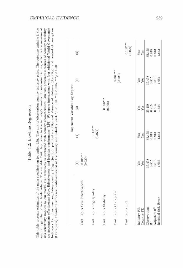
EMPIRICAL EVIDENCE 239
Tab
le4.
2:B
asel
ine
Reg
ress
ion
Thi
sta
ble
pres
ents
esti
mat
esof
the
mai
nsp
ecifi
cati
on(e
quat
ion
4.5)
.The
unit
ofob
serv
atio
nco
untr
y-in
dust
rypa
irs.
The
outc
ome
vari
able
isth
ena
tura
llo
gari
thm
ofto
tal
trad
evo
lum
e.T
heva
riab
leC
ust.
Inp.
refe
rsto
the
indu
stry
’snu
mbe
rof
cust
omiz
edin
puts
,w
hich
isth
em
easu
reof
risk
sens
itiv
ity
impl
ied
byou
rm
odel
.ri
skse
nsit
ivity
isin
tera
cted
wit
hco
untr
y-ch
arac
teri
stic
s.O
urtw
opr
efer
red
mea
sure
sof
coun
try
relia
bilit
yar
ego
vern
men
teff
ecti
vene
ss(G
ov.E
ffect
iven
ess)
and
logi
stic
spe
rfor
man
ce(L
PI)
.W
ere
port
inte
ract
ions
wit
hfo
urad
diti
onal
Wor
ldG
over
nanc
eIn
dica
tors
for
robu
stne
ss:
regu
lato
ryqu
ality
(Reg
.Q
ualit
y),
polit
ical
stab
ility
and
abse
nce
ofvi
olen
ce(S
tabi
lity)
,an
dco
ntro
lof
corr
upti
on(C
orru
ptio
n).St
anda
rder
rors
are
doub
le-c
lust
ered
atth
eco
untr
yan
din
dust
ryle
vel.
∗ p<
0.10,∗∗
p<
0.05,∗∗
∗ p<
0.01
Dep
ende
ntV
aria
ble:
Log
Exp
orts
(1)
(2)
(3)
(4)
(5)
Cus
t.In
p.x
Gov
.E
ffect
iven
ess
0.108∗∗
∗(0.029)
Cus
t.In
p.x
Reg
.Q
ualit
y0.110∗∗
∗(0.029)
Cus
t.In
p.x
Stab
ility
0.098∗∗
∗(0.028)
Cus
t.In
p.x
Cor
rupt
ion
0.087∗∗
∗(0.025)
Cus
t.In
p.x
LP
I0.105∗∗
∗(0.029)
Indu
stry
FE
Yes
Yes
Yes
Yes
Yes
Cou
ntry
FE
Yes
Yes
Yes
Yes
Yes
Obs
erva
tion
s35
,458
35,4
5835
,458
35,4
5835
,458
R2
0.81
50.
815
0.81
50.
815
0.81
5A
djus
ted
R2
0.81
30.
813
0.81
30.
813
0.81
3R
esid
ualSt
d.E
rror
1.65
31.
653
1.65
41.
654
1.65
3
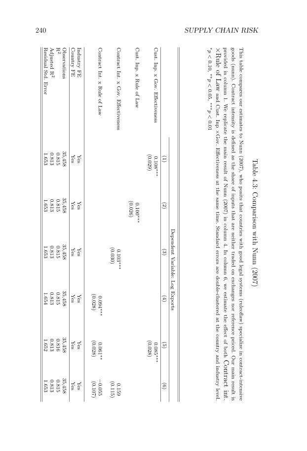
240 SUPPLY CHAIN RISK
Table
4.3:Com
parisonw
ithN
unn(2007)
This
tablecom
paresour
estimates
toN
unn(2007),
who
positsthat
countriesw
ithgood
legalsystem
s(ruleoflaw
)specialize
incontract-intensive
goods(nunn).
Contract
intensityis
definedas
theshare
ofinputs
thatare
neithertraded
onexchanges
norreference
priced.O
urm
ainresult
isprovided
incolum
n1.
We
replicatethe
main
resultof
Nunn
(2007)in
column
4.In
column
6,w
eestim
atethe
effectof
bothC
ontractint.
×R
uleof
Lawand
Cust.
Inp×
Gov.
Effectiveness
atthe
same
time.
Standarderrors
aredouble-clustered
atthe
countryand
industrylevel.
∗p<
0.10, ∗∗
p<
0.05, ∗∗∗
p<
0.01
Dependent
Variable:
Log
Exports
(1)(2)
(3)(4)
(5)(6)
Cust.
Inp.x
Gov.
Effectiveness
0.108 ∗∗∗
0.085 ∗∗∗
(0.029)
(0.028)
Cust.
Inp.x
Rule
ofLaw
0.100 ∗∗∗
(0.026)
Contract
Int.x
Gov.
Effectiveness
0.103 ∗∗∗
0.159
(0.030)
(0.115)
Contract
Int.x
Rule
ofLaw
0.094 ∗∗∗
0.061 ∗∗
−0.055
(0.028)
(0.028)
(0.107)
IndustryFE
Yes
Yes
Yes
Yes
Yes
Yes
Country
FE
Yes
Yes
Yes
Yes
Yes
Yes
Observations
35,45835,458
35,45835,458
35,45835,458
R2
0.8150.815
0.8150.815
0.8160.815
Adjusted
R2
0.8130.813
0.8130.813
0.8130.813
Residual
Std.E
rror1.653
1.6531.653
1.6541.652
1.653
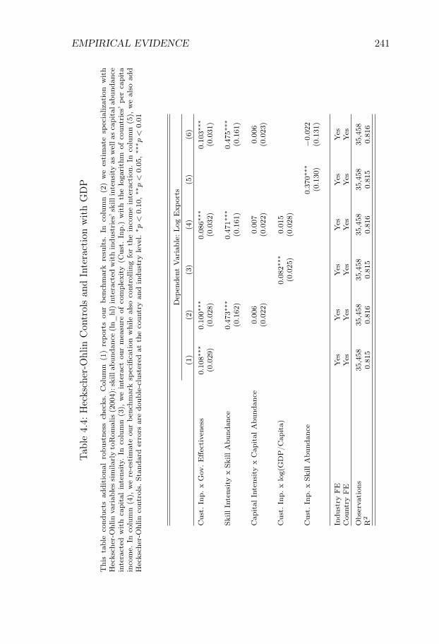
EMPIRICAL EVIDENCE 241
Tab
le4.
4:H
ecks
cher
-Ohl
inC
ontr
ols
and
Inte
ract
ion
wit
hG
DP
Thi
sta
ble
cond
ucts
addi
tion
alro
bust
ness
chec
ks.
Col
umn
(1)
repo
rts
our
benc
hmar
kre
sult
s.In
colu
mn
(2)
we
esti
mat
esp
ecia
lizat
ion
wit
hH
ecks
cher
-Ohl
inva
riab
lessi
mila
rly
toR
omal
is(2
004)
:ski
llab
unda
nce
(ln_
hl)in
tera
cted
wit
hin
dust
ries
’ski
llin
tens
ity
asw
ella
sca
pita
labu
ndan
cein
tera
cted
wit
hca
pita
lin
tens
ity.
Inco
lum
n(3
),w
ein
tera
ctou
rm
easu
reof
com
plex
ity
(Cus
t.In
p.)
wit
hth
elo
gari
thm
ofco
untr
ies’
per
capi
tain
com
e.In
colu
mn
(4),
we
re-e
stim
ate
our
benc
hmar
ksp
ecifi
cati
onw
hile
also
cont
rolli
ngfo
rth
ein
com
ein
tera
ctio
n.In
colu
mn
(5),
we
also
add
Hec
ksch
er-O
hlin
cont
rols
.St
anda
rder
rors
are
doub
le-c
lust
ered
atth
eco
untr
yan
din
dust
ryle
vel.
∗ p<
0.10,∗∗
p<
0.05,∗∗
∗ p<
0.01
Dep
ende
ntV
aria
ble:
Log
Exp
orts
(1)
(2)
(3)
(4)
(5)
(6)
Cus
t.In
p.x
Gov
.E
ffect
iven
ess
0.10
8∗∗∗
0.10
0∗∗∗
0.08
6∗∗∗
0.10
3∗∗∗
(0.0
29)
(0.0
28)
(0.0
32)
(0.0
31)
Skill
Inte
nsity
xSk
illA
bund
ance
0.47
3∗∗∗
0.47
1∗∗∗
0.47
5∗∗∗
(0.1
62)
(0.1
61)
(0.1
61)
Cap
ital
Inte
nsity
xC
apit
alA
bund
ance
0.00
60.
007
0.00
6(0
.022
)(0
.022
)(0
.023
)
Cus
t.In
p.x
log(
GD
P/C
apit
a)0.
082∗
∗∗0.
015
(0.0
25)
(0.0
28)
Cus
t.In
p.x
Skill
Abu
ndan
ce0.
370∗
∗∗−0
.022
(0.1
30)
(0.1
31)
Indu
stry
FE
Yes
Yes
Yes
Yes
Yes
Yes
Cou
ntry
FE
Yes
Yes
Yes
Yes
Yes
Yes
Obs
erva
tion
s35
,458
35,4
5835
,458
35,4
5835
,458
35,4
58R
20.
815
0.81
60.
815
0.81
60.
815
0.81
6
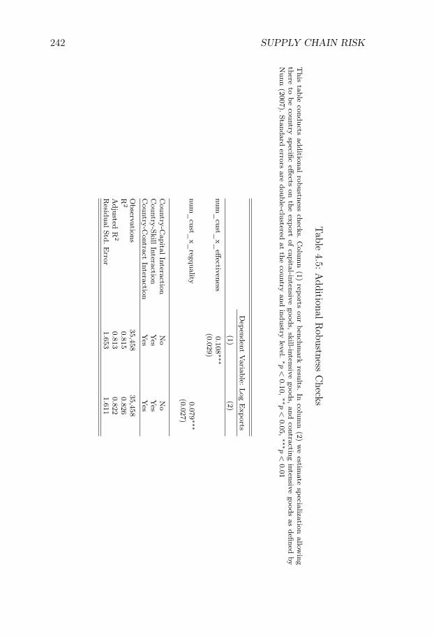
242 SUPPLY CHAIN RISK
Table
4.5:AdditionalR
obustnessC
hecks
This
tableconducts
additionalrobustness
checks.C
olumn
(1)reports
ourbenchm
arkresults.
Incolum
n(2)
we
estimate
specializationallow
ingthere
tobe
countryspecific
effectson
theexport
ofcapital-intensive
goods,skill-intensive
goods,and
contractingintensive
goodsas
definedby
Nunn
(2007).Standard
errorsare
double-clusteredat
thecountry
andindustry
level.∗p<
0.10, ∗∗
p<
0.05, ∗∗∗
p<
0.01
Dependent
Variable:
Log
Exports
(1)(2)
num_
cust_x_
effectiveness0.108 ∗∗∗
(0.029)
num_
cust_x_
regquality0.079 ∗∗∗
(0.027)
Country-C
apitalInteraction
No
No
Country-Skill
InteractionY
esY
esC
ountry-Contract
InteractionY
esY
es
Observations
35,45835,458
R2
0.8150.826
Adjusted
R2
0.8130.822
Residual
Std.E
rror1.653
1.611
EMPIRICAL EVIDENCE 243
4.4.6 Robustness Checks
The main result is biased if our regressors are correlated with the errorterm, and this can happen in many different ways. First, our measuresof reliability can be correlated with other country characteristics whichgive a comparative advantage in goods with many customized compo-nents. Second, the number of customized components can be correlatedwith other industry features, and high reliability can give a comparativeadvantage due to these industry features as well. There can also be somemixture of these two effects, for example that high government reliabilityis correlated with high financial development, and that a large number ofcustomized components is correlated with having high external financingneeds. We assess the robustness of our results by including other inter-action terms between country and good characteristics in our regressionspecification.
First, we test whether Heckscher-Ohlin effects can explain the resultsby controlling for the interaction between factor endowments and factorintensity of different industries similar to Romalis (2004). It could be thecase that reliable countries are simply countries with a large endowmentof skilled labor and risk-sensitive industries tend to be skill-intensive.In column (2) of Table 4.4, we replicate the result that skill-abundantcountries specialize in skill-intensive industries (the coefficient on theinteraction between country skill abundance and industry skill intensity).Importantly, our main estimate (Cust Inp. × Gov. Effectiveness) barelychanges when we control for factor endowments. In unreported results,we confirm that the same is true for other measures of reliability.
Second, we add an interaction term between industry risk sensitiv-ity and the logarithm of income as a catch-all term for variables thatmight proxy for being a rich country. It should be noted that this isover-controlling: countries might be rich because they have reliable sup-ply chains, which makes them productive in complex goods. Hence, wecontrol for an outcome. Despite that, as shown in Table 4.4, our mainresult remains statistically significant (column 5). Quantitatively, the es-
244 SUPPLY CHAIN RISK
timate becomes only marginally weaker when we (over-) control for logincome. This suggests that alternative explanations connected to countryincome levels do not eliminate the effects from our risk proxies.
Lastly, we make a demanding robustness check by running a regres-sion specification
log (xig) = β (ri × ng)+μi+μskilli hg+μk
i kg+μnunni (contrac_intg)+θg+εig
Here, kg is a measure of an industry’s capital intensity, hg is a measureof an industry’s skill intensity, and contract_intg is Nunn’s measure ofan industry’s contracting intensity. The μi−terms capture a country-specific term which allows for country-specific tilts of trade patterns infavor of capital intensive, skill intensive, and contracting intensive indus-tries. This specification is more flexible than the Heckscher-Ohlin controlswhere we assumed that the tilt in favor of capital and skill intensive goodswere due to capital and skill abundance on the country level. Similarly,it is more flexible than the regression where we included our variabletogether with Nunn’s, as that specification constrained countries to betilted towards contracting intensive industries only due to good rule oflaw. The current specification does not place any such constraints on thepattern of specialization. We present the results in Table 4.5. There is asmall change in the point estimate, and the effect is still significant effectat the 1%-level. This suggests that our risk sensitivity measure capturesa dimension of trade patterns distinct from that attributable to capital,skill, and contracting intensity.
4.5 Conclusion
This paper provides a tractable model of the effect of supply chain risk ontrade patterns. Supply chain risk damages productivity through a com-bination of input supply disruption risk combined with pre-commitedinputs. In our model, we show how the behavior of a sector with idiosyn-cratic delivery risk can be described by a representative firm. Supply
CONCLUSION 245
chain risk enters as a productivity penalty, which grows exponentiallywith the number of specialized inputs. Therefore, the appropriate mea-sure of supply chain sensitivity on a sectoral level is the number of spe-cialized inputs. In an international setting, the theory implies that lowrisk countries specialize in risk-sensitive industries, and this predictionis borne out in the data.
Our paper suggests a number of policy relevant conclusions. First,it suggests that reducing risk can attract industries that produce risk-sensitive goods. The paper also implies that measures of the businessenvironment would be more informative if they described the variabilityin outcomes. The World Bank’s Doing Business Survey, for instance,measures the time to start a business. However, it does not contain therisk of severe delays during the process, which might also be important.
Looking ahead, there are several natural extensions to the paper.One extension is to include trade in intermediate inputs. The model nowassumes that all inputs are produced domestically, and that there is acountry-specific risk of supply chain disruption. In practice, intermedi-ate input trade is important, and variations in supply chain risk is apotentially important factor for understanding patterns in intermediateinput trade. A modificaction of the model to include intermediate in-put trade should also include that some delivery risks are only relevantfor cross-border trade. For example, customs procedures might be slowand frictions to international contracting can make deliveries uncertain.We conjecture that such an extension could have rich predictions forthe connection between country variations in supply chain risk, the spa-tial organization of production, and the structure of intermediate inputtrade.
Given the potential endogeneity concerns in our empirical work, weare also interested in extensions to improve identification. One such ex-tension would be to use the panel dimension of trade data. The WorldGovernance Indicators goes back to 1996 and the BACI trade data goesback to 1995. This would allow us to test whether countries that im-prove on institutional measures also see a concomitant rise in trade of
246 SUPPLY CHAIN RISK
risk sensitive goods.
References
Antràs, P. (2003). Firms, contracts, and trade structure. The QuarterlyJournal of Economics, 118(4):1375–1418.
Antràs, P. and Chor, D. (2013). Organizing the global value chain.Econometrica, 81(6):2127–2204.
Antras, P. and Helpman, E. (2004). Global sourcing. Journal of PoliticalEconomy, 112(3):552–580.
Arvis, J.-F. (2010). Connecting to compete 2010: trade logistics in theglobal economy; the logistics performance index and its indicators.World Bank.
Barro, R. J. and Lee, J. W. (2013). A new data set of educational at-tainment in the world, 1950-2010. Journal of Development Economics,104:184–198.
Barrot, J.-N. and Sauvagnat, J. (2016). Input specificity and the propa-gation of idiosyncratic shocks in production networks. The QuarterlyJournal of Economics, page qjw018.
Bartelsman, E. J. and Gray, W. (1996). The NBER Manufacturing Pro-ductivity Database.
Blanchard, O. and Kremer, M. (1997). Disorganization. The QuarterlyJournal of Economics, 112(4):1091–1126.
Blyde, J. and Molina, D. (2015). Logistic infrastructure and the inter-national location of fragmented production. Journal of InternationalEconomics, 95(2):319–332.
Blyde, J. S. (2014). The drivers of global value chain participation: Cross-country analyses. In Synchronized Factories, pages 29–73. Springer.
REFERENCES 247
Carvalho, V. M., Nirei, M., Saito, Y. U., and Tahbaz-Salehi, A. (2016).Supply chain disruptions: Evidence from the great east japan earth-quake.
Costinot, A. (2009a). An Elementary Theory of Comparative Advantage.Econometrica, 77(4):1165–1192.
Costinot, A. (2009b). On the origins of comparative advantage. Journalof International Economics, 77(2):255–264.
Costinot, A., Vogel, J., and Wang, S. (2013). An elementary theory ofglobal supply chains. The Review of Economic Studies, 80(1):109–144.
Cuñat, A. and Melitz, M. J. (2012). Volatility, Labor Market Flexibility,and the Pattern of Comparative Advantage. Journal of the EuropeanEconomic Association, 10(2):225–254.
Dixit, A. K. and Grossman, G. M. (1982). Trade and protection withmultistage production. The Review of Economic Studies, 49(4):583–594.
Eaton, J. and Kortum, S. (2002). Technology, Geography, and Trade.Econometrica, 70(5):1741–1779.
Feenstra, R. C., Inklaar, R., and Timmer, M. P. (2015). The next gen-eration of the penn world table. The American Economic Review,105(10):3150–3182.
Gaulier, G. and Zignago, S. (2010). BACI: International Trade Databaseat the Product-Level (the 1994-2007 Version). SSRN Electronic Jour-nal.
Grossman, S. J. and Hart, O. D. (1986). The costs and benefits ofownership: A theory of vertical and lateral integration. Journal ofpolitical economy, 94(4):691–719.

248 SUPPLY CHAIN RISK
Kaufmann, D., Kraay, A., and Mastruzzi, M. (2011). The worldwide gov-ernance indicators: methodology and analytical issues. Hague Journalon the Rule of Law, 3(2):220–246.
Kremer, M. (1993). The O-Ring Theory of Economic Development. TheQuarterly Journal of Economics, 108(3):551–75.
Levchenko, A. A. (2007). Institutional quality and international trade.The Review of Economic Studies, 74(3):791–819.
Manova, K. (2013). Credit Constraints, Heterogeneous Firms, and In-ternational Trade. The Review of Economic Studies, 80(2):711–744.
Nunn, N. (2007). Relationship-Specificity, Incomplete Contracts, and thePattern of Trade. The Quarterly Journal of Economics, 122(2):569–600.
Nunn, N. and Trefler, D. (2014). Domestic institutions as a source ofcomparative advantage. Handbook of International Economics, 4:263.
Psacharopoulos, G. (1994). Returns to investment in education: A globalupdate. World development, 22(9):1325–1343.
Rauch, J. E. (1999). Networks versus markets in international trade.Journal of International Economics, 48(1):7–35.
Romalis, J. (2004). Factor Proportions and the Structure of CommodityTrade. American Economic Review, 94(1):67–97.

ADDITIONAL RESULTS 249
Additional Results
Table 4.1: Top 10 Industries by Risk Sensitivity
Code Name
336390 Other Motor Vehicle Parts Manufacturing326191 Plastics Plumbing Fixture Manufacturing326199 All Other Plastics Product Manufacturing321920 Wood Container and Pallet Manufacturing321991 Manufactured Home (Mobile Home) Manufacturing321992 Prefabricated Wood Building Manufacturing321999 All Other Miscellaneous Wood Product Manufacturing333618 Other Engine Equipment Manufacturing336120 Heavy Duty Truck Manufacturing334413 Semiconductor and Related Device Manufacturing
Table 4.2: Bottom 10 Industries by Risk Sensitivity
Code Name
312140 Distilleries311710 Seafood Product Preparation and Packaging113310 Logging113210 Forest Nurseries and Gathering of Forest Products311221 Wet Corn Milling311920 Coffee and Tea Manufacturing311213 Malt Manufacturing311212 Rice Milling311211 Flour Milling331410 Nonferrous Metal (except Aluminum) Smelting and Refining
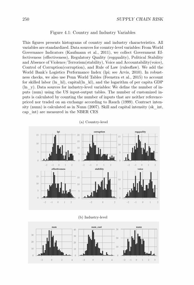
250 SUPPLY CHAIN RISK
Figure 4.1: Country and Industry Variables
This figures presents histograms of country and industry characteristics. Allvariables are standardized. Data sources for country-level variables: From WorldGovernance Indicators (Kaufmann et al., 2011), we collect Government Ef-fectiveness (effectiveness), Regulatory Quality (regquality), Political Stabilityand Absence of Violence/Terrorism(stability), Voice and Accountability(voice),Control of Corruption(corruption), and Rule of Law (ruleoflaw). We add theWorld Bank’s Logistics Performance Index (lpi; see Arvis, 2010). In robust-ness checks, we also use Penn World Tables (Feenstra et al., 2015) to accountfor skilled labor (ln_hl), capital(ln_kl), and the logarithm of per capita GDP(ln_y). Data sources for industry-level variables: We define the number of in-puts (num) using the US input-output tables. The number of customized in-puts is calculated by counting the number of inputs that are neither reference-priced nor traded on an exchange according to Rauch (1999). Contract inten-sity (nunn) is calculated as in Nunn (2007). Skill and capital intensity (sk_int,cap_int) are measured in the NBER CES
(a) Country-level
lpi corruption regquality
effectiveness stability voice
0
5
10
15
0
5
10
15
20
0
5
10
15
0
5
10
15
0
5
10
15
0
5
10
−2 −1 0 1 2 −2 −1 0 1 2 −2 −1 0 1 2
−2 −1 0 1 2 −2 0 2 −2 −1 0 1 2
(b) Industry-level
num num_cust nunn
0
10
20
30
0
10
20
30
40
0
10
20
30
−2 0 2 4 −2 0 2 4 −2 −1 0 1 2 3
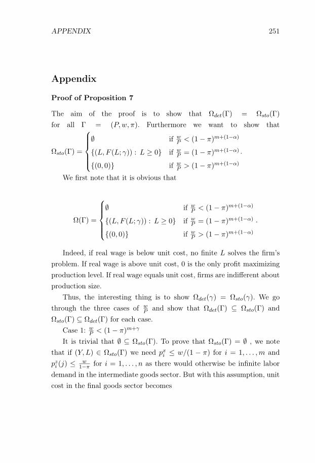
APPENDIX 251
Appendix
Proof of Proposition 7
The aim of the proof is to show that Ωdet(Γ) = Ωsto(Γ)
for all Γ = (P,w, π). Furthermore we want to show that
Ωsto(Γ) =
⎧⎪⎪⎪⎨⎪⎪⎪⎩∅ if w
P < (1− π)m+(1−α)
{(L,F (L; γ)) : L ≥ 0} if wP = (1− π)m+(1−α)
{(0, 0)} if wP > (1− π)m+(1−α)
.
We first note that it is obvious that
Ω(Γ) =
⎧⎪⎪⎪⎨⎪⎪⎪⎩∅ if w
P < (1− π)m+(1−α)
{(L,F (L; γ)) : L ≥ 0} if wP = (1− π)m+(1−α)
{(0, 0)} if wP > (1− π)m+(1−α)
.
Indeed, if real wage is below unit cost, no finite L solves the firm’sproblem. If real wage is above unit cost, 0 is the only profit maximizingproduction level. If real wage equals unit cost, firms are indifferent aboutproduction size.
Thus, the interesting thing is to show Ωdet(γ) = Ωsto(γ). We gothrough the three cases of w
P and show that Ωdet(Γ) ⊆ Ωsto(Γ) andΩsto(Γ) ⊆ Ωdet(Γ) for each case.
Case 1: wP < (1− π)m+γ
It is trivial that ∅ ⊆ Ωsto(Γ). To prove that Ωsto(Γ) = ∅ , we notethat if (Y, L) ∈ Ωsto(Γ) we need pxi ≤ w/(1 − π) for i = 1, . . . ,m andpzi (j) ≤ w
1−π for i = 1, . . . , n as there would otherwise be infinite labordemand in the intermediate goods sector. But with this assumption, unitcost in the final goods sector becomes
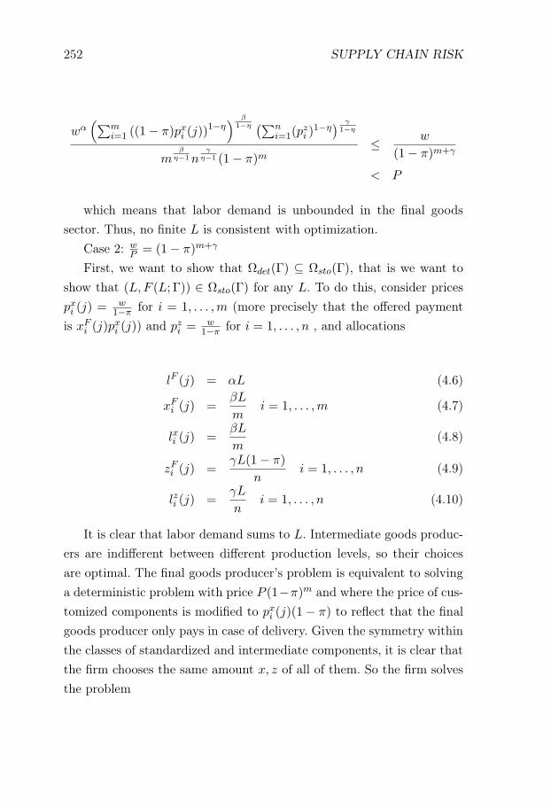
252 SUPPLY CHAIN RISK
wα(∑m
i=1 ((1− π)pxi (j))1−η) β
1−η (∑ni=1(p
zi )
1−η) γ
1−η
mβ
η−1nγ
η−1 (1− π)m≤ w
(1− π)m+γ
< P
which means that labor demand is unbounded in the final goodssector. Thus, no finite L is consistent with optimization.
Case 2: wP = (1− π)m+γ
First, we want to show that Ωdet(Γ) ⊆ Ωsto(Γ), that is we want toshow that (L,F (L; Γ)) ∈ Ωsto(Γ) for any L. To do this, consider pricespxi (j) =
w1−π for i = 1, . . . ,m (more precisely that the offered payment
is xFi (j)pxi (j)) and pzi =
w1−π for i = 1, . . . , n , and allocations
lF (j) = αL (4.6)
xFi (j) =βL
mi = 1, . . . ,m (4.7)
lxi (j) =βL
m(4.8)
zFi (j) =γL(1− π)
ni = 1, . . . , n (4.9)
lzi (j) =γL
ni = 1, . . . , n (4.10)
It is clear that labor demand sums to L. Intermediate goods produc-ers are indifferent between different production levels, so their choicesare optimal. The final goods producer’s problem is equivalent to solvinga deterministic problem with price P (1−π)m and where the price of cus-tomized components is modified to pxi (j)(1− π) to reflect that the finalgoods producer only pays in case of delivery. Given the symmetry withinthe classes of standardized and intermediate components, it is clear thatthe firm chooses the same amount x, z of all of them. So the firm solvesthe problem
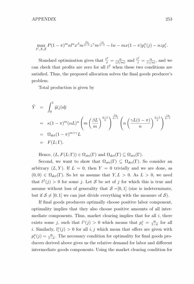
APPENDIX 253
maxlf ,X,Z
P (1− π)mκlαxβmβηη−1 zγm
γηη−1 − lw −mx(1− π)pxi (j)− nzpzi .
Standard optimization gives that lf
x = α(β/m) and lf
z = α(γ/n) , and we
can check that profits are zero for all lf when these two conditions aresatisfied. Thus, the proposed allocation solves the final goods producer’sproblem.
Total production is given by
Y =
∫ 1
0y(j)dj
= κ(1− π)m(αL)α
(m
(βL
m
) η−1η
) βηη−1(n
(γL(1− π)
n
) η−1η
) γηη−1
= Ωdet(1− π)m+γL
= F (L; Γ).
Hence, (L,F (L; Γ)) ∈ Ωsto(Γ) and Ωdet(Γ) ⊆ Ωsto(Γ).
Second, we want to show that Ωsto(Γ) ⊆ Ωdet(Γ). So consider anarbitrary (L, Y ). If L = 0, then Y = 0 trivially and we are done, as(0, 0) ∈ Ωdet(Γ). So let us assume that Y, L > 0. As L > 0, we needthat lf (j) > 0 for some j. Let S be set of j for which this is true andassume without loss of generality that S =[0, 1] (size is indeterminate,but if S = [0, 1] we can just divide everything with the measure of S).
If final goods producers optimally choose positive labor component,optimality implies that they also choose positive amounts of all inter-mediate components. Thus, market clearing implies that for all i, thereexists some j, such that lz(j) > 0 which means that pzi = w
1−π for alli. Similarly, lxi (j) > 0 for all i, j which mean that offers are given withpxi (j) =
w1−π . The necessary condition for optimality for final goods pro-
ducers derived above gives us the relative demand for labor and differentintermediate goods components. Using the market clearing condition for
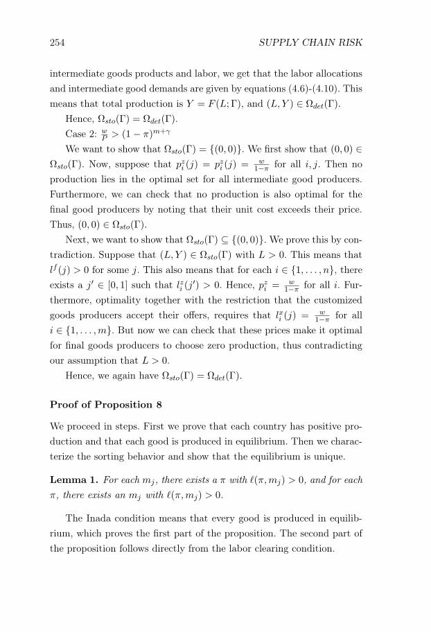
254 SUPPLY CHAIN RISK
intermediate goods products and labor, we get that the labor allocationsand intermediate good demands are given by equations (4.6)-(4.10). Thismeans that total production is Y = F (L; Γ), and (L, Y ) ∈ Ωdet(Γ).
Hence, Ωsto(Γ) = Ωdet(Γ).Case 2: w
P > (1− π)m+γ
We want to show that Ωsto(Γ) = {(0, 0)}. We first show that (0, 0) ∈Ωsto(Γ). Now, suppose that pzi (j) = pzi (j) = w
1−π for all i, j. Then noproduction lies in the optimal set for all intermediate good producers.Furthermore, we can check that no production is also optimal for thefinal good producers by noting that their unit cost exceeds their price.Thus, (0, 0) ∈ Ωsto(Γ).
Next, we want to show that Ωsto(Γ) ⊆ {(0, 0)}. We prove this by con-tradiction. Suppose that (L, Y ) ∈ Ωsto(Γ) with L > 0. This means thatlf (j) > 0 for some j. This also means that for each i ∈ {1, . . . , n}, thereexists a j′ ∈ [0, 1] such that lzi (j
′) > 0. Hence, pzi = w1−π for all i. Fur-
thermore, optimality together with the restriction that the customizedgoods producers accept their offers, requires that lxi (j) = w
1−π for alli ∈ {1, . . . ,m}. But now we can check that these prices make it optimalfor final goods producers to choose zero production, thus contradictingour assumption that L > 0.
Hence, we again have Ωsto(Γ) = Ωdet(Γ).
Proof of Proposition 8
We proceed in steps. First we prove that each country has positive pro-duction and that each good is produced in equilibrium. Then we charac-terize the sorting behavior and show that the equilibrium is unique.
Lemma 1. For each mj, there exists a π with �(π,mj) > 0, and for eachπ, there exists an mj with �(π,mj) > 0.
The Inada condition means that every good is produced in equilib-rium, which proves the first part of the proposition. The second part ofthe proposition follows directly from the labor clearing condition.
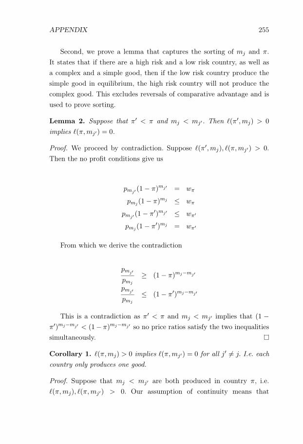
APPENDIX 255
Second, we prove a lemma that captures the sorting of mj and π.It states that if there are a high risk and a low risk country, as well asa complex and a simple good, then if the low risk country produce thesimple good in equilibrium, the high risk country will not produce thecomplex good. This excludes reversals of comparative advantage and isused to prove sorting.
Lemma 2. Suppose that π′ < π and mj < mj′ . Then �(π′,mj) > 0
implies �(π,mj′) = 0.
Proof. We proceed by contradiction. Suppose �(π′,mj), �(π,mj′) > 0.Then the no profit conditions give us
pmj′ (1− π)mj′ = wπ
pmj (1− π)mj ≤ wπ
pmj′ (1− π′)mj′ ≤ wπ′
pmj (1− π′)mj = wπ′
From which we derive the contradiction
pmj′
pmj
≥ (1− π)mj−mj′
pmj′
pmj
≤ (1− π′)mj−mj′
This is a contradiction as π′ < π and mj < mj′ implies that (1 −π′)mj−mj′ < (1− π)mj−mj′ so no price ratios satisfy the two inequalitiessimultaneously.
Corollary 1. �(π,mj) > 0 implies �(π,mj′) = 0 for all j′ = j. I.e. eachcountry only produces one good.
Proof. Suppose that mj < mj′ are both produced in country π, i.e.�(π,mj), �(π,mj′) > 0. Our assumption of continuity means that
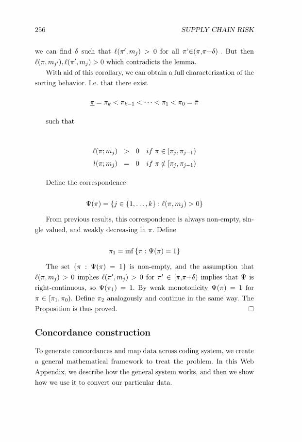
256 SUPPLY CHAIN RISK
we can find δ such that �(π′,mj) > 0 for all π’∈(π,π+δ) . But then�(π,mj′), �(π
′,mj) > 0 which contradicts the lemma.With aid of this corollary, we can obtain a full characterization of the
sorting behavior. I.e. that there exist
π = πk < πk−1 < · · · < π1 < π0 = π
such that
�(π;mj) > 0 if π ∈ [πj , πj−1)
l(π;mj) = 0 if π /∈ [πj , πj−1)
Define the correspondence
Ψ(π) = {j ∈ {1, . . . , k} : �(π,mj) > 0}
From previous results, this correspondence is always non-empty, sin-gle valued, and weakly decreasing in π. Define
π1 = inf {π : Ψ(π) = 1}
The set {π : Ψ(π) = 1} is non-empty, and the assumption that�(π,mj) > 0 implies �(π′,mj) > 0 for π′ ∈ [π,π+δ) implies that Ψ isright-continuous, so Ψ(π1) = 1. By weak monotonicity Ψ(π) = 1 forπ ∈ [π1, π0). Define π2 analogously and continue in the same way. TheProposition is thus proved.
Concordance construction
To generate concordances and map data across coding system, we createa general mathematical framework to treat the problem. In this WebAppendix, we describe how the general system works, and then we showhow we use it to convert our particular data.

APPENDIX 257
The basic building block of our concordance system is amany-to-many concordance between coding systems A and B where wehave weights on both A and B. We call such concordances two-weightedconcordances. An example of such a concordance is provided below:
A B Aw Bw
1 a 10 702 b 20 502 c 20 1003 c 15 404 d 5 705 d 25 706 e 30 90
Note that each code in system A can be converted to multiple Bcodes (in this example, code “2” in System A maps to both code “b” and“c” in System B). The converse is also true: both code “4” and “5” map tocode “e”. The weights code how important the respective industries are.This could for example be total value of shipments, total trade value,etc. Notice the weights are both on A and B, and that they are constandwhenever they stand for the same industry.
We can define this mathematically as there being two sets A,B withmeasures wA, wB giving the mass on each code, and a concordance beinga correspondence
φ : A ⇒ B.
We will write results in terms of this mathematical definition, butalso in terms of examples to show the working of the system.
We will go through three operations relating to two-weighted concor-dances:
1. How to transform quantity variables such as total industry salesusing a two-weighted concordance
2. How to transform property variables such as capital intensity using
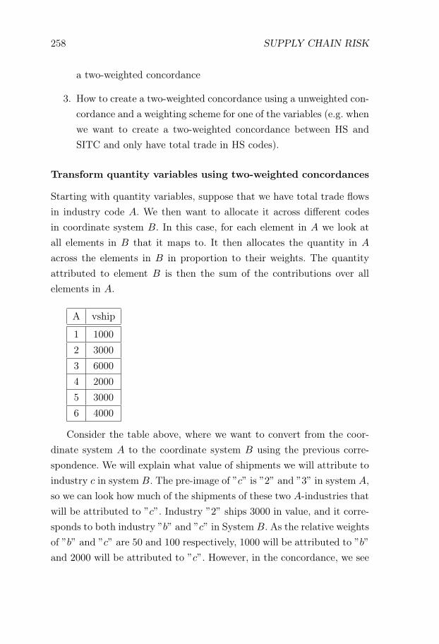
258 SUPPLY CHAIN RISK
a two-weighted concordance
3. How to create a two-weighted concordance using a unweighted con-cordance and a weighting scheme for one of the variables (e.g. whenwe want to create a two-weighted concordance between HS andSITC and only have total trade in HS codes).
Transform quantity variables using two-weighted concordances
Starting with quantity variables, suppose that we have total trade flowsin industry code A. We then want to allocate it across different codesin coordinate system B. In this case, for each element in A we look atall elements in B that it maps to. It then allocates the quantity in A
across the elements in B in proportion to their weights. The quantityattributed to element B is then the sum of the contributions over allelements in A.
A vship
1 10002 30003 60004 20005 30006 4000
Consider the table above, where we want to convert from the coor-dinate system A to the coordinate system B using the previous corre-spondence. We will explain what value of shipments we will attribute toindustry c in system B. The pre-image of ”c” is ”2” and ”3” in system A,so we can look how much of the shipments of these two A-industries thatwill be attributed to ”c”. Industry ”2” ships 3000 in value, and it corre-sponds to both industry ”b” and ”c” in System B. As the relative weightsof ”b” and ”c” are 50 and 100 respectively, 1000 will be attributed to ”b”
and 2000 will be attributed to ”c”. However, in the concordance, we see
APPENDIX 259
that 3 only maps to ”c”, so all 6000 shipments from 3 will be attributedto c. Hence, total attribution to ”c” is 2000 + 6000 = 8000.
We can write this in terms of the mathematical representation Φ aswell, together with the weights μA and μB. If
fA : A → R
is an arbitrary quantity measure on A we convert it to B by
fB(y) =∑
x∈Φ−1(y)
fA(x)× μB(y)∑y′∈Φ(y) μB(y′)
.
The equation is quite difficult to parse, but it says that we take allthe values from the pre-image to y. The value of each of those pre-imagesx attributed to y is equal to the relative weight of μB(y) compared tothe total weights of those codes in B that x maps to.
Transform property variables using two-weighted concordances
The situation is different when we have so-called property variables, forexample capital intensity, skill intensity or other industry level proper-ties. We can see how these differs by means of an example. Suppose thatwe have a concordance between HS 2007 six-digit and HS 2007 ten-digitdata. If we want have data on trade flows on six-digit level and want toconvert these to ten-digit level. Then, the reasonable thing is to split itup across the ten digits according to some weighting scheme.
However, if we instead have measured capital intensity on the six-digit level, the natural thing is to give this capital intensity as a predic-tion for the capital intensity in all ten-digit descendant categories (if wehave no additional information on capital intensity on ten-digit level).Similarly, if we wanted to convert from ten-digit to six-digit, trade flowsought to be summed, whereas for properties it is appropriate to take aweighted average of industry-level properties on the ten digit level.
Thus, we see that property variables translate across coding systemsin a fundamentally different way from quantity variables. We define the
260 SUPPLY CHAIN RISK
transformation scheme for property variables by saying that for each codey ∈ B in the target system, we define its property as a weighted averageof the properties that its pre-images x ∈ A, where we use the weightson A as a weighting scheme. For example, in our example concordance,we would attribute c a property which is the weighted average of 2, 3
in System A, using the measures μA({2}) = 20 and μA({3}) = 15 asweights.
More formally, if we have a property measure
gA : A → R
defined on A, then we translate it to B using φ by the equation
gB(y) =
∑x∈φ−1(y) gA(x)μA(x)∑
x∈φ−1(y) μA(x).
Construct a two-side weighted concordance from a one-sidedweighted concordance
Above we defined how you translate between different coordinate systemsif you have a two-sided weighted concordance. However, sometimes weonly have a one-sided concordance. For example, if we have total tradedata in HS 2007 six-digtit and want to create a concordance between HS2007 6-digit and NAICS 2007 it might be that we do not have data tocreate a natural weighting scheme for NAICS 2007 data.
For this case, we have a procedure to create a two-sided weightedconcordance from a one-sided weighted concordance. It is quite similar tothe quantity transformation above. Suppose that we have a concordanceφ and a measure μA on A and want to create a measure μB on B. Thequestion is how much weight we should attribute to each element y ∈ B.In this case, we go through each element x ∈ A and take its weight μA(x)
and portion it out equally on all elements y′ in B that x maps to. Thisgives us how much weight element x gives to element y, that is μA(x)
|φ(x)|where |φ(x)| gives how many codes x maps to. By summing over all x

APPENDIX 261
we get the total contribution to y. In mathematical terms
μB(y) =∑
x∈φ−1(y)
μA(x)
|φ−1(x)| .
Practical implementation
The process above allows us to define three primitive operations: creatinga two-sided concordance, using it to convert between property variables,and use it to convert between quantity variables. We can use these threeoperations to create arbitrary chains of concordances between data. Be-low we list the actual concordances we create, which weights are used,and how we use these concordances to translate everything into NAICS2012 six-digit data.
Created concordance sequence:
1. Create concordance between HS 2007 six-digit and HS 2007 ten-digit from one sided concordance with total world trade as weighton HS 2007 six digit.
2. Create concordance from HS 2007 10-digit to NAICS 2007 six digitfrom a one sided concordance using [...] as a basic concordance andthe HS 2007 10-digit weights obtained from previous exercise
3. Create concordance from NAICS 2007 six digits to NAICS 2002 sixdigits using a one sided concordance with [...] as basic concordanceand the NAICS 2007 six digits weights obtained from previous step
4. Create concordance from NAICS 2002 six digit to NAICS 1997 sixdigit analogously to previous step
5. Create concordance from NAICS 2007 six digit to NAICS 2012 sixdigit analogously to previous step
6. Create concordance between IO 2007 six-digit and NAICS 2007 sixdigit directly using [....] as basic concordance, total production as

262 SUPPLY CHAIN RISK
weight on IO-codes and previously constructed weights from step2 for NAICS 2007 six digit
7. Create concordance between HS 2007 six digit and SITC rev.2 fourdigits using a one-sided concordance with [...] as basic concordanceand total world trade as weight on HS 2007 six digit.
Once we created these concordances, we can translate all variables toNAICS 2012 six-digit code. We use the following transitions.
Source data set Code Path
NBER CES NAICS 1997 6 digits NAICS 1997 6 digitsNAICS 2002 6 digitsNAICS 2007 6 digitsNAICS 2012 6 digits
IO-table IO 2007 6 digits IO 2007 6 digitsNAICS 2007 6 digitsNAICS 2012 6 digits
BACI Trade data HS 2007 6 digits HS 2007 6 digitsHS 2007 10 digits
NAICS 2007 6 digitsNACIS 2012 6 digits
Rauch SITC rev 2 4 digits SITC rev 2 4dHS 2007 6 digitsHS 2007 10 digits
NAICS 2007 6 digitsNAICS 2012 6 digits

Sammanfattning
Denna avhandling består av fyra oberoende kapitel som berör frågor imakroekonomi, utvecklingsekonomi och utrikeshandel.
Kapitel I, Human Capital and Development AccountingRevisited, är huvudkapitlet i avhandlingen. Kapitlet undersökerhumankapitalets roll i att förklara inkomstskillnaderna mellan världensländer.
Att förstå de stora skillnaderna mellan rika och fattiga länder är enav de största utmaningarna för nationalekonomin, och en framträdandeteori har varit att skillnader i humankapital är viktiga för att förståskillnader i inkomstnivåer (Lucas, 1988).
Teorin tycks fånga ett antal samband väl. Vi vet att högkvalificeradearbetare är mer produktiva än lågkvalificerade arbetare, och en slåendeskillnad mellan rika och fattiga länder är de stora skillnaderna iutbildningsnivåer. Ett liknande mönster framträder när vi analyserarskillnaderna i yrkesfördelningen mellan rika och fattiga länder. I defattigaste länderna jobbar färre än 10 procent av arbetskraften inomett högkvalificerat yrke, medan motsvarande siffra överstiger 50 procenti vissa rika länder.
Inom utvecklingsekonomi har det dock funnits ett inflytelseriktargument mot att humankapital skulle spela en central roll i attförklara inkomstskillnaderna mellan världens länder. Argumentetbygger på att inkomstskillnaderna mellan länder är långt större änden mikroekonomiska avkastningen på humankapital. Med andra ord,skillnaden mellan högkvalificerades och lågkvalificerades löner inom
263

264 SAMMANFATTNING
länder är långt mindre än medelinkomstskillnaderna mellan länder.Om lönen reflekterar produktiviten hos högkvalificerade arbetare, kaninte ett högre utbud av högkvalificerade arbetare förklara rika ländersvälstånd.
Argumentet är enkelt att förstå med överslagsräkning. Människori rika länder utbildar sig i snitt omkring åtta år längre än människori fattiga länder, och avkastningen på utbildning är ca 10 procent perskolår. Om man använder avkastningen på utbildning som ett riktmärke,tyder detta på att fattiga länder ungefär kan fördubbla sina inkomst-nivåer genom att öka sina utbildningsnivåer till rika länders nivåer. Dettaär självklart en stor inkomstökning, men den räcker inte på lång väg föratt överbrygga inkomstgapet mellan fattiga och rika länder: världensfattiga länder är cirka 30 till 40 gånger fattigare än de rikaste länderna.
Inom utvecklingsekonomi har det här argumentet formaliserats ilitteraturen om "utvecklingsbokföring", eller development accounting(Klenow and Rodriguez-Clare, 1997; Hall and Jones, 1999). Slutsatsernafrån den litteraturen är att humankapitalskillnader kan förklara enbegränsad – om icke oansenlig – del av inkomstskillnaderna i världen.Huvuddelen av inkomstskillnaderna går inte att förklara med skillnaderi vare sig fysiskt kapital eller humankapital, och hänförs därför till enicke-observerad restterm som ofta kallas teknologi. Denna term kaninkludera skillnader i vad som traditionellt sett ses som teknologi,men den innefattar också allt annat som förändrar inkomster utanatt mängden insatsvaror förändras. Man kan jämföra teknologi medbegreppet mörk energi i fysik: det är en storhet som måste postulerasför att modellen ska gå ihop.
Det har varit ett inflytelserikt resultat i utvecklingsekonominatt humankapital enbart kan förklara en liten del av världensinkomstskillnader. Resultatet har lett till att forskningen har fokuseratpå att förklara vad de stora teknologiskillnaderna mellan länder bestårav, medan skillnader i humankapital har förutsatts spela en merbegränsad roll.
Det centrala argumentet i traditionell utvecklingsbokföring är att

265
lönepremien reflekterar kvalificerade arbetares produktivitet. Då löne-premien inom länder är långt mindre än inkomstskillnaderna mellanländer antas humankapital spela en begränsad roll. Det finns dock enalternativ syn, nämligen att kvalificerade arbetare är väldigt produktivai rika länder, men att deras relativlöner begränsas av det höga utbudetav kvalificerade tjänster i rika länder. Detta argument har framförts iJones (2014) och bygger på en nedåtlutande efterfrågekurva för kvali-ficerade tjänster. Formellt sker detta om okvalificerade och kvalificeradetjänster inte är perfekt utbytbara.
Avsaknad av perfekt utbytbarhet kan leda till att humankapitaletsroll underskattas, men det finns mindre samsyn på hur kvantitativt viktigdenna mekanism är. För att bedöma denna mekanism behöver man göraen skattning av hur mycket lägre det relativa priset på kvalificeradetjänster är i rika länder.
I mitt kapitel använder jag evidens från utrikeshandelsdata för attgöra detta. Jag noterar att länder med relativt dyra kvalificerade tjänsterkan förväntas exportera relativt få kunskapsintensiva produkter. Jagvisar sedan hur den här insikten kan användas för att skatta skillnaderi relativpriset mellan kvalificerade och okvalificerade tjänster med hjälpav internationell handelsdata.
Min analys av handelsdatan tyder på att kvalificerade tjänster ärrelativt sett mycket dyrare i fattiga jämfört med i rika länder. Prisetpå arbetstjänster beror både på hur mycket en arbetare kostar (lönen)samt hur många tjänster en arbetare levererar (effektiviteten). Jag visaratt det höga priset på kvalificerade tjänster i fattiga länder både berorpå en hög relativlön, samt på en låg relativ effektivitet hos kvalificeradearbetare.
Mina resultat tyder på att humankapital kan spela en större roll iatt förklara världens inkomstskillnader än vad som hävdas i traditionellutvecklingsbokföring. Om jag följer traditionell utvecklingsbokföringoch antar att effektivitetsskillnader hos kvalficerad arbetskraft speglarhumankapital, kan humankapital förklara en majortiet av världensinkomstskillnader. Det här tyder på att vi inte kan utesluta en central
266 SAMMANFATTNING
roll för humankapital när vi försöker modellera ekonomisk utveckling.Att tolka effektivitet av kvalificerad arbetskraft som humankapital
är i linje med hur traditionell utvecklingsbokföring fungerar. Däremot ärdet svårt att utesluta andra tolkningar, då pris- och kvantitetsdata intelåter oss skilja mellan humankapital och andra källor av produktivitet.Intuitivt sett är det svårt att se utifrån styckpris och lönebetalningar omnågon är bra på att hamra eller har en bra hammare. Vad vi däremot kansäga är att alternativa förklaringar till effektivitetsskillnader fortfarandemåste förklara den selektivt höga effektiviteten av kvalificerad arbet-skraft i rika länder. Därför är slutsatsen att inkomstskillnader antingenberor på rena humankaptitalskillnader, eller på skillnader mellan rikaoch fattiga länder som selektivt ökar produktiviteten av kvalificerad ar-betskraft i rika länder.
Kapitel II, Price Level Determination When Tax Paymentsare Required in Money, är författat tillsammans med Erik Öberg.Det utforskar hur ett krav på att skatter ska betalas i pengar påverkarhur pengar värderas.
Penningvärdet har visat sig vara svårt att modellera inomnationalekonomin. Utmaningen är att pengar är värdelösa i sig, vilketinnebär att vanlig konsumtionsteori förutspår att de saknar värde. Enklass av modeller som har försökt förklara penningvärdet bygger påatt pengar har ett likviditetsvärde, då pengar av sedvänja användssom transaktionsmedel i ekonomin. Intuitionen är att jag accepterardina pengar som betalning under antagandet att andra kommer attacceptera dem i sin tur. Pengars värde upprätthålls genom ett nät avförväntningar.
Även om sådana likviditetsteorier är rimliga, kan de inte förklaravarför detta nät av förväntningar nästan alltid leder till att statenspengar blir det allmänna transaktionsmedlet. Ett likviditetsvärde skil-jer sig också från andra typer av konsumtionsvärden då det är självref-ererande, i den bemärkelsen att en varas likviditetsvärde beror på desspris: pengar har ett värde som transaktionsmedel just för att pengarär värdefulla. Detta betyder att likviditetsteorier inte kan utesluta att

267
pengar plötsligt förlorar sitt värde genom att det nät av förväntningarsom upprätthåller deras värde bryts.
Men för statliga pengar tycks vi sällan, om ens någonsin, observeraatt pengar förlorar sitt värde på detta sätt. Det sedvanliga sättet förstatliga pengar att bli värdelösa är istället genom en övertryckning avpengar – som i Tyskland under 1920-talet eller mer nyligen i Zimbabwe –eller genom att den understödjande staten kollapsar – som för Sydstater-nas valuta efter amerikanska inbördeskriget eller för ett antal japanskaockupationsvalutor efter andra världskriget.
Dessa fakta tyder på att penningvärdet på något plan hänger ihopmed statlig makt. Detta väcker en fråga om hur denna koppling ser ut.Kapitel I visar att ett sätt för staten att tillförsäkra pengar ett värde ärgenom att kräva att skatter ska betalas med pengar.
Idén att penningvärdet kan förklaras med ett krav påskattebetalningar är gammal inom nationalekonomin. En informellversion finns redan hos Adam Smith. I kapitlet formaliserar vi dennaidé i en allmän jämviktsmodell, och visar under vilka villkor staten kantillförsäkra pengar ett specifikt värde genom att reglera penningutbudetsamt genom att kräva att skatter ska betalas med pengar.
I vår grundmodell saknar pengar ett intrinsikalt värde. Vi utforskaräven hur resultaten påverkas om vi antar att pengar dessutom har ettlikviditetsvärde. Vi visar att penningvärdet under detta antagande intebestäms direkt av skattekraven, men att skattekraven utesluter möj-ligheten att pengar kan förlora sitt värde enbart för att folk gemensamttappar tron på dem.
Kapitel III, Swedish Unemployment Dynamics: New Methodsand Results, är författat tillsammans med Niels-Jakob Harbo Hansenoch studerar de statistiska egenskaperna hos arbetslöshetsvariationer.
Kapitlet behandlar en känd fråga inom arbetsmarknadsekonomi. Vivet att små nettoflöden på arbetsmarknaden döljer stora bruttoflöden.Det betyder att en ökning av arbetslösheten antingen kan drivas av attarbetstagare förlorar sina arbeten i en högre takt, eller att det tar längretid för arbetslösa att hitta ett nytt jobb. För att förstå vad som driver

268 SAMMANFATTNING
en viss förändring på arbetsmarknaden måste man studera arbetsmark-nadens underliggande flöden.
Kapitlet utvecklar en ny metod för att bryta ned variationerna iarbetslöshet till underliggande flöden. Metoden modifierar ett antal an-taganden i de mest använda metoderna inom litteraturen för att anpassadem till analys av europeiska arbetsmarknader. Det sedvanliga antagan-det som har använts i litteraturen är att arbetsmarknaden befinner signära sitt fortvarighetstillstånd (Shimer, 2007).1
Detta antagande fungerar väl för att beskriva den amerikanskaarbetsmarknaden som kännetecknas av stora flöden och en snabbkonvergens mot sitt fortvarighetstillstånd. Det är dock välkänt attantagandet fungerar sämre för europeiska arbetsmarknader, därstorleken på arbetsmarknadens flöden är mindre, vilket gör attarbetsmarknaden långsammare når sitt fortvarighetstillstånd efter enförändring av de underliggande flödena. Vidare kännetecknas europeiskaarbetsmarknader av dualitet, med en mer eller mindre skarp skiljelinjemellan fasta och tillfälliga anställningar. Då flödesegenskaperna ärmycket annorlunda för olika typer av anställningsformer är detvärdefullt att använda analysmetoder som tillåter en analys avarbetsmarknader med olika anställningsformer.
För att hantera dessa frågor utvecklar vi en metod som tillåter bådei) långsam konvergens mot arbetsmarknadens fortvarighetstillstånd, ochii) ett godtyckligt antal tillstånd som arbetare kan befinna sig i. Vitillämpar vår metod på en ny svensk datamängd som täcker åren 1987-2012. Metoden passar väl för den svenska tillämpningen. Den svenskaarbetsmarknaden kännetecknas av dualitet – under perioden är ca 13procent av den arbetsföra befolkningen anställda på tillfälliga kontrakt –och en tämligen långsam konvergenstakt mot sitt fortvarighetstillstånd.
Vi finner att arbetslöshetsvariationer i ungefär lika stor grad drivs avförändringar i (i) flöden mellan arbete och arbetslöshet, (ii) flöden från
1Begreppet är en översättning av engelskans steady-state, och används inomarbetsmarknadsekonomi för att beskriva det tillstånd som skulle råda om dagensflödesstorlekar fortsatte för alltid.
269
arbetlöshet till arbete, samt (iii) flöden in och ut ur arbetskraften. Flödensom innefattar tillfälligt anställda bidrar med 44 procent av variationeni arbetslöshet, vilket är mycket med tanke på den relativt låga andelenav arbetskraften som har tillfälliga kontrakt.
Vi visar också att det är viktigt att ta den långsamma konvergen-stakten till fortvarighetstilltståndet i beaktande. Om vi antar att arbets-marknaden omedelbart når sitt fortvarighetstillstånd, stiger den skattadebetydelsen av flöden till och från fasta anställningar. En trolig orsak tilldetta är att fortvarighetstillståndet nås långsamt när det sker en förän-dring av flöden till och från fasta anställningar, då det finns många fastaanställda och flödena är små. Antagandet om omedelbar konvergens göratt flödesförändringens betydelse överdrivs. Dessa resultat är av bredareintresse för studier av europeiska arbetsmarknader, då de tyder på attdet kan vara problematiskt att använda antagandet om omedelbar kon-vergens när man studerar duala arbetsmarknader.
Kapitel IV, Supply Chain Risk and the Pattern of Trade, ärförfattat tillsammans med Maximilian Eber. Vi utforskar huruvida län-der som erbjuder tillförlitliga försörjningskedjor specialiserar sig i attproducera varor som är känsliga för risker i försörjningskedjan.
Vi formaliserar den här hypotesen genom att bygga en modell avinternationell handel med flera sektorer och riskabla försörjningskedjor.Varje sektor producerar en vara och använder ett antal olika insatsvaror,och det finns en risk att leveransen av en insatsvara inte kommer attfungera.
Effekten av ett leveransmisslyckande beror på insatsvaranskaraktär. Vissa insatsvaror är standardiserade, såsom vete, och fördessa insatsvaror påverkas inte det sammantagna utbudet av enskildaleverantörers problem. Enskilda problem tidigt i kedjan stör inteproduktionen nedåt i kedjan, då det är lätt att byta leverantör.Andra insatsvaror är specialgjorda, i vilket fall störningar tidigt ileveranskedjan sprids nedåt. Då varje specialgjord insatsvara är enpotentiell felkälla, är industrier med många specialgjorda insatsvarormer känsliga för störningar i försörjningskedjan. Vi bygger in den

270 SAMMANFATTNING
här mekanismen i en handelsmodell, och visar att länder med säkraförsörjningskedjor kan förväntas specialisera sig i industrier med mångaspecialgjorda insatsvaror.
Vi testar den här förutsägelsen genom att utföra en regressions-analys på internationella handelsflöden. Vi följer en metod som utveck-lats i litteraturen för att testa teorier om komparativa fördelar. Meto-den går ut på att utföra en regression av handelsflöden på fixeffekterav land och industri, samt på en interaktionsterm mellan en landegen-skap och en industriegenskap (Romalis, 2004; Nunn, 2007; Nunn andTrefler, 2015). I vårt fall är landegenskapen ett mått på försörjnings-kedjans tillförlitlighet, och industriegenskapen är antalet specialgjordainsatsvaror som en industri använder. Vi visar att interaktionstermenär positiv, och att en standardavvikelses ökning i en försörjningskedjastillförlitlighet och en industris störningskänslighet leder till en ökning avexporten om 10 procent. Denna effekt är robust med avseende på en radmodifikationer i den empiriska modellspecifikationen.
Litteraturförteckning
Hall, R. E. and Jones, C. I. (1999). Why do Some Countries Produce SoMuch More Output Per Worker than Others? The Quarterly Journalof Economics, 114(1):83–116.
Jones, B. F. (2014). The Human Capital Stock: A Generalized Approach.American Economic Review, 104(11):3752–3777.
Klenow, P. and Rodriguez-Clare, A. (1997). The Neoclassical Revival inGrowth Economics: Has It Gone Too Far? Technical report.
Lucas, R. E. (1988). On the mechanics of economic development. Journalof Monetary Economics, 22(1):3–42.
Nunn, N. (2007). Relationship-Specificity, Incomplete Contracts, and thePattern of Trade. The Quarterly Journal of Economics, 122(2):569–600.

LITTERATURFÖRTECKNING 271
Nunn, N. and Trefler, D. (2015). Domestic Institutions as a Source ofComparative Advantage. Handbook of International Economics, 4:263–315.
Romalis, J. (2004). Factor Proportions and the Structure of CommodityTrade. American Economic Review, 94(1):67–97.
Shimer, R. (2007). Reassessing the Ins and Outs of Unemployment.NBER Working Paper, 13421.

272 SAMMANFATTNING
MONOGRAPH SERIES
1. Michaely, Michael The Theory of Commercial Policy: Trade andProtection, 1973
2. Söderström, Hans Tson Studies in the Microdynamics of Productionand Productivity Change, 1974
3. Hamilton, Carl B. Project Analysis in the Rural Sector with SpecialReference to the Evaluation of Labour Cost, 1974
4. Nyberg, Lars and Staffan Viotti A Control Systems Approach toMacroeconomic Theory and Policy in the Open Economy, 1975
5. Myhrman, Johan Monetary Policy in Open Economies, 1975
6. Krauss, Melvyn International Trade and Economic Welfare, 1975
7. Wihlborg, Clas Capital Market Integration and Monetary Policyunder Different Exchange Rate Regimes, 1976
8. Svensson, Lars E.O. On Competitive Markets and IntertemporalResources Allocation, 1976
9. Yeats, Alexander J. Trade Barriers Facing Developing Countries,1978
10. Calmfors, Lars Prices, Wages and Employment in the Open Econ-omy, 1978
11. Kornai, János Economics of Shortage, Vols I and II, 1979
12. Flam, Harry Growth, Allocation and Trade in Sweden. An Empir-ical Application of the Heckscher-Ohlin Theory, 1981
13. Persson, Torsten Studies of Alternative Exchange Rate Systems.An Intertemporal General Equilibrium Approach, 1982
14. Erzan, Refik Turkey’s Comparative Advantage, Production andTrade Patterns in Manufactures. An Application of the FactorProportions Hypothesis with Some Qualifications, 1983
15. Horn af Rantzien, Henrik Imperfect Competition in Models of WageFormation and International Trade, 1983
273

274 MONOGRAPH SERIES
16. Nandakumar, Parameswar Macroeconomic Effects of Supply SidePolicies and Disturbances in Open Economies, 1985
17. Sellin, Peter Asset Pricing and Portfolio Choice with InternationalInvestment Barriers, 1990
18. Werner, Ingrid International Capital Markets: Controls, Taxes andResources Allocation, 1990
19. Svedberg, Peter Poverty and Undernutrition in Sub-SaharanAfrica: Theory, Evidence, Policy, 1991
20. Nordström, Håkan Studies in Trade Policy and Economic Growth,1992
21. Hassler, John, Lundvik, Petter, Persson, Torsten and Söderlind,Paul The Swedish Business Cycle: Stylized facts over 130 years,1992
22. Lundvik, Petter Business Cycles and Growth, 1992
23. Söderlind, Paul Essays in Exchange Rates, Business Cycles andGrowth, 1993
24. Hassler, John A.A. Effects of Variations in Risk on Demand andMeasures of Business Cycle Comovements, 1994
25. Daltung, Sonja Risk, Efficiency, and Regulation of Banks, 1994
26. Lindberg, Hans Exchange Rates: Target Zones, Interventions andRegime Collapses, 1994
27. Stennek, Johan Essays on Information-Processing and Competi-tion, 1994
28. Jonsson, Gunnar Institutions and Incentives in Monetary and Fis-cal Policy, 1995
29. Dahlquist, Magnus Essays on the Term Structure of Interest Ratesand Monetary Policy, 1995
30. Svensson, Jakob Political Economy and Macroeconomics: On For-eign Aid and Development, 1996
31. Blix, Mårten Rational Expectations and Regime Shifts in Macroe-conometrics, 1997
32. Lagerlöf, Nils-Petter Intergenerational Transfers and Altruism,1997
33. Klein, Paul Papers on the Macroeconomics of Fiscal Policy, 1997
34. Jonsson, Magnus Studies in Business Cycles, 1997
275
35. Persson, Lars Asset Ownership in Imperfectly Competitive Markets,1998
36. Persson, Joakim Essays on Economic Growth, 1998
37. Domeij, David Essays on Optimal Taxation and Indeterminacy,1998
38. Flodén, Martin Essays on Dynamic Macroeconomics, 1999
39. Tangerås, Thomas Essays in Economics and Politics: Regulation,Elections and International Conflict, 2000
40. Lidbom, Per Pettersson Elections, Party Politics and EconomicPolicy, 2000
41. Vestin, David Essays on Monetary Policy, 2001
42. Olofsgård, Anders Essays on Interregional and International Po-litical Economics, 2001
43. Johansson, Åsa Essays on Macroeconomic Fluctuations and Nom-inal Wage Rigidity, 2002
44. Groth, Charlotta Topics on Monetary Policy, 2002
45. Gancia, Gino A. Essays on Growth, Trade and Inequality, 2003
46. Harstad, Bård Organizing Cooperation: Bargaining, Voting andControl, 2003
47. Kohlscheen, Emanuel Essays on Debts and Constitutions, 2004
48. Olovsson, Conny Essays on Dynamic Macroeconomics, 2004
49. Stavlöt, Ulrika Essays on Culture and Trade, 2005
50. Herzing, Mathias Essays on Uncertainty and Escape in TradeAgreements, 2005
51. Bonfiglioli, Alessandra Essays on Financial Markets and Macro-economics, 2005
52. Pienaar, Natalie Economic Applications of Product Quality Regu-lation in WTO Trade Agreements, 2005
53. Song, Zheng Essays on Dynamic Political Economy, 2005
54. Eisensee, Thomas Essays on Public Finance: Retirement Behaviorand Disaster Relief, 2005
55. Favara, Giovanni Credit and Finance in the Macroeconomy, 2006
56. Björkman, Martina Essays on Empirical Development Economics:Education, Health and Gender, 2006
276 MONOGRAPH SERIES
57. Larsson, Anna Real Effects of Monetary Regimes, 2007
58. Prado, Jr., Jose Mauricio Essays on Public Macroeconomic Policy,2007
59. Tonin, Mirco Essays on Labor Market Structures and Policies, 2007
60. Queijo von Heideken, Virgina Essays on Monetary Policy and As-set Markets, 2007
61. Finocchiaro, Daria Essays on Macroeconomics, 2007
62. Waisman, Gisela Essays on Discrimination and Corruption, 2008
63. Holte, Martin Bech Essays on Incentives and Leadership, 2008
64. Damsgaard, Erika Färnstrand Essays on Technological Choice andSpill- overs, 2008
65. Fredriksson, Anders Bureaucracy, Informality and Taxation: Es-says in Development Economics and Public Finance, 2009
66. Folke, Olle Parties, Power and Patronage: Papers in Political Eco-nomics, 2010
67. Yanagizawa-Drott, David Information, Markets and Conflict: Es-says on Development and Political Economics, 2010
68. Meyersson, Erik Religion, Politics and Development: Essays inDevelopment and Political Economics, 2010
69. Klingelhöfer, Jan Models of Electoral Competition: Three Essayson Political Economics, 2010
70. Perrotta, Maria Carmela Aid, Education and Development, 2010
71. Caldara, Dario Essays on Empirical Macroeconomics, 2011
72. Mueller, Andreas Business Cycles, Unemployment and Job Search:Essays in Macroeconomics and Labor Economics, 2011
73. Von Below, David Essays in Climate and Labor Economics, 2011
74. Gars, Johan Essays on Macroeconomics of Climate Change, 2012
75. Spiro, Daniel Some Aspects on Resource and BehavioralEconomics, 2012
76. Ge, Jinfeng Essays on Macroeconomics and Political Economy,2012
77. Li, Yinan Institutions, Political Cycles and Corruption: Essays onDynamic Political Economy of Government, 2013
78. Håkanson, Christina Changes in Workplaces and Careers, 2013
277
79. Qin, Bei Essays on Empirical Development and PoliticalEconomics, 2013
80. Jia, Ruixue Essays on the Political Economy of China’s Develop-ment, 2013
81. Campa, Pamela Media Influence on Pollution, and Gender Equal-ity, 2013
82. Seim, David Essays on Public, Political and Labor Economics, 2013
83. Shifa, Abdulaziz Essays on Growth, Political Economy andDevelopment, 2013
84. Panetti, Ettore Essays on the Economics of Banks and Markets,2013
85. Schmitt, Alex Beyond Pigou: Climate Change Mitigation, PolicyMaking and Distortions, 2014
86. Rogall, Thorsten The Economics of Genocide and War, 2015
87. Baltrunaite, Audinga Political Economics of Special Interests andGender, 2016
88. Harbo Hansen, Niels-Jakob Jobs, Unemployment, and Macroeco-nomic Transmission, 2016
89. Stryjan, Miri Essays on Development Policy and the Political Econ-omy of Conflict, 2016
90. Karadja, Mounir On the Economics and Politics of Mobility, 2016
91. Kitamura, Shuhei Land, Power, and Technology: Essays on Polit-ical Economy and Historical Development, 2016

Copyright © 2022 FDOKUMEN