Essays on Sub-National Value Added Tax of India and Tax ...

Georgia State University Georgia State University

ScholarWorks @ Georgia State University ScholarWorks @ Georgia State University

Economics Dissertations

Summer 6-30-2015

Essays on Sub-National Value Added Tax of India and Tax Essays on Sub-National Value Added Tax of India and Tax

Incidence Incidence

Astha Sen

Follow this and additional works at: https://scholarworks.gsu.edu/econ_diss

Recommended Citation Recommended Citation Sen, Astha, "Essays on Sub-National Value Added Tax of India and Tax Incidence." Dissertation, Georgia State University, 2015. https://scholarworks.gsu.edu/econ_diss/112

This Dissertation is brought to you for free and open access by ScholarWorks @ Georgia State University. It has been accepted for inclusion in Economics Dissertations by an authorized administrator of ScholarWorks @ Georgia State University. For more information, please contact [email protected].

https://scholarworks.gsu.edu/

https://scholarworks.gsu.edu/econ_diss

https://scholarworks.gsu.edu/econ_diss?utm_source=scholarworks.gsu.edu%2Fecon_diss%2F112&utm_medium=PDF&utm_campaign=PDFCoverPages

mailto:[email protected]

ABSTRACT

ESSAYS ON SUB-NATIONAL VALUE ADDED TAX OF INDIA AND TAX INCIDENCE

By

ASTHA SEN

August 2015

Committee Chair: Dr. Sally Wallace

Major Department: Economics

The three essays of this dissertation inform tax policy design. It is a compilation of

empirical and experimental research work. The first and the second essays explore the

performance of a recent tax policy reform at the sub-national level in India in terms of revenue

efficiency as well as economic efficiency. India is among the only three countries in the world to

have adopted a sub-national VAT. Therefore, empirically examining its performance not only

improves the understanding of this important tax policy reform but also informs tax policy

decision-making at the sub-national level in other developing countries.

India transitioned to the state-level VAT between the years 2003 and 2008. Among other things,

it was expected to achieve revenue growth and decrease tax cascading on commodities by

improving economic efficiency of the indirect tax system. In the first essay, I model the impact

of the VAT on revenue by adding revenue dependent administrative and compliance costs

associated with taxation to an existing model developed by Keen and Lockwood (2010). The

theoretical results show that replacing one type of indirect tax with another improves long-run

revenue efficiency only if there is a net decrease in the administrative, compliance and

distortionary costs of taxation at the margin. I then compile a unique state-level dataset for the

years 1990 to 2010 to determine changes in the long-run revenue efficiency from the use of the

VAT. This essay contributes to the literature by extending an existing revenue efficiency model

and testing it in the unique situation of India’s sub-national VAT. The results reveal a significant

improvement in the long-run revenue efficiency of the sales tax instrument used by state

governments. The model implies this improvement is driven by a net fall in the marginal taxation

costs from the use of the state-level VAT. This finding has important implications on the role of

a sub-national VAT in the future as an effective tax instrument in the developing countries.

The second essay appeals to the general theory of tax incidence which suggests that a

VAT will have less impact on prices than a traditional turnover tax because the VAT does not

“get stuck” in the production process as a turnover tax does. The impact should be larger for

goods that have more components to the production process as the tax then “touches” more of

the final product. In this essay I measure the change in the level of tax cascading with VAT by

using multiple waves of the state- and household-level expenditure surveys. Specifically I test

the impact of the VAT on the real consumption of households on a variety of consumption

goods. I find the biggest significant decrease in the tax cascading burden of the long-term

durable goods which essentially involve the maximum production components. This result is

found in the 18 more developed states of India which are the focus of the empirical analysis due

to data constraints.

The third essay is an experimental research which looks at the influence of institutions on

the economic burden of an excise tax. The traditional long-run tax incidence theory establishes

that the economic incidence of an excise tax is independent of the assignment of the liability to

pay tax. However, the theory is silent on the possible effects of the market institutions on tax

incidence. Since all markets need an institution to function and every market institution has its

own unique price and quantity determination property, it is important to understand its bearings

on the incidence of taxes. Existing experimental research has tested economic incidence under

many different market institutions but no previous research systematically analyzes and

compares the incidence of a unit tax under two important market institutions we deal with in

everyday life. One of these institutions is posted offer which dominates the consumer goods

markets in developed countries and the other is double auction which is frequently observed in

developing countries. I report a significant impact of these market institutions on tax incidence.

In particular, I find that consumers bear a much higher burden of a unit tax in the posted offer

markets as compared to the double auction markets and their burden further increases when the

liability to pay the tax is on the seller.

ESSAYS ON SUB-NATIONAL VALUE ADDED TAX OF INDIA AND TAX INCIDENCE

By

ASTHA SEN

A Dissertation Submitted in Partial Fulfillment

of the Requirements for the Degree

of

Doctor of Philosophy

in the

Andrew Young School of Policy Studies

of

Georgia State University

GEORGIA STATE UNIVERSITY

2015

Copyright by

Astha Sen

2015

ACCEPTANCE

This dissertation was prepared under the direction of the candidate's Dissertation Committee. It

has been approved and accepted by all members of that committee, and it has been accepted in

partial fulfillment of the requirements for the degree of Doctor of Philosophy in Economics in

the Andrew Young School of Policy Studies of Georgia State University.

Dissertation Chair: Dr. Sally Wallace

Committee: Dr. Yongsheng Xu

Dr. Shiferaw Gurmu

Dr. Abdu Muwonge

Electronic Version Approved By:

Dr. Mary Beth Walker, Dean

Andrew Young School of Policy Studies

Georgia State University

August 2015

iv

DEDICATION

Most of all, this dissertation is dedicated to my parents and my husband Nikhil Mathur. My

parents always believed in me and taught me to be sincere and honest towards whatever I chose

to pursue. They endlessly motivated me to work hard. My father has been my idol and I have

always tried to be as hard-working and sincere towards my work as he has been all his life. My

words cannot begin to thank my parents for their endless love and support. My husband has been

there for me and I am extremely grateful to him for his unfathomable support and encouragement

throughout my PhD years. I also extend my heartfelt thanks to my younger brother, the rest of

my family and my friends for their unyielding and unbroken support, love and encouragement.

v

ACKNOWLEDGEMENTS

I would like to express my deepest gratitude to my committee chair, Dr. Sally Wallace for her

tremendous mentorship and guidance at every step, for always having time for me, for funding

my research work, for her persistent support, for believing in me and for being patient with me. It

has been an absolute honor and joy to work under her mentorship. I have learnt immensely from

her expert and ingenious ideas and advice. I would also like to express most sincere gratitude to

all my dissertation committee members, Dr. James Cox, Dr. Mark Rider, Dr. Melinda Pitts, Dr.

Jorge Martinez-Vazquez, and Dr. Julie Hotchkiss for their generous and extraordinary

mentorship and for their time. I want to thank you all for constantly helping me learn and strive

for improvement, and for stirring the utmost enthusiasm of learning and research in me. It has

been an honor to work with each one of you. I would like to thank all my professors at Georgia

State University for their remarkable courses, guidance, help and support. I want to thank the

Andrew Young School and the research department of Federal Reserve Bank of Atlanta for

funding my Ph.D. education. I would like to extend my special thanks to Dr. Melinda Pitts and

Dr. Julie Hotchkiss for giving me the exceptional opportunity to work at the Federal Reserve

Bank of Atlanta. I want to thank Bess Blyler for her phenomenal help and support with

everything in all my years at GSU, especially with my job market packet for two years.

vi

TABLE OF CONTENTS

CHAPTER ONE– THE REVENUE EFFICIENCY OF INDIA’S SUB-NATIONAL VAT. ..................................... 1

1 ABSTRACT ....................................................................................................................................... 1

2 INTRODUCTION................................................................................................................................ 2

3 BACKGROUND ................................................................................................................................. 6

3.1 FISCAL CRISIS IN THE STATES BEFORE THE VAT ......................................................................... 6

3.2 FEATURES OF THE INDIRECT TAX SYSTEM AT THE SUB-NATIONAL LEVEL ................................... 8

4 THEORETICAL FRAMEWORK .......................................................................................................... 12

4.1 BASIC MODEL ............................................................................................................................ 13

4.2 MODEL WITH ENDOGENOUS COMPLIANCE COST ....................................................................... 18

4.3 EXTENDED REVENUE EFFICIENCY MODEL ................................................................................. 22

5 DATA AND THE EMPIRICAL RESULTS ............................................................................................. 32

5.1 DATA ......................................................................................................................................... 34

5.2 SUMMARY STATISTICS AND THE TRENDS IN THE DATA ............................................................. 34

5.3 REGRESSION ANALYSES ............................................................................................................ 38

6 CONCLUSION ................................................................................................................................. 42

7 FIGURES ........................................................................................................................................ 43

8 TABLES ......................................................................................................................................... 47

CHAPTER TWO - DID INDIA’S SUB-NATIONAL VAT IMPROVE ECONOMIC EFFICIENCY? ...................... 54

vii

1 ABSTRACT ..................................................................................................................................... 54

2 INTRODUCTION.............................................................................................................................. 54

3 BACKGROUND ............................................................................................................................... 57

4 THEORETICAL MODEL ................................................................................................................... 59

5 DATA AND METHODOLOGY ........................................................................................................... 62

5.1 DATA ......................................................................................................................................... 62

5.2 REAL CONSUMPTION EXPENDITURE ANALYSIS .......................................................................... 63

5.3 REAL PRICE ANALYSIS ............................................................................................................... 64

6 RESULTS AND CONCLUSION .......................................................................................................... 65

6.1 RESULTS .................................................................................................................................... 65

6.2 CONCLUSION ............................................................................................................................. 76

7 TABLES ......................................................................................................................................... 78

CHAPTER THREE - TAX INCIDENCE: DO INSTITUTES MATTER? AN EXPERIMENTAL STUDY ................ 88

1 ABSTRACT ..................................................................................................................................... 88

2 INTRODUCTION.............................................................................................................................. 88

3 EXPERIMENTAL DESIGN AND PROTOCOL ....................................................................................... 96

4 DATA FROM THE EXPERIMENT .................................................................................................... 102

5 CONCLUSIONS ............................................................................................................................. 108

6 TABLES ....................................................................................................................................... 110

7 FIGURES ...................................................................................................................................... 114

viii

APPENDIX INDEX ................................................................................................................................ 119

APPENDIX 1.1 ...................................................................................................................................... 120

APPENDIX 1.2 ...................................................................................................................................... 136

APPENDIX 1.3 ...................................................................................................................................... 151

APPENDIX 1.4 ...................................................................................................................................... 169

APPENDIX 2 ......................................................................................................................................... 187

VITA .................................................................................................................................................... 195

ix

LIST OF FIGURES

Figure 1 : Graph ....................................................................................................................................... 15

Figure 2: Average state’s OTR as a percentage of GSDP over the period of 1990 to 2000 ..................... 43

Figure 3 : Average revenue deficit as a percentage of GSDP ................................................................... 43

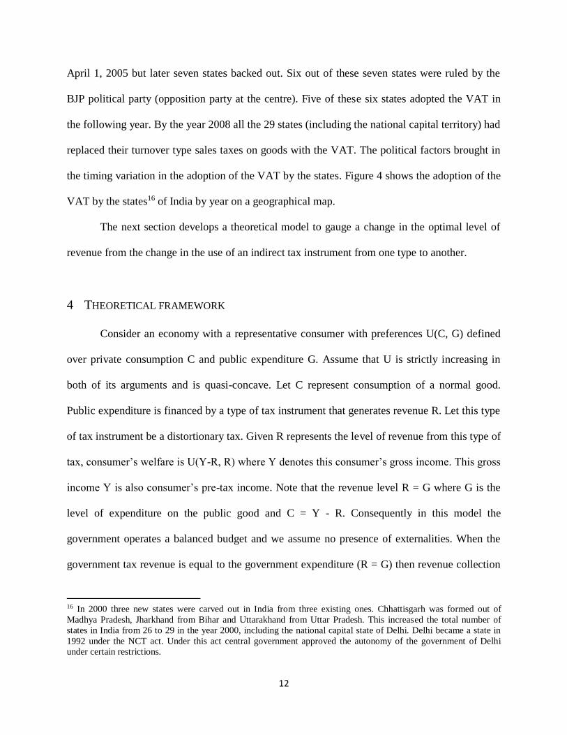
Figure 4: Implementation of the VAT in the states of India by year ........................................................ 44

Figure 5 : Trend in state’s revenue ratios (in percent) .............................................................................. 45

Figure 6: Growth rate in ITR as a percentage of TTR for special and non-special category of states ...... 45

Figure 7: Growth rate in sales tax / VAT revenue as a percentage of TTR for special and non-special

category of states ...................................................................................................................................... 46

Figure 8: Percentage differences in pair-wise comparisons of average buyer prices .............................. 114

Figure 9: Cumulative distribution functions of the buyer prices for the two double auction market

treatments. .............................................................................................................................................. 115

Figure 10: Cumulative distribution functions of the buyer prices, using the last 15 trading periods of each

market session, for the two posted offer market treatments. ................................................................... 116

Figure 11: Cumulative distribution functions of the buyer prices from the double auction and posted offer

market treatments with the tax on the buyer. .......................................................................................... 117

Figure 12: Cumulative distribution functions of the buyer prices for the double auction and posted offer

market treatments with the tax on the sellers. ......................................................................................... 118

file:///C:/Users/mathurn/Desktop/Final%20Defense/Dissertation_Astha_June17_new.docx%23_Toc422692429

x

LIST OF TABLES

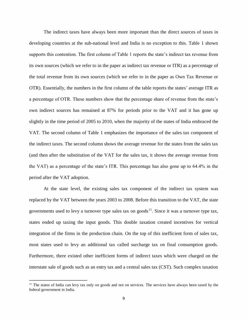
Table 1: Percentage share of ITR to OTR and Sales tax / VAT revenue to ITR ...................................... 47

Table 2: Summary statistics ..................................................................................................................... 48

Table 3: Average annual growth rates in ITR and sales tax / VAT revenues before and after the VAT... 49

Table 4: Results using the FE estimator with ITR per capita as the dependent variable........................... 50

Table 5: Results using the FE estimator with sales tax/ VAT revenue per capita as the dependent variable

.................................................................................................................................................................. 51

Table 6: Results using the FE estimator with AR (1) errors ..................................................................... 52

Table 7: Results using the IV estimator of the First-difference model ..................................................... 53

Table 8 : Price and tax revenue when a single –stage sales tax is imposed at different points of production

.................................................................................................................................................................. 60

Table 9: Sample means of real consumption expenditure per capita by commodity groups .................... 78

Table 10. Sample means of real consumption expenditure per capita by commodity groups ................... 79

Table 11 : Consumption expenditure results for urban sector and developed states ................................. 80

Table 12: Consumption expenditure results for urban sector and developed states .................................. 80


Table 14:. Consumption expenditure results for urban sector and developed states ................................. 81


Table 16: Consumption expenditure results for urban sector and developed states ................................. 82

Table 17: Consumption expenditure results for rural sector and developed states .................................. 83

Table 18. Consumption expenditure results for rural sector and developed states .................................... 83




xi


Table 23. Price Results for urban areas and developed states including state and year fixed effects ........ 86

Table 24. Price Results for rural areas and developed states including state and year fixed effects ......... 87

Table 25: Individual marginal costs and values per unit......................................................................... 110

Table 26: Demographic characteristics of the full sample and by treatment .......................................... 111

Table 27: Earnings in U.S. dollars, by treatment .................................................................................... 112

Table 28: Equilibrium buyer prices (ED) and tax burden as a percent of tax revenue, by treatment ...... 112

Table 29: Equilibrium quantities and excess burdens, by treatment ....................................................... 113

1

1. CHAPTER ONE– THE REVENUE EFFICIENCY OF INDIA’S SUB-NATIONAL

VAT.

1 ABSTRACT

Despite the demonstrated success and widespread adoption of a national level value-added

tax (VAT), there is a great deal of skepticism among tax policy experts regarding the

administrative feasibility and potential efficiency of this same tax as a revenue source for sub-

national governments. Canada is one of only three countries in the world with a sub-national

VAT and its success is generally attributed to the high quality of its tax administration. Since few

countries have tax administrations of comparable quality, it is widely believed that Canada’s

success cannot be replicated in other countries, particularly in low- and middle-income countries

which generally have weak tax administrations. Between 2003 and 2008 the states of India

transitioned from distortionary sales taxes as their main source of revenue to a more uniform

sub-national VAT. This transition provides an ideal natural experiment to gauge the efficiency

gains from substituting a consumption type, sub-national VAT for a sales tax. Our theoretical

model shows that substituting one type of indirect tax for another improves long-run revenue

efficiency when there is a net marginal decrease in the administrative, compliance and

distortionary costs of taxation. We test this prediction of the model using a unique data set on

state finances for all 29 states of India over the past 21 years. We report a 6.5 to 8 percent

increase in the long-run revenue efficiency in the 18 most developed states of India from the

transition to the VAT. This is an important finding because it suggests that a sub-national,

2

consumption type VAT may be a feasible and efficient tax for sub-national governments even in

low- and middle-income countries.

2 INTRODUCTION

The rise of the value-added tax (VAT) has undoubtedly been one of the most significant

tax developments since its inception in 1954 in France. The VAT has become a prime instrument

in tax policy among a majority of the developed and developing countries. The main reason for

the popularity of the VAT is its efficiency over other types of indirect taxes. Not only does it

eliminate production inefficiencies associated with the turnover tax, it also is generally thought

to be superior to retail sales taxes as they are more vulnerable to evasion and avoidance. This is

because with retail sales tax, the revenue is lost completely if the tax is evaded at the final point

of sale. On the other hand, the VAT is collected at all the stages of production. Therefore, if the

sale of goods escapes tax at one point, the hope is to catch it at another point in the chain of

production under the VAT regime. In addition, the VAT is compliance incentivizing because

under the VAT regime, wholesalers and retailers have to ensure that the traders they deal with

pay the tax in order to be eligible for input tax credit. This self-policing of the VAT has a higher

probability of exposing forged accounts and an informal economy than the retail sales tax (Bird

2005 and Agha et al 1996). Primarily for the same reason, a VAT is generally regarded as a more

promising consumption tax for developing countries where the size of the informal sector is

bigger. However, opponents of the VAT do not quite agree. Some studies argue that the opposite

is true. For example, Emran and Stiglitz (2005) show that in the presence of a substantial

‘informal’ sector, the VAT that falls on the formal sector acts to deter the growth and

development of the economy as a whole. Also, the retail sales tax may be cheaper to administer

3

since there are fewer taxpayers and thus it is less complicated. Despite these contradictory views,

the VAT has replaced the retail sales tax regime in many developing countries and it continues to

do so.

From the arguments advanced above, questions which naturally come to mind are: do

countries with the VAT have a more efficient system than the ones without it? Has the VAT

improved revenue mobilization in these countries? There is no simple way to answer these sorts

of questions. The answers clearly depend on many factors including the federal structure of the

country we are looking at, the type of a VAT (national, sub-national or/and origin–based or

destination based, income-type or consumption-type), base of the VAT, its threshold limit, and

its many other design features. Additionally, no one type of a VAT is supreme to the other.

Different VATs may be best for different nations at different points of time as Bird (2005) points

out that ‘no one size fits all’. Therefore the questions raised above demand empirical

investigation.

Nellor (1987) performed one of the earliest analyses of the impact of a VAT on revenue

growth on a sample of 11 European countries and his results establish that the VAT improves

revenue performance. Bogetic and Hassan (1993) examine the main determinants of the VAT

revenue using a cross country framework of 34 countries. Their main findings show that, other

things being constant, the VAT generates higher revenue in countries with a single VAT rate

than in countries with multiple VAT rates. Keen and Lockwood (2010) answer the same question

using a panel of 143 countries over 26 years. They establish that in general the VAT has a

significant but modest effect on the revenue performance. Martinez and Bird (2011) build on the

empirical question of Keen and Lockwood (2010) using different econometric techniques and

focusing more on the comparisons of the impact on developing versus developed countries. Their

4

research shows that the positive effect of the VAT is significant only in the developing countries.

At the same time, other related studies provide evidence of poor revenue performance of

a VAT in the low-income countries1. Bird and Gendron (2006) assert that the unsatisfactory

performance of the VAT in the developing countries is grounded in its inefficient administration

and poor tax design. Tanzi (2000) points out the formidable challenges faced by the developing

countries in the establishment of efficient tax systems. These include large informal sector

activities, a large share of agriculture in total output and employment, many small

establishments, and limited capacity of the tax administration. Also, opponents of a VAT argue

that a broken VAT chain gives rise to production inefficiencies and this could more than offset

the benefits from the VAT leading to an overall reduction in the efficiency. All this cited

research brings out one critical fact, that is, in reality the presence of the VAT may or may not

improve overall government revenue efficiency.

All of the above cited literature evaluates the performance of a national level VAT. The

reality becomes even more complicated in the case of a sub-national VAT. Effective

implementation of a sub-national VAT gets more challenging because of the cross border trade2

and the non-uniformity of the VAT rates across the states or regions within a country3. All these

facts make it imperative to empirically evaluate performances of the existing VAT reforms to

better understand their accomplishments and to continually improve their designs. This paper

explores the performance of a recently implemented consumption type, sub-national VAT in

1 Baunsgaard and Keen (2005) raise concerns of revenue gains from a VAT in low-income countries. Emran and

Stiglitz (2005) show that the VAT reduces welfare in the developing countries. 2 The application of a VAT on the interstate trade is often pointed out, by tax policy experts, as the most serious

practical issue with the use of a sub-national VAT (Bird and Gendron (1998)). There is no general consensus on the

best way to apply a destination-based VAT to the interstate trade. (McLure (2005) explains why a sales tax with a

destination principle is more desirable). Bird (1993) points out other problems related to a sub-national VAT. These

include coordination of federal and regional taxes, loss of macroeconomic control and high administrative and

compliance costs. 3 The logical reasoning behind the existence of the non-uniform rates is to preserve the regional government’s

autonomy.

5

India. We believe it is a valuable contribution because performance of a sub-national,

consumption type VAT is far from well-understood in low and middle-income countries.

The type of a sub-national VAT which was put in place in India neither resembles the

theoretically optimal form of a sub-national VAT suggested by Charles McLure (2000)4 or Keen

and Smith (1999)5 nor replicates a successful ‘Dual-VAT’ system thriving in Canada. The VAT

in the states of India replaced an administratively complex and economically distortionary

turnover type of sales tax. However, the homegrown design of a state level VAT which came

into existence casts concerns regarding its performance so far. Therefore it is worthwhile to

empirically evaluate the performance of this major tax reform of India. As far as we know, no

existing research work systematically examines the performance of the state level VATs

introduced in India.

The purpose of this paper is to analyze changes in revenue efficiency from substitution of

a consumption type VAT for a highly distortionary sales tax at the sub-national level in India. By

increase in revenue efficiency we mean an increase in the level of optimal revenue raised by a

benevolent government. We first build on the theoretical model developed by Keen and

Lockwood (2010) by incorporating revenue dependent administrative and compliance costs of

taxation in the model, to gauge the change in revenue efficiency from a tax innovation like a

VAT. Our theoretical model differentiates between long-run revenue dependent administrative

costs and short-run exogenous administrative costs. We then proceed to empirically investigate a

change in the revenue efficiency using data on all the 29 states of India (including the national

4 Subnational VATs are considered infeasible or undesirable for varied reasons (Bird (1993)). The sub-national VAT

recommended by Mclure (2000) is called Compensating VAT (CVAT). This VAT proposes a feasible solution for

implementing a destination- based VAT on inter-state trade. 5 Keen and Smith(1999) propose a viable integrated VAT (VIVAT). This type of VAT implements differential tax

rates on the interstate sales made to registered merchants and sales made to non-registered buyers (which implies

final consumption).

6

capital territory of Delhi) for the years 1990 to 2010. In the empirical analyses we use revenue

per capita to measure the revenue efficiency.

The paper proceeds as follows. Section 3 broadly reviews the fiscal background of the

states of India before the VAT in 1990s and briefly outlines the salient features of the existing

state-level VAT. Section 4 explains the theoretical model and Section 5 presents the results and

Section 6 concludes.

3 BACKGROUND

3.1 FISCAL CRISIS IN THE STATES BEFORE THE VAT

The second half of the 1990s is characterized by a period of fiscal crisis for all the states

of India. At this time the states were grappling with serious erosion of the state finances lead by

the unsustainable debt trends and a remarkable pressure on the availability of resources for the

infrastructure and the basic social services (World Bank, Policy Notes (2008)). The reasons for

high fiscal and revenue deficits in the states in the second half of the 1990s include inadequate

increases in the tax receipts, negative or negligible returns from the public investments due to

public sector units (PSU) losses, large subsidy payments, increases in expenditures on salaries

due to pay revisions, and higher pension payments (Reserve Bank of India (RBI), State Finances

(2002-03)). State Finances (2002-03) pointed out that the tax to GSDP (Gross State Domestic

Product) ratio of the states did not change much throughout the1990s.

The trend in the state’s own tax revenue (OTR) as a percent of its GSDP during the year

1990s is shown in figure 2. Figure 2 shows this trend separately for the special and the non-

special category of states. The states in India are classified as special and non-special category

states by the Government of India (Saxena 1999). In 2001, 11 out of the 29 states were classified

7

as the special category states (or less developed states), which share the common characteristics

of poor infrastructure, hilly and difficult terrain, and large tribal populations6. They have limited

revenue generating capacity of their own. According to the Gadgil formula7 (which determines

the allocation of central assistance for development to the states of India), special category states

are given preference in terms of the development based financial assistance from the federal

government over the non-special states.

Figure 2 shows that in the late 1990s, the state’s own tax revenue remained between 6 to

7% for the non-special category states and between 2 to 3% for the special category states. While

the own revenue of the states was decreasing or flat, they were consistently required to undertake

increasing developmental responsibilities. Consequently the states had to turn to an increased

level of borrowing to meet their expenses. This led to an increase in their revenue deficits as an

absolute figure and also as a proportion of the gross fiscal deficit.

A trend in the revenue deficit (RD), which is the deficit on the current or the revenue

account as a percentage of Gross state domestic product (GSDP) for the years 1991 to 2010 is

shown in Figure 38. Figure 3 shows the five year time trends in RD of the states of India between

years 1991 to 2010. The figure also shows these trends separately for the special and the non-

special states. As clear from the figure, the severity of this crisis was more intense in the non-

special states, or the more developed states, of India as compared to the special category9 states.

Driven by this uniformly spread financial structural weakness across the states, the majority of

the state governments actively initiated various fiscal and institutional reforms. As a result of the

6 Saxena (1999) and Das-Gupta (2012) 7 30 percent of these funds to the states go to the special category sates. In addition, 90 percent of the center’s

development plan assistance received by these states is in the form of grants and just 10 per cent is in the form of

loans as opposed to 30 percent grant and 70 percent loan to the non-special category states. 8 A negative value of revenue deficit implies a surplus on the revenue account. 9There are 11 special category states in India. These states are considered to have geographical hindrances in

infrastructural development. The centre sanctions 90% in grants in plan assistance to these states as they are less

developed.

8

improved economic growth in India since 2003-04 and the fiscal correction efforts initiated by

both the center and the states (World Bank, Policy Notes (2008)), the states achieved fiscal

improvement during 2000-06. The overall fiscal correction for the states of India can also be

seen in Figure 3 where the revenue deficit for the non-special states or the more developed states

turned into surplus over the time period of 2006 to 2010.

The Twelfth Finance Commission10 recommended that the states implement a “golden

rule” by 2008/09. This golden rule specifies that the state government’s current account must not

be in deficit. The golden rule was one of the main objectives of the state governments in the

Fiscal Responsibility Acts of 2003 (State Finances (2002-03)). Since the year 2000, these acts

were put in place in majority of the states as one of the main fiscal reform policies. Figure 3

shows the average value of the revenue deficit for all the state governments in the second-half of

2000s. It can be seen in the figure that the states achieved this objective over a five year period

from 2006 to 2010. Implementation of the VAT was one of the most important tax reforms

undertaken by the states on the revenue side in the second-half of 2000s. Among other things, the

near stagnation in the tax to GSDP ratio of the states at around 8% throughout the 1990s

triggered the initiation of a VAT implementation. The states realized that they needed a strategy

to augment their revenue receipts. In this paper we evaluate the performance of this pivotal tax

reform.

3.2 FEATURES OF THE INDIRECT TAX SYSTEM AT THE SUB-NATIONAL

LEVEL

10The Twelfth Finance Commission was appointed by the President of India on 1st November 2002, (Report of the

Twelfth Finance Commission (2004)). Among other things, the Commission makes recommendations on the

distribution between the union and the states of the tax revenues which are shared between them under Chapter I

Part XII of the Constitution and the allocation of such proceeds between the states.

9

The indirect taxes have always been more important than the direct sources of taxes in

developing countries at the sub-national level and India is no exception to this. Table 1 shown

supports this contention. The first column of Table 1 reports the state’s indirect tax revenue from

its own sources (which we refer to in the paper as indirect tax revenue or ITR) as a percentage of

the total revenue from its own sources (which we refer to in the paper as Own Tax Revenue or

OTR). Essentially, the numbers in the first column of the table reports the states’ average ITR as

a percentage of OTR. These numbers show that the percentage share of revenue from the state’s

own indirect sources has remained at 87% for periods prior to the VAT and it has gone up

slightly in the time period of 2005 to 2010, when the majority of the states of India embraced the

VAT. The second column of Table 1 emphasizes the importance of the sales tax component of

the indirect taxes. The second column shows the average revenue for the states from the sales tax

(and then after the substitution of the VAT for the sales tax, it shows the average revenue from

the VAT) as a percentage of the state’s ITR. This percentage has also gone up to 64.4% in the

period after the VAT adoption.

At the state level, the existing sales tax component of the indirect tax system was

replaced by the VAT between the years 2003 to 2008. Before this transition to the VAT, the state

governments used to levy a turnover type sales tax on goods11. Since it was a turnover type tax,

states ended up taxing the input goods. This double taxation created incentives for vertical

integration of the firms in the production chain. On the top of this inefficient form of sales tax,

most states used to levy an additional tax called surcharge tax on final consumption goods.

Furthermore, there existed other inefficient forms of indirect taxes which were charged on the

interstate sale of goods such as an entry tax and a central sales tax (CST). Such complex taxation

11 The states of India can levy tax only on goods and not on services. The services have always been taxed by the

federal government in India.

10

system is expected to impose significant compliance, administrative and distortionary costs. To

remove these inefficiencies a VAT at the state level was proposed and instituted in all the states

by the end of the year 2008. The federal government of India proposed its implementation to

abolish the burden of the turnover type sales taxes and the additional surcharge taxes which were

levied on top of the sales taxes (White Paper 2005). The Government of India (GOI), in general,

expected the VAT to rationalize the overall tax burden, eliminate inefficiencies, decrease tax

evasion and eventually lead to the state’s tax revenue growth. Although the VAT successfully

replaced the turnover type sales tax of the states, other unnecessary indirect taxes such as the

CST continue to exist. The surcharge taxes were removed by the states at the time of the

transition to the VAT. Some states also held onto the entry taxes but others removed them with

the introduction of VAT.

The initial official commitment towards a sub-national VAT was made by the Finance

Minister of India in his 1993/94 Budget Speech in which he alluded to India’s long-term aim to

move to a VAT system. He also stated that a broad agreement would have to be reached between

the central and the various state governments regarding the design of such a system12. In May

1994, a committee of the state finance ministers was formed. During its meetings in 1995, the

Committee reached an agreement on the principle of introducing a state VAT but its

implementation was postponed. The next initiative took place on 16 November 1999, when the

Ministry of Finance, set up a committee called Empowered Committee of State Finance

Ministers. This Committee, after several rounds of consultations and the consent of all the states

for the VAT’s implementation, made final decisions on the design of the VAT system by 2005.

12 S. Mukhopadhyay (2005)

11

On 17 January 2005, the Committee released a White Paper13 which revealed the salient

features of the sub-national VAT. The White Paper mentions that the VAT is a state subject. It

laid down the foundation of a common model based on which each state was expected to develop

its own VAT legislation. This way the states got to choose the specific features in the design

under the basic rules set by the central government, for example the threshold limit and the

specific list of the exempted goods. Three main rates of the VAT were outlined by the central

government. The first is the 12.5% standard rate. The second is the 4% reduced rate which is

applicable to most of the items of basic necessities.14 The third and the last rate is the 1% rate

which is applicable on gold, silver and precious and semi-precious stones. All the states of India

uniformly adopted all the three VAT rates outlined by the central government at the time of their

transition to the VAT. However, since the year 2010, some of the states have increased the

standard rate from 12.5% to 14% or 14.5% and very few have increased the 4% rate on the basic

necessities to 5%. These rates exist in addition to a specific category of exempted goods15.

India’s state-level VAT allows input tax deductions on the basis of invoices with respect to the

purchases made within the state for the purposes of both sales within the state and to the other

states. In the case of capital goods, the input tax is deductible over a period of one year from the

date of purchase. Also the state VAT does not allow input tax deductions on petroleum or natural

gas as these are not treated as inputs by the state governments.

The state of Haryana introduced a VAT on its own initiative in 2003 and became the first

state to adopt it. According to the White Paper, all the other states agreed to embrace the VAT on

13 White paper on state level value added tax (Jan 2005) 14 These include goods such as medicines, agricultural and industrial inputs, capital goods etc. This category

includes 270 goods approximately on average. 15 The states have the discretion to decide which goods to exempt from VAT. Although the White paper stated that

the exempted goods would include 46 commodities including natural and unprocessed goods in the unorganized

sector. The states were allowed to choose 10 items of these goods. However, the states do not strictly follow the

number of exemption goods restriction specified by the central government.

12

April 1, 2005 but later seven states backed out. Six out of these seven states were ruled by the

BJP political party (opposition party at the centre). Five of these six states adopted the VAT in

the following year. By the year 2008 all the 29 states (including the national capital territory) had

replaced their turnover type sales taxes on goods with the VAT. The political factors brought in

the timing variation in the adoption of the VAT by the states. Figure 4 shows the adoption of the

VAT by the states16 of India by year on a geographical map.

The next section develops a theoretical model to gauge a change in the optimal level of

revenue from the change in the use of an indirect tax instrument from one type to another.

4 THEORETICAL FRAMEWORK

Consider an economy with a representative consumer with preferences U(C, G) defined

over private consumption C and public expenditure G. Assume that U is strictly increasing in

both of its arguments and is quasi-concave. Let C represent consumption of a normal good.

Public expenditure is financed by a type of tax instrument that generates revenue R. Let this type

of tax instrument be a distortionary tax. Given R represents the level of revenue from this type of

tax, consumer’s welfare is U(Y-R, R) where Y denotes this consumer’s gross income. This gross

income Y is also consumer’s pre-tax income. Note that the revenue level R = G where G is the

level of expenditure on the public good and C = Y - R. Consequently in this model the

government operates a balanced budget and we assume no presence of externalities. When the

government tax revenue is equal to the government expenditure (R = G) then revenue collection

16 In 2000 three new states were carved out in India from three existing ones. Chhattisgarh was formed out of

Madhya Pradesh, Jharkhand from Bihar and Uttarakhand from Uttar Pradesh. This increased the total number of

states in India from 26 to 29 in the year 2000, including the national capital state of Delhi. Delhi became a state in

1992 under the NCT act. Under this act central government approved the autonomy of the government of Delhi

under certain restrictions.

13

efficiency is one hundred percent. This happens when the revenue collection costs incurred by

the government are zero and there is no leakage in the form of tax evasion or tax avoidance or in

the form of corruption. The basic model explained below is the model developed by Keen and

Lockwood (2010). In sections 3.1 and 3.2 we modify their model by including endogenous

compliance and administrative costs associated with the process of taxation. These two types of

costs imposed by taxation play a compelling role in determining the effectiveness of a tax policy.

Theoretical implications of the model become more realistic with incorporation of these two

important forms of costs. We conclude this section by comparing the modified optimization rule

derived here with the one derived by Keen and Lockwood (2010) and discussing the implications

of the extended model.

4.1 BASIC MODEL

Y (gross income) is a function of R and V. R is the level of tax revenue collected by the

government from the use of a given type of tax instrument and V is the type of tax instrument

used. A change in V implies a change in the tax instrument from one type to another. In our

empirical case a change in V can be thought of as a tax innovation brought about by the

replacement of a turnover type sales tax by the consumption- type VAT. In this model Y is

assumed to be a function of R in order to make the loss coming from the excess burden of a tax

explicit. The excess burden or deadweight loss is taken away from the consumer but is not

recovered from the government’s tax revenue. It is a pure distortionary cost17 which arises from

the act of levying an indirect tax or a consumption tax. The excess burden is created from the

generation of the tax revenue R and it leads to a loss in consumer’s utility from the reduction of

gross income available to the consumer for the purchase of the private and the public good. Also,

17 This distortionary cost is separate from administrative costs incurred by the government in the process of levying

a tax.

14

this utility loss created from excess burden is a function of the level of tax revenue raised i.e. R.

It is a function of R because the excess burden increases with the increase in tax revenue

(as 𝑑𝑒𝑎𝑑𝑤𝑒𝑖𝑔ℎ𝑡 𝑙𝑜𝑠𝑠 ≈1

2× 𝑡𝑎𝑥 𝑟𝑎𝑡𝑒 × ∆𝑞𝑢𝑎𝑛𝑡𝑖𝑡𝑦). Therefore Y is a nonlinear function of R.

The decrease in gross income (Y) with one unit increase in R is defined here as marginal

deadweight loss (MDL). Since it is a loss, it is negative and denoted by 𝑌𝑅 < 0 (throughout this

paper subscripts denote derivatives). Also, since MDL increases with the amount of tax revenue

which is explained above, we have, 𝑌𝑅𝑅 < 0. Note in the special case of lumpsum taxes or head

taxes (when there is no excess burden incurred) there will be no loss of utility because of the

presence of taxation and so 𝑌𝑅 will be zero. Therefore under this case Y is independent of R.

However, here we only consider distortionary taxes. The excess burden or the utility loss is also

a function of the type of the tax instrument used i.e. V as MDL will change with the change in

the tax instrument. This explains the dependence of Y on V. Note that a change in the tax

instrument (or tax innovation like adoption of a VAT in our empirical analyses) will raise the

revenue productivity of the tax system if and only if it decreases MDL, so that 𝑌𝑅𝑉 > 0. A

decrease in MDL will increase the consumer’s gross income which could be used to consume

more of the private good or the public good or both. This will increase the consumer’s total

utility.

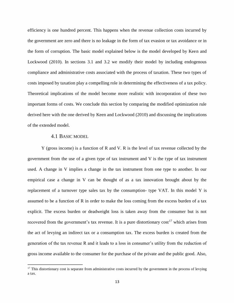
To summarize, the gross income function Y is a nonlinear function of R and is inversely

related to R. Y decreases with R because of the loss of utility associated with excise taxation.

Additionally, Y decreases at an increasing rate as R increases. Y is also a function of V because

V determines the magnitude of 𝑌𝑅 for every level of R. Figure 1 shows this relationship in a

graphical form.

15

In Figure 1, 𝑌𝑅 is the original relationship between 𝑌 and 𝑅 when a type of tax

instrument 𝑉 is used. It also shows an example where the type of the tax instrument used changes

from 𝑉 to say 𝑉′. This example illustrates a hypothetical case where the change to 𝑉′ increases

the excess burden or efficiency costs associated with every level of revenue. Now the new curve

is shown by 𝑌𝑅′. Due to the increase in the excess burden associated with the new tax

instrument 𝑉′, if the entire gross income were to be collected as tax revenue by the government

to finance the public good, then only 𝑅′ instead of 𝑅 could be raised.

Summary of the functional form of Y:

Y = f (R, V) where

R = Revenue collected by the government

V = Type of tax instrument used (In the empirical analyses it will be a dummy variable and will

take a value of unity in the presence of a VAT. In its absence it will take a value zero)

We also assume that the government is benevolent. Keeping this in mind, for a given

value of V, this economy’s government chooses R to maximize the representative consumer’s

utility U(Y(R, V) – R, R) subject to the balanced budget constraint. The objective function is

shown below:

max𝑅

{ U(Y(R, V)– R, R)} s.t. R = G and 𝐶 = 𝑌(𝑅, 𝑉) − 𝑅

Y

R R’

Figure 1 : Graph

16

Maximizing representative consumer’s utility U(C,G) with respect to R, subject to the condition

of balanced budget, R = G, gives the following first order condition:

F.O.C

𝜕𝑈𝜕𝐶⁄ 𝜕𝐶

𝜕𝑅⁄ + 𝜕𝑈𝜕𝑅⁄ = 0 (1)

𝐶 = 𝑌(𝑅, 𝑉) − 𝑅 (2)

If we take derivative of equation (2) w.r.t R, we obtain:

𝜕𝐶𝜕𝑅⁄ = 𝜕𝑌

𝜕𝑅⁄ − 1 (3)

Substitute (3) into (1), we get

𝜕𝑈𝜕𝐶⁄ ( 𝜕𝑌

𝜕𝑅⁄ − 1 ) + 𝜕𝑈𝜕𝑅⁄ = 0

𝜕𝑈𝜕𝑅⁄ = 𝜕𝑈

𝜕𝐶⁄ ( 1 − 𝑌𝑅) Where 𝜕𝑌𝜕𝑅⁄ = 𝑌𝑅

𝑈𝑅𝑈𝑐

⁄ = 1 − 𝑌𝑅 > 1 Where 𝜕𝑈𝜕𝑅⁄ = 𝑈𝑅 𝑎𝑛𝑑 𝜕𝑈

𝜕𝐶⁄ = 𝑈𝐶 (4)

Note: As pointed earlier, 𝑌𝑅 ≠ 0 in this model as the tax system under consideration here is

excise tax or the commodity tax and other distortionary taxes. 𝑌𝑅 = 0 only for a lumpsum tax.

Also 𝑌𝑅 < 0. This explains the strict inequality in equation (4)

𝑈𝐺𝑈𝑐

⁄ = 1 − 𝑌𝑅 = 1 − 𝑀𝐷𝐿 (5)

Equation (5) follows from equation (4) as 𝑈𝑅 = 𝑈𝐺 because R = G in this model. Y – R* is the

amount spent on the consumption of the private good at the optimum. The more is spent on

17

public good in form of R*, the lesser is available to spend on private consumption in the form of

Y – R*. We always get a unique maximum point because of the well-defined properties of utility

function.

Equation (5) can be thought of as a modified Samuelson rule as Keen and Lockwood

(2010) point out. The ratio of marginal utilities on the left hand side gives the marginal rate of

substitution between the public and the private good. Equation (5) shows that under the

optimization rule the marginal rate of substitution between the public and the private good will

be set equal to unity minus the MDL (𝑌𝑅) from taxation. To understand the intuition behind

equation (5), let’s consider a case where the left hand side of equation (5) is greater than the right

hand side. This implies that at the margin, the utility gained by the consumer from consumption

of the public good is more than the consumption of the private good. In such a case it will be

welfare improving to consume more of the public good18. With higher consumption of the public

good, the consumer’s total utility will increase. However, there will be a simultaneous fall in the

marginal utility of the public good 𝑈𝐺 with the increase in government expenditure G. An

increase in G implies an increase in R. This increase in R will increase 𝑌𝑅. As 𝑌𝑅 (MDL) or the

loss increases, the right hand side of equation (5) gets bigger. This means that although greater

consumption of the public good brings in more utility, it also simultaneously increases the loss

(MDL) associated with its consumption. Essentially, in equation (5), the left hand side will

decrease and the right hand side will increase with more and more consumption of the public

good until equality holds. The consumer will prefer to consume the public good up until the gain

equals the loss from its consumption.

18 Public Good is considered a normal good here.

18

Impact of a change in V on the optimal revenue level R*

In the described economy let us start at the point of equilibrium where equation (5) holds

with equality. Now suppose that the absolute value of 𝑌𝑅 decreases (or MDL decreases) because

of an exogenous change in V (or a tax innovation). As a result, the right hand side of equation (5)

will become smaller as compared to the left hand side. In order to restore the equality in equation

(5), the amount of consumption of the public good must go up and this in turn will increase the

expenditure G on it. This means the tax revenue (R) will also increase to sponsor the increased

expenditure on the public good. This explanation of changes illustrates that the fall in efficiency

cost or MDL increases the optimum level of tax revenue (R*).

4.2 MODEL WITH ENDOGENOUS COMPLIANCE COST

The basic model explained above is the revenue efficiency model presented by Keen and

Lockwood (2010). Keen and Lockwood (2010) include only the deadweight loss of tax in their

revenue efficiency model. Although they discuss the presence of a variable called resource loss

(K) which is defined as a fixed amount of loss arising from administrative and compliance

activities, they do not include it in the objective function. We modify their revenue efficiency

model by introducing compliance and administrative costs in their model as two different types

of costs and as a function of R. The compliance costs are introduced at the consumer’s end

because consumers bear this cost and the administrative costs come into play through the

government’s budget constraint because the government incurs it. Both the costs come into play

as a tax is levied by the government. It is important to recognize them in revenue optimizing

problem as they account for a sizeable proportion of the taxation costs. Absence of these costs in

the revenue efficiency model will underestimate the overall costs of taxation. The compliance

and administrative costs can be thought of as substitutes of each other to an extent. An increase

19

in one may reduce the other. For example, with a VAT, traders need to maintain a record of all

the transactions in order to obtain a refund of the input taxes which makes the VAT self-

enforcing. This record keeping by the traders increases the compliance costs while reduces the

government’s administrative costs. The compliance costs incorporated in this sub-section are

assumed to be a function of the level of tax revenue, R. Both exogenous and revenue varying

administrations costs are also integrated later in the model.

In simple terms, the compliance costs involve both money and time costs which arise

from the process of estimation of the tax liability, filing of the tax related paperwork,

maintenance of the record of all the transactions, and keeping with the latest updates in the tax

laws. In other words, these are simply costs of abiding by the law. These costs are expected to

depend on characteristics of a tax instrument such as multiplicity of tax rates. The more complex

a tax system, the more expensive and time consuming it is to comply with it. If more hours are

spent by the consumer in complying with the tax code, then the consumer has lesser time to be

productive at work or consume leisure. Therefore an increase in the compliance costs reduces

private consumption. The compliance costs are also a function of time simply because over time,

taxpayers learn how to comply if the tax system is stable.

With compliance costs, the modified equation for private consumption looks like the following:

𝐶 = 𝑌(𝑅, 𝑉) − 𝑅 − 𝑡(𝑅, 𝑉; ℎ) (6)

Where,

t = compliance costs

h = hours spent in maintaining and filing of tax records

All other variables in equation (6) are defined as before.

20

Compliance costs depend on both the amount of revenue raised by the government R and

the type of the tax instrument used V. t is a function of R because t is assumed to increase with

the increase in tax liability. This is primarily the reason why businesses employ tax analysts /

experts to maintain and calculate the amount businesses owe in corporate tax, sales tax, turnover

tax and so on. Also, t may increase with R at a decreasing rate because of the economies of scale.

However, we are not assuming any specific form t takes as a function of R in this model. t could

be a linear or a non-linear function of R of any form. All we assume here is that t is revenue

dependent and increases with an increase in R. Given this, we re-optimize using equation (6)

The new objective function is shown below:

max𝑅

{ U(Y(R, V)– R − t(R, V; h), R)} s.t. G = R (7)

F.O.C

𝜕𝑈𝜕𝐶⁄ 𝜕𝐶

𝜕𝑅⁄ + 𝜕𝑈𝜕𝑅⁄ = 0 (8)

𝐶 = 𝑌(𝑅, 𝑉) − 𝑅 − 𝑡(𝑅, 𝑉; ℎ) (9)

Take derivative of equation (9) above w.r.t R,

we get, 𝜕𝐶𝜕𝑅⁄ = 𝜕𝑌

𝜕𝑅⁄ − 1 − 𝜕𝑡𝜕𝑅⁄ (10)

Substitute (10) into (8), we get

𝜕𝑈𝜕𝐶⁄ ( 𝜕𝑌

𝜕𝑅⁄ − 1 − 𝜕𝑡𝜕𝑅⁄ ) + 𝜕𝑈

𝜕𝑅⁄ = 0

𝑈𝑅 = 𝑈𝐶 [ 1 + (𝑡𝑅 − 𝑌𝑅)] (Subscripts denote derivatives as in section 3.1) (11)

Equation (11) above can be rewritten as follows:

21

𝑈𝐺

𝑈𝐶= 1 + (𝑡𝑅 − 𝑌𝑅) > 0 (12)

Equation (12) is the modified form of equation (5). In this equation the marginal rate of

substitution between the public and the private good is equal to unity plus the marginal

compliance cost (MCC) and MDL.

Define TMC (total marginal cost) as:

TMC = MCC + MDL

TMC = 𝑡𝑅 − 𝑌𝑅 (13)

TMC > 0 since 𝑡𝑅 > 0 𝑎𝑛𝑑 𝑌𝑅 < 0

Therefore, 1 + (𝑡𝑅 − 𝑌𝑅) > 1 and (1+ TMC) > 1 in Equation (12)

Equation (12) above can be re-written as:

𝑈𝐺

𝑈𝐶= 1 + 𝑇𝑀𝐶 (14)


In equation (12), TMC (total marginal cost) will change with a change in V (tax

instrument), which will change the optimal revenue level R*. A change in TMC depends on the

change in MCC and MDL.

(a) If 𝑡𝑅 (𝑀𝐶𝐶) 𝑖𝑛𝑐𝑟𝑒𝑎𝑠𝑒𝑠 𝑜𝑟 𝑌𝑅 (𝑀𝐷𝐿) 𝑖𝑛𝑐𝑟𝑒𝑎𝑠𝑒𝑠 𝑜𝑟 𝑏𝑜𝑡ℎ 𝑖𝑛𝑐𝑟𝑒𝑎𝑠𝑒 then TMC will

increase.

(b) If 𝑡𝑅 (𝑀𝐶𝐶) 𝑑𝑒𝑐𝑟𝑒𝑎𝑠𝑒𝑠 𝑜𝑟 𝑌𝑅 (𝑀𝐷𝐿) 𝑑𝑒𝑐𝑟𝑒𝑎𝑠𝑒𝑠 𝑜𝑟 𝑏𝑜𝑡ℎ 𝑑𝑒𝑐𝑟𝑒𝑎𝑠𝑒 then TMC will

decrease.

Following the reasoning in section 3.1, a change in V leading to an increase in the overall

marginal cost or TMC will decrease the optimal level of tax revenue R* raised by the

22

government. On the other hand, a decrease in TMC will increase the optimal revenue level of R*.

A benevolent government is able to increase the representative consumer’s welfare by increasing

the tax revenue iff the total taxation costs borne by the consumer fall at the margin. A given tax

instrument is associated with a higher level of revenue efficiency only when the government is

able to raise more tax revenue optimally. Therefore an increase in the optimal level of R* is

indicative of the use of a more efficient tax system. We now move on to introduce administrative

costs in this model. We then compare the new derived optimization rule with the optimum

condition derived by Keen and Lockwood (2010).

4.3 EXTENDED REVENUE EFFICIENCY MODEL

Administrative costs are the costs incurred by the tax levying authority or the government

in the process of establishing and operating a tax system. The basic model presented above

makes one prominent assumption that R = G. This implies zero revenue collection costs incurred

by the government which is not realistic as in the real world a government has to typically bear

substantive tax enforcement and collection costs. We now modify this unrealistic assumption. As

the administrative costs come into play G < R because the amount the government is able to

spend on the public good G is strictly less than the revenue collected19. Part of the collected

revenue is lost in the form of the administrative costs. Real world examples of such costs include

computerization and technological advancement of the tax administrative system, tax audits

conducted by the government to reduce tax evasion, training of the government employees in

new technology, reforming of the tax laws and the maintenance of taxpayer’s records. Before

we discuss endogenous administrative costs and their inclusion in the model, we take a look at

the exogenous form of administrative costs and discuss its impact on the optimal level of

19 We assume no government borrowing.

23

revenue. For the moment let us assume that the administrative costs are independent of the

revenue R. Then this type of cost takes the following functional form.

Case of exogenous (or temporary) administrative cost

A = a (V,D,T) (15)

where,

A = administrative cost

D = regional or country’s characteristics which includes institutions, corruption, level of

education and existing revenue productivity

T = time and

V = type of tax instrument

Administrative cost A depends on V as a change in the tax instrument used is expected to

lead to a modification of the existing tax collection system or installation of a new system. With

the use of a new tax instrument, this cost could increase or decrease. This models a temporary

impact of a change in V on A. The idea is analogous to some type of a start-up cost associated

with a change in the tax instrument. This startup cost or a fixed cost is like a onetime exogenous

shock in the government’s administrative costs. We believe this is a short-run or a temporary

impact of a change in tax instrument. A is also expected to be a function of some regional

characteristics D and the time T. For example, for a given region, its specific institutional

characteristics or the existing education level may keep the administrative costs of the

government lower in this region as compared to other regions or states thereby making it cheaper

to administer any tax instrument. Note that in the analysis presented below we only consider a

case of positive exogenous shock. The magnitude of an increase in the onetime costs or a

24

positive shock is determined by the regional characteristics outlined by D. We rule out the case

of a negative exogenous shock in the government’s administrative costs because it does not seem

realistically possible. Such administrative costs when greater than zero reduces the amount of the

tax revenue collected and make lesser amount available to the government for financing of the

public good. The new budget constraint is as follows:

𝐺 = 𝑅 − 𝑎(𝑉, 𝐷, 𝑇) (16)

With A in equation (15), the new objective function is shown by equation (17) below.

New objective function:

max𝑅

{ U(Y(R, V)– R − t(R, V; h), G)} s.t. G = R – A (17)

The optimization rule remains the same as in equation (14) for the above maximization problem.

Equation (14) is:

𝑈𝐺

𝑈𝐶= 1 + 𝑇𝑀𝐶

Where, TMC = 𝑡𝑅 − 𝑌𝑅 and TMC > 0


A change in the optimal level of R from a change in V for the modified maximization

problem in the equation (17) is not the same as for the maximization problem in section 3.2.

With the change of V now two things are changing simultaneously for every given level of R,

which are the absolute values of A and TMC (MDL and MCC). A increases with a change in V

for a given region at a point of time. Note that the increase in A in this argument is a pure effect

of a change in the tax instrument used. With increase in A with a change in V, the government

expenditure on the public good G will decrease for a given level of revenue R. This follows from

equation (16). As public expenditure decreases, the consumer is now able to consume less

25

quantity of the public good as compared to before for the same amount of the tax revenue R.

Since20 the public good considered here is a normal good, a decrease in its consumption for a

given level of R, will decrease the consumer’s total utility but increase the marginal utility i.e.

𝑈𝐺 . If this economy was in equilibrium before the change in V then, after the change, A will rise

and the left hand side of equation (14) will be greater than the right hand side. However, this is

not a complete description of the changes occurring. With a change in V, the absolute value of

TMC will also change. The net effect on the optimal level of revenue R* due to a change in V is

determined by the magnitude and direction of the simultaneous changes in A and 𝑌𝑅 , 𝑡𝑅 in

TMC.

One possible scenario is that a change in V increases TMC and also A. The final change

in the optimal R is then determined by the magnitude of the increase in the two losses. Below we

consider all the possible scenarios associated with a change in V leading to an increase in A and

their net effect on the optimal level of R*

Scenario III.A1: With a change in V, both TMC and A increase. Note that the increase in A

implies a decrease in the total utility and a simultaneous increase in the marginal utility of the

public good 𝑈𝐺 . The net effect is discussed below:

(i) If 𝑇𝑀𝐶 ↑ > 𝑈𝐺 ↑ then in equation (5) 𝑈𝐺

𝑈𝐶⁄ < 1 + 𝑇𝑀𝐶 and R* will decrease

with a change in V

(ii) If 𝑇𝑀𝐶 ↑ < 𝑈𝐺 ↑ then in equation (5) 𝑈𝐺

𝑈𝐶⁄ > 1 + 𝑇𝑀𝐶 and R* will increase

with a change in V.

20 Note that we are doing a purely partial equilibrium analysis here. Better tax administration in period zero may

lead to higher consumption in period one, but we are not modeling the dynamic time component here.

26

(iii) If 𝑇𝑀𝐶 ↑ = 𝑈𝐺 ↑ then in equation (5) 𝑈𝐺

𝑈𝐶⁄ = 1 + 𝑇𝑀𝐶 and R* will not change

with a change in V.

Intuition: At the margin, if the increase in revenue-varying taxation costs are greater than the loss

in the total utility from lower expenditure on the public good due to an increase in the

administrative costs, the consumer would want to consume lesser of the public good and so the

optimal revenue R* will decrease. If the increase in costs is smaller than the loss in the total

utility from a lower level of G, then the consumer would desire more of the public good and so

R* will increase.

Scenario III.A2: With a change in V, the absolute value of 𝑌𝑅 decreases and A increases

(i) If 𝑇𝑀𝐶 ↓ 𝑎𝑛𝑑 𝑈𝐺 ↑ then in equation (5) 𝑈𝐺

𝑈𝐶⁄ > 1 + 𝑇𝑀𝐶 and R* will increase

with a change in V.

Intuition: At the margin, if the revenue-varying costs decrease and the total utility also decreases

from lower expenditure on the public good due to an increase in the administrative costs, the

consumer would want to consume more of the public good and so the optimal revenue R* will

increase.

The above explanations show that the net impact of the change in costs on R* is not

straightforward. When both the endogenous and exogenous costs are rising simultaneously, then

the net effect on R* could be an increase or a decrease (depending on the magnitude of the costs)

and vice versa. We now move on to solve the optimization problem in an economy when the

administrative costs also vary with the level of revenue.

27

Case of endogenous administration costs

For a given tax instrument, in the long-run part of the administrative costs will vary with

the level of tax revenue raised by the government. This section models the long-run impact of a

change in V on A by incorporating the revenue-varying component of the administrative costs.

As the size of the government expands, the costs of administering this government are expected

to go up. We know from Wagner’s law that the size of the government increases with an increase

in national income. So if R increases because of an increase in the per capita income, then a

simultaneous increase in the government size is expected to lead to an increase in the

administrative costs. Therefore an increase in R would cause an increase in A. However these

administrative costs could increase with R at a decreasing rate because of the economies of scale.

As in the case of compliance costs, we are not making any assumptions about the functional

form of A. The only assumption we make here is that the administrative costs are revenue

dependent and directly proportional to R i.e. the first derivative of A w.r.t R is positive. The

modified equation of A is shown below:

A= a (V,D,t,R) (18)

𝐴𝑅 denotes the partial derivative of A w.r.t to R. 𝐴𝑅 is defined as the marginal administrative

cost (MAC) associated with a change in R. Following presents the consumer maximization

problem with A as a function of R.

max𝑅

{ U(Y(R, V)– R − t(R, V; h), G)} s.t. G = R – A (19)

Differentiating equation (19) w.r.t R, we obtain:

𝜕𝑈𝜕𝐶⁄ 𝜕𝐶

𝜕𝑅⁄ + 𝜕𝑈𝜕𝐺⁄ 𝜕𝐺

𝜕𝑅⁄ = 0 (20)

From equation (9) we know,

28

𝐶 = 𝑌(𝑅, 𝑉) − 𝑅 − 𝑡(𝑅, 𝑉; ℎ)

Taking derivative of the above w.r.t R, we obtain:

𝜕𝐶𝜕𝑅⁄ = 𝜕𝑌

𝜕𝑅⁄ − 1 − 𝜕𝑡𝜕𝑅⁄

Also, we know

𝐺 = 𝑅 − 𝐴

Differentiate w.r.t R, we obtain:

𝜕𝐺𝜕𝑅⁄ = 1 − 𝐴𝑅 (21)

Now, Substitute 𝜕𝐶𝜕𝑅⁄ and 𝜕𝐺

𝜕𝑅⁄ into equation (20)

𝜕𝑈𝜕𝐶⁄ ( 𝜕𝑌

𝜕𝑅⁄ − 1 − 𝜕𝑡𝜕𝑅⁄ ) + 𝜕𝑈

𝜕𝐺⁄ (1 − 𝐴𝑅) = 0

𝑈𝐺(1 − 𝐴𝑅) = 𝑈𝐶 [ 1 + (𝑡𝑅 − 𝑌𝑅)]

𝑈𝐺𝑈𝐶

⁄ =[ 1 + (𝑡𝑅∗ − 𝑌𝑅∗)]

(1 − 𝐴𝑅∗)⁄ (22)

Now substitute 𝑡𝑅 = 𝑀𝐶𝐶 and 𝑌𝑅 = 𝑀𝐷𝐿 in equation (22) above and MAC = 𝐴𝑅 , we get

𝑼𝑮𝑼𝑪

⁄ =(𝟏 + 𝑴𝑪𝑪 − 𝑴𝑫𝑳)

(𝟏 − 𝑴𝑨𝑪)⁄ > 0, where MDL < 0 (23)

The Samuelson rule from Keen and Lockwood (2010) is as follows:

𝑈𝐺𝑈𝐶

⁄ = 1 − 𝑀𝐷𝐿 > 0 , where MDL < 0 (24)

29

Equation (23) presents the modified optimization rule derived here when both the compliance

and the administrative costs of taxation are present and endogenous. The optimal level of

revenue 𝑅∗ should satisfy this equation in order to maximize the representative consumer’s

utility. Comparison of the modified Samuelson rule derived here which is given by equation (23)

with the one derived by Keen and Lockwood (2010) given by equation (24), show that equation

(23) has an additional term of marginal compliance cost (MCC) in the numerator and an

additional term of marginal administrative cost (MAC) in the denominator. The result in

equation (23) shows that at the margin, we need to account for all the types of taxation costs in

order to gauge the net impact of a change in the tax instrument used by the government on the

optimal level of revenue R*.

Since, TMC = MCC + MDL and TMC > 0 as 𝑡𝑅 > 0 𝑎𝑛𝑑 𝑌𝑅 < 0

We can rewrite equation (23) as the following:

𝑼𝑮𝑼𝑪

⁄ =(𝟏 + 𝑻𝑴𝑪)

(𝟏 − 𝑴𝑨𝑪)⁄ (25)


We now discuss the impact of a change in V on the optimal level of tax revenue R using

equation (25). A change in V, changes two things simultaneously for every given level of R.

These are TMC and MAC. Let’s start at a point where equation (25) holds and the economy is in

the equilibrium. Now V changes as a result of which TMC and MAC may both change and lead

to a change in optimal R*. Let’s consider all the possibilities and their net impact on the optimal

revenue.

30

Scenario III.B1: With a change in V, TMC decreases and MAC does not change. Note that

TMC could decrease because of a decrease in MCC or MDL or both of its components. This is

because TMC = MCC + MDL.

If 𝑇𝑀𝐶 ↓ and ∆𝑀𝐴𝐶 = 0, then 𝑈𝐺

𝑈𝐶⁄ > 1 + 𝑇𝑀𝐶

1 − 𝑀𝐴𝐶⁄ and the optimal 𝑅∗ will increase

with a change in V.

Scenario III.B2: With a change in V, TMC decreases and MAC also decreases.

If 𝑇𝑀𝐶 ↓ and 𝑀𝐴𝐶 ↓, then 𝑈𝐺

𝑈𝐶⁄ > 1 + 𝑇𝑀𝐶

1 − 𝑀𝐴𝐶⁄ and the optimal 𝑅∗ will increase with

a change in V.

Intuition: At the margin, when some or all the endogenous costs are decreasing then higher

consumption of the public good will increase the consumer’s total utility which will increase R*.

Scenario III.B3: With a change in V, TMC increases and MAC does not change. Again, note

that TMC could increase because of the increase in MCC or MDL or both of its components.

If 𝑇𝑀𝐶 ↑ and ∆𝑀𝐴𝐶 = 0, then 𝑈𝐺

𝑈𝐶⁄ < 1 + 𝑇𝑀𝐶

1 − 𝑀𝐴𝐶⁄ and optimal 𝑅∗ will decrease

with a change in V.

Scenario III.B4: With a change in V, TMC increases and MAC also increases.

If 𝑇𝑀𝐶 ↑ and 𝑀𝐴𝐶 ↑, then 𝑈𝐺

𝑈𝐶⁄ < 1 + 𝑇𝑀𝐶

1 − 𝑀𝐴𝐶⁄ and the optimal 𝑅∗ will decrease

with a change in V.

Intuition: At the margin, when some or all the endogenous costs are increasing then lower

consumption of the public good will increase the consumer’s total utility which will decrease R*.

Scenario III.B5: With a change in V, TMC increases and MAC decreases.

31

(i) If 𝑇𝑀𝐶 ↑ > 𝑀𝐴𝐶 ↓, then 𝑈𝐺

𝑈𝐶⁄ < 1 + 𝑇𝑀𝐶

1 − 𝑀𝐴𝐶⁄ and the optimal 𝑅∗ will

decrease with a change in V.

(ii) If 𝑇𝑀𝐶 ↑ < 𝑀𝐴𝐶 ↓, then 𝑈𝐺

𝑈𝐶⁄ > 1 + 𝑇𝑀𝐶

1 − 𝑀𝐴𝐶⁄ and the optimal 𝑅∗ will

increase with a change in V.

Scenario III.B5: With a change in V, TMC decreases and MAC increases.

(i) If 𝑇𝑀𝐶 ↓ > 𝑀𝐴𝐶 ↑, then 𝑈𝐺

𝑈𝐶⁄ > 1 + 𝑇𝑀𝐶

1 − 𝑀𝐴𝐶 ⁄ and the optimal 𝑅∗ will

increase with a change in V.

(ii) If 𝑇𝑀𝐶 ↓ < 𝑀𝐴𝐶 ↑, then 𝑈𝐺

𝑈𝐶⁄ < 1 + 𝑇𝑀𝐶

1 − 𝑀𝐴𝐶 ⁄ and the optimal 𝑅∗ will

decrease with a change in V.

Intuition: At the margin, if all the endogenous costs are changing simultaneously then a net

decrease / increase in the marginal costs will lead to an unambiguous increase/decrease in R*

respectively. The impact of a change in V on the optimal revenue R* in all of the scenarios

described above can be summarized by two important points.

First, exogenous and endogenous administrative costs have a differential impact on R*. In

presence of an exogenous increase in the government’s administrative costs, the net change in R*

is not straightforward. For example, R* may increase even when the exogenous administrative

costs and other endogenous costs are rising. When all the three types of taxation costs considered

32

here are endogenous in the model, things are simpler. Equation (25) is valid when this is

the case and it shows that as long as the net endogenous costs of taxation are falling at the

margin, it will always be welfare improving to increase the consumption of the public good

which implies that R* will increase. Hence it is important to distinguish between exogenous and

endogenous tax administration costs.

Second, it is important to consider the change in direction and the magnitude of all the

costs incurred from taxation when analyzing the impact of a change in the type of the tax

instrument used by the government and there is more than one type of taxation cost. A final

change in the optimal level of R* will be determined by the net change in all the types of taxation

costs21.

5 DATA AND THE EMPIRICAL RESULTS

The main empirical question of interest is the following: has the tax innovation in the

form of the replacement of the turnover sales tax by the VAT improved the revenue efficiency at

the state level? According to the theoretical model explained above the impact of the transition to

the VAT is ambiguous in the short-run when the administrative costs are more likely to be

independent of the level of revenue. Recall from the model that a change of an indirect tax

instrument used by the government is likely to cause a one-time positive exogenous shock in the

government’s administrative costs. This positive shock in the costs is independent of the revenue

and in its presence the impact of the VAT on the optimal level of revenue R* is ambiguous. In

this case, in order to pin down the exact change in R*, a complete knowledge of the direction and

the magnitude of the changes in all the costs is required. But, fortunately this exogenous shock is

21 This model does not incorporate two other important forms of taxation costs which are costs of tax evasion and

tax avoidance.

33

temporary and over a longer period of time the administrative costs tend to be revenue-varying.

When this is the case, the optimal revenue R* or the revenue efficiency will increase if and only

if there is a net fall in the deadweight loss (or distortionary costs), compliance costs and the

administrative costs at the margin.

The empirical analyses presented in this paper uses data for the years 1990 to 2010.

Twenty-two out of 29 states had adopted the VAT by the year 2005, and 5 more states put it in

place in the following year. Therefore for these 27 states (which represent more than 93% of the

total number of states) we are able to capture the impact of the VAT on the revenue efficiency

over a 4 to 5 year period. Considering a 4 to 5 year period to be a reasonably long period of time,

all the costs of taxation are expected to be endogenous. Therefore, from the model, we infer that

if we observe an increase in the optimal level of revenue R* in our empirical results, this increase

is a result of a net decrease in the marginal costs of taxation and vice versa. If the VAT led tax

reform is found to reduce the taxation costs, then this efficiency gain will show up as an increase

in R* and we will be able to conclude that the VAT reform in India has proved to be efficiency

improving at the state level.

We use the state’s tax revenue per capita to measure R* (or revenue efficiency). Two

different measures of the revenue are used; one is the state’s own revenue from all the types of

indirect taxes (ITR) and the other is the state’s own revenue from the sales taxes component. As

explained before, these sales taxes are levied by the state governments on goods and it is the

main form of indirect tax for the states (Its importance is best illustrated by Table 1). Also 28%

of the state’s total tax revenue comes from the state’s sales tax component. States essentially

replaced this tax instrument by the VAT. The measure of the state’s own revenue from all the

indirect taxes takes into account the surcharge taxes which used to be levied on top of the sales

34

taxes before the presence of the VAT. The states got rid of these inefficient forms of taxes at the

time of the transition to the VAT. Therefore this revenue measure could be thought of as a

broader measure or an aggregate measure of the revenue efficiency. Also, Keen and Lockwood

(2010) point to the fact that the performance of the VAT needs to be evaluated with respect to

the total revenue collected from all the types of indirect taxes. This argument makes it useful to

capture the change in revenue efficiency of both of the revenue measures explained above from

the use of the VAT as a type of sales tax instrument.

5.1 DATA

We use the state level data for the years 1990 to 2010 for 29 states of India including the

national capital territory of Delhi22. Union territories are excluded from the analyses because

they do not have autonomous state governments except for Puducherry. Union territories

together represent only about 7% of India’s population. All data used in the following empirical

analyses is obtained from RBI publications, Ministry of Statistics and Programme

Implementation (MOSPI), National Sample Survey Office (NSSO) at MOSPI, Ministry of

Labour and Employment, Labour Bureau, Government of India and Indiastat. Details on the state

level VAT are obtained from the website of Empowered Committee of State Finance Ministers.

5.2 SUMMARY STATISTICS AND THE TRENDS IN THE DATA

Summary statistics of the covariates used in the empirical analyses to explain the

overtime trends in the revenue measures are presented in Table 2. Table 2 reports the summary

statistics of the key covariates for all the states and also separately for the 11 special category

states and the 18 non-special category states. A lower average of GSDP per capita (GSDP pc)

and a higher percentage share of agriculture sector in GSDP for the special states compared to

22 Three states of India split into two states each, in the year 2000. For the years prior to 2000, we generate value of

variables in the data for the split states using their actual figures in years 2000 and 2001.

35

the non-special states illustrates a lower level of development in the special category of states.

Education expenditure is the amount spent by the respective state governments on education as a

part of the development expense. Education expenditure per capita is used as a proxy of the

literacy level in any given state. In addition to the agricultural sector, the unregistered

manufacturing sector is also difficult to tax and it hides within the shadow economy of a country.

The size of this unregistered manufacturing sector in the states of India is non-trivial and

therefore it is used as one of the explanatory variables in our analyses.

Table 2 shows that its average size across the non-special states is about 7% of GSDP;

however it is only 2% of GSDP in the special category states. The central government provides

numerous tax concessions to the manufacturing industry in the special states which could explain

the modest size of the unregistered manufacturing in these states as compared to the non-special

states.

The Central government’s grants to all the states had increased temporarily for 3 to 4

years during the time period when the states were transitioning to the VAT. The state

governments were mainly concerned about the initial revenue loss from the transition to the VAT

and the central government agreed to compensate them for any such losses upto a certain

percentage through temporary grants. To account for this special form of assistance to the states

from the center on the state’s revenue effort, we use the non-plan grants from the center to the

states as one of the covariates in the analyses. The average value of such grants made to the

special states was higher than the grants made to the other 18 states.

Total interest payments paid by the states annually including their interest on loans,

internal debt and market loans is used as a proxy for the fiscal crisis the states of India were

36

grappling with in the second half of the 1990s23. NEC (North Eastern Council) grants are a

special form of grants prominently given by the federal government for the development

purposes to 8 states of India which are located in the north eastern region. All these states fall

into the special category. We control for these grants also in our analyses. All other covariates

reported in Table 2 are popularly used by the previous tax effort literature to explain the tax

revenue ratio or the revenue productivity. For example the level of urbanization is shown to have

a positive and significant effect on the revenue performance in the previous literature. The

mining sector is usually dominated by a few large sized firms and hence it could generate large

tax surpluses for the government. Therefore we include the share of the mining sector as an

explanatory variable.

Table 2 also reports four different measures of tax revenue per capita (pc). The broadest

measure among them is the state’s total tax revenue (TTR) pc. It includes the state’s own

revenue from the direct and the indirect taxes and also the state’s revenue share in the direct and

the indirect central taxes. The second measure is the state’s own tax revenue (OTR) which

includes both the indirect and the direct sources of tax revenue. Third measure is the state’s own

indirect tax revenue (ITR) which is a subset of the above two measures and the last and the

narrowest measure is the state’s revenue from the sales tax / VAT which is a subset of the ITR

measure. The state’s revenue from the sales tax instrument came from the turnover type sales tax

before the transition to the VAT and from the VAT after the VAT was implemented. All the four

revenue measures are consistently lower in value for the special states as compared to the non-

special states which explains the lower revenue productivity in these states.

Figure 5 shows the average trend in OTR, ITR and the sales tax/ VAT revenue measure

as a percentage of TTR for all the states. Dotted vertical lines mark the years when one or more

23 Details of this crisis are discussed in section 3 of the paper.

37

states adopt the VAT. The two ratios OTR to TTR and ITR to TTR follow very similar trends

overtime. These two ratios reach their respective peaks in the year 2002 and then they start

descending in 2003. They begin trending up after 2007. For the majority of the VAT adoption

period from 2005 to 2007, these ratios are falling. A slightly different trend is followed by the

sales tax / VAT revenue measure. The fall in it after 2002 quickly vanishes and it manages to

stabilize at 30% of TTR for the coming years up until it starts to rise upwards after 2007. The

consistent drops in all the three revenue ratios after the year 2003 are perhaps coming from a

sharp deterioration in the state’s fiscal conditions in the year 2003-04.

Figure 6 unfolds the growth trend in ITR to TTR separately for the special and the non-

special states. Again vertical lines in the graph mark the years of the adoption of the VAT by one

or more states. We observe that the growth rate has been marginally trending downwards for the

non-special states starting from 2002 and it starts to increase post 2007 although this increase is

not sustained in the later years. On the other hand, the special states experienced dramatic

fluctuations in the growth rate over the entire time period and no systematic trend emerges. Same

is true for the trends in the growth of the sales tax / VAT revenue measure as a percentage of

TTR which is shown in Figure 7. It is hard to tell from these pictures if the VAT’s

implementation changed revenue productivity in either category of the states.

We also look at Table 3 in an attempt to expose some trends in the revenue performance

before and after the VAT. This table presents the average annual growth rates in ITR as a

percentage of TTR and sales tax / VAT revenue as a percentage of TTR for the pre and the post

VAT periods. We now look at these growth rates individually in each of the 18 non-special

states. For majority of these states, annual growth rates improved in the post VAT period as

compared to the pre VAT, although the improvements are modest. The state of Chattisgarh

38

shows the most dramatic improvement in the growth rate of the sales tax / VAT revenue

component from a negative 10.5 % in the pre VAT to a positive 11.8% in the post VAT period.

These growth rates declined sharply in the special category states in the post VAT period.

5.3 REGRESSION ANALYSES

We first estimate equation (26) using fixed effects methodology.

𝑟𝑖𝑡 = 𝛼 𝑣𝑖𝑡 + 𝛽′𝑋𝑖𝑡 + 𝜇𝑖 + 𝜀𝑖𝑡 (26)

Where,

i = index which represents state (i = 1,…, 29)

t = index which represents time (t = 1990,…, 2010)

𝑟𝑖𝑡 = log ITR per capita or log sales tax / VAT revenue per capita of a state i at a

time t. It is a (NT X 1) vector of N states and T years.

𝑣𝑖𝑡 = takes a value 1 if a state i has a VAT in a year t, and takes a value

zero otherwise

𝑋𝑖𝑡 = denotes a column vector of other observable time varying covariates and it also

includes a time trend variable.

𝜇𝑖 = denotes a state specific error

𝜀𝑖𝑡 = denotes an idiosyncratic error

The estimators of the parameters 𝛼 and 𝛽 in equation (26) are shown in Tables 4 and 5

using a fixed effects (FE) model. The only difference between the results in Tables 4 and 5 is

that in Table 4 the dependent variable is the state’s own indirect tax revenue per capita (ITR pc)

and in Table 5 the dependent variable is the sales tax / VAT revenue pc. The sales tax / VAT

revenue pc measures the state’s sales tax revenue pc from the turnover tax in the period prior to

the VAT, and it measures the state’s sales tax revenue pc from the VAT in the post VAT period.

39

The ITR pc measure of the state’s revenue captures the revenue efficiency of the entire indirect

tax system whereas the sales tax / VAT revenue measure captures the revenue efficiency of only

the sales tax component of the entire indirect tax system. DVAT in all the tables is the dummy

variable indicating the presence of the VAT. The coefficient of interest to us is the coefficient of

DVAT which is ∝ in equation (26). The FE estimates are shown for all the states and then

separately for the special and the non-special states in Tables 4 and 5. We also control for time

trend in all the above specifications. We observe a significantly positive effect of GSDP per

capita in all the specifications of Table 4 and Table 5. This effect is well established in the

previous tax effort literature and it is popularly known as Wagner’s law. We also observe a

positive and a significant impact of the presence of the VAT on the outcome variable for non–

special states in these tables. The estimate in Table 4 shows that in the presence of the VAT,

state’s ITR pc increases by 3.4%. The time trend is significant in all columns of Table 4 bu it

becomes insignificant in Table 5. Table 5 shows that the presence of the VAT has a bigger

significant effect on the revenue efficiency of the sales tax component. From Table 5 we see that,

with the use of a consumption type VAT by the state governments instead of the turnover tax, the

sales tax / VAT revenue per capita increased by 8.46%.

We cluster the standard errors over the states for all the FE estimates. This produces

robust standard error estimates that allow heteroskedasticity within the states. The reason to

suspect heteroskedasticity is that error 𝜀𝑖𝑡 is expected to be correlated over time for a given

state24. To solve for the problem of autocorrelation in the dependent variable (which is a

common problem of a dynamic model and also of tax effort regression specification), we use the

first order of the lagged dependent variable as one of the regressors. Its coefficient is significant

24 Note that the specification used still does not allow for the correlation of errors across the states.

40

and positive in Tables 4 and 525. We use Wooldridge (2002) test of serial correlation in the

presence of the fixed effects. The statistics of this test are also reported in Tables 4 and 5 which

reveal the presence of serial correlation. The inclusion of the lagged term of the dependent

variable in the specification perhaps does not completely solve the underlying problem. It is

commonly the case that the errors are serially correlated when the dynamic model is

misspecified26.

If the correlation in errors follows AR (1) (𝑢𝑖𝑡 = 𝜌𝑢𝑖,𝑡−1 + 𝜀𝑖𝑡) , we can obtain more

efficient estimates in its presence by using the FE estimator which explicitly allows AR(1)

errors. The results of this model are shown in Table 6 for all the states and the non-special

states27. Columns (1) and (2) of Table 6 present results using ITR pc as the dependent variable

and (3) and (4) use the sales tax/ VAT revenue pc as the dependent variable. The significant

effect of the VAT on ITR pc vanishes with the use of the FE model of AR (1) errors. However,

the impact of the VAT is still significantly positive on the sales tax / VAT revenue pc for the

non- special states. The size of the effect is 6.67% which is close in magnitude to the results

reported in Table 5.

Cameron and Trivedi (2009) note that the within estimator (or the FE estimator) is

inconsistent once lagged regressors are introduced because the first lagged term of the dependent

variable for a given state i can be shown to be correlated with the error terms of this state i.

Nonetheless, consistent parameter estimates can be obtained from the IV estimators of first-

difference (FD) model by instrumenting the first lagged term of the dependent variable with its

own lagged term of the higher order. Anderson and Hsiao (1981) estimator uses this model.

25Interaction terms of the VAT dummy variable with GSDP and other variables are excluded from of the results

presented in the paper because they were consistently found to be insignificant. 26 See Wooldridge, Introductory Econometrics, 4th ed, Chapter 12 27 Results for special category states are not presented in the table because coefficient of VAT dummy variable is

insignificant.

41

Table 7 presents the results using this estimator. The VAT’s presence is found to be significantly

positive on the sales tax / VAT revenue pc for the non-special states and the size of this effect is

6.5% in Table 7. The magnitude of this effect was 8.6% from using the FE estimator as discussed

above. Even though the VAT does not seem to improve efficiency of the aggregate indirect tax

system of the states, it does seem to improve efficiency of the sales tax component of the indirect

tax system which it had essentially replaced.

Tables 5, 6 and 7 report a consistent increase in the long–run28 revenue efficiency of the

sales tax instrument used by the state governments from the substitution of a consumption type

VAT for a turnover type sales tax. Our theoretical model implies that the observed increase in

the revenue efficiency of the sales tax component is a result of a net decrease in the marginal

costs of taxation associated with the sales tax instrument. Similarly a no change in the revenue

efficiency of the aggregate indirect tax system can be inferred a result of no net change in the

marginal distortionary, compliance and administrative costs. Note that here we are talking about

a net change in all the costs of taxation. So when the net change in the total marginal costs is

zero, it could mean that some costs increased and other costs decreased in such a way that the net

effect is zero.

As explained above, our findings provide some evidence of a net decrease in the marginal

taxation costs from the use of a VAT as an indirect tax instrument at the state-level. However we

are not able to pin-point which type of taxation costs fall more/less than the others. We believe

this is a question which can be addressed by future research work. It will be worthwhile to

identify which taxation costs changed the most and in which direction among the compliance

costs, distortionary costs and the administrative costs.

28 We consider time period of 4 to 5 years as a long-run time period. This is discussed in detail in paragraph 2 on

page 29 of this paper.

42

6 CONCLUSION

The theoretical model in this paper establishes that, in the long-run, when all the costs

from taxation are endogenous, then a net fall in these costs at the margin, makes it efficient for

the government to increase the optimal revenue R*. This increase in the level of revenue

therefore reflects an efficiency gain. In our empirical analyses we identify such an efficiency

gain in the sales tax component in the developed states of India, over a 4 to 5 year time period,

from the use of a consumption type VAT. This makes intuitive sense as a consumption type

VAT replaced an administratively complex, non-uniform and a distortionary sales tax. However,

this efficiency gain is not robust enough and it does not lead to the efficiency improvement of the

aggregate indirect tax system. We observe an insignificant effect of the VAT on the revenue

efficiency of the entire indirect tax system. Nonetheless, the estimation results presented in this

paper provide evidence of efficiency improvement of the sales tax component in a less developed

economy from the use of a VAT at the sub-national level. This is an important finding which

shows that a sub-national VAT can prove to be an effective tax instrument in the low and middle

income countries also.

43

7 FIGURES

Figure 2: Average state’s OTR as a percentage of GSDP over the period of 1990 to 2000

Figure 3 : Average revenue deficit as a percentage of GSDP

44

Figure 4: Implementation of the VAT in the states of India by year

45

Figure 5 : Trend in state’s revenue ratios (in percent)

Figure 6: Growth rate in ITR as a percentage of TTR for special and non-special category of states

46

Figure 7: Growth rate in sales tax / VAT revenue as a percentage of TTR for special and non-special category of

states

8 TABLES

Table 1: Percentage share of ITR to OTR and Sales tax / VAT revenue to ITR

All-India average ITR to OTR ( in percent) Sales tax / VAT revenue to

ITR (in percent)

1990 to 1995 87.85% 50.96%

1996 to 2000 87.6% 52.98%

2001 to 2005* 87.8% 58.42%

2006 to 2010 88.5% 64.38%

Notes:

*2005 is a significant year as 21 out of 29 states adopted the VAT in this year. Haryana was the first state to adopt a

VAT in the year 2003.

ITR = State’s own indirect tax revenue

OTR = State’s own tax revenue

Sales tax/ VAT revenue = Revenue collected by states by charging indirect taxes on goods.

48

Table 2: Summary statistics

Variable Obs Mean Std. Dev. Min Max

GSDPpc All states 609 25547.13 24065.72 2582.67 197423.50

Special 231 22398.96 17912.22 3818.52 123533.30

Non- special 378 27471.01 26990.76 2582.67 197423.50

Agri. GSDP share (in %) All states 606 44.61 172.77 0.71 1804.05

Special 228 77.29 278.64 7.96 1804.05

Non- special 378 24.89 10.82 0.71 48.93

Unreg. Manuf. GSDP share ( in %) All states 592 5.15 25.52 0.63 622.96

Special 223 2.60 1.42 0.63 7.20

Non- special 369 6.69 32.22 1.23 622.96

Mining scetor GSDP share ( in %) All states 587 2.46 3.48 0.00 19.41

Special 215 1.85 2.76 0.00 10.94

Non- special 372 2.82 3.80 0.00 19.41

Urban Pop ( in %) All states 602 29.05 16.61 7.00 95.00

Special 224 22.13 10.94 8.00 52.00

Non- special 374 33.15 18.00 7.00 95.00

Education expenditure per capita All states 605 946.84 892.24 50.54 9232.50

Special 231 1345.26 1127.41 200.00 9232.50

Non- special 374 700.76 588.49 50.54 5150.65

Non plan grants from Centre per capita All states 595 716.90 1380.98 0.00 9305.10

Special 228 1677.92 1857.49 0.00 9305.10

Non- special 367 119.87 149.86 0.00 1408.87

NEC grants per capita All states 604 37.54 115.59 0.00 1006.55

Special 230 98.02 171.00 0.00 1006.55

Non- special 374 0.35 2.70 0.00 38.05

Interest payments per capita All states 603 728.96 612.12 40.84 3825.88

Special 231 889.59 673.64 40.84 3113.33

Non- special 372 629.21 548.29 51.34 3825.88

TTR pc All states 605 2440.62 2075.30 285.36 16022.24

Special 231 2269.26 1797.99 311.81 13408.67

Non- special 374 2546.47 2225.15 285.36 16022.24

OTR pc All states 605 1492.83 1697.65 29.44 12585.59

Special 231 814.62 928.00 29.44 5356.44

Non- special 374 1911.72 1917.04 95.52 12585.59

ITR pc All states 605 1328.42 1526.90 25.67 11643.76

Special 231 729.13 846.77 25.67 5154.28

Non- special 374 1698.58 1724.33 81.17 11643.76

Sales tax / VAT revenue pc All states 521 875.11 1062.83 2.80 7504.24

Special 214 402.61 484.39 2.80 2643.10

Non- special 307 1204.49 1221.18 63.66 7504.24

Notes:

GSDP = Gross state domestic product of state; TTR = State’s total tax revenue; OTR = State’s own tax revenue;

ITR = State’s own indirect tax revenue

49

Table 3: Average annual growth rates in ITR and sales tax / VAT revenues before and after the VAT

Average growth rate in ITR to TTR Average growth rate in Sales tax / VAT rev to

TTR

( in per cent per annum) ( in per cent per annum)

Five year period before

VAT

Post

VAT

Five year period before VAT Post

VAT

Andhra Pradesh -0.14 0.37 0.02 0.21

Bihar -3.88 1.65 -2.23 -1.52

Chattisgarh 1.58 -0.39 -10.46 11.82

Delhi -0.83 0.22 -2.91 1.77

Goa 0.40 -1.62 -3.56 -1.51

Gujarat -1.27 -0.72 -1.07 6.18

Harayana 2.22 -1.30 1.42 4.08

Jharkhand 3.39 -3.19 -0.11 0.95

Karnataka -0.24 0.37 -2.04 1.10

Kerala -0.22 -0.11 0.58 0.99

Madhya Pradesh 1.38 -0.60 3.40 -0.47

Maharashtra 0.30 -1.25 0.54 5.02

Orissa 0.66 0.29 -3.92 2.10

Punjab -0.74 -0.70 -2.17 4.54

Rajasthan -0.33 -1.17 0.49 0.78

Tamil Nadu -0.61 0.40 1.22 -0.19

Uttar Pradesh -3.42 2.16 -7.65 4.76

West Bengal -2.96 0.05 -4.43 1.02

Special Category

states

17.92 -1.22 31.44 2.09

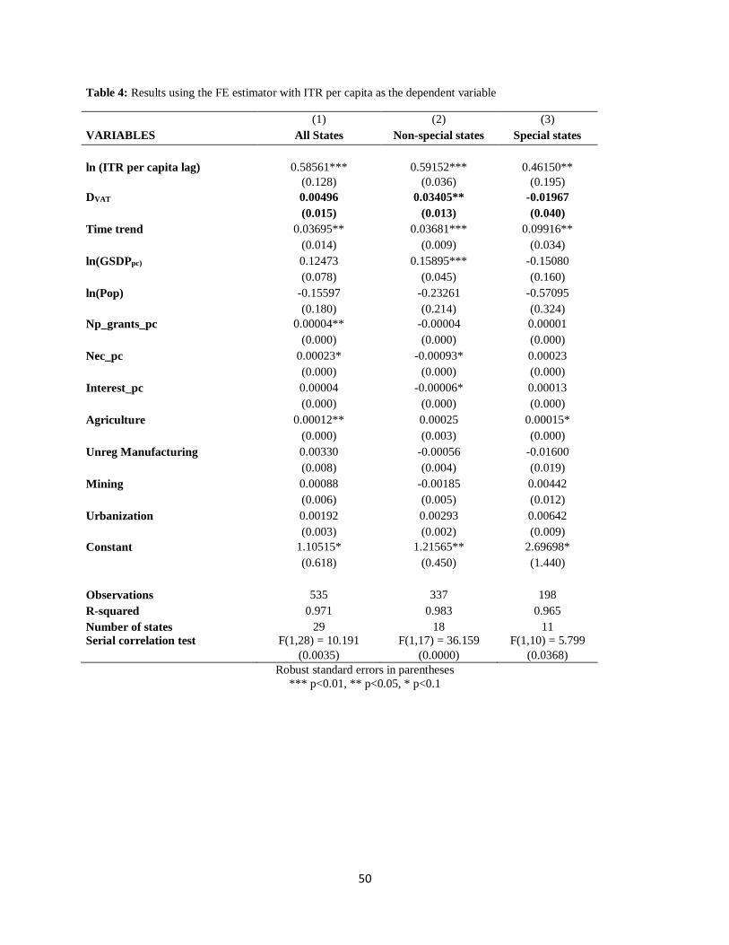
50

Table 4: Results using the FE estimator with ITR per capita as the dependent variable

(1) (2) (3)

VARIABLES All States Non-special states Special states

ln (ITR per capita lag) 0.58561*** 0.59152*** 0.46150**

(0.128) (0.036) (0.195)

DVAT 0.00496 0.03405** -0.01967

(0.015) (0.013) (0.040)

Time trend 0.03695** 0.03681*** 0.09916**

(0.014) (0.009) (0.034)

ln(GSDPpc) 0.12473 0.15895*** -0.15080

(0.078) (0.045) (0.160)

ln(Pop) -0.15597 -0.23261 -0.57095

(0.180) (0.214) (0.324)

Np_grants_pc 0.00004** -0.00004 0.00001

(0.000) (0.000) (0.000)

Nec_pc 0.00023* -0.00093* 0.00023

(0.000) (0.000) (0.000)

Interest_pc 0.00004 -0.00006* 0.00013

(0.000) (0.000) (0.000)

Agriculture 0.00012** 0.00025 0.00015*

(0.000) (0.003) (0.000)

Unreg Manufacturing 0.00330 -0.00056 -0.01600

(0.008) (0.004) (0.019)

Mining 0.00088 -0.00185 0.00442

(0.006) (0.005) (0.012)

Urbanization 0.00192 0.00293 0.00642

(0.003) (0.002) (0.009)

Constant 1.10515* 1.21565** 2.69698*

(0.618) (0.450) (1.440)

Observations 535 337 198

R-squared 0.971 0.983 0.965

Number of states 29 18 11

Serial correlation test F(1,28) = 10.191 F(1,17) = 36.159 F(1,10) = 5.799

(0.0035) (0.0000) (0.0368)

Robust standard errors in parentheses

*** p<0.01, ** p<0.05, * p<0.1

51

Table 5: Results using the FE estimator with sales tax/ VAT revenue per capita as the dependent variable

(1) (2) (3)

VARIABLES All States Non-special States Special states

ln (sales tax/ VAT per capita lag) 0.45996*** 0.60711*** 0.37000*

(0.159) (0.086) (0.180)

DVAT 0.00353 0.08456** -0.12056

(0.046) (0.031) (0.128)

Time trend 0.01035 0.01536 0.09152

(0.029) (0.016) (0.086)

ln(GSDPpc) 0.41028 0.26883** -0.13286

(0.271) (0.115) (0.714)

ln(Pop) 0.20594 0.27536 -1.16388

(0.475) (0.465) (1.054)

Np_grants_pc 0.00009 -0.00001 0.00007

(0.000) (0.000) (0.000)

NEC_pc 0.00011 0.00166* 0.00008

(0.000) (0.001) (0.000)

Interest_pc 0.00010 -0.00002 0.00027

(0.000) (0.000) (0.000)

Agriculture 0.00053** 0.00097 0.00066**

(0.000) (0.003) (0.000)

Unreg Manufacturing -0.00582 0.00776 -0.10057*

(0.017) (0.009) (0.052)

Mining 0.00554 0.00960 -0.03805

(0.015) (0.008) (0.035)

Urbanization -0.01718* -0.00159 -0.04050**

(0.009) (0.006) (0.017)

Constant -0.63643 -0.64541 3.01584

(2.322) (1.190) (4.940)

Observations 454 276 178

R-squared 0.887 0.965 0.866

Number of states 29 18 11

Serial correlation test F(1,28) = 7.609 F(1,17) = 35.459 F(1,10) = 6.498

(0.0101) (0.0000) (0.0289)


*** p<0.01, ** p<0.05, * p<0.1

52

Table 6: Results using the FE estimator with AR (1) errors

All states Non-special

states

All states Non-special states

VARIABLES Ln (ITR pc) Ln (ITR pc) Ln ( Sales tax pc) Ln ( Sales tax pc)

DVAT -0.00337 0.02046 0.01160 0.06662**

(0.027) (0.021) (0.068) (0.032)

Time trend 0.04184*** 0.03445*** 0.03510* 0.03522**

(0.008) (0.010) (0.019) (0.014)

ln(GSDPpc) 0.35865*** 0.23627*** 0.39117*** 0.24999***

(0.046) (0.063) (0.098) (0.091)

ln(Pop) -0.03340 -0.16182 0.29518 -0.15762

(0.155) (0.243) (0.341) (0.385)

Np_grants_pc 0.00005*** -0.00004 0.00011*** -0.00001

(0.000) (0.000) (0.000) (0.000)

Nec_pc 0.00020** -0.00085 0.00005 0.00252

(0.000) (0.002) (0.000) (0.003)

Interest_pc 0.00006* -0.00007** 0.00014 -0.00003

(0.000) (0.000) (0.000) (0.000)

Agriculture 0.00020*** 0.00061 0.00075*** 0.00195

(0.000) (0.002) (0.000) (0.004)

Unreg Manufacturing 0.01218 0.00277 -0.00826 0.01008

(0.009) (0.006) (0.024) (0.010)

Mining 0.00731 0.00087 -0.00699 0.00045

(0.008) (0.006) (0.020) (0.009)

Urbanization 0.00174 0.00266 -0.01513 -0.00287

(0.004) (0.002) (0.010) (0.005)

ln (ITR per capita lag) 0.32504*** 0.55394***

(0.043) (0.050)

ln (Sales tax per capita lag) 0.26384*** 0.54768***

(0.047) (0.051)

Constant 0.18058 0.57794 0.20357 0.30881

(0.258) (0.636) (0.603) (0.822)

Observations 506 319 425 258

Number of states 29 18 29 18

Standard errors in parentheses

*** p<0.01, ** p<0.05, * p<0.1

53

Table 7: Results using the IV estimator of the First-difference model

All States Non-special

states

All states Non-special states

VARIABLES Ln (ITR pc) Ln (ITR pc) Ln (Sales tax pc) Ln (Sales tax pc)

LD.ln (ITR pc) -0.11055 0.57471**

(0.117) (0.293)

L3D.ln (ITR pc) 0.06398 0.04434

(0.041) (0.065)

DVAT 0.01620 -0.04118 -0.00729 0.06506*

(0.029) (0.034) (0.079) (0.035)

ln(GSDPpc) 0.11936 -0.06481 0.10444 0.31436*

(0.120) (0.164) (0.367) (0.176)

ln(Pop) -0.82210*** -0.89060 -1.93123** 0.22455

(0.311) (0.797) (0.890) (0.853)

Np_grants_pc 0.00002 0.00004 0.00012*** 0.00000

(0.000) (0.000) (0.000) (0.000)

Nec_pc -0.00013 -0.00325 -0.00010 -0.00102

(0.000) (0.003) (0.000) (0.003)

Interest_pc 0.00009* 0.00000 0.00003 0.00002

(0.000) (0.000) (0.000) (0.000)

Agriculture 0.00003 0.00725* 0.00013 0.00124

(0.000) (0.004) (0.000) (0.004)

Unreg Manufacturing 0.00589 0.01881 -0.01353 0.01856

(0.013) (0.013) (0.037) (0.015)

Mining -0.01161 -0.04215** -0.05011 -0.00841

(0.013) (0.017) (0.034) (0.018)

Urbanization 0.01767* 0.01124 -0.00992 0.00868

(0.009) (0.011) (0.029) (0.014)

Educationpc 0.00009*** 0.00026*** 0.00002 0.00014*

(0.000) (0.000) (0.000) (0.000)

LD.ln (Sales tax pc) -0.08885 0.03467

(0.129) (0.347)

L3D.ln (Sales tax pc) 0.00281 -0.03246

(0.049) (0.059)

Constant 0.12659*** 0.06000* 0.16202*** 0.08118*

(0.023) (0.033) (0.060) (0.048)

Observations 457 286 357 214

Number of states 29 18 29 18

Standard errors in parentheses

*** p<0.01, ** p<0.05, * p<0.1

54

2. CHAPTER TWO - DID INDIA’S SUB-NATIONAL VAT IMPROVE ECONOMIC

EFFICIENCY?

1 ABSTRACT

We investigate the efficiency of a recently implemented sub-national value-added tax

(VAT) in India between the years 2003 and 2008. A system of state-level VATs in India was

expected to eliminate the cascading tax burden associated with a long-dominate turnover tax on

commodities by solving the problem of double taxation which had considerably impaired the

efficiency of the sales tax system of the states before the introduction of the VAT. We believe if

cascading tax burden is wiped out with the replacement of a turnover type sales tax with a

consumption-type VAT, then the price growth across commodities must decrease due to a fall

in the real tax burden. This in turn would lead to a simultaneous increase in the real private

consumption of commodities. We analyze the impact of the VAT on the prices and

consumption of multiple commodity groups in rural and urban areas using time series data of

household level consumption expenditure surveys collected by a federal government

organization. As expected, we find the biggest impact of the VAT on consumption and prices of

the durable goods indicating the biggest efficiency gain in these goods.

2 INTRODUCTION

Value added tax (VAT) is a multistage sales tax and is collected on the ‘value added’ at

every production-distribution stage of a good or a service. The retail value of a good is equal to

the sum of the added values at each stage of production. Therefore a consumption–type VAT and

a retail sales tax (RST) must raise equivalent tax revenues if applied at the same rate on the same

55

goods and services. However, in practice, a VAT is considered superior to a RST as a RST is

more vulnerable to tax evasion and avoidance. With a RST, unlike VAT, the tax revenue is lost

completely if the tax is evaded at the final point of sale. A VAT is also considered compliance

incentivizing because under a VAT regime, wholesalers and retailers have to ensure that the

traders they deal with pay the tax in order to be eligible for input tax credit. So a VAT is self-

policing and is better at exposing forged accounts and an informal economy as compared to a

RST (Bird (2005) and Agha et. al (1996)). For the same reason, a VAT is generally regarded as a

more promising consumption tax for developing countries where the size of the informal sector

is bigger. For the reasons discussed above, at the national level, a VAT has been widely accepted

by tax policy experts29 as one of the most efficient forms of indirect taxation. However its

performance at the sub-national level remains far from clear. Researchers question the efficiency

of a sub-national VAT for various reasons including high efficiency and administrative costs

associated with the taxation of cross border trade30 and the non-uniformity of the VAT rates

across the states or regions within a country31. Moreover it is hard to empirically evaluate the

performance of a sub-national VAT simply because it is not very commonly found in practice.

India is among the only three countries in the world which has embraced a sub-national

VAT. The other two countries to ever have adopted a sub-national VAT are Canada and Brazil.

Canada’s success with VAT is largely attributed to its exceptionally high tax administrative

29 Refer to McLure (1993), Ebrill (2001), Keen and Lockwood (2010), Bird et. al (2007) 30 The application of a VAT on the interstate trade is often pointed out, by tax policy experts, as the most serious

practical issue with the use of a sub-national VAT (Bird et. al (1998)). There is no general consensus on the best

way to apply a destination-based VAT to the interstate trade. (McLure (2005) explains why a sales tax with a

destination principle is more desirable). Bird (1993) points out other problems related to a sub-national VAT. These

include coordination of federal and regional taxes, loss of macroeconomic control and high administrative and

compliance costs. 31 McLure (2000) emphasizes the desirability of allowing state governments to charge their own VAT rates. The

logical reasoning behind the existence of the non-uniform rates is to preserve the regional government’s autonomy.

56

quality32. Since few countries have tax administrations of comparable quality, it is widely

believed that Canada’s success cannot be replicated in other countries, particularly in low- and

middle-income countries with inadequately developed tax administration systems. Therefore,

empirically examining India’s experience with a sub-national VAT will not only help to better

understand the impact of an important tax policy reform in India but will also inform important

tax policy decision-making at the sub-national level in other developing countries.

The adoption of the VAT was primarily expected to improve economic efficiency through

the reduction in the level of tax cascading. The Government of India believed that the VAT will

rationalize the overall tax burden and bring down the general level of prices. The turnover type

sales tax which existed prior to the VAT created severe problems of double taxation on the final

consumption goods. The forbidding distortionary costs stemming from the double taxation were

expected to fall substantially following the adoption of the VAT. Therefore it is meaningful to

investigate if the VAT of India, in its existing form, managed to reduce the cascading tax burden

on commodities.

The main research question at hand is whether the state-level VATs improved the efficiency

of India’s indirect tax-system by reducing the level of tax cascading. We are able to gauge this in

the following manner. If the VAT managed to weed-out or diminish the cascading tax burden,

we would observe a fall in the real price level of commodities in the years following its adoption.

With the reduction in the level of tax cascading, the real value of sales taxes collected on

commodities33, in the form of the VAT, must fall causing a fall in the price growth. In addition,

this fall in the prices would trigger a subsequent increase in the overall economic activity and

32 Refer to Bird et. al (2001). 33 The states of India can levy tax only on the final consumption goods only. Most of the services have always been

taxed by the federal government in India. Only very few services are taxed by the state governments and there exist

separate taxes on them such as entertainment tax and luxury tax.

57

higher growth in the real private consumption. In this paper, we not only capture the change in

real prices of commodities from VAT, we also capture the VAT driven growth in the real private

consumption, if any, by using the state-level household surveys conducted in India. The

important question is, even if the prices fell with the adoption of VAT, was the fall in prices

sufficient enough to improve the economic efficiency of the tax system and the welfare of the

consumers. By tracking the real private consumption at the micro-level, we are able to address

this question. We conduct a micro-level analysis of the trends in real prices and consumption

across multiple commodities for urban and rural regions. The details of the price and

consumption analyses are explained in detail below in the results section. As far as we know, no

previous research work has analyzed the impact of India’s VAT on its level of tax cascading.

The paper proceeds as follows. Section 3 broadly reviews the state-level sales tax system of

India before VAT and outlines the salient features of the existing state-level VATs, Section 4

outlines the theoretical model, Section 5 explains the data and the methodology and Section 6

presents the results and concludes.

3 BACKGROUND

In India, the state governments collect sales taxes only on commodities and not on services.

The type of commodity sales tax which existed in the states of India before VAT was highly

distortionary because of multiple reasons. One of the biggest problems was that it resulted in a

cascading tax burden. This was mainly because the tax instrument used was a turnover type sales

tax and it taxed both the input and the final consumption goods. This cascading effect was

further pronounced due to the presence of additional taxes collected by the states on the same

58

commodities such as surcharge on sales tax, additional surcharge and entry tax34. Other primary

source of inefficiency in the old sales tax system was the multiplicity of rates across

commodities within a state. This led to heterogeneous tax rates not only across states but also

across commodities within the states. Under the old system, it was not uncommon for states to

have 17 to 20 categories of commodity tax rates ranging from as low as zero percent to as high

as seventy percent35. Since the taxes cascaded, the effective tax rates were much higher than the

applicable rates. Such a distorted taxation system was bound to impose high deadweight loss and

administrative and compliance costs.

A much awaited tax reform made its way through the introduction of the state-level VATs.

The use of VATs simplified the old system, removed the multiplicity of rates and made the

overall tax rates uniform across commodities and states. With the adoption of the VAT, states

also got rid of their additional unnecessary taxes such as the surcharge on sales tax36. Finance

Minister of India in his budget speech of 1993 / 94 stated that a broad agreement would have to

be reached between the central and the various state governments regarding the uniform design

of the state –level VATs. In May 1994, a committee of the state finance ministers was formed to

outline a uniform design of the VAT across states. On 17 January 2005, the Committee released

a White Paper37 which revealed the salient features of the sub-national VAT. It laid down the

foundation of a common model based on which each state was expected to develop its own VAT

legislation. This way the states got to choose the specific features in the design under the basic

rules set by the central government, for example the states could choose the specific list of the

exempted goods. The Committee specified three basic rates under the VAT system. These

34 See Purohit (2001) and Bagchi (2005) 35 See Purohit (2001), Sthanumoorthy (2006). Tax rates as high as 70% were charged on beer, wine and other types

of alcohol. 36 Few states continue to hold onto the entry taxes they used to charge before moving towards VAT. 37 White paper on state level value added tax (Jan 2005)

59

included a standard rate of 12.5% and a reduced rate of 4% . The reduced rate was applicable to

most of the items of basic necessities.38 The third rate of 1% rate was applicable on gold and

silver ornaments. All the states of India uniformly adopted the three VAT rates. These rates exist

in addition to a specific category of exempted goods39.

The state of Haryana introduced a VAT on its own initiative in 2003 and became the first

state to adopt it. According to the White Paper, all the other states agreed to bring in the VAT on

April 1, 2005 but later seven states backed out. Five of these seven states adopted the VAT in the

following year. By the year 2008 all the 29 states (including the national capital territory) had

replaced their turnover type sales taxes on goods with the VAT. The political factors brought in

the timing variation in the adoption of the VAT by the states.

4 THEORETICAL MODEL

The theoretical model presented in this section shows how prices and tax revenues behave

under a retail sales tax and a turnover tax. A turnover tax or a multi-stage sales tax is collected on

every stage of production whereas a single-stage sales tax is imposed at only one stage of

production. A RST is a single-stage sales tax which is imposed on a retailer. However, other

variants of a single-stage tax include scenarios where a sales tax is collected from a producer or a

wholesaler instead of a retailer. Our theoretical model first compares the per unit price of a good

and the total tax revenue collected on that good when a single-stage sales tax is levied at

38 These include goods such as medicines, agricultural and industrial inputs, capital goods etc. This category

includes 270 goods approximately on average. 39 The states have the discretion to decide which goods to exempt from VAT. Although the White paper stated that

the exempted goods would include 46 commodities including natural and unprocessed goods in the unorganized

sector. The states were allowed to choose 10 items of these goods. However, the states do not strictly follow the

number of exemption goods restriction specified by the central government.

60

different points of production. Following are the notations we will use in the model presented

below:

Let P stand for producer, W stand for wholesaler, and R stand for retailer.

If a = price markup

b = marginal costs (MC)

t = per unit tax charged on a good

T = total tax revenue

X = units of good produced, then Table 8 below illustrates the level of tax inclusive price per

unit and tax revenue under different scenarios.

Table 8 shown below illustrates that the maximum tax revenue is collected under scenario C

when the single-stage sales tax is collected from the retailer. It also shows that the tax inclusive

price per unit would be the same under each scenario in the special case where 𝑡𝑝 = 𝑡𝑤 = 𝑡𝑟

Table 8 : Price and tax revenue when a single –stage sales tax is imposed at different points of production

Point of collection of a single-stage

sales tax

Tax inclusive price per unit of a

good

Total tax revenue collected on the

good

Scenario A: When the sales tax is

imposed on the producer

𝑃 = 𝑏 (1 + 𝑡𝑝)(1 + 𝑎𝑤)(1

+ 𝑎𝑟)

𝑇𝑝 = 𝑡𝑝𝑏 𝑋

Scenario B: When the sales tax is

imposed on the wholesaler

𝑃 = 𝑏 (1 + 𝑎𝑤)(1 + 𝑡𝑤)(1

+ 𝑎𝑟)

𝑇𝑤 = 𝑡𝑤𝑏 (1 + 𝑎𝑤) 𝑋

Scenario C: When the sales tax is

imposed on the retailer

𝑃 = 𝑏 (1 + 𝑎𝑤)(1 + 𝑎𝑟)(1

+ 𝑡𝑟)

𝑇𝑟 = 𝑡𝑟𝑏 (1 + 𝑎𝑤) (1 + 𝑎𝑟)𝑋

Notes:

1. 𝑡𝑝 is the per unit tax imposed on the producer , 𝑡𝑤 is the per unit tax imposed on the wholesaler and so on.

2. 𝑇𝑝 is the total tax revenue collected on a good by imposing a tax on the producer. Similarly, 𝑇𝑤 is the total tax

revenue collected on a good by imposing a tax on the wholesaler and so on.

61

Next, we move on to derive the tax inclusive price per unit of good and total tax revenue

collected on it under a turnover tax. As explained above, a turnover tax is collected on every

production stage. As a result, it inefficiently inflates the per unit price of a good and generates a

higher level of tax revenue. Under the turnover tax, let 𝑡𝑐denote the per unit tax charged on every

production stage of a good and let 𝑇𝑐 denote the total revenue collected under this tax system.

Given this, tax inclusive per unit price of a good is shown by the following expression:

𝑷𝒓𝒊𝒄𝒆 𝒊𝒏𝒄𝒍𝒖𝒔𝒊𝒗𝒆 𝒐𝒇 𝒕𝒂𝒙 = 𝑏 (1 + 𝑡𝑐)(1 + 𝑎𝑤)(1 + 𝑡𝑐)(1 + 𝑎𝑟)(1 + 𝑡𝑐)

𝑷𝒓𝒊𝒄𝒆 𝒊𝒏𝒄𝒍𝒖𝒔𝒊𝒗𝒆 𝒐𝒇 𝒕𝒂𝒙 = 𝑏 (1 + 𝑎𝑤)(1 + 𝑎𝑟)(1 + 𝑡𝑐)3 (1)

Similarly we can estimate the tax revenue under a turnover tax which is given by the following

equation:

𝑻 = 𝑡𝑐𝑏𝑋 + 𝑡𝑐𝑏𝑋 (1 + 𝑡𝑐)(1 + 𝑎𝑤) + 𝑡𝑐𝑏𝑋 (1 + 𝑡𝑐)2(1 + 𝑎𝑤)(1 + 𝑎𝑟) (2)

The price equation under scenario C (which is a RST) in Table 8 above illustrates the per unit

price of the good when it is taxed once. On the other hand, equation (1) above illustrates the

price of a good when the good is taxed multiple times under a turnover tax. Equation (1) shows

the tax cascading phenomena on the price from the use of a turnover tax. As demonstrated by

this equation, charging a tax at every stage of production results in a tax on a tax and inflates

prices. This simple theoretical model confirms our economic intuition that a cascading tax

burden considerably magnifies the general price growth. In addition, the model illustrates that

the exact number of times the price of a good is taxed under a multi-stage sales tax depends on

the number of production stages. The intuition derived from this simple model is that the greater

the number of production steps, the greater will be the level of price inflation. Therefore the

62

cascading effect of a turnover tax magnifies with the number of production stages. We will delve

into this intuition to better understand the price and the consumption results presented in section

6 of this paper.

5 DATA AND METHODOLOGY

5.1 DATA

We are using three waves of the large sample rounds of the state- and household-level

consumer expenditure survey (CES) conducted by the National Sample Survey organization

(NSSO). NSSO, an organization of the central government, conducts these large sample rounds

of the surveys once in every five years. The three waves used in our data belong to the years

1999, 2004 and 2009. Consequently, the first two years identify the price and consumption

trends in the period before the adoption of the VAT40 and the third year identifies the price and

consumption trends in the period after the adoption of the VAT.

The CES collects information on the consumption expenditures of the sample households for

a variety of goods and services at the state level, separately for the rural and urban regions. In

addition, the surveys also record the level of quantity consumed for some of these goods and

services. More specifically, the survey records consumption on 142 food related goods and

services, 19 addictive substances including tobacco, alcohol and illicit drugs, 15 types of fuel and

energy generating goods and services and 79 types of durables goods. The surveys also record

expenditures on medical and education related goods and services. To analyze the impact of the

VAT on real consumption we use the household-level consumption expenditures per capita

recorded in the surveys and adjust these estimates for inflation. To gauge the responsiveness of

40 One of the 29 states in India adopted VAT in the year 2003.

63

the commodity prices to the VAT, we use the state- and the household-level prices of individual

commodities. The commodity prices used in our analyses are estimated from within the survey

data. Since these surveys record the quantity consumed by the households of certain goods, we

are able to estimate the prices of these goods by dividing the household expenditures by quantity

consumed. Further details on the identification strategy are presented in the results section

below.

We adjust the nominal consumption expenditures of households for inflation by using the

CPI numbers estimated by the Ministry of Labour, Government of India. The state-level CPI data

includes a general CPI index which summarizes price trend of all the goods and services

commonly consumed. In addition, the state-level CPI data provides separate estimates for the

urban and the rural areas and also for different groups of goods and services. For example, the

nominal food consumption expenditure for a given state in the urban sector is adjusted for

inflation by using the CPI food estimate for the urban area of that state.

5.2 REAL CONSUMPTION EXPENDITURE ANALYSIS

First, we take a look at the impact of the VAT on the real consumption of households. We

estimate our regression equation (3) shown below, separately for the rural and the urban areas

across 18 commodity groups. The dependent variable, 𝐶𝑖𝑠𝑡𝛼 , is the log of real consumption

expenditure per capita for household i in state s and year t. A household i belongs to a sector 𝛼

(urban or rural) in a given state. We analyze 𝐶𝑖𝑠𝑡𝛼 across 18 broad groups of commodities. The

variable of interest is the coefficient of 𝑣𝑠𝑡. 𝑣𝑠𝑡 is a dummy variable and it takes a value one if

state s has VAT in year t. We include log of gross state domestic product (GSDP) per capita as

an explanatory variable in our regressions. This GSDP variable is specific to a sector 𝛼 and

therefore it is equal to GSDP generated from agriculture and other rural activities in the analysis

64

of the rural sector. The urban sector GSDP is estimated by subtracting the rural sector GSDP

from the overall GSDP of the state. The vector 𝜃 in equation (3) includes the explanatory

variables we use to control for the income effect of households41. We also include the state and

year fixed effects in our regression specifications to control for any state specific and time trends.

𝐶𝑖𝑠𝑡𝛼 = 𝛽 𝑣𝑠𝑡 + 𝜌𝐺𝑆𝐷𝑃_𝑝𝑐𝑠𝑡

𝛼 + 𝜏𝜃𝑖𝑠𝑡𝛼 + 𝜇𝑠

𝛼 + 𝛾𝑡𝛼 + 𝜀𝑖𝑠𝑡

𝛼 (3)

The dependent variable, real consumption expenditure per capita identifies the consumption

expenditure on various goods over the last 30 days, expect the long-term durable goods. The

expenditure on the long-term durable goods is recorded over the last 365 days.

5.3 REAL PRICE ANALYSIS

Next, we look at the impact of the VAT on the real prices. We generate the state- and

household-level prices of individual commodities from within the survey data to conduct this

analysis.

We estimate the price regressions shown by equation (4) below, separately for the rural and

the urban areas for the 18 more developed states of India. The dependent variable, 𝑃𝑖𝑠𝑡𝛼 , is the log

of per unit price paid for a commodity by household i in state s and year t. A household i belongs

to a sector 𝛼 (urban or rural) in a given state s. We analyze 𝑃𝑖𝑠𝑡𝛼 across 32 individual commodities

in the rural and the urban areas42. These 32 individual commodities represent the most popularly

consumed goods in the 18 broad commodity categories used to analyze the consumption

41 Previous literature using NSSO data uses monthly per capita expenditure as a proxy for household income

(Kumar et.al (2011)) . We use this and additional variables to control for the income of households. The additional

variables control for the type of employment of the household members, land ownership and the primary cooking

and lighting sources used by a household. We believe all these variables indicate the level of a household’s wealth. 42 Some of the selected commodities differ across the rural and urban areas depending on their popularity of

consumption.

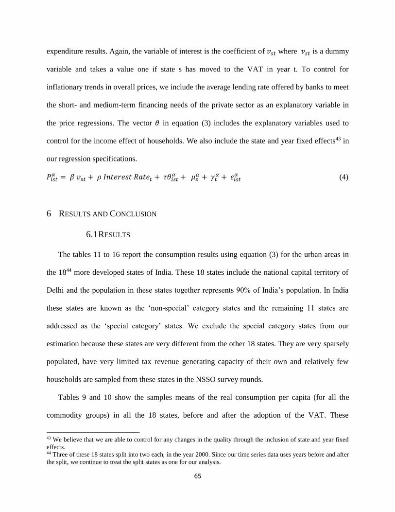
65

expenditure results. Again, the variable of interest is the coefficient of 𝑣𝑠𝑡 where 𝑣𝑠𝑡 is a dummy

variable and takes a value one if state s has moved to the VAT in year t. To control for

inflationary trends in overall prices, we include the average lending rate offered by banks to meet

the short- and medium-term financing needs of the private sector as an explanatory variable in

the price regressions. The vector 𝜃 in equation (3) includes the explanatory variables used to

control for the income effect of households. We also include the state and year fixed effects43 in

our regression specifications.

𝑃𝑖𝑠𝑡𝛼 = 𝛽 𝑣𝑠𝑡 + 𝜌 𝐼𝑛𝑡𝑒𝑟𝑒𝑠𝑡 𝑅𝑎𝑡𝑒𝑡 + 𝜏𝜃𝑖𝑠𝑡

𝛼 + 𝜇𝑠𝛼 + 𝛾𝑡

𝛼 + 𝜀𝑖𝑠𝑡𝛼 (4)

6 RESULTS AND CONCLUSION

6.1 RESULTS

The tables 11 to 16 report the consumption results using equation (3) for the urban areas in

the 1844 more developed states of India. These 18 states include the national capital territory of

Delhi and the population in these states together represents 90% of India’s population. In India

these states are known as the ‘non-special’ category states and the remaining 11 states are

addressed as the ‘special category’ states. We exclude the special category states from our

estimation because these states are very different from the other 18 states. They are very sparsely

populated, have very limited tax revenue generating capacity of their own and relatively few

households are sampled from these states in the NSSO survey rounds.

Tables 9 and 10 show the samples means of the real consumption per capita (for all the

commodity groups) in all the 18 states, before and after the adoption of the VAT. These

43 We believe that we are able to control for any changes in the quality through the inclusion of state and year fixed

effects. 44 Three of these 18 states split into two each, in the year 2000. Since our time series data uses years before and after

the split, we continue to treat the split states as one for our analysis.

66

summary statistics tables show that, in general, the real consumption expenditure per capita is

high for the urban areas as compared to the rural areas. The commodity groups with high

consumption include food, medical goods and services and long-term durable goods (including

household appliances and jewelry). For long-term durable goods such as recreation goods,

furniture and jewelry we have data for the year 2004 (before VAT) and 2009 (after VAT) only.

Data for year 1999 is not available on these goods. Table 10 shows that the real expenditure on

some long-term durable goods category namely furniture and recreation decreases in the year

after VAT is adopted. Tables 17 to 22 present the consumption results for equation (3) for the

rural areas in the 18 more developed states of India. The last row of the columns in the tables

indicate whether state / year fixed effects are included in the specification. Tables 23 and 24

present the price results for equation (4) for the urban and the rural areas respectively.

Before we discuss the significance and the magnitude of the VAT coefficients, here is a

quick reminder of the relationship we expect between the real consumption and prices of

commodities and the VAT. In general, we suspect a positive (negative) impact of the VAT on

real consumption (real prices) of those commodities which were brought under the system of

VAT rates and/ or whose production is characterized by multiple production steps. We expect

that the efficiency of the sales tax system should improve with the use of a VAT not only

because of the reduction in the level of tax cascading, but also because of the elimination of

multiple tax rates which existed under the previous sales tax system. The introduction of a state-

level VAT in India brought down the number of sales tax rates used by the states from as large as

20 to 3 basic rates for most of the goods. As mentioned before these 3 basic rates of the VAT

were uniformly adopted by all the states. However, the states were given some freedom to

determine the list of commodities to be included in the tax-exempted category (Bagchi (2005)).

67

With the introduction of VAT, the central government specified a floor rate of 20% on a

special list of goods which include alcohol, petrol, diesel and other fuels. The states were given

the discretion to determine the actual rate on each of these commodities. Most of the states taxed

these goods at rates ranging from 20% to 35%. Before the VAT, the tax rates on these goods

ranged from 20% to 80%. Although, the tax rates reduced on some of these goods45 in some

states with adoption of the VAT, tax policies on these goods are still complicated46 and therefore

it is hard to derive inferences on the behavior of their prices and consumption under the VAT.

The list of commodities included under tax-exempted category and other VAT rates can be found

in the documents released by each individual state at the time of the introduction of the VAT.

These documents are called VAT ACTS47.

Using the intuition from the theoretical model presented in section 4, we know that the level

of tax cascading is higher among those goods which involve multiple production steps.

Therefore, we predict that our results should capture a bigger reduction in the cascading effect

(in the form of an increase in real consumption and a decrease in real prices) among commodities

involving large number of production stages. Under the India’s VAT system, the registration of

individual dealers/ manufacturers was voluntary if their annual sales turnover was equal to or

below Rs 5 million. This implies that the impact of the VAT on the price and consumption of a

good is also tied to the size of the dealers involved in its production since the size will determine

if a given dealer will enter the VAT system or not. Consequently, we predict a greater increase

(decrease) in the real consumption (price) of the goods which are manufactured by large-sized

45 For example, tax on beer and wine decreased in some states from 70 - 80% to 30-35%. 46 Also the state VAT does not allow for input tax deductions on petrol, natural gas and other fuels as these are not

treated as inputs by the state governments. 47 Refer to the following link to the states’ VAT ACTS: http://empcom.gov.in/index.aspx

http://empcom.gov.in/index.aspx

68

dealers and also involve multiple production steps. The goods which best fit these descriptions

are the long-term durable goods.

Now we derive some intuition on the comparison of the results of the urban areas with those

of the rural areas. In general, we expect a greater presence of the small-sized manufacturers/

dealers in the rural areas, who fall below the threshold limit of Rs 5 million, as compared to the

urban areas. Since India’s VAT fails to bring these producers into its formal system, they would

cause multiple breaks in the VAT chain. Such breaks in the VAT chain can cast serious doubts

on its performance. Therefore, it is reasonable to assume that the VAT on goods in the urban

areas would work more efficiently than the VAT on the same goods in the rural areas. As a

result, we are more likely to capture a bigger increase (decrease) in real consumption (price) of

commodities produced and sold in the urban areas.

Given the prediction of the results outlined above, we now take our attention to the VAT

coefficients in the result tables. The results in Table 11 show that the VAT significantly increases

the food consumption expenditure in urban areas by 7.7%. Food identifies the expenditure on the

unprocessed and the processed food. It includes the consumption of staple food such as rice,

lentils and cereals and it also includes the consumption of nutritive and expensive food such as

green vegetables, fruits, dairy products, meat and fish, bakery goods like cakes and pastries and

dried fruits and nuts such as almonds. In majority of the states, the unprocessed food items were

exempted from the VAT and the processed food was taxed at 4% VAT rate. With the adoption of

VAT the effective rates on all food items reduced as compared to those before VAT and hence

we find evidence of a reduction in tax cascading. VAT also significantly reduces the real prices

of majority of the food items in the urban and the rural areas as shown in Tables 23 and 24. VAT

has the biggest significant decrease on the urban prices of onion, clear butter, milk, cooking oil

69

and groundout (which is a type of dry fruit). For instance, the adoption of VAT significantly

reduces the price of milk per litre by 5.7%. Note that the impact of VAT is more pronounced on

the nutritive and the more processed food items like milk and groundnut. This finding is

consistent with our hypothesis that we should observe a greater efficiency on the more processed

goods due to a bigger drop in the level of tax cascading on these goods.

The urban prices of eggs, potato, suji48 and Indian spices (turmeric) are falling with VAT

also but their coefficients are not precisely estimated. There is an exception of one or two food

items whose prices are not falling but rising with VAT. For example, urban price of salt is

significantly increasing with VAT. This makes sense because the sales tax system which existed

before VAT did not tax processed salt. However the VAT taxes it at the 4% rate in majority of

the states. Same is true for processed rice. We do not capture an equally significant impact of the

VAT on the overall food consumption in the rural areas (Table 17), although the sign of the

coefficient is as expected. The impact of the VAT on rural prices is less significant as compared

to urban prices as shown in Tables 23 and 24. These findings are also consistent with our

hypothesis that we would find smaller efficiency gains in the rural areas because of the higher

probability of multiple breaks in the VAT chain.

The results capture a significant and a positive effect of the VAT on the consumption of

addictive substances in the urban areas. This coefficient becomes insignificant for rural areas as

seen from Table 17. Addictive Substances identify the consumption of tobacco in various forms,

alcohol and drugs. India’s tobacco consumption is heavily dominated by non-cigarette tobacco in

the form of bidis49, chewing tobacco, paan masala50 and gutka51. (Deshpande et. al (2010).

48 A type of commonly used flour. 49 Bidis are made by rolling a dried, rectangular piece of temburni or tendu leaf (diospyros melanoxylon) with an

average of 0.33 g ofsun-dried, flaked tobacco into a cone secured with thread (Deshpande et. al (2010). 50 Paan masala is a betel-quid ingredient that may or may not contain tobacco (Deshpande et. al (2010).

70

Taxation of these popular tobacco products in India is very complex and both the state and the

central governments levy taxes on them. The actual tax rates charged by the central government

vary across different types of tobacco products52. In the first year of the introduction of the VAT,

states governments were not allowed to tax tobacco in any form. After the first year, states could

tax cigarettes and other finished tobacco products53. However, majority of the states’ VAT

ACTS include raw tobacco and betel leaves54 in the list of exempted goods. These exemptions,

along with much lower taxes on alcohol55 (beer and wine) after the introduction of the VAT, can

explain a significant increase in the consumption of the addictive substances under VAT in the

urban areas. In the rural areas we expect that the local and the small-sized tobacco and alcohol

producers would not be affected considerably by the VAT as these producers are more likely to

be a part of the informal sector of the economy.

The price results give a more detailed picture of individual items. We observe that the price

of pan (for which major ingredient is betel leaves) falls significantly with VAT (in both urban

(Table 23) and rural (Table 24) sectors) but the price of locally produced alcohol and tobacco

products in the form of bidi and chewing tobacco increases. As mentioned before, alcohol is not

taxed under the 3 basic rates of VAT so trends in its prices are hard to interpret. Since the

adoption of the VAT, states are continuing to increase their tax rates on local tobacco products

every year through VAT and other type of tax instruments such as luxury and/or entry tax. This

could explain the observed increase in prices of tobacco products.

51 Gutka is a preparation of crushed betel nut, tobacco, catechu, lime and sweet or savory flavorings (Deshpande et.

al (2010). 52 Bidis (locally produced cigarettes) are taxed the lowest by the central government (Kumar et. al (2011)) and

chewing tobacco is taxed the highest at 86%. 53 Most of the states levied 12.5% rate on the finished tobacco products. 54 It is used as an important ingredient in the preparation of a commonly used addicitive substance in India called

paan masala. 55 With the introduction of VAT, the state-level taxes on different kinds of alcohol fell substantially from as high as

80% to 20%.

71

Our results in Table 11 show a significant reduction in the consumption of energy related

goods from VAT in the urban regions. Energy includes the consumption of all types of fuel

commonly used by households for cooking and lighting. This category includes the consumption

of electricity which is the most commonly used source of energy in the urban areas. However

electricity is not taxed under the VAT system. State governments charge a separate excise duty

on electricity consumption. Perhaps the relative price of electricity is going up with VAT and

some households decrease its consumption. We do observe an increase in the real price of

electricity in the presence of VAT and this is shown in Table 23. The second most commonly

used good in this category in the urban areas is LPG (a cooking fuel) which is produced from

natural gas. India’s VAT does not allow input tax deductions on the use of natural gas. Since the

VAT on LPG continues to cascade, we would expect a negative effect of VAT on its

consumption. However, Table 23 shows that the price of LPG decreases significantly with the

VAT. Some states tax final consumption of LPG at 4% whereas others tax it at 12.5%. Perhaps

our price regressions are picking up the VAT’s effect on those states which tax LPG at lower

rates. The price of fuels commonly used in rural areas decrease with the VAT and this finding is

consistent with the observed significant increase in the consumption of energy in the rural areas

as shown in Table 17.

The next consumption category is Clothing, bedding. Clothing, bedding category (shown in

Tables 12 and 18) identifies the expenses56 incurred on clothing, footwear, bedspreads, and home

accessories such as rugs and curtains. This is a broadly defined category which represents

consumption on a variety of clothing, bedding and footwear goods. Therefore it is hard to predict

the impact of VAT on its overall consumption. Some of the clothing and bedding goods

included in this category are usually produced by small-sized manufacturers in both the rural and

56 Expenses in this category are recorded over the last 365 days.

72

the urban areas. The results presented in Tables 12 and 18 show that the VAT negatively impacts

the overall consumption in this category. Perhaps multiple breaks in the VAT chain of the goods

produced by the small-sized manufacturers create inefficiencies which more than offset the

benefits of the VAT on other goods. This could explain why we capture a negative impact on the

overall consumption. The price results in Tables 23 and 24 shed light on the efficiency of some

individual goods included in this category. The impact of the VAT is significant and negative on

the price of garments, hosiery, bed sheets (both urban and rural areas), bed accessories, blankets,

rubber footwear, slippers and upholstery. This shows that the VAT manages to improve

efficiency of all of these individual goods. In addition, as expected the VAT coefficients of these

goods are bigger and more significant in urban areas than in rural areas. However this efficiency

improvement, as reflected by the fall in prices of the individual goods, is not carried over to the

overall consumption of clothing bedding and footwear commodity group.

Education records mostly the expenses on education services57 including tuition and fees. A

smaller portion is contributed by the expenses on goods purchased for the purpose of education.

Medical care In-patient58 and Out-patient categories record expenditures incurred as in-patient

and out-patient at the private and the government hospitals, nursing homes etc, respectively. We

do not identify any significant impact of the VAT on the consumption of education services or

medical in-patient expenses (shown in Tables 12 and 18) when both state and the year fixed

effects are included. This is not surprising because none of these expenses are taxed under the

VAT system. However, we capture a significant and a positive impact of the VAT on the

medical out-patient consumption in the urban areas. This is shown in Table 13. All expenses on

medicines are recorded in this category and hence the above finding makes sense because drugs

57 Expenses in this category are recorded over the last 365 days. 58 Medical care in-patient expenses are recorded over the last 365 days.

73

and medicines in most states are taxed at the 4% rate under the VAT. We do not have

information on the quantity consumed on any individual goods within these categories.

Therefore we cannot run a parallel price analysis on these groups.

We also identify a positive impact of the VAT on the entertainment category in Table 13 in

the urban areas. Entertainment includes the expenses incurred by households on entertainment

goods and services. This group represents the expenses on short-term durable goods used for

entertainment and includes items such as movie theatre ticket expenses, expenses on movie and

music CDs/DVDs, toys and sports goods. The significant increase in its urban consumption with

the use of VAT is also intuitive because the VAT was applied on all the entertainment goods

included in this category and these goods are much more widely consumed in the urban areas

than in the rural areas. Personal Care records expenses on minor durable goods of personal use

such as spectacles, umbrella and cigarette lighter. We do not observe a significant effect of VAT

on this category in the urban areas. In the rural areas, the efficiency of these goods appears to

have decreased with VAT59 as shown in Table 19.

Rent determines rental expenses and includes house, garage and land rent and hotel lodging

expenses. A luxury tax is charged by the states on the hotel services and accommodation.

Multiple taxes are levied by the central and the state governments on the rental income although

the rental expense is out of scope of the state-level VAT. Nevertheless, we find a significant and

a negative impact of the VAT on the rental expenditure in the urban sector (Table 14). Perhaps,

with a use of a more efficient tax on goods in the form of the state-level VAT, the economic

activity is going up in general as we suspect. If this is the case then it would become cheaper to

buy a house and therefore people will purchase their own homes and move out of the rental

59 This may be justified on the basis that the breaks in the VAT chain due to the small-sized manufacturers create

inefficiencies which more than offset the benefits of VAT.

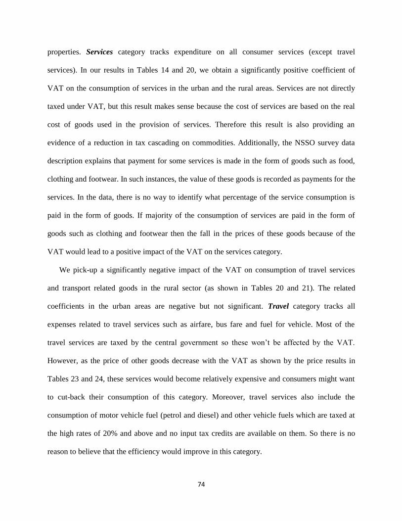
74

properties. Services category tracks expenditure on all consumer services (except travel

services). In our results in Tables 14 and 20, we obtain a significantly positive coefficient of

VAT on the consumption of services in the urban and the rural areas. Services are not directly

taxed under VAT, but this result makes sense because the cost of services are based on the real

cost of goods used in the provision of services. Therefore this result is also providing an

evidence of a reduction in tax cascading on commodities. Additionally, the NSSO survey data

description explains that payment for some services is made in the form of goods such as food,

clothing and footwear. In such instances, the value of these goods is recorded as payments for the

services. In the data, there is no way to identify what percentage of the service consumption is

paid in the form of goods. If majority of the consumption of services are paid in the form of

goods such as clothing and footwear then the fall in the prices of these goods because of the

VAT would lead to a positive impact of the VAT on the services category.

We pick-up a significantly negative impact of the VAT on consumption of travel services

and transport related goods in the rural sector (as shown in Tables 20 and 21). The related

coefficients in the urban areas are negative but not significant. Travel category tracks all

expenses related to travel services such as airfare, bus fare and fuel for vehicle. Most of the

travel services are taxed by the central government so these won’t be affected by the VAT.

However, as the price of other goods decrease with the VAT as shown by the price results in

Tables 23 and 24, these services would become relatively expensive and consumers might want

to cut-back their consumption of this category. Moreover, travel services also include the

consumption of motor vehicle fuel (petrol and diesel) and other vehicle fuels which are taxed at

the high rates of 20% and above and no input tax credits are available on them. So there is no

reason to believe that the efficiency would improve in this category.

75

Transport is the expenditure on long-term durable goods used for personal transport such as

bicycle, tyres, cars etc. Motor vehicles are one of the few goods (like petrol and diesel) for which

input tax deductions are not allowed by majority of the states under the current VAT system.

This explains a continued tax cascading on the transport goods as compared to other durable

goods. As a result, under the VAT system, the price of these goods is expected to be relatively

higher than other durable goods. This discourages their consumption significantly in rural areas.

Therefore we obtain a negative impact of the VAT on transport category in the rural areas. Since

these are expensive goods and the budget constraints are expected to be higher in rural than in

urban areas, the substitution effect on these goods is more evident in the rural consumption.

Other long-term durable goods include the following categories. Recreation includes

expenditure on long-term durable goods used for recreation such as television, camera and

photography equipment. Furniture category characterizes expenses on all sorts of domestic

furniture and their repairs. Jewelry records expenses incurred on gold, silver and other

ornaments. Appliances category determine expenses borne on all sorts of household appliances

including washing machine, sewing machine, refrigerator etc. As explained in the introduction of

the results section, we anticipate the greatest efficiency gain in the long-term durable goods

because these goods are produced by large-sized manufacturers and involve multiple production

steps. This intuition is confirmed in our findings. We capture a positive, significant and an

economically substantive impact of the VAT on the consumption of recreation goods in the

urban areas (Table 15). Recreation goods are luxury goods and are sparsely consumed in the

rural areas, so its consumption trend in the rural area is not as meaningful. Tables 15, 16, 21 and

22 demonstrate a significantly positive increase in the consumption of furniture and appliances

76

from the VAT in both rural and the urban areas and coefficients in urban areas are more

significant.

On the other hand, the impact of the VAT on jewelry consumption is significant and

negative. This negative effect is coming from the 1% tax rate charged on all gold and silver

ornaments. Before VAT these ornaments were tax free in most of the states. Lastly, we look at

the final category of goods which we name ‘All Durables’. This category records consumption

of all the long-term durables goods included in the survey. Note that Recreation, Transport,

Furniture, Jewelry and Appliances are sub-categories of ‘All Durables’. When we analyze the

impact of the VAT on the consumption trends of all long-term durable goods together, the VAT

coefficient for the urban region becomes insignificant. However, it becomes negative and

significant for the rural areas. This implies that for some categories of long-term durable goods,

the adoption of VAT fails to sufficiently improve the efficiency of the tax system in the rural

areas as evident in the transport category explained above.

6.2 CONCLUSION

We identify the biggest efficiency improvements from the adoption of the sub-national

VAT in India in certain long-term durable goods in both rural and the urban sectors. These

improvements arise from the decrease in the level of tax cascading which reduces the real tax

burden and the prices on these goods. This reduction in the real prices consequently leads to an

increase in the real consumption of these goods. We identify such an increase in the real

consumption of long-term durables goods used for recreation in the urban areas. This increase in

real consumption is not only statistically significant at the convention levels but also

economically substantive. We observe a similar increase in the real consumption of furniture

goods and household-appliances in both the rural and the urban areas. As a result we conclude

77

that there is evidence of reduction in tax-cascading with the introduction of an important tax

policy reform in India which took place in the form of a sub-national VAT.

78

7 TABLES

Table 9: Sample means of real consumption expenditure per capita by commodity groups

VARIABLES Rural Urban

Before VAT1 After VAT2 Before VAT After VAT

Food 331.626 343.574 447 439.825

Std. Dev. 186.113 182.523 456.48 270.83

Sample Size 139,344 56,943 80,529 36,693

Addictive Substance 22.817 22.125 35.161 43.414

Std. Dev. 37.246 40.341 66.926 88.448

Sample Size 99,264 38,032 41,246 17,268

Energy 48.412 55.938 70.135 83.052

Std. Dev. 33.26 33.9 729.29 62.732

Sample Size 139,143 56,905 79,787 36,534

Clothing, Bedding and Footwear 307.098 692.759 421.372 768.531

Std. Dev. 396.89 554.977 613.416 769.04

Sample Size 139,042 56,910 80,365 36,649

Education 219.239 578.578 463.12 1330.223

Std. Dev. 849.442 1822.592 1,705 3,742

Sample Size 83,984 38,425 55,397 26,811

Medical In-Patient 471.672 1255.402 604.588 1894.252

Std. Dev. 2278.61 4911.358 3411.09 5342.506

Sample Size 20,379 8,211 11,823 5,091

Medical Out-Patient 42.579 46.666 59.39 72.275

Std. Dev. 101.676 127.291 190.408 172.126

Sample Size 87,368 39,719 50,294 24,966

Entertainment 14.417 18.504 28.796 28.882

Std. Dev. 28.886 33.759 42 33

Sample Size 31,371 23,186 36,867 24,143

Personal Care 9.913 11.365 15.449 20.771

Std. Dev. 19.416 42.884 32 38

Sample Size 22,458 11,281 13,864 5,810

Notes: 1Before VAT includes years 1999 and 2004 2After VAT includes year 2009

79

Table 10. Sample means of real consumption expenditure per capita by commodity groups

VARIABLES Rural Urban

Before VAT After VAT Before VAT After VAT

Services 22.376 39.335 56.771 74.12

Std. Dev. 47.374 67.955 113.016 120.765

Sample Size 131,917 55,765 78,123 36,138

Rent 50.235 63.986 148.156 263.685

Std. Dev. 98.621 178.307 208.944 448.414

Sample Size 7,889 3,974 26,624 11,334

Travel 30.841 44.174 65.066 84.617

Std. Dev. 62.189 101.1 130.814 170.485

Sample Size 104,864 48,598 62,645 31,155

Recreation goods 248.513 140.463 408.389 186.002

Std. Dev. 678.726 466.966 975.282 745.752

Sample Size 5,673 6,282 3,798 5,175

Transport 227.987 320.214 318.912 405.957

Std. Dev. 3030.652 4243.195 2,476 3,433

Sample Size 34,909 32,697 19,087 20,421

Furniture 162.324 142.628 290.916 284.77

Std. Dev. 644.496 524.07 874.901 1065.537

Sample Size 8,528 8,015 3,266 4,193

Household Appliances 104.624 95.74 164.209 164.326

Std. Dev. 462.219 394.407 623.148 557.988

Sample Size 7,902 11,487 7,205 10,546

Jewelry 532.321 770.62 765.203 945.988

Std. Dev. 3804.955 6085.153 4122.74 3268.678

Sample Size 9,324 7,966 3,782 4,423

All Durable Goods 448.688 617.416 689.312 763.071

Std. Dev. 3194.712 4648.998 3326.383 3749.062

Sample Size 57,704 47,825 28,861 29,522

Notes:

All the long-term durable goods categories include recreation, transport, furniture, appliance and all

durable goods. For these groups ‘Before VAT’ observations come from year 2004 only. Data for year

1999 is not available for these categories.

80

Table 11 : Consumption expenditure results for urban sector and developed states

(1) (2) (3) (4) (5) (6)

VARIABLES Food Food Addictive Substance Addictive Substance Energy Energy

LN(GSDPpc) -0.201*** -0.168*** -0.327*** -0.046 -0.008 1.661**

(0.032) (0.046) (0.100) (0.285) (0.190) (0.722)

VAT 0.010 0.077*** 0.330*** 0.243*** 0.100 -0.143**

(0.029) (0.015) (0.088) (0.050) (0.105) (0.060)

Observations 109,403 109,403 53,641 53,641 108,618 108,618

R-squared 0.805 0.805 0.270 0.271 0.518 0.546

State FE YES YES YES YES YES YES

Year FE NO YES NO YES NO YES


*** p<0.01, ** p<0.05, * p<0.1

Table 12: Consumption expenditure results for urban sector and developed states

(1) (2) (3) (4) (5) (6)

VARIABLES Clothing Clothing Education Education Medical Medical

Bedding Bedding In-patient In-patient

LN(GSDPpc) 5.938*** -0.068 6.612*** 0.370 7.507*** 0.219

(0.557) (0.199) (0.627) (0.332) (0.640) (0.489)

VAT -2.426*** -0.112*** -2.481*** 0.101 -2.655*** 0.030

(0.265) (0.020) (0.301) (0.072) (0.346) (0.091)

Observations 109,207 109,207 76,444 76,444 15,988 15,988

R-squared 0.765 0.880 0.586 0.647 0.659 0.722




*** p<0.01, ** p<0.05, * p<0.1

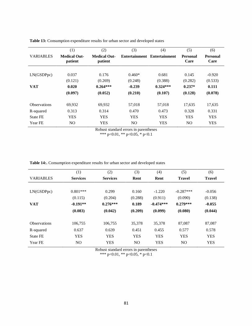
81


(1) (2) (3) (4) (5) (6)

VARIABLES Medical Out-

patient

Medical Out-

patient

Entertainment Entertainment Personal

Care

Personal

Care

LN(GSDPpc) 0.037 0.176 0.460* 0.681 0.145 -0.920

(0.121) (0.269) (0.248) (0.388) (0.282) (0.533)

VAT 0.020 0.264*** -0.239 0.324*** 0.237* 0.111

(0.097) (0.052) (0.210) (0.107) (0.128) (0.078)

Observations 69,932 69,932 57,018 57,018 17,635 17,635

R-squared 0.313 0.314 0.470 0.473 0.328 0.331




*** p<0.01, ** p<0.05, * p<0.1

Table 14:. Consumption expenditure results for urban sector and developed states

(1) (2) (3) (4) (5) (6)

VARIABLES Services Services Rent Rent Travel Travel

LN(GSDPpc) 0.801*** 0.299 0.160 -1.220 -0.287*** -0.056

(0.115) (0.204) (0.288) (0.911) (0.090) (0.138)

VAT -0.191** 0.276*** 0.189 -0.474*** 0.279*** -0.055

(0.083) (0.042) (0.209) (0.099) (0.080) (0.044)

Observations 106,755 106,755 35,378 35,378 87,087 87,087

R-squared 0.637 0.639 0.451 0.455 0.577 0.578




*** p<0.01, ** p<0.05, * p<0.1

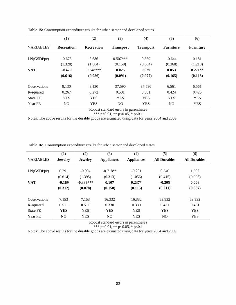
82


(1) (2) (3) (4) (5) (6)

VARIABLES Recreation Recreation Transport Transport Furniture Furniture

LN(GSDPpc) -0.675 2.686 0.507*** 0.559 -0.644 0.181

(1.328) (1.604) (0.159) (0.634) (0.368) (1.210)

VAT -0.470 0.648*** 0.025 0.039 0.053 0.271**

(0.616) (0.086) (0.091) (0.077) (0.165) (0.118)

Observations 8,130 8,130 37,590 37,590 6,561 6,561

R-squared 0.267 0.272 0.501 0.501 0.424 0.425




*** p<0.01, ** p<0.05, * p<0.1

Notes: The above results for the durable goods are estimated using data for years 2004 and 2009


(1) (2) (3) (4) (5) (6)

VARIABLES Jewelry Jewelry Appliances Appliances All Durables All Durables

LN(GSDPpc) 0.291 -0.094 -0.718** -0.291 0.540 1.592

(0.614) (1.395) (0.313) (1.056) (0.415) (0.995)

VAT -0.169 -0.339*** 0.107 0.237* -0.305 0.008

(0.312) (0.078) (0.158) (0.115) (0.211) (0.087)

Observations 7,153 7,153 16,332 16,332 53,932 53,932

R-squared 0.511 0.511 0.330 0.330 0.431 0.431




*** p<0.01, ** p<0.05, * p<0.1


83

Table 17: Consumption expenditure results for rural sector and developed states

(1) (2) (3) (4) (5) (6)

VARIABLES Food Food Addictive Substance Addictive Substance Energy Energy

LN(GSDPpc) -0.097* 0.008 -0.363** -0.127 0.082 -0.136

(0.049) (0.024) (0.149) (0.135) (0.236) (0.143)

VAT -0.106*** -0.008 -0.147*** 0.030 -0.032 0.099***

(0.012) (0.008) (0.040) (0.026) (0.050) (0.021)

Observations 162,001 162,001 109,515 109,515 161,800 161,800

R-squared 0.800 0.803 0.267 0.269 0.471 0.486




*** p<0.01, ** p<0.05, * p<0.1

Table 18. Consumption expenditure results for rural sector and developed states

(1) (2) (3) (4) (5) (6)

Clothing Clothing Education Education Medical Medical

VARIABLES Bedding Bedding In-patient In-patient

LN(GSDPpc) 3.697* 0.234** 3.841* 0.080 4.104* 0.042

(1.808) (0.087) (2.027) (0.201) (2.062) (0.271)

VAT 0.440 -0.024 0.495 -0.001 0.799 -0.010

(0.383) (0.023) (0.425) (0.026) (0.543) (0.076)

Observations 161,739 161,739 98,231 98,231 22,831 22,831

R-squared 0.425 0.899 0.388 0.677 0.477 0.747




*** p<0.01, ** p<0.05, * p<0.1

84


(1) (2) (3) (4) (5) (6)

VARIABLES Medical Out-

patient

Medical Out-

patient

Entertainment Entertainment Personal

Care

Personal

Care

LN(GSDPpc) -0.128 0.008 0.265 0.249 0.564 0.411

(0.300) (0.282) (0.190) (0.176) (0.360) (0.367)

VAT -0.112 0.079 0.092 0.069 0.057 -0.200**

(0.070) (0.048) (0.057) (0.042) (0.097) (0.077)

Observations 106,029 106,029 45,311 45,311 25,141 25,141

R-squared 0.298 0.298 0.429 0.429 0.240 0.240




*** p<0.01, ** p<0.05, * p<0.1


(1) (2) (3) (4) (5) (6)

VARIABLES Services Services Rent Rent Travel Travel

LN(GSDPpc) 0.395** 0.153 0.847 -0.132 0.128 -0.043

(0.167) (0.154) (0.752) (0.661) (0.142) (0.113)

VAT 0.345*** 0.178*** 0.070 -0.053 0.073* -0.139***

(0.045) (0.036) (0.241) (0.109) (0.040) (0.024)

Observations 156,303 156,303 8,243 8,243 123,714 123,714

R-squared 0.532 0.535 0.744 0.752 0.507 0.509




*** p<0.01, ** p<0.05, * p<0.1

85


(1) (2) (3) (4) (5) (6)

VARIABLES Recreation Recreation Transport Transport Furniture Furniture

LN(GSDPpc) -1.252*** -1.437*** -0.553 -0.677* -0.715* -0.557

(0.273) (0.259) (0.320) (0.373) (0.385) (0.464)

VAT -0.207*** -0.512*** 0.159* -0.151*** 0.025 0.154**

(0.068) (0.054) (0.082) (0.043) (0.096) (0.055)

Observations 9,636 9,636 59,989 59,989 12,920 12,920

R-squared 0.298 0.298 0.399 0.399 0.385 0.385




*** p<0.01, ** p<0.05, * p<0.1



(1) (2) (3) (4) (5) (6)

VARIABLES Jewelry Jewelry Appliances Appliances All Durables All Durables

LN(GSDPpc) 0.475 0.467 -1.253** -1.239* -0.202 -0.328

(0.483) (0.508) (0.471) (0.587) (0.332) (0.348)

VAT -0.085 -0.132 0.119 0.132** 0.092 -0.252***

(0.148) (0.088) (0.113) (0.059) (0.103) (0.043)

Observations 12,479 12,479 15,431 15,431 87,147 87,147

R-squared 0.534 0.534 0.327 0.327 0.379 0.380




*** p<0.01, ** p<0.05, * p<0.1


86

Table 23. Price Results for urban areas and developed states including state and year fixed effects

VARIABLES Price of

Rice

Price of

Wheat

Price of

Milk

Price of

Clear

Butter

Price of

Cooking

Oil

Price of

Eggs

Price of

Goat

Price of

Chicken

VAT 0.034*** -0.047*** -0.057*** -0.051** -0.056*** -0.002 -0.053*** 0.119***

(0.009) (0.009) (0.012) (0.021) (0.006) (0.010) (0.015) (0.010)

Sample Size 97,860 82,984 92,253 24,823 39,045 42,432 26,523 28,243

VARIABLES

Price of

Onion

Price of

Potato

Price of

Groundnut

Price of

Sugar

Price of

Salt

Price of

Turmeric60

Price of

Chilli

powder61

Price of

Suji62

VAT -0.072*** -0.003 -0.049*** -0.013** 0.064*** -0.022 0.009 -0.007

(0.012) (0.016) (0.013) (0.006) (0.018) (0.027) (0.017) (0.017)

Sample Size 101,769 99,658 29,063 92,779 104,517 101,202 97,408 40,048

VARIABLES

Price of

Yellow

Lentil

Price of

Banana

Price of

Tea Leaves

Price of

Pan63

Price of

Bidi64

Price of

Cigarette

(Foreign)

Price of

Alcohol

(Local)

Price of

Electricit

y

VAT -0.020 -0.003 -0.070*** -0.059*** 0.112*** 0.100*** 0.286*** 0.038

(0.021) (0.012) (0.011) (0.019) (0.012) (0.024) (0.058) (0.036)

Sample Size 77,112 70,703 93,692 9,297 18,730 9,279 5,597 95,988

VARIABLES

Price of

LPG65

Price of

Hosiery

Goods

Price of

Garments

Price of

Bedsheet

Price of

Other

Bedding

Price of

Rubber

Footwear

Price of

Slippers

Price of

Upholste

ry

VAT

-0.050** -0.001 -0.069** -0.184*** -0.175** -0.047** -0.094*** -0.339***

(0.021) (0.014) (0.025) (0.016) (0.059) (0.018) (0.013) (0.048)

Sample Size 59,663 98,951 88,484 45,602 10,733 87,903 54,065 3,375

Notes: Values in parentheses are the estimated robust standard errors

*** p<0.01, ** p<0.05, * p<0.1

60 It is one of the most commonly used spices in India. 61 It is one of the most commonly used spices in India. 62 It is commonly used flour used to make bread and sweets. 63 It is an addictive substance popularly consumed in India. Betel leaves is the most important ingredient in it. 64 It is a locally made cigarette. It is one of the most commonly consumed forms of tobacco. 65 It is made from natural gas and is used as a cooking fuel.

87

Table 24. Price Results for rural areas and developed states including state and year fixed effects

VARIABLES

Price of

Rice

Price of

Wheat

Price of

Milk

Price of

Clear

Butter

Price of

Cooking

Oil

Price of

Eggs

Price of

Goat

Price of

Chicken

VAT 0.105***

-

0.048*** -0.029** -0.009

-

0.020*** -0.021** 0.024** -0.026**

(0.007) (0.008) (0.013) (0.022) (0.006) (0.009) (0.010) (0.011)

Sample Size

140,963 105,077 121,441 15,655 76,667 50,979 30,739 34,283

VARIABLES

Price of

Onion

Price of

Potato

Price of

Groundnut

Price of

Sugar

Price of

Salt

Price of

Turmeric66

Price of

Chilli

powder67

Price of

Suji

VAT

-0.035** -0.006 -0.095*** -

0.013*** 0.088*** 0.025 0.063***

0.00268

(0.013) (0.016) (0.014) (0.004) (0.024) (0.025) (0.014) (0.015)

Sample Size 156,126 150,471 34,218 133,609 160,510 155,681 149,654 38,912

VARIABLES

Price of

Yellow

Lentil

Price of

Banana

Price of

Tea Leaves

Price of

Pan69

Price of

Bidi70

Price of

Chewing

Tobacco

Price of

Alcohol

(Local)

Price of

Firewood71

VAT -0.002

-

0.040*** -0.068*** -0.128** 0.103*** 0.652*** 0.173***

-0.009

(0.025) (0.012) (0.011) (0.055) (0.014) (0.063) (0.055) (0.033)

Sample Size 94,721 80,561 130,836 14,346 49,312 31,029 15,230 139,389

VARIABLES

Price of

Kerosene72

Price of

Hosiery

Goods

Price of

Garments

Price of

Bedsheet

Price of

Blanket

Price of

Rubber

Footwear

Price of

Slippers

Price of

Upholstery

VAT

-0.000

-0.031***

-0.051*** -0.103* -

0.091*** -0.241*** -0.013 -0.036

(0.003) (0.008) (0.014) (0.054) (0.013) (0.026) (0.015) (0.085)

Sample Size 121,706 144,368 123,009 135,808 54,088 17,013 135,534 2,009

Notes: Values in parentheses are the estimated robust standard errors

*** p<0.01, ** p<0.05, * p<0.1

66 It is one of the most commonly used spices in India. 67 It is one of the most commonly used spices in India. 68 It is commonly used flour used to make bread and sweets. 69 It is an addictive substance popularly consumed in India. Betel leaves is the most important ingredient in it. 70 It is a locally made cigarette. It is one of the most commonly consumed forms of tobacco. 71 It is an important source of energy in the rural areas. 72 A type of fuel commonly used for cooking and lighting in the rural areas.

88

CHAPTER THREE - TAX INCIDENCE: DO INSTITUTES MATTER? AN

EXPERIMENTAL STUDY

1 ABSTRACT

There is perhaps no more important question in public finance than who ultimately bears the

burden of a tax. According to tax incidence theory, the long-run incidence of a unit tax is

independent of the assignment of the liability to pay tax. However, the theory is silent on the

possible effects of market institutions on tax incidence. We report data from an experiment

designed to address two questions. Is tax incidence independent of the assignment of the liability

to pay tax in experimental markets? Is tax incidence independent of the market institution in

experimental markets? We conduct laboratory experiments, using double auction and posted

offer markets. Based on the results of Kolmogorov-Smirnov tests of experimental market prices,

we conclude that the answer to both questions is an emphatic “no.” We report evidence that the

observed differences from the theoretical values are statistically significant and economically

meaningful.

2 INTRODUCTION

To understand the distributional effects of a tax, it is necessary to know who ultimately

bears the tax burden. The theory of tax incidence concerns itself with answering this very

question, and there may be no more important question in the field of public finance. According

to the liability side equivalence (LSE) hypothesis, the incidence of a tax in long-run competitive

equilibrium has nothing to do with the statutory assignment of the liability to pay tax. Rather, it

89

depends on the relative elasticity’s of supply and demand; the more inelastic of the two

ultimately bears the greater tax burden.

The economic intuition for this conclusion is straightforward. Suppose, for example, that

a firm is liable to pay tax on every unit sold. The firm can try to shift the tax forward onto the

consumer through higher prices. The ability of the firm to do so, however, is limited by the own-

price elasticity of demand for the good. If demand is sufficiently inelastic relative to supply, the

change in quantity demanded will be small in response to a given increase in the price. In this

case, the firm will find it profitable to shift much of the tax burden onto consumers. If, on the

other hand, demand is elastic relative to supply, increasing the price to shift the tax onto

consumers will lead to a large decrease in the quantity demanded. In this case, the firm will not

find it profitable to shift as much of the tax onto the consumer as in the inelastic case. From this

perspective, nothing changes if the consumer is assigned the liability to pay the tax rather than

the seller.73

Since governments seldom change the statutory assignment of the liability to pay tax,

there are seldom opportunities to test the LSE hypothesis using observational data. An exception

is Saez et al. (2012) who test the LSE hypothesis using evidence from a natural experiment

created by a change in the assignment of the liability to pay the payroll tax in Greece. They

report evidence that contradicts the LSE hypothesis. Furthermore, there is a growing literature

indicating that informational, behavioral, and institutional factors influence tax incidence.74

Indeed, markets need institutions to function. These institutions specify how buyers and sellers

73 Of course, the firm has not exhausted all of its options; it could also attempt to shift the tax backward onto the

suppliers of factors of production. Again, according to the LSE hypothesis, the firm’s ability to do so depends on the

relative price elasticities of factor supplies and demands. 74 Using a laboratory experiment, Sausgruber and Tyran (2005) test the “Mill hypothesis” that the burden of an

indirect tax may differ from that of a direct tax because the latter is more visible or salient. In a related study using a

field experiment and observational data on gasoline and liquor sales, Chetty et al. (2009) examine the impact of tax

salience on tax incidence. In a related study, Finkelstein (2009) reports evidence that salience influences the

elasticity of demand for tolled roads.

90

interact to determine prices and quantities. Different market institutions are known to have

different price formation and quantity determination properties, and these properties may affect

the incidence and excess burden of taxes.75 Yet, the theoretical literature on tax incidence does

not account for the potential influence of market institutions on tax incidence. In this study, we

use laboratory experiments to see if two important market institutions – double auction and

posted offer markets – produce results that are consistent with the LSE hypothesis.

Perfect competition is a theoretical construct of an idealized market structure. In

everyday life, however, we deal with market institutions rather than idealized market structures.

There is no discussion in the theoretical literature on the impact of market institutions on tax

incidence. Consider the following example as a case in point. Perfectly competitive markets

assume price-taking behavior by buyers and sellers. In the case of retail markets, sellers

obviously set or post prices, and buyers purchase as many units as they wish to at the posted

price. Furthermore, in contrast to the assumption of complete information in perfectly

competitive markets, buyers and sellers do not have perfect information about prices of

comparable goods on offer at other stores as assumed by the theory of perfect competition absent

a costly search for such information.

In laboratory experiments, the market institutions that are the focus of this study exhibit

the price convergence property predicted by the theory of perfectly competitive markets. Strictly

speaking, we do not claim to be testing the theory of long-run tax incidence for perfectly

competitive markets. Rather we are testing whether the data generated in laboratory experiments

with two important market institutions are consistent with the LSE hypothesis. In this way we are

75 See, for examples: Williams (1973), Plott and Smith (1978), Hong and Plott (1982), Smith (1982b), and Ketcham

et al. (1984).

91

attempting to add an important dimension to our understanding of the potential influence of

market institutions on tax incidence.

We are not the first to propose testing the LSE hypothesis in a laboratory setting.

Kachelmeier et al. (1994), Kerschbamer and Kirchsteiger (2000), Borck et al. (2002), Riedl et al.

(2005), and Ruffle (2005) test the LSE hypothesis in laboratory settings using a variety of tax

types and market institutions. Kerschbamer and Kirchsteiger (2000) test the LSE hypothesis by

imposing a tax on either the proposer or the responder in a one-stage ultimatum bargaining game.

They contend that the LSE hypothesis should hold in the tax version of the ultimatum game as

long as the fairness norm threshold below which offers are rejected remains unaffected by a

change in the statutory assignment of the liability to pay the tax. Based on the results of their

experiments, they reject the LSE hypothesis at conventional levels of significance. To explain

this finding, they hypothesize that the assignment of the liability to pay tax may lead those with

the legal responsibility for remitting the tax to the government to feel a moral duty to bear the tax

economically. There is no market institution in this experiment.

Riedl and Tyran (2005) test the LSE hypothesis, using a gift-exchange game. They

contend that LSE should hold in gift-exchange games when gross wages adjust to changes in

taxes and market participants are exclusively concerned with net-of-tax profits and wages. They

test the LSE hypothesis in a gift-exchange game where social norms may cause LSE to

breakdown. In contrast to Kerschbamer and Kirschsteiger, Riedl and Tyran cannot reject the LSE

hypothesis at conventional levels of significance. However, there is no market institution in the

Riedl and Tyran experiment.

Kachelmeier et al. (1994) use an elaborate experimental design to test the LSE

hypothesis. Their design involves two interrelated, double auction markets, three agents

92

(customers, retailers, and wholesalers), and three different tax instruments (an ad valorem tax

levied on customers, a turnover tax levied on retailers, and a value-added tax levied on

wholesalers and retailers). In their experimental design, there are 10 periods without a tax; then,

there are 10 periods with one of the tax instruments described above. They conduct 10 market

sessions. They cannot reject the LSE hypothesis at conventional levels of significance. Borck et

al. (2002) test the LSE hypothesis in posted offer markets, using a unit excise tax. In their

experimental design, there is no tax in the first 12 periods; then they introduce a unit tax in

periods 13 through 24. They conduct 10 market sessions. They also conduct two market sessions

using a double auction market design. They cannot reject the LSE hypothesis for either market

institution. However, they do not report whether tax incidence differs between the two market

institutions.76

Ruffle (2005) tests the LSE hypothesis for taxes and subsidies. They use a pit market

where at least eight pairs of buyers and sellers participate in all experiments.77 All sessions

consist of 19 three-minute trading periods. During the first eight periods, subjects participate in

an ordinary pit market, with no tax or subsidy. Beginning in period 9, a single change is

introduced, namely a 10-unit tax (subsidy) on either the buyers or the sellers. They find strong

support for the LSE hypothesis for both subsidies and taxes.

76 Although sellers are in a position to behave strategically, posted offers are typically discussed in experimental

studies as deviations from or convergent to the perfectly competitive price. Holt and Solis-Soberon describe a Nash

equilibrium pricing strategy involving randomization in laboratory posted offer markets that may differ from the

competitive equilibrium. Borck et al. (2002) point out that the Nash equilibrium described by Holt and Solis-

Soberon assumes non-strategic behavior by buyers which may limit the applicability of this equilibrium.

Furthermore, Borck et al. do not find empirical support for the Nash equilibrium pricing strategy in their posted

offer markets. We return this issue below. 77 A pit market closely resembles a double auction market. The two institutions differ in the way bids and asks are

organized. In a pit market, traders negotiate directly with whomever they choose from the other side of the market,

with participants freely exchanging bids and asks between them until a transaction price is agreed upon. In the

double auction market, bids and asks are publicly recorded. In a double auction market, actual trade occurs when a

seller accepts the most attractive bid price, or a buyer accepts the most attractive offer price among the outstanding

bid and offer prices.

93

In each of the experimental designs with market institutions described above, the

experiment begins with a no-tax treatment in the initial trading periods; then, a tax is introduced

and trading proceeds for an equal number of periods as in the initial no-tax treatment. In these

experiments, there is a striking difference in the speed of price convergence in the initial, no-tax

trading periods and in the subsequent trading periods with a tax. In the initial no-tax trading

periods, the trading prices are rather noisy, and it takes a few trading periods for prices to begin

to converge to an equilibrium. In contrast, the initial rounds of the tax treatment converge almost

immediately to an equilibrium. For example, Borck et al., report the mean and variance of the

prices by trading period in their Table 1. We use these data to compute the coefficient of

variation in the initial three periods and the last period with no tax and with a tax on the seller.78

The coefficients of variation in the initial three periods and the last period without a tax are 41.2,

28.7, 16.5, and 8.0, respectively, and with a tax on the seller, they are 17.9, 9.7, 8.2, and 4.6,

respectively. When the tax is on the buyer, the coefficients of variation by period exhibit the

same pattern. This raises the question of whether the LSE hypothesis is robust to alternative

experimental treatments. More specifically, we ask and attempt to answer whether the findings

reported above depend on the initial trading periods without a tax. The reason for pursuing this

question is concern about cross-treatment contamination. We are also interested to compare the

incidence of a tax, holding the liability to pay tax the same, for two different market institutions.

Our experimental design differs from the existing literature in a number of important

ways. We introduce a unit tax in the first trading period and maintain that tax throughout all 30

trading periods. In addition to testing the LSE hypothesis for two market institutions, we also test

78 Introducing a tax in the 13th trading period changes the scale of the price series; therefore, the variances for the

two price series with and without a tax are not comparable. We use the coefficient of variation to compare the

variation in the two price series, which is defined as follows: (σ ÷ μ)×100, where σ is the standard deviation and μ is

the mean. The coefficient of variation accounts for the change in the scale of the two series by dividing the standard

deviation by the mean.

94

whether the incidence of a unit tax is the same in both market institutions holding the liability to

pay tax the same. We also calculate the excess burden due to the unit tax for each of the four

treatments that result from our 2×2 design. Our underlying research question therefore is whether

two prominent features of a controlled experimental economy – the assignment of the liability to

pay tax and the type of market institution – influence the incidence of a tax using two important

market institutions observed in the field.

More specifically, we conduct laboratory experiments comparing computerized double

auction (DA) and posted-offer (PO) markets to investigate whether tax incidence is independent

of the assignment of the liability to pay tax and the type of market institution. The rules of the

computerized DA market in our experiments are essentially the same as those that govern trading

on the New York Stock Exchange and on many organized futures markets. An experimental DA

market is open for a specified interval of time; buyers are free to announce at any instant a bid

price for the commodity they wish to buy; and sellers are free to announce an offer price for the

commodity they wish to sell. In the simplified DA markets used in many experiments, including

ours, each bid, offer, or contract is for a single unit. Actual trade occurs when a seller accepts the

most attractive bid price, or a buyer accepts the most attractive offer price among the outstanding

bid and offer prices.

The rules of the computerized PO market in our experiments are similar to those that

govern most of the consumer goods markets in developed countries. Think, for example, of a

supermarket or department store. The seller posts a sales price for a commodity and may also

limit the quantity they are willing to sell at that price. Buyers may compare prices available to

them from different sellers and make the decision to buy or not to buy a given commodity from a

95

given seller at the posted price. The computerized PO market in our experiments is similar to this

field institution.

The choice of DA and PO markets are particularly well suited to the research questions at

hand. Smith (1976b), Smith et al. (1982), Williams (1980), and Smith and Williams (1983)

report the robust result that DA markets converge rapidly to a competitive equilibrium thus

exhausting the potential gains from trade. In other words, DA markets achieve the Pareto

efficient resource allocation of competitive market theory. It would seem that DA markets give

the LSE hypothesis very good chances for success. In contrast, Plott and Smith (1978), Williams

(1980), Hong and Plott (1982), Smith (1982b), and Ketcham et al. (1984) report evidence that

PO markets produce prices that converge to the competitive equilibrium price from above and

more slowly than in DA markets. PO markets also yield less efficient allocations than DA

markets. Consequently, the LSE hypothesis may not apply to PO markets. However, PO

exchange is the most common retail market institution in advanced market economies; thus, it is

important to investigate the effect of this market institution on tax incidence.

Our experimental design includes four treatments that use the same induced, stationary

supply and demand schedules: (1) a double auction market with a unit tax on the buyer (DATB);

(2) a double auction market with a unit tax on the seller (DATS); (3) a posted offer market with a

unit tax on the buyer (POTB); and (4) a posted offer market with a unit tax on the seller (POTS).

Tax incidence theory is silent about the role market institutions play in determining who

ultimately bears the burden of a tax. However, according to the LSE hypothesis, the incidence

and excess burden of a unit excise tax are independent of the assignment of the liability to pay

tax. This hypothesis is robust to many market structures.

96

To test the LSE hypothesis, we conduct Kolmogorov-Smirnov (K-S) two independent

sample tests using pairwise comparisons of the empirical cumulative distributions of the buyer

prices produced by the four experimental treatments. In contrast to the predictions of the LSE

hypothesis, the K-S tests reject the LSE hypothesis at conventional levels of significance. The K-

S tests also reject the hypothesis at conventional levels of significance that the type of market

institution has no effect on the distribution of buyer prices. In short, we report evidence that the

assignment of the liability to pay tax and the type of market institution have statistically

significant and economically meaningful effects on tax incidence in the two market institutions

that are the focus of this study.

The remainder of this paper is organized as follows. The next section describes our

experimental design in greater detail, and the subsequent section explains the results. We

conclude in the final section.

3 EXPERIMENTAL DESIGN AND PROTOCOL

Our experimental design tests the ability of a widely accepted economic theory to predict

the influence of changes in the type of market institution and in the assignment of the liability to

pay tax on tax incidence. Following Smith (1976a, 1982a), we induce stationary demand and

supply functions for a fictitious commodity. We use a balanced design in which tax incidence

theory predicts that the economic burden of a unit tax on a homogeneous good will be equally

shared between buyers and sellers, independently of the assignment of the liability to pay tax.79

As previously noted, the theory makes no prediction regarding the influence of a change

in the type of market institution on the incidence of a tax. To gauge the impact of the market

79 A “balanced design” is the discrete-variables analogue of a continuous-variables model in which: (a) the slope of

the linear market demand function is the negative of the slope of the linear market supply function; and (b)

consumers’ surplus equals sellers’ surplus at the theoretical competitive equilibrium price and quantity.

97

institution, we change the market institution from a DA to a PO market, keeping the assignment

of the liability to pay tax the same. Similarly, we change the assignment of the liability to pay tax

from the seller to the buyer, keeping the market institution the same, in order to gauge the impact

of this change on the incidence of a tax. The result is a 2×2 design with a total of four treatments.

This illustrates the advantage of laboratory experiments. They are performed in well-defined,

controlled environments, where one variable at a time is changed to measure its impact on the

outcome of interest. We proceed below by describing our basic experimental design.

We conduct a total of four sessions, where each session is devoted to one of the four

treatments. The subject’s role as a buyer or a seller in the experimental market is randomly

assigned by a computer at the beginning of each session and remains the same throughout the

session. In each session, four independent markets, consisting of five buyers and five sellers in

each market, are simultaneously trading. Each buyer and seller is given five (no-tax) infra-

marginal units to sell or buy at the beginning of each trading period, and there are 30 trading

periods in each of the four markets in a given session. In short, the experiment uses a between

subjects design, with 40 subjects randomly assigned to the role of buyer or seller in equal

numbers in each of the four treatments, resulting in a total of 160 subjects.

Table 25 below shows an individual seller’s marginal costs and an individual buyer’s

marginal values per unit. The table shows the five (no-tax) infra-marginal costs and values and

the marginal cost and value for a sixth, extra-marginal unit. Each buyer in all four treatments is

assigned a value of 50 experimental dollars (ED) for unit 1 of the fictitious commodity, 47 ED

for unit 2, 44 ED for unit 3, 41 ED for unit 4, 38 ED for unit 5, and 35 ED for unit 6. These

marginal values represent the induced individual demand schedules used in the experiment.

Similarly each seller in all four treatments is assigned a cost of 23 ED for unit 1, 26 ED for unit

98

2, 29 ED for unit 3, 32 ED for unit 4, 35 ED for unit 5, and 38 ED for unit 6. These marginal

costs identify the induced individual supply schedules used in the experiment. Costs and values

are private information. Throughout each session, the subjects are seated in a manner that

protects the privacy of this information. The amount of the unit tax (12 ED) and the assignment

of the liability to pay tax are announced to the subjects at the beginning of each session. The

costs, values, and tax per unit remain the same throughout each session.

In the absence of a tax, the unique competitive equilibrium quantity is 25 units, consisting

of 5 units traded by each buyer and seller. After we impose a unit tax of 12 ED, the unique

equilibrium quantity predicted by the theory is 15 units, consisting of 3 units traded by each

buyer and seller. The predicted excess burden of this tax is 60 ED [= 5×(38 − 35) + 5×(41 − 32)].

At the beginning of each experimental session, subjects read through detailed instructions

appearing on their computer screens on how to interact with the computer to trade in the market.

The instructions for buyers and sellers for all four treatments are available at the following URL:

http://expecon.gsu.edu/jccox/subjects.html. These instructions are also available to the reader in

the appendix of this paper. After the subjects read through the instructions, summary instructions

are projected on a screen and read to the subjects to increase understanding of the market

participation process. The scripts of the oral summary instructions are available at the URL given

above. Subjects are permitted to ask questions of the experimenter, either publically or privately.

Before actual trading periods begin, there are five practice trading periods to ensure the subjects

are comfortable with the software. These practice periods acquaint the subjects with the software

and help them to understand the decision-making process. The practice periods are followed by

30 actual trading periods in each session (treatment). The total number of trading periods is not

announced to the subjects.

99

The subjects are mostly undergraduate students at a large urban university in the United

States. Table 26 provides information on the demographic profile of the subjects. They are nearly

equally divided among class ranks, with 25 percent freshmen, 31 percent sophomores, 20 percent

juniors, and 22 percent seniors. Masters students make up two percent of the sample.

Approximately 75 percent of the sample has previous experience in an experiment; 59 percent

are female; 51 percent are African-American; 20 percent are white; 15 percent are foreign born;

and the remaining 14 percent are either Asian-American, Hispanic-American, or mixed race. The

average age in our sample is 20 years old; the minimum age is 18; and the maximum age is 24.

Approximately 34 percent of the sample is either a business major (accounting, finance, or

management) or an economics major. The modal (39 percent) grade point average (GPA) is

between 3.25 and 3.74; 9 percent have a GPA between 1.25 and 2.74; 29 percent between 2.75

and 3.24, and 19 percent between 3.75 and 4.0. A small percentage of the sample (4 percent) has

yet to receive a final grade in a college course. Although there is some variation in the

demographic profiles among the four treatments, the percentages are similar across treatments

suggesting that the randomization was successful.

2.1 Induced value information given to subjects

Subjects are given the same information about induced marginal costs and values in

every experimental session with either market institution. A seller’s trading screen shows “cost

per unit” in one column and the “cost plus tax per unit” in an adjacent column.80 If, however, the

80 For both the double auction and posted offer market treatments, we include separate columns for “cost per unit”

and “cost plus tax per unit” in the seller’s trading screen and “value per unit” and ‘value minus tax per unit’ in the

buyer’s trading screen in order to make the tax salient. Chetty et al. (2009) defines tax salience as the price of a good

calculated at the gross-of-tax price. He reports evidence of the impact of tax salience on behavioral responses to

taxes from a field experiment and regression analysis using observational data. When taxes are less salient, agents

do not optimize relative to the true tax-inclusive prices, and so demand becomes less sensitive to a tax. In other

words, a less salient tax makes the own-price elasticity of demand more inelastic relative to a more salient tax,

making consumers bear more of the tax burden. Furthermore, Finkelstein (2009) shows that less salient tolls result in

more inelastic demand.

100

buyer is assigned the liability to pay tax, the figures in these two columns are identical, because

the unit tax on the seller is equal to zero. Similarly, a buyer’s trading screen shows “value per

unit” in one column and the “value minus tax per unit” in an adjacent column. If, however, the

seller is assigned the liability to pay tax, the figures in these two columns are identical, because

the unit tax on the buyer is equal to zero. For further details on the exact layout of the buyer and

seller trading screens, the interested reader may see the screen shots in the subject instructions

which are available at the URL given above.

2.2 Computerized double auction markets

Two treatments are conducted with DA markets. In one treatment, the liability to pay tax

is assigned to the seller in the market and, in the other treatment, to the buyer in the market. The

assignment of the liability to pay tax is the only difference in the two DA treatments. The unit

tax in both treatments is the same and equal to 12 ED. In both treatments sellers and buyers are

given two and a half minutes to complete their transactions in each trading period. The time

remaining in the trading period, the subject’s own number of units available to buy or sell, own

cumulative earnings, own profit or loss from each traded unit, outstanding bid and ask prices in

the market, tax charged per unit, and the market transaction prices are displayed on the trading

screens of the buyers and sellers at all times. The bid, ask, and transaction price information

provided is a characteristic of the DA market institution.

2.3 Computerized posted offer markets

The remaining two treatments are PO markets. In this market institution, sellers make the

first move by posting an offer price and the number of units they are willing to sell at that offer

price. Buyers then enter the market in a random queue, one by one, and accept the sellers’ offers

if they find them attractive. If an offer is accepted, then trade occurs. In one posted-offer

101

treatment, the liability to pay a unit tax on each traded unit of a fictitious commodity is assigned

to the seller. In the other treatment, the liability to pay a unit tax on each traded unit of the

commodity is assigned to the buyer. Again, the assignment of the liability to pay tax is the only

difference between these two treatments. In both treatments, sellers have two and a half minutes

to post offers to the market in each trading period. Each buyer has an equal amount of time (30

seconds) to accept the available offers in the market. The time remaining to make decisions, own

number of units available to buy or sell, own cumulative earnings, own profit or loss from each

traded unit, and the unit tax are displayed on the sellers’ and buyers’ trading screens. A seller’s

trading screen also lists the offers posted by oneself. Sellers are not able to see the offers posted

by other sellers in the market. We believe that this feature of the treatment best reflects the field

institution that we are trying to replicate in the laboratory. In the field, knowledge of the prices

offered by other sellers in the market can only be obtained through costly surveillance; this

information is not provided without cost by the PO market institution.

A buyer’s trading screen lists the number of units available for sale and the offer price

corresponding to each of these units as posted by the sellers. For further details on the trading

screen’s presentation of information and layout, please refer to the screenshots provided in the

subject instructions which are available at the URL given above.

2.4 Questionnaire and subject payments

At the end of each session, the subjects are asked to complete a short survey, and then

they are paid their cumulative earnings for all 30 trading periods, according to the conversion

rate (1 ED = $0.07) announced at the beginning of the session. Table 27 reports the minimum,

average, and maximum earnings for each of the 4 treatments. In the DATS treatment, the

minimum earnings are $14.25, the average earnings $26.99, and the maximum earnings $38.75.

102

Turning to the DATB treatment, the minimum, average, and maximum earnings are $16.75,

$27.66, and $35.25, respectively. In the POTS (POTB) treatment, the minimum earnings are

$9.25 ($6.75), the average earnings $20.12 ($20.79), and the maximum earnings $40.75

($38.50). A session takes approximately 2 hours to complete; thus average earnings exceed

$10.00 per hour, which is a favorable hourly earnings rate for student subjects. A copy the

questionnaire is available in the appendix of the paper.

4 DATA FROM THE EXPERIMENT

We investigate two questions in this study. Is tax incidence independent of the

assignment of the liability to pay tax for a given market institution? Is tax incidence independent

of the type of market institution? We proceed below by making pairwise comparisons of the

average buyer prices from the four treatments. Then, we test the statistical significance of these

pairwise comparisons, using the Kolmogorov-Smirnov (K-S) test for two independent samples.

We begin by making pairwise comparisons of the average buyer prices from the four

treatments. According to the LSE hypothesis, there should be no difference between the average

buyer prices in the two DA treatments and no difference in the two PO treatments.81

Figure 8 shows the percentage differences in pairwise comparisons of average buyer

prices from the four treatments. The average buyer price from the DATS treatment is 1.46

percent greater than that from the DATB treatment. Similarly, the average buyer price in the

POTS markets is 1.82 percent greater than the average buyer price in the POTB markets. A

comparison of prices between market institutions reveals that the average buyer price is 5.40

81 The choice of buyer or seller prices has no bearing on the inferences drawn from the data. The buyer price is the

amount paid by a buyer for a unit of the fictitious commodity. The difference between the buyer price and the seller

price is always equal to the unit tax or 12 ED. The comparisons among prices across the four treatments would be

the same if the analysis were conducted in terms of seller prices.

103

percent higher in the POTS than in the DATS markets and 5.14 percent higher in the POTB than

in the DATB markets. Clearly, the differences in average buyer prices are greater for the

comparisons between market institutions, holding the assignment of the liability to pay tax the

same, than for the comparisons between the assignments of the liability to pay tax, holding the

market institution the same. These differences may appear to be rather modest; however, as

discussed in greater detail below, relatively small differences in buyer prices lead to much larger

differences in excess burdens.

To test the LSE hypothesis, we use the K-S test for two independent samples. 82 The K-S

test has several advantages over alternative statistical procedures. Since the K-S test is based on

the empirical cumulative distributive functions (CDFs) of the price series, it uses all the moments

of the data. Furthermore, the K-S test is robust to alternative distributional properties of the data,

non-normal distributions, and heteroskedasticity. In contrast, the Student’s t-test only uses the

first moment of the data and is sensitive to significant departures from normality and

homoscedasticity.

There is a lot of “noise” in the prices in the initial trading periods, which undoubtedly

reflects the price discovery process. This noise appears to fade away by the 15th trading period.

Prices stabilize more rapidly in the DA markets than in the PO markets, which is consistent with

previous findings reported in the literature for experimental markets without taxes. Since the K-S

test assumes the observations are independent draws from a given distribution, we conduct a runs

test for serial randomness of the price data for the last 15 trading periods of each treatment. The

runs tests fail to reject the null hypothesis of serial independence at conventional levels of

82 The intuition behind this test is as follows. If two independent samples are drawn from the same population, the

two cumulative frequency distributions would be expected to be reasonably similar. The protocol for the K-S test of

two independent samples is based on the principle that if there is a significant difference at any point along the two

cumulative frequency distributions, the researcher can conclude there is a high likelihood the samples come from

two different populations. For further details, see Daniel (1990) and Smirnov (1936).

104

significance for each treatment.83 More specifically, the runs test is equal to -1.26 (p-value =

0.21) for the DATB buyer price series; to 1.07 (p-value = 0.29) for the DATS price series; to

-0.59 (p-value = 0.55) for the POTB price series; and to -0.01 (p-value = 1.00) for the POTS

price series.84 This provides statistical support for our conclusion based on merely looking at the

price series that they have converged by the 15th trading period. Consequently, we feel justified

in using the data from the last 15 trading periods to conduct the K-S test for two independent

samples.

Figures 9 through 12 provide pairwise comparisons of the CDFs of buyer prices from

pairwise comparisons of the four treatments. Beneath each figure, we report the maximum

difference between the two CDFs and the associated p-value of the K-S test statistic.

We begin by examining whether the incidence of a tax is independent of the assignment

of the liability to pay tax for the two market institutions that are the focus of this study. Figure 9

compares the CDFs of the average buyer prices from the DATB and DATS treatments. The

maximum difference between the two CDFs is 0.2023 (p-value = 0.000), which is statistically

different from zero at conventional levels of significance. Thus, we can reject the null hypothesis

that the two price series come from identical probability distributions. This finding for the DA

treatments is inconsistent with the prediction of the LSE hypothesis that the incidence of a tax is

independent of the assignment of the liability to pay tax.

Figure 10 makes a similar comparison for the two CDFs of the buyer prices from the PO

treatments. The distributions appear to be quite different. The maximum difference between the

two CDFs is 0.3030 (p-value = 0.000), which is statistically significantly different from zero at

conventional levels of significance. Again, this leads us to reject the hypothesis that the

83 See Zar (1999) for further details on the runs test of serial randomness. 84 The p-value is the probability of obtaining a test statistic at least as extreme as the one that is actually observed,

assuming that the null hypothesis is true that the two samples are drawn from the same probability distribution.

105

incidence of a tax is independent of the assignment of the liability to pay tax in the PO

treatments, too.

Now we turn to our second question: Is the incidence of a tax independent of the type of

market institution, holding the assignment of the liability to pay tax the same. Figure 11

compares the two CDFs of the buyer prices from the DATB and POTB treatments. Again the

two distributions appear to be quite different, and, indeed, the maximum difference between the

two CDFs is 0.7022 (p-value = 0.000), which is statistically significantly different from zero at

conventional levels of significance. Finally, Figure 12 compares the two CDFs of the buyer

prices from the DATS and POTS treatments. The maximum difference between these two CDFs

is 0.7253 (p-value = 0.000), which is also statistically significantly different from zero at

conventional levels of significance.

Although these differences are highly statistically significant, it is also important to gauge

whether these differences are economically meaningful. We use several measures of economic

significance. We compare the proportions of the total tax revenue paid by buyers and sellers in

the four treatments. We also compare the excess burdens created by the tax in each of the four

treatments.

Table 28 reports average buyer prices, total tax revenue, and the incidence of the tax as a

percent of total revenue for the last 15 periods of each of the four treatments. Since we use a

balanced design, the theory of tax incidence predicts that the burden of the tax will be equally

shared between buyers and sellers. This is what we observe in the DATB treatment, where

approximately 50 percent of the tax burden is borne by buyers and 50 percent by sellers, as

shown in the first row of Table 28. Consequently, we use these results to gauge the incidence of

the tax in the other three treatments. In the DATS treatment, 55.1 percent of the tax revenue of

106

180.4 ED is borne by buyers and 44.9 percent by sellers. In contrast, 67.9 percent of the tax

revenue of 133.6 ED is borne by buyers and 32.1 percent by sellers in the POTB treatment. The

burden of the tax is even further shifted onto buyers in the POTS treatment; here 74.5 percent of

the tax revenue of 124.8 ED is borne by buyers and 25.5 percent by sellers. Clearly, these

differences in tax incidence among the four treatments are economically meaningful.

Now, we turn to the analysis of excess burdens. Table 29 shows the average quantity,

average excess burden, average excess burden as a percentage of tax revenue, and average excess

burden as a percentage of participant earnings for the last 15 periods of each treatment. The

average quantities shown in Table 29 are consistent with the observed differences in tax shifting

documented in Table 28. The equilibrium quantity in the DATB treatment is approximately

equal to 15 units, which is the post-tax equilibrium quantity predicted by the theory. As a result,

the excess burden in the DATB treatment is approximately equal to 60 ED which is the value

predicted by the theory. In the DATS treatment, the average quantity is 15.03, and the excess

burden is 63.85 ED. In contrast, the average quantities are clearly lower and excess burdens

strikingly greater in the POTB and POTS treatments. The average quantities (excess burdens) are

11.13 (134.7 ED) and 10.40 (147.4 ED) in the POTB and POTS treatments, respectively. Table

29 also shows that there are stark differences in excess burdens as a share of tax revenue and as a

share of participant earnings among the four treatments.

In short, the data generated by the DATB treatment are consistent with the theory of

long-run tax incidence in competitive markets. Using this treatment as the benchmark, we find

substantial differences in the average prices and quantities as well as the excess burdens as a

share of participant earnings among the other three treatments. Contrary to the predictions of the

107

LSE hypothesis, tax incidence is not independent of the assignment of the liability to pay tax.

Incidence also depends on the type of market institution in our laboratory experiments.

Despite the similarities in research question, our conclusions dramatically differ from

those of Borck et al. (2002) who fail to reject the LSE hypothesis in posted offer and double

auction markets. Therefore, it may be worthwhile to discuss what may be giving rise to these

discrepant conclusions. There are two plausible explanations: differences in our experimental

and statistical procedures.

Beginning with the differences in the experimental procedures, Borck et al have the

traders begin with 12 trading periods without a tax. In the 13th trading period, they introduce a

unit tax and allow trade to continue for an additional 12 periods. The induced supply and demand

schedules are the same in all 24 trading periods. Our experimental protocals differ from theirs in

that we introduce a tax in the first trading period. This difference in our experimental designs

may account for the discrepancy in our conclusions. In this case, we believe that both sets of

findings are interesting and raise potentially interesting questions for further research.

There are also important differences in our statistical procedures that may explain the

discrepancies in our conclusions. We use a non-parametric K-S test of independent samples to

test the LSE hypothesis. As previously noted the K-S test has a number of attractive statistical

properties. Furthermore, we use a runs test to verify that the data satisfy the independence

assumption of the K-S test. In contrast, they estimate a random effects model. The reason they

give for doing so is to account for potential serial correlation in the data. An alternative would be

to estimate a first or second order autoregressive model with random effects. We use our data to

estimate both types of models (a random effects model using an identical specification as theirs

108

and an AR(1) model with random effects). Both econometric specifications reject the LSE

hypothesis in all four cases at conventional levels of significance.

It is well known that significant deviations from normality, homoskedasticity, and

independence can substantially affect the performance of statistical inferences in regression

models. When estimating regression models with small samples, therefore, good statistical

practice should include diagnostic tests of the residuals to verify that they are well behaved.

Borck et al. do not report the results of such diagnostic tests. This is not unusual in econometric

studies. However, when we use our data to estimate these regression models, a Jarque-Bera

(1987) test rejects the null hypothesis that the residuals from these models are normally

distributed. In other words, the statistical procedures that they employ to make inferences with

their data would not be valid using our data.85

In sum, the discrepancies in the conclusions between these two studies may reflect

differences in our experimental and statistical procedures. In the case of the former, we believe

that the conclusions of the two studies address slightly different but still important questions and

raise potentially interesting questions for further research.

5 CONCLUSIONS

We analyze data from an experiment designed to examine two important questions

regarding tax incidence in two important field markets. Is tax incidence independent of: (a) the

assignment of the liability to pay tax; and/or (b) the market institution that exists in the taxed

market? We use the Kolmogorov-Smirnov (K-S) test for two independent samples to examine

85 We asked the authors to share their data with us, and they kindly shared the data that they were able to locate.

Unfortunately, the data were not complete which is certainly understandable given the length of time that has passed

since they collected those data. Therefore, we could not assess whether the residuals from their regressions satisfied

the statistical properties required for valid inferences.

109

the statistical significance of differences in pairwise comparisons of the CDFs of buyer prices

generated by the four experimental treatments in a 2×2 design that crosses selection of buyer or

seller tax liability with a double auction or posted-offer market institution.

In contrast to the predictions of the LSE hypothesis, we find that the assignment of the

liability to pay tax has a statistically significant and economically meaningful effect on the long-

run incidence of a tax in the two market institutions examined in this study. We also find that a

change in the market institution has a greater impact on tax incidence than a change in the

assignment of the liability to pay tax. Interestingly, we find evidence of greater tax shifting in the

case of the POTS (posted-offer institution with a tax on the sellers) treatment, which is consistent

with the econometric evidence of unusual tax-shifting in the analogous field institution. Our

results additionally show more tax shifting onto consumers when the assignment of the liability

to pay tax is on the seller in both market institutions examined here. Finally, the excess burden

created by a unit tax in the DATB (double auction institution and tax on buyers) treatment is

consistent with that predicted by the theory of long-run tax incidence in competitive markets.

Given the prominence of the LSE hypothesis in the public finance canon and the practical

importance of tax incidence to tax policy design, we believe that the potential influence of

market institutions on tax incidence merits further study.

110

6 TABLES

Table 25: Individual marginal costs and values per unit

Quantity Marginal cost Marginal value

1 23 50

1 26 47

1 29 44

1 32 41

1 35 38

1 38 35

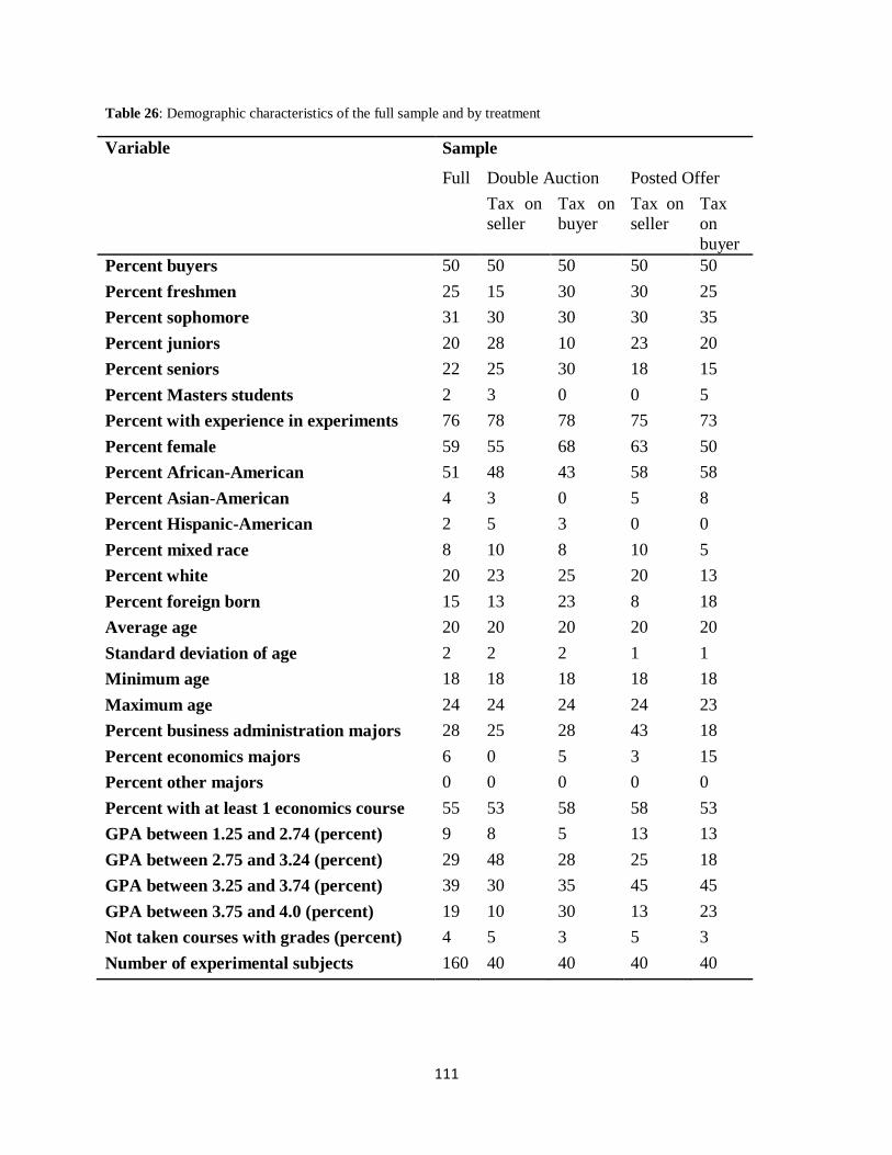
111

Table 26: Demographic characteristics of the full sample and by treatment

Variable Sample

Full Double Auction Posted Offer

Tax on

seller

Tax on

buyer

Tax on

seller

Tax

on

buyer

Percent buyers 50 50 50 50 50

Percent freshmen 25 15 30 30 25

Percent sophomore 31 30 30 30 35

Percent juniors 20 28 10 23 20

Percent seniors 22 25 30 18 15

Percent Masters students 2 3 0 0 5

Percent with experience in experiments 76 78 78 75 73

Percent female 59 55 68 63 50

Percent African-American 51 48 43 58 58

Percent Asian-American 4 3 0 5 8

Percent Hispanic-American 2 5 3 0 0

Percent mixed race 8 10 8 10 5

Percent white 20 23 25 20 13

Percent foreign born 15 13 23 8 18

Average age 20 20 20 20 20

Standard deviation of age 2 2 2 1 1

Minimum age 18 18 18 18 18

Maximum age 24 24 24 24 23

Percent business administration majors 28 25 28 43 18

Percent economics majors 6 0 5 3 15

Percent other majors 0 0 0 0 0

Percent with at least 1 economics course 55 53 58 58 53

GPA between 1.25 and 2.74 (percent) 9 8 5 13 13




Not taken courses with grades (percent) 4 5 3 5 3

Number of experimental subjects 160 40 40 40 40

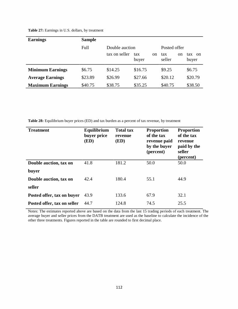
112

Table 27: Earnings in U.S. dollars, by treatment

Earnings Sample

Full Double auction Posted offer

tax on seller tax on

buyer

tax on

seller

tax on

buyer

Minimum Earnings $6.75 $14.25 $16.75 $9.25 $6.75

Average Earnings $23.89 $26.99 $27.66 $20.12 $20.79

Maximum Earnings $40.75 $38.75 $35.25 $40.75 $38.50

Table 28: Equilibrium buyer prices (ED) and tax burden as a percent of tax revenue, by treatment

Treatment Equilibrium

buyer price

(ED)

Total tax

revenue

(ED)

Proportion

of the tax

revenue paid

by the buyer

(percent)

Proportion

of the tax

revenue

paid by the

seller

(percent)

Double auction, tax on

buyer

41.8 181.2 50.0 50.0


seller

42.4 180.4 55.1 44.9

Posted offer, tax on buyer 43.9 133.6 67.9 32.1

Posted offer, tax on seller 44.7 124.8 74.5 25.5

Notes: The estimates reported above are based on the data from the last 15 trading periods of each treatment. The

average buyer and seller prices from the DATB treatment are used as the baseline to calculate the incidence of the

other three treatments. Figures reported in the table are rounded to first decimal place.

113

Table 29: Equilibrium quantities and excess burdens, by treatment

Treatment Equilibrium

quantity

(Units)

Excess

burden

(ED)

Excess

burden as a

percent of

tax revenue

Excess

burden as

a percent

of

participant

earnings


buyer

15.10 60.60 33.44 21.91


seller

15.03 63.85 35.39 23.65

Posted offer, tax on buyer 11.13 134.70 100.82 64.78

Posted offer, tax on seller 10.40 147.40 118.11 73.26

114

7 FIGURES

Figure 8: Percentage differences in pair-wise comparisons of average buyer prices

Notes: DATB = double auction market with tax on buyer;

DATS = double auction market with tax on seller;

POTB = posted offer market with tax on buyer; and

POTS = posted offer market with tax on seller.

1.46

1.82

5.40

5.03

0.00

1.00

2.00

3.00

4.00

5.00

6.00

DATS & DATB POTS & POTB POTS & DATS POTB & DATB

115

Figure 9: Cumulative distribution functions of the buyer prices for the two double auction market treatments.

Notes: DATB = double auction market with the tax on the buyer.

DATS = double auction market with the tax on the seller.

Kolmogorov–Smirnov test of the maximum difference between the cumulative distribution

functions of the buyer prices of the two double auction market treatments, using the last 15

trading periods. Maximum difference between the two cumulative distribution functions =

0.2023 (p-value = 0.000).

116

Figure 10: Cumulative distribution functions of the buyer prices, using the last 15 trading periods of each market

session, for the two posted offer market treatments.

Notes: POTB = posted offer market with the tax on the buyer. POTS = posted offer market with the tax on the seller.

Kolmogorov-Smirnov test of the maximum difference between the cumulative distribution

functions of the average buyer prices from the two posted offer market treatments, using the last

15 trading periods. Maximum difference between the two cumulative distribution functions =

0.3030 (p-value = 0.000).

117

Figure 11: Cumulative distribution functions of the buyer prices from the double auction and posted offer market

treatments with the tax on the buyer.

Notes: DATB = double auction market with the tax on the buyer.

POTB = posted offer market with the tax on the buyer.

Kolmogorov-Smirnov test of the maximum difference between the cumulative distributions of

the average buyer prices, using the last 15 trading periods, from the double auction and posted

offer markets with the tax on the buyers. Maximum difference between the two cumulative

distribution functions = 0.7022 (p-value = 0.000).

118

Figure 12: Cumulative distribution functions of the buyer prices for the double auction and posted offer market

treatments with the tax on the sellers.

Notes: DATS = double auction market with tax on seller.

POTS = posted offer market with tax on seller.

Kolmogorov-Smirnov test of the maximum difference between the cumulative distribution

functions of the buyer prices from double auction and posted offer markets with tax on the

sellers, using the last 15 trading periods. Maximum difference between the two cumulative

distribution functions = 0.7253 (p-value = 0.000).

119

Appendix for the paper “TAX INCIDENCE: DO INSTITUTIONS MATTER?

AN EXPERIMENTAL STUDY”

EXPERIMENTAL INSTRUCTIONS

APPENDIX INDEX

Appendix 1: This appendix presents the experiment instructions to the participants for

all the four treatments of the study.

Appendix 1.1. This section presents the experimental instructions when market

institution is posted offer and the seller is liable to pay a per unit tax.


institution is posted offer and the buyer is liable to pay a per unit tax.


institution is double auction and the seller is liable to pay a per unit tax.


institution is double auction and the buyer is liable to pay a per unit tax.

Appendix 2: This appendix presents the questionnaire given out to the participants as a

short survey at the end of the study.

120

APPENDIX 1.1

Treatment 1

The market institution is a posted offer market; the Seller is liable to pay a tax on each unit sold.

Today’s experiment:

This is an experiment in the economics of decision making in markets.

Your earnings will be determined by your own decisions and the decisions of others as described

in the following instructions. SO IT IS IMPORTANT THAT YOU READ THESE

INSTRUCTIONS CAREFULLY. This experiment is structured so that only you know your

earnings. All of the money that you earn will be paid to you privately IN CASH immediately

following the end of today’s experiment.

Scenario

You will be randomly assigned to the role of a Buyer or a Seller. As such, you will decide the

number of units of a fictitious commodity that you would like to buy or sell. You will keep the

same role for the entire experiment.

Anonymity

Your role and the role of others will be kept private. You will not know anyone’s role other than

your own.

Trading screens

Sellers post offers to sell and Buyers accept offers through a series of action screens. We explain

below how Sellers interact with these screens to post Offers to sell in the market.

Seller’s instructions:

You are a Seller. Sellers in the market can post Offers to sell units of a fictitious commodity to

Buyers in the market. During each round of today’s experiment, you are given an opportunity to

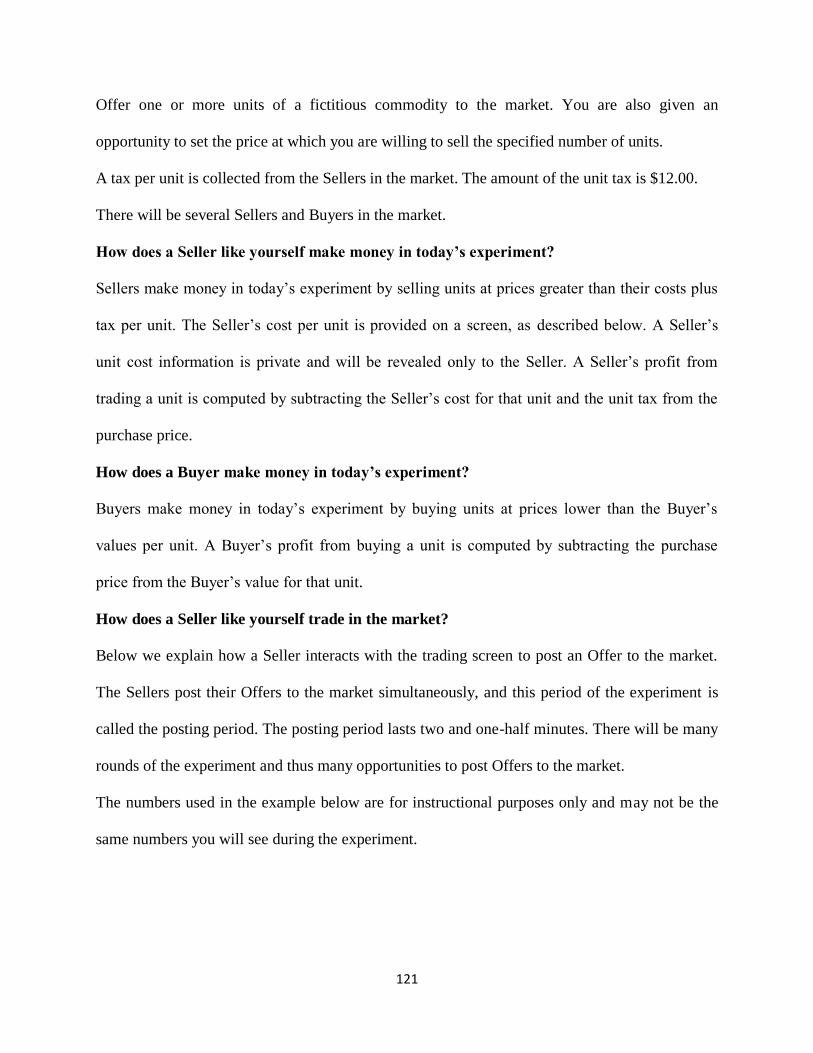
121

Offer one or more units of a fictitious commodity to the market. You are also given an

opportunity to set the price at which you are willing to sell the specified number of units.

A tax per unit is collected from the Sellers in the market. The amount of the unit tax is $12.00.

There will be several Sellers and Buyers in the market.

How does a Seller like yourself make money in today’s experiment?

Sellers make money in today’s experiment by selling units at prices greater than their costs plus

tax per unit. The Seller’s cost per unit is provided on a screen, as described below. A Seller’s

unit cost information is private and will be revealed only to the Seller. A Seller’s profit from

trading a unit is computed by subtracting the Seller’s cost for that unit and the unit tax from the

purchase price.

How does a Buyer make money in today’s experiment?

Buyers make money in today’s experiment by buying units at prices lower than the Buyer’s

values per unit. A Buyer’s profit from buying a unit is computed by subtracting the purchase

price from the Buyer’s value for that unit.

How does a Seller like yourself trade in the market?

Below we explain how a Seller interacts with the trading screen to post an Offer to the market.

The Sellers post their Offers to the market simultaneously, and this period of the experiment is

called the posting period. The posting period lasts two and one-half minutes. There will be many

rounds of the experiment and thus many opportunities to post Offers to the market.

The numbers used in the example below are for instructional purposes only and may not be the

same numbers you will see during the experiment.

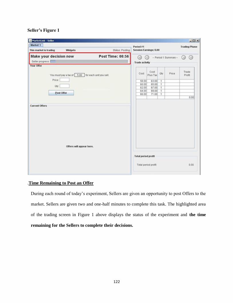
122

Seller’s Figure 1

.Time Remaining to Post an Offer

During each round of today’s experiment, Sellers are given an opportunity to post Offers to the

market. Sellers are given two and one-half minutes to complete this task. The highlighted area

of the trading screen in Figure 1 above displays the status of the experiment and the time

remaining for the Sellers to complete their decisions.

123

Seller’s Figure 2

.Selling in the market

The highlighted area of the screen in Figure 2 above provides information on the Seller’s costs

and tax per unit. A Seller should consider this information before posting an Offer to the

market. An Offer consists of a price and quantity, or, in other words, the number of units that a

Seller is willing and able to sell at a given price of the Seller’s choosing.

In deciding what price and quantity to post to the market, you should always check the cost to

you of selling the last unit that you post to sell. The cost to you of each unit is given by the

numbers in the Cost Plus Tax column.

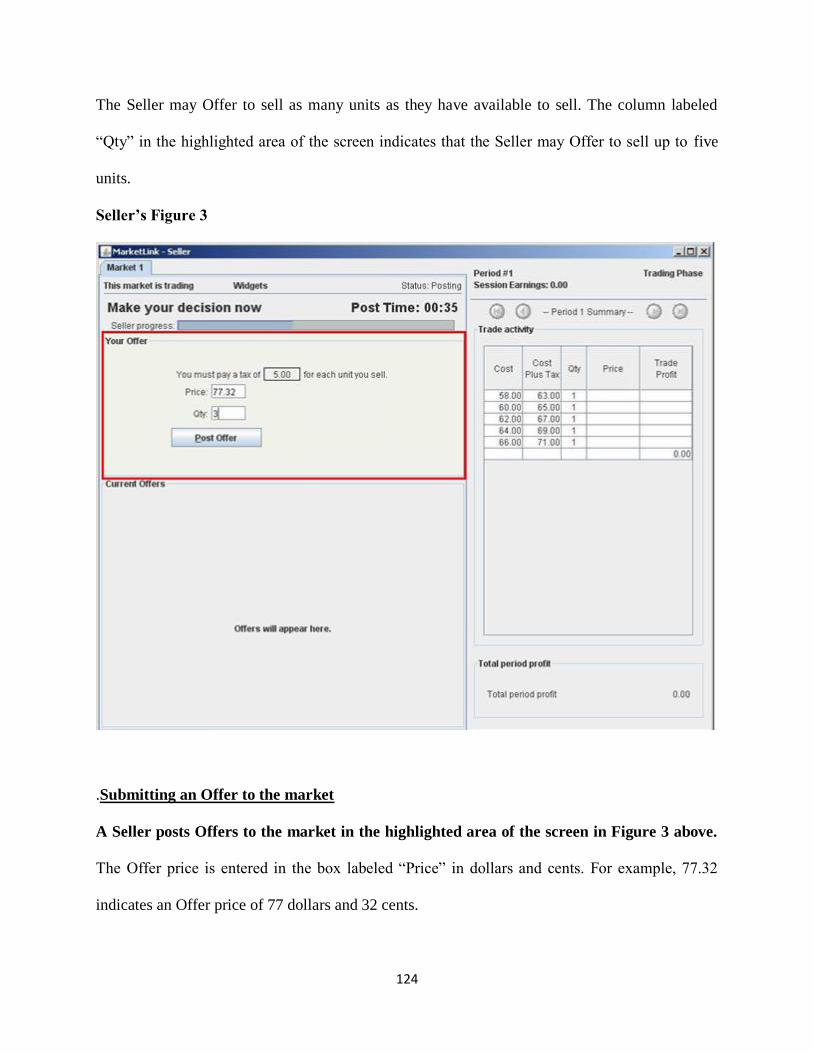
124

The Seller may Offer to sell as many units as they have available to sell. The column labeled

“Qty” in the highlighted area of the screen indicates that the Seller may Offer to sell up to five

units.

Seller’s Figure 3

.Submitting an Offer to the market

A Seller posts Offers to the market in the highlighted area of the screen in Figure 3 above.

The Offer price is entered in the box labeled “Price” in dollars and cents. For example, 77.32

indicates an Offer price of 77 dollars and 32 cents.

125

A Seller can post any price greater than $0 but less than $100.

The quantity is entered in the box labeled “Qty” and must be a whole number. For example, 3

indicates an Offer to sell 3 units. The posted quantity is the maximum number of units the Seller

is willing to sell at the posted offer price. As previously explained, the Seller may offer to sell as

many units as they have available to sell.

The Seller posts an Offer to the market by clicking on the “Post Offer” button on the trading

screen. Be aware that once the Offer is posted to the market, it cannot be retrieved or recalled.

Consider your decisions carefully before clicking on the “Post Offer” button. Note that in this

example there is a 5.00 dollar tax per unit which is collected from the Seller.

126

Seller’s Figure 4

Market Information: Knowing where you stand in the market

Once all Sellers have submitted their offers, Buyers will take turns accepting offers. The

screen in Figure 4 above shows the sort of information that will be provided to you while

buyers are making their decisions. Note that a buyer bought one unit of your offer. You

made profit of 14.32 dollars, and you still have an offer to sell two additional units at a

price of $77.32 in the market.

A. The progress bar in the highlighted area of the trading screen labeled A in Figure 4 above

displays the amount of time remaining for Buyers to buy in this period.

B. The highlighted area labeled B displays your own Offer which is labeled You.

127

C. The highlighted area labeled C displays your profit on each unit sold as well as the total

period profit.

D. The highlighted area labeled D displays your total period profit for the period or round

just completed.

Questionnaire and payment

After you have finished all of your decisions in today’s experiment, you will complete a brief on-

line questionnaire. We will convert your total earnings in experimental dollars into U.S. dollars

at the exchange rate announced at the beginning of today’s experiment. The more experimental

dollars you earn, the more U.S. dollars you will be paid at the end of today’s experiment. You

will receive payment of your earnings, and the experiment is over.

128








Scenario




Anonymity


your own.

Trading screens


below how Buyers interact with these screens to accept Offers posted to the market by Sellers.

129

Buyer’s instructions:

You are a Buyer. Buyers are given an opportunity to purchase units of a fictitious commodity

from Sellers in the market, by accepting Offers posted by Sellers


There will be several Buyers and several Sellers in the market.

How does a Buyer like yourself make money in today’s experiment?

Buyers make money in today’s experiment by purchasing units at prices lower than the Buyer’s

values per unit. The Buyer’s values for units are provided on a trading screen, as described

below. A Buyer’s unit value information is private and will be revealed only to the Buyer. A

Buyer’s profit from buying a unit is computed by subtracting the purchase price from the

Buyer’s value for the unit.

How does a Seller make money in today’s experiment?


tax per unit. A Seller’s profit from selling a unit is computed by subtracting the Seller’s cost for

that unit and the unit tax from the purchase price.

How does a Buyer like yourself trade in the market?

Below we explain how a Buyer interacts with the trading screen to accept Offers from the

market. The Buyers take turns accepting offers from the market, and this phase of the experiment

is called the accepting phase. There will be many rounds of the experiment and thus many

opportunities to accept Offers from the market.



130

Buyer’s Figure 1

Time Remaining to Accept Offers:

During each round of today’s experiment, Buyers are given an opportunity to accept offers

available in the market. Each Buyer enters the market in a randomly assigned sequence.

When a Buyer’s turn arrives, the Buyer, and only that Buyer, may accept Offers in the

market. Each Buyer is given the same amount of time to complete their decisions. The

highlighted area of the trading screen in Figure 1 above displays the status of the

experiment. The pink area graphically represents when it is your turn and the time

remaining for you to accept offers. Once the progress bar reaches the pink area, it is your

turn to accept offers. In this example, some other Buyer has 30 seconds remaining to

complete her (his) decisions.

131

Buyer’s Figure 2

Buying in the market BY ACCEPTING AN OFFER

The highlighted area of the screen in Figure 2 above is the Buyer’s action screen. The

highlighted area shows the number of units available for sale and the Offer price of each

Seller in the market.

When it is your turn to accept offers, you can accept a Seller’s Offer by clicking the “Buy”

button next to the respective Seller’s quantity and price information. You will buy 1 unit each

time you click the Buy button, as long as the respective Seller still has units available to sell.

Note that in this example, you bought one unit at a price of 59.12 dollars and made a

profit of 12.88 dollars.

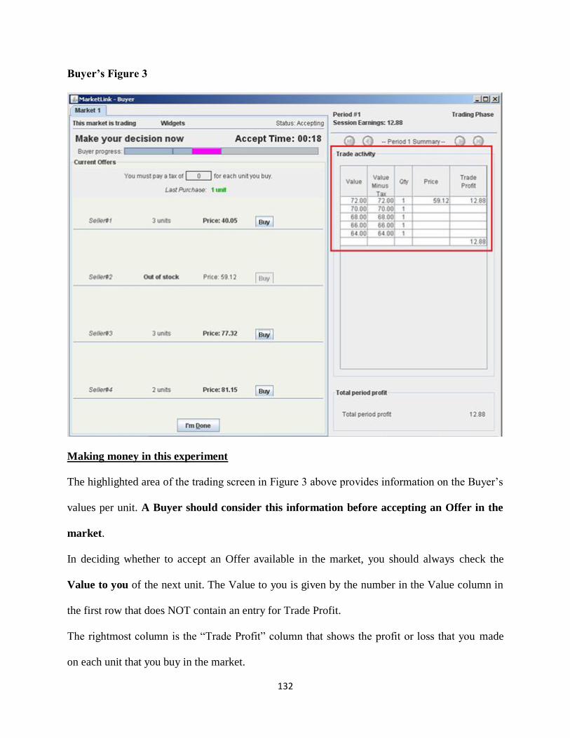
132

Buyer’s Figure 3

Making money in this experiment

The highlighted area of the trading screen in Figure 3 above provides information on the Buyer’s

values per unit. A Buyer should consider this information before accepting an Offer in the

market.

In deciding whether to accept an Offer available in the market, you should always check the

Value to you of the next unit. The Value to you is given by the number in the Value column in

the first row that does NOT contain an entry for Trade Profit.

The rightmost column is the “Trade Profit” column that shows the profit or loss that you made

on each unit that you buy in the market.

133

When you have completed your decisions, you may click on the “I’m Done” button at the bottom

of the screen.

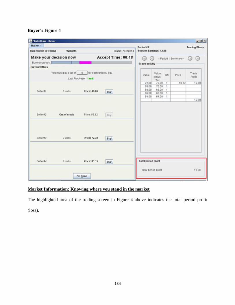
134

Buyer’s Figure 4


The highlighted area of the trading screen in Figure 4 above indicates the total period profit

(loss).

135







136

APPENDIX 1.2

Treatment 2

The market institution is a posted offer market; the Buyer is liable to pay a tax on each unit sold.








Scenario




Anonymity


your own.

Trading screens


below how Sellers interact with these screens to post Offers to sell in the market.

Seller’s instructions:

You are a Seller. Sellers in the market can post Offers to sell units of a fictitious commodity to

Buyers in the market. During each round of today’s experiment, you are given an opportunity to

137

Offer one or more units of a fictitious commodity to the market. You are also given an

opportunity to set the price at which you are willing to sell the specified number of units.

A tax per unit is collected from the Buyers in the market. The amount of the unit tax is $12.00.

There will be several Sellers and Buyers in the market.

How does a Seller like yourself make money in today’s experiment?

Sellers make money in today’s experiment by selling units at prices greater than their costs per

unit. The Seller’s cost per unit is provided on a screen, as described below. A Seller’s unit cost

information is private and will be revealed only to the Seller. A Seller’s profit from trading a unit

is computed by subtracting the Seller’s cost for the unit from the purchase price.

How does a Buyer make money in today’s experiment?


values minus tax per unit. A Buyer’s profit from buying a unit is computed by subtracting the

purchase price and the tax per unit from the Buyer’s value for that unit.


Below we explain how a Seller interacts with the trading screen to post an Offer to the market.

The Sellers post their Offers to the market simultaneously, and this period of the experiment is

called the posting period. The posting period lasts two and one-half minutes. There will be many

rounds of the experiment and thus many opportunities to post Offers to the market.



138

Seller’s Figure 1

Time Remaining to Post an Offer

During each round of today’s experiment, Sellers are given an opportunity to post Offers to the

market. Sellers are given two and one-half minutes to complete this task. The highlighted area

of the trading screen in Figure 1 above displays the status of the experiment and the time

remaining for the Sellers to complete their decisions.

139

Seller’s Figure 2

Selling in the market

The highlighted area of the screen in Figure 2 above provides information on the Seller’s costs

per unit. A Seller should consider this information before posting an Offer to the market.

An Offer consists of a price and quantity or, in other words, the number of units that a Seller is

willing and able to sell at a given price of the Seller’s choosing.

In deciding what price and quantity to post to the market, you should always check the cost to

you of selling the last unit that you post to sell. The cost to you of each unit is given by the

numbers in the Cost column.

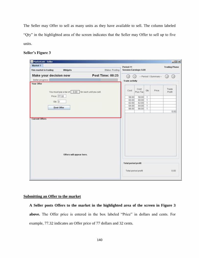
140

The Seller may Offer to sell as many units as they have available to sell. The column labeled

“Qty” in the highlighted area of the screen indicates that the Seller may Offer to sell up to five

units.

Seller’s Figure 3

Submitting an Offer to the market

A Seller posts Offers to the market in the highlighted area of the screen in Figure 3

above. The Offer price is entered in the box labeled “Price” in dollars and cents. For

example, 77.32 indicates an Offer price of 77 dollars and 32 cents.

141

A Seller can post any price greater than $0 but less than $100.

The quantity is entered in the box labeled “Qty” and must be a whole number. For example,

3 indicates an Offer to sell 3 units. The posted quantity is the maximum number of units the

Seller is willing to sell at the posted offer price. As previously explained, the Seller may offer

to sell as many units as they have available to sell.

The Seller posts an Offer to the market by clicking on the “Post Offer” button on the trading

screen. Be aware that once the Offer is posted to the market, it cannot be retrieved or

recalled. Consider your decisions carefully before clicking on the “Post Offer” button.

142

Seller’s Figure 4


Once all Sellers have submitted their offers, Buyers will take turns accepting offers. The

screen in Figure 4 above shows the sort of information that will be provided to you while

buyers are making their decisions. Note that a buyer bought one unit of your offer. You

made profit of 19.32 dollars, and you still have an offer to sell two additional units at a

price of $77.32 in the market.

E. The progress bar in the highlighted area of the trading screen labeled A in Figure 4

above displays the amount of time remaining for Buyers to buy in this period.

F. The highlighted area labeled B displays your own Offer which is labeled You.

143

G. The highlighted area labeled C displays your profit on each unit sold as well as the total

period profit.

H. The highlighted area labeled D displays your total period profit for the period or round

just completed.







144








Scenario




Anonymity


your own.

Trading screens


below how Buyers interact with these screens to accept Offers posted to the market by Sellers.

145


You are a Buyer. Buyers are given an opportunity to purchase units of a fictitious commodity

from Sellers in the market, by accepting Offers posted by Sellers.



How does a Buyer like yourself make money in today’s experiment?

Buyers make money in today’s experiment by purchasing units at prices lower than the Buyer’s

values minus tax per unit. The Buyer’s value minus tax per unit is provided on a trading screen,

as described below. A Buyer’s unit value information is private and will be revealed only to the

Buyer. A Buyer’s profit from buying a unit is computed by subtracting the purchase price and

the tax per unit from the Buyer’s value for the unit.

How does a Seller make money in today’s experiment?

Sellers make money in today’s experiment by selling units at prices greater than their costs. A

Seller’s profit from selling a unit is computed by subtracting the Seller’s cost for that unit from

the purchase price.


Below we explain how a Buyer interacts with the trading screen to accept Offers from the

market. The Buyers take turns accepting offers from the market, and this phase of the experiment

is called the accepting phase. There will be many rounds of the experiment and thus many

opportunities to accept Offers from the market.



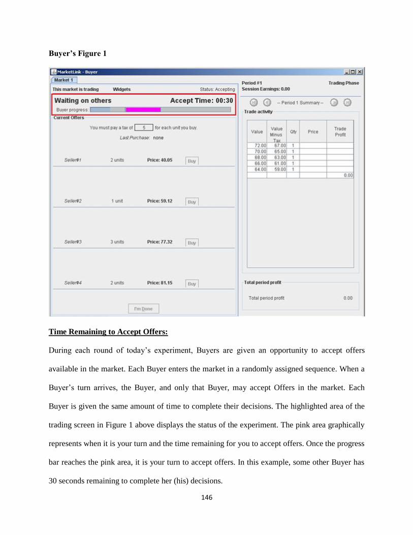
146

Buyer’s Figure 1

Time Remaining to Accept Offers:

During each round of today’s experiment, Buyers are given an opportunity to accept offers

available in the market. Each Buyer enters the market in a randomly assigned sequence. When a

Buyer’s turn arrives, the Buyer, and only that Buyer, may accept Offers in the market. Each

Buyer is given the same amount of time to complete their decisions. The highlighted area of the

trading screen in Figure 1 above displays the status of the experiment. The pink area graphically

represents when it is your turn and the time remaining for you to accept offers. Once the progress

bar reaches the pink area, it is your turn to accept offers. In this example, some other Buyer has

30 seconds remaining to complete her (his) decisions.

147

Buyer’s Figure 2

Buying in the market BY ACCEPTING AN OFFER

The highlighted area of the screen in Figure 2 above is the Buyer’s action screen. The

highlighted area shows the number of units available for sale and the Offer price of each Seller in

the market. The highlighted area also shows that a 5.00 dollar tax per unit will be collected from

the Buyer in this example.

When it is your turn to accept offers, you can accept a Seller’s Offer by clicking the “Buy”

button next to the respective Seller’s quantity and price information. You will buy 1 unit each

time you click the Buy button, as long as the respective Seller still has units available to sell.

148

Note that in this example, you bought one unit at a price of 59.12 dollars and made a profit

of 7.88 dollars.

Buyer’s Figure 3



values per unit. A Buyer should consider this information before accepting an Offer in the

market. Note that in this example there is a 5.00 dollar tax per unit which is collected from the

Buyer.

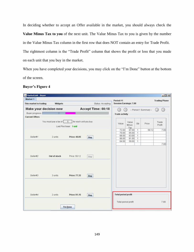
149

In deciding whether to accept an Offer available in the market, you should always check the

Value Minus Tax to you of the next unit. The Value Minus Tax to you is given by the number

in the Value Minus Tax column in the first row that does NOT contain an entry for Trade Profit.

The rightmost column is the “Trade Profit” column that shows the profit or loss that you made

on each unit that you buy in the market.

When you have completed your decisions, you may click on the “I’m Done” button at the bottom

of the screen.

Buyer’s Figure 4

150


The highlighted area of the trading screen in Figure 4 above indicates the total period profit

(loss).







151

APPENDIX 1.3

Treatment 3

The market institution is a double auction market. The Seller is liable to pay a tax on each unit

sold.





INTRUCTIONS CAREFULLY. This experiment is structured so that only you know your



Scenario




Anonymity


your own.

Trading screens

Sellers make offers and Buyers make purchases through a set of trading screens. We explain

below how Sellers and Buyers interact with the trading screens to make offers and purchases in

the market.

152

Sellers’ instructions:

You are a Seller. Sellers in the market have two options. You can sell units of a fictitious

commodity by accepting Bid prices submitted by Buyers, and you can also post Ask prices and

wait for Buyers to buy units, by accepting your Ask prices.

A tax per unit is collected from the Sellers in the market. The amount of the unit tax is $12.00. .

There will be several Sellers and several Buyers in the market.

How does a Seller like yourself make money in this experiment?


tax per unit. The Seller’s cost per unit is provided on a trading screen, as described below. A

Seller’s unit cost information is private and will be revealed only to the Seller. A Seller’s profit

from trading a unit is computed by subtracting the Seller’s cost for the unit and the unit tax from

the purchase price.

How does a Buyer make money in this experiment?


values per unit. A Buyer’s profit from buying a unit is computed by subtracting the purchase

price from the Buyer’s value for the unit.


Below we explain how a Seller interacts with the trading screen to submit an Ask price to the

market or accept a Bid price from the market. Each trading period lasts two and one-half

minutes. There will be many trading periods.



153

Seller’s Figure 1

Time Remaining in a Trading Period and Summary Information:

Sellers (and Buyers) are given two and one-half minutes to complete their transactions in each

round of today’s experiment. The highlighted area of the trading screen in Figure 1 above

displays the current trading period, the Seller’s earnings during the session, and the time

remaining in the trading period.

154

Seller’s Figure 2

Selling in the market BY ACCEPTING A BID:

The highlighted area of the screen in Figure 2 above is the Seller’s action screen. Sellers can

accept Bids in the market by clicking the “Sell” button in the rightmost lower corner of the

Seller’s action screen. You will sell 1 unit each time you click the Sell button, if the Buyer’s

Bids have not already been accepted.

How do you know what price you will receive if you click on the Sell button? The price you

would receive appears in the “Price” box just above the Sell button. In this example, the price is

78.00 dollars. If you are the first Seller to click on the Sell button, then 78.00 dollars would be

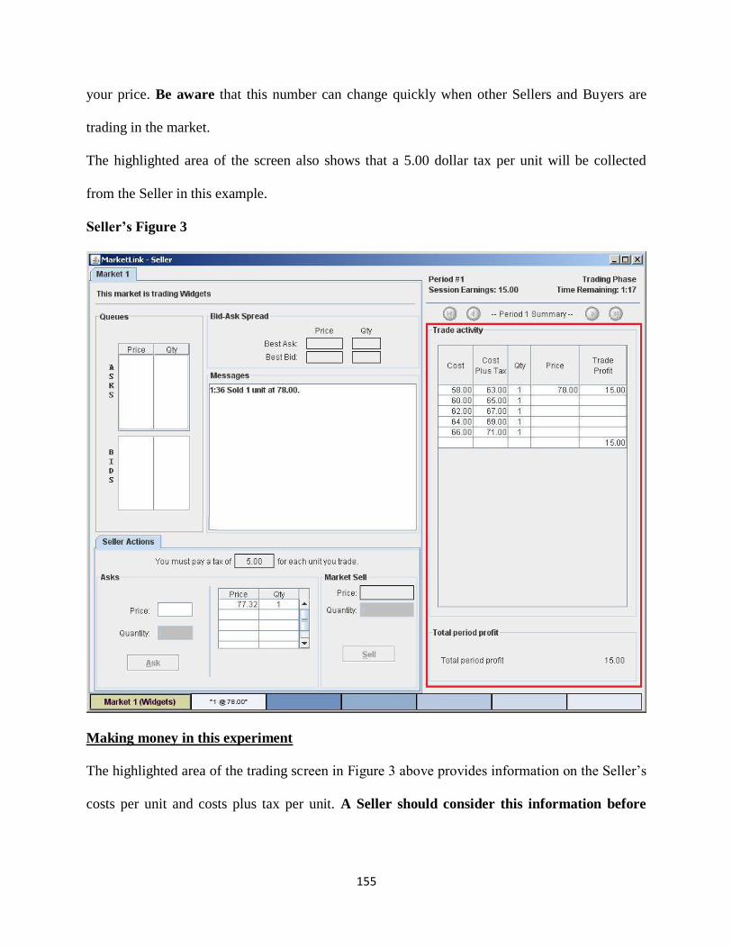
155

your price. Be aware that this number can change quickly when other Sellers and Buyers are

trading in the market.

The highlighted area of the screen also shows that a 5.00 dollar tax per unit will be collected

from the Seller in this example.

Seller’s Figure 3


The highlighted area of the trading screen in Figure 3 above provides information on the Seller’s

costs per unit and costs plus tax per unit. A Seller should consider this information before

156

submitting an Ask price or accepting a Bid price in the market. Note that in this example

there is a 5.00 dollar tax per unit which is collected from the Seller.

Suppose you accepted a bid of 78.00 dollars. Since it was your first unit, your cost plus tax

was 63.00 dollars, and you made a profit of 15.00 (78.00 - 63.00) dollars. The rightmost

column is the “Trade Profit” column that shows the profit or loss that you made on each unit that

you trade in the market.

In deciding whether to submit an Ask price or accept a Bid price, you should always check the

Cost Plus Tax to you of trading the next unit. The cost to you is given by the number in the

Cost Plus Tax column in the first row that does NOT contain an entry for Trade Profit. In Figure

3, your next unit’s cost is 65.00 dollars.

157

Seller’s Figure 4

Selling in the market BY SUBMITTING AN ASK:


make offers in the market by clicking the “Ask” button in the leftmost lower corner of the

Seller’s action screen. Before clicking the Ask button, you need to enter your ask price in the

“Price” box. The price entered can be in dollars and cents; for example, 77.32 denotes a price of

77 dollars and 32 cents. Note that your next unit’s cost plus tax is 65.00 dollars. If a buyer

accepts your ask, you will make a profit of 12.32 (77.32 - 65.00) dollars.

A Seller can post any Ask price greater than $0 but less than $100.

158

After you have entered an Ask price, you can always replace it with a lower Ask price. To do so,

just type in the new price and then click on the “Ask” button.

The highlighted area of the screen also shows that a 5.00 dollar tax per unit will be collected

from the Seller in this example.

Seller’s Figure 5


The highlighted area of the screen in Figure 5 above shows all outstanding Asks and Bids in the

market. Your own outstanding Asks in the market will be indicated by an asterisk (*) symbol.

Therefore, you will always be able to find out whether your Asks are high or low compared to

159

others in the queue of all Asks. You are also able to see how the best Bid that you could accept

compares to other outstanding Bids and to the outstanding Asks. In Figure 5, there are two

outstanding bids of $37.32 and $29.12.

Remember that you can always replace your Ask price with a lower one, as explained on the

preceding page.







160








Scenario




Anonymity


your own.

Trading screens



the market.

161


You are a Buyer. Buyers in the market have two options. You can buy units of a fictitious

commodity by accepting Ask prices submitted by Sellers, and you can also post Bid prices and

wait for Sellers to sell units, by accepting your Bid prices.



How does a Buyer like you make money in this experiment?


values per unit. The Buyer’s value per unit is provided on a trading screen, as described below. A

Buyer’s unit value information is private and will be revealed only to the Buyer. A Buyer’s profit

from buying a unit is computed by subtracting the purchase price from the Buyer’s value for the

unit.

How does a Seller make money in this experiment?


tax per unit. A Seller’s profit from selling a unit is computed by subtracting the Seller’s cost for

the unit and the unit tax from the purchase price.


Below we explain how a Buyer interacts with the trading screen to submit a Bid price to the

market or accept an Ask price from the market. Each trading period lasts for two and one-half




162

Buyer’s Figure 1


Buyers (and Sellers) are given two and one-half minutes to complete their transactions in each


displays the current trading period, the Buyer’s earnings during the session, and the time


163

Buyer’s Figure 2

Buying in the market BY ACCEPTING AN ASK:

The highlighted area of the screen in Figure 2 above is the Buyer’s action screen. Buyers can

accept Asks in the market by clicking the “Buy” button in the rightmost lower corner of

the Buyer’s action screen. You will buy 1 unit each time you click the Buy button, if the Sellers

have made Asks that have not already been accepted.

How do you know what price you will receive if you click on the Buy button? The price you

would receive appears in the “Price” box just above the Buy button. In this example, the price is

38.00 dollars. If you are the first Buyer to click on the Buy button, then 38.00 dollars would be

164

your price. Be aware that this number can change quickly when other Buyers and Sellers are


Buyer’s Figure 3



values per unit. A Buyer should consider this information before submitting a Bid price or

accepting an Ask price in the market.

Suppose you accepted an ask of 38.00 dollars. Since it was your first unit, your value was

72.00 dollars, and you made a profit of 34.00 (72.00 - 38.00) dollars. The rightmost column is

165

the “Trade Profit” column that shows the profit or loss that you make on each unit that you trade

in the market.

In deciding whether to submit a Bid price or accept an Ask price, you should always check the

value to you of trading the next unit. The value to you is given by the number in the Value

column in the first row that does NOT contain an entry for Trade Profit. In Figure 3, your next

unit’s value is 70.00 dollars.

Buyer’s Figure 4

166

Buying in the market BY SUBMITTING A BID:


make bids in the market by clicking the “Bid” button in the leftmost lower corner of the

Buyer’s action screen. Before clicking the Bid button, you need to enter your bid price in the

“Price” box. The price entered in the box labeled “Price” can be in dollars and cents; for

example, 37.32 denotes a price of 37 dollars and 32 cents. Note that your next unit’s value is

70.00 dollars. If a seller accepts your bid, you will make a profit of 32.68 (70.00 - 37.32)

dollars.

A Buyer can submit any bid price greater than $0 but less than $100.

After you have entered a Bid price, you can always replace it with a higher Bid price. To do so,

just type in the new price and then click on the “Bid” button.

167

Buyer’s Figure 5



market. Your own outstanding Bids in the market will be indicated by an asterisk (*) symbol.

Therefore, you are always able to find out whether your Bids are high or low compared to others

in the queue of all Bids. You are also able to see how the best Ask that you could accept

compares to other outstanding Asks and to the outstanding Bids. In Figure 5, there are two

outstanding asks of $59.12 and $77.32.

168

Remember that you can always replace your Bid price with a higher one, as explained on the

preceding page.







169

APPENDIX 1.4

Treatment 4

The market institution is a double auction market. The Buyer is liable to pay a tax on each unit

sold.








Scenario




Anonymity


your own.

Trading screens



the market.

Sellers’ instructions:

170

You are a Seller. Sellers in the market have two options. You can sell units of a fictitious

commodity by accepting Bid prices submitted by Buyers, and you can also post Ask prices and

wait for Buyers to buy units, by accepting your Ask prices.


There will be several Sellers and several Buyers in the market.

How does a Seller like yourself make money in this experiment?

Sellers make money in today’s experiment by selling units at prices greater than their costs. The

Seller’s cost per unit is provided on a trading screen, as described below. A Seller’s unit cost

information is private and will be revealed only to the Seller. A Sellers’s profit from trading a

unit is computed by subtracting the Seller’s cost for the unit from the purchase price.

How does a Buyer make money in this experiment?


values less tax per unit. A Buyer’s profit from buying a unit is computed by subtracting the

purchase price and the tax per unit from the Buyer’s value for the unit.


Below we explain how a Seller interacts with the trading screen to submit an Ask price to the

market or accept a Bid price from the market. Each trading period lasts two and one-half




171

Seller’s Figure 1


Sellers (and Buyers) are given two and one-half minutes to complete their transactions in each


displays the current trading period, the Seller’s earnings during the session, and the time


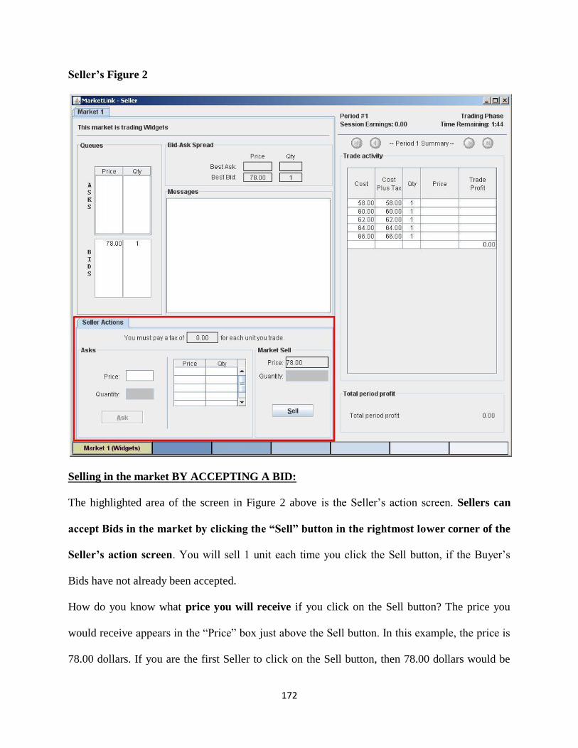
172

Seller’s Figure 2

Selling in the market BY ACCEPTING A BID:


accept Bids in the market by clicking the “Sell” button in the rightmost lower corner of the

Seller’s action screen. You will sell 1 unit each time you click the Sell button, if the Buyer’s

Bids have not already been accepted.

How do you know what price you will receive if you click on the Sell button? The price you

would receive appears in the “Price” box just above the Sell button. In this example, the price is

78.00 dollars. If you are the first Seller to click on the Sell button, then 78.00 dollars would be

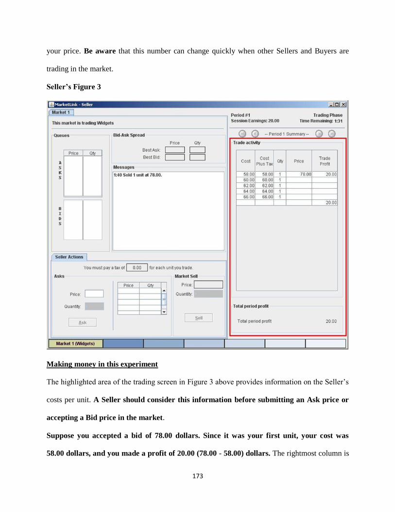
173

your price. Be aware that this number can change quickly when other Sellers and Buyers are


Seller’s Figure 3


The highlighted area of the trading screen in Figure 3 above provides information on the Seller’s

costs per unit. A Seller should consider this information before submitting an Ask price or

accepting a Bid price in the market.

Suppose you accepted a bid of 78.00 dollars. Since it was your first unit, your cost was

58.00 dollars, and you made a profit of 20.00 (78.00 - 58.00) dollars. The rightmost column is

174

the “Trade Profit” column that shows the profit or loss that you made on each unit that you trade

in the market.

In deciding whether to submit an Ask price or accept a Bid price, you should always check the

cost to you of trading the next unit. The cost to you is given by the number in the Cost column

in the first row that does NOT contain an entry for Trade Profit. In Figure 3, your next unit’s cost

is 60.00 dollars.

Seller’s Figure 4

175

Selling in the market BY SUBMITTING AN ASK:


make offers in the market by clicking the “Ask” button in the leftmost lower corner of the

Seller’s action screen. Before clicking the Ask button, you need to enter your ask price in the


77 dollars and 32 cents. Note that your next unit’s cost is 60.00 dollars. If a buyer accepts

your ask, you will make a profit of 17.32 (77.32 - 60.00) dollars.

A Seller can post any Ask price greater than $0 but less than $100.

After you have entered an Ask price, you can always replace it with a lower Ask price. To do so,

just type in the new price and then click on the “Ask” button.

176

Seller’s Figure 5



market. Your own outstanding Asks in the market will be indicated by an asterisk (*) symbol. In

this example, your ask is $77.32. Therefore, you will always be able to find out whether your

Asks are high or low compared to others in the queue of all Asks. You are also able to see how

the best Bid that you could accept compares to other outstanding Bids and to the outstanding

Asks. In Figure 5, there are two outstanding bids of $37.32 and $29.12.

177

Remember that you can always replace your Ask price with a lower one, as explained on the

preceding page.







178








Scenario




Anonymity


your own.

Trading screens



the market.

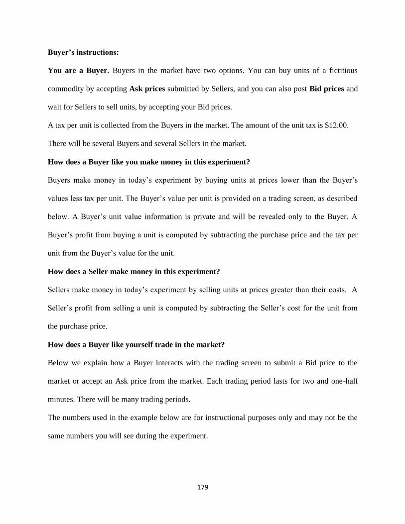
179


You are a Buyer. Buyers in the market have two options. You can buy units of a fictitious

commodity by accepting Ask prices submitted by Sellers, and you can also post Bid prices and

wait for Sellers to sell units, by accepting your Bid prices.



How does a Buyer like you make money in this experiment?


values less tax per unit. The Buyer’s value per unit is provided on a trading screen, as described

below. A Buyer’s unit value information is private and will be revealed only to the Buyer. A

Buyer’s profit from buying a unit is computed by subtracting the purchase price and the tax per

unit from the Buyer’s value for the unit.

How does a Seller make money in this experiment?

Sellers make money in today’s experiment by selling units at prices greater than their costs. A

Seller’s profit from selling a unit is computed by subtracting the Seller’s cost for the unit from

the purchase price.


Below we explain how a Buyer interacts with the trading screen to submit a Bid price to the

market or accept an Ask price from the market. Each trading period lasts for two and one-half




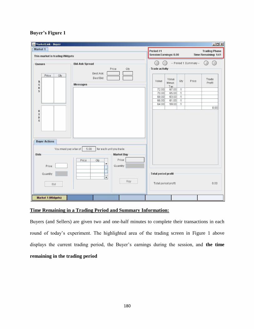
180

Buyer’s Figure 1


Buyers (and Sellers) are given two and one-half minutes to complete their transactions in each


displays the current trading period, the Buyer’s earnings during the session, and the time

remaining in the trading period

181

Buyer’s Figure 2

Buying in the market BY ACCEPTING AN ASK:


accept Asks in the market by clicking the “Buy” button in the rightmost lower corner of

the Buyer’s action screen. You will buy 1 unit each time you click the Buy button, if the Sellers

have made Asks that have not already been accepted. The highlighted area of the screen also

shows that a 5.00 dollar tax per unit will be collected from the Buyer in this example.

How do you know what price you will receive if you click on the Buy button? The price you

would receive appears in the “Price” box just above the Buy button. In this example, the price is

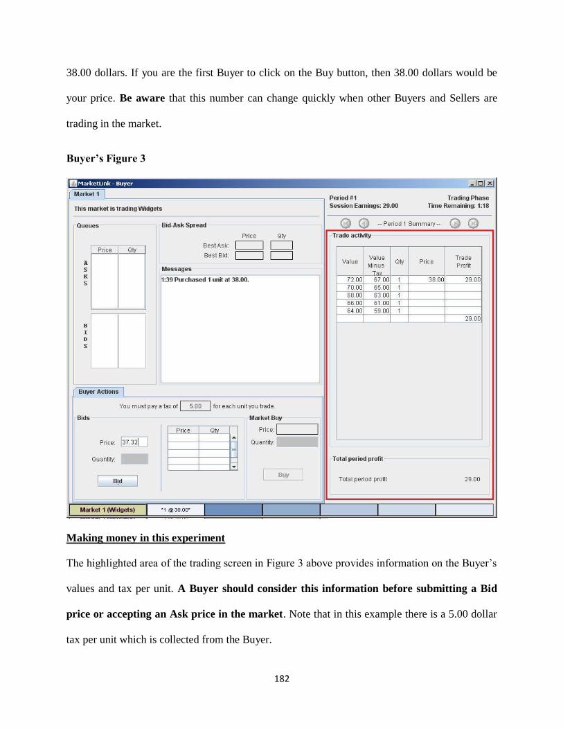
182

38.00 dollars. If you are the first Buyer to click on the Buy button, then 38.00 dollars would be

your price. Be aware that this number can change quickly when other Buyers and Sellers are


Buyer’s Figure 3



values and tax per unit. A Buyer should consider this information before submitting a Bid

price or accepting an Ask price in the market. Note that in this example there is a 5.00 dollar

tax per unit which is collected from the Buyer.

183

Suppose you accepted an ask of 38.00 dollars. Since it was your first unit, your value minus

tax was 67.00 dollars, and you made a profit of 29.00 (67.00 - 38.00) dollars. The rightmost

column is the “Trade Profit” column that shows the profit or loss that you make on each unit that

you trade in the market.

In deciding whether to submit a Bid price or accept an Ask price, you should always check the

Value Minus Tax to you of trading the next unit. The Value Minus Tax to you is given by the

number in the Value Minus Tax column in the first row that does NOT contain an entry for

Trade Profit. In Figure 3, your next unit’s value minus tax is 65.00 dollars.

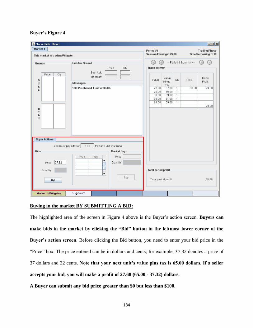
184

Buyer’s Figure 4

Buying in the market BY SUBMITTING A BID:


make bids in the market by clicking the “Bid” button in the leftmost lower corner of the

Buyer’s action screen. Before clicking the Bid button, you need to enter your bid price in the


37 dollars and 32 cents. Note that your next unit’s value plus tax is 65.00 dollars. If a seller

accepts your bid, you will make a profit of 27.68 (65.00 - 37.32) dollars.

A Buyer can submit any bid price greater than $0 but less than $100.

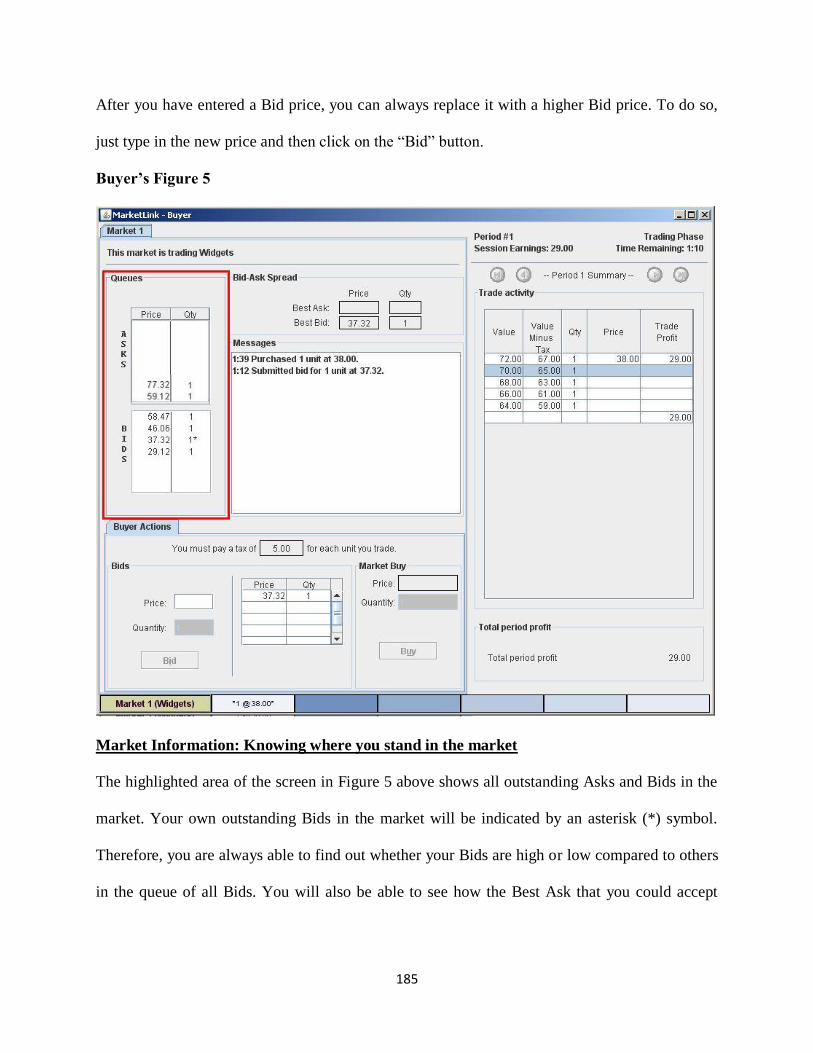
185

After you have entered a Bid price, you can always replace it with a higher Bid price. To do so,

just type in the new price and then click on the “Bid” button.

Buyer’s Figure 5



market. Your own outstanding Bids in the market will be indicated by an asterisk (*) symbol.

Therefore, you are always able to find out whether your Bids are high or low compared to others

in the queue of all Bids. You will also be able to see how the Best Ask that you could accept

186

compares to other outstanding Asks and to the outstanding Bids. In Figure 5, there are two

outstanding asks of $59.12 and $77.32.

Remember that you can always replace your Bid price with a higher one, as explained on the

preceding page.





dollars you earn, the more U.S. dollars you will be paid at the end of the experiment. You will

receive payment of your earnings, and the experiment is over.

187

APPENDIX 2

QUESTIONNAIRE

For questions 1-5, please check the appropriate box.

1. In today’s experiment, I was a BUYER SELLER

2. What year are you in your studies? Freshmen Sophomore Junior Senior

3. Have you ever participated in an economics experiment before? Yes No

4. Gender: Male Female

5. Race: Asian White Black Other

6. Age: ____

7. Major: ______________________ [ ] undecided

8. How many economics courses have you taken (include currently enrolled) ______

9. What is your cumulative grade point average? _______

188

BIBLIOGRAPHY

Agha, A., & Haughton, J. (1996). Designing VAT systems: Some efficiency considerations. The

Review of Economics and Statistics, 303-308.

Alm, J., Martinez-Vazquez, J., & Wallace, S. (2004). Taxing the Hard-to-tax: Lessons from

Theory and Practice. Emerald Group Pub Ltd.

Anderson, T. W., & Hsiao, C. (1981). Estimation of dynamic models with error

components. Journal of the American statistical Association, 76(375), 598-606.

Bagchi, A. (2005). VAT and State Autonomy. Economic and Political Weekly, 1806-1807.

Bird, R. M., & Slack, N. E. (1993). Urban public finance in Canada. J. Wiley.

Bird, R. M., & Gendron, P. P. (1998). Dual VATs and cross-border trade: Two problems, one

solution?. International Tax and Public Finance, 5(3), 429-442.

Bird, M. R. M. (1999). Rethinking subnational taxes: A new look at tax assignment (No. 99-165).

International Monetary Fund.

Bird, R. M., & Gendron, P. P. (2001). VATS in federal states: International experience and

emerging possibilities. Bulletin for International Fiscal Documentation, 55, 293-309.

Bird, R., Martínez-Vázquez, J., & Torgler, B. (2005). Value-added taxes in developing and

transitional countries: lessons and questions. ITP paper, 505.

Bird, R. M., & Gendron, P. (2006). Is VAT the best way to impose a general consumption tax in

developing countries?. Bulletin for International Taxation,60(7), 287.

Bird, R., Martinez-Vazquez, J., & Torgler, B. (2006). Societal institutions and tax effort in

developing countries. The Challenges of tax reform in the global economy. New York: Springer,

283-338.

Bird, R., & Gendron, P. P. (2007). The VAT in developing and transitional countries. Cambridge

University Press.

Bogetic, Z., & Hassan, F. (1993). Determinants of value-added tax revenue: a cross section

analysis (No. 1203). The World Bank.

Borck, R., Engelmann, D., Müller, W., & Normann, H. T. (2002). Tax liability-side equivalence

in experimental posted-offer markets. Southern Economic Journal, 672-682.

Brueckner, J. K. (2003). Strategic interaction among governments: An overview of empirical

studies. International regional science review, 26(2), 175-188.

189

Cameron, A. C., & Trivedi, P. K. (2010). Microeconometrics using stata.

Case, A. C., Hines Jr, J. R., & Rosen, H. S. (1989). Copycatting: Fiscal policies of states and

their neighbors (No. w3032). National Bureau of Economic Research.

Case, A. C., Rosen, H. S., & Hines, J. R. (1993). Budget spillovers and fiscal policy

interdependence: Evidence from the states. Journal of public Economics,52(3), 285-307.

Charron, N. (2010). The correlates of corruption in India: Analysis and evidence from the

states. Asian Journal of Political Science, 18(2), 177-194.

Chelliah, R. J. (1971). Trends in Taxation in Developing Countries (Les tendances de la fiscalité

dans les pays en voie de développement)(Tendencias tributarias en los países en desarrollo). Staff

Papers-International Monetary Fund, 254-331.

Chelliah, R. J., Baas, H. J., & Kelly, M. R. (1975). Tax Ratios and Tax Effort in Developing

Countries, 1969-71 (Pression fiscale et effort fiscal dans les pays en développement, 1969-

71)(Coeficientes y esfuerzo tributarios en los países en desarrollo, 1969-71). Staff Papers-

International Monetary Fund, 187-205.

Chetty, R., Looney, A., & Kroft, K. (2007). Salience and taxation: Theory and evidence (No.

w13330). National Bureau of Economic Research.

Cnossen, S. (1994). Administrative and Compliance Costs of the VAT: A Review of the Evidence.

OCfEB, Research Centre for Economic Policy.

Daniel, W. W. (1990). Applied nonparametric statistics.

Deshpande, R. S., John, R. M., Rao, R. K., Selvaraj, S., Sengupta, J., Moore, J., ... & Jha, P. The

Economics of Tobacco and Tobacco Taxation in India.

Drukker, D. M. (2003). Testing for serial correlation in linear panel-data models.Stata

Journal, 3(2), 168-177.

Ebrill, L. P. (2001). The modern VAT. International Monetary Fund.

Elhorst, J. P. (2014). Spatial panel data models. In Spatial Econometrics (pp. 37-93). Springer

Berlin Heidelberg.

Emran, M. S., & Stiglitz, J. E. (2005). On selective indirect tax reform in developing

countries. Journal of Public Economics, 89(4), 599-623.

Finkelstein, A. (2007). E-ztax: Tax salience and tax rates (No. w12924). National Bureau of

Economic Research.

190

Franzoni, L. A. (2008). Tax compliance. ENCYCLOPEDIA OF LAW AND ECONOMICS,

Boudewijn Bouckaert and Gerrit De Geest, eds., Edward Elgar.

Fullerton, D., & Metcalf, G. E. (2002). Tax incidence. Handbook of public economics, 4, 1787-

1872.

Ghura, D. (1998). Tax revenue in sub-Saharan Africa: effects of economic policies and

corruption.

Hines Jr, J., & Desai, M. A. (2005). Value-Added Taxes and International Trades: The

Evidence. Unpublished Manuscript.

Holt, C. A., & Solis-Soberon, F. (1992). The calculation of equilibrium mixed strategies in

posted-offer auctions. Research in experimental economics, 5(1), 189-228.

Hong, J. T., & Plott, C. R. (1982). Rate filing policies for inland water transportation: an

experimental approach. The Bell Journal of Economics, 1-19.

Isaac, R. M., & Plott, C. R. (1981). Price controls and the behavior of auction markets: An

experimental examination. The American Economic Review, 448-459.

Jarque, C. M., & Bera, A. K. (1980). Efficient tests for normality, homoscedasticity and serial

independence of regression residuals. Economics letters, 6(3), 255-259.

Jarque, C. M., & Bera, A. K. (1987). A test for normality of observations and regression

residuals. International Statistical Review/Revue Internationale de Statistique, 163-172.

Kachelmeier, S. J., Limberg, S. T., & Schadewald, M. S. (1994). Experimental Evidence of

Market Reactions to New Consumption Taxes*. Contemporary Accounting Research, 10(2),

505-545.

Keen, M., Smith, S., Baldwin, R. E., & Christiansen, V. (1996). The future of value added tax in

the European Union. Economic Policy, 375-420.

Keen, M., & Smith, S. (1999). Viva VIVAT!. International Tax and Public Finance, 6(2), 741-

751.

Keen, M. M., & Baunsgaard, M. T. (2005). Tax revenue and (or?) trade liberalization (No. 5-

112). International Monetary Fund.

Keen, M., & Lockwood, B. (2006). Is the VAT a money machine?. National Tax Journal, 905-

928.

Keen, M., & Lockwood, B. (2010). The value added tax: Its causes and consequences. Journal of

Development Economics, 92(2), 138-151.

191

Kerschbamer, R., & Kirchsteiger, G. (2000). Theoretically robust but empirically invalid? An

experimental investigation into tax equivalence. Economic Theory,16(3), 719-734.

Ketcham, J., Smith, V. L., & Williams, A. W. (1984). A comparison of posted-offer and double-

auction pricing institutions. The Review of Economic Studies, 595-614.

Kumar, P., Kumar, A., Parappurathu, S., & Raju, S. S. (2011). Estimation of demand elasticity

for food commodities in India. Agricultural Economics Research Review, 24(1), 1-14.

Leuthold, J. H. (1991). Tax shares in developing economies A panel study.Journal of

development Economics, 35(1), 173-185.

Lotz, J. R., & Morss, E. R. (1967). Measuring" Tax Effort" in Developing Countries (Evaluation

de l'effort fiscal dans les pays en voie de développement)(Medición del" esfuerzo tributario" de

los países en desarrollo). Staff Papers-International Monetary Fund, 478-499.

Manski, C. F. (1993). Identification of endogenous social effects: The reflection problem. The

review of economic studies, 60(3), 531-542.

Martinez-Vazquez, J., & Bird, R. M. (2011). Value Added Tax: Onward and Upward?. The

Elgar Guide to Tax Systems: Critical Views on Contemporary Theory, Policy and

Administration, 218-273.

Mbakile-Moloi, C. E. (2007). Copycat Theory: Testing for Fiscal Policies Harmonization in the

Southern African Coordinating Community (SADC) and Sub-Saharan Africa (SSA).

McLure Jr, C. E. (1993). The Brazilian tax assignment problem: ends, means, and constraints. A

Reforma Fiscal no Brasil, 6-10.

McLure Jr, C. E. (2000). Implementing subnational value added taxes on internal trade: the

compensating VAT (CVAT). International Tax and Public Finance, 7(6), 723-740.

McLure Jr, C. E. (2005). Coordinating state sales taxes with a federal VAT: Opportunities, risks,

and challenges. State Tax Notes, 36(20), 907-21.

Miller, R. M., Plott, C. R., & Smith, V. L. (1977). Intertemporal competitive equilibrium: an

empirical study of speculation. The Quarterly Journal of Economics, 599-624.

MukhopadhyayS.2005,http://www.epw.org.in/showArticles.php?root=2005&leaf=02&filename

=8297&filetype=html

Nellor, D. (1987). The Effect of the Value-Added Tax on the Tax Ratio.

Piancastelli, M. (2001). Measuring the Tax Effort of Developed and Developing Countries:

Cross Country Panel Data Analysis-1985/95.

http://www.epw.org.in/showArticles.php?root=2005&leaf=02&filename=8297&filetype=html

http://www.epw.org.in/showArticles.php?root=2005&leaf=02&filename=8297&filetype=html

192

Piffano, H. L. (2003). Reconsidering the Question: Is Subnational Value Added Tax the Best

Alternative?. Paper written for the project:“Regional Disparities and Fiscal Federalism: A

proposal for the Reform of the Argentine Revenue Sharing System.

Plott, C. R., & Smith, V. L. (1978). An experimental examination of two exchange

institutions. The Review of economic studies, 133-153.

Purohit, M. C. (2001). National and Sub-National VATs: A Road Map for India.Economic and

Political Weekly, 757-772.

Ravishankar, V. J., Zahir, F., & Kaul, N. (2008). Indian States' Fiscal Correction: An Unfinished

Agenda. Economic and Political Weekly, 57-62.

Redoano, M. (2003). Fiscal interactions among European countries.

Report of the Twelfth Finance Commission (2005-2010), November 2004,

http://finance.rajasthan.gov.in/doc/12fcreng.pdf

Riedl, A., & Tyran, J. R. (2005). Tax liability side equivalence in gift-exchange labor

markets. Journal of public Economics, 89(11), 2369-2382.

Rodrik, D. (1996). Why do more open economies have bigger governments?(No. w5537).

National Bureau of Economic Research.

Ruffle, B. J. (2005). Tax and subsidy incidence equivalence theories: experimental evidence

from competitive markets. Journal of Public Economics,89(8), 1519-1542.

Saez, E., Matsaganis, M., & Tsakloglou, P. (2012). Earnings determination and taxes: evidence

from a cohort-based payroll tax reform in Greece. The Quarterly Journal of Economics, qjr052.

Salmon, P. (1987). Decentralisation as an incentive scheme. Oxford review of economic policy,

24-43.

Sandford, C. T., Godwin, M., & Hardwick, P. (1989). Administrative and compliance costs of

taxation. Bath: Fiscal publ..

Sandford, C. (1995). Tax compliance costs measurement and policy. Fiscal Publications.

Sausgruber, R., & Tyran, J. R. (2005). Testing the Mill hypothesis of fiscal illusion. Public

choice, 122(1-2), 39-68.

Saxena, N. C. (1999). Medium-Term Fiscal Reforms Strategy for States.Government of India,

Planning Commission.

Sen Gupta, A. (2007). Determinants of tax revenue efforts in developing countries. IMF Working

Papers, 1-39.

http://finance.rajasthan.gov.in/doc/12fcreng.pdf

193

Sennoga, Edward. 2006, “Essays on tax Evasion, Ph.D Dissertation”, AYSPS, GSU.

Slemrod, J. (1989). Optimal taxation and optimal tax systems (No. w3038). National Bureau of

Economic Research.

Slemrod, J. (1992). Why people pay taxes: Tax compliance and enforcement. University of

Michigan Press.

Smirnov, N. V. (1939). Estimate of deviation between empirical distribution functions in two

independent samples. Bulletin Moscow University, 2(2), 3-16.

Smith, V. L. (1962). An experimental study of competitive market behavior. The Journal of

Political Economy, 111-137.

Smith, V. L. (1976a). Experimental economics: Induced value theory. The American Economic

Review, 274-279.

Smith, V.L. (1976b). Bidding and auctioning institutions: experimental results, in: Amihud, Y.

(Ed.), Bidding and Auctioning for Procurement and Allocation. New York University Press, New

York, pp. 43-64.

Smith, V. L. (1981). An empirical study of decentralized institutions of monopoly

restraint. Essays in Contemporary Fields of Economics in Honor of Emanuel T. Weiler, Purdue

University Press, West Lafayette, 83-106.

Smith, V. L. (1982a). Microeconomic systems as an experimental science. The American

Economic Review, 923-955.

Smith, V.L. (1982b). Reflections on some experimental market mechanisms for classical

environments, in: McAlister, L. (Ed.), Proceedings Conference on Choice Theory. JAI Press,

Greenwich, pp. 206-39.

Smith, V. L. (1982). Markets as economizers of information: experimental examination of the

“Hayek hypothesis”. Economic Inquiry, 20(2), 165-179.

Smith, V.L., Williams, A.W. (1983). An experimental comparison of alternative rules for

competitive market exchange, in: Engelbrecht-Wiggans, R., Shubik, M., Stark, R. (Eds.)

Auctions, Bidding and Contracting: Uses and Theory. New York University Press, New York, pp.

172-200.

Smith, V. L., Williams, A. W., Bratton, W. K., & Vannoni, M. G. (1982). Competitive market

institutions: Double auctions vs. sealed bid-offer auctions.The American Economic Review, 58-

77.

Sthanumoorthy, R. (2006). Rate war, race to the bottom and uniform state VAT rates: An

empirical foundation for a difficult policy issue. Economic and Political Weekly, 2460-2469.

194

State Finances: A Study of Budgets of 2002-03, Reserve Bank of India.

Stotsky, J. G., & WoldeMariam, A. (1997). Tax effort in sub-Saharan Africa.

Tanzi, V. (1992). 12 Structural factors and tax revenue in developing countries: a decade of

evidence. Open Economies: Structural Adjustment and Agriculture, 267.

Wildasin, D. E. (1989). Interjurisdictional capital mobility: Fiscal externality and a corrective

subsidy. Journal of urban economics, 25(2), 193-212.

Wooldridge, J. M. (2010). Econometric analysis of cross section and panel data. MIT press.

Williams, A. W. (1980). Computerized double-auction markets: some initial experimental

results. Journal of Business, 235-258.

Wooldridge, J. (2012). Introductory econometrics: A modern approach. Cengage Learning.

Zar, J.H., 1999. Biostatistical analysis, 4th edition. Prentice Hall, Upper-Saddle River.

195

VITA

Astha Sen was born on March 10, 1984 in the city of Alwar in India. She spent majority of her

childhood in Jaipur, India. She received her bachelor’s degree in economics from Delhi

University, India in 2005. She acquired her Master of Science degree in finance from Illinois

Institute of Technology, Chicago in 2008. She is motivated by policy relevant research in the

fields of public, experimental and behavioral economics. She is particularly interested in

studying the effectiveness of tax policy reforms in developed and developing economies. Her

dissertation extends an existing revenue efficiency model of taxation and looks at the effect of an

important tax policy reform at the sub-national level in India on the revenue growth of indirect

taxes and tax incidence. The last paper of her dissertation is an experimental research which

captures the influence of market institutions on tax incidence. Her other working paper uses the

YRBSS dataset to study the trends in risky behavior of the youth during recessions and this

research has health policy implications. Her teaching interests include Principles of

Microeconomics and Macroeconomics, Intermediate Microeconomics and Macroeconomics,

Public Finance and Behavioral Economics. She joined Truman State University as a Temporary

Assistant Professor of economics in the academic year of 2014-2015. She will be joining the

economics department of Sonoma State University as an Assistant Professor in the fall of 2015.

Essays on Sub-National Value Added Tax of India and Tax ...

Documents

Transcript of Essays on Sub-National Value Added Tax of India and Tax ...