Essays on Agricultural and Financial Markets in Pakistan

DISSERTATION

Presented in Partial Fulfillment of the Requirements for the Degree Doctor of Philosophy in the Graduate School of The Ohio State University

By

Muhammad Imran Chaudhry, M.A.

Graduate Program in Agricultural, Environmental and Development Economics

The Ohio State University

2016

Dissertation Committee:

Mario Miranda, Advisor

Abdoul Sam, Co-Advisor

Joyce Chen

Ani Katchova

               

Copyrighted by

Muhammad Imran Chaudhry

2016

  

ii

     

Abstract

In the spirit of applied economics, my dissertation comprises three interdisciplinary and

policy-oriented Chapters, broadly related to the fields of development economics,

agricultural economics and financial accounting. Methodologically, I have utilized a wide

array of methods including economic modeling, time-series econometrics, mathematical

analysis and numerical simulations.

In the first Chapter, I extend the burgeoning literature examining the adverse effects of

the industrial organization of the microfinance sector and competition for donor money

on poverty alleviation to highlight problems with the existing structure of the microcredit

markets. My model explains the stylized facts associated with the recent crisis in the

microfinance sector of less developed countries. First, I establish that no information

sharing between competing firms on defaulters is a suboptimal Nash equilibrium in

competitive microcredit markets. Second, I formulate a simple model of strategic default

to show that the probability of ex-post default increases with the number of competitors

and lending volumes in a given microcredit market via dilution of the dynamic incentives

of loan repayment. Thereafter, I use the seminal work of Stiglitz & Weiss (1981) to argue

that in the presence of ex-ante adverse selection and strategic default, there exists a

unique profit maximizing interest rate independent of lending levels. Based on these

iii

findings we formulate a dynamic optimization problem to capture the objective functions

of credit unconstrained and credit constrained lenders. The default rates in a symmetric

Nash equilibrium are compared with default rates from the analogous social planner

problem to prove that intra-firm competition results in inefficiently high default rates.

Subsequently, I show that increasing flows of donor funds lead to even higher default

rates regardless of lender types. Lastly, I analyze the location choices of lenders to show

that competition among lenders leads to an over emphasis on urban areas at the cost of

the exclusion of rural areas, resulting in financial exclusion of rural poor and sub-

optimally high default rates in urban areas.

In the second Chapter, I study the underlying mechanisms behind price fluctuations in the

Pakistan poultry sector. Currently, the industry is at the brink of a crisis due to persistent

fluctuations. The paper makes several timely contributions to the literature. First, based

on extensive fieldwork, we document the organization of production and the price

discovery process in the poultry sector in Pakistan. Second, I develop a parsimonious,

dynamic model to simultaneously capture the optimizing behavior of chick and poultry

farmers. I explicitly model the mutual interdependencies between upstream famers and

downstream farmers arising from vertically linkages in agricultural values chains, an

aspect of agricultural production overlooked in the theoretical literature on cobweb

models. Third, empirically testable hypothesis about farmers’ expectation regime are

derived from the underlying model as a system of linear time-delay difference equations.

Estimations resulted based on a unique, hand-collected dataset comprising weekly farm-

iv

gate prices of chicks and broilers in Pakistan reveal that the behavior of poultry prices is

broadly consistent with a naïve expectation regime and hence cobweb cycles. Fourth,

mathematical and numerical analysis are used to demonstrate that the underlying model

reproduces the stylized patterns observed in the actual poultry prices, i.e., cyclical

behavior, positive first order autocorrelation, negative kurtosis and randomness.

In the third and final Chapter, I examine the relationship between firm-specific

accounting information and stock prices in the Karachi Stock Exchange (KSE). I use the

information capitalization approach within the value relevance regression framework to

motivate an empirical test of the hypothesis that growth in KSE was driven by market

manipulation and devoid of economic reality. Estimation results clearly show that

accounting information is an important determinant of stock prices and merit a

reconsideration of the hypothesis that KSE is a ‘phantom’ stock market. However, time-

series regressions reveal a gradual decline in the value relevance of accounting

information that cannot be fully explained by the earning lack of timeliness hypothesis or

changes in earnings quality. In light of macroeconomic developments and the prevalent

institutional environment, I hypothesize that “noise trading” driven by herding behavior

has led to the decline in the value relevance of accounting information in KSE. Empirical

estimates from the Hwang & Salmon (2004) state space model lend support to this

hypothesis. Lastly, the theoretical literature on asset price bubbles is used to formulate a

simple econometric model to evaluate the impact of different macroeconomic factors on

herding behavior. Estimation results reveal that increases in liquidity (expansionary

v

monetary policy) and foreign portfolio investment are key drivers of herding behavior in

the KSE.

vi

Acknowledgments First and foremost, all praise and gratitude to Almighty Allah, the most Gracious and the

most Beneficent, Who has helped me at each and every step of this long and at times

arduous endeavor. I am indebted to my mother Dr. Yasmin Abassi and my father Dr.

Abdus Sattar Chaudhry for showering me with immense love and care throughout my life

whilst inculcating in me the values of discipline and perseverance. I sincerely hope that

the completion of my PhD will be a source of great joy and happiness for them. Also, this

journey would not have been possible without the initial impetus and subsequent

encouragement provided by Mufti Kamaluddin Ahmed and Dr. Zeeshan Ahmed.

Secondly, I would like to take this opportunity to thank the Pakistan Fulbright program

for funding my PhD. More importantly, I want to express my gratitude to my advisor

Professor Mario Miranda for his continuous support and assistance during my research.

Not only has my research benefited greatly from his expertise in economic modeling but

it would be fair to say that this dissertation would not have been possible without his

enthusiasm for my initial research ideas and subsequent patience at my sluggish progress!

I am also thankful to my co-advisor Professor Abdoul Sam for sharing his knowledge of

econometrics with me whilst teaching me the “art” of doing good empirical work and

Professor Joyce Chen for introducing me to the captivating world of development

vii

economics. Finally, I am grateful to Professor Ani Katchova for agreeing to be on my

dissertation committee on very short notice and providing valuable feedback. A special

thanks to my teachers at Ohio State University in particular Dr. James Peck, Dr. Ian

Sheldon, Dr. Julia Thomas, Dr. Brian Roe and Dr. Jane Hathaway, all of them have had a

deep impact on my thinking. I would also like to acknowledge excellent administrative

support provided by Sasz Stephanie (IIE), Susan Miller and Gina Hnytka.

Last but not least, I am grateful to my wife for patiently waiting while I was busy

working on my PhD and my kids, Ahmed and Aisha, for providing priceless moments of

joy and laughter when I needed them the most. A special thanks to Dr. Qadeer Ahmed

(Center of Automotive Research) because a friend in need is a friend indeed!

viii

Vita

June 2009 .......................................................B.S Accounting & Finance, Lahore

University of Management Sciences

June 2011 .......................................................CFA, The CFA Institute

December 2013 .............................................M.Sc. Applied Economics, The Ohio State

University

December 2013 ..............................................M.A. Economics, The Ohio State University

August 2014 to July 2015 ..............................Teaching Fellow, Karachi School for

Business & Leadership

Publications

Chaudhry, M. I., & Sam, A. G. (2014). The information content of accounting earnings,

book values, losses and firm size vis-à-vis stocks: empirical evidence from an

emerging stock market. Applied Financial Economics,24(23), 1515-1527.

Ashraf, J., Ahmad, Z., & Chaudhry, I. (2013). Livestock Valuation in a Dairy

Business. Issues in Accounting Education Teaching Notes, 28(4), 1-9.

Fields of Study

Major Field: Agricultural, Environmental and Development Economics

ix

Table of Contents Abstract ............................................................................................................................... ii 

Acknowledgments.............................................................................................................. vi 

Vita ................................................................................................................................... viii 

Table of Contents ............................................................................................................... ix 

List of Tables ..................................................................................................................... xi 

List of Figures .................................................................................................................. xiii 

Chapter 1-When More is Less: Suboptimal Equilibrium in Microcredit Markets in Less

Developed Countries ........................................................................................................... 1 

Chapter 2-Endogenous Price Fluctuations in a Vertically Linked Agricultural Value

Chain: A Simple Model and Empirical Evidence from the Pakistan Poultry Sector ...... 107 

Chapter 3-The Declining Value Relevance of Accounting Information and Herding

Behavior: Empirical Evidence from an Emerging Stock Market ................................... 229 

References ....................................................................................................................... 327 

Appendix A: Proof of Proposition 2A in Chapter 1 ....................................................... 348 

Appendix B: Derivation of Equation 3 in Chapter 1 ...................................................... 349 

Appendix C: Derivation of Equation 4 in Chapter 1 ...................................................... 352 

x

Appendix D: Proof of Proposition 2B in Chapter 1 ........................................................ 354 

Appendix E: Poultry Farmer Survey Questionnaire ....................................................... 357 

Appendix F: Derivation of the System of Linear Price Equations ................................. 360 

Appendix G: Unique Steady-State of the Time Delay System ....................................... 362 

Appendix H: Eigenvalues & Stability of the Linear Time-Delay System ...................... 364 

Appendix I: Stability of Linear Time Delay System independent of Time-Delays ....... 367 

Appendix J: Bifurcation diagram MATLAB Routine .................................................... 371 

Appendix K: Summary of KSE performance indicators from 2000-2011 ..................... 373 

xi

List of Tables Table 1 Extent of Poverty in South Asia .......................................................................... 14 

Table 2 Payoff Matrix of Location Choice Game ............................................................ 95 

Table 3 Production & Consumption of Poultry Chicken in Pakistan ............................. 117 

Table 4 Summary Statistics for Broiler & Chick Prices ................................................. 126 

Table 5 Time Series Properties of Poultry Price Data .................................................... 164 

Table 6 Engle & Granger Cointegration Test ................................................................. 173 

Table 7 Estimates from Restricted Model ...................................................................... 175 

Table 8 Estimates from Unrestricted Model ................................................................... 180 

Table 9 Relevant Statistical Measures of Simulated Price Data ..................................... 219 

Table 10 Stock Price Data Summary Statistics ............................................................... 246 

Table 11 Price Model Regressions ................................................................................. 249 

Table 12 Return Model Regressions ............................................................................... 254 

Table 13 Fixed Effect Regression Models with Controls for Losses ............................. 258 

Table 14 Return Model Regression Results with Controls for Losses &Firm Size ....... 261 

Table 15 Return Model Year by Year Regressions ........................................................ 262 

Table 16 Earnings Quality-Estimates of Earnings Persistence & Smoothness .............. 268 

Table 17 Earnings Lack of Timeliness Hypothesis ........................................................ 276 

Table 18 Summary Statistics: SD of OLS Betas ............................................................ 300 

xii

Table 19 Estimates of Herding Behavior from State Space Model ................................ 301 

Table 20 Decline in the Value Relevance of Accounting Information-Determinants .... 311 

Table 21 Stationarity-Unit Root Tests ............................................................................ 315 

Table 22 Macroeconomic Drivers of Herding Behavior ................................................ 317 

xiii

List of Figures Figure 1 Dynamic Incentives & Probability of Strategic Default ..................................... 45 

Figure 2 Interest Rates: The Price of a Loan and a Screening Device ............................. 54 

Figure 3 Project Return Distributions of Good and Bad Types ........................................ 55 

Figure 4 Probability of Strategic Default for Good and Bad Types ................................. 58 

Figure 5 Effect of Competition on Equilibrium Default Rates under Different Market

Structures .......................................................................................................................... 78 

Figure 6 Effect of Competition for Donor Funds on Equilibrium Default Rates ............. 87 

Figure 7 Location Choice Game Tree ............................................................................... 97 

Figure 8 Poultry Production Cycle ................................................................................. 123 

Figure 9 Time Series Line Plots of Broiler & Chick Prices ........................................... 128 

Figure 10 System Eigenvalues on Real-Imaginary Axis ................................................ 201 

Figure 11 Simulated Prices-Linear Time Delay Models ................................................ 207 

Figure 12 Simulated Prices-Non-Linear Time Delay Model .......................................... 209 

Figure 13 Linear Time Delay Model Sensitive Dependence on Initial Conditions ........ 213 

Figure 14 Bifurcation Diagram of Linear Time-Delay System ...................................... 216 

Figure 15 KSE-100 Index 1999-2013 ............................................................................. 231 

Figure 16 Decline in Value Relevance of Accounting Information ............................... 278 

Figure 17 Evolution of Herding Behavior in KSE .......................................................... 306 

xiv

Figure 18 The Inverse Relationship between Herding Behavior & the Explanatory Power

of Accounting Information ............................................................................................. 309 

1

Chapter 1

When More is Less: Suboptimal Equilibrium in Microcredit Markets in Less Developed Countries

1 Introduction

Microfinance plays a key role in the poverty alleviation strategy of international

development agencies and an array of donor funded microfinance institutions are

increasingly the preferred option for microcredit interventions in less developed

countries. As a result, the microfinance sector has witnessed exponential growth over the

past two decades, especially in South Asia, Latin America, and Africa, where poverty

rates are among the highest in the world. For instance, South Asia has a poverty

headcount of 993 million people with poverty rates of up to 70.9%1 (World Bank 2008).

The emergence of microfinance in the 1990s was touted as “the” solution to endemic

poverty in less developed countries. The appeal of microfinance lay in its simple yet

powerful idea that the financially excluded poor can “work” themselves out of poverty by

engaging in micro-entrepreneurship if given access to credit. Low rates of default on

commercial microloans in Bangladesh recorded by the founder of microfinance,

Professor Muhammad Yunus, gave further credence to this idea. While, related financial

innovations (e.g. joint liability contracts, dynamic repayment incentives etc.) led many

                                                            1Calculated as the poverty headcount ratio at $2 a day (PPP) as percentage of total population

2

economists to correctly believe that well known problems (i.e., adverse selection, moral

hazard and strategic default) associated with lending in undeveloped financial markets

were adequately mitigated. It seemed that microfinance ticked all the right boxes, i.e.,

intuitive appeal, theoretical foundations, and favorable empirical evidence.

Unfortunately, no one knew at the time that all three were to be seriously disputed over

the coming years.

In fact, the idea that access to microcredit would lead to economic growth was not new at

all. From the 1950s-70s, development agencies aggressively supported and funded many

public sector agricultural banks that provided heavily subsidized loans to the financially

excluded, rural agricultural households (Robinson 2001). This emphasis was not

unjustifiable, since subsistence agriculture was the primary source of livelihood for

poverty stricken rural populations, usually comprising of 70-80% of the population in

less developed countries. But the underlying idea was remarkably similar to

contemporary microfinance, i.e., access to loans will allow credit constrained households

to exploit profitable investment opportunities and over time these investments will pull

clients out of poverty. Consequently, policy makers anticipated that investments in

agricultural technology and cottage industry in rural areas, spurred by access to

credit,would herald mechanization, capital accumulation and investment in human capital

and would accelerate the structural transformation of poor agrarian countries into affluent

industrialized economies.

3

However, the expected results were nowhere to be seen and by the 1980s policy makers

reluctantly accepted that the idea had failed. Diagnostics revealed that due to wide scale

corruption and politically motivated loan disbursements, credit did not reach the intended

recipients, i.e., the rural poor, but was instead given to large, politically connected

farmers. Poor management driven by bureaucratic apathy inevitably led to high

administrative costs and low recovery rates, leading to the insolvency of several

agricultural development banks. Hence, the time of targeted, subsidized rural credit as a

panacea to poverty had finally come to an end. More importantly, this failure challenged

the basic tenants of state interventions in markets and called for a more market driven

approach to economic development. Thus minimalist state intervention in markets

became the new mantra of the time.

The success of commercial microfinance in the 1990s and emergence of related financial

innovations also seemed to fit perfectly with the rise of the neo-liberal ideology of

economic growth, which was imbued with a renewed faith in market mechanisms after

the dissolution of the Soviet Union in 1991. And financial sector growth driven by

financial engineering was considered to be a prerequisite of growth in the real sector. The

rise of the neo-liberal ideology of economic growth along with the previous failure of

public sector rural agricultural banks paved the way for the so-called “microfinance

revolution”.

4

The microfinance revolution called for complete paradigm shift from the earlier, largely

unsuccessful poverty lending approach of the 1950s-70s, which promoted subsidized

credit for the rural poor, to a financial systems approach (Robinson 2001). In the true

spirit of capitalism, the financial systems approach encouraged market based micro credit

interventions, sugarcoated with the alluring slogan of a double bottom line, whereby

higher profits would lead to more poverty alleviation. The idea of profitable poverty

alleviation was supported by developments in other fields, succinctly captured in the title

of the influential book “The Fortune at the Bottom of the Pyramid: Eradicating Poverty

through Profits” by well-known business thinker C.K. Prahalad. And alas, backed by

neoliberal ideology, alluring slogans and (non-scientific) anecdotal evidence, another

magic bullet was born!

Since, the microfinance bullet was destined to wipe out poverty for good, just like its

numerous predecessors (e.g., aid for infrastructure development, subsidized rural credit,

structural reform, etc.), the next logical step was to scale-up the microfinance whilst

improving the efficiency of the sector. However, this time, in line with standard policy

prescriptions of the neoliberal economic growth ideology, scale and efficiency were to be

achieved via market mechanisms, whereby entry of profit motivated firms into the sector

would not only lead to a larger supply of loanable funds but the ensuing competition

among lenders would result in higher efficiency, transpiring into greater poverty

alleviation.

5

Interestingly, in contradiction to the true spirit of market based economics, in order to

promote the financial systems approach, large sums of donor money were pumped into

the commercial microfinance sector in the form of subsidized debt, soft loans, technical-

assistance grants and in some cases simple giveaways. For instance, Viada and Gaul

(2011) documented that donors committed $800 million to $1 billion to microfinance per

year on average. The underlying logic was that commercial microfinance needed to be

subsidized until it reached a scale at which profitable lending would be feasible. But in

reality, the microfinance revolution had essentially chosen to subsidize commercial

microfinance institutions over poverty stricken borrowers.

To summarize, the microfinance revolution emphasized market driven mechanisms based

on the slogan of double bottom line as the best solution to poverty alleviation in less

developed countries. Competition in the private sector was assumed to create the right

incentives for improved outreach and efficiency. Therefore, both local and international

donors readily agreed to pump money into the sector to help the microfinance revolution

achieve its goal, i.e., poverty alleviation, through large-scale profitable provision of

microfinance services. Consequently, by a UN resolution, 2005 was marked as the year

of microfinance and Professor Yunus was honored with the Nobel Peace Prize.

Nevertheless, several economists (e.g., Murdoch 2000) and practitioners (e.g., Dichter

1996) saw the writing on the wall, even during the heyday of microfinance in the early

2000s. In particular, Murdoch (1999a) showed that Grameen bank, the shining star of the

6

microfinance revolution, was actually not commercially viable after adjusting for donor

subsidies and giveaways. And the story was pretty similar for other well-known

commercial microfinance institutions (Murdoch 1999b and Conning & Murdoch 2011).

Likewise, Dichter and Harper (2007) along with many other practitioners highlighted

several internal contradictions inherent to the microfinance revolution. Unsurprisingly,

the microfinance “bandwagon” pushed forward unfettered by “academic” criticisms or

“philosophical” moral dilemmas under the pretext that the microfinance sector still

needed more resources and time to fulfill its promise. But unfortunately, some times,

more is actually less!

Fast forwarding 10 years to 2016, despite the backing of billions of dollars in financial

assistance and organizational support of different developmental agencies, the

microfinance revolution has failed to deliver on its promise of profitable poverty

alleviation (Conning & Murdoch 2011, Weiss & Montgomery 2005 & Murdoch 1999b).

In fact, significant improvements in measures of competitiveness and funding have

actually had the opposite effect on performance measures. And the microfinance sector

has been rocked by several repayment crises over the past few years in less developed

countries across the world, e.g., India (Duflo and Walton 2007, Sriram 2010, Ghosh 2013

and Mader 2013), Bolivia (Vogelgesang 2003), Morocco (Chen et al. 2010), Pakistan

(Burki 2009), Bosnia (Chen et al. 2010) and Nicaragua (Bastiaensen et al. 2013) etc. The

microfinance sectors in Bangladesh and South America, the pioneers of the microfinance

revolution, have not fared much better either. Grameen bank has been pegged back by

7

scandals of corruption and embezzlement, and rising default rates. While, with rising loan

balances, many large micro lenders in South America have failed to remain true to their

original mission, i.e., providing access to credit to the poor, and have instead slowly

drifted towards serving the lower middle class by becoming small retail banks, or what

some would call “glorified payday loan shops”, undermining the original purpose of

subsidies.

More importantly, rigorous empirical work based on randomized control trials (Augsburg

et al. 2012, Banerjee et al. 2013, Crépon et al. 2014 and Angelucci et al. 2015) has

suggested that earlier studies exaggerated the impact of microfinance on poverty

alleviation and has raised doubts over whether microfinance has a positive impact on

poverty alleviation in the first place. Nonetheless, despite the lack of clarity on the impact

of microcredit on poverty and frequent repayment crises, microcredit continues to play a

dominant role in the poverty alleviation strategy of development agencies and

governments. For example, the Bill and Melinda Gates Foundation announced a $500

million initiative called “Financial Services for the Poor” with an objective of improving

accessibility of microfinance services for poor people in the less developed world.

Likewise, the State Bank of Pakistan has implemented several polices over the past few

years to promote commercial microfinance in Pakistan. Part of the resilience of

microfinance to the abovementioned setbacks is driven by the alluring appeal of

commercial microcredit, which combines the warm glow effect of charity with the

8

dynamism of market based capitalism (Dichter 2010). The other part is evidently driven

by the naivety of its supporters.

In light of abovementioned context, we focus on the supply side dynamics of the

microfinance industry in this paper. Our primary objective is to elucidate the mechanisms

that have resulted in frequent repayment crises that have plagued the microfinance sector

in less developed countries over the past few years. In particular, we are interested in

addressing why repayment rates have plummeted after a period of steady growth, despite

improvements in competitiveness and availability of funding? Of course, we are not the

first ones to be interested in these questions and a burgeoning literature examining the

effects of the industrial organization of the development sector on poverty alleviation has

emerged over the past decade (Ghosh & Tassel 2013; Guha & Chowdhury 2013; Roy &

Chowdhury 2009; Mcintosh& Wydick 2005, Mcintoshet al. 2005, Fruttero & Gauri 2005

and Aldashev & Verdier 2010).

We provide a brief overview of this literature to highlight the nature of our contribution

in the next Section. But, very briefly, we extend this stream of literature by focusing on

the strategic interaction among lenders to highlight the adverse effects of different

formsof intra-firm competition on repayment rates. To this end, we try to integrate

existing research on the effects of the organization of the microfinance sector on poverty

alleviation (Guha & Chowdhury 2013 and Mcintosh& Wydick 2005) with the literature

looking at the consequences of competition amongNGOs for donor money (Rose-

9

Ackerman 1982, Castaneda et al. 2007 and Aldashev & Verdier 2010). The main

conclusion of our analysis is that intra-firm competition among lenders can result in

inefficiently high default rates in urban markets (where transaction costs are assumed to

be lower compared to rural areas) and exclusion of rural markets from access to credit,

undermining the original goals of microfinance revolution, i.e., sustainable lending and

financial inclusion. Moreover, increasing inflows of donor money only exacerbate the

problems associated with intra-firm competition.

Intuitively, these results are based on the simple yet powerful idea that microfinance

institutions have a private supply curve of “poverty alleviation effort” that does not

account for the positive externalities of serving financially excluded microcredit markets.

Likewise, in the absence of information sharing on defaulters in equilibrium, the private

supply curve of “poverty alleviation effort” also does not account for the negative

externality imposed on competing lenders from higher lending volumes, resulting in

inefficiently high default rates and overconcentration in urban markets. Empirical

research (McIntosh et al. 2005, Fruttero & Gauri 2005 and Assefa et al. 2013) and case

studies on recent microfinance crises (Duflo and Walton 2007, Burki 2009 and Chen et

al. 2010) lend support to our findings.

Our findings have important policy implications. Contrary to popular belief, increasing

levels of competition and access to funding are actually not optimal in the institutional

environment prevalent in less developed countries. But in fact adverse incentives created

10

by private provision of microfinance services results in the same market failures that

microfinance were originally designed to overcome, undermining the rationale for

subsidizing microfinance in the first place. In order to overcome these problems we

recommend a return towards public sector provision of microcredit, despite its failures in

the past.

We have organized the paper as follows. In Section 2 we describe some distinctive

features of microcredit markets in less developed countries and dissect the anatomy of

recent microfinance crisis to highlight key mechanisms behind falling repayment rates.

This is followed by a brief overview of the theoretical and empirical literature to draw

attention towards the nexus between the organization of the microfinance sector and

poverty alleviation. In Section 3, we establish that no information sharing on defaulters

among competing lenders is the sub-optimal equilibrium in microcredit markets in less

developed countries. Thereafter, in order to trace the implications of this equilibrium

outcome on the demand side, i.e., borrower’s behavior, we develop and analyze a simple

model of strategic default. Building on Section 3, Section 4 characterizes the equilibrium

default rates in different market structures under the cooperative and non-cooperative

solution. The adverse effects of increasing donor inflows on default rates and the location

choices of different types of lenders are studied in Section 5. Finally in Section 6, we

provide a summary of key findings and offer some policy recommendations.

11

2 Literature Review: Microfinance in Less Developed Countries-Important

Issues, Stylized Facts and Repayment Crisis

As mentioned before, the exponential growth of microcredit rested upon the assumption

that access to credit leads to higher incomes and eventually poverty alleviation. The

impact of microcredit is an empirical question. Therefore, before proceeding further, we

need to arrive at a reasonable conclusion vis-à-vis the impact of microfinance on poverty

alleviation.

The influential work of Pitt and Khandker (1998), suggested that that approximately 5%

of households were pulled out of poverty due to microcredit in Bangladesh and there was

10.5% to 18% increase in the consumption levels of microfinance clients compared to

non-clients. But some economists, notably Roodman and Morduch (2014) challenged

their empirical strategy and showed that their estimates were positively biased due to the

presence of outliers and self-selection bias. Nevertheless, the positive impact of

microfinance on poverty alleviation has been subsequently documented by later research

(Imai et al. 2012, Chemin 2008, Mosley & Hulme 1998), albeit to varying extents. The

recent emergence of randomized controlled trials in economics promised to resolve the

self-selection bias controversy. And early work based on randomized controlled trials has

suggested that microcredit has no discernable impact on client income, health, education

or women empowerment (Augsburg et al. 2012, Banerjee et al. 2013, Crépon et al. 2014

and Angelucci et al. 2015). However, evidence from randomized control trials is scant at

12

best and hopefully answers to questions about the impact of microcredit will become

clearer with more experimental studies in the future.

In this paper we take the impact of microfinance as given, although admittedly it remains

a contested area. But in our view the impact of microcredit is dependent upon the client’s

repayment capacity, which arises from the existence of viable production opportunities. If

clients have repayment capacity, then access to credit will generate additional income

resulting in poverty alleviation. However, if clients do not have repayment capacity, then

clients will eventually default on microloans, leading to long run impoverishment as

physical and social collateral decays. Of course, if a large number of clients default then

the microfinance institution is also rendered insolvent, and the whole community is

impoverished as a result. Therefore, repayment capacity is the key determinant of the

success of microfinance and may also explain why microfinance has failed in some

environments but succeeded in others (Imai et al. 2012).

Given the supply side focus of this paper, we assume throughout that clients possess the

necessary repayment capacity such that existing projects have the potential to generate

additional income whilst covering loan repayment. Therefore, we take the repayment

capacity of clients as exogenously determined by the macroeconomic environment and

initial conditions2. This assumption helps us focus on the effects of supply side dynamics

on repayment behavior and determine under what supply-side conditions does

                                                            2 This does not imply that, in a given microcredit market, the repayment capacity or quality of projects is uniform across all potential clients.

13

microcredit flourish or vice versa. However, in reality, the success or failure of

microfinance is obviously determined by the interaction of both supply and demand side

factors.

Lastly, since money is fungible, apart from additional income, microcredit offers other

benefits to clients, e.g., reduction in income volatility and disaster insurance. Of course,

these additional benefits imply that households simply consume microloans as a source of

additional liquidity when faced with adverse shocks. This may also explain why the poor

are willing to pay exorbitantly high interest rates on microloans, because, given a

concave period utility, the marginal utility from additional consumption can be extremely

high at very low levels of consumption. But consumption of investment loans is

inefficient in the long run and problematic for lenders in the absence of collateral,

although, additional liquidity in times of need has a positive impact on a client’s health

and education outcomes in the short run. We do not incorporate issues related to the

consumption of loans in our paper, because its impact on default rates is well known.

And the effects of competitive pressures in the microfinance industry on the consumption

of microloans are extensively examined in Guha and Chowdhury (2013).

2.1 Key Features of Microfinance in Less Developed Countries

Undoubtedly, overcoming poverty is arguably the biggest challenge of the 21st century.

Despite decades of policy interventions and billions of dollars in financial aid, the breadth

and depth of poverty continues to be a major concern in less developed countries, as an

14

estimated 2.6 billion people live on less than $2 a day, 1.4 billion of whom are extremely

poor and survive on less than $1.25 a day (Chen & Ravallion 2008). Particularly high

levels of poverty are present in South Asian countries, which are also beset by rising

populations, low per capita incomes and rural-urban inequalities. Table 1 depicts poverty

levels in Bangladesh, Pakistan and India:

Table 1 Extent of Poverty in South Asia

Population GNI per Capita($)

Poverty Headcount at <$23

Agriculture as % of GDP

GDP Growth

% of Rural Population

Bangladesh 150,500,000 780 76.5% 18% 7% 72%

India 1,241,000,000 1,410 60.2% 17% 7% 69%

Pakistan 176,700,000 1,120 68.7% 22% 3% 64%

Source: World Bank 2011 Database Table 1 highlights large populations, poverty rates in excess of 60% and a positive

correlation between rural population and poverty. Of course, in addition to statistical

measures, poverty is also associated with a lack of access to basic services including

credit. And there are a very few sources of credit for the poor despite the high demand for

it.

What do these massive poverty levels mean for microfinance? In one word, credit

rationing. Because demand for credit simply outstrips the size of loanable funds, many

                                                            3 The data for 2011 was unavailable; this refers to 2010 figures for Bangladesh and India, and 2008 figures for Pakistan, all retrieved from the World Bank database.

15

loan applicants are denied access to credit even though they are willing to pay the quoted

interest rates. For instance, back of the envelope calculations based on Table 1 reveal that

with an average loan size of $100 per client, lending reserves of approximately 100

billion dollars are needed to fulfill demand for microloans in these countries. Practically

speaking, in physical terms, the microfinance sector may never reach this scale in South

Asia. And as we show later, simply pumping additional money into the sector also does

not solve the problem. We return to issues related to excess demand, interest rates and

credit rationing in the context of financial markets in Section 4.1.

An inherently poor institutional environment is another important feature of less

developed countries. Consequently, existing information asymmetry problems in

financial markets are compounded by several institutional voids, e.g., absence of

functioning credit bureaus, lack of proper identification documents and weak contract

enforcement mechanisms4. Hoff and Stiglitz (1990) have emphasized the importance of

contract enforcement problems in the credit markets of less developed countries, whereby

it is difficult to compel loan repayment in weak institutional environments, leading to

higher likelihood of ex-post default. The stylized facts associated with the microfinance

crises also highlights that in most cases clients “rationally” default on loan obligations

despite possessing the ability to repay, often in full cognizance of meager default

penalties. It is for these reasons that we choose to focus on the relationship between

competitive pressures and ex-post moral hazard or strategic default in the microfinance

                                                            4 For example, absence of proper identification documents and credit bureaus, exacerbate client screening problems.

16

industry in our paper, an area that has not been fully examined in the existing literature to

best of our knowledge.

Important organizational characteristics of the microfinance sector like market structure,

complexity of business operations, type of funding and distribution of branch network

etc., vary from one country to another based on a myriad factors including level of

development of the microfinance sector, geographical economic disparities and cost of

doing business. Nevertheless, the microfinance sectors in less developed countries also

share several common features. First, consistent with the paradigm shift in the

microfinance sector, lending volumes in the sector have become increasingly dominated

by profit-based lenders over the last decade. But as mentioned before, very few for-profit

microcredit lenders actually make a profit and thus rely on injections of donor money and

subsidies to stay afloat. The microfinance sector in less developed countries is also

characterized by negligible deposit base, resulting in an over reliance on donor funds in

nascent markets like Pakistan, Nicaragua, Uganda, Bosnia etc. or commercial debt in

mature markets like India, Bolivia and Bangladesh etc. In the case of the former,

competition for donor funds introduces another channel of strategic dependence between

competing lenders.

Second, the microfinance sector in most developing countries is based on a simple

business model that primarily offers a standardized microcredit product. Therefore, in our

paper we look at pooling equilibrium by assuming that lenders offer a homogenous

17

contract to all clients. This minimalist approach keeps operating costs low, but offers a

standardized loan contract that also limits the set of feasible growth strategies (Sriram

2010). Consequently, many lenders opt for an extensive growth strategy, i.e., increasing

the number of borrowers (outreach) as opposed to an intensive growth strategy, i.e.,

expanding the portfolio of financial product. Of course the lack of differentiation in the

sector also implies that borrowers can readily switch between lenders, since credit

contracts offered by competitors are similar if not identical. In the absence of information

sharing on defaulters, the lack of differentiation also erodes dynamic repayment

incentives, increasing the likelihood of ex-post default. In more developed microcredit

markets especially in South America, lenders use different contract designs as an indirect

mechanism to screen clients, issues related to separating equilibrium and competition

among lenders in these markets are the subject of Casini (2015) and Navajas et al. (2003)

and not pursued herein.

Third, over the past few years a large influx of lenders in the microfinance sector in less

developed countries has challenged the local monopolies that first movers (e.g., Grameen

in Bangladesh, Kashf in Pakistan and Bhartiya Samruddhi Finance in India) enjoyed

during the early 2000s. Due to the presence of several lenders, microcredit markets can

be classified as competitive in nature. But development of a supporting institutional

environment has not kept pace with the increasing levels of competitiveness. Anecdotal

evidence from several countries including Pakistan (Burki & Shah 2007), Uganda

(McIntosh et al. 2005) and India (Ghosh 2013), suggests that information sharing on

18

defaulters among competing lenders does not take place. We examine these

developments along with the effect of increasing competitiveness on repayments rates in

the absence of information sharing on defaulters in Section 3.

Lastly, the distribution of microcredit markets is becoming increasingly asymmetric and

is generally biased towards urban and peri-urban areas in less developed countries5.

Consequently, some urban areas have witnessed an almost 10-fold increase in borrowers,

often driven by multiple borrowing or double-dipping by clients (Burki 2009 and Chen et

al. 2010). On the other hand, lending volumes in rural areas, where the transaction costs

of delivering credit are usually higher compared to urban areas, have witnessed no

change or in some cases even declined. This has resulted in a largely segmented market

distribution (i.e., congested urban areas and largely vacant rural areas), although

individual markets are fairly homogenous in terms of loan demand and repayment

capacity. Interestingly, the schism between rural and urban lending has been more

pronounced in countries where the microfinance sector is driven by donor funded micro-

credit interventions (Chen et al. 2010). We use simple game theoretic arguments to

address the location choice dilemmas of lenders in Section 5.2.

In summary, microcredit markets in less developed countries (LDCs) are usually

characterized by the following institutional features. First, excess demand for microcredit

along with the relatively limited size of industry loan reserves results in credit rationing.

                                                            5 Bangladesh and to an extent India are expectations to this trend.

19

Second, the sector is fairly nascent in most less developed countries and dependent on

donor funds. Moreover, lenders generally offer standardized loan contracts due to the

high administrative costs associated with writing and managing credit contracts that force

borrowers to self-select into different contracts by their types. Third, for-profit lenders

increasingly dominate the industry and intra-firm competition has risen sharply over the

past few years. Lastly, over time lenders largely operate in concentrated urban regions

without systematic information sharing mechanisms about defaulters, and rural areas are

increasingly marginalized from access to microcredit.

2.2 The Anatomy of Recent Microfinance Crisis and Overview of Literature

The global microfinance sector has been plagued by several major repayment crises over

the past few years. Although the factors leading to a crisis differ on a case to case basis,

Chen et al. (2010) in a report commissioned by CGAP documented common driving

factors behind the microfinance crisis in Pakistan, Morocco, Bosnia & Herzegovina,

Nicaragua. First, they find that repayment crises were often preceded by periods of high

industry growth, which was primarily fueled by abundant funding from donors and social

investors; e.g., cross-border investments in microfinance reached US$10 billion by 2008,

almost a seven-fold increase over previous five years. Second, they find that growth was

driven by shallow client-lender credit relationships often based on simple credit contracts

in existing markets, giving rise to concentrated market competition thatdiminished

dynamic repayment incentives and often led to multiple borrowing. Third, they find that

incentives to increase outreach quickly or “credit push” led to the erosion of lending

20

disciplines. Interestingly, Chen et al. (2010) also find that external shocks like the global

financial crisis were not major drivers of high default rates and in almost all cases the

crisis was a story of strategic default or ex-post moral hazard. In summary, their analysis

indicates that the soaring default rates were driven by increases in competition, i.e., more

resources and more players, weak institutional environment and excessive concentration

in a few markets.

The well-known Indian repayment crisis of 2010 in Andhra Pradesh confirms the

abovementioned mechanisms. For example, the microfinance sector enjoyed a strong

presence in Andhra Pradesh and many lenders flocked to the fertile Andhra Pradesh

market in hope of securing additional funding from donors and investors. Consistent with

the financial systems approach, many existing NGOs converted into non-banking finance

companies and for-profit finance companies to better serve the huge demand for credit

from a largely unbanked local population. A strategy of extensive growth led to an

exponential increase in lending volumes and the number of borrowers increased from

10,000 in 2000 to approximately 15 million by 2008. However, with increasing

competitive pressures, cracks started to appear. For example, competition for increasing

market share led to erosion of lending disciplines on one hand and encouraged strategic

behavior by borrowers on the other hand. Lack of information sharing on defaulters

meant that clients started to take out loans from multiple lenders and indulge in

consumption goods, whilst defaulting on previous loan obligations.

21

In wake of a series of suicides by microfinance clients in October 2010, largely blamed

on coercive loan collection methods employed by lenders, the government intervened and

effectively sealed the microfinance sector. At the same time to gain political mileage

local politicians got involved and advised villagers not to repay loans. Consequently,

repayment rates came down from a reported 97% to less than 30% in matter of a few

weeks and lenders suffered massive erosion of lending reserves. Note that these losses

were not driven by adverse macro-economic shocks or any change in the repayment

capacity of clients. Given the size of the Indian microfinance sector, the crises set ripple

waves around the global development sector and called for rethink and introspection on

where the so-called microfinance revolution failed.

Like Chen et al. (2010), Quidt et al. (2012) and several others economists (Duflo and

Walton 2007, Ghosh 2013 and Mader 2013 etc.) blamed the Indian crisis on the

weakening of repayment incentives caused by increasing levels of competitiveness,

lender’s obsession with portfolio volumes, spatial concentration of lending activities and

shallow client-lender relationships usually based on a simple credit contract. These trends

were exacerbated by the lack of supporting infrastructure, in particular functioning credit

bureaus, encouraging double-dipping and strategic default by clients. The Indian

microfinance crisis is an extreme example of the potential ramifications of increasing

levels of competitiveness in the absence of a supporting institutional environment.

22

Although, less acute, the current developments in Pakistan microfinance sector highlight

other interesting issues and mechanisms. The microfinance industry in Pakistan, the

world 6th populous country, is fairly nascent with a history of roughly a decade. In the

recent past, access to donor funds in Pakistan has fueled the exponential growth of a wide

array non-profit NGOs offering microcredit services. Consequently their market share in

the industry has risen from 26% in 2006 to approximately 36% in 2012.

But several policy papers highlight the increasingly uneven geographic distribution of

microfinance providers between rural and urban areas and show that micro-credit NGOs

are concentrated in the large cities and (Oxford Policy Management 2006; International

Finance Corporation & KfWBankengruppe 2009). For instance, from 2005 to 2011 the

percentage of active borrowers in the microfinance sector that are rural clients declined

from 69% to 46%. The tendency of micro-credit NGOs to cluster around metropolitan

centers at the expense of servicing the rural areas, where the extent and depth of poverty

is higher, is clearly a type of “mission drift” in the case of altruistic lenders. Interestingly,

as we show in Section 5.2, these rural-urban schisms are actually driven by competition

for donor funds among non-profit organizations. Moreover, at the same time practitioners

are complaining about increasing loan write-offs due to multiple borrowing by clients in

congested urban centers, resulting in over indebtedness of clients and eventual default.

And in 2012, the percentage of portfolio at risk in the micro-credit NGO category

reached 10.2% compared to only 0.8% in 2006 (Pakistan Microfinance Network Industry

Review 2012). Note that these trends were not observable in the Indian microfinance

23

crisis, which was primarily fueled by intra-firm competition among for-profit lenders.

But in Section 5, we highlight that similar crises can materialize due to intra-firm

competition for donor funds among non-profits, whereby increasing competition among

MFIs for higher levels of donor money leads to concentrated credit markets and “credit

push”, eventually leading to wide scale default similar to the microcredit crisis

experienced in India.

Mechanisms highlighted in the above-mentioned case-studies elucidate the anatomy of

microfinance crises in less developed countries. In summary, willingness to repay is

drastically reduced by the interaction of weak institutional environments and competitive

landscapes, making default attractive despite the possessing the ability to repay. And

likelihood of microfinance crises is positively correlated with different measures of intra-

firm competition and access to funding resources, donor money or otherwise. Given that

information sharing among lenders on defaulters does not take place, insufficient

screening due competitive pressures results in poor client selection. Finally, the “credit-

push” encourages clients to act strategically by borrowing from multiple lenders or

willingly defaulting on existing loan obligations.

Researchers have employed a wide variety of methods including economic modeling,

statistical methods, quasi-experiments and careful description to study the underlying

causes and mechanisms behind the abovementioned crises. An exhaustive survey of

24

theoretical and empirical research on these issues is clearly beyond the scope of this

paper and instead we only draw attention to some major contributions.

There is a large theoretical literature examining the effects of the industrial organization

of microfinance sector on poverty alleviation. The contended issue in this stream of

literature is to determine the effects of different organizational structure and competitive

pressures on the ability of microfinance to achieve its objectives, i.e., poverty alleviation

and outreach in a sustainable manner. Most papers show that competition proves

detrimental to some or all of the borrowers in a microfinance markets. Mcintosh &

Wydick (2005) were among the earliest researchers to look at the adverse effects of

competition on borrowers and proved that competition among incumbent monopolist and

client maximizing microfinance institution exacerbates information asymmetry problems,

imposing a negative externality on all borrowers, especially the poorest ones. They also

proved that in competitive markets the extent and nature of grant funding, not the

motivation of lenders, matters most; hence profit-maximizers and client-maximizers

behave identically. However, they were not concerned with intra-firm competition and

primarily relied on cross subsidization to drive their results. But, in our view, their

assumption that client endowments can be observed by lenders is not realistic in light of

the institutional environment prevalent in less developed countries.

Guha & Chowdhury (2013) use the Salop circular city model with socially motivated

microfinance institutions to prove that competition in the microfinance sector leads to

25

double-dipping equilibrium, i.e., some clients engage in borrowing from multiple lenders.

In particular, they demonstrate that increases in competition among lenders necessarily

results in an increase in overall defaults rates via the double dipping channel and may

even lead to higher interest rates if donor funding or subsides attract new entrants into

existing microcredit markets. They also show that the double-dipping equilibrium is

inefficient because it involves consumption. Although our conclusions are similar to

Guha & Chowdhury (2013),we look at a different mechanism as clients cannot borrow

from multiple lenders in our model. Moreover, focusing on socially motivated lenders

seems problematic given the abovementioned paradigm shift from a poverty lending

approach to a financial system approach in contemporary microfinance.

Interestingly, in contrast to Mcintosh & Wydick (2005) and Guha & Chowdhury (2013),

Boyd and De Nicoló (2005) prove that if both the deposit and loan market are allowed to

respond to changes in competition, then greater competition actually leads to higher

deposit rates and lower loan rates in the banking industry, leading to a Pareto optimal

increase in the supply of loans and a decrease in default rates. Therefore, the effect of

competition on borrower defaults is not clear-cut and actually depends on the prevalent

institutional settings.

In contrast to the burgeoning literature on competition and poverty alleviations, existing

research on the strategic interactions between lenders and donors is limited. Ghosh and

Tassel (2011) find that because lenders are only concerned about their own impact on

26

poverty, it is optimal for altruistic donors concerned with maximizing poverty alleviation

working in an environment of asymmetric information to charge a rate of return on

donated funds in order to drive inefficient lenders out of the market. In non-microfinance

settings, Aldashev & Verdier (2010) prove that competition for donor funds among

differentiated NGOs is potentially inefficient due to the diversion of resources from

project related activities to fundraising activities. Moreover, with a fixed level of donor

funding, entry of each additional NGO into the development sector imposes a negative

externality on all other competing NGOs by reducing the return on their fund-raising

efforts. Rose-Ackerman (1982) arrives at similar conclusions while examining the effects

of competition for funds among charities. All these studies emphasize the failure of

individual microfinance lenders or NGOs to account for the negative externalities that

their poverty alleviation effort imposes on other competing participants. We incorporate

this stream of literature into our paper by looking at the strategic interdependence created

by competition for donor funds based on relative outreach in the microfinance sector.

Despite the plethora of theoretical research, empirical work on these subjects is scant. In

a recent study based on a large dataset comprising of 362 microfinance institutions across

73 countries, Assefa et al. (2013), find that increasing levels of competition during 1995-

2008 was negatively associated with repayment performance. McIntosh et al. (2005) find

that rising competition led to a decline in repayment performance in Uganda, primarily

driven by lack of information sharing among competing lenders and a tendency of clients

to borrow from multiple lenders. In an interesting application of theory and empirics,

27

Fruttero & Gauri (2005) find that NGO location choices for developmental projects in

Bangladesh are driven by organizational concerns or a desire to secure additional donor

funding as opposed to considerations for the needs of recipient communities. Their

research clearly highlights that NGOs are not passive executors of development policy

but act as economic agents interacting with donors, clients and competitors to maximize

an objective function in which social welfare is just one of myriad arguments.

In light of findings from the previous literature and the institutional environment

prevalent in less developed countries, we develop a simple model to explain the stylized

facts associated with the abovementioned microfinance crises. In doing so, we explicate

new mechanisms and channels behind the positive relationship between defaults rates and

different measures of competition in the microfinance sector in less developed countries.

In following Section we first show that due to public good nature of information sharing

mechanisms, no information sharing on defaulters among lenders takes place. Thereafter,

we use a strategic default model to show that measures of competition (extensive and

intensive) dilute dynamics repayment incentives, leading to higher probability of default.

In order to focus on supply side dynamics, we rely on the seminal work of Stiglitz &

Weiss (1981) to make some justifiable simplifications on the demand side. Thereafter, we

use non-cooperative game theory to examine the adverse effects of intra-firm competition

on default rates under different market scenarios. Lastly, we illustrate how rising inflows

of donor exacerbate repayment problems and create incentives for lenders concentrate on

28

densely populated, cheap urban markets at the expense of more costly rural markets. Our

findings are supported by the relevant theoretical and empirical literature.

3 The Good, the Bad and the Ugly: Dynamic Incentives, Competition &

Strategic Default

We begin this Section by formulating a simple model to show that no information sharing

on defaulters takes place among microfinance institutions in equilibrium. Thereafter, we

use a stylized strategic default model to highlight the adverse effects of this equilibrium

outcome on the strategic behavior of borrowers.

3.1 Setup

At the start of each period, a given microfinance institution receives several applications

for microloans. All applications are virtually identical except for information associated

with the repayment history of each applicant. The repayment history includes private and

non-private information pertaining to the repayment record of each applicant in previous

periods. Private information alludes to the repayment record of an applicant held by a

given microfinance institution in previous periods, e.g., repayment or default. Consistent

with dynamic incentives, applicants are guaranteed a loan in the current period in the case

of the former (repayment in previous period) while in the case of the latter (default in the

previous period) they are barred from receiving a loan in the current period.

29

The non-private credit history refers to the non-repayment record of loan applicants in the

previous period maintained by other microfinance institutions6. Of course, this implies

that these applicants have not received a loan from the given microfinance institution in

the previous period. The (public) availability of non-private information is contingent

upon voluntary information sharing on defaulters among competing microfinance

institutions. But in equilibrium, information sharing on defaulters among competing

microfinance institutions will only take place if the perceived benefits outweigh the

associated costs of sharing information on defaulters.

Clearly, information sharing on defaulters among competing microfinance institutions

has a positive effect on the profits of a given microfinance institution7. For example, if

loan applications include clients prone to default, possessing information on their

identities at the time of loan appraisal will have a positive impact on repayment rates and

hence the profits of a given microfinance institution. Likewise, as we shall show later,

lack of information sharing on defaulters erodes the dynamic incentives associated with

loan repayment, leading to a higher probability of strategic default by borrowers and

hence lower profits. For the time being, in order to keep the model simple, we do not

attempt to characterize the specific nature of these benefits. Therefore, the forthcoming

analysis is independent of the specific nature of the benefits associated with information

                                                            6 Note that a client who repays a loan will not apply to other microfinance institutions since he is guaranteed a loan with the existing microfinance institution, whilst due to credit rationing applying for loans at other microfinance institutions does not guarantee a loan. Moreover, recall that microcredit contracts offered by all microfinance finance institutions are assumed to be identical. 7Ideally, optimal information sharing between lenders involves sharing data on both “good” and “bad” clients. However, lenders are unlikely to share information on “good” borrowers with competitors due to the threat of the business stealing effect in competitive markets.

30

sharing on defaulters among competing microfinance institutions and remains valid as

long as information sharing on defaulters is beneficial to a given microfinance institution.

3.2 A Simple Model of Sharing Private Information on Defaulters with Competing

Microfinance Institutions

The problem of sharing private information regarding defaulters among competing

microfinance institutions can be represented by an infinitely repeated stage game. Given

identical microfinance institutions, let denote the optimal lending volume of the ith

microfinance institution and denote the number of borrowers that default on

their loans in a given period. We assume that a quadratic cost function represents the

cost of sharing private information on last period’s defaulters with another microfinance

institution, while ∑ represents the expected value of benefits accruing to a given

microfinance institution from access to non-private information on defaulters in the

previous period held by other microfinance institutions at the time of evaluating loan

applications in the current period. By the law of diminishing returns, . is assumed to

be a concave function to represent the (declining) positive effect on profits from

possessing additional information on loan applicant’s repayment record. Using this

notation, the expected payoff for the ith microfinance institution from sharing private

information on defaulters with competing microfinance institutions in the stage game

can be expressed as:

12

31

Note that the payoffs of microfinance institutions are interdependent. More specifically,

the ith microfinance institutions decision to share private information about defaulters

with its competitors benefits other competing microfinance institutions, whilst the burden

of the cost of sharing private information on defaulters falls on the ith microfinance

institution only and vice versa. Given this strategic interdependence, we look for a

symmetric Nash equilibrium to the information sharing problem in order to derive the

optimal decision rule vis-à-vis information sharing for a given microfinance institution.

The similarities with a standard public good provision game are evident; however, a

closer look will highlight some important differences. The optimization problem for the

stage game is given by:

max 12

Taking the F.O.C with respect to and imposing symmetry, it is straightforward to note

that the optimal amount of private information sharing on defaulters ( ∗) among

competing microfinance institutions is uniquely given by ∗ 0.8 Intuitively, given that

(private) information sharing is non-binding, the marginal benefit accruing to the ith

microfinance institution from sharing information with other microfinance institutions is

zero but with a non-zero marginal cost. Therefore, in equilibrium no information sharing

                                                            8Because

∑0, the associated F.O.C is ∗ 1 0 andthisobviously implies ∗ 0. 

32

takes place because sharing (private) information on defaulters with competing

microfinance institutions is not individually rational9.

But is the lack of information sharing on defaulters Pareto optimal? Solving the

analogous social planner problem:

max 1 12

Taking the F.O.C, we get 1 and the F.O.C is sufficient because the

second derivative: 1 is always negative. Note that since, 0 is

positive and 0 is a decreasing function by definition, while the RHS side of the

F.O.C is the positively sloped 45 line through the origin. Therefore, by the single

crossing property, we know that ∗ 0 is the unique solution to the equivalent fixed

point problem, i.e., 1 0.

Clearly information sharing on defaulter is Pareto optimal. But in a non-cooperative

equilibrium information sharing is non-binding, therefore the marginal benefit accruing

to the ith microfinance institution is independent of the amount of information shared with

competing microfinance institutions. As a result no information sharing on defaulters

takes place in equilibrium. Intuitively, in the cooperative solution to the information

sharing problem, the social planner equates the sum of marginal benefits to all the

                                                            9As a simplification, throughout this paper we assume that competition is represented by N>2, in reality this may not be so and information sharing may collapse only after N exceeds a certain threshold. The threshold level can be easily incorporated into the model at the expense of additional notation but without changing the major results.

33

microfinance institutions from information sharing (L.H.S of the F.O.C) with the

aggregate (marginal) cost of sharing information (R.H.S of the F.O.C). While in a non-

cooperative equilibrium, each microfinance institution selfishly equates private marginal

benefit with private marginal cost of sharing information on defaulters. This is a classical

manifestation of the free rider problem, whereby agents benefit from the private

contributions of other agents but private contributions are individually costly. But

interestingly, in contrast to the standard under provision result in public good game, we

get no provision of non-private (or public) information on defaulters in equilibrium in the

abovementioned settings.

Since this is an infinitely repeated game, other equilibrium strategies may exist which

involve mechanisms to punish microfinance institutions that fail to disclose private

information on defaulters to competitors. However, even in such a scenario, detection of

non-compliance becomes difficult as the size and number of competing microfinance

institutions increases over time. The cost of information sharing among lenders increases

as the number of lenders in the market increase, limiting the efficacy of punishment

strategies and resulting in a lack of information sharing in equilibrium. The simple model

also explains the fact that despite the perceived benefits of credit bureaus maintaining

records of defaulters, microfinance institutions are reluctant to contribute to their onetime

setup costs10. Similarly, even when such credit bureaus are set up with the help of donor

                                                            10 By backwards induction, contributing towards the one time fixed cost of credit bureaus is not sub-game perfect. Because there will be no private information sharing on defaulters between microfinance institutions in subsequent periods, therefore contributions towards the fixed cost of setting up a credit bureau initially is simply not sequentially rational.

34

funds, they seldom remain functional beyond a certain period due to the lack of

incentives to share private information on defaulters with competing microfinance

institutions. In simple words, as long as the private costs of information sharing on

defaulters exceed the associated private benefits, adjustment towards the optimal

outcome cannot occur due to the free-rider problem.

However, the primary focus of this paper is to examine the supply side dynamics of

microfinance sector in less developed countries. Nonetheless, in order to succeed in this

endeavor, we need to fathom the implications of the abovementioned result on the

demand side, i.e., borrower’s behavior. Therefore in the next subsection, we develop a

simple strategic default model to examine how the behavior of borrowers is affected by

the lack of information sharing on defaulters among competing microfinance institutions.

3.3 The Importance of Dynamic Incentives in the Microfinance Revolution

It is well known that a debt contract is enforced if the benefits from repayment exceed the

costs associated with default. However, in the presence of several institutional voids in

less developed countries, enforcement of microcredit contracts is not an easy task.

Moreover, in the absence of physical collateral, the likelihood of strategic default

increases significantly, leading to potentially high rates of default (Kelly et al. 2003) and

at times even complete unraveling of microcredit markets. However, although group

lending or joint liability contracts effectively transfer the costs of client selection (ex-ante

adverse selection) and monitoring (ex-ante moral hazard) from microfinance institutions

35

to borrowers, they have a limited impact on the likelihood of strategic default (Kono &

Takahashi 2010). Dynamic incentives or the threat of termination of credit, are widely

believed to be the panacea to the problem of strategic default arising from poor debt

contract enforcement in countries characterized by weak institutional environments (Hoff

& Stiglitz 1990).

So what are dynamic incentives and how do they work? In essence, dynamic incentives

use the threat of exclusion from future credit to incentivize the repayment of outstanding

loans in the current period. In simple words, borrowers who repay their loan in the

current period are guaranteed a loan in the next period, whilst borrowers who default in

the current period are barred from future access to credit. Given the importance of

microcredit to households excluded from the formal financial sector (project finance,

consumption smoothing, and at times even disaster insurance), borrowers go to great

lengths to repay outstanding loans in order to remain in good standing and thus maintain

(guaranteed) access to future credit. Put simply, due to poor contract enforcement and the

absence of collateral, dynamic incentives provided by the option value of future access to

credit services (contingent on repayment) serve as a potent deterrent to default in

microfinance. Consequently, dynamic incentives are viewed as a major factor behind the

surprisingly high repayments rates observed in the microfinance industry around the

world (Weiss & Montgomery 2005).

36

Given the results from the previous subsection, we now develop a stylized strategic

default model to examine the effects of competition on dynamic incentives and hence the

probability of strategic default, in the absence of information sharing on defaulters in a

given microcredit market. The underlying model is similar to the canonical strategic

default model described by Kono & Takahashi (2010) in their survey paper examining

the commonly employed theoretical models in the microfinance literature. In many ways,

our modeling approach is also related to Adjognon et al. (2015) who look at the effect of

competition on default in input-credit markets, Tedeschi (2006) who endogenizes the

default penalty associated with dynamic incentives and Gine et al. (2010) who examines

the differential effect of dynamic incentives on borrower behavior in the presence of

adverse selection. However, unlike previous work, we characterize the adverse impact of

competition on the probability of strategic default whilst identifying mechanisms or

channels (i.e., extensive and intensive measures of competition) that lead to the

manifestation of this effect.

3.4 A Simple Model of Strategic Default with Dynamic Incentives

We assume that all borrowers are infinitely lived, risk neutral agents seeking to maximize

the discounted steam of expected lifetime income. For sake of simplicity, let ∗

denote the expected value of discounted lifetime income with access to credit and ∗

denote the expected value of discounted lifetime income without access to credit for a

given representative borrower. Here, denotes the equilibrium interest rate in the given

microcredit market and ∗ ∗ by definition. Each borrower has access to a project

37

that requires an investment of 1 unit of capital each period, and generates a stochastic

return of randomly distributed between [ , ] with distribution function . It is well

known that distribution function of a standard normal random variable is strictly

increasing, i.e., ′ 0 and ′′ 0 for project realizations below the mean of

and ′′ 0 for values of above its mean. Borrowers do not have access to the

formal financial sector or savings. Therefore, they cannot undertake the project without

taking out a loan from a microfinance institution. We assume that in any given period, a

borrower can only work on one project, hence takes out a single microloan11 and

realizations of project return are assumed to be sufficient to cover loan repayment i.e. the

lower bound of the support of the project return exceeds the amount the borrower is

required to repay or he has other means to repay the loan even when faced with an

adverse project realization. Lastly, in order to digress from issues related to ex-ante moral

hazard, we assume that a borrower’s actions cannot influence the return generated from

the project, i.e., there is no ex-ante choice over effort levels.

In the spirit of this paper, we assume that a given microcredit market is populated with

identical microfinance institutions. Each microfinance institution offers a standard loan

contract, i.e., $1 loaned out at the start of the period with a repayment of (1+ ) due at the

end of the period12. To incorporate dynamic incentives into the model, borrowers of a

                                                            11 In case a loan application is approved by multiple microfinance institutions, the borrowers randomly selects a loan contract (recall all microloan contracts are identical in our setting). Of course, potential borrowers only submit a maximum of one application to a given microfinance institution at time . 12The number of MFIs in a given region ( ) and the interest rate ( ) are determined endogenously, we characterize the latter in the next section and assume the former is fixed in the short-run. 

38

given microfinance institution are guaranteed another loan upon repayment of the

previous outstanding loan, while defaulters of a previous loan are not granted another

loan. The borrower either repays the loan in full or defaults in full, no partial repayments

are allowed. In order to simplify the analysis and focus on the strategic default decision,

we assume that borrowers can always repay the loan if he chooses to do so. The borrower

will choose to repay if, and only if, the discounted, expected lifetime benefits of

repayment exceed the discounted, expected lifetime costs of default. The borrowers

discount future payoffs by a factor of ,per period, where 0 1. In order to capture

uncertainties and risks, such as social stigma and litigation, associated with strategic

default, we assume that if a borrower decides to default, then with probability , the

microfinance institution successfully litigates against the borrower and in that case is

entitled to seize the (entire) realized project return13.

It is straightforward to show that dynamic incentives, i.e., guaranteed access to credit in

future upon repayment of an existing loan, reduces the probability of strategic default.

Let denote the probability of default in the absence of dynamic incentives. Obviously,

rational agents will choose to default ex-post only if the expected benefits of default

exceed the benefits of loan repayment in a given period: 1 1 14. This

gives us the project return threshold for default: and hence the probability of

                                                            13This is just an analytical simplification; identical results can be obtained with a concave period utility function but at the expense of additional algebra. 14Note that the inequality represents the decision to default ex-post, i.e., after the realization of the actual project return. This is different from the ex-ante participation constraint discussed in section 5.1 which entails the decision to enter into a debt contract before the realization of actual project return. Obviously if the ex-ante participation constraint is non-binding then the question of ex-post default is immaterial.

39

strategic default, i.e., . Likewise, let denote the probability of strategic

default with dynamic incentives. The agent will default (ex-post) in a given period only if

the discounted value of expected benefits from default exceeds the discounted value of

loan repayment, i.e., 1 ∗ 1 ∗ . Simplifying we get the

following project return threshold for strategic default:∗ ∗

. Since,

∗ ∗ by assumption and the distribution function is strictly increasing (

0) by definition, we get the following result: ∗ ∗

,

i.e., dynamic incentives reduce the probability of strategic default.

3.5 The Effect of Competition on the Likelihood of Strategic Default

Classical economic theory suggests that increased competition is synonymous with

improvements in different measures of performance. However, it is well known that this

conventional wisdom can fail in financial markets beset by information asymmetries and

other strategic interdependencies (McIntosh& Wydick 2005 and Guha & Chowdhury

2013). For instance, the power of dynamic incentives relies upon an endogenously

generated default penalty equal to the lost value of access to future credit (Beasley &

Coate 1995). However, a higher default penalty translates into a lower probability of

strategic default and vice versa. Therefore, the efficacy of dynamic incentives vis-à-vis

repayment rates in a standard strategic default model is dependent upon the effective

exclusion of defaulters from access to future credit. Likewise, under different settings

Hoff & Stiglitz (1998) show that dynamic incentives are weakened by entry of new

40

lenders into the markets since this improves the reservation loan contract available to

borrowers in case of default.

However, in a competitive market with multiple microfinance institutions, dynamic

incentives can be sustained only if there is perfect information sharing on defaulters

among competing microfinance institutions in order to exclude defaulters from access to

future credit. In the absence of information sharing on defaulters among competing

microfinance institutions, the penalty from the denial of future credit is significantly

diluted because defaulters can apply for loans at competing microfinance institutions and

secure future credit with non-zero probability. Consequently, compared to the standard

dynamic incentive model described above, a defaulter is no longer (perfectly) excluded

from future access to credit in this case. Clearly, this diminishes the penalty from default

and leads to a higher aggregate probability of strategic default. Note that in the presence

of a single microfinance institution in a given microcredit market, i.e., a monopoly, there

is no non-private information on defaulters. Hence, in the case of default, defaulters can

be easily identified and penalized by exclusion from access to future credit.

Consequently, dynamic incentives of loan repayment remain intact in a monopolistic

microcredit market, independent of information sharing mechanisms.

The existing literature on microfinance does not account for the effect of the

abovementioned institutional features on dynamic incentives and hence default rates.

Often, the simplifying assumption of a single provider of microcredit services is used to

41

overlook issues related to the impact of competition on dynamic incentives and hence

default rates. We try to incorporate these issues into the strategic default model and

illustrate that in the absence of information sharing on defaulters, both intensive and

extensive measures of competition can adversely impact loan repayment rates.

3.6 Strategic Default in the Absence of Information Sharing on Defaulters between

Competing Microfinance Institutions

Recall that excess demand of credit services vis-à-vis supply of credit is an important

feature of the microfinance sector in less developed countries. More formally, if

denotes the (endogenously determined) lending reserves of a representative microfinance

institution in a given region and denotes the (given) aggregate demand for microcredit

loans in the region, then∑ 15. Therefore, all else equal, the probability of

the success of a microloan application submitted to the ith microfinance institution is an

increasing function of the size of the lending reserves of the ith microfinance institution

relative to aggregate loan demand, i.e., due to credit rationing.16

For example, in the absence of information sharing on defaulters among microfinance

institutions, a clean borrower (one who has never defaulted) can default on a loan taken

from the ith microfinance institution and still manage to get a loan next period with non-

                                                            15 This equals the quantity of loans demanded since loan size is normalized to $1. Of course, and are functions of other variables including the lending rate , cost of lending and the risk-free rate . We suppress this dependence for expositionary clarity here. 16 More realistically, the number of clients who repaid loans in the previous periods needs to be subtracted from both the numerator and denominator. Nevertheless, the basic idea remains the same.

42

zero probability by approaching the remaining 1 microfinance institutions in the

region. Therefore, in general, the probability that a th time defaulter gets a loan next

period, i.e., , can be expressed as a function of the ratio of lending reserves of the

remaining microfinance institutions relative to the given aggregate loan demand,

i.e.,∑

, where the sub-index (1 ) captures the number of times a given

defaulter has defaulted on the loans from different microfinance finance institutions. Note

that since all microfinance institutions are identical by assumption, ∑

can be

rewritten as . Finally, the probability that a th time defaulter gets another

loan can be expressed as where 0 0, 1, 0 and

hence 0. For sake of simplicity, we assume . is a linear function17.

Note that due to credit rationing a given borrower defaults “strategically” only if the

project return is below a certain threshold , hence the expected time before an agent

defaults is given by: ∗ 1. Although unlikely, it is theoretically possible that

over time a given borrower defaults on loans received from all the microfinance

institutions present in the region. As a result he is no longer able to take out further loans

and consequently (permanently) drops out of the pool of loan applicants18. However,

given ∗ is large enough and with several competing microfinance institutions, it is

                                                            17The utility of this assumption will become obvious in section 4.2, when we try to sign the second derivative of the aggregate default function. 18This eventuality nontrivially impacts the assumption of fixed aggregate demand ( ) at any given period, complicating the derivation of the probability of strategic default.  

43

reasonable to assume that a given defaulter never “runs out” of potential microfinance

willing to consider his loan application. Another way to rule out this unlikely and

uninteresting case is to assume that after a certain number of periods say the default

records of previous defaulters are thrown away by microfinance institutions given cost

considerations of tracking dormant past clients. Therefore, as long as 1 ∗

∗, all borrowers, regardless of default history, have a chance to secure credit at any

given time in expectation. Moreover, note that approaches 0 as becomes large.

Therefore, a defaulter is less likely to default as increases because of the lower

probability of securing another loan in future and the hence a higher default penalty.

In summary, if a borrower chooses to repay the outstanding loan from the previous period

he is guaranteed access to credit in the current period and thus is able to avoid the

uncertainty associated with the rejection of new loan applications due to credit rationing.

However, a defaulter is no longer able to apply for a loan with microfinance institutions

on whose loans he has defaulted on in the previous periods. Although he can apply for a

new loan with other microfinance institutions in the next period, in the presence of credit

rationing, the probability of obtaining another loan is obviously less than one. Intuitively,

in the absence of information sharing on defaulters, the dynamic repayment incentives

created by denial to access to future credit are diminished. Consequently, the penalty of

default is reduced, leading to higher aggregate probability of default. Mathematically, a

borrower will choose to default (ex-post) in this period if the discounted value of

44

expected benefits from default exceeds the discounted value of expected benefits from

repayment, i.e.:

∗ 1 ∗ 1 1 ∗

This implies that the project return threshold for defaulting strategically is given by:

1 1 ∗ ∗

Thus, the associated aggregate default probability is given by

∗ ∗, which is strictly greater then

∗ ∗

because 0, while ∗ ∗ and 0 1.

In a nutshell, lack of information sharing about defaulters among microfinance

institutions diminishes the dynamic incentives of repayment or the default penalty (i.e.,

lost option value of expected benefits from future access to credit) in case of strategic

default, leading to higher default rates. It is straightforward to verify that if 0

(defaulter never gets another loan due to lack of competing microfinance institutions or

perfect information sharing among competing microfinance institutions), then ,

i.e., full restoration of dynamic repayment incentives. While, if 1 (defaulter always

gets another loan due to excessive competition or no credit rationing), then , i.e.,

full abolition of dynamic repayment incentives. The strategic default probabilities under

different scenarios described above are summarized in figure 1 below:

45

Figure 1 Dynamic Incentives & Probability of Strategic Default This stylized model allows us to arrive at some interesting conclusions, necessary to

derive the forthcoming results about the effect of competition and resource allocation on

default rates in microfinance. The threshold project return at which the borrower is

indifferent between repayment and default be given by ∗ ∗

. Given

the distribution function . , we can define probability of default as and use the

chain rule to compute the effect of extensive competition (increase in number of

microfinance institutions whilst keeping the total size of resources devoted to

microfinance fixed) on default rates all else equal:

Proposition1A:∗ ∗

0 ∀ ∈ 1

The inequality above holds because . and . are increasing functions by definition

and clearly ∗ ∗. Intuitively, as the number of microfinance institutions increase

46

for a given level of aggregate lending reserves, the share of each microfinance institution

as the percentage of aggregate lending reserves decreases. Consequently, the expected

penalty of a onetime default ( 1) by a borrower of a given microfinance institution is

diminished because each microfinance institution represents only a small share of the

overall market. Hence, the decision to default has a smaller impact on the probability of

obtaining another loan in future. Anecdotal evidence, highlighted earlier, lends support to

this result. For example, increasing default rates in the microfinance hubs of countries

like Bangladesh, India, Pakistan and Uganda over the past decade have coincided with an

influx of new entrants into microcredit markets in these regions.

Similarly, all else equal, we can employ the chain rule to look at the effect of intensive

competition (increase in the level of resources devoted to microfinance sector whilst

keeping the number of competing microfinance institutions constant) on default rates:

Proposition1B:∗ ∗

0 ∀ ∈ 1

The inequality holds because in addition to the results used previously for the

derivation of Proposition 1A. The comparative static result shows that as the resources

devoted to microfinance sector increase, the probability of default increases. The logic is

straightforward, additional resources reduce the gap between excess demand of

microcredit loans and the limited supply of loanable funds, leading to a decline in credit

47

rationing. In other words, an increase in the loan supply increases the ex-post probability

of getting a new loan for all potential borrowers including defaulters. However, lower

credit rationing practices dilute dynamic incentives associated with loan repayment by

reducing the penalty of default, i.e., larger size of loanable funds increase the chances of

a borrower getting a loan from another microfinance institution after defaulting on his

existing loan obligation. Interestingly, note that in the absence of competition (i.e., =1),

additional resources pumped into the sector do not result in an increase in default rates

because in that case = 0 0.19

This result also fits the stylized facts associated with the development of microfinance

sector in less developed countries. For instance, initially with only a few key players,

additional resources devoted to microfinance sector did not result in an increase in default

rates. However, higher levels of funding in the face of increasing levels of competition in

the absence of information sharing on defaulters eroded borrower discipline in several

microfinance markets and resulting in a sharp spike in default rates. For example, it is

widely believed that an exponential rise in funding to microfinance institutions in India

encouraged opportunistic behavior among borrowers, which eventually transpired into

the infamous microfinance crisis of 2010. Similar crises have been documented in the

microfinance sector in Nicaragua, Bosnia and Uganda, to name a few.

                                                            19Clearly, in this case,the number of microfinance institutions with which a client can default ( ) cannot exceed 1.

48

3.7 Overview of Results

To summarize, we first established that no information sharing on defaulters among

microfinance institutions is the unique Nash equilibrium of the infinitely repeated stage

game described in Section 4.1, although sharing information on defaulters is Pareto

optimal. Thereafter, we developed a stylized strategic default model to show that

dynamic repayment incentives are adversely affected by increasing levels of competition

in the absence of information sharing on defaulters. In particular, all else equal, the

probability of default unambiguously increases with both intensive (higher number of

competing microfinance institutions holding aggregate resources devoted to microfinance

constant) and extensive (higher levels of resources devoted to microfinance institutions

holding number of competing microfinance institutions constant) measures of

competition. More formally, the analysis highlights that in the abovementioned

institutional settings (credit rationing, lack of information sharing on defaulters among

lenders etc.) the aggregate probability of default is a function of different measures of

competition. Although the adverse impact of competition on financial markets is well

known (Hoff & Stiglitz 1998, Mcintosh & Wydick 2005 and Guha & Chowdhury 2013),

the present work identifies mechanisms relevant to the performance of the microfinance

industry that have not been fully examined in the literature.

The empirical literature lends support to the results derived from the abovementioned

stylized strategic default model. For example, based on a large dataset, Assefa et al.

(2013), find that increasing levels of competition between 1995-2008 was negatively

49

associated with repayment performance. Likewise, McIntosh et al. (2005) document the

adverse impact of increases in competition on repayment rates in Uganda. In general,

anecdotal evidence from the microfinance sector in less developed countries like

Bangladesh, India, Pakistan, Uganda and Kenya, also conforms to the predictions made

by our model. These findings highlight the fact that the institutional environment has an

important effect on aggregate default rates. Moreover, often the success of microcredit in

the past has been driven by the context or institutional environment of a given region. For

example, monopolistic microcredit markets and limited loan reserves relative to loan

demand during the early period of the microfinance revolution resulted in high dynamic

incentives for loan repayment and hence low default rates. The low default rates attracted

the interest of donors and entrepreneurs towards the microfinance sector. However, in the

absence of an appropriate institutional environment in less developed countries,

increasing levels of competition along with higher resources devoted to the microfinance

sector, a standard policy prescription for successful poverty alleviation strategies,

unfortunately led to higher default rates and often eventual failure.

4 Effect of Intra-Firm Competition on Default Rates under Different Market

Structures

The previous Section highlighted that increases in different measures of competition can

potentially lead to deterioration in repayment rates in the absence of information sharing

on defaulters among microfinance institutions. However, defaults in equilibrium are a

rule rather than an exception in the microfinance sector. The fundamental questions about

50

default rates in microcredit markets are not related to its existence in equilibrium but

rather to its extent. Or in other words, we want to answer the question: how much is too

much? From a policy perspective, we are we are primarily interested in characterizing the

adverse effects of intra-firm competition on aggregate default rates under different

market structures and benchmarking it against the solution to the analogous social

planner problems.

To this end, we first determine the equilibrium lending rate in microcredit markets

characterized by the aforementioned institutional features. Given the equilibrium lending

rate, we determine the optimal lending volumes and hence the equilibrium default rates

under different market structures e.g. non-credit constrained profit maximizing

microfinance institutions, credit constrained profit maximizing microfinance institutions

and outreach maximizing altruistic microfinance institutions. Thereafter, the equilibrium

default rates are compared to the corresponding default rates derived from the solution to

the analogous social planner problems in order to determine whether intra-firm

competition leads to “inefficiently” high default rates and compare and contrast the “size”

of the negative competition externality under different market structures.

4.1 Equilibrium Interest Rates with Ex-Ante Adverse Selection & Strategic Default

As described in Section 2, microcredit markets in less developed countries are

characterized by credit rationing due to the excess demand of credit vis-à-vis supply, a

competitive landscape with several rational lenders, usually a standard loan offering

51

(pooling loan contracts), information asymmetries caused by ex-ante adverse selection

and a weak institutional environment (i.e., poor contract enforcement). Obviously the

presence of these factors leads to considerable complications in the analysis of

microcredit markets in less developed countries. However, even in the absence of many

of these factors, financial transactions are inherently different from real or

commodity/service based transactions. Unlike real transactions, financial transactions

involve an exchange of a certain purchasing power in the current period (e.g. $100 or a

car etc.) against a “promise” to repay in future. Evidently, all promises to repay are not

equal and the “quality” of a promise varies from one borrower to another. Therefore, in

essence, financial transactions involve an exchange of an exact value in the present with

an uncertain value in future. Accordingly, lenders face the difficult task of valuing an

uncertain promise to repay.

Moreover, in practice, due to stochastic project return and limited liability, lenders are

exposed to the downside risk of adverse project realizations but do not benefit from

favorable project realizations, while an inability to observe the “true” type of borrowers

leads to pooling within classes of borrowers. In the presence of these factors, the so

called “law” of demand and supply does not always hold in financial markets. Whereby,

prices are expected to adjust until demand equals supply. In fact in financial markets,

equilibrium is not synonymous with market clearing but is defined as an allocation where

market participants have no incentive or opportunity to deviate from the equilibrium

52

outcome. This understanding fundamentally changes the underlying solutions concepts

needed to examine equilibrium in financial markets.

Stiglitz & Weiss (1981) were among the first to expound some of these concepts in their

research on credit rationing in financial markets. Their seminal contribution was that in

the presence of ex-ante adverse selection (or moral hazard), the interest rate on a loan

serves as a screening device. Therefore, lenders choose not to increase the quoted interest

rates even when there is excess demand for credit due to the adverse selection (or ex-ante

moral hazard) effects of a higher interest rate. Higher quoted interest rates attract riskier

borrowers (ex-ante adverse selection) or riskier actions (ex-ante moral hazard) whilst

driving out safe borrowers from the applicant pool, resulting in lower repayment rates

and hence lower profits20. Consequently, in contrast to standard textbook economics, the

price of loans (interest rate) does not adjust such that there is zero excess demand for

credit. The result is credit rationing in equilibrium, i.e., some applicants are granted loans

whilst other observationally identical applicants are rejected even though they are willing

to pay the market interest rate or at times even more. In summary, Stiglitz & Weiss

proved that the benefits of an increase in interest rates (the price effect, i.e., higher profits

due to higher prices) are counteracted by the associated costs of higher defaults rates (the

screening effect, i.e., lower profits due to higher default rates). Thus, equilibrium interest

                                                            20The quoted loan rate determines the amount that borrowers “promise” to repay and the expected rate of return on a loan is the quoted rate adjusted for expected loss in case of default. 

53

rates are determined by the tradeoffs between the price and screening effects,

independent of the standard market clearing arguments.

More formally, in the Stiglitz & Weiss (1981) model, each borrower gets the same loan

size and the proceeds are invested in the project with a stochastic return. The market is

populated with a continuum of borrower types, possessing project with identical expected

return but different project return variances. The safe or good types have a lower project

return variance compared to the risky or bad types, leading to lower defaults by the good

types on average. On supply side, the market is competitive with several profit

maximizing firms. Each firm knows the proportion of good and bad borrowers in the

population but cannot tell the difference between loan applicants from each type. The

cost of loanable funds to the lenders is assumed to be exogenously fixed.

Under these settings, Stiglitz & Weiss (1981) rigorously prove that as the quoted interest

rate is increased, good borrowers begin to drop out of the potential client pool at a faster

rate compared to the bad borrowers due to the adverse selection effect, leading to a

decline in profits after interest rates cross a certain threshold. In a nutshell, the bank is

caught in a dilemma whereby it cannot get rid of the bad borrowers without losing the

good borrowers, since the good borrowers are more sensitive to increase in interest rates.

The upshot of their work is succinctly summarized in the figure below. Figure 2 shows

that expected profit is maximized at a given interest rate in the presence of credit

rationing independent of the standard supply/demand models that entail interactions

54

between loan supply and credit demand until markets clear, i.e., non-zero excess demand

for credit in equilibrium persists.

Figure 2 Interest Rates: The Price of a Loan and a Screening Device The Stiglitz & Weiss (1981) paper is based on a static model where there is no voluntary

default, i.e., strategic default and borrowers always repay if they have the ability to do so,

i.e., when project proceeds can cover the cost of loan plus interest. Nevertheless, the

basic idea that ex-ante adverse selection negatively impacts ex-ante default rates can be

extended to study the impact of ex-ante adverse selection on the probability of ex-post

default rates (strategic default). Therefore, we exploit their basic idea to show that profit

maximizing interest rate in the latter case is also determined by information effects as

opposed to the standard demand/supply arguments.

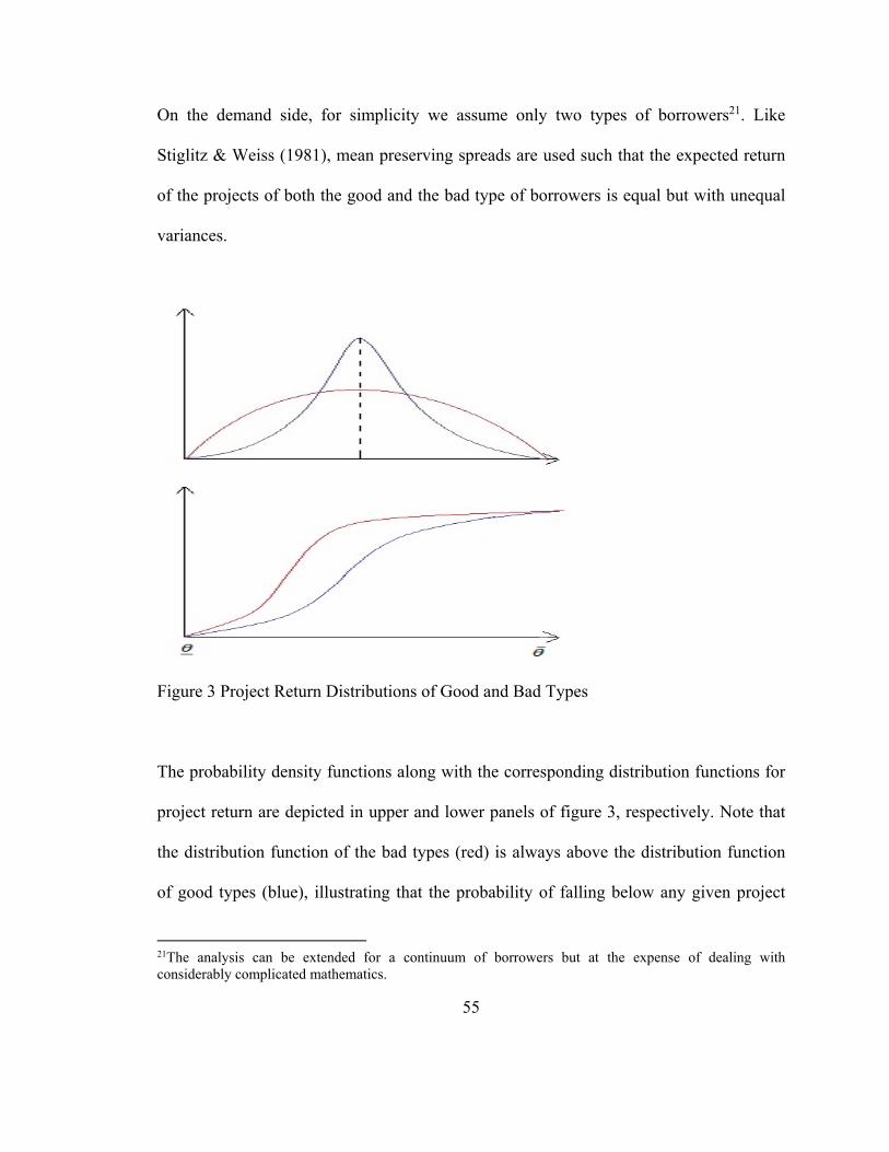
55

On the demand side, for simplicity we assume only two types of borrowers21. Like

Stiglitz & Weiss (1981), mean preserving spreads are used such that the expected return

of the projects of both the good and the bad type of borrowers is equal but with unequal

variances.

Figure 3 Project Return Distributions of Good and Bad Types The probability density functions along with the corresponding distribution functions for

project return are depicted in upper and lower panels of figure 3, respectively. Note that

the distribution function of the bad types (red) is always above the distribution function

of good types (blue), illustrating that the probability of falling below any given project

                                                            21The analysis can be extended for a continuum of borrowers but at the expense of dealing with considerably complicated mathematics.

56

return is higher for the bad types compared to good types. This implies that, all else

equal, bad types are more likely to default.

Lenders offer a uniform (pooling) loan contract with a quoted interest rate of and

cannot differentiate among the types of borrowers but know the fraction of each in the

applicant pool. We assume that both good and bad types have identical endowments of

in each period but different rates of return on an outside investment option, i.e., and

respectively, where . Thus, the associated ex-ante loan contract participation

constraints for each type are given by:

1

1

Since, = , it is easy to see that the participation constraint of the

good types bind at a lower interest rate ( 1) compared to the bad types

( 1). Therefore, the good types drop out of the applicant pool once the

interest rate surpasses this threshold, leaving only the bad types in the applicant pool. But

what happens to the aggregate probability of ex-post (strategic) default once the good

types drop out? The answer is not as simple as it seems.

Introducing an index for types, recall that probability of ex-post default in the absence of

information sharing on defaulters among microfinance institutions was derived in Section

3.6 as:

57

1 1 ∗ ∗

By our assumptions we know that ∗ but at

the same time ∗ ∗ because

. And all else equal the probability, of

strategic default increases with value of outside option, i.e.,∗

0. Intuitively, the

size of the default, i.e., denial of future access to credit is diminished if the income in the

autarky state (i.e., outside option) is higher.

However, in order to reconcile the contradicting effects of borrower type on the

probability of ex-post default, we assume that the mean preserving spreads are

sufficiently large while the differences in the return on the outside option are adequately

small such that: although ∗ ∗

∗ ∗. We feel this is also a more reasonable conclusion because in

practice one would expect good types to default (ex-post) less frequently compared to

bad types. However, the analysis also highlights that simple results derived from a static

model are no longer straightforward after addition of simple dynamics. The graphical

representation of abovementioned arguments in figure 4 crystallizes the desired

conclusion.

58

Figure 4 Probability of Strategic Default for Good and Bad Types Given that the good types are less likely to default strategically, i.e., . It

is easy to see that the profit maximizing ∗ is set sufficiently low such that the ex-ante

participation constraint of the good types is satisfied: 1 ∗ ,

where is small in order to ensure that ∗ ∗ ∗ 022. Of course, this implies that

the ex-ante participation constraint of bad types is satisfied and dynamic repayment

incentives for bad types ( ∗ ∗ ∗ 0) are also intact. If interest rates are increased

beyond ∗ then the good types drop out leading to a higher (overall) probability of

strategic default and hence lower profits (the screening effect). On the other hand, profits

can be increased if interest rates are below ∗ by increasing the interest rate (the price

effect). Therefore, akin to Stiglitz& Weiss (1981), in the presence of ex-ante adverse

                                                            22 If the participation constraint for the good types strictly binds, i.e., 1 than this implies that ∗ ∗ .Hence, there are no dynamic repayment incentives for the good types leading to an increase in the probability of strategic default among the good types and hence lower overall profits for lenders.

59

selection and ex-post default, 1 serves as an interest rate ceiling

derived from profit maximizing behavior of lenders independently of standard market

clearing conditions.

Anecdotal evidence from the microfinance sector lends support to the abovementioned

conclusions. Quoted interest rates on microloans have remained more or less identical

over time despite significant changes in the supply of loanable funds. For example, an

increasing loan supply, spurred by favorable donor funding, has not always lead to a

reduction in interest rates as would be implied by a standard demand-supply model,

Moreover at times, even rising lending costs have not resulted in any meaningful increase

in quoted interest rates in some areas. This observation also suggests that interest rates

are primarily driven by information effects (moral hazard and adverse selection) as

opposed to supply-demand considerations. Although, after a certain threshold when

supply of loanable funds is physically much greater than the demand for credit, it is likely

that standard supply and demand arguments hold whereby interest rates fall drastically as

lenders try to “steal” competitor’s business. However, given the extent of poverty in

South Asia and Africa this seems very unlikely in the near future.

The abovementioned analysis is primarily based on the work of Stiglitz & Weiss (1981)

and the results are no longer applicable if separating loan contracts are considered. Casini

(2015) and Navajas et al. (2003) look at default rates under separating loan contracts, a

setting which is perhaps more appropriate for developed microcredit markets in South

60

America. In summary, given uniform loan contracts, asymmetric information leads to

credit rationing in equilibrium in which profit maximizing microfinance institutions

charge a unique interest rate ∗) independent of lending levels in equilibrium. Because

raising interest rates above ∗ leads to lower profits due to the negative effects of adverse

selection, lowering the interest rate below ∗ results in lower profits since lending

volumes are capped by (endogenous) capacity constraints, i.e., reserves. In the next

subsection we derive the equilibrium lending volumes to pin down the lending reserves

and hence the equilibrium default rates under different market structures.

4.2 Negative Externality of Intra-Firm Competition among Credit-Unconstrained

Lenders

Up until now we have treated lending reserves in microcredit markets as exogenous.

However, in reality, the level of loan reserves is endogenously determined by the solution

to the maximization problem of the representative microfinance institution in a given

microcredit market. In this subsection, we develop a simple model to capture the

underlying constrained optimization problem faced by microfinance institutions, allowing

us to compare the equilibrium lending reserves and default rates under different market

structures with the associated social optima, the primary objective of this paper.

Recall that, by Proposition 1B, in the absence of information sharing among competing

microfinance institutions on defaulters, default rates are an increasing function of

aggregate lending reserves. Evidently, the level of loan reserves is a function of optimal

lending volumes. Therefore, armed with the equilibrium interest rate, we formulate an

61

infinite horizon, dynamic optimization problem to capture the objective function of a

credit unconstrained profit maximizing microfinance institution and derive the optimal

lending volumes and hence loan reserves.

For the time being, we focus on short run dynamics, holding the number of microfinance

institutions in a given market to be exogenously fixed like Guha & Chowdhry (2013).

We assume that profit maximizing microfinance institutions operate in a given

microcredit market, each with the objective of maximizing itsdiscounted stream of

expected profits over an infinite horizon. Each microfinance institution has an initial loan

reserve (equity) of and can save/borrow from the central bank at a net rate of up to an

upper limit of . Thus, the maximum lending volume is capped by . Each period,

competing microfinance institutions simultaneously decide the interest rate to charge on a

loan ( ) and how much to lend, i.e., lending volume. The loan size is normalized to one

unit so that the number of loans lent out also equals the monetary value of the loan

portfolio. Let denote the number of loans made by the ith microfinance institution

and the origination cost for each loan, which is incurred at the beginning of each period.

Finally, is the risk-free (net) rate of return on saving/borrowing with the central bank

and microfinance institutions discount future payoffs at the rate of .

In the previous subsection we showed that in the presence of ex-ante adverse selection

and ex-post moral hazard (strategic default) ∗∀ , where, ∗ is the unique profit

maximizing quoted gross lending rate in a given micro credit market. While, ∑

62

is the (aggregate) probability distribution function of strategic default in a given

microcredit market and ∑ 0 by Proposition 1B23. Given a non-zero

opportunity cost of capital, it is easy to see that, in equilibrium, the optimal lending

reserves of a representative microfinance institution are given by 1 ,

where0 1 . Given this setup, the objective function of a representative

microfinance institution can be expressed as:

max ∗ 1 1 1

s.t

0 → 01

The first bracketed term in the period payoff function adjusts the profit maximizing gross

quoted rate for defaults, i.e., ∗ 1 ∑ 1 represents expected repayment

rate. Therefore, ∗ 1 ∑ 1 is the expected revenue or total cash

inflow from lending activities. The lending costs or negative outflows associated with the

loan principal and the marginal costs of loan origination are denoted by . In order

to capture the opportunity cost of making additional loans, the last term in the period

payoff captures the lender’s borrowing costs, i.e., if 1 or additional income

from savings at the state bank if 1 . Lastly, the period resource constraint

                                                            23 The aggregate probability distribution function of default in the market is the weighted sum of the probability distribution function of strategic default of the good and bad types, i.e., and . Since both and are increasing in ∑ , their sum is also increasing in ∑ .

63

ensures that outlays associated with loan principal and loan origination remain within the

upper bound on lending resources, i.e., and are non-negative.

On closer analysis the solution to the cumbersome looking infinite horizon, constrained

optimization problem is essentially equivalent to the solution of the following simpler

unconstrained, period by period profit-maximization problem:

Max ∗ 1 1 1

Note that although each firm maximizes profits with respect to the variable under its

control, i.e., ,profits depend on the lending levels of competing firms as well because

default rates are a function of aggregate lending reserves, i.e., ∑ 1 . Hence,

from the perspective of a manager in a competitive market with the absence of

information sharing on defaulters, the expected repayment rate is a function of a (known)

lending volume of the given microfinance institution and an unknown quantity lent out

by other lenders in equilibrium. This strategic interaction determines the aggregate

lending volume and hence equilibrium default rates in microcredit markets.

Given strategically interdependent payoff functions and lack of coordination among

competing microfinance institutions, we look for a (non-cooperative) symmetric Nash

equilibrium of the abovementioned game. Taking the first order conditions (F.O.C) with

respect to we get:

64

∗ 1 1 1 1 ∗ 1 1

0 0

0 1

0 1

Note that second derivative is given by ∗ 2 ∑ 1 ∑ and

is strictly negative if . is weakly convex, i.e., . 0, because ∗ and are positive

by definition and ∑ 0 by Proposition 1B.24 Consequently, the first order

condition also becomes a sufficient condition for the optimization problem. We ignore

the uninteresting corner solutions of no lending and lending at capacity but instead

choose to focus on an interior solution of the problem. Summing over F.O.Cs for the

microfinance institutions we have:

∗ 1 1 ∗ 1 1 1 1 0

In a symmetric Nash equilibrium ⋯ ⋯ ∗, where ∗ is

the profit maximizing lending volume, substituting into the F.O.C we get:

∗ 1 1 ∗ ∗ ∗ 1 ∗ 1 1 1 0

                                                            24 Intuitively, the weak convexity of . can also be derived from model primers given the threshold of strategic default ( ) is less than the mean of the stochastic project return ( . If this is the case, it is well known that the distribution function of a standard normally distributed random variable is increasing and convex below the mean and increasing and concave above it, i.e., the mean of the random variable is a point of inflexion. Using the earlier assumption that the probability that a defaulter gets a loan is linear (y′′ . 0) and taking the second derivative of the result shown in proposition 1B with respect to , we get

′′∗ ∗

′

0. Alternatively,if . is not weakly convex than2 ′ ∑

1 ′′ ∑ also guarantees the sufficiency of the first order condition.

65

Now let ∗ denote the aggregate lending volume in this market structure scenario,

substituting into the F.O.C and dividing throughout by we get Equation 1:

∗ 1 1∗

1 1 1 1 0

Equation 1, a nonlinear equation, implicitly determines the optimal lending volume and

hence the default rates in a symmetric Nash equilibrium given a profit maximizing

(gross) lending rate of ∗. Multiplying and rearranging, we get the following root finding

problem with as the free variable:

∗ 1 1 ∗ 1 1 1 0

Positive lending volumes are guaranteed if and only if ∗ 1 1 , which also

implies that the first term in the square brackets is a positive constant independent of

lending volumes. Note that the second term in the square brackets is a positively valued

function of and it equals zero if 0, (i.e., no defaults if no lending) and is non-

negative by assumption. This term is also increasing in . Therefore, the solution to the

associated root finding problem 0 is a unique and real-valued.

In partial equilibrium analysis, welfare is measured as the difference between social

benefit and social cost. And in competitive markets social benefit is measured by the

aggregate revenues while social cost is measured by aggregate costs (Davis & Whinston

1962). It is well known that in order to maximize welfare, the objective of the social

planner is to maximize the “joint” profits of firms in an industry. Therefore, we setup the

66

analogous social planner problem to determine the so called cooperative solution of the

aforementioned game and hence arrive at the “socially optimal” rate of default. The

objective function of the social planner’s problem is given by:

max ∗ 1 1 1

s.t.

0 → 01

Note that social planner maximizes not , where denotes aggregate lending

volume in the microcredit market and the upper case letters are simply the aggregates of

corresponding lower case variables, i.e., (sum of lender equity) and (sum

of borrowing limits). As argued before, the abovementioned dynamic optimization

problem of the social planner is equivalent to a period by period maximization problem

represented as:

max ∗ 1 1 1

In order to determine the “optimal” default rate in the market we solve for aggregate

lending volumes under the cooperative solution. Taking the F.O.C with respect to , we

get Equation 2:

∗ 1 1 ∗ 1 1 1 1 0

67

The default rates implied by Equation 1 and Equation 2 are not directly comparable.

Nevertheless, in Appendix A we use proof by contradiction method to show that default

rates are sub optimally high in the presence of intra-firm competition, leading us to the

following result:

Propostion-2A: Intra-firm competition among credit unconstrained microfinance

institutions results in inefficiently high default rates in equilibrium given a lack of

information sharing on defaulters among microfinance institutions, ex-ante

adverse selection and ex-post default.

Intuitively, in a non-cooperative equilibrium, lending volumes are based on

considerations for private incentives only and the adverse effects of private actions on

aggregate default rates are disregarded. But in the presence of institutional voids, a sole

focus on “private” poverty alleviation efforts ignores the negative externalities associated

with higher levels of private credit supply on aggregate default rates. The empirical and

theoretical literature supports this result. For example, in their empirical work, Fruttero &

Gauri (2005) find that NGO location choices are primarily driven by concerns for private

benefits as opposed to the developmental considerations of a given community.

Consequently, NGOs ignore the (positive and negative) externalities associated with the

so-called private “poverty alleviation” supply curves in order to further organizational

objectives, often to the detriment of local communities. Likewise, under very different

settings (i.e. allowing borrowing from multiple lenders), McIntosh and Wydick (2005)

68

and later Guha and Chowdhury (2013) illustrate that microfinance institutions choose to

ignore the negative externalities created by their private credit supply curves whilst

lending to already indebted borrowers25.

4.3 Negative Externality of Intra-Firm Competition among Credit-Constrained

Lenders

In the previous subsection we showed that default rates are inefficiently high due of intra-

firm competition among microfinance institutions. In this Section we look at a more

realistic case, where much like their potential clients, microfinance institutions are also

credit constrained, i.e., cannot borrow from a central bank. This is quite true in general

but especially so in less developed countries, where microfinance institutions do not

possess physical collateral for money lent to clients or significant deposits, so that

securing credit from the commercial sector is often not possible. Nevertheless,

microfinance institutions do have access to savings in the commercial sector. We also

incorporate economies of scale, whereby, all else equal, higher levels of lending reserves

lead to lower (marginal) lending costs.

Note that loan defaults have two effects. First clients who choose to strategically default

do not repay the promised quoted rate resulting in lost revenue for lenders. Second, and

more importantly, lending reserves are also diminished because the original loan

                                                            25Given the assumption that probability of default is increasing in the level of debt or the number of creditors, lending to an already indebted borrower increases the loan volume and hence the payoff of a given microfinance institution. But at the expense of imposing a negative externality on the microfinance institution which had lend to the given borrower first.

69

principal is forfeited in case of default. If microfinance institutions can borrow from the

commercial sector, then the lost principal is simply deducted from each period’s payoff.

The difference between actual reserves at the end of period and targeted level of reserves

are borrowed from the central bank to continue lending at the optimal scale and the cycle

continues. However, if microfinance institutions cannot borrow from the commercial

sector, then they have to reinvest in their loan reserves each period to ensure that reserves

are not depleted to point of exhaustion. Because, in the absence of access to commercial

credit, microfinance institutions simply go out of business when lending reserves equal

zero. Therefore, in the presence of equilibrium defaults, credit constrained microfinance

institutions need to continually reinvest in lending reserves in order to remain a going

concern.

We now write down and solve the optimization problem of a representative microfinance

institution. The microcredit market is populated with identical credit-constrained

microfinance institutions that seek to maximize the discounted stream of expected profits

over an infinite horizon. Microfinance institutions are assumed to have identical initial

loan reserves denoted by 26. At the beginning of each period a representative

microfinance has to decide how much to lend in the market and how much to reinvest

into the loan reserves, given the profit maximizing net lending rate of ∗ (characterized in

subsection 4.1). As before, represents lending volumes, . is the (aggregate)

                                                            26 In the absence of external borrowing the initial loan reserve level represents equity, likely provided by donors for the purpose of provision of microcredit services only and hence its opportunity cost is not included in the analysis.

70

probability distribution of default as a function of lending volumes (see Proposition 1B),

is the loan origination or marginal lending cost and is the net rate of return on the

outside investment option.. Finally, denotes the level of reinvestment into the loan

reserves each period, whereby invested in outside investment option at the beginning

of each period yields 1 at the end of period.

In terms of the mathematical formulation of the abovementioned problem, we account for

revenue (in its strictest sense) from lending operations in current reward function and

capital losses (from defaults) and gains (from reinvestment in lending reserves) in the

state equation27. The associated bellman equation is given by:

max

∗ 1 1

s.t.

1

In other words, given an initial level of reserves at the beginning of period, lenders

optimize with respect to the choice of lending volumes ( ) and reinvestment levels .

The current reward function comprises of revenues from lending operations, i.e., quoted

loan rate adjusted for defaults multiplied by loan volume less loan origination costs. Note

                                                            27A simple 2-period model can be used to easily verify the “accounting” identity holds, i.e., separation of revenue and capital accounting is valid.

71

that compared to the base line scenario presented in Section 4.2, we incorporate the

effects of economies of scale in this formulation, i.e., marginal lending cost declines with

increases in the size of loan reserves. The first constraint represents the (simplified) law

of motion for loan reserves28. The second constraint is the resource constraint, i.e.,

outflows on lending activities and investment activities in each period cannot exceed the

initial level of loan reserves for a credit constrained lender. It is easy to see that the

resource constraint always binds in equilibrium, substituting the resource constraint

into the maximization problem and law of motion we get:

max ∗ 1 1

s.t.

1

Now we look for the symmetric Nash equilibrium of this problem in the steady state,

where the unconstrained optimization program is given by:

                                                            28 Loan reserves next period are current reserves less the value of loans made out at the beginning of the period and investment in the outside investment option plus loan principal repaid at the end of the period

along with the return from investment on outside option, i.e., ′ 1 ∑

1 , simplifying we get ′ ∑ .

72

max ∗ 1 1

1

Taking first order condition of the problem with respect to we get:

:0 ∗ 1 1 ∗ 1 1

1 1 1

By the envelope theorem condition we know that:

:

Substituting the envelope theorem condition into the F.O.C for we get:

∗ 1 1 ∗ 1 1

1 1 1

0

Note that in a steady substituting into the law of motion we can show that

lending reserves are strictly positive in equilibrium, i.e., ∑

73

1 0. Lastly, substituting the steady state into the F.O.C for we

get:

∗ 1 1 ∗ 1 1

∑ 1

∑ 1 1 ∑ 1

∑ 1

0

In Appendix B, we perform some additional algebra. We first sum over optimality

conditions of all lenders, thereafter we impose symmetry, i.e., ⋯

⋯ ∗ to arrive at a symmetric Nash Equilibrium. Lastly, we define

∑ ∗ as the aggregate lending in this market structure and after some

simplifications we get Equation 3 that implicitly defines the default rates under this

market structure:

∗ 1 1 1 1

∗ 1 1 1 1

1 11 1

0

74

Similar to the previous subsection, we now derive the default rates implied by the

solution to social planner problem. Again, the goal is compare the socially optimal

default rates with the default rates in the presence of intra-firm competition. The

analogous social problem can be written as:

max ∗ 1 1 ′

Subject to

′ 1

Where, denotes the aggregate initial lending reserves and represents the aggregate

lending volumes. Each term in the optimization term has already been discussed in detail

before, therefore, for sake of brevity we jump to the analysis of the following

unconstrained optimization problem:

max ∗ 1 1

1

Now we derive the solution to the abovementioned problem in the steady state, taking

first order condition with respect to we get:

0 ∗ 1 1 ∗ 1 1

1 1 1

The envelope theorem condition gives us:

:

Substituting the envelope theorem condition into the F.O.C for we get:

75

∗ 1 1 ∗ 1 1

1 1 1 0

Note that in a steady ′ substituting into the law of motion we get:

1 0. Substituting the steady state level of into the F.O.C for

we get:

∗ 1 1 ∗ 1 11

1 1 1 1

0

Details of further simplifications and algebraic manipulations can be found in Appendix

C, the final expression characterizing the default rates under the social planner allocation

are given in Equation 4 below:

∗ 1 1 1 1

∗ 1 1 1 1

1 1 1 1

Now we can compare the socially optimal default rates under the cooperative equilibrium

given intra-firm competition among credit constrained lenders (Equation 4) with the

default rates under the non-cooperative equilibrium (Equation 3). Direct comparison

76

between default rates under both scenarios is not feasible. Therefore, once again the

method of proof by contradiction is employed to show that default rates are inefficiently

high in the presence of intra-firm competition. Details of the related algebra are relegated

to Appendix D and the final result is summarized in Proposition 2B below:

Propostion-2B. Intra-firm competition among credit-constrained microfinance

institutions results in inefficiently high default rates in equilibrium given a lack of

information sharing on defaulters among microfinance institutions, ex-ante

adverse selection and ex-post default.

Before moving onto the next subsection, we want to highlight some important features of

the equilibrium default rates under the aforementioned cases. First, note the socially

optimal lending volumes and hence the associated defaults rates are independent of the

number of competitors in the market under both scenarios, i.e., credit unconstrained or

credit constrained lenders. In other words the “size” of the central planner allocation is

the same regardless of number of players in the market, obviously smaller shares for each

competitor as increases. Interestingly, as the number of players in the market increase,

competition intensifies and as more resources are pumped into the market, the incentives

do default are greater than before leading to a higher rate of resource dissipation. Second,

the inefficiencies caused by sub optimally high default rates due to intra-firm competition

remains regardless of the organizational structure of the microfinance sector.

77

4.4 Section Overview

The setting of credit unconstrained profit maximizing behavior is more appropriate if the

market is populated primarily by microfinance banks. Whereas, the objective function of

credit constrained lenders is more suitable for analyzing markets with non-banking NGO

type microfinance institutions. But which market structure leads to higher defaults in

equilibrium? And what is the size of the negative competition externality in each case? In

order to answer these fundamentally important questions we cannot rely on analytical

methods and need to revert to tools for numerical analysis29.

Figure 5 shows the equilibrium default rates plotted against the number of competitors

under different market structures (credit constrained or unconstrained lenders) and

scenarios (cooperative or non-cooperative). Since, the number of competitors was taken

as given in our model, we solve for equilibrium default rates for different values of

using the Broyden’s method. These numerical simulations, under reasonable calibrations,

corroborate earlier results derived using analytical methods. For example, the equilibrium

default rates under the non-cooperative solution are significantly higher compared to the

equilibrium default rates under the cooperative solution regardless of market structure as

shown in Proposition 2A and 2B. Likewise, consistent with Proposition 1A, figure 5

shows that default rates increase with , i.e., extent of competition.

                                                            29 The analytical proof of proposition 2B is not as elegant as that of proposition 2A.The forthcoming numerical analysis also addresses this deficiency.

78

Figure 5 Effect of Competition on Equilibrium Default Rates under Different Market Structures Author: The equilibrium default rates are based on the following model calibrations: net profit maximizing interest rate ∗ 0.40 (corresponding gross rate is 1.40), risk free rate 0.025, marginal lending costs 0.05, time preference 0.99. The strategic

default function was assumed to be.

,, where the denominator denotes market capacity, i.e., total number of potential clients.

Broyden’s method routine developed by Miranda and Fackler (2004) was used to solve the nonlinear root finding problems represented in equations 1-4 for different values of .

However, the rate at which defaults increase is much higher in the case of credit

constrained lender with economics of scale compared to credit unconstrained lenders.

Intuitively, with economies of scale and continual reinvestment into the lending reserves,

credit constrained lenders have an additional inventive to disburse loans, leading to

higher equilibrium loan reserves and hence higher defaults in the given institutional

environment. Moreover, the “size” of the negative competition externality is also larger

(both in the absolute sense and the relative sense) in case of a market structure with intra-

firm competition among credit-constrained lenders. From a policy perspective, the

79

numerical analysis clearly highlights that removing credit constraints faced by lenders in

microcredit markets is a Pareto optimal intervention from the societal point of view.

We have looked at only two types of lenders in the microcredit market. Credit

unconstrained lenders represent large microfinance banks with operations in different

regions and credit unconstrained lenders represent small microcredit NGOs often present

in only a limited number of areas. Of course, other organizational types, such as the

output maximizing microcredit institution analyzed by Mcintosh and Wydick (2005), are

also present in the microfinance sector, although their share has declined significantly

over the past decade due to a paradigm shift from the poverty lending approach towards

to the financial systems approach. Nevertheless, Mcintosh and Wydick (2005) showed in

their paper that profit maximizing and output maximizing microcredit institutions charge

identical interest rates in equilibrium. Using this result, it is trivial to show that lending

levels and hence default rates will be higher in case of an output maximizing or size

maximizing firm subject to a breakeven constraint compared to the cases studied herein30.

However, the analogous social planner allocation in the presence of intra-firm

competition among output-maximizing lenders is not apparent because, socially optimal

allocations balance the marginal costs and benefits of actions in given settings, whereas

in the case of output maximization there is no such tradeoff. Hence, we choose not to

                                                            30 For example, consider the well-known case of a sales maximizing firm originally expounded by Baumol (1959). In this case production is determined at the point where marginal revenue equals zero in contrast to the standard optimality conditions given by the equating marginal revenue to marginal cost. Therefore, as long as marginal costs are non-zero and marginal revenues are declining with production then the sales maximizing firm will produce more than the profit maximizing firm.

80

explore this market structure further here, although we return to its implication on

location choices later.

But are the equilibrium default rates depicted in figure 5 a reasonable approximation of

reality? In the case of credit unconstrained, profit maximizing lenders the equilibrium

default rates in the presence of intra-firm competition are low for a full blown crisis.

However, our model is only concerned with strategic default and does not account for

negative shocks that may hamper the ability to repay. The interaction of negative shocks

and increased likelihood of strategic default due to intra-firm competition can lead to

default rates that are within reasonable bounds of the default rates observed during a

repayment crisis in the microfinance sector. The increase in default rates associated with

rising competition among credit constrained lenders seem unrealistically large. However,

the number of competitors is varied exogenously; therefore, non-positive profits are not

inconsistent with short-run maximization problems. At the same time, short-run defaults

rates of 60-70% are not uncommon during a full-fledged repayment crisis.

In reality, the microfinance sector is populated with different types of organizations

ranging from large profit maximizing microfinance banks to small, liquidity constrained

lending operations. Moreover, both types of lenders are neither entirely altruistic (output

maximizing) nor motivated by profits only, but located somewhere on a spectrum with

profit motives on one end and social mission on the other end. It is well known that the

presence of subsidized government sponsored microcredit programs can have adverse

81

effects on commercial lenders vis-à-vis the interest rate channel, effectively driving the

commercial sector out of business. In truth, the implications of the interactions between

different types of institutions on default rates in microcredit markets cannot be accurately

predicted and in all likelihood the actual default rates will probably fall within the bounds

shown in figure 5. Nevertheless, the channels highlighted in the preceding analysis are

expected to hold regardless of market structure, although the strength of these effects may

vary based on the specific characteristics of each market.

5 Further Analysis

In this Section we extend the preceding analysis to further highlight some interesting

results arising from intra-firm competition that are consistent with the stylized facts

associated with the development of microcredit sector in less developed countries. In

particular, we examine the effects of intra-firm competition for donor funds on

equilibrium default rates and look at the location choices of different types of

microfinance institutions. Our analysis shows that competition for donor funds leads to

further deterioration in repayment rates in the existing institutional environment. A focus

on private pay-offs leads to the exclusion of rural markets and excessive concentration in

urban markets. This leads to excessively high default rates in the latter leading to

resource dissipation and financial exclusion of the former. Both tendencies undermine the

original objectives of the microfinance revolution, i.e., sustainable provision of access to

financial services.

82

5.1 Effect of Intra-Firm Competition for Donor Funds on Default Rates

We introduce competition for donor funds in the baseline model described in Section 4.2

in order to look at the effect of donor money on the materialization of microfinance

repayment crisis.31 We assume that benevolent donors have allocated a fixed (exogenous)

amount of donor money for microcredit sector in a given region in each period denoted

by , under the assumption that access to microcredit results in poverty alleviation.

These donors do not have the capacity to undertake microcredit projects themselves due

to the risks, regulatory costs and long term commitments involved in operating a

microfinance institution, and are better off disbursing funds to microcredit providers

rather than holding on to them for other purposes, i.e., non-distribution constraint.

Outreach or quantity of loan disbursements is widely used as a criterion to evaluate the

performance of different types of microfinance institutions and serves as an objective

metric of a given lender’s poverty alleviation “effort”. For example Chen et al. (2010)

find that funding, national influence, and international recognition all flowed to the

largest players. Therefore, the poverty reduction “effort” of a given microfinance

institution is judged relative to other competing microfinance institutions based on its

relative outreach. And hence donor money is distributed among competing microfinance

institutions based on relative outreach. In other words, donor money is a “prize” that

lenders in a given market vie for with “outreach effort”, where the payoff of the ith lender

                                                            31 Identical results hold for credit constrained profit maximizing lenders with economies of scale but with considerably tedious algebra.

83

is given by ∑

. It is easy to see that this payoff function introduces another

channel of strategic interdependence into the baseline model, whereby a given

microfinance institution’s share of the so called “prize” is decreasing in the “outreach

effort” of competing lenders, i.e., 0.

Note that the amount of donor funds allocated to the microfinance sector is assumed to be

exogenously fixed. However, the distribution of these funds among competing

institutions is endogenous. Moreover, in contrast to Aldashev & Verdier (2010), the

competition for donor money in this paper takes place through “on-project effort” as

opposed to “off-project effort”. This feature makes our results potentially more

interesting. As before, microfinance lenders are assumed to be rational payoff

maximizing agents with an infinite horizon. Given the results of the previous Section, the

equilibrium default rate with competition for donor money is defined by the solution to

following period by period optimization problem:

Max ∗ 1 1 1 ∑

The first order condition is given by:

∗ 1 1 1 1 ∗ 1 1

∑

∑0

84

We look for a symmetric Nash Equilibrium, such that … ∗,

substituting this into the first order condition and summing over we get:

∗ 1 1 ∗ ∗ ∗ 1 ∗ 1 1 1

1 ∗

∗ 0

Let ∗ denote aggregate lending volume. Substituting it into the expression above

we get Equation 5 which implicitly pins down the aggregate default rates in this case:

∗ 1 1∗

1 1 1 1 1

0

Now we can also write down the analogous social planner problem:

Max ∗ 1 1 1

Note that there is no intra-firm competition for donor funds in a cooperative equilibrium

because the amount of donor money allocated to the microfinance sector (as a whole) is

exogenously fixed independent of outreach effort. Obviously, the first order condition

associated with the abovementioned optimization problem is identical to Equation 2

derived in Section 4.2, i.e., in the social planner allocation donor money has no effect on

equilibrium default rates since each lender simply gets an equal share of the prize, i.e., .

Formally, it is straightforward to show that competition for donor money results in sub-

optimally high default rates. Note that the default rate implied by the analogous social

planner problem with a fixed donor inflow of is 1 , identical to Equation 2

85

in Section 4.2. Also recall that in Proposition 2A we showed that , where is

lending volume with intra-firm competition (without donor inflows). We can equate

Equation 1 and Equation 5 since the LHS is zero, after some simplifications we get:

1 11

1 1

1∗

Now we compare and . Note that the LHS is always positive since 1 by

definition. Therefore, if then all the terms on the RHS cancel out. Whereas, if

, then since 0 by Proposition 1B and 0 by assumption then the RHS is

always negative. Consequently, it must be that and hence 1

1 1 , i.e., competition for donor money leads to sub-optimally

high default rates. Intuitively, although the marginal revenue from each additional loan

declines below the marginal cost, microfinance institutions continue to lend given the

benefits of the share of donor money.

Proposition 3: Intra-firm competition for donor money, distributed among

competing lenders on the basis of relative outreach, results in inefficiently high

default rates in equilibrium given a lack of information sharing on defaulters

among microfinance institutions, ex-ante adverse selection and ex-post default.

Clearly, competition for donor money is suboptimal because lenders purse higher lending

volumes (i.e., larger lending reserves) as a goal in itself, in order to gain a larger chunk of

86

the donor “prize” money. Although not considered here, larger lending volumes (hence

larger reserves) also come with additional benefits including economies of scale, prestige

and reputation which can be used to attract further funding. However, these types of

“credit push” incentives have often led to the oft discussed phenomena of double dipping

in the microfinance sector. Whereby, microfinance institutions knowingly lend to already

indebted and marginal clients resulting in the over indebtedness and eventually wide

scale default, similar to the 2010 Indian microfinance crisis (Guha & Chowdhury 2013).

We once again use numerical simulations to highlight the effect of donor money inflows

on equilibrium default rates in the aforesaid institutional settings.

Figure 6 confirms earlier claims that large inflows of donor money can lead to an

exponential increase in default rates and at times even a full blow repayment crisis in the

given institutional environment. For example, if donor inflows in a given period amount

to approximately 1% of total loan demand then default rates range from 50-60%, very

close to the threshold of a default crisis. Moreover, increasing donor inflows are also

likely to draw in additional competitors in expectation of higher future profits, leading to

further erosion of dynamic repayment incentives and hence higher default rates.

87

Figure 6 Effect of Competition for Donor Funds on Equilibrium Default Rates Author: The equilibrium default rates are based on the following model calibrations: net profit maximizing interest rate ∗ 0.40 (corresponding gross rate is 1.40), risk free rate 0.025, marginal lending costs 0.05 and 100 and 1000 corresponds to

0.1% and 1% of total credit demand (100,000), respectively. The strategic default function was assumed to be.

,, where the

denominator denotes market capacity, i.e., total number of potential clients. Broyden’s method routine developed by Miranda and Fackler (2004) was used to solve the nonlinear fixed point problems represented in equations 1 & 5 for different values of .

Note that we are not trying to argue that donor money is inherently bad, but merely

stating that in the absence of information sharing on defaulters among competing

microfinance institutions, polices seemingly designed to benefit the microcredit sector

can actually have the opposite effect. The conclusions drawn from propsition-3 also fall

in line with the stylized facts associated with a microfinance crisis. For example, Viada &

Gaul (2011) documented that increasing donor inflows (and investment in general) was

recorded leading up to a microfinance crisis in many countries like Bosnia, Uganda, India

etc., reaffirming the central theme of this, i.e., under certain circumstances more is

actually less!

88

5.2 Effect of Intra-Firm Competition on the Location Choices of Lenders

Continuing with the analysis of the supply side, we extend the preceding analysis to

highlight the adverse effects of intra-firm competition on the location choices of lenders

in this subsection. The correlation between rural agricultural households and poverty is

markedly strong in South Asia; therefore, interventions in rural markets are key to

poverty alleviation. However, geographically, microfinance service providers are

increasingly concentrated in large urban cities in less developed countries (Oxford Policy

Management 2006 and International Finance Corporation & KfWBankengruppe 2009).

For example, the percentage of urban clients in the microfinance industry portfolio of

Pakistan increased from approximately 30% in 2005 to 44% in 2012 (Pakistan

Microfinance Network Industry Review 2012). In some African markets the rural and

urban divide is even larger. The schism between provision of microfinance services in

rural and urban areas in less developed countries becomes wider if government funded

public microcredit programs are excluded from the analysis. This increasingly uneven

distribution of commercial microfinance services between rural and urban areas is not

optimal from the societal point of view.

Firstly, as highlighted in Proposition 1A and subsequently, in the absence of information

sharing on defaulters an increase in the number of lenders in a given market dilutes

dynamic repayment incentives leading to a higher likelihood of strategic default.

Likewise, Guha & Chowdhury (2013) have shown that with an increase in number of

lenders, microfinance clients are more likely to engage in double dipping, resulting in

89

over indebtedness and eventually wide scale default. In a nutshell, excessive

concentration in urban areas dilutes dynamics repayment incentives whilst the tendency

to “push” credit in face of competitive pressures results in over-indebtedness. Together

both factors have contributed towards the materialization of frequent microfinance crisis

over the past decade in countries like Bosnia, Uganda, Pakistan, India and Nicaragua.

Secondly, the exclusion of rural areas undermines the original objectives of microfinance,

i.e., providing access to credit to the financial excluded sector. Moreover, rural poor are

often the largest component of poor and vulnerable populations in less developed

countries. Therefore, “real” economic development is not possible without overcoming

the financial exclusion of the rural poor. For instance, access to credit can help poor

farmers, often engaged in subsistence farming based on traditional labor-based farming

methods, overcome credit constraints associated with technology adoption. And increases

in income are often a harbinger of agricultural mechanization, which eventually leads to

structural change from an agriculture based economy to an industrialized economy.

Moreover, at the very least, improvements in economic opportunities in rural areas will

curtail excessive migration into sprawling urban centers of less developed countries,

along with its negative repercussions for example increase in crime rates, pollution,

squatter settlements etc. Likewise, compared to urban poverty alleviation, rural poverty

alleviation has larger spillover effects due to the increased demand of secondary goods in

the often isolated rural local economies.

90

However, lending costs in rural areas are unsurprisingly higher compared to lending costs

in urban areas for several reasons32. First, due to limited infrastructure facilities in rural

areas, the management of microcredit operations is typically done from offices located in

urban areas. Likewise, rural areas have a poor transportations and communications

network. Therefore, lending costs associated with vetting loan applications, delivering

credit, collecting payments and monitoring clients increase with distance from urban

centers. Second, geographically, rural clients are spread over a larger area compared to

urban clients and delivering microfinance services at several, small, scattered locations is

more costly compared to urban clients concentrated in densely populated cities.

Consequently, given the labor intensive operations of microfinance institutions, more

clients can be served per worker in urban areas compared to rural areas due to

aforementioned factors. However, on the positive side, Imai etal. (2012) find that

information costs are usually lower in agriculture based microloans in rural areas

compared to non-agricultural microenterprises in urban centers.

Nevertheless, despite the abovementioned pros and cons of lending in rural and urban

microcredit markets, one can clearly see a noticeable trend in the commercial

microfinance sector of less developed countries, i.e., a marked focus on urban microcredit

markets at the expense of rural credit markets. This also increases lack of diversification

                                                            32 This does not hold for all countries. For example, in a densely populated country like Bangladesh microcredit institutions have a strong presence in rural areas. However, in more geographically diverse countries like Pakistan, Uganda and Kenya the rural-urban dichotomy is clear. For example in Pakistan, microfinance providers are predominantly present in the metropolitan cities of the affluent provinces, i.e., Punjab and Sind. Whilst, ignoring the less developed rural provinces of KPK and Baluchistan, although, both the extent and depth of poverty is higher in the later.

91

in the loan portfolio of microfinance institutions and increases their vulnerability to

external shocks. Is intra-firm competition responsible for this adverse geographical

distribution?33 And is this distribution suboptimal? In order to answer these questions, we

use simple game theoretic arguments. The following analysis, although not as rigorous as

some of the earlier work presented above, nevertheless, it promises to offer logical and

intuitive insights into the location choices of different types of lenders34.

We assume there are only two microcredit markets, i.e., rural and urban. The loan

origination or marginal lending costs are higher in the rural markets compared to the

urban markets, i.e., . Both markets are identical in all other aspects, i.e.,

ex-ante adverse selection with ex-post default, hence, the profit maximizing interest rate

( ∗ is assumed to be equal in both markets.

We begin our analysis with the simplest case of an altruistic microfinance institutions,

i.e., client (output) maximizer as in Mcintosh & Wydick (2005). It is a commonly held

view that the adverse geographical distribution of microfinance institutions is driven by

the rise of commercially oriented microfinance institutions rather than socially motivated

                                                            33Chen et al. (2010) find that In Pakistan and Morocco it had been a common practice among some lenders to follow other lenders into local markets n order to lend to the same clientele. Since, first movers are the first to screen and train new borrowers whereas later arrivals can skip over these up-front preparatory costs and significantly lowering client acquisition costs. 34 I hope to further develop the decision making process that goes into the location choices of lenders rigorously in future work and test it empirically with branch location data from Pakistan. This will basically require optimization of an integral over a continuum of microcredit markets differing in marginal lending costs in addition to channels of strategic dependence highlighted in this paper.

92

lenders. This is not entirely true. In fact it is easy to see that an output maximizer will

always choose to enter the cheaper urban markets.

The objective of a socially motivated client maximizer is to simply maximize number of

clients subject to a resource constraint. Therefore, the production function of a client

maximizer is simply given by . Since clients in urban and

rural markets are perfect substitutes as far as loan volume is concerned, it is trivial to

show that a rational lender will always choose to lend in the cheaper market, i.e.,

0 as along as .

Intuitively, most altruistic microfinance institutions are funded by donors and, as

mentioned before, outreach is a commonly used metric to judge the “poverty alleviation

effort” of competing lenders. Therefore, facing competitive pressures for securing

additional donor funds, altruistic lenders are even more likely to focus lending operations

in cheaper urban markets. Because, serving the relatively expensive rural markets will

lead to a reduction in loan volume given a fixed resource constraint. In a non-cooperative

equilibrium, this in turn leads to a decline in the share of donor money received next

period, which necessarily results in lower lending volumes in future. The cycle continues,

until altruistic lenders focusing on rural markets eventually go out of “business”35. As

rational agents, altruistic microfinance institutions realize the negative repercussions of

lending in rural markets and focus lending activities in urban centers. As discussed

                                                            35 We assume founders of altruistic lenders get some non-monetary utility from providing credit to the poor for example social prestige, “warm-glow effect” etc., therefore, always prefer to continue operations.

93

before, an overconcentration of micro-lenders in urban centers dilutes the dynamic

incentives associated with loan repayment, leading to inefficiently high default rates and

at times even a repayment crisis. Adding an additional break-even constraint complicates

the preceding analysis, nevertheless the conclusions still hold especially if marginal

lending costs in rural areas are significantly higher.

The stylized facts also support the abovementioned arguments. For example, in Pakistan

the widening gap between rural and urban borrowers in the industry portfolio has

coincided with an increase in the market share of non-profit microcredit NGOs from 17%

in 2005 to almost 34% in 2007. Similar trends have been observed in other less

developed countries, where microfinance NGOs have consistently followed an intensive

growth strategy, i.e., vied for growth in existing markets and products without expanding

into new markets or new products. In fact, these trends have led several economists and

practitioners to heavily criticize the rise of the so called “NGO industry” in general and

microcredit NGO sector in particular e.g. see Dichter and Harper (2007) and Dichter

(2010).

However, in the case of profit maximizing microfinance institutions, arguments for a

rural-urban schism are less crisp because profit maximizing lenders are primarily

interested in profits, not output. And given the negative externality of intra-firm

competition, profit maximizing microfinance institutions are more likely to move to rural

markets if benefits of doing so outweigh the costs. This involves a continuous assessment

94

of expected profit differentials in both types of markets. But if the relative payoffs from

donor money are large enough (as shown in Proposition 3), then the arguments presented

above clearly hold and will lead to a rural-urban divide.

In order to simplify the analysis we assume that profit maximizing lenders can only enter

one market36. This is a reasonably justifiable assumption given that fixed costs of entry

may be high, lenders might lack the capacity to enter multiple markets or simply with a

large number of potential markets each lender can only serve a limited number of

markets. To highlight the underlying mechanisms we look at a simple example with two

identical lenders.

Let , denote profits of a given microfinance institution if both enter the rural

market. Likewise, , denote profits of a given microfinance institution if both

enter the urban market. Given that the profit maximizing interest rate ( ∗ and the

aggregate strategic default function are identical in both markets but , it

is straightforward to use results presented in Section 4.2 to show that ,

, . Finally, let , represent profits of a microfinance institution that

enters the urban market, given its competitor enters the rural market; and let

, represents profits of a microfinance institution that enters the rural market,

given its competitor enters the urban market. Again we can use Proposition 2A to arrive

at the conclusion that , , due to the negative externality of

                                                            36 Note that in the case of output maximizing lender it was clearly never optimal to enter both markets.

95

intra-firm competition. Of course this implies that , , . Under the

assumption that , , , it can be easily shown that both lenders

enter the urban market in a Nash equilibrium. To see this note that the abovementioned

results can be represented in the following payoff matrix:

Table 2 Payoff Matrix of Location Choice Game

Players Lender-2

Len

der-1

Strategy Rural Urban

Rural ( , , , ) ( , , , )

Urban ( , , , ) ( , , , )

Each row in table 2 represents the strategy choices of lender-1 and each column

represents the strategy choices of lender-2, whereas the first number in the brackets

denotes the payoff of lender-1 and second number denotes the payoff of lender-2. It is

easy to note that ( , , , ) is the unique Nash equilibrium of this

game. For instance, if lender-2 decides to enter the rural market than lender-1 obviously

enters the urban market because , , , by

Proposition 2A. And if lender-2 decides to enter the urban market then lender-1 is still

better off entering the urban market since , , by assumption.

Given the game is symmetrical; we conclude that entering the rural market is the

dominant strategy of each player.

96

Note that , , , or , , , is the cooperative or

social planner allocation. Therefore, the non-cooperative equilibrium is not Pareto

optimal as long as , , , , 037,

i.e., the positive value of the first bracketed term dominates the negative value of the

second bracketed term. Intuitively, the social planner maximizes total welfare by

assigning different lenders to different locations thereby minimizing the negative

externality of intra-firm competition. Obviously, this cannot be done in a decentralized

solution due to a sole focus on private incentives, resulting in exclusion of the rural poor

from access to credit along with sup optimally high default rates in urban areas.

Equivalently, this strategic interaction among competing lenders can be modeled as a two

stage, simultaneous move game. Here, in the first stage each lender (simultaneously)

decides which market to enter and optimal lending levels are determined in the second

stage. Using sequential rationality it is straightforward to see that no lender chooses to

service the rural microcredit markets. Therefore, all lenders enter the cheaper urban

markets. Identical results for the abovementioned location choice games can be derived

for multiple lenders and markets.

The equilibrium of the game tree depicted below can be solved using backwards

recursion. While, the optimal geographic coverage can be retrieved from the solution to                                                             37 We simply compute the total payoffs from the cooperative solution and the non-cooperative solution. Subtracting the latter from the former yields a positive number, i.e., total payoff from the cooperative solution is greater than total payoff from the non-cooperative solution because , , by proposition 2A.

97

the social planner problem which involves equating the marginal revenue from each type

of market to the marginal cost of the cheapest market. Assuming an interior solution, we

get non-zero lending in rural markets in the cooperative equilibrium, although, lending

volumes are higher in urban markets compared to rural markets due to the lower marginal

costs in the former.

Figure 7 Location Choice Game Tree However, due to strategic interdependencies, the non-cooperative equilibrium always

entails a sub optimally high concentration of lenders in the cheaper urban markets and no

lending in the costly rural markets. The results described above are summarized below:

98

Propostion-4: Given that marginal lending costs are higher in rural markets

compared to urban markets, an altruistic output maximizer will never enter rural

markets due to efficiency considerations.

While in the presence of intra-firm competition among profit maximizing lenders,

servicing the cheaper rural markets is a dominated strategy if ,

, and it is also sub-optimal given that ,

, , , 0. Hence, distribution of donor

money among competing lenders on the basis of relative outreach further

exacerbates the schisms between rural-urban lending.

Several simplifying assumptions were made to keep the analysis as straightforward as

possible. It would be interesting to see if identical results can be derived from a more

general model with several lenders and an entire spectrum of microcredit markets, such

that profit maximizing lenders may enter multiple markets simultaneously. But for the

time being, Proposition 4 highlights that market mechanisms to solve problems of

poverty alleviation are plagued with incentive problems. Whereby, altruistic, client

maximizing lenders decide to ignore the rural poor due to simple efficiency based

considerations and serving the rural poor is a dominated strategy for the (more maligned)

commercial lenders. These location choices lead to a sub-optimally high concentration of

lenders in cheaper urban markets resulting in dilution of dynamic repayment incentives,

double dipping (client over-indebtedness) and eventually high default rates. Whereas,

exclusion of the rural poor from access to credit not only undermines the original

99

objectives of microfinance movement but retards the speed of structural change and

economic growth.

6 Conclusion

6.1 Overview and Summary of Findings

Microfinance plays a key role in the poverty alleviation strategy of international

development agencies. Moreover, an array of donor funded institutions is increasingly the

preferred option for microcredit interventions in less developed countries. In this paper

we have extended the burgeoning literature examining the effects of the industrial

organization of microfinance sector on poverty alleviation (Guha & Chowdhury 2013 and

Mcintosh& Wydick 2005) and the adverse consequences of competition among NGOs

for donor money on poverty alleviation (Fruttero & Gauri 2005 and Aldashev & Verdier

2010) to highlight problems with the existing structure of the microcredit markets.

In summary, we first established that no information sharing on defaulters among

competing microfinance institutions is the unique (sub-optimal) Nash equilibrium in

competitive microcredit markets in less developed countries. Second, we developed a

simple model of strategic default by borrowers to show that probability of ex-post default

is a function of the number of competing lenders in a region and “credit rationing” as

measured by the ratio of aggregate lending reserves to loan demand. More specifically,

we proved that the probability of strategic default increases with the number of

competitors and lending volumes in a given microcredit market via the dilution of the

100

dynamic incentives of loan repayment. Based on these findings we specified the behavior

of aggregate default function . in microcredit markets. Thereafter, building on the

seminal work of Stiglitz&Weiss (1981) we demonstrated that in the presence of ex-ante

adverse selection and strategic default, there exists a unique profit maximizing interest

rate ∗ that is independent of lending levels. Because in a symmetric Nash equilibrium

raising interest rates above ∗ leads to lower profits due to the negative effects of adverse

selection and in the presence of excess demand, lowering interest rate below ∗obviously

results in lower profits.

Armed with the equilibrium interest rate and the aggregate default function, we

formulated an infinite horizon, dynamic optimization problem to capture the objective

function along with the relevant constraints of credit unconstrained lenders and credit

constrained lenders with economies of scale. We solved for the default rates in a

symmetric Nash equilibrium in each case and compared it with corresponding default

rates from the analogous social planner problem to prove that intra-firm competition

results in inefficiently high default rates. Moreover, we find that the equilibrium default

rates in a market with credit constrained lenders are significantly higher compared to

equilibrium default rates in a market with credit unconstrained lenders.

Subsequently, we introduced competition for donor funds among lenders through relative

outreach and proved that increasing flows of donor funds lead to higher default rates

regardless of the of lenders objective functions in microfinance markets. Lastly, we

101

extended the model to include multiple microcredit markets that differ in marginal

lending costs, and show that competition among lenders leads to an over emphasis on

urban areas (where transaction costs are assumed to be lower compared to rural areas) at

the cost of the exclusion of rural areas, resulting in financial exclusion of rural poor on

one hand and sub optimally high default rates in urban areas on the other. Increases in the

level of donor funding towards the microfinance sector exacerbate the aforementioned

negative effects of location bias in both the short and long run, especially in the case of

output maximizing altruistic lenders.

In a nutshell, the abovementioned results are based on the simple yet powerful idea that

microfinance institutions have a private supply curve of “poverty alleviation effort” that

does not account for the positive externalities of serving financially excluded microcredit

markets. Likewise, in the absence of information sharing on defaulters, the private supply

curve of “poverty alleviation effort” do not account for the negative externality imposed

on competing lenders, resulting in inefficiently high default rates and overconcentration

in urban markets. And it is well known that in a competitive equilibrium there is

underproduction of goods with positive externalities and overproduction of goods with

negative externalities. At the same time, competition for the ever increasing inflows of

donor funding into the microfinance sector further exacerbates these inefficiencies. Of

course we are not the first ones to point this out in the context of development economics.

102

Empirical evidence presented in Fruttero & Gauri (2005) highlight that developmental

interventions by NGOs are driven by private organizational concerns as opposed to the

developmental needs of recipient communities. Consequently, NGO project choices do

not reflect community needs or take into consideration externalities of existing

developmental projects but are often driven by a desire to secure donor funds or other

organizational goals38. Guha & Chowdhury (2013) highlight another important channel

whereby intra-firm competition results in “credit push” such that microfinance

institutions willingly lend to already indebted clients. This double-dipping equilibrium

eventually leads to soaring default rates and repayment crisis like the one witnessed by

the Indian microfinance sector in 2010. Similarly, Aldashev & Verdier (2010) prove that

entry of additional NGOs into the so-called “development market” imposes a negative

externality on existing NGOs by reducing the return on existing fund-raising efforts.

Consequently, in a symmetric Nash equilibrium all NGOs increase fund raising efforts.

This increase in competition for donor funds is potentially inefficient because resources

are increasingly diverted from project related activities towards fundraising activities,

diluting the actual impact of NGOs. Therefore, to a large extent, our conclusions mirror

the findings of prior literature albeit under very different settings and assumptions.

Nevertheless, it would be interesting to see the how intra-firm competition in the given

institutional environment effects investment in lending technologies that have the

                                                            38 For example, a village with an existing microfinance institution will benefit more from an educational project like a school or training center as opposed to another microfinance institution. However, often NGO project and location choices do not reflect these externalities but driven by selfish organizational concerns

103

potential to reduce the lending costs. Similarly, it would be worthwhile to look at market

dynamics if lenders are assumed to reinvest profits into existing lending reserves in order

to maximize the size of lending reserves. Lastly, the association between different

measures of poverty incidence and microcredit institution’s branch location choices can

be studied, after controlling for covariates, to empirically test the validity of the results

presented in this Chapter.

6.2 Some Policy Prescriptions

Despite the support of millions of dollars and the neoliberal theory of economic

development, microfinance has failed to live up to its claim of sustainable poverty

alleviation via market mechanisms. Therefore from a policy perspective, our analysis

calls for a complete paradigm shift in the current policy prescriptions meted out to the

microfinance sector. We conclude the paper by presenting policy recommendations to

mitigate some of the adverse effects of the abovementioned market failures. Thereafter,

we address some of the inherent fallacies in the existing microfinance narrative and

suggest a way forward.

Firstly, the microfinance sector has remained largely unregulated in most developing

countries under the pretext the market based solutions are by design the best solution to

the problem of lack of access to credit. The preceding analysis highlights that this

approach needs to change and microcredit lenders should be regulated in order to reduce

or at least manage the negative effects of intra-firm competition, since competition can

104

introduce new market dynamics that are not always easy to see. Policies could include

subsidies for lenders operating in rural areas to reduce the profit differentials between

rural and urban markets. Interestingly, globally the financial sector is best characterized

by oligopolistic or monopolistic competition. Therefore, creating similar incentives for

local microcredit monopolies by offering regional licenses does not seem like a bad idea.

In a nutshell, market mechanisms for provision of microfinance services have not worked

in the past hence state intervention is necessary to prevent further misallocation of

valuable resources.

Secondly, the onus of financial inclusiveness has fallen entirely on practitioners, but

donors need to start taking more responsibility towards the agenda of financial

inclusiveness for microfinance to succeed. In the past donors have been content with

pumping funds into the sector without being cognizant of the adverse incentives of

distributing donor funds based on hard rules of operational efficiency (cost minimization)

and effectiveness (relative outreach). Donors clearly need to focus on coming up with

ways to incentivize provision of microcredit services for the financial excluding, even

though, this may entail larger outlays on monitoring and evaluation of funded lenders and

a transition from hard to soft funding allocation rules. More importantly, donors need to

realize that microfinance is not “the” solution to poverty and balance contributions

towards the microfinance sector with other philanthropic interventions. Unfortunately,

donors are often culpable of bringing in “magic bullets” by funneling large amount of

resources into new ideas whilst ignoring past projects. This has forced practitioners in the

105

past, which obviously comprises of both sincere and opportunistic individuals, to jump on

the microfinance bandwagon and the ensuing intra-firm competition has created adverse

incentives that have resulted in unnecessarily high default rates.

Lastly, all else equal, any meaningful reduction in the probability of ex-post default is

dependent upon improvements in the underlying institutional environment in less

developed countries. Therefore, more than the establishment of centralized credit

bureaus, this entails better contract enforcement mechanism and legal systems to curtail

ex-post default. Unfortunately, institutional change is neither easy nor swift due to vested

interests and lack of political will. However, given that the speed of growth in the

microfinance industry has outstripped the capacity of microcredit lender’s information

systems, investments in information systems are necessary. Moreover, over time these

investments have the potential to reduce the marginal cost of sharing information on

defaulters among competing lenders to effectively zero.

In a nutshell, there are no magic bullets to the multifaceted and complex problem of

poverty and microcredit is merely just another piece of this puzzle. Therefore,

development policy needs to be multidimensional and based on the scientific approach of

trial and error. This requires a dispassionate analysis of polices and mechanisms in

addition to a deep understanding of the context of developmental problems. It is only

through a firm commitment to this type of continuous experimentation and learning that

106

we can make a dent in poverty. Otherwise, we may well remain stuck trying to solve the

wrong problem!

107

Chapter 2

Endogenous Price Fluctuations in a Vertically Linked Agricultural Value Chain: A Simple Model and Empirical Evidence from the Pakistan Poultry Sector

1 Introduction

Fluctuations in prices of agricultural products have a large impact on the welfare of

consumers and farmers, especially in less developed countries characterized by heavy

dependence on domestic production of food-based commodities and imperfect or even

nonexistent risk-sharing markets (futures contracts and crop insurance etc.). Despite, the

emergence of a vast empirical and theoretical literature on the dynamics of agricultural

product prices in the aftermath of the 2008 food price crisis, many important research

questions remain unresolved. In particular, one finds significant disagreement among

economists regarding the mechanisms that drive often large fluctuations in agricultural

commodity prices over time, in spite of relatively stable fundamentals. Given the

relatively inelastic demand for agricultural products (particularly food-based

commodities), even small changes in supply can lead to large fluctuations in prices

(Tomek 2000). Compared to non-agricultural commodities, the analysis of the supply of

agricultural products is greatly complicated by interlinked value chains, uncertainty

caused by the biological nature of the production process and time lags between the

decision to produce and the marketing of output.

108

At the expense of generalization, theories of commodity price fluctuations can be broadly

classified into two categories. On the one hand, the theory of exogenous price

fluctuations developed by Muth (1961), Deaton & Laroque (1996, 1992) and Miranda &

Glauber (1993) etc., among others, argues that fluctuations in agricultural commodity

prices are a result of exogenous factors that affect farm supply, for example, random

weather and disease shocks or seasonality of production. The competitive storage model

and its different variants, extensively reviewed by Gouel (2012), is the workhorse behind

the development of this theory. In these models, consistent with the rational expectation

hypothesis, the distribution of shocks conditional on information available in the current

period is assumed to be common knowledge. Therefore, prices fluctuate around the long-

run equilibrium level due to random shocks and not any systematic changes in farmers’

behavior. Though, very much within the tradition of modern neoclassical economics,

however, in contrast to real world prices, which are usually characterized by irregular

fluctuations, high first order autocorrelation, positive skewness and small kurtosis, prices

generated from these models usually exhibit low first order autocorrelation, high

skewness and kurtosis (Mitra and Boussard 2012)39.

On the other hand, the theory of endogenous fluctuations can be traced back to the early

work of Ezekiel (1938) on cobweb cycles. In cobweb models, expectations of future

prices are based on past prices (i.e., backward looking expectations) and lead to periods

                                                            39 High autocorrelation is possible in rational expectations competitive storage models, whereby intertemporal arbitrage through storage produces autocorrelation, and it can be made quite high by assuming appropriate parametric specification of the cost of storage and by using a framework that allows for multiple periods during a standard production cycle.   

109

of oversupply and undersupply, resulting in periodic cycles of low and high prices,

respectively. Yet, with linear farm supply and demand functions, dynamics in a simple

cobweb model are limited to three unrealistic scenarios: rapid convergence to a steady-

state, two-period cycles of high-low prices (negatively auto-correlated prices), and

explosive oscillations (divergence that results in negative or infinite prices). Clearly, none

of these patterns fits the stylized facts associated with real world price data.

However, more recent refinements of the original cobweb model (Finkenstadt and

Kuhbier 1992, Boussard 1996 and Hommes 1998), commonly known as chaotic40cobweb

models of agricultural markets, have resuscitated interest in the theory of endogenous

price fluctuations. This stream of literature addresses key shortcomings of the original

cobweb model (i.e., negatively auto-correlated prices and convergence to equilibrium) by

introducing nonlinearities into the demand/supply functions without changing the

essential features of the original model, i.e., backward looking expectations and

production lags (Lichtenberg & Ujihara 1989, Day and Hanson 1991, Hommes 1994 and

Finkenstädt 1995). As a result, unlike simple cobweb models, the price trajectories

derived from chaotic cobweb models display irregular and random behavior, consistent

with the observed price fluctuations in real world data. Unfortunately, in contrast to real

world data, these price trajectories are often typified by negative skewness and low first

order autocorrelation.

                                                            40 Werndl (2009) defines chaos as “chaotic systems are deterministic systems showing irregular, or even random, behavior and sensitive dependence to initial conditions,” which “means that small errors in initial conditions lead to totally different solutions.”

110

Given the adverse sociopolitical ramifications of price fluctuations and the high priority

given to agricultural product prices by governments across the world, disagreement about

the drivers of price fluctuations is not merely an academic debate but one that has

profound policy implications. The predicted impacts of policy interventions designed to

mitigate price fluctuations hinges upon adherence to a particular theory of agricultural

price fluctuations. Policies based on the first theory of price dynamics (exogenous

fluctuations) discourage direct intervention in markets and instead push for the

diversification of production at the farm level and maintaining appropriate aggregate

levels of inventory in storage. Policies based on the second theory of price dynamics

(endogenous fluctuations) endorse market interventions through planned production or

production quotas in order to stabilize prices.

In light of the abovementioned debates about the theory of price fluctuations and its

policy relevance in less developed countries, we examine the mechanisms behind the

price dynamics in the Pakistan poultry sector, which currently generates $5 billion in

annual sales, employs approximately 1.5 million people, and contributes 1.3% towards

the GDP of Pakistan.

The Pakistan poultry sector is at the brink of a crisis (Government of Pakistan 2014).

Many poultry farmers, particularly small and liquidity constrained farmers, have been

forced to shut down their businesses due to persistent extreme fluctuations in the prices of

intermediate poultry products (i.e., chicks and broilers). For instance, between 2011 and

111

2013,over 2500 poultry farms were shut down in Punjab (10% of total farms in Punjab),

the hub of Pakistani poultry production (The Nation 2013).

Using the setting of the current Pakistani poultry sector, our paper makes several timely

contributions to the applied economics literature. First, based on extensive fieldwork, we

document the organization of production and the price discovery process in the poultry

sector in Pakistan41.In doing so we shed light on the often poorly understood mechanics

of agricultural value chains in less developed countries from a purely descriptive

standpoint. Second, after taking into account the decision making practices at the level of

the farm, we develop a stylized dynamic model that captures the optimizing behavior of

both chick and poultry farmers within the prevalent institutional environment. We

explicitly model the structural interdependencies between upstream (chick) famers and

downstream (broiler) farmers, an important aspect of agricultural production that has

been overlooked in the theoretical literature on chaotic cobweb models. Third, under very

general assumptions regarding cost and demand functions, we derive empirically testable

hypothesis about farmers’ expectations from a derived system of coupled difference

equations. Thereafter, we employ a unique, hand-collected dataset of weekly farm-gate

chick and broiler prices in Pakistan from Janaury-2008 to June-2015 to fit different time

                                                            41These findings are based on a research project (PI: Muhammad Imran Chaudhry) funded by the Pakistan Poultry Association. This project involved detailed, structured interviews with key stakeholders in the poultry value chain during field work in Pakistan from April-2015 to October-2015. Under the supervision of the PI, a marketing research company was hired to interview approximately 50 major players in the poultry sector including grandparent stock companies, breeders, hatcheries, broiler farmers and retailers. The interview questionnaire is given in Appendix-E. The primary purpose of this exercise was to understand the organization of production and the price discovery process, in particular the structure of the poultry supply chain, information flows and the economics of decision making at the level of the farm.

112

series models. Our empirical analysis reveals that the behavior of poultry prices in

Pakistan is broadly consistent with the theory of endogenous price fluctuations.

Lastly, we employ analytical methods and numerical tools to examine the dynamical

behavior of the underlying system of time-delay difference equations derived from our

theoretical model under the naïve expectations hypothesis. First, we prove existence of a

unique equilibrium state. Second, we compute the system’s eigenvalues to establish

asymptotic stability under the assumption of quadratic costs and linear retail demand for

broilers, whereby the underlying model reduces to a system of linear time-delay

difference equations. Interestingly, Hale et al. (1985) stability criterion for time delay

systems independent of delays reveals that the resulting linear system is unstable

independent of time-delays. Therefore in this case inclusion of time delays, usually

associated with instability, actually stabilize the underlying model.

Thereafter, for the purpose of simulations, the model is calibrated with convex power

functions (quadratic function being a special case of convex power functions) to represent

the production costs of both types of farmers, an appropriate linear retail demand curve

for broilers and reasonable values for model parameters derived from industry reports.

We examine price dynamics in several interesting cases, including the special case of a

linear system of time-delay difference equations and the more general case of system of

nonlinear time-delay difference equations.

113

The simulations reveal that the model reproduces the patterns observed in Pakistani

poultry prices, i.e., cyclical behavior, positive first order correlation, low skewness and

negative kurtosis. Likewise, consistent with the existing literature, we document chaotic

behavior in the presence of nonlinearities in the underlying system. We also implement

the BDS test (Brock et al. 1987 and Brock et al. 1996) in order to characterize any

chaotic dynamics in the actual price data. Although, non-chaotic behavior in the strictest

sense is due to the presence of nonlinearities, interestingly, simulation results from the

linear model show a markedly high sensitivity to initial conditions and model parameters.

This type of behavior, at times referred to as “thin chaos”, may arise in linear time-delay

models due to the intricate dynamics and complexities generated by time-delays in the

feedback mechanisms.

Our findings have important ramifications vis-à-vis the literature on endogenous price

fluctuations. First, we address an important gap in the theoretical literature on agricultural

price dynamics. First, we find that naïve expectations can lead to complicated and even

chaotic fluctuations in a vertically linked agricultural supply chain with asymmetric

production lags. Second, we also bridge the gap between theory and empirics in the

endogenous price fluctuations literature. Specifically, employing farmer survey

responses, empirical analysis and numerical simulations and drawing on a broader

understanding of the institutional environment, we make a compelling case for the

existence of cobweb cycles in less developed countries.

114

The remainder of the paper is organized as follows. In Section 2, we describe the

Pakistani poultry supply chain and present the stylized facts associated with behavior of

farm-gate prices of chicks and broilers, based on extensive structured interviews of

farmers, opinion surveys and market visits. In Section 3, we explain the importance of

price expectations in agricultural commodity markets and summarize the literature on

cobweb cycles, highlighting the key assumptions and criticisms of these models.

Thereafter, we use a bounded rationality framework to argue in favor of the optimality of

backward looking (naïve) expectations within the Pakistani institutional environment. In

Section 4, we draw on findings presented in the previous Sections to motivate and

develop a stylized dynamic model based on profit maximization by upstream (chick) and

downstream (broilers) farmers in an interlinked poultry value chain. Solving the model

under the naïve expectation hypothesis leads to a coupled-system of difference equations

for chick and broiler prices along with related, empirically testable comparative static

results.

In Section 5, we describe our empirical strategy and discuss estimates obtained from

different time series models vis-à-vis cobweb cycles. In Section 6, we use analytical and

numerical methods to highlight some important characteristics of the underlying

dynamical system. The system of difference equations is calibrated and simulated under

different scenarios in order to compare the statistical properties of the simulated data with

that of observed historical data. We then employ numerical techniques commonly used in

the analysis of chaotic systems to study the global behavior of orbits generated by our

115

theoretical model. Finally, we conclude with a discussion of the policy implications and

the limitations of our underlying economic model.

2 Pakistan Poultry Sector: Organization of Production, Price Discovery &

Price Dynamics

2.1 Background-Poultry Industry in Pakistan

Pakistan is the 6th most populous country in the world and is categorized as a low income

agrarian economy (World Bank 2012). Agriculture is the 2nd largest sector of the

economy, accounting for over 21% of GDP and providing employment to 45% of the

total labor force (Pakistan economic Survey 2010). Livestock is the largest subcomponent

of agriculture, contributing 11.6% towards the national GDP during 2010-12. Fueled by

private sector investments and rapid mechanization, the poultry industry is the most

vibrant segment of the livestock sector, with an investment of $2 billion and an annual

turnover of approximately $7 billion; it generates employment for 1.5 million people

(Government of Pakistan 2014). The poultry industry is also by far the most organized

agricultural sector in Pakistan, with interests represented by the Pakistan Poultry

Association, a non-profit business association comprising of key stakeholders in the

poultry value chain.

Commercialization of poultry production began in 1964 at the behest of the federal

government in major cities like Karachi, Lahore, Faisalabad, Rawalpindi, and Hyderabad.

From there on the industry witnessed rapid growth primarily driven by the private sector

116

enterprise and facilitated by favorable government policies, including cheap credit, tax

exemptions and generous subsidies on the import of breeding stock, farm equipment and

poultry feed (Hussain et al. 2015). As a result, the share of traditional poultry farming

(predominantly in rural areas) has steadily declined to less than 10% of chicken

production over time. Production practices at modern Pakistani commercial poultry farms

are increasingly consistent with global poultry industry standards. In fact, Pakistan’s

breeder population is considered one of the top 10 in poultry industries worldwide

(USDA 2010). To sum up, private sector involvement has fueled the rapid transition from

low productivity, subsistence poultry farming to high productivity, technology intensive

commercial poultry farming methods.

At the same time, due to the shortages in the supply of beef and lamb caused by the

continued adherence to traditional production methods in rural areas, the share of poultry

in total meat production in Pakistan has consistently increased over the past decades.

According to conservative estimates, poultry products now account for between30-40%

of total meat production in Pakistan and are now relatively cheaper (substitution effect)

than beef, lamb, etc. However as highlighted in table 3 below, despite the growth of the

poultry sector, per capita consumption of chicken is low compared to international

standards. Furthermore, with rising incomes and growth in an already large population

(income effect), the demand for poultry products is expected to increase substantially

over the coming decades. Therefore, from a food security perspective, continued

117

expansion in poultry production is critically needed to meet the rising demand for poultry

products and to fulfill nutritional deficiencies among the poor.

Table 3 Production & Consumption of Poultry Chicken in Pakistan

2006 2007 2008 2009 2010 2011 2012

Total Production (KT) 521 564.3 575.1 517.7 539.7 563.7 589.6

Total Consumption(KT) 521.5 569.5 574.7 517.9 540.1 564.4 590.7

Per Capita Consumption(Kg) 3.1 3.3 3.2 2.9 2.9 3.0 3.1 Source: OECD-FAO Agricultural Outlook 2010-2019. KT denotes kilotons and Kg stands for kilograms.

It is interesting to note that, unlike developed countries, due to the lack of cold storage

facilities and consumer preference for fresh chicken42, the Pakistani poultry sector is

primarily a live bird, rather than chilled/frozen bird market. Consequently, international

trade in poultry products (chicks and broilers) plays a negligible role in Pakistan as

evidenced by the relatively equal levels of production and consumption in table 3. At the

same time, export of chicken to adjacent India, Iran and Afghanistan is officially banned.

These observations have important ramifications vis-à-vis price volatility, because in the

absence of inventory and international trade, even small changes in supply can result in

large price fluctuations. We take these features of the poultry sector into account in the

formulation of our theoretical model in Section 3.

                                                            42 A primary driver of preferences for freshly slaughtered chicken is a high concern about the halal status of chicken among consumers in Pakistan, a predominantly Muslim country.

118

2.2 Key Features of the Pakistani Poultry Value Chain

Despite gains in production efficiency, the organizational structure of the Pakistani

poultry sector poses several challenges to sustained growth in poultry production. First,

unlike poultry farming in the US, the poultry sector in Pakistan is neither vertically

integrated nor characterized by contract farming agreements. Second, in contrast to the

pervasiveness of integrators43 in developed countries, the value chain in Pakistan consists

of relatively small number of firms operating independently, often based on shortsighted

goals. Third, institutional voids and an opaque information environment further convolute

production decisions at the farm level. We discuss each of the aforementioned factors in

the following paragraphs.

The key players the Pakistani poultry supply chain can be categorized into: grandparent

stock companies, parent stock companies/breeders, hatcheries and broiler farmers.

Grandparent stock companies import broiler stock and rear it to produce parent stock or

broiler breeders44. However, as is often the case in developing countries, artificial

scarcity created by trade quotas makes import licenses valuable and a source of

monopoly rents. Consequently licenses are contested through political connections and

kickbacks (Krueger 1974). Likewise, in Pakistan, in 2008 only two companies imported

grandparent stock at an unofficial fixed price of Rs. 250/bird. In 2014, this number

increased to four, causing the price of parent stock to decline to Rs. 150 per bird. Parent

                                                            43Integrators are firms that have expanded their operations to span the entire poultry value chain, i.e., beginning with acquisition of parent stock, to raising parent stock and chicks, to rearing broilers and even selling to consumers. 44Famous brands of Grand Parent stock being imported in Pakistan include Hubbard and Ross.

119

stock chicks purchased from grandparent stock companies are reared to produce fertilized

eggs by the breeders. Thereafter, the fertilized eggs are sold to hatcheries and incubated

in order to produce day-old chicks. The hatcheries sell the day-old chicks to broiler

farmers, who grow them into broilers that are eventually sold to retailers via

commissioned agents45.

Geographically, production is concentrated in the northern part of Pakistan, in particular

Punjab, the most populous and economically productive province of Pakistan. The

southern part of Pakistan, in particular Karachi and adjoining areas represent the other

production belt. The poultry sector in northern Punjab accounts for approximately 70% of

the total national production and is relatively more capital intensive, due to the relatively

higher percentage of control sheds compared to the poultry farms in the southern part of

Pakistan. Apart from a limited degree of integration among breeders and hatcheries, the

value chain is fragmented and spanned by thousands of independent poultry farms.

According to PPA (2015), there are more than 25,000 poultry farms spread over the two

production belts, while estimates of production show parent stock placement of 11

million along with chick and broiler production of 1.1 billion and 1.05 billion,

respectively.                                                             45The focus of this paper is gaining an understanding of the underlying causes behind the price fluctuations in the farm-gate prices of day old chicks and broilers, i.e., the production value chain as opposed to price transmission from the farm sector to the retail sector. Therefore, we digress from a detailed description of the marketing channel. Nevertheless, very briefly, based on fieldwork in Pakistan we found that unlike the marketing channel in the developed countries which is dominated by large retailers and processors, the retailers don’t enjoy any market power in Pakistan. In fact, retailers comprise of small setups scattered around towns, which primarily slaughter live chicken for consumers on demand and possess little bargaining power vis-à-vis poultry farmers, empirical estimates from standard price transmission models support these observations.

120

Despite the relatively large size of the poultry sector, there is a lack of coordination of

production decisions at different stages of the poultry value chain. Moreover, there is no

timely source of official publically available data on key variables such as parent stock

placement by breeders or production at hatcheries at the association level or regionally.

Decision making at the farm level across the value chain is further complicated by the

absence of futures exchanges for poultry products, particularly broilers. The weak

institutional environment and poor contract enforcement implies that production cannot

be pre-contracted. Since contracts carry little value in situations of adverse price

movements (e.g. if market price of chicks falls below the contracted chick price), many

broiler farmers renege on their contracts with hatcheries. To make matters worse, an

underdeveloped marketing channel means that farmers cannot preempt changes in

demand and adjust production based on pre-order information received from retailers. We

reiterate these issues in the subsection on Pakistani poultry farm economics below.

To summarize, the price of parent stock is fixed due to the monopoly rents generated by

import licenses held by grandparent stock companies. Nevertheless, the relatively large

number of chick and broiler farmers diminishes any market power concerns further

downstream.46 Even though production is concentrated in northern Punjab, the poultry

sector is not vertically integrated despite the fact that the production of chicken involves

various intermediate and closely interlinked production processes. We now turn our

attention towards the mechanical aspects of the broiler chicken production cycle.

                                                            46Based on data provided by PPA, the eight firm-concentration ratio is approximately 50% and 10%, respectively in the hatchery and broiler subsector of poultry value chain. 

121

2.3 Mechanics of the Production Cycle

Compared to other agricultural commodities, i.e., crops and livestock, a unique feature of

the poultry value chain is its relatively short production cycle, which is most

appropriately measured in weeks compared to months and or years. Moreover, in the

absence of vertical integration or contract farming, another interesting feature of the

poultry production cycle arises from the interdependencies between upstream and

downstream farmers created by the interlinked and sequential nature of the production

process. Therefore, unlike the previous theoretical literature on cobweb models, one

cannot merely focus on price fluctuations in the final downstream product whilst ignoring

the price dynamics in the upstream product. We specifically model these

interdependencies in our paper; for further details please refer to Section4 below.

In the first stage, breeders purchase the parent stock from the grandparent stock

companies at a predetermined, fixed price.47 After an unproductive rearing period of 25

weeks, the parent stock enters production for approximately 66 weeks and produces on

average 120 fertilized eggs over its life cycle. However, productivity declines after an

initial surge, and if chick prices are low, the parent stock is sometimes strategically culled

and sold on the broiler market before the end of its productive life to take advantage of

high broiler prices. Based on feedback received from poultry farmers in Pakistan, the

average productive period of parent stock is around 60 weeks. Breeders in Pakistan

maintain parent stock at different stages of the lifecycle at any given time to smooth cash

                                                            47There is no domestic production of the grandparent stock and it is simply imported from abroad, therefore we begin the description of the production cycle from the parent stock.

122

flows and on average buy new parent stock chicks thrice a year. Fertilized eggs produced

by the parent stock technically can be sold in the table egg market, although this rarely

happens in practice due to price considerations.

The hatcheries purchase fertilized eggs from breeders and incubate the fertilized eggs in

controlled environment sheds for exactly 3 weeks. Unlike breeders, hatcheries, at any

given time possess a single batch of fertilized eggs, all of the same age. Although some

farmers have multiple sheds and purchase fertilized eggs continuously, fertilized eggs for

a given hatchery are purchased on a 3-week cycle. The eggs hatch on the 22nd day and the

resultant chicks must be sold as soon as possible in order to maintain cash flows and

prepare the shed for the incubation of a new batch of fertilized eggs. According to chick

farmers, after the 22nd day, chick mortality increases drastically with time; therefore they

are in a rush to sell the chicks to broiler farmers.

Broiler farmers’ purchase the chicks directly from the hatcheries48. The chicks are grown

into broilers and reach market weight in approximately 6-7 weeks depending on the type

of shed, quality of feed and the season. Like hatcheries, broilers at a given broiler farm

are, at any point in time, all of the same age and are sold to retailers via commission

agents as soon as they reach market weight, because the ratio of feed-cost to weight-gain

and the mortality rate increases significantly after this weight. Since the market for

                                                            48 There is no intermediary between the chick farmers and broiler farmers in the Northern production belt, while in southern production belt commission agents act as an intermediary between hatcheries and broiler farmers. As mentioned later, our price dataset concerns the northern production belt, therefore we make the above statement. 

123

poultry chicken in Pakistan is primarily a live bird market, broiler farmers are forced to

sell broilers at the prevalent market rate. Thereafter, broiler farmers buy the next batch of

chicks and the cycle continues. Figure 8 summarizes the production linkages of the

poultry value chain.

Figure 8 Poultry Production Cycle 2.4 Price Discovery Process

The price discovery process deals with issues related to the “mechanics” of pricing. In

particular, it describes the institutional arrangements, information flows and methods

employed by buyers and sellers to arrive at transaction prices (Tomek & Robinson 2003).

Unsurprisingly, price discovery process depends on the economic settings, institutional

environment, technical advancements and transactions costs. We describe these factors

along with their impact on price discovery in the following paragraphs.

The chicken market in Pakistan is primarily a live bird market with approximately 98%

of the demand for chicken met by freshly slaughtered broilers, with approximately 5

124

million broilers slaughtered daily (Haq 2014). Therefore, markets for intermediate

poultry products, especially the chick and broiler markets are very active. In the absence

of cold storage facilities, vertical integration or pre-contracted production, the current

supply and demand fully determines the market clearing price for both chicks and

broilers. The impact of current supply on market prices is further amplified by the fact

that both chicks and broilers are highly perishable products and must be sold off as soon

as “ready”, often on the same day. Consequently, poultry farmers have to sell their

production at the prevailing market price and cannot “hold” supply in anticipation of

more favorable prices in the future. Therefore, as opposed to short-run, very short-run

supply determines equilibrium prices. At the same time because of the interlinked nature

of the production process, the supply of chicks and broilers is mutually interdependent;

therefore, chick prices are affected by broiler prices and vice versa.

The government plays a minimal role in the price determination processes in poultry

markets in Pakistan. Prices adjust to ensure that markets clear instantaneously in both the

broiler and chick markets. Market clearing farm-gate prices for both chicks and broilers

are published daily by the Pakistan Poultry Association (PPA). These prices are finalized

after reviewing the going rate at poultry auction markets known as Mandis in northern

Punjab and consulting large hatcheries and broiler farmers active in the chick/broiler

markets on a given day. The Mandis serve as congregation points for potential buyers and

sellers of chicks and broilers from different locations across Pakistan. The availability of

good road networks in the production hub of northern Punjab facilitates the participation

125

of large number of buyers and sellers from different adjoining areas. The continuous

interaction between buyers and sellers leads to rapid aggregation of information on

demand and supply into prices, leading to the determination of equilibrium, market

clearing prices.

The PPA rate serves as the reference rate for the transactions between both chick and

broiler farmers and broiler farmers and retailers across Pakistan. Given the relatively

short poultry production cycle, information regarding prevailing prices spreads quickly

due to significant improvements and expansion in the information and communications

infrastructure (ICT) in Pakistan over the last decade. Additionally, due to the

improvements in the road and transportation network, many arbitrageurs seek to exploit

regional price differentials. Consequently, large regional price differentials net of

transportation cost are quickly arbitraged away. Although negotiations and bargaining on

the transaction price takes place between counter parties based on payment terms and

sometimes even product quality, the highly competitive nature of poultry sector ensures

that major deviations from official PPA prices are uncommon.

In summary, broiler and chick prices are, by and large, determined by the current (or very

short-run) supply and demand situations. Mandis, arbitrageurs, good road networks and

widespread use of ICTs facilitate the aggregation of demand/supply information into

prices and leads to rapid price adjustments across different regions engaged in poultry

production. Therefore, the market clearing price documented and disseminated by the

126

Pakistan Poultry Association is representative of price levels at which broilers and chicks

are bought and sold in Pakistan, and thus reflective of overall demand and supply.

2.5 Price Data-Stylized Facts

We now highlight the stylized facts associated with the prices of broilers and chicks.

Price data provided by Pakistan Poultry Association and comprises daily, market clearing

farm-gate prices for chicks and broilers in Punjab (PPA-North Region), the production

hub of poultry and the most populous province of Pakistan, from June 2008 to June 2015.

According to Pakistan Poultry Association, these prices are representative of prices in

other parts of Pakistan and are used by the Federal government in computation of price

levels (CPI, inflation etc.). Given that the poultry production cycle is most aptly

measured in weeks, we converted daily prices into average weekly prices for the sake of

consistent estimation and intuitive interpretation49. Summary statistics are shown in table

4.

Table 4 Summary Statistics for Broiler & Chick Prices

Max Min Mean Std-

Deviation

Coefficient of

Variation Skewness Kurtosis

Broiler 173.29 58.00 110.37 23.14 0.21 0.21 -0.48

Chicks 74.00 4.29 36.29 16.36 0.45 0.26 -0.65

The summary statistics are based on average weekly prices from June 2008 to June 2015. The data was sourced from Pakistan Poultry Association (North). All prices are in nominal units of the local currency.

                                                            49Section 4 provides several reasons for converting daily prices into weekly prices.

127

Table 4 highlights the variation in both price series. The difference between weekly

minimum and maximum prices for broilers and chicks is particularly noteworthy. Using

the coefficient of variation to normalize average price variability (measured by the

standard deviation), we find that on average the variability in chicks prices is

approximately twice that of broiler prices. Both price series depict low skewness and

negative kurtosis, compared to the positive kurtosis displayed by most agricultural

commodities. Taken together, these observations imply that both price series are

characterized by a relatively flat probability distribution, i.e., fatter tails (frequent peaks

and troughs).

The relatively long coverage of the dataset (8 years) allows us to observe the dynamics of

price fluctuations. Figure 9 shows the evolution of broiler prices and chick prices over

time with(nominal) price in Pakistan Rupees on the vertical axis. The solid lines show a

simple time trend of each price series, whereas the dotted black line denotes a six-week

moving average50.

First, and foremost, we note that there has been dramatic variation in poultry product

prices that show no sign of dampening; in fact fluctuations have actually increased over

time. A simple linear trend line, drawn for each price series reveals that broiler prices on

average have risen over time, but chick prices have remained largely stagnant. Second,

                                                            50As the forthcoming analysis will show, the broiler prices play a fundamental role in the production decisions of both chick and broiler farmers. Therefore we used 6-week moving averages, the approximate length of the broiler production cycle, to analyze the variability in broiler and chick prices.

128

both series show very strong cyclical behavior, i.e., prices repeatedly rise and fall in

cycles, often multiple times in a given year. However, the “amplitude” and “frequency”

of these cycles is not constant and changes over time. These cycles cannot be explained

by seasonal dummies based on the Gregorian calendar51.This is intuitive, since chick and

broilers are continuously produced throughout the year, whilst demand for chicken is

fairly stable within a certain price range.

Figure 9 Time Series Line Plots of Broiler & Chick Prices

                                                            51In the empirical literature price cycles driven by seasonality are usually assumed to be deterministic and thus relatively easy to identify based on the Gregorian calendar within a simple regression framework. In our case, monthly dummies based on the Gregorian calendar could not explain the cyclical behavior. Other types of seasonality are discussed in Section 4.

0

20

40

60

80

100

120

140

160

180

Jun‐08

Aug‐08

Oct‐08

Dec‐08

Feb‐09

Apr‐09

Jun‐09

Aug‐09

Oct‐09

Dec‐09

Feb‐10

Apr‐10

Jun‐10

Aug‐10

Oct‐10

Dec‐10

Feb‐11

Apr‐11

Jun‐11

Aug‐11

Oct‐11

Dec‐11

Feb‐12

Apr‐12

Jun‐12

Aug‐12

Oct‐12

Dec‐12

Feb‐13

Apr‐13

Jun‐13

Aug‐13

Oct‐13

Dec‐13

Feb‐14

Apr‐14

Jun‐14

Aug‐14

Oct‐14

Dec‐14

Feb‐15

Apr‐15

Jun‐15

Chick Prices

Broiler Prices

129

The dotted lines, representing the 6-week moving average, lend support to the

abovementioned observations and reveal a systematic component to the cyclical

behavior. In a nutshell, both prices series are characterized by dramatic variability and

cyclical behavior that, as we will argue later, cannot be explained by fundamentals and

may be a manifestation of chaotic cobweb cycles.

3 Cobweb Models: Key Assumptions, Criticisms & Refinements

3.1 Cyclical Behavior of Agricultural Product Prices

In theory, a price cycle is defined as a price pattern that repeats itself over time with a

fixed period and amplitude. But this idealistic definition of cyclical behavior seldom

holds in reality due to the interaction of several systematic components in agricultural

product prices, e.g., seasonality, random shocks and deterministic time trends. As a

result, the period and amplitude of price cycles in agricultural commodities usually varies

from one cycle to another due to the presence of the abovementioned systematic

components. Therefore, exact empirical identification of cycles, i.e., isolating the stage

that a cycle is in at any given time, is almost impossible in practice. Nevertheless, price

cycles in agricultural commodities usually depict (qualitatively) repetitive behavior

which is characterized by periods of rising prices followed by periods of declining prices

and vice versa.

The literature has provided two major explanations to explain the underlying causes

behind cyclical behavior of prices and the associated price volatility. The theory of

130

exogenous price fluctuations originally developed by Muth (1961) and vastly improved

upon by later researchers (Deaton & Laroque 1992, Deaton & Laroque 1996, Chambers

& Bailey 1996, Osborne 2004 and Williams & Wright 2005) is based upon different

models of competitive storage under the rational expectation hypothesis. According to

this theory, random shocks like droughts and epidemics lead to a temporary reduction in

supply and hence high prices, whilst good weather shocks and low incidence of diseases

may lead to a supply glut and hence low prices. However, given that such shocks are rare,

price cycles caused by external shocks dampen over time as production returns to normal

levels and prices converge to levels consistent with long run equilibrium in the absence of

new shocks. Similarly, price cycles may be driven by seasonality of production (Miranda

& Glauber 1993b and Lowry et al. 1987). For example, the production of certain crops is

tied to particular seasons, i.e., periodic production and prices gradually increase after the

end of the production season due to lack of new supplies entering the market.

Gouel (2012) provides a detailed review of the price dynamics and key features of

different versions of the competitive storage model employed in agricultural economics

literature. Consistent with the rational expectation hypothesis, farmers are assumed to

possess complete albeit imperfect knowledge of the underlying structure of the aggregate

supply and demand equations along with the relevant information on variables related to

prices in these models. Although uncertain about the actual realization of prices, farmers

know the probability distribution of future prices and hence the mean price. Therefore,

price cycles are a short term phenomena and represent deviations from the long run

131

equilibrium level due to the incidence of external shocks or seasonality of production and

not any systematic changes in the production decisions of farmers. However, the stylized

facts associated with real world price data, in particular large first-order autocorrelations,

positive skewness and kurtosis cannot be easily replicated by price fluctuations generated

from models of competitive storage.

In fact, in the absence of storage, price data generated from these type of models is

characterized by unrealistically low first order correlation and large negative skewness.

This is noteworthy, because poultry products are not storable at all the stages of

production in our institutional environment. Thus, even though the competitive storage

model is appropriate for seasonally produced storable commodities (grain etc.), it is

clearly not very relevant to continuously produced nonstorable commodities (poultry

etc.). This brings us to another theory of price cyclicality, i.e., endogenous fluctuations.

3.2 The Cobweb Model Underlying Phenomena & Key Assumptions

The cobweb model is a popular conceptual framework to explain persistent cyclical

movements in the prices of agricultural products. The original model, due to the seminal

work of Ezekiel (1938), challenged the notion in neoclassical economics that

production/prices converge to equilibrium following random shocks and instead showed

that systematic forecast errors can lead to periods of over and undersupply, resulting in

cyclical price fluctuations. However due to its simplistic nature, the original cobweb

model was merely a pedagogic tool with limited applicability to real agricultural markets,

132

although later work by Nerlove (1958) addressed some of the early criticisms directed at

the original cobweb model. Nonetheless, despite not being the mainstream approach,

simple cobweb models symbolized an alternative view of price fluctuations, i.e., theory

of endogenous price fluctuations till the early 1990s. However, recent advancements in

the analysis of chaotic systems and the emergence of chaos theory has resuscitated

interest of economists in cobweb models of commodity prices (Mitra & Boussard 2012,

Westerhoff & Wieland 2010, Schenk-Hoppé 2004 and Lundberg et al. 2015). We put off

a discussion of this stream of literature for now, in order to first lay out the essential

features of a simple cobweb model.

In a simple cobweb model, quantities and prices are determined sequentially in a linked

causal chain due to the time lags between the decision to produce and realization of

actual production plans. The underlying phenomenon is intuitive: farmers increase

(decrease) planned future production in view of high (low) current prices under the

presumption that high (low) prices today will translate into high (low) prices in the next

period. This results in a supply glut (shortage) when planned production is realized in the

next period, leading to low (high) prices. Therefore, simple cobweb models generate

periodic oscillations of high and low prices, resulting in negatively auto-correlated prices.

Like all models, the cobweb model of price fluctuations relies on some key assumptions.

First, a time lag must exist between the decision to produce and the realization of actual

production. Evidently, in the case of agricultural commodities, this assumption almost

133

always holds in reality due to the biological nature of the production process. Second,

producers are price takers in the output market and current prices are primarily

determined by the realization of current production, i.e., absence of inventories and trade

in the given agricultural commodity. Though true in our specific institutional

environment, this assumption may not hold in other agricultural commodities like grains

that can be easily stored and imported/exported. Lastly and most controversially,

producers in cobweb models are assumed to base their production decisions on current

prices (naïve expectations) or a weighted average of current and past prices (adaptive or

quasi-naïve expectations). In other words, producers use information embedded in

today’s prices to forecast future prices in a cobweb model or put more simply producers

simply expect current (or recent past) prices to continue in the next period (extrapolative

or backward looking expectations).

Many have criticized the assumption of naïve expectations or backward looking

expectations in cobweb models. The standard argument is that farmers can adopt counter

cyclical strategies, i.e., plan to produce less (more) when current prices are high (low). In

doing so they not only earn superior profits but their counter cyclical production

strategies will also dampen the price cycles. But the issue is not as simple as it seems,

because the development and evolution of price cycles is difficult to predict ex-ante due

to the interactions between different systematic components in agricultural prices, i.e.,

seasonality, time trends and random shocks (Tomek & Robinson 2003). Moreover, as

argued above, the period and amplitude of price cycles changes over time in response to

134

interaction of many factors. Therefore, though straightforward in theory, successful

adoption of countercyclical strategies is not easy in practice due to inadequate knowledge

about future trajectories of price cycles. Moreover, if the price series depicts chaotic

behavior, then adopting a simple countercyclical strategy does not guarantee superior

profits due to the inherent randomness in prices, especially in our settings, where

production cannot be stored and has to be sold at the prevailing market rate.

3.3 Importance of Expectation Regimes in Agricultural Economics

The specification of an expectation regime is a key ingredient of dynamic models in

neoclassical economics52, and even more so in agricultural economics due to the time lag

between production decisions and actual realization of agricultural output. Consequently,

expectations (i.e., forecasts of future output prices) play a key role in the production

decisions of farmers and as a result much of the analysis pertaining to the supply of

agricultural commodities revolves around future (output) price expectations of farmers

(Sulewski et al. 1994). Of course, there is a direct link between producers’ formulation of

expectations and the dynamics of agricultural product prices (volatility, cyclicality etc.).

If production decisions in the current period depend on the expectations of output prices

in the next period, then expectations of future output prices today will have a large impact

on the future realization of actual prices (assuming minimal effect of inventories and

trade).

                                                            52The theoretical foundations of modern macroeconomics, developed by renowned economists like Lucas, Sargent & Barro in the 1980s, draws heavily on the rational expectations hypothesis proposed by Muth (1961).

135

Given the significance of expectations in economic models, unsurprisingly, one finds

disagreements among economists regarding the “correct” formulation of expectation

regimes. However, since expectations about future prices cannot be directly observed in

the absence of efficient futures markets, there is no easy resolution to this debate.

Nonetheless, the unobservability of expectations has not hindered economists from

employing several different methodologies including econometric techniques, direct

surveys and laboratory experiments to empirically test hypothesis related to the different

expectation regimes, e.g., rational expectations, quasi-rational expectations, adaptive

expectations or naïve expectations. Before reviewing the empirical literature on

expectations, we briefly highlight the key features and implicit assumptions of the

rational expectation hypothesis.

3.4 Rational Expectation Hypothesis-Key Features, Implicit Assumptions &

Empirical Tests

Few would doubt that the rational expectation hypothesis, originally formulated by Muth

(1961), is the dominant approach in the economics literature to formulate expectations.

However, the popularity of the rational expectation hypothesis does not stem from an

accumulated body of empirical evidence but instead is based on a logical structure that

allows economists to formulate and solve economic models (Lovell 1986).Nevertheless,

the emergence of the bounded rationality framework has increasingly challenged the

dominance of the rational expectation hypothesis, especially in the aftermath of the recent

financial crisis.

136

According to Muth (1961), expectations that are consistent with the underlying economic

model are rational, i.e., the subjective expectation of economic agents equals the

mathematical expectation in the underlying economic model conditional on the available

information. However, as many economists have pointed out, the requirements of the

abovementioned consistency requires stringent and often unrealistic assumptions. First,

agents have perfect knowledge of the structure of the model and equilibrium relationships

derived from the underlying model are used to forecast endogenous variables. Second,

acquisition and processing of information is costless. Whilst the information set of agents

contains information on all available variables that are thought to influence future prices,

including endogenous variables, exogenous processes (the probability distribution of

random shock) and expectation of other agents etc. (Irwin & Thraen 1994). A corollary of

this representational scheme is that agents know the probability distribution of future

prices (hence the mean price) even though the actual realization of future prices is

unknown. Consequently, forecasts of agents in a rational expectations equilibrium

converge towards actual realizations in expectation.

From the implementation standpoint, apart from the computational difficulties, the

validity or “rationality” of prices derived from the rational expectation equilibrium

requires that the underlying economic model is correctly specified vis-à-vis the

information set of agents, i.e., variables included in the demand and supply equations

(Irwin & Thraen 1994). Therefore, predictions from rational expectation models are

sensitive to the underlying structure of economic models and any empirical test of the

137

rational expectation hypothesis is also a joint test of the underlying model (the joint

hypothesis problem). Consequently, many researchers simply employ a futures market

quote (assuming futures markets are efficient and aggregate all relevant information) to

operationalize the rational expectations hypothesis in empirical research or use forecasts

from an econometric model (quasi-rational expectations).

Although firmly embedded within the tradition of neoclassical economics, the rational

expectation hypothesis has little empirical support. Empirical work on expectations can

be divided into two broad categories, i.e., indirect tests based on structural econometric

models and direct tests based on (model free) survey results53. Irwin & Thraen (1994)

present a detailed review of empirical tests of rational expectation hypothesis in

agricultural economics and find that tests based on econometric models fail to offer any

consensus regarding the verification or falsification of the rational expectation

hypothesis, despite spanning an array of agricultural commodities and different time

periods.

For example, Shonkwiler & Emerson (1982) find that expectations of farmers in the US

tomato sector are consistent with rational expectations but Shonkwiler & Spreen (1982)

find that expectations of farmers in the US lettuce market are consistent with naïve

expectations. Likewise, while Goodwin &Sheffrin (1982) make a strong case for rational

                                                            53 ”Model free" means that a survey measure of expectations is independent of an econometrician's specification of the market's structure. This characteristic of survey expectations is attractive, and leads some economists to argue that direct tests of rationality are superior to tests based on structural econometric models” Irwin & Thraen 1994 pg.

138

expectations in the US broiler industry, while Antonovitz & Green (1990) reject the

rational expectation hypothesis in the US beef cattle market. According to Irwin &

Thraen (1994) the variability in the results of empirical tests of the rational expectation

hypothesis is driven by the low power of statistical tests and specification searching by

researchers.

More recent work presents a similar picture. For instance, Chavas (1999a) estimates a

dynamic structural model of profit maximization by farmers in the US poultry sector and

finds that expectations of approximately 90% of poultry farmers are consistent with

backward looking expectations. Based on a similar approach, Chavas (1999b& 2000)

find that a large proportion of US beef and pork producers’, respectively behave naively,

i.e., base future production decisions only on the most recently observed market prices,

while a significant minority conforms to quasi-rational expectations. Our paper also

contributes towards this stream of empirical literature, i.e., empirical test of farmers’

expectation regimes based on a structural economic model.

However, direct tests of expectations, i.e., empirical analysis of survey data (checking for

unbiasedness and orthogonality of forecasts), reveals a less ambiguous picture of

expectation formation. Based on analysis of micro survey data on exchange rate

expectations of financial institutions, Ito (1990) rejects the rational expectation

hypothesis but finds significant heterogeneity within the expectations regimes of different

agents. Kawasaki and Zimmermann (1986) arrive at similar conclusions, using survey

139

data from manufacturing firms about future demand forecasts. After reviewing several

empirical studies based on surveys pertaining to expectation formation, Lovell (1986)

concludes “….it seems to me that the weight of empirical evidence is sufficiently strong

to compel us to suspend belief in the hypothesis of rational expectations, pending the

accumulation of additional empirical evidence.”

This view is mirrored in the agricultural economics literature as well. Irwin & Thraen

(1994) conclude that the overall results of survey studies favor rejection of the rational

expectation hypothesis. For example Beach et al. (1995) find that expectations of

vegetable farmers are inconsistent with the rational expectation hypothesis. Likewise,

Runkle (1991) finds that hog farmers breeding decisions are not rational; similarly Irwin

et al. (1992) reject the rational expectations hypothesis after analyzing the expectations of

hog and cattle farmers in the US.

The burgeoning behavioral and experimental economics literature echoes a similar view.

For example, Heemeijer et al., (2009) finds that that subjects prefer to use simple rules of

thumb that are inconsistent with the rational expectation hypothesis to forecast future

prices. Hey (1994) finds that though subjects “try to” behave rationally, but their

expectations bear a clear resemblance to backward looking expectation regimes. The

abovementioned findings are consistent with anecdotal evidence, which suggests that

farmers normally use the most recently received price to predict prices in the next period

as opposed to forecasts from complicated models.

140

3.5 Naïve Expectations or Rational Expectations-Towards a Resolution

Given the fairly strong assumptions of the rational expectation hypothesis, it is not

surprising to find a lack of empirical support for the rational expectation hypothesis.

Undoubtedly the rational expectations hypothesis has a certain appeal that draws from it

logical structure and internal consistency, which allows economists to build elegant

models and derive strong analytical results. However, the assumptions of the rational

expectation hypothesis, i.e., perfect knowledge of the underlying structure of the data

generating process and costless acquisition/processing of available information simply do

not hold in reality. Perfect knowledge of an underlying model that is essentially

unobservable overestimates the processing ability of economic agents. For example, the

experimental economics literature has clearly shown that agents prefer simple rules of

thumbs to forecast prices as opposed to complicated models. This is even more likely in

the case of the largely uneducated farmers in less developed countries, unfamiliar with

basic concepts of mathematical modeling and statistical forecasting. More importantly,

often accurate information on stocks, inventories and competitors production plans is

simply not available, especially in less developed countries.

Second, as argued by Grossman and Stiglitz (1976), if the costs of acquiring and

processing information exceed the perceived benefits of better forecasts, then even

rational actors will choose not to employ all the available information to forecast future

variables. An alternative and more realistic view, the bounded rationality framework

argues that economic agents possess limited information processing ability and thus

141

weight the costs and benefits of acquiring additional information whilst formulating

expectations about future outcomes. This is in contrast to models based on rational

expectations (Miranda & Helmberger 1988), where only the benefits of additional

information vis-à-vis expectations are considered whilst ignoring the cost of collecting

and processing information. Interestingly, in their seminal work, Brock and Hommes

(1997) show that forecasts based on naïve expectations can be both rational and optimal

if acquisition and processing of information is costly. Moreover, they show that several

expectations regimes are potentially rational in an environment where agents have

heterogeneous information processing costs.54 We further elaborate these points in

Section 4.1.

In summary, in light of the empirical literature on expectations and anecdotal evidence

derived from fieldwork and surveys in Pakistan, the assumption of naïve expectations

does not seem unrealistic or “irrational”. In fact, the suitability of a given expectation

regime hinges upon the specific institutional environment and background of the

underlying research problem. Therefore, a solid understanding of the context of the

research problem is essential to correctly specify an appropriate expectation regime. This

understanding should help researchers’ answer the fundamental question: What types of

information are commonly available to farmers at the time of making production

decisions? Few would argue with the fact that current prices are the only source of

                                                            54As mentioned above, industry studies also indicate that commodity producers have heterogeneous price expectations. This is not surprising given that different producers possess different information and have different costs associated with information collection and processing (Burton & Love 1996). However, we do not explicitly account for this aspect in our paper.

142

reliable information easily available to poultry farmers in less developed countries

plagued by numerous institutional voids and information asymmetries. Additionally, low

levels of human capital (poor literacy rates compounded by limited opportunities of

quality education) mean that prices also represent a category of information that is

relatively “cheaper” to process, compared to information on stock levels, aggregate

production and demand. In short, while, rational expectations hypothesis may be valid in

certain economic environments, it does not seem to be a viable assumption in our

settings. We reiterate features of the economic environment that lend support to the

assumption of naïve expectations in the poultry sector in Pakistan in Section 4

3.5 Price Dynamics in Chaotic Cobweb Models

As mentioned before, price dynamics in the original cobweb model are limited to three

simple but unrealistic cases, i.e., explosive divergence, periodic cycles and convergence

to a steady state. Explosive divergence, leading to negative prices is obviously not

feasible. Deterministic cycles with fixed periods can be exploited by farmers pursuing

counter-cyclical production plans, which will lead to dampening of the price cycles.

Convergence to a steady state, though consistent with the neoclassical economic theory,

contradicts the actual poultry price data, which is best characterized by quasi-cyclical

behavior.

However, researchers have developed several refinements of the original cobweb models

over the past decades that depict price dynamics consistent with real world data. This

143

stream of literature, popularly known as chaotic cobweb cycles, introduces non-linearities

into the supply/demand equations whilst keeping the essential features of the original

cobweb model, i.e., backward looking expectations and production lags. Analogous to

real world prices, price dynamics generated from chaotic cobweb models depict

seemingly random behavior, even though the models are entirely deterministic. Another

interesting feature of chaotic cobweb models is their sensitivity to initial conditions,

whereby small perturbations to parameters or initial values results in qualitatively

different price trajectories. However, data generated by chaotic cobweb models show low

first order autocorrelations and negative skewness, in contrast to high first-order

autocorrelation and positive skewness (occasional spikes) in the real price data.

Researchers have proposed several explanations for the differences between data

simulated from chaotic cobweb models and actual prices, including slow adjustment

towards optimal production in response to changes in prices (Onozaki et al. 2000),

heterogeneous expectations (Chavas 1999a and Chavas 2000), risk aversion (Boussard

1996) and storage (Mitra & Boussard 2012). Several other factors, like prices of

substitutes and complements, consumer preferences, institutional factors like tariffs and

production technology, also have a nontrivial impact on the cyclical behavior of actual

prices of agricultural products. For example, Westerhoff and Wieland (2010) develop a

cobweb commodity model that accounts for interaction among consumers, producers and

heterogeneous speculators, and which reproduces price dynamics that mimic the cyclical

price movements in actual commodity markets. Similar to our approach, Dieci and

144

Westerhoff (2012), set up a model with two interacting linear cobweb markets, whereby

farmers choose to produce either good based on profit differentials between the markets

in any given period. Non-linearities in their model are endogenously generated by

allowing suppliers to “switch” between markets. They find that interacting cobweb

markets contribute to the price cyclicality observed in real world data. Lundberg et al.

(2015) arrive at similar conclusions in a model of interacting cobweb markets with land-

use competition between food and bioenergy crops.

Though, horizontal linkages between agricultural markets have been studied in the

burgeoning theoretical literature on cobweb models, mutual interdependencies between

upstream farmers and downstream farmers, an important aspect of agricultural

production, have been largely overlooked. In addition to the empirical contribution, we

address this gap in the theoretical literature by developing a simple model to capture the

vertical linkages between upstream and downstream farmers in agricultural value chains

under the naïve expectation hypothesis. Although specific to the poultry industry, our

model can be modified to analyze other vertically-linked cobweb markets, especially

livestock markets. An interesting feature of the vertically linked agricultural value chains

is the interdependency between upstream and downstream farmers, which imply that that

prices of upstream products are a function of expected prices of both downstream and

upstream products. Also, in contrast to the theoretical literature on horizontally linked

agricultural markets, our model has asymmetric production lags (also known as a time

delay system) due to the differences in the length of production cycles of upstream

145

(chicks) and downstream farmers (broilers). The details of the model are provided in the

next Section.

To summarize, in this Section we have briefly reviewed the theoretical literature on price

fluctuations in agricultural market. Thereafter, in light of the relevant empirical literature

on the formation of expectations, we argued that the observed fluctuations in prices of

poultry products in Pakistan are a manifestation of cobweb cycles. Lastly, we highlighted

important features of chaotic cobweb markets and important contributions in this area. In

the next Section we formulate a stylized dynamic model to simultaneously capture the

optimizing behavior of chick and poultry farmers within the prevalent institutional

environment under the naïve expectation hypothesis.

4 Theoretical Framework: Endogenous Price Fluctuations in an Interlinked

Agricultural Market

Armed with an understanding of the institutional environment, the mechanics of the

production cycle and the price discovery process in the poultry sector in Pakistan, along

with an overview of the broader literature on cobweb cycles, we turn our attention toward

the production decisions of poultry farmers at the farm level.

4.1 Poultry Farm Economics-Some Key Observations from Farmer Surveys

Based on fieldwork in Pakistan (see Appendix-E for details of fieldwork), we found that

the price of parent stock does not play a significant role in the short-term production

146

decisions of farmers in the poultry value chain for several reasons. First, for reasons

described above, breeders are generally cash rich companies with market power and

hence produce at optimal capacity regardless of market prices in the short run.

Accordingly, the price of parent stock remained fixed at Rs. 250/unit between 2008 and

2014, and decreased to Rs. 150/unit afterwards due to entry of additional grandparent

stock companies. Second, as described in Section 1, the lifecycle of parent stock is

approximately 100 weeks, compared to 3 weeks and 6-7 weeks for chicks and broilers,

respectively. Therefore unlike hatcheries and broiler famers, breeders or parent stock

farmers cannot adjust production levels over short intervals in response to price signals.

Therefore, one can conclude that the observed short-run price fluctuations do not stem

from the decisions of parent stock farmers since the price of parent stock is fixed during

and parent stock production is fairly stable. However, parent stock placement is not

important in explaining short run price dynamics, we acknowledge that it has an impact

on poultry prices in the long run. Moreover, on average, the cost of parent stock

procurement represents approximately 5% of the total production cost of breeders.

Therefore, we believe that overlooking parent stock dynamics in our theoretical model

does not impact the validity of our conclusions.

Feed costs, which comprise approximately 60% of the total production costs, are a major

component of production expenditures incurred by breeders and broiler farmers55. For

                                                            55 More specifically, for breeders variable costs comprise of feed (60%), parent stock price (5%), vaccinations and medicine (10%), while fixed costs (25%) include rent of controlled sheds, overheads and wages (5%). In the case of broiler farms, variable cost comprises of chick price (30%) and feed (60%), while fixed costs (10%) include rent of controlled sheds, overheads and wages.

147

broiler farmers, production costs are driven primarily by the rearing expenses incurred on

chicks and hence tied to the number of chicks procured at the beginning of the production

cycle, whereas, for chick farmers, production costs are driven by the number of fertilized

eggs incubated in hatcheries. The cost of fertilized eggs is correlated with the production

costs of breeders, which largely consists of the rearing cost of parent stock. Based on the

responses of poultry farmers in our survey, we observed that although a fundamental

determinant of profitability, feed costs are not the source of price fluctuations in the

industry. First, although feed costs witnessed an upward trend over the past decade but in

contrast to chick and broiler prices, the changes in feed prices were fairly constant in the

short run. Second, poultry farmers maintain a reasonable inventory of feed stock at any

given time (usually for one production cycle and at times for several months), limiting

the impact of contemporaneous changes in feed costs on production decisions in the short

run. Lastly, due to the competitive nature of poultry markets, increases (decreases) in

production costs translate into lower (higher) production and hence high (low) prices.

Due to the biological nature of the production process, production decisions (quantity

supplied in future) are determined to a large extent by expectations about future prices

today. Given the relatively large market for chicken products in Pakistan, the lack of cold

storage facilities and limited demand for frozen chicken means that production of poultry

products takes place continuously throughout the year. For instance, approximately 5

million broilers are slaughtered everyday in Lahore, the provincial capital of Punjab

(poultry production hub), to meet demand. However, future prices are highly uncertain

148

due to the absence of vertical integration, production planning via regional cooperatives

or associations, pre-contracted production and agricultural futures markets56. Weak

contract enforcement and incomplete risk markets further complicate the production

decisions at the farm level. Furthermore, an opaque information environment

characterized by lack of timely and accurate data on key variables like parent stock

levels, incubated fertilized eggs, broiler placement and consumer demand, limits the

usefulness of formal forecasting models. In an uncertain economic environment plagued

with numerous institutional voids, farmers in the poultry value chain are very secretive

about individual production plans. Consequently, coordination or communication among

key players in the supply chain regarding production decisions is almost nonexistent.

Based on the responses of farmers during structured interviews, we observed that chick

farmers look at current prices of chicks and broilers whilst formulating future production

plans, i.e., current prices of chicks and broilers serve as a proxy for expected future price

of chicks and broilers. Their underlying logic was that if chick prices are high (low)

today, then chick prices are expected to remain high (low) at the time of realization of

planned production due to relatively short chick production cycle. On the other hand,

higher (lower) broiler prices today were viewed as an indicator of higher (lower) broiler

prices once the chicks hatched 3 weeks from now, implying a higher (lower) demand for

chicks and thus higher (lower) chick prices. Likewise, in addition to chick prices, broiler

                                                            56 In agricultural cooperatives, pervasive in US and other developed countries, retailers generally submit future procurement orders to cooperatives based on forecasted demand. This information is quickly relayed to farmers in the value chain, so that they may adjust production plans accordingly.

149

farmers employed current broiler prices as a proxy for expected future price of broilers,

whilst formulating their production plans.57 As a result, broiler farmers increased

(decreased) planned production, in view of high (low) current broiler prices under the

expectation that the current high (low) price levels will continue into the following

weeks. Unsurprisingly, actual chick prices also influence the production decisions of

broiler farmers.58 For example if chick prices are exorbitantly high, liquidity constrained

broiler farmers are compelled to buy fewer chicks, eventually leading to lower production

of broilers and hence high broiler prices at the end of production cycle. Though not

immediately obvious, the consistency of these observations with the naïve expectations

hypothesis is crystallized upon examination of the equilibrium relationships derived from

the forthcoming theoretical model.

However a key question remains: under what conditions would rational agents choose

backward looking expectations over forward looking expectations? Or, in other words,

under what conditions are naïve expectations consistent with economic rationality? In

order to answer this question we need to examine the relative costs and benefits of

different expectation regimes. Looking at costs first, one can easily conclude that the cost

of acquiring relevant information is very high in the prevalent institutional environment                                                             57 Note that broiler farmers face no uncertainty regarding chick prices, since they can observe chick prices at the time of production, whilst, chick farmers face uncertainty regarding both chick and broiler prices at the time of production. 58Credit constraints are a likely explanation for the impact of chick prices on broiler farmers’ production decisions. For example, one broiler farmer remarked that chick prices were a fundamental driver of his production decisions. If chick prices were low he simply bought more chicks and hence produced more broilers and vice versa. Credit plays a key role in business model of poultry farmers and latest data shows that banks made net loans of Rs.4 billion in 2011 to the poultry sector and distributed loans of around Rs.3 billion in 2012,a fairly large amount given the size of the poultry sector. But over the last two years financing to poultry farms has fallen short of actual needs. (Dawn 2012) 

150

due to the absence of future markets on poultry products, limited communication and

coordination among poultry farmers and lack of access to reliable data on key variables

driving demand/supply. In addition to the opaque information environment, low levels of

human capital, due to the lack of access to quality education and limited exposure to

basic forecasting models, mean that the cost of processing information is also relatively

high. Clearly, under such a situation, the relatively high costs of formulating “better”

forward-looking expectations outweigh its perceived benefits. Moreover, as we argue in

Section 6, if price trajectories are characterized by chaotic behavior, “better” forward-

looking expectations offer minimal incremental benefits over “cheap” backward looking

expectations. The aforementioned arguments highlight that in the presence of high

information costs and chaotic price trajectories, naïve expectations are consistent with

both rationality and optimality within a framework of bounded rationality. Consequently,

the net benefits of simple forecasting rules of thumb based on backward looking

expectation may exceed the net benefits of “expensive” alternatives based on forward

looking expectations. However, the former method clearly neglects important

information related to the dynamics of agricultural prices.

Furthermore, note that unlike other agricultural commodities, poultry products have very

short production cycles of only a few weeks. Given such a short window, the assumption

that current prices persist into the future seems quite reasonable. Moreover, continuously

updating forecasts over such a short window based on forward looking expectations is

both impractical and exorbitantly expensive. Therefore, the materialization of naïve

151

expectations and the associated cobweb cycles is very likely in agricultural products like

poultry, which possesses short production cycles compared to crops. Lastly, many

economists acknowledge that assumptions of the rational expectation hypothesis are

violated even in highly developed countries (Chavas 1999a, 1999b & 2000). Clearly

these stringent assumptions do not hold in the weak institutional environment of less

developed countries. Likewise, there is nothing in the empirical literature that supports

the pervasiveness of rational expectations/forward looking expectations over naïve

expectations. In fact, the balance of empirical evidence seems to favor the latter category.

In the following Sections, we use economic modeling, statistical testing and numerical

simulations to provide quantitative evidence to support the preceding analysis that has

largely relied on qualitative evidence (prior literature, stylized facts, and anecdotal

evidence based on surveys) to argue that price fluctuations in Pakistan poultry sector are

a manifestation of cobweb cycles.

4.2 Poultry Value Chain-A Simple Model of Vertically Linked Cobweb Markets

In this subsection, we develop a stylized model to capture the optimizing behavior of

chick and broiler farmers given the abovementioned institutional features of the Pakistan

poultry sector. An interesting feature of the poultry value chain is the interlinked profit

functions along with the mutual interdependency between upstream and downstream

farmers. These vertical relationships between upstream and downstream agents have been

examined extensively in the agricultural economics literature albeit under very different

settings. Whereby, at any given point, the demand for intermediate products is derived

152

from the solution to the profit maximization problem of agents further downstream in the

value chain (Gardner 1975).Given the constraint that price data as opposed to quantity

data is generally available at reasonable frequencies in less developed countries, we use

the abovementioned setup in a dynamic environment to derive empirically testable

hypothesis on chick (upstream) and broiler (downstream) price series under the naïve

expectations hypothesis.

Let denote actual chick price at time and represent the expectation of future

chick prices -periods (in other words a -period forecast at time ) from now, formulated

at time .Under naïve expectations: . Similarly, denotes the actual broiler

price at time and represents expected price of broilers periods from now

formulated at time . Time lags in our model capture the fact that poultry farmers cannot

respond immediately to price signals, instead the response time/delay is a function of the

length of the production cycle. Of course the market situation may change over the

duration of the production cycle, introducing ex-ante uncertainty into the model. For

expository clarity, we assume ∆ 3 weeks (the chick production cycle) and revert to

the original time configurations later in the empirical Section. and represent the

corresponding levels of production at time for chick and broiler farmers, respectively.

The cost functions for chick and broiler farmers are given by and respectively,

where is a continuously differentiable, convex function, i.e., 0and 0. Both

chick and broiler markets are competitive thus farmer are price takers. Lastly, , and

153

denote the total number of chick farmers, broiler farmers and retailers in the sector,

respectively59.

As is often the case with dynamic models involving multiple agents and interlinked

payoffs, we proceed to solve for the equilibrium backwards rather than forwards. Notice

that due to the biological nature of the broiler production, i.e., rearing of chicks into

broilers, production plans need to be formulated in 1 but will only be realized in

3 (recall that the production cycle of broiler is six weeks, i.e., 2 periods since we

assumed∆ 3). Therefore, at time 1, a representative broiler farmer solves the

following profit maximization problem:

ArgMax :

subject to

, 0 1

In words, the broiler farmer has to decide how many broilers to produce given the price

of chicks at time 1 and subject to a simple fixed proportions production technology

that converts chicks purchased at time 1 into broilers at time 3 at a conversion

rate of . This technology parameter is assumed to be fixed since reliable estimates of

this conversion ratio are easily available from industry reports. Production costs, which

consist largely of feed costs, are a convex function of the number of chicks purchased at

time 1. As mentioned before the broiler market in Pakistan is a live bird market, and

                                                            59In the section on numerical simulations, we will use the relative size of counter parties in a given market to incorporate the effects of any bargaining power on price fluctuations.

154

in the absence of vertical integration or production contracts, broiler farmers have to sell

their produce at the going market rate. Therefore, given the time lag between formulation

of production plans and realization of production, the expectation of future broiler prices

plays a key role in determining the optimal level of broiler production.

Given that ′ is always invertible, we can simply substitute in the broiler production

function into the profit equation and use the Hotelling’s Lemma to get the optimal supply

curve for broiler farmers60:

0 ⇒

Note that since is convex, so is an increasing function by definition and the inverse

of an increasing function is also increasing. As a result, it is straightforward to observe

that the quantity of broilers produced is increasing in price expectations in period 3

and decreasing in the price of chicks, i.e., the input price.

As mentioned before, in our institutional environment, there are no future contracts on

either broilers or chicks, the poultry sector is not vertically integrated and binding

contracts are seldom enforceable. Given this settings, and in light of the literature

reviewed in Section 2, along with the anecdotal evidence collected from field work

                                                            60 Note that the convexity of cost function insures that the first order condition is a sufficient condition for

optimality since 0 if ( + ) and 0.

155

(interviews and surveys of poultry farmers) in Pakistan, naïve expectations seems a

reasonably justified expectation regime in the poultry sector. Interestingly, the academic

literature lends support to this expectation regime in the poultry sector e.g. even in a

highly developed country like U.S, Chavas (1999a) empirically estimates a structural

model based on joint profit maximization and finds that approximately 91% of poultry

farmers expectations are consistent with naïve expectations. By definition, the naïve

expectation hypothesis implies that here, i.e., current prices are expected to

continue into the future. We substitute this into the optimal supply curve of a

representative farmer, assume homogeneity and aggregate over the broiler farmers in

the poultry sector to arrive at the aggregate broiler supply function at time 3:

,

Assuming a negatively sloped broiler retail demand curve for homogenous retailers is

given by , where 0, we can define aggregate demand for broilers at time

3 as , . Now recall that the chicken market in Pakistan

ispredominantly a live bird market with limited cold storage facilities. In the absence of

inventory or trade, current demand and supply determines the market clearing price.

Therefore we simply equate aggregate quantity demanded and supplied for broilers in

time 3,i.e., , , , to get:

156

Assuming is invertible and after some simplifications, we get the following recursive

broiler price equation:

Since this equilibrium relationship holds for all time , we can express it as time delay

difference equation given by:

1

Note that since is a decreasing function, is also a decreasing function. Using this

result along with the fact that is an increasing function, it is straightforward to

arrive at the following comparative static results via the chain rule61:

: 0

: 0

Both results are intuitive. Result-I represents the standard cobweb phenomenon, i.e.,

assuming naïve expectations, if prices were high when production decisions were made

(time 2), then prices will be low in time due to the resulting supply glut and vice

versa. The vertically linked nature of the poultry production process is driving Result-II,

e.g. if price of chicks was high when production decisions were made (time 2) then

broiler farmers will reduce procurement of chicks, leading to lower production of broilers

in time and hence higher broiler prices.

                                                            61The composition of a decreasing function and an increasing function is always a decreasing function.

157

In order to close the model and fully specify the dynamics of broiler prices, we need to

understand the dynamics of chick prices. Upstream prices play a key role in determining

the supply of the final downstream product, i.e., broiler farmers cannot produce broilers

without chicks! Consequently, prices at different levels of the value chain are interlinked,

representing a coupled system of difference equations. A failure to account for this facet

of agricultural markets can lead to erroneous conclusions.

We follow essentially the same steps to derive the difference equation for chick prices.

Proceeding backwards, the chick farmer’s profit maximization problem at time can be

written as:

ArgMax :

Chick farmers simply need to decide how many chicks to produce next period. In light of

the arguments mentioned in the previous subsection, we do not account for parent stock

dynamics in our model and simply assume unconstrained production of chicks with a

production lag of 1 period (i.e., 3 weeks). Given is invertible, first order condition

yields the supply curve for the chick farmers:

0 ⇒ ,

As expected the quantity of chicks supplied in period 1 is increasing in the expected

price of chicks in the next period because is increasing function. Now, assuming

158

chick farmers are homogenous and summing over the chick farmers, we get the

aggregate supply curve of chicks under naïve expectations ( ):

, ,

As pointed out previously, chick prices and broiler prices are closely interrelated.

Anecdotal evidence based on field work also suggests that broiler prices play a key role

in the current production decisions of chick farmers. This is not surprising since higher

broiler prices will have a positive effect on the willingness to pay of broiler farmers for

chicks. The resultant higher demand for chicks will translate into higher chick prices.

Consequently, expectations about the (derived) demand for chicks at time 1,

formulated in period impact the optimal production decision of chick farmers.

Following the standard method for analyzing vertically linked markets, we solve the

broiler farmers profit maximization problem to derive the input (chick) demand at time

t 1. Substituting the production function into the profit equation and applying

Shephard’s Lemma, the optimal demand for chicks is given by:

0 ⇒ , .

Clearly, the demand for chicks increases with the expected broiler prices in time

t 3.Since chick farmers anticipate expected demand for chicks by broilers farmers at the

time of formulating production decisions, i.e., time t, therefore, under naïve expectations

we have . Thus, the aggregate demand for chicks in time t 1under the naïve

expectation hypothesis is given by:

159

, , .

Because chick farmers sell all their chicks to broiler farmers, we simply use the market

clearing condition and equate aggregate quantity demanded of chicks with aggregate

quantity supplied at time t 1, i.e., , , :

After some algebra and re-indexing of the time subscripts as before (since the equilibrium

relationship holds for all time , we get the following difference equation for chick

prices:

2

Since the composition of two increasing functions is increasing, we arrive at the

following intuitive comparative static results for the chick prices difference equation:

: 0

: 0

Result-III is the standard outcome in cobweb models, i.e., under the naïve expectation

hypothesis, if prices were high at the time production plans were formulated then prices

will be low at the end of the production period due to an oversupply and vice versa. In a

vertically linked value chain, result-IV represents the positive effect of high broiler prices

on the demand for chicks and vice versa. More specifically, broiler farmers are willing to

pay higher prices to chick farmers in view of high broiler prices in the previous period,

160

under the (naïve) expectation of benefiting from these higher broiler prices in future.

Likewise, chick farmers can successfully bargain over higher chick prices if broiler prices

were high in the previous period.

Together equation (1) & (2) represent a coupled system of time-delay difference

equations that determine the trajectory of prices under the naïve expectation hypothesis.

Since we do not account for the long run profit considerations, whereby the number of

chick farmers, broiler farmers and retailers are endogenously determined by the zero

profit or free entry condition, thus, Model A is a representation of short run price

dynamics only:

1

2

Like all economic models, this model is a simplified depiction of reality that aims to only

capture the essential mechanisms driving price fluctuations, while ignoring auxiliary yet

potentially important factors like capacity constraints, adjustment costs, market power,

farmer risk averseness or price stickiness. Nevertheless, given the data limitations, we

feel that our modeling approach captures key aspects of agricultural value chains, i.e.,

vertical linkages, production lags and price uncertainty. At the same time, it provides us

with a parsimonious framework to specify and interpret results from an empirical model.

More specifically, we seek to empirically test whether results I-IV are confirmed by

161

actual data, lending support to the theory of endogenous price fluctuations in the Pakistan

poultry sector. Therefore, in the next Section, we use actual data to estimate the

aforementioned coupled system of time delay difference equations in order to empirically

evaluate the validity of results I-IV and thus determine whether or not the observed price

fluctuations are consistent with the cobweb phenomena.

5 Empirical Evidence-Naïve Expectations & Cobweb Cycles in the Pakistan

Poultry Sector

Up till now, we have presented some qualitative evidence (unique institutional

environment of the poultry sector, responses of poultry farmers during structured

interviews and stylized facts associated with poultry price data in Pakistan) that lends

support to the theory of endogenous price fluctuations (i.e., existence of cobweb cycles)

in the Pakistan poultry sector. The primary objective of this Section is to formulate an

appropriate econometric model to evaluate the validity of this theory empirically. To this

end, we first analyze the time series properties of the data. Thereafter, we develop an

econometric methodology to statistically test whether or not the actual price data

conforms to the predictions (results I-IV) made by our stylized model of price dynamics

in a vertically linked agricultural value chain under the naïve expectation hypothesis.

The unique nature of our dataset lends itself perfectly for this type of analysis. Because

estimates from econometric models of price dynamics based on high-frequency data are

generally considered to be more reliable compared to estimates based on low-frequency

162

data (Von-Crammon Taubadel & Loy 1996). The original data comprised of daily prices;

however, given the length of the poultry production cycle, using daily data would lead to

an exponential rise in the number of estimated parameters62. Since the production cycle

can be easily divided into weekly increments, i.e., 3 weeks for chicks and approximately

6-7 weeks for broilers, we converted the daily prices into average weekly prices. In

addition to generating smoother data, aggregation over weekly periods is also more

intuitive. Because Farmers are more likely to use prices over the past few days to

formulate (naïve) expectations about future prices as opposed to merely the prices on a

given day.

The nature of the production cycle rules out monthly aggregation, since the frequency of

aggregation will not match the duration of the production cycle, masking the production

dynamics along with the associated production decisions at the farm level. Additionally,

with monthly aggregation it will be difficult to pinpoint the “current” price farmers use to

form future expectations. Perhaps, the frequency mismatch between the length of

production cycle and data aggregation is a key factor behind the (incorrect) rejection of

the naïve expectations hypothesis in previous work on price fluctuations in some

agricultural markets. Cleary, data at annual or quarterly frequency is not suitable for the

evaluation of the naïve expectation/cobweb cycle hypothesis, since low frequency data

masks the uncertainty faced by farmers and the dynamics of production decisions at the

                                                            62 For example in an unrestricted model with daily data, we would have to estimate more than 100 parameters, severely compromising the consistency of the estimates. At the same time there was minimal day to day variation in daily prices, e.g. there is no price change on consecutive days for more than 50% of the data in both chick and broiler price series, therefore we do not lose significant information by averaging over weekly intervals.

163

farm level, although knowledge of both is essential to devise an appropriate empirical test

to identify cobweb cycles.

5.1 Time Series Properties of the Data-Tests for Stationarity & Cointegration

It is well known that prices, especially prices of agricultural products, are characterized

by non-stationary behavior, i.e., time varying mean, variance or covariance. Therefore,

we need to carefully evaluate the time series properties of the data before specifying an

econometric model to empirically test results I-IV. Since, OLS estimates based on non-

stationary data are usually spurious and standard regression diagnostics are no longer

valid. Therefore, we first need to establish whether chick and broiler prices are stationary

or non-stationary. In the case of the latter, we also need to check the order of integration

of both series to determine whether or not both series are cointegrated. Once we have this

information, an appropriate econometric model can be specified to empirically test results

I-IV.

In view of the low power of the augmented Dicky Fuller (ADF) unit root test, Elliott et

al. (1996) proposed the Dicky Fuller-Generalized Least Square (DF-GLS) unit root test.

Their test is identical to the ADF unit root test except that the underlying data is

transformed using a generalized least squares (GLS) regression before performing the

ADF test. The theoretical literature has shown that DF-GLS unit root test possesses

significantly higher power and efficiency compared to the simple ADF unit root test(Ng

and Perron 2001 & Perron and Ng 1996). Therefore, we report the test statistic from DF-

164

GLS unit root test instead of the standard ADF unit root test in table 563. The DF-GLS

unit root test shows that both chick and broiler prices are non-stationary, i.e., possess unit

roots in levels but are stationary in first differences. This conclusion is supported by a

visual analysis of chick and broiler prices line plots presented in figure 10.

Table 5 Time Series Properties of Poultry Price Data A-Test for Stationarity: Dicky Fuller-Generalized Least Square (DF-GLS) Unit Root Test

Broiler Prices ( )

Levels First Difference

-2.16 -10.23***

Chick Prices -1.75 -6.57***

B-Test for Cointegration: Johansen (1995) Cointegration Test

Trace Statistic ( 1) Max Statistic( 1)

Broiler prices ( ) & Chick

prices 12.14** 12.14**

All statistical tests are based on average weekly prices from June 2008 to June 2015. The data was sourced from Pakistan Poultry Association (North). All prices are in nominal units of the local currency. Note that the null hypothesis in the DF-GLS test is presence of a unit root. Therefore, accepting the null corresponds to non-stationarity while rejecting the null corresponds to stationarity. The Ng–Perron modified Akaike information criterion (MAIC) was used to determine the optimal number of lags in autoregressive models for the DF-GLS unit root test. A restricted trend specification was used for the Johansen (1995) cointegration test based on the Pantula principle (1989), while, the optimal number of lags in the underlying model were based on commonly used information criterion (SBIC & HQIC). Note that denotes the number of cointegrating vectors under the null, in bivariate system is either 1 or 0. ***, **, * represent significance at 1%, 5% and 10% respectively.

                                                            63 Based on the ADF test, broiler price series was marginally stationary in levels. This conclusion seemed erroneous because the autocorrelation function showed that the autocorrelations don’t die out as the lags are increased. A clear violation oflim

→∞, 0, an important property of stationary data. Visual

inspection of the line plots in figure-9, also lead one to doubt the conclusion of stationarity.

165

Given that both series are I(1), we employ the Johansen & Juselius (1990) co-integration

test to determine if chick and broiler prices are cointegrated. It is a maximum likelihood

ratio test based on the maximal eigenvalue or the trace of the coefficient matrix of the

underlying vector autoregressive (VAR) model. The max and trace statistic, reported in

panel-B, show that both price series are cointegrated, i.e., move together in the long run64.

This result is intuitive, since one would expect a relationship between input (chick) and

output (broiler) prices in the long run.

In light of these findings, an empirical model in price levels in not a viable strategy. A

simple vector autoregressive (VAR) model in first differences seems an appropriate

choice given the equilibrium relationships derived in the previous Section represent a

coupled system of difference equations of chick and broiler prices. But, as we argue later,

a bivariate vector error correction model (VECM) is our preferred specification.

5.2 Identification & Empirical Strategy

In the previous Section we used a simple dynamic model of profit maximization with

vertical linkages between upstream and downstream farmers to derive difference

equations for chick and broiler prices (equations I & II) under the naïve expectation

hypothesis. In order to empirically test the comparative static results (I-IV) in an OLS

framework we calibrate the underlying model with a quadratic cost function for both type

of farmers and a negatively sloped linear retail demand curve for broilers. These

                                                            64 Neither statistic follows a chi-square distribution but critical values are provided by Johansen & Juselius (1990) paper.

166

functional forms are commonly used in research on cobweb markets in the agricultural

economics literature (Onozaki et al. 2000; Dieci and Westerhoff 2009; Dieci and

Westerhoff 2012). The comparative static results (I-IV) can also be identified with other

more general class of functions satisfying the relevant assumptions by taking a first order

Taylor series expansion of the resulting nonlinear system of equations. However, we

avoid this approach for the sake of simplicity. Details of the derivation are relegated to

Appendix F, but it is easy to see that the comparative static results I-IV are well identified

in the resulting system of difference equations65:

ModelB 2 2 3

4

Note that denotes the extent/size of the market and represents price sensitivity in the

linear retail demand function of broilers, all other variables are as defined above.

Since we are primarily interested in the verification or falsification of results I-IV as

opposed to point estimates, we estimate the following well-identified system of equations

to empirically evaluate the existence of cobweb cycles in the poultry sector after

reverting to the actual time configurations based on weekly data66:

                                                            65 All variables in the above equations are strictly positive, therefore the original comparative static results

(I-IV) hold true, i.e., 0, 0, 0 & 0 66 Recall that the length of the chick production cycle is 22 days (approximately 3 weeks), whereas the length of the broiler production cycle is 6-7 weeks or twice the length of the chick production cycle. We assume a 7 week production cycle for broilers since it results in a better fit of the model compared to a 6 week cycle.

167

, ,

, , .

Here, the subscript of the parameters represents the underlying lag, while the superscript

identifies the relevant price equation ( for broiler price equation and for chick price

equation). Since the price data is non-stationary in levels, we cannot estimate this system

in levels due to the possibility of spurious estimates. Additionally, standard regression

diagnostics are no longer valid if the underlying variables are I(1). Therefore, we simply

take first differences of the above-mentioned system and instead estimate a model in first

differences. However, we lose significant information due to first differencing, but this

loss is offset by the gains derived from the reliability of parameter estimates based on

stationary data. At the same time the basic intuition behind results I-IV remains intact in

the system of equations specified in first differences67.

∆ , ∆ , ∆ ∆

∆ , ∆ , ∆ ∆

More specifically, parameter estimates of , 0, , 0, , 0 and , 0 will

lend support to the existence of cobweb cycles. Obviously, other factors beyond

expectations of chick and broiler prices impact the production decisions of poultry

farmers and hence actual prices. To improve the fit of the model and reduce the

likelihood of omitted variable bias, we describe the key factors influencing poultry prices

along with their relevant proxies in our empirical model in the next subsection.

                                                            67Parameter estimates from a model specified in levels and in first differences have identical interpretation in a linear model. 

168

5.2 Model Specification-Incorporating Additional Explanatory Variables

In the Section on poultry farm economics, we documented that feed costs comprise a

large portion of production costs in the poultry sector. The price of poultry feed is linked

to prices of primary agricultural commodities, whilst overheads at poultry farms are

primarily driven by energy and labor costs. Poultry farmers decide how many

chicks/broiler to produce based on estimates of rearing costs at the beginning of the

production cycle and usually procure an adequate amount of inventory to cover feeding

requirements for the duration of the production cycle. In the absence of data on poultry

feed costs, which unarguably varies from farm to farm depending on management

practices and quality of feed, We use the sensitive price indicator (SPI) at the beginning

of a given production cycle as a (noisy) proxy for production costs (or more aptly rearing

costs) during the production cycle in our empirical model68. The sensitive price indicator,

which is published by Pakistan Bureau of Statistics on a weekly basis, represents a

weighted index that comprises prices of different agricultural commodities (corn, wheat,

maize, rice etc), energy (petrol, diesel & electricity costs) and labor (wages of workers in

the primary/secondary sector). All other things equal, an increase in production costs at

the beginning of the production cycle (proxied by an increase in SPI) would result in a

decrease in planned production and hence higher prices at the end of the production

cycle, assuming competitive markets. Therefore, we expect the coefficient on SPI to be

positive and statistically significant in the difference equations of both chick and broiler

prices.

                                                            68 The SPI series was non-stationary in levels but stationary in first differences, thus we used the first difference of SPI in our econometric specification.

169

The summer season is particularly harsh in Punjab, the production hub of poultry in

Pakistan, with temperatures ranging from of 100-120 F (38-50 C). Moreover, chronic

energy shortages, amplified by the high demand for the air-conditioning in the summer

season, lead to long hours of energy outage. Poultry farmers are adversely affected by the

planned load shedding, since broilers and chicks raised in control environments are

sensitive to changes in temperature. Due to electricity outages, the temperature in

controlled sheds cannot be controlled properly (or controlled at a higher cost via privately

generated energy) and excessive heat leads to high rates of mortality. Likewise, due to the

rudimentary and often crude transportation methods, mortality rates during delivery of

chicks and broilers increase substantially in the summer season. Both factors have an

adverse impact on marketed production, leading to higher prices in the summer season. In

order to capture this effect, we use a dummy variable, spanning from the beginning of

May to the end of July (the hottest months in Punjab), to control for the effect of summer

season on the prices of poultry products69.

In a country like Pakistan, where diet is deficient in proteins and other sources of animal

protein (beef/lamb/fish) are relatively expensive, demand for poultry products is high.

Moreover, given that poultry products are a food based commodity, all other things equal,

the demand for poultry products remains fairly constant over the year. Nevertheless,

Pakistan is also a low income country (GDP per capita of less than $1,000), therefore,

                                                            69 Extremely cold weather also has an adverse impact on the supply of poultry products. However, the winter season in Pakistan is both short and mild. More importantly, over the last 8 years the winter season has overlapped with Eid-ul-Azha, a period of low demand (hence lower prices) potentially confounding the effect of winter season (low supply and high prices). Therefore, we do not include the winter dummy in the model.

170

large increase in prices of poultry products result in a significant reduction in demand for

chicken. Religious festivities also have an impact on the demand for chicken, especially

in predominantly Muslim countries like Pakistan70.During Eid-ul-Azha the price of

chicken declines due to a reduction in demand, as meat from cattle and lamb slaughtered

on these days is stored and consumed for several weeks thereafter.71Although our model

is primarily geared towards capturing supply side dynamics, in order to capture this key

demand side effect in our model, we use a contemporaneous dummy variable to capture

the effect of the festive season of Eid-ul-Azha on broiler and chick prices.

However, unlike festivities in the USA & Europe (Thanksgiving, Christmas, Easter etc),

festive seasons in Muslim countries like Pakistan are based on the lunar calendar as

opposed to the Gregorian calendar. Therefore, we converted the Gregorian calendar into

the lunar calendar to capture the effect of Eid-ul-Azha.72 The Eid-ul-Azha dummy

variable in our model corresponds to a 7-week period in a given lunar year, starting 2

weeks prior to Eid-ul-Azha and continuing thereafter for another 5 weeks. Based on

                                                            70 Ramzan is another important month in Islamic societies, which includes fasting for 30 days, followed by feasting for 3 days. The effect of Ramzan on consumer behavior vis-à-vis poultry prices is less clear, on one hand fasting results in lower consumption. But on the other hand an increase in charitable giving/ feeding of the poor during the month, followed by feasting in the final days leads to higher consumption. At the same time over the past decade, Ramzan has overlapped with the summer season; therefore it is difficult to identify the effect of Ramzan on poultry prices due to the supply effect described earlier. 71Eid-ul-Azha is celebrated from 10th-12th of Zul-Hijjah, the 12th month of the Islamic Calendar. Muslims slaughter large animals (cattle, camel, lamb and sheep etc.) to commemorate the sacrifices of Prophet Abraham on this occasion. 72Since, the lunar calendar is based on the moon; the length of a given month is not fixed but depends on moon sighting. Consequently, the months of the lunar calendar shift by approximately 11days vis-à-vis the Gregorian calendar in a given year, thus lunar months do not correspond to seasons. All lunar month dates were identified based on the Ummul Qura, Saudi Arabian lunar calendar.

171

survey responses, the reduction in demand of chicken due to an increased consumption of

lamb/beef is adequately captured in this 7-week period.

Taking the abovementioned exogenous factors into account and adding controls for any

time trends in the difference equations for broiler and chick prices gives us Model I73:

∆ , ∆ , ∆ ∆

D Sum D EidAzha

∆ t , ∆ , ∆ ∆ D Sum D EidAzha

Given that both chick and broiler prices are endogenously linked, we call Model 1 a

restricted VAR model in first differences since intermediate lags are not included.

Inclusion of intermediate lags results in a near VAR model in first differences74. For the

sake of robustness we estimate both versions, to rule out the possibility that estimates

from the restricted model are merely statistical artifacts.

However recall that unit root tests revealed that broiler and chick prices are I(1) variables,

while the Johansen cointegration showed that both variables are cointegrated. Although

Model 1 fully captures the short run dynamics derived from our theoretical model, a

failure to control for cointegration in Model I; throws away useful information about the

                                                            73 Note that SPI was non-stationary in levels but stationary in first differences. 74 A VAR model with different lag length in the underlying equations is called a near VAR model. The same definition applies for a near VECM model.

172

long run behavior of prices. In order to remove this bias, we employ the Engle & Granger

(1987) two-step procedure. Engle & Granger (1987) showed that if two variables are non-

stationary in levels but their linear combination is stationary, then this implies that a

common stochastic trend is driving these variables. Thus, although the variables may drift

apart in the short run, they will tend to converge towards the equilibrium relationship in

the long run.

In the first stage of the Engle & Granger (1987) two-step procedure, the long-run

(equilibrium) relationship is estimated as a simple OLS regression of the I(1) variables. If

the residuals from this regression are stationary, then this implies that the underlying

variables are cointegrated. In the second stage, Engle & Granger (1987) showed that if

two variables are cointegrated (residuals from stage-1 regression are stationary) then the

underlying data generating process can be represented by an error correction model and

vice versa. Following this approach, we first estimate the cointegrating (long-run)

relationship between broiler and chick prices. Note that given that chicks are a key input

for broiler production, it is straightforward to derive a long run relationship between

broiler and chick prices, i.e., 75. Taking a linear approximation of this

relationship, we can estimate a simple OLS model, given by 76. The

                                                            75This involves removing time subscripts (and hence expectations)from the profit maximization problem of broiler farmers in Section 3, including long run costs into the model and taking first order conditions. In addition to the first order optimality conditions, the (long-run) zero profit condition will determine the number of farmers and hence total production in a long run equilibrium. 76 Traditional diagnostics, like t-statistics from the cointegrating (long-run) equation are not easily interpretable, because the distribution of the t-ratio in not known due to the presence of I(1) variables. The only purpose of estimating the cointegrating equation is to test whether the residuals are stationary or non-stationary.

173

resulting residuals: = , are tested for stationarity. The results are

summarized below:

Table 6 Engle & Granger Cointegration Test A-Estimate the Cointegrating Relationship:

OLS Estimates

91.51*** 0.52***

B-Test for Cointegration: = Stationarity Tests

ADF DF-GLS

-4.23*** -5.08***

All statistical tests are based on average weekly prices from June 2008 to June 2015. The data was sourced from Pakistan Poultry Association (North). All prices are in nominal units of the local currency. Note that the null hypothesis in unit root tests is the presence of a unit root. Therefore, accepting the null corresponds to non-stationarity while rejecting the null corresponds to stationarity. ***, **, * represent significance at 1%, 5% and 10% respectively.

Unit root tests clearly indicate that the predicted residuals are stationary, confirming the

earlier conclusion from the Johansen cointegration test. In the second step, Engle &

Granger (1987) showed that if the underlying series is cointegrated, OLS estimates from

an error correction model are super consistent. An error correction model captures how

the underlying endogenous variables behave in the short run consistent with the long-run

(cointegrating) equilibrium relationship. To this end, lagged residuals from the

cointegrating equation are included in the model to capture the contemporaneous effect of

deviations from long run equilibrium on the current dynamics of the endogenous

variables. However, note that for the error correction model to be valid, the adjustment

174

parameters ( ) should be negative, signifying that short run deviations from the long-run

relationship are corrected.

The error correction model applied to our settings can be represented by Model II:

∆ , ∆ , ∆ ∆

∆ t , ∆ , ∆ ∆

Model II does not include intermediate lags; doing so would result in a near vector error

correction model (VECM) or an unrestricted VECM. As before, for sake of robustness,

we will estimate both the restricted and unrestricted versions of Model II.

5.3 Discussion of Estimation Results from Restricted Model

Note that all the variables in Model I and Model II are I(0), allowing us to use OLS

estimation and employ standard hypothesis testing methods (t-statistics, F-statistics etc.)

and diagnostics to evaluate the estimation results. Since chick and broiler prices are

endogenous, we estimate the difference equations in each model simultaneously to

capture any contemporaneous correlation between error terms in the chick and broiler

price equations. Parameter estimates from the restricted VAR and VECM model are

reported in Table 7.

175

Table 7 Estimates from Restricted Model Model I: Restricted VAR Model II: Restricted VECM

Chick Price Equation

(∆ω )

Broiler Price Equation

(∆p )

Chick Price Equation

(∆ω )

Broiler Price Equation

(∆p )

0.205 (0.635)

-0.252 (0.918)

-0.439 (0.799)

-3.669*** (1.103)

0.00007 (0.003)

0.0010 (0.004)

0.003 (0.004)

0.019*** (0.005)

∆

-0.092* (0.052)

-0.092* (0.052)

∆

0.096*** (0.037)

0.093** (0.038)

∆

0.145** (0.074)

0.176** (0.072)

∆

-0.076 (0.054)

-0.040 (0.053)

∆

0.500* (0.271)

0.484* (0.272)

∆

0.717* (0.388)

0.700* (0.375)

0.642 (0.691)

1.553 (0.989)

0.798 (0.696)

2.419** (0.969)

-3.019*** (0.923)

-2.107 (1.322)

-3.282*** (0.941)

-3.26*** (1.29)

-0.026 (0.019)

-0.136*** (0.026)

R Square 5.73% 3.36% 6.28% 9.93%

Portmanteau Test 8.227 33.377*** 7.946 38.351*** Estimates based on weekly prices from June 2008 to June 2015 for a total of 367 observations. The data was sourced from Pakistan Poultry Association (North). All prices are in nominal units of the local currency. Parameter estimates reported adjacent to the corresponding row variables while standard errors provided in the parenthesis below the parameter estimates. Summer denotes a dummy variable representing the period May-July in a given year. EidAzha denotes a dummy variable corresponding to the period 2 weeks before and 5 weeks after the 10th of Zul-Hijjah (12th month in the Islamic calendar). The underlying equations were estimated simultaneously using SUR. The portmanteau (or Q) test for white noise is based on 7 lags of the residuals, where the maximum lag length in the underlying model is used as the criterion for the selection of the number of residual lags to test for zero autocorrelation. Serially uncorrelated errors is the null hypothesis of the portmanteau test. Asterisks indicate statistical significance, where ***, **, * represent significance at 1%, 5% and 10% respectively.

176

For sake of brevity, we focus on the dissecting the empirical estimates rather than delving

into the economic intuition behind Results-I-IV, which has been discussed in Section 4.

The first column in table 18 reports the Results from the Model 1, i.e., restricted VAR

model. Estimates from the chick price equation lend strong support to our theory of

endogenous price fluctuations in the poultry sector, i.e., , >0 (Result-IV: 0)

with a p-value of 0.01 and , <0 (Result-III: 0) with a p-value of 0.07. The

estimates from the broiler price equation are also broadly consistent with the theory of

endogenous price fluctuations. For instance, , >0 (Result-II: 0) with a p-value

of 0.05 and , 0 (Result-I: 0), although, the latter coefficient is marginally

insignificant at conventional levels of significance (p-value of 0.16). Column 2 reports

the results from Model II, the restricted VECM model which accounts for the long run

equilibrium relationship between chick prices and broiler prices whilst modeling the

short-run price dynamics. The empirical estimates are similar to the results from Model I

and broadly consistent with results I-1V.

Perhaps one explanation for the insignificance of , is the dominance of the effect of

actual chick prices on broiler farmers’ production decisions (hence actual broiler prices in

future) compared to the effect of (naïve) expected future prices of broilers on broiler

farmers’ production decisions. For example, if a broiler farmer is credit constrained, he

may not be able to purchase additional chicks given high chick prices, even though

177

higher expected prices of broilers in future call for additional procurement of chicks.

Other possible explanations for the insignificance of , include noisy data, factors not

captured in our simplified model (market power, bargaining, farmer heterogeneity etc.) or

the restrictivefunctional form assumptions used to identify the comparative static results

for the broiler price equation. Nevertheless, it is very unlikely that cobweb cycles in the

upstream product do not translate into cobweb cycles in the upstream products, given the

fact that market for intermediate goods (chicks) clear and all chicks are eventually

converted into broilers. Therefore, we conclude that, taken together, the overall results

presented in table 7 lend support to the theory of endogenous price fluctuations, i.e.,

naïve expectations in the given institutional environment leads to cobweb cycles in the

prices of poultry products in Pakistan.

Table 7 also shows that all else equal, an increase in price levels (proxy for feed prices) at

the beginning of the production cycle leads to a reduction in planned production and

hence higher prices (for both broilers and chicks) at the end of the production cycle. As

explained before, this result in intuitive, since famers facing increasing feeds costs at the

beginning of the production cycle curtail planned production resulting in higher prices at

the end of the production cycle. Similarly, Eid-ul-Azha, a period characterized by

increased consumption of beef/lamb, has a negative effect on the prices of both chicks

and broilers, due to a reduction in the demand of chicken during this period. The summer

season does not have a statistically significant (adverse) impact on the production of

chicks. Although, broiler prices increase significantly during the summer season in lieu of

178

supply-side reasons, described in Section4.1. Lastly, broiler prices on average

experienced a positive trend over the past decade while chick prices remained stagnant, a

finding substantiated by line plots in figure 9. Also, note that the signs of the error

correction terms ( ) in Column II are negative for both prices equation, indicating that

the VECM is valid representation of the underlying data generating process.

As far as model specification is concerned, controlling for the long run-relationship

between chicks and broilers leads to a significant improvement in model fit, especially in

the broiler price equation. Bearing in mind that a relatively low R-squared is not

uncommon in econometric models specified in first differences, due to the information

lost as a result of first differencing the data.

For model diagnostics, we use the portmanteau (or Q) test to check for serially correlated

residuals77. In order to check whether residuals from the underlying empirical model are

white noise, the portmanteau test determines whether autocorrelations between residuals

at multiple lags are statistically different from zero. Serially uncorrelated residuals (null

hypothesis of the portmanteau test) suggest that the model is well specified while serially

correlated residuals (alternative hypothesis of the portmanteau test) are an indication of

model specification errors. Based on portmanteau test for white noise, we cannot reject

the null hypothesis of serially uncorrelated errors in the chick price equation (in both

                                                            77It is well known that the Durbin Watson Test is not applicable if lagged values of the dependent variables appear on the right hand side of the regression equation. Moreover, the portmanteau test is able to check for serially correlated errors at multiple lags compared to just one lag in the Durbin Watson test.

179

models), suggesting that the chick price equation is properly specified and hence

parameter estimates are valid78. However, we reject the null hypothesis of no residual

correlation for broiler equation (in both models), signaling towards possible model

specification errors in the broiler price equation.

For the sake of robustness, estimates from the more conventional econometric models,

i.e., near VAR model (unrestricted Model I) and the near VECM model (unrestricted

Model II) are presented in table 8. The purpose of these tests is to determine whether

parameter estimates obtained from the restricted models are statistical artifacts driven by

the exclusion of intermediate lags of explanatory variables. Moreover, we also want to

see if (possible) specification errors in the broiler equation are mitigated in the

unrestricted models.

5.3.1 Estimates from Chick Price Difference Equation Near VAR & VECM models

The results from the near VAR and the near VECM model provide further support to the

theory of endogenous price fluctuations. All lags of chick prices are negative in the chick

price equation in the near VAR model. This implies that periods of increasing prices

witnessed during the chick production cycle are followed by periods of decreasing prices

(high production) and vice versa, this is a clear manifestation of the classic cobweb

effect.

                                                            78 Note that both comparative static results related to chick prices vis-à-vis cobweb cycles are validated by empirical estimates from the chick price equation.

180

Table 8 Estimates from Unrestricted Model Model I: Near VAR Model II: Near VECM

Chick Price Equation

(∆ω )

Broiler Price Equation

(∆p )

Chick Price Equation

(∆ω )

Broiler Price Equation

(∆p )

0.278 -0.056 -0.905 -5.41***

-0.0002 0.0003 0.006 0.027***

∆ -0.037 0.120 -0.054 0.040

∆ -0.057 0.015 -0.066 -0.043

∆ -0.096* 0.100 -0.105* 0.042

∆ 0.127* 0.082

∆ 0.062 0.046

∆ 0.050 0.050

∆ 0.181*** 0.187***

∆ 0.070* 0.256*** 0.088** 0.347***

∆ 0.028 -0.155*** 0.050 -0.047

∆ 0.092** -0.012 0.115*** 0.082

∆ -0.087 -0.007

∆ -0.018 0.055

∆ -0.098* -0.039

∆ -0.067 0.004

∆ 0.209 -0.025 0.258 0.261

∆ -0.334 -0.179 -0.299 0.040

∆ 0.497* -0.400 0.558** 0.252

∆ -0.383 -0.194

∆ -0.590 -0.468

∆ 0.207 0.239

∆ 0.669* 0.770**

0.567 1.86** 0.732 2.54***

-3.039*** -1.229 -3.527*** -2.56**

-0.046** -0.191***

R Square 7.51% 16.18% 8.77% 23.58%

Portmanteau Test 9.399 0.496 8.992 1.29

Continued

181

Table 8 continued

Estimates based on weekly prices from June 2008 to June 2015 for a total of 367 observations. The data was sourced from Pakistan Poultry Association (North). All prices are in nominal units of the local currency. Parameter estimates reported adjacent to the corresponding row variables while standard errors provided in the parenthesis below the parameter estimates. Summer denotes a dummy variable representing the period May-July in a given year. EidAzha denotes a dummy variable corresponding to the period 2 weeks before and 5 weeks after the 10th of Zul-Hijjah (12th month in the Islamic calendar). The underlying equations were estimated simultaneously using SUR. The portmanteau (or Q) test for white noise is based on 7 lags of the residuals, where the maximum lag length in the underlying model is used as the criterion for the selection of the number of residual lags to test for zero autocorrelation. Serially uncorrelated errors is the null hypothesis of the portmanteau test. Asterisks indicate statistical significance, where ***, **, * represent significance at 1%, 5% and 10% respectively.

Furthermore, as predicted by our model (Result-III: 0), only the third lag,

i.e., , is statistically significant, suggesting that farmers use the current chick prices at

the beginning of the production cycle to formulate expectation of future prices and hence

production plans.

Moving onto the effect of broiler prices on chick farmer production decisions, consistent

with Result-IV, i.e., 0, we find that , is positive and statistically significant.

This represents the cobweb effect in a vertically linked market, whereby (naïve )

expectation of higher demand in lieu of high current broiler prices induces chick farmers

to increase production and vice versa. Note that although the first broiler price lag ( , )

is also positive, its effect is both smaller in terms of magnitude and statistical significance

(p-value of 0.09) compared to the magnitude and significance of , (p-value of 0.03).

The significance of , is perhaps driven by the following phenomenon.

First, from the organization of production in poultry sector we know that broiler farmers

buying chicks in a given week are the ones who sold broilers in the last week. Therefore,

182

if broiler prices were high in last week, broiler farmers experienced a positive cash inflow

and are now willing to pay a higher price for chicks and vice versa. Another intuitive

explanation is that , denotes the positive effect of last week’s broiler price on the

bargaining over chick prices between chick and broiler farmers. For example, if broiler

prices witnessed an increase in the last week, broiler farmers are willing to pay chick

farmers a higher price in (naïve) expectation of the continuation of current increasing

trend. These interpretations are consistent with survey responses, where participants

noted that broiler prices served as reference price for transactions between chick/broiler

farmers and broiler farmers /retailers.

The effect of feed costs reaffirms findings from the restricted VAR model, i.e., positive

and statistically significant ,whereby high feed prices at the beginning of the

production cycle lead to lower production and hence higher prices at the end of

production cycle. Interestingly, all intermediate lags of feed price changes are

insignificant, suggesting that production plans are made in view of current feed prices

only, consistent with the responses of farmers documented in Section 4.1.

Estimates from the chick price equation in the near VECM model present an identical

picture albeit at markedly higher significance levels compared to the results from the near

VAR model. More specifically, , (Result-III: 0), is negative and statistically

significant (p-value 0.06), , (Result-IV: 0) is positive and statistically

183

significant (p-value 0.01) and is positive and statistically significant (p-value 0.05).

Likewise, coefficients on intermediate lags of all explanatory variables are statistically

insignificant expect , , which reflects the role of last week’s broiler prices as the

reference price during bargaining between chick and broiler farmers over chick prices.

The estimates presented in table 8 clearly show that empirical evidence in favor of

cobweb cycles is not merely a statistical artifact, driven by the exclusion of intermediate

lags in the restricted model.

Lastly, the negative effect of EidAzha on chick prices remains regardless of model

specification, while summer season does not have statistically significant impact on chick

prices (via reduced chick production channel) in either model. Note that compared to the

restricted VECM model, the error correction term is negative and statistically significant

(p-value 0.02) in the near VECM or unrestricted model, an indication that the near

VECM is a valid approximation of the underlying data generating process. Also, the

higher R-square in the near VECM model, along with smaller standard errors makes it

our preferred specification. Although, based on portmanteau test statistic, we cannot the

reject the null of uncorrelated residuals in both the near VAR and near VECM models,

suggesting that both models are well specified. Overall, empirical estimates presented in

table 8 not only corroborate estimates reported in table 7 but in fact further strengthen the

argument in favor of endogenous price fluctuations (cobweb cycles) in chick prices.

184

5.3.2 Estimates from Broiler Price Difference Equation Near VAR & VECM models

We now focus our attention towards the broiler price equations. In the near VECM

model, coefficients on all lags of chick prices are insignificant except , , which is not

only significant at the 1% level but has a relatively large positive magnitude. Again, this

is consistent with result-II ( 0) derived from the stylized model of profit

maximization by upstream and downstream farmers in a vertically linked agricultural

value chain under the naïve expectations hypothesis. Similar results are obtained from

estimates of the broiler price equation in the near VAR model, although , is also

marginally significant in this model. In both the near VAR and near VECM model, , is

positive and highly significant. Similar to chick prices, this effect may represent the fact

that last week’s broiler prices serve as reference prices in negotiations between broiler

farmers and retailers. Therefore, high prices last week translate into higher prices today

and vice versa. Another explanation, drawn from the price transmission literature, is that

, merely represents the statistical effect of stickiness or inertia in final good (in this

case broiler) prices. Since, final good (broiler) prices don’t change abruptly due to the

presence menu or transaction costs of relabeling etc. The effect of feed costs on broiler

prices mirrors the results from the restricted models, i.e., only is (positive)

statistically significant among all the lags of .

185

In the case of result-I 0), empirical evidence is ambiguous at best. The estimates

from the near VAR model offer some support to the cobweb effect. For instance other

than , , all lags of broiler prices are negative, in the near VAR model, consistent with

the standard cobweb effect, although only , and , are statistically significant.

However, all lags of broiler prices are statistically insignificant apart from , in the near

VECM model. In light of the strong empirical evidence in favor of cobweb cycles in

chick production (hence prices), it is very unlikely that cobweb cycles in chick prices do

not translate into cobweb cycles in the broiler production (hence prices), given that chicks

are eventually converted into broilers. Nevertheless, we present three explanations to

resolve this conundrum.

First, as argued earlier, the effect of chick prices on broiler farmers’ production decision

dominates the effect of future expectation of broiler prices. Second, recall that the

production cycle of broilers varies from 6-7 weeks. At the same time, in contrast to chick

farmers, broiler farmers have a certain degree of flexibility vis-à-vis timing of the sale of

broilers. Therefore, it may be that at times broiler farmers sell their output in the 5th week

to profit from favorable prices while at other times they wait until the seventh week. As a

result, the relevant price that is used to form (naïve) expectation about future prices

changes from one cycle to another, diluting the predictive power of our empirical model

that relies on the identifying assumption of a fixed production cycle of approximately 7

weeks. Consequently, ignoring intermediate lags, as is done in the restricted models,

mitigates this bias to an extent, since the cobweb effect of excluded lags is partially

186

captured by the 7th lag. Recall that in the restricted model , was negative regardless of

model specification, although p-values were high but nonetheless within a neighborhood

of acceptability. Third, recall that the identification of the comparative static results of the

broiler price difference equation was not straightforward, but relied on additional

assumptions on the functional forms79. Perhaps these restrictive assumptions weaken the

effect of broiler price expectations on broiler production (and hence realized prices).

As observed in the restricted models, summer has a positive effect on broiler prices, an

effect that seems to be based on the reduction of supply due to higher broiler mortality in

hot weather. EidAzha, a period of increased lamb/beef consumption, has a negative effect

on broiler prices due to a reduction in the demand of chicken. Likewise, consistent with

previous empirical evidence, results in table 6 show that broiler prices have witnessed an

upward trend over the past decade while chick prices have remained largely stagnant.

Consistent with the prior literature of agricultural production, we also find a higher effect

of feed costs on the prices of downstream product compared to the prices of the upstream

sector, i.e., ( > with p-value of 0.03).

Lastly, regression diagnostics reveal that R-squared increases significantly in the

unrestricted model, especially for the broiler price equations. Most importantly, in

                                                            79 It is straightforward to note that identification of the comparative static results of the chick price difference equation is independent of any assumptions on functional forms, due to the separability of chick and broiler prices. However the comparative static results for the broiler price equations cannot be identified without additional assumptions on the nature of the broiler cost function and the broiler retail demand function due to the fact that broiler and chick price lags are not separable, and their difference is the argument in the RHS.

187

contrast to the restricted models, we cannot reject the null hypothesis of serially

uncorrelated errors in the chick and broiler price equations in both unrestricted models

(near VAR or VECM model) based on portmanteau test, suggesting that the unrestricted

models are well specified. We arrive at similar conclusions vis-à-vis model specification

based on the autocorrelation (ACF) and partial autocorrelation (PACF) functions.

5.3.2 Summary of Empirical Analysis

A simple dynamic model of profit maximization by downstream and upstream farmers in

a vertically linked agricultural value chain provides us with a parsimonious theoretical

framework to empirically test the theory of endogenous price fluctuations in the Pakistan

poultry sector. In general, the empirical estimates based on a unique dataset comprising

of weekly farm-gate prices of chicks and broilers from June 2008 to June 2015 lend

support to the naïve expectation hypothesis and hence cobweb web cycles. Our findings

are robust to different econometric specifications and estimation methodologies. More

specifically, estimates from the restricted VAR and the restricted VECM models, derived

directly from the theoretical model under the assumption of a quadratic cost function and

a linear retail demand curve, are corroborated by estimates from the more conventional

near VAR and near VECM models.

In addition to the major results, we also find that higher feed costs (proxied by SPI) at the

beginning of the production cycle lead to lower production and hence higher prices at the

end of the production cycle for both chick and broiler prices. Furthermore, as predicted

188

by theory, there is a strong long run relationship between prices of intermediate (chicks)

and final (broiler) agricultural products, evidenced by the negative and statistically

significant error correction terms in the estimated VECM models, whereby deviations

from the long-run equilibrium are periodically corrected in the short run. Lastly,

following the burgeoning literature on the effect of Islamic festivals on economic

behavior (Gavriilidis et al. 2015 and Seyyed et al. 2005), we convert the Gregorian

calendar into the lunar calendar to isolate the demand side effect of EidAzha, a festive

period characterized by increased consumption of beef/lamb, on chicken prices.

Unsurprisingly, we document a negative effect of EidAzha on broiler and chick prices

due to the lower demand for chicken during this season.

Nevertheless, the abovementioned findings are not without important caveats. First,

empirical tests of expectation regimes based on aggregate data are indirect by nature and

hence inherently weak. Second, in the absence of aggregate output data, empirical tests of

cobweb cycles based on price dynamics, derived from an underlying model of vertically

linked upstream and downstream farmers, assume that demand behavior for broiler

chicken is given. This does not seem like an unreasonable assumption because broiler

chicken is a food based commodity with fairly stable demand. At the same time, given

the constraint that aggregate price data is usually available at reasonable frequencies as

opposed to quantity data, there seems to no other viable alternatives. Third, the empirical

tests are based on theoretical results derived from a stylized model with several

simplifying assumptions. However, the validity of a model is not judged by its

189

assumptions but by its ability to explain reality. Therefore in the next Section, we use

simulations to examine whether the stylized facts of the actual data can be reproduced by

the price dynamics implied generated our theoretical model.

The low explanatory power of empirical models, in particular the restricted models, vis-à-

vis poultry prices is another potential source of concern. Although, a relatively low R-

squared is not uncommon in models specified in first differences compared to models

specified in levels. However, in our context, explanatory power is less of an issue given

the fact that we are primarily interested in the verification or falsification of comparative

static results as opposed to point estimates. Besides, regression diagnostics based on

portmanteau test for white noise reveal that the empirical models are sufficiently well

specified. Nevertheless, given the fact that a large body of theoretical literature has

shown that, in the presence of non-linearities, chaotic dynamics can arise in simple non-

stochastic cobweb markets. Here, chaotic systems are defined as deterministic dynamical

systems that generate apparently random data characterized by excessive variability and

unpredictability. Therefore, we cannot rule out chaotic dynamics in the underlying

system of difference equations as the underlying factor behind the low explanatory power

of our empirical models. We examine some of the key issues related to non-linearities

and the associated chaotic dynamics in the next Section.

In summary, an econometrician cannot observe the underlying data generating process

driving the prices of chicks and broilers in Pakistan and, instead, can only seek

190

approximation of systematic components in the trajectory of poultry prices that capture

empirical regularities in a given dataset. In this regard, few would argue that the overall

empirical estimates presented in this Section are inconsistent with the naïve expectation

hypothesis and hence the existence of cobweb cycles in the Pakistan poultry sector. At

the same time, by imposing restrictions on the estimated parameters, our theoretical

framework allows us to circumvent a common critique of empirical research on price

dynamics based on standard autoregressive time-series models, i.e., difficulty in

“interpreting” parameter estimates due to the inherently atheoretical and often arbitrary

structure of autoregressive time-series models. Robustness checks ensure that our

findings are not driven by mere statistical artifacts.

6 A Simple Model of Endogenous Price Fluctuations: Numerical Analysis

The evidence presented in the previous Sections clearly illustrates the relevance of the

theory of endogenous price fluctuations in explaining price dynamics in the Pakistan

poultry sector. However, models and theories are judged upon their predictive ability in

the framework of neoclassical economics (Lucas 1980). Therefore, in this Section we

employ numerical analysis to examine whether the stylized model of price fluctuations

proposed in Section 3 can reproduce the patterns observed in the actual data. However,

before delving into the simulations, we draw attention towards some interesting features

of the system of difference equations derived from the underlying theoretical model. This

understanding is essential to grasp the intuition behind the forthcoming simulation

results.

191

In Section 4 we showed that the system of coupled, time-delay difference equations for

chick and broiler prices derived from a simple model of profit maximization by upstream

and downstream farmers in a vertically interlinked competitive cobweb agricultural

market is given by:

Recall that and represent the curvature of the cost functions for chick farmers

( ) and broiler farmers ( ) respectively, where 1 and

1 guarantees convexity. The curvature of the cost curves determine whether the

underlying model behaves linearly or non-linearly; the model is linear if = 2 and is

non-linear otherwise. The demand for broiler by retailers is given by , ,

where 0denotes the extent (or maximum capacity) of a given retailer and 0

represents the sensitivity of demand to broiler prices. A fixed proportions production

technology, i.e., the conversion rate of chicks into broilers, is represented by ∈

0,1 .Each discrete time interval (or step) in the abovementioned differences equations

represent one week. , and represent the number of chick farmers, broiler farmers

and retailers in the market respectively. Although, we documented that markets for

poultry products were competitive, farmer surveys revealed significant bargaining over

prices among counter parties in spot markets. Therefore, we use the ratio of the sizes

192

(within reasonable bounds) of counter parties (chick farmers, broiler farmers and

retailers) in a given transaction (chicks or broilers) to capture the effect of bargaining

power on poultry price dynamics80. Our stylized model is simple yet powerful, as it

captures several key aspects of agricultural markets, including the effects of cost

structures, technological advancements, broiler chicken demand and relative bargaining

powers of counterparties on poultry price dynamics.

6.1 Brief Overview-Effect of Time Delays on the Behavior of Dynamic Models

Unlike in static models, in dynamic models we are not only interested in the existence of

a steady-state but also in its local stability and the global behavior of orbits generated by

the underlying model. By and large, the literature on chaotic agricultural cobweb markets

is limited to 1-dimensional maps. This simplifies analysis, since standard analytical

results on the stability of one-dimensional systems are well known, making

characterization of system dynamics fairly straightforward. However, many standard

results derived for one-dimensional chaotic maps cannot be easily extended to two-

dimensional systems (Sedaghat 2003). Research by Dieci and Westerhoff (2009 and

2012) is one of the few attempts in the agricultural economics literature to study chaotic

dynamics in two dimensional systems. But their work deals with a “standard” system of

difference equations, i.e., the future state of the system is completely determined by the

current state of the system. This is no longer true in difference equations with time delays

                                                            80 For example, broiler farmers and chick farmers bargain over chick prices while broiler farmers and retailers bargain over broiler prices at any given time. In the simulations, we keep relative bargaining power low in order to ensure that considerations for imperfect competition don’t arise.

193

because the evolution of the system is dependent upon both the current and the past state

of the system. Consequently, conventional tools used to analyze the behavior of

“standard” dynamical systems are not directly applicable to the analysis of systems with

time-delays81.

But, in reality, time delays in feedback mechanisms are frequently encountered in both

the natural and social phenomenon. For example, the effect of time delays on the

behavior of physical models is extensively studied in engineering sciences, particularly in

the discipline of control systems (Zavaeri & Jamshidi 1987). Likewise, time delays are

ubiquitous in biological models of cellular automaton, epidemics and population

dynamics (Campbell 2007). Compared to other disciplines, the study of time delays in

economics has been somewhat neglected over past decades. Nevertheless, analysis of the

effects of lagged investment on business cycles and economic growth in the

macroeconomics literature, popularly known as the Kaldor-Kalecki model due to Kaldor

(1940) and Kalecki (1935), was one of the earliest attempts to study the impact of time

delays on the behavior of dynamic models. However, the effects of time delays vis-à-vis

transmission of information related to the competitor’s output on the stability of Nash

equilibrium in the Cournot model continues to be an active research area in the industrial

organization literature (Howroyd & Russell 1984; Chiarella & Khomin 1996; Yassen &

Agiza 2003; Hassan 2004 and Elsadany 2010). However, to the best of our knowledge,

                                                            81 Asymptotic stability of linear systems can be analyzed by computing the eigenvalues of the system transition matrix. While eigenvalues of the Jacobian, used to linearize nonlinear systems around the steady state, are employed to study issues related to local stability of nonlinear systems. As will become obvious later, both strategies need to be significantly modified to examine the behavior of dynamical system with time delays.

194

the effect of time delays on the dynamics of agricultural prices has not been carefully

examined in the agricultural economics literature.

So, how do time-delays affect the global behavior of dynamic agricultural commodity

models? It turns out that the answer is not straightforward82. Initially, time delays were

considered to be a cause of instability. However, later research has shown than this is not

always true (Campbell2007). For example Yassen and Agiza (2003) and Elsadany (2010)

prove that time delays increase the probability of convergence towards the Nash

equilibrium in a Cournot duopoly game. Likewise, Hassan (2004) shows that time delays

increase the region of stability in a Cournot duopoly game. However, Howroyd & Russell

(1984) find that decreasing time delays increases the likelihood of stability in a Cournot

oligopoly game. In fact, Huang (2008) argues that the relationship between the system

stability and delays is not monotonic but varies from one case to case.

Nevertheless, Campbell (2007) has identified several qualitative attributes commonly

associated with the underlying dynamics of time-delay models. She finds that time delays

often lead to delay induced oscillatory behavior created by Hopf bifurcations83. Whereas,

other complicated dynamics associated with time-delay models include the existence of

                                                            82 Although, the continuous time analogue of time-delay difference equations, i.e., time-delay differential equations are used in the vast majority of these applications. Nonetheless, qualitative results related to the effects of time delays on the dynamics of continuous time problems are generalizable to discrete time problems as well. 83In simple words, Hopf bifurcation is used to describe the change in the behavior of an underlying system from a stable equilibrium state to periodic trajectory as a given bifurcating parameter crosses some critical threshold. It is normally associated with purely imaginary eigenvalues. Of course, as mentioned before, adding delays to the model can also lead to the opposite effect, i.e., transition from a periodic solution to a stable equilibrium point.

195

solutions with multiple frequencies (quasi-periodicity), attractor switching and multi-

stability, i.e., coexistence of more than one stable solution (Guckenheimer & Holmes

1983) and switching from one behavior to another as some parameter is varied

(Kuznetsov 1995). In a nutshell, time delays significantly impact the behavior of dynamic

models and thus, failing to account for time-delays in a model may lead to incorrect

conclusions.

Many of the abovementioned features commonly observed in time-delay models are also

typically found in chaotic systems. This is not surprising, since the continuous time

analogue of time-delay differences equations, i.e., time delay differential equations

belong to the class of functional differential equations that are inherently infinite

dimensional problems. Thus, although finite dimensional in the strictest sense, the

presence of time delays in difference equations also leads to an increase in the dimension

of the state-space of the underlying model.84 The increase in the dimension of the state

space of an underlying model comes at the additional cost of both analytical difficulty

and complicated dynamics. In fact, current research on linear chaotic operators has

confronted the popular view that chaotic behavior can only arise in the presence of non-

linearities. For example, Godefroy & Shapiro (1991) in their seminal work proved that a

class of linear functions defined on an infinite dimensional state-space is chaotic.

                                                            84 A system of discrete time-delay equations can be recast into a system of higher order difference equations and order reductions methods used convert a system of higher order difference equations into a system of first order difference equations in order to perform stability analysis leads to an increase in the dimension of the state-space.

196

Likewise, Grosse-Erdmann et al. (2011) document several linear operators on an infinite

dimensional state-space that behave chaotically.

Even linear time-delay differential equations do not have closed form analytical

solutions, except for some special cases, because continuous time-delay systems possess

a spatial component in addition to a temporal component. Thus, unlike a system of

ordinary differential equations, time delay systems belong to the class of systems with a

functional state variable and hence an infinite dimensional state space. As a result, the

characteristic equation of time-delay differential equations is a quasi-polynomial with

infinite number of roots in the complex plane (Zavaeri & Jamshidi 1987). Consequently,

characterization of eigenvalues on the real-imaginary axis, the workhorse of stability

analysis, is no longer applicable. Just like the transition matrix, the Jacobian of the

system also contains exponential terms, greatly complicating linearization of non-linear

systems around the steady state85. Therefore, numerical methods and simulations are

usually employed to study the local and global behavior of the continuous time delay

systems. Of course, numerical solutions rely on discretization of the infinite dimensional

state space of the underlying model into a finite dimensional state-space.

                                                            85 The Lypanov-Krasovski functionals, Razumikhin techniques and Padé approximations are some of the commonly used analytical tools to study the stability of systems with a functional state variable, each method with its own pros and cons.

197

Although the state-space of time-delay difference equations is finite dimensional86, many

difficulties remain in studying the dynamics of time-delay system in discrete time. For

example, the eigenvalues of the characteristic equation of a system of time delay

difference equations are finite. However, due to the presence of power terms in addition

to polynomials in the characteristic equation, eigenvalues often cannot be analytically

factorized as a function of model parameters (Zavaeri & Jamshidi 1987). Likewise,

standard linearization methods based on the Jacobian are no longer applicable. Moreover,

the number of eigenvalues is directly proportional to the size or dimension of the state

vector corresponding to an arbitrary initial condition, i.e., length of the delay. Therefore,

as the length of the delay increases, the analytical study of a system’s eigenvalues

becomes cumbersome. Therefore, numerical analysis is often employed to study time-

delay difference equations as well. However, due to the discrete-time nature of these

problems, a simple forward looking loop can be used to simulate the underlying model in

contrast to the complicated algorithms needed to numerically solve a system of time

delay differential equations.

In summary, time delays in the feedback mechanisms limit the efficacy of standard

analytical tools used in the study of dynamical systems. At the same time, even in linear

systems, time delays can result in complicated trajectories including delay induced

oscillations, quasi-periodicity, attractor switching and multi-stability. In fact, in the case

                                                            86 The state spaces of discrete-time time delay systems is finite-dimensional because the state vector of past values at each instant has a finite number of elements, compared to delay differential equations where the past values have to be defined over a continuous interval with infinite number of sampling points.

198

of time-delay differential equations, even linear models can behave chaotically due to the

existence of an infinite dimensional state-space. These behavioral features of time-delay

systems are particularly relevant for agricultural economists interested in the theory of

endogenous price fluctuations, an area where delays in feedback mechanisms are (in

reality) a rule rather than an exception. Therefore, it will be interesting to see the insights

that can be gained from incorporating time delays into cobweb models of agricultural

markets, an endeavor that we purse in the following pages.

6.2 Equilibrium & Stability Analysis

In light of the properties of time-delay systems documented in the previous subsection,

we now direct our attention towards examining the equilibrium states and stability of the

underlying system of time-delay difference equations. We begin our analysis with the

special case of a linear system, i.e., = 2. Note that in an equilibrium or steady state

of the system = and similarly . Substituting

into the system of linear equations and after some algebraic manipulation we get the

following equilibrium state:

22

22

In Appendix G, we use the single crossing property to prove the uniqueness of the

equilibrium state of the underlying model in the more general case, i.e., without imposing

the restriction that 2.

199

Proposition 1: The equilibrium of the coupled time-delay system on the real axis

is unique, non-zero and positive.87

The steady state of possesses several interesting features. First, note that both equilibrium

prices are non-zero and strictly positive given the specifications of the parameters in our

model. Second, as expected, we have in equilibrium88. Third, the comparative

static results are intuitive e.g. 0 and 0, i.e., equilibrium price of broiler and

chicks increases if the retail chicken demand curve shifts upwards. 0 and 0,

i.e., equilibrium price of broiler and chicks decreases if the retail chicken demand curve

becomes steeper (consumers become more price sensitive).And fourth, an increase in

number of farmers at a given level in the value chain leads to a decrease in equilibrium

prices of products at that level due to the decline in relative size vis-à-vis the counterparty

in the given transaction (the bargaining power effect), i.e., 0 and 0. These

findings lend support to the validity of the underlying model and also highlight that the

equilibrium state is economically “relevant”. The abovementioned comparative static

results also hold for the more general, non-linear system89.

                                                            87 From a stability perspective if , the system blows up and the equilibrium is no longer unique. Nevertheless even if , the economically relevant equilibrium state, i.e., on the positive real line is still unique. 88Since the denominators of the fixed points are equal, comparing the numerators for 2 and 2 , it is easy to see that since because 1 and is a positive integer. 89The comparative statics of the nonlinear model are similar to the results derived from the linear model but require additional and at times considerably more involved algebra. Therefore, given the scope of this paper and for sake of brevity, we choose not to show these calculations here, but are available upon request.

200

In a dynamic economic model, in addition to the existence of an equilibrium state,

researchers are also interested in the stability of the equilibrium. For example, is the

equilibrium asymptotically stable? And how does the system respond to small

perturbations from the equilibrium state etc.? However, as mentioned before, the tools

used to study the stability of “standard” dynamical systems are not directly applicable to

time-delay systems due to delayed feedback mechanisms. Nevertheless, economists have

developed methods and techniques to analytically study the properties of time-delay

difference equations.

A well-known method to examine the stability of time-delay models in the literature is

based on the conversion of a system of time-delay difference equations into a sequence of

first-order difference equations (Yassen & Agiza 2003;Hassan 2004 and Elsadany 2010).

This approach is based upon the fact that a time-delay difference equation is equivalent to

a higher order difference equation90. Given an arbitrary nth order difference equation, it is

fairly straightforward to produce a system of n first order difference equations by

defining n-1 new variables for each higher order difference term (Neusser2015).

Thereafter, standard tools can be employed to study the stability of the resulting first

order system of difference equations. In particular, it has been shown that the original

time-delay system is asymptotically stable if and only if, all the eigenvalues of the

augmented systems lie within the unit circle in the real-imaginary axis space and vice-

versa. More importantly, well known rules pertaining to the eigenvalues of the

                                                            90 The order of a system of difference equation refers to the maximal difference between the highest and lowest time indexes for a given variable in any system of difference equations.

201

augmented first order system can be used to understand the qualitative behavior of the

original time-delay model, i.e., convergence to equilibrium, diversion from equilibrium

or oscillations around the equilibrium.

In Appendix H, we apply this method to study the stability in particular and the

qualitative behavior in general of the system of linear coupled- time delay difference

equations derived from our theoretical model under the naïve expectations hypothesis.

For sake of brevity, the details of the computations are relegated to Appendix H, and

eigenvalues under suitable calibrations of the model parameters are plotted below.91

Figure 10 System Eigenvalues on Real-Imaginary Axis Author: The horizontal axis represents the real component of the eigenvalues and the vertical axis represents the imaginary components of the eigenvalues, computed at the baseline parameter values given in Appendix H.

                                                            91 Due to the nature of the underlying time-delay system, the roots of the characteristic equation corresponding to the system transition matrix cannot be expressed in terms of the model parameters due to the presence of higher order terms; for details see appendix-H. Therefore we compute the eigenvalues numerically under reasonable calibrations. The details of the calibration under the baseline scenario are provided in the subsection on numerical simulations.  

‐1

‐0.5

0

0.5

1

‐1 ‐0.8 ‐0.6 ‐0.4 ‐0.2 0 0.2 0.4 0.6 0.8 1

202

Figure 10 shows that the original system of linear time-delay difference equations is

asymptotically stable because the eigenvalues are within the unit circle in the real-

imaginary axis space. This is an important finding since an unstable system, i.e., one with

trajectories that explode, is not meaningful and in most cases a clear indication that the

underlying economic model is invalid. Moreover, it is well known that complex

eigenvalues are associated with oscillatory behavior and it is interesting to note that 10

out of the 12 eigenvalues are complex conjugates, with large imaginary components.

Qualitatively similar eigenvalues were obtained using different sets of parameter values.

A larger imaginary component relative to the real component is an indication of long-

lasting oscillations around the equilibrium92. The persistent cycles in the underlying time-

delay system are clearly highlighted during numerical simulations.

Mathematically, it is important to note that the channel of price cyclicality in the

underlying coupled time-delay system is different from the source of cyclicality in a

standard one dimensional cobweb market. In the case of the latter, the border line case of

an eigenvalue of negative one is driving the cyclical behavior, severely limiting the range

of parameter values at which long-term price cycles arise. However, in higher

dimensional systems, complex eigenvalues and hence persistent price cycles are

associated with a large range of parameter values. The bifurcation diagrams presented in

the next subsection clearly illustrate the changes in the behavior of the underlying system

                                                            92In the extreme case of non-zero imaginary-component but a real component of zero, the equilibrium is called a center point, i.e., perpetual oscillations around the steady state.

203

from a unique steady state (|real eigenvalues|<1) to persistent oscillations (complex

eigenvalues) in our settings.

Lastly, the abovementioned analysis reveals that the dynamics of a two-dimensional

linear time-delay system is equivalent to the dynamics in a 12 dimensional linear first-

order system. Naturally, the complexity of system dynamics increases manifold with an

increase in the state space of the model. And, although finite dimensional linear systems

are never chaotic in theory high-dimensional linear systems can generate complicated

behavior in practice, with markedly high sensitivity to initial conditions. High

dimensional systems are known to possess several complex eigenvalues, increasing the

likelihood that different initial conditions correspond to the manifolds of different

eigenvectors and hence produce different trajectories. Moreover, given that initial states

cannot be known with certainty, different sets of initial conditions result in different types

of behavior which may lead an external observer to incorrectly conclude that the

underlying data generating process is nonlinearly chaotic, unstable or changing over time.

Even for linear systems, direct delay-dependent stability criterion cannot be analyzed

analytically (barring some special cases) due to the presence of matrix power terms in the

characteristic equation (Zavaeri & Jamshidi 1987). Nevertheless, as shown above,

indirect methods used to study the stability of linear time-delay systems reveal that our

underlying model is asymptotically stable and characterized by cyclical behavior.

However, stability criterion independent of delay can be derived analytically in order to

204

determine whether delays have a stabilizing or destabilizing effect on the underlying

model.

Hale et al. (1985) have provided necessary and sufficient conditions of asymptotic

stability independent of time delays for a given time-delay system. In Appendix I, we

follow the approach of Hale et al. (1985) to prove that independent of time delays, the

underlying model is asymptotically unstable since the absolute value of the dominant

eigenvalue is greater than one.

Proposition 2: The underlying linear time-delay system is asymptotically

unstable independent of time-delays because the absolute value of the dominant

eigenvalue is greater than 1.

Proposition 2 and results from the stability analysis of the original linear time-delay

systems using an indirect state-space augmentation approach lead us to conclude that

feedback delays are a source of stability. These findings have important ramifications vis-

à-vis the literature on agricultural cobweb markets, which has, by and large, failed to

incorporate time-delays into price dynamics.

The objective of this subsection has been to study the fixed points and stability of the

underlying system of time-delay difference equations. The analysis has revealed several

important features of the model. First, the fixed-point or equilibrium of the original

unrestricted model is unique. Second, in the special case of a linear time delay system,

205

the original model can be rewritten as set of twelve first order difference equations. The

eigenvalues of the resulting system reveal that the original time-delay system is

asymptotically stable and characterized by cyclical behavior due to the presence of

complex eigenvalues with large imaginary components. Lastly, delays have a stabilizing

effect on the dynamics of the model or, in other words, make prices inherently unstable

by generating oscillatory behavior around the equilibrium state. We now turn to

numerical analysis to crystallize the conclusions derived from the analytical analysis in

this subsection.

6.3 Numerical Analysis & Simulations

Numerical simulations are commonly employed to study the global dynamics of time-

delay models. However, in contrast to the complicated algorithms needed to solve time-

delay differential equations, a simple forward looking loop with appropriate model

calibrations can be used to trace the trajectories or orbits of time-delay difference

equations.

6.3.1 Model Calibrations

We utilize the findings from fieldwork in Pakistan (refer to Section 1 and Section 3 for

details), to calibrate the parameters of the model. The production technology of broiler

farmers, i.e., the conversion rate of chicks into broiler ( ) equals one minus the mortality

rate of chicks in a given production cycle. Industry reports (Poultry Research Institute

2012, 2013 and 2014) and interviews with broiler farmers revealed that approximately

206

5% of the chicks die during the broiler production cycle on average. Therefore, in the

baseline model we use 0.95. Contrary to conventional wisdom, it is well known that

the upstream farm sector (chick famers) is relatively more concentrated compared to the

downstream farm sector (broiler farmers)in the Pakistan poultry industry. Likewise, the

downstream farm sector is more concentrated than the retail sector. Given that industry

concentration is inversely related to the number of firms in a sector we use 10,

11 and 12 in the baseline model. As argued before, the size vis-à-vis the relevant

counterparty is employed as a proxy for bargaining power on poultry prices.

Lastly, after taking into account the overall economic environment in less developed

countries like Pakistan, we assume a relatively elastic demand for broiler chicken because

budget-constrained consumers dramatically curtail consumption if prices increase beyond

certain thresholds (and vice versa). But at the same time, broiler chicken is a food based

commodity and demand for food based commodities is relatively inelastic. In light of

these observations, we assume 90 and 0.45 in the retail demand curve for

broilers in the baseline model. The simulation results showed that these calibrations yield

point-price elasticity of demand between 1% and 4% andthe elasticity of demand

equals 1.85% at the mean broiler price.Anecdotal evidence and responses of consumers

during fieldwork support these hypothesized estimates of the price-elasticity of demand.

207

6.3.2 Chaotic Dynamics

The top-left panel in Figure 11 illustrates the simulated trajectories of chick and broiler

prices over time under the linear time-delay system, i.e., 2, without an

exogenous production shocks. Simulated prices with a production shock of

~ 0,0.75 each period related to the mortality of chicks, i.e., are shown in

the top-right panel. The lower panel shows the corresponding phase-space plots.

Figure 11 Simulated Prices-Linear Time Delay Models Author: From left to right, the top panel shows the line plots of chick and broiler prices from the linear deterministic time-delay model and the linear stochastic time-delay model, respectively. The baseline model calibrations are 2, 2, 0.95, 90,0.45, 10, 11& 12.Where, the red and blue lines represent weekly chick and broiler prices respectively, simulated over a period of 100 weeks after dropping the transient phase associated with initial conditions. The initial conditions for both simulations are identical. The bottom panel shows the corresponding phase-space plots, i.e., plot of (y-axis) on (x-axis.)

Simulated prices from the deterministic linear time-delay model are characterized by

oscillations around an equilibrium state with a fixed amplitude and period. This type of

dynamical behavior is consistent with complex eigenvalues with large imaginary

208

components relative to real components. Moreover, in contrast to the price trajectories

derived from standard cobweb models, the simulated prices from the linear time-delay

model are smooth and positively autocorrelated. Introducing production shocks with a

zero mean into the linear time-delay model results in more realistic random, non-periodic

(the amplitude and period is non-constant) yet cyclical dynamic around an equilibrium

state. The simulations demonstrate that a simple model of endogenous price fluctuations

with exogenous production shocks can generate the stylized features commonly

associated with commodity prices, i.e., positive autocorrelation, cyclicality and random

variation.

As expected, the corresponding phase-space plots show that the deterministic linear time-

delay model possesses a smooth limit cycle and is thus non-chaotic in strictest sense,

while the stochastic linear time-delay model does not have a limit cycle due to production

shocks in each period. However, it is well known that non-linearities in difference

equations can lead to complicated and often chaotic dynamics even in purely

deterministic systems. In order to examine the effect of non-linearities on the dynamics of

the underlying system of time-delay difference equations we introduce different types of

non-linearities into the system by varying the cost function parameters, i.e., and . The

resulting price trajectories are shown in figure 12.

The time series plots in the top panel depict bounded, non-periodic orbits which

randomly oscillate around an equilibrium state. However, although the orbits are

209

approximately quasi-cyclical (periods of increasing prices followed by periods of

decreasing prices), the orbits do not possess a constant period or amplitude. Moreover,

the orbits do not show any repeating patterns. This is highlighted in the phase-space plots,

in which price trajectories consist of dense orbits encircling the equilibrium state without

converging to a stable limit cycle or the equilibrium itself. It is well known that the

aforementioned features typify chaotic systems, i.e., deterministic non-linear maps

exhibiting highly complicated, random and unpredictable behavior (Brock 1986). It is

also interesting to note that even the slightest non-linearities, e.g., the scenario at the top-

left of figure 12, leads to chaos. Likewise, different types of nonlinearities generate

completely different price trajectories.

Figure 12 Simulated Prices-Non-Linear Time Delay Model Author: From left to right, the top panel shows the line plots of chick and broiler prices from different nonlinear deterministic time-delay models, parameter values for each simulation are given by: (1) 2.5, 2.1, 0.95, 70, 0.45, 10,11& 12. (2) 1.75, 1.65, 0.95, 1000, 6.5, 10, 10& 10and (3) 3, 2, 0.95,70, 0.6, 10, 11& 12.The initial conditions for all simulations are identical. The red and blue lines represent weekly chick and broiler prices respectively, simulated over a period of 100 weeks after dropping the transient phase associated with initial conditions. The bottom panel shows the corresponding phase-space plots, i.e., plot of (y-axis) on (x-axis.)

210

If our model accurately captures the price dynamics in the Pakistan poultry sector, it is

more likely that the true data generating process is non-linear and hence chaotic because

the linear system of time-delay equations is only a special case of the underlying model.

Note that if prices are chaotic and information acquisition is costly, then naïve

expectations about future prices are perfectly rational, as explained in detail in Section 3.

But is the actual price data chaotic?

Unfortunately, methods to detect chaos in actual data are rudimentary at best.

Consequently, most applications of chaos in economics lack an empirical content (Brock

1999). In practice, identification of chaos in real world data employs a battery of

statistical tests but the conclusions are seldom definitive. In fact, Sprott (2003) forcefully

argues that due to the presence of environmental shocks, it is extremely difficult to

disentangle deterministic randomness or chaos from noise in real world data. For

example, Chatrath et al. (2002) use numerous empirical tests to determine whether daily

futures prices of wheat, corn, soybean and cotton are chaotic. Although they find

evidence of non-linear dependence in the price data, they nevertheless fail to conclusively

detect chaotic dynamics. Finkenstadt and Kuhibier (1992) arrive at similar conclusions

using weekly price data of pigs and potatoes in Germany from 1955 to 1989.

Nonetheless, data generated from chaotic systems often has a certain degree of structure

or determinism relative to pure white noise. The BDS test statistic, due to Brock et al.

(1987) is commonly employed to detect determinism in a dataset and thus serves as an

211

ad-hoc test for deterministic chaos in the literature. The BDS test uses the concept of

spatial correlation from chaos theory to compute the correlation integral for a given

embedding dimension in the actual data and serves as a powerful statistical test for

nonlinearities and deterministic chaos (Chatrath et al. 2002; Finkenstadt and Kuhibier

1992). The rejection of the null hypothesis is construed as evidence of deterministic

chaos. Details of the related computations and the properties of the test statistic can be

found in Brock et al. (1996).

We use, MATLAB code written by Kanzler (1998) to compute the BDS test statistic for

the actual chick and broiler price series along with the companion program (Kanzler

1999), to adjust the corresponding p-values for small sample bias. The BDS test statistics

for chick and broiler prices are 58.63 and 56.18, respectively, and are both statistically

significant at 1%. The rejection of the null-hypothesis suggests that the actual price data

is generated by a chaotic system.

However, as mentioned before, the BDS test is not a conclusive test of chaos, but merely

suggestive of determinism in the underlying price series. Moreover, as pointed out be

Sprott (2003), the confounding effect of environmental noise in real world data makes

clean identification of deterministic chaos virtually impossible. Nonetheless, from an

econometrician’s perspective, chaotic dynamics severely limit the efficacy of statistical

models vis-à-vis long range price forecasts (Chatrath et al. 2002). In fact, if the

underlying data is chaotic, then the current price is the “best” prediction of future price,

212

very much in tune with the naïve expectation hypothesis. This may be one reason for the

low explanatory power of the econometric models estimated in Section 5 of this paper.

It is well known that nonlinearities can generate chaotic dynamics, i.e., bounded, non-

periodic and dense orbits characterized by sensitive dependence to initial conditions and

small changes in parameters. Interestingly, as highlighted in the beginning of this

Section, many of these properties are also commonly observed in time-delay models. For

example, delay induced oscillatory behavior created by Hopf bifurcations, existence of

solutions with multiple frequencies (quasi-periodicity), multi-stability, i.e., coexistence of

more than one stable solution (Guckenheimer & Holmes 1983) and attractor switching,

i.e., switching from one type of behavior to another as some parameter is varied

(Kuznetsov 1995).

Research has also shown that many linear operators on an infinite dimensional state space

can generate chaotic data e.g. Godefroy & Shapiro (1991) and Grosse-Erdmann et al.

(2011). It is important to note that time delay differential equations belong to a class of

functional differential equations known to be inherently infinite dimensional problems.

Although finite dimensional in the strictest sense, in practice the presence of time delays

in linear difference equations leads to an increase in the dimension of the state-space of

the underlying model. And it is well known that increases in the dimension of the state

space lead to complicated dynamics (as shown in Appendix H).

213

Although we do not find dense, non-periodic orbits without a limit cycle in simulations of

the linear model, we find markedly high sensitivity to initial conditions and small

changes in parameter values linear time delay model. Figure 13 shows the simulated price

trajectories of the baseline linear time-delay model with different initial conditions. The

initial condition vectors for each scenario are sampled from a reasonable range within the

domain of chick and broiler prices.

Figure 13 Linear Time Delay Model Sensitive Dependence on Initial Conditions Author: The figure shows line plots of chick and broiler prices from the linear deterministic time-delay model with calibrations of parameter identical to the baseline model shown in the top left corner of figure 4 but different initial conditions. The red and blue lines represent weekly chick and broiler prices respectively, simulated over a period of 100 weeks after dropping the transient phase associated with initial conditions. The initial conditions for the baseline model shown in figure 4 are , ={[100 85 79 70 72 80][20 25 30 30 27 20]}.Clockwise from left the initial conditionvector for is given by : 149141134117105101 514139352521 121132135135133127 335357514345 , 110110110110110110 363636363636 and 404644525856 333233302819 .

Note that although the price trajectories for different initial conditions are qualitatively

similar, i.e., oscillations around an equilibrium state, they nevertheless look remarkably

214

different despite the fact that model calibration is identical to the baseline model. This

type of behavior is uncharacteristic of asymptotically stable linear systems. However, as

mentioned before, time-delays in the feedback mechanisms add significant complexity to

the behavior of otherwise simple linear dynamical systems, even though the underlying

linear time-delay system is not chaotic in the strictest sense due to the presence of an

observable (but clearly unstable) limit cycle93. Yet, a remarkably high sensitivity to initial

conditions points towards “thin” chaos or complicated behavior in the absence of dense,

non-periodic orbits. Chaos poses major problems to the discipline of statistical modeling

for long-range price forecasts since it is often not possible to precisely identify the “true”

initial conditions. And as highlighted in figure 13, small measurement errors in initial

conditions can lead to very different price trajectories even in “thinly” chaotic systems.

Intuitively, the abovementioned sensitive dependency to initial conditions is perhaps

driven by two factors. First, recall that the dynamics of the underlying 2-dimensional

system of linear time-delay difference equations is equivalent to a 12-dimensional system

of first order difference equations (see Appendix H for details). Therefore, different

initial conditions may be associated with different eigenvalues as they lie on the stable

manifold of different eigenvectors, resulting in different, albeit qualitatively similar

behavior. Secondly, retarded differential equations, the continuous time analogue of time-

delay difference equations are infinite dimensional problems, and, as mentioned before,

chaotic behavior of linear functions on an infinite dimensional state-space is well                                                             93However, note that lack of a stable limit cycle or in other words existence of solutions with multiple frequencies (quasi-periodicity) is not in time-delay systems (Campbell 2007).

215

documented in the literature (Grosse-Erdmann et al. 2011). Although time-delay

difference equations are not infinite dimensional because of a fixed step-size,

nevertheless, as the length of the delay increases, the behavior of a system of time-delay

difference equations approaches that of a retarded differential equation.

Moreover, given that numerical methods used to solve time-delay differential equations

rely on discretization algorithms, a time-delay differential equation is equivalent to a

system of first order difference equations with a very large but finite state-space

dimension. And it is well known that the complexity of system dynamics and in some

cases even emergence of chaotic behavior is directly related to the dimension of the state-

space. Therefore, if retarded linear differential equations can behave chaotically in

principle due to a high dimensional state-space, the same can be expected of linear time

delay difference equations with long time-delays in general. In summary, although

technically finite dimensional, the presence of time-delays in difference equations results

in an increase in the dimension of the underlying state-space, which may potentially lead

to “thin” chaos, as documented in the simulations in figure 13.

The sensitive dependence of chaotic systems to small changes in parameters is studied

with the help of bifurcation diagrams. Bifurcation diagrams illustrate the transitions in the

nature of the limiting behavior of a dynamical system as a parameter of interest is

systematically varied. A bifurcation is said to have occurred if the limiting behavior of

the underlying system is qualitatively different for parameter values on both sides of a

216

given critical threshold. For example, transition from steady state to periodic state or

transition from a periodic state to an unstable state and vice versa. This type of

“switching” behavior is well documented in time-delay systems (Kuznetsov 1995). Given

the plethora of research on bifurcations in non-linear systems, we again choose to study

the bifurcating behavior of the linear time-delay system. We use as the bifurcating

parameter, since it is conveniently bounded between 0 1 by definition and at the same

time it possess a meaningful interpretation, i.e., the efficiency of chick to broiler

conversion technology. The bifurcation diagram is presented in figure 1494.

Figure 14 Bifurcation Diagram of Linear Time-Delay System Author: The bifurcation diagram is based on following parameter values 2, 2, 90, 0.5, 10, 11& 12. To ensure non-negative chick prices values of were restricted between0.075 and 1, with an incremental step size of 0.001.To understand the limiting behavior of the system, as is common practice, a transient phase comprising of 50 periods was omitted from the original state vectors comprising of simulated prices over 200 periods.

                                                            94 Details of computations used for the bifurcation diagram along with the associated MATLAB code are provided in Appendix-J.

0 0.1 0.2 0.3 0.4 0.5 0.6 0.7 0.8 0.9 10

20

40

60

80

100

k

Chick

Pric

e

0 0.1 0.2 0.3 0.4 0.5 0.6 0.7 0.8 0.9 1100

120

140

160

180

200

k

Bro

iler Pric

e

217

The bifurcation diagram reaffirms earlier conjectures about the supposedly chaotic

behavior of the underlying system of linear time-delay equations. For instance, the

limiting behavior of chick and broiler price trajectories transitions or “switches” from a

unique stable equilibrium state into unstable yet periodic oscillatory cycles as crosses

the (approximate) threshold of 0.8. This type of behavior is characteristic of Hopf

bifurcations, usually associated with a change from real to imaginary eigenvalues in low

dimensional non-linear systems. At the same time it is well known that delay induced

oscillations, a commonly encountered feature of time-delay systems; often arise out of

Hopf bifurcations (Campbell 2007). The thick lower tail of the bifurcation diagram,

corresponding to values of (approximately) below 0.3, represents the opposite

phenomenon, i.e., transition from a oscillatory periodic state to a stable equilibrium state

as increases beyond the (approximate) threshold of 0.3, albeit at a lesser scale.

The above mentioned numerical analysis highlighted several interesting features of the

price trajectories generated by the underlying system of time-delay difference equations

derived from a simple model of profit maximization by farmers in a vertically linked

cobweb market. In a nutshell, the simulated prices exhibit complicated cyclical behavior

with and without nonlinearity in the system. For example, the behavior of the system is

clearly chaotic in the presence of any nonlinearity as shown by an absence of stable limit

cycles. However, although the special case of linear system possesses a stable limit

cycle, its dynamical behavior is characterized by sensitive dependence to initial

conditions and small changes to parameters. These findings limit the efficacy of long

218

range statistical price forecasting methods and lend credence to the argument that naïve

expectations about future prices are rational in chaotic markets given information

acquisition is costly.

6.4 Comparison of Statistical Properties of Simulated and Actual Price Data

As mentioned at the beginning of this Section, the primary objective of numerical

simulations is to determine whether the stylized patterns observed in the actual price data

can be reproduced by the proposed model. To this end, we compare and contrast the

statistical properties of the simulated price data with the actual data to better understand

the strengths and limitations of the underling model of endogenous price fluctuations.

The parsimonious structure of the model allows us to look at several scenarios including

exogenous shocks to mortality rate, i.e., chick to broiler conversion technology, effect of

different types of nonlinearities on price trajectories etc.

Firstly, simple visual inspection of line plots of simulated prices reported in figure 11 and

12 reveal a non-explosive cyclical/quasi-cyclical behavior broadly similar to the strongly

cyclical behavior of actual prices depicted in figure 9. Secondly, the average (normalized)

variation in chick prices is twice that of broiler prices in both the simulated data and the

actual data. The simulated price series also possess sufficiently high, positive first order

autocorrelations, comparable to the autocorrelations (approximately 0.9) in the actual

price data. This, in particular, is an important finding because negative autocorrelation in

standard cobweb models is a common criticism of the theory of endogenous price

219

fluctuations. Thirdly, the kurtosis is negative in both the price series, although rather high

in the simulated data. But simulated broiler prices show negative skewness in contrast to

the positive skewness observed in the actual broiler prices, although, simulated chick

prices show positive skewness similar to the actual chick price data. It is evident that

scenarios 1-3 are the best depiction of the underlying data generating process95.

Table 9 Relevant Statistical Measures of Simulated Price Data

Scenario Coefficient

of Variation Skewness Kurtosis

Auto-

correlation

1 Broiler-linear deterministic Chick-linear deterministic

0.15

0.29

-0.23

0.14

-1.47

-1.50

0.75

0.75

2 Broiler-linear stochastic Chick-linear stochastic

0.15

0.28

-0.24

0.18

-1.20

-1.17

0.60

0.59

3 Broiler-nonlinear1 Chick- nonlinear1

0.09

0.12

-0.03

0.06

-0.86

-0.96

0.60

0.61

4 Broiler-nonlinear2 Chick- nonlinear2

0.12

0.19

-0.12

-0.46

-1.32

-1.18

0.60

0.59

5 Broiler-nonlinear3 Chick- nonlinear3

0.08

0.09

0.00

-0.03

-1.09

-1.09

-0.15

-0.12

                                                            95Note that it is has already been shown that even a linear-time delay system can be characterized by “thin” chaos, i.e., sensitive dependence to initial conditions and small changes in parameters despite possessing a stable limit cycle. In this case, a linear model is not inconsistent with rationality of naïve expectations.

220

6.4.1 Model Appraisal: Limitations and Extensions

Taken together, the results from table 9 suggest that, apart from scenario 5, the

underlying model generates, to a reasonable extent, the stylized features observed in the

actual price data. At the same time, it is clear that the underlying model cannot reproduce

the actual price series to a level of satisfactory precision. However, economic models are

not expected to reproduce the exact data generating process behind actual commodity

prices in the first place. Models of commodity prices are created to shed light on

fundamental mechanisms behind price fluctuations whilst capturing the decisions making

processes of agents in a specific economic environment. Obviously, this process entails

(intentionally) overlooking potentially important factors like capacity constraints, market

power, adjustment costs and risk aversion etc.

These weaknesses withstanding, nevertheless, from a theoretical perspective, the major

objective of this paper was to examine the effects of vertical linkages and asymmetric

production lags (time-delays) in agricultural values chains on commodity price dynamics.

Given the data limitations, a deliberate attempt was made to keep the structure of the

model as simple as possible in order to ensure that the analytical results derived from the

underlying model can be evaluated statistically using real world data. Of course, this

simplicity could not be achieved without ignoring some importation factors pertinent to

agricultural markets. Therefore, we take some time out here to point out important

weaknesses of the underlying model with the intention of pursuing them in future work

221

and hopefully succeeding in addressing the shortcomings of the existing model vis-à-vis

recreating the original price series.

Firstly, in reality, farmers cannot simply increase/decrease planned production as a best

response to favorable/unfavorable changes in prices due to short-run adjustment costs and

long-run capacity constraints. Especially in the case of livestock business, planned

production is constrained in the short-run by the size of the breeding herd (parent stock in

the case of poultry industry).The resulting inertia leads to higher first order

autocorrelation in the actual data compared to the simulated data. In a model with

nonlinear supply, Onozaki et al. (2000)incorporate the short run effect of adjustment

costs by allowing only partial adjustment towards optimal production in response to a

given price change. They show that faster adjustment towards optimal production in face

of a given price change increases the likelihood of chaotic behavior and vice versa.

Incorporating heterogeneous expectations seems like another valuable modification to the

baseline model. For instance, Chavas (1999a) and Chavas (2000) find strong empirical

evidence in support of heterogeneous expectation regimes in US broiler and beef sectors,

respectively. In presence of heterogeneous expectations about future prices, different

farmers respond differently to price changes, resulting in comparatively stable production

(hence stable prices) and higher first order autocorrelation in actual prices.

222

Secondly, another limitation of the model is the failure to incorporate long run dynamics

into the price trajectories96. For instance, a cursory look at figure 9 clearly reveals several

vertical shifts (regime switching) in the actual price data over time, consistent with entry

and exit of farmers to preserve the long-run zero profit condition. Such vertical shifts are

by and large absent from the simulated price trajectories. One way to incorporate long

run dynamics into the model is to endogenize the number of chick farmers, broiler

farmers and retailers via the free-entry equilibrium condition. Of course, this stratagem

entails the inclusion of additional state variables making the analysis much more

complicated. Dieci & Weshterhoff (2010) purse this line of inquiry by using the profit

differentials between two horizontally linked cobweb markets to determine the

equilibrium number of participating farmers in each market, although the total number of

farmers is held to be fixed. Market power, especially in vertically linked agricultural

markets, is another pertinent issue that was not considered in our paper. Interestingly, to

the best of our knowledge, the effect of market power on the price dynamics in cobweb

agricultural markets has not been fully examined in the literature, although the effect of

market power on the chaotic dynamics of prices in Cournot-type markets is an active area

of research in the industrial organization literature (Yassen & Agiza 2003; Hassan 2004

and Elsadany 2010).

                                                            96Consequently, in order to ensure minimal influence of long-run dynamics on prices, we limit the time-span of simulations to approximately 100-120 periods in the numerical section. This period is approximately equal to two years and in all likelihood long-run dynamics can be assumed to be fixed over such a short duration in practice. Furthermore, we do not compare the statistical properties related to the levels of accrual data due to the aforementioned shifts in the actual prices. 

223

It may also be worthwhile to explore a scenario in which planned production responses to

a price increase differs from changes in planned production in response to a price

decrease. Because additions to breeding herd in response to favorable price changes will

bear fruition vis-à-vis increased production several periods later. On the contrary, the

breeding herd may be immediately culled in response to unfavorable expected prices,

resulting in relatively faster decline in future production. This effect can be clearly seen

in the actual price data depicted in figure 10, whereby prices do not rise and fall at the

same “speed”. Anecdotal evidence also suggests that risk averse farmers rapidly decrease

production in response to adverse price movements by culling breeding stock or leaving

cropland fallow. Interestingly, Boussard (1996) shows that in the presence of risk averse

producers, prices depict chaotic behavior and hedging facilities like future markets fail to

reduce the magnitude of price fluctuations. Undoubtedly, pursuing this line of enquiry

will lead to the introduction of further complexity into the model due to the

discontinuities in the production function.

Some important and seemingly important extensions can be easily incorporated into the

original model, e.g., adaptive expectations instead of naïve expectations and

predetermined percentage of planned production produced at a pre-contracted fixed rate.

We choose not to pursue these extensions for sake of brevity with the reasoned belief that

incorporating these factors will not have a qualitatively meaningful impact on the existing

price dynamics.

224

7 Conclusion

The behavior of prices of agricultural products is potentially interesting and at the same

time complicated due to the interaction of myriad factors, e.g., production delays,

expectation regimes, random supply shocks and seasonality of demand. Although

commodity prices depict quasi-cyclical behavior, identification of the period and

amplitude of cycles is often impossible due to the presence of several unobserved

systematic components in agricultural prices, e.g., seasonality of demand and

endogenously changing production patterns. Moreover, interactions of continuous

random supply shocks and “cobweb” responses of farmers to price changes may lead to

periods of relative stability (quasi-periodic cycles) and instability (explosive cycles).

Thus, researchers have to be very careful given the numerous pitfalls associated with

examining issues related to agricultural commodity prices.

In this paper we integrated research on theoretical models of chaotic cobweb markets

with standard econometric tools for analysis of time-series data and insights from

extensive fieldwork to examine the underlying reasons behind the price fluctuations in

the Pakistan poultry sector. In doing so we have addressed the well-known shortcomings

associated with purely theoretical research, empirical work and descriptive studies. For

example, though illuminating, theoretical work often fails to adequately consider whether

key assumptions of cobweb models hold in practice and statistical relationships derived

from empirical work are often devoid of an economic framework, difficult to interpret

and often meaningless. Lastly, farmer surveys and interviews lend support to the

225

conclusions of the paper and provide an interesting context for the research questions.

Although we do not claim that the aforementioned pieces of evidences, i.e., qualitative

study, empirical estimation, theoretical modeling and numerical simulation, are

individually conclusive, their accumulation presents a coherent picture. In summary, we

conclude that numerical simulations and empirical analysis lend support to anecdotal

evidence in favor of the relevance of the theory of endogenous price fluctuations in the

Pakistan poultry industry.

Methodologically, structured interviews were carried out with different stakeholders in

the poultry value chain during field work in Pakistan. The primary purpose of this

endeavor was to understand the production and price discovery process, particularly the

structure of the poultry supply chain, information flows and the economics of poultry

farms in Pakistan. Unsurprisingly, we documented significant organizational differences

between the supply chain and institutional environment of the poultry sector in Pakistan

and USA. Given an understanding of the domestic price formation mechanisms and a

review of the literature on price fluctuations, we developed an economic model to derive

relationships between chick and broiler prices under naïve expectations, given the

constraint that price data is generally available at reasonable frequencies as opposed to

quantity data. In contrast to the previous literature on cobweb markets, we explicitly

incorporated vertical linkages in poultry supply chain and asymmetric production time-

delays into our model of price fluctuations. Thereafter, standard time-series econometric

tools are employed to determine whether the actual broiler and chick prices conform to

226

the predictions made from the underlying model. Lastly, numerical analyses were used to

highlight the “strange” behavior of the underlying system of time-delay difference

equations. Under reasonable calibrations, simulations reproduced the stylized patterns

observed in the real world data, i.e., quasi-cyclical behavior, positive first-order

autocorrelation, high variability and negative kurtosis.

The paper makes several key contributions to the literature. Firstly, fieldwork in Pakistan

sheds light on the often poorly understood mechanics of agricultural markets in less

developed countries. From an economic theory perspective, we extend the literature on

chaotic cobweb markets by incorporating two important aspects, which have been largely

overlooked by pervious research, i.e., vertical linkages in agricultural value chains and

the associated asymmetric production delays. We also add an empirical dimension to the

otherwise largely theoretical literature on cobweb markets by employing standard time-

series econometrics methods to statistically evaluate the comparative static results

derived from the underlying model using real-world data. Lastly, our numerical analysis

highlights that incorporating linkages between vertically linked farmers and asymmetric

production-delays helps overcome commonly cited critiques of cobweb models, i.e.,

negatively autocorrelated prices and simple, predictable dynamics97.These are non-trivial

findings because backward looking expectations are boundedly rational if prices are

unpredictable, i.e., chaotic and information acquisition is costly.

                                                            97For example, we find evidence of chaotic behavior, even in the absence of any explicit nonlinearity

227

6.1 Policy Implications

In light of the abovementioned findings, we conclude the paper by offering some policy

recommendations to mitigate price volatility in the Pakistan poultry sector. The

development of future markets on poultry products in Pakistan is highly improbable

given the prevalent institutional environment. Therefore, in the short-run, some sort of

market intervention is needed to mitigate endogenous price fluctuations. For example, the

Pakistani government may fix broiler and chick price over regular periods to ensure that

farmers are aware of the expected price and hence future profitability of production plans.

This will lead to stabilization of production and hence prices, if done over a significantly

long period time, so that both upstream and downstream farmers are able to benefit from

predetermined prices. Stabilizing the upstream sector, seldom discussed in policy debates

of price fluctuations, is key to mitigating price fluctuations, since a production glut or

shortage originates from the upstream sector and feeds into the downstream sector.

Increases in the market power of the upstream sector is one way to achieve stabilization

of production because a monopolist sets production (and hence prices) such that marginal

revenue equals marginal cost. In fact simulations (not reported) revealed that increasing

the bargaining power of the chick farmers mitigated the price cyclicality to a large extent.

Of course, both of these policies are merely stop-gap solutions and it is well known that

market interventions and imperfections leads to significant deadweight loss.

In the long run, policies that promote vertical integration of the entire poultry value chain

are perhaps the best solution to the underlying problem of endogenous price fluctuations.

228

Even basic level integration between hatcheries and broiler farmers can also lead to

significant reduction in the observed price volatility. By stabilizing short run supply,

storage leads to a significant reduction in price volatility (Mitra &Boussard 2012),

especially given the strong seasonal patterns in the demand for broiler chicken in

Pakistan. Seasonal swings in demand can have a large impact on current prices, and

hence future prices given current prices are used as a proxy of future price. However, this

is not possible without engendering a smooth transition from a live-bird market to frozen

bird market. Of course, this requires significant investment in cold storage facilities

across the poultry value chain along with relevant extension work to educate farmers and

consumers about the benefits of frozen chicken over live-chicken98.

At the poultry association level, investments in information systems to collect, process

and disseminate relevant poultry data e.g. placement of parent stock, chicks in hatcheries

and broilers sold in a given week etc. will go a long way in helping farmers formulate

production plans efficiently. However, the success of such systems relies on voluntary

information sharing by participating farmers but in the context of developing countries,

the incentives to accurately share production information are usually absent.

                                                            98 The Pakistan government was fairly successful in converting customers from consumption of untreated open-milk to packaged milk through extensive advertising campaigns in the 1990s. 

229

Chapter 3

The Declining Value Relevance of Accounting Information and Herding Behavior: Empirical Evidence from an Emerging Stock Market99

1 Introduction

As the global economy slowed down at the end of the “dotcom era”, emerging markets in

Asia provided a new channel of growth. From 2002 to 2006, Asia’s GDP growth was

twice that of the US (Quah 2008). Economic growth led to higher stock returns and

trading volumes in local markets. The Karachi Stock Exchange (KSE) exemplified the

growth witnessed by stock markets in Asia. The total market capitalization in the KSE

increased from $4.9 billion in 2001 to $70.3 billion in 2007 (World Development

Indicators 2012). This period coincided with strong GDP growth, macroeconomic

stability, low interest rates and high foreign direct investment (FDI). For example,

average GDP growth between 2002-2006 was 6.75%, monthly treasury bill rates dropped

from 10.25% in September-1999 to 1.21% in July-2003, FDI increased from $474.7

million in 2002 to $6.96 billion in 2007 and foreign remittances reached $5.5 billion in

2007, up from $913.5 million in 2000 (State Bank of Pakistan 2013).

                                                            99 A paper primarily based on the first half of this chapter was published as “Chaudhry, M. I., & Sam, A. G. (2014). The information content of accounting earnings, book values, losses and firm size vis-à-vis stocks: empirical evidence from an emerging stock market. Applied Financial Economics, 24(23), 1515-1527.”

230

The KSE outperformed better known emerging markets like Brazil, India and China and

at the same time the KSE was relatively inexpensive. In 2006, the average price-earnings

(P/E) ratio in Pakistan was 12.2 compared to India’s 16.9 (Hussain 2006). Due to the

aforementioned factors, the KSE attracted foreign capital and international media

coverage.100 At its peak in February 2008, foreigners held an ownership interest in 327

stocks, including more than 49% of the free float in 11 stocks, and total inflow of foreign

portfolio investment (FPI) in the previous year amounted to $ 1.2 billion (Securities and

Exchange Commission Pakistan 2008). Figure 15 depicts the growth of the KSE-100

index, a capital weighted index that tracks the performance of the KSE.

In spite of the strong macroeconomic indicators, the KSE’s performance was marred by

volatility. For example, in February 2005 the KSE-100 index crossed 8,261 points, a 50%

increase on the November 2004 level, but plunged back to 6,860 points in May 2005.

Investors suffered losses of approximately $10 billion and a commission was formed to

investigate allegations of manipulation. Economists, most notably Khawaja and Mian

(2005) claimed that influential brokerage firms engaged in unscrupulous trading

activities, similar to a “pump and dump” strategy, to distort the stock market. Based on a

unique trade level dataset spanning 1999-2001, they claimed that colluding brokers

artificially inflated stock prices by carrying out wash trades.101 Once the stock prices

                                                            100The Karachi Stock exchange was declared the world’s top performing stock market by Bloomberg Business Week magazine in its edition on 10th April 2003 and continued to be among the top-5 performing markets for several years. The KSE was also included in the list of top-5 stock markets by CNNMoney 2012. KSE’s exponential yet enigmatic growth was covered by The Economist in June 2013. 101Wash trades are illegal trading practices, whereby an investor simultaneously buys and sells shares in a given company through two different brokers. Wash trades artificially enhance the trade activity in a stock,

231

were high enough the colluding brokers simultaneously liquidated their positions, driving

down stock prices and making windfall gains at the expense of other market participants.

Figure 15 KSE-100 Index 1999-2013 Amidst the global financial meltdown, the KSE plummeted in 2008; protests and political

unrest was followed by government intervention in August 2008. A floor was established

and the KSE was frozen for the first time since its inception. Trade based manipulation as

opposed to firm fundamentals was widely believed to be the reason behind the meteoric

rise and the fall of the KSE102. Historical evidence provided a basis to these beliefs, since

pervasive price manipulation in the New York Stock Exchange (NYSE) during the 1900s

                                                                                                                                                                                 giving the impression of active trading without any change in beneficial ownership. It is a violation of the Securities and Exchange Ordinance in Pakistan. 102Fundamental analysis involves the utilization of information embedded in current and past financial statements, in conjunction with industry and macroeconomic data to arrive at a firm’s intrinsic value. 

0

4000

8000

12000

16000

20000

24000

Jan‐99

Jul‐99

Jan‐00

Jul‐00

Jan‐01

Jul‐01

Jan‐02

Jul‐02

Jan‐03

Jul‐03

Jan‐04

Jul‐04

Jan‐05

Jul‐05

Jan‐06

Jul‐06

Jan‐07

Jul‐07

Jan‐08

Jul‐08

Jan‐09

Jul‐09

Jan‐10

Jul‐10

Jan‐11

Jul‐11

Jan‐12

Jul‐12

Jan‐13

232

was well documented (Gordon 2000). However, steady growth from 2009 onwards

dampened the pessimism permeating from claims of rampant manipulation and in

October 2012 KSE-100 surpassed all previous records. Nevertheless, the growth of this

emerging stock market continues to attract the attention of economists. Azad et al.

(2014), use price-volume relationships to argue that prices in stock markets in India,

Pakistan and Bangladesh systematically diverge from fundamentals due to trade based

manipulation. On the other hand, Rahman and Hassan (2012) employ a cross country

panel dataset to estimate the relationship between variations in stock returns and firm

fundamentals. They find that stock prices in emerging stock markets impound a

significant amount of firm-specific information.103

The abovementioned economic context and unresolved debates raise interesting questions

about the nature of the relationship between stock prices and firm-specific information

embedded in the annual, audited financial statements (accounting information) in

Pakistan. For example, what types of information are capitalized in stock prices? What is

the explanatory power of accounting information vis-à-vis stock returns relative to other

emerging markets? How has the value relevance of financial statements changed over

time and why? Despite, extensive research on value relevance of accounting information

in developed countries, quality research in emerging markets, especially in Pakistan is

lacking. In order to address this gap, we study the explanatory power of accounting

information vis-à-vis stocks and examine potential mechanisms that may have

                                                            103Rahman and Hassan (2012) analyzed the following emerging stock markets: China, India, Indonesia, Korea, Malaysia, Pakistan Philippines, Taiwan and Thailand. 

233

contributed to changes in the explanatory power of accounting information over time e.g.

earnings lack of timeliness and changes in earnings quality. Finally, in light of the

stylized facts associated with the growth of KSE and the prevalent institutional

environment, we examine whether the phenomenon of “herding affected the relationship

between accounting information and stock returns. In the absence of a reliable electronic

dataset, a commonly encountered barrier to empirical research in emerging stock

markets, we meticulously collected data from different publicly available sources to

construct a representative panel dataset comprising of 100 firms listed on the KSE from

1999-2011104.

The paper extends the empirical literature in an important emerging market and provides

key insights into the phenomenal growth of the KSE over the past decade. First, contrary

to the popular hypothesis that growth in KSE was completely superficial and unrelated to

firm fundamentals, our empirical results show a nontrivial relationship between stock

prices and firm specific, accounting information. Second, in line with the accounting

literature, we find a shift in explanatory power from earnings per share to book value per

share in case of losses and a negative relationship between stock returns and firm size.

However, time-series regressions (year by year regressions) reveal a gradual decline in

the explanatory power of accounting information that cannot be explained by changes in

earnings quality or the earnings lack of timeliness hypothesis. Lastly, we find strong

                                                            104 Unfortunately stock price data collected from Thompson Reuters Datastream contained systematic errors prior to 2011, while financial statement data in Thompson Reuters Datastream suffered from missing values and duplication.

234

evidence in support of “herding”, especially before the global financial turmoil. This

suggests that investors focus on market sentiment and overlook firm specific information

embedded in financial statements during bullish periods, consequently weakening the

relationship between accounting information and stock prices.

The paper is organized as follows; Section 2 describes important features of the stock

markets in Pakistan and summarizes findings from the relevant literature. In order to

motivate our empirical analysis, we develop a simple conceptual framework to analyze

the different types of information capitalized into stock prices in Section 3. This is

followed by a description of the dataset. The pros and cons of econometric models

commonly employed in the value relevance literature are critically examined in Section

4, followed by a discussion of the estimation results. Section 5 analyses the effect of

additional controls to the baseline model. Changes in the explanatory power of

accounting information over time are discussed in Section 6 along with potential

explanations including changes in earnings quality, the institutional environment and

earnings lack of timeliness. Lastly, in order to assess the validity of our theory that

“herding” contributed to the decline in the value relevance of accounting information in

the KSE we employ the state-space model of Hwang & Salmon (2004) to analyze the

existence and evolution of herding in Section 7.

235

2 Background

The Karachi Stock Exchange (KSE) accounts for 85% of the total stock market turnover

in Pakistan, the Lahore Stock Exchange (LSE) and the Islamabad Stock Exchange (ISE)

account for the remainder (Iqbal 2012).We use KSE as a proxy for the stock market in

Pakistan, as it is the principal stock market in the country (State Bank of Pakistan 2004).

The KSE was founded in September 1947 and incorporated shortly afterwards in March

1949. As of 2002, the exchange is fully automated and trading takes place through an

electronic system capable of handling 1 million trades a day. The KSE is also a member

of the World Federation of Exchanges, the International Organization of Securities

Commissions, and the South Asian Federation of Exchanges. The KSE-100 is the

benchmark index used to track the performance of the KSE. A market capitalization

weighted index, the KSE-100 was introduced in 1991 with a base value of 1000 points

and comprises of 100 stocks selected semi-annually from approximately 650 listed firms

based on the highest market capitalization.

The stock market in Pakistan was officially liberalized in 1991 but growth did not begin

until the early 2000s. The IMF country report (2004) attributed the rapid growth to

improved macroeconomic conditions, low interest rates, excess liquidity and improved

regulation. Strong growth in corporate earnings reinforced the ‘bull run’, as average

earnings of listed firms grew by 26.5% in 2004 and privatization policies led to many

successful IPOs of state owned enterprises (SBP Capital Market Review 2004).

236

According to Iqbal (2012) the return on equity of top firms in Pakistan is among the

highest in the world.

From a regulatory perspective, the inception of the Securities and Exchange Commission

Pakistan (SECP) in 1997 improved the corporate governance environment. An SECP

Corporate Governance Code was adopted in 2002, as a result more than 60 firms

voluntary delisted from the KSE due to the additional burden of compliance with this

code. According to the World Bank’s Corporate Governance Country Assessment

(2005), Pakistan’s ranking in several categories of corporate governance is above

average. Pakistan adheres to the international accounting standards (IAS) and the

international financial reporting standards (IFRS) and listed companies are required to

comply with IAS by law since 1986 (Ashraf and Ghani 2005). The aforementioned facts

highlight that the regulatory and accounting systems in Pakistan are comparable with

international standards (US Department of State 2012).

2.1 Stock Prices & Accounting Information

From an information economics perspective, financial statements play an important role

in a stock market by reducing information asymmetry among firms and investors.

Accounting rules are principally designed to enhance the role of financial statements in

firm valuation. According to the conceptual framework of International Accounting

Standards (IAS), a major objective of financial statements is to help investors assess the

amount, timing and uncertainty of future cash flows. Two additional attributes have

237

contributed to the widespread use of financial statements in firm valuation105. First,

unlike financial press, well-defined accounting principles (IAS, IFRS and GAAP)

guarantee minimal divergence in performance measurement across firms.106 Second,

corporate governance and external auditors provide credibility to the information

presented in financial statements.

Whereas, stock prices are a function of a firm’s intrinsic value and noise. Intrinsic value

is defined as the conditional expectation of discounted future cash flows and noise refers

to deviations of stock prices from intrinsic values due to the presence of noise traders107.

Given this framework, stock prices in period t can defined as:

∑ ∈

Where represents future cash flows, is the risk-adjusted discount rate,∈ is noise

and . is the conditional expectation operator given information in period t.

Future cash flows and the risk profile of a firm are a function of a wide array of variables

(or fundamentals) including firm’s current and expected future financial performance,

leverage, growth opportunities, industry outlook and the macroeconomic environment

                                                            105From an industry standpoint, the widespread use of price-earnings ratios in relative valuation techniques corroborates the findings of the academic literature. 106International Accounting Standards (IAS) also known as the International Financial Reporting Standards (IFRS) are accounting rules designed to measure and compare the financial performance of listed firms across the globe. The Generally Accepted Accounting Principles (GAAP or US GAAP) are primarily followed in the US. 107There are many different definitions of noise traders in the literature, in our paper noise traders’ refer to market participants who use unsophisticated methods, usually based on market sentiment to formulate their investment strategies, which are not based any type of fundamental analysis and often characterized by excessive trading.

238

etc. (Fama and Miller 1972). In an ideal setting changes in stock prices in period t are

driven by information flows related to these variables, however, in the real world noise

trader demand is an additional driver of stock prices. Therefore in theory, price changes

can be divided into two categories: price changes due to information flows related to firm

fundamentals and price changes due to information flows unrelated to firm fundamentals,

i.e., noise. The former are usually derived from either accounting (financial statements)

or non-accounting (financial press) sources of information and are indirectly measurable

(to an extent). While information flows related to the latter category are neither

observable nor easily measurable, and usually a result of some kind of market

imperfection, bias or mechanism that causes stock prices to deviate from firm

fundamentals.

2.2 Review of Empirical Literature

Stock prices reflect a large information set, of which accounting information is only a

subset (Beaver et al.1997). Nonetheless, the importance of accounting information in

general and earnings in particular in explaining cross-sectional changes in stock prices is

well-documented in a vast empirical literature (Ball & Brown 1968; Fama & French

1992; Collins et al. 1997; Francis & Schipper 1999 and Chen & Zhang 2007). Ball and

Brown (1968) were the first to empirically test the strength of this relationship as a

statistical association between market values and accounting measures. Their influential

work demonstrated that accounting earnings contemporaneously capture a portion of the

239

information set reflected in stock returns, and led to the emergence of voluminous

literature popularly known as value relevance research.

Kothari (2001) states that the objective of a value relevance study is to measure the extent

of changes in stock returns that can be explained by accounting information over a long

period of time or equivalently the ability of accounting information to capture or

summarize information that enters stock prices. Subsequent research (Easton et al. 1992,

Francis and Schipper 1999, Chen and Zhang 2007) validated the early findings of Ball

and Brown (1968), most notably Collins et al. (1997) showed that value relevance of

financial statements has increased over the past 40 years and claims that accounting

information has lost its value relevance are premature. This stream of literature not only

argued that accounting information is a key subset of the information set driving changes

in stock prices (Beaver et al.1997) but moreover suggested that earnings serve as a proxy

for the market’s (unobserved) expectations about future cash flows (Easton & Harris

1991).

Over the years, a large body of value relevance research has employed various empirical

models and estimation techniques to measure the degree to which changes in cross-

sectional returns can be explained by changes in accounting information in different

countries and institutional settings. The extensive literature cannot be summarized in this

paper, nonetheless, we highlight key findings relevant to our research objectives.

240

Several theories have been proposed to explain differences in the predictive power of

accounting information across countries and over time. For example, Healy and Palepu

(2001) find that the credibility of management disclosures is enhanced by regulators,

standard setters and auditors. Similarly, Defond et al. (2007) illustrate that investors don’t

view financial statements to be transparent or clear of material omissions in countries

with an under developed accounting profession or poor quality of external audits,

resulting in lower value relevance of accounting information. Therefore, weak regulatory

control and a poor corporate governance environment, leads to low-quality earnings that

weaken the relationship between stock prices and accounting information. The positive

effect of earnings quality, stock market liberalization, development of legal institutions

on the value relevance of accounting information is well documented in the literature (Ali

& Hwang 2000; Barth et al. 2008; Cahan et al. 2009). But at the same time, several

researchers (Lee 2001; Penman 2003; Dontoh et al. 2004 & Fung et al. 2010) have shown

that high levels of noise trading, speculation and investors’ behavioral biases (e.g.

irrational exuberance or herding behavior that leads to momentum investing) reduces the

explanatory power of accounting information vis-à-vis stock prices.

The growing empirical literature on the value relevance of financial statements in

emerging capital markets provides important insights about the role of accounting

information in different regions. Al-Sehali and Spear (2004) observe that disclosure of

accounting earnings does not cause any significant revisions in the market’s assessment

of future cash flows in Saudi Arabia. Graham and King (2000) also report low value

241

relevance of financial statements in Taiwan and Malaysia, in contrast to the relatively

higher explanatory power of accounting information in Korea and the Philippines. On the

other hand, the explanatory power of accounting information in the Chinese stock market

refutes the perception of inadequate financial reporting standards and widespread

speculation (Chen et al. 2001). Likewise, Alali and Foote’s (2012) findings based on an

unbalanced panel of 56 firms from 2000-2006 contradicts claims of speculation and

market manipulation in Abu Dhabi’s stock market. Anandarajan et al. (2006) and Filip

and Raffournier (2010) arrive at similar conclusions using data from the stock markets in

Turkey and Romania.

Interestingly, Chen et al. (2001), Ragab & Omran (2006), Anandarajan et al. (2006) and

Naceur & Goaied (2004) argue that the lack of competing sources of reliable non-

accounting information in China Egypt, Turkey and Tunisia respectively, is a key factor

behind the relatively higher value relevance of financial statements compared to more

sophisticated, developed stock markets. They suggest that in the absence of an

established information intermediation industry (financial analyst reports, earning

forecasts, financial press etc.) and the resulting lack of timely, high quality sources of

non-accounting information, investment decisions largely reflect publicly available

accounting information.

242

3 Conceptual Framework

Taking into account the abovementioned arguments, we propose a contemporaneous

association between accounting information and stock returns. More specifically, changes

in stock prices in any given stock market can be expressed as a function of

contemporaneous changes in accounting information flows, in particular accounting

earnings ( )108, other relevant non-accounting information related to firm fundamentals

( ) and noise (∈). It is important to note that this relationship does not correspond to an

equilibrium asset pricing model based on risk-return tradeoffs. But instead we follow the

information capitalization approach proposed by Morck et al (2000) and use (I) to

motivate our analysis of the types of information that enter stock prices.

∆ ∆ , ∆ , ∆∈ 109 (I)

In any given stock market the function “ ” maps accounting information contained in

financial statements about firm fundamentals into stock prices. As indicated by the time

subscript ( ), the strength of the relationship between accounting information and stock

returns in a given stock market is not static and changes over time. Moreover, upon

examination of (I), one can infer that these changes are driven by the properties of

accounting information, relative abundance & quality of non-accounting information and

                                                            108The literature has documented the value relevance of many other types of accounting information including book values, total assets, accruals etc. Our focus on accounting earnings is guided by the following realizations: 1) Among the different categories of accounting information there is relatively more emphasis on earnings by investors, especially in less developed stock markets 2) On average, earnings do a better job in explaining cross-sectional stock returns compared to other types of accounting information including reported cash flows and 3) data limitations. 109Investors are interested in changes in stock prices as opposed to mere price levels.

243

noise levels110. We defer a discussion of each category along with their relative bearing

on the explanatory power of accounting information in the KSE to the second half of the

paper and instead direct our attention to the primary research question: is KSE a phantom

stock market, completely unrelated to firm fundamentals and devoid of economic reality?

3.1 Hypothesis

Given the abovementioned conceptual framework of stock price dynamics, widespread

market manipulation will result in systematic deviations of stock prices from intrinsic

values and the associated firm fundamentals (Lee 2001). The logic is straightforward, if a

stock market is overwhelmingly dominated by market manipulators then changes in stock

prices are driven noise instead of information flows related to firm fundamentals.

Therefore, all else equal, widespread market manipulation based on pump & dump

trading strategies111 will lead to systematic deviations between prices and fundamentals.

Given the assumption that accounting information is associated with firm fundamentals

(as argued above), widespread market manipulation will inevitably reduce the value

relevance of financial statements. Because in such a scenario, changes in stock prices are

driven by noise and independent of accounting information, consequently, accounting

                                                            110Another common explanation for the weak relationship between earnings and stock returns is known as the deficient “GAAP/IAS hypothesis” or more generally value irrelevant noise in financial statements (Kothari 2001). The value irrelevant noise refers to earnings measurement rules that require or allow management to estimate the present value of cash flows in a manner that systematically differs (i.e., without reversing) from the market’s valuation of cash flows (Collins et al., 1994). This value irrelevant noise in financial statements is not priced by the market and weakens the relationship between earnings and returns. We don’t account for this channel in our conceptual framework. 111 The success of manipulation schemes based on pump and dump trading strategies rely on positive feedback investors, i.e., traders who buy stocks when prices are rising and sell stocks when prices are falling, clearly this kind of investor behavior is a consistent with our definition of noise trading.

244

information is not capitalized into stock prices and the explanatory power of accounting

information vis-à-vis stock prices is diminished.

Therefore, if Khawaja & Mian (2005) hypothesis that stock prices in KSE are

orchestrated by a group of colluding brokers is indeed true then one would expect

changes in stock prices to be unrelated (or at least very weakly related) to the firm

specific information embedded in financial statements. Before proceeding to an empirical

test of this hypothesis we provide a brief description of our dataset.

3.2 Description of Dataset

The dataset comprises of a balanced panel of 100 firms listed on the KSE from 1999 to

2011. A balanced panel spanning over a long horizon was preferred over a shorter

unbalanced panel for two reasons. Firstly, from an econometrics standpoint, changes in

cross-Sections over time in an unbalanced panel limit the usefulness of comparisons

between parameter estimates in the year by year regressions commonly employed in

value relevance studies112. Secondly, the period from 2002 to 2005 witnessed a high

number of IPOs, spurred by the government’s privatization scheme of nationalized

industries. The financial economics literature on IPO pricing puzzles (Ibbotson 1975,

Allen & Faulhaber 1989, Ritter 1999) points towards the absence of a clear relationship

between financial statement information and IPO prices in the years immediately

                                                            112 The same argument applies to unobserved herding levels backed out from the Hwang & Salmon (2004) state space model. 

245

following an IPO. Therefore, IPOs were excluded from the analysis by imposing the

constraint of a balanced panel.

Illiquid and closely held stocks are commonly encountered in emerging stock markets.113

The Karachi Stock Exchange is no different. Although a significant percentage of the

total listed firms, illiquid stocks make a negligible contribution towards market

capitalization and free float. Infrequent trading in illiquid stocks by investors wary of

insider information and liquidity premiums result in “stale” prices that do not reflect the

information available to the market. Consequently, information about underlying

fundamentals contained in the audited financial statements is not embedded in the prices

of illiquid stocks. Thus, including illiquid stocks in the dataset will result in an artificial

downward bias on the value relevance of financial statements without improving the

representativeness of the sample. Historically, the KSE-100 has captured 80-90% of the

market capitalization and trading volume in the KSE. Therefore, a conscious effort was

made to exclude illiquid stocks from the dataset by selecting stocks from the KSE-100

index114. The dataset is fairly representative of the investment activities in Pakistan and is

composed of stocks that satisfy the commonly used criterion of active trading, investor

interest and liquidity.

                                                            113 The criterion for illiquid stocks: No variation in stock prices for 3 or more months in a given financial year. 114A one to one correspondence could not be achieved, since the KSE-100 index is recomposed semi-annually. Approximately 70% of the firms included in the dataset have been listed one or more times on the KSE-100 index based on its composition in 2000, 2005 and 2012.

246

The data was meticulously collected from different publicly available sources of

information. Stock prices were retrieved from “Business Recorder”, the leading business

newspaper in Pakistan. To compensate for the time lag before audited financial

statements are made public, we follow the standard in the literature and use stock price 3

months after financial year end of a given firm to calculate annual buy and hold stock

returns. Financial data was retrieved from the State Bank of Pakistan. Lastly, since the

financial reporting period of listed firms in Pakistan is not uniform, the financial

reporting period for each firm was identified from the respective annual reports of the

firms.115 Table 10 reports the summary statistics of the dataset. The average stock return

of 14.9% and earnings growth of 25.2% are notable, along with the corresponding

standard deviations.

Table 10 Stock Price Data Summary Statistics

Variable Min Max Mean Median Standard Deviation

P

BVPS

EPS

(millions)

∆

0.36

1.1

-66.2

37.4

-88.4%

-373.3%

-245.2%

-350%

5601

2250

443.9

656,324.8

227.8%

263.1%

319.5%

669.2%

143.4

92.1

21.7

24,453.8

14.9%

11.9%

5.45%

25.2%

46.71

40.75

8.3

5,619.7

3.66%

17.3%

1.5%

11.0%

389.6

198.2

44.1

57,624.4

55.3%

54.9%

45.8%

113.9%

Levels variables are Price(P), earnings per share before tax (EPS), book value per share (BVPS) and total assets (A), all measured in the local currency, i.e., Pakistani rupee, the average exchange rate between 1999-2011 was 1 USD= 65.8 Pakistani rupees, the exchange rate remained relatively stable, with a standard deviation of 11.2 during this period. Other variables are defined as: buy and

hold stock return exclusive of dividends ,

,, Earnings yield

,, changes in earnings yield∆

, and

earnings growth .

                                                            115Although June is the financial year end of most firms in the sample, September and March were also observed.

247

4 Value Relevance of Financial Statements: Empirical Models

The price model and the return model are commonly employed to test the value relevance

of financial statements, where R-square is the principal measure of the explanatory power

of accounting information (Francis and Schipper 1999). The price model and the return

model are based on different functional forms and possess different statistical properties;

as a result estimates of earnings response coefficients and R-square are often different

(Ota 2003).116For example Harris et al. (1994) find that the explanatory power of the

value relevance regressions for German firms relative to that of U.S. firms is lower for

the price model but comparable for the return model. The econometrics of the price and

the return models has been the subject of much debate in the literature. A common

solution is to utilize both models to ensure that inferences are not sensitive to the

econometric specification.

4.1 Price Model

Economists assume that stock price equals the present value of expected dividends. If

are future dividends, is the appropriate discount rate and . is the conditional

expectation operator given information in period t, we can express the price of a firm’s

share in period t as:

1

                                                            116 Both models also capture different aspects of the relationship between accounting information and stock prices, which will become obvious in the following pages.

248

Ohlson (1995) exploited the clean surplus assumption given in equation 2, to substitute

out dividends from equation (1) and express stock price as a function of only accounting

information, earnings per share (EPS) and book value per share (BVPS).117

2

3

Thereafter, Ohlson (1995) used an information dynamic to simplify equation 3 and show

that stock price can be expressed as a linear function of current earnings and book values.

: ∈

Ohlson (1995) received acclaim for establishing a theoretical basis for ad-hoc regressions

of stock prices on accounting variables, given the parsimonious assumptions, his paper is

widely acknowledged as a classic (Beaver 2002). The model is also intuitively appealing,

current earnings reflect information about a firm’s revenue generating abilities and serve

as a proxy for future cash flows. While book value per share represents the value of

assets in place, analogous to an abandonment option for investors, especially for firms in

distress (Collins, et al. 1997; Barth et al. 1998). Moreover, Kothari and Zimmerman

(1995) show that unlike the return model which suffers from the attenuation bias the

earnings response coefficient ( in the Price model is unbiased because stock price

                                                            117The clean surplus assumption states that dividends reduce book value per share but do not affect current earnings per share. 

249

reflects the cumulative effect of earnings information, i.e., stock price varies due to both

the surprise and stale components of earnings.

We estimate the Price model using the standard method of pooled OLS. For robustness,

the two-way fixed effects model is also estimated to control for time invariant firm

specific effects and time varying factors. Observations with negative book value per

share were excluded and the remaining data was winsorized at the top and bottom 1% to

exclude outliers. Newey-West standard errors were used to correct for hetroscedasticity

and autocorrelation in the error term structure. The results are presented in Table 11.

Table 11 Price Model Regressions Pooled OLS Model: ∈ (A)

R-Square N

OLS -4.399 7.072*** -0.063 61.90 1240

(7.837) (0.176) (0.039)

Fixed Effects Model: ∈ (B)

R-square N Test for fixed effects

FE -45.089 4.926*** 0.178** 76.50 1240 6.29***

(59.93) (0.229) (0.083)

An R-square of 61.90 % in the pooled OLS model, shows the high explanatory power of

accounting earnings vis-à-vis stock prices. This is not surprising, Easton & Sommers

= Stock price 3 months after the end of financial year of firm i. = earnings per share before tax in a given financial year. = Net assets divided by outstanding shares in a given financial year. captures the time-related shocks across firms in a

given year and accounts for the time-invariant, firm-specific effects, ∈ is white noise. Standard errors provided in the parenthesis below the parameter estimates. Asterisks indicate statistical significance, where ***, **, * represent significance at 1%, 5% and 10% respectively.

250

(2003), report an R-square of 78.2% in the US, Anandarajan et al. (2006) document an R-

square of 62.8% in Turkey while and Ragab and Omran (2006) find an R-square of

40.3% based on pooled OLS estimates of the Price model. Teets and Wasley (1996) show

that in the presence of cross-sectional differences between firm specific factors, pooled

estimation may lead to incorrect inferences in the value relevance regression framework.

We employed an F-test to check whether or not the time invariant firm specific effects in

the fixed effects model are significantly different from zero, i.e., tested the null

hypothesis … =…. =0. With an F-test statistic of 6.71 (significant at

the 1% level) the null hypothesis was rejected, thus statistical insignificance of in the

pooled OLS may indeed be driven by time invariant firm fixed effects. Once we control

for firm fixed effects, the results in panel-B show that coefficient on BVPS is positive

and statistically significant, consistent with the literature (Beaver 2002).

Generally from an econometrics standpoint, coefficient estimates that control for fixed

effects are more reliable compared to pooled OLS estimates. Nevertheless, the R-square

from pooled OLS regressions is the primary measure of the value relevance of accounting

information in the literature because the pooled OLS model contains only accounting

information as the explanatory variables. While, the fixed effects model accounts for both

firm and time specific factors in addition to accounting information, resulting in a higher

R-square. Therefore, for the remainder of this paper, we report results from both the

pooled OLS and the fixed effect models, R-square from the former is a measure of value

251

relevance of financial statements and coefficients estimates from the latter provide a

robustness check.

Despite the theoretical basis and intuitive appeal of the Price model, financial economists

have increasingly questioned the implausibly high explanatory power of accounting

information vis-à-vis stock prices. Easton (1999) shows that a positive relationship

between stock prices, earnings and book values in a price model may be driven by scale

effects rather than value relevance of accounting information. For example larger firms

generally have a higher stock price, earnings per share and book values per share and vice

versa, have also argued that the statistical association between prices and explanatory

variables in price-level regression is due to the spurious effect of scale. They show that

the omission of a scale factor results in an upwardly biased R-square and expressing

variables on a per-share basis does not overcome this problem. Similarly, Brown et al.

(1999) observe that the higher R-square observed in price model regression compared to

return model regressions in the US data is due to the presence of scale effects in the price

model. Thus, scale effects and the risk of spurious regression limit the usefulness of

estimates of value relevance of financial statements derived from the Price model.

Before estimating the Return model, we turn our attention to a series of intuitive methods

that can be used to overcome the scale effects in the price model. We highlight simple

manipulations that not only overcome the econometric problems associated with the Price

model but at the same time effectively transform it into the Easton & Harris (1991) return

252

model. In doing so, we are able to emphasize the often ignored relationship between the

Price and Return models and their common theoretical foundations.

Given that stock prices series are usually non-stationary and OLS estimates based on

non-stationary variables are generally spurious. First, we take first differences to

transform the specification of the price model given in equation (4). The method of first

differencing is commonly used in the economics literature to solve problems associated

with non-stationarity, especially in time series data. First differencing also mitigates the

scale effects in the price model to an extent (Easton 1999). Intuitively as well, investors

are more interested in changes in stock prices as opposed to mere price levels.

∈ ∈ 5

Since changes in book values have no direct economic intuition, we invoke the clear

surplus assumption in equation (2) to substitute out book value per share (BVPS) from

equation (5), i.e., . Collecting earnings terms and

simplifying we get:

∆ 6

Lastly, we deflate the model by the lagged stock price. Brown et al. (1999), Barth and

Kallapur (1996) and Christie (1987) have all shown that lagged price is the most effective

cure of scale effects in the price model.

∆ 7

253

Since buy and hold return exclusive of dividends is commonly employed in the literature

to measure stock returns (Kothari & Zimmerman 1995), we exclude dividends from

equation (7).118 The resulting model is identical to the Easton & Harris (1991) expect

that net return is used instead of gross return as the dependent variable, econometrically

this has no effect on estimates of the earnings response coefficients119.

4.2 Return Model

Due to the aforementioned shortcomings of the Price model, the Easton and Harris (1991)

return model is commonly employed alongside the Price model in the literature. As

derived earlier, the Easton and Harris (1991) return model uses a regression of stock

returns on earnings yield (reciprocal of P/E ratio) and changes in earnings yield to

measure the explanatory power of accounting information.

: ∆

∈

However, stock returns in a given period reflect only the unexpected (surprise)

component of the current period’s earnings growth and news that cause the market to

revise expectations about future earnings growth. In reality, neither the unexpected

growth in current period earnings nor the revisions in market expectations about future

earnings are observed in a given period (Collins et al. 1994). A researcher can only                                                             118 In the context of our derivation, excluding dividend yields is necessary to ensure that the OLS estimates of the model parameters are identified. 119Using net return as opposed to gross return has no effect on the ERCs because

,,

statistically this is equivalent to ,

becauseCov 1 r, EPS Cov r, EPS .

254

observe actual earnings and changes in actual earnings that comprise of both the expected

and unexpected parts of earnings. The inability to differentiate between the value-

irrelevant expected earnings growth and the value-relevant unexpected earnings growth

leads to the classical measurement error problem, resulting in an attenuation bias on the

earnings response coefficient.120Nonetheless, unlike price models the direction of this

bias is known with certainty in a return model. Therefore, a researcher can establish a

lower bound on the value relevance of accounting information and draw conservative

inferences about the relationship between stock prices and accounting information.

Table 12 Return Model Regressions Pooled OLS Model: ∆ ∈ (A)

R-square N OLS 0.113*** 0.215*** 0.182*** 9.62 1160

(0.016) (0.031) (0.037)

Fixed Effects Model: ∆ ∈ (B)

R-square N Test for fixed effects

FE -0.045 0.230*** 0.160*** 35.48 1160 3.81***

(0.143) (0.039) (0.038)

                                                            120Beaver et al. (1997) provide a list of instrumental variables commonly used to mitigate the measurement error problem in the value relevance literature, they find that none functions as a clean instrumental variable.

Annual buy & hold rate of return (excluding dividends) of firm i in period t., i.e., ,

,. represents the earnings yield of

firm i in period t,

,, similarly changes in earnings yield of firm i in period t are∆

,. captures the time-

related shocks across firms in a given year and accounts for the time-invariant, firm-specific effects, ∈ is white noise. Standard errors provided in the parenthesis below parameter estimates. Asterisks indicate statistical significance, where ***, **, * represent significance at 1%, 5% and 10% respectively.

255

We use both pooled OLS and two-way fixed effects to estimate this return model. Data

was winsorized at the top and bottom 1.5% to exclude outliers and Newey-West standard

errors were used to account for autocorrelation in the error term structure121. As

expected, the regression results in Table 12 show that the explanatory power of

accounting information vis-à-vis stock returns is significantly reduced after controlling

for scale effects in the Price model. Nonetheless, both earnings yield and changes in

earnings yield are positive and statistically significant at the 1% level, the coefficient

estimates are robust to estimation method. Intuitively, coefficient on earnings yield ( ) is

a proxy for market’s expectation about a firms future cash flowswhile the coefficient on

changes in earnings yield ( ) serves as a noisy proxy for changes in stock return due to

revisions in the market’s expectation about future earnings (Collins et al. 1994). The

results from the corresponding time series regressions (not reported for the sake of

brevity) reveal a decline in the explanatory power of earnings, an issue that we address in

Section 6.

The R-square of 9.62% from the pooled OLS model can be used to compare the

explanatory power of accounting information in the KSE with other studies that use the

Easton & Harris (1991) model. Easton et al. (1994) report an R-square of 7% in the US

and Germany using data on 230 listed firms from 1982-1991. Similarly, Chen. et al.

(2000) observes an R-square of 11% in the Chinese stock market and Filip and

                                                            121We excluded dividend yield from buy and hold stock returns since reliable data on dividends over the sample period was available for less than 30% of the firms in the dataset, no meaningful differences were observed between estimates based on this subset of the data and the final results. 

256

Raffournier (2010) report an R-square ranging from 15-20% in Romania. On the other

side of the spectrum, using a return-earnings yield model Ragab and Omran (2006)

observe an R-square of 5% in Egypt, Alali & Foote (2012) find an R-square of 3% in

Abu Dhabi and finally Dobija and Klimczak (2010) report an R-square of only 0.65% in

Poland.

4.3 Summary of Results

To summarize, we critically examined and estimated the econometric models commonly

used to examine the relationship between stock prices and firm specific information

embedded in annual financial statements. The empirical results presented in this Section

clearly document a nontrivial relationship between stock prices and firm fundamentals in

the KSE, robust to different econometric specifications and estimation methodologies.

Our empirical results show that the effect of trade based manipulation on the growth of

KSE was greatly exaggerated. These findings warrant a reconsideration of the hypothesis

that KSE is a “phantom” stock market (Khawaja and Mian 2003; Azad et al. 2014)

devoid of economic reality. From an economic theory perspective, several developments

support our conclusion. First, concrete plans of cross border listing and a demutualized

exchange in KSE undermine the incentives necessary to sustain the theory of systematic

collusion among large brokers. Because increases in stock market capitalization along

with broad based investor participation reduce the influence of dominant, incumbent

brokers on stock prices. Given that, trade based manipulation is an exercise of market

power, it becomes less pervasive as the market opens up. Second, in capital markets

257

collusion among brokers in equilibrium requires very strong disincentives to inhibit

cheating or defection. Goods market pricing models based on collusion have failed to

explain the policies of OPEC (Smith 2005), a setting where the disincentives from

cheating are much stronger. Lastly, the naive positive-feedback investment strategy (a

central part of Khawaja and Mian 2005) is difficult to justify over a long horizon. Since,

investor’s beliefs about the growth of stock market driven by trade based manipulation

will eventually correct over time and lack of investment will lead to a decline in the stock

market rather than the observed exponential growth.

5 Further Analyses

In order to further understand the relationship between stock prices and accounting

information we analyze the information content of accounting losses and the effect of

firm size on stock returns in this Section.

5.1 Controlling for Losses

Negative earnings, transitory earnings and non-recurring items can adversely affect the

relationship between stock prices and earnings (Collins et al. 1997). Basu (1997) finds

that since profits tend to persist whereas losses are transitory, earnings response

coefficients are higher for positive earnings than for negative earnings. Similarly, Hayn

(1995) shows that because shareholders hold a liquidation/abandonment option, the

informativeness of losses with respect to future cash flows is limited, hence, pooling

profit and loss observations results in a downward bias on the information content of

258

reported earnings. To take into account this non-linear relationship between stock prices

and earnings, we allow for different coefficients on positive and negative earnings by

using a dummy variable to control for losses.

Table 13 Fixed Effect Regression Models with Controls for Losses Price Model: 1 1

∈

R-square N FE -74.542 5.516*** -0.897 0.140* 1.021*** 77.29 1240

(59.148) (0.244) (1.841) (0.082) (0.256)

Return Model: 1 ∆ ∈

R-square N

FE -0.266** 0.818*** -0.069 0.107*** 42.91 1160

(0.136) (0.063) (0.045) (0.036)

The empirical estimates in Table 13 reaffirm the hypothesized non-linear relationship

between stock prices and earnings. The earnings response coefficient on negative

earnings is statistically insignificant in both the Price and Return models while the

earnings response coefficient on profits is statistically significant and higher compared to

the earlier specifications that do not control for losses. For instance, the earnings response

coefficient in the return model ( ) rises to 0.818 in Table 13 from 0.230 in the baseline

The model is estimated using two-way fixed effects to control for time invariant firm specific factors and time varying shocks. D is a dummy variable that equals 1 if company reported a loss in the period t and 0 otherwise. Losses comprised approximately 15%of the sample data. All other variables are as defined earlier (see table 1 and table 2). Standard errors provided in the parenthesis below the parameter estimates. Asterisks indicate statistical significance, where ***, **, * represent significance at 1%, 5% and 10% respectively.

259

fixed effects model estimated in Table 12. Likewise the R-square, also increases across

both the Price and Return models.

The results of the Price model also show that book value per share is significantly and

positively related to the stock price of firms reporting losses while only marginally

significant for firms reporting profits. More importantly, there is a clear shift in

explanatory power from earnings to book values in the case of negative earnings. The

earnings response coefficient for firms reporting profit ( is positive and significant at

the 1% level while the earning response coefficient for firms operating losses ( is

statistically insignificant. Likewise, the coefficient on book value per share for firms

reporting losses ( is 1.02 compared to only 0.140 for firms operating profits ( , and

while is statically significant at the 1% level, is only marginally significant. These

observations can be understood in view of the work of Collins et al. (1999) and Berger et

al. (1996), who show that book value per share serves as a proxy for the value of the

abandonment option on a firm’s stock and investors focus on balance sheet information

(book value per share) in the case of negative earnings to assess their liquidation value.

Consequently, book values display a relatively stronger association with stock prices

when firms are making losses.

5.2 Effect of Firm Size

Though stock risks are multidimensional, Fama & French (1992), show that firm size

serves as an effective proxy of firm specific risk and does a good job in explaining

260

returns on NYSE, AMEX and NASDAQ stocks for the 1963-1990 period. Subsequent

work (Fama & French 1993) also documents a negative relationship between firm size

and stock returns. The underlying logic is straightforward, smaller firms are relatively

riskier investments compared to larger firms, thus in equilibrium returns on smaller firms

are higher compared to larger firms. Since, the objective of this paper is to analyze the

relationship between stock returns and firm specific information embedded in financial

statements, book value of total assets is used to account for firm size instead of Fama &

French’s (1992; 1993) measure of market capitalization. Book value of total assets and

market capitalization both measure firm size, but while the former is derived directly

from financial statements, market capitalization is based on the stock market. Therefore,

book value of total assets is a less noisy proxy of firm size in emerging stock markets,

which are generally viewed as volatile.

Table 14 reports the results of the specification with the controls for losses and firm size.

As predicted by economic theory, the effect of firm size on stock returns is statistically

significant at the 1% level and negative in both the pooled and fixed effects model. The

R-square of 17.1% in the pooled OLS model, shows that the explanatory power of

accounting information vis-à-vis stock returns approximately doubles after controlling for

losses and firm size, compared to the baseline model estimated in Table 12 (R-square

9.6%). Apart from an increase in R-square, no other noteworthy changes are observed in

the coefficient estimates. Next, we exploit the relatively long panel dataset, to examine

changes in the value relevance of financial statements over time.

261

Table 14 Return Model Regression Results with Controls for Losses &Firm Size Model: 1 ∆ ∈

R-square N

OLS 0.201** 0.702*** -0.003 0.104*** -0.025*** 17.09 1160

(0.083) (0.060) (0.038) (0.037) (0.009)

Model: 1 ∆ ∈

R-square N

FE 0.693* 0.805*** -0.075 0.112*** 0.103*** 43.32 1160

(0.373) (0.063) (0.045) (0.036) (0.037)

D is a dummy variable that equals 1 if company operated a loss in the current period and 0 otherwise. is the natural logarithm of firm i’s total assets in period t. All other variables are as defined earlier. T-

values provided in the parenthesis below the parameter estimates. Asterisks indicate statistical significance, where ***, **, * represent significance at 1%, 5% and 10% respectively. 6 Changes in the Value Relevance of Financial Statements

From financial economics theory, we know that stock returns are a function of current

and expected future earnings growth rates, hence regression of stock return on earnings

growth rates is another popular specification of the return model (Kothari 2001).122 In

order to examine changes in the value relevance of financial statements we estimate the

following model using both pooled OLS and year by year (time series) regressions123:

∈

The earnings response coefficient and R-square in the pooled OLS model are similar to

their counter parts from the Easton & Harris (1991) model reported in Table 12.

                                                            122Nonetheless, like all return model this specification also suffers from attenuation bias. 123Following the literature if earnings were negative in the denominator, the absolute value of earnings was used. 

262

Table 15 Return Model Year by Year Regressions Model: ∈ (I)

R-square N

Pooled 0.145*** 0.215*** 12.63 1140 (0.020) (0.017) Year 1999 0.090 0.176*** 9.29 94 (0.068) (0.057) Year 2000 0.036 0.298*** 19.44 94 (0.064) (0.063) Year 2001 0.303*** 0.507*** 32.34 96 (0.085) (0.076) Year 2002 0.792*** 0.391*** 29.64 99 (0.078) (0.052) Year 2003 0.334*** 0.268*** 13.83 96 (0.067) (0.069) Year 2004 0.178*** 0.136*** 8.63 98 (0.054) (0.045) Year 2005 0.053 0.165*** 14.08 98 (0.035) (0.042) Year 2006 0.297*** 0.247*** 15.23 91 (0.055) (0.062) Year 2007 -0.90*** 0.075** 4.92 93 (0.043) (0.035) Year 2008 -0.061 0.061 2.52 92 (0.047) (0.039) Year 2009 -0.111** 0.118*** 10.39 93 (0.052) (0.036) Year 2010 0.045 -0.0035 0.00 95 (0.046) (0.037)

However, the year by year regressions reveal that the association between accounting

information and stock returns has declined over time. The value relevance of financial

= Annual buy and hold net stock return excluding dividend yield, prices 3 months after the end of financial year used to calculate

return. , net earnings growth rate in period t, calculated as the annual growth in earnings per share before tax in a

financial year. Standard errors provided in the parenthesis below the parameter estimates. Asterisks indicate statistical significance where ***, **, * represent significance at 1%, 5% and 10% respectively.

263

statements increased significantly between 1999-2002 most likely due to the formation of

SECP and implementation of capital market reforms in 1999 and 2002 respectively.

Thereafter, it declined steadily especially during 2008 and 2010. In light of the

conceptual framework of stock prices changes introduced in Section 3, we can conclude

that changes in the value relevance of accounting can arise due to changes in the

properties of accounting information, relative abundance & quality of non-accounting

information and level of noise. We discuss each category separately in this Section along

with their relative bearing on the explanatory power of accounting information vis-à-vis

stocks in the KSE.

As highlighted in the conceptual framework, earnings properties are an important

determinant of the value relevance of financial statements. More importantly, unlike

noise, earnings properties are relatively easier to measure and analyze. Therefore, in this

Section we investigate three different properties of accounting earnings that may have led

to the observed decline in the explanatory power of accounting information, i.e., earnings

persistence, earnings predictability and lastly earnings lack of timeliness.

6.1 Earnings Quality

Stock valuation models are either based on discounted future cash flows or price-earnings

multiples, evidently earnings levels are a key input in both types of models. However, in

addition to earning levels, empirical research has shown that not all changes in earnings

are priced uniformly by the market (Lipe 1990; Basu 1997; and Dechowetal. 2010). For

264

example negative earnings, volatile earnings, or increases in earnings that are

accompanied by high accruals are perceived by investors as “low-quality”, lowering the

price impact of earnings announcements. The underlying logic straightforward: low-

quality earnings are a biased measure of current firm performance and hence a poor

indicator of unobserved future cash flows. Consequently, low- quality earnings are

viewed by the market as transitory and receive less weightage in valuation models,

resulting in a lower association between changes in stock prices and accounting

information.

All else equal, the relationship between stock prices and accounting information is

dependent upon the both the ability of financial statements to accurately capture firm

performance and the prevalent financial reporting environment in a given country.

Therefore, an observed decline in the value relevance of financial statements could be

driven by a decline in the average quality of accounting earnings or changes in the

institutional environment.

6.1.1 Accounting Measures of Earnings Quality-Persistence and Predictability

Measures of earnings quality are classified into two groups: accounting-based attributes

and market-based attributes, the former relies on only accounting information while the

later is based on accounting and market information. Given our focus changes in

properties of accounting information over time, we focus on two widely used accounting

based measures of earnings quality, i.e., earnings persistence and earnings predictability.

265

This choice is supported by the accounting literature, which shows that earnings

persistence and predictability are key determinants of changes in the value relevance of

financial statements (Kormendi & Lipe 1987; Lipe 1990; Ramakrishnan & Thomas 1998

and Cahan et al. 2009). For example Lipe (1990) finds that ERCs estimated from

standard value relevance regressions are an increasing function of earnings persistence

and predictability, i.e., high (low) earnings persistence and predictability is associated

with high (low) value relevance of financial statements. Thus, a decline in average

earnings persistence & predictability over time may lead to lower value relevance of

accounting information.124

The rationale behind the impact of earnings persistence and predictability on value

relevance of financial statements is simple; earnings comprise of a permanent component

directly related to firm fundamentals, a transitory component related to earnings

management (smoothing or manipulation) and noise arising from shocks. Changes in

earnings in a given period, attributable to the transitory component or noise are temporary

and unrelated to long term firm performance (low quality earnings), while changes due to

the permanent component are expected to continue into the future and representative of

long term firm performance (high quality earnings). Therefore, the former is not an

appropriate measure of the company’s intrinsic value and thus receives a weak stock

price response, lowering the contemporaneous relationship between earnings and stock

                                                            124 Even within a country, many external factors can lead to synchronous changes in aggregate earnings quality over time for example macroeconomic shocks, stock market liberalization, changes in the financial reporting or competitive environment, distribution of stock ownership and industry trends etc can incentivize earnings manipulation or smoothing by the management in a bid to conceal actual firm performance.

266

returns (Dechowetal. 2010), while changes in earnings due to the permanent component

solicit a strong valuation from the market since they are indicative of future cash flows.

Econometrically, if the earnings time series comprises largely of the transitory

component or noise, one would observe large year to year variations in earnings (low

persistence) and a poor fit of a autoregressive model (low predictability). In order to test

this empirically, we employ the following standard models (Lipe 1990, Dechow.et al.

2010 and Gaio & Raposo 2011) to capture earning persistence and predictability:

Model III

EPS α ρEPS μ

σ

∑ ∈ ∈

In Model III, the coefficient ρ measures earnings persistence. A positive and statistically

significant value close to 1 would show that earnings are high quality (on average) and

changes in earnings are primarily driven by the permanent component of earnings.

Likewise, σ is a proxy for earnings predictability and measures variations in earnings

changes due to the transitory earnings components or noise. In order to standardize this

proxy for year to year comparisons, we scale σ by the cross-sectional mean of earnings

to control for any trends in the earnings over time. Lower values of σ are indicative of

high quality earnings. Some researchers employ R-square from Model III to proxy for

earnings predictability and in that case a high R-square would indicate high quality

earnings (Cahan 2009).

267

Before presenting the results we reiterate our estimation approach. Most researchers

(Harris et al. 1994; Sloan 1996; Xie 2001 & Hanlon 2005) use cross-sectional analysis to

estimate parameters in different empirical analogues of earnings quality models in

country level studies. Whereby, firm-year observations within a year are pooled to

estimate a single parameter, representing the average level of earnings quality in a given

year. This allows researchers to digress from intra firm heterogeneity and focus on the

average level of earnings quality prevailing in a given stock market based on different

proxies of earnings quality.

Another practical advantage of the cross-sectional approach is the reliability of parameter

estimates due to a large estimation sample unlike firm-level estimates which are usually

based on only 10-15 time series observations125. Nonetheless, depending on the research

question and data set, many researchers have effectively contributed to the value

relevance literature by employing firm level estimates based on time-series data (Cahan

et al. 2009 and Gaio & Raposo 2011). However, given the nature of our research

question, i.e., understanding the stock market wide, aggregate impact of accounting

information on stock returns over time in the KSE, following (Sloan 1996 and Dechow

and Schrand 2004) we digress from firm level differences in measures of earning quality

and limit our analysis to cross-sectional estimation methods.

                                                            125For many emerging/frontier markets reliable data for 10-15 years is generally not available, limiting the usefulness of firm level estimates based on time series data.

268

Table 16 Earnings Quality-Estimates of Earnings Persistence & Smoothness Model: ∈

∑ ∈ ∈1

R-square N t-test 1

2000 0.57 1.44*** 0.740 0.830 92 3.71* 12.75 (1.45) (0.22) 2001 3.36 0.78*** 1.794 0.371 99 2.93* 12.52 (3.11) (0.13) 2002 1.242 1.11*** 0.794 0.872 99 0.91 15.22 (1.23) (0.12) 2003 1.77 1.15*** 0.602 0.915 96 0.93 19.95 (1.78) (0.16) 2004 7.01 0.66* 0.814 0.724 97 0.89 20.40 (5.19) (0.36) 2005 3.22 1.04*** 0.765 0.762 100 0.03 23.78 (3.28) (0.24) 2006 0.410 1.11*** 0.465 0.913 96 3.22* 28.05 (1.49) (0.07) 2007 0.50 1.01*** 0.658 0.855 96 0.02 27.59 (2.06) (0.08) 2008 1.31 1.03*** 0.995 0.761 92 0.03 27.25 (3.76) (0.19) 2009 -0.17 0.825*** 1.479 0.671 95 1.21 20.58 (2.28) (0.16) 2010 9.61*** 0.976*** 0.969 0.770 95 0.03 28.95 (3.57) (0.13) 2011 1.46 1.22*** 0.784 0.854 91 9.23*** 36.55 (2.42) (0.07) EPS represents earnings per share before tax. Standard errors are provided in the parenthesis below the parameter estimates. Asterisks indicate statistical significance, where ***, **, * represent significance at 1%, 5% and 10% respectively. We lose one year at the beginning of the sample (1999) due to the lag structure of the estimated model.

Table 16 shows that though earnings per share depicted a positive trend on average but a

decline between 2006-2009, especially after the 2008 financial crisis is evident. The

269

estimation results also reveal that earnings were highly persistent throughout this period

as ρ is statistically significant, positive and close to 1, and the null hypothesis that ρ 1

(perfectly persistent earnings) can only be rejected in 4 out of the 12 years. This suggests

that the earnings series was smooth and changes in earnings were primarily driven by the

permanent component of earnings, resulting in high quality earnings. Nonetheless, the

magnitude of ρ has declined slightly over time. Likewise, earnings predictability has also

shown a marginal decline, given that σ increased and the R-square of the earnings

persistence model decreased during this period, especially between 2006-2009.

The estimated results from both measures of earnings quality, i.e., persistence and

predictability show a marginal decline. Qualitatively, it seems difficult to attribute the

sharp decline in the explanatory power of accounting information in the KSE to

deterioration in earnings quality alone, especially since both measures of earnings quality

improve post 2009. We return to questions about the quantitative impact of earnings

quality on the value relevance of accounting information at the end of Section 7.

Before examining the prices lead earnings or the earnings lack of timeliness hypothesis as

a determinant of the observed decline in the explanatory power of accounting information

in the KSE we analyze the institutional environment of KSE to determine its impact on

the value relevance of accounting information.

270

6.3 Institutional Environment

As far as the accounting institutional environment in Pakistan is concerned, there was no

significant change in the financial reporting environment that may have adversely

affected the value relevance of accounting information. On the contrary, several

developments suggest a gradual improvement e.g. the mandatory adoption of

International Financial Reporting Standards in 2002. Likewise, Big-4 accounting firms

maintained a strong presence in Pakistan throughout the period of study and

approximately 65% of the firms in our sample were audited by one of the Big-4

accounting firms.126 Lastly, based on World Bank’s Corporate Governance Country

Assessments of Pakistan from 1999 to 2012, one can observe a gradual improvement in

the financial & regulatory reporting environment.

6.3.1. Relative Accessibility and Quality of Non-Accounting Information on Firm

Fundamentals

Despite the importance of financial statement analysis in valuation models, financial

statements are not a particularly timely source of information. The rapid development of

the financial industry over the past decade has heralded the rise of stock market

information intermediaries (financial press, analysts, mutual funds, brokers etc.),

responsible for aggregation, analysis and certification of information on firm

fundamentals, collected from different public and private sources of data. The

                                                            126 Teoh and Wong (1993) find that all else equal, higher audit quality provides greater credibility to the financial statements, consequently, on a greater percentage of audits by top audit firms lead to on average higher value relevance of financial statements in a given stock market.

271

information provided by information intermediaries often preempts information

embedded in financial statements, which are prepared annually (or at best quarterly)

under a set of strict rules, consequently weakening the contemporaneous relationship

between stock returns and accounting information. Therefore, despite “high-quality”

accounting information, the value relevance of financial statement may decline due to an

increase in the relative availability and quality of more timely sources of non-accounting

information provided by stock market information intermediaries. This may lead to the

phenomenon commonly known as “prices lead earnings” or the related “earnings lack of

timeliness” hypothesis, a detailed discussion of this phenomenon is provided in the next

Section.

Though difficult to quantify, economic theory suggests that the emergence of information

intermediaries and resulting non-accounting information flows is correlated with the size,

growth and development of the stock market vis-à-vis the overall economy. As a result,

institutional changes that lead to the sufficient provision of timely, high quality non-

accounting information are more likely to materialize in developed countries with large,

stable, lucrative financial sectors. Therefore, in countries with small, under developed

stock markets, non-accounting information about firm fundamentals is expected play a

limited role in driving stock returns, due to the dearth of sufficient information

intermediaries. The empirical literature supports this view and highlights the key role of

accounting information vis-à-vis stocks in several emerging stock markets e.g. China

(Lam et al. 2013), Egypt (Ragab & Omran 2006) , Greece (Maditinos etal. 2013),

272

Tunisia (Naceur & Goaied 2004), Turkey (Anandarajan et al. 2006) and Pakistan

(Chaudhry & Sam 2014) compared to developed markets, despite market imperfections

and weaknesses in the regulatory environment in developing countries. On the other

hand, the pervasiveness of information intermediaries in countries like US, Japan &

Germany, is a key factor behind the low explanatory power of accounting information

(usually less than 10%) vis-à-vis cross-sectional stock returns (Harris et al. 1994 and

Kothari 2001). This is an important observation, given the fact that corporate governance

and financial reporting environment is stronger in developed countries leading to

relatively higher-quality earnings compared to less developed countries.

In the specific case of Pakistan, the stock market information intermediation industry is

underdeveloped, even by developing country standards. For instance, DeFond et al.

(2007) show that the mean number of forecasts per firm in Pakistan is very low relative to

other regional stock markets and the dispersion in earnings forecasts is also much higher

in Pakistan compared to similar stock markets.127 Both observations point towards an

underdeveloped information intermediation sector. Pakistan’s fundamentally bank

oriented financial system (as opposed to a stock market oriented financial system) is

another important factor behind the limited the growth of stock market intermediaries,

whereby firms prefer to finance projects through bank loans rather than through stock

market issues and similarly investors prefer to deposit surplus wealth in banks over

                                                            127 In their research the mean number of forecasts per firm varied from a low of 3.24 in Pakistan to 9.23 in Philippines, 10.67 in Malaysia, and 13.32 in Australia. Similarly, the mean forecast dispersion in Pakistan is significantly higher to that of India, Malaysia and Australia.

273

investment in stock market. Naturally, this limits the demand for services provided by

stock intermediaries. Anecdotal evidence also suggests that despite the exponential

growth of KSE, there was no dramatic decline in the relative scarcity of reliable non-

accounting information that may have potentially weakened the contemporaneous

relationship between accounting information and stock returns.

The abovementioned stylized facts allow us to rule out improvements in accessibility and

quality in alternative sources of non-accounting information as a valid explanation for the

decline in the value relevance of financial statements in the KSE.

6.4 Earnings Lack of timeliness Hypothesis

Collins et al. (1994) explain that earnings lack of timeliness vis-à-vis stock return implies

that some of the information in current earnings is already impounded in the past prices

and thereby unrelated to the current stock returns, consequently weakening the

contemporaneous association between current earnings and returns. Likewise, Kothari

and Sloan (1992) show that stock returns are expected to lead changes in earnings

because stock returns over a period reflect the market’s revision of future expected

earnings and are based on “forward-looking” information. While, accounting earnings

over the same period, prepared under the notions of conservatism, prudence and historical

cost are “backward looking” and thus cannot reflect revised expectations about future

earnings. Thus, under the prices lead earnings hypothesis earnings incorporate the

information reflected in price changes with lags (Kothari 1992).This effect may become

274

more prominent over time, given the fact that as emerging stock markets develop, prices

tend to impound more and more information about future earnings, i.e., prices become

forward looking. Therefore, earnings lack of timeliness/prices lead earnings can lead to a

reduction in the contemporaneous explanatory power of accounting information.

The econometric consequence of earnings lack of timeliness is that stock returns of a

given time period are related to earnings growth rates of contemporaneous and future

time periods. In order to evaluate the strength of the earnings lack of timeliness

hypothesis, we follow the approach of Collins et al. (1994) and estimate the following

model:128

Model IV: ∑ ∑ ∈

Collins et al. (1994) show that a statistically significant, positive coefficient on earnings

growth leads will lend support to the lack of earning timeliness hypothesis. They also

illustrate that inclusion of stock return leads mitigates the measurement error problem

inherent to return models and its coefficient is expected to be negative129.

                                                            128 Their original specification included growth in investment and lagged earnings yield as additional proxies for measurement errors in the model, however coefficients on both variables were found to be statistically insignificant in our case. Therefore we don’t include them in our model. 129They argue that the coefficient on stock return leads is expected to be negative in order to ensure “that irrelevant components positively related to future returns are removed from X , leaving a better approximation to the changes in expectations of future earnings growth that occurred in period t” ( Collins et al.1994 pg. 299).

275

In order to determine the optimal number of leads to include in the model, we use the

standard F-test approach instead of Collins et al. (1994) arbitrary approach of selecting 3

leads. We progressively augmented the model with earnings growth and stock return

leads, however statistically insignificant coefficients on the two-period ahead earning

growth were observed regardless of the estimation method. Jindrichovska (2001) and

Maditinoset al. (2013) observed similar results in the Czech Republic and Greece

respectively, i.e. trivial relationship between stock returns and future earnings growth

leads beyond one-period. To ensure reliable parameter estimates, we use both pooled

OLS and two-way fixed effects with robust standard errors.

The earnings response coefficient and R-square in this model are similar to their counter

parts the Easton & Harris (1991) model estimated in Table 12. But the statistically

significant, positive coefficient on the one-period earnings growth lead, in both models

lends support to the prices lead earnings/lack of earning’s timeliness hypothesis.

Nonetheless, the economic significance of this effect is very limited, because, the ERC on

the earnings growth lead is approximately 5-6 times smaller compared to the ERC on the

contemporaneous earnings growth rate suggesting that the prices lead earnings/lack of

earning’s timeliness effect is weak. This observation supports our earlier claim that due to

the underdeveloped information intermediation industry in less developed countries, non-

accounting information flows to play a limited role in explaining stock returns relative to

accounting information flows.

276

Table 17 Earnings Lack of Timeliness Hypothesis Model: ∈ (A)

R-square N 0 Pooled OLS 0.14*** 0.245*** 0.054*** -0.004 15.4% 1034 8.08**

(0.02) (0.02) (0.02) (0.03)

Model: ∈ (B)

R-square N 0 Fixed Effects -0.13 0.229*** 0.08*** -0.208*** 32.9% 1034 4.27***

(0.18) (0.02) (0.02) (0.03)

= Annual buy and hold net stock return excluding dividend yield, prices 3 months after the end of financial year are used to calculate return. = Net earnings growth rate in period t, calculated as the annual growth in earnings per share before tax in a

financial year, i.e.,| |

. Standard errors are provided in the parenthesis below the parameter estimates. Asterisks indicate

statistical significance, where ***, **, * represent significance at 1%, 5% and 10% respectively. Note that the estimation sample is reduced by one year for each earnings lead included in the model, as our dataset is limited to earnings growth rates till 2010 only.

As argued by Collins et al. (1994) the coefficient ( ) on future stock returns is negative

and significant at the 1% level in the fixed effects model. The insignificance of in the

pooled OLS model is most likely due to the presence of fixed effects (F-Test for No

Fixed Effects=3.76*** with p-value <0.001). Also consistent with Collins et al. (1994),

inclusion of stock return leads mitigates the attenuation bias due to measurement errors in

the model and estimates of without stock return leads in the fixed effects model (not

reported) were approximately 50% smaller.

The empirical estimates suggest that the lack of earning’s timeliness may be a valid

explanation for the decline of the value relevance of earnings in the KSE. Given these

findings, we re-estimated the year by year regressions by including one- period ahead

earnings growth and stock return leads in order to observe whether the decline in value

277

relevance of financial statements was due to the prices lead earnings/earnings lack of

timeliness effect. For sake of brevity, detailed estimation results are not reported and

instead we plot the year by year adjusted R-square from the original value relevance

model and the earnings lack of timeliness model in figure 16.

Figure 16 shows the movements in the explanatory power of accounting information over

time and reveal a cyclical, wave like pattern. For example, R-square peaked in 2002

followed by a steady decline through 2003 and 2004. In 2006, R-square improved again

but only to decline in 2007 and 2008, followed by another surge in 2009 and finally

dropping in 2010. This trend suggests that stock prices deviate from fundamentals

cyclically. The markedly higher value relevance of accounting information in 2002, 2006

and 2009 indicate that these deviations are periodically reversed, consistent with prior

research on the mean reversion of asset prices (Poterba & Summers 1989 and Cecchetti et

al. 1999). It is also evident that controlling for earnings lack of timeliness does not

change the overall decline in the value relevance of financial statements, apart from a

parallel shift upwards due to the higher explanatory power of the augmented model.

Moreover, the associated trend lines (dotted lines) for both models show a remarkably

similar negative trend (statistically significant) over time. Therefore, we can conclude

that earnings lack of timeliness cannot explain the decline in the value relevance of

financial statements.

278

Figure 16 Decline in Value Relevance of Accounting Information 6.5 Overview of Findings

In this Section we examined some important determinants of the value relevance of

accounting information to isolate the bearing of different factors on the steady decline of

the value relevance of financial statements in the KSE. To summarize, we find that

earnings quality, measured by the cross-sectional mean of firm level estimates of

earnings persistence and predictability, remained stable during this period albeit with a

negative trend. The domestic financial reporting environment improved over time.

Whereas, the underdeveloped information intermediation industry in Pakistan, allowed us

to rule out the impact of changes in non-accounting information flows on the value

relevance of accounting information in the KSE. Lastly, though we find evidence in

support of the earnings lack timeliness effect, however it cannot explain the decline of the

explanatory power of accounting information over time.

0%

5%

10%

15%

20%

25%

30%

35%

40%

45%

1999 2000 2001 2002 2003 2004 2005 2006 2007 2008 2009 2010

Adj R‐Square‐Earnings Lack ofTimeliness ModelAdj R‐square‐Orignal Model

279

7 Value Relevance of Financial Statements and Noise

In light of our conceptual framework of stock price dynamics, the abovementioned

findings lead us to focus on changes in the levels of noise as an explanation for the

observed decline in the explanatory power of accounting information. Financial

economists agree that noise trading levels130 have an effect on the ability of stock prices

to impound firm-specific fundamentals information. Lee (2001) explains that in the polar

case where stock markets are completely dominated by noise traders, stock prices are

determined exclusively by noise trading and systematically diverge from the firm

fundamentals in equilibrium. These types of capital markets are often characterized by

unusually high price volatility, where the price volatility is independent of new

information flows about firm fundamentals. From an econometrics standpoint, excessive

volatility in stock prices results in a downward bias on the R-square of value relevance

regressions and in the case of extremely high price volatility, R-square approaches zero

regardless of the quality of accounting information. As a result, many researchers have

coined the term “quality” of stock prices to describe the ability of stock prices to

impound information about firm fundamentals (Cahan et al. 2009 and Fung et al.

2010).131

In general, issues related to stock price quality are tied to market microstructure. Market

microstructure principally deals with the process of price formation and price discovery

                                                            130 Recall our definition of noise trading, i.e., trading not based on accounting or non-accounting sources of information about firm fundamentals. 131High (low) “quality” of stock prices implies a high (low) correlation between stock prices and firm fundamentals, implying low (high) levels of noise in the stock prices.

280

in stock markets. Including for example, how this process is affected by information and

transaction costs, behavioral patterns and biases of market participants, distribution of

stock market participants and the broader institutional environment.132 Changes in the

abovementioned factors over time will affect the “quality” of stock prices and thereby

lead to changes in the relationship between actual stock prices and information about firm

fundamentals embedded in financial statements. Hence, given all other factors are

constant, a decline in value relevance of financial statement may stem from a decline in

the quality of stock prices. For example, Dontoh et al. (2004) and Fung et al. (2010) show

that the return-earnings relationship also reflects the informativeness of stock prices and

due to the increasing level of non–information-based trading in the modern era, stock

prices have deviated from fundamental values, consequently weakening the return-

earnings association. The natural question then arises, which mechanism is the dominant

source of noise in the KSE and more importantly how can we quantify it?

After taking into account the literature, the stylized facts associated with the growth of

KSE and the broader institutional environment prevalent in Pakistan, we argue that the

phenomenon of “herding” led to the decline in the “quality” of stock prices and hence the

value relevance of financial statements. We present specific arguments to support our

point of view in the following paragraphs.

                                                            132For example, within the framework of bounded rationality, behavioral biases in expectation formulation methods i.e., naïve and quasi-naïve expectations. Or the proportion of market participants that can be classified as institutional investors, rational investors, noise traders, arbitragers and speculators.

281

7.1 The Phenomenon of “Herding”

Our approach of equating herding with noise is not unprecedented in the literature. It is

well known that herding causes market prices to systematically deviate from

fundamentals (Banerjee 1992). DeLong et al. (1990) explicitly show that herding by

investors on market sentiment, beyond what is justified by fundamentals, is an important

source of noise in stock markets and may lead to asset price bubbles. Though, deviations

from firm fundamentals beyond a certain threshold are periodically corrected in lieu of

the standard arbitrage arguments, nevertheless herding behavior may persist in

equilibrium under certain market conditions133. For example, DeLong et al. (1990) and

Dow & Gorton (1994) prove that if stock market participants are risk averse and have

short investment horizons then deviations of prices from fundamentals persist over time.

But, what triggers the so called herding behavior and what are its propagation mechanics?

Herding (or convoy) behavior of investors is usually driven by “irrational exuberance”

(Greenspan 1996 and Shiller 2000) after enduring periods of bullish market behavior.134

This leads to an overemphasis on the current market performance and momentum

investing replaces fundamental investing (Penman 2003). Excess demand created by

investors eager to reap the high returns from equity investments leads to even higher

returns in the short run. This attracts more investors and the cycle continues unabated, a

manifestation of what behavioral economists’ term as the “bandwagon effect.” As a

result, investors are falsely led to belief that increases in (unobservable) future earnings,

                                                            133 Note, that in the presence of high uncertainty, short investment horizons and binding capital constraints the standard arbitrage arguments to correct for mispricing are typically no longer valid. 134Empirical literature suggests that the opposite may also be true, i.e., irrational pessimism after long periods of bearish market behavior see for example Hwang & Salmon (2004).

282

rather than herding behavior is driving prices and thus naively expect current price trends

to continue into the future. On the flip side, the aforementioned behavioral biases result in

Bayesian rigidity, i.e., a failure to update current beliefs about stock prices given new

information about firm fundamentals (Liebowitz 2005). This process eventually

culminates into “information cascades”, whereby investors disregard privately held

information and merely “follow” the market sentiment. Thus, the quality of stock prices

is compromised because information about firm fundamentals is no longer capitalized

into stock prices.

In a nutshell, herding behavior disrupts the price discovery process by preventing the

aggregation of privately held information into the stock prices. Consequently, as stock

prices diverge from firm fundamentals, the association between stock returns and firm

specific information embedded in financial statements is weakened.

In light of the findings of the abovementioned theoretical literature, we posit that the

phenomenon of herding resulted in the decline of the explanatory power of accounting

information vis-à-vis stock returns in the KSE. Our hypothesis is also supported by the

empirical literature. For example, Morris and Alam (2012) observed a decline in the

value relevance of financial statements in the US during the “dot com” bubble and recent

work by Lam et al. (2013) also suggests that value relevance of financial statements in

China declined during periods of high stock market growth.

283

We draw attention to some specific, stylized facts related to the growth of KSE that lend

support to our hypothesis. By and large, the increased likelihood of the emergence of

herding behavior in KSE can be broadly traced to two categories of stylized facts, i.e.,

sudden surge in macroeconomic growth and the opaque information environment.

7.2 Materialization of Herding in the KSE: Stylized Facts

The stylized facts associated with the 2008 global financial crisis, revived interest in the

financial instability hypothesis proposed by Minsky in 1982. He argued that during an

economic boom fundamentals are often overlooked in favor of the positive market

sentiment. This leads to overinvestment, followed by asset price bubbles and eventually

financial disaster as the economy returns to its balanced growth path. The

macroeconomic developments in Pakistan present an interesting case study of Minsky’s

theory at work in an emerging market context.

Pakistan experienced a period of unprecedented growth from 2002 to 2005: GDP growth

was 6.75%, total investment increased by 23.5%, and more importantly private

investment increased by 38.3% and 40.5% in 2004 and 2005 respectively, surpassing all

previous records. At the same time, the usually volatile exchange rate was remarkably

stable at approximately 1 Pak Rs= $0.017 and interest rates hit record lows.135

Furthermore, in the post 2001 era, remittances and FDI increased exponentially in lieu of

                                                            135 All macroeconomic data was retrieved from State Bank of Pakistan website (www.sbp.org.pk)

284

Pakistan’s participation in the war on terror, leading to high liquidity in the economy.

Unsurprisingly, the economic boom had a positive impact on the KSE.

Policy interventions provided further momentum to the KSE. First, the capital gains tax

was temporality absolved in 2002 until about 2005 to promote the stock market (Daily

Times 2002). Second, spurred by the government’s privatization scheme of lucrative

nationalized industries, the period from 2002 to 2005 witnessed a high number of

successful IPOs that generated more than 100 Billion Pak Rs. of revenue. Third, interest

rates continued to plummet and nominal government T-bill rates remained below 2%

between April-2003 to April-2004 while real deposit rates were close to zero, a rare

scenario for a country where interest rates are usually recorded in double digits.

Clearly, all the elements needed to encourage herding behavior and the ensuing asset

price bubbles were in place. For example, as documented by Reinhard & Rogoff (2009),

asset price bubbles in emerging markets are often preceded by cheap credit. Second, the

abrupt surge in overall macroeconomic conditions supported “irrational exuberance”

(Greenspan 1996 and Shiller 2000). High rates of return incentivized investments in

stocks while low interest rates reduced the opportunity cost of these investments. As

investors flocked to participate in the KSE, stock prices soared even further, providing

further impetus to the herding behavior. The bandwagon effect was further reinforced by

record growth in corporate earnings in 2004, when earnings of all listed firms grew on

average by 26.5% (SBP Capital Market Review 2004). These developments, lead to what

285

Liebowitz (2005) has termed as Bayesian rigidity, i.e., a failure to update beliefs given

new information on fundamentals.

However, new information on fundamentals did not justify the investors’ enthusiasm.

First, the supply of credit started to dry up and the policy rate jumped to approximately

10% by end of 2007. Political instability returned and steady rise in commodity prices,

especially oil, inhibited growth. By 2008, annual GDP growth had gradually slowed

down to less than 1%. More importantly in our context, firm level financial performance

indicators showed signs of deterioration as early as 2006. For example, based on sample

averages, annual earnings growth between 2005-2008 was only 2.3% compared to 38.4%

in the three year period 2002-2005. Similarly, in 2005 only 8% of the firms reported

negative earnings per share, by 2008, this number had monotonically risen to 31%. Yet,

spurred by the bandwagon effect, the total market capitalization in the KSE increased

from 30% of GDP in 2004 to approximately 50% by end of 2007 (World Development

Indicators 2012), a clear indication that information about firm fundamentals was not

being capitalized into stock prices.

Several features of the institutional environment also played a critical role in the

materialization and persistence of herding behavior in the KSE. For example, high

information costs, uncertainty and limited participation of institutional investors

increased the likelihood of herding behavior. As discussed in detail in Section 6, lack of

reliable information intermediary services (financial press, financial analyst reports and

286

investment management services etc.) in the KSE resulted in high information gathering

and processing costs for investors. Whereas, weak regulatory environment, common to

less developed countries increased the likelihood of a few traders benefiting from insider

information. Moreover, incomplete risk markets (lack of derivatives and futures markets)

increased the risk of making the wrong “bets”. Given this opaque information

environment, with high risks and information costs, one can easily use the concept of

“bounded rationality” to argue that, for any given investor, merely following the market

sentiment is both perfectly rational and optimal (Banarjee 1992).

The different types of investors participating in a stock market also plays a key role in

determining the informativeness of prices and hence the persistence of herding behavior.

In the case of limited participation of institutional investors (insurance companies,

pension funds, mutual funds and banks etc.) mispricing can persist in equilibrium for

several reasons. Firstly, due to economies of scope, institutional investors readily employ

sophisticated analysis to determine intrinsic values of stocks before making a buy/sell

decision. This has a positive effect on the overall quality of stock prices in a market. For

example, Pi and Timme (1993) illustrate that institutional investors in the developed

countries contribute to the efficient pricing of securities due to their sophisticated

investment analyses and experience. On the other hand, individual investors usually

avoid detailed analysis due to the lack of the necessary information processing skills and

instead rely on market signals. Consequently, in the absence of institutional investors,

287

individual investors may fail to recognize a systematic divergence between prices and

fundamentals, driven by herding among other mechanisms, in a timely manner.

Secondly, institutional investors usually make portfolio allocation decisions based on

long investment horizons. This allows them to successfully employ contrarian strategies

(selling when everyone is buying and buying when everyone is selling, the exact opposite

of herding behavior), which are widely believed to mitigate equilibrium mispricing and

market instability. However, as is commonly observed in less developed countries, the

exponential rise of KSE attracted individual investors with short investment horizons,

eager to make quick gains. As opposed to institutional investors with long horizons136.

For instance, during 2006 to 2011, the average ratio of mutual fund assets to GDP in

Pakistan was only 1.8% (Global Financial Database 2015). Similarly, according to Asian

Development Bank Report (2006), a high volume of short-term individual investors in

the KSE was a major reason for the observed stock market volatility.

It is well known that contrarian strategies cannot be employed by investors with short

investment horizons because the success of contrarian strategies requires a sufficiently

long investment horizon to allow for correction of mispricings as stock prices converge to

their intrinsic values (DeLong et al. 1990). Besides, in contrast to institutional investors,

individuals also do not have the capital to maintain long positions in distressed stocks

                                                            136 For example, Didier & Schmukler (2014) find that institutional investors in emerging markets are significantly smaller (in term of size of assets under management) in emerging markets compared to developed countries. They also report that most of assets of institutional investors in Asia, similar to emerging markets in general, are in the form of government bonds and bank deposits as opposed to corporate securities.

288

during prolonged periods of market stress. Therefore, in the absence of institutional

investors with long horizon, systematic divergences between prices and firm

fundamentals will not be quickly arbitraged away.

Lastly, DeLong et al. (1990) show that as the percentage of “trend chasers” in the

markets increases, they may actually drive out the institutional investors, adding impetus

to the phenomenon of herding and further deteriorating the price discovery process.

DeLong et al. (1990) succinctly state “Noise traders who follow a herding strategy

benefit from the risk that their own participation creates. They make risk averse informed

traders less willing to participate in the market so prices are lower and returns higher,

and these higher returns are more likely to be earned by the participating noise traders.

This suggests a positive association between returns and the level of speculative

intensity137.” Their theory is highly consistent with the observed facts, i.e., KSE

outperformed better known emerging markets like Brazil, India and China in terms of

return and at the same time it was also relatively inexpensive (Hussain 2006).

To summarize, our narrative of herding behavior in the KSE is based on the following

salient features: Initially, good macroeconomic performance and strong firm

fundamentals led to high stock returns in the KSE. Abolishment of capital gains tax and

cheap credit further incentivized participation in the KSE. Record earnings

announcement in 2004 reinforced the “irrational exuberance” of investors and stock

                                                            137In DeLong et al. 1990 herding not based on information is referred to as speculation. 

289

prices overshot due to high demand. This attracted even more investors towards the KSE

and added further impetus to price inflation caused by herding. The herding phenomenon

was in full swing by now; reinforced by certain institutional features of the KSE, in

particular the opaque information environment and limited participation of institutional

investors. As asset prices diverged from firm fundamentals, value relevance of financial

statements declined because investors disregarded new information about firm

fundamentals embedded in financial statements, a manifestation of Bayesian rigidity. We

now turn our attention towards the empirical methods used to identify herding behavior.

7.3 Empirical Models of Herding

The increasing popularity of behavioral finance over the past decade has generated a lot

of interest in herd behavior in financial markets. Nevertheless, despite the large

theoretical literature on herding, the existence and persistence of herding behavior in

stock markets remains primarily an empirical question. This gap has been filled by the

burgeoning literature on the empirical analysis of market wide herd behavior in different

stock markets. This literature initially focused on developed markets like US, UK

(Christie & Huang 1995; Chang et al. 2000 and Hwang & Salmon 2004) and Italy

(Caparrelli et al. 2004) etc, but emerging economies e.g. Taiwan (Demirer et al. 2010),

China (Demirer & Kutan 2006), South Korea (Hwang & Salmon 2004) and Saudi Arabia

(Rahman et al. 2015) have begun to increasingly attract the interest of researchers. Given

the special circumstances associated with the rise of KSE and its unique institutional

environment, our paper also contributes to this stream of literature.

290

Econometric models to identify market wide herding behavior can be divided into two

categories. The return dispersion methodology originally developed by Christie & Huang

(1995) and later improved by Chang et al., (2000). And the more recent, beta dispersion

methodology developed by Hwang & Salmon (2004).

Christie & Huang (1995) argued that investors are more likely to suppress their private

information and herd on market sentiment during periods of market stress. Their

identifying assumption was that if investors herd on the market sentiment then the

dispersion of individual stock returns from the market return will decrease during periods

of market stress. This is in contrast to rational asset pricing models like CAPM, which

predicts that during periods of market stress dispersion of individual stock returns from

the market return should increase due to the different factor sensitivities of different

stocks. The empirical analogue of their idea lies in first computing return dispersion as

the cross-sectional mean of absolute deviations of individual stock returns from the

market return. Thereafter, observations in the tails of the market return distribution are

used to identify periods of extreme movements. Lastly, an OLS regression, with return

dispersion as the dependent variable and dummy variables corresponding to extreme

positive and negative movements in market return as independent variables, is estimated

to determine whether return dispersion increased or decreased during periods of extreme

market movements. A negative and statistically significant coefficient on both dummy

variables lends support to herding behavior and vice versa. Later on, Chang et al., (2000)

291

suggested that a more robust strategy of identifying herding behavior should be based on

a non-liner relationship between return dispersion and market returns as opposed to the

linear model proposed by Christie & Huang (1995).

Prior to the seminal work of Hwang & Salmon (2004), the return dispersion methodology

dominated the literature. However, Hwang & Salmon (2004) highlighted a key weakness

of the return dispersion methodology by pointing out that the return dispersion

methodology cannot differentiate between “spurious” herding, i.e., trading in the same

direction due to common movements in fundamentals and “true” herding behavior,

i.e.,trading in the same direction in the absence of any common movements in

fundamentals. Since, return dispersion models treat both types of “decision-clustering”

identically thus, herding behavior cannot be separated from spurious herding, i.e.,

clustering of decisions due to movements in fundamentals. For example, public

announcements of positive fundamentals may lead to clustering around the market return

even in the absence of “true” herding behavior.

Another weakness of the return dispersion methodology, in particular the Christie &

Huang (1995) approach, is the fact that it is based on the identifying assumption that

herding behavior is only manifested during extreme movements in the market. This

assumption may not be valid. First, a large body of theoretical literature has clearly

shown that herding is a persistent phenomenon, given the appropriate environmental

conditions (DeLong et al. 1990 and Banarjee 1992). Second, the manifestation of herding

292

behavior is driven by the effect of economic trends and institutional environment on the

behavior of market participants as opposed to extreme movements in market return138.

Lastly, another drawback of the return dispersion methodology is the often arbitrary

definition of extreme movements e.g. cutoffs of 1% or 5% for observations in the tails of

the distribution. These drawbacks have led to a decline in the popularity of the return

dispersion methodology. For a more detailed comparison of both methodologies along

with their underlying assumptions and possible interpretations the interested reader is

referred to the (Demirer et al. 2010).

The Hwang & Salmon (2004) state-space model is also more suitable for addressing our

research question. Because, as opposed to mere existence, we are interested in the

evolution of herding behavior in order to understand whether changes in herding behavior

can explain the decline in the value relevance of financial statements. At the same time,

given the assumption that accounting information is associated with firm fundamentals

and properties of accounting information have not changed over time, we can interpret a

simultaneous increase in herding behavior and a decrease in the value relevance of

accounting information as empirical evidence in support of the theory that herding

behavior leads to deviations of stock prices from firm fundamentals. The next subsection

provides a description of the Hwang and Salmon (2004) state space model.

                                                            138In fact, large shocks may lead to a reduction in herding behavior or “adverse” herding” as stocks converge towards fundamentals (Hwang & Salmon 2004).

293

7.4 Beta Dispersion Methodology: The Hwang & Salmon (2004) State Space Model

The Hwang & Salmon (2004) state-space model, based on the CAPM framework,

examines the dispersion of stocks betas or factor sensitivities to market return instead of

return dispersion in order to differentiate between co-movements in stock returns based

on fundamental and non-fundamental factors. This approach allows them to control for

movements in fundamentals and isolate true herding behavior, i.e., herding based on non-

fundamental factors from spurious herding, i.e., herding based on fundamental factors.

Their approach also allows herding behavior to emerge over time, as opposed to the

restrictive identifying assumption of the Christie & Huang (1995) model that herding

behavior is only manifested during extreme market movements.

In the spirit of CAPM, Hwang & Salmon (2004) start with the following equilibrium

asset pricing equation:

where is the conditional expectation at time t, and are the equilibrium returns on

the ith stock and market portfolio at time t, respectively and is the systematic risk

measure or the sensitivity of stock returns to the market return. In equilibrium,

knowledge of the ith stock is sufficient to determine stock price. However, Hwang &

Salmon (2004) argue that in the presence of herding behavior, investors’ beliefs compel

them to follow market trends by matching individual stock returns with that of the market

portfolio and disregard the equilibrium relationship implied by CAPM. Consequently,

294

biasing the stock betas based on the CAPM asset pricing equation and instead leading to

following relationship:

1

Where and reflect the biased expected return and biased beta of the ith stock

respectively and is the true beta of ith stock. While is the latent parameter that

represents aggregate herding behavior towards the market over time, conditional on

market fundamentals. Though, the latent herding parameter changes over time but is

bounded above and below by 1, i.e., | | 1 and 0 represents herding behavior

towards the market. It is straightforward to verify that equation (A) reduces to the

standard CAPM relationship if 0, i.e., in the absence of herding behavior we get:

. While in the case of perfect herding towards the market ( 1), we get

=1, i.e., the return of each stock exactly equals the return on the market portfolio.

Hwang & Salmon (2004), also discuss the case of 0, which corresponds to the

opposite of herding behavior or “adverse herding”, representing mean reversion towards

the CAPM equilibrium. They propose that periods of herding are followed by periods of

adverse herding and vice versa to correct mispricing.

However, given that both and are unobserved, Hwang & Salmon (2004) adopt a

state-space modeling approach to extract these latent variables from the cross-sectional

295

standard deviation of . Since, the cross-sectional mean of 1 by definition of

the market portfolio, the standard deviation of can be written as:

1 1

Where denotes the cross-sectional expectation operator. We can factorize this

expression to show that it is mathematically equivalent to:

1 1

Now, given that represents aggregate herding behavior common to all stocks, the

cross-sectional expectation operator simply passes over and allows us to rewrite the

above expression as:

1 1

From elementary statistics we know that this expression is identical to:

1

Note that at any given time, 0, therefore the cross sectional dispersion of

betas would decrease (increase) with an increase (decrease) in the intensity of herding

behavior towards the market portfolio. Intuitively, this makes sense because in the

presence of herding behavior the beta of each individual stock would converge towards

the beta of the market portfolio, i.e., 1, resulting in a smaller dispersion. For instance, in

the extreme case of perfect herding, i.e., when 1 we get 0. Because

perfect herding implies that investors completely ignore the CAPM relationship and

296

instead naively map the return of each stock to the market return, leading to a beta of

unity for all stocks and a cross-sectional variance of zero. Finally, we can use logarithmic

transformation to linearize the above expression and replace log 1 by for

notational convenience:

log log

The first term on the R.H.S represents the unobserved cross-sectional standard deviation

of equilibrium (true) betas implied by CAPM and the second term is a function of the

latent herding variable. We now turn our attention to the identifying assumptions of the

Hwang & Salmon (2004) state-space model.

To arrive at the state-space analogue of the above model, Hwang & Salmon (2004)

assume that equilibrium or true betas don’t change over time, just like in the conventional

CAPM. This is a reasonable assumption from a theoretical standpoint, given that changes

in stock beta are usually driven by either significant changes in the financial structure or

significant changes in business activities. Both occurrences are usually rare and only

likely to occur over a long horizon. Thus, Hwang & Salmon (2004) argue that empirical

evidence of time varying betas (Harvey 1989 and Ferson & Harvey 1991) is driven by

behavioral anomalies like herding rather than fundamental changes in true betas or the

equilibrium relationship between and . From an estimation standpoint,

work of Ghysels (1998) supports their assumption of constant equilibrium or true betas.

He explicitly shows that even under the assumption of time varying betas, no statistical

297

model is able to correctly capture time variation in betas and that pricing errors based on

the traditional CAPM with a constant beta are smaller relative to pricing errors based on

CAPMs with non-constant betas. Therefore, he recommends the use of constant

equilibrium betas in CAPM asset pricing equations as opposed to time varying

equilibrium betas.

Their identifying assumption implies that changes in log over time can be

attributed to changes in unobserved herding parameter. More specifically, in their model

the dispersion of the true betas is time invariant although stochastic. Econometrically, this

implies that log , where = log is the time

invariant dispersion of true betas and is noise, given that ~ 0, .

Accordingly, the state space representation of equation (B) is given by the following

measurement and state transition equations, respectively:

: ∅

The measurement equation is employed to linearly relate the observed time series, i.e.,

cross-sectional standard deviation of biased betas with the unobserved state, i.e., herding

levels. Whereas, the state equation provides the evolution of the unobserved state through

a Markovian process and the errors terms ( and ) are assumed to be independent

of each other. Given this setup, the parameters of this state-space model can be estimated

using Kalman filtering techniques. Kalman filtering techniques basically use recursive

formulations of the first and second order conditional moments to estimate the unknown

298

parameters using a quasi-maximum likelihood algorithm, details can be found in Harvey

(1989).

This state-space formulation allows herding behavior ( ) to evolve over time, where

the parameter ∅ measures the persistence of herding behavior. While, the existence of

herding behavior rests upon the statistical significance of the empirical estimate of ,

which is derived from the behavior of ~ 0, 139.

7.5 Estimation & Results

Before implementing the above-mentioned model, we need to construct a time series of

the cross-sectional standard deviation of betas in the KSE. Evidently, this requires us to

first the estimate the firm level estimates of stock betas. Despite the simplicity of the task,

there is a lot variation and almost no consensus in the literature on the best way to

estimate firm level betas, especially with reference to the length of the estimation period.

For example, Hwang & Salmon (2009), Messis and Zapranis (2014), and Caparrelli et al.

(2004) employ rolling estimation techniques to estimate firm level betas using monthly

data over 5-year periods. While, Hwang & Salmon (2004) and Rahman et al. (2015) use

daily data over non-overlapping monthly intervals to estimate firm level betas. In lieu of

our institutional environment, we employ the former approach because it is well known

that stocks in emerging markets suffer from illiquidity, especially over daily intervals,

                                                            139Note that when 0, the measurement equation reduces to log , implying that herding behavior is not present. Also, the absolute value of estimates of ∅ should be less than 1,in order to ensure that the process is stationary and does not explode.

299

and this can bias estimates of beta (Antoniou et al. 1997 and Andronikidi and

Kallinterakis 2010). Moreover, as argued by Messis and Zapranis (2014), employing

monthly returns instead of daily returns also reduces the estimation error in estimates of

beta. Furthermore, they explain that herding is not a short-lived, ephemeral phenomenon

but instead herding behavior is a persistent, slowly moving process that causes prices to

deviate from fundamentals. Therefore, focusing on short-windows e.g. daily returns over

monthly periods to compute the betas can be potentially misleading.

We use a simple one factor model to compute the betas, where the KSE-100 index is used

as a proxy for the market portfolio. Given the tradeoff of between the estimation accuracy

of firm level beta estimates and the number of observations available for the state-space

model, we use rolling estimations over a three year period instead of a five year period.

Following the approach of Caparrelli et al. (2004), we remove non-significant estimates

of beta from the sample. In line with literature, the full sample mean of the estimated

betas was close to 1 ( = 0.93), suggesting that our sample forms a fairly well

diversified portfolio. We compute the cross-sectional standard deviation of the estimated

betas as:

∑

Since, our dataset comprises of monthly stock prices from Jan-2000 to Dec-2011, rolling

estimations over a 3-year period leaves us with a total of 108 observations of cross-

sectional standard deviation of biased beta. The summary statistics of cross-sectional

300

standard deviation in levels along with its logarithm are summarized in Table 18. Based

on the Skewness and Kurtosis test, the null hypothesis of normality was rejected in levels

but accepted in logarithm at conventional levels of statistical significance.

Table 18 Summary Statistics: SD of OLS Betas

Cross-Sectional SD of betas Logarithmic Cross-Sectional SD of betas

Mean SD

Skewness Kurtosis

0.400 0.061

-0.269*** 2.472***

-0.403 0.069 -0.603 2.764*

We employed rolling estimations over 3-year window to estimate betas using a one factor market model with KSE-100 index used as the only factor. The estimated betas were used to obtain cross-sectional standard deviation of betas. Asterisks indicate statistical significance, ***, **, * represent significance at 1%, 5% and 10% respectively with a Null-hypothesis of normality.

Estimates from the state-space model using the stationary Kalman filter method are

reported in table-19. The baseline model is reported in Column 1. For the sake of

robustness, Column 2 reports the parameter estimates with an equally weighted portfolio

of sample stocks used as the market portfolio instead of the KSE-100 index in the market

model. Lastly, following Hwang & Salmon (2004), the augmented model in Column 3

conditions on other variables that may have potentially driven changes in the cross-

sectional standard deviation of betas for example market return, realized volatility and

monthly T-bill rates.

301

Table 19 Estimates of Herding Behavior from State Space Model Column 1 Column 2 Column 3 Measurement Equation:

μ -0.3912*** -0.2967*** -0.3238***

(0.034) (0.038) (0.028)

0.0038 3.42e-8 0.0028

(0.014) N/A (0.018)

-0.6029

(0.457)

-0.0032

(0.003)

-0.8293**

(0.356)

State Equation:

∅ 0.9467*** 0.966*** 0.9413***

(0.030) (0.021) (0.032)

0.0217*** 0.0159*** 0.0215***

(0.005) (0.002) (0.005)

Signal: / log 0.3120 0.2456 0.3117

log likelihood 254.0786 292.6418 256.2779

Schwarz’s information Criterion -489.4658 -569.6783 -479.8462

Column 1 specification: measurement equation is given by log and the state equation is ∅ . The model in Column 2 is identical to Column 1 specification, expect that the is calculated using an equally weighted portfolio as opposed to the KSE-100 as the market index in the one factor model. Column 3: measurement equation is given by: log and the state equation: ∅ . Where the represents the realized monthly return on KSE-100 index, is the monthly realized volatility calculated using variations in daily data and represents the government of Pakistan monthly treasury bill/policy rate. The respective errors terms are

~ 0, and ~ 0, . The signal-proportion value is calculated as the ratio of and the sample standard deviation

of log . Standard errors are given below the parameter estimates and asterisks indicate statistical significance, where ***, **, * represent significance at 1%, 5% and 10% respectively.

302

7.6 Discussion of Estimation Results

Even though variables in the measurement equation are potentially interesting, given our

research objectives, the parameters and ∅ in Table 19 are the primary focus of our

analysis. The results of the baseline model in Column 1 show that is statistically

significant at the 1% level. Recall that a statistically significant estimate of , provides

evidence in support of the herding behavior while the estimate of ∅ tells us about the

dynamics of herding behavior. Estimates in Column 2 corroborate our findings and show

that the presence of herding behavior is not sensitive to the choice of market index, albeit

based on the information criterion the model in Column 1 (with KSE-100 index as the

market index) provides a better fit, hence we use it as our preferred model.

The results of the augmented model in Column 3 clearly demonstrate that herding

behavior extracted from the cross-sectional standard deviation of betas is robust to the

inclusion of variables reflecting stock market fundamentals. Because if herding behavior

vanished after controlling for market fundamentals in the measurement equation then we

could conclude that changes in cross-sectional standard deviation of betas were driven by

these fundamentals rather than herding. Though statistically significant, T-bill rate does

not affect the herding dynamics, while market return is only marginally insignificant (p-

value=0.132). Nonetheless inclusion of these variables improves the fit of the model

(SBIC of -479.8462 compared to -489.4658 in the baseline model) and leads to a

statistically significant reduction in (-0.3238 compared to -0.3912 in the baseline

303

model), the time-invariant cross-sectional standard deviation of the true (equilibrium)

betas.

Likewise, regardless of model specification, the estimates of ∅ show that herding

behavior is highly persistent in the KSE. The signal-proportion value ( /

log of approximately 0.30 implies that herding explains on average

30% of the variation in cross-sectional standard deviation of the observed (biased) betas.

The relatively low signal-proportion value supports our hypothesis that herding behavior

is highly persistent and smooth in KSE. Because compared to lower values, higher values

of signal-proportion mean that dynamic evolution of herding behavior is not smooth

(Hwang & Salmon 2004). To put our empirical estimates into context, we highlight

findings on herding behavior in emerging markets from studies based on the beta-

dispersion methodology. Using a dataset spanning 2002-2012, Rahman et al (2015) find

presence of herding behavior in Saudi Arabia, a market dominated by domestic retail

traders rather than institutional investors. However, a signal-proportion value of 0.70

suggests that herding behavior is not smooth in Saudi Arabia. Furthermore, Andronikidi

and Kallinterakis (2010) show that the levels of latent herding increase after adjusting for

thin-trading bias in Israel during the period 1997-2006. They also find that herding

measures becomes smoother after controlling for thin-trading bias, for example in their

case the signal-proportion value declines from 0.69 to 0.22 after controlling for thin

trading bias.

304

Messis and Zapranis (2014) document several cycles of herding and adverse herding in

Greece from 1995 to 2010. Interestingly, Solakoglu & Demir (2014) don’t find evidence

of herding behavior in BIST30, an index representing the segment of the Borsa Istanbul

(BIST) stock market dominated by investors with access to high quality information

intermediation services. While, they find strong evidence in support of herding in the

Second National Market (SMN), a segment dominated by local investors’ possessing

smaller portfolios and facing high information costs. Hwang & Salmon (2004) document

significant differences in herding behavior between US and South Korea during 1991-

2002, herding behavior in South Korea is smoother (signal-proportion value of

approximately 0.20) compared to US (signal-proportion value of 0.40). The overall

empirical evidence suggests that cycles of herding behavior are more persistent and

smoother in emerging markets compared to developed stock markets.

Though not always useful due to the differences in institutional settings and timeframes,

nonetheless, the magnitude our parameter estimates are comparable to prior studies on

emerging markets. For instance Solakoglu & Demir (2014) report of 0.035 in

Turkey, Hwang & Salmon (2004) report of 0.086 in South Korea, Messis and

Zapranis (2014) of 0.071 and Andronikidi and Kallinterakis (2010) report of

0.065 in Israel. Lower values of (0.022) in our case, reiterate that herding behavior is

more persistent and smoother in the KSE compared to other emerging markets.

Comparison of estimates of ∅ with the above-mentioned stock markets leads to the

same conclusion.

305

Given that the estimates of are statistically significant at the 1% level across all

specifications in Table 19, we can unambiguously conclude that herding behavior is

present in the KSE, while, estimates of ∅ show that herding behavior is persistent. In

light of the relevant literature, we also observe that compared to other emerging markets,

herding behavior in the KSE is relatively smooth. Next, in order to get a better

understanding of the evolution of herding behavior in KSE, we exploit the state-space

structure of the Hwang & Salmon (2004) model to back out the unobserved herding

behavior in the KSE as 1 exp from the baseline model. Figure 17 shows a

line-plot of the predicted valued of over time.

The evolution of herding highlights many interesting patterns that are broadly consistent

with the stylized facts associated with the growth of KSE. First note that prior to 2005,

herding behavior was virtually non-existent, recall that as highlighted in Section 7.3 this

period coincided with strong macroeconomic performance and positive firm performance

indicators. In fact, in the jargon of Hwang & Salmon (2004), this period showed signs of

“adverse” herding which is consistent with emphasis of investors on firm fundamentals to

spot “good” stocks. However, post Jan-2005 we witness a strong, almost vertical rise in

herding behavior, representing the so called “irrational exuberance” that usually follows

sustained periods of positive growth. This effect lingers till mid-2006, after which we

observe another surge that lasts till the beginning on 2008.

306

Figure 17 Evolution of Herding Behavior in KSE As emphasized in Section 7.3, both macro and firm level indicators during 2005-2008

were not particularly impressive, therefore a plausible explanation for this surge in

herding behavior is the “band wagon effect” that led to asset price bubble. As investors

flocked to invest in the KSE, stock prices soared due to excess demand in the short-run,

resulting in higher returns, the higher returns attracted even more investors who

overlooked fundamentals and the cycle continued. This “story” is supported by some

stylized facts. For example Appendix-K shows that market capitalization monotonically

increased from approximately 30% of the GDP at the end of 2004 to approximately 50%

of the GDP by end of 2007. The trend of KSE-100 index in figure 1 also shows that KSE

experienced rapid growth during this period. This period of exponential growth also

coincided with relatively high volatility as market capitalization reached a record Rs. 70

billion in 2007. These developments our consistent with the theoretical literature on

‐0.3

‐0.2

‐0.1

0

0.1

0.2

0.3

Jan‐03

Jun‐03

Nov‐03

Apr‐04

Sep‐04

Feb‐05

Jul‐05

Dec‐05

May‐06

Oct‐06

Mar‐07

Aug‐07

Jan‐08

Jun‐08

Nov‐08

Apr‐09

Sep‐09

Feb‐10

Jul‐10

Dec‐10

May‐11

Oct‐11

Latent Herding State‐hmt

307

increasing levels of herding, i.e., high returns and “churn” created by noise trader demand

(De Jong et al. 1990).

Remarkably, one can clearly observe a sharp decline in herding levels beginning 2008.

We present two explanations to explain this trend. Perhaps the decline was due to the

imminent shock of the global financial crisis and the rising uncertainty in the future

outlook of the domestic economic environment due to the political crisis.140 Hwang &

Salmon (2004) argue that herding levels decrease during periods of shocks because the

market becomes difficult to “predict” and investors turn towards fundamentals resulting

in what they refer to as adverse herding. On the other hand, during periods of relative

certainty (positive or negative), investors are prone to follow the market sentiment and

become too optimistic or pessimistic resulting in herding. Another, explanation of the

observed decline in herding behavior is derived from the folk-theorem that asset price

bubbles often burst at their peak, i.e., after the extent of mispricing caused by herding

exceeds a certain threshold, asset prices return towards equilibrium or mean reversion in

asset prices. These explanations are not mutually exclusive, and in all likelihood both

mechanisms contributed to the decline of herding levels at the start of 2008.

                                                            140General Musharraf came to power as a result of military coup in 1999 and oversaw a period of political stability and economic growth. A tussle with the Judiciary ensued after the sacking of the Chief Justice in March 2007 and eventually led to his ouster from power. Emergency rule was imposed in September 2007 followed by mass arrests of political workers of the opposition party. 2008 was a year of great political uncertainty, on her return the former exiled Prime Minister Benazir Bhutto was assassinated while addressing a political rally in Islamabad on 27th December 2007. This sparked country wide protests and general elections were postponed due to the prevailing law and order situation. After a spate of violence and bomb blasts, Benazir Bhutto party won the general election in 2008 and impeached General Musharraf from the presidential officein 2009.

308

Though not obvious, but the evolution of herding behavior is broadly consistent with the

changes in the explanatory power of accounting information. The primary difficulty in

directly observing the effect of herding levels on the value relevance of accounting

information draws from the fact that our measure of the former is based on a monthly

frequency while the latter is based on an annual frequency. In order to circumvent this

problem, we take simple average of monthly herding levels over the financial year, this

allows us to clearly observe the effect of herding levels on the explanatory power of

accounting information, without compromising the economic intuition that excessive

herding behavior leads to divergence of stock prices from firm fundamentals and hence a

reduction in the explanatory power of accounting information141. Figure 18 shows the

inverse relationship between degree of herding and the explanatory power of accounting

information.

The line plot shows that during 2002-2005, the explanatory power of accounting

information was significantly above the sample mean, although on a declining trend.

While at the same time herding levels, though insignificant but were gradually on the

rise. From 2005-2007 we see a sharp increase in herding behavior and a corresponding

decline in the explanatory power of accounting information, clearly suggesting that stock

prices driven by herding behavior diverged from firm fundamentals during this asset

price bubble period. The bubble burst in 2008 and the period 2008-2009, saw a sharp

                                                            141Interpolation of value relevance measure over months is both unintuitive and statistically invalid. If we interpolate R-square from annual regressions over monthly frequency than our dependent variable will have minimal variation. For example for a given financial year, there will be 12 consecutive data points where the dependent variable does not change while the independent variable varies. The same situation will arise in the next year and so on. Obviously regression estimates will be biased towards insignificance.

309

decline in herding levels due to reasons explained above. While, the value relevance of

financial statements improved from 2008 to 2009, suggesting that prices started to

converge to fundamentals.

Figure 18 The Inverse Relationship between Herding Behavior & the Explanatory Power of Accounting Information Author: Since we used 3 year rolling window to estimate betas, latent herding levels are only available from Jan-2002. The red line

represents , i.e., average of monthly herding levels over a given financial year e.g. corresponding to 2003 represents monthly average of herding levels from Jul-2002 to Jun-2003. The green line represents explanatory power of accounting information, i.e., the Adj-R-square of value relevance regressions from the base line model.

Though our analysis presents a strong narrative and provides suggestive evidence in favor

of our original hypothesis that increases in levels of herding led to the decline of the

value relevance of financial statements but it lacks the rigor to establish a robust

association. At the same time, the small sample size (9 observations) severely limits the

power of statistical tests; nevertheless we fit a simple regression model with adjusted R-

square from the value relevance regressions as the dependent variable and average

herding levels from the state-space model as the independent variable in column 1 of

‐0.20

‐0.10

0.00

0.10

0.20

0.30

0.40

2002 2003 2004 2005 2006 2007 2008 2009 2010

Latent HerdingBehavior

Explanatory Powerof AccountingInformation

310

Table 20. As expected the coefficient on herding levels is negative suggesting that

increases in herding levels lead to divergence of stock prices from firm fundamentals and

hence a reduction in the explanatory power of accounting information vis-à-vis stock

prices. But the large standard errors, most probably due to small sample size or perhaps

model misspecification mean that null hypothesis cannot be rejected at conventional

levels (p-value 0.23).

In light of our framework of stock price dynamics, we augment the baseline model in

Column 1 with our measure of average earnings quality, i.e., earnings persistence ( in

order to control for changes in earnings properties over time. The estimates of this model

are reported in Column 2. The overall fit of the model clearly improves, as R-square

more than doubles. While, the positive sign on earnings persistence is in line with our

expectations that increases in earnings quality improve the value relevance of financial

statements and vice versa (Lipe 1990). Furthermore, the coefficients on both herding

levels (p-value 0.09) and earnings persistence (p-value 0.03) are now statistically

significant at conventional levels, signifying that perhaps the model in Column 1 was

severely misspecified. In order to reaffirm this intuition, Column 3 reports the regression

results of the value relevance of financial statements on earnings quality only. The R-

square falls to approximately zero and nothing is statistically significant, lending support

to the model misspecification explanation. Such a behavior is usually observed in the

presence of severe misspecification errors especially omitted variable bias and once we

311

control for it by including proxies for earnings quality ( ) and stock price quality( ),

we get a better fit and statistical significant estimates.

Table 20 Decline in the Value Relevance of Accounting Information-Determinants Column 1 Column 2 Column 3

α 0.112** -0.196* 0.062

(0.03) (0.09) (0.11)

β -0.316 -0.382*

(0.24) (0.19)

β 0.311** 0.073

(0.10) (0.02)

R-square 15.35 34.76 1.73

The models are as follows: Column 1 specification: Rsq α β ϵ , Column 2 specification: Rsq α β β ϵ and Column 3 specification: Rsq α β ϵ . Where Rsq represents the adjusted R-square from the year by year value relevance regressions reported in Table 6, is the latent state variable from Table 10 reflecting average herding levels, is earnings persistence estimates from Table 7 reflecting earnings quality. We took simple average of monthly herding levels over the financial year to compute from , the financial year in KSE runs from 1st July to 30th June. Standard errors are given below the parameter estimates and asterisks indicate statistical significance, where ***, **, * represent significance at 1%, 5% and 10% respectively.

Overview

Before concluding this Section, we review the major results. First, after taking into

consideration the sudden economic spurt in Pakistan during early 2000 and the opaque

information environment we make a compelling case for the existence of herding

behavior in the KSE. Empirical estimates from the Hwang & Salmon (2004) state-space

model provide strong evidence in support of this hypothesis. We also show that that the

existence of herding behavior is robust to the inclusion to key macroeconomic

312

fundamentals like direction of stock market, volatility and Treasury bill rates. Second, the

dynamic pattern of unobserved levels of herding behavior, backed out from the state-

space model, is, to a large extent, consistent with the stylized facts associated with the

growth of the KSE can explain. In particular, we find insignificant levels of herding

between 2002-2005, this is followed by a sharp increase in 2005, which continues till

2008 and is followed by a steep decline. Third, figure 18 highlights the inverse

relationship between the value-relevance of financial statements and herding behavior,

especially during periods of excessive herding. This inverse relationship is confirmed by

empirical estimates presented in Table 20. Estimation results in Table 20 also lend

support to our stock price dynamics framework (Section 2) by showing that both stock

price quality and earnings quality were important determinants of the reduction in

explanatory power of accounting over time in KSE. And ignoring either can result in

severe model misspecification problems. Although, the small sample size, limits the

statistical power of these conclusions.

8 Macroeconomic Determinants of Herding Behavior

Keeping in the view the opaque institutional environment and the peculiar economic

circumstances associated with the exponential growth of the KSE, the preceding analysis

has documented the existence of herding behavior in the KSE and highlighted its adverse

effects on the informativeness of stock prices. But an important question remains, apart

from an enabling institutional environment and positive economic shocks, which factors

313

triggered or provided impetus to herding behavior? Answer to this question, has

important policy ramifications.

Economists generally concur that monetary expansion has a positive effect on assets

markets in general and stock markets in particular (Muradogalu and Metin 1996). And

monetary expansion is expected to lead to an increase in investments in the stock market.

However, all other things equal, higher investments in stock translate into higher stock

prices in the short run which induces further investment in stocks; the feedback process

may continue unabated, eventually transpiring into asset price bubbles (Cecchetti 2000).

In similar vein, Brunnermeier (2008) and Acharya & Naqvi (2012) have shown that

positive liquidity shocks to the banking system can lead to asset price bubbles. The 2008

financial crisis has reinforced both views. Likewise, Reinhard & Rogoff (2009), provide

numerous case studies to highlight that bubbles in emerging markets are often preceded

by cheap credit. The intuition behind the burgeoning theoretical literature on monetary

aggregates and asset price bubbles is straightforward, i.e., by lowering the opportunity

cost of investments; excess liquidity encourages risk taking behavior. Therefore, we

argue that buoyed by monetary expansion investors overlooked fundamentals and instead

choose to herd on the positive market sentiment.

Another interesting mechanism, perhaps peculiar to less developed countries, is related to

the effect of foreign portfolio investment on herding behavior. Investors in less developed

countries like Pakistan see foreign portfolio investments as a “hard” indicator of the stock

314

market performance, under the assumption that capital flows from developed countries

are a result of high-quality due diligence. Moreover, given the opaque information

environment, i.e., underdeveloped information intermediation industry and inadequate

investment advisory services, the direction of foreign portfolios provides valuable

information on the “true” value of stocks and functions as an important driver of herding

behavior. Anecdotal evidence supports this view. For example in March-2015, the KSE

suffered a strong bout of volatility following news that foreign institutional investors

pulled out approximately $ 130 million from the stock market (Dawn 2015). Though the

outflow was negligible compared to the overall market capitalization, nonetheless it

created panic among the investors and led to a large decline in the market, a clear

manifestation of herding behavior. Several episodes of similar nature in the past show the

vulnerability of the stock market to sentiments created by foreign portfolio investment.

We interpret this mechanism, as the information effect, whereby foreign portfolio flows

are viewed by the market participants as a reliable signal of market outlook and thus

serve as a “factor” that investors herd on.

Under the assumption, that herding behavior is captured by the latent herding parameter

in the Hwang & Salmon (2004) state space model, we can empirically test the validity of

the abovementioned mechanisms identified in the theoretical literature on asset price

bubbles. To this end, we collect data on monetary aggregates (M1), average deposit rates

and net foreign portfolio flows in Pakistan at a monthly frequency from the Global

Financial Database (GFD) & State Bank of Pakistan respectively. However, given the

315

time series nature of the data, we need to carefully investigate the properties of the data

before specifying a regression model. Because OLS estimates based on non-stationary

data are generally spurious. Likewise, failure to account for cointegration between non-

stationary I(1) variables can lead to model misspecification.

Table 21 Stationarity-Unit Root Tests

Augmented Dicky-Fuller

Unit Root Test

Phillips-Perron Unit Root

Test

Variables Levels First

Differences Levels

First

Differences

Herding ( -1.834 -3.648*** -1.899 -11.01***

M1-Monetary Aggregates

-2.256 -6.294*** 0.424 -9.93***

Deposit Rate ( ) -1.443 -3. 93*** -0.373 -9.75***

Net Foreign Portfolio

Investment -2.934* -9.773*** -10.30*** -26.38***

KSE-100 Return ( -6.60*** N/A -8.39*** N/A

All variables are recorded at the monthly frequency. Herding ( ) a proxy of herding behavior was backed out from the estimation results of the Salmon & Hwang state space model in Table 4. KSE-100 Return ( represents realized monthly return using within month daily price data retrieved from KSE website. M1-monetary aggregates measured in trillion Rs, represent money in circulation (according to definition of money in M1) retrieved from Global Financial Database (GFD). While Data on net foreign portfolio investment (in billions) and average deposit rates was taken from State bank of Pakistan database. The dataset spans Jan-03 to Dec-11, for a total of 108 observations. Based on the Johansen (1995) test we did not find cointegration between any one of the I(1) variables above.

316

Table 21 reports the results from the augmented Dicky-Fuller unit root test and the

Phillips-Perron unit root. Results from both tests clearly show that the null of non-

stationarity cannot be rejected if herding, M1 and deposit rate are measured in levels, but

it is easily rejected upon taking first differences. Note that by definition the net foreign

portfolio investment variable is a first differenced variable and thus stationary, therefore

we do not take another first difference. The same argument applies for the KSE return.

Based on the results of Johansen (1995) cointegration test (results not reported) we

concluded that the none of the I(1) variables above are cointegrated.

Given these finding we estimate the following regression model, denoting an essentially

short term, contemporaneous relationship between herding levels and macroeconomic

factors:

: ∆ ∆ ∆ ∈

Although we lose information by first differencing, nonetheless the intuition remains the

same, i.e., we seek to understand how changes in herding behavior are driven by changes

in certain macroeconomic factors. A positive and statistically significant effect of M1 and

net foreign portfolio investment on herding levels will lend support to the

abovementioned hypotheses, i.e., positive effect of liquidity and information flows on

herding behavior. For the sake of robustness, we augment the baseline model with other

controls including lagged herding behavior and monthly realized return of KSE. Table 22

shows OLS estimates of Model IV.

317

Table 22 Macroeconomic Drivers of Herding Behavior Column 1 Column 2 Column 3 Column 4

Money Supply 0.048** 0.044** 0.044* 0.048**

(0.02) (0.02) (0.02) (0.02)

Portfolio Investment 0.056* 0.059* 0.058* 0.059*

(0.03) (0.03) (0.03) (0.03)

Deposit Rate -2.74 -2.70 -3.21

(2.34) (2.38) (2.19)

KSE-100 Return 0.001

(0.01)

Lagged Herding -0.04

(0.10)

R-Square 2.66% 4.47% 4.27% 5.60%

Portmanteau white noise test 31.3 29.2 29.16 27.39

Herding ( ) a proxy of herding behavior was backed out from the estimation results of the Salmon & Hwang state space model in Table 4. KSE-100 Return ( represents realized monthly return using within month daily price data retrieved from KSE website. M1-monetary aggregates measured in trillion Rs, represent money in circulation (according to definition of money in M1) retrieved from Global Financial Database (GFD). While Data on net foreign portfolio investment (in billions) and average deposit rates was taken from State bank of Pakistan database. The dataset spans Jan-03 to Dec-11, for a total of 108 observations. Newey-West standard errors are given below the parameter estimates and asterisks indicate statistical significance, where ***, **, * represent significance at 1%, 5% and 10% respectively.

The regression results provide strong evidence in support of the nexus between excess

liquidity and changes in herding behavior. Whereby, changes to the monetary base effect

herding behavior. For example, the coefficient on M1 is statistically significant in all

of specifications. Similarly, the positive effect of net foreign portfolio flows on herding

behavior is also documented regardless of model specification. In Column II we augment

the baseline model with average deposit rate, the coefficient on deposit rate is negative as

318

expected (a higher deposit rate corresponds to a tight monetary policy) but statistically

insignificant at conventional levels of significance. One possible explanation for

statistical insignificance draws from the nature of the deposit rate data, which is a

weighted average of interest rate paid on all types of deposit accounts, including long

term deposits. Whereas, short term deposit rates are more likely to influence changes in

herding behavior given the short term investment horizon of investors in the KSE.

In column 3 we add the lag of KSE-100 index return to control for the effect of market

movements on herding behavior. We cannot, include contemporaneous market return in

the model due to the endogeneity problem, i.e., high herding levels lead to high returns

today whilst high returns in turn promote herding behavior. The results are qualitatively

similar to Column I and Column II, although the overall fit of the model deteriorates

slightly. We also estimated the model with other key macroeconomic variables vis-à-vis

the Pakistan economy e.g. remittances, exchange rates and T-bill rates, but none had any

meaningful impact on herding behavior. Given the persistence of herding behavior, we

include the lagged values of changes in herding levels in the model. The resulting

specification in Column IV is our preferred model based on model fit and diagnostics

tests. The Portmanteau white noise test shows that the null hypothesis of serially

uncorrelated errors cannot be rejected in all specifications, suggesting that our empirical

models are sufficiently well specified.

319

Overall the empirical results in Table 22 lend support to the hypothesized relationships in

the theoretical literature on asset price bubbles. First, the coefficient on M1 is positive

and statistically significant (p-value 0.02%) implying that an expansionary monetary

policy adds impetus to herding behavior and vice versa. Likewise the coefficient on

deposit rates is negative although marginally insignificant (p-value 0.14) in our preferred

specification (columns-IV). Therefore, we can conclude that expansionary monetary

policy encourages herding behavior. Second, consistent with anecdotal evidence in the

KSE, foreign portfolio investment (p-value 0.08) reinforces herding behavior. Therefore,

foreign portfolio investment can be viewed as an informational factor indicative of future

stock market performance. In the presence of an opaque domestic information

environment domestic investors simply herd on foreign portfolio investment flows.

These finding have important policy ramifications. Firstly, stock market bubbles can be

an unintended adverse effect of expansionary monetary policies originally designed to

promote economic growth. In fact, this was a major lesson of the 2008 financial crisis.

Consequently, many economists have urged central banks to actively counteract stock

market bubbles by “leaning against the wind”, i.e., pursuing contractionary monetary

policies to counteract asset price bubbles even at the cost of temporarily deviating from

the inflation/output targets (Gali 2013). From a developing country context, Rafiq (2015)

calibrates a structural model developed to study the interaction of monetary policy and

stock market bubbles with data from Bangladesh to show that monetary policy may have

unintended spillovers with respect to stock market bubbles. Therefore, policy makers

320

need to look beyond the conventional output and inflation objectives of monetary policy

in order to carefully consider the effects of monetary policy on stock market bubbles.

Second, foreign portfolio investment flows or “hot” money can have a large effect on

investor sentiment in stock markets characterized by institutional voids and weak price

discovery processes. Under these conditions, unregulated flows of foreign portfolio funds

may increase volatility, undermining the long term growth of underdeveloped stock

markets. Therefore, policy makers need to carefully weigh the cost and benefits of

maintaining a certain degree of stock market oversight vis-à-vis foreign portfolio

investment versus a complete transition to stock market liberalization.

Of course, herding behavior and stock market bubbles are a complex phenomenon,

arising from the interaction of several confounding factors. Therefore, many

identification issues can be raised. Nonetheless, at the very least, the abovementioned

analysis captures a strong association between herding behavior, monetary policy and

foreign portfolio investments.

9 Conclusions

In this Chapter, we examined the nature of the relationship between firm-specific

accounting information and stock prices in the KSE, an emerging stock market that has

witnessed phenomenal growth over the past decade. Financial and accounting data for

100 representative firms listed on the KSE from 1999 to 2011 was meticulously collected

321

from various publicly available sources of information. The utilization of a new dataset,

rigorous empirical methodology and an interesting institutional context make this paper

an important contribution to the growing literature on emerging stock markets. The

major findings of the paper can be divided into parts.

First, within the value relevance regression framework, we use the information

capitalization approach (Morck et al. 2000) to motivate an empirical test of the

hypothesis that KSE is a market devoid of economic reality (Khwaja and Mian, 2003;

Azad et al., 2014). Thereafter, we highlight the common theoretical underpinnings and

evaluate the econometric properties of the Ohlson (1995) price model and the Easton and

Harris (1991) return model. Estimation results based on both models clearly show that

accounting information is an important determinant of stock prices in the KSE. In

addition, consistent with prior accounting literature, we find that the explanatory power

of accounting information shifts from earnings (income statement) to book values

(balance sheet) in case of negative earnings and firm size is inversely related to stock

returns. While, we acknowledge that capitalization of accounting information into stock

prices and trade based market manipulation are not mutually exclusive outcomes but at

the same time attributing the entire growth of a stock market over a period of 13 years to

colluding brokers is difficult to justify in theory. At the very least, our findings suggest

that the effect of trade-based manipulation on the growth of KSE was greatly exaggerated

and warrant a reconsideration of the hypothesis put forward by (Khawaja & Mian 2003)

that KSE is a ‘phantom’ stock market.

322

On the other hand, though trade trade-based market manipulation in the KSE has

attracted interest (Azad. et al., 2014), but in reality, it is notoriously difficult to detect and

often confused with volatility (Allan & Gale 1992). Nobel laureate Fama (1991) referred

to this issue as the ‘joint hypothesis problem’, whereby bubbles in stock markets are

indistinguishable from rational time-varying expected returns. Fama (1991, p. 1581)

explained that ‘a ubiquitous problem in time series tests of market efficiency, with no

clear solution, is that irrational bubbles in stock prices are indistinguishable from rational

time-varying expected returns’. Therefore, high volatility and manipulation are not

always synonymous.

The second half of this Chapter primarily deals with the question why did the explanatory

power of accounting information decline over time? Again, by using the information

capitalization approach, we draw attention to different mechanisms that might have led to

the observed decline in the value relevance of accounting information, e.g., increased

accessibility of non-accounting sources of information, adverse changes in earnings

quality and stock price quality. We critically analyze each explanation and find that

earnings quality proxied by earnings persistence and earnings predictability experienced a

marginal decline over time. We also find support for the earnings lack of timeliness

hypothesis but controlling for it does not change the overall decline in the value relevance

of accounting information. While, the stylized facts associated with the information

intermediation industry in KSE allows us to rule out increased accessibility of non-

accounting sources of information as a valid explanation.

323

Thereafter, we employ the theoretical literature on herding behavior alongside the

macroeconomic developments in early 2000 and the opaque institutional environment in

KSE to argue that “noise trading” driven by herding behavior led to a divergence of stock

prices from firm fundamentals in the KSE. Under the assumption that accounting

information is associated with firm fundamentals, this phenomenon resulted in the

observed decline in the explanatory power of accounting information. After highlighting

the identifying assumptions of the return dispersion methodology (Christie & Huang

1995; Chang et al. 2000) and beta dispersion methodology (Hwang & Salmon 2004), we

conclude that the latter is a more appropriate measure of herding behavior, given the

nature of our research questions. Our empirical estimates from the Hwang & Salmon

(2004) state space model establish the existence of herding behavior in the KSE and also

illustrate that the evolution of herding behavior is broadly consistent with

macroeconomic developments in Pakistan. Lastly, though limited by small sample size,

estimates from a simple regression of value relevance of financial statements on earnings

quality and herding levels corroborates our narrative. In particular increasing levels of

herding negatively impacted the explanatory power of accounting information, especially

during periods of excessive herding, while, a decline in earnings persistence also had a

negative effect on value relevance of financial statements. Lastly, in light of the

theoretical literature on asset price bubbles, we find that increases in liquidity

(expansionary monetary policy) and foreign portfolio investment were key drivers of

herding behavior.

324

These findings are not without important caveats. The level of noise trading and its

impact on stock prices is difficult to observe directly, let alone measure accurately.

Consequently, as researchers we have instead indirectly gauged levels of noise trading by

estimating the extent to which actual stock prices deviate from their associated intrinsic

values. Unfortunately, as researchers we cannot observe intrinsic values either and have

to rely on some type of equilibrium pricing model to pin down intrinsic values.

Therefore, under this approach any empirical test of changes in levels of noise trading is

also a joint test of the equilibrium pricing model (CAPM in our case). Put simply,

deviations of actual stock prices from the associated intrinsic values could be either due

to increasing levels of noise or a misspecified equilibrium pricing model. Unfortunately,

the financial economics literature is yet to find an acceptable solution to this “joint

hypothesis” problem. At the same time, we also believe that like all economics models

CAPM is a paradigm, a theoretical construct to formally think about interesting problems.

Given that no market is perfectly “perfect” or perfectly “imperfect”, we see no reason

why the CAPM cannot be utilized to study herding behavior in KSE.

The paper has important policy implications. First, the paper is a significant step towards

explaining the exponential yet enigmatic growth of capital markets in Pakistan from 1999

to 2011. Second, although, our sample is somewhat dated, nevertheless, the simultaneous

growth of the KSE in the post 2008 era and the increasingly low explanatory power of

accounting information between 2008-2010 does not bode well for investors. Third, the

evolution of herding behavior highlights that short sighted policies during periods of

325

rapid economic growth, for example cheap credit and abolishment of capital gains tax in

Pakistan, can inadvertently induce herding behavior, lead to asset price bubbles, and

result in misallocation of valuable resources. At the same time, institutional voids e.g.

high information costs and limited participation of institutional investors increase the

chances of bubbles in the future and instability. Finally, strong evidence of herding

behavior in KSE highlights that behavioral biases of investors are another important risk

factor in emerging markets.

It would be interesting to see if the hypothesized inverse relationship between value

relevance of accounting information and herding levels holds true in the KSE post 2011

and in different countries with different institutional settings. Also, given our measure of

earnings quality is limited to earnings persistence; research that employs additional

accounting based measures of earnings quality like the Jones (1991) accrual model will

be useful. The integration of accounting and finance models is another promising

direction, however, one commonly encountered problem in this type of interdisciplinary

research is frequency mismatch, for example high frequency data in finance but annual or

at best quarterly data in accounting. Obviously, this leads one to average over the lower

frequency, leading to a significant reduction in statistical power. On the other hand, by

allowing researchers to back out unobserved herding behavior, Kalman filtering

techniques have opened up interesting avenues for future research. For example, time

series analysis to study the drivers of herding behavior, i.e., identifying macroeconomic

factors that influence herding levels or exploring the application of herding levels as a

326

factor in traditional asset pricing models. It also allows us to empirically test predictions

of theoretical models of herding behavior, for example are periods of high stock market

volatility caused by herding levels after controlling for other variables?

327

References Acharya, V., & Naqvi, H. (2012). The seeds of a crisis: A theory of bank liquidity and

risk taking over the business cycle. Journal of Financial Economics, 106(2), 349-366.

Adjognon, S., Liverpool-tasie, S. L., & Shupp, R. (2016). Sustaining Input on Credit

Through Dynamic Incentives and Information Sharing (No. 234951). Michigan State University, Department of Agricultural, Food, and Resource Economics.

Alali, F. A. and Foote, P. S. (2012) The value relevance of International Financial

Reporting Standards: empirical evidence in an emerging market, The International Journal of Accounting, 47, 85–108.

Aldashev, G., & Verdier, T. (2010). Goodwill bazaar: NGO competition and giving to

development. Journal of Development Economics, 91(1), 48-63. Allen, F., & Faulhaber, G. R. (1989). Signalling by underpricing in the IPO market.

Journal of financial Economics, 23(2), 303-323. Allen, F., & Gale, D. (1992). Stock-price manipulation. Review of financial studies, 5(3),

503-529. Ali, A. and Hwang, L. S. (2000) Country-specific factors related to financial reporting

and the value relevance of accounting data, Journal of Accounting Research, 38, 1−21.

Al-Sehali, M. and Spear, N. (2004) The decision relevance and timeliness of accounting

earnings in Saudi Arabia. The International Journal of Accounting, 39, 197–217. Anandarajan, A., Hasan, I., Isik., I. et al. (2006) The role of earnings and book values in

pricing stocks: evidence from Turkey, Advances in International Accounting, 19, 59–89.

Andronikidi, A., & Kallinterakis, V. (2010). Thin trading and its impact upon herding:

the case of Israel. Applied Economics Letters, 17(18), 1805-1810.

328

Angelucci, M., Karlan, D., & Zinman, J. (2015). Microcredit impacts: Evidence from a randomized microcredit program placement experiment by Compartamos Banco. American Economic Journal: Applied Economics, 7(1), 151-182.

Antonovitz, F., & Green, R. (1990). Alternative estimates of fed beef supply response to

risk. American Journal of Agricultural Economics, 72(2), 475-487. Antoniou, A., Ergul, N., & Holmes, P. (1997). Market Efficiency, Thin Trading and

Non‐linear Behaviour: Evidence from an Emerging Market. European Financial Management, 3(2), 175-190.

Ashraf, J., & Ghani, W. I. (2005). Accounting development in Pakistan. The International

Journal of Accounting, 40(2), 175-201. Assefa, E., Hermes, N., & Meesters, A. (2013). Competition and the performance of

microfinance institutions. Applied Financial Economics, 23(9), 767-782. Augsburg, B., De Haas, R., Harmgart, H., & Meghir, C. (2012). Microfinance at the

margin: Experimental evidence from Bosnia and Herzegovina.Available at SSRN 2021005.

Azad, A. S. M., Azmat, S., Fang, V. et al. (2014) Unchecked manipulations, price–

volume relationship and market efficiency: evidence from emerging markets, Research in International Business and Finance, 30, 51–71.

Ball, R. and Brown, P. (1968) An empirical evaluation of accounting income numbers,

Journal of Accounting Research, 6, 159–77. Banerjee, A. V. (1992) A simple model of Herd behavior, The Quarterly Journal of

Economics, 107, 797–817. Banerjee, A. V., Duflo, E., Glennerster, R., & Kinnan, C. (2013). The miracle of

microfinance? Evidence from a randomized evaluation. Bärbel Finkenstädt and Peter Kuhbier Chaotic dynamics in agricultural markets. Annals

of Operations Research December 1992, Volume 37, Issue 1, pp 73-96. Barth, M. and Kallapur, S. (1996) The effects of cross-sectional scale differences on

regression results in empirical accounting research, Contemporary Accounting Research, 13, 527–67.

Barth, M. E., Landsman, W. R., & Lang, M. H. (2008). International accounting

standards and accounting quality. Journal of accounting research,46(3), 467-498.

329

Bastiaensen, J., Marchetti, P., Mendoza, R., & Pérez, F. (2013). After the Nicaraguan Non‐Payment Crisis: Alternatives to Microfinance Narcissism.Development and Change, 44(4), 861-885.

Basu, S. (1997) The conservatism principle and the asymmetric timeliness of earnings,

Journal of Accounting and Economics, 24, 3–37. Baumol, W. J. (1959). Business behavior, value and growth. New York, 32. Beach, E. D., Fernandez-Cornej, J., & Uri, N. D. (1995). Testing the rational expectations

hypothesis using survey data from vegetable growers in the USA. Journal of Economic Studies, 22(6), 46-59.

Beaver, W. H. (2002) Perspectives on recent capital market research, The Accounting

Review, 77, 453–74. Beaver, W. H., McAnally, M. L., & Stinson, C. H. (1997). The information content of

earnings and prices: A simultaneous equations approach. Journal of Accounting and Economics, 23(1), 53-81.

Besley, T., & Coate, S. (1995). Group lending, repayment incentives and social collateral.

Journal of development economics, 46(1), 1-18. Boussard, Jean-Marc, 1996. "When risk generates chaos," Journal of Economic Behavior

& Organization, Elsevier, vol. 29(3), pages 433-446, May. Boyd, J. H., & De Nicolo, G. (2005). The theory of bank risk taking and competition

revisited. The Journal of finance, 60(3), 1329-1343. Brock "Distinguishing Random and Deterministic Systems," Journal of Economic

Theory, 40 (1), October 1986, 68-95. Brock, W.A. and Hommes, C.H. (1997). ‘A Rational Route to Randomness’,

Econometrica, vol. 65, pp. 1059–1160. Brock With C. Hommes, “Rational Animal Spirits,” in The Theory of Markets, P.

Herings, A. Talman and G. van der Laan (eds.), North Holland: Amsterdam, for the Royal Netherlands Academy of Arts and Sciences, 1999, 109-137.

Brock, William, Davis Dechert & JosÈ Scheinkman (1987), "A Test for Independence

Based on the Correlation Dimension", University of Wisconsin-Madison, Social Science Research Working Paper, no. 8762

330

Brock, William, Davis Dechert, JosÈ Scheinkman & Blake LeBaron (1996), "A test for independence based on the correlation dimension", Econometric Reviews, vol. 15, no. 3 (August), pp. 197-235,

Brown, S., Lo, K. and Lys, T. (1999) Use of R2 in accounting research: measuring

changes in value relevance over the last four decades, Journal of Accounting and Economics, 28, 83–115.

Brunnermeier, M. K. (2008). Deciphering the liquidity and credit crunch 2007-08 (No.

w14612). National Bureau of Economic Research. Burki, H. B. (2009). Unraveling the Delinquency Problem (2008/2009) in Punjab,

Pakistan. Pakistan Microfinance Network, MicroNote, 10. Burki, H. B., & Shah, M. (2007). The dynamics of microfinance expansion in Lahore.

Islamabad: Pakistan Microfinance Network, June. Burton, D. M., & Love, H. A. (1996). A review of alternative expectations regimes in

commodity markets: specification, estimation, and hypothesis testing using structural models. Agricultural and Resource Economics Review, 25, 213-231.

Cahan, S. F., Emanuel, D., & Sun, J. (2009). The effect of earnings quality and country-

level institutions on the value relevance of earnings. Review of Quantitative Finance and Accounting, 33(4), 371-391.

Campbell (2007). Time delays in neural systems. In Handbook of Brain Connectivity, R.

Mcintosh and V.K. Jirsa, editors. Springer-Verlag. Caparrelli, F., D'Arcangelis, A. M., & Cassuto, A. (2004). Herding in the Italian stock

market: a case of behavioral finance. The Journal of Behavioral Finance, 5(4), 222-230.

Castaneda, M. A., Garen, J., & Thornton, J. (2008). Competition, contractibility, and the

market for donors to nonprofits. Journal of Law, Economics, and Organization, 24(1), 215-246.

Casini, P. (2015). Competitive microcredit markets: differentiation and ex ante incentives

for multiple borrowing. Oxford Economic Papers, gpv047. Cecchetti, S. G. (2000). Asset prices and central bank policy. Centre for Economic Policy

Research. Cecchetti, S. (2000). Making monetary policy: Objectives and rules. Oxford Review of

Economic Policy, 16(4), 43-59.

331

Cecchetti, S. G., Lam, P. S. and Mark, N. C. (1990) Mean reversion in equilibrium asset

prices, American Economic Review, 80, 398–418. Chambers, M.J. and Bailey, R.E. (1996) A theory of commodity price fluctuations. The

Journal of Political Economy 104: 924–957. Chang, E.C., Cheng, J.W., Khorana, A., 2000. An examination of herd behavior in equity

markets: an international perspective. Journal of Banking and Finance 24 (10), 1651–1699.

Chatrath, A., Adrangi, B., & Dhanda, K. K. (2002). Are commodity prices chaotic?.

Agricultural Economics, 27(2), 123-137. Chaudhry, M. I., & Sam, A. G. (2014). The information content of accounting earnings,

book values, losses and firm size vis-à-vis stocks: empirical evidence from an emerging stock market. Applied Financial Economics,24(23), 1515-1527.

Chavas, Jean-Paul, 1999a. "On Dynamic Arbitrage Pricing and Information: The Case of

the US Broiler Sector," European Review of Agricultural Economics, Foundation for the European Review of Agricultural Economics, vol. 26(4), pages 493-510, December

Chavas, Jean-Paul, 1999b. "On the Economic Rationality Of Market Participants: The

Case Of Expectations In The U.S. Pork Market," Journal of Agricultural and Resource Economics, Western Agricultural Economics Association, vol. 24(01), July.

Chavas, Jean-Paul, 2000. "On information and market dynamics: The case of the U.S.

beef market," Journal of Economic Dynamics and Control, Elsevier, vol. 24(5-7), pages 833-853, June.

Chemin, M. (2008). The benefits and costs of microfinance: Evidence from Bangladesh.

The journal of development studies, 44(4), 463-484. Chen, G., Rasmussen, S., & Reille, X. (2010). Growth and vulnerabilities in

microfinance. Focus Note, 61, 1-21. Chen, S., & Ravallion, M. (2008). The developing world is poorer than we thought, but

no less successful in the fight against poverty. World Bank Policy Research Working Paper Series, Vol.

332

Chen, P. and Zhan, G. (2007) How do accounting variables explain stock price movements? Theory and evidence, Journal of Accounting and Economics, 43, 219–44.

Chen, C. J. P., Chen, S. and Su, X. (2001) Is accounting information value-relevant in the

emerging Chinese stock market?, Journal of International Accounting, Auditing and Taxation, 10, 1–22.

Chiarella, C., & Khomin, A. (1996). An analysis of the complex dynamic behaviour of

nonlinear oligopoly models with time delays. Chaos, Solitons & Fractals, 7(12), 2049-2065.

Christie, A. (1987) On cross-sectional analysis in accounting research, Journal of Accounting and Economics, 9, 231– 58.

Christie, W. G., & Huang, R. D. (1995). Following the pied piper: Do individual returns

herd around the market?. Financial Analysts Journal, 51(4), 31-37. Collins, D., Kothari, S., Shanken, J. et al. (1994) Lack of timeliness and noise as

explanations for the low contemporaneous return earnings association, Journal of Accounting and Economics, 18, 289–324.

Collins, D. W., Maydew, E. L. and Weiss, I. S. (1997) Changes in the value – relevance

of earnings and book values over the past forty years, Journal of Accounting and Economics, 24, 39–67.

Conning, J., & Morduch, J. (2011). Microfinance and social investment. Annu. Rev.

Financ. Econ., 3(1), 407-434. Cramon‐Taubadel, S., & Loy, J. P. (1996). Price asymmetry in the international wheat

market: Comment. Canadian Journal of Agricultural Economics/Revue canadienne d'agroeconomie, 44(3), 311-317.

Crépon, B., Devoto, F., Duflo, E., & Parienté, W. (2014). Estimating the impact of

microcredit on those who take it up: Evidence from a randomized experiment in Morocco (No. w20144). National Bureau of Economic Research.

DAWN (2015) Stock market upheaval accessed June 2016

http://www.dawn.com/news/1173076 Davis, O. A., & Whinston, A. (1962). Externalities, welfare, and the theory of games.

The Journal of Political Economy, 241-262.

333

Day R.H. and Hanson K.A. (1991) Cobweb chaos in T.K. Kaul, J.K. Sengupta (Eds.), Economic models, estimation and socioeconomic systems, North-Holland, Amsterdam Essays in honor of Karl A. Fox

Deaton, A., Laroque, G., (1992). On the behavior of commodity prices. Rev. Econ. Stud.

59, 1–23. Deaton, A., Laroque, G., (1996). Competitive storage and commodity price dynamics.J.

Pol. Econ. 104, 896–923. Dechow, P., Ge, W., & Schrand, C. (2010). Understanding earnings quality: A review of

the proxies, their determinants and their consequences. Journal of Accounting and Economics, 50(2), 344-401.

Dechow, P. M., & Schrand, C. M. (2004). Earnings quality. Defond, M., Hung, M. and Trezevant, R. (2007) Investor protection and the information

content of annual earnings announcements: international evidence, Journal of Accounting and Economics, 43, 37–67.

De Long, J. B., Shleifer, A., Summers, L. H., & Waldmann, R. J. (1990). Positive

feedback investment strategies and destabilizing rational speculation. the Journal of Finance, 45(2), 379-395.

Demirer, R., & Kutan, A. M. (2006). Does herding behavior exist in Chinese stock

markets? Journal of international financial markets, institutions and money, 16(2), 123-142.

Demirer, R., Kutan, A. M., & Chen, C. D. (2010). Do investors herd in emerging stock

markets?: Evidence from the Taiwanese market. Journal of Economic Behavior & Organization, 76(2), 283-295.

Dichter, T. W. (1996). Questioning the future of NGOs in microfinance.Journal of

International Development, 8(2), 259-269. Dichter, T. W. (2010). Too good to be true: the remarkable resilience of microfinance.

Harvard International Review, 32(1), 18. Dichter, T. W., & Harper, M. (Eds.). (2007). What's wrong with microfinance? Rugby:

Practical Action Publishing. Dieci, R., & Westerhoff, F. (2009). Stability analysis of a cobweb model with market

interactions. Applied Mathematics and Computation, 215(6), 2011-2023.

334

Dieci, R., & Westerhoff, F. (2010). Interacting cobweb markets. Journal of Economic Behavior & Organization, 75(3), 461-481.

Dieci, R., & Westerhoff, F. (2012). A simple model of a speculative housing market.

Journal of Evolutionary Economics, 22(2), 303-329. Dimitrios., I. M. , Sevic., Z , Stankeviciene., J and Karakoltsidis,.N. 2013. Earnings

response coefficients in the Greek market Journal of Business Economics and Management.Vol 14, 414-425.

Dobija, D., & Klimczak, K. M. (2010). Development of accounting in Poland: Market

efficiency and the value relevance of reported earnings. The International Journal of Accounting, 45(3), 356-374.

Dontoh, A., Radhakrishnan, S., & Ronen, J. (2004). The Declining Value‐relevance of

Accounting Information and Non‐Information‐based Trading: An Empirical Analysis*. Contemporary Accounting Research, 21(4), 795-812.

Dow, J., & Gorton, G. (1994). Arbitrage chains. The Journal of Finance,49(3), 819-849. Duflo, R. T., & Walton, M. (2007). Credit Market Failures and Microfinance: From

Promise to Practice-A Case Study of the Andhra Pradesh crisis. Easton, P. D. (1999) Security returns and the value relevance of accounting data,

Accounting Horizons, 13, 399–412. Easton, P. D. and Harris, T. S. (1991) Earnings as an explanatory variable for returns,

Journal of Accounting Research, 29, 19–36. Easton, P. D., Harris, T. S., & Ohlson, J. A. (1992). Aggregate accounting earnings can

explain most of security returns: The case of long return intervals. Journal of Accounting and Economics, 15(2-3), 119-142.

Elliott G., Rothenberg T.J. and Stock J.H. (1996), Efficient tests for an autoregressive

unit root, Econometrica 64 813–836. Elsadany, A. A. (2010). Dynamics of a delayed duopoly game with bounded rationality.

Mathematical and Computer Modelling, 52(9), 1479-1489. Engle, R. F. and C. W. J. Granger (1987). Co-integration and Error Correction:

Representation, Estimation and Testing. Econometrica, 55, 251–276. Ezekiel M. (1938). The cobweb theorem. Quarterly Journal of Economics 52: 255–280.

335

Fama, E. and Miller, M. (1972) The Theory of Finance, Dryden Press, Hinsdale, IL. Fama, E. F. and French, K. R. (1992) The cross-section of expected stock returns, The

Journal of Finance, 47, 427–65. Fama, E. F. and French, K. R. (1993) Common risk factors in the returns on stocks and

bonds, Journal of Financial Economics, 33, 3–56. Ferson, W. E., & Harvey, C. R. (1991). The variation of economic risk premiums.

Journal of Political Economy, 385-415. Filip, A., & Raffournier, B. (2010). The value relevance of earnings in a transition

economy: The case of Romania. The International Journal of Accounting, 45(1), 77-103.

Francis, J. and Schipper, K. (1999) Have financial statements lost their relevance?, Journal of Accounting Research, 37, 319–52.

Fruttero, A., & Gauri, V. (2005). The Strategic Choices of NGOs: Location Decisions in

Rural Bangladesh 1. Journal of Development Studies, 41(5), 759-787. Fung, S. Y. K., Su, L. and Zhu, X. (2010) Price divergence from fundamental value and

the value relevance of accounting information, Contemporary Accounting Research, 27, 829–54.

Gaio, C., & Raposo, C. (2011). Earnings quality and firm valuation: international

evidence. Accounting & Finance, 51(2), 467-499. Galí, J. (2013). Monetary policy and rational asset price bubbles (No. w18806). National

Bureau of Economic Research. Gardner, B. L. (1975). The farm-retail price spread in a competitive food industry.

American Journal of Agricultural Economics, 57(3), 399-409. Ghysels, E. (1998). On Stable Factor Structures in the Pricing of Risk: Do Time‐Varying

Betas Help or Hurt? The Journal of Finance, 53(2), 549-573. Ghosh, J. (2013). Microfinance and the challenge of financial inclusion for development.

Cambridge journal of economics, 37(6), 1203-1219. Ghosh, S., & Van Tassel, E. (2013). Funding microfinance under asymmetric

information. Journal of Development Economics, 101, 8-15. Giné, X., Goldberg, J., & Yang, D. (2010). Identification strategy: A field experiment on

dynamic incentives in rural credit markets. Available at SSRN 1633517

336

Global Financial Database 2015 https://www.globalfinancialdata.com Godefroy, G., & Shapiro, J. H. (1991). Operators with dense, invariant, cyclic vector

manifolds. Journal of Functional Analysis, 98(2), 229-269. Gordon, J. S. (2000) The Great Game: The Emergence of Wall Street as a World Power

1653–2000, Touchstones Books, New York. Goodwin, T. H., & Sheffrin, S. M. (1982). Testing the rational expectations hypothesis in

an agricultural market. The Review of Economics and Statistics, 658-667. Gouel C. (2012), Agricultural Price Instability: A Survey of Competing Explanations and

Remedies. Journal of Economic Surveys, 26(1), 129–156 Government of Pakistan (2014) Economic Survey of Pakistan, Ministry of finance,

Government of Pakistan. Graham, R. and King, R. (2000) Accounting practices and the market valuation of

accounting numbers: evidence from Indonesia, Korea, Malaysia, the Philippines, Taiwan, and Thailand, The International Journal of Accounting, 35,445–70.

Greenspan, A. (1996) The Challenge of Central Banking in a Democratic Society, In a

speech before the American Enterprise Institute for Public Policy Research, Washington, DC.

Grosse-Erdmann, K. G., & Manguillot, A. P. (2011). Linear chaos. Springer Science &

Business Media. Grossman, S. J., & Stiglitz, J. E. (1976). Information and competitive price systems. The

American Economic Review, 246-253. Guckenheimer, J., & Holmes, P. (1983). Local Bifurcations (pp. 117-165). Springer New

York. Hale J.K., Infante E.F., and Tsen F.S.P. (1985) Stability in linear delay equations, Journal

of Mathematical Analysis and Applications, Vol. 105, 533-555. Hanlon, M. (2005). The persistence and pricing of earnings, accruals, and cash flows

when firms have large book-tax differences. The accounting review, 80(1), 137-166.

337

Harris, T. S., Lang, M. and Moller, H. P. (1994) The value relevance of German accounting measures: an empirical analysis, Journal of Accounting Research, 32, 187–209.

Harvey, C. R. (1989). Time-varying conditional covariances in tests of asset pricing

models. Journal of Financial Economics, 24(2), 289-317. Hassan, S. Z. (2004). On delayed dynamical duopoly. Applied Mathematics and

Computation, 151(1), 275-286. Healy, P. M., & Palepu, K. G. (2001). Information asymmetry, corporate disclosure, and

the capital markets: A review of the empirical disclosure literature. Journal of accounting and economics, 31(1), 405-440.

Heemeijer, P., Hommes, C., Sonnemans, J., & Tuinstra, J. (2009). Price stability and

volatility in markets with positive and negative expectations feedback: An experimental investigation. Journal of Economic dynamics and control, 33(5), 1052-1072.

Hey, J. D. (1994). Expectations formation: Rational or adaptive or…?. Journal of

Economic Behavior & Organization, 25(3), 329-349. Hoff, K., & Stiglitz, J. E. (1990). Introduction: Imperfect information and rural credit

markets: Puzzles and policy perspectives. The World Bank economic review, 4(3), 235-250.

Hoff, K., & Stiglitz, J. E. (1998). Moneylenders and bankers: price-increasing subsidies

in a monopolistically competitive market. Journal of Development Economics, 55(2), 485-518.

Hommes, C.H. (1994) Dynamics of the cobweb model with adaptive expectations and

nonlinear supply and demand. Journal of Economic Behavior & Organization 24: 315–335.

Hommes, C.H. (1998) On the consistency of backward-looking expectations: the case of

the cobweb. Journal of Economic Behavior & Organization 33: 333–362. Howroyd,T., & Russel, A. (1984). Cournot oligopoly models with time delays. Journal of

Mathematical Economics,13, 97-103 Huang, W. (2008). Information lag and dynamic stability. Journal of Mathematical

Economics, 44(5), 513-529.

338

Hussain, Z. (2006) Wall Street Journal, Eastern edn. 12 May, Dow Jones, New York, p. C.16.

Hwang, S., & Salmon, M. (2004). Market stress and herding. Journal of Empirical

Finance, 11(4), 585-616. Ibbotson, R. G. (1975). Price performance of common stock new issues.Journal of

financial economics, 2(3), 235-272. Imai, K. S., Gaiha, R., Thapa, G., & Annim, S. K. (2012). Microfinance and poverty—a

macro perspective. World Development, 40(8), 1675-1689. IMF Country Report. (2004) Pakistan Economic Performance Assessment. Available at

http://www.imf.org/external/country/pak/?pn=0 (accessed 20 May 2014). International Finance Corporation & KfWBankengruppe (2009). Pakistan: Microfinance

and financial sector diagnostic study-final report. Iqbal, J. (2012) Stock market in Pakistan: an overview, Journal of Emerging Market

Finance, 11, 61–91. Irwin, Scott, and Cameron Thraen, (1994) “Rational Expectations in Agriculture: A

Review of the Issues and the Evidence.”, Review of Agricultural Economics 16 (1994) 133-158.

Irwin, S.H., M.E. Gerlow, and T.R. Liu (1992). "Are Outlook P rice Forecasts Rational?"

Proceedings of the1992 NCR-134 Applied Commodity P rice Analysis, Forecasting and Market Risk Management Conference. Chicago, IL, 20-21 April, 1992, pp. 335-54.

Ito, T. (1990). Foreign Exchange Rate Expectations: Micro Survey Data. The American

Economic Review, 80(3), 434-449. James L. Smith Inscrutable OPEC? Behavioral Tests of the Cartel Hypothesis The

Energy Journal 26(1) May 2003 Jindrichovska, I. (2001). The relationship between accounting numbers and returns: some

empirical evidence from the emerging market of the Czech Republic. European Accounting Review, 10(1), 107-131.

Johansen, S. (1995). Likelihood-based inference in cointegrated vector autoregressive

models. Advanced texts in econometrics.

339

Johansen, S., & Juselius, K. (1990). Maximum likelihood estimation and inference on cointegration—with applications to the demand for money.Oxford Bulletin of Economics and statistics, 52(2), 169-210.

Jones, J. J. (1991). Earnings management during import relief investigations.Journal of

accounting research, 193-228. Kaldor N, A Model of the Trade Cycle, Economic Journal, 1940, V.50, 78–92. Kalecki M, A Macrodynamic Theory of Business Cycles, Econometrica, 1935, V.3, 327–

344. Kanzler, Ludwig (1998), "Very Fast and Correctly Sized Estimation of the BDS

Statistic", Oxford University, Department of Economics, working paper, available on http://users.ox.ac.uk/~econlrk

Kanzler, L. (1999). Very fast and correctly sized estimation of the BDS statistic.

Available at SSRN 151669 Kawasaki, S., & Zimmermann, K. F. (1986). Testing the rationality of price expectations

for manufacturing firms. Applied Economics, 18(12), 1335-1347. Kelly, V., Adesina, A. A., & Gordon, A. (2003). Expanding access to agricultural inputs

in Africa: a review of recent market development experience. Food Policy, 28(4), 379-404.

Khan, F., Muneer, S., & Ahmad, A. M. (2013). Relationship between stock prices and

economic variables: Sectoral analysis. Актуальні проблеми економіки, (5), 544-553.

Khwaja, A. and Mian, A. (2005) Unchecked intermediaries: price manipulation in an

emerging stock market, Journal of Financial Economics, 78, 203–41. Kono, H., & Takahashi, K. (2010). Microfinance revolution: Its effects, innovations, and

challenges. The Developing Economies, 48(1), 15-73. Konstantinos G, Vasileios K,Ioannis T (2015) Investor mood, herding and the Ramadan

effect. Journal of Economic Behavior & Organization In Press Kormendi, R., & Lipe, R. (1987). Earnings innovations, earnings persistence, and stock

returns. Journal of business, 323-345. Kothari, S., 1992.“Price–earnings regressions in the presence of prices leading earnings”

Journal of Accounting and Economics, Volume 15: 173 –202.

340

Kothari, S. (2001) Capital markets research in accounting, Journal of Accounting and

Economics, 31, 105–231. Kothari, S. P., & Sloan, R. G. (1992). Information in prices about future earnings:

Implications for earnings response coefficients. Journal of Accounting and Economics, 15(2), 143-171.

Kothari, S. P. and Zimmerman, J. L. (1995) Price and return models, Journal of

Accounting and Economics, 20, 155–92. Kuznetsov Y.A., Elements of Applied Bifurcation Theory, Vol. 112 of Applied

Mathematical Sciences, Springer-Verlag, Berlin/New York, 1995. Lam, K. C., Sami, H. and Zhou, H. (2013) Changes in the value relevance of accounting

information over time: evidence from the emerging market of China, Journal of Contemporary Accounting and Economics, 9, 123–35.

Lee, M. (2001) Market efficiency and accounting research: a discussion of ‘capital

market research in accounting’ by S.P. Kothari, Journal of Accounting and Economics, 31, 233–53.

Lichtenberg, A. J., & Ujihara, A. (1989). Application of nonlinear mapping theory to

commodity price fluctuations. Journal of Economic Dynamics and Control, 13(2), 225-246.

Liebowitz, M. L. (2005) Alpha hunters and beta grazers, Financial Analysts Journal, 61,

1–8. Lipe, R. (1990). The relation between stock returns and accounting earnings given

alternative information. Accounting Review, 49-71. Lo, K. and Lys, T. (2000) The Ohlson model: contribution to valuation theory,

limitations, and empirical application, Journal of Accounting, Auditing & Finance, 15, 337–67.

Lovell, M. C. (1986). Tests of the rational expectations hypothesis. The American

Economic Review, 76(1), 110-124. Lowry, M., Glauber, J., Miranda, M., & Helmberger, P. (1987). Pricing and storage of

field crops: A quarterly model applied to soybeans. American Journal of Agricultural Economics, 69(4), 740-749.

341

Lucas, R. E. (1980). Methods and problems in business cycle theory. Journal of Money, Credit and banking, 12(4), 696-715.

Mader, P. (2013). Rise and fall of microfinance in India: The Andhra Pradesh crisis in

perspective. Strategic Change, 22(1‐2), 47-66. Maditinos, D. I., Šević, Ž., Stankevičienė, J., & Karakoltsidis, N. (2013). Earnings

response coefficients in the Greek market. Journal of Business Economics and Management, 14(2), 414-431.

Mcintosh, C., & Wydick, B. (2005). Competition and microfinance. Journal of

development economics, 78(2), 271-298. Mcintosh, C., Janvry, A., & Sadoulet, E. (2005). How Rising Competition Among

Microfinance Institutions Affects Incumbent Lenders*. The Economic Journal, 115(506), 987-1004.

Messis, P., & Zapranis, A. (2014). Herding behaviour and volatility in the Athens Stock

Exchange. The Journal of Risk Finance, 15(5), 572-590. Minsky, H.P. 1982, “The Financial – Instability Hypothesis: Capitalist Processes and the

Behavior of the Economy”, in Kindleberger, C.P. and Laffargue, J. (eds.) Financial Crises: Theory, History, and Policy, Cambridge: Cambridge University Press.

Miranda, M. J., & Fackler, P. L. (2004). Applied computational economics and finance.

MIT press. Miranda, M. J., & Helmberger, P. G. (1988). The effects of commodity price stabilization

programs. The American Economic Review, 46-58. Miranda, Mario J. and Joseph W. Glauber. 1993a. “Estimation of Dynamic Nonlinear

Rational Expectations Models of Primary Commodity Markets with Private and Government Stockholding.” Review of Economics and Statistics 75(3):463–70.

Miranda, Mario J. and Joseph W. Glauber. 1993b. “Intraseasonal Demand for Fall

Potatoes under Rational Expectations.” American Journal of Agricultural Economics 75(1):104–112.

Morck, R., Yeung, B., & Yu, W. (2000). The information content of stock markets: why

do emerging markets have synchronous stock price movements? Journal of financial economics, 58(1), 215-260.

342

Morduch, J. (1999a). The role of subsidies in microfinance: evidence from the Grameen Bank. Journal of development economics, 60(1), 229-248

Morduch, J. (1999b). “The Microfinance Promise". Journal of Economic Literature 37

(4), 1569 - 1614. Morduch, J. (2000). The microfinance schism. World development, 28(4), 617-629. Morris, J. and Alam, P. (2012) Value relevance and the dot-com bubble of the 1990s, The

Quarterly Review of Economics and Finance Volume, 52, 243–55. Mosley, P., & Hulme, D. (1998). Microenterprise finance: is there a conflict between

growth and poverty alleviation? World development, 26(5), 783-790 Muth, J.F., 1961. Rational expectations and the theory of price movements. Econometrica

29, 315–335. Naceur, S. B. and Goaied, M. (2004) The value relevance of accounting and financial

information: panel data evidence, Applied Financial Economics, 14, 1219–24. Navajas, S., Conning, J., & Gonzalez‐Vega, C. (2003). Lending technologies,

competition and consolidation in the market for microfinance in Bolivia.Journal of International Development, 15(6), 747-770

Nerlove M. 1958. Adaptive expectations and cobweb phenomenon. Quarterly Journal of

Economics 72: 227–240. Neusser, K. (2015). Difference equations for economists. Ng S. and P. Perron, (2001). Lag length selection and the construction of unit root tests

with good size and power, Econometrica 69 1519–1554. Ohlson, J. (1995) Earnings, book values, and dividends in equity valuation,

Contemporary Accounting Research, 661–86. Onozaki, T., Sieg, G. and Yokoo, M. (2000) Complex dynamics in a cobweb model with

adaptive production adjustment. Journal of Economic Behavior & Organization 41: 101–115.

Osborne, T. (2004). Market news in commodity price theory: Application to the

Ethiopian grain market. The Review of Economic Studies, 71(1), 133-164. Ota, K. (2003). The impact of price and return models on value relevance studies: A

review of theory and evidence. Accounting Research Journal,16(1), 6-20.

343

Oxford Policy Management 2006 Poverty and Social Impact Assessment: Pakistan Microfinance Policy

Pakistan Microfinance Network Industry Review 2012 accessed

http://www.pmn.org.pk/assets/articles/PMN%20-%20Annual%20Report%202012.pdf

Pantula, S.G., 1989. Testing for unit roots in time series data. Econometric Theory 5,

256–271 Penman, S. H. (2003) The quality of financial statements: perspectives from the recent

stock market bubble, Accounting Horizons, 17, 77–96. Perron, P. and S. Ng, (1996) Useful modifications to some unit root tests with dependent

errors and their local asymptotic properties, Review of Economic Studies 63 435–463.

Pi, L., & Timme, S. G. (1993). Corporate control and bank efficiency. Journal of Banking

& Finance, 17(2), 515-530. Pitt, M. M., & Khandker, S. R. (1998). The Impact of Group‐Based Credit Programs on

Poor Households in Bangladesh: Does the Gender of Participants Matter?. Journal of political economy, 106(5), 958-996.

Poterba, J. M. and Summers, L. H. (1988) Mean reversion in stock prices: evidence and

implications, Journal of Financial Economics, 22, 27–59. PPA (2015) Pakistan Poultry Association Statistics accessed from

http://www.pakistanpoultryassociationnz.pk/statistic-of-ppa/ Puu, T. (2013). Attractors, bifurcations, & chaos: Nonlinear phenomena in economics.

Springer Science & Business Media. Quah, D. (2010) Post-1990s East Asian economic growth, in Growth and Structural

Changes of the Korean Economy After the Crisis: Coping with the Rise of China, Ito, T. (Ed), Edward Elgar, Cheltenham, pp. 43–87.

Quidt, J., Fetzer, T., & Ghatak, M. (2012). Microfinance, Market Structure, and Borrower

Welfare: Regulatory Lessons from the Indian Crisis. LSE Paper. Rafiq, S. (2015). Monetary Policy Transmission and Financial Stability in a Lie: The

Case of Bangladesh.

344

Ragab, A. A. and Omran, M. M. (2006) Accounting information, value relevance, and investors’ behavior in the Egyptian equity market, Review of Accounting and Finance, 5, 279–97.

Rahman, M. A., Chowdhury, S. S. H., & Sadique, M. S. (2015). Herding where retail

investors dominate trading: The case of Saudi Arabia. The Quarterly Review of Economics and Finance, 57, 46-60.

Rahman, A. R. and Hassan, M. K. (2012) Firm fundamentals and stock prices in

emerging Asian stock markets: some panel data evidence, Review of Quantitative Finance and Accounting, 41, 463–87.

Ramakrishnan, R. T., & Thomas, J. K. (1998). Valuation of permanent, transitory, and

price-irrelevant components of reported earnings. Journal of Accounting, Auditing & Finance, 13(3), 301-336.

Reinhard, C. M., & Rogoff, K. S. (2009). The Aftermath of Financial Crisis.American

Economic Review, 99(2), 1-10. Ritter, J. R. (1991) The long-run performance of initial public offerings, The Journal of

Finance, 46, 3–27. Robinson, M. S. (2001). The microfinance revolution: sustainable finance for the poor.

World Bank Publications. Roodman, D., & Morduch, J. (2014). The impact of microcredit on the poor in

Bangladesh: Revisiting the evidence. Journal of Development Studies, 50(4), 583-604.

Rose-Ackerman, S. (1982). Charitable giving and" excessive" fundraising.The Quarterly

Journal of Economics, 193-212. Roy, J., & Chowdhury, P. R. (2009). Public-private partnerships in micro-finance: Should

NGO involvement be restricted? Journal of Development Economics, 90(2), 200-208.

Schenk‐Hoppé, K. R. (2004). Resuscitating the cobweb cycle. Journal of Forecasting,

23(8), 621-624. Securities and Exchange Commission Pakistan. (2008) Press Release. 3rd March 2008. Sedaghat, H. (2013). Nonlinear difference equations: Theory with applications to social

science models (Vol. 15). Springer Science & Business Media.

345

Seyyed, F. A. Abraham, M. Al-Hajji (2005) Seasonality in stock returns and volatility: the Ramadan effect Res. Int. Bus. Finan., 19 (3), pp. 374–383

Shahram Haq (2014) Poultry sector is spreading its wings. The Rxpress Tribune-Business

accessed from http://www.thepoultrysite.com/poultrynews/32813/pakistan-poultry-sector-spreading-its-wings/

Shiller, R. J. (2005) Irrational Exuberance, Random House, New York. Shonkwiler, J. S., & Spreen, T. H. (1982). A dynamic regression model of the US hog

market. Canadian Journal of Agricultural Economics/Revue canadienne d'agroeconomie, 30(1), 37-48.

Shonkwiler, J. S., & Emerson, R. D. (1982). Imports and the supply of winter tomatoes:

An application of rational expectations. American Journal of Agricultural Economics, 64(4), 634-641.

Sloan, R. (1996). Do stock prices fully reflect information in accruals and cash flows

about future earnings?(Digest summary). Accounting review,71(3), 289-315. Solakoglu, M. N., & Demir, N. (2014). Sentimental herding in Borsa Istanbul: informed

versus uninformed. Applied Economics Letters, 21(14), 965-968. Sophie Mitra & Jean‐Marc Boussard, 2012. "A simple model of endogenous agricultural

commodity price fluctuations with storage," Agricultural Economics, International Association of Agricultural Economists, vol. 43(1), pages 1-15, 01

Sprott J C (2003) Chaos and Time-Series Analysis Oxford University Press Sriram, M. S. (2010). Microfinance: a Fairy tale turns into a nightmare.Economic and

political weekly, 10-13. State Bank of Pakistan. (2013) Financial Statement Analysis of Companies Listed at

Karachi Stock Exchange. Available at http://www.sbp.org.pk/publications (accessed March 2013)

State Bank of Pakistan 2004.Financial Markets Review for the Year 2004. Retrieved

March 2013 http://www.sbp.org.pk/publications State Bank Pakistan Capital Market Review 2004. Retrieved March 2013

http://www.sbp.org.pk/publications Stiglitz, J. E., & Weiss, A. (1981). Credit rationing in markets with imperfect

information. The American economic review, 71(3), 393-410.

346

Sulewski, T., Sprigs, J., & Schoney, R. A. (1994). Agricultural producer price

expectations. Canadian Journal of Agricultural Economics/Revue canadienne d'agroeconomie, 42(3), 301-310.

Tedeschi, G. A. (2006). Here today, gone tomorrow: Can dynamic incentives make

microfinance more flexible?. Journal of development Economics, 80(1), 84-105. Teets, W. R. and Wasley, C. E. (1996) Estimating earnings response coefficients: pooled

versus firm-specific models, Journal of Accounting and Economics, 21, 279–95. Teoh.S.W. and Wong.T.J.,1993. “Perceived Auditor Quality and the Earnings Response

Coefficient”. The Accounting Review, Vol. 8, 346-366. The Nation (2013). Over 2,500 Punjab poultry farms closed in two years accessed from

http://nation.com.pk/business/14-Jan-2013 Tomek W. G., (2000). Commodity Prices Revisited Agricultural and Resource

Economics Review 29/2 (October) 125-137 Tomek, W. G., & Robinson, K. L. (2003). Agricultural Prices. Ithaca, NY: Cornell

University Press US Department of State Bureau of Economic and Business Affairs. (2012) Investment

Climate in Pakistan Report. Available at http://www.state.gov/e/eb/rls/othr/ics/2012/191214.htm (accessed April 2013).

Vas L. (2016) Modeling with Systems of Difference and Differential Equations.

Mathematical Modeling accessed http://www.usciences.edu/~lvas/math422/systems.pdf

Vogelgesang, U. (2003). Microfinance in times of crisis: The effects of competition,

rising indebtedness, and economic crisis on repayment behavior. World Development, 31(12), 2085-2114.

Viada, L., & Gaul, S. (2011). The tipping point: overindebtedness and investment in

microfinance. MicroBanking Bulletin. Weiss, J., & Montgomery, H. (2005). Great expectations: microfinance and poverty

reduction in Asia and Latin America. Oxford Development Studies, 33(3-4), 391-416.

Werndl, C. (2009). What are the new implications of chaos for unpredictability?. The

British Journal for the Philosophy of Science, 60(1), 195-220.

347

Westerhoff, F., & Wieland, C. (2010). A behavioral cobweb-like commodity market

model with heterogeneous speculators. Economic Modelling, 27(5), 1136-1143. Williams, J. C., & Wright, B. D. (2005). Storage and commodity markets. Cambridge

university press. World Bank. (2005) Report on the Observance of Standards and Codes (ROSC):

Corporate Governance Country Assessment Pakistan. Available at http://www.worldbank.org/ifa/rosc_cg_pak.pdf (accessed April 2013).

World Bank. (2012)World Development Indicators. Available at

http://data.worldbank.org (accessed March 2013). Xie, H. (2001). The mispricing of abnormal accruals. The accounting review,76(3), 357-

373. Yassen, M. T., & Agiza, H. N. (2003). Analysis of a duopoly game with delayed bounded

rationality. Applied Mathematics and computation, 138(2), 387-402. Zavarei., M.M. and Jamshidi. M (1987) Time-delay Systems-Analysis, Optimization and

Applications (North–Holland Systems and Control Series). North Holland, Amsterdam

348

Appendix A: Proof of Proposition 2A in Chapter 1

Since the RHS of both Equation 1 and Equation 2equals zero, we equate them and after

some simplifications we get:

1 11

1 1 0

Now in order to show that defaults are inefficiently high due to intra-firm competition we

need to prove that 1 1 , which essentially boils down to

establishing since . is an increasing function by Proposition 1B. A direct

approach is not feasible so we employ the method of proof by contradiction. Let

then note that:

(a) By Proposition 1B ′ . 0, so if then 1 1

(b) By earlier assumption of . 0, if then ′ 1 ′ 1

(c) Now if , it must be that , as long as 1 where 1 represents

competition.

Combining (a)-(c), we know that the LHS is always negative yet the RHS equals zero.

Therefore, is not feasible solution and it must be that . Hence,

1 1 , i.e., sub optimally high default rates in the presence of intra-firm

competition.

349

Appendix B: Derivation of Equation 3 in Chapter 1

The following simplifications involve dense yet simple algebra. We try to be as coherent

as possible without missing out important details or stating the obvious. The FOC for

after substituting the envelope theorem condition and the law of motion for lending

reserves was shown to be:

∗ 1 1 ∗ 1 1

∑ 1

∑ 1 1 ∑ 1

∑ 1

0

Simplifying the last two terms we get:

∗ 1 1 ∗ 1 1

∑ 1 1 ∑ 1 1 ∑ 1

∑ 1 1

0

350

Now further simplifying and multiplying throughout by ∑ 1 1

we get:

∗ 1 1 1 1

∗ 1 1 1 1

1 1 1 1

1 0

Now we sum over the F.O.Cs for all mfis:

∗ 1 1 1 1

∗

1 1 1 1

1 1

1 1 0

351

Now let ⋯ ⋯ ∗ denote the symmetric Nash

Equilibrium:

∗ ∗ 1 ∗ 1 ∗ 1 1

∗ 1 ∗ ∗ 1 ∗ 1 1

1 ∗ ∗ 1 1 ∗ 1

0

Finally let ∑ ∗ be the aggregate lending in this market structure, substituting we

get:

∗ 1 ∗ 1 1 1

∗ 1 1 1 1

1 1 1 1

0

Dividing throughout by gives us eqution-3, which implicitly defines the aggregate

default rates in this market structure:

∗ 1 1 1 1

∗ 1 1 1 1

1 11 1

0

352

Appendix C: Derivation of Equation 4 in Chapter 1

The FOC for the social planner problem after substituting the envelop theorem and steady

state conditions was is given by:

∗ 1 1 ∗ 1 11

1 1 1 1

0

Simplifying the denominator of the last two terms we get:

∗ 1 1 ∗ 1 11 1

1 1 1 1 1

Now adding the last two terms we get:

∗ 1 1 ∗ 1 1

1 1 1 1 1 1 1

Now further simplifying by multiplying throughout by 1 1 , we get

Equation 4 which implicitly defines the aggregate default rates under the social planner

problem:

353

∗ 1 1 1 1

∗ 1 1 1 1

1 1 1 1

354

Appendix D: Proof of Proposition 2B in Chapter 1

The default rates under the non-cooperative and cooperative scenarios were derived in

Equation 3 and Equation 4, respectively. Since the R.H.S of both equations equals zero

we can equate them, simplifying gives us:

∗ 1 1 1 1

∗ 1 1 1 1

1 11 1

∗ 1 1 1 1

∗ 1 1 1 1

1 1 1 1 0

For ease of exposition we divide the resulting expression into four parts we get:

A: ∗ 1 1 1 1∗

B:∗

∗ 1 1 1 1

C: 1 1

355

D: 1 1 1 1

Now, we need to show that , to prove Proposition 2B. We show this by employing

the proof by contradiction method. Let then note that by Proposition B ′ . 0

so if then so 1 1 so expression D is

always non-positive. Given . 0, then note 1 1 and

if , so expression C is always strictly negative. Likewise, for expression

B, 1 1 1 1 , as long as non-zero

lending levels ( >1) and by the assumption that . 0 we know that

1 1 . Hence, expression C is also always negative if . However the

sign of expression A is indeterminate because on one hand 1 1 1

1 but on the other hand 1 1 1 1

and .

Therefore to complete the proof we need another assumption, i.e., B C D. If this

is so, then is not feasible as the RHS of equation 3 equals zero, so it must be that

and hence 1 1 , i.e., higher default rates due to the

presence of intra-firm competition. Unlike the proof of Proposition 2A, this proof is not

elegant and relies on an additional assumption. Nevertheless, to verify these results the

model was calibrated with reasonable parameter estimates and numerical methods were

356

used to solve for the equilibrium default rates implied by Equation 3 and 4, results are

shown at the end of Section 4.3.

357

Appendix E: Poultry Farmer Survey Questionnaire

A stacked survey methodology was adopted to gain maximum information about the

poultry industry at minimum cost. Approximately 50 subjects, belonging to different

categories (parent stock companies and hatcheries, chick and broiler farmers, middlemen

and retailers) involved in the poultry value chain, were interviewed by a professional

marketing research company called The Learning Organization (TLO) under my

supervision between August-October 2015. The questions for structured interviews,

usually lasting for approximately 1-2 hours, are provided below along with the relevant

subject headings.

1-Business Model and the Poultry Value Chain

Briefly describe your role in the poultry value chain?

Who are the most powerful players in the chick and broiler value chain?

What is the reason for engaging intermediary in the value chain instead of direct

dealing with hatchery/retailer?

What is the commission structure of middlemen in the value chain?

2-Demand/Supply Trends and Determinants

What are the major trends of demand for chicken in Pakistan?

358

What are the major determinants of supply (production) of chicks and broiler in

Pakistan?

How do individual farmers make their decisions about when/how much to supply

in a given time period?

What are the reasons for overproduction?

Are the market dynamics for chick and broiler different in other regions of

Pakistan? Yes/No? Why?

3-Poultry Data related to Demand and Supply

What are the main cost components in the production of chick and broiler?

Do you think that cost components have shown considerable volatility over the

past five years? If yes than why and which components?

What are the main cost components vis-à-vis the selling and marketing expenses

of chick and broiler? Do you think that selling/marketing costs have changed

considerably over the past 5 years? If yes than why?

4-Price determination and Communication

How are farm gate prices set in the chick and broiler industry?

How are the prices communicated to various stakeholders?

Is there any mechanism to ensure that everyone is selling chick and broiler at the

circulated prices?

359

5-Price Volatility

What do you think are the possible reasons behind the volatility in prices of chick

and broiler?

What is the impact of price volatility on your business?

What is the possible impact of price volatility on other participants in the value

chain (e.g. feed mills, breeding farms, broiler farms, retailers, final consumer)?

Who do you think gains the most in the value chain due to these price

fluctuations?

Who do you think loses the most in the value chain due to these price

fluctuations?

What measures can be to taken to stabilize the prices of poultry products?

360

Appendix F: Derivation of the System of Linear Price Equations

In order to calibrate the theoretical model presented in Section 4, we use a power function

to represent the convex cost functions of poultry farmers and a linear function to capture

the retail demand for broilers142. More specifically we employ:

A convex cost function of chick farmers at time t: where 1

A convex cost function of broiler farmers at time t: where 1

A linear retail demand function for broilers at time t: , where

0represents the extent (or maximum capacity) of a given retails demand and

0 represents the sensitivity of demand to broiler prices.

Given these primers, recall that the derivation of broiler price dynamics under the naïve

expectations hypothesis yielded the following difference equation:

Substituting in the above-mentioned functional forms and performing some algebraic

manipulations yields:

                                                            142 Since the domain of cost functions is strictly positive by definition, therefore all power functions are convex functions. Likewise, both power functions and linear functions have a well-defined inverse, note that since prices are always positive, the range of the inverse function is also the real line.

361

Similarly the difference equation for broiler prices was given by:

Substituting in the relevant functional forms, and performing some algebraic

manipulations gives us the following price dynamic for chick prices:

In the special case of quadratic cost functions ( 2), the difference equations of

broiler and chick prices can be reduces to the following system of linear equations:

2 2

362

Appendix G: Unique Steady-State of the Time Delay System

Again in an equilibrium or steady state we have and

. Substituting into the system of equations we get:

From the chick price equation we get:

1

Substituting the above expression into the broiler price equation and simplifying yields:

1

10

This equation is non-linear as long as ( 2). In order to study the characteristics of

the fixed point of this equation we can decompose it into a function

363

, where the domain of is the positive real

line and a constant , where 0 ∞ by definition of the parameters in the

model. Obviously at the solution .

Clearly, 0 0 and ∞ ∞. Note that ′ 1

0, since 1 and 1 by definition and all other model

parameters are strictly positive. Therefore, given is a strictly increasing function

on its domain, we can use the single crossing property to conclude that intersects

at a single point. Given the unique steady state , we can compute the corresponding

equilibrium broiler price .Note, that we do not consider economically irrelevant steady

states, i.e., when and/or are less than zero, since prices are positive by definition.

The actual steady states are only implicitly defined and cannot be expressed as a function

of the model parameters. Nevertheless, actual values can be computed via numerical

methods given suitable model calibrations.

364

Appendix H: Eigenvalues & Stability of the Linear Time-Delay System

The special case of a system of linear time-delay difference equations is given by:

2 2

It is straightforward to notice that this is a system with sixth-order difference equations

and two state variables. In order to study the stability and qualitative behavior of the

system we can rewrite it as a system of first order difference equations with a dimension

of 2x6. Whereby, n-1 new variables are defined to represent each higher order difference

term along with a new system constant . Therefore, let and for

1 to 6.

0 0 0 0 0 0 0 0 0 02 2

0 0 0 0 0 0 0 0 0 0

1 0 0 0 0 0 0 0 0 0 0 00 1 0 0 0 0 0 0 0 0 0 00 0 1 0 0 0 0 0 0 0 0 00 0 0 1 0 0 0 0 0 0 0 00 0 0 0 1 0 0 0 0 0 0 00 0 0 0 0 1 0 0 0 0 0 00 0 0 0 0 0 1 0 0 0 0 00 0 0 0 0 0 0 1 0 0 0 00 0 0 0 0 0 0 0 1 0 0 00 0 0 0 0 0 0 0 0 1 0 0

365

It is easy to notice that the augmented system comprises of first order difference

equations, i.e., after making the appropriate substitutions we get the relevant price

equations and 10 identities:

0 0 0 0 0 0 0 0 0 02 2

0 0 0 0 0 0 0 0 0 0

1 0 0 0 0 0 0 0 0 0 0 00 1 0 0 0 0 0 0 0 0 0 00 0 1 0 0 0 0 0 0 0 0 00 0 0 1 0 0 0 0 0 0 0 00 0 0 0 1 0 0 0 0 0 0 00 0 0 0 0 1 0 0 0 0 0 00 0 0 0 0 0 1 0 0 0 0 00 0 0 0 0 0 0 1 0 0 0 00 0 0 0 0 0 0 0 1 0 0 00 0 0 0 0 0 0 0 0 1 0 0

For notational simplicity, let denote the LHS vector of variables and represent the

transition matrix, then the model can be succinctly written as a first order system:

. It is well known, that eigenvalues of the matrix will determine the behavior

of the original time-delay system. Note that in equilibrium , substituting

into the augmented first order system and simplifying we get: . It is easy

to show that is always invertible and thus the augmented system has a unique

fixed point just like the original time-delay system.

Due to the large dimension of the system matrix , formulating and factorizing the

associated characteristic equation is not feasible. Therefore, we use MATLAB to

366

calculate eigenvalues under suitable model calibrations, these calibrations are identical to

ones used for numerical simulations of the baseline model in Section 5.3, i.e.,

0.95, 0.45 , 90, 10, 11 and 12. The eigenvalues are: ,

0.9392 0.3434i, , 0.1722 0.9851i, , 0.7670 0.6417i, ,

0.2184 0.3784i, , 1.4733e 06 2.5519e 06i, 0.4367 and

2.9467e 06 respectively. Qualitatively, similar eigenvalues are obtained for

within the domain of .

Although, the above-mentioned analysis has been performed for the special case of our

time-delay model, i.e., a linear system when 2.This method can be followed to

study the local stability of the non-linear systems as well, i.e., when 2, by

replacing the coefficient or system transition matrix by the Jacobian of the resulting first

order system so as to linearize the non-linear system around the fixed point.143 Again, for

sake of brevity, we choose not to pursue this line of inquiry further since it entails

numerical computation of the fixed point of the non-linear system (please refer to

Appendix H) along with other detailed computations.

                                                            143 Note that for linear systems, local stability and asymptotic stability are equivalent notions. While for non-linear system we can only study the local behavior of the system analytically and need to use numerical simulations to investigate the global behavior.

367

Appendix I: Stability of Linear Time Delay System independent of Time-Delays

Derivation of delay-dependent stability criterion for time-delay systems is possible in

very few cases, usually for very simple systems. However, stability criterion independent

of delay can be easily derived for most time-delay systems. Hale et al. (1989) have

provided necessary and sufficient conditions for the asymptotic stability of time-delay

systems independent of delay:

Let represent a vector of endogenous state variables with a fixed time-delay and

related coefficient matrix and , such that the resulting system of retarded differential

equations is given by:

.This is system is asymptotically stable, independent of delay if

| | 0 under standard normality conditions.

It is well known that time-delay difference equations with a fixed delay are just the

discrete time analogue of retarded differential equations, and can be readily converted

into the latter, the resulting theorem for difference equations is given by:

368

∆ . This is system is asymptotically stable, independent of

delay if | | 1 under standard normality conditions.144

Applying this theorem to time-delay system under study in this paper, we get:

∆∆

1 00 1

0 0

2 20 0 0

Following Hale et al. (1989), we need to look at the eigenvalues of the following matrix

in order to determine the asymptotic stability of the abovementioned system independent

of time delay:

12 2

1

The corresponding characteristic equation is given by:

12

12

0

Multiplying out and collecting terms we get:

22

12

0

                                                            144Simply subtract from both sides, such that we have the change in on the left hand side, see Vas (2016) for details. Note that in contrast to continuous time whereby the eigenvalues are the exponent in the symbolic dynamic of the system, in discrete time the eigenvalues are the base of the exponent in the symbolic dynamics. Therefore, asymptotic stability is discrete time systems is achieved if the absolute value of the eigenvalue is less than 1, i.e., all eigenvalues are within the unit circle.  

369

Now, using the quadratic root formula: √

, where 2 , 1

and 1. It is straightforward to notice that >1, since and are non-

zero positive numbers by definition of the parameters. Similarly, simplifying the

expression 4 we get: , this expression is also strictly

positive by definition of the parameters145.

We know with certainty that that absolute value of√

is greater than

1, since both and √

are positive, while >1 by definition. For ourpurposes it

suffices to note that | |>| |, where √

. Because the asymptotic

behavior of the system is determined by the dominant or largest eigenvalue and it is well

known that the underlying system is asymptotically unstable if the absolute value of the

dominant eigenvalue is greater than 1. Therefore, we conclude that the underlying system

is asymptotically unstable independent of time-delays.

Note that in addition to | |>1, is also negative, consistent with oscillatory diverging

behavior, while the sign of depends on the parameter values. Likewise,depending on

the parameter values either | |>1>| | which corresponds to a saddle point or an

unstable explosive system | |>| | 1. In order to get a better idea of the behavior of

                                                            145 Recall that the was used to measure relative bargaining power of the ith counterparty and assumed to be such that the ratio of any two is within reasonable bounds such that considerations of imperfect competition do not arise. Therefore 2 is not feasible given our model. Also note that based on surveys data assuming .

370

the underlying model without the effects of time-delays on system dynamics, we compute

the eigenvalues using model calibrations for the baseline case, i.e., 0.95, 0.45

, 90, 10, 11 and 12. The resulting eigenvalues are 2.70 and

0.96, consistent with a saddle-point, whereby the system is best characterized by

oscillatory divergence away from the equilibrium or explosion in the direction of and

oscillatory convergence towards equilibrium in the direction of . Also, note that is

approximately equal to -1 in the baseline case, indicative of the borderline case of

perpetual oscillations around the equilibrium. Of course, the baseline model independent

of time-delay is also asymptotically unstable due to the effect of the dominant eigenvalue.

371

Appendix J: Bifurcation diagram MATLAB Routine

In order to create a bifurcation diagram, a researcher needs to code three key routines.

First, forward solve the system of difference equations for different values of the

bifurcation parameter and save the results. Second, truncate the resulting trajectories at a

suitable point (often arbitrary and based on the researcher’s judgment) to focus on the

limiting behavior of the system. Lastly, plot the truncated trajectories against the

bifurcating parameter, the resultant MATLAB code is:

clear all close all clc A=2;%alpha in appendix-F%; B=2;%beta in appendix-F% n1=10; n2=11; n3=12; a=90; b=0.5; Npre = 50; Nplot = 200; chickprice = zeros(Nplot,1); broilerprice=zeros(Nplot,1); for k = 0.075:0.0001:1, chickprice(1) = 20; chickprice(2) = 25; chickprice(3) = 30; chickprice(4) = 30; chickprice(5) = 27; chickprice(6) = 20; broilerprice(1) = 100; broilerprice(2) = 85; broilerprice(3) = 79;

372

broilerprice(4) = 70; broilerprice(5) = 72; broilerprice(6) = 80; for t = 7:Nplot, chickprice(t)= k*broilerprice(t-3) - ((n1*B/n2)^(B-1))*(chickprice(t-3)/A)^((B-1)/(A-1)); broilerprice(t)= a/b-((n2*k)/(n3*b))*(k*broilerprice(t-6)/B-chickprice(t-6)/B)^(1/(B-1)); end, subplot(211) plot(k*ones(Nplot-Npre,1),real(chickprice(Npre:Nplot-1)), '.', 'markersize', 3); hold on subplot(212) plot(k*ones(Nplot-Npre,1),real(broilerprice(Npre:Nplot-1)), '.', 'markersize', 3); hold on; end, xlabel('k'); ylabel('Price'); set(gca, 'xlim', [0 1]); hold off;

373

Appendix K: Summary of KSE performance indicators from 2000-2011

 

Market Capitalization

(Pak Rs)

Market Capitalization (% of GDP)

Stocks Traded

(% of GDP)

S&P Global (Price Change

Index) 2000 6,581,370,000 8.9 44.6 -16.7

2001 4,943,970,000 6.8 17.2 -32.8

2002 10,199,740,000 14.1 36 112

2003 16,578,610,000 19.9 80 50.4

2004 29,002,180,000 29.6 75.4 20.7

2005 45,936,760,000 41.9 128.6 58.5

2006 45,517,640,000 35.6 99.3 1.3

2007 70,262,230,000 49.1 70.2 41.7

2008 23,490,665,415 14.3 33.2 N/A

2009 33,238,531,669 20.5 14.5 56.7

2010 38,168,586,546 21.6 7.3 15.3

2011 32,763,702,675 15.6 4.8 -18.8

Average 29,723,665,525 23.16 50.93 26.21