Biol Cybern (2011) 105:121–138DOI 10.1007/s00422-011-0445-7

ORIGINAL PAPER

Multiscale modeling of skeletal muscle propertiesand experimental validations in isometric conditions

Hassan El Makssoud · David Guiraud ·Philippe Poignet · Mitsuhiro Hayashibe ·Pierre-Brice Wieber · Ken Yoshida ·Christine Azevedo-Coste

Received: 4 February 2010 / Accepted: 20 June 2011 / Published online: 15 July 2011© Springer-Verlag 2011

Abstract In this article, we describe an approach to modelthe electromechanical behavior of the skeletal muscle basedon the Huxley formulation. We propose a model thatcomplies with a well established macroscopic behavior ofstriated muscles where force-length, force–velocity, andMirsky–Parmley properties are taken into account. Theseproperties are introduced at the microscopic scale and relatedto a tentative explanation of the phenomena. The methodused integrates behavior ranging from the microscopic tothe macroscopic scale, and allows the computation of thedynamics of the output force and stiffness controlled by EMGor stimulation parameters. The model can thus be used tosimulate and carry out research to develop control strategiesusing electrical stimulation in the context of rehabilitation.Finally, through animal experiments, we estimated modelparameters using a Sigma Point Kalman Filtering techniqueand dedicated experimental protocols in isometric conditionsand demonstrated that the model can accurately simulate

H. El MakssoudAzm center for research in biotechnology and its applications,Lebanese University, El Mitein Street, Tripoli, Lebanon

D. Guiraud (B) · P. Poignet · M. Hayashibe · C. Azevedo-CosteDEMAR team, INRIA and University of Montpellier 2 - LIRMM,161 Rue Ada, 34095 Montpellier Cedex 5, Francee-mail: David.Guiraud@lirmm.fr

P.-B. WieberBIPOP team, INRIA, Innovalle, 655 Av. de l’Europe, Montbonnot,38334 St. Ismier Cedex, France

K. YoshidaDepartment of Biomedical Engineering, Indiana University-PurdueUniversity, Indianapolis, IN, USA

individual variations and thus take into account subjectdependent behavior.

Keywords Muscle model · Parameters identification ·Kalman filtering · Electrical stimulation

1 Introduction

Mathematical models of muscles help to give us insightinto the mechanisms and develop strategies to understandthe normal and pathologic motor control of limbs, andcan be used to aid the clinical restoration of movementof the paralyzed limbs using functional Electrical Stimu-lation (ES). Moreover, modeling can help the quantitativeand objective evaluation of both voluntary or ES-inducedmuscle contraction by parameterizing behavior to mean-ingful variables linked to the physiology. Finally, mod-els can be used to improve the realism of virtual humanmovements.

In the 20th century, the development of ES of skeletalmuscle has been particularly inspired by the developmentof the artificial cardiac pacemaker (Furman and Schwedel1959). Liberson et al. (1961) are generally credited as the firstinvestigators to chronically utilize ES to restore functionalcontrol of paralyzed limbs and muscles. This idea openedthe way to the birth of a new field of modern rehabilitationbased on ES (Kralj and Bajd 1989; Popovic and Sinkjaer2000; Kobetic et al. 1997). The recent, rapid advance inmicroprocessor technology provided the means to miniatur-ize and more accurately control the delivery of ES throughthe use of digital computer-based control algorithms (Daviset al. 1997; Donaldson et al. 1997; Kobetic et al. 1999; Loebet al. 2001; Guiraud et al. 2006a,b). This enables flexibleprogramming of stimulation sequences or even the design

123

122 Biol Cybern (2011) 105:121–138

of complex feedback control strategies (Mohammed et al.2005a,b; Riener and Fuhr 1998). However, a fundamentalproblem is to control the movement induced by electricallystimulating the highly complex, nonlinear neuro-musculo-skeletal system (Durfee 1993; Riener 1999; Zahalak 1992).Moreover, effects such as muscle fatigue, spasticity, and lim-ited force in the stimulated muscle complicate the controltask. The use of mathematical models of the neuro-musculo-skeletal system can improve and accelerate the design andadvance the control of neuroprostheses for rehabilitationpurposes.

ES can also be used, eventually in conjunction with vol-untary contraction, to characterize muscle’s properties suchas mechanical properties, time responses, fatigue, H and Mwave analyses. Modeling is then used to sum up the results ofsuch assessments through the estimated values for propertiessuch as stiffness, viscosity, maximum force, [Ca2+] dynam-ics main features, recruitment, and length of the contrac-tile and passive elements. The evolution of these parameterscan be monitored during the whole period of a rehabilitationprotocol to track the response of the muscle to treatment. Itallows to analyze which ES parameters or movement practicemay enhance muscle’s properties through a quantitative eval-uation. It also gives an insight of which part of the muscle ismodified by the protocol.

A great variety of muscle models has been proposed overthe years, differing in intended application, mathematicalcomplexity, level of physiological structures considered, andfidelity to biological behavior. In this context, we aim atdeveloping meaningful models, i.e., with parameters relatedto physiological processes that can be directly measured orat least observed. Our contributions are mostly linked to themodel of the contractile element, through the introduction of:(i) the recruitment at the fibre scale through the relationshipbetween the parameters of the ES stimulator or EMG ampli-tude and the recruitment on one hand, and the [Ca2+] signalpath, (ii) force-velocity and force–length relationships at thesarcomere scale, being in accordance with the physiologicalreality. The resulting model is able to reproduce both short-(twitch) and long-term (tetanus) responses with the same setof parameter’s values, and it matches with the most importantand well-established properties of the dynamic behavior ofmuscles, such as the Hill force–velocity relationship or theinstantaneous stiffness of the Mirsky–Parmley model Mirskyand Parmley (1973).

The outline of the article is as follows: a short review ofexisting muscle models in Sect. 2 is followed by the intro-duction of the mathematical formulation of our skeletal mus-cle model controlled by ES inputs or voluntary contractionsin Sect. 3. Section 4 describes mathematical properties andSect. 5 the computational implementation issues. Experimen-tal results are described in Sect. 6 and the main properties

found are discussed in Sect. 7. We finally conclude and giveperspectives.

2 Brief overview of existing muscle models

Muscle cells have the ability to conduct action potentials(APs) along the surface of their membranes and to translatethis AP into a mechanical force by converting energy pre-viously stored in chemical form (Keener and Sneyd 1998).Length change and force is produced as the myosin and actinfilaments in the muscle sarcomere move relative to each otherwith the cycling of myosin bridge formation, hydrolysis ofATP, power stroke and release.

The literature on muscle modeling is vast, but mostlyfocuses either upon the microscopic and or the macroscopicfunctional behaviors. This classification is based on the levelof biological structures primarily addressed. The most widelyused microscopic model of muscle contraction has been pro-posed by Huxley (1957) who proposed an explanation ofthe cross-bridges interaction in the sarcomeres, and its math-ematical formulation. The most widely used macroscopicmodel is the Hill–Maxwell/Hill–Voigt model, derived fromthe original model introduced by Hill (1938) in his study ofheat production in muscles. He mostly considers a muscle asa visco-elastic material.

A sarcomere model can be used to represent a whole mus-cle but assumes the muscle to be a homogeneous assem-bly of identical sarcomeres. Conversely, the Hill model canbe used to represent the dynamics of individual sarcomereswithin a fibre (Leeuwen 1991). The distribution-momentmodel (Zahalak 1981; Shi-Ping and Zahalak 1987) representsanother category where models of sarcomeres or whole mus-cles are derived through a formal mathematical approxima-tion from the Huxley cross-bridges model. They constitute abridge between the microscopic and the macroscopic levels.Other models (Zajac 1989) integrate the geometry of the ten-dons and other macroscopic considerations, isolating musclebehavior from other tissues in series and in parallel with themuscle. Finally, some models, generally called macroscopicsystemic models, consider muscles as black boxes, whosecontents are determined by formal parameter identificationprocedures. Such models fit the behavior to an arbitrary bestfit mathematical function unconnected with real physiologi-cal parameters and generally do not provide physiologicallyrelevant insight (Sommacal et al. 2006).

In an original study combining Huxley and Hill mod-els, Bestel and Sorine (2000) and Bestel (2000) proposed anexplanation of the beating of the cardiac muscle by a chem-ical control input connected to the calcium dynamics in themuscle cells, which stimulates the contractile elements of themodel. Following this idea, we first adapted it to the striated

123

Biol Cybern (2011) 105:121–138 123

Fig. 1 Complete model of themuscle exhibits three blocks

muscle (El Makssoud et al. 2003, 2004; El Makssoud 2005)and used it in a complete model of the lower limb Guiraudet al. (2003). Continuation of this work, described in this arti-cle, includes the generation of a new complete model specificto the striated muscle, which includes a new recruitment func-tion, with more accurate dynamics. The model was developeddirectly from the Huxley model and includes description ofthe force–length relationship, and adds the influence of thevelocity on cross-bridge breakage at the microscopic scale.Original work was conducted to estimate model parametersbased on animal and human muscles and simulates musclebehavior.

3 A controlled muscle model

Our goal is to provide a model based on physiological factsto get meaningful physiological parameters. The goal is notonly to perform numerical simulations for movement synthe-sis and control, but also to estimate meaningful quantitativeparameters that can be used by a physiotherapist to evalu-ate muscle’s state. Another issue is to obtain a model thatcan be adapted accurately to different situations. Meaningfulparameters give the ability to observe a combined phenom-enon separately, giving greater insight to the phenomenon.Separation of parameters increases the accuracy and versatil-ity of the model and enables tuning to allow its use in variousscenarios.

Basically, muscle models are composed of two parts: thefirst half is an activation model describing how a stimulusgenerates an AP and initiates the contraction. The secondhalf is a mechanical model describing the generation of forcesand the evolution of lengths (Fig. 1). Our main contributionin this article concerns the mechanical model and the fibrerecruitment model. The definition of the chemical control,including the [Ca2+] dynamics, is based on previous adaptedworks.

3.1 Activation model

When an AP reaches a muscle fibre, a release of Ca2+ions from the sarcoplasmic reticulum is initiated. When the

Fig. 2 Correspondence between calcium concentration and control

concentration of these ions exceeds a threshold, the mus-cle fibre begins to contract. The contraction continues untilthis concentration of the ion decreases below the threshold.Detailed models of the dynamics of this concentration pro-posed include Hatze (1978), Wexler et al. (1997), and Ding(2007). However, since we focus on the number of MUsactivated and on the corresponding mechanical phenomena,a simpler model was chosen and illustrated in (Fig. 2). Thecontraction–relaxation cycle is considered therefore to stickto the following two phases: every time an AP reaches a fibremuscle, a contraction takes place with a kinetics Uc for aduration τc, then, if no other AP has been received in themean time, an active relaxation follows indefinitely with akinetics Ur. Uc is linked to the rate of actin–myosin cyclewhereas Ur is related to the rate of cross-bridge breakage.The Ca2+ release is fast enough to be considered as instan-taneous whereas the Ca2+ uptake is slower so that a lineartransition between contraction and relaxation phases is intro-duced with a duration τr. A time delay τd is also consideredfor taking into account both the propagation time of the APand the average time delay due to the Ca2+ dynamics. u(t)function needs for the delays and the levels to be identified.Finally, u(t) can be written:

u(t) = Πc(t) Uc + (1 − Πc(t)) Ur. (1)

Πc(t) =

⎧⎪⎪⎨

⎪⎪⎩

1 during the contraction phase τcτr−tr

τrduring the transition phase

(tr being the relative time position)

0 otherwise

(2)

N is the total number of Motor Units (MUs), in the caseof ES, the number of MUs contracting at a given instantbecomes α N where α represents the level of recruitment

123

124 Biol Cybern (2011) 105:121–138

and is defined between 0 and 1. α depends mostly on the cur-rent intensity i and on the pulse width pw of the electricalstimulus. The stronger the intensity and the longer the pulsewidth, the bigger the number of contracting MUs. Few stim-ulators allow varying these two parameters independentlyin real time. This is the reason why recruitment models areoften sigmoid functions of only one parameter, i, pw or thetotal injected charge q = pw · i . It has been shown how-ever (Crago et al. 1980; Durfee and MacLean 1989) that thesetwo parameters have significantly different influences on therecruitment of MUs. We propose, therefore, a recruitmentmodel with these two parameters:

α(pw, i) = d (tanh(R − c) + tanh(c)) , (3)

with

R = b

(

1 + apw

pw

pwmax

) (

1 + aii

imax

)q

qmax. (4)

imax and pwmax are determined depending on the stimula-tor range of variation and the experimental measurement ofthe recruitment curve (Benoussaad et al. 2009a). A mono-tonic increase of the parameter R is necessary to ensure thatthe recruitment α is increasing with the inputs pw and i.Checking the partial derivatives of R, we easily obtain thenecessary conditions:

ai > −1

2, apw > −1

2. (5)

The recruitment rate α is then kept to 0 when either ior pw are 0. Its cross sections along the i and pw axes fol-low sigmoid-like functions as observed experimentally whenvarying only one of these parameters. The simplified mono-variable version of R is thus:

Rvar = bvar

(

1 + avarvar

varmax

)var

varmax. (6)

The recruitment rate α is updated synchronously with thestimulator pulses. It is then kept constant until the next stim-ulus occurs or during at least the whole contraction phase.When α is decreasing, some fibers relax whereas others con-tract so that two populations must be considered. Let β bethe number of relaxing fibers. α and β remain unchangedduring one stimulus period. Since the MUs are contractingand relaxing always in the same order with respect to α, mostof them are in fact moving from the contracting group to therelaxing group and vice versa when α is changing. This way,the sum α + β is kept constant or strictly increasing whenmore and more MUs are recruited for contraction (Fig. 3). Ageneral rule for describing this strictly increasing sum mightbe therefore that when the number of contracting MUs goesfrom α (obtained from Eq. 3) for the current i and pw valuesto α′ (obtained from Eq. 3) for the next i and pw values, thenumber of relaxing MUs moves from β to:

β ′ = max(α + β − α′, 0). (7)

Finally, as the AP are generated synchronously by a ESstimulus, the u(t) signal is triggered by the stimulus so thatthe modulation of the force generated by the muscle could besimulated through the modulation of the u(t) function, fromtwitch to tetanic contractions. The equivalent U (t) commandwhen stimulating at a period P with n pulses equals to:

U (t) = maxn

(u(t), . . . , u(t − nT )) (8)

Tetanic contraction occurs when P < τc: U becomes con-stant. Below this period, i.e., for high frequency stimulation,the force increase is not modeled. This mode is not currentlyused in clinical ES for movement restoration, and it needsmore accurate [Ca2+] dynamics model to take into accountthe more complex effects of potentiation.

3.2 Mechanical model

Using the distribution moment technique introduced by Hux-ley and developed later by Zahalak (1981), we proposed amechanical model based on a multi-scale approach, includ-ing therefore both a modified macroscopic Hill–Maxwellmodel, and the microscopic description of Huxley (1957).This model (Fig. 4) is composed of macroscopic passiveelements interacting with a Contractile Element Ec whichcontracts depending on the activation model described in theprevious section: the chemical input u(t) at the sarcomerescale, we adapted from Bestel and Sorine (2000) for the car-diac muscle to be synchronized with the stimulus event, andthe recruitmentα that we proposed in (3-4), or EMG triggeredsignals—not described in this article—at the fibre scale.

3.2.1 Macroscopic passive elements

Two macroscopic models are defined. The classical one(Fig. 4a) is used when the contraction is non-isometric, orwhen the model is part of multijoint model. In this case,

Fig. 3 Recruitment principle at the fibre scale

123

Biol Cybern (2011) 105:121–138 125

Fig. 4 Complete mechanical model including masses and dampers inspired from the Hill–Maxwell model

the passive torques cannot be determined for each individ-ual muscle. They are modeled at the joint level along withglobal viscosity. The embedded mass is also not considered toavoid too complex computations when segments are moving.Moreover, the overall contribution of the mass movement in amultijoint movement cannot be assessed. The second model(Fig. 4b) is used only when an isolated muscle dynamics isstudied to get accurate data on muscle’s state, given that thelimb on which the muscle is located does not move. Symme-try simplifies the computation without loss of significance.Doing so, the parameters values represent the average esti-mation without the possibility to assess dissymmetries. Addi-tional parameters are masses m (kg) and the linear viscousdampers λ (N s m−1) to include some power dissipation. Tostay close to the structure proposed by Hill and Maxwell,the springs are assumed to be linear (ks1, ks (Nm−1)) or tofollow an exponential response (kp (dimensionless), ke (N )).Ls10 and Ls0 are the lengths of all the mechanical elementsat rest condition, when no force is generated by the differ-ent springs. L0 is the length at rest condition of the parallelspring or Lc0 is defined as the length for which the muscleproduces the maximum isometric force. Ls0 or Ls10, Lc0 andL0 are geometrically linked so that an offset may be addedto one of the relative lengths, depending on the context ofuse. We define then the relative variations of the lengths asfollows (i = p, c, s, s1):

εi = Li − Li0

Li0, (9)

3.2.2 Dynamics of the contractile element

The active part of the muscle, the contractile element Ec oflength Lc, is modeled using a modified Huxley model thatwe integrated from the microscopic to the macroscopic scale.

From the sarcomere scale to the fibre scale We assume thatall the sarcomeres are identical, and that they contract andrelax simultaneously so that the relationship between the twoscales is proportional. Thus, if S is the length of a sarcomereand S0 its length when producing the maximum force, wecan state:

S − S0

S0= Lc − Lc0

Lc0= εc. (10)

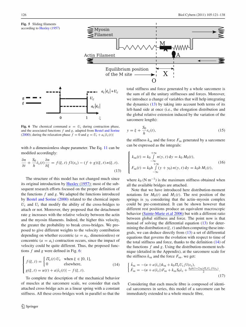
Huxley proposed that a cross-bridge between actin fil-aments and myosin heads could exist in two biochemicalstates, attached and detached, and that one myosin head couldattach to only one actin site. Considering the longitudinal dis-tance ξ between actin binding sites and myosin heads, nor-malized with respect to h which is the maximum elongationof the myosin spring (Fig. 5), we focus on the distributionn(ξ, t) of the fraction of actin–myosin pairs of length ξ whichare attached at a time t. The evolution with time of this dis-tribution can be written as:

∂n

∂t+ S0

hεc(t)

∂n

∂ξ= f (ξ, t) (1 − n(ξ, t)) − g(ξ, t) n(ξ, t),

(11)

where the functions f and g denote the rates of attachmentand detachment of the cross-bridges. With S0εc(t) the globalvelocity of the actin filaments with respect to the myosin fil-aments, the second term in the left-hand side represents theeffect of this global velocity on the distribution of attachedpairs (details in Bestel (2000)).

The maximum number of actin–myosin pairs that canbind depends on the relative length of the contractile elementand is generally known as the force–length relationship f lsince its macroscopic consequence is a variation of the max-imum force that the muscle can produce (Leeuwen 1991).This effect is generally introduced at the macroscopic levelthrough a multiplicative factor, but since we focus on physio-logical facts, we take this relationship into account directly atthe microscopic scale. Various functions can be considered toexpress this force–length relationship. In our case, we aim atusing the model close to its nominal length so that assuminga Gaussian approximation is sufficient:

f l(εc) = exp

(

−ε2c

b

)

, (12)

123

126 Biol Cybern (2011) 105:121–138

Fig. 5 Sliding filamentsaccording to Huxley (1957)

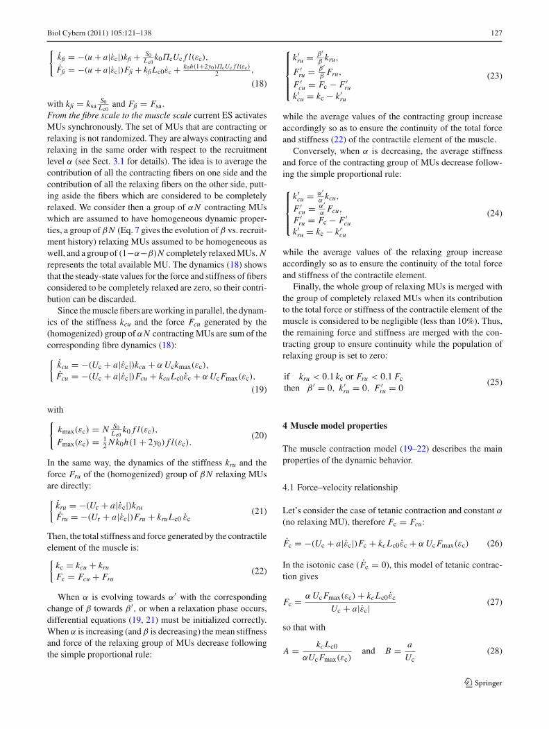
Fig. 6 The chemical command u = Uc during contraction phase,and the associated functions f and g, adapted from Bestel and Sorine(2000); during the relaxation phase f = 0 and g = Ur + ac|εc(t)|

with b a dimensionless shape parameter. The Eq. 11 can bemodified accordingly:

∂n

∂t+ S0

hεc(t)

∂n

∂ξ= f (ξ, t) f l(εc) − ( f + g)(ξ, t) n(ξ, t).

(13)

The structure of this model has not changed much sinceits original introduction by Huxley (1957): most of the sub-sequent research efforts focused on the proper definition ofthe functions f and g. We adapted the functions introducedby Bestel and Sorine (2000) related to the chemical inputsUc and Ur that modify the ability of the cross-bridges toattach or not. Moreover, they proposed that the detachmentrate g increases with the relative velocity between the actinand the myosin filaments. Indeed, the higher this velocity,the greater the probability to break cross-bridges. We pro-posed to give different weights to the velocity contributiondepending on whether eccentric (a = ae, dimensionless) orconcentric (a = ac) contraction occurs, since the impact ofvelocity could be quite different. Thus, the proposed func-tions f and g were defined in Fig. 6:⎧⎪⎨

⎪⎩

f (ξ, t) ={

Πc(t) Uc when ξ ∈ [0, 1],0 elsewhere,

g(ξ, t) = u(t) + a|εc(t)| − f (ξ, t).

(14)

To complete the description of the mechanical behaviorof muscles at the sarcomere scale, we consider that eachattached cross-bridge acts as a linear spring with a constantstiffness. All these cross-bridges work in parallel so that the

total stiffness and force generated by a whole sarcomere isthe sum of all the unitary stiffnesses and forces. Moreover,we introduce a change of variables that will help integratingthe dynamics (13) by taking into account both terms of itsleft-hand side at once (i.e., the elongation distribution andthe global relative extension induced by the variation of thesarcomere length):

y = ξ + S0

hεc(t), (15)

the stiffness ksa and the force Fsa generated by a sarcomerecan be expressed as the integrals:⎧⎪⎪⎪⎨

⎪⎪⎪⎩

ksa(t) = k0

+∞∫−∞

n(y, t) dy = k0 M0(t),

Fsa(t) = k0h+∞∫−∞

(y + y0) n(y, t) dy = k0h M1(t),(16)

where k0 (N m−1) is the maximum stiffness obtained whenall the available bridges are attached.

Note that we have introduced here distribution-momentnotations for M0(t) and M1(t). The rest position of thesprings is y0 considering that the actin–myosin complexcould be pre-constrained. It can be shown however thatdifferent rest positions produce an equivalent macroscopicbehavior (Sainte-Marie et.al 2006) but with a different ratiobetween global stiffness and force. The point now is thatinstead of solving the differential equation (13) for deter-mining the distribution n(ξ, t) and then computing these inte-grals, we can deduce directly from (13) a set of differentialequations that governs the evolution with respect to time ofthe total stiffness and force, thanks to the definition (14) ofthe functions f and g. Using the distribution-moment tech-nique (detailed in the Appendix), at the sarcomere scale forthe stiffness ksa and the force Fsa, we get:{

ksa = −(u + a|εc|)ksa + k0ΠcUc f l(εc),

Fsa = −(u + a|εc|)Fsa + ksa S0εc + k0h(1+2y0)ΠcUc f l(εc)2 .

(17)

Considering that each muscle fibre is composed of identi-cal sarcomeres in series, this model of a sarcomere can beimmediately extended to a whole muscle fibre,

123

Biol Cybern (2011) 105:121–138 127

{kfi = −(u + a|εc|)kfi + S0

Lc0k0ΠcUc f l(εc),

Ffi = −(u + a|εc|)Ffi + kfi Lc0εc + k0h(1+2y0)ΠcUc f l(εc)2 ,

(18)

with kfi = ksaS0Lc0

and Ffi = Fsa.

From the fibre scale to the muscle scale current ES activatesMUs synchronously. The set of MUs that are contracting orrelaxing is not randomized. They are always contracting andrelaxing in the same order with respect to the recruitmentlevel α (see Sect. 3.1 for details). The idea is to average thecontribution of all the contracting fibers on one side and thecontribution of all the relaxing fibers on the other side, putt-ing aside the fibers which are considered to be completelyrelaxed. We consider then a group of αN contracting MUswhich are assumed to have homogeneous dynamic proper-ties, a group of βN (Eq. 7 gives the evolution of β vs. recruit-ment history) relaxing MUs assumed to be homogeneous aswell, and a group of (1−α−β)N completely relaxed MUs. Nrepresents the total available MU. The dynamics (18) showsthat the steady-state values for the force and stiffness of fibersconsidered to be completely relaxed are zero, so their contri-bution can be discarded.

Since the muscle fibers are working in parallel, the dynam-ics of the stiffness kcu and the force Fcu generated by the(homogenized) group of αN contracting MUs are sum of thecorresponding fibre dynamics (18):{

kcu = −(Uc + a|εc|)kcu + α Uckmax(εc),

Fcu = −(Uc + a|εc|)Fcu + kcuLc0εc + α Uc Fmax(εc),

(19)

with{

kmax(εc) = N S0Lc0

k0 f l(εc),

Fmax(εc) = 12 Nk0h(1 + 2y0) f l(εc).

(20)

In the same way, the dynamics of the stiffness kru and theforce Fru of the (homogenized) group of βN relaxing MUsare directly:{

kru = −(Ur + a|εc|)kru

Fru = −(Ur + a|εc|)Fru + kruLc0 εc(21)

Then, the total stiffness and force generated by the contractileelement of the muscle is:{

kc = kcu + kru

Fc = Fcu + Fru(22)

When α is evolving towards α′ with the correspondingchange of β towards β ′, or when a relaxation phase occurs,differential equations (19, 21) must be initialized correctly.When α is increasing (and β is decreasing) the mean stiffnessand force of the relaxing group of MUs decrease followingthe simple proportional rule:

⎧⎪⎪⎪⎨

⎪⎪⎪⎩

k′ru = β ′

βkru,

F ′ru = β ′

βFru,

F ′cu = Fc − F ′

ruk′

cu = kc − k′ru

(23)

while the average values of the contracting group increaseaccordingly so as to ensure the continuity of the total forceand stiffness (22) of the contractile element of the muscle.

Conversely, when α is decreasing, the average stiffnessand force of the contracting group of MUs decrease follow-ing the simple proportional rule:

⎧⎪⎪⎨

⎪⎪⎩

k′cu = α′

αkcu,

F ′cu = α′

αFcu,

F ′ru = Fc − F ′

cuk′

ru = kc − k′cu

(24)

while the average values of the relaxing group increaseaccordingly so as to ensure the continuity of the total forceand stiffness of the contractile element.

Finally, the whole group of relaxing MUs is merged withthe group of completely relaxed MUs when its contributionto the total force or stiffness of the contractile element of themuscle is considered to be negligible (less than 10%). Thus,the remaining force and stiffness are merged with the con-tracting group to ensure continuity while the population ofrelaxing group is set to zero:

if kru < 0.1 kc or Fru < 0.1 Fc

then β ′ = 0, k′ru = 0, F ′

ru = 0(25)

4 Muscle model properties

The muscle contraction model (19–22) describes the mainproperties of the dynamic behavior.

4.1 Force–velocity relationship

Let’s consider the case of tetanic contraction and constant α

(no relaxing MU), therefore Fc = Fcu:

Fc = −(Uc + a|εc|)Fc + kc Lc0εc + α Uc Fmax(εc) (26)

In the isotonic case (Fc = 0), this model of tetanic contrac-tion gives

Fc = α Uc Fmax(εc) + kc Lc0εc

Uc + a|εc| (27)

so that with

A = kc Lc0

αUc Fmax(εc)and B = a

Uc(28)

123

128 Biol Cybern (2011) 105:121–138

we obtain a Hill type force–velocity relationship in the con-centric case (εc < 0|εc| = −εc),

Fc = 1 + A εc

1 − B εcα Fmax(εc) (29)

and a relationship compatible with the one described inLeeuwen (1991) in the eccentric case (εc > 0|εc| = εc),

Fc = 1 + A εc

1 + B εcα Fmax(εc) (30)

In the concentric case, before the isotonic contraction canoccur, the muscle contracts in an isometric condition untilthe force generated by the muscle equilibrates the imposedone. Then, isotonic contraction becomes possible. The dif-ferential equations (19) show that kfi increases up to thesteady state value αkmax(εc) (Bestel 2000). The Eq. 29 can berewriten as follows:

εc = Fc − αFmax(εc)

B Fc + AαFmax(εc)(31)

Then, A is increasing and the shortening speed (31) isdecreasing so that the maximum speed is obtained at thebeginning of the isotonic contraction, as reported by Hill(1938).

The second equation, in the eccentric case, may need tobe reshaped to fit experimental data. We can achieve this bychoosing a different constant a for concentric (ac) and eccen-tric (ae) contractions inducing a different value for the Bparameter. It accounts for an asymmetric effect of the short-ening (lengthening) speed to facilitate the breaking of thecross bridge. The A parameter is also different because thebeginning isometric contraction phase is different in bothcases due to a different initial value of kfi(0). In any case, themodel remains consistent with experimental data collectedin the literature.

4.2 Force–length relationship

At steady state, and in isometric conditions (Fc = 0 andεc = 0), we have:

Fc = α Fmax(εc) (32)

Following the definition (20) of Fmax, we can observe thatthe contraction force generated by the contractile elementimmediately reflects the force–length relationship (12) intro-duced in (13) at the sarcomere scale. It reflects also directlythe recruitment modulation. Taking into account the force–length relationship at the macroscopic scale with regards tothe total length of the muscle (including the serial element),does change only the scale of the twitch response withoutany effect on the dynamics. On the contrary, introducing theforce–length relationship at the microscopic scale related tothe length of the contractile element alone may change thedynamicsa littleas reported inRackandWestbury(1969)with

Fig. 7 For computing the whole mechanical model in the case of noembedded masses, we need to intersect a line with two half-lines

an increase of the time needed to reach the maximum forcewhen the force–length relationship becomes close to 100%.

4.3 Mirsky–Parmley property

In the case of concentric contraction (εc < 0), the tetaniccontraction model (26) can also be written as:

dFc = (kcLc0 + ac Fc)dεc + Uc(α Fmax(εc) − Fc)dt (33)

from what we can directly deduce the corresponding instan-taneous stiffness:

kinst = ∂ Fc

∂εc= kcLc0 + ac Fc (34)

agreeing with the Mirsky–Parmley model described for thestriated cardiac muscle (Mirsky and Parmley 1973). Classi-cal Hill model approaches can not comply with this propertybecause no active stiffness is modeled contrary to ours.

5 Computation of the whole mechanical model

When considering the whole muscle model of Fig. 4 withembedded masses, what we need to do first is to computethe dynamics of these masses subject to the forces gener-ated by the contractile element and by the linear springs anddampers:

m x1 = Fc − ks1(Ls1 − Ls10) − λs1 Ls1, (35)

m x2 = −Fc + ks1(Ls1 − Ls10) + λs1 Ls1. (36)

subtracting these two dynamics leads to:

m Lc0 εc = −2Fc + ks1(L0 εp − Lc0 εc)

+λs1(L0 εp − Lc0 εc), (37)

where we can observe that the dynamics εc of the contrac-tile element is coupled only with the full length L0 εp of

123

Biol Cybern (2011) 105:121–138 129

the muscle, and totally decoupled with the movement of theembedded masses within the muscle.

The total force that it generates on the articulations willdepend on the movement of these embedded masses, whichdepends itself on the global movement of the muscles in theenvironment: one needs to know everything about the move-ments of the whole body in its environment before beingable to compute the forces generated by the muscles. For thisreason, this model with embedded masses might be tractableonly in static or quasi-static experiments such as isometriccontractions. Moreover, as the model is quite accurate, theinput must be well defined so that this model may be usedwith ES induced contractions but not with voluntary ones. Inall other cases, a model without embedded masses might bepreferred.

Without mass, it has been proposed in Sect. 3.2.1 to con-sider only the contractile element and one serial elementwithout any damper. Without any mass between these twoelements, we have no immediate indication on the variationεc of the length of the contractile element, which is necessaryfor computing the contraction model (19–22). The solutionlies in the fact that the force Fc generated by the contractileelement must equilibrate with the force Fs generated by thespring in series, Fc = Fs, what gives us a hint about thevariation of their respective lengths. Considering the time-derivative of the model of this linear spring, we obtain

Fs = ksL0 εp = ksL0 ε − ksLc0 εc. (38)

After some straightforward rewriting, the model (19–22)gives us a second relationship between Fc and εc,

Fc = (ΠcUcαFmax(εc) − uFc) − ac Fc|εc| + kcLc0 εc. (39)

Finally, when an isolated muscle is considered, the con-tribution of the parallel element could be added:

Fp = ke

kp

(ekpεp − 1

). (40)

What we need to do then is equate those two relationships,for example, plot them on Fig. 7 and find the intersection.This intersection gives us the variation εc of the length of thecontractile element, that we can use then to compute the restof the model (19–22). The first relationship gives a simpleline, with a negative slope −ksLc0. Because of the absolutevalue function | · |, the second relationship gives two half-lines, the first one for negative values of εc, with a positiveslope kcLc0+ac Fc, and the second one for negative values ofεc, with a slope kcLc0 − ae Fc, the sign of which is not clear.If the slope of this second half-line happens to be lower thanthe slope of the full line, it can be seen on Fig. 7 that this linewould either intersect both half-lines or none of them. Bothcases would mean anyway that our model without embeddedmasses is not well posed.

To verify that the solution exists and is unique, a conditionon these slopes, that appears to be a simple condition on theforces and stiffnesses needs to be continuously satisfied:

Fc <ks + kc

aeLc0. (41)

This condition concerns only eccentric contractions; we haveobserved throughout all our numerical experiments so far thatthis is always the case.

6 Preliminary model validation in isometric conditions

The main objective of this study was to develop a musclemodel that describes the major features of a muscle thatcan be experimentally identified on a specific subject. Inthis context, we developed meaningful modeling based onparameters related to physiological processes through vari-ables that can be extracted from literature, directly measuredor observed. Physiological parameters identification couldthen also be helpful for the clinical diagnosis because theirvalue could be related to some clinical indicators such asmuscle masses, muscle maximum forces, time response, etc.The differential equations 19, 21 are highly non linear due toabsolute values and the εc, εc variable coupling with dynam-ics of muscle contraction. The classical linear methods wetested, including EKF, failed to robustly estimate parametervalues because of their poor quality of their approximation,proximity to the non linearities and to their high sensitivity toinitial values. Moreover, measurements are subject to noiseand inaccuracy, especially for non invasive human proce-dures, so that algorithms must be as insensitive as possibleto uncertainty of measures.

Consequently, we develop methodologies specificallyadapted to the identification of our skeletal muscle modelfrom in-vivo measurements and Sigma Point Kalman Fil-tering (SPKF, see annex for details). A Kalman filter is atechnique for determining optimal estimates of the valuesof state variables (such as the active stiffness of the mus-cle), including unmeasured or infrequently measured statevariables (length variation and acceleration of tendon) andmodel parameters. In both cases, the estimation algorithmis based on a limited set of noisy measurements. Variationsof muscle’s properties due to fatigue, for instance, are notmodeled so that the identification remains valid for a specificstate of the muscle. We manage the experimental protocolsto avoid as much as possible fatigue effect using short pulsetrains.

6.1 Recruitment model validation

The recruitment model (3) that we propose is able to takeinto account the difference between the recruitment due to

123

130 Biol Cybern (2011) 105:121–138

00.2

0.40.6

0.81

0

0.2

0.4

0.6

0.8

10

0.2

0.4

0.6

0.8

1

Normalized Pulse Width

Crago et al. data

Normalized Intensity

Nor

mal

ized

Rec

ruitm

ent

00.2

0.40.6

0.81

0

0.2

0.4

0.6

0.8

10

0.2

0.4

0.6

0.8

1

Model

0

1

Fig. 8 Measured and modeled data from Crago et al. (1980)

the variation of the pulse width pw, and the intensity i thata classical model involving q = pw · i is not able to accountfor. We illustrate this feature through the estimation of theparameters of the model using published data from Cragoet al. (1980). We use least mean square minimization algo-rithm to perform the parameter estimation.

The RMS error between both curves (Fig. 8) is about 4.4%and the absolute error less than 8% for all the points exceptfor 4 isolated points among 270. Figure 8 shows the resultswith the estimated parameter values reported in Table 1: notethat they satisfy the conditions (5) that ensure a monotoni-cally increasing function R. The modeling is good enough forour purpose and is able to account for the difference betweeni and pw recruitment processes through the parameters ai

and apw. The sensibility is greater using the i parameter sothat in this case, the force modulation should be performedthrough pw modulation.

6.2 Identification with full model in the animal

Animal experiments were performed to evaluate the com-plete model with masses, validate the computational method,and assess the accuracy of the parameter estimation. Priormodels were not evaluated together with animal experiments,and the technique needed validation—including the determi-nation of the minimal set of experiments to carry out—beforeits use in human experiments.

Table 1 Estimated parameters from Eq. 3

apw ai b c d

−0.428 1.56 2.74 0.661 0.634

6.2.1 Experimental setup

Experimental data were obtained from in-situ MedialGastrocnemius (MG) muscle in the rabbit under isometricconditions. The work was performed on two New-Zealandwhite rabbits at Aarhus University Hospital in Aalborg, Den-mark. Anesthesia was induced and maintained with periodicintramuscular doses of a cocktail of 0.15 mg/kg Midazo-lam (Dormicum, Alpharma A/S), 0.03 mg/kg Fetanyl, and1 mg/kg Fluranison (combined in Hypnorm, Janssen Phar-maceutica). The left leg of the rabbit was anchored at kneeand ankle joints to a fixed mechanical frame using bone pinsplaced through the distal epiphyses of the femur and tibia.Tendon of MG muscle was attached to the arm of a motor-ized lever system (Dual-mode system 310B Aurora Scien-tific Inc.) (Fig. 9) using a yarn of polyaramid fibers (Kevlar49, Goodfellow Cambridge Ltd). The position of the leverarm was controlled and both force and relative position wererecorded. The Aurora system was accurately calibrated sothat the raw data without any post processing were used.An initial muscle-tendon length was established by placingthe ankle at 90◦. A bipolar cuff electrode 3-mm diameter,6 mm between contact centers (MXM manufacturing, Val-lauris, France) was implanted around the sciatic nerve, andallowed us to stimulate the MG muscle through its motornerve (Fig. 9). The EMG signal of the MG muscle wasrecorded using an intramuscular EMG bipolar electrode. Acomputer controlled stimulator (co-developed by DEMARteam and MXM company, Vallauris France) based on a pre-vious developed technology for human neural stimulation(Guiraud et al. 2006a,b) was used and modified to obtain abetter current accuracy down to 12.5 µA (full range 787.5µA), a frequency up to 31.25 Hz, pulse width up to 1 ms

123

Biol Cybern (2011) 105:121–138 131

Fig. 9 Setup of rabbit experiment

with a 1 µs step. Data acquisition (muscle force, length, andEMG) was performed using an 8-channel tape recorder with48 kHz sampling rate (ADAT-XT, Alesis).

The delay between ES pulse and muscle force depends onthe activation dynamics (AP propagation, [Ca2+] dynamics,etc) and is discarded from the data because we do not studythis part. However, in our simplified model of the activationdynamics, it represented the time delay τd, estimated hereat 5 ms, between the ES stimulus and the generation of thechemical control (Fig. 2).

6.2.2 Identification results

In this study, we identify only the parameters in the mechan-ical part of skeletal muscle model. The input controls of themodel are the constant static recruitment rate α and the chem-ical control input u from the activation model. These twocontrols are computed from ES input signal. It should bementioned that the experiment was performed with constantES parameters for pulse width and intensity of ES so that therecruitment rate is constant. The trigger of u signal can becalculated by the timing of ES.

When we measured the tension of the skeletal muscle dur-ing in-vivo condition, the experimental force correspondedto Fe which is the sum of the spring force Fs and the damp-ing force Fd as in (42). In case of isometric contraction, therewas the relationship of (43). Then, (37) can be rewritten as in(44). When we take the ratio of Fc and Fe in Laplace trans-form, it can be written as (45). From the relationship, thedifferential equation (46) can be obtained.

Fe = Fs + Fd = ks1Ls10εs1 + λLs10εs1 (42)

2Ls10εs1 + Lc0εc = L0εp = 0 (43)

Fc = mLs10εs1 + ks1Ls10εs1 + λLs10εs1 (44)

L[Fc]L[Fe] = ms2 + λs + ks1

λs + ks1(45)

m Fe + λFe + ks1 Fe = λFc + ks1 Fc (46)

Finally, differential equations can be described as follows:

kc = −(u + a|εc|)kc + αkmaxΠcUc (47)

Fc = −(u + a|εc|)Fc + αFmaxΠcUc + kcLc0εc (48)

Fe = − λ

mFe − ks1

mFe + λ

mFc + ks1

mFc (49)

εc = − 2Fc

mLc0− ks1

mεc − λ

mεc (50)

In this case, kc Fc Feεc are unknown time-varying statesand mλLc0 are unknown static parameters to be estimated.The high non linearity of the state-space model, the impos-sibility to directly measure some state-variables and noisyin-vivo experimental data need for an efficient recursive filterthat estimates the state of a dynamic system. In skeletal mus-cle dynamics, its state-space is dramatically changed betweencontraction and relaxation phase. At this time, partial deriva-tives of states will be incorrect due to the discontinuity. There-fore, we introduced Sigma-Point Kalman Filter (SPKF). Theinitial idea was proposed by Julier and Uhlmann (2004), andwell described by Merwe and Wan (2003). SPKF uses adeterministic sampling technique known as the unscentedtransform to pick a minimal set of sample points (calledsigma points) around the mean. These sigma points are prop-agated through the true nonlinearity. This approach results inapproximations that are accurate to at least the second orderin Taylor series expansion. In contrast, EKF results only infirst-order accuracy.

The stimulation signal input used for the estimation wascomposed of two successive pulses at 20 Hz which ampli-tude is 105 µA and pulse width was 300 µs. The stimula-tion signal input was used to prepare the two control inputs(α, u) of the mechanical model. The current amplitude andpulse width were selected to recruit the maximum of mus-cular fibers, then α was approximated to 90% for the fiberrecruitment. The stiffness ks has been estimated separatelyfrom the experiments achieved on the isolated muscle afterthe force acquisition. The stiffness was taken as equal to theslope of linear line of the passive length-force relationship.ks was 4500 N/m. Fm and km can be obtained knowing theforce response of muscle to a stimulation pattern with max-imum value of signal parameters (in frequency, amplitude,and pulse width). In this case, km = 1000 N/m and Fm = 15N were used. a = 1 was assumed as in Bestel and Sorine(2000).

The experimental muscle force against a doublet stimula-tion is plotted in Fig. 10 with red line. It was used for param-eter estimation as measurement updates for Fe in SPKF. The

123

132 Biol Cybern (2011) 105:121–138

Fig. 10 Measured andestimated forces of Fe.

0 0.05 0.1 0.15 0.2 0.25 0.3 0.35 0.4 0.45 0.50

0.5

1

1.5

2

2.5

3

3.5

4

4.5

Time [s]

Exp

erim

enta

l for

ce F

e [N

]

Magnification

measured

estimated

blue curve is the estimated muscle force of Fe. The part sur-rounded by the rectangle was magnified at the upper rightside to indicate that the resultant estimated Fe was wellfiltered against the noisy experimental data. Figure 11 is theerror covariance for Fe. Figures 12 and 13 show the esti-mated parameter Lc0 and the error covariance. Both figuresshow the convergence of the estimation. The evolutions ofinternal state values for εc and Fc are obtained as in Figs. 14and 15. From these behaviors, we can confirm that the con-tractile element of the model was successfully activated andcontracted following the dynamics of differential equationsunder the estimation process.

After the complete estimation process for geometric anddynamic parameters, the estimated values were obtainedas shown in Table 2. As seen from resulted computationalbehavior in graphs (Fig. 11), the internal state vectors of skel-etal model converged well to stationary values. We tested theestimation from few slightly different values for initial states,same results could be obtained in stable conditions. The esti-mated length of contractile element showed close value toits measured length which was approximately 7 cm in theisolated muscle as in Fig. 16. Similar results were obtainedin two individual rabbit experiments.

A cross-validation of the identified model was carried outto confirm the validity of this method on data that have notbeen used for the estimation. The activation level (both inten-sity and pulsewidth) were the same as the ones used forthe identification. Frequency has been changed from 20 to31.25Hz, and the number of pulses from 2 to 3. The resul-tant muscle force was simulated using the identified valuesand the information of stimulation, i.e., electrical intensity,pulse width, and frequency. Figure 17 shows the measuredforce response of the MG muscle of the rabbit and the

0 0.05 0.1 0.15 0.2 0.25 0.3 0.35 0.4 0.45 0.50

0.001

0.002

0.003

0.004

0.005

0.006

0.007

0.008

0.009

0.01

Time [s]

Err

or c

ovar

ianc

e

Fig. 11 Error covariance of Fe.

0 0.05 0.1 0.15 0.2 0.25 0.3 0.35 0.4 0.45 0.50

0.01

0.02

0.03

0.04

0.05

0.06

0.07

0.08

0.09

Time [s]

Lc0

[m]

0.1

Fig. 12 Estimated parameter of Lc0

123

Biol Cybern (2011) 105:121–138 133

0 0.05 0.1 0.15 0.2 0.25 0.3 0.35 0.4 0.45 0.50

0.002

0.004

0.006

0.008

0.01

0.012

Time [s]

Err

or c

ovar

ianc

e of

Lc0

Fig. 13 Error covariance of Lc0

0 0.05 0.1 0.15 0.2 0.25 0.3 0.35 0.4 0.45 0.5-0.12

-0.1

-0.08

-0.06

-0.04

-0.02

0

0.02

0.04

0.06

Time [s]

Inte

rnal

sta

te

cε

Fig. 14 Estimated state of εc

0 0.05 0.1 0.15 0.2 0.25 0.3 0.35 0.4 0.45 0.50

0.5

1

1.5

2

2.5

3

3.5

4

4.5

Time [s]

Inte

rnal

sta

te F

c [N

]

Fig. 15 Estimated state of Fc

Table 2 Estimated parameters

Rabbit Estimated Measured

Lc0(cm) m(g) λ(Ns/m) Lc0(cm)

1 6.86 19.2 19.4 7.02 6.63 40.3 18.8 7.0

simulated force with the identified model. The model couldpredict the nonlinear force properties of stimulated musclequite well. There was good agreement between the measuredand the predicted force, the normalized root mean squared(NRMS) deviation showed 5.5%. When the muscle fatigued,the experimental force was lower than the simulated force.The small difference at the third wave may be considered asthe error coming from modeling without fatigue factor. How-ever, we confirmed the effectiveness of the identification aswell as the feasibility of our skeletal muscle model under ESuse.

7 Discussion

The objective of this study was to develop a model of thestriated skeletal muscle mechanics based on Huxley’s the-ory as very few macroscopic researches can be reported.In particular, it can be used favorably in experiments withES to simulate, synthesize, and control movements underES-based rehabilitation protocols. Moreover, the parametersin our model are linked to physiological or biomechanicalbehaviors of the muscle providing quantitative and mean-ingful estimated values related to the state of the muscle. Inthe future, many of these parameters may be used for quanti-tative clinical assessment to provide quantitative feedback totrack the efficacy of a treatment. Compared to the literature,we introduced:

– 2D recruitment curve model that allows to take intoaccount, separately, the relationship between the forceoutput and the 2 ES (i and pw) controlled inputs. It allowsthe selection of the more sensitive parameter and enablesa more accurate control of the force output. The modelconformed to experimental data reported in literature.

– An original set of definitions of the f and g rate functionsin Huxley equations that allows:

– To explicitly introduce the command inputs comingfrom the chemical dynamics and the recruitment func-tion.

– To compute the macroscopic behavior without Zaha-lak’s assumption of a Gaussian distribution to create amechanical model linked to the microscopic behavior.

123

134 Biol Cybern (2011) 105:121–138

Fig. 16 Extracted muscle usedin the rabbit experiment

– To compute the dynamics of the macroscopic forcewithout the need of computing the distribution of theformed crossbridges. It induces efficient and accu-rate numerical computation. This was one of the maindrawbacks of Huxley-type models. Realtime compu-tation is now possible on a single joint simulation withtwo antagonist muscles.

– To get not only the force output but also the activestiffness of the contractile element.

– To introduce at the microscopic scale the influence ofsarcomere length and shortening/lengthening speedwith a plausible biomechanical interpretation.

– These new definitions allow for the intrinsic accountingof the force–length relationship that exhibits also an influ-ence on the dynamics contrary to classic scale factor func-tion.

– They also allow accounting of the force–velocity rela-tionship as Hill stated in both contraction schemes, i.e.,eccentric and concentric without explicitly defining thisrelationship.

– Mirsky–Parmley property is checked and as far as weknow, no other striated muscle model accounts for this.

The mathematical developments and numerical simu-lations show, for all these features, conformity to exist-ing literature with even extended abilities—described above(Sect. 4)—compared to classical models.

The other main set of contributions is related to the abil-ity to estimate parameters of the model and then to test itagainst acquired data. There is little or no other work thatdeals with estimation of parameters of Huxley-based mod-els. None use such identified models to perform movementsynthesis or even subject specific simulations. We show thatan advanced non linear algorithm such as SPKF succeeded inthe estimation of a subset of model parameters that are sub-ject specific, SPKF could further provide insight in the statevariables that are not measurable. The algorithm shows goodaccuracy and robustness performances. We show that even acomplex model with masses and dampers can be identifiedin isometric conditions, and give some parameters close tothe actual measured values.

0 0.05 0.1 0.15 0.2 0.25 0.3 0.35 0.4 0.450

1

2

3

4

5

6

7

8

Time [s]

For

ce [N

] measured

simulated

Fig. 17 Measured and simulated isometric muscle force with threesuccessive pulses (I = 105 µA, pw = 300 µs, Freq = 31.25 Hz)

Extended work has been carried out by our team onhumans using the same model but without masses becausewe studied the knee joint instead of isolated muscle. Theseresults show that the model can be fully identified and usedin non isometric conditions and variable recruitment rates.Moreover, the parameters estimation and thus the simulationswere performed on three paraplegic—ASIA A—patientswith external ES and one patient with implanted ES (seeBenoussaad et al. 2009a,b for details). As far as we knowthe second article is a unique case, and in both articles themodel show good performance as regard accuracy: less than8% RMS error between measured knee joint angle and sim-ulated one in dynamic conditions even on data not used tofit the model. We also demonstrated that the model is ableto account for voluntary contraction using EMG as input,with a better range of function than with classical Hill modelapproaches (Hayashibe et.al 2009). Even if these results arelimited to the isometric contraction, they show that the intrin-sic non linearities of the temporal summation can be betteraccounted with our model.

Finally, we performed isometric tests in conditions closeto the ones used in this article but with the simplified modeldefined in Sect. 5. Stimulation was provided by Prostim

123

Biol Cybern (2011) 105:121–138 135

Fig. 18 Model behavior versusmeasured data while continuousstimulation is performed on twopatients with spinal cord injury.Stimulation is provided on thequadriceps at 300 µs,frequencies are 15 and 20 Hz,respectively. Model couldfollow accurately the dynamicsof stimulated muscle. In the lastrelaxation phase, since thetension of the strap in the chairis not strictly maintained, thetorque measurement can bemuch less than the reality

0 0.2 0.4 0.6 0.8 1 1.2 1.40

50

100

150

200

250

Forc

e [N

]

MeasuredEstimated

0

50

100

150

Forc

e [N

]

0.60 0.2 0.4 0.8 1 1.2

Time [s]

15Hz

20Hz

15Hz

20Hz

sub1

sub2

(Hardtech, Montpellier, France) surface stimulator, with sur-face electrodes above the quadriceps. Torque was measuredwith a dynamometric chair (Biodex 3, Shirley Corporation,NY, USA). Two patients with spinal cord injury (ASIAA) were tested under ethical committee approval (Nîmes,France, 2008–2010) at Propara clinical center (Montpellier,France) with their individual consent. For the sake of consis-tency, we convert the measured torque into force using themoment arm which was obtained from the Hawkins equa-tion of muscle length at different knee joint angles combinedwith the anthropometrical of the limbs length for each sub-ject (Hayashibe et al. 2010). In addition to animal experi-ment, we wanted to investigate longer stimulation train atdifferent frequencies with constant current and pulse widthto assess frequency influence on both the recruitment andthe dynamics without introducing explicit frequency depen-dency. Details on how parameters are found are described inHayashibe et al. (2010). We show that the identified modelis able to accurately follow the dynamics of contraction intwo different frequency setup (15 and 20Hz) as shown onFig. 18. All the parameters for each patient with the twofrequencies remained the same except the maximum forceFm that have to be readjusted. These demonstrate that ourmodel is able to account for the dynamics in different stimu-lation frequency range—below tetanus—but with a modifiedactivation level. Indeed, modifying Fm is equivalent to mod-ulate the recruitment rate α. This is consistent with knownresults in literature and a simple activation—frequency rela-tionship as proposed in Riener (1999) could be added tothe activation box. We decided to avoid close fitting of the

relaxation phase because the data were not as reliable as onthe rabbit experiments when the muscle stops contractingsuddenly: The mechanical link between the dynamometerand the limb is not so strictly maintained and so a rapiddecrease of the force induces a temporary loss of a rigidlink.

Fatigue remains perhaps the most problematic phe-nomenon since the corresponding physiological mecha-nisms are still not clear. However, if fatigue modifies thedynamics or the maximum available force, the structureof our model allows accounting for effectively. Models ofthe fatigue phenomenon (Riener 1999; Riener et.al 1996;Rabischong and Guiraud 1993) can be introduced how-ever easily through additional coefficients introduced in thedynamics (13) of the contraction at the sarcomere scale.However, these approaches remain blackboxes. Accordingly,we have started to investigate how fatigue modifies modelparameters. Hayashibe et al. (2010) showed that mainly Fm

is altered. The fatigue process under ES was further inves-tigated (Papaiordanidou et al. 2010a,b) to enable building ameaningful model of peripheral fatigue and further refine ourmodel.

8 Conclusion

We proposed a model based on Huxley’s theory that weintegrated to obtain a macroscopic behavior. This behaviorfulfills all well-known muscle properties among which force–length, force–velocity, and Mirsky–Parmley. In addition, we

123

136 Biol Cybern (2011) 105:121–138

proposed an efficient algorithm (SPKF) that allows the esti-mation of the parameters of the model for individual subjects.These parameters are related to physiology or biomechanicsso that their values can be meaningfully interpreted. Finally,the model can be used as a controlled actuator under ES tohelp development of complex control strategies to be used inmovement rehabilitation.

Perreault et al. (2003) discussed Hill models and theyshowed limitations when the full range of movements wereperformed. They proposed that Huxley-based model shouldbe a solution in particular if they consider the muscle prop-erties at the microscopic level. They mention that veryfew works were carried out on the macroscopic behav-ior of human muscles using Huxley theory. They finallynoted very few experimental validations on humans. Wepropose a new way, linked to physiological reality, to man-age this complex model to consider again these power-ful and meaningful class of models. We thus propose alsoeffective parameters estimation accurately validated on ani-mals but suited for humans to go forward subject specificsimulations.

However, in its present form, this model is not able toreproduce phenomena such as dependence of the activationto the stimulation frequency, facilitation/potentiation phe-nomenon, and other nonlinear effects related to the [Ca2+]dynamics. It also does not account for fatigue and the spe-cific behavior of muscles presenting a mix of slow and fastfibers. Nevertheless, the structure of this model allows theintroduction of such phenomena at various levels: the sepa-rate contribution of slow and fast fibers can be modeled bytwo parallel contractile elements with different parametersand different recruitment curves, [Ca2+] dynamics can bemodeled more accurately within the activation block and fre-quency influence can directly modulate the recruitment rate.However, when considering the restoration of movementsthrough ES, these phenomenon are avoided or at least limited:frequency is usually fixed and potentiation avoided, fatigueis monitored and compel to stop session if it reaches toohigh level.

Such an accurate modeling requires extensive experi-mental validations: this is our on going work on humansubjects. Considering our present research efforts on move-ment restoration using ES, we show that this model issufficient for performing realistic simulations, for syn-thesizing stimulation patterns for open loop movementsgenerated by ES, and for developing complex control strate-gies such as achieving active balance for quiet and effortlessstanding.

Acknowledgment This study was supported by a national Frenchgrant RNTS MIMES.

Appendixes

Huxley equation’s integration

Beginning with the computation of the time-derivative of thetwo distribution-moments:

M0(t) =+∞∫

−∞

(∂n

∂t+ S0

hεc(t)

∂n

∂y

)

dy,

M1(t) =+∞∫

−∞

S0

hεc(t) n(y, t) dy

++∞∫

−∞(y + y0)

(∂n

∂t+ S0

hεc(t)

∂n

∂y

)

dy.

The left-hand side of the differential equation (13) can bereplaced, and we obtain with a rewriting of the first term ofM1(t):

M0(t) =+∞∫

−∞f (y, t)fl(εc) dy −

+∞∫

−∞( f + g)(y, t) n(y, t) dy,

M1(t) = S0

hεc(t)M0(t) +

+∞∫

−∞(y + y0) f (y, t)fl(εc) dy

−+∞∫

−∞(y + y0) ( f + g)(y, t) n(y, t) dy.

The integral terms here are now trivial to compute becauseof the definition (14), the function f is zero outside of theinterval [0, 1] and independant from the variable y on thisinterval, while the sum f + g is independant from the vari-able y,

( f + g)(y, t) = u(t) + a|εc(t)|.Not precising anymore the time variable, we readily obtainthen the following differential equations for the moments M0

and M1:

M0 = ΠcUcfl(εc) − (u + a|εc|)M0,

M1 = S0

hεc M0 + (1 + 2y0)ΠcUcfl(εc)

2− (u + a|εc|)M1.

SPKF algorithm

An outline of the SPKF algorithm is described. For moredetails, refer to Merwe and Wan (2003) and Julier andUhlmann (2004). The general Kalman framework involves

123

Biol Cybern (2011) 105:121–138 137

estimation of the state of a discrete-time nonlinear dynamicsystem,

xk+1 = f(xk, vk), yk = h(xk, nk) (51)

where xk represents the internal state of the system to beestimated and yk is the only observed signal. The processnoise vk drives the dynamic system, and the observation noiseis given by nk . The filter starts by augmenting the state vec-tor to L dimensions, where L is the sum of dimensions inthe original state, model noise, and measurement noise. Thecorresponding covariance matrix is similarly augmented to aLxL matrix. In this form, the augmented state vector xa

k andcovariance matrix Pa

k can be defined as in (52)(53).

xak = E[xa

k ] = [xT

k vTk nT

k

]T(52)

Pak = E[(xa

k − xak )(xa

k − xak )T]

=⎡

⎣Pxk 0 00 Rvk 00 0 Rnk

⎤

⎦ (53)

where Px is the state covariance, Rv is the process noisecovariance, and Rn is the observation noise covariance.

In the process update, the 2L+1 sigma points are computedbased on a square root decomposition of the prior covarianceas in (54), where γ is a scaling parameter that determinesthe spread of the sigma-points around prior mean. The aug-mented sigma point matrix is formed by the concatenation ofthe state sigma point matrix, the process noise sigma pointmatrix, and the measurement noise sigma point matrix, such

that X a = [(X x )T (X v)T (X n)T

]T. Let’s ωc

i and ωmi be

the sigma point weights.

X ak−1 =

[xa

k−1 xak−1+ γ

√Pa

k−1 xak−1− γ

√Pa

k−1

](54)

Predicted mean and covariance are computed as in (56)(57)and predicted observation is calculated like (59).

X xk|k−1 = f(X x

k−1,X vk−1) (55)

x−k =

2L∑

i=0

ωmi X x

i,k|k−1 (56)

P−xk

=2L∑

i=0

ωci (X x

i,k|k−1 − x−k )(X x

i,k|k−1 − x−k )T (57)

Yk|k−1 = h(X xk|k−1,X n

k−1) (58)

y−k =

2L∑

i=0

ωmi Yi,k|k−1 (59)

The predictions are then updated with new measurements byfirst calculating the measurement covariance and state-mea-surement cross correlation matrices, which are then used todetermine the Kalman gain. Finally, updated estimate and

covariance could be computed through this kalman gain asbelow.

Pyk =2L∑

i=0

ωci (Yi,k|k−1 − y−

k )(Yi,k|k−1 − y−k )T (60)

Pxk yk =2L∑

i=0

ωci (X x

i,k|k−1 − x−k )(Yi,k|k−1 − y−

k )T (61)

xk = x−k + Kk(yk − y−

k ), Kk = Pxk yk P−1yk

(62)

Pxk = P−xk

− KkPyk KTk (63)

These process and measurement updates should be recur-sively calculated for k = 1, . . . until the last measurementdatum. For the implementation, we used efficient square-rootforms which propagate the square-root of the state covariancedirectly in Cholesky factored form.

References

Benoussaad M, Hayashibe M, Fattal C, Poignet P, Guiraud D (2009)Identification and validation of FES physiological musculoskele-tal model in paraplegic subjects. EMBC: Engineering in Medicineand Biology Society, Minneapolis, MN, USA

Benoussaad M, Guiraud D, Poignet P (2009) Physiological musculo-skeletal model identification for the lower limbs control of para-plegic under implanted FES. IROS: The IEEE/RSJ internationalconference on intelligent robots and systems. St. Louis, MO, USA

Bestel J (2000) Modèle différentiel de la contraction musculaire con-trolée. Application au système cardio-vasculaire. PhD Thesis, Uni-versity Paris IX Dauphine

Bestel J, Sorine M (2000) A differential model of muscle contractionand applications. In: schloessmann Seminar on mathematical mod-els in biology, chemistry and physics. Max Plank Society, BadLausick, Germany, pp 19–23

Crago PE, Peckham PH, Thrope GB (1980) Modulation of muscle forceby recruitment during intramuscular stimulation. IEEE Trans Bio-med Eng 27(12):679–684

Davis R, Houdayer T, Andrews B, Emmons S, Patrick J (1997) Para-plegia: prolonged closed-loop standing with implanted nucleusFES-22 stimulator and Andrews’s foot-ankle orthosis”. Proc XIIthWorld Soc Stereotact Funct Neurosurg 69:281–287

Ding J, Chou LW, Kesar TM, Lee SCK, Johnston TE, Wexler AS,Macleod SA (2007) Mathematical model that predicts the force-intensity and force-frequency relationships after spinal cord injury.Muscle Nerve 36:214–222

Donaldson NN, Perkins TA, Worley ACM (1997) Lumbar root stimu-lation for restoring leg function: stimulator and measurement ofmuscle actions. Artif Organs 21:247–249

Durfee KW (1993) Control of standing and gait using electrical stimu-lation: influence of muscle model complexity on control strategy.Prog Brain Res 97:369–381

Durfee KW, MacLean KE (1989) Methods for estimating isometricrecruitment curves of electrically stimulated muscle. IEEE TransBiomed Eng 36:654–667

El Makssoud H (2005) Modélisation et Identification des Muscles Squ-elettiques sous Stimulation Electrique Fonctionnelle. PhD Thesis,University of Montpellier II

El Makssoud H, Poignet P, Guiraud D (2003) Modeling of the skele-tal muscle under functional electrical stimulations. InternationalFunctional Electrical Stimulation Society, Australia, pp 206–209

123

138 Biol Cybern (2011) 105:121–138

El Makssoud H, Guiraud D, Poignet P (2004) Mathematical musclemodel for functional electrical stimulation control strategies, IEEEICRA. New Orleans, LA, USA, pp 1282–1287

Furman S, Schwedel JB (1959) An intracardiac pacemaker for Stokes-Adams seizures. N Engl J Med 261:943–948

Guiraud D, Poignet P, Wieber PB, El Makssoud H, Pierrot F, Brogl-iato B, Fraisse P, Dombre E, Divoux JL, Rabischong P (2003)Modeling of the human paralysed lower limb under FES. IEEEinternational conference on robotics and automation Taipei, Tai-wan, pp 2218–2223

Guiraud D, Stieglitz T, Koch KP, Divoux JL, Rabischong P (2006) Animplantable neuroprosthesis for standing and walking in paraple-gia: 5-year patient follow-up. J Neural Eng 3:268–275

Guiraud D, Stieglitz T, Taroni G, Divoux JL (2006) Original electronicdesign to perform epimysial and neural stimulation in paraplegia.J Neural Eng 3:276–286

Hatze H (1978) A general myocybernetic control model of skeletalmuscle. Biol Cybern 28:143–157

Hayashibe M, Guiraud D, Poignet P (2009) EMG-to-force estimationwith full-scale physiology based muscle model. IROS 2009: The2009 IEEE/RSJ international conference on intelligent robots andsystems, Saint Louis, USA, pp 1621–1626

Hayashibe M, Benoussaad M, Guiraud D, Poignet P, Fattal C (2010)Nonlinear identification method corresponding to muscle prop-erty variation in FES—experiments in Paraplegic Patients. IEEERAS/EMBS international conference on biomedical robotics andbiomechatronics, pp 401–406

Hill AV (1938) The heat of shortening and the dynamic constants inmuscle. Proc R Soc, London, Sre. B 126: 136–195

Huxley AF (1957) Muscle structure and theories of contraction. ProgBiophys Biophys Chem 7:255–318

Julier SJ, Uhlmann JK (2004) Unscented filtering and nonlinear esti-mation. Proc IEEE 92(3):401–422

Keener J, Sneyd J (1998) Systems physiology. Part II. In: Marsden JE,Sirovich L, Wiggns S (eds) Mathematical physiology. SpringerVerlag, NYC, pp 542–578

Kobetic R, Triolo RJ, Marsolais EB (1997) Muscle selection and walk-ing performance of multichannel fes systems for ambulation inParaplegia. IEEE Trans Rehabil Eng 5:23–29

Kobetic R, Triolo RJ, Uhlir JP, Bieri C, Wibowo M, Polando G, Marso-lais EB, Davis JA (1999) Implanted functional electrical stimula-tion system for mobility in Paraplegia: a follow-up case report.IEEE Trans Rehabil Eng 7(4):390–398

Kralj A, Bajd T (1989) Functional electrical stimulation: standing andwalking after spinal cord injury. CRC Press Inc, Boca Raton

Leeuwen JL (1991) Optimum power output and structural design ofsarcomeres. J Theor Biol 19:229–256

Liberson WT, Holmquest ME, Scot D, Dow M (1961) Functional elec-trotherapy: stimulation of the peroneal nerve synchronized withthe swing phase of gait of hemiplegic patients. Arch Phys MedRehabil 42:101–105

Loeb GE, Peck RA, Moore WH, Hood K (2001) BIONtm system fordistributed neural prosthetic interfaces. Med Eng Phys 23:9–18

Merwe R, Wan E (2003) Sigma-Point Kalman Filters for probabilisticinference in dynamic state-space models. Workshop on Advancesin Machine Learning, Montreal

Mirsky I, Parmley WW (1973) Assessment of passive elactic stiff-ness for isolated heart muscle and intact heart. Circ Res 33:233–243

Mohammed S, El Makssoud H, Fraisse P, Guiraud D, Poignet P(2005) Robust control law strategy based on high order slidingmode: towards a muscle control. International conference on intel-ligent robots and systems, Alberta

Mohammed S, Fraisse P, Guiraud D, Poignet P, El Makssoud H (2005)Towards a co-contraction muscle control strategy, Conference onDecision and Control, CDC, pp 7428–7483

Papaiordanidou M, Guiraud D, Varray A (2010a) Does central fatigueexist under low-frequency stimulation of a low fatigue-resistantmuscle?. Eur J Appl Physiol 110(4):815–823

Papaiordanidou M, Guiraud D, Varray A (2010b) Kinetics of neuro-muscular changes during low-frequency electrical stimulation.Muscle Nerve 41:54–62

Perreault EJ, Heckman CJ, Sandercock TG (2003) Hill muscle modelerrors during movement are greatest within the physiologicallyrelevant range of motor unit firing rates. J Biomech 36: 211–218

Popovic D, Sinkjaer T (2000) Control of movement for the physicallydisabled: control for rehabilitation technology. Spinger-Verlag,London

Rabischong E, Guiraud D (1993) Determination of fatigue in the elec-trically stimulated quadriceps muscle and relative effect of ischae-mia. J Biomed Eng 15:443–450

Rack PMH, Westbury DR (1969) The effects of length and stimulus rateon tension in the isometric soleus muscle. J Physiol 204:443–460

Riener R, Quintern J, Psaier E, Schmidt G (1996) Physiological basedmulti-input model of muscle activation. In: Pedotti A, Ferrarin F,Quintern J, Riener R (eds) Neuroprosthetics from basic researchto clinical applications, Chap. 2. Springer-verlag, New York, pp95–114

Riener R, Fuhr T (1998) Patient-driven control of FES supported stand-ing up: a simulation study. IEEE Trans Rehabil Eng 6:113–1240

Riener R (1999) Model-based development of neuroprostheses forparaplegic patients. R Soc 354:877–894

Sainte-Marie J, Chapelle D, Cimrman R, Sorine M (2006) Modelingand estimation of the cardiac electromechanical activity. ComputStruct 84(28):1743–1759

Shi-Ping M, Zahalak GI (1987) Simple self-consistent distribution-moment model for muscle: chemical energy and heat rates. MathBiosci 84:211–230

Sommacal L, Dossat A, Melchior P, Petit J, Cabelguen JM, OustaloupA, Ljspeert AJ (2006) A comparison between two fractional multi-models structures for rat muscle modelling. 6th IFAC symposiumon modelling and control in biomedical systems, Reims, France,pp 20–22

Wexler AS, Ding J, Binder Macleod SA (1997) A mathematical modelthat predicts skeletal muscle force. IEEE Trans Biomed Eng4(5):337–348

Zajac FE (1989) Muscle and tendon: properties, models, scaling andapplication to biomechanics and motor control. Crit Rev BiomedEng 17:359–411

Zahalak GI (1981) A distribution-moment approximation for kinetictheories of muscular contraction. Math Biosci 55:89–114

Zahalak GI (1992) An overview of muscle modelling. Neural prosthe-ses. In: Stein R, Peckham H, Popovic D (eds) Replacing motorfunction after disease or disability. Oxford University Press, NewYork, Oxford

123