Neurocomputing journal homepage: www.e lsevier .com

Epileptic Seizure Detection by Analyzing EEG Signals using Different

Transformation Techniques

Mohammad Zavid Parvez * and Manoranjan Paul

Centre for Research in Complex Systems, School of Computing & Mathematics, Charles Sturt University, Bathurst, NSW 2795, Australia

1. Introduction

The human brain processes sensory information received by

external/internal stimuli. Human brain is an organic

electrochemical computer as neurons exploit chemical reaction to

generate electricity [1]. Electroencephalogram (EEG) is a

graphical record of ongoing electrical activity, which measures

the changes of the electrical activity in term of voltage

fluctuations of the brain through multiple electrodes place on the

brain [2]. In the clinical contexts, the main diagnosis of EEG is

to discover abnormalities of brain activities referred to the

epileptic seizure. A seizure occurs when the neurons generate

uncoordinated electrical discharges that spread throughout the

brain and epilepsy is a recurrent seizure disorder caused by

abnormal electrical discharges from brain cells, often in the

cerebral cortex [3]. Another clinical use of EEG is in diagnosis of

coma, brain death, encephalopathies, and sleep disorder, etc.

Moreover, EEG can be used in many applications such as

emotion recognition [4], video quality assessment [5], alcoholic

consumption measurement [6], sleep stage detection [7], change

the brainwaves by smoking [8], and mobile phone usages [9], etc.

People may experience abnormal activities in sensation,

movement, awareness, and behavior during seizure as a result

they cannot perform normal task. Ictal and interictal both are

medical condition of seizure where ictal represents the period of

seizure and interictal represents the intermediate period between

two seizures. Note that interictal is significantly different from

normal non-seizure (mainly for healthy people) signal in terms of

signal characteristics. A prediction of seizures (i.e., ictal) from

interictal could aware a patient to put away from the next seizure

and also can make sure better treatment and precaution. A

number of existing EEG features extraction and classification

techniques [11]-[17] are able to classify seizure and non-seizure

EEG signals for a small size dataset almost perfectly. However,

those methods are struggling to provide acceptable classification

accuracy for ictal (i.e., seizure period) and interictal (i.e., period

between seizures) EEG signals due to the non-abruptness and

inconsistence phenomena [10] of the signals in different brain

locations. Moreover, it is more challenging to get acceptable

label of accuracy by a particular method if we do not have any

domain knowledge of the available EEG signals due to different

types of seizures (i.e., generalized or partial), patients, hospital

setting, brain location, and artifact. Note that Ictal signals are

considered the EEG signals during the seizure period when a

patient shows abnormal activities, whereas interictal signals are

considered as non-ictal signals between two seizure periods of an

epileptic patient. Thus, we can consider the characteristics of

interictal signal as a middle stage of non-seizure and ictal signals

(although a patient may show normal brain activities similar to

the non-seizure signals during the interictal period).

Existing methods [11]-[18] used small epilepsy dataset [19]

(for detailed information of the dataset, see Section 3.1). The

small dataset with duration 23.6 second has seizure (i.e., ictal)

and non-seizure signals which can be distinguished by their

visual phenomena such as magnitude of amplitude and changing

rate of frequency (see in Figure 1 (a)). For the non-seizure signal

the amplitude is low and the frequency is high while the nature of

seizure signal is totally opposite (see Figure 1(a)). Figure 1(b)

ART ICLE INFO AB ST R ACT

Article history:

Received

Received in revised form

Accepted

Available online

Feature extraction and classification are still challenging tasks to detect ictal (i.e., seizure period)

and interictal (i.e., period between seizures) EEG signals for the treatment and precaution of the

epileptic seizure patient due to different stimuli and brain locations. Existing seizure and non-

seizure feature extraction and classification techniques are not good enough for the classification

of ictal and interictal EEG signals considering for their non-abruptness phenomena,

inconsistency in different brain locations, type (general/partial) of seizures, and hospital settings.

In this paper we present generic seizure detection approaches for feature extraction of ictal and

interictal signals using various established transformations and decompositions. We extract a

number of statistical features using novel ways from high frequency coefficients of the

transformed/decomposed signals. The least square support vector machine is applied on the

features for classifications. Results demonstrate that the proposed methods outperform the

existing state-of-the-art methods in terms of classification accuracy, sensitivity, and specificity

with greater consistence for the large size benchmark dataset in different brain locations.

© 2014 Elsevier Ltd. All rights reserved.

Keywords:

EEG

Epilepsy and Seizure

Ictal and Interictal

EMD

LS-SVM

and (c) show the ictal and interictal EEG signals from a large

dataset [22]. The figure demonstrates the non-abrupt phenomena

(i.e., not easily distinguishable between ictal and interictal based

on amplitude and frequency) of the ictal and interictal signal for

both cases of Frontal and Temporal lobes compared to the dataset

in [19]. Moreover, EEG signals from different locations exhibit

different phenomenal activities for an ictal and interictal period.

Thus, classification of ictal and interictal EEG signals are

challenging compared to that of seizure (i.e., ictal) and non-

seizure EEG signals. It also demonstrates that the characteristics

of EEG signals are varied from dataset to dataset.

Birvinskas et al [17] used DCT (discrete cosine

transformation) to reduce the EEG signals and then extracted

features from the reduced signals to classify EEG signals. They

achieved good classification accuracy by keeping low frequency

DCT coefficient for feature extractions. Worrell et al [33]

claimed that the seizure onset frequencies are in the gamma

frequency i.e., high frequency band (typically between 30 to 100

Hz). They explicitly mentioned that seizure onset frequencies are

on the range of frequency 74.3±6 13.7 and 23.7± 6 2.8 Hz for

Frontal and Temporal lobes respectively. They also observed that

dominant spectral peaks are observed in the high frequency

spectral components for the Frontal lobe and in the lower gamma

frequency for the Temporal lobe during the seizure period. Other

literature such as Panda et al. [11], Ocak et al. [13], and Ghosh-

Dastidar et al. [12] used other frequency bands such as delta,

theta, alpha, and beta with gamma band to extract features for

EEG signal classification. From the above findings and the

characteristics of the different datasets, we find that the

frequency range of seizure onset can be varied based on the brain

location, seizure type (general/partial), patient, and hospital

setting (e.g., capturing machine quality, artifacts, etc.). However,

we observe that the signal has larger spikes i.e., high amplitude in

the ictal (i.e., seizure) period compared to the interictal period.

Thus, based on the temporal and spatial features of raw EEG

signals and the above findings of the recent literatures, our

hypothesis is that the distinguishing features between ictal and

interictal signals would be in the high frequency spectral area

irrespective of the brain location, patient, type of seizure, and

hospital setting.

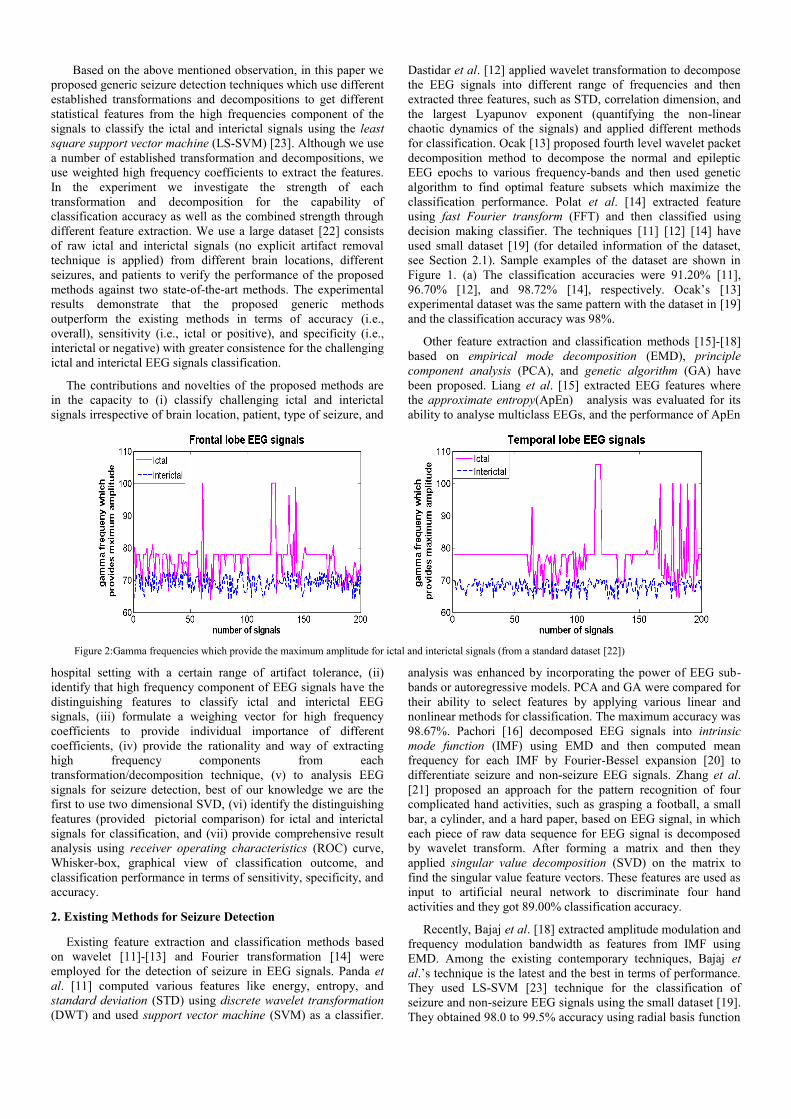
To verify our hypothesis we perform an experiment to find the

gamma frequency of signals which provides the maximum

amplitude using ictal and interictal signals in different brain

locations. The results for 200 EEG signals from ictal and

interictal are shown in Figure 2. The figure reveals that relatively

high gamma frequencies i.e., high frequencies in the signals

provide the maximum amplitude of ictal compared to the

interictal signals for both Frontal and Temporal lobes from

different patients. We use the maximum amplitude criteria for the

gamma band selection in this analysis as our observation and

Worrell et al.’s observation indicate that dominant spectral peaks

for the seizure onset are in the high frequency (i.e., gamma band).

Thus, the features extracted from gamma frequencies i.e., the

high frequencies should provide better classification accuracy

between the ictal and interictal irrespective of brain location,

patients, type of seizure, and hospital setting.

(a)

(b)

(c)

Figure 1: Ictal and interictal EEG signals from different datasets and different brain locations: (a) Seizure and non-seizure EEG signals from the small dataset

[19], the first row and remaining four rows indicated the seizure and non-seizure signals respectively [19]. (b) Ictal (patient one, 7th datablock, channel one) and

interictal (patient one, 95th datablock, channel one) of Frontal lobe signals [22] and (c) Ictal (patient 12, 15th datablock, channel one) and interictal (patient 12, 35th datablock, channel one) of Temporal lobe signals [22].

Based on the above mentioned observation, in this paper we

proposed generic seizure detection techniques which use different

established transformations and decompositions to get different

statistical features from the high frequencies component of the

signals to classify the ictal and interictal signals using the least

square support vector machine (LS-SVM) [23]. Although we use

a number of established transformation and decompositions, we

use weighted high frequency coefficients to extract the features.

In the experiment we investigate the strength of each

transformation and decomposition for the capability of

classification accuracy as well as the combined strength through

different feature extraction. We use a large dataset [22] consists

of raw ictal and interictal signals (no explicit artifact removal

technique is applied) from different brain locations, different

seizures, and patients to verify the performance of the proposed

methods against two state-of-the-art methods. The experimental

results demonstrate that the proposed generic methods

outperform the existing methods in terms of accuracy (i.e.,

overall), sensitivity (i.e., ictal or positive), and specificity (i.e.,

interictal or negative) with greater consistence for the challenging

ictal and interictal EEG signals classification.

The contributions and novelties of the proposed methods are

in the capacity to (i) classify challenging ictal and interictal

signals irrespective of brain location, patient, type of seizure, and

hospital setting with a certain range of artifact tolerance, (ii)

identify that high frequency component of EEG signals have the

distinguishing features to classify ictal and interictal EEG

signals, (iii) formulate a weighing vector for high frequency

coefficients to provide individual importance of different

coefficients, (iv) provide the rationality and way of extracting

high frequency components from each

transformation/decomposition technique, (v) to analysis EEG

signals for seizure detection, best of our knowledge we are the

first to use two dimensional SVD, (vi) identify the distinguishing

features (provided pictorial comparison) for ictal and interictal

signals for classification, and (vii) provide comprehensive result

analysis using receiver operating characteristics (ROC) curve,

Whisker-box, graphical view of classification outcome, and

classification performance in terms of sensitivity, specificity, and

accuracy.

2. Existing Methods for Seizure Detection

Existing feature extraction and classification methods based

on wavelet [11]-[13] and Fourier transformation [14] were

employed for the detection of seizure in EEG signals. Panda et

al. [11] computed various features like energy, entropy, and

standard deviation (STD) using discrete wavelet transformation

(DWT) and used support vector machine (SVM) as a classifier.

Dastidar et al. [12] applied wavelet transformation to decompose

the EEG signals into different range of frequencies and then

extracted three features, such as STD, correlation dimension, and

the largest Lyapunov exponent (quantifying the non-linear

chaotic dynamics of the signals) and applied different methods

for classification. Ocak [13] proposed fourth level wavelet packet

decomposition method to decompose the normal and epileptic

EEG epochs to various frequency-bands and then used genetic

algorithm to find optimal feature subsets which maximize the

classification performance. Polat et al. [14] extracted feature

using fast Fourier transform (FFT) and then classified using

decision making classifier. The techniques [11] [12] [14] have

used small dataset [19] (for detailed information of the dataset,

see Section 2.1). Sample examples of the dataset are shown in

Figure 1. (a) The classification accuracies were 91.20% [11],

96.70% [12], and 98.72% [14], respectively. Ocak’s [13]

experimental dataset was the same pattern with the dataset in [19]

and the classification accuracy was 98%.

Other feature extraction and classification methods [15]-[18]

based on empirical mode decomposition (EMD), principle

component analysis (PCA), and genetic algorithm (GA) have

been proposed. Liang et al. [15] extracted EEG features where

the approximate entropy(ApEn) analysis was evaluated for its

ability to analyse multiclass EEGs, and the performance of ApEn

analysis was enhanced by incorporating the power of EEG sub-

bands or autoregressive models. PCA and GA were compared for

their ability to select features by applying various linear and

nonlinear methods for classification. The maximum accuracy was

98.67%. Pachori [16] decomposed EEG signals into intrinsic

mode function (IMF) using EMD and then computed mean

frequency for each IMF by Fourier-Bessel expansion [20] to

differentiate seizure and non-seizure EEG signals. Zhang et al.

[21] proposed an approach for the pattern recognition of four

complicated hand activities, such as grasping a football, a small

bar, a cylinder, and a hard paper, based on EEG signal, in which

each piece of raw data sequence for EEG signal is decomposed

by wavelet transform. After forming a matrix and then they

applied singular value decomposition (SVD) on the matrix to

find the singular value feature vectors. These features are used as

input to artificial neural network to discriminate four hand

activities and they got 89.00% classification accuracy.

Recently, Bajaj et al. [18] extracted amplitude modulation and

frequency modulation bandwidth as features from IMF using

EMD. Among the existing contemporary techniques, Bajaj et

al.’s technique is the latest and the best in terms of performance.

They used LS-SVM [23] technique for the classification of

seizure and non-seizure EEG signals using the small dataset [19].

They obtained 98.0 to 99.5% accuracy using radial basis function

Figure 2:Gamma frequencies which provide the maximum amplitude for ictal and interictal signals (from a standard dataset [22])

(RBF) kernel and also obtained 99.5 to 100% accuracy using

Morlet kernel.

We have observed that the existing methods [11]-[18] exhibit

almost perfect classification accuracy for the small dataset of

seizure and non-seizure EEG signals. However, their

performance is below the expected results using the large dataset

[22] for ictal and interictal EEG signal classifications. For

example, when we applied Bajaj et al.’s [18] feature extraction

and classification method to differentiate ictal and interictal EEG

signals for the first IMF in the large dataset from Epilepsy Center

of the University Hospital of Freiburg [22], the classification

accuracy is 77.90% for Frontal lobe and 80.20% for Temporal

lobe which is far below the accuracy 98.50% obtained using the

small dataset [19] of seizure and non-seizure EEG signals.

The paper is organized as follows: the detailed of the proposed

four methods with dataset, feature extractions, classification

techniques, and computational time are described in section 3;

the detail experimental results are explained in section 4 while

section 5 concludes the paper.

3. Proposed Methods

In this paper, we propose four methods based on the various

new features extracted from DCT, DCT-DWT, SVD, and IMF.

We use the transformation and decompositions to separate high

frequency components and then apply innovative ways to extract

different statistical features. When we extract features from the

high frequency component (i.e., IMF and detail signals

respective) using EMD and DWT, we take total length of the

high frequency components and we do not use any weighting for

them as all the coefficients represent the high frequency

components. As the SVD and DCT provide coefficients of all

frequencies, we need to select a subset of the coefficients which

can represent high frequency components. We investigate the

strength of each transformation and decomposition for the

capability of classification accuracy as well as the combined

strength through different feature extractions. The dataset,

individual method, their corresponding rationality, and detailed

methodology of feature extractions are described in the following

sub-sections.

3.1. Dataset

Small Dataset [19]: The existing seizure and non-seizure

feature extraction and classification schemes [11]-[18] except

[13] used small dataset [19]. The dataset consists of five subsets,

each subset contains 100 single-channels recoding, and each

recoding has 23.6 seconds in duration captured by the

international 10–20 electrode placement scheme i.e., 32

electrodes [14]. Among them two subsets are taken from healthy

volunteers, two subsets are taken from seizure free intervals and

another subset is also taken during seizure period [18] (see

sample examples in Figure 1 (a)). Ocak [13] used different

dataset with the same pattern of small dataset where 300 were

normal and 100 were epileptic patients.

Large Dataset [22]: Seizure and brain discharges are much

more complicated than what can be seen in the scalp. Thus, in the

paper we have used intracranial EEG dataset using grid, strip and

depth electrodes rather than scalp EEG. The dataset used in the

paper was recorded at Epilepsy centre of the University Hospital

of Freiburg, Germany [22]. The database contains invasive EEG

recordings of 21 patients suffering from medically intractable

focal epilepsy. The data obtained by Neurofile NT digital video

EEG system with 128 channels, 256 Hz sampling rate, and 16 bit

analogue-to-digital converter. According to the dataset [22],

epileptic EEG signals can be classified into (i) ictal (i.e., seizure),

(ii) preictal (a certain period before seizure onset), (iii) interictal

(period between seizures), (iv) non-seizure (period without any

seizure activity after a certain time of interictal). Normally,

duration of ictal is varied from few seconds to 2 minutes. The

ictal records contain epileptic seizures with at least 50 minutes of

preictal data preceding each seizure. The median time period

between the last seizure and the interictal data set is 5 hours and

18 minutes, and the median time period between the interictal

data set and the first following seizure is 9 hours and 36

minutes[29]. As suggested in the dataset, we have treated preictal

and ictal period as an ictal signals in our experiments. We do not

consider any non-seizure signals into the interictal period as we

carefully select the same duration of interictal signal (with the

ictal signal) from the above duration of interictal signal.

3.2. Feature Extraction using DCT

DCT is a transformation method for converting a time series

signal into basic frequency in such a way that the DCT

coefficients are arranged from low frequency to high frequency

components. Low frequency components represent the coarse

signals and high frequency components represent the detail

signals. DCT is widely used in the image processing and video

coding areas to compress image signals based on their

frequencies [34]. As the ictal and interictal EEG signals have

different amplitude and frequency (not visually separable), thus

(a)

(b)

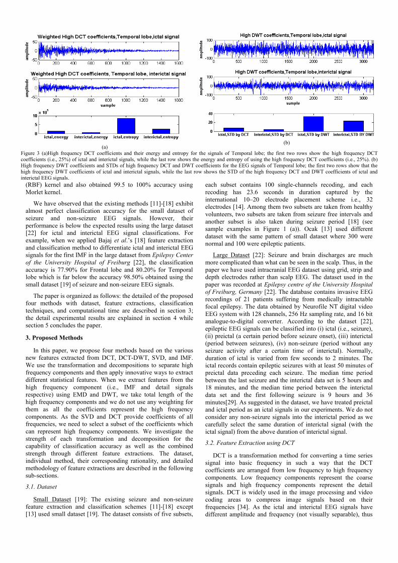
Figure 3 (a)High frequency DCT coefficients and their energy and entropy for the signals of Temporal lobe; the first two rows show the high frequency DCT

coefficients (i.e., 25%) of ictal and interictal signals, while the last row shows the energy and entropy of using the high frequency DCT coefficients (i.e., 25%). (b) High frequency DWT coefficients and STDs of high frequency DCT and DWT coefficients for the EEG signals of Temporal lobe; the first two rows show that the

high frequency DWT coefficients of ictal and interictal signals, while the last row shows the STD of the high frequency DCT and DWT coefficients of ictal and

interictal EEG signals.

the most distinguishable features should be located in the high

frequency components of DCT coefficients see in Figure 3(a). As

the EEG signal is non-linear and non-stationary in nature, thus,

for real time processing of EEG signals, DCT may not be correct

to directly correspond to the frequency analysis, however, if we

segment the EEG signals in time window and apply DCT on

them to find DCT coefficients; we can avoid non-linear and non-

stationary nature of the signals. In our experiment, we apply DCT

on the benchmark dataset [22] and take the higher frequency

component (i.e., the last quartile (Q4) i.e., last 25% of DCT

coefficient). Then, we extract statistical features such as entropy

and energy of the weighted higher frequency coefficients to

classify ictal and interictal signals.

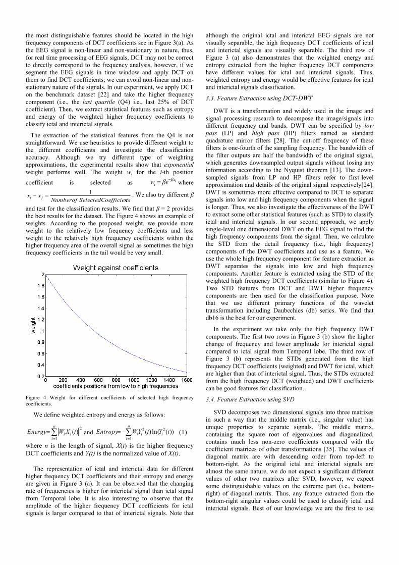
The extraction of the statistical features from the Q4 is not

straightforward. We use heuristics to provide different weight to

the different coefficients and investigate the classification

accuracy. Although we try different type of weighting

approximations, the experimental results show that exponential

weight performs well. The weight wi for the i-th position

coefficient is selected as ixi ew

where

tsCoefficienSelectedofNumberxx ji

1 . We also try different β

and test for the classification results. We find that β = 2 provides

the best results for the dataset. The Figure 4 shows an example of

weights. According to the proposed weight, we provide more

weight to the relatively low frequency coefficients and less

weight to the relatively high frequency coefficients within the

higher frequency area of the overall signal as sometimes the high

frequency coefficients in the tail would be very small.

Figure 4 Weight for different coefficients of selected high frequency coefficients.

We define weighted entropy and energy as follows:

n

iii tXWEnergy

1

2)( and

n

iiii tYtYWEntropy

1

22 ))(ln()( (1)

where n is the length of signal, X(t) is the higher frequency

DCT coefficients and Y(t) is the normalized value of X(t).

The representation of ictal and interictal data for different

higher frequency DCT coefficients and their entropy and energy

are given in Figure 3 (a). It can be observed that the changing

rate of frequencies is higher for interictal signal than ictal signal

from Temporal lobe. It is also interesting to observe that the

amplitude of the higher frequency DCT coefficients for ictal

signals is larger compared to that of interictal signals. Note that

although the original ictal and interictal EEG signals are not

visually separable, the high frequency DCT coefficients of ictal

and interictal signals are visually separable. The third row of

Figure 3 (a) also demonstrates that the weighted energy and

entropy extracted from the higher frequency DCT components

have different values for ictal and interictal signals. Thus,

weighted entropy and energy would be effective features for ictal

and interictal signals classification.

3.3. Feature Extraction using DCT-DWT

DWT is a transformation and widely used in the image and

signal processing research to decompose the image/signals into

different frequency and bands. DWT can be specified by low

pass (LP) and high pass (HP) filters named as standard

quadrature mirror filters [28]. The cut-off frequency of these

filters is one-fourth of the sampling frequency. The bandwidth of

the filter outputs are half the bandwidth of the original signal,

which generates downsampled output signals without losing any

information according to the Nyquist theorem [13]. The down-

sampled signals from LP and HP filters refer to first-level

approximation and details of the original signal respectively[24].

DWT is sometimes more effective compared to DCT to separate

signals into low and high frequency components when the signal

is longer. Thus, we also investigate the effectiveness of the DWT

to extract some other statistical features (such as STD) to classify

ictal and interictal signals. In our second approach, we apply

single-level one dimensional DWT on the EEG signal to find the

high frequency components from the signal. Then, we calculate

the STD from the detail frequency (i.e., high frequency)

components of the DWT coefficients and use as a feature. We

use the whole high frequency component for feature extraction as

DWT separates the signals into low and high frequency

components. Another feature is extracted using the STD of the

weighted high frequency DCT coefficients (similar to Figure 4).

Two STD features from DCT and DWT higher frequency

components are then used for the classification purpose. Note

that we use different primary functions of the wavelet

transformation including Daubechies (db) series. We find that

db16 is the best for our experiment.

In the experiment we take only the high frequency DWT

components. The first two rows in Figure 3 (b) show the higher

change of frequency and lower amplitude for interictal signal

compared to ictal signal from Temporal lobe. The third row of

Figure 3 (b) represents the STDs generated from the high

frequency DCT coefficients (weighted) and DWT for ictal, which

are higher than that of interictal signal. Thus, the STDs extracted

from the high frequency DCT (weighted) and DWT coefficients

can be good features for classification.

3.4. Feature Extraction using SVD

SVD decomposes two dimensional signals into three matrixes

in such a way that the middle matrix (i.e., singular value) has

unique properties to separate signals. The middle matrix,

containing the square root of eigenvalues and diagonalized,

contains much less non-zero coefficients compared with the

coefficient matrices of other transformations [35]. The values of

diagonal matrix are with descending order from top-left to

bottom-right. As the original ictal and interictal signals are

almost the same nature, we do not expect a significant different

values of other two matrixes after SVD, however, we expect

some distinguishable values on the extreme part (i.e., bottom-

right) of diagonal matrix. Thus, any feature extracted from the

bottom-right singular values could be used to classify ictal and

interictal signals. Best of our knowledge we are the first to use

two dimensional SVD to analysis EEG signals for seizure

detection.

To extract the features using SVD, we reshape the EEG

signals into a two dimensional matrix. The column vector of

EEG signal is rearranged to square matrix for the computation of

singular value components using SVD. From the singular values,

we take the weighted Q4 (weight is similar to Figure 4 but the

number of selected coefficients are different) of the non-zero

diagonal values to calculate the STDs and energy and treat as the

two features to classify ictal and interictal signals. The SVD

allows transforming any given matrix mxnCA to diagonal form

using unitary matrices, i.e. HVUA where nmA is a matrix, mmU and nnV are orthogonal matrix, and

nm matrix with

non-negative diagonal entries.

The columns of U are called left singular vectors and the rows of

VH are called right singular vectors. If A is a rectangular m×n

matrix of rank K than U will be m×m and will be:

where λ1 ≥ λ2≥... λn-1 ≥λn. (2)

The data distribution of non-zero singular values of the ictal

and interictal signals from the Frontal lobe is shown in Figure 5

(a). The top part of the figure clearly shows that the Q4 singular

values of interictal signals are larger than that of the ictal signals.

The bottom part of Figure 5 (a) shows the STD and energy

extracted from the weighted Q4 of non-zero singular values from

ictal and interictal signals respectively. The figure exposes that

the STDs extracted from the ictal and interictal signals have

distinguishable values, thus, they can be used for ictal and

interictal signal classification.

3.5. Feature Extraction of IMF using EMD

The main strength of EMD is its ability to analyze nonlinear

and non-stationary signals like EEG signals. When we apply

EMD on a signal, the signal is decomposed into a finite number

of signals into IMFs, which are ordered from higher frequency

component to lower frequency component. The number of IMFs

in a signal depends on the local characteristics of the signal rather

than pre-defined number of IMFs. This feature makes each IMF

crucial to identify some characteristics of the original signal.

Since the IMFs are the representations of different

frequencies/amplitudes of the original signal and the

distinguishing features between ictal and interictal EEG signals

lie on the frequency/amplitude, our hypothesis is that any feature

extracted from IMFs will be an effective feature to classify ictal

and interictal successfully. We also observe that the ictal and

interictal signals are deferred in higher order frequency

components, thus our other hypothesis is that features extracted

from the first few IMFs should be enough to classify ictal and

interictal signals successfully. Through the decomposition we

keep only few mode functions of the original signals for the final

feature extraction, however, we are able to keep the important

mode functions for the classification purpose. Experimental

results reveal that our both hypothesis are correct as extracted

features from the first IMF successfully classify ictal and

interictal signals (see Section 4). Thus, IMFs can be used in

classification applications where the original signals are non-

linear and non-stationary and distinguishing features exist on the

different frequencies/amplitudes.

Each IMF satisfies two following conditions: (i) the number of

extrema and the number of zero crossing are identical or differ at

most by one and (ii) the mean value between the upper and the

lower envelope is equal to zero at any time.

The EMD algorithm can be summarized as follows:

1. Extract the extrema (minima and maxima)of the signal

).(tx

2. Interpolate between minima and maxima to obtain

)(min t and )(max t .

(a) (b)

Figure 5 (a) Non-zero singular value of SVD for Frontal lobe. The first row shows that the non-zero singular value distribution for ictal and interictal signals from

Frontal lobe and the last row shows the STD and energy of the last 25% non-zero singular values of ictal and interictal EEG signals. (b) The first IMFs of ictal and

interictal signals with the extracted features; the top two rows represent the first IMF from the ictal and interictal signals of Temporal lobe; bottom row represents STD of the first IMF and STD of the normalized PSD (power spectral density) of the same IMF of ictal and interictal EEG signals.

000

00

00

00

Σ

2

1

n

3. Calculate local mean /2)()()( maxmin tttm .

4. Extract the detail )()()( tmtxtd .

5. Check )(td is an IMF according to the conditions

which are mentioned above. If yes, repeat the

procedure from the step 1 on the residual signal

)()()( tmtxtr . If no, replace )(tx with )(td and

repeat the procedure from step 1.

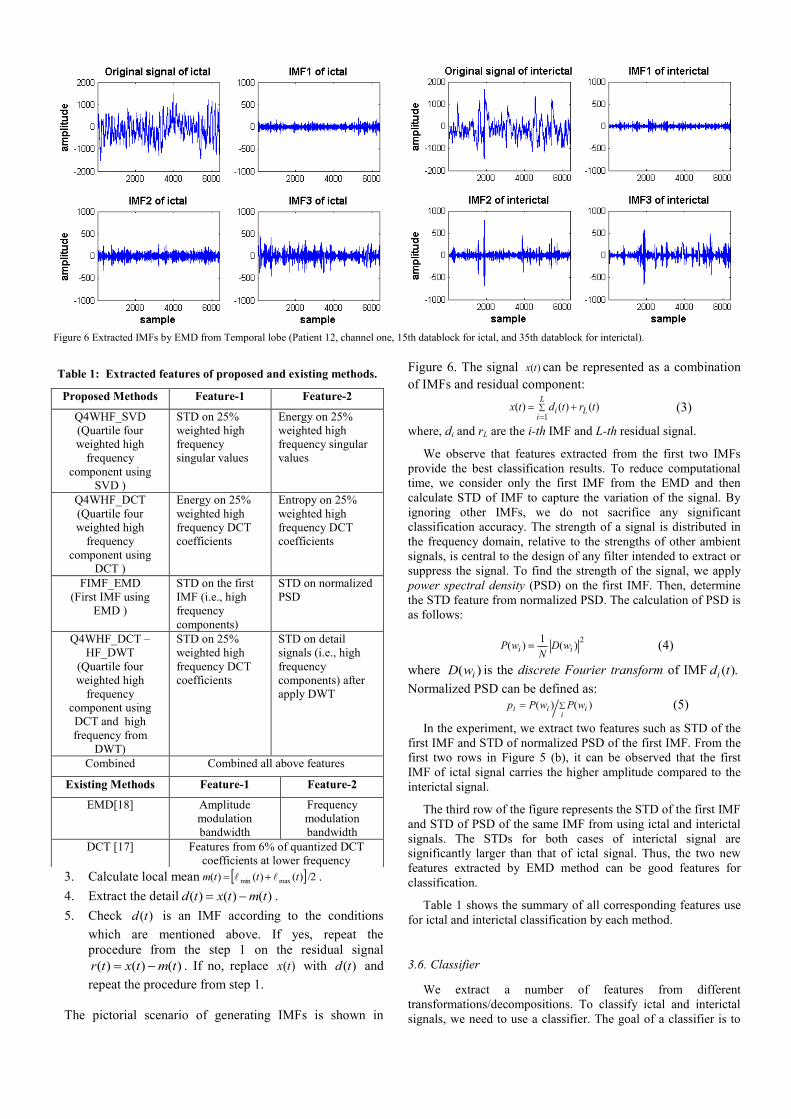
The pictorial scenario of generating IMFs is shown in

Figure 6. The signal )(tx can be represented as a combination

of IMFs and residual component:

L

iLi trtdtx

1)()()( (3)

where, di and rL are the i-th IMF and L-th residual signal.

We observe that features extracted from the first two IMFs

provide the best classification results. To reduce computational

time, we consider only the first IMF from the EMD and then

calculate STD of IMF to capture the variation of the signal. By

ignoring other IMFs, we do not sacrifice any significant

classification accuracy. The strength of a signal is distributed in

the frequency domain, relative to the strengths of other ambient

signals, is central to the design of any filter intended to extract or

suppress the signal. To find the strength of the signal, we apply

power spectral density (PSD) on the first IMF. Then, determine

the STD feature from normalized PSD. The calculation of PSD is

as follows:

2

)(1

)( ii wDN

wP (4)

where )( iwD is the discrete Fourier transform of IMF ).(tdi

Normalized PSD can be defined as:

i

iii wPwPp )()( (5)

In the experiment, we extract two features such as STD of the

first IMF and STD of normalized PSD of the first IMF. From the

first two rows in Figure 5 (b), it can be observed that the first

IMF of ictal signal carries the higher amplitude compared to the

interictal signal.

The third row of the figure represents the STD of the first IMF

and STD of PSD of the same IMF from using ictal and interictal

signals. The STDs for both cases of interictal signal are

significantly larger than that of ictal signal. Thus, the two new

features extracted by EMD method can be good features for

classification.

Table 1 shows the summary of all corresponding features use

for ictal and interictal classification by each method.

3.6. Classifier

We extract a number of features from different

transformations/decompositions. To classify ictal and interictal

signals, we need to use a classifier. The goal of a classifier is to

Figure 6 Extracted IMFs by EMD from Temporal lobe (Patient 12, channel one, 15th datablock for ictal, and 35th datablock for interictal).

Table 1: Extracted features of proposed and existing methods.

Proposed Methods Feature-1 Feature-2

Q4WHF_SVD

(Quartile four

weighted high

frequency

component using

SVD )

STD on 25%

weighted high

frequency

singular values

Energy on 25%

weighted high

frequency singular

values

Q4WHF_DCT

(Quartile four

weighted high

frequency

component using

DCT )

Energy on 25%

weighted high

frequency DCT

coefficients

Entropy on 25%

weighted high

frequency DCT

coefficients

FIMF_EMD

(First IMF using

EMD )

STD on the first

IMF (i.e., high

frequency

components)

STD on normalized

PSD

Q4WHF_DCT –

HF_DWT

(Quartile four

weighted high

frequency

component using

DCT and high

frequency from

DWT)

STD on 25%

weighted high

frequency DCT

coefficients

STD on detail

signals (i.e., high

frequency

components) after

apply DWT

Combined Combined all above features

Existing Methods Feature-1 Feature-2

EMD[18] Amplitude

modulation

bandwidth

Frequency

modulation

bandwidth

DCT [17] Features from 6% of quantized DCT

coefficients at lower frequency

find patients states such as ictal (class 1) and interictal (class 2)

using machine learning approaches with cross-validation. The

challenge is to find the mapping that generalizes from training

sets to unseen test sets. For the cross-validation, data are

partitioned into training set and test set. In our experiment we use

4-fold cross validation where each dataset was randomly divided

into 4 splits, where three of them were used for training and the

fourth one used for testing.

To classify the ictal and interictal signals, we extract various

features from DCT, DWT, SVD, and IMF of EMD. For

classification, we use SVM-based classifier as the SVM is one of

the best classifiers in the EEG signal analysis. SVM is a potential

methodology for solving problem in linear and nonlinear

classification, function estimation, and kernel based learning

methods [25]. It can minimize the operational error and

maximize the margin hyperplane, as a result it will maximize the

classification performance [25]. LS-SVM is the extended version

of SVM and it is closely related to regularization networks and

Gaussian process, and it also has primal-dual interpretations [23].

The major drawback of SVM is in its higher computational

burden of the constrained optimization programming. However,

LS-SVM can solve this problem [26].

The classifier is a LS-SVM, which learns nonlinear

mapping from the training set features {x}i=1…nT, where nT is

the number of training features into the patient’s state, ictal

(+1) and interictal (-1). For unbiased classification results

[27], we divide the whole 1000 trials into four subsets; in each

subset we randomly select 75% samples for the validation

training set and the remaining 25% for the validation testing

set. Let 2,1Ciiy

designate the LS-SVM validation test

outputs mapping to class 1 or class 2. The equation of LS-

SVM can be defined in [18] as:

N

iiii cxxKysignxf

1),()( (6)

where K(x, xi) is a kernel function, αi are the Lagrange

multipliers, c is the bias term, xi is the training input, and yi is

the training output pairs. Linear, RBF and Morlet kernel are

used in our experiments and RBF and Morlet functions can be

defined in [18] as:

)2exp(),( 22ii xxxxk (7)

where σ controls the width of the RBF function;

d

k

ki

kki

ki axxaxxxxk

1

20 )2exp())((cos),( (8)

where d is the dimension, a is the flexible coefficient, kix is

the k-th component of i-th training data. Matlab codes for LS-

SVM classifier are available at

http://www.esat.kuleuven.ac.be/sista/lssvmlab/.

3.7. Computational Time

Feature extractions using IMF through EMD take longer time

due to two fold iterations to find all IMFs. In the first iteration

EMD decomposes a signal and checks whether the signal makes

an IMF and in the second iteration it subtracts the current IMF

from the signal and continues for the next IMF. Even if we stop

the iteration for the first IMF, the EMD-based technique takes a

full first iteration for calculating the IMF. The experimental data

reveals that the proposed technique using DCT, DWT, and SVD

takes less computational time compared to the EMD-based

technique as DCT, DWT, and SVD transformation is faster

compared to the EMD decomposition. Thus, the proposed

methods (except FIMF_EMD method i.e., First IMF using EMD)

take insignificant time compared to the existing method [18].

4. Experimental Results

Sometimes EEG signals have line noise and other kinds of

artifacts due to muscle and body movements. Notch filter and

independent component analysis (ICA)-based method are

recommended to remove the line noise and artifacts respectively

for sufficient amount of EEG signals [30]-[32]. However, in this

experiment we do not use any explicit noise/ artifacts removal

technique to see the tolerance of the proposed method against

noise/ artifacts.

We propose fours method and the experimental results of the

proposed methods are compared with existing methods

[17][18]and corresponding features are explained in Table 1.Our

ultimate target is to classify ictal and interictal EEG signals using

LS-SVM with different kernels such as RBF and Morlet where

the value of regularization parameter and kernel parameter are 10

and 6, respectively for both kernels. We also use linear kernel. In

this paper, four methods are proposed based on the new features

of ictal and interictal EEG signals captured from Frontal and

Temporal lobes using DCT, DWT, SVD, and IMF of EMD to see

the strength of individual transformation/decomposition

techniques for seizure detection. Then we also test the

classification accuracy by combining all features. In our

experiment, we use 200 signals from ictal and 800 signals from

interictal EEG signals. After training and testing of all features,

we calculate average value from the four subsets to compute

sensitivity, specificity, and accuracy [18]. The sensitivity,

specificity, and accuracy are defined as:

100))(( FNTPTPySensitivit (9)

100))(( FPTNTNySpecificit (10)

100))()(( FNFPTNTPTNTPAccuracy (11) where TP and TN represents the total number of detected true

positive events and true negative events respectively. The FP and

FN represent false positive and false negative respectively.

The technique in [18] claims that the second IMF provides

better classification results while they use frequency and

amplitude modulation bandwidth features for the dataset [19].

We conduct experiments using first four IMFs; however, we

provide results using only the first IMF in Table 2 as it carries the

best result compared to other IMFs. For the RBF kernel function,

the proposed methods outperform the state-of-the-art method

consistently and the average sensitivity using the proposed

methods, such as Quartile four weighted high frequency

component using SVD (Q4WHF_SVD), Quartile four weighted

high frequency component using DCT (Q4WHF_DCT), First IMF

using EMD (FIMF_EMD), and Quartile four weighted high

frequency component using DCT and high frequency from DWT

(Q4WHF_DCT–HF_DWT) are 83.33%, 99.12%, 96.47%, and

87.13% for RBF kernel, respectively, whereas, the average

sensitivity using the state-of-art-methods[17] and [18] are 6.35%

and 48.04%. Using Morlet kernel, the average sensitivity of the

proposed methods is higher compared to the existing methods [17]

and [18]. Moreover, we justify our result applying linear kernel.

Table 2 also shows that the most of the cases the proposed

methods with linear kernel provide better results compared to the

proposed methods with Morlet and RBF kernels in terms of

sensitivity. Table 2 also reveals that the proposed Q4WHF_DCT

method is the best among all proposed methods in terms of

sensitivity. It is also interesting to note that the accuracy of the

proposed Q4WHF_DCT–HF_DWT method is reasonably

consistence in terms of three criteria for RBF and Morlet kernel.

According to the Table 2, all proposed methods always

outperform the existing methods [17][18] in terms of sensitivity

(i.e., seizure i.e., ictal detection rate), however, some cases the

existing methods [17][18] outperform one or more proposed

methods in terms of specificity (interictal detection rate). For

seizure detection, sensitivity is more important compared to the

specificity detection as the cost of failure detecting ictal is

heavier compared to interictal. In overall classification the

proposed methods are also better compared to the existing

methods. We combine all features to classify ictal and interictal

EEG signals. However, combine is not good because LS-SVM

may not properly combine all available features to make a good

prediction model. The average sensitivity of the proposed

methods is 91.36% (average result of all kernel and lobe),

whereas the sensitivity of the state-of-the-arts methods are

54.61% [18] and 7.99% [17], respectively.

The performance of the LS-SVM is evaluated by (ROC) plot

is shown in Figure 7(a) ROC illustrates the performance of a

binary classifier system where it is created by plotting the

fraction of true positives from the positives i.e., true positive rate

(TPR) vs. the fraction of false positives from negatives i.e., false

positive rate (FPR) with various threshold settings. TPR is known

as sensitivity, and FPR is one minus the specificity or true

negative rate. Figure 7(a) demonstrates that the proposed four

methods are carrying good classification results than that of the

state-of-the-art method [18] using dataset from Frontal lobe of

the third subset of training and testing EEG signals.

Figure 7(b) shows the distribution of normalized feature

values (i.e., energy & entropy in the Q4WHF_DCT method, STD

in the Q4WHF_DCT–HF_DWT method, STD & energy in the

Q4WHF_SVD method, and STD in the FIMF EMD method) of

ictal and interictal from the Frontal lobe dataset [22]. The figure

shows that the range of feature values for ictal is different from

that of the interictal signals. This phenomenon is the other

evidence why we use those features to classify ictal and interictal

EEG signals in the proposed methods.

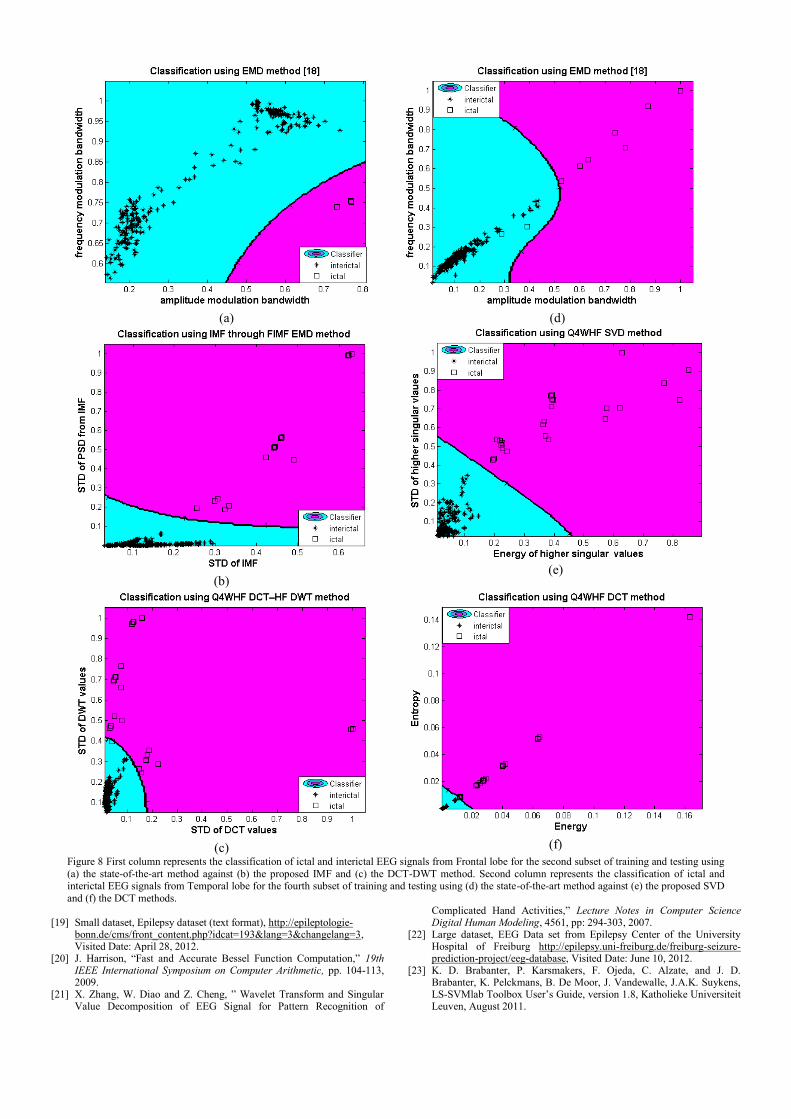
First column of Figure 8 represents classification comparison

using the proposed methods (i.e., FIMF EMD and

Q4WHF_DCT–HF_DWT) and the state-of-the-art method [18].

Figure 8 (b) and (c) show the LS-SVM classification results

using the proposed FIMF EMD and Q4WHF_DCT–HF_DWT

against the state-of-the-art method (i.e., EMD Figure 8 (a)). We

generate first column of Figure 8 from Frontal lobe for the

second subset of training and testing and obtain the classification

accuracy 91.20% for the Q4WHF_DCT–HF_DWT method,

Table 2: Sensitivity, specificity, and accuracy for different features of ictal and interictal EEG signals from Frontal and Temporal lobe.

Classifier Brain

Location

Existing Method Proposed Method

Kernel Lobe Criteria EMD[18] DCT[17] Q4WHF_SVD Q4WHF_DCT FIMF_EMD Q4WHF_DCT

–HF_DWT Combined

RBF

Frontal

SEN 29.41 8.70 66.66 100 95.83 76.78 49.14

SPE 80.51 79.73 82.20 81.30 81.86 83.37 83.82

ACC 77.90 78.10 81.50 81.60 82.20 83.00 79.80

Temporal

SEN 66.67 4.00 100 98.24 97.10 97.47 96.47

SPE 80.28 98.63 83.51 84.73 85.71 86.65 87.10

ACC 80.20 79.70 84.20 85.50 86.50 87.50 87.90

Average

SEN 48.04 6.35 83.33 99.12 96.47 87.13 72.81

SPE 80.40 89.18 82.86 83.02 83.79 85.01 85.46

ACC 79.05 78.90 82.85 83.55 84.35 85.25 83.85

Morlet

Frontal

SEN 33.82 0.00 63.83 88.89 93.33 60.00 24.42

SPE 81.01 79.78 82.16 81.26 81.12 83.96 80.42

ACC 77.80 78.9 81.30 81.40 81.30 81.80 75.60

Temporal

SEN 84.62 2.00 100 98.41 90.12 93.68 94.68

SPE 83.54 99.00 84.30 85.27 86.18 86.32 87.75

ACC 83.60 79.60 85.10 86.10 86.50 86.90 88.40

Average

SEN 59.22 1.00 81.92 93.65 91.73 76.84 59.55

SPE 82.28 89.39 83.23 83.27 83.65 85.14 84.09

ACC 80.70 79.25 83.20 83.75 83.90 84.35 82.00

Linear

Frontal

SEN 28.95 27.28 80.95 100 100 100 87.50

SPE 80.35 80.61 81.31 80.89 81.55 80.81 82.23

ACC 78.40 76.6 81.30 81.10 81.90 81.00 82.40

Temporal

SEN 84.21 6.00 98.00 97.22 98.11 98.00 98.36

SPE 85.28 96.13 84.11 82.88 84.37 84.12 85.09

ACC 85.20 78.10 84.80 83.40 85.10 84.80 85.90

Average

SEN 56.58 16.64 89.48 98.61 99.06 99.00 92.93

SPE 82.82 88.37 82.71 81.89 82.96 82.47 83.66

ACC 81.80 77.35 83.05 82.25 83.50 82.90 84.15

87.20% for the FIMF_EMD method, and 80.80% for the EMD

method. It can be concluded from these figures that the proposed

method based on the DCT-DWT and the IMF outperform the

state-of-the-art method (i.e., EMD). The same classification

comparisons are also provided in second column of Figure 8

using the state-of-the-art method based on the EMD and the

proposed method based on the SVD and DCT respectively. We

consider Temporal lobe for the fourth subset of training and

testing; obtain classification accuracy 91.20% for Q4WHF_SVD,

89.60% for Q4WHF_DCT, and 85.20% for EMD [18].Thus, it is

concluded that the proposed methods based on the DCT and SVD

also outperform the EMD method [18].

5. Conclusion

Unlike seizure and non-seizure EEG signals, classification of

ictal and interictal EEG signal is a challenging task due to non

abrupt phenomena (i.e., visually non-separable) between ictal and

interictal EEG signals. Moreover, the features of ictal and

interictal signals are not consistence in different brain locations,

patient, types of seizure, and hospital setting during epileptic

period of a patient. Thus, the classification performance for ictal

and interictal EEG signals using the existing features extraction

and classification techniques is not at expected level. Our initial

observation indicates that high frequency components of EEG

signals have distinguished characteristics. To improve the

accuracy, in this paper we propose novel feature extractions

strategies from the high frequency components based on a

number of established transformation and decompositions. The

average sensitivity (which is the measure for seizure) of the

proposed methods is 91.36% (average result of all kernel and

lobe) whereas the sensitivity of the state-of-the-arts methods are

54.61% [18] and 7.99% [17], respectively. The experimental

results show that the proposed methods outperform the state-of-

the-art methods in terms of accuracy, sensitivity, and specificity

for the ictal and interictal EEG signals with greater consistence

from the large benchmark dataset in two different brain locations.

References [1] Neurology Applied: How Science is Bringing Music Instruction Back to

Expressive Development, URL: http://www.thomasjwestmusic.com/neurologyapplied.htm, Visited Date: August 27, 2012.

[2] EEG Signal, The science behind Bo-Tau, URL: http://www.bo-tau.co.uk/index.php?action=the_science_behind_bo_tau, Visited date: August 27,2012.

[3] Epilepsy-Seizures,URL: http://www.healthcommunities.com/epilepsy-seizures/about-seizures.shtml, Visited date: August 27, 2012.

[4] M. Soleymani, T. Pun, and M. Pantic, "Multi-Modal Emotion Recognition in Response to Videos", IEEE Transactions on Affective Computing, 3(2), pp. 211 - 223, 2012.

[5] S. Scholler, S. Bosse, M. S. Treder, B. Blankertz, G. Curio, K.-R. Müller, and T. Wiegand,” Toward a Direct Measure of Video Quality Perception Using EEG”, IEEE Transactions on Image Processing, 21(5), pp. 2619-2629.,2012.

[6] W. Di, C. Zhihua, F. Ruifang, L. Guangyu, and L. Tian, “Study on human brain after consuming alcohol based on EEG signal,” Inernational Conference on Computer Science and Information Technology (ICCSIT), 5, pp. 406 – 409, 2010.

[7] E. Estrada, H. Nazeran, F, Ebrahimi, and M Mikaeili, “EEG signal features for computer-aided sleep stage detection”, IEEE EMBS conference on neural engineering, pp. 669 - 672, 2009.

[8] Z. M. Hanafiah, K. F. M. Yunos, Z. H. Murat, M. N. Taib, S. Lias, “ EEG brainwave pattern for smoking behaviour after horizontal rotation treatment”, IEEE student conference on research and development, 2009.

[9] Z. H. Murat, R. Shilawani, S. A. Kadir, R. M. Isa, and M N. Taib, “The effects of mobile phone usage on human braingwave using EEG”, 13th International conference on modelling and simulation, 2011.

[10] K. Lehnertz, R. G.Andrzejak, J. Arnhold, T. Kreuz, F. Mormann, C. Rieke, G. Widman, and C. E. Elger,”Nonliner EEG analysis in Epilepsy: Its possible use for interictal focus localization, seizure ancipation, and prevention,” Journal of Clinical Neurophsysiology, pp. 209-222, 2001.

[11] R. Panda, P.S. Khobragade, P.D. Jambhule, S. N. Jengthe, P. R. Pal, and T. K. Gandhi, “Classification of EEG signal using wavelet transform and support vector machine for epileptic seizure diction,” International Conference on Systems in Medicine and Biology (ICSMB), pp. 405-408, 2010.

[12] S. G. Dastidar, H. Adeli, and N. Dadmehr, “Mixed-band wavelet chaos-neural network methodology for epilepsy and epileptic seizure detection,” IEEE Transactions on Biomeical Engineering, 54(9), pp. 1545-1551, 2007.

[13] H. Ocak, “Optimal classification of epileptic seizures in EEG using wavelet analysis and genetic algorithm,” Signal Proecssing, 88, pp. 1858-1867, 2008.

[14] K. Polat and S. G¨unes, “Classification of epileptiform EEG using a hybrid system based on decision tree classifier and fast Fourier transform,” Applied Mathematics and Computation, 187(2), pp. 1017-1026, 2007.

[15] S. F. Liang, H. C. Wang, and W. L. Chang, “Combination of EEG complexity and spectral analysis for epilepsy diagnosis and seizure detection,” EURASIP Journal on Advances in Signal Processing, Article ID 853434, 2010.

[16] R. B. Pachori, “Discrimination between ictal and seizure-free EEG signals using empirical mode decomposition,” Research Letters in Signal Processing, Article ID 293056, 2008.

[17] D. Birvinskas, V. Jusas, I. Martisius, and R. Damasevicius, “EEG Dataset Reduction and Feature Extraction Using Discrete Cosine Transform,” European Symposium on Computer Modeling and Simulation (EMS), pp. 199-204, 2012.

[18] V. Bajaj and R. B. Pachori, “Classification of Seizure and Non-seizure EEG Signals using Empirical Mode Decomposition,” IEEE Transaction on Information Technology in Biomedicine, 16(6), 2012.

(a)

(b)

Figure 7 (a) The receiver operating characteristics (ROC) curves of the third subset of training and testing EEG signals by three proposed methods (

Q4WHF_SVD, , FIMF_EMD, and Q4WHF_DCT–HF_DWT,) against the EMD method using LS-SVM with RBF kernel from Frontal lobe and (b)

Normalized distribution of feature values extracted from ictal and interictal EEG signals using DCT, DWT, SVD, and IMF based method where 200 samples are taken from each of ictal and interictal categories in Frontal lobe.

[19] Small dataset, Epilepsy dataset (text format), http://epileptologie-

bonn.de/cms/front_content.php?idcat=193&lang=3&changelang=3, Visited Date: April 28, 2012.

[20] J. Harrison, “Fast and Accurate Bessel Function Computation,” 19th IEEE International Symposium on Computer Arithmetic, pp. 104-113, 2009.

[21] X. Zhang, W. Diao and Z. Cheng, ” Wavelet Transform and Singular Value Decomposition of EEG Signal for Pattern Recognition of

Complicated Hand Activities,” Lecture Notes in Computer Science Digital Human Modeling, 4561, pp: 294-303, 2007.

[22] Large dataset, EEG Data set from Epilepsy Center of the University Hospital of Freiburg http://epilepsy.uni-freiburg.de/freiburg-seizure-prediction-project/eeg-database, Visited Date: June 10, 2012.

[23] K. D. Brabanter, P. Karsmakers, F. Ojeda, C. Alzate, and J. D. Brabanter, K. Pelckmans, B. De Moor, J. Vandewalle, J.A.K. Suykens, LS-SVMlab Toolbox User’s Guide, version 1.8, Katholieke Universiteit Leuven, August 2011.

(a)

(d)

(b)

(e)

(c)

(f)

Figure 8 First column represents the classification of ictal and interictal EEG signals from Frontal lobe for the second subset of training and testing using

(a) the state-of-the-art method against (b) the proposed IMF and (c) the DCT-DWT method. Second column represents the classification of ictal and interictal EEG signals from Temporal lobe for the fourth subset of training and testing using (d) the state-of-the-art method against (e) the proposed SVD

and (f) the DCT methods.

[24] S. Sanei and J.A. Chambers, “EEG Signal Processing,” Centre of Digital Signal Processing, Cardiff University, UK, John Wiley & Sons, Ltd., 2007.

[25] S. Abe, Support vector machine for pattern classification, Second Edition, Springer, 2010.

[26] H. Wang and D. Hu,” Comparison of SVM and LS-SVM for Regression,” International Conference on Neural Networks and Brain, 1, pp. 279 – 283, 2005.

[27] H. Xing, M. Ha, B. Hu, and D. Tian, “Linear feature- weighted support vector machine,” Springer and Fuzzy Information and Engineering Branch of the Operations Research Society of China, 2009.

[28] A.Subasi,” EEG signal classification using wavelet feature extraction and a mixture of expert model,” Expert Systems with Applications, Elsevier, pp. 1084–1093, 2007.

[29] J. R. Williamson, D. W. Bliss, D. W. Browne, and J. T. Narayanan, “Seizure prediction using EEG spatiotemporal correlation structure,” Epilepsy & Behavior, 25(2), pp. 230-238, 2012.

[30] TP. Jung, S. Makeig, C. Humphries, et al., “Removing electroencephalographics artifacts by blind source separation,” Psychophysiology, 37, pp. 163-78, 2000.

[31] W. De Clercq, A. Vergult, B. Vanrumste, W. V. Paesschen, S. V. Huffel, “Canonical Correlation Analysis Applied to Remove Muscle Artifacts From the Electroencephalogram,” IEEE Transactions on Biomeical Engineering, 53(12), pp. 2583-2587, 2006.

[32] J. Ma, P. Tao, S. Bayram, V. Svetnik, “Muscle artifacts in multichannel EEG: characteristics and reduction,” Clinical neurophysiology, 123(8), pp. 1676-86, 2012.

[33] G.A. Worrell, L . Parish, S. D. Cranstoun, R. Jonas, G. Baltuch,B. Litt,” High-frequency oscillations and seizure generation in neocortical epilepsy,” Brain, 127, pp. 1496-1506, 2004.

[34] M. Paul, W. Lin, C. T. Lau, and B. –S. Lee, "A Long Term Reference Frame for Hierarchical B-Picture based Video Coding," IEEE Transactions on Circuits and Systems for Video Technology, DOI 10.1109/TCSVT.2014.2302555, 2014.

[35] Z. Gu, W. Lin, C. T. Lau, B. –S. Lee, and M. Paul, “Two dimensional singular value decomposition (2D-SVD) based video coding,” IEEE Conference on Image Processing (IEEE ICIP-10), pp. 181-184, 2010.

Mohammad Zavid Parvez received BSc.Eng. (hons.) degree in Computer Science and Engineering

from Asian University of Bangladesh in 2003 and

MSc. Degree in Electrical Engineering with

emphasis on Signal Processing from Blekinge

Institute of Technology, Sweden in 2010. Parvez’s

research interests include biomedical signal processing and machine learning.

He has more than three year industry experience as a

software developer. Moreover, he was involved several software projects in Denmark. Currently he is a PhD student and

teaching staff in Charles Sturt University.

Parvez is a Graduate student member of IEEE. He has received full funded scholarship from the Faculty. He has published several journal and

conference papers in the area of EEG signal analysis and cognitive radio.

Manoranjan Paul received B.Sc.Eng. (hons.)

degree in Computer Science and Engineering from

Bangladesh University of Engineering and Technology (BUET), Bangladesh, in 1997 and PhD

degree from Monash University, Australia in 2005.

He was an Assistant Professor in Ahsanullah University of Science and Technology. He was a

Post-Doctoral Research Fellow in the University of

New South Wales, in 2005~2006, Monash University, in 2006~2009, and Nanyang Technological University, in

2009~2011. He has joined in the School of Computing and Mathematics, Charles Sturt University (CSU) at 2011. Currently he is a Senior Lecturer and

Associate Director of the Centre for Research in Complex Systems (CRiCS)

in CSU. Dr Paul is a senior member of the IEEE and ACS. He is in editorial board of

three international journals including EURASIP Journal on Advances in

Signal Processing (JASP). Dr. Paul has served as a guest editor of Journal of Multimedia and Journal of Computers for five special issues. He has been in

Technical Program Committees of more than 25 international conferences. Dr

Paul obtained more than A$1M competitive grant money including Australian Research Council (ARC) Discovery Project. He has published

more than 65 refereed publications including journals and conferences. He

organized a special session on “New video coding technologies” in IEEE ISCAS 2010. He was a keynote speaker on “Vision friendly video coding” in

IEEE ICCIT 2010 and tutorial speaker on “Multiview Video Coding” in

DICTA 2013. His major research interests are in the fields of video coding, computer vision, and EEG Signals analysis. Dr Paul received Vice Chancellor

Research Excellence Award in Faculty level at 2013.