www.elsevier.com/locate/ynimg

NeuroImage 30 (2006) 1161 – 1170

EEG–fMRI of epileptic spikes: Concordance with EEG source

localization and intracranial EEG

Christian-G. Benar, Christophe Grova, Eliane Kobayashi, Andrew P. Bagshaw,

Yahya Aghakhani, Francois Dubeau, and Jean Gotman*

Montreal Neurological Institute, 3801 University Street, Montreal, Quebec, Canada H3A 2B4

Received 22 June 2005; revised 7 October 2005; accepted 2 November 2005

Available online 18 January 2006

Simultaneous EEG and fMRI recordings permit the non-invasive

investigation of the generators of spontaneous brain activity such as

epileptic spikes. Despite a growing interest in this technique, the precise

relationship between its results and the actual regions of activated

cortex is not clear.

In this study, we have quantified for the first time the concordance

between EEG–fMRI results and stereotaxic EEG (SEEG) recordings

in 5 patients with partial epilepsy. We also compared fMRI and SEEG

with other non-invasive maps based on scalp EEG alone.

We found that SEEG measures largely validated the results of EEG

and fMRI. Indeed, when there is an intracranial electrode in the

vicinity of an EEG or fMRI peak (in the range 20–40 mm), then it

usually includes one active contact. This was the case for both increases

(Factivations_) and decreases (Fdeactivations_) of the fMRI signal: in our

patients, fMRI signal decrease could be as important in understanding

the complete picture of activity as increase of fMRI signal.

The concordance between EEG and fMRI was not as good as the

concordance between either of these non-invasive techniques and

SEEG. This shows that the two techniques can show different regions

of activity: they are complementary for the localization of the areas

involved in the generation of epileptic spikes.

Moreover, we found that the sign of the fMRI response correlated

with the low frequency content of the SEEG epileptic transients, this

latter being a reflection of the slow waves. Thus, we observed a higher

proportion of energy in the low frequencies for the SEEG recorded in

regions with fMRI signal increase compared to the regions with fMRI

signal decrease. This could reflect an increase of metabolism linked to

the presence of slow waves, which suggests that fMRI is a new source of

information on the mechanisms of spike generation.

D 2005 Elsevier Inc. All rights reserved.

Introduction

The possibility to record the electroencephalogram (EEG)

within the magnetic resonance (MR) scanner (Ives et al., 1993)

1053-8119/$ - see front matter D 2005 Elsevier Inc. All rights reserved.

doi:10.1016/j.neuroimage.2005.11.008

* Corresponding author. Fax: +1 514 398 8106.

E-mail address: jean.gotman@mcgill.ca (J. Gotman).

Available online on ScienceDirect (www.sciencedirect.com).

has recently opened the way to the study of spontaneous brain

activity with functional MR imaging (fMRI). Indeed, epileptic

spikes (Krakow et al., 1999; Seeck et al., 1998; Warach et al.,

1996) or physiological brain rhythms (Goldman et al., 2002) can

be observed on the EEG and this information used in the analysis

of the fMRI images.

The advantage of fMRI (Ogawa et al., 1992) is that it can

measure activity directly within the brain, contrary to the classical

EEG source localization techniques that attempt to infer the

distribution of sources in the head given measurement performed

on the scalp (reviews in Baillet, 2001; Michel et al., 2004).

Moreover, the high spatial resolution of fMRI makes it a good

candidate to complement the excellent temporal resolution of EEG.

Logothetis et al. have reported a good correlation between

fMRI signal and local field potentials within the brain (Logothetis

et al., 2001), which are linked to the EEG potentials observed on

the scalp (Speckmann and Elger, 1999). However, one has to keep

in mind that EEG and fMRI measure different physiological

phenomena and are subject to different types of limitations (Nunez

and Silberstein, 2000). It is therefore not clear to what extent

localization results from the two approaches can be expected to be

concordant. While Disbrow and colleagues have found an overlap

of 55% between electrophysiogical measurements on the cortex

and fMRI responses in monkeys (Disbrow et al., 2000), such

invasive studies in humans are difficult to conduct.

Some studies of patients with epilepsy report a relatively good

agreement between fMRI signal increase and EEG source

localization (Lemieux et al., 2001) or fMRI signal increase and

intracranial EEG (Lazeyras et al., 2000), but no systematic

quantification of the degree of concordance between the three

modalities taken together has been performed. Moreover, there are

several reports of fMRI signal decrease to epileptic discharges

(Aghakhani et al., 2004; Archer et al., 2003), the meaning and

significance of which are not clear.

Our goal was to investigate the concordance between electro-

physiological and MR measurements related to epileptic spikes in

the human brain, on a series of five patients with frequent interictal

spikes who had also undergone invasive EEG recordings. First, we

C.-G. Benar et al. / NeuroImage 30 (2006) 1161–11701162

measured the correspondence between the following three sources

of information: scalp EEG source localization obtained by a new

statistically based method (Benar et al., 2005), fMRI responses –

positive and negative – and intracranial EEG (or stereotaxic EEG,

SEEG) recordings. Second, we studied the differences in neural

activity measured intracranially between the regions of positive

and negative fMRI responses. The intracranial recordings were

performed for presurgical evaluation of patients with medically

intractable epilepsy and gave a unique opportunity to validate in

humans the results of scalp EEG and fMRI.

Methods

Patient selection

The patients were selected from the group of patients with

partial epilepsy for whom simultaneous EEG–fMRI recordings

were conducted at our institute. Originally, these patients were

selected for the simultaneous EEG–fMRI protocol on the basis of

frequent spiking. We selected the subpopulation of patients for

whom there was a significant fMRI response (cf. Processing of

simultaneous EEG–fMRI data section below) and who had been

implanted with intracranial electrodes, before or after the simul-

taneous EEG–fMRI examination. See Table 1 for a description of

the patients. Informed consent was obtained in accordance to the

regulation of the Research Ethics Board of our institution.

Data acquisition

The MRI images were acquired on a 1.5 T scanner (Vision or

Sonata, Siemens, Erlangen, Germany), during a 2-h session. In the

first part of the session, an anatomical T1-weighted scan (256 �256 sagittal images, 1 � 1 � 1 mm voxel size, TE = 9.2 ms, TR =

22 ms, flip angle 30-) was performed for superposition with the

fMRI results. Then, runs of 120 BOLD-sensitized EPI frames were

acquired (64 � 64 matrix, 25 axial slices aligned on AC–PC line,

5 � 5 � 5 mm voxel size, TE = 50 ms, TR = 3 s, flip angle 90-),with a gap of a few minutes between runs, resulting in 6 to 12 runs

per session.

EEG was acquired within the scanner with an EMR32 amplifier

(Schwarzer, Munich, Germany), with 19 channels placed according

to the 10/20 system and 2 channels of electrocardiogram (ECG).

Table 1

Patient clinical data

Patient number Description MRI

1 Prenatal static encephalopathy

with sz and microcephaly

Periv

diffu

2 Frontal (SMA), L MCA

congenital ischemia

L MC

3 Bi-temporo-occipital epilepsy Corti

4 Secondary generalized epilepsy LT ar

5 Centroparietal epilepsy R pe

previ

Abbreviations: L left, R right, T temporal, P parietal, CPS complex partial seizu

generalized tonic–clonic seizures, sz seizures.

The procedure is described in details elsewhere (Gotman et al.,

2004).

After the scanning session, 22 additional EEG electrodes were

placed according to the 10/10 system, and an additional recording

session was performed outside the scanner. This EEG, of better

quality and with higher spatial sampling than that obtained in the

scanner, was used for source localization.

Processing of simultaneous EEG–fMRI data

The EEG recorded in the scanner was filtered offline

(Hoffmann et al., 2000) with the FEMR software (Schwarzer,

Munich). The timing of the spikes was marked by an experienced

electroencephalographer (E.K.). Linear models of the fMRI time

course were constructed by convolving the timing of the spikes

with four different hemodynamic response function (HRF) models

(Bagshaw et al., 2004) consisting of gamma functions peaking at 3,

5, 7 and 9 s. The data were processed with the software fMRIstat

(Worsley et al., 2002), resulting in four t-stat maps. The maps were

combined into one by taking at each voxel the maximum absolute

value over the four maps (Bagshaw et al., 2005).

We considered the clusters of voxels above t = 3.1 or below t =

�3.1 (P = 0.001, uncorrected). We obtained a threshold of

significance for single voxels by taking the minimum between a

threshold based on random field theory and a threshold based on

Bonferroni correction (Worsley et al., 2002). We took into account

the fact that we had combined four maps by computing both types

of thresholds for P = 0.05/4, which results in P = 0.05 corrected for

multiple comparisons. The resulting single voxel threshold was

approximately 4.7 for all patients. A cluster was considered

significant if the local maximum in the cluster was above the

single voxel threshold. Clusters with a majority of voxels in the

cerebellum, in the brainstem, in a ventricle or outside of the brain

were excluded. The number of excluded clusters ranged from 0 to

8 (mean of 2.4).

For inter-patient comparisons, the anatomical T1-weighted MRI

of each subject was registered automatically onto an average MRI

brain (n > 300 subjects) from the Montreal Neurological Institute

(MNI) (Collins et al., 1994). We used a linear transformation (3

translations, 3 rotations and 3 scaling parameters). Such a

geometrical transformation allowed us to resample all the fMRI

maps within the MNI coordinate system. We computed the

coordinates of the local maxima in this coordinate system.

findings Seizures

entricular leukomalacia with

se atrophy more posteriorly

CPS and some L hemibody sz

A infarct Blank episodes, tonic elevation

of R arm and sometimes leg

cal atrophy on PO regions Visual aura, change in objects

position and shape, flashing

lights, CPS, GTCS

achnoid cyst Drop attacks, or moves both

arms and extends his back,

GTCS

risylvian polymicrogyria +

ous TP resection

Whistling + abnormal

numbness on L arm, clonic sz

res, MCA middle cerebral artery, SMA supplementary motor area, GTCS

C.-G. Benar et al. / NeuroImage 30 (2006) 1161–1170 1163

EEG source localization

The spikes were marked in the EEG recording acquired

outside the scanner. Special attention was paid to mark the same

type of spikes as those obtained in the recordings inside the

scanner. One typical spike was marked manually and identified as

a template. The most correlated events to this template (r > 0.85)

were then automatically marked (BESA software, MEGIS,

Grafelfing, Germany). The detected spikes were checked indi-

vidually, and some were excluded. In particular, for each spike,

effort was made to avoid having other spikes in a window

spanning 3 s to 8 s prior to the event in order to provide a good

estimation of the background EEG. The resulting number of

spikes ranged from 10 to 39 (mean of 24.8). The sections of EEG

spanning 8 s prior to the spike up to 1 s after the spike were

averaged and filtered with a band pass filter from 1.6 Hz to 35

Hz. This resulted in an average spike with high signal to noise

ratio (ratio of energy across channels ranging from 7.9 to 29.8

dB, mean of 23.1), as well as an average background that was

considered representative of the noise present in the window

containing the spike. See Table 2 for a summary of the

characteristics of the averaged spikes.

In order to compute the potentials created by a given source

inside the head, we created a realistic head model with the Curry

4.5 software (Neuroscan, El Paso, TX) using the boundary element

method (BEM). The model was based on the subject’s own T1-

weighted MRI scan, with BEM surfaces (Hamalainen and Sarvas,

1989) corresponding to the brain (7 mm mesh), skull (10 mm

mesh) and skin (12 mm mesh). Conductivities were set to 0.33 S

m�1, 0.0083 S m�1 and 0.33 S m�1 respectively (ratio of skull to

brain of 1/40). Patients 2 and 5 presented resected regions filled

with cerebro-spinal fluid that were modeled as a closed surface of

conductivity 1 S m�1. Patient 5 presented skull holes that were

included in the model by using only one surface for inner and outer

skull, joined at the level of the holes (Benar and Gotman, 2002). As

the 10/20 system electrodes were visible on the anatomical scan

recorded during the fMRI protocol, we could mark them manually

onto the realistic head model using a 3D rendering of the skin

surface (Gotman et al., 2004). The remaining 10/10 system

electrodes were placed manually.

We created a uniform cubic grid inside the brain volume

with 10 mm spacing. Points corresponding to deep brain

structures and the cerebellum were not included. For each point

of the grid, we computed the potentials generated on the scalp

by three unit orthogonal dipoles. These potentials were

referenced to the average over all channels. We computed

source maps representing the likelihood that each grid point

contains a dipolar source, corresponding to dipole scans with up

to three dipolar sources. The fit of dipolar sources was

performed on a global time window containing both the spike

Table 2

Summary of EEG spikes characteristics

Patient

number

Spike type # spikes in

the average

SNR

(dB)

1 Right temporal 33 24.5

2 Left frontal 31 7.9

3 Bi-occipital 91 26.7

4 Bi-frontal 13 26.8

5 Bilateral, right predom 8 29.8

and the following slow wave. For the source map corresponding

to s sources, we tested all the combinations of s sources on the

10 mm grid. For each combination of sources, we tested with an

F test if this combination explained better the data than any

combination of (s � 1) sources. We used empirical distributions

to compute a threshold of significance for the F test

corresponding to P = 0.05, corrected for multiple comparisons

with the Bonferroni method using the maximum number of

independent parameters (i.e., minimum value between the total

number of combinations and the product of the number of

channels by the number of time points). At each point of the

grid, we summed the F scores of all the significant combina-

tions containing this point. The method is described in details in

Benar et al. (2005).

We obtained three source maps corresponding to a number of

sources s = 1, 2 and 3. For each source map, we retained the

maximum F score across all combinations. We considered only

the map with the higher number of sources for which the

maximum F score was significant. As for the fMRI maps, the

EEG source maps were resampled within the MNI coordinate

system. We then computed the coordinates of all the local

maxima. As we did not consider only the best combination of s

sources, but rather integrated at each point over a large number of

combinations, the resulting source map could present more than s

peaks.

SEEG recordings

Intracranial EEG recordings were performed as part of the

presurgical evaluation of the patients. The planning of electrode

implantation was determined using clinical data: ictal features,

surface EEG and structural MRI findings. The recordings made

use of multicontact intracerebral electrodes (contact spacing 5

mm), epidural electrodes or a combination of both. Because of

the risk of infection, no scalp electrode could be placed under

the bandage that covers the head during the period of

implantation. In patient 1, with temporal spikes, a set of low

surface electrodes (F7, F8, F9, F10, ZY1, ZY2, T9 and T10) was

used to help define the correlation between surface and

intracranial spikes. All the recordings were reviewed by

experienced electroencephalographers (Y.A., F.D. and E.K) in

order to infer which intracranial pattern of interictal spiking was

the most likely to correspond to the activity visible on the scalp.

Typically, it was considered that a necessary condition for the

spikes to be visible on scalp EEG was that they involved several

electrodes, including superficial intracerebral contacts or epidural

electrodes.

We registered the electrode coordinates onto the patient’s T1-

weighted MRI, using anatomical landmarks (nasion, tip of the

nose, inner and outer cantus, pre-auricular points). Then, these

coordinates were converted to the MNI coordinate system. The

SEEG contacts showing spiking activity were marked, and their

coordinates registered onto the MNI average brain as for the EEG

and fMRI local maxima.

Comparison of EEG, fMRI and SEEG results

We defined peaks in EEG source maps as local maxima, i.e.

points with values greater than the values of all their neighbors. We

defined the peaks in the fMRI maps as the maxima of each cluster.

We computed all the distances between the locations of the peaks

C.-G. Benar et al. / NeuroImage 30 (2006) 1161–11701164

of EEG and the peaks of fMRI, and the distances between those

peaks and SEEG contacts with spiking activity. For inter-patient

comparison, distances were computed within the MNI space. We

assessed the concordance between EEG, fMRI and SEEG findings

as the percent of matches between the peaks of one modality versus

the peaks of another modality for a set of distance thresholds

ranging from 10 to 80 mm.

For a given distance threshold D, a peak in EEG (or fMRI) was

said to be matched to a peak in fMRI (resp. EEG) if their distance

was smaller than D. For both modalities (EEG or fMRI), we

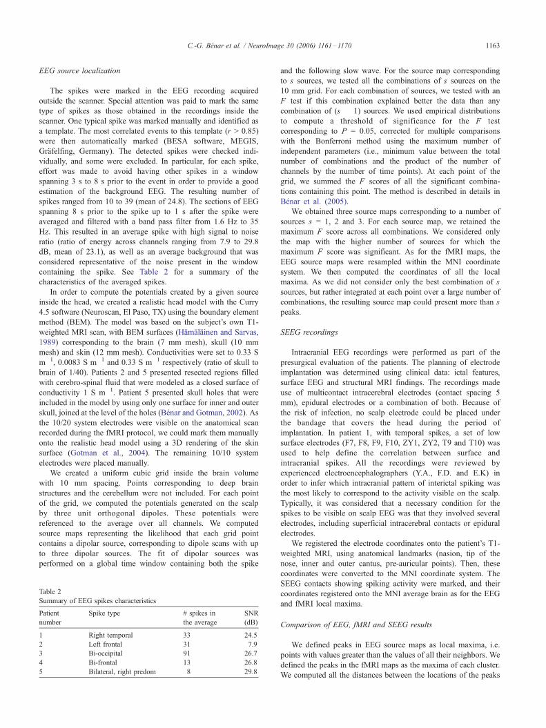
Fig. 1. Comparison of EEG source maps, SEEG findings and fMRI maps for the fi

source maps, three sources were used in the construction of the map for patients 1

all significant combinations of sources, normalized by the total number of combin

yellow, other contacts in orange. Note that the spatial sampling of SEEG is very lim

fMRI maps are very consistent with SEEG findings: when there is an SEEG elect

spiking activity. Some EEG findings do not correspond to fMRI activations: for ex

patient 4 in the left mesial temporal region (z = 137) and in the midline frontal re

peaks: for example, for patient 2 in the midline frontal region (z = 197–202) an

measured the proportion of peaks that could be matched to at least

one peak of the other modality.

For all the local maxima of EEG and fMRI, we computed the

minimum distance to an SEEG contact (with or without spiking

activity) in order to assess whether we had SEEG measurements

in that area. We also computed the minimum distance to an

SEEG contact with spiking activity. For a given distance

threshold D, a local maximum in EEG or fMRI was said to

match SEEG spiking activity if the minimum distance to a

contact with spiking was below D. We computed the ratio of the

ve patients. The main local maxima are indicated with arrows. For the EEG

to 4 and two sources for patient 5; the values are the average F scores across

ations. For the SEEG findings, contacts with spiking activity are shown in

ited. For the fMRI maps, the values are t statistics. The results of EEG and

rode close to an EEG or fMRI peak, then one contact is usually presenting

ample, patient 1 in the right temporal region (z = 129 and z = 154–159) or

gion (z = 182). Conversely, some fMRI findings do not correspond to EEG

d for patient 4 in the left superior frontal region (z = 207).

C.-G. Benar et al. / NeuroImage 30 (2006) 1161–1170 1165

number of peaks that could be matched to SEEG spiking to the

number of peaks that were within a distance D of an intracranial

electrode, whether spiking or not. This means we considered

only the subset of EEG or fMRI peaks located in the vicinity of

an intracranial electrode. Indeed, for the other peaks, no

conclusion could be drawn regarding the match with intracranial

activity.

We assessed the sensitivity of EEG (or fMRI) by measuring the

proportion of spiking SEEG contacts for which there was an EEG

(resp. fMRI) local maximum within a distance D.

Spectral analysis of intracranial EEG data

We identified the SEEG contacts that were within significant

clusters of the fMRI statistical maps, for both positive and

negative fMRI responses. Sections of approximately 1.3 s were

marked around the spikes, with care to include the slow wave

that follows the spike. We used a bipolar reformatting of the

montage in order to estimate local activity. We performed

spectral analysis on each section using a fast Fourier transform

(FFT) of 512 points (2.56 s), starting 0.64 s before the

beginning of the spike and using a Hanning window to limit

edge effects. For each section, we computed the ratio of energy

in the low frequencies (0.5–4 Hz) and in the high frequencies

(20–40 Hz) over the energy in the band 0.5 Hz to 50 Hz. The

bands were chosen to reflect the activity corresponding

primarily to slow waves and to spikes respectively. These

measures were averaged across sections for each channel of

SEEG.

Table 3

EEG, fMRI and SEEG findings

Patient

number

# EEG

peaks

# positive

fMRI peaks

# negative

fMRI peaks

# intracranial

contacts

# spiking

contacts

1 3 1 0 70 13

2 3 14 4 52 13

3 3 0 2 109 14

4 6 9 4 96 7

5 2 8 1 11 11

Results

We will first describe qualitatively the localizations obtained

by fMRI and EEG statistical maps, comparing them to SEEG

findings. We will then establish quantitatively the level of

concordance between these methods and finally show the SEEG

patterns corresponding to positive and negative BOLD

responses.

Localization results

The localization results are presented in Fig. 1 for the five

patients.

Patient 1

The EEG source map presents three peaks, in the right superior

temporal (z = 154–159), right anterior temporal (z = 129) and right

parieto-occipital (z = 164) regions. The first two peaks are in the

vicinity of SEEG contacts with spiking activity at z = 154–159 and

z = 134. In the fMRI map, there is a positive fMRI peak at z = 159,

which is close to the third EEG peak (z = 164). There is no fMRI

cluster that corresponds to the first or second EEG peak. In the

temporal region, this could be due to MR signal loss because of a

susceptibility effect.

Patient 2

The three peaks for the EEG source map (z = 182–187, z =

202–207 and z = 212) are close to the large cyst in the left

hemisphere. The main clusters of positive fMRI response are in the

left superior frontal (z = 202) and midline frontal (z = 197–202)

regions, distinct from the EEG peaks. The negative fMRI findings

are in the left frontal region (z = 182–207) and in the posterior

parietal region (z = 202–212) and correspond well to the peaks of

the EEG source map. All EEG and fMRI peaks correspond well to

SEEG contacts with spiking activity (z = 187–212).

Patient 3

The main peak of the EEG source map is located very deep

mesially in the posterior region (z = 119). This could be artifactual

as we are trying to model a widespread discharge with point

dipoles, and an equivalent dipole located very deep gives a

widespread field. This effect may be emphasized because we are in

a region with low spatial sampling of the EEG. The second EEG

peak is in the midline occipital region (z = 119–124). The third

EEG peak is the subcortical central region (z = 139), which could

be reflecting a central generator or could be again an artifact of a

widespread component of the EEG discharge. The fMRI response

is only negative and is very widespread in the occipital regions

bilaterally (z = 109 to z = 179). This is consistent with the second

EEG peak and the spiking SEEG contacts in both hemispheres (z =

124 and z = 134–139).

Patient 4

The two main peaks of the EEG source map are in the

midline frontal region (z = 182 and z = 187) and are consistent

with the SEEG results at z = 172–187. There are other EEG

peaks located in lower regions: left mesial temporal (z = 127)

and left inferior central (z = 157) regions. The more anterior

peaks are consistent with SEEG, the more posterior cannot be

confirmed by SEEG because there is no electrode in these

regions. The main positive fMRI activation is a large positive

cluster in the left superior frontal region (z = 207), concordant

with activity in SEEG contacts in the same region (z = 207), but

not in correspondence with EEG peaks. There is another fMRI

positive peak at z = 167 in the left parietal region that could be

related to the EEG peak in the left inferior central region (z =

157). The negative fMRI clusters at z = 157 are consistent with

SEEG. There is a diffuse distribution of voxels above the 3.1

threshold on both positive and negative fMRI statistical images in

the inferior brain regions, which are not confirmed by SEEG

recordings and could be artifactual. The fact that there is no clear

fMRI activation that corresponds to the EEG peak in the mesial

temporal region could be due to fMRI signal loss associated with

susceptibility artefacts.

Patient 5

The EEG source map has only one significant combination of

dipoles, which are located deep in the right hemisphere. The fact

that the dipoles are deep could be explained by the widespread

nature of the discharge, as seen on all the epidural SEEG contacts

C.-G. Benar et al. / NeuroImage 30 (2006) 1161–11701166

(z = 166–216). The main fMRI clusters in terms of t value and

extent are positive in the right central region (z = 186–216); they

are consistent with the epidural electrodes at z = 186–196 and z =

Fig. 2. (a) Validation of EEG and fMRI results: percentage of matches between

thresholds from 10 to 100 mm. Only the subset of EEG and fMRI peaks located wi

considered. The percentages of matches are high for thresholds in the range 10

electrode in the vicinity of EEG or fMRI peak, then one contact is often active. (b

fMRI peaks. The percentage of matches is not as high as the matches with EEG or

peak in the vicinity, as well as the converse. (c) Sensitivity of EEG and fMRI: perc

There is no clear difference between the performance of EEG and fMRI. Conside

the results compared to each modality taken separately.

216 but more posterior than the EEG peak at z = 186–191. The

only significant cluster for negative fMRI is in the right parieto-

occipital region, close to midline (z = 176).

EEG and fMRI peaks with SEEG spiking contacts for a set of distance

thin the distance threshold of an SEEG contact (whether spiking or not) was

–30 mm (over 50%, up to 100%), meaning that, when there is an SEEG

) Concordance of EEG and fMRI: percentage of matches between EEG and

fMRI and SEEG. This means that there are some EEG peaks with no fMRI

entage of matches between SEEG spiking contacts and EEG or fMRI peaks.

ring all the modalities together (bottom right corner) significantly improves

C.-G. Benar et al. / NeuroImage 30 (2006) 1161–1170 1167

Concordance between modalities

We studied quantitatively the concordance between fMRI and

EEG statistical maps by counting the number of matches between

EEG and fMRI peaks for a set of distance thresholds D ranging

from 10 mm to 80 mm. We also compared the peaks in EEG and

fMRI to the location of SEEG contacts presenting spiking activity.

Table 3 presents the number of peaks for each patient. As described

above, one patient had only positive fMRI results and one only

negative fMRI results. The three others had both types of fMRI

responses.

We validated the results of EEG statistical source maps by

measuring the percentage of matches between the EEG peaks

and the SEEG contacts presenting spiking activity for a set of

distance thresholds (Fig. 2a). We validated similarly the results

of fMRI maps. We only considered the EEG or fMRI peaks that

were within the distance threshold of an intracranial contact,

whether presenting spiking activity or not. Indeed, EEG or fMRI

peaks that are remote from any SEEG contact cannot be

validated or invalidated. Note that, when the threshold increases,

more peaks are included in the computation, and the proportion

of matches over the number of peaks can decrease. Within a

distance D = 20 mm, there was a mean of 75% of matches for

EEG (number of patients: N = 4), 78.3% for positive fMRI (N =

3) and 100% for negative fMRI (N = 4). For a distance

Fig. 3. Example of SEEG traces for electrode contacts located inside a region of p

Corresponding time–frequency analysis (lower parts of the figures). The trace

concentrated in the low frequencies because of the presence of prominent very sl

threshold of D = 40 mm, the results were 88.3% for EEG (N =

5), 85.4% for positive fMRI (N = 4) and 100% for negative

fMRI (N = 4).

For a given distance threshold, we measured the proportion

of peaks of one modality (EEG, positive fMRI or negative

fMRI) that could be matched to at least one peak of another

modality. That gave us a percentage of matches for the first

modality with respect to the second as a function of the distance

threshold.

The results for the concordance between EEG and fMRI results

are shown in Fig. 2b. For a threshold of D = 20 mm, there was a

mean percent of matches across patients of 16.7% for EEG versus

positive fMRI (N = 4), 20.8% for EEG versus negative fMRI (N =

4), 30.6% for positive fMRI versus EEG (N = 4) and 20.8% for

negative fMRI versus EEG (N = 4). For a threshold of D = 40 mm,

the mean percentage of matches increased to 62.5% for EEG

versus positive fMRI, 58.3% for EEG versus negative fMRI, 50%

for positive fMRI versus EEG and 47.9% for negative fMRI versus

EEG.

We assessed the sensitivity of EEG and fMRI by measuring the

percentage of the SEEG contacts presenting spiking activity that

could be matched with EEG or fMRI peaks (Fig. 2c). Within D =

20 mm, there was 20.3% of matches on average with EEG (N = 5),

11.3% with positive fMRI (N = 4) and 21.3% with negative fMRI

(N = 4). For D = 40 mm, the average matches were of 68.5% for

ositive (a, b) or negative (c, d) fMRI response (upper parts of the figures).

s corresponding to positive fMRI responses have most of their energy

ow waves.

C.-G. Benar et al. / NeuroImage 30 (2006) 1161–11701168

EEG, 56% for positive fMRI and 59.3% for negative fMRI. When

considering all the modalities (EEG, positive fMRI and negative

fMRI) together, the average percentage of matches was 34% within

D = 20 mm (N = 5) and 86.9% within D = 40 mm.

Electrophysiological correlates of negative and positive fMRI

responses

In order to assess if particular EEG activities were related to

specific fMRI responses, we identified intracerebral contacts with

spiking activity that were within fMRI-activated areas. We

performed spectral analysis of the corresponding SEEG time

course (Fig. 3). We computed the energy in two frequency bands:

0.5 to 4 Hz and 20 to 40 Hz, normalized with respect to the total

energy in the 0.5 to 50 Hz band, in order to investigate the activity

corresponding to the slow waves and to the spikes respectively. We

observed a higher normalized energy in the low frequencies for the

traces corresponding to positive fMRI responses in comparison to

those corresponding to negative responses (Fig. 4a). The difference

in the mean energy over SEEG electrodes was highly significant

(P < 10�5). This finding probably originates from the presence of

very slow waves in the traces corresponding to positive BOLD

(Figs. 3a and b, upper traces). For high frequencies, the difference

in the mean energy was not significant, although a trend could be

observed (Fig. 4b).

Fig. 4. Results of frequency analysis of the SEEG. Proportion of energy in

the low frequencies (0.5–5 Hz) (a) and high frequencies (20–40 Hz). For

contacts located inside regions of negative fMRI signal changes (blue), the

energy is more concentrated in the low frequencies than for contacts located

inside regions of positive fMRI signal changes (red).

Discussion

Whereas considerable work has been done on quantifying the

relationship between fMRI signal changes and invasive electro-

physiology in animals (Disbrow et al., 2000; Logothetis et al.,

2001), there is little corresponding work in humans. We propose a

quantitative comparison of fMRI responses to (1) epileptic

discharges in the intracranial EEG and (2) the results of a novel

source analysis method for scalp EEG. We assessed the level of

correspondence between sets of fMRI, EEG and SEEG examina-

tions in a series of five patients presenting epileptic spikes. All

results should be viewed in light of our knowledge of the spatial

resolution of each technique.

The fMRI BOLD signal at 1.5 T originates mainly from

relatively large veins that drain the neuronally activated area (Lai et

al., 1993). Following the calculations of Turner (2002), an

activated area of 6 cm2 could lead to a BOLD signal change at a

distance of approximately 10 mm from the region of neuronal

activity. Imprecision in EEG source localization can originate from

the ill-posed nature of the problem, from errors in the head and

source models, from low spatial sampling on the head (i.e. low

number of electrodes) and from noise arising from background

neuronal activity. Mean errors reported for dipole source localiza-

tion of focal sources are in the range of 10 to 20 mm (Baillet, 2001;

Krings et al., 1999). Merlet and Gotman have specifically

compared the location of dipole models fitted on epileptic spikes

to that of the intracerebral electrode of maximum activity, using 28

scalp electrodes. They found a mean distance of 11 T 4.2 mm, with

a spherical head model (Merlet and Gotman, 1999). The SEEG

electrodes, in turn, are maximally sensitive to the electrical activity

in their immediate vicinity, as a result of the quadratic decay of the

field with distance.

With these limitations in mind, SEEG measures largely

validated the results of EEG and fMRI. Indeed, when there is an

intracerebral or epidural electrode in the vicinity of an EEG or

fMRI peak (in the range 20–40 mm), it usually includes one active

contact. However, within a distance of 20 mm, the average

percentages of matches between fMRI peaks (positive or negative)

and intracranial EEG were better than those between EEG source

localization and SEEG. This could be due to the limitations of the

dipole model for representing extended regions of active cortex.

Distributed source models (Hamalainen and Ilmoniemi, 1994;

Pascual-Marqui et al., 1999) might give more accurate localizing

results in these cases.

Still, EEG dipoles identified regions that were not shown

in fMRI and vice versa. This is reflected in the results of the

concordance between EEG and fMRI that were not as good

as the concordance between either of these non-invasive

techniques and SEEG. In particular, there were two instances

of basal temporal peaks in EEG not present in fMRI (Patients

1 and 4). This could be due to signal loss caused by

magnetic field inhomogeneities near the boundaries between

tissues with very different magnetic susceptibilities, which

represents a limitation of EPI-based fMRI acquisitions (Oje-

mann et al., 1997). The converse situation is also observed. For

example, for patient 2, the fMRI results identify midline activity at

the level of the supplementary motor area, whereas EEG activity

was restricted to regions around the large cyst. This could be

because EEG is less sensitive to deep discharges or because of the

presence of bilateral medial discharges that would cancel each

other out.

C.-G. Benar et al. / NeuroImage 30 (2006) 1161–1170 1169

Results on the sensitivity of the different methods to the

presence of SEEG spiking activity show that considering EEG

and fMRI together significantly increases the chances of detecting

the active regions. This is to be noted as fMRI is considered to

have higher localizing capacities than EEG—it is usually the

temporal abilities of EEG that are emphasized. A common

expectation is that fMRI can bring spatial localization of neuronal

activity, whereas EEG and MEG have the capacity to bring

millisecond timing information. Our results raise two issues in

this respect.

First, the examples of discordance suggest that one should be

very cautious when attempting to integrate fMRI findings in the

solution of the EEG inverse problem. In particular, strictly

enforcing a one-to-one correspondence between dipoles and fMRI

activated areas could be detrimental to the solution. Indeed, a

spurious EEG source placed in an fMRI-activated region will

wrongfully explain a part of the EEG signal. Conversely, the

possibility of a source in a region with no fMRI activation should

be probed (Ahlfors et al., 1999).

Second, even when peaks are concordant, they do not match

perfectly (i.e. within 10 mm). This is consistent with observations

in monkeys of a mean error of 1 cm between unmatched

electrophysiological measures and fMRI centroids (45% of the

cases) (Disbrow et al., 2000). This imprecision implies that it can

be difficult to establish exactly the correspondence between

regions activated in the two modalities. Bayesian methods, which

can incorporate knowledge on fMRI signal generation or effect of

head model errors, could be of help in that sense (Trujillo-Barreto

et al., 2001). A model based on such a priori knowledge would

permit to assess if one neuronally activated area could give rise to

regions activated differently in EEG and fMRI.

We found that, in our series of patients, the negative fMRI

responses could be as important in understanding the complete

picture of activity as the positive fMRI results. For example, for

patient 3, we observed only negative fMRI results and, for patient

2, the regions with negative fMRI were very consistent with EEG

findings. This is an important finding as the series reported so far

for EEG–fMRI of partial epilepsy have concentrated on the

positive fMRI findings (Al-Asmi et al., 2003; Krakow et al., 1999;

Lazeyras et al., 2000; Patel et al., 1999). This also suggests another

complementary aspect of fMRI with respect to EEG: the fMRI

results may shed light on the metabolic aspects of the interictal

spikes. As an example of this, we have shown that the differences

in positive and negative responses correlated with the low

frequency content of the SEEG traces. This could mean that slow

waves are an important factor in terms of the energy requirements

of the neurons involved in epileptic discharges.

We observed a higher proportion of energy in the low

frequencies for the SEEG recorded in regions with positive fMRI

response. This is somewhat counter-intuitive as slow waves

occurring during interictal discharges are thought to reflect

inhibitory potentials. However, inhibitory post-synaptic potentials

consume energy, and the positive BOLD could reflect increased

metabolism and blood flow corresponding to large slow waves

reflecting profound inhibition. For smaller slow waves, the

decrease in metabolism induced by moderate inhibition could

predominate over the increase in energy required for that

inhibition, thereby leading to negative BOLD response (Stefanovic

et al., 2004).

In conclusion, fMRI is a new source of information in the study

of epileptic discharges. It appears to provide information that is

complementary to scalp EEG in the localization of the sources of

epileptic discharges. The analysis of intracerebral EEG recordings

at the location of fMRI changes may help to elucidate the neuronal

correlates of the metabolic changes measured by fMRI.

References

Aghakhani, Y., Bagshaw, A.P., Benar, C.G., Hawco, C., Andermann, F.,

Dubeau, F., et al., 2004. fMRI activation during spike and wave

discharges in idiopathic generalized epilepsy. Brain 127, 1127–1144.

Ahlfors, S.P., Simpson, G.V., Dale, A.M., Belliveau, J.W., Liu, A.K.,

Korvenoja, A., et al., 1999. Spatiotemporal activity of a cortical

network for processing visual motion revealed by MEG and fMRI.

J. Neurophysiol. 82, 2545–2555.

Al-Asmi, A., Benar, C.G., Gross, D.W., Khani, Y.A., Andermann, F., Pike,

B., et al., 2003. fMRI activation in continuous and spike-triggered

EEG–fMRI studies of epileptic spikes. Epilepsia 44, 1328–1339.

Archer, J.S., Abbott, D.F., Waites, A.B., Jackson, G.D., 2003. fMRI

‘‘deactivation’’ of the posterior cingulate during generalized spike and

wave. NeuroImage 20, 1915–1922.

Bagshaw, A.P., Aghakhani, Y., Benar, C.G., Kobayashi, E., Hawco, C.,

Dubeau, F., et al., 2004. EEG–fMRI of focal epileptic spikes: analysis

with multiple haemodynamic functions and comparison with gadolin-

ium-enhanced MR angiograms. Hum. Brain Mapp. 22, 179–192.

Bagshaw, A.P., Hawco, C., Benar, C.G., Kobayashi, E., Aghakhani, Y.,

Dubeau, F., et al., 2005. Analysis of the EEG–fMRI response to

prolonged bursts of interictal epileptiform activity. NeuroImage 24,

1099–1112.

Baillet, S., 2001. Electromagnetic brain mapping. IEEE Signal Process.

Mag. 18, 14–30.

Benar, C.G., Gotman, J., 2002. Modeling of post-surgical brain and skull

defects in the EEG inverse problem with the boundary element method.

Clin. Neurophysiol. 113, 48–56.

Benar, C.G., Gunn, R.N., Grova, C., Champagne, B., Gotman, J., 2005.

Statistical maps for EEG dipolar source localization. IEEE Trans.

Biomed. Eng. 52, 401–413.

Collins, D.L., Neelin, P., Peters, T.M., Evans, A.C., 1994. Automatic 3D

intersubject registration of MR volumetric data in standardized

Talairach space. J. Comput. Assist. Tomogr. 18, 192–205.

Disbrow, E.A., Slutsky, D.A., Roberts, T.P., Krubitzer, L.A., 2000.

Functional MRI at 1.5 tesla: a comparison of the blood oxygenation

level-dependent signal and electrophysiology. Proc. Natl. Acad. Sci.

U.S.A. 97, 9718–9723.

Goldman, R.I., Stern, J.M., Engel Jr., J., Cohen, M.S., 2002. Simultaneous

EEG and fMRI of the alpha rhythm. NeuroReport 13, 2487–2492.

Gotman, J., Benar, C.G., Dubeau, F., 2004. Combining EEG and FMRI in

epilepsy: methodological challenges and clinical results. J. Clin.

Neurophysiol. 21, 229–240.

Hamalainen, M.S., Ilmoniemi, R.J., 1994. Interpreting magnetic fields of

the brain: minimum norm estimates. Med. Biol. Eng. Comput. 32,

35–42.

Hamalainen, M.S., Sarvas, J., 1989. Realistic conductivity geometry model

of the human head for interpretation of neuromagnetic data. IEEE

Trans. Biomed. Eng. 36, 165–171.

Hoffmann, A., Jager, L., Werhahn, K.J., Jaschke, M., Noachtar, S., Reiser,

M., 2000. Electroencephalography during functional echo-planar

imaging: detection of epileptic spikes using post-processing methods.

Magn. Reson. Med. 44, 791–798.

Ives, J.R., Warach, S., Schmitt, F., Edelman, R.R., Schomer, D.L., 1993.

Monitoring the patient’s EEG during echo planar MRI. Electro-

encephalogr. Clin. Neurophysiol. 87, 417–420.

Krakow, K., Woermann, F.G., Symms, M.R., Allen, P.J., Lemieux, L.,

Barker, G.J., et al., 1999. EEG-triggered functional MRI of interictal

epileptiform activity in patients with partial seizures. Brain 122 (Pt. 9),

1679–1688.

C.-G. Benar et al. / NeuroImage 30 (2006) 1161–11701170

Krings, T., Chiappa, K.H., Cuffin, B.N., Cochius, J.I., Connolly, S.,

Cosgrove, G.R., 1999. Accuracy of EEG dipole source localization

using implanted sources in the human brain. Clin. Neurophysiol. 110,

106–114.

Lai, S., Hopkins, A.L., Haacke, E.M., Li, D., Wasserman, B.A., Buckley, P.,

et al., 1993. Identification of vascular structures as a major source of

signal contrast in high resolution 2D and 3D functional activation

imaging of the motor cortex at 1.5T: preliminary results. Magn. Reson.

Med. 30, 387–392.

Lazeyras, F., Blanke, O., Perrig, S., Zimine, I., Golay, X., Delavelle, J.,

et al., 2000. EEG-triggered functional MRI in patients with pharmaco-

resistant epilepsy. J. Magn. Reson. Imaging 12, 177–185.

Lemieux, L., Krakow, K., Fish, D.R., 2001. Comparison of spike-triggered

functional MRI BOLD activation and EEG dipole model localization.

NeuroImage 14, 1097–1104.

Logothetis, N.K., Pauls, J., Augath, M., Trinath, T., Oeltermann, A., 2001.

Neurophysiological investigation of the basis of the fMRI signal. Nature

412, 150–157.

Merlet, I., Gotman, J., 1999. Reliability of dipole models of epileptic

spikes. Clin. Neurophysiol. 110, 1013–1028.

Michel, C.M., Murray, M.M., Lantz, G., Gonzalez, S., Spinelli, L., Grave

de Peralta, R., 2004. EEG source imaging. Clin. Neurophysiol. 115

(10), 2195–2222.

Nunez, P.L., Silberstein, R.B., 2000. On the relationship of synaptic activity

to macroscopic measurements: does co-registration of EEG with fMRI

make sense? Brain Topogr. 13, 79–96.

Ogawa, S., Tank, D.W., Menon, R., Ellermann, J.M., Kim, S.G., Merkle,

H., et al., 1992. Intrinsic signal changes accompanying sensory

stimulation: functional brain mapping with magnetic resonance imag-

ing. Proc. Natl. Acad. Sci. U. S. A. 89, 5951–5955.

Ojemann, J.G., Akbudak, E., Snyder, A.Z., McKinstry, R.C., Raichle, M.E.,

Conturo, T.E., 1997. Anatomic localization and quantitative analysis of

gradient refocused echo-planar fMRI susceptibility artifacts. Neuro-

Image 6, 156–167.

Pascual-Marqui, R.D., Lehmann, D., Koenig, T., Kochi, K., Merlo, M.C.,

Hell, D., et al., 1999. Low resolution brain electromagnetic tomography

(LORETA) functional imaging in acute, neuroleptic-naive, first-episode,

productive schizophrenia. Psychiatry Res. 90, 169–179.

Patel, M.R., Blum, A., Pearlman, J.D., Yousuf, N., Ives, J.R., Saeteng, S.,

1999. Echo-planar functional MR imaging of epilepsy with concurrent

EEG monitoring. Am. J. Neuroradiol. 20, 1916–1919.

Seeck, M., Lazeyras, F., Michel, C.M., Blanke, O., Gericke, C.A., Ives, J.,

et al., 1998. Non-invasive epileptic focus localization using EEG-

triggered functional MRI and electromagnetic tomography. Electro-

encephalogr. Clin. Neurophysiol. 106, 508–512.

Speckmann, E.J., Elger, C.E., 1999. Introduction to the neurophysiological

basis of the EEG and DC potentials. Electroencephalography: Basic

Principles, Clinical Applications, and Related Fields, (forth edR).

Stefanovic, B., Warnking, J.M., Pike, G.B., 2004. Hemodynamic

and metabolic responses to neuronal inhibition. NeuroImage 22,

771–778.

Trujillo-Barreto, N.J., Martınez-Montes, E., Melie-Garcıa, L., Valdes-Sosa,

P.A. A symmetrical Bayesian model for fMRI and EEG/MEG neuro-

image fusion. Int Journ Bioelectromag 2001; 3. url:http://www.ijbem.

org/volume3/number1/valdesosa/index.htm.

Turner, R., 2002. How much cortex can a vein drain? Downstream dilution

of activation-related cerebral blood oxygenation changes. NeuroImage

16, 1062–1067.

Warach, S., Ives, J.R., Schlaug, G., Patel, M.R., Darby, D.G., Thangaraj, V.,

et al., 1996. EEG-triggered echo-planar functional MRI in epilepsy.

Neurology 47, 89–93.

Worsley, K.J., Liao, C.H., Aston, J., Petre, V., Duncan, G.H., Morales, F.,

et al., 2002. A general statistical analysis for fMRI data. NeuroImage

15, 1–15.