AIChE Paper Number 39f

USE OF PROCESS SIMULATION IN ETHYLENE PLANT ADVANCED CONTROL AND OPTIMIZATION

Akitoshi Takinami, Ayumu Fujita, Takeshi Seki, Youichi Takeuchi

Showa Denko K.K. Oita, Japan

Soichi Iwamoto, Tomoo Niikura

Yamatake Corp. Kanagawa, JAPAN

Paul Yap and Ravi Nath Honeywell Process Solutions

Singapore and Houston, TX, USA

Prepared for Presentation at the 2011 Spring National Meeting, Chicago, IL

March 13-17, 2011

AIChE and the EPC shall not be responsible for statements or opinions contained in papers or printed in its publications.

USE OF PROCESS SIMULATION IN ETHYLENE PLANT ADVANCED CONTROL AND OPTIMIZATION

Akitoshi Takinami, Ayumu Fujita, Takeshi Seki, Youichi Takeuchi

Showa Denko K.K. Oita, Japan

Soichi Iwamoto, Tomoo Niikura

Yamatake Corp. Kanagawa, JAPAN

Paul Yap and Ravi Nath Honeywell Process Solutions

Singapore and Houston, TX, USA

ABSTRACT

Showa Denko owns and operates a large Ethylene plant in Oita, Japan. Depending on the economic environment, plant objective is a combination of Energy Efficiency and Production Capacity. In order to achieve these objectives, Showa Denko had contracted Yamatake and Honeywell to design, configure and commission Advanced Control and Optimization (ACO) on the Ethylene Plant. The project was completed in 2002 and the ACO applications have been continuously operational for the last decade. The solution at Showa Denko comprises multiple multivariable Model Predictive Controllers (MPC) and a Dynamic Optimizer. The Dynamic Optimizer is a layer above the MPC and inherits the models from MPC and thus maintains a complete consistency between MPC and the Optimizer. As is customary, the MPC models are linear and dynamic. Since the optimizer inherits the controller models, the optimizer model is also linear and dynamic. Certain parts of the process especially the cracking reactions however are highly non-linear, where a linear model would not be adequate. A strategy for incorporating the process non-linearities is to continuously update non-linear gains in the ACO applications. A gain updating strategy was designed and successfully implemented. The original gain updating strategy utilized custom calculations and a custom interface to Technip’s Spyro. Since the initial commissioning, Showa Denko has continued to enhance the ACO applications. Additional variables that accounted for all major energy usage were added. Gain updating for all major energy variables was also added. The operator workflow was made more effective by

• a hierarchy of displays in Japanese language,

• a continuous display of active bottlenecks, and • daily optimization reports.

In 2010, Showa Denko added two MPCs for a newly commissioned cracking furnace and a new Quench system. The development of MPC was significantly simplified by use of Honeywell’s Profit Stepper. Concurrently, Showa Denko contracted Yamatake and Honeywell to convert the custom calculations and custom interface to Spyro for gain updating by a standard methodology that uses a commercially available Process Simulator. Major advantage of this approach is that the ACO applications can now be more easily maintained and enhanced by Showa Denko. This paper summarizes the existing Advanced Control and Optimization solution at Showa Denko and discusses the details of the gain updating strategy that was recently implemented.

INTRODUCTION

Showa Denko KK (SDK), a diversified group of manufacturing companies owns and operates a large olefins complex in Oita, Japan. The main products from the olefins complex include ethylene, propylene and cracked gasoline. Ethylene and propylene products are primarily used internally for production of derivatives and polymers. The Oita Ethylene complex cracks a variety of feed stocks including C2s, C3s, C4s, LPG and Naphthas. In general, the operation of Ethylene plants is a challenging task because of the following complicating factors;

• A mix of fast ands slow Process dynamics • Frequent Feed quality and product demand variations, • Frequent operations disturbances • Multiple interacting tradeoffs

In addition, Ethylene producers in Japan face additional challenges due to a shrinking domestic economy, fierce competition from emerging Asian producers and government edict to reduce CO2 emissions. Showa Denko has dealt with these challenges by use of Honeywell’s Advanced Control and Optimization solution. Section I below gives a brief description of the process; it is followed by a discussion of the process characteristics in section II and a discussion of degrees of freedom in section III. Section IV describes Honeywell’s ACO solution in general terms and compares them to the traditional ACO solution. Section V discusses the particulars of implementation of the ACO solution at Showa Denko.

I. PROCESS DESCRIPTION

Showa Denko K. K.’s Olefins Plant in Oita was started up in 1969 and has expanded over the years. The current Ethylene production capacity is 672 thousand metric tonnes per year. The Ethylene and propylene products are consumed by the downstream plants with some exported; however there is only limited intermediate storage capacity for these products. Depending on the business cycle, the demand for the olefins products varies significantly. The original ethylene facility comprised two parallel olefins production trains: No. 1 and No. 2. However the present configuration is that of a single train which comprises the following process units:

• Feed system, No. 1 cracking Furnaces and No. 2 cracking furnaces • 3 Quench Systems

• Cracked Gas Compressor • Condensate Stripper • Dryer, Cold Box, Prefractionator, Demethanizer and Ethylene Refrigeration System

• 2 Deethanizers • 3 Acetylene Converter Units • 3 Ethylene Fractionators and Propylene Refrigeration System • 2 Depropanizer • 3 Propylene Fractionators

• Debutanizer • Depentanizer, and • Rerun tower

Figure 1 shows an overview of the process, each of the process areas are briefly discussed below.

FURNACES AND FEED SYSTEM

There are a total of 15 furnaces of four different geometries. The furnaces crack a variety of feedstock including ethane, propane, butane, LPG, and Naphthas. There is a complex arrangement of piping that connects the feedstock to the furnaces. Most feed arrives by tankers while some arrives by pipeline. There is a furnace effluent analyzer that cycles between the furnaces.

QUENCH SYSTEM

The quench system comprises oil quench and water quench towers. A gasoline blend is separated as a product from the quench system. Fuel Oil byproduct is also produced.

CRACKED GAS COMPRESSION (CGC)

The CGC consists of four compression stages with inter-stage knockout drums and cooling water exchangers. The compressor is driven by a turbine. A C3s and heavier stream is recovered from the bottoms of the condensate stripper and sent to the Depropanizers.

DRYER, PREFRACTIONATOTR, DEMETHANIZER AND ETHYLENE REFRIGERATION SYSTEM

Cracked gas from the cracked gas compressor fourth stage is dried and fed to the pre-fractionator tower. Overhead from the tower goes to the Demethanizer and the bottoms goes to the Deethanizer towers. The tower is reboiled with propylene refrigerant vapors. The methane and hydrogen-rich overhead stream is partially condensed in the cold box via ethylene and propylene refrigerants and the Joule-Thompson Effect.

DEETHANIZER

The bottom stream from the Pre-fractionator enters the two Deethanizers. The towers are reboiled with utility steam. The condenser uses propylene from the suction drum of the propylene refrigeration compressor to partially condense the overhead product.

ACETYLENE CONVERTER UNITS

Deethanizer overhead streams along with the Demethanizer bottoms streams go to the three Acetylene Converter Units for removal of Acetylene impurity by hydrogenation.

ETHYLENE FRACTIONATORS, PROPYLENE REFRIGERATION

Effluent streams form the Acetylene Converter Units are the feed to the three Ethylene Fractionators. Each of these towers is a super-fractionator with a pasteurization section. It is reboiled with medium pressure propylene refrigerant. The overhead condenser uses low pressure propylene refrigerant. A vent stream off the reflux drum is used to purge hydrogen and methane back to the CGC. When producing directly to the pipeline instead of storage, energy is recovered from the product by the propylene refrigeration system. When producing to storage additional cooling is required to condense the product for storage, in which case the propylene refrigeration system can become overloaded and rates may be lowered. Ethane from the bottoms is recycled back to the furnaces.

DEPROPANIZERS

There are two depropanizers, each comprises two towers, the rectifying tower is operated at higher pressure, while the stripping tower is operated at lower pressure to minimize polymer formation. There are two feeds to a Depropanizer - one from the Deethanizer bottoms, and

the other from the Condensate Stripper. The tower is reboiled with utility steam and condensed with propylene from the suction drum of the propylene refrigeration compressor.

MAPD CONVERTER UNITS

Overhead streams from the depropanizers go to two MAPD Converter Units to hydrogenate Methyl Acetylene and Propadiene impurities.

PROPYLENENE FRACTIONATORS

Effluent streams form the MAPD Converter Units are the feed to the three Propylene Fractionators. Each of these towers is reboiled with quench water waste heat. The overhead condenser uses sea water. Polymer grade propylene product from the overhead is send to the consuming processes and propane from the bottoms is recycled back to the furnaces.

DEPENTANIZER

The Depropanizer bottoms enter the Depentanizer that is reboiled with utility steam and condensed with cooling water. The bottoms gasoline product is sent to the Rerun tower for further processing.

DEBUTANIZER

The Depentanizer overhead stream enters the Debutanizer that is reboiled with utility steam and condensed with cooling water. The overhead C4s and bottoms C5s streams are sent to OSBL.

RERUN TOWER

The Depentanizer bottoms enter the Rerun tower that is reboiled with utility steam and condensed with cooling water. The overhead gasoline product is sent to OSBL hydrotreater for further processing. The bottoms stream is recycled back to the Quench Oil tower.

II. PROCESS CHARACTERISTICS Olefins Plants in general have some unique characteristics that have a strong bearing on the optimizer design. These are:

SEMI-CONTINUOUS OPERATION OF FURNACES AND DRYERS

Coke is a byproduct of thermal cracking of hydrocarbons, it accumulates on the inside of the tubes in the furnace and ultimately limits selectivity. Cracking furnaces are therefore periodically decoked. Decoking operation however causes a huge disturbance in the operation of an ethylene plant. For the Oita plant with 15 furnaces, this disturbance occurs once a week on an average.

The dryers situated at the back end of the Charge Gas Compressor are switched frequently which causes a short but significant disturbance in the flow to the cold side of the plant.

FEED QUALITY VARIATIONS

For the Oita plant, business opportunities offered by free market means that there usually is significant variability in quality of feed stock. This also results in significant operations disturbances. On an average, significant feed quality disturbances occur twice a week.

PRODUCT DEMAND VARIATION

Showa Denko’s Oita plants produces ethylene majority of which is consumed by the downstream polymer or derivatives plants, however there is limited product storage capacity. Therefore any significant swing in the ethylene demand by the downstream plants requires a corresponding change in the operation of the plant.

On the whole, semi-continuous operation of the furnaces and dryers, frequent feed quality and product demand variations result in a process that is very dynamic and seldom at steady state. Dynamic operating environment of the plant is an important consideration in the use of a dynamic optimizer for the ethylene plant.

III. DEGREES OF FREEDOM

Optimization of the operations of an Ethylene plant is complicated as there are multiple, interacting tradeoffs at work. The following are some of the significant ones; Feed availability Feed cost Feed quality Olefins production Furnace capacity Furnace severity Olefins yield Furnace run-length

Furnace Energy Olefins yield CGC suction pressure CGC Energy

Column capacity Column Recoveries Column Energy In general, higher quality feeds, yield more ethylene but cost more. Olefins yield increases by increasing the cracking severity but it adversely impacts the furnace run-length and furnace energy consumption. Ethylene yield increases by decreasing the CGC suction pressure but at the cost of increased CGC energy consumption. Column capacity increases by increasing energy flow in the column, or by backing off on component recoveries. These tradeoffs are made by a careful optimization of the degrees of freedom which include the following; For each furnace: Feed rate, Feed mix, Cracking severity, and Dilution Steam flow.

For each columns Overhead purity,

Bottoms purity, and Column operating pressure.

For each multistage compressors: First stage suction pressure.

IV. SOLUTION TECHNOLOGY Honeywell’s Advanced Control and Optimization (ACO) solution comprises the following elements;

• Multiple Profit Controllers with embedded gain mappers for multivariable Model Predictive Control (MPC)

• A Profit Optimizer with embedded gain mapper for dynamic Real Time Optimization (RTO)

• A UniSim Design model for computation of inferentials and derivatives, and • A Profit Bridge application for Real Time execution of the UniSim Design model for gain

extraction

Each of the solution elements is discussed below. MPC TECHNOLOGY

Multivariable Model Predictive Control (MPC) refers to a class of control algorithms in which dynamic process models are used to predict and control a process. MPC is well suited for high performance control of constrained multivariable processes because explicit pairing of Controlled Variables (CV) and Manipulated Variables (MV) is not required and constraints are directly imbedded in the problem formulation. We will discuss two MPC approaches here. First the traditional approach which is available from a number of vendors, and then a unique robust approach that has been embodied in Honeywell's Profit Controller.

Traditional MPC Technology

Traditional MPC attempts to keep all process CVs at their target values. A CV target value could be a setpoint or could be a zone. Setpoint applies to a regulatory CV, and zone applies to a constrained CV. Reference trajectory is a specified transition path for a CV. In addition, MPC formulation may also allow for weighing of MVs to convey a sense of preference among the various MVs. MPC problem can be represented as the following minimization problem [1]:

( )[ ]∑=∆

∆+−h

i

MVe

MV

iMVWiVCirW1

22

)()()(min)

subject to

UL CViVCCV << )()

UL MViMVMV << )(

UL MViMVMV ∆<∆<∆ )(

where

i discretized time

h control horizon

We CV weight

WMV MV weight

r(i) CV target: setpoint or reference trajectory

)(iVC)

CV prediction

)(iMV∆ MV moves

Profit Controller MPC Technology

CONTROLLER ROBUSTNESS

One drawback in conventional MPC technology is that it requires specification of CV reference trajectories for constrained CVs. Reference trajectories are typically set equal to the steady state targets and are not dynamically optimum and are often dynamically infeasible and would result in excessive MV movements without additional move suppression. Honeywell's Profit Controller removes this requirement. Honeywell's patented Robust MPC Technology is called RMPCT.

Profit Controller employs Honeywell's patented funnel design [2] in its problem formulation that enables a simultaneous determination of both the MV moves and the CV reference trajectories. RMPCT's solution procedure is called the Range Control Algorithm (RCA) and in matrix notation is as follows [3]:

( )[ ]2

,min yAxW

yx

− (1)

subject to CVL ≤ y ≤ CVH

MVL ≤ Sx ≤ MVH

∆MVL ≤ x ≤ ∆MVH

where A is the process dynamic matrix W is a user-specified diagonal weighting matrix S accumulating sum matrix for MV moves x control solution in terms of MV moves, and y CV response trajectories.

For practical applications, there usually are an infinite number of solutions to (1). In RMPCT, a minimum effort solution is sought which means minimum movement to the process. The minimum effort solution brings a significant robustness to the control solution. This treatment of robustness differs from the standard robust control design in that the control robustness is gained from the freedom provided by CV high/low bounds and not by specification of model uncertainty.

UNIT OPTIMIZATION

When there are degrees of freedom (DOF) remaining in a controller, a steady-state objective function could be defined. The objective function in general can be linear, quadratic, or a combination of the two. For most applications, a steady-state quadratic objective (2) is versatile enough, which is the default objective function form in Profit Controller.

J c x c y x x x x y y y yxt

ss yt

ss ss ot

x ss o ss ot

y ss o= + + − − + − −( ) ( ) ( ) ( )D D (2)

subject to CVL ≤ yss ≤ CVH

MVL ≤ xss ≤ MVH

where J is the unit optimization cost objective function cx is MV cost coefficient cy is CV cost coefficient xss is MV steady state value yss is CV steady state value xo the MV desired value yo the CV desired value Dx is the cost of deviating from MV desired value Dy is the cost of deviating from CV desired value

The steady-state optimization problem (2) defines a new economically optimal “setpoint” and can be solved separately from dynamics of the control system without sacrificing any rigor.

Solution to (2) is xsso

.

COMBINED CONTROL AND DYNAMIC UNIT OPTIMIZATION

In Profit Controller, the complete unit dynamic optimization is solved as an augmentation of (2) to (1) as shown below [4];

min,x y ss

ox

y

x

W 0

0 W

A

S0

2

−

(3)

subject to CVL ≤ y ≤ CVH

MVL ≤ Sx ≤ MVH

∆MVL ≤ x ≤ ∆MVH

where 0W is a user-specified diagonal weight for tuning optimization speed

Profit Controller not only solves for the steady-state optimum, but also determines the trajectory of ‘how to get there’ while handling the control tasks currently at hand. This trajectory is a combination of control response and economic optimization path. Thus Profit Controller unifies the control and optimization problems.

Note also that xsso

does not have to come from (2). If xsso

comes from a plant-wide optimization solution, (3) can achieve a plant-wide optimization dynamically. This is exactly how Profit Optimizer integrates with Profit Controller.

ON THE FLY GAIN UPDATING

Unlike, traditional MPC, Profit Controller allows “on the fly” gain updating; that is the controller gains can be changed at any time without stopping or reinitializing the controller. This is a very powerful capability as it makes application of Profit Controller possible for non-linear areas of the process, such as the cracking furnaces. RTO TECHNOLOGY

Functionally, Real Time Optimization (RTO) is a supervisory layer on top of existing process controllers. RTO continuously strives to maintain the plant operating conditions at the most profitable point. In order to achieve this functionality, an RTO system must have the following three capabilities; 1. way to assess its current state (State Estimation), 2. way to determine the optimum state (Optimum State),

3. way to determine a path from the current to the optimum (Dynamic Path). Next we discuss the above mentioned three capabilities. State Estimation: refers to the determination of the current state of the system. The plant is a dynamic entity with all manners of disturbances, fast and slow dynamic responses, inverse and delayed responses. This means that a "snapshot" of process data gives an incomplete and sometimes incorrect view. A complete assessment of current state requires analysis of process history. State estimation defines both where the plant is right now as well as where it is expected to be in the future. Optimum State: refers to the determination of the steady state optimum point. For a system described by a set of algebraic equations, there are useful mathematical tools such as linear algebra and optimality theorems. The task then is to describe the reality of the plant operation into a set of algebraic equations. Having defined the equations finding the optimum can be via well established mathematical algorithms. Dynamic Path: refers to the path to be taken in going from the current state to the optimum state. In general a multitude of paths exist and the most direct path may not necessarily be the best path and it may not even be feasible for a process with dynamic interactions. Next we will analyze two approaches to RTO and their suitability to the problem in hand. First the traditional approach (first principles, steady state Equation Based Optimization) is discussed. Then a unique dynamic optimization approach that is embodied in Honeywell's Profit Optimizer will be discussed.

Traditional RTO

Traditionally, RTO has been formulated as an extension of steady state simulation. The process is represented by steady state heat, material, and sometimes momentum balances. Mathematically, the model comprises a massive set of "sparse" algebraic equations that are amenable to optimum state algorithms, such as Successive Quadratic Programming (SQP). Traditional RTO formulations for an ethylene process may have several hundred thousand variables. Obviously, this large problem size would require significant amount of compute time. For details of the traditional RTO approach refer to [5, 6].

AN EVALUATION

This section evaluates traditional RTO with respect to the above mentioned three capabilities:

State Estimation: Traditional RTO requires a rigorous fitting of steady state process model to current plant conditions using data reconciliation and parameter estimation. Determining an accurate current state to update these steady state models is problematic for a dynamic process such as the one under consideration as it is seldom at steady state. In practical terms

this becomes a tuning issue as to what constitutes a steady state. There are two extremes: 1) strict criteria for steady state which could mean a long wait, or 2) relaxed criteria for steady state to reduce the wait. Both approaches have problems. In the first approach, all the waiting means lost opportunity for optimization, although when you get steady state your results are more meaningful. In the second approach, optimization can run more frequently, but you are less sure of the current state which implies that integrity of data reconciliation, parameter estimation and in fact the whole optimization is compromised. Optimum State: There are two issues here. First, the optimizer execution time, which of course depends on the model size, could be up to 60 minutes for a full fledged ethylene plant optimizer running on a modern computer. Second, intermediate disturbances during program execution can invalidate results of an optimization solution and result in lost benefits. Because of wait for steady state, long execution time and intermediate disturbances; traditional ethylene RTO runs fairly infrequently. Dynamic Path: A steady state optimizer is incapable of giving a dynamic implementation path. The path to the optimal state is typically determined by manually entered step size constraints. Since the optimization model is steady state in nature, typically fairly small optimization steps are taken to minimize the risk of large dynamic CV violations.

ONE PROCESS TWO MODELS

The traditional RTO approach necessarily requires that two sets of process models be maintained. One for MPC that has linear, dynamic models and another one for RTO that is a rigorous, nonlinear, steady state model of the process. The MPC models are empirical and obtained experimentally by observing process responses to applied stimulus. RTO models, on the other hand, are typically configured from a canned library of models. Both the MPC and the RTO models are representations of the same process but typically have little in common!

There is a price to be paid for this duality, first in terms of initial model development effort, and then in terms of long term model maintenance effort. Another implication of this duality is manifested in terms of a somewhat adversarial relationship between the optimizer and MPC. Typical thinking goes like this, the optimizer has a global and more thorough view of the process, whereas the MPC has a narrower view of the process. This way of thinking justifies that the optimum results be dictated to the underlying MPCs. But keep in mind that RTO model although more comprehensive is totally blind to the dynamic aspects of the process. So, this logic has merit but only for very fast acting processes, which is not the case for most ethylene plants particularly the one under consideration.

In summary, traditional RTO for a dynamic process such as the one under consideration is problematic. At the root of the problem lies the fact that traditional RTO is based on steady state models. Much of the time traditional RTO is waiting for the plant to be steady and when the plant does get steady one has to hope that no intermediate disturbance will act on the plant before the optimal state is reached. This is unlikely since the optimization steps in

general are kept very small to avoid unnecessary dynamic violations. On the whole, for a dynamic process traditional RTO is problematic, not to mention high initial development and high long-term maintenance costs.

Profit Optimizer

Honeywell's Profit Optimizer is based on Honeywell's patented Distributed Quadratic Programming (DQP) technology. Profit Optimizer is a paradigm shift in RTO of dynamic processes. Here one starts with the Profit Controller models of the process and then leverages these models to create a framework for dynamic optimization. Profit Controller models provide a basic structure for the optimization problem and capture most of the interactions in the process. But of course, the controller models have a limited vision. A global vision is created by adding the following structures to the optimization model;

• Source/clone Models, • Bridge Models, and

• Combined Constraint Models.

Next the above mentioned model structures are described briefly. Source Clone Models: A Source Clone model is a simple one to one connection between two separate Profit Controller applications. Source clone models define common inputs across multiple controllers to eliminate redundant inputs.

Bridge Models: A Bridge model is a more comprehensive structure that relates interactions between multiple Profit Controllers. In effect, it defines the interactions between separate areas of the plant controlled by separate Profit Controllers. An additional benefit of Bridge models is that they provide intermediate state estimation which is used to correct downstream optimization variables (e.g., product yields) making the optimization models more accurate and robust.

Combined Constraint Models: A Combined Constraint Model defines new multi-application CV constraint that can not possibly be addressed by any one underlying Profit Controller. As an

example consider total hydrocarbon feed to the process which depends on MVs of multiple Profit Controllers.

Details of these modeling components are beyond the scope of this paper. Interested reader is referred to [2,7] for details.

AN EVALUATION

Next, we will evaluate Profit Optimizer from the point of view of above mentioned three capabilities:

State Estimation: With Profit Optimizer plant steady state is not a requirement for optimization as Profit Optimizer has a dynamic model of the process. In addition Profit Optimizer typically runs every minute at which time it gets process feedback. This frequent process feedback also compensates for model mismatch. Profit Optimizer model knows where each process variable is and where it is going to be in the future.

Optimum State: With Profit Optimizer, the optimization problem is formulated as a (semi-positive definite) Quadratic Programming problem (QP) for which optimum state calculation is fast and guaranteed. Profit Optimizer is typically scheduled at the same frequency as the slowest Profit Controller; that is once every minute. Dynamic Path: Profit Optimizer has a mathematical property that it will move the process towards the optimum along the minimum energy path. The minimum energy path is the path of minimum MV movement. What can happen for non-linear processes with significant gain changes is that the predictions of optimal state may shift from execution to execution. Practically speaking this iterative approach to the optimal state is not a problem, as the optimizer will settle out at the ultimate optimum within the optimization time horizon. In addition, the path will be robust in the sense of least process MV movement and always in the direction of improvement.

ONE PROCESS ONE MODEL

In Profit Optimizer, the underlying Profit Controller models form the basic structure for optimization model. In this approach, there is no duplication of modeling effort. Additional model structure for Profit Optimizer in terms of Source-Clone, Bridge and Combined Constraint models that are unique to Profit Optimizer represent a small fraction of the total modeling effort. For applications with non-linear gain updating, gains are passed to Profit Controllers and are automatically picked up by the next execution of the Profit Optimizer model.

Profit Optimizer's approach to RTO therefore represents tremendous savings of development efforts, both in terms of initial development of models as well as in terms of long term maintenance of the models. Another implication of this unification is manifested in terms of a cooperative relationship that exists between the optimizer and the controllers. Bridge Models continue to provide feed forward information to Profit Controllers even when the Profit Optimizer is turned off. In addition, Profit Optimizer model knows if dynamic violations exist or are imminent, and if necessary attempts to solve the control problem from a global perspective. This way Profit Optimizer unifies optimization and control problems.

In summary, Profit Optimizer is an effective technology for optimization of dynamic processes such as the ethylene application described here. Since Profit Optimizer is based on dynamic models, steady state for process is not a requirement for optimization to proceed. Profit Optimizer formulates a Quadratic Programming problem that can be solved efficiently with guaranteed optimum, typically at the same frequency as the controllers. Profit Optimizer

allows for on-the-fly gain updating, which in essence makes it a successive linear programming (SLP) optimization. Since Profit Controller models provide bulk of optimization model, initial development efforts as well as the long-term maintenance efforts for the optimization are greatly reduced. On the whole, Profit Optimizer is an optimization solution that can be effectively used to optimize real world dynamic problems in real time. GAIN UPDATING TECHNOLOGY

Consider the following 2 facts;

1. In general all processes are non-linear, at least to some extent. 2. Over a narrow operating range, any non-linear relationship can be accurately

represented by a linear relationship (using Taylor Series expansion)

For MPC, both the traditional MPC and Profit Controller employ linear dynamic process models. This raises a question, how can we employ MPC for process areas that are highly non-linear? A practical and effective solution is to modify the MPC gains so that at any time the linear model accurately represents the actual non-linear behavior of the process. Profit Controller is well suited for gain updating, the controller models can be updated “on the fly” without stopping or re-initializing the controller. Since the controller execution is minute-by-minute (or faster) and there is a continuous feedback from the process, gain updating is a very effective and practical solution for handling non-linearities such as those encountered in an ethylene process (such as the Cracking Furnaces yields). For RTO, the traditional technology utilizes a non-linear steady state model of the process (which is totally different than the linear dynamic controller model) and uses quadratic approximations to solve the optimization problem giving a SQP type performance. So while non-linearities are handled properly the simplification is made in temporal dimension (steady state model). Profit Optimizer, on the other hand, has linear but dynamic models which are completely consistent with the controller models. Similar to Profit Controller, Profit Optimizer is also designed for “on-the-fly” gain updating. Since Profit Optimizer execution is minute-by-minute and there is a continuous feedback from the process, gain updating is a very effective and practical solution for non-linearities such as encountered in the optimization of ethylene process. In effect, Profit Optimizer with continuous gain updating is in essence gives a Successive Linear Programming (SLP) performance for a dynamic optimization problem where as traditional RTO gives Successive Quadratic Programming (SQP) type performance which is applicable but only when the process is steady.

PROFIT BRIDGE

Honeywell’s solution for gain updating is called Profit Bridge. It comprises three components;

• Gain Extractor, • Profit Controller Gain Mapper, and

• Profit Optimizer Gain Mapper. Gain Extraction is the extraction (or computation) of gains. It is accomplished by perturbation of a non-linear process model configured in UniSim Design (USD) which is Honeywell’s Process Simulation program. UniSim Design is an offline Process Simulation program. Real Time execution of a UniSim Model is made possible by a software component called “USD socket”. For gain updating purposes a platform application is configured in Honeywell’s Unified Real Time (URT) framework. The URT platform application computes the gains for Profit Controllers and Profit Optimizer. Profit Controller Gain Mapper updates gains in the controller gain matrix that have been provided by the gain extractor. The Gain Mapper validates and optionally filters the gains and deposits the validated, filtered gains in the control matrix without re-initializing the controller. Similarly, Profit Optimizer Gain Mapper updates optimizer gains (Bridge Model and Combined Constraint gains) provided by the gain extractor in the optimizer gain matrix. The Gain Mapper validates and optionally filters the gains and deposits the validated, filtered gains without re-initializing the optimizer.

V. THE SHOWA DENKO PROJECT

SCOPE

In 2002 Honeywell Process Solutions jointly with Yamatake Corp. had completed the original ACO project. The ACO applications were updated in 2005. Until this point, all gain updating was accomplished by means of custom programming. In 2010, in an upgrade project, the gain updating was switched to use the standard Profit Bridge software.

MPC

NEW CONTROLLERS In 2010, Showa Denko added a new Cracking furnace and a new quench system to the Ethylene plant. When the original project was done, MPC models were identified in two separate steps. The first step comprised applying open-loop, univariate, manual perturbations to the process and collecting process response to these perturbations. The second step comprised, analyzing the process response and identifying the dynamic models. This methodology of generating dynamic process models was both time consuming and tedious.

Since then, Honeywell has introduced a closed-loop, multivariate, automated, dynamic process models generation methodology for Profit Controller [8]. This new methodology is embedded in a product called Profit Stepper. Profit Stepper provides multivariate closed-loop automated step testing, data collection, online model identification and model visualization. In 2010, Showa Denko used the new methodology for model identification for the new Cracking Furnace and the new quench system. Use of Profit Stepper significantly reduced the effort for MPC model generation which resulted in quick startup of the new controllers..

MPC SUMMARY In the current state, there are 34 Profit Controllers, 13 for the furnaces, 3 for quench system, 1 for CGC, 14 for the separations area and 3 for the olefins main products. In designing the controllers it was decided to keep logically related units under a single controller to improve controller performance. So, the feed chilling, cold box, Preefractionator, Demethanizer and ethylene refrigeration were consolidated under one Profit Controller. Similarly, Ethylene fractionator and Propylene refrigeration were consolidated under a single Profit Controller. Similarly, the Depropanizer and the Condensate Stripper were consolidated under another Profit Controller. During the controller design stage, Manipulated MV, CV and DVs for individual Profit Controllers were defined, plant step tests were conducted and dynamic models were identified. Profit Controllers were commissioned and installed on the three Engineering Workstations. Controller execution frequency for all Profit Controllers is once per minute. Table 1 summarizes the various Profit Controllers. Typical constraints for a furnace Profit Controller include the following: Severity Steam to hydrocarbon ratio Total hydrocarbon feed rate Tube skin temperature, and Combustion constraints such as excess O2, damper positions etc. Typical constraints for a column Profit Controller include the following: Overhead purity Bottoms purity Approach to flooding Reflux drum level

Column pressure Selected tray temperatures, and Other constraints such as valve positions etc. The objective of Profit Controllers is to maintain control of the process and to implement Profit Optimizer solution.

The controllers execute every minute and the gains for furnace severity and TMT CVs are updated once every 5 minutes by Profit Bridge.

RTO

The scope of Profit Optimizer is comprehensive and includes the entire Olefins plant. 34 Profit Controllers mentioned above form the base Profit Optimizer model. 16 Bridge models were added that provide dynamic feed forward information to the downstream column controllers and the 3 production controllers. Profit Optimizer also includes 90 Combined Constraints which define global CVs for constraints or for objective function definition or both. Bridge Models and Combined Constraint Models were identified from data collected during MPC step testing and from plant historical data, no additional plant tests were required. The objective of Profit Optimizer is to maximize the gross profit margin for the Olefins plant operation by trading off production versus energy and raw material costs.

MAX ( Product value + By product value – raw material cost – energy cost)

= MAX( ∑ vpi * Pi + ∑ vbj * Bj - ∑ crk * Rk - ∑ cel * El ) Where vpi is the unit value of product i vbj is the unit value of by product j crk is the unit cost of raw material k cel is the unit cost of energy l Pi is the rate of production of product i Bj is the rate of production of by product j Rk is the rate of consumption of raw material k El is the rate of consumption of energy l The rates of production of products and by products and the rates of consumption of raw materials and energy are all variables in the optimizer (MV, CV or Combined Constraint). The value of these variables are calculated by the optimizer; the user can change the range for any of these variables. The unit values for products and by products and unit costs for raw materials and energy sources are user supplied coefficients that are specified on the “Optimize” pages of MV, CV and Combined Constraint. x

The objective of optimization can be changed by changing the values of the coefficients and to some extent by changing the range of variables. For example, profit maximization, the full set of coefficients are specified. However, when production is constrained, the upper limit on the production variables is set and under this constrained condition the optimizer will maximize profit by improving product selectivity and by reducing the raw material and energy costs. And for maximum ethylene production objective, coefficient for ethylene variable could set to a positive number and all other coefficients could be zeroed. Profit Optimizer executes every minute and the gains for furnace controllers, all the Bridge Models and the Combined Constraints Models are updated every 5 minutes by Profit Bridge.

GAIN UPDATING

In all, 190 Profit Controller gains, 2001 Bridge Models gains and 2231 Combined Constraint gains are computed and updated every 5 minutes by Profit Bridge. Gain updating requires a non-linear process simulation model, so a UniSim Design process simulation model for Ethylene plant was configured. The UniSim Model process flow diagram is shown in Figure 2. The UniSim model has Technip USA Corporation’s, on-line Spyro as a Unit Op in its library. All furnaces are modeled using the on-line Spyro Unit Op. The UniSim model also computes derivatives. Additionally, Showa Denko has configured gain updating for non-linearities in the energy consumption variables. Ultimately, Profit Bridge pushes the new gains to the Profit Controllers and the Profit Optimizer and next execution of the Gain Mappers updates the gains. Real time execution of the USD model is via Profit Bridge which is a Function Block in the Profit Bridge application. Profit Bridge application performs the several functions;

• Validate process validation • Maintain furnace Coke profiles • Apply severity feedback • Invokes USD socket • Extracts gains for Profit Controllers and Profit Optimizer, and

• Populates the gains in the Profit Controller and Profit Optimizer gain mappers In short, Profit Bridge pushes the extracted gains to the Gain Mappers in the Profit Controllers and the Profit optimizer. The gain mappers in the Profit Controllers and the profit Optimizer update the gain upon their next execution. Figure 3 summarizes the overall solution architecture.

SYSTEMS OVERVIEW

The Olefins plant has Yokogawa DCS system and Honeywell PHD data histotrian. There are 3 Experion Engineering Workstations that run data historian, the 34 Profit Controllers, the Profit Optimizer and the Profit Bridge. All communication with the DCS is via PHD. In addition, Showa Denko also maintains a development system; it has 2 engineering workstations that have identical environment to the production system. The development system is used for prototyping of new ideas and for staging of major upgrades such as the current upgrade. Engineering access is in English on the Engineering Workstations using Profit Suite Operator Station or URT. Figure 4 shows a sample of URT interface.

OPTIMIZER PERFORMANCE

Optimization of ethylene plant operation is complicated as it involves multiple trade offs between raw material, production and energy. It is strongly influenced by the cost coefficients and active constraints. The results of optimization are not always obvious and are at times even counter intuitive. Active constraint analysis is helpful in understanding the optimum and could be very insightful as it may be possible to further increase profit by relaxing the active constraints. Although, active constraints can be determined by observing the optimizer displays, it is a cumbersome exercise that is likely to be neglected by a busy operator. To ease this important task for the operator, Showa Denko has developed a new set of operator graphic displays that clearly show the optimizer status, the current and future furnace loads and active constraints. This displays are alive and show the current status at a glance. Figure 5 shows a sample of this Operators graphics. In addition Showa Denko has also creates a daily on-line optimizer report which shows process trends of the active constraints and manipulated variables. The daily reports are generated automatically. With the report, the operation of ethylene plant is checked and fine-tuning for the on-line optimizer is performed in the spirit of “kaizen”. Figure 6 shows a sample daily report. The introduction of operator graphics and daily optimizer reporting has led to excellent acceptance of the controller and the optimizer by the operations staff. As a result, the APC and RTO solution has been in continuous operation for the last decade and is now part of the normal work flow. The continuous use of ACO applications along with the operators display and the daily optimizer reports has resulted in new production records at times of high product demand, as

shown in Figure 7 and an overall improvement in the energy efficiency as is shown in Figure 8. [9]

VII. CONCLUSIONS Operation of large ethylene plant is seldom at steady state. Operations optimization of such dynamic plants is further complicated due to many interacting tradeoffs between production, raw material and energy. MPC controller based Dynamic Optimizer is a practical solution to this challenging problem. Such an optimizer however has linear dynamic models whereas certain parts of the process are highly non-linear. An effective strategy for handling non-linearties is to continuously update non-linear MPC and Optimizer gains. A commercial Process Simulator based gain updating eases design, configuration and maintenance of gain updating task. At Showa Denko’s, Oita Ethylene plant, MPC and Dynamic Optimization with continuous gain updating has been operational since 2002. In 2010, the gain updating was upgraded from custom solution to a standard solution that utilizes a commercial Process Simulator. Increased operator involvement has been achieved by a continuous display of active constraints and by daily reporting of optimizer result in the “kaizen” tradition. Such strategy has resulted in threefold benefit: (a) stabilization of plant, (b) increase in production capacity and (c) decrease in energy intensity. These benefits have come about without increase in operators’ load. Benefits achieved have far surpassed Showa Denko’s original expectations. ACKNOWLEDGEMENTS We would like thank J. Escarcega, S. Sharma and the Honeywell APC and UniSim development groups for their support of this project. We would also like to thank the management of Honeywell and Showa Denko K. K. for permission to publish this work.

REFERENCES [1] Hokanson, D. A. and J. G. Gerstle "Dynamic Matrix Control Multivariable Controllers", Chapter 12 in Practical Distillation Control, William L. Luyben, Editor. Van Nostrand Reinhold (1992). [2]"PROFIT Optimizer (DQP) Concepts and Implementation Course Notes", Honeywell Training Document (2010).

[3] Lu, Z. J., J. W. MacArthur and B. Horn “Method of multivariable predictive control utilizing range control” US Patent 5,351,184 granted to Honeywell (1996). [4] Lu, Z. J. “Systems and methods using bridge models to globally optimize a process facility” US Patent 6,055,483 granted to Honeywell (2000). [5] Nath, R., M. Laiseca, and J. B. Poje, "Operations Optimization of Cold End of an Ethylene Plant Using OPTCOM/RTOPT", paper presented at ASPENWORLD, Boston, MA, November, 1994. [6] Rickard, K. A. et. al. “Some Key Issues on a Successful Application of Real-Time Optimization to an Ethylene Plant”, paper presented at the 19th. Annual Ethylene Producers Conference, Houston, TX, April 2007.

[7] Lu, J. and J. Escarcega, "Introduction to Dynamic Economic Optimization", Honeywell Internal Technology Document (1998). [8] MacArthur, J. W. and C. Zhan, “A Global Multi-Stage (GMS) Method for Fully Automated Closed-Loop Identification of Industrial Processes”, Journal of Process Control, Volume 17, Issue 10, December 2007.

[9] Takanami, A and Y. Takeuchi, " Model Gain Scheduling and Reporting System for Ethylene Plant On-line Optimizer", Paper presented at the CCA Conference, Taipei, September 2004.

Table-1: MPC and RTO scope

Process Area Profit Controller

Furnaces and feed system a

Quench Area a

Cracked Gas Compression a

Dryers

Prefractionator, Demethanizer, Cold Box, Ethylene Refrigeration

a

Deethanizers a

Acetylene Converters

Ethylene Fractionators, Propylene Refrigeration

a

Depropanizers and Condensate Stripper a

MAPD Converters

Propylene Fractionators a

Depentanizer a

Debutanizer a

Rerun tower a

Product Controllers a

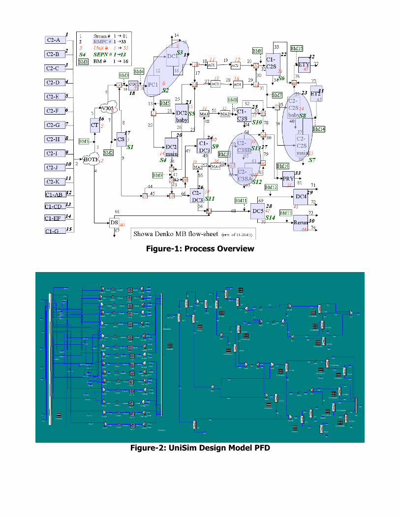
Figure-1: Process Overview

Figure-2: UniSim Design Model PFD

Figure-3: Solution Architecture

Figure-4: Engineering Access

Tecnip’

s

UniSim

Model

Figure-5: Operations Access

Figure-6: Daily Optimizer summary report

Figure-7: Ethylene Production Maximization

Figure-8: Energy Intensity Minimization