African Journal of

Environmental Science and

Technology

Volume 10 Number 8, August 2016

ISSN 1996-0786

ABOUT AJEST The African Journal of Environmental Science and Technology (AJEST) (ISSN 1996-0786) is published monthly (one volume per year) by Academic Journals.

African Journal of Environmental Science and Technology (AJEST) provides rapid publication (monthly) of articles in all areas of the subject such as Biocidal activity of selected plant powders, evaluation of biomass gasifier, green energy, Food technology etc. The Journal welcomes the submission of manuscripts that meet the general criteria of significance and scientific excellence. Papers will be published shortly after acceptance. All articles are peer-reviewed

Contact Us

Editorial Office: ajest@academicjournals.org

Help Desk: helpdesk@academicjournals.org

Website: http://www.academicjournals.org/journal/AJEST

Submit manuscript online http://ms.academicjournals.me/

Editors Oladele A. Ogunseitan, Ph.D., M.P.H. Professor of Public Health & Professor of Social Ecology Director, Industrial Ecology Research Group University of California Irvine, CA 92697-7070, USA. Prof. Sulejman Redzic Faculty of Science of the University of Sarajevo 33-35 Zmaja od Bosne St., 71 000 Sarajevo, Bosnia and Herzegovina. Dr. Guoxiang Liu Energy & Environmental Research Center (EERC), University of North Dakota (UND) 15 North 23rd Street, Stop 9018, Grand Forks, North Dakota 58202-9018 USA.

Associate Editors Dr. Suping Zhou Institute of Agricultural and Environmental Research Tennessee State University Nashville, TN 37209, USA

Dr. Hardeep Rai Sharma Assistant Professor, Institute of Environmental Studies Kurukshetra University, Kurukshetra, PIN-136119 Haryana, India Phone:0091-9034824011 (M) Dr. Ramesh Chandra Trivedi Chief Environmental Scientist DHI (India) Wateer & Environment Pvt Ltd, B-220, CR Park, New Delhi - 110019, India.

Prof. Okan Külköylüoglu Department of Biology, Faculty of Arts and Science, Abant Izzet Baysal University, BOLU 14280, TURKEY

Dr. Hai-Linh Tran Korea (AVCK) Research Professor at National Marine Bioenergy R&D Consortium, Department of Biological Engineering - College of Engineering, Inha University, Incheon 402-751, Korea

Editorial Board Dr Dina Abbott University of Derby,UK Area of Expertise: Gender, Food processing and agriculture, Urban poverty Dr. Jonathan Li University of Waterloo, Canada Area of Expertise: Environmental remote sensing, Spatial decision support systems for informal settlement Management in Southern Africa Prof. Omer Ozturk The Ohio State University Department of Statistics, 1958 Neil Avenue, Columbus OH, 43210, USA Area of Expertise: Non parametric statistics, Ranked set sampling, Environmental sampling Dr. John I. Anetor Department of Chemical Pathology, College of Medicine, University of Ibadan, Ibadan, Nigeria Area of Expertise: Environmental toxicology & Micronutrient metabolism (embracing public health nutrition) Dr. Ernest Lytia Molua Department of Economics and Management University of Buea, Cameroon Area of Expertise: Global warming and Climate change, General Economics of the environment Prof. Muhammad Iqbal Hamdard University, New Delhi, India Area of Expertise: Structural & Developmental Botany, Stress Plant Physiology, and Tree Growth Prof. Paxie W Chikusie Chirwa Stellenbosch University, Department of Forest & Wood Science,South Africa Area of Expertise: Agroforestry and Soil forestry research, Soil nutrient and Water dynamics Dr. Télesphore SIME-NGANDO CNRS, UMR 6023, Université Blaise Pascal Clermont-Ferrand II, 24 Avenue des Landais 63177 Aubière Cedex,France Area of Expertise: Aquatic microbial ecology

Dr. Moulay Belkhodja Laboratory of Plant Physiology Faculty of Science University of Oran, Algeria Area of Expertise: Plant physiology, Physiology of abiotic stress, Plant biochemistry, Environmental science, Prof. XingKai XU Institute of Atmospheric Physics Chinese Academy of Sciences Beijing 100029, China Area of Expertise: Carbon and nitrogen in soil environment, and greenhouse gases Prof. Andrew S Hursthouse University of the West of Scotland, UK Area of Expertise: Environmental geochemistry; Organic pollutants; Environmental nanotechnology and biotechnology Dr. Sierra Rayne Department of Biological Sciences Thompson Rivers University Box 3010, 900 McGill Road Kamloops, British Columbia, Canada Area of Expertise: Environmental chemistry Dr. Edward Yeboah Soil Research Institute of the Council for Scientific and Industrial Research (CSIR), Ghana Area of expertise: Soil Biology and Biochemistry stabilization of soil organic matter in agro-ecosystems Dr. Huaming Guo Department of Water Resources & Environment, China University of Geosciences, Beijing, China Area of Expertise: Groundwater chemistry; Environmental Engineering Dr. Bhaskar Behera Agharkar Research Institute, Plant Science Division, G.G. Agarkar Road, Pune-411004, India Area of Expertise: Botany, Specialization: Plant physiology & Biochemistry Prof. Susheel Mittal Thapar University, Patiala, Punjab, India Area of Expertise: Air monitoring and analysis

Dr. Jo Burgess Rhodes University Dept of Biochem, Micro & Biotech, Grahamstown, 6140, South Africa Area of Expertise: Environmental water quality and Biological wastewater treatment Dr. Wenzhong Shen Institute of heavy oil, China University of Petroleum, Shandong, 257061, P. R.,China Area of Expertise: Preparation of porous materials, adsorption, pollutants removal Dr. Girma Hailu African Highlands Initiative P. O. Box 26416 Kampala, Uganda Area of Expertise: Agronomy, Entomology, Environmental science (Natural resource management) Dr. Tao Bo Institute of Geographic Science and Natural Resources, C.A.S 11A Datun Road Anwai Beijing 100101,China Area of Expertise: Ecological modeling, Climate change impacts on ecosystem Dr. Adolphe Zézé Ecole Supérieure d’Agronomie, Institut National Polytechnique,Côte d’Ivoire Houphouet Boigny BP 1313 Yamoussoukro, Area of Expertise: Molecular ecology, Microbial ecology and diversity, Molecular diversity, Molecular phylogenie Dr. Parshotambhai Kanani Junagadh Agricultural University Dept.of agril.extension, college of agriculture,moti bagh,j.a.u Junagadh 362001 Qujarat, India Area of Expertise: Agril Extension Agronomy Indigenous knowledge, Food security, Traditional healing, resource Dr. Orish Ebere Orisakwe Nigeria Area of Expertise: Toxicology

Dr. Christian K. Dang University College Cork, Ireland

Area of Expertise: Eutrophication, Ecological stoichiometry, Biodiversity and Ecosystem Functioning, Water pollution

Dr. Ghousia Begum Indian Institute of Chemical Technology, India Area of Expertise: Toxicology, Biochemical toxicology, Environmental toxicology, Environmental biology

Dr. Walid A. Abu-Dayyeh Sultan Qaboos University Department of Mathematics and statistics/ Al-Koud/ Sultanate of Oman, Oman Area of Expertise: Statistics Dr. Akintunde Babatunde Centre for Water Resources Research, Department of Civil Engineering, School of Architecture, Landscape and Civil Engineering, Newstead Building, University College Dublin, Belfield, Dublin, Area of Expertise: Water and wastewater treatment, Constructed wetlands, adsorption, Phosphorus removal Ireland Dr. Ted L. Helvoigt ECONorthwest 99 West 10th Avenue, Suite 400, Eugene, Oregon 97401, Area of Expertise: Forest & Natural Resource Economics; Econometrics; Operations Research USA Dr. Pete Bettinger University of Georgia Warnell School of Forestry and Natural Resources, Area of Expertise: Forest management, planning, and geographic information systems. USA Dr. Mahendra Singh Directorate of Wheat Research Karnal, India Area of Expertise: Plant pathology

Prof. Adesina Francis Adeyinka

Obafemi Awolowo University Department of Geography, OAU, Ile-Ife, Nigeria Area of Expertise: Environmental resource management and monitoring Dr. Stefan Thiesen Wagner & Co Solar Technology R&D dept. An der Berghecke 20, Germany Area of Expertise: Climate change, Water management Integrated coastal management & Impact studies, Solar energy Dr. Leo C. Osuji University of Port Harcourt Department of Industrial Chemistry, Area of Expertise: Environmental/petroleum chemistry and toxicology Nigeria Dr. Brad Fritz Pacific Northwest National Laboratory 790 6th Street Richland WA, USA Area of Expertise: Atmospheric measurements & groundwater-river water interaction Dr. Mohammed H. Baker Al-Haj Ebrahem Yarmouk University Department of Statistics , Yarmouk University, Irbid - Jordan Area of Expertise: Applied statistics Dr. Ankur Patwardhan Lecturer, Biodiversity Section, Dept. of Microbiology,Abasaheb Garware College, Karve Road,Deccan Gymkhana, Pune-411004. and Hon. Secretary, Research and Action in Natural Wealth Administration (RANWA), Pune-411052, India Area of Expertise: Vegetation ecology and conservation, Water pollution Prof. Gombya-Ssembajjwe William Makerere University P.O.Box 7062 KAMPALA, Uganda Area of Expertise: Forest Management

Dr. Bojan Hamer

Ruđer Bošković Institute, Center for Marine Research, Laboratory for Marine Molecular Toxicology Giordano Paliaga 5, HR-52210 Rovinj, Croatia Area of Expertise: Marine biology, Ecotoxicology, Biomarkers of pollution, Genotoxicity, Proteomics Dr. Mohideen Wafar National Institute of Oceanography, Dona Paula, Goa 403 004, India Area of Expertise: Biological Oceanography Dr. Will Medd Lancaster University, UK Area of Expertise: Water consumption, Flood,Infrastructure, Resilience, Demand management Dr. Liu Jianping Kunming University of Science and Technology Personnel Division of Kunming University of Science and Technology, Wenchang Road No 68, Kunming city, Yunnan Province, China Area of Expertise: Application technology of computer Dr. Timothy Ipoola OLABIYI Coventry University Faculty of Business, Environment & Society, CV1 5FB, Coventry, UK Area of Expertise: Crop protection, nematology, organic agriculture Dr. Ramesh Putheti Research Scientist-Actavis Research and development 10065 Red Run Blvd.Owings mills,Maryland,USA. Area of Expertise: Analytical Chemistry,PharmaceuticalResearch & develoment,Environmental chemistry and sciences Prof. Yung-Tse Hung Professor, Department of Civil and Environmental Engineering, Cleveland State University, Cleveland, Ohio, 44115 USA Area of Expertise: Water and waste treatment, hazardous waste, industrial waste and water pollution control

Dr. Harshal Pandve Assistant Professor, Dept. of Community Medicine, Smt. Kashibai Navale Medical College, Narhe, Pune, Maharashtra state, India Area of Expertise: Public health, Environmental Health, Climate Change Dr. SATISH AMBADAS BHALERAO Environmental Science Research Laboratory, Department of Botany Wilson College, Mumbai - 400 007 Area of Expertise: Botany (Environmental Botany) Dr. Qing Huang Institute of Urban Environment, Chinese Academy of Sciences, China Dr. PANKAJ SAH Department of Applied Sciences, Higher College of Technology (HCT) Al-Khuwair, PO Box 74, PC 133 Muscat,Sultanate of Oman Area of Expertise: Biodiversity,Plant Species Diversity and Ecosystem Functioning,Ecosystem Productivity,Ecosystem Services,Community Ecology,Resistance and Resilience in Different Ecosystems, Plant Population Dynamics

Dr. Bensafi Abd-El-Hamid Department of Chemistry, Faculty of Sciences, Abou Bekr Belkaid University of Tlemcen, P.O.Box 119, Chetouane, 13000 Tlemcen, Algeria. Area of Expertise: Environmental chemistry, Environmental Engineering, Water Research. Dr. Surender N. Gupta Faculty, Regional Health and Family Welfare Training Centre, Chheb, Kangra-Himachal Pradesh, India. Pin-176001. Area of Expertise: Epidemiologist

International Journal of Medicine and Medical Sciences

African Journal of Environmental Science and Technology

Table of Contents: Volume 10 Number 8 August 2016

ARTICLES

Assessment of the effect of effluent discharge from coffee refineries on the quality of river water in South-western Ethiopia 230 Tadesse Mosissa Ejeta and Alemayehu Haddis The analysis of physicochemical characteristics of pig farm seepage and its possible impact on the receiving natural environment 242 Dikonketso S. Mofokeng, Rasheed Adeleke, and Olayinka A. Aiyegoro Modeling sludge accumulation rates in lined pit latrines in slum areas of Kampala City, Uganda 253 Yvonne Lugali, Ahamada Zziwa, Noble Banadda, Joshua Wanyama, Isa Kabenge, Robert Kambugu and Peter Tumutegyereize

Vol. 10(8), pp. 230-241, August 2016

DOI: 10.5897/AJEST2015.1886

Article Number: 367729859595

ISSN 1996-0786

Copyright © 2016

Author(s) retain the copyright of this article

http://www.academicjournals.org/AJEST

African Journal of Environmental Science and Technology

Full Length Research Paper

Assessment of the effect of effluent discharge from coffee refineries on the quality of river water in South-

western Ethiopia

Tadesse Mosissa Ejeta1*

and Alemayehu Haddis

2

1Department of Natural Resource Management, College of Agriculture and Veterinary Medicine, Jimma University,

Jimma, Ethiopia. 2Department of Environmental Health, Jimma University, Jimma, Ethiopia.

Received 5 February, 2015; Accepted 8 May, 2015

The ecohydrological quality of water resource of Ethiopia is declining at an alarming rate, resulting in severe environmental degradation. This study finds out the effects of effluent discharge from intensive coffee refineries on river water quality based on physicochemical parameters and benthos assemblages as biological indicators. The experiment was done using complete randomized design (CRD) with three composite replicates in each refinery and on 24 river water sampling sites selected from four rivers in Limu Kosa District. A total of 72 water samples were collected from six sites: (upstream site (UPS), influent (INF), effluent (EFF), entry point (ENP), downstream one (DS1) and downstream two (DS2) in four rivers. Data analysis was performed by analysis of variance (ANOVA) using statistical analysis software (SAS). Spearman’s median rank correlation among physicochemical and benthos assemblages as biological indicators of ecohydrological river water quality was characterized. Results reveal that there is a highly negatively significant difference in effect between the four rivers and 24 sites at p<0.05 and 0.01. The benthos assemblage communities of DS2 and UPS of the ecohydrological rivers were more influenced by the effluents. Quality of DS2 was more adversely affected compared to UPS. The alteration in river water quality parameters was more pronounced during the peak of coffee refineries. The impact of private refineries on receiving water was more significant than that of government refineries. Therefore, urgent attention should be given to the coffee refinery for effluent management options to avoid further damage to the ecohydrological river water quality using well-designed treatment technologies. Key words: Biological indicators, benthos, ecohydrolological integrity, upstream downstream.

INTRODUCTION Water is an essential and inevitable commodity for human growth and development than any other resource

for life’s sustenance. Although, the water resource of Ethiopia is declining at an alarming and accelerating rate,

*Corresponding author. E-mail: tadesse88@gmail.com. Tel: +251-0917082424.

Author(s) agree that this article remain permanently open access under the terms of the Creative Commons Attribution

License 4.0 International License

resulting in severe environmental degradation (Beyene et al., 2011; Dejen et al., 2015). South-western Ethiopia is a major and famous coffee growing region in Ethiopia; it has a number of coffee refineries situated along the bank of rivers and/or streams with a varying degree of hydraulic gradients. Wet coffee requires considerable amount of water during processing to receive the cherries, transport them hydraulically through the pulping machine, remove the pulp, and sort and re-pass any cherries with residual pulp adhering to them. The rise in the number of wet coffee refineries has therefore resulted in the generation of enormous disposal of these wastes which are discharged unwisely into nearby natural water way that flows into rivers and/or infiltrates ground water, becoming main threat to surface and ground water qualities as reported by Dejen et al. (2015). With intensification of wet coffee refineries and rampant waste discharges into ecohydrological integrity of river water, an increased pressure on fauna and flora of ecohydrological integrity of river water bodies becomes evident. Water bodies are the primary dump sites for disposal of effluents from coffee refineries containing wide varieties of synthetic and organic wastes that are near them (Haddis and Devi, 2008; Beyene et al., 2011; Dejen et al., 2015). Water pollution is an acute problem in all water bodies, and major river water quality is the gloomy setback for development in coffee producing zone, especially in South-western Ethiopia. According to rough estimates, effluent from 1000 kg of parchment coffee is generated by wet-processing method compared to the human waste that can be generated by 3000-5600 people per day (Beyene et al. 2011). Alarmingly increasing rampant wet coffee refineries contribute to dwindling surface water quality in South-western Ethiopia to a greater extent. As a consequence, there is a risk to ecosystems structures and their functions which allow for regulation of ecosystem processes, and risk to local community health and welfare as they might take in pollutants through consumption of crops such as onion, tomato, potatoes and maize and using of this river for domestic purposes (Kassahun et al. 2010; Dejen et al. 2015).

This has often gradually rendered the ecohydrological quality of rivers of the Limu Kosa District unsuitable for various beneficial purposes as well as their maintenance and restoration. Benthos assemblages within ecological water quality are interrelated and excellent indicators of water quality; they easily respond to organic and inorganic pollution load from human interferences (Kassahun et al., 2010; Beyene et al., 2011). Few, if any, studies have investigated this issue in Ethiopia to assess the effect and extent of the problem and to suggest solutions and recommendations accordingly. Virtually, no studies have specifically addressed the spatial variation of different ecohydrological integrity of river water quality based on the physico-chemical parameters and benthos

Ejeta and Haddis 231 assemblages as biological indicators of receiving water bodies of South-west Ethiopia. The objective of this study is to determine the effect and extent of effluents generated from coffee refineries on ecohydrological integrity of river water quality based on the physicochemical parameters and benthos assemblages as biological indicators of river water quality in Limu Kosa District (Figure 1). MATERIALS AND METHODS Descriptions of the study area The study was conducted in Limu Kosa District of Jimma Zone (Figure 1). Limu Kosa District is located 420 km southwest of Addis Ababa, the capital city of Ethiopia, lying between Latitude of 7°50 and 8°36′ North and Longitude of 36°44′ and 37o 29′ East. The altitude of district ranges from 1200 to 3020 m above sea level. It has an area of 2770.5 km2. Several perennial rivers (Gibe, Awetu, Kebena, Ketalenca, Bonke and Dembi), intermittent streams, springs and notable landmarks including Cheleleki Lake and Bolo Caves were found in the Limu Kosa District (data from the Limu Kosa District Agricultural and Rural Development Office). The availability and quality of river water not only impact human health and wellbeing, but also the functioning of essential ecosystems, including rivers, wetlands, lakes and coastal ecosystems. Without sound ecohydrological of river basin management, human activities can upset the delicate balance between ecohydrological integrity and environmental sustainability. As might be expected, water quality in Limu Kosa District rivers and wetlands ranges from absolutely pristine to dangerously poor. Methods Study period

A cross sectional study was conducted to assess the impact of wastewater discharge on ecohydrological river water quality by coffee refineries in Limu Kosa District from August 2011 to December 2013. During the whole study period, the primary data (three days of a week from the chosen sampling points) were collected through direct measurement of river water quality parameters of the selected study sites in-situ and under laboratory condition. Experimental design of the study and selection of sampling sites

The experiment was conducted using complete randomized design (CRD) with three composite replicates to minimize the variation of all sample collected from the same sample site. In order to assess the ramification of coffee refineries effluent being discharged, physico-chemical samples were taken from the 24 ecohydrological river water sites (12 among each private and government refineries). Six sampling sites were selected for physico-chemical samples along each ecohydrological river. These sites were upstream site (UPS), influent (INF), effluent (EFF), entry point (ENP), downstream one (DS1) and downstream two (DS2). In order to understand the influence of effluent discharge by coffee refineries on ecohydrological river water quality, benthos assemblages as biological indicators of river water quality samples were also taken from the upstream (UPS) and downstream two

232 Afr. J. Environ. Sci. Technol.

Figure 1. Map of Kosa District indicating sampling sites.

(DS2) of the discharge points of ecohydrological rivers. UPS was the control sites without any effects from the effluent because of their sites. Influent (INF) was the point at which waste water enters the treatment plants; in this case lagoon. Effluent (EFF) is wastewater leaving the lagoon before it enters the river water. Entry point (ENP) is highly impacted; it is located after the EFF and the point at which lagoon effluent enters the river. Downstream one (DS1) is located 500 meters below ENP. Downstream two (DS2) is located 500 meters below DS1. The aim of taking samples at different sites of the downstream is to analyze spatial variations and determine the rivers’ recovery potential. At each sampling point, three samples were taken cross sectionally (corners and center) and three similar sampling campaigns were conducted. This makes the total analyzed samples 180. The distance between UPS, ENP, DS1 and DS2 was set at an interval of 500 m. Also, samples were taken from INF and EFF. No actual distance was determined because it depends on the coffee refineries designed. Specially, these wastewater samples were collected at the peak hours of coffee refineries three days in a week from the chosen sampling points (Figure 2) (Kobingi et al., 2009; Kassahun et al. 2010; Akali et al., 2011; Dejen et al. 2015). Sampling procedure of physicochemical parameters data Samples were collected in sterilized plastic BOD and glass bottles to maintain accuracy or minimize contamination of physicochemical changes that can occur between time of collection and analysis as indicated in APHA standard method (APHA) (2005). The water samples were collected by inserting the plastic and glass bottles to

the opposite direction of the river flow and capped tightly immediately after filling to the tip of the mouth of this bottle by using depth-integrated sampling technique. Determinations of pH, EC, temperature, turbidity and DO fixing were carried out in-situ as APHA (2005). These samples were properly and carefully labeled, sealed and transported to the laboratory of the Department of Environmental Health Sciences and Technology, Jimma University. Cold storage was maintained throughout the process till analysis. Sampling method of macro-invertebrates (benthos) from river water sites A triangular D-frame Dip-Net (mesh size = 500 μm, sampled area = 0.9 m2) was used to collect benthos by kick sampling method. In this method, the river bed was disturbed for a distance of about 100 m for 3-5 min. Benthos sample was conducted three times from each riffle and run sample site. These samples were properly and carefully labeled, sealed and transported to the laboratory of the Department of Environmental Health Sciences and Technology, Jimma University, Jimma, Ethiopia. Cold storage was maintained throughout the process till analysis. Identification to a family level was done using a compound light microscope and assisted by a standard identification key (Bouchard 2004; Kobingi et al., 2009). Statistical analysis The data were subjected to different statistical analysis such as analysis of variance (ANOVA) using SAS version 9.2, Minitab

Ejeta and Haddis 233

Figure 2. Map indicating general flow diagram of coffee refinery and effluent sampling points.

Version 16.0 software and MS Excel. When significant interaction effects were observed among the four rivers with river water and sites using a two-way ANOVA, One-way ANOVA was computed to see significant difference between each sample site for the physico-chemical parameters and benthos assemblages as biological indicators. Mean separation of different sources of variation among

each river water and site was done using Tukey’s test at = 0.05 level of minimum significance difference (MSD). Pearson correlation matrix analysis was used to reveal the magnitude and direction of relationship between different physic-chemical parameters within and among benthos assemblages as biological indicators of river water quality. Benthos assemblages as biological indicators of ecohydrological river water quality samples were determined by using benthos assemblages multimetric indices.

RESULTS Physical parameters and their significance level in four river water of the study sites The average mean values of river water temperature ranged between 12.11±0.78-43.09±0.78˚C at Kebena UPS and Awetu EFF respectively. This result showed that there was highly significant difference in all sampling sites, but very high 43.96°C in the Awetu EFF, indicating much stress from the coffee refineries disposal at p<0.05 and 0.01. There was highly significant difference in the concentration of EC among the four river water and sites at p<0.05 and 0.01. The average mean values of EC

ranged from 167.65±15.38-1187.26±15.38µS/cm among all sites. DS1 to DS2 exhibited non- significant variation of EC and TDS in contrast to other sites. The EC alarmingly increased with increase in TDS and water temperature (Tables 1 and 2).

The observed turbidity mean values ranged from 3.3±11.05-1363.67±11.05 NTU at Bonke UPS and Kebena INF respectively. The maximum average mean value obtained from the polluted sites (1397NTU) was higher than 2.86NTU recorded at UPS. The turbidity mean concentration at DS1 to DS2 was 114.10±11.05 -980.58±11.05NTU which significantly exceeded the allowable limit set by WHO and EPA (10 mg/L). Consequently, various analytical mean values of TSS and TDS fluctuated between 756.35 ± 15.31 - 1063.35 ± 15.31 mg/L to 394.14 ± 15.31 - 342.09 ± 15.31 mg/L and 1095.64 ± 53.71 - 1197.37 ± 53.71 mg/L to 435.26 ± 53.71 - 481.92 ± 53.71 mg/L amongst the polluted sites of Kebena and Ketalenca DS1 to DS2, respectively. These mean values of TSS and TDS obtained from the polluted sites were higher than 16.79 ± 15.31 - 10.02 ± 15.31 mg/L to 302.96 ± 53.71 - 235.04 ± 53.71 mg/L recorded at Kebena and Ketalenca UPS, respectively. There were highly significant differences (p<0.05 and 0.01) in the values of TSS among the different sampling sites across the river water course. These results show significant increased values from DS1 to DS2 sites of the river water in TSS, but non- significant differences from DS1 to

Washing and Grading

(Vast Volume of Waste Water)

Waste water or Influent

Sample (INF) (Point 1)

De-mucilage

Effluent on Lagoon

Effluent Discharged Sites

Sample (EFF) (Point2)

UPS (Point 3)

DS1 (Point 5)

DS2 (Point 6)

ENP (Point 4)

Fermented 36-72 hr

in Fermentation Tank

234 Afr. J. Environ. Sci. Technol.

Table 1. Physico-chemical parameters selected for the study site and techniques used for methods of analysis.

Physico-chemical parameters Abbreviation Methods of analysis Unit

Water temperature WT Probes multi parameter methods °C

Turbidity TURB Turbidity meter NTU

Electrical conductivity EC Probes multi parameter methods (EC meter) µS/cm

pH pH Probes multi parameter methods (pH meter) -

Total dissolved solids TDS Gravimetric Method, dried at 180°C mg/L

Total suspended solid TSS Gravimetric Method, dried at 103-105°C mg/L

Total solid (TS) TS Gravimetric Method, dried at 103-105°C mg/L

Dissolved oxygen (DO) DO Probes multi parameter methods (DO meter) mg/L

Biological oxygen demand BOD5 The Azide Modification of the Winkler Method mg/L

Chemical oxygen demand COD Kit (Hachlange cuvette test, LCk 614 &114) mg/L

Nitrate-nitrogen NO3-N2 Phenoldisulfonic Acid Method mg/L

Ammonia-nitrogen NH3-N2 Direct Nesslerization Method mg/L

Total nitrogen TN Kit (Hachlange cuvette test, LCK 138 & 338) mg/L

Orthophosphate Orth-P Stannous Chloride Method mg/L

Source: APHA, 2005.

DS2 in TDS (Table 2). Chemical parameters and their significance level in four river water of the study sites The average mean values of pH in all six sites of river water were acidic and ranged between 3.12 ± 0.10-7.67 ± 0.10 at Kebena EFF and Awetu UPS respectively. The lowest values obtained from the EFF (2.9) were very lower than 7.93 recorded at UPS. Acidity was found to be potent at ENP than DS1 which in turn was stronger than DS2 (Table 3). The pH has shown significant differences among DS1 and DS2 river water at p< 0.05 and 0.01.

The average mean values of DO were fluctuated between 0.00±0.10 to 8.04±0.10 mg/L in river water samples collected among the four river water with river water and sites. Kebena EFF and INF showed the lowest value of DO as 0.00±0.10 mg/L. These variations may be attributed to oxygen consumption by aerobic organisms due to increase in oxygen demanding wastes. Level of DO in the river water was almost normal in the UPS. DO concentrations below 5 mg/L may also adversely affect the functioning and survival of biological communities and hence all pollution-sensitive taxa failed to retrieve (Table 3). There were highly significant inconsistencies of interaction effect of BOD and COD among all river waters at (p<0.05 and 0.01). The maximum average mean values of BOD and COD were recorded (2972.67±30.27 to 2576.05±30.37 mg/L) at Kebena EFF and INF;h minimum values were recorded (2.36 ± 30.27 to 3.99 ± 30.37 mg/L) at Ketalenca and Bonke UPS. BOD and COD showed alarming increment from 1773 ± 30.27- 1719.83 ± 30.37 mg/L to 1797.89 ± 30.27-1836.40 ±

30.37 mg/L at Kebena DS1 and DS2; then decreased slowly towards the rest of the Ketalenca and Bonke of DS1 and DS2 respectively.

TN concentration analysis revealed that there was highly significant difference in interaction effect among the four rivers but not at Kebena River of ENP, DS1, DS2

and Bonke ENP as well as EFF and PUS of all river water at p ≤ 0.05 and 0.01. This is due to highly mobility or fixation of TN concentration among each river water site. The concentrations of NO3-N and NH3-N2 in the river water were found to be statistically highly significant and the average mean values ranged from 2.43±0.03 to 4.99±0.07 mg/L. They were higher concentrations in all INF and alarmingly increment from DS1 to DS2 due to high coffee refineries’ activities that ultimately discharge almost untreated effluent to the river (Table 3). The average mean values of orthophosphate (Orth-P) showed significant difference in all river water, but not DS1 and DS2 in all river water (Table 3). Benthos assemblages as biological indicators of river water quality UPS and DS2 benthos assemblages of fauna from 8 taxonomic orders were collected from Limu Kosa District rivers. A total of 30 families fewer than 8 orders representing classes and comprising 1293 individuals were collected from the eight sampling sites. A total number of individuals found in the DS2 were 387 compared to 906 individuals collected from the UPS. The pollution sensitive taxa of Ephemeroptera, Hemispheres, Trichoptera, Plecoptera and Coleoptera were present in greater number in the UPS. On the other hand, pollution

Ejeta and Haddis 235

Table 2. Interaction effects of effluent discharges by coffee refineries on physical characteristics between the all river waters and among sites of river water.

River Mean separation of physical parameters

Site TSS TDS TS EC TURB WT

Kebena

EFF 1800.35A 2239.30

B 4039.64

BA 1045.80

B 1335.23

A

28.12EF

INF 1527.23B 2681.23

A 4208.46

A 1160.68

A 1363.67

A 37.267

B

ENP 1460.03CB

2052.26B 3512.29

ED 858.65

C 1190.48

B 24.27

FIHG

DS2 1063.35D 1197.37

E 2260.72

HG 661.09

D 980.58

C 19.60

JK

DS1 756.35E 1095.64

E 1851.98

JI 616.73

D 972.10

C 18.67

K

UPS 16.79I 302.96

GH 319.75

M 188.65

H 3.99

H 12.11

L

Awetu

EFF 1778.87A 1508.64

DC 3287.51

EF 1035.56

B 1195.25

B 43.09

A

INF 1126.52D 2773.59

A 3900.1

BAC 1187.26

A 1188.10

B 36.75

B

ENP 586.98F 1537.99

C 2124.97

HI 844.00

C 675.94

D 34.97

CB

DS2 431.65G 762.07

F 1193.72

K 505.65

E 514.38

E 25.40

FHG

DS1 434.23G 753.82

F 1188.05

K 513.28

E 514.56

E 29.747

ED

UPS 33.24I 335.24

GH 368.48

M 197.94

H 6.99

H 20.08

JIK

Bonke

EFF 757.29E 2298.43

B 3055.72

F 890.99

C 1316.66

A 37.82

B

INF 1382.24C 2202.67

B 3584.9

EDC 1151.17

A 1202.01

B 37.27

B

ENP 578.45F 1227.24

DE 1805.68

J 582.78

ED 520.62

E 36.86

B

DS2 543.76F 577.02

F 1120.78

LK 395.69

F 128.70

G 23.64

JIHG

DS1 584.03F 569.84

GF 1153.87

K 393.62

F 128.39

G 35.77

B

UPS 28.07I 230.00

H 258.07

M 167.65

H 3.30

H 27.32

FEG

Ketalenca

EFF 1381.05C 1177.33

E 2558.38

G 1015.70

B 1352.37

A 31.29

CED

INF 1051.68D 2746.18

A 3797.86

BDC 1179.37

A 1237.58

B 33.95

CBD

ENP 419.74HG

753.73F 1173.47

K 318.35

GF 334.88

F 30.10

ED

DS2 342.09H 481.92

GFH 824.02

L 240.14

GH 122.30

G 21.36

JIHK

DS1 394.14HG

435.26GH

829.39L 226.71

H 114.10

G 19.60

JK

UPS 10.02I 235.04

H 245.06

M 169.10

H 5.12

H 14.28

L

Mean 770.34 1257 2028 647.77 683.64 28.31

Max 1812 2816 4302 1227.16 1397 43.96

Min 9.70 222.27 236.84 165.43 2.86 11.70

WHO 500 1000 500 1000 10 -

CV (%) 3.44 7.39 4.98 4.11 2.80 4.78

MSD 83.45 292.79 318.08 83.85 60.24 4.26

SEM(±) 15.31 53.71 58.35 15.38 11.05 0.78

River <0.0001 <0.0001 <0.0001 <0.0001 <0.0001 <0.0001

River*Site <.0001 <.0001 <.0001 <.0001 <.0001 <.0001

CV, Coefficient of variation in percent; MSD, minimum significance difference at 5 and1%; SEM, standard error mean. Mean with different letters in the same column were significantly different (withTukey’s test at 5 and 1% level of probability) as established by MSD test. Except EC (µS/cm), TURB (NTU) and WT (°C) the others parameters were expressed in mg/L. These six river sites were averages among each site. Awetu and Kebena river water from private and the other two were from the government refineries. Significant interactions and main effects were explored by Tukey’s test, using the GLM procedure at P<0.05 and 0.01as established by MSD test.

tolerant species of families Chironomidae, Simuliidae and Leeches present in greater number in the DS2 sections throughout the experimental period reflected the coffee

refineries’ stresses of the ecological status of rivers in its DS2 sections (Appendix Table 1).

Analysis of the results of benthos assemblages as

236 Afr. J. Environ. Sci. Technol.

Table 3. Interaction effects of effluent discharges by coffee refineries on chemical water quality between the all ecohydrological river waters and among sites of river water.

River Mean separation of chemical parameters

Site pH BOD COD DO TN NO3-N NH3-N Ort-P

Kebena

EFF 3.12I 2972.67

A 2735.50

A 0.00

H 98.40

A 3.36

C 7.04

C 13.18

E

INF 3.33HI

2689.67B 2576.05

A 0.01

H 92.60

BA 3.86

A 8.11

A 22.90

A

ENP 3.36HI

2478.88C 1940.57

B 0.02

H 78.61

DE 3.08

D 6.92

DCE 10.87

F

DS2 4.06DGEF

1797.89E 1836.40

CB 0.05

H 76.22

DE 2.81

E 6.83

DCE 10.83

F

DS1 4.28D 1773.00

FE 1719.83

C 0.07

H 76.66

DE 2.74

FE 6.65

DE 10.34

F

UPS 7.43A 6.70

I 4.57

G 8.04

A 0.31

K 0.03

J 0.07

K 0.34

I

Awetu

EFF 3.59HGIF

2254.95D 1850.27

CB 0.11

H 88.72

BC 3.09

D 7.00

DC 11.47

F

INF 3.31HI

2205.32D 1982.94

B 0.12

H 94.57

BA 3.60

B 7.49

B 20.37

B

ENP 3.71HGEF

1868.24E 1525.88

D 1.49

E 82.56

DC 2.67

FE 6.93

DCE 11.00

F

DS2 4.12DEF

1010.05HG

1020.21FE

3.16C

35.14H 2.64

F 6.63

FE 10.82

F

DS1 4.20DE

989.30HG

1035.08FE

3.33C 21.10

J 2.64

F 6.63

GF 10.40

F

UPS 7.67A 9.75

I 8.96

G 6.64

B 5.44

K 0.66I 0.06

K 0.91

I

Bonke

EFF 4.15DEF

1849.67E 1451.67

D 1.23

FE 96.02

A 2.98

D 5.40

H 15.40

D

INF 3.55HGI

2201.63D 1835.09

CB 0.14

H 72.47

FE 3.97

A 6.01

G 17.56

C

ENP 4.96C 1129.35

G 1163.20

E 2.15

D 77.62

DE 2.78

FE 6.14

G 13.79

E

DS2 5.69B 1030.60

HG 928.69

F 3.40

C 13.06

I 1.35

H 3.83

J 8.28

G

DS1 5.57B 992.55

HG 961.88

F 3.55

C 41.52

H 1.95

G 3.81

J 8.19

G

UPS 7.52A 4.34

I 3.99

G 6.14

B 4.47

K 0.66

I 0.07

K 0.13

I

Ketalenca

EFF 3.48HI

1618.17F 1488.03

D 0.73

FG 95.29

A 3.09

D 5.12

H 8.25

G

INF 4.55DC

1717.18FE

1551.15D 0.25

HG 66.36

F 3.60

B 6.29

FE 10.60

F

ENP 4.60DC

1109.83G 1014.92

FE 2.19

D 50.09

G 2.64

F 4.62

I 8.84

G

DS2 5.90B 902.88

H 874.23

F 3.64

C 19.88

I 1.51

H 3.83

J 4.86

H

DS1 5.66B 1009.38

HG 912.93

F 3.27

C 35.31

H 1.96

G 4.26

I 5.84

H

UPS 7.52A 2.36

I 9.74

G 8.01

A 5.87

K 0.66

I 0.05

K 0.34

I

Mean 4.80 1401 1268 2.40778 55.35 2.43 4.99 9.81

Max 7.93 2993 2867 8.31 99.23 3.99 8.37 23.31

Min 2.90 2.03 3.19 0.00 0.30 0.03 0.05 0.13

WHO 65-8.5 10 40 6 - 10-45 0.2-5 5

CV (%) 6.03 6.74 8.16 5.80 3.71 2.17 2.30 3.97

MSD 0.56 165.01 165.57 0.52 6.48 0.17 0.36 1.23

SEM(±) 0.10 30.27 30.37 0.10 1.19 0.03 0.07 0.23

River <0.0001 <0.0001 <0.0001 <0.0001 <0.0001 <0.0001 <0.0001 <0.0001

River*Site <0.0001 <0.0001 <0.0001 <0.0001 <0.0001 <0.0001 <0.0001 <0.0001

CV, Coefficient of variation in percent; MSD, minimum significance difference at 5 and 1%, SEM, Standard error mean. Mean with different letters in the same column were significantly different (with Tukey’s test at 5 and 1% level of probability) as established by MSD test. Except pH, the others parameters were expressed in mg/L. These six river sites were averages among each site. Awetu and Kebena river water from private and the other two were from the government refineries. Significant interactions and main effects were explored by Tukey’s test, using the GLM procedure at P<0.05 and 0.01 as established by MSD test.

biological indicators illustrated a highly significant difference between rivers and all sites at p<0.05 and 0.01. These benthos assemblages would indicate the environmental effects of coffee refinery activities on the

ecohydrological river water quality and its vicinity. The analysis of the average species diversity of benthos assemblages as biological indicators (Shannon, equitability and Simpson) was much reduced in the DS2

Ejeta and Haddis 237

Table 4. Summary of benthos assemblages diversity indices and taxa richness among ecohydrological rivers.

River F S D H’ E Min Max

UPS DS2 UPS DS2 UPS DS2 UPS DS2 UPS DS2 UPS DS2 UPS DS2

Awetu 9 11 266 157 0.88 0.85 2.15 2.09 0.98 0.89 0 0 42 42

Bonke 9 6 169 54 0.88 0.63 2.14 1.32 0.97 0.74 0 0 29 31

Ketalenca 15 8 266 127 0.92 0.58 2.62 1.31 0.97 0.63 0 0 41 80

Kebena 13 3 205 49 0.92 0.50 2.54 0.87 0.99 0.79 0 0 25 33

Total 906 387 0.90 0.64 2.36 1.40 0.98 0.76 0 0 35 47

Grand 1293 - - - - - - - - - -

Average 647 0.77 1.88 0.87 0 41

Table 5. Results of ANOVA for benthos assemblage composition, abundance and distribution among sites.

Site Mean separation of diversity indices and taxa richness

F S H’ D E

UPS 12a 227

a 2.36

a 0.90

a 0.98

a

DS2 7b 97

b 1.40

b 0.64

b 0.76

b

CV (%) 29 7 19.35 11.42 6.17

MSD (0.05) 2.98 12.52 0.40 0.097 0.052

SEM (±) 0.95 4.02 0.13 0.03 0.02

F=Total number of Families, S=Total number of Richness, H’= Shannon- Wiener diversity index, D=, Simpson's diversity index E= Equitability or Evenness diversity indices. Means with different letters in the same column are significantly different (Tukey’s test at P<0.05) as established by MSD test.

as against UPS, which was very high throughout the experimental period (Tables 4 and 5). Pearson correlation matrix (r) among selected physicochemical parameters and benthos assemblages as biological indicators of river water quality PH and DO exhibited that they are positively and highly significant correlated with benthos assemblages, while BOD and COD are negatively and highly correlated with benthos at p<0.05. Meanwhile, TN, NO3-N and Orth-P had negative correlation with all diversity indices and taxa richness, except evenness at p<0.05. The richness and all diversity revealed that there is a highly significant dependence on pH and DO parameters. This suggests that a local increase in pH and DO was responsible for increase in the richness of benthos (Table 6). DISCUSSION The good ecohydrological status of sampling sites in the

UPS of Limu Kosa District areas was indicated by high proportion of pollution sensitive benthos, whereas entry point segment received huge volume of effluents that acts as physical-chemical barrier, which restricts the movement of benthos from DS2 to UPS and vice versa. The results showed that the physicochemical parameter of the effluent discharged from government coffee refineries into the river water (Bonke and Ketalenca river water) decreased slowly towards DS2, while physico-chemical parameter of the effluent discharged from private coffee refineries into the river water (Kebena and Awetu river water) alarmingly increased towards DS2. Deterioration of the river water quality increases during the peak time of coffee refineries when rampant discharges are discharged into the river water. It could lead to reduction in volume of river water and also impede the free flow of the river water. The ecohydrological river water banks were disrupted by most processing.

High physicochemical and nutrient parameters concentration widely exceed assimilation capacity of ecohydrological integrity of river water quality and do not allow for aquatic life and complex effects on flowing river water and increased eutrophication concentration at DS2.

238 Afr. J. Environ. Sci. Technol. Table 6. Spearman’s median rank correlation among physico-chemical parameters with benthos assemblages as biological indicators of river water quality characteristics.

Parameter pH DO BOD COD TN NO3-N Orth-P S H’ D E

pH 1.00

DO 0.93** 1.00

BOD -0.94** -0.97** 1.00

COD -0.95** -0.95** 0.98** 1.00

TN -0.93** -0.91** 0.91** 0.94* 1.00

NO3-N -0.96** -0.94** 0.89** 0.90** 0.90** 1.00

Orth-P -0.99** -0.91** 0.94** 0.88** 0.81** 0.94** 1.00

S 0.89** 0.86** -0.86** -0.80** -0.65* -0.65* -0.78* 1.00

H’ 0.79** 0.91** -0.88** -0.85** -0.72* -0.69* -0.72* 0.88** 1.00

D 0.77** 0.87** -0.88** -0.85** -0.71* -0.65* -0.69* 0.86** 0.97** 1.00

E 0.86** 0.88** -0.83** -0.81** -0.43 -0.53* -0.60* 0.75** 0.84** 0.89** 1.00

**= Correlation are highly significant at p < 0.05 probability levels, *= Correlation are moderately significant at p < 0.05 probability levels and ‘-’ indicate negative correlation. E = Equitability or evenness index, BOD = biological oxygen demand, COD = chemical oxygen demand, DO = dissolved oxygen, D= Simpson's diversity index, H’ = Shannon-Wiener diversity index, Orth- P= orthophosphate, NO3-N= nitrate nitrogen, S= specious richness taxa and TN= total nitrogen).

TN is not strongly adsorbed on effluent cation exchange complex. Low adsorption coefficients of waste stabilization pond lagoon and constructed wetlands effluent result in maintenance of high dissolved NH3-Nconcentrations in the effluent river water quality (Akan et al., 2009; Akali et al., 2011).

This result indicates that the decline at an alarming and accelerating rate of ecohydrological river application benefits both watershed and their surrounding environment and society (health and welfare) deterioration. Due to drawdown river discharge (hypoxia or anoxia), increased temperatures and reduced water quality in peak time (mid-September to mid of December) of coffee refineries, the health of ecosystem is usually at stake in these months; so maintaining ecosystem health and improving biodiversity in such months is more important for water resources planners. This poses a health risk to several rural communities which rely on the receiving water bodies primarily as their sources of domestic water and for other purpose (Walakira and James, 2011). Biological indicators were strongly positive correlated with pH and DO while negative correlations were noticed in BOD and COD of river water quality. This showed that there was hypoxia or anoxia which affected taxa richness and all diversity indices (Aina, 2012a, 2012b).

Outfalls from private coffee refineries that are discharged into the river water column as well as into vicinity revealed highly significant variation of physico-chemical and nutrient characterization as compared to government site. Lagoons that were intended to serve as

wastewater stabilization were neither properly constructed nor were they of the right dimension to accommodate the generated waste during peak time of refineries lead to overflow of raw effluents into natural river water column. There is need for the intervention of appropriate regulatory agencies to ensure production of high quality treated final effluents by wastewater treatment facilities in rural communities coffee refineries (Sharma and Samita 2011; Mary Joyce and Macrina, 2012). Conclusion and recommendation High proportion of pollution sensitive taxa of benthos assemblages (Ephemeroptera, Hemispheres, Trichoptera, Plecoptera and Coleoptera) in the UPS as against high pollution tolerant species of families Chironomidae, Simuliidae and Leeches DS2 was recorded. Coffee refinery effluents having contaminants are intensively incorporated with river water regularly. This study clearly reveals that river water quality was found to be unfit for human consumption and other domestic purposes due to the exceeding level of physico-chemical parameters values recommended by WHO at DS2 of Limu Kosa District. Thus the challenges to continuous physico-chemical parameters and biological indicators monitoring will be immense. Both planners, regulatory agencies & the scientific community should work together to establish sustainable coffee production that is economically viable, environmentally amendable and maintain ecological

integrity of receiving water bodies. Therefore, urgent intervention in the area of coffee refinery for effluent management options should be dealt with top priority to avoid further needless damage to ecohydrological integrity, and the development of river water quality using well-designed treatment technologies (lagoons) for coffee waste treatment is highly recommended. Conflict of Interest The author has not declared any conflict of interests. REFERENCE Aina OA (2012a). Spatial and Temporal Variations in Water and

Sediment Quality of Ona River, Ibadan, Southwest Nigeria. Eur. J. Sci. Res. 74(2):186-204.

Aina OA (2012b). Impact of Industrial Effluent on Water Quality and Gill Pathology of Clarias Gariepinus from Alaro Stream, Ibadan, Southwest, Nigeria. Eur. J. Sci. Res. 76(1):83-94.

Akali NM, Nyongesa ND, Neyole EM, Miima JB (2011). : An Empirical Investigation of the Pollution of River Nzoia. Sacha J. Environ. Stud. 1(1):1-30.

Akan JC, Abdulrahman FI, Ogugbuaja VO, Reuben KD (2009). Study of the Physicochemical Pollutants in Kano Industrial Areas, Kano State, Nigeria. J. Appl. Sci. Environ. Sanit. 4(2):89-102.

American Public Health Association (APHA) (2005). Standard methods

for examination of water and wastewater (21st

ed). Washington: American Public Health Association, American Water Works Association and the Water and Environment Federation board.

Beyene A, Kassahun Y, Addis T, Assefa F, Amsalu A, Legesse W, Helmut K, Ludwig T (2011). The Impact of Traditional Coffee Processing on River Water Quality in Ethiopia and the Urgency of Adopting Sound Environmental Practices. Environ. Monit Assess. DOI 10.1007/s10661-011-2479-7.

Bouchard RW (2004). Guide to aquatic macro-invertebrates of Effluent Discharge by Mumias Sugar Company in Kenya the upper Midwest. Water resources centre, University of Minnesota. St. Paul, MN. 208pp.

Dejen YT, Abebe BH, Taffere AW, Azeb GT (2015). Effect of coffee processing plant effluent on the physicochemical properties of receiving water bodies, Jimma zone Ethiopia. Am. J. Environ. Protect. 4(2):83-90.

Ejeta and Haddis 239 Haddis A, Dev R (2008). Effect of effluent generated from coffee

processing plant on the water bodies and human health in its vicinity. J. Hazard. Mater. 152: 259-262.

Kassahun Y, Kebede T, Assefa F, Amsalu A (2010). Environmental Impact of Coffee Processing Effluent on The Ecological Integrity of Rivers Found in Gomma Woreda of Jimma Zone, Ethiopia. Ecohydrology for Water Ecosystems and Society in Ethiopia. 10(2-4):259-270.

Kobingi N, Raburu PhO, Masese FO, Gichuki J (2009). Assessment of pollution impacts on the ecological integrity of the Kisian and Kisat rivers in Lake Victoria drainage basin, Kenya. Afr. J. Environ. Sci. Technol. 3 (4):097-107.

Mary Joyce LF, Macrina TZ (2012). Macro invertebrates Composition, Diversity and Richness in Relation to the Water Quality Status of Mananga River, Cebu, Philippines. Philipp. Sci. Lett. 5(2):1-11.

Sharma KA, Samita Ch (2011). Macro invertebrate Assemblages as Biological Indicators of Pollution in a Central Himalayan River, Tawi (J&K). Int. J. Biodivers. Conserv. 3(5):167-174.

Walakira P, James OO (2011). Impact of Industrial Effluents on Water Quality of Receiving Streams in Nakawa-Ntinda, Uganda. J. Appl. Sci. Environ. Manage. 15(2):289-296.

240 Afr. J. Environ. Sci. Technol. Appendix Table 1. Total number (n) of macro-invertebrates caught at four river water in Limu Kosa District. .

Taxa

Kebena Awetu Bonke Ketalenca

UPS DS UPS DS UPS DS UPS DS

N % N % N % n % N % N % n % N %

Odonata 37 18.05 0 0.00 91 34.21 41 26.11 67 39.64 6 11.11 74 27.82 6 4.72

Coenagrionidae 10 4.88 0 0.00 37 13.91 9 5.73 23 13.61 4 7.41 22 8.27 0 0.00

Gonphidae 8 3.90 0 0.00 0 0.00 0 0.00 18 10.65 0 0.00 10 3.76 0 0.00

Libellulidae 19 9.27 0 0.00 27 10.15 13 8.28 26 15.38 2 3.70 11 4.14 6 4.72

Aeshnidae 0 0.00 0 0.00 0 0.00 0 0.00 0 0.00 0 0.00 31 11.65 0 0.00

Lestidae 0 0.00 0 0.00 0 0.00 11 7.01 0 0.00 0 0.00 0 0.00 0 0.00

Cordulegastridae 0 0.00 0 0.00 27 10.15 8 5.10 0 0.00 0 0.00 0 0.00 0 0.00

Hemiptera 30 14.63 0 0.00 28 10.53 12 7.64 29 17.16 6 11.11 31 11.65 16 12.60

Belostomatidae 14 6.83 0 0.00 28 10.53 12 7.64 0 0.00 0 0.00 13 4.89 5 3.94

Gerridae 16 7.80 0 0.00 0 0.00 0 0.00 0 0.00 0 0.00 18 6.77 0 0.00

Corixidae 0 0.00 0 0.00 0 0.00 0 0.00 29 17.16 6 11.11 0 0.00 11 8.66

Coleoptera 42 20.49 0 0.00 36 13.53 0 0.00 30 17.75 0 0.00 9 3.38 1 0.79

Gyrinidae 25 12.20 0 0.00 36 13.53 0 0.00 19 11.24 0 0.00 9 3.38 0 0.00

Dytiscidae 17 8.29 0 0.00 0 0.00 0 0.00 0 0.00 0 0.00 0 0.00 1 0.79

Elmidae 0 0.00 0 0.00 0 0.00 0 0.00 11 6.51 0 0.00 0 0.00 0 0.00

Trichoptera 46 22.44 0 0.00 71 26.69 8 5.10 18 10.65 0 0.00 63 23.68 3 2.36

Hydropsychidae 17 8.29 0 0.00 0 0.00 0 0.00 18 10.65 0 0.00 0 0.00 0 0.00

Hydroptilidae 11 5.37 0 0.00 29 10.90 0 0.00 0 0.00 0 0.00 16 6.02 0 0.00

Leptoceridae 18 8.78 0 0.00 42 15.79 0 0.00 0 0.00 0 0.00 17 6.39 0 0.00

Brachycentridae 0 0.00 0 0.00 0 0.00 0 0.00 0 0.00 0 0.00 12 4.51 0 0.00

Polycentropodae 0 0.00 0 0.00 0 0.00 8 5.10 0 0.00 0 0.00 0 0.00 3 2.36

Psychomyiidae 0 0.00 0 0.00 0 0.00 0 0.00 0 0.00 0 0.00 18 6.77 0 0.00

Diptera 13 6.34 40 81.63 0 0.00 92 58.60 13 7.69 39 72.22 19 7.14 101 79.53

Ceratopeganidae 13 6.34 0 0.00 0 0.00 0 0.00 13 7.69 0 0.00 0 0.00 9 7.09

Chironomidae 0 0.00 33 67.35 0 0.00 42 26.75 0 0.00 31 57.41 0 0.00 80 62.99

Pschodidae 0 0.00 0 0.00 0 0.00 6 3.82 0 0.00 0 0.00 0 0.00 0 0.00

Simuliidae 0 0.00 7 14.29 0 0.00 38 24.20 0 0.00 8 14.81 0 0.00 12 9.45

Tipulidae 0 0.00 0 0.00 0 0.00 0 0.00 0 0.00 0 0.00 19 7.14 0 0.00

Syrphidae 0 0.00 0 0.00 0 0.00 6 3.82 0 0.00 0 0.00 0 0.00 0 0.00

Ejeta and Haddis 241

Appendix Table 1. Cont.

Ephemeroptera 20 9.76 0 0.00 26 9.77 0 0.00 12 7.10 0 0.00 70 26.32 0 0.00

Baetidae 0 0.00 0 0.00 0 0.00 0 0.00 0 0.00 0 0.00 41 15.41 0 0.00

Ephemeridae 20 9.76 0 0.00 0 0.00 0 0.00 0 0.00 0 0.00 14 5.26 0 0.00

Heptageniidae 0 0.00 0 0.00 26 9.77 0 0.00 0 0.00 0 0.00 15 5.64 0 0.00

Caenidae 0 0.00 0 0.00 0 0.00 0 0.00 12 7.10 0 0.00 0 0.00 0 0.00

Plecoptera 17 8.29 0 0.00 14 5.26 0 0.00 0 0.00 0 0.00 0 0.00 0 0.00

Perlidae 17 8.29 0 0.00 14 5.26 0 0.00 0 0.00 0 0.00 0 0.00 0 0.00

Hirudinea 0 0.00 9 18.37 0 0.00 4 2.55 0 0.00 3 5.56 0 0.00 0 0.00

Leeches 0 0.00 9 18.37 0 0.00 4 2.55 0 0.00 3 5.56 0 0.00 0 0.00

Total 205 49 266 157 169 54 266 127

Total # of Taxonomic order= 8 and Total # of individuals = 1293 UPS=906 DS=387

Vol. 10(8), pp. 242-252, August 2016

DOI: 10.5897/AJEST2016.2084

Article Number: 9FA407359598

ISSN 1996-0786

Copyright © 2016

Author(s) retain the copyright of this article

http://www.academicjournals.org/AJEST

African Journal of Environmental Science and Technology

Full Length Research Paper

The analysis of physicochemical characteristics of pig farm seepage and its possible impact on the receiving

natural environment

Dikonketso S. Mofokeng1*, Rasheed Adeleke2,3 and Olayinka A. Aiyegoro1

1Gastro intestinal Microbiology and Biotechnology, Agricultural Research Council - Animal Production Institute, Old

Olifantsfontein Road, Irene, 0062, South Africa. 2Soil Health Unit, Agricultural Research Council - Institute of Soil Climate and Water, 600 Belvedere Street, Arcadia,

Pretoria, 0001, South Africa. 3Unit for Environmental Science and Management, North-West University (Potchefstroom Campus) Potchefstroom

2520, South Africa.

Received 10 February, 2016; Accepted 27 May, 2016

Pig farm seepage poses an environmental risk, considering that seepage can be generally applied on land without appropriate agronomic criteria or may accidentally spill on the natural environment. These environmental risks include increasing oxygen demand, nutrient loading of water-bodies, promoting toxic and algal blooms eutrophication, thus, leading to a destabilized environment. This research was conducted to determine the impact that the pig farm seepage may have the receiving environment based on the analyses of the physicochemical parameters of the adjacent environments. Wastewater and soil samples were collected between the periods of March 2013 to August 2013 and wastewater was analyzed for pH, temperature, Biological Oxygen Demand (BOD), Chemical Oxygen Demand (COD), Total Dissolved Solids (TDS), salinity, turbidity, Dissolved Oxygen (DO), NO3, NO2, and PO4

3−. The

results for wastewater samples for BOD (163 mg/L to 3350 mg/L), TDS (0.77 g/L to 6.48 mg/L), COD (210 mg/L to 9400 mg/L), and NO3 (55 mg/L to 1680 mg/L), were higher than the maximum permissible limits. Results of soil samples for TDS (0.01g/L to 0.88 g/L), COD (40 mg/L to 304 mg/L), NO3 (32.5 mg/L to 475 mg/L), and NO2 (7.35 mg/L to 255 mg/L) were also higher than recommended limits. The results revealed that the seepage from pig farm degraded the natural environment by causing eutrophication, promote toxic and algal blooms, increase oxygen demand and thus destabilize the homeostatic balance of the receiving environment. Key words: Physicochemical parameters, pollution, soil, wastewater, seepage, pig farm, environment.

INTRODUCTION Agricultural activities in South Africa are advancing and increasing at an alarming rate and this may overburden

the environment with organic substances from seepage mainly livestock droppings, heavy metals, fertilizers and

*Corresponding author. E-mail: mofokengd@arc.agric.za.

Author(s) agree that this article remain permanently open access under the terms of the Creative Commons Attribution

License 4.0 International License

pesticides (Muhibbu-din et al., 2011). Mismanagement of seepage may pollute the environment with nitrogen, phosphorus, bacteriological pathogens, and parasites, which may impact negatively on the environment (Ramı´rez et al., 2005). Pollution is caused when a change in the physical, chemical, or biological condition in the environment harmfully affects the quality of the environment.

Pollution of the environment can have serious consequences, with negative impact on the aquatic life, from microorganisms to insects, birds, fish, and at the same time, the health of terrestrial animals and plants (Pachepsky et al., 2006). Land application of seepage may expose the receiving environment to pollutants, and it might become hazard and even toxic to the receiving environment (Obasi et al., 2008). Mass storage production of seepage of pig farm wastewater may also be a serious hazard for biological balance of the environment (Pachepsky et al., 2006). Most pig farms, store their seepage in lagoons for a long time and this may cause pollutants to leach through the soil and pollute ground water (Pachepsky et al., 2006).

Pig farms, also known as feedlots that house thousands of pigs, produce staggering amounts of animal seepage (Tymczyna et al., 2000). The way this seepage is stored in lagoons and used has profound effects on the natural environment (González et al., 2009). These cesspools often break, leak or overflow, sending dangerous microbes, nitrate pollution, organic and inorganic pollutants into the environment (Rufete et al., 2006). Environmental contamination by pig farm seepage can be associated with heavy disease burden and the assessment of disposal and management of this seepage is very important to safeguard the environment from pollution (Okoh et al., 2007). Monitoring the physicochemical parameters of soil and water systems is important to safely assess the environment for contamination (Singh et al., 2012). High seepage discharge or spillage is a major component of water pollution contributing to oxygen demand, nutrient loading, toxicity, eutrophication and algal blooms that destabilize the environment (González et al., 2009).

The physicochemical parameters of the receiving environment that may be affected by seepage includes pH, temperature, Electrical Conductivity (EC), salinity, turbidity, total dissolved solids (TDS), dissolved oxygen (DO), chemical oxygen demand (COD), concentrations of nitrate (NO3), nitrite (NO2), and orthophosphate (PO4

3)

(Muhibbu-din et al., 2011). Surrounding environments in the vicinity of pig farms may be contaminated due to fecal residues, seepage runoff and mismanagement of pig farm seepage. Thus, this may cause a threat to rivers, lakes and land surrounding the pig farms, with a significantly high contamination potential for groundwater (Villamar et al., 2011). The aim of this study is to assess the possible impacts of pig farm seepage on the natural

Mofokeng et al. 243 environment by monitoring the physicochemical parameters of the seepage. METHODOLOGY Study area The project was conducted at the Agricultural Research Council (Animal Production Institute). The ARC-Irene Campus is situated about 25 km south of Pretoria (25° 52′S, 28° 13′E/25.867°S 28.217°E/-25.867; 28.217) in Gauteng. The institution houses a dairy farm, pig farm, sheep farm and chicken farm. Sampling Wastewater samples and top soil (30 cm deep) samples were collected at the ARC-API pig farm. These samples were collected monthly from March to August 2013 between 07h00 and 09h00 A.m., on weekly basis. These samples were collected to determine their physicochemical parameters namely BOD, COD, Salinity, pH, Temperature, EC, TDS, Turbidity, DO, concentrations of NO3, NO2, and PO4

3-. Wastewater samples (1 L) were collected in triplicates in 1 L

glass bottles cleaned with dilute nitric acid (HNO3) and detergent, then followed by deionized water (Igbinosa and Okoh, 2009; Standard Methods, 2001). Wastewater samples were collected from 4 sites at the pig farm that is Pig farm enclosures (Enc W), pig farm influent 2 m from the constructed wetland (Influent), constructed wetland for wastewater treatment (CW), and final effluent 2 m from the constructed wetland (effluent). Before sampling from each site, sampling glass bottles were flushed three times before being filled with the sample. Sampling of wastewater was done by dipping each sample bottle at approximately 20-30 cm below surface, projecting the mouth of the container against the flow direction (Igbinosa and Okoh, 2009).

Soil samples about 2 kg were collected using soil auger in sterile polythene bags at depth of 30 cm (Bhat et al., 2011). Soil samples were collected from 5 sites at pig farm that is, pig farm enclosures (Enc S), soil 20 m (Enc S-20 m) and 100 m (Enc S-100 m) away from the pig farm enclosures, soil 20 m (CW S-20 m) and 100 m (CW S-100 m) from pig farm constructed wetland. Wastewater and soil samples were placed on ice in a cooler box immediately after sampling and transported to the lab to be analyzed.

Critical parameters such as BOD, Salinity, pH, Temperature, EC, TDS, Turbidity, DO, concentrations of NO3, NO2, and PO4

3-, were tested on the same day of sampling while the COD parameter was tested within its time limit. Samples for analyses of COD were collected separately in 1 L bottles and preserved with 0.2 mL of concentrated sulphuric acid on point of sampling and were analyzed within 28 days. Physicochemical analysis Parameters such as pH, temperature, electrical conductivity (EC), total dissolved solids (TDS), salinity, dissolved oxygen (DO), turbidity and biological oxygen demand (BOD) for water samples were determined onsite using a multi-parameter ion specific meter (Hanna instruments, version HI9828). Analysis of each parameter for wastewater was performed in triplicates. Blank samples (deionized water) were passed between every three measurements of samples to check for any eventual contamination or abnormal response of equipment. Temperature and pH were measured for

244 Afr. J. Environ. Sci. Technol. both water and soil samples (Singh et al., 2012).

First analyses of BOD and DO were performed onsite, then again in the laboratory. BOD and DO were measured using BOD LDO Probe (Model LBOD 10101). The BOD and DO determination of the wastewater samples was carried out using standard methods described by APHA (1998). A 300 ml BOD bottle was used to add 297 ml of BOD nutrient pillow and 3 ml of sample. The results for BOD were recorded when the BOD LDO probe had stabilized. The dissolved oxygen (BOD) content was determined before and after incubation. Sample incubation for BOD was for five days in the dark at 20°C in BOD bottle. The following formula was used to calculate BOD5: BOD5 = (D1 - D2)/P Where: BOD5 = BOD value from the five day test D1 = DO of diluted sample immediately after preparation D2 = DO of diluted sample after five days incubation at 20 ± 1°C, in mg/L P = Decimal volumetric fraction of sample used. For measuring DO in samples, 300 ml of sample was poured into 300 ml BOD bottles (Singh et al., 2012). The results for DO were recorded when the probe had stabilized.

Analyses of TDS, EC NO3, NO2, PO43-, and salinity were also

adopted from Singh et al. (2012) (with amendments) and Standard Methods (2001) were followed in determining the aforementioned variables. Salinity, TDS, and EC were measured using HACH CDC401 probe. About 250 ml of the sample was poured into a 300 mL beaker, the HACH CDC401 probe was placed in the sample and the results were taken in triplicates. The probe was rinsed in deionized water after each test.

Concentrations of NO3, NO2, PO43-, and COD were read using

spectrophotometer HACH DR 500. Blank determinations were performed for COD, PO4

3-, NO3, and NO2. PO43- and was

determined using the Molybdovanadate method (HACH Method 8114) (HACH, 2008). PO4

3- was measured by adding 20 ml of the sample into a 25 ml graduated mixing cylinder. 1 content of Molybdate, 1 Reagent Powder Pillow was added to sample. The cylinder was stoppered and shaken to dissolve reagents. Then 10 ml of prepared samples was added to a 10 mL square sample cell and 0.5 mL of molybdenum, 2 Reagent was added and the cell was swirled and left to stand for 2 min for reaction to complete and results were taken immediately upon completion.

NO3 was analyzed using the cadmium reduction method (HACH Method 8039) (HACH, 2008). Nitrate was then measured by adding 10 ml of sample into a 10 mL square sample cell and NitraVer 5 Nitrate Reagent powder pillow (HACH) was added to the sample. The reaction was left standing for 1 min and then shaken vigorously and left for another 5 min for the reaction to complete. The results were read immediately.

NO2 was analyzed using the ferrous sulphate method (HACH Method 8153) (HACH, 2008). Nitrite was measured by adding 10 mL of sample into a 10 mL square sample cell and 1 content of NitriVer 2 Nitrite Reagent Powder pillow (HACH). The cell was stoppered and shaken to dissolve the contents. When completely dissolved, the solution was left to stand for 10 min for the reaction to complete and the results were taken immediately.

Standard Methods (2001) was followed for analyses of COD, where 100 ml of sample was homogenized in a blender for 30 s and 250 ml of sample was poured into a beaker and gently stirred on a magnetic stir plate. About 2 mL of the homogenized sample was pipette from the beaker into a vial containing potassium dichromate. The vial was inverted several times and then placed into a 150°C preheated DRB200 reactor for 2 h. Results were read when vials

were completely cooled.

Turbidity was measured using DR5000 spectrophotometer. About 1.5 ml of sample was pipetted into 2 mL cuvettes and placed in the DR 5000 spectrophotometer 1-inch cell adapter (Singh et al., 2012). The results were read at 860 nm wavelength.

For soil samples, 100 g of air dried soil sample (air dried at 65°C) was mixed with 1 L of deionized water in a 1 L bottle previously cleaned with dilute Nitric acid (HNO3) and detergent, then followed by deionized water (Bhat et al., 2011). This soil solution was mixed for 5 h using a magnetic stir plate. The solution was then removed and placed on the bench and left for 30 min for the soil to settle completely at the bottom (Bhat et al., 2011). Soil samples were analyzed for pH, temperature, salinity, EC, DO, TDS, COD, PO4

3-, NO3, and NO2. Similar procedure for analyzing the physicochemical parameter for water was also adopted for analyzing physicochemical parameters of soil. Statistical analysis Calculation of means and standard deviations were performed using Microsoft Excel office 2010 version. Correlations (paired T-test) and test of significance (two-way ANOVA) were performed using SPSS 17.0 version for Windows program (SPSS, Inc.). All tests of significance and correlations were considered statistically significant at P values of < 0.05.

RESULTS Mean and standard deviation (SD) values for each of the physicochemical parameter analyses were done in triplicates of wastewater. Samples are given in Table 1, and sample for soil is given in Table 3. Their P-value and F-value along with their significance are given in Table 2 for wastewater samples and in Table 4 for soil samples.

The results for physicochemical parameters of wastewater samples (Table 1) ranged from 6.5 to 9 (pH), 1.25 mS/cm to 5.58 mS/cm (EC), 8 to 28°C (temperature), 163 to 3550 mg/L (BOD), 0.77 to 6.48 g/L (TDS). Table 1 also shows results for salinity, COD, turbidity, and DO for wastewater samples ranged from 0.83 to 6.35 psu, 210 to 9400 mg/L, 0.21 to 3.65 NTU and 4.14 to 7.64 mg/L, respectively. Concentrations of PO4

3-, NO3, and NO2 for wastewater samples (Table 1)

ranged from 55 to 1680 mg/L, 37.5 to 2730 mg/L and 50 to 1427 mg/L, respectively. Results for pH, BOD, COD, DO, salinity, temperature, nitrate, nitrite, orthophosphate varied significantly (p<0.05) and results variation for EC, TDS, turbidity were insignificant (Table 2).

Physicochemical parameters analyzed for soil samples were, pH, temperature, salinity, EC, DO, COD, TDS, and the concentrations of PO4

3-, NO3, and NO2. Table 3

shows that results for the physiochemical parameters of soil samples ranged from 6.28 to 8.43 (pH), 0.11 mS/cm to 1.37 mS/cm (EC), 12 to 25.5°C (temperature). Results for TDS, salinity, COD, and DO (Table 3) for soil samples ranged from 0.01 to 0.88 g/L, 0.01 to 0.13 psu, 40 to 304 mg/L, and 5.31 to 8.45 mg/L, respectively. Results for the concentration of PO4

3-, NO3, and NO2 (Table 3) also

Mofokeng et al. 245

Table 1. Physicochemical parameters of wastewater for pig farm.

Sampling period Sampling point

parameters

pH Temp.

( OC)

Salinity

( psu)

EC

(mS/cm)

BOD

(mg/L)

TDS

(g/L)

Turbidity

( NTU)

COD

(mg/L)

DO

(mg/L) PO43-(mg/L)

NO2

(mg/L)

NO3

(mg/L)

March

Enc W 7.25±0.5 22.4±0.95 1.18±0.07 3.10±0.13 413.54±15.94 6.19±0.17 1.23±0.13 3122.8±22 7.35±0.66 246.89±7.60 308.78±12 430.51±6.6

Influent 9±0.00 25±0.00 2.08±0.06 3.50±003 694.5±31.25 6.48±0.10 1.79±0.31 4050±78.25 5.18±0.09 324.5±0.45 498.5±0.05 517.50±2.3

CW 8.5±0.71 28±1.41 0.99±0.06 2.11±0.31 289.2±95.05 6.10±0.23 1.01±0.20 1025.3±704 6.14±0.93 331.04±40 209.13±93 438.1±232

Effluent 8±0.00 26±0.00 1.08±0.01 1.58±0.04 163±5.23 4.07±0.01 0.41±0.11 521±13.50 6.51±0.25 55.9±0.35 75±0.13 550±0.31

April

Enc W 7.5±0.8 15.8±1.05 2.90±0.49 2.64±0.19 767.25±5.91 2.28±0.48 2.57±0.20 5087.5±246 7.64±0.09 825.13±53 66.88±7.12 146±27.53

Influent 8±0.00 20±0.00 3.74±0.10 4.17±0.05 770±49.35 3.66±0.11 3.10±0.71 9400±99.1 5.64±0.47 980.5±0.4 202.5±1.1 625±3.41

CW 8.±0.00 19.5±0.71 1.21±0.27 2.02±0.39 645.5±160.5 1.16±0.02 1.41±0.45 843±357.80 7.25±0.70 833.96±42.2 109.9±55.3 169.5±85.6

Effluent 8±0.00 18±0.00 0.83±0.04 1.25±0.06 623±11.31 1.03±0.04 0.58±0.52 512±96.07 6.19±0.05 992.32±0.08 52±0.71 70.83±0.72

May

Enc W 8.25±0.5 8.75±1.5 4.58±0.58 3.49±0.35 1247.95±292 3.73±1.14 2.43±0.17 6545±456.9 5.94±0.52 893.88±69.9 169.75±13 1306±134

Influent 8±0.00 15±0.00 6.35±0.16 5.58±0.13 2562.5±25 6.32±0.26 2.85±0.27 7065±87 5.23±0.11 1427±0.2 233.5±0.4 1407±48.4

CW 8±0.00 18±1.41 3.42±1.76 2.75±0.63 1758.95±320 3.91±1.05 1.93±0.74 3288±1403 5.39±0.20 1170.5±112.4 170.5±112 464.3±89.4

Effluent 8±0.00 18±0.00 1.13±0.05 2.24±0.08 1263.2±83 2.12±0.05 0.41±0.36 760±99.6 5,43±0.02 853.19±0.1 37.5±1.37 637.5±2.0

June

Enc W 7.5±0.58 9.0±4.08 1.42±0.16 2.72±0.28 2168.5±244.3 1.61±0.29 2.26±0.18 5832.5±541 5.87±0.79 829±44.80 1425±132 471.3±22.9

Influent 8±0.00 14±0.00 2.04±0.07 3.04±0.07 3350±209 2.03±0.05 2.60±0.39 7500±74. 4.14±0.05 925±0.28 2458±1.0 693±0.99

CW 8±0.00 14±1.41 1.04±0.18 2.03±0.34 1745±625.80 1.02±0.17 1.33±0.34 6210±622.3 4.54±0.11 373.16±229 1131±149 325±176.8

Effluent 8±0.00 15±0.00 0.93±0.07 2.24±0.04 1010±99.0 0.77±0.06 0.74±0.29 4560±94 4.87±0.08 99.31±0.3 653±0.17 145±0.93

July

Enc W 7.75±0.5 8.13±1.65 1.66±0.37 3.23±0.61 2066.38±607 1.67±0.33 2.26±0.25 6464±373.9 5.22±0.31 175.75±14 1625±64.5 581.3±41.5

Influent 8±0.00 12,5±0.00 3.64±0.09 4.29±0.02 3152±68.3 2.64±0.09 3.65±0.46 7295±89.9 4.71±0.06 235±0.31 2730±1.21 1680±1.80

CW 7.5±0.71 13.25±2.48 1.06±0.18 2.07±0.34 1020±38.89 1.05±0.18 1.01±0.57 1792.5±894 5.05±0.55 170±21.21 1125±460 1060±283

Effluent 7±0.00 13±0.00 0.84±0.06 1.67±0.04 402.5±34.5 0.83±0.04 0.21±0.19 940±79.83 5.80±0.08 125±0.32 350±0.07 530±0.61

August

Enc W 7.5±0.58 8.0 ±0.82 1.46±0.43 2.20±0.82 1583.63±317 1.53±0.33 1.49±0.17 1718.5±132 5.73±0.45 173.75±14.9 1173.5±33. 178.8±11.8

Influent 6±0.00 11±0.00 2.64±0.13 4.01±0.06 3550±480.8 3.35±0.06 2.24±0.51 3580±90.91 4.46±0.21 240±0.27 1850±0.86 490±1.31

CW 8±0.00 11.5±1.41 1.15±0.15 2.54±0.71 1405±134.35 1.13±0.14 0.92±0.25 1100±608.1 4.97±0.35 107.5±38.89 425±35.36 105±35.36

Effluent 8±0.00 16±0.00 0.93±0.07 1.84±0.06 1170±10.61 0.93±0.01 0.52±0.22 210±127.28 4.75±0,08 50±0.10 250±0.01 55±0.20

Standards Error 6-9 <25 33-35 70 <40 450 <5 ≤1000 ≥5 ≤30 ≤0.5 ≤20

Temp: Temperature; EC: Electrical Conductivity; BOD: Biological Oxygen Demand; TDS: Total Dissolved Solids; COD: Chemical Oxygen Demand; DO: Dissolved Solids; PO43-:

Orthophosphate; NO2: Nitrite; NO3: Nitrate. The table shows results for physicochemical parameters of pig farm wastewater samples where the standards were adopted from DWARF (1996).

246 Afr. J. Environ. Sci. Technol. Table 2. The P-value and F-value for physicochemical parameters of wastewater for pig farm.

P and F values

Parameters

pH Temp. Salinity EC BOD TDS Turbidity COD DO Ortho-P NO2 NO3

F valuesa

2.91 71.59 32.21 1.01 28.62 0.86 0.74 3.79 32.58 13.95 39.53 7.22

P valuesb

0.02* 0.00* 0.00* 0.42 0.00* 0.51 0.60 0.00* 0.00* 0.00* 0.00* 0.00*

F valuesc

6.07 4.75 7.85 1.01 7.23 1.21 1.25 2.45 6.37 9.90 4.99 2.08

P valuesd

0.00* 0.00* 0.00* 0.43 0.00* 0.30 0.28 0.02* 0.00* 0.00* 0.00* 0.05*

F valuese

3.55 10.22 11.52 0.93 10.28 0.98 0.98 2.87 4.95 9.14 12.58 4.00

P valuesf

0.00* 0.00* 0.00* 0.52 0.00* 0.47 0.47 0.00* 0.00* 0.00* 0.00* 0.00*

Temp: Temperature; EC: Electrical Conductivity; BOD: Biological Oxygen Demand; TDS: Total Dissolved Solids; COD: Chemical Oxygen Demand; DO: Dissolved Solids; Ortho-P: Orthophosphate; NO2: Nitrite; NO3: Nitrate. *P<0.05 significant variation. Values are expressed in milligrams per litre except in pH, temperature (in degrees Celsius), salinity (in practical salinity unit), and EC (in micro-Siemens per centimetre), TDS (grams per litre). aF values for parameters and month.

bP values for parameters and month.

cF values for parameters and sampling point.

dP values for parameter and

sampling point. eF values for combined effect of month and sampling point on parameters.

fP values for combined effect of month and sampling point

on parameter.

ranged from 32.5 to 475 mg/L, 9 to 142 mg/L and 7.35 to 255 mg/L. All the results for the physicochemical parameters of soil samples varied significantly (p<0.05), monthly (Table 4).

The correlation of the physicochemical parameter of wastewater samples from pig farm is shown in Table 5 and those of soil sample in Table 6. The highest significant correlations (p<0.05) for wastewater physicochemical parameters (Table 5) observed in this study were between Salinity and orthophosphate (positive correlation), and between BOD and temperature (negative correlation). The lowest insignificant correlation for pig farm wastewater physicochemical parameters (Table 5) observed in this study were between salinity and DO (positive correlation), and between TDS and nitrate (negative correlation). The highest significant correlations (p<0.05) for soil physicochemical parameters (Table 6) observed in this study were between orthophosphate and COD (positive correlation), and between orthophosphate and nitrate (positive correlation). The lowest insignificant correlation for soil physicochemical parameters (Table 6) observed in this study were between pH and nitrite (negative correlation), and between temperature and orthophosphate (positive correlation) DISCUSSION The pH values for wastewater samples (Table 1) and soil samples (Table 3) fell within the recommended limit of 6-9 (DWAF, 1996c; Government Gazette, 2012). The near neutral and alkaline nature observed for soil samples may be attributed to surface runoff or overflow of the observed alkaline wastewater. The pH values for wastewater and soil samples varied significantly (Table 2

and Table 4). High pH in soil and water systems altered the solubility of other chemical pollutants and caused the volatilization as well as microbial decomposition of organic acid. Thus, the subsequent release of ammonia through mineralization of organic nitrogen source (Singh and Agrawal, 2012) can be elevated due to high pH in soil and water systems. Low pH in soil can increase the availability of metals since hydrogen ions have the affinity for competing with metals ions and releasing them in soil solution for uptake by plants (Singh and Agrawal, 2012). Results were similar to those observed by Aguilar et al. (2011), where pH values of 6 to 8 was recorded for wastewater samples and 6.2 to 8.6 for soil samples from pig farm in this study.

The South African guideline for EC in wastewater and effluent that could be discharged into the receiving water system is 70 mS/cm and limit for soil EC is set at 2 mS/cm for the protection of plants and groundwater (Government Gazette, 2012). The variation of EC values for wastewater samples were insignificant (table 2) while EC values for soil samples varied significantly (p<0.05) at the monthly intervals (Table 4). This may be due to the low salinization and alkaline nature of soil and wastewater sample observed in all sampling sites.

High temperature affects the toxicity of some chemicals in the environment as well as the sensitivity of living organisms to toxic substances (Akan et al., 2008). Low temperature in soil slows the chemical and biological rate processes, while high temperature in soil affects seed germination, regenerates absorption and transport of water and nutrients (Roth et al., 2014). According to the South African standard for wastewater and effluent temperature, the limit was set at ≤25°C (Department of Water Affairs and Forestry (DWAF), Water Research Commission (WRC), 1995). Temperature for both soil and wastewater samples (Table 1 and Table 3) fell within

Mofokeng et al. 247 Table 3. Physicochemical parameters of pig farm soil samples.

Period Sampling point Parameters

pH Temp. (°C) Sal.(psu) EC (mS/cm) TDS (g/L) COD (mg/L) DO (mg/L) PO43- (mg/L) NO2 (mg/L) NO3(mg/L)

March

Enc-S 6.75±0.37 25.00±1.0 0.06±0.03 0.54±0.01 0.66±0.10 242.67±4.73 7.68±0.21 62.27±6.72 56.23±3.15 152.7±46.89

Enc S-20m 7.2±0.03 13±0.0 0.03±0.01 0.48±0.0 0.49±0.02 258±2.15 7.91±0.1 53.61±0.07 46.37±0.67 79.5±0.57

Enc S-100m 6.67±0.01 23±0.0 0.01±0.00 0.39±0.0 0.37±0.00 159±2.89 7.69±0.3 27.19±0.9 39.26±0.1 51±2.01

CW S-20m 6.54±00 25.5±0.0 0.05±0.01 0.45±0.0 0.29±0.01 217±3.05 8.03±0.2 33.38±0.54 12.67±0.10 273.5±1.15

CW S-100m 6.91±0.01 22±0.0 0.02±0.01 0.33±0.0 0.13±0.00 152±1.89 8.45±0.1 19.01±0.31 11.05±1.22 117.5±1.09

April

Enc-S 6.95±0.23 20.17±0.76 0.05±0.01 0.28±0.04 0.13±0.02 141.13±2.52 7.54±0.10 52.40±3.15 49.39±6.57 162.17±35.3

Enc S-20m 7.4±0.03 13±0.0 0.02±0.00 0.22±0.0 0.16±0.01 108±3.75 7.61±0.1 40.50±0.1 29.77±0.2 87±2.06

Enc S-100m 7±0.02 20±0.0 0.07±0.01 0.12±0.0 0.10±0.01 91±3.12 7.81±0.2 21.37±0.3 10.84±0.4 64.5±1.45

CW S-20m 6.28±0.01 18.5±0 0.03±0.01 0.14±0.0 0.14±0.01 117±2.56 7.55±0.1 28.50±0.3 41.91±0.1 280.5±0.7

CW S-100m 7.03±0.01 16±0.0 0.01±0.01 0.11±0.0 0.05±0.01 86±4.35 8.01±0.0 14.02±0.29 12.35±1.31 110.5±0.37

May

Enc-S 7.14±0.48 17.67±1.53 0.07±0.03 0.75±0.48 0.24±0.02 169.33±8.50 6.69±0.60 37.83±2.70 48.33±5.75 135±28.83

Enc S-20m 7.07±0.01 13±00 0.06±0.00 0.43±0.0 0.16±0.00 118±4.32 7.34±0.2 26.8±0.08 31.00±0.1 77.5±0.72

Enc S-100m 6.98±0.01 17±00 0.09±0.02 0.32±0.0 0.09±0.02 82±3.65 7.56±0.1 12.05±0.29 15.50±0.03 32.5±1.74

CW S-20m 7.98±0.02 15±00 0.01±0.00 0.34±0.0 0.07±0.00 152±2.50 7.36±0.3 21.7±0.35 52.50±0.1 217.5±1.3

CW S-100m 7.11±0.03 14.5±00 0.02±0.01 0.18±00 0.05±0.0 92±1.55 7.71±0.3 10.17±0.49 10.25±0.07 122.5±1.75

June

Enc-S 6.91±0.52 14.00±1.00 0.04±0.02 0.65±0.41 0.22±0.04 122.67±4.73 5.64±0.55 24.37±0.96 29±7.72 272.83±19.8

Enc S-20m 6.97±0.01 13±00 0.01±0.00 0.33±0.0 0.14±0.01 98±2.56 7.14±0.3 13.1±0.36 13.9±0.10 135±1.10

Enc S-100m 6.87±0.02 12±00 0.01±0.00 0.28±0.0 0.08±0.01 41±1.25 7.48±0.4 9.2±0.30 9.6±0.37 50±0.42

CW S-20m 7.73±0.02 16±00 0.03±0.01 0.30±0.0 0.15±0.02 107±2.55 7.44±0.1 15±0.14 21±0.29 225±1.81

CW S-100m 6.93±0.01 14±00 0.00±0.00 0.19±0.0 0.06±0.00 72±3.01 7.75±0.1 7.35±0.27 9.23±0.34 112.5±2.00

July

Enc-S 8.01±0.60 13.33±2.08 0.05±0.01 0.73±0.08 0.29±0.15 260.17±9.57 5.31±0.40 41.82±2.46 79.67±95.62 241.67±27.5

Enc S-20m 7.41±0.02 13±00 0.01±0.00 0.42±0.0 0.11±0.01 140±2.43 6.02±0.1 21.7±0.58 17±0.13 130±1.15

Enc S-100m 7.67±0.02 12±00 0.01±0.00 0.31±0.0 0.03±0.01 124±1.46 6.25±0.0 10±0.26 9.01±0.39 52.2±0.96

CW S-20m 8.15±0.01 15±00 0.04±0.02 0.48±0.0 0.54±0.01 260±2.03 7.10±0.3 64±0.17 71±0.32 301.5±2.78

CW S-100m 7.99±0.02 13±00 0.01±0.00 0.33±00 0.01±0.01 108±2.99 7.89±0.2 24±0.20 11±0.19 90±1.42

August

Enc-S 7.82±0.34 13.17±0.29 0.02±0.01 0.28±0.02 0.15±0.03 266±4.58 6.12±0.13 137.67±6.43 17.33±2.52 146.67±12.6

Enc S-20m 7.76±0.01 13±00 0.01±0.00 0.21±0.0 0.09±0.01 140±3.45 6.69±0.2 45±0.09 19±0.51 80±1.66

Enc S-100m 6.95±0.01 12.5±00 0.01±00 0.23±0.4 0.011±00 40±2.18 7.01±0.1 29±0.21 8±0.21 75±1.38

CW S-20m 8.43±0.01 16±00 0.13±0.02 1.37±0.0 0.88±0.01 304±2.79 6.52±0.4 255±0.68 142±0.15 475±1.19

248 Afr. J. Environ. Sci. Technol. Table 3. Cont.

CW S-100m 7.75±0.02 14±00 0.02±0.01 0.54±0.0 0.03±0.01 152±4.04 6.85±0.2 48±0.31 12±0.31 100±1.74

Standards 6.5-8 <40 ≤0.2 ≤2 ≤500 ≤ 200 ≥ 5 ≤ 5 ≤ 13 ≤ 120

Temp: Temperature; EC: Electrical Conductivity; TDS: Total Dissolved Solids; COD: Chemical Oxygen Demand; DO: Dissolved Solids; Ortho-P: Orthophosphate; NO2: Nitrite; NO3: Nitrate. All parameters are expressed in mg/L except for Temperature (

OC), Electrical Conductivity (mS/cm), Salinity (psu). Standards were adopted from FME and Government Gazette.

Table 4. The P-value and F-value for physicochemical parameters of pig farm soil samples.

P and F values

Parameters

pH Temp. Salinity EC TDS COD DO Ortho-P NO2 NO3

F values a

26.03 20.68 15.96 7.62 17.69 20.58 17.37 20.57 48.21 2.80

P values b

0.00* 0.00* 0.00* 0.00* 0.00* 0.00* 0.05* 0.00* 0.00* 0.02*

F values c

4.88 0.86 8.80 10.32 5.88 9.74 7.64 4.74 13.63 38.77

P values d

0.00* 0.53 0.00* 0.05* 0.00* 0.00* 0.00* 0.00* 0.00* 0.00*

F values e

2.09 6.88 8.50 6.56 9.34 8.62 3.32 9.13 5.38 8.36

P values f

0.03* 0.00* 0.00* 0.00* 0.00* 0.00* 0.00* 0.00* 0.00* 0.00*

Temp: Temperature; EC: Electrical Conductivity; BOD: Biological Oxygen Demand; TDS: Total Dissolved Solids; COD: Chemical Oxygen Demand; DO: Dissolved Solids; Ortho-P: Orthophosphate; NO2: Nitrite; NO3: Nitrate. *P<0.05 significant variation. Values are expressed in milligrams per litre except in pH, temperature (in degrees Celsius), salinity (in practical salinity unit), and EC (in micro-Siemens per centimetre), TDS (grams per litre).

a F values for parameters and month.

b P values for parameters and month.

c F values for parameters

and sampling point. d P values for parameter and sampling point.

e F values for combined effect of month and sampling point on

parameters. f P values for combined effect of month and sampling point on parameter.

the recommended limits of ≤25°C for wastewater to be discharged to water systems (DWAF, WRC, 1995) and for soil at ≤40°C for the protection of plants and groundwater (FME, 2011). This may be because samples were collected in the morning and atmospheric temperature (differed monthly due to seasons) never reached as high as 25°C during sampling periods. This explains the significant interaction effect of month and sampling point on temperature (Table 2 and Table 4) and indicates that temperature was not only a

function of season but also dependent on sampling point. Thus, the observation of temperature values in this study implies that seepage temperature may not offset the homeostatic balance of the receiving environment.

The levels of BOD for wastewater samples (Table 1) exceeded the recommended limit of 40 mg/L set by FAO (1992) for agricultural purposes and varied significantly (Table 2). This may be attributed to the high use of chemicals at the pig farm that are organic or inorganic in nature and

this can promote an increase in microbial growth and microbial degradation of organic or inorganic matter. High BOD values can cause greater oxygen demand in the receiving environment and thus leading to depletion of available oxygen to critical levels (Roth et al., 2014). BOD for wastewater samples observed in this study were lower than those reported by Vanotti et al., (2002) and were also higher than those reported by González et al., (2009).

TDS results for wastewater samples (Table 1)

Mofokeng et al. 249

Table 5. Correlation matrix of physicochemical parameters of pig farm wastewater samples.

pH BOD Temperature EC Salinity TDS DO Turbidity Ortho-P COD Nitrate Nitrite

pH 1

BOD -0.0503 1

Temperature 0.2075* -0.5933* 1

Conductivity 0.0415 0.1173* 0.0064 1

Salinity 0.0379 0.2685* -0.1843* 0.2731* 1

TDS -0.1011* 0.0184 -0.0418 0.021 0.0359 1

DO -0.2956* -0.582* 0.3268* -0.0486 0.0017 -0.0219 1

Turbidity 0.0266 0.0786 -0.1212* 0.0178 0.0687 0.0213 -0.088 1

Orthophosphate -0.0914 0.1827* -0.1343* 0.2563* 0.6206* -0.0091 0.1874* 0.0561 1

COD 0.0512 0.3591* -0.1856* 0.0269 0.3199* 0.0434 -0.1467* 0.0335 0.1472* 1

Nitrate -0.1561* 0.3184* -0.218* 0.0423 0.176* -0.0003 -0.2076* 0.0468 -0.0085 -0.0247 1

Nitrite -0.0543 0.171* 0.0905 -0.0489 -0.0961 0.055 -0.1921* -0.012 -0.0475 0.0922 0.0647 1

COD: Chemical Oxygen Demand; BOD: Biological Oxygen Demand; TDS: Total Dissolved Oxygen; DO: Dissolved Oxygen; EC: Electrical Conductivity; Ortho-P: orthophosphate. -: negative correlation *= P<0.05 significant variation

Table 6. Correlation matrix of physicochemical parameters of pig farm soil samples.

pH Temperature EC Salinity TDS DO 0rtho-P COD Nitrate Nitrite

pH 1

Temperature -0.4* 1

EC 0.1404* 0.1068* 1

Salinity -0.007 0.2909* 0.6358* 1

TDS -0.113* 0.5796* 0.3488* 0.5266* 1

DO -0.453* 0.4721* -0.5026* -0.2149* -0.0658 1

0rtho-P 0.2924* -0.0650 -0.0889 0.0661 0.3472* -0.1805* 1

COD 0.3655* 0.1083* 0.3338* 0.2920* 0.5927* -0.3851* 0.6897* 1

Nitrate 0.1551* -0.0994 0.1666* 0.5571* 0.1975* -0.3276* 0.4373* 0.3679* 1

Nitrite -0.004 0.3241* 0.1625* 0.4737* 0.5120* 0.0577 0.6111* 0.4238* 0.5935* 1

COD: Chemical Oxygen Demand; BOD: Biological Oxygen Demand; TDS: Total Dissolved Oxygen; DO: Dissolved Oxygen; EC: Electrical Conductivity; Ortho-P: orthophosphate. -: negative correlation *= P<0.05 significant variation

were higher than the recommended standards set by DWAF, (1998) which set the limit of ≤ 450 mg/L of no risk to aquatic life for seepage released into the receiving environment. TDS values for

wastewater samples did not vary significantly (Table 2). This may be attributed to the possible presence of potassium chloride and sodium which are known to elevate TDS concentrations. High

TDS can be toxic to freshwater animals by causing osmotic stress and affecting the osmoregulatory capability of organisms (Akan et al., 2008). The results obtained for soil TDS

250 Afr. J. Environ. Sci. Technol. (Table 3) were within the limits of ≤500 mg/L for the protection of ground water as set by FME and varied significantly (Table 4). Soil TDS was observed to be higher in March in enclosure soil (Enc S), and in July and August Soil 20 m from constructed wetland (CW S-20 m) as shown in Table 1, where TDS was recorded to be 0.66±0.10 g/L (March), 0.54±0.01 g/L (July), and 0.88±0.01 g/L (August). The significant difference (P<0.05) in soil TDS values observed in March (Enc S), July and August (CW S-20 m) may be responsible for the observed monthly variation.

The salinity results for wastewater fell within the acceptable limit of 33 psu to 35 psu of no risk for all biological activities in the marine ecosystem (Whitefield and Bate, 2007). Salinity for soil must not exceed 0.2 psu for the protection of plants and ground water (Government Gazette, 2012). Salinity levels in soil samples (Table 3) were within the recommended limits set by Government Gazette (2012). This may be due to the low EC observed in soil samples (Table 3). High salinity levels in water resources increases requirements for pre-treatment of water for selected seepage. This can cause serious ecological disturbance that may result in adverse effects on the aquatic biota (Oluyemi et al., 2006). High salinity in soil hinders plant growth by affecting the soil-water balance in soil. Salinity values for both soil and wastewater samples varied significantly (Tables 2 and 4). This significant variation may be due to salinity level at effluent, Enc S- 100 m and CW S-100 m which consistently remained lower as compared to other sampling points (Table 1 and Table 3). This may be caused by low EC observed at these sampling points as EC is a measure of salinity in the environment.

The COD results for wastewater samples (Table 1) fell short of the acceptable limit of < 30 mg/L as recommended by the South African government (Government Gazette, 1984). COD values for wastewater samples varied significantly (P<0.05) (Table 2). An elevated level of COD in water system leads to drastic oxygen depletion which adversely affects the aquatic life (Fatoki et al., 2003). High COD values observed in wastewater samples in June and July compared to other sampling months could be attributed to low degradation rate of organic matter due to low microbial activity due to cold temperatures. This is shown by the observed positive correlation between COD and temperature (Table 5). The results obtained for soil COD met the required limit of ≤ 200 mg/L for protection of ground water as set by Government Gazette (1984) except for CW S-20 m and Enc S in March, July, and August (Table 3). This may be attributed to surface run off or leaching of pig farm wastewater with high COD levels (Table 1). The COD values for soil samples varied significantly (Table 4). The significant variation may be attributed to COD values at Enc S and CW S-20 m and Enc S- 20 m were consistently high. This may be due to an increase in the

addition of both organic and inorganic substrate leaching from wastewater emanating from Enc W and CW. High COD in soil causes soil fixation, resulting in lower availability of nutrients for plants (Chukwu, 2005). Similar results were also reported by Aguilar et al. (2011) where COD from pig farm seepage was recorded to be as high as 9960.83 mg/L due to low microbial activity caused by cold temperature.

Turbidity values for wastewater (Table 1) fell within acceptable limits of ≤5 NTU by DWAF (DWAF, 1996c). The variation in turbidity values in wastewater samples was insignificant (Table 2). Excessive turbidity in seepage can cause problem with water purification processes such as flocculation and filtration, which may increase treatment cost (DWAF, 1998). High turbid waters are often associated with the possibility of microbiological contamination and high load of organic and inorganic nutrients, as high turbidity makes it difficult to disinfect water properly (DWAF, 1998).

The results of DO for wastewater samples (Table 1) and soil samples (Table 3) fell within the acceptable limit (≥5 mg/L) of no risk for the support of aquatic life and protection of ground water (DWAF, 1998) except for Influent, CW, and Effluent in June and August (Table 1). This may be attributed to the high nutrient load in seepage which can be a contributing source of nutrient to the receiving environment (Akan et al., 2008). DO values vary significantly (p< 0.05) for both soil and wastewater samples (Tables 2 and 4). Dissolved oxygen is essential in maintaining the oxygen balance in the environment especially aquatic ecosystem (Fatoki et al., 2003). Low DO can negatively impact an aquatic life by increasing their feeding migration and thus, leading to loss of life (Environment Canada, 2001).

Nitrate concentration for seepage must not be exceeded by the acceptable limit of 20 mg/L set by (DWAF, 1996c) and FME has set the limit for soil nitrate at ≤ 13 mg/L for the protection of ground water. As observed in this study, both soil and wastewater samples (Tables 1 and 3) did not meet the required limit set by DWAF and FME. This may be attributed to high nutrient load due to surface run-off and leaching of wastewater with high nitrate concentration from pig farm on the surrounding natural environment. Nitrate values for both wastewater and soil samples varied significantly (p<0.05) (Tables 2 and 4). High nitrate levels may result in excessive nutrient enrichment in water systems (eutrophication) leading to loss of diversity in the aquatic biota, environmental degradation through algal blooms, oxygen depletion and reduced sunlight penetration (Canadian Environmental Quality Guidelines (CCME), 2006). Nitrite like nitrate is also a source of nutrition that could have negative impacts on aquatic ecosystems at elevated concentrations. The nitrite levels for wastewater samples (Table 1) fell short of the South African standard (<0.5 mg/L NO2) for preservation of aquatic ecosystem

(DWAF, 1996c). Nitrite levels for soil samples (Table3) also did not fall within the limit of ≤ 13 mg/L as set by FME for protection of ground water. This nitrite levels for wastewater and soil observed in this study can put the aquatic ecosystems and ground water at risk of eutrophication. Nitrite values for both soil and wastewater samples varied significantly (p<0.05) (Table 2 and Table 4). Soil nitrite concentration at Enc S, Enc S-20m, CW S-20m exceeded the required limit and this may be caused by surface run-off or leaching from wastewater with high nitrate concentration of surrounding environment. Results for wastewater samples in this study were higher than those observed by knight et al., (2000). Results obtained in this study for soil nitrite were higher than those obtained by Roth et al., (2014).

Orthophosphate levels for wastewater samples (Table 1) observed in this study exceeded the standard of 30 mg/L (DWAF, 1996c) and orthophosphate levels for soil samples (Table 3) also exceeded the FME standard of ≤ 5 mg/L. This observed PO4

3- level will promote growth of

algae and suggest that seepage from pig farm is polluted and poses a serious threat to the aquatic biota and the ecosystem of the receiving environment in general. PO4

3-

values for both soil and wastewater samples in this study varied significantly (p<0.05) (Tables 2 and 4). High PO4

3-

concentrations in wastewater samples (Table 1) in April, May, and June as compared to other sampling months may be the cause of PO4

3- concentration (44 to 88 mg /L)

variation. High orthophosphate concentration increase algae and plant growth in aquatic systems. Orthophosphate concentration for soil samples ranged from 3.69 to 9.5 mg/g near pig farm’s enclosure.

The correlation of the physicochemical parameter of water samples from pig farm is shown in Table 5 and those of soil sample in Table 6. In Table 5, the insignificant correlation between pH and salinity (r = 0.038) was caused by the almost neutral pH concentration observed in samples. The insignificant negative correlation between DO and salinity (r = -0.121) in soil and the positive insignificant correlation in water samples (r = 0.002) as shown in Table 5 and Table 6 indicates that DO concentration decrease with an increase in salinity levels as observed in this study which may be due to a high nutrient load in pig farm seepage.

Several studies have reported that EC and TDS are good indicators of salinity (Akan et al., 2008; Oluyemi et al., 2006). Correlation of EC and TDS (r = 0.0211) in water samples (Table 5) was insignificant in this study, while the correlation of EC and TDS (r = 0.349) in soil samples (Table 6) were significantly higher as compared to salinity. It is expected that seepage should be high in EC and TDS levels to promote microbial growth. The significant correlation of salinity and nitrates (r=0.176) in water samples (Table 5) indicates that the less saline seepage of nitrates can be attributed to the consistent high concentration of nitrate in pig enclosures and

Mofokeng et al. 251 influent, as compared to other sampling points.

The insignificant correlation between salinity and turbidity (r = 0.068), TDS and turbidity (r = 0.021) in water samples (Table 5) shows that effluents released in the pig farm may be a source of turbidity in the receiving environment. However as observed in this study, there was no correlation between salinity and TDS in both soil (r = 0.11872) and water samples (r = 0.035976) (Tables 5 and 6). This may be due to the high concentrations in organic and inorganic nutrients in the pig farm seepage. The insignificant correlation of COD with EC (r = 0.0270), TDS (r = 0.0434), pH (r = 0.0513), DO (r = 0.147), in waters samples (Table 5) and the insignificant correlation of COD with salinity (r = 0.086) in soil samples (Table 6) was due to the high COD levels caused by high rate of organic breakdown of organic and inorganic nutrients in seepage. This study is still ongoing, and efforts to further determine the impact on the microbial diversity of natural environment in the vicinity of pig farm due to impacts of pig farm seepage on the physicochemical parameters of the natural environment are still in progress.

Conclusion High BOD, COD, and TDS levels as observed in wastewater and soil samples in this study could constitute potential pollution problems to the natural environment since they contain organic compounds that will require large quantities of oxygen for degradation. High levels of PO4

3-, NO3 and NO2 leads to the

eutrophication of the natural environment, which was evident of organic matter infiltration occurring at pig farm. It is therefore concluded that the pig farm seepage caused negative impact on the receiving site and its environment due to depletion in available oxygen, increase solubility of heavy metals and increase toxicity of other chemicals. Pig farm seepage also caused an increase in the sensitivity of living organisms to other toxic substances in soil and water systems. Furthermore, pig farm seepage may cause osmotic stress to the natural environment and affects osmoregulatory capability of organisms, and may cause eutrophication of water systems and soil in the natural environment in the vicinity of pig farm. Thus, efforts are still ongoing to further determine the impacts of pig farm seepage on the microbial diversity in the natural environment in the vicinity of pig farm in ARC-API. If microbial diversity is determined, mitigation for preventing microbial contamination of natural environment in vicinity of pig farm can be effected to reduce degradation of the environment.

Conflict of interest

The authors have not declared any conflict of interest.

252 Afr. J. Environ. Sci. Technol. REFERENCES Aguilar Y, Bautista F, Diaz-Pereira E (2011). Soils as natural reactors of

swine wastewater treatment. J. Trop. Subtrop. Agroecosys. 13(6):199-210.

Akan JC, Abdulrahman FI, Dimari GA, Ogugbuaja VO (2008). Physicochemical determination of pollutants in wastewater and vegetable samples along the Jakara wastewater channel in Kano Metropolis, Kano State, Nigeria. Eur. J. Sci. Res. 23(1):122-133.

APHA (1998). Standards methods for examination of wastewater.18th edition. American public health association Washington, DC. pp. 45-60.

Bhat SH, Darzi AB, Dar MS, Ganaie MM, Bakhshi SH (2011). Correlation of soil physico-chemical factors with vam fungi distribution under different agroecological conditions. Int. J. Pharm. Bio. Sci. 2(2):98-107.

Canadian Council of Ministers of the Environment [CCME] (2006). Municipal wastewater effluent in Canada: a report of the municipal wastewater effluent development committee.

Chukwu O (2005). Development of predictive models for evaluating environmental impact of the food processing industry: Case studies of Nasco Foods Nigeria Limited and Cadbury Nigeria PLC. Unpublished PhD. Thesis, DEA, FUT, Minna Niger State, Nigeria.

DWAF (1998). Quality of Domestic Water Supplies. Assessment Guide. 1 (2nd. Ed.) Department of Water Affairs and Forestry, Department of Health and Water Research Commission.

DWAF (1996c). South African Water Quality Guidelines, Aquatic ecosystems (1st. Ed.). Department of Water Affairs and Forestry, Pretoria. Vol. 7.

DWAF, WRC (1995). Procedures to assess effluent discharge impacts. WRC Report No. TT 64/94. South African water quality management series; Department of water Affairs and Forestry and Water Research Commission, Pretoria.

Environment Canada (2001). The state of municipal wastewater effluent in Canada. Minister of Public Works and Government Services Canada, Ottawa, Ontario K1A 0H3.

FAO (1992). Wastewater treatment and use in agriculture Food and Agricultural Organization irrigation and drainage paper 47. FAO corporate document repository, Available at: http://www.fao.org/docrep/T0551E/t0551e00.htm.

Fatoki SO, Gogwana P, Ogunfowokan AO (2003). Pollution assessment in the Keiskamma River and in the impoundment downstream. Water SA 29(3):183-187.

Federal Ministry for the Environment, FME (2011). Soil, groundwater and sediments standards for use under part xv.1 of the environment protection act. Queens Printer Ltd (Pty).

González FT, Vallejos GG, Silveira1 JH, Franco CQ, García J, Puigagu J (2009). Treatment of swine wastewater with subsurface-flow constructed wetlands in Yucatán, Mexico: Influence of plant species and contact time. Water SA 35(3):335-342.

Government Gazette (1984). Requirements for the purification of wastewater or effluent. Gazette No. 9225, Regulation. P 991.

Government Gazette (2012). Draft national norms and standards for the remediation of contaminated land and soil quality. Volume 561, Gazette No.35160.

HACH, DR500 user manual (2008). 2nd edition, HACH Company. Germany.

Igbinosa EO, Okoh, AI (2009). Impact of discharge wastewater effluents on the physicochemical qualities of a receiving watershed in a typical rural community. Int. J. Environ. Sci. Tech. 6(2): 175-182.

Knight RL, Pyne VWE, Borer RE, Clarke RA, Pries JH (2000). Constructed wetlands for livestock wastewater management. J. Ecol. Eng. 15(1-2):41-55.

Muhibbu-din OI, Aduwo AO, Adedeji AA (2011). Study of

Physiochemical Parameter of Effluent Impacted Stream in Obafemi Awolowo University, Ile-Ife, Nigeria. A Dissertation Submitted to the Department of Zoology, Obafemi Awolowo University, Ile-Ife.

Obasi LN, Nwadinigwe CA, Asegbeke JN (2008). Study of Trace Heavy Metal in Fluted Pumpkin leaves grown on Soil Treated with Sewage Sludge and Effluents. Proceedings 31st International Conference of C.S.N Petroleum Training Institute (PTI) Conference Centre Complex Warri. pp. 241-244.

Okoh AI, Odjadjare EE, Igbinosa EO, Osode AN (2007). Wastewater treatment plants as a source of pathogens in receiving watersheds. Afr. J. Biotechnol. 6(25):2932-2944.

Oluyemi EA, Adekunle AS, Makinde WO, Kaisam JP, Adenuga AA, Oladipo AA (2006). Quality evaluation of water sources in Ife North Local Government Area of Osun State, Nigeria. Eur. J. Sci. Res. 15(3):319-326.

Pachepsky YA, Sadeghi AM, Bradford SA, Shelton DR, Guber AK, Dao T (2006). Transport and fate of manure-borne pathogens: Modeling perspective. J. Agric. Manage. 86(1-2):81-92.

Ramı´rez G, Martı´nez R, Herradora M, Castrejo´n F, Galvan E (2005). Isolation of Salmonella spp. from liquid and solid excreta prior to and following ensilage in ten swine farms located in central Mexico. J. Bioresour. Technol. 96(5):587–595.

Roth E, Gunkel-Grillon P, Joly L, Thomas X, Decarpenterie T, Mappe-Fogaing I, Lapoerte-Magoni C, Dumelié N, Durry G (2014). Impact of raw pig slurry and pig farming practices on physicochemical parameters and on atmospheric NO2 and CH4 emission of tropical soils, Uvéa Island (South Pacific). Environ. Sci. Pollut. Res. 21(17):10022-10035.

Rufete B, Perez-Murcia MD, Perez-Espinosa A, Moral R, Moreno-Casseles J, Paredes C (2006). Total and faecal coliform bacteria persistence in a pig slurry amended soil. J. Biosec. Livest. Efflu. 102(3): 211-215. .

Singh A, Agrawal M (2012). Effects of wastewater irrigation on the physicochemical characteristics of soil and metal partitioning in Beta vulgaris L. J. Agric. Res. 1(4):379-391.

Singh SN, Srivastav G, Bhatt A (2012). Physicochemical determination of pollutants in wastewater in Dheradun. J. Curr. World Environ. 7(1):133-138.

Standard Methods (2001). Standard methods for the examination of water and wastewater (20th Ed.). APHA-AWWA-WEF, American Public Health Association, Washington DC.

Tymczyna L, Chmielowiec-Korzeniowska A, Saba L (2000). Bacteriological and Parasitological pollution of the natural environment in the vicinity of pig farm. Pol. J. Environ. Stud. 9(3):209-214

Vanotti MB, Rashash DM, Hunt PG (2002). Solid-Liquid separation of flushed swine manure with PAM: Effect of wastewater strength. J. Am. Soc. Agric. Eng. 45(6):1959-1969.

Villamar CA, Cañuta T, Belmonte M, Vidal G (2011). Characteristics of swine wastewater by toxicity identification evaluation methodology (TIE). Water Air Soil Pollut. 223(1):363-369.

Whitefield A, Bate G (2007). A review of information on temporarily open/closed estuaries in the warm and cool temperate biogeographic regions of South Africa, with particular emphasis on the influence of river flow on These Systems. WRC Report No. 1581/1/07.

Vol. 10(8), pp. 253-262, August 2016

DOI: 10.5897/AJEST2016.2106

Article Number: 86CF9C059601

ISSN 1996-0786

Copyright © 2016

Author(s) retain the copyright of this article

http://www.academicjournals.org/AJEST

African Journal of Environmental Science and Technology

Full Length Research Paper

Modeling sludge accumulation rates in lined pit latrines in slum areas of Kampala City, Uganda

Yvonne Lugali, Ahamada Zziwa*, Noble Banadda, Joshua Wanyama, Isa Kabenge, Robert Kambugu and Peter Tumutegyereize

Department of Agricultural and Biosystems Engineering, Makerere University, P.O. Box 7062, Kampala, Uganda.

Received 22 March, 2016; Accepted 27 May, 2016

Disposal of faecal sludge particularly in slum areas is a difficult undertaking given the lack of space and resources. Inaccurate prediction of sludge accumulation rates (SAR) in pit latrines leads to unplanned pit latrine emptying. Given that the users and owners cannot afford the conventional emptying techniques frequently, inappropriate methods such as open defecation and emptying into storm drainages are employed which consequently contribute to environmental and health-related challenges. The main objective of this study was to develop a predictive model for sludge accumulation rates in lined pit latrines in slum areas of Kampala so as to guide routine management of pit latrines. This mathematical model was developed using a mass balance approach with a sample space of 55 lined pits. The developed model gave an average sludge accumulation rate of 81±25 litres/person/year with an efficiency of 0.52 and adjusted R

2 value of 0.50. The model was found to be sufficient and most

suited for rental and public pit latrines given their bigger percentage in the slums. Further studies should include geo-physical characterization of soil and drainage of pit latrine sites so as to improve model accuracy. Key words: Faecal, sludge accumulation rates, slum areas, lined pit latrines.

INTRODUCTION Like many developing countries, the rural-urban migration has constrained local council authorities in Kampala City of Uganda to a level that they cannot cope with service delivery. The lack of proper urban housing has forced millions into informal settlements such as slums, where basic services including sanitation and hygiene are

appalling. Slums are mainly located in areas of high ground water table (Fogg, 2008; Katukiza et al., 2014) that necessitate frequent pit emptying. The common emptying methods include use of vacuum tankers, manual emptying and the newer use of gulpers and nibblers. Most of the informal settlements are temporary

*Corresponding author. E-mail: engzziwa@gmail.com, zziwa@caes.mak.ac.ug.

Author(s) agree that this article remain permanently open access under the terms of the Creative Commons Attribution

License 4.0 International License

254 Afr. J. Environ. Sci. Technol. and illegal (UN-HABITAT, 2007; Ministry of Lands, Housing & Urban Development (MLHUD), 2008) and based on the sanitation policy, on-site sanitation is the responsibility of the user (Kariuki et al., 2003). The business of pit emptying is mainly carried out by private pit emptiers using vacuum tankers. Emptying charges are mainly based on distance and the capacity of the truck. The charges also depend on the pit latrine characteristics such as depth and accessibility, faecal sludge characteristics, disposal site and geography of the site (Thye et al., 2011; Murungi and Van Dijk, 2014; Mikhael et al., 2014). As a result, pit emptiers charge a fee that ranges from 25 to 50 US dollars for a trip within a distance of 5 km. In cases where there is need to remove non faecal matter such as polythene bags, sanitary towels, clothes and in congested areas requiring disposal trips within a distance of 5 km where there is need for an extra vacuum pipe to be added, the price goes up by 3 to 10 US dollars (Murungi and Van Dijk, 2014).

Most of the residents in slum areas are low-income earners (Morella et al., 2008) thus, the cost of conventional pit emptying is high. It requires pit owners to actively save and plan for pit emptying. For pit latrines that cannot be emptied by tankers due to poor accessibility and cost, manual emptying is carried out (Kone and Chowdhry, 2012; WUP, 2003). This involves accessing the pit by inserting a hole on the side, and removing the sludge usually with simple tools such as spades, shovels and buckets (WSP, 2014; Eales, 2005). This practice is risky due to the pathogenic content of the sludge with the presence of dangerous micro-organisms such as Ascaris, Salmonella species (Parkinson and Quader, 2008; Murungi and Van Dijk, 2014). Besides, sludge is often dumped into the environment (Klingel et al., 2002) by simply disposing it off in the nearest streams and drainage channels (Schaub-Jones et al., 2006; Samuel, 2008). Given that the pit latrines are located in high water table areas, they are usually shallow. The pit latrines were not meant for solid waste disposal but given the poor management practices in the slum areas (Musiige, 2010) they fill up when the owners and users are not well-prepared for their emptying (Still et al., 2013). Desperate times call for desperate measures and so the pit latrines are either used when full or pit users seek alternative methods such as use of plastic bags and emptying into streams during the rainy season leading to a deplorable sanitation in the areas (Kulabako et al., 2007; Kimuli et al., 2016). This affects the environment and health of the residents in these areas with frequent opportunistic disease (e.g. cholera and typhoid) outbreaks among the slum dwellers in Kampala (Kulabako et al., 2010). In addition, the pit latrines in the slum areas are few compared to the population, so it is not an unusual sight to have a pit latrine with many users (Isunju et al., 2013) and there is always vandalism of the locks on the pit latrines and so the number of people using the pit

latrines is usually higher than that reported (personal observation in the field data collection).

The responsibility of pit emptying and maintenance is still carried out by the pit owners or landlords for the case of rentals. Given that most of the landlords do not stay near their tenants or the pit latrine, pit latrines are usually emptied past the time they are full. There has been attempts by earlier researchers (Runyoro, 1981; Brouckaert et al., 2013) to address the issue of inaccurate prediction of sludge fill-up rates but this information was generalized for a wide range of pit latrines and it was not very applicable to the slum areas and it was necessary to determine the pit filling rates specifically for these areas (Bakare, 2014). It is against this background that the overarching objective of this study is to develop a predictive mathematical model capable of simulating sludge accumulation rates in lined pit latrines in the slum areas, and this model can be used to develop an algorithmic tool that would aid in the planning for emptying of the pit latrines. MATERIALS AND METHODS Study area This study was carried out in the slum areas of Kamwokya, Luzira, Bwaise, Ndeeba, Banda, Nakulabye, Naguru, Kibuye and Kabalagala, all located within the five divisions of Kampala city (Figure 1). A total of fifty five pit latrines were studied from August, 2014 to July, 2015 and these were purposively chosen basing on the pit history available and willingness of the owner/ user to engage with the team carrying out the study. Pit latrines in the slum areas of Kampala city have unique characteristics unlike those study observed elsewhere in Africa (Bakare, 2014; Still and Foxon, 2012; Buckley, 2008). The majority of slum areas in Kampala are located in low lying areas (altitudes between 650-850 m above sea level) with high water tables. This means that the majority of pit latrines are shallow (not more than eight feet in depth). There is also frequent flooding especially during the rainy season and this is the reason the practice of emptying into streams is very common (Kulabako et al., 2007). The slum areas are unplanned informal settlements and with the exception of the public pit latrines that are built by the city authorities, the other pits are built with different construction designs and styles. The pits have very many users and most of them take on the solid waste disposal role as well (Isunju et al., 2013; MLHUD, 2008).

The pit latrines in the slum areas were classified into lined and unlined. Majority of the pit latrines were lined although areas such as Ndeeba, Luzira and Nakulabye that were not originally slum areas had most of the pit latrines as unlined. This study specifically focused on the lined pit latrines and these were divided into public pit latrines (more than 82 users); rental pit latrines (single pit used by several households but limited to only those households) and private pit latrines (used by single household). Field data collection Pit sampling The type of material deposited in the pit was assessed basing on

Lugali et al. 255

Figure 1. Map of Kampala showing selected pit latrines.

observation of the pit latrine contents in the pit and as the pit latrines were being emptied. Samples were collected using the pit sludge sampler (Figure 2). This tool was developed specifically for sampling faecal sludge. It was lowered into the pit latrine, adjusted

by pushing the inner handle to ensure that the bottom can is open. The piston was then pulled to suck a reasonable quantity of sample. The sampling tool was removed from the pit latrine and the contents emptied into a sample container that was clearly marked

256 Afr. J. Environ. Sci. Technol.

Figure 2. Sampling of faecal sludge: Pit sludge sampler (Left)-; Pit sludge sampler in action (Right).

Figure 3. Depth tool with sludge markings.

with the sample location, date and description of the pit latrine. Pit size and depth measurements The size of the pit latrine was measured with a tape measure for the length and width. The sludge depth was measured using a sludge depth measuring tool that was purposely developed for monitoring sludge depth changes (Figure 3). The tool was dipped into the pit latrine and the top layer of the sludge registered a mark on the tool which had a metric ruler attached to it. This reading gave the depth of sludge in the pit latrine.

Rate of degradation test The rate of degradation on faecal samples measured the long term

effect of aerobic and anaerobic degradation. The rate of degradation was measured in an experiment that was set up to measure mass loss rates at different moisture content levels; that is 80-90% and 90-100% (Buckley et al., 2008) which were the moisture content ranges found in the sampled pit latrines. Six samples were randomly selected for this experiment because of the time duration of the test (three months) and space requirements for the set-up. A small quantity (15 grams) of each of the selected samples was placed in sealed containers at each of the moisture levels and each sample was replicated three times. A control with only water was also set up to cater for the loss due to evaporation. The test was set up for three months with mass loss measurements taken weekly to determine the average mass loss over a predetermined period of time. After the three months, the percentage mass loss was computed and used to estimate the rate of degradation in the pit latrines. The rate of degradation was determined using the first-order kinetic equations:

ktdtdM /

With separation and integrating;

kteMM 12

(1) Where M1 is initial mass at start of experiment; M2 is mass after time, t= three months. Given that all these values are known, k, first order reaction rate constant can be calculated. Modelling sludge accumulation rates

Model selection

Earlier model approaches to sludge accumulation rates considered the amount of faecal matter that would go into a pit latrine and accumulated over a period of time as contributed to by the number of users (Runyoro, 1981; Wagner and Lanoix, 1958). For situations where this data was not available, sludge accumulation rates were assumed based on relative location to ground water and type of

Lugali et al. 257

Table 1. Model parameter

Parameter Value and its unit Source

Faecal excretion rate 260g/person/day Niwagaba (2009)

Fractional content of non-faecal matter 25.8% Zziwa et al. (2016)

Density of faecal excreta 1000g/l Murphy, 2015

Yield of un-biodegradable material from degradation of biodegradable material, z

0.1 m3/m

3 Brouckaert et al., (2013)

First-order kinetic constant, k 0.002 Rate of degradation test and comparable with Brouckaert et al, 2013

anal cleansing material used (Franceys et al., 1992; Mihelcic et al., 2009). This had some shortcomings for areas where this data was not available or easily accessible and hence, a new model approach was developed that considered the inflow of faecal matter into the pit latrine, the degradation process that takes place and the new solid material formed plus the outflow. In addition, non-biodegradable material that is thrown into the pit latrines was later included in the inflow (Still and Foxon, 2012; Bakare, 2014; Murphy, 2015). This more comprehensive modeling approach was adapted and modified for this study. As a consequence, lined pit latrines were considered only to have input of faecal matter in the pit latrine; degradation of the faecal matter and addition of new material from the degradation process. This was assumed so because lined pit latrines are closed up to the environment so there is negligible outflow or inflow of any material through the pit surface apart from through the pit drop hole. Thus, given the nature of the lined pit latrines in Kampala slums, a simple mass balance was considered for sludge accumulation as shown in Equation (2).

(2) The inflow included; urine, faeces, anal cleansing materials, detergents, rubbish and water used for cleaning; the reaction conversion was considered to be due to anaerobic processes though some aerobic processes could take place especially at the top of the pit latrine and the outflow included drainage from the pit and evaporation to the atmosphere (WINSA and WRC, 2011).

Model development Model development included using a set of equations that took into account the input of faecal matter in the pit latrines, the degradation and finally the accumulation in the pit latrine. The rate at which a pit fills depends on the rate of addition of material in the pit and the rate of degradation. The process of model development followed the series of equations 3 to 6.

(3) Where: N is the number of users and v is the average volume of faecal excreta per person per year. For a first-order reaction, the volume of initial faecal sludge reacting depends on the reaction rate and is expressed in the form of differential equation, that is

kVdtdVr /

Which separating and integrating will give;

kt

oeVV

(4) Where: r is the reaction rate, and k is the first order reaction rate constant; Vo is the initial volume of faecal sludge in the pit latrine; V is the volume of sludge in pit after degradation during time, t. For every 1 m3 of biodegradable material, z m3 of unbiodegradable residue is formed and this also contributes to the final volume of sludge in the pit latrine after an accumulated time as given in equation (5). The mass balance equation; (5) Where: VR is the total volume accumulated in a pit after time, t in years; z is the fraction of un-biodegradable residue; and Vn is the volume of non-degradable products in the pit latrine in litres. Sludge accumulation rates are in units of litres per person per year and so the volume of accumulated sludge in the pit latrine is converted into this format.

tn

VSAR R

(6)

Where: n is the number of users for a particular pit latrine.

Table 1 is a summary of the model parameters as adopted from various researchers. The percentage of non-faecal matter, in the pit latrines was adopted from Zziwa et al. (2016). The faecal excretion (Table 1) rate used was based on the assumption of one stool per person per day on average. This was a realistic assumption in the slum areas as most adults were at work most of the day and used the pit latrines either in the morning or at night after work.

vNInflowFaecal

noR VVVzVV )(

258 Afr. J. Environ. Sci. Technol. Model calibration Model calibration was carried out using fifteen (15) pit latrines (27% of the total pit latrines) that were selected from the same slum and whose sludge accumulation rates were calculated using equations 4 and 5. The pit latrines were randomly chosen from the same slum to ensure that there was no variability caused by geo-physical factors and soil characteristics in the collected data. In the first phase, the sludge depth in the pit latrine was measured. In the subsequent phases, the sludge depth was measured and the change in the depth was used to calculate the sludge accumulation rate after a pre-defined period of time of five months followed by measurements after one month. The model was calibrated by correcting the model results with an addition factor that varied depending on the pit latrine and its calculated sludge accumulation rate (a form of correction factor) to ensure that they were similar to the field results. Model validation While the performance of the identified models is promising, the overall quality of the models had to be assessed by validation on separate data sets; thirty five (35) pit latrines from different slum areas in Kampala. The software used to run the model validation was GenStat discovery edition 4 and Microsoft excel 2010 to carry out the paired t-tests to determine a significant difference in the predicted and observed values. Optimization criteria In order to select the correct model structure, it was important to have a performance measure which captures the essential features of the model, so that the question of how good a model really is can be answered in a satisfying way. After all, the first and most straightforward test of appropriateness for any model is its ability to reproduce observed dynamics given relevant inputs. The criterion to be maximized in this paper was the R2 value from regression model, which is often expressed in percentage form (Neter et al., 1990). The values obtained from the criterion reflect the percentage of output variation explained by the model (i.e., yh(t)). Moreover, the R2 as given by equation (7) does not address the tradeoff between the model accuracy and number of parameters.

(7) With y (t) the measured output at discrete time t and yh (t) the model output at discrete time t, the performance index was used to evaluate the adequacy of the model.

It should be noted that R2 with value 100% means a perfect fit between model and data over the entire data set; that is., yh (t) equal to mean (y (t)) over the entire interval which is not satisfactory at all for the highly dynamic system in this study; R2 with value 0% means that the model explains none of the variability of the response around its mean and R2 with negative value means that the model predictions are even worse than the mean value. Another criterion used in this paper to assess the performance of the identified model was the Nash Sutcliffe value. The approach followed by Nash and Sutcliffe (1970) was to build a relative index of agreement or disagreement between the observed and computed values of the model and this can be used to compare model performance between periods. It basically measures the

improvement made by the model in predicting sludge accumulation rates in comparison to the average value of the observed values. It starts from the sum of square errors given by equation 8;

2

1

, )( obs

n

i

iobso QQF

(8)

Where F is the index of disagreement, Qobs,i and Qsim,i are the observed and predicted values at time step i, the sum being taken over n times steps of a pre-selected period. F is analogous to the residual variance of a regression analysis. The initial variance Fo is given by equation 9:

2

1

, )( obs

n

i

iobso QQF

(9)

Where obsQ is the mean of the observed values over the pre-

selected period. Nash and Sutcliffe (1970) defined the efficiency of the model E as the proportion of the initial variance accounted for by the model as given by equation 10:

oF

FNS 1

(10)

The range of NS is from negative infinity to 1. A value of 1 indicates a perfect agreement and a value of 0 indicates that the model predictions are as accurate as the mean of the observed data. A negative value indicates that the model performs worse than the mean of the observed data.

RESULTS AND DISCUSSION

Predictive mathematical modeling

The percentage of non-faecal matter in the pit latrines as adopted from Zziwa et al. (2016) was taken to be 25.8% (Table 1), a value close to what was reported in earlier studies by Bakare (2014) and Still and Foxon (2012). The simulated results from the Equation (6) are shown in Figure 4 and Figure 5. The average sludge accumulation rate according to the developed model was 81 ± 25 litres/ person/ year. The model was calibrated by first removing outliers, that is, values with very high or very low sludge accumulation rates (greater than 350 litres/ person /year or lower than 30 litres/ person/ year). For pits that had values lower than 30 litres/person/year and those greater than 350 litres/per/year, the stated field emptying time

Lugali et al. 259

Figure 4. Comparison of simulated and experimental data.

Figure 5. Simulation of model and field results showing R2 value.

was averagely twice a year while that which was calculated was much less ( less than 3 months) which meant that some of the information given by the pit users

might have been inaccurate. The model parameters were adjusted to ensure that the model fits the data used for its development.

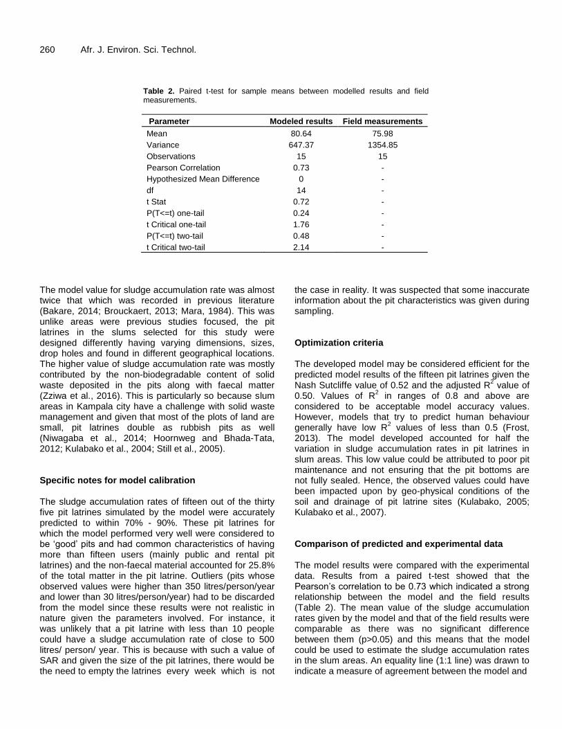
260 Afr. J. Environ. Sci. Technol.

Table 2. Paired t-test for sample means between modelled results and field measurements.

Parameter Modeled results Field measurements

Mean 80.64 75.98

Variance 647.37 1354.85

Observations 15 15

Pearson Correlation 0.73 -

Hypothesized Mean Difference 0 -

df 14 -

t Stat 0.72 -

P(T<=t) one-tail 0.24 -

t Critical one-tail 1.76 -

P(T<=t) two-tail 0.48 -

t Critical two-tail 2.14 -

The model value for sludge accumulation rate was almost twice that which was recorded in previous literature (Bakare, 2014; Brouckaert, 2013; Mara, 1984). This was unlike areas were previous studies focused, the pit latrines in the slums selected for this study were designed differently having varying dimensions, sizes, drop holes and found in different geographical locations. The higher value of sludge accumulation rate was mostly contributed by the non-biodegradable content of solid waste deposited in the pits along with faecal matter (Zziwa et al., 2016). This is particularly so because slum areas in Kampala city have a challenge with solid waste management and given that most of the plots of land are small, pit latrines double as rubbish pits as well (Niwagaba et al., 2014; Hoornweg and Bhada-Tata, 2012; Kulabako et al., 2004; Still et al., 2005). Specific notes for model calibration The sludge accumulation rates of fifteen out of the thirty five pit latrines simulated by the model were accurately predicted to within 70% - 90%. These pit latrines for which the model performed very well were considered to be ‘good’ pits and had common characteristics of having more than fifteen users (mainly public and rental pit latrines) and the non-faecal material accounted for 25.8% of the total matter in the pit latrine. Outliers (pits whose observed values were higher than 350 litres/person/year and lower than 30 litres/person/year) had to be discarded from the model since these results were not realistic in nature given the parameters involved. For instance, it was unlikely that a pit latrine with less than 10 people could have a sludge accumulation rate of close to 500 litres/ person/ year. This is because with such a value of SAR and given the size of the pit latrines, there would be the need to empty the latrines every week which is not

the case in reality. It was suspected that some inaccurate information about the pit characteristics was given during sampling. Optimization criteria The developed model may be considered efficient for the predicted model results of the fifteen pit latrines given the Nash Sutcliffe value of 0.52 and the adjusted R

2 value of

0.50. Values of R2 in ranges of 0.8 and above are

considered to be acceptable model accuracy values. However, models that try to predict human behaviour generally have low R

2 values of less than 0.5 (Frost,

2013). The model developed accounted for half the variation in sludge accumulation rates in pit latrines in slum areas. This low value could be attributed to poor pit maintenance and not ensuring that the pit bottoms are not fully sealed. Hence, the observed values could have been impacted upon by geo-physical conditions of the soil and drainage of pit latrine sites (Kulabako, 2005; Kulabako et al., 2007). Comparison of predicted and experimental data The model results were compared with the experimental data. Results from a paired t-test showed that the Pearson’s correlation to be 0.73 which indicated a strong relationship between the model and the field results (Table 2). The mean value of the sludge accumulation rates given by the model and that of the field results were comparable as there was no significant difference between them (p>0.05) and this means that the model could be used to estimate the sludge accumulation rates in the slum areas. An equality line (1:1 line) was drawn to indicate a measure of agreement between the model and

field results. The equality line (Figure 5) showed that the model was a good approximation since it showed an even distribution between the points. The 1:1 line in Figure 5 shows that the model was efficient for values between 40 and 110 litres/person/year. For values below this range, the model is overestimated the sludge accumulation rates while for those above the range, the model is underestimated. This is because the model considered a constant value for the non-faecal matter (Zziwa et al., 2016) which in reality is not the case. Hence, for pits with better use and less non-faecal matter; the model did not capture this and so overestimated the SAR while it underestimated the same for pit latrines that had more non-faecal matter. The developed model was however, found to be a better approximation of sludge accumulation rates in slum areas since it considered solid waste deposited in the pit latrines and was able to cover a range of pit latrines with different designs and user behaviour unlike previous studies that had been carried out (Brouckaert, 2013; Bakare, 2014; Murphy, 2015). The model was found to be a better approximation for rentals and public pit latrines compared to the private pit latrines, given their numbers were more in the study. CONCLUSION AND RECOMMENDATIONS The average sludge accumulation rate determined by

model was 81 25 litres/person/year. Model validation showed that the developed model was 52% efficient and accounted for 50% of the variation in the sludge accumulation rates. The model is sufficient for prediction of filling rates in the public and rental pit latrines within the studied slums given the variation in pit latrine designs, user behaviour, pit dimensions, location and solid waste deposal patterns. The model can therefore be adequately used for prediction of sludge accumulation rates of lined pit latrines in slum areas. The model was found to have limitations for determining sludge accumulation rates for private pit latrines and those pits that are managed properly. This study did not provide a specific emptying plan for each pit latrine but with the information provided on the sludge accumulation rates and the estimates provided, each pit latrine owner is able to adequately plan for emptying, given the different sizes of the pit latrine. Further studies can be taken on the effect of geo-physical factors such as soil characteristics and drainage patterns on sludge accumulation rates and a study to model sludge accumulation rates in unlined pit latrines in the slum areas. .

Conflict of interest The authors have not declared any conflict of interest.

Lugali et al. 261 ACKNOWLEDGEMENTS This study was financed through the Sanitation Research Fund for Africa (SRFA) Project that was co-funded by the Water Research Commission (South Africa) and the Bill and Melinda Gates Foundation. Kampala City Council Authority (KCCA) and Uganda National Council for Science and Technology (UNCST) are acknowledged for the permission granted to carry out this research. REFERENCES

Bakare BF (2014). Scientific and Management Support for Ventilated

Improved Pit Latrines (VIP) Sludge Content. School of chemical engineering. University of KwaZulu-Natal Durban (Unpublished).

Brouckaert CJ, Foxon KM, Wood K (2013). Modelling the filling rates of pit latrines. Pollution Research Group, School of Engineering, University of KwaZulu-Natal, Durban.

Buckley CA, Foxon KM, Brouckaert CJ, Nwaneri C, Balboni E, Couderc AMD (2008). Scientific support for the design and operation of ventilated improved pit latrines (vips). (S. of C. E. U. of K.-N. Pollution Research Group, Ed.). Durban: Water Research Commission. doi:TT 357/08.

Eales K (2005). Sanitation partnership series: Bringing pit emptying out of the darkness: A comparison of approaches in Durban, South Africa, and Kibera, Kenya. Building Partnerships for Development. Available at: http://www.bpdws.org/bpd/web/d/doc_131.pdf?statsHandlerDone=1

Fogg NA (2008). The Blame Game: Water and Sanitation in Kampala's Urban Slums. Independent Study Project (ISP) Collection. Paper 98.

Franceys R, Pickford J, Reed R (1992). A guide to the development of onsite sanitation. World Health Organization: Geneva.

Frost J (2013). Regression Analysis: How Do I Interpret R-squared and Assess the Goodness-of-Fit? Available at: http://blog.minitab.com/adventures-in-statistics/regression-analysis-how-do-i-interpret-r-squared-and-assess-the-goodness-of-fit.

Hoornweg D, Bhada-Tata P (2012). What a waste; A global review of solid waste management. Urban Development Series Knowledge Papers, World Bank.

Isunju JB, Etajak S, Mwalwega B, Kimwaga R, Atekyereza P, Bazeyo W, Ssempebwa JC (2013). Financing of sanitation services in the slums of Kampala and Dar-es-Salaam. Health 5(4):783-791.

Kariuki M, Collignon B, Taisne R, Valfrey B, Plummer J (2003). Better Water and Sanitation for the Urban Poor: Good Practice from Sub-Saharan Africa. Kenya: Water utility partnership for capacity building (WUP) Africa.

Katukiza AY, Ronteltap M, Oleja A, Niwagaba CB, Kansiime F, Lens PNL (2014). Identification of Sustainable Sanitation Options for Urban Slums- A Case of Bwaise III in Kampala Uganda. Department of Environmental Resources, UNESCO-IHE Institute for Water Education, Netherlands.

Kimuli D, Zziwa A, Banadda N, Kabenge I, Kiggundu N, Kambugu RK, Wanyama J, Tumutegyereize P, Kigozi J (2016). Quantification of Physico-Chemical Characteristics and Modeling Faecal Sludge Nutrients from Kampala City Slum Pit Latrines. Int. J. Res. Eng. Adv. Tech. 3(6):129-141.

Klingel F, Montenegro A, Koné D, Strauss M (2002). Fecal Sludge Management in Developing Countries: A planning manual, (April), 55.

Kone D, Chowdry S (2012). Business analysis of faecal sludge management: Emptying and transportation services in Africa and Asia. Draft Final Report.

Kulabako NR, Nalubega M, Roger T (2004). Characterization of Peri-Urban Anthropogenic Pollution in Kampala, Uganda. 30th WEDC International Conference, Vientiane, Lao PDR.

Kulabako NR, Nalubega M, Thunvik R (2007). Study of the impact of land use and hydrogeological settings on the shallow groundwater

262 Afr. J. Environ. Sci. Technol.

quality in a peri-urban area of Kampala, Uganda. Sci. Tot. Environ. 381(1):180-199.

Kulabako NR, Nalubega M, Wozei E, Thunvik R (2010). Environmental health practices, constraints and possible interventions in peri-urban settlements in developing countries–a review of Kampala, Uganda. Int. J. Environ. Health Res. 20(4):231-257.

Mara DD (1984). The Design of Ventilated Improved Pit Latrines. TAG Technical Note 13:83.

Mihelcic JR, Fry LM, Myre EA, Phillips LD, Barkdoll BD (2009). Field Guide to Environmental Engineering for Development Workers: Water, Sanitation and Indoor Air. Reston: ASCE Press.

Mikhael G, Robbins, DM, Ramsay JE, Mbéguéré M (2014). Methods and means for collection and transport of faecal sludge. In: Strande

L, Ronteltap M, Brdjanovic D (Eds.), Faecal Sludge Management – Systems Approach Implementation and Operation. IWA Publishing, London, UK: pp. 67-96.

Ministry of Lands, Housing and Urban development, MLHUD (2008). A situation analysis of slums in Uganda and national slum upgrading strategy and action plan. Department of Human Settlements. UNDP program.

Morella E, Foster V, Banerjee GS (2008). Climbing the Ladder: The State of Sanitation in Sub-Saharan Africa. Africa Infrastructure Country Diagnostic (AICD) Background Paper 13 (Phase 1). The World Bank, Washington, DC, USA.

Murphy CM (2015). Solids Accumulation rates of Pit latrines at Rural Schools in Nimba County, Liberia. Graduate Theses and Dissertations, University of South Florida, Scholar Commons.

Murungi C, Van Dijk MP (2014). Emptying, transportation and disposal of faecal sludge in informal settlements of Kampala Uganda: the economics of sanitation. Habitat Int. 42:69-75.

Musiige R (2010). Pollution of groundwater in shallow aquifers-a critical moment in Uganda. Groundwater Quality Sustainability. XXXVIII IAH Congress, Krakow.

Nash JE, Sutcliffe JV (1970). River flow forecasting through conceptual models. Part 1-A discussion of principles. J. Hydrol. 27(3):282-290.

Neter J, Wasserman W, Kutner M (1990). Applied linear statistical models, 2nd edn. Richard E. Irwin, Inc. Home-wood, IL.

Niwagaba CB (2009). Treatment technologies for human faeces and urine. Doctoral thesis, Swedish University of Agricultural Sciences, Uppsala.

Niwagaba CB, Mbéguéré M, Strande L (2014). Faecal Sludge Quantification, Characterisation and treatment objectives. Faecal Sludge Management; Systems Approach for Implementation and Operation. IWA Publishing.

Nwaneri CF (2009). Physico-Chemical characteristics and biodegradability of contents of Ventilated Improved Pits in eThekwini Municipality. Master of Science dissertation. School of Biological and Conservation Science. University of KwaZulu-Natal. South Africa.

Parkinson J, Quader M (2008). The challenge of servicing on-site sanitation in dense urban areas: Experiences from a pilot project in Dhaka. Waterlines 27(2):149-163.

Runyoro SK (1981). Pit Latrine Emptying. Department of Civil

Engineering, Loughborough University of Technology (Unpublished Thesis).

Samuel E (2008). The financing of sanitary facilities in urban slums of Kampala. A case study of Bwaise slum. Master’s degree thesis, Makerere University. Unpublished work.

Schaub-Jones D, Eales K, Tyers L (2006). Sanitation partnerships: harnessing their potential for urban on-site sanitation. BPD Sanitation series.

Still D, Foxon K (2012). Understanding Sludge Accumulation in VIPs and Strategies for Emptying Full Pits. Water research Commission. 1. DOI: 978-1-4312-0291-1

Still D, Riordan MO, McBride A, Louton B (2013). Adventures in search of the ideal portable pit-emptying machine. Waterlines 32:187-199.

Still DA, Salisbury RH, Foxon KM, Buckley CA, Bhangwan JN (2005). The challenges of dealing with full VIP latrines.

Thye YP, Templeton MR, Ali M (2011). A critical review of technologies for pit latrine emptying in developing countries. Crit. Rev. Environ. Sci. Technol. 41:1793-1819.

UN-HABITAT (2007). Situational Analysis of Informal Settlements in Kampala. Cities without slums sub-regional programme for Eastern and Southern; Kivulu (Kagugube) and Kinawataka (Mbuya 1) Parishes.

Wagner EG, Lanoix JN (1958). Excreta disposal for rural areas and small communities. Geneva Switzerland: World Health Organisation (WHO).

Water and Sanitation Program, WSP (2014). The Missing Link in Sanitation Service Delivery: A review of faecal sludge management in 12 cities. Targeting the urban poor and Improving Services in small towns, a research brief.

WINSA, WRC (2011). What Happens When the Pit is Full? Developments in on-site Faecal

Wood K (2013). Modeling fill rate with an unsteady-state mass balance. Transformation of feacal sludge in VIP.

WUP (2003). Better Water and Sanitation for the Urban Poor. Kenya, European Communities and Water Utility Partnership.

Zziwa A, Kabenge I, Kayondo H, Lugali Y, Kambugu RK, Wanyama, J (2016). Fractional content of non-feacal matter and its contribution to filling rates of pit latrines in Kampala slums. Glob. J. Eng. Sci. Res. Manage. 3(2):36-45.

African Journal of

Environmental Science and

Technology

Related Journals Published by Academic Journals Journal of Ecology and the Natural Environment Journal of Bioinformatics and Sequence Analysis Journal of General and Molecular Virology International Journal of Biodiversity and Conservation Journal of Biophysics and Structural Biology Journal of Evolutionary Biology Research