Agricultural Research - Academic Journals
202
African Journal of Agricultural Research Volume 11 Number 39 29 September 2016 ISSN 1991-637X
-
Upload
khangminh22 -
Category
Documents
-
view
2 -
download
0
Transcript of Agricultural Research - Academic Journals

African Journal of
Agricultural Research Volume 11 Number 39 29 September 2016
ISSN 1991-637X

ABOUT AJAR The African Journal of Agricultural Research (AJAR) is published weekly (one volume per year) by Academic Journals.
African Journal of Agricultural Research (AJAR) is an open access journal that publishes high-quality solicited and unsolicited articles, in English, in all areas of agriculture including arid soil research and rehabilitation, agricultural genomics, stored products research, tree fruit production, pesticide science, postharvest biology and technology, seed science research, irrigation, agricultural engineering, water resources management, marine sciences, agronomy, animal science, physiology and morphology, aquaculture, crop science, dairy science, entomology, fish and fisheries, forestry, freshwater science, horticulture, poultry science, soil science, systematic biology, veterinary, virology, viticulture, weed biology, agricultural economics and agribusiness. All articles published in AJAR are peer- reviewed.
Contact Us
Editorial Office: [email protected]
Help Desk: [email protected]
Website: http://www.academicjournals.org/journal/AJAR
Submit manuscript online http://ms.academicjournals.me/

. Editors
Prof. N.A. Amusa
Editor, African Journal of Agricultural Research Academic Journals.
Dr. Panagiota Florou-Paneri Laboratory of Nutrition, Faculty of Veterinary Medicine, Aristotle University of Thessaloniki, Greece.
Prof. Dr. Abdul Majeed Department of Botany, University of Gujrat,India, Director Horticulture, and landscaping. India.
Prof. Suleyman TABAN Department of Soil Science and Plant Nutrition, Faculty of Agriculture, Ankara University, 06100 Ankara-TURKEY.
Prof.Hyo Choi
Graduate School Gangneung-Wonju National University Gangneung, Gangwondo 210-
702, Korea.
Dr. MATIYAR RAHAMAN KHAN
AICRP (Nematode), Directorate of Research, Bidhan Chandra Krishi
Viswavidyalaya, P.O. Kalyani, Nadia, PIN-741235, West Bengal. India.
Prof. Hamid AIT-AMAR University of Science and Technology, Houari Bouemdiene, B.P. 32, 16111 EL-Alia, Algiers, Algeria.
Prof. Sheikh Raisuddin Department of Medical Elementology and
Toxicology,Jamia Hamdard (Hamdard University) New Delhi, India.
Prof. Ahmad Arzani Department of Agronomy and Plant Breeding College of Agriculture Isfahan University of Technology
Isfahan-84156, Iran.
Dr. Bampidis Vasileios
National Agricultural Research Foundation (NAGREF), Animal Research Institute 58100 Giannitsa, Greece.
Dr. Zhang Yuanzhi Laboratory of Space Technology, University of Technology (HUT) Kilonkallio Espoo, Finland. Dr. Mboya E. Burudi International Livestock Research Institute (ILRI) P.O. Box 30709 Nairobi 00100, Kenya. Dr. Andres Cibils Assistant Professor of Rangeland Science
Dept. of Animal and Range Sciences Box 30003, MSC 3-I New Mexico State University Las Cruces, NM 88003 (USA). Dr. MAJID Sattari
Rice Research Institute of Iran, Amol-Iran. Dr. Agricola Odoi University of Tennessee, TN., USA.
Prof. Horst Kaiser Department of Ichthyology and Fisheries Science Rhodes University, PO Box 94, South Africa.
Prof. Xingkai Xu Institute of Atmospheric Physics, Chinese Academy of Sciences, Beijing 100029,
China.
Dr. Agele, Samuel Ohikhena Department of Crop, Soil and Pest Management, Federal University of Technology
PMB 704, Akure, Nigeria. Dr. E.M. Aregheore The University of the South Pacific, School of Agriculture and Food Technology Alafua Campus, Apia, SAMOA

Editorial Board
Dr. Bradley G Fritz Research Scientist, Environmental Technology Division, Battelle, Pacific Northwest National Laboratory, 902 Battelle Blvd., Richland, Washington, USA.
Dr. Almut Gerhardt LimCo International, University of Tuebingen, Germany.
Dr. Celin Acharya Dr. K.S.Krishnan Research Associate (KSKRA), Molecular Biology Division, Bhabha Atomic Research Centre (BARC), Trombay, Mumbai-85, India.
Dr. Daizy R. Batish Department of Botany, Panjab University, Chandigarh, India.
Dr. Seyed Mohammad Ali Razavi University of Ferdowsi, Department of Food Science and Technology, Mashhad, Iran.
Dr. Yasemin Kavdir
Canakkale Onsekiz Mart University, Department of Soil Sciences, Terzioglu Campus 17100 Canakkale Turkey.
Prof. Giovanni Dinelli Department of Agroenvironmental Science and Technology Viale Fanin 44 40100, Bologna
Italy.
Prof. Huanmin Zhou College of Biotechnology at Inner Mongolia Agricultural University, Inner Mongolia Agricultural University, No. 306# Zhao Wu Da Street, Hohhot 010018, P. R. China, China.
Dr. Mohamed A. Dawoud Water Resources Department, Terrestrial Environment Research Centre, Environmental Research and Wildlife Development Agency (ERWDA), P. O. Box 45553, Abu Dhabi, United Arab Emirates.
Dr. Phillip Retief Celliers
Dept. Agriculture and Game Management, PO BOX 77000, NMMU, PE, 6031, South Africa.
Dr. Rodolfo Ungerfeld Departamento de Fisiología, Facultad de Veterinaria, Lasplaces 1550, Montevideo 11600, Uruguay. Dr. Timothy Smith Stable Cottage, Cuttle Lane, Biddestone, Chippenham, Wiltshire, SN14 7DF. UK. Dr. E. Nicholas Odongo,
27 Cole Road, Guelph, Ontario. N1G 4S3 Canada. Dr. D. K. Singh Scientist Irrigation and Drainage Engineering Division, Central Institute of Agricultural Engineeinrg Bhopal- 462038, M.P. India.
Prof. Hezhong Dong Professor of Agronomy, Cotton Research Center, Shandong Academy of Agricultural Sciences, Jinan 250100 China.
Dr. Ousmane Youm Assistant Director of Research & Leader, Integrated Rice Productions Systems Program Africa Rice Center (WARDA) 01BP 2031, Cotonou, Benin.

Table of Contents: Volume 11 Number 39, 29 September, 2016
ARTICLES
Effects of potassium fertilization and commercial substrates on development of passion fruit seedlings under greenhouse condition 3720 Rodrigo Takashi Maruki Miyake, William Hiroshi Suekane Takata, Wellington Eduardo Xavier Guerra, Fernanda Forli, Nobuyoshi Narita and José Eduardo Creste Tolerance of coriander cultivars under saline stress 3728 Francisco Vanies da Silva Sá, Lauter Silva Souto, Emanuela Pereira de Paiva, Miguel Ferreira Neto, Rosilene Agra da Silva, Maria Kaline do Nascimento Silva, Evandro Franklin de Mesquita, Fernandes Antônio de Almeida and Antônio Alves Neto
The Assistat Software Version 7.7 and its use in the analysis of experimental data 3733 Francisco de Assis Santos e Silva and Carlos Alberto Vieira de Azevedo
Association of on-farm feeds handling practices with fungal growth and Mycotoxin production on feeds in smallholder dairy farms, Nakuru, Kenya 3741 Makau Caroline Mwende, Matofari Joseph Wafula, Muliro Patrick Simiyu and Bebe Bockline Omedo
Measurement of apparent electrical conductivity of soil and the spatial variability of soil chemical properties by electromagnetic induction 3751 Glécio Machado Siqueira, Jorge Dafonte Dafonte, Antonio Paz González, Monteserrat Valcarcel Armesto, Ênio Farias de França e Silva, Mayanna Karlla Lima Costa and Raimunda Alves Silva
Characterization of water-stress tolerant cotton cultivars based on plant growth and in activity of antioxidant enzymes 3763 Jessica Damasceno Rodrigues, Carliane Rebeca Coelho da Silva, Rennan Fernandes Pereira, Jean Pierre Cordeiro Ramos, Péricles de Albuquerque Melo Filho, José Jaime Vasconcelos Cavalcanti and Roseane Cavalcanti Santos
Selection of input vectors for estimation of aboveground biomass of Mimosa scabrella Benth. using an artificial neural network 3771 Aline Bernarda Debastiani, Ana Paula Marques Martins, Carlos Roberto Sanquetta, Sebastião do Amaral Machado and Edilson Urbano
Guava rootstocks growth under incorporation of cattle manure and application of organic fertilizer the base of fruit of peel 3777 Mario Leno Martins Véras, José Sebastião de Melo Filho, Lunara de Sousa Alves, Toni Halan da Silva Irineu, Nelto Almeida Sousa, Lucimara Ferreira de Figueiredo, Edinete Nunes de Melo, Leandra de Melo Cavalcante, Thiago Jardelino Dias and Alvaro Carlos Gonçalves Neto
African Journal of Agricultural Research

Table of Contents: Volume 11 Number 39, 29 September, 2016
African Journal of Agricultural Research
ARTICLES
Diversity, abundance and incidence of fruit pest insects on three Solanum varieties (Solanaceae) in two agro-ecological zones of Southern Cameroon 3788 Elono Azang Pierre Stephan, Aléné Désirée Chantal, Heumou Cyril Roméo, Ngassam Pierre and Djiéto-Lordon Champlain
Yield response of canola (Brassica napus L.) to different inter-row spacings and sowing dates in northwest of Paraná, Brazil 3799 Lucas Caiubi Pereira, Gabriel Loli Bazo, Alessandro Lucca Braccini, Luiz Henrique da Silva Lima, Mayara Mariana Garcia and Keila Regina Hossa
Root system distribution and vegetative characteristics of Prata type bananas under different irrigation strategies 3806 Marcelo Rocha dos Santos, Lilian Leal Lourenço, Sérgio Luiz Rodrigues Donato, Bismarc Lopes da Silva, Igor Nogueira de Castro and Maurício Antônio Coelho Filho
Evaluation of mineral composition of endogenous and improved varieties of maize (Zea mays) cultivated in Southern Benin 3816 A. J. Semassa, V. B. Anihouvi, S. W. Padonou, D. Aly, A. Adjanohoun and L. Baba-Moussa
Fungitoxicity activity of homeopathic medicines on Alternaria solani 3824 Márcia Vargas Toledo, José Renato Stangarlin, Carlos Moacir Bonato, Thaísa Muriel Mioranza, Mônica Anghinoni Müller, Bruna Broti Rissato, Eloisa Lorenzetti, Sidiane Coltro-Roncato, Carla Rosane Kosmann and Lindomar Assi
Biofouling and performance of labyrinth-type emitters in drip irrigation with treated domestic sewage 3839 Flavio Daniel Szekut, Delfran Batista dos Santos, Carlos Alberto Vieira de Azevedo, Márcio Roberto Klein, Maycon Diego Ribeiro and Salomão de Sousa Medeiros
Effects of boron fertilization on a crambe crop cultivated in oxisols 3847 Felipe Samways Santos, Luiz Antônio Zanão Júnior, Deonir Secco e Natália Pereira, Reginaldo Ferreira Santos and Luciene Kazue Tokura
Performance of different genotypes of maize subjected to inoculation with Azospirillum brasilense 3853 Fernando Nobre Cunha, Nelmício Furtado da Silva, Carlos Ribeiro Rodrigues, Wilker Alves Morais, Flávio Henrique Ferreira Gomes, Luiz César Lopes Filho, Lays Borges dos Santos Cabral, Marconi Batista Teixeira, Gustavo da Silva Vieira and Cicero Teixeira Silva Costa Population dynamism and agrarian transformation in Ethiopia 3863 Reta Hailu Belda

Table of Contents: Volume 11 Number 39, 29 September, 2016
ARTICLES
Contribution of soybean seed treatment with Fluquinconazole to manage yield losses caused by Phakospora pachyrhizi using meta-analysis 3880 Lucas H. Fantin, Marcelo G. Canteri, André L. da Silva, Fernando L. Buss Tupich and Laurence V. Madden
Enhancing the productivity of groundnut (Arachis hypogaea) through earthening up practices at Tanqua-Abergelle district, Central Tigray, Ethiopia 3889 Berhane Sibhatu, Hintsa Meresa, Guesh Tekle and Melese Harf
Stability of soil aggregates in Latosols and Cambisols via standard method and sonification 3894 Érika Andressa da Silva, Geraldo César de Oliveira, Carla Eloize Carducci, José Maria de Lima, Laura Beatriz Batista de Melo and Pedro Antônio Namorato Benevenute
Chemical ripeners and different harvest periods in sugarcane in State of Paraná, southern Brazil 3904 Paulo Barbosa de Oliveira Filho, José Barbosa Duarte Júnior, Antônio Carlos Torres da Costa, Paulo Sérgio Rabello de Oliveira, Eurides Kuster Macedo Júnior, Vandeir Francisco Guimarães and Willian Bosquette
African Journal of Agricultural Research

Vol. 11(39), pp. 3720-3727, 29 September, 2016
DOI: 10.5897/AJAR2016.11509
Article Number: E86E98960811
ISSN 1991-637X
Copyright ©2016
Author(s) retain the copyright of this article
http://www.academicjournals.org/AJAR
African Journal of Agricultural
Research
Full Length Research Paper
Effects of potassium fertilization and commercial substrates on development of passion fruit seedlings
under greenhouse condition
Rodrigo Takashi Maruki Miyake1*, William Hiroshi Suekane Takata1, Wellington Eduardo Xavier Guerra1, Fernanda Forli1, Nobuyoshi Narita2 and José Eduardo Creste1
1Department of Agriculture, University of Western of São Paulo, UNOESTE, Highway Raposo Tavares, Km 572,
Presidente Prudente, SP, 19.033-390, Brazil. 2Agency Paulista for Technology Agribusiness, APTA, Highway Raposo Tavares, Km 561, 19.015-970, Presidente
Prudente, SP, Brazil.
Received 2 August, 2016; Accepted 15 September, 2016
The aim of this work was to evaluate commercially available substrates and levels of potassium on the development of passion fruit seedlings in protected conditions. The experiment was conducted at the city of Presidente Prudente, São Paulo within the period from April to September of 2010. The treatments were made with three different substrates (Bioplant
®, Coconut fiber and Vivatto
®) and four
levels of potassium (0, 150, 300 and 600 mg-1
of K dm-³), arranged in a 3 × 4 factorial design with five
repetitions. The following parameters were analyzed 120 days after seedlings transplanting: Plant height, number of leaves, length of root, dry matter of shoot, root, total matter and chlorophyll content. The dose of 600 mg dm
-3 of K provided the highest seedling height, 85.83 cm independent of the
substrate. The commercial substrates Bioplant® and Coconut fiber with a dose of 150 mg dm
-3 of K
influenced the maximum accumulation of total dry matter of seedlings. However, Vivatto® substrate
provided the highest accumulation of total dry matter with application dose of 600 mg dm-3
of K. Mineral potassium fertilization in the substrate Bioplant
® and Coconut fiber with a dose of 150 mg dm
-3 reduced
the length of passion fruit’s roots. Key words: Passiflora edulis Sims., mineral nutrition, protected cultivation.
INTRODUCTION The passion fruit (Passiflora edulis Sims.) is a widespread culture in all Brazilian regions, both due to the highly favorable soil and weather conditions. Besides,
this fruit is largely commercialized in nature at public markets and for juice pulp industry (Pires et al., 2008). It is estimated that Brazil currently is the world's largest
*Corresponding author. E-mail: [email protected].
Author(s) agree that this article remain permanently open access under the terms of the Creative Commons Attribution
License 4.0 International License

producer of this fruit crop with a production of around 838,000 tons (IBGE, 2016).
In general, the low productivity of passion fruit fields may be related to several factors, including disease, especially viruses and inadequate fertilization practices. Some scientific studies showed that the use of low genetic quality seedlings/plants combined with malnourishment compromise yield production and culture longevity (Silva et al., 2010; Souza et al., 2016). Little has been reported about research analyses of seedlings production in a protected environment, specifically evaluating efficiency of nutrient levels such as potassium and different substrate types.
Traditionally passion fruit seedlings are transplanted to the field during March/April when they are about 30 cm high, coinciding with previous harvest time. Such overlapping period, enhance chances of early infection of passion fruit by virus causing lower productivity and fruit quality. The strategy of producing seedling in protected nurseries and holding their transference to the field until they are about 1.0 m high (at August) can, therefore avoid the previous crop, then bringing important advantages as breaking disease cycle and increasing fruit yields from December to March.
Potassium deficiency in passion fruit is involved with delay of flowering process and reduced production, including fruit size. Thus, interfering negatively with fruit and juice quality (Borges et al., 2002). It has been described, that cultivation of passion fruit requires more potassium than nitrogen (Borges et al., 2003). Moreover, it was shown that high doses of K and Cl can cause plants toxicity, when using potassium.
The growth of seedlings using substrate aims to ensure their development into maturity with higher quality in a short period of time, reducing cost production. However, the substrate must present physical and chemical characteristics to promote, respectively, moisture retention and nutrient availability, thus meeting the nourishment requirements of this plant crop (Cunha et al., 2005).
Silva et al. (2010) reported the effect of different types of substrates in the production of yellow passion fruit seedlings. They found that the substrate Plantmax
®
favored all growth parameters tested. Santos et al. (2012) studied the early development of Passiflora-cincinnata seedlings, and concluded that the substrate Vivatto
®
provided greater accumulation of fresh and dry root production.
Almeida et al. (2006) evaluated the effects of nitrogen and potassic fertilization on the development and nutrition of yellow passion fruit seedlings, cultivated in dystrophic Red Latosol. After 84 days, the plant height, diameter of the stem, number of leaves and leaf area showed best development of seedlings at the levels of 150 mg of N dm
-3 and 300 mg of K dm
-3. Dias et al. (2012) studied the
effects of potassium on the growth of guava seedlings in Red-Yellow Argisol. At 120 days, the fertilization with
Miyake et al. 3721 potassium did not influence the biometric parameters the height, stem diameter, number of leaves, SPAD index, dry weight of leaves. However, the doses of K of 1.452 mg dm
-3 and K aids in the efficiency of 84.9% of
absorption and utilization of N and K for seedlings. Given the facts above, the aim of this work was to
evaluate, in protected conditions, the effects of potassium levels in the development of yellow passion fruit seedlings using 3 commercially available substrates.
MATERIALS AND METHODS The scientific work was conducted in a greenhouse located in a field area belonging to Agency Paulista for Technology of Agribusiness (APTA) located at the city of Presidente Prudente in the western region of São Paulo, in the period from April to September 2010, whose geographical coordinates are: Latitude 22° 07 '04 "S and longitude 51° 23' 01"O.
The roof of the greenhouse was made of transparent plastic film while the sides were with anti-aphid screen. From inside, bellow roof, a 50% shade fabric was used for protection while the countertops were disposed 80 cm above the ground.
The experiments were conducted in randomized blocks in a factorial 3 × 4 with five repetitions. For treatments were used three commercial substrates (Bioplant®, Coconut Fiber and Vivatto®) and four potassium doses (0, 150, 300 and 600 mg K dm-³) supplied by potassium chloride (60% K2O). The experimental plots were composed of 5 plant (1 per plastic bag). The substrates were subjected to chemical analysis (UNOESTE, at Soil Laboratory) and physical characteristics are presented in Table 1.
The yellow passion fruit seeds (P. edulis Sims.) cultivar 'South Brazil Afruvec' were germinated in trays with 200 divisions. After germination, they were transplanted into 2 L plastic bags with different substrates. The seedlings were monitored and conducted by stakes. During early development seedlings were irrigated until they reached field capacity point at each substrate tested.
In each analyzed experimental unit it was employed 2 L of substrate per bag. When transplanting, each bag received fertilization with P (450 mg dm-³), N (300 mg dm-3), B (0.5 mg dm-³) and Zn (5 mg dm-3) as Lopes (2000). As a source of N, P, B and Zn were used as urea (45% N), triple superphosphate (42% P2O5), boric acid (17% B) and zinc sulfate (21% Zn), respectively. The total phosphorus was mixed with the substrate at the time of filling plastic bags. Nitrogen and potassium were applied by fertigation in five applications 20 days apart from transplanting, 20% applied at transplanting and four applications of 20% every 20 days.
After 120 days the assessment was performed by collecting treatments of following parameters: Plant height (PW), number of leaves (NL) per plant; dry weight of shoot (DWS), dry weight of roots (DWR), and total dry weight (TDW), length of root (LR) and the leaf chlorophyll content (LCC) (SPAD value).
The plants’ height was evaluated considering the distance between the plant laps until the apex of seedlings, using graduated ruler (mm). For leaves number it was considered only the fully expanded ones. The dry matter content of plants was quantified after collection and drying of material in an oven (with forced air circulation at 65°C for 72 h to reach constant weight). Biomass of root and shoot were determined using analytical precise scale, 0.0001. The chlorophyll content was determined directly by a digital chlorophyll (Chlorophyll Content Meter, CCM-200). The reading of three expanded middle leaves for each plant was considered obtaining the chlorophyll results in SPAD values.
All data were submitted to analysis of variance by F test (p <0.05) and the significant effect of each factor or interaction was compared by the Tukey test (p <0.05). For substrate types and through the

3722 Afr. J. Agric. Res.
Table 1. Chemistry composition and physical characteristics of substrates.
Substrate pH MO Ca Mg K P S SB CTC V B Zn
Cacl2 mg dm-3
mmolcdm-3
mg dm-3
% mg dm-3
Bioplant® 5.0 218 22 12 16.3 230 193 50 87 58 2.7 28
Coc. fiber 5.0 213 12 4 23.4 104 154 40 59 69 6.4 29
Vivatto® 4.8 211 19 22 12.0 230 234 52 89 59 6.3 8
Substrate WRC Density (Kg/m³) EC (mScm-1
) H (%) TP
Bioplant® 38% 288 1.7 65 85
Coc. fiber 30% 92 0.2 95 90
Vivatto® 40% 267 0.5 48 91
Obs. WRC- water retention capacity; CE- eletric conductivity; U-percentage of humidity; PT- total porosity.
regression analysis of variance in the case of potassium doses it was applied computationally SISVAR 5.6 program (Ferreira, 2011). RESULTS The physical characteristics and chemical composition of each substrate are shown in Table 1. With regard of leaf variables analyzed DWS, DWR and TDW; significant correlation between potassium levels and substrate types studied were not observed (Figures 2 and 3). Effect of substrate types on seedlings height Table 2 shows that the type of substrate utilized did not influenced significantly the plants’ height 120 days after transplanting. The average size obtained was 67.43, 61.96 and 61.34 cm for Bioplant
® substrate, Coconut fiber
and Vivatto® respectively.
Effect of potassium levels on seedlings height The plant height obtained for passion fruit seedlings correlated directly to the potassium doses applied, as observed in Figure 1. The maximum response of seedlings occurred at the maximum dose of K (600 mg dm
-3), while height average reached 85.83 cm.
Influence of substrate types and potassium levels on seedlings development It was observed that potassium levels provided gains in leave numbers with a dose of 300 mg dm
-3 K when plants
were grown in Bioplant® and Vivatto
® substrate (Figure
2). However, when Coconut fiber was used a positive effect was already achieved with a dose of 150 mg dm
-3
of K. The variables of DWS, DWR and TDW of seedlings are
shown in Figure 3A to C, respectively. The results of DWS were influenced by the interaction between the type of substrate and potassium doses (Figure 3A). The dry roots weight of yellow passion fruit seedlings showed highest value when applied 300 mg dm
-3 of K on
substrates Bioplant® and Vivatto
® (Figure 3B). In the
Coconut fiber substrate the potassium application reduced the dry matter of the roots of seedlings.
The responses evaluated in the TDW seedlings differ significantly between the substrates, combined with the dose of K (Figure 3C). In the substrate Bioplant
® the best
response in the TDW was verified with the use of 300 mg dm
-3 of K and Coconut fiber the maximum dry matter
yield was obtained at a dose of 150 mg dm-3
of K. However, when it was used the substrate Vivatto
®, the
largest dry mass was obtained by applying 600 mg dm-3
of K.
The response related to root length varied according to the types of substrates analysed and the potassium doses applied (Figure 4). It can be seen that the substrate Bioplant
® and Coconut fiber showed the best
results for development of seedlings roots without potassium application. The seedlings which were planted in Vivatto
® substrate showed the best average root length
without potassium application and maximum dose of 600 mg dm
-3 of K.
The commercial substrates were accepted statistically for chlorophyll content values (SPAD value) evaluated in yellow passion fruit seedlings (Figure 5). It was observed SPAD values obtained with a dose of 300 mg dm
-3 of K
was higher on Coconut fiber, followed by Bioplant®
respectively at 120 days. While development of seedlings sown in Vivatto
® presented lower SPAD index for
chlorophyll content.
DISCUSSION
For plant height parameters the averages in the three commercial substrates showed not difference statistic (Table 2). Nevertheless, it was found that average were

Miyake et al. 3723
Figure 1. Plant height of yellow passion fruit in fuction of dose of potassium and substrate, after 120 days.
Figure 2. Number of leaves in function of dose of potassium and substrate, at 120 days [(▪) Bioplant; (∆) Coconut fiber and (•) Vivatto].
higher than that of traditional seedlings that are 25 to 40 cm. The substrates with high porosity physical characteristics offers less resistance to root growth and also has the ability to maintain the temperature and humidity of the substrate that influence of growing of plants (Ristow et al.; 2012). These physicals characteristic were verified in the substrates used in this experiment (Table 1).
The positive effect of increase in K levels in the height of passion fruit presenting increasing linear. The
potassium effects the main functions in plants such as enzyme activation, protein synthesis, absorption, transport and ion balance, and is also involved in photosynthesis, respiration, transportation and long distance distribution of assimilates (Hawkesford et al., 2012). Prado et al. (2004) evaluating application of potassium doses at 60 days, verified that the development of yellow passion fruit seedlings reached maximum development in height with a dose of 220 mg K dm
-3.

3724 Afr. J. Agric. Res.
Figure 3. Dry weight of shoot (3A), dry weight of root (3B) and total dry weight (3C) of passion fruit seedlings in function of the applied potassium dose and substrate, at 120 days [(▪) Bioplant; (∆) Coconut fiber and (•) Vivatto].
The potassium dose difference ideal for maximum response varied according with type of substrate due to the difference in the humidity content (H) between the substrates (Table 1) which can be interfered in the nutrient absorption which may have required greater
nutrition of seedlings. Almeida et al. (2006) when producing passion fruit seedlings verified maximum of 14 leaves, but the dose of 218 mg dm
-3 of K grown in Oxisol
as a substrate, which shows the seedlings showed good numbers of leaves.

Miyake et al. 3725
Figure 4. Length of root of passion fruit seedlings in function of the applied potassium dose and substrate, at 120 days [(▪) Bioplant; (∆) Coconut fiber and (•) Vivatto].
Figure 5. Leaf chlorophyll content of passion fruit seedlings in fuction of the applied potassium dose and substrate, at 120 days [(▪), Bioplant; ∆, coconut fiber; •, Vivatto].
Table 2. Plant height (cm) of passion fruit in fuction of substrate, after 120 days of transplanting.
Substrate Plant height (cm)
Bioplant® 67.43
a
Coconut fiber 61.96a
Vivatto® 61.34
a
C.V. (%) 19.90
Mean of same letter have no difference statistic.

3726 Afr. J. Agric. Res. In DWS significant difference occurred varying responses on dry matter in accordance with the interaction between potassium dose and type of substrate (Figure 3A). The different results showed can be explained by different chemical characteristics of three substrates (Table 1), which influenced the accumulation of dry matter of seedlings of yellow passion fruit. The effects of increasing doses of K depend on the decrease in the accumulation of Ca and Mg in the substrate. The increase of available K in the soil enhances the competitive effect on the absorption of Ca and Mg, during the root absorption process, these nutrients used the same loading sites (Radane-Malvi, 2011). Prado et al. (2004) found a decrease in dry matter of passion fruit seedlings using a higher dose of 225 mg dm
-3 of K.
Substrate Coconut fiber was presented as the better in roots accumulation of seedlings, presenting best values than substrate Bioplant
® and Vivatto
® in the gain of dry
matter was without application of potassium (Figure 3B). Probably, the content of substrate of 23.4 mmolcdm
-3
(Table 1) was sufficient to express the maximum result in DWR. The difference in accumulation of DWR occurred due to interaction between K: Ca/Mg with application of potassium doses, principality high relation Ca/Mg in the substrate could have hampered K absorption by the plant due to competition for the same absorption site (Radane-Malvi, 2011).
In variable of TDW accumulation of seedlings, significant difference and interaction between types of substrates and doses of K was observed (Figure 3C). This difference to the ideal dose for maximum dry matter accumulation were probably due to differences in chemical composition and physicals of commercial substrates (Table 1), where the interaction between chemical and physical of substrates influenced on responses of TDW. Almeida et al. (2006) studied the mineral nutrition of passion fruit seedlings recommended dose of 300 mg K dm
-³ to obtain the maximum
accumulation 16 g of dry matter of seedlings, but this value was obtained by the sum of total dry matter of two plants that were sown in the same vessel. Boechat et al. (2010) observed that substrates with manure + soil and Plantmax
® showed higher values total dry matter in
passion fruit seedlings compared the Coconut fiber and presenting 0.80 to 1.20 g dry matter plant
-1 at 60 days in
the dose of 6.4 g K2O. In general, it was observed that the increased
application of K doses caused reduced growth of the roots of plants yellow passion fruit in the three substrates, this response may be due to two factors combined (Figure 4). This response may be due to two factors combined. First, the salt effect caused by Cl to the fertilization potassium, when using chloride potassium as a fertilizer added to the nitrogen supply of plants in the form that increases the salinity of the substrate, may cause toxicity micronutrient plants (Malavolta, 1997).
The use of potassium chloride as a K source may have
caused a toxic salinity roots of seedlings that inhibited growth in excess salts with three commercial substrates. Furthermore, there substrates contains Mg and K in the composition. The omission of plant growth under saline conditions may either be due to osmotic reduction in water availability or to excessive ion levels (Marschner, 1995).
The chlorophyll content (SPAD) in passion fruit seedlings showed difference according to the substrate and potassium doses used (Figure 5). There was an increase in the SPAD values until the dose of 300 mg dm
-
3 using Coconut fiber. Potassium participates in the onset of metabolic
processes of nitrogen, the absorption of mineral nitrogen, and in particular the nitrate reductase and the efficiency of N is reduced in plants that are deficient K (Ruan et al., 2015). Photosynthesis constitute the basis for the production of a culture and using the absorption of light energy by the plant can be estimated by chlorophyll fluorescence analysis (Freire et al., 2013).
The amount of Ca, Mg substrate Vivatto® (Table 1) plus
potassium fertilization resulted nutritional unbalance the changes which explains the low content of chlorophyll passion fruit sheet. Authors have reported the feasibility of measurement of chlorophyll as indicators of the nutritional status and quality of passion fruit plants in relation to nutrient (Freire et al., 2013; Cavalcante et al., 2011). Santos et al. (2011) in the study of initial growth of yellow passion fruit seedlings found SPAD value of 57 to 127 days after sowing the seedlings. However, this work were evaluated sources of N being that results better were with bovine + urea manure. The use of salts in the soil, including potassium in high concentrations reduces the nutritional balance of passion fruit seedlings by decreased total chlorophyll levels (Freire et al., 2013). Conclusion The doses of potassium that provided the maximum accumulation of total dry matter of seedlings of yellow passion fruit was the dose of 600 mg of K dm
-³ for
substrate Vivatto® and 300 mg of K dm
-³ for substrate
Bioplant®. For substrate, Coconut fiber the potassium
dose not reflected in increased dry matter accumulation of seedlings. The types of commercial substrates Bioplant
®, Coconut fiber and Vivatto
® provoked
differences during seedlings development in protected conditions. The response varied among substrate tested and potassium doses, affecting leaves features, dry weight, root length and chlorophyll content of seedlings of yellow passion fruit. Conflict of Interests The authors have not declared any conflict of interests.

REFERENCES Almeida EV, Natale W, Prado RM, Barbosa JC (2006) Nitrogen and
potassic fertilization on development of passion fruit seedlings. Ciênc. Rural 36:1138-1142.
Boechat CL, Teixeira AM, Costa ASV, Sousa BAPS (2010) Influence of substrates associated with mineral fertilization on the initial growth of two cultivars of yellow passion fruit. Rev. Caatinga 23:19-25.
Borges AL, Caldas RC, Lima AA, Almeida IE (2002) Effect of NPK on nutrient levels in leaves and soil, and on yield of yellow passion fruit. Rev. Bras. Frutic. 24:208-213.
Borges AL, Rodrigues MGV, Lima AA, Almeida IE, Caldas RC (2003) Nitrogen and potassium effects on yield and quality of yellow passion fruit, under irrigation. Rev. Bras. Frutic. 25:259-262.
Cavalcante LF, Dias TJ, Nascimento R, Freire JLO (2011) Chlorophyll and carotenoids in yellow passion fruit plants irrigated with saline water on soil with bovine biofertilizer. Rev. Bras. Frut. Special issue pp. 699-705.
Cunha AO, Andrade LA, Bruno RLA, Silva JAL, Souza VC (2005). Effects of substrate and containers dimensions on the quality of Tabebuia impetiginosa (Mart. Ex D.C.) Standl. Seedlings. Rev. Árvore 29:507-516.
Dias MJT, Souza HA, Natale W, Modesto VC, Rozane DE (2012) Fertilization with nitrogen and potassium in guava seedlings in a commercial nursery. Semina, supplement: pp. 2837-2848.
Ferreira DF (2011). Sisvar: A computer statistical analysis system. Ciênc. Agrotechnol. 35:1039-1042.
Freire JLO, Cavalcante LF, Nascimento R, Requebi AM (2013) Chlorophyll content of leaf and mineral composition of passion fruits irrigated with saline water and biofertilizers. Rev. Ciênc. Agrar. 36:57-70.
IBGE- Brazilian Institute of Geography and Statistics. Municipal Agricultural Production. Available at: http://www.cnpmf.embrapa.br/planilhas/Maracuja_Brasil_2010.pdf. Acessed: 13/05/ 2016.
Hawkesford M, Horst W, Kichey T, Lambers H, Schjoerring J, Skrumsager MI, White P (2012). Functions of macronutrients. In: Marschner P (Ed.). Marschner's mineral nutrition of higher plants 4:135-189.
Lopes PSN (2000). Micronutrients in younger plants of sweet passion fruit (Passiflora alata Dryand). These (Doctoral in Crop Science) - Federal University of Lavras, 2000.
Malavolta E, Vitti GC, Oliveira SA (1997). Evaluation of the nutritional status of plants: principles and applications. Piracicaba (Ed) POTAFÓS 319.
Marschner H (1995). Mineral nutrition of higher plants. 2nd ed., p. 889. Acad. Press, London, New York.
Pires AA, Monnerat PH, Marciano CR, Pinho LGR, Zampirolli PD, Rosa RCC, Muniz RA (2008) Alternative manuring of the yellow passion fruit plant: effects on chemical and physical characteristics of the soil. Rev. Bras. Ciênc. Solo 32:1997-2005.
Prado RM, Braghirolli LF, Natale W, Corrêa MCM, Almeida EV (2004) Potassium application on the nutricional status and dry matter production of passion fruit cutting. Rev. Bras. Frutic. 26:295-299.
Radane-Malvi U (2011). Interaction of micronutrients with major nutrients with special reference to potassium. J. Agric. Sci. 24:106-109.
Ristow NC, Antunes LEC, Carpenedo S (2012) Substrates for rooting microcutting blueberrry cultivar georgiagem. Rev. Bras. Frutic. 34:262-268.
Ruan J, Gerendás J (2015) Absorption of foliar-applied urea-15
N and the impact of low nitrogen, potassium, magnesium and sulfur nutritional status in tea (Camellia sinensis L.) plants. J. Soil Sci. Plant Nutr. 61:653-6563.
Santos JL, Matsumoto SN, D’arêde LO, Luz IS, Viana AES (2012) Vegetative propagation of cuttings of Passiflora cincinnata mast. in different commercial substrates and containers. Rev. Bras. Frutic. 34:581-588. Santos PC, Lopes LC, Freitas SJ, Sousa LB, Carvalho AJC (2011). Initial growth and nutritional content of yellow passion fruit subjected to fertilization with different nitrogen sources. Rev. Bras. Frutic. 33:722-728.
Miyake et al. 3727 Silva EAS, Maruyama WI, Mendoça V, Francisco MGS, Bardiviesso
DM, Tosta MS (2010) Composition of substrates and volume of recipients in the production and quality of yellow passion fruit seedlings. Ciênc. Agrotechnol. 34:588-595.
Souza JTA, Cavalcante LF, Nunes JC, Bezerra FTC, Nunes JAS, Silva AR, Oresca D, Cavalcante AG (2016). Effect of saline water, bovine biofertilizer and potassium on yellow passion fruit growth after planting and on soil salinity. Afr. J. Agric. Res 11:2994-3003.

Vol. 11(39), pp. 3728-3732, 29 September, 2016
DOI: 10.5897/AJAR2016.11390
Article Number: 7A49C0960814
ISSN 1991-637X
Copyright ©2016
Author(s) retain the copyright of this article
http://www.academicjournals.org/AJAR
African Journal of Agricultural Research
Full Length Research Paper
Tolerance of coriander cultivars under saline stress
Francisco Vanies da Silva Sá1*, Lauter Silva Souto1, Emanoela Pereira de Paiva2, Miguel Ferreira Neto2, Rosilene Agra da Silva1, Maria Kaline do Nascimento Silva1, Evandro Franklin
de Mesquita3, Fernandes Antônio de Almeida1 and Antônio Alves Neto1
1Federal University of Campina Grande, Campina Grande, Paraíba, Brazil.
2Federal University of Rural of Semi-Árido, Mossoró, Rio Grande do Norte, Brazil.
3State University of Paraíba (UEPB), Catolé do Rocha, Paraíba, Brazil.
Received 3 July, 2016; Accepted 19 September, 2016
This study aimed to evaluate the emergence, growth and phytomass accumulation of coriander cultivars under saline stress. The experiment was carried out from August to September 2014, in a protected environment (greenhouse), at the Center of Sciences and Food Technology - CCTA of the Federal University of Campina Grande – UFCG, located in the municipality of Pombal-PB, Brazil (6°47’20’’ S; 37°48’01’’ W; 194 m). Two coriander cultivars (C1 – ‘Verdão SF 177’ and C2 – ‘Português Pacífico’) were evaluated under five levels of irrigation water salinity (0.6 (control); 1.2; 1.8, 2.4 and 3.0 dS m
-1), arranged in a 2 x 5 factorial scheme, in a randomized block design, with four replicates and five
plants per replicate. Coriander plants were cultivated on trays of 36 cells with capacity for 0.1 dm3 of
substrate, until 20 days after sowing, and evaluated for emergence, growth, phytomass accumulation and tolerance to salinity. The increase in irrigation water salinity reduced emergence percentage, growth and phytomass accumulation of coriander plants. The cultivar ‘Português Pacífico’ is more tolerant to salinity than ‘Verdão SF 177’. The cultivars ‘Português Pacífico’ and ‘Verdão SF 177’ can be irrigated with water of up to 2.6 and 1.9 dS m
-1, respectively, in the initial growth stage.
Key words: Coriandrum sativum, salinity, emergence, initial growth.
INTRODUCTION Coriander (Coriandrum sativum L.) is a leafy vegetable widely consumed in Brazil, especially in the Northeast region, where it is largely used in the regional cuisine; thus having great alimentary and socioeconomic importance for being cultivated during the entire year, generating jobs and income to small- and medium-sized producers (Silva et al., 2012; Sales et al., 2015). However, its cultivation in the Northeast region requires
irrigation, due to the climatic conditions, such as high atmospheric demand and low rainfalls (Oliveira et al., 2010).
In the Brazilian semiarid region, there is great availability al., 2015; Araújo et al., 2016). However, depending on of waters with saline concentrations unviable for direct use in the conventional irrigation of most crops (Silva et al., 2012) the period of the year, the
*Corresponding author. E-mail: [email protected].
Author(s) agree that this article remain permanently open access under the terms of the Creative Commons Attribution
License 4.0 International License

da Silva Sá et al. 3729
Table 1. Chemical characteristics of the components of the substrate used in coriander cultivation.
CE pH P K
+ Ca
+2 Mg
+2 Na
+ Al
3+ H
++Al
3+ SB T MO
dS m-1
H2O mg dm-3
-----------------------------cmolcdm-3
------------------------------- g kg-3
A 0.09 8.07 3.00 0.32 6.40 3.20 0.18 0.00 0.00 10.49 10.49 16.0
B 1.65 5.75 86.00 1.67 11.60 28.50 17.84 0.00 11.88 59.61 71.49 570.0
SB = Sum of bases; EC = electrical conductivity; T = total cation exchange capacity; OM = organic matter; A = soil; B = commercial substrate.
Table 2. Chemical analysis of the public-supply water used in the preparation of the solutions.
CEa pH K Ca Mg Na SO4-2
CO3-2
HCO3-
Cl-
SAR1
dSm-1
.....................................(mmolcL-1
)................................ (mmolcL-1
)0,5
0.3 7.0 0.3 0.2 0.6 1.4 0.2 0.0 0.8 1.3 2.21 1SAR = Sodium adsorption ratio.
water used for the irrigation of crops contains high levels of salts, which limit the development of the crops, especially coriander (Rebouças et al., 2013). In addition, most rural producers of vegetables perform irrigations with water collected in superficial reservoirs, which may have high concentration of dissolved salts (Oliveira et al., 2014). In these cases, the use of saline water is conditioned to the tolerance of the crops to salinity and the adequate irrigation management (Medeiros et al., 2007).
Considering that not all crops respond equally tosalinity, some produce acceptable yields at high saline levels and others are sensitive to relatively low levels (Santana et al., 2007). It can be said that the tolerance to salinity is variable among species and, even within the same species, among development stages, in each stage, the tolerance to salinity is controlled by more than one gene, highly influenced by environmental factors (Flowers and Flowers, 2005; Esteves and Suzuki, 2008; Munns and Tester, 2008; Taiz and Zeiger, 2013). These differences are due to the capacity of osmotic adaptation that some genotypes have, which allows them to absorb greater amount of water, even under conditions of high salinity (Ayers and Westcot, 1999).
Given the above, this study aimed to evaluate the emergence, growth and phytomass accumulation of coriander cultivars under saline stress. MATERIALS AND METHODS The experiment was carried out from August to September 2014, in a protected environment (greenhouse), at the Center of Sciences and Food Technology – CCTA of the Federal University of Campina Grande – UFCG, located in the municipality of Pombal-PB, Brazil (6°47’20’’ S; 37°48’01’’ W; 194 m).
Two coriander cultivars (C1 – ‘Verdão SF 177’ and C2 – ‘Português Pacífico’) were evaluated under five levels of irrigation water salinity (0.6 (control); 1.2; 1.8, 2.4 and 3.0 dS m-1), arranged in a 2 x 5 factorial scheme, in a randomized block design, with four replicates and five plants per replicate, totaling 200 plants.
Coriander plants were cultivated on trays of 36 cells with capacity for 0.1 dm3 of substrate, until 20 days after sowing (DAS). The substrate for seedlings production was composed of soil (typic Tb eutrophic Fluvic Neosol) (Embrapa, 2013) and commercial substrate, mixed at the proportion of 1:1, respectively, and its chemical characterization is shown in Table 1 (Embrapa, 2011). At sowing, five tray cells were used for each treatment, and each cell received two seeds, totaling 10 seeds per treatment. After seedlings emergence finished, thinning was performed leaving only the most vigorous plant per cell. The seeds of both cultivars were purchased in a store, with 99% of purity and 95% of germination.
Irrigations were daily performed, in order to maintain the substrate with moisture content close to the maximum retention capacity, based on the method of drainage lysimetry, and the applied water depth was added to a leaching fraction of 20%. The volume applied (Va) per container was obtained by the difference between the previous volume applied (Vprev) minus the mean drainage (D), divided by the number of containers (n), as indicated in Equation 1.
LF
nDVV
prev
a
1
)/( (1)
Irrigation waters with different levels of salinity were prepared considering the relationship between ECw and concentration of salts (10*meq L-1 = 1 dS m-1 of ECw), according to Rhoades et al. (1992), which is valid for ECw of 0.1 to 5.0 dS m-1, which comprehend the tested levels. Water from the local supply system (ECw= 0.3 dS m-1) was used, mixed with salts (NaCl) as necessary (Table 2).
After preparation, the salinized waters were stored in 30-L plastic containers, one for each studied level of ECw, which were properly protected to avoid evaporation, entry of rainwater and contamination with materials that could compromise their quality. For the preparation of the waters, with the respective levels of electrical conductivity (EC), the salts were weighed according to the treatments and water was added until the desired EC level. The values were confirmed using a portable conductivity meter, adjusted to temperature of 25°C.
During the experiment, the emergence of coriander plants was monitored by counting the number of emerged plants, that is, with cotyledons above soil surface, without discarding them, thus obtaining a cumulative value. After stabilization of emergence, emergence percentage (EP) (%) was determined through the relationship between the number of emerged plants and the number of planted seeds.

3730 Afr. J. Agric. Res.
Crop morphological aspects were monitored through the growth analysis of the seedlings at 20 DAS, was performed with the determination of plant height (PH) (cm), measured with a graduated ruler as the distance from the soil to the apex of the plant, stem diameter (SD), measured with a digital caliper, 1 cm high from the soil surface, and number of leaves (NL), through the count of mature leaves. After growth analysis, the plants were collected, separated into shoots and roots, and dried in a forced-air oven at 65°C until constant mass. Then, the material was weighed on an analytical scale for the determination of shoot dry matter (SDM) (mg) and root dry matter (RDM) (mg). Total dry matter (TDM) (mg) was then determined through the sum of SDM and RDM.
The data of total dry matter production were used to calculate the percentages partitioned between vegetative organs and the salinity tolerance index, comparing the saline treatments with the control (ECw = 0.6 dS m-1), as indicated in Equation 2:
100 treatmentcontrolin production TDM
treatmentsalinein production TDM(%) xSTI
(2)
The total dry matter production of the genotypes was used in the calculation of these indices as the main parameter for the determination of their tolerance to saline stress.
The obtained data were subjected to analysis of variance by F test and, in cases of significance, regression analyses were applied for the factor levels of irrigation water salinity and Tukey test for the factor cultivars, both at 0.05 probability level, using the statistical program SISVAR® (Ferreira, 2011).
RESULTS AND DISCUSSION There was significant influence (p < 0.05) of the interaction of coriander cultivars vs. levels of irrigation water salinity in the studied variables (Figure 1). The increase in irrigation water salinity linearly reduced EP of coriander plants, with decreases of 18.52% for the cultivar ‘Verdão SF 177’ (C1) and 9.26% for the cultivar ‘Português Pacífico’ (C2), per unit increase in irrigation water salinity (Figure 1A). It can also be observed that the reductions in EP were more pronounced in C1 than in C2, which indicates greater sensitivity to salinity in C1 in the germination stage, when compared with the cultivar C2.
The progressive increase in irrigation water salinity linearly reduced the growth in PH, SD and NL of the coriander cultivars (Figure 1B, C and D). The cultivar C2 showed the highest reductions in the growth in PH and SD, in relation to C1, per unit increase in irrigation water salinity. However, the cultivar C2 obtained the greatest growth in PH, SD and NL at all studied levels of salinity, in comparison with C1, showing greater growth potential, even under saline stress conditions, thus expressing higher tolerance to salinity.
The reductions in EP, PH, SD and NL are related to the decrease in the osmotic potential of the substrate, due to the accumulation of salts, increasing soil salinity and sodicity and, therefore, inhibiting the imbibition of seeds, germination and, consequently, seedlings emergence and the initial growth of coriander plants. The observed results corroborate those of Sales et al. (2015), Oliveira
et al. (2015a) and Albuquerque et al. (2016), who evaluated emergence and initial growth of seedlings of coriander, beet and cucumber, respectively, under different levels of irrigation water salinity. These authors pointed out that the excessive increase in the salinity of the substrate, due to the saline irrigation water, directly affects the physiological responses of the seeds, besides causing hormonal disorders in young plants; thus, leading to reductions in emergence and initial growth of the plants.
As observed for emergence and initial growth, phytomass accumulation was also reduced as a function of the increase in irrigation water salinity, with reductions of 2.31, 0.38 and 2.69 mg for SDM, RDM and TDM, respectively, in plants of the cultivar C1, and reductions of 2.23, 0.51 and 3.06 mg for SDM, RDM and TDM, respectively, in plants of the cultivar C2, per unit increase in irrigation water salinity (Figures 1E, F and G). Despite the higher reductions observed in C2, its phytomass accumulation at the highest salinity level (3.0 dS m
-1) was
53.0, 32.1 and 45.6% higher for SDM, RDM and TDM, respectively, in comparison with those of C1 under the same salinity condition. Thus, the higher reductions observed in C2 are not related to its lower tolerance, but to its greater phytomass accumulation in relation to C1.
The reduction in phytomass accumulation is related to the deleterious effects caused by the saline stress, since the high concentrations of sodium salts interact negatively with the physiological aspects of the plant, promoting ionic, osmotic, hormonal and nutritional alterations that are deleterious to the plants, causing reductions in growth and, consequently, in phytomass accumulation (Flowers and Flowers, 2005; Munns and Tester, 2008; Esteves and Suzuki, 2008; Taiz and Zeiger, 2013). The reduction in phytomass accumulation as a function of the increase in irrigation water salinity was also observed in the coriander crop by Oliveira et al. (2010) and Rebouças et al. (2013), as well as in other vegetables: lettuce (Oliveira et al., 2011); broccoli (Maciel et al., 2012); pumpkin (Oliveira et al., 2014); cabbage (Oliveira et al., 2015b); melon (Araújo et al., 2016), cucumber (Albuquerque et al., 2016) and eggplant (Oliveira et al., 2016). The results observed in the salinity tolerance index confirm the results observed for emergence, growth and phytomass accumulation, with linear reductions in the tolerance as irrigation water salinity increased (Figure 1H). Considering the classification of Fageria et al. (2010), based on four levels: T (tolerant; 0 to 20%), MT (moderately tolerant; 21 to 40%), MS (moderately sensitive; 41 to 60%) and S (Sensitive; >60%), adopting the total dry matter of plants not subjected to salinity as the reference, the cultivar ‘Verdão SF 177’ (C1) was moderately sensitive to salinity from the level of 1.94 dS m
-1, while ‘Português Pacífico’ (C2) was moderately
sensitive to salinity from the level of 2.70 dS m-1
, in the initial growth stage.

da Silva Sá et al. 3731
Figure 1. Emergence percentage (EP) (A.), plant height (PH) (B.), stem diameter (SD) (C.), number of leaves (NL) (D.), shoot dry matter (SDM) (E.), root dry matter (RDM) (F.), total dry matter (TDM) (G.) and salinity tolerance index (STI) (H.) of coriander cultivars (C1 – ‘Verdão SF 177’ and C2 – ‘Português Pacífico’) under different levels of irrigation water salinity. ** = Significant at 0.01 probability level; Equal letters do not differ by Tukey test at 0.05 probability level.
Conclusions
The increase in irrigation water salinity reduced emergence percentage, growth and phytomass accumulation of coriander plants. The cultivar ‘Português Pacífico’ is more tolerant to salinity when compared with the cultivar ‘Verdão SF 177’. The cultivars ‘Português Pacífico’ and ‘Verdão SF 177’ can be irrigated with water of up to 2.6 and 1.9 dS m
-1, respectively, in the initial
growth stage.
Conflict of Interests The authors have not declared any conflict of interests. REFERENCES Albuquerque JRT, Sá FVS, Oliveira FA, Paiva EP, Araújo EBG, Souto
A.
B.
C.
D.
E.
F.
G.
H.
Salinity of water (dSm-1) Salinity of water (dSm-1)

3732 Afr. J. Agric. Res.
LS (2016). Crescimento inicial e tolerância de cultivares de pepino sob estresse salino. Rev. Bras. Agric. Irrigada, 10(2):486-495.
Araujo EBG, da Silva Sá FV, de Oliveira FA, Souto LS, de Paiva EP, do Nascimento SMK, de Mesquita EF, Brito MEB (2016). Crescimento inicial e tolerância de cultivares de meloeiro à salinidade da água. Rev. Ambiente Água, 11(2):462.
Ayers RS, Westcot DW (1999). A qualidade da água na agricultura. 2.ed. Campina Grande: UFPB, 1999. 153p. FAO. Estudos de Irrigação e Drenagem, 29 revisado.
Empresa Brasileira De Pesquisa Agropecuária (EMBRAPA) (2011). Centro Nacional de Pesquisa de Solos. Manual de métodos de análise do solo. 3. ed. Rio de Janeiro, 230 p. (Documentos, 132).
Empresa Brasileira De Pesquisa Agropecuária – EMBRAPA (2013). Centro Nacional de Pesquisa de Solos. Sistema Brasileiro de Classificação de Solos. 3. ed. Brasília, DF: Embrapa Solos,. 353p.
Esteves BS, Suzuki MS (2008). Efeito da salinidade sobre as plantas. Oecologia brasiliensis 12(3):662-679.
Fageria NK, Soares FWS, Gheyi HR (2010). Melhoramento genético vegetal e seleção de cultivares tolerantes à salinidade. In: Manejo da salinidade na agricultura: Básicos e aplicados. INCTSal, cap 13:205-216.
Ferreira DF (2011). Sisvar: a computer statistical analysis system. Ciência e Agrotecnologia 35(6):1039-1042.
Flowers TJ, Flowers SA (2005). Why does salinity pose such a difficult problem for plant breeders? Agric. Water Manag., 78(1):15-24.
Maciel KS, Lopes JC, Mauri J (2012). Germinação de sementes e vigor de plântulas de brócolos submetida ao estresse salino com NaCl. Nucleus, 9(2):221-228.
Medeiros JF, Silva MCC, Sarmento DHA, Barros AD (2007). Crescimento do meloeiro cultivado sob diferentes níveis de salinidade, com e sem cobertura do solo. Rev. Bras. Engenharia Agríc. Ambient., 11(3):248-255.
Munns R, Tester M (2008). Mechanism of salinity tolerance. Ann. Rev. Plant Biol. 59(3):651-681.
Oliveira FA, Carrilho MJSO, Medeiros JF, Maracajá PB, Oliveira MKT (2011). Desempenho de cultivares de alface submetidas a diferentes níveis de salinidade da água de irrigação. Rev. Bras. Engenharia Agríc. Ambient., 15(8):771-777.
Oliveira FA, Martins DC, Oliveira MKT, Souza Neta ML, Ribeiro MSS, Silva RT (2014). Desenvolvimento inicial de cultivares de abóboras e morangas submetidas ao estresse salino. Agro@mbiente On-line, 8(2):222-229.
Oliveira FA, Sá FVS, Paiva EP, Araújo EBG, Silva MKN, Andrade RA,
Moreira RCL, Solto LS (2015b). Emergência e crescimento inicial de plântulas de repolho cv. Chato de Quintal sob estresse salino. Agropecu. Técnica 36(1):273-279.
Oliveira FS, Sá FVS, Souto LS, Paiva EP, Oliveira FA, Araújo EBG, Oliveira NHT (2016). Seedling of development and tolerance of eggplant cultivars under saline stress. Afr. J. Agric. Res. 11(26):2310-2315.
Oliveira KP, Freitas RMO, Nogueira NW, Praxedes SC, Oliveira FN (2010). Efeito da irrigação com água salina na emergência e crescimento inicial de plântulas de coentro cv. Verdão. Rev. Verde de Agroecologia e Desenvolvimento Sustentável 5(2):201-208.
Rebouças JRL, Ferreira NM, Dias NS, Souza NON, Diniz AA, Lira RB (2013). Cultivo hidropônico de coentro com uso de rejeito salino. Irrigation 18(4):624-634.
Rhoades JD, Kandiah A, Mashali QM (1992). The use of saline waters for crop production. Rome: FAO. (Irriga. Drainage Paper, 48). 133p.
Sales MAL, Moreira FJC, Eloi WM, Ribeiro AA, Sales FAL, Monteiro RNF (2015). Germinação e crescimento inicial do coentro em substrato irrigado com água salina. Braz. J. Biosyst. Eng. 9(3):221-227.
Santana MJ, Carvalho JA, Souza KJ, Sousa AMG, Vasconcelos CL, Andrade LAB (2007). Efeitos da salinidade da água de irrigação na brotação e desenvolvimento inicial da cana-de-açúcar (Saccharum spp) e em solos com diferentes níveis texturais. Ciênc. Agrotecnol. 31(5):1470-1476.
Silva MAD, Coelho Júnior LF, Santos AP (2012). Vigor de sementes de coentro (Coriandrum sativum L.) provenientes de sistemas orgânico e convencional. Rev. Bras. Plantas Med. 14:192-196.
Silva MG, Soares TM, Oliveira IS, Santos JCS, Pinho JS, Freitas FTO (2015). Produção de coentro em hidroponia nft com o uso de águas salobras para reposição do consumo evapotranspirado. Rev. Bras. Agric. Irrig. 9(4):246-258.
Taiz L, Zeiger E (2013). Fisiologia vegetal. Porto Alegre: Artmed, 5.ed. 918 p.

Vol. 11(39), pp. 3733-3740, 29 September, 2016
DOI: 10.5897/AJAR2016.11522
Article Number: 5E8596460818
ISSN 1991-637X
Copyright ©2016
Author(s) retain the copyright of this article
http://www.academicjournals.org/AJAR
African Journal of Agricultural
Research
Full Length Research Paper
The Assistat Software Version 7.7 and its use in the analysis of experimental data
Francisco de Assis Santos e Silva1 and Carlos Alberto Vieira de Azevedo2*
1Department of Food Engineering, Federal University of Campina Grande, Campina Grande, Paraíba, Brazil.
2Department of Agricultural Engineering, Federal University of Campina Grande. Campina Grande, Paraíba, Brazil.
Received 4 August, 2016; Accepted 8 September, 2016
Statistical programs are essential tools for those who deal with scientific research and need to analyze experimental data. In agriculture, there are often uncontrolled factors, which determine the necessity of statistical analyses of the data. The Assistat software version 7.7 is one of these tools and this study aimed to demonstrate its functionality and efficiency in the analyses of experimental data of agricultural research and evaluate its acceptance. In order to exemplify its utilization, data of agricultural experiments were analyzed using the models of analysis of variance for randomized block and factorial experiments. In addition, the regression was used in the analysis of variance for quantitative treatments. It was concluded that the software was used in many papers published in journals and that it is functional and efficient in the analysis of experimental data of agricultural research. Key words: Analysis of variance (ANOVA), statistical software, Tukey's test.
INTRODUCTION Tools such as statistical programs are essential for those who deal with agricultural research and need to analyze experimental data. There are good professional programs to meet this demand, such as: SAS, SAEG, STATISTICA, SPSS, XLSTAT and others. Nonetheless, some of these programs have a considerable cost and it makes their acquisition by the students difficult; in addition, SAS and SAEG are packages and it is necessary to write a routine to perform the desired analysis. There are many other free programs available for those who need to analyze experimental data.
The Assistat software (Silva and Azevedo, 2006) is one
more free tool available to meet the demand for data analysis. Although it caters to other areas, it is basically intended for agricultural research, since it contemplates the main models of the analysis of variance (ANOVA) and the like. It has a friendly and easy-to-use interface. Besides the ANOVA models, it has, among others, the principal component analysis (PCA) and the main tests of the non-parametric statistics.
According to Cox and Reid (2000), there is a wide selection of statistical computing packages, and most of these provide the facility for analysis of variance and estimation of treatment contrasts in one form or another.
*Corresponding author. E-mail: [email protected]. Tel: (83) 21011056.
Author(s) agree that this article remain permanently open access under the terms of the Creative Commons Attribution
License 4.0 International License

3734 Afr. J. Agric. Res.
Figure 1. Initial screen.
With small data sets it is often straightforward, and very informative, to compute the contrasts of interest by hand. In 2
k factorial designs this is easily done using Yates's
algorithm. The package GENSTAT is particularly well suited to analysis of complex balanced designs arising in agricultural application. SAS is widely used in North America, partly for its capabilities in handling large databases. GLIM is very well suited to empirical model building by the successive addition or deletion of terms, and for analysis of non-normal models of exponential family form.
The analysis of a complex process requires the identification of target quality attributes that characterize the output of the process and of factors that may be related to those attributes. Once a list of potential factors
is identified from subject‐matter expertise, the strengths of the associations between those factors and the target
attributes need to be quantified. A naïve, one‐factor‐at‐a‐time analysis would require many more trials than necessary. Additionally, it would not yield information about whether the relationship between a factor and the target depends on the values of other factors (commonly referred to as interaction effects between factors). As demonstrated in Douglas Montgomery’s Design and Analysis of Experiments textbook, principles of statistical theory, linear algebra, and analysis guide the development of efficient experimental designs for factor settings. Once a subset of important factors has been isolated, subsequent experimentation can determine the
settings of those factors that will optimize the target quality attributes. Fortunately, modern software has taken advantage of the advanced theory. This software now facilitates the development of good design and makes solid analysis more accessible to those with a minimal statistical background (Montgomery, 2008).
This study aimed to demonstrate the functionality and efficiency of the Assistat software version 7.7 in the analysis of experimental data of agricultural research and evaluate its acceptance. MATERIALS AND METHODS The Assistat software is an application for Windows and works with TXT files. Data entry can be performed through typing (via keyboard), reading of data in a TXT file and through importation of data from an Excel worksheet. It is freely distributed for physical and legal persons, thus for all of those for whom it can be useful in the analysis of experimental data. Figures 1 to 4 show the main screens of the Assistat. Figure 1 shows the initial screen. Figure 2 shows the options of analysis and tests. Figure 3 is the final menu of an analysis of variance; before the analysis, it is possible to transform the data, verify normality etc. Figure 4 shows the options for the selection of the test of comparison of means; after the selection, the results are presented. On the screen of the results, there is a button called Previous Menu, which allows to go back and select another test of comparison of means.
The utilization of the Assistat software was exemplified using experimental data of the agricultural area from the literature. The Tukey test was used to compare the means, for being the most used among the tests, but it is possible to see that the Assistat

e Silva and de Azevedo 3735
Figure 2. Menu of analyses and tests.
Figure 3. Final menu.

3736 Afr. J. Agric. Res.
Figure 4. Tests of comparison of means.
Table 1. Content of copper (ppm) in sugarcane leaves.
Block Treatment
A B C D E
1 11.5 7.7 9.8 10.7 12.0
2 12.7 9.0 8.0 10.8 10.9
3 12.6 9.1 7.4 10.2 10.3
4 12.2 8.6 9.5 9.6 9.8
5 10.4 8.8 8.3 9.8 9.4
6 12.0 8.6 8.9 10.1 9.5
7 12.2 8.4 10.5 11.1 9.7
8 8.5 8.4 10.4 11.5 10.1
Source: Campos (1984:66).
software allows the selection of other tests (Figure 3). The study used data of one randomized block experiment (Campos, 1984) and one factorial experiment (Snedecor and Cochran, 1979). In addition, regression was used in the analysis of variance for quantitative treatments (Gomes, 2009). The data of these experiments are respectively presented in Tables 1 to 3.
RESULTS AND DISCUSSION The data in Table 1, for the experiment in randomized
blocks, were analyzed and the results of the analysis of variance (ANOVA) are shown in Table 4. The effect of blocks was not significant and, even if it was, in field experiment the comparison of means of this effect is irrelevant and, therefore, dispensable. On the other hand, the effect of treatment was significant; thus, there is difference between the treatments, which indicates the necessity of comparison of means, presented in Table 5.
For the data of Table 2, factorial experiment, the result of the ANOVA is presented in Table 6. All the effects

e Silva and de Azevedo 3737 Table 2. "Pajade guisante" yield (pounds/100 "morgen" parcelle) of three varieties.
Variety Spacing Block
1 2 3 4
I 4 56 57 56 53
I 8 45 50 60 62
I 12 43 50 53 68
II 4 46 65 53 67
II 8 60 61 48 60
II 12 50 60 55 73
III 4 45 63 60 77
III 8 48 60 61 77
III 12 66 58 50 65
Source: Snedecor and Cochran (1979;435).
Table 3. Maize production, in kg/plot, of an experiment of fertilization.
Block Treatment (kg/hectare of P2O5)
0 25 50 75 100
1 3.38 7.15 10.07 9.55 9.14
2 5.77 9.78 9.73 8.95 10.17
3 4.90 9.99 7.92 10.24 9.75
4 4.54 10.1 9.48 8.66 9.5
Source: Gomes (2009), page 232.
Table 4. ANOVA for the data of Table 1.
Variation source Degrees of freedom Mean square
Blocks 7 0.6141ns
Treatments 4 10.7919**
Error 28 1.0189
** Significant at 0.01 probability level (p < 0.01), * Significant at 0.05 probability level (0.01 ≤ p <0 .05), ns Not significant (p ≥ 0.05).
Table 5. Comparison of means referring to the data of Table 1 by Tukey test at 0.05 probability level.
Treatment Mean
1 11.5125a
2 8.5750c
3 9.1000bc
4 10.4750ab
5 10.2125ab
Means followed by the same letter do not differ statistically.
were significant; however, the important ones are the effects of variety, spacing and the interaction between
them. Table 7 shows the comparison of means for the effects

3738 Afr. J. Agric. Res.
Table 6. Results of the ANOVA for the data of Table 3.
Variation source Degrees of freedom Mean square
Variety (V) 2 513.6944**
Spacing (S) 2 77.5278*
Interaction V x S 4 191.3611**
Treatments 8 243.4861**
Blocks 3 85.2130**
Error 24 17.6713
** Significant at 0.01 probability level (p < 0.01), * Significant at 0.05 probability level (0.01 ≤ p <0 .05), ns Not significant (p ≥ 0.05).
Table 7. Comparison of means for the effects of variety and spacing by Tukey test at 0.05 probability level.
Variety Mean Spacing Mean
I 51.3333c 4 55.2500
b
II 57.6667b 8 57.8333
ab
III 64.4167a 12 60.3333
a
Means followed by the same letter in the column do not differ statistically.
Table 8. Comparison of means for the interaction variety x spacing by Tukey test at 0.05 probability level.
Variety Spacing 4 Spacing 8 Spacing 12
I 47.5000bB
50.7500bAB
55.7500bA
II 62.2500aA
58.5000aAB
52.2500bB
III 56.0000aC
64.2500aB
73.0000aA
Means followed by the same letter in columns or rows do not differ statistically (Column = lowercase letters; Rows = uppercase letters).
of variety and spacing. The three varieties are different, while the spacing 8 does not differ from the spacings 4 and 12. The spacings 4 and 12, however, are different. Table 8 shows the result of the crossed Tukey test, also known as A inside B and B inside A. It is observed that the varieties II and III do not differ at the spacings 4 and 8, and that the varieties I and II do not differ at the spacing 12. On the other hand, the three spacings behave differently for each one of the three varieties.
Table 9 shows the result of the regression in the analysis of variance for the data of Table 3. In this case, the important effects are only the effects of regression, and it is observed that the effects of linear, quadratic and cubic regressions were significant. This means that these three types of equations express the dependence between the response variable (Maize production) and the quantitative treatments (0, 25, 50, 75 and 100 kg/ha of P2O5). Nevertheless, in a case like this, the second-degree equation may be accepted, but the third-degree equation is actually the one that best expresses this
dependence, because it has higher coefficients of correlation (r) and determination (R
2).
The next step of the analysis was to obtain the equations for the significant effects. In the Assistat software, these equations are provided as part of the results. Table 10 shows the first-, second- and third-degree equations (linear, quadratic and cubic) and their respective coefficients of correlation (r) and determination (R
2).
Results similar to those of the present study were obtained, using the Assistat software, by Borcioni (2016), Brandelero et al. (2015), Campos et al. (2014), Carvalho et al. (2016), Dias et al. (2014), Diniz Neto et al. (2014), Gassen et al. (2014), Mendonça et al. (2014), Modesto et al. (2014), Oliveira and Albrecht (2014), Schwalbert et al. (2016), Silva et al. (2015), Silva et al. (2016), Sousa et al. (2014) and Zeist et al. (2014).
These cited papers and many others that were reviewed and that used the Assistat software confirm its acceptance, which points to its functionality and efficiency

e Silva and de Azevedo 3739
Table 9. Regression in the analysis of variance for the data of Table 3.
Variation source Degrees of freedom Mean square
Linear regression 1 40.6426**
Quadratic regression 1 21.2791**
Cubic regression 1 9.2256**
Fourth-degree regression 1 1.0726ns
Treatments 4 18.0550
Blocks 3 0.9116ns
Error 12 0.9094
** Significant at 0.01 probability level (p < 0.01), * Significant at 0.05 probability level (0.01 ≤ p <0 .05), ns Not significant (p ≥ 0.05).
Table 10. Regression equations in the analysis of variance and their respective coefficients of correlation (r) and determination (R2).
Degree y = a + b.x + c.x
2 + d.x
3
a b c d r R2
1 6.42250 0.04032 0 0 0.75017 0.56276
2 5.18964 0.13895 -9.86286E-04 0 0.92596 0.85740
3 4.70939 0.27662 -4.82826E-03 2.56133E-05 0.99255 0.98516
y = Maize production (kg/plot); x = Quantitative treatments (0, 25, 50, 75 and 100 kg/ha of P2O5).
in the analysis of experimental data of agricultural research, since most of the papers are from this area. Besides these references, many others in which the software was used can be found in various journals; only a small part of them were cited here. Conclusion Considering the results of the present study and the utilization in published papers, it can be concluded that the Assistat software version 7.7 is functional and efficient in the analysis of experimental data of agricultural research. It is available for download at: http://www.assistat.com Conflict of interests The authors have not declared any conflict of interests. REFERENCES Borcioni E, Mógor AF, Pinto F (2016). Aplicação de ácido fúlvico em
mudas influenciando o crescimento radicular e produtividade de alface americana. Rev. 510 Ciênc. Agron. 47(3):509-515, jul-set.
Brandelero EM, Araújo AG, Ralisch R (2015). Mobilização da cobertura vegetal na linha de semeadura e sua influência na temperatura e conteúdo de água no solo e na emergência do milho. Eng. Agríc. 35:1 Jaboticabal jan./fev.
Campos H (1984). Estatística experimental aplicada à experimentação com cana-de- açucar. São Paulo: FEALQ 292 p.
Campos PF, Alves Júnior J, Casaroli D, Fontoura PR, Evangelista AWP (2014). Variedades de cana-de-açúcar submetidas à irrigação suplementar no cerrado goiano. Eng. Agríc. 34:6.
Carvalho CA, Silva J, Alves CZ. (2016). Envelhecimento acelerado em sementes de mogno. Rev. Ciênc. Agron. 47(4):691-699, out-dez.
Cox DR, Reid N (2000). The Theory of the Design of Experiments. Chapman and Hall/CRC, Boca Raton. 323 p.
Dias VO, Alonço AS, Carpes DP, Veit AA, Souza LB (2014). Tamanho amostral para ensaios de mecanismos dosadores de sementes de milho em esteira carpetada. Eng. Agríc. 34:5.
Diniz Neto MAD, Silva IF, Cavalcante LF, Diniz BLMT, Silva JCA, Silva EC (2014). Mudas de oiticica irrigadas com águas salinas no solo com biofertilizante bovino e potássio. Res. Bras. Eng. Agríc. Ambient. 18(1):10-18.
Gassen JRF, Alonço AS, Baumhardt UB, Mateus P, Bellé MP, Bonotto GJ (2014). Resistência específica à tração na operação de escarificação do solo em camadas de forma simultânea. Res. Bras. Eng. Agríc. Ambient. 18(1):116-124.
Gomes FP (2009). Curso de estatística Experimental. 15ed. Piracicaba: FEALQ 451p.
Mendonça VZ, Mello
LMM, Pereira
FCBL, Silva
JOR, Yano
EH (2014).
Produção de milho para silagem consorciado com forrageiras na integração lavoura-pecuária. Eng. Agríc. 34:4.
Modesto LR, Lustri EA, Vasconcelos FJ, Soares FJVL, Silva RPF, Fluminhan Junior A (2014). Seleção recorrente fenotípica visando à obtenção de uma variedade sintética de milho (Zea mays L.). Colloq. Agrar. 10(2):20-31.
Montgomery DC (2008). Design and Analysis of Experiments. Ed. Wiley; 7th edition.
Oliveira DP, Albrecht JM (2014). Avaliação de substratos na germinação de Plathymenia reticulata Benth. Rev. Biodiversidade 10:1.
Schwalbert R, Maldaner J, Schwalbert RA, Silva LOS, Steffen GPK, Steffen B (2016). Optimization of culture media for desmodium incanum micropropagation. Afr. J. Agric. Res. 11(12):1062-1070.
Silva LMM, Cavalcanti Mata MERM, Duarte MEM (2015). Teor de água limite para crioconservação de sementes de romã (Punica granatum L.). Eng. Agríc. 35:2 Jaboticabal mar./abr.

3740 Afr. J. Agric. Res. Silva RC, Grzybowski CRS, Panobianco M (2016). Vigor de sementes
de milho: influência no desenvolvimento de plântulas em condições de estresse salino. Rev. Ciênc. Agron. 47(3):491-499..
Silva FAS, Azevedo CAV (2006). A New Version of The Assistat-Statistical Assistance Software. In: WORLD CONGRESS ON COMPUTERS IN AGRICULTURE, 4, Orlando-FL-USA: Anais.. Orlando: Am. Soc. Agric. Biol. Eng. pp. 393-396.
Snedecor GW, Cochran WG (1979). Metodos estadisticos. 6.ed. Tradução de J. A. Fuller. México: Compañia Editora Continental SA 704 p.
Sousa CHC, Lacerda CF, Silva FLB, Neves ALR, Costa RNT, Gheyi HR
(2014). Produtividade de sistemas de rotação algodão/ feijão-de-corda e girassol/ feijão-de- corda durante o processo de recuperação de um solo salino-sódico. Eng. Agríc. 34:5.
Zeist AR, Zeist RA, Giacobbo CL, Resende JTV (2014). Produção de mudas de tomateiro utilizando substratos à base de substrato comercial (turfa fértil®), vermiculita expandida e fibra de coco. RAMVI, Getúlio Vargas 01:02.

Vol. 11(39), pp. 3741-3750, 29 September, 2016
DOI: 10.5897/AJAR2016.11525
Article Number: C31B56560820
ISSN 1991-637X
Copyright ©2016
Author(s) retain the copyright of this article
http://www.academicjournals.org/AJAR
African Journal of Agricultural
Research
Full Length Research Paper
Association of on-farm feeds handling practices with fungal growth and Mycotoxin production on feeds in
smallholder dairy farms, Nakuru, Kenya
Makau Caroline Mwende*, Matofari Joseph Wafula, Muliro Patrick Simiyu and Bebe Bockline Omedo
Department of Dairy and Food Science and Technology, Faculty of Agriculture, Egerton University, P. O. Box 536-20115
Egerton, Kenya.
Received 4 August, 2016; Accepted 1 September, 2016
Practices used by smallholder dairy farmers for handling of feeds at the farm pose a risk of mycotoxins to dairy animals and dairy products, hence a public health concern. The aim of the study was to document the on-farm practices of handling feeds used by these farmers and how they influence the growth of mycotoxin producing fungi together with prevailing extrinsic conditions. Study involved the use of structured questionnaire for interview of smallholder dairy farmers (n=120) for on-farm feed handling practices and collection of feed samples (n=97) for microbial analysis of the mycotoxin producing molds. The fungi counts were interrelated with the feed handling practice and therefore a measure of its impact. Results found out that rural dairy system was characterized by practice of free range grazing unlike peri-urban system practice that had semi-intensive stall feeding. At the farm level, the type feeds storage facility and the type and condition of feeds were found to be significant risk factors (p<0.05) for infestation of mycotoxic fungi. Feed contamination on farm at the sub-value chains with mycotoxic fungi is primarily due to poor storage facilities exposing feed to environmental conditions that favors fungi growth. Key words: Feeds, fungi, mycotoxins, Aspergillus, Fusarium, Kenyan smallholder farmers.
INTRODUCTION Smallholder dairying is dependent on stall feeding, using cultivated fodder and crop residues. Due to feed shortages for cattle during the dry seasons, farmers do either store feeds during the rainy season for later consumption or buy forage, silage and concentrates from
agrovet shops. Poor quality dairy feed serve as a carrier for pathogenic fungal species. Fungus can affect feeds quality by reducing dry matter, nutrients, causing musty or sour flavour, caking of feed and important production of mycotoxins (Maciorowski, 2002). Mycotoxins are
*Corresponding author. E-mail: [email protected]. Tel: +254723156082.
Author(s) agree that this article remain permanently open access under the terms of the Creative Commons Attribution
License 4.0 International License

3742 Afr. J. Agric. Res. secondary metabolites produced by saprophytic fungi that grow on substrates kept under conditions that favor the toxins production (Sertova, 2015).
Mycotoxin production can occur when favorable conditions are met that allow fungi to grow on crops in the field, at harvest, in storage or during the processing of feed (Iheshiulor et al., 2011). These conditions for mycotoxin biosynthesis are both, physical and chemical of the substrate. The physical conditions include temperature, relative humidity and presence of oxygen while chemical conditions include pH, water activity (aw) and nutrients among others (Dagnas and Membré, 2013). In East Africa, the hot and humid climatic environmental conditions favor and mycotoxin production (Wagacha and Muthomi, 2008). Consumption of contaminated feeds exposes dairy cows to the risk of mycotoxicosis. The fungal genera associated with mycotoxin production includes Aspergillus and Fusarium among others (Richard and Bullerman, 2007; Iheshiulor et al., 2011).
Small scale dairy farmers in Kenya lack best animal feed production and management practices (Lukuyu et al., 2011). The methods and handling practices of on-farm feed formulations at rural and peri-urban dairy sub-value chains are likely to act as risks to the occurrence of mycotoxins by creating conditions conducive to fungal growth. Therefore the aim of this study was to document these on-farm feeds handling practices and relate to occurrence of common mycotoxin producing fungals in the feeds. The data from this study can be used to inform stakeholders in the dairy industry of Kenya during developing of intervention mechanisms of reducing mycotoxins contaminations in milk. MATERIALS AND METHODS Study area The study was carried out in three divisions in Nakuru County, Kenya namely; Bahati, Olenguruone, and Dundori. Olenguruone division represented rural dairy system and lies at 35° 40’60”E and 0° 34’60”Sin DMS (degree minute seconds) while Bahati and Dundori divisions represented peri-urban dairy system and lie at 36° 16′ 12″ E and 0° 12′ 0″ S. Nakuru county is located 160 km North West of Nairobi. Nakuru County where the divisions are found covers a total area of 1036.5 km2 and has 52,670 small scale farms with a population density of 35,500 dairy cows, 20,500 zebu (Bos indicus) and 15,000 exotic dairy cattle (Bos Taurus).
Study design and data collection A cross sectional study was carried out in Nakuru County, Kenya between March 2015 and October 2015. The study units were individual farms and agrovet shops that were directly involved in farm feed formulations and handling of feeds. In rural dairy system a total of 78 respondents were interviewed while in peri-urban system a total of 42 respondents were interviewed. Respondents were interviewed to collect information on type of feed handling practices employed at farm level. Key elements of the questionnaire included socio-economic aspects, farm intensification characteristics and farm management practices that influence mycotoxin contamination
of feed. Animal feed samples were also collected into sterile plastic bags and transported within 24 h to the Egerton University laboratory for analysis. Data was also obtained through critical observations of practices, personnel actions and key informant discussion during the sampling.
Sample analysis Determination of environmental temperature, environmental humidity, and temperature and humidity inside storage feeds bags Voltcraft, Lindenweg 15, D-92242 Hischau/Germany 4 in 1 digital multimeter with a humidity probe and temperature probe was used to measure environmental temperature and environmental humidity of animal feed stores on the farms. This was done according to the manufacturer’s instructions.
Fungi isolation and identification Five-fold serial dilution of 10 g of feed with 90 ml peptone water then 0.1 ml of the dilution was cultured by spread plate technique into Potato dextrose agar (PDA) supplemented with chloramphenicol at 40 µg/ml and Gentamycin at 500 µg/ml and incubated for 5 to 14 days at 25°C. Pure culture of the different colonies (based on morphology) was obtained by sub-culture of the isolates on potato dextrose agar (PDA) plates and sabouraud’s dextrose agar plates. The fungal isolates were identified to the genus/species level based on macroscopic and microscopic characteristics of the isolates obtained from pure cultures (Islam et al., 2014).
Statistical analysis Data obtained from the on-farm animal feeding practices were analyzed by means of general descriptive statistics and chi-square test for determination of independence using SPSS version 20 (IBM Corp.) Data obtained from fungal counts was transformed to log10
colony forming unit per gram (cfu/g) before analysis. This Logarithmic transformation was applied to the fungal counts data to meet the assumptions of analysis of variance (ANOVA) and was tested for normality using Komolgorov–Smirnoff's test while the homogeneity of variances was tested using the Levene's test (Goberna et al., 2005). The microbiological data and environmental factors data were analyzed for analysis of variance (ANOVA) using General Linear Model procedure (PROC GLM) of SAS version 9.1.3 (Cary NC: SAS Institute Inc). Means comparisons were done using Least Significant Differences (LSD) method at the 95% confidence level.
RESULTS Farmers’ on-farm practices influencing fungal and mycotoxin contamination of feeds The intensification type’s dairy farming as practiced by smallholder dairy farmers between the two dairy systems are shown in Table 1. It was found that 75% (59/78) of smallholder farmers in the rural system practice free range type of intensification while 93% (39/42) of the smallholder farmers in the peri-urban practice either

Mwende et al. 3743
Table 1. The intensification types practiced by smallholder farmers between the two dairy systems.
Dairy system
Intensification type Rural (n=78) Peri-urban (n=42) Overall (n=120)
Zero-grazing (%) 2 29 15
Semi zero-grazing (%) 23 64 43
Free range (%) 75 7 42
Table 2. Practices used by smallholder in rural and peri-urban dairy systems related to the feeds handling and animal feeding.
Feed handling practices and associated risk factors
Dairy system
Rural (n=78)
Peri-urban (n=42)
Overall (n=120)
Type of feed given to dairy cows (%)
1. Commercial dairy meal
7
7
7 2. Pasture and Napier 66 7 37 3. Commercial dairy meal, Pasture and crop residues 14 57 35 Source of commercial dairy meal (%)
1. Cooperative agrovet
96
0
49 2. Local retail agrovet 0 100 50 Supplementation using dairy meal (%)
1. Purchased dairy meal formulation
30
86
57 2. Homemade dairy meal formulation 0 7 4 Feed storage facilities (%)
1. In stores
68
64
66 2. In a store, on the floor and humid 2 21 12 3. In a store, raised rack and dry 5 14 9 4. On open raised rack and humid 11 0 6 5. No storage facilities 10 0 10 Training on silage making (%)
1. Farmers practicing silage making
20
14
17 2. Trained farmers on silage making 41 21 31 Practices to obtain aerobic stable fermented silage (%)
1. Proper sealing once silage is removed from silo
9
7
8 2. Proper silo wall management 7 7 7 Awareness of mycotoxin contamination (%)
1. Routine checking of fungal growth in animal feeds
34
64
45
2. Knowledge on aflatoxicosis in dairy cows 30 68 49
exclusive zero-grazing or semi-zero grazing type of intensification (Table 1). Farmers’ on-farm practices influencing fungal and contamination of animal feed in rural and peri-urban dairy systems is shown on Table 2. As a result of different intensification types among the systems, the practices on types of feeds used and use of the supplementation with dairy meal was also found to be different among the two dairy systems as shown in Table 2. The environmental factors affecting growth of mycotoxigenic fungi in feeds The rural dairy system had a mean environmental temperature of 16.60±1.0°C while peri-urban dairy
system had a mean environmental temperature of 15.96±1.5°C (Figure 2). In addition, the mean temperatures in the feeds storage bags were not significantly different between the two dairy systems. Rural system was found have a mean storage bag temperature of 16.60±1.0°C while peri-urban had a mean storage bag temperature of 15.96±1.5°C. Therefore it was established that there are a very strong relationship between environmental temperature and the feeds storage bag temperature which are very strongly correlated (r=0.999, p<0.001, Table 3).
It was found out that the mean environmental humidity were significantly different between the two dairy systems (Figure 3). Rural system was found have a mean environmental humidity of 37.77±0.8% while peri-urban had a mean humidity of 36.90±0.9% (Figure 3). Also,

3744 Afr. J. Agric. Res.
Figure 1. Different fungal species at ×100 magnification isolated from animal feeds. Where A= Aspergillus; B=Cladosporium; C=Mucor; D= penicillium; E= Fusarium and F= Alternaria.
there exists a strong relationship between environmental humidity and storage bag humidity which were found to be strongly correlated (r=0.799, p<0.001 - Table 3). Rural system had 2.4 and 3.5% higher environmental and storage bag temperatures respectively than peri-urban. High average humidity levels were noted in silage silos of 72.00±0.6%. Fungal count, isolation and identification in feed samples as indicator of risk factors for mycotoxins The mean count of fungal growth in feeds was significantly different between the two dairy systems p≤0.05 (Figure 4). Concentrates had the highest fungal count of log10 4.92 ±0.4 cfu/g as compared to log10 3.99±0.9 cfu/g forages (Figure 4). The dominant toxigenic fungi genera in both dairy systems were Aspergillus spp. 77%, and Fusarium spp. 70% respectively (Table 4).
Microscopic monographs showing different fungal species were used for identification (Figure 1). The risk factors associated with the prevalence of fungal in feeds At the farm level, the type feeds storage facility and the type and condition of feeds were found to be significant risk factors (p<0.05) for infestation of mycotoxigenic fungi while the type of the dairy system, the source of feeds and any training on feed formulation and handling were found to present no significant risk factors (p>0.05) for infestation of mycotoxigenic fungi (Table 5). DISCUSSION The study identified three risk factors for mycotoxin

Mwende et al. 3745
Figure 2. Environmental and storage temperatures prevailing in the dairy systems.
Table 3. Correlation coefficients among different environmental parameters, physico chemical parameters and microbial counts.
StoreTemp EnvTemp StoreHum EnvHum TVC MC
StoreTemp ___ 0.999***
-0.618***
-0.179 0.013 0.0002 EnvTem ___ ___ -0.618
*** -0.179 0.015 0.002
StoreHum ___ ___ ___ 0.799***
-0.122 -0.111 EnvHum ___ ___ ___ ___ -0.421 -0.158 TVC ___ ___ ___ ___ ___ 0.881
***
MC ___ ___ ___ ___ ___ ___
StoTemp = storage bag temperature; Envtemp = environment temperature; Stohum = storage bag humidity; envhum = environmental humidity; TVC=total viable counts; MC= fungal counts, * is significant at P<0.05, ** is significant at P<0.01 and *** is significant P<0.001.
Figure 3. Environmental and storage humidity prevailing in the dairy systems.
16.6
15.8
16.5
15.9
14.5
15
15.5
16
16.5
17
17.5
peri-urban rural
Dairy system
Tem
per
ature
C
Environmental Storage
36.9 37.7 37.4
42.6
0
5
10
15
20
25
30
35
40
45
50
peri-urban rural
Dairy system
% R
elat
ive
hum
idit
y
Environmental Storage

3746 Afr. J. Agric. Res.
Figure 4. Mean count of fungal growth in feeds.
Table 4. The prevalence of fungi in feeds from the two dairy systems.
Fungal genera
Number of samples Frequency (%)
Rural (n= 57)
Peri-urban (n= 40)
Overall (n=97) Rural Peri-urban Overall
Aspergillus 45 30 75 79 75 77 Fusarium 42 26 68 74 65 70 Cladosporium 13 12 25 23 40 26 Mucor 16 13 29 28 33 29 Penicillium 1 2 3 2 15 3 Alternaria 3 2 5 5 5 5
contamination at the farm level; the type of feeds, type of storage facility and the type and condition of feeds were found to be significant risk factors (p<0.05) for infestation of mycotoxigenic Fungi, while the type of the dairy system, the source of feeds and any training on feed formulation and handling were found to present no significant risk factors (p>0.05) for infestation of mycotoxigenic fungi (Table 2). Feeds can be contaminated during pre-harvest and therefore control of additional fungal growth and mycotoxin formation is dependent on storage management. After harvesting, temperature, moisture content and insect damage are major factors influencing mycotoxin contamination of feed grains and foods (Krnjaja et al., 2011).
The type of feeds was found to be significant risk factor (p<0.05) for infestation of mycotoxigenic fungi. Dry Concentrates had the highest fungi count of 4.39±1.0 cfu/g as compared to 3.76±1.0 cfu/g in wet forages
(Figure 4). The dominant toxigenic fungi genera in both dairy systems were Aspergillus spp. 77%, and Fusarium spp. 70%, respectively (Table 4). This was attributed by different extrinsic and intrinsic factors affecting the different types of feeds. Mycotoxin producing fungi establishment, development and subsequent mycotoxins production in feeds depended on extrinsic abiotic factors that were temperature, pH, water activity and gaseous composition of the surrounding atmosphere. Intrinsic factors were chemical composition of feed which had an influence on growth and mycotoxin biosynthesis. The moisture in feeds determined fungi colonization of concentrates or forages by enabling them to breakdown complex macromolecular compounds and utilize them for metabolism, growth and eventually mycotoxin production (Oyeka and Kushwaha, 2004).
The type of storage facility was found to be significant risk factors (p<0.05) for infestation of mycotoxigenic
6.08
5.58 5.99
5.01
5.6 5.82
6.01
5.48
3.64
4.22 4.39
3.76 4.2 4.3 4.3 4.12
0
1
2
3
4
5
6
7
Rural Peri-urban Concentrates forages commercial Farmsourced open racks Roofed stores
Dairy sysytem Type of feeds Source storage
Lo
g1
0 C
FU
/g
Factors influencing fungal counts in feeds among smallholder farmers Total viable counts Mold counts

Mwende et al. 3747
Table 5. Feeds types and feed handling practices influencing mycotoxin fungal and mycotoxin contamination of feed in rural and peri-urban dairy systems.
Factors Fungi
infested feeds
Fungi
free feeds
Prevalence (%)
Prevalence
Ratio
p-Value
Dairy system Peri-urban 30 10 75.0
χ2
=60.809* 0.650 Rural 45 12 78.9
Storage Enclosed stores 24 28 53.8
1.78 0.040 On open racks 43 2 95.6
Source of feeds On-farm formulation 55 25 68.8
1.28 0.144 Bought from agrovets 15 2 88.2
Types of animal feed Concentrate 50 7 87.7
2.34 0.032 Forages 15 25 37.5
Any training on feed formation and handling
Yes 27 10 72.9 1.23 0.087
No 52 6 89.7
Condition of feeds Dry 50 7 87.7
2.34 0.011 Wet 15 25 37.5
fungi. Farmers’ mostly stored feeds under open structures (Table 2). Feeds stored in open structures had the fungal count of 4.30±2.0 cfu/g as compared to 4.02±1.0 cfu/g in feeds stored in roofed stores (Figure 4). This is attributed to exposure of feeds to unpredictable environmental conditions temperature ranging between 15.8 to 16.6°C and humidity ranging between 36.9 and 42.6% (Figures 2 and 3). The role of temperature and humidity in the survival of fungi was related to its influence on the cell membrane structure as well as on enzyme activities within the cell as indicated by earlier similar studies that had found that factors that contribute to mycotoxin contamination feed in Africa include environmental, socio-economic and many others (Wagacha and Muthomi, 2008).
This study revealed intensification types practiced by smallholder farmers were significantly influenced by the dairy system farmers’ that were found in the rural dairy system was characterized by a majority 75% of the rural smallholder farmers practiced free range type of intensification (Table 2). This is credited to the low intensive farming system found in Olenguruone (rural system), an area of high agro-ecological potential for cropping and dairying. In addition, 23% of rural smallholder farmers practiced semi intensive which is attributed to the general characteristics of the farming system of integrating dairying with crop production and shifting from free grazing to semi-zero grazing in response to inter-generational partition of landholdings, keeping of lesser herds of dairy breeds, reliance on external feed resources and poor reproductive
performance (Bebe, 2008). In contrast, the peri-urban dairy system was
characterized by a majority 93% of farmers practicing exclusively stall feeding and semi-zero grazing type of intensification (Table 2). This was attributed to the dairy farmers using their residential units as their space to practice dairying. Peri-urban areas have restricted space for dairying and due to small land holdings thus zero grazing and semi-zero grazing were opted (Gillah et al., 2012). An earlier study has shown higher incidences of hazardous mycotoxin residues in feeds and raw milk produced in intensive systems in Kenya (Kang'ethe and Lang'a, 2009).
The study revealed that the feeding practices were significantly associated at dairy systems and in each dairy system was significantly influenced by the type of intensification the farmer practiced. The 66% of farmers under the rural dairy system fed their dairy cattle with pasture and grass characteristic of the free range intensification as earlier shown in similar study (Msangi et al., 2005). Also, the 57% of in peri-urban dairy system farmers fed their cows on mixed crop residues, commercial dairy meal and Napier in the exclusive zero grazing and semi-zero grazing. This is because the dairy farmers in peri-urban areas had little or no access to grazing land and they relied mainly on purchased feeds and communal grazing lands such as pasture by the road side pavements (Gillah et al., 2012) (Table 2).
As a consequence of different types of intensification in each dairy system, which had varying practices on feeds, the levels of mycotoxins contamination in milk is

3748 Afr. J. Agric. Res. expected to vary due different levels of exposure to the risk. The risk of contamination was found to be high in peri-urban system where most farmers practice stall feeding which was characterized by the animal feeding that are dry, concentrates and mostly purchased. On other hand, rural system had many farmers who have farms for free range and forages growing and as a result the risk of mycotoxins contamination was relatively lower.
During the wet season, napier, pasture and crop residues are the main source of feed in both dairy systems with 82% in rural and 64% in peri-urban dairy system respectively (Table 2). Napier grass was the main forage grown by over 70 % of smallholder farmers in both dairy systems especially to animals that were confined in stalls and fed mainly fed by cut-and-carry system (Orodho, 2005). This is credited to Napier grass being a high yielding forage producing dry matter yields that exceed most tropical grasses (Nyaata et al., 2002). While during the dry season, additional sources of feed that include silage and hay with 25% in rural dairy system and 59% in peri-urban dairy system were administered. A majority of farmers in both dairy systems used dried crop residues to feed animals during the dry season with 75% in rural dairy system and 41% in peri-urban dairy system. This is credited to seasonal quantitative, and qualitative feed shortages (Olaloku and Smith, 1998). This has a consequence risking the dairy cattle receiving sub-optimal level of nutrition especially during the dry periods (Msangi et al., 2005; Cole et al., 2008). In addition, high presence of fungi and mycotoxins in preserved forages such as silage, hay and straw have been reported (Lukuyu et al 2011; Skládanka et al., 2011). Hence, it can conclude that the risk of exposure to mycotoxins among dairy animals is higher during dry season than in wet season.
A higher percentage of peri-urban smallholder dairy farmers, 86% reported using dairy meal to concentrates for their dairy animals compared to 30% of rural small holder dairy farmers. This finding was similar to study of Kang’ethe and Lang’a (2009), which reported that majority 81% of urban smallholder dairy farmers used commercial feeds. The 96% of rural smallholder farmers who used commercial dairy meal was from farmers’ cooperative society while 100% peri-urban smallholder dairy farmers purchased theirs from local retail agrovet shops (Table 2).
A majority of farmers in both dairy systems had never received training on proper feed storage from extension officers and this leads to farmers engaging in poor storage practices such as constructing poor storage facilities for feed conservation leading to feed contamination and feed losses (Lukuyu et al., 2011). Also many these farmers in both dairy systems had never received training of feed preservation about silage production. Silage is green forage preserved by lactic acid fermentation under anaerobic conditions. Lack of proper knowledge on silage production results to farmers
who practice this producing low quality silage from poor fermentation that lead to excessive runoff, loss of nutrients and production of spoiled silage contaminated with mycotoxins producing fungi and their metabolites (Alonso et al., 2013; Cheli et al., 2013). Lack of awareness of source of mycotoxin contamination in animal, routine check of commercial feeds for fungal growth, knowledge on mycotoxicosis in dairy cows, knowledge about fungi in feeds and how to control them was, therefore, a risk for mycotoxins contamination. The finding of storage facilities for feeds at the farmers’
homes were in poor condition was similar to the study of Kang'ethe and Lang'a (2009), which revealed that storage facilities at Kenyan smallholder dairy farmers were not ideal for keeping feeds reporting that 6.5% of farmers kept feeds in raised stores, but under humid conditions, while 6.8% of farmers kept feeds on the floor under humid conditions. As presented in Table 6, poorly constructed storage feed or storage on open racks facilities lead to exposure of animal feed to favourable environmental conditions for fungal growth and mycotoxin production (Dagnas, and Membré, 2013).
In addition, studies have shown that interactions between these factors influence the dominance of fungi, particularly mycotoxigenic spp. (Magan et al., 2003). Often, fungi invade only a minor portion of a commodity where appropriate conditions for a growth such as sufficient water availability and aeration exist (Murphy et al., 2006).
Fungal growth and mycotoxin production are related to extreme weather conditions. Environmental conditions, especially high humidity and temperatures, favor fungal proliferation resulting in contamination of food and feed (Wagacha and Muthomi, 2008). The temperature of the surroundings affects fungal growth and influence mycotoxin production. The role of temperature in the survival of fungi may be related to its influence on the cell membrane structure as well as on enzyme activities within the cell as indicated by (Chin et al., 2010). Fungal grow over a temperature range of 10 to 40°C. Maximum fungal growth rates have obtained at 25°C and maximum mycotoxins produced at different temperatures with a range between 15 and 30°C (Oviedo et al., 2009). High relative humidity of 70 to 90% and warm temperatures 22 to 30°C enhance fungal growth and toxin production (Wu et al., 2011). The temperatures and humidity parameters observed were within the range that predisposed animal feed to the risk of fungal growth and mycotoxin production. The low mean feeds storage bag humidity of 37.40±0.0 % in rural system and 42.68±0.6% in peri-urban prevent growth of mycotoxigenic fungi when storing hay and dried crop residues (Wu et al., 2011). However the high mean humidity levels that were noted in silage silos of 72.00±0.6% favor fungal growth.
The optimal temperature range of 28 to 30°C is ideal for Penicillium spp .and 37 to 47°C for most Aspergillus (Pitt and Hocking, 1997). Conversely, Fusarium spp. can

be regarded as psychrophilic, because capable of growth and reproduction in cold temperatures (Robert and Raymond, 1994). While that required for optimal production of most mycotoxins varies between 25 to 33°C depending on the fungus and the type of mycotoxins they produce (Pitt and Hocking, 1997). Trichothecenes could be produced by some members belonging to the Fusarium genera at lower temperatures as compared to most mycotoxins (Bhat et al., 2010). Optimal conditions for fungal growth do not coincide with those for mycotoxin production. However, the production of several different mycotoxins by the same species, or even the same strain, may not occur optimally under identical conditions.
Oxygen is an essential element required for fungal growth, but certain spp. can also grow under anaerobic conditions with the formation ethanol and organic acids (Wu et al., 2011). Most fungi require at least 1 to 2% O2 for growth while mycotoxin production can also be influenced by the presence or absence of O2 in the environment (Pitt and Hocking, 2009).
Biotic factors that can influence fungal growth and mycotoxins production are mainly living organisms that impact and influence the growth, composition, and structure of the fungi and mycotoxins (Magan and Aldred, 2007). Among these, insect pests are common invaders of crops and can causes problems in grains. They grow and multiply at water availabilities much drier than those at which fungal growth happens in grain. They can generate metabolic heat that generates water via metabolism of the organic material as metabolic water that can condense on grain surfaces due to temperature differentials and develop classic hot spots, which can quickly result in heating and induce fungal growth and grain spoilage (Magan et al., 2004).
Total fungal count is key for evaluation of hygiene quality of feeds and used for orientation in lower or higher probability of feeds containing mycotoxins (Alonso et al., 2013). The mean count of fungal growth in feeds was significantly different between the two dairy systems at (P≤0.001) with feeds from peri-urban had the higher fungi count of 4.22 ±0.4 cfu/g compared to 3.64±0.9 cfu/g feeds from rural (Figure 4). These fungal counts have exceeded levels proposed by European Union the as feed hygiene quality limits (1 x 10
4 cfu/g). These results
show a high fungal activity that could affect palatability and reduced nutrient absorption determining a low hygienic quality and improper storage mycotoxins (Alonso et al., 2011; Krnjaja, 2011). Conclusion On-farm practices of handling of the feeds by the smallholder farmers predispose them to fungal growth and consequently mycotoxin contamination. Some of these predisposing practices include improper storage of
Mwende et al. 3749 the feeds among others. This study reveals that the risk of mycotoxin contamination was high in peri-urban dairy system than rural system because of several factors. First, peri-urban system is characterized by stall feeding of the dairy animals using dairy concentrates which have a higher risk for fungal growth than pastures used in the rural system. Secondly, these farmers have poor storage facilities for these concentrates and crop residues which offer predisposing conditions for fungal growth on feeds during storage. Lastly, most of these farmers have no knowledge on control of fungal growth in feeds. Therefore, we recommend that monitoring and evaluation of the commercial feeds by relevant authorities be done and also farmers especially in the peri-urban systems be sensitized about mycotoxins. Conflict of Interests The authors of this article declare that there is no conflict of interest whatsoever. ACKNOWLEDGEMENT This research work was supported financially by GlobE Project: RELOAD: Reduction of Post-Harvest Losses and Value Addition in East African Food Value Chains. REFERENCES Alonso VA, Monge MP del, Dalcero AM, Keller KM, Rosa CA da R,
Cavaglieri LR, Chiacchiera SM (2009). Contribution of raw materials on dairy cattle feedstuff aflatoxin contamination in central Argentina. Rev. Bras. Med. Vet. 31(2):92-99.
Alonso VA, Pereyra CM, Keller LAM, Dalcero AM, Rosa CAR, Chiacchiera SM, Cavaglieri LR (2013). Fungi and mycotoxins in silage: an overview. J. Appl. Microbiol. 115(3):637-643.
Bebe BO (2008). Assessing potential for producing dairy replacements under increasing intensification of small holder dairy systems in Kenya highlands. Livestock Res. Rural Dev. 20:2.
Bhat AR, Bhat GV, Shenoy GG (2010) Synthesis and invitro antimicrobial activity of new 1,2,4 triazole. J. Pharm. Pharm. 53(2):267-272.
Cheli F, Campagnoli A, Dell'Orto V (2013). Fungal populations and mycotoxins in silages: from occurrence to analysis. Anim. Feed Sci. Technol. 183(1/2):1-16
Chin JP, Megaw J, Magill CL, Nowotarski K, Williams JP, Bhaganna P, Linton M, Patterson MF, Underwood GJ, Mswaka AY, Hallsworth JE (2010). Solutes determine the temperature windows for microbial survival and growth. Proc. Natl. Acad. Sci. 107(17):7835-7840.
Cole DC, Lee-Smith D, Nasinyama GW (2008) Healthy city harvests: Generating evidence to guide policy on urban agriculture, CIP/Urban Harvest and Makerere University Press. Lima, Peru. P 282.
Dagnas S, Membré JM (2013). Predicting and preventing fungal spoilage of food products, J. Food Prot. 76 (3):538-551.
Gillah KA, Kifaro GC, Madsen J (2012). Urban and peri urban dairy farming in East Africa: A review on production levels, constraints and opportunities. Livest. Res. Rural Dev. 24(11):198.
Goberna M, Insam H, Klammer S, Pascual JA, Sanchez J (2005). Microbial community structure at different depths in disturbed and undisturbed semiarid Mediterranean forest soils. Microb. Ecol. 50(3):315-326.

3750 Afr. J. Agric. Res. Iheshiulor OOM, Esonu BO, Chuwuka OK, Omede AA, Okoli IC,
Ogbuewu IP ( 2011). Effects of mycotoxins in animal nutrition: a review. Asian J. Anim. Sci. 5(1):19-33.
Islam MT, Elahi AT, Purkayastha M, Rahman MM (2014). Isolation and identification of common fungal spp. from commercial broiler feeds. Int. J. Nat. Sci. 4(2):38-41.
Kang'ethe EK, Lang'a KA (2009). Aflatoxin B1 and M1 contamination of animal feeds and milk from urban centers in Kenya. Afr. Health Sci. 9(4):218-226.
Krnjaja V, Stojanovic´ L, Trenkovski S, Bijelic´ Z, Tomaševic´ D (2011). The frequency of pathogenic fungi genera in poultry feed. Maced. J. Anim. Sci. 1(1):187-190.
Lukuyu B, Franzel S, Ongadi PM, Duncan AJ (2011). Livestock feed resources: current production and management practices in central and northern rift valley provinces of Kenya. Livest. Res. Rural Dev. 23(5):112
Maciorowski KG, Pillai SD, Ricke SC (2002). Rapid assessment of poultry feed microbial quality using polymerase chain reaction detection of microbial ribosomal gene sequences. J. Rapid Methods Autom. Microbiol. 10(1):9-18.
Magan N, Aldred D (2007). Postharvest control strategies: minimizing mycotoxins in the food chain. Int. J. Food Microbiol. 119(1-2):131-139.
Magan N, Hope R, Ciarns V, Aldred D (2003). Post-harvest fungal ecology. Impact of fungal growth and mycotoxin accumulation in stored grain. Eur. J. Plant Pathol. 109(7):723-730.
Magan N, Sanchis V, Aldred D (2004) Role of spoilage fungi in seed deterioration. Chapter 28. In fungal biotechnology in Agricultural, food and environment application. (D.K. Aurora Ed) Marcell Dekkar Newyork pp. 311-323.
Msangi BSJ, Bryant MJ, Thorne PJ (2005) Some factors affecting reproductive success in crossbred dairy cows on smallholder farms in coastal North-East Tanzania. Trop. Anim. Health Prod. 37(5):413- 426.
Murphy PA, Hendrich S, landgren C, Bryant MC (2006). Food Mycotoxins: An update. J. Food Sci. 71:51- 65.
Nyaata OZ, O'Neill MK, Dorward PT, Keatinge JD (2002). Harvesting strategies for improved mixtures of calliandra and Napier grass in the Central Kenyan highlands. J. Sustain. Agric. 19(3):77-95.
Olaloku OB, Smith EA (1998). Peri-urban livestock production systems in sub-saharan africa . Dakar, Senegal: International Development Research Centre.
Orodho AB (2005). Intensive forage production for smallholder dairying in East Africa. In S. G. Frame, Grasslands: Developments, Opportunities, Perspectives. Food and Agricultural Organization and Science Publishers. Enfield, USA.
Oviedo MS, Ramirez ML, Barros GG, Chulze SN (2009). Effect of environmental factors on tenuazonic acid production by Alternaria alternata on soybean-based media. J. Appl. Microbiol. 107(4):1186-1192.
Oyeka CA, Kushwaha RKS (2004). Mycotoxins and mycotoxicoses.
Fungi in human and animal health, Scientific publishers Jodhpur India pp. 297-315.
Pitt JI, Hocking AD (1997). Fungi and mycotoxins in foods. In fungi of Australia Vol. 1B. Introduction fungi in the environment, Ed A.E. Orchard Canberra, Australia: Aust. Biol. Res. Stud. 315-342
Pitt JI, Hocking AD (2009). Fungi and food spoilage 3rd Edition,
Springer, USA. ISBN-10: 0387922067, 519. Aflatoxin B1 production in sorghum grains. Afr. J. Biotechnol. 9:4247-4250.
Richard JL, Bullerman LB (2007). Some major mycotoxins and their mycotoxicoses - an overview. Int. J. Food Microbiol. 119(1/2):3-10.
Robert RG, Raymond ST (1994). Chloride dioxide for reduction of post harvest pathogen inoculum during handling of tree fruits. Appl. Environ. Microbiol. 60:2864-2868.
Sertova NM (2015). Application of nanotechnology in detection of mycotoxins and in agricultural sector. J. Central Eur. Agric. 16(2):117-130.
Skl danka , Ned ln k , Adam V, Dole al , Moravcov , Dohnal V (2011). Forage as a primary source of mycotoxins in animal diets. Int. J. Environ. Res. Public Health 8(1):37-50.
Wagacha JM, Muthomi JW (2008). Mycotoxin problem in Africa: current status, implications to food safety and health and possible management strategies. Int. J. Food Microbiol. 124(1):1-12.
Wu F, Bhatnagar D, Bui-Klimke T, Carbone I, Hellmich R, Munkvold G, Paul P, Payne G, Takle E (2011). Climate change impacts on mycotoxin risks in US maize. World Mycotoxin J. 4(1):79.

Vol. 11(39), pp. 3751-3762, 29 September, 2016
DOI: 10.5897/AJAR2016.11088
Article Number: A01750D60822
ISSN 1991-637X
Copyright ©2016
Author(s) retain the copyright of this article
http://www.academicjournals.org/AJAR
African Journal of Agricultural Research
Full Length Research Paper
Measurement of apparent electrical conductivity of soil and the spatial variability of soil chemical properties by
electromagnetic induction
Glécio Machado Siqueira1*, Jorge Dafonte Dafonte2, Antonio Paz González3, Monteserrat Valcarcel Armesto2, Ênio Farias de França e Silva4, Mayanna Karlla Lima Costa1 and
Raimunda Alves Silva1
1Departamento de Geociências - São Luís (MA), Universidade Federal do Maranhão - Brazil.
2Departamento de Ingeniería Agroflorestal - Lugo (Galicia), Universidad de Santiago de Compostela - Spain.
3Universidade da Coruña - Facultad de Ciencias - La Coruña (Galicia), Spain.
4Departamento de Engenharia Agrícola - Recife (Pernambuco), Universidade Federal Rural de Pernambuco - Brazil.
Received 5 April, 2016; Accepted 2 June, 2016
The aim of this research is to evaluate the relationship between the measurement of apparent electrical conductivity of soil and its chemical attributes by electromagnetic induction. Geophysics methods used for soil measurement, with electromagnetic induction technique for measuring apparent electrical conductivity of the soil (ECa) is important for soil digital mapping, as it determines soil properties, with which ECa is directly related. The apparent soil electrical conductivity (ECa) was measured by electromagnetic induction with EM38-DD device (Geonics Ltd) at two depths: Vertical dipole (effective depth of 1.5 m- ECa-V) and horizontal dipole (effective depth of 0.4 m - ECa-H) in 6 ha of land located in the Northwest of Spain (Castro de Ribeiras de Lea, Lugo) on several dates. The experimental semivariogram showed that there was a drift for ECa-V and ECa-H data. Soil chemical properties were shown in 23/06/2008 following the sample scheme building by ESAP program (40 spots). At the 40 optimized sampling points, the following soil properties were measured at 0.0 to 0.3 m depth: Organic matter (OM), pH in CaCl2, phosphorus (P), potassium (K), calcium (Ca), magnesium (Mg), potential acidity (H+Al), sum of the basis (SB), cation exchange capacity (CEC) and percent of base saturation (V%). The moderate negative correlation coefficient was found between Log ECa-V and organic matter. Both ECa-H and ECa-V exhibited comparatively low correlations with the chemical properties of soil. Key words: EM38-DD, geostatistics, soil management, precision agriculture.
INTRODUCTION Precision agriculture follows the management of agricultural production areas, taking into account soil
heterogeneity. For this reason, it uses advanced techniques for the spatial application of inputs variable,
*Corresponding author. E-mail: [email protected].
Author(s) agree that this article remain permanently open access under the terms of the Creative Commons Attribution
License 4.0 International License

3752 Afr. J. Agric. Res. allowing low production costs and the environmental impacts of agricultural activity (Siqueira et al., 2015). According to Schueller (2000), the precision agriculture is divided into three subsystems: monitoring (data collection and storage); management (decision-making); and control (management and manipulation of information).
Spatial technologies give room for the elaboration of maps and interpretation of soil properties of plants. This step that tries to get the sampling process of soil is the most efficient and economical in precision agriculture. The costs of the soil samples are higher, making propagation difficult for most of the farmers (Juan et al., 2011; Rodrigues et al., 2012).
The sampling techniques in most cases cause system series. Some of the experimental character and others already in commercial use aim to develop indirect techniques for measuring soil proprieties (Juan et al., 2011). In this way, the use of geophysics methods for measuring soil properties, and electromagnetic induction technique for measuring the apparent electrical conductivity of soil (ECa) are really important for digital mapping soil, as it determines soil properties, with which ECa is directly related (Heil and Schmidhalter, 2012; Doolittle and Brevik, 2014). Apparent electrical conductivity is the ability of a material to transmit or conduct electrical current (Doerge, 2004). It is influenced by various factors of soil such as porosity, dissolved electrolyte concentration, texture, quantity and composition of colloids, organic matter, inorganic C and water content (Machado et al., 2015; Neely et al., 2016). Some research reports that ECa readings are related to soil characteristics and properties such as pH, humidity, texture and CEC (Molin and Rabello, 2011). It is possible to obtain good correlations between them since the ECa readings are obtained in the field (Sudduth et al., 2005). Several studies (Amezketa, 2007; Morari et al., 2009; Saey et al., 2009) have demonstrated the efficiency of the use of ECa data as secondary information for the sample of other soil properties. Bronson et al. (2005) reported that soil properties that correlated with ECa included soil extractable Ca
2+, Mg
2+, Na
+, CEC, silt and
soluble salts. This study aimed to determine the relation between the
apparent soil electrical conductivity measured by electromagnetic induction and soil chemical attributes (organic matter, pH, phosphorus, potassium, calcium, magnesium and H+Al, the sum of bases, cation exchange capacity, and percent base saturation). MATERIALS AND METHODS Study area description The study area is located in Terra Chá Region in the inner area of Northeast of Lugo (Galicia, Spain); the largest Galicia District, occupying an extensive area of 1.624 km2 (Tragsa, 2009); it is delimited at the edges by mountain reliefs and runs inside a dense network of watercourses (Figure 1). Geographic coordinates are
43°09′49′′N and 7°29′47′′ W, the average elevation is 410 m, and the mean slope is 2% (Figure 2). The annual average temperature is 11,2°C, with a total average precipitation of 930 mm.
The climate classification according to Koppen is Cfb type; with humid climate and warm summer; there is no dry season.
Table 1 shows the analytics data of soil in the study area. The texture of the fine earth is sandy-loam in Ap horizon, sandy-clay-loam in Bw horizon, and clayey in the Btg horizon, and there is a general clay increase with soil depth.
The organic matter content is rather high on Ap horizon (5.05%), contrasting with the lower contents at the underlying horizons of the soil profile. Determination of the apparent electrical conductivity of soil The apparent soil electrical conductivity was determined by an electromagnetic induction tool- EM38-DD. The tool is composed of two interpretation units, one in the horizontal position (ECa-H) and the other in the vertical position (ECa-V); the relative response curve demonstrates a high sensitive to the equipment at 0.4 m in the horizontal dipole and at 1.5 m in the vertical dipole (Siqueira et al., 2015).
According to Wait (1962) and McNeill (1980), the relative response of the electromagnetic induction of the equipment in the soil profile can be described by the following equations.
( )2
12 1+4
42=)(
Z
ZZφ VV
(1)
( )2
12 1+4
42=)(
Z
ZZφ HH
(2)
Where the relative sensibility of the electromagnetic induction sensor decreased with the increase of the depth in the horizontal dipole (ΦH-H) and vertical dipole (ΦV-V).
Electrical conductivity of the soil sample was done in 3/14/2008 (1887 samples), 4/3/2008 (1871 samples), and 6/23/2008 (1859 samples). To do the georeferencing interpretation of the equipment, EM38-DD, GPS RTK (StarFire de John Deere) was used. It was mounted in a metallic car developed in the hydraulic laboratory of the Superior Polytechnic School, University of Santiago de Compostela. Soil chemical properties The soil chemical properties were sampled on 6/23/2008 following the optimized sample scheme building by ESAP program (40 spots). In the laboratory, the samples removed at 0.0-0.3 m depth were dried in stove at 105° C and divided into sub-samples to determine the chemical properties of the soil. The chemical properties (OM, pH, H+Al, CEC, K, Ca, Mg, SB, P, and V%) were determined according to the method proposed by Raij et al. (2001).
The organic matter was determined by humid oxidation and colorimetric interpretation. The pH was determined in a solution of 0.01 mol L-1 of CaCl2. The potential acidity (H+Al) was estimated by the pH values of one soil suspension in buffer solution (Raij et al., 2001). To determine the percentage saturation by basis (V, %), Ca contents (mmolc dm-3), Mg (mmolc dm-3), K (mmolc dm-3) and Na (mmolc dm-3) (Raij et al., 2001) were determined first. The cation exchange capacity (CEC, mmolc dm-3) was determined considering the summation of the sum of the bases (K, Ca, Mg and Na) and potential acid (H+Al, mmolc dm-3).

Siqueira et al. 3753
Castro de Ribeiras de
Lea (Lugo, Spain)
Figure 1. Geographical location of the study area.
Figure 2. Study area and digital elevation map.
Table 1. Soil texture data for a representative profile of the study area.
Horizon Depth
(m)
Organic Matter
(g dm-3
)
Clay Silt Sand Gravel
g kg-1
Ap 0,0-0,35 50,50 175,00 191,00 634,00 370,00
Bw 0,35-0,70 7,20 192,00 207,00 591,00 448,00
Btg +0,70 2,60 479,00 280,00 241,00 -
Statistical and geostatistical analysis
The statistical analyses were made by R software (Ayres et al., 2007), providing the main statistics moments: average, variance, average deviation, the coefficient of variation, asymmetry, kurtosis and maximum deviation related to the normal frequency distribution by the Kolmogorov-Smirnov test, with a probability of 1% error. In this research, the geostatistics analyses were made by building and
modeling the experimental semivariogram and the values of the sampled spots were determined by kriging interpolation technique. The initial analysis shows that some variables had some tendencies; in this case, the ordinary residual kriging and universal kriging were used.
In the case of ordinary residual kriging, first, the tendency was removed using the following equations (3, 4 and 5) to determinate the residues.

3754 Afr. J. Agric. Res. 1. Linear
xyAyAxAAxm 3210 +++=)(
(3)
2. Quadratic or parabolic
xyAyAxAyAxAAxm 5
2
4
2
3210)(
(4)
3. Cubical
2
9
2
8
3
7
3
65
2
4
2
3210 +++++++++=)( xyAyxAyAxAxyAyAxAyAxAAxm
(5) For those with tendency removal, it was possible to determine the experimental semivariogram of residuals, adjusting the semivariogram model by cross-validation using PROGEOESTAT software (Vieira et al., 2002). For the maps of isolines building, tSURFER 11 software (GOLDEN SOFTWARE, 1999) was used, considering the determined values by residual kriging, where the drift m(x) is supposed to to be known. The spatial drift was estimated by the quadratic minimum method, and the sediments were calculated by equation 6.
)()()( xmxZxR
(6)
The residue would be the difference between regionalized variable and the drift
RESULTS AND DISCUSSION
Apparent electrical conductivity variability of soil
The mean values (Table 2) show that in the first two sample dates (3/14/2008 and 4/3/2008) were found the highest mean values of apparent soil electrical conductivity measured in the vertical (ECa-V) and horizontal dipoles (ECa-H). The variance values are similar in the first two sample dates (3/14/2008 and 4/3/2008), showing an increase of two variance units in the third sample date (6/23/2008).
The statistical analysis (Table 2) shows that the data presented lognormal frequency distribution using the Kolmogorov-Smirnov test with a probability error of 1%. In all dates sampled, ECa presented the highest values of skewness coefficient, mainly because the dates are concentrated at the beginning of the frequency distribution graph, presenting a large dispersion of dates with a difference of the main value.
According to Stadler et al. (2015) and Costa et al. (2014), the ECa is influenced by soil humidity content. Table 3 presents the accumulated precipitation and evapotranspiration between the sample dates. In the period before the first sample date (3/14/2008) there was a period with low precipitation, but with low values of evapotranspiration, which provides a high water content in the soil. Moreover, in the Southwest zone of the parcel level groundwater is closest to the surface. In the period before the second sample date (4/3/2008), there was an
increase in precipitation allowing the storage of water on the soil surface. This led to a higher main value of ECa-H with 14.59 mS m
-1. During this period, there were
practically no changes in evapotranspiration values. From June 2008, the amount of precipitation over the study area was significantly decreased, with an increase in evapotranspiration values.
The highest ECa-V average value is 14.04 mSm-1
on 4/3/2008 due to winter precipitation combined with a B horizon of reduced permeability and flat topography of the area. This caused high phreatic level during most of the year. In the present study, the ECa-H measured in 3/14/2008 (5.53 %) and the ECa-H in 03/04/2008 (5.32%) showed low values of variation coefficient (CV, %); all other measured variables at different sample dates presented average coefficients variations. Vitharana et al. (2008), studying the use of CEa dates in Belgium, observed CV values of 25,30 % and 19,80 % respectively in ECa-V and ECa-H. These values were higher than those described in the present study for ECa.
The ECa-H on 4/3/2008 presented the lowest value of the range (a, 40 m). ECa-H presented the lowest values of range in all sampled dates. In general, ECa-V presented an average value range of 126.66 m and ECa-H has an average value range of 58.00 m. Molin et al. (2005) described the range values for ECa-V of 255.60 m and 281.50 m for the ECa-H in a clay Ferralsol in the Southern region of Brazil. On all sampled dates, ECa-V and ECa-H values were different. The relative sensibility of the electromagnetic induction sensor decreases with incease in depth. Note that the horizontal dipole has a higher sensibility than the vertical dipole, which influences the values found in this way.
The semivariograms of ECa-H and ECa-V were fitted to the spherical model, coinciding with other authors who stated that this model prevails in soil science studies (Siqueira et al, 2008; Molin and Faulin, 2013) (Table 4). Spatial variability of the soil chemical properties (ECe, MO, pH, P, K, Ca, Mg, H+Al, SB, CEC and V%) The statistical parameters of the chemical properties of the soil (ECe, MO, pH, P, K, Ca, Mg, H+Al, SB, CEC and V%) are presented in Table 5. The value of coefficient variation (CV %) shows the dates of organic matter (O.M) and the pH present the lower values of CV (7.88 and 6.07%). The other properties show the CV average value according to the classification of Warrick and Nielsen (1980).
The content of K and Mg presents the log normal frequency distribution (Ln) by the average of the Kolmogorov-Smirnov with an error probability of 1% (D, Table 5); other studied properties (ECe, MO, pH, P, K, Ca, H+Al, SB, CEC, and V%) present normal frequency distribution (n). The electrical conductivity of the saturation extract (ECe) presents an average value of 13.82 mS m
-1,

Siqueira et al. 3755 Table 2. Statistical parameters of the continuously recorded ECa data sets.
Date Variable Unit N Mín. Máx. Mean Variance CV Skew Kurt D
3/14/2008 ECa-V
mS m-1
1887 5.75 18.38 10.48 4.42 20.07 0,527 0.124 0.045Ln
ECa-H 9.25 19.00 14.10 0.60 5.53 0.065 1.810 0.040Ln
4/3/2008 ECa-V
1871 9.63 20.50 14.04 4.64 15.34 0.662 0.083 0.073Ln
ECa-H 6.63 19.50 14.59 0.60 5.32 0.160 10.514 0.095Ln
6/23/2008 ECa-V
1859 4.13 20.13 11.21 6.12 22.07 0.485 -0.243 0.071Ln
ECa-H 6.63 20.00 12.12 3.22 14.81 0.839 1.285 0.092Ln
N, Number of measures; Min., minimum value; Max., maximum value; Mean ± SD: mean ± standard deviation; CV: coefficient of variation (%); Skew, skewness; Kurt, kurtosis; D: normality of the data for test of Kolmogorov-Smirnov (P < 0.01, n, normality, and Ln: log-normality).
Table 3. Precipitation and evapotranspiration of cumulative reference between successive dates, in which apparent electrical conductivity of the soil (ECa-V and ECa-H) was recorded.
Period Precipitation (mm) Evapotranspiration reference (mm)
2/15/2008-3/14/2008 52.60 38.00
3/15/2008-4/3/2008 80.40 37.07
4/4/2008-6/23/2008 397.80 214.55
Table 4. Fitted semivariogram parameters (ECa-V and ECa-H) measured on sample dates.
Date Variable Unit Model C0 C1 a (m) GD (%)
3/14/2008 Log ECa-V Residual
mS m-1
Spherical 0.0001 3.14 105.00 0.00
Log ECa-H Residual Spherical 0.14 0.302 44.00 31.67
4/3/2008 Log ECa-V Residual Spherical 0.00 5.10 145.00 0.00
Log ECa-H Residual Spherical 0.10 0.32 40.00 23.80
6/23/2008 Log ECa-V Residual Spherical 0.001 0.01 130.00 9.09
Log ECa-H Residual Spherical 0.001 0.05 130.00 1.96
C0: nugget effect; C1: structural variance; a: range; SD: spatial dependence (%).
Table 5. Statistical parameters of the soil chemical properties.
Variable Unit N Min. Max. Mean Variance CV skew Kurt. D
ECe 40 7.00 28.00 13.82 25.94 36.84 1.200 1.008 0.159n
MO g dm-3
40 64.00 98.00 81.50 41.28 7.88 -0.076 0.773 0.132n
pH - 40 4.40 6.00 4.87 0.08 6.07 1.813 5.423 0.186n
P mg dm-3
40 81.00 425.00 160.00 7479.74 54.05 1.959 3.295 0.248n
K
mmolc dm
-3
40 1.50 14.80 3.52 6.95 74.90 2.925 9.651 0.253Ln
Ca 40 24.00 110.00 46.75 280.50 35.82 2.121 5.729 0.200n
Mg 40 3.00 26.00 5.90 17.32 70.54 3.668 15.248 0.291Ln
H+Al 40 31.00 121.00 69.30 280.57 24.17 0.684 1.668 0.199n
SB 40 31.50 134.50 56.17 446.70 37.63 2.449 7.163 0.238n
CEC 40 98.90 174.00 125.50 360.46 15.13 1.000 0.429 0.198n
V% % 40 29.00 81.00 44.20 127.08 25.51 1.473 3.180 0.147n
N, number of measurements; Min., minimum value; Max., maximum value; Mean ± SD, mean ± standard deviation; CV,: coefficient of variation (%); Skew, skewness; Kurt, kurtosis; D, normality of the data for test of Kolmogorov-Smirnov (P < 0.01, n: normality, and Ln: log-normality).
according to USDA classification (1999). The studied area soil is classified as non- saline (CEe < 98.00 mS m
-
1), presenting no problems to the development of the
plants and microorganism of the soil.

3756 Afr. J. Agric. Res. Table 6. Linear correlation matrix between the apparent electrical conductivity (ECa-V and ECa-H) and the chemical properties (ECe, MO, pH, P, K, Ca, Mg, H+Al, SB, CEC and V%) of soil, measured on 23/06/2008.
Log ECa-V Log ECa-H ECe OM pH P Log K Ca Log Mg H+Al SB CEC V%
1.000
0.751 1.000
0.156 0.224 1.000
-0.627 -0.446 0.164 1.000
0.050 0.246 0.475 -0.008 1.000
-0.084 0.000 0.515 0.372 0.033 1.000
-0.018 0.214 0.470 0.210 0.037 0.697 1.000
-0.118 0.043 0.525 0.271 0.879 0.378 0.171 1.000
0.066 0.121 0.565 0.024 0.850 0.265 0.168 0.862 1.000
-0.248 -0.331 -0.332 0.292 -0.816 0.331 0.228 -0.554 -0.670 1.000
-0.073 0.098 0.585 0.258 0.861 0.465 0.307 0.983 0.888 -0.519 1.000
-0.318 -0.183 0.359 0.547 0.239 0.813 0.546 0.607 0.399 0.302 0.657 1.000
0.052 0.214 0.544 0.074 0.950 0.189 0.130 0.927 0.904 -0.794 0.917 0.323 1.000
ECa-V, CEa in vertical dipole; ECa-H, CEa in horizontal dipole; ECe, Electrical conductivity of soil saturation extract; OM: Organic Matter; P, phosphorous; Log K, Potassium logarithmic; Ca, Calcium; Log Mg, Magnesium logarithmic; H+ Al, hydrogen + aluminum; SB, sum of bases; CEC, Cation exchange capacity; V%, percent base saturation.
Table 6 shows a matrix with a linear relation between the apparent electrical conductivity (ECa-V and ECa-H) and the chemical properties (ECe, MO, pH, P, K, Ca, Mg, H+Al, SB, CEC and V%) of soil. ECa values on 3/23/2008 were used because it was the date used for the determination of 40 optimized sampling for the chemical attributes.
Electrical conductivity of the saturation extract (ECe, mS m
-1) presented one low positive relation (Table 6) with
the apparent electrical conductivity of the soil measured by electromagnetic induction in the vertical (ECa-V, mS m
-1) and horizontal dipoles (ECa-H, mS m
-1); r = 0.156 to
ECe x Log ECa-V and r = 0.224 to ECe x Log ECa-H. Corwin and Lesch (2005) found the highest coefficient correlation value of ECe x ECa-V (r = 0.840) and ECe x ECa-H (r = 0.890) at 0.00-1.20 m depth. Slavich and Petterson (1990) and Sharma and Gupta (2000) found correlation values between ECe x ECa-V and ECe x ECa-H, similar to that described by Corwin and Lesch (2005). Usually, the ECa values are different from those measured from the saturation extract because they are determined in the field and are influenced by factors such as slope soil, humidity and soil volume.
The saturation extract of the electrical conductivity (ECe, mS m
-1) presents one positive moderate relation
with the content of P (r = 0.515), Ca (r = 0.525), Log Mg (r = 0.565), SB (r = 0.585) and V% (r = 0.544). Valente et al (2012) obtained low correlations between EC and soil properties. In this study, the highest correlation coefficients for EC was found in the remaining phosphorus, which had values of 0.447.
The relation between ECe x MO (r = 0,164), ECe x pH (r = 0.475) and ECe x K (r = 0.438) was low. The moderate value of the relation coefficient between the exchange
complex elements (P, K, Ca e Mg) was expected, dates that the ECe was an indicator of the salinity of soil, represented in this way the quantity of salt in the solution of the soil. In the present study, there was a positive relation between P x ECe (r = 0.515). Heiniger et al. (2003) also described the content of P as a part of the salinity of the soil, and the agricultural excrement in the soil is due to the degradation of organic matter.
The linear relation between MO x Log ECa-V (r = -0.627) is almost a moderate negative and the correlation between the MO x ECa-H (r = -0.446) is classified as low negative. These values are smaller than the others indicated by Kitchen et al. (2003); it was ≥ 0.80 between the organic matter content and the apparent electrical conductivity of the soil (CEa).
Linear relation between pH x Log ECa-V (r = 0.050) is null and the relation between pH x Log ECa-H (r = 0.246) is low. Aini et al. (2014), studying the determination of the soil pH value in oil palm plantation based on ECa parameter measured by the soil sensor, found that ECa parameter had a significant negative correlation with soil pH and was highly related to deep ECa at the depth of 15 - 30 cm with R 2 = 0.484.
In the present study, the values of relation between K, Ca, Mg with the ECa-V and ECa-H are classified as low: Log K x Log ECa-V (r = -0.018), Log K x Log ECa-H (r = 0.214), Ca x Log ECa-V (r = -0.118), Ca x Log ECa-H (r = 0.043), Log Mg x Log ECa-V (r = 0.066) and Log Mg x Log ECa-H (r = 0.121). Heiniger et al. (2003) described that the presence of low values of relation (r < 0.7) between K, Ca and Mg are indicative of the interaction of other soil parameters above the ECa, such as water content, composition of texture and quantity of the free salt in the soil solution.

Siqueira et al. 3757 Table 7. Fitted semivariogram parameters (Log ECa-V Residual, Log ECa-H Residual, ECe, OM, pH, P, K, Ca, Mg, H+Al, SB, CEC and V%) measured on 6/23/2008.
Variable Unit Model C0 C1 a (m) SD (%)
Log ECa-V Residual mS m
-1
Spherical 0.001 0.01 130.00 9.09
Log ECa-H Residual Spherical 0.001 0.05 130.00 1.96
CEe Residual Spherical 0.001 0.01 130.00 9.09
MO Residual g dm-3
Spherical 0.001 35.00 130.00 0.00
pH Residual - Spherical 0.00 0.07 110.00 0.00
P Residual mg dm-3
Spherical 0.00 6500.00 80.00 0.00
Log K
mmolc dm-3
Pure nugget effect
Ca Residual Spherical 0.00 325.00 100.00 0.00
Log Mg Spherical 0.00 0.050 100.00 0.00
H+Al Residual Spherical 0.00 320.00 80.00 0.00
SB Residual Spherical 0.00 470.00 100.00 0.00
CEC Residual Spherical 0.00 360.00 70.00 0.00
V% Residual % Spherical 0.00 135.00 70.00 0.00
C0,: Nugget effect; C1, structural variance; a: range; SD, spatial dependence (%).
The correlation between CEC x Log ECa -V (r = -0.318) and CEC x Log ECa-H (r = -0.183) has low negative. Korsaeth et al. (2005), studying the correlation between CEC x ECa in two areas of study, found low correlations in the Apelsvoll area (NC, USA) (CEC x ECa-V = 0.210 and CEC x ECa-H = 0.290 ) and high correlations in the area of Kise (NC, USA) (CEC x ECa-V = 0.930 and ECa-H x CEC = 0.930). Sudduth et al. (2001) reported for saline soils, that their texture is related more to the ECa than the CEC, justifying the differences in the values of correlation between CEC x ECa found by Korsaeth et al. (2005), and low correlation values found in this study.
The potential acidity (H+Al, mmolc dm-3
), the sum of bases (SB, mmolc dm
-3) and the percentage of saturation
bases (V%) present low values of relation with the apparent electrical conductivity of the soil (ECa-V and ECa-H): H+Al x Log ECa-V = -0.248; H+Al x Log ECa-H = -0.331; SB x Log ECa-V = -0.073; SB x Log ECa-H = 0.098; V% x Log ECa-V = 0.052 and V% x Log ECa-H = 0.214.
Table 7 presents the semivariogram parameters adjusted to the soil properties in this study (ECe, MO, pH, P, K, Ca, Mg, H+Al, SB, CEC y V%). All the properties in the study were adjusted in spherical math;n the content of K in the soil presented pure nugget effects.
The higher value range (a, m) data were found of MO Waste and ECe waste, which had a value range of 130.00 m. Paz González et al. (2000) studied the spatial variability of cultivated land and other natural vegetation in Gayoso-Castro (Galicia, Spain) in a soil similar to the one found in this study values range (a) for OM around 6.5 m. The remaining properties values range presented in the following order of highest to lowest: pH Waste (110.00 m), Ca Waste (100.00 m), Log Mg (100.00 m), SB Waste (100.00 m), BS Residues (80.00 m), H + Al
Waste (80.00 m), CEC Waste (70.00 m) and V% waste (70.00)
The degree of spatial dependence (GD%) is high for all properties under the study according to the classification of Cambardella et al. (1994). The presence of low nugget effect values (C0) for soil chemical properties match the values found by Paz González et al. (2000) and Al-Omran et al. (2013). The spatial variability maps in the properties of the study are presented in Figure 3 (CEe, pH, P and Ca) and 4 (Mg, H+Al, SB, CEC and V%).
The spatial variability maps of the matter content (MO, g dm
-3) show that the higher value of OM is located in the
Northeastern area (≥ 84 g dm-3
). The pH map in the study area demonstrated in the west part of the area presented
the lower value ( 4.9), and therefore, the soil is more acidic in this zone. The spatial variability maps (Figures 3 and 4) for other soil chemical element (P, Ca, Mg, SB, CEC, and V%) showed a similar behavior in the distribution of contour lines, there being a rise in values mainly in the northeastern part of the study area. The comparative analysis of P, Ca, Mg, SB, CEC, and V% maps with the electrical conductivity of extract saturation map (ECe, mS m
-1) demonstrate a similar pattern
between soil chemical properties. Several authors (Corwin and Lesch, 2005; Amezketa,
2007; Triantafilis et al., 2009; Neely et al., 2016) have shown strong correlations between the soil electrical conductivity and the electrical conductivity of extract saturation (CEe, mS m
-1), the content of organic matter
(OM, g dm-3
) and cation exchange capacity (CEC, mmolc dm
-3); but in this study the greatest correlation coefficient
values were found for OM. According to Figure 5, it was not observed spatial
similarity among the maps of the apparent electrical conductivity of the soil (ECa-V and ECa-H) and the soil

3758 Afr. J. Agric. Res.
CEe (mS m-1
) OM (g dm-3
)
pH
P (mg dm-3
)
Distance X (m)
Dis
tance
X (
m)
622550 622600 622650 622700 622750 622800
Distancia X (m)
4779650
4779700
4779750
4779800
4779850
4779900
Dis
tan
cia
Y (
m)
80
180
280
380
Ca (mmolc dm-3
)
Distance X (m)
Dis
tance
X (
m)
622550 622600 622650 622700 622750 622800
Distancia X (m)
4779650
4779700
4779750
4779800
4779850
4779900
Dis
tan
cia
Y (
m)
20
42
64
86
Distance X (m)
Dis
tance
X (
m)
622550 622600 622650 622700 622750 622800
Distancia X (m)
4779650
4779700
4779750
4779800
4779850
4779900
Dis
tan
cia
Y (
m)
7
13
19
25
622550 622600 622650 622700 622750 622800
Distancia X (m)
4779650
4779700
4779750
4779800
4779850
4779900
Dis
tan
cia
(Y
)
64
74
84
94
Distance X (m)
Dis
tance
X (
m)
Distance X (m)
Dis
tance
X (
m)
622550 622600 622650 622700 622750 622800
Distancia X (m)
4779650
4779700
4779750
4779800
4779850
4779900
Dis
tan
cia
Y (
m)
4.4
4.9
5.4
5.9
Figure 3. Spatial variability maps of the electrical conductivity of soil extract saturation (ECe). Organic Matter (OM), pH, phosphorus (P) and calcium (Ca).

Siqueira et al. 3759
Mg (mmolc dm-3
)
Distance X (m)
Dis
tance
X (
m)
622550 622600 622650 622700 622750 622800
Distancia X (m)
4779650
4779700
4779750
4779800
4779850
4779900
Dis
tan
cia
Y (
m)
2
8
14
20
H+Al (mmolc dm-3
)
SB (mmolc dm-3
)
Distance X (m)
Dis
tance
X (
m)
622550 622600 622650 622700 622750 622800
Distancia X (m)
4779650
4779700
4779750
4779800
4779850
4779900
Dis
tan
cia
Y (
m)
30
60
90
120
CEC (mmolc dm-3
)
Distance X (m)
Dis
tance
X (
m)
622550 622600 622650 622700 622750 622800
Distancia X (m)
4779650
4779700
4779750
4779800
4779850
4779900D
ista
ncia
Y (
m)
95
120
145
170
V%
Distance X (m)
Dis
tance
X (
m)
622550 622600 622650 622700 622750 622800
Distancia X (m)
4779650
4779700
4779750
4779800
4779850
4779900
Dis
tan
cia
Y (
m)
30
45
60
75
Distance X (m)
Dis
tance
X (
m)
622550 622600 622650 622700 622750 622800
Distancia X (m)
4779650
4779700
4779750
4779800
4779850
4779900
Dis
tan
cia
Y (
m)
30
55
80
105
Figure 4. Spatial variability maps of the magnesium (Mg), potential acidity (H+Al), sum of bases (SB), Cation exchange capacity (CEC) and percent base saturation (V%)

3760 Afr. J. Agric. Res. 3/14/2008 ECa-V (mS m
-1)
622550 622600 622650 622700 622750 622800
Distancia X (m)
4779650
4779700
4779750
4779800
4779850
4779900
Dis
tan
cia
Y (
m)
6
9.5
13
16.5
Distance
Dis
tance
ECa-H (mS m-1
)
4/3/2008 ECa-V (mS m
-1)
Distance
Dis
tance
622550 622600 622650 622700 622750 622800
Distancia X (m)
4779650
4779700
4779750
4779800
4779850
4779900
Dis
tan
cia
Y (
m)
10
13
16
19
ECa-H (mS m-1
)
6/23/2008 ECa-V (mS m
-1)
622550 622600 622650 622700 622750 622800
Distancia X (m)
4779650
4779700
4779750
4779800
4779850
4779900
Dis
tan
cia
Y (
m)
6
10
14
18
Dis
tance
Distance
ECa-H (mS m-1
)
Distance
Dis
tance
622550 622600 622650 622700 622750 622800
Distancia X (m)
4779650
4779700
4779750
4779800
4779850
4779900
Dis
tan
cia
Y (
m)
9.5
11.5
13.5
15.5
Distance
Dis
tance
622550 622600 622650 622700 622750 622800
Distancia X (m)
4779650
4779700
4779750
4779800
4779850
4779900D
ista
ncia
Y (
m)
8
11
14
17
Distance
Dis
tance
622550 622600 622650 622700 622750 622800
Distancia X (m)
4779650
4779700
4779750
4779800
4779850
4779900
Dis
tan
cia
Y (
m)
8
12
16
20
Figure 5. Spatial variability maps of the ECa-V and ECa-H in different sample dates.

chemical properties maps (Figures 3 and 4).
Conclusion The electrical conductivity of the extract saturation (ECe, mS m
-1) presented a positive moderate relation with the
content of P (r = 0.515), Ca (r = 0.525), Log Mg (r = 0.565), SB (r = 0.585) and V% (r = 0.544). The moderate negative correlation coefficient was found between the Log ECa-V and the organic matter. Both ECa-H and ECa-V exhibited comparatively low correlations with the soil chemical properties. The moderate negative correlation coefficient was found between the Log ECa-V and the organic matter.
Conflict of Interests The authors have not declared any conflict of interests.
ACKNOWLEDGMENTS The authors are grateful to the Ministry of Foreign Affairs and Cooperation (MAEC-AECID), Spain for the granting of scholarships for Ph.D. studies. This work has been funded by the Ministry of Education and Science, within the framework of research Projects CGL200508219-C02-02 and CGL2009-13700-C02-02, co-funded by Galicia Xunta, within the framework of research project PGIDIT06PXIC291062PN and by the European Regional Development Fund (ERDF). The authors would like to thank SECTI (Secretariat of Science, Technology and Innovation of Maranhão) and FAPEMA (Maranhão Foundation for the Protection of Research and Scientific and Technological Development, Brazil) financial support for publication (APCINTER-02587/14, BATI-02985/14, UNIVERSAL-00735/15, BEPP-01301/15, APEC 01697/15, BM-01267/15 and BD-01343/15). REFERENCES Aini IN, Ezrin MH, Aimrun W (2014). Relationship between Soil
Apparent Electrical Conductivity and pH Value of Jawa Series in Oil Palm Plantation. Agric. Agric. Sci. Proceed. 2:199-206.
Al-Omran AM, Al-Wabel MI, El-Maghraby SE, Nadeem ME, Al-Sharani S (2013). Spatial variability for some properties of the wastewater irrigated soils. J. Saudi Soc. Agric. Sci. 12:167-175.
Amezketa E (2007). Soil salinity assessment using directed soil sampling from a geophysical survey with electromagnetic technology: a case study. Span. J. Agric. Res. 5(1):91-101.
Ayres M, Ayres Jr M, Ayres DL, Santos AA (2007). BioEstat: aplicações estatísticas nas áreas das ciências biológicas e médicas. Belém; Sociedade Civil Mamirauá: MCT-CNPq.
Bronson KF, Booker JD, Officer SJ, Lascano RJ, Maas SJ, Searcy SW, Booker J (2005). Apparent Electrical Conductivity, Soil Properties and Spatial Covariance in the U.S. Southern High Plains. Precis. Agric. 6:297-311.
Cambardella CA, Mooman TB, Novak JM, Parkin TB, Karlem DL, Turvo RF, Konopa AE (1994). Field scale variability of soil properties in central Iowa soil. Soil. Sci. Soc. Am. J. Madison 47:1501-1511.
Siqueira et al. 3761 Corwin DL, Lesch SM (2005). Apparent soil electrical conductivity
measurements in agriculture. Comput. Electron. Agr. 46:11-43. Costa MM, Queiroz DM, Pinto FAC, Reis EF, Santos NT (2014).
Moisture content effect in the relationship between apparent electrical conductivity and soil attributes. Acta Sci. Agron. 36:395-401.
Doerge T, Kitchen NR, Lund ED (2004). Soil electrical conductivity mapping. Site-Specific Management Guidelines. N.30. http://www.ppi-far.org/ssmg
Doolittle JA, Brevik EC (2014). The use of electromagnetic induction techniques in soils studies. Geoderma 223-225:33-45.
Paz González A, Vieira SR, Taboada Castro MT (2000). The effect of cultivation on the spatial variability of selected properties of an umbric horizon. Geoderma 97:273-292.
Heil K, Schmidhalter U (2012). Characterisation of soil texture variability using the apparent soil electrical conductivity at a highly variable site. Comput. Geosci. 39:98-110.
Heiniger RW, Mcbride RG, Clay DE (2003). Using Soil Electrical Conductivity to Improve Nutrient. Manage. Agron. J. 95:508-519.
Juan P, Mateu J, Jordan MM, Mataix-Solera J, Meléndez-Pastor I, Navarro-Pedreño J (2011). Geostatistical methods to identify and map spatial variations of soil salinity. J. Geochem. Explor. (USA) 108:62-72.
Kitchen NR, Drummond ST, Lund ED, Sudduth KA, Buchleiter GW (2003). Soil Electrical Conductivity and Topography Related to Yield for Three Contrasting Soil–Crop Systems. Agron. J. 95:483-495.
Korsaeth A (2005). Soil apparent electrical conductivity (ECa) as a means of monitoring changes in soil inorganic N on heterogeneous morainic soils in SE Norway during two growing seasons. Nutr. Cycl. Agroecosyst. 72:213-227.
Machado FC, Montanari R,Shiratsuchi LS, Lovera LH, Lima ES (2015). Spatial Dependence of Electrical Conductivity and Chemical Properties of the Soil By Electromagnetic Induction. R. Bras. Ci. Solo 39:1112-1120.
McNeill JD (1980). Electromagnetic terrain conductivity measurements at low induction numbers. Technical Note, TN-6, Geonics Ltda, Ontario 15 p.
Molin JP, Rabello LM (2011). Estudos sobre a mensuração da condutividade elétrica do solo. Eng. Agríc. 31:90-10.
Molin JP, Gimenez LM, PaulettI V, Schmidhalter U, Hammer J (2005). Mensuração da condutividade elétrica do solo por indução e sua correlação com fatores de produção. Eng. Agríc. 25:420-426.
Molin, JP, Faulin GDC (2013). Spatial and temporal variability of soil electrical conductivity related to soil moisture. Sci. Agric. 70:15.
Morari F, Castrignanò A, Pagliarin C (2009). Application of multivariate geostatistics in delineating management zones within a gravelly vineyard using geo-electrical sensors. Comput. Electron Agr. 68:97-107.
Neely HL, Morgan CLS, Hallmark CT, McInnes KJ, Molling CC (2016). Apparent electrical conductivity response to spatially variable vertisol properties. Geoderma 263:168-175.
Raij BV, Andrade JC, Cantarella H, Quaggio JA (2001). Análise química para avaliação da fertilidade de solo tropicais. Campinas: Instituto Agron. 285 p.
Rodrigues MS, Corá JE, Fernandes C (2012). Soil sampling intensity and spatial distribution pattern of soils attributes and corn yield in no-tillage system. Eng. Agric. 32:852-865.
Saey TM, Van Meirvenne M, Vermeersch H, Ameloot N, Cockx L (2009). A Pedotransfer function to evaluate the soil profile textural heterogeneity using proximally sensed apparent electrical conductivity. Geoderma 150:389-395.
Schueller JK (2000). A Agricultura de precisão: visão externa. O estado-da-arte da agricultura de Precisão nos Estados Unidos. In: BALASTREIRE, L. A. (Ed.) O estudo da arte da agricultura de precisão no Brasil. ESAQ-USP. Piracicaba pp. 8-16.
Sharma DP, Gupta SK (2000). Application of EM38 for soil salinity appraisal: an Indian experience. In: EM38 Workshop, New Delhi, India 15 p.
Siqueira GM, Silva EFF, Dafonte JD (2015). Spatial distribution of soil apparent electrical conductivity measured by electromagnetic induction and sugarcane yield. Bragantia 74:215-223.
Siqueira GM, Vieira SR, Ceddia MB (2008). Variabilidade de atributos físicos do solo determinados por métodos diversos. Bragantia

3762 Afr. J. Agric. Res.
67:203-211. Slavich PG, Petterson GH (1990). Estimating Average Rootzone
Salinity from Electromagnetic Induction (EM-38) Measurements. Aust. J. Soil. Res. 28:453-463.
Stadler A, Rudolph S, Kupisch M, Langensiepen S, Van der Kruk J, Ewert F (2015). Quantifying the effects of soil variability on crop growth using apparent soil electrical conductivity measurements. Eur. J. Agron. 64:8-20.
Sudduth KA, Kitchen NR, Wiebold WJ (2005). Relating apparent electrical conductivity to soil properties across the north-central USA. Comput. Comput. Electron Agric. 43:263-283.
Tragsa (2009). Terra Chá. 5p. Accessing in 20 of June of 2009: http://redrural.tragsatec.es/redrural/fichas/GA11.pdf
Valente DSM, Queiroz DM, Pinto FAC, Santos NT, Santos FL (2012). The relationship between apparent soil electrical conductivity and soil properties. Rev. Cienc. Agron. 43:683-690.
Vieira SR, Millete J, Topp GC, Reynolds WD (2002). Handbook for geoestatistical analysis of variability in soil and climate data. In Alvarez, V.V.H., schaefer, C.E.G.R., Barros, N.F., Mello, J.W.V., Costa, J.M. (Eds.), Tópicos em Ciência do Solo. Viçosa: Soc. Bras. Ciênc. Solo 2:1-45.
Vitharana UWA, Saey T, Cockx L, Simpson D, Vermeersch H, Van
Meirvenne M (2008). Upgrading a 1/20,000 soil map with an apparent electrical conductivity survey. Geoderma 148:107-112.
Wait JR (1962). A note on the electromagnetic response of a stratifi ed earth. Geophysics 27:382-385.
Warrick AW, Nielsen DR (1980). Spatial variability of soil physical properties in the field. In: HILLEL D. Applications of soil physics. New York: Academic Press.

Vol. 11(39), pp. 3763-3770, 29 September, 2016
DOI: 10.5897/AJAR2016.11301
Article Number: A71A9CE60824
ISSN 1991-637X
Copyright ©2016
Author(s) retain the copyright of this article
http://www.academicjournals.org/AJAR
African Journal of Agricultural Research
Full Length Research Paper
Characterization of water-stress tolerant cotton cultivars based on plant growth and in activity of
antioxidant enzymes
Jessica Damasceno Rodrigues1*, Carliane Rebeca Coelho da Silva1, Rennan Fernandes Pereira2, Jean Pierre Cordeiro Ramos2, Péricles de Albuquerque Melo Filho1, José Jaime
Vasconcelos Cavalcanti3 and Roseane Cavalcanti Santos3
1Federal Rural University of Pernambuco, Recife, PE, Brazil.
2Federal University of Paraiba, Areia, PB, Brazil.
3Biotechnology Laboratory, Embrapa Cotton, Campina Grande, PB, Brazil.
Received 6 June, 2016; Accepted 14 July, 2016
The aim of this study was to characterize cotton cultivars based on growth data and on antioxidant enzymes activity, in order to identify better-adapted cultivars to water-stress conditions. Nine genotypes were submitted to 7 days of water suppression starting at 45 days after seedling emergence (phase R1). The essay was carried out in greenhouse conditions, where plants were grown in 5 L vases filled with sandy soil previously fertilized as recommended for the crop. A completely randomized experimental design adopted in a 9×2 (genotypes × water treatment) factorial scheme and 4 replications. Cultivar classifications were performed by multivariate analysis, using canonical variable and UPGMA cluster analysis. The following growth traits were recorded: Plant height, leaf stalk diameter, number of leaves and root length and weight. Antioxidative activities (SOD, CAT and APX) were also tested by spectrophotometry. Water stress affected all genotypes with different response level. The genotypes adapted to semiarid environment showed better capacity to grow under water limitation, and also better performance of antioxidative enzymes in order to avoid cellular damages. BRS 286, CNPA 7MH and CNPA 5M were better adapted to drought period and regarded as the best cultivars to use in cotton breeding aiming tolerance to water stress. Key words: Gossypium hirsutum L., antioxidative enzymes, water stress.
INTRODUCTION Plants submitted to environmental stresses respond with several physiological and biochemical chain reactions in order to minimize or avoid the cell damages. Drought is
one of the more critical environmental problems because it leads to losses in several crops, worldwide. Damages took place in varied level, depending on genotype,
*Corresponding author. E-mail: [email protected]
Author(s) agree that this article remain permanently open access under the terms of the Creative Commons Attribution
License 4.0 International License

3764 Afr. J. Agric. Res. phenological stage and mainly, intensity and length of dry period. At cell level, when stress signs are perceived by cell, an excessive amount of ROS is generated, such as ¹O2, O2•-, H2O2 and OH•, which lead to oxidative damage at various levels, depending on the tolerance mechanisms of genotype (Sekmen et al., 2014; Farooq et al, 2009). Excessive ROS may cause cell death due to the inactivation of enzymes essential to defense metabolism, and also damages in organelles and membranes due to degradation of proteins, lipids and nucleic acids. The cytotoxic action of ROS is controlled by combined action of plant defense machinery, which includes both enzymatic and non-enzymatic systems. In the enzymatic, the most known involves the actions in cascade started by SOD, which starts the neutralization process and acts as catalyzer of O2•- dismutation into H2O2 and O2. Subsequently, CAT promotes H2O2 inactivation, which is mainly produced during photorespiration process, converting it into H2O and O2. Finally, APX acts in H2O2 decomposition by using ascorbate as reductor, donating electrons to formation water and monodehydroascorbate (Barbosa et al., 2014; Shigeoka et al., 2002; Alscher et al., 2002).
In growth aspect, water stress affects the plant in all phase of development, especially before blooming and the fruit development. Symptoms are often phenotypically apparent, affecting plant height, canopy and root systems due to inhibition of cell expansion (Baldo et al., 2009; Ball et al., 1994). Physiologically, water suppression leads to changes in cell division and expansion. Consequently, other processes are triggered such as reduction in photosynthesis and respiration rates, delay in nutrients absorption and assimilation, losses in turgidity and stomatal conductance, senescence and leaf shedding, among others (Farooq et al., 2009). The response of plant to water stress tolerance depends on several factors, among which are photosynthetic metabolism, genetic inheritance and water suppression period.
Gossypium L. is a malvaceae with more than fifty identified species. Many of them have wide variability to growth in semiarid environment. In Brazil, the types, Gossypium hirsutum subsp. latifolium Hutch, a short cycle-herbaceous and annual and var. Marie-galante Hutch, a late cycle-arbustive and perennial are the main accepted by growers (Freire and Vidal Neto, 2013). The genotypes from M. galante types have broad adaptation to dry environments, although they show less fiber yield than latifolium ones.
Drought tolerance in herbaceous cotton is genotype-dependent, and reduction in canopy, plant height and boll numbers are often seen in sensible plants. The effect of water stress is most critical in reproductive phase, mainly in boll and fiber developments (Baldo et al., 2009; Ball et al., 1994).
Baldo et al. (2009) evaluated cotton genotypes submitted to 45 days of water suppression and observed severe reduction on plant height, stem diameter, number
of leaves, number of leaves and reduction of 25% on boll yield, as well. Batista et al. (2010) corroborated these results when evaluated cotton genotypes submitted to 23 days of water suppression. The authors also observed losses on fiber quality, although elongation on root system was verified in tolerant genotypes, as a defense response to desiccation.
In Brazil, the main commercial cultivars growth in Savanna region have limited yield in environments with water irregularities. Considering the world climatic changes, mainly those related to water availability, the development of cultivars tolerant to drought is a valuable strategy adopted by several plant breeder in several countries. Since 1970's, the Brazilian Agricultural Research Corporation (Embrapa) coordinates a robust cotton breeding program, focusing on the development of high yield cultivars, with broad environmental adaptation. Annually, several genotypes are tested by using biochemical and agronomic traits in order to identify promising parental for further use in dialelic crossing aiming tolerance to drought. Several top lines have been obtained by this procedure, revealing expressive production and broad adaptation to semiarid environment, in field conditions (Cavalcanti et al., 2016). As the genetic improvement is a dynamic process, it is necessary that new materials could be periodically evaluated in order for further use in hybridization platforms.
In this work, we evaluated the response to water stress in nine Brazilian cotton cultivars, based on growth analysis and in activity of antioxidative enzymes, during early growth.
MATERIALS AND METHODS
Genetic resources and experimental design
The experiment was carried out in greenhouse, in Campina Grande, PB (7º13’50”S, 35º52’52”W, 551m), from July to September 2015. Seeds of nine cultivars were grown in 5L vessels filled with sandy soil previously fertilized with urea (20 Kg ha-1), single super-phosphate (60 Kg ha-1), and potassium chloride (30 Kg ha-1). Two seedlings were maintained per vessel, all daily watered, maintaining moisture near field capacity. The water requirements of plants were estimated according to Almeida et al. (2015).
Treatments were established at R1 phase (45 days after emergence), represented by the beginning of flowering (Marur and Ruano, 2001). Plants were submitted to regular watering (control) and water suppression (stressed treatment) for 7 days. A factorial-completely randomized design was adopted with four replications. Temperature and relative air humidity data were daily collected during assay.
After stresses period, the following data were collected: plant height, main stem diameter, total number of leaves, main root length and fresh weight of root mass. The main characteristics of cultivars used in this work are shown in Table 1.
Biochemical analysis
Biochemical assays were based on activity of antioxidative

Rodrigues et al. 3765
Table 1. Main characteristics of cotton cultivars used in this work.
Cultivar Type EA Main traits
FMT 705 H Cerrados WF, HY, HYB
FM 966 H Cerrados WF, E, HYB
BRS RUBI H Semiarid BF, HY
BRS 286 H Semiarid WF, DT, HYB
FMT 701 H Cerrados WF, HYB
CNPA ITA 90 H Cerrados WF, DT, HYB
CNPA 5M A Semiarid WF, DR, HY
CNPA 7MH1
A Semiarid WF, DR, HYB
BRA Seridó1
H Semiarid WF, DT, HYB 1obtained from crossing between Marie Galant and latifolium subspecies. H, herbaceous, A, arbustive; EA,
environmental adaptation - White fiber; BF, brown fiber; E, earliness, HY, high fiber yield; HYB, high yield of
mature bools; DT, drought tolerance; DR, drought resistance.
enzymes. Leaf tissues were collected at the end of water suppression, in control and stressed plants. A crude extract (25%) was obtained from fully expanded leaves, by using monobasic phosphate buffer (100 mM) and EDTA (0.1 mM) (pH 7.0). The activity of antioxidative enzymes (SOD, CAT and APX) was estimated by spectrophotometry (Thermo Scientific-Biomate).
SOD procedure was followed as described in Bulbovas et al. (2005), with minor modifications. The reaction (2.0 ml: 100 mM of monobasic potassium phosphate (pH 7.8), 1 mM EDTA, 13 mM methionine, 75 mM of nitrobluetetrazolium (NBT), 1 nM of riboflavin and 40 µl of plant extract) was exposed to fluorescent light (75 W) for 15 min and read at 560 nm. APX methodology was followed as described in Nakano and Asada (1981). The reaction (1.5 ml: 50 mM of monobasic phosphate buffer and 0.1 µM of EDTA (pH 6.0), 0.5 mM of ascorbate, 1 mM of H2O2 and 75 µM of plant extract. The activity was determined by oxidation of sodium ascorbate during 1 min, at 290 nm. Measurement was carried out using the molar extinction coefficient of 2.8 M-1cm-1. The CAT activity was estimated following Beers Júnior and Sizer (1952) methodology (1.5 ml: 100 mM of monobasic phosphate buffer and 0.1 M of EDTA (pH 7.0), 20 mM of H2O2 and 50 µM of the plant extract). The activity was determined by H2O2 degradation in 1 min, at 240 nm. Measurement was carried out using the molar extinction coefficient of 36 M-1cm-1. Multivariate statistical analysis Growth and biochemical data were submitted to Lilliefors test in order to verify the normality. Then, data were submitted to variance analysis, by using F test (p≤0.05). Tukey test (p≤0.05) was used to mean comparisons. For multivariate analysis, we use only statistically significant data from stressed treatment. Dissimilarity measurement between genotypes were based on Mahalanobis method (D2) in which 9 × 9 matrix served as basis to UPGMA clustering method and also to estimate the relative contribution of traits to differentiation of genotypes (Cruz et al., 2012). The adjustment of hierarchical method was based on cophenetic correlation coefficient (Sokal and Rohlf, 1962).
The CV were estimated through transformation of original data into a set with equivalent dimension of uncorrelated data (Cruz et al., 2012). The first CV often explains the maximal amount of variance in the data set and its direction. The scores corresponding to the CVs were calculated from the correlation matrix. The first two CV scores were used to group the genotypes in dispersion graphic. Cluster analysis was performed using the software GENES, version 2013.5.1(Cruz, 2013).
RESULTS AND DISCUSSION Nine cotton cultivars were submitted to water suppression at beginning of flowering and evaluated as tolerance based on growth traits and activity of antioxidative enzymes. The symptoms of water stress were verified from the fourth day on late cultivars (developed to Cerrado environment), however, at the end of the seventh day, all plants had developed significant growth alterations (Figure 1), particularly on height, number of leaves and root length.
Statistically significant differences (p≤0.01) were verified by analysis of variance (F test) in genotypes and treatments for most growth traits but no significant effect on G x TH interaction was seen for stem diameter or root mass weight, meaning that the behavior of genotypes were similar in both treatments.
Table 2 shows the means obtained for plant height (PH), number of leaves (NL) and root length (RL). Cultivars showed different responses to plant height and number of leaves during water suppression period. FMT 701, CNPA 7MH, FMT 705, FMT 966 and BRS 286 showed minor losses, under to 15% in relation to control plants.
Taking into account the behavior of root system in plants from stressed treatment, we found that the most cultivars showed adjustment to drought condition because they were able to deep their roots into the soil, especially CNPA 7MH, CNPA 5M and 286. As this trait is associated with a morphological mechanism of drought tolerance, these results agree with genealogy of these three cultivars, once they were generated from drought resistance parents and are all adapted to semiarid environment (Carvalho et al., 2014).
However, the behavior of FMT 705 and FMT 701 are inedited because both were developed to Brazilian Cerrados (Freire and Vidal Neto, 2013), and no record about drought tolerance have been found, so far. According to reports in literature, the impact of water
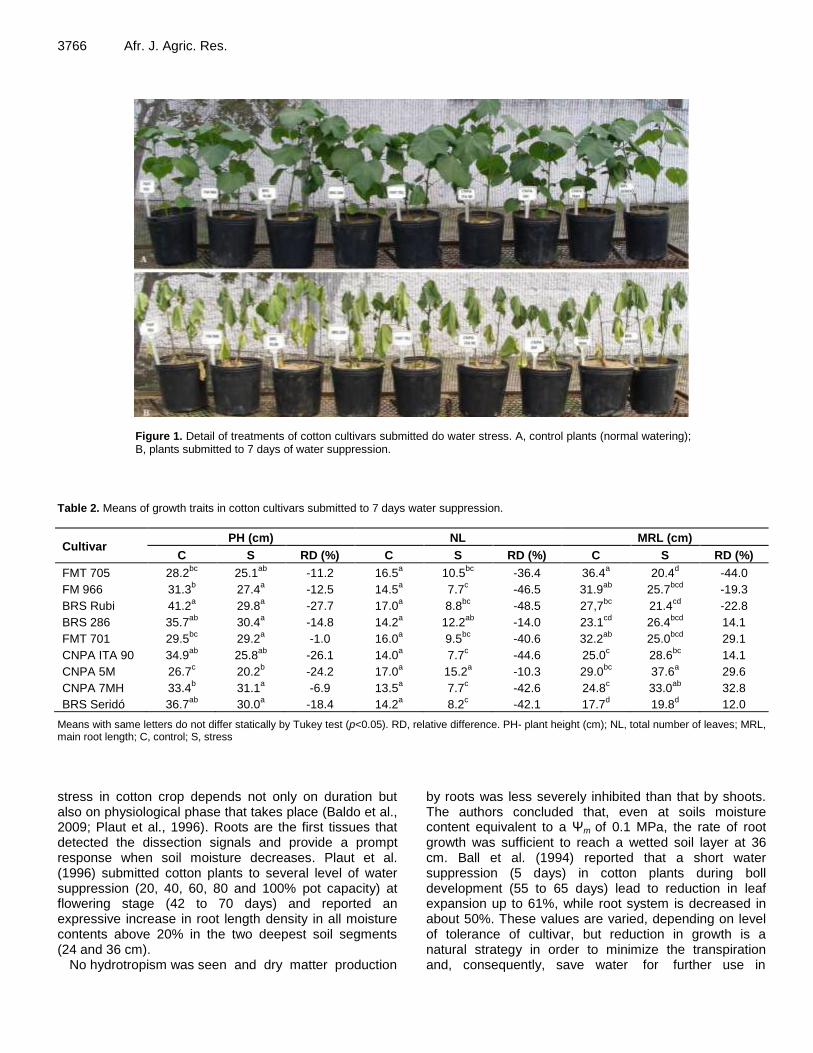
3766 Afr. J. Agric. Res.
Figure 1. Detail of treatments of cotton cultivars submitted do water stress. A, control plants (normal watering); B, plants submitted to 7 days of water suppression.
Table 2. Means of growth traits in cotton cultivars submitted to 7 days water suppression.
Cultivar PH (cm) NL MRL (cm)
C S RD (%) C S RD (%) C S RD (%)
FMT 705 28.2bc
25.1ab
-11.2 16.5a 10.5
bc -36.4 36.4
a 20.4
d -44.0
FM 966 31.3b 27.4
a -12.5 14.5
a 7.7
c -46.5 31.9
ab 25.7
bcd -19.3
BRS Rubi 41.2a 29.8
a -27.7 17.0
a 8.8
bc -48.5 27,7
bc 21.4
cd -22.8
BRS 286 35.7ab
30.4a -14.8 14.2
a 12.2
ab -14.0 23.1
cd 26.4
bcd 14.1
FMT 701 29.5bc
29.2a -1.0 16.0
a 9.5
bc -40.6 32.2
ab 25.0
bcd 29.1
CNPA ITA 90 34.9ab
25.8ab
-26.1 14.0a 7.7
c -44.6 25.0
c 28.6
bc 14.1
CNPA 5M 26.7c 20.2
b -24.2 17.0
a 15.2
a -10.3 29.0
bc 37.6
a 29.6
CNPA 7MH 33.4b 31.1
a -6.9 13.5
a 7.7
c -42.6 24.8
c 33.0
ab 32.8
BRS Seridó 36.7ab
30.0a -18.4 14.2
a 8.2
c -42.1 17.7
d 19.8
d 12.0
Means with same letters do not differ statically by Tukey test (p<0.05). RD, relative difference. PH- plant height (cm); NL, total number of leaves; MRL, main root length; C, control; S, stress
stress in cotton crop depends not only on duration but also on physiological phase that takes place (Baldo et al., 2009; Plaut et al., 1996). Roots are the first tissues that detected the dissection signals and provide a prompt response when soil moisture decreases. Plaut et al. (1996) submitted cotton plants to several level of water suppression (20, 40, 60, 80 and 100% pot capacity) at flowering stage (42 to 70 days) and reported an expressive increase in root length density in all moisture contents above 20% in the two deepest soil segments (24 and 36 cm).
No hydrotropism was seen and dry matter production
by roots was less severely inhibited than that by shoots. The authors concluded that, even at soils moisture content equivalent to a Ψm of 0.1 MPa, the rate of root growth was sufficient to reach a wetted soil layer at 36 cm. Ball et al. (1994) reported that a short water suppression (5 days) in cotton plants during boll development (55 to 65 days) lead to reduction in leaf expansion up to 61%, while root system is decreased in about 50%. These values are varied, depending on level of tolerance of cultivar, but reduction in growth is a natural strategy in order to minimize the transpiration and, consequently, save water for further use in

Figure 2. Activity of antioxidative enzymes in cotton cultivars submitted to 7 days of water suppression. SOD (Ug-1 FW min-1), CAT (µmol H2O2 g
-1 FW min-1) and APX (µmol ascorbate g-1 FW min-1).
physiological processes (Baldo et al., 2009). As to antioxidative enzyme analyses, statistically
significant differences were found in variance analysis to genotypes, water treatments and G x TH (p<0.01) to all three enzymes evaluated, meaning that the antioxidative machinery of cultivars responded differently to water treatments.
The individual behavior of each cultivar to SOD, CAT and APX is presented in Figure 2. These enzymes act in cascade events in order to avoid cell damages caused by ROS production, in response to oxidative stresses.
We found an input of 85, 52, 30 and 19% in SOD activity to CNPA 5M, BRS Seridó, BRS 286 and CNPA
Rodrigues et al. 3767 7MH, respectively, in stressed treatment. The availability of SOD in cells of these genotypes contributed to better adjustment in defense processes, generating reasonable amounts of CAT, so that, in the end of the antioxidant chain complex, the APX production was normalized (CNPA 5M and BRS 286 in both treatments) or minimized (CNPA 7MH and BRS Seridó). These cultivars, therefore, were more adjusted to water stress, based on conditions of this assay. We also found that FMT 705, FM 966, BRS Rubi and CNPA ITA 90 did not show enough SOD input to trigger the first process of antioxidative complex, so that, the next steps involving neutralization of H2O2 by CAT and APX, were probably circumstantial, and not directly involved with water stress response.
Finally, the behavior of FMT 701 was different from all other cultivars, with low activity of SOD in stressed treatment and a high input of APX (about 135%), at end of antioxidative process. This reaction suggests that the sum of peroxides not neutralized by CAT, overloaded the cell machinery, generating an expressive input of APX. Besides, as peroxidase also generated by photorespiration process, we suggests that the increase seen here may be associated to this event, whose metabolic pathway naturally generates enough ROS. This could explain the over-expression of CAT and APX in this cultivar.
Several works are available in literature reporting the role of antioxidative enzymes in response to water stress. The input of SOD is often reported as a response to drought tolerance in plants due to better ability to eliminate super-oxide from cells (Sekmen et al., 2014; Cataneo et al., 2010; Rahman et al., 2004). As a consequence, the levels of H2O in cells are increased, and further neutralized by CAT and APX, which convert H2O2 into H2O2 +½ O2 and H2O2 into H2O + R(O)2, respectively. The reduction of H2O2 level will contribute to minimize the cell damages caused by oxidative stresses.
Sekmen et al. (2014) submitted two cotton cultivars (tolerant and sensitive to drought), during 10 days of water suppression, from 21 days of emergence. They found an input of 71 and 57% in SOD activity, in tolerant and sensible plants of stressed treatment, indicating that tolerant plants have better adjustment to eliminate O2-. When this elimination is limited by cell machinery, the superoxides may form hyperoxides in the cell leading to cell damages and further physiological changes.
In order to estimate the genetic divergence among cultivars, CV analysis was performed using six statistically significant traits from stressed treatment. Table 3 displays the eigenvalues, individual and accumulated variance (%) associated with CV. The first two CV explained 86% of total variance (CV1 = 58.72%; CV2 = 27.28%), indicating that the most variability may be summarized in these two components and genotypes may be plotted in a two-dimensional graphical dispersion.
Figure 3 displays the graphical dispersion of cultivars.

3768 Afr. J. Agric. Res.
Table 3. Estimate of variance (eigenvalues and accumulated variation) of the canonical variables for six cotton traits.
CV Eigenvalue Variance (%) Acumulated variance (%)
CV1 23.48 58.72 58.72
CV2 10.91 27.28 86.00
CV3 3.00 7.51 93.51
CV4 1.20 3.00 96.51
CV5 0.84 2.10 98.61
CV6 0.55 1.39 100.0
Figure 3. Graphical dispersion of scores based on CV 1 and CV2, generated by traits obtained from cotton cultivars submitted to water suppression.
Three groups were formed with clear distinction as to drought tolerance: 1: represented by six annual cultivars: Two mid-cycle and developed for Cerrado region (FM 966 and CNPA ITA 90) and three earliness and developed for semiarid conditions (BRS 286, BRS Rubi, BRS Seridó and CNPA 7MH). It worth noting that, although FM 966 and CNPA ITA 90 are not recommended for dry regions, both have broad environmental adaptation, inherited from Deltapine Acala 90, an annual cultivar developed in USA West (Longenberger, 2008); 2: Represented by FMT 705 and FMT 701, both late cycle cultivars, developed for Cerrado region, with high technological input (Freire and Vidal Neto, 2013; Anselmo et al., 2009); and 3: represented only by CNPA 5M, a perennial type, with broad adaptation to dry environments (Souza and Silva, 1994).
The relative contribution of traits to the genetic
divergence was estimated based on S.j statistical (Singh, 1981). The analysis showed that APX, number of leaves, root length and plant height were the most contributive traits, with 53, 15, 13 and 12%, respectively.
In order to corroborate the results seen by graphical dispersion, an UPGMA clustering analysis was also performed, based on dissimilarity coefficient ≥ 80% and CCC = 0.79 (p<0.01). Three groups were formed (Figure 4), with identical clustering seen in Figure 3, indicating consistency of both multivariate methods as to genetic divergence of cotton cultivars.
Drought is a phenomenon established in tropical and semiarid environments and leads to different levels of damage in several crops. The improvement focused on drought tolerance is a relevant goal in many breeding programs around the world. Plants with ability to adjust the solutes in order to avoid the cell damages faced by

Rodrigues et al. 3769
Figure 4. Dendrogram generated by UPGMA clustering method, based on traits obtained from cotton cultivars submitted to 7 days of water suppression.
water suppression are robust candidates to breeding focusing on yield and environmental adaptations.
Cotton is a fiber crop of significant importance to textile industry. The Brazilian breeding program coordinates by Embrapa have made efforts in order to develop competitive cultivars, to attend the national and international fiber markets. Previous knowledge of genetic background of parents is quite useful in order to shorten the selection procedures, often requested for development of cultivars. The results showed here are contributive to assist in cotton breeding and provide information about promising candidates for further improvement to environment with water limitation.
Conclusion Based on climatic changes verified in several Brazilian regions, especially in water availability, we suggest the use of cotton cultivars from Groups I and II in dialelic crossings in order to combine yield and drought tolerance for further selection of promising top lines with broad yield stability and environmental adaptation.
Conflict of interests The authors have not declared any conflict of interests. Abbreviations
SOD, Superoxide dismutase; APX, ascorbate peroxidase; CAT, catalase; EDTA, ethylenediamine tetra-acetic acid; NBT, nitrobluetetrazolium; ROS, reactive oxigen species; ¹O2, oxigen singlet; O2•, superoxide; OH•, hydroxil radical; H2O2, hydrogen peroxide; O2, molecular oxigen; CV, canonical variables; UPGMA, unweighted pair group method with arithmetic mean; CCC,
cophenetic correlation coefficient. REFERENCES Almeida LLS, Nobre RG, Souza LP, Barbosa JL, Elias JJ
(2015). Crescimento do algodoeiro colorido pós-poda em solos com distintas PSTs e doses de esterco. RVADS 10(4):06-11.
Alscher RG, Erturk N, Heath LS (2002). Role of superoxide dismutases (SODs) in controlling oxidative stress in plants. J. Exp. Bot. 53(372):1331-1341.
Anselmo JL, Costa DS, Leal JF (2009). Ensaio de competição de cultivares de algodoeiro em Chapadão do Sul - MS. In: Congresso Brasileiro do Algodão, Campina Grande. Anais, Embrapa Algodão. pp. 1567-1571.
Baldo R, Scalon SPQ, Rosa YBCJ, Mussury RM, Betoni R, Barreto WS (2009). Comportamento do algodoeiro cultivar delta opal sob estresse hídrico com e sem aplicação de bioestimulante. Cienc.Agrotec. 33:1804-1812.
Ball RA, Oosterhuis DM, Mauromoustakos A (1994). Growth dynamics of the cotton plant during water-deficit stress. Agron. J. 86:788-795.
Barbosa MR, Silva MMA, Willadino L, Ulisses C, Camara TR (2014). Geração e desintoxicação enzimática de espécies reativas de oxigênio em plantas. Cienc. Rural. 44(3):453-460.
Batista CH, Aquino LA, Silva TR, Silva HRF (2010). Crescimento e produtividade da cultura do algodão em resposta a aplicação de fósforo e métodos de irrigação. Rev. Bras. Agric. Irrigada. 4(4):197-206.
Beers Júnior RF, Sizer IW (1952). A spectrophotometric method for measuring the breakdown of hydrogen peroxide by catalase. J. Biol. Chem. 195(2):133-140.
Bulbovas P, Rinaldi MCS, Delitti WBC, Domingos M (2005). Variação sazonal em antioxidantes em folhas de plantas jovens de Caesalpinia echinata Lam. (pau-brasil). Rev. Bras. Bot. 28(4):687-696.
Carvalho LP, Farias JFC, Lima MMA, Rodrigues JIS. (2014). Inheritance of different fiber colors in cotton (Gossypium barbadense L.). Crop Breed. Appl. Biotechnol. 14(4):256-260.
Cataneo AC, Chamma KL, Ferreira LC, Déstro GFG, Sousa DCF (2010). Atividade de superóxido dismutase em plantas de soja (Glycine max L.) cultivadas sob estresse oxidativo causado por herbicida. Rev. Bras. Herbicidas. 4(2):23-31.
Cavalcanti JJV, Vasconcelos UAA, Vasconcelos WS, Santos RC, Farias FJC, Araújo GP, Assunção JH (2016). Combining ability estimates for agronomic and morphological traits in cotton under water stress. In: World Cotton Research Conference – 6. Goiana: Brazilian Cotton Institute. Abstracts. P 131.

3770 Afr. J. Agric. Res. Cruz CD (2013). GENES - a software package for analysis in
experimental statistics and quantitative genetics. Acta Sci. Agron. 35(3):271-276.
Cruz CD, Regazzi AJ, Carneiro PCS (2012). Modelos biométricos aplicados ao melhoramento genético. Viçosa: UFV. 514p.
Farooq M, Wahid A, Kobayashi N, Fujita D, Basra SMA (2009). Plant drought stress: Effects, mechanisms and management. Agron. Sustain. Dev. 29:185-212.
Freire EC, Vidal Neto FC (2013). Melhoramento Genético do Algodoeiro. In: Vidal Neto FC, Cavalcanti JJV. (Ed.) Melhoramento Genético de Plantas no Nordeste - Brasília, DF: Embrapa. p. 49-83.
Longenberger PS (2008). Evaluation of chlorophyll fluorescence as a tool for the identification of drought tolerance in upland cotton (Dissertation).Texas A&M University: Texas. 129p.
Marur CJ, Ruano O (2001). A reference system for determination of cotton plant development. Rev. Oleaginosas Fibrosas 5(2):313-317.
Nakano Y, Asada K (1981). Hydrogen peroxide is scavenged by ascorbate-specific peroxidases in spinach chloroplast. Plant Cell Physiol. 22(5):867-880.
Plaut Z, Carmi A, Grava A (1996). Cotton root and shoot responses to subsurface drip irrigation and partial wetting of the upper soil profile. Irrig. Sci.16:107-113.
Rahman SML, Mackay WA (2004). Superoxide dismutase and stress tolerance of four tomato cultivars. Hortic Sci. 39(5):983-986.
Sekmen AH, Ozgur R, Uzilday B, Turkan I (2014). Reactive oxygen
species scavenging capacities of cotton (Gossypium hirsutum) cultivars under combined drought and heat induced oxidative stress. Environ. Exp. Bot. 99:141-149.
Singh D (1981). The relative importance of characters affecting genetic divergence. Indian J. Genet. Plant Breed. 41(2):237-245.
Shigeoka S, Ishikawa T, Tamoi M, Miyagaw Y, Takeda T, Yabuta Y, Yoshimura K (2002). Regulation and function of ascorbate peroxidase isoenzymes. J. Exp. Bot. 53(372):1305-1319.
Sokal RR, Rohlf FJ (1962).The comparison of dendrograms by objective methods. Taxonomy 11(1):30-40.
Souza JG, Silva JV (1994). Fenologia e fisiologia do algodoeiro arbóreo após a seleção para acúmulo de amido nas raízes. Rev. Bras. Fisiol. Veg. 6(2):145-148.

Vol. 11(39), pp. 3771-3776, 29 September, 2016
DOI: 10.5897/AJAR2016.11533
Article Number: B98AE5360826
ISSN 1991-637X
Copyright ©2016
Author(s) retain the copyright of this article
http://www.academicjournals.org/AJAR
African Journal of Agricultural Research
Full Length Research Paper
Selection of input vectors for estimation of aboveground biomass of Mimosa scabrella Benth.
using an artificial neural network
Aline Bernarda Debastiani*, Ana Paula Marques Martins, Carlos Roberto Sanquetta, Sebastião do Amaral Machado, Ana Paula Dalla Corte and Edilson Urbano
Post Graduation in Forest Engineering, Federal University of Parana, City of Curitiba, State of Paraná, Brazil.
Received 8 August, 2016; Accepted 19 September, 2016
The objective of this study was to evaluate the effect of input vectors in an artificial neural network (ANN) and determine their best combination to estimate the individual dry biomass of native bracatinga. The dataset consisted of 178 trees of Mimosa scabrella Benth. (bracatinga) from the Metropolitan Region of Curitiba. The ANN used was a Multi-Layer Perceptron; the learning algorithm was the Levenberg-Marquardt, consisting of an occult layer where 50% of the data were used for training, 25% for cross-validation and the other 25% for the test. The input vectors were all the variables collected in the field, such as: diameter at breast height (dbh), total height (ht), crown height (hc), stem height (hf), crown diameter (dc) and age (i). The treatment 1 consisted of all the vectors; after the MLP trained, the Garson algorithm was executed for obtaining relative contribution of each vector; the less important vector was deleted and the MPL was retrained (treatment 2) and so on until only one vector was left. Based on the coefficient of determination and root mean square error, treatment 3 provided the best performance (i, hc, ht and dbh), followed by treatment 6 (dbh). The method of selecting attributes by the Garson algorithm was remarkable and provided the definition of essential vectors, allowing minimal costs and optimizing the performance of the MLP. Key words: Bracatinga, multi-layer perceptron, Garson algorithm, relative contribution.
INTRODUCTION Studies on forest biomass are done with various objectives, among which it is possibility to highlight the quantification of nutrient cycling, the quantification for energetic ends and as information base for studies on carbon sink (Trautenmüller, 2015). Sanquetta (2002) affirms that in researches focused on the carbon fixation,
the biomass is one of the most relevant factors, and for this reason, it must be determined and estimated precisely, or else there will not be consistency in the quantification of the carbon fixed in forest ecosystems.
According to Sanquetta et al. (2015), though biomass is important for the quantification of carbon in the plants, its
*Corresponding author. E-mail: [email protected].
Author(s) agree that this article remain permanently open access under the terms of the Creative Commons Attribution
License 4.0 International License

3772 Afr. J. Agric. Res. direct determination is complex, expensive and destructive. For this reason, the quantification may be performed in an indirect way, which consists of estimates generally made by mathematical relations, as reasons or regressions, with data coming from forest inventory. The direct quantification may also be performed with data from a remote sensing in a geographic information system (Silveira et al., 2008).
However, when used in natural forests, the use of the referred techniques becomes more complex due to the great floristic, physiognomic and phenological diversity of this forest type, and so may present limitations (Sanquetta et al., 2015). Besides, a single equation may not be able to reproduce a large variation regarding natural forests, in addition to the need of this technique to attend to some prerequisites as additivity and linearity, residue independence, homoscedasticity and residue normality (Osborne and Waters, 2002).
In contrast, some machine learning techniques have presented themselves as promising alternatives to conventional statistical methods. Among these techniques, the artificial neural networks (ANN) have been used successfully in the forest sector in estimating dendrometric variables, such as height (Ferreira et al., 2014; Binoti et al., 2013), volume (Binoti et al., 2014; Cordeiro et al., 2015), thinning (Martins et al., 2016; Mendonça et al., 2015) and growth and production (Castro et al., 2013).
However, this technique presents some difficulties in understanding how they reach such estimates, and for this reason are named as black box system, for it is not possible to know what are the intermediate relations between the input and output variables, knowing only that this relation consists of adjusting synaptic weights.
There are techniques commonly utilized that seek to clarify how the ANN reaches such estimates, for example: the neural interpretation diagram technique (Gozlan et al., 1999), sensitivity analysis (Olden and Jakson, 2002) and the Garson algorithm (Garson, 1991). From these, the Garson algorithm has proven to be quicker and more decisive to be strictly quantitative (Kalteh, 2008).
It is necessary for the acquisition of some answers in the forest sector, the measurement of dendrometric variables with some level of difficulty in obtainment, it is of utmost importance to determine which are the input vectors and their effects, as well as identify the best combination of variables that produce the most accurate response. In this sense, the Garson algorithm is highlighted; it consists of considering the variation of absolute values of synaptic weights between the vectors of the input layer and the output layer, with the objective of determining the relative relevance of each vector of the input layer (Garson, 1991).
Thus, the objective of the present research was to evaluate the contribution of input vectors of an ANN to estimate the individual aboveground biomass of Mimosa
scabrella Benth. using the Garson (1991) algorithm and determine the best set of input vectors.
MATERIALS AND METHODS Data collection In this study, data from native bracatinga trees of the Metropolitan Region of Curitiba were used. The total data set was 178 trees, which were sampled seeking representation in the age classes and diameters. The methodology was obtaining biomass according to Sanquetta (2002). More details may be obtained in Urbano (2007).
The measured variables were: age (years), crown diameter (m), crown height (m), stem height (m), total height (m) and diameter of breast height (cm) collected at 1.3 m from the ground. With the objective to verify the correlation between the input variables, the analysis of linear correlation of Pearson was performed between these and output variables, in this case, the total individual aboveground dry biomass (kg). Artificial neural network used
The ANN used was the multi-layer perceptron (MLP) applied to the Matlab 2014a software in the Neural Network Toolbox. The learning algorithm used was the Levenberg-Marquardt backpropagation due to its quickness and stable convergence, being basically an integration of classic methods of Error Back Propagation and Gauss-Newton (Hagan and Menhaj, 1994). A learning rate of 0.01 was adopted; this represents how much of the error is backpropagated.
A tangent hyperbolic sigmoidal activation function, which compresses the answer to a known interval, from -1 to 1 was used. The activation functions to prevent the saturation and attenuation of the input signal (Haykin, 2001).
The MLP constituted of a hidden layer, in which, according to Atkinson and Tatnal (1997), generally is sufficient. In the hidden layer, the number of neurons (units of signal processing between the input layer and the output layer) varied ±5 with the satisfactory number of neurons, which, according to Heath (2010), corresponds to a relation of 10 times more training samples (Equation 1) than weights or the also named synaptic weights (Equation 2), which concentrates the knowledge of the network through the weighting of the connection between the neurons of the input layer and the hidden layer. Ten initializations of synaptic weights were also evaluated.
asonOIOsamplesTrainNeurons Re/))1/()_(1( (1)
ONeuronsNeuronsIWeights *)1(*)1( (2)
Where, Neurons: number of satisfactory neurons; Train_samples: number of training samples; O: number of output vectors; I: number of input vectors; Reason: reason of about 10 times more training samples than the number of hidden layer weights.
For each combination of input vectors (treatments), many configurations of the MLP were evaluated (initialization of weights and number of neurons of the hidden layer), and the best performance configuration was selected from the determination coefficient (R²) in the testing phase. The total dataset was subdivided in three parts, constituting 50, 25 and 25% of training, cross validation and the testing statistics calculation, respectively. The training consists of the process in which the input value is presented as the ANN and the corresponding answer (output

vector), adjusting the weights and connections to obtain the expected output. After the MLP was trained, the individual aboveground dry biomass (ba) for the whole dataset was obtained. The cross validation technique was used as the criterion to stop training and to avoid overfitting of the MLP, being done in a distinct dataset. The goal is to build a MLP in a manner that the same may simulate, for a distinct dataset (testing), the answer variable and obtain good performance in this phase to be considered well trained. The MLP input vectors were the dendrometric variables: Age (i), crown diameter (dc), crown height (hc), stem height (hf) and total height (ht) and diameter at breast height (dbh). These were standardized to the same scale to improve convergence (FU, 1994). The MLP output vector was configured to correspond to the individual dry aboveground biomass (ba). Relative contribution of vectors For the synaptic weight that presented the largest R² for treatment 1 (all vectors), the relative contribution of each input vector was calculated through the Garson algorithm (1991) (Equation 3). The vector with the lowest relative contribution was removed from the configuration of the next treatment, and this process was repeated until only one value remained.
N
i
L
j
jkN
r
rj
ij
L
j
jkN
r
rj
ij
ik
v
w
w
v
w
w
CR
1 1
1
1
1 (3)
Where, CRik represents the influence percentage of each input
vector i on the output vector k;
N
r
rjw1
is the sum of the weights
connecting the input layer i and the j neuron; N corresponds to the total of input vectors; L corresponds to the total of neurons of the hidden layer, Vjk corresponds to the weights of the connection between the j neuron and the k input vector.
The relative contribution of Garson seeks to determine the best combination of input vectors, based on the selection of attributes, optimizing the adjustment process. Statistical analysis The performance at the different treatments of the MLP was calculated by the adjustment statistics and model selection, which is the determination coefficient (R²) (Equation 4) and the root of the mean quadratic error in percentage (RMSE) (Equation 5), in addition to the graphical analysis of residue dispersion.
)²(*)²(
)]²(*)([²
isimisimiobsobs
isimisimobsiobs
babababa
babababaR
i
i (4)
100*
)²(1
%1
mínmáx
n
i iobsisim
baba
baban
RMSE
(5)
Debastiani et al. 3773 Where, baobsi: observed aboveground biomass (kg); basimi:
simulated aboveground biomass (kg);
ba : average aboveground
biomass observed (kg); bamín: minimum observed value of aboveground biomass (kg); bamáx: maximum observed value of aboveground biomass (kg); n: number of observations.
RESULTS AND DISCUSSION
As shown in Table 1, the bracatinga have an age range varying from 4 to 17 years. The lowest variability was found in total height (CV = 20.01%) and the highest for the individual dry aboveground biomass (CV = 108.13%). Since treatment is done with native bracatinga trees, the high data variability was already expected.
The Pearson linear correlation (r) between the input and output variables was calculated with the objective to determine the existing relations between them (Table 2). The vector corresponding to the dbh was the variable correlating to ba (r = 0.954), followed by dc (r = 0.794) and i (r = 0.751), with a strong positive correlation, indicating that the higher the dbh, dc, and the older the tree is, the more individual dry aboveground biomass is produced by it.
Table 3 shows the input vectors, the architecture and the adjustment statistics for training and testing for each treatment. The number of neurons in the hidden layer ranged from 3 (treatment 5) to 6 (treatment 3), representing a low number of neurons needed to estimate the individual dry aboveground biomass of bracatinga.
The adjustment statistics for the training phase resulted in R² varying from 0.948 (treatment 2) to 0.962 (treatment 4), and the RMSE varying from 5.281 (treatment 2) to 4.343% (treatment 5). It should be noted that the RMSE for the testing tends to decrease from treatment 1, which contains all possible vectors, until treatment 3, due to the removal of less relevant vectors according to their relative contribution. Since this treatment (3) was the one with the best performance of adjustment statistics (R² = 0.934 e RMSE = 8.304%), demonstrating the importance of the Garson algorithm in the selection of attributes and the ideal composition of the input vectors to estimate dendrometric variables.
Having determined the treatment with the best input vectors, the removal of less relevant vectors from following treatments resulted in the decrease of model adjustment statistics, with the exception of treatment 6 that was classified as the second best performance (R² = 0.919, RMSE = 9.388%).
The relative contribution of each vector at the treatments may be observed in Figure 1, which served as base for the composition of input vectors of each treatment. Treatment 1 was composed of all input vectors, in which, by the relative contribution, the least important vector, in this case hf, was removed from the composition of treatment 2; followed by the removal of the dc vector from the composition of treatment 3, and

3774 Afr. J. Agric. Res.
Table 1. Descriptive statistics of the input and output vectors to estimate the individual aboveground biomass of Mimosa scabrella Benth. in the Metropolitan Region of Curitiba.
Variables i (years) dc (m) hc (m) hf (m) ht (m) dbh (cm) ba (kg)
Minimum 4 0.55 1.70 2.56 9.15 4.80 6.90
Average 9 3.11 5.16 8.95 14.11 13.64 101.32
Maximum 17 8.85 12.00 15.45 21.80 35.00 586.90
CV% 31,31 55.48 39.43 27.74 20.01 46.61 108.13
CV%: Coefficient of variation.
Table 2. Pearson linear correlation (r) between the input and output vectors to estimate the individual dry aboveground biomass for the Mimosa scabrella Benth. in the Metropolitan Region of Curitiba.
Variables i (years) dc (m) hc (m) hf (m) ht (m) dbh (cm) ba (kg)
i (years) 1.000 - - - - - -
dc (m) 0.700 1.000 - - - - -
hc (m) 0.386 0.586 1.000 - - - -
hf (m) 0.332 0.286 -0.231 1.000 - - -
ht (m) 0.570 0.674 0.517 0.713 1.000 - -
dbh (cm) 0.759 0.836 0.588 0.339 0.722 1.000 -
ba (kg) 0.751 0.794 0.573 0.281 0.660 0.954 1.000
Table 3. Performance of the MLP with regards to the different combinations of input vectors, chosen based on the attribute selection described by the Garson algorithm (1991).
S/N Input vectors Architecture Training Test
R² RMSE (%) R² RMSE (%)
1 i, dc, hc, hf, ht, dbh 6/4/1 0.959 4.533 0.914 10.309
2 i, dc, hc, ht, dbh 5/5/1 0.948 5.281 0.903 9.525
3 i, hc, ht, dbh 4/6/1 0.950 5.094 0.934 8.304
4 hc, ht, dbh 3/5/1 0.962 4.393 0.917 9.475
5 hc, dbh 2/3/1 0.961 4.343 0.919 9.436
6 dbh 1/5/1 0.959 4.355 0.919 9.388
N: Number of treatment; Architecture: represents the number of neurons in the input layer/hidden/output.
successively for the remaining treatments, until only dbh remained in the composition of the last treatment, in other words, treatment 6.
As shown in Figure 1, dbh presented the largest relative contribution in all treatments, and this fact may be explained by the largest linear correlation of this variable with the individual dry aboveground biomass (r = 0.954), and also by the efficiency of using only the dbh at the MLP that resulted in R² = 0.919 and RMSE of 9.388% in testing (treatment 6), in addition to a good graphic distribution of residues (Figure 2), which indicates that in the absence of dendrometric variables hard to obtain, for example, height and age, the individual dry aboveground biomass of native bracatinga trees may be estimated without substantial losses in the accuracy of the estimation using only dbh.
In a general manner, treatments tend to overestimate
the individual dry aboveground biomass of trees. However, treatments 3 and 6 present a more homogenous residue distribution around the zero axis, confirming the superiority of these treatments in estimating individual dry aboveground biomass of native bracatinga trees of the Metropolitan Region of Curitiba, Paraná.
Urbano (2007) found lower results for the estimation of individual dry aboveground biomass, for this same dataset, and when he used dbh as the input vector for allometric equations, the value obtained for R²aj. was 0.909. This author found that the best estimate for biomass resulted from the forward method, which selected dbh, dbh², dbh³, dbh
-1, ht, hc, hf and dc and
resulted in R²aj. of 0.972. Other studies analyzed the effect of the composition of
input vectors on estimating biomass (Miranda, 2015) and

Debastiani et al. 3775
Figure 1. Relative contribution result of the Garson algorithm for the input vectors of MLP for each treatment.
Figure 2. Residue dispersion generated from many treatments for the estimation of individual dry aboveground biomass of M. scabrella Benth.

3776 Afr. J. Agric. Res. when he utilized a MLP to model the total biomass from a fragment of a Deciduous Seasoned Forest, found R² varying from 0.67 to 0.98 when employing input vectors dbh and the ht. Vahedi (2016) used a MLP to estimate the aboveground biomass in northern Iran forests, and used a dbh and ht input layer and found R² = 0.873 and RMSE of 10.16% in the testing phase.
Other studies that used other machine learning techniques like the study of Sanquetta et al. (2015) that estimated the individual dry aboveground biomass of native trees of Mata Atlântica at Seropédica (RJ), when using variables independent of classification based on instance the dbh, dc, ht, hc, apparent density and basic density, concluded that the use of all variables provided more precise biomass estimates as compared to the reduced number, and the worst performance occurred with the exclusive use of dap.
Conclusion
Composition of input vectors of the MLP that provided the best performance included the variables, age, crown height, total height and the diameter at breast height. The use of only diameter at breast height propitiates consistent estimates when compared with the remaining estimates that used a higher number of input vectors and harder collection, indicating depenence on the desired precision and the resources available; only the dbh propitiates good estimates of individual dry aboveground biomass of native bracatinga trees of the Metropolitan Region of Curitiba, using the referred MLP.
The Garson algorithm presented itself as an interesting tool that assists in the method of attributing selection to determine which input vector have higher relative contribution, providing a better learning of the MLP and selecting the variables essential for the modelling, which may contribute to minimizing costs of forest inventories.
Conflict of Interests
The authors have not declared any conflict of interests.
ACKNOWLEDGEMENT
The authors thank the Coordination for the Improvement of Higher Education Personnel (Coordenação de Aperfeiçoamento de Pessoal de Nível Superior-CAPES) for their financial support. REFERENCES Atkinson PM, Tatnall ARL (1997). Neural networks in remote sensing.
Int. J. Remote Sens. 18:699-709. Binoti DHB, Binoti MLMS, Leite HG (2014). Configuração de redes
neurais artificiais para estimação do volume de árvores. Rev. Ciênc. Madeira 5(1):1-6.
Binoti MLMS, Binoti DHB, Leite HG (2013). Aplicação de redes neurais
artificiais para estimação da altura de povoamentos equiâneos de eucalipto. Rev. Árvore 37(4):639-645.
Castro RVO, Soares CPB, Martins FB, Leite HG (2013). Crescimento e produção de plantios comerciais de eucalipto estimados por duas categorias de modelos. Pesqui. Agropecu. Bras. 48(3):287-295.
Cordeiro MA, Pereira NNJ, Binoti DHB, Binoti MLMS, Leite HG (2015). Estimativa do volume de Acacia mangium utilizando técnicas de redes neurais artificiais e máquinas vetor de suporte. Pesqui. Florest. Bras. 35(83):255-261.
Ferreira JCB, Lafetá BO, Penido TMA, Campos PM, Castro PM (2014). Altura de mudas de Tibouchina granulosa cogn. (melastomataceae) estimada por redes neurais artificiais. Rev. Soc. Bras. Arb. Urbana 9(1):151-160.
Fu L (1994). Neural networks in computer intelligence. New York: McGraw-Hill.
Garson GD (1991). Interpreting neural-network connection weights. Artif. Intell. Expert. 6:47-51.
Gozlan RE, Mastrorillo S, Copp GH, Lek S (1999). Predicting the structure and diversity of young-of-the-year fish assemblages in large rivers. Freshwater Biol. 41:809-820.
Hagan MT, Menhaj M (1994). Training feed-forward networks with the Marquardt algorithm. IEEE T. Neural Networ. 5(6):989-993.
Haykin S (2001). Redes neurais: princípios e prática. Porto Alegre: Bookman P 900.
Heath GE (2010). Training, testing and validating data set in Neural Network. Disponível em: <http://www.mathworks.com/matlabcentral/newsreader/view_thread/295781#917734>. Access: 04 de july 2013.
Kalteh AM (2008). Rainfall-runoff modelling using artificial neural networks (ANNs): modelling and understanding. Caspian J. Environ. Sci. 6(1):53-58.
Martins ER, Binoti MLMS, Leite HG, Binoti DHB, Dutra GC (2016). Configuração de redes neurais artificiais para estimação do afilamento do fuste de árvores de eucalipto. Rev. Bras. Ciênc. Agrár. 11(1):33-38.
Mendonça NP, Carvalho MC, Gomide LR, Ferraz Filho AC, Ferreira MA (2015). Previsão de diâmetros ao longo do fuste de eucalipto via redes neurais artificiais. Rev. Encicl. Biosfera 11(22):2419-2429.
Miranda JFN (2015). Modelos de regressão e de redes neurais artificiais na quantificação de carbono e biomassa lenhosa em floresta estacional decidual no Brasil central. Dissertação (mestrado). Univ. Bras. Bras. 76 p.
Olden JD, Jackson DA (2002). Illuminating the “black box”: a randomization approach for understanding variable contributions in artificial neural networks. Ecol. Model. 154:135-150.
Osborne J, Waters E (2002). Four assumptions of multiple regression that researchers should always test. Pract. Asses. Res. Eval. 8(2):1-8.
Sanquetta CR (2002). Métodos de determinação de biomassa florestal. In. As Florestas e o Carbono. Curitiba pp. 119-140.
Sanquetta CR, Wojciechowski J, Corte APD, Behlinga, Péllico Neto S, Rodrigues AL, Sanquetta MNI (2015). Comparison of data mining and allometric model in estimation of tree biomass. Bioinformatics 16(247):2-9.
Silveira P, Koehler HS, Sanquetta CR, Arce JE (2008). O estado da arte na estimativa de biomassa e carbono em formações florestais. Rev. Flor. 38(1):185-206.
Trautenmüller JW (2015). Quantificação e distribuição do estoque de biomassa acima do solo em floresta estacional decidual. Dissertação (Mestrado) – Universidade Federal de Santa Maria 92 p.
Urbano E (2007). Quantificação e estimativa da biomassa aérea e do carbono fixado em árvores de bracatingais nativos da região metropolitana de Curitiba. Dissertação (Mestrado) – Universidade Federal do Paraná 140 p.
Vahedi AA (2016). Artificial neural network application in comparison with modeling allometric equations for predicting above-ground biomass in the Hyrcanian mixed-beech forest of Iran. Biomass Bioenergy 8(5):66-76.

Vol. 11(39), pp. 3777-3787, 29 September, 2016
DOI: 10.5897/AJAR2016.11536
Article Number: 89AC2ED60828
ISSN 1991-637X
Copyright ©2016
Author(s) retain the copyright of this article
http://www.academicjournals.org/AJAR
African Journal of Agricultural
Research
Full Length Research Paper
Guava rootstocks growth under incorporation of cattle manure and application of organic fertilizer the base of
fruit of peel
Mario Leno Martins Véras1*, José Sebastião de Melo Filho1, Lunara de Sousa Alves2, Toni Halan da Silva Irineu3, Nelto Almeida Sousa1, Lucimara Ferreira de Figueiredo1, Edinete
Nunes de Melo4, Leandra de Melo Cavalcante1, Thiago Jardelino Dias1 and Alvaro Carlos Gonçalves Neto5
1Programa de Pós-Graduação em Agronomia, Universidade Federal da Paraíba, Centro de Ciências Agrárias, Universidade Federal da Paraíba, Campus II, Rodovia PB 079 - Km 12, 58.397-000, Areia, Paraíba, Brasil.
2Programa de Pós-Graduação em Sistemas Agroindustriais, Universidade Federal de Campina Grande, Brasil.
3Programa de Pós-Graduação em Fitotecnia, Universidade Federal Rural do Semi-árido, Brasil.
4Programa de Pós-Graduação em Horticultura Tropical, Universidade Federal de Campina Grande, Brasil.
5Centro de Ciências Humanas, Sociais e Agrárias, Universidade Federal da Paraíba, Brasil.
Received 9 August, 2016; Accepted 7 September, 2016
The use of rootstocks in fruit production is extremely important, as well as reducing juvenility also enables faster production. In this context, the objective was to evaluate the effect of different rates of manure and application of organic fertilizer on the growth of guava rootstocks. The experiment was conducted in the greenhouse of the State University of Paraíba (UEPB) in municipality of Catolé do Rocha-PB, Brazil. The experimental design was completely randomized (CRD), with in factorial 5 × 2, with 6 repetitions. The treatments consisted of the combination of manure proportions: (0, 20, 40, 60 and 80% v/v) mixture to the ground (2: 1 v v
-1) and the second factor consisted of organic fertilizer
application (with and without). 30, 60, 90 and 120 days after sowing (DAS) evaluated the following variables: plant height, leaf number, stem diameter, leaf area, root length, absolute growth rate and relative plant height , stem diameter and leaf area, dry matter of root mass, shoot dry matter mass, the total dry matter and Dickson quality index. The use of cattle manure at the rate of 80% positively influenced the growth of guava rootstocks with the application of organic fertilizer. Key words: Psidium guajava L., substrate, organic agriculture.
INTRODUCTION In Brazilian Fruits there are several fruit of enormous economic importance, among them stands out the guava (Psidium guajava L.), a plant native to tropical America, which is distributed naturally throughout Brazil, with great economic importance because of the flavor
nice, high nutritional value and great market acceptance, since its fruits are eaten both in natura as processed form (Oliveira et al., 2015). In the culture of the guava tree and some fruit, orchards consist of grafted seedlings, as the first step in the implementation of an orchard is the

3778 Afr. J. Agric. Res. formation of seedlings, it influences the orchard productivity. Several factors affect the production of seedlings, including the substrate that will be used as well as its volume, which can lead to nullity or germination irregularity, malformation of plants and the appearance of symptoms of deficiency or excess of some nutrients (Mesquita et al., 2012). One of the problems in the production of seedlings is the inadequate management of nutrition, and well - nourished plants become less susceptible to pests and diseases, are more tolerant to drought and other stresses, moreover, well - nourished plants increase productivity and quality of fruit. Thus, the fertilization of the plants is a crucial step, however, the culture of guava fertilization is done with formulated fertilizers as well as the doses are equal in all seedlings. However, it is essential that the dose is recommended as to cultivate and age changes. Therefore it is essential studies to obtain the optimal dose in guava rootstocks growth and the fertilizer that provides good quality seedlings (Dias et al., 2012).
In the preparation of substrates several fertilizers and manures among them have been used, since they possess features that are beneficial to seedlings, such as improvement of physico-chemical properties, stimulating microbial processes. The manure are most organic materials used as substrate however, the type and amount of manure vary according to the plant species (Morais et al., 2012). Several research on the use of organic sources in the development of seedlings are found in literature, especially the use of manures and organic fertilizers (Mesquita et al., 2012; Morais et al., 2012; Oliveira et al., 2015). However, more studies are needed related to the use of manure in the substrate formulation for formation of fruit seedlings, as well as interaction with organic fertilizers.
Another factor that influences the production of good quality seedlings is the application of fertilizers. Organic fertilizers have many essential nutrients for plant growth. However, the lack of studies related to the supply of nutrients and the amount that should be applied is one of the obstacles faced by producers of seedlings. Another advantage with the use of organic fertilizer is to reduce the use of chemical fertilizers which in addition to being expensive pollute the environment.
While have high nutritional value and have high fiber content, furthermore, various fruit peels have high potential nutraceutical, such as passion fruit peel, used to reduce the glucose level. Moreover, the fruit peels can be used in agriculture, because they have many plant nutrients, therefore, aimed to evaluate the effect of cattle manure proportions as a function of organic fertilizer application to fruit peel based on growth rootstocks
guava. Furthermore, the use of organic inputs provide an improvement in the physical characteristics of the soil, in addition to increasing the microbiological poulação and soil fauna diversity (Sall et al., 2015). In this context, the objective was to evaluate the effect of different rates of manure and application of organic fertilizer on the growth of guava rootstocks.
MATERIALS AND METHODS The experiment was conducted from September 2015 to January 2016 in the greenhouse of the Center for Human Sciences and Agricultural in the Department of Agricultural and Exact State University of Paraíba (UEPB) in municipality of Catolé of Rock-PB, Brazil (6 20 '38 "S, 37 ° 44'48" W) and 275 meters. The experimental design was completely randomized (CRD), with a factorial 5 × 2, with 6 repetitions. The treatments consisted of the combination of manure dry proportions: (0, 20, 40, 60 and 80% v/v) mixture to the ground (2:1 v/v -1) and the second factor consisted of organic fertilizer application (with and without). The experimental units were composed of five seedlings grown in polyethylene bags with 2 kg capacity. The water used for irrigation had electrical conductivity of 0.8 dS m -1. The water analysis was carried out by the Irrigation and Salinity Laboratory (LIS) of the Center for Technology and Natural Resources of the Federal University of Campina Grande - UFCG and presented the following physicochemical characteristics: pH = 7.53, Ca = 2.30 cmol c dm -3, Mg = 1.56 cmol c dm -3, Na = 4.00 cmol c dm -3, K = 0.02 cmol c dm -3, Chloride = 3.90 cmol c dm -3, Carbonate = 0.57 cmol c dm -3, Bicarbonate = 3.85 cmol c dm -3, RAS = 2.88 (mmol c l
-
1)1/2. The soil was classified as Fluvisol sandy clay loam
texture. Samples were collected in the layer 0-20 cm in native area located on the campus of UEPB. The soil sample used for filling polyethylene bags was removed a sub-sample to be analyzed chemically, with the following characteristics: Ca = 4.63 cmol c dm -3, Mg = 2.39 cmol c dm -3, Na = 0.30 cmol c dm -3, K = 0.76 cmol c dm -3, Sum of bases - SB = 8.08 cmol c dm -3, H = 0.00 cmol c dm -3, Al = 0.00 cmol c dm -3, CTC = 8.08 and = 1.88% organic matter. The organic fertilizer was obtained by aerobic fermentation. For the preparation of fertilizer used was 20 kg peeling of fruits and 1 kg of charcoal, adding 5 kg of sugar and 5 L of milk to accelerate the metabolism of the bacteria. The fertilizer was applied 15 days after emergence and thereafter at 8 day interval, 10% of the substrate volume. Before application, the fertilizer was subjected to screen for filtering process to reduce the risk of clogging of the sieve watering holes. A sample of this fertilizer was analyzed and had the following chemical characteristics (Table 1). The sample of cattle manure was analyzed in the Soil Laboratory of Federal University of Paraíba and physicochemical analysis of this compound showed the following characteristics: pH = 7.75, P = 5.61 g kg -1, K = 2.34 g kg -1, Ca = 7.70 g kg -1, Mg = 6.90 g kg -1, In = 9.18 cmolc.dm-³ and MO = 38.4 g kg -1.
Guava seeds were used (Psidium guajava L.), coming from healthy and ripe fruit. For the extraction of the seeds, the fruits were cut separating the seed from the pulp. Later, the seeds were washed in running water on fine mesh sieve for disposal of waste
*Corresponding author. E-mail: [email protected]
Author(s) agree that this article remain permanently open access under the terms of the Creative Commons Attribution
License 4.0 International License

Véras et al. 3779
Table 1. Chemical attributes of organic fertilizer used in the experiment. Catolé do Rocha - PB, UEPB 2015.
Chemical properties Obtained values
pH 8.46
EC (dS m -1
) 13.65
Nitrogen (g kg -1
) 6.2
Phosphorus (g kg -1
) 1.66
Potassium (g kg -1
) 136.77
Calcium ++
(mmol c L -1
) 2.00
Magnesium ++
(mmol c L -1
) 37,30
Sodium + (mmol c L
-1) 13.83
Figure 1. Plant height (PH) of guava rootstocks at 30 DAS (A) and 90 DAS (B) under the effect of different proportions of manure due to the presence (▲) and absence (■) of organic fertilizer.
from pulp and peel. The seeds were dried in a ventilated and shady place for a period of four days. The seeds were sown in plastic bags of 2 kg capacity, dimensions 20 × 30 cm, containing bovine manure and soil using four seeds of Paluma. At 20 days after sowing, there was thinning of seedlings keeping only the most vigorous seedling. At 30, 60, 90 and 120 days after sowing (DAS), the following variables were evaluated: plant height, leaf number, stem diameter, leaf area. At the end of the experiment were also evaluated the dry matter of the root, stem, leaf, shoot, and total Quality Index of Dickson.
For plant height, measurement was used a graduated tape measure in centimeter, the distance between the neck and the apex of the plant (younger sheet insert fully formed). The number of leaves was obtained by counting. The stem diameter measurements were taken with a digital caliper two (2) cm above the plant lap. The leaf area was obtained by measuring the width and length of the sheet (L x C). The dry matter of root, dry matter stem, dry matter of leaf and dry matter of shoots, were determined after fresh material to be approximately 48 hours in air circulation oven forced to a temperature of 60 ° C until obtaining a constant weight was weighed 0.0001 g on a precision balance. The mass of the total dry matter was obtained by adding up all the dry parts of the plant (root, stem and leaf). From the monthly average values of plant height, stem diameter and leaf area were calculated their respective absolute growth rate (AGR) and relative growth rates (RGR) as Benincasa (2003). The relationship root shoot (R/S) was measured as Benincasa (2003). The Dickson quality index was calculated according to the methodology of Dickson et al. (1960). Data were evaluated by analysis of variance by F test at 0.05 and 0.01 probability and in cases of significance, there was analysis of
linear and quadratic polynomial regression using the statistical software SISVAR 5.0 (Ferreira, 2011).
RESULTS AND DISCUSSION There was significant effect of interaction x cattle manure organic fertilizer for the plant height, stem diameter at 30 and 120 DAS to the number of sheets at 90 and 120 DAS and leaf area at 60 and 120 DAS. For the isolated effect of cattle manure, it was observed that the plant height, leaf number showed significant effects at 30, 90 and 120 DAS, to stem diameter in all periods and leaf area at 90 and 120 DAS. Regarding the application of organic fertilizer, there was a significant effect on plant height and number of leaves only the 120 DAS, to stem diameter at 30 DAS and leaf area at 30 and 60 DAS. Figure 1 shows the effect of cattle manure proportions at the time of guava rootstocks to plant 30 (A) and 90 (B) DAS. The guava rootstocks at 30 DAS, had increased plant height of 9.5 cm (0% of cattle manure) to 14 cm (80% of cattle manure), soil with organic fertilizer, an increase of 85% ratio between the minimum (0%) and maximum (80%) (Figure 1A). At 90 DAS, the door guava grafts showed a height of maximum plant of 25.12 cm, representing an increase of 68.15% by increasing the proportion of cattle

3780 Afr. J. Agric. Res.
Figure 2. Plant height (PH) of guava rootstocks at 120 DAS under the influence of different proportions of manure due to the presence (▲) and absence (■) of organic fertilizer.
manure (Figure 1B). These results show that the use of organic fertilizer provides more nutrients to guava rootstocks, even in the absence of manure.
Cavalcante et al. (2010) studied saline water and liquid manure in the formation of guava plants Paluma observed that the plant height was higher in plants treated with cattle manure, getting a height of 16.56 cm plants with manure. Silva et al. (2008) found that the application of manure (3kg to 100kg soil) significantly increased the Paluma guavas high irrigated with saline water, which found that plants treated with manure had a height of 51.1 cm. Oliveira et al. (2015) observed that the greatest shoot length was obtained with the addition of 39.49% of cattle manure to the substrate, which reached a maximum height of 73.29 cm this ratio. It was observed that plant height of guava rootstocks at 120 DAS showed a positive effect of the manure ratios (Figure 2), obtaining with the maximum percentage (80%), 48 - point, 72 cm in the presence of organic fertilizer and 41.35 cm in the absence of organic fertilizer, a difference of 7.37 cm. In the absence of organic fertilizer lower values were observed plant height in all proportions of manure. Each unit increase of the manure proportions, there was an increase on the order of 0.354 cm and 0.288, corresponding to presence or absence of organic fertilizer respectively.
Among the most used organic fertilizers in the substrate composition, the manure is one of the most used since it improves the physical characteristics, in addition, stimulates microbial process (Arthur et al., 2007).The increase of manure proportions increased the number of guava rootstocks leaves linearly to 30 DAS. Observed maximum values of 11.75 sheets obtained in the maximum proportion of cattle manure (80%) (Figure 3) an increase of 76.59%, each unit
increase in cattle manure proportions there was an increase in the order 0, 0324 sheets. Mesquita et al. (2012) in papaya, observed that the amount of 79.1% of cattle manure per plant obtained the maximum number of leaves getting an average of 15.72 leaves. In passionflower, Ribeiro (2005), yellow passion fruit seedlings substrates found that the soil base + manure in plastic bags had more leaves. The number of leaves port guava grafts at 90 and 120 DAS treated with manure proportions due to the organic fertilizer application is shown in Figure 3. Note that the highest values were obtained with the application of organic fertilizer, corresponding the maximum number of sheets 17 in rootstocks treated with 80% of bovine manure to DAS 90 (Figure 4A), the DAS 120, it was observed that the rootstocks presented a number of leaves 24.75 maximum at the ratio of 80% bovine under organic fertilizer application manure (Figure 4B), showing thus that the guava rootstocks respond directly when it raises the level of organic matter in the soil. One of the benefits of the manure is the provision of organic material, one of the fundamental components of the substrate, it provides an increase in water and nutrient retention capacity for the cuttings, besides, it reduces the apparent and bulk density as well as increasing the porosity the means (Silva et al., 2008).
Regarding the stem diameter at 30 DAS, the proportions of manure provided a linear increase as its increase, with the highest value of 1.59 mm for a ratio of 80% of cattle manure under organic fertilizer application. It is also observed that as they increased the amounts of manure there was an increase in stem diameter, representing a difference of 89.93% in the proportion of 0% and 80% of cattle manure (Figure 5A) with the application organic fertilizer. At 60 and 90 DAS, it

Véras et al. 3781
Figure 3. Number of guava rootstocks of leaves at 30 DAS under the influence of different proportions of manure.
Figure 4. Number of guava rootstocks leaves at 90 DAS (A) and 120 DAS (B) under the effect of different proportions of manure due to the presence (▲) and absence (■) of organic fertilizer.
Figure 5. Stem diameter of guava rootstocks stem to 30 DAS (A) and 60 and 90 (B) DAS the under the influence of different proportions of manure due to the presence (▲) and absence (■) of organic fertilizer.

3782 Afr. J. Agric. Res.
Figure 6. Stem diameter of guava rootstocks to 120 DAS under the influence of different proportions of manure due to the presence (▲) and absence (■) of organic fertilizer.
Figure 7. Leaf area of guava rootstocks to 30 (A) and 60 (B) OF THE under the influence of different proportions of manure due to the presence (▲) and absence (■) of organic fertilizer.
is observed that the proportions of manure provided an increase in stem diameter, with better adaptation to the linear model for the proportions of cattle manure (Figure 5B). The rootstocks showed continued growth to achieve greater stem diameter of 2.59 to 2.91 mm and 60 DAS to 90 DAS in the proportion of 80% of cattle manure. Cavalcante et al. (2010) studied saline water and liquid manure in the formation of guava plants grow paluma observed that the stem diameter was higher in plants treated with cattle manure, with a maximum of 2 mm with the use of liquid manure. Sá et al. (2015) in custard, observed that the substrate consists of 50% soil + 25% manure + 25% sand showed the best results in stem diameter (2.32 mm). Cavalcante et al. (2009) in passionflower noted that the maximum dose (10%) of liquid manure gave the highest results for the stem diameter (2.4 mm).The increase in cattle manure
proportions promoted linear increase in the diameter of guava rootstocks stem to 120 DAS, the level of 0.324 mm in the presence and 0.229 in the absence of organic fertilizer for each unit increase in cattle manure (Figure 6). Treatment with the maximum proportion of manure (80%) rootstocks showed superior results (5.24 mm) in the presence of organic fertilizer, which corresponds to an increase of 49.04% in stem diameter compared to the untreated rootstocks with organic fertilizer, which showed 4.11 mm in maximum proportion of cattle manure (80%) and in the presence of organic fertilizer.
The leaf area at 30 DAS (Figure 7A) and 60 (Figure 7B) of guava rootstocks were significantly marked by the increase of cattle manure proportions. We observed the rootstocks treated organic fertilizer provide superior results when compared to those without treatment with the organic raw material. At 30 DAS, an increase of

Véras et al. 3783
Figure 8. Leaf area of guava rootstocks to 90 (A) and 120 (B) DAS the under the influence of different proportions of manure due to the presence (▲) and absence (■) of organic fertilizer.
Figure 9. Absolute growth rate - AGRph height guava rootstocks plant under the influence of different proportions of cattle manure (A) due to the presence and absence of organic fertilizer (B) in the period 60-120 DAS.
0.0154 cm² and 90 DAS an increase in the order of 0.0252 cm² in rootstocks under organic fertilizer application, respectively. Cavalcante et al. (2010) in guava plants observed that treatment with cattle manure was superior to the leaf area and length of the guava root, with a maximum of 167.5 cm² value for leaf area and 29 cm long root. Barros et al. (2013) in passion fruit, obtained the best results for leaf area (966.3 cm²) and root length (17 cm) with substrates composed of hardened soil + cattle manure. In guava rootstocks treated with manure proportions, there was increasing linear behavior due to the increase of manure ratios for the leaf area to 90 (Figure 8A) and 120 DAS (Figure 8B), representing increases of 0,0349 cm² to 90 DAS for each unit increase in cattle manure proportions. At 120 DAS 0.2357 and 0.1933 cm² in the presence and absence of organic fertilizer, respectively, for each unit increase in cattle manure proportions. For the absolute growth rate and relative plant height, stem diameter and leaf area, there was significance to the interaction between the
factors proportions of fertilizer x manure only for the absolute growth rate of leaf area, while the isolated effect of manure provided significant effect on all variables. It was further found that the organic fertilizer showed a significant effect only for the absolute growth rate of plant height and leaf area. The proportions of cattle manure (Figure 9A) and organic fertilizer application (Figure 9B) provided an increase in the absolute growth rate of the plant height of guava rootstocks. It was observed that the maximum proportion rootstocks treated manure results showed peak (0.15 cm day
-1), resulting in increasing order of 0.001 every unit
increase in the bovine manure proportions. For the application of organic fertilizers, it was found that without its application, a reduction in the absolute growth rate of plant height, giving a value of 0.28 cm
-1 and day under
application of organic fertilizer on 0.36 cm -1.
The increase in the proportion of manure also gave an
increase in relative growth rate in height of the rootstocks guava plant, as it increased the manure proportions a

3784 Afr. J. Agric. Res.
Figure 10. Growth rate relative – RGRph plant height guava rootstocks plant under the influence of different proportions of cattle manure in the period 60-120 DAS.
Figure 11. Absolute growth rate – AGRsd (A) and relative - RGRsd (B) diameter of guava rootstocks stem under the influence of different proportions of cattle manure in the period 60-120 DAS.
gain so that the control presented 0.003 cm cm
-1 day
-
1 and the maximum ratio showed a growth rate relative
height of 0,006 cm -1
cm -1
day plant, resulting in an increase in the order of 50% per unit increase in the bovine manure ratios (Figure 10). As for the plant height growth rate, absolute and relative growth rate of stem diameter was a linear increase with rising of manure proportions. It also appears that each unit increase in the bovine manure proportions rootstocks showed an increase of 0.0004 mm
-1 to day
absolute growth rate
(Figure 11A) and the relative growth rate was observed that the witness showed a value of 0.001 while the maximum proportion of cattle manure (80%) was obtained a value of 0.006, an increase of 16.66% for each increase in the proportion of cattle manure (Figure 11B). The absolute growth rate of leaf area responded
significantly to the effects of cattle manure interaction × organic fertilizer. It was observed that the treatments with organic fertilizer values increased linearly at the level of 0.0038 cm
2 d
-1 per unit increase in the proportion of
cattle manure, 0.38 in the treatment with the highest proportion of cattle manure (80%). In rootstocks without organic fertilizer application, it was observed that the results were lower, resulting in the highest percentage of cattle manure (80%) a value of 0.26 cm
-1 d
2 (Figure
12A). The increase in cattle manure proportions provided a
linear increase in the relative growth rate of leaf area. Upon verification, the treatments with the highest proportion of cattle manure (80%), rootstocks showed a50% increase compared to rootstock treated with the control (0%) (Figure 12B). It was found that significant

Véras et al. 3785
Figure 12. Absolute growth rate - AGRlf (A) and relative – RGRlf (B) of leaf area guava rootstocks under the influence of different proportions of manure due to the presence (▲) and absence (■) of fertilizer organic in the period 60-120 DAS.
Figure 13. Dry mass of root guava rootstocks under the influence of different proportions of manure due to the presence (▲) and absence (■) of organic fertilizer.
effect of cattle manure x interact organic fertilizer to the root dry weight, shoot dry weight, total dry weight and Quality Index of Dickson.For the isolated effect of cattle manure was no significant effect on all variables. Regarding the application of fertilizer, significant effects were observed for dry root mass, shoot dry weight, total dry weight, relative root and shoot Dickson Quality Index. Figure 13 shows the interaction between the proportions of cattle manure in the presence and absence of organic fertilizer to the root dry mass, noting that the rootstocks of guava treated with cattle manure at the rate of 80% was superior in the results, yielding 6.99 g plant
-1 values in the presence of organic
fertilizer and 6.52 g plant-1
in the absence organic fertilizer. Oliveira et al. (2015) observed that the proportion of 37.25% of manure gave the highest root dry mass values (3.49 g). Barros et al. (2013) in
passionflower, achieved the best results (1.32 g) to root dry mass with substrates composed of cattle manure + hardened soil. Cavalcante et al. (2010) studied saline water and liquid manure in the formation of guava plants grow paluma observed that plants treated with liquid manure bovine had damage to a lesser extent in the treatments with organic input. It is noted that there was an increase of dry matter of the stem (Figure 14A) and leaves (Figure 14B), with the increase in the percentage of cattle manure in the composition of the substrate to achieve the maximum dry mass 10.76 g plant stem
-1 and
dry weight of leaf 24.73 g plant -1
, referring to the proportion of 80% of cattle manure, respectively. Similar results were obtained by Cavalcante et al. (2010) evaluated guava plants, and found that the treatment eat liquid manure was superior in getting the dry weight values of the root.
As for the other variables, the dry weight of shoot (Figure 15A) and total (Figure 15B) were significantly scaled up as they increased manure proportions beef and higher in treatments with organic fertilizer. The largest increases were obtained in the ratio of 80% of cattle manure and in the presence of organic fertilizer, resulting in an increase of 46.21% to the dry weight of shoot and 47.14% to the total dry mass. Cavalcante et al. (2010) and guava, observed that plants treated with liquid manure bovine showed superior results in dry mass of shoot and total dry matter in the treatments with the use of manure. Oliveira et al. (2015) in guava rootstocks, observed that the incorporation of increasing proportions of manure provided the best results for dry matter of shoot and total, which observed that the highest values were 12.53 and 16.01 g plant
- 1 in the proportions of
40.16 and 39.64% of cattle manure, respectively. For the relationship root shoot, there was an increase as increased the proportions of manure, where the best result was found in the maximum proportion of cattle manure (80%), a difference of 45.86% between the

3786 Afr. J. Agric. Res.
Figure 14. Dry stem mass (A) and dry weight of the sheet (B) of guava rootstocks under effect of different proportions of manure
Figure 15. Dry mass of shoot (A) and total dry matter (B) rootstocks of guava under the influence of different proportions of manure due to the presence (▲) and absence (■) of organic fertilizer.
proportion minimum and maximum of cattle manure (Figure 16A). It was also observed that the treatments with the application of fertilizer was made was an increase in the shoot root ratio, obtaining a value of 1.83 in rootstocks treated with organic input (Figure 16B). The manure acts to increase the availability of nutrients in addition, the manure is widely used in most farms, since it presents low cost. Kumar and Ponnuswami (2013) indicate that the manure suitably provides the organic material, nurturing plants and can thus contribute to greater production as well as the quality of the fruit, since the supply of organic material improves the properties soil, increasing microbial biochemical activity of soil and edaphic (Mandal et al., 2007; Dunjana et al., 2012.).The use of manure had a positive effect on the Quality Index of Dickson, and the corresponding treatment to 80% of cattle manure and in the presence of organic fertilizer provided the best results, showing that the guava rootstocks respond positively to increase cattle manure in
the substrate. Dickson Quality Index adjusted to the linear equation in terms of the proportion of cattle manure in the substrate and showed a continuous increase until reaching the highest rates in the order of 2.52 in the maximum proportion (80% cattle manure) in the presence of fertilizer (Figure 17).The Quality Index of Dickson is one of the most important parameters to assess the quality of a change; good quality seedlings are more robust and better distribution of biomass, allowing greater development capacity in the field, for their high force (Silva et al., 2011). Conclusion Proportions of 80% of cattle manure provide rootstock higher quality guava. The use of manure positively influenced the growth of guava rootstocks together with the organic fertilizer application.

Véras et al. 3787
Figure 16. Aerial root ratio (R/PA) of guava rootstocks under the influence of different proportions of manure due to the presence and absence of organic fertilizer.
Figure 17. Quality Dickson guava rootstocks Index under the influence of different proportions of manure due to the presence (▲) and absence (■) of organic fertilizer.
Conflict of interests The authors have not declared any conflict of interests. REFERENCES Arthur AG, Cruz MCP, Ferreira ME, Barretto VCM, Yagi R (2007).
Esterco bovino e calagem para formação de mudas de guanandi. Pesqui. Agropec. Bras. 42(6):843-850.
Barros CMB, Müller MML, Botelho RV, Michalovicz L, Vicensi M, Nascimento R (2013). Substratos com compostos de adubos verdes e biofertilizante via foliar na formação de mudas de maracujazeiro-amarelo. Semina: Cienc. Agric. 34(6):2575-2588.
Benincasa MMP (2003). Análise de crescimento de plantas, noções básicas. 2 ed. Jaboticabal: FUNEP 41 p.
Cavalcante LF, Silva GF, Gheyi HR, Dias TJ, Alves JDC, Costa ADP (2009). Crescimento de mudas de maracujazeiro amarelo em solo salino com esterco bovino líquido fermentado. Rev. Bras. Cienc. Agric. 4(4):414-420.
Cavalcante LF, Vieira MDS, Santos AD, Oliveira WD, Nascimento JD (2010). Água salina e esterco bovino líquido na formação de mudas de goiabeira cultivar Paluma. Rev. Bras. Frutic. 32(1):251-261.
Dias MJT, Souza HA, Natale W, Modesto VC, Rozane DE (2012). Adubação com nitrogênio e potássio em mudas de goiabeira em viveiro comercial. Semina: Cienc. Agric. 33(suplemento): 2837-2848.
Dickson A, Lead AL, Osmer JF (1960). Quality appraisal of white spruce and white pine seedling stock in nurseries. Forest. Chron. 36(1):10-13.
Dunjana N, Nyamugafata P, Shumba A, Nyamangara J, Zongore S (2012). Effects of cattle manure on selected soil physical properties of smallholder farms on two soils of Murewa, Zimbabwe. Soil Use Manage. 28(2):221-228.
Ferreira DF. (2011). Sisvar: A computer statistical analysis system. Ci. Agrotec. 35(6): 1039-1042.
Kumar SM, Ponnuswami V (2013). Effect of different water regimes and organic manures on quality parameters of noni (Morinda citrifolia). Afr. J. Agric. Res. 8(27):3534-3543.
Mandal A, Patra AK, Singh D, Swarup A, Masto RE (2007). Effect of long-term application of manure and fertilizer on biological and biochemical activities in soil during crop development stages. Bioresour. Technol. 98(18):3585-3592.
Mesquita EF, Chaves LHG, Freitas BV, Silva GA, Sousa MVR, Andrade R (2012). Produção de mudas de mamoeiro em função de substratos contendo esterco bovino e volumes de recipientes. Rev. Bras. Cienc. Agric .7(1):58-65.
Morais FA, Góes GB, Costa ME, Melo IGC, Veras ARR, Cunha GOM (2012). Fontes e proporções de esterco na composição de substratos para produção de mudas de jaqueira. Rev. Bras. Ci. Agric. 7(suplemento):784-789.
Oliveira FT, Hafle OM, Mendonça V, Moreira JN, Junior EBP, Rolim HO (2015). Respostas de porta-enxertos de goiabeira sob diferentes fontes e proporções de materiais orgânicos. Commun. Sci. 6(1):17-25.
Ribeiro MCC, Morais MJA, Sousa AH, Linhares PCF, Júnio, APB (2005). Produção de mudas de maracujá-amarelo com diferentes substratos e recipientes. Rev. Caatin. 18(3):155-158.
Sá FVS, Brito MEB, Pereira IB, Neto PA, Andrade Silva L, Costa F (2015). Balanço de sais e crescimento inicial de mudas de pinheira (Annona squamosa L.) sob substratos irrigados com água salina. Irrigation 20(3):544-556.
Sall SN, Ndour NYB, Diedhiou-Sall S, Dick R, Chotte JL (2015). Microbial response to salinity stress in a tropical sandy soil amended with native shrub residues or inorganic fertilizer. J. Environ. Manag. 161(1):30-37.
Silva ABF, Fernandes PD, Gheyi HR, Blanco FF (2008). Growth and yield of guava irrigated with saline water and addition of farmyard manure. Rev. Bras. Cienc. Agric. 3(4):354-359.
Silva EA, Oliveira AC, Mendonça V, Soares FM (2011). Substratos na produção de mudas de mangabeira em tubetes. Pesqui. Agropec. Trop. 41(2):279-285.

Vol. 11(39), pp. 3788-3798, 29 September, 2016
DOI: 10.5897/AJAR2016.11206
Article Number: 9FDA7CC60830
ISSN 1991-637X
Copyright ©2016
Author(s) retain the copyright of this article
http://www.academicjournals.org/AJAR
African Journal of Agricultural Research
Full Length Research Paper
Diversity, abundance and incidence of fruit pest insects on three Solanum varieties (Solanaceae) in two agro-
ecological zones of Southern Cameroon
Elono Azang Pierre Stephan1,2, Aléné Désirée Chantal1, Heumou Cyril Roméo1,3, Ngassam Pierre4 and Djiéto-Lordon Champlain1*
1Laboratory of Zoology, Department of Animal Biology and Physiology, Faculty of Science, University of Yaounde I,
P. O. Box 812 Yaounde, Cameroon. 2Laboratory of Zoology, Department of Biological Sciences, Higher Teacher‟s Training College, University of Yaounde I,
P. O. Box 47 Yaounde, Cameroon. 3Department of Biology, Higher Teacher‟s Training College, University of Bamenda, P. O. Box 39 Bamenda, Cameroon. 4Laboratory of Parasitology and Ecology, Department of Animal Biology and Physiology, Faculty of Science, University
of Yaounde I, P. O. Box 812 Yaounde, Cameroon.
Received 10 May, 2016; Accepted 17 August, 2016
Various species and varieties of the genus Solanum (Solanaceae) are among the most important market crops produced worldwide. They may be considered as multipurpose crops since leaves and/or fruits are eaten fresh or cooked in various dishes. The increase of garden surfaces and the permanence of gardening have induced frequent outbreaks and diversification of pests and cryptogrammic diseases. In order to improve farmer’s capacities in controlling these constraints, the present study assessed diversity, abundance and incidence of fruit pests on Solanum spp. Data collection was conducted in two agroecological zones of southern Cameroon: Okola (Center Region) and Koutaba (Western Region), on three plant varieties from the genus Solanum: Solanum aethiopicum (African scarlet eggplant) with two varieties (jakatu and zong) and Solanum melongena (brinjal eggplant) var. inerme. The study aimed to (1) characterise the community of fruit pests associated with these plant varieties, (2) assess damage due to the main pests and (3) determine their impact on fruit yield. To achieve this, systematic sampling were done by visual observations in experimental gardens set up at the above cited sites. Harvests and incubations of infested fruits allowed identifying 15 insect species, belonging to three orders and 12 families: Lepidopterans with Leucinodes orbonalis, Cryptophlebia leucotreta, Helicoverpa armigera, Chrysodeixis chalcites and Hypolycaena phylippus), Dipterans
with Batrocera
(Batrocera) dorsalis, Ceratitis (Ceratitis) capitata, Ceratitis (Pterandrus) anonae, Neosilba sp., Atherigona sp. three unidentified species belonging to undetermined genera and Coleopterans with Diplognatha gagates and Formicomus sp.. Among them, H. phyllipus and C. chalcites were absent from Koutaba’s samples. Without site considerations, L. orbonalis was the most abundant with higher incidence on fruit production. At Okola, fruit losses on S. aethiopicum var. jakatu, on S. aethiopicum var. zong and on S. melongena var. inerme were 53.8-76.97, 43.65-61.51 and 29.42-46.61% respectively while at Koutaba, they were 49.51-68.57, 33.41-60.23 and 11.68-30.44%. The present study provided baseline data for integrated pest management strategies of Solanum in Cameroon.
Key words: Solanum, yield, fruit pests, L. orbonalis, damages.

Stephan et al. 3789 INTRODUCTION The increase of market crop trade in national and sub-regional markets has led to intensification of gardening in various production basins in Cameroon. Among crops involved are various species of the genus Solanum (Solanaceae) that includes species of high nutritional and sociocultural values. Fruits and vegetables production in Cameroon provides 154 billion of CFA francs (representing about 3% of the country's GDP 1997/1998). Theses incomes constitute a great component in the fight against poverty (Temple, 2001). The gardening faces important threats among which the presence of insect pests that include mainly dipteran and lepidopteran fruit feeders. Eggs are laid on various parts of the plant for lepidopterans or under the fruit cuticle for dipterans. After hatching, larvae develop in the fruit pulp from which they leave at the pre-nymph stage to pupate in the soil. Because larvae feed and live inside the fruit, they cannot be effectively controlled by contact insecticides (Djiéto-Lordon and Aléné, 2002, 2006), while systemic insecticides are not appropriates for vegetables. In these conditions efficient control strategies may associates appropriates use of pesticides with other control technics such as biological control, mass trapping, or physical and biotechnology control technics in integrated pest management strategies. Implementation of these strategies needs a good knowledge of insects diversity in the ecosystem and the ecology of the pests. In this framework, the present study aimed to gather baseline data necessary for improvement of pest control strategies, the present study aimed to characterize fruit pests on three plant varieties belonging to two species of the genus Solanum, commonly grown in the Central and West African sub-regions: (1) The highly economic potential crop S. aethiopicum with two varieties, the var. zong (Figure 1a to c) and the var. jakatu (Figure 1 d to f). The first variety is among the most important native varieties cultivated in the forest region of Central Africa. Despite its weak commercial value, it is a great component of various unsalted meals e.g. „Sanga‟, „Kpwem‟ (Franqueville, 1972). The second variety, also called sweet Solanum constitutes a significant source of income for farmers and retailers in urban and peri-urban zones and can be encountered in almost all the markets in West and Central Africa, where it is one of the five most important vegetables (Adeyeye and Adanlawo, 2011); its fruits are rich in vitamins and minerals and are consumed fresh, dried or transformed into association with other vegetables (salads), cooked in soup or boiled (Messiaen, 1989; Lester and Seck, 2004; Shippers 2004). (2) The third variety is Solanum melongena var. inerme (Figure 1 g to i). It is less known than the two
others, but is an important component of traditional and highly valuable meals of the western highlands of Cameroon, e.g. „Yellow soup‟, „Nah poh‟ and „Nkui soup‟ (Noumi, 1984; Tchiégang and Mbougueng, 2005).
The species S. aethiopicum is a plant of sunny area distributed throughout the southern Cameroon and other countries in Africa (Sekara et al., 2007). Its phenology is closely correlated with the local climatic conditions. During the rainy season, the plant has a greenish appearance with several leaves and maturing fruits while in the dry season, it has a jagged appearance (Schippers, 2004). The var. zong of S. aethiopicum and inerme of S. melongena grow well in full sunny woodland on relatively well drained deep soils with a pH of 5.5 to 6.8 and temperatures ranging from 25 to 35°C during diurnally and 20 to 27°C nightly. The var. jakatu of S. aethiopicum grows in warmer climates (45°C during the day) but may tolerate relatively dry conditions with sometimes less than 20% moisture (when irrigated) (Grubben and Denton, 2004; Schippers, 2004).
Despite highly nutritional, cultural and commercial values, few studies have focused on the diversity and geographic distribution of fruit pests of Solanum spp. in southern Cameroon (Djiéto-Lordon and Aléné, 2006; Djieto-Lordon et al., 2007). The aim of the present study, conducted in two agroecological zones of southern Cameroon, Central plateau and Western highlands were: (i) To identify the insect pests associated with the fruit of three Solanum varieties; (ii) To assess host specificity of the pests on the three plant varieties, and finally, (iii) To evaluate the incidence of each specific fruit pests on the yield of each variety.
MATERIALS AND METHODS
Study site
Field study was carried out simultaneously in two localities from two agro-ecological zones of southern Cameroon: Okola (04°01‟39.0‟‟N, 011°23‟00.1‟‟E, asl: 604 m) in the Southern plateau, and Koutaba (05°38‟47.9‟‟N, 010°48‟22.2‟‟E, asl: 1186 m) in the Bamoun Plateau. The latter is situated in one of the main market crop basin of Cameroon (Westphal et al., 1981). Both agroecological zones differed in their topographic and climatic characteristics. At Okola, the study area undergoes an equatorial climate with bimodal rainfall regime marked by a succession of four seasons while Koutaba is under a humid tropical climate characterized by two seasons with unimodal rainfall regime (Suchel, 1988). For landscapes, more description and climatic conditions of the study sites, is found in Mokam et al. (2014) and Heumou et al. (2015). The study period extended from June 2010 to October 2011 at Okola and from August 2010 to November 2011 at Koutaba.
*Corresponding author. E-mail: [email protected]. Tel: (+00237) 675 04 33 33.
Author(s) agree that this article remain permanently open access under the terms of the Creative Commons Attribution
License 4.0 International License

3790 Afr. J. Agric. Res.
g i
h
d f
e
c
b
a
Figure 1. Solanum species involved in the study. (a) plant, (b) flower, (c) fruit of S. aethiopicum var. zong; (d) plant, (e) flower, (f) fruit of S. aethiopicum var. jakatu and (g) plant, (h) flower, (i) fruit of S. melongena var. inerme.
Biological material The biological material in this study was composed of healthy and infested harvested fruits from three varieties Solanum spp. (Solanaceae): S. aethiopicum var. zong with less sweet fruits (Figure 1a to c), S. aethiopicum var. jakatu sweet (Figure 1d to f) and Solanum melongena var. inerme with bitter fruits (Figure 1g to i). Experimental design For data collection, experimental gardens were set up at each site. At Okola, the experimental garden consisted in 06 ridges of 10 m × 1 m separated each other by furrow of 0.5 m wide. Each ridge supported 24 plants of the same variety (two ridges per variety), placed on two lines, and separated by 0.80 m. At Koutaba, they
were made of 9 ridges (three ridges per variety). For the two localities, seedlings were obtained from the same nursery set up at the Laboratory of Zoology of the University of Yaoundé I (03°51‟35.3‟‟N, 011°30‟00.6‟‟E, asl: 770 m). Sampling method Biological diversity and abundance of fruit pest insects Data were collected during 184 sampling days unequally distributed among the two study sites; 112 at Okola and 72 at Koutaba. From the Blooming stage of the earliest variety up to the end of the fruiting period of the latest, plots were visited weekly at Okola and Koutaba in order to assess by count, the number of fruits produced, the number of fruits affected by insects and/or diseases and the number of mature fruits. All mature fruits and those affected were systematically

harvested, individually isolated in labelled bags and brought to the laboratory for further observations. Once in the Laboratory, fruits were weighed and categorised as followed: (i) Fruits attacked by fruit feeding insects, characterised by the presence of entrance/exit holes, (ii) quasi-healthy fruits, with no sign of insect attack, (iii) fruits with other affection symptoms. Fruits with insect attack signs were individually incubated in plastic boxes of appropriate size. Each box was previously provided with wet sand, then covered with a fine gauze and followed up to the emergence of adult insects (Djiéto-Lordon and Aléné, 2006, Djieto Lordon et al. 2007; Mokam et al., 2014; Heumou et al., 2015).
Fruits of the two other categories were dissected in order to detect any cryptic insect attack (in case of cryptic attacks, they were incubated as above). This process allowed us discriminating healthy fruits, fruits lost by insects‟ attacks, and fruits lost by other biotic factors. To improve sample collection for the biodiversity study, sampling was extended to peasants‟ gardens in the neighboring areas. In this particular case, only infested fruits were collected and incubated separately. After the emergence, adult insects from each incubating box were separated on the base of morphological features, counted and preserved dry (Lepidoptera) or in vial tubes provided with 70% alcohol (other taxa) for future identifications. Assessment of yield loss due to specific fruit pests The number of healthy and infected fruits per plant variety was recorded at each harvest to calculate the incidence of specifics fruits pests on the yield. For this purpose, the ratio of the number of fruits of each cultivated plant which have been attacked over the total number of fruits harvested was used (Heumou et al., 2015). The total number of fruits and the number of infested fruits were recorded from all varieties weekly during the period from June 2010 to October 2011 at Okola and from August 2010 to November 2011 at Koutaba. Damage index from each plant variety was calculated and expressed in percentage using the following formula: ID (%) = (Nif / Nthf)*100 Where: ID (%) = Damage index; Nif = Number of infested fruits by specific pest; Nthf = Number of total harvested fruits Identification method Insect determinations were done at the Laboratory of Zoology of the University of Yaoundé I, and confirmed by the taxonomists of CIRAD/CBGP at Montpellier (France). These determinations were based on various keys, including Delvare and Aberlenc (1989) for insect families in general, White (2006) and White and Elson-Harris (2004) for fruit flies, Wharton and Gilstrap (1983) and Wharton et al. (1992) for parasitoïds. The monographs of Bordat and Arvanitakis (2004) and Bordat and Daly (1995) were also used. Voucher specimens were deposited in the collections of the two above cited institutions. Statistical analysis After transformation, data were submitted to variance analysis test (ANOVA) using the Statistica software version 6.0. Then, a multiple comparison of means was performed using the Tukey HSD test. These statistics treatments aimed to compare the diversity, the abundance and the incidence of fruit pest insects between species/varieties of Solanum form one study site to another and from a season to another. All probabilities were appreciated at the 5% threshold.
Stephan et al. 3791 RESULTS Biological diversity of the fruit feeding insects and abundance A total of 15 insect species belonging to 12 families and 3 orders were recorded from incubated fruits of the three species/varieties of Solanum in the two study sites. Orders represented were (i) Lepidoptera with 5 species, (ii) Diptera with 8 species and (iii) Coleoptera with 2 species (Table 1). At the site level, there were weak variations as all the 15 species were recorded at Okola while two species Hypolycaena phylippus and Chrysodeixis chalcites were absent from Koutaba. It is important to notice that the two species absent from Koutaba are highly polyphagous and weakly represented at Okola. The butterfly Leucinodes orbonalis (Lepidoptera: Pyralidae) and the fly Neosilba sp. (Diptera: Lonchaeidae) were the most important pests at both the two sites (Table 1). Their relative abundances were higher than those of other fruit pests at both Okola and Koutaba without plant species/variety considerations. At Okola, the relative abundance of the pests did not varied significantly in relation to plants species/varieties. For S. aethiopicum var. zong, S. aethiopicum var. jakatu and S. melongena var. inerme, the relative abundances were: 75.1, 68 and 70.3% for L. Orbonalis, 15.5, 17.9 and 18.2% for Neosilba sp. respectively while at Koutaba, they were 65.9, 68.84 and 67.6% for L. orbonalis, and 19.44, 16.47 and 20.98% for Neosilba sp. respectively. Apart from these two main species, other pests were weakly abundant on Solanum (≤ 10 and 2%) (Table 1).
Insect orders and families associated with species/varieties of Solanum The ANOVA test for the three orders of fruit pests showed non-significant variation of the relative abundance between the two study sites with Lepidoptera (F = 0.001, DF=1, P = 0.96); Diptera (F = 0.02, DF = 1, P = 0.87) and Coleoptera (F = 0.001, DF = 1, P = 0.97). Lepidopterans were the most represented group, with a relative abundance of 73.98% at Okola and 70.19% at Koutaba, followed by dipterans (25.11% at Okola, 28.95% at Koutaba) and coleopterans (0.9% at Okola and 0.86% at Koutaba) (Figure 2).
At the family level, Pyralidae (Lepidoptera) were the most represented with relative abundances of 71.13% at Okola and 67.44% at Koutaba, followed by Lonchaeidae (Diptera) which contributed for 17.2% at Okola and 18.96% at Koutaba. These two families were followed by Muscidae (Diptera) (4.03% at Okola, 5.64% at Koutaba), Tephritidae (Diptera) (3.4% at Okola, 3.43% at Koutaba) and Tortricidae (Lepidoptera) (2.8% at Okola, 2.4% at Koutaba). The other families showed the lowest abundances throughout the study (< 1%) in the both agroecological sites. Pyralidae and Tortricidae were more

3792 Afr. J. Agric. Res. Table 1. Frequencies Distribution of insect‟s morphospecies recorded from incubated Solanum fruits collected from June 2010 to November 2011 with reference to fruit species/variety and study sites.
Orders Families Fruit pests species
Contribution of fruit losses Fi (%)
Okola (Southern plateau) Koutaba (Western Highlands)
Var. zong Var. inerme Var. jakatu Var. zong Var. inerme Var. jakatu
Lepidoptera Pyralidae Leucinodes orbonalis 75.10 70.30 68.00 65.9 67.6 68.84
Tortricidae Cryptophlebia leucotreta 2.50 3.20 2.72 2.23 2.17 2.82
Noctuidae
Noctuidae
Chrysodeixis chalcites 00 00 0.06 00 00 00
Helicoverpa armigera 0.04 00 00 0.11 00 0.9
Lycaenidae Hypolycaena phylippus 0.04 00 00 00 00 00
Diptera
Tephritidae Batrocera (Batrocera) dorsalis 1.88 1.80 2.10 1.56 2.17 1.04
Tephritidae Ceratitis (Ceratitis) capitata 0.98 0.90 0.6 1.53 00 1.78
Tephritidae Ceratitis (Pterandrus) anonae 0.04 00 0.75 0.3 1.65 0.29
Lonchaeidae Neosilba sp. 15.50 18.20 17.90 19.27 20.98 16.47
Muscidae Atherigona sp. 2.60 4.80 5.70 6.70 4.89 5.34
Micropezidae Gn.1 sp.1 0.50 00 1.00 1.67 00 1.04
Sarcophagidae Gn.2 sp.2 0.04 00 0.06 0.04 00 0.06
Stratiomyidae Gn.3 sp.3 00 00 0.06 0.04 00 00
Coleoptera Anthicidae Formicomus sp. 0.75 0.80 1.00 0.56 0.54 1.38
Cetonidae Diplognatha gagates 0.03 00 0.05 0.09 00 0.04
N 12 15 2431 fruits 738 fruits 1466 fruits 1203 fruits 266 fruits 884 fruits
Fi (%) = Relative abundance of fruit pests; var. zong = S. aethiopicum var. zong; var. jakatu = S. aethiopicum var. jakatu; var. inerme = S. melongena var. inerme.
abundant at Okola than at Koutaba while all other families were more abundant at Koutaba than at Okola (Figure 3).
Mean number of individuals per fruit on Solanum spp. In the both study sites, larvae of L. orbonalis were present in field during the period of pre-flowering, flowering (on shoot and flowers) and fructification (on fruits) and those of Neosilba sp. during fruit maturation only. The means number of pest individual per fruit varied significantly in relation to
fruit species/varieties and pest species. At Okola, the variation of the mean number of L.
orbonalis individuals per fruit was highly significant between the three species/varieties of Solanum (F = 18.06, DF = 2, P = 0.0001), with 1.51 ± 0.77 individuals per fruit on S. aethiopicum var. zong (N = 1891 fruits), 1.61 ± 0.82 individuals per fruit on S. aethiopicum var. jakatu (N = 1069 fruits) and 1.37 ± 0.61 individuals per fruit on S. melongena var. inerme (N = 545 fruits). Similar trend was observed between the mean number of other fruit pest individuals per fruit (F = 3.9, DF = 2, P = 0.02), with 1.89 ± 1.54 individuals per fruit on S. aethiopicum var. zong (N = 151 fruits), 2.21
± 2.30 individuals per fruit for S. aethiopicum var. jakatu (N = 115 fruits) and 1.38 ± 0.97 individuals per fruit for S. melongena var. inerme (N = 52 fruits). Contrarily, with Neosilba sp., the mean number of individuals per fruit did not vary significantly with respect to Solanum varieties (F = 197, DF = 2, P = 0.13) (with 4.37 ± 3.7 individuals per fruit for S. aethiopicum var. zong, (N = 389 fruits), 4.74 ± 4.20 individuals per fruit for S. aethiopicum var. jakatu (N = 282 fruits) and 3.97 ± 3.27 individuals per fruit for S. melongena var. inerme (N = 141 fruits). Globally, the highest number of fruit pests per fruit was recorded on S. aethiopicum var. jakatu, followed by the one on S.

Stephan et al. 3793
0
10
20
30
40
50
60
70
80
Lepidoptera Diptera Coleoptera
Re
lati
ve a
bu
nd
ance
(%
) /
stu
dy
site
Fruit pests orders
Okola
Koutaba
Figure 2. Relative abundance of fruit pest‟s orders at Okola and Koutaba from June 2010 to October 2011 and from August 2010 to
0
10
20
30
40
50
60
70
80
Re
lati
ve a
bu
nd
ance
(%
) /
stu
dy
site
Fruit pests families
OkolaKoutaba
Figure 3. Relative abundance of fruit pest families at Okola and Koutaba from June 2010 to November 2011.
aethiopicum var. zong and finally the one on S. melongena var. inerme (Figure 4).
At Koutaba, the mean number of L. orbonalis individuals per fruit also varied significantly on Solanum species/varieties (F = 6.24, DF = 2, P = 0.01), with 2.62 ± 3.03 individuals per fruit on S. aethiopicum var. zong (N = 896 fruits), 2.16 ± 1.87 individuals per fruit on S. aethiopicum var. jakatu (N = 674 fruits) and 2.35 ± 2.38 individuals per fruit on S. melongena var. inerme (N = 184 fruits). Also, the mean number of individuals per fruit of other pests varied significantly (F = 3.8; DF = 2; P = 0.02), with 2.98 ± 2.48 individuals per fruit on S. aethiopicum var. zong (N = 131 fruits), 2.40 ± 1.86 individuals per fruit on S. aethiopicum var. jakatu (N = 99
fruits) and 1.76 ± 0.53 individuals per fruit on S. melongena var. inerme (N = 21 fruits). Also, the mean number of Neosilba sp. individuals per fruit presented a significant variation (F = 7.7, DF = 2, P = 0.005), with 5.84 ± 5.04 individuals per fruit on S. aethiopicum var. zong (N = 176 fruits); 4.03 ± 3.61 individuals per fruit on S. melongena var. inerme (N = 57 fruits) and 4.0 ± 3.22 individuals per fruit on S. aethiopicum var. jakatu (N = 111 fruits).
So, the mean numbers of L. orbonalis and Neosilba sp. individuals per fruit were high on S. aethiopicum var. zong followed by those on S. melongena var. inerme and the mean number of other fruit pests was high on S. aethiopicum var. zong followed by the one on S.

3794 Afr. J. Agric. Res.
0
2
4
6
8
10
12
S. aethiopicum var.zong
S. aethiopicum var.jakatu
S. melongena var.inerme
S. aethiopicum var.zong
S. aethiopicum var.jakatu
S. melongena var.inerme
Okola Koutaba
Me
an n
um
be
r o
f fr
uit
pe
st /
var
iety
Species/varieties of Solanum
L. orbonalis
Neosilba sp.
Other
Figure 4. Mean number of individuals/fruit of L. orbonalis, Neosilba sp. and other fruit pests on Solanum spp. at Okola and Koutaba from June 2010 to November 2011.
***
*
**
0
1
2
3
4
5
6
7
8
9
10
L. orbonalis Neosilba sp Other
Me
an n
um
be
r o
f fr
uit
pe
st /
stu
dy
site
Fruit pests
Koutaba
Okola
Figure 5. Mean number of L. orbonalis, Neosilba sp. and other pest‟s individuals/fruit (Solanum spp. cumulated) at Koutaba and Okola from June 2010 to October 2011 and from August 2010 to November 2011, respectively.
aethiopicum var. jakatu (Figure 4).
With the ANOVA, a significant variation was revealed on the mean abundance per fruit of L. orbonalis (F = 360.3, DF= 1, P = 0.00), Neosilba sp. (F = 3.9, DF = 1, P = 0.04) and other fruit pests (F = 15.27, DF = 1, P = 0.0005) in the two sites: (i) For L. orbonalis, the mean abundance was higher at Koutaba with 2.42 ± 2.58 individuals per fruit (Min = 2.34, Max = 2.49, N = 1754 fruits) than at Okola with 1.52 ± 0.77 individuals per fruit (Min = 1.46, Max = 1.57, N =
3505 fruits); (ii) For Neosilba sp., the mean abundance was higher at Koutaba with 4.94 ± 4.38 individuals per fruit (Min = 4.52, Max = 5.37, N = 344 fruits) than at Okola with 4.43 ± 3.82 individuals per fruit (Min = 4.16, Max = 4.71, N = 812 fruits); (iii) For the other species, the mean abundance was higher at Koutaba than at Okola. These data allowed demonstrating that the mean number of L. orbonalis, Neosilba sp. and other pests were higher at Koutaba than at Okola (Figure 5).

Stephan et al. 3795
b
a
c
b
a
c
b
a
c
b
a
c
b a
c
b a
c
0
10
20
30
40
50
60
70
80
90
S. aethiopicum var.zong
S. aethiopicum var.jakatu
S. melongena var.inerme
S. aethiopicum var.zong
S. aethiopicum var.jakatu
S. melongena var.inerme
Okola Koutaba
Dam
age
(%
) /
fru
it p
est
/ S
ola
nu
m
L. orbonalis
Neosilba sp
Other
Figure 6. Mean damage due to L. orbonalis, Neosilba sp. and other fruit pests on Solanum spp. at Okola and Koutaba from June 2010 to October 2011 and August 2010 to November 2011 respectively.
Table 2. Damage due to L. orbonalis, Neosilba sp. and other fruit pests on Solanum spp. at Okola and Koutaba from June 2010 to October 2011 and from August 2010 to November 2011.
Fruit pests %damage index ± SD due to the pests on fruits
T-value P-value Okola (Southern Plateau) Koutaba (Western Highlands)
L. orbonalis 51.99 ± 20.04% (45.75-58.24) 44.42 ± 23.57% (35.10-53.74) 1.42 0.15ns
Neosilba sp. 12.14 ± 6.91% (9.99-14.3) 16.04 ± 11.17% (11.58-20.42) -1.77 0.08ns
Other pests 7.64 ± 6.66% (5.56-9.72) 10.71 ± 8.01% (7.54-13.88) -1.72 0.09ns
Mean ± SD 23.92 ± 9.47% 22.91 ± 9.94% - -
ns = non-significant (p≥0.05).
Damage due to specific fruit pests on Solanum spp. The losses of young fruits of Solanum spp. in the present study were mainly caused either by the borer L. orbonalis or the black fruit fly Neosilba sp. and sometimes the both. Then, the two insect species could be regarded as the main causes of fruit losses on the three varieties. The presence of other pest species was so far not neglected despite the fact that their injuriousness in different sites remained weak. It could however cause significant damage in other agroecological zones. So the pattern of damage caused by each species was as follow: 1. Leucinodes orbonalis: At Okola, the mean damage index per month due to L. orbonalis showed a significant variation on Solanum species/varieties (F = 9.12, DF = 2, P = 0.005) with 52.58 ± 15.46% (Min = 43.65%, Max = 61.51%, N = 14 months) on S. aethiopicum var. zong, 65.39 ± 20.06% (Min = 53.8%, Max = 76.97%, N = 14 months) on S. aethiopicum var. jakatu and with 38.01
± 14.88% (Min = 29.42%, Max = 46.61%, N = 14 months) on S. melongena var. inerme.
At Koutaba, the mean damage index per month due to L. orbonalis showed a significant variation on the Solanum species/varieties (F = 16.73, DF = 2, P = 0.0028) with 46.82 ± 17.44% (Min = 33.41%, Max = 60.23%, N = 9 months), 59.04 ± 12.39% (Min = 49.51%, Max = 68.57%, N = 9 months) and 21.06 ± 12.19% (Min = 11.68 %, Max = 30.44%, N = 9 months) respectively on S. aethiopicum var. zong, S. aethiopicum var. jakatu and S. melongena var. inerme (Figure 6).
By comparing this value from the two sites using the Student test, there was no significant difference (t = 1.42, P = 0.15) (Table 2). 2. Neosilba sp.: At Okola, mean damage index due to this pest showed a significant variation on the Solanum species/varieties (DF= 2, F = 10.02, P = 0.003) with 11.19 ± 5.10% (Min = 8.24%, Max = 14.17%, N = 14 months) on S. aethiopicum var. zong, 17.42 ± 7.55% (Min = 13.06%, Max = 21.78%, N = 14 months) on the S.

3796 Afr. J. Agric. Res. aethiopicum var. jakatu and 7.81 ± 4.05% (Min = 5.47%, Max = 10.15%, N = 14 months) on S. melongena var. inerme.
At Koutaba, the mean damage index due to Neosilba sp. showed a significant difference on the Solanum species/varieties (F = 4.10, DF = 2, P = 0.029) with 13.27 ± 7.71% (Min = 7.34%, Max = 19.20%, N = 9 months), 23.72 ± 12.84% (Min = 13.85%, Max = 33.59 %, N = 9 months) and 11.01 ± 8.82% (Min = 4.23%, Max = 17.79%, N = 9 months) on S. aethiopicum var. zong, S. aethiopicum var. jakatu and S. melongena var. inerme respectively (Figure 6).
The comparison of this value from the two sites using the Student test showed no significant difference (t = -1.77, P = 0.08) (Table 2). 3. Other fruit pests: The mean damage index due to other fruit pests showed a significant variation on Solanum species/varieties at Okola and Koutaba (F = 5.16, DF = 2, P = 0.01 and F = 7.73, DF = 2, P = 0.002 respectively). Damage were higher on S. aethiopicum var. jakatu in both sites with 11.63 ± 6.75% (Min = 7.73%, Max = 15.53%, N = 14 months at Okola and 16.97 ± 7.32% (Min = 11.34%, Max = 22.60%, N = 9 months at Koutaba) (Figure 6). The mean indexes of damage due to other pests in the two study sites were not significantly different on the two study sites (t = -1.72, P = 0.09) (Table 2).
According to these results, L. orbonalis was the main pest for which the highest damage index was recorded on the three Solanum species/varieties in the two sites. This butter fly appeared to be one of the most injurious pests on Solanum spp. fruits in southern Cameroon, followed somewhat by Neosilba sp. This study also reveals that fruits of S. aethiopicum var. jakatu were the mostly attacked by the pests at the two sites, followed by fruits of S. aethiopicum var. zong. Solanum melongena var. inerme was slightly less susceptible than the two others. DISCUSSION Biodiversity of fruit pests on species/varieties of Solanum The inventory of fruit pests on the three Solanum species/varieties recorded the main pest species and revealed their economic importance. Although some species fed on leaves and stems, they were usually controlled by various chemicals. However, the task was highly difficult for fruit pests since they were hidden inside the carpels of young fruits. Thus, the borer L. orbonalis, which was present on all the studied species/varieties in the two study sites, appeared to be the most injurious pest on fruits of Solanum species. This borer has been reported in Ghana, Uganda and Nigeria by Schippers(2004) on the same species/varieties. Its young
larvae (13 mm) bore into the fruit and develop living holes which persist after their emergence. These holes induce fruit rot, making them uneatable and then unmarketable. Furthermore, Neosilba sp. is known to be the most injurious pest on fruits of Jatropha curcas in Brazil by Dias et al. (2012). Apart from these two species, we also found some other fruit flies such as Atherigona sp., Batrocera (Batrocera) dorsalis, Ceratitis (Ceratitis) capitata and Ceratitis (Pterandrus) anonae, some other caterpillars such as C. leucotreta, H. armigera and C. chalcites which could be regarded as minor fruit pests. These fruit pests have never been recorded as pest on the plants involved in this study but as main fruit pests on other fruits species. The members of the genus Ceratitis, widespread on the African continent were found on guajava fruits in the region of Yaounde by Ndzana Abanda et al. (2007). These authors and Bwomushana et al. (2008) also found on the same fruit species members of the genus Batrocera. Abundance of fruit pest’s insects on Solanum spp. From the present study, L. orbonalis and Neosilba sp. are recorded as the most abundant species among all other fruit pests associated with species/varieties of Solanum at Okola and Koutaba. In both sites, S. aethiopicum var. jakatu supported the highest abundance of L. orbonalis, Neosilba sp. and other pests per fruit followed by S. aethiopicum var. zong and finally by S. melongena var. inerme. The jakatu and zong are among the most common Solanum varieties in Africa and therefore more attractive to various fruit pests (Schippers, 2004). The species L. orbonalis was the most abundant pest on the three studied varieties. The variety S. melongena inerme presented a relatively low abundance compared to the other two varieties. This low abundance correlated with low attack rate. Mannan et al. (2003) showed that the eggplant variety „Jumki‟ was resistant to L. orbonalis so that infestation due to this pest on its fruits was low. These authors also noticed that the attacks due to fruit pests were low for this variety because the fruit is smaller than other varieties. Then the variety inerme is therefore unable to contain a large population of fruit pests and due to its bitterness, only a few species of fruit pests able to support the bitter taste was feeding on this variety. Moreover, the mean number of L. orbonalis per fruit in both sites is lower than those of Neosilba sp. This can be linked to the late colonization of larvae of Neosilba sp. after fruits maturation. Some larvae of L. orbonalis end their development cycle before fruit maturation while other fruit pests colonized fruits up to maturation. In addition, larvae of some flies secondary colonized fruits and emerged in large number during incubations (e.g. Neosilba sp. and other fruit flies such as Atherigona sp. which prefered very ripe fruits or fruits at the end of maturation) (Dias et al., 2012). The lower number of L.

orbonalis individuals could also be explained by the presence of a high number of parasites associated with larvae during incubations and field predators that would have reduced their populations. Damage due to fruit pest insects on species/varieties of Solanum S. aethiopicum var. jakatu presented the highest damage among the three varieties followed by S. aethiopicum var. zong and finally by S. aethiopicum var. inerme. This may be due to the difference in tastes of the studied varieties (S. aethiopicum var. jakatu is sweet, S. aethiopicum var. zong is moderately sweet and S. melongena var. inerme is bitter). Resistance and susceptibility of Solanum spp. to fruit feeder insects‟ attacks could then be due to some biochemical characteristics such as chlorophylls, Phenols and Sugars in fruits (Mannan et al., 2003). Elanchezhyan et al. (2008) reported that the sweet Solanum varieties with high rate of chlorophyll and low rate of phenol were infested. This could explain why the S. aethiopicum var. jakatu presented the highest damage index. These biochemical parameters can play a great role in the behaviour of Solanum spp. vis-à-vis fruit pests attacks (Mofazzel et al., 2002). In S. melongena var. inerme, damage were the lowest compared to S. aethiopicum var. zong and S. aethiopicum var. jakatu. This variety is stronger than S. aethiopicum var. zong and S. aethiopicum var. jakatu which in turn would be respectively tolerant and susceptible to fruit pests‟ attacks. Indeed, the study of Mannan et al. (2003) showed that some local varieties of Solanum such as the Jumki-1 and Jumki-2 were strongly resistant to L. orbonalis whose attack rates ranged from 1 to 10 %, whereas other varieties were weakly resistant (Islampuri-3, BL-34 and Muktakeshi) with infestation rate ranging from 11 to 20 % rate, tolerant (with infestation rates ranging from 21-30 %) and susceptible (with infestation rates ranging from 31 to 40 %). In this way, S. melongena var. inerme was resistant to the attacks of L. orbonalis with a lower attack rate.
In this study, L. orbonalis caused fruits losses on S. aethiopicum var. jakatu, var. zong, and S. melongena var. inerme in the two study sites. These losses were almost constant from June 2010 to November 2011 and varied on the three species/varieties of Solanum. In India, attacks due to L. orbonalis were studied on 25 varieties of eggplants and these varieties showed different sensitivities to this fruit pest (Elanchezhyan et al., 2008). It is known that the estimated damage caused by L. orbonalis may considerably vary (Djiéto-Lordon et al., 2014). On S. melongena for example, Patnaik (2000) reported field damage due to L. orbonalis ranged from 47.6 to 85.8%. Mehto et al. (1983) observed a reduction in yield ranged from 50 to 60% and Mall et al. (1992) an average field loss of 13% due to L. orbonalis. Neosilba
Stephan et al. 3797 sp. caused also damage on Solanum spp. fruits at Okola (12.14%) and Koutaba (16.04%). Infestation due to this pest on Jatropha fruit was reported by Dias et al. (2012) in Brazil with 53 pupae/kg of fruit and 0.6 pupae/fruit. According to this author, Neosilba sp. was regarded as secondary invader of fruit. Helicoverpa armigera obtained on Solanum during the study were also observed by Etienne and Delvare (1987) on the fruits of S. aethiopicum var. jakatu in Casamance (Senegal). These authors noticed that H. armigera did not cause serious damage. Merely, it perforated fruits and was known to cause similar damage on tomato (Appert and Deuse, 1982, 1988).
In the present study, attacks due to L. orbonalis and somewhat Neosilba sp. were always observed during the study period, and more than half of the harvested fruits of S. aethiopicum var. jakatu, var. zong, and S. melongena var. inerme were affected in the two sites.
Conclusion At Okola and Koutaba, 15 and 13 species belonging to three orders were inventoried. Leucinodes orbonalis and Neosilba sp. were the most abundant and the damages they caused on species/varieties of Solanum in both sites were noticeable. The borer L. orbonalis was the most injurious. Fruits of S. aethiopicum var. jakatu were the most susceptible in the two study sites. Infestation from this pest was due to its larvae which develops in carpel of the young fruits.
Conflict of Interests The authors have not declared any conflict of interests.
ACKNOWLEGMENTS The present study was carried out with the financial support of the French Ministry of Foreign Affairs via the program “Corus 2” (Project CORUS 6080). The authors are especially grateful to Mrs. Nji Moussa, Ndaga, Nga Tchanga and other farmers who allowed them to work in their farms and gave them land for setting up trap gardens. Their hospitality during their stay in the various study sites is quite appreciable. REFERENCES Adeyeye EI, Adanlawo IG (2011). Amino acid composition of the ripe
fruits of Solanum aethiopicum and Solanum macrocarpon. Int. J. Pharm. BioSci. 2(2):39-51.
Appert J, Deuse J (1982). Les ravageurs des cultures vivrières et maraîchères sous les tropiques. Maisonneuve et Larose, Paris, France.
Appert J, Deuse J (1988). Insectes nuisibles aux cultures vivrières maraîchères. Maisonneuve et Larose, Paris, France.

3798 Afr. J. Agric. Res. Bordat D, Arvanitakis (2004). Catalogues des Arthropodes des cultures
légumières d‟Afrique de l‟Ouest, Centrale, Mayotte et Réunion. CIRAD, Montpellier. France 291 p.
Bordat D, Daly P (1995). Catalogue des principaux Arthropodes présents sur les cultures légumières de Nouvelle-Calédonie. CIRAD/Mandat de gestion Nouvelle-Calédonie., Montpellier. France 95 p.
Bwomushana I, Ekesi S, Gordon I, Ogol GKPO (2008). Host Plants and Host Plant Preference Studies for Batrocera invadens (Diptera: Tephritidae) in Kenya, a new Invasive Fruit Fly Species in Africa. Ann. Entomol. Soc. Am. 101(2):331-340.
Delvare G, Aberlenc HP (1989). Les insectes d‟Afrique et d‟Amérique tropicale. Clés pour la reconnaissance des familles. Prifas/cirad/Gerdat. Montpellier, France. 302 p.
Dias NS, Broglio SMF, Santos DS, dos Santos JM, Strikis PC (2012). First record of Neosilba (Diptera: Lonchaeidae) on Jatropha curcus L. in Brasil. Scientific communication. Arq. Inst. Biol. 79(3):423-424.
Djiéto-Lordon C, Aléné DC (2002). Inventaire des insectes ravageurs et auxiliaires des cultures maraîchères dans la région de Yaoundé. Rapport – CIRAD Yaoundé P 35.
Djiéto-Lordon C, Aléné DC (2006). Inventaire diagnostique des insectes de quelques cultures dans les exploitations maraîchères périurbaines dans la région de Yaoundé – Cameroun. In «Pôle de compétence en Partenariat (PCP) Grand Sud Cameroun. Actes atelier de présentation des résultats de recherche participative». IRAD/IRAD. Yaoundé, Cameroun pp. 7-17.
Djiéto-Lordon C, Heumou CR, Elono Azang PS, Aléné DC, Ngueng AC, Ngassam P (2014). Assessment of pest insects of Capsicum annuum L.1753 (Solanaceae) in a cultivation cycle in Yaoundé. Int. J. Biol. Chem. Sci. 8(2):621-632.
Elanchezhyan K, Murali Baskaran RK, Rajavel DS (2008). Fiel screening of brinjal varieties on major pests and their natural enemies. J. Biopest 1(2):113-120.
Etienne J, Delvare G (1987). Les insectes associés au fruit du diakhatu (Solanum aethiopicum) en Casamance (Sénégal) : composante de l‟entomofaune et phénologie des principaux ravageurs. L‟AGRONOMIE TROPICALE, 42-3.
Franqueville A (1972). Les relations ville-campagne sur la route au nord de Yaoundé. Cah. O.R.S.T.O.M., sér. Sci. HI. 9(3):337-387.
Heumou CR, Djiéto-Lordon C, Aléné DC, Elono Azang PS (2015). Diversity and agronomic status of tomato and pepper fruit pests in two agroecological zones of Southern Cameroun: Western Highland and the Southern Plateau of Cameroun. Afr. J. Agric. Res. 10(11):1224-1232.
Lester RN, Seck A (2004). Solanum aethiopicum L., pp. 530-536. In: Grubben G.J.H. and Denton O.A. (Eds.). Ressources végétales de l‟Afrique Tropicale 2: Légumes. Fondation PROTA / Backhuys Publishers / CTA, Wageningen-Pays Bas.
Mall NP, Pandey RS, Singh SV, Singh SK (1992). Seasonal incidence of insect-pests and estimation of the losses caused by shoot and fruit borer on brinjal. Indian J. Ent. 54(3):241-247.
Mannan MA, Begum A, Rahman MM, Hossain MM (2003). Screening of Local and Exotic Brinjal Varieties/Cultivars for Resistance to Brinjal Shoot and Fruit Borer, Leucinodes orbonalis Guen. Pak. J. Biol. Sci. 6 (5):488-492.
Mehto DN, Singh KM, Singh RN, Prasad D (1983). Biology of brinjal fruit and shoot borer, Leucinodes orbonalis Guen. Bull. Entomol. 24(2):112-115.
Messiaen CM (1989). Le potager tropical. 2nd
ed. ACCT/CILF. PUF. Paris, France 580 p.
Mofazzel HM, Shahjahan M, Mosaddeqque HM, Bari MN (2002). Chlorophyll Contents of Brinjal Plants Influencing the Resistance and Susceptibility to Brinjal Shoot and Fruit borer, Leucinodes orbonalis Guenne. Pak. J. Biol. Sci. 5(8):825-829.
Mokam DG, Djiéto-Lordon C, Bilong Bilong CF (2014). Patterns of species richness and diversity of insects associated with Cucurbit fruits in the Southern part of Cameroun. J. Insect Sci. 14(248):1-9.
Ndzana Abanda FX, Quilici S, Vayssières JF, Kouodiekong L, Woin N (2007). Inventaire des espèces de mouches des fruits sur goyave dans la région de Yaoundé au Cameroun. Fruits 63(1):19-26.
Noumi E (1984). Les plantes à épices, à condiments et à arômes du
Cameroun: Thèse de Doctorat 3ième cycle en sciences biologiques. Faculté des Sciences, Université de Yaoundé, Cameroun 165 p.
Patnaik HP (2000). Flower and fruit infestation by brinjal shoot and fruit borer Leucinodes orbonalis Guenée. Damage potential vs. weather. Veg. Sci. 27(1):82-83.
Schippers RR (2004). Légumes africaines indigènes : Présentation des espèces cultivées. Margraf Publishers. CTA, Wegeningen, Pays-Bas 482 p.
Sekara A, Cebula S, Kunicki E (2007). Cultivated eggplants – origin, breeding objectives and genetic resources, a review. Folia Hortic. Ann. 19/1:97-114.
Suchel FG (1988). Les régions climatiques du Cameroun. Les climats du Cameroun. Thèse de Doctorat d‟Etat. Université de S
t. Etienne,
France 1188 p. Tchiégang C, Mbougueng FD (2005). Composition chimique des épices
utilisées dans la préparation du Nah poh et du Nkui de l‟ouest Cameroun. Tropicultura 23(4):193-200.
Temple L (2001). Quantification des productions et des échanges de fruits et légumes au Cameroun. Cahiers Agric. 10(2):87-94
Westphal E, Embrechts J, Mbouemboue PMB, Westphal-Stevels JMC (1981). Agriculture autochtone au Cameroun. Veenman & B.V Wageningen, Pays-Bas 175 p.
Wharton RA, Gilstrap FE (1983). Key to and status of opiine braconid (Hymenoptera) parasitoids used in biological control of Ceratitis and Dacus s. l. (Diptera: Tephritidae). Annals of the Entomological SociR. Aety Am. 76:721-742.
Wharton RA, Shaw SR, Sharkey NJ, Wahl DB, Woolley JB, Marsh PM, Johnson W (1992). Phylogeny of the subfamilies of the family Braconidae (Hymenoptera: Ichneumonoïdae). A reassessment. Cladistics 8:199-235.
White IM (2006). Taxonomy of the Dacina (Diptera: Tephritidae) of Africa and the Middle East. Afr. Entomol. Memoir 2:1-156.
White IM, Elson-Harris MM (2004). Fruit flies of economic significance: their identification and bionomics, London, CAB/ACIAR.

Vol. 11(39), pp. 3799-3805, 29 September, 2016
DOI: 10.5897/AJAR2016.11431
Article Number: A22418860832
ISSN 1991-637X
Copyright ©2016
Author(s) retain the copyright of this article
http://www.academicjournals.org/AJAR
African Journal of Agricultural Research
Full Length Research Paper
Yield response of canola (Brassica napus L.) to different inter-row spacings and sowing dates in
northwest of Paraná, Brazil
Lucas Caiubi Pereira1*, Gabriel Loli Bazo1, Alessandro Lucca Braccini2, Luiz Henrique da Silva Lima1, Mayara Mariana Garcia1 and Keila Regina Hossa1
1Graduate Program in Agronomy, State University of Maringá, Brazil.
2Department of Agronomy, State University of Maringá, Avenida Colombo, 5790, CEP:87020-900, Maringá, PR, Brazil.
Received 13 July, 2016; Accepted 25 August, 2016
In Brazil, the cultivation of canola has increased as a result of higher demand for biodiesel production. However, the current knowledge on planting arrangement and sowing time to boost the crop’s yield in the southern part of the country is limited. On this point, the goal of this work was to evaluate the yield potential of four canola hybrids submitted to different sowing dates and inter-row spacings in 2011 and 2012 crop years in Maringá, city located in the Brazilian state of Parana's Northwest area. The experiment was conducted with 16 treatments constituted of 2 sowing dates (April 08 and May 10), 2 inter-row spacings (0.17 and 0.45 m) and 4 hybrids (Hyola 76, Hyola 61, Hyola 433 and Hyola 411). The experimental design was a randomized complete block design with the treatments in a split-split plot design with four replications in the field. The yield potential of each hybrid was evaluated through the weight of a thousand seeds, the grain yield, and the oil content. From the results of grain and oil yields found, the canola hybrid Hyola 433 showed stable production in both crop years and, therefore, are indicated for sowing in early May. On the other hand, Hyola 61 and Hyola 71 can be recommended for sowing in early April. Mostly, the evaluated inter-row spacings did not affect the grain and oil yields over the two crop years. Key words: Rapeseed, harvest, oilseed content and plant arrangement.
INTRODUCTION Canola (Brassica napus L. var. oleifera DC.) is a winter oilseed crop originally derived from the breeding of rapeseed. The crop seeds contain about 40 to 44% of oil content and 23 to 35% of protein (Kandil and Gad, 2012) and currently ranked at second position in the world in
edible oil consumption, after soybean (USDA, 2016). With the growing interest in canola as feedstock, mainly
for biodiesel production, it may become a profitable crop choice for winter cultivation in the Southern region of Brazil, such as corn or wheat (Kaefer et al., 2014).
*Corresponding author. E-mail: [email protected]. Tel: +55 (44) 3011-8963.
Author(s) agree that this article remain permanently open access under the terms of the Creative Commons Attribution
License 4.0 International License

3800 Afr. J. Agric. Res.
Table 1. Soil chemical properties in the 0-20 cm depth of the field area in 2011 and 2012, in Maringá-PR, Brazil.
Analysis 2011 2012 Unit Extractor or Method
pH (CaCl2) 4.7 4.8 - CaCl2
pH (H2O) 5.5 5.6 - H2O
Al3+
0.1 0.0 cmolc dm-3
KCl 1 mol L-1
H++Al
3+ 3.42 3.17 cmolc dm
-3 SMP
K+ 0.54 0.38 cmolc dm
-3 Mehlich
P 7.0 6.5 mg dm-3
Mehlich
Ca2+
2.82 3.41 cmolc dm-3
KCl 1 mol L-1
Mg2+
1.01 1.43 cmolc dm-3
KCl 1 mol L-1
S 6.54 5.27 mg dm-3
Monocalcium phosphate
SB 4.37 4.31 cmolc dm-3
-
CTC 7.79 15.20 cmolc dm-3
-
V 56.10 57.62 % -
Ca 36.20 38.37 % -
Mg 12.97 14.17 % -
K 6.93 5.08 % -
M 2.24 0.00 % -
Source: Agrochemical Laboratory of UEM’s Department of Chemistry (Maringá – PR, Brazil).
However, on one hand the country’s demand is increased, but on the other hand, studies on canola seed production and technology with hybrids potentials which are useful in biofuel production are very limited.
Since there is little information available regarding the performance of canola growth in Northwest of Paraná, farmers mostly adopt cropping practices based on other species. On this point, the commercial inter-row spacings used in canola production are either of 0.17 or 0.45 m, which are, respectively, the same values used for wheat and soybean (Krüger et al., 2011; Bandeira et al., 2013).
Yan and Holland (2010) pointed out that the expression of crop yield potential depends on the genetic and environmental components and on the interaction between them. Therefore, as stated in Burton et al. (2008), an in-deep understanding of the phenological and physiological factors able to cause genotype-environment interaction could help growers to optimize grain yield and quality. In this context, the aim of this research was to evaluate the grain yield response and the oil content of four canola hybrids submitted to different sowing dates and inter-row spacings in the state of Parana Northwest area. MATERIALS AND METHODS The experiment was carried out during the crop years of 2011 and 2012 at Iguatemi Research Station (FEI) of the State University of Maringá (UEM), in Maringá in Northwestern Paraná state, located at latitude 23°25’ south and longitude 51°57’ west of Greenwich and with an average altitude of 540 m. The region's climate and soil are, respectively, classified as Cfa just as Köppen classification (Caviglione et al., 2000) and Typical Red Dystrophic Argisol according to the Brazilian Classification System (EMBRAPA, 2013).
In both crop years, the trials consisted of 16 treatments,
comprising 4 different hybrids sown at two planting dates (08, April and 10, May) and grown using two distinct inter-row spacings (0.17 m and 0.45 m). The tested hybrids were the late-cycle Hyola 76, the medium-cycle Hyola 61 and the both short-cycle Hyola 411 and Hyola 433.
The experimental design was a randomized block factorial 4×2×2 (hybrid × sowing date × row spacing) with four replications arranged in a split-split plot layout, which is, according to Gomez and Gomez (1984), suited for a three-factor experiment where three different levels of precision are desired. The authors further stated that in this layout the main-plot is divided into subplots, which are further divided into sub-subplots. The less important factor is allocated at random to the main plot whereas the most important is allocated to the sub-subplot. In the present work, the main plot, the subplot, and the sub-subplot were, respectively, the dates of sowing, the inter-row spacings, and the hybrids.
The plots comprised either of six rows of 5 m × 0.45 m apart for the wider row spacing or of sixteen rows of 5 m × 0.17 m apart for the narrower row spacing. The harvesting area of each experimental unit consisted of only 3.6 m2, since the lateral rows and the end boundaries of the central portion were not considered as a way of minimizing the border effect described in Peterson (1994).
After the chemical analysis (EMBRAPA, 2011), of which the results are shown in Table 1, soil correction and fertilization were adopted just as summarized in Tomm (2009). As seeds were sown manually into the soil, in order to reach the final population of about 40 plants m-2, seedlings of all plots were thinned after the true leaf appeared as was updated in Ren et al. (2014).
As stated in Tomm (2009) and updated in Sanches et al. (2014), manual or chemical methods of control were carried out to deal with weeds and, later on, to control Diabrotica speciosa and Brevicoryne brassicae infestations. On this point, the active ingredients of the preemergence herbicide and the contact and ingestion insecticide used were, respectively, the fenoxaprop-P-ethyl + clethodim (Podium S®) and the alpha-cypermethrin (Cipermetrina Nortox 250 EC®).
The weather data were recorded at a nearby weather station within the FEI-UEM, located 3 km west of the field area (Figure 1). Adverse weather conditions such as low temperature and drought

Pereira et al. 3801
Figure 1. Climatic data indicating the means of the minimum and maximum temperatures and rainfall precipitation for the three 10-day period of each month from April to September for the years of 2011 (A) and 2012 (B) (FEI’s weather station, Maringá-PR, Brazil).
were observed during the cropping seasons. On this point, in both crop years, the monthly rainfall total stood at around 100 mm in April, whereas the month of May was characterized by low precipitation, which was combined with the decrease of the temperatures along time (Figure 1).
A very high total precipitation was observed over the second 10-day period of June of 2012. However, June of 2011 showed reasonable regularity, with rain occurring during the first and second 10-days periods. Over July, 2011 the total rainfall observed
was of 137.80 mm, which corresponds to about two and a half times above the seasonal average (56.2 mm). On the other hand, in August, 2011 the precipitation was of 33.8mm, remaining close to the monthly expected value (35 mm). Regarding 2012, the precipitation was very low in July (18.4 mm), and stayed below 5 mm in the course of August (INMET, 2014). The minimum temperature over the third 10-days period of July of 2011 (8.9°C) as well over the second 10-days period of July of 2012 (11.6°C) were out of the amplitude of 12-30°C, which is considered adequate for canola’s

3802 Afr. J. Agric. Res. growth (Zhang et al., 2015). Nevertheless, all the other means of the minimum temperature were within the crop’s range of tolerance. Regarding the maximum temperature, only in the first 10-days period of September of 2012 it was noted a peak out of that range (33.5°C).
Manual harvesting took place when the main plant stem presented around 60% of the seeds with dark brown to black color (Portella and Tomm, 2007). The harvested plants from each plot were, then, packed, identified and transferred to a through-air drying process of 5 days. Once dried, the plants were threshed manually and then hand sieves and a digital impurities selector were used to obtain a very clean seeds. At the UEM’s Seed Technology Laboratory, located at the Applied Research Center for Agriculture, the following assessments were carried out:
(i) Thousand seed weigh (TSW): it was determined by weighing 8 subsamples of 100 seeds for each field plot, with an analytical scale accurate to 1 mg. For all plots, the coefficient of variation was less than four, and the results were multiplied by 10 (Brasil, 2009). (ii) Grain yield (GY): the GY of each plot was weighed after threshing and was converted into kg ha-1 after a proper moisture content adjustment of 9.5% as described in the Brazilian Rules for Seed Testing (Brasil, 2009). (iii) Oil yield (OY): the quantification of total lipids involved Soxhlet extraction with hexane for 6h according to the analytical standards of the Adolfo Lutz Institute (IAL, 2008), but with the adjustments performed in Wang et al. (2010). Four sub-samples constituted of 2 g of canola bran from the seeds of each experimental unit were assessed. The results were shown based on the percentage of oil extracted, obtained by weighing difference. The total oil yields were calculated by multiplying the oil percentage with the mass of seeds from each plot. The results were shown in kg ha-1. The data obtained in this study were analyzed just as summarized in Perecin and Cargnelutti Filho (2008), in which the analytical framework adopted is the joint analysis of the experiments. The data were subjected to analysis of variance at 5% probability (p < 0.05) and when significant, the means were compared by the Fisher's LSD test (Least Significant Difference) (p < 0.05) according to Banzatto and Kronka (2006). When comparing the means from sowing dates and inter-row spacings the F test was conclusive. The computer package Sisvar (Ferreira, 2011) was used to perform all the statistical analyses.
RESULTS AND DISCUSSION A significant first-order interaction was observed between hybrids and sowing dates for the variables GY and OY in both crop years, as well for the TSW regarding 2011. On the other hand, in 2012 the F-test at level of 5% showed a significant second-order interaction for TSW, which means that in the second crop year, besides the first-order interaction above mentioned, this variable revealed a significant contribution from the inter-row spacing (Banzatto and Kronka, 2006).
Thousand seed weight (TSW) TWS is a suitable indicative parameter of seed physiological quality, as within the same lot high-density seeds tend to perform better in germination, vigor, seedling establishment and, thus in yield (Moshatati and Gharineh,
2012). Table 2 shows the first-order (sowing date × hybrid) and the second-order interactions (sowing date × hybrid × inter row spacing) of this variable in both years of 2011 and 2012, respectively. While at the first sowing date of the first crop year Hyola 433 presented the lowest value among the tested hybrids, no significant difference was found between the genotypes at the later sowing.
Just as Melgarejo et al. (2014) found, Hyola 433 performance was impaired as a result of limited water availability observed in May, 2011 (Figure 1), which could have compromised the flowering formation of this short-cycle hybrid.
Interestingly in 2011, even sharing with Hyola 433 similar maturation cycle, Hyola 411 did not perform the same, fact that may be related to the difference in the water requirement of each hybrid. Further, as documented in Tomm et al. (2009) and Marco et al. (2014), Hyola 433 is considered one of the tested hybrids with the highest sensitivity to water deficit, followed, in a decreasing sequence by Hyola 411, Hyola 76 and Hyola 61. At the second sowing date of 2011 (Table 2), no significant difference was found among the genotypes. On average, higher TSW values were found at the second sowing date regardless, of course, of the inter-row spacing. In 2012, Table 2 shows that at early sowing, the hybrids Hyola 61 and Hyola 411 grown using the row spacing of 0.17m had superior results than the others. Nevertheless using 0.45m as row spacing, Hyola 61 showed the lowest performance, while between the others no difference was observed.
Regarding the later sowing date of 2012 (Table 2), Hyola 61 was the only hybrid to present superior performance for TSW regardless of row spacing. However, when using the wider row spacing, Hyola 61 and Hyola 76 did not show statistical differences from each other. Overall, in 2012 Hyola 61 showed high stability performance for TSW, with an exception result at early sowing using the row spacing of 0.45 m. On the other hand, still in 2012, Hyola 433 presented the lowest TSW values, except when sown early and using the wider inter-row spacing.
Comparable results were documented in Marco et al. (2014), whom studying efficiency of water use of canola found that Hyola 433 showed higher values of evapotranspiration than Hyola 61 over the crop cycle. The authors further commented that Hyola 61 had a very high TSW stability even under conditions of water stress, albeit Hyola 433 needed high requirement of favorable environmental conditions to express its full productive potential. Conflicting responses to inter-row spacing between the tested years were recorded for TSW, as in 2011 no difference was found. Generally, at early sowing of 2012, while Hyola 411 showed greater TSW regardless of the row spacing, Hyola 61 performed the same at late sowing. Such variation between years could be attributed to the precipitation in 2012, in which the rainfall observed was very unevenly distributed with more than 90% of its total concentrated until June, albeit

Pereira et al. 3803
Table 2. Partition for interaction of the variable thousand seed weight, in Maringá-PR, Brazil.
Thousand seed weight (g)
Hybrids Sowing dates in 2011
08 April 10 May
Hyola 76 2.595 aB
2.690 aA
Hyola 61 2.944 aA
2.837 aA
Hyola 411 2.647 aB 2.744
aA
Hyola 433 2.343 bC
2.879 aA
Hybrids
Sowing dates and inter-row spacings in 2012
08 April 08 April 10 May 10 May
0.17 m 0.45 m 0.17 m 0.45 m
Hyola 76 2.59 ab
2.72 a 2.66
bc 2.44
a
Hyola 61 2.64 a 2.21
b 3.11
a 2.37
a
Hyola 411 2.79 a 2.81
a 2.86
ab 2.32
ab
Hyola 433 2.34 b 2.79
a 2.48
c 2.10
b
Within each crop year, means followed by equal letters, uppercase in the column and lowercase in the line, do not differ significantly at 5% probability by LSD test and F test, respectively.
Table 3. First-order interaction (hybrid x sowing date) for the variables grain and oil yields in 2011 and 2012, in Maringá-PR, Brazil.
Hybrids
Grain yield (kg ha-1
) Oil yield (kg ha-1
)
Sowing dates in 2011
08, April 10, May 08, April 10, May
Hyola 76 1304.25 aBC
870.74 Bc
465.36 aAB
303.15 bC
Hyola 61 1516.03 aA
1050.16 bBC
529.46 aA
357.39 bBC
Hyola 411 1385.20 aAB
1371.64 aA
495.45 aA
505.39 aA
Hyola 433 1168.71 aC
1234.44 aAB
402.37 aB
425.06 aB
Hybrids Sowing dates in 2012
08, April 10, May 08, April 10, May
Hyola 76 1321.53 aA
793.05 bC
390.91 aB
268.58 bC
Hyola 61 1306.25 aA
1030.55 bB
453.76 aA
345.64 bB
Hyola 411 1122.57 aB
1281.59 aA
459.27 aA
390.28 aB
Hyola 433 977.08 bB
1147.91 aAB
331.20 bC
462.72 aA
Within each crop year, means followed by equal letters, uppercase in the column and lowercase in the line, do not differ significantly at 5% probability by LSD test and F test, respectively.
in 2011 this amount was of about 60%. Hence, these findings suggest that the TSW of canola is affected by the inter-row spacing, but only under water restriction from flowering. Grain yield (GY) Regarding the GY (Table 3), at the sowing date of 08 April, 2011, Hyola 61 presented superior performance than all of the others. Further, Hyola 411 presented higher results than
Hyola 433 at this first sowing date. However, when sown on 10 May, 2011, Hyola 411 showed higher performance than Hyola 61, Hyola 76 and Hyola 433.
At the earlier sowing date of 2012 (Table 3), the late-cycle Hyola 76 and the medium-cycle Hyola 61 had both higher GY than that of the short-cycle hybrids Hyola 411 and Hyola 433. Such results were not observed at the later sowing period, in which Hyola 411 showed superior values than Hyola 61 and Hyola 76, whereas Hyola 433 had higher performance than Hyola 76. At the second sowing date of 2012, a non-significant difference was found (p>0.05)

3804 Afr. J. Agric. Res. within the short- cycle group (Hyola 411 and Hyola 433) and between Hyola 433 and Hyola 61, but the first ones presented greater performance than the other two.
Comparing the GY data from both sowing dates of 2012, while the late and the medium-cycle hybrids (Hyola 76 and Hyola 61, respectively) presented productivity reduction, the short-cycle Hyola 411 and Hyola 433 maintained stable GY results. Additionally, it was noted that Hyola 433 showed productivity gain when sown on 10 May, 2012, performance that could be partly explained by the higher water availability observed on July, 2012 (Figure 1). Tomm et al. (2009) pointed out that the crop water needs range from 312 to 500mm over the plant cycle. In the present work, this requirement was met, but the uneven rainfall distribution regime, especially in 2012, appeared to be determinant on the hybrids yield response. On average, it is plausible to suggest that under the environmental conditions recorded at the first sowing date, the GY of Hyola 61 was positively correlated with its TSW, regardless of the crop year. However, considering the second sowing date no direct effect on GY was observed since Hyola 61 productivity was less than Hyola 433 and Hyola 433 in both growing seasons.
Oil yield (OY) Concerning the variable OY (Table 3), Hyola 76, Hyola 61 and Hyola 411 presented higher oil content per hectare when sown on 08 April, 2011. Also, when sowing took place on 10 May, 2011, Hyola 411 showed superior values than all of the tested hybrids. Overall, in 2011 higher OY values were found for Hyola 76 and Hyola 61 at early sowing than at the late one. The short-cycle hybrids Hyola 411 and Hyola 433 did not differ significantly from each other, which mean that the tested sowing dates had no influence on their responses.
Now, regarding the OY in 2012 (Table 3), at the first sowing Hyola 61 and Hyola 411 presented superior performance, whereas at the second one Hyola 433 was superior among the other hybrids. Furthermore, at late sowing, Hyola 61 and Hyola 411 presented greater OY than Hyola 76. Comparing the OY data from both sowing periods in 2012 (Table 3), Hyola 76 and Hyola 61 presented both upper values when sown at the first sowing period than at the second one, whereas an opposite finding was observed for Hyola 433. Hyola 61, however, maintained a stable productivity regardless of the sowing date.
As discussed in Zhang et al (2015), canola achieves its full productive development at an optimal temperature of 20°C, with extreme limits ranging from 12 to 30°C. Further, Faraji (2012) summarized that the crop productivity compounds such as TSW, OY and GY are determined during seed filling period, which is highly linked to the environmental conditions. As a result, an increasing in temperature during that period decreases its duration and thereby the oil content, for instance.
In this trial, although few temperatures out of that range
were observed (Figure 1), the uneven precipitation regime played the most important part in the yield results. In both crop years, regardless of row spacing, Hyola 61 and Hyola 76 decreased their GY and OY when sown at the later date, which indicates that for those hybrids 08, April is the best date for obtaining maximum yield in Parana's Northwest region.
It is believed that the water deficit measured at the beginning of cycle (May) could have adversely affected Hyola 61 and Hyola 76 growth, mainly, the seed emergency. However, as mentioned, all plots were conducted using a population of about 40 plants m
-2. On
the other hand, as pointed out in Faraji (2012), here the low water availability observed from flowering seemed to impact negatively on the hybrids yield response, as for both the seed filing period initiated, on average, in the middle of July.
Conclusion The short-cycle hybrid Hyola 411 showed stable production regardless of the sowing date. However, the variables GY and OY of Hyola 433, also a short-cycle hybrid, were impaired by the water restriction observed from flowering. Hybrids with late maturity such as Hyola 76 and Hyola 61 performed better when sown in early April. The tested inter-row spacings did not impact on the canola yield, including its oil content. On the other hand, to maximize the TSW it is recommended to sow Hyola 76 and Hyola 433 using the wider inter-row spacing, while Hyola 61 showed superior performance using the narrower one. Conflict of Interests
The authors have not declared any conflict of interests. REFERENCES Bandeira TP, Chavarria G, Tomm GO (2013). Desempenho agronômico
de canola em diferentes espaçamentos entre linhas e densidades de plantas. Pesq. Agropec. Bras. 48(10):1332-1341. Banzatto DA, Kronka SN (2006). Experimentação agrícola 4 ed. FUNEP, Jaboticabal, Brazil 237p.
BRASIL (2009). Regras para análise de sementes. Ministério da Agricultura, Pecuária e Abastecimento. Brasília, Brazil. 395p.
Burton WA, Flood RF, Norton RM, Field B, Potts DA, Robertson MJ, Salisbury PA (2008). Identification of variability in phenological responses in canola-quality Brassica juncea for utilization in Australian breeding programs. Aust. J. Agric. Res. 59(9):874-881.
Caviglione JH, Kiihl LRB, Caramori PH, Oliveira D (2000). Cartas climáticas do Paraná. Instituto Agronômico do Paraná. Londrina, Brazil. Compact Disc (CD).
EMBRAPA (2011). Manual de Métodos de análises de solos 2 ed. Embrapa Solos. Rio de Janeiro, Brazil 230p.
EMBRAPA (2013). Sistema brasileiro de classificação de solos. Embrapa Solos. Rio de Janeiro, Brazil 306p.
Faraji A (2012). Oil concentration in canola (Brassica napus L) as a function of environmental conditions during seed filling period. Int. J. Plant Prod. 6:267-278.

Ferreira DF (2011). Sisvar: a computer statistical analysis
system. Ciênc. Agrotecu. 35(6):1039-1042. Gomez KA, Gomez AA (1984). Statistical procedures for agricultural
research. John Wiley and Sons, Inc. New York, USA. 680p. IAL (2008). Métodos físico-químicos para análise de alimentos 1 ed.
Instituto Adolfo Lutz. São Paulo, Brazil 1020p. INMET (2014). Boletim Agrometeorológico Mensal 1967, V.1, N.1.
Instituto Nacional de Meteorologia. Brasília, Brazil. 50 p. Available at: http://www.inmet.gov.br/portal/arq/upload/BOLETIM-AGRO_MENSAL_201407.pdf.
Kaefer JE, Guimarães VF, Richart A, Tomm GO, Müller AL (2014). Produtividade de grãos e componentes de produção da canola de acordo com fontes e doses de nitrogênio. Pesqui. Agropecu. Bras. 49(4):273-280.
Kandil H, Gad N (2012). Growth and oil production of canola as affected by different sulphur sources. J. Basic. Appl. Sci. Res. 2(5):5196-5202.
Krüger CAMB, Silva JAG, Medeiros SLP, Dalmago GA, Sartori CO, Schiavo J (2011). Arranjo de plantas na expressão dos componentes da produtividade de grãos de canola. Pesqui. Agropecu. Bras. 46(11):1448-1453.
Marco K, Dallacort R, Santi A, Okumura RS, Inoue MH, Barbieri JD, Araujo DV, Martinez RAS, Fenner W (2014). Thermic sum and crop coefficient of canola (Brassica napus L.) for the region of Tangará da Serra, Mato Grosso State, Brazil. J. Food Agric. Environ. 12(3):232-236.
Melgarejo MA, Duarte Júnior JB, Costa ACT, Mezzalira ÉJ, Piva AL, Santin A (2014). Características agronômicas e teor de óleo da canola em função da época de semeadura. Rev. Bras. Eng. Agríc. Ambient. 18(9):934-938.
Moshatati A, Gharineh MH (2012). Effect of grain weight on germination and seed vigor of wheat. Int. J. Agric. Crop Sci. 4(8):458-460.
Perecin D, Cargnelutti Filho A (2008). Efeitos por comparações e por experimento em interações de experimentos fatoriais. Ciênc. Agrotec. 32(1):68-72.
Peterson R (1994). Agricultural field experiments: Design and analysis. Marcel Dekker Inc., New York, USA. 426p.
Portella JA, Tomm GO (2007). Enleiramento e colheita de canola Passo Fundo: Embrapa Trigo Documentos Online 89. Passo Fundo, Brazil 11p.
Ren Y, Zhu J, Hussain N, Ma S, Ye G, Zhang D, Hua S (2014). Seedling age and quality upon transplanting affect seed yield of canola (Brassica napus L). Can. J. Plant Sci. 94(8):1461-1469.
Sanches AC, Gomes EP, Ramos WB, Mauad M, Santos S, Biscaro G A (2014). Produtividade da canola sob irrigação e doses de adubação nitrogenada. Rev. Bras. Eng. Agríc. Ambient. 18(7):688-693.
Tomm GO, Wiethölter S, Dalmago GA, Santos HP (2009). Tecnologia para produção de canola no Rio Grande do Sul. Embrapa Trigo- Documentos online 113. Passo Fundo, Brazil 41 p. Available at: http://www.infoteca.cnptia.embrapa.br/infoteca/bitstream/doc/863304/1/31306.pdf.
Pereira et al. 3805 USDA (2016). Oilseeds: world markets and trade. World markets and
trade, 07.12.2016. United States Department of Agriculture. Washington, USA. 37p. Available at: http://www.fas.usda.gov/data/oilseeds-world-markets-and-trade.
Wang XF, Liu GH, Yang Q, Hua W, Liu J, Wang HZ (2010). Genetic analysis on oil content in rapeseed (Brassica napus L.). Euphytica. 173(1):17-24.
Yan W, Holland JB (2010). A heritability-adjusted GGE biplot for test environment evaluation. Euphytica 171(3):355-369.
Zhang J, Mason AS, Wu J, Liu S, Zhang X, Luo T (2015). Identification of putative candidate genes for water stress tolerance in canola (Brassica napus). Front. Plant Sci. 6 (Art. 1058).

Vol. 11(39), pp. 3806-3815, 29 September, 2016
DOI: 10.5897/AJAR2016.11556
Article Number: 1D4A40860836
ISSN 1991-637X
Copyright ©2016
Author(s) retain the copyright of this article
http://www.academicjournals.org/AJAR
African Journal of Agricultural Research
Full Length Research Paper
Root system distribution and vegetative characteristics of Prata type bananas under different irrigation
strategies
Marcelo Rocha dos Santos1*, Lilian Leal Lourenço1, Sérgio Luiz Rodrigues Donato1, Bismarc Lopes da Silva1, Igor Nogueira de Castro1 and Maurício Antônio Coelho Filho2
1Instituto Federal Baiano Campus Guanambi, Zona Rural - Distrito de Ceraíma, Guanambi, Bahia, Brazil.
2Embrapa Mandioca e Fruticultura, Rua Embrapa s/nº, Caixa Postal 007, CEP: 44380-000, Cruz das Almas, BA, Brazil.
Received 14 August, 2016; Accepted 7 September, 2016
This study aimed to analyze the root system distribution and vegetative characteristics (pseudo-stem perimeter, plant height, number of leaves and the leaf area) in ‘Dwarf-Prata’ and ‘BRS-Platina’ in their third production cycles under different five irrigation strategies. The vegetative characteristics were measured at the flowering stage and the root sampling was done after the harvesting in the third production cycle. The irrigation depths (ID) were obtained by the model ID= K × AF × ETo, where K is an empirical transpiration coefficient, AF is the leaf area of Dwarf-Prata’ plants and ETo is the reference evapotranspiration. Irrigation strategy 5 was based on the crop evapotranspiration, ETc = ETo × Kc, where Kc is the crop coefficient. Drip irrigation was used, with two laterals per plant row and emitters with flow rate of 8 L h
-1, which were spaced out at 0.5 m, totaling 10 emitters per plant. The irrigation
strategies based on crop evapotranspiration and on the model ID = K × AF × ETo, with K ranging from 0.2 to 0.65, exhibited similar values for vegetative characteristics, as well as for the root length density (RLD) in Prata type banana; however, higher RLD is found in deeper layers when using a lower K coefficient. The ‘Dwarf-Prata’ displays taller plants, longer pseudo-stem perimeter, higher number of leaves and larger leaf area than the ‘BRS-Platina’, although both exhibit similar root distribution. Key words: Musa species, root, irrigation management, water deficit, semiarid, leaf area.
INTRODUCTION The Brazilian semiarid exhibits high productive potential for banana production. However, shortage of rainfall and its inconsistency limit the banana production. This makes irrigation necessary if banana production is to be successful. The water shortage is a universal phenomenon and represents a great challenge for
producing bananas (Ravi et al., 2013). Therefore, the irrigation efficiency should be increased. This justifies carrying out studies that deal with local specificities by involving strategies that allow the farmer to manage the irrigation to increase water productivity.
The irrigation management has been generally done
*Corresponding author. E-mail: [email protected].
Author(s) agree that this article remain permanently open access under the terms of the Creative Commons Attribution
License 4.0 International License

dos Santos et al. 3807
Table 1. Physical characteristics of the soil in the study area.
Soil layer (m)
Specific weight of soil (kg dm
3)
Sand (kg/kg)
Silt (kg/kg)
Clay (kg/kg)
Water content at -10kPa (m
3 m
-3)
Water content at
-1500 kPa (m3 m
-3)
0-0.30 1.6 0.648 0.153 0.198 0.20 0.11
0.30- 0.60 1.59 0.610 0.155 0.235 0.20 0.11
based on the crop evapotranspiration (ETc), which is the product of the reference evapotranspiration (ETo) and crop coefficient (Kc). Nevertheless, the Kc of a given crop is not available in literature for every condition. Accordingly, the use of strategies that base on the local climate, crop development and crop physiology might be more accurate. In this context, the volume of applied water per plant (ID) can be determined by the product of the ETo, leaf area (LA) and a coefficient (K) to adjust the model. This improves the water use efficiency of a given crop, since the LA refers to the crop and ETo is local.
The use of different irrigation strategies causes changes in the soil water condition, which when associated with the climate, may influence the plant water status, resulting in changes in crop growth and development. The knowledge of root system distribution and shoot growth in bananas allows a better understanding of how to arrange the irrigation system for an increase in water use efficiency.
Plant height is an important vegetative characteristic from a crop production standpoint, as it interferes with plant spacing and density and ultimately impacts on yield. A negative feature of taller plants is the higher vulnerability to breaking the pseudo-stem or toppling of the plant due to strong winds (Nomura et al., 2013). Conversely, larger pseudo-stem perimeter gives the plant higher capacity of sustaining the mass of the bunch and exhibits higher resistance to breaking of the pseudo-stem and toppling, as well as showing higher vigor.
Banana plants reproduce asexually by shooting suckers (daughter) from an underground stem. Harvesting the mother plants defines the transition from a production cycle to another, as daughters replace the mothers in the following cycle as the main plant. An adequate number of leaves during the flowering stage is important for the development of daughter plants and the bunch (Rodrigues et al., 2009; Rodriguez et al., 2012) since there is no sprouting of leaves after flowering (Donato et al., 2015). Leaf area is important because it is related to the surface responsible for transpiration and assimilation of carbon dioxide (CO2) (Turner et al., 2007).
Knowing the highest root length density (RLD) in the soil profile permits the development of irrigation projects and indicates, under different irrigation system arrangements, the correct positioning of moisture sensors in the soil (Sant’ana et al., 2012) and where to fertilize. This results in an increase in yield in the banana grove (Borges et al., 2011). According to Azevedo et al. (2008), the RLD is a fundamental parameter to determine the
potential of crops to absorb water and nutrients. The distribution of RLD is influenced by the water
content in the soil as a result of several factors, such as the adopted irrigation management practice (Santos et al., 2014), the irrigation system (Sant’ana et al., 2012) and the chemical, physical and microbiological conditions in the soil (Segura et al., 2015). These factors are associated with the growth, development and production of banana plants. In literature, there is still need for information about the root system distribution of Prata type bananas under different irrigation strategies. Therefore, this study aimed to evaluate the root system distribution and vegetative characteristics (pseudo-stem perimeter, plant height, number of leaves and the leaf area of ‘Dwarf-Prata’ and ‘BRS-Platina’ bananas grown under different irrigation strategies. MATERIALS AND METHODS
The study was conducted in a banana plantation that was planted in March, 2012, at 2.5 × 3.0 m spacing, in a medium-textured Red-Yellow Latosol (Hapludox). Its physical characteristics are shown in Table 1. The area is located in the Irrigated District of Ceraíma, municipality of Guanambi, state of Bahia, Brazil, 14° 13’ 30" S, 42° 46’ 53" W and altitude of 545 m. The average annual rainfall and temperature of the study area are 680 mm and 25.78°C, respectively.
The following variables were assessed in the third productive cycle of Dwarf Prata (AAB) and BRS Platina (AAAB) cultivars subjected to the different treatments of irrigation strategies: root distribution and vegetative characteristics of the shoot, plant height, pseudo-stem perimeter at 0.30 m in height, leaf area and number of leaves.
Five irrigation strategies were used. Four strategies are based on leaf area and an empirical transpiration coefficient – K (Coelho Filho et al., 2004; Oliveira et al., 2009) following the model:
ID = K × LA × ETo (1)
where ID is the volume of applied water (L plant-1), K is a coefficient of 0.20, 0.35, 0.50, and 0.65 for the strategies S1, S2, S3 and S4, respectively; LA is the leaf area in m2 of Dwarf-Prata, the most planted cultivar, measured every fifteen days during the cycle. ETo is the reference evapotranspiration in mm, daily determined during the cycle, as shown in Figure 1.
The choice of the coefficients 0.20, 0.35, 0.50 and 0.65 for the strategies based on the leaf area considered the work of Oliveira et al. (2013), who, by evaluating the growth of ‘Grand Nain’ using the same model with coefficients varying from 0.0 to 0.8, verified that 0.57 displayed the best performance.
To determine the leaf area, the mother and daughter of ‘Dwarf-Prata’ banana were used, as it is the most planted cultivar in Brazil. The leaf area (LA), in m2, was estimated every fifteen days from the

3808 Afr. J. Agric. Res.
0
5
10
15
20
25
30
0.1
0.3
0.5
0.7
0.9
1.1
1.3
1.5
0 50 100 150 200 250 300 350 400 450 500 550 600 650 700 750 800 850 900
Lea
f ar
ea (
m2)
Coef
fici
ent
-K
c an
d K
l
Days after planting - DAP
Kc
Kl
LA
Figure 1. Leaf area (LA) (1st, 2nd and 3rd cycles) of ‘Dwarf Prata’ banana, crop coefficient (Kc) and location coefficient (Kl).
0
100
200
300
400
500
600
700
0
300
600
900
1200
1500
1800
2100
2400
2700
3000
0 50 100 150 200 250 300 350 400 450 500 550 600 650 700 750 800 850 900
Cum
ula
tive
rain
fall
(m
m)
Cu
mula
tive
irri
gat
ion
(m
m)
Days after planting - DAP
S1
S2
S3
S4
S5
Rainfall
1st cycle 2nd cycle 3rd cycle
Figure 2. Cumulative rainfall and cumulative irrigation depth of strategies 1, 2, 3, 4 and 5 (S1, S2, S3, S4 and S5, respectively).
length and width measurements of the third leaf and from the total number of leaves in the plant, as Oliveira et al. (2013).
The strategy 5 (full irrigation) is based on the crop evapotranspiration, ETc, obtained by using Penman Monteith, FAO 56 and Kc, crop coefficient, of banana plant for the northern region of the Brazilian state of Minas Gerais (Borges et al., 2011) (Figure 1). Irrigation was performed daily by drip irrigation, with two lateral lines per row of plants and pressure compensating emitters with flow rate of 8 L h-1 spaced every 0.50 m, totaling 10 emitters per plant. The crop evapotranspiration (ETc), in mm, for managing the irrigation strategy 5, was calculated by the product of the ETo and crop coefficient. Since drip irrigation is a localized irrigation system, ETc was adjusted by the location coefficient (Kl) (Bernardo et al., 2006). Kl = P/100 (2) where, P is either the percentage of wetted area or shaded area, whichever is higher. As the assessments were done in the third cycle, the leaf area of banana plants covers 100% of the surface, resulting in a unitary location coefficient. This condition is reached after 275 days after planting, DAP (Figure 1).
The cumulative gross irrigation depth in the different strategies and the occurrence of rain over the four cycles are depicted in
Figure 2. In the first cycle, all plants from every strategy were fully irrigated until the 144th day after planting. It can be seen in Figure 2 that the duration of the second cycle is shorter than the remaining cycles. The harvest was used to separate one cycle from the other; however, when harvesting in the first cycle, the daughter plant was already under development, in the bunch emergence phase, which justifies the shorter duration of this cycle. It should also be noted that there was a small occurrence of rain at the end of the second cycle because it matched with the dry season (drought) of the region.
The evaluation of vegetative characteristics was performed at flowering stage of the third cycle of ‘Dwarf-Prata’ and ‘BRS-Platina’ banana plants for all the irrigation strategies, with three replicates and six plants per experimental unit (Figure 3).
After harvesting in the third cycle, roots of the plants were sampled from the different treatments to assess the root system distribution. For each irrigation strategy, roots of three plants were collected longitudinally and perpendicularly to the laterals lines, in which, for each plant, twenty samples were collected, with five distances from the pseudo-stem: 0.15, 0.40, 0.65, 0.90 and 1.20 m and four depths: 0.00 to 0.20; 0.20 to 0.40; 0.40 to 0.60; and 0.60 to 0.80 m. Each sample was pushed out by a cylindrical core sampler with 20 cm in height, corresponding to 623.45 cm3 in volume (Vr).
After removing the roots from the soil, the samples were placed in plastic bags and taken to a laboratory where the roots were

dos Santos et al. 3809
D5 D5 D4 D3 D2 D1 D1 D2 D3 D4 D5 D5 D4 D3 D2 D1 D1 D2 D3 D4 D5 D5 D5
D5 D5 D4 D3 D2 D1 D1 D2 D3 D4 D5 D5 D4 D3 D2 D1 D1 D2 D3 D4 D5 D5 D5
D5 D5 D4 D3 D2 D1 D1 D2 D3 D4 D5 D5 D4 D3 D2 D1 D1 D2 D3 D4 D5 D5 D5
D5 D5 D4 D3 D2 D1 D1 D2 D3 D4 D5 D5 D4 D3 D2 D1 D1 D2 D3 D4 D5 D5 D5
D5 D5 D4 D3 D2 D1 D1 D2 D3 D4 D5 D5 D4 D3 D2 D1 D1 D2 D3 D4 D5 D5 D5
D5 D5 D4 D3 D2 D1 D1 D2 D3 D4 D5 D5 D4 D3 D2 D1 D1 D2 D3 D4 D5 D5 D5
D5 D5 D4 D3 D2 D1 D1 D2 D3 D4 D5 D5 D4 D3 D2 D1 D1 D2 D3 D4 D5 D5 D5
D5 D5 D4 D3 D2 D1 D1 D2 D3 D4 D5 D5 D4 D3 D2 D1 D1 D2 D3 D4 D5 D5 D5
D5 D5 D4 D3 D2 D1 D1 D2 D3 D4 D5 D5 D4 D3 D2 D1 D1 D2 D3 D4 D5 D5 D5
D5 D5 D4 D3 D2 D1 D1 D2 D3 D4 D5 D5 D4 D3 D2 D1 D1 D2 D3 D4 D5 D5 D5
D5 D5 D4 D3 D2 D1 D1 D2 D3 D4 D5 D5 D4 D3 D2 D1 D1 D2 D3 D4 D5 D5 D5
D5 D5 D4 D3 D2 D1 D1 D2 D3 D4 D5 D5 D4 D3 D2 D1 D1 D2 D3 D4 D5 D5 D5
D5 D5 D4 D3 D2 D1 D1 D2 D3 D4 D5 D5 D4 D3 D2 D1 D1 D2 D3 D4 D5 D5 D5
D5 D5 D4 D3 D2 D1 D1 D2 D3 D4 D5 D5 D4 D3 D2 D1 D1 D2 D3 D4 D5 D5 D5
D5 D5 D4 D3 D2 D1 D1 D2 D3 D4 D5 D5 D4 D3 D2 D1 D1 D2 D3 D4 D5 D5 D5
D5 D5 D4 D3 D2 D1 D1 D2 D3 D4 D5 D5 D4 D3 D2 D1 D1 D2 D3 D4 D5 D5 D5
D5 D5 D4 D3 D2 D1 D1 D2 D3 D4 D5 D5 D4 D3 D2 D1 D1 D2 D3 D4 D5 D5 D5
D5 D5 D4 D3 D2 D1 D1 D2 D3 D4 D5 D5 D4 D3 D2 D1 D1 D2 D3 D4 D5 D5 D5
D5 D5 D4 D3 D2 D1 D1 D2 D3 D4 D5 D5 D4 D3 D2 D1 D1 D2 D3 D4 D5 D5 D5
D5 D5 D4 D3 D2 D1 D1 D2 D3 D4 D5 D5 D4 D3 D2 D1 D1 D2 D3 D4 D5 D5 D5
D5 D5 D4 D3 D2 D1 D1 D2 D3 D4 D5 D5 D4 D3 D2 D1 D1 D2 D3 D4 D5 D5 D5
D5 D1 D2 D3 D4 D5 D5 D4 D3 D2 D1 D1 D2 D3 D4 D5 D5 D4 D3 D2 D1 D5 D5
D5 D1 D2 D3 D4 D5 D5 D4 D3 D2 D1 D1 D2 D3 D4 D5 D5 D4 D3 D2 D1 D5 D5
D5 D1 D2 D3 D4 D5 D5 D4 D3 D2 D1 D1 D2 D3 D4 D5 D5 D4 D3 D2 D1 D5 D5
D5 D1 D2 D3 D4 D5 D5 D4 D3 D2 D1 D1 D2 D3 D4 D5 D5 D4 D3 D2 D1 D5 D5
D5 D1 D2 D3 D4 D5 D5 D4 D3 D2 D1 D1 D2 D3 D4 D5 D5 D4 D3 D2 D1 D5 D5
D5 D1 D2 D3 D4 D5 D5 D4 D3 D2 D1 D1 D2 D3 D4 D5 D5 D4 D3 D2 D1 D5 D5
D5 D1 D2 D3 D4 D5 D5 D4 D3 D2 D1 D1 D2 D3 D4 D5 D5 D4 D3 D2 D1 D5 D5
D5 D1 D2 D3 D4 D5 D5 D4 D3 D2 D1 D1 D2 D3 D4 D5 D5 D4 D3 D2 D1 D5 D5
D5 D1 D2 D3 D4 D5 D5 D4 D3 D2 D1 D1 D2 D3 D4 D5 D5 D4 D3 D2 D1 D5 D5
D5 D1 D2 D3 D4 D5 D5 D4 D3 D2 D1 D1 D2 D3 D4 D5 D5 D4 D3 D2 D1 D5 D5
D5 D1 D2 D3 D4 D5 D5 D4 D3 D2 D1 D1 D2 D3 D4 D5 D5 D4 D3 D2 D1 D5 D5
Dwarf-Prata BRS-Platina
Figure 3. Experimental set up exhibiting the arrangement of the strategies 1, 2, 3, 4 and 5 (S1, S2, S3, S4 and S5, respectively).
separated from soil by washing with water. Once separated, the roots from each position of the soil profile were scanned and converted into Tagged Image File Format (TIFF). These images were analyzed using Adobe Photoshop to clean dark edges caused by the scanning process and submitted to the application Rootedge (Kaspar and Ewing, 1997) for determining geometric characteristics: length and diameter of the roots. The root length, Lr (cm) was used to determine the root density length, RDL (cm cm-3) in a sample volume Vr (cm3) by:
RDL = Lr Vr-1 (3)
Root density length was analyzed considering all roots per treatment, very fine roots (diameter below 0.55 mm), fine roots (diameter between 0.55 and 2.00 mm), small roots (diameter between 2.00 and 5.00 mm) and medium to very large roots (diameter above 5.05 mm) as described by Santos et al. (2014). As for this study, only very fine roots and fine roots were observed.
Concerning the data for vegetative characteristics, two cultivars and five irrigation strategies were arranged in a 2 × 5 factorial experiment in completely randomized design. Conversely, for the analysis of root distribution, two factorial experiments were used: (a) 2 × 2 × 5, two cultivars, two sampling direction and five irrigation strategies in a completely randomized design; (b) 5 × 4 × 5, five irrigation strategies, four sampling depths and five distances from
the plant in a completely randomized design. The data for vegetative characteristics and very fine, fine and total root density length (RDL) were subjected to analysis of variance and the interactions were deployed according to their significance. The means of these variables were compared to one another using the Tukey’s test for the irrigation strategies, cultivars and sampling direction factors. As for distances and depths factors, regression was used instead.
RESULTS AND DISCUSSION
According to the analysis of variance, the vegetative characteristics varied only for the cultivars (p<0.05), regardless of the irrigation strategy (Table 2). The ‘Dwarf-Prata’, despite being parent of ‘BRS-Platina’, exhibited greater plant height, pseudo-stem perimeter, number of leaves during the flowering stage and leaf area. The average height of the plants was 3.67 and 3.52 m; the pseudo-stem perimeter, 1.11 and 1.01 m; number of leaves for the mother plant, 20.30 and 16.28; number of leaves for the daughter plant, 4.11 and 3.41; total leaf

3810 Afr. J. Agric. Res. Table 2. Analysis of variance of the arrangement of the 2 × 5 factorial experiment, with two cultivars and five irrigation strategies.
SV DF PHT PSP TLA NLM NLD
MS Fc Pr>Fc MS Fc Pr>Fc MS Fc Pr>Fc MS Fc Pr>Fc MS Fc Pr>Fc
VAR 1 0.138 5.184 0.034 0.072 28.057 0.000 218.807 123.268 0.000 115.379 121.570 0.000 4.033 9.132 0.007
IS 4 0.010 0.379 0.821 0.004 1.542 0.228 1.921 1.082 0.392 0.469 0.494 0.741 0.238 0.540 0.708
VAR×EI 4 0.008 0.317 0.863 0.002 0.627 0.649 0.267 0.151 0.961 0.018 0.019 0.999 0.063 0.144 0.964
Error 20 0.027 - - 0.003 - - 1.775 - - 0.949 - - 0.442 - -
CV (%)
4.54 4.79 6.57 5.31 17.59
Plant height in m (PHT), plant perimeter in m (PSP), total leaf area in m2 (TLA), number of leaves in the mother plant (NLM), number of leaves in the daughter plant (NLD), source of variation (SV),
degrees of freedom (DF), mean square (MS), coefficient of variation (CV), F value (Fc) and P value (Pr).
area, 22.98 and 17.58 m
2 for the ‘Dwarf-Prata’
and ‘BRS-Platina’, respectively. Marques et al. (2011), who evaluated the
vegetative characteristics of these two cultivars, recorded in the first and second production cycles higher values of pseudo-stem diameter and leaf area for the ‘Dwarf-Prata’ as well. The same authors found out higher number of leaves at flowering stage for ‘Dwarf-Prata’ in comparison with ‘BRS-Platina’, which is consistent with the results of this study. Therefore, the parent (Dwarf-Prata) exhibits higher number of leaves than the progeny (BRS-Platina). On the other hand, Donato et al. (2009) noticed similarities in plant height, pseudo-stem perimeter and number of leaves in the first and second production cycles, between the ‘Dwarf-Prata’ and ‘BRS-Platina’. Nonetheless, the study of Donato et al. (2009) was carried out in a region with incidence of Yellow Sigatoka, leaf disease to which ‘Dwarf-Prata’ is susceptible and the ‘BRS-Platina’ is resistant, which contributes to the decrease in quantity of functional leaves and vigor in the parent.
From the analysis of variance, the root length density (RLD) of fine roots was influenced by the double interaction between the distance and the
depth, and the very fine and total RLD varied in an independent way for distance and depth (Table 3).
There were no differences in RLD between the cultivars, which may be due to the fact that ‘Dwarf-Prata’ and ‘BRS-Platina’ are parent and progeny, in spite of the differences in the shoot. Likewise, there were no differences in RLD between the longitudinal and perpendicular directions to the laterals, which can be explained by the wet bulb created by two irrigation laterals, one of each side, favoring the moisture to reach higher distances perpendicularly to the plant row and, consequently, the root development.
Although there are no differences within the means of RLD among the irrigation strategies, it can be seen in Figure 4 different root system distribution in the soil profile. The root system distribution of Prata banana plants when subjected to lower irrigation depth, obtained by the model ID = 0.2 × ETo × LA, results in higher expansion of roots in greater depths (Figure 4 1A). These results may imply that there is a tendency to increase the RLD when the plant is subjected to lower water availability, creating a partial water-deficit, and as is discussed by Taiz and Zeiger (2013), in water-deficit condition, there may be a greater investment in roots and
reduction in leaf area as a result of changes in the ratio shoot/root and preferential drain, which depends on the intensity and length of the drought season. In this study, there was no reduction in leaf area in relation to the irrigation strategy for any cultivar, though there was a change in the ratio shoot/root through the greater root expansion; therefore, indicating a higher sensitivity to root development regarding the depletion of water in the soil.
The root length density in the strategy S4 (K = 0.65) is higher up to 0.50 m deep, reaching values above 0.045 cm cm
-3 of roots up to the distance of
1.20 m. The application of higher volume of water in this strategy, perhaps, resulted in greater moisture distribution in the superficial layer, which favored the development of roots in these layers, The root system growth towards deeper layers associated to irrigation deficit (K = 0.20) (Figure 4 1A) could be attributed to physiologic mechanisms to cope with abiotic stress, involving investment in roots under lower availability of water. However, the greater root deepening in water-deficit condition is more related to the survival of the plant than its yield (Pereira, 2011). The observed results with K = 0.65 agree with San’Ana et al. (2012) who observed predominance of roots near

dos Santos et al. 3811
Table 3. Analysis of variance of the arrangement in 2 × 2 × 5 factorial, for two cultivars (VAR), two directions (DIREC) and five irr igation strategies (IS) in a 5 × 5 × 4 factorial experiment, for five irrigation strategies, five distances (DIST) from the plant and four depths.
SV DF Very fine RLD Fine RLD Total RLD
MS Fc Pr>Fc MS Fc Pr>Fc MS Fc Pr>Fc
VAR 1 0.000276 0.44 0.51 0.000404 3.71 0.06 0.000010 0.012 0.912
DIREC 1 0.000004 0.01 0.94 0.000002 0.02 0.89 0.000002 0.002 0.965
IS 4 0.000450 0.71 0.59 0.000098 0.90 0.47 0.000684 0.848 0.503
VAR×DIREC 1 0.000460 0.72 0.40 0.000074 0.68 0.42 0.000717 0.890 0.351
VAR×IS 4 0.000931 1.46 0.23 0.000037 0.34 0.85 0.000853 1.058 0.390
DIREC×IS 4 0.000179 0.28 0.89 0.000057 0.53 0.72 0.000298 0.370 0.828
VAR×DIREC×IS 4 0.000657 1.03 0.40 0.000068 0.62 0.65 0.000818 1.015 0.411
Error 40 0.000636
0.000109
0.000806
CV (%)
45.92 58.89 45.60
SV DF MS Fc Pr>Fc MS Fc Pr>Fc MS Fc Pr>Fc
IS 4 0.002096 1.07 0.37 0.000212 1.78 0.13 0.002651 1.306 0.269
DIST 4 0.017496 8.90 0.00 0.003652 30.62 0.00 0.031777 15.658 0.000
DEPTH 3 0.010499 5.34 0.00 0.002027 16.99 0.00 0.017923 8.832 0.000
IS×DIST 16 0.002439 1.24 0.24 0.000086 0.72 0.77 0.002646 1.304 0.197
IS×DEPTH 12 0.001853 0.94 0.51 0.000214 1.80 0.051 0.002569 1.266 0.241
DIST×DEPTH 12 0.002475 1.26 0.25 0.000382 3.20 0.00 0.003028 1.492 0.129
IS×DIST×DEPTH 48 0.001937 0.99 0.51 0.000095 0.80 0.82 0.002139 1.054 0.390
Error 200 0.001966
0.000119
0.002029
CV (%)
87.23 112.93 79.97
Source of variation (SV), degrees of Freedom (DF), mean square (MS), coefficient of variation (CV), F value (Fc) and P value (Pr).
the soil surface, as 80% were concentrated at 0.61 m deep for the ‘Dwarf-Prata’ cultivar irrigated by dripping, with one lateral line per plant row and irrigation management based on the crop coefficient Kc, closer to that coefficient. Similar results were also found by Santos et al. (2014), who, by studying the root system distribution of ‘Tommy Atkins’ mango tree under regulated deficit irrigation, found out a tendency to increase the root length density with partial deficit of 50% of the ETc when the deficit is applied in the stage when the water requirement of the crop is the highest. The results also agree with those found by Boni et al. (2008) who verified higher root distribution of cashew tree, both vertically and horizontally in the soil for the conditions with no irrigation, in comparison with irrigated cashew trees. These authors point out that the search for water is more intense by smaller roots in conditions of reduced availability of water in the soil. It is widely accepted in the literature that the plant roots under moderate water deficit grow more than those that receive water adequately (Kramer and Boyer, 1995), as it was observed by He et al. (2014) who reported that the RLD in rice at 0.2 to 0.6 m soil layer was approximately 2.5 to 5 times higher under water-limiting condition than flooding irrigation. Santos et al. (2014) mention that this behavior is explained by the greater allocation of photo-assimilates to roots, allowing the absorption of water in deeper soil
layers, and by the availability of water in the soil, sufficient to maintain the turgor and root growth.
The roots of ‘Dwarf-Prata’ and ‘BRS-Platina’ banana plants decrease as the depth in the soil and the distance from the pseudo-stem increase (Figure 5). Considering the very fine roots and all roots (very fine and fine), there is a linear decrease as it becomes deeper (Figure 5A) regardless of the distance from the pseudo-stem, and there is a reduction as the distance from the pseudo-stem increases, regardless of the depth. It can be explained by modeling a quadratic function, with lower RLD at 1.0 m. Since the irrigation was performed by dripping, making a continuous wet strip, it possibly favored the development of roots in the longitudinal direction to the wet strip, occurring overlapping roots after 1.0 m from the pseudo-stem between two plants in the row, thus explaining the quadratic behavior of the model for estimating the RLD as a function of the distance from the pseudo-stem.
It is noted, still, in Figure 5, by the distribution of RLD, the predominance of very fine roots in the whole profile, while the fine roots exhibit greater concentrations near the pseudo-stem. Sant’ana et al. (2012) observed predominance of very fine roots in the whole root zone, in which the zones with higher root length density, up to 0.40 m deep, were the regions with higher water extraction for plants watered by drip, micro-sprinkler and

3812 Afr. J. Agric. Res.
0.0 0.1 0.2 0.3 0.4 0.5 0.6 0.7 0.8 0.9 1.0 1.1 1.2-0.8
-0.7
-0.6
-0.5
-0.4
-0.3
-0.2
-0.1
0.0
0.0 0.1 0.2 0.3 0.4 0.5 0.6 0.7 0.8 0.9 1.0 1.1 1.2-0.8
-0.7
-0.6
-0.5
-0.4
-0.3
-0.2
-0.1
0.0
0.0 0.1 0.2 0.3 0.4 0.5 0.6 0.7 0.8 0.9 1.0 1.1 1.2-0.8
-0.7
-0.6
-0.5
-0.4
-0.3
-0.2
-0.1
0.0
0.0 0.1 0.2 0.3 0.4 0.5 0.6 0.7 0.8 0.9 1.0 1.1 1.2-0.8
-0.7
-0.6
-0.5
-0.4
-0.3
-0.2
-0.1
0.0
0.0 0.1 0.2 0.3 0.4 0.5 0.6 0.7 0.8 0.9 1.0 1.1 1.2-0.8
-0.7
-0.6
-0.5
-0.4
-0.3
-0.2
-0.1
0.0
0.0 0.1 0.2 0.3 0.4 0.5 0.6 0.7 0.8 0.9 1.0 1.1 1.2-0.8
-0.7
-0.6
-0.5
-0.4
-0.3
-0.2
-0.1
0.0
0.0 0.1 0.2 0.3 0.4 0.5 0.6 0.7 0.8 0.9 1.0 1.1 1.2-0.8
-0.7
-0.6
-0.5
-0.4
-0.3
-0.2
-0.1
0.0
0.0 0.1 0.2 0.3 0.4 0.5 0.6 0.7 0.8 0.9 1.0 1.1 1.2-0.8
-0.7
-0.6
-0.5
-0.4
-0.3
-0.2
-0.1
0.0
0.0 0.1 0.2 0.3 0.4 0.5 0.6 0.7 0.8 0.9 1.0 1.1 1.2-0.8
-0.7
-0.6
-0.5
-0.4
-0.3
-0.2
-0.1
0.0
0.0 0.1 0.2 0.3 0.4 0.5 0.6 0.7 0.8 0.9 1.0 1.1 1.2-0.8
-0.7
-0.6
-0.5
-0.4
-0.3
-0.2
-0.1
0.0
0.0 0.1 0.2 0.3 0.4 0.5 0.6 0.7 0.8 0.9 1.0 1.1 1.2-0.8
-0.7
-0.6
-0.5
-0.4
-0.3
-0.2
-0.1
0.0
0.0 0.1 0.2 0.3 0.4 0.5 0.6 0.7 0.8 0.9 1.0 1.1 1.2-0.8
-0.7
-0.6
-0.5
-0.4
-0.3
-0.2
-0.1
0.0
0.0 0.1 0.2 0.3 0.4 0.5 0.6 0.7 0.8 0.9 1.0 1.1 1.2-0.8
-0.7
-0.6
-0.5
-0.4
-0.3
-0.2
-0.1
0.0
0.0 0.1 0.2 0.3 0.4 0.5 0.6 0.7 0.8 0.9 1.0 1.1 1.2-0.8
-0.7
-0.6
-0.5
-0.4
-0.3
-0.2
-0.1
0.0
0.0 0.1 0.2 0.3 0.4 0.5 0.6 0.7 0.8 0.9 1.0 1.1 1.2-0.8
-0.7
-0.6
-0.5
-0.4
-0.3
-0.2
-0.1
0.0
Distância do pseudocaule (m)
Pro
fundid
ade
(m)
1A 1B 1C
2A 2B 2C
3A 3B 3C
4A 4B 4C
5A 5B 5C
Distance from the pseudo-stem (m)
Dep
th (
m)
Figure 4. Root length density of very fine (A), fine (B) and all roots (C) for the irrigation strategy 1 (1A, B and C), 2 (2A, B and C), 3 (3A, B e C), 4 (4A, B and C), 5 (5A, B and C).
conventional sprinkler irrigation systems. As for the very fine roots, which are those more related to the absorption of water and nutrients, even with no differences among the treatments in RLD, the influence of the irrigation strategies on the root distribution is observed, in which, in the irrigation strategy 1 (K = 0.20) and based on ETc, the highest RLD is located between 0.30 and 0.70 m in depth, and, in the irrigation strategies 2, 3 and 4 (K of 0.35, 0.50 and 0.65, respectively), it is located between
0.10 and 0.60 m. In these cases, these depths are indicated for the installation of moisture sensors.
Concerning the fine roots (diameters between 0.50 and 2.00 mm), there was interaction between the distance from the pseudo-stem and the RLD, which is adjusted by the response surface (Figure 5C). It is observed that as the distance from the pseudo-stem and depth increase, there is a reduction in RLD, indicating that these roots are those more related to the plant anchoring and they are

dos Santos et al. 3813
RLDT = -0.01174x** + 0.08568
r² = 0.961
RLD<0.5 = -0.008778x** + 0.07277
r² = 0.9170.00
0.01
0.02
0.03
0.04
0.05
0.06
0.07
0.08
0.09
0.10
0 0.1 0.2 0.3 0.4 0.5 0.6 0.7 0.8
RL
D (
cm c
m-3
)
Depth (m)
A
DCRT
DCR<0.5
RLDT = 0.00475x2** - 0.04185x** + 0.1296
R² = 0.989
RLD<0.5 = 0.00327x2* - 0.02955x** + 0.10353
R² = 0.975
0.00
0.01
0.02
0.03
0.04
0.05
0.06
0.07
0.08
0.09
0.10
0 0.1 0.2 0.3 0.4 0.5 0.6 0.7 0.8 0.9 1 1.1 1.2 1.3
RL
D (
cm c
m-3
)
Distance from the pseudo-stem (m)
B
DCRT
DCR<0.5
RL
D (
cm3
cm-3
)
RLD(0.5-2.0) = 0.02123 – 0.03632De – 0.05731De2 – 0.0413Di – 0.00182Di De Y + 0.01995Di2
C
Figure 5. Root length density (RLD) when considering all diameters and diameters lower than 0.5 mm in relation to the depth (A) and in relation to the distance from the pseudo-stem (B), and in relation to the depth and distance from the pseudo-stem when considering roots with diameter between 0.5 and 2.0 mm (C).
located more closely to the pseudo-stem. As it can also be seen in the Figure 4 1B, 2B, 3B, 4B, 5B and in the Figure 5A and 5B, the increase in depth and distance from the pseudo-stem, the estimative model tends to approach the values of very fine and total RLD.
The percentage of cumulative root length in the longitudinal and perpendicular direction to the lateral line as function of the depth and the distance from the pseudo-stem is depicted in Figure 6. Regardless of the cultivar and irrigation strategy, 80% of roots are concentrated up to 0.51 m in depth, both in the longitudinal and perpendicular direction. On the other hand, by considering the distance from the pseudo-stem, 80% of all roots are concentrated up to 0.87 m and 0.84 m in the longitudinal and perpendicular direction, respectively. Sant’ana et al. (2012), who evaluated the distribution of the root system of ‘Dwarf-Prata’ banana plants watered by different irrigation systems, verified that, under dripping at the end of the second cycle, there was predominance of roots near the soil surface, with 80% at 0.61 m in depth and at 0.63 m from the pseudo-stem of the plant. This is a common characteristic in the
root system’s design of banana plants irrigated by dripping, as its wet bulb limits the root distribution up to about 0.50 m from the pseudo-stem (Sant’ana et al., 2012). As Pereira (2011) discusses, localized irrigation that creates wet bulb in the soil induces the concentration of roots around points where water is applied. By watering the papaya plants with drip irrigation, Coelho et al. (2005) verified that 80% of roots were concentrated in the first 0.45 m in depth, while Lopes et al. (2014) reported that 90% of the roots of peach-palm watered by drip irrigation are found at depths from 0 to 0.30 m, indicating that 0.3 m is the effective depth of the root system for irrigation purposes. Conclusions The irrigation strategies based on the crop evapotranspiration and based on the model ID = K × LA × ETo, with K varying from 0.20 to 0.65, allow the exhibition of similar values for vegetative characteristics, as well as the root length density (RLD) in Prata type banana plants;

3814 Afr. J. Agric. Res.
y = 23.573 + 111.4 x
r² = 0.9975
0
10
20
30
40
50
60
70
80
90
100
0.10 0.30 0.50 0.70
% o
f ro
ot
len
gh
t
AD1 D2 D3 D4 D5
y = 25.248 + 63.122 x
r² = 0.992
0
10
20
30
40
50
60
70
80
90
100
0.15 0.40 0.65 0.90 1.20
BD1 D2 D3 D4 D5
y = 22.998 + 112.21 x
r² = 0.9965
0
10
20
30
40
50
60
70
80
90
100
0.10 0.30 0.50 0.70
% o
f ro
ot
len
gh
t
Depth (m)
C
D1 D2 D3 D4 D5
y = 22.998 + 67.886 x
r² = 0.9794
0
10
20
30
40
50
60
70
80
90
100
0.15 0.40 0.65 0.90 1.20
Distance from the pseudo-stem (m)
D
D1 D2 D3 D4 D5
Figure 6. Percentage of cumulative root length in the longitudinal direction to the lateral line for depth (A) and for distance from the pseudo-stem (B) and perpendicularly to the lateral line for depth (C) and for distance from the pseudo-stem (D).
however, soil profiles with higher RLD are created in deeper layer when lower values of K are used.
The ‘Dwarf-Prata’ exhibits taller plants, longer pseudo-stem perimeter, higher number of leaves and larger leaf area than ‘BRS-Platina’, despite both exhibiting similar root distribution.
In the third production cycle, the application of fertilizers to the soil can be performed within a radius of 0.84 cm from the pseudo-stem and the installation of moisture sensors should be done within the same radius, up to 0.50 m in depth.
Conflict of Interests The authors have not declared any conflict of interests. REFERENCES Azevedo JHO, Bezerra FML (2008). Respostas de dois cultivares de
bananeira a diferentes lâminas de irrigação. Rev. Ciênc. Agrôn. 39:28-33.
Bernardo S, Soares AA, Mantovani EC (2006). Manual de Irrigação. 8. Ed. Viçosa: UFV. 625p.
Boni G, Costa CAG, Gondim RS, Montenegro AAT, Oliveira VH (2008). Distribuição do sistema radicular do cajueiro-anão precoce (clone CCP-09) em cultivo irrigado e sequeiro, Ceará, Brasil. Rev. Ciênc. Agron. 39:1-6.
Borges AL, Coelho EF, Costa EL, Teixeira AHC (2011). In: Souza VF, Marouelli WA, Coelho EF, Pinto JM, Coelho Filho MA. Irrigação e fertirrigação em fruteiras e hortaliças. Brasília: Embrapa Inform.
Tecnol. 771 p. Coelho EF, Santos MR, Coelho Filho MA (2005). Distribuição de raízes
de mamoeiro sob diferentes sistemas de irrigação localizada em Latossolo de Tabuleiros Costeiros. Rev. Bras. Frutic. 27(1):175-178.
Coelho Filho MA, Angelocci LR, Campeche LFSM, Rojas JSD, Folegatti MV (2004). Relações entre transpiração máxima, área foliar e evapotranspiração de referência em pomar jovem de lima ácida ´Tahiti´ (Citrus latifolia Tan.). Rev. Bras. Agrometeorol. 12(2):265-274.
Donato SLR, Arantes AM, Marques PRR, Rodrigues MGV (2015). Considerações ecofisiológicas e estratégias de manejo da bananeira. Informe Agropecu. 36(288):13-26.
Donato SLR, Arantes AM, Silva SO, Cordeiro ZJM (2009). Comportamento fitotécnico da 'Prata-Anã' e de seus híbridos. Pesqui. Agropec. Bras. 44(12):1608-1615.
He HB, Yang R, Chen L, Fan H, Wang X, Wang SY, Cheng HW, Ma FY (2014). Rice root system spatial distribution characteristics at flowering stage and grain yield under plastic mulching drip irrigation (PMDI). J. Anim. Plant Sci. 24(1):290-301.
Kaspar TC, Ewing RP (1997). Rootedge: Softare for measuring root length from desktop scanner images. Agron. J. (89):932-940.
Kramer PJ, Boyer JS (1995). Water relations of plants and soil. 2. ed. New York: Academic Press. 495 p.
Lopes AS, Hernandez FBT, Alves Júnior J, Oliveira JQ (2014). Distribution of the root system of peach palm under drip irrigation. Acta Sci. Agron. 36(3):317-321.
Marques PRR, Donato SLR, Pereira MCT, Coelho EF, Arantes AM (2011). Características agronômicas de bananeiras tipo Prata sob diferentes sistemas de irrigação. Pesqui. Agropecu. Bras. 46(8):852-859.
Nomura ES, Damatto Junior ER, Fuzitani EJ, Amorim EP, Silva SO (2013). Avaliação agronômica de genótipos de bananeiras em condições subtropicais, Vale do Ribeira, São Paulo - Brasil. Rev. Bras. Frutic. 35(1):112-122.
Oliveira GXS, Coelho Filho MA, Pereira FAC, Coelho EF, PAZ VPS, Castro Neto MT (2009). Relações entre transpiração máxima,

evapotranspiração de referência e área foliar em quatro variedades de mangueira. Rev. Bras. Frutic. 31(1):20-27.
Oliveira JM, Coelho FMA, Coelho EF (2013). Crescimento da bananeira Grande Naine submetida a diferentes lâminas de irrigação em tabuleiro costeiro. Rev. Bras. Eng. Agríc. Ambient. 17(10):1038-1046.
Pereira AR (2011). Balanço hídrico para irrigação de precisão aplicada em pomares. Campinas, SP: Fundag. 90 p.
Ravi I, Uma S, Vaganam MM, Mustaffa MM (2013). Phenotyping bananas for drought resistance. Frontiers Physiol. 4(9):1-15.
Rodrigues MGV, Dias MSC, Pacheco DD (2009). Influência de diferentes níveis de desfolha na produção e qualidade dos frutos da bananeira ‘Prata-Anã’. Rev. Bras. Frutic. 31(3):755-762.
Rodríguez GC, Cayón SDG, Mira Castillo JJ (2012). Effect of number of functional leaves at flowering on yield of banana Grand Naine (Musa AAA Simmonds). Rev. Faculdad Nacional Agron. Medellin 65(2):6585-6591.
Sant’ana JAV, Coelho EF, Faria MA, Silva EL, Donato SLR (2012). Distribuição de raízes de bananeira "Prata- Anã" no segundo ciclo de produção sob três sistemas de irrigação. Rev. Bras. de Frutic. 34(1):124-132.
Santos MR, Martinez MA, Donato SLR, Coelho EF (2014). Fruit yield and root system distribution of 'Tommy Atkins' mango under different irrigation regimes. Rev. Bras. Eng. Agríc. Ambiental. 18(4):362-369.
Segura RA, Serano E, Pocasangre L, Acuña O, Bertsch F, Stoorvogel JJ, Sandoval JA (2015). Chemical and microbiological interactions between soils and roots in commercial banana plantations (Musa AAA, cv. Cavendish). Sci. Hortic. 197:66-71.
dos Santos et al. 3815 Taiz L, Zeiger E (2013). Fisiologia vegetal. Porto Alegre, Brasil: 4ed.
Artmed 954 p. Turner DW, Fortescue JA, Thomas DS (2007). Environmental
physiology of the bananas (Musa spp.). Brazilian J. Plant Physiol. 19(4):463-484.

Vol. 11(39), pp. 3816-3823, 29 September, 2016
DOI: 10.5897/AJAR2016.11451
Article Number: 3FEF48460842
ISSN 1991-637X
Copyright ©2016
Author(s) retain the copyright of this article
http://www.academicjournals.org/AJAR
African Journal of Agricultural
Research
Full Length Research Paper
Evaluation of mineral composition of endogenous and improved varieties of maize (Zea mays) cultivated in
Southern Benin
A. J. Semassa1,2, V. B. Anihouvi1,2*, S. W. Padonou1,3, D. Aly4, A. Adjanohoun4 and L. Baba-Moussa2
1Laboratoire des Sciences des Aliments, Ecole de Nutrition et des Sciences et Technologies Alimentaires, Faculté des
Sciences Agronomiques, Université d’Abomey-Calavi, 03 BP 2819 Cotonou, Bénin Republic.
2Laboratoire de Biologie et de Typage Moléculaire en Microbiologie, Département de Biochimie et de Biologie Cellulaire,
Faculté des Sciences et Techniques, Université d’Abomey-Calavi, Cotonou, 01 BP 526, Cotonou, Bénin Republic. 3Programme Technologie Agricole et Alimentaire, Centre de Recherches Agricoles d’Agonkanmey, Institut National des
Recherches Agricoles du Benin, 01 BP 128 Porto-Novo, Benin Republic. 4Centre de Recherches Agricoles Sud, Institut National des Recherches Agricoles du Bénin, Attogon, Bénin Republic.
Received 18 July, 2016; Accepted 7 September, 2016
This study aims to establish the mineral potential of 30 varieties of corn mainly used in the traditional and industrial processing sectors. The samples were collected from all agro-ecological zones of corn production in southern Benin. The nutritional profile of samples was evaluated through their mineral composition using AOAC methods. The results of cluster analysis revealed that the samples analysed were ranked in three groups consisting of fairly homogeneous varieties. The results also showed that the 30 varieties contained variable amounts of phosphorus, potassium, sodium, zinc, magnesium, calcium and iron. Varieties of cluster 1 were very rich in iron (710 ± 0.01 mg/kg), those of cluster 3 contained the highest potassium contents (7958 ± 0.1 mg/kg) while samples of cluster 2 contained the lowest contents in potassium (1883±0.02 mg/kg), sodium (213.40 ± 0.00 mg/kg), magnesium (352.10± 0.01 mg/kg) and calcium (93 ± 0.00 mg/kg). Moreover, Ca/P and Na/K ratios were 0.38 and 0.13 for cluster 1 corn varieties, 0.21 and 0.11 for cluster 2 samples, and 0.07 and 0.03 for cluster 3 varieties respectively. With the exception of cluster 3 samples that meet the nutritional requirement in iron and dietary intake of magnesium for children, the remaining maize varieties samples did not showed a satisfactory mineral composition. Key words: Corn, mineral status, variety, Benin.
INTRODUCTION Corn (Zea mays L.) is widely cultivated in Benin, and represents about 3/4 of the total country's cereal production (MAEP, 2010). It is cultivated in all the districts with variable importance, and remains the first cereal produced, followed by sorghum, rice and millet. Indeed, corn production increased from 230,000 tons in 1970 to
800,000 tons in 2000 and over to 1 345820 tons in 2013 (DPP, 2013). In this respect corn plays an important role in human diet in Benin, and it is used in various forms according to different destinations (Adégbola et al., 2011; Balogoun, 2012). Over 40% of the country's production is market at national level, and the main customers are the

households and the urban food small craft industry (ONS, 2010). Exports to the neighboring countries are not recorded but represent significant amounts (Hell et al., 2000). Maize is mainly used as food and feed (poultry, pigs, cattle) and as raw material for some industries (brewing, soap and oil factories) (Boone et al., 2008). In Benin, corn is consumed in various forms and goes into preparation of several dishes. The average level of maize consumption in Benin is estimated to about 96 kg/capita /year (Gandonou et al., 2010), which places the country in the forefront of major consumers of corn in West Africa. Smith et al. (1997) predicted that corn will become a cash crop and will ensure food security better than any other culture. In Benin, farmers have a large range of corn varieties they cultivate and of which some are often oriented toward specific agro-food processing according to their technological characteristics. These corn varieties include both the local and the improved ones managed by farmers themselves. However, there is a lack of adequate information on the mineral composition (sodium, potassium, calcium, magnesium, zinc, iron, phosphorus, etc.) of most of these varieties of corn mainly consumed by the populations. So, there is a need to characterize these varieties of maize in order to enhance their contribution to food security. The present study aims to investigate the mineral composition of varieties of maize mainly used in southern Benin with the purpose of knowing which of them could be more encouraged for cultivation and consumption.
MATERIALS AND METHODS Plant material used in the present study was composed of endogenous and improved varieties of maize (Zea mays) cultivated in the southern region of Benin. Grains were collected from farmers who provided information concerning the local name and the type (improved or local) of each variety (Table 1 and Figure 1). Sampling of maize The sampling was conducted in 12 municipalities located in the agro-ecological zones (AEZ) V, VI, VII and VIII according to (CIPB, 2007), where maize is mainly cultivated (Figure 1). A total of 30 samples of corn including seven improved and 23 local varieties were collected from producers randomly selected in the sampling zones. The samples were then transported to the laboratory, packaged in canvas bag and stored in cold room at 4°C.
Samples preparation Samples of each variety of maize were crushed using a crusher (Falling Number, type 3600) and then ground with a laboratory mill (Retsch, Type Z M 1). The maize flours obtained were used for
Semassa et al. 3817 the determination of mineral elements.
Analysis of mineral elements The first step of the determination of mineral elements was the mineralization of flours from each of 30 samples according to Hach (1999). Then, sodium, potassium, calcium and magnesium contents were determined using Atomic Absorption Spectrophotometry method (Atomic Absorption Spectrophotomer, Unicam ATI 929 s.a.a with flame). For the determination of phosphorus, iron and zinc, Molecular Absorption Spectrophotometry (Spectrophotometer DR 2800) was used. Determination of sodium, potassium, calcium and magnesium contents For mineralization, two g of corn flour was incinerated in a muffle furnace at 550°C for 24 h. The ash obtained was dissolved in 2 ml of hydrochloric acid solution 6N and then evaporated on a hotplate at 125°C. The viscous residue obtained was dissolved again and recovered in a 100 ml volumetric flask using nitric acid 0.1 M. The solution obtained was then diluted to determine the mineral elements in accordance with the standard EN 14082 (Hach, 1999). Determination of iron, zinc and phosphorus contents Known volume of the solution previously obtained was neutralized (pH between 4 and 5) by addition of 5N sodium hydroxide. The final volume was adjusted with distilled water to a known proportion. Then, ferrozine method 8147, zincover method 8009 and ascorbic acid method 8048 were used for the determination of iron, zinc and phosphorus contents respectively (Hach, 1999).
Statistical analysis Cluster analysis (agglomerative hierarchical cluster; Ward’s method) was computed using SAS software (version 9.2) in order to classify all the varieties in a more limited number of groups of relatively homogeneous items. Corn varieties groups obtained were subjected to analysis of variance (ANOVA). Means difference were determined using Student Newman Keuls (SNK) test, and significance of difference was established at p < 0.05. Clusters of corn varieties were then associated with different mineral elements through principal component analysis (PCA) using XLSTAT software (version 2011, Addinsoft, Paris, France).
RESULTS The mineral contents of maize varieties analysed are summarized in Table 2. The data showed that phosphorus (P) and potassium (K) contents of samples varied from 51.04 to 4860.98 mg/kg and from 117 to 11949 mg/kg respectively. Sodium (Na), magnesium (Mg) and zinc (Zn) contents ranged between 104 -
*Corresponding author. E-mail: [email protected].
Author(s) agree that this article remain permanently open access under the terms of the Creative Commons Attribution
License 4.0 International License

3818 Afr. J. Agric. Res.
Table 1. Maize varieties (endogenous and improved) collected in study zones.
Sampling code Varieties local names Type Sampling areas Agro-ecological zones
TF2013-2-016 Gnonli Local Hounsa/Niaouli VI
AB-3-2013-017 Tchigbadé Local Adjaïgbonou VII
AB-3-2013-021 Tchankpo improved Adjaïgbonou VII
TF2013-2-015 Gogodomé Local Hounsa /Niaouli VI
TF2013-2-003 Ovinonboè Local Anavié/Houèzeto VI
AB-3-2013-001 DMR-ESRW improved Covè VI
AB-3-2013-048 Edouatchi Local Sèglahoué VI
TF2013-2-009 Tchoké Local Dohinhonko VI
TF2013-1-020 EVDT97 STR improved Ayihounzo VI
AB-3-2013-043 Gotin-wlin Local Ahogbéya VI
TF2013-1-019 Massahoué Local Vidjinan VI
AB-3-2013-043 Gotin-wlin Local Ahogbéya VI
TF2013-1-021 Massahoué Local Sémè VI
TF2013-1-035 Akobi-gbadé local Kpankou V
AB-3-2013-018 Edouanti Local Adjaïgbonou VII
AB-3-2013-011 Sounwèkoun Local Lohounvodo VIII
TF2013-2-002 Yagbo Local Anavié/Sèdjè VI
AB-3-2013-044 Kpégladé Local Ahogbéya VI
AB-3-2013-051 Acthivi or Ghana Baffokouin Local Gbenounkochihoué VI
AB-3-2013-040 Carder/wilin-wilin improved Ahogbéya VI
TF2013-2-011 Tchikoun Local Agonmey VII
AB-3-2013-004 white improved Avlimè VI
AB-3-2013-035 Carder improved Sènouhouè VI
TF2013-2-004 Massahoué Local Anavié-Sèdjè VI
AB-3-2013-009 Houévi Local Gbèdji VI
TF2013-1-018 Tchahounkpo Local Vidjinan VI
AB-3-2013-014 Sounaton-kouin Local Djèhadji VIII
TF2013-2-010 Edouatin Local Dohinhonko /Sèkanmey VI
AB-3-2013-053 Kpédévi-non-ovo Local Gbénounkochihoué VI
AB-3-2013-014 Sounaton-kouin Local Djèhadji VIII
295.48 mg/kg, 174 – 2759.28 mg/kg, and 52.05 –382.82 mg/kg respectively. Iron (Fe) contents varied from 151.06 to 976.36 mg/kg whereas for calcium (Ca) amounts ranging between 41.98 and 271 mg/kg were obtained (Table 2). The results of cluster analysis indicated that the maize varieties samples analysed were clustered into three different groups according to similarity in mineral composition (Figure 2). Cluster 1 is consisted of 7 varieties namely: TF-2013-2-016 and TF-2013-2-015 collected from Hounsa-Niaouli, TF-2013-2-004 (Anavié-sèdjè), AB-3-2013-021 (Adjaïgbonou), TF-2013-2-003 (Anavié-Houèzeto), AB-3 2013-035 (Sènouhouè) and AB-3-2013-009 (Gbèdji). Cluster 2 comprised 7 varieties including: AB-3-2013-017 from Adjaïgbonou, TF-2013-01-020 (Ayihounzo), AB-3-2013-039 (Agohoué), TF-2013-01-019 (Vidjinan), TF-2013- 01-021 (Sémè), TF-2013-2-010 (Dohinhonko/Sèkanmey) and AB-3-2013-053 (Gbénounkochihoué) while cluster 3 grouped 16 varieties: AB-3-2013-001 from Covè, TF-2013-2-009 (Dohinhonko), AB-3-2013-043 (Ahogbéya), AB-3-2013-
004 (Houéyogbé), TF-2013-01-035 (Kpankou), TF-2013-2-011 (Agonmey), TF-2013-2-014 (Houèglé), AB-3-2013-014 (Djéhadji), TF-2013- 2-002 (Anavié-Sèdjè), AB-3-2013-018 (Adjaïgbonou), AB-3-2013-051 (Gbénounkochihoué), AB-3-2013-011 (Lohounvodo), AB-3-2013-044 (Ahogbéya), AB-3-2013-048 (Sèglahoué), AB-3-2013-040 (Ahogbéya) and TF2013-01-018 (Vidjinan). The analysis of variance showed that the three (3) clusters were different regarding the mineral contents of maize varieties comprising each cluster. The clusters were very significantly different (p < 0.001) when considering phosphorus (P), potassium (K), magnesium (Mg), zinc (Zn), calcium (Ca) and iron (Fe) contents, and highly different (p < 0.01) while considering Na content. Student Newman Keuls (SNK) test revealed that the varieties of cluster 3 had high contents in phosphorus (2310 ± 0.04 mg/kg), potassium (7958 ± 0.01 mg/kg), magnesium (1842 ± 0.12 mg/kg), zinc (270 ± 0.00 mg/kg) and calcium (166 ± 0.02 mg/kg), while those of group 1 contained the higher level of iron (375 ± 0.00 mg/kg).

Semassa et al. 3819
Figure 1. Map showing the sampling areas in southern Benin.
With regard to maize varieties of cluster 2, they contained the lowest contents in potassium (1883 ± 0.02 mg/kg), sodium (213.40 ± 0.00 mg/kg), magnesium (352.10 ± 0.01 mg/kg), iron (229.4 ± 0.00) and calcium (93 ± 0.00 mg/kg) (Table 3).
The principal component analysis (PCA) on corn groups and mineral contents resulted in two axes accounting for 100% of the total variation of which 70.1% was explained by the first axe (Axe 1) and 28.9% by the second axe (Axe 2) (Table 4 and Figure 3). The first axe opposes Na and Fe contents to Mg, Zn and Ca contents of maize varieties (Table 5 and Figure 3). This means that any maize varieties having high contents in Fe and Na, had low contents in Mg, Ca and Zn and vice-versa. Regarding the second axe, it opposes Zn content to Na and Fe contents (Table 4 and Figure 3). It’s also appeared that corn samples having high content in Zn, had low contents in Fe and Na and vice-versa. DISCUSSION Several essential trace elements have effects on organisms functions (Sodipo et al., 2012). In addition, information of food composition data and its chemical components is important in nutritional planning and source of data for epidemiological studies (Ali et al.,
2008). This study allowed to classify different corn varieties into three clusters consisting of relatively homogeneous items. Among the three clusters obtained, samples of cluster 3 contained higher level of P, K, Na, Mg, Ca and Zn, those of cluster 1 contained higher amount of Fe, while samples of cluster 2 were poor in Fe (Table 3). The average of phosphorus content of cluster 3 samples was 2310 ± 0.04 mg/kg. This results agree with the findings of Nago (1997) (2360-3490 mg/kg), but comparatively higher than the value of 0.1 mg/kg found by Adeoti et al. (2013) and lower than 200 000 mg/kg reported by Sule Enyisi et al (2014). The recommended daily intake of phosphorus for adults and children is 8000 mg/kg per day (Pillai and Nair, 2013). Phosphorus associated with calcium, helps to strengthen bones and teeth, especially with children and nursing mothers (Andzouana and Mombouli, 2012). The average phosphorus content obtained for varieties of cluster 3 was lower than the recommended standard. Therefore the varieties of cluster 3 were not the best corn for phosphorus intake despite being richer in phosphorus than the varieties of clusters 1 and 2. The average potassium content in samples of cluster 3 (7958 ± 0.09 mg/kg) was 4.7 times higher than that of cluster 1 (2033 ± 0.02 mg/kg) and three times higher than that of cluster 2 (1883 ± 0.02 mg/kg). However, this level of potassium in cluster 3 samples is lower than the value of 90 000 mg/kg

3820 Afr. J. Agric. Res.
Table 2. Mineral elements contents of maize varieties samples collected.
Sampling code Mineral contents (mg/kg)
P K Na Mg Ca Zn Fe
TF 2013-2-016 86.37 1359.98 247.53 402.88 69.60 84.06 976.36
AB-3-2013-17 122.82 1146.14 254.22 305.37 41.98 52.05 200.00
AB-3-2013-21 812.54 3633.02 260.91 630.39 124.84 84.06 904.60
TF-2013-2-15 74.47 1906.46 258.68 467.88 152.46 62.72 545.77
TF-2013-2-03 281.42 1724.3 264.25 500.39 124.84 94.73 474.00
AB--2013-001 1244.76 4583.42 282.095 971.67 180.08 126.74 438.12
AB-3-2013-48 2741.88 10800.62 276.52 2336.75 97.22 116.07 402.24
TF 2013-2-009 1384.08 5985.26 266.48 1377.94 124.84 126.74 366.35
TF 2013-01-20 186.26 1961.9 248.64 386.63 97.22 137.41 330.47
AB-3-2013-39 339.57 1312.46 247.53 386.63 69.60 233.44 151.06
TF 2013-01-019 51.04 1581.74 247.53 321.63 97.22 286.79 186.94
AB-3-2013-43 1946.11 6104.06 250.87 1605.45 152.46 265.45 330.47
TF 2013-01-021 779.26 2801.42 253.10 695.40 97.22 244.11 294.59
TF 2013-01-35 2426.81 6959.42 257.56 1686.71 207.70 265.45 330.47
AB-32013-018 4274.53 11473.82 272.06 2483.00 180.08 329.47 402.24
AB-3-2013-011 4065.22 11949.02 257.56 2759.28 152.46 308.13 474.00
TF 2013-2-002 2803.95 9747.26 263.14 2580.51 124.84 265.45 438.12
AB-3-2013-44 4530.71 11806.46 264.25 2743.00 124.84 276.12 402.24
AB-3-2013-51 4860.98 10079.9 277.63 2613.00 152.46 361.48 366.35
AB-3-2013-040 74.47 11861.9 295.47 2743.00 152.46 372.15 402.24
TF 2013-2-011 2008.18 8068.22 274.29 2158.00 180.08 382.82 366.35
AB-32013-004 2217.50 7078.22 269.83 1621.71 124.84 212.10 366.35
AB-3-2013-035 247 1986 264 484 125 73 653
TF 2013-2-004 186 1724 265 419 70 73 761
AB-3-2013-09 117 1899 263 338 125 95 653
TF 2013-1-018 1259 1714 247 676 271 300 303
TF 2013-2-14 841 1570 257 745 213 250 253
TF 2013-2-10 1425 2513 104 174 114 110 189
AB 3-2013-53 209 1867 138 195 132 250 254
AB 3-2013-014 273 7540 237 375 220 360 360
Figure 2. Agglomerative cluster analysis dendrogram for clustering maize varieties samples (n=30) into groups of similar mineral profile.
R-Squared
1.00
0.75
0.50
0.25
0.00
Variety
TF_2016
TF_2004
AB_3021
TF_2015
TF_2003
AB_3035
AB_309
AB_317
TF_01020
AB_3039
TF_0119
TF_01021
TF_210
AB_353
AB_3001
TF_2009
AB_343
AB_3004
TF_0135
TF_2011
AB_3040
TF_1018
TF_214
AB_314
AB_348
TF_2002
AB_3018
AB_351
AB_3011
AB_344
R2

Semassa et al. 3821
Table 3. Quantitative contents (mean ± standard deviation) of mineral elements associated with different groups of maize varieties.
Mineral elements Mineral contents (mg/kg)
F CV Cluster 1 Cluster 2 Cluster 3
Phosphorus (P) 300±0.01b 445±0.02b 2310±0.04a 10.99*** 91.87
Potassium (K) 2033±0.03b 1883±0.02b 7958±0.1a 20.16*** 37.07
Sodium(Na) 261±0.00a 213.4±0.00b 266±0.00a 6.72**
12.55
Magnesium (Mg) 463±0.00b 352.1± 0.01b 1842±0.12a 19.99***
37.90
Zinc (Zn) 81±0.00c 188±0.00b 270±0.00a 14.85***
31.26
Calcium (Ca) 113±0.00b 93±0.00b 166±0.02a 10.11***
28.77
Iron (Fe) 710±0.01a 229.4±0.00c 375±0.00b 43.51*** 22.94
Ca/P 0.38 0.21 0.07 - -
Na/K 0.13 0.11 0.03 - -
**: P < 0.01; ***: P < 0.001. a, b
: Means with the same letters in a row are not significantly different (P > 0.05).
Table 4. Eigen value of the first three principal components.
PCA axes Eigen value Proportion Cumulative proportion
PC1 4.9773 0.711 0.711
PC2 2.0227 0.289 1.000
PC3 0 0 1
Figure 3. Principal Component Analysis (PCA) to reveal linkage between groups of corn and mineral elements analysed on axes 1 and 2. P: Phosphorus; K: Potassium; Na: Sodium; Mg: Magnesium; Zn: Zinc; Ca: Calcium; Fe: Iron.
reported by Sule Enyisi et al. (2014). Moreover, when comparing the potassium content of varieties under study to the mineral contents of other cereal such as millet (3300-3700 mg/kg) (Békoye, 2011), the cluster 3 varieties could be considered as very good sources of potassium. Sodium is an important mineral that contributes to the regulation of blood flow and holding potential of electrons
in body tissues (Alinnor and Oze, 2011). The average sodium contents in maize varieties of clusters 1, 2 and 3 were 261 ± 0.00 mg/kg, 213.4 ± 0.00 mg/kg and 266 ± 0.00 mg/kg respectively. These levels of sodium contents were lower than the reported values of 594 mg/kg (FAO, 1993) and 1000 mg/kg (Enyisi et al., 2014), but higher than 178.6 mg/kg found by Adeoti et al. (2013).
First Component
Se
co
nd
Co
mp
on
en
t
10-1-2-3
1.5
1.0
0.5
0.0
-0.5
-1.0
-1.5
CLUSTER_3
CLUSTER_2
CLUSTER_1
First Component
Se
co
nd
Co
mp
on
en
t
0.10.0-0.1-0.2-0.3-0.4-0.5
0.50
0.25
0.00
-0.25
-0.50
-0.75
0
0
Fe
Zn
Ca
Mg
Na
K
P

3822 Afr. J. Agric. Res.
Table 5. Variables associated to the first two components.
Variable PC1 PC2
P -0.446* 0.071ns
K+ -0.448* -0.002
ns
Na+ -0.264
ns -0.569*
Mg2+
-0.448* -0.034ns
Zn2+
-0.366* 0.406*
Ca2+
-0.434* -0.177ns
Fe 0.092ns
-0.688*
*: P < 0.05; ns: not significant at 5%.
Therefore, the flours from maize varieties of clusters 3 are significant sources of sodium and could be recommended for pregnant women and those with hypertension and kidney diseases of whom the direct consumption of salt should be minimized (Emebu and Anyika, 2011). In addition, cluster 3 samples showed the higher content in zinc, followed by cluster 2 and cluster 1 varieties (Table 3). According to Sandstead et al. (1998), zinc is very useful for protein synthesis, cell division, cell maturation, immunity and sexual function. In the same way, the samples of cluster 3 had the higher content in magnesium, followed by samples of clusters 1 and 2. The recommended dietary intake of magnesium is 3500 mg/kg for adults and 1700 mg/kg for children (Alinnor and Oze, 2011). Based on the results concerning the magnesium content of corn varieties analysed, we can conclude that only the samples of cluster 3 had magnesium content that meet daily needs of children. According to Alinnor and Oze (2011), magnesium plays a vital role in calcium metabolism and bone formation and is also involved in the prevention of diseases related to the circulatory system. It also helps to regulate blood pressure and secretion of insulin. The average calcium contents of samples of clusters 1, 2 and 3 were 113, 93 and 166 mg/kg respectively (Table 3). These values are in agreement with the findings of Nago (1997) (49-159 mg/kg) but were comparatively higher than 10 and 100 mg/kg found respectively by Adeoti et al. (2013) and Sule Enyisi et al. (2014), and lower than data reported by FAO (1993) (483 mg/kg) for maize and millet (300-400 mg/kg) (Békoye, 2011). The recommended daily intake of calcium stipulated by the World Health Organization of the United Nations (WHO) is 8000 mg/kg for adults and children. This study showed that the calcium contents in all the varieties of corn studied were below the standard recommended by WHO. Calcium is the most abundant mineral in the human body and is involved in blood clotting, muscle contraction, neurological function, formation of bones and teeth (Senga Kitumbe et al., 2013). It is also an important factor in the enzymatic metabolic processes (Karau et al., 2012). The iron contents in corn varieties of three clusters were largely
above the daily level recommended by WHO which is 100 to 150 mg/kg (Senga Kitumbe et al., 2013). According to Andzouana and Monbouli (2012), iron as oligo-element, plays many biochemical roles and constitutes a fundamental element in the metabolism of all living organisms. In human, iron is an essential component of many types of proteins and enzymes (Andzouana and Monbouli, 2012). Therefore, corn varieties investigated meet the nutritional requirement in iron if consumed reasonably.
The ratios of calcium to phosphorus (Ca/P) and sodium to potassium (Na/K) were presented in Table 3. According to Shills and Young (1988) diets rich in protein and phosphorus may promote the loss of calcium in the urine; this had led to the concept of the Ca/P ratio (Adeoti al., 2013). The Ca/P values were 0.38, 0.21 and 0.07 for clusters 1, 2 and 3 samples respectively. Ca/P ratio greater than 2 contributes to increase the absorption of calcium in small intestine (Adeyeye and Aye, 2005; Alinnor and Oze, 2011). Furthermore, food is considered as good if Ca/P ratio is greater than 1 and poor if this ratio is less than 0.5 (Alinnor et Oze, 2011). Consequently, the 30 maize varieties cannot be considered as good source of mineral since the Ca/P ratios were lower than 0.5 for all of them (Table 3). The Na/K ratios of cluster 1, cluster 2 and cluster 3 were 0.13, 0.11 and 0.03 respectively (Table 3). According to Alinnor and Oze (2011), Na/K ratio is of great importance for prevention of high blood pressure. Indeed, Na/K ratio helps to control blood pressure and food having a Na/K ratio less than 1 lowers blood pressure. Thus, flour obtained from the 30 maize varieties investigated would probably reduce the risk of high blood pressure.
The 30 samples analysed were collected in four agro-ecological zones representative of all agro-ecological zones of maize production in Benin (Figure 1). All the four zones have the same climate (sudano-guinean) with an annual rainfall ranging between 800 and 1400 mm/year (MEPN, 2008). However, it appeared through the analytical data that maize varieties of cluster 3 collected from agro-ecological zones V (cotton culture zone),VI (bar ground zone) and VII (depression zone) showed the higher contents in phosphorus, potassium, magnesium, zinc and calcium. In addition, in these three areas corn is usually cultivated in association with other crops such as legume plants, and tuber and to a lesser extent cotton (MEPN, 2008). Based on these observations we can conclude that ecological conditions of production areas may have an impact on the mineral composition of corn varieties as reported by Hussaini et al. (2008) and Saïdou et al. (2012).
Conclusion This study revealed the mineral potential of 30 corn varieties produced in Southern Benin. The results showed that the 30 corn varieties can be divided into

three groups based on their mineral composition profile. With the exception of iron, cluster 3 corn varieties contained the highest mineral contents whereas cluster 2 samples showed the lowest levels of potassium, magnesium, zinc and iron. In return, cluster 1 varieties contained the highest amount of iron but very poor in zinc. Based on the results obtained, some of the studied maize varieties could be considered as complementary sources of mineral in spite of their ratios of calcium to phosphorus were lower than 1. Thus, when consumed frequently, they can help to meet the daily recommendations of essential mineral nutrients and improve the nutritional status of rural and urban populations. Conflict of Interests The authors have not declared any conflict of interests. ACKNOWLEDGEMENTS The authors wish to thank the Project 1-CNS-maïs of the West African Agricultural Productivity Project (WAAPP) for material and financial support. REFERENCES Adégbola PY, Aloukoutou A, Diallo B (2011). Analyse de la compétitivité
du maïs local au Bénin, Programme de Renforcement et de Recherche sur la Sécurité alimentaire en Afrique del’Ouest (PRESAO), Composante SRAI, Résumé N°1-2011-12-Maïs, http://www.aec.msu.edu/fs2/presao.htm, consulté le 05/10/2015.
Adeoti OA, Elutilo OO, Babalola JO, Jimoh KO, Azeez LA, Rafiu KA (2013). Proximate, mineral, amino acid and fatty acid compositions of maize Tuwo-Cirina Forda flour blends. Greener J. Biol. Sci. 3(4):165-171.
Adeyeye EI, Aye PA (2005). Chemical composition and the effect of salts on the food properties of Triticum durum whole meal flour. Pak. J. Nutr. 4:187-196.
Ali M, Ali W, Ahmed S, Ullah I (2008). Mineral composition, quality and physico-Chemical parameters of the local tallow of Pakistan. Pak. J. Nutr. 7:717-720.
Alinnor IJ, Oze R (2011). Chemical evaluation of the nutritive value of Pentaclethra macrophylla benth (African Oil Bean) Seeds. Pak. J. Nutr. 10(4):355-359.
Andzouana M, Mombouli JB (2012). Assessment of the Chemical and Phytochemical Constituents of the Leaves of a Wild Vegetable Ochthocharis dicellandroides (Gilg). Pak. J. Nutr. 11(1):94-99.
Balogoun I (2012). Essai de validation des formules d’engrais et des périodes de semis recommandées par le modèle DSSAT pour la production de maïs (Zea mays L.) au Sud et Centre Bénin. Mémoire de Diplôme d’Etude Approfondie, Faculté des Sciences Agronomiques, Université d’Abomey Calavi, Bénin 78 p.
Békoye BM (2011) Caractérisation chimique et minérale des grains de mil (Pennisetum glaucum L.R.Br.) de Côte d’Ivoire. Int. J. Biol. Chem. Sci. 5:2039-2044.
Boone PS, Charles JD, Wanzie LR (2008). Évaluation sous régionale de la chaîne de valeurs du maïs, rapport technique, ATP n°1. Bethesda, MD: Projet ATP, Abt Associates Inc.
CIPB (Council of Private Investors in Benin) (2007). An overview of the agricultural sector in Benin. Newsletter N°11. Cotonou, December 07th 2007.
Semassa et al. 3823 DPP (2013). Country Stat Food and agriculture data network. Direction
de la Programmation et de la Prospective–MAEP Bénin. Emebu PK, Anyika JU (2011). Proximate and mineral composition of
kale (Brassica oleracea) grown in Delta State, Nigeria. Pak. J. Nutr. 10:190-194.
Gandonou E, Gounou E, Mitchikpè E, Biaou A, Kpènavoun S (2010). Etude sur les niveaux de consommation des principaux produits vivriers et l’insécurité alimentaire au Bénin, rapport CePED-Bénin 73 p.
Hach (1999). Digesdahl digestion apparatus: Instruction manual for models 23130-20-21. Hach, United States of America, 95 p.
Hell K, Cardwella KF, Setamou M, Poehling HM (2000). The influence of storage practices on aflatoxincontamination in maize in four agro ecological zones of Benin, West Africa. J. Stored Prod. Res. 36:365-382.
Hussaini MA, Ogunlela VB, Ramalan AA, Falaki AM (2008). Mineral composition of dry season maize (Zea mays L.) in response to varying levels of nitrogen, phosphorus and irrigation at Kadawa, Nigeria. World J. Agric. Sci. 4(6):775-780.
Karau GM, Njagi NM, Machocho AK, Wangai LN (2012). Phytonutrient, mineral composition and in vitro antioxidant activity of leaf and stem bark powders of Pappea capensis (L.). Pak. J. Nutr. 11:123-132.
MAEP-Ministère de l’Agriculture, de l’Elevage et de la Pêche. (2010). Annuaire de la statistique: campagne 2009-2010, Cotonou, Bénin.
MEPN (Convention cadre des Nations Unies sur le changement climatique) (2008). Programme d’action National d’adaptation aux changements climatiques du Bénin, (PANA- Bénin).
ONS-Office National de Soutien des Revenus Agricoles (2010). Rapport d’étude du Prix plancher du maïs au titre de la campagne 2010-2011. MAEP, Cotonou-Bénin 79 p.
Pillai LS, Nair BR (2013). Proximate composition, Mineral elements and Anti-nutritional factors in Cleome viscosa L. and Cleome burmanni W. & A. (Cleomaceae). Int. J. Pharm. Sci. 5:384-387.
Saïdou A, Kossou D, Acakpo C, Richards P, Kuyper WT (2012). Effects of farmers’ practices of fertilizer application and land use types on subsequent maize yield and nutrient uptake in central Benin. Int. J. Biol. Chem. Sci. 6:363-376.
Sandstead HH, Penland JG, Alcock NW, Dayal HH, Chen XC, Li JS, Zhao F, Yang JJ (1998). Effects of repletion with zinc and other micronutrients on neuropsychologic performance and growth of Chinese children. Am. Soc. Clin. Nutr. 68(2):470-475.
Senga Kitumbe P, Opota Onya D, Tamba Vemba A, Tona Lutete G, Kambu Kabangu O, Covaci A, Apers S, Pieters L, Cimanga K (2013). Chemical composition and nutritive value study of the seed oil of Adenanthera pavonina L. (Fabaceae) growing in Democratic Republic of Congo. Int. J. Pharmtechnol. Res. 5:205-216.
Shills ME, Young VR (1988). Modern nutrition in health and disease. In: Nutrition. Nieman DC, Butterworth DE and Nieman CN (eds). Winc Brow Publishers. Dubugne, USA. pp. 276-282.
Smith J, Weber G, Manyong VM, Fakorede MAB (1997). Fostering sustainable increases in maize productivity in Nigeria. In: Africa’s emerging maize revolution. Byerlee D. Eicher C. K. (Eds.) Lynne Rienner Publishers, London, UK, pp. 5-56.
Sodipo OA, Abdulrahman FI, Alemika TE, Gulani IA (2012). Chemical composition and biological properties of the petroleum ether extract of Solanum macrocarpum L. (Local Name: Gorongo). Brit. J. Pharm. Res. 2:108-128.
Sule Enyisi I, Umoh VJ, Whong CMZ, Abdullahi IO, Alabi O (2014). Chemical and nutritional value of maize and maize products obtained from selected markets in Kaduna State, Nigeria. Afr. J. Food Sci. Technol. 5(4):100-104.

Vol. 11(39), pp. 3824-3838, 29 September, 2016
DOI: 10.5897/AJAR2016.11030
Article Number: DCF0F9F60846
ISSN 1991-637X
Copyright ©2016
Author(s) retain the copyright of this article
http://www.academicjournals.org/AJAR
African Journal of Agricultural Research
Full Length Research Paper
Fungitoxicity activity of homeopathic medicines on Alternaria solani
Márcia Vargas Toledo1, José Renato Stangarlin2, Carlos Moacir Bonato3, Thaísa Muriel Mioranza3*, Mônica Anghinoni Müller4, Bruna Broti Rissato2, Eloisa Lorenzetti2, Sidiane
Coltro-Roncato2, Carla Rosane Kosmann2 and Lindomar Assi2
1EMATER - Parana Institute of Technical Assistance and Rural Extension, Marechal Cândido Rondon – Paraná, Street
Pastor Mayer, Number 759, Zip Code 85960-000, Brazil. 2UNIOESTE - State University of West Paraná, Marechal Cândido Rondon – Paraná – Brazil, Street Pernambuco,
Number 1777, Zip Code: 85960-000, Box: 91, Brazil. 3UEM - State University of Maringá, Maringá– Paraná – Brazil, street Colombo, Number 5790, Zip Code:
87020-900, Brazil. 4UFPR – Federal University of Paraná, Curitiba – Paraná – Brazil, street XV de Novembro, Number 1299, Zip Code:
80060-000, Brazil.
Received 22 March, 2016; Accepted 25 August, 2016
The black spot disease caused by the fungus Alternaria solani (Ellis and Martin) L. R. Jones and Gront is one of the most important diseases of tomato (Lycopersicon esculentum Mill.). The control is usually performed with fungicides, resulting in products contaminated with pesticide residues. In recent years, the use of homeopathic medicines has been highlighted in research for disease control. The aim of this study was to evaluate the in vitro fungitoxicity against A. solani by the homeopathic medicines Propolis, Isotherapic of A. solani and Isotherapic of ash, at 6, 12, 30 and 60CH (hahnemanian centesimal) dynamizations, and Sulphur, Silicea terra, Staphysagria, Phosphorus, Ferrum sulphuricum and Kali iodatum at 6, 12, 30 and 100CH dynamizations. Distilled water and 30% hydroalcoholic solution were used as controls at 12, 30, 60 and 100CH dynamizations. Mycelial growth, sporulation and conidial germination of A. solani were evaluated. The results indicated that for mycelial growth only in Sulphur and Staphysagria 100CH showed suppressive effect compared to both controls. For sporulation, Propolis 6, 30 and 60CH and Ferrum sulphuricum 6 and 30CH caused inhibition and differed from both controls. Isotherapic of A. solani 6CH, Isotherapic of ash 6CH and Ferrum sulphuricum 30CH reduced spores germination of the pathogen. It was also found that distilled water at 60 and 100CH inhibited mycelium growth. These results indicate the potential of some homeopathic medicines for trials aiming to control the black spot disease in tomato crops. Key words: Homeopathy, alternative control, black spot, Solanum lycopersicum.
INTRODUCTION The black spot caused by Alternaria solani (Ellis and Martin) L. R. Jones and Grout is one of the most important and common diseases of tomato (Solanum lycopersicum Mill.) crops, with high destructive potential,
focusing on leaves, but also in stems, petioles and fruits, causing significant economic losses (Jones et al., 2014).
The fungus which causes this disease survives in crop debris and infecting other vegetables such as potatoes

and eggplant.
The small number of cultivars with genetic resistance to this disease, associated with the high cost of seeds, results in the control with chemical products to those traditionally grown tomato varieties that are susceptible to the pathogen (Kurozawa and Pavan, 2005). According to the Program for Analysis of Pesticide Residues in Food, 18% of tomato samples analyzed were unsatisfactory due to the use of unauthorized pesticides and presence of pesticide residues above the acceptable limits in the produce (Anvisa, 2008).
Thus, it is necessary to develop new strategies for management of tomato diseases with the use of natural pesticides (Hamerschmidt et al., 2012) such as extracts and essential oils from medicinal plants (Monteiro et al., 2013), fungal extracts (Stangarlin et al., 2011) and homeopathic medicines (Bonato et al., 2007a; Toledo et al., 2015). Homeopathy, science developed by Hahnemann for over 200 years, is an option with great potential in diseases control (Modolon et al., 2012). It is a low-cost alternative, easy to use by farmers, and it is also environmentally friendly (Bonato, 2007).
Few studies demonstrate the direct effect of homeopathic medicines on the pathogen. Khanna and Chandra (1992) observed inhibition of spore germination of Alternaria alternata (Fr.) Keissler, Colletotrichum gloeosporioides (Penz.) Penz. and Sacc., Fusarium roseum (Link) Snyd. et Hansen x gramineae and Gloeosporium psidii Delacr. by various drugs. Sinha and Singh (1983) found that Sulphur (200CH) inhibited in 100% the growth of Aspergillus parasiticus, while Silicea terra and Dulcamara caused 50% inhibition. Saxena et al. (1987) conducted a study on Thuya ocidentalis, Nitric acidum and Sulphur at 200CH observed inhibition of 22 fungi genera. This study was aimed at analyzing in vitro the antifungal effect of some homeopathic medicines on mycelial growth, sporulation and spore germination of Alternaria solani in order to develop alternative methods for controlling black spot disease in tomato. MATERIALS AND METHODS The study comprised two assays: a) test to determine the in vitro fungitoxicity activity of homeopathic medicines on the mycelial growth and sporulation of Alternaria solani; and b) test to verify the action of drugs on the spore germination of this fungus. Obtaining A. solani isolates The isolate 1707 from EMBRAPA-Hortaliças (CNBH) was used. This was recovered by subculture to Petri dishes containing about 20 mL PDA (potato dextrose agar), followed by new subculture to V8-agar medium. The isolate was incubated at 25°C and 12 h
Toledo et al. 3825 photoperiod (Balbi-Peña et al., 2006). Choice of treatments Choice of drugs was carried out according to the potential described in the literature review relevant to disease control and by analogy to the human medical field. Isopathy was also used, which is described by Bonato (2007b) as the use of the causal agent for medicine preparations. Treatments were separated into three study groups: one with the homeopathic preparations Propolis, Isotherapic of A. solani (IAS) and Isotherapic of ash of tomato leaves (ICF) with black spot lesions; another with Sulphur, Silicea terra, Staphysagria, Phosphorus, Ferrum sulphuricum and Kali iodatum; and a third with distilled water (DW) and hydroalcoholic solution (HS) with dynamizations. This separation was done in order not mix drugs that have gone through the process of classical homeopathy trial (Pustiglione, 2004).
The choice for propolis, though no papers in which this substance has been homeopatized, was due to characteristics cited in literature, as the mother-tincture is recommended for fungi control. According to Longhini et al. (2007), propolis is a resin collected by bees Apis mellifera L. and has antifungal action (Marini et al., 2012).
Considering this is a typical work into area of organic production, none of commercial pesticides were used as a pattern for comparing the efficiency of homeopathic drugs. Preparation of homeopathic medicines and treatments The homeopathic medicines Sulphur, Silicea terra, Staphysagria, Phosphorus, Ferrum sulphuricum and Kali iodatum were acquired in homeopathic pharmacy at 6CH and handled to 12, 30 and 100CH (CH: hahnemanian centesimal) according to the Brazilian Homeopathic Pharmacopoeia (2011), diluting 1:100 (1 part drug to 99 parts 30% alcohol p.a.) and succussing 100 times.
For the Isotherapic of ash (ICF) of tomato leaves infected with A. solani, leaves were dried at 60°C to constant weight and then incinerated to obtain ashes. It was used a piece of raw material and four parts of 70% ethanol P.A. at sterilized amber glass being left 15 days in the dark with daily stirrings (Bonato, 2007b). After the time required, material was filtered resulting in the mother-tincture. Subsequently, 1:100 was diluted (1 part mother-tincture to 99 parts 70% ethanol P.A.) and succussed 100 times, obtaining 1CH dynamization to 6, 12, 30 and 60CH dynamizations.
The drug Propolis was prepared with 20 g mass of propolis in 100 mL 70% ethanol P.A., left for 20 days for maceration, then filtered to obtain the different dynamizations (6, 12, 30 and 60CH). For the Isotherapic of structures of A. solani fungus (IAS), one part of hyphae and spores was added to four parts 70% ethanol P.A., in sterilized amber glass and kept for 15 days in the dark with daily agitation. Afterwards, the material was filtered and succused. Distilled water (DW) and 30% hydroalcoholic solution (HS) were also prepared at 6, 12, 30, 60 and 100CH as Homeopathic Pharmacopoeia standards (2011) obeying the 1:100 proportion and using distilled water and 30% hydroalcoholic solution as solvents, respectively.
As controls were used distilled water and 30% hydroalcoholic solution (ethanol) by being solvents in homeopathic medicine preparations. All preparations from 6CH were performed with 30% ethanol P.A. and kept in dark amber glass.
*Corresponding author. E-mail: [email protected].
Author(s) agree that this article remain permanently open access under the terms of the Creative Commons Attribution
License 4.0 International License

3826 Afr. J. Agric. Res. In vitro bioassays for antifungal activity determination
Test for mycelial growth inhibition
Treatments at appropriate dynamizations were incorporated into the V8 culture medium at 45°C and 0.005% concentration (Bonato, 2007b; Cupertino, 2004), and then poured into Petri dishes. One 7 mm diameter disk containing A. solani mycelium was sub-cultured to the center of Petri dishes and then sealed with plastic film and incubated at 25°C in the dark. Controls were also diluted to 0.005% obtaining the 0.0015% alcohol graduation in the application (Bonato and Silva, 2003).
The fungistatic activity effectiveness was evaluated according to the methodology described by Stangarlin et al. (1999) through daily measurements of colonies diameter (average of two diametrically opposed measures), starting 24 h after the experiment to date in which fungal colonies reached 75% culture medium surface at 144 h.
Test for spore production
Sporulation of each of these colonies, used in the assay for mycelial growth inhibition, was assessed at the end of the test for mycelial growth inhibition. For this, a suspension was prepared by adding 10 mL distilled water on the Petri dish, scraping the colony and filtration in cheese cloth, being determined the number of spores per mL with a Neubauer chamber in optical microscopy (Balbi-Peña et al., 2006). Test for spore germination To Petri dishes containing V8-agar medium and A. solani were added 10 mL sterile water and then scraping the colony with sterile stainless steel spatula with 7 days of age. After one hour of drying in flow chamber, plates were sealed with plastic wrap and then placed under a 12 h dark and 12 h light photoperiod according to methodology adapted by Pulz (2007), temperature ranging from 22 to 28°C until sporulation, which occurred 11 days after scraping the colony.
A 40 uL aliquot of spore suspension with 2 x 10⁴ conidia/mL A. solani and another with 40 mL of each treatment corrected to maintain the same concentration as in the mycelial growth test (0.005%), were placed together on a microscope slide coated with a thin layer of water-agar (1%). These plates were incubated in a moist chamber in the dark at 25°C and germination percentage determined at the time of maximum spore germination (± 16 h), established in the curve of pathogen’ spores germination (Balbi-Peña et al., 2006). Data analysis
The experiment was arranged in randomized design with two factors: the group of homeopathic preparations factorial 5 x 5 (Propolis, IAS, ICF, DW and HS at 0, 6, 12, 30 and 60CH), the group of medicines factorial 8 x 5 (Sulphur, Silicea terra, Staphysagria, Phosphorus, Ferrum sulphuricum, Kali iodatum, DW e HS at 0, 6, 12, 30, 100CH) and the group of distilled water and hydroalcoholic solution factorial 2 x 6 at 0, 6, 12, 30, 60, 100CH, with four repetitions, with each Petri dish and slide considered a plot. Data were analyzed by group: homeopathic preparations, medicines and distilled water and 30% hydroalcoholic solution controls. Hydroalcoholic solution was considered the 0CH for each treatment. Data were subjected to analysis of variance (ANOVA), and means discriminated by the Scott-Knott test at 5% probability using the SISVAR program (Ferreira, 2011), version 5.1 (Build72).
RESULTS
Mycelial growth inhibition
Figure 1 presents the results obtained in the mycelial growth inhibition of A. solani in the presence of homeopathic preparations Propolis, IAS and ICF, compared with DW and HS (30%). Data indicate that Propolis (A) at 12 and 60CH did not differ from control DW. At 6 and 30CH they did not differ significantly from the HS control, but were 5.8 and 8.2% lower than DW. With IAS (B), at 6CH, it was equal to distilled water and the other dynamizations (12, 30 and 60CH) did not differ from the HS, but minimized mycelial growth at 4.78% (12CH) and 3.62% (30 and 60CH) compared to control DW.
With ICF (C), 12 and 30CH dynamizations differ from controls DW and HS but with intermediate values between them. Dynamizations 6 and 60CH were statistically equal to HS but reduced mycelial growth by 6.26 and 4.78% compared to control DW.
Results indicated that despite homeopathic preparations studied showing statistically lower values than the control DW, none had average colony diameter lower than the HS control and thus, there is a joint toxic action on the fungus, i.e. medicine and ethanol acting together with regard to mycelial growth inhibition of A. solani.
Figure 2 shows data regarding the mycelial growth inhibition of A. solani under the influence of medicines Sulphur, Silicea terra, Staphysagria, Phosphorus, Ferrum sulphuricum and Kali iodatum compared with controls and DW and HS. Data show that Sulphur (A) Staphysagria (C) at 100CH showed the lowest values and inhibited mycelia growth in 16.97% and 12.9% respectively, compared with controls. In addition, 6, 12 and 30CH were lower and statistically different from control DW but equal to HS. The medicines, Silicea terra (B), Phosphorus (D), Ferrum sulphuricum (E) and Kali iodatum (F) had similar behavior, showing values lower than the DW control at all dynamizations but statistically equal to HS.
Figure 3 shows the results of the average colony diameter of A. solani in the presence of DW and HS activated at 6, 12, 30, 60 and 100CH, compared with DW and 30% HS not activated.
Distilled water at 60 and 100CH inhibited 12.4 and 11.0% fungal mycelial growth different from the controls, while 6CH (8.7%) and 30CH (6.9%) were lower than non-activated DW but statistically identical to HS (Figure 3A). Due to these differences, the control group was considered a subgroup, i.e. treatment as well, since there was dynamization effect. Data suggest that water, when activated, behaves like a homeopathic medicine conferring specific properties not yet elucidated by science. With the HS, 60 and 100CH dynamizations were equal to the HS control to mycelial growth inhibition and

Toledo et al. 3827
6
7
8
Água dest. 6 12 30 60
a
a
ab
b
b
Sol.hidro
alc.30%
A
6
7
8
Água dest. 6 12 30 60
a
bbb
b
a
Sol.hidro
alc.30%
B
diâ
metr
o m
édio
(cm
)
6
7
8
Água dest. 6 12 30 60
a
b
c
b
cc
Sol.hidro
alc.30%
C
CH
tratamentos
A
B
C
Co
lon
y d
iam
eter
(cm
)
Treatments
DW HS
DW HS
DW HS
Figure 1. Effect of homeopathic medicines Propolis (A), IAS (B) and ICF (C) at 6, 12, 30 and 60CH on mycelial growth of A. solani compared with DW and HS. Bars represent + SD. Same letters do not differ by the Scott-Knott test (p <0.05). CV = 2.8%.

3828 Afr. J. Agric. Res.
4
5
6
7
8
Água dest. 6 12 30 100
a
b cbb
b
Sol.hidro
alc.30%
A
4
5
6
7
8
Água dest. 6 12 30 100
a
b
b
bb
b
Sol.hidro
alc.30%
B
4
5
6
7
8
Água dest. 6 12 30 100
a
b
c
b
b
b
Sol.hidro
alc.30%
C
diâ
me
tro
mé
dio
(cm
)
4
5
6
7
8
Água dest. 6 12 30 100
a
bb
b
b
b
Sol.hidro
alc.30%
D
4
5
6
7
8
Água dest. 6 12 30 100
a
bb
b
b
b
Sol.hidro
alc.30%
E
CH
tratamentos
4
5
6
7
8
Água dest. 6 12 30 100
a
bb
b
b
b
Sol.hidro
alc.30%
F
CH
tratamentos
A B
C D
E F
Treatments Treatments
Co
lon
y d
iam
eter
(cm
)
DW HS DW HS
DW HS DW HS
DW HS DW HS
Figure 2. Effect of homeopathic medicines Sulphur (A), Silicea terra (B), Staphysagria (C), Phosphorus (D), Ferrum Sulphuricum (E) and Kali iodatum (F) at 6, 12, 30 and 100CH on the mycelial growth of A. solani compared with 30% HS and DW. Bars represent + SD. Same letters do not differ by the Scott-Knott test (p <0.05). CV = 3.76%.
different from DW. At 6, 12 and 30CH were higher than the SD but lower than the DW. Hydroalcoholic solution

Toledo et al. 3829
4
5
6
7
8
Água dest. 6 12 30 60 100
a
a
c
bb b
Sol.hidro
alc.30%
A
c
diâ
metr
o m
édio
(cm
)
4
5
6
7
8
Água dest. 6 12 30 60 100
a
b
cb
c
Sol.hidro
alc.30%
B
cb
diâ
metr
o m
édio
(cm
)
CH
tratamentosTreatments
DW HS
DW HS
Colo
ny d
iam
eter
(cm
) C
olo
ny d
iam
eter
(cm
)
A
B
Figure 3. Effect DW (A) and HS (B) at 6, 12, 30, 60 and 100CH on the mycelial growth of A. solani compared with 30% HS and non-activated DW. Bars represent + SD. Same letters do not differ by the Scott-Knott test (p <0.05). CV = 2.56%.
inhibited 7.58% mycelial growth showing that alcohol had antifungal effect. Spore formation inhibition Figure 4 shows the results for sporulation inhibition of A. solani by homeopathic medicines Propolis (A), IAS
(B) e ICF (C). Propolis at 6, 30 and 60CH had suppressive effect on sporulation (65.5, 58.5 and 52.1% respectively), whereas 12CH behaved equal to the 30% HS control but 20.0% lower that DW.
With IAS (B), 12, 30 and 60CH dynamizations did not differ statistically from hydroalcoholic solution, but inhibited sporulation in 32.90 and 52.52% compared to distilled water and with no effect at 6CH.

3830 Afr. J. Agric. Res.
0
1
2
3
Água des
t. 6 12 30 60
a
c
c
c
b
b
Sol.hidro
alc.30%
A
0
1
2
3
Água des
t. 6 12 30 60
a
bb
b
b
a
Sol.hidro
alc.10%
B
núm
ero
esporo
s x
10
4
0
1
2
3
Água dest. 6 12 30 60
a
b
b
b
b
b
Sol.hidro
alc.30%
C
CH
tratamentos
B
A
C
Treatments
DW HS
DW HS
DW HS
Nu
mb
er o
f sp
ore
s x 1
04
Figure 4. Effect of homeopathic medicines Propolis (A), IAS (B) and ICF (C) at 6, 12, 30 and 60CH on the sporulation of A. solani, compared with 30% HS and DW. Bars represent + SD. Same letters do not differ by the Scott-Knott test (p <0.05). CV = 8.47%. Transformed data (X +1.0) ^ 0.5.

All ICF (C) dynamizations were not different from HS control but different from DW. At 6, 12, 30 and 60CH sporulation was inhibited by 30.19, 56.9 and 46 and 29.2% respectively.
Results showed that isotherapics had no effect on sporulation compared with the control HS, but were effective when considering the control DW. This was also observed in the mycelial growth inhibition, indicating that there may be a sum of factors in the mixture of ethanol, water and medicine. Propolis at 6, 30 and 60CH were effective in inhibiting sporulation, since it had suppressive effect compared with both controls and presented as homeopathy with potential to control diseases in plants through the effect on the pathogen reproduction.
Figure 5 shows the results of the sporulation inhibition of A. solani by homeopathic medicines Sulphur, Silicea terra, Staphysagria, Phosphorus, Ferrum sulphuricum and Kali iodatum at 6, 12, 30 and 100CH.
Sporulation of A. solani was inhibited by Ferrum sulphuricum (E) in 45.0% and 30.2% at 6CH and 30CH, respectively compared with controls. At 12 and 100CH were equal to SH but lower in 36.36 and 21.86% than DW, respectively. Comparing 6CH with DW there is 63.1 and 53.1% inhibition at 30CH. These data confirm the results obtained with isotherapics in mycelial growth suppression, conferring a better result with the presence of ethanol plus medicine.
Other medicines, Sulphur (A), Silicea terra (B), Staphysagria (C), Phosporus (D) and Kali iodatum (F) were statistically different from distilled water but equal to 30% HS. Staphysagria at 6CH was the medicine that showed greatest suppression of sporulation (63.1%) compared to the DW. Kali iodatum (F) at 6CH increased sporulation compared with the control HS but was statistically equal to the DW (Figure 5).
Figure 6 shows the results of sporulation inhibition of A. solani by the effects of DW and HS at 6, 12, 30, 60 and 100CH compared with non-activated solutions.
The number of spores found in the presence of DW at 6 and 12CH were 56.6 and 36.1% lower than non-activated DW but equal to 30% HS. The dynamizations 30 and 60CH were different and higher than the HS and 100CH was 26.2% higher than the distilled water (Figure 6A). Results suggest that water, when activated, behaves as a homeopathic medicine, a phenomenon that also occurred in the mycelium growth, sometimes with a suppressive either promoter effect (100CH).
The number of spores with 30% HS at 12, 30, 60 and 100CH was 30.1, 51.6 and 30.2% lower than the DW and equal to it at 6CH. Data show significant effect of alcohol on sporulation of A. solani (Figure 6B). Spore germination inhibition Figure 7 shows the effect of homeopathic medicines Propolis (A), IAS (B) and ICF (C) at 6, 12, 30 and 60CH
Toledo et al. 3831 compared with controls DW and 30% HS on the spore germination of A. solani. Propolis did not differ from controls at tested dynamizations. For IAS (B) and ICF (C) there was 8.1 and 6.7% reduction on spore germination of A. solani at 6CH but other dynamizations were statistically identical to controls. The homeopathic medicines Sulphur, Silicea terra, Staphysagria, Phosphorus and Kali iodatum at all dynamizations studied had no effect on inhibiting spore germination of A. solani despite several dynamizations presenting lower averages than controls, especially Sulphur at 12 and 30CH (Figure 8).
Ferrum sulphuricum at 12 and 30CH suppressed the germination of A. solani at 4.6 and 3.10% compared with the control DW and 5.5 and 4.0% compared with HS. At 6 and 100CH were statistically equal to controls DW and 30% HS.
For spore germination of A. solani, there was no statistical difference for DW and HS compared among each other and with the controls (Figure 9). DISCUSSION Sinha and Singh (1983) studied the phytotoxic effect of several homeopathic medicines on Aspergillus parasiticus responsible for contamination in stored products and the toxin aflatoxin production. This study found that Sulphur at 200CH inhibited 100% fungal growth and Silicea terra and Dulcamara reduced the fungal growth by 50% and toxin production by more than 90%. Phosphorus had little effect on fungal growth inhibition (less than 10%) but decreased by almost 30% aflatoxin production.
In this study Sulphur at 100CH, Staphysagria at 100CH, DW at 60CH and 100CH reduced mycelial growth of A. solani, indicating thereby the potential in reducing injuries and development of black spot disease. This could be possible, since hemibiotrophic fungal diseases such as those caused by A. solani, have development based on the increased size of lesions, production of enzymes and toxins that cause death of host cells (Leite and Stangarlin, 2008).
In nature, pathogen’s propagating structures are produced and disseminated to achieve a new site of infection, where they will infect, colonize and reproduce again. If the environment is favorable and there is host tissue available, multiple infectious cycles will be produced successively (Amorim, 1995). In this study several homeopathic medicines had no effect on reproduction of A. solani by inhibiting the inoculums production, which thus might act directly on its infectious cycles and reduce the rate of disease progression in a tomato tree- pathogen interaction.
The process of spore germination is one of the basic steps on the infectious process and directly linked to the pathogen-host relationships. The cycle of this relationship

3832 Afr. J. Agric. Res.
0
1
2
3
Água des
t. 6 12 30 100
a
b
b
b
b
b
Sol.hidro
alc.30%
A
0
1
2
3
Água des
t. 6 12 30 100
a
b
b
bb
b
Sol.hidro
alc.30%
B
0
1
2
3
Água des
t. 6 12 30 100
a
b
b
b
b
b
Sol.hidro
alc.30%
C
núm
ero
esporo
s x
10
4
0
1
2
3
Água des
t. 6 12 30 100
ab
b
bb
b
Sol.hidro
alc.30%
D
0
1
2
3
Água dest. 6 12 30 100
a
c
b
c
b
b
Sol.hidro
alc.30%
E
CH
tratamentos
0
1
2
3
Água des
t. 6 12 30 100
a
a
bb
bb
Sol.hidro
alc.30%
F
CH
tratamentosTreatments Treatments
Nu
mb
er o
f sp
ore
s x 1
04
A B
C D
E F
DW HS DW HS
DW HS DW HS
DW HS DW HS
Figure 5. Effect of homeopathic medicines Sulphur (A), Silicea terra (B), Staphysagria (C), Phosphorus (D), Ferrum sulphuricum (E) and Kali iodatum (F) at 6, 12, 30 and 100CH on the sporulation of A. solani compared with 30% HS and DW. Bars represent + SD. Same letters do not differ by the Scott-Knott test (p <0.05). CV% = 10.36%. Transformed data (X +1.0) ^ 0.5.
according to Amorim (1995) consists of five basic sub-processes: survival, dissemination, infection, colonization
and reproduction. The infection begins with phenomena linked to pre-penetration, adhesion and germination of

Toledo et al. 3833
núm
ero
esporo
s x
10
4
0
1
2
3
Água des
t. 6 12 30 60 100
b
a
b
c
b
Sol.hidro
alc.30%
A
c
c
0
1
2
3
Água dest. 6 12 30 60 100
a
bbb
b
Sol.hidro
alc.30%
Ba
b
núm
ero
esp
oro
s x
10
4
CH
tratamentosTreatments
Nu
mb
er o
f sp
ore
s x 1
04
Nu
mb
er o
f sp
ore
s x 1
04
A
B
DW HS
DW HS
Figure 6. Effect of DW (A) and HS (B) at 6, 12, 30, 60 and 100CH on the sporulation of A. solani compared with non-activated 30% HS and DW. Bars represent + SD. Same letters do not differ by the Scott-Knott test (p <0.05). CV = 7.78%. Transformed data (X +1.0) ^ 0.5.

3834 Afr. J. Agric. Res.
70
75
80
85
90
95
100
Água dest. 6 12 30 60
Sol.hidro
alc.30%
A
70
75
80
85
90
95
100
Água dest. 6 12 30 60
aa
a
aa
b
Sol.hidro
alc.30%
B
% G
erm
inação d
e e
sporo
s
70
75
80
85
90
95
100
Água dest. 6 12 30 60
aa
a
a
a
b
Sol.hidro
alc.30%
C
CH
tratamentos
A
B
C
Treatments
Sp
ore
ger
min
atio
n (
%)
DW HS
DW HS
DW HS
Figure 7. Effect of homeopathic medicines Propolis (A), IAS (B) and ICF (C) at 6, 12, 30 and 60CH on spore germination of A. solani compared with 30% HS and DW. Bars represent + SD. Same letters do not differ by the Scott-Knott test (p <0.05). CV = 3.93%.

Toledo et al. 3835
70
75
80
85
90
95
100
Água dest. 6 12 30 100
Sol.hidro
alc.30%
A
70
75
80
85
90
95
100
Água dest. 6 12 30 100
Sol.hidro
alc.30%
B
70
75
80
85
90
95
100
água dest. 6 12 30 100
Sol.hidro
alc.30%
C
% G
erm
inaçã
o d
e e
sporo
s
70
75
80
85
90
95
100
Água dest. 6 12 30 100
Sol.hidro
alc.30%
D
70
75
80
85
90
95
100
Água dest. 6 12 30 100
Sol.hidro
alc. 30%
E
bb
aaa
a
CH
tratamentos
70
75
80
85
90
95
100
Água dest. 6 12 30 100
Sol.hidro
alc.30%
F
CH
tratamentos
D
Treatments Treatments
Sp
ore
ger
min
atio
n (
%)
A B
C
E F
DW HS DW HS
DW HS DW HS
DW HS DW HS
Figure 8. Effect of homeopathic medicines Sulphur (A), Silicea terra (B), Staphysagria (C), Phosphorus (D), Ferrum sulphuricum (E) and Kali iodatum (F) at 6, 12, 30 and 100CH on spore germination of A. solani compared with 30% HS and DW. Bars represent + SD. Same letters do not differ by the Scott-Knott test (p <0.05). CV = 4.37%.
spores and presents itself as a critical process, since it functions as a landmark for pathogenesis. Data from this trial showed that Ferrum sulphuricum may be a potential
medicine for the control of black spot disease, working in reducing germination of spores and thus reducing the risk of pathogen penetration in the plant.

3836 Afr. J. Agric. Res.
70
75
80
85
90
95
100
Água dest. 6 12 30 60 100
Sol.hidro
alc.30%
A%
Germ
inação d
e e
sporo
s
70
75
80
85
90
95
100
Água dest. 6 12 30 60 100
Sol.hidro
alc.30%
B
CH
% G
erm
inação d
e e
sporo
s
tratamentosTreatments
Sp
ore
ger
min
atio
n (
%)
Sp
ore
ger
min
atio
n (
%)
A
B
DW HS
DW HS
Figure 9. Effect of DW (A) and HS (B) at 6, 12, 30, 60 and 100CH on the spore germination of A. solani compared with non-activated 30% HS and DW. Bars represent + SD. Same letters do not differ by the Scott-Knott test (p <0.05). CV = 3.45%.

Khanna and Chandra (1992) observed respiration suppression of the fungi Alternaria alternata, Colletotrichum gloeosporioides, Fusarium roseum and, Gloeosporium psidii with various homeopathic medicines. Authors found correlation between the inhibitions of spores’ germination with their respiration rate. In this study there was greater effect of homeopathic medicines analyzed on the sporulation of A. solani. This fact is important regarding the application method of these products in the field, since when there is the effect on the pathogen; results were more significant in the reproduction and thus, could interfere more effectively with the disease progress having little curative effect. In this sense, it is important to combine practical alternatives to control plant diseases aiming to add the effects of these products to have a more effective effect. Although the coefficient of variation of the trials was low, there is a high standard deviation in the results, which demonstrates that data did not behave homogeneously. This fact leads us to speculate that other factors may interfere when using and researching with ultra high diluted solutions, since the control of environmental conditions is high in laboratory bioassays. Alcohol has effect on the homeopathic preparations, since it was significantly different from distilled water for mycelial growth and sporulation, demonstrating the importance of being used in the preparation of homeopathic medicines. There were also major differences when comparing medicines with the control DW than with HS, indicating a sum of effects when mixing ethanol and medicine.
Several homeopathic medicines had negative effect, or equal to control alcohol. Bonato (2007) mentioned that some dynamizations enhanced the values of variables measured while others show a suppressive effect.
Results of the tests were arranged in figures per variable and study group, that is, homeopathic preparations, homeopathic medicines and controls for each variable. Due to the cyclical or sinusoidal behaviors in dynamizations, despite the attempt, it was not possible to fit equations for these variables studied. Kolisko and Kolisko (1978) were the first to study the plant response to gradual and successive dynamizations of several ultra-high diluted solutions. These authors found that by treating plants with increasing dynamizations of ultra-diluted and succussed preparations could provide standard curves, similar to electromagnetic waves. Responses in form of waves had several peaks of maximum and minimum. Thus, responses could be higher or lower than the control even having no effect. Such cyclical behaviors may reflect the internal dynamics of the substance of which is activating and its similarity to the plant organism studied.
According to Bonato (2007), the plant could be a model of dynamic biorhythms of the substance to be used and they cited that this behavior has been observed in almost all previous studies. The author emphasizes that works on the area prove the results obtained by Kolisko and
Toledo et al. 3837 Kolisko (1978), which depending on the homeopathic medicine and studied plant, responses in the form of wave can be horizontal, upward or downward, but always in the wave form. These responses are still a mystery to researchers.
Silva (2006) investigated the effects of ultra-dilutions of Apis mellifica on the liquid photosynthesis in Sphagneticola trilobata (L.) Pruski and fit linear, quadratic and cubic equations but worked with 1CH to 12CH dynamizations, unlike the subject of this work which prioritized dynamizations more widely spaced (6, 12, 30, 60 and 100CH) and thus it was considered inappropriate to extrapolate data in case equations were adjusted. Homeopathic medicines have fungitoxic action against A. solani, which was dependent on the nature of the medicine and dynamization used, as Propolis for mycelial growth, isotherapics from pathogen and tomato leaf for spore germination, Ferrum sulphuricum for sporulation and spore germination and Sulphur and Staphysagria for mycelial growth.
Although none of commercial pesticides were used as a pattern for comparing the effectiveness of homeopathic drugs in this work, in the literature is possible to get some data showing the amount of A. solani inhibition by chemicals. Balbi-Peña et al. (2006) verified that curcumin at 400 mg L
-1 inhibited about 25% the mycelial growth of
A. solani. Franzener et al. (2007) found 20% of mycelial growth inhibition of Alternaria brassicae using azoxystrobin 80 mg L
-1. These values of inhibition are
similar that one found in this work when we use high diluted solutions of the homeopathic drugs Sulphur and Staphysagria 100CH, with almost 20% of inhibition. Thus, our results showed the potential of homeopathic drugs for controlling A. solani in organic tomato production.
Conflict of Interests The authors have not declared any conflict of interests. REFERENCES
Amorim L (1995). Ciclo das relações patógeno hospedeiro In: Bergamin Filho A, Kimati H, Amorim L. (Ed.). Manual de Fitopatologia – Princípios e Conceitos. Vol. 1. São Paulo: Agronômica Ceres pp. 234-341.
ANVISA (2008). Programa de análise de resíduos de agrotóxicos em alimentos – PARA. Disponível em www.anvisa.gov.br/divulga/noticias/2009/150409.
Balbi-Peña MI, Becker A, Stangarlin JR, Franzener G, Lopes MC, Schwan-Estrada KRF (2006). Controle de Alternaria solani em tomateiro por extratos de Curcuma longa e curcumina – I Avaliação in vitro. Fitopatol. Bras. 31(3):310-314.
Bonato CM, Silva EP (2003). Effect of the homeopathic solution Sulphur on the qrowth and productivity of radish. Acta Scientiarum. Agronomy 25(2):259-263.
Bonato CM (2007). Homeopatia na fisiologia do hospedeiro. Fitopatol. Bras. 32(supl.):78-82.
Bonato CM, Viotto EG, Hara JHR, Reis B, Mizote AT, Cisneiros JAO (2007a). Os Medicamentos homeopáticos Lachesis e Isoterápico do vírus do mosaico da cana-de-açúcar (SCMV) afetam o crescimento e

3838 Afr. J. Agric. Res.
infecção viral em sorgo (Sorghum bicolor (L.) Moench). Fitopatol. Bras. 32:274-275.
Bonato CM, Souza AF, Oliveira LC, Toledo MV, Peres PGP, Grisa S, Saar VV (2007b). Homeopatia simples: alternativa para agricultura familiar. Marechal Cândido Rondon: Líder 36 p.
Cupertino MC (2004). Agropecuária orgânica com preparados homeopáticos. In: Encontro Mineiro Sobre Produção Orgânica, 7, Barbacena. Anais. Minas Gerais pp. 109-127.
Farmacopeia Homeopática Brasileira (2011). 3a Ed, Brasil. Disponível em http://www.anvisa.gov.br/hotsite/farmacopeiabrasileira/conteudo/3a_edicao.pdf.
Ferreira DF (2011). Sisvar: a computer statistical analysis system. Ciênc. Agrotecnol. 35(6):1039-1042.
Franzener G, Martinez-Franzener AS, Stangarlin JR, Czepak MP, Schwan-Estrada KRF, Cruz MES (2007). Antibacterial, antifungal and phytoalexins induction activities of hydrolates of medicinal plants. Semina: Ciênc. Agrár. 28(1):29-38.
Hamerschmidt I, Toledo MV, Popia AF, Assis O (2012). Manual de olericultura orgânica. Curitiba EMATER/SEAB 130 p.
Khanna KK, Chandra S (1992). Effect of homeopathic drugs on respiration of germinating fungal spores. Indian Phytopathol. 45(3):348-353.
Jones JB, Zitter TA, Momol TM, Miller SA (2014). Compendium of tomato diseases and pests. Am. Phytopathol. Soc. 168 p.
Kolisko E, Kolisko L (1978). Agriculture of Tomorrow. 2a Ed. Bournemouth: Acorn Press, England 321 p.
Kurozawa C, Pavan MA (2005). Doenças do tomateiro. In: Kimathi H, Amorim L, Rezende JAM, Bergamin Filho A, Camargo LEA (Eds.). Manual de Fitopatologia – doenças das plantas cultivadas. São Paulo: Editora Agron. Ceres 2:607-626.
Leite B, Stangarlin JR (2008). Fisiologia e bioquímica de doenças fúngicas. In: Pascholati SF, Leite B, Stangarlin JR, Cia P. Interação Planta-Patógeno: Fisiologia, Bioquímica e Biologia Molecular. Piracicaba: FEALQ pp. 115-152.
Longhini R, Raksa SM, Oliveira ACP, Svidzinski TIE, Franco SL (2007). Obtenção de extratos de própolis sob diferentes condições e avaliação de sua atividade antifúngica. Rev. Bras. Farmacogn. 17(3):388-395.
Marini D, Mensch R, Freiberger MB, Dartora J, Franzener G, Garcia RC, Stangarlin JR (2012). Efeito antifúngico de extratos alcoólicos de própolis sobre patógenos da videira. Arqui. Inst. Biol. 79(2):305-308.
Modolon TA, Boff P, Boff MIC, Miquelluti DJ (2012). Homeopathic and high dilution preparations for pest management to tomato crop under organic production system. Hortic. Bras. 30(1):51-57.
Monteiro FP, Ferreira LC, Silva JL, Pacheco LP, Souza PE (2013). Influence of plant extracts and essential oils against Panama disease (Fusarium oxysporum f.sp. cubense) in banana seedlings. J. Agric. Sci. 5(4):63-74.
Pustiglione M (2004). O moderno ORGANOM da arte de curar. 2.ed. São Paulo: Typus 320 p.
Saxena A, Pandey ML, Gupta RC (1987). Effect of certain homeopathic
drugs on incidence of seed-borne fungi and seed germination of Abelmoschus esculentus. Indian J. Mycol. Plant Pathol. 17:191-192.
Silva RTB (2006). Interpretação matemático-físico dos efeitos de ultradiluições em Sphagneticola trilobata (L.) Pruski. Viçosa, 2006. 140p. Dissertação (Magister Scientiae). Universidade Federal de Viçosa.
Sinha KK, Singh P (1983). Homeopathic drugs – inhibitors of growth and aflatoxin production by Aspergillus parasiticus. Indian Phytopathol. 36(2):356-357.
Stangarlin JR, Schwan-Estrada KRF, Cruz MES, Nozaki MH (1999). Plantas Medicinais e Controle Alternativo de Fitopatógenos. Rev. Biotecnol. Ciênc. Desenvolvimento 11:16-21.
Stangarlin JR, Kuhn OJ, Assi L, Schwan-Estrada KRF (2011). Control of plant diseases using extracts from medicinal plants and fungi. In: Méndez-Vilas A. (Ed.). Science against microbial pathogens: communicating current research and technological advances. Badajoz: Formatex pp. 1033-1042.

Vol. 11(39), pp. 3839-3846, 29 September, 2016
DOI: 10.5897/AJAR2016.11584
Article Number: E86355360850
ISSN 1991-637X
Copyright ©2016
Author(s) retain the copyright of this article
http://www.academicjournals.org/AJAR
African Journal of Agricultural Research
Full Length Research Paper
Biofouling and performance of labyrinth-type emitters in drip irrigation with treated domestic sewage
Flavio Daniel Szekut1*, Delfran Batista dos Santos2, Carlos Alberto Vieira de Azevedo1, Márcio Roberto Klein1, Maycon Diego Ribeiro1 and Salomão de Sousa Medeiros3
1Federal University of Campina Grande (COPEAG/CTRN/UFCG), Campina Grande, Brazil.
2Federal Institute of Education, Science and Technology of Bahia (IF Baiano), Senhor do Bonfim, Brazil.
3National Semiarid Institute (INSA), Campina Grande, Brazil.
Received 22 August, 2016; Accepted 15 September, 2016
The use of wastewater in irrigated agriculture is an alternative to the lack of water resources of higher quality and allows obtaining, besides the reuse, environmental improvements. In the application of wastewaters, such as treated domestic sewage, localized drip systems are affected by the decrease in application of uniformity and discharge rate of the emitters, due to clogging. In this context, this study aimed to characterize the material of the biofouling and evaluate its effects on the hydraulic performance of emitters utilized in drip irrigation with wastewater from treated domestic sewage. The experiment was carried out on a bench at the field, in the Brazilian semi-arid region, in the state of Paraíba, Brazil, and consisted of the application of wastewater and public-supply water using three models of labyrinth-type emitters. The hydraulic performance of the emitters was monitored through the variation in discharge rate and coefficient of uniformity along 1188 h of operation. X-ray spectroscopy analysis was performed to characterize the chemical composition of the material that caused biofouling. The chemical elements identified in the characterization of the biofouling material were sodium, magnesium, aluminum, silicon, chlorine, calcium, iron, carbon and oxygen; the latter two were found in higher amounts. In addition, the presence of fluorine was also detected. Biofouling caused linear and quadratic reduction in the discharge rate of the emitters over the time of operation. Both wastewater and the hydraulic characteristics of the labyrinth contributed to clogging of the emitters. Key words: Biofilm, X-ray spectroscopy, uniformity coefficient, wastewater, emitter clogging.
INTRODUCTION One of the reasons for the utilization of wastewaters in irrigated agriculture is the scarcity of water in some regions. According to Cirelli et al. (2009), the use of wastewater, with or without treatment, is in increase in arid and semi-arid regions; it is a valuable resource, but
the environmental effects of its use in irrigation need to be studied. Besides the environmental effects, the consequences on the irrigation systems may lead to loss of efficiency and reduction of useful life of the equipment and materials.
*Corresponding author. E-mail: [email protected]. Tel:+055 45 9859-1226.
Author(s) agree that this article remain permanently open access under the terms of the Creative Commons Attribution
License 4.0 International License

3840 Afr. J. Agric. Res.
For the application of wastewaters, such as treated domestic sewage, in irrigated agriculture, the adequate choice, due to the contamination, is drip irrigation (Tripathi et al., 2014). With regards to the form of application with higher efficiency and lower water volumes, however, one of the problems of this application of wastewaters is the clogging of the emitters.
Water quality is directly associated with the clogging process. Nakayama et al. (2006) classified some physicochemical parameters for the risk of clogging. These parameters are fundamental for the control of the quality of the water applied through the system in order to prevent problems related to the wear and clogging of the emitters.
Emitter clogging by the use of domestic sewage, according to Batista et al. (2010), the problem is the biofilm, a result of the interaction between colonies of bacteria and fungi, causing partial or total clogging of the emitters, leading to decrease in distribution uniformity. For Oliver et al. (2014), the fouling biomass in the emitters is a compound of microbial secretions and particles in suspension.
Irrigation using wastewaters with high bacterial load promotes the formation of biofilm in the piping. For Beech et al. (2005), the produced extracellular polymeric substances (EPS) comprehend different macromolecules, interfere with the initial cellular adherence on the surface of the material and form the matrix of the biofilm.
Besides the quality characteristics of the applied water, various factors influence the clogging process, for instance, irrigation frequency (Zhou et al., 2015), flow speed (Li et al., 2012) and the depth of the pathway in the emitter (Zhou et al., 2014).
In labyrinth-type emitter, the channels that form the flow path to dissipate energy and standardize the output discharge rate are prone to clogging, due to regions with low flow speed where small particles accumulate. Li et al. (2008) recommend the elimination of these low-speed regions to improve the anti-clogging capacity.
For biofouling of piping systems used in irrigation, the energy-dispersive X-ray spectroscopy in electronic microscopy analysis allows the identification of the clogging material caused by inadequate quantity of water.
In this context, the effects of biofouling on the performance of systems subjected to operation with wastewater from treated domestic sewage and clean water from the public supply system were monitored in a Brazilian semi-arid region, with subsequent chemical characterization through X-ray spectroscopy analysis, in the labyrinth channels of the emitters. MATERIALS AND METHODS Conduction of the experiment The experiment of emitter clogging was carried out at the headquarters of the National Institute of the Semi-Arid Region
(INSA), located in the municipality of Campina Grande, in the state of Paraíba, Brazil, at the geographic coordinates of 7° 16’ 20’’ S and 35° 56’ 29’’ W, and altitude of 550 m. The local climatic conditions along the experimental period were dry, that is, there were no rainfalls. Köppen’s classification classifies the climate of the region as As, with rains in the autumn and dry periods in the rest of the year. The electronic microscopy with analysis through X-ray spectroscopy was performed in the same municipality, at the laboratory of Materials Engineering of the Federal University of Campina Grande.
The freshwater (FW) used in the experiment was provided by the Company of Water and Sewerage of the Paraíba State (CAGEPA) to the INSA. The wastewater (WW) comes from the anaerobic sewage treatment station, composed of septic tank and filter formed by a bed of crushed stone contained in a rectangular tank. The sewage supplying the station comes from disposals of the research institute.
Three models of labyrinth-type, non-pressure compensating emitters were used in the experiment. The non-pressure compensating emitters have higher potential for the formation of biofilm; another reason for the choice is the wide use of these emitters in the area encompassed by the Brazilian semi-arid region, where they are subjected to varied water quality, with big clogging potential.
The selected emitters were: Netafim® Streamline 16080, referred to as E1, with discharge rate of 1.6 L h-1 at pressure of 100.0 kPa, arranged in the lateral line at spacing of 0.3 m; Naandanjain® Taldrip, referred to as E2, with discharge rate of 1.7 L h-1 at pressure of 100.0 kPa, spaced by 0.2 m; and Netafim® Tiran 16010, referred to as E3, with discharge rate of 2.0 L h-1 at pressure of 100.0 kPa and spacing of 0.4 m.
In order to have the interference of the climate on the clogging of the emitters, an experimental bench (10 x 2 x 1.5 m, L x W x H) was mounted at the field, without climate protection, the experiment were carried out in the summer, with no rain and high temperature; at the end, gutters channeled the waters to the individual storage systems at a lower level.
The experiment had one lateral line for each emitter and type of water, totaling six lateral lines; they were suspended at 0.3 m from the bench to facilitate the determination of the discharge rates of the emitters through a simultaneous collection mechanism with expanded polystyrene plates and collecting cups.
The types of water (wastewater and freshwater) had individual systems, which contained: controller with 120-mesh disc filter (IRRITEC® - Model FLD), opening and closing valves, hydrometer (LAO® - Model UJB1) with nominal discharge rate of 1.5 m3 h-1, glycerin-filled Bourdon-type manometer (GE®) with resolution of 0.1 kg cm-2 and direct-action pressure controllers (BERMAD® - Model 0075 PRVy).
The inlet pressure was regulated at 100.0 kPa, within the ranges of use described in the catalogues of the manufacturers of the three emitter models. Figure 1 shows the layout of the bench, controller, pumping system and storage systems of the waters. The length of 10.0 m of the lateral line was necessary to obtain the minimum of emitters tested for the model with highest spacing, according to the Brazilian technical norm ABNT/NBR ISO 9261:2006 for tests with emitters.
The hydraulic performance of the system was monitored through an initial evaluation with the new emitters and, later, every 36 h of operation; the operation time was 12 h per day, controlled by an automatic system.
Evaluations were performed with the collection of water for 4 min using collecting cups in each emitter, simultaneously. Twenty-five emitters (replicates) were randomly selected for each type of water and model of emitter; then, using a graduated cylinder, the volume was determined and transformed to discharge rate (L h-1).
The operation limit of the system was a value higher than 1000 h, time necessary for a probable clogging of the drippers, according to

Szekut et al. 3841
Figure 1. Layout of the individual systems for wastewater and freshwater with the return gutters and storage systems.
Liu and Huang (2009). At the end of the experiment, thirty-three evaluations were obtained, in a total of 1188 h of operation. Hydraulic performance monitoring With the data of discharge rate of the initial and subsequent evaluations, the variation of the discharge rate (Dra) and the coefficient of uniformity (CU), also used by Zhou et al. (2013), were calculated using Equations 1 and 2.
new
n
i i
nq
qDra 1100 (1)
Where: Dra, variation of discharge rate, %; iq , discharge rate of
the tested emitter, L h-1; newq , discharge rate of the new emitter, L
h-1; and n, number of tested emitters.
qn
qqCU
n
ni i
1100 (2)
Where: CU, Coefficient of uniformity, %; and q = mean discharge
rate of the emitters, L h-1. Physicochemical and microbiological analyses of the waters At the beginning of the experiment, the wastewater and freshwater were subjected to physicochemical and microbiological characterization. The analyses were carried out by the Reference Laboratory in Desalination (LABDES) of the Federal University of Campina Grande (UFCG) using the defined substrate technology (Colilert) for the microbiological analysis, while the physicochemical analysis used the Standard Methods methodology. Table 1 shows the physicochemical and microbiological characteristics of both types of water.
Coliform is only microbiological parameter: indicate bacterial
population, main constituent of biofilm. The other elements are at risk of clogging in drip irrigation. Energy-dispersive X-ray spectroscopy (EDS) analysis In order to know the chemical composition of the biofouling in the labyrinth of the emitters subjected to irrigation, energy-dispersive X-ray spectroscopy (EDS) was performed using a scanning electron microscope (SEM), one of the techniques used in the study of biofouling (Beech et al., 2005). The electronic microscope used was a Shimadzu Corporation® - Superscan SSX-550. The analysis through EDS identifies the composition of the sample, informing the qualitative or semi-quantitative characteristics. In the SEM, the beam of electrons excites the sample, which, according to the photoelectric effect, emits X rays that are characteristic of the chemical elements present.
At the end of the experiment, one emitter was removed from the middle of each lateral line for both types of water for the EDS analysis. For each emitter, one channel of the flow labyrinth was removed, totaling six samples, which were subjected to analysis in triplicate.
Statistical analysis For the relationship between operation time and discharge rate variation, analysis of variance was performed, with later regression using the model of best fit; for the coefficient of uniformity, the Student’s t-test was used for the comparison between two means. The software Minitab 16 was used for the analyses.
RESULTS AND DISCUSSION Chemical composition of the biofouling material Morphological and composition characteristics of the biofoulings formed inside the flow labyrinth and which promote total or partial clogging of the emitters are dependent on many factors. The characterization of these pro-clogging agents is important in order to make good decisions in relation to the application of products

3842 Afr. J. Agric. Res.
Table 1. Physicochemical and microbiological characterization of the wastewater from treated domestic sewage and freshwater.
Physicochemical parameters Results
Freshwater Wastewater
Electric conductivity (mmho cm-1
at 25°C) 1092.0 2139.0
pH 6.6 7.6
Aluminum (mg L-1
) 0,13 0,09
Calcium (mg L-1
) 26.6 48.0
Sodium (mg L-1
) 148.9 234.7
Magnesium (mg L-1
) 35.0 37.2
Potassium (mg L-1
) 5.3 60.6
Total iron (mg L-1
) 0.01 0.08
Chloride (mg L-1
) 305.3 388.7
Silica (mg L-1
) 3.7 6.2
Total solids dissolved at 180°C (mg L-1
) 662.4 1160.0
Microbiological parameter
Total coliforms (CFU) 520.0 10112.0
Table 2. Energy-dispersive X-ray spectroscopy (EDS) analysis for each emitter and type of water.
Chemical elements Freshwater Wastewater
E1 E2 E3 E1 E2 E3
C (at.%) 37.9 54.8 39.9 43.5 57.5 53.2
O (at.%) 36.2 31.2 35.1 35.5 29.9 32.9
F (at.%) - - - 6.1 7.0 5.4
Na (at.%) 4.0 4.7 5.0 2.9 2.6 2.4
Mg (at.%) 2.3 2.0 2.3 1.5 1.7 1.1
Al (at.%) 3.6 1.5 2.4 1.7 1.1 1.3
Si (at.%) 5.5 1.5 4.6 6.0 - 3.7
Cl (at.%) 3.3 2.8 3.1 1.2 - -
Ca (at.%) 2.2 1.5 0.9 1.4 - -
Fe (at.%) 5.0 - 6.5 - - -
at.% - atom percentage.
and processes to unclog the system.
The results of the X-ray spectroscopy analysis of the chemical elements of the biofouling samples from the emitters used with wastewater and freshwater are shown in Table 2.
The largest amounts were related to the elements carbon and oxygen; however, the EDS analysis has limitation in the detection of light elements, underestimating their amounts. The values of carbon can be attributed to the organic matter adhered to the labyrinth walls, especially in the constitution of the EPS. In the EPS, there are carbohydrates, proteins, humic substances and nucleic acids, which interfere with the properties of microbial aggregates, such as mass transfer, characteristics of surface, adsorption capacity,
stability and formation of aggregates (Sheng et al., 2010). The oxygen can be attributed to the formation of carbonates, bicarbonates and hydroxides in the biofouling, such as calcium carbonate, one of the most common factors for the clogging of emitters with chemical precipitates.
The estimate of fluorine found in the wastewater samples is due to the high concentration existing in the sewage, because of the procedure of oral hygiene with dental products such as toothpastes and mouthwashes. Thus, the concentration increases in relation to the freshwater, which is also fluoridated to combat dental cavity.
The existence of fluorine in the chemical composition of the biofouling, which is not an element with risk of

clogging, is justified by the high affinity, especially to di- and trivalent metals, favoring the retention of fluorine in living organisms, as in the case of the biofilm.
Besides carbon, oxygen and fluorine, the elements sodium, magnesium, aluminum, silicon, chlorine, calcium and iron were also identified. The elements that were not quantified in the analysis have low concentrations; thus, the device is not able to measure them. The analysis of the waters demonstrates the existence of the elements found through the EDS analysis; however, the deposit of these elements was different between the emitters and types of water, indicating the interference of the hydraulic characteristics of the emitter, such as discharge rate and inlet and outlet sections of the labyrinth.
In studies on fouling with treated wastewaters in localized irrigation system, Tarchitzky et al. (2013) also observed higher values for carbon and oxygen; other elements were sulfur, phosphorus, magnesium, calcium, silicon, aluminum and iron. In addition, the elements were the same in the change of water quality, but with different proportions.
According to Oliver et al. (2014), there is no single reason for the clogging of emitters with reclaimed waters; these authors also point out that the bacterial secretions are the beginning of the biofouling process and, later, are structured by particles that escape from the filtering mechanism, such as inorganic residues.
The beginning of biofilm formation and its adhesion were identified by Yan et al. (2010) in 96 h of operation, and induced the clogging of the emitters by treated wastewaters. For Shelton et al. (2013), biofilm formation is highly irregular, unpredictable and, besides all, its effect on the microbiological quality of the water is a casual process. Biofouling is a complex process with many factors and the quality of the applied water and the hydraulic characteristics of the emitter and the system stand out as determinant components in the clogging process.
The development of image microscopy and techniques of surface analysis change the perception of the impact of microorganisms on the materials in natural environments and artificial systems (Beech et al., 2005). Hydraulic performance of the emitters The variation in discharge rate (Dra) expresses the reduction in the discharge rate of the system affected by the biofouling inside the emitter, causing first a partial clogging, which evolves to a total clogging along the operation time. Thus, along the operation, there was a significant relationship with the variation in the discharge rate.
For Tarchitzky et al. (2013), the measurements of emitter discharge rate show the operation affected by the fouling, which is expressed by the difference between the mean rates and the nominal flow, and also by high
Szekut et al. 3843 coefficients of variation.
In the regression analysis between the independent variable, time and the discharge rate variation, linear and quadratic models showed the best fit. Figure 2 shows the regression analysis for the three models of emitters and for both types of water, besides the fitting equation and the coefficient of correlation (R²).
In the regression analysis, the discharge rate showed a linear response as a function of the operation time for the emitter E1, in the wastewater (Figure 2a), and for E3 in the freshwater (Figure 2f); the others showed a quadratic polynomial fit. However, the emitter E2 (R² = 0.50) utilized with freshwater (Figure 2d) obtained an unsatisfactory coefficient of determination, demonstrating little relationship between the discharge rate in the emitter and the operation time.
In the study of many emitters, pressure compensating and non-pressure compensating, with treated reclaimed water, Pei et al. (2014) identified that the variation in the discharge rate of the emitter and uniformity coefficient decreased linearly in an experiment with 540 h of operation.
The coefficient of uniformity provides the application uniformity based on the variability of the discharge rates in the system and suffers interference from the process of biofouling and, as a consequence, of the clogging. The operating time also determines the reduction in discharge rate as seen by the big drop in uniformity coefficients. According to Figure 3, the freshwater showed the best coefficients of uniformity along the operation time of 1188 h. In the application of wastewater, at the end of the operation time, coefficients of uniformity of 77.77, 30.64 and 22.45% were obtained for the emitters E1, E2 and E3, respectively. The hydraulic performance of the emitters was affected by the biofouling and the formation of biofilm, resulting from the inadequate quality of the irrigation water, mainly represented by the intermediate risk of clogging by total coliforms and dissolved solids found in the analysis, according to Nakayama et al. (2006) (Table 1).
The amount of total coliforms in the freshwater was lower than in the wastewater (Table 1), obtaining a low risk of clogging of the piping, the only water quality parameter with difference in the classification of risk according to Nakayama et al. (2006).
In the application of freshwater, the emitters showed satisfactory performance at the end of the experiment and E1 showed the lowest coefficient of uniformity, 83.03%. The emitters E2 and E3 at the operation time of 1188 h showed coefficients of uniformity of 92.75 and 93.56%, respectively. The reductions in distribution uniformity were accentuated from 540 h of operation on (Figure 3), indicating the influence of the operating time; until this time, the coefficients of uniformity were all above 90%. In the use of treated sewage effluent, Yan et al. (2009) obtained significant reductions in the discharge rate and uniformity from 360 h of operation on.

3844 Afr. J. Agric. Res.
Figure 2. Variation of discharge rate as a function of operation time for the three models of emitters and each type of water. Wastewater: (a) E1, (c) E2 and (e) E3. Freshwater: (b) E1, (d) E2 and (f) E3
Table 3. Results of the t-test between two means of coefficient of uniformity (CU) for the emitters and types of water.
Water Emitters Wastewater Freshwater
E1 E2 E3 E1 E2 E3
Wastewater
E1
E2 *
E3 * ns
Freshwater
E1 ns * *
E2 * * * *
E3 * * * * *
ns– not significant, *significant (p < 0.05).
Using reclaimed water, Zhou et al. (2013) observed linear correlation between the dry weight, PLFAs and extracellular polymers (EPS) of the biofilm and the variation in discharge rate (Dra) and the coefficient of uniformity, describing well the mechanism of clogging by biofilm. In the comparison between emitters through the hydraulic performance demonstrated by the coefficient of uniformity, the influence of water quality and internal arrangement of the emitter between the studied treatments was observed. The results of the t-test for the coefficient of uniformity in each emitter and type of water are shown in Table 3.
The coefficient of uniformity showed no statistical

Szekut et al. 3845
Figure 3. Coefficient of uniformity (CU) during the operation time for the three emitters and two types of water. E1WW, E2WW, E3WW, E1FW, E2FW, E3FW – Emitters 1, 2 and 3, respectively, with wastewater (WW) and freshwater (FW).
difference at 5% significance between the types of water for the emitter E1 (Table 3), in which the physicochemical and biological quality of the waters did not interfere with the water distribution uniformity with this type of emitter. The results do not indicate influence on the type of water in the drip E1.
For the application of wastewater, the emitters E2 and E3 did not differ statistically (Table 3). Additionally, the coefficients of uniformity are lower than those of E1 (Figure 3), demonstrating a dependence with the quality of the applied water, since, for freshwater, the coefficients of uniformity were higher for E2 and E3 (Figure 3) in relation to E1. The emitter E1 has no influence on the applied water.
Studies must be conducted in order to obtain information regarding the characteristics of biofouling and its origins, for the development of devices, emitters and systems with anti-clogging capacity. Thus, the application of water of lower quality or wastewater mainly found in regions with water scarcity may provide better performance indices and prolonged useful life for the localized irrigation systems. Conclusions The chemical elements identified in the characterization of the biofouling material were sodium, magnesium,
aluminum, silicon, chlorine, calcium, iron, carbon and oxygen; the latter two were found in larger amounts. In addition, the presence of fluorine was also detected. The biofouling caused linear and quadratic reductions in the discharge rate of the emitters along the operation time; both wastewater and the hydraulic characteristics of the labyrinth contributed to the process of clogging of the emitters.
The coefficient of uniformity remained above 90% for all treatments until 540 h of operation; there was difference in relation to the application of wastewater and freshwater in hydraulic performance of emitters. Conflict of Interests The authors did not declare any conflict of interests. ACKNOWLEDGMENTS The authors are grateful to the National Institute of the Semi-Arid Region (INSA), the Federal Institute of Education, Science and Technology of Bahia (IF Baiano) and the Federal University of Campina Grande (UCFG), for the logistic and infrastructure support; to the Coordination for the Improvement of Higher Education Personnel (CAPES), for granting the scholarship; and to

3846 Afr. J. Agric. Res. the National Council for Scientific and Technological Development (CNPq), for the financial support through the project no. 94/2013 MEC/SETEC/CNPq. REFERENCES Batista RO, Souza JAR, Ferreira DC (2010). Influência da aplicação de
esgoto doméstico tratado no desempenho de um sistema de irrigação. Rev. Ceres 57(1):18-22.
Beech IB, Sunner JA, Hiraoka K (2005). Microbe–surface interactions in biofouling and biocorrosion processes. Int. Microbiol. 8:157-168.
Cirelli AF, Arumí JL, Rivera D, Boochs PW (2009). Environmental effects of irrigation in arid and semi-arid regions. Chilean J. Agric. Res. 69(1):27-40.
Li GB, Li YK, Xu TW, Liu YZ, Jin H, Yang PL, Yan D, Ren SM, Tian ZF (2012). Effects of average velocity on the growth and surface topography of biofilms attached to the reclaimed wastewater drip irrigation system laterals. Irrig. Sci. 30:103-113.
Li Y,Yang P, Xu T, Ren S, Lin X, Wei R, Xu H (2008). CFD and digital particle tracking to assess flow characteristics in the labyrinth flow path of a drip irrigation emitter. Irrig. Sci. 26:427-438.
Nakayama FS, Boman BJ, Pitts D, (2006). Maintenance. In: Lamm FR, Ayars JE, Nakayama FS (Ed.). Microirrigation for crop production: Design, Operation, and Management. Elsevier 11:389-430.
Oliver MMH, Hewa GA, Pezzaniti D (2014). Bio-fouling of subsurface type drip emitters applying reclaimed water under medium soil thermal variation. Agr. Water Manage. 133:12-23.
Pei Y, Li Y, Liu Y, Zhou B, Shi Z, Jiang Y (2014). Eight emitters clogging characteristics and its suitability under on-site reclaimed water drip irrigation. Irrig. Sci. 32:141-157.
Shelton DR, Kiefer LA, Pachepsky YA, Blaustein RA, Martinez G (2013). Coliform retention and release in biofilms formed on new and weathered irrigation pipes. Irrig. Sci. 31:971-981.
Sheng GP, Yu HQ, Li XY (2010). Extracellular polymeric substances (EPS) of microbial aggregates in biological wastewater treatment systems: A review. Biotechnol. Adv. 28:882 894.
Tarchitzky J, Rimon A, Kenig E, Dosoretz CG, Chen Y (2013). Biological and chemical fouling in drip irrigation systems utilizing treated wastewater. Irrig. Sci. 31:1277-1288.
Tripathi VK, Rajput TBS, Patel N (2014). Performance of different filter combinations with surface and subsurface drip irrigation systems for utilizing municipal wastewater. Irrig. Sci. 32:379-391.
Yan D, Bai Z, Mike Rowan, Gu L, Ren Shumei, Yang P (2009). Biofilm
structure and its influence on clogging in drip irrigation emitters distributing reclaimed wastewater. J. Environ. Sci. 21:834-841.
Yan D, Yang P, Rowan M, Ren S, Pitts D (2010). Biofilm accumulation and structure in the flow path of drip emitters using reclaimed wastewater. Trans. ASABE. 53(3):751-758.
Zhou B, Li Y, Liu Y, Pei Y, Jiang Y, Liu H (2014). Effects of flow path depth on emitter clogging and surface topographical characteristics of biofilms. Irrig. Drain. 63:46-58.
Zhou B, Li Y, Liu Y, Xu F, Pei Y, Wang Z (2015). Effect of drip irrigation frequency on emitter clogging using reclaimed water. Irrig. Sci. 33:221-234.
Zhou B, Li Y, Pei Y, Liu Y, Zhang Z, Jiang Y (2013). Quantitative relationship between biofilms components and emitter clogging under reclaimed water drip irrigation. Irrig. Sci. 31:1251-1263.

Vol. 11(39), pp. 3847-3852, 29 September, 2016
DOI: 10.5897/AJAR2016.10929
Article Number: 03740F260854
ISSN 1991-637X
Copyright ©2016
Author(s) retain the copyright of this article
http://www.academicjournals.org/AJAR
African Journal of Agricultural
Research
Full Length Research Paper
Effects of boron fertilization on a crambe crop cultivated in oxisols
Felipe Samways Santos*, Luiz Antônio Zanão Júnior, Deonir Secco e Natália Pereira, Reginaldo Ferreira Santos and Luciene Kazue Tokura
Masters Course of Engineering of Energy in Agriculture, Post-Graduation Program, State University of West Paraná
(UNIOESTE), Rua Universitária, 2069, CEP: 85.819-130 Bairro Faculdade, Cascavel, Paraná, Brasil.
Received 23 February, 2016; Accepted 8 September, 2016
The consolidation of crambe crops in the agricultural and industrial scenarios comes up against the lack of recommendations and technical information on their cultivation. Thus, this study aims to analyze the effects of boron fertilization on a crambe crop cultivated in two oxisols. The experiment was conducted in a greenhouse owned by the Agronomic Institute of Paraná, in the city of Santa Tereza do Oeste - PR. The treatments were arranged in a 2×3 factorial scheme. Two oxisols with different textures (clayey and medium texture) were used, and three boron rates (0, 1, and 8 mg kg
-1) were applied to the
soil. A randomized complete block design with five replications was used. The experimental unit consisted of a vase containing 2.0 kg of soil with two crambe plants. Plant height, dry matter yield of roots, stems and fruit, number of fruit per plant, number of branches per plant, 100-seed weight and leaf boron content were assessed. Soil texture did not affect any variable. There was no significant interaction between the boron rates applied and soil texture. Plant heights, number of branches per plant and fruit dry matter were not influenced by the boron fertilizer. The number of fruit per plant as well as the dry matter yield of roots, stems and fruit was higher with the application of 1 mg B kg
-1 of
soil. The amount of boron in the leaves was proportional to the fertilizer rates applied. The application of 8 mg B kg
-1 of soil caused toxicity symptoms on crambe leaves.
Key words: Crambe abyssinica, fertilizing, nutrition of energy crops.
INTRODUCTION Crambe is a winter crop that has stood out in the agricultural scenario due to the application possibilities of its oil, which is inedible and consequently best suited for biofuel production. Crambe oil also stands out for replacing oil fluids. According to Santos et al. (2012), crambe oil may be employed in various industries in the
production of industrial lubricants, rubber, nylon, plastics, adhesives and others.
Pitol et al. (2010) highlight some advantages of the crambe crop, as its low cost for implementation and maintenance, tolerance to drought and low temperatures, short growing season (approximately 90 days) and seed
*Corresponding author. E-mail: [email protected].
Author(s) agree that this article remain permanently open access under the terms of the Creative Commons Attribution
License 4.0 International License

3848 Afr. J. Agric. Res.
Table 1. Chemical and physical properties of the soils.
Parameter Soil
Clayey Medium textured
pH (CaCl2) 4.60 5.00
C (g dm-3
) 35.06 24.15
K (cmolc dm-3
) 1.24 0.33
Ca (cmolc dm-3
) 4.93 3.98
Mg (cmolc dm-3
) 2.49 1.83
Al (cmolc dm-3
) 0.00 0.00
H+Al (cmolc dm-3
) 9.00 4.96
V % 50.00 55.31
P (mg dm-3
) 1.50 6.90
B (mg dm-3
) 0.35 0.34
Sand (g kg-1
) 23 70
Silt (g kg-1
) 28 10
Clay (g kg-1
) 49 20
Extractor: P, K, Cu, Fe, Mn, Zn = (HCl 0.05 mol L-1 + H2SO4 mol L
-1); Al, Ca, Mg = (KCl 1 mol
L-1); B = hot water; S = Ca(H2PO4)2 /HOAc 2 mol L
-1; sand, silt and clay = pipette method.
oil content of roughly 40%. Santos et al. (2012) also point out that crambe shows easy adaptation, rusticity and precocity. It also allows mechanization at all stages of cultivation, using adapted technologies that have already been employed in the production of other crops. In light of its advantages, Pitol et al. (2010) highlight the crambe crop as an option for the off-season in the Midwest, South and Southeast of Brazil. However, crambe is an exotic and unfamiliar crop in Brazil and research on its development is still required in order to bring to light technical information and support to future large-scale production in the agro-energy scenario. Knowing the amount of nutrients required by a crop is highly important for its development, however, recommendations concerning to the fertilization of crambe crops are still scarce (Rosolem and Steiner, 2014).
Crambe has an elevated boron extraction power and requires larger quantities of this element than other crops. Bergamin et al. (2005) explain that boron nutrition should be performed frequently for the cultivation of plants of the Brassica family, in view of the positive responses observed as a result of boron fertilization.
Boron acts directly on the transport of sugars, respiration, formation of the plasma membrane, nitrogen metabolism, RNA metabolism, ascorbate metabolism, indole acetic acid, hormone activity and reduced aluminum toxicity (Gondim et al., 2014; Zanão-Junior, 2012; Guerra, 2013). According to Dechen and Nachtigall (2007), boron also acts on pollen tube growth and consequently on flowering and grain yield.
Boron deficiency causes several changes in plant physiology. Symptoms vary according to plant species and age (Zanão-Junior, 2012). The main symptom of boron deficiency is reduced leaf surface, which causes
younger leaves to become deformed, small and fragile. There is also accumulation of nitrogen compounds in old leaves and little root development, as well as low resistance to diseases (Dechen and Nachtigall, 2007; Guerra, 2013). According to Bastos and Carvalho (2004), evidence shows that short-term boron deficiency leads to decreased yield.
Studies on crambe phytotechnology, macronutrient fertilization and use of its oil in industrial processes are found in the literature, however, little is known about its responses to nutrition with micronutrients such as boron or about its development in different types of soil. Thus, the purpose of this study was to evaluate crambe response to boron fertilization in two oxisols.
MATERIALS AND METHODS
The experiment was conducted from July to October, 2014, in a greenhouse owned by the Agronomic Institute of Paraná, in Santa Tereza do Oeste, State of Paraná.
The treatments were arranged in a 2×3 factorial scheme with two Oxisols of different textures (clayey and medium texture). Three boron rates (0, 1, and 8 mg kg-1) were applied. A randomized complete block design with five replications was used. The experimental unit consisted of a vase containing 2.0 kg of soil with two crambe plants. Samples of both soils were collected at a depth of 0-20 cm and characterized in terms of physical and chemical properties (Table 1).
Twenty crambe seeds (cv. FMS Brilhante) were sown per vase at a depth of 1 cm and 200 mg P dm-3 of soil were added. Calcium phosphate fertilizer (CaHPO4) was added as the source of phosphorus.
Thinning was carried out 11 days after emergence, leaving five plants per vase, when boric acid (17.7% B) was also applied.
The first application of nutrient solution composed of N, K, Ca, Mg, S, Zn, Cu and Mn took place at 15 days after emergence. The second thinning was performed at 30 days after emergence,

Santos et al. 3849
Table 2. Plant height, dry matter yield of roots, stems and fruit, fruit/plant, branches/plant, 100-seed weight and leaf boron content as a function of the type of soil. Santa Tereza do Oeste, PR, 2014.
Variable Soil
Clayey Medium textured
Plant height, cm
132ns
118ns
Root dry matter, g/plant 2.07
ns 2.04
ns
Stem dry matter, g/plant 4.19ns
4.65ns
Fruit dry matter, g/plant 3.33ns
3.31ns
Fruit/plant 601.2ns
568.9ns
Branches/plant 17.87ns
17.15ns
100-seed weight, g 0.59ns
0.63ns
Leaf boron content, mg kg-1
180ns
194ns
*Average values followed by the same letter in the lines do not differ significantly from each other by the F-test (P<0.05). ns, Non-significant.
leaving two plants per vase. Then, the second portion of the fertilizer was added. At all stages, fertilization was performed using nutrient solutions (100 ml vase-1 in each application). Soil moisture was measured using a small evaporation tank maintained at approximately 80% of its field capacity.
At the end of the cycle, the plant shoot was collected, washed with deionized water and dried in an oven with forced air at 65°C for 72 h. Then, the dry matter yield of stems, fruit and roots, 100-seed weight, average plant height and number of branches and fruit per plant were determined.
After being weighed, the leaves were ground in a Wiley mill with a 0.84 mm sieve and calcined at 550°C. Boron rates were determined by using the colorimetric method with azomethine-H reagent (Wolf, 1971).
Data obtained were processed in Assistat® software and subjected to analysis of variance (ANOVA). The interaction soil texture/boron rate was analyzed by Tukey’s test at 5% significance in order to assess the effects of boron rates on each soil.
RESULTS AND DISCUSSION There was no significant interaction between soil texture and boron rates for the variables, therefore, the average data were presented separately. The type of soil in which the experiment was conducted did not affect the responses obtained for the variables presented in Table 2.
The average plant height was 132 cm in the clayey soil and 118 cm in the medium textured soil (Table 2). These values were higher than those presented by Reginato et al. (2013), in which crambe plants reached on average 117 cm in an Oxisol, depending on the time and depth of seeding.
Root dry matter yield reached 2.07 g/plant in the clayey soil and 2.04 g/plant in the medium textured soil (Table 2). Janegitz et al. (2010) achieved an average root dry matter yield of 4.9 g crambe/plant in an experiment that evaluated the effect of base saturation on medium textured soils.
The average stem dry matter yield in the clayey soil
was 4.19 and 4.65 g/plant in the medium textured soil (Table 2). Prates et al. (2014) reported a stem dry matter yield of 1.56 and 4.02 g crambe/plant with the application of silicate, with and without the application of sulfur, respectively.
Fruit dry matter averaged 3.33 g/plant in the clayey soil and 3.31 g/plant in the medium textured soil. The number of branches per crambe plant reached averages of 17.87 in the clayey soil and 17.15 in the medium textured soil (Table 2).
The average number of fruit per plant in the clayey soil was 601.2 and 568.9 in the medium textured soil (Table 2). Such results are superior to those found by Ferreira and Silva (2011) in the assessment of grain yield and oil content of a crambe crop under different management systems in a Red-Yellow Latosol. The authors found an average yield of 153.32 fruit per plant in the soil under reduced tillage, 160.84 fruit per plant in the soil under conventional tillage and 177.52 fruit per plant in the soil under no-tillage.
Both clayey and medium textured soils presented an average 100-fruit weight of 0.59 and 0.63 g, respectively (Table 2). These results are inferior to those obtained by Rogério et al. (2013) in the assessment of different phosphorous fertilizer rates applied to a crambe crop. These authors found an average 100-fruit weight of 2.3 g in a typical dystrophic Red Latosol. The lack of statistically significant effects according to the type of soil may be justified by the suitable pH and base saturation of both soils. Moreover, irrigation and the application of nutrients were performed homogenously in both soils, which provided similar conditions for plants to develop.
Table 3 shows the effects of the boron rates applied on plant height, number of fruit per plant and number of branches per plant. The rates applied presented no significant effect on plant height and number of branches per plant. However, the number of fruit per plant presented a significant response to the boron rates

3850 Afr. J. Agric. Res.
Table 3. Crambe plant height, number of fruit per plant and number of branches per plant as a function of the boron rates applied to the soil. Santa Tereza do Oeste, PR, 2014.
Boron rates (mg kg-1
) Plant height (cm) Fruit/plant Branches/plant
0 122a 568.70
b 19.32
a
1 134a 632.80
a 17.31
a
8 120a 553.68
b 15.89
a
*Average values followed by distinct letters in the columns differ significantly from each other by Tukey’s test (P<0.05).
Table 4. Dry matter yield of roots, stems and fruits; dry matter of a hundred grains and boron content in the crambe leaves as a function of the doses of boron applied to the soil, Santa Tereza do Oeste, PR, 2014.
Doses of B
(mg kg-1)
Dry matter yield, g plant-1
Dry matter of a hundred grains
(g)
Leaf boron content
(mg kg-1
) Roots Stem Fruits
0 1.80b 4.38
b 3.12
b 0.58
ns 54.50c
1 2.62a 4.61
a 3.68
a 0.62
ns 132.46
b
8 1.75b 4.26
b 3.15
b 0.63
ns 397.35
a
**Average values followed by distinct letters in the columns differ significantly from each other by Tukey’s test (P<0.05). applied.
The average height of the crambe plants was 122, 134 and 120 cm for the application of 0, 1 and 8 mg kg
-1
boron doses, respectively (Table 3). Bonacin et al. (2009) did not find significant effect on plant height when applying boron doses between 0 and 4 kg ha
-1 in
sunflower (Helianthus annuus) cultivated in a Red Latosol. Furlani et al. (2001) did not verify height difference in four soybean (Glycine max) cultivars (IAC-1, IAC-8, IAC-15 and IAC-17) as a result of boron fertilization. According to the authors, only one cultivar (IAC-8) had a significant response for this variable, likely due to a genetic enhancement. Guerra (2013) assessed four boron doses (0, 0.5, 1 and 2 kg ha
-1) applied to a
Red Latosol with sandy texture with two canola (Brassica napus) cultivars (Hyola 76 and Hyola 401) and also did not observe any significant effect on plant height as a function of the boron doses applied to the soil.
Grain yield was higher with the application of 1 mg kg-1
B to the soil, with an average of 632.8 fruits per crambe plant. Other averages presented were 568.70 and 553.68 fruits for applications of 0 and 8 mg kg
-1 doses of boron to
the soil, respectively. The averages did not differ from each other (Table 3).
The average number of branches per plant was 19.32, 17.31 and 15.89 for 0, 1 and 8 mg kg
-1 B doses,
respectively (Table 3). The lack of significant response for this variable as a function of the doses of boron applied to the soil was also observed by Guerra (2013) in a canola crop. One reason that might justify the lack of significant response of the number of branches to the application of boron is that the number of branches is a genetic characteristic little influenced by it.
The crambe root dry matter yield was higher with the application of 1 mg kg
-1 B, reaching 2.62 g plant
-1 (Table
4). Other dry matter yields were 1.80 and 1.75 g/plant with the application of 0 and 8 mg kg
-1 B, respectively, not
differing from each other. The content of boron naturally present in the soil (0 mg kg
-1 B) was not enough to
promote increment in the variable assessed. The dose of 8 mg kg
-1 B had a toxic effect on the development of the
root system (Table 4). Souza et al. (2010) reported significant difference in the
dry matter yield of the root system of arum-lily as a function of the boron doses added to the nutritive solution. Silva et al. (2008) also reported that ricinus plants cultivated without the presence of boron presented lower root dry matter yield than the ones with different boron doses. However, Silva et al. (2014) did not find significant difference in the dry matter yield in the assessment of papaya trees treated with 0, 1.43, 2.86, 4.29 and 5.72 mg L
-1 B. In a work assessing boron doses
of 1, 2 and 4 mg dm-3
in a sunflower crop, Marchetti et al. (2001) did not find any significant difference in the root dry matter yield as a function of the boron doses applied. Thus, this response seems to be related to the vegetal species and to the boron doses assessed.
As for the stem dry matter yield, there was a significant difference between the doses of boron applied. The highest yield, 4.61 g plant
-1, was obtained with the
application of 1 mg kg-1
B (Table 4). Fruit dry matter yield (3.68 g plant
-1) was also higher with the application of 1
mg kg-1
B (Table 4). There was no significant difference in fruit dry matter yield: 3.12 and 3.15 g plant
-1 with the
application of 0 and 8 mg kg-1
B, respectively. Boron has a higher effect on the reproduction phase of the plant, as

Figure 1. Toxicity symptoms in crambe leaves caused by the excessive application of boron to the soil (8 mg kg-1),Santa Tereza do Oeste, PR, 2014.
it acts directly in grain formation.
Guerra (2013), in the assessment of two canola cultivars, found the best response of fruit dry matter yield with the cultivar Hyola 76 treated with 5 kg ha
-1 B. Pizetta
et al. (2005) obtained a significant yield increase in brassica crops (Brassica oleracea var. italica, B. oleracea and B. oleracea var. capitata) as a function of boron fertilization in sandy soil. Echer and Creste (2011) reported yield increase as a function of the application of boron (0, 1 and 2 kg ha
-1) in sweet potato in a sandy Red-
Yellow clay soil. Yield increase as a result of boron fertilization is observed not only in brassicas. Although Pizetta et al. (2005) state that species of this family respond positively to boron application, the addition of this element to the soil, regardless of the type of soil or crop, promotes yield increase in species of other families too.
The thin line between ideal and toxic boron levels for plants is mentioned by Malavolta et al. (1997). In their work, 1 mg kg
-1 B resulted in better dry matter yield of
fruits, roots and stems as well as number of fruits. For the same variables, the 8 mg kg
-1 dose of boron presented
results that do not differ from those of the crop without boron application. The application of 8 mg kg
-1 B possibly
caused boron levels in the soil that are toxic to the plants. There was no significant difference in the dry matter of
a hundred grains as a function of the different doses applied, with averages of 0.58, 0.62 and 0.63 g for doses of 0, 1 and 8 mg kg
-1 B, respectively (Table 4). Queiroga
(2011) reported similar response in a sunflower crop. Guerra (2013) did not verify significant difference in the responses obtained for the dry matter of a hundred grains in two canola cultivars as a function of the application of
Santos et al. 3851 boron.
Boron content in the leaves is shown in Table 4. Plants without the application of the nutrient presented leaf boron content of 54.50 mg kg
-1. With the application of 1
mg kg-1
boron to the soil, leaf boron content was 132.46 mg kg
-1. In the treatment with the application of 8 mg kg
-1
B, crambe leaves presented visual symptoms of toxicity and the leaf boron content was 397.35 8 mg kg
-1. Leaf
boron content in crambe leaves is directly related to the boron doses applied to the soil. According to Marschner (1995), the critical boron toxicity limit varies according to the species, being 100 mg kg
-1 for soybean and corn
(Zea mays), 400 mg kg-1
for cucumber (Cucumis sativus) and 1000 mg kg
-1 for pumpkin (Curcubita pepo). Zanão-
Junior et al. (2014) found leaf boron content in rose (Rosa hybrida) ranging from 271 to 675 mg kg
-1, the latter
being considered toxic. Visual symptoms of toxicity in crambe leaves due to
excessive boron levels were observed in older leaves and only in plants that received doses of 8 mg kg
-1 boron.
They are similar to waterlogging symptoms and start in the boundary of the foliar limb. Posteriorly, there is the occurrence of chlorosis in the waterlogged areas that evolves to necrosis, what causes the leaves to fall. The main toxicity symptoms caused by the excess of boron observed are in accordance with those described by Zanão-Junior (2012).
The toxicity symptoms caused by the excess of boron occurred only in older leaves, what proves to be the low mobility of this element in plants. Thus, the location of these symptoms reflects boron distribution in most species, with its build up occurring in the parts of the plant where there is the last stage of the transpiration stream (Nable et al., 1997; Roessner et al., 2006).
Similar toxicity symptoms caused by excess boron were also found in experiments with B. oleracea, B. oleracea var. italica, B. oleracea var. capitate, B. napus, soybean and rose (Furlani et al., 2001; Pizetta et al., 2005; Guerra, 2013; Zanão-Junior et al., 2014) (Figure 1). Conclusion Plant height, number of branches per plant and 100-fruit dry matter was not influenced by boron fertilization. However, the number of fruit per plant and dry matter yield of roots, stems and fruit were higher with the application of 1 mg B kg
-1 of soil. No variables were
influenced by soil texture and the application of 8 mg B kg
-1 of soil caused visual symptoms of toxicity in the
crambe leaves.
Conflict of interests The authors have not declared any conflict of interests.
0 mg kg-1
Dose de B
8 mg kg-1

3852 Afr. J. Agric. Res. REFERENCES Bastos ARRS, Carvalho JG (2004). Absorção radicular e redistribuição
do boro pelas plantas, e seu papel na parede celular. Rev. Universidade Rural 24(2):47-66.
Bergamin LG, Da Cruz MCP, Ferreira ME, Barbosa JC (2005). Produção de repolho em função da aplicação de boro associada a adubo orgânico. Hortic. Bras. 23(2):311-315.
Bonacin GA, Rodrigues TJD, Da Cruz MCP, Banzatto DA (2009). Características morfofisiológicas de sementes e produção de girassol em função de boro no solo. Rev. Bras. Engenharia Agríc. Ambient. 13(2):111-116.
Dechen AR, Nachtigall GR (2007). Elementos requeridos à nutrição de plantas. In: NOVAIS, R.F. et. al. Fertilidade do Solo. Viçosa: SBCS/UFV, Cap.3. pp. 91-132.
Echer FR, Creste JE (2011). Adubação com boro em batata-doce: efeito das fontes, doses e modos de aplicação. Semina: Ciênc. Agrár. 32(1):1831-1836.
Ferreira FM, Silva ARB (2011). Produtividade de grãos e teor de óleo da cultura do crambe sob diferentes sistemas de manejo de solo em Rondonópolis – MT. Enciclopédia Biosfera 7(12):1-11.
Furlani AMC, Tanaka ART, Tarallo M, Verdial MF, Mascarenhas HAA (2001). Exigência a boro em cultivares de soja. Rev. Bras. Ciênc. do Solo 25(4):929-937.
Gondim ARO, Prado RM, Cecilio-Filho AB, Alves AU, Correia MAR (2014). Boron Foliar Application in Nutrition and Yield of Beet and Tomato. J. Plant Nutr. 38(10):1573-1579.
Guerra WEX (2013). Adubação de Boro na cultura da canola em latossolo vermelho arenoso na região Oeste paulista. 51p. Dissertação (Mestrado em Agronomia) – Programa de Pós Graduação em Agronomia, Universidade do Oeste Paulista, Presidente Prudente.
Janegitz MC, Souza SGD, Tropaldi L, Cardoso SM (2010). Influência da saturação por bases no crescimento e produção de crambe. Rev. Cultivando o Saber 3(4):175-182.
Malavolta E, Vitti GC, Oliveira AS (1997). Avaliação do estado nutricional das plantas: princípios e aplicações. 2. ed. Piracicaba: POTAFOS.
Marchetti ME, Motomya WR, Fabricio AC, Novelino JO (2001). Resposta do girassol, Helianthus annuus, a fontes e níveis de boro. Acta Sci. 23(5):1107-1110.
Marschner H (1995). Mineral nutrition of higher plants. 2.ed. Orlando: Academic Press.
Nable RO, Bañuelos GS, Paull JG (1997). Boron toxicity. Plant Soil 198(12):181-198.
Pitol C (2008). Cultura do crambe. Tecnologia e produção: Milho safrinha e culturas de inverno. Fundação MS.
Pitol C, Broch DL, Roscoe R (2010). Tecnologia e Produção: Crambe 2010. Maracaju: Fundação MS. 60 p.
Pizetta LC, Ferreira ME, Da Cruz MCP, Barbosa JC (2005). Resposta de brócolis, couve-flor e repolho à adubação com boro em solo arenoso. Hortic. Bras. 23(1):51-56.
Prates FBS, Genuncio GC, Ferrari AC, Nascimento EC, Alvez GZ, Palermo DP, Zonta E (2014). Acúmulo de nutrientes e produtividade de crambe em função da fertilização com torta de mamona e serpentinito. Ciênc. Rural 44(5):810-816.
Queiroga FM (2011). Resposta da cultura do girassol a doses de potássio, magnésio, boro, zinco, cobre e a fontes de nitrogênio. 69p. Dissertação (Mestrado em Ciência do Solo) – Programa de Pós Graduação em Ciências do Solo, Universidade Federal Rural do SemiÁrido, Mossoró.
Reginato P, Souza CMA, Silva CJ, Rafull LZL (2013). Desempenho agronômico e qualidade de sementes de crambe. Pesqui. Agropecuária Bras. 48(10):1410-1413.
Roessner U, Patterson JH, Forbes MG, Fincher GB, Langridge P, Bacic A (2006). An investigation of boron toxicity in barley using metabolomics. Plant Physiol. 142(3):1087-1101.
Rogério F, Silva TRB, Santos JI, Poletine JP (2013). Phosphorus fertilization influence over grain yield and oil content of crambe crop in two growing seasons. Ind. Crops and Prod. 41:266-268.
Rosolem CA, Steiner F (2014). Adubação potássica para o crambe. Biosci. J. 30(3):140-146.
Santos JI, Rogerio F, Migliavacca RA, Gouveia B, Silva TRB, Barbosa
MC (2012). Efeito da adubação potássica na cultura do crambe. Biosci. J. 28(3):346-350.
Silva IP, Rodas CL, Carvalho JG (2014). Doses de boro no desenvolvimento do mamoeiro em solução nutritiva. Rev. Agrar.7(23):171-175.
Silva DH, Rossi ML, Boaretto AE, Nogueira NL, Muraoka T (2008). Boron affects the growth and ultrastructure of castor bean plants. Sci. Agric. 6(6):659-664.
Souza RR, Paiva PDO, Carvalho JG, Almeida EFA, Barbosa JCV (2010). Doses de boro no desenvolvimento de copo-de-leite em solução nutritiva. Ciênc. Agrotecnol. 34(6):1396-1403.
Wolf B (1971). Improvents in the azomethine-H method for determination of boron. Commun. Soil Sci. Plant Anal. 5(1):39-44.
Zanão-Júnior LA (2012). Importância e função dos nutrientes no crescimento e desenvolvimento de plantas. In: ZAMBOLIM, L.; VENTURA, J.A.; ZANÃO JUNIOR, L.A. Efeito da nutrição mineral no controle de doenças de plantas. Viçosa: UFV, Cap.1. pp. 3-46.
Zanão-Júnior LA, Carvalho-Zanão MP, Fontes RLF, Grossi JAS (2014). Produção e qualidade de rosas em razão de doses de boro aplicadas no substrato. Rev Bras. de Ciência do Solo 38(2):524-531.

Vol. 11(39), pp. 3853-3862, 29 September, 2016
DOI: 10.5897/AJAR2016.11496
Article Number: 95AD70C60858
ISSN 1991-637X
Copyright ©2016
Author(s) retain the copyright of this article
http://www.academicjournals.org/AJAR
African Journal of Agricultural Research
Full Length Research Paper
Performance of different genotypes of maize subjected to inoculation with Azospirillum brasilense
Fernando Nobre Cunha*, Nelmício Furtado da Silva, Carlos Ribeiro Rodrigues, Wilker Alves Morais, Flávio Henrique Ferreira Gomes, Luiz César Lopes Filho, Lays Borges dos Santos Cabral, Marconi Batista Teixeira, Gustavo da Silva Vieira and Cicero Teixeira Silva Costa
Federal Institute of Goiás (Instituto Federal Goiano – IF Goiano), Campus Rio Verde, Goiás GO Brazil.
Received 30 July, 2016; Accepted 7 September, 2016
The lack and/or inconsistent behavior of results found in literature have limited Azospirillum use in maize crops. In this regard, this study aimed at evaluating the performance and chlorophyll a fluorescence of maize hybrids inoculated with Azospirillum brasilense under different nitrogen levels and protected crop conditions with nutrient solution. The experiment was conducted in a greenhouse at Instituto Federal Goiano, Rio Verde Campus. Adapted jars from "Leonard" were used in the experiment. For each bottle, 1.5 kg of substrate with washed sand and vermiculite in a proportion of 1:1 and nutrient solution of Sarruge was used. The experiment was conducted in a completely randomized design in a 4 × 2 × 2 factorial arrangement with four replications, totaling 160 treatments: four maize hybrids: simple hybrid– H1 (NS 90); modified simple hybrid– H2 (AS 1581); double hybrid– H3 (DKB 310); triple hybrid– H4 (ATL 310); with absence and presence of N (NP and NA) and absence and presence of inoculation (IP and IA). Physiological evaluations of chlorophyll a fluorescence using a modulated portable fluorometer, MINI-PAM model were performed at the end of the experiment. Initial fluorescence (F0), maximum fluorescence (Fm), potential quantum yield (Fv/Fm) variable fluorescence/maximum fluorescence), effective quantum yield (ΔF/Fm’), photochemical dissipation (qp), non-photochemical dissipation (qn and NPQ) and electron transport rate (ETR) were determined. On average, there was a difference in ETR of about 34% between treatments. For H4, it was observed that Fv/Fm was lower with inoculant when compared with plants without inoculation, a difference of approximately 11%, on average, was observed in value of Fv/Fm ratio. Due to better efficiency in absorption and utilization of nitrogen promoted by bacteria (A. brasilense), inoculated maize hybrids showed a good photosynthetic performance. Key words: biological nitrogen fixation, nitrogen economy, maize hybrids.
INTRODUCTION Maize (Zea mays L.) is one of the most important consumed cereals in the world due to its productive potential and nutritional value and can be used both in food and feed (Fancelli, 2011). In Brazil, large maize areas are cultivated, about 16 million ha (crop and off-season or second crop), concentrated mainly in the states of South, Southeast and Midwest, with average
national productivity of about 4.4 tha-1
(Conab, 2013). In off-season maize crop, the recommendation to lower amounts of fertilizers is routine. This is justified by the lower yield potential due to higher climate risks, such as low water and heat availability and less solar radiation (Shioga et al., 2004).
Nitrogen is the most important and limiting mineral in

3854 Afr. J. Agric. Res. maize yields, requiring its application in large quantities to meet crop demand. Nitrogen is one of nutrients that have the most significant effect on increased grain yield in maize. It has great importance as constituent of protein molecules, enzymes, co-enzymes, nucleic acids and cytochromes as well as its important role as a member of chlorophyll molecule (Gross et al., 2006). According to research of Fancelli (2011), nitrogen deficiency may affect grain yield from 14 to 80%, and also reduce its protein content. The management of nitrogen fertilizations is one of the most complexes due to factors related to nitrogen fertilizer cost due to problems in the efficiency of some sources (Menezes, 2004). This nutrient is characterized by having one of the highest loss indexes, which may occur by leaching, surface runoff, erosion, volatilization and ammonium denitrification. The higher or lower loss index can be controlled by implementation, management and nutrient source to be used (Queiroz et al., 2011). Its availability in soil depends on organic matter content, climatic factors which are difficult to predict, C/N ratio and microbial activities. Nitrate (NO
3-) and ammonium (NH4
+) are the more
readily absorbed forms by plants (Camargo and Sá, 2004). Each ton of produced grain demands on average 16.4 kg of N, which 64% is exported to grain (Setiyono et al., 2010). Thus, due to growing demand for sustainability in agricultural production systems, some authors have presented biological nitrogen fixation (BNF) as an alternative to nitrogen fertilizer saving, which can supplement or even replace this fertilizer use (Bergamaschi, 2006).
Biological fixation may be responsible for approximately 65% of total N set on Earth, therefore it is the second most important biological process after photosynthesis (Cantarella, 2007). Among the N fixer microorganisms found in association with grass roots of species of Azospirillum genus are one of the most studied groups (Hartmann and Baldam, 2006). Although, Azospirillum genus is consisted of seven species, the most extensively studied for the use on inoculation is Azospirillum brasilense (Huergo et al., 2008). Despite the potential use of this technique, the application of diazotrophic A. brasilense through solution in seeds, with or without synthetic nitrogen rates, does not interfere with plant development and maize crop yield. The adoption of this practice does not replace the use of nitrogen fertilizers and neither allows rate reduction (Repke et al., 2013).
Plants inoculated with Azospirillum showed a higher rate of photosynthesis and of stomatal conductance, resulting in higher grain yield when compared with non-
inoculated plants, as well as the nutrient content in the grains was higher in inoculated plants (Saikia et al., 2007). The lack of results and inconsistent behavior of results found in literature and that of Bartchechen et al. (2010) may vary according to the cultivar, climatic conditions, research methodology and has limited the use of Azospirillum in maize crop.
In this regard, this study aimed at evaluating the performance and chlorophyll a fluorescence of maize hybrids inoculated with A. brasilense under different nitrogen levels and protected crop conditions with nutrient solution.
MATERIALS AND METHODS
The experiment was conducted in a controlled environment with temperature and relative humidity of 27°C and 70%, respectively, at Instituto Federal Goiano, Rio Verde Campus, located in the southwestern of the state of Goiás, situated at 17° 47’ 53’’ North latitude and 51° 55’ 53’’ South latitude with 743 m of altitude.
Adapted Leonard jars were used (Vincent, 1970) for experiment conduction, however in order to maintain sterile conditions, "pet" bottles were cut with scissors, 14 to 15 cm height from base. Subsequently, an aseptic process immersed in sodium hypochlorite (5%) for 1 h was performed. After this period, material was rinsed in running water with distilled water and autoclaved.
To each bottle, 1.5 kg of substrate with washed sand and vermiculite in a proportion of 1:1 was used. It were placed in polyethylene plastic bags and washed for sterilization in autoclave for 1 h at 121°C, for two consecutive days. Autoclaved mixture was placed on top of bottle, and nutritive solution of Sarruge (1975) was inserted at the bottom, according to Table 1. And afterwards, pots were covered with plastic bags paper of "kraft" type in order to prevent algae development.
Maize seeds were surface disinfected for 2 min with ethyl alcohol at 70% and sodium hypochlorite at 2% for 3 min (Hungria et al., 1994), then washed for 10 times in distilled water and autoclaved. Two seeds per pot were planted and after seven days of germination, manual thinning of excess plants was performed, leaving only one plant per pot.
The experiment was conducted in a completely randomized design in a 4 × 2 × 2 factorial arrangement with four replications, totaling 160 treatments: four maize hybrids (simple hybrid– H1; modified simple hybrid– H2; double hybrid– H3; triple hybrid– H4); with presence and absence of N (NP and NA); and presence and absence of inoculation (IP and IA).
Maize hybrids were chosen according to materials for planting in the region, which are widespread among crop producers in the Southwestern of the State of Goiás, (H1–NS 90; H2–AS 1581; H3–DKB 310 and H4–ATL 310), N supply was in accordance with nutrient solution (Table 1) and inoculation with Azototal®
Azospirillum brasilense based commercial product (AbV5 and AbV6 strains) and was performed at sowing time with 100 mL of liquid inoculate for each 25 kg of seed with 2.0 × 10⁸ CFU ml-1
guaranteed, applied and directly homogenized in seeds, according to the Manufacturer’s specifications.
Nutrient solution was prepared in a quantity sufficient to fill the
*Corresponding author. Email. [email protected].
Author(s) agree that this article remain permanently open access under the terms of the Creative Commons Attribution
License 4.0 International License

Table 1. Chemical composition of nutrient stock solution in molar (M), and treatments, in ml l-1, used in this study (Sarruge, 1975).
Stock solution1
Concentration
(M)
Treatments
Complete -N
KH2PO4 1 1 1
KNO3 1 5 -
Ca(NO3)2.4H2O 1 5 -
MgSO4.7H2O 1 2 2
KCl 1 - 5
CaCl2.2H2O 1 - 5
NH4H2PO4 1 - -
NH4NO3 1 - -
(NH4)2SO4 1 - -
Mg(NO3)2.6H2O 1 - -
Micronutrients1– Fe - 1 1
Fe – EDTA2 - 1 1
1Stock solution of micronutrients (g l
-1): H3BO3 – 2.86;
MnCl2.4H2O – 1.81; ZnCl2 – 0.10; CuCl2.2H2O – 0.04; H2MoO4.H2O – 0.02.
2To dissolve 26.1 g of disodium EDTA on
89.6 ml of NaOH 1.0 M, to mix with 24.9 g of FeSO4.7H2O and complete to 1,000 ml.
bottom of jars. A total of 200 mL of nutrient solution per pot was used. Different solutions were performed according to treatments (with N "complete solution” and without N “solution – N"). Solution was remade every time that a replacement was necessary.
Physiological assessments concerned with chlorophyll a fluorescence were performed at 35 days after emergence, when all hybrids reached a total of four expanded leaves, recommended time to perform nitrogen fertilizer application. The chlorophyll a fluorescence measures were obtained using modulated portable fluorometer, MINI-PAM model (Walz, Effeltrich, Germany), equipped with a special clamp to model sheet support 2030-B (Bilger et al., 1995; Rascher et al., 2000). Initial fluorescence (F0), maximum fluorescence (Fm), potential quantum yield (Fv/Fm = variable fluorescence/maximum fluorescence), effective quantum yield (ΔF/Fm’), photochemical dissipation (qp), non-photochemical dissipation (qn and NPQ) and electron transport rate (ETR) were used. The maximum quantum efficiency of photosystem II (Van Kooten and Snel, 1990) was calculated after 30 min of dark adaptation using equation Fv/Fm = (Fm-F0)/Fm; where F0 is the minimum fluorescence yield, excited by a low intensity modulated red light (0.03 mmol m-2 s-1), and Fm is the maximum fluorescence obtained by applying 0.8 s pulse of saturating actinic light (>6,000 μmol m-2 s-1). The effective quantum efficiency of photosystem II (Genty et al., 1989) will be determined by overlapping a saturation pulse in leaves prior adapted to ambient light, calculated as ΔF/Fm’= (Fm’-F) /Fm’; where F is the maximum fluorescence yield during saturation pulse. The ΔF/Fm’ is used to estimate the apparent rate of electron transport (ETR). According to Bilger et al. (1995) by using the equation ETR = ΔF/Fm’ × PFD × 0.5 × 0.84, which PFD is the photon flux density (μmol m-2 s-1) incident on sheet; 0.5 is the corresponding value to fraction of excitation energy distributed to FSII (Laisk and Loreto, 1996); and 0.84 is the corresponding value to fraction of incident light that is absorbed by leaves (Ehleinger, 1981). The non-photochemical coefficient of Stern-Volmer was calculated as NPQ = (Fm, Fm')/Fm' (Bilger and Bjorkman, 1990). The chlorophyll a fluorescence measurements occurred in the period between 7 and 10 a.m.
Cunha et al. 3855
Data were tabulated and submitted to analysis of variance by F test (p≤0.05), and when significant, they were submitted to Tukey test using the statistical software SISVAR ® (Ferreira, 2011).
RESULTS AND DISCUSSION
For the maximum quantum yield of photosystem II (Fv/Fm), a significant effect (p ≤ 0.05) for the interaction between inoculant and maize hybrids was observed, however there was no significant effect of nitrogen. Živčák et al. (2008) observed that Fv/Fm is insensitive to many factors that negatively affect plant photosynthesis.
Regardless of treatment, with and without inoculation, H1, H2 and H3 maize hybrids showed no difference in values of Fv/Fm ratio. For H4, it was observed that Fv/Fm was lower with inoculant when compared with plants without inoculation, a difference of approximately 11%, on average, was observed in value of Fv/ Fm ratio (Figure 1). Canelas et al. (2013) observed effect on promoting greater photosynthetic capacity of the plant of corn when inoculated with Herbaspirillum seropedicae.
With inoculant presence, Fv/Fm mean obtained in H1, H2, H3 and H4 maize hybrids were 0.78, 0.79, 0.78 and 0.71, respectively. It was noted, therefore, that there were differences between H2 and H4 in Fv/Fm ratio. The highest value was recorded in H2 and the lowest value in H4. In plants with inoculation absence, however, there were no differences in Fv/Fm ratio among maize hybrids. The Fv/Fm mean obtained from these plants was 0.78 for H1, 0.77 for H2, 0.75 for H3 and 0.79 for H4 (Figure 2).
The Fv/Fm ratio is a sensitive indicator of plant photosynthetic performance, because it shows the functional state of photosynthetic apparatus (Björkman and Demming, 1987; Johnson et al., 1993). For most species, the values of Fv/Fm ratio are between 0.75 and 0.85 when plants are not under stress conditions; however, values lower than 0.75 would be indicative of plant exposure to stress, indicating occurrence of photoinhibition in photosynthetic apparatus (Ronquim et al., 2009).
In this study, from all evaluated maize hybrids, only H4 hybrid when inoculated with the bacteria, A. brasilense presented Fv/Fm values below 0.75. The other hybrids (H1, H2 and H3) maintained their Fv/Fm values within normal, independent of inoculation, indicating that there was no reduction in photochemical efficiency of FSII. However, although H4 has presented decreases in Fv/Fm, there are some studies in literature describing as normal values until 0.71, especially in crops. Thus, it can be said that there was no damage in photosystem II of maize hybrids. Araújo et al. (2014) observed that the inoculation with the Z-94 strain of H. seropedicae promoted increase in root volume, root length, shoot dry mass, chlorophyll content, shoot N content and N use efficiency.
The interaction between nitrogen and inoculant

3856 Afr. J. Agric. Res.
Figure 1. Maximum quantum yield of photosystem II (Fv/Fm) for different maize hybrids with and without inoculation. With inoculation presence (IP); with inoculation absence (IA); Simple hybrid (H1); simple modified hybrid (H2); triple hybrid (H3) and silage hybrid (H4).
Figure 2. The maximum quantum yield of photosystem II (Fv/Fm) with and without inoculation for different maize hybrids. With inoculation presence (IP); with inoculation absence (IA); Simple hybrid (H1); Simple modified hybrid (H2); Triple hybrid (H3) and Silage hybrid (H4).
was significant for effective quantum efficiency variable of photosystem II (∆F/Fm’), according to F test, at 5%. In plants with inoculants, differences between nitrogen levels in the value of ∆F/Fm’ were observed. Similar responses were found in plants without inoculation
(Figure 3). Apostol et al. (2008) observed that the effective PSII quantum yield computed as ΔF/Fm’ is fluorescence parameter that gives better results in discriminating between treatments with doses intermediate to nitrogen.
Maize hybrids
H1 H2 H3 H4
Fv/F
m
0.0
0.2
0.4
0.6
0.8
1.0 IP
IA
a a a a ab
aa
Inoculation Azospirillum brasilense
IP IA
Fv/F
m
0.0
0.2
0.4
0.6
0.8
1.0 H1
H2
H3
H4ab a ab
b
a a aa

Cunha et al. 3857
Figure 3. The maximum quantum yield of photosystem II (∆F/Fm’) for interaction between nitrogen and inoculant. With inoculation presence (IP); with inoculation absence (IA); with nitrogen presence (NP) and with nitrogen absence (NA).
Figure 4. The maximum quantum yield of photosystem II (∆F/Fm’) for interaction between nitrogen and inoculant. With inoculation presence (IP); with inoculation absence (IA); with nitrogen presence (NP) and with nitrogen absence (NA).
With inoculant, the highest and lowest value of ∆F/Fm’ was 0.35 and 0.20 in plants with nitrogen and without nitrogen, respectively. In plants without inoculant, the highest value was 0.31, with nitrogen, and the lowest value of 0.22 without nitrogen for ∆F/Fm’. An increase of
56% with inoculant, and 71% without inoculation in ∆F/Fm’ with nitrogen application is shown in Figure 3. In Figure 4, it is observed that, regardless of with or without nitrogen, the inoculation did not affect the ∆F/Fm’ in maize hybrids. The parameters derived from rapid and
Inoculation Azospirillum brasilense
IP IA
F/F
m'
0.0
0.1
0.2
0.3
0.4NP
NA
b
a
a
b
Nitrogen
NP NA
F/F
m'
0.0
0.1
0.2
0.3
0.4 IP
IA
a
a
a
a

3858 Afr. J. Agric. Res.
Figure 5. Electron transport rate (ETR). With nitrogen presence (NP) and with nitrogen absence (NA).
non-invasive measurements of the ChlF kinetics can serve for assessment of leaf photosynthetic performance influenced by different nitrogen nutrition, useful for crop research and practical applications (Živčák et al., 2014).
The ∆F/Fm’ is the most sensitive indicator of plant physiological state and usually, decrease in values of this characteristic denotes stress condition. With nitrogen deficit, and independent of inoculation with A. brasiliense, plants showed a smaller ∆F/Fm’, thus, indicating a better physiological response of maize hybrids supplied with nitrogen. Nitrogen application provides to plants a better use of energy absorbed to photosynthetic processes. Kappes et al. (2013) observed that the application of N in coverage provided greater foliar chlorophyll content in maize plants.
Similar responses to ∆F/Fm’ were obtained in ETR, which increased with nitrogen application, confirming a higher CO2 assimilation rate as compared to plants with nitrogen deficit. It is noted, therefore, that in maize plants, absence of nitrogen caused substantial reduction in transport of electrons to carbon fixation. In contrast, H4 maize hybrid showed increase in ETR in plants with no inoculation with A. brasilense. Galindo et al. (2016) verified that nitrogen rates of up to 200 kg ha
-1 improve
grain yield for corn that has been inoculated with A. brasilense, regardless of the N source utilized.
Electron transport rate (ETR) was significantly affected by nitrogen (p ≤ 0.01) and interaction between inoculant and maize hybrids (p ≤ 0.05). For maize hybrids without and with nitrogen, average ETR values of 91 and 138 mmol m
-2 s
-1 were obtained, respectively. On average,
there was a difference in ETR of about 34% between treatments. Therefore, with nitrogen, maize plants showed increase of 47 mmol m
-2 s
-1, which means
increase of approximately 66% in ETR value (Figure 5). Tang (2000), Yang et al. (2002), Duan et al. (2007) and
Ji-rui et al. (2013) observed that the nitrogen fertilizer application had a great impact on the ETR and the EQY, increased the chlorophyll content of crop leaves, electron transport capacity of PS I and PS II, and extended the high-value duration of the photosynthetic rate in leaves.
Electron transport rate showed no significant difference between with and without inoculation for H1, H2 and H3, but when compared with inoculant effect in H4, there was an increase in ETR of about 67% in maize plants without inoculation (Figure 6).
In plants with inoculants, there were no differences among maize hybrids for ETR values, which for H1, H2, H3 and H4 were 125.5, 125.1, 107.2 and 93.8 mmol m
-2
s-1
, respectively. However, without inoculation, it was found that H4 showed the highest mean ETR value (140 mol m
-2 s
-1) and H3, the lowest value (94 mmol m
-2 s
-1)
(Figure 7). Carvalho et al. (2011) observed in six maize genotypes that the stress was recorded to limit photosynthetic machinery.
The interaction between nitrogen and maize hybrids for non-photochemical quenching (NPQ) was significant (p ≤ 0.01). By comparing nitrogen within each maize hybrid, it was found that only H3 showed no difference between NPQ values. However, in H1, H2 and H4 hybrids, differences of 33, 54 and 36%, respectively were observed in NPQ values, between plants with and without
a ab ab
b
a a aa
Nitrogen
NP NA
ET
R (
mm
ol
m-2
s-1
)
0
20
40
60
80
100
120
140
160
a
b

Cunha et al. 3859
Figure 6. Electron transport rate (ETR) for interaction between inoculant and maize hybrids. With inoculation presence (IP); with inoculation absence (IA); Simple hybrid (H1); Simple modified hybrid (H2); Triple hybrid (H3) and Silage hybrid (H4).
Figure 7. Electron transport rate (ETR) for maize hybrids within level without inoculation. Simple hybrid (H1); Simple modified hybrid (H2); Triple hybrid (H3) and Silage hybrid (H4).
nitrogen. It must be noted that there was high NPQ values obtained in maize hybrids with nitrogen absence (Figure 8). Souza et al. (2013) verified increase in the NPQ of maize genotypes to conserve their photosystems
from adverse effects of stress. In plants with nitrogen, there were no differences in
NPQ values among H4, H1, H2 and H3 maize hybrids with values of 0.41, 0.51, 0.65 and 0.84, respectively.
Maize hybrids
H1 H2 H3 H4
ET
R (
mm
ol
m-2
s-1
)
0
20
40
60
80
100
120
140
160 IP
IA
aa
a
a
a b
a
a
Inoculation Azospirillum brasilense
IP IA
ET
R (
mm
ol
m-2
s-1
)
0
20
40
60
80
100
120
140
160 H1
H2
H3
H4
a abab
a
a
aa
b

3860 Afr. J. Agric. Res.
Figure 8. Non-photochemical quenching (NPQ). With nitrogen presence (NP) and with nitrogen absence (NA); Simple hybrid (H1); Simple modified hybrid (H2); Triple hybrid (H3) and Silage hybrid (H4).
Figure 9. Non-photochemical quenching (NPQ) for hybrid within level with no nitrogen. Simple hybrid (H1); Simple modified hybrid (H2); Triple hybrid (H3) and Silage hybrid (H4).
However, H1 and H3 maize hybrids with no nitrogen whose obtained values were 1.57 and 0.90, respectively, showing a difference of approximately 57% on average, equivalent to a NPQ value of 0.67. The H2 and H4 maize hybrids do not differ from the others, in plants with no nitrogen, although it also showed higher NPQ values
(Figure 9). Kumagai et al. (2009) observed that the NPQ in the flag leaves of the six cultivars increased particularly in the nitrogen-deficient plants.
NPQ acts on excess energy dissipation absorbed by reaction centers through heat. Generally, normal NPQ values are between 0.3 and 0.7. This means that, in
Maize hybrids
H1 H2 H3 H4
NP
Q
0.0
0.2
0.4
0.6
0.8
1.0
1.2
1.4
1.6
1.8 NP
NA
b
a
b
a
a
b
a
a
Nitrogen
NP NA
NP
Q
0.0
0.2
0.4
0.6
0.8
1.0
1.2
1.4
1.6
1.8 H1
H2
H3
H4
aa
a
ab
abab
a

plants with nitrogen, NPQ values remained as normal. In maize hybrids without nitrogen, NPQ results obtained in this study are indicative of the presence of some plant protection mechanism. Normally, when values of ∆F/Fm’ and ETR are low, there is increase in NPQ in order to dissipate energy that is not being used in photochemical processes. Pandolfo et al. (2015) did not observe a positive effect from inoculation when they studied N rates in topdressing and A. brasilense inoculation in corn crops.
Good photosynthetic performance of maize hybrids inoculated with A. brasilense may be due to better efficiency in absorption and nitrogen utilization promoted by associated bacteria, probably to some plant damage control mechanism aiming at maintaining photosynthetic process by chlorophyll degradation reduction. When reviewing studies on physiological responses of plants induced by Azospirillum, Barassi et al. (2008) reported improvement in photosynthetic parameters, including chlorophyll content. Thus, A. brasilense inoculation showed great use potential in different maize hybrids, therefore contribute to nitrogen fertilizer saving, as well as provide a greater use of available resources and thus, more sustainable agriculture. Conclusions The silage hybrid, when inoculated with A. brasilense, showed values of Fv/Fm below 0.75. The simple, simple modified and triple hybrids maintained its Fv/Fm values within normal and it can be stated that there was no damage on photosystem II of maize hybrids. The nitrogen application provided to plants better use energy absorbed to photosynthetic processes (∆F/Fm’).
Also, for maize hybrids without and with nitrogen, average ETR values of 91 and 138 mol m
-2 s
-1,
respectively, were obtained. Due to better efficiency in absorption and nitrogen utilization provided by bacteria (A. brasilense), inoculated maize hybrids showed good photosynthetic performance. Conflict of Interests The authors have not declared any conflict of interests.
ACKNOWLEDGEMENTS The authors thank the Ministry of Science and Technology (MCT), the Foundation for Research Support of the State of Goiás (FAPEG), the Coordination for Upgrading Higher Institution Personnel (CAPES) and the Brazilian Council for Scientific and Technological Development (CNPq) for funding the current scientific project.
Cunha et al. 3861 REFERENCES Apostol SL, Ion RM, Tugulea L (2008). Spectral methods for nitrogen
deficiency evaluation in maize plants. J. Optoelectronics Adv. Mater. 10(6):1478-1481.
Araújo ÉO, Mercante FM, Vitorino ACT, Paim LR (2014). Inoculation of Herbaspirillum seropedicae in three corn genotypes under different nitrogen levels. Afr. J. Agric. Res. 9(21):1628-1634.
Barassi CA, Sueldo RJ, Creus CM, Carrozzi L, Casanovas EM, Pereyra MA (2008). Potencialidad de Azospirillum en optimizer el crecimiento vegetal bajo condiciones adversas. In: Cassán, F.D.; Garcia de Salamone, I. (Ed.) Azospirillum sp.: cell physiology, plant interactions and agronomic research in Argentina. Argentina: Asociación Argentina Microbiol. pp. 49-59.
Bartchechen A, Fiori CCL, Watanabe SH, Guarido RC (2010). Efeito da inoculação de Azospirillum brasilense na produtividade da cultura do milho (Zea mays L.) - Campo Digit@l, Campo Mourão 5(1):56-59.
Bergamaschi C (2006). Ocorrência de bactérias diazotróficas associadas às raízes e colmos de cultivares de sorgo. Dissertação (Mestrado em Microbiologia Agrícola) - Universidade Federal do Rio Grande do Sul, Porto Alegre pp. 14-83.
Bilger W, Björkman O (1990). Role of xanthophyll cycle in photoprotection elucidated by measurements of light induced absorbance changes, fluorescence and photosynthesis in leaves of Hedera canariensis. Photosyn. Res. 25(1):173-185.
Bilger W, Schreiber U, Bock M (1995). Determination of the quantum efficiency of photosystem II and of non-photochemical quenching of chlorophyll fluorescence in the field. Oecologia 102(1):425-432.
Björkman O, Demming B (1987). Photon yield of O2 evolution and chlorophyll fluorescence characteristics at 77 K among vascular plants of diverse origin. Planta, New York 170(1):489-504.
Camargo FAO, Sá ELS (2004). Nitrogênio e adubos nitrogenados. In: Bissani CA, Gianello C, Tedesco MJ, Camargo FAO. (Ed.) Fertilidade dos solos e manejo da adubação de culturas. Porto Alegre: Genesis pp. 93-116.
Canelas LP, Balmori DM, Médici LO, Aguiar NO, Campostrini E, Rosa RCC, Façanha AR, Olivares FL (2013). A combination of humic substances and Herbaspirillum seropedicae inoculation enhances the growth of maize (Zea mays L.). Plant Soil 366:119-132.
Cantarella H (2007). Nitrogênio. In: Novais, R. F.; Alvarez, V. H.; Barros, N. F; Fontes, R. L.; Cantarutti, R. B.; Neves, J. C. L. (Ed.). Fertilidade do solo. Viçosa, MG: Soc. Bras. Ciênc. Solo pp. 375-470.
Carvalho RC, Cunha A, Silva, JM (2011). Photosynthesis by six Portuguese maize cultivars during drought stress and recovery. Acta Physiol. Plantarum 33:359-374.
Conab (2013). Acompanhamento da safra brasileira: grãos. Companhia nacional de abastecimento. Décimo levantamento, Brasília: Conab pp. 2-28.
Duan WW, Zhao HM, Guo CJ, Xiao K, Li YM (2007). Responses of photosynthesis characteristics to nitrogen application rates in summer maize (Zea mays L.). Acta Agron. Sin. 33(6):949-954.
Ehleringer J (1981). Leaf absorptances of Mohave and Sonoran desert plants. Oecologia 102(1):366-370.
Fancelli AL (2011). Fenologia, fisiologia da produção e implicações práticas de manejo. In: Milho: produção e produtividade, Piracicaba: USP/ESALQ/LPV. pp. 1-34.
Ferreira DF (2011). Sisvar: a computer statistical analysis system. Ciênc. Agrotecnol. 35(6):1039-1042.
Galindo FS, Teixeira Filho MCM, Buzetti S, Santini JMK, Alves CJ, Nogueira LM, Ludkiewicz MGZ, Andreotti M, Bellotte, JLM (2016). Corn Yield and Foliar Diagnosis Affected by Nitrogen Fertilization and Inoculation with Azospirillum brasilense. Rev. Bras. Ciênc. Solo 40(1):1-18.
Genty B, Briantais JM, Baker NR (1989). The relationship between the quantum yield of photosynthetic electron transport and quenching of chlorophyll fluorescence. Biochim. Biophys. Acta 990(1):87-92. Gross MR, Von Pinho RG, Brito AH (2006). Adubação nitrogenada, densidade de semeadura e espaçamento entre fileiras na cultura do milho em sistema plantio direto. Ciênc. Agrotecnol. Lavras 30(3):387-393.
Hartmann A, Baldam JI (2006). The genus Azospirillum. In: Dworkin M, Falkow S, Rosenberg E, Schleifer KH, Stackebrandt E. (Ed.). The

3862 Afr. J. Agric. Res.
Prokaryotes. New York: Springer. pp. 115-140. Huergo LF, Monteiro RA, Bonatto AC, Rigo LU, Steffens MBR, Cruz
LM, Chubatsu LS, Souza EM, Pedrosa FO (2008). Regulation of nitrogen fixation in Azospirillum brasilense. In: Cassán FD, Garcia de Salamone I. Azospirillum sp.: cell physiology, plant interactions and agronomic research in Argentina. Asociación Argentina de Microbiologia, Argentina pp. 17-35.
Hungria M, Araújo RS, James E (1994). Manual de métodos empregados em estudos de microbiologia agrícola. Brasília: Embrapa/SPI. pp. 20-542.
Ji-Rui L, Guo-Hui M, Yi-Zheng W, Chun-Fang S, Jian S, Rui-Jun Q (2013). Effects of Nitrogen Fertilizer Level on Chlorophyll Fluorescence Characteristics in Flag Leaf of Super Hybrid Rice at Late Growth Stage. Rice Sci. 20(3):220−228.
Johnson GN, Young AJ, Scholes JD, Horton P (1993). The dissipation of excess excitation energy in British plant species. Plant Cell Environ. 16(1):673-679.
Kappes C, Arf O, Arf MV, Ferreira JP, Dal Bem EA, Portugual JR, Vilela RG (2013). Inoculation of seeds with diazotrófica bacteria and nitrogen application on leaf and cover in corn. Semina Agric. Sci. 34(2):527-538.
Kumagai E, Araki T, Kubota F (2009). Characteristics of Gas Exchange and Chlorophyll Fluorescence during Senescence of Flag Leaf in Different Rice (Oryza sativa L.) Cultivars Grown under Nitrogen-Deficient Condition. Plant Prod. Sci. 12(3):285-292.
Laisk A, Loreto F (1996). Determining photosynthetic parameters from leaf CO2 exchange and chlorophyll fluorescence. Plant Physiol. 110(3):903-912.
Menezes MJT (2004). Eficiência agronômica de fontes nitrogenadas e de associações de fertilizantes no processo de diferimento de Brachiaria brizanta cv. Marandu. Dissertação (Mestrado) - Escola Superior de Agricultura Luiz de Queiroz, Universidade de São Paulo, Piracicaba pp. 20-113.
Pandolfo CM, Vogt GA, Balbinot Júnior AA, Gallotti GJM, Zoldan SR (2015). Desempenho de milho inoculado com Azospirillum brasilense associado a doses de nitrogênio em cobertura. Agropecu. Catarin 27:94-9.
Queiroz AM, Souza CHE, Machado VJ, Lana RMQ, Korndorfer GH, Silva AA (2011). Avaliação de diferentes fontes e doses de nitrogênio na adubação da cultura do milho (Zea mays L.). Rev. Bras. Milho Sorgo 10(3):257-266.
Rascher U, Liebig M, Luttge U (2000). Evaluation of instant light-response curves of chlorophyll fluorescence parameters obtained with a portable chlorophyll fluorometer on site in the field. Plant Cell Environ. 23(1):1397-1405.
Repke RA, Cruz SJS, Silva CJ, Figueiredo PG, Bicudo SJ (2013). Eficiência da Azospirillum brasilense combinada com doses de nitrogênio no desenvolvimento de plantas de milho. Rev. Bras. Milho Sorgo 12(3):214-226.
Ronquim CC, Prado CHBA, Souza JP (2009). Growth, photosynthesis and leaf water potential in young plants of Capaifera langsdorffii Desf. (Caesalpiniaceae) under contrasting irradiances. Braz. Soc. Plant Physiol. 21(3):197-208.
Saikia SP, Jain V, Khetarpal S, Aravind S (2007). Dinitrogen fixation activity of Azospirillum brasilense in maize (Zea mays). Curr. Sci. 93:9.
Sarruge JR (1975). Soluções nutritivas. Summa Phytopathol. Bot. 1(3):231-233.
Setiyono TD, Walters DT, Cassman KG, Witt C, Dobermann A (2010). Estimating maize nutrient uptake requirements. Field Crops Res. Amsterdam 118(1):158-168.
Shioga OS, Oliveira EL, Gerage AC (2004). Densidade de plantas e adubação nitrogenada em milho cultivado na safrinha. Rev. Bras. Milho Sorgo Sete Lagoas 3(1):381-390.
Souza TC, Magalhaes PC, Castro EM, Albuquerque PEP, Marabesi MA
(2013). The influence of ABA on water relation, photosynthesis parameters, and chlorophyll fluorescence under drought conditions in two maize hybrids with contrasting drought resistance. Acta Physiol. Plantarum 35(1):515-527.
Tang XR (2000). Effect of N supply on yield and protein content and its mechanism in fodder hybrid rice. Hybrid Rice 15(2):34-37.
van Kooten O, Snel JFH (1990). The use of chlorophyll fluorescence nomenclature in plant stress physiology. Photosyn. Res. 25(1):147-150.
Vincent JM (1970). A manual for the practical study of root nodule bactéria. Oxford: Blackwell Sci. pp. 100-164.
Yang Q, Li YM, Xiao K, Dou YH (2002). Effect of different amount of nitrogen on flag leaf senescence and yield components of wheat. J. Hebei Agric. Univ. 25(4):20-24.
Živčák M, Brestič M, Olšovská K, Slamka P (2008). Performance index as a sensitive indicator of water stress in Triticum aestivum L. Plant Soil Environ. 54:133-139.
Živčák M, Olšovská, K, Slamka P, Galambošová J, Rataj V, Shao HB, Brestič M (2014). Application of chlorophyll fluorescence performance indices to assess the wheat photosynthetic functions influenced by nitrogen deficiency. Plant Soil Environ. 60(5):10-215.

Vol. 11(39), pp. 3863-3879, 29 September, 2016
DOI: 10.5897/AJAR2014.8959
Article Number: A4EDF0A60864
ISSN 1991-637X
Copyright ©2016
Author(s) retain the copyright of this article
http://www.academicjournals.org/AJAR
African Journal of Agricultural Research
Full Length Research Paper
Population dynamism and agrarian transformation in Ethiopia
Reta Hailu Belda
Addis Ababa University, College of Development Studies, Addis Ababa, Ethiopia.
Received 1 July, 2014; Accepted 17 March, 2016
Ethiopia is the second most populous country in Africa yet one of the least urbanized in the world. Despite the population of Ethiopia are overwhelmingly living in the rural area and agriculture has immense role in the national economy, the relationship between population and agrarian change is underrated. The objective of this paper is to comprehend agrarian change with population dynamism in terms of agrarian population and agricultural growth and productivity. It is construed based on desk research. The paper employed the population theory of Boserup to underpin the analysis. It found that the performance of agriculture is poorly hampered by its own structural problems. It failed to increase production and productivity neither properly feed the population. This is mainly the historical biases against agriculture; government poorly advised and devised policies, low investment in the sector, high population growth, climatic challenges, and uneven population distribution. It is also observed that population growth is not solely responsible for slow and lag of agrarian transformation. Instead, there are several structural and policy issues that setback agrarian transition. Finally, it is concluded that under slow rate of rural-urban migration and low agricultural productivity, the rate of agrarian transformation is slothful. Key words: Population, Ethiopia, agrarian, agricultural growth, transformation.
INTRODUCTION Ethiopia, with population of 94.351 million in 2014, is the second most-populous country in Africa (Central Statistical Agency, 2013), yet it is one of the least urbanized countries in the world with 79.8% rural population in the same year. The economy remains largely agrarian
1. The small-scale farmers produce 94%
1 In this paper rural population is used synonymous to agrarian however
the rural community engage in non-agricultural activities and the urban
and peri-urban community engage in agricultural livelihood portfolio. The
fact that most rural communities in Ethiopian context is overwhelmingly
agrarian and diversify their livelihood side by side away from it may
tempted me to equate with well recognition of the role of non-agricultural
economic activities in rural Ethiopia. The facts that Central Statistical
of the food crops and 98% of the coffee; the latter being Ethiopia‟s leading export good and large-scale private and state commercial farms produce just 6% of food crops and 2% of the coffee grown (Patterson, 2007). These commercial farms use about 5% of the total cultivated land (Atsbaha and Tessema, Undated). However, with the current boom in investment on agricultural production, the size and share of land of the commercial-private-large-scale farms are growing. It is, thus, not overemphasized that Ethiopia is predominantly
Agency (CSA) all 1984, 1994 and 2007 estimated nearly 95% of rural
people are practicing agriculture.

3864 Afr. J. Agric. Res. an agrarian country unable to produce sufficient food for its population for long time. Being agrarian society, Ethiopia‟s agriculture is amenable to challenges with paradoxes. The country‟s agricultural productivity per hectare as well as labour productivity is the lowest in the world. On one hand, this agrarian society are mainly peasantry and responsible to produce sufficient food for both rural and urban population, raw materials for industry, surplus transfer to other economic sector, pay tax for central government, and generate export earnings. On the other hand, they are the majority and a potential effective demand for industrial products that absorb trade commodities, and release labour to industrial sector.
Despite the growing population and the need for more resources, the issues of population were missed in agrarian change while a process of transformation undergoing. Hence, from 1928 to 1991, the nexus between population and development was completely ignored. And it has had no concern of population related policies and practices until the Transitional Government of Ethiopia declared National Population Policy of Ethiopia in 1993. It was under the pressure and financial support of United Nation Population Fund. In agrarian change, age structures of agrarian population, sex, productive labour, land to labour ratio, fertility, mortality, Contraceptive Prevalence Rate, among others that clearly informs characteristics of population and demographic dividend and hence contribute to agrarian transition. Moreover, demographic pressure, land scarcity, and land fragmentation drive greater agrarian vulnerability and poverty, marked by decreased food security, inadequate response to such natural disasters as drought or pest infestations, weakened resilience to shocks, and poor health undermine agrarian transformation in Ethiopia. Thus, the analysis of the link between agrarian change and populations in Ethiopian is a primacy not a luxury. The objective of this paper is to comprehend the state of agrarian change with population dynamism in terms of agrarian population and agricultural growth and productivity. The paper also questions whether agricultural growth is growing in pace with population and the implication for development policy making using trend data of productivity, rural population growth and agricultural productivity and overall contribution to the agrarian change; whether population is the causality for sluggish agrarian transformation in Ethiopia. The paper is construed based on desk research and assembles data from Population and Housing Censuses, Ethiopian Demographic and Health Survey (EDHS), relevant databases, published and unpublished documents. The data are presented using tables and figures.
The next sections of the work are organized as follow. The second and third parts present theoretical under-pinning to understand the agrarian community and population of Ethiopia, and materials and methods employed in the research, respectively. This is followed by the discussion about population growth and agriculture. It looks at the trend of population increment and agricultural growth. The fifth section elucidates the state of agriculture and its performance from agrarian growth lens. The sixth part presents different demographic and other challenges for the agrarian change. The final section concludes key points discussed so far. THEORETICAL FRAMEWORK The relationship between agricultural change and population dynamism is not a recent phenomenon to underpin agrarian communities throughout the world. It is the very old concept. Particularly, the relationship between agricultural population and food production/ supply has remain a controversial essence since the emergency of the classical school of thought in the 18
th
century English agrarian transformation that led to industrial revolution. The most prominent work of Malthus (1826) and Boserup (1965) often echoed and referred. These are also, with particular focus in developing country, categorized into the two antagonistic views- the pessimistic and optimistic views.
According to the classical school of Thomas Malthus, the pessimistic view, increased population demands parallel increase in food production which can be achieved either through bringing more land under cultivation (supplying more land) or cultivating the existing land intensively (through applying more labour). In other words, sufficient food can be supplied under population growth either through extensive and intensive margins of cultivation. However, the classical thought rejects both as options to cope up with population growth. Often respond to the critique of Malthus, the neoclassical thinkers-neo-Malthusians who propound that the agrarian population is a key predicament for agrarian change in the context of developing countries are evident. Neo-Malthusians argue that the natural system that provides for food, raw materials, fossil fuels, and the ecological system that supports life and absorbs wastes have limited capacity and, rapid growth in human population and its activities are threatening it with damage and destruction (Hardin, 1998; Brown, 1996). They further explained that land scarcity due to a larger population, and the unequal distribution of that population, compels people to cultivate marginal land, such as high-altitude
E-mail: [email protected].
Author(s) agree that this article remain permanently open access under the terms of the Creative Commons Attribution
License 4.0 International License

pastures and steep hillsides. Accompanied by deforestation and vegetative removal, cultivation of marginal land drives environmental degradation. In addition, the loss of common pasture and other non-arable land means that families are forced to keep fewer and smaller livestock, which in turn yield less manure and decreased soil fertility. The school of thought is criticized as it is linear and technological progress is not the part of the debate on agrarian change and population.
On the contrary, Boserup (1965) viewed from different angle- optimistic view. She analysed the pre-industrial society- overwhelmingly agrarian society of African and Asian peasantry
2. She brought to light that population
growth is an autonomous factor and given which induce steady intensification in agriculture which in turn leads to change in economic and institutional set up of agrarian community. Other study (Yang, 2013), basing China as example, concluded that the major engine for boosting agricultural productivity is population pressure consistence with Boserupian view and the major reasons for agricultural productivity were improved seed, substitution of rice with other grains (modest), multiple cropping practices, increased irrigation and flood control, better farm implements, increased input of fertilizer, mainly animal fertilizer and right soil. Ultimately, China, being the world most populous country, has been able to reduce rural poverty and feed millions with only one-tenth of an average landholding of Ethiopia. The application of Boserupian thesis in general and implication of Chinese mode of agricultural development are tremendous for vast agrarian society of Ethiopia. It must be noted that the Chinese agrarian transformation is its own. The population of China was predominantly agrarian. In the process of transformation, it followed partially the Boserup theory and partially the frontier model of agricultural growth. The population growth had been accompanied by the expansion of farmland until in the 1950s when China adopted modern techniques of intensification, which consequently increased agricultural yield (Yang, 2013). After the 1950s, China adopted modern techniques of intensification through the utilization of chemical fertilizers and High Yield Variety seeds. Hand in hand, the country implemented a package of policies such as population control, the generation of off-farm activities and promotion of the migration of population to the industrial zones so as to change the living standard of rural poor (Dejene, 2011).
Moreover, several studies in Asian, Africa and Latin America have conceptualize and generated and
2 In this paper peasant, smallholders, and farmers were used as synonymous as
far as Ethiopian farming community concerned whereas agrarian society/community is the collection of farming community who mainly
engaged in agricultural activities. It does not mean that there is some scope of
non-agricultural activity in the rural milieu. According to Bernstein (2010), peasant widely and often loosely, used to describe “subsistence”-oriented
“small” farmers or “family” farmers in different historical conditions and
periods, from pre-capitalist agrarian civilizations to capitalism today, especially in the South.
Belda 3865
explained the interface between agrarian change and population growth in different context but supported the thesis of Boserup with some limitations. To cite an example, the study of Machakos community of Kenya demonstrated a positive interaction between rising population, environmental conditions and agricultural production (Tiffen et al., 1994), Kusasi community in Ghana (Webber, 1996), Negri Simbilan rice farming community of Malay (Lewis, 1976). Thus, it is a fundamental theory need to be considered in the context of smallholder peasantry under resource scarcity and population pressure. However, the theory seemingly does not rely on industry for farm inputs and technological innovations.
In Ethiopian context, the Boserupian thesis can be employed to underpin population and agrarian change in Ethiopia. Though extensification is almost closed in the highlands of Ethiopia, where the majority of agrarian population dwellers, overcoming its limitations, the theory can fit into the agrarian system of Ethiopia in the mixed farming system in the highlands through considering industrial inputs and technological innovations for transformation of agrarian population of Ethiopia. Consistent with Boserup (1965) view “under the pressure of increasing population, there has been a shift in recent decades from more extensive to more intensive systems of land use…”, recently, it is observed that even in the previously land surplus areas of Ethiopia intensification is undergoing.
More practically, according to Dejene (2011), the concept and interaction of agriculture and population can be approached and operationalized from three perspectives. First, the consumption approach focuses on the size of agricultural population and the area can support (the carrying capacity of land) at a certain standard of personal consumption. Here, the population pressure of agrarian society becomes a key entity in this perspective. Second, there is the production approach which is defined in terms of the standard number of producers or the optimum population required for agricultural production in a given country. It is mainly depends on agricultural productivity and output per workers.
Third, the mobility concept of agricultural population, which is defined as the number of people whose productivity of labour is zero or close to zero. This is entered at the classical theory of economics that explains the existence of agricultural surplus labour productivity that can possibly mover to urban industrial area. In this paper, the three contexts are used to explain agrarian change vis-a-vis population dynamism either in isolation or in combination.
Agrarian change can be conceived as proximity of change in productivity, technology use, migration, livelihood diversification away from agriculture. There are several indicators of agrarian change. Some are structural transformation of the economy predominantly agriculture to industry in the form of movement of labour and capital.

3866 Afr. J. Agric. Res.
Figure 1. Trends of Ethiopian population growth rate 1950 to 2025. Source: Processed from the United Nations Division (2012) and Aynalem (Undated).
The other is economic transformation from heavily reliance on agriculture to industry/manufacturing or service sector. It is the change when most economic output is from other than agriculture which manifested in the form of output per capita or output per worker- and economic growth sign. Indeed, it is believed that Green Revolution and other form of agricultural revolution is a precondition for agrarian change. History shows that agricultural revolution is achieved through increase in agricultural labour and land productivity. MATERIALS AND METHODS
The empirical material is gathered from literature, official reports and policy documents from Central Statistical Agency (CSA), National Bank of Ethiopia (NBE), Ministry of Finance and Economic Development (MoFED), Demographic Health Survey (DHS) and international organizations such as IFAD, FAO, UNEPA and other relevant organizations. Moreover, databases of CSA, FAOSTAT, DHS, United Nations, Department of Economic and Social Affairs, Population Division were used.
The data collection covers a time period from the 1950s to 2015 and beyond in case of projection but not consistently depicted due to data unavailability. The particular focus of the study is on the period from the 1991 to 2015. During this period, new population policy came to existence for first time and several versions of agricultural development and transformation policies, strategies, programs and projects were implemented.
The data are entered to Excel data sheet and analysed. The outcomes of analysis are presented using graphs and tables.
POPULATION GROWTH AND AGRICULTURE Population growth in Ethiopia Ethiopian population is growing fast for a century. The growth of rural population was tremendous as there was negligible urban population at the beginning of 20
th
century. Despite, the rate of population growth is declining, mainly because of contraceptive prevalence; the absolute increment is still high. Figure 1 presents the trends of national, rural and urban population growth in Ethiopia since the beginning of 1950 and prediction up to 2025; the time benchmark when the country aspires to be a level of middle-income country. It also shows Ethiopian population has sharply increased between 1950 and 1995, except the period 1975 to 1980, then decline. The prediction is also showing that it will keep declining. Yet, the demographic transition has lagged in the past (Teller et al., 2007) seems to occur in Ethiopia without agrarian transformation.
Regarding the rate of population growth in urban and rural, urban population growth is higher as compared to rural. It is worth to note that Ethiopia is the least urbanized country in Sub-Saharan Africa and probably in the world. Despite the population growth rate and proportion of rural population is declining at slow rate (88.8% in 1984, 86.2% in 1994, 83.8% in 2007, 82.4% in 2010, 79.8%, in 2014), the actual size of population in

rural area is increasing. Following the demographic transition, expected to occur when the urban population is increasing and rural population is declining, as shown in Figure 1. Though it is slow, the urban population are growing, and proportion of rural population is decreasing with the recent economic growth (Dorosh et al., 2011). This could trigger agrarian transition through augmenting labour productivity, shift from heavy reliance on agriculture to non-agricultural activities, and emergency of other economic subsector like service and manufacturing/agro-processing spurs.
The population density in urban area is high and the livelihood base is wage employment or trade/ manufacturing. In rural area, unlike urban areas, the implication of the population density is immense. In Ethiopia, being an agrarian societies (over four-fifths of the population is engaged in traditional subsistence farming), a different measure of population density known as agricultural density would be more appropriate than just crude density. This measure also referred to as physiological density that relates the number of rural inhabitants to the size of arable land. It is difficult to compute agricultural densities here, mainly, due to the unavailability of data on rural population sizes, and the exact sizes of arable land for all districts or sub-divisions of districts. However, it is possible to speculate that, based on the national trend and population settlement, the agricultural density is by far higher in the highlands than the lowland areas and population distribution is not even.
In sum, the population density measure offers a glimpse of the agrarian pressure and concentration in resourceful areas. However, a simple reliance on crude is potentially misleading, into how the population of a country is distributed, and whether or not there are too many", or too few, persons per unit area. It is useful to stress here, however, that the terms “too many” and “too few” can be deceptive since no threshold population sizes could be accurately defined for a given geographical location.
When we see the structure of agrarian population, it is a predominantly rural and young society, 84% living mainly in densely populated highland settlements. While the urban population is growing at around 4% per year, the rural population is still growing at around 2.3%. The proportion of the population under age 15 is 45%, with only 3.2% above age 65 (Ringheim et al., 2009). About half of Ethiopian agrarian population (50.65%) is not economically active. They are depending on the economically active population (female is 22.46%, male 26.89%) (Figure 2). According to this figure, the agrarian population is scrambled with high dependency and, principally due to land scarcity and low productivity.
Structural bottlenecks of Agriculture
Agriculture employs about 82.4% of total population and
Belda 3867 still so as the rate of rural-urban mobility is low. Only about 8.2 million people were added to the urban population during the past 40 years (1962/63 and 2002/03), while the rural population increased by about 38 million during the same period (Samuel, 2004). The same trend shows over the last decade the population of urban is almost constant (only increased by three millions) while the rural population increased by 20 million. This is due to the influence of geography and structural economic features associated with low levels of income. Moreover, there are evidence that the government policies have slowed the rural-urban transformation through land regulations and restrictions on labour mobility. Government investment policies, particularly those related to levels and locations of investments in roads, electricity and telecommunications, greatly influence the relative pace of income growth in rural and urban areas (Dorosh et al., 2011).
The food producers, majority of peasants, to consumers is very high. The economy is also characterized by high food insufficiency problem and its population is chronically food insecure, in addition to millions of seasonal food insecurity problem. The agrarian community relies on rainfall in which distribution as well as reliability is uneven. The subsistence mode of production is the doldrums since agriculture started mainly producing to meet the food need. It is generally the least commercialized with little surplus production by the peasantry. One area in which there has been little change over the years in Ethiopian agriculture is the utilization of agricultural technologies. Except for some small areas of the highlands where hoe cultivation is practiced, all land preparation is carried out with oxen pulling- the traditional plough. It is believed that the Ethiopians inhabiting the highlands were introduced to animal traction between 1000 and 400 BC. The traditional plough, sickles, hoe, Mofer and Kember, axe and pickaxe which remained unchanged, requires several passes to prepare land for planting. In most highland areas, some 5 or 6 months of the year are spent on seedbed preparation, which involves a pair of local zebu oxen pulling the traditional plough. This is also another structural problem of Ethiopian agriculture to propel the economy mainly because it employs backward tools and far from technology.
According to Ethiopian Rural Sample Survey (ERSS) report (CSA and the World Bank, 2013), the majority of the Ethiopian farmers are engaged in traditional implement for cultivation and agricultural operation. Sickles, traditional plough, pick axe and ordinary axe are the common tools among the agrarian society of Ethiopia that also features the traditional mode of production. Only 3.2% are using modern plough (Broad Bed Maker-BBM) (Figure 3). The implication is that with overwhelming involvement of backward agricultural implements, huge labour has to engage in to operate the agricultural

3868 Afr. J. Agric. Res.
Figure 2. Active agricultural population in Ethiopia (Thousands). Note that AP = Agricultural population; FEAPA = Female economically active population in Agr; MEAPA = Male economically active population in Agr; RP = Rural Population; TP = Total Population.Source: Processed from FAOSTAT (FAO, 2013).
Figure 3. Ownership and employment of farm implements among Agrarian Society of Ethiopia. Source: Central Statistical Agency and the World Bank (2013).
activities and show labour extensification. This is also seemingly the mystery that agriculture accommodates huge proportion of population. As Boserup explained, agrarian population has to innovate technologies, as necessity is the mother of innovation but Ethiopian agrarian system fail to do so for centuries.
Another indicator of structural problem is labour productivity in agriculture. It is possible to guess agricultural labour productivity from the proportion of population engaged in agriculture. As Allen (undated)
puts if countries are self-sufficient in food and if per capita consumption is a constant, then agricultural labour productivity is the reciprocal of the fraction of the population in agriculture. If half of the people, for instance, are farming, then each farmer has to produce enough food for two people-himself and one counterpart off the farm. Output per worker is, therefore, two. If only one quarter of the people is farming, each must support four people-himself and three off the farm-so output per worker in agriculture is four.

Belda 3869
Figure 4. Trends in public spending on agriculture and food security (in millions). Source: Ministry of Finance and Economic Development (MoFED) (2006).
Obviously, the assumptions of self-sufficiency and constant consumption are simplification but they provide a rough standard to see Ethiopian in long-term agriculture. In this regard, Ethiopia is very much to do- agricultural labour productivity is only about 1.2- an Ethiopian farmer can feed him/herself and other 0.2 off farm worker. Notwithstanding is the declining trend in rural labour productivity; together with declining per capita food production, not only indicates the structural weakness of the agricultural sector but also the sector‟s declining capacity to serve as the engine of the economy.
The other key structural problem is raised from fiscal commitment in agriculture and agricultural research and technology and food security is not negligible between 1997 and 2003. In some instances, it shows a declining trend. Figure 4 shows the trend of public spending on agriculture and food security. The astonishing thing is that the government policies are rural focused without allotting a budget to realize the policy. These shows obsolesce between the policy and the reality on the ground.
However, there was a complete shift in strategies, plans and interventions notably a Plan for Accelerated and Sustained Development to End Poverty (PASDEP), 2005/06-2009/10, Productive Safety Net (PSNP) since 2005, and Growth and transformation Plan (GTP) 2010-2015 have changed the agricultural production and productivity in general and food security conditions in particular. It is the outcome of this endeavours that the Ethiopian government declared that the country has achieved food self-sufficient although it is believed that food access and stability is still questionable.
Concomitantly, the Food and Agriculture Organization of United Nation declare that Ethiopia met the Millennium Development Goal (MDG) -1c target by halving the proportion of hungry people or bringing it under 5% by 2015. The country cut off the proportion of under nourished population by more than half (Figure 5) in the last two and half decades. However, this is not sufficient but a piece of precondition for agricultural transitions/ transformations. The proportion of undernourished population is the highest even in Sub-Saharan African standard. Despite this, in the last two decades there are tremendous achievements in this regards and yet much has to be done to eradicate poverty and hunger.
Overall, Ethiopian agriculture and agrarian community are sluggish if not stagnant at all to transform to a dynamic and high productive economic activities. This is a mainly attributed to the structural bottleneck of the sector which in turn triggered by poor commitments, policy biases, and weak performances of the sector. The next section presents an evidence of the poor performance of agriculture manifesting its structural problems and its failures to act as a propeller of economic growth. POPULATION AND AGRICULTURAL PERFORMANCE Agricultural GDP growth One of the major hallmarks of agrarian transformation in Ethiopia was begun after 1974 land reform. During the Socialist regime, annual growth of agricultural GDP

3870 Afr. J. Agric. Res.
Figure 5. Proportion of undernourished in total population. Source: Based on FAO (Food and Agriculture and Organization), IFAD (International Fund for Agricultural Development) and WFP (World Food Program) (2015).
Table 1. Growth rate of real GDP in 2011/12 (in percent).
Sector 2005/06 - 2009/10
average performance
2010/11 performance
2011/12 2010/11 and 2011/12 average
2010/11 and 2011/12 average
plan Planned Actual
Over all real GDP 11.0 11.4 11.1 8.5 9.95 11.2
Agriculture and allied activities 8.4 9.0 8.5 4.9 6.95 8.6
Industry 10.1 15.0 17.9 13.6 14.3 20
Services 14.4 12.5 11.5 11.1 11.8 10.6
Source: MoFED, 2013.
plunged below zero in seven years after 16 years (1975 to 1990). However, the aggregate GDP for the same period grew by an average of 2% per annum of which negative records for four years. Between 1975 and 1984, agricultural GDP per annum stagnated, while attained 2% per annum from 1985 to 1990. In general, agricultural growth rate was much lower than the agricultural rate of pre-reform era, particularly between 1964 and 1974. Moreover, between 1974 and 1990, per capita GDP declined at the rate of 0.8 per annum and poor agricultural performance was mainly responsible for it (Alene, 2003).
Over the period of four decades, agricultural value added is steadily declining. Consequently, during this period harvest had fallen, food and raw material deficient economy was created, agricultural production growth rate is less than the population growth rate, and failed to act as an engine of economic growth. However, beginning from 2003/04, annual GDP is increasing at the rate of 10.1 to 12.7% until 2011/2012 as shown in Table 1. The
performance of agriculture is also high but with great fluctuates of the agricultural subsector; the performance of crop production is high- as high as 25.6% in 2003/04 bumper year as Figure 6 portray (MoFED, 2013). Still, millions of populations are food unsecured. Food production per capita One of the key roles of agriculture is to supply sufficient food for agrarian and metropolitan populations. To this end, agrarian population has to produce sufficient food beyond their own consumption. The increase in production of food should be judicious with population growth and food demand. This is measured in terms of per capita food availability per person per year. Over the last five decade, the population of Ethiopia has increased about 2.7 folds, while food production has grown by 2.4 folds. Moreover, the food net import over the same period has tremendously increased- by more than 43 times.

Belda 3871
Figure 6. Sectorial contribution to GDP and GDP growth. Source: Based on National Bank of Ethiopia (NBE) (2007).
Despite increase in local production and exponential growth of net import of food, the food availability per capita per person is merely raised from 133.4 to 156.3 kg/person/year between 1961/62 and 2008/09 (Figure 7).
The figure further demonstrates that the production of food in Ethiopia is by far lower than the total population. As a result, the country has been the new importer of food over the last five decade. The absolute volume of the import has shown an increasing trend. However, the per capita availability of food, given the local production supplemented by import of food, has been steadily increasing but not sufficient to evade food shortage. In other word, agriculture is not in position to produce sufficient food for and the problem of food insecurity is still prevailing year in year out.
The above evidence is also overtly confirming that agriculture is not in position to provide sufficient food over the time in steady its growth is stagnant, even some times negative. This is due to the poor performance of agriculture attributed to poor agricultural development policies, which had affected the livelihoods of the agrarian people as well as the economy as a whole. Several evidences (Samuel, 2004; Tadesse and Belay, 2004; Sharp et al., 2006; Dorosh, 2011) indicated that agricultural performance is poor because it is vulnerable to the vagaries of nature; natural resource degradation; employ backward technology and traditional production tools, methods, crops and livestock.
There are paradoxes within efforts to improve agriculture and overcome food poverty. On one hand, the new national agricultural extension program that has promoted a new technology package of high-yielding seeds and fertilizers to peasants has helped to improve national grain production. As farmers adopted the new
technology and weather conditions favoured, cereal output in the last half of the 1990s averaged 10 million metric tons a year- 4 million more metric tons per year than in the 1980s. On other hand, despite this seeming success, nearly 14 million Ethiopians faced starvation in 2002/03 (Samuel, 2004). According to FDRE Ethiopian Government Communication Affairs Office (2016), in 2015/2016, the country is facing one of the most serious droughts in history and at least 10.2 million people are receiving emergency food aid. Still Diao and Pratt (2007) suggested that under a high population density in most of Ethiopia‟s rural areas, boosting „land productivity is the only feasible strategy for improving food security‟. This implies that Ethiopia has to intensify the existing land through promoting agricultural technologies and conservation strategies to feed increasing population. In this regard, Boserup thesis (1965) is theoretical relevant and can inform the agrarian change of Ethiopia to employ technological induction for increasing the production and productivity of highly populous areas.
The slow rate of agricultural growth in the previous decades meaningfully contributed to income of the entire population. The price of food kept increasing and people spent much of their income on food than saving. In poverty driven agrarian community or agriculture based economy, food accounts for a large percentage of household expenses. This is also a trend in Ethiopia that the whole population in general and rural population in particular are not saving and not adequately accumulating assets for reinvestment in the economy. In 2012, the domestic saving rate is estimated to be 12.6 and 16.5% of GDP. Despite recent effort to encourage massive saving, it is long way to go to contribute to agricultural development and transformation. Figure 8 shows the

3872 Afr. J. Agric. Res.
Figure 7. Trends of population growth and food availability. Note: 1961/62 -1979/80 from FAO production data and 1981/82-2008/09 CSA production data. Source: Compiled from CSA (2006/07); CSA (2007), Dorosh (2011), and CSA and ICF International (2012)
Figure 8. Proportion of income spent on food in Ethiopia. Source: Based on United Nation Development Program (2012).
proportion of income went to food in rural and urban areas as well as poor and rich segments of Ethiopia.
Ethiopian agriculture is exhibiting high variability in terms of cultivable area and production over the past decade. Table 2 shows the percentage change of total area cultivation between 2000/01 and 2010/11. It depicts
the percentage change of total area cultivation declined by 30.83 whereas production fall by 29.24 due to rainfall fail in 2001/2002 and in consequence, 14 million people were starved in 2002/2003. It clearly demonstrates the vulnerability of Ethiopian agriculture under vagaries of nature on one hand and the high correlation of area

Belda 3873
Table 2. Growth of area cultivation and total production over a decade.
Year Cultivated area Total production Percentage change of area Percentage change of production
2000/01 9,445.47 106,159.86 30.85 16.48
2001/02 7,813.00 99,394.38 -30.83 -29.24
2002/03 7,849.62 73,637 7.53 1.37
2003/04 8,664.01 103,509.01 12.83 39.44
2004/05 9,807.00 119,057 27.37 57.33
2005/06 10,158 133,744 3.6 12.3
2006/07 10,576 149,404 4.1 11.7
2007/08 10,930 160,654 3.3 7.5
2008/09 11,176 170,791 2.3 6.3
2009/10 11,503 180,685 2.9 5.8
2010/11 11,822 203,485 2.8 12.6
Source: Based on CSA (2006/07), CSA (2007) and CSA and ICF International (2012).
Figure 9. Area cultivated under peasant holding.
under cultivation and production on other hand- extensification path way followed among Ethiopian agrarian community to increase production than intensification using improved technologies of production. As population increases labour is used intensively. The marginal productivity of labour may be zero or even negative under such circumstances. It seems contrary to Boserupain thesis in first sight.
In general, the area cultivation has been increasing as rural population grows. With the slow growth of non-agricultural sectors, the new entrants in the peasant society are absorbed by agriculture. They have either to share farmlands from their parents or bring uncultivated lands such as grazing land, forestland, and marginal lands into cultivation at expense of environmental problem it may triggers. The area under cultivation of cereal is even fluctuating; pulse and oilseeds are
gradually increasing. However, there is no tendency for the introduction or expansion of cash crops or new crops (Figure 9).
Over the period of five decade, traditional crops such as Teff, in which its productivity is very low, continues dominating the Ethiopian agriculture. Other traditional crop such as wheat, maize, sorghum, and barley productivity is perhaps the least per person as well as per hectare. The trend of productivity and area cultivated is depicted in Figure 10.
On other hand, the area cultivated has increased by more than 1.24 times (6.23 to 7.72 million hectares) in the same period only for the major staple crops. The increment has attributed to the conversion of forestland, marginal areas like valley bottom, mountainside, and grazing land, which might have implication on environment and trade-offs on livestock production. Regarding percentage share of total cultivated area, Teff constitutes one-third of the cultivated area mainly in the fertile highland of Ethiopia where population pressure is high. While maize and sorghum share are gradually increasing, barley is declining and the trend for wheat and Teff is even fluctuating over time.
In addition to crop production, the agrarian population is rearing livestock for different purposes. The sub-sector plays an important role in the Ethiopian economy. The majority of peasants depend on animals for draught power, cultivation and transport of goods. The sub-sector makes also significant contribution to the food supply in terms of meat and dairy products as well as to export in terms of hides and skins which make up the second major export category (Belay and Manig, 2004). However, the livestock sector is also not satisfactory despite Ethiopia has high population of livestock resources in Africa and the world. The country‟s livestock resource is estimated at 43 million heads of cattle, 23.6 million heads of sheep, 18.6 million heads of goats in 2006/2007 mainly kept by smallholders (MoFED, 2013) (Figure 11). The livestock sector provides multiple

3874 Afr. J. Agric. Res.
Figure 10. Trend of major cereal decadal average. Source: Based on data from Dorosh (2011)
functions, such as source of food, cash, draught power, and transport to mention but a few. For example, smallholders‟ dairy farms, though not specialized, contribute 97% of total national milk production and three-quarters of commercial milk production (Nagayets, 2005).
Despite the huge livestock resource and important role expected of it, the sub sector is characterized by low productivity and production even in SSA average (MoFED, 2013). An average yield per slaughtered cattle and goats are estimated to be 105 kg of beef and 10 kg of mutton, respectively. Similarly, milk yield per cow is 213 kg and 40 to 60 eggs per hen per annum (Ethiopian Economic Association (EEA), 2005).
According to the Ethiopian Economic Association Report (2005), like the crop production, livestock production and growth rates are very low (0.15%) and lag behind the human population growth (2.5%). According to the same source, the per capita consumption of milk, meat, egg, fish and honey is approximated at 19 L, 8 kg, 1.23 kg, 0.25 kg and 0.29 kg, respectively, putting Ethiopia as the least even in comparison to the neighbouring countries. The report further shows that the annual consumption per capita of meat and milk is 43 and 49% of 14 kg and 20 L, respectively, below the African average.
Both the livestock and crop subsectors are low productive and operated under peasant population with traditional mode of production. These remain the challenge of Ethiopian agriculture which is far from commercialization. There is an increasingly recognized that the commercialization of surplus output from small-scale farming is closely linked to higher productivity, greater specialization, and higher income. It is also
suggested that in a world of efficient markets, commercialization leads to the separation of households‟ production decisions from their consumption decisions, supporting food diversity and overall stability (Bernard et al., 2007). Sadly, the Ethiopian peasants are still producing for consumption and traditional cereals are overwhelmingly their production portfolio. They are not surplus producers neither shifts to higher output and/or high value crop and hence the economy is food deficient. There are trade-offs between livestock sub-sector and crop production, however. DEMOGRAPHIC CHALLENGE FOR AGRARIAN CHANGE Agricultural productivity and population Agrarian mode of existence is a long history in Ethiopia. Evidences showed that the ox-plough system, the dominant form of agriculture in Ethiopia, began in the highlands more than 2,000 years ago (Patterson, 2007). The system is still the most popular among smallholders without technological transition except a piecemeal approached for trail. This remains the paradox and absurdity of the agrarian history of the country. It is also not surprising that employing the traditional technology, the smallholder agriculture accounts for over 95% of the cultivated land and production and responsible for more than 90% of the total agricultural output. The production system is largely characterized by subsistence orientation, low levels of external inputs, dependency on rainfall, and limited integration into the market. About 12.7 million smallholders produce 95% of agricultural GDP (IFAD, 2012). Figure 12 depicts the trends of crop production in Ethiopia. Accordingly, it is highly fluctuating and even declining in some instances. Climate is the major cause for this. For example, the yield sharply dropped in 1984/85 great drought. Over the same period, the population growth was high as seen in section three above.
The other challenge of agrarian community was the dwindling of landholding due to increase in farm population, expropriation in the name of development program and „land grab‟, land degradation, inheritance customs led to a steady decrease in rural land holdings, from an average of 0.50 ha per person in the 1960s to 0.21 ha per person in 1999 in highly populated areas. As the culture of sharing and intensity of investment underwent, the shrinking of the landholding size is further shrinking. It is a noticeable effect of rapid population growth that declines land holding size, which accompanied by growing landlessness and this in turn one of the main constraints for achieving food security in Ethiopia (EEA, 2004).
Notwithstanding is an even distribution of population. Population density is varied as low as two persons per

Belda 3875
Figure 11. Livestock Population of Ethiopia from 1998/99 to 2004/05. Source: Based on CSA (2006/07), CSA (2007), CSA and ICF International (2012).
Pro
du
ctio
n (
qu
inta
l/h
ect
are)
Figure 12. Trends of food production per hectare in Ethiopia. Source: Computed from Alene (2003); EEA (2005); CSA (2012).
square kilometre in the pastoral area to as high as more than 1121 person per square kilometre in highly populated area of Wonago, SNNPRS, for example (Aynalem, Undated). The population distribution follows altitudinal and agro-ecological lines mainly for suitability in agriculture or absence of infectious diseases. The highlands (dega) are the most densely populated where most agricultural practices vastly takes place, while the lowlands (k’olla) have the lowest population densities where the calamity is dry spelt and not conducive for crop
production (Selome and Assefa, 2010). As a result, nearly 80% of the population lives on only 37% of the total area of the country, while the remaining 20% lives on 63% of the country‟s land area (Aynalem, Undated). This is one challenge of the agricultural sector under the traditional system of production and where agricultural technology is minimal.
Owing to the low productivity/low production and insignificant saving, the smallholder producers are predominantly caught in the poverty trap. Lack of saving

3876 Afr. J. Agric. Res. constrains capital investment in expansion and intensification of production. Hence, with low external input, the crop cultivation and natural resources manage-ment operates at an imbalance between nutrient input and extraction leading to soil and land degradation, with consequent declining productivity and production. The rising population pressure particularly in the highland agricultural zones has exacerbated the problem in relation to declining farm holdings and land fragmentation (Berhanu, 2006). For example, on cultivated farmland in 2009/10, only 4% used improved seeds, 12% used chemical fertilizer, 15% used natural fertilizer, and just 1% used irrigation (Dorosh et al., 2011). Policy challenges Over the last two decades, since 1994/95, Ethiopian agrarian societies are guided by Agricultural Development Led Industrialization (ADLI) policy framework. The essence of Agricultural Development Led Industrialization (ADLI), the present strategy, strives around productivity enhancement of smallholder agriculture and industrialization based raw material with labour-intensive technology. In order to achieve this goal, different strategies were envisaged. These include improvement of agricultural practices, improving animal husbandry and utilization of better seeds, development of agricultural structure, such as small-scale irrigation, fertilizers, and agrochemicals and increasing farm size that would takes place alongside the shifting of population from agriculture to non-agricultural activities (MoFED, 2006).
These very much-hoped strategy to shed light on agrarian transition of Ethiopia- Agricultural Development Led Industrialization (ADLI), remain a mere hope than a fruit bearing policy framework that guided a several policy agendas. ADLI‟s failure is manifested by persistent food insecurity and reliance on food aid: More than seven million Ethiopians are „chronically food insecure‟ and receive regular support from the cash- and food-for-work Productive Safety Net Programme (PSNP), while in any given year several million others face shocks requiring emergency assistance. Food aid constitutes 11 to 50% of domestic supply since 2000 and the country is net importer of food and subsidized to low-income groups due to inflationary economy since 2008. For instance, the Ethiopian population affected by drought over the last two decades ranges more than 7.5% in 1978 to 20% in 2002 with an annual increase at the rate of 3.4% (EEA, 2004). Since 2008, there was exorable inflation, mainly food price spike that was kept down through food import and huge subsidy.
The question here is where is impact of ADLI in increasing production and productivity since the mid 1995? Where is the power of agriculture as „engine of economic growth‟? Some has tried to provide the premises of failure in ADLI mainly due to limited
production of agricultural inputs, insufficient context-specific agricultural research, lack of infrastructure and lack of credit markets. Whereas government tries to reflect the current „economic growth‟ successes are the result of policy pursued. Of course, since 2004 progresses are thriving but multitudes of home works remain to be done to climb the ladder of agrarian transformation.
The other policy challenge to the agricultural population is the incomplete liberalization of agricultural inputs and outputs. The state has withdrawn interventionism partially. For example, in Ethiopia fertilizer subsidy was withdrawn since 1994. While fertilizer subsidy was removed at expense of poor smallholder farmers and held in the hand of cooperatives and semi- autonomous party owed companies; the output market was somehow liberalized except some cash crops operated by Ethiopian Commodity Exchange (ECX). The paradox is that: What is the use of output liberalization without input liberalization for the same? The few cooperatives and state owned firms created an oligopoly market to supply agricultural inputs particularly fertilizers and improved seeds. Hence, agrarian population is not accessing sufficient agricultural inputs in case they have capital to do so unless state developmentalism get move.
Moreover, literature widely denounce that both the Ethiopian land and Population Policies discourage the rural-urban mobility and transformation. The world economic history shows that predominant agrarian society transit to urban as economy grew and land and labour productivity enhanced. This is restrained in Ethiopia for political, economic and social reasons. Thus, the country‟s policy plays its part in the process of population dynamism and agrarian transition. Slow urbanization The peculiar characteristics of Ethiopian agrarian population are the highest proportion are still in rural engaging in agricultural activities and millions of this population is either seasonally or chronically food unsecured, high prevalence of malnutrition and one-third live under absolute poverty trap. The agrarian society remain high even after the 1974‟s agrarian reform and large proportion of population of the country live and work in rural. Yet, there are some sort of agrarian changes due to technological change, population pressure, migration and economic growth. In 1960, the rural population was 94 per cent of the total population as compared to 92.6% for Eastern Africa and 81.3% for Africa as a whole. In 1980, the proportion had decreased to 89.6% compared to 85.3% for Eastern Africa and 72.1% for Africa as a whole, while in 2007 the proportion in Ethiopia declined to 84% compared to 79% for Eastern Africa and 64% for all of Africa. By 2010, the proportion of the rural population shrunk to 82.4, 76.3 and 60% for Ethiopia, Eastern Africa and Africa, respectively (Bernard et al., 2007) (Figure 13).

Belda 3877
Figure 13. The trend of decrease in proportion rural population in Ethiopia. Source: CSA (2013), Bernard et al. (2007), Dorosh et al. (2011) and CSA (1984, 1994, 2007).
This suggests that the country is still predominantly an agrarian society with very slow transformation even by African standards if it hoped that agrarian transformation to industrial and service community is an engine of growth.
According to Selome and Assefa (2010), medium variant projection, by 2020, one out of every five Ethiopians will be living in an urban area, and by 2030, half of the country‟s population will be living in urban centres and only half remain in rural-agricultural activities. Therefore, gradually agrarian change is inevitable to occur and government has to be prepared through devising appropriate policies and strategies and unleashing the potential of demographic transition to ignite the process of transformation in context of population distribution and structure. Conclusions The foregoing discussions and evidences confirmed that Ethiopian agrarian population is not seemingly changing due to its scramble in high dependency, low productivity, food insecurity, out-dated technologies, low investment on agricultural sector, and ill devised and poorly understood policies. Population growth is not solely responsible for slow and lag of agrarian transformation. Instead, there are several structural, institutional, social, geographical, calamity, and policy issues.
Over several decades, the rate of growth of population is higher than food production and the need was met through food imports. There are geographical disparities in production. The distributions of Ethiopian agrarian population are not even. High concentration in highlands and sparsely populated in the lowlands. Though high population pressures in highland and drought in the lowlands have their own part, the structural problem of agriculture and government own policy of labour restriction, land policy and urban-based huge investment not only slowed down agrarian transition but also triggered economic vulnerability. The current regime has designed a policy framework called Agricultural Development Led Industrialization (ADLI) such as the recent Growth and Transformation Plans (I, II) to shift agrarian population from agriculture to non-agricultural activities through externally induced highly productive farm technologies. ADLI, the much hoped policy framework and that guided several policies, remained hope and unable to shift economic structure. The strategies have brought about fast economic growth but without distribution of benefits to the rural majority. Moreover, the policy is not allowing smallholders‟ freedom to obtain sufficient inputs on competitive base in the market. The land and population policies are also implicitly discouraging agrarian transition. Still, govern-ment hopes agriculture as a potential and a promise for economic transformation and devising another generation of Growth and Transformation Plan. This demands

3878 Afr. J. Agric. Res. commitment to introduce high farm production technologies, changes of farm practices, augmenting productivity and production, amendments of land and allied policies, and sturdy investment in the agricultural sector.
It was also observed that under low rate of migration, diminishing soil fertility, slow rate of non-agricultural activities and dwindling landholding size, increase in population seems Malthusian trap. However, family farms are diversified and intensified and create a sort of agrarian change in farm a management practices as Boserup stated. Theoretically, the Boserupian thesis may work partially in the highly populated Enset-Root crop complex as well as the highly populated highlands where land is extremely fragmented, scarce, intensively used for centuries, and hence degraded. However, intensification under traditional technology is not as such responsive. Thus, the Boserup thesis worked contextually and partially in Ethiopian context though the rate of agrarian transition is extremely slow in Ethiopia.
Conflict of Interests
The authors have not declared any conflict of interests. REFERENCES Belay K, Manig W (2004). Access to Rural Land in Eastern Ethiopia:
Mismatch between Policy and Reality. J. Agric. Rural Dev. Trop. Subtrop. 105(2):123-138.
Alene AD (2003). Smallholder Agriculture in Ethiopia. Available at: http://upetd.up.ac.2a/thesis/available/etd-10122007 115628/unrestricted/02chapter2 .pdf., Accessed on April 2013.
Allen RC (Undated). Ethiopian Agriculture in a World-Historical Content. Briefing note prepared for the DFID funded study “Understanding the constraints of continued rapid growth in Ethiopia: the role of agriculture”.
Atsbaha G, Tessema B (Undated). A Review of Ethiopian Agriculture: Roles, Policy and Small-scale Farming Systems. Country Analyses: Ethiopia and D. R. Congo. Global Growing Casebook.
Aynalem A (Undated). Lesson 2 Population Distribution. www.EthioDemographyAndHealth.Org, accessed on June, 2014.
Berhanu A (2006). Effective Aid for Small Farmers in Sub-Saharan Africa: Southern Civil Society Perspectives. Canadian Food Security Policy Group. Addis Ababa.
Bernard T, Gebre-Madhin E, Alemayehu S (2007). Smallholders‟ Commercialization through cooperatives: A Diagnostic from Ethiopia. International Food Policy Research Institute (IFPR). Discussion paper 00722. Markets, Trade, and Institutions Division and Development Strategy and Governance Division. IFPRI. Washington, DC., USA.
Bernstein H (2010). Class Dynamics of Agrarian Change: Writing a „Little Book on a Big Idea‟. For presentation to the Agrarian Studies Colloquium, Yale University.
Boserup E (1965). The Conditions of Agricultural Growth: The Economics of Agrarian Change under Population Pressure. Chicago: Aldine.
Brown LR (1996). Tough choices: Facing the challenges of Food Scarcity. The World Watch Environmental Alert Series. W. W. Norton and Company. New York and London.
Central Statistical Agency (CSA) and World Bank (2013). Ethiopia Rural Socioeconomic Survey (ERSS) May 7th, Addis Ababa, Ethiopia.
Central Statistical Agency (CSA) (1984). Population Report. Statistical Abstracts. Addis Ababa, Ethiopia.
Central Statistical Agency (CSA) (1994). Population Report. Statistical
Abstracts. Addis Ababa, Ethiopia Central Statistical Agency (2007). Population Report. Statistical
Abstracts. Addis Ababa, Ethiopia. Central Statistical Agency (2012). Annual production estimates, Addis
Ababa, Ethiopia. Central Statistical Agency (CSA) (2006/07). Report on Livestock and
Livestock Characteristics. Agricultural sample Survey 2006/07. Private Peasant holdings, Volume II. Statistical Bulletin 388. Addis Ababa, Ethiopia.
Central Statistical Agency [Ethiopia] and ICF International (2012). Ethiopia Demographic and Health Survey 2011. Addis Ababa, Ethiopia and Calverton, Maryland, USA: Central Statistical Agency and ICF International.
Dejene A (2011). Agricultural Development: Theory, Policy, and Practice. Aster Nega Printing Enterprise. Addis Ababa, Ethiopia.
Dorosh P, Getnet A, Brauw A, Mehrab M, Mueller V, Schmidt E, Kibrom T, Thurlow J (2011). The Rural-Urban Transformation in Ethiopia. Ethiopia Strategy Support Program (ESSP II) – EDRI REPORT. Ethiopia Strategy Support Program II (ESSP II) and International Food Policy Research Institute (IFPRI).Addis Ababa, Ethiopia.
Ethiopian Economic Association (EEA) (2004). Report on Ethiopian Economy. Industrialization and Industrial Policy in Ethiopia. Volume III, 2003/04. EEA, Addis Ababa, Ethiopia.
Ethiopian Economic Association (EEA) (2005). Report on Ethiopian Economy. Transformation of Ethiopian Agriculture: Potentials, constraints and suggested intervention measures. Volume IV, 2004/05. EEA. Addis Ababa, Ethiopia.
FAO (Food and Agriculture and Organization), IFAD (International Fund for Agricultural Development) and WFP (World Food Program) (2015). The State of Food Insecurity in the World 2015. Meeting the 2015 international hunger targets: taking stock of uneven progress. Rome.
Federal Democratic Republic of Ethiopia, Central Statistical Agency (2013). Population Projection of Ethiopia for All Regions at Wereda Level from 2014 – 2017, Addis Ababa.
Federal Democratic Republic of Ethiopia (FDRE). Ethiopian Government Communication Affairs Office (2016). Addis Ababa.
Food and Agricultural Organization (FAO) (2013). http://www.fao.org/statistics/en/ Accessed: June, 2013.
Hardin G (1998). The Ostrich Factor: Our Population Myopia. New York Oxford: Oxford University Press.
International Fund for Agricultural Development (IFAD) (2012). Enabling poor rural people to overcome poverty in Ethiopia. Via Paolo di Dono, Rome, Italy.
Lewis DK (1976). Rules for Agrarian Change: Negri Sembilan Malays and Agricultural Innovation. Journal of Southeast Asian Studies. 7(1): 74-91: Cambridge University Press.
Malthus TR (1826). An Essay on the Principle of Population, or a View of its Past and Present Effects on Human Happiness; with an Inquiry into our Prospects respecting the Future Removal or Mitigation of the Evils which it Occasions (London: John Murray 1826). 6thed. Available at: http://oll.libertyfund.org/title/1945 PLL v5 (generated January 22, 2010). Accessed on: June 2010.
Ministry of Finance and Economic Development (MoFED) (2006). A plan for Accelerated and Sustained Development to End Poverty (PASDEP), 2005/06-2009/10. Main Report. Volume I. MoFED, Addis Ababa, Ethiopia.
Ministry of Finance and Economic Development (MoFED) (2013). Annual Progress Report for F.Y. 2011/12 Growth and Transformation Plan. Federal Democratic Republic of Ethiopia, Addis Ababa.
Nagayets O (2005). Small Farms: Current Status and Key Trends. Prepared for the Future of Small Farms Research Workshop. Wyne College, June 26-29. The 2020 vision for Food, Agriculture, and the Environment. Information brief. International Food Policy Research Institute (IFPRI). Washington, D.C, USA, 2005.
National Bank of Ethiopia (NBE) (2007). Annual Report, 2006/07. NBE. Addis Ababa, Ethiopia.
Patterson KP (2007). Integrating Population, Health, and Environment in Ethiopia. Population Reference Bureau, Making the Link Series.
Ringheim K, Teller C, Sines E (2009) Ethiopia at a Crossroads:

Demography, Gender, and Development. Policy Brief. Samuel G (2004). The Roles of Agriculture in the Development
Process: Recent Experiences and Lessons from Ethiopia. Agriculture for Development: The Role of Social Scientists. Proceedings of the Inaugural Symposium, 6 to 8 December 2004, Grand Regency Hotel, Nairobi, Kenya, 2004.
Selome B, Assefa H (2010). Population Dynamics and Environment in Ethiopia: An Overview in Edwards, Sue (ed.), Ethiopian Environment Review No. 1. Forum for Environment, Addis Ababa.
Sharp K, Ludi E, Samuel G (2006). Commercialisation of Farming In Ethiopia: Which Pathways? Ethiop. J. Econ. 15(1):41-54.
Tadesse M, Belay K (2004). Factors Influencing Adoption of Soil Conservation Measures in Southern Ethiopia: The Case of Gununo Area. J. Agric. Rural Dev. Trop. Subtrop. 105(1):49-62.
Teller CH, Tesfayi G, Assefa H (2007). The lagging demographic and health transitions in rural Ethiopia: Socio-economic, agro-ecological and health service factors effecting fertility, mortality and nutrition trends. Paper presented at Session 104, Population growth and poverty linkages in Africa, Fifth African Population Conference, Union of African Population Studies (UAPS), Arusha, Tanzania, 10-14 December.
Tiffen M, Mortimore M, Gichuki F (1994). More People, Less Erosion: Environmental Recovery in Kenya, Chichester: Wiley.
Belda 3879 United Nations Development Program (2012). Africa Human
Development Report 2012: Towards a Food Secure Future. Regional Bureau for Africa (RBA). 1 UN Plaza, New York, NY 10017, USA.
United Nations, Department of Economic and Social Affairs, Population Division (2012). World Urbanization Prospects: The 2011 Revision, CD-ROM Edition.
Webber P (1996). Agrarian Change in Kusasi, North-East Ghana. Africa. J. Int. Afr. Inst. 66(3):437-457.
Yang C (2013). Urbanization and Impact of Rural-Urban Migration on Chinese Cities' Flagship Initiative 'Agenda for New Skills and Jobs' Sci. J. Econ. 132:11.

Vol. 11(39), pp. 3880-3888, 29 September, 2016
DOI: 10.5897/AJAR2016.11395
Article Number: 34D1F2E60869
ISSN 1991-637X
Copyright ©2016
Author(s) retain the copyright of this article
http://www.academicjournals.org/AJAR
African Journal of Agricultural Research
Full Length Research Paper
Contribution of soybean seed treatment with Fluquinconazole to manage yield losses caused by
Phakospora pachyrhizi using meta-analysis
Lucas H. Fantin1*, Marcelo G. Canteri1, André L. da Silva1, Fernando L. Buss Tupich1 and Laurence V. Madden2
1Agronomy Department, Universidade Estadual de Londrina, Rodovia, Celso Garcia Cid/Pr 445 Km 380, CEP 86051-
980, Londrina, Paraná, Brazil. 2Department of Plant Pathology, Ohio State University, USA.
Received 5 July, 2016; Accepted 15 September, 2016
The reduction in efficiency of triazole and strobilurin fungicides sprayed on soybean crops has stimulated investigations into alternative ways of controlling Asian rust (Phakopsora pachyrhizi). Treating seeds with fluquinconazole may provide additional benefits in terms of disease management. Results obtained through research are inconclusive, however, with studies presenting both positive and negative outcomes. In cases such as these, meta-analysis is recommended to systematically summarize and quantify the effects of treatment. Data collection brought together 74 different results obtained between 2004 and 2016 on the efficiency of this product in seed treatment. Analysis demonstrated high heterogeneity, indicating variability between study results and therefore the random-effect model was used. This also enabled data to be analysed using moderator variables. Across the datasets, the soybean yield gain with fluquinconazole treated seed was 120. 4 kg.ha
-1 with a
95% confidence varying from 66 to 174 kg.ha-1
. There was a 69.4% probability of an increase of 60 kg.ha-
1, a 53.3% probability of an increase of 120 kg.ha
-1, a 36.7% probability of an increase of 180 kg.ha
-1 and
a 22.3% probability of an increase of 240 kg.ha-1
. Therefore, this is another tool that can contribute to the integrated management of Asian rust. Key words: Systematic review, effect size, software R, Phakopsora pachyrhizi.
INTRODUCTION Soybean (Glycine max (L.) Merrill) is affected by various diseases, including Asian rust, caused by Phakopsora pachyrhizi Syd. & P. Syd. considered obligate pathogen. In Brazil, this disease was first recorded in 2001 (Yorinori
et al., 2004) and is the most devastating soybean disease in tropical and subtropical regions (Kawuki et al., 2004) – in Brazil alone, it causes annual losses of approximately US$ 2 billion (Godoy et al., 2015). Chemical control is the
*Corresponding author. E-mail: [email protected].
Author(s) agree that this article remain permanently open access under the terms of the Creative Commons Attribution
License 4.0 International License

main method used, and the triazole and strobilurin fungicides groups, whether used alone or mixed together were efficient in the control of this disease (Godoy and Canteri, 2004).
Changes observed in the behaviour of this fungus and the lower efficiency of triazoles (Godoy, 2012) and a significant reduction in strobilurins efficacy (Godoy, 2011; Barbosa et al., 2013; Reis et al., 2015) has stimulated reviews and the testing of alternative methods of control in recent harvests. Seed treatment (ST) with fungicides was then tested as a way of managing P. Pachyrhizi in 2004 (Araujo et al., 2012). This type of practice aims not just to control pathogens in the seed, but also in the shoots, as they attack the crop during its initial stages of its development.
Fluquinconazole is a systemic fungicide in the triazole group. It was recommended in 2007 as treatment of soybean seeds and has been adopted in different soybean producing regions across the country (Tecnologias, 2013). However, research results such as those presented by Godoy and Henning (2008) question the efficacy of this method in controlling disease and subsequently increasing yields. Salam et al. (2013) cited that individual experiments provided vital information regarding the specific experimental conditions and do not provide information relating to the general response. Some statistical techniques can provide a more detailed analysis of the effects of ST and its influence on disease severity and yield, and one of these is meta-analysis.
The technique involves the statistical synthesis of results from a series of independent studies (Borenstein et al., 2009) and the objective according to Viechtbauer (2010) is to add together and contrast results from various related studies. Ramalho (2005) summarizes meta-analysis as an observational study of evidence based on statistical methods. This increases statistical power and the ability to examine the variability between studies, which is not possible by simply calculating the average of the published results (Fagard et al., 1996). The results provide a general quantitative conclusion that a single experiment cannot provide (Adams et al., 1997).
Therefore, the aim of this study is elucidate the effect of ST with fluquinconazole to control Asian rust and subsequent yield losses using meta-analysis. MATERIALS AND METHODS Data collection Initially, a systematic review of the Brazilian literature was carried out and data was also obtained from other collaborators to identify studies evaluating the treatment of soybean seeds with fluquinconazole in order to control Asian rust and resultant yield responses. The studies selected to make up the database met the following criteria: they were carried out in Brazil between 2004 and 2016 and treated seeds with fluquinconazole to control Asian rust; they were quantitative studies set up with a completely randomized design (CRD) or a randomized block design (RBD); they evaluated yield as a variable in response to seed treatment control of Asian
Fantin et al. 3881 rust; and they studied yield effect size and included a measure of statistical dispersion, such as the coefficient of variation (CV) or mean squared error (MSE). Distribution and frequency of the data The use of meta-analysis is based on the basic statistical assumption that data should present normality and independence between combined estimates (Hedges and Olkin, 1985). The normality was analysed using the Shapiro-Wilk test (Shapiro and Wilk, 1965), adopting a 5% level of significance. Outliers may be excluded where necessary to achieve normality of data through analysis of the residuals in a simple linear regression (Rodrigues and Ziegelmann, 2010). In this study, box-plot graphs, data distribution, data frequency distribution and a Forest plot were created in order to visualize the behaviour of the treatments and the standard error for each parameter.
Effect size Effect size or productivity response, called D (kg ha-1), was estimated for the difference between the group with ST with fluquinconazole (treatment) and the group without ST (control). The value of D gives an indication of the effect that treating seeds has on grain yield and as such is suitable for the purposes of this investigation (Madden and Paul, 2011). As part of the meta-analysis, each study was given an initial weighting that was inversely proportional to the sample variance (within each study), calculated as follows: S2
i = ( 2 x V) / r (1) where S2
i refers to the study, r is the number of repetitions in the study, V is the mean squared error (total variance given by the residual mean square – RMS) of the analysis of variance (ANOVA). RMS was deduced by transforming the coefficient of variation (CV), using the methodology proposed by Ngugi, Eser and Scherm (2010). RMS= (CV*ȳ)/100 (2) ȳ is the treatment mean.
Heterogeneity To evaluate heterogeneity, the Q statistic test was used which estimated using the method of moments. This was calculated from the deviation of each effect size from the average, squaring this value and weighting it according to the inverse of the variance of the relevant study. The sum of the values for all of the studies is the weighted sum of the squared deviations, or Q:
(3)
where Wi is the inverse of the variance for the effect size for the jth
study, Yi is the effect size for each study and k is the number of studies. The Q test indicates the total heterogeneity of the effect sizes, but this is not effective when a small number of studies is used. This led to Higgins and Thompson proposing H2 and I2 indices to measure the extent of the real heterogeneity. The H2 index is calculated as follows:
(4)

3882 Afr. J. Agric. Res. The I² index (Higgins and Thompson, 2002) measures to what extent the variance proportion is true, or what proportion of the dispersion is a result of the heterogeneity. The inconsistency of the studies included in the meta-analysis is evaluated using the I2 index. The I2 index is calculated as follows:
(5)
where df is degree of freedom. In addition to the indices provided by the heterogeneity between the treatments, the p-value was analysed in order to reject the null hypothesis, meaning that if p<0.05, the hypothesis should be rejected.
Random-effect model
The random-effect model takes into consideration not just the sampling error, but also the variability between studies (Borenstein et al., 2009; Madden and Paul, 2011). Using the random-effect model, weighting factors for the effect sizes (ESs) are used to consider the variability between studies, as well as the sampling error (Viechtbauer, 2007; Borenstein et al., 2009; Madden and Paul, 2011).
(6)
where is the effect size observed in study, is the measurement
of the meta-analysis, is the random effect of each study and is the random error.
The data was introduced using R Statistical Software (R Development Core Team, 2011) and processed using the Metafor Package (Viechtbauer, 2010), using the RMA function, applying the fixed, random and mixed-effect methods and using a restricted maximum likelihood (REML) estimator. The REML estimator is recommended by Vietchbauer (2010) for conducting meta-analyses with a low number of studies due to its sound statistical properties.
Subgroups
The studies focused on the control of Asian rust (P. pachyrhizi) using ST and demonstrated the effect of this control through yield. However, many of these studies included spraying fungicides onto the shoots of the plants after ST. These treatments were applied during one, two or three different time periods and were considered to be subgroups for the purposes of the meta-analysis. Another subgroup was obtained by separating the studies into two groups: onset of epidemic during the vegetative period and onset of epidemic during the reproductive stage.
In order to study these subgroups, the mixed-effect model was used on the following moderator variables: number of applications (0, 1, 2 and 3) and time of onset of the disease (vegetative period and reproductive period). Analysis of moderator variables was carried out using the I index, tau, tau2 and the p-value.
Performance of the analysis
To perform the meta-analysis, the R program used the effect size (D) and the previously calculated estimated standard error and residual standard error, or standard error of regression, Si2(D). From these results, the total variance and the variance between and within the studies were presented as tau2.
Probability of occurrence The effect size (D) and the estimate for the variance between the studies (σ2) were used to estimate the probability of achieving pre-set levels of return per effect size, in this case for yield. The pre-established levels chosen were 60, 120, 180 and 240 kg.ha-1. The probability was estimated as follows:
(5)
where φ is the standard normal cumulative function and is the estimated standard deviation between the studies. These estimates allow the probability of economic return as a result of ST to be calculated. This probability is expressed in terms of risk probability (the risk of not increasing yield through the use of fluquinconazole).
RESULTS AND DISCUSSION Data collection The selection of study data is key to obtaining reliable results from meta-analyses. Borestein et al. (2009), Rodrigues and Ziegelmann (2010) and Madden and Paul (2011) reported that data selection criteria must be precise so that results that truly reflect the real behaviour of the evaluated effect can be obtained. Twenty studies were selected originally and twelve of these were eventually used. Exclusion criteria included no measure of dispersion, no effect sizes, no control without ST and no treatments using fluquinconazole.
Although some authors disagree with the use of more than one input per study, the papers of Ojiambo and Scherm (2006), Paul et al. (2006, 2008), Ojiambo et al. (2010) and Calvo et al. (2016) used more than one input per study, and thus, that criteria was adopted. Pre-analysis Before obtaining the statistical inferences, the data was visualized using an effect size histogram (Figure 1). The data was concentrated above the zero axis, suggesting that treatment with fluquinconazole has a positive yield effect.
According to Madden and Paul (2011), histograms should not be used alone as they may be misleading due to the fact that they do not present the measures of precision or variation attributed to effect sizes. The authors also state that models that present a standard error for effect size are frequently used for meta-analyses. These have a confidence interval of 95% and are called forest plots. The forest plot for this study is presented in Figure 2 and also indicates that most of the data is concentrated above zero yield effect.
Another graph was created for this study to give an idea of the effect size. Figure 3 presents the effect sizes of all the studies before the meta-analysis was carried

Fantin et al. 3883
Figure 1. Frequency distribution of the difference between means for seed treatment with fluquinconazole and an untreated control for Asian rust in soybean, taken from studies conducted between 2004 and 2016. Values above zero show a positive yield effect.
Figure 2. Mean yield difference between seed treatment of fluquinconazole and an untreated control, sorted from lowest to highest. Each bar represents the yield difference averaged across two to six replicates and the vertical lines extending from each bar represent the standard errors.
out. It was observed that despite fluquinconazole treatment having a larger median, it could not be statistically confirmed that ST increases yield. In other words, this type of graphical analysis was inconclusive. Data normality The Shapiro-Wilk test indicated the normality of the data used. According to Rodrigues and Ziegelmann (2010), data presenting discrepancies in meta-analysis can be
excluded or disconsidered through residual analysis of regression. Analysis did not present any outliers, meaning data with standard error values larger or smaller than 3 and -3, therefore all 74 pieces of data were considered.
Evaluation of heterogeneity Measuring heterogeneity is useful in order to isolate and identify the true variance of the studies effects and this

3884 Afr. J. Agric. Res.
Figure 3. Distribution of yield effect size (kg.ha-1) for the data collected with systematic revision for ST with fluquinconazole (treatment) for the control of P. pachyrhizi, compared to yields for the control, without the use of ST with fluquinconazole.
Table 1. Heterogeneity measurements (Q, Tau, I2, H2) for the meta-analysis using a random effects model for the treatment of soybean seeds with fluquinconazole to control Asian rust.
P value Q Heterogenity
I2(%)
H2 tau
<0.001 161.48 4.52 132.02 77.87
can be inferred using the Cochran’s Q test, which comprises the weighted sum of the squared deviations and reflects the total dispersion of the data. The Q value for the test was 161.48 (Table 1), and using the p-value to test the null hypothesis of homogeneity between effect sizes in the studies, the desired heterogeneity was verified for the dispersion of the study data (p<0.001).
Borenstein et al. (2009) report that the Q value is not a good measurement to use in studies. It represents the sum of the dispersion and is dependent on the number of degrees of freedom, as well as the fact that the p-value can be extremely significant in some cases. However, Higgins and Thompson (2002) propose indices such as H-squared (H
2), R-squared (R
2) and I-squared (I
2), which
are not dependent on the number of studies considered, and these help measure the real extent of the heterogeneity. These indices are not associated with determining the existence of significant heterogeneity either. H
2 is the ratio between the total quantity of
variability in the observed results and the sampling variability. I
2 estimates as a percentage how much of the
total variability can be attributed to the heterogeneity between the effects. Higgins and Thompson (2002)
suggest bands of 0-25, 25-50, 50-75 and 75-100% for low, moderate, average and high heterogeneity, respectively. The value of I
2 for this study was 77.87%,
demonstrating high heterogeneity (Table 1). In addition, the hypothesis test presented p<0.001 (Table 1), demonstrating statistically that there is significant heterogeneity between the observed effect studies, meaning a better investigation into the cause of this is required. The observed effect may be causing by difference between ingredient active using on foliar sprays and number of foliar sprays.
In order to do this, moderator variables, or covariables, were defined in order to isolate groups of studies with similar characteristics, reducing the heterogeneity and increasing knowledge about this phenomenon. These results are explored further in item 3.5. Effect of seed treatment on effect size The meta-analytic model considered the number of data pairs (treatment-test) in each study to estimate the precision of the effect size, defining its contribution to the

Fantin et al. 3885
Table 2. Effect size summary statistics for the meta-analysis of seed treatment with fluquinconazole and an untreated control to combat Asian rust in soybean and subsequent soybean yield loss, taken from studies conducted between 2004 and 2016.
Effect model Study K Effect size (C%) Confidence interval
P value Mean SE Upper limit Lower limit
Random 12 74 120.43 27.37 174.07 66.79 <0.001
Fixed 12 74 67.44 7.84 82.81 52.09 <0.001
K: Number of studies; SE: Standard deviation.
mean estimate (Borenstein et al., 2009). Therefore, two effect models can be considered, fixed and random. The fixed-effect model, which considers the variation between the studies to be the same and the differences observed to be caused by experimental error (variability within each study), is described by Rodrigues and Ziegelmann (2010). With the random-effect model, the real effect of the treatments can vary from study to study. It was assumed that the behaviour of the variable in question was different for different sampling environments (Borenstein et al. 2009). Therefore, despite not being considered equal, they are connected (Rodrigues and Ziegelmann, 2010). In this study, due to the different methodologies and additional data of the studies included, the random-effect model was considered more suitable. For this reason, variability between the studies and sampling variability were used as the weighting factor for the effect sizes (Viechtbauer, 2007; Borenstein et al., 2009; Madden and Paul, 2011).
After performing the meta-analysis (Table 2), the estimate reached using the random-effect model confirmed that there was a significant positive yield effect for ST (p<0.001), demonstrating an average increase of 120 kg.ha
-1 with a confidence interval varying from 66 to
174 kg.ha-1
. Note that these results are from all studies included in the meta-analysis, without considering conditions that could influence the effect of ST as the beginning of the epidemic, environmental conditions, number of foliar sprays, active ingredient. Fluquinconazole and yield This significant increase in yield (Table 3) differs from the results presented by Togni et al. (2007), Goulartet al. (2011), Pimenta et al. (2011), Araujo et al. (2012), and Goulart et al. (2015) who did not demonstrate a statistically significant difference in yield between treatments with and without fluquinconazole (p<0.05). On the other hand, the authors of these studies cited that ST with fluquinconazole delayed the spread of disease, compared to plants with untreated seeds, even with foliar applications to control the disease. Unfortunately, the present study was not able to use meta-analysis to measure disease severity, because only few papers
presented such information. Fluquinconazole and the reduction of the severity of Asian rust Other studies, such as that by Goulart et al. (2011, 2015) described that the main advantage of ST is a lower incidence of the disease during the initial phase of an epidemic. Rezende and Juliatti (2010) also report that the use of fluquinconazole for ST slowed the onset of epidemics and the progress of Asian soybean rust, as well as the defoliation of the plants, although again without these results being significant in terms of yield. The delay in the onset and progress of the epidemic contributes to maintenance of the low population of P. pachyrhizi. The delay in the progress of the disease can also be affected by nutritional balance. Gaspar et al. (2015) demonstrated that the relationship between nutritional Ca, Mg and K influence the severity and area under the Asian rust progress curve. In a study conducted in a greenhouse, Furlan et al. (2005) observed that ST with fluquinconazole significantly reduced disease severity in treated plots up to 61 days. Togni et al. (2007) verified that ST significantly reduced the number of pustules up to 75 days after sowing; however, once again without any significant difference to yield. General observations The evidence presented by Goulart et al. (2015) indicate that ST with fluquinconazole has a positive effect to control the initial phases of this epidemic. However, due to the use of the traditional statistical method, in the majority of these cases it was not possible to prove that there was a significant difference between the treatments (p<0.05). One study published by Godoy and Henning (2008) aimed to be more comprehensive, testing ST for three different sowing periods in combinations with and without ST with fluquinconazole. The authors used a randomized block design with a factorial arrangement and did not observe any significant difference between the treatments. The onset of the disease was noted just after the R3 reproductive stage. This led to the

3886 Afr. J. Agric. Res.
Table 3. Effect size summary statistics for meta-analysis of seed treatment with fluquinconazole and number of foliar applications for the control of Asian rust in soybean, and soybean yield, taken from studies conducted between 2004 and 2016.
Subgroup k Mean Se Confidence interval
P value Lower limit Upper limit
No spray 10 83.99 68.46 -50.19 218.16 0.2199
1 spray 23 203.89 82.18 81.34 403.50 0.0032
2 sprays 23 131.11 35.58 38.51 177.98 0.0023
3 sprays 18 211.4 110.12 -4.12 224.35 0.0589
K: Number of studies; SE: Standard deviation.
conclusion that ST was not effective in delaying the progression of the disease and did not increase yield. This conclusion was correct for the analysis used in that study, which considered only the mean tests and significant results (p<0.05). In order to be used in meta-analysis, studies must present mean data and the study variability, normally expressed as the coefficient of variation. Therefore, the study published by Godoy and Henning (2008) could not be in this study as it did not contain this data.
The use of meta-analysis increases statistical power and enables the real effect of seed treatment to be identified with greater precision. This method involves weighting the values according to the level of reliability of the study, meaning that studies with less statistical variability are given a bigger weighting. Effect of subgroups on effect size Due to the results obtained for heterogeneity, the subgroup model was used as recommended (Borenstein et al., 2009). This involves separating the original data into groups with similar effects. Meta-analysis using moderator variables, or covariables, enables the factors that have a significant influence on global effect size estimates to be identified (Paul, Lipps and Madden, 2006; Paul et al., 2010; Madden and Paul, 2011).
The moderator variable used was number of foliar applications, and this had four levels of effect (0, 1, 2 and 3 applications). It is important to emphasize that the effect measure was obtained from the difference between the control (without ST) and treatment (with ST). For example, for the sub-group with two leaf sprays the data inputs were given by the difference between “treatment with ST + two foliar sprays” minus “treatment with two foliar spray”. Thus, treatments that make up each input data have the same inoculum pressure characteristics, environmental conditions of disease development, genotype, fertilization, cultural practices. The only difference between them is the treatment of seeds with fluquinconazole.
Due to a lack of information in the studies, the
moderator “onset of disease” was not used. Table 3 shows that the results for ST in three foliar applications and ST without foliar applications have higher p-values, giving them a significance level of just 10%.
The moderator variable presented a significant difference (p<0.01) for 1 and 2 applications, with effect size intervals for increased yield varying from 81.34 to 403.50 and 38.51 to 177.98 kg.ha
-1 respectively.
According to changes observed in the behaviour of the P. pachyrhizi and the lower efficiency of triazoles cited by Godoy (2012) and a significant reduction in strobilurins efficacy cited by Godoy (2011), Barbosa et al. (2013) and Reis et al. (2015) the integration of foliar spray and seed treatment may be benefits in management of soybean rust, through reducing the action of initial inoculum and delaying development, as presented by Goulart et al. (2011, 2015) using only fluquinconazole in TS was observed delay in the progression in severity and defoliation caused by rust. Probability of occurrence Analysis of the probability of occurrence, which enables growers to estimate the probability of return on their investment, indicated a probability of 82.4% of there being an increase in yield, using ST with fluquinconazole (Figure 4). The probability of an increase of 60 kg.ha
-1
was 69.4% and the probability of an increase of 120 kg.ha
-1 was 53.3%, indicating a positive relationship
with the use of this treatment. As yield increase rises, the probability for the control without ST decreases by 36.7% for increases of 180 kg.ha
-1 and by 22.3% for increases of
240 kg.ha-1
. Madden and Paul (2011) cite that even if the global
effect size (D) indicates an advantage, this alone cannot reveal the probability of this occurring. Therefore, Figure 4 presents results that are important for growers, helping them to know what to expect from a determined treatment or crop management method and being able to use it for a future growth season. In addition, this probability analysis may also be used to estimate the risk of financial loss associated with increases in production

Fantin et al. 3887
Figure 4. Probability of increased soybean yield using seed treatment with fluquinconazole to control Asian rust.
costs. Conclusion The epidemic is influenced by many variables as amount of primary inoculum, genotypes, environmental conditions and agricultural practices. The metanalysis has the advantage to summarize over the average of tested conditions (Fagard et al., 1996). So, the papers analysed allow concluding that the treatment of seeds with fluquinconazole increased at 120.4 kg.ha
-1 the soybean
yield (P<0.001), with a confidence interval from 66 to 174 kg.ha
-1. Nevertheless, it would be interesting if there were
more studies using ST with this active ingredient, thus the effect of other variables could be analysed. If there was more data entry it will be possible to measure the effect of ST with fluquinconazole on subgroups as: epidemics beginning during the vegetative stage compared to those starting during the reproductive stage, or considering others variables as genotypes, environmental conditions and agricultural practices. Conflict of Interests The authors have not declared any conflict of interests. REFERENCES Adams DC, Gurevitch J, Rosenberg MS (1997). Resampling tests for
meta-analysis of ecological data. Ecology 78(5):1277-1283. Araujo FG, Rocha MR, Aguiar RA, Garcia RÁ, Cunha MG (2012)
Management of soybean rust with fungicides for seed treatment and foliar application. Semina: Ciências Agrárias, Londrina, v. 33, suplemento 1, pp. 2585-2592.
Barbosa GF, da Cruz Centurion MAP, Marin BT, Barbosa GF (2013). Effect of reduced fungicide doses on control of soybean Asian rust
and bean yield. Interciencia 38:347-352. Borenstein M, Hedges LV, Higgins JPT, Rothstein HR (2009).
Introduction to Meta-Analysis. Wiley. https://dx.doi.org/10.1002/9780470743386
Calvo NS, Fantin LH, Canteri MG, Sumida CH (2016). Meta-analytic Model in the evaluation of yield increase with the use of fungicides to control Sclerotinia sclerotiorum. Agron. Sci. Biotechnol. v.2. (In press)
Fagard RH, Staessen JA, Thijs L (1996). Advantages and disadvantages of meta-analysis approach. J. Hypertens. 14:9-13. Supplement 2.
Furlan SH, Scallopi EAG, Scherb CT(2005) Tratamento de sementes de soja com fungicidas visando o controle de ferrugem asiática. In: Reunião de Pesquisa de Soja da Região Central do Brasil, 28, pp. 213-214.
Gaspar GG, Takahashi HW, Canteri MG, Almeida JCV, Fioretto RA, Andrade BLG, Fantin LH (2015). Balance among calcium, magnesium and potassium levels affecting Asian Soybean Rust severity. Agron. Sci. Biotechnol. 1:39-44.
Godoy CV, Bueno AdF, Gazziero DLP (2015). Brazilian soybean pest management and threats to its sustainability. Outlooks Pest Manage. 26:113-117.
Godoy CV, Canteri MG (2004). Efeitos protetor, curativo e erradicante de fungicidas no controle da ferrugem da soja causada por Phakopsora pachyrhizi, em casa de vegetação. Fitopatol. bras., 29:1.
Godoy CV, Henning AA (2008). Seed treatment and foliar fungicide application to control soybean rust. Pesqui. agropecu. Bras. 43(10):1297-1302.
Godoy CV (2011). Risk and management of fungicide resistance in the Asian soybean rust fungus Phakopsora pachyrhizi. In: Thind, T.S. (Org.). Fungicide Resistance in Crop Protection: Risk and management. London, UK: CABI, pp. 87-95.
Godoy CV (2012). Risk and management of fungicide resistance in the Asian soybean rust fungus Phakopsora pachyrhizi in Fungicide Resistance in Crop Protection: Risk Manag., ed. T.S.Thind (Wallingford: CABI), pp. 87-95.
Goulart ACP, Furlan SH, Fujino MT(2011) Integrated control of soybean rust (Phakopsora pachyrhizi) using the fungicide fluquinconazole applied as seed dressing associated with other fungicides spraying on soybean above ground parts. Summa Phytopathol. Botucatu. 37(2):113-118.
Goulart ACP, Roese AL, Melo CLP (2015). Integration of seed dressing with fungicides spraying in the control of Asian soybean rust on soybean. Biosci. J. Uberlândia 31(3):737-747.
Hedges LV, Olkin I (1985). Statistical methods for meta-analysis. London: Academic Press, 369p.
Higgins JP, Thompson SG (2002). Quantifyng heterogeneity in a meta-
kg.ha-1
%
00
10
20
30
40
50
60
70
80
90
> 0 <0 60 120 180 240

3888 Afr. J. Agric. Res.
analysis. Stat. Med. 21:1539-1558. Kawuki RS, Tukamuhabwa P, Adipala E (2004). Soybean rust severity,
rate of rust development, and tolerance as influenced by maturity period and season. Crop Prot. 23:447-455.
Madden LV, Paul PA (2011). Meta-analysis for evidence synthesis in plant pathology: an overview. Phytopathol. 101:16-30.
Ngugi HK, Esker PD, Scherm H (2010). Meta-analysis to determine the effects of plant disease management measures: review and case studies on soybean and apple. Phytopahol. 101:31-41.
Ojiambo PS, Paul PA, Holmes GJ (2010). A quantitative review of fungicide efficacy for managing downy mildew in cucurbits. Phytopathol. 100:1066-1076.
Ojimbo PS, Scherm H (2006). Biological and application-oriented factors influencing plant disease suppression by biological control: A meta-analytical review. Phyopathology 96:1168-1174.
Paul PA, Lipps PE, Hershman DE, McMullen MP, Draper MA, Madden LV (2008). Efficacy of triazole-based fungicides for fusarium head blight and deoxynivalenol control in wheat: A multivariate meta-analysis. Phytopathology 98:999-1011.
Paul PA, Lipps PE, Madden LV (2006). Meta-analysis of regression coefficients for the relationship between Fusarium head blight and deoxynivalenol content of wheat. Phytopathology 96:951-961.
Pimenta CB, Juliatti FC, Nunes JJ (2011). Efeito do tratamento de semente com fungicidas associado à pulverização foliar no controle da ferrugem asiática da soja. Summa Phytopathol. 37(4):187-197.
R Development Core Team (2011). R: A language and environment for statistical computing. R Foundation for Statistical Computing, Vienna, Austria.
Ramalho A (2005). Manual para redação de estudos e projetos de revisão sistemática com e sem metanálise. Coimbra: FORMASAU. ISBN 972-8485-54-9
Reis EM, Deuner E, Zanatta M, Reis EM, Deuner E, Zanatta M (2015).
In vivo sensitivity of Phakopsora pachyrhizi to DMI and QoIfungicides. Summa Phytopathol. 41:21-24.
Rezende AA, Juliatti FC (2010). Soybean seeds treatment with fluquinconazole in the control of the Asian rust. Biosci. J. Uberlândia 26(1):84-94.
Rodrigues CL, Ziegelmann PK (2010). Metanálise: um guia prático. Rev. HCPA 30(4):436-447.
Salam KP, Thomas GJ, Beard C, Loughman R, MacLeod WJ, Salam MU (2013). Application of meta-analysis in plant pathology: a case study examining the impact of fungicides on wheat yield loss from the yellow spot-septoria nodorum blotch disease complex in Western Australia. Food Secur. 5:319-325.
Shapiro SS, Wilk MB (1965). An analysis of variance test for normality (complete samples). Biometrika London 52(3-4):591-611.
Tecnologias de produção de soja (2013). Região Central do Brasil 2014. – Doenças e Medidas de Controle Londrina: Embrapa Soja, cap 11, pp. 201-254. 2013 (ISSN 2176- 2902; n.16).
Togni DAJ, Menten JOM, Stasievski A (2007). Efeito do tratamento de sementes + aplicação de fungicidas no manejo da ferrugem asiática da soja. In: 29. Reunião de Pesquisa de Soja da Região Central do Brasil. Londrina PR. Embrapa Soja. Documentos 287:66-69.
Viechtbauer W (2007). Hypothesis tests for population heterogeneity in meta‐analysis. Br. J. Math. Stat. Psychol. 60(1):29-60.
Viechtbauer W (2010). Conducting meta-analyses in R with the metafor package. J. Stat. Software 36(3):1-48.
Yorinori JT, Nunes JJ, Lazzarotto JJ (2004). Ferrugem “asiática” da soja no Brasil: evolução, importância econômica e controle. Londrina: Embrapa Soja, 36p.

Vol. 11(39), pp. 3889-3893, 29 September, 2016
DOI: 10.5897/AJAR2015.10115
Article Number: 2CF1EAC60872
ISSN 1991-637X
Copyright ©2016
Author(s) retain the copyright of this article
http://www.academicjournals.org/AJAR
African Journal of Agricultural Research
Full Length Research Paper
Enhancing the productivity of groundnut (Arachis hypogaea) through earthening up practices at Tanqua-
Abergelle district, Central Tigray, Ethiopia
Berhane Sibhatu, Hintsa Meresa*, Guesh Tekle and Melese Harf
Abergelle Agricultural Research Center, P. O. Box 44, Abi-Adi, Ethiopia.
Received 6 July, 2015; Accepted 29 October, 2015
Groundnut, an important crop provides significant sources of cash, oil and an important role in diets but the yield is low due to different constraints like earthening up. In this regard, this study was carried out to improve yields by identifying the best stages of earthening up practices. The experiment was conducted at Abergelle Agricultural Research Centre testing site in 2010/2011 and 2011/2012 cropping seasons. The experiment was carried out in a randomized complete block design with three replications. There were seven treatments of earthening up (pre-flowering, 25% flowering stage, 50% flowering stage, 75% flowering stage, 50% pegging, pre-flowering + 50% flowering + 50% peg formation and control). The analyzed variables (days to 90% maturity, biomass yield, grain yield, harvest index, 1000 seed weight, number of pods/plant and number of seeds/pod) revealed significantly difference (p=5%). The analysis of variance showed that highest yield was obtained from 50% earthening up (23 ql/ha) and lowest grain yield was observed in control/no earthening up (18 qt/ha). Generally, earthening up practices at 50% flowering stage enhances the yield of groundnut. So, it should be practiced or applied at similar agro-ecology for better yield of ground nut. Key words: Yield, yield components, groundnut, earthening up.
INTRODUCTION The groundnut (Arachis hypogaea L.) is an important oilseed crop of the semi-arid tropics (Tarimo, 1997) that ranks thirteenth (13th) in importance among world crops (Hatam et al., 1994). It is a staple food in a number of developing countries much valued for its protein content and as source of income for small holder farmers. It is also a good source of edible oil for humans, as well as a nutritive feed supplement for livestock. Yields obtained from the crop are traditionally low due to a combination of
factors including unreliable rains, little technology available to small scale farmers, pest and disease occurrences, poor seed technology and agronomic practices, as well as increased cultivation on marginal lands (Konlan et al., 2013).
Groundnut (Arachis hypogaea L.) is the 6th most im-portant oil seed crop in the world. It contains 48-50% oil, 26 to 28% protein and 11 to 27% carbohydrate, minerals and vitamin (Mukhtar, 2009). Groundnut is grown on 26.4
*Corresponding author. E-mail: [email protected]. Tel: +251914837625.
Author(s) agree that this article remain permanently open access under the terms of the Creative Commons Attribution
License 4.0 International License

3890 Afr. J. Agric. Res. million hectare worldwide, with a total production of 37.1 million metric tons and an average productivity of 1.4 metric tons /ha. Developing countries constitute 97% of the global area and 94% of the global production of this crop (FAO, 2011). The production of groundnut is concentrated in Asia and Africa, where the crop is grown mostly by smallholder farmers under rain-fed conditions with limited inputs.
Among the several legumes, groundnut by far is the most important, usually grown as cash crop. The added benefit groundnut brings to the agricultural production systems through biological nitrogen fixation have been well studied and documented (Toomsan et al., 1995). Grain legumes like groundnut have been reported to provide an equivalent of 60 kg N ha
-1 to subsequent non-
legume crop (Ghosh, 2007). There have been several reports on increased production of cereal following groundnut in the crop sequence (Hedge and Dwivedi, 1993). It was reported that lower doses of N (20 kg N ha-1) fertilizer were required by sorghum following groundnut as compared to sorghum following cowpea (60 kg N ha
-1)
to achieve the same yield results. Similarly, wheat which followed groundnut recorded higher grain yield than that following pearl millet (
Bado et al., 2006). In a fodder
legume experiment, the carry-over of N from groundnut for use by the succeeding crop was found to be 54-58 kg N ha
-1 (Hedge et al., 1993).
In legume/legume
intercropping, practiced largely in India, the predominant intercropping system is pigeon pea/groundnut system found in most parts of dry land areas because of the ability of groundnut to establish rapid canopy cover over the ground and efficiently utilize growth resources (Ghosh, 2007). Groundnut included in the cropping system is known to help solubilize insoluble P in the soil, improve the soil physical environment, increase soil microbial activity, restore organic matter and smother weeds
(Ghosh, 2007). Together with other factors; use of
low plant population density per unit area is responsible for low yields in groundnut. Yayock (1979) reported that as much as 150 to 250% increase in pod yield can be expected by cropping at higher population densities and applying better management. Similarly, other researchers (Giri, 1986; Tanimu, 1998)
have reported that it is
possible to produce higher yields of groundnut by increasing plant population.
Groundnut is grown for its oil seed and grain legume, it is a major cash crop grown around the country and some areas of the Tigray region for direct use as food oil and high protein meal. Around Tanqua Abergelle area, groundnut is one of the crops widely grown in the area. It is better grown in sandy soils of poor fertility and low humus content. This is because it does not respond well to more fertile soils and well drained sandy loams with good structure are the most favorable for groundnuts by providing suitable environmental condition to penetrate the pegs easily which exactly fits the Tanqua Abergelle woreda. It has suitable agro-ecology for production of
ground nut and the farmers grow it for various purposes. Groundnut needs many agronomic practices during production in order to get the maximum yield. Among them, earthening up is one of the major agronomic practices in groundnut production farms. This practice has significant effect on the productivity of groundnut. However, farmers in Tanqua Abergelle do not practice it. Thus, it is important to introduce and familiarize this practice for groundnut production in the area. The objective the study was to increase yield and yield components of groundnut through earthening up practices, to identify the best stage of earthening up of groundnut and to familiarize farmers with the practice of earthening up techniques. MATERIALS AND METHODS Description of the study area The study area is located at Central Zone of Tigray which is 120 km far from Mekelle. The experiment was conducted in Abergelle Agricultural Research Center testing site. It is located 13°14’06”N Latitude and 38°58’50”E longitudes. It is agro-ecologically characterized as hot warm sub-moist low land (SMl-4b) below 1500 m.a.s.l. The mean annual rainfall is 350 to 700 mm and with minimum and maximum temperature is 24 and 41°C, respectively.
Experimental details The experiment was conducted in Tanqua at Abergelle Agricultural Research Center testing site in a randomized complete block design with three replications having a plot size of 3 x 4 m (12 m2) and the inter and intra row spacing was 60 and 20 cm, respectively (Ethiopia Agricultural Research Institute, 2004, Directory of released crop varieties). The spacing between blocks and plots was 100 and 50 cm, respectively. Groundnut variety, Sedi, was planted at a seed rate of 80 kg/ha. At planting, 100 kg/ha DAP was applied. The treatments included: Earthening up at pre flowering stage; earthening up at 25% flowering stage; earthening up at 50% flowering stage; earthening up at 75% flowering stage; earthening up at 50% pegging formation; earthening up at pre-flowering + 50% flowering + 50% pegging formation; Control or no earthening up.
Before and after planting, all the necessary agronomic practices were applied as per recommendation such as land preparation, spacing, fertilizer, weeding and hoeing.
Data collection
The following data were collected during the experiment. Days to 90% maturity; biomass yield (qt/ha); grain yield (qt/ha); harvest index; 1000 seed weight; number of pods/plant; number of seeds per pod.
Data analysis
The data that were collected during the season were analyzed using GenStat® (cairns, 2011. 13th edition). appropriate computer software program. The treatment means were separated using LSD test at 5% level of probability.

Sibhatu et al. 3891
Table 1. Maturity date, number of pods per plant and grain yield of groundnut as affected by earthening up.
Treatments Maturity date
Number of pods per plant
Grain yield (qt/ha)
Y-1 Y-2 Mean Y-1 Y-2 Mean Y-1 Y-2 Mean
Pre-flowering 105.3bc
93.7c 99 31.67
d 30.7
ab 31.2 25.53d 11.7
b 19
At 25% flowering 122.7a 101.7
a 112 52.33
a 30
b 41.2 30.76
a 12.9
a 22
At 50% flowering 125a 102.3
a 113 52.67
a 28.3
c 40.5 31.91
a 13.5
a 23
At75% flowering 118ab
98.3b 100 46
b 31.7
a 38.8 28.33
c 11.5
b 20
At50% pegging 130a 95.3
bc 112 46
b 30.3
ab 38.1 28.46
c 11.6
b 20
Preflowering + 50% flowering + 50% peg formation
130a 102
a 116
47.33
ab 31.3
ab 39.3
29.11
bc 11.5
b 20
Control 104c 96.7
bc 100 38.67
c 31.7
a 35.2 24.84
d 11.1
b 18
CV (%) 5.72 1.67 5.48 5.34 3.21 4.62
LSD(0.05) 13.64 3.29 6.02 1.66 1.82 1.14
SE(±) 3.94 0.95 1.73 0.48 0.52 0.32
Y-1 = year one; Y-2 = year two ; SE= standard error of mean
RESULT AND DISCUSSION Days to maturity A day to maturity is the day in which the varieties are 90% matured which are ready for harvesting. According to the data analysis of the 2010/2011 cropping season, there was statistically significant difference at p=5% among the different earthening up of ground nut in days to maturity (Table 1). The highest days to maturity were observed in the combined application of pre-flowering + 50% flowering + 50% peg formation and the lowest days to maturity were observed at control or no earthening up practices. On the same way, the analyzed data of the 2011/2012 cropping season showed that there was statistically significance difference among the varieties of groundnut at p=5% in days to maturity. In general, the cumulative average of the two cropping seasons, the highest days to maturity was recorded in the combined application pre-flowering + 50% flowering + 50% peg formation and the lowest days to maturity were observed in no earthening up practices. This difference may be due to the environmental condition during the earthening up application of the season. Earthening up at pre-flowering + 50% flowering + 50% peg formation conserves more moisture and this prolongs the maturity date of the crop. Number of pods per plant The analyzed data during 2010/2011 cropping season showed that there was statistically significant difference among the earthening up practices in pods per plant (Table 1). The highest and the lowest number of pods per plant were observed at 50% earthening practices and at pre-flowering stage which are 52.67 and 31.67 pods per plant, respectively. In 2011/2012 cropping season, the
analyzed data indicated that there was statistically significance difference among earthening up of groundnut in pod number per plant. But, the highest and lowest number of pods per plant was shown in 75% flowering stage and 50% flowering stage which is 31.7 and 28.3 pods, respectively. The cumulative pod number per plant during the two cropping seasons showed that the highest and lowest pod number per plant was observed in earthening up of 50% flowering stage and pre-flowering stage which is 41.2 pod numbers per plant and 31.3 pod number/plant, respectively.
Grain yield
The analyzed data during 2010/2011 cropping season showed that there was statistically significant difference among the earthening up practices in grain yield (Table 1). The highest and the lowest number of grain yield were observed at 50% earthening practices and control which are 31.91 and 24.84 Qt/ha, respectively. In 2011/2012 cropping season, the analyzed data indicated that there was statistically significance difference among earthening up of groundnut in grain yield. But, the highest and lowest number of grain was shown in 50% flowering stage and control which is 13.5 and 11.10 Qt/ha, respectively. This yield reduction was due to the cropping season of 2011/2012 there was no adequate rain fall as compared to the 2010/2011 cropping season. The cumulative grain yield during the two cropping seasons showed that the highest and lowest grain yield was observed in 50% earthening up and control or no earthening which is 23 and 18 Qt/ha, respectively.
Biomass yield
Data presented in Table 2 revealed that at 25% stage

3892 Afr. J. Agric. Res. Table 2. Biomass yield, harvest index, number of seeds per pod and 1000 seed weight of groundnut as affected by earthening up practice.
S/N Treatments Biomass yield
(qt/ha) (mean of Y-1 & Y-2)
Harvest index (mean of Y-1 &
Y-2)
No. of seeds per pod (mean of Y-1
and Y-2)
1000 seed weight (g) (mean of Y-1
and Y-2)
1 Pre-flowering 36 0.56 3 0.387
2 At25% flowering 54 0.55 3 0.407
3 At50% flowering 44 0.56 4 0.413
4 At75% flowering 39 0.59 4 0.377
5 At50% pegging 39 0.58 4 0.373
6 Preflowering+50%flowering+50%peg formation
39 0.59 4 0.373
7 Control 36 0.55 2 0.37
CV (%) 7 9.95 6.09 6.39
LSD (0.05) 6.35 0.11 0.52 0.06
SE(±) 1.8 3.32 0.15 0.01
Y-1 = Year one; Y-2 = year two; SE= standard error of mean.
and at 50% flowering stage, highest significant (p=0.05) biomass yield (56.66Qt/ha and 56.67Qt/ha) was produced in the first cropping season. On the other hand, the lowest biomass yield was recorded in pre-flowering which is 27 Qt/ha. In the second cropping season, there was statistically significant difference in biomass yield of the different earthening up stages. The highest and lowest biomass yield was observed in 25% earthening up stage and both in the control or no earthening up practices and pre-flowering stages which is 52.2 and 36 Qt/ha, respectively. The cumulative average of the two cropping seasons showed that the highest and lowest biomass yield was observed in 25% earthening up practice and equally in control and pre-flowering earthening up practices which is 54 and 36 Qt/ha, respectively.
Number of seeds per pod
The analyzed data (Table 2) showed that there was statistically significant difference in number of seeds per pod among the different earthening up stages. Thus, the highest and lowest number of seeds per pod was recorded in pre-flowering + 50% flowering + 50% peg formation and control which is 3.60 seeds and 2.87 seeds per pod, respectively. Harvest index
The analyzed data showed that there was no statistically significance difference in harvest index among the different stages of earthening up. However, the highest and lowest harvest index was observed to be equally at both 75% flowering earthening up and pre-flowering + 50% flowering + 50% peg formation and both equally at 25% flowering and control which is 0.59 and 0.55,
respectively. 1000 seed weight (gm)
The analyzed data showed that there was no statistically significance difference in thousand seed weight among the different stages of earthening up. However, the highest and lowest thousand seed weight was observed at 50% flowering earthening up practices which is 0.413 and 0.37 g, respectively (Table 2).
Conclusions
The analyzed data indicated that there was statistically significant difference in yield and yield components of the treatments. The highest yield was obtained from the earthning up at 50% flowering stage than the other treatments (Table 1). The variation in yield may due to earthning up at 50% flowering which is critical to Arial pegs developing into pods without waste, and may be converted into productive pods with good seed filling. Those in which earthning up was performed had maximum yield as compared to the control, that is, no earthening up was done. This may also indicate earthening up at 50% flowering stage initiates the pegs changing to pod. So, earthening up of groundnut at 50% flowering stage enhanced 5 Qt/ha yield advantage as compared to control/no earthening up. Therefore, farmers should apply these practices and should be scaled out to other groundnut potential areas with similar agro-ecology like the study area.
Conflict of interest The authors have not declared any conflict of interest.

ACKNOWLEDGEMENTS The authors thank Abergelle Agricultural Research Center for funding the research work appropriately. They also express their great gratitude to researchers of the center by devoting their time to support this work effectively. REFERENCES Bado BV, Bationo A, Cescas MP (2006). Assessment of cowpea and
groundnut contributions to the soil fertility and succeeding legume yields in the Guinea zone of Burkina Faso (West Africa). Biol. Fertil. Soils 43:171-176.
Food and Agricultural Organization (2011). Report- FAOSTAT Production Year 2011.
Ghosh PK (2007). A legume effect for enhancing productivity and nutrient use efficiency in major cropping systems-An Indian perspective. J. Sustain. Agric. 30(1):59-86.
Giri G, Saran G (1986). Response of groundnut (Arachis hypogaea L.) varieties to plant density under semi arid rain fed conditions. Indian J. Agric. 31(3):264-266.
Hatam M, Abbasi GQ (1994). History and economic importance of groundnuts (Arachis hypogaea L.). In: Crop production. Bashir E,
Sibhatu et al. 3893
Bantel R (Eds.). Pub. NB. 350-351. Hedge DM, Dwivedi BS (1993). Integrated nutrient supply and
management as a strategy to meet nutrient demand. Fertil. Res. 38(12):49-59.
Konlan S, Sarkodie-Addo J, Asare E, Kombiok MJ (2013). Groundnut (Arachis hypogaea L.) varietal response to spacing in the Guinea Savanna agro-ecological zone of Ghana: Nodulation and nitrogen fixation. Agric. Biol. J. North Am. 4(3):324-335.
Mukhtar AA (2009). Performance of three groundnut (Arachis hypogaea L.) varieties as affected by basin size and plant population at Kadawa. Ph.D. Dissertation Submitted to post graduate school, Ahmadu Bello University, Zaria P 173.
Tanimu BB (1998). Effect of inter and intra row spacing’s on growth and yield of groundnut. Plant Sci. 1(1):69-82.
Tarimo AJP (1997). Physiological response of groundnut to plant population density. Afr. Crop Sci. J. 5(3):267-272.
Toomsan B, McDonagh JF, Limpinuntana VJHA, Giller KE (1995). Nitrogen fixation by groundnut and soyabean and residual nitrogen benefits to rice in farmers' fields in Northeast Thailand. Plant soil 175(1):45-56.
Yayock JY (1979). Effects of variety and spacing on growth, development and dry matter distribution on groundnut (Arachis hypogaea L.). Exp. Agric. 15(04):339-351.

Vol. 11(39), pp. 3894-3903, 29 September, 2016
DOI: 10.5897/AJAR2016.11192
Article Number: D0F2DEE60874
ISSN 1991-637X
Copyright ©2016
Author(s) retain the copyright of this article
http://www.academicjournals.org/AJAR
African Journal of Agricultural
Research
Full Length Research Paper
Stability of soil aggregates in Latosols and Cambisols via standard method and sonification
Érika Andressa da Silva*, Geraldo César de Oliveira, Carla Eloize Carducci, José Maria de Lima, Laura Beatriz Batista de Melo and Pedro Antônio Namorato Benevenute
Soil Science Department, Federal University of Lavras - DCS-UFLA, Lavras, MG, Brazil.
Received 5 May, 2016; Accepted 15 September, 2016
The results of determining the stability of aggregates in water are sometimes contrasting, and do not permit a definition of the energy level or force involved in this analysis. The objective of this study was to compare two methods to determine the geometric mean diameter (GMD) and the percentage of aggregates > 2 mm in Latosol and Cambisol submitted to management under coffee. To conduct this study we collected soil blocks with preserved structure at the following depths, having gypsum as the soil surface reference: Hilled layer (soil above the gypsum layer) and depths of 0.0-0.20 m and 0.20-0.40 m below the gypsum line, with three repetitions, in two soil classes: Latosol and Cambisol. The aggregate stability was determined via wet sieving (standard method) and sonification. For the sonification, 5 g of aggregate were subjected to increasing levels of ultrasonic energy, 2.2, 6.4, 12.8 and 25.5 J mL
-1. After sonification at each energy level, samples were passed through the same set of sieves
used in the standard method. Geometric mean diameter of the aggregates and the percentage of aggregates > 2 mm was calculated. The data were submitted to variance analysis and the averages were compared by the Scott-Knott test (p < 0.05). In Cambisol, the GMD and percentage of aggregates > 2.0 mm were higher when these aggregation indices were determined by the standard method, and sonification demonstrated a difference in depth regarding aggregate stability, the 0.20 to 0.40 m depth being more susceptible to breakdown. sonification methods S15 and S30, which respectively correspond to ultrasonic energy levels 6.4 and 12.8 J mL
-1, were more sensitive in detecting differences
in depth in the GMD aggregation index of the soil used. Key words: Ultrasonic energy, wet sieving, aggregation.
INTRODUCTION In general, in research laboratories the measurement of aggregate stability of a soil aims to reproduce some mechanism that causes the breakdown of these
aggregates, and then evaluates their resistance degree. There are at least four mechanisms responsible for soil aggregate breakdown: 1- hydration processes: In which
*Corresponding author. E-mail: [email protected]. Tel: +55 35 3829 2165.
Author(s) agree that this article remain permanently open access under the terms of the Creative Commons Attribution
License 4.0 International License

breakdown would occur by compression of the air entrapped within the aggregate due to the sudden entry of water; 2- breakdown by raindrop impact; 3- microcracks during wetting and drying cycles; 4- dispersion by physicochemical processes (Le Bissonnais, 1996; Amezketa, 1999). Thus there are different methods to measure the aggregate stability of a soil, but all simulate a single mechanism (Beare and Bruce, 1993).
The wet sieving (WS) of Yoder (1936) is considered the standard recommended procedure to determine the aggregate stability for all soil types, and it has been used as a predictor of water erosion effects on soil structure for many years. However, this method has some limitations, such as the lack of standardization in the water content of the aggregates under analysis, and even regarding the pre-wetting procedures (Castro et al., 1998).
Nevertheless, this method requires control of the aggregate wetting, in order to better manage hydration energy with the slow expulsion of air trapped inside the aggregates, since these are the forces responsible for aggregate breakdown in the weakness zones. It is noted that the slower the aggregate moistening speed, the lower the disintegrating effects generated by the saturation of the samples by the occupation of the water within the voids. The pressure buildup within the matrix is lower and, consequently, the clay expansion rate is reduced and lower still is the aggregates breakdown rate (Lado et al., 2004).
Moreover, according to Castro et al. (1998), direct immersion of the air-dried aggregates in water simulates the soil disintegration under natural flood conditions (Kemper and Chepil, 1965) and pre-wetting of the aggregates allows for wetting by capillary action, improving simulation of field conditions during rain, when considering that a flood is formed gradually and only an initial water depth flows slowly towards the slope.
On the other hand, the ultrasound or sonification method is based on the phenomenon of cavitation (Chen and Zhu, 2011), where ultrasonic waves are irradiated in a suspension of water and soil aggregates. This phenomenon only occurs if the acoustics of the ultrasound pressure is enough to stimulate cavitation (Mayer et al., 2002), which is characterized by the formation, growth and implosion of air bubbles in the suspension (Pilli et al., 2011), responsible for disintegration of the soil material (Norte, 1976).
The main advantage of sonification is in the control of the energy level used to promote the breakdown of aggregates, allowing comparison of the results obtained in different soil types (Raine and So, 1993, 1994). However, several experimental conditions may influence the results: (I) The output energy can be different from the actual energy applied, which leads to the previous calibration of the actual power emitted (Sá et al., 2000); (II) The immersion depth and geometric shape of the ultrasonic probe can interfere with the energy spread (Mayer et al., 2002; Schmidt et al., 1999), and the deeper
da Silva et al. 3895 the probe, the higher the energy distribution in the medium, and as such, the immersion depth of the rod should be the same for all samples; (ii) The water:aggregate ratio affects the effectiveness of the ultrasonic energy dispersion, due to the water:aggregate proportion being identical in the analyzes (Schomakers et al, 2011.); (iii) The cavitation phenomenon is reduced, the temperature of the soil suspension exceeds 40°C (Roscoe et al., 2000), thus the temperature during the test procedure must be monitored and the equipment always cooled when reaching this temperature; (iv) The probe vibration amplitude is influenced by the polishing state of the tip, therefore, the tips must be replaced when worn (Mayer et al., 2002).
Although with distinct analytical principles, both methods, wet sieving and sonification, allow to obtain soil aggregation indices such as geometric mean diameter (GMD) and percentage of aggregates > 2 mm (Kemper and Chepil, 1965). Therefore, this study aimed to compare the methods for determining these aggregation indices in a Latosol and Cambisol in a coffee (Coffea arabica L.) plantation. MATERIALS AND METHODS Description of the study area and soil sampling The soil samples were collected in areas of five-year-old commercial coffee field, implanted under a conservationist soil management system that has been used in the cities of São Roque de Minas and Vargem Bonita in the upper São Francisco river basin, Minas Gerais, Brazil (Serafim et al., 2013). The climate is Cwa, according to the Köppen classification, with average annual rainfall of 1,344 mm, and a well-defined dry season from May to September (Menegasse et al., 2002).
We sampled two crops: Both stands are ca. two hectare in size and rectangular in shape. The soils of these areas originating from pelitic rocks (siltstones of the Canastra formation) were classified according to the Brazilian Classification System (Embrapa, 2013), as dystrophic Red Latosol and typic dystrophic Tb Haplic Cambisol. Physical and chemical characterization of the soils were conducted and the calculation of kaolinite and gibbsite content (Table 1) carried out by means of stoichiometric ratios derived from their ideal chemical formulas as proposed by Resende et al. (1987).
The same conservation soil management system was used in both soil classes. This system employs the use of soil and water conservation practices that seek to improve or maintain physical quality in different soil classes. To implement the primary soil tillage (plowing + two diskings) in the total area, dolomitic limestone (4 Mg ha-1) and gypsum (1.92 Mg ha-1) incorporated up to 0.20 m deep were applied. Subsequently, the planting furrows were opened to a depth of 0.60 and 0.50 m wide, by means of a subsoiler coupled to a fertilizer spreader that allows, besides furrow opening, soil mixing and homogenization of lime and fertilizer to the depth of 0.40 m (2 kg gypsum m-1 and formula 08-44-00 + 1.5% Zn and 0.5% B). Three months after the planting of the coffee seedlings, which is held in the first half of November, 7 kg m-1 of agricultural gypsum was surface-applied distributed along the row (Serafim et al., 2011; Serafim et al., 2013).
Thereafter, the application of gypsum is performed via the hiling process in the crop row. In this practice, brachiaria that was established before the coffee planting, after reaching 50 cm, is

3896 Afr. J. Agric. Res. Table 1. Physical, chemical and mineralogical characterisation of the diagnostic horizons “Bi” and “Bw” of the typic dystrophic Tb Haplic Cambisol and dystrophic Red Latosol, respectively.
Horizon/Prof Clay Silt Sand SiO2 Al2O3 Fe2O3 P2O5 Ki(1)
Kr Ct(2)
Gb(3)
m g kg-1
%
Bi (0.1-0.31) 518 432 50 233 285 122 1.1 1.45 1.14 50.08 13.29
Bw (0.65-1.23 ) 848 118 32 127 364 158 1.2 0.59 0.46 27.29 39.16 (1)
Index weathering; (2)
Ct, kaolinite; (3)
Gb, gibbsite. Ki, SiO2: Al2O3 molecular ratio, Kr: SiO2, (Al2O3 + Fe2O3) molecular ratio. Fonte: Carducci et al. (2014) and Serafim (2011).
barred to 10 cm and the resulting plant material mixed in the soil is applied around the coffee trunk. Thus, the soil piled up along the crop row covers all the gypsum applied to the surface, forming a layer of 0.5 m of soil mixed with brachiaria waste from the interrows. This hilling over the gypsum reduces its solubilization rate, allowing a gradual release of the calcium sulfate throughout the years (Serafim, 2011).
The chemical characterization of the soil before and after five years of management system implementation is in Table 2.
To conduct this study blocks of soil (0.15 m × 0.10 m × 0.05 m) were collected in the hilled layer, in addition to the 0.20-0.40 and 0.0 to 0.20 m depths, in three repetitions, in both soil classes.
It is highlighted that the hilled layer was chosen for evaluation as it contributes to the increase of soil organic matter on the soil surface and this may promote the aggregation of mineral particles as observed by Silva et al. (2013). The layers of 0.0-0.20 m and 0.20-0.40 m are located in a row below the gypsum line that was applied to the surface, so the aggregation of these layers can be influenced by the gypsum.
Subsequently, the blocks were gently broken down and sieved manually through sets of sieves at intervals of 4.76 to 8 mm mesh widths, wherein the aggregates retained in the 4 mm sieve were packaged in open plastic containers to be air-dried and used for the physical analyzes. Wet sieving method 25 g of aggregates were weighed with 4.76 to 8 mm of diameter. These were placed on filter paper and put into a tray with a thin layer of distilled water for pre-wetting for 12 h. The wet sieving of the samples was then performed using of a set of sieves of 2.00, 1.00, 0.50, 0.25 and 0.105 mm in diameter, as described in Yoder (1936). The aggregates were agitated in the equipment with an oscillating movement of 32 rpm (revolutions per minute) for 15 min. Portions of aggregates retained in each sieve were transferred to aluminum containers with the aid of water jets and dried in an oven at 105 to 110°C for 24 h with subsequent weighing and obtaining of moisture content and aggregation indices, as described by Kemper and Chepil (1965): (1) Percentage of aggregates larger than 2 mm; and (2) Geometric mean diameter (GMD). Sonification methods 5 g of aggregates were used (dry weight, oven-dried at 105°C) and placed on a base with adjustable inclination (45°C) with the aid of a volumetric burette and subjected to slow pre-wetting by drip. The pre-moistened aggregates were then transferred to a 200 mL beaker, where the final volume of the beaker was completed with distilled water (soil:distilled water 1:40).
Sonifications were carried out with a Qsonica Q500 apparatus operating at 20 kHz, whose output was calibrated by the method
described in Sá et al. (2000), for 5, 15, 30 and 60 s. In this work, the sonification times will be refered to as S5, S15, S30 and S60 The material sonification exposure times correspond to specific energies applied (EA) of 2.2, 6.4, 12.8 and 25.5 J mL-1, respectively, calculated from Sá et al. (2000) according to Equation 1:
(1) Where: EA is the energy applied to the suspension (J mL -1); P is the power emitted by the apparatus (85 kW) obtained by means of calibration described in Sa et al. (2000); T is the sonification time (seconds) and v is the suspension volume (mL). We highlight that the shaft of the apparatus was introduced in the beaker with the sample (aggregate + water) to a depth of 20 mm and the temperature was controlled during the tests remaining at 35°C.
After sonification at each of the energies (one sample per energy level) the samples were passed through a series of sieves (2.00, 1.00, 0.50, 0.25 and 0.105 mm) equivalent to the standard method, and then GMD indices and percentage of aggregates larger than 2 mm were calculated for each sonification time, based on the initial sample. Statistical analysis The experimental design was completely randomized in a factorial arrangement (2 × 3 × 5), as follows: 2 soils (LVd and CXbd), 3 soil layers (hilled layer; 0.0 - 0.20 and 0.20 - 0.40 m) and 5 methods (WS, S5, S15, S30 and S60). The data were submitted to the Shapiro-Wilk normality test and then the analysis of variance. When significant, data were compared using the mean test of Scott-Knott at a significance level of 5% probability with the aid of the Sisvar program (Ferreira, 2011). Correlation analyzes were performed using the R and Sigma programs.
RESULTS AND DISCUSSION For Latosol, that has a strong microgranular structure largely favored by its oxidic mineralogy (Table 1), it became clear that a lot of energy would be necessary to breakdown the aggregates, in both methods (Table 3), independent of depth evaluated, to determine the aggregation indices; the opposite of that in Cambisol that has a kaolinitic mineralogy (Table 1), and therefore low aggregate resistance when wet (Ferreira et al., 1999).
Thus, for Cambisol, we found significant differences

da Silva et al. 3897
Table 2. Chemical characterization of Cambisol and Latosol before and after five years of coffee emplantation.
Soil
Before planting After five years from planting
Soil layers (m)
0.0-0.20 m 0.20-0.40 m hilled 0.0-0.20 m 0.20-0.40 m
Cambisol 4.9 5.2 3.8 4.23 4.57
Latosol 4.4 4.7 4 4.23 4.33
K+
( mg dm-3
)
Cambisol 162.6 41.3 100.67 206 104.67
Latosol 73.33 38.67 84.67 37.33 35.33
P (mg dm-3
)
Cambisol 1.71 0.65 18.25 7.58 0.75
Latosol 1.91 1.13 10.65 3.74 3.22
Ca2+
(cmolc dm-3
)
Cambisol 0.5 0.1 6.23 4.33 2.3
Latosol 0.1 0.1 3.5 5.73 4.8
Mg2+
(cmolc dm-3
)
Cambisol 0.47 0.1 0.1 0.2 0.1
Latosol 0.1 0.1 0.1 0.1 0.2
Al3+
(cmolc dm-3
)
Cambisol 1.4 1.37 2.3 0.77 0.63
Latosol 1.37 0.87 2.63 1.5 1.13
H+Al (cmolc dm-3
)
Cambisol 7.87 4.87 13.24 8.8 4.7
Latosol 9.83 7.87 15.39 11.46 10.22
SB(cmolc dm-3
)
Cambisol 1.38 0.3 6.59 5.06 2.67
Latosol 0.38 0.3 3.82 5.93 5.09
t (cmolc dm-3
)
Cambisol 2.78 1.67 8.89 5.83 3.3
Latosol 1.75 1.17 6.45 7.43 6.22
T(cmolc dm-3
)
Cambisol 9.25 5.18 19.83 13.86 7.37
Latosol 10.21 8.17 19.21 17.39 15.31
V (%)
Cambisol 14.95 5.93 31.97 36.41 36.25
Latosol 3.8 3.66 19.76 34.24 33.27
m (%)
Cambisol 50.31 81.82 28.41 12.95 19.17
Latosol 78.08 74.23 41.17 20.2 18.24
SOM (%)
Cambisol 3.89 1 3.18 3.56 1.29
Latosol 3.89 2.96 3.7 3.32 3.24
P-REM (mg L-1
)
Cambisol 12.95 5.26 10.5 11.54 5.3
Latosol 6.42 4.76 5.48 5.32 5.26
SB, Sum of bases; t, effective cation exchange capacity; T, cation exchange capacity at pH7; V, base saturation; m, aluminum saturation; SOM, soil organic matter; P-REM, remaining phosphorus. Source: The authors.
between the WS (WS) and the S15 to S60 energies applied (Table 3). The aggregates of this soil disintegrated under these applied energies. There was a
significant reduction of aggregates larger than 2 mm, decreased geometric diameter (Table 3), increased percentage of aggregates retained in smaller diameters

3898 Afr. J. Agric. Res.
Table 3. Aggregate stability indexes, aggregate class > 2 mm and geometric mean diameter in Latossolo and Cambisol submitted to the standard method (wet sieving -WS) and the modern method (sonification- S5, S15, S30, S60) at different depths.
Soil
Aggregate stability determination methods
WS S5 S15 S30 S60
% of aggregates > 2.00 mm
Cambisol 97Aα
87Aβ
85Aβ
79Aβ
70Aβ
Latosol 98Aα
87Aβ
84Aβ
80Aβ
69Aγ
0.0-0.20 m
Cambisol 96Aα
73Aβ
57Bγ
57Bγ
34Bδ
Latosol 90Aα
81Aα
70Aβ
66Bβ
53Bγ
0.20-0.40 m
Cambisol 89Aα
30Bβ
29Cβ
17Cβ
3Cγ
Latosol 86Aα
90Aα
88Aα
87Aα
77Bβ
Geometric mean diameter (mm)
Hilled layer
Cambisol 4.7Aα
3.0Aβ
3.2Aβ
2.6Aβ
1.7Aγ
Latosol 4.8Aα
3.6Aβ
3.2Bβ
2.8Bβ
1.9Aγ
0.0-0.20m
Cambisol 4.6Aα
2.0Bβ
1.1Bγ
1.0Bγ
0.33Bδ
Latosol 4.6Bα
3.0Aβ
2.1Cγ
1.8Cγ
1.2Aδ
0.20-0.40m
Cambisol 3.8Bα
0.7Cβ
0.4Cβ
0.18Cβ
0.07Bβ
Latosol 4.2Bα
3.6Aα
3.6Aα
3.5Aα
1.6Aβ
Means followed by the same letter do not differ by the Scott-Knott test (p <0.05): Greek letters compare methods within each depth (within each soil) and uppercase compare the depths of the same soil.
classes (< 0.105 mm) (Figure 1).
The highest breakdown resistance of Cambisol in both the WS as well as at the lowest power, especially within the first depth (hilled layer and from 0.0 to 0.20 m) may be due to the soil management effects, that favored high organic matter and calcium content in that depth region (Table 2). As already pointed out, in this management system, Brachiaria grown in the rows is managed through periodic cuts with subsequent distribution of residue near the coffee plants in the crop row (Serafim et al., 2011; Silva et al., 2013). Thus, the decomposition of plant residue, on releasing low molecular weight organic acids capable of forming organic complexes with aluminum, calcium and magnesium, has positive effects on aggregation, favoring the formation of macroaggregates in the surface layers (Amaral et al., 2004).
Calcium is a crucial element for the stabilization of soil organic matter and aggregates through its role in the formation of complexes with clay and organic matter via the cation bridge (Matkin and Smart, 1987; Muneer and Oades, 1989; Six et al., 2004; Bronick and Lal, 2005). This bond is a way to stabilize and increase the carbon residence time in the soil, due to the physical protection derived from the formation of microaggregates (Edwards and Bremner, 1967; Six et al., 2004; Bayer et al., 2011). Thus, it is suggested that the higher organic matter content found in the management systems with high
gypsum doses, such as that studied here (Table 2), are related to higher Ca
2+ content and that the calcium and
organic matter interaction favor improvements in soil aggregation properties (Silva et al., 2013).
In Latosol there was a macroaggregate reduction and a more homogenous redistribution of aggregates in the other size classes (Figure 1). In the 0.20 to 0.40 m depth of this soil it was found that the sonification methods S5, S15 and S30 used promoted the same breakdown as prmoted by the WS (Table 3), confirming that low energy levels (2.2 to 12.8 J mL
-1) are insufficient to rupture the
aggregates of very weathered soils rich in iron and aluminum oxides (Vitorino et al., 2003; Indiá Júnior et al., 2007; Silva et al., 2015). Sá et al. (1999) found that in the A horizon of a distroferric Red Latosol total dispersion occurred at an energy level near 476.53 J mL
-1, while in Horizon A the
aggregates of a Red Nitosol reached the maximum dispersion at an energy level near 238.27 mL
-1, which
proves the greater aggregate stability of Latosols. Silva et al. (2015) studying the dispersion of oxidic soils derived from volcanic ash from Hawaii observed that for more weathered soils, like the Latosols of the present study, rich in carbon, aluminum oxides and crystalline and non-crystalline iron, and positively charged, power levels of approximately 1600 J mL
-1 are required to cause total
dispersion.

da Silva et al. 3899
Figure 1. Aggregates distribution in different size classes obtained by the sonification method for the following soil layers: Hilled layer, from 0.0 to 0.20 and 0.20-0.40 m for Red Latosol (a, b, c) and a Cambisol (d, e, f), respectively.
Particularly at a depth of 0.20 to 0.40 m in Cambisol, which coincides with the Bi horizon where the organic matter content is reduced (Table 2), the sonification promoted strong breakdown even at lower energy levels (Table 3 and Figure 1). It should be noted that this horizon presents a weak structure, combined with high silt content (Table 1) which makes this soil more likely to breakdown (Ribeiro et al., 2009). The energy applied of 25.5 J mL
-1 (U60), for example, left the soil completely
dispersed, thus not being a good choice in the evaluation of the stability of these aggregates (North, 1979; Tippkötter, 1994). This value is much lower than those found by Sá et al. (1999), that is, energy higher than 127 J mL
-1 leads fragile soils, like Cambisols, to total
dispersion. Ribeiro et al. (2009) also observed that due to low
structure and low organic matter content, the maximum dispersion of aggregates in Horizons Bi and C of Haplic Cambisol typical tb was achieved with the application of only 9.4 J mL
-1. These findings highlight the need for
more detailed studies with the lowest possible energy levels to improve understanding of the flocculation-dispersion phenomena in young soils.
The results of GMD for the Latosol profile showed that the S15 and S30 methods, which correspond, respectively, to the energy levels 6.4 and 12.8 J mL
-1,
detected the soil management and mineralogy influences
on the aggregation. At these energy levels a higher GMD at the 0.20 to 0.40 m depth was observed, followed by the hilled layer, and finally the of 0.0 0.20 m depth (Table 3).
This fact may be related to the primary importance of mineralogy and secondary importance of organic matter in the aggregation processes of very weathered soils (Silva et al., 2015), since it is observed that a higher correlation coefficient (r = 0.71, P <0.001) was found between GDM and soil organic matter when the aggregation rate was determined by the S5 sonification method (Figure 2), that is, organic bonds are ruptured with ease at the first energy levels applied, and aggregate stability would possibly be maintained via more resistant bonds (covalent) from the minerals.
These results agree with those of Inda Junior et al. (2007), who when evaluating the organomineral complex stability in Brazilian tropical soils, found that the sonification energy required for complete dispersion of soils is related to clay mineralogy, particularly the levels of low crystalline iron oxide (hematite, goethite, maghemite, lepidocrocite and ferrihidrita) and kaolinite, and gibbsite ratios. Organomineral complexes and non- crystalline aluminum oxides (gibbsite) increase the aggregate stability, requiring application of higher energy levels to soils rich in these elements when using ultrasonic energy (Asano and Wagai, 2014; Candan and

3900 Afr. J. Agric. Res.
Figure 2. Correlations between soil organic matter content and geometric mean of aggregate diameters, obtained by different stability methods. WS (a) = Wet sieving method; S = Sonification methods: S5 (b), S15 (c), S30 (d) and S60 (e), respectively correspond to energy levels of 2.2, 6.4, 12.8 and 25.5 J mL-1. IC = confidence interval. The whole database was considered.
Broquen, 2009; Igwe et al., 2013; Silva et al., 2015).
For each soil type, correlations were made between the GMD obtained by the WS and sonification (Figures 3 and 4). In general, in Cambisol high correlation coefficients were found between the methods (Figure 3), which indicates that there may be, for this soil class, a relationship between the ultrasonic energy levels and the energy applied by the WS.
In the Cambisol it was observed that the correlation coefficients of the equations decrease with the increase of the applied energy level, which is consistent since high energy levels tend to completely disintegrate the aggregates of this soil class (Table 3 and Figure 1) (Ribeiro et al., 2009).
Sá et al. (2000b) evaluated the stability of aggregates in the A horizon of a Red Nitosol and found that sonification energy levels from 1.32 to 15.8 J mL
-1 were
equivalent to the energy imposed by the WS, however, when assessing the aggregate stability of the Bt horizon of this soil class no relationship was observed between the sonification and the WS, especially by the fact that low ultrasonic energy levels were sufficient to cause a strong breakdown of soil, while in the WS, aggregates remained stable.
For the aggregates of the A horizon of a distroferric Red Latosol, Sá et al. (2000b) observed the GMD, average weight diameter and aggregate class > 2 mm, and the ultrasonic energy of 1.32 J mL
-1 promoted the
same breakdown as the WS. In our study, in Latosol, by the GMD and aggregates retained in the class > 2 mm (Table 3), we observed that only in the 0.20 - 0.40 m layer did the WS promote the same breakdown as sonification methods S5, S15 and S30 (2.2, 6.4 and 12.8 J mL
-1) and only by the results of aggregates retained in
the > 2 mm class were the methods equivalent in the 0.0 to 0.20 m layer, wherein the WS promoted the same breakdown as the S5 sonification method.
Furthermore, for Latossol positive relationships were not found between the GMD results obtained by WS and sonification (Figure 4) at low energy levels (up to S30 = 12.8 J mL
-1), possibly because the energy band used to
promote the soil breakdown was not enough to disperse the microaggregates of this very weathered soil (Table 1).
It was found that at the energy level of 25.5 J mL-1
(S60), the correlation coefficient (r = 0.11) becomes positive, confirming, for Latosol, that there is a relationship between the methods at higher energy levels (Figure 4). In dispersion curve analysis, seeking to verify

da Silva et al. 3901
Figure 3. Correlation of geometric mean of aggregate diameters (GMD) between wet sieving (WS) and sonification methods (S) in Cambisol. S5 (a), S15 (b), S30 (c) and S60 (d), respectively correspond to energy levels of 2.2; 6.4; 12.8 and 25.5 J mL-1. IC = confidence interval.* P < 0.05; ** p < 0.01.
Figure 4. Correlation of geometric mean of aggregate diameters (GMD) between wet sieving (WS) and sonification methods (S) in Latosol. S5 (a), S15 (b), S30 (c) and S60 (d), respectively correspond to energy levels of 2.2, 6.4, 12.8 and 25.5 J mL-1. IC = confidence interval.

3902 Afr. J. Agric. Res. differences in the aggregate stability of a eutro eutroferric Red Latosol under different uses (Eucalyptus sp, Pinus sp, forest, pasture, 13-year-old coffee plantation, 2-year-old coffee plantation and annual crops), Sá et al. (2002) noted that the best range for detecting differences in aggregate stability of the soil was 30 to 90 J mL
-1.
The results of this study corroborate Sá et al. (2000), demonstrating that the stability of the aggregates depends on the characteristics of each soil and the type of disruptive forces applied. Thus, differences in the aggregate stability can be related to the type and amount of energy applied, and the methodological procedures involved in each type of analysis. Conclusion Sonification methods S15 and S30, which respectively correspond to ultrasonic energy levels J 6.4 and 12.8 mL
-
1, were more sensitive in detecting differences in depth in
the GMD aggregation index of the soil used. Conflict of Interests The authors have not declared any conflict of interests. REFERENCES Amaral AS, Anghinoni I, Deschamps FC (2004). Resíduos de plantas
de cobertura e mobilidade dos produtos da dissolução do calcário aplicado na superfície do solo. R. Bras. Cienc. Solo 28:115-123.
Amezketa E (1999). Soil aggregate stability: A review. J. Sustain. Agric. 14:83-151.
Asano M,Wagai R (2014). Evidence of aggregate hierarchy at micro- to submicron scales in an allophanic Andisol. Geoderma 216:62-74.
Beare MH, Bruce RRA (1993). comparison of methods for measuring water-stable aggregates: implications for determining environmental effects on soil structure. Geoderma 56:87-104.
Bronick CJ, Lal R. (2005) Soil structure and management: A review. Geoderma 124:3-22.
Candan F, Broquen P. (2009). Aggregate stability and related properties in NW Patagonian Andisols. Geoderma 154:42-47.
Carducci CE, Oliveira GC, Curi N, Heck RJ, Rossoni DF, de Carvalho TS, Costa AL (2014). Gypsum effects on the spatial distribution of coffee roots and the pores system in oxidic Brazilian Latosol. Soil Till. Res. 145:171-180.
Castro Filho C, Muzilli O, Podanoschi AL (1998). Estabilidade dos agregados e sua relação com o teor de carbono orgânico num Latossolo Roxo distrófico, em função de sistema de plantio, rotações de culturas e métodos de preparo das amostras. Rev. Bras. Cienc. Solo 22:527-38.
Chen Z, Zhu C (2011). Combined effects of aqueous chlorine dioxide and ultrasonic treatments on postharvest storage quality of plum fruit (Prunus salicina L.). Postharv. Biol. Technol. 61(2):117-123.
Edwards AP, Bremner J M (1967). Dispersion of soil particles by sonic vibration. J. Soil Sci. 18:47-63.
EMBRAPA -Empresa Brasileira De Pesquisa Agropecuária (2013) Centro Nacional de Pesquisas de Solos. Sistema brasileiro de classificação de solos. 3.ed. Rio de Janeiro 353 p.
Ferreira MM, Fernandes B, Curi N (1999a). Influência da mineralogia da fração argila nas propriedades físicas de Latossolos da região sudeste do Brasil. R. Bras. Cienc. Solo 23:515–524.
Ferreira MM, Fernandes B, Curi N (1999b). Mineralogia da fração argila
e estrutura de Latossolos da região sudeste do Brasil. Rev. Bras. Cienc. Solo 23:507-514.
Igwe CA, Zarei M, Stahr K. (2013). Stability of aggregates of some weathered soils in south-eastern Nigeria in relation to their geochemical properties. J. Earth Syst. Sci. 122:1283-1294.
Inda Junior AV, Bayer C, Conceição PC, Boeni M, Salton JC, Tonin AT (2007). Variáveis relacionadas à estabilidade de complexos organo-minerais em solos tropicais e subtropicais brasileiros. Cienc. Rural 37:1301-1307.
Kemper WD, Chepil WS (1965). Size distribution of aggregates In: BLACK, C.A. (Ed.). Methods of soil analysis. Am. Soc. Agron.1:499-509.
Lado M, Ben-Hur M, Shainberg I (2004). Soil wetting and texture effects on aggregate stability, seal formation, and erosion. Soil Sci. Soc. Am. J. 68:1992-1999.
Le Bissonnais Y (1996). Aggregate stability and assessment of soil crustability and erodibility. I. Theory and methodology. Eur. J. Soil Sci. 47:425-437.
Matkin EA, Smart PA (1987). Comparison of tests of soil structural stability. J. Soil Sci.38:123-135.
Mayer H, Mentler A, Papakyriacou M, Rampazzo N, Marxer Y, Blum WEH (2002). Influence of vibration amplitude on the ultrasonic dispersion of soils. Int. Agrophys. 16:53-60.
Menegasse LN, Gonçalves JM, Fantinel LM (2002). Disponibilidades hídricas na Província cárstica de Arcos-Pains-Doresopolis, Alto São Francisco, Minas Gerais, Brasil. Rev. Águas Subterrâneas 16:9–21.
Muneer M, Oades JM (1989a). The role of Ca-organic interactions in soil aggregate stability. 1. Laboratory studies with 14C-glucose, CaCO3, CaSO4·2H2O. Aus. J. Soil Res. 27:389-399.
Muneer M, Oades JM (1989b). The role of Ca-organic interactions in soil aggregate stability. 2. Field studies with 14C-labelled straw, CaCO3, CaSO4·2H2O. Austr. J. Soil Res. 27:401-409.
Muneer M, Oades JM (1989c). The role of Ca-organic interactions in soil aggregate stability. 3. Mechanisms and models. Austr. J. Soil Res. 27:411-423.
North PF (1979). Assessment of the ultrasonic method of determining soil structural stability in relation to soil management properties. J. Soil Sci. 30:463-472.
Pilli S, Bhunia P, Yan S, Leblanc RJ, Tyagi RD, Surampalli RY (2011). Ultrasonic pretreatment of sludge: A review. Ultrason. Sonochem. 18:1-18.
Raine SR, So HB (1993). An energy based parameter for the assessment of aggregate bond energy. J. Soil Sci. 44:249-259.
Raine SR, So HB (1994). Ultrasonic dispersion of soil in water: the effect of suspension properties on energy dissipation and soil dispersion. Austr. J. Soil Res. 32:1157-1174.
Resende M, Bahia F AFC, Braga JM. (1987). Mineralogia da argila de Latossolos estimada por alocação a partir do teor total de óxidos do ataque sulfúrico. Rev. Bras. Cienc. Solo 11:17-23.
Ribeiro BT, Lima JM, Mello CR, Sá MAC, Oliveira GC (2009). Relationship between raindrops and ultrasonic energy on the disruption of a Haplic Cambisol. Cienc. Agrotec. 33:814-823.
Roscoe R, Buurman P, Velthorst EJ (2000). Disruption of soil aggregates by varied amounts of ultrasonic energy in fractionation of organic matter of a clay Latosol: carbon, nitrogen, and δ
13C
distribution in particle-size fractions. Eur. J. Soil Sci. 5:445-454. Sá MAC, LimA JM, Lage G (2000a). Procedimento-padrão para medida
da potência liberada pelo aparelho de ultra-som. Cienc. Agrotechnol. 24:300-306.
Sá MAC, Lima JM, Mello CR (2002). Nível de energia ultra-sônica para o estudo da estabilidade de agregados de um Latossolo sob diferentes usos. Pesqui. Agropecu. Bras. 37:1649-1655.
Sá MAC, Lima JM, Silva MLN, Dias Junior MS (1999). Índice de desagregação do solo baseado em energia ultra-sônica. R. Bras. Cienc. Solo 23:525-531.
Sá MAC, Lima J M, Silva M L N, Dias Júnior M S (2000b). Comparação entre métodos para o estudo da estabilidade de agregados em solos. Pesqui. Agropecu. Bras. 35:1825-1834.
Schmidt MWI, Rumpel C, Kögel-Knabner I (1999). Evaluation of an ultrasonic dispersion procedure to isolate primary organomineral complexes from soils. Eur. J. Soil Sci. 50:87-94.
Schomakers J, Mentler A, Steurer T, Klik A, Mayer H (2011).

Characterization of soil aggregate stability using low intensity ultrasonic vibrations. Int. Agrophys. 25:165-172.
Serafim ME, Oliveira GC, Curi N, Lima JM, Guimarãe SPTG, Lima VMP (2013). Potencialidades e limitações de uso de Latossolos e Cambissolos, sob sistema conservacionista em lavouras cafeeiras. Biosci. J. 29:1640-1652.
Serafim ME (2011). Sistema conservacionista e de manejo intensivo na melhoria de atributos do solo para a cultura do cafeeiro (2011) Tese (Doutorado em Ciência do Solo) - Universidade Federal de Lavras, Lavras, 120f.
Serafim ME, Oliveira GC, Oliveira AS, Lima JM, Guimarães PTG, Costa JC (2011). Sistema conservacionista e de manejo intensivo do solo no cultivo de cafeeiros na região do Alto São Francísco, MG: um estudo de caso. Biosci. J. 27:964-977.
Silva ÉA da, Oliveira GC, Silva BM, Oliveira LM de, Costa JC (2013). Increasing doses of agricultural gypsum, aggregate stability and organic carbon in cerrado latosol under coffee crop. Rev. Ciênc. Agrárias/Amazonian J. Agric. Environ. Sci. 56:25-32.
Silva JHS, Deenik JL, Russell S, Yost RS, Bruland GL, Crow ES (2015). Improving clay content measurement in oxidic and volcanic ash soils of Hawaii by increasing dispersant concentration and ultrasonic energy levels. Geoderma 1:211-223.
Six J, Bossuyt H, De Gryze S, Denef K. (2004) A history of research on the link between (micro) aggregates, soil biota, and soil organic matter dynamics. Soil Till. Res.79:7-31.
da Silva et al. 3903 Tippkötter R (1994). The effect of ultrasound on the stability of
mesoaggregates (60-200 μm). Zeitschrift fuer Pflanzenernährung und Bodenkunde 157:99-104.
Vitorino ACT, Ferreira MM, Curi N, Lima JM, Silva MLN, Motta PMF (2003). Mineralogy, chemistry and stability of silt-size aggregates of soils from the Southeast Region of Brazil. Pesqui. Agropecu. Bras. 38:133-41.
Yoder RE (1936). A direct method of aggregate analysis of soils and a study of the physical nature of erosion. Am. Soc. Agron. J. 28:337-351.

Vol. 11(39), pp. 3904-3913, 29 September, 2016
DOI: 10.5897/AJAR2014.9142
Article Number: DFD026F60880
ISSN 1991-637X
Copyright ©2016
Author(s) retain the copyright of this article
http://www.academicjournals.org/AJAR
African Journal of Agricultural
Research
Full Length Research Paper
Chemical ripeners and different harvest periods in sugarcane in State of Paraná, southern Brazil
Paulo Barbosa de Oliveira Filho1,2,4*, José Barbosa Duarte Júnior2, Antônio Carlos Torres da Costa2, Paulo Sérgio Rabello de Oliveira2, Eurides Kuster Macedo Júnior2, Vandeir Francisco
Guimarães2 and Willian Bosquette3
1Pós-Graduação em Agronomia – PPGA, Centro de Ciências Agrárias – CCA, Universidade Estadual do Oeste do Paraná – UNIOESTE, Campus de Marechal Cândido Rondon, Rua Pernambuco, n° 1777 - 85960-000 - Marechal
Cândido Rondon, PR – Brasil. 2PPGA/CCA/UNIOESTE, Campus de Marechal Cândido Rondon. Rua Pernambuco, n° 1777 - 85960-000 - Marechal
Cândido Rondon, PR – Brasil. 3Acadêmico do Curso de Agronomia, CCA/UNIOESTE, Marechal Cândido Rondon, PR – Brasil.
4Pontifícia Universidade Católica do Paraná – PUCPR, School of Agricultural Sciences and Veterinary Medicine,
campus Toledo. Avenida da União, n° 500 – 85902-532 – Toledo, PR – Brasil.
Received 10 September, 2014; Accepted 15 September, 2016
The objective of this work was to evaluate the effects of control action (natural ripening, without ripeners) and of glyphosate, paraquat, fluazi-p-butil, ethephon, etyl-trinexapac, sulfometuron methyl and KNO3 on the number of stalks per area, diameter of the median third of stalks and productivity (tons of canesstalks per hectare), and brix, pol of the sugarcane and extractable sugar. It was used a randomized block design with four replicates in a sub-split plots. KNO3 contributes to improve agronomic quality by increasing productivity of stalks and the most favorable harvest period to the variable was from 60 to 120 days after ripener application (DAA). Etyl-trinexapac, sulfometuron methyl and KNO3 increased technological variables and the most adequate harvest period for ratoon sugar cane was 120 days after application (DAA) of ripeners and control, because they provided gains for variables ATR, Brix and PC in comparison to the respective initial reference times. Key words: Plant regulators, Saccharum spp., technological quality.
INTRODUCTION The major objectives are yields in cane and sugar production process are the cane and sugar yields of
stalks; the technological quality of raw materials and agronomic and operational durability of crop, aiming at
*Corresponding author. Email: [email protected].
Author(s) agree that this article remain permanently open access under the terms of the Creative Commons Attribution
License 4.0 International License

Filho et al. 3905
Figure 1. Monthly precipitation, maximum, average and minimum temperatures, wind speed and global solar radiation recorded during the experiment with ratoon sugar cane at the Automatic Weather Station of the INMET-MAPA in 2010 crop, in Icaraíma-PR.
the economic revenues of the enterprise (Segato et al., 2006).
Natural ripening is induced by the climatic conditions with the gradual decreasing in temperature and precipitation. Which reduces vegetative stage benefiting the accumulation of sucrose that supply the plants, with the continued qualitative and quantitative supply of stalks with suitable levels of sucrose, it is necessary to increase the agronomic and technological yield of the crop (Leite et al., 2008). Martins and Castro (1999) define chemical ripeners who compounds that are able to interfere vegetative development is a part of the plant physiology of sugarcane by inducing ripening; increasing the qualitative content of sucrose; and sugar productivity of stalks in order to anticipate harvest.
Glyphosate, which is inhibitor of EPSPs (5-enolpyruvylshikimate-3-phosphate) and biosynthesis of essential amino acids, stands out at sub-dosage; Paraquat, which inhibits the Photosystem I (PS I), the fluazifop-p-butyl, ACCase (Acetyl Coa carboxylase) synthesis inhibitor (Crusciol et al., 2010),and ethephon as well, whose action mode which releases ethylene, affecting cell elongation and stalk growth with accumulation of sucrose (Rodrigues, 1995). Etyl-trinexapac acts on the metabolism of sugar cane by reducing the production of active gibberellins, facilitating the accumulation of sucrose (Viana et al., 2008). Sulfometuron-methyl acts by inhibiting ALS enzyme (Acetolactate synthase), interfering with cellular metabolism, paralyzing the growth without killing the
apical bud (Leite and Crusciol, 2008). Also, potassium nitrate (KNO3) which also acts as an inducer of the synthesis of ethylene, inhibiting the growth of stalks and inducing the accumulation of sucrose (Rodrigues, 1995).
The objective of this work was to evaluate the effects of control action (natural ripening, without ripeners) and of glyphosate, paraquat, fluazi-p-butil, ethephon, etyl-trinexapac, sulfometuron methyl and KNO3 on the number of stalks per area, diameter of the median third of stalks and productivity (tons of canes stalks per hectare), and brix, pol of the sugarcane and extractable sugar. MATERIALS AND METHODS The experiment was conducted in Icaraíma, State of Paraná (southern Brazil), located at latitude 23°25'49" and longitude 53°28'50" W and at altitude of 371 m, during the 2009/2010 crop. The soil was classified as Paleudults Soil (USDA-NRCS, 2011). According to Köppen, climate prevailing in the region is Cfa (humid subtropical), with minimum temperature below 18°C, maximum temperature above 22°C and rainfall from 1200 to 1500 mm per year (IAPAR, 2009). Monthly climatic data concerning maximum, average and minimum temperatures, rainfall, wind speed and global solar radiation during the experiment were collected from the Estação Meteorológica Automática of INMET-MAPA (Automatic Weather Station) in Icaraíma, Paraná in the 2010 crop (Figure 1). The soil showed particle size analysis showed 180; 770 and 50 g dm-³ of clay, sand and silt, respectively, and chemical analysis of soil at 0-20 cm depth showed the following results: P (mg dm-³) =
13.29; OM (g dm-³) = 10.7, pH (CaCl₂) = 5.47, H + Al (cmolc dm-³) = 2.34; Al (cmolc dm-³) = 0.0, K (cmolc dm-³) = 0.06, Ca (cmolc dm-³) = 1.12, Mg (cmolc dm-³) = 0.42.

3906 Afr. J. Agric. Res. A randomized block design was used with four replicates in a split subplot. The plots were four harvest periods (15, 30, 60 and 120 days after application – DAA – of ripeners) and the control subplots (no ripener application) and seven types of chemical ripener, using the commercial doses recommended by the respective manufacturers (glyphosate 0.4 L ha-¹.; paraquat 2.0 L ha-¹; fluazifop-p-butyl 0.4 L ha-¹, ethephon 0.67 L ha-¹; etyl-trinexapac 1.0 L ha-¹; sulfometuron methyl 0.02 kg ha-¹ and KNO₃ 3.0 kg ha-¹). It was used 0.1% v/v of ethanol-etilenoxi adhesive spreader in all applications.
Ripeners were applied at the phenological stage 4 (maturation) in the third stalk, with a manual sprayer with a metal "spear “tube with a double exit for the 110.02 twin flat spray tips of the fan type spray. The volume of the solution was 220 L ha-¹ at constant flow. The application was done in the early morning and late afternoon, in the period during which the monitoring of the conditions of relative humidity (64%), temperature (27°C) and wind speed (5.0 km h-¹) was made with the aid of a portable thermo-hygrometer and anemometer gadget. The values found in the monitoring were considered appropriate for the application of pesticides.
The sugarcane variety used was 'RB 867515', at third ratoon (three years harvest) in a row spacing of 1.10 m. Its main features are the average cycle (period for industrial use - PIU - more than 150 days); high productivity; high adaptability and stability in various soil and climatic conditions. This variety is responsive to the application of ripeners (UFSCAR-PMGCA, 2010).
The following agronomic variables were evaluated: number of stalks per hectare (NCH), diameter of the median third of the stalks (DMC) and productivity or cane yield (TCH). The technological variables Brix, sugar cane pol (PC) and total recoverable (extractable) sugar (TRS) were evaluated as well in the municipality of Ivaté, State of Paraná.
During the experiment, the entire experimental area was sampled by collecting randomly and at turns 10 samples of stalks. They were cut at ground level and at the apical bud height, then bunched, identified with labels and sent to a laboratory for technological analysis. Determination of the initial conditions of Brix, PC and TRS, named initial times of reference ITBRIX, ITPC and ITTRS, respectively with 119 kg t-¹, 12% and 17%, evaluated before application of ripeners.
Each plot consisted of four rows with sugar cane, with an area of 26.40 m² and dimensions of 4.40 x 6.00 (m), with two central rows forming the plot useful area with dimensions of 8.80 m² and 2.20 x 4.00 (m). Counting of all industrially stalks was performed at every harvest period (15; 30; 60 and 120 DAA) by which the variable agronomic NCH was obtained; measurement by using digital caliper of the diameter of the middle third of 10 stalks sampled randomly. The variable agronomic DMC and cutting of all stalks of the useful area (at ground level and at the height of the apical bud), and its weighing by a “roman scale” type (weighing capacity of 150 ± 0.5 kg) to obtain s cane productivity variable (TCH). After weighing, the 10 randomly sampled stalks were bunched, identified with labels and sent to the laboratory of technological analyses at USACUCAR - Usina Santa Terezinha- in Ivaté-Paraná, for technological analysis (Brix, PC and TRS).
The results were submitted to analysis of variance, in which harvest period were submitted to regression analysis to check effect of ripeners. Tukey test at 5% level of probability was used when there was significantly effect (FCal> FTab). The software System of Statistical Analysis and Genetics was used (SAEG) to perform the statistical analysis (Ribeiro Júnior, 2001).
RESULTS AND DISCUSSION The study of the application of different ripeners and
sugarcane ratoon harvests at different times showed that in number of stalks per hectare (NCH) and average diameter of stalks (ADC) there were not statistically difference (p > 0.05). Therefore, it was obtained an average of 59797 stalks per hectare with an average diameter of 25.30 mm measured in middle third of the stalks. Similarly, these results were also observed by Leite and Crusciol (2008).
The result of the cane productivity (TCH) demonstrates that there were significant effects (p ≤ 0.05) of ripeners and harvest time interaction. However, it can be seen that even in harvest time increasing, when sugar cane ratoon is not submitted to the application of ripeners, it did not show significant differences (p > 0.05) in the cane yield (TCH) with 67,220 kg ha
-1. Under the same condition, the
agronomic variable TCH also showed no significant difference (p > 0.05) when submitted to the application of sulfometuron methyl, with a cane yield of 78,380 kg ha
-¹.
Meschede et al. (2010) found no significant effect (p > 0.05) of sulfometuron methyl in any of the analyzed harvest periods, similar to the results of this study. When KNO3 was applied, it was observed that there was an average 43 p.c of increase in TCH compared to control and that the best harvest time was within 60 to 120 days after application (DAA) in comparison to the other harvest times (Table 1).
Rodrigues (1995) and Crusciol et al. (2010) report on the significant increase (p ≤ 0.05) of TCH at 60 DAA with the application of KNO3, confirming only the harvest period found in this study. Glyphosate, paraquat, fluazifop-p-butyl, methyl and sulfometuron ethephon did not provide significant yield gains (p > 0.05) compared with the control at 60 and 120 DAA, not corresponding to the results obtained by Meschede et al. (2009). Ethyl-trinexapac provided significant gains (p ≤ 0.05) of 43 p.c compared to the control at 120 DAA, which was confirmed by observations of Viana et al. (2008).
With the application of glyphosate and ethyl trinexapac, an increase in productivity by 70 and 52 p.c respectively was observed with ratoon sugar cane harvested at 120 DAA, compared to 15 DAA, but there were no significant differences (p > 0.05) between the two types of products and the other harvest periods. Concerning to glyphosate, Meschede et al. (2009) reported on significant results (p ≤ 0.05) of productivity at 30 DAA, not confirming the response of this study. But Viana et al. (2008) observed a significant result (p ≤ 0.05) with ethyl-trinexapac at 120 DAA, corroborating the response observed in this study.
Although the applications of paraquat, fluazifop-p-butyl and ethephon did not cause significant increases (p > 0.05) of TCH compared to the control and other ripeners, at least they provided 59, 68 and 64 p.c more yield when the ratoon sugar cane was harvested at 60, 30t and 30-60 DAA, respectively. Meschede et al. (2009) did not confirm the result obtained in this study at 30 DAA by the action of fluazifop-p-butyl. Concerning ethephon, Silva et al. (2010) corroborate the significant result (p ≤ 0.05)

Filho et al. 3907 Table 1. Ratoon sugar cane Productivity (TCH) as a function of the application of ripeners and harvest times (DAA), in the crops 2009/2010 at Icaraíma, State of Paraná, Brazil.
Harvest Time (DAA)
Ripeners
Mean LSD Control Glyphosate Paraquat Fluazifop-p-butil Ethephon Etyl-
trinexapac Sulfometuron
methyl KNO3
------------------------------------------------------------------- TCH -------------------------------------------------------------------
15 56.10aA 53.12bA 60.79bA 55.54bA 56.65bA 63.63bA 67.90a 53.27bA 58.38
27.20 30 74.86aA 75.57abA 79.40abA 93.75a 90.62aA 78.98abA 76.99a 74.29abA 80.56
60 70.31aB 80.40abAB 96.85aAB 75.14abAB 96.17aAB 85.65abAB 77.99aAB 100.5a 85.39
120 67.62aB 90.49aAB 80.68abAB 81.82abAB 86.38abAB 96.73a 90.62aAB 97.16a 86.40
Mean 67.22 74.90 79.43 76.56 82.46 81.25 78.38 81.32
CV (%) 15.94
LSD 31.59 1/Means followed by the same
capital letters in the rows and the same lower case letters in the columns do not differ significantly at the level of 5%
of probability by the Tukey test.
Table 2. Ratoon sugar cane Brix as a function of ripener application and harvest times (days after application DAA) in 2009/2010 crop at Icaraíma, State of Paraná, Brazil.
Harvest time (DAA)
Ripeners
Mean LSD Control Glyphosate Paraquat Fluazifop-
p-butil Ethephon
Etyl-trinexapac
Sulfometuron methyl
KNO3
----------------------------------------------------------------- BRIX (%) ------------------------------------------------------------
15 18.45bA
18.83cA
17.28bA
18.64cA
18.36bA
18.37cA
18.69cA
18.55cA
18.40
1.62 30 19.34
abA 19.88
bcA 16.38
b 19.83
bcA 18.70
bA 19.47
bcA 18.88
cA 19.06
cA 18.94
60 19.29abB
20.50bAB
20.20aAB
20.92abA
19.61bAB
20.68bAB
20.97bA
20.71bAB
20.36
120 20.40aC
22.68aAB
21.54aBC
22.08aAB
23.07aAB
23.49a 23.40
a 23.61
a 22.53
Mean 19.37 20.47 18.84 20.37 19.94 20.50 20.49 20.48
CV (%) 3.67
LSD 1.34 1/ Means followed by the same
capital letters in the rows and the same lower case letters in the columns do not differ significantly at the level of 5% of
probability by the Tukey test.
obtained in this study at 30 DAA, and Caputo et al. (2007) confirm the significant response (p ≤ 0.05) in this study for the yield of stalks at 60 DAA.
The result of the Brix of the ratoon sugarcane showed that the significant effects (p ≤ 0.05) of the interaction between the application of different ripeners in relation to control and the harvest period 30, 60 and 120 days after application (DAA) of ripeners. On the other hand, the results of Brix were statistically similar (p > 0.05) when ripeners worked- compared to the control - at 15 DAA, presenting an average value of 18.40%. Viana et al. (2008) observed results statistically similar (p > 0.05) for the control, glyphosate and sulfometuron methyl at 15 DAA, partially corroborating the response in this study (Table 2).
Ratoon sugarcane not submitted to the application of ripeners presented the technological variable Brix at 120 DAA with a significant increase (p ≤ 0.05) of 10% compared to the initial period of 15 DAA, with no
significant difference (p > 0.05) provided to the variable at 30 and 60 DAA compared to 15 DAA. Paraquat, ethephon and fluazifop-p-butyl provided significant increases (p ≤ 0.05) by 23, 22 and 12% to the variable Brix at 120 DAA compared to 15 DAA, respectively. Similarly, applications of glyphosate and etyl-trinexapac, and sulfometuron methyl and KNO3 as well, gave average significant increases (p ≤ 0.05) of 20 and 18% for the Brix compared to 15 DAA, respectively. Castro and Christoffoleti (2005) found significant responses (p ≤ 0.05), but contradictory to the results of this study on the action of paraquat and glyphosate, fluazifop-p-butyl, sulfometuron methyl and ethefon, respectively, on the Brix of the ratoon sugar cane. Leite et al. (2008) inferred on the inducing action of etyl- trinexapac on the Brix of the sugar cane, just as Silva et al. (2007) reported a significant result for the Brix at 120 DAA, confirming the response in this study. On the other hand, Viana et al. (2008) and Crusciol et al. (2010) inferred on the

3908 Afr. J. Agric. Res.
Table 3. Sugar cane Pol (PC) of sugar cane ratoon as a function of ripeners appliaction and harvest times (days after application DAA) in 2009/2010 crop at Icaraíma, State of Paraná, Brazil.
Harvest time (DAA)
Ripeners
Mean LSD Control Glyphosate Paraquat Fluazifop-
p-butil Ethephon
Etyl-trinexapac
Sulfometuron methyl
KNO3
----------------------------------------------------------------- SP (%) ----------------------------------------------------------------
15 13.81bA
13.73cA
12.63bA
13.67cA
13.44cA
13.48cA
13.85cA
13.77cA
13.60
1.48 30 14.52
abA 14.89
bcA 11.84
b 14.90
bA 13.88
bcA 14.54
bcA 14.14
cA 14.68
bcA 14.20
60 14.50abB
15.84bAB
15.22aAB
16.01abA
14.91bAB
15.69bAB
16.00bA
15.86bAB
15.50
120 15.35aC
17.20aAB
16.26aBC
16.51aABC
17.52aAB
17.77a 17.79
a 17.95
a 17.00
Mean 14.54 15.42 13.99 15.27 14.94 15.37 15.45 15.57
CV (%) 4.46
LSD 1.22 1/ Means followed by the same
capital letters in the rows and the same lower case letters in the columns do not differ significantly at the level of 5% of
probability by the Tukey test.
significant effect (p ≤ 0.05) of KNO3 at 60 DAA, compared with 15 DAA, but which does not support the result in this study.
The other products used as ripeners did not differ significantly (p > 0.05) regarding the Brix compared to control. Rodrigues (1995), Castro and Christoffoleti (2005), Leite and Crusciol (2008), Viana et al. (2008) and Crusciol et al. (2010) confirm that they obtained significant results (p ≤ 0.05) until 45 DAA with the ripeners in this experiment, overall, not corroborating the observations of this study.
At 60 DAA, fluazifop-p-butyl and sulfometuron methyl provided significant increase (p ≤ 0.05) of 9% to the Brix, compared to the control. The other ripeners showed similarity (p > 0.05) with the control. Meschede et al. (2009) reported on getting significant results (p > 0.05) of Brix by applying the product at 60 DAA, corroborating the results of this study.
At 120 DAA, glyphosate, fluazifop-p-butyl and ethephon showed similarity (P <0.05) among themselves, but with significant differences (p ≤ 0.05) of 11% of increase in Brix compared to control. Just as the etyl-trinexapac, sulfometuron methyl and KNO3 showed similarities (p > 0.05) among themselves, but resulting in a significant increase (p ≤ 0.05) by 15% to the technological variable compared to 15 DAA.
The most appropriate harvest time to the Brix of ratoon sugarcane was at 120 days after applying the ripeners (DAA), and the performance of etyl-trinexapac, sulfometuron methyl and KNO3 on the technological variable under study stood out.
The study on the application of different chemical ripeners, compared with the control, and harvesting of sugarcane ratoon at different times resulted in a significant difference (p ≤ 0.05) for the sugar cane Pol (PC) at 30, 60 and 120 days after application (DAA) of ripeners. So that the variable showed a significant effect (p ≤ 0.05) of the interaction between harvest time and
each of the ripeners and control (Table 3). On the other hand, ripeners’ action did not present
significant effect (p > 0.05) on PC at 15 days after application (DAA) in comparison to the control, resulting in 13.60% of the sugar cane Pol.
Ratoon sugarcane not submitted to the application of ripeners presented the PC variable with significant increases (p ≤ 0.05) of 11% at 120 DAA, compared to 15 DAA. However, it did not provide significant gain (p > 0.05) to PC at 30 and 60 DAA, in the same comparison.
The action of the ripeners conferred significant gain (p ≤ 0.05) of 23% at 120 DAA, compared to 15 DAA. Viana et al. (2008) inferred on significant responses (p ≤ 0.05) of the main ripeners on PC from 30 to 60 DAA, partially corroborating the response of this study. Authors like Crusciol et al. (2010) and Meschede et al. (2009) specifically cited the significant response (p ≤ 0.05) resulting from the individual actions of sulfometuron methyl, and KNO3 on the variable at 60-120 DAA also partially confirms the response observed in this study.
At 30 DAA, the action of ripeners did not confer significant responses (p > 0.05) to the variable PC, and paraquat gave significant response (p ≤ 0.05) by 20% less for the technological variable. The responses observed in this study contradict the results obtained by Rodrigues (1995), Leite et al. (2008) and Meschede et al. (2009).
At 60 DAA, applications of fluazifop-p-butyl and sulfometuron methyl caused an average significant increase (p ≤ 0.05) by 10% on the variable PC compared to the control with similarity (p > 0.05) between the control and the other ripeners.
But, in relation to the action of fluazifop-p-butyl, Almeida et al. (2005) inferred on the significant responses (p ≤ 0.05) of the ripener at 60 DAA compared with the control, confirming the result of this study.
At 120 days after application (DAA) of glyphosate and ethephon, significantly increases (p ≤ 0.05) of 12 and

Filho et al. 3909
Table 4. Total recoverable sugar (TRS) of ratoon sugar cane as a function of ripener application and harvest times in days after application (DAA) in 2009/2010 crop at Icaraíma, State of Paraná, Brazil.
Harvest time (DAA)
Ripeners
Mean LSD Control Glyphosate Paraquat Fluazifop-p-
butil Ethephon
Etyl-trinexapac
Sulfometuron methyl
KNO3
---------------------------------------------------------------- TRS (kg t-1) ----------------------------------------------------------
15 137.02bA 136.70cA 126.47bA 136.12cA 133.97cA 134.36cA 137.72cA 136.91cA 134.91
13.64 30 143.42aA 147.08bcA 119.24b 147.35bcA 137.81bcA 143.83bcA 141.13cA 145.27bcA 140.64
60 143.20abB 155.70bAB 149.88aAB 157.27abA 147.02bAB 154.22bAB 157.15bA 155.84bAB 152.54
120 151.30aC 168.29aAB 159.11aBC 161.96aABC 171.29aAB 173.65a 173.73aA 175.46a 166.85
Mean 143.74 151.94 138.68 150.68 147.52 151.52 152.43 153.37
CV (%) 4.18
LSD 11.24 1/ Means followed by the same
capital letters in the rows and the same lower case letters in the columns do not differ significantly at the level of 5% of
probability by the Tukey test.
14% respectively, were observed for the variable PC, compared to control. The other ripeners showed similarity (p > 0.05) in comparison with sugarcane ratoon not submitted to the application of ripeners. Almeida et al. (2005) observed significant results (p ≤ 0.05) for sugar cane Pol until 60 DAA after application of glyphosate and ethephon, respectively, not confirming the response observed in this study.
The study of the application of different chemical ripeners, compared to ratoon sugar cane control, and the harvest times resulted in a significant difference (p ≤ 0.05) for the technological variable total recoverable sugar (TRS) at 30, 60 and 120 days after application (DAA) of chemicals (Table 4).
Similarly, the variable TRS showed significant effect (p ≤ 0.05) of interaction between harvest periods of ratoon sugarcane and each ripener and control. On the other hand, the variable showed significant similarity (p > 0.05) in the action of ripeners at 15 DAA, compared to the control, resulting in 134.91 kg t
-1 of TRS.
Ratoon sugarcane not submitted to the action of the ripeners presented technological variable TRS with a significant increase (p ≤ 0.05) of 10% at 120 days after application (DAA), compared to the initial harvest at 15 DAA. When sugar cane is submitted to normal weather conditions, it is ready for harvest under low temperature and low rainfall conditions (Deuber, 1988).
Glyphosate and sulfometuron methyl gave significant gains (p ≤ 0.05) by 24 and 12% TRS at 120 and 60 days after application (DAA), respectively, compared to harvest at 15 DAA. On the other hand, paraquat, fluazifop-p-butyl, ethephon, trinexapac etyl and KNO3 provided a significant increase (p ≤ 0.05) by 26% TRS at 120 DAA. Caputo et al. (2008) and Meschede et al. (2010) corroborate the responses of this study until 60 DAA by the action of glyphosate and sulfometuron methyl. Almeida et al. (2005) and Leite et al. (2009) inferred on responses of action of fluazifop-p-butyl,
ethephon and KNO3 which did not corroborate any responses of this study.
At 30 days after application (DAA), ripeners showed no significant differences (p > 0.05) between itself and the control. The responses observed by Rodrigues (1995), Leite et al. (2008) and Crusciol et al. (2010) did not corroborate the results found in this study.
At 60 DAA, fluazifop-p-butyl and methyl sulfometuron provided individually, an average significant gain (p ≤ 0.05) of 10% for total recoverable sugar (TRS), and the other ripeners showed similarity (p > 0.05) between itself and the control. Meschede et al. (2009) and Caputo et al. (2008) inferred on significant results (p ≤ 0.05) by the action of fluazifop-p-butyl and methyl sulfometuron, respectively, on the technological variable total recoverable sugar at 60 days after application (DAA) of ripeners, confirming the responses observed in this study.
At 120 days after application (DAA) the actions of glyphosate and ethephon resulted in significant responses (p ≤ 0.05) of 11 and 13% on TRS, compared to the control. Similarly, action mode of etyl-trinexapac, methyl sulfumeturon and KNO3 resulted in an overall gain of 15%, also in comparison to control. The other ripeners showed similarities (p > 0.05) compared to control. Meschede et al. (2009) inferred on the ripeners previously mentioned, noting significant responses (p ≤ 0.05) until 60 DAA, compared to the control, not corroborating the results of this study.
The best harvest period was at 120 days after application (DAA), and the ripeners which provided the significant increase (p ≤ 0.05) of the TRS were etyl -trinexapac, sulfometuron methyl and KNO3.
Harvest times 15, 30, 60 and 120 days after application (DAA) of ripeners were also assessed by regression analysis to determine the effect of ripeners on the technological variable total recoverable sugar (TRS), pol and brix of ratoon sugar cane compared to the respective

3910 Afr. J. Agric. Res.
Figure 2. Total recoverable sugar (TRS), sugarcane Pol (SP) and ratoon sugar cane BRIX submitted to application of control (a), glyphosate (b), paraquat (c) and fluazifop-p-buthyl (d) harvest time at 15, 30, 60 and 120 days after application (DAA) of the treatments in comparison to the initial reference times IRTTRS, IRTSP and IRTBRIX, in 2009/2010 crop, Icaraíma, State of Paraná, Brazil.
initial periods of reference IRTRS, IRPC and IRBRIX which were evaluated prior to application of ripeners and whose corresponding values are 119 kg t
-¹, 12 and 17%.
Quadratic adjustment was determined for all treatments. Control has provided significant increases (p ≤ 0.05) for
the technological variables TRS, PC and Brix of 27, 28 and 20% for the respective initial reference periods (Figure 2a) were observed in ratoon sugar cane. Rodrigues (1995) mentions on the natural action of environmental conditions - cool temperatures and reduced precipitation - on the maturation of cane sugar, also similar on the ratoon sugarcane.
Glyphosate (Figure 2b) has provided significant gains (p ≤ 0.05) of 41, 43 and 33% for the variables in the study, compared to the respective initial reference periods IRTRS, IRPC and IRBRIX at 120 days after application (DAA), considered the best time for harvest. Meschede et al. (2010) inferred on similar results, corroborating the responses obtained in this study.
The result of the technological variables TRS, PC and Brix showed significant effect (p ≤ 0.05) in the action of paraquat (Figure 2c), resulting in increases of 34, 36 and 27% in relation to their initial reference periods, being the best time of harvest at 120 DAA. Netto (2006) mentions
(a) (b)
(c) (d)

Filho et al. 3911
Figure 3. Total recoverable sugar (TRS), sugarcane Pol (SP) and ratoon sugar cane BRIX submitted to application of ethephon (a) Etyl-trinexapac (b) Sulfometuron methyl (c) and KNO3 (d) harvest time at 15, 30, 60 and 120 days after application (DAA) of the treatments in comparison to the initial reference times IRTTRS, IRTSP and IRTBRIX, in 2009/2010 crop at Icaraíma, State of Paraná, Brazil.
that the best time of harvest by using this ripener was observed at 30 DAA, which is a result that does not support the response in this study.
Fluazifop-p-butyl (Figure 2d) contributed to the improvement of technological quality of ratoon sugarcane by significantly increasing (p ≤ 0.05) by 36, 38 and 30% for the variables in the study in relation to the respective reference periods EIATR, EIPC and EIBRIX. Castro and Christoffoleti (2005) and Meschede et al. (2009) inferred on the significant responses (p ≤ 0.05) that the ripener gave to the variables in the study at 60 DAA, a result that does not corroborate the responses observed in this study.
Ethephon (Figure 3a) contributed to the improvement of sugarcane ratoon by providing significant increases (p ≤ 0.05) of 44, 46 and 36% for technological variables ATR, PC and Brix at the best time of harvest, 120 days after application (DAA) of the chemical agent in relation to the reference initial periods EIATR, EIPC and EIBRIX, respectively. Leite et al. (2009) inferred on the significant effect (P ≤ 0.05) of ethephon on the sugar cane Pol (PC) on anticipation of the harvest by up to 25 days, a result that does not corroborate the responses obtained in this study. However, Meschede et al. (2009) and Leite et al. (2009), inferred from the effect significantly differentiated (p ≤ 0.05) from the chemical agent on the PC and ATR
(a) (b)
(c) (d)

3912 Afr. J. Agric. Res. 60 DAA and on the PC until 90 DAA, respectively. In both cases, the responses found by the authors do not corroborate the results found in this study.
Etyl-trinexapac (Figure 3b) contributed to the improvement of technological quality of ratoon sugarcane by providing significant increases (p ≤ 0.05) of 45, 47 and 38% for ATR, PC and Brix at the best time to harvest the ratoon sugar cane submitted to chemical agent, at 120 days after application (DAA) compared to the corresponding initial periods of reference EITRS, EIPC and EIBRIX. Viana et al. (2008) say that the mode of action of this chemical agent favors technological variables of sugar cane under study, inferring on the significant responses (p ≤ 0.05) of TRS between 46 and 117 DAA, corroborating the responses found in this study related to this variable.
Sulfometuron methyl (Figure 3c) contributed to the improvement of ratoon sugarcane by increasing (p ≤ 0.05) by 46, 48 and 38% the technological variables under study at 120 days after application (DAA) - considered the best harvest time - compared to the corresponding initial reference periods EIATR, EIPC EIBRIX. Meschede et al. (2010) found that ATR presented significant increases (p ≤ 0.05) in treatments with this chemical agent in the sugarcane harvest period until 120 DAA, corroborating the results of this study, which was also confirmed by Caputo et al. (2007) for the same condition and technological variable. On the other hand, Silva et al. (2010) inferred on significant responses (p ≤ 0.05) to the variable PC due to the action of this chemical agent until 45 DAA. The results presented by the authors do not confirm the responses found in this study.
At the most suitable harvest time, at 120 days after application (DAA), KNO3 action (Figure 3d) conferred a significant increase (p ≤ 0.05) of 47, 50 and 37% for technological variables TRS, PC and Brix of ratoon sugar cane compared to the reference periods EITRS, EIPC and EIBRIX, respectively. Crusciol et al. (2010) confirm that this chemical agent induces maturation by chemical injury caused by its mode of action, releasing endogenous ethylene and temporarily reducing growth rate, favoring qualitative storage quality of sucrose in the stalks. Leite et al. (2008) confirmed that they obtained significant results (p ≤ 0.05) for the variables PC and TRS until 30 DAA, a result that corroborates the responses obtained in this study. Conclusions
KNO3 contributed to improving the agronomic quality by increasing the productivity of the stalks (TCH) by 43% compared to control and the most favorable harvest period was from 60 to 120 days after application (DAA) of ripeners, compared to other harvest periods.
The application of etyl-trinexapac, sulfometuron methyl and KNO3 resulted in an increase of 12, 13 and 14% for TRS variables, Brix and PC, respectively, compared to
the control and the best harvest period was 120 days after application (DAA) of those ripeners.
Thus, the most suitable harvest period was 120 days after application (DAA) of ripeners and control, as it provided gains of 40, 32 and 42% for technological variables TRS, Brix and PC, in relation to their initital reference periods IRTRS, IRBRIX and IRPC. Conflict of Interests The authors have not declared any conflict of interests. AKNOWLEDGMENTS The author thanks UNIOESTE-PPGA for the Masters Science course; to the Group USACUCAR, represented by the direction board and technical, operational and laboratory of analysis staff of Usina Santa Terezinha for giving ratoon sugar cane area and by the operational support to the experiment. And to CAPES (Coordenação de Aperfeiçoamento do Pessoal de Nível Superior) for the granting and financial support. REFERENCES Almeida JCV, Leite CRF, Souza JRD (2005). Effect of technological
characteristics of maturing sugar cane with and without water stress. Semina, Ciênc. Agrár. Londrina 26(4):441-448.
Castro PRC, Christoffoleti PJ (2005). Physiology of sugar cane. In: Mendonça, A.F., ed. Mahanarva fimbriolata: biocontrol. Maceió. Insecta: pp. 3-48.
Caputo MM, Silva MA, Beauclair EGF, Gava GJC (2007). Sucrose accumulation, productivity and flowering of sugar cane in growth regulators. Interciênc. Caracas 32(2):834-849.
Crusciol CAC, Leite GHP, Siqueira GF (2010). Use of ripeners with or without mixing. In: Crusciol, C.A.C.; Silva, M. de A.; Rossetto, R.; Soratto, R.P. eds. Topics on ecophysiology of sugarcane. Botucatu, FEPAF – Fund. Estud. Pesqui. Agríc. Flore pp. 93-102.
IAPAR (2009). Instituto Agronômico do Paraná. Charts Climate. Available at: <http://iapar.br/modules/conteudo/conteudophp?conteudo=597> [Accessed Jul. 24, 2009].
Leite GHP, Crusciol CAC, Silva M de A, Venturini FWG (2008). Plant regulators and technological quality of sugar cane in the middle of harvest. Ciênc. Agrotecnol. Lavras 32(6):1843-1850.
Leite GHP, Crusciol CAC, Silva M de A, Venturini FWG, Suriano A (2009). Technological quality, productivity and agricultural contribution of sugar cane, according to the application of growth regulators at the beginning of the harvest. Ciênc. Rural Santa Maria 39(4):726-732.
Leite GHP, Crusciol CAC (2008). Plant regulators in development and productivity of sugar cane. Pesqui. Agropecu. Bras. Bras. 43(8):995-1001. Martins MGB, Castro PR de C (1999). Effects of gibberellin and ethephon on the anatomy of the sugar cane plants. Pesqui. Agropecu. Bras. Bras. 34:1855-1863.
Meschede DK, Carbonari CA, Velini ED (2009). Action of different ripeners in productivity and technological quality of sugar cane. Rev. Bras. Herbic. Maringá 8(2):62-67.
Meschede DK, Velini ED, Carbonari CA (2010). Effects of Glyphosate and Sulfomethuron-Methyl on Growth and Technological Quality of Sugar Cane. Planta Daninha. Viçosa 28(2):62-67.
Netto JM (2006). Ripeners and plant growth regulators in the culture of

sugar cane. In: Segato SV, Pinto A de S, Jendiroba E, Nobrega JCM de (coord.) Updated on sugar cane. Piracicaba. Livroceres 308-318.
Ribeiro Junior JI (2001). Statistical analysis in SAEG. Viçosa. UFV. 301p.
Rodrigues JD (1995). The physiology of sugarcane. Botucatu: UNESP - Instituto de Biociências 101 p.
Segato SV, Mattiuz CFM, Mozambani AE (2006). The phenological aspects of sugar cane. In: Segato SV, Pinto AS de S, Jendiroba E, Nobrega JCM de (coord.). Updated on sugar cane. Piracicaba. Livroceres pp. 19-36.
Silva M de A, Santos CM, Arantes MT, Pincelli RT (2010). Phenology of the sugar cane. In: Crusciol, C.A.C. Silva, M. de A.; Rossetto, R.; Soratto, R.P. (tech.ed.). Topics in Eco physiology of sugar cane. Botucatu. FEPAF. pp. 93-102.
UFSCAR (2010). Universidade Federal de São Carlos. Breeding Program of Sugar Cane. RB varieties of sugar cane, in November 2008. Available at: <http://pmgca.dbv.cca.ufscar.br/dow/Variedades RB_2008.pdf>. [Accessed Jun.23, 2010].
Filho et al. 3913 USDA (2011). United States Department of Agriculture. . Official Soil
Series Descriptions. Available online at <http://soils.usda.gov/technical/classification/osd/index.html>. [Accessed March 22, 2011].
Viana RS, Silva PH, Mutton MA, Mutton MJR, Guimarães ER, Bento M (2008). Application effect of chemical ripeners in the culture of sugarcane (Saccharum spp) of the variety SP81-3250. Acta Scient. Agron. Maringá 30(1):65-71.

African Journal of
Agricultural Research
Related Journals Published by Academic Journals
African Journal of Environmental Science & Technology
Biotechnology & Molecular Biology Reviews
African Journal of Biochemistry Research
African Journal of Microbiology Research
African Journal of Pure & Applied Chemistry
African Journal of Food Science
African Journal of Biotechnology
African Journal of Pharmacy & Pharmacology
African Journal of Plant Science
Journal of Medicinal Plant Research
International Journal of Physical Sciences
Scientific Research and Essays