arX

iv:q

uant

-ph/

0506

080

v2

19 D

ec 2

005

Entropy and Quantum Kolmogorov Complexity: a

Quantum Brudno’s Theorem

Fabio Benatti1 Tyll Kruger2,3 Markus Muller2

Rainer Siegmund-Schultze2 Arleta Szko la2∗

1University of Trieste

Department of Theoretical Physics

Strada Costiera, 11, 34014 Trieste, Italy

2Technische Universitat Berlin

Fakultat II - Mathematik und Naturwissenschaften

Institut fur Mathematik MA 7-2

Straße des 17. Juni 136, 10623 Berlin, Germany

3Universitat Bielefeld

Fakultat fur Mathematik

Universitatsstr. 25, 33619 Bielefeld, Germany

December 20, 2005

Abstract

In classical information theory, entropy rate and algorithmic com-plexity per symbol are related by a theorem of Brudno. In this pa-per, we prove a quantum version of this theorem, connecting the vonNeumann entropy rate and two notions of quantum Kolmogorov com-plexity, both based on the shortest qubit descriptions of qubit stringsthat, run by a universal quantum Turing machine, reproduce them asoutputs.

1 Introduction

In recent years, the theoretical and experimental use of quantum systemsto store, transmit and process information has spurred the study of howmuch of classical information theory can be extended to the new territoryof quantum information and, vice versa, how much novel strategies andconcepts are needed that have no classical counterpart.

∗e-mail: benatti@ts.infn.it; tkrueger, mueller, siegmund, szkola@math.tu-berlin.de

1

We shall compare the relations between the rate at which entropy isproduced by classical, respectively quantum, ergodic sources, and the com-plexity of the emitted strings of bits, respectively qubits.

According to Kolmogorov [23], the complexity of a bit string is the min-imal length of a program for a Turing machine (TM) that produces thestring. More in detail, the algorithmic complexity K(i(n)) of a string i(n) isthe length (counted in the number of bits) of the shortest program p that fedinto a universal TM (UTM) U yields the string as output, i.e. U(p) = i(n).For infinite sequences i, in analogy with the entropy rate, one defines thecomplexity rate as k(i) := limn

1nK(i(n)), where i(n) is the string consisting

of the first n bits of i, [2]. The universality of U implies that changing theUTM, the difference in the complexity of a given string is bounded by aconstant independent of the string; it follows that the complexity rate k(i)is UTM-independent.

Different ways to quantify the complexity of qubit strings have beenput forward; in this paper, we shall be concerned with some which directlygeneralize the classical definition by relating the complexity of qubit stringswith their algorithmic description by means of quantum Turing machines(QTM).

For classical ergodic sources, an important theorem, proved by Brudno[10] and conjectured before by Zvonkin and Levin [41], establishes that theentropy rate equals the algorithmic complexity per symbol of almost allemitted bit strings. We shall show that this essentially also holds in quantuminformation theory.

For stationary classical information sources, the most important param-eter is the entropy rate h(π) = limn

1nH(π(n)), where H(π(n)) is the Shannon

entropy of the ensembles of strings of length n that are emitted accordingto the probability distribution π(n). According to the Shannon-McMillan-Breiman theorem [6, 12], h(π) represents the optimal compression rate atwhich the information provided by classical ergodic sources can be com-pressed and then retrieved with negligible probability of error (in the limitof longer and longer strings). Essentially, nh(π) is the number of bits thatare needed for reliable compression of bit strings of length n.

Intuitively, the less amount of patterns the emitted strings contain, theharder will be their compression, which is based on the presence of regu-larities and on the elimination of redundancies. From this point of view,the entropy rate measures the randomness of a classical source by means ofits compressibility on the average, but does not address the randomness ofsingle strings in the first instance. This latter problem was approached byKolmogorov [23, 24], (and independently and almost at the same time byChaitin [11], and Solomonoff [34]), in terms of the difficulty of their descrip-tion by means of algorithms executed by universal Turing machines (UTM),see also [25].

On the whole, structureless strings offer no catch for writing down short

2

programs that fed into a computer produce the given strings as outputs.The intuitive notion of random strings is thus mathematically characterizedby Kolmogorov by the fact that, for large n, the shortest programs thatreproduce them cannot do better than literal transcription [37].

Intuitively, one expects a connection between the randomness of singlestrings and the average randomness of ensembles of strings. In the classicalcase, this is exactly the content of a theorem of Brudno [10, 39, 21, 35] whichstates that for ergodic sources, the complexity rate of π-almost all infinitesequences i coincides with the entropy rate, i.e. k(i) = h(π).

Quantum sources can be thought as black boxes emitting strings ofqubits. The ensembles of emitted strings of length n are described by adensity operator ρ(n) on the Hilbert spaces (C2)⊗n, which replaces the prob-ability distribution π(n) from the classical case.

The simplest quantum sources are of Bernoulli type: they amount toinfinite quantum spin chains described by shift-invariant states characterizedby local density matrices ρ(n) over n sites with a tensor product structureρ(n) = ρ⊗n :=

⊗ni=1 ρ, where ρ is a density operator on C2.

However, typical ergodic states of quantum spin-chains have richer struc-tures that could be used as quantum sources: the local states ρ(n), not any-more tensor products, would describe emitted n−qubit strings which arecorrelated density matrices.

Similarly to classical information sources, quantum stationary sources(shift-invariant chains) are characterized by their entropy rate s :=limn

1nS(ρ(n)), where S(ρ(n)) denotes the von Neumann entropy of the den-

sity matrix ρ(n).The quantum extension of the Shannon-McMillan Theorem was first ob-

tained in [18] for Bernoulli sources, then a partial assertion was obtained forthe restricted class of completely ergodic sources in [17], and finally in [7],a complete quantum extension was shown for general ergodic sources. Thelatter result is based on the construction of subspaces of dimension closeto 2ns, being typical for the source, in the sense that for sufficiently largeblock length n, their corresponding orthogonal projectors have an expecta-tion value arbitrarily close to 1 with respect to the state of the quantumsource. These typical subspaces have subsequently been used to constructcompression protocols [9].

The concept of a universal quantum Turing machine (UQTM) as a pre-cise mathematical model for quantum computation was first proposed byDeutsch [13]. The detailed construction of UQTMs can be found in [4, 1]:these machines work analogously to classical TMs, that is they consist ofa read/write head, a set of internal control states and input/output tapes.However, the local transition functions among the machine’s configurations(the programs or quantum algorithms) are given in terms of probability am-plitudes, implying the possibility of linear superpositions of the machine’s

3

configurations. The quantum algorithms work reversibly. They correspondto unitary actions of the UQTM as a whole. An element of irreversibilityappears only when the output tape information is extracted by tracing awaythe other degrees of freedom of the UQTM. This provides linear superposi-tions as well as mixtures of the output tape configurations consisting of thelocal states 0, 1 and blanks #, which are elements of the so-called compu-tational basis. The reversibility of the UQTM’s time evolution is to be con-trasted with recent models of quantum computation that are based on mea-surements on large entangled states, that is on irreversible processes, subse-quently performed in accordance to the outcomes of the previous ones [30].In this paper we shall be concerned with Bernstein-Vazirani-type UQTMs

whose inputs and outputs may be bit or qubit strings [4].Given the theoretical possibility of universal computing machines work-

ing in agreement with the quantum rules, it was a natural step to extend theproblem of algorithmic descriptions as a complexity measure to the quan-tum case. Contrary to the classical case, where different formulations areequivalent, several inequivalent possibilities are available in the quantumsetting. In the following, we shall use the definitions in [5] which, roughlyspeaking, say that the algorithmic complexity of a qubit string ρ is the log-arithm in base 2 of the dimension of the smallest Hilbert space (spanned bycomputational basis vectors) containing a quantum state that, once fed intoa UQTM, makes the UQTM compute the output ρ and halt.

In general, quantum states cannot be perfectly distinguished. Thus, itmakes sense to allow some tolerance in the accuracy of the machine’s output.As explained below, there are two natural ways to deal with this, leadingto two (closely related) different complexity notions QCց0 and QCδ, whichcorrespond to asymptotically vanishing, respectively small but fixed toler-ance.

Both quantum algorithmic complexities QCց0 and QCδ are thus mea-sured in terms of the length of quantum descriptions of qubit strings, in con-trast to another definition [38] which defines the complexity of a qubit stringas the length of its shortest classical description. A third definition [15] isinstead based on an extension of the classical notion of universal probabilityto that of universal density matrices. The study of the relations among theseproposals is still in a very preliminary stage. For an approach to quantumcomplexity based on the amount of resources (quantum gates) needed toimplement a quantum circuit reproducing a given qubit string see [26, 27].1

The main result of this work is the proof of a weaker form of Brudno’stheorem, connecting the quantum entropy rate s and the quantum algorith-mic complexities QCց0 and QCδ of pure states emitted by quantum ergodicsources. It will be proved that there are sequences of typical subspaces of(C2)⊗n, such that the complexity rates 1

nQCց0(q) and 1

nQCδ(q) of any of

1Other considerations concerning quantum complexity can be found in [36] and [33].

4

their pure-state projectors q can be made as close to the entropy rate s asone wants by choosing n large enough, and there are no such sequences witha smaller expected complexity rate.

The paper is divided as follows. In Section 2, a short review of the C∗-algebraic approach to quantum sources is given, while Section 3 states as ourmain result a quantum version of Brudno’s theorem. In Section 4, a detailedsurvey of QTMs and of the notion of quantum Kolmogorov complexity ispresented. In Section 5, based on a quantum counting argument, a lowerbound is given for the quantum Kolmogorov complexity per qubit, whilean upper bound is obtained in Section 5 by explicit construction of a shortquantum algorithm able to reproduce any pure state projector q belongingto a particular sequence of high probability subspaces.

2 Ergodic Quantum Sources

In order to formulate our main result rigorously, we start with a brief intro-duction to the relevant concepts of the formalism of quasi-local C∗-algebraswhich is the most suited one for dealing with quantum spin chains. At thesame time, we shall fix the notations.

We shall consider the lattice Z and assign to each site x ∈ Z a C∗-algebraAx being a copy of a fixed finite-dimensional algebra A, in the sense thatthere exists a ∗-isomorphism ix : A → Ax. To simplify notations, we writea ∈ Ax for ix(a) ∈ Ax and a ∈ A. The algebra of observables associatedto a finite Λ ⊂ Z is defined by AΛ :=

⊗

x∈Λ Ax. Observe that for Λ ⊂ Λ′

we have AΛ′ = AΛ ⊗AΛ′\Λ and there is a canonical embedding of AΛ intoAΛ′ given by a 7→ a ⊗ 1Λ′\Λ, where a ∈ AΛ and 1Λ′\Λ denotes the identityof AΛ′\Λ. The infinite-dimensional quasi-local C∗-algebra A∞ is the norm

completion of the normed algebra⋃

Λ⊂ZAΛ, where the union is taken over

all finite subsets Λ.In the present paper, we mainly deal with qubits, which are the quantum

counterpart of classical bits. Thus, in the following, we restrict our consid-erations to the case where A is the algebra of observables of a qubit, i.e. thealgebra M2(C) of 2×2 matrices acting on C2. Since every finite-dimensionalunital C∗-Algebra A is ∗-isomorphic to a subalgebra of M2(C)⊗D for someD ∈ N, our results contain the general case of arbitrary A. Moreover, thecase of classical bits is covered by A being the subalgebra of M2(C) con-sisting of diagonal matrices only.

Similarly, we think of AΛ as the algebra of observables of qubit strings oflength |Λ|, namely the algebra M2|Λ|(C) = M2(C)⊗|Λ| of 2|Λ|×2|Λ| matricesacting on the Hilbert space HΛ := (C2)⊗|Λ|. The quasi-local algebra A∞

corresponds to the doubly-infinite qubit strings.The (right) shift τ is a ∗-automorphism on A∞ uniquely defined by its

5

action on local observables

τ : a ∈ A[m,n] 7→ a ∈ A[m+1,n+1] (1)

where [m,n] ⊂ Z is an integer interval.A state Ψ on A∞ is a normalized positive linear functional on A∞. Each

local state ΨΛ := Ψ AΛ, Λ ⊂ Z finite, corresponds to a density operatorρΛ ∈ AΛ by the relation ΨΛ(a) = Tr (ρΛa), for all a ∈ AΛ, where Tr is thetrace on (C2)⊗|Λ|. The density operator ρΛ is a positive matrix acting onthe Hilbert space HΛ associated with AΛ satisfying the normalization con-dition TrρΛ = 1. The simplest ρΛ correspond to one-dimensional projectorsP := |ψΛ〉〈ψΛ| onto vectors |ψΛ〉 ∈ HΛ and are called pure states, whilegeneral density operators are linear convex combinations of one-dimensionalprojectors: ρΛ =

∑

i λi|ψiΛ〉〈ψi

Λ|, λi ≥ 0,∑

j λj = 1. We denote by T +1 (H)

the convex set of density operators acting on a (possibly infinite-dimensional)Hilbert space H, whence ρΛ ∈ T +

1 (HΛ).A state Ψ on A∞ corresponds one-to-one to a family of density operators

ρΛ ∈ AΛ, Λ ⊂ Z finite, fulfilling the consistency condition ρΛ = TrΛ′\Λ (ρΛ′)for Λ ⊂ Λ′, where TrΛ denotes the partial trace over the local algebra AΛ

which is computed with respect to any orthonormal basis in the associatedHilbert space HΛ. Notice that a state Ψ with ΨT = Ψ, i.e. a shift-invariantstate, is uniquely determined by a consistent sequence of density operatorsρ(n) := ρΛ(n) in A(n) := AΛ(n) corresponding to the local states Ψ(n) :=ΨΛ(n), where Λ(n) denotes the integer interval [1, n] ⊂ Z, for each n ∈ N.

As motivated in the introduction, in the information-theoretical context,we interpret the tuple (A∞,Ψ) describing the quantum spin chain as a sta-tionary quantum source.

The von Neumann entropy of a density matrix ρ is S(ρ) := −Tr(ρ log ρ).By the subadditivity of S for a shift-invariant state Ψ on A∞, the followinglimit, the quantum entropy rate, exists

s(Ψ) := limn→∞

1

nS(ρ(n)) .

The set of shift-invariant states on A∞ is convex and compact in the weak∗-topology. The extremal points of this set are called ergodic states: they arethose states which cannot be decomposed into linear convex combinationsof other shift-invariant states. Notice that in particular the shift-invariantproduct states defined by a sequence of density matrices ρ(n) = ρ⊗n, n ∈ N,where ρ is a fixed 2 × 2 density matrix, are ergodic. They are the quantumcounterparts of Bernoulli (i.i.d.) processes. Most of the results in quantuminformation theory concern such sources, but, as mentioned in the intro-duction, more general ergodic quantum sources allowing correlations can beconsidered.

More concretely, the typical quantum source that has first been con-sidered was a finite-dimensional quantum system emitting vector states

6

|vi〉 ∈ C2 with probabilities p(i). The state of such a source is the den-sity matrix ρ =

∑

i p(i)|vi〉〈vi| being an element of the full matrix algebraM2(C); furthermore, the most natural source of qubit strings of length nis the one that emits vectors |vi〉 independently one after the other at eachstroke of time.2 The corresponding state after n emissions is thus the tensorproduct

ρ⊗n =∑

i1i2···inp(i1)p(i2) · · · p(in)|vi1 ⊗ vi2 ⊗ · · · vin〉〈vi1 ⊗ vi2 ⊗ · · · vin | .

In the following, we shall deal with the more general case of ergodicsources defined above, which naturally appear e.g. in statistical mechanics(compare 1D spin chains with finite-range interaction).

When restricted to act only on n successive chain sites, namely on the lo-cal algebra A(n) = M2n(C), these states correspond to density matrices ρ(n)

acting on (C2)⊗n which are not simply tensor products, but may contain clas-sical correlations and entanglement. The qubit strings of length n emitted bythese sources are generic density matrices σ acting on (C2)⊗n, which are com-patible with the state of the source Ψ in the sense that supp σ ≤ supp ρ(n),where supp σ denotes the support projector of the operator σ, that is theorthogonal projection onto the subspace where σ cannot vanish. More con-cretely, ρ(n) can be decomposed in uncountably many different ways into

convex decompositions ρ(n) =∑

i λiσ(n)i in terms of other density matrices

σ(n)i on the local algebra A(n) each one of which describes a possible qubit

string of length n emitted by the source.

3 Main Theorem

It turns out that the rates of the complexities QCց0 (approximation-schemecomplexity) and QCδ (finite-accuracy complexity) of the typical pure statesof qubit strings generated by an ergodic quantum source (A∞,Ψ) are asymp-totically equal to the entropy rate s(Ψ) of the source. A precise formulationof this result is the content of the following theorem. It can be seen asa quantum extension of Brudno’s theorem as a convergence in probabilitystatement, while the original formulation of Brudno’s result is an almostsure statement.

We remark that a proper introduction to the concept of quantum Kol-mogorov complexity needs some further considerations. We postpone thistask to the next section.In the remainder of this paper, we call a sequence of projectors pn ∈ A(n),n ∈ N, satisfying limn→∞ Ψ(n)(pn) = 1 a sequence of Ψ-typical projectors.

2Here we use Dirac’s bra-ket notation, where a bra |v〉 is a vector in a Hilbert spaceand a ket 〈v| is its dual vector.

7

Theorem 3.1 (Quantum Brudno Theorem)Let (A∞,Ψ) be an ergodic quantum source with entropy rate s. For everyδ > 0, there exists a sequence of Ψ-typical projectors qn(δ) ∈ A(n), n ∈ N, i.e.limn→∞ Ψ(n)(qn(δ)) = 1, such that for n large enough every one-dimensionalprojector q ≤ qn(δ) satisfies

1

nQCց0(q) ∈ (s− δ, s + δ) , (2)

1

nQCδ(q) ∈ (s− δ(2 + δ)s, s + δ) . (3)

Moreover, s is the optimal expected asymptotic complexity rate, in the sensethat every sequence of projectors qn ∈ A(n), n ∈ N, that for large n maybe represented as a sum of mutually orthogonal one-dimensional projectorsthat all violate the lower bounds in (2) and (3) for some δ > 0, has anasymptotically vanishing expectation value with respect to Ψ.

4 QTMs and Quantum Kolmogorov Complexity

Algorithmic complexity measures the degree of randomness of a single ob-ject. It is defined as the minimal description length of the object, relativeto a certain ”machine” (classically a UTM). In order to properly introducea quantum counterpart of Kolmogorov complexity, we thus have to specifywhat kind of objects we want to describe (outputs), what the descriptions(inputs) are made of, and what kind of machines run the algorithms.

In accordance to the introduction, we stipulate that inputs and outputsare so-called (pure or mixed) variable-length qubit strings, while the refer-ence machines will be QTMs as defined by Bernstein and Vazirani [4], inparticular universal QTMs.

4.1 Variable-Length Qubit Strings

Let Hk :=(

C0,1)⊗kbe the Hilbert space of k Qubits (k ∈ N0). We write

C0,1 for C2 to indicate that we fix two orthonormal computational basisvectors |0〉 and |1〉. Since we want to allow superpositions of different lengthsk, we consider the Hilbert space H0,1∗ defined as

H0,1∗ :=

∞⊕

k=0

Hk .

The classical finite binary strings 0, 1∗ are identified with the computa-tional basis vectors in H0,1∗ , i.e. H0,1∗ ≃ ℓ2(λ, 0, 1, 00, 01, . . .), whereλ denotes the empty string. We also use the notation

H≤n :=n

⊕

k=0

Hk

8

and treat it as a subspace of H0,1∗ . A (variable-length) qubit string σ ∈T +

1 (H0,1∗) is a density operator on H0,1∗ . We define the length ℓ(σ) ∈N0 ∪ ∞ of a qubit string σ ∈ T +

1 (H0,1∗) as

ℓ(σ) := minn ∈ N0 | σ ∈ T +1 (H≤n) (4)

or as ℓ(σ) = ∞ if this set is empty (this will never occur in the following).There are two reasons for considering variable-length and also mixed

qubit strings. First, we want our result to be as general as possible. Second,a QTM will naturally produce superpositions of qubit strings of differentlengths; mixed outputs appear naturally while tracing out the other partsof the QTM (input tape, control, head) after halting.

In contrast to the classical situation, there are uncountably many qubitstrings that cannot be perfectly distinguished by means of any quantummeasurement. If ρ, σ ∈ T +

1 (H0,1∗) are two qubit strings with finite length,then we can quantify their distance in terms of the trace distance

‖ρ− σ‖Tr :=1

2Tr |ρ− σ| =

1

2

∑

i

|λi| , (5)

where the λi are the eigenvalues of the Hermitian operator |ρ − σ| :=√

(ρ− σ)∗ (ρ− σ).In Subsection 4.3, we will define Quantum Kolmogorov Complexity

QC(ρ) for qubit strings ρ. Due to the considerations above, it cannot beexpected that the qubit strings ρ are reproduced exactly, but it rather makessense to demand the strings to be generated within some trace distance δ.Another possibility is to consider ”approximation schemes”, i.e. to have someparameter k ∈ N, and to demand the machine to approximate the desiredstate better and better the larger k gets. We will pursue both approaches,corresponding to equations (9) and (10) below.

Note that we can identify every density operator ρ ∈ A(n) on the lo-cal n-block algebra with its corresponding qubit string ρ ∈ T +

1 (Hn) ⊂T +

1 (H0,1∗) such that ℓ(ρ) = n. Similarly, we identify qubit strings σ ∈T +

1 (H0,1∗) of finite length ℓ with the state of the input or output tape of aQTM (see Subsection 4.2) containing the state in the cell interval [0, ℓ − 1]and vice versa.

4.2 Mathematical Description of QTMs

Due to the equivalence of various models for quantum computation, thedefinition of Quantum Kolmogorov Complexity should be rather insensitiveto the details of the underlying machine. Nevertheless, there are some de-tails which are relevant for our theorem. Thus, we have to give a thoroughdefinition of what we mean by a QTM.

9

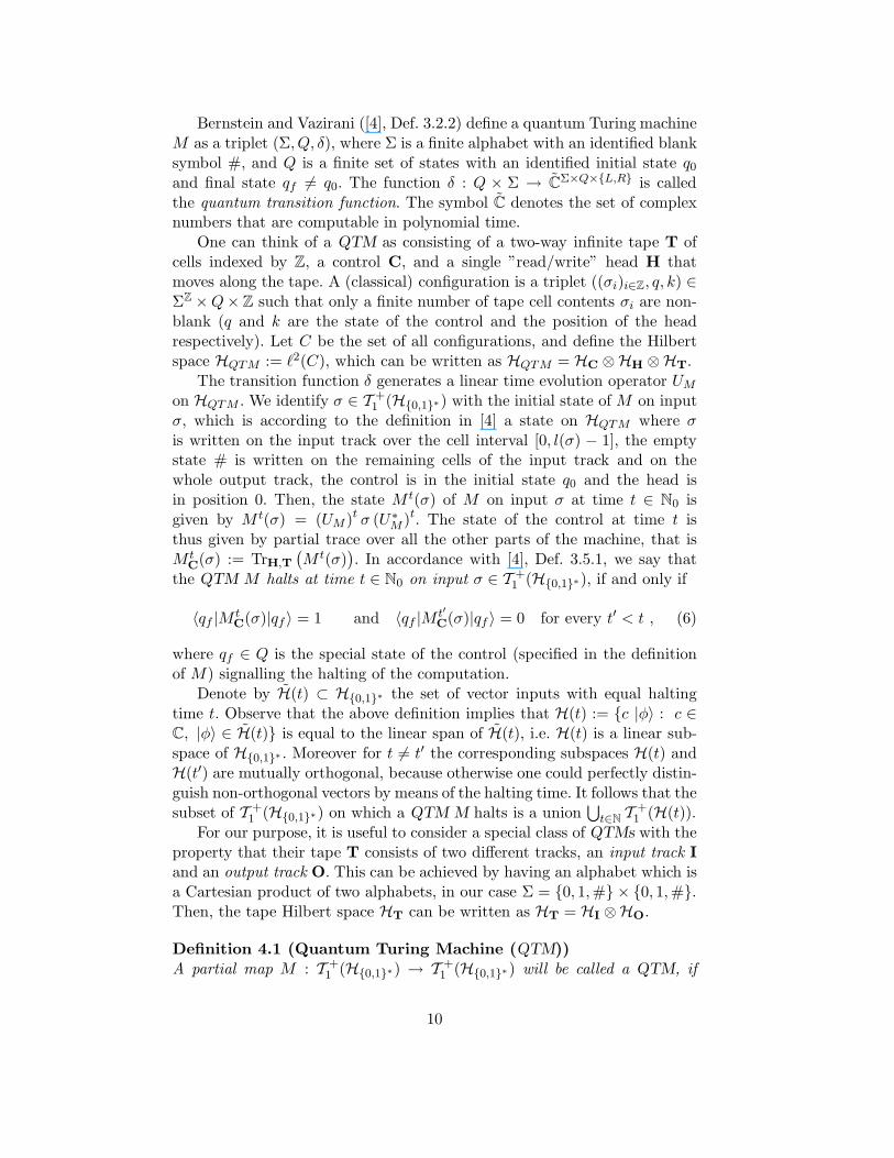
Bernstein and Vazirani ([4], Def. 3.2.2) define a quantum Turing machineM as a triplet (Σ, Q, δ), where Σ is a finite alphabet with an identified blanksymbol #, and Q is a finite set of states with an identified initial state q0and final state qf 6= q0. The function δ : Q × Σ → CΣ×Q×L,R is calledthe quantum transition function. The symbol C denotes the set of complexnumbers that are computable in polynomial time.

One can think of a QTM as consisting of a two-way infinite tape T ofcells indexed by Z, a control C, and a single ”read/write” head H thatmoves along the tape. A (classical) configuration is a triplet ((σi)i∈Z, q, k) ∈ΣZ ×Q× Z such that only a finite number of tape cell contents σi are non-blank (q and k are the state of the control and the position of the headrespectively). Let C be the set of all configurations, and define the Hilbertspace HQTM := ℓ2(C), which can be written as HQTM = HC ⊗HH ⊗HT.

The transition function δ generates a linear time evolution operator UM

on HQTM . We identify σ ∈ T +1 (H0,1∗) with the initial state of M on input

σ, which is according to the definition in [4] a state on HQTM where σis written on the input track over the cell interval [0, l(σ) − 1], the emptystate # is written on the remaining cells of the input track and on thewhole output track, the control is in the initial state q0 and the head isin position 0. Then, the state M t(σ) of M on input σ at time t ∈ N0 isgiven by M t(σ) = (UM )t σ (U∗

M )t. The state of the control at time t isthus given by partial trace over all the other parts of the machine, that isM t

C(σ) := TrH,T

(

M t(σ))

. In accordance with [4], Def. 3.5.1, we say thatthe QTM M halts at time t ∈ N0 on input σ ∈ T +

1 (H0,1∗), if and only if

〈qf |M tC(σ)|qf 〉 = 1 and 〈qf |M t′

C(σ)|qf 〉 = 0 for every t′ < t , (6)

where qf ∈ Q is the special state of the control (specified in the definitionof M) signalling the halting of the computation.

Denote by H(t) ⊂ H0,1∗ the set of vector inputs with equal haltingtime t. Observe that the above definition implies that H(t) := c |φ〉 : c ∈C, |φ〉 ∈ H(t) is equal to the linear span of H(t), i.e. H(t) is a linear sub-space of H0,1∗ . Moreover for t 6= t′ the corresponding subspaces H(t) andH(t′) are mutually orthogonal, because otherwise one could perfectly distin-guish non-orthogonal vectors by means of the halting time. It follows that thesubset of T +

1 (H0,1∗) on which a QTM M halts is a union⋃

t∈NT +

1 (H(t)).For our purpose, it is useful to consider a special class of QTMs with the

property that their tape T consists of two different tracks, an input track Iand an output track O. This can be achieved by having an alphabet which isa Cartesian product of two alphabets, in our case Σ = 0, 1,# × 0, 1,#.Then, the tape Hilbert space HT can be written as HT = HI ⊗HO.

Definition 4.1 (Quantum Turing Machine (QTM))A partial map M : T +

1 (H0,1∗) → T +1 (H0,1∗) will be called a QTM, if

10

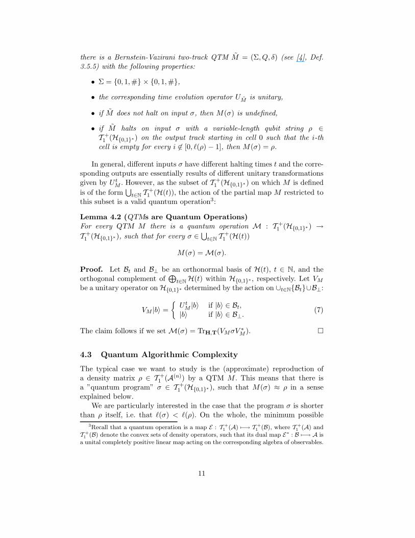
there is a Bernstein-Vazirani two-track QTM M = (Σ, Q, δ) (see [4], Def.3.5.5) with the following properties:

• Σ = 0, 1,# × 0, 1,#,

• the corresponding time evolution operator UM is unitary,

• if M does not halt on input σ, then M(σ) is undefined,

• if M halts on input σ with a variable-length qubit string ρ ∈T +

1 (H0,1∗) on the output track starting in cell 0 such that the i-thcell is empty for every i 6∈ [0, ℓ(ρ) − 1], then M(σ) = ρ.

In general, different inputs σ have different halting times t and the corre-sponding outputs are essentially results of different unitary transformationsgiven by U t

M . However, as the subset of T +1 (H0,1∗) on which M is defined

is of the form⋃

t∈NT +

1 (H(t)), the action of the partial map M restricted tothis subset is a valid quantum operation3:

Lemma 4.2 (QTMs are Quantum Operations)For every QTM M there is a quantum operation M : T +

1 (H0,1∗) →T +

1 (H0,1∗), such that for every σ ∈⋃

t∈NT +

1 (H(t))

M(σ) = M(σ).

Proof. Let Bt and B⊥ be an orthonormal basis of H(t), t ∈ N, and theorthogonal complement of

⊕

t∈NH(t) within H0,1∗ , respectively. Let VM

be a unitary operator on H0,1∗ determined by the action on ∪t∈NBt∪B⊥:

VM |b〉 =

U tM |b〉 if |b〉 ∈ Bt,

|b〉 if |b〉 ∈ B⊥.(7)

The claim follows if we set M(σ) = TrH,T(VMσV∗M ).

4.3 Quantum Algorithmic Complexity

The typical case we want to study is the (approximate) reproduction ofa density matrix ρ ∈ T +

1 (A(n)) by a QTM M . This means that there isa ”quantum program” σ ∈ T +

1 (H0,1∗), such that M(σ) ≈ ρ in a senseexplained below.

We are particularly interested in the case that the program σ is shorterthan ρ itself, i.e. that ℓ(σ) < ℓ(ρ). On the whole, the minimum possible

3Recall that a quantum operation is a map E : T +1 (A) 7−→ T +

1 (B), where T +1 (A) and

T +1 (B) denote the convex sets of density operators, such that its dual map E∗ : B 7−→ A is

a unital completely positive linear map acting on the corresponding algebra of observables.

11

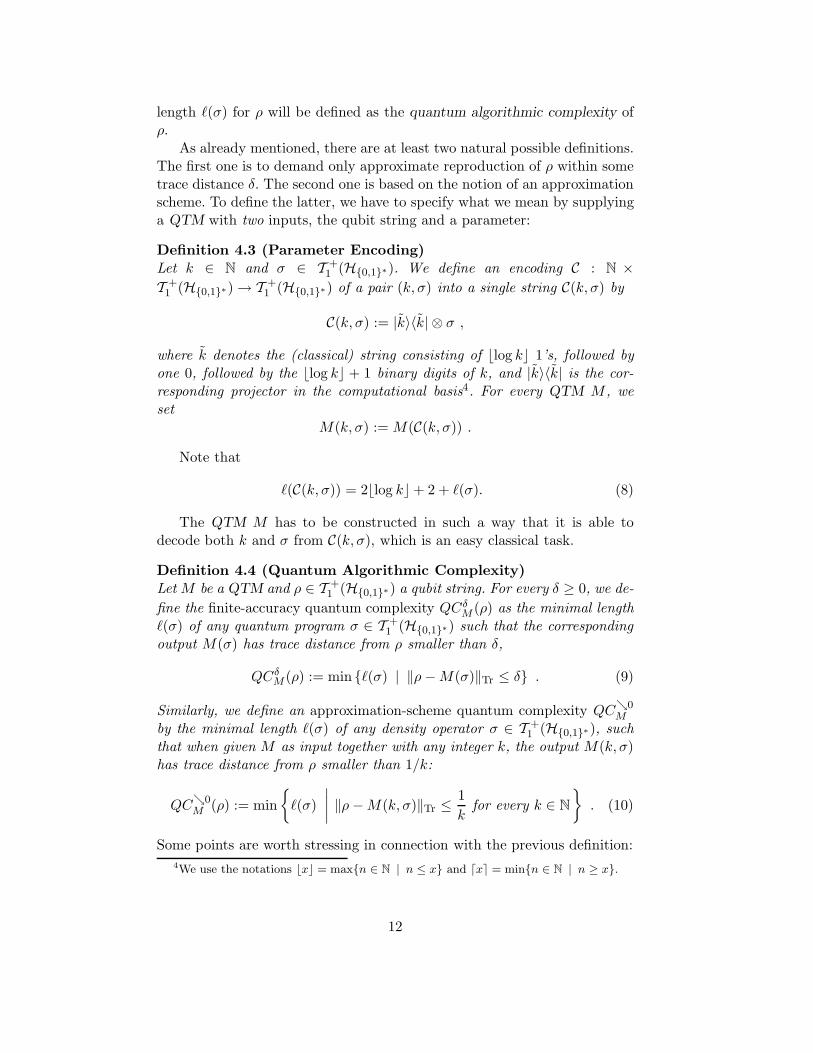
length ℓ(σ) for ρ will be defined as the quantum algorithmic complexity ofρ.

As already mentioned, there are at least two natural possible definitions.The first one is to demand only approximate reproduction of ρ within sometrace distance δ. The second one is based on the notion of an approximationscheme. To define the latter, we have to specify what we mean by supplyinga QTM with two inputs, the qubit string and a parameter:

Definition 4.3 (Parameter Encoding)Let k ∈ N and σ ∈ T +

1 (H0,1∗). We define an encoding C : N ×T +

1 (H0,1∗) → T +1 (H0,1∗) of a pair (k, σ) into a single string C(k, σ) by

C(k, σ) := |k〉〈k| ⊗ σ ,

where k denotes the (classical) string consisting of ⌊log k⌋ 1’s, followed byone 0, followed by the ⌊log k⌋ + 1 binary digits of k, and |k〉〈k| is the cor-responding projector in the computational basis4. For every QTM M , weset

M(k, σ) := M(C(k, σ)) .

Note that

ℓ(C(k, σ)) = 2⌊log k⌋ + 2 + ℓ(σ). (8)

The QTM M has to be constructed in such a way that it is able todecode both k and σ from C(k, σ), which is an easy classical task.

Definition 4.4 (Quantum Algorithmic Complexity)Let M be a QTM and ρ ∈ T +

1 (H0,1∗) a qubit string. For every δ ≥ 0, we de-

fine the finite-accuracy quantum complexity QCδM (ρ) as the minimal length

ℓ(σ) of any quantum program σ ∈ T +1 (H0,1∗) such that the corresponding

output M(σ) has trace distance from ρ smaller than δ,

QCδM (ρ) := min ℓ(σ) | ‖ρ−M(σ)‖Tr ≤ δ . (9)

Similarly, we define an approximation-scheme quantum complexity QCց0M

by the minimal length ℓ(σ) of any density operator σ ∈ T +1 (H0,1∗), such

that when given M as input together with any integer k, the output M(k, σ)has trace distance from ρ smaller than 1/k:

QCց0M (ρ) := min

ℓ(σ)

∣

∣

∣

∣

‖ρ−M(k, σ)‖Tr ≤1

kfor every k ∈ N

. (10)

Some points are worth stressing in connection with the previous definition:

4We use the notations ⌊x⌋ = maxn ∈ N | n ≤ x and ⌈x⌉ = minn ∈ N | n ≥ x.

12

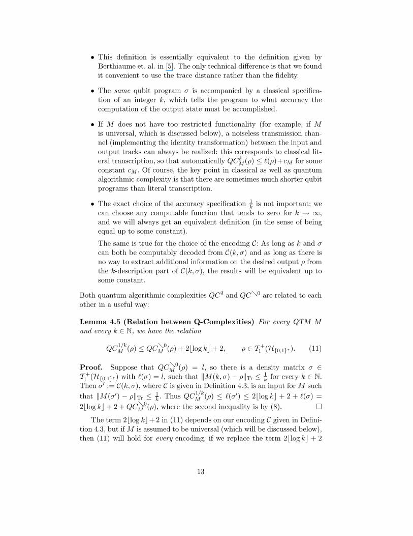
• This definition is essentially equivalent to the definition given byBerthiaume et. al. in [5]. The only technical difference is that we foundit convenient to use the trace distance rather than the fidelity.

• The same qubit program σ is accompanied by a classical specifica-tion of an integer k, which tells the program to what accuracy thecomputation of the output state must be accomplished.

• If M does not have too restricted functionality (for example, if Mis universal, which is discussed below), a noiseless transmission chan-nel (implementing the identity transformation) between the input andoutput tracks can always be realized: this corresponds to classical lit-eral transcription, so that automatically QCδ

M(ρ) ≤ ℓ(ρ)+cM for someconstant cM . Of course, the key point in classical as well as quantumalgorithmic complexity is that there are sometimes much shorter qubitprograms than literal transcription.

• The exact choice of the accuracy specification 1k is not important; we

can choose any computable function that tends to zero for k → ∞,and we will always get an equivalent definition (in the sense of beingequal up to some constant).

The same is true for the choice of the encoding C: As long as k and σcan both be computably decoded from C(k, σ) and as long as there isno way to extract additional information on the desired output ρ fromthe k-description part of C(k, σ), the results will be equivalent up tosome constant.

Both quantum algorithmic complexities QCδ and QCց0 are related to eachother in a useful way:

Lemma 4.5 (Relation between Q-Complexities) For every QTM Mand every k ∈ N, we have the relation

QC1/kM (ρ) ≤ QCց0

M (ρ) + 2⌊log k⌋ + 2, ρ ∈ T +1 (H0,1∗). (11)

Proof. Suppose that QCց0M (ρ) = l, so there is a density matrix σ ∈

T +1 (H0,1∗) with ℓ(σ) = l, such that ‖M(k, σ) − ρ‖Tr ≤ 1

k for every k ∈ N.Then σ′ := C(k, σ), where C is given in Definition 4.3, is an input for M such

that ‖M(σ′) − ρ‖Tr ≤ 1k . Thus QC

1/kM (ρ) ≤ ℓ(σ′) ≤ 2⌊log k⌋ + 2 + ℓ(σ) =

2⌊log k⌋ + 2 +QCց0M (ρ), where the second inequality is by (8).

The term 2⌊log k⌋+2 in (11) depends on our encoding C given in Defini-tion 4.3, but if M is assumed to be universal (which will be discussed below),then (11) will hold for every encoding, if we replace the term 2⌊log k⌋ + 2

13

by K(k) + cM , where K(k) ≤ 2⌊log k⌋ + O(1) denotes the classical (self-delimiting) algorithmic complexity of the integer k, and cM is some constantdepending only on M . For more details we refer the reader to [25].

In [4], it is proved that there is a universal QTM (UQTM) U that cansimulate with arbitrary accuracy every other machine M in the sense thatfor every such M there is a classical bit string M ∈ 0, 1∗ such that

‖U(M , σ, k, t) −M tO(σ)‖Tr ≤

1

kfor every σ ∈ T +

1 (H0,1∗), (12)

where k, t ∈ N. As it is implicit in this definition of universality, we willdemand that U is able to perfectly simulate every classical computation,and that it can apply a given unitary transformation within any desiredaccuracy (it is shown in [4] that such machines exist).

We choose an arbitrary UQTM U which is constructed such that it de-codes our encoding C(k, σ) given in Definition 4.3 into k and σ at the be-ginning of the computation. Like in the classical case, we fix U for the restof the paper and simplify notation by

QCց0(ρ) := QCց0U

(ρ), QCδ(ρ) := QCδU(ρ) .

5 Proof of the Main Theorem

As already mentioned at the beginning of Section 2, without loss of gener-ality, we give the proofs for the case that A is the algebra of the observablesof a qubit, i.e. the complex 2 × 2-matrices.

5.1 Lower Bound

For classical TMs, there are no more than 2c+1 − 1 different programs oflength ℓ ≤ c. This can be used as a ”counting argument” for proving thelower bound of Brudno’s Theorem in the classical case ([21]). We are nowgoing to prove a similar statement for QTMs.

Our first step is to elaborate on an argument due to [5] which states thatthere cannot be more than 2ℓ+1 − 1 mutually orthogonal one-dimensionalprojectors p with quantum complexity QCց0(p) ≤ ℓ. The argument is basedon Holevo’s χ-quantity associated to any ensemble Eρ := λi, ρii consistingof weights 0 ≤ λi ≤ 1,

∑

i λi = 1, and of density matrices ρi acting on aHilbert space H. Setting ρ :=

∑

i λiρi, the χ-quantity is defined as follows

χ(Eρ) := S (ρ) −∑

i

λi S(ρi) (13)

=∑

i

λi S(ρi, ρ) , (14)

14

where, in the second line, the relative entropy appears

S(ρ1 , ρ2) :=

Tr(

ρ1

(

log ρ1 − log ρ2

))

if supp ρ1 ≤ supp ρ2 ,

∞ otherwise.(15)

If dim(H) is finite, (13) is bounded by the maximal von Neumann entropy:

χ(Eρ) ≤ S(ρ) ≤ log dim(H). (16)

In the following, H′ denotes an arbitrary (possibly infinite-dimensional)Hilbert space, while the rest of the notation is adopted from Subsection 4.2.

Lemma 5.1 (Quantum Counting Argument)Let 0 < δ < 1/e, c ∈ N such that c ≥ 2

δ

(

2 + log 1δ

)

, P an orthogo-nal projector onto a linear subspace of an arbitrary Hilbert space H′, andE : T +

1 (H0,1∗) → T +1 (H′) a quantum operation. Let N δ

c be a maximumcardinality subset of one-dimensional projectors from the set

Aδc(E , P ) := p ≤ P | p 1-dim. proj.,∃σ ∈ T +

1 (H≤c) : ‖E(σ) − p‖Tr ≤ δ,

that is, the set of all pure quantum states which are reproduced within δ bythe operation E on some input of length ≤ c. Then it holds that

log |N δc | < c+ 1 +

2 + δ

1 − 2δδc .

Proof. Let pj ∈ Aδc(E , P ), j = 1, . . . , N , be a set of mutually orthogonal

projectors and pN+1 := 1H′ − ∑Ni=1 pi. By the definition of Aδ

c(E , P ), forevery 1 ≤ i ≤ N , there are density matrices σi ∈ T +

1 (H≤c) with

‖E(σi) − pi‖Tr ≤ δ . (17)

Consider the equidistributed ensemble Eσ :=

1N , σi

, where σ :=1

N

N∑

i=1

σi

also acts on H≤c. Using that dimH≤c = 2c+1 − 1, inequality (16) yields

χ(Eσ) < c+ 1. (18)

We define a quantum operation R on T +1 (H′) by R(a) :=

∑N+1i=1 piapi.

Applying twice the monotonicity of the relative entropy under quantumoperations, we obtain

1

N

N∑

i=1

S (R E(σi),R E(σ)) ≤ 1

N

N∑

i=1

S (E(σi), E(σ)) ≤ χ(Eσ) . (19)

Moreover, for every i ∈ 1, . . . , N, the density operator R E(σi) is closeto the corresponding one-dimensional projector R(pi) = pi. Indeed, by the

15

contractivity of the trace distance under quantum operations (compare Thm.9.2 in [28]) and by assumption (17), it holds

‖R E(σi) − pi‖Tr ≤ ‖E(σi) − pi‖Tr ≤ δ .

Let ∆ := 1N

∑Ni=1 pi. The trace-distance is convex ([28], (9.51)), thus

‖R E(σ) − ∆‖Tr ≤1

N

N∑

i=1

‖R E(σi) − pi‖Tr ≤ δ ,

whence, since δ < 1e , Fannes’ inequality (compare Thm. 11.6 in [28]) gives

S(R E(σi)) = |S(R E(σi)) − S(pi)| ≤ δ log(N + 1) + η(δ)

and |S(R E(σ)) − S(∆)| ≤ δ log(N + 1) + η(δ) ,

where η(δ) := −δ log δ. Combining the two estimates above with (18) and(19), we obtain

c+ 1 > χ(Eσ) ≥ S(R E(σ)) − 1

N

N∑

i=1

S(R E(σi))

≥ S(∆) − δ log(N + 1) − η(δ) − 1

N

N∑

i=1

(δ log(N + 1) + η(δ))

= logN − 2δ log(N + 1) − 2η(δ)

≥ (1 − 2δ) logN − 2δ − 2η(δ). (20)

Assume now that logN ≥ c + 1 + 2+δ1−2δ δc. Then it follows (20) that c <

2δ

(

2 + log 1δ

)

. So if c is larger than this expression, the maximum number|N δ

c | of mutually orthogonal projectors in Aδc(E , P ) must be bounded by

log |N δc | < c+ 1 +

2 + δ

1 − 2δδc.

The second step uses the previous lemma together with the following the-orem [7, Prop. 2.1]. It is closely related to the quantum Shannon-McMillanTheorem and concerns the minimal dimension of the Ψ−typical subspaces.

Theorem 5.2 Let (A∞,Ψ) be an ergodic quantum source with entropy rates. Then, for every 0 < ε < 1,

limn→∞

1

nβε,n(Ψ) = s, (21)

where βε,n(Ψ) := min

log Trn(q) | q ∈ A(n) projector ,Ψ(n)(q) ≥ 1 − ε

.

Notice that the limit (21) is valid for all 0 < ε < 1. By means of this property,we will first prove the lower bound for the finite-accuracy complexity QCδ,and then use Lemma 4.5 to extend it to QCց0.

16

Corollary 5.3 (Lower Bound for 1nQC

δ)Let (A∞,Ψ) be an ergodic quantum source with entropy rate s. Moreover,let 0 < δ < 1/e, and let (pn)n∈N

be a sequence of Ψ-typical projectors. Then,there is another sequence of Ψ-typical projectors qn(δ) ≤ pn, such that for nlarge enough

1

nQCδ(q) > s− δ(2 + δ)s

is true for every one-dimensional projector q ≤ qn(δ).

Proof. The case s = 0 is trivial, so let s > 0. Fix n ∈ N and some0 < δ < 1/e, and consider the set

An(δ) :=

p ≤ pn | p one-dim. proj., QCδ(p) ≤ ns(1 − δ(2 + δ))

.

¿From the definition of QCδ(p), to all p’s there exist associated densitymatrices σp with ℓ(σp) ≤ ns(1−δ(2+δ)) such that ‖M(σp)−p‖Tr ≤ δ, whereM denotes the quantum operation M : T +

1 (H0,1∗) → T +1 (H0,1∗) of the

corresponding UQTM U, as explained in Lemma 4.2. Using the notation ofLemma 5.1, it thus follows that

An(δ) ⊂ Aδ⌈ns(1−δ(2+δ))⌉(M, pn) .

Let pn(δ) ≤ pn be a sum of a maximal number of mutually orthogonalprojectors from Aδ

⌈ns(1−δ(2+δ))⌉(M, pn). If n was chosen large enough such

that ns(1 − δ(2 + δ)) ≥ 1δ

(

4 + 2 log 1δ

)

is satisfied, Lemma 5.1 implies that

log Tr pn(δ) < ⌈ns(1 − δ(2 + δ))⌉ + 1 +2 + δ

1 − 2δδ⌈ns(1 − δ(2 + δ))⌉, (22)

and there are no one-dimensional projectors p ≤ pn(δ)⊥ := pn − pn(δ) suchthat p ∈ Aδ

⌈ns(1−δ(2+δ))⌉(M, pn), Namely, one-dimensional projectors p ≤pn(δ)⊥ must satisfy 1

nQCδ(p) > s− δ(2 + δ)s. Since inequality (22) is valid

for every n ∈ N large enough, we conclude

lim supn→∞

1

nlog Trnpn(δ) ≤ s− 2δ3s− 5δ4s

1 − 2δ< s. (23)

Using Theorem 5.2, we obtain that limn→∞ Ψ(n)(pn(δ)) = 0. Finally, setqn(δ) := pn(δ)⊥. The claim follows.

Corollary 5.4 (Lower Bound for 1nQC

ց0)Let (A∞,Ψ) be an ergodic quantum source with entropy rate s. Let (pn)n∈N

with pn ∈ A(n) be an arbitrary sequence of Ψ-typical projectors. Then, forevery 0 < δ < 1/e, there is a sequence of Ψ-typical projectors qn(δ) ≤ pn

such that for n large enough

1

nQCց0(q) > s− δ

is satisfied for every one-dimensional projector q ≤ qn(δ).

17

Proof. According to Corollary 5.3, for every k ∈ N, there exists a sequenceof Ψ-typical projectors pn( 1

k ) ≤ pn with 1nQC

1k (q) > s− 1

k (2 + 1k )s for every

one-dimensional projector q ≤ pn( 1k ) if n is large enough. We have

1

nQCց0(q) ≥ 1

nQC1/k(q) − 2 + 2⌊log k⌋

n

> s− 1

k

(

2 +1

k

)

s− 2(2 + log k)

n,

where the first estimate is by Lemma 4.5, and the second one is true forone-dimensional projectors q ≤ pn( 1

k ) and n ∈ N large enough. Fix a large

k satisfying 1k (2 + 1

k )s ≤ δ2 . The result follows by setting qn(δ) = pn( 1

k ).

5.2 Upper Bound

In the previous section, we have shown that with high probability and forlarge m, the finite-accuracy complexity rate 1

mQCδ is bounded from below

by s(1− δ(2 + δ)), and the approximation-scheme quantum complexity rate1mQC

ց0 by s− δ. We are now going to establish the upper bounds.

Proposition 5.5 (Upper Bound)Let (A∞,Ψ) be an ergodic quantum source with entropy rate s. Then, forevery 0 < δ < 1/e, there is a sequence of Ψ-typical projectors qm(δ) ∈ A(m)

such that for every one-dimensional projector q ≤ qm(δ) and m large enough

1

mQCց0(q) < s+ δ and (24)

1

mQCδ(q) < s+ δ . (25)

We prove the above proposition by explicitly providing a short quantumalgorithm (with program length increasing like m(s + δ)) that computes qwithin arbitrary accuracy. This will be done by means of quantum universaltypical subspaces. Kaltchenko and Yang have constructed such subspaces in[20]. We adapt their proof and apply it to show the upper bound in 3.1.

Theorem 5.6 (Universal Typical Subspaces)

Let s > 0 and ε > 0. There exists a sequence of projectors Q(n)s,ε ∈ A(n),

n ∈ N, such that for n large enough

Tr(

Q(n)s,ε

)

≤ 2n(s+ε) (26)

and for every ergodic quantum state Ψ ∈ S(A∞) with entropy rate s(Ψ) ≤ sit holds that

limn→∞

Ψ(n)(Q(n)s,ε ) = 1 . (27)

18

We call the orthogonal projectors Q(n)s,ε in the above theorem universal typ-

ical projectors at level s. In the remainder of this section, we sketch theirconstruction. Suited for designing an appropriate quantum algorithm, weslightly modify the presentation given by Kaltchenko and Yang in [20].

Let l ∈ N and R > 0. We consider an Abelian quasi-local subalge-bra C∞

l ⊆ A∞ constructed from a maximal Abelian l−block subalgebraCl ⊆ A(l). The results in [40, 22] imply that there exists a universal se-

quence of projectors p(n)l,R ∈ C(n)

l ⊆ A(ln) with 1n log Tr p

(n)l,R ≤ R such that

limn→∞ π(n)(p(n)l,R) = 1 for any ergodic state π on the Abelian algebra C∞

l

with entropy rate s(π) < R. Notice that ergodicity and entropy rate of πare defined with respect to the shift on C∞

l , which corresponds to the l-shifton A∞.

The first step in [20] is to apply unitary operators of the form U⊗n,

U ∈ A(l) unitary, to the p(n)l,R and to introduce the projectors

w(ln)l,R :=

∨

U∈A(l) unitary

U⊗np(n)l,RU

∗⊗n ∈ A(ln). (28)

Let p(n)l,R =

∑

i∈I |i(n)l,R〉〈i

(n)l,R | be a spectral decomposition of p

(n)l,R (with I ⊂ N

some index set), and let P(V ) denote the orthogonal projector onto a given

subspace V . Then, w(ln)l,R can also be written as

w(ln)l,R = P

(

spanU⊗n|i(n)l,R〉 : i ∈ I, U ∈ A(l) unitary

)

.

It will be more convenient for the construction of our algorithm in 5.2.1 toconsider the projector

W(ln)l,R := P

(

spanA⊗n|i(n)l,R〉 : i ∈ I,A ∈ A(l)

)

. (29)

It holds that w(ln)l,R ≤ W

(ln)l,R . For integers m = nl + k with n ∈ N and

k ∈ 0, . . . , l − 1 we introduce the projectors in A(m)

w(m)l,R := w

(ln)l,R ⊗ 1⊗k, W

(m)l,R := W

(ln)l,R ⊗ 1⊗k. (30)

We now use an argument of [19] to estimate the trace of W(m)l,R ∈ A(m). The

dimension of the symmetric subspace SYM(A(ln)) := spanA⊗n : A ∈ A(l)is upper bounded by (n+ 1)dimA(l)

, thus

Tr W(m)l,R = Tr W

(ln)l,R · Tr 1⊗k ≤ (n+ 1)2

2l

Tr p(n)l,R · 2l

≤ (n+ 1)22l · 2Rn · 2l. (31)

Now we consider a stationary ergodic state Ψ on the quasi-local algebraA∞ with entropy rate s(Ψ) ≤ s. Let ε, δ > 0. If l is chosen large enough

19

then the projectors w(m)l,R , where R := l(s + ε

2), are δ−typical for Ψ, i.e.

Ψ(m)(w(m)l,R ) ≥ 1−δ, for m ∈ N sufficiently large. This can be seen as follows.

Due to the result in [7, Thm. 3.1] the ergodic state Ψ convexly decomposesinto k(l) ≤ l states

Ψ =1

k(l)

k(l)∑

i=1

Ψi,l, (32)

each Ψi,l being ergodic with respect to the l−shift on A∞ and having anentropy rate (with respect to the l−shift) equal to s(Ψ) · l. Moreover, thereis the following Density Lemma proven in [7, Lemma 3.1]:

Lemma 5.7 (Density Lemma) Let Ψ be an ergodic state on A∞. Forevery ∆ > 0, we define the set of integers

Al,∆ := i ∈ 1, . . . , k(l) : S(Ψ(l)i,l ) ≥ l(s(Ψ) + ∆). (33)

Then it holds

liml→∞

|Al,∆|k(l)

= 0. (34)

Let Ci,l be the maximal Abelian subalgebra of A(l) generated by the one-

dimensional eigenprojectors of Ψ(l)i,l ∈ S(A(l)). The restriction of a compo-

nent Ψi,l to the Abelian quasi-local algebra C∞i,l is again an ergodic state. It

holds in general

l · s(Ψ) = s(Ψi,l) ≤ s(Ψi,l C∞i,l ) ≤ S(Ψ

(l)i,l Ci,l) = S(Ψ

(l)i,l ). (35)

For i ∈ Acl,∆, where we set ∆ := R

l − s(Ψ), we additionally have the up-

per bound S(Ψ(l)i,l ) < R. Let Ui ∈ A(l) be a unitary operator such that

U⊗ni p

(n)l,RU

∗⊗ni ∈ C(n)

i,l . For every i ∈ Acl,∆, it holds that

Ψ(ln)i,l (w

(ln)l,R ) ≥ Ψ

(ln)i,l (U⊗n

i p(n)l,RU

∗⊗ni ) −→ 1 as n→ ∞. (36)

We fix an l ∈ N large enough to fulfill|Ac

l,∆|k(l) ≥ 1 − δ

2 and use the ergodic

decomposition (32) to obtain the lower bound

Ψ(ln)(w(ln)l,R ) ≥ 1

k(l)

∑

i∈Acl,∆

Ψ(nl)l,i (w

(ln)l,R ) ≥

(

1 − δ

2

)

mini∈Ac

l,∆

Ψ(nl)i,l (w

(ln)l,R ). (37)

From (36) we conclude that for n large enough

Ψ(ln)(W(ln)l,R ) ≥ Ψ(ln)(w

(ln)l,R ) ≥ 1 − δ. (38)

20

We proceed by following the lines of [20] by introducing the sequence lm,m ∈ N, where each lm is a power of 2 fulfilling the inequality

lm23·lm ≤ m < 2lm23·2lm . (39)

Let the integer sequence nm and the real-valued sequence Rm be defined bynm := ⌊ m

lm⌋ and Rm := lm ·

(

s+ ε2

)

. Then we set

Q(m)s,ε :=

W(lmnm)lm,Rm

if m = lm23·lm ,

W(lmnm)lm,Rm

⊗ 1⊗(m−lmnm) otherwise .(40)

Observe that

1

mlog Tr Q(m)

s,ε ≤ 1

nmlmlog Tr Q(m)

s,ε

≤ 4lm

lm

log(nm + 1)

nm+Rm

lm+

1

nm(41)

≤ 4lm

lm

6lm + 2

23lm − 1+ s+

ε

2+

1

23lm − 1, (42)

where the second inequality is by estimate (31) and the last one by thebounds on nm

23lm − 1 ≤ m

lm− 1 ≤ nm ≤ m

lm≤ 26lm+1.

Thus, for large m, it holds

1

mlog Tr Q(m)

s,ε ≤ s+ ε. (43)

By the special choice (39) of lm it is ensured that the sequence of projec-

tors Q(m)s,ε ∈ A(m) is indeed typical for any quantum state Ψ with entropy

rate s(Ψ) ≤ s, compare [20]. This means that Q(m)s,ε m∈N is a sequence of

universal typical projectors at level s.

5.2.1 Construction of the Decompression Algorithm

We proceed by applying the latter result to universal typical subspaces forour proof of the upper bound. Let 0 < ε < δ/2 be an arbitrary real num-

ber such that r := s + ε is rational, and let qm := Q(m)s,ε be the universal

projector sequence of Theorem 5.6. Recall that the projector sequence qm isindependent of the choice of the ergodic state Ψ, as long as s(Ψ) ≤ s.

Because of (26), for m large enough, there exists some unitary transfor-mation U∗ that transforms the projector qm into a projector belonging toT +

1 (H⌈mr⌉), thus transforming every one-dimensional projector q ≤ qm intoa qubit string q := U∗qU of length ℓ(q) = ⌈mr⌉.

21

As shown in [4], a UQTM can implement every classical algorithm, andit can apply every unitary transformation U (when given an algorithm forthe computation of U) on its tapes within any desired accuracy. We canthus feed q (plus some classical instructions including a subprogram forthe computation of U) as input into the UQTM U. This UQTM starts bycomputing a classical description of the transformation U , and subsequentlyapplies U to q, recovering the original projector q = UqU∗ on the outputtape.

Since U = U(qm) depends on Ψ only through its entropy rate s(Ψ), thesubprogram that computes U does not have to be supplied with additionalinformation on Ψ and will thus have fixed length.

We give a precise definition of a quantum decompression algorithm A,which is, formally, a mapping (r is rational)

A : N × N × Q ×H0,1∗ → H0,1∗ ,

(k,m, r, q) 7→ q = A(k,m, r, q) .

We require that A is a ”short algorithm” in the sense of ”short in descrip-tion”, not short (fast) in running time or resource consumption. Indeed, thealgorithm A is very slow and memory consuming, but this does not matter,since Kolmogorov complexity only cares about the description length of theprogram.

The instructions defining the quantum algorithm A are:

1. Read the value of m, and find a solution l ∈ N for the inequality

l · 23l ≤ m < 2 · l · 23·2l

such that l is a power of two. (There is only one such l.)

2. Compute n := ⌊ml ⌋.

3. Read the value of r. Compute R := l · r.

4. Compute a list of codewords Ω(n)l,R, belonging to a classical universal

block code sequence of rate R. (For the construction of an appropriatealgorithm, see [22, Thm. 2 and 1].) Since

Ω(n)l,R ⊂

(

0, 1l)n

,

Ω(n)l,R = ω1, ω2, . . . , ωM can be stored as a list of binary strings. Ev-

ery string has length ℓ(ωi) = nl. (Note that the exact value of the

cardinality M ≈ 2nR depends on the choice of Ω(n)l,R.)

During the following steps, the quantum algorithm A will have to deal with

• rational numbers,

22

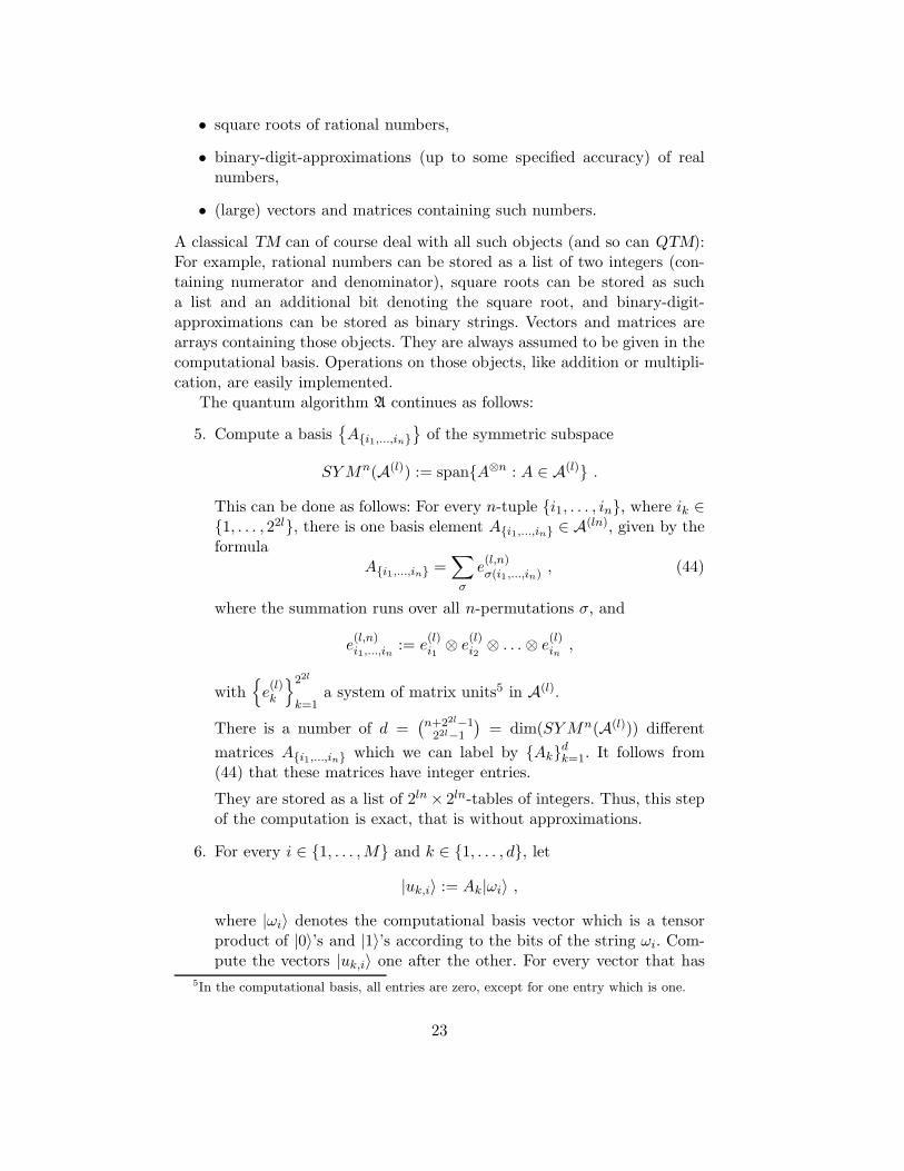
• square roots of rational numbers,

• binary-digit-approximations (up to some specified accuracy) of realnumbers,

• (large) vectors and matrices containing such numbers.

A classical TM can of course deal with all such objects (and so can QTM):For example, rational numbers can be stored as a list of two integers (con-taining numerator and denominator), square roots can be stored as sucha list and an additional bit denoting the square root, and binary-digit-approximations can be stored as binary strings. Vectors and matrices arearrays containing those objects. They are always assumed to be given in thecomputational basis. Operations on those objects, like addition or multipli-cation, are easily implemented.

The quantum algorithm A continues as follows:

5. Compute a basis

Ai1,...,in

of the symmetric subspace

SYMn(A(l)) := spanA⊗n : A ∈ A(l) .

This can be done as follows: For every n-tuple i1, . . . , in, where ik ∈1, . . . , 22l, there is one basis element Ai1,...,in ∈ A(ln), given by theformula

Ai1,...,in =∑

σ

e(l,n)σ(i1,...,in) , (44)

where the summation runs over all n-permutations σ, and

e(l,n)i1,...,in

:= e(l)i1

⊗ e(l)i2

⊗ . . . ⊗ e(l)in,

with

e(l)k

22l

k=1a system of matrix units5 in A(l).

There is a number of d =(n+22l−1

22l−1

)

= dim(SYMn(A(l))) different

matrices Ai1,...,in which we can label by Akdk=1. It follows from

(44) that these matrices have integer entries.

They are stored as a list of 2ln × 2ln-tables of integers. Thus, this stepof the computation is exact, that is without approximations.

6. For every i ∈ 1, . . . ,M and k ∈ 1, . . . , d, let

|uk,i〉 := Ak|ωi〉 ,

where |ωi〉 denotes the computational basis vector which is a tensorproduct of |0〉’s and |1〉’s according to the bits of the string ωi. Com-pute the vectors |uk,i〉 one after the other. For every vector that has

5In the computational basis, all entries are zero, except for one entry which is one.

23

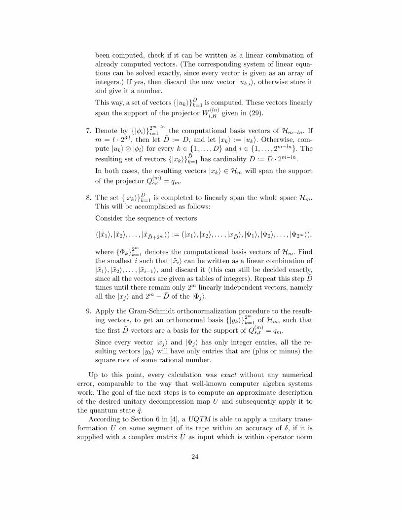
been computed, check if it can be written as a linear combination ofalready computed vectors. (The corresponding system of linear equa-tions can be solved exactly, since every vector is given as an array ofintegers.) If yes, then discard the new vector |uk,i〉, otherwise store itand give it a number.

This way, a set of vectors |uk〉Dk=1 is computed. These vectors linearly

span the support of the projector W(ln)l,R given in (29).

7. Denote by |φi〉2m−ln

i=1 the computational basis vectors of Hm−ln. Ifm = l · 23·l, then let D := D, and let |xk〉 := |uk〉. Otherwise, com-pute |uk〉 ⊗ |φi〉 for every k ∈ 1, . . . ,D and i ∈ 1, . . . , 2m−ln. The

resulting set of vectors |xk〉Dk=1 has cardinality D := D · 2m−ln.

In both cases, the resulting vectors |xk〉 ∈ Hm will span the support

of the projector Q(m)s,ε = qm.

8. The set |xk〉Dk=1 is completed to linearly span the whole space Hm.

This will be accomplished as follows:

Consider the sequence of vectors

(|x1〉, |x2〉, . . . , |xD+2m〉) := (|x1〉, |x2〉, . . . , |xD〉, |Φ1〉, |Φ2〉, . . . , |Φ2m〉),

where Φk2m

k=1 denotes the computational basis vectors of Hm. Findthe smallest i such that |xi〉 can be written as a linear combination of|x1〉, |x2〉, . . . , |xi−1〉, and discard it (this can still be decided exactly,since all the vectors are given as tables of integers). Repeat this step Dtimes until there remain only 2m linearly independent vectors, namelyall the |xj〉 and 2m − D of the |Φj〉.

9. Apply the Gram-Schmidt orthonormalization procedure to the result-ing vectors, to get an orthonormal basis |yk〉2m

k=1 of Hm, such that

the first D vectors are a basis for the support of Q(m)s,ε = qm.

Since every vector |xj〉 and |Φj〉 has only integer entries, all the re-sulting vectors |yk〉 will have only entries that are (plus or minus) thesquare root of some rational number.

Up to this point, every calculation was exact without any numericalerror, comparable to the way that well-known computer algebra systemswork. The goal of the next steps is to compute an approximate descriptionof the desired unitary decompression map U and subsequently apply it tothe quantum state q.

According to Section 6 in [4], a UQTM is able to apply a unitary trans-formation U on some segment of its tape within an accuracy of δ, if it issupplied with a complex matrix U as input which is within operator norm

24

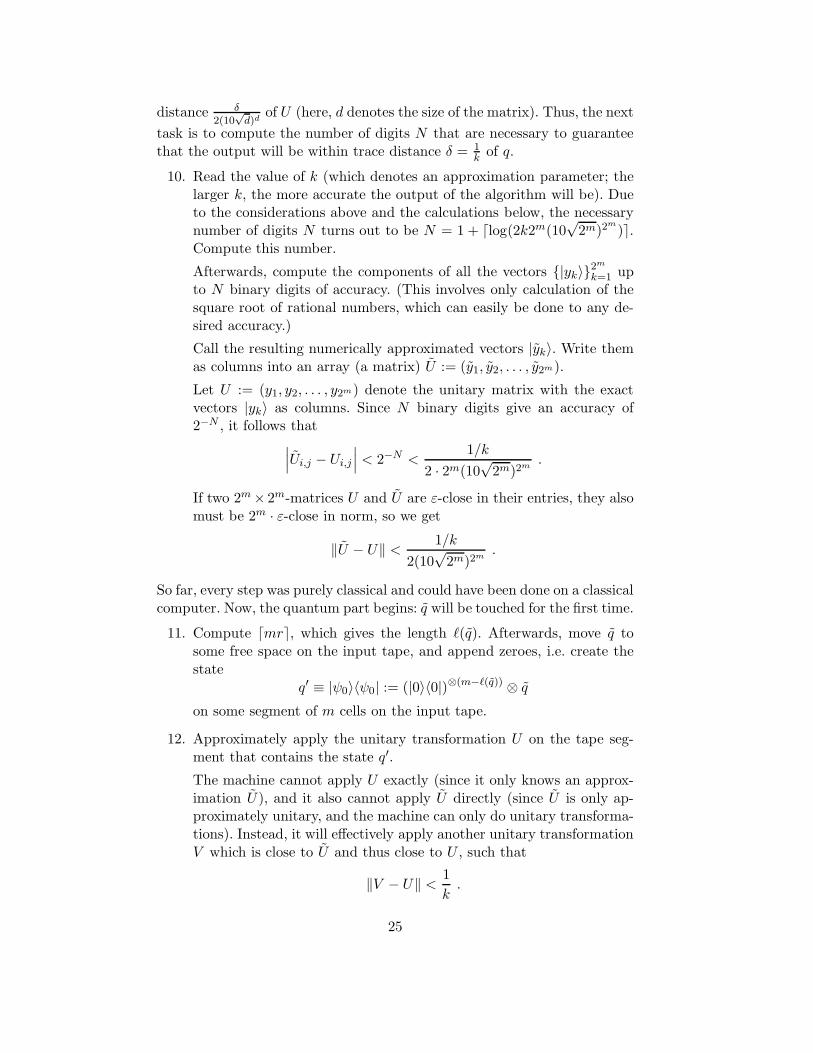
distance δ2(10

√d)d

of U (here, d denotes the size of the matrix). Thus, the next

task is to compute the number of digits N that are necessary to guaranteethat the output will be within trace distance δ = 1

k of q.

10. Read the value of k (which denotes an approximation parameter; thelarger k, the more accurate the output of the algorithm will be). Dueto the considerations above and the calculations below, the necessarynumber of digits N turns out to be N = 1 + ⌈log(2k2m(10

√2m)2

m

)⌉.Compute this number.

Afterwards, compute the components of all the vectors |yk〉2m

k=1 upto N binary digits of accuracy. (This involves only calculation of thesquare root of rational numbers, which can easily be done to any de-sired accuracy.)

Call the resulting numerically approximated vectors |yk〉. Write themas columns into an array (a matrix) U := (y1, y2, . . . , y2m).

Let U := (y1, y2, . . . , y2m) denote the unitary matrix with the exactvectors |yk〉 as columns. Since N binary digits give an accuracy of2−N , it follows that

∣

∣

∣Ui,j − Ui,j

∣

∣

∣< 2−N <

1/k

2 · 2m(10√

2m)2m.

If two 2m × 2m-matrices U and U are ε-close in their entries, they alsomust be 2m · ε-close in norm, so we get

‖U − U‖ < 1/k

2(10√

2m)2m.

So far, every step was purely classical and could have been done on a classicalcomputer. Now, the quantum part begins: q will be touched for the first time.

11. Compute ⌈mr⌉, which gives the length ℓ(q). Afterwards, move q tosome free space on the input tape, and append zeroes, i.e. create thestate

q′ ≡ |ψ0〉〈ψ0| := (|0〉〈0|)⊗(m−ℓ(q)) ⊗ q

on some segment of m cells on the input tape.

12. Approximately apply the unitary transformation U on the tape seg-ment that contains the state q′.

The machine cannot apply U exactly (since it only knows an approx-imation U), and it also cannot apply U directly (since U is only ap-proximately unitary, and the machine can only do unitary transforma-tions). Instead, it will effectively apply another unitary transformationV which is close to U and thus close to U , such that

‖V − U‖ < 1

k.

25

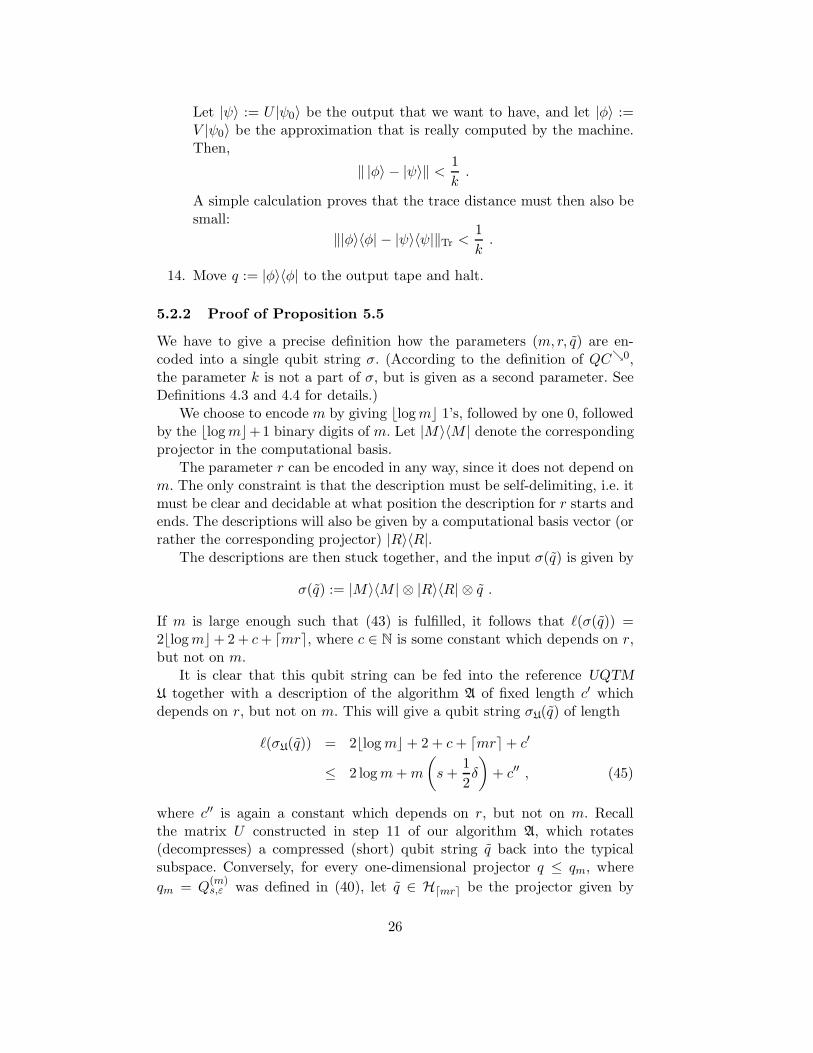
Let |ψ〉 := U |ψ0〉 be the output that we want to have, and let |φ〉 :=V |ψ0〉 be the approximation that is really computed by the machine.Then,

‖ |φ〉 − |ψ〉‖ < 1

k.

A simple calculation proves that the trace distance must then also besmall:

‖|φ〉〈φ| − |ψ〉〈ψ|‖Tr <1

k.

14. Move q := |φ〉〈φ| to the output tape and halt.

5.2.2 Proof of Proposition 5.5

We have to give a precise definition how the parameters (m, r, q) are en-coded into a single qubit string σ. (According to the definition of QCց0,the parameter k is not a part of σ, but is given as a second parameter. SeeDefinitions 4.3 and 4.4 for details.)

We choose to encode m by giving ⌊logm⌋ 1’s, followed by one 0, followedby the ⌊logm⌋+1 binary digits of m. Let |M〉〈M | denote the correspondingprojector in the computational basis.

The parameter r can be encoded in any way, since it does not depend onm. The only constraint is that the description must be self-delimiting, i.e. itmust be clear and decidable at what position the description for r starts andends. The descriptions will also be given by a computational basis vector (orrather the corresponding projector) |R〉〈R|.

The descriptions are then stuck together, and the input σ(q) is given by

σ(q) := |M〉〈M | ⊗ |R〉〈R| ⊗ q .

If m is large enough such that (43) is fulfilled, it follows that ℓ(σ(q)) =2⌊logm⌋+ 2 + c+ ⌈mr⌉, where c ∈ N is some constant which depends on r,but not on m.

It is clear that this qubit string can be fed into the reference UQTM

U together with a description of the algorithm A of fixed length c′ whichdepends on r, but not on m. This will give a qubit string σU(q) of length

ℓ(σU(q)) = 2⌊logm⌋ + 2 + c+ ⌈mr⌉ + c′

≤ 2 logm+m

(

s+1

2δ

)

+ c′′ , (45)

where c′′ is again a constant which depends on r, but not on m. Recallthe matrix U constructed in step 11 of our algorithm A, which rotates(decompresses) a compressed (short) qubit string q back into the typicalsubspace. Conversely, for every one-dimensional projector q ≤ qm, where

qm = Q(m)s,ε was defined in (40), let q ∈ H⌈mr⌉ be the projector given by

26

(|0〉〈0|)⊗(m−⌈mr⌉) ⊗ q = U∗qU . Then, since A has been constructed suchthat

‖U(σU(q), k) − q‖Tr <1

kfor every k ∈ N ,

it follows from (45) that

1

mQCց0(q) ≤ 2

logm

m+ s+

1

2δ +

c′′

m.

If m is large enough, Equation (24) follows.Now we continue by proving Equation (25). Let k := ⌈ 1

2δ ⌉. Then, wehave for every one-dimensional projector q ≤ qm and m large enough

1

mQC2δ(q) ≤ 1

mQC1/k(q) ≤ 1

mQCց0(q) +

2⌊log k⌋ + 2

m

< s+ δ +2 log k + 2

m< s+ 2δ , (46)

where the first inequality follows from the obvious monotonicity propertyδ ≥ ε ⇒ QCδ ≤ QCε, the second one is by Lemma 4.5, and the thirdestimate is due to Equation (24).

Proof of the Main Theorem 3.1. Let qm(δ) be the Ψ-typical projectorsequence given in Proposition 5.5, i.e. the complexities 1

mQCց0 and 1

mQCδ

of every one-dimensional projector q ≤ qm(δ) are upper bounded by s + δ.Due to Corollary 5.3, there exists another sequence of Ψ-typical projectorspm(δ) ≤ qm(δ) such that additionally, 1

mQCδ(q) > s−δ(2+δ)s is satisfied for

q ≤ pm(δ). From Corollary 5.4, we can further deduce that there is anothersequence of Ψ-typical projectors qm(δ) ≤ pm(δ) such that also 1

mQCց0(q) >

s − δ holds. Finally, the optimality assertion is a direct consequence of theQuantum Counting Argument, Lemma 5.1, combined with Theorem 5.2.

6 Summary and Perspectives

Classical algorithmic complexity theory as initiated by Kolmogorov, Chaitinand Solomonoff aimed at giving firm mathematical ground to the intuitivenotion of randomness. The idea is that random objects cannot have shortdescriptions. Such an approach is on the one hand equivalent to Martin-Lof’s which is based on the notion of typicalness [37], and is on the otherhand intimately connected with the notion of entropy. The latter relation isbest exemplified in the case of longer and longer strings: by taking the ratioof the complexity with respect to the number of bits, one gets a complexityper symbol which a theorem of Brudno shows to be equal to the entropy persymbol of almost all sequences emitted by ergodic sources.

The fast development of quantum information and computation, with theformalization of the concept of UQTMs, quite naturally brought with itself

27

the need of extending the notion of algorithmic complexity to the quantumsetting. Within such a broader context, the ultimate goal is again a mathe-matical theory of the randomness of quantum objects. There are two possiblealgorithmic descriptions of qubit strings: either by means of bit-programs orof qubit-programs. In this work, we have considered a qubit-based quantumalgorithmic complexity, namely constructed in terms of quantum descrip-tions of quantum objects.

The main result of this paper is an extension of Brudno’s theorem tothe quantum setting, though in a slightly weaker form which is due to theabsence of a natural concatenation of qubits. The quantum Brudno’s relationproved in this paper is not a pointwise relation as in the classical case, rathera kind of convergence in probability which connects the quantum complexityper qubit with the von Neumann entropy rate of quantum ergodic sources.Possible strengthening of this relation following the strategy which permitsthe formulation of a quantum Breiman theorem starting from the quantumShannon-McMillan noiseless coding theorem [8] will be the matter of futureinvestigations.

In order to assert that this choice of quantum complexity as a formal-ization of ”quantum randomness” is as good as its classical counterpart inrelation to ”classical randomness”, one ought to compare it with the otherproposals that have been put forward: not only with the quantum complex-ity based on classical descriptions of quantum objects [38], but also with theone based on the notion of universal density matrices [15].

In relation to Vitanyi’s approach, the comparison essentially boils downto understanding whether a classical description of qubit strings requiresmore classical bits than s qubits per Hilbert space dimension. An indicationthat this is likely to be the case may be related to the existence of entangledstates.

In relation to Gacs’ approach, the clue is provided by the possible for-mulation of ”quantum Martin-Lof” tests in terms of measurement processesprojecting onto low-probability subspaces, the quantum counterparts of clas-sical untypical sets.

One cannot however expect classical-like equivalences among the variousdefinitions. It is indeed a likely consequence of the very structure of quantumtheory that a same classical notion may be extended in different inequivalentways, all of them reflecting a specific aspect of that structure. This fact ismost clearly seen in the case of quantum dynamical entropies (compare forinstance [3]) where one definition can capture dynamical features which areprecluded to another. Therefore, it is possible that there may exist differ-ent, equally suitable notions of ”quantum randomness”, each one of themreflecting a different facet of it.

Acknowledgements. We would like to thank our colleagues Ruedi Seiler

28

and Igor Bjelakovic for their constant encouragement and for helpful discus-sions and suggestions.

This work was supported by the DFG via the project “Entropie, Geome-trie und Kodierung großer Quanten-Informationssysteme” and the DFG-Forschergruppe “Stochastische Analysis und große Abweichungen” at theUniversity of Bielefeld.

References

[1] L.M. Adleman, J. Demarrais and M. A. Huang, ”Quantum Computabil-ity”, SIAM J. Comput. 26 1524-1540 (1997)

[2] V.M. Alekseev, M.V. Yakobson, ”Symbolic Dynamics and HyperbolicDynamic Systems”, Phys. Rep. 75 287 (1981).

[3] R. Alicki and H. Narnhofer, ”Comparison of dynamical entropies forthe noncommutative shifts”, Lett. Math. Phys. 33 241-247 (1995)

[4] E. Bernstein, U. Vazirani, ”Quantum Complexity Theory”, SIAM Jour-nal on Computing 26 1411-1473 (1997)

[5] A. Berthiaume, W. Van Dam and S. Laplante, ”Quantum Kolmogorovcomplexity”, J. Comput, System Sci. 63 201-221 (2001)

[6] P. Billingsley, ”Ergodic Theory and Information”, Wiley Series in Prob-ability and Mathematical Statistics, John Wiley & Sons, New York 1965

[7] I. Bjelakovic, T. Kruger, Ra. Siegmund-Schultze, A. Szko la, ”TheShannon- McMillan theorem for ergodic quantum lattice systems”, In-vent. Math. 155 203-222 (2004)

[8] I. Bjelakovic, T. Kruger, Ra. Siegmund-Schultze and A. Szko la,”Chained Typical Subspaces- a Quantum Version of Breiman’s The-orem”, quant-ph/0301177

[9] I. Bjelakovic and A. Szko la, ”The Data Compression Theorem for Er-godic Quantum Information Sources”, Quant. Inform. Proc. 4 No. 149-63 (2005)

[10] A. A. Brudno, ”Entropy and the complexity of the trajectories of adynamical system”, Trans. Moscow Math. Soc. 2 127-151 (1983)

[11] G. J. Chaitin, ”On the Length of Programs for Computing Binary Se-quences”, J. Assoc. Comp. Mach. 13 547-569 (1966)

[12] T. M. Cover, J. A. Thomas, ”Elements of Information Theory”, WileySeries in Telecommunications, John Wiley & Sons, New York 1991

29

[13] D. Deutsch, Quantum theory, the Church-Turing principle and the uni-versal quantum computer, Proc. R. Soc. Lond., A400 (1985)

[14] R. Feynman, Simulating physics with computers, International Journalof Theoretical Physics, 21(1982) pp. 467-488

[15] P. Gacs, ”Quantum algorithmic entropy”, J. Phys. A: Math. Gen. 346859-6880 (2001)

[16] J. Gruska, ”Quantum Computing”, McGraw–Hill, London 1999

[17] F. Hiai, D. Petz, ”The Proper Formula for Relative Entropy and itsAsymptotics in Quantum Probability”, Commun. Math. Phys. 143 99-114 (1991)

[18] R. Jozsa and B. Schumacher, ”A new proof of the quantum noiselesscoding theorem”, J. Mod. Optics 41 2343-2349 (1994)

[19] R. Jozsa, M. Horodecki, P. Horodecki and R. Horodecki, ”UniversalQuantum Information Compression” Phys. Rev. Lett. 81 1714-1717(1998)

[20] A. Kaltchenko and E. H. Yang, ”Universal compression of ergodic quan-tum sources”, Quantum Information and Computation 3, No. 4 359-375 (2003)

[21] G. Keller, ”Wahrscheinlichkeitstheorie”, Lecture Notes, UniversitatErlangen-Nurnberg (2003)

[22] J. Kieffer, ”A unified approach to weak universal source coding”, IEEETrans. Inform. Theory 24 No. 6 674-682 (1978)

[23] A. N. Kolmogorov, Three Approaches to the Quantitative Definition onInformation, Problems of Information Transmission 1 4-7 (1965)

[24] A. N. Kolmogorov, ”Logical Basis for Information Theory and Proba-bility Theory”, IEEE Trans. Inform. Theory 14, 662-664 (1968)

[25] M. Li and P. Vitanyi, ”An Introduction to Kolmogorov Complexity andIts Applications”, Springer Verlag 1997

[26] C. Mora and H. J. Briegel, ”Algorithmic complexity of quantum states”,quant-ph/0412172

[27] C. Mora and H. J. Briegel, ”Algorithmic complexity and entanglementof quantum states”, quant-ph/0505200

[28] M. A. Nielsen, I. L. Chuang, ”Quantum Computation and QuantumInformation”, Cambridge University Press, Cambridge, 2000

30

[29] M. Ozawa and H. Nishumura, Local Transition Functions of QuantumTuring Machines, Theoret. Informatics and Appl. 34 (2000) 379-402

[30] S. Perdrix, P. Jorrand, ”Measurement-Based Quantum Turing Ma-chines and their Universality”, quant-ph/0404146

[31] D. Petz and M. Mosonyi, ”Stationary quantum source coding”, J. Math.Phys. 42 4857-4864 (2001)

[32] P. Shor, ”Algorithms for quantum computation: Discrete log and factor-ing”, Proceedings of the 35th Annual IEEE Symposium on Foundationsof Computer Science (1994)

[33] G. Segre, ”Physical Complexity of Classical and Quantum Objectsand Their Dynamical Evolution From an Information-Theoretic View-point”, Int. J. Th. Phys. 43 1371-1395 (2004)

[34] R. J. Solomonoff, ”A Formal Theory of Inductive Inference”, Inform.Contr. 7 1-22, 224-254 (1964)

[35] D. M. Sow, A. Eleftheriadis, ”Complexity distortion theory”, IEEETrans. Inform. Theory, IT-49, 604-608 (2003)

[36] K. Svozil, ”Randomness and Undecidability in Physics”, World Scien-tific (1993)

[37] V.A. Uspenskii, A.L. Semenov and A.Kh. Shen, ”Can an individualsequence of zeros and ones be random”, Uspekhi Mat. Nauk. 45/1 105-162 (1990)

[38] P. Vitanyi, ”Quantum Kolmogorov complexity based on classical de-scriptions”, IEEE Trans. Inform. Theory 47/6 2464-2479 (2001)

[39] H. White, ”Algorithmic complexity of points in a dynamical system”,Erg. Th. Dyn. Sys. 13 807 (1993)

[40] J. Ziv, ”Coding of sources with unknown statistics–I: Probability ofencoding error”, IEEE Trans. Inform. Theory 18 384-389 (1972)

[41] A. K. Zvonkin, L. A. Levin, ”The complexity of finite objects and thedevelopment of the concepts of information and randomness by meansof the theory of algorithms”, Russian Mathematical Surveys 25 No. 683-124 (1970)

31