Hurst-Kolmogorov dynamics and uncertainty

Demetris Koutsoyiannis

Professor and Head, Department of Water Resources and Environmental Engineering, Faculty of Civil

Engineering, National Technical University of Athens, Heroon Polytechneiou 5, GR 157 80

Zographou, Greece, Tel. +30 210 772 2831, Fax +30 210 772 2832; dk@itia.ntua.gr;

http://www.itia.ntua.gr/dk

Abstract. The non-static, ever changing hydroclimatic processes are often described as

nonstationary. However, revisiting the notions of stationarity and nonstationarity, defined

within stochastics, suggests that claims of nonstationarity cannot stand unless the evolution in

time of the statistical characteristics of the process is known in deterministic terms,

particularly for the future. In reality, long-term deterministic predictions are difficult or

impossible. Thus, change is not synonymous with nonstationarity, and even prominent change

at a multitude of time scales, small and large, can be described satisfactorily by a stochastic

approach admitting stationarity. This “novel” description does not depart from the 60- to 70-

year old pioneering works of Hurst on natural processes and of Kolmogorov on turbulence.

Contrasting stationary with nonstationary has important implications in engineering and

management. The stationary description with Hurst-Kolmogorov (HK) stochastic dynamics

demonstrates that nonstationary and classical stationary descriptions underestimate the

uncertainty. This is illustrated using examples of hydrometeorological time series, which

show the consistency of the HK approach with reality. One example demonstrates the

implementation of this framework in the planning and management of the water supply

system of Athens, Greece, also in comparison with alternative nonstationary approaches,

including a trend-based and a climate-model-based approach.

Key terms (MODELING) stochastic models, uncertainty analysis, simulation; (CLIMATE)

climate variability/change; (HYDROLOGY) meteorology, streamflow; (WATER

RESOURCES MANAGEMENT) planning, water supply.

Introduction

«Αρχή σοφίας ονοµάτων επίσκεψις» (Αντισθένης)

“The start of wisdom is the visit (study) of names” (Antisthenes; ~445-365 BC)

Perhaps the most significant contribution of the intensifying climatic research is the

accumulation of evidence that climate has never in the history of Earth been static. Rather, it

2

has been ever changing at all time scales. This fact, however, has been hard, even for

scientists, to accept, as displayed by the redundant (and thus non scientific) term “climate

change”. The excessive use of this term reflects a belief, or expectation, that climate would

normally be static, and that its change is something extraordinary which to denote we need a

special term (“climate change”) and which to explain we need to invoke a special agent (e.g.

anthropogenic influence). Examples indicating this problem abound, e.g., “climate change is

real” (Tol, 2006) or “there is no doubt that climate change is happening and that we should

be taking action to address it now” (Institute of Physics, 2010). More recently the scientific

term “nonstationarity”, contrasted to “stationarity”, has also been recruited to express similar,

or identical ideas to “climate change”. Sometimes their use has been dramatized, perhaps to

communicate better a non-scientific message, as in the recent popular title of a paper in

Science: “Stationarity is Dead” (Milly et al., 2008). We will try to show below (in section

“Visiting names: stationarity and nonstationarity”), that such use of these terms is in fact a

diversion and misuse of the real scientific meaning of the terms.

Insisting on the proper use of the scientific terms “stationarity” and “nonstationarity” is not

just a matter of semantics and of rigorous use of scientific terminology. Rather, it has

important implications in engineering and management. As we demonstrate below,

nonstationary descriptions of natural processes use deterministic functions of time to predict

their future evolution, thus explaining part of the variability and eventually reducing future

uncertainty. This is consistent with reality only if the produced deterministic functions are

indeed deterministic, i.e., exact and applicable in future times. As this is hardly the case as far

as future applicability is concerned (according to a saying attributed to Niels Bohr or to Mark

Twain, “prediction is difficult, especially of the future”), the uncertainty reduction is a

delusion and results in a misleading perception and underestimation of risk.

In contrast, proper stationary descriptions, which, in addition to annual (or sub-annual)

variability, also describe the inter-annual climatic fluctuations, provide more faithful

representations of natural processes and help us characterize the future uncertainty in

probabilistic terms. Such representations are based on the Hurst-Kolmogorov (HK) stochastic

dynamics (section “Change under stationarity and the Hurst-Kolmogorov dynamics”), which

has essential differences from typical random processes. The HK representations may be

essential for water resources planning and management, which demand long time horizons

and can have no other rational scientific basis than probability (or its complement, reliability).

3

It is thus essential to illustrate the ideas discussed in this paper and the importance of rigorous

use of scientific concepts through a real-world case study of water resources management.

The case study we have chosen for this purpose is the complex water supply system of

Athens. While Athens is a very small part of Greece (about 0.4% of the total area), it hosts

about 40% of its population. The fact that Athens is a dry place (annual rainfall of about 400

mm) triggered the construction of water transfer works from the early stages of the long

history of the city (Koutsoyiannis et al., 2008b) . The modern water supply system transfers

water from four rivers at distances exceeding 200 km.

0

100

200

300

400

1900 1920 1940 1960 1980Year

Ru

no

ff (

mm

)

Annual runoff ''Trend''

200

400

600

800

1000

1200

1900 1920 1940 1960 1980Year

Rain

fall (

mm

)

Annual rainfall ''Trend''

0

100

200

1988 1989 1990 1991 1992 1993 1994Year

Ru

no

ff (

mm

)

Annual runoff Average 1988-94 Average 1908-87

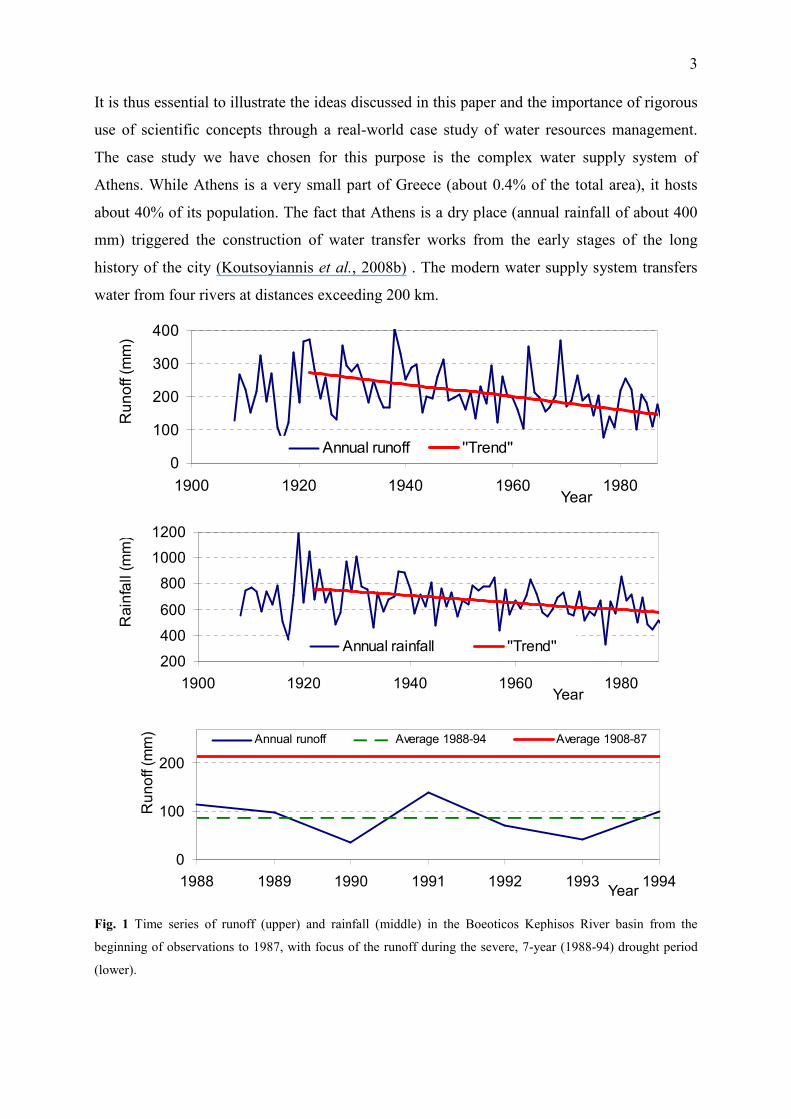
Fig. 1 Time series of runoff (upper) and rainfall (middle) in the Boeoticos Kephisos River basin from the

beginning of observations to 1987, with focus of the runoff during the severe, 7-year (1988-94) drought period

(lower).

4

Fig. 1 (upper panel) shows the evolution of the runoff of one of these rivers, the Boeoticos

Kephisos River (in units of equivalent depth over its about 2 000 km2 catchment) from the

beginning of observations to 1987. A substantial falling trend is clearly seen in the time

series. The middle panel of Fig. 1 shows the time series of rainfall in a raingauge in the basin

(Aliartos), where a trend is evident and explains (to a large extent) the trend in runoff. Most

interesting is the runoff in the following seven years, 1988-1994, shown in the last panel of

Fig. 1, which is consistently below average, thus manifesting a long-lasting and severe

drought that shocked Athens during that period. The average flow during these seven years is

only 44% of the average of the previous years. A typical interpretation of such time series

would be to claim nonstationarity, perhaps attributing it to anthropogenic global warming, etc.

However, we will present a different interpretation of the observed behavior and its

implications on water resources planning and management (section “Implications in

engineering design and water resources management”). For Athens, these implications were

particularly important even after the end of the persistent drought, because it was then

preparing for the Olympic games—and these would not be possible in water shortage

conditions. Evidently, good planning and management demand a strong theoretical basis and

the proper application of fundamental (but perhaps forgotten or abused) notions.

Visiting names: stationarity and nonstationarity

Finding invariant properties within motion and change is essential to science. Newton’s laws

are eminent examples. The first law asserts that, in the absence of an external force, the

position x of a body may change in time t but the velocity u := dx/dt is constant. The second

law is a generalization of the first for the case that a constant force F is present, whence the

velocity changes but the acceleration a = du/dt is constant and equal to F/m, where m is the

mass of the body. In turn, Newton’s law of gravitation is a further generalization, in which the

attractive force F (weight) exerted, due to gravitation, by a mass M on a body of mass m

located at a distance r is no longer constant. In this case, the quantity G = F r 2

/(m M) is

constant, whereas in the application of the law for planetary motion another constant emerges,

i.e., the angular momentum per unit mass, (dθ/dt) r 2

, where θ denotes angle.

However, whilst those laws give elegant solutions (e.g., analytical descriptions of trajectories)

for simple systems comprising two bodies and their interaction, they can hardly describe the

irregular trajectories of complex systems. Complex natural systems consisting of very many

elements are impossible to describe in full detail nor their future evolution can be predicted in

detail and with precision. Here, the great scientific achievement is the materialization of

5

macroscopic descriptions rather than modeling the details. This is essentially done using

probability theory (laws of large numbers, central limit theorem, principle of maximum

entropy). Here lies the essence and usefulness of the stationarity concept, which seeks

invariant properties in complex systems.

According to the definitions quoted from Papoulis (1991), “A stochastic process x(t) is called

strict-sense stationary … if its statistical properties are invariant to a shift of the origin” and

“… is called wide-sense stationary if its mean is constant (E[x(t)] = η) and its autocorrelation

depends only on [time difference] τ…, (E[x(t + τ) x(t)] = R(τ)]”. We can thus note that the

definition of stationarity applies to stochastic processes (rather than to time series; see also

Koutsoyiannis, 2006b). Processes that are not stationary are called nonstationary and in this

case some of their statistical properties are deterministic functions of time.

Abstract representation

Model

Ensemble: mental copies of natural system

Stochastic process

Abstract representation

Model

Ensemble: mental copies of natural system

Stochastic process

Real world

Natural system

Unique evolution

Time series

Real world

Natural system

Unique evolution

Time series

Many different models can be constructed

Mental copies depend on model constructed

Can generate arbitrar-ily many time series

Stationarity and

nonstationarity

apply here

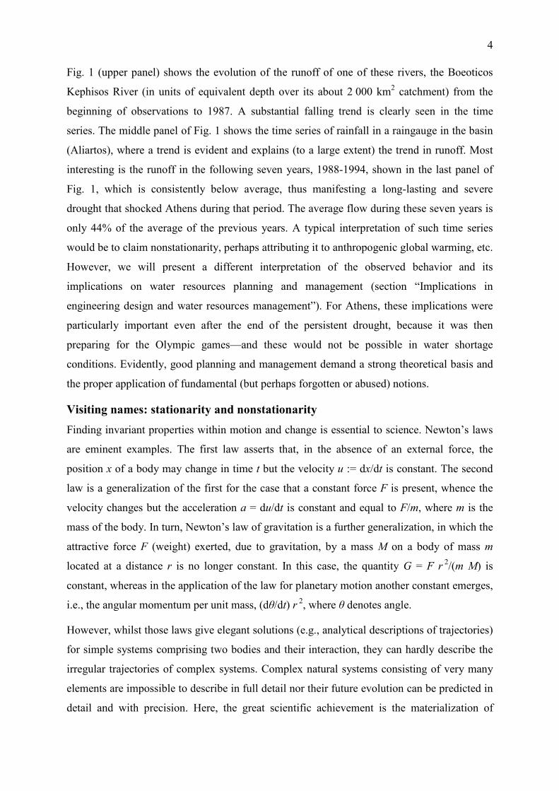
Fig. 2 Schematic for the clarification of the notions of stationarity and nonstationarity.

Fig. 2 helps us to further clarify the definition. The left part of this graphic symbolizes the real

world. Any natural system we study has a unique evolution (a unique trajectory in time), and

if we observe this evolution, we obtain a time series. The right part of the graphic symbolizes

the abstract world, the models. Of course, we can build many different models of the natural

system, any one of which can give us an ensemble, i.e., mental copies of the real-world

system. The idea of mental copies is due to Gibbs, known from statistical thermodynamics.

An ensemble can also be viewed as multiple realizations of a stochastic process, from which

we can generate synthetic time series. Clearly, the notions of stationarity and non-stationarity

6

apply here, to the abstract objects—not to the real-world objects. In this respect, profound

conclusions such as that “hydroclimatic processes are nonstationary” or “stationarity is dead”

may be pointless.

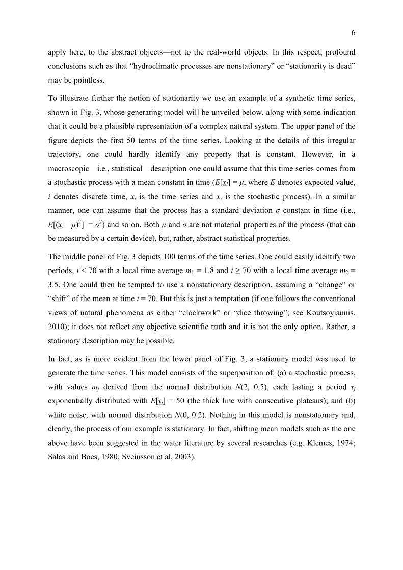
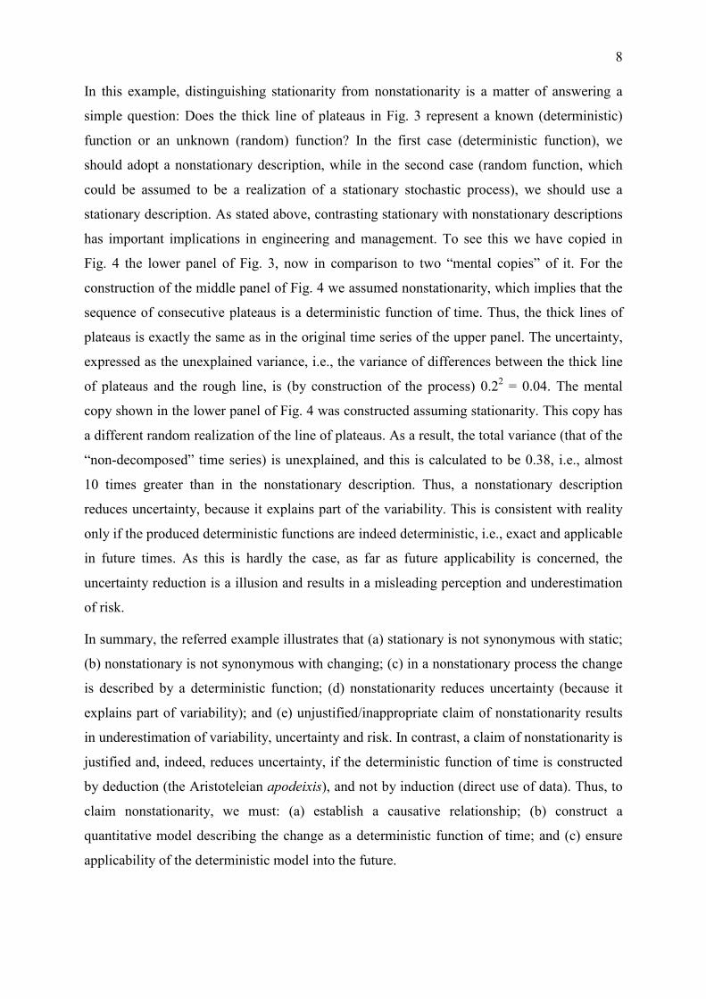
To illustrate further the notion of stationarity we use an example of a synthetic time series,

shown in Fig. 3, whose generating model will be unveiled below, along with some indication

that it could be a plausible representation of a complex natural system. The upper panel of the

figure depicts the first 50 terms of the time series. Looking at the details of this irregular

trajectory, one could hardly identify any property that is constant. However, in a

macroscopic—i.e., statistical—description one could assume that this time series comes from

a stochastic process with a mean constant in time (E[xi] = µ, where E denotes expected value,

i denotes discrete time, xi is the time series and xi is the stochastic process). In a similar

manner, one can assume that the process has a standard deviation σ constant in time (i.e.,

E[(xi – µ)2] = σ

2) and so on. Both µ and σ are not material properties of the process (that can

be measured by a certain device), but, rather, abstract statistical properties.

The middle panel of Fig. 3 depicts 100 terms of the time series. One could easily identify two

periods, i < 70 with a local time average m1 = 1.8 and i ≥ 70 with a local time average m2 =

3.5. One could then be tempted to use a nonstationary description, assuming a “change” or

“shift” of the mean at time i = 70. But this is just a temptation (if one follows the conventional

views of natural phenomena as either “clockwork” or “dice throwing”; see Koutsoyiannis,

2010); it does not reflect any objective scientific truth and it is not the only option. Rather, a

stationary description may be possible.

In fact, as is more evident from the lower panel of Fig. 3, a stationary model was used to

generate the time series. This model consists of the superposition of: (a) a stochastic process,

with values mj derived from the normal distribution N(2, 0.5), each lasting a period τj

exponentially distributed with E[τj] = 50 (the thick line with consecutive plateaus); and (b)

white noise, with normal distribution N(0, 0.2). Nothing in this model is nonstationary and,

clearly, the process of our example is stationary. In fact, shifting mean models such as the one

above have been suggested in the water literature by several researches (e.g. Klemes, 1974;

Salas and Boes, 1980; Sveinsson et al, 2003).

7

1

1.5

2

2.5

0 10 20 30 40 50

Time, i

Time series

Local average

0

0.5

1

1.5

2

2.5

3

3.5

4

4.5

0 10 20 30 40 50 60 70 80 90 100

Time, i

Time series

Local average

0

0.5

1

1.5

2

2.5

3

3.5

4

4.5

0 100 200 300 400 500 600 700 800 900 1000

Time, i

Time series

Local average

Fig. 3 A synthetic time series for the clarification of the notions of stationarity and nonstationarity (see text);

(upper) the first 50 terms; (middle) the first 100 terms; (lower) 1000 terms.

8

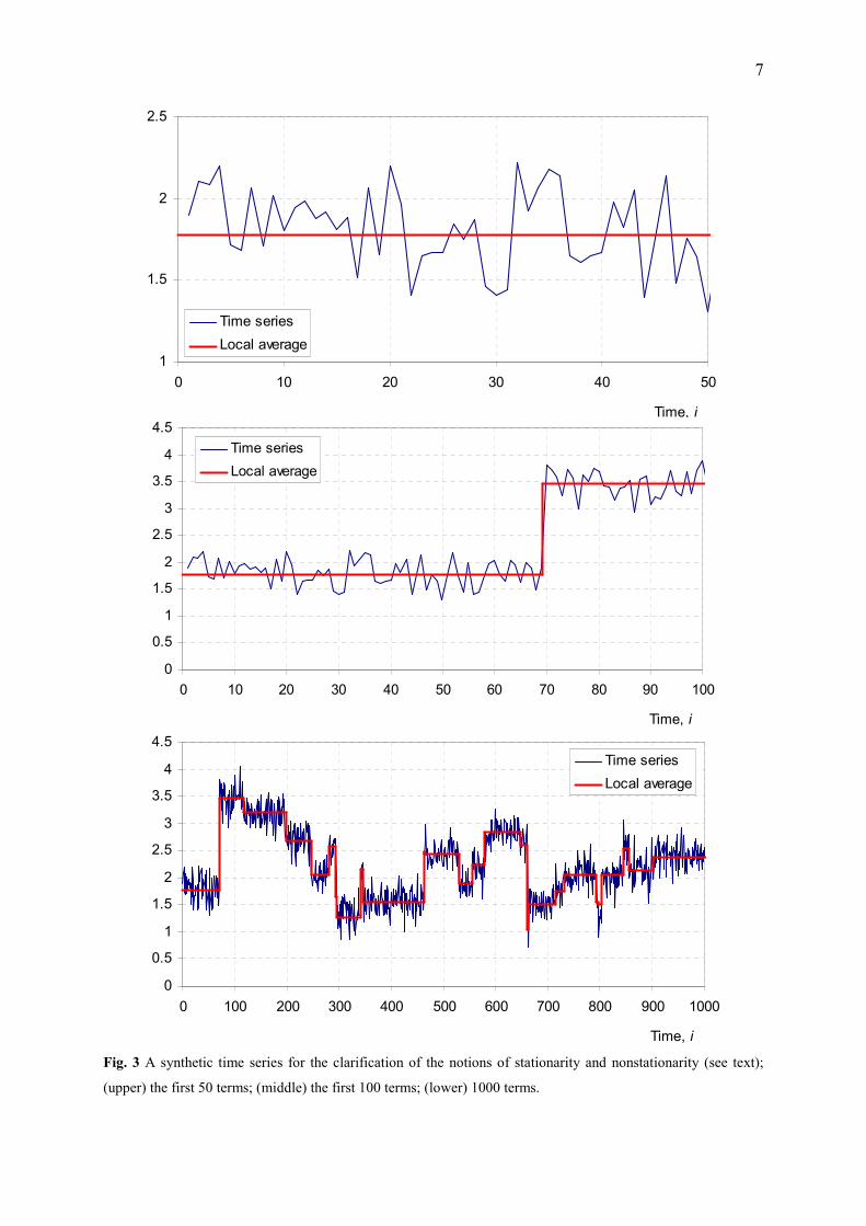
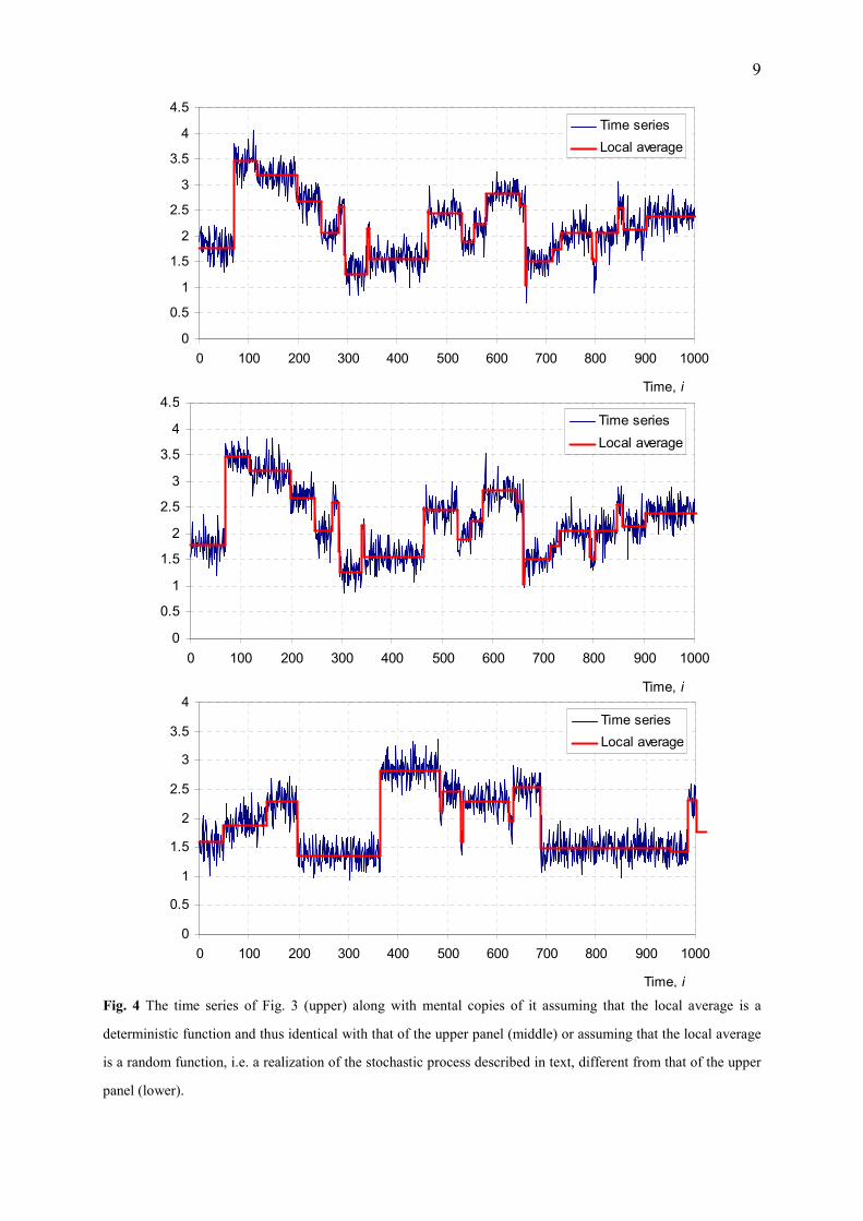
In this example, distinguishing stationarity from nonstationarity is a matter of answering a

simple question: Does the thick line of plateaus in Fig. 3 represent a known (deterministic)

function or an unknown (random) function? In the first case (deterministic function), we

should adopt a nonstationary description, while in the second case (random function, which

could be assumed to be a realization of a stationary stochastic process), we should use a

stationary description. As stated above, contrasting stationary with nonstationary descriptions

has important implications in engineering and management. To see this we have copied in

Fig. 4 the lower panel of Fig. 3, now in comparison to two “mental copies” of it. For the

construction of the middle panel of Fig. 4 we assumed nonstationarity, which implies that the

sequence of consecutive plateaus is a deterministic function of time. Thus, the thick lines of

plateaus is exactly the same as in the original time series of the upper panel. The uncertainty,

expressed as the unexplained variance, i.e., the variance of differences between the thick line

of plateaus and the rough line, is (by construction of the process) 0.22 = 0.04. The mental

copy shown in the lower panel of Fig. 4 was constructed assuming stationarity. This copy has

a different random realization of the line of plateaus. As a result, the total variance (that of the

“non-decomposed” time series) is unexplained, and this is calculated to be 0.38, i.e., almost

10 times greater than in the nonstationary description. Thus, a nonstationary description

reduces uncertainty, because it explains part of the variability. This is consistent with reality

only if the produced deterministic functions are indeed deterministic, i.e., exact and applicable

in future times. As this is hardly the case, as far as future applicability is concerned, the

uncertainty reduction is a illusion and results in a misleading perception and underestimation

of risk.

In summary, the referred example illustrates that (a) stationary is not synonymous with static;

(b) nonstationary is not synonymous with changing; (c) in a nonstationary process the change

is described by a deterministic function; (d) nonstationarity reduces uncertainty (because it

explains part of variability); and (e) unjustified/inappropriate claim of nonstationarity results

in underestimation of variability, uncertainty and risk. In contrast, a claim of nonstationarity is

justified and, indeed, reduces uncertainty, if the deterministic function of time is constructed

by deduction (the Aristoteleian apodeixis), and not by induction (direct use of data). Thus, to

claim nonstationarity, we must: (a) establish a causative relationship; (b) construct a

quantitative model describing the change as a deterministic function of time; and (c) ensure

applicability of the deterministic model into the future.

9

0

0.5

1

1.5

2

2.5

3

3.5

4

4.5

0 100 200 300 400 500 600 700 800 900 1000

Time, i

Time series

Local average

0

0.5

1

1.5

2

2.5

3

3.5

4

4.5

0 100 200 300 400 500 600 700 800 900 1000

Time, i

Time series

Local average

0

0.5

1

1.5

2

2.5

3

3.5

4

0 100 200 300 400 500 600 700 800 900 1000

Time, i

Time series

Local average

Fig. 4 The time series of Fig. 3 (upper) along with mental copies of it assuming that the local average is a

deterministic function and thus identical with that of the upper panel (middle) or assuming that the local average

is a random function, i.e. a realization of the stochastic process described in text, different from that of the upper

panel (lower).

10

Because the inflationary use of the term “nonstationarity” in hydrology has recently been

closely related to “climate change”, it is useful to examine whether the terms justifying a

nonstationary description of climate hold true or not. The central question is: Do climate

models (also known as general circulation models—GCMs) enable a nonstationary approach?

More specific versions of this question are: Do GCMs provide credible deterministic

predictions of future climate evolution? Do GCMs provide good predictions for temperature

and somewhat less good for precipitation (as often thought)? Do GCMs provide good

predictions at global and continental scales and, after downscaling, at local scales? Do GCMs

provide good predictions for the distant future (albeit less good for the nearer future, e.g., for

the next 10-20 years—or for the next season or year)? In the author’s opinion, the answers to

all these questions should be categorically negative. Not only are GCMs unable to provide

credible climatic predictions for the future, but they also fail to reproduce the known past and

even the past statistical characteristics of climate (see Koutsoyiannis et al., 2008a;

Anagnostopoulos et al., 2010). An additional, very relevant question is: Is climate predictable

in deterministic terms? Again, the author’s answer is negative (Koutsoyiannis, 2006a; 2010).

Only stochastic climatic predictions could be scientifically meaningful. In principle, these

could also include nonstationary descriptions wherever causative relationships of climate with

its forcings are established. But until such a stochastic theory of climate, which includes

nonstationary components, could be shaped, there is room for developing a stationary theory

that characterizes future uncertainty as faithfully as possible; the main characteristics of such

a theory are outlined in section “Change under stationarity and the Hurst-Kolmogorov

dynamics” (see also Koutsoyiannis et al., 2007).

While a nonstationary description of climate is difficult to establish or possibly even

infeasible, in cases related to water resources it may be much more meaningful. For example,

in modeling streamflow downstream of a dam, we would use a nonstationary model with a

shift in the statistical characteristics before and after the construction of the dam. Gradual

changes in the flow regime, e.g., due to urbanization that evolves in time, could also justify a

nonstationary description, provided that solid information or knowledge (as opposed to

ignorance) of the agents affecting a hydrological process is available. Even in such cases, as

far as modeling of future conditions is concerned, a stationary model of the future is sought

most frequently. A procedure that could be called “stationarization” is then necessary to adapt

the past observations to future conditions. For example, the flow data prior to the construction

of the dam could be properly adapted, by deterministic modeling, so as to determine what the

11

flow would be if the dam existed. Also, the flow data at a certain phase of urbanization could

be adapted so as to represent the future conditions of urbanization. Such adaptations enable

the building of a stationary model of the future.

Change under stationarity and the Hurst-Kolmogorov dynamics

It was asserted earlier that nonstationarity is not synonymous with change. Even in the

simplest stationary process, the white noise, there is change all the time. But, as this case is

characterized by independence in time, the change is only short-term. There is no change in

long-term time averages. However, a process with dependence in time exhibits longer-term

changes. Thus, change is tightly linked to dependence and long-term change to long-range

dependence. Hence, stochastic concepts that have been devised to study dependence also help

us to study change.

0

0.2

0.4

0.6

0.8

1

0 10 20 30 40 50 60 70 80 90 100

Lag

Auto

corr

ela

tion

Empirical

Markov

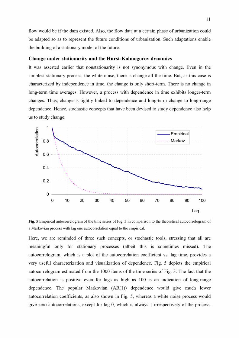
Fig. 5 Empirical autocorrelogram of the time series of Fig. 3 in comparison to the theoretical autocorrelogram of

a Markovian process with lag one autocorrelation equal to the empirical.

Here, we are reminded of three such concepts, or stochastic tools, stressing that all are

meaningful only for stationary processes (albeit this is sometimes missed). The

autocorrelogram, which is a plot of the autocorrelation coefficient vs. lag time, provides a

very useful characterization and visualization of dependence. Fig. 5 depicts the empirical

autocorrelogram estimated from the 1000 items of the time series of Fig. 3. The fact that the

autocorrelation is positive even for lags as high as 100 is an indication of long-range

dependence. The popular Markovian (AR(1)) dependence would give much lower

autocorrelation coefficients, as also shown in Fig. 5, whereas a white noise process would

give zero autocorrelations, except for lag 0, which is always 1 irrespectively of the process.

12

We recall that the process in our example involves no “memory” mechanism; it just involves

change in two characteristic scales, 1 (the white noise components) and 50 (the average length

of the plateaus). Thus, interpretation of long-range dependence as “long memory”, despite

being very common (e.g. Beran, 1994), may be misleading; it is more insightful to interpret

long-range dependence as long-term change. This has been first pointed out—or implied—by

Klemes, 1974, who wrote “… the Hurst phenomenon is not necessarily an indicator of infinite

memory of a process”. The term “memory” should better refer to systems transforming inputs

to outputs (cf. the definition of memoryless systems in Papoulis, 1991), rather than to a single

stochastic process.

Slope = -1

0.001

0.01

0.1

1

10

100

0.001 0.01 0.1 1

Frequency

Spectr

al density

Empirical

Power law approximation

Fig. 6 Empirical power spectrum of the time series of Fig. 3.

The power spectrum, which is the inverse finite Fourier transform of the autocorrelogram, is

another stochastic tool for the characterization of change with respect to frequency. The

power spectrum of our example is shown in Fig. 6, where a rough line appears, which has an

overall slope of about –1. This negative slope, which indicates the importance of variation at

lower frequencies relative to the higher ones, provides a hint of long-range dependence.

However, the high roughness and scattering of the power spectrum does not allow accurate

estimations. A better depiction is provided in Fig. 7 by the climacogram (from the Greek

climax, i.e., scale), which provides a multi-scale stochastic characterization of the process.

Based on the process xi at scale 1, we define a process xi(k)

at any scale k ≥ 1 as:

13

∑+−=

=ik

kil

l

k

i xk

x1)1(

)( 1: (1)

A key multi-scale characteristic is the standard deviation σ(k)

of xi(k)

. The climacogram is a

plot (typically double logarithmic) of σ(k)

as a function of the scale k ≥ 1. While the power

spectrum and the autocorrelogram are related to each other through a Fourier transform, the

climacogram is related to the autocorrelogram by a simpler transformation, i.e.,

kk

kα

σσ =)( , ∑

−

=

−+=

1

1

121k

j

jkk

jρα ↔ 11

2

1

2

1−+

−+−

+= jjjj

jj

jαααρ (2)

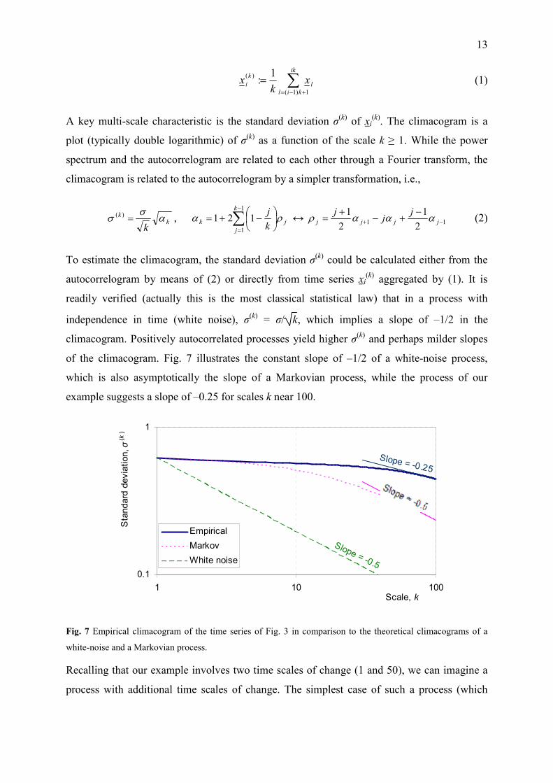
To estimate the climacogram, the standard deviation σ(k)

could be calculated either from the

autocorrelogram by means of (2) or directly from time series xi(k)

aggregated by (1). It is

readily verified (actually this is the most classical statistical law) that in a process with

independence in time (white noise), σ(k)

= σ/ k, which implies a slope of –1/2 in the

climacogram. Positively autocorrelated processes yield higher σ(k)

and perhaps milder slopes

of the climacogram. Fig. 7 illustrates the constant slope of –1/2 of a white-noise process,

which is also asymptotically the slope of a Markovian process, while the process of our

example suggests a slope of –0.25 for scales k near 100.

Slope = -0.5

Slope = -0.25

0.1

1

1 10 100Scale, k

Sta

ndard

devia

tion, σ

(k)

Empirical

Markov

White noise

Fig. 7 Empirical climacogram of the time series of Fig. 3 in comparison to the theoretical climacograms of a

white-noise and a Markovian process.

Recalling that our example involves two time scales of change (1 and 50), we can imagine a

process with additional time scales of change. The simplest case of such a process (which

14

assumes theoretically infinite time scales of fluctuation, although practically, three such scales

suffice; Koutsoyiannis, 2002), is the one whose climacogram has a constant slope H – 1, i.e.

σ(k)

= k H – 1

σ (3)

This simple process, which is essentially defined by (3), has been termed the Hurst-

Kolmogorov (HK) process (after Hurst, 1951, who first analyzed statistically the long-term

behavior of geophysical time series, and Kolmogorov, 1940, who, in studying turbulence, had

proposed the mathematical form of the process), and is also known as simple scaling

stochastic model or fractional Gaussian noise (cf. Mandelbrot and Wallis, 1968). The constant

H is called the Hurst coefficient and in positively-dependent processes ranges between 0.5

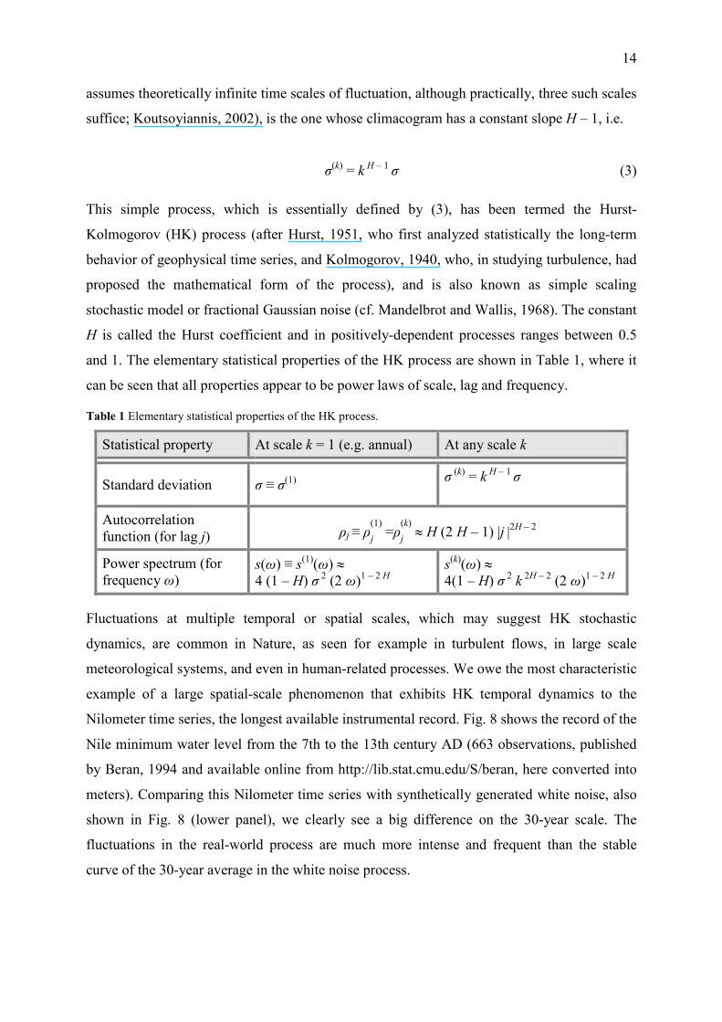
and 1. The elementary statistical properties of the HK process are shown in Table 1, where it

can be seen that all properties appear to be power laws of scale, lag and frequency.

Table 1 Elementary statistical properties of the HK process.

Statistical property At scale k = 1 (e.g. annual) At any scale k

Standard deviation σ ≡ σ(1)

σ

(k) = k

H – 1 σ

Autocorrelation

function (for lag j) ρj ≡ ρ(1)

j =ρ(k)

j ≈ H (2 H – 1) |j

|2H – 2

Power spectrum (for

frequency ω) s(ω) ≡ s

(1)(ω) ≈

4 (1 – H) σ 2

(2 ω)1 – 2 H

s(k)

(ω) ≈

4(1 – H) σ 2

k 2H – 2

(2 ω)1 – 2 H

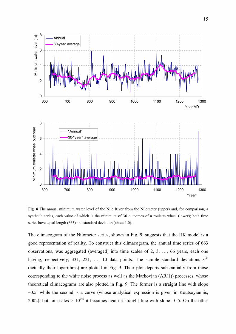
Fluctuations at multiple temporal or spatial scales, which may suggest HK stochastic

dynamics, are common in Nature, as seen for example in turbulent flows, in large scale

meteorological systems, and even in human-related processes. We owe the most characteristic

example of a large spatial-scale phenomenon that exhibits HK temporal dynamics to the

Nilometer time series, the longest available instrumental record. Fig. 8 shows the record of the

Nile minimum water level from the 7th to the 13th century AD (663 observations, published

by Beran, 1994 and available online from http://lib.stat.cmu.edu/S/beran, here converted into

meters). Comparing this Nilometer time series with synthetically generated white noise, also

shown in Fig. 8 (lower panel), we clearly see a big difference on the 30-year scale. The

fluctuations in the real-world process are much more intense and frequent than the stable

curve of the 30-year average in the white noise process.

15

0

2

4

6

8

600 700 800 900 1000 1100 1200 1300

Year AD

Min

imum

wate

r le

vel (m

)Annual

30-year average

0

2

4

6

8

600 700 800 900 1000 1100 1200 1300

"Year"

Min

imum

roule

tte w

heel outc

om

e

"Annual"

30-"year" average

Fig. 8 The annual minimum water level of the Nile River from the Nilometer (upper) and, for comparison, a

synthetic series, each value of which is the minimum of 36 outcomes of a roulette wheel (lower); both time

series have equal length (663) and standard deviation (about 1.0).

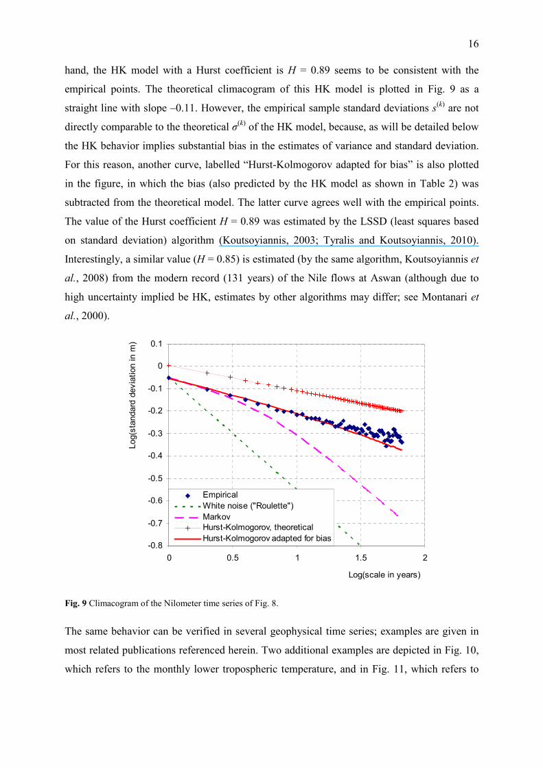
The climacogram of the Nilometer series, shown in Fig. 9, suggests that the HK model is a

good representation of reality. To construct this climacogram, the annual time series of 663

observations, was aggregated (averaged) into time scales of 2, 3, …, 66 years, each one

having, respectively, 331, 221, …, 10 data points. The sample standard deviations s(k)

(actually their logarithms) are plotted in Fig. 9. Their plot departs substantially from those

corresponding to the white noise process as well as the Markovian (AR(1)) processes, whose

theoretical climacograms are also plotted in Fig. 9. The former is a straight line with slope

–0.5 while the second is a curve (whose analytical expression is given in Koutsoyiannis,

2002), but for scales > 100.5

it becomes again a straight line with slope –0.5. On the other

16

hand, the HK model with a Hurst coefficient is H = 0.89 seems to be consistent with the

empirical points. The theoretical climacogram of this HK model is plotted in Fig. 9 as a

straight line with slope –0.11. However, the empirical sample standard deviations s(k)

are not

directly comparable to the theoretical σ(k)

of the HK model, because, as will be detailed below

the HK behavior implies substantial bias in the estimates of variance and standard deviation.

For this reason, another curve, labelled “Hurst-Kolmogorov adapted for bias” is also plotted

in the figure, in which the bias (also predicted by the HK model as shown in Table 2) was

subtracted from the theoretical model. The latter curve agrees well with the empirical points.

The value of the Hurst coefficient H = 0.89 was estimated by the LSSD (least squares based

on standard deviation) algorithm (Koutsoyiannis, 2003; Tyralis and Koutsoyiannis, 2010).

Interestingly, a similar value (H = 0.85) is estimated (by the same algorithm, Koutsoyiannis et

al., 2008) from the modern record (131 years) of the Nile flows at Aswan (although due to

high uncertainty implied be HK, estimates by other algorithms may differ; see Montanari et

al., 2000).

-0.8

-0.7

-0.6

-0.5

-0.4

-0.3

-0.2

-0.1

0

0.1

0 0.5 1 1.5 2

Log(scale in years)

Log(s

tandard

devia

tion in m

)

Empirical

White noise ("Roulette")

Markov

Hurst-Kolmogorov, theoretical

Hurst-Kolmogorov adapted for bias

Fig. 9 Climacogram of the Nilometer time series of Fig. 8.

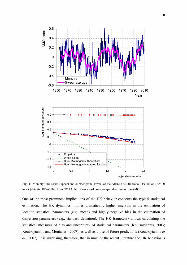
The same behavior can be verified in several geophysical time series; examples are given in

most related publications referenced herein. Two additional examples are depicted in Fig. 10,

which refers to the monthly lower tropospheric temperature, and in Fig. 11, which refers to

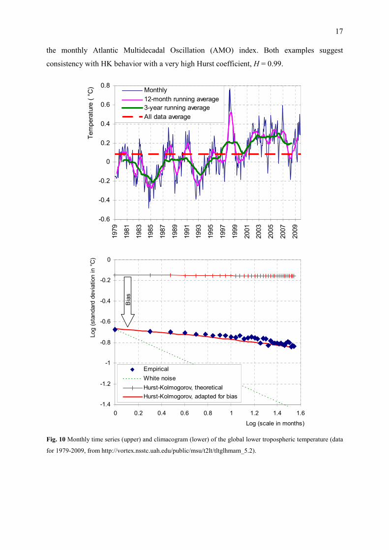
17

the monthly Atlantic Multidecadal Oscillation (AMO) index. Both examples suggest

consistency with HK behavior with a very high Hurst coefficient, H = 0.99.

-0.6

-0.4

-0.2

0

0.2

0.4

0.6

0.8

1979

1981

1983

1985

1987

1989

1991

1993

1995

1997

1999

2001

2003

2005

2007

2009

Tem

pera

ture

( °

C) Monthly

12-month running average

3-year running average

All data average

-1.4

-1.2

-1

-0.8

-0.6

-0.4

-0.2

0

0 0.2 0.4 0.6 0.8 1 1.2 1.4 1.6

Log (scale in months)

Log (

sta

ndard

devia

tion in °

C)

Empirical

White noise

Hurst-Kolmogorov, theoretical

Hurst-Kolmogorov, adapted for bias

Bia

s

Fig. 10 Monthly time series (upper) and climacogram (lower) of the global lower tropospheric temperature (data

for 1979-2009, from http://vortex.nsstc.uah.edu/public/msu/t2lt/tltglhmam_5.2).

18

-0.6

-0.4

-0.2

0

0.2

0.4

0.6

1850 1870 1890 1910 1930 1950 1970 1990 2010

Year

AM

O index

Monthly5-year average

-1.6

-1.4

-1.2

-1

-0.8

-0.6

-0.4

-0.2

0

0 0.5 1 1.5 2 2.5

Log(scale in months)

Log(S

tandard

devia

tion)

Empirical

White noiseHurst-Kolmogorov, theoretical

Hurst-Kolmogorov adapted for bias

Fig. 11 Monthly time series (upper) and climacogram (lower) of the Atlantic Multidecadal Oscillation (AMO)

index (data for 1856-2009, from NOAA, http://www.esrl.noaa.gov/psd/data/timeseries/AMO/).

One of the most prominent implications of the HK behavior concerns the typical statistical

estimation. The HK dynamics implies dramatically higher intervals in the estimation of

location statistical parameters (e.g., mean) and highly negative bias in the estimation of

dispersion parameters (e.g., standard deviation). The HK framework allows calculating the

statistical measures of bias and uncertainty of statistical parameters (Koutsoyiannis, 2003;

Koutsoyiannis and Montanari, 2007), as well as those of future predictions (Koutsoyiannis et

al., 2007). It is surprising, therefore, that in most of the recent literature the HK behavior is

19

totally neglected, despite the fact that books such as those by Salas et al. (1980), Bras and

Rodriguez-Iturbe (1985), and Hipel and McLeod (1994) have devoted a significant attention

to the Hurst findings and methods to account for it. Even studies recognizing the presence of

HK dynamics usually do not account for the implications in statistical estimation and testing.

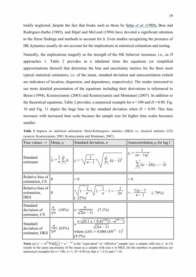
Naturally, the implications magnify as the strength of the HK behavior increases, i.e., as H

approaches 1. Table 2 provides in a tabulated form the equations (or simplified

approximations thereof) that determine the bias and uncertainty metrics for the three most

typical statistical estimators, i.e. of the mean, standard deviation and autocorrelation (which

are indicators of location, dispersion, and dependence, respectively). The reader interested to

see more detailed presentation of the equations including their derivations is referenced to

Beran (1994), Koutsoyiannis (2003) and Koutsoyiannis and Montanari (2007). In addition to

the theoretical equations, Table 2 provides, a numerical example for n =

100 and H = 0.90. Fig.

10 and Fig. 11 depict the huge bias in the standard deviation when H = 0.99. This bias

increases with increased time scale because the sample size for higher time scales becomes

smaller.

Table 2 Impacts on statistical estimation: Hurst-Kolmogorov statistics (HKS) vs. classical statistics (CS)

(sources: Koutsoyiannis, 2003; Koutsoyiannis and Montanari, 2007).

True values → Mean, µ Standard deviation, σ Autocorrelation ρl for lag l

Standard

estimator x– :=

1

n ∑i = 1

n

xi s := 1

n – 1 ∑

i = 1

n

(xi – x–)2

rl := 1

(n – 1)s2 ·

∑i = 1

n – l

(xi – x–)(xi + l – x

–)

Relative bias of

estimation, CS 0 ≈ 0 ≈ 0

Relative bias of

estimation,

HKS

0 1 − 1

n΄/ 1 −

1

n − 1 ≈ −

1

2n΄

(–22%)

≈ – 1/ρl − 1

n΄− 1 (–79%)

Standard

deviation of

estimator, CS

σ

n (10%) ≈

σ

2(n – 1) (7.1%)

Standard

deviation of

estimator, HKS

σ

n΄ (63%)

≈ σ (0.1 n + 0.8)

λ(H)(1 –n

2H − 2)

2(n – 1)

where λ(H) := 0.088 (4H 2

– 1)

2

(9.3%)

Notes (a) n΄ := σ2/Var[x

–] = n

2 – 2H is the “equivalent” or “effective” sample size: a sample with size n΄ in CS

results in the same uncertainty of the mean as a sample with size n in HKS; (b) the numbers in parentheses are

numerical examples for n =

100, σ = 1, H = 0.90 (so that n΄

= 2.5) and l = 10.

20

Implications in engineering design and water resources management

Coming back to the Athens water supply system, it is interesting to estimate the return period

of the multi-year drought mentioned in the Introduction. Let us first assume that the annual

runoff in the Boeoticos Kephisos basin can be approximated by a Gaussian distribution (this

is fairly justified given that the coefficient of skewness is 0.35 at the annual scale and drops to

zero or below at the 3-year scale and beyond) and that the multi-year standard deviation σ(k)

at

scale (number of consecutive years) k is given by the classical statistical law, σ(k)

= σ/ k,

which assumes independence in time. We can then easily assign a theoretical return period to

the lowest (as well as to the highest) recorded value for each time scale. More specifically, the

theoretical return period of the lowest observed value xL(k)

, for each time scale k, can be

determined as TL = k δ / F(xL

(k)), where δ = 1 year and F denotes the probability distribution

function. The latter is Gaussian with mean µ (independent of scale, estimated as the sample

average x– at the annual scale) and standard deviation σ(k)

(for scale k, determined as σ/ k,

with σ estimated as the sample standard deviation s at the annual scale). Likewise, for the

highest value xH(k)

the theoretical return period is TH = k δ / (1 – F(xH

(k)).

1

10

100

1000

10000

100000

0 2 4 6 8 10

Scale, k

Retu

rn p

eriod (

years

)

Loewest value, classical

Highest value, classical

Lowest value, HK

Highest value, HK

Emprirically expected

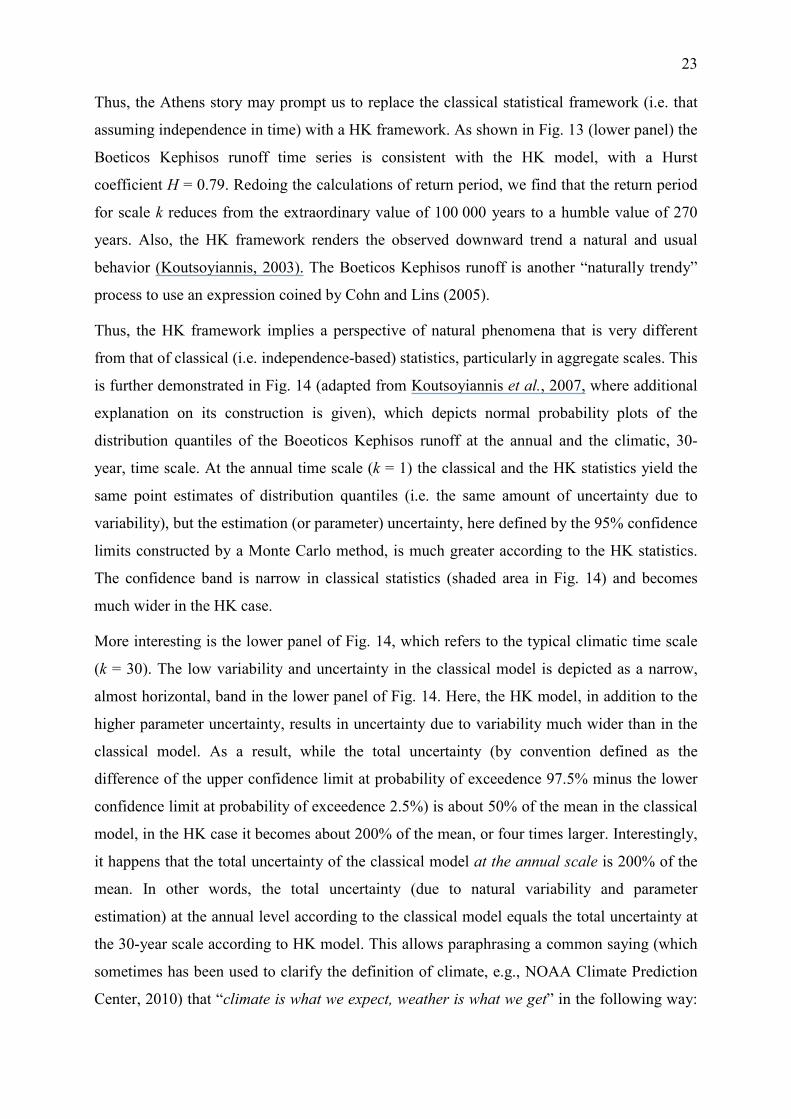
Fig. 12 Return periods of the lowest and highest observed annual runoff, over time scale (or number of

consecutive years) k = 1 (annual scale) to 10 (decadal scale), of the Boeoticos Kephisos basin assuming normal

distribution (adapted from Koutsoyiannis et al., 2007).

21

Fig. 12 shows the assigned return periods of the lowest and highest values for time scales

(number of consecutive years) k = 1 to 10. Empirically, since the record length is about 100

years, we expect that the return period of lowest and highest values would be of the order of

100 years for all time scales. This turns out to be true for k = 1 to 2, but the return periods

reach 10 000 years at scale k = 5. Furthermore, the theoretical return period of the lowest

value at scale k = 10 (10-year-long drought) reaches 100 000 years!

0

100

200

300

400

1900 1920 1940 1960 1980 2000Year

Runoff

(m

m)

Annual 30-year average1907-2002 average

1.5

1.6

1.7

1.8

1.9

0 0.2 0.4 0.6 0.8 1

Log(scale in years)

Log(s

tandard

devia

tion in m

m)

Empirical

Classical statistics

Hurst-Kolmogorov, theoretical

Hurst-Kolmogorov, adapted for bias

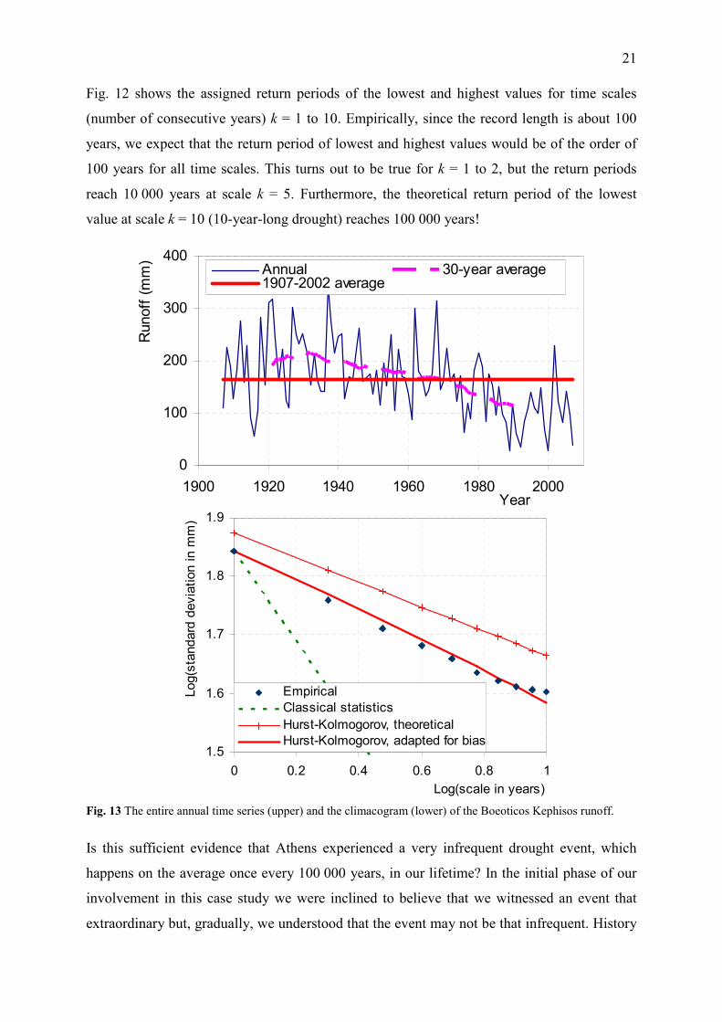
Fig. 13 The entire annual time series (upper) and the climacogram (lower) of the Boeoticos Kephisos runoff.

Is this sufficient evidence that Athens experienced a very infrequent drought event, which

happens on the average once every 100 000 years, in our lifetime? In the initial phase of our

involvement in this case study we were inclined to believe that we witnessed an event that

extraordinary but, gradually, we understood that the event may not be that infrequent. History

22

is the key to the past, to the present, and to the future; and the longest available historical

record is that of the Nilometer (Fig. 8). This record offers a precious empirical basis of long-

term changes. It suffices to compare the time series of the Beoticos Kephisos runoff (shown in

its entirety in Fig. 13) with that of the Nilometer series. We observe that a similar pattern had

appeared in the Nile flow between 680 and 780 AD: a 100-year falling trend (which, notably,

reverses after 780 AD), with a clustering of very low water level around the end of this

period, between 760 and 780 AD. Such clustering of similar events was observed in several

geophysical time series by Hurst (1951), who stated: “Although in random events groups of

high or low values do occur, their tendency to occur in natural events is greater. This is the

main difference between natural and random events.”

0.990.950.80.50.20.050.01

0

100

200

300

400

500

-3 -2 -1 0 1 2 3

Reduced normal variate

Dis

trib

utio

n q

uantil

e (

mm

)

PE/classicalMCCL/classicalPE/HKMCCL/HK

0.990.950.80.50.20.050.01

0

100

200

300

400

500

-3 -2 -1 0 1 2 3

Reduced normal variate

Dis

trib

utio

n q

uantil

e (

mm

)

PE/classicalMCCL/classicalPE/HKMCCL/HK

0.01 0.05 0.2 0.5 0.8 0.95 0.99

0

100

200

300

400

500

Dis

trib

utio

n q

uantil

e (

mm

)

PEMCCL/classicalMCCL/HK

Probability of nonexceedence

0.01 0.05 0.2 0.5 0.8 0.95 0.99

0

100

200

300

400

500

Dis

trib

utio

n q

uantil

e (

mm

)

PEMCCL/classicalMCCL/HK

Probability of nonexceedence

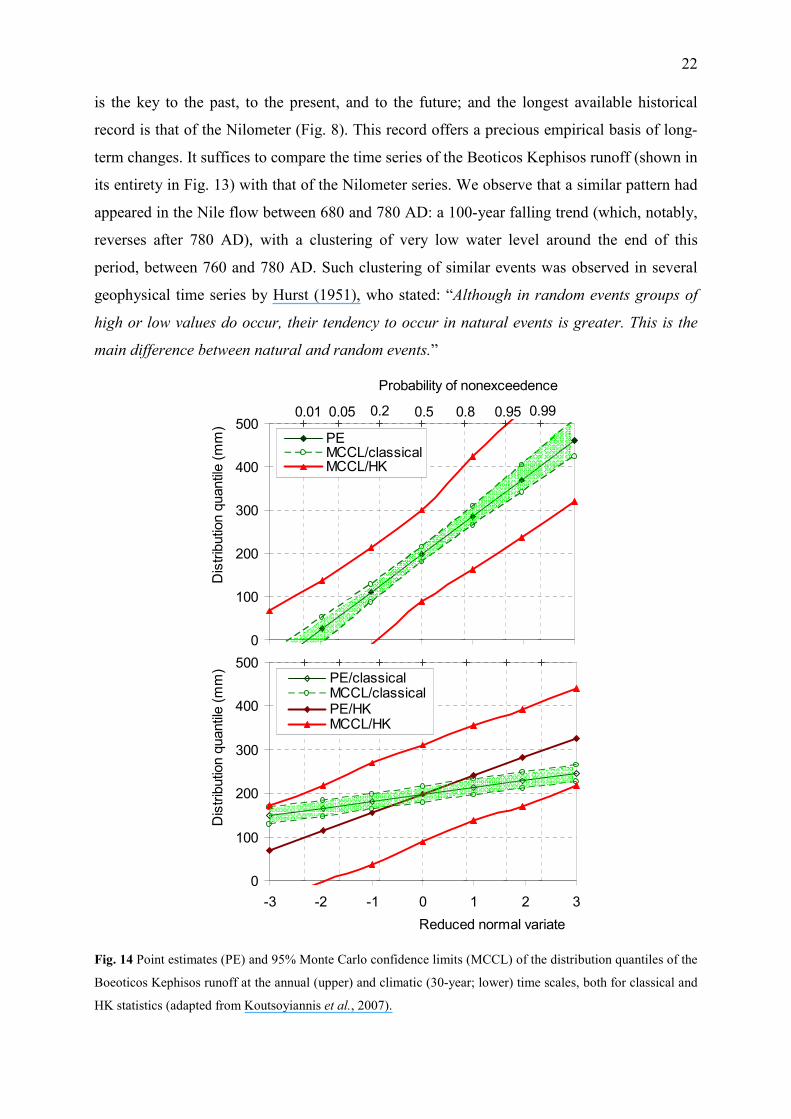
Fig. 14 Point estimates (PE) and 95% Monte Carlo confidence limits (MCCL) of the distribution quantiles of the

Boeoticos Kephisos runoff at the annual (upper) and climatic (30-year; lower) time scales, both for classical and

HK statistics (adapted from Koutsoyiannis et al., 2007).

23

Thus, the Athens story may prompt us to replace the classical statistical framework (i.e. that

assuming independence in time) with a HK framework. As shown in Fig. 13 (lower panel) the

Boeticos Kephisos runoff time series is consistent with the HK model, with a Hurst

coefficient H = 0.79. Redoing the calculations of return period, we find that the return period

for scale k reduces from the extraordinary value of 100 000 years to a humble value of 270

years. Also, the HK framework renders the observed downward trend a natural and usual

behavior (Koutsoyiannis, 2003). The Boeticos Kephisos runoff is another “naturally trendy”

process to use an expression coined by Cohn and Lins (2005).

Thus, the HK framework implies a perspective of natural phenomena that is very different

from that of classical (i.e. independence-based) statistics, particularly in aggregate scales. This

is further demonstrated in Fig. 14 (adapted from Koutsoyiannis et al., 2007, where additional

explanation on its construction is given), which depicts normal probability plots of the

distribution quantiles of the Boeoticos Kephisos runoff at the annual and the climatic, 30-

year, time scale. At the annual time scale (k = 1) the classical and the HK statistics yield the

same point estimates of distribution quantiles (i.e. the same amount of uncertainty due to

variability), but the estimation (or parameter) uncertainty, here defined by the 95% confidence

limits constructed by a Monte Carlo method, is much greater according to the HK statistics.

The confidence band is narrow in classical statistics (shaded area in Fig. 14) and becomes

much wider in the HK case.

More interesting is the lower panel of Fig. 14, which refers to the typical climatic time scale

(k = 30). The low variability and uncertainty in the classical model is depicted as a narrow,

almost horizontal, band in the lower panel of Fig. 14. Here, the HK model, in addition to the

higher parameter uncertainty, results in uncertainty due to variability much wider than in the

classical model. As a result, while the total uncertainty (by convention defined as the

difference of the upper confidence limit at probability of exceedence 97.5% minus the lower

confidence limit at probability of exceedence 2.5%) is about 50% of the mean in the classical

model, in the HK case it becomes about 200% of the mean, or four times larger. Interestingly,

it happens that the total uncertainty of the classical model at the annual scale is 200% of the

mean. In other words, the total uncertainty (due to natural variability and parameter

estimation) at the annual level according to the classical model equals the total uncertainty at

the 30-year scale according to HK model. This allows paraphrasing a common saying (which

sometimes has been used to clarify the definition of climate, e.g., NOAA Climate Prediction

Center, 2010) that “climate is what we expect, weather is what we get” in the following way:

24

“weather is what we get immediately, climate is what we get if you keep expecting for a long

time”.

For reasons that should be obvious from the above discussion, the current planning and

management of the Athens water supply system are based on the HK framework. Appropriate

multivariate stochastic simulation methods have been developed (Koutsoyiannis, 2000, 2001)

that are implemented within a general methodological framework termed parameterization-

simulation-optimization (Nalbantis and Koutsoyiannis, 1997; Koutsoyiannis and Economou,

2003; Koutsoyiannis et al., 2002, 2003; Efstratiadis et al., 2004). The whole framework

assumes stationarity, but simulations always use the current initial conditions (in particular,

the current reservoir storages) and the recorded past conditions:, in a Markovian framework,

only the latest observations affect the future probabilities, but in the HK framework the entire

record of past observations should be taken into account to condition the simulations of future

(Koutsoyiannis, 2000).

Nonetheless, it is interesting to discuss two alternative methods that are more commonly used

than the methodology developed for Athens. The first alternative approach, which is

nonstationary, consists of the projection of the observed “trend” into the future. As shown in

Fig. 15, according to this approach the flow would disappear by 2050. Also, this approach

would lead to reduced uncertainty (because it assumes that the observed “trend” explains part

of variability); the initial standard deviation of 70 mm would decrease to 55 mm. Both these

implications are glaringly absurd.

0

100

200

300

400

1900 1950 2000 2050Year

Ru

no

ff (

mm

)

Before time of modelling

After time of modelling

Trend

Fig. 15 Illustration of the alternative method of trend projection into the future for modeling of the Boeoticos

Kephisos runoff.

25

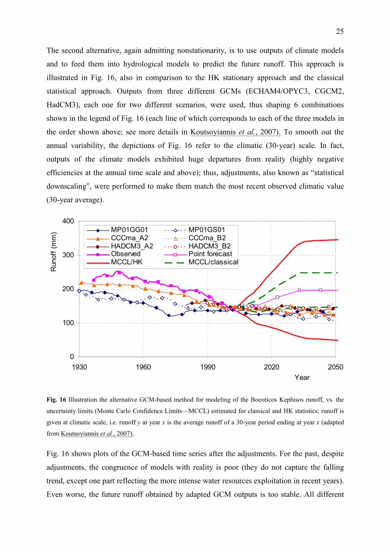
The second alternative, again admitting nonstationarity, is to use outputs of climate models

and to feed them into hydrological models to predict the future runoff. This approach is

illustrated in Fig. 16, also in comparison to the HK stationary approach and the classical

statistical approach. Outputs from three different GCMs (ECHAM4/OPYC3, CGCM2,

HadCM3), each one for two different scenarios, were used, thus shaping 6 combinations

shown in the legend of Fig. 16 (each line of which corresponds to each of the three models in

the order shown above; see more details in Koutsoyiannis et al., 2007). To smooth out the

annual variability, the depictions of Fig. 16 refer to the climatic (30-year) scale. In fact,

outputs of the climate models exhibited huge departures from reality (highly negative

efficiencies at the annual time scale and above); thus, adjustments, also known as “statistical

downscaling”, were performed to make them match the most recent observed climatic value

(30-year average).

0

100

200

300

400

1930 1960 1990 2020 2050

Year

Runoff

(m

m) MP01GG01 MP01GS01

CCCma_A2 CCCma_B2HADCM3_A2 HADCM3_B2Observed Point forecastMCCL/HK MCCL/classical

Fig. 16 Illustration the alternative GCM-based method for modeling of the Boeoticos Kephisos runoff, vs. the

uncertainty limits (Monte Carlo Confidence Limits—MCCL) estimated for classical and HK statistics; runoff is

given at climatic scale, i.e. runoff y at year x is the average runoff of a 30-year period ending at year x (adapted

from Koutsoyiannis et al., 2007).

Fig. 16 shows plots of the GCM-based time series after the adjustments. For the past, despite

adjustments, the congruence of models with reality is poor (they do not capture the falling

trend, except one part reflecting the more intense water resources exploitation in recent years).

Even worse, the future runoff obtained by adapted GCM outputs is too stable. All different

26

model trajectories are crowded close to the most recent climatic value. Should one attempt to

estimate future uncertainty by enveloping the different model trajectories, this uncertainty

would be lower even from that produced by the classical statistical model. Hence, the GCM-

based approach is too risky, as it predicts a future that is too stable, whereas the more

consistent HK framework entails a high future uncertainty (due to natural variability and

unknown parameters), which is also shown in Fig. 16. The planning and management of the

Athens water supply system is based on the latter uncertainty.

Some interesting questions were raised during the review phase of the paper and need to be

discussed: Isn’t there a danger in ignoring results from deterministic models? What if, unlike

in the Athens example, the GCM results were not contained within the uncertainty limits of

the HK statistics? In the author’s opinion, whether results from deterministic model should be

considered or ignored depends on whether the models results have been validated against

reality. In hydrology there is a long tradition in model building, assessing the prediction skill

of models, and evaluating the skill not only in the model calibration period, but also in a

separate validation period, whose data were not used in the calibration (the split-sample

technique, Klemeš, 1986). Models that have not passed such scrutiny, may not be provide

usable results regardless of whether these results are contained or not into confidence limits.

In the Athens case, as stated above, the outputs of the climate models exhibited huge

departures from reality. In contrast, the HK approach seems to have provided a better

alternative with a sound yet parsimonious theoretical basis and an appropriate empirical

support. Obviously, any modeling framework is never a perfect description of the real world

and can never provide solution to all problems over the globe—and this holds also for the HK

approach. Obviously, any model involves uncertainty in parameter estimation. In the HK

approach this uncertainty is amplified, as detailed above, and this amplification may even hide

the presence of the HK dynamics if observation records are short. On the other hand, as far as

long-term future predictions are concerned, a macroscopic—and thus stochastic—approach

may be more justified than deterministic modeling. This approach should be consistent with

the long-term statistical properties of hydroclimatic processes, like the HK behavior, as

observed from long instrumental and proxy time series, where available. Incorporating in such

a stochastic approach what is known about the driving causal mechanisms of hydroclimatic

processes could potentially provide a more promising scientific and technological direction

than the current deterministic GCM approach.

27

Additional remarks

Whilst this exposition has focused on climatic averages and low extremes (droughts), it may

be useful to note that change, which underlies HK dynamics, also affects high extremes such

as intense storms and floods. This concerns both the marginal distribution tail as well as the

timing of high intensity events. For example, Koutsoyiannis (2004) has shown that an

exponential distribution tail of rainfall may shift to a power tail if the scale parameter of the

former distribution changes in time; and it is well known that a power tail yields much higher

rainfall amounts in comparison to an exponential tail for high return periods. Also, Blöschl

and Montanari (2010) demonstrated that five of the six largest floods of the Danube River at

Vienna (100 000 km2 catchment area) in the 19

th century were grouped in its last two decades.

This is consistent with Hurst’s observation about grouping of similar events and should

properly be taken into account in flood management—rather than trying to speculate about

human-induced climate effects. Likewise, Franks and Kuczera (2002) showed that the usual

assumption that annual maximum floods are identically and independently distributed is

inconsistent with the gauged flood evidence from 41 sites in Australia whereas Bunde et al.

(2005) found that the scaling behavior leads to pronounced clustering of extreme events and

demonstrated that this can be seen in long climate records.

Overall, the “new” HK approach presented herein is as old as Kolmogorov’s (1940) and

Hurst’s (1951) expositions. It is stationary (not nonstationary) and demonstrates how

stationarity can coexist with change at all time scales. It is linear (not nonlinear) thus

emphasizing the fact that stochastic dynamics need not be nonlinear to produce realistic

trajectories (while, in contrast, trajectories from linear deterministic dynamics are not

representative of the evolution of complex natural systems). The HK approach is simple,

parsimonious, and inexpensive (not complicated, inflationary and expensive) and is

transparent (not misleading) because it does not hide uncertainty and it does not pretend to

predict the distant future deterministically.

Conclusions

• Change is Nature’s style.

• Change occurs at all time scales.

• Change is not nonstationarity.

• Hurst-Kolmogorov dynamics provides a useful key to perceive multi-scale change and

model the implied uncertainty and risk.

28

• In general, the Hurst-Kolmogorov approach can incorporate deterministic descriptions

of future changes, if available.

• In the absence of credible predictions of the future, Hurst-Kolmogorov dynamics admits

stationarity.

Acknowledgment. I am grateful to J. D. Salas for his very detailed and constructive

suggestions and an additional anonymous reviewer for his very positive and encouraging

comments. I also thank a third anonymous reviewer for his criticism and disagreement, the

Associate Editor for the constructive attitude and the Editor Kenneth Lanfear for the positive

decision.

Literature Cited

Anagnostopoulos, G., D. Koutsoyiannis, A. Efstratiadis, A. Christofides and N. Mamassis, A

comparison of local and aggregated climate model outputs with observed data,

Hydrological Sciences Journal, 2010 (in press).

Beran, J., Statistics for Long-Memory Processes, Vol. 61 of Monographs on Statistics and

Applied Probability, Chapman and Hall, New York, 1994.

Bunde, A., J. F. Eichner, J. W. Kantelhardt and S. Havlin, Long-term memory: A natural

mechanism for the clustering of extreme events and anomalous residual times in climate

records, Physical Review Letters, 94, 048701, DOI:10.1103/PhysRevLett.94.048701,

2005.

Blöschl, G., and A. Montanari, Climate change impacts - throwing the dice?, Hydrological

Processes, DOI:10.1002/hyp.7574, 24(3), 374-381, 2010.

Bras, R., and I. Rodriguez-Iturbe, Random Functions and Hydrology, Addison Wesley Pub.

Co., 1985.

Chanson, H., Hydraulic jumps: Bubbles and bores, 16th Australasian Fluid Mechanics

Conference, Crown Plaza, Gold Coast, Australia, 2007

(http://espace.library.uq.edu.au/eserv/UQ:120303/afmc07_k.pdf).

Cohn, T.A., and H.F. Lins, Nature's style: Naturally trendy, Geophysical Research Letters,

32(23), L23402, 2005.

Efstratiadis, A., D. Koutsoyiannis, and D. Xenos, Minimising water cost in the water resource

management of Athens, Urban Water Journal, 1 (1), 3–15, 2004.

29

Franks, S. W., and G. Kuczera, Flood frequency analysis: Evidence and implications of

secular climate variability, New South Wales, Water Resour. Res., 38(5), 1062,

doi:10.1029/2001WR000232, 2002.

Hipel, K.W. and A. I., McLeod, Time Series Modeling of Water Resources and

Environmental Systems, Elsevier, 1994.

Hurst, H.E., Long term storage capacities of reservoirs, Trans. Am. Soc. Civil Engrs., 116,

776–808, 1951.

Institute of Physics, IOP and the Science and Technology Committee’s inquiry into the

disclosure of climate data, http://www.iop.org/News/news_40679.html, accessed March

2010.

Klemes, V., The Hurst phenomenon: A puzzle?, Water Resour. Res., 10(4) 675-688, 1974.

Klemeš, V., Operational testing of hydrological simulation models, Hydrol. Sci. J., 31 (1),

13–24, 1986.

Kolmogorov, A. N., Wienersche Spiralen und einige andere interessante Kurven in

Hilbertschen Raum, Dokl. Akad. Nauk URSS, 26, 115–118, 1940.

Koutsoyiannis, D., A generalized mathematical framework for stochastic simulation and

forecast of hydrologic time series, Water Resources Research, 36 (6), 1519–1533, 2000.

Koutsoyiannis, D., Coupling stochastic models of different time scales, Water Resources

Research, 37 (2), 379–392, 2001.

Koutsoyiannis, D., The Hurst phenomenon and fractional Gaussian noise made easy,

Hydrological Sciences Journal, 47 (4), 573–595, 2002.

Koutsoyiannis, D., Climate change, the Hurst phenomenon, and hydrological statistics,

Hydrological Sciences Journal, 48 (1), 3–24, 2003.

Koutsoyiannis, D., Statistics of extremes and estimation of extreme rainfall, 1, Theoretical

investigation, Hydrological Sciences Journal, 49(4), 575-590, 2004.

Koutsoyiannis, D., A toy model of climatic variability with scaling behaviour, Journal of

Hydrology, 322, 25–48, 2006a.

Koutsoyiannis, D., Nonstationarity versus scaling in hydrology, Journal of Hydrology, 324,

239–254, 2006b.

30

Koutsoyiannis, D., A random walk on water, Hydrology and Earth System Sciences, 14, 585–

601, 2010.

Koutsoyiannis, D., and A. Economou, Evaluation of the parameterization-simulation-

optimization approach for the control of reservoir systems, Water Resources Research,

39 (6), 1170, doi:10.1029/2003WR002148, 2003.

Koutsoyiannis, D., A. Efstratiadis, and G. Karavokiros, A decision support tool for the

management of multi-reservoir systems, Journal of the American Water Resources

Association, 38 (4), 945–958, 2002.

Koutsoyiannis, D., G. Karavokiros, A. Efstratiadis, N. Mamassis, A. Koukouvinos, and A.

Christofides, A decision support system for the management of the water resource

system of Athens, Physics and Chemistry of the Earth, 28 (14-15), 599–609, 2003.

Koutsoyiannis, D., A. Efstratiadis, and K. Georgakakos, Uncertainty assessment of future

hydroclimatic predictions: A comparison of probabilistic and scenario-based

approaches, Journal of Hydrometeorology, 8 (3), 261–281, 2007.

Koutsoyiannis, D., A. Efstratiadis, N. Mamassis, and A. Christofides, On the credibility of

climate predictions, Hydrological Sciences Journal, 53 (4), 671–684, 2008a.

Koutsoyiannis, D., N. Zarkadoulas, A. N. Angelakis, and G. Tchobanoglous, Urban water

management in Ancient Greece: Legacies and lessons, Journal of Water Resources

Planning and Management - ASCE, 134 (1), 45–54, 2008b.

Koutsoyiannis, D., and A. Montanari, Statistical analysis of hydroclimatic time series:

Uncertainty and insights, Water Resources Research, 43 (5), W05429,

doi:10.1029/2006WR005592, 2007.

Koutsoyiannis, D., H. Yao, and A. Georgakakos, Medium-range flow prediction for the Nile:

a comparison of stochastic and deterministic methods, Hydrological Sciences Journal,

53 (1), 142–164, 2008.

Mandelbrot, B. B., and J. R. Wallis, Noah, Joseph, and operational hydrology, Water Resour.

Res., 4 (5), 909-918, 1968.

Milly, P. C. D., J. Betancourt, M. Falkenmark, R. M. Hirsch, Z. W. Kundzewicz, D. P.

Lettenmaier and R. J. Stouffer, Stationarity Is Dead: Whither Water Management?

Science, 319, 573-574, 2008.

31

Montanari, A., R. Rosso, and M. Taqqu, A Seasonal Fractional ARIMA Model Applied to the

Nile River Monthly Flows at Aswan, Water Resour. Res., 36(5), 1249-1259, 2000.

Nalbantis, I., and D. Koutsoyiannis, A parametric rule for planning and management of

multiple reservoir systems, Water Resources Research, 33 (9), 2165–2177, 1997.

NOAA Climate Prediction Center, Climate Glossary, http://www.cpc.noaa.gov/products/

outreach/glossary.shtml, accessed March 2010.

Papoulis, A., Probability, Random Variables, and Stochastic Processes, 3rd ed., McGraw-

Hill, New York, 1991.

Salas, J.D. and D. C. Boes, Shifting level modeling of hydrologic series, Jour. Adv. in Water

Resour., 3., 59-63, 1980.

Salas, J.D., J. Delleur, V. Yevjevich and W. Lane, Applied Modeling of Hydrologic Time

Series, Water Resources Publications, Littleton, CO., 1980.

Sveinsson, O., J. D. Salas, D. C. Boes and R. A. Pielke Sr., Modeling the dynamics of long

term variability of hydroclimatic processes, Journal of Hydrometeorology, AMS, 4,

489-496, 2003.

Tol, R.S.J., The Stern Review of the Economics of Climate Change: A Comment, Energy &

Environment, 17(6), 977-982, 2006.

Tyralis, H., and D. Koutsoyiannis, Simultaneous estimation of the parameters of the Hurst-

Kolmogorov stochastic process, Stochastic Environmental Research & Risk Assessment,

DOI: 10.1007/s00477-010-0408-x, 2010.