Enrichment at Vapour-Liquid Interfaces of Mixtures - OSF

Enrichment at Vapour-Liquid Interfaces of Mixtures: Establishing a Link between

Nanoscopic and Macroscopic Properties

Simon Stephan and Hans Hasse*

Laboratory of Engineering Thermodynamics (LTD), TU Kaiserslautern, 67663 Kaiserslautern, Germany

ARTICLE HISTORY

Compiled Friday 3rd July, 2020

ABSTRACT

Component density profiles at vapour-liquid interfaces of mixtures can exhibit a non-monotonic behaviour

with a maximum that can be many times larger than the densities in the bulk phases. This is called en-

richment and is usually only observed for low-boiling components. The enrichment is a nanoscopic property

which can presently not be measured experimentally – in contrast to the classical Gibbs adsorption. The

available information on the enrichment stems from molecular simulations, density gradient theory, or den-

sity functional theory. The enrichment is highly interesting as it is suspected to influence the mass transfer

across interfaces. In the present work, we review the literature data and the existing knowledge on this

phenomenon and propose an empirical model to establish a link between the nanoscopic enrichment and

macroscopic properties – namely vapour-liquid equilibrium data. The model parameters were determined

from a fit to a dataset on the enrichment in about 100 binary Lennard-Jones model mixtures that exhibit

different types of phase behaviour, which has recently become available. The model is then tested on the

entire set of enrichment data that is available in the literature, which includes also mixtures containing non-

spherical, polar, and H-bonding components. The model predicts the enrichment data from the literature

(2,000 data points) with an AAD of about 16%, which is below the uncertainty of the enrichment data.

This establishes a direct link between measurable macroscopic properties and the nanoscopic enrichment

and enables predictions of the enrichment at vapour-liquid interfaces from macroscopic data alone.

KEYWORDS

Enrichment, vapour-liquid interface, molecular simulations, density gradient theory

*Email: [email protected]

Outline

1. Introduction

2. Nanoscopic Interfacial Properties: Enrichment and Relative Adsorption

3. Review of Data on the Enrichment at Vapour-Liquid Interfaces and Database

4. Enrichment Model and Parametrisation

4.1 Dataset used for the Parametrisation

4.2 Empirical Enrichment Model

5. Testing the Model Predictions

6. Conclusions and Future Work

1. Introduction

Vapour-liquid interfaces of mixtures are important in many fields, such as chemical engineering, environ-

mental science, and energy technology. In macroscopic models, the interface is generally considered to be

a two-dimensional boundary where the density exhibits a discontinuous change. On the nanoscale, how-

ever, the density changes continuously from its liquid bulk to its gas bulk value in the interfacial region.

While experimental information can be obtained on the orientation of molecules and on dielectric prop-

erties at the interface [1–6], there are currently no experimental methods available to study the profiles

of thermodynamic properties like the density and pressure in the interfacial region, which is mainly due

to the fluctuations of the interface. However, such profiles can be predicted by theoretical methods based

on molecular thermodynamics, namely molecular simulations, density gradient theory (DGT), and density

functional theory (DFT).

While the total number density of mixtures changes monotonously at vapour-liquid interfaces this does

not necessarily hold for the individual component densities. The density of the low-boiling component

is often found to exhibit a maximum at the interface. We refer to this phenomenon as enrichment. This

interesting phenomenon has been reported since the early days of theoretical studies of interfacial properties

of mixtures [7–13]. Its presence has been confirmed by different independent theoretical methods for many

systems [13–27]. The enrichment has caused much attention in the past decades, e.g. Refs. [7, 9, 12, 28–31],

not least because it is believed to have an influence on the mass transfer through the interface [10, 12, 25,

26, 32–36] and might therefore be important for many technical applications like fluid separation processes.

Strong enrichment at vapour-liquid interfaces is usually found in systems in which one of the com-

ponents is supercritical. Furthermore, strong enrichment is usually found at low temperatures and low

concentrations of the low-boiling component. These results indicate that mixtures that are typical for ab-

sorption processes for fluid separation usually show an important enrichment, whereas the enrichment is

2

less important for mixtures that are typically separated by distillation. It is well-known that absorption

and distillation processes are generally designed differently, even though the columns that are used in both

processes are similar: while rate-based models are preferred for absorption, equilibrium stage models are

the standard choice for distillation. These differences might be related to the presence of the enrichment in

the absorption systems. Rate-based models do not account explicitly for the influence of the enrichment,

but they can do this indirectly as a result of their parametrisation.

Predictions of the enrichment with theoretical methods is a complex task: for molecular simulations,

suitable force fields must be available and time-consuming direct simulations of the interface must be

carried out; similarly DGT requires a suitable equation of state (EOS) together with a parametrisation

of the gradient term, and a DGT-code, which is presently not standard in process simulators. Hence, a

reliable short-cut method for the estimation of the enrichment would be desirable.

In the present work, we review the available literature data on component density profiles at vapour-

liquid interfaces, give an account on central points of the existing knowledge on the enrichment, and propose

a simple model for the prediction of the enrichment from vapour-liquid equilibrium (VLE) properties. The

literature data is evaluated and the available data on the enrichment is collected in a database that is

provided in an electronic form in the Supplementary Material. A comprehensive dataset on the enrichment

at vapour-liquid interfaces in simple model mixtures [14, 25, 27] was used for the training of the model,

which is then tested on all available enrichment data. The predictions from that model are practically

within the uncertainties of the theory-based computations, which provides a short-cut method to reliably

estimate the enrichment from macroscopic properties instead of using complex theoretical methods such

as molecular simulations or DGT.

The present work is limited to the investigation of vapour-liquid interfaces of binary mixtures of molecular

fluids. Related work on electrolyte solutions and ionic liquids [2, 37–43], on the behaviour of surfactants at

interfaces [44–49], as well as on the enrichment of components at liquid-liquid interfaces [27, 31, 33, 50–54]

is not covered. Since theoretical methods for the prediction of component density profiles, namely molecular

simulation, DGT, and DFT have been reviewed in detail elsewhere [55–59] their description is not subject

of the present paper.

This paper is organised as follows: As different terminologies are used in the literature, first, the studied

properties are defined. Then, the literature data on the enrichment of components at vapour-liquid interfaces

in binary mixtures is reviewed and discussed. Subsequently, the development and parametrisation of the

empirical model for the prediction of the enrichment from macroscopic properties is presented, including

a brief discussion of the choice of descriptors. Then, the empirical model is tested on available enrichment

data from the literature. Finally, conclusions are drawn and options for future developments in the field

are discussed.

3

2. Nanoscopic Interfacial Properties: Enrichment and Relative Adsorption

To quantify the non-monotonicity of component density profiles, Becker et al. [17] introduced the enrich-

ment Ei of a component i at the interface as

Ei =max(ρi(z))

max(ρ′i, ρ′′i ), (1)

where ρi(z) are the component number density profiles across the vapour-liquid interface, z indicates the

direction normal to a (nanoscopically) planar interface, and ρ′i and ρ′′i indicate the saturated liquid and

vapour densities of component i, respectively.

The focus of the present work is on the investigation of the non-monotonicity of component density

profiles ρi(z) at vapour-liquid interfaces of mixtures. Two similar effects are not covered: the oscillatory

layering structure at fluid interfaces (a structural effect which is also observed for pure components) [60–63]

and the non-monotonic behaviour of the total density which is sometimes observed at liquid-liquid and fluid-

fluid interfaces [27, 34, 63–68]. The amplitude of the enrichment, i.e. the peak height of component density

profiles ρi(z) at vapour-liquid interfaces, is usually significantly larger than the amplitude of the peaks in

the aforementioned phenomena. But, it should be noted that the enrichment and the two aforementioned

phenomena may be present simultaneously in some situations, cf. Ref. [69].

In the present work, vapour-liquid interfaces of binary mixtures are discussed; the low-boiling component

is denoted by ’2’ and the high-boiling component by ’1’. By definition, cf. Eq. (1), the enrichment Ei has

values equal to or larger than unity. In binary mixtures, an enrichment Ei > 1 is only observed for the low-

boiling component 2. At least, no contrary evidence has been reported yet to the best of our knowledge. In

the case of multicomponent mixtures, a simultaneous enrichment has been reported for several low-boiling

components [16, 70–75].

Fig. 1 shows snapshots of two exemplary mixtures with the corresponding density profiles of component

2: the mixture that is depicted in the top panel of Fig. 1 exhibits an enrichment of the low-boiling component

at the vapour-liquid interface, while no enrichment is observed for the mixture shown in the lower panel.

Besides the enrichment E2, also the relative adsorption Γ(1)2 of a low-boiling component 2 with respect

to component 1 (blue shaded area in Fig. 1) characterises the surface excess. Γ(1)2 quantifies the number of

adsorbed molecules per unit area at the interface, as described in more detail in the Appendix. The relative

adsorption Γ(1)2 can be calculated from macroscopic properties or the nanoscopic density profiles ρi(z) [76].

The relative adsorption Γ(1)2 can be determined experimentally – at least indirectly [57, 77]: The Gibbs

adsorption equation provides a direct link between macroscopic properties and the relative adsorption,

cf. Appendix. The relative adsorption obtained from that macroscopic route and from its nanoscopic

4

Figure 1. Schemes of vapour-liquid interfaces of two exemplary mixtures. The particles of the high-boiling component 1 are shown in

red, those of the low-boiling component 2 in blue. Top: component 2 exhibits an enrichment E2 > 1 and relative adsorption Γ(1)2 > 0;

Bottom: component 2 exhibits no enrichment E2 = 1 but a relative adsorption Γ(1)2 > 0. The scheme is based on simulation screen shots

from the simulation data from earlier work of our group [27]. For the visualization, the distance of the particles from the image plane is

indicated by their transparency.

definition, i.e. the integral under the density profiles (cf. Fig. 1), are usually found to be in good agreement

[12, 15, 17, 18, 20, 23, 78–86]. This indicates that the underlying density profiles (including the contribution

of the enrichment to Γ(1)2 , cf. Fig. 1 - top) predicted from theoretical methods are in agreement with the

reality.

Comparing the enrichment E2 and the relative adsorption Γ(1)2 , it should be noted that only the latter

is thermodynamically rigorously defined, in a sense that it can be derived from thermodynamic potentials

(see Appendix), whereas the enrichment was introduced as a simple geometric measure to characterise

the surface excess regarding the non-monotonicity of the density profiles. E2 is a dimensionless property,

whereas Γ(1)2 has the dimension number of particles per unit area.

Even though both Γ(1)2 and E2 characterise the surface excess of the low-boiling component, both prop-

erties show important differences. For example for systems solvent 1 + supercritical gas 2 [15, 17, 25]:

Starting at infinite dilution of component 2, the relative adsorption Γ(1)2 increases with increasing mole

fraction of component 2 in the liquid phase x′2, passes through a maximum and decreases to zero at the

critical point of the mixture. The enrichment E2 in such mixtures, on the other hand, is highest at infinite

dilution of component 2 and decreases monotonously with increasing x′2.

Furthermore, it is not unusual that mixtures exhibit a positive relative adsorption Γ(1)2 > 0 but no

enrichment, i.e. E2 = 1 [25, 27]. Such a case is visualised in Fig. 1 - bottom. Both component density

profiles exhibit a monotonic transition across the interface, but the profiles are slightly shifted with regard

to one another in z-direction, which causes a positive relative adsorption Γ(1)2 > 0 – without an enrichment.

5

However, an enrichment E2 > 1 usually favours high relative adsorption Γ(1)2 > 0, cf. Fig. 1 - top. Hence,

both the relative adsorption Γ(1)2 and the enrichment E2 characterise the surface excess and are closely

linked, but do not express the same information.

3. Review of Literature Data on the Enrichment at Vapour-Liquid Interfaces and Database

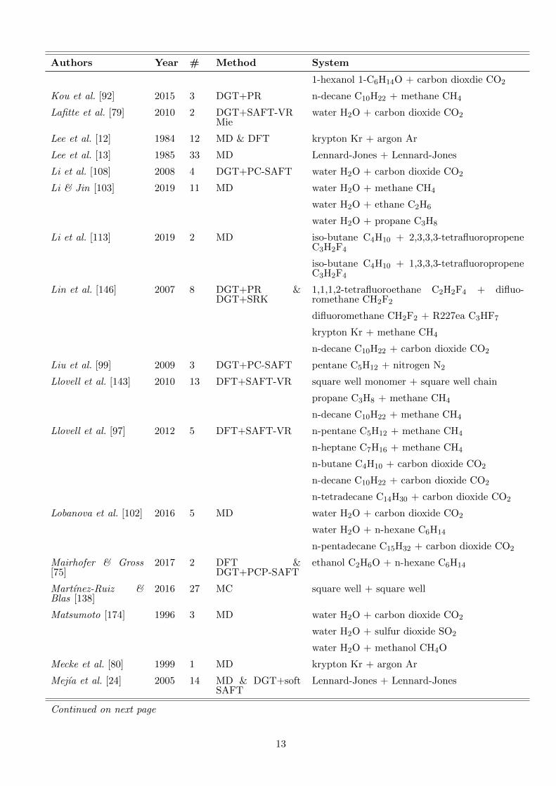
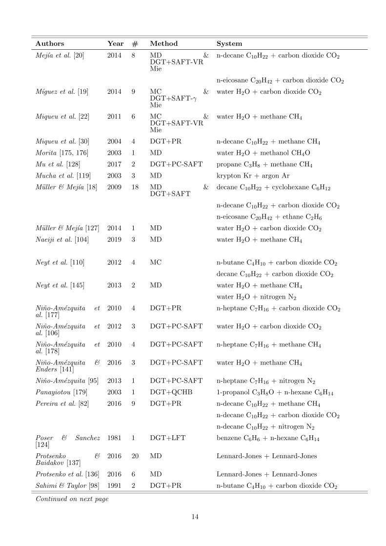
There is a large body of studies in the literature (approx. 100 publications) reporting on component density

profiles ρi(z) at vapour-liquid interfaces of binary mixtures, of which Table 1 gives an overview. The density

profiles ρi(z) were obtained from different theoretical methods (molecular simulations, DGT, DFT, or a

combination of those). Since data on ternary and multicomponent mixtures have been reported relatively

scarcely in the literature [36, 54, 70–75, 87–93], they are not listed in Table 1.

Studies on the prediction of interfacial properties of mixtures by theoretical methods mostly focus on

the prediction of the surface tension, but also often report density profiles and the relative adsorption Γ(1)2 .

In most cases, a qualitative description and discussion of the observations regarding the monotonicity of

the component density profiles ρi(z) is given in the publications. But those findings are rarely put into

relation with other works and to the phase behaviour of the considered mixture.

In most publications on vapour-liquid interfacial properties, cf. Table 1, the density profiles are unfor-

tunately only reported for a small subset of the performed simulations (the surface tension is the main

observable of interest). Hence, a large number of primary data remained unpublished in this field. The

vast majority of studies (cf. Table 1) report the density profiles ρi(z) only graphically. The enrichment E2

according Eq. (1) was rarely computed and reported. For the density profiles, unfortunately no consistent

form for plotting the data was established, i.e. sometimes only one of the component density profiles was

reported and sometimes all. Electronic data of density profiles was practically never reported.

From the density profiles ρ2(z) reported in the literature, cf. Table 1, the enrichment E2 was calculated

in the present work. If, as in most cases, ρ2(z) was only reported graphically in the publication, the data

were digitalised [94] and the maximum of the low-boiling component’s density profile as well as the larger

bulk density were metered from the plots, which introduces a considerable uncertainty. To estimate the

uncertainty of this ’measuring’ process, the digitalisation and evaluation was repeated five times and the

standard deviation was taken as a measure of the uncertainty due to the digitalisation procedure. The

average uncertainty of the results for E2 is approximately δE2 = ±0.1. The digitalised data E2(T, x′2,∆ρ2)

are reported in an electronic spread sheet in the Supplementary Material, where also more details on the

procedure are given.

Studies reporting vapour-liquid interfacial properties focus on a large variety of different systems and ap-

plications, such as enhanced oil recovery [18, 20, 23, 95–100], natural gas [19, 22, 101–105], CO2 absorption

6

and carbon-capture and storage (CCS) [20, 79, 102, 106–111], refrigerants [112–115], evaporation and nucle-

ation [32, 116], environmental science [117–119], process and chemical engineering [15, 17, 26, 83, 108, 120–

123], polymers [124, 125], fundamental physics [7, 13, 14, 69, 126, 127], and the development of computa-

tional methods and algorithms [8, 21, 32, 80, 92, 128–131]. Hence, they were published in a large variety

of different journals. Due to this heterogeneity of applications and motivations, there is no dense citation

network present in this field. It was one goal of the present paper to establish the corresponding links.

Density profiles at vapour-liquid interfaces have been investigated for both model fluids [7, 10–14, 24,

25, 76, 80, 132–138] (very often the Lennard-Jones fluid) and models of real substances [9, 17–19, 22, 28–

30, 32, 35, 75, 79, 88, 106, 124, 139–141]. These groups differ mainly in the way the molecular model is

used: model fluids are usually used to study the effect of a variation of the molecular parameters on a given

observable, whereby a generic information is obtained, whereas models of real substances are used to study

properties of a given mixture, which causes the findings to be primarily restricted to that case.

The influence of the molecular parameters on density profiles and other interfacial properties has been

studied several times in the literature. Results are available for the influence of the size and energy pa-

rameters of the pure components [10, 11, 13, 14, 24, 25, 27, 52, 133, 136, 137, 142], the cross interactions

[10, 11, 13, 14, 24, 25, 27, 133, 142], and the chain length of the components [18, 32, 98, 102, 132, 143, 144].

Some studies also investigated the influence of associating components [17, 79, 106, 109] on vapour-liquid in-

terfacial properties. Asymmetric mixtures have caused special interest [9, 18, 79, 98, 102, 106, 108, 109, 141]

since a particularly high enrichment is found in such cases.

The most frequently studied systems are (H2O + CO2), (H2O + alcohols), as well as (CO2 or N2 +

alkanes), and Lennard-Jones mixtures (cf. Table 1). The latter were mostly used for systematic studies of

the influence of molecular parameters on different interfacial and bulk properties. Also, most of the early

simulation studies on interfacial properties [7, 10–13] were performed with Lennard-Jones fluids. Mixtures

of simple fluids (argon, neon, krypton, methane etc.) can be modelled reasonably well as Lennard-Jones

mixtures. Hence, such data can be considered real substance data or model fluid data. Table 1 reports such

data as it is referred to in the respective publication.

Also the influence of the temperature [13, 15, 17, 27] and the composition [25, 26] on the interfacial

enrichment has been investigated systematically in the literature. Overall it was found that an enrichment

is favoured by asymmetric molecular interactions, large differences in the volatility of the pure components

(i.e. wide-boiling phase behaviour), low concentrations of the low-boiling components, and low temperatures

[14, 17, 18, 22, 25, 26, 98, 106, 109, 145, 146]. In most cases, starting at infinite dilution of component 2,

the enrichment E2 was found to decrease monotonically with increasing concentration of the low-boiling

component 2 at constant temperature to converge to unity either at a critical point, an azeotropic point,

or the high-boiling pure component vapour pressure (depending on the phase behaviour).

7

Furthermore, two types of enrichment behaviour have been reported for wide-boiling mixtures [14, 25]

depending on the sign of the density difference of component 2 ∆ρ2 = ρ′2 − ρ′′2: mixtures with ∆ρ2 > 0

usually yield large enrichment, whereas mixtures with ∆ρ2 < 0 usually yield small enrichment. For example

solvent + nitrogen systems usually yield ∆ρ2 < 0, which goes in hand with small enrichment, whereas

solvent + carbon dioxide or solvent + methane systems usually have ∆ρ2 > 0, which goes in hand with

large enrichment (see Supplementary Material). This differentiation has also been confirmed for different

types of Lennard-Jones model mixtures, cf. Ref. [14].

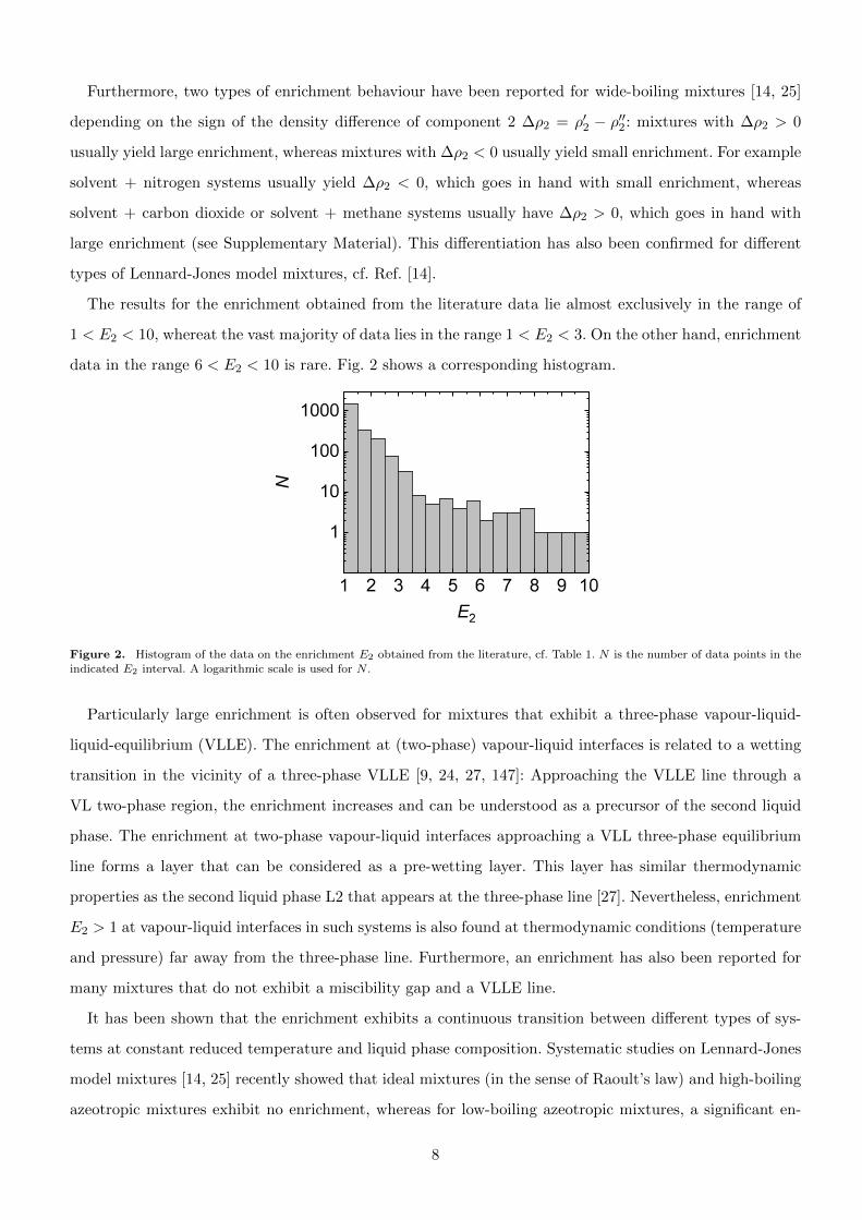
The results for the enrichment obtained from the literature data lie almost exclusively in the range of

1 < E2 < 10, whereat the vast majority of data lies in the range 1 < E2 < 3. On the other hand, enrichment

data in the range 6 < E2 < 10 is rare. Fig. 2 shows a corresponding histogram.

Figure 2. Histogram of the data on the enrichment E2 obtained from the literature, cf. Table 1. N is the number of data points in the

indicated E2 interval. A logarithmic scale is used for N .

Particularly large enrichment is often observed for mixtures that exhibit a three-phase vapour-liquid-

liquid-equilibrium (VLLE). The enrichment at (two-phase) vapour-liquid interfaces is related to a wetting

transition in the vicinity of a three-phase VLLE [9, 24, 27, 147]: Approaching the VLLE line through a

VL two-phase region, the enrichment increases and can be understood as a precursor of the second liquid

phase. The enrichment at two-phase vapour-liquid interfaces approaching a VLL three-phase equilibrium

line forms a layer that can be considered as a pre-wetting layer. This layer has similar thermodynamic

properties as the second liquid phase L2 that appears at the three-phase line [27]. Nevertheless, enrichment

E2 > 1 at vapour-liquid interfaces in such systems is also found at thermodynamic conditions (temperature

and pressure) far away from the three-phase line. Furthermore, an enrichment has also been reported for

many mixtures that do not exhibit a miscibility gap and a VLLE line.

It has been shown that the enrichment exhibits a continuous transition between different types of sys-

tems at constant reduced temperature and liquid phase composition. Systematic studies on Lennard-Jones

model mixtures [14, 25] recently showed that ideal mixtures (in the sense of Raoult’s law) and high-boiling

azeotropic mixtures exhibit no enrichment, whereas for low-boiling azeotropic mixtures, a significant en-

8

richment is found. This is in line with findings for real substance mixtures reported in the literature

[10, 25, 35, 121]. Furthermore, it was found that the enriching component changes at the azeotropic point

[121]. Hence, in each azeotropic branch, the respective low-boiling component exhibits an enrichment at

the interface. Nevertheless, enrichment data on azeotropic mixtures is relatively scarce in the literature.

The number of theoretical studies of vapour-liquid interfaces has grown significantly in the last decade,

which is probably due to the fact that MD and MC studies of direct VLE simulations, where the vapour and

the liquid phase coexist in a simulation box, became computationally readily affordable. Approximately

60% of the available studies reporting vapour-liquid density profile data of binary mixtures have been

published in the last ten years, cf. Table 1.

Most studies on density profiles of vapour-liquid interfaces employ either molecular simulations, i.e.

molecular dynamics (MD) or Monte Carlo (MC) simulations using classical force fields [148, 149], or DGT

in combination with an EOS. Approximately half of the studies reporting vapour-liquid interfacial density

profiles employ density gradient theory (DGT) in combination with an equation of state (EOS). Not all

EOS are suited for such studies. An essential prerequisite is that they exhibit only a single van der Waals

loop in the two-phase region [150], like cubic EOS or well-behaving SAFT type EOS [151–157]. Density

functional theory (DFT) was only applied in few cases, cf. Table 1. In some studies two methods were

employed for a given mixture – usually molecular simulations and DGT. Even though, both methods were

found to yield good qualitative agreement for the predicted enrichment in practically all cases, significant

quantitative differences have been reported many times [15–20, 22–25, 100, 142, 158]. For a given mixture,

the reported absolute deviation for the predicted enrichment among different methods mostly lies in the

range δE2 = 0.1 .. 1.

Systematic deviations between molecular simulations and DGT results for the enrichment have been

observed several times: for low E2 values, molecular simulations typically yield larger enrichment than

DGT, whereas for high E2 values the DGT results mostly overestimate the MD results for the enrichment

[12, 13, 15–24, 27].

Assessing these deviations between the results from molecular simulations and DGT, several sources of

error and uncertainties should be considered: leaving aside the problem of the topic of the reproducibility of

molecular simulations results [159–163], the underlying pure substance models (EOS and force field) have

to be parametrised adequately to yield conformal representations of the VLE, which is not trivial even

for the most simple fluids [157]. Furthermore, molecular simulations and DGT have some fundamental

differences, e.g. fluctuations are present in the MD density profiles ρi(z) but not in the corresponding DGT

results, cf. Ref. [27] for a detailed discussion.

For the sake of completeness, we briefly point out further interesting aspects related to the enrichment

that have been studied in the literature: the peak position and the shape of the peak was found to depend

9

on the system and varies with temperature and composition such that the position of the peak can either

be on the liquid or the vapour side of the interface [15, 25, 27] (with respect to the centre of the interface

defined as ρcentre = 0.5(ρ′ + ρ′′)). Furthermore, the interfacial thickness, the enrichment, and the relative

adsorption have been examined simultaneously in some cases as these three properties comprehensively

characterise the structure of an interface [15, 27]. Long-range interactions were found to have a minor

influence on the enrichment in simple fluid mixtures [142]. Also the pressure tensor across vapour-liquid

interfaces of mixtures was measured by many authors [9, 12, 109, 119, 138, 145, 164]. The pressure profiles

do not exhibit additional oscillations in cases of high E2 compared to cases with low E2. Moreover, the

orientation of enriching species at the interface [2, 41, 117, 118] and the details on the distribution of

functional groups at the interface [3, 21, 41, 42] has been investigated. In several cases, a preferential

orientation of low-boiling components with respect to the interface was observed [3, 117, 118], compared

to a stochastic orientation in the bulk phases.

10

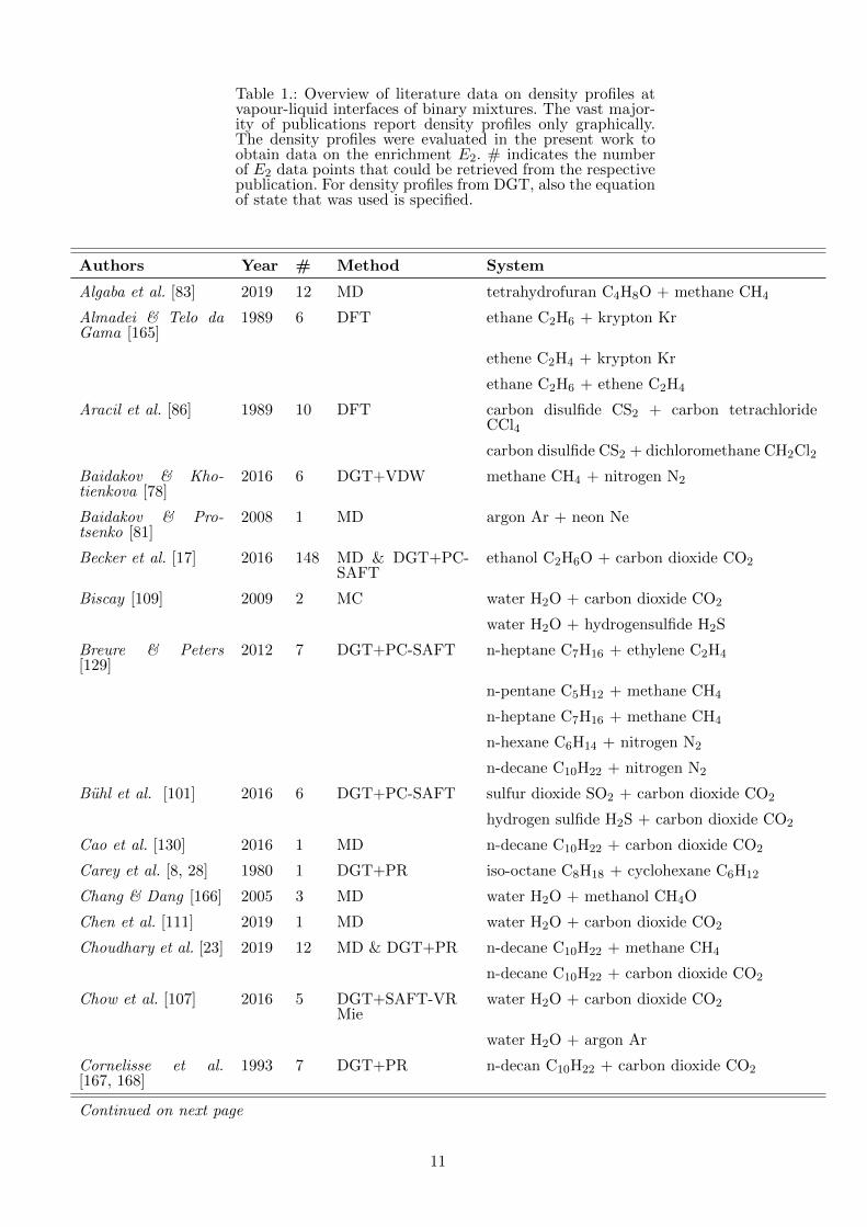
Table 1.: Overview of literature data on density profiles atvapour-liquid interfaces of binary mixtures. The vast major-ity of publications report density profiles only graphically.The density profiles were evaluated in the present work toobtain data on the enrichment E2. # indicates the numberof E2 data points that could be retrieved from the respectivepublication. For density profiles from DGT, also the equationof state that was used is specified.

Authors Year # Method System

Algaba et al. [83] 2019 12 MD tetrahydrofuran C4H8O + methane CH4

Almadei & Telo daGama [165]

1989 6 DFT ethane C2H6 + krypton Kr

ethene C2H4 + krypton Kr

ethane C2H6 + ethene C2H4

Aracil et al. [86] 1989 10 DFT carbon disulfide CS2 + carbon tetrachlorideCCl4

carbon disulfide CS2 + dichloromethane CH2Cl2

Baidakov & Kho-tienkova [78]

2016 6 DGT+VDW methane CH4 + nitrogen N2

Baidakov & Pro-tsenko [81]

2008 1 MD argon Ar + neon Ne

Becker et al. [17] 2016 148 MD & DGT+PC-SAFT

ethanol C2H6O + carbon dioxide CO2

Biscay [109] 2009 2 MC water H2O + carbon dioxide CO2

water H2O + hydrogensulfide H2S

Breure & Peters[129]

2012 7 DGT+PC-SAFT n-heptane C7H16 + ethylene C2H4

n-pentane C5H12 + methane CH4

n-heptane C7H16 + methane CH4

n-hexane C6H14 + nitrogen N2

n-decane C10H22 + nitrogen N2

Buhl et al. [101] 2016 6 DGT+PC-SAFT sulfur dioxide SO2 + carbon dioxide CO2

hydrogen sulfide H2S + carbon dioxide CO2

Cao et al. [130] 2016 1 MD n-decane C10H22 + carbon dioxide CO2

Carey et al. [8, 28] 1980 1 DGT+PR iso-octane C8H18 + cyclohexane C6H12

Chang & Dang [166] 2005 3 MD water H2O + methanol CH4O

Chen et al. [111] 2019 1 MD water H2O + carbon dioxide CO2

Choudhary et al. [23] 2019 12 MD & DGT+PR n-decane C10H22 + methane CH4

n-decane C10H22 + carbon dioxide CO2

Chow et al. [107] 2016 5 DGT+SAFT-VRMie

water H2O + carbon dioxide CO2

water H2O + argon Ar

Cornelisse et al.[167, 168]

1993 7 DGT+PR n-decan C10H22 + carbon dioxide CO2

Continued on next page

11


Cornelisse [29] 1997 2 DGT+PR water H2O + ethanol C2H6O

n-hexane C6H14 + ethanol C2H6O

Eckelsbach et al.[164]

2014 3 MD acetone C3H6O + nitrogen N2

Eckelsback & Vrabec[123]

2015 2 MD acetone C3H6O + oxygen O2

acetone C3H6O + nitrogen N2

Enders & Kahl [35] 2008 4 DGT+SAFT water H2O + ethanol C2H6O

water H2O + butanol C4H10O

Fabian et al. [118] 2014 4 MD water H2O + hydrogen cyanid HCN

Falls et al. [9] 1983 5 DGT+PR n-decane C10H22 + carbon dioxide CO2

Fouad and Vega[112]

2017 3 DGT+PC-SAFT propane C3H8 + difluoromethane CH2F2

Fu et al. [122] 2011 6 DGT+PC-SAFT ethanol C2H6O + carbon dioxide CO2

methanol CH4O + carbon dioxide CO2

Garrido et al. [100] 2017 8 MD &DGT+SAFT-VRMie

n-hexane C6H14 + nitrogen N2

n-octane C8H18 + nitrogen N2

Greberg et al. [169] 2001 2 DGT krypton Kr + argon Ar

Ghobadi & Elliot [21] 2014 4 MD &DFT+SAFT-γ

heptane C7H16 + ethane C2H6

Horvath et al. [117] 2019 7 MD water H2O + methylamine CH3N2

Ibarra-Tandi et al.[170]

2013 1 MD Morse fluid + Morse fluid

Kahl & Enders [140] 2002 3 DGT+SAFT n-hexane C6H14 + methanol CH4O

Kahl et al. [171] 2005 1 DFT methane CH4 + argon Ar

Khosharay et al.[172]

2014 4 DGT+sPC-SAFT water H2O + carbon dioxide CO2

water H2O + hydrogen sulfide H2S


2014 2 DGT+PR dufluoroethane C2H4F2 + propane C3H8

dufluoroethane C2H4F2 + pentafluorethanC2HF5


2014 2 DGT+CK-SAFT water H2O + carbon dioxide CO2

water H2O + methane CH4


2016 2 DGT+PR propane C3H8 + methane CH4

heptane C7H16 + methane CH4

Klink & Gross [32] 2014 5 DFT+PC-SAFT methane CH4 + carbon monoxide CO

Koller et al. [120] 2019 4 MD n-hexane C6H14 + carbon dioxide CO2



12


1-hexanol 1-C6H14O + carbon dioxdie CO2

Kou et al. [92] 2015 3 DGT+PR n-decane C10H22 + methane CH4

Lafitte et al. [79] 2010 2 DGT+SAFT-VRMie


Lee et al. [12] 1984 12 MD & DFT krypton Kr + argon Ar

Lee et al. [13] 1985 33 MD Lennard-Jones + Lennard-Jones

Li et al. [108] 2008 4 DGT+PC-SAFT water H2O + carbon dioxide CO2

Li & Jin [103] 2019 11 MD water H2O + methane CH4

water H2O + ethane C2H6

water H2O + propane C3H8

Li et al. [113] 2019 2 MD iso-butane C4H10 + 2,3,3,3-tetrafluoropropeneC3H2F4

iso-butane C4H10 + 1,3,3,3-tetrafluoropropeneC3H2F4

Lin et al. [146] 2007 8 DGT+PR &DGT+SRK

1,1,1,2-tetrafluoroethane C2H2F4 + difluo-romethane CH2F2

difluoromethane CH2F2 + R227ea C3HF7

krypton Kr + methane CH4


Liu et al. [99] 2009 3 DGT+PC-SAFT pentane C5H12 + nitrogen N2

Llovell et al. [143] 2010 13 DFT+SAFT-VR square well monomer + square well chain

propane C3H8 + methane CH4

n-decane C10H22 + methane CH4

Llovell et al. [97] 2012 5 DFT+SAFT-VR n-pentane C5H12 + methane CH4

n-heptane C7H16 + methane CH4

n-butane C4H10 + carbon dioxide CO2


n-tetradecane C14H30 + carbon dioxide CO2

Lobanova et al. [102] 2016 5 MD water H2O + carbon dioxide CO2

water H2O + n-hexane C6H14

n-pentadecane C15H32 + carbon dioxide CO2

Mairhofer & Gross[75]

2017 2 DFT &DGT+PCP-SAFT

ethanol C2H6O + n-hexane C6H14

Martınez-Ruiz &Blas [138]

2016 27 MC square well + square well

Matsumoto [174] 1996 3 MD water H2O + carbon dioxide CO2

water H2O + sulfur dioxide SO2

water H2O + methanol CH4O

Mecke et al. [80] 1999 1 MD krypton Kr + argon Ar

Mejıa et al. [24] 2005 14 MD & DGT+softSAFT

Lennard-Jones + Lennard-Jones


13


Mejıa et al. [20] 2014 8 MD &DGT+SAFT-VRMie


n-eicosane C20H42 + carbon dioxide CO2

Mıguez et al. [19] 2014 9 MC &DGT+SAFT-γMie


Miqueu et al. [22] 2011 6 MC &DGT+SAFT-VRMie

water H2O + methane CH4

Miqueu et al. [30] 2004 4 DGT+PR n-decane C10H22 + methane CH4

Morita [175, 176] 2003 1 MD water H2O + methanol CH4O

Mu et al. [128] 2017 2 DGT+PC-SAFT propane C3H8 + methane CH4

Mucha et al. [119] 2003 3 MD krypton Kr + argon Ar

Muller & Mejıa [18] 2009 18 MD &DGT+SAFT

decane C10H22 + cyclohexane C6H12


n-eicosane C20H42 + ethane C2H6

Muller & Mejıa [127] 2014 1 MD water H2O + carbon dioxide CO2

Naeiji et al. [104] 2019 3 MD water H2O + methane CH4

Neyt et al. [110] 2012 4 MC n-butane C4H10 + carbon dioxide CO2

decane C10H22 + carbon dioxide CO2

Neyt et al. [145] 2013 2 MD water H2O + methane CH4

water H2O + nitrogen N2

Nino-Amezquita etal. [177]

2010 4 DGT+PR n-heptane C7H16 + carbon dioxide CO2


2012 3 DGT+PC-SAFT water H2O + carbon dioxide CO2


2010 4 DGT+PC-SAFT n-heptane C7H16 + methane CH4

Nino-Amezquita &Enders [141]

2016 3 DGT+PC-SAFT water H2O + methane CH4

Nino-Amezquita [95] 2013 1 DGT+PC-SAFT n-heptane C7H16 + nitrogen N2

Panayiotou [179] 2003 1 DGT+QCHB 1-propanol C3H8O + n-hexane C6H14

Pereira et al. [82] 2016 9 DGT+PR n-decane C10H22 + methane CH4


n-decane C10H22 + nitrogen N2

Poser & Sanchez[124]

1981 1 DGT+LFT benzene C6H6 + n-hexane C6H14

Protsenko &Baidakov [137]

2016 20 MD Lennard-Jones + Lennard-Jones

Protsenko et al. [136] 2016 6 MD Lennard-Jones + Lennard-Jones

Sahimi & Taylor [98] 1991 2 DGT+PR n-butane C4H10 + carbon dioxide CO2


14



Salomons &Mareschal [134]

1991 4 MC Lennard-Jones + Lennard-Jones

Salomons &Mareschal [135]

1991 3 MC Lennard-Jones + Lennard-Jones

Schafer et al. [121] 2014 2 DGT+PC-SAFT N,N-dimethylformamid DMF + n-heptaneC7H16

N,N-dimethylformamid DMF + n-dodecaneC12H26

Schenk et al. [180] 2019 3 MD carbon dioxide CO2 + methane CH4

Shi etl a. [125] 2015 3 MD polydimethylsiloxane C2H6SiO + carbon diox-ide CO2

Stephan et al. [181] 2020 296 MD &DGT+PCP-SAFT

toluene C7H8 + carbon dioxide CO2

toluene C7H8 + nitrogen N2

Stephan et al. [15] 2020 135 MD &DGT+PCP-SAFT

cyclohexane C6H12 + carbon dioxide CO2

Stephan et al. [26] 2018 6 MD & DGT toluene C7H8 + carbon dioxide CO2

ethanol C2H6O + carbon dioxide CO2


Stephan et al. [25] 2019 186 MD &DGT+PeTS

Lennard-Jones + Lennard-Jones (six systems)

Stephan & Hasse[142]

2019 142 MD & DGT+LJEOS

Lennard-Jones + Lennard-Jones (six systems)

Stephan & Hasse[14]

2020 180 MD &DGT+PeTS

Lennard-Jones + Lennard-Jones (90 systems)

Stephan & Hasse[27]

2020 330 MD &DGT+PeTS

Lennard-Jones + Lennard-Jones (two systems)

Stephan &Hasse[182]

2020 381 MD LJ + LJD (15 systems)

LJ + LJQ (7 systems)

LJD + LJD (4 systems)

LJQ + LJQ (4 systems)

LJD + LJQ (3 systems)

Sullivan [183] 1982 5 DGT+VDW vdW fluid + vdW fluid

Teixeira et al. [85] 1992 20 DFT acetonitrile CH3CN + carbon tetrachlorideCCl4

methyl iodide CH3I + carbon tetrachloride CCl4

Tardon et al. [158] 2012 4 MD & DGT+LJEOS


Telo da Gama [7] 1980 4 SGA krypton Kr + argon Ar

Telo da Gama &Evans [10]

1983 5 SGA Lennard-Jones + Lennard-Jones

Telo da Gama &Evans [11]

1983 9 SGA Lennard-Jones + Lennard-Jones


15


Vilaseca et al. [114] 2010 3 DGT+soft SAFT dufluoroethane C2H4F2 + propane C3H8

Wadewitz & Winkel-mann [84]

1996 20 DFT argon Ar + nitrogen N2

toluene C7H8 + n-heptane C7H16

Werth et al. [16] 2016 159 MD & DGT+PC-SAFT

toluene C7H8 + carbon dioxide CO2

toluene C7H8 + hydrocloric HCl

Winkelmann [69] 2001 6 MD methane CH4 + argon Ar

Zeng & Oxtoby [116] 1991 2 DFT krypton Kr + argon Ar

Abbreviations:

DFT density functional theory

DGT density gradient theory

EOS equation of state

LFT lattice fluid theory [184]

LJ Lennard-Jones fluid EOS [157, 185–188]

MC Monte Carlo simulation [189, 190]

MD molecular dynamics simulation [189]

PC-SAFT perturbed-chain statistical associating fluid theory EOS [191, 192]

PCP-SAFT perturbed-chain polar statistical associating fluid theory EOS [193–195]

PeTS perturbed truncated shifted EOS [25, 154]

PR Peng-Robinson EOS [196]

QCHB quasi-chemical hydrogen bonding [179]

SAFT statistical associating fluid theory EOS [151, 197, 198]

CK-SAFT Chen-Kreglewski SAFT [199, 200]

SAFT-VR Mie EOS SAFT variable range Mie potential EOS [201]

SAFT-γ Mie group contribution SAFT-VR Mie EOS version [202]

SAFT VR SAFT variable range EOS [203, 204]

soft SAFT soft SAFT EOS [205, 206]

SRK Soave-Redlich-Kwong EOS [207, 208]

VDW van der Waals EOS

4. Enrichment Model and Parametrisation

4.1. Dataset used for the Parametrisation

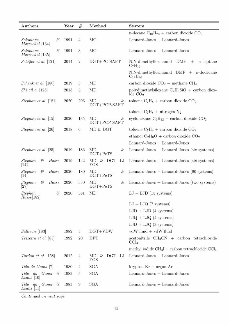
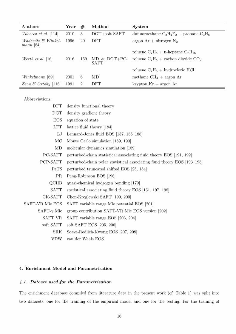
The enrichment database compiled from literature data in the present work (cf. Table 1) was split into

two datasets: one for the training of the empirical model and one for the testing. For the training of

16

the empirical enrichment model, the comprehensive dataset on binary Lennard-Jones mixtures that was

recently published by our group was used [14, 25, 27]. The test-dataset comprises the remaining enrichment

data from the literature, cf. Table 1.

The training-dataset comprises a large variety of mixture types and thermodynamic conditions (tem-

perature and liquid phase composition). An overview of the Lennard-Jones mixtures comprised in the

training-dataset [14, 25, 27] is given in Fig. 3, in which the molecular interaction parameters are depicted.

For all mixtures, the high-boiling component 1 was the same and both components have the same size

parameter σ and mass M . The mixtures differ in the dispersion energy of the low-boiling component ε2

and the parameter ξ that was used in the modified Berthelot combination rule for describing the cross

interactions dispersion energy ε12 = ξ√ε1ε2. Values of ξ > 1 indicate an increased cross affinity of the two

components and ξ < 1 a decreased cross affinity. A selection of the resulting isothermal phase diagrams is

given in the Supplementary Material.

Figure 3. Overview of the binary Lennard-Jones mixtures that were used for the training of the empirical enrichment model. Component

1 was the same for all mixtures. ε2/ε1 denotes the ratio of the two component’s dispersion energy and ξ the cross interaction parameterused in the modified Berthelot combination rule. The particle size σ was the same for both components in all cases. Mixtures that are

indicated by circles were studied at x′2 = 0.05 mol mol−1 and T/Tc,1 = 0.7 [14]. Mixtures indicated by triangles were studied in the

entire composition range at T/Tc,1 = 0.7 [25]. Mixtures indicated by crosses were studied in the entire composition range and at thetemperatures T/Tc,1 = 0.6, 0.65, 0.7, 0.75, 0.8 [27].

Fig. 4 shows the results for the enrichment obtained in these systematic studies [14, 25, 27]. The obtained

enrichment is plotted as a function of the liquid phase concentration for the data from Refs. [25, 27] (panels

a) - d) and as a function of the partition coefficient for the data from Ref. [14] (panel e).

The training-dataset thereby contains enrichment data of 90 Lennard-Jones systems at only one tem-

perature and liquid phase composition (x′2 = 0.05 mol mol−1) [14], six systems at one temperature but the

entire composition range [25], and two systems at five temperatures in the entire composition range [27].

All three studies [14, 25, 27] were carried out using both MD and DGT. For the parametrisation of the

enrichment model, only the MD results reported in Refs. [14, 25, 27] were used. The training-dataset covers

17

0.0 0.1 0.2 0.31

3

5

7

0 5 10 151

2

3

4

0.0 0.2 0.4 0.61.0

1.5

2.0

2.5

3.0

0.0 0.2 0.4 0.6 0.8 1.01.0

1.1

1.2

1.3

E2

e2/e1 = 0.9 x = 1

T/Tc,1 = 0.6T/Tc,1 = 0.65

T/Tc,1 = 0.7T/Tc,1 = 0.75

T/Tc,1 = 0.8

c)

e2/e1 = 0.5

e2/e1 = 0.9

d) e2/e1 = 0.6 x = 0.85

E2

x'2 / mol mol-1

T/Tc,1 = 0.8T/Tc,1 = 0.75

T/Tc,1 = 0.7T/Tc,1 = 0.65

T/Tc,1 = 0.6

E2

K2

T/Tc,1 = 0.7

Dr2 < 0D r2 ³ 0

x'2 = 0.05 mol mol -1e)

0.0 0.2 0.4 0.6 0.8 1.01.0

1.2

1.4

1.6

E2

a)T/Tc,1 = 0.7

x E2

redblackblue

0.8511.2

b)T/Tc,1 = 0.7

x redblackblue

0.8511.2

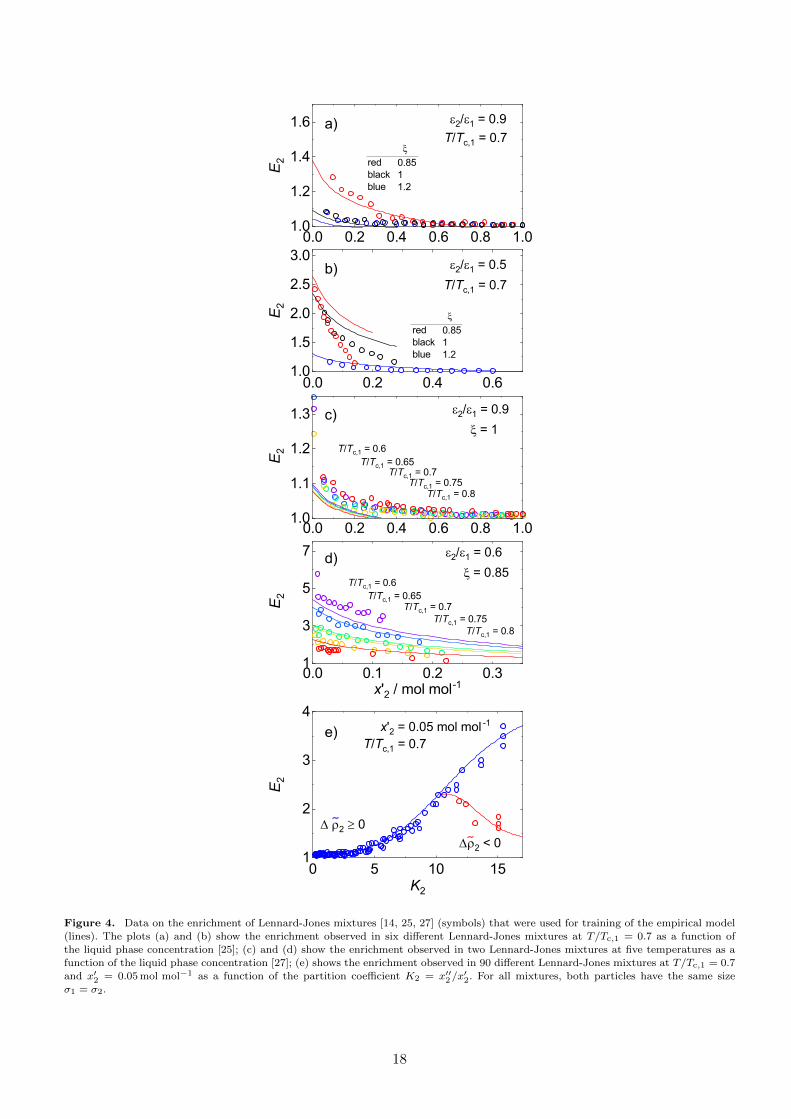
Figure 4. Data on the enrichment of Lennard-Jones mixtures [14, 25, 27] (symbols) that were used for training of the empirical model(lines). The plots (a) and (b) show the enrichment observed in six different Lennard-Jones mixtures at T/Tc,1 = 0.7 as a function of

the liquid phase concentration [25]; (c) and (d) show the enrichment observed in two Lennard-Jones mixtures at five temperatures as afunction of the liquid phase concentration [27]; (e) shows the enrichment observed in 90 different Lennard-Jones mixtures at T/Tc,1 = 0.7

and x′2 = 0.05 mol mol−1 as a function of the partition coefficient K2 = x′′2/x′2. For all mixtures, both particles have the same size

σ1 = σ2.

18

a wide range of types of phase behaviour. Furthermore, it contains data for a selection of mixtures in the

temperature range between the triple point temperature and the critical temperature of the high-boiling

component, and the entire concentration range where vapour-liquid equilibria exist in these systems. In

total, the training-dataset consists of 338 data points.

For all studied mixtures in the training-dataset, the enrichment E2 predicted by MD is largest at infinite

dilution of the low-boiling component and monotonically decreases with increasing x′2. The enrichment

increases with decreasing temperature, cf. Fig. 4 c) and d). The enrichment data at constant temperature

and liquid phase concentration (x′2 = 0.05 mol mol−1) plotted as a function of the partition coefficient

K2 = x′′2/x′2 (Fig. 4 e) shows an interesting behaviour: All data points collapse to a single curve for values

of K2 of up to about 12. This is not completely surprising, as in Ref. [14], a general monovariate dependency

of the interfacial properties on the internal energy of the liquid phase was found. However, at K2 ≈ 12 a

second branch appears in the plot shown in Fig. 4 e). The existence of this second branch is related to the

difference of the partial densities of component 2 in the two phases ∆ρ2 = ρ′′2 − ρ′2. For most systems, the

partial density difference ∆ρ2 is positive, i.e. ρ2 in the liquid phase is larger than ρ2 in the gas phase (which

is related to the gas solubility [14]). However, for some systems, the inverse is true, i.e. ∆ρ2 is negative.

Both types of systems show large values of K2 (the limit is about K2 = 12). As shown in Ref. [14], the

sign of ∆ρ2 has an important influence on the enrichment. As a consequence, for K2 > 12 a distinction is

necessary between systems with ∆ρ2 > 0 and systems with ∆ρ2 < 0. The branch found for ∆ρ2 > 0 in this

range of K2 is a simple extension of the curve found for lower K2, whereas on the other branch (∆ρ2 < 0),

distinctly smaller values of E2 are found. While the database is dense for low K2, not as many data points

are currently available at high K2 in the training-dataset, cf. Fig. 4.

4.2. Empirical Enrichment Model

As described above, the enrichment E2 is considered here as a function of T and x′2 for a given mixture.

The aim was to establish a correlation of E2 with readily available macroscopic data on the VLE of the

mixture. Correlations in dimensionless variables are preferred. Many options are available for establishing

such correlations, and we have tested a number of them in preliminary work. For brevity, we will not

describe all these tests and present here only the final result. Our only claim is the usefulness of the

correlation, i.e. a good description of the available E2 data, not any kind of optimality. A clear indication

of the usefulness is the fact that the simple correlation presented here describes the available data on E2

in most cases within the uncertainty of the prediction of E2 from different methods.

The proposed correlation describes E2 as a product of two terms:

E2 = α0 + fa(x′2) fb(VLE) , (2)

19

and an empirical offset parameter α0. The term fa describes the concentration-dependence of E2 in a gen-

eralised way, the term fb includes the information on the VLE of the considered binary system. Preliminary

tests showed that it is not necessary to introduce a universal function of the temperature. The influence

of temperature is accounted for in the term fb. In the following, empirical parameters employed in the

functions fa and fb are labelled as αi.

Following the findings shown in Figure 4 e), the VLE of a mixture is characterised here by the partition

coefficient of component 2, i.e. K2 = x′′2/x′2. This is convenient, as in all studies of interfacial properties in

the literature, the partition coefficient K2 can be calculated easily from the available data. Furthermore,

the required data on x′′2 and x′2 are readily available in databases for a large number of mixtures of practical

relevance.

The partition coefficient K2 depends both on the temperature and composition. For characterising the

studied system, the partition coefficient at infinite dilution would have been a convenient choice, since E2

was found in all cases to be largest at infinite dilution and monotonically decrease with increasing x′2 (see

discussion above). But since MD simulations can only be carried out at finite concentrations and based on

an analysis of the available data and preliminary tests, it was decided to use the partition coefficient at

the liquid phase concentration of x′2 = 0.05 mol mol−1:

K5%2 =

x′′2x′2 ≡ 0.05 mol mol−1 . (3)

For a given mixture, the value ofK5%2 depends on the temperature. This is how the temperature is accounted

for in the model.

The dependency of the enrichment on the liquid phase concentration is described by a simple monoton-

ically decaying universal function

fa(x′2) = α1 + ln

(1

x′2 + α2

)− α2

x′2 + α2. (4)

The function fa has a finite value at x′2 = 0 and monotonically decreases with a convex curvature to zero at

x′2 = 0. The outlined model does not explicitly take three-phase VLLE and critical points into account as

termination points for E2 isotherms [27]. It would be desirable to consider these end points in the model,

but there is presently not enough data to do this in a meaningful way. If more data were available, this is

expected to lead to further improvements of the model.

As discussed above, for mixtures with large K2, the influence of the density difference of the low-boiling

component ∆ρ2 = ρ′2 − ρ′′2 must be taken into account. This is incorporated in the empirical model by

20

defining

fb = α3 gI(K5%2 ) δ(∆ρ2) + α4 gII(K

5%2 ) (1− δ(∆ρ2)) , (5)

where δ is a smoothed step function taking values between 0 and 1 of the form

δ (∆ρ2) =tanh (100 ·∆ρ2) + 1

2. (6)

In Eq. (6), ∆ρ2 is the reduced density difference with respect to the critical density of the high-boiling

component, i.e. ∆ρ2 = ∆ρ2/ρc,1. Hence, also ∆ρ2 is a dimensionless variable. The reduced density dif-

ference ∆ρ2 is only used for the decision function δ(∆ρ2) to navigate between the terms gI(K5%2 ) and

gII(K5%2 ) depending on the sign of ∆ρ2. The value of ∆ρ2 can easily be obtained from saturated density

and concentration data, which is readily available for a large number of systems [209, 210].

The two functions for the modelling of the enrichment dependency on the partition coefficient gI and gII

are defined as

gI(K5%2 ) =

(exp

(tanh

(α5 ·K5%

2 − α6

)))α7

, (7)

gII(K5%2 ) = α8 + exp

α9 ·

(K5%

2 − α10

α11

)2 . (8)

The equations (2) - (8) define an empirical enrichment model as a function E2 = E2(x′2, K5%2 ,∆ρ2). All

three variables are dimensionless macroscopic VLE properties that are easily accessible by experiment and

are available in data bases for a large number of systems [209, 210]. The values for K5%2 and ∆ρ2 can be

determined conveniently for both the training-dataset and the test-dataset. For the training-dataset, all

required numeric values were reported in the respective publications. The determination of K5%2 and ∆ρ2

for the test-dataset is discussed in the next section.

The empirical enrichment model has 12 adjustable parameters αi with i = 0 to 11, which were fitted to

the training-dataset, i.e. the MD Lennard-Jones mixture data from Refs. [14, 25, 27]. The parametrisation

was carried out by minimising the absolute average deviation

AADE2= 1/N

N∑j=1

|∆E2,j |Eref

2,j

, (9)

where N is the number of enrichment data points in the training-dataset, Eref2,j is the reference enrichment

from the training-dataset [14, 25, 27], and ∆E2 is the absolute deviation between the reference value and

21

the value predicted by the empirical enrichment model ∆E2,j = Eref2,j −Emodel

2,j . Table 2 reports the obtained

parameter values for αi.

Table 2. Parameters of the empirical enrichment model Eq. (2).

i αi i αi0 0.9594 6 0.55211 0.0199 7 2.70992 0.01 8 0.47063 0.0811 9 -0.054 0.3414 10 10.855 0.1345 11 0.8

The model described above is empirical. Experience tells us that the limits of applicability of such models

are related to the range of states covered by the training-dataset. In our case the considered VLE regions

ended always in the boiling point of the high-boiling component 1, i.e. infinite dilution of component 2,

and the temperatures were between the triple point temperature and the critical temperature of the high-

boiling component 1. The upper limit of the concentration of the low-boiling component 2 was determined

by the occurrence of a critical point or a three-phase line. For more details see Ref. [27]. For low-boiling

azeotropic systems, the model should be applied taking the azeotropic point into account, i.e. the low-boiling

component has to be assigned to each branch separately. However, such data is presently very scarce, see

electronic Supplementary Material. Furthermore, reference data was available for 0 < K5%2 < 15. It is noted

that neither the training-dataset nor the test-dataset contain data points with ∆ρ2 < 0 and K5%2 < 10.

Hence, the empirical enrichment model is not valid in that region. We therefore assume that, if such data

exist at all, they are rare. But should they exist, the model would probably not describe them well. Likewise,

the performance of the enrichment model at high-pressure phase equilibria comprising isopycnic states is

presently unknown.

Fig. 5 depicts the enrichment determined from the empirical model as a function of the liquid phase

concentration x′2 and the partition coefficient K5%2 – also extrapolating into the region K5%

2 > 15.

The plot shown in Fig. 5 was obtained for Delta ∆ρ2 = 0.1 or ∆ρ2 = −0.1, respectively. Due to the

character of the Eqs. (2) - (8) other choices of ∆ρ2 yield similar results as long as the sign of ∆ρ2 is the

same. Only for ∆ρ2 values with a very small absolute value |∆ρ2| < 0.01, there is a smooth transition

between the branches, which is numerically convenient.

For K5%2 < 12 and ∆ρ2 > 0 (the region where only a single branch exists), the model converges to

unity with decreasing K5%2 at infinite dilution of component 2. For the composition dependency, the model

decreases monotonically to approximately unity for all K5%2 and ∆ρ2 with increasing x′2. At infinite dilution

of component 2, the enrichment model yields E2 = 4.3 at K5%2 = 15 and ∆ρ2 > 0 (upper branch depicted

in Fig. 5). At infinite dilution of component 2 at ∆ρ2 < 0 (bottom branch in Fig. 5), the enrichment model

converges to approximately E2 = 1.4 with increasing K5%2 .

22

Figure 5. Results of the empirical enrichment model E2 = E2(x′2, K5%2 ). Results are shown for ∆ρ2 = 0.1 and −0.1. The colour coding

refers to the magnitude of E2. The branches of the graph for K5%2 > 12 correspond to ∆ρ2 < 0 (low E2) and ∆ρ2 > 0 (high E2), cf. Eq.

(5).

The empirical enrichment model is compared to the training-dataset in Fig. 4. The enrichment model

generally describes the influence of the composition, the temperature, and the partition coefficient on E2

well. However, Fig. 4 b) shows deviations for the composition dependency for isotherms that exhibit a

critical point. Figs. 4 c) and d) show that the temperature dependency is captured reasonably well by the

model. Fig. 4 e) shows the enrichment as a function of K5%2 , i.e. the performance of the term fb(K

5%2 ) in Eq.

(2). Deviations are observed for data points K5%2 > 12, which is mainly due to the fact that the training data

was sparsely populated in that region. Figs. 4 a) - e) contain data points from a large range of temperatures

and large variety of mixture types, which are described well by the empirical enrichment model. Hence,

the implicit temperature dependency of the model via K5%2 (T ) is found to perform astonishingly well,

considering the fact that both the influence of the temperature and the mixture type is taken into account

only by K5%2 .

Fig. 6 shows the deviation plots for the performance of the empirical enrichment model on the training

data. The fit yields an absolute average deviation of AADE2= 6.5%. Fig. 6 a) shows the absolute deviation

∆E2 as a function of the partition coefficient K5%2 (for different T and x′2); Fig. 6 b) shows ∆E2 as a

function of the liquid phase concentration x′2 (for different T and K5%2 ); and Fig. 6 c) shows the absolute

deviation ∆E2 as a function of the enrichment E2 itself (for different T , x′2, and K5%2 ). The model captures

generally the enrichment behaviour well. The largest absolute deviations are observed for high values of

E2 and high values K5%2 and are about 0.75. The model slightly underestimates the training data in the

range E2 = 1.2 .. 2.5 and slightly overestimates the training data for E2 > 2.5.

Assessing the performance of the empirical model, it should be kept in mind that the MD data that

were used here as training data, deviate also from the corresponding data obtained by DGT by up to

|EMD2 − EDGT

2 | = 1 [14, 25, 27] (indicated by the dashed lines in Fig. 6) which is more than the largest

23

Figure 6. Deviation plots of the enrichment data from the training-dataset (MD data from Refs. [14, 25, 27]) and the results from the

empirical model: a) shows the absolute deviation ∆E2 as a function of the partition coefficient K5%2 ; b) shows ∆E2 as a function of the

liquid phase concentration x′2; c) shows ∆E2 as a function of the enrichment E2 itself. Red indicates data points with ∆ρ2 < 0 and bluedata points with ∆ρ2 > 0. The dashed lines indicate δE2 = ±1, which corresponds to the uncertainty of the data.

deviations of the empirical model to the training data. Furthermore, the MD results exhibit statistical

uncertainties from the simulation sampling of up to δE2 = ±0.1.

Fig. 7 depicts the histogram of the absolute deviations of the enrichment obtained from the empirical

model Emodel2 and the corresponding training-dataset values Eref

2 . 97.3% of the data points of the training-

dataset are described with an absolute deviation below |∆E2| = 0.5. For the majority of the data points

with |∆E2| > 0.5, the empirical model slightly underestimates the training data.

5. Testing the Model Predictions

The empirical enrichment model was tested on available enrichment data for binary mixtures from the

literature, cf. Table 1 – excluding the training-dataset from Refs. [14, 25, 27].

The test-dataset comprises data on real mixtures as well as on model mixtures, e.g. LJ mixtures. For

applying the model, VLE data on the mixtures is needed. For the real mixtures, the VLE data was taken

24

-2 -1 0 1 20

50

100

150

200

250

N

DE2

Figure 7. Histogram of the absolute deviations ∆E2 = Eref2 − Emodel

2 of the empirical enrichment model from the training-dataset.

The bin width is 0.2.

from thermophysical property databases [209, 210]; for the model mixtures, the vast majority of publications

reporting vapour-liquid density profiles also report the corresponding T, x′, x′′-data, which was employed

here. 2% of the enrichment data points of the test-dataset (cf. Table 1) could not be used for the testing

of the empirical model, as no T, x′, x′′-data for the calculation of K5%2 (T ) was available. In many cases

the VLE data – required for the computation of the partition coefficient – was not available at exactly

x′2 = 0.05 mol mol−1 and the required temperature. The required input was estimated from the available

data as described in more detail in the Supplementary Material.

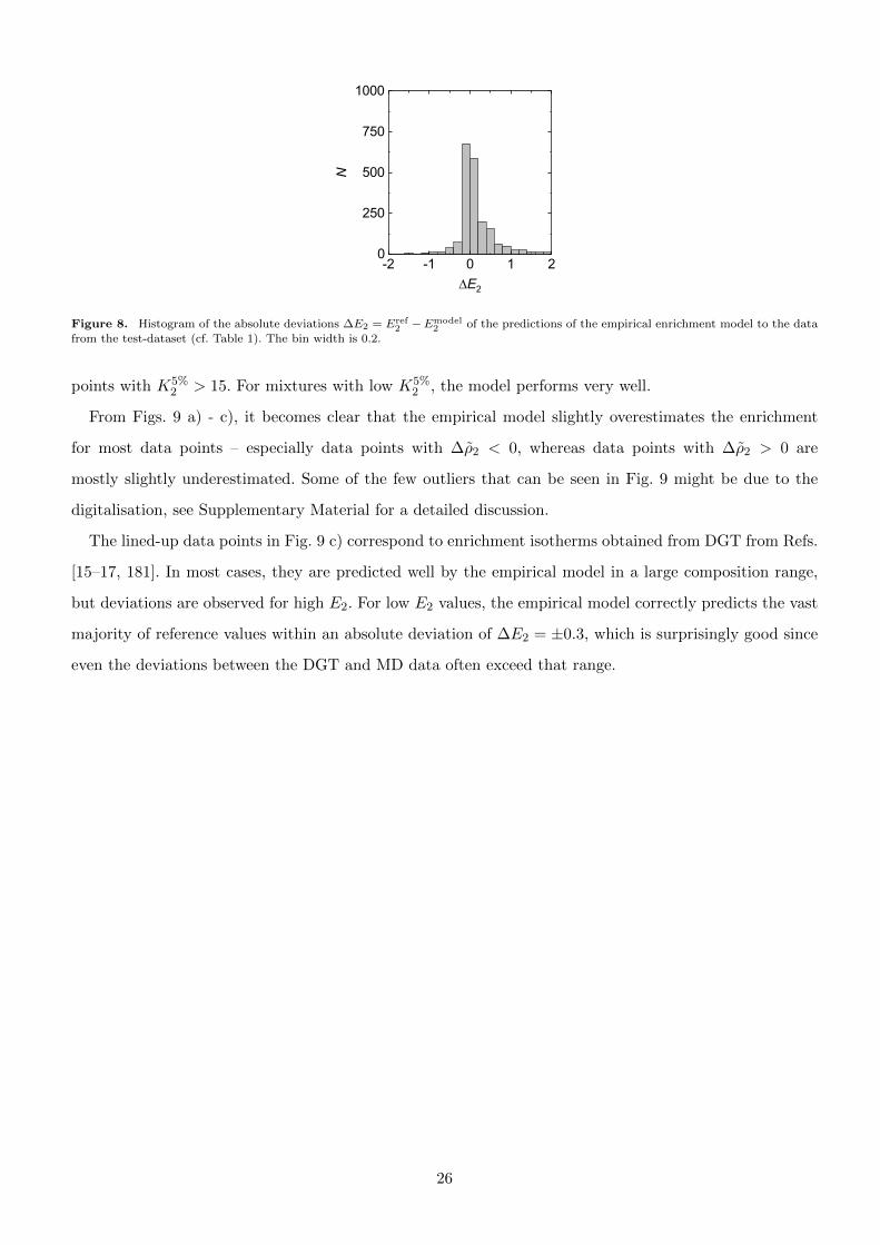
Fig. 8 shows the histogram of the absolute deviations of the enrichment predicted from the empiri-

cal model Emodel2 and the reference values Eref

2 from the test-dataset. The absolute average deviation is

AADE2= 16.1%, which is astonishingly low considering the fact that the empirical model was trained to

an MD dataset based on purely dispersively interacting fluids, whereas the test-dataset contains a large va-

riety of molecular interactions, mixture types, and employed methods. 84% of the data points are described

within an absolute deviation of ∆E2 = ±0.5 by the empirical model. Hence, the empirical model predicts

the enrichment of a low-boiling component E2 practically within the uncertainty of the determination of

E2 with different theoretical methods. However, as found for the performance on the training-dataset, the

empirical model shows a trend to slightly overestimate the enrichment.

The performance of the model predictions are analysed in more detail in Fig. 9, which shows the deviation

plots for E2 predicted by the empirical model and the values from the test-dataset. Its layout is analogue

to that of Fig. 6. Fig. 9 a) shows the absolute deviation ∆E2 as a function of the partition coefficient K5%2 ;

Fig. 9 b) shows ∆E2 as a function of the liquid phase concentration x′2; and Fig. 9 c) shows the absolute

deviation ∆E2 as a function of the enrichment E2 itself. Absolute deviations ∆E2 > 1 are mainly found

for large partition coefficients K5%2 , low x′2, and large E2, which is attributed to simplifications in the term

fb in the empirical model. Also, this is likely due to the fact that the training-dataset has only a relatively

small amount of data points at large K5%2 > 12 and the fact that the model was applied to predict data

25

-2 -1 0 1 20

250

500

750

1000

N

DE2

Figure 8. Histogram of the absolute deviations ∆E2 = Eref2 −Emodel

2 of the predictions of the empirical enrichment model to the datafrom the test-dataset (cf. Table 1). The bin width is 0.2.

points with K5%2 > 15. For mixtures with low K5%

2 , the model performs very well.

From Figs. 9 a) - c), it becomes clear that the empirical model slightly overestimates the enrichment

for most data points – especially data points with ∆ρ2 < 0, whereas data points with ∆ρ2 > 0 are

mostly slightly underestimated. Some of the few outliers that can be seen in Fig. 9 might be due to the

digitalisation, see Supplementary Material for a detailed discussion.

The lined-up data points in Fig. 9 c) correspond to enrichment isotherms obtained from DGT from Refs.

[15–17, 181]. In most cases, they are predicted well by the empirical model in a large composition range,

but deviations are observed for high E2. For low E2 values, the empirical model correctly predicts the vast

majority of reference values within an absolute deviation of ∆E2 = ±0.3, which is surprisingly good since

even the deviations between the DGT and MD data often exceed that range.

26

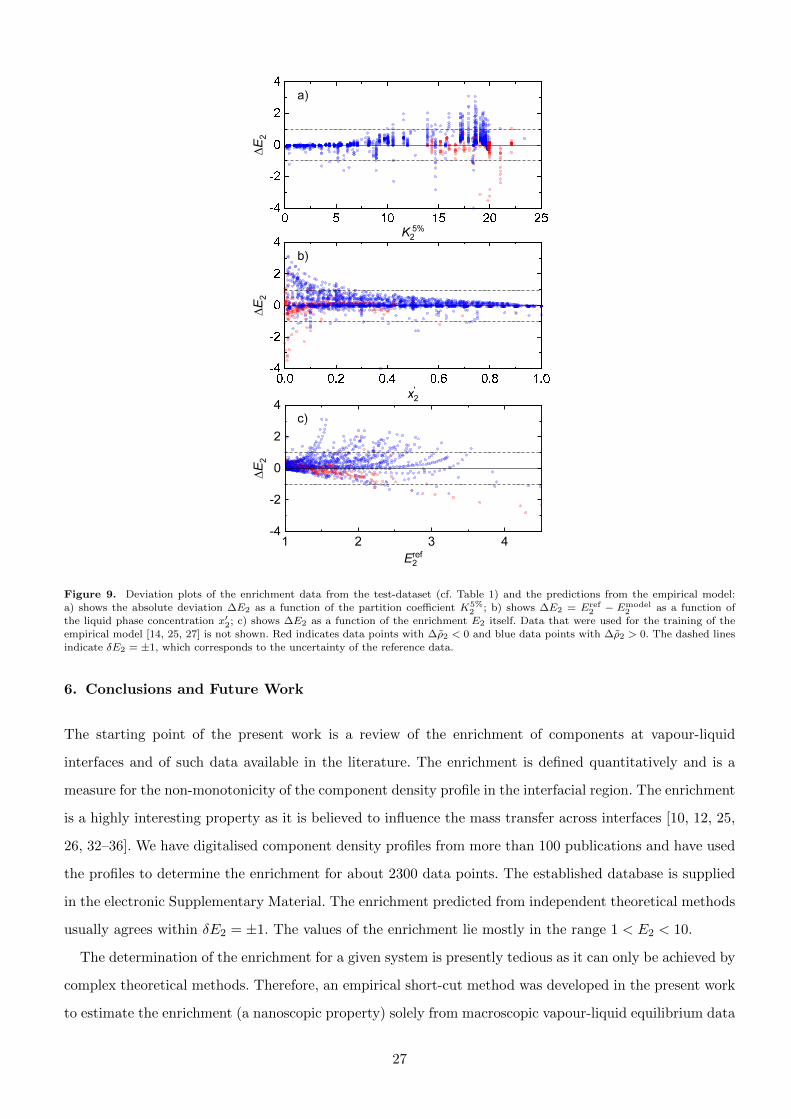
Figure 9. Deviation plots of the enrichment data from the test-dataset (cf. Table 1) and the predictions from the empirical model:

a) shows the absolute deviation ∆E2 as a function of the partition coefficient K5%2 ; b) shows ∆E2 = Eref

2 − Emodel2 as a function of

the liquid phase concentration x′2; c) shows ∆E2 as a function of the enrichment E2 itself. Data that were used for the training of theempirical model [14, 25, 27] is not shown. Red indicates data points with ∆ρ2 < 0 and blue data points with ∆ρ2 > 0. The dashed lines

indicate δE2 = ±1, which corresponds to the uncertainty of the reference data.

6. Conclusions and Future Work

The starting point of the present work is a review of the enrichment of components at vapour-liquid

interfaces and of such data available in the literature. The enrichment is defined quantitatively and is a

measure for the non-monotonicity of the component density profile in the interfacial region. The enrichment

is a highly interesting property as it is believed to influence the mass transfer across interfaces [10, 12, 25,

26, 32–36]. We have digitalised component density profiles from more than 100 publications and have used

the profiles to determine the enrichment for about 2300 data points. The established database is supplied

in the electronic Supplementary Material. The enrichment predicted from independent theoretical methods

usually agrees within δE2 = ±1. The values of the enrichment lie mostly in the range 1 < E2 < 10.

The determination of the enrichment for a given system is presently tedious as it can only be achieved by

complex theoretical methods. Therefore, an empirical short-cut method was developed in the present work

to estimate the enrichment (a nanoscopic property) solely from macroscopic vapour-liquid equilibrium data

27

for a given mixture. The database on the enrichment data established in the present work was therefore split

into a training-set and a test-set. The training-set consists of data from comprehensive studies on binary

Lennard-Jones mixtures [14, 25, 27] (approximately 300 data points). The test-set contains all remaining

data on the enrichment available in the literature (approximately 2000 data points). The empirical model

describes the enrichment of the training-dataset with an AAD of 6.5%. The vast majority of data points

is described by the empirical model with an error of ∆E2 = ±0.5, which is well below the uncertainty of

the reference data. Applying the empirical model on the test-dataset yields an AAD of 16.1%, whereat

84% of the data points are described within ∆E2 = ±0.5. This is remarkable considering the fact that the

enrichment model characterises a mixture only by its partition coefficient at x′2 = 0.05 mol mol−1 K5%2 and

the density difference in the bulk phases ∆ρ2 = ρ′2−ρ′′2 of the low-boiling component 2. Moreover, for ∆ρ2,

basically only the sign has to be known. As further input for the model only the liquid phase concentration

x′2 is needed. The model gets its information on the temperature only indirectly, through the specification

of K5%2 , which depends on the temperature. Hence, the model is designed in a way that the enrichment can

be computed from the bulk compositions and densities solely, which is available in thermophysical property

databases for a large number of systems.

For future work, it would be interesting to extend the dataset employed for the training of the model to

systems with K5%2 > 15, i.e. particularly wide-boiling phase behaviour, comprising mixtures with ∆ρ2 > 0

and ∆ρ2 < 0 as well as azeotropic systems. Furthermore, the performance of the model could probably be

further improved by extending the model such that information on the critical composition or the three-

phase equilibrium (if present) are incorporated. However, this would have the drawback that such data is

not as readily available for most mixtures.

Finally, we would like to emphasise that it would be desirable that data on density profiles or profiles

of other thermodynamic properties in interfacial regions, which is obtained by costly simulations, should

be reported electronically. This has often not been the case in the past such that the vast majority of the

corresponding data that has been obtained in previous studies by expensive simulations is now lost for the

community.

Based on the developed enrichment model, it was shown, that the nanoscopic enrichment is closely linked

to the macroscopic phase behaviour. This knowledge can be used for the screening of systems to identify

mixtures with large enrichment.

28

Acknowledgements

Appendix – Definition of the Relative Adsorption

The relative adsorption Γ(1)2 characterises – as the enrichment E2 – the surface excess of a low-boiling

component on a vapour-liquid interface. It can be computed from the macroscopic and the nanoscopic

definition. The first approach follows the Gibbs adsorption equation, which relates the relative adsorption

to the dependency of the surface tension of the chemical potential [77]. The relative adsorption Γ(1)2 is

thereby defined as

Γ(1)2 = −

(∂γ

∂µ2

)T

, (10)

where µ2 is the chemical potential of component 2 in the equilibrated phases. Hence, the relative adsorption

can be obtained from the experimental surface tension data in combination with a thermodynamic model

for the bulk phases.

The nanoscopic definition relates the relative adsorption to the component density profiles ρi(z) at a

fluid interface (with high-boiling and low-boiling component i = 1, 2, respectively). Γ(1)2 can be computed

by the symmetric interface segregation according to Telo da Gama and Evans [10]

Γ(1)2 = −

(ρ′2 − ρ′′2

) ∫ ∞−∞

[ρ1(z)− ρ′1ρ′1 − ρ′′1

− ρ2(z)− ρ′2ρ′2 − ρ′′2

]dz , (11)

where ρ′1, ρ′′1 and ρ′2, ρ′′2 are the component densities at saturation in the two coexisting bulk phases ′ and

′′, respectively.

Disclosure statement

No potential conflict of interest was reported by the authors.

Funding

This work was supported by the European Research Council under the Advanced Grant ENRICO [No.

694807].

29

References

[1] Andersson G, Krebs T, Morgner H. Activity of surface active substances determined from their surface excess.

Physical Chemistry Chemical Physics. 2005;7(1):136.

[2] Ishiyama T, Morita A, Miyamae T. Surface structure of sulfuric acid solution relevant to sulfate aerosol:

Molecular dynamics simulation combined with sum frequency generation measurement. Physical Chemistry

Chemical Physics. 2011;13(47):20965.

[3] Saito K, Peng Q, Qiao L, Wang L, Joutsuka T, Ishiyama T, Ye S, Morita A. Theoretical and experimental

examination of SFG polarization analysis at acetonitrile-water solution surfaces. Physical Chemistry Chemical

Physics. 2017;19(13):8941–8961.

[4] Gopalakrishnan S, Liu D, Allen HC, Kuo M, Shultz MJ. Vibrational spectroscopic studies of aqueous interfaces:

Salts, acids, bases, and nanodrops. Chemical Reviews. 2006;106(4):1155–1175.

[5] Shultz MJ, Schnitzer C, Simonelli D, Baldelli S. Sum frequency generation spectroscopy of the aqueous interface:

Ionic and soluble molecular solutions. International Reviews in Physical Chemistry. 2000;19(1):123–153.

[6] Stocco A, Tauer K. High-resolution ellipsometric studies on fluid interfaces. The European Physical Journal E.

2009;30(4):431.

[7] Telo da Gama MM, Evans R. Theory of the liquid-vapour interface of a binary mixture of Lennard-Jones fluids.

Molecular Physics. 1980;41(5):1091–1112.

[8] Carey BS, Scriven LE, Davis HT. Semiempirical theory of surface tension of binary systems. AIChE Journal.

1980;26(5):705–711.

[9] Falls AH, Scriven LE, Davis HT. Adsorption, structure, and stress in binary interfaces. The Journal of Chemical

Physics. 1983;78(12):7300–7317.

[10] Telo da Gama MM, Evans R. The structure and surface tension of the liquid-vapour interface near the upper

critical end point of a binary mixture of Lennard-Jones fluids I. the two phase region. Molecular Physics. 1983;

48(2):229–250.

[11] Telo da Gama MM, Evans R. The structure and surface tension of the liquid-vapour interface near the upper

critical end point of a binary mixture of Lennard-Jones fluids II. the three phase region and the Cahn wetting

transition. Molecular Physics. 1983;48(2):251–266.

[12] Lee DJ, Telo da Gama MM, Gubbins KE. The vapour-liquid interface for a Lennard-Jones model of argon-

krypton mixtures. Molecular Physics. 1984;53(5):1113–1130.

[13] Lee DJ, Telo da Gama MM, Gubbins KE. Adsorption and surface tension reduction at the vapor-liquid interface.

The Journal of Physical Chemistry. 1985;89(8):1514–1519.

[14] Stephan S, Hasse H. Molecular interactions at vapor-liquid interfaces: Binary mixtures of simple fluids. Physical

Review E. 2020;101:012802.

[15] Stephan S, Becker S, Langenbach K, Hasse H. Vapor-liquid interfacial properties of the binary system cyclo-

hexane + CO2: Experiment, molecular simulation and density gradient theory. Fluid Phase Equilibria. 2020;

518:112583.

30

[16] Werth S, Kohns M, Langenbach K, Heilig M, Horsch M, Hasse H. Interfacial and bulk properties of vapor-

liquid equilibria in the system toluene+hydrogen chloride+carbon dioxide by molecular simulation and density

gradient theory + PC-SAFT. Fluid Phase Equilibria. 2016;427:219.

[17] Becker S, Werth S, Horsch M, Langenbach K, Hasse H. Interfacial tension and adsorption in the binary

system ethanol and carbon dioxide: Experiments, molecular simulation and density gradient theory. Fluid

Phase Equilibria. 2016;427:476.

[18] Muller EA, Mejıa A. Interfacial properties of selected binary mixtures containing n-alkanes. Fluid Phase Equi-

libria. 2009;282(2):68–81.

[19] Mıguez JM, Garrido JM, Blas FJ, Segura H, Mejıa A, Pineiro MM. Comprehensive characterization of interfacial

behavior for the mixture CO2 + H2O + CH4: Comparison between atomistic and coarse grained molecular

simulation models and density gradient theory. The Journal of Physical Chemistry C. 2014;118(42):24504–

24519.

[20] Mejıa A, Cartes M, Segura H, Muller EA. Use of equations of state and coarse grained simulations to com-

plement experiments: Describing the interfacial properties of carbon dioxide + decane and carbon dioxide +

eicosane mixtures. Journal of Chemical & Engineering Data. 2014;59(10):2928.

[21] Ghobadi AF, Elliott JR. Adapting SAFT-γ perturbation theory to site-based molecular dynamics simulation.

II. confined fluids and vapor-liquid interfaces. The Journal of Chemical Physics. 2014;141(2):024708.

[22] Miqueu C, Miguez JM, Pineiro MM, Lafitte T, Mendiboure B. Simultaneous application of the gradient theory

and Monte Carlo molecular simulation for the investigation of methane/water interfacial properties. The Journal

of Physical Chemistry B. 2011;115(31):9618–9625.

[23] Choudhary N, Nair AKN, Ruslan MFAC, Sun S. Bulk and interfacial properties of decane in the presence of

carbon dioxide, methane, and their mixture. Scientific Reports. 2019;9(1):1–10.

[24] Mejıa A, Pamies JC, Duque D, Segura H, Vega LF. Phase and interface behaviors in type-I and type-V

Lennard-Jones mixtures: Theory and simulations. The Journal of Chemical Physics. 2005;123(3):034505.

[25] Stephan S, Langenbach K, Hasse H. Interfacial properties of binary Lennard-Jones mixtures by molecular

simulations and density gradient theory. The Journal of Chemical Physics. 2019;150(17):174704.

[26] Stephan S, Langenbach K, Hasse H. Enrichment of components at vapour-liquid interfaces: A study by molec-

ular simulation and density gradient theory. Chemical Engineering Transactions. 2018;69:295–300.

[27] Stephan S, Hasse H. Interfacial properties of binary mixtures of simple fluids and their relation to the phase

diagram. Physical Chemistry Chemical Physics. 2020;22(22):12544–12564.

[28] Carey B. The gradient theory of fluid interfaces [dissertation]. Minneapolis: University of Minnesota; 1979.

[29] Cornelisse PM. The square gradient theory applied simultaneous modelling of interfacial tension and phase

behaviour [dissertation]. Technische Universiteit Delft; 1997.

[30] Miqueu C, Mendiboure B, Graciaa C, Lachaise J. Modelling of the surface tension of binary and ternary

mixtures with the gradient theory of fluid interfaces. Fluid Phase Equilibria. 2004;218(2):189–203.

[31] Enders S, Quitzsch K. Calculation of interfacial properties of demixed fluids using density gradient theory.

Langmuir. 1998;14(16):4606–4614.

31

[32] Klink C, Gross J. A density functional theory for vapor-liquid interfaces of mixtures using the perturbed-chain

polar statistical associating fluid theory equation of state. Industrial & Engineering Chemistry Research. 2014;

53(14):6169.

[33] Nagl R, Zimmermann P, Zeiner T. Interfacial mass transfer in water-toluene systems. Journal of Chemical &

Engineering Data. 2020;65(2):328–336.

[34] Garrido JM, Pineiro MM, Mejıa A, Blas FJ. Understanding the interfacial behavior in isopycnic Lennard-Jones

mixtures by computer simulations. Physical Chemistry Chemical Physics. 2016;18:1114–1124.

[35] Enders S, Kahl H. Interfacial properties of water + alcohol mixtures. Fluid Phase Equilibria. 2008;263(2):160–

167.

[36] Karlsson B, Friedman R. Dilution of whisky – the molecular perspective. Scientific Reports. 2017;7(6489):1–9.

[37] Chang TM, Peterson KA, Dang LX. Molecular dynamics simulations of liquid, interface, and ionic solvation of

polarizable carbon tetrachloride. The Journal of Chemical Physics. 1995;103(17):7502–7513.

[38] Ishiyama T, Morita A. Molecular dynamics analysis of interfacial structures and sum frequency generation

spectra of aqueous hydrogen halide solutions. The Journal of Physical Chemistry A. 2007;111(38):9277–9285.

[39] Ishiyama T, Morita A. Molecular dynamics study of gas-liquid aqueous sodium halide interfaces. I. flexible

and polarizable molecular modeling and interfacial properties. The Journal of Physical Chemistry C. 2007;

111(2):721–737.

[40] Imamura T, Mizukoshi Y, Ishiyama T, Morita A. Surface structures of NaF and Na2SO4 aqueous solu-

tions: Specific effects of hard ions on surface vibrational spectra. The Journal of Physical Chemistry C. 2012;

116(20):11082–11090.

[41] Perez-Blanco ME, Maginn EJ. Molecular dynamics simulations of CO2 at an ionic liquid interface: Adsorption,

ordering, and interfacial crossing. The Journal of Physical Chemistry B. 2010;114(36):11827–11837.

[42] Perez-Blanco ME, Maginn EJ. Molecular dynamics simulations of carbon dioxide and water at an ionic liquid

interface. The Journal of Physical Chemistry B. 2011;115(35):10488–10499.

[43] Nguyen CV, Nakahara H, Shibata O, Phan CM. Adsorption of sodium iodine at air/water interface. Journal

of Molecular Liquids. 2020;298:112076.

[44] Moghimikheirabadi A, Sagis LMC, Kroger M, Ilg P. Gas-liquid phase equilibrium of a model langmuir monolayer

captured by a multiscale approach. Physical Chemistry Chemical Physics. 2019;21(5):2295–2306.

[45] Liu ZY, Wang C, Zhou H, Wang Y, Zhang L, Zhang L, Zhao S. Characterizing the impact of surfactant

structure on interfacial tension: a molecular dynamics study. Journal of Molecular Modeling. 2017;23(4):112.

[46] Liu ZY, Wei N, Wang C, Zhou H, Zhang L, Liao Q, Zhang L. Interfacial assignment of branched-alkyl benzene

sulfonates: A molecular simulation. AIP Advances. 2015;5(11):117203.

[47] Hantal G, Partay LB, Varga I, Jedlovszky P, Gilanyi T. Counterion and surface density dependence of the

adsorption layer of ionic surfactants at the vapor-aqueous solution interface: A computer simulation study. The

Journal of Physical Chemistry B. 2007;111(7):1769–1774.

[48] Moghimikheirabadi A, Ilg P, Sagis LMC, Kroger M. Surface rheology and structure of model triblock copolymers

at a liquid-vapor interface: A molecular dynamics study. Macromolecules. 2020;53(4):1245–1257.

32

[49] Kim HY, Fichthorn KA. Molecular dynamics simulation of amphiphilic dimers at a liquid-vapor interface. The

Journal of Chemical Physics. 2005;122(3):034704.

[50] Kruber KF, Krapoth M, Zeiner T. Interfacial mass transfer in ternary liquid-liquid systems. Fluid Phase

Equilibria. 2017;440:54–63.

[51] Kulaguin-Chicaroux A, Zeiner T. Interfacial behavior of aqueous two-phase systems based on linear and hy-

perbranched polymers. Journal of Chemical & Engineering Data. 2018;63(7):2467–2476.

[52] Buhn JB, Bopp PA, Hampe MJ. A molecular dynamics study of a liquid-liquid interface: Structure and dy-

namics. Fluid Phase Equilibria. 2004;224(2):221–230.

[53] Choi JS, Bae YC. Phase equilibrium and interfacial tension of binary and ternary polymer solutions. Journal

of Chemical & Engineering Data. 2016;61(12):4157–4163.

[54] Telo da Gama MM, Thurtell JH. Interfacial phase transitions in molecular fluids and multicomponent mixtures.

J Chem Soc, Faraday Trans 2. 1986;82:1721–1737.

[55] Ghoufi A, Malfreyt P, Tildesley DJ. Computer modelling of the surface tension of the gas-liquid and liquid-

liquid interface. Chemical Society Reviews. 2016;45:1387–1409.

[56] Lamorgese A, Mauri R, Sagis L. Modeling soft interface dominated systems: A comparison of phase field and

Gibbs dividing surface models. Physics Reports. 2017;675:1–54.

[57] Rowlinson JS, Widom B. Molecular theory of capillarity. New York: Dover Publications; 1982.

[58] Evans R. The nature of the liquid-vapour interface and other topics in the statistical mechanics of non-uniform,

classical fluids. Advances in Physics. 1979;28(2):143–200.

[59] Evans R. Fundamentals of inhomogeneous fluids. New York: Marcel Dekker; 1992.

[60] Evans R, Henderson JR, Hoyle DC, Parry AO, Sabeur ZA. Asymptotic decay of liquid structure: Oscillatory

liquid-vapour density profiles and the Fisher-Widom line. Molecular Physics. 1993;80(4):755–775.

[61] Evans R. Oscillatory behaviour of density profiles: Relevance for fluid interfacial phenomena. Berichte der

Bunsengesellschaft fur physikalische Chemie. 1994;98(3):345–352.

[62] Stephan S, Liu J, Langenbach K, Chapman WG, Hasse H. Vapor-liquid interface of the Lennard-Jones truncated

and shifted fluid: Comparison of molecular simulation, density gradient theory, and density functional theory.

The Journal of Physical Chemistry C. 2018;122(43):24705–24715.

[63] Geysermans P, Elyeznasni N, Russier V. Layered interfaces between immiscible liquids studied by density-

functional theory and molecular-dynamics simulations. The Journal of Chemical Physics. 2005;123(20):204711.

[64] Toxvaerd S, Stecki J. Density profiles at a planar liquid-liquid interface. The Journal of Chemical Physics.

1995;102(18):7163–7168.

[65] Dıaz-Herrera E, Alejandre J, Ramırez-Santiago G, Forstmann F. Interfacial tension behavior of binary and

ternary mixtures of partially miscible Lennard-Jones fluids: A molecular dynamics simulation. The Journal of

Chemical Physics. 1999;110(16):8084–8089.

[66] Napari I, Laaksonen A, Talanquer V, Oxtoby DW. A density functional study of liquid-liquid interfaces in

partially miscible systems. The Journal of Chemical Physics. 1999;110(12):5906–5912.

[67] Martinez-Ruiz FJ, Moreno-Ventas Bravo AI, Blas FJ. Liquid-liquid interfacial properties of a symmetrical

33

Lennard-Jones binary mixture. The Journal of Chemical Physics. 2015;143(10):104706.

[68] Brown JR, Seo Y, Maula TAD, Hall LM. Fluids density functional theory and initializing molecular dynamics

simulations of block copolymers. The Journal of Chemical Physics. 2016;144(12):124904.

[69] Winkelmann J. The liquid-vapour interface of pure fluids and mixtures: Application of computer simulation

and density functional theory. Journal of Physics: Condensed Matter. 2001;13(21):4739.

[70] Rehner P, Gross J. Predictive density gradient theory based on nonlocal density functional theory. Physical

Review E. 2018;98:063312.

[71] Buhl C, Enders S. Prediction of interfacial properties of ternary, sulfur-containing mixtures. Journal of Chemical

& Engineering Data. 2016;61(12):4261–4269.

[72] Mohammed S, Mansoori GA. Molecular insights on the interfacial and transport properties of supercritical

CO2/brine/crude oil ternary system. Jorunal of Molecular Liquids. 2018;218:268–273.

[73] Mohammed S, Mansoori G. Effect of CO2 on the interfacial and transport properties of water/binary and

asphaltenic oils: Insights from molecular dynamics. Energy & Fuels. 2018;32(4):5409–5417.

[74] Herdes C, Totton TS, Muller EA. Coarse grained force filed for the molecular simulation of natural gases and

condensates. Fluid Phase Equilibria. 2015;406:91–100.

[75] Mairhofer J, Gross J. Modeling of interfacial properties of multicomponent systems using density dradient

theory and PCP-SAFT. Fluid Phase Equilibria. 2017;439:31.

[76] Telo da Gama MM, Evans R. Surface segregation and surface tension at the liquid-vapour interface of a binary

mixture of Lennard-Jones fluids. Faraday Symposia of The Chemical Society. 1981;16:45–58.

[77] Defay R, Prigogine I, Bellmans A, Everett DH. Surface tension and adsorption. London: Longmans; 1966.

[78] Baidakov VG, Khotienkova MN. Surface tension of methane-nitrogen solutions: 2. description in the framework

of the van der Waals gradient theory. Fluid Phase Equilibria. 2016;425:402–410.

[79] Lafitte T, Mendiboure B, Pineiro MM, Bessieres D, Miqueu C. Interfacial properties of water/CO2: A compre-

hensive description through a gradient theory SAFT-VR Mie approach. The Journal of Physical Chemistry B.

2010;114(34):11110–11116.

[80] Mecke M, Winkelmann J, Fischer J. Molecular dynamics simulation of the liquid-vapor interface: Binary mix-

tures of Lennard-Jones fluids. The Journal of Chemical Physics. 1999;110(2):1188–1194.

[81] Baidakov VG, Protsenko SP. Molecular-dynamics investigation of phase equilibrium and surface tension in

argon-neon system. The Journal of Physical Chemistry C. 2008;112(44):17231–17234.

[82] Pereira LM, Chapoy A, Burgass R, Tohidi B. Measurement and modelling of high pressure density and inter-

facial tension of (gas + n-alkane) binary mixtures. The Journal of Chemical Thermodynamics. 2016;97:55–69.

[83] Algaba J, Cartes M, A M, Miguez JM, Blas FJ. Phase equilibria and interfacial properties of the tetrahydrofuran

+ methane binary mixture from experiment and computer simulation. The Journal of Physical Chemistry C.

2019;123(34):20960–20970.

[84] Wadewitz T, Winkelmann J. Density functional theory: Structure and interfacial properties of binary mixtures.

Berichte der Bunsengesellschaft fur physikalische Chemie. 1996;100(11):1825–1832.

[85] Teixeira PIC, Almeida BS, Telo da Gama MM, Rueda JA, Rubio RG. Interfacial properties of mixtures of

34

molecular fluids: comparison between theory and experiment; methyl iodide + carbon tetrachloride and ace-

tonitrile + carbon tetrachloride. The Journal of Physical Chemistry. 1992;96(21):8488–8497.

[86] Aracil J, Luengo G, Almeida BS, Telo da Gama MM, Rubio RG, Diaz Pena M. Surface properties of mixtures

of molecular fluids: an experimental and theoretical study of carbon disulfide + dichloromethane and carbon

disulfide + carbon tetrachloride. The Journal of Physical Chemistry. 1989;93(8):3210–3218.

[87] Liu B, Shi J, Wang M, Zhang J, Sun B, Shen Y, Sun X. Reduction in interfacial tension of water–oil interface by

supercritical CO2 in enhanced oil recovery processes studied with molecular dynamics simulation. The Journal

of Supercritical Fluids. 2016;111:171–178.

[88] Miqueu C, Mendiboure B, Graciaa A, Lachaise J. Modeling of the surface tension of multicomponent mixtures

with the gradient theory of fluid interfaces. Industrial & Engineering Chemistry Research. 2005;44(9):3321–

3329.

[89] Herdes C, Ervik A, Mejıa A, Muller EA. Prediction of the water/oil interfacial tension from molecular simula-

tions using the coarse-grained SAFT-γ Mie force field. Fluid Phase Equilibria. 2018;476:9–15.

[90] Zambrano HA, Walther JH, Jaffe RL. Molecular dynamics simulations of water on a hydropholic silicia surface

at high air pressures. Journal of Molecular Liquids. 2014;198:107–113.

[91] Telo da Gama MM. Phase equilibria and interfacial properties of model ternary mixtures. Molecular Physics.

1987;62(3):585–604.

[92] Kou J, Sun S, Wang X. Efficient numerical methods for simulating surface tension of multi-component mixtures

with the gradient theory of fluid interfaces. Computer Methods in Applied Mechanics and Engineering. 2015;

292:92–106.

[93] Miqueu C, Mendiboure B, Graciaa A, Lachaise J. Petroleum mixtures: An efficient predictive method for

surface tension estimations at reservoir conditions. Fuel. 2008;87(6):612–621.

[94] Rohatgi A. Webplotdigitizer ; 2019. Used december 2019; Available from: https://automeris.io/

WebPlotDigitizer.

[95] Nino-Amezquita OG. Interfacial properties and phase equilibria for mixtures relevant in the oil industry [dis-

sertation]. TU Berlin; 2013. Available from: https://depositonce.tu-berlin.de/bitstream/11303/4321/

1/nino%20amezquita_oscar%20gabriel.pdf.

[96] Nino-Amezquita OG, Enders S. Prediction of interfacial tension of binary mixtures. In: Pierucci S, Ferraris GB,

editors. 20th european symposium on computer aided process engineering. (Computer Aided Chemical Engi-

neering; Vol. 28). Elsevier; 2010. p. 85–90.

[97] Llovell F, Dowell NM, Blas FJ, Galindo A, Jackson G. Application of the SAFT-VR density functional theory

to the prediction of the interfacial properties of mixtures of relevance to reservoir engineering. Fluid Phase

Equilibria. 2012;336(Supplement C):137–150.

[98] Sahimi M, Taylor BN. Surface tension of binary liquid-vapor mixtures: A comparison of mean-field and scaling

theories. The Journal of Chemical Physics. 1991;95(9):6749–6761.

[99] Liu ST, Fu D, Lu JY. Investigation of bulk and interfacial properties for nitrogen and light hydrocarbon

binary mixtures by perturbed-chain statistical associating fluid theory combined with density-gradient theory.

35

Industrial & Engineering Chemistry Research. 2009;48(23):10734–10739.

[100] Garrido JM, Cartes M, Mejıa A. Coarse-grained theoretical modeling and molecular simulations of nitrogen +

n-alkanes: (n-pentane, n-hexane, n-heptane, n-octane). The Journal of Supercritical Fluids. 2017;129:83–90.

[101] Buhl C, Danzer A, Enders S. Prediction of surface properties of binary, sulfur containing mixtures. Fluid Phase

Equilibria. 2016;416:94–103.

[102] Lobanova O, Mejıa A, Jackson G, Muller EA. SAFT-i force field for the simulation of molecular fluids 6: Binary

and ternary mixtures comprising water, carbon dioxide, and n-alkanes. The Journal of Chemical Thermody-

namics. 2016;93:320–336.

[103] Li W, Jin Z. Molecular dynamics simulation of natural gas-water interfacial tensions over wide range of pres-

sures. Fuel. 2019;236:480–492.

[104] Naeiji P, Woo T, Alavi S, Varaminian F, Ohmura R. Interfacial properties of hydrocarbon/water systems

predicted by molecular dynamic simulations. Journal of Chemical Physics. 2019;150(11):114703.

[105] Khosharay S, Rezakhani N. Using a new proposed influence parameter of gradient theory for CH4/n-alkane

binary systems: What advances can be achieved? Periodica Polytechnica Chemical Engineering. 2016;60(4):282–

289.

[106] Nino-Amezquita OG, van Putten D, Enders S. Phase equilibrium and interfacial properties of water+CO2

mixtures. Fluid Phase Equilibria. 2012;332:40.

[107] Chow YTF, Eriksen DK, Galindo A, Haslam AJ, Jackson G, Maitland GC, Trusler JP. Interfacial tensions

of systems comprising water, carbon dioxide and diluent gases at high pressures: Experimental measurements

and modelling with SAFT-VR Mie and square-gradient theory. Fluid Phase Equilibria. 2016;407:159–176.

[108] Li XS, Liu JM, Fu D. Investigation of interfacial tensions for carbon dioxide aqueous solutions by perturbed-

chain statistical associating fluid theory combined with density-gradient theory. Industrial & Engineering Chem-

istry Research. 2008;47(22):8911–8917.

[109] Biscay F, Ghoufi A, Lachet V, Malfreyt P. Monte Carlo simulations of the pressure dependence of the water-acid

gas interfacial tensions. The Journal of Physical Chemistry B. 2009;113(43):14277–14290.

[110] Neyt JC, Wender A, Lachet V, Malfreyt P. Modeling the pressure dependence of acid gas + n-alkane interfacial

tensions using atomistic Monte Carlo simulations. Journal of Physical Chemistry. 2012;116(19):10563–10572.

[111] Chen C, Hu W, Li W, Song Y. Model comparison of the CH4/CO2/water system in predicting dynamic and

interfacial properties. Journal of Chemical Engineering Data. 2019;64:2464–2474.

[112] Fouad WA, Vega LF. The phase and interfacial properties of azeotropic refrigerants: the prediction of aneotropes

from molecular theory. Physical Chemistry Chemical Physics. 2017;19:8977–8988.

[113] Li Y, Fouad WA, Vega LF. Interfacial anomaly in low global warming potential refrigerant blends as predicted

by molecular dynamics simulations. Physical Chemistry Chemical Physics. 2019;21(39):22092–22102.

[114] Vilaseca O, Llovell F, Yustos J, Marcos RM, Vega LF. Phase equilibria, surface tensions and heat capacities of

hydrofluorocarbons and their mixtures including the critical region. The Journal of Supercritical Fluids. 2010;

55(2):755–768.

[115] Khosharay S, Mazraeno MS, Varaminian F, Bagheri A. A proposed combination model for predicting surface

36

tension and surface properties of binary refrigerant mixtures. International Journal of Refrigeration. 2014;

40:347–361.

[116] Zeng XC, Oxtoby DW. Binary homogeneous nucleation theory for the gas-liquid transition: A nonclassical

approach. The Journal of Chemical Physics. 1991;95(8):5940–5947.

[117] Horvath RA, Fabian B, Szori M, Jedlovszky P. Investigation of the liquid-vapour interface of aqueous methy-

lamine solutions by computer simulation methods. Journal of Molecular Liquids. 2019;288:110978.

[118] Fabian B, Szori M, Jedlovszky P. Floating patches of HCN at the surface of their aqueous solutions – can they

make “HCN world” plausible? The Journal of Physical Chemistry C. 2014;118(37):21469–21482.

[119] Mucha M, Hrobarik T, Jungwirth P. Surface tension from molecular dynamics simulation: Adsorption at the

gas-liquid interface. Israel Journal of Chemistry. 2003;43(3-4):393–397.

[120] Koller TM, Yan S, Steininger C, Klein T, Froba AP. Interfacial tension and liquid viscosity of binary mixtures

of n-hexane, n-decane, or 1-hexanol with carbon dioxide by molecular dynamics simulations and surface light

scattering. International Journal of Thermophysics. 2019;40(8).

[121] Schafer E, Sadowski G, Enders S. Interfacial tension of binary mixtures exhibiting azeotropic behavior: Mea-

surement and modeling with PCP-SAFT combined with density gradient theory. Fluid Phase Equilibria. 2014;

362:151.

[122] Fu D, Hua X, Xu Y. Cross-association model for the phase equilibria and surface tensions of CO2-methanol

and CO2-ethanol mixtures. The Journal of Physical Chemistry C. 2011;115(8):3340–3345.

[123] Eckelsbach S, Vrabec J. Fluid phase interface properties of acetone, oxygen, nitrogen and their binary mixtures

by molecular simulation. Physical Chemistry Chemical Physics. 2015;17:27195–27203.

[124] Poser CI, Sanchez IC. Interfacial tension theory of low and high molecular weight liquid mixtures. Macro-

molecules. 1981;14(2):361–370.

[125] Shi W, Siefert NS, Morreale BD. Molecular simulations of CO2, H2, H2O, and H2S gas absorption into hydropho-

bic poly(dimethylsiloxane) (pdms) solvent: Solubility and surface tension. The Journal of Physical Chemistry

C. 2015;119(33):19253–19265.

[126] Telo da Gama MM, Evans R. The density profile and surface tension of a Lennard-Jones fluid from a generalized

van der Waals theory. Molecular Physics. 1979;38(2):367–375.

[127] Muller EA, Mejıa A. Resolving discrepancies in the measurements of the interfacial tension for the CO2 + H2O

mixture by computer simulation. The Journal of Physical Chemistry. 2014;5(7):1267–1271.

[128] Mu X, Frank F, Alpak FO, Chapman WG. Stabilized density gradient theory algorithm for modeling interfacial

properties of pure and mixed systems. Fluid Phase Equilibria. 2017;435:118–130.

[129] Breure B, Peters C. Modeling of the surface tension of pure components and mixtures using the density

gradient theory combined with a theoretically derived influence parameter correlation. Fluid Phase Equilibria.

2012;334:189–196.

[130] Cao F, Deetz JD, Sun H. Free energy-based coarse-grained force field for binary mixtures of hydrocarbons,

nitrogen, oxygen, and carbon dioxide. Journal of Chemical Information and Modeling. 2016;57(1):50–59.

[131] Baidakov VG, Protsenko SP, Bryukhanov VM. Relaxation processes at liquid-gas interfaces in one- and two-

37

component Lennard-Jones systems: Molecular dynamics simulation. Fluid Phase Equilibria. 2019;481:1–14.

[132] Duque D, Pamies JC, Vega LF. Interfacial properties of Lennard-Jones chains by direct simulation and density

gradient theory. The Journal of Chemical Physics. 2004;121(22):11395–11401.

[133] Garrido JM, Quinteros-Lama H, Pineiro MM, Mejıa A, Segura H. On the phase and interface behavior along

the three-phase line of ternary Lennard-Jones mixtures: A collaborative approach based on square gradient

theory and molecular dynamics simulations. The Journal of Chemical Physics. 2014;141(1):014503.

[134] Salomons E, Mareschal M. Atomistic simulation of liquid-vapour coexistence: Binary mixtures. Journal of

Physics: Condensed Matter. 1991;3(46):9215–9228.

[135] Salomons E, Mareschal M. Surface tension, adsorption and surface entropy of liquid-vapour systems by atomistic

simulation. Journal of Physics: Condensed Matter. 1991;3(20):3645–3661.

[136] Protsenko SP, Baidakov VG, Bryukhanov VM. Binary Lennard-Jones mixtures with highly asymmetric interac-

tions of the components. 2. effect of the particle size on phase equilibria and properties of liquid-gas interfaces.

Fluid Phase Equilibria. 2016;430:67–74.

[137] Protsenko SP, Baidakov VG. Binary Lennard-Jones mixtures with highly asymmetric interactions of the com-

ponents. 1. effect of the energy parameters on phase equilibria and properties of liquid-gas interfaces. Fluid

Phase Equilibria. 2016;429:242–253.

[138] Martinez-Ruiz FJ, Blas FJ. Interfacial properties of binary mixtures of square-well molecules from Monte Carlo

simulation. The Journal of Chemical Physics. 2016;144(15):154705.

[139] Mejıa A, Cartes M, Segura H. Interfacial tensions of binary mixtures of ethanol with octane, decane, dodecane,

and tetradecane. The Journal of Chemical Thermodynamics. 2011;43(9):1395–1400.

[140] Kahl H, Enders S. Interfacial properties of binary mixtures. Physical Chemistry Chemical Physics. 2002;4:931–

936.

[141] Nino-Amezquita OG, Enders S. Phase equilibrium and interfacial properties of water+methane mixtures. Fluid

Phase Equilibria. 2016;407:143–151.

[142] Stephan S, Hasse H. Influence of dispersive long-range interactions on properties of vapour-liquid interfaces of

binary Lennard-Jones mixtures. Molecular Physics. 2019;187:1–14.

[143] Llovell F, Galindo A, Blas FJ, Jackson G. Classical density functional theory for the prediction of the surface

tension and interfacial properties of fluids mixtures of chain molecules based on the statistical associating fluid

theory for potentials of variable range. The Journal of Chemical Physics. 2010;133(2):024704.

[144] Martinez-Ruiz FJ, Blas FJ, Moreno-Ventas Bravo AI, Miguez JM, MacDowell LG. Vapour-liquid interfacial

properties of square-well chains from density functional theory and Monte Carlo simulation. Physical Chemistry

Chemical Physics. 2017;19:12296–12309.

[145] Neyt JC, Wender A, Lachet V, Ghoufi A, Malfreyt P. Molecular modeling of the liquid-vapor interfaces of a

multi-component mixture: Prediction of the coexisting densities and surface tensions at different pressures and

gas compositions. The Journal of Chemical Physics. 2013;139(2):024701.

[146] Lin H, Duan YY, Min Q. Gradient theory modeling of surface tension for pure fluids and binary mixtures.

Fluid Phase Equilibria. 2007;254(1):75.

38

[147] Cornelisse PM, Peters CJ, de Swaan Arons J. Interfacial phase transitions at solid-fluid and liquid-vapor

interfaces. International Journal of Thermophysics. 1998;19(6):1501–1509.

[148] Eggimann BL, Sunnarborg AJ, Stern HD, Bliss AP, Siepmann JI. An online parameter and property database

for the TraPPE force field. Molecular Simulation. 2014;40(1-3):101–105.

[149] Stephan S, Horsch M, Vrabec J, Hasse H. MolMod - an open access database of force fields for molecular

simulations of fluids. Molecular Simulation. 2019;45(10):806–814.

[150] Rowlinson JS, Swinton FL. Liquids and liquid mixtures. London: Butterworth; 1982.

[151] Chapman WG, Gubbins KE, Jackson G, Radosz M. SAFT: Equation-of-state solution model for associating

fluids. Fluid Phase Equilibria. 1989;52:31–38.

[152] Muller EA, Gubbins KE. Molecular-based equations of state for associating fluids: A review of SAFT and

related approaches. Industrial & Engineering Chemistry Research. 2001;40(10):2193–2211.

[153] Gubbins KE. Perturbation theories of the thermodynamics of polar and associating liquids: A historical per-

spective. Fluid Phase Equilibria. 2016;416:3–17.

[154] Heier M, Stephan S, Liu J, Chapman WG, Hasse H, Langenbach K. Equation of state for the Lennard-Jones

truncated and shifted fluid with a cut-off radius of 2.5σ based on perturbation theory and its applications to

interfacial thermodynamics. Molecular Physics. 2018;116(15):2083–2094.

[155] Span R, Wagner W, Lemmon E, Jacobsen RT. Multiparameter equation of state - recent trends and future

challenges. Fluid Phase Equilibria. 2001;183-184:1.

[156] Span R. Multiparameter equations of state. Berlin: Springer; 2000.

[157] Stephan S, Staubach J, Hasse H. Review and comparison of equations of state for the Lennard-Jones fluid.

submitted. 2020;.

[158] Tardon MJ, Garrido JM, Quinteros-Lama H, Mejıa A, Segura H. Molar isopycnicity in heterogeneous binary

mixtures. Fluid Phase Equilibria. 2012;336:84–97.

[159] Schappals M, Mecklenfeld A, Kroger L, Botan V, Koster A, Stephan S, Garcia EJ, Rutkai G, Raabe G,

Klein P, Leonhard K, Glass CW, Lenhard J, Vrabec J, Hasse H. Round robin study: Molecular simulation

of thermodynamic properties from models with internal degrees of freedom. Journal of Chemical Theory and

Computation. 2017;13(9):4270–4280.

[160] Stephan S, Thol M, Vrabec J, Hasse H. Thermophysical properties of the Lennard-Jones fluid: Database and

data assessment. J Chem Inf Model. 2019;59(10):4248–4265.

[161] Abraham M, Apostolov R, Barnoud J, Bauer P, Blau C, Bonvin AM, Chavent M, Chodera J, Condic-Jurkic K,

Delemotte L, Grubmueller H, Howard RJ, Jordan EJ, Lindahl E, Ollila OHS, Selent J, Smith DGA, Stans-

feld PJ, Tiemann JK, Trellet M, Woods C, Zhmurov A. Sharing data from molecular simulations. Journal of

Chemical Information and Modeling. 2019;59(10):4093–4099.

[162] Loeffler HH, Bosisio S, Duarte Ramos Matos G, Suh D, Roux B, Mobley DL, Michel J. Reproducibility of free

energy calculations across different molecular simulation software packages. Journal of Chemical Theory and

Computation. 2018;14(11):5567–5582.

[163] van Gunsteren WF, Mark AE. Validation of molecular dynamics simulation. The Journal of Chemical Physics.

39

1998;108(15):6109–6116.

[164] Eckelsbach S, Janzen T, Koster A, Miroshnichenko S, Munoz-Munoz YM, Vrabec J. Molecular models for cyclic

alkanes and ethyl acetate as well as surface tension data from molecular simulation. In: Nagel WE, Kroner DH,

Resch MM, editors. High performance computing in science and engineering ‘14. Springer International Pub-

lishing; 2014. p. 645–659.

[165] Almeida BS, Telo da Gama MM. Surface tension of simple mixtures: comparison between theory and experi-

ment. The Journal of Physical Chemistry. 1989;93(10):4132–4138.

[166] Chang TM, Dang LX. Liquid-vapor interface of methanol-water mixtures: A molecular dynamics study. The

Journal of Physical Chemistry B. 2005;109(12):5759–5765.

[167] Cornelisse PM, Peters CJ, de Swaan Arons J. Simultaneous prediction of phase equilibria, interfacial tension

and concentration profiles. Molecular Physics. 1993;80(4):941–955.

[168] Cornelisse PM, Peters CJ, de Swaan Arons J. Application of the Peng-Robinson equation of state to calculate

interfacial tensions and profiles at vapour-liquid interfaces. Fluid Phase Equilibria. 1993;82:119–129.

[169] Greberg H, Paolini GV, Satherley J, Penfold R, Nordholm S. Generalized van der Waals theory of interfaces

in simple fluid mixtures. Journal of Colloid and Interface Science. 2001;235(2):334–343.

[170] Ibarra-Tandi B, Lira A, Lopez-Lemus J. Effect of softness on relative adsorption for binary mixtures of simple

fluids. Journal of Molecular Liquids. 2013;185:62–69.

[171] Kahl H, Mecke M, Winkelmann J. Prediction of internal structure and properties in fluid model interfaces of

binary and ternary liquid mixtures. Fluid Phase Equilibria. 2005;228-229:293–302.

[172] Khosharay S, Abolala M, Varaminian F. Modeling the surface tension and surface properties of CO2+H2O and

H2S+H2O with gradient theory in combination with sPC-SAFT EOS and a new proposed influence parameter.

Journal of Molecular Liquids. 2014;198(Supplement C):292–298.

[173] Khosharay S, Varaminian F. Experimental and modeling investigation on surface tension and surface properties

of (CH4 + H2O), (C2H6 + H2O), (CO2 + H2O) and (C3H8 + H2O) from 284.15 K to 312.15 K and pressures

up to 60 bar. International Journal of Refrigeration. 2014;47:26–35.

[174] Matsumoto M. Molecular dynamics simulation of interphase transport at liquid surfaces. Fluid Phase Equilibria.

1996;125(1):195–203.

[175] Morita A. Molecular dynamics study of mass accommodation of methanol at liquid-vapor interfaces of

methanol/water binary solutions of various concentrations. Chemical Physics Letters. 2003;375(1):1–8.

[176] Morita A, Garrett BC. Molecular theory of mass transfer kinetics and dynamics at gas-water interface. Fluid

Dynamics Research. 2008;40(7-8):459–473.

[177] Nino-Amezquita OG, Enders S, Jaeger PT, Eggers R. Interfacial properties of mixtures containing supercritical

gases. The Journal of Supercritical Fluids. 2010;55(2):724.

[178] Nino-Amezquita OG, Enders S, Jaeger PT, Eggers R. Measurement and prediction of interfacial tension of

binary mixtures. Industrial & Engineering Chemistry Research. 2010;49(2):592–601.

[179] Panayiotou C. Interfacial tension and interfacial profiles: an equation-of-state approach. Journal of Colloid and

Interface Science. 2003;267(2):418–428.

40

[180] Schenk MR, Koddermann T, Kirschner KN, Knauer S, Reith D. Molecular dynamics in the energy sector:

Experiment and modeling of the CO2/CH4 mixture. Journal of Chemical & Engineering Data. 2019;65(3):1117–

1123.

[181] Stephan S, Hasse H. unpublished data of vapor-liquid interfacial properties of the binary systems toluene +

CO2 and toluene + N2. 2020;.

[182] Stephan S, Hasse H. unpublished data of binary mixtures of Lennard-Jones + dipolar fluids. 2020;.

[183] Sullivan DE. Interfacial density profiles of a binary van der Waals fluid. The Journal of Chemical Physics. 1982;

77(5):2632–2638.

[184] Sanchez IC. Statistical thermodynamics of bulk and surface properties of polymer mixtures. Journal of Macro-

molecular Science, Part B. 1980;17(3):565–589.

[185] Jones J. On the determination of molecular fields. I. from the variation of the viscosity of a gas with temperature.

Proc R Soc London Ser A. 1924;106(738):441–462.

[186] Jones J. On the determination of molecular fields. II. from the equation of state of a gas. Proc R Soc London

Ser A. 1924;106(738):463–477.

[187] Lennard-Jones JE. Cohesion. Proceedings of the Physical Society. 1931;43(5):461–482.

[188] Johnson JK, Zollweg JA, Gubbins KE. The Lennard-Jones equation of state revisited. Molecular Physics. 1993;

78(3):591.

[189] Allen MP, Tildesley DJ. Computer simulation of liquids. Oxford: Oxford University Press; 1989.

[190] Metropolis N, Rosenbluth AW, Rosenbluth MN, Teller AH, Teller E. Equation of state calculations by fast

computing machines. The Journal of Chemical Physics. 1953;21(6):1087–1092.

[191] Gross J, Sadowski G. Perturbed-Chain SAFT: An equation of state based on a perturbation theory for chain

molecules. Industrial & Engineering Chemistry Research. 2001;40(4):1244.

[192] Gross J, Sadowski G. Application of the perturbed-chain SAFT equation of state to associating systems.

Industrial & Engineering Chemistry Research. 2002;41(22):5510–5515.

[193] Gross J. An equation-of-state contribution for polar components: Quadrupolar molecules. AIChE Journal. 2005;

51(9):2556–2568.

[194] Gross J, Vrabec J. An equation-of-state contribution for polar components: Dipolar molecules. AIChE Journal.

2006;52(3):1194–1204.

[195] Vrabec J, Gross J. Vapor-liquid equilibria simulation and an equation of state contribution for dipole-quadrupole

interactions. The Journal of Physical Chemistry B. 2008;112(1):51–60.

[196] Peng DY, Robinson DB. A new two-constant equation of state. Industrial & Engineering Chemistry Funda-

mentals. 1976;15(1):59–64.

[197] Chapman WG, Jackson G, Gubbins KE. Phase equilibira of associating fluids. Chain molecules with multiple

bonding sites. Molecular Physics. 1988;65:1057–1079.

[198] Chapman WG, Jackson G, Gubbins KE, Radosz M. New reference equation of state for associating liquids.

Industrial & Engineering Chemistry Research. 1990;29:1709.

[199] Yarrison M, Chapman WG. A systematic study of methanol+n-alkane vapor-liquid and liquid-liquid equilibria

41

using the CK-SAFT and PC-SAFT equations of state. Fluid Phase Equilibria. 2004;226:195–205.

[200] Huang SH, Radosz M. Equation of state for small, large, polydisperse, and associating molecules. Industrial &

Engineering Chemistry Research. 1990;29(11):2284–2294.

[201] Lafitte T, Apostolakou A, Avendano C, Galindo A, Adjiman CS, Muller EA, Jackson G. Accurate statistical

associating fluid theory for chain molecules formed from Mie segments. The Journal of Chemical Physics. 2013;

139(15):154504.

[202] Papaioannou V, Lafitte T, Avendano C, Adjiman CS, Jackson G, Muller EA, Galindo A. Group contribution

methodology based on the statistical associating fluid theory for heteronuclear molecules formed from Mie

segments. The Journal of Chemical Physics. 2014;140(5):054107.

[203] Gil-Villegas A, Galindo A, Whitehead PJ, Mills SJ, Jackson G, Burgess AN. Statistical associating fluid theory

for chain molecules with attractive potentials of variable range. The Journal of Chemical Physics. 1997;106:4168.

[204] Galindo A, Davies LA, Gil-Villgeas A, Jackson G. The thermodynamics of mixtures and the corresponding

mixing rules in the SAFT-VR approach for potentials of variable range. Molecular Physics. 1998;93(2):241–252.

[205] Blas FJ, Vega LF. Thermodynamic behaviour of homonuclear and heteronuclear Lennard-Jones chains with

association sites from simulation and theory. Molecular Physics. 1997;92:135–150.

[206] Blas FJ, Vega LF. Prediction of binary and ternary diagrams using the statistical associating fluid theory

(SAFT) equation of state. Industrial & Engineering Chemistry Research. 1998;37(2):660–674.

[207] Soave G. Equilibrium constants from a modified Redlich-Kwong equation of state. Chemical Engineering Sci-

ence. 1972;27(6):1197–1203.

[208] Redlich O, Kwong JNS. On the thermodynamics of solutions. V. an equation of state. fugacities of gaseous

solutions. Chemical Reviews. 1949;44(1):233–244.

[209] Dortmund data bank (accessed january 2020) [Www.ddbst.com]; 2020.

[210] Linstrom P, Mallard W. NIST Chemistry WebBook, NIST standard reference database number 69 [Website];

2019. National Institute of Standards and Technology, Gaithersburg MD (retrieved january 2020).

42

Supporting Information

Enrichment at Vapour-Liquid Interfaces of

Mixtures: Establishing a Link between

Nanoscopic and Macroscopic Properties

Simon Stephan and Hans Hasse∗

Laboratory of Engineering Thermodynamics (LTD), TU Kaiserslautern, Kaiserslautern 67663, Germany

∗[email protected]

Friday 3rd July, 2020

This Supplementary Material of the publication Enrichment at Vapour-Liquid Interfaces of Mixtures:

Establishing a Link between Nanoscopic and Macroscopic Properties contains the following points:

• Details on the digitalisation procedure

• Summary of the VLE data employed for empirical enrichment model

• Selection of isothermal p − x phase diagrams of binary Lennard-Jones mixtures employed for the

training-dataset

1

Details on the Digitalisation Procedure

Since the vast majority of publications (cf. Table 1 in the main body of this work) report on density profiles

ρi(z) only graphically, the enrichment E2 (cf. Eq. (1) in the main body of this work) had to be extracted

from that data manually. Therefore, screenshots of the ρi(z) plots were extracted from a given publication

and required data for the computation of the enrichment E2 was metered using the Web Plot Digitizer

[94]. A database was established (see attached spread sheet file) based on that data.

Each data point j consists of the following data obtained from a given publication reporting vapour-liquid

interfacial density profiles (cf. Table 1) or databases [209]:

• The temperature Tj and

• the liquid bulk phase mole fraction x′2,j to specify the state point.

• The enrichment E2,j and the difference of the bulk densities ∆ρ2,j measured from the density profile

ρ2,j(z).

• The standard deviation from five repeated ’measurements’ for all manually digitalised data.

• The partition coefficient K5%2,j at x′2 = 0.05 mol mol−1 at Tj (either taken from the same publication

reporting the density profiles or taken from the Dortmund Data Base [209] or NIST database [210]).

• The critical density ρc,1 of the high-boiling component 1 (also either taken from the same publication

reporting the density profiles or taken from the Dortmund Data Base [209] or NIST database [210]).

To compute E2,j and ∆ρ2,j , the three points max(ρ2(z)), ρ′2, and ρ′′2 were measured from a given ρ2(z)

plot. If the concentration of the low-boiling component in the liquid phase x′2,j – to specify the state point

– was not explicitly reported, it was computed from

x′2 =ρ′2

ρ′1 + ρ′2, (1)

which additionally required the measuring of the bulk phase density ρ′1. In some cases, neither the high-

boiling component density profile ρ1(z), nor the bulk phase composition was reported. In such cases, x′2,j

was taken from reported phase diagrams.

Each digitalisation was repeated five times; the actual value for each required property was taken from the

mean value of the individual measurements and an uncertainty caused by the digitalisation was estimated

from the standard deviation of the repeated values. The mean value of the absolute uncertainty was

δE2 = ±0.11.

For some mixtures, the required VLE data was not available in databases – especially the model mixtures.

In such cases, x′′2 at x′2 = 0.05 mol mol−1 for the computation of K5%2,j was also obtained by digitalisation

from phase diagrams reported in respective publications.

2

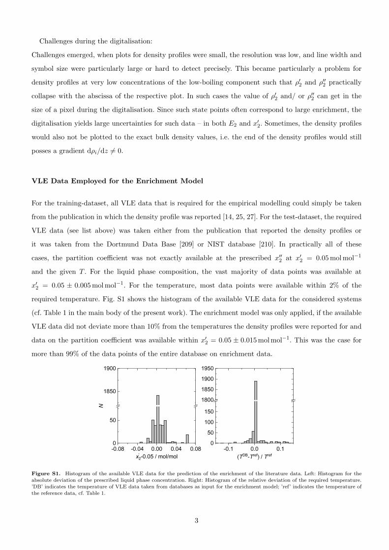
Challenges during the digitalisation:

Challenges emerged, when plots for density profiles were small, the resolution was low, and line width and

symbol size were particularly large or hard to detect precisely. This became particularly a problem for

density profiles at very low concentrations of the low-boiling component such that ρ′2 and ρ′′2 practically

collapse with the abscissa of the respective plot. In such cases the value of ρ′2 and/ or ρ′′2 can get in the

size of a pixel during the digitalisation. Since such state points often correspond to large enrichment, the

digitalisation yields large uncertainties for such data – in both E2 and x′2. Sometimes, the density profiles

would also not be plotted to the exact bulk density values, i.e. the end of the density profiles would still

posses a gradient dρi/dz 6= 0.

VLE Data Employed for the Enrichment Model

For the training-dataset, all VLE data that is required for the empirical modelling could simply be taken

from the publication in which the density profile was reported [14, 25, 27]. For the test-dataset, the required

VLE data (see list above) was taken either from the publication that reported the density profiles or

it was taken from the Dortmund Data Base [209] or NIST database [210]. In practically all of these

cases, the partition coefficient was not exactly available at the prescribed x′′2 at x′2 = 0.05 mol mol−1

and the given T . For the liquid phase composition, the vast majority of data points was available at

x′2 = 0.05 ± 0.005 mol mol−1. For the temperature, most data points were available within 2% of the

required temperature. Fig. S1 shows the histogram of the available VLE data for the considered systems

(cf. Table 1 in the main body of the present work). The enrichment model was only applied, if the available

VLE data did not deviate more than 10% from the temperatures the density profiles were reported for and

data on the partition coefficient was available within x′2 = 0.05 ± 0.015 mol mol−1. This was the case for

more than 99% of the data points of the entire database on enrichment data.

Figure S1. Histogram of the available VLE data for the prediction of the enrichment of the literature data. Left: Histogram for theabsolute deviation of the prescribed liquid phase concentration. Right: Histogram of the relative deviation of the required temperature.

’DB’ indicates the temperature of VLE data taken from databases as input for the enrichment model; ’ref’ indicates the temperature ofthe reference data, cf. Table 1.

3

Phase Diagrams of Binary Lennard-Jones Mixtures of the Training-Dataset

Fig. S2 shows a selection of the isothermal p − x phase diagrams of the Lennard-Jones mixtures used

in the training-dataset. They were calculated by the PeTS EOS, which is known to give an excellent

representation of the vapour-liquid equilibrium of that particular Lennard-Jones fluid and its mixtures

[25, 62, 154]. Representative results for 30 systems are shown in Fig. S2. For all mixtures the high-boiling

component 1 is the same, while the low-boiling component 2 in the mixtures varies. The variation of the

molecular interaction parameters yields a large variety of phase behaviours. For a detailed discussion see

Refs. [14, 25].

4

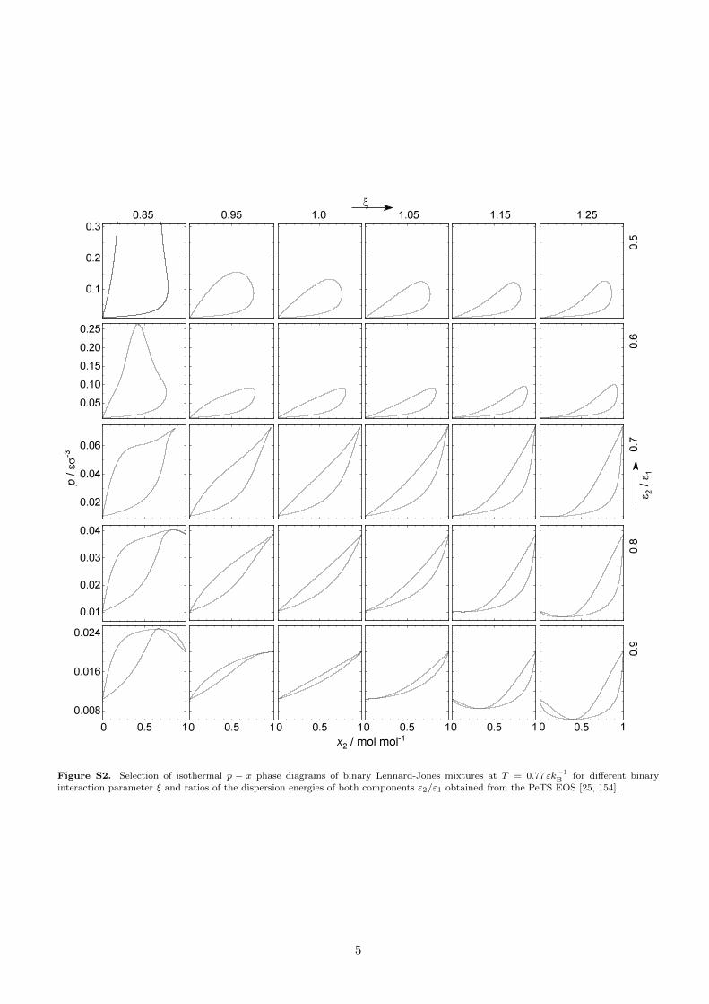
Figure S2. Selection of isothermal p − x phase diagrams of binary Lennard-Jones mixtures at T = 0.77 εk−1B for different binary

interaction parameter ξ and ratios of the dispersion energies of both components ε2/ε1 obtained from the PeTS EOS [25, 154].

5

Enrichment at Vapour-Liquid Interfaces of Mixtures - OSF

Documents

Transcript of Enrichment at Vapour-Liquid Interfaces of Mixtures - OSF