Detection of Atmospheric Water Vapour using the

Global Positioning System

A.Z.A. Combrink

Dissertation submitted in partial fulfilment of the requirements for the degree

Magister Scientiae in Physics

at the Potchefstroomse Universiteit vir Christelike H e r Onderwys

Supervisor: Dr. W.L. Combrinck

Co-supervisor: Prof. H. Moraal

2003

Potchefstroom

DEDICATION

This work is dedicated to my parents who, through love and hard work over many years

ensured that I have only had the best opportunities available in life.

I would also like to thank Mariska for the support and encouragement that she gave me

whilst I was writing this dissertation.

"And without controversy great is the mystery of godliness: God was manifest in the

flesh, justified in the Spirit, seen of angels, preached unto the Gentiles, believed on in the

world, received up into glory."

1 Timothy 3:l6.

ACKNOWLEDGEMENTS

I would like to express my gratitude to the following individuals whose support made this

work possible:

Dr. Ludwig Combrinck, the promoter of this project and programme leader of

HartRAO's Space Geodesy Programme, for teaching me all that I know about

geodesy. It was only through his innovative approach to every problem that the

success of this project was ensured.

Prof. Harm Moraal of the Potchefstroom University for CHE, co-promoter of this

project, for patiently working on this dissertation with me during his sabbatical.

Richard Wonnacott, Chief Directorate: Surveys and Mapping, who made Trignet data

available to me for use in my research.

Tracey Gill at the South African Weather Service, who made radiosonde data

available to me and who showed a keen interest in the results.

I would also like to acknowledge the support received from the National Research

Foundation.

ABSTRACT

The Global Positioning System (GPS) has been used for more than a decade for the

accurate determination of position on the earth's surface, as well as navigation. The

system consists of approximately tlurty satellites, managed by the US Department of

Defense, orbiting at an altitude of 20 200 kilometres, as well as thousands of stationary

ground-based and mobile receivers. It has become apparent from numerous studies that

the delay of GPS signals in the atmosphere can also be used to study the amosphere,

particularly to determine the precipitable water vapour (PWV) content of the troposphere

and the total elecmn content (TEC) of the ionosphere.

This dissertation gives an overview of the mechanisms that contribute to the delay of

radio signals between satellites and receivers. The dissertation then focuses on software

developed at the Hartebeesthoek Radio Astronomy Observatory's (HartRAO's) Space

Geodesy Programme to estimate tropospheric delays (from which PWV is calculated) in

near real-time. In addition an application of this technique, namely the improvement of

tropospheric delay models used to process satellite laser ranging (SLR) data, is

investigated. The dissertation concludes with a discussion of opportunities for future

work.

KEY TERMS

Global Positioning System

zenith tropospheric delay

total electron content

precipitable water vapour

ionosphere

troposphere

WAARNEMING VAN ATMOSFERIESE WATERDAMP MET BEHULP VAN

DIE GLOBALE POSISIONERINGSISTEEM

UITTREKSEL

Die Globale Posisioneringsisteem (GPS) word alreeds vir meer as 'n dekade gebmik vu

akkurate navigasie en posisionering op die oppewlak van die aarde. Die sisteem bestaan

uit ongeveer dertig satelliete wat om die aarde wentel op 'n hoogte van 20 200 kilometer,

en word bestuur dew die Amerikaanse Departement van Verdediging. Verder sluit die

sisteem ook duisende stasion6re en mobiele ontvangers in. Verskeie studies het getoon

dat die vertraging van GPS-seine in die atmosfeer gebruik kan word om die atmosfeer te

bestudeer, in besonder om die presipiteerbare waterdampinhoud van die troposfeer en die

totale elektroninhoud van die ionosfeer te bepaal.

Hierdie verhandeliig lewer 'n oorsig oor die meganismes wat bydra tot die vertraging

van radioseine tussen satelliete en ontvangers. Die sagteware wat ontwikkel is dew die

Hartebeesthoek Radio-astronomie Observatorium se Ruimtegeodesie Program om

troposferiese vertraging (waaruit die presipiteerbare waterdampinhoud bereken word)

intyds te bepaal, word ook bespreek. Die berekende presipiteerbare waterdampinhoud

kan ook gebruik word om troposferiese verfxagingsmodelle, wat gebmik word om

satelliet-lasemikafstandsbepaling data te prosesseer, te verbeter. Hierdie tegniek word

bespreek, en die verhandeliig word afgesluit dew 'n oorsig van toekomstige

navorsingsgeleenthede op hierdie gebied.

Globale Posisioneringsisteem

seniet troposferiese vertraging

totale elektroninhoud

presipiteerbare waterdamp

ionosfeer

troposfeer

TABLE OF CONTENTS

Introduction and Background 1

1. The Global Positioning System (GPS) 3

2. The Propagation of Electromagnetic Waves in Matter 7

2.1. The Tropospheric Delay 8

2.2. The Ionospheric Delay 13

3. The Zenith Tropospheric Delay (ZTD) of Radio Waves 20

3.1. Mapping Functions 25

4. The Acquisition and Processing of GPS Observational Data 27

4.1. The Acquisition of GPS Observational Data 27

4.2. The Processing of GPS Observational Data 29

5. Results of PWV Determination 30

6. An Application: Improving SLR Tropospheric Delay Models 38

7. The Square Kilometre Array in South Africa and the Surface-upgraded 26m

Radio Telescope at HartRAO 47

7.1. The Influence of Precipitable Water Vapour on Centimetre

Wavelength Radio Astronomy 48

7.2. The Influence of Free Electrons in the Ionosphere on VLBI

Astrometry 49

7.3. Results from the SKA Site Survey 49

Summary and Conclusions 55

Bibliography 58

LIST OF FIGURES AND TABLES

Figure 1: The two existing GPS networks in southern Africa are HartRAO's SADC

IGS Network and the Chief Directorate: Surveys and Mapping's Trignet

(Cilliers et al., 2003:52) ...................................................................... .5

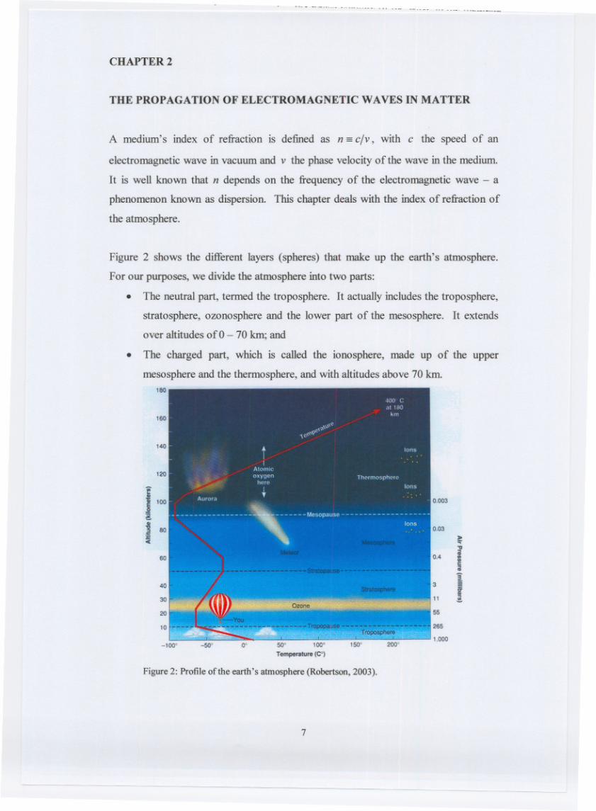
Figure 2: Profile of the earth's atmosphere (Robertson, 2003). ............................... ..7

Figure 3: The electrons in a dielectric substance are pictured as if attached to the end

of an imaginary spring, and driven by a varying electric field (Gfiths, 1999:

400). .......................................................................................... .8

Figure 4: Anomalous dispersion and absorption in the frequency region of a resonance

(Gaths, 1999:403).. ................................................................... ..I2

Table 1: Properties of the ionospheric layers (Medeiros, 2000). ............................ .14

Figure 5: Radio signals from a GPS satellite arrive at a ground-based receiver, from a

direction with an associated elevation angle 0 above the horizon, travelling

along an electrical (true) path; for elevation angles greater than 15 degrees the

electrical path can be approximated by the shortest geometric path G.. ............ 20

Figure 6: The Niell Mapping Function (NMF) for latitudes of 45 degrees (Niell,

1996:3230,3250). ......................................................................... ..26

Figure 7: A comparison of the Zenith Tropospheric Delay (ZTD) as calculated by

HartRAO and IGS for the IGS GPS station HRAO; an arbitrary 20day dataset

was chosen.. ............................................................................... .30

Figure 8: A comparison of the Zenith Tropospheric Delay (ZTD) as calculated by

HartRAO and IGS for the IGS GPS station HRAO; the HartRAO estimates

generally agree with the IGS post-processed estimates.. ........................... ..3 1

Figure 9: The ZTD estimated over Africa and the surrounding oceans at 12:00 UT on

day 154 of 2003. The isoline figure (top) shows the absolute tropospheric

delay (in metres). Relative ZTD is represented in the bottom figure, where

warmer colours represent less delay and cooler colours represent more delay.. ..32

10: An isoline map of the zenith tropospheric delay over South Africa for

12:00 UT on day 154 of 2003 ............................................................. 33

vii

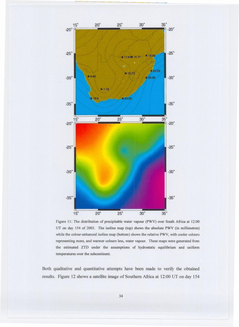
Figure 1 1: The distribution of precipitahle water vapour (F'WV) over South Africa at

1200 UT on day 154 of 2003. The isoline map (top) shows the absolute PWV

(in millimetres) while the colour-enhanced isoliie map (bottom) shows the

relative PWV, with cooler colom representing more, and warmer colom less,

water vapour. These maps were generated from the estimated ZTD under the

assumptions of hydrostatic equilibrium and uniform temperatures over the

.............................................................................. subcontinent.. .34

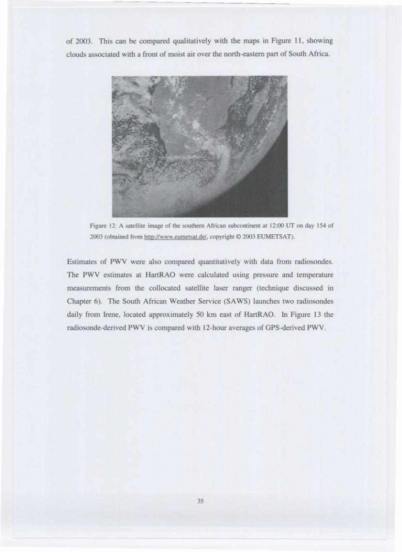
Figure 12: A satellite image of the southern African subcontinent at 12:00 UT on day

154 of 2003 (obtained from htto://www.eumetsat.de/, copyright O 2003

............................................................................. EUMETSAT). .35

Figure 13: A comparison of precipitable water vapour (PWV) for May 2003, obtained

from GPS observations at Hartebeesthoek, and radiosondes launched at Irene,

50 km east of Hartebeesthoek. PWV is presented as a function of time in

Figure A, while Figure B presents the correlation between GPS-derived and

radiosonde-derived PWV.. ................................................................ 36

Figure 14: The position time series of the MOBLAS6 satellite laser ranger at

HartRAO, calculated using the standard Marini and Murray model.. ............ ..42

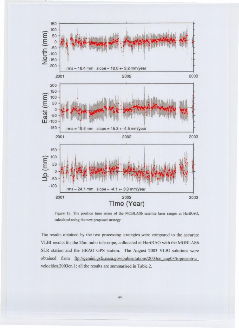
Figure 15: The position time series of the MOBLAS6 satellite laser ranger at

HartRAO, calculated using the new proposed strategy.. ........................... ..44

Table 2: A comparison of station velocities obtained by VLBI and two SLR

..................................................................... processing strategies.. 45

Figure 16: A comparison between the tropospheric delay as predicted by the Marini

and Murray model and the new proposed strategy (Combrinck & Combrink,

2003). ....................................................................................... .46

Figure 17: Statistics of TEC values as determined by GPS over the period 1998-

2003.. ......................................................................................... 50

Figure 18: TEC values for a one week period during the April 2001 solar outburst

indicates a negative ionospheric stom effect. A rapid recovery follows the

day of the negative storm effect ........................................................... 51

Figure 19: The partial solar eclipse of 4 December 2002 caused a small negative

effect which has been circled in the figure.. .......................................... ..52

viii

Figure 20: Total electron content (TEC) during the 4 December 2002 partial solar

eclipse, normalised to the average TEC of the two days prior and two days

after the eclipse.. . . . .. . . . . . . . . . . .. . . . . . . . . . . . . . . . . . . . .. . . . . . . . . . . . . . .. . ... . ... . ... . . . . . . . .... 53

LIST OF KEY TERMS AND ABBREVIATIONS

CDSM

DoD

ESA

EUMETSAT

Gm.

GIF

GIMs

GLONASS

GMT

GNSS

GPS

HartRAO

IERS

IGS

ILRS

JF'L

MIT

MOBLAS6

NASA

NMF

NOAA

NRCan

PPm

PWV

RINEX

=ometer

rms

SAAO

SAC

SADC

Chief Directorate: Surveys and Mapping

United States Department of Defense

European Space Agency

European Organisation for the Exploitation of Meteorological Satellite

GeoForschungsZeneUm Potsdam

Graphic Interchange Format

Global Ionospheric Maps

Global Navigation Satellite System

Generic Mapping Tools

Global Positioning and Global Navigation Satellite Systems

Global Positioning System

Hartebeesthoek Radio Astronomy Observatory

International Earth Rotation Service

International GPS Service

International Laser Ranging Service

Jet Propulsion Laboratory

Massachusetts Institute of Technology

Mobile Laser Ranging System 6

National Aeronautics and Space Administration

Niell Mapping Function

National Oceanic and Atmospheric Administration

Natural Resources Canada

Parts per million

Mipitable Wakr Vapour

Receiver Independent Exchange Format

Relative Ionospheric Opacity Meter

Root mean square

South Afiican Asbonomical Observatory

Satellite Application Centre

Southern African Development Community

X

SAWS

SKA

SLR

SNR

SOPAC

TEC

TECU

TEQC

USNO

UT

VLBI

ZTD

South African Weather Service

Square Kilometre Array

Satellite Laser Ranging

Signal-to-Noise Ratio

Scripps Orbit and Permanent Array Center

Total Electron Content

Total Electron Content Units

TranslateRdit/Quality Check

United States Naval ObSe~atOq

Universal T i e

Very Long Baseline Interferometry

Zenith Tropospheric Delay

INTRODUCTION AND BACKGROUND

Radio astronomers, space geodesists and meteorologists all have an interest in the

amount of water vapour in the atmosphere for various reasons. To the radio

astronomer observing electromagnetic waves at the centimetre wavelength level,

atmospheric water vapour is a nuisance, causing absorption and emission at these

wavelengths, as discussed in Chapter 7. Atmospheric water vapour also causes

satellites, used in space geodetic techniques, to appear further than they really are, as

a result of the refraction of electromagnetic waves. Accurate measurements of water

vapour enable radio astronomers and space geodesists to correct their observations by

including it in tropospheric models.

Meteorologists bring atmospheric water vapour a little closer to the man in the street.

The atmosphere's water vapour content is an extremely important parameter in

numerical weather prediction. The high cost of radiosondes (weather balloons) -

currently the only source of water vapour data - forced South African meteorologists

to reduce the number of launches to approximately two per day, at a maximum of

seven selected sites only (Cilliers et al., 200353).

The Global Positioning System (GPS), described in Chapter 1, offers a solution. If

the position of a ground-based GPS station and the orbit of a GPS satellite is known,

one can calculate how long it should take for a radio signal to travel between the two,

assuming that the radio signal travels at the speed of light in vacuum. Refraction

caused by the ionosphere and the troposphere results in a delay, as shown in Chapter

2. Chapter 3 concludes the theoretical component of this dissertation and shows how

the precipitable water vapour (PWV) content of the troposphere can be obtained from

this delay.

The research performed for the sake of this dissertation aims to determine whether it

will be possible to determine PWV from observational GPS data, using the existing

southern African GPS network, and the available processing software, discussed in

Chapter 4, thus confirming the theory. The results obtained with the software,

developed specifically with this research project in mind, are shown in Chapter 5. If

it was shown to be feasible, a further aim would be to make the results available in

near real-time to anyone who wishes to use them in their applications, or to use the

results to solve existing problems in space geodesy or radio astronomy.

One application of the determination of PWV, namely the improvement of satellite

laser ranging (SLR) tropospheric models, is explored in Chapter 6. Chapter 7

explores some of the results and a summary is given of the site suitability s w e y

conducted for the South African Square Kilometre Array (SKA) Steering Committee.

The committee's intention is to include these results in their bid to build a new state-

of-the-art radio telescope in the Northern Cape. The dissertation concludes with a

summary and a short discussion of future work.

CHAPTER 1

THE GLOBAL POSITIONING SYSTEM (GPS)

GPS is a satellite-based radio navigation system, designed and controlled by the US.

Department of Defense @OD) in its NAVSTAR navigation satellite programme. In

the 1970s DoD decided to create a space-based navigation system to save the costs

associated with the navigation systems in use at that time (Hoffmann-Wellenhof et al.,

1993:3). The first GPS satellite was launched in 1978.

There is also a Russian equivalent to GPS, called the Global Navigation Satellite

System (GLONASS), from which signals have been received since 1996 (Borbhs,

1997:262). The European equivalent, of which the first satellite is to be launched in

2005, is called GALILEO. GPS, GLONASS and GALILEO together form the GNSS,

or Global Positioning and Global Navigation Satellite Systems (Cilliers et al.,

2003:51). This research focuses specifically on GPS, since diierent equipment is

needed to receive signals from GLONASS.

GPS consists of approximately thirty satellites, of which at least 24 are active at any

given time. They are uniformly dispersed in six circular orbits, each with an

inclination of 5S0 relative to the equatorial plane. They orbit at an altitude of

approximately 20 200 krn with an orbital period of 11.967 hours, or one half of a

sidereal day (Cilliers et al., 200351).

The satellites transmit coded signals at two different carrier frequencies in the L-band.

Denoted by LI and Lz, the frequencies are 1.57542 GHz and 1.22760 GHz

respectively (Ros et al., 2000:357). A signal contains information about the satellite's

approximate position (broadcast ephemeris with an accuracy of -260 cm (IGS,

2003)), as well as a time stamp of the time when the signal was emitted. In the case

of the latter, GPS satellites carry accurate atomic clocks - also called "atomic time

and frequency standards" (King, 2002) - for which relativistic corrections are made

by an on-board computer.

The principles used to determine the location of a GPS receiver, are Einstein's second

postulate, namely that electromagnetic waves in vacuum propagate at the constant 3

speed c, and triangulation. A GPS receiver receives digital signals like these

continuously, and can then determine its position. The GPS processing software used

for this research uses a technique called "double differencing" and is discussed in

Section 4.2.

GPS was o r i d l y designed for military purposes. For this reason, a deliberate

satellite clock bias - the so-called "selective availability" - was introduced to derate

the accuracy of GPS for non-U.S. military users. On the 1st of May 2000 the

selective availability was de-activated, because the value of GPS research, e.g. crustal

dynamics, plate tectonics, GPS meteorology, TEC mapping and ocean level

monitoring, which requires accurate data, became apparent (Ashby, 2002:47). Also,

commercial users of GPS data had developed signal processing techniques using,

among others, Kalman filtering to overcome the limitations introduced by selective

availability.

High-precision geodetic measurements with GPS are performed using the carrier beat

phase. This is the difference between the phase of the carrier wave of the signal

received from the satellite, and the phase of a local oscillator within the receiver. The

carrier beat phase can be measured with sufficient precision and results in the

instrumental resolution being less than a rnillimetre in equivalent path length. The

dominant source of error in a phase measurement between a single satellite and a

single ground station is the unpredictable behaviour of the "time and frequency

standards" (clocks) serving as reference for the transmitter and receiver (King, 2002).

For a single satellite, differencing the phases of signals, received simultaneously at

each of two ground stations, eliminates the effect of bias or instabilities in the satellite

clock. This measurement is commonly called the single-difference observable. A

double dierence is formed by differencing the between-station differences between

satellites, to completely cancel the effects of variations in the station clocks.

Since the phase biases of the satellite and receiver oscillators at the initial epoch are

eliminated in doubly-differenced observations, the doubly-differenced range is the

measured phase plus an integer number of cycles. If the measurement errors - which

may arise from mismodelled orbits, receiver noise or a poorly modelled propagation

medium - are small compared to a cycle, it is possible to determine the integer values 4

signals to travel the distance between a specific satellite and receiver. However, as

the radio signals travel through the atmosphere, they undergo refraction and delay

relative to the propagation time in vacuum due to the phase velocity differing from

that in free space. As a result of the refraction they do not travel in a straight line and

do not travel at the speed of light (c). However, the increased path length due to the

refraction is negligible compared to the apparent increase in path length due to the

diierent phase velocity. Therefore, in the next chapter we will consider the transport

of electromagnetic waves in matter, and in Chapter 3 we will indicate how the delay

experienced by a radio wave in the troposphere can be used to estimate the

atmospheric water vapour content.

The refractivity (and the resultant delay) of each of these parts of the atmosphere will

now be derived from first principles.

2.1. The Tropospheric Delay

In this section we make a model of dispersion that takes place on atomic scale. We

follow the derivation by Griffiths (1999:398-404), which is only an approximation of

the quantum mechanical model, but yields satisfactory results nevertheless.

The electrons in a dielectric substance are bound to specific molecules. We shall

picture each electron as attached to the end of an imaginary spring, with force

constant k,,, , so that F,,,, = -k,,,x = -moix is the centrifugal force acting on

the electron as it orbits the atom's nucleus, with x being the displacement from

equilibrium, m the mass of the electron and o, = d G the natural oscillation

frequency, as shown in Figure 3.

Electron

Figure 3: The electrons in a dielectric substance are pictured as if attached to the end of an

imaginary spring, and driven by a varying electric field (Grifiths, 1999:400).

The electrons will also experience a damping force Fh-g = -rny(dx/dt), with y a

damping coefficient and where the negative sign follows from the fact that the force is

in the direction opposite to the velocity of the electron. This damping is a result of the

fact that oscillating charges radiate electromagnetic waves, canying off energy with

them.

In the presence of an electromagnetic wave of frequency w, polarised in the x-

direction, there is a driving force Fdnving = qE = qEOcos(at) acting on the electron,

with q the charge of the electron and Eo the amplitude of the wave.

Newton's second law now states

d2x m,=

dt 4n01 = Fbindinp + FdampinE + Fdnvind

This model describes the electron as a damped harmonic oscillator, driven at

frequency w.

Consider (1) as the real part of the complex equation

In the steady state, the system oscillates at the driving frequency w:

?(t) = ?oe-ia.

Placing this in (I), it follows that Zo = dm E,. -a2 -im

The dipole moment (defined as p = qx) is the real part of

Electrons in the same molecule that have different orientations will, of course,

experience diierent damping coefficients and natural frequencies. Assume that there

are fj electrons with frequency 4 and damping coefficient in each molecule. If

there are N molecules per unit volume, the polarisation (defied as dipole moment per

unit volume) will be given by the real part of

Because of the phase difference between P and E we have to define a complex

susceptibility by - - P = E,Z,E.

The permittivity of the substance is defined as E =&,(I + z), while the dielectric

constant is defied as E, = E I&, . For this model it implies that

2: = &,(I + 2,) and

In a dispersive medium the wave equation for a given frequency is

with p,, the permeability of vacuum. It admits plane wave solutions of the form

with complex wave number

We can also write the complex wave number in terms of real and imaginary

components:

i = k + i ~ . (5)

Using (5). expression (3) now becomes E(z,t) = E,e~mei'"~m', indicating that the

wave is being damped.

The power of the electromagnetic wave is proportional to 2, and therefore also to e-

24. Consequently, the quantity

a= 2~ (6)

is called the absorption coefficient. Furthermore, the phase velocity is d k , and the

index of refraction is

n = cklw. (7)

For gasses, as in the case of the troposphere, the second term of the complex dielectric

constant is small. Using equation (2), expression (4) and the binomial expansion

6 s 1 + Yu;, we can write

so that it follows from (5) and (7) that

and from (6) follows

The index of refraction rises gradually with increasing frequency, except in the

vicinity of a resonance w = wj , where it drops sharply, as shown in Figure 4. The

resonances are caused by electrons being driven at specific (resonance) frequencies,

which correspond to relatively large amplitudes and, consequently, the dissipation of

large amounts of energy due to the damping mechanism. Therefore, the resonances

also coincide with frequencies of maximum absorption. This atypical behaviour in

the vicinity of a resonance is called anomalous dispersion.

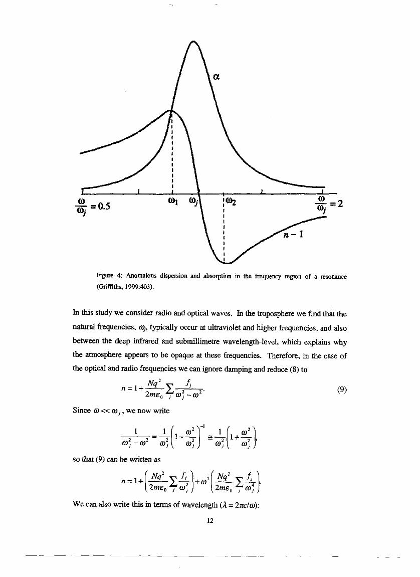
Eigure 4: Anomalous dispersion and absorption in the frequency region of a resonance

(GIiffiths, 1999.403).

In this study we consider radio and optical waves. In the troposphere we find that the

natural frequencies, cq., typically occur at ultraviolet and higher frequencies, and also

between the deep infrared and submillimetre wavelength-level, which explains why

the atmosphere appears to be opaque at these frequencies. Therefore, in the case of

the optical and radio frequencies we can ignore damping and reduce (8) to

Since w c< oj , we now write

so that (9) can be written as

We can also write this in terms of wavelength (2 = 2 m l ~ ) :

12

This is known as the Cauchy equation, with N,, the refractivity and B the dispersion 14 2 coefficient. B was found to be 1 .7~10- m for the atmosphere (Riepl & Schliiter,

2000).

Optical wavelengths are typically of the order of - 5.0~lO-'m, so that l2 is

comparable to B; N,, is typically of the order of -0.4 for air. Cauchy's equation (10)

applies reasonably well to most gases in the optical region (Griffiths, 1999:404). One

can therefore conclude that the transport of optical waves in the troposphere is

dispersive.

The typical radio wavelengths we consider are of the order of -0.2 m (L-band), so

B that - << 1, and consequently N,, = n - 1. Thus we can conclude that the a2 propagation of radio waves in the troposphere is non-dispersive.

In the troposphere n > 1 for both the radio and optical cases; from the definition of the

index of refraction ( n s c/v) follows that an electromagnetic wave traversing the

atmosphere will experience a delay (or longer apparent path length) relative to the

propagation time (or apparent path length) of the same wave in vacuum, if the

propagation velocity is assumed to be c in both cases. Consequently, we will explore

the delay of radio waves in the troposphere in Chapter 3, and the tropospheric delay of

optical waves in Chapter 6.

2.2. The Ionospheric Delay

The ionosphere is the upper, partially charged part of the atmosphere, which is

responsible for the absorption and reflection of radio waves at low frequencies

(generally below 25 MHz). Atoms in the upper atmosphere are ionised by absorbing

radiation energy from the sun - the electrons gain kinetic energy and are displaced

from their orbits around the nucleus. Free electrons and ions in the ionosphere

continuously recombine, so that only a fraction of the ionosphere is charged at any

given time. 13

The ionosphere has traditionally been split up into three layers, D, E and F, which are

classified according to altitude, maximum reflected radio frequency and the most

dominant chemical component (Medeiros, 2000). During the daytime, when

ionisation from solar radiation is at a maximum, the F layer splits up into two layers,

namely the F1 and F2 layers. Table 1 gives a summary of the basic characteristics of

the ionospheric layers; the altitudes and maximum reflected radio frequencies are

averages of quantities that vary with time (these quantities are dependent on season,

time of day and solar activity, also discussed in Chapter 7).

Table 1: Properties of the ionospheric layers (Medeiros, 2000)

The ionosphere is characterised by its content of free electrons and ions. The F2 layer

of the ionosphere has the largest density of charged particles, with values up to

3x 1012 m-' (Ros et al., 2000:357).

The total electron content (TEC) is defmed as the number of electrons in a column of

unit area cross section along the transionospheric ray path, written as

E, = 1' ~ d h , 0

(1 1)

where N is the spatial density of elechons, h is the coordinate of propagation of the

wave, and corresponds to the effective top of the ionosphere.

Most representative chemical

component

Ozone

Layer

D

TEC is highly variable and depends on several factors, such as local time,

geographical location (latitude in particular), season and solar activity. TEC can have 16 -2 values between 1 TECU (or TEC unit, defined as 10 m ) and lo3 TECU (Ros et al.,

2000:357).

Altitude (km)

65 - 80

Maximum reflected

~ ~ P J = Y (MHz)

16

Because the ionosphere is partially charged, we would expect that the propagation of

electromagnetic waves would differ drastically from the tropospheric case. Therefore,

in this section we derive the refractivity of the ionosphere, following Chen (1984:114-

116) and Choudhuri (1998:239-243). neglecting the effects of electron collisions and

the Earth's magnetic field on wave propagation.

Free electrons in the ionosphere interact with electromagnetic waves travelling

through the ionosphere. Maxwell's equations state

E and B are the electric and magnetic components of the electromagnetic waves

respectively, and J is the resulting current density.

The curl of (12) is

aB V x ( V x E ) = v(v.E)-VE=-VX-, at

while the time derivative of (13) is

From (14) and (15) it follows that

Assuming that the electromagnetic waves have an dependence, it follows from

(16) that

kZE - k(k.E) = iapJ +a2&,~oE. (17)

Electromagnetic waves are transverse in nature, so that k.E = 0, and (17) becomes

Electromagnetic waves in both the radio and optical regions have such high

frequencies that the ions can be considered as f m d , comparing their inertial mass to

those of electrons, we expect that the motion of electrons will be the only source of

current:

J = -n,,ev, (19)

with -e the charge of an electron, the number density of electrons and v their

velocity.

dv Newton's second law states rn- = -eE ; from the assumption that the waves have an

dt

ei'k.r-'U' dependence, follows v =* . Combining (18) and (19), it follows that im

2 2 - ' w The plasma frequency is defined as w, = -. From (20) we then obtain the

&om

dispersion relation 2 w = 0 2 , + c 2 k 2 .

One can also write this as ck = o 1 + 2 . From (21) and the definition of the j (3 0

phase velocity, vMse = -, follows vh, = c2 + @ i l k 2 > c2 ; i.e. the phase velocity of k

an electromagnetic wave in the ionosphere is greater than c. The definition of group

am velocity, vg,, = - kc2 - c2 . and (21) leads to v,,, = -- - < c , showing that the

ak W vphare

group velocity of an electromagnetic wave in the ionosphere is less than c . The

effects of the ionosphere on microwaves are therefore referred to as phase advance

and group delay; the latter can be defmed as the rate of change of the phase shift with

respect to the frequency through a medium.

Per definition the relationship between w and k is given by w(k) = *. Group n(k)

velocity can then also be expressed in the general form

C -- - = V'TJ - ak ($)I n(@) + o (dnido) '.

where n(w) is the conventional index of

refraction as depicted in Figure 4 (in Section 2.1). Furthermore, from Figure 4 it is

evident that (dnldw) > 0 and n >l for normal dispersion, while (dn ldo) can also

become large and negative in the vicinity of a resonance. The ionosphere is

transparent in both the optical and radio frequencies, so that one would expect normal

16

dispersion at these frequencies because of the absence of resonances. This argument

also c o n f i i that the group velocity of optical and radio waves in the ionosphere

should be less than c and that the group refractivity should be positive.

Consequently, two indices of refraction can be d e f m d the conventional (phase)

C index of refraction, np i - , as depicted in Figure 4, and the group index of

"*S<

C refraction, n, = - . Therefore,

"sw

where the negative sign applies to phase velocities and the positive sign to group

velocities. From (22) it is clear that n, = 0 at w = w p ; therefore, k becomes zero and

the wavelength of the electromagnetic wave becomes infmitely long in this limit.

Thus, w p is a cut-off frequency, so that no electromagnetic waves below this

frequency can propagate through the ionosphere.

For the radio frequencies used for GPS communication (1.2 and 1.6 GHz) and the

optical frequencies used for satellite laser ranging (2.8 x 1014 Hz to 4.3 x 1014 Hz),

W P - << 1 and - <<< 1 respectively, and by means of the binomial expansion & W 0

2 1 + L/&, (22) becomes

1 w; n 2 IT-? (radio) and n z 1 (optical).

2w (23)

Defining the refractivity of the ionosphere as N, = n - 1, we obtain

for the case of radio waves. In the ionosphere no is typically of the order of 10'~m",

so that the refractivity of a 1.6 GHz GPS signal in the ionosphere is

typically N, = ~ 1 . 6 ~ 1 0 ~ .

For vertical incidence of radio waves, the correction to the path distance of the waves,

i.e. the experienced delay through the ionosphere, is defined as

with z the coordinate of propagation.

Thus the vertical path correction for the ionosphere is given by

with Er the so-called "total electron contenttt in m-' (Lynn and Gubbay, 1975:s). as

defined in (11). As seen in Chapter 7, a typical value of the TEC is

50 T E C U = ~ X ~ O ' ~ ~ - ~ , so that the experienced ionospheric delay of a 1.6 GHz GPS

signal is - ~ 8 m .

From (26) one can determine that the path correction is proportional to the total

electron content (TEE), and inversely proportional to the square of the frequency of

the incoming electromagnetic wave. It is also apparent from (23) that the transport of

optical waves in the ionosphere is non-dispersive, while the transport of radio waves

in the ionosphere is dispersive.

GPS satellites emit signals at two frequencies, namely 1.57542 GHz (LI) and 1.22760

GHz (L2). The refractivity for the LL signal is a factor (1.57542/1.22760y 51.65

larger than for the L1 signal.

It is therefore easy to correct for the ionospheric delay using the following argument:

the GPS receiver measures a time difference Af between the propagation delays of

the L1 and I.Q signals, relative to vacuum propagation times over the d i i t path

between the satellite and the receiver. As shown above, the ionospheric time delay of

the LL signal is a factor 1.65 larger, so that At,/Atl =1.65. From the measured time

difference At = At2 - Af, follows At, = At 10.65 and At2 = 1.65At 10.65. These

ionospheric corrections are being done very accurately, to the submillimetre-level in

path length, by GPS processing software such as GAhtlT (Combrinck W.L., personal

communication, 2003). which is discussed in Section 4.2.

It should be noted that the accuracy of ionospheric corrections determines the

accuracy of zenith tropospheric delay (ZTD) estimations. The determination of TEC

is therefore relevant to the determination of ZTD and tropospheric precipitable water

vapour (PWV) content from GPS data.

THE ZENITH TROPOSPHERIC DELAY (ZTD) OF RAI: lI0 WAVES

The index of refraction for radio waves in the troposphere is always greater than 1

(per d e f ~ t i o n equals 1 for vacuum), as can be seen from expression (10). These

waves traversing the troposphere experience a resulting delay, which appears to add

up to -2 metres to the path length of the waves; this is -lo-'% of the total path length

of 20 200 km.

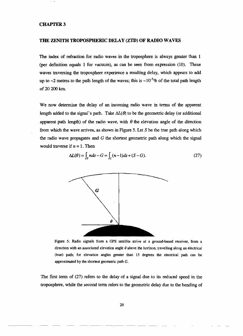
We now determine the delay of an incoming radio wave in terms of the apparent

length added to the signal's path. Take AL(@ to be the geometric delay (or additional

apparent path length) of the radio wave, with 0 the elevation angle of the direction

from which the wave arrives, as shown in Figure 5. Let S be the true path along which

the radio wave propagates and G the shortest geometric path along which the signal

would traverse if n = 1. Then

A L ( 8 ) = j s n d s - ~ = j s (n-l)ds+(S-G). (27)

Figure 5: Radio signals from a GPS satellite arrive at a ground-based receiver, from a

direction with an associated elevation angle 0 above the horizon, travelling along an electrical

(W) path; for elevation angles greater than 15 degrees the elecirical path can be

approximated by the shortest geometric path G.

The fist term of (27) refers to the delay of a signal due to its reduced speed in the

troposphere, while the second term refers to the geometric delay due to the bendimg of

the signal, which can be neglected for elevation angles greater than 15' (Gradmarsky,

2000: 12). We can therefore approximate S = Isds = G.

The tropospheric zenith delay, conventionally abbreviated as ZTD, is one of the

quantities estimated by the GPS processing software discussed in Section 4.2, and can

be defmed as U a AL(90°). The focus now shifts to the contributions of water

vapour and the "dry" gasses to the zenith delay, and in Section 3.1. we will look at

techniques to map the zenith delay to a real measured delay.

In parts per million (ppm) notation, the refractivity can be written as N = 106(n-I), so

that (27) becomes

AL = 10"j N(s)dr. S

(28)

We now calculate N and the consequent delay experienced by a radio wave in the

troposphere as a function of the precipitable water vapour content (PWV) of the

troposphere, and pressure and temperature measured at ground level. This will enable

us to estimate PWV from the pressure, the temperature and the delay of a radio wave

measured at ground level.

For the troposphere, consisting of, say, q gasses, the delay depends on the density pi

of each gas. Following Gradinarsky (2000: 12) we write

as first derived by Debye (1929:30-35). T is the temperature and Ai and Bi are

constants for each gas. In the case of monatomic and diatomic gasses, which account

for the biggest part of the atmosphere, Bi = 0. However, this is not the case for H20,

because of its permanent dipole moment. (As in Chapter 2, the dipole moment of a

pair of opposite charges of magnitude q is defined as the magnitude of the charge

multiplied by the distance between the charges, and the defined direction is toward the

positive charge.) In his classical work, Debye (1929:30-35) gives a quantitative

explanation for the temperature dependence of water's coefficient of refraction. The

temperature dependence can also be understood qualitatively, as explained in the

following argument: For higher temperatures, the average distance between atoms in

water molecules increases. Therefore, the dipole moment and volume per molecule

21

increase with temperature. Let the temperature dependence of the average distance

between the atoms be expressed by d = T, so that the polarisation P = T"" , because

the dipole moment p = d and volume V = d. Consequently, the relative permittivity

E, = TZn and the refractivity will decrease as the temperature T increases.

This means that, because the water molecules are permanent electric dipoles, we will

have to treat atmospheric water vapow and the "dry" gasses in the atmosphere,

separately.

The equation of state for the atmosphere's ith component, with Zi the dimensionless

compressibility, is p;V = Z;n;RiT, where the gas constant of the ith component is

defined as Ri = RIMi, with R = 8.3U.~~'.mole~' the universal gas constant and Mi the

molar mass, and all other symbols have their normal meaning. Using p,=nJC: it is

clear that

From (29) and (30) follows that the refractivity is

where distinction has been made between water vapow and the dry gasses. This can

also be expressed as

with ki constants, pd and p, the partial pressure of the dry and wet components

respectively (Emardson, 1998:5). The first term of (31) can be written in terms of the

total density, p = pd, + p,,,. Defining k; = k, - k, - Mwt , with M,,, en Md, the molar Md,,

masses of the water vapour and dry air respectively, (31) becomes

Pw Pw N = k , ~ , p + k , - - ~ ; ~ + k , - - ~ ; ~ . T T,

It is assumed that the condition of hydrostatic equilibrium,

is satisfied, with g(z) the gravitational acceleration and p(z) the mass density at a

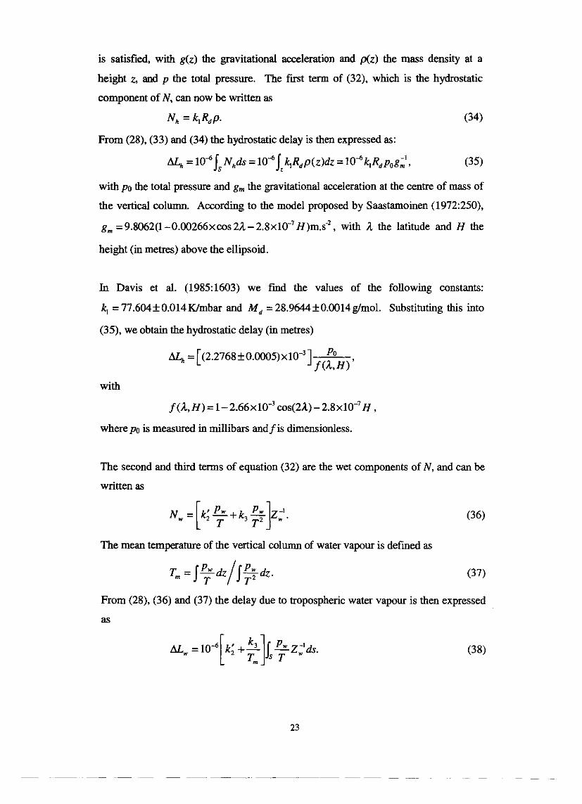
height z, and p the total pressure. The first term of (32). which is the hydrostatic

component of N, can now be written as

N h = 4 Rd P. (34)

From (28), (33) and (34) the hydrostatic delay is then expressed as:

ALh =lo41 s N,ds =lo4/ hR,p(z)dz = 1 0 ~ k , ~ , ~ ~ g , ' , (35)

with po the total pressure and g, the gravitational acceleration at the centre of mass of

the vertical column. According to the model proposed by Saastamoinen (1972:250),

gm =9.8062(1-0.00266xcos2A-2.8~10-~~)m.s", with A the latitude and H the

height (in metres) above the ellipsoid.

In Davis et al. (1985:1603) we find the values of the following constants:

4 = 77.6O4f O.Ol4Wmbar and M, = 28.9644&0.0014g!mol. Substituting this into

(33, we obtain the hydrostatic delay (in metres)

with

f (A, H) = 1-2.66~10" cos(2A)- 2 . 8 ~ 1 0 - ~ ~ ,

where po is measured in millibars and f is dimensionless.

The second and third terms of equation (32) are the wet components of N, and can be

written as

The mean temperature of the vertical column of water vapour is defined as

From (28), (36) and (37) the delay due to tropospheric water vapour is then expressed

as

nR The equation of state for water vapour can be written in the form "z;' = -,

T V

where all the symbols have their normal meanings. The right hand side can further be

written in terms of the specific gas constant R, and molar mass M, of water, so that

&z" = nRwMw = Dp,Rw, with p, the density of water (lo3 kg.m3) and D the T " V

relative density of the precipitable wat& vapour in the troposphere. Defining the total

precipitable water vapour content (PWV) of the troposphere as PWV = I s ~ d r , we can

write it as

lo6 with k(<,rn,) = and the mean temperature approximated as

p , ~ w (k; + k,~;')

T,,, = 70.2K +0.72T following Bevis et al. (1992). Further, k; = 2 2 . 1 ~ . h ~ a " ,

k, = 3.739~10~~~.hF'a- ' and R, = 4 . 6 1 4 ~ 1 0 ~ ~ . ~ ~ ' . k g ~ ' , according to BorbL

(1997).

We have therefore shown that the ZTD is the sum of the hydrostatic and wet delay

components, i.e. ALz = & + q, and how PWV can be calculated from ZTD if

pressure and temperature measurements are available. The hydrostatic delay is

typically in the range of 1.7 to 2.1 metres; it does not vary much at a specific site and

depends mainly on the site's altitude. Although hydrostatic delay is the main

contributor to the total delay, the wet delay is the main contributor to variation in the

total delay, with values ranging between zero and forty centimetres, depending on

local meteorological conditions. Very few, if any, GPS observations are made at

zenith and as a result Section 3.1. is devoted to discussing how ZTD can be mapped to

estimated delays from arbitrary elevation angles.

3.1. Mapping functions

Conventionally, the tropospheric delay at an arbitrary elevation angle 0 is expressed

as a function of hydrostatic and wet delays (Mi) and mapping functions (mLB))

respectively:

a ( e ) = ~ , m , ( 0 ) + 4 m , ( 0 ) . (40)

Thus, through the use of mapping functions we can map the zenith delay to a delay

that a signal would experience at an arbitrary elevation angle.

On the basis of the assumption that the atmosphere in the vicinity of a GPS station is

uniform, a simple sine function can be used to map the zenith delay ALz to the delay

for an arbitrary elevation angle 8.

AL(0) = llL' /sin(@). (41)

This mapping function is sufficient for elevation angles 0 > 20'; for lower elevation

angles, more complex functions must be used to account for the curvature of the earth

(Gradinarsky, 2000: 15).

The Niell Mapping Function (NMF) proposed by Niell (1996:3230) is most

commonly used in space geodesy, because it is presently believed to be the most

accurate at elevation angles from 90' down to below 10', and it does not require any

meteorological observations. The NMF was also employed in the processing of GPS

observational data for this project. The NMF is of the form

with a, b and c diierent constants for the hydrostatic and wet mapping functions, and

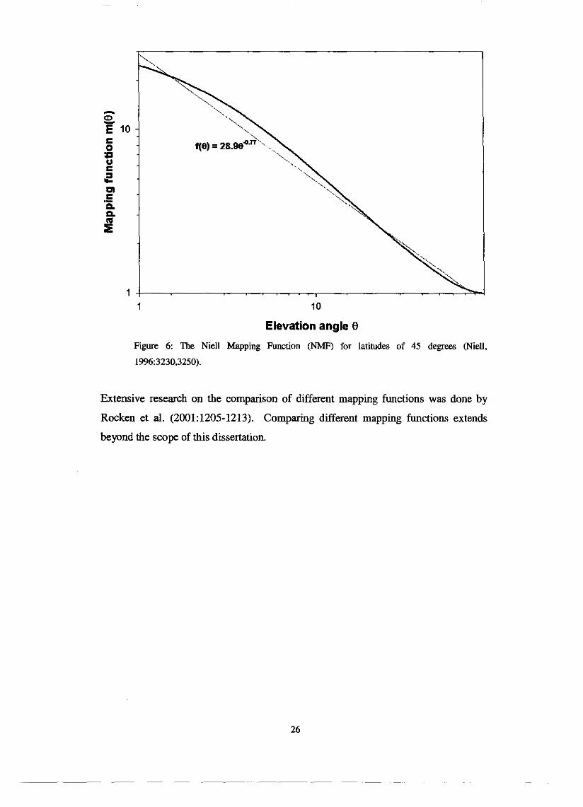
also varying with latitude. Figure 6 shows the form of equation (35), where we have

used the values of the constants as given by Niell (1996:3250) for latitudes of 45".

This figure shows that the mapping function is nearly a power law in 8, approximately

of the form f = 2 8 . ~ ~ " ' (shown by the straight line).

10

Elevation angle 9

Figure 6: The Niell Mapping Function (NMF) for latitudes of 45 degrees (Niell,

1996:3230,3250).

Extensive research on the comparison of different mapping functions was done by

Rocken et al. (2001:1205-1213). Comparing different mapping functions extends

beyond the scope of this dissertation.

CHAPTER 4

THE ACQUISITION AND PROCESSING OF GPS OBSERVATIONAL DATA

4.1. The Acquisition of GPS Observational Data

HartRAO serves as a regional data centre for the International GPS Service (IGS).

Currently, about 30 IGS stations' observational data, from January 1998 to the

present, are stored at HartRAO and can be obtained from

ftp://~wid.hartrao.ac.za/rinex/ (Combrinck, 1999). The data are stored in RINEX

(Receiver INdependent Exchange) format, containing 24-hour data sets.

Hourly RINEX files can be obtained from the SOPAC (Scripps Orbit and Permanent

Array Center) ftp site at ft~://~amer.ucsd.edu/ for near real-time applications. The

TEQC (TranslatelEdit/Quality Check) software package, which can be downloaded

from h~://www.unavco.ucar.edu/sofiwarelteqc/, was used to concatenate an

arbitrary number of hourly RINEX files into a single file. This strategy was not only

applied to the observatiod files, but also to the m x navigatiod files required by

the GAMIT processing software which is described in Section 4.2.

The predicted and precise orbits of the satellites can both be obtained from the

SOPAC ftp site. The predicted orbits, which are used for the near real-time

processing, have an accuracy of -25 cm, while the precise orbits, which are used for

precise geodetic measurements, have an accuracy of less than 5 cm, but are only

available after -13 days. These accuracies are relevant for the along-orbit as well as

the across-orbit coordinates of the satellites.

Only data from the following IGS stations were available for the near real-time

determination of zenith tropospheric delays over southern Africa (i.e. the 1-hour

RINEX files of these stations were made available hourly):

HRAO (HartRAO, Hartebeesthoek, South Africa)

SUTH (SAAO, Sutherland, South Africa)

SUTM (GFZ Potsdam, Sutherland, South Africa)

SIMO (Simon's Town, South Africa)

RBAY (Richards Bay, South Africa)

MALI (Malindi, Kenya)

DAVl (Davis, Antarctica)

MAW1 (Mawson, Antarctica)

LPGS (La Plata, Argentina)

MAS1 (Maspolomas, Canary Islands)

To estimate the tropospheric delay during post-processing, observational data (24-

hour RINEX files) from another 13 IGS stations could be used (obtained from the

HartRAO flp archive):

HARB (SAC, Hartebeesthoek, South Africa)

OH12 (O'Higgins, Antarctic Peninsula)

KERG (Port aux Francais, Kerguelen Island)

VESL (SANAE IV, Vesleskarvet, Antarctica)

GOUG (Gough Island)

PALM (Palmer, Antarctica)

SEY 1 (La Misere, Seychelles)

CASl (Casey, Antarctica)

MSKU (Masuku, Franceville, Gabon)

NKLG (NKoltang, Libreville, Gabon)

RABT (Rabat, Morocco)

SYOG (Syowa, Antarctica)

ZAMB (Lusaka, Zambia)

The Chief Directorate: Surveys and Mapping has also set up a network of

approximately 30 permanent GPS receivers in South Africa, called Trignet. The

observational data from seven of these stations were also made available for day 154

of 2003:

BFTN (Bloemfontein)

DRBN(Durban)

MFKG (Mafieng)

NSPT (Nelspmit)

PELB (Port Elizabeth)

SBOK (Springbok) 28

4.2. The Processing of GPS Obsewational Data

The GAMIT GPS processing software used for this project was developed at the

Massachusetts Institute of Technology (MIT) by R. King, T. Herring and several co-

workers. The software is freely distributed for use in scientific research, and can be

downloaded from ft~:/howie.mit.edu/.

GAlvllT was initially designed to process GPS data in 24-hour sets, for high-precision

geodetic measurements, utilising precise satellite ephemerides, published weekly by

the IGS. Some software scripts were written and some GAMIT input tables were

changed to adapt the software for our specific purpose, namely to estimate

tropospheric parameters in near real-time, with arbitrary data spans, and utilising

predicted satellite ephemerides.

GAMlT incorporates a weighted least squares algorithm to estimate the positions of

stations, orbital and earth rotation parameters and atmospheric delays, by fitting it to

doubly-differenced phase observations, which were discussed in Chapter 1 and are

derived from the carrier beat phase observations using difference-operator algorithms.

These algorithms are described by King (2002) and a critical evaluation thereof is

beyond the scope of this dissertation.

Graphical results were generated with the Generic Mapping Tools (GMT programs),

which can also be obtained freely from h~://gmt.soest.hawaii.edu/ . The results are

in Postscript (*.ps) format.

Optionally, the ImageMagick programs "convert" and "animate" (available from

htt~://www.ima~emagick.org/) can be used to convert the Postscript files to GIF

images (*.gif) and generate an animation of a series of images.

All the programming for this project was done in CShell, running the scripts under the

LINUX Debian (Woody version, kernel version 2.2) operating system on a PentiumII-

266MHz personal computer. 29

There is a definite offset between the PWV values measured at HartRAO and Irene.

This difference may be due to the different techniques used in the two cases, but it is

more likely due to the distance between the two sites. Combrinck (2000:lOl) has

shown that for baseline lengths longer than -15 km the de-comlation of troposphere

and ionosphere becomes so large that one cannot simply assume uniformity. Even so,

a strong correlation exists between these two data sets; the comparison in Figure

13(B) yielded a correlation coefficient r2 =0.60 and a regression coefficient of

b=O.81.

CHAPTER 6

AN APPLICATION: IMPROVING SLR TROPOSPHERIC DELAY MODELS

The international satellite laser ranging (SLR) network consists of approximately

forty stations (ILRS, 2003), with the purpose of tracking artificial satellites and

determining their orbits.

As in the case of GPS, the basic principles underlying SLR are Einstein's second

postulate of Special Relativity and basic geometry. An SLR station would send out a

laser pulse at a specific time and measure the time it takes the pulse to reflect off an

array of mirrors on a satellite and return to the satellite laser ranger.

SLR is one of the four space geodetic techniques in use at Hartebeesthoek; the others

are GPS, Very Long Baseline Interometry (VLBI) and Doris, which is a Doppler

satellite geodesy system. VLBI is the most accurate of these techniques, but the high

cost associated with the large radio telescopes required for VLBI experiments, gives

the VLBI network a very poor spatial resolution, with the HartRAO 26m antenna

being the only one in Africa. All these techniques operate in the radio window of the

electromagnetic spechum, except SLR, which operates at optical frequencies, the only

other part of the electromagnetic spectrum where the (dry) atmosphere appears to be

transparent, i.e. where the attenuation of electromagnetic radiation is small due to the

absence of nuclear and molecular absorption bands (Rohlfs & Wilson, 2000:4). The

radio window was chosen for GPS, because navigation systems have to be able to

operate under all weather conditions, and clouds are opaque at optical frequencies.

Optical frequencies are, however, ideal for ranging to satellites because of the high

coherence of laser beams and the absence of radio transmitters on board many low

earth orbiting geodetic satellites. It is important to note that GPS's accuracy depends

on orbit determinations performed by SLR.

Scientists in the SLR community are working hard to improve SLR accuracy - in

October 2003 the Iutemational Laser Ranging Service (ILRS) hosted a workshop

under the theme of "Working toward the full potential of the SLR capability". One of

the existing errors in SLR analysis is the estimation of tropospheric delays

experienced by laser beams, which are currently estimated using ground-based

38

meteorological measurements. A new estimation strategy is proposed here, using

GPS-derived water vapour, as discussed in Chapter 3, as an input parameter for the

tropospheric delay modelling.

During an SLR observation session a cokction of observations, called normal points,

is written to a data file, containing information about the SLR station, the satellite,

meteorological conditions (pressure, temperature and relative humidity) at the SLR

station, time-of-flight of the laser pulses, and the direction of ranging. Corrections

then have to be made to the observed time-of-flight by processing software, because

the laser pulses experience delays while travelling through the troposphere, as

discussed in Chapter 2. The ionospheric delay is negligible in the optic wavelengths,

as can be seen from (23).

In an attempt to improve the existing tropospheric delay model used in SLR

processing, the following hypotheses were formulated.

Although the contribution of water vapour to the total tropospheric delay is

much smaller (approximately 20 times) for optical wavelengths than for radio

wavelengths, it must be included in tropospheric delay models when aiming to

achieve millimetre-level accuracy.

Upper-air measurements of water vapour are highly uncorrelated with relative

humidity measurements at ground level. Furthermore, relative humidity

measurements are the most inaccurate of all the measurements done with

every observation, with uncertainties of up to 2% (ILRS, 2003).

It is believed that tropospheric delay models should include the influence of

water vapour, but that this will over-estimate the delay at times of low, and

under-estimate the delay at times of high PWV conditions.

The RGODYN software used for this analysis, was developed by Graham Appleby

and Andrew Sinclair at the Royal Greenwich Observatory, and was made available to

HartRAO's Space Geodesy Programme for research purposes. RGODYN uses the

Marini and Murray model (USNO, 2002) to predict the delay experienced by laser

pulses, as a function of temperature, pressure and relative humidity at the SLR station,

the elevation angle of the satellite as seen from the SLR station, the laser's

wavelength, and the station's latitude and geodetic height.

According to the Marini and Murray model, the delay of a one-way range can be

calculated from

where

A =0.002357P+0.000141e

and where atmospheric pressure P is measured in millibars, atmospheric temperature

T in Kelvin, relative humidity Rh measured in percentage points, elevation angle 6'

measured in degrees, laser wavelength 2 measured in microns, latitude q measured in

degrees, geodetic height H measured in kilometres, and lastly, the latitude and height

correction term proposed by Saastamoinen (1972250) is

f ((p, H) = 1 - 0 . 0 0 2 6 ~ 0 ~ 2(p-0.00031H.

This is the standard tropospheric model used for SLR data processing. Because it

employs ground-based relative humidity measurements, we expect that a strategy

using the remote sensing of atmospheric water vapour will improve this standard

model.

Therefore, we now propose a new approach, namely to split up the experienced delay

into wet and hydrostatic zenith components. As in the case of radio signals travelling

through the troposphere, we assume the "hydrostatic delay" to be proportional to the

total atmospheric pressure, with the coefficient of proportionality a function of the

SLR station's latitude, geodetic height and the laser wavelength. We calculate the

"wet delay" by multiplying the PWV, which was determined by the GPS method

discussed in Chapter 3 and given by equation (39), with the refractivity of water,

which is 0.33.

One of the weaknesses of the Marini and Murray model is that it has no separate

mapping function as in the case of radio waves, l i e the Niell Mapping function

discussed in Section 3.1. Rather, it has a very complex mapping function embedded

in the delay calculation. To ensure that all the changes in tropospheric delay, for any

elevation angle 8, can be attributed only to the new calculated znith delay, no new

mapping function was introduced. To do this, the following simple strategy was

employed: relative humidity Rh was set to zero and atmospheric temperature T was set

to 273.15 K. A new pressure parameter P was calculated by

P = Pmd +[412.74x wet delay (in metres)], with Pmcosvrcd the originally measured

atmospheric pressure. When these new parameters were put into the Marini and

Murray model, the predicted zenith tropospheric delay matched the delay calculated

by the new proposed strategy.

To test our new approach, we first processed the 2001 and 2002 observational data for

the geodetic satellites Lageos 1 and 2, using the Marini and Murray model. The

observational data (in QuickLook format) were obtained via ftp from

ftD:llcddisa.asfc.nasa.eov/~ub/slr/slr~U. Seven-day windows of data were used,

stepping one day forward between every processing session. During every processing

session RGODYN was fust employed to determine the orbits of the two satellites,

based on the global observations in the data files, and from this the position of the

MOBLAS6 SLR station located at HartRAO, was calculated. Using GMT, CShell

and C, scripts were developed to represent the position of MOBLAS6 at different

times, and to do a linear least squares fit through the points. The resulting time series

can be seen in Figure 14, indicating the station's velocity as calculated by this

method. The root mean square (rms) values of the uncertainties of the individual

positions are also shown in the figure.

THE SQUARE KILOMETRE ARRAY IN SOUTH AFRICA AND THE

SURFACE-UPGRADED 26M RADIO TELESCOPE AT HARTRAO

This chapter contains a summary of the theoretical part of a document on the

ionosphere and troposphere's influence on radio astronomical observations, submitted

to the Steering Committee of the South African Square Kilometre Array (SKA) in

November 2003, as well as some of the results obtained from the SKA site survey.

The SKA is a planned state-of-the-art radio telescope with an effective surface area of

one square kilometre, to be operational by 2015. South Africa is one of the five

countries actively bidding to host the SKA on its own soil.

The following two sections, one covering the influence of water vapour in the

troposphere and the other concerning the influence of free electrons in the ionosphere,

are also important to consider when doing single-dish radio astronomy, currently

taking place at HartRAO. A thii section is included in this chapter, showing results

obtained by HartRAO's Space Geodesy Programme while performing the SKA site

survey.

The 26m radio telescope at Hartebeesthoek is the only radio telescope in Africa. It

has recently undergone a surface upgrade in which the perforated surface has been

replaced by a solid surface. This will enable radio astronomers to observe at the

centimetre wavelength level. One of the important bands to be studied for the

observation of water masers is around 22.235 GHz, a strong spectral line of water.

This means that the atmospheric water vapour would emit and absorb radio waves at

this frequency.

The ionosphere's influence is also ever-present when doing VLBI experiments.

Whereas the troposphere is responsible for absorption and emission, the ionosphere

causes a dispersive delay of radio waves; the astrometric observables have to be

corrected for ionospheric delay.

7.1. The Influence of Precipitable Water Vapour on Centimetre Wavelength

Radio Astronomy

The earth's atmosphere is fairly transparent to radio waves if their frequency is above

the ionosphere's cut-off frequency (which is usually in the region below 25 MHz). In

the case of radio astronomical observations made from the ground, the signal entering

the receiver, however, has been attenuated by the earth's atmosphere, thus affecting

the apparent brightness of the source. In addition, there is also broadband emission

from the atmosphere, and consequently, for the centitnetre and millimetre wavelength

range, tropospheric absorption and emission has to be taken into account (Rohlfs &

Wilson, 2000:186).

It has become customary in radio astronomy to measure the brightness of a source by

its brightness temperature Tb. However, the actual quantity measured by radio

astronomers is the antenna temperature TA, which relates the output of the antenna to

the power of a matched resistor (Rohlfs & Wilson, 2000:131). By introducing an

effective temperature for the atmosphere T A ~ , which can be determined from

atmospheric profiles, we write

TA (s) = T,e-' + TA, (1 - e-') , (43)

with s the frequency-dependent total opacity along the line of sight. The total opacity

is defined as z = ~ ( s ) d s , with K an absorption coefficient along the path s of a

radio wave through the atmosphere. The first term of (43) is due to absorption in the

earth's atmosphere, while the second is due to emission.

The magnitude of opacity depends on the composition of the atmosphere; for the

22.235 GHz spectral line of water, r has typical values of -1.2, so that the received

signal will be attenuated by a factor of -0.3. Furthermore, during these typical

conditions of 20 mm PWV the atmosphere will contribute -35 K to the total antenna

temperature, while the total antenna temperature would be -6 K for a dry atmosphere.

It is therefore important to be able to determine how much atmospheric water vapour

is present during observations at this frequency.

Rohlfs and Wilson (2000:189) show how the opacity along the lime of site at any

zenith angle can be calculated from the zenith opacity. Stark (2002) has shown that a

48

tight linear relation exists between the zenith opacity of the atmosphere and the

precipitable water vapour (at zero PWV the opacity has a non-zero cut-off due to the

dry air's contribution to the opacity). The constant of proportionality and the cut-off

opacity for a specific frequency can be determined by a technique called "skydips"

(Stark, 2002).

Therefore, using skydips and the method discussed in Chapter 3 to determine the

precipitable water vapour, a radio astronomer can calculate the amount by which a

received signal's intensity was modified.

7.2. The Inkluence of Free Electrons in the Ionosphere on VLBI Astrometry

A limiting factor in centimetre-wavelength VLBI astrometry is the uncertainty in the

contribution of the ionosphere to the astrometric observables. As shown in (26), the

dispersive character of the ionosphere makes its contribution to the astrometric

observable scale as f -', which in principle allows it to be determined accurately.

One strategy to take advantage of this scaling, as in standard astromehic VLBI

experiments, is to observe in two well separated bands of frequency simultaneously.

The main disadvantage of this option is that the fixed bandwidth of the recording

equipment has to be split between two frequency bands, decreasing the signal-to-noise

ratio (SNR) for each. Alternatively, one may compute corrections based on estimates

of the ionosphere total electron count (TEC) obtained independently from the Global

Positioning System (GPS). The advantage of the latter approach is that only single-

band VLBI observations are needed, avoiding loss of sensitivity (Pirez-Torres et d.,

2000: 162).

7.3. Results from the SKA site survey

The importance of monitoring PWV and TEC for radio astronomical purposes, is

evident from the previous two sections. In Chapter 5 the current capabilities of

Figure 18 illustrates the clear diurnal signal in ionisation levels. This is due to the

recombition of electrons and ions during night time, when solar radiation, the

source of the ionising energy, is absent. Figure 18 further illustrates the effect of a

solar outburst as experienced at the proposed SKA sites.

TEC a 30s 20E duing 10 April 2001 Sdar Outburst

i

0 J

"" T '

5201 0 5201 2 5201 4

Modified Jdian Day

Figure 18: TEC values for a one week period during the April 2001 solar outburst indicates a

negative ionospheric storm effect. A rapid recovery follows the day of the negative storm

effect.

The solar outburst, which has been dubbed "the resurrection event" because it took

place during the Easter of 2001, is indicated by an arrow in Figure 18. Its effect on

the ionosphere could only be observed three days later when the plasma ejected from

the sun, reached the earth.

The April 2001 solar outburst caused a negative ionospheric storm effect (decrease in

ionisation density). Currently, negative storm effects are attributed to composition

51

changes of the ionosphere. These effects are the dominant characteristic in

ionospheric response to geomagnetic activity enhancements (Tsagouri et al.,

2000:3579).

Figure 19 indicates TEC measured at the proposed SKA sites during the 4 December

2002 partial solar eclipse.

TEC at 305 20E dulng 4 December 2002 Solar Eclipse

Modified Julian Day

Figure 19: The partial solar eclipse of 4 December 2002 (Modified Julian Day 52612) caused

a small negative effect, which has been circled in the figure.

Figure 19 clearly demonstrates the sensitivity of GPS to detect small scale short term

variations in ionisation density. A further analysis, not included in the report

submitted to the SKA Steering Committee, was done on the eclipse TEC data: a linear

fit was plotted through the minima of the two days prior and two days after the

eclipse. The minima obtained from the straight line were subtracted from the TEC

data for these four days and average TEC values were calculated for every 2-hour

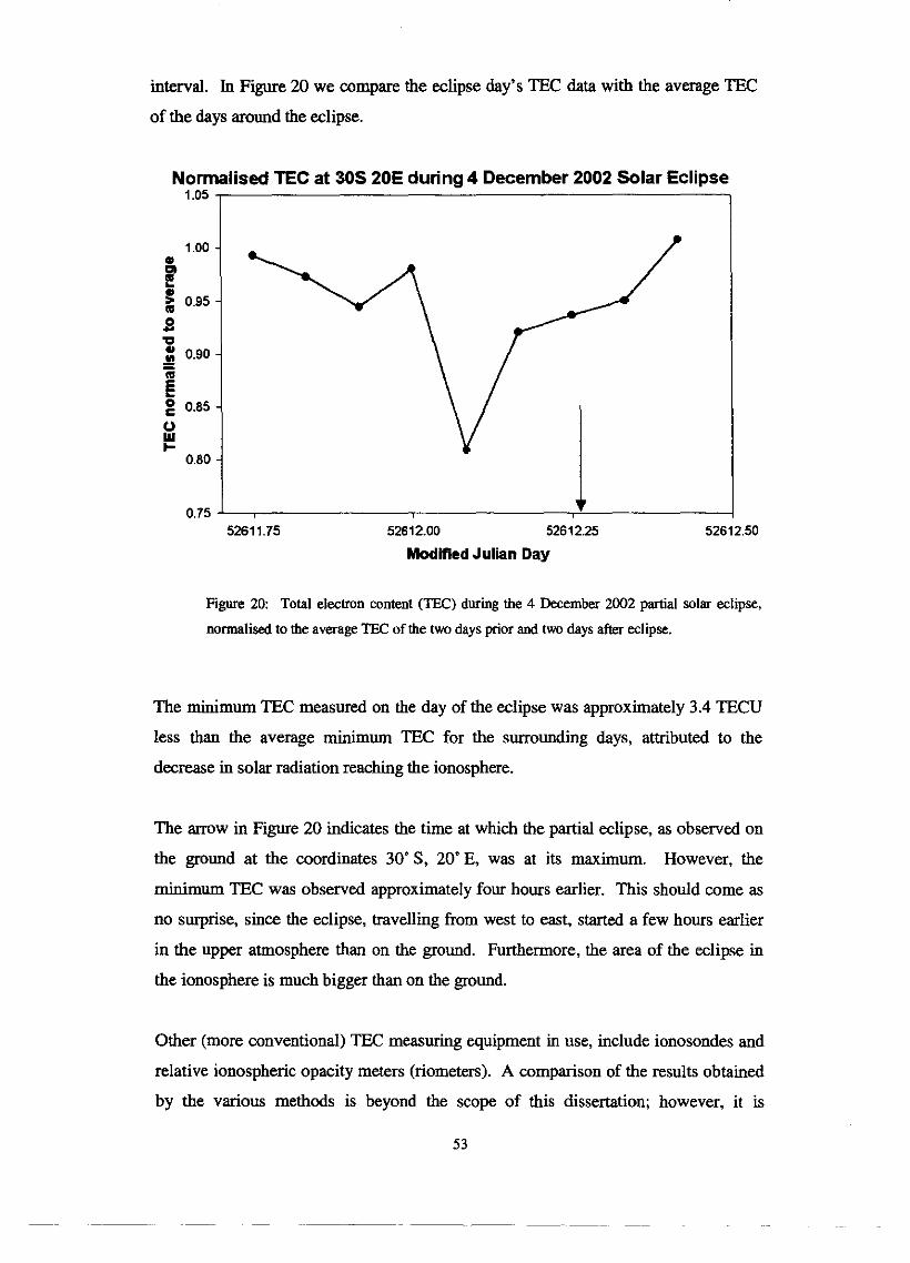
interval. In Figure 20 we compare the eclipse day's TEC data with the average TE€

of the days around the eclipse.

Normalised TEC at 30s 20E during 4 December 2002 Solar Eclipse

''o= I

Modifted Julin Day

Figure 20: Total electron content (TEC) during the 4 December 2002 partial solar eclipse,

normalised to the average TEC of the two days prior and two days after eclipse.

The minimum TEC measured on the day of the eclipse was approximately 3.4 TECU

less than the average minimum TEC for the surrounding days, attributed to the

decrease in solar radiation reaching the ionosphere.

The arrow in Figure 20 indicates the time at which the partial eclipse, as observed on

the ground at the coordinates 30" S, 20" E, was at its maximum. However, the

minimum TEC was observed approximately four hours earlier. This should come as

no surprise, since the eclipse, travelling from west to east, started a few hours earlier

in the upper atmosphere than on the ground. Furthermore, the area of the eclipse in

the ionosphere is much bigger than on the ground.

Other (more conventional) TEC measuring equipment in use, include ionosondes and

relative ionospheric opacity meters (riometers). A comparison of the results obtained

by the various methods is beyond the scope of this dissertation; however, it is

necessary to note that the TEC decrease measured by GPS could not be replicated by

riometer measurements done at Potchefstroom during the eclipse (Stoker P.H.,

personal communication, 2003). indicating the sensitivity of GPS to monitor the

ionosphere.

Figures 19 and 20 directly illustrate the usefulness of a dense network of GPS stations

in the proposed SKA region. To cater for additional nodes of the SKA, densification

of the IGS GPS network in the southern part of Africa will be necessary.

SUMMARY AND CONCLUSIONS

The theory of the propagation of electromagnetic waves in the troposphere and

ionosphere was discussed in Chapter 2. It was shown that the ionosphere acts as a

dispersive and non-dispersive medium for radio and light waves respectively, while

the troposphere acts as a non-dispersive and dispersive medium for radio and light

waves respectively. Therefore, dual-frequency GPS receivers enable users to correct

for the delay of radio signals traversing the ionosphere. The tropospheric delay of

radio waves can then be estimated by GPS processing software from GPS

observational data.

The troposphere can be split into hydrostatic and wet components; due to the

permanent dipole moment of water molecules, the wet and hydrostatic components of

the troposphere will interact differently with electromagnetic waves. The numerically

larger contribution to the total tropospheric delay comes from the hydrostatic

component, while the major contributor to variations in the total tropospheric delay is

the variation of the troposphere's water vapour content. In Chapter 3 it was shown

that the total atmospheric pressure, which is proportional to the hydrostatic

component of the tropospheric delay, and the air temperature measured at the GPS

antenna, can be used to determine the amount of precipitable water vapour above the

GPS site from the estimated total delay.

The data sources used and processing techniques followed to obtain results, were

sumrnarised in Chapter 4. It was shown in Chapter 5 that the HartRAO Space

Gwdesy Programme has the capability to produce estimates of the tropospheric delay

and the distribution of water vapour over southern Africa in near real-time, using GPS

observational data from the southern African IGS network.

One application of the estimation of the water vapour content of the troposphere, is

the improvement of tropospheric models used to predict the delay of laser pulses

travelling through the troposphere. In Chapter 6 a new strategy for the processing of

satellite laser ranging data was proposed, and the results obtained using this strategy

indicate the feasibility and improved accuracy of this technique.

In view of South Africa's bid to host the Square Kilometre Amy, it is important to

establish a network of dual-hquency GPS receivers to monitor changes in the

ionosphere and the troposphere. The influence of the ionosphere on astrometric

observables and the tropospheric influence on observed radio intensities were

discussed in Chapter 7. Some results from the site survey were also presented,

proving the ability of monitoring the ionosphere using the IGS GPS network in

southern Africa.

In the work done for this dissertation, software was developed to estimate

tropospheric delays from GPS observational data in near real-time, i.e. within the

three hour window allowed by SAWS for inclusion in numerical weather predictions,

and have it available for any potential users. One can then derive the atmospheric

water vapour content from the estimated tropospheric delay. The obtained results

compare well with zenith delay estimates from IGS and water vapour measurements

from SAWS.

The use of water vapour measurements to improve tropospheric models used for

satellite laser ranging, is currently beiig investigated by the ILRS Refractivity Study

Group. SAWS is also in the process of evaluating water vapour measurements

obtained from GPS techniques, possibly to include it in operational numerical weather

prediction models in the future. Verification of PWV estimates will also be done at

GPS sites collocated with SAWS stations from where radiosondes are launched.

Centimetre wavelength radio astronomy, to be performed at HartRAO in the near

future, requires estimates of water vapour to correct measured intensities; the

technique and theory presented in this dissertation to determine the tropospheric water

vapour content, can readily be implemented by radio astronomers.

Apart from future work to be done in the fields of SLR, numerical weather prediction

and radio astronomy, TEC mapping will also be investigated as a potential product to

the scientific community, comparing obtained TEC results with those from other

techniques, such as ionosondes and riometers.

The densification of the southern African GPS network is high on the priority list of

HartRAO's Space Geodesy Programme. Access to Trignet data, to be used for near

56

real-time products, is another issue to be resolved. Due to the remoteness of many

IGS GPS stations, the lack of connectivity reduces the number of stations that can be

used to produce near real-time tropospheric estimates. Connectivity between GPS

stations and the database at HartRAO will also be investigated and thereby the spatial

resolution of results can be improved.

In the near future HartRAO will set up a computer cluster as a powerful real-time

processing tool. This will enable the inclusion of more stations' data for near real-

time processing to improve both the spatial and temporal resolution of results.

Fially, the conclusion can be made that the network of dual-frequency receivers in

southern Africa can, apart from its use in geodetic research and surveying, be used as

a remote sensing tool for the troposphere and ionosphere and that some exciting

research in this field lies ahead.

~~ ~

BIBLIOGRAPHY

ASHBY, N. 2002. Relativity and the Globa

May 2002:41-47.

ling System. Physics TOI

BEVIS, M., BUSINGER, S., HERRING, T.A., ROCKEN, C., ANTHES, R.A.,

WARE, R.H. 1992. GPS Meteorology: Remote Sensing of Atmospheric

Water Vapour Using the Global Positioning System. Joumal of Geophysical

Research. 97@14): 15787-15801.

BORBAS, E. 1997. Determination of Precipitable Water for a fixed site using the

Global Positioning System technique. Quarterly Journal of the Hungarian

Meteorological Service. 101(4):261-273.

CHEN, F.F. 1984. Introduction to Plasma Physics and Controlled Fusion (2nd

edition). Plenum Press. 421p.

CHOUDHURI, A.R. 1998. The Physics of Fluids and Plasmas. Cambridge

University Press. 427p.

CILLIERS, P.J., GOUWS, D., OPPERMAN, B., WONNACOTT, R.T.,

COMBRINCK, L. 2003. The South African network of dual-frequency

global positioning system satellite receiver base stations: a national asset with

many applications and research opportunities. South Afncan Journal of

Science. 99:51-55.

COMBRWCK, W.L. 1999. The HartRAO Space Geodesy Programme. [Internet:]

htt~://www.hartrao.ac.za/peodesv/~eodesv indexbtml. [Date of access: 23

October 20021

COMBRINCK, W.L. 2000. Crustal Deformation and Geodetic Site Stability

Determination using GPS. University of Cape Town. 306p.

COMBRINCK, W.L., COMBRINK, A.Z.A. 2003. Applications of tropospheric

parameters derived using the SADC GPS Network. Proceedings of the 2003

ESA Symposium on Almospheric Remote Sensing using Satellite Navigation

Systems.

DAVIS, J.L., HERRING, T.A., SHAPIRO, LI., ROGERS, A.E.E., ELGERED, G.

1985. Geodesy by radio interferometry: Effects of atmospheric modelling

errors on the estimates of the baseline length. Radio Science. 20(6):1593-

1609.

DEBYE, P. 1929. Polar Molecules. Dover Publications Inc.

EMARDSON, T.R. 1998. Studies of atmospheric water vapour using the Global

Positioning System Chalmers University of Technology. 29p.

GRADINARSKY, L. 2000. Remote sensing of small-scale structures of atmospheric

water vapor. Chalmers University of Technology. 56p.

GRIFFITHS, D.J. 1999. Introduction to Electrodynamics (3d edition). Prentice Hall.

576p.

HOFFMANN-WELLENHOF, B., LICHTENEGGER, H., COLLINS, J. 1993. GPS

- Theory and Practice. Springer Verlag. 326p.

IGS. 2003. International GPS Service: Data & Products. [Internet:]

htt~://igscb.ipl.nasa.aov/~~mponentdvrods.html. [Date of access: 2 October

20031

U S . 2003. International Laser Ranging Service. [Internet:]

httv://ilrs.esfc.nasa.aov/. [Date of access: 15 October 20031

KING, R. 2002. Documentation for the GAMlT GPS Analysis Software. [Internet:]

f i ~ : / h w i e . m i t . e d d v u b / ~ s l u p d a t e s l d o c ~ F files/. [Date of

access: 10 January 20031

LYNN, K.J.W., GUBBAY, J.S. 1975. The Effect of the Earth's Atmosphere on

Baseline Determinations by Very Long Baseline Interferometry. Australian

Defence Scientific Service. 23p.

MEDEIROS, A.L. 2000. Radio propagation through the ionosphere layers.

[Internet:] h ~ : / / w w w . ~ e o c i t i e s . c o m / e l e c t r i c a l t ~

radiovro.html. [Date of access: 3 October 20031

NIELL, A.E. 1996. Global mapping functions for the atmosphere delay at radio

wavelengths. Journal of Geophysical Research. 101:3227-3246.

PEREZ-TORRES, M.A., MARCIADE, J.M., GUIRAO, J.c., ROS, E., SHAPIRO,

1.L RATNER, M.I., SARDON, E. 2000. Towards global phase-delay VLBI

astromehy: observations of QSO 1150+812 and BL 1803+784. Astronomy

and Astrophysics. 360: I6 1- 170.

RIEPL, S., SCHL-, W. 2000. Normal Point Algorithm for Reduction of Two

Colour SLR Observations. [Internet:] htt~://www.wettzell.ifa~.ddvubW2cnptl

nizza.html. [Date of access: 25 September 20031

ROBERTSON, E. 2003. Atmosphere profile. [Internet:] httP://facultv.mill~~~.edu/

-erobertson.nsm.facultv.mdGlobal Studies Cliiate2003/Atmprofile.html.

[Date of access: 14 November 20031

ROCKEN, C., SOKOLOSVSKIY, S., HUNT, D., JOHNSON, J.M. 2001. Improved

mapping of tropospheric delays. Journal of Annospheric and Oceanic

Technology. 18: 1205-1213.

ROHLFS, K., WILSON, T.L. 2000. Tools of Radio Astronomy (3d Revised and

Enlarged edition). Springer. 441p.

ROS, E., MARCIADE, J.M., GUIRADO, J.C., SARDON, E., SHAPIRO, 1.1. 2000.

A GPS-based method to model the plasma effects in VLBI observations.

Astronomy and Astrophysics. 356:357-362.

SAASTAMOINEN, J. 1972. Atmospheric correction for the troposphere and

stratosphere in radio ranging of satellites. The Use of Arfij?cial Satellites for

Geodesy. 15:247-251.

STARK, A.A. 2002. Atmospheric Opacity. [Internet:] httu://cfa-www.harvard.edu/

-aas/tenmeter/o~acitv.html. [Date of access: 9 October 20031

TSAGOURI, I., BELEHAKI, A., MORAITIS, G., MAVROMICHAJAKI, H.

Positive and negative ionospheric disturbances at middle latitudes during

geomagnetic storms. Geophysical Research Letters. 27(21):3579-3582.

USNO. 2002. 1996 IERS Conventions. [Internet:] http://maia.usno.navy.miU

conventions.htm1. [Date of access: 15 October 20031