Abstract— Improving the accuracy of prediction

on future values based on the past and current

observations has been pursued by enhancing the

prediction’s methods, combining those methods or

performing data pre-processing. In this paper,

another approach is taken, namely by increasing

the number of input in the dataset. This approach

would be useful especially for a shorter time series

data. By filling the in-between values in the time

series, the number of training set can be increased,

thus increasing the generalization capability of the

predictor. The algorithm used to make prediction

is Neural Network as it is widely used in literature

for time series tasks. For comparison, Support

Vector Regression is also employed. The dataset

used in the experiment is the frequency of

USPTO’s patents and PubMed’s scientific

publications on the field of health, namely on

Apnea, Arrhythmia, and Sleep Stages. Another

time series data designated for NN3 Competition in

the field of transportation is also used for

benchmarking. The experimental result shows that

the prediction performance can be significantly

increased by filling in-between data in the time

series. Furthermore, the use of detrend and

deseasonalization which separates the data into

trend, seasonal and stationary time series also

improve the prediction performance both on

original and filled dataset. The optimal number of

increase on the dataset in this experiment is about

five times of the length of original dataset.

I. INTRODUCTION

HIS Forecasting is the process of making

predictions about events whose actual outcomes

usually have not yet been observed. Time series

problems typically involves task of predicting

sequence of future values based on the observed

values in the past. Improving the accuracy of

prediction on future values based on past and current

observations has been pursued by many researchers

and elaborated in many literatures in recent years.

Several methods proposed to improve the prediction‟s

accuracy include data pre-processing, enhancing the

prediction‟s methods, and combining those methods.

Data pre-processing, which includes de-trending

and de-seasonalizing, is usually performed especially

for statistical method in which the time series of

observations is required to be stationer. In machine

learning methods, however, this method is not a

mandatory [4, 9]. Some researcher, on the other hand,

suggest this method is not even necessary [11, 12, 13].

Related to data pre-processing, is the use of input

selection, namely cross-validation, bagging, and

boosting that form an ensemble of several predictions

[5, 7, 8]. Recently, Phetking et al. [33] propose a

method, namely a zigzag based perceptually important

point, to reduce noise in time series without losing the

nature of financial time series such as uptrends,

downtrends, and sideway trends.

Meanwhile, several prediction methods have been

studied and used in practice. The most common ones

are linear methods based on autoregressive models of

time series [13, 14]. More advanced approaches apply

nonlinear models based mainly on artificial neural

networks (NNs), support vector machine (SVM), and

other machine learning methods [2, 9, 15, 16]. It is

reported that NNs are nonlinear structures, capable of

taking into account more complex relations existing

among the analyzed data, thus making prediction more

accurate [2]. However, it is stated in [15] that NNs

may exhibit inconsistent and unpredictable

performance on noisy data.

In order to predict future values, several

consecutive values are required for training data. In

some domain, for example in macroeconomic, the

time series are usually long enough to decompose

such that sufficient training dataset can be obtained. In

other domain, however, such as certain technology in

patent or scientific publication, the frequency of such

technological terms may not be very long. In fact,

certain newly growth technology may appear only in

the past few years.

For this reason, this paper aims to improve the

prediction result by increasing the number of dataset.

Having longer time series, we may have more training

data, which could improve the chance of better

prediction.

Enriching Time Series Datasets using Nonparametric

Kernel Regression to Improve Forecasting Accuracy

Agus Widodo, Mohamad Ivan Fanani, and Indra Budi

Information Retrieval Laboratory

Faculty of Computer Science, University of Indonesia

E-mail: agus.widodo@ui.ac.id, ivan@cs.ui.ac.id, indra@cs.ui.ac.id

T

ICACSIS 2011 ISBN: 978-979-1421-11-9

227

II. LITERATURE REVIEW

The effect of generating additional training data

have studied by several researchers such as by adding

noises to the input data on neural network modeling

and generalization performance. Several literature

concludes that that adding noises into the training

patterns may improve neural network generalization

[21,22,23]. Bishop [24] indicates that training with

more dataset is approximately equivalent to a form of

the regularization technique. In addition, [25]

conducts a rigorous analysis of how the various types

of noise affect the learning cost function for both

regression and classification problems. He

demonstrates that input noise is effective in improving

the generalization performance. Zhang [20] also adds

noises to the input data and reports that proposed

method is able to consistently outperform the single

modeling approach with a variety of time series

processes. He uses several methods to generate the

noise, namely Autoregressive, ARMA, Bilinear

process, Nonlinear autoregressive and smooth

transition autoregressive.

Meanwhile, the Kernel Parametric Regression for

time series is applied by Li and Tkacz [26] to select

weights in a forecast-combining regression. They

propose nonparametric kernel regression time-varying

weighting approach to allow the form of the weight

function to be determined by the forecast errors,

which should allow maximum flexibility in situations

of structural change of unknown form.

In addition, Auestad and Tjostheim [27] use a

kernel estimator to estimate the k-step ahead

prediction in time series using the Nadaraya-Watson

estimator. Chen and Hafner [28] also propose krenel

regression for prediction using multistage kernel

smoother, which includes the current prediction to

predict the next values. Thus, the work in [27] is

similar to direct method and the latter is similar to

iterative approach in [1].

Meanwhile, Shang and Hyndman [29] present a

nonparametric method to forecast a seasonal time

series, and propose dynamic updating methods,

namely the block moving, ordinary least squares,

penalized least squares, and ridge regression, to

improve point forecast accuracy.

In this paper, instead of using Kernel Parametric

Regression to forecast future values, it is used to

predict the the neighboring values. Non-parametric

method is very dependent on the adjacent data, thus,

we assume that this mothod is more appropriate to

compute in-between values in time series rather than

predicting some consecutive values in the futures.

Thus, the novelty of this paper is the use of

Nonparametric Kernel Regression to lengthen the time

series which in turns may increase the prediction

accuracy.

III. THEORETICAL BACKGROUND

A. Time Series Analysis

As stated in [4], a time series is sequence of

observations in which each observation xt is recorded a

particular time t. A time series of length t can be

represented as a sequence of X=[x1,x2,...,xt]. Multi-

step-ahead forecasting is the task of predicting a

sequence of h future values, 𝑋𝑡+1𝑡+𝑕 , given its p past

observations, 𝑋𝑡−𝑝+1𝑡 , where the notation 𝑋𝑡−𝑝

𝑡 denotes

a segment of the time series [xt-p,xt-p+1,...,xt].

Time series methods for forecasting are based on

analysis of historical data assuming that past patterns

in data can be used to forecast future data points [17].

When there are trend and seasonal factors in the data

series, those factors shall be removed first, and

computed separately, in order to correctly compute the

forecast. De-trend and de-seasonalize time-series to

separate base from trend and seasonality effects can be

done by this exponential smoothing, as stated in [18]:

𝐵𝑡 = 𝛼𝐷𝑡

𝑆𝑡−𝑚+ 1 − 𝛼 (𝐵𝑡−1 + 𝑇𝑡−1)

𝑇𝑡 = 𝛽 𝐵𝑡 − 𝐵𝑡−1 + (1 − 𝛽)𝑇𝑡−1

𝑆𝑡 = 𝛾𝐷𝑡

𝐵𝑡+ (1− 𝛾)𝑆𝑡−𝑚

where equation (1) is used to smooth the base forecast

Bt, equation (2) to smooth the trend forecast Tt, and

equation (3) to smooth the seasonality forecast St.

Meanwhile, α, β, and γ are the degree of importance of

the current data compared to the previous ones,

whereas subscript t and m denotes the current time

and seasonal period. The forecast of the next k period

using exponential smoothing with trend and

seasonality can be calculated by:

𝐹𝑡+𝑘 = (𝐵𝑡−1 + 𝑘𝑇𝑡−1)𝑆𝑡+𝑘−𝑚

Furthermore, the multi-step-ahead prediction task of

time series can be achieved by either explicitly

training a direct model to predict several steps ahead,

or by doing repeated one-step ahead predictions up to

the desired horizon. The former is often called as

direct method, whereas the latter is often called as

iterative method.

The iterative approach is used and the model is

trained on a one-step-ahead basis in [1]. After training,

the model is used to forecast one step ahead, such as

one week ahead. Then the forecasted value is used as

an input for the model to forecast the subsequent

point. In the direct approach, a different network is

used for each future point to be forecasted. In

addition, a parallel approach is also discussed in [1]. It

consists of one network with a number of outputs

equal to the length of the horizon to be forecasted. The

network is trained in such a way that output number k

produces the k-step-ahead forecast. However, it was

reported that this approach did not perform well

compared to the two previous methods.

ICACSIS 2011 ISBN: 978-979-1421-11-9

228

B. Non-parametric Kernel Regression

Non-parametric Kernel Regression which is also

sometimes related to the smoothing methods, typically

requires three phases, namely (1) a fitting step to find

the best combine of model type, kernel function, and

bandwidth, using a test sample, (2) a validation phase

that allows to validate the model on new observations

for which the prediction is known, and (3) an

application phase, where the model is applied to a new

set of data for which the prediction is unknown.

Fernandez and Cao [31] indicate that Nonparametric

regression estimation has several advantages over

classical parametric methods. It is a more flexible

approach and can be very well adapted to local

features in time series. Usual non-parametric

estimators of m(u) are of the general form:

𝑚 𝑢 = 𝑊(𝑢, 𝑥𝑗 )𝑦𝑗𝑛𝑗=1

where W(u,xj) are some smoothing positive weights

with high values if u is close to xj and valuse close to

zero otherwise. The shape of the weight function

W(u,xj) is often referred as kernel, which is a

continuous, bounded, and symmetric real function

which integrates to one. The form of weight has been

proposed by Nadaraya-Watson as

𝑊𝑕(𝑢, 𝑥𝑗 ) =𝐾𝑕 (𝑥𝑗−𝑢)

𝐾𝑕 (𝑥𝑖−𝑢)𝑛𝑖=1

where h is the bandwidth. As stated in [32], a very

large bandwidth will result in an oversmooth curve,

whereas small bandwith will reproduce the data.

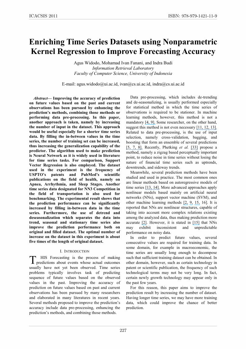
C. Neural Network on Time Series

The algorithm used for evaluating the forecasting

performance is the Multilayer Perceptron, which is

widely employed Neural Network (NN) architecture

according to [4]. This method is well researched

regarding their properties and their ability in time

series prediction [6]. Data are presented to the network

as a sliding window [10] over the time series history,

as shown in Figure 1. The neural network will learn the

data during the training to produce valid forecasts

when new data are presented.

Fig. 1. Predicting future value using Neural Network.

The general function of NN, as stated in [7] is as

follows:

𝑓 𝑥,𝑤 = 𝛽0 + 𝛽𝑕𝑔 𝛾0 + 𝛾𝑕𝑖𝑥𝑖𝐼𝑖=0 𝐻

𝑕=1 (7)

where X =[x0, x1, ..., xn] is the vector of the lagged

observations of the time series and w=(β, γ) are the

weights. I and H are the number of input and hidden

units in the network and g(.) is a non-linear transfer

function [19]. Default setting from Matlab is used in

this experiment, that is 'tansig' for hidden layers, and

'purelin' for output layer, since this functions are

suitable for problems in regression that predict

continuous values. Tansig is smooth transfer function

having maximum value of 1 and minimum of -1,

whereas purelin is linear transfer functions.

D. Mean Squared Error

The mean squared error (MSE) of an estimator is one

of many ways to quantify the difference between

values implied by an estimator and the true values of

the quantity being estimated. Let X={x1, x2,..xT} be a

random sample of points in the domain of f, and

suppose that the value of Y={y1, y2,..yT} is known for

all x in X. Then, for all N samples, the error is

computed as

𝑀𝑆𝐸 =1

𝑁 (𝑓 𝑥𝑖 − 𝑦𝑖)

2𝑁𝑖=1 (8)

An MSE of zero means that the estimator predicts

observations with perfect accuracy, which is the ideal.

Two or more statistical models may be compared

using their MSEs as a measure of how well they

explain a given set of observations.

IV. EXPERIMENTAL SETUP

A. Steps

The steps to conduct this experiment are as follows:

(1) read and scale the time series so that they have

equivalent measurement (2) fill the in-between values

(3) construct matrices of input and output for training

as well as for testing, (4) detrend and deaseasonalize

data, (5) run the prediction algorithm, which is using

Neural Network and SVR, on the data, (6) record and

compare the performance of the prediction.

Fig. 2. Steps of the experiment.

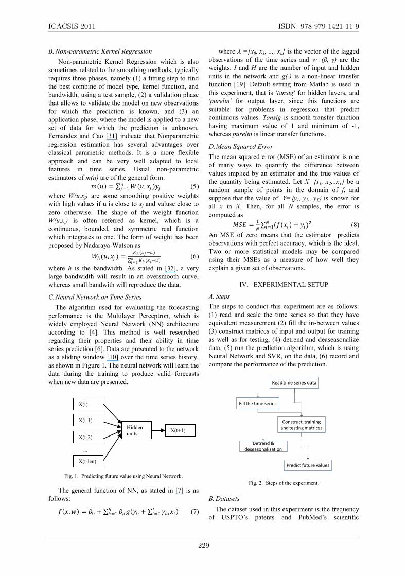
B. Datasets

The dataset used in this experiment is the frequency

of USPTO‟s patents and PubMed‟s scientific

Read time series data

Fill the time series

Construct training and testing matrices

Predict future values

Detrend & deseasonalization

X(t)

X(t-1)

Hidden

units X(t-2)

X(t+1)

...

X(t-len)

ICACSIS 2011 ISBN: 978-979-1421-11-9

229

publications on the field of health, namely on Apnea,

Arrhythmia, and Sleep Stages. These frequencies are

obtained by querying the USPTO and Pubmed online

database from the year 1976 until 2010, which means

35 years. The other dataset used in this experiment is

yearly time series of the number of passengers of

airport and railway in several cities in Europe and

United States taken from Time Series Forecasting

Competition for Computational Intelligencei, known

as NNGC (Neural Network Grand Competition). The

task of this competition is to predict the amount of

passengers of the next 6 consecutive years. The

number of time series used in this experiment is 5

series, having a length of 23 years.

Fig. 3 Dataset form USPTO and Pubmed.

Fig. 4 Dataset form NNGC.

The input matrix of training is two dimensional matrix

having the row size of the length of time series and the

column size of the number of samples. Thus, having 6

values to predict, for example, the vector ytest consists

of 6 values, and the matrix xtest consists of 6×(23-6)

series having one sliding window each. In addition,

the ytrain and xtrain are similarly constructed.

C. Performance Evaluation

For performance evalution, MSE is used for out-of-

sample predictions along with head-to-head count.

Running time is also recorded to compare the

effectivenes of algorithm employed on different input

settings.

D. Hardware and Tools

This experiment is conducted on computer with

Pentium processor Core i3 and memory of 2GB. The

software used is Matlab version 2008b. The Matlab‟s

command used to perform the NN is „newff‟, using the

number of hidden nodes as log(T). To record the

execution time, the commands used are „tic‟ and „toc‟.

To normalise data into the range of -1 to 1, the

command used is „mapminmax‟. The toolbox for

Support Vector Regression is provided by Gun [23],

whereas toolbox for Kernel Regression is available

from Farahmand [30].

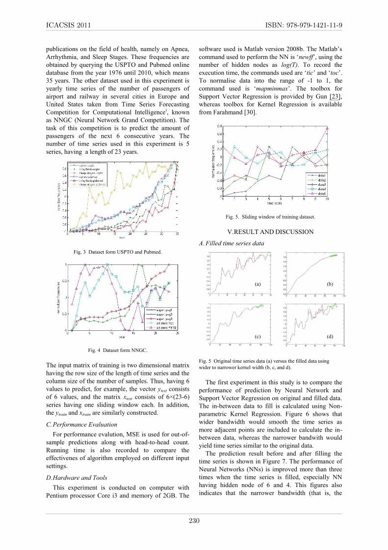
Fig. 5. Sliding window of training dataset.

V. RESULT AND DISCUSSION

A. Filled time series data

Fig. 5 Original time series data (a) versus the filled data using

wider to narrower kernel width (b, c, and d).

The first experiment in this study is to compare the

performance of prediction by Neural Network and

Support Vector Regression on original and filled data.

The in-between data to fill is calculated using Non-

parametric Kernel Regression. Figure 6 shows that

wider bandwidth would smooth the time series as

more adjacent points are included to calculate the in-

between data, whereas the narrower bandwith would

yield time series similar to the original data.

The prediction result before and after filling the

time series is shown in Figure 7. The performance of

Neural Networks (NNs) is improved more than three

times when the time series is filled, especially NN

having hidden node of 6 and 4. This figures also

indicates that the narrower bandwidth (that is, the

(a) (b)

(c) (d)

ICACSIS 2011 ISBN: 978-979-1421-11-9

230

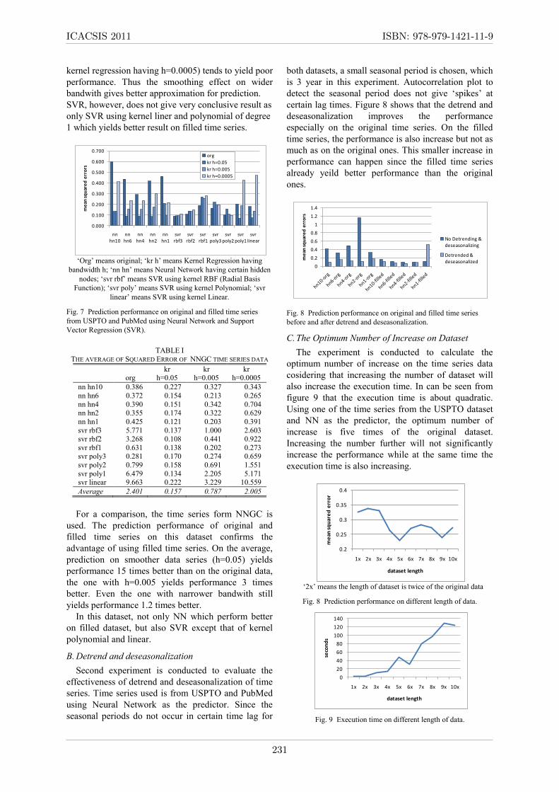
kernel regression having h=0.0005) tends to yield poor

performance. Thus the smoothing effect on wider

bandwith gives better approximation for prediction.

SVR, however, does not give very conclusive result as

only SVR using kernel liner and polynomial of degree

1 which yields better result on filled time series.

„Org‟ means original; „kr h‟ means Kernel Regression having

bandwidth h; „nn hn‟ means Neural Network having certain hidden

nodes; „svr rbf‟ means SVR using kernel RBF (Radial Basis

Function); „svr poly‟ means SVR using kernel Polynomial; „svr

linear‟ means SVR using kernel Linear.

Fig. 7 Prediction performance on original and filled time series

from USPTO and PubMed using Neural Network and Support

Vector Regression (SVR).

TABLE I

THE AVERAGE OF SQUARED ERROR OF NNGC TIME SERIES DATA

org kr

h=0.05 kr

h=0.005 kr

h=0.0005

nn hn10 0.386 0.227 0.327 0.343

nn hn6 0.372 0.154 0.213 0.265

nn hn4 0.390 0.151 0.342 0.704 nn hn2 0.355 0.174 0.322 0.629

nn hn1 0.425 0.121 0.203 0.391

svr rbf3 5.771 0.137 1.000 2.603 svr rbf2 3.268 0.108 0.441 0.922

svr rbf1 0.631 0.138 0.202 0.273 svr poly3 0.281 0.170 0.274 0.659

svr poly2 0.799 0.158 0.691 1.551

svr poly1 6.479 0.134 2.205 5.171 svr linear 9.663 0.222 3.229 10.559

Average 2.401 0.157 0.787 2.005

For a comparison, the time series form NNGC is

used. The prediction performance of original and

filled time series on this dataset confirms the

advantage of using filled time series. On the average,

prediction on smoother data series (h=0.05) yields

performance 15 times better than on the original data,

the one with h=0.005 yields performance 3 times

better. Even the one with narrower bandwith still

yields performance 1.2 times better.

In this dataset, not only NN which perform better

on filled dataset, but also SVR except that of kernel

polynomial and linear.

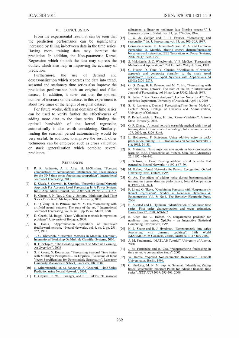
B. Detrend and deseasonalization

Second experiment is conducted to evaluate the

effectiveness of detrend and deseasonalization of time

series. Time series used is from USPTO and PubMed

using Neural Network as the predictor. Since the

seasonal periods do not occur in certain time lag for

both datasets, a small seasonal period is chosen, which

is 3 year in this experiment. Autocorrelation plot to

detect the seasonal period does not give „spikes‟ at

certain lag times. Figure 8 shows that the detrend and

deseasonalization improves the performance

especially on the original time series. On the filled

time series, the performance is also increase but not as

much as on the original ones. This smaller increase in

performance can happen since the filled time series

already yeild better performance than the original

ones.

Fig. 8 Prediction performance on original and filled time series

before and after detrend and deseasonalization.

C. The Optimum Number of Increase on Dataset

The experiment is conducted to calculate the

optimum number of increase on the time series data

cosidering that increasing the number of dataset will

also increase the execution time. In can be seen from

figure 9 that the execution time is about quadratic.

Using one of the time series from the USPTO dataset

and NN as the predictor, the optimum number of

increase is five times of the original dataset.

Increasing the number further will not significantly

increase the performance while at the same time the

execution time is also increasing.

„2x‟ means the length of dataset is twice of the original data

Fig. 8 Prediction performance on different length of data.

Fig. 9 Execution time on different length of data.

0.000

0.100

0.200

0.300

0.400

0.500

0.600

0.700

nn hn10

nn hn6

nn hn4

nn hn2

nn hn1

svr rbf3

svr rbf2

svr rbf1

svr poly3

svr poly2

svr poly1

svr linear

me

an s

qu

are

d e

rro

rs

org

kr h=0.05

kr h=0.005

kr h=0.0005

0

0.2

0.4

0.6

0.8

1

1.2

1.4

me

an s

qu

are

d e

rro

rs

No Detrending & deseasonalizing

Detrended & deseasonalized

0.2

0.25

0.3

0.35

0.4

1x 2x 3x 4x 5x 6x 7x 8x 9x 10x

me

an s

qu

are

d e

rro

r

dataset length

0

20

40

60

80

100

120

140

1x 2x 3x 4x 5x 6x 7x 8x 9x 10x

seco

nd

s

dataset length

ICACSIS 2011 ISBN: 978-979-1421-11-9

231

VI. CONCLUSION

From the experimental result, it can be seen that

the prediction performance can be significantly

increased by filling in-between data in the time series.

Having more training data may increase the

prediction. In addition, the Non-parametric Kernel

Regression which smooth the data may supress the

outlier, which also help in improving the acurracy of

prediction.

Furthermore, the use of detrend and

deseasonalization which separates the data into trend,

seasonal and stationary time series also improve the

prediction performance both on original and filled

dataset. In addition, it turns out that the optimal

number of increase on the dataset in this experiment is

about five times of the length of original dataset.

For future works, different domains of time series

can be used to verify further the effectiveness of

adding more data to the time series. Finding the

optimal bandwidth of the kernel regression

automatically is also worth considering. Similarly,

finding the seasonal period automatically would be

very useful. In addition, to improve the result, other

techniques can be employed such as cross validation

or stack generalization which combine several

predictors.

REFERENCES

[1] R. R. Andrawis, A. F. Atiya, H. El-Shishiny, “Forecast combinations of computational intelligence and linear models for the NN5 time series forecasting competition”, International Journal of Forecasting, 2011.

[2] K. Siwek, S. Osowski, R. Szupiluk, “Ensemble Neural Network Approach For Accurate Load Forecasting In A Power System, Int. J. Appl. Math. Comput. Sci., 2009, Vol. 19, No. 2, 303–315

[3] H. Cheng, P. N. Tan, J. Gao, J. Scripps, “Multistep-ahed Time Series Prediction”, Michigan State University, 2005.

[4] G. Q. Zang, B. E. Patuwo, and M. Y. Hu, “Forecasting with artificial neural network: The state of the art, “ International Journal of Forecasting, vol 14, no 1, pp 35062, March 1998.

[5] D. Cocchi, M. Raggi, “Cross-Validation methods in regression problems”, University of Bologna, 2000.

[6] K. Honik, “Approximation capabilities of multilayer feedforward network, “ Neural Networks, vol. 4, no. 2, pp. 251-257, 1991.

[7] T. G. Dietterich, “Ensemble Methods in Machine Learning”, International Workshop On Multiple Classifier Systems, 2000.

[8] R. E. Schapire, “The Boosting Approach to Machine Learning, An Overview”, 2003

[9] S. F. Crone, N. Kourentzes, “Forecasting Seasonal Time Series with Multilayer Perceptrons – an Empirical Evaluation of Input Vector Specifications for Deterministic Seasonality”, Lancaster University Management School, Lancaster, UK, 2007.

[10] N. Mirarmandehi, M. M. Saboorian, A. Ghodrati, “Time Series Prediction using Neural Network”, 2004.

[11] E. Ghysels, C. W. J. Granger, and P. L. Siklos, “Is seasonal

adjustment a linear or nonlinear data filtering process?,” J. Business Econom. Statist., vol. 14, pp. 374–386, 1996.

[12] J. G. de Gooijer and P. H. Franses, “Forecasting and seasonality,” Int. J. Forecasting, vol. 13, pp. 303–305, 1997.

[13] Gonzalez-Romera, E., Jaramillo-Moran, M. A. and Carmona-Fernandez, D. Monthly electric energy demandforecasting based on trend extraction, IEEE Transations on Power Systems, 2006, 21(4): 1946–1953.

[14] S. Makridakis, S. C. Wheelwright, V. E. McGee, “Forecasting: Methods and Applications”, 2nd Ed, John Wiley & Sons, 1983.

[15] C. Huang, D. Yang, Y. Chuang, “Application of wrapper approach and composite classifier to the stock trend prediction”, Elsevier, Expert Systems with Applications 34 (2008) 2870–2878.

[16] G. Q. Zang, B. E. Patuwo, and M. Y. Hu, “Forecasting with artificial neural network: The state of the art, “ International Journal of Forecasting, vol 14, no 1, pp 35062, March 1998.

[17] R. Ihaka, “Time Series Analysis”, Lecture Notes for 475.726, Statistics Department, University of Auckland, April 14, 2005

[18] S. R. Lawrence,“Demand Forecasting:Time Series Models”, Lecture Notes, College of Business and Administration, University of Colorado

[19] P. Refaeilzadeh, L. Tang, H. Liu, “Cross-Validation”, Arizona State University, 2008.

[20] G. P. Zhang, “A neural network ensemble method with jittered training data for time series forecasting”, Information Sciences 177, 2007, pp. 5329–5346.

[21] L. Holmstrom, P. Koistinen, Using additive noise in back-propagation training, IEEE Transactions on Neural Networks 3 (1), 1992, 24–38.

[22] K. Matsuoka, Noise injection into inputs in back-propagation learning, IEEE Transactions on System, Man, and Cybernetics 22, 1992, 436–440.

[23] J. Sietsma, R. Dow, Creating artificial neural networks that generalize, Neural Networks 4 (1991) 67–79.

[24] M. Bishop, Neural Networks for Pattern Recognition, Oxford University Press, Oxford, 1995.

[25] G. An, The effect of adding noise during backpropagation training on a generalization performance, Neural Computation 8 (1996), 643–674.

[26] F. Li and G. Tkacz, "Combining Forecasts with Nonparametric Kernel Regressions", Studies in Nonlinear Dynamics & Econometrics: Vol. 8: No.4, The Berkeley Electronic Press, 2004.

[27] B. Auestad and D. Tjstheim, “Identification of nonlinear time series: First order characterization and order estimation, Biometrika 77, 1990, 669-687

[28] R. Chen and C. Hafner, “A nonparameric predictor for nonlinear time series, XploRe – an Interactive Statistical Computing Environment, 1995.

[29] H. L. Shang and R. J. Hyndman, “Nonparametric time series forecasting with dynamic updating”, 18th World IMAS/MODSIM Congress, Cairns, Australia 13-17 July 2009.

[30] A. M. Farahmand, “MATLAB Tutorial”, University of Alberta, 2008.

[31] J. M. Fernandez and R. Cao, “Nonparametric forecasting in time series. A comparative Study”, 2002.

[32] W. Hardle, “Applied Non-parametric Regression”, Humbolt Universitat zu Berlin, 1994.

[33] C. Phetking, M. N. M. Sap, A. Selamat, “Identifying Zigzag based Perceptually Important Points for indexing financial time series”. IEEE ICCI 2009: 295-301, 2009.

ICACSIS 2011 ISBN: 978-979-1421-11-9

232