Enhancement of an Industrial Finite-Volume

Code for Large-Eddy-Type Simulation of

Incompressible High-Reynolds Number Flow

Using Near-Wall Modelling

Tobias Knopp a,∗, Xiaoqin Zhang b, Roland Kessler a,Gert Lube b

aInstitut fur Aerodynamik und Stromungstechnik, Deutsches Zentrum fur

Luft- und Raumfahrt, Bunsenstr. 10, D-37073 Gottingen, Germany

bInstitut fur Numerische und Angewandte Mathematik, Georg-August-Universitat

Gottingen, Lotzestrasse 16-18, D-37083 Gottingen, Germany

Abstract

We present a validation strategy for enhancement of an unstructured industrialfinite-volume solver designed for steady RANS problems for large eddy-type simu-lation with near-wall modelling of incompressible high-Reynolds number flow. Dif-ferent parts of the projection-based discretisation are investigated to ensure LEScapability of the numerical method. Turbulence model parameters are calibrated byusing a minimisation of least-squares functionals for first and second order statisticsof the basic benchmark problems decaying homogeneous turbulence and turbulentchannel flow. Then the method is applied to the flow over a backward-facing step atReh = 37500. Of special interest is the role of the spatial and temporal discretisationerror for low order schemes. For wall-bounded flows, present results confirm existingbest practice guidelines for mesh design. For free shear layers, a sensor to quantifythe resolution quality of the LES based on the resolved turbulent kinetic energy ispresented and applied to the flow over a backward-facing step at Reh = 37500.

Key words: Navier-Stokes model, large-eddy simulation, detached-eddysimulation, wall functions, projection method, finite volume method.

∗ Corresponding author.Email address: Tobias.Knopp@dlr.de (Tobias Knopp).

Preprint submitted to Elsevier Science 9 December 2008

1 Introduction

CFD has reached such a technology readiness level that it is used as standardpredictive tool in a broad range of application areas. Virtually all of thesetools rely on the (U)RANS approach which solves the statistically averaged(or: Reynolds averaged) Navier Stokes equations. Since RANS models are de-signed for problems with steady state solutions, the corresponding numericalmethods traditionally use low order schemes. Here we restrict ourselves toincompressible flows, for which second order finite volume schemes are stillvery popular. The basic algorithms are well-established since more than twodecades, see e.g. [13], and are still used by most research and commercial flowsolvers. For a recent review see e.g. [12].Comprehensive studies have shown that for certain classes of flows the (U)RANSmodelling approach has become the limiting factor for getting high-qualitynumerical predictions. For most engineering simulations at design conditions,e.g., without (unsteady) flow separation, (U)RANS methods give predictionsof satisfying accuracy. However, there is a strongly growing demand in pre-dicting flows with incipient and moderate separation because industry requiresmore and more reliable predictions at the boundary of the operative range andfor off-design conditions for airfoils, wind turbines, turbo-machinery etc.The strong interest by research institutions and industry to use LES capa-bilities leads to the question whether existing RANS solvers or existing LESsolvers should be used. Classical LES codes often provide higher order meth-ods, but this restricts the applicability to simple geometries. Instead, RANSsolvers are typically low order methods but often support unstructured meshesof hybrid element types and thus allow to deal with very complex geometries ofindustrial relevance easily. Several additional reasons lead to the aim to extendexisting RANS solvers to LES capabilities. As RANS will be the backbone forindustrial applications for the next future, the first application scenario willbe to apply LES to carefully selected configurations after a broad simulationcampaign using (U)RANS was performed. Moreover one has to keep in mindthat development of a flow solver for complex industrial applications requireslarge costs for design, implementation, verification and validation until matu-rity is reached. Another important point is that it takes a long-term experiencefor engineers to become familiar with a CFD code and to acquire best-practiceexpertise until the code can be used as predictive tool, because there are al-ways code-specific differences among different flow solvers. Moreover CFD hasto be seen more and more as part of multiphysics applications, although a veryimportant one. Such coupling of different codes and exchange of suitable datahas been established for existing RANS solvers. Achieving LES capabilitieswhile maintaining such interfaces is also of considerable interest.When judging the industrial applicability of LES-type methods, one has todistinguish between two completely different groups. On the one hand, LESfor complex configurations is naturally a grand challenge problem requiring

2

O(104) processors. On the other hand, industrial applicability of LES meansthat engineering design studies become feasible, meaning ultimately overnightLES simulations for configurations of moderate complexity. Currently the ma-jor part of industrial CFD applications is done by small and middle enterprisesand engineering companies. Making LES amenable for clusters of O(101) pro-cessors used by this group should be a driving force regarding algorithmicdevelopment. For this purpose all simulations in this paper were performedon a single processor Linux machine. Acceleration techniques for LES are alsoof great interest for large scale applications because then the parameter spacefor design optimisation can be extended at the same total computing time.Having pointed out the industrial need for LES and the reason to use existingRANS solvers, the question arises, whether it is possible to extend any secondorder RANS method to LES capability or not. Whereas (U)RANS solutionsare characterized by smooth large-scale structures, turbulent flows have broadband spectra and the resolution of the medium to small eddies is crucial, see[23]. Thus the first question that arises is: Is it possible to adopt second-orderschemes in space and/or time for LES (or do we need higher order schemes)?It is well-known that there are a variety of second order methods which allowfor adequate LES simulations, e.g. the CDP-α code developed at Stanford uni-versity, see also e.g. [22]. The theoretical considerations by [9,14] have beenrecently reviewed by [27] with much more optimistic conclusions regardingthe magnitude of numerical errors for second-order schemes. From this weconclude a positive answer for the first question. On the other hand it has tobe mentioned that recent investigations clearly show significant advances ofusing sophisticated higher-order methods, see e.g. [5], which confirms earlierstudies by [20,24].The second question faces the huge computing costs: Which (modelling) ap-proaches are useful and applicable also to complex configurations to make LESamenable to high Reynolds number flows? In this paper the focus is on wall-functions for alleviating the huge costs of wall-resolved LES by one order ofmagnitude, see e.g. [37,36]. As an alternative, the DES approach by [34] isalso considered, which has been used as a wall-model for LES in [26]. It hasbecome obvious that the coupling of a RANS type solution near the wall andan LES type solution for the outer flow requires special care, see e.g. [18]. Thispoint will also be addressed in this paper.The third question is: How reliable are LES results in terms of numerical andmodelling error? This issue cannot be overestimated, in particular from anindustrial point of view. Even when using RANS methods, CFD tools cannotproduce results at the push of a button. Large user experience in choosing thecorrect numerical settings (grid design, parameters for the numerical solver)and turbulence modelling aspects is required. This is much more true for LES.The quality of the results strongly depends on the experience of the user. Inthe present work we focus on role of the discretisation error. For industrial ap-plications of LES to flows in complex geometries, grid convergence cannot bereached or ensured by a global mesh refinement study due to extremely large

3

computational costs. For this reason we present a sensor based on the resolvedturbulent kinetic energy which measures the resolution quality of the LES forfree shear layers and in regions of separated flow. This sensor may then beused as a refinement indicator for local mesh adaptation. It is well known thatalso the sensitivity of the LES results to the inflow boundary conditions canbe large, see e.g. [3,7,19], but this issue cannot be addressed here.This fourth question is strongly related to the third one: What are best-practiceguidelines for LES? Due to the extremely high computing costs, industry needsguidelines for mesh design, time step size and modelling aspects, see [33] as avery first step. Such guidelines should minimize erroneous computations andprovide some general criteria for ensuring a proper use of LES in terms ofnumerical and modelling error. However, even for (U)RANS simulations, onlyfirst versions of best practice guidelines are available, e.g. [1].In the present paper, we consider the unstructured incompressible finite vol-ume solver THETA, developed at the German Aerospace Center (DLR) inGottingen. At the start of this work, the THETA-code was validated only forlaminar flows and for turbulent flows based on the RANS equations. For timeaccurate simulations only a first order accurate time discretisation scheme wasavailable. Turbulence modelling was restricted to the standard k-ǫ model withclassical wall functions.The paper is organized as follows: In Section 2, we briefly describe the basicdiscretisation. Moreover, the models of LES and DES and aspects of the near-wall modelling will be introduced. Section 3 summarizes some tools to param-eter identification problems for turbulent flows. The benchmark test case ofdecaying homogeneous turbulence is considered in Section 4. Turbulent chan-nel flow is considered for Reynolds number Reτ = 395, see Section 5.1, and forhigher Reynolds number Reτ = 4800 using wall-functions as near-wall model,see Section 5.2. In Section 6 the turbulent flow over a backward facing step atReh = 37500 is addressed and the sensor to measure the turbulence resolutionis presented in Section 7. Summary and outlook are given in Section 8.

2 Basic discretisation and turbulence modelling

Consider the non-stationary, incompressible Navier-Stokes model

∂t~u− ~∇ · (2νS(~u)) + ~∇ · (~u⊗ ~u) + ~∇p = ~f in Ω × (0, T ] (1)

~∇ · ~u = 0 in Ω × (0, T ] (2)

for velocity ~u and pressure p in a bounded, polyhedral domain Ω ⊂ R3 with

given source term ~f and viscosity ν > 0. S(~u) = 12(~∇~u + ~∇~uT ) is the rate of

strain tensor. To simplify the presentation we set density to one. Appropriateboundary and initial conditions have to be added.The spatial discretisation of (1)-(2) is based on a finite volume scheme on un-structured collocated grids. The primal and dual grids are sketched in Figure

4

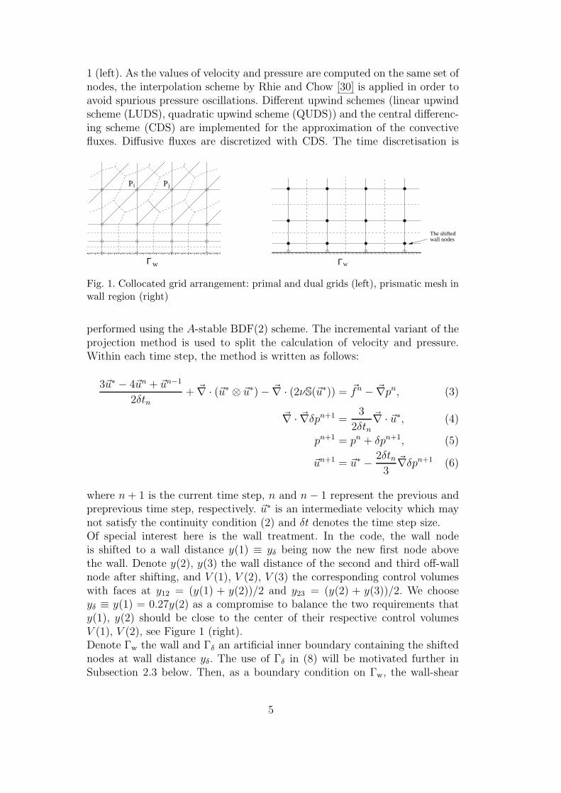
1 (left). As the values of velocity and pressure are computed on the same set ofnodes, the interpolation scheme by Rhie and Chow [30] is applied in order toavoid spurious pressure oscillations. Different upwind schemes (linear upwindscheme (LUDS), quadratic upwind scheme (QUDS)) and the central differenc-ing scheme (CDS) are implemented for the approximation of the convectivefluxes. Diffusive fluxes are discretized with CDS. The time discretisation is

jPPi

Γ W ΓW

The shiftedwall nodes

Fig. 1. Collocated grid arrangement: primal and dual grids (left), prismatic mesh inwall region (right)

performed using the A-stable BDF(2) scheme. The incremental variant of theprojection method is used to split the calculation of velocity and pressure.Within each time step, the method is written as follows:

3~u∗ − 4~un + ~un−1

2δtn+ ~∇ · (~u∗ ⊗ ~u∗) − ~∇ · (2νS(~u∗)) = ~fn − ~∇pn, (3)

~∇ · ~∇δpn+1 =3

2δtn~∇ · ~u∗, (4)

pn+1 = pn + δpn+1, (5)

~un+1 = ~u∗ − 2δtn3

~∇δpn+1 (6)

where n + 1 is the current time step, n and n− 1 represent the previous andpreprevious time step, respectively. ~u∗ is an intermediate velocity which maynot satisfy the continuity condition (2) and δt denotes the time step size.Of special interest here is the wall treatment. In the code, the wall nodeis shifted to a wall distance y(1) ≡ yδ being now the new first node abovethe wall. Denote y(2), y(3) the wall distance of the second and third off-wallnode after shifting, and V (1), V (2), V (3) the corresponding control volumeswith faces at y12 = (y(1) + y(2))/2 and y23 = (y(2) + y(3))/2. We chooseyδ ≡ y(1) = 0.27y(2) as a compromise to balance the two requirements thaty(1), y(2) should be close to the center of their respective control volumesV (1), V (2), see Figure 1 (right).Denote Γw the wall and Γδ an artificial inner boundary containing the shiftednodes at wall distance yδ. The use of Γδ in (8) will be motivated further inSubsection 2.3 below. Then, as a boundary condition on Γw, the wall-shear

5

stress τw is prescribed instead of no-slip:

~u · ~n = 0, (I − ~n⊗ ~n)2νS(~u)~n = −τw~ut,δ on Γw . (7)

with I − ~n⊗ ~n being the projection operator onto the tangential space of Γw,unit velocity vector in wall-parallel direction ~ut,δ = ~vt,δ/|~vt,δ| and

τw = ν ~∇uδ · ~n , where uδ = |~vt,δ| , ~vt,δ = (I − ~n⊗ ~n) ~u|Γδ. (8)

For LES of turbulent flows, the basic Navier-Stokes model (1)-(2) has to bemodified. In LES, a scale separation operator subdivides the scales into filteredscales and unresolved scales. Only the filtered scales are solved. In this workthe effects of the unresolved scales are modeled by a sub-grid stress (SGS)term of so-called eddy-viscosity type.

2.1 Smagorinsky model

In this classical LES model, viscosity ν is replaced by ν+νt. The eddy-viscosityνt is given by

νt = (CS∆)2|S| , |S| = (2S : S)1/2 (9)

with A : B =∑d

i,j=1AijBij . Therein the filter width ∆ is given by ∆ = nhc,

with hc = Vol1/3c , where Volc is the volume of the control volume surrounding

~x and n = 1, 2, . . .. The model constant to be calibrated is CS.Near solid walls, the turbulent viscosity νt is multiplied with the van Driestdamping function D(y+). For ~x ∈ Ω, denote ~xw = ~xw(~x) ∈ Γw the correspond-ing nearest wall point with distance d from ~x. Then

D(y+) = (1 − exp(−y+/A+))2 , y+ = yuτ/ν , uτ = uτ |~xw=

√τw (10)

with friction velocity uτ , y = dist(~x, ~xw(~x)) ≡ d and A+ = 26. Due to itsnon-local character van Driest damping is not very suitable for unstructuredmethods or if parallelisation is used.

2.2 Detached-eddy simulation model

Detached-eddy simulation (DES) is a single non-zonal hybrid RANS-LESmethod [34]. The SA-DES is based on the one-equation RANS model bySpalart & Allmaras which computes the eddy viscosity νt = fv1ν from theauxiliary viscosity ν using a near-wall damping function fv1 = χ3/(χ3 + c3v1)with χ = ν/ν which involves only local variables. Here ν solves the transportequation

∂tν + ~u · ~∇ν − ~∇ ·(

ν + ν

σ~∇ν)

− cb2σ

(~∇ν)2 = cb1Sν − cw1fw(ν

d)2

with S = |Ω| + ν/(κ2d2)fv2, |Ω| = (2Ω(~u) : Ω(~u))1/2, and Ω(~u) = (~∇~u −(~∇~u)T )/2. The functions fw, fv2 and the constants σ, cb2, cb1, Cw1 are given in

6

[34].In the SA-DES model, the wall distance d is replaced by

d = min( d , CDES∆) with ∆ = max(∆x,∆y,∆z). (11)

The model constant to be calibrated is CDES.

2.3 Near-wall treatment for LES at high Reynolds numbers

Wall-functions are used to bridge the near-wall region at high Reynolds num-bers. The wall shear stress τw can be computed from (8) only if y+

δ < 2. Forlarger y+

δ , τw = u2τ is computed from friction velocity uτ : The universal velocity

profile of RANS-type by Reichardt F (y+) is matched with the instantaneousLES solution uδ at the shifted node yδ

uδ

uτ= F

(

yδuτ

ν

)

, F (y+) ≡ ln(1 + 0.4y+)

κ+ 7.8

(

1 − e−y+

11.0 − y+

11.0e−

y+

3.0

)

.

(12)Equation (12) is solved for uτ using Newton’s method. In the implementationa single formula for an auxiliary eddy viscosity νrd at the shifted node yδ isused to compute τw

τw = νrduδ

yδ, νrd = νmax

(

1,y+

F (y+)

)

(13)

For y+δ < 2, νrd = ν and (13) reduces to (8). In the general case, (13) can be

rewritten as τw = ν(y+δ /u

+δ )(uδ/yδ) = u2

τ .We remark that (12) is an approximative solution of the boundary layer equa-tion for (magnitude of) wall-parallel velocity in wall-normal direction using thestress equilibrium assumption, i.e., neglecting convective and pressure gradientterm. Then, for each ~xw ∈ Γw and given uδ seek the wall-parallel componentof velocity uRANS(y) such that

d

dy

(

(ν + νRANSt )

d

dyuRANS

)

=0 in ~xw − y~n | y ∈ (0, yδ) (14)

uRANS(0) = 0 , uRANS(yδ) = uδ . (15)

3 Evaluation tools for model calibration

It is desirable to treat the calibration problem of basic turbulence modelswithin the framework of optimisation problems. Consider the abstract equa-tion

A(q, u) = f in Ω. (16)

7

(here: quasi-stationary turbulent Navier-Stokes model) for the state variableu (here: velocity/pressure) in a Hilbert space V (here: V ⊆ [H1(Ω)]3 ×L2(Ω))with the parameter vector q (here: model and grid parameter) in the controlspace Q := R

np. Let C : V → Z be a linear observation operator mapping uinto the space of measurements Z := R

nm with nm ≥ np. Then q is calculatedfrom the constrained optimisation problem

Minimize J(q, u) :=1

2‖C(u) − C‖2

Z (17)

with the cost functional J : Q × V → R under constraint (16) and usingmeasurements C ∈ Z. Assume the existence of a unique solution to (16)-(17) and of an open set Q0 ⊂ Q containing the optimal solution. Using thesolution operator S : Q0 → V , one defines via u = S(q) the reduced costfunctional j : Q0 → R by j(q) = J(q, S(q)). The reduced observation operatorc(q) := C(S(q)) leads to an unconstrained problem

Minimize j(q) =1

2‖c(q) − C‖2

Z , q ∈ Q0. (18)

An efficient framework to the solution of the necessary optimality conditionj′(q) = 0 of (18) provides the adjoint approach, see [16] for a review. Theapproach can be generalized to time-dependent problems. This makes the op-timisation problem and solution techniques even much more expensive.Techniques of (sub)optimal control have been applied to LES of turbulentchannel flow in [35], see also the references given there. Different simplifi-cations are made in order to reduce the computational costs of the adjointapproach. In particular, the turbulent viscosity νt is assumed to be solution–independent in the adjoint equation.The simulation of turbulent flows with a statistically steady solution usinga turbulence resolving model requires long time intervals. Although sophisti-cated tools such as a-posteriori based optimisation can reduce the costs, e.g.[6], recent optimisation tools for time-dependent problems are still extremelyexpensive regarding both CPU time and memory consumptions. Moreover, itis not yet clear how to treat the (nonlinear) turbulence model for the adjointequation for time-dependent flows correctly.As a conclusion of this discussion, a rather simple approach to the least-squaresminimisation of the cost functional (18) is applied. As a basic step, a seriesof numerical simulations for a given flow problem will provide look-up tablesfor the cost functional depending on relevant model and grid parameters as abasis for further systematic considering. In some cases, a Newton type methodis feasible to determine optimized parameters.

8

4 Calibration for decaying isotropic turbulence

The benchmark problem of decaying isotropic turbulence (DIT) mimics theexperiment by [10] at a Taylor microscale Reynolds number Reλ ∼ 150. Here,it is used to select proper spatial discretisations of the convective term and tocalibrate basic parameters of the LES and the SA-DES turbulence models.For the DIT problem, we choose a cubic box domain Ω = (0, 2π)3 and anequidistant mesh with N3 nodes. As initial condition, we use a divergence-free velocity field with energy spectrum E(κ)|t=0 (κ = |~κ|, 1 ≤ κ ≤ M ,M = N/2 − 1) given by data in [10] which can be computed as

~u(~x)|t=0 =M∑

κ1=0

M∑

κ2,κ3=−M

|~κ|≤κmax

(

E(κ)|t=0

Sκ

)1/2

2(

I − ~κ⊗ ~κ

|~κ|2)

~γ(~κ) cos(~κ · ~x+ Θ(~κ)).

The components of ~γ(~κ) are real random numbers with Gaussian distributionin [0, 1], Sκ is the number of wave-vectors ~κ with κ− 1/2 ≤ |~κ| ≤ κ+ 1/2 andΘ(~κ) is a random phase with uniform distribution in 0 ≤ Θ ≤ 2π.Denote 〈·〉 the averaging operator over the three homogeneous directions. The

expectation values of the velocity ~U = 〈~u〉 (mean velocity) as relevant first or-der flow statistics are constant for fixed time and therefore not of interest. Theturbulent kinetic energy k = 1

2〈(~u − 〈~u〉)2〉 represents second order statistics.

It can be characterized in Fourier space via the energy spectral density

k(t) =M∑

κ=0

E(κ, t) , E(κ, t) =∑

κ− 1

2<|~q|≤κ+ 1

2

1

2~u(~q, t) · ~u∗(~q, t) , (19)

with κ = 1, 2, . . . ,M , where ~u∗ denotes the complex conjugate of ~u

~u(~κ, t) =1

N3

( N−1∑

x1,x2,x3=0

~u(~x, t) cos(−~κ · ~x) + iN−1∑

x1,x2,x3=0

~u(~x, t) sin(−~κ · ~x))

.

(20)We consider experimental data for t = 0.87[s] and t = 2.0[s] by [10]. Therefore,the cost functional (depending on some parameter C) is based on a discreteleast-squares functional for the energy spectral density:

J(C) =( M∑

i=1

[

(E(κi, C) −Eexp(κi))2t=0.87[s] + (E(κi, C) − Eexp(κi))

2t=2.0[s]

]

)1/2

.

The model parameter CS resp. CDES and the filter width ∆ (more precisely,the ratio ∆/h with mesh size h) play an important role in the modelling. Ina preliminary study (with N ≤ 64) not given here, best results were obtainedfor∆/h = 2.The time step size used was δt = 0.0087[s]. Additional simulations with a

time step size which was 5 times and 10 times smaller showed that temporal

9

1e-04

0.001

0.01

0.1

10 20 40

E(κ

)

κ

EXP_CBCUDS

LUDSQUDS

QUDS_skCDS

CDS_sk 1e-04

0.001

0.01

0.1

10 20 40

E(κ

)

κ

EXP_CBCUDS

LUDSQUDS

QUDS_skCDS

CDS_sk

Fig. 2. Testcase DIT on 643 mesh. Energy spectrum at t = 0.87[s] (left) and t = 2.0[s](right) for CS = 0.1.

discretization errors are insignificant. Then different discretisations and for-mulations of the convective term are studied. We consider the divergence form~∇ · (~u⊗ ~u) and the skew-symmetric form 1

2~∇ · (~u⊗ ~u) + 1

2[(~u · ~∇)~u+ (~∇ · ~u)~u],

which are analytically but not computationally equivalent, see e.g. [20]. Figure2 shows the computed energy spectra at t = 0.87[s] (left) and t = 2.0[s] (right)for CS = 0.1 and N = 64. Only the central discretisation (CDS) with diver-gence form is suitable to resolve the large wave-number part of the spectrumappropriately, whereas the upwind schemes LUDS and also the higher orderQUDS produce excessive damping at high wave-numbers. Combining QUDSwith a skew-symmetric formulation (QUDS sk) for the convective fluxes givessome improvement for the DIT test case, but poor results for the turbulentchannel flow at Reτ = 395, see next section. For CDS with skew-symmetricform, too much energy is contained in the high wave numbers. For more detailswe refer to [38].Figure 3 (left) shows the dependence of the cost functional on the Smagorin-sky constant C = CS for N = 64. A Newton-type method (based on nu-merical differentiation) delivers a global minimum with CS = 0.094 for CDSand CS = 0.123 for QUDS sk. The value for CDS is in close agreement withCS = 0.085 from literature (using ∆/h = 2), see [28]. For the SA-DES modela similar Newton-type approach yields a global minimum of the functionalfor C = CDES = 0.67. This result might seem to be just confirmatory. But itis important to note that low-order methods typically used by industry cansuffer from too large numerical dissipation at the large wave numbers if theunderlying numerical methods are not appropriate. Then altered, i.e. lower,values for the above model constants are used in order to obtain a betteragreement with the energy spectra, see e.g. [15]. Therefore the fact that thestandard values are obtained confirms that the underlying numerical methodis appropriate. In Figure 3 (right), the energy spectrum for Smagorinsky modeland SA-DES model using CDS with optimized values for CS and CDES re-spectively are shown for N = 64 and the agreement with the experimental

10

data is very satisfying.Results on a 1283 mesh are shown in Figure 4. Simulations on the fine

0.009

0.012

0.015

0.018

0.021

0.08 0.1 0.12 0.14

J(C

S)

CS

QUDS_skCDS

1e-04

0.001

0.01

0.1

1

1 10

E(κ

)

κ

EXP_CBC t=0.87SA-DES t=0.87

SMG t=0.87EXP_CBC t=2.0

SA-DES t=2.0SMG t=2.0

Fig. 3. Testcase DIT on 643 mesh. Left: Calibration of Smagorinsky constant CS.Right: Energy spectrum for optimized CS resp. CDES for CDS scheme.

mesh give a minimum for J at CS = 0.09, but values for J in the rangeCS ∈ 0.08, 0.1 are close. Spectra for CS = 0.094 for N = 64 and CS = 0.1for N = 128 (see Figure 4 (right)) show that the k−5/3 range is relativelysmall for the present low Reynolds number. As a consequence of these results,

0

0.001

0.002

0.003

0.004

0.005

0.006

0.007

0.08 0.1 0.12 0.14

J(C

S)

CS

64 QUDS_sk64 CDS

128 QUDS_sk128 CDS

1e-05

1e-04

0.001

0.01

0.1

1 10 100

E(κ

)

κ

κ-5/3

EXP_CBC t=0.87t=0.87 h=1/64

t=0.87 h=1/128EXP_CBC t=2.0

t=2.0 h=1/64t=2.0 h=1/128

Fig. 4. Testcase DIT on 1283 mesh. Left: Calibration of Smagorinsky constant CS.Right: Energy spectrum using CS = 0.094 for N = 64 and CS = 0.1 for N = 128.

only the CDS scheme for the convective term in divergence form and the ratio∆/h = 2 are considered in further simulations.Finally, the mesh convergence of the results is addressed. For this purpose, weconsider ǫ(0,κ) which describes the dissipation in wavenumbers less than κ, see[28] p.189. From this quantity, the corresponding Kolmogorov scale η = η(0,κ)

is computed, see [28] p.128, which is given by

η(0,κ) = (ν3/ǫ(0,κ))1/4 , ǫ(0,κ) =

∫ κ

02νκ′2E(κ′)dκ′ .

This allows to assess convergence of the results in a spectral sense, see Figure 5.For each κ = 15, 31, 63, it can be seen that the numerical value of η(0,κ) comescloser to the experimental value if N is increased. This indicates convergence

11

0.05

0.07

0.09

0.11

0 32 64 96 128

η

N

η(0,15)η(0,31)η(0,63)

0.06

0.08

0.1

0.12

0 32 64 96 128

η

N

η(0,15)η(0,31)η(0,63)

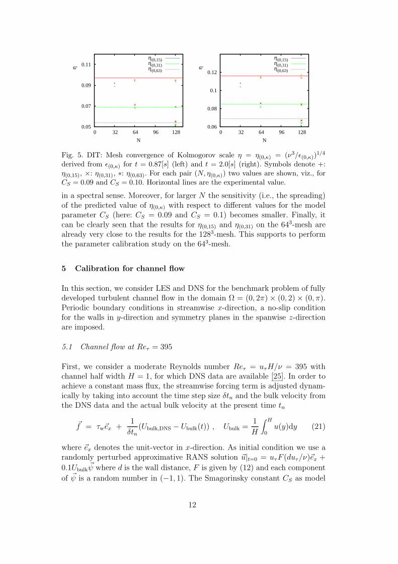
Fig. 5. DIT: Mesh convergence of Kolmogorov scale η = η(0,κ) = (ν3/ǫ(0,κ))1/4

derived from ǫ(0,κ) for t = 0.87[s] (left) and t = 2.0[s] (right). Symbols denote +:η(0,15), ×: η(0,31), ∗: η(0,63). For each pair (N, η(0,κ)) two values are shown, viz., forCS = 0.09 and CS = 0.10. Horizontal lines are the experimental value.

in a spectral sense. Moreover, for larger N the sensitivity (i.e., the spreading)of the predicted value of η(0,κ) with respect to different values for the modelparameter CS (here: CS = 0.09 and CS = 0.1) becomes smaller. Finally, itcan be clearly seen that the results for η(0,15) and η(0,31) on the 643-mesh arealready very close to the results for the 1283-mesh. This supports to performthe parameter calibration study on the 643-mesh.

5 Calibration for channel flow

In this section, we consider LES and DNS for the benchmark problem of fullydeveloped turbulent channel flow in the domain Ω = (0, 2π) × (0, 2) × (0, π).Periodic boundary conditions in streamwise x-direction, a no-slip conditionfor the walls in y-direction and symmetry planes in the spanwise z-directionare imposed.

5.1 Channel flow at Reτ = 395

First, we consider a moderate Reynolds number Reτ = uτH/ν = 395 withchannel half width H = 1, for which DNS data are available [25]. In order toachieve a constant mass flux, the streamwise forcing term is adjusted dynam-ically by taking into account the time step size δtn and the bulk velocity fromthe DNS data and the actual bulk velocity at the present time tn

~f = τw~ex +1

δtn(Ubulk,DNS − Ubulk(t)) , Ubulk =

1

H

∫ H

0u(y)dy (21)

where ~ex denotes the unit-vector in x-direction. As initial condition we use arandomly perturbed approximative RANS solution ~u|t=0 = uτF (duτ/ν)~ex +

0.1Ubulk~ψ where d is the wall distance, F is given by (12) and each component

of ~ψ is a random number in (−1, 1). The Smagorinsky constant CS as model

12

parameter and y+(1) as grid parameter are the quantities that we want toidentify via sampling of the cost functionals.The spatial discretisation usesNx×Ny×Nz = N3 nodes withN = 24, 32, 48, 64, 96.For N = 64, the equidistant spacing in x- and z-direction corresponds to∆x+ = ∆xuτ/ν = 38.8 and ∆z+ = ∆zuτ/ν = 19.4 respectively. The grid inwall-normal direction is stretched using a hyperbolic tangent function

y(j)

H=

tanh[γ(2j/Ny − 1)]

tanh(γ)+ 1.0 , j = 0, 1, . . . , Ny (22)

where y(j) is the coordinate of the jth grid point in y-direction providingthus an anisotropic, layer-adapted mesh, see [24]. The stretching parame-ter γ is taken to be γ ∈ 1.2, 1.5, 1.72, 2.2 which corresponds to y+(1) ∈0.39, 0.79, 1.06, 1.45 for the shifted wall node (for N = 64). The computa-tional time step is chosen as δt+ ≡ δtu2

τ/ν = 0.4. After reaching a statisticallysteady solution, first-order and second-order statistics are computed. Denote〈·〉 the averaging operator over the two homogeneous directions and in time.8000 time steps are performed to let the flow develop and reach the statisticallysteady state, statistics are collected over another 6000 steps. The quantities ofinterest are the mean velocity in streamwise direction U = 〈~u〉 ·~ex, the turbu-lent kinetic energy k = 1

2〈(~u − 〈~u〉)2〉 and their normalized variants U+ = U

uτ

and k+ = ku2

τ.

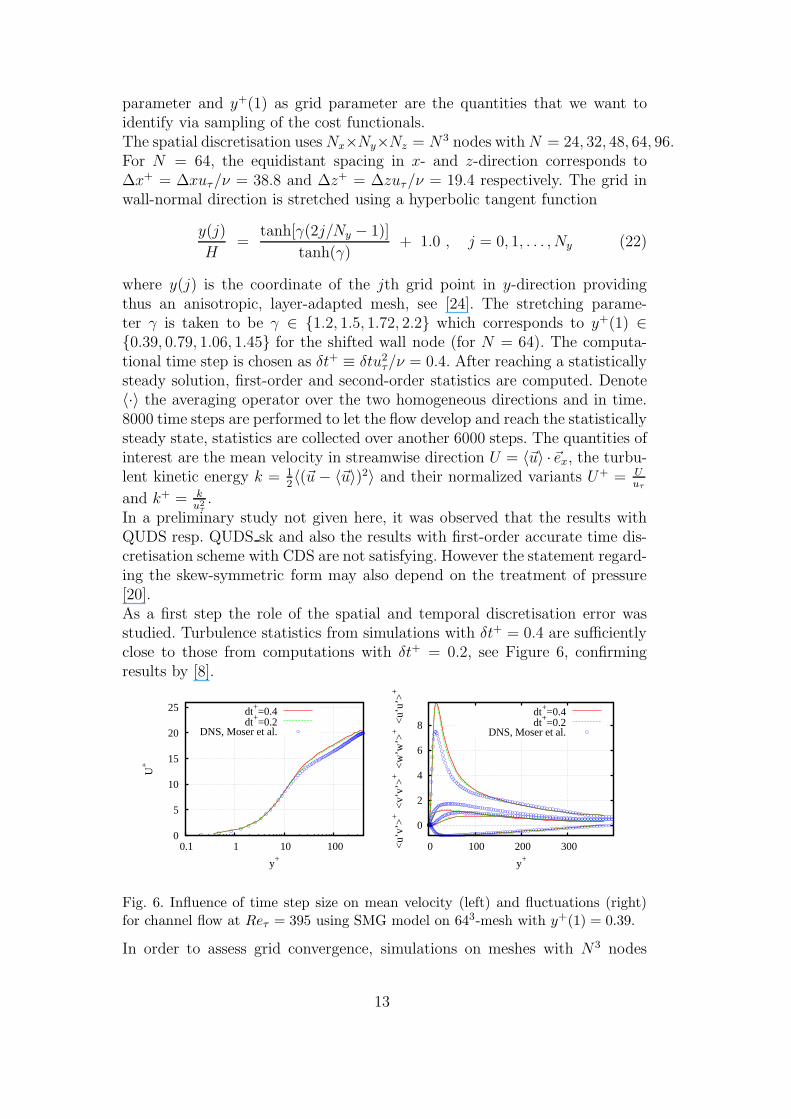
In a preliminary study not given here, it was observed that the results withQUDS resp. QUDS sk and also the results with first-order accurate time dis-cretisation scheme with CDS are not satisfying. However the statement regard-ing the skew-symmetric form may also depend on the treatment of pressure[20].As a first step the role of the spatial and temporal discretisation error wasstudied. Turbulence statistics from simulations with δt+ = 0.4 are sufficientlyclose to those from computations with δt+ = 0.2, see Figure 6, confirmingresults by [8].

0

5

10

15

20

25

0.1 1 10 100

U+

y+

dt+=0.4dt+=0.2

DNS, Moser et al.

0

2

4

6

8

0 100 200 300<u’

v’>

+ <

v’v’

>+ <

w’w

’>+ <

u’u’

>+

y+

dt+=0.4dt+=0.2

DNS, Moser et al.

Fig. 6. Influence of time step size on mean velocity (left) and fluctuations (right)for channel flow at Reτ = 395 using SMG model on 643-mesh with y+(1) = 0.39.

In order to assess grid convergence, simulations on meshes with N3 nodes

13

with N = 24, 32, 48, 64, 96 for the Smagorinsky model with standard valuefor channel flow CS = 0.05 are considered. Figure 7 shows that on the finestmesh N = 96 results are much closer to the DNS data than for N = 64, inagreement with the notion in [24].

0

5

10

15

20

25

0.1 1 10 100

U+

y+

N24 SMGN32 SMGN48 SMGN64 SMGN96 SMG

DNS, Moser et al.

0

2

4

6

8

10

0 100 200 300

<u’

v’>

+ <

v’v’

>+ <

w’w

’>+ <

u’u’

>+

y+

N24 SMGN32 SMGN48 SMGN64 SMGN96 SMG

DNS, Moser et al.

Fig. 7. Convergence study for channel flow at Reτ = 395 using SMG model onN×N×N -meshes with N = 24, 32, 48, 64, 96 and y+(1) = 0.39. Left: Mean velocity.Right: Fluctuations.

For the parameter optimization the l2-error functional of the LES results com-pared to the DNS data for U and k are defined by

Ju(y+(1), C) =

( N∑

j=0

(Uj(y+(1), C) − Uj,DNS)

2∆yj

)1/2

(23)

Jk(y+(1), C) =

( N∑

j=0

(kj(y+(1), C) − kj,DNS)

2∆yj

)1/2

(24)

with φj = φ(y(j)) and spacing ∆yj in y-direction of cell j. The parameterspace CS, y

+(1) is now two-dimensional and too large to compute the entirelook-up table on the 963 meshes. Therefore the following two-step optimiza-tion strategy is used. First we perform a (precursor) optimization using therelatively coarse 643 mesh. This first step is to reduce the parameter range. Ju

and Jk are almost constant for CS ∈ [0, 0.10] and y+(1) ∈ [0.5, 1.5] and becomesmallest for CS ∈ [0, 0.06], see Figure 8. In the second step we perform fine gridLES on the 963 mesh in order to find the optimal parameter CS not effectedsignificantly by the numerical error. Here we only investigate the reduced pa-rameter range CS, y

+(1) with CS ∈ [0, 0.10] and fixed y+(1) = 0.39. For thecost functionals, no distinct minimum can be concluded, but there is a plateauof minimum values for Ju in the range 0 ≤ CS ≤ 0.06. This is supported bythe observation that the profiles for mean flow and statistics almost coincidefor CS ∈ 0.01, 0.03, 0.05, and also the relative error in uτ w.r.t. the imposedvalue is also almost constant.It is well known that the standard optimal value for the Smagorinsky modelCS = 0.05 for ∆/h = 2 differs from the optimal value for DIT, see [28]. Thepresent results do not disagree with this standard choice, although Ju and Jk

14

0.6 0.9 1.2 0.04 0.08

0.12 0.001

0.01

0.1

JuSMG

SMG-MOD

y+(1)

CS

Ju

0.6 0.9 1.2 0.04 0.08

0.12 1e-05

1e-04

JkSMG

SMG-MOD

y+(1)CS

Jk

Fig. 8. Cost functionals for channel flow Reτ = 395 on 643-mesh, Left: mean velocity.Right: kinetic energy.

0

5

10

15

20

25

0.1 1 10 100

U+

y+

CS=0.01CS=0.03CS=0.05

CS=0.085DNS, Moser et al.

0

2

4

6

8

0 100 200 300<u’

v’>

+ <

v’v’

>+ <

w’w

’>+ <

u’u’

>+

y+

CS=0.01CS=0.03CS=0.05

CS=0.085DNS, Moser et al.

Fig. 9. Variation of CS for channel flow at Reτ = 395 using SMG model on 963-mesh.Left: Mean velocity. Right: Fluctuations.

do not show a distinct minimum for CS = 0.05.

5.2 Application to channel flow at higher Reτ

Now, the goal is to simulate turbulent channel flow at Reτ = 4800 usingthe calibrated model parameters. Numerical results are compared also withexperimental data by Comte-Bellot from [2], but these should be seen withcaution, since for the three cases considered (Reτ = 2340, 4800, 8160) thevalues obtained for slope 1/κ and constant C of the log law u+ = log(y+)/κ+Cshow a relatively large spreading and also differ from the standard values. Asa wall-resolved LES (as for Reτ = 395) is very expensive due to the much finermesh not only in wall-normal direction, but also in streamwise and spanwisedirection in conjunction with a much smaller time step, wall functions (seeSubsec. 2.3) are used together with the Smagorinsky model (WSMAG).First the role of the time discretisation error is studied on a mesh with 96 ×24 × 96 nodes and y+

δ = 50 for the (shifted) first node above the wall, seeFigure 10. For Reτ = 4800, ∆t = 0.02, 0.01, 0.005, 0.0025 correspond toδt+ = 7.0, 3.5, 1.75, 0.875. The statistics are sampled over 10,000 time stepsafter 10,000 steps flow developing (for δt+ = 7). Recall that δt+ = 0.4 was

15

5

10

15

20

25

30

1 10 100 1000

U+

y+

dt+=7.0dt+=3.5

dt+=1.75dt+=0.875

log lawComte-Bellot

0

2

4

6

8

0 1000 2000 3000 4000<u’

v’>

+ <

v’v’

>+ <

w’w

’>+ <

u’u’

>+

y+

dt+=7.0dt+=3.5

dt+=1.75dt+=0.875

Comte-Bellot

Fig. 10. Time-discretisation error for Smagorinsky model with near-wall modelling(WSMG) for channel flow at Reτ = 4800, Left: Mean velocity. Right: Fluctuations.

required for sufficiently small time discretisation error for wall-resolved LESat Reτ = 395. For Reτ = 4800 using wall-functions, δt+ = 1.75 is required toensure that time discretisation error is sufficiently small. This is only a factorof four larger compared to wall resolved LES. The second observation is thatthe log-layer mismatch is most pronounced for the too large δt and can bereduced largely by decreasing δt.Secondly the role of the spatial discretisation error is studied, see Figure 11.Three meshes are considered with Nx × Ny × Nz nodes where Nx = Nz ∈

5

10

15

20

25

30

1 10 100 1000

U+

y+

64x24x6496x24x96

128x24x128log law

Comte-Bellot

0

2

4

6

0 1000 2000 3000 4000<u’

v’>

+ <

v’v’

>+ <

w’w

’>+ <

u’u’

>+

y+

64x24x6496x24x96

128x24x128Comte-Bellot

Fig. 11. Study of spatial discretisation error for Smagorinsky model with near-wallmodelling (WSMG) for channel flow at Reτ = 4800 using δt+ = 1.75, Left: Meanvelocity. Right: Fluctuations.

64, 96, 128 corresponding to ∆x+ = 2∆z+ = 470, 317, 235. For Nx = 64streamwise fluctuations are largely overpredicted showing an underresolvedLES, see [18]. Results on the two meshes Nx = 96 and Nx = 128 are close.However, they differ in the channel center, since spacing in the channel centeris relatively coarse. The spacing in x- and z-direction is relatively coarse evenfor Nx = 128, cf. [31], but mesh convergence of the results is judged to bealready satisfactory.

16

6 Flow over backward facing step at Reh = 37500

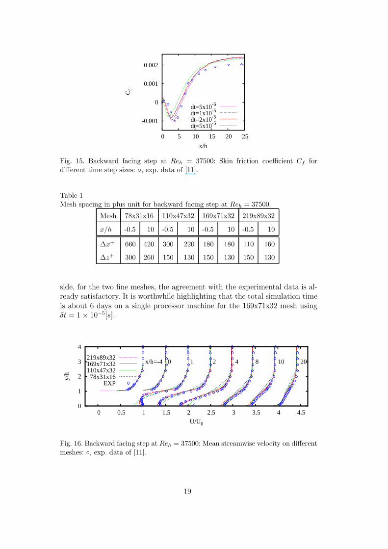
In this section we consider the turbulent flow over a backward-facing step ata higher Reynolds number Reh = U0h/ν = 37500 using wall functions. Ex-perimental data by Driver and Seegmiller [11] are available. The length of theinflow part is 4h, the channel height upstream is 8h, where h = 0.0127[m]is the step height and the channel length after the step is 25h. The inflowcenterline velocity is U0 = 44.2[m/s].Wall-functions are used at the upper and bottom walls and periodic boundaryconditions in spanwise direction. The wall opposite the step was parallel tothe wall in the experiment considered here. If we remove the upper half of thechannel and treat the centerline as a symmetry plane, a RANS calculationusing the Spalart-Allmaras model showed that the velocity at the outlet willslow down around 12% compared with the case using the full geometry. There-fore the full configuration has to be considered. A blending of DNS data [32]in the near-wall region and experimental data [11] otherwise is used for themean velocity profile at the inflow boundary. The method by [19] is appliedto generate turbulence structures at the inflow boundary.Since wall functions are used, relatively coarse grids in the near-wall regioncan be used. A hyperbolic tangent function is adopted to generate anisotropicgrid spacing in wall normal y−direction. The mesh is equidistant in x− andz−direction and only a small stretching is applied in x−direction near theoutlet.First the role of the time step size is studied on a grid consisting of 169×Ny×32nodes, where in wall-normal direction Ny = 54 for x ≤ 0 and Ny = 71for x > 0 (∆x+, ∆z+ are given in Table 1). For the time step size we useδt = 5 × 10−5[s], 2 × 10−5[s], 1× 10−5[s], 5 × 10−6[s] corresponding to a factorof 100, 40, 20 and 10 compared to the DNS at Reh = 5100 by [21] and wenote that δt = 1× 10−5[s] ≃ 0.035h/U0. In Figures 12-14 the profiles of meanvelocity and fluctuations for different time step sizes are shown at 8 cross sec-tions where experimental data are available. The average is performed over asimulation time 348h/U0 and spanwise direction after a flow developing time348h/U0, which is around 12 ”flow through” times. The results for mean flowand statistics from simulations with δt = 1× 10−5[s] and δt = 5× 10−6[s] arevery close, which can be seen also from Cf in Figure 15. The time discreti-sation error is therefore judged to be sufficiently small. Agreement with theexperimental data is also satisfying.Since wall functions are used, skin friction coefficient Cf is computed using(12). Figure 15 presents Cf in comparison with the experimental data. Theuncertainties in Cf were assessed by [11] to be ±8% for a 95% confidence level(with an uncertainty of ±15% in the region of separated flow).In order to study grid convergence, four meshes are considered, see Table 1.Mesh spacing in plus units at x/h = −0.5 and x/h = 10 is also given. Weused δt = 2 × 10−5[s]. Results in Figures 16-18 show that the solutions on

17

0

1

2

3

4

0 0.5 1 1.5 2 2.5 3 3.5 4 4.5

y/h

U/U0

x/h=-4 0 1 2 4 8 10 20dt=5x10-6

dt=1x10-5

dt=2x10-5

dt=5x10-5

Fig. 12. Backward facing step at Reh = 37500: Mean streamwise velocity for differ-ent time step sizes: , exp. data of [11].

0

1

2

3

4

0 0.05 0.1 0.15 0.2 0.25 0.3 0.35

y/h

<u’u’>/U02

x/h=-4 0 1 2 4 8 10 20

Fig. 13. Backward facing step at Reh = 37500: Fluctuations < u′u′ > for differenttime step sizes: , exp. data of [11]. Same line legend as in Figure 12.

0

1

2

3

4

0 0.02 0.04 0.06 0.08 0.1 0.12 0.14

y/h

<v’v’>/U02

x/h=-4 0 1 2 4 8 10 20

Fig. 14. Backward facing step at Reh = 37500: Fluctuations < v′v′ > for differenttime step sizes: , exp. data of [11]. Same line legend as in Figure 12.

the two coarser meshes deviate discernibly from the solution on the two finemeshes. This is at least in part due to the underresolved LES before the stepwhich cannot maintain the turbulent structures in the boundary layer, whichtrigger the destabilisation of the shear layer downstream of the step and playan important role for the recirculation length, see e.g. [3,7]. On the positive

18

-0.001

0

0.001

0.002

0 5 10 15 20 25

Cf

x/h

dt=5x10-6

dt=1x10-5

dt=2x10-5

dt=5x10-5

Fig. 15. Backward facing step at Reh = 37500: Skin friction coefficient Cf fordifferent time step sizes: , exp. data of [11].

Table 1Mesh spacing in plus unit for backward facing step at Reh = 37500.

Mesh 78x31x16 110x47x32 169x71x32 219x89x32

x/h -0.5 10 -0.5 10 -0.5 10 -0.5 10

∆x+ 660 420 300 220 180 180 110 160

∆z+ 300 260 150 130 150 130 150 130

side, for the two fine meshes, the agreement with the experimental data is al-ready satisfactory. It is worthwhile highlighting that the total simulation timeis about 6 days on a single processor machine for the 169x71x32 mesh usingδt = 1 × 10−5[s].

0

1

2

3

4

0 0.5 1 1.5 2 2.5 3 3.5 4 4.5

y/h

U/U0

x/h=-4 0 1 2 4 8 10 20219x89x32169x71x32110x47x32

78x31x16EXP

Fig. 16. Backward facing step at Reh = 37500: Mean streamwise velocity on differentmeshes: , exp. data of [11].

19

0

1

2

3

4

0 0.05 0.1 0.15 0.2 0.25 0.3 0.35

y/h

<u’u’>/U02

x/h=-4 0 1 2 4 8 10 20

169x71x32110x47x3278x31x16

EXP

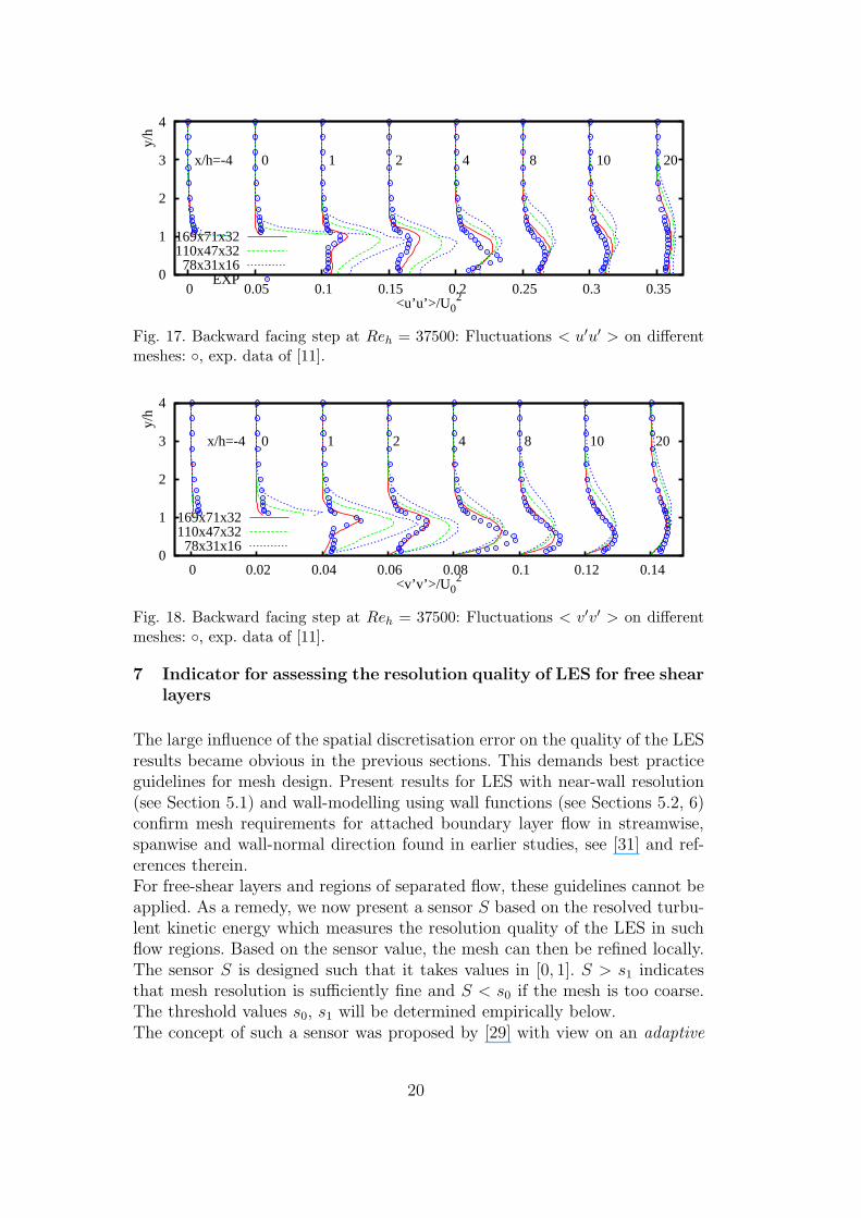
Fig. 17. Backward facing step at Reh = 37500: Fluctuations < u′u′ > on differentmeshes: , exp. data of [11].

0

1

2

3

4

0 0.02 0.04 0.06 0.08 0.1 0.12 0.14

y/h

<v’v’>/U02

x/h=-4 0 1 2 4 8 10 20

169x71x32110x47x3278x31x16

Fig. 18. Backward facing step at Reh = 37500: Fluctuations < v′v′ > on differentmeshes: , exp. data of [11].

7 Indicator for assessing the resolution quality of LES for free shear

layers

The large influence of the spatial discretisation error on the quality of the LESresults became obvious in the previous sections. This demands best practiceguidelines for mesh design. Present results for LES with near-wall resolution(see Section 5.1) and wall-modelling using wall functions (see Sections 5.2, 6)confirm mesh requirements for attached boundary layer flow in streamwise,spanwise and wall-normal direction found in earlier studies, see [31] and ref-erences therein.For free-shear layers and regions of separated flow, these guidelines cannot beapplied. As a remedy, we now present a sensor S based on the resolved turbu-lent kinetic energy which measures the resolution quality of the LES in suchflow regions. Based on the sensor value, the mesh can then be refined locally.The sensor S is designed such that it takes values in [0, 1]. S > s1 indicatesthat mesh resolution is sufficiently fine and S < s0 if the mesh is too coarse.The threshold values s0, s1 will be determined empirically below.The concept of such a sensor was proposed by [29] with view on an adaptive

20

LES, where ∆ = ∆(x) is interpreted as a model parameter, and, if the ra-tio h/∆ is fixed, ∆ is adapted by varying the mesh spacing until a desiredturbulence resolution is obtained. As an abstract measure of turbulence reso-lution the fraction of the resolved to total turbulent kinetic energy is proposed.However, the turbulent kinetic energy in the residual or subgrid scale motioncannot be computed from resolved quantities and hence requires modelling,but no operational definition is given in [29]. For statistically steady flow, wepropose

S(~x) =k

k + ksgs, k =

1

2〈(~u− 〈~u〉)2〉 , ksgs =

1

2〈(~u− ~u)2〉 (25)

where 〈·〉 denotes the filtering operator in homogeneous directions and in timeand ~u is defined by the convolution integral

~u(x, t) =∫

Rdg∆(~x− ~y)~u(~y, t)d~y (26)

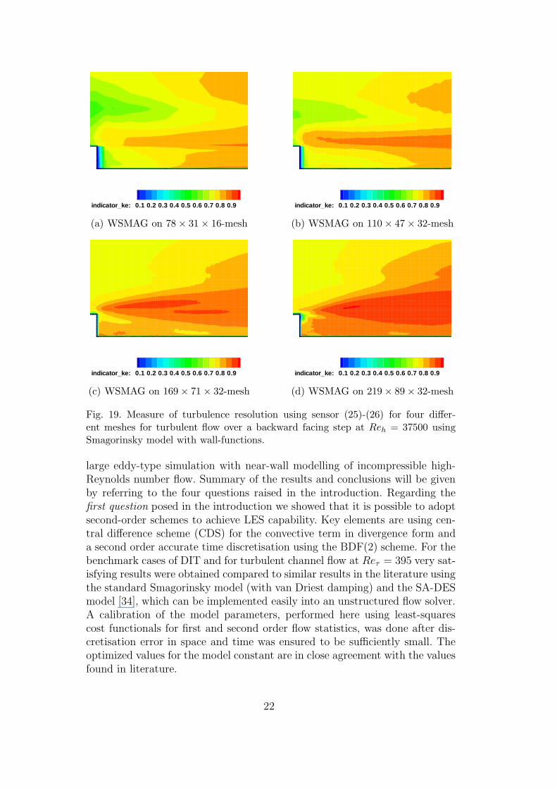
with g∆ being the top hat filter function. The underlying idea is to use ascale similarity assumption for the subgrid scale velocity ~usgs(~x, t) ≈ ~u(~x, t)−~u(~x, t). Since we are interested in S only remote from walls, there is no specialadjustment of the filter definition for near-wall cells. The question whether anadaption of the filter definition at inflow and outflow boundaries is needed,requires additional investigation, but this is only fine tuning of the method.Figures 19(a)-19(d) show sensor S for the turbulent flow over a backwardfacing step at Reh = 37500 on the four meshes in Table 1. From Figures 16-18we concluded that grid convergence on the two fine meshes is satisfactory butthat the solution on the coarse mesh suffers from large error. For the coarsemesh S < 0.8 in large part of the free-shear layer and the recirculation region(see Figure 19(a)), but for the finest mesh S > 0.85 in the recirculation regionand S around 0.9 in the free-shear layer (see Figure 19(d)). From this wesuggest the threshold values s0 = 0.8 and s1 = 0.9. The separation between s0

and s1 should be large enough to make an automatic grid refinement methodsuccessful. Otherwise an additional scaling of the indicator could be used tomake this distance larger.Small sensor values in the channel center demonstrate that the sensor needs

improvement for practical applications. In the channel center, k is small due tosmall turbulence production, since velocity gradients are small. As a remedy,an additional sensor hased on the mean flow (averaged over homogeneousdirections and in time) is needed. The present mean flow is almost irrotationalin the channel center, and the sensor (25)-(26) should be deactivated there.

8 Summary. Conclusions

In this paper we showed a validation strategy for enhancement of an unstruc-tured industrial finite-volume solver designed for steady RANS problems for

21

indicator_ke: 0.1 0.2 0.3 0.4 0.5 0.6 0.7 0.8 0.9

(a) WSMAG on 78 × 31 × 16-mesh

indicator_ke: 0.1 0.2 0.3 0.4 0.5 0.6 0.7 0.8 0.9

(b) WSMAG on 110 × 47 × 32-mesh

indicator_ke: 0.1 0.2 0.3 0.4 0.5 0.6 0.7 0.8 0.9

(c) WSMAG on 169 × 71 × 32-mesh

indicator_ke: 0.1 0.2 0.3 0.4 0.5 0.6 0.7 0.8 0.9

(d) WSMAG on 219 × 89 × 32-mesh

Fig. 19. Measure of turbulence resolution using sensor (25)-(26) for four differ-ent meshes for turbulent flow over a backward facing step at Reh = 37500 usingSmagorinsky model with wall-functions.

large eddy-type simulation with near-wall modelling of incompressible high-Reynolds number flow. Summary of the results and conclusions will be givenby referring to the four questions raised in the introduction. Regarding thefirst question posed in the introduction we showed that it is possible to adoptsecond-order schemes to achieve LES capability. Key elements are using cen-tral difference scheme (CDS) for the convective term in divergence form anda second order accurate time discretisation using the BDF(2) scheme. For thebenchmark cases of DIT and for turbulent channel flow at Reτ = 395 very sat-isfying results were obtained compared to similar results in the literature usingthe standard Smagorinsky model (with van Driest damping) and the SA-DESmodel [34], which can be implemented easily into an unstructured flow solver.A calibration of the model parameters, performed here using least-squarescost functionals for first and second order flow statistics, was done after dis-cretisation error in space and time was ensured to be sufficiently small. Theoptimized values for the model constant are in close agreement with the valuesfound in literature.

22

Concerning the second question posed in the introduction, turbulent channelflow at Reτ = 4800 was considered. Wall-functions allow to use larger timestep size by factor four and increased spacing in streamwise and spanwise di-rection by factor five. The savings in wall-normal direction are at least by afactor of four. Based on these numbers, the total savings are thus by a factorof 400. Then turbulent flow over a backward facing step at higher Reynoldsnumber Reh = 37500 by [11] was simulated successfully using wall-functions.It is worth highlighting that the total simulation time using sufficiently finemesh and time step size is about six days on a single processor machine. Thisdemonstrates the industrial feasibility for engineering design studies for con-figurations of moderate complexity and relatively large Reynolds numbers.The third and fourth question posed in the introduction concern reliability ofLES results in terms of numerical error and best-practice guidelines. Conver-gence studies for turbulent channel flow and backward-facing step showed thatthe numerical discretisation error in space and time has a dominant influenceon the solution and that underresolution can cause poor results. From an in-dustrial view point, the danger of an underresolved LES is judged to be themajor hurdle for LES in complex geometries, since it is well-known practicein industry to prefer increasing the complexity of the CAD model rather thanto refine the mesh and keep geometrical details constant. The large influenceof the spatial discretisation error on the quality of the LES results stronglydemands best practice guidelines for mesh design. For LES with near-wallresolution and wall-modelling using wall functions, mesh requirements insideattached boundary layers in streamwise, spanwise and wall-normal directionfound in this work confirmed existing best practice guidelines for mesh design.For free-shear layers and regions of separated flow these guidelines cannot beapplied. As a remedy, we presented a sensor based on the resolved turbulentkinetic energy which measures the resolution quality of the LES in such flowregions. The sensor values can then be used to refine the mesh locally, e.g. us-ing the techniques in [4]. This will be subject to future research since it wouldraise a new important question concerning LES on unstructured meshes. Sincethe present refinement strategy does not support hanging nodes, the refine-ment of hexaedral elements leads to prismatic and tetraedral elements. Thenumerical properties of the present method for LES has not yet been studiedon such elements. This needs to be done before applying a local mesh refine-ment.For LES of flows in complex geometries, grid convergence can generally notbe ensured by a global mesh refinement study due to extremely large compu-tational costs. The question whether or not the number of degrees of freedom,which is necessary to achieve mesh converged results for LES, can be reducedby using higher order methods, is beyond the scope of this paper. In any case,the proposed approach of a local grid refinement using a measure for LESresolution quality offers a promising tool to automatically design a mesh suchthat the LES solution is sufficiently converged for engineering design problemsusing a low-order code at affordable computational costs.

23

Acknowledgements

The authors are grateful to Dr. M. Klein for providing the fortran routinesfor the method [19]. This work benefited immeasurably from the discussionsof the first author within the DESider project (Detached Eddy Simulationfor Industrial Aerodynamics) a collaboration between ALA, CFX, DASSAV,EADS-M, ECD, LML, NLR, EDF, NUMECA, DLR, FOI, IMFT, ONERA,Chalmers University, Imperial College, TU Berlin, UMIST and NTS. Theproject is funded by the European Union and administrated by the CEC, Re-search Directorate-General, Growth Programme, under Contract No. AST3-CT-2003-502842. Special thanks are to Drs. Matthias Orlt, Keith Weinman,Charles Mockett, and Dieter Schwamborn. The second author gratefully ac-knowledges financial support by the GK 1023 by the Deutsche Forschungs-gemeinschaft (DFG). Finally the valuable suggestions by the reviewers aregratefully acknowledged.

References

[1] Guide for the Verification of Computational Fluid Dynamics Simulations. Tech.rep., AIAA G-077-1998 (1998)

[2] A selection of test cases for the validation of large-eddy simulations ofturbulent flows (quelques cas d’essai pour la validation de la simulation desgros tourbillons dans les ecoulements turbulents. Tech. rep., AGARD-AR-345(1998)

[3] Aider, J.L., Danet, A., Lesieur, M.: Large-eddy simulation applied to studythe influence of upstream conditions on the time-dependant and averagedcharacteristics of a backward-facing step flow. Journal of Turbulence 8, DOI:10.1080/14685240701701,000 (2007)

[4] Alrutz, T., Orlt, M.: Parallel dynamic grid refinement for industrialapplications. In: Proceedings of the European Conference on ComputationalFluid Dynamics (ECCOMAS CFD 2006) (2006)

[5] Bazilevs, Y., Calo, V., Cottrell, J., Hughes, T., Reali, A., Scovazzi, G.:Variational multiscale residual-based turbulence modeling for large eddysimulation of incompressible flows. Computer Methods in Applied Mechanicsand Engineering 197(1-4), 173–201 (2007)

[6] Becker, R., Braack, M., Vexler, B.: Parameter identification for chemical modelsin combustion problems. Applied Numerical Mathematics 54(3-4), 519–536(2005)

[7] Benhamadouche, S., Jarrin, N., Addad, Y., Laurence, D.: Synthetic turbulentinflow conditions based on a vortex method for large-eddy simulation. Progressin Computational Fluid Dynamics 6, 50–57 (2006)

24

[8] Choi, H., Moin, P.: Effects of the computational time step on numerical solutionsof turbulent flow. Journal of Computational Physics 113, 1–4 (1994)

[9] Chow, F.K., Moin, P.: A further study of numerical errors in large-eddysimulations. Journal of Computational Physics 184, 366–380 (2003)

[10] Comte-Bellot, G., Corrsin, S.: Simple eulerian time correlation of full- andnarrow-band velocity signals in grid-generated, ’isotropic’ turbulence. Journalof Fluid Mechanics 48(2), 273–337 (1971)

[11] Driver, D.M., Seegmiller, H.L.: Features of a reattaching turbulent shear layerin divergent channel flow. AIAA Journal 23, 163–171 (1985)

[12] Faure, S., Laminie, J., Temam, R.: Collocated finite volume schemes for fluidflows Communications in Computational Physics 4, 1–25 (2008)

[13] Ferziger, J.H., Peric, M.: Computational Methods for Fluid Dynamics. Springer-Verlag, Heidelberg (1996)

[14] Ghosal, S.: An analysis of numerical errors in large-eddy simulations ofturbulence. Journal of Computational Physics 125, 187–206 (1996)

[15] Haase, W., Braza, M., Laurence, D. (eds.): DESider - Detached eddy simulationfor industrial aerodynamics. Results of the European-Union funded project,2004 - 2007. Notes on Numerical Fluid Mechanics and Multidisciplinary Design.Springer, Berlin (to appear)

[16] Johansson, H., Runesson, K., Larsson, F.: Parameter identification withsensitivity assessment and error computation. GAMM-Mitteilungen 30(2),430–457 (2007)

[17] Jovic, S., Driver, D.: Backward-facing step measurements at low reynoldsnumber. Tech. rep., NASA TM 108807 (1994)

[18] Keating, A., Piomelli, U.: A dynamic stochastic forcing method as a wall-layermodel for large-eddy simulation. Journal of Turbulence 7, 1–24 (2006)

[19] Klein, M., Sadiki, A., Janicka, J.: A digital filter based generation of inflow datafor spatially developing direct numerical or large eddy simulations. Journal ofComputational Physics 186, 1652–1665 (2003)

[20] Kravchenko, A.G., Moin, P.: On the effect of numerical errors in large eddysimulations of turbulent flows. Journal of Computational Physics 131, 310–322(1997)

[21] Le, H., Moin, P., Kim, J.: Direct numerical simulation of turbulent flow over abackward-facing step. Journal of Fluid Mechanics 330, 349–374 (1997)

[22] Mahesh, K., Constantinescu, G., Moin, P.: A numerical method for large-eddysimulation in complex geometries. Journal of Computational Physics 197, 215–240 (2004)

[23] Moin, P.: Advances in large eddy simulation methodology for complex flows.International Journal of Heat and Fluid Flow 23, 710–720 (2002)

25

[24] Morinishi, Y., Vasilyev, D.: A recommended modification to the dynamic two-parameter mixed subgrid scale model for large eddy simulation of wall boundedturbulent flow. Physics of Fluids 13, 3400–3410 (2001)

[25] Moser, R.D., Kim, J., Mansour, N.N.: Direct numerical simulation of turbulentchannel flow up to Reτ = 590. Physics of Fluids 11, 943–946 (1999)

[26] Nikitin, N.V., Nicoud, F., Wasistho, B., Squires, K.D., Spalart, P.R.: Anapproach to wall modeling in large-eddy simulation. Physics of Fluids 12(7),1629–1632 (2000)

[27] Park, N., Mahesh, K.: Analysis of numerical errors in large eddy simulationusing statistical closure theory. Journal of Computational Physics 222, 194–216 (2007)

[28] Pope, S.B.: Turbulent flows. Cambridge University Press, Cambridge (2000)

[29] Pope, S.B.: Ten questions concerning the large-eddy simulation of turbulentflows New Journal of Physics 6, 1–24 (2004)

[30] Rhie, C.M., Chow, W.L.: Numerical study of the turbulent flow past an airfoilwith trailing edge separation. AIAA Journal 21, 1525–1532 (1983)

[31] Sagaut, P.: Large eddy simulation for incompressible flows. Springer-Verlag,Berlin (2001)

[32] Spalart, P.R.: Direct simulation of a turbulent boundary layer up to Rθ = 1410.Journal of Fluid Mechanics 187, 61–98 (1988)

[33] Spalart, P.R.: Young-person’s guide to detached-eddy simulation grids. Tech.rep., NASA/CR-2001-211032 (2001)

[34] Spalart, P.R., Jou, W.H., Strelets, M., Allmaras, S.R.: Comments on thefeasibility of les for wings, and on a hybrid rans/les approach. First AFOSRInternational Conference on DNS/LES, Ruston, LA, 4-8, August, 1997, in:Advances in DNS/LES, edited by C. Liu and Z. Liu (Greyden, Columbus, OH,1997) (1997)

[35] Templeton, J.A., Wang, M., Moin, P.: An efficient wall model for large-eddysimulation based on optimal control theory. Physics of Fluids (2006). DOI10.1063/1.2166457

[36] Tessicini, F., Temmerman, L., Leschziner, M.: Approximate near-walltreatments based on zonal and hybrid RANS-LES methods for LES at highReynolds numbers. International Journal of Heat and Fluid Flow 27, 789–799(2006)

[37] Wang, M., Moin, P.: Dynamic wall modeling for large-eddy simulation ofcomplex turbulent flows. Physics of Fluids 14, 2043–2051 (2002)

[38] Zhang, X.Q.: Identification of model and grid parameters for incompressibleturbulent flows. Ph.D. thesis, University Gottingen (2007)

26