(NASA-CR-12425U) PARTICLE-FLUID N73-23379INTERACTION CORRECTIONS FDR PLOWMEASUREMENTS WITH A LASER DOPPLERPLOWMETER (Arizona State Univ.) 61 p HC. Unclas5.25 C5CL TUB G3/12 038U6 j

Engineering Research CenterCollege of Engineering Sciences

Arizona State UniversityTempe, Ariz. 85281

https://ntrs.nasa.gov/search.jsp?R=19730014652 2020-03-23T05:10:05+00:00Zbrought to you by COREView metadata, citation and similar papers at core.ac.uk

provided by NASA Technical Reports Server

PARTICLE-FLUID INTERACTION CORRECTIONS FOR FLOW MEASUREMENTS

WITH A LASER DOPPLER FLOWMETER

byNeil S. Berman

Prepared under Contract No. NAS 8-21397

National Aeronautics and Space AdministrationGeorge C. Marshall Space Flight Center

Aero-Astrodynamics LaboratoryAerophysics Division

Thermal Environment BranchPhysics Section

ENGINEERING RESEARCH CENTER

COLLEGE OF ENGINEERING SCIENCES

ARIZONA STATE UNIVERSITY

TEMPE, ARIZONA 85281

TABLE OF CONTENTS

INTRODUCTION 1t

I. ONE DIMENSIONAL MEAN VELOCITY OF SINGLE PARTICLES .... 3

II. MOTION OF PARTICLES IN AN OSCILLATING FLUID 15

III. MOTION OF A SINGLE PARTICLE IN A TURBULENT FLUID 22

A. Application of Single Particle Analysis to TurbulentJets 34

B. Single Particle in Pipe Flow . . 44

C. Experimental Studies of Turbulent Velocities of SmallParticles 45

IV. OTHER CONSIDERATIONS IN PARTICLE-FLUID FLOWS 47

V. CONCLUSIONS 54

VI. LITERATURE CITED . , 55

ABSTRACT

A discussion is given of particle lags in mean flows, acoustic

oscillations at single frequencies and in turbulent flows. Some

simplified cases lead to exact solutions. For turbulent flows lineariza-

tion of the equation of motion after assuming the fluid and particle

streamlines coincide also leads to a solution. The results show that

particle lags are a function of particle size and frequency of oscillation.

Additional studies are necessary to evaluate the effect of turbulence

when a major portion of the energy is concentrated in small eddies.

INTRODUCTION

A promising method of measuring turbulent flow characteristics is

the Laser-Doppler technique. Local mean and fluctuating velocities of

small particles suspended in a fluid stream are determined. The seeding

of small particles is necessary to provide scattered light for the Laser-

Doppler instrument. The question then arises: "How well do the particles

follow the flow?" This report considers the motion of a single particle

or group of particles in a fluid stream with emphasis on solid particles

in a gas. Flow in pipes and in an isothermal round free jet are used as

examples.

Motion of a single particle is a simplified case of dilute gas-solid

suspension flow. Large particles will only follow the slow large scale

turbulent motions of fluid, while particles small compared to the smallest

scale of turbulence will respond to all turbulence components of the fluid.

Since the particle contributes to energy dissipation due to lags between

particle and fluid, large numbers of particles will modify the energy

spectrum of the fluid.

Many studies on particle fluid interactions have been made because

this problem is of importance in several fields. The motions of small

particles have been analyzed by comparisons of the amplitudes of oscilla-

tions of particle and fluid in an accoustic field, and by comparison of

the mean velocities in turbulent flow. Special problems exist when solid

boundaries are present or particle-particle interactions are important.

At speeds below the velocity of sound the difference velocity between

2.

fluid and solid is near the continuum regime and viscous effects are

important. Corrections for compressibility and rarefaction are necessary

for higher speeds when slip or transition flows are encountered.

The results of calculations on particle fluid interactions for small

particles generally show that individual particles below one micron in

diameter follow the flow. Turbulence measurements on particles are then

a good representation of the fluid behavior as long as the turbulent

fluctuations are not extremely rapid. Further work is necessary to

consider the energy dissipation range of some turbulent flows or high speed

f1ows.

In the following pages the velocity of the fluid and particle are

compared for several conditions of physical interest. First the mean

velocity and then the velocity fluctuations are calculated for a single

particle. A survey of the literature on experimental work is also pre-

sented. Finally some consideration of multiparticle systems is given.

Although the equations are the same, the conclusions for flow in a liquid

are much different from those given in this report for a gase.

Extensive introductions to the field are available in the books by

Fuchs [1] and Soo [2]. These references have been used extensively in

this report.

I. ONE DIMENSIONAL MEAN VELOCITY OF SINGLE PARTICLES

We begin with the simplified case of one dimensional flow when the

particle does not distrub the fluid motion.

The equation of motion for a single spherical particle in creeping

flow is given in many texts as:

i *£

t t _ ui ^ i[uu d(V^U) dtP

dV c /,, ,A m1 dp m' dV du c 2_. = 67Tyr (u_V) . _ J. _ _ _ . _ _ 6r

This equation was originally obtained by Basset [3] and is discussed by

Tchen [4] and Hinze [5]. The notation is as follows:4 .3m = mass of particle = -~ irr po p

4 3m1 = mass of fluid = 5- irr p

V = particle velocity

U = fluid velocity

y = fluid viscosity

p = fluid density

p = particle density

r = particle radius

t = time

• F = external potential force •

Equation 1.1 then equates the force to accelerate a particle to the follow-

ing in order of their appearance in the equation:

1. Viscous drag on the particle for slow relative motion.

2. Pressure gradient in the fluid surrounding the particle.

3. Force to accelerate the apparent mass of the particle relative

to the fluid.

4. The effect of acceleration on the viscous drag. (Basset force)

5. The external potential force such as gravity.

To account for instantaneous motion in a turbulent field, this

equation must be written in vector form in the proper frame of reference.

However, the equation as it stands can be used to determine the behavior

of the mean flow. In a later section the particle velocity in a fluctuat-

ing medium will be considered. In general the pressure term can be

obtained from the equation of motion of the fluid assuming the particles

do not have an effect on the fluid behavior. The equation then depends

upon the viscous forces and inertia! forces in the fluid and the results

will be functions of velocity gradient (dv/dz) and the gradient of velocity2 2gradient (d v/dz ) . In this discussion these terms are assumed small or

that any effect can be included in an experimental drag coefficient.

That is the viscous drag term in Equation 1.1 is replaced by mFp(U-V)

where

and CD is the drag coefficient. At low particle Reynolds number, r^ " '$•• ,

the first term in Equation 1.1 is obtained.

If the particle is in a fluid moving with constant velocity, the

Basset force is neglected and the pressure gradient and external potential

force are constant, the solution to Equation 1.1 is:

5.

3F

U-V =

CI " dl 4Trr3/

On1

0

r2(2p +p)- e (1.2)

when at t = 0, the particle and fluid have the same velocities. The largest2r2 I do-— I —^ need only be con-dzdifference then occurs at t = ~ and the factor

sidered in the absence of a potential force. For flow in a pipe the pressure

drop is a function of the pipe diameter, D, and average velocity, <v>. In

terms of the Fanning friction factor, f,

The friction factor is given by:

f = 0.0791 NRe^

at Reynolds numbers between 10 and 105 but for purposes of comparison it

can be assumed that the result holds for higher fluid Reynolds numbers.

Then:

(U - V)m ,„<> 3/1(1.3)

where R is the pipe radius. To obtain less than 1% relative error at

6 ,NRe = 1° in a 4 inch diameter pipe a particle less than 300 microns in

radius is required. If the pipe is vertical, the potential force due to

gravity must be included.

3 -Fe.= (pp - p) g

I 1

6.

Then:

9 (p -- p)n2 ,/u 2= .0088 (£)Z N 3/* + f-R Re 9y

9u<v>

When p = 1.0 g/cnr and y = 2 x 10 g/cm sec.,

106r2

The gravity force is larger than the pressure force and results in a lower

particle size limit for a 1% error. This limit is approximately equal to\,

<y> 2 microns when the velocity is given in cm./sec. For example under the

same conditions as above a 95y diameter particle is the 1% limit while a

300 micron particle would give an error over 10% when the fluid stream iso

air and the particle density is 1.0 g/cnr.

The analysis appears valid for pipe flow mean velocities in isothermal

turbulent flow when compared with experimental data. Recently Reddy, Wijk

and Pei measured particle and fluid velocities in a 10 cm. diameter vertical

pipe [6]. Using 200 micron particles the error at the centerline was 16%.

Assuming they used alumina particles with a density of 2.42 g/cnr the cal-

culated error at t = « is 25%. The agreement is good and could be improved

by using a correction to the viscous drag.

If the terminal velocity is not reached, the particles may show varia-

tions in velocity due to different times of approach to terminal conditions.

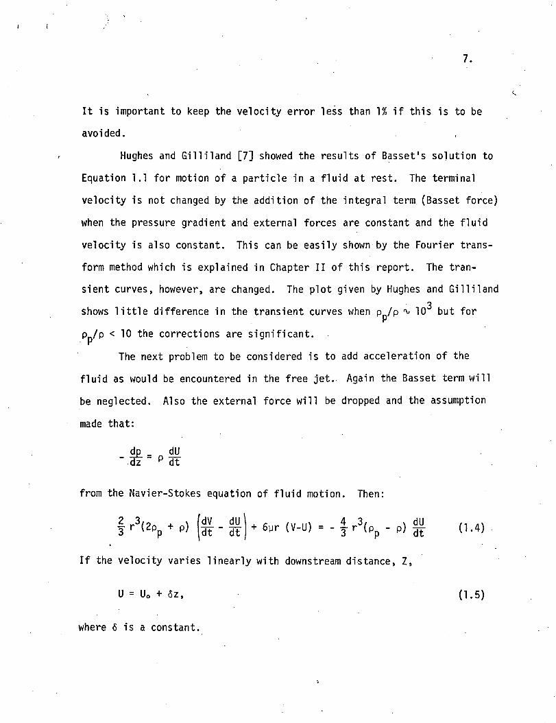
It is important to keep the velocity error less than 1% if this is to be

avoided.

Hughes and Gilliland [7] showed the results of Basset's solution to

Equation 1.1 for motion of a particle in a fluid at rest. The terminal

velocity is not changed by the addition of the integral term (Basset force)

when the pressure gradient and external forces are constant and the fluid

velocity is also constant. This can be easily shown by the Fourier trans-

form method which is explained in Chapter II of this report. The tran-

sient curves, however, are changed. The plot given by Hughes and Gilliland3

shows little difference in the transient curves when p /p 10 but for

p /p < 10 the corrections are significant.

The next problem to be considered is to add acceleration of the

fluid as would be encountered in the free jet. Again the Basset term will

be neglected. Also the external force will be dropped and the assumption

made that:

dUdo dUdt= p dt

from the Navier-Stokes equation of fluid motion. Then;

2 r33 r

If the velocity varies linearly with downstream distance, Z,

U = U0 + 6z, (1.5)

where 6 is a constant.

I I

8.

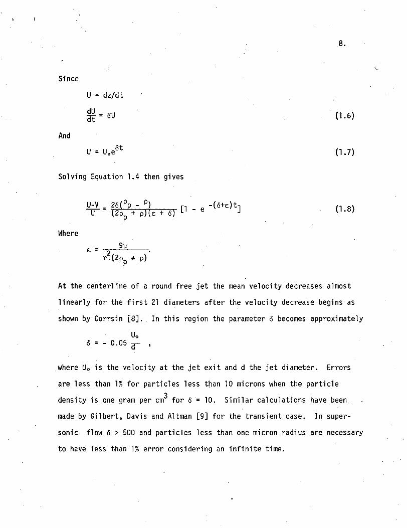
Since

U = dz/dt<

^= 6U . (1.6)

And

U = U0e6t (1.7)

Solving Equation 1.4 then gives

U (2pp + p)(e + 6).e

Where

9ue =r2(2Pp + p)

At the centerline of a round free jet the mean velocity decreases almost

linearly for the first 21 diameters after the velocity decrease begins as

shown by Corrsin [8]. In this region the parameter 6 becomes approximately

U06 = - 0.05

where U0 is the velocity at the jet exit and d the jet diameter. Errors

are less than 1% for particles less than 10 microns when the particle3

density is one gram per cm for 6 = 10. Similar calculations have been

made by Gilbert, Davis and Altman [9] for the transient case. In super-

sonic flow 6 > 500 and particles less than one micron radius are necessary

to have less than 1% error considering an infinite time.

V.

Inclusion of the Basset force will effect the transient behavior

but not significantly the terminal velocity difference at infinite time.

Measurements of particle mean velocities will, therefore, closely approx-

imate the mean stream velocity when the particle size is on the order of

one micron.

A general solution to equation 1.4 including the gravity term was

given by Tchen but the solution is difficult to apply. Most measurements

are taken under conditions where the time from the flow source is much

shorter than that to reach the terminal velocity. Therefore, errors in

mean velocities are less than the figures used in the illustrations above.

Deviations from the creeping flow assumption occur when the particle

Reynolds number is greater than 0.1. Empirical equations can be used to

modify a drag coefficient in Equation 1.1 for these higher Reynolds numbers.

The results will lead to a reduction in velocity lag and are discussed in

the section on turbulent flow. Numberous theoretical studies are avail-

able in the literature on the flow of a compressible gas containing solid

particles. A review up to 1966 has been given by James, Babcock and

Seifert [10]. In this report the effects of compressibility and rarefac-

tion will only be considered in the section on turbulent fluctuations.

Only a limited number of experimental studies have been made in

which the particle and fluid velocities are measured. These are listed

below with a short description of the results.

1. Recent Studies of Mean Velocities in Pipes

1969 - Reddy, Van Wijk and Pei [6] - Measured air and

10.

particle velocities in 10 cm. tube at Air Reynolds

number of 55,000. At center!ine 200y particle velocity

was 8.13 m/sec compared to 9.8 m/sec for the air.

1968 - McCarthy and 01 sen [11] - Summarizes work on

drag coefficients and measures particle and fluid

velocity in a pipe for 64 micron glass beads and 3

micron CaC03 in accelerating flow. After the initial

entry the velocity of the 3y particles was indistin-

guishable from the gas while the 64y particles had a

velocity 10% less than the air velocity. Using the

formula

dv 3CDp(U-V)2

dz 8p rV

They found good agreement with the experiment when CD

was the standard drag coefficient. Their results

support the work of Torobin and Gauven [12] who found

that wake interaction and free stream turbulence can

be neglected in dilute particle suspensions.

2. Recent Studies of Mean Velocities in Nozzles or Jets.

1969 - Morse, Tullis, Seifert and Babcock [13] - Used a

laser Doppler method for nozzle flows. In their Al^O^

system errors of 6.8% for a one micron particle to

41.9% for a 7 micron particle were predicted. From the

11.

particle size distribution they matched the signal

amplitude vs velocity. However, signals at lower

velocities were unexplained by a collisionless

model. Computations based on the effect of colli-

sions showed that smaller particles would undergo

large velocity changes in collisions with larger

ones. They concluded that particle size distri-

bution must be known in order to calculate the

velocity distribution and particle collisions must

be included in the model for calculating velocity

lags.

1968 - James, Babcock and Seifert [14] - Used a

laser-Doppler technique to measure nozzle flows.

Indicated that particle collisions are important

at low velocities. Results agreed with calculated

according to the authors but no quantative values

are given.

1965 - Fulmer and Wirtz [15] - Measured photograph-

ically the particle and gas flow at a nozzle exit

as a function of particle size. The gas velocity was

2,900 feet per second. Figure 1.1 is a plot of the

data for the aluminum powder velocity - gas velocity

ratio vs the particle diameter.

12.

en

Q.

l.Ojr

10 15 20 25 30 35 40 45 50

Particle Diameter, Microns

Figure 1.1 Mean Velocity Lags in Nozzle Flow. Gas Velocity2900 ft/sec. From Fulmer and Wirtz [15].

13.

Other references are listed by Soo [2] for the pipe flow case but no others

could be found for the nozzle flow. Measurements on turbulent spectra and

fluctuations will be discussed in a later section.

Another factor often questioned is the effect of particle rotation.

Afanasev and Nikolaevskii [16] have shown that the rotational oscillations

of a solid particle decay exponentially with characteristic relaxation

time

\ = TT JT pp

Small particles in air then will equilibrate very rapidly to the condition.

of the surrounding fluid. A one micron particle with density of 1 g/cm

has a decay proportional to exp(- 3 x 10 t) when t is in seconds. Only

particles over 100 microns in radius would maintain their rotation for a

sufficient time to effect results unless very short times are investigated.

In mean velocity measurements, rotation is not significant; but for tur-

bulent fluctuation measurements these decay times may be significant in

small eddies.

Rotation of a solid particle in a fluid stream can be created in

many ways including:

1. Velocity gradients in the flow field.

2. Collisions with solid boundaries.

3. Collisions with other particles.

A rotating particle adds a lift force to the equation of motion but

does not effect the drag coefficient unless the relative Reynolds number

is high. At the high Reynolds numbers rotation thickens the boundary layer

14.

and changes the characteristics of flow separation. [17]

Some studies of the effects of rotation have been made by Rubinow

and Keller [18], Eichhorn and Small [19] and Saffman [20]. Although

Saffman concludes the result of Rubinow and Keller is high, their lift

force is to the first order

where & is the vector angular velocity. For small spheres on the order

of one micron in diameter in air, the angular velocity must be very large

before this term is significant.

The ratio of the magnitude of lift force to drag force is approxi-

mately [2]

For a one micron particle in air at a rotational frequency of 20 KHz this

amounts to only 6%, but for particles two microns or larger this force is

significant at high frequencies. Another discussion of the left problem

has been recently given by Kondic [21].

II. MOTION OF PARTICLES IN AN OSCILLATING FLUID

Although turbulence is composed of random f luctuat ions , before an

attempt is made to consider turbulent f luctuations, it is well to examine

fluctuations of a s ingle frequency. The one dimensional equation of

motion of a particle in a vibrat ing medium consists of Equation 1.1 plus

terms due to the osci l la t ion. Additional terms, one proportional to the

velocity which increases the drag and one proportional to the acceleration

which increases the inertia part are required. The extra forces added to

Equation 1.1 are:

(2.1)

-1 1Where u is the frequency in sec. and 6 = — /2]a/pcj . This formula is

derived in Lamb [22], and Landau and Li fshi tz [23] based on the earlier

work of Stokes. The equation of motion is then:

dt

m 1

dT

I 1 + 9

[ 2 ~ + 4

i1 o>0B(l + B ) ( V - U )

4V dU. - 6r2

dt dt brd ( V - U ) dx

dr (2 .2)

or in terms of A = U-V

m + m1 m'u> 0 B(l /iryp dAJi_ = (m.m.) dU

(2.3)

16.

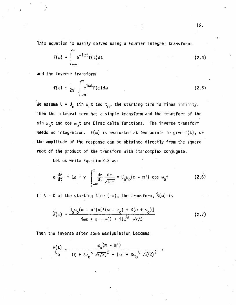
This equation is easily solved using a Fourier integral transform:

F(co) = e- ia)tf(t)dt ' (2 .4)

and the inverse transform

1f(t) =

r<X>

e

-co

(2.5)

We assume U = U sin w t and t , the starting time is minus infinity.

Then the integral term has a simple transform and the transform of the

sin co t and cos <o t are Dirac delta functions. The inverse transform

needs no integration. F(to) is evaluated at two points to give f(t), or

the amplitude of the response can be obtained directly from the square

root of the product of the transform with its complex conjugate.

Let us write Equation2.3 as:

rt(2.6)

If A = 0 at the starting time (-«>), the transform,

. 0A(U) =

- m')ir[6(o) - u>

icoe + Sn/2

s

(2.7)

Then the inverse after some manipulation becomes

a(t) .uo "

co (m - riT)

(we

17.

cos u)Qt + we + /F72") sin u t> (2.8)

Or:A(t} w (m - m1)Q \ » / ' w

uo [(5 + j^* rfTZ)' + (« + /i7Z)z J

Where: ^E, + 60)^ 2 A/2

tan A - °ue + 6(0 2 /7T/2

0

In terms of r, p, p_ and y the amplitude is then:P

/p |

Amp A(t) - A° - I**" ^/\mp. y U fr n2 rp< 7i 3 ( 1 + 3 ) + 3 . + ~^ "1 T1 /I~/T P

V^.3;

.cin (.. * + j.\|VSln 'W01' . *'

(2.10)

(2.11)

T2 1h 1 + 9 B+ 9 Y\

2 + 4 e + /,,o-6 r

which i$ a function of p /p and 3 only. This particular form of the

comparision is not found in the literature and it is convenient to solve

Equation 2.8 for V(t) to compare amplitudes directly. The result is

= VQ sin (2.12)

Where

i + V'1-

and

tan

P '

j. i- /-TO-+ 6a)Q2 /rr/2 o(m-m

1)v

(2.13)

(2.14)

coe

UJoo

OOUJ

ooUJ

UJ

QQ

CO

o

oo

CO

oO

UJ

ooLUoooouiccQQ

eno

>> QJS- OO C•M O)TO S-S- <U <UO M- >

COo

cr>

re

i— a)

O

TOUJ

s- s:Q

S-O CUto -4->J- V)S- OJ0) O

TO OL S- C_l Q S-

OC >, O) »t-O S? > •<-•r- TO O i—CO S- S- TO

r— jQ CIS C_)3 ••-

o re TOi- O CQ. .. CU

c o -a4-> +-> O COa> •*-> co TOrs <: <*• a.

oco

TO

s_o

S- i—3 iao o

c_>«\

3 TO OU_ r— r—

CO •—• I— I •!—

I— S_

•* TO£ 00 E•i- CO TO1— i— I <_>

18.

To compare with previous results we consider simplifications of Equation

2.2 and their solutions.

If all the terms on the right hand side of Equation 2.2 are dis-9 2carded except j m'ooB (V-U), the resulting equation represents motion in

a medium whose resistance is non-inertial . Then for U = U sin u)t,

m 31 + f m' m (2.15)

The amplitude of the solution is

(2.16)

Equation 2.16 was used by Rosenweig, Mottle and Williams [24] to justify

their light scattering measurements of smoke to determine turbulence

fluctuations. Fuchs [1] cites several experimental confirmations of this

expression and also shows that the solution to Equation.2.2 without the

integral term gives almost identical results. Since the experimental

data scatter widely, there is some doubt of the validity of the analysis.

The solution to eq. 2.2 without the integral term has been widely used

since its derivation by Konig [25]. The result is

1 + 3g + 9 + i 1

_g9 23g$ + f 9 3 9 4

T 3 + T 3(2.17)

1 pnwhere g = 4- (2- + 1). Since in all cases the amplitudes are functionso P

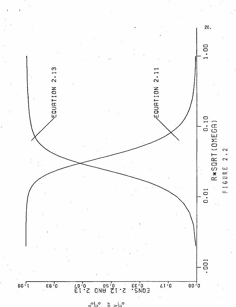
of r^C"and pp/p, plots can be made by varying these two parameters. Figures

2.1 and 2.2 show such plots.

c 19.

0 0 - 1 £8 '0 L Q - 0L\ '

o s - oQNU 91

e e - o-SN03

o o - o

o o

O O ' I £ 9 - o 09 -0 ee-oE l - 2 Q N U Z \ ' 1 . ' SN03

u-o

20,

oo

\— ' CC

z:o

CNI

fV CM

oCO UJ

01CD

O•

O

o— o

O O ' O

0 0 S -<] IZD O

21.

In the first, Figure 2.1, Equations 2.16 and 2.17 are plotted

for air at room temperature and for a particle density of l.Og/cm .

Figure 2.2 shows equations 2.12,and 2.13 for the same conditions. Equa-

tion 2.16 would apply only for low relative Reynolds numbers between

particle and fluid and in the absence of other forces. Fuchs lists additional

forces such as hydrodynamic sound pressure due to changes in density of

the gas which cause particles in a standing wave to drive to the nodes.

Other effects are scattering and absorption of sound waves, hydrodynamic

interaction between particles and electrostatic scattering of particles.

Little is known about the importance of these forces as functions of

concentration, mean velocity or frequency.

III. MOTION OF A SINGLE PARTICLE IN A TURBULENT FLUID

In turbulent flow the oscillations do not occur at one frequency

or amplitude but vary in time and space. Although the acoustic wave gives

apparent agreement with single frequency experiments, it would not account

for the frequency spectrum found in turbulence. If the measuring instrument

is able to determine precisely the instantaneous velocities, the only errors

in using the results for the fluid velocity will be the difference between

the fluid and particle. Most instruments measure the velocities over a

finite volume and a finite time span. Therefore a distribution of veloc-

ities is obtained. The problem of investigating the relationship between

the measured distribution and the true distribution involves the simul-

taneous consideration of the instrument, the particle lags and the fluctu-

ations due to turbulence. Only the interaction between the particle lag

and the turbulent fluctuations are considered in this report. A possible

way to allow for turbulence is to assume that Equation 2.17 also applies

to the ratio of amplitudes of the frequency spectra curves of particle

and fluid turbulence.

t

Then

23.•

where F(u) is the amplitude of the normalized frequency spectra density

curves for the fluid and V2", and U7" are time mean square averages. A/

similar expression can be obtained for the relative velocity V = V-U.

We will compare Equation 3.1 with another analysis for examples of F(m)

obtained from experiments later.

As in the ease of the acoustic field the equation of motion of a

particle in a turbulent field is obtained from the momentum balance.

dV r« . P-ft = L, Forces,

where

in vector notation. For simplicity the vector symbol will be dropped.

For a spherical particle when continuum equations are valid the forces

are the following:

1) Gravity = mg

2) Buoyancy = m'g

3) The variation of hydrostatic pressure in the fluid = m1 —-,dt1

where the substantial derivative is based on the fluid

velocity (indicated by — = — + U.v)dt1 9t

4) The force necessary to accelerate the "apparent" mass of the

particle relative to ambient flow = * m1 dt " dt

5) The deviation of the flow pattern from steady state (Basset

force) =

c 26r

24.

6) The drag force = mFD(U-V)

7) The Lift due to spin.4 -

8) The pressure =

9) Intermolecular forces.

10) Forces induced in the neighborhood of an interface.

11) Forces due to temperature gradients in fluid or particle.

12) Forces due to molecular diffusion.

13) The force due to oscillating pressure

14) Other body forces

Only 3, 4, 5, 6, and 8 are usually retained in the equation of motion.

These terms form an equation which has been solved only when additional

assumptions are valid. Here we take a modification of the approach given

by Soo [2] based on solutions by Tchen and Chao. The assumptions are

a) The particle is small and spherical so that a simple

expression can be used for the drag coefficient based

on the relative motion. The drag coefficient appears in

6) above when FD = | Cp- r |U-V| .

i t ' f> ar.Torobin and Gauvin [26] have reviewed the effect of tur-

bulence on C . Literature results show both increased

and decreased drag coefficients. An empirical correction

which fits the standard drag curve over a large range of

particle Reynolds numbers is given by Torobin and Gauvin

and is convenient for computer calculations.

CQ = /^- (1 + 0.15 NRe°'687) (3.2)

Re

25.

where

At high speeds approaching sonic velocity the drag co-

efficient can be modified to include effects of gas

compressibility and rarefaction [27]. If the effects

of velocity gradient and derivatives of velocity grad-

ient can be expressed as a constant multiplied by the

relative velocity, the drag coefficient can be further

modified.Cn (modified)

Let K • C° (Stokes) ' <3'3>

Then only the factor K will appear in the equation of

motion. K is a function of the variables mentioned

above.

b) The particle is small compared to the smallest wavelength

of turbulence.

c) The flow field is not perturbed by the presence of the solid

particle. Then the components of the pressure term can be

taken from the Navier - Stokes equation for the single phase

fluid.

= pir - yV2U,

where

Dt " 3t U U>

When a cloud of particles is present this equation includes

the effects of flow around the solid. A modification of this

26.

can be made if we can include the effect of the nonlinear

terms in the drag.coefficient.

d) The path of the solid particle coincides with the fluid

streamline. That is -rr = -TTT .

This assumption leads to the conclusion that the particle

diffusivity is the same as the Lagrangion eddy diffusivity

of turbulence. Soo discusses the experimental and theoret-

ical reasons why this is not true for a finite size particle.

The particle diffusivity is a function of particle response

time and the Lagrangion and Eulerian scales of turbulence.

However, without the assumption that the particle and fluid

paths coincide, no rigorous solution to the equation of

motion is available [28].

e) The turbulence is homogeneous and steady. Then a simple

velocity spectrum can be used. Also the mean flow can be

omitted, from the equations by having the coordinates follow

the mean motion. This assumption has been discussed in

Section I. I.f we use a coordinate system which moves with

the particle, the total time derivatives of the fluid velocity

must be replaced by the derivative moving with the coordinate

system:$r=!£+ (V'V)U 0.4)

f) The turbulence is not effected-by solid boundaries and the

starting time, tQ, in the Basset force term can be set at

minus infinity.

27.

With these assumptions the equation of motion becomes

m THT = 67ryrK(U-V) + m1 [|£ + (U'V) U - vV2U]

i nil AM o r d(u'V) dT

' - 0.5)dt

.CO

Or

(U-V)

t d (U-V)

Now .let a = -2" , and 6 = ' y-f- , then:pr pp p

(3.6)

. (3.6a)

To write the components of equation 3.6 in a cartesian coordinate system

we have

— = — + (V-V) V. = (^) (3.7)dt at i dt i

and we note that

|£+ (U-V)U = |^-+ ( V - V ) U + [(U-V)'V]U = ^-+ [(U-V)-V]U. (3.8)

28.

So that

all T du, au. au. au.+ (U'V)UI = —U (U: - V.) —U (U. - V.) —U (U. - V.) —L3t Ji dt n 1 ax- J J ax. K k axk

Then equation 3.6a becomes

dv. du. 0 au. 0 au._L = 6 _1+ a6K (u v.) +|6(U.-V.)—

L+ j6(UrV.) — l-

dt dt ^ 1 J 1 1 3X. J J J 3X.' v

o o i 1 ^- (u.-v.)dx2 T '

o i ri + 6^ 2 I1

U + 6 2 T (3.9)

This derivation is also given by Hinze [5], and it represents the

particle motion from a Lagranian point of view. That is the particle

follows the detailed motion of the fluid. Friedlander [29] suggested a

Eulerian formulation when the particle is large. The true situation lies

in between the Lograngian and Eulerian models. A short discussion of this

point and a review of the literature pointing out the important parts of

the preceeding derivation is given by Brodkey [30].

Equation 3.9 contains three nonlinear terms and the term involving

the second derivative with respect to the space coordinates. Conditions

for the neglect of these terms have been given by Corrsin and Lumley [31]

and Hinze [5], A similar argument is given here. Let us assume that

(U.-V.) and (U.-V.) are porportional to (U.-V.). Then the nonlinear termsJ J K K - 1 1

can be grouped together

29.

3U. 3U. 3U."l ..— + a. — = 4<5 (U-V.)A (3.10)

•\y J 2YL3Xi 3X..

where a. and a. are constants.

If a<SK(U.-V.) is much larger than this term, we can neglect the non-

linear term. The condition becomes if a. and a. are equal to one and allJ K

the derivatives are equal

3U.26(U.-V.) —- « a6K(U.-V.)

I 1 r. V 11

or since K is near one, .

3U.2 —*-« a (3.11)

3X.

Since a is approximately 10' for a one micron particle in air, the velocity

gradient must be extremely large to be significant. Of course for a lOOy

particle or a somewhat smaller particle in water this term may be important.

It is possible then to calculate a particle velocity error in the same

manner as shown below by taking the local value of A and using it to form

a new correction K.

Kn = K + !£ (3.12)

This approach has been taken by Tchen [4]. The second derivative term can

be neglected if it is small compared to the others. Hinze compares it to

the velocity gradient term which gives

V5 >» 1, (3.13)

30.

where d: is the particle diameter. Comparing it to the same term as the

velocity gradient we find.

| v6V2U. « a6K(U.-V.)0 1 1 1

and we can define

':A_|2!_i . (3>14)oCt »3ct /

i 1 1

From eq. 3.14 we see that

2v 1 - 1 (3.15)a (urv.)

is the condition to be met. Typical numbers in air are v = 0.2, a =

(Uj-V^) = 10"3; so V2Ui « 103 which is not the general situation. We will

examine the effect of a local correction considered as a constant using

eq. 3.14 later.

Equation 3.9 can be written as a linear first order differential

equation using K as follows:

rt-^(u.-v.(U.-V.) + 6(—) / _ (3.16)

dt dt

If the Basset term is dropped and K =1, the equation becomes:

a6V = a6U + 6 (3.17)

31.

The Fourier transform of the solution is

<\, a + iioU (3.18)

We follow the procedure given by Soo [2] which was developed by Tchen [4]

and Chao [32]. Multiplying eq. 3.18 by the complex conjugates of each side

gives

, ,2VV . ( ) * 1 (3.19)

** 2

which is the square of the amplitude ratio for the frequency, w. For the

particle the energy spectrum density function is introduced so that

- (3'2d)

Integration with respect to to gives

9 -2=/•*** / U) \ c. , -I

•*o 1 /uh2V= u -5 - f (u) du (3.21)

and

f "~? ^^ +1_£= U_ ^a; ' (3.22)

~2 1- f^2 + V '/ .2 aj + 'o

32.

where f is the energy spectrum density function for the fluid.

The same problem can be solved for the relative velocity and if the

Basset term is included. Details are given by Soo. Inclusion of the

Basset term or corrections to the drag coefficient have the same effect as

decreasing the particle size. Therefore, the particles follow the flow

better than would be indicated by eq. 3.21.

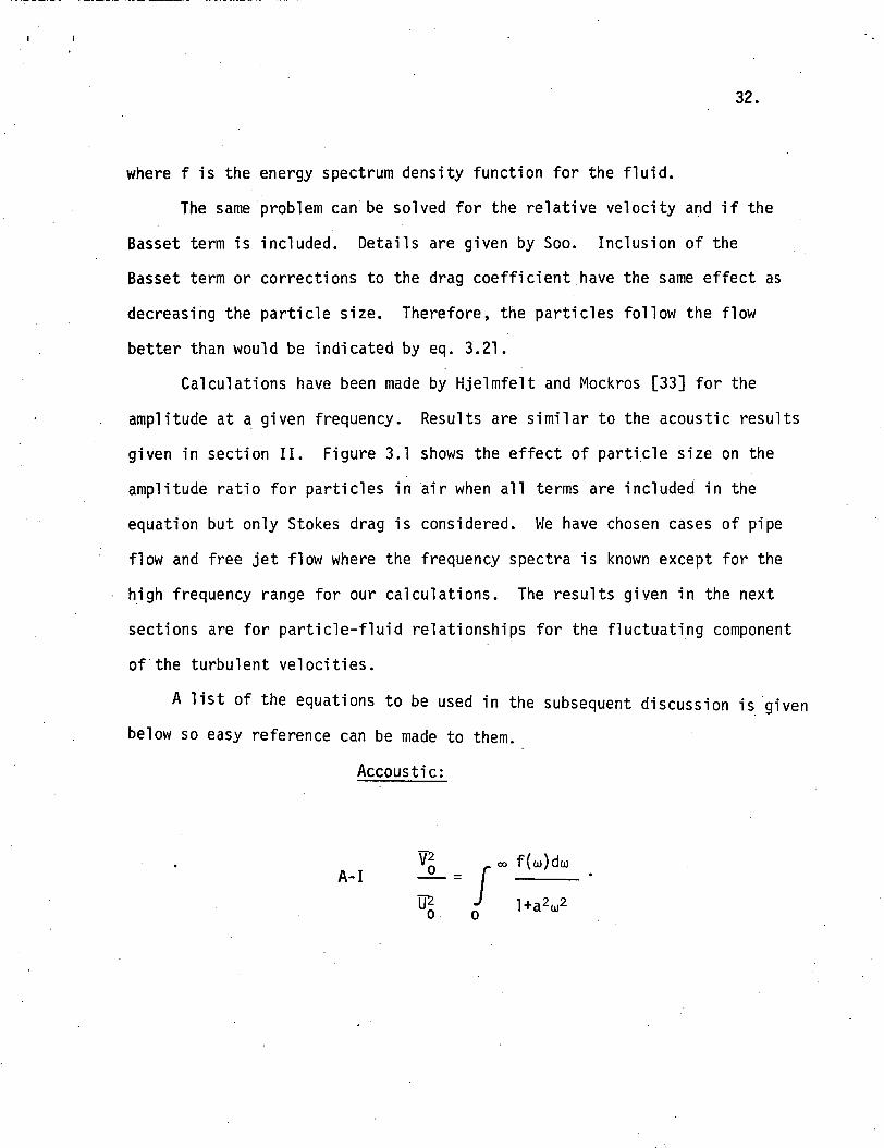
Calculations have been made by Hjelmfelt and Mockros [33] for the

amplitude at a given frequency. Results are similar to the acoustic results

given in section II. Figure 3.1 shows the effect of particle size on the

amplitude ratio for particles in air when all terms are included in the

equation but only Stokes drag is considered. We have chosen cases of pipe

flow and free jet flow where the frequency spectra is known except for the

high frequency range for our calculations. The results given in the next

sections are for particle-fluid relationships for the fluctuating component

of the turbulent velocities.

A list of the equations to be used in the subsequent discussion is given

below so easy reference can be made to them.

Accoustic:

V* co f(u))duA-1 = I

> J

33.

A-II ^ , <"*T ~*.

a =9y

Approximate Turbulent:

T-Ir2 J 1_ (U)2 + i

f(w) dui

T-II -f(u)d.0)

Turbulent with Basset force.

T-III — =2

r

u2f (u>)dco

?r r nR0 )

T-IV —L= / -Au2 J° n^

I I

34.

(2) , 1 ((0)2 ^ (fiL)'./2 3((o} + ^ (fiL)

.2 ^a.' 6 vcr ^a.' voro

Turbulent with Basset force and drag coefficient (24/NRe)K.

fo\ / -1 \ / ? \ /1 \T-V Replace the last two terms in Jr ; and ftv ' with

ft K (^)^2 + K2.xa'

All velocities in the above are fluctuations from the mean.

Figure 3.1 shows the amplitude function $r '/Sr ' as a function of

frequency and particle size for air as the fluid. Errors of over 1% exist

when the frequency is over 6kH2 for a one micron particle and for frequencies

considerably less as the particle size increases. The effect of changing

the parameter K is shown in Figure 3.2. As K is increased the drag increases

and the amplitude function increases. This means that the relative velocity

lag is reduced.

Fortunately in a turbuTent field most of the energy is concentrated

in low frequency oscillations. That is f(u) drops off rapidly as frequency

is increased. We examine the cases of the free jet and the center of fully

developed pipe flow in the following subsections. The assumptions that the

particle and fluid diffusivities are the same (long diffusion time) and no

particle-particle interactions are retained.

A. Application of Single Particle Analysis to Turbulent Jets

Based on J. C. Laurence's [34] measurements in the mixing region of a

free jet, the spectral density function can be represented by f,v, fUlaX W

8ooO.o

CO

accor:UJ

h-or.cco_

o o—i CMCD Oo oo oo o

CO COID ID

CD OCE CE

O CD OLO O CDCD —* OCD O <-*O CD O

O O O

! I ! I II

CO CO COID ID ID

CD CD CDCE CE CE

o

LiJ LU LU LiJ UJ

CJ CJ CJ CJ CJ

!__ H_ |__ v__ |__

'""T— r 'T" '"T~ ' T— .- »<w_L Ci_ >-L L-I_ o_CL. G... d. D_ C_

1 O <J O X

o (-Jo o o o o o. 0 0 0 0

CD LT> l> CDII

O LL U_ L_ LL. U_.O O O O O

LU> LU LU LU LU LU_j ID ID ID ZD ID(X _J _J _J _J _J> cr cr en cr cr

LUUJ UJ LU LU LUn ic in HI x(_.. (_. (_. J_ I—

02' I 00 ' I 08 '0 09 '0 Cfr os-'o

ooo

ooo

ooo

oo

OJ '—'

CJ

ocn

36-

CO

OCT

CO GC OJ

LU

oo_oCM

CD

0001 I G j W O JO

37.

and a decay slope of -2 on a log-log plot of f(w) vs w as shown in Fig. 3.3.

Using Equation T-IV extensive calculations showed the results were sensi-

tive only to f when particle diameter and density were held constant.

The density function decay as the inverse square cannot exist beyond

some upper limit frequency. Most references on turbulence give a change

from a minus 5/3 slope to a minus 7 slope for isotropic turbulence at some

high frequency. That is at some frequency of turbulence all the energy

should be dissipated by the viscous forces. If this frequency is taken

as 20 kHz and we neglect everything beyond 20 kHz, calculations can be made

giving mean square differences between particles and fluid using the equations

listed. For a one micron diameter particle with a density of one gram per

cubic centimeter in an air jet mixing region with f = 2000 Hz the results

are:

Equation Result

A-I .991

T-I 1.000

T-III .990

A-II ,.009

T-II :T009

T-IV .008

Further calculations using formula T-IV are summarized in Figs. 3.4

and 3.5, Figure 3.4 shows the effect of particle density for different f

and particle size. Figure 3.5 shows the effect of particle size when

particle density is held constant at one gram per cubic centimeter.

38.

CDO

l\

slope -2

max

LOG FREQUENCY,

Figure 3.3 Turbulent Jet Frequency Spectra

39,

s-os-

<u

3CT

CO

croOl

OJ>

CO

O)DC:

0.5 0.6

0.4

0.3

0.2

0.1

0

.04

.03

.02

.01

0

.0004

.0003

.0002

.0001

01

r = 1 micron

P = 1

r = 0.5 micron

r = 0.15 micron —

2 4 6 8 1 0

fu x 10~3 Hz

Figure 3.4 Particle Density Effect on Velocity Lag.

40.

oi.

<uto3CTtoc.to0)

(U>

.00001

.0001

Particle Size, Microns

Figure 3.5 Effect of Upper Cut Off Frequency

41.

In each case the frequency spectrum density function was taken from

Laurence's equation.

(i(4f*)[1

ma?

2TTf*

fu~2

c 2

t •

1 + /I -1 m1 • y 1

irf

ax] 2

u ' _f * =

The integration was carried out using 50 points and the trapezoidal rule

between 0 and 20 kHz. The f(w) function in equations is the above E

function divided by

r20 kHz E do) to normalize the function.

-2A simpler analysis 'can be made using E a linear function of uf . Figures

3.6 and 3.7 show the ratios of particle mean or relative velocity fluctua-

tions to the fluid fluctuation for selected particle sizes from one micron

diameter to 200 micron diameter. Air is taken as the fluid at room temper-

ature .

The effects of non Stokes drag, rarefaction, compressibility and

inertia can be included in the equation of motion by letting

LO O • O O OO CM LO O. OO O O *-> OO O O O —O O O O O

• • • • •

O O O O O

OO

42

II II II II II

en co en en enZD ZD ZD => IDI— « I — I I— I I— I I— Ia o a a acr cr cr CE CErv f£ fK (V rv

LU UJ UJ LU LU_J _J _l _l _JO (_) (_) C_> CJ

ex ex 'cr .cr crQ_ Q_ Q_ Q_ Q_

00 ' I 88-0A1I3013A

os-o ee-o Z . T - O

ooo'en

oo

o .

OLU

c£UJ

OQ_O

o •_OQ

C£I

OU_

CJ

OCJ

.§£a

OU-

IsQ_Q_

OO

•_o

oo

OC

CO

LiJ

ILUUJ

oo-cP

I ]

O O ' t £ 8 * 0 L Q ' QA1I3013A

oo•

o-CD

CO

OO•

O.CMCO

OO

•V

o .

°0OLLJ

LJJOQ_O

O •

"CMQ;

ce:I

OLl_

s2'^ZD

CJ

oo

•

_o

OS ;0 0 L \ '0

oo

00-0°

43.

OI—I

I—CE

CO

I—UJ

LU

44.

(1 + 0.15NR°'687)(1 + exp (-0.427/M4-63 - 3.0/NR°'

88))

1 + /- (A + B exp (-1.25NRe/M))RG

t •where the Reynolds number, NR , and the Mach Number, M, are for the

difference velocity between the fluid and particle. The constants A and

B are 3.82 and 1.28 respectively at Mach numbers sufficiently high, but

may be lower for lower Mach numbers. The equation above is derived by

Carlson and Hoglund [27].

For a one micron diameter particle with a density of one gram per

cubic centimeter moving in air at room temperature, the following results

were obtained:

Mach No.of fluid

0.10.30.51.02.0

Mean squareratio ofvelocities

.9878

.9889

.9897

.9909

.9924

Mean squarerelative velo-city to fluidvelocity

.0096*

.0087*

.0082*

.0072

.0061

ParticleReynoldsNumber

.218

.6231.0031.8833.454

ParticleMachNumber

.0098

.0281

.0452

.0848

.1556

In the table the complete equation was used although the rarefaction

correction in the denominator is not valid for the starred points. In

general for this particle size at a cut-off frequency of two KHz as used

in the calculations there is no significant change. All of the conditions,

however, fall in the slip flow regime and not the continuum regime.

B.' Single Particle in Pipe Flow

A similar analysis can be made for fully developed turbulent pipe

flow. For the frequency spectra Laufer's data [35] can be used. The upper

45.

cut off frequency is now a function of Reynolds number or average velocity.

If the minus second power decay of the frequency spectra can be used, the

curves for the free jet would also be valid for the drag corrections. From

Laufer's curve at the centerline of the one dimensional spectra

°'28 UX1 max *

fu

where fu is in radians per second and U in cm./sec. Laufers curveXi fflclX

is for a Reynolds number of 5 x 10^, however, and may not be representative

of lower Reynolds numbers.

C. Experimental Studies of Turbulent Velocities of Small Particles

A summary of the few experimental measurements on turbulence inten-

sities in particle-fluid flows is given by Reddy and Pei [36]. Other

studies discussed in Part IV of this report are indirect in that measure-

ments were made on concentration fluctuations and not velocities. The

velocity studies were made photographically using particles greater than

100 microns. Reddy and Pei conclude that "the particle turbulence compo-

nents can be correlated principally with the fluid turbulence." It is

difficult to justify this statement based on the calculations in this

report. Only the slowly varying large scale motions follow the flow and

therefore the turbulence intensities of the particle and the fluid check

closely. However, it is impossible to measure the high frequency turbulence

components by measuring velocities of particles larger than one micron.

A study in liquids using 0.5 micron particles was recently reported

by Corino and Brodkey [37]. They were successful in measuring particle

velocity fluctuations near the wall of a pipe at Reynolds numbers up to

50,000. Velocity gradients as high as 10^ sec."^ could be determined.

46.

Soo [2] reviews other experiments but the interaction of the solid

particles with the wall has been a problem. Min [38] indicates that the

spread of velocities after collision with the wall must be considered and

not confused with the turbulence of the main stream. In section I of this

report the time decay was seen to influence the relative mean velocity.

Measurements of turbulence from velocities of large particles would con-

sist of large effects due to these adjustments following collisions.

IV. OTHER CONSIDERATIONS IN PARTICLE-FLUID FLOWS

Two assumptions of the previous section are not substantiated by

experiments. These are the assumption that particle and fluid diffusivities

are the same, and the neglect of particle-particle collisions. Extensive

theoretical and experimental investigations have appeared in the literature

on both problems, but it is not possible to predict or measure the effects

in most real situations.

Soo [2] derives the eddy diffusivity for the particle from the mean

square displacement. If the mean square displacement is related to the

Lagrangian velocity auto correction coefficient, R(t), the result is

-- rtDp(t) = T \ Rp(T)dx (4.1)

o

The fluid eddy diffusivity similarly is

~? rD = IT /

-'

R(x) di (4.2)

o

Friedlander [29] explains that R(T) is Lagrangian only for small particles

and may be between the Eulerian and Lagrangian correlations for the real

case. The ratios of particle to fluid eddy diffusivity become

D ~2• jf- = — for short times

2IT

and D—fy = 1 for long times

48.

Both Soo and Friedlander give results for an assumed Lagrangian coefficient.

In the previous section the assumption was made that D /D = 1, but studies

by Lumley [28] and others show that this is not true. To account for the

difference we must relax the assumption that a particle remains always with

the same fluid element. Soo gives a review of calculations to correct the

eddy diffusivity for some practical cases. If the particles are below one

micron in diameter, however, the assumptions of section III appear to be

valid when sufficient time is given for the particle-fluid system to

equilibrate. Collisions with walls or other particles, velocity gradients

or coalescence will affect this time period.

Some of the first work in the field of particle-particle interactions

was published by Smoluchowski in 1916. He developed an infinite set of

simultaneous differential equations to describe the interactions and growth

of floes. His results may be written in condensed form as

(4.3)dt 3 dZLi=lj=k-i

where dN/dt is the rate of change of the number of particles of the indicated

size, dU/dZ is the velocity gradient, N is the number of particles of an

indicated size, and R is the radius of the particles. It is not possible

to solve this set of equations in a closed form for real cases; however,

with the advent of large computer systems approximate solutions have been

made. [39, 4(3-

49.

A program is available from R. S. Gremmell [41] in which the

growth, breakup, and steady state size of floes in laminar flow are,

simulated as a function of the maximum floe size, the breakup floe sizes,

the velocity gradient, and the initial concentration of the suspension.

This type of simulation is very helpful if the necessary variables are

known for a particular system. Such simulations are, of course, only

useful if the particles tend to floe or coagulate.

The availability of sophisticated equipment has made experimental

studies of single particle interactions possible. In the study of rigid

spheres, Mason and others [42] discovered a repeatable pattern of approach,

interaction, and separation. The spheres approach each other rectilinearly

in a path parallel to the x-axis (i.e. axis parallel to the flow). Although

they never come into true physical contact the two approaching spheres

form a doublet which rotates with a constant angular velocity ofG

(0 = 2

where G is the velocity gradient in the fluid. The doublet rotates about

an axis perpendicular to the planes of shear, and in the case of rigid

spheres the doublet only rotates 180°. The separation is a mirror image

of the approach because of the 180° rotation before separation. Deform-

able spheres do not separate after the first half cycle but may rotate

for several full cycles before coalescing or separating. They will

coalesce only if the van der Waals forces are strong enough to displace

the intervening liquid. [43]

The tubular pinch effect is a fluid induced particle disturbance

found only in tubular Poiseuille flow and not in Couette flow. The

50.

tubular pinch effect is essentially the tendency for rigid or deformable

bodies to migrate under certain conditions toward a radial position,of

distance r from the center of the tube. The particles closer to the

center of the tube migrate inward. This effect is apparently not en-

countered in turbulent flows although the forces causing the phenomenum

may be important in the analysis given in the previous section.

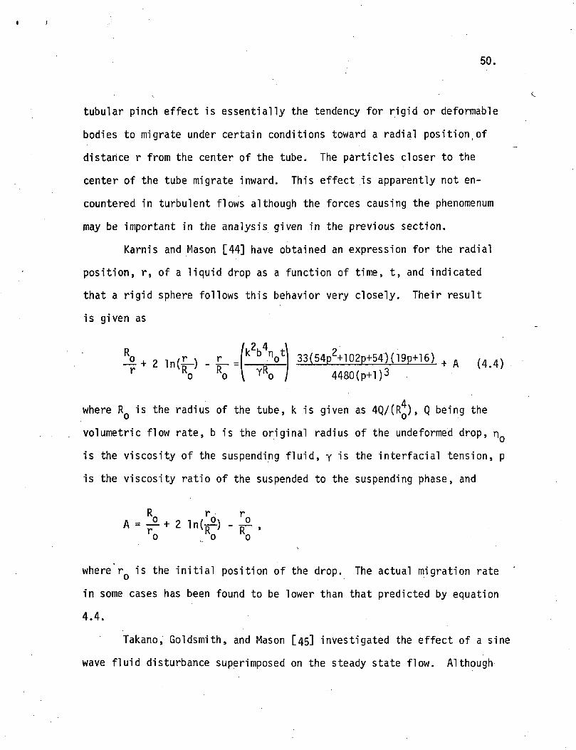
Karnis and Mason [44] have obtained an expression for the radial

position, r, of a liquid drop as a function of time, t, and indicated

that a rigid sphere follows this behavior very closely. Their result

is given as

33(54p2+102p+54)(19p+16) + A /4 4»

4480(p+l)3

where R is the radius of the tube, k is given as 4Q/(R~j, Q being the

volumetric flow rate, b is the original radius of the undeformed drop, n0

is the viscosity of the suspending fluid, y is the interfacial tension, p

is the viscosity ratio of the suspended to the suspending phase, and

R r r" "~ v* *U' "" D '

o , 0 0

where rQ is the initial position of the drop. The actual migration rate

in some cases has been found to be lower than that predicted by equation

4.4.

Takano, Goldsmith, and Mason [45] investigated the effect of a sine

wave fluid disturbance superimposed on the steady state flow. Although

51

their work is not complete, they have come to some qualitative conclusions

The migration rates and equilibrium positions for a given suspension

depend on a dimensionless parameter, a, as well as the flow rate. The

parameter

where R and n are the same as before, co is the angular frequency of

oscillation, and p is the density of the suspending fluid. This parameter

was used in the analysis of both rigid and deformable spheres.

In experiments made with polystyrene spheres, the initial stages

of oscillatory flow, a<5, revealed an increased migration rate over that

of steady state Poiseuille flow. The particles collided in approximately

the same manner as observed in the former particle interaction studies in

steady state laminar flow. As a became larger than ten, more than one

migration or equilibrium position was noted. Some of these positions,

defined as radii where dr/dt for the particle equaled zero, were found to

be quasi-stable. The number of these positions increased with increasing

a, and it would be expected that at sufficiently high a the number of these

quasi-stable positions would destroy any noticeable migration caused by

the tubular pinch effect.

In a study concerned with the agglomeration of aerosols induced by

high energy sound waves St. Clair [46] listed three fluid effects on

particle movements. These were convibrational , hydrodynamic and radiation

pressure.

52.

Another analysis by Shaffman and Turner [47] concerned the collision

of liquid droplets in turbulent clouds. Assuming isotropic turbulence, the

collisions of the drops are attributed to two main sources: (1) collisions

due to the motions of the droplets in (within) the air, (2) collisions due

to motions of the droplets relative to the air (i.e. inertia! effects).

The two effects are discussed separately; the two effects may be calculated

separately and then added together.

The collisions caused by the drops moving with the fluid are discussed

assuming spherical droplets with a sphere of influence, R, equal to the sum

of the radii of two particles, r, + r,,. With a radial particle velocity

of w(r), some fluid relations can be used to transform w(r) into fluid

properties. After the transformation, the number of collisions, N, bet-

ween two population concentrations, n, and n^j is

N = 1.3 nin2 (^ + r2) (£) , (4.5)

where e is the rate of energy dissipation per unit mass, and y is the

kinematic viscosity.

In order to obtain the total effect of the collisions, the collision

rate is substituted into the Smoluchowski equation.

In dealing with the second part of the problem, that of droplet

motions relative to the air as causes of collisions, a probability function

P(w)for the relative velocity of the particles is assumed and the collision

rate thus obtained is

N = irR n,n9 / u P(u)du (4.6)\ £. j — ~ —

53,

By introducing a collision efficiency a quantitative prediction of droplet

formation in turbulent clouds can be obtained.v

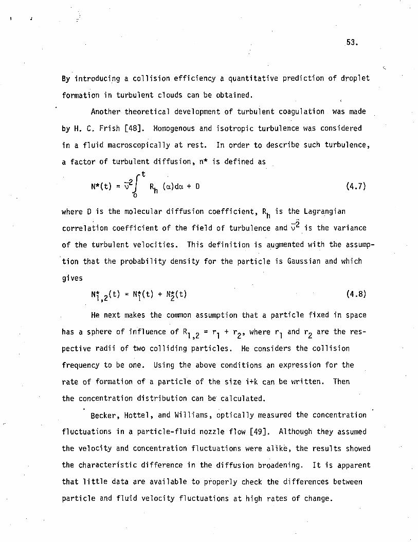
Another theoretical development of turbulent coagulation was made

by H. C. Frish [48]. Homogenous and isotropic turbulence was considered

in a fluid macroscopically at rest. In order to describe such turbulence,

a factor of turbulent diffusion, n* is defined as

k(t) = #J Rh (oc)da + D (4.7)

where D is the molecular diffusion coefficient, R, is the Lagrangian_.O

correlation coefficient of the field of turbulence and v is the variance

of the turbulent velocities. This definition is augmented with the assump-

tion that the probability density for the particle is Gaussian and which

gives

Nfj2(t) = N*(t) + N*(t) (4.8)

He next makes the common assumption that a particle fixed in space

has a sphere of influence of R, ~ ~ ri + r2> where r, and r^ are the res-

pective radii of two colliding particles. He considers the collision

frequency to be one. Using the above conditions an expression for the

rate of formation of a particle of the size i+k can be written. Then

the concentration distribution can be calculated.

Becker, Hottel, and Hilliams, optically, measured the concentration

fluctuations in a particle-fluid nozzle flow [49]. Although they assumed

the velocity and concentration fluctuations were alike, the results showed

the characteristic difference in the diffusion broadening. It is apparent

that little data are available to properly check the differences between

particle and fluid velocity fluctuations at high rates of change.

V. CONCLUSIONS

Small particles can be used to measure the fluid velocity motions

except under conditions of high frequency fluctuations. At high velocities,

in supersonic flow and for detailed analyses of turbulence, all particle-

fluid-instrument interactions must be considered. Both more theoretical

correlations for these conditions and experimental measurements under more

ideal conditions are needed to determine the exact limits of the Laser-

Doppler Flowmeter and the particle lag corrections.

VI. LITERATURE CITED

1. Fuchs, N. A., "The Mechanics of Aerosols", Macmillan Co., New York1964.

2.1 Soo, S. L., "Fluid Dynamics of Multiphase Systems," Blaesdell PublishingCo., Waltham, Mass. 1967.

3. Basset, A. B., "A Treatise on Hydrodynamics", Vol. 2, Dover PublicationsNew York, 1961, Chapter 22.

4. Tchen, C. M., "Mean Value and Correlation Problems Connected with theMotion of Small Particles Suspended in a Turbulent Fluid," PhD Thesis,Delft, 1947.

5. Hinze, J. 0., "Turbulence", McGraw-Hill Book Company, Inc., New York,1959.

6. Reddy, K.V.S., M. C. Van Wijk and D. C. T. Pei, "Stereophotogrammetryin Particle-Flow Investigation," Canadian Journal of Chemical Engineer-ing, 47, 85 (1969).

7. Hughes R. R. and E. R. Gilliland, "The Mechanics of Drops," ChemicalEngineering Progress, 48, 497 (1952).

8. Corrsin, S., and M. S. Uberoi, NACA Tech. Note 1965, 1949.

9. Gilbert, M., L. Davis and D. Altman, "Velocity Lag of Particles inLinearly Accelerated Combustion Gases," Jet Propulstion, 25^ 26 (1955).

10. James, R. N., W. R. Babcock and H. S. Seifert, "Application of a Laser-Doppler Technique to the Measurement of Particle Velocity in GasParticle Two Phase Flow," SUDAAR No. 265, Dept. of Aeronautics andAstronautics, Stanford University, Stanford, California, May 1966.

11. McCarthy, H. E. and J. H. Olson, "Turbulent Flow of Gas Solids Suspensions,"I&EC Fundamentals, 1_, 471 (1968).

12. Torobin, L. B. and Gauvin Wtt, AIChE J., 7_, 406 (1961), AIChE J., 7_,615 (1961), Can. J. Chem Eng 37, 1959 (1959), Can. J. Chem Eng, 38, •189 (1960). ~~ —

13. Morse, H. L., B. J. Tullis, H. S. Seifert, and Wayne Babcock, "Develop-ment of a Laser-Doppler Particle. Sensor for the Measurement ofVelocities in Rocket Exhausts," J. Spacecraft and Rockets, 6_, 264 (1969).

56.

14. James, R. N., W. R. Babcock and H. S. Seifert, "A Laser-DopplerTechnique for the Measurement of Particle Velocity," AIAA Journal6_, 160 (1968).

t

15. Fulmer, R. D. and D. P. Wirtz, "Measurement of Individual ParticleVelocities in a Simulated Rocket Exhaust," AIAA paper 65-11 andAIAA J. _3, 1506 (1965).

16. Afanasev, E. F. and V, N. Nikolaevskii, "On the Development ofAsymmetric Hydrodynamics of a Suspension With Rotating SolidParticles," Problems of Hydrodynamics and Continuum Mechanics,SIAM,Philadelphia, 1969.

17. Hoerner, S. F., Fluid Dynamic Drag, Homer, Midland Park, N. J.(1958).

18.:: Rubinow, S. I. and,J.,B. Kel1er,.j;iFluid.:Mech.-lJL."477'(1961).

19, Eichhorn, R. and S. Small, J. Fluid Mech. 20_, 513 (1964).

20, Saffman, P. G., J. Fluid Mech. 22_, 385 (1965).

21, Kondic, N. N., "Lateral Motion of Individual Particles in ChannelFlow - Effect of Diffusion and Interaction Forces: Part 1 - ParticleBehavior as a Function of Systematic Motion," ASME 69-HT-32.

22, Lamb, H., "Hydrodynamics," Dover Publications, New York, 1945.

23, Landau, L. D. and E. M. Lifshitz, "Fluid Mechanics," Pergamon Press,London, 1959.

24, Rosensweig, R. E., Hoyt C. Hottel and G. -C. Williams, "Smoke-scatteredLight Measurement of Turbulent Concentration Fluctuations," ChemicalEngineering Science 15, 111 (1961).

25, Konig, W., Ann. Physik 42_, 353 (1891).

26, Torobin, L. B. and W. H. Gaurin, Can J. Chem. Eng. 37 , 129, 167, 224,(1959), Can. J. Chem. Eng. 38^ 1.42, 189 (1960), and Can. J. Chem.Eng. 39_,113 (1961).

27, Carlson, D. J. and R. F. Hoglund, "Particle Drag and Heat Transferin Rocket Nozzles," AIAA Journal 2_, 1980 (1964).

28, Lumley, J. L., "Some Problems Connected With the Motion of SmallParticles in Turbulent Fluid," Dissertation, Johns Hopkins University,Baltimore, Maryland, 1957.

-> 1

57.

29. Friedlander, S. K., AIChE Journal .3, 381 (1957).

30. Brodkey, R. S., "The Phenomena of Fluid Motions," Chap. 18, Addison-Wesley Publishing Co., 1967. ,

31. Corrsin and J. Lumley, Appl. Sci Res 6A, 114 (1956).

32. Chao, B. T., Osteneichisches Ingenieur-Archiv 18, 7 (1964).

33. Hjelmfelt, A. T. and C. F. Mockres, "Motion of Discrete Particlesin a Turbulent Fluid," Appl. Sci Res J6_, 149 (1966).

34. Laurence, J. C.."Intensity, Scale, and Spectra of Turbulence inMixing Region of Free Subsonic Jet," NACA Report 1292.

35. Laufer, J., NACA Tech Report 1147 (1954).

36. Reddy, K. V. S. and D. C. T. Pei, I&EC Fund. 8, 490 (1969).

37. Corino, E. R. and R. S. Brodkey, J. Fluid Mech. 37., 1 (1969).

38. Min, K, J. Appl. Phys. 38, 564 (1967).

39. Fair, G. M. and R. S. Gremmell, J. Colloid Science ]£, 360 (1964).

40. Void, M. J., J. Colloid Science 18.,- 684 (1963).

41. Gremmel, R. S., "Some Aspects of Orthokenetic Flocaelation, PhDThesis, Cambridge, 1963.

42. Mason, S. G. and R. St. J. Manley, Canadian J. of Chemistry 33,763 (1955).

43. Mason, S. G. and W. Bartok, J. Colloid Science 14, 25 (1959).

44. Mason, S. G. and A. Karnis, J. of Colloid and Interface Science 24,165 (1967).

45. Takano, M., H. L. Goldsmith and S. G. Mason, J Colloid InterfaceScience 27_, 254 (1968).

46. St. Clair, H., Industrial and Engineering Chemistry 41_, 2434 (1949).

47. Saffman, P. G. and J. F. Turner, J. Fluid Mechanics ]_, 16 (1956).

48. Frish, H. L., J. Phys. Chem. 60_,463 (1956).

49. Becker, H. A., H. C. Hottel and G. C. Williams, J. Fluid Mech 30_, 259(1967).