Endogenous Cycles in a Stiglitz–Weiss Economy
25
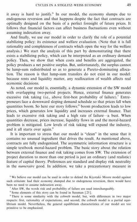
journal of economic theory 76, 4771 (1997) Endogenous Cycles in a StiglitzWeiss Economy* Javier Suarez CEMFI, Casado del Alisal 5, 28014 Madrid, Spain and Oren Sussman Ben-Gurion University of the Negev, Beer-Sheva 84105, Israel Received December 13, 1995; revised February 7, 1997 The literature on financial imperfections and business cycles has focused on propagation mechanisms. In this paper we model a pure reversion mechanism, such that the economy may converge to a two-period equilibrium cycle. This mechanism confirms that financial imperfections may have a dramatic amplification effect. Unlike in some related models, contracts are complete. Indexation is not assumed away. The welfare properties of a possible stabilizing policy are analyzed. The model itself is a dynamic extension of the well-known Stiglitz-Weiss model of lend- ing under moral hazard. Although stylized the model still captures some important features of credit cycles. Journal of Economic Literature Classification Numbers: D82, E32, E51. 1997 Academic Press 1. INTRODUCTION Economic research in recent years has revitalized the idea that financial factors should play a central role in business-cycle theory. 1 On the one hand, there exists a growing body of empirical work showing that financial imperfections affect real economic decisions 2 in a way which varies systemati- cally along the business-cycle. On the other hand, theoretical workBernanke article no. ET972297 47 0022-053197 25.00 Copyright 1997 by Academic Press All rights of reproduction in any form reserved. * This work was initiated during the 1994 European Summer Symposium in Financial Markets at the Gerzensee Studienzentrum. Earlier versions of this paper were presented at the CEPR Conference on Macroeconomics and Finance in Gerzensee, 1620 January 1996, and the V ``Tor Vergata'' Financial Conference in Rome, 2829 November 1996. We thank Martin Hellwig, Bengt Holmstrom, and John Moore for extremely helpful comments and suggestions. 1 Fisher [10] gives one of the first coherent statements; see King [19]. For many years, however, it was ignored: it is not quoted by Patinkin [22], the authoritative handbook of the 1950's and 1960's. 2 Usually, this literature shows that liquidity affects economic decisions, in contrast to the prediction of the ModiglianiMiller theorem where only net-present value matters. See Bernanke et al. [3] for an up-to-date survey.
-
Upload
independent -
Category
Documents
-
view
0 -
download
0
Transcript of Endogenous Cycles in a Stiglitz–Weiss Economy

File: 642J 229701 . By:DS . Date:05:09:97 . Time:08:41 LOP8M. V8.0. Page 01:01Codes: 4431 Signs: 2440 . Length: 50 pic 3 pts, 212 mm
Journal of Economic Theory � ET2297
journal of economic theory 76, 47�71 (1997)
Endogenous Cycles in a Stiglitz�Weiss Economy*
Javier Suarez
CEMFI, Casado del Alisal 5, 28014 Madrid, Spain
and
Oren Sussman
Ben-Gurion University of the Negev, Beer-Sheva 84105, Israel
Received December 13, 1995; revised February 7, 1997
The literature on financial imperfections and business cycles has focused onpropagation mechanisms. In this paper we model a pure reversion mechanism, suchthat the economy may converge to a two-period equilibrium cycle. This mechanismconfirms that financial imperfections may have a dramatic amplification effect.Unlike in some related models, contracts are complete. Indexation is not assumedaway. The welfare properties of a possible stabilizing policy are analyzed. Themodel itself is a dynamic extension of the well-known Stiglitz-Weiss model of lend-ing under moral hazard. Although stylized the model still captures some importantfeatures of credit cycles. Journal of Economic Literature Classification Numbers:D82, E32, E51. � 1997 Academic Press
1. INTRODUCTION
Economic research in recent years has revitalized the idea that financialfactors should play a central role in business-cycle theory.1 On the onehand, there exists a growing body of empirical work showing that financialimperfections affect real economic decisions2 in a way which varies systemati-cally along the business-cycle. On the other hand, theoretical work��Bernanke
article no. ET972297
470022-0531�97 �25.00
Copyright � 1997 by Academic PressAll rights of reproduction in any form reserved.
* This work was initiated during the 1994 European Summer Symposium in FinancialMarkets at the Gerzensee Studienzentrum. Earlier versions of this paper were presented at theCEPR Conference on Macroeconomics and Finance in Gerzensee, 16�20 January 1996, andthe V ``Tor Vergata'' Financial Conference in Rome, 28�29 November 1996. We thank MartinHellwig, Bengt Holmstrom, and John Moore for extremely helpful comments and suggestions.
1 Fisher [10] gives one of the first coherent statements; see King [19]. For many years,however, it was ignored: it is not quoted by Patinkin [22], the authoritative handbook of the1950's and 1960's.
2 Usually, this literature shows that liquidity affects economic decisions, in contrast to theprediction of the Modigliani�Miller theorem where only net-present value matters. SeeBernanke et al. [3] for an up-to-date survey.

File: 642J 229702 . By:DS . Date:05:09:97 . Time:08:41 LOP8M. V8.0. Page 01:01Codes: 3841 Signs: 3176 . Length: 45 pic 0 pts, 190 mm
and Gertler [2] and more recently Kiyotaki and Moore [20]��shows howtransitory shocks are propagated via imperfections in financial markets. Thenovel contribution of this paper is the modeling of an endogenous reversionmechanism, such that the economy may converge to a two-period equilibriumcycle. The model is kept deliberately simple so as to allow a transparentexposition of the mechanism. Indeed, the model is a dynamic extension ofthe well-known Stiglitz�Weiss [24] (henceforth SW) model of lendingunder moral hazard.3
Let it be clear that we view the reversion mechanism as a complementto the propagation mechanism. Obviously, it takes both to produce acomplete theory of business fluctuations. But further, we use our model toclarify some theoretical issues. First, it is often argued that financialimperfection provide a crucial amplification effect that can solve the ``smallshocks, large cycles'' puzzle (see Bernanke et al. [3]). In our model theamplification effect is dramatic: the variance of external shocks is zerowhile output fluctuations may still be sizable.
Secondly, in both Bernanke and Gertler [2] and Kiyotaki and Moore[20] the external shock is not anticipated in advance. Hence, agents do nothedge in precaution. It seems, however, that agents who fail to foresee arepeated shock do not have rational expectations. That raises the concernthat irrationality is an indispensable ingredient within such a theory. Weshow that this is not the case. In our model the whole sequence of futureprices is rationally (and perfectly) foreseen. Moreover, contracts are``complete'' and all relevant information (future prices included) is inter-nalized. To the best of our knowledge our example is the first clear-cutdemonstration of a cycle generated solely by financial imperfections,without any modification of the rationality assumption.
More to the point, the issue at hand is that of ``indexation.'' Consider,again, Kiyotaki and Moore [20].4 The external shock operates via a pricedecline that decreases the value of collateral and, hence, borrowingcapacity. It is well known that in that case insurance can easily be providedby price indexation.5 Since such indexation is mutually beneficial, assuming
48 SUAREZ AND SUSSMAN
3 SW also contains a, maybe better known, adverse-selection section.4 The problem goes back to Fisher [10]. In his view, the Great Depression was a result of
money-price deflation that increased the real value of corporate debt, drained capital out ofthe corporate sector, which caused an adverse supply effect. But the initial effect can beindexed away to the mutual benefit of lenders and borrowers. Note that Fisher's explanationhas two ingredients: lack of indexation and financial imperfections (which create the linkbetween corporate wealth and supply). We show that the second effect is sufficient for abusiness-cycle theory. Needless to say, the first ingredient is extremely problematic. It mayhave been one of the reasons that prevented a serious consideration of Fishers's theory for solong.
5 Indexation is assumed away for the shock period only. All subsequent price dynamics isindexed.
File: 642J 229703 . By:DS . Date:05:09:97 . Time:08:41 LOP8M. V8.0. Page 01:01Codes: 3910 Signs: 3065 . Length: 45 pic 0 pts, 190 mm
it away is hard to justify.6 In our model, the economy slumps due toendogenous reversion and that happens despite the fact that contracts areoptimally designed on the basis of a perfect foresight of future prices. Itfollows that financial factors can affect business fluctuations even withoutassuming indexation away.
And finally, we use our model in order to clarify the role of a potentialstabilizing policy: its existence and welfare evaluation. (Note that it is fullrationality and completeness of contracts which open the way for the welfareanalysis.) We start the analysis of this part by demonstrating that thereexists a stabilizing policy, which can be interpreted as an ordinary demandpolicy. Then, we show that when costs and benefits are aggregated, thepolicy produces a net positive surplus. But, unfortunately, the surplus cannotbe lump-sum redistributed so as to generate a Pareto-dominating alloca-tion. The reason is that lump-sum transfers do not exist in our model:because rents and liquidity matter, any reallocation of wealth affects realeconomic decisions.
As noted, our model is, essentially, a dynamic extension of the SW modelwith overlapping two-period projects. Hence, external finance generatesexcessive risk taking (i.e., above first-best probability of failure).7 Entre-preneurs face a downward sloping demand schedule so that prices fall whenquantities boom. So here our story follows:8 boom production leads to lowprices, which generates low liquidity and increases external finance. Thatleads to excessive risk taking and a high rate of failure��a bust. Whenquantities decrease, prices increase, liquidity flows in and the moral-hazardproblem is mitigated. Low levels of risk taking will expand the industry,and it all starts over again.9
It is important to stress that our model is ``clean'' in the sense that itcontains no unusual ingredient that drives the result. As mentioned above,contracts are fully endogenized. The asymmetric information structure is asimple textbook moral-hazard problem. The basic story about the relationbetween external finance and risk taking comes from SW. The extension ofproject duration to more than one period is just an ordinary (and realistic)feature of capital theory. Preferences are standard and display risk neutralityin the numeraire good. In addition, we take a precautionary measure in
49CYCLES IN A STIGLITZ�WEISS ECONOMY
6 We believe our model can be used in order to defend the Kiyotaki�Moore model againstsuch criticism: had their economy slumped due to endogenous reversion, there would havebeen no need to assume indexation away.
7 After SW, the words risk and probability of failure are used interchangeably.8 Some elements of this story can be found in Sussman [25].9 There is some similarity with the cobweb model, but, with differences in two major
respects: first, rationality of expectations, and second, the cobweb model is a partial equi-librium model. Nevertheless, the general equilibrium characteristics of our model are tooprimitive to be emphasized.

File: 642J 229704 . By:DS . Date:05:09:97 . Time:08:41 LOP8M. V8.0. Page 01:01Codes: 3703 Signs: 3071 . Length: 45 pic 0 pts, 190 mm
order to assure that our result is properly interpreted: we prove formally (inAppendix A), that output quickly converges to a stationary level once themoral hazard is removed. Hence, the cycle results from the financial imperfection.
We have already made clear that the primary goal of this paper istheoretical. Obviously, it does not produce realistic time series. Yet, it isnot without empirical value. A salient feature of the business cycle is thatit is usually accompanied by a ``credit cycle:'' profits tend to declinetowards the peak of the cycle, and the ``liquidity crunch'' leads the economyinto the bust.10 The essence of this story is captured in our model: it is thehigh quantities of the boom which depress prices and create the liquidityshortage that increases the propensity to default that ends in a bust.
It is also noteworthy that our model can, in principle, be calibrated. Themain behavioral relationship��the inverse relation between liquidity anddefault risk��is observable and can be estimated. Indeed, Holtz-Eakin et al.[17] examine the wealth effect of an ``exogenous'' windfall (bequest) on theprobability of survival of individual entrepreneurs. They find a significantpositive effect which is consistent with our modeling. Needless to say thereis, still, much work to be done before the model is ripe for calibration.
There are two other branches of the literature which deserve to bementioned. Boldrin and Woodford [6] survey the general equilibriumtheory on endogenous fluctuations (a la Day [8] or Grandmont [12]).They argue that although endogenous cycles are compatible with completemarkets, some ``friction'' (financial or other) is probably needed in order toget empirically relevant results. A step in that direction is taken byWoodford [26] (see also Bewley [4] and Scheinkman and Weiss [23]). Inhis model equilibrium dynamics may be chaotic, but financial structure iscrude and exogenously determined. Secondly, there is a growing literature,mostly of a static nature, on more realistic features of financial structureand aggregate economic activity. Many emphasize the role of the bankingsystem, and describe mechanisms by which aggregate economic activitymay be affected by changes in the cost of financial intermediation or by thelevel of banks' capitalization.11 Some authors have stressed the role ofbankruptcy costs (Greenwald and Stiglitz [14]). Others still have remarkedon the role different financial instruments (i.e., debt and equity) play in the``transmission mechanism'' (see [14] or King [19]).
The paper is organized as follows. Section 2 presents the model. Section 3analyzes the contract problem and shows the relationship between liquidityand risk taking. Section 4 derives the aggregate supply and defines a marketequilibrium. Section 5 discusses the existence and stability of equilibrium
50 SUAREZ AND SUSSMAN
10 See Gertler and Gilchrist [11], Kashyap et al. [18] and Bernanke et al. [3].11 See Bernanke [1], Bolton and Freixas [7], Blum and Hellwig [5], Holmstrom and
Tirole [16].

File: 642J 229705 . By:DS . Date:05:09:97 . Time:08:41 LOP8M. V8.0. Page 01:01Codes: 2915 Signs: 2072 . Length: 45 pic 0 pts, 190 mm
cycles. A welfare analysis of the stabilizing policy is provided in Section 6.Section 7 contains some concluding remarks.
2. THE MODEL
Consider an infinite horizon, discrete time (t=0, 1, . . .) economy withtwo goods. One is a numeraire good which is used for both consumptionand investment, the other is a perishable staple good which is used forconsumption only. We call it coffee.12 At each date there is a perfectlycompetitive spot market in which coffee is exchanged for the numerairegood at a price pt .
There are two types of agents in our economy: entrepreneurs (who growcoffee) and consumers-lenders (who consume coffee and provide externalfinance to the entrepreneurs). Consumers are identical and live forever.They consume both the numeraire and coffee and they are risk-neutral interms of the numeraire good:
Et { :�
s=0\ 1
1+r+s
[xt+s+u(ct+s)]= . (1)
xt+s and ct+s are the consumption of the numeraire and coffee, respec-tively, at date t+s; u(c) is an increasing and concave utility function; theconstant r>0 is the rate of time preference; Et denotes expectations formedat date t. Let at denote the amount of (period t) external finance theysupply; and let R� t be the gross (random) rate of return per unit of financeextended at period t (to be determined by the contract problem below).Then, the consumers' budget constraint is
xt+ ptct+at=e+R� t&1at&1 . (2)
Suppose that consumers' endowments are such that the solution to theirproblem is always interior.13 Their behavior is characterized by two simplebehavioral functions: (i) a time-invariant perfectly elastic supply of lendingat the expected gross rate of return 1+r (namely, r is the riskless rate), and(ii) a time-invariant downward sloping demand for coffee, D( pt), which
51CYCLES IN A STIGLITZ�WEISS ECONOMY
12 We use this name to hint that the coffee sector may be interpreted as a small openeconomy which is highly dependent on the production of a single staple good.
13 It is sufficient to assume that the endowment e is large enough to cover the entrepreneurs'financing requirements at each date.

File: 642J 229706 . By:DS . Date:05:09:97 . Time:08:41 LOP8M. V8.0. Page 01:01Codes: 3085 Signs: 2443 . Length: 45 pic 0 pts, 190 mm
will only depend on the spot price of coffee at each period. The one-periodindirect utility function of the consumers can be written as
U( pt),
where, by Roy's Identity,
U$( pt)=&D( pt). (3)
At each period a measure one continuum of entrepreneurs is born, eachof which lives for three periods. They consume no coffee themselves, andhave linear preferences in the numeraire good; their rate of time preference,r, is the same as the consumers'. (Hence, given that r is the riskless rate,entrepreneurs are indifferent about the timing of consumption.) Entrepreneurshave exclusive access to the production technology of coffee: each isendowed with a single, indivisible, project that can be activated by investingone unit of the numeraire good. Once invested, this amount is sunk.
Once activated (at the entrepreneurs' first period of life), a project hastwo production periods. In the first period it yields Y>0 units of coffeedeterministically. In the second period it yields Y units of coffee in caseof ``success'' and zero in case of ``failure.'' The probability of success is ?.Returns in the second period of production are independent across projects,which means that there is no aggregate uncertainty in the economy. Boththe entrepreneur, his project and the capital invested perish, simultaneously,after the second production period. It may be useful to think of failure asa random event which destroys capital after the first production period.
An entrepreneur can affect the probability of ``success,'' ?, through theamount of ``effort'' he puts into the project. We denote the disutility ofeffort (evaluated at the second production period, in terms of thenumeraire) by �(?), and assume
�(0)=0, �$�0, �">0, �$$$�0, �$(0)=0, �$(1)=+�. (4)
Hence, increasing the probability of success entails a sacrifice of entrepreneurialutility (at an increasing rate). The last two assumptions are made toguarantee that the entrepreneurs' problem has an interior solution. Theassumption about the third derivative guarantees that the solution is acontinuous function of the relevant prices (see below).
Entrepreneurs are born penniless, and have to borrow in order toactivate their projects. Note, however, that the t&1 born entrepreneur hasa deterministic cash flow of pt Y, in the first production period, which is notaffected by the agency problem. This source of ``liquidity'' plays a crucialrole in the analysis below.
52 SUAREZ AND SUSSMAN

File: 642J 229707 . By:DS . Date:05:09:97 . Time:08:41 LOP8M. V8.0. Page 01:01Codes: 3008 Signs: 2266 . Length: 45 pic 0 pts, 190 mm
We assume that effort is not observable by the consumers. It is thereforeimpossible to write contracts contingent upon the amount of effort theentrepreneur puts into his project. A certain level of effort can be implementedonly by making it incentive compatible with the entrepreneur's self interest.Crucially, we impose no other constraint on the problem, and allowentrepreneurs and financiers to use any observable information they wishso as to minimize the agency problem.
It is worth mentioning that our story is, in essence, the same as in SW.14
The crucial assumption is that the (t&1 born) entrepreneur may increasehis second-period income (net of the disutility of effort), pt+1Y&�(?), byincreasing the risk of failure. As we show below, the outcome is the sameas in SW: when investment is externally financed, entrepreneurs tend totake an excess risk of failure. We differ from SW in that we split net incomeinto an observable (pecuniary) part and a non-observable (non-pecuniary)part. That is done in order to make effort unobservable ex post, so that thecontract is resilient to a De Meza and Webb [9] sort of criticism. Also. wehave a continuum of failure probabilities rather than two (``risky'' and``safe'' in SW), but that is done, mainly, for analytical convenience.
3. THE CONTRACT PROBLEM
In this section we solve the contract problem. It is convenient to considerthe problem of the generation born at t&1 so that t is the first productionperiod and t+1 the second production period.
To establish a benchmark, consider the first-best, full-information problem.In that case, the interests of the entrepreneur and the financier are aligned:to maximize the project's net present value and to activate it if such valueis positive. Hence
Maximize?
&1+\ 11+r+ } ptY+\ 1
1+r+2
[?pt+1 Y&�(?)]. (5)
The first order condition of this problem is
pt+1Y=�$(?), (6)
which has an ordinary production-theory interpretation. Effort is an input;to find its optimal amount one should equate the value of its marginalproduct to its marginal cost.
We plot, in Fig. 1, a rotated (by 90%, counter clock-wise) �$ curve withits origin at the point ( pt+1Y, 0). For reasons to become clear below, we
53CYCLES IN A STIGLITZ�WEISS ECONOMY
14 In the moral-hazard section of their paper.

File: 642J 229708 . By:XX . Date:25:08:97 . Time:09:35 LOP8M. V8.0. Page 01:01Codes: 1927 Signs: 1088 . Length: 45 pic 0 pts, 190 mm
Fig. 1. The contract problem.
call it the IC curve.15 It follows from Eq. (6) that the first-best level of effortis at the intersection of the IC curve with the vertical axis (see Fig. 1).Obviously, when the price of second-period output increases, the value ofthe marginal product of effort increases as well and the input of effortshould be increased. We refer to this as the profitability effect.
To check whether activating the project is profitable at all, denote thesolution of (5) by the function
?=6� ( pt+1), where 6� $>0, (7)
and the value of the project by
v� ( pt , pt+1)#&1+\ 11+r+ } pt Y
+\ 11+r+
2
[6� ( pt+1) pt+1Y&�[6� ( pt+1)]], (8)
which is increasing in both prices. Then the project is activated if and onlyif its value is positive. Note that pt has a pure rent effect on profits (andthe activation decision), but it does not interfere with the optimal alloca-tion of effort. The reason is that effort is an input in the production ofsecond-period output; hence, it is not affected by first-period prices.
54 SUAREZ AND SUSSMAN
15 The shape of the IC curve is determined by the assumptions in (4).

File: 642J 229709 . By:DS . Date:05:09:97 . Time:08:41 LOP8M. V8.0. Page 01:01Codes: 2605 Signs: 1852 . Length: 45 pic 0 pts, 190 mm
Now the asymmetric-information case. It is important to recognizethat the constraint imposed by the asymmetry of information may not bebinding. Suppose that first-period revenue is sufficient to pay back theexternal financiers, namely ptY�(1+r). Then, by the time the effort decisionis made, the project is already internally financed. Hence the entrepreneursolves the same problem as in (5) and inserts the first-best level of effortinto the project.
Consider next the case where first-period income is not sufficient to payback the financiers, namely ptY<(1+r). The problem is how to guaranteethe required repayment to the financiers with a minimal decrease in theentrepreneur's welfare. A contract should be designed which is contingentupon all relevant, observable information, i.e., the success or failure of theproject in the second production period. A feasible contract is a repayment,R # [0, pt+1Y] in case of success, and zero in case of failure. Technically,the optimal contract maximizes the entrepreneur's welfare (9), subject to anincentive compatibility constraint (IC)��Eq. (10)��and participationconstraints (PC) for both the financier and the entrepreneur��Eq. (11)and (12), respectively:
Maximize?, R \ 1
1+r+2
[?( pt+1Y&R)&�(?)] (9)
subject to:
? # arg max? \ 1
1+r+2
[?( pt+1Y&R)&�(?)], (10)
\ 11+r+ } ptY+\ 1
1+r+2
?R�1, (11)
\ 11+r+
2
[?( pt+1Y&R)&�(?)]�0. (12)
By standard considerations one can show that the constraint in (12) isnot binding. It follows that the feasibility set is defined by Eq. (10) and (11)only. First, consider the first-order condition of Eq. (10):
pt+1 Y&R=�$(?). (13)
Hence, for any repayment R, the incentive-compatible level of effort can befound with the aid of the IC curve of Fig. 1: just measure R on the horizon-tal axis and find ? on the curve. Next, consider the financier's participation
55CYCLES IN A STIGLITZ�WEISS ECONOMY

File: 642J 229710 . By:DS . Date:05:09:97 . Time:08:41 LOP8M. V8.0. Page 01:01Codes: 2857 Signs: 2036 . Length: 45 pic 0 pts, 190 mm
constraint (11). The (R, ?) combinations that satisfy this constraint lieabove the PC curve, which is given by
\ 11+r+ } ptY+\ 1
1+r+2
?R=1. (14)
That is the rectangular hyperbola in Fig. 1. Hence, the feasibility set isdefined by the arc of the IC curve between points A and A$. It is easy tosee that moving leftwards, and closer to the first-best point, would increasethe value of the objective (9).16 Hence, point A, where (11) holds withequality, is the second-best, optimal contract.
It is obvious that the IC and PC curves may not intersect at all, in whichcase the feasibility set defined by constraints (10)�(12) is empty. In thatcase no funds can be obtained by the entrepreneur. Let the boundary of theset of activation prices be given by the pt+1= f ( pt) function, defined by thetangency of the IC and PC curves. Then, the project is activated if pricesare above f, and is not activated if prices fall below f. It is easy to see thatf is downward sloping.
Hence, the optimal contract is characterized by three ``regimes:'' internalfinance, external finance and no activation as follows:
6� ( pt+1) if pt>(r+1)�Y?t=6( pt , pt+1)={ ``point A'' if pt<(1+r)�Y and pt+1> f ( pt).
0 if pt+1< f ( pt)
(15)
Let us summarize the solution with the aid of Fig. 2, where the threeregimes are clearly visible.
(i) Internal finance: this regime is effective when pt is sufficientlyhigh for the project to be financed out of the first-period deterministicincome. Higher first-period prices will increase rents but will have no effecton the allocation of effort as it is already at the first-best level. Hence, the6 function is flat with respect to pt (see Fig. 2).
(ii) External finance: this regime is effective for interim pt 's such thatthe project cannot be internally financed, but is still activated. It is clearfrom Fig. 1 that effort is below the first-best level. Further, 61>0: as pt
56 SUAREZ AND SUSSMAN
16 To prove this claim diagrammatically notice that the area below the IC and right of Rrepresents the value of the objective multiplied by (1+r)2.

File: 642J 229711 . By:XX . Date:25:08:97 . Time:09:35 LOP8M. V8.0. Page 01:01Codes: 2067 Signs: 1332 . Length: 45 pic 0 pts, 190 mm
Fig. 2. The three regimes.
increases, effort increases continuously17 and approaches its first-best level.The reason is straightforward: pt is a source of liquidity which allows theentrepreneur to mitigate the distortionary effect of external finance. Hence,the 6 function is upward sloping with respect to pt (see Fig. 2). The crucialdifference between this regime and the one above is in the presence of thisliquidity effect: whether first-period income has a pure-rent or an alloca-tional effect. Note also that 62>0 (see Fig. 1), thus, since 6� $>0 as well,the whole curve in Fig. 2 shifts upwards when pt+1 increases.
(iii) No activation: this regime is effective when pt is very low.Financial requirements are so high that incentive-compatible effort falls to alevel at which financiers cannot get the market return on their funds. Financeis not supplied, the project is not activated, and effort jumps discontinously tozero.18
57CYCLES IN A STIGLITZ�WEISS ECONOMY
17 Within the external finance regime continuity is guaranteed by �$$$>0 (see Fig. 1);continuity is preserved at the switch from the external to the internal finance regime: as pt
approaches (1+r)�Y (from below) the PC curve collapses to the axes and effort approachesthe first best level.
18 When the IC and the PC curves are tangent ? is still strictly positive.

File: 642J 229712 . By:DS . Date:05:09:97 . Time:08:41 LOP8M. V8.0. Page 01:01Codes: 2649 Signs: 1828 . Length: 45 pic 0 pts, 190 mm
For the sake of the welfare analysis in Section 6, we define
v( pt , pt+1)#&1+\ 11+r+ pt Y
+\ 11+r+
2
[6( pt , pt+1) pt+1 Y&�[6( pt , pt+1)]], (16)
which represents the present value of entrepreneurial profits, provided theproject is activated at all.19 It is easy to check that the two partialderivatives of (16) are positive.
4. AGGREGATE SUPPLY AND MARKET EQUILIBRIUM
Credit rationing is a possibility in our model. Intuitively, suppose thatprices are pt and pt+1= f ( pt) such that the IC and the PC curves are justtangent. These prices are demand determined and some (t&1 born)entrepreneurs do not participate in the market. Now what would happenif they participated? Prices would fall further below, which would drive allentrepreneurs into the no activation regime. Hence the credit rationing.We focus, below, on no-rationing equilibria because they are simplerto analyze and sufficient to illustrate the functioning of the reversionmechanism in which we are interested.
Suppose there exist an equilibrium with no rationing at any point on theequilibrium path. (We provide a condition that guarantees the existence ofsuch an equilibrium at the end of this section.) Hence all entrepreneursparticipate in the market, and the market-clearing condition in period t+1is simply
[1+6( pt , pt+1)] Y=D( pt+1). (17)
Note that the t+1 supply is made up of the output of all the t bornentrepreneurs who are producing for the first time, and the successful t&1born entrepreneurs who are producing for the second time.
Equation (17) defines a first-order difference equation in prices. Denoteit by
pt+1= g( pt).
58 SUAREZ AND SUSSMAN
19 Equation (14) is obviously valid for the internal finance regime, but also for theexternal finance regime. To see the latter, one can use the fact that the financier's participationconstraint (11) is binding to rewrite (9)

File: 642J 229713 . By:XX . Date:25:08:97 . Time:09:35 LOP8M. V8.0. Page 01:01Codes: 1808 Signs: 1144 . Length: 45 pic 0 pts, 190 mm
The function g has two properties which are essential to our analysis. First,if projects are internally financed, i.e., pt�(1+r)�Y, then the market-clearing condition is
[1+6� ( pt+1)] Y=D( pt+1). (18)
The solution of (18) in terms of pt+1 is unique. Denote it by p� . It followsthat, for pt�(1+r)�Y, pt+1 equals p� as Fig. 3 shows. Intuitively, projectsare internally financed, so that higher period t prices create additionalrents, but rents do not affect effort, so the next period price does notchange in response.
On the other hand, if pt<(1+r)�Y, g is downward sloping
g$( pt)=&61
62&D$<0. (19)
Notice that g is continuous at point (1+r)�Y (see Fig. 3 again) due to thecorresponding continuity of 6. As for the magnitude of g$ (to the left of(1+r)�Y), note that the more responsive demand is to changes in prices,the flatter the curve is. It is useful to describe two limiting cases:
(i) Inelastic demand. As D$ � 0, g approaches the level set definedby 6( pt , pt+1)=6� ( p� ). Using (13) and (14) one can verify that this levelset is linear with a (downward) slope of &(1+r)�?<&1.
Fig. 3. The difference equation.
59CYCLES IN A STIGLITZ�WEISS ECONOMY

File: 642J 229714 . By:DS . Date:05:09:97 . Time:08:41 LOP8M. V8.0. Page 01:01Codes: 2964 Signs: 2281 . Length: 45 pic 0 pts, 190 mm
(ii) Perfectly elastic demand. If D$ � &�, g will be flat and equalto p� .
Thus, for intermediate values of D$, the g function lies anywhere in thetriangle below the above mentioned level set, and the horizontal linept+1= p� . So, it turns out, the slope of g may be greater than one (inabsolute value).
Having discussed the law of motion, let us look at the initial conditions.Suppose that at t=0 there is a measure one continuum of entrepreneurs(born at t=&1) who have only one production period left. Given theirwealth, they choose an effort level ?0 such that the initial price, p1 , isdetermined by
(1+?0) Y=D( p1).
Since there exist a one-to-one mapping from the wealth of the initialgeneration to p1 ,20 we consider the initial price p1 as a given data for oureconomy.
We can now state a sufficient condition for a no-rationing equilibrium.Obviously, any pair of consecutive prices ( pt , pt+1) should lie above thegraph of the f function. So consider the case where g and f intersect like inFig. 3; if the point ( p� , p� ) lies above f, then whenever pt exceeds (1+r)�Y,the following pt+1 and the whole continuation equilibrium sequence will beabove f ; if, in addition, the initial point is above f the equilibrium pathwill have no rationing at any point. Hence, a sufficient condition for ano-rationing equilibrium is
p� > f ( p� ), and p1�p� . (20)
That condition (20) can be satisfied at all is clear from the fact that if thedemand D became larger the graph of g would shift upwards and to theright, whereas the graph of f would remain unchanged. Hence, for somedemand schedules this sufficient condition can be satisfied.
Before we continue, let us just point out that the downward slopingsegment of g captures the basic intuition of our model. When the period tprice of coffee increases, entrepreneurs are more liquid. They are thus lessdependent on external finance, which gives them an incentive to increase ?.That increases the quantity supplied next period and decreases prices. Sonext period entrepreneurs would be less liquid. Hence, a cobweb sort ofdynamics appears and cycles may be generated.
60 SUAREZ AND SUSSMAN
20 Namely: for any initial price p1 there exists a level of initial wealth, g&1( p1) Y, such that?0 is a rational choice for a perfectly-foreseen p1 .

File: 642J 229715 . By:DS . Date:05:09:97 . Time:08:41 LOP8M. V8.0. Page 01:01Codes: 3544 Signs: 2674 . Length: 45 pic 0 pts, 190 mm
5. DYNAMICS, STEADY STATES AND CYCLES
Denote the stationary point of g by p*. Then, given an initial price p1 ,three types of equilibria can emerge
(i) If the point [(1+r)�Y, p� ] lies to the left of the 45% line thenp*= p� . The system would converge to its stationary point at t=3, thelatest.
(ii) If the point [(1+r)�Y, p� ] lies to the right of the 45% line thenp*>p� . If | g$( p*)|<1, the system would converge21 to p* with short runoscillations which would die out, eventually.
(iii) If p*>p� (like in the previous case), but the system cannotconverge to its stationary point (say) because | g$( p*)|>1, then thesystem would converge (after a finite number of periods) to a (two-period)periodic equilibrium as in Fig. 4. The only exception is when the initialprice happens to equal p*. Since the high price is associated with a contractionof supply we call it the ``bust price.'' By the same logic, we call the otherprice the ``boom price.'' Note that entrepreneurs live through both a boomand a bust, but they face different sequences of the two prices dependingon whether they start to produce in a boom (``boom start-ups'') or in abust (``bust start-ups'').
A few points are in place here. The stationary cycle may not be unique.But all stationary cycles have a periodicity of two.22 Further, the wholeequilibrium path is uniquely determined by the g function and the initialcondition. If there are many stationary cycles, the initial price will deter-mine to which of these the system will converge. Our story involves noelement of multiplicity of equilibria. Note also that the system cannot``jump'' to p* by means of saddle path convergence because of the tightcorrespondence between initial prices and initial wealth as discussed above.
It is obvious that without the informational problem, the system wouldquickly converge to the stationary price p� .23 That reflects some fundamen-tal differences in the way a moral-hazard economy operates, relative to thefull-information one. As already emphasized, rents have no allocationalrole in the full-information economy. In that case pt+1 is not affected at allby pt , and can ``freely'' jump to p� . The whole dynamic relation between pt
and pt+1 results from the mechanics of the contract and the agencyproblem. Without that mechanism cycles are not generated. In fact one
61CYCLES IN A STIGLITZ�WEISS ECONOMY
21 At least from a neighborhood of p*.22 It is well-known that it takes a non-monotonic (first-order) difference equation to
produce higher order cycles, see Grandmont [13].23 As indicated, a non-negative net present value condition should be satisfied. It is easy to
see that condition (20) ensures that.

File: 642J 229716 . By:XX . Date:25:08:97 . Time:09:36 LOP8M. V8.0. Page 01:01Codes: 2189 Signs: 1724 . Length: 45 pic 0 pts, 190 mm
Fig. 4. Endogenous cycles.
should be more careful about that argument: the discussion above alreadyassumes (via the restriction on the location of f ) that the demand for coffeeis high enough so that all entrepreneurs get sufficiently high rents and par-ticipate in the market. What would happen in the full information case ifdemand is not high enough to assure positive net present value under fullparticipation? Can the dynamics of partial entry generate cyclical prices?The answer is no. In Appendix A we explore partial entry dynamics witha binding ``zero profit'' condition v� ( pt , pt+1)=0, and prove that this equi-librium has a unique saddle path convergence to a stationary point. (Notethat in this case, unlike in the asymmetric information case entrepreneursare indifferent between participating in the market and staying out of it.)Hence, a full-information economy will not oscillate even without therestrictions imposed on the location of the demand schedule. This propertygives extra power to our claim that moral hazard is the very ingredient thatgenerates cycles in our model.
It is obvious that the economy is more cyclical the steeper is the gfunction. Looking again at Eq. (18) we can relate its slope to the liquidityand the profitability effects mentioned above (in relation to Fig. 2). g issteeper the stronger is the liquidity effect 61 , and the weaker is theprofitability effect 62 . That a strong liquidity effect contributes to cyclicalityis in line with the main thrust of the paper: entrepreneurs depend more onexternal finance, and effort is reduced further away from the first best.Note, however, that a weak profitability effect contributes to cyclicality. To
62 SUAREZ AND SUSSMAN

File: 642J 229717 . By:DS . Date:05:09:97 . Time:08:41 LOP8M. V8.0. Page 01:01Codes: 3594 Signs: 2938 . Length: 45 pic 0 pts, 190 mm
understand why, consider an entrepreneur who starts to produce in the bust(see Fig. 4). Obviously he is little liquid and may be tempted to choose alow level of effort. But then, he anticipates that other entrepreneurs will dothe same, generating high second period prices which will bring about highprofits. This will push him in the direction of a higher level of effort. Themore effort he puts, the lower are next period prices, the flatter is the gfunction, and the smaller is the magnitude of output fluctuations.
So flows of wealth in and out of the entrepreneurial sector keep on fuel-ing the cycle. A boom leads to a bust and the bust to a boom. Importantly,no constraints on rationality, either via expectations formation or sub-optimal contracting are imposed. In particularly, we do not assumeindexation away: all contracts written from period one onwards make useof all available information, including the future price of coffee. But thissort of indexation does not provide insurance and it does not smoothentrepreneurs' income. We may think about it in the following way: sincethe state of the world (i.e., the initial p1) is already realized when anentrepreneur is born, insurance markets are closed by a standard Hirshleifer[15] argument. On the other hand, our theory depends on some initial,maybe just a little deviation, from the stationary price p*. We build notheory to explain the initial discrepancy, but we show that the cycle canpersist even as we get arbitrarily further away from period one.24
6. STABILIZATION: WELFARE ANALYSIS
Now to the policy issue: can a stabilizing policy be implemented, andcould such a policy be justified on the basis of some welfare accounting?We focus on the case in which the economy is at the periodic equilibriumas in Fig. 4, with alternating ``boom'' (low) and ``bust'' (high) prices, p� andp̂ respectively (see Fig. 5). Obviously, entrepreneurs who start up produc-tion in the bust (when prices are high) put the first-best amount of effortinto their projects. Hence, there is no point in trying to improve on them.But those who start up in the boom (when prices are low) are excessiverisk-takers. Getting them closer to the first-best level of effort would requireenhancing the liquidity or the profitability of their projects by means of asubsidy. Suppose that is done by an expansionary demand policy in thebust, just like in an old-fashioned macroeconomics textbook.
Consider a perfectly foreseeable policy that allocates a subsidy s per unitof output to old boom start-up entrepreneurs, in a bust period.25 Note that
63CYCLES IN A STIGLITZ�WEISS ECONOMY
24 Unlike in Kiyotaki and Moore [20] where the cycle dies out, eventually, and it takes anadditional ``unanticipated'' shock to start it all over again.
25 A policy giving a subsidy per unit of first period output or per investment project to eachgeneration of boom start-ups has an identical impact.

File: 642J 229718 . By:XX . Date:25:08:97 . Time:09:36 LOP8M. V8.0. Page 01:01Codes: 1895 Signs: 1310 . Length: 45 pic 0 pts, 190 mm
Fig. 5. Stabilization policy.
the policy is discriminating: entrepreneurs who start producing in the bustdo not get the subsidy. To see the effect of the subsidy, use the implicitfunction theorem on the market-clearing condition for the bust price
[1+6( p� , p̂+s)] Y&D( p̂)=0,
in order to set
&1<�p̂�s
=&62Y
62 Y&D$( p̂)<0. (21)
Consider the boom start-ups and assume, for the moment, that they facethe same boom price, p� , as before. The subsidy drives these entrepreneurscloser to the first-best level of effort. Hence, bust quantities are expanded(see the broken line in Fig. 5); the market-price of coffee��as seen by coffeebuyers and bust start-ups (who do not get the subsidy)��falls to p̂$. Sincethe price falls by less than the subsidy (see (21)), the price, as seen by theboom start-ups increases to p̂$+s. Note that if the subsidy is not too big,the lower bust price will not affect the effort of the bust start-ups, who arealready at the first best. Hence, the boom price, p̂, is indeed unaffected. Itfollows that the price combination observed by the boom start-ups is givenby point B, while the price combination observed by the bust start-ups isgiven by point C. But then, the market (i.e., buyers) price combinationis given by point A. Obviously, the amplitude of boom-bust market prices
64 SUAREZ AND SUSSMAN

File: 642J 229719 . By:DS . Date:05:09:97 . Time:08:41 LOP8M. V8.0. Page 01:01Codes: 3008 Signs: 2360 . Length: 45 pic 0 pts, 190 mm
is decreased by the policy: from ( p� , p̂) to ( p� , p̂$). Since market prices aremonotonic in quantities the policy is, indeed, unambiguously stabilizing.
It is obvious that the bust start-ups are hurt by the policy: they face alower price when starting-up and the same price when old. Obviously,boom start-ups gain by the policy. Also, coffee buyers gain by facing alower price in the bust. To see whether the benefits exceed the losses, let usadd-up both (they are easy to evaluate in terms of the numeraire); thewhole computation is done for a bust period
W=(1+r)2 } v( p� , p̂+s)+(1+r) } v� ( p̂, p� )+U( p̂)&s6( p� , p̂+s) Y.
W adds up the (properly capitalized) values of the projects of the boomand bust start-ups, the utility of the consumers, and the cost of the subsidyto the taxpayers.
Differentiating W with respect to s and evaluating at s=0, we get
�W�s
=(1+r)2 }�v�p̂ \1+
�p̂�s++(1+r) }
�v��p̂
}�p̂�s
+U$( p̂) }�p̂�s
&6( p� , p̂) Y.
(See Appendix B for the derivatives in this and the next equation.) Forbrevity, denote ��p̂��s by &* (recalling that 0<*<1 by Eq. (21)), 6( p� , p̂)by ?̂, and the repayment obligation of the boom start-ups by R� . Then,using Eq. (3), (8), (16), and D( p̂)=(1+?̂) Y, we can write
�W�s
=?̂ \Y&�R��p̂+ (1&*)&Y*+(1+?̂) Y*&?̂Y=&?̂
�R��p̂
(1&*),
where �R� ��p̂ can be computed using (13) and (14). Note that if R� werezero (as it is for the bust start-ups), the above derivative would equal zero;this confirms our intuition that there is no room for a subsidy like s ina boom. If R� is positive (as it is for the boom born generation), then�R� ��p̂<0 and the aggregate welfare measure can be improved by choosinga positive s. Intuitively, unlike other agents, the marginal value of incomefor the entrepreneurs who start to produce in a boom is higher than one,since, in addition to the direct distributive effect, increasing their incomehas an allocational effect, that pushes them closer to the first best. Thus,when they obtain additional rents by means of the subsidy, they generateadded value in excess of the taxpayers' loss.
From this result, it is tempting to say that Pareto improvements couldbe achieved by compensating the losers by lump-sum taxation. But this isnot true. In a world where rents have a role in providing incentives, lump-sumtaxes are not neutral. Consumers and bust start-ups could be lump-sum
65CYCLES IN A STIGLITZ�WEISS ECONOMY

File: 642J 229720 . By:DS . Date:05:09:97 . Time:08:41 LOP8M. V8.0. Page 01:01Codes: 3404 Signs: 2794 . Length: 45 pic 0 pts, 190 mm
taxed without affecting their marginal decisions.26 But if the boom start-upentrepreneurs were lump-sum taxed for compensation purposes (say, out oftheir first-period revenue) that would undo the allocational effect of thesubsidy.27
Hence, the question of whether cycles as those described in this modelshould be stabilized has no clear answer. Stabilization policies are desirableaccording to a policy criterion which is weaker than Pareto optimality.
7. CONCLUDING REMARKS
As noted above, our modeling gives priority to analytical transparencyrather than to realism. Since we model a pure reversion mechanism thesystem (while in a stationary cycle) reverts each period to its previousstate: from boom to bust and vice versa, one period after another. Ofcourse, this is an incomplete description of the fluctuations observed in thereal world, as captured by macroeconomic time series.
There is no reason why the reversion and the propagation mechanismscannot be combined, within a single model, in order to generate equilibriawith realistic time-series properties. Namely, after a reversion period thepropagation mechanism takes over for several periods and the systemgrows out of the recession. At a certain point it reverts back to a bust andit all starts over again. It is unlikely, however, that such a combined modelcan preserve the simplicity and transparency that characterizes the currentone. Our experience with related models (work in progress) shows thatimportant properties may vanish: the equilibrium path may not be unique,the dynamic system may be of a higher order, numerical procedures mayhave to replace analytical arguments. Also, getting a more realistic financialstructure may require to depart from complete contracts, thus underminingone of the main points we make. We have thus chosen, in this paper, to putdown the bare bones of the theoretical skeleton and prove some basicresults. Hopefully, that would provide better foundations for future, moreempirically motivated, work.
Meanwhile, it is useful to point out that even in its crude form our modelcan provide some insight into an important policy question. It is sometimesargued that insufficient indexation, especially in the banking sector is thesource of financial instability. The remedy would be to make banks' assets
66 SUAREZ AND SUSSMAN
26 It is immediate to check that the consumers' gain from the subsidy does not suffice tocompensate for both its direct cost to the taxpayers and the losses caused to the buststart-ups.
27 Strictly speaking, entrepreneurs cannot be lump sum taxed in the second period. Sincethey have zero wealth in case of failure, any tax is necessarily state contingent, and can beavoided in probability by excessive risk taking. Hence, it is not neutral.

File: 642J 229721 . By:DS . Date:05:09:97 . Time:08:42 LOP8M. V8.0. Page 01:01Codes: 2789 Signs: 1874 . Length: 45 pic 0 pts, 190 mm
and liabilities more responsive to market conditions, either through indexa-tion or via securitization. It is argued that by the mere replacement ofbanks by mutual funds, much of the problem can be resolved.28 Ouranalysis does not support that sort of an argument. Rather, it shows thateven after contracts are made responsive to any relevant market price,``financial instability'' is still a basic fact of life: an inherent feature of acompetitive market economy subject to moral hazard.
APPENDIX A
Existence and Uniqueness of a Saddle-Path in the Full-Information Economy
This Appendix analyzes first-best full-information dynamics. We provethat the system converges, within at most one period, to an equilibriumwith stationary prices and stationary total output. It has been shown inthe text that the optimal choice of ? by the entrepreneurs facing prices( pt , pt+1) is 6� ( pt+1) and the associated net present value of the project isv� ( pt , pt+1). Investment is feasible if and only if v� ( pt , pt+1)�0. In fact,when v� ( pt , pt+1)=0 entrepreneurs are indifferent between investing andnot investing, and we may have a situation where only a fraction qt<1 ofthe entrepreneurs who can start up production at t activate their projectsat t&1. Allowing for that possibility, the dynamics of the system can bedescribed by the market-clearing condition
[qt+1+qt6� ( pt+1)] Y=D( pt+1), (A1)
and the free-entry condition
>0 and qt=1
v� ( pt , pt+1) {=0 and qt # [0, 1] (A2)
<0 and qt=0.
Notice that v� ( pt , pt+1)=0 defines a first-order difference equation in pt
with
dpt+1 �dpt=(1+r)�6� ( pt+1)<&1. (A3)
It intersects with the horizontal axis at pt=(1+r)�Y. Denote the station-ary point of this difference equation by p~ and recall that p� was defined by
67CYCLES IN A STIGLITZ�WEISS ECONOMY
28 See Mankiw [21] for an argument along these lines, though more in the context ofliquidity provision and bank-runs.

File: 642J 229722 . By:DS . Date:05:09:97 . Time:08:42 LOP8M. V8.0. Page 01:01Codes: 3185 Signs: 2377 . Length: 45 pic 0 pts, 190 mm
[1+6� ( p� )] Y=D( p� ). Clearly, if p� �p~ then p� is the stationary equilibriumwith qt=1 for all t and, as shown in the text, the system converges tothis steady state immediately.29 If p� <p~ the stationary price is p~ and thestationary qt is the value q~ which satisfies [1+6� ( p~ )] q~ Y=D( p~ ). We nowshow that convergence to the stationary price p~ (within, at most, oneperiod) is the unique equilibrium in the system. The proof is done in twosteps.
Step 1: Existence of an equilibrium convergent to p~ . Let q0 and ?0
represent the initial conditions of the system in terms of the fraction andeffort decision of the entrepreneurs who start up production at t=0 andwhose projects are activated. Consider the following two cases:
(i) q0?0 # [0, [1+6� ( p~ )] q~ ]. Then pt= p~ and qt=[1+6� ( p~ )] q~ &6� ( p~ ) qt&1 for t=1, 2, . . . is an equilibrium of the system given by (A1) and(A2).
(ii) q0?0 # ([1+6� ( p~ )] q~ , 1]. Then p1<p~ and pt= p~ for t=2, 3, ...,and q1=0 and qt=[1+6� ( p~ )] q~ &6� (p~ ) qt&1 for t=2, 3, , ..., where p1
solves q0?0Y=D( p1), is an equilibrium of the system given by (A1) and(A2).
Checking the previous assertions is immediate. Notice that in (ii)v� ( p1 , p2)<v� ( p~ , p~ )=0 since p1<p~ . Note also that in both (i) and (ii) theconvergence of qt to q~ is asymptotic and non-monotonic. Note also thatno agent cares about these oscillations in q, least of all entrepreneursthemselves who are on the zero profit condition (A1) along the wholeprocess.
Step 2: Uniqueness. We now show that there are no oscillations inprices after t=2. Suppose that there exists an equilibrium with suchoscillations. Notice, first, that we can rule out the possibility of havingoscillations with v� ( pt , pt+1)=0 for all t since that dynamics is explosiveaccording to (A3); two consecutive v� >0 or v� <0 periods can be also excluded.Thus, oscillations must involve either (a) periods of v� >0 between periodsof v� �0 or (b) periods of v� <0 between periods of v� �0. Further, some ofthese switching periods must dampen the otherwise explosive oscillations.Suppose (a): the cycle is dampened at t=s with v� ( ps , ps+1)>0, henceqs=1. Then, ps&1�ps+1<ps . Using (A1), D( ps+1)>D( ps) implies
qs+1&qs&1 6� ( ps)>1&6� ( ps+1). (A4)
68 SUAREZ AND SUSSMAN
29 Actually, the demonstration in the text is for an initial value of q0=1. But it extendsimmediately to other initial values, only that convergence will then take one period.

File: 642J 229723 . By:DS . Date:05:09:97 . Time:08:42 LOP8M. V8.0. Page 01:01Codes: 2002 Signs: 979 . Length: 45 pic 0 pts, 190 mm
Similarly, as D( ps&1)�D( ps+1) and 6� is increasing, qs&1&qs+1�6� ( ps+1)&qs&2 6� ( ps&1)>0. Then,
qs+1&qs&1 6� ( ps)�qs+1&qs+16� ( ps). (A5)
Using the property of 6� again, we get
qs+1[1&6� ( ps)]<1&6� ( ps+1). (A6)
Combining (A5) and (A6) we contradict (A4). A similar contradiction canbe obtained for (b) where v� ( ps , ps+1)<0 and ps<ps+1�ps&1.
From here we deduce that the saddle-path convergence to the stationaryprice described in Step 1 is the unique equilibrium of the system given by(A1) and (A2).
APPENDIX B
Derivatives Used in the Welfare Analysis
The partial derivatives of the solution of the contract problem for theexternal finance regime are
�?�pt
=(1+r) Y
?�"(?)&R,
�?�pt+1
=?Y
?�"(?)&R,
�R�pt
=�"(?)(1+r) Y
?�"(?)&R,
�R�pt+1
=RY
?�"(?)&R.
Notice that ?�"(?)&R>0 because of the relative slopes of the IC and PCcurves at the optimum. The partial derivatives of Eq. (16) for the externalfinance regime are
�v�pt
=&6( pt , pt+1)
1+r�R�pt
,
�v�vt+1
=6( pt , pt+1)
1+r \Y&�R
�pt+1+ .
69CYCLES IN A STIGLITZ�WEISS ECONOMY

File: 642J 229724 . By:DS . Date:05:09:97 . Time:08:42 LOP8M. V8.0. Page 01:01Codes: 8621 Signs: 3174 . Length: 45 pic 0 pts, 190 mm
REFERENCES
1. B. Bernanke, Non-monetary effects in the propagation of the Great Depression, Amer.Econ. Rev. 73 (1983), 257�276.
2. B. Bernanke and M. Gertler, Agency costs, net worth, and business fluctuations, Amer.Econ. Rev. 79 (1989), 14�31.
3. B. Bernanke, M. Gertler, and S. Gilchrist, The financial accelerator and the flight toquality, Rev. Econ. Statist. 78 (1996), 1�15.
4. T. Bewley, Dynamic implications of the form of the budget constraint, in ``Models ofEconomic Dynamics'' (H. Sonnenschein, Ed.), Springer-Verlag, New York, 1983.
5. J. Blum and M. Hellwig, ``The Macroeconomic Implications of Capital AdequacyRequirements for Banks,'' WWZ Discussion Paper No. 9416 University of Basel,1994.
6. M. Boldrin and M. Woodford, Equilibrium models displaying endogenous fluctuationsand chaos, J. Monet. Econ. 25 (1990), 189�222.
7. P. Bolton and X. Freixas, Direct bond financing, financial intermediation and invest-ment: an incomplete contract perspective, unpublished manuscript, ECARE, Brussels,1994.
8. R. Day, Irregular growth cycles, Amer. Econ. Rev. 72 (1982), 406�414.9. D. De Meza and D. C. Webb, Too much investment: a problem of asymmetric information,
Quart. J. Econ. 102 (1987), 281�292.10. I. Fisher, The debt-deflation theory of Great Depressions, Econometrica 1 (1933),
337�357.11. M. Gertler and S. Gilchrist, Monetary policy, business cycles, and the behavior of small
manufacturing firms, Quart. J. Econ. 109 (1994), 309�340.12. J. M. Grandmont, On endogenous competitive business cycles, Econometrica 53 (1985),
995�1046.13. J. M. Grandmont, Periodic and aperiodic behavior in discrete, one-dimensional, dynamical
systems, in ``Contributions to Mathematical Economics'' (W. Hildenbrand and A. Mas-Collel,Eds.), North-Holland, New York, 1986.
14. B. C. Greenwald and J. E. Stiglitz, Financial market imperfections and business cycles,Quart. J. Econ. 108 (1993), 77�114.
15. J. Hirshleifer, The private and social value of information and the reward to inventiveactivity, Amer. Econ. Rev. 61 (1971), 561�574.
16. B. Holmstrom and J. Tirole, Financial intermediation, loanable funds and the real sector,unpublished manuscript, Massachusetts Institute of Technology, 1994.
17. D. Holtz-Eakin, D. Joulfaian, and H. Rosen, Sticking it out: Entrepreneurial survival andliquidity constraints, J. Polit. Economy 102 (1994), 53�75.
18. A. K. Kashyap, J. C. Stein, and D. W. Wilcox, Monetary policy and credit conditions:Evidence from the composition of external finance, Amer. Econ. Rev. 83 (1993), 78�98.
19. M. King, Debt deflation: Theory and evidence, Eur. Econ. Rev. 38 (1994), 419�445.20. N. Kiyotaki and J. H. Moore, Credit cycles, J. Polit. Economy 105 (1997), 211�248.21. N. G. Mankiw, Discussion of ``Looting: The economic underworld of bankruptcy for
profit'' by G. Akerlof and P. Romer, Brookings Pap. Econ. Act. 2 (1993), 64�67.22. D. Patinkin, ``Money, Interest, and Prices,'' Harper and Row, New York, 1965.23. J. Scheinkman and L. Weiss, Borrowing constraints and aggregate economic activity,
Econometrica 54 (1986), 23�45.24. J. Stiglitz and A. Weiss, Credit rationing in markets with imperfect information, Amer.
Econ. Rev. 71 (1981), 393�410.
70 SUAREZ AND SUSSMAN

File: 642J 229725 . By:DS . Date:05:09:97 . Time:08:42 LOP8M. V8.0. Page 01:01Codes: 1230 Signs: 410 . Length: 45 pic 0 pts, 190 mm
25. O. Sussman, On moral hazard and spontaneous fluctuations, unpublished manuscript,Ben-Gurion University of the Negev, 1993.
26. M. Woodford, Imperfect financial intermediation and complex dynamics, in ``EconomicComplexity: Chaos, Sunspot, Bubbles, and Nonlinearity'' (W. A. Barnett, J. Geweke, andK. Shell, Eds.), Cambridge Univ. Press, Cambridge, 1989.
71CYCLES IN A STIGLITZ�WEISS ECONOMY