Encapsulation Process Study and Yield Model

for Smart Phone Manufacturing

Shu-Hua Li

Graduate Institute of Technology Innovation & Intellectual Property Management (TIIPM)

National Chengchi University, Taipei, Taiwan

Tel: (+886) 934-282-578, Email: 104364504@nccu.edu.tw

Chien-Yi Huang

Department of Industrial Engineering and Management

National Taipei University of Technology, Taipei, Taiwan

Tel: (+886) 2-27712171-2331, Email: jayhuang@mail.ntut.edu.tw

Gwo-Donq Wu

Department of Industrial Engineering and Management

National Taipei University of Technology, Taipei, Taiwan

Tel: (+886) 2-2771-2171 ext.2323, Email: gdwu@ntut.edu.tw

Abstract. The demand for microelectronic manufacturing grow dramatically. Products with handheld

applications are rapidly moving towards miniaturization and higher performance. This trend has accelerated

the need for continuous miniaturization within the integrated circuit (IC) packaging industry. The solder balls

located on the bottom side of component offers electrical connection. During service environment, the

mismatch of Coefficient of Thermal Expansion (CTE) may result in fatigue failure of the solder

interconnection. The encapsulation using underfill process helps protect solder balls from damage. In the

telecommunication industry, metal shielding is used to cover the electronics component to reduce the

influence of electromagnetic wave. This further complicates the underfill process. This study focuses on the

BGA (Ball Grid Array) memory and CPU (Center Process Unit) device. Firstly, the cause-effect diagram is

used to explore key factors on the occurrence of voiding, incomplete underfilling and overflow. Taguchi

experimental design is then employed for process optimization. Secondly, the underfilling of encapsulant

should complete before the occurrence of material gelling. Thus, the material characteristics at the optimal

process scenario are investigated through the flow experiments. Finally, the Monte Carlo analysis is

conducted to sample data of certain distribution, and predicted the flow time required for components of

specific dimensions as well as the gelling time. The process yield of encapsulation can therefore be

determined.

Keywords: Microelectronics manufacturing, Encapsulation, Underfill, Taguchi experimental design, Monte

Carlo Simulation

1. INTRODUCTION

Amid increasingly shrinking electronic product design

the semiconductor package technology is poised with high

density of break over points, limited spacing and large

quantity in meeting the rising demands of high performance.

Assessing electronic package reliability is critical to the

electronic packaging industry. The strength of the solder

ball for electric connection is key to product quality. Solder

balls at the bottom of electronic components connect the

latter and PCB or transmits signal. Components made of

different materials may have their own Coefficient of

Thermal Expansion (CTE) and may end up with poor

soldering points. The latter are poised to result in hot

fatigue and components damage due to lost or broken

connection points due to displacement. Manufacturers also

suffer with poor process yields and reliability in the future.

1 2(cos cos )

12front

hv

X

frontv

21

Filling the bottom side (underfilling) with gel in the

packaging process was first adopted in C4 (Controlled

Collapse Chip Connection) technology developed by IBM

in 1960 to reduce hot stress suffered by solder balls and

components. This mechanism connects the chips and high-

temperature resistant sub-strates with bumps, assemble

them with Surface Mount Technology (SMT), fill the gap

between chip and PCB with package material by capillary

force, and improve on the components soldering strength

and fatigue resistance of solder balls. This technique is

adopted for Chip-Scale Package (CSP) components

soldering to improve on the reliability required by handheld

devices as well as cut the failure rate due to long term

exposure to high temperature, high humidity and heavy

shock and prevent the leakage flow of leak the current

transmitted by foreign matters contained in the solder ball

and extend the fatigue life of the contact point by curbing

solder ball breakage. All these are attracting more and more

attention from middle and high end mobile phone

manufacturers on Underfill Technology.

This technology comes with its own shortcomings as

indicated by M M. Yazdan (2016) including bubbles, under

and over gel fill. LAI Chengzhan (2003) argues that the

longer time required by underfill may lengthen the

operating time, cut production performance, generate more

bubbles by its capillary flow or partial fill due to weak

capillary force. Manzione et al (1990) noted that pressure

settings in the plastic injection process may leave bubbles

or only partially fill the space after packaging and proposed

a method for an optimum pressure setup. QIAN Zhenhuan

(2006) noted that injecting liquid polymer gel to one side of

or in-between flip-chip dice may drive accumulated gel into

the space between the dice and PCB. This may lead to

bubbles or only partial filling in case of poor gel flow force.

These contribute to low yield and reliability. Tackling this

problem mandates an optimized underfill process parameter

and the creation of relevant models.

Delmdahl (2016) and Li (2016) suggest that scores of

factors may result in poor component functions or uneven

features.

Smartphone manufacturers add a metal shielding to

the SMT process to curb electromagnetic waves brought by

mobile phones. This leads to a limited jet injection points

and more demanding control to prevent over-gel in a later

underfill process. The tolerance enjoyed by metal shield

and components also contribute to these flaws. As only

very limited researches are available now, this study is

trying to review, optimize , and flow modeling the underfill

process for key components of smartphones including the

Central Processing Unit (CPU) and memory.

2. Research Purpose

This paper is aimed at dealing with bubbles, under and

over gel filling in the underfill process due to long filling

time or weak capillary force with goals outlined below:

1. Explore key factors of impact on bubble, under and

over gel fill before optimizing the process parameter

of target products with the Taguchi experimental

design for better yields.

2. Build a flow velocity model to identify flow

characteristics of materials under different

temperature conditions, predict underfill time and its

variances among electronic components of different

dimensions and gelling time and its variances.

3. Predict yields with the Monte Carlo simulation

methods by taking the PCB temperature, gel

characteristics (stickiness) and product characteristics

(including components dimension and spacing from

PCB) as well as recommend pre-heating temperature

of PCB of new products.

3.1 Taguchi quality engineering Kemal Subulan and Mehmet Cakmakci (2012) suggest

that the Taguchi experiment design not only enables

systems or technique optimization in product development

or process improvement but also cuts costs and time for the

feasibility study. This paper reviews and selects process

parameters with a cause effect chart before designing an

experiment plan and orthogonal array setup and run data

analysis (SN ratio and variance analysis). The optimized

parameter mix will then be used by a flow velocity model

for the experimental parameter range setup.

3.2 Flow velocity model Scores of factors may create an impact on the flow of

underfill gel including material characteristics, components

dimension, conditions of sub-strate surface, and gel

injection pattern. See Formula 1 for the relationship

between the leading edge speed of the capillary flow and

the contact angle between the upper and the lower flow

surfaces, gap height, gel surface tension and viscosity

(Fosberry, 1996).

(1)

Where is the flow velocity of the gel at its leading

edge, γ the surface tension, h the gap height, and

the contact angle between upper and lower flow surfaces, η

the gel viscosity, and X the flow distance.

3.2.1. Temperature function model

This is aimed at identifying the function of individual

experiment combinations and reviews its temperature and

time relations. Take the natural log of slope (Arrhenius) to

get a linear relation with temperature reciprocal as shown

in Formula 2 (Huang, 1996). Different board temperatures

may lead to different slops which may be used in

comparing flow velocity and determining the time needed

to flow through given the speed on account of experimental

results. That is the impact of temperature on flow velocity.

lnS=lnX2

t0=a+b (

1

T)

(2)

where S is the slope of distance over time, X the flow

distance, 𝑡0 the time to fill gel for a distance of X, T the

absolute temperature, 𝑎 and 𝑏 the constant after

regression.

3.2.2. Modify wettability

The flow velocity experiment run by this paper

employs a slide as the flow surface of gel which differs

from the one of PCB and components in a practical process.

This leads to different wettability of the underfill gel.

Formula 3 is used to modify flow velocity of the gel under

wettability of actual production (Huang, 2000)

tflow = t0 2cosθg

cosθp+cosθc (3)

Where tflow is the time required for the gel to make

complete filling, t0 the time to fill the gel for a distance of X,

θg the contact angle with the slide, θp the contact angle with

PCB, θc the contact angle with component surface.

3.3 Process yield prediction by the Monte Carlo method

Babiker (2016) suggests that the results of simulation

by the Monte Carlo method may be aligned with ideal

equipment. This benefits a lot as it's easy to compare

different scenarios:

Save costs and time taken by direct experiment,

observation and study over system changes.

Identify regular changes of the system with repeated

simulation.

Show insight into problem solution when other

management science methods fail, predict performance of

the current system under modified conditions without

interruption to its existing operations and identify hidden

flaws and issues in the actual production environment. In

many case, the highly competitive and costly electronic

industries just cannot afford to shut down the production

line for an experiment. Simulation is the only way to

predict production yield and improve the process without

the forbidden costs and time suffered by its conventional

counterpart.

3.3.1. The Monte Carlo simulation theory

The Monte Carlo simulation method is used in solving

problems with probabilistic interpretation where each

impact factor can be presented with a probability rather

than specific mathematic formula to get an approximate

solution. The probability distribution of each random

variable has to be determined before applying this method.

A random sample of this variable is then set with a random

number and finds a solution with the data acquired. It is

employed to get an approximate value in risk analysis

including financial accounting, reliability estimates and

cases where a physical experiment is just impossible to do.

This method enjoys the following advantages:

It’s easy to estimate results and compare variances

among them if a simulation model is available.

Save costs and time taken by a direct experiment,

observation and study over system changes.

When predicting production yield with simulation

technology in the highly competitive and costly electronic

industries saves a lot in components consumption and

production line down time. This paper will simulate the

gelling probability with the Monte Carlo simulation by

software package Crystal Ball. A case study is conducted

with BGA components (CPU: 14mm x 14mm x1mm and

Memory: 13mm x 11.5mm x 0.96mm) adopted by the

mobile phone manufacturer.

3.3.2. Generation of random variables

The Monte Carlo simulation mandates random

sampling, i.e. every sampling value is subjected to its own

probability distribution. A random variable enjoys the same

probability of being samples every time regardless of the

results of earlier sampling. Let F(X) the cumulative

distribution function of variable X, the probability of X <

any real number “a” is shown in Formula 4:

𝐹(𝑎) = 𝑃{𝑋 ≤ 𝑎} = ∫ 𝑓(𝑥)𝑑𝑋𝑎

−∞ (4)

Probability of X in between two real numbers 𝑎 and 𝑏, 𝑎

< X < 𝑏, is shown in Formula 5:

vfront =γh(cosθ1+cosθ2)

12ηX (5)

The cumulative density function of any real number “a” is

characterized by Formula 6 and 7:

aaadxxfaF 1)(lim)(lim (6)

a

aadxxfaF 0)(lim)(lim (7)

Random variable F(x) is the uniform distribution in interval

(0,1). Let F(x) equal to uniform random number r after the

latter was generated.

Identifying distribution of the population for sampling.

As variance of all variables under consideration of this

paper are subject to the impact of random variables x1,……,

xn the Central Limit Theorem tells that their variances will

be in a normal distribution when enough number of

samples are drawn from the population. In a normal

distribution the more a value is close to the mean the higher

probability that it may occur.

Monte Carlo simulation sampling requires a large

enough number of samples to get the function distribution

close to the real situation and numeric characteristics. To

get more precise simulation and cut sample variances to the

actual level of mass production, it is necessary to increase

the number of samples drawn. With an insufficient number

of simulations, the placement yield prediction may suffer

great variance (the so called labile status). This is not the

case with a sufficient number of simulations as the

simulation results get stable and the placement yield

prediction gets closer to the actual production environment.

This study runs the simulation for ten thousand times to get

more realistic production status.

The random sampling employed by the Monte Carlo

simulation in this paper is conducted in the steps described

below:

Step 1: get one set of samples in a normal distribution

at a given flow time average and standard deviation.

Step 2: get one set of samples in normal distribution at

a given gelling time average and standard deviation.

Step 3: compare flow velocity and gelling time one by

one

(a) Set a sample record as normal if its flow velocity

time is greater than its gelling time

(b) In case the flow velocity time is less than gelling

time then calculate its ratio to get yield after the underfill

has gelled.

This study assumes the variance of a given flow

velocity time in normal distribution with average at μ and

variance at σ2. Select a random constant in range of 0~999,

say 751, then its random normal variable 0.7 can be derived

from the standard normal cumulative probability chart. The

formula “flow velocity average + random normal variable x

flow velocity time standard deviation = flow velocity time”

then gives the flow velocity time and gelling time of this

sample and the ratio of the two may be set as the yield.

4. Method

This study tries to optimize the gel injection process

for active components CPU and memory of phone Model A

which features a metal cover capped PCB for

electromagnetic wave shielding. The metal cover is bored

for gel injection at points #1~#6. A marker point (#7) is

added on the PCB to for the gel injection completion

identification which prevents confusion in the production

line as shown in Figure 4.3. The gel injection holes in the

metal cover are located beside individual components

which enables the injected gel to fill the gap in between

chips and PCB by capillary forces. See Figure 1 for metal

cover removed PCB for relative positions of the gel

injection holes and components.

CPU and memory used in this study features the ball

grid array (BGA) package. The CPU is of dimension 14mm

x 14mm x 1mm (LxWxH) with 533 solder balls hollow

arrayed beneath the PCB while the memory 13mm x

11.5mm x 0.96mm (LxWxH) with 153 solder balls beneath

the PCB. CPU and PCB is 0.17mm-0.18mm spaced apart

while memory and PCB 0.14mm~0.16mm.

Figure 1: Relative positions of gel injection holes and

components

The H-brand underfill gel is composed of ingredients

including epoxy resin, hardener, catalyst, filler and other

additives. The catalyst may have an impact on the

temperature and tackiness of the crosslinking reaction in

gel (Shijian, 2000). As recommended by the gel supplier,

gels are subject to warming up for 4 hours before their use

(open up bottles storing them) to prevent condensing due to

exposure to external environment and changing tackiness.

Bottled gel may be kept for 6 month in a refrigerator at

temperature -20 ±3℃ and 5 days at room temperature after

unfreezing. It features a viscosity of 6,000psi at

temperature of 25°C with glass transition temperature (Tg)

at 115°C.

4.1 Process parameter and level Scores of flaws may be found in the gel injection

process including bubbles, under and over gel fill on

account of PCB quality, components design, gel

characteristics, injection machine settings, and process

conditions. Bubbles may be a result of irregular leading

flow, impact of solder balls, gel blocked by flux residual,

dirt on PCB surface, PCB temperature control, warped

board, temperature of gel injection nozzle, aged gel, inter-

actions by gel injection orders and positions, and pushes

between adjacent gel injection points. Gel aging, frequency

of gel warming and unfreezing, and applicability of gel in

room temperature are correlated with the gel aging speed.

Under gel fill may be caused by blocked gel flow by flux

residual, insufficient gel injection, and gelation before gel

fill. Over gel fill may be contributed by over injection,

improper interval between two consecutive injections, too

small gap between metal cover and components,

component form factors (including its dimension, gap

between components and PCB, and solder ball array), too

close a gel injection tip to the PCB.

This study runs experiment over the factor of gel

injection quantity, time span between consecutive gel

injection points, gel injection orders and board temperature

to determine the optimum process parameter mix. See

Table 1 and description below for parameter level setup.

1. Total gel injection quantity: take gel injection quantity

and gel injection position from current production

(74mg) and set ±10% of it as experiment level (67mg,

74mg, 81mg) to determine the optimum total gel

injection quantity on account of gel costs and product

reliability.

2. Time span between consecutive gel injection points:

the production line of this study employs a panel

carrying 8 PCBs. The first gel injection machine takes

care of the first four PCBs while the second the later

four of them. Each machine takes 23 seconds to inject

the gel. Upper limit of time span between consecutive

gel injection points is 23 seconds less total time from

one PCB to the next (4 PCBs require 3 moves with

each move lasting 2 seconds) which is 6 seconds.

There are 17 seconds left to 6 gel injection points on 4

PCBs (a total of 24 points). This leads to a maximum

waiting time of 0.7 seconds and the selection level is

thus set to 0.01, 0.35, and 0.7 seconds.

3. Gel injection orders: GAN Lixing (1999) found that

the change gel injection path may cut filling time, e.g.

extend gel injection points along both sides of the

components. In addition, the flow of the gel may get

faster when nearing the wetted solder ball and get

slower after being reached and started wrapping the

ball. This study takes the gel injection position, relative

position of target component to be gel filled and solder

ball density in the filling area into account and

experiment with three gel injection path levels of

pattern “T” (T-123456) and “I” (I-34567, I-54637).

4. Board temperature: Flow of gel in gel injection process

may get better by pre-warming the PCB as viscosity of

the gel may decline and free more easily. The flow

speed gets slower and becomes solid along with

gelation. This study sets the warm-up temperature at

70℃, 85℃ and 100℃ as suggested by technical data

sheet (TDS) of the gel material employed.

This paper employs an L9 orthogonal array of the

Taguchi experiment with 4 levels and 3 factors for 2

experiment runs. The response variable is set to a ratio of

the gel filling area (the gel filling area beneath components

divided by the components area) which is closer to 100%

the better. The LTB data analysis of this study employs the

following criteria. Regarding bubbles: Solder balls at the

outer four rows cannot have more than two consecutive

ones wrapped in bubbles. Bubbles in the center of

components (without solder ball) cannot account for more

than 35% of the components area. Regarding the coverage

area: Underfill gels shall cover at least 90% of the

components area with solder balls at four corners

completely covered. Regarding over filling: Area of

components covered by gel cannot account for 20% of the

total and exceed more than 3mm over edge of metal cover.

An experiment is designed to determine the gel

injection nozzle temperature and flowrate to cut variance in

gel injection quantity. With the target gel quantity set to

6mg, the experiment runs 32 times with gel injection

quantity set at 0.15mg/dot, 0.30mg/dot, 0.45mg/dot and

temperature at 50℃, 60℃, 70℃. Gel injection quality

under these nine sets of conditions (nozzle temperature and

gel injection rate) is measured along with the process

capability index (Cpk) analysis. Outcome of these

experiments suggest the best Cpk of the gel injection rate of

0.30mg/dot and nozzle temperature at 60℃. These two set

the fixed parameter in later experiment design.

The ProgRes2.7.7 microscope software is used in

calculating the filling area by steps below: Identify area of

flaws including bubbles and under fill, calculate area ratio

of each experiment conditions, determine qualification of

samples under individual experiment construction. The

experiment outcome suggest sample 4-1 (the fourth

experiment run with the first duplicated sample comes with

a coverage rate of 95.5% and with bubbles), 7-1 (with

coverage rate of 99.3% and with bubbles), 9-1 (with a

coverage rate of 91.11% and with bubbles), 1-2 (with a

coverage rate of 95.18% and with bubbles), and 2-2 (with a

coverage rate of 99.22% and with bubbles). These

experiments indicate major flaws of under fill and bubbles.

The SN ratio of total gel injection quantity of 67mgs

and 74mgs outperforms that of 81mg, i.e. more gel supply

does not help in raising the filling area. The 0.35 seconds

interval is better than the 0.01 and 0.77 seconds ones, i.e.

more time in the range of 0.01 and 0.35 seconds enables

gels of the next gel injection point to fill the area (missed)

filling in the last point while adding more time after 0.77

seconds may lead to more bubbles due to irregular leading

edge of gel flow. The best gel injection path is I-54637

which prioritizes the gel supply to gel injection points

along both sides of the components (hole ID 4, 5, 6 and

relative to the worst route of I34567) as it leads to a more

uniform leading edge of flow which results in less bubble

generation. The T-pattern gel injection employed by this

study is the I-pattern for memory components with less gel

supply and leads to under fill due to insufficient gel supply.

The T-pattern for CPU is an L-pattern which may lead to

bubbles along the diagonal of gel injection route. Sample of

board temperature at 85℃ is better than 70℃ and 100℃

as gel viscosity rises along with the temperature. Gel at a

temperature below 70℃ may flow too slowly and generate

bubbles yet a too high temperature may also lead to early

gelling which results in bubbles or under fill.

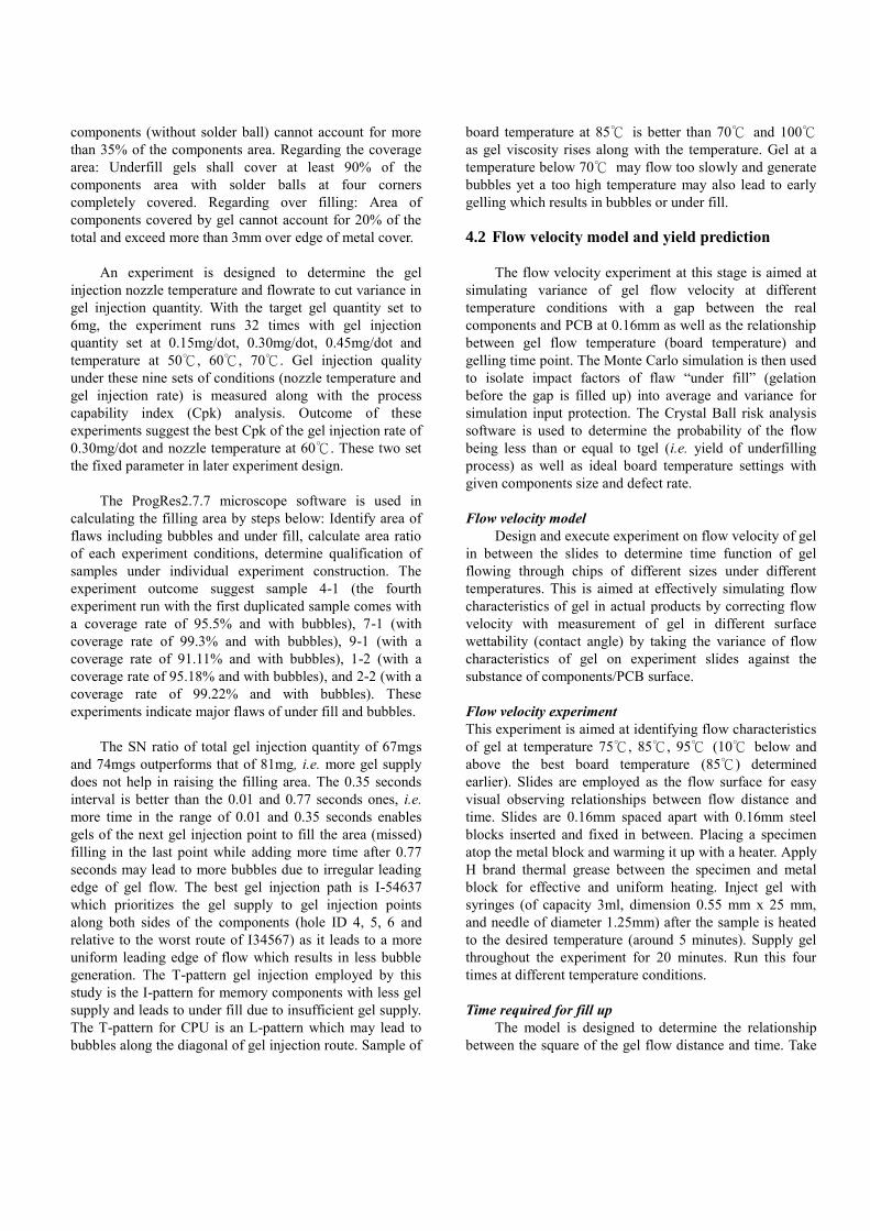
4.2 Flow velocity model and yield prediction

The flow velocity experiment at this stage is aimed at

simulating variance of gel flow velocity at different

temperature conditions with a gap between the real

components and PCB at 0.16mm as well as the relationship

between gel flow temperature (board temperature) and

gelling time point. The Monte Carlo simulation is then used

to isolate impact factors of flaw “under fill” (gelation

before the gap is filled up) into average and variance for

simulation input protection. The Crystal Ball risk analysis

software is used to determine the probability of the flow

being less than or equal to tgel (i.e. yield of underfilling

process) as well as ideal board temperature settings with

given components size and defect rate.

Flow velocity model

Design and execute experiment on flow velocity of gel

in between the slides to determine time function of gel

flowing through chips of different sizes under different

temperatures. This is aimed at effectively simulating flow

characteristics of gel in actual products by correcting flow

velocity with measurement of gel in different surface

wettability (contact angle) by taking the variance of flow

characteristics of gel on experiment slides against the

substance of components/PCB surface.

Flow velocity experiment

This experiment is aimed at identifying flow characteristics

of gel at temperature 75℃, 85℃, 95℃ (10℃ below and

above the best board temperature (85℃) determined

earlier). Slides are employed as the flow surface for easy

visual observing relationships between flow distance and

time. Slides are 0.16mm spaced apart with 0.16mm steel

blocks inserted and fixed in between. Placing a specimen

atop the metal block and warming it up with a heater. Apply

H brand thermal grease between the specimen and metal

block for effective and uniform heating. Inject gel with

syringes (of capacity 3ml, dimension 0.55 mm x 25 mm,

and needle of diameter 1.25mm) after the sample is heated

to the desired temperature (around 5 minutes). Supply gel

throughout the experiment for 20 minutes. Run this four

times at different temperature conditions.

Time required for fill up

The model is designed to determine the relationship

between the square of the gel flow distance and time. Take

a natural log of the curve (slop) and its linear with

temperature reciprocal according to the Arrhenius Theorem.

This flow represents a flow velocity at different board

temperature while the model gives time to flow through a

given distance. The flow velocity of gel at a board

temperature of 95℃ and 85℃ is much faster than at 75℃

for the first three minutes. For ModelA product at current

board temperature 75℃-85℃ for the production of phone

ModelA. Automatically, it takes about 40 seconds to fill the

bottom of the components of length 14mm (area 256 mm2).

Figure 5.3, 5.4 and 5.5 illustrates the relationship between

the square of the gel flow length and time. The experiments

indicate that there is a linear relation between gel flow

length and time before gelation. With board temperature at

75℃, 85℃, 95℃ the slop of it is 6.42, 7.43 and 10.95

respectively. This linearity breaks and variance in the flow

velocity rises sharply. Goodness of fit of this linear relation

is worse than R-sq=99.0% in this experiment while the

average gelation time span at different temperature

conditions (75℃, 85℃, 95℃) are 175, 125, and 77.5

seconds, respectively. At a lower board temperature,

gelation takes a longer time to happen and less time at a

higher board temperature. Distance of the gel flow before

gelation at a higher temperature is shorter than the lower

temperature ones. In addition, bubbles and un-uniform

leading edge of the gel flow are found in every temperature

condition (e.g. 85℃). Board temperature is critical in

getting at the space below the components are filled up

completely before gelation.

Take the first sample. Gelation occurs in 170, 130, and

60 seconds at temperatures 75℃, 85℃, 95℃, respectively.

Values of natural log over the ratio (S = X2/t0 ) of the

individual square of the distance traveled in this time span

over time (lnS) are 1.859, 2.004, 2.391 while the reciprocal

of the absolute temperature (1/T) is 0.002849, 0.00277 and

0.002695. The relationship between lnS and 1/T by

regression analysis is shown in formula 8 (with goodness of

fit at 84.9%). Function of time (t0) required for gel to fill up

the space of length X is shown in Formula 9.

lnS=lnX2

t0=11.63-3443 (

1

T) (8)

t0 = exp( 2lnX-11.63+3443 (1

T) (9)

Adjust impact of surface wettability on gel flowing

This flow velocity experiment takes a slide for the gel

flow surface which differs from the substance of

components and PCB surface in the actual production

process. The relationship between the leading speed of the

capillary flow, contact angle and gap height between the

upper and lower surfaces, and surface tension and viscosity

of the gel during gel filling operation is shown in Formula

3.7 (Fosberry, 1996). This experiment is aimed at finding

the variance of the gel in a different surface, wet to adjust

prediction by flow velocity experiment. Warm up

components, PCB and slide to 80℃, inject one drop of gel

to these surfaces with a syringe and measure the contact

angle of the gel to each surface 20 seconds later. Angles to

surfaces of the slide, PCB, and components are 25°, 28°

and 31°, respectively. With selected gel brands, viscosity (γ)

and surface tension ( η ) remain constant, the gel-slide

surface angle at 25° and components-PCB gap at 0.16mm,

the gel flow velocity on the slide surface is defined in

Formula 5.3. As the leading speed of the gel is proportional

to the sum of the cosine of the upper/lower surface contact

angle (Formula 10) the adjusted time (tflow) required to fill

up the gap between components and PCB surface may be

revised as shown in Formula 11.

vfront-glass=γ×0.16(cos(25°)+cos(25°))

12ηX= 0.289γ

12ηX (10)

tflow = t02cosθg

cosθp+cosθc=exp(2lnX-11.63+3443

1T

× 1.04)(11)

Variance of fillup time and gelation occur time

Repeat the experiment in individual temperature

conditions. The fillup time at board temperature 75℃, 85℃,

95℃ is 39.81 seconds, 34.54 seconds and 23.47 seconds,

respectively, and average gelation time of 165(s), 127.5(s)

and 90(s). That is, the higher the board temperature is the

shorter the fillup time is, the earlier gelation time is, and the

greater the variance is. Warmer board may shorten the

process time at the expense of more “under fillup” flaws

due to early gelation and greater variance.

Monte Carlo process yield prediction

Determine averages and variances of fillup time and

gelation occur time at different temperature conditions with

figures from these flow velocity experiment and predict the

yield of successful components fillup under different

temperature conditions with the Monte Carlo simulation

method.

This study predicts the production yield with

simulation methods to reduce the time and costs at the

process development stage. Determine board temperature

settings against products of the components at a given

dimension. This study assumes a normal distribution of

time ( tflow ) required for completely filling up the

components area and gelation occur time (tgel) as shown in

Formula 12 and 13 Flow velocity data out of the

experiment under different temperature connection are used

to determine the average and standard deviation of time

required for complete filling up components area and

gelation occur time as input parameter for process yield

prediction by Monte Carlo simulation.

tflow=N (X2

S ,σflow)

(12)

tgel=N(1

exp((2ln 11.63 3443 ) 1.04) , gelXT

(13)

where σgel and σflow are standard deviation of time

required for complete filling up components area and

gelation occur time

Random sample 10,000 times of the time required for

completely the filling up components area and gelation

occur time at these three temperature conditions with the

Crysball software. Under different temperature conditions

if, if tflow is greater than tgel then set the filling as

acceptable one and rejectable one vice versa. Distribution

of simulation sampling time required for complete filling

up the components area and gelation occur time at

individual temperature conditions as illustrated in Figure 2.

Overlapped area indicates the probability of gelation before

complete fillup (i.e. risk area) and the high temperature

conditions account for a larger area. Outcome of the

simulation suggests that a 100% process yield may be

reached at board temperature 75℃ and 85℃ but was not

the case at temperature 95℃. Yield of the latter down to

99.98% as a result of 200ppm fraction defective. In this

case, board temperature at 85℃ is recommended on

account of the output requirements and risks of poorer

quality.

Distribution of simulation sampling of time requi

red for complete filling up components area (blu

e) and gelation occur time (red) at 75℃

Distribution of simulation sampling of time requi

red for complete filling up components area (blu

e) and gelation occur time (red) at 85℃

Distribution of simulation sampling of time requi

red for complete filling up components area (blu

e) and gelation occur time (red) at 95℃

Distribution of simulation sampling of time requi

red for complete filling up components area (blu

e) and gelation occur time (red) at 95℃

Figure 2: Distribution of simulation sampling of time

required for completely filling up the components area and

gelation occur time.

5. CONCLUSIONS

The underfilling technique is getting more important

as signal transmission solder points in electronic products

tend to break due to thermal fatigue by the heat cycle

generated in its use. Metal shielding metal caps are

complicating this technique as it imposes more restrictions

on gel injection point availability and more demanding

control on gel quantity applied at individual components.

This study reviews the impacts of process flaws of bubbles,

under fill and over fill as well as design and execute an

experiment for process parameter optimization against

individual products. The preliminary experiment finds the

best gel injection nozzle temperature and injection rate at

60℃ and 0.30mg/dot in terms of process capacity

(variance level) of the injection rate. The process

optimization experiment suggests the optimum parameter

mix of the total gel injection quantity at 74mgs, time span

at 0.35 seconds, injection route at I-54637 and board

temperature at 85℃.

Run gel flow velocity experiment at temperature

minus and plus 10℃of the best board temperature (85℃) to

observe the flow characteristics of the gel on the slide at

different temperature conditions. Another experiment

followed for wettability of the surface where gels flow on

and flow velocity correction to simulate flow

characteristics of gel between chip and PCB and get

gelation time at different temperature conditions. Both

experiments suggest the square of the flow distance before

the gel gets solidified is linear to the time. As the board

temperatures of 75℃, 85℃, 95℃ slope of curve is 6.42,

7.43 and 10.95, and fillup time is 39.81 seconds, 34.54

seconds and 23.47 seconds, respectively, we can conclude

that the injected gel flows faster under higher board

temperatures. Average gelation time is 175 seconds, 125

seconds, 77.5 seconds, respectively which suggests raised

board temperature may shorten the process time at the

expense of more “under fillup” flaws due to early gelation

and shorter flow distance. The Monte Carlo simulation

method is then used in estimating the fillup and gelation

time for (different sizes of chips) at different temperature

conditions for the prediction of the underfilling process

yield. Outcome of simulation suggests 100% process

yield may be reached at board temperature 75℃ and 85℃

but was not the case with temperature 95℃. Yield of the

latter down to 99.98% as a result of 200ppm fraction

defective. In this case, board temperature at 85℃ is

recommended on account of output requirements and risks

of poorer quality.

Addressing the underfilling process parameter optimization,

the flow velocity modeling and yield prediction this study

may have the following contributions to the industry:

1. In spite of scores papers on underfill only a few were

made on handheld electronic products (gel injection

through limited holes in metal caps for electromagnetic

wave prevention). Outcomes of this study may of help

in the new process development.

2. The preliminary experiment on the control factor of gel

injection nozzle temperature gives 9 variances of gel

injection quantity at different temperatures. Enterprises

may rely on this for gel injection quantity control.

3. The best parameter mix determined by the Taguchi

method may provide general assessment on new

product process.

4. Simulating the gel flow velocity with s slide to get gel

flow characteristics under different temperature

conditions may cut the costs of pilot runs by adjusting

the process before gel injection operations.

5. The function of time required for fillup with regression

analysis in the gel flow velocity experiment provides

fillup time and speed of components with different

dimensions at different temperature help in improving

precise capacity prediction.

6. Simulate flow distance at different temperature to

estimate gelation time of components of different

dimension with the Monte Carlo simulation to help

predicting new product or process yields with

minimized materials and costs.

REFERENCES

Babiker, Sharief. "Simple approach to include external

resistances in the Monte Carlo simulation of MESFETs

and HEMTs." (2016).

iswasa and Alok Satapathya, ”A Study on Tribological

Behavior of Alumina-Filled Glass-Epoxy Composites

Using Taguchi Experimental Design,” Tribology

Transactions, vol. 53, 2010, pp.520-532.

Delmdahl, Ralph, et al. "Enabling laser applications in

microelectronics manufacturing." Applied Physics A

122.2 (2016): 1-7.

Fosberry, J., ”An investigation of the physical properties

and applications,” Master’s Thesis, State University of

New York, Binghamton, New York, August 1996.

Fowlkes, W.Y. and Creveling, C.M., ”Engineering

Methods for Robust Product Design,” Addison-Wesley

Publishing Company. 1995.

Guo, Y. , Lehmann, G.L. , Driscoll, T. , Cotts, E.J. “A

model of the underfill flow process: particle distribution

effects,” Electronic Components and Technology

Conference, 1999.

Huang, C.Y., “Process research in the encapsulation of

direct chip attach components,” Doctoral Dissertation,

State University of New York, Binghamton, New York,

May 1996.

Huang, C.Y., “The investigation of the capillary flow of

underfill materials,” Microelectronics International,

Vol.19 No1, 2002.

Huang, C.Y., ”Optimization of the Substrate Preheat

Temperature for the Encapsulation of Flip Chip

Devices,” Int J Adv Manuf Technol, Department of

Systems Science and Industrial Engineering, State

University of New York, 2000

Jinlin Wang, “Underfill of flip chip on organic substrate:

viscosity, surface tension, and contact angle,”

Microelectronics Reliability, Volume 42, Issue 2, Pages

293–299, 2002.

Kooi,Chee Choong; Lim Szu Shing; Periaman, S.; Chui, J.;

Then, E.; Ng Cheong Huat; Low Mun Fai “Capillary

underfill and mold encapsulation materials for exposed

die flip chip molded matrix array package with thin

substrate,” Electronics Packaging Technology, 2003.

Li, M.-H.C., Al-Refaie, A., Cheng-Yu Yang, “DMAIC

Approach to Improve the Capability of SMT Solder

Printing Process,” IEEE TRANSACTIONS ON

ELECTRONICS PACKAGING MANUFACTURING,

VOL.31, NO. 2, APRIL 2008.

Li, Gang, et al. "Comparative study of anhydride and

amine-based underfill materials for flip chip

applications." 2016 China Semiconductor Technology

International Conference (CSTIC). IEEE, 2016.

Manzione, Louis T.,” Plastic Packaging of Microelectronic

Devices,” Van Nostrand Reinhold, New York ,1990.

Mehr, M. Yazdan, et al. "An overview of scanning acoustic

microscope, a reliable method for non-destructive

failure analysis of microelectronic components."

Thermal, Mechanical and Multi-Physics Simulation and

Experiments in Microelectronics and Microsystems

(EuroSimE), 2015 16th International Conference on.

IEEE, 2015.

Romenesko, M., ”Ball Grid Array and Flip Chip

Technologies,” The International Journal of

Microcircuits and Electronic

Packaging,vol.19,no.1,pp.64-74,1996.

Subulan, K., Cakmakci, M.: A feasibility study using

simulation-based optimization and Taguchi

experimental design method for material handling-

transfer system in the automobile industry. Int. J. Adv.

Manuf. Technol. 59, 433–444 (2012)

TAI, C.Y., CHEN, T.S., WU, M.C., “An enhanced Taguchi

method for optimizing SMT processes,” Journal of

Electronics Manufacturing, Volume: 2, Issue: 3(1992)

pp. 91-100, 1992.

Vadim Gektin, ”Coffin-Manson Fatigue Model of

Underfilled Flip-Chips,” IEEE Transactions on

Components, Packging and Manufacturing Technology

Part A, vol.20, no.3, pp.317-325, 1997.

Yi He, Brian E Moreira, Alan Overson, Stacy H Nakamura,

Christine Bider, John F Briscoe “Thermal

characterization of an epoxy-based underfill materials

for flip chip packaging,” Thermochimica Acta,

Volumes 357–358, 14 August 2000, Pages 1–8.