EMG 25(1) #37057 Scattering of Plane Waves at the Junction of Two Corrugated Half-Planes

EMG 25(1) #37057

Electromagnetics, 25:21–38, 2005Copyright © 2005 Taylor & Francis Inc.ISSN: 0272-6343 print/1532-527X onlineDOI: 10.1080/02726340590522111

Scattering of Plane Waves at the Junction ofTwo Corrugated Half-Planes

A. HAMIT SERBEST

Department of Electrical and Electronics EngineeringÇukurova UniversityAdana, Turkey

ALI KARA

Department of Electrical and Electronics EngineeringAtilim UniversityAnkara, Turkey

ERNST LÜNEBURG

EML ConsultantsGeorg Schmid Weg 4, 83324Wessling, Germany

In this paper, the boundary conditions given by Weinstein (1969) are employed tosimulate two corrugated half-planes with the same slot height but different slot width.The scattering mechanism at the junction of these half-planes is investigated via theFourier transform technique, which leads to two coupled Wiener–Hopf equations. Thesolution of the Wiener–Hopf system is obtained by the Daniele–Khrapkov method andsome numerical results are presented about the analysis of the scattered field.

Keywords electromagnetic wave diffraction, scattering, high-frequency techniques,anisotropic impedance, corrugated structures

Introduction

Waveguides with transversely corrugated walls have been used for many years in linearaccelerators for both low-loss and high-power applications. Corrugated walls are used inhorn antennas also; plane walls of rectangular horns are replaced by corrugated surfaces toimprove radiation patterns. Some of the early works in these fields are given by Hougardyand Hansen (1958), Bryant (1969), Dybdal, Peters, and Peake (1971), and Narasimhanand Rao (1973). Corrugated surfaces have also been treated as electromagnetic soft andhard surfaces by filling the corrugations with dielectric materials or choosing suitablecorrugation heights at operating frequency (Kildal, 1990). It has been shown that there

Received 1 April 2004; accepted 5 August 2004.Address correspondence to Ali Kara, Dept. of Electrical and Electronics Engineering, Atilim

University, Kizilcasar Koyu, Golbasi-Ankara, 06836, Turkey. E-mail: [email protected]

21

22 A. Hamit Serbest et al.

are similarities between waves propagating on a corrugated infinite plane-conductingsurface and those in a waveguide with one wall corrugated (Elliot, 1954). Hurd (1954)has investigated the propagation of surface waves along an infinite corrugated surface.To facilitate the solution of the problem, he has assumed an idealized physical structureon which the corrugations are vanishingly thin and the slot width is small comparedwith both the slot height and the free space wavelength. The method employed by Hurdinvolves writing the complete fields both above the corrugations and in the slots, matchingthe tangential components at the boundaries, and then using the calculus-of-residuestechnique to evaluate the resulting infinite set of simultaneous equations.

It has been known for a long time that impedance boundary conditions can be em-ployed to simulate corrugated surfaces with infinitely thin boundaries. Weinstein (1969)has given a set of second-order boundary conditions for a corrugated surface whichreduces to the standard impedance boundary conditions in the case of a first-order ap-proximation. These conditions show the anisotropic character of the corrugated structureexplicitly.

On the other hand, there have been investigations for the diffraction effects ofanisotropic surfaces including half-planes, full planes, wedges, or discontinuities formedby any of these canonical structures (Serbest, Büyükaksoy, & Uzgören, 1991; Büyükak-soy, Serbest, & Kara, 1996; Nepa, Manara, & Armogida, 2001; Generalli et al., 1999;Lyalinov & Zhu, 1999). In some of these works, the solution (Serbest, Büyükaksoy, &Uzgören, 1991; Büyükaksoy, Serbest, & Kara, 1996) is obtained by the Fourier transformtechnique leading to a matrix Wiener–Hopf equation, and the others are based on theuse of the Sommerfeld–Maliuzhinets method (Lyalinov & Zhu, 1999; Nepa, Manara, &Armogida, 2001) or equivalent surface currents of physical optics (PO) (Generalli et al.,1999).

In this work, the diffraction mechanism at the junction of two corrugated half-planes with the same slot height but different slot widths is considered. The boundaryconditions given by Weinstein (1969) are employed to simulate the corrugated half-planeswith different anisotropic impedances. So, the problem is reduced to the diffraction at thejunction of two different anisotropic impedance half-planes. First, the above-mentionedboundary conditions are summarized and the formulation of the related boundary-valueproblem via the Fourier transform technique is given. Then, the problem is reduced to thesolution of a matrix Wiener–Hopf equation, which is accomplished via the Khrapkov–Daniele method (Khrapkov, 1971; Daniele, 1978; Büyükaksoy & Serbest, 1993). Finally,the results about the analysis of the diffracted field are presented and compared withknown solutions related to special cases of the problem considered here.

Approximate Boundary Conditions

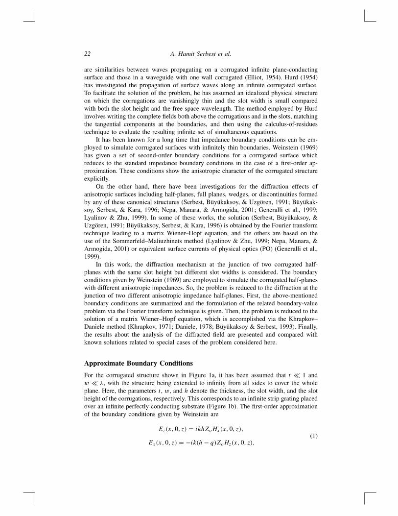
For the corrugated structure shown in Figure 1a, it has been assumed that t � 1 andw � λ, with the structure being extended to infinity from all sides to cover the wholeplane. Here, the parameters t , w, and h denote the thickness, the slot width, and the slotheight of the corrugations, respectively. This corresponds to an infinite strip grating placedover an infinite perfectly conducting substrate (Figure 1b). The first-order approximationof the boundary conditions given by Weinstein are

Ez(x, 0, z) = ikhZoHx(x, 0, z),Ex(x, 0, z) = −ik(h− q)ZoHz(x, 0, z),

(1)

Scattering of Plane Waves 23

(a)

(b)

Figure 1. Illustration of a corrugated surface: (a) real structure with material thickness; (b) ideal-ized structure with vanishingly thin corrugations.

with

q = (w/π) ln[cosh(πh/w)], (2)

and Zo being the intrinsic impedance of free space. They are valid for the case whenkh� 1 and kw � 1. They show the anisotropic character of the structure explicitly andgive the dependence of the surface impedance values to the corrugation parameters.

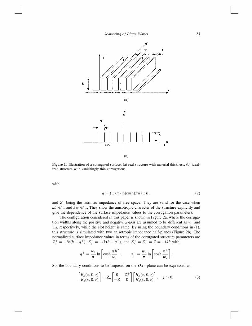
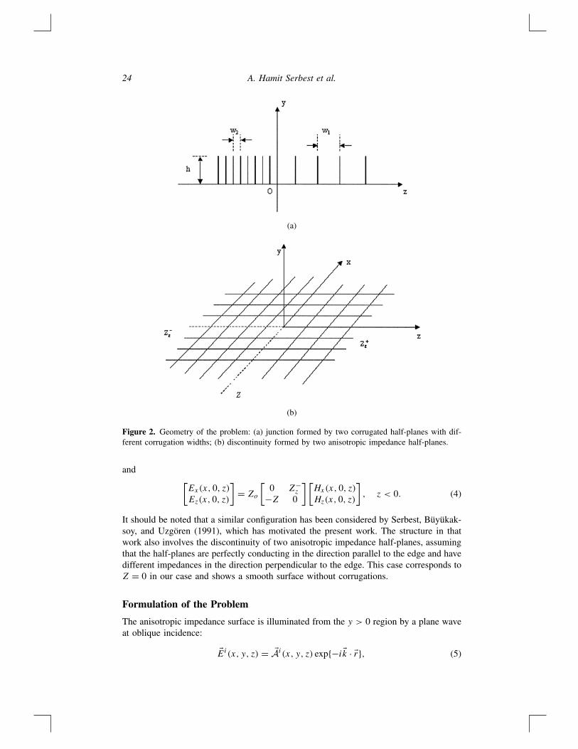
The configuration considered in this paper is shown in Figure 2a, where the corruga-tion widths along the positive and negative x-axis are assumed to be different as w1 andw2, respectively, while the slot height is same. By using the boundary conditions in (1),this structure is simulated with two anisotropic impedance half-planes (Figure 2b). Thenormalized surface impedance values in terms of the corrugated structure parameters areZ+z = −ik(h− q+), Z−

z = −ik(h− q−), and Z+x = Z−

x = Z = −ikh with

q+ = w1

πln

[cosh

πh

w1

], q− = w2

πln

[cosh

πh

w2

].

So, the boundary conditions to be imposed on the Oxz plane can be expressed as:[Ex(x, 0, z)Ez(x, 0, z)

]= Zo

[0 Z+

z

−Z 0

] [Hx(x, 0, z)Hz(x, 0, z)

], z > 0, (3)


(a)

(b)

Figure 2. Geometry of the problem: (a) junction formed by two corrugated half-planes with dif-ferent corrugation widths; (b) discontinuity formed by two anisotropic impedance half-planes.

and [Ex(x, 0, z)Ez(x, 0, z)

]= Zo

[0 Z−

z

−Z 0

] [Hx(x, 0, z)Hz(x, 0, z)

], z < 0. (4)

It should be noted that a similar configuration has been considered by Serbest, Büyükak-soy, and Uzgören (1991), which has motivated the present work. The structure in thatwork also involves the discontinuity of two anisotropic impedance half-planes, assumingthat the half-planes are perfectly conducting in the direction parallel to the edge and havedifferent impedances in the direction perpendicular to the edge. This case corresponds toZ = 0 in our case and shows a smooth surface without corrugations.

Formulation of the Problem

The anisotropic impedance surface is illuminated from the y > 0 region by a plane waveat oblique incidence:

�Ei(x, y, z) = �Ai (x, y, z) exp{−i�k · �r}, (5)


where �Ai = Aix �x + Aiy �y + Aiz�z and �k. �Ai = 0 with kx = k cosφo, ky = k sin φo sin θo,kz = −k sin φo cos θo. Here k is the wave number of the surrounding medium and foranalytical convenience it is assumed that the wave number has a small positive imaginarypart. The x-dependence exp(−ikxx) and the time dependence exp(−iω t), which arecommon to all field quantities, will be suppressed throughout the analysis.

Let us split up the total field as follows for all y:

�E( �H) = �Ei( �Hi)+ �Er( �Hr)+ �Ed( �Hd), (6)

where the superscripts i, r , and d denote the incident, reflected, and diffracted fields,respectively. The reflected field components are given by

Er[Hr

](x, y, z) = Re,mEi

[Hi

](x,−y, z),

which will be written for x and z components of the fields. Here Rex,z and Rmx,z are theelectric and magnetic field reflection coefficients, respectively.

To determine the diffracted fields, electric and magnetic Hertz vectors �!e and �!mare introduced in the form �!e,m = (!e,mx , 0, 0) with

!ex =∫ ∞

−∞M(α) exp{iαz− i$(α)y} dα;!mx =

∫ ∞

−∞N(α) exp{−iαz− i$(α)y} dα.

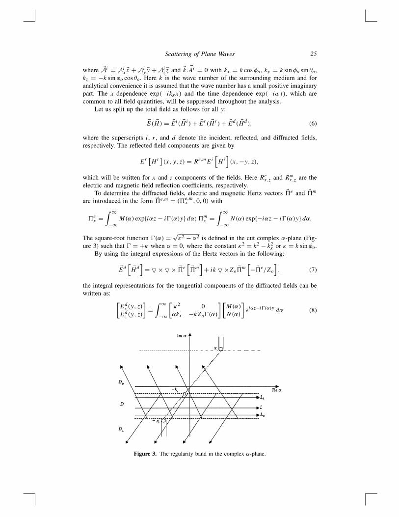
The square-root function $(α) = √κ2 − α2 is defined in the cut complex α-plane (Fig-

ure 3) such that $ = +κ when α = 0, where the constant κ2 = k2 − k2x or κ = k sin φo.

By using the integral expressions of the Hertz vectors in the following:

�Ed[ �Hd

]= � × � × �!e

[ �!m]

+ ik � ×Zo �!m[− �!e/Zo

], (7)

the integral representations for the tangential components of the diffracted fields can bewritten as: [

Edx (y, z)

Edz (y, z)

]=

∫ ∞

−∞

[κ2 0αkx −kZo$(α)

] [M(α)

N(α)

]eiαz−i$(α)y dα (8)

Figure 3. The regularity band in the complex α-plane.


and [Hdx (y, z)

Hdz (y, z)

]=

∫ ∞

−∞

[0 κ2

(k/Zo)$(α) αkx

] [M(α)

N(α)

]eiαz−i$(α)y dα. (9)

Substituting the field expressions (8)–(9) into the boundary conditions (3)–(4) and ap-plying standard steps, two coupled functional equations of the Wiener–Hopf type areobtained. They are expressed in matrix form:

G(α)L(α) = U(α)+ V(α), (10)

where

G(α) = 1

'(α)

[Zκ2 + kb$(α)+ Z+

z (k2 − α2) αkx(Z

−z − Z+

z )

0 Zκ2 + ka$(α)+ Z−z (k

2 − α2)

]

(11)

with a = −(1 + ZZ−z ), b = −(1 + ZZ+

z ), and

'(α) = Zκ2 + ka$(α)+ Z−z (k

2 − α2). (12)

U(α) and L(α) are unknown column vectors whose element functions are regular, re-spectively, in an upper and lower half of the complex α-plane. They correspond to thecombinations of the field components determined by the boundary conditions. The col-umn vector V(α) corresponds to the contributions of the incident and reflected fields:

V1(α) = − 1

2πi(α + kz)[Aix(1 + Rex)−

Z+z

k(1 + Rmz )(kyAix − kxAiy)

], (13)

V2(α) = − 1

2πi(α + kz)[Aiz(1 + Rez)+

Z

k(1 + Rmx )(kzAiy − kyAiz)

]. (14)

During the inversion of the integral equations given by (8)–(9), the integrations relatedto the source functions are accomplished in the strip D, where D = DU ∩ DL withDL = {α | Im(α) < Im(−kz)} and DU = {α | Im(α) > Im(−κ)}, as shown in Figure 3.This implies that the reflected field terms, inserted in the total field representation foranalytical convenience, correspond to the fields that would be reflected from the z < 0part of the original configuration.

Solution of the Matrix Wiener–Hopf System

For the factorization of the kernel matrix given by (11), the Daniele–Khrapkov method(Khrapkov, 1971; Daniele, 1978; Büyükaksoy & Serbest, 1993) will be employed, whichrelies on the logarithmic approach suggested by the analogy with the factorization ofa scalar function. Since one of the elements of G(α) is zero, we should note that (10)can also be solved by eliminating the unknowns successively, as is done in Serbest,Büyükaksoy, and Uzgören (1991). Let the matrix G(α) be written as

G(α) = k

'(α)$(α)BG(α) (15)


with

G(α) = I + a2(α)

[/1(α) m(α)

0 /2(α)

]and B =

[b 00 a

],

where B is a constant matrix. Here, I is the unit matrix and the scalar functions that appearare a2(α) = [ka b$(α)]−1, m(α) = a(Z−

z − Z+z )αkx , /1(α) = aZκ2 + aZ+

z (k2 − α2),

and /2(α) = bZ κ2 + bZ−z (k

2 − α2). Since B is a constant matrix, only the factorization

of G(α) will be considered. By reorganizing the terms, it can easily be written as followsin Daniele–Khrapkov form:

G(α) = s(α)I + a2(α)J(α), J(α) =[/(α) m(α)

0 −/(α)]

with

s(α) = [2abk$(α)]−1{2abk$(α)+ (aZ+z + bZ−

z )(k2 − α2)+ (a + b)Z κ2} (16)

and

/(α) = (1/2){(aZ+z − bZ−

z )(k2 − α2)+ Z(a − b)κ2}. (17)

For the subsequent factorization procedure it is necessary to introduce the followingrepresentation of the kernel matrix:

G(α) = √g(α) [I cosh ε(α)+ C(α) sinh ε(α)] , (18)

where C(α) = [f (α)]−1/2J(α) and g(α) = det G(α), ε(α) = 12 ln [λ1(α)/λ2(α)] .

Here C(α) and ε(α) are called the commutant and the index of the matrix ˆG(α),respectively, with f (α) = l2(α). The eigenvalues of the matrix G(α) are

λ1(α) = [ak$(α)]−1{ak$(α)+ Zκ2 + Z−z (k

2 − α2)}, (19)

λ2(α) = [bk$(α)]−1{bk$(α)+ Zκ2 + Z+z (k

2 − α2)}. (20)

As is known, the factorization of the kernel matrix requires the multiplicative split of thedeterminant g(α) as

g(α) = gU(α)gL(α), (21)

and the additive split of F(α) as

F(α) = ε(α)√f (α)

= FU(α)+ FL(α). (22)

Now, in order to perform the multiplicative split of the determinant, it is helpful tointroduce the following equality related to λ1(α):

−Z−z α

2 + ak$(α)+ Zκ2 + Z−z k

2 = Z−z

ξ1ξ2

κ2 − α2

χ(ξ1, α)χ(ξ2, α)(23)


with ξ1,2 = κ/σ1,2, where σ1,2 = (−γ1/2) ± (1/2)√γ12 − 4γ2 and γ1 = (−ak/Z−

z ),γ2 = −κ2 +k2 + (Z/Z−

z )κ2. Naturally, a similar expression is written for λ2(α) with the

following: ξ3,4 = κ/σ3,4, where σ3,4 = (−γ3/2)±(1/2)√γ3

2 − 4γ4 and γ3 = (−bk/Z+z ),

γ4 = −κ2 + k2 + (Z/Z+z )κ

2. The function χ(ξ, α) given in (48) is defined as

χ(ξ, α) = $(α)

κ + ξ$(α) = χU(ξ, α)χL(ξ, α), (24)

which is factorized in terms of the Maliuzhinetz function (Uzgören, Büyükaksoy, &Serbest, 1989). So, the factors of g(α) read

gU,L(α) = 1

k√ab

·√Z−z Z

+z√

ξ1 ξ2 ξ3 ξ4· κ ± αχU,L(ξ1, α)χU,L(ξ2, α)χU,L(ξ3, α)χU,L(ξ4, α)

.

(25)

For the additive split of F(α), the usual integral definition is used,

FU,L(α) = ± 1

2πi

∫LU,L

1

2√/(t)

lnλ1(t)

λ2(t)· dt

(t − α) = 1

2/(α)ln

{λ1U,L(α)

λ2U,L(α)

}. (26)

The integration lines are taken as shown in Figure 3, and it is considered that the integranddoes not have any poles.

Now, the factors of G(α) can be written as

GU,L(α) = √gU,L(α)

{I cosh[√fFU,L(α)] + 1√

fJ(α) sinh[√fFU,L(α)]

}. (27)

Since f (α) is a fourth-order polynomial, it is obvious that the factor matrices will havean exponential behavior. The next step is to introduce a polynomial matrix to cancel thisexponential growth.

As is known, the order of this polynomial matrix will be at the order of√f , and

since it is a second-order polynomial for the problem under consideration, it will involveonly one unknown coefficient to be determined with the aid of the regularity condition.Regarding these points and following the approach introduced by Daniele (1978), P(α)can be written as

P(α) = (δ − α2)I + J(α) (28)

so that the product G(α)P−1(α) will have algebraic behavior at infinity. In order toperform the factorization of this matrix product, a representation similar to (27) is written:

G(α)P−1(α) =√(GP−1)

{I cosh[ε(α)− εp(α)] + C(α) sinh[ε(α)− εp(α)]

}. (29)

Here εp(α) corresponds to the index of the polynomial matrix

εp(α) = 1

2ln

[λp1(α)/λp2(α)

](30)


and the eigenvalues of the matrix P(α) read λp1,p2(α) = (δ − α2) ± /(α). Now, δ isa scalar constant that is to be determined by the regularity condition (Büyükaksoy &Serbest, 1993) given as:

∫ ∞

−∞1√f (t)

[ε(t)− εp(t)]dt = 0. (31)

This yields

δ = t2o[

1 + 1

2(bZ−

z − aZ+z )

]+ 1

2(bZ−

z − aZ+z )ν

2 (32)

with to = ν tan[ 12 tan−1(k/ν)] and ν =

√[Z(b − a)κ2/(aZ+

z − bZ−z )

] − k2. The additiveand multiplicative splits related to the polynomial matrix can easily be performed. So,the factors of the matrix product in (29) are

(G(α)P−1)U,L =√λ1U,Lλ2U,L

λp1U,Lλp2U,L

× {I cosh[√f (FU,L − FpU,L)] + C(α) sinh[√f (FU,L − FpU,L)]}(33)

with Fp(α) = [1/√f (α)]εp(α) by definition, where the additive decomposition of Fp(α)is obtained in the same way as for F(α) and the multiplicative split of λp1,p2(α) isachieved as for λ1,2(α).

Now, the matrix G(α) can be written as

G(α)P−1(α)P(α) = [G(α)P−1(α)]LP(α)[G(α)P−1(α)]U , (34)

and it remains to factorize the polynomial matrix as P(α) = PL(α)PU(α). By inspection

PU(α) =[√

1 − l1(c1 − α) d1

0√

1 + l1(c2 − α)]

(35)

and

PL(α) =[√

1 − l1(c1 + α) d2

0√

1 + l1(c2 + α)]

(36)

are obtained. Here

d1 = c1akx(Z−z − Z+

z )√1 + l1(c1 + c2)

, d2 = −c2akx(Z−z − Z+

z )√1 − l1(c1 + c2)

,

and

c1 = √(δ + lo)/(1 − l1), c2 = √

(δ − lo)/(1 + l1)


are written. The function /(α) is expressed as /(α) = lo + α2l1, with lo = − 12Zκ

2(b −a)− k2l1 and l1 = − 1

2 (aZ+z − bZ−

z ). Thus, (11) is written as

G(α) = k

'(α)$(α)B[G(α)P−1(α)]LPL(α)PU(α)[G(α)P−1(α)]U (37)

with

GL(α) ={√

k√κ − α

'L(α)B[G(α)P−1(α)]LPL(α)

},

GU(α) ={√

k√κ + α

'U(α)PU(α)[G(α)P−1(α)]U

}.

(38)

The expressions of the factor matrices are:

GL(α) =√k√κ − α

'L(α)

√λ1Lλ2L

λp1Lλp2L

[a 00 b

]

×{[

1 00 1

]cosh

[1

2lnλ1Lλp2L

λ2Lλp1L

]

+ 1

l

[l m

0 −l]

sinh

[1

2lnλ1Lλp2L

λ2Lλp1L

]}PL(α)

(39)

and

GU(α) =√k√κ + α

'U(α)

√λ1Uλ2U

λp1Uλp2UPU(α)

×{[

1 00 1

]cosh

[1

2lnλ1Uλp2U

λ2Uλp1U

]

+ 1

l

[l m

0 −l]

sinh

[1

2lnλ1Uλp2U

λ2Uλp1U

]},

(40)

which completes the factorization of the kernel matrix.Now, substituting the factor matrices into (10),

GL(α)L(α) = [GU(α)]−1U(α)+ [GU(α)]−1V(α) (41)

is obtained. The following matrix is the contribution of the source terms:

W(α) = [GU(α)]−1V(α) = (α + kz)−1[GU(α)]−1Vo,

and its additive decomposition is necessary according to the standard procedure. Here,WU(α) and WL(α) are defined as follows:

WU,L(α) = ± 1

2πi

∫LU,L

(t + kz)−1[GU(t)]−1Vodt

(t − α), (42)


and considering the complex α-plane and the integration lines (Figure 3),

WL(α) = (α + kz)−1[GU(kz)]−1Vo (43)

and

WU(α) = (α + kz)−1{[GU(α)]−1 − [GU(kz)]−1}Vo (44)

are obtained. Then, substituting these expressions into (73),

U(α) = (α + kz)−1{GU(α)[GU(kz)]−1 − I}Vo (45)

and

L(α) = (α + kz)−1 [GL(α)]−1 [GU(kz)]−1Vo (46)

are written with Vo = (α + kz)V.

Diffraction Coefficient

The total field will be the sum of the incident, reflected, and diffracted field terms. Theunknown reflection coefficients Rex , Rez , R

mx , and Rez are determined, during the reduction

of the boundary-value problem to the matrix Wiener–Hopf system. For the diffractedfields, the unknown spectral functions can easily be expressed in terms of the upper U(α)or lower L(α) analytic functions. Here, the solution with the lower analytic functionsL(α) is used as follows:

[M(α)

N(α)

]= 1

'(α)

[ZoZκ

2 − kZo$(α) αkxZoZ−z

−αkx κ2 − kZ−z $(α)

] [L1(α)

L2(α)

]. (47)

By using the expressions of M(α) and N(α), x and z components of the diffracted fieldgiven by (8)–(9) can be obtained in terms of the integral expression. Since it is notpossible to calculate these integrals rigorously, it is difficult to make general commentsabout the behavior of the diffracted fields. However, high-frequency asymptotic behavioris of interest for most practical applications, which can be obtained for k >> 1 byapplying the steepest descent path method. For this purpose, it is necessary to introducez = ρ cos θ , y = ρ sin θ , where ρ = r sin φ. Now, making the following change for thecomplex variable α = −κ cos τ ,

[Edx (ρ, θ)

Edz (ρ, θ)

]=

∫C

κ sin τ

[κ2 0

−kxκ cos τ −kZoκ sin τ

]

·[M(−κ cos τ)N(−κ cos τ)

]eiκρ cos(θ−τ)dτ.

(48)

The saddle point evaluation yields the diffracted fields as follows:

[Edx (ρ, θ)

Edz (ρ, θ)

]≈

[Dx(φo, θo, θ)

Dz(φo, θo, θ)

]eiκρ√κρ, (49)


where the diffraction coefficients are obtained as[Dx(φo, θo, θ)

Dz(φo, θo, θ)

]= κ sin θ

[M(−κ cos θ)N(−κ cos θ)

]eiπ/4√

2π. (50)

It should be noted that the function inside the steepest descent path integral is analyticeverywhere, except that it may have some simple poles in addition to complex poleswhose residues can be interpreted as surface waves departing from the junction. Thesesurface waves propagate in the Oxz plane and attenuate exponentially in the y-direction.Here, only the diffraction effect of the junction is considered and the propagation ofsurface waves over a similar structure will be the subject of another study.

Numerical Results and Concluding Remarks

As known, various forms of approximate boundary conditions in impedance form areintroduced to simulate corrugated structures, and anisotropy is clear from all types ofthe impedance conditions that are used. But, there is an important difference betweenthese and the one given by Weinstein. In these conditions, the anisotropic impedancesurface behaves as PEC (Z = 0) in either the transversal or the longitudinal directionin the corrugated surface plane, and the impedance is taken as a pure reactance in theother direction. Weinstein’s condition gives impedances in both directions as differentthan zero, and they are negative reactances.

On the other hand, the most important issue for all conditions introduced for simulat-ing a corrugated surface is to determine the range of validity or practical applicability. Forexample, Dragone (1985) has given conditions for a rectangular horn of four corrugatedplanes. The author says that this condition is valid to a good approximation, and then heexplains this approximation as “assuming a large number of grooves per wavelength.”Similarly, a circumferentially corrugated waveguide wall has been modelled in Thumn,Jacobs, and Ayza (1991) by an effective anisotropic surface reactance. The circumferen-tial component of the reactance was zero and the longitudinal component was given to“a good approximation,” where the region of validity of these conditions was determinednumerically. In this respect, Weinstein’s conditions also have the same difficulty. Theywere introduced for the case kh � 1 and kw � 1, where the reactance values in thisrange are very small and their values are very close to each other. To clarify the appli-cability range, the kh values with which these conditions will be valid are determinednumerically. It is seen that for kh values greater than 0, 573 Weinstein’s conditions areno longer applicable, which corresponds to a corrugation of maximum 9 mm height at3 GHz operation frequency.

The diffraction of electromagnetic plane waves at the junction of two anisotropicimpedance half-planes with nonzero impedances in all directions is studied for the firsttime in this paper. A structure similar to the one considered here was investigated inSerbest, Büyükaksoy, and Uzgören (1991), where the anisotropic impedance half-planeswere perfectly conducting in one direction and had different surface impedances in theother direction. Although zero impedance in one of the directions corresponds to a smoothsurface and it is not possible to consider this problem as a model for a corrugationdiscontinuity, it is possible to compare it with ours from a mathematical point of view.Since the functions appearing in both solutions are rather complicated, it was not possibleto make an analytical comparison; therefore, it is performed numerically. The geometryof the present problem is reduced to the geometry in Serbest, Büyükaksoy, and Uzgören


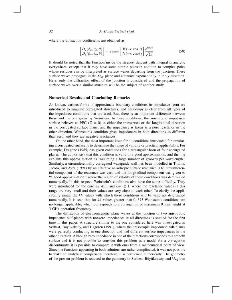
Figure 4. The variation of the amplitude of the diffraction coefficient Dz with respect to theobservation angle θ for the incidence angles θo = π/3, φo = π/2 and for impedance valuesZ+z = −j0.1, Z−

z = −j0.2, while Z = 0.0.

(1991) by interchanging x with z and θ with φ. For both solutions, Figure 4 shows thevariation of the amplitude of the diffraction coefficient Dz with respect to the observationangle θ for the incidence angles θo = π/3, φo = π/2 and for impedance values Z+

z =−j0.1, Z−

z = −j0.2, while Z = 0.0. There is good agreement between two solutionsexcept for small errors for observation angles close to the impedance surface. This slightdifference was also observed for different incidence angles and impedances. The reasonfor this error is due to the fact that, in our solution, the impedance Z cannot attain zerobut very small values during computer implementation.

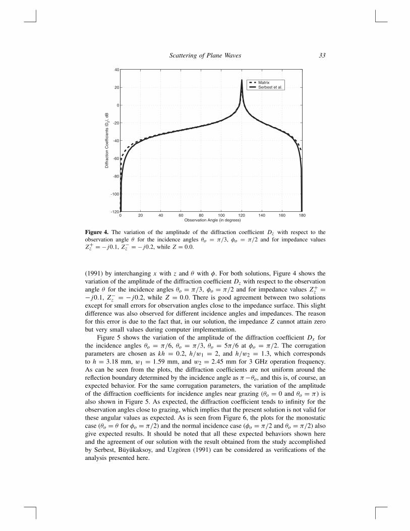
Figure 5 shows the variation of the amplitude of the diffraction coefficient Dx forthe incidence angles θo = π/6, θo = π/3, θo = 5π/6 at φo = π/2. The corrugationparameters are chosen as kh = 0.2, h/w1 = 2, and h/w2 = 1.3, which correspondsto h = 3.18 mm, w1 = 1.59 mm, and w2 = 2.45 mm for 3 GHz operation frequency.As can be seen from the plots, the diffraction coefficients are not uniform around thereflection boundary determined by the incidence angle as π−θo, and this is, of course, anexpected behavior. For the same corrugation parameters, the variation of the amplitudeof the diffraction coefficients for incidence angles near grazing (θo = 0 and θo = π ) isalso shown in Figure 5. As expected, the diffraction coefficient tends to infinity for theobservation angles close to grazing, which implies that the present solution is not valid forthese angular values as expected. As is seen from Figure 6, the plots for the monostaticcase (θo = θ for φo = π/2) and the normal incidence case (φo = π/2 and θo = π/2) alsogive expected results. It should be noted that all these expected behaviors shown hereand the agreement of our solution with the result obtained from the study accomplishedby Serbest, Büyükaksoy, and Uzgören (1991) can be considered as verifications of theanalysis presented here.


Figure 5. The variation of the amplitude of the diffraction coefficient Dx for the incidence anglesθo = 0, θo = π/6, θo = π/3, θo = 5π/6, and θo = π at φo = π/2. The corrugation parametersare chosen as kh = 0.2, h/w1 = 2, and h/w2 = 1.3.

Figure 6. The plots for the monostatic case (θo = θ for φo = π/2) and the normal incidence case(φo = π/2 and θo = π/2). The corrugation parameters are chosen as kh = 0.2, h/w1 = 2, andh/w2 = 1.3.


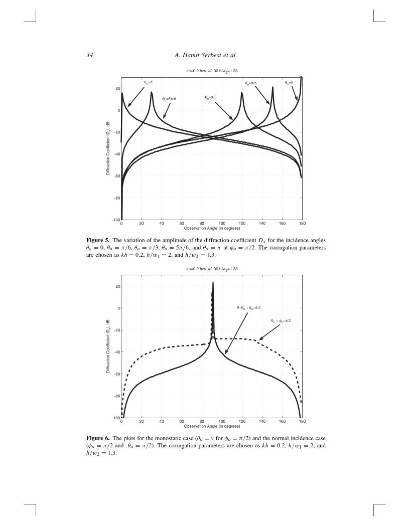
Figure 7. The variation of the diffraction coefficient with respect to the corrugation widths w1 ash/w1 = 2, 5, 8, 10.1, 15 for the incidence angle θo = π/6, kh = 0.5, and h/w2 = 10.0.

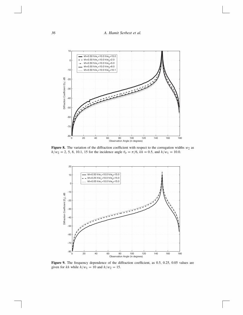
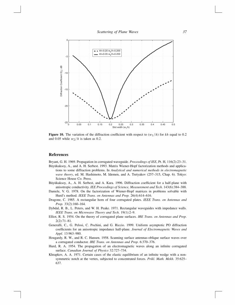
The influence of the corrugation parameters on the diffraction coefficients is de-rived numerically. Since the variation of the diffraction in the direction transversal tothe corrugation will be of interest to see the sensitivity to the corrugation parameters,the skewness angle φo was chosen as π/2. The diffraction coefficients do not changevery much with increasing corrugation height or corrugation width, since the surfaceimpedances determined by these parameters are relatively small. Although the x compo-nent of the diffraction coefficient (Dx) usually follows a similar behavior as the Dz, the zcomponent is taken into consideration to see the dependence on the geometrical param-eters. For the incidence angle θo = π/6, the variation of the diffraction coefficient withrespect to the corrugation widths w1 and w2 are given in Figures 7 and 8, respectively.For all plots, kh = 0.5 is taken and the behavior is investigated for h/w1 = 2, 5, 8,10.1, 15 while h/w2 = 10.0, or vice versa. Since the incidence angle is chosen suchthat the wave comes towards w2 corrugations, the diffraction coefficients for w2 variation(Figure 8) are approximately 10 dB more pronounced compared to the w1 variations (Fig-ure 7). In both cases, the dependence of the amplitude of the diffraction coefficient withcorrugation width varies in a 10 dB range. The frequency dependence of the diffractioncoefficient is shown in Figure 9, where h/w1 = 10, while h/w2 = 15 and 0.5, 0.25, 0.05values are given for kh. If the height of the corrugations is assumed as 3 mm, kh = 0.5corresponds to 7.96 GHz, while 0.25 and 0.05 correspond to 3.96 GHz and 0.398 GHz,respectively. As is seen from the plots, the diffraction effects are reduced with increasingfrequency. Finally, the variation of the diffraction coefficient with respect to (w1/h) isinvestigated for kh equal to 0.2 and 0.05, while w2/h is taken as 0.2 (Figure 10). Forw1/h = 0.2, which is the value w2/h has attained, the diffraction coefficient takes theminimum value and as the diference between the two corrugation widths increases theamplitude of the diffraction coefficient also increases on both sides.


Figure 8. The variation of the diffraction coefficient with respect to the corrugation widths w2 ash/w2 = 2, 5, 8, 10.1, 15 for the incidence angle θo = π/6, kh = 0.5, and h/w1 = 10.0.

Figure 9. The frequency dependence of the diffraction coefficient, as 0.5, 0.25, 0.05 values aregiven for kh while h/w1 = 10 and h/w2 = 15.


Figure 10. The variation of the diffraction coefficient with respect to (w1/h) for kh equal to 0.2and 0.05 while w2/h is taken as 0.2.

References

Bryant, G. H. 1969. Propagation in corrugated waveguide. Proceedings of IEE, Pt. H, 116(2):23–31.Büyükaksoy, A., and A. H. Serbest. 1993. Matrix Wiener-Hopf factorization methods and applica-

tions to some diffraction problems. In Analytical and numerical methods in electromagneticwave theory, ed. M. Hashimoto, M. Idemen, and A. Tretyakov (257–315, Chap. 6). Tokyo:Science House Co. Press.

Büyükaksoy, A., A. H. Serbest, and A. Kara. 1996. Diffraction coefficient for a half-plane withanisotropic conductivity. IEE Proceedings of Science, Measurement and Tech. 143(6):384–388.

Daniele, V. G. 1978. On the factorization of Wiener-Hopf matrices in problems solvable withHurd’s method. IEEE Trans. on Antennas and Prop. 26(4):614–616.

Dragone, C. 1985. A rectangular horn of four corrugated plates. IEEE Trans. on Antennas andProp. 33(2):160–164.

Dybdal, R. B., L. Peters, and W. H. Peake. 1971. Rectangular waveguides with impedance walls.IEEE Trans. on Microwave Theory and Tech. 19(1):2–9.

Elliot, R. S. 1954. On the theory of corrugated plane surfaces. IRE Trans. on Antennas and Prop.2(2):71–81.

Generalli, C., G. Pelosi, C. Pochini, and G. Riccio. 1999. Uniform asymptotic PO diffractioncoefficients for an anisotropic impedance half-plane. Journal of Electromagnetic Waves andAppl. 13:963–980.

Hougardy, R. W., and R. C. Hansen. 1958. Scanning surface antennas-oblique surface waves overa corrugated conductor. IRE Trans. on Antennas and Prop. 6:370–376.

Hurd, R. A. 1954. The propagation of an electromagnetic waves along an infinite corrugatedsurface. Canadian Journal of Physics 32:727–734.

Khrapkov, A. A. 1971. Certain cases of the elastic equilibrium of an infinite wedge with a non-symmetric notch at the vertex, subjected to concentrated forces. Prikl. Math. Mekh. 35:625–637.


Kildal, P. S. 1990. Artificially soft and hard surfaces in electromagnetics. IEEE Trans. on Antennasand Prop. 38(10):1537–1544.

Lyalinov, M. A., and N. Y. Zhu. 1999. Diffraction of a skewly incident plane wave by an anisotropicimpedance wedge: Exactly solvable cases. Wave Motion 30:275–288.

Narasimhan, M. S., and V. V. Rao. 1973. Radiation characteristics of corrugated E-plane sectoralhorns. IEEE Trans. on Antennas and Prop. 21(3):320–327.

Nepa, P., G. Manara, and A. Armogida. 2001. Electromagnetic scattering by anisotropic impedancehalf and full planes illuminated at oblique incidence. IEEE Trans. on Antennas and Prop.49(1):106–108.

Serbest, A. H., A. Büyükaksoy, and G. Uzgören. 1991. Diffraction at a discontinuity formed byanisotropic impedance half planes. IEICE Transactions E74(5):1283–1287.

Thumm, M., A. Jacobs, and M. S. Ayza. 1991. Design of short high-power TE11-HE11 modeconverters in highly overmoded corrugated waveguides. IEEE Trans. on Microwave Theoryand Tech. 39:301–309.

Uzgören, G., A. Büyükaksoy, and A. H. Serbest. 1989. Diffraction coefficient related to a discon-tinuity formed by impedance and resistive halfplanes. IEE Proceedings, Pt. H, 136(1):19–23.

Weinstein, L. A. 1969. The theory of diffraction and the factorization method. Boulder, Colorado:The Golem Press, pp. 295–299.

EMG 25(1) #37057 Scattering of Plane Waves at the Junction of Two Corrugated Half-Planes

Documents

Transcript of EMG 25(1) #37057 Scattering of Plane Waves at the Junction of Two Corrugated Half-Planes