1

EMagPy: open-source standalone 1

software for processing, forward 2

modeling and inversion of 3

electromagnetic induction data 4

5 Authors: 6 Paul McLachlan1,* 7 Guillaume Blanchy1 8 Andrew Binley1 9 10 Affiliations 11 1Lancaster Environment Centre, Lancaster University, Lancaster, UK 12 13 Corresponding author 14 Paul McLachlan, p.mclachlan@outlook.com 15 16 Authorship statement 17 GB and PM wrote the code, the jupyter notebook for the cases and the manuscript. AB 18 contributed to writing the manuscript and supervised work on the field case studies. 19 20 Code availability 21 The code is available under the GPL-licence at https://gitlab.com/hkex/emagpy. 22 23 Highlights (max 85 characters) 24

The cumulative sensitivity forward model is limited in some cases. 25 EMagPy is an open-source Python API and GUI for 1D EMI modeling/inversion. 26 Application of EMagPy is illustrated through cases studies with real and synthetic data. 27 Both Maxwell-based and cumulative sensitivity forward models are implemented. 28 Inversion algorithms include deterministic and stochastic methods. 29

30

Declaration of interest 31

None 32

33

2

Abbreviations 34

EC : electrical conductivity 35

ECa : apparent electrical conductivity 36

EMI : electromagnetic induction 37

ERT : electrical resistivity tomography 38

CS : cumulative sensitivity 39

LIN : low induction number approximation 40

FS : full solution, refers to the full solution of Maxwell’s equation 41

Q : quadrature component (expressed as parts per thousand, ppt) 42

VCP : vertical co-planar 43

HCP : horizontal co-planar 44

PRP : perpendicular co-planar 45

46

Abstract 47

Frequency domain electromagnetic induction (EMI) methods have had a long history of 48 qualitative mapping for environmental applications. More recently, the development of multi-49 coil and multi-frequency instruments is such that the focus has shifted to inverting data to 50 obtain quantitative models of electrical conductivity. Whilst collection of EMI data is relatively 51 straightforward, the inverse modeling is more complicated. Although several commercial and 52 open-source inversion codes, exist, there is still a need for a user-friendly software that can 53 bring EMI inversion to non-specialist audience. Here the open-source EMagPy software is 54 presented as an intuitive approach to modeling EMI data. It comprises a graphical user (GUI) 55 interface and a Python application programming interface (API). EMagPy implements both 56 cumulative sensitivity and Maxwell based solution and can model/invert data for 1D and 57 quasi-2D using either deterministic or probabilistic minimization methods. The EMagPy GUI 58 has a logical ‘tab-based’ layout to lead the user through data importing, data filtering, 59 inversion, and plotting of raw and inverted data. In addition, a dedicated forward modeling tab 60 is presented to generate synthetic data. In this publication necessary considerations of EMI 61 theory are described before its capabilities are presented through a series of environmental 62 case studies. Specifically, the performance of cumulative sensitivity and Maxwell based 63 forward models; the calibration of EMI data, a waterborne application and a time-lapse 64 inversion are investigated. It is anticipated that despite the number of available EMI software, 65 EMagPy offers a user-friendly tool suitable for novice and experienced practitioners alike, in 66 addition to be useful for teaching purposes. 67

3

68

1 Introduction 69

1.1 Applications of electromagnetic induction 70

Ground-based frequency domain electromagnetic induction (EMI) methods use phenomena 71 governed by Maxwell’s equations to infer information about the electrical conductivity (EC) of 72 the subsurface. As EC is the reciprocal of electrical resistivity, EMI methods can provide 73 comparable information to electrical resistivity methods. However, given that they do not 74 require direct coupling with the ground, they can, consequently, be more productive than 75 standard electrical resistivity tomography (ERT) methods, particularly for surveying large 76 areas. EMI measurements are typically expressed in terms of apparent electrical conductivity 77 (ECa) and have a long history of being used to reveal spatial patterns of a number of 78 hydrogeologically and agriculturally important properties and states; e.g. salinity (Corwin, 79 2008), water content (Corwin and Rhoades, 1984; Williams and Baker, 1982; Sherlock and 80 McDonnell, 2003), soil texture (Triantafilis and Lesch, 2005) and soil organic matter (Huang et 81 al., 2017). Furthermore, some studies have used repeated (i.e. time-lapse) measurements of 82 ECa to also reveal temporal patterns, e.g. for soil water content estimation (Robinson et al., 83 2012; Martini et al., 2017). 84 85 In addition to ECa mapping, the development of multi-frequency and multi-coil instruments 86 has enabled the possibility of inversion of EMI data to provide quantitative models of depth 87 specific EC. For instance, by obtaining multiple EMI measurements with different sensitivity 88 patterns, models of EC-ECa can be obtained. EMI inversions can be formulated as the 89 minimization of the difference between measured and synthetic ECa values generated from a 90 forward model. Most EMI inversion algorithms use a 1D forward model based on either the 91 linear cumulative sensitivity (CS) forward model proposed by McNeill (1980) or non-linear full 92 solution (FS) forward models based on Maxwell’s equations (e.g. Wait, 1982; Frischknecht et 93 al., 1987). Moreover, some EMI inversion programs, such as EM4Soil (Monteiro Santos, 94 2004) and the Aarhus Workbench (Auken et al., 2015), use lateral constraints to encourage 95 laterally smoothed images using a 1D forward model; these methods are typically referred to 96 as quasi-2D/3D inversion. 97 98 As with ECa mapping, EMI inversion has also been used in a wide range of applications, see 99 Table 1. It is important to note differences in how EMI data are collected, processed and 100 modeled. For instance, whether the EMI device is operated at ground level or an elevated 101 level has implications for its sensitivity patterns. Furthermore, despite the availability of 102 inversion software using FS forward models the CS forward model is still commonly used 103 (e.g. Huang et al., 2016; Saey et al., 2016), despite its inherent simplifications. Lastly, there 104 has also been interest in calibrating EMI measurements to account for factors relating to 105

4

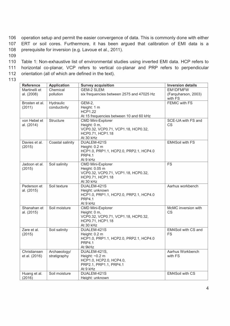
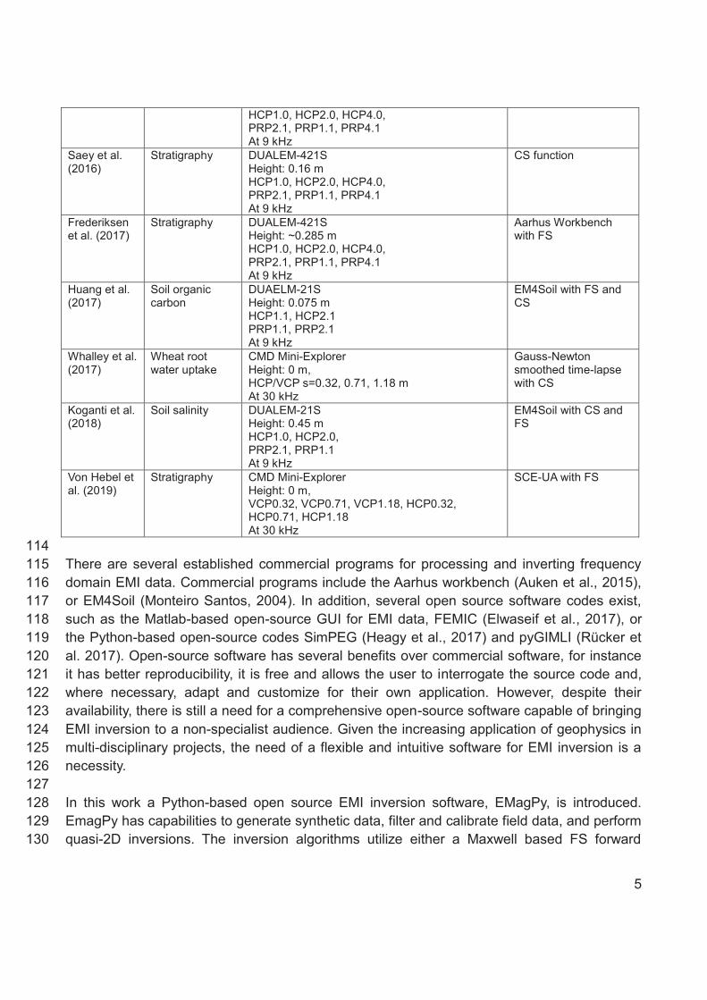
operation setup and permit the easier convergence of data. This is commonly done with either 106 ERT or soil cores. Furthermore, it has been argued that calibration of EMI data is a 107 prerequisite for inversion (e.g. Lavoue et al., 2011). 108 109 Table 1: Non-exhaustive list of environmental studies using inverted EMI data. HCP refers to 110 horizontal co-planar, VCP refers to vertical co-planar and PRP refers to perpendicular 111 orientation (all of which are defined in the text). 112 113 Reference Application Survey acquisition Inversion details Martinelli et al. (2008)

Chemical pollution

GEM-2 SLEM: six frequencies between 2575 and 47025 Hz

EM1DFMFW (Farquharson, 2003) with FS

Brosten et al. (2011)

Hydraulic conductivity

GEM-2, Height: 1 m HCP1.22 At 15 frequencies between 10 and 60 kHz

FEMIC with FS

von Hebel et al. (2014)

Structure CMD Mini-Explorer Height: 0 m, VCP0.32, VCP0.71, VCP1.18, HCP0.32, HCP0.71, HCP1.18 At 30 kHz

SCE-UA with FS and CS

Davies et al. (2015)

Coastal salinity DUALEM-421S Height: 0.2 m HCP1.0, PRP1.1, HCP2.0, PRP2.1, HCP4.0 PRP4.1 At 9 kHz

EM4Soil with FS

Jadoon et al. (2015)

Soil salinity CMD Mini-Explorer Height: 0.05 m VCP0.32, VCP0.71, VCP1.18, HCP0.32, HCP0.71, HCP1.18 At 30 kHz

FS

Pederson et al. (2015)

Soil texture DUALEM-421S Height: unknown HCP1.0, PRP1.1, HCP2.0, PRP2.1, HCP4.0 PRP4.1 At 9 kHz

Aarhus workbench

Shanahan et al. (2015)

Soil moisture CMD Mini-Explorer Height: 0 m, VCP0.32, VCP0.71, VCP1.18, HCP0.32, HCP0.71, HCP1.18 At 30 kHz

McMC inversion with CS

Zare et al. (2015)

Soil salinity DUALEM-421S Height: 0.2 m HCP1.0, PRP1.1, HCP2.0, PRP2.1, HCP4.0 PRP4.1 At 9kHz

EM4Soil with CS and FS

Christiansen et al. (2016)

Archaeology/ stratigraphy

DUALEM-421S, Height: ~0.2 m HCP1.0, HCP2.0, HCP4.0, PRP2.1, PRP1.1, PRP4.1 At 9 kHz

Aarhus Workbench with FS

Huang et al. (2016)

Soil moisture DUALEM-421S Height: unknown

EM4Soil with CS

5

HCP1.0, HCP2.0, HCP4.0, PRP2.1, PRP1.1, PRP4.1 At 9 kHz

Saey et al. (2016)

Stratigraphy DUALEM-421S Height: 0.16 m HCP1.0, HCP2.0, HCP4.0, PRP2.1, PRP1.1, PRP4.1 At 9 kHz

CS function

Frederiksen et al. (2017)

Stratigraphy DUALEM-421S Height: ~0.285 m HCP1.0, HCP2.0, HCP4.0, PRP2.1, PRP1.1, PRP4.1 At 9 kHz

Aarhus Workbench with FS

Huang et al. (2017)

Soil organic carbon

DUAELM-21S Height: 0.075 m HCP1.1, HCP2.1 PRP1.1, PRP2.1 At 9 kHz

EM4Soil with FS and CS

Whalley et al. (2017)

Wheat root water uptake

CMD Mini-Explorer Height: 0 m, HCP/VCP s=0.32, 0.71, 1.18 m At 30 kHz

Gauss-Newton smoothed time-lapse with CS

Koganti et al. (2018)

Soil salinity DUALEM-21S Height: 0.45 m HCP1.0, HCP2.0, PRP2.1, PRP1.1 At 9 kHz

EM4Soil with CS and FS

Von Hebel et al. (2019)

Stratigraphy CMD Mini-Explorer Height: 0 m, VCP0.32, VCP0.71, VCP1.18, HCP0.32, HCP0.71, HCP1.18 At 30 kHz

SCE-UA with FS

114 There are several established commercial programs for processing and inverting frequency 115 domain EMI data. Commercial programs include the Aarhus workbench (Auken et al., 2015), 116 or EM4Soil (Monteiro Santos, 2004). In addition, several open source software codes exist, 117 such as the Matlab-based open-source GUI for EMI data, FEMIC (Elwaseif et al., 2017), or 118 the Python-based open-source codes SimPEG (Heagy et al., 2017) and pyGIMLI (Rücker et 119 al. 2017). Open-source software has several benefits over commercial software, for instance 120 it has better reproducibility, it is free and allows the user to interrogate the source code and, 121 where necessary, adapt and customize for their own application. However, despite their 122 availability, there is still a need for a comprehensive open-source software capable of bringing 123 EMI inversion to a non-specialist audience. Given the increasing application of geophysics in 124 multi-disciplinary projects, the need of a flexible and intuitive software for EMI inversion is a 125 necessity. 126 127 In this work a Python-based open source EMI inversion software, EMagPy, is introduced. 128 EmagPy has capabilities to generate synthetic data, filter and calibrate field data, and perform 129 quasi-2D inversions. The inversion algorithms utilize either a Maxwell based FS forward 130

6

model or the CS forward model, and provide the capability of obtaining smoothly and sharply 131 varying models of EC. EmagPy provides a tab-based, user-friendly interface to that makes it 132 accessible for novice users, making it ideal for teaching and training purposes. This 133 manuscript provides a summary of the theoretical background to the software and highlights 134 its capabilities through several case studies. Specifically, the case studies investigated are: 135 (1) the performance of CS and FS solutions, (2) the impact of noise on the inversion results, 136 (3) the impact of EMI calibration on inversion results, (4) EMI inversion for waterborne 137 applications, and (5) time-lapse inversion of EMI data. 138

2 Material and methods 139

2.1 Theoretical background around on EMI 140

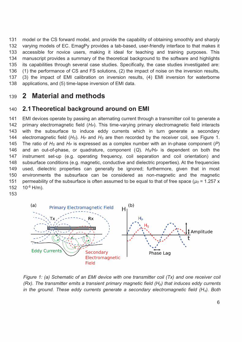
EMI devices operate by passing an alternating current through a transmitter coil to generate a 141 primary electromagnetic field (HP). This time-varying primary electromagnetic field interacts 142 with the subsurface to induce eddy currents which in turn generate a secondary 143 electromagnetic field (HS). HP and HS are then recorded by the receiver coil, see Figure 1. 144 The ratio of HS and HP is expressed as a complex number with an in-phase component (P) 145 and an out-of-phase, or quadrature, component (Q). HS/HP is dependent on both the 146 instrument set-up (e.g. operating frequency, coil separation and coil orientation) and 147 subsurface conditions (e.g. magnetic, conductive and dielectric properties). At the frequencies 148 used, dielectric properties can generally be ignored; furthermore, given that in most 149 environments the subsurface can be considered as non-magnetic and the magnetic 150 permeability of the subsurface is often assumed to be equal to that of free space (μ0 = 1.257 x 151 10-8 H/m). 152 153

Figure 1: (a) Schematic of an EMI device with one transmitter coil (Tx) and one receiver coil (Rx). The transmitter emits a transient primary magnetic field (Hp) that induces eddy currents in the ground. These eddy currents generate a secondary electromagnetic field (Hs). Both

7

primary and secondary electromagnetic field are sensed by the receiver coil (b). From the complex ratio of their signals, information about the subsurface can be inferred. 154 For any given ground properties, the obtained HS/HP is dependent upon the separation 155 distance between the transmitter and receiver coil, the operation frequency and the 156 orientation of coils. The most used orientations are referred to as co-planar loops in which 157 both the transmitter and receiver coils are orientated either horizontally (HCP) or vertically 158 (VCP), with respect to ground. Another coil orientation is the perpendicular orientation (PRP) 159 in which the transmitter and receiver loops are oriented at 90 degrees from each other. In 160 addition, many devices are multi-coil or multi-frequency, meaning that measurements with 161 different sensitivity patterns can be obtained by the same instrument, often simultaneously, 162 and used for inverse modeling. 163 164 Most EMI instruments express their measured HS/HP values as values of apparent electrical 165 conductivity, Eca. This term was introduced by McNeill (1980) to provide a more 166 comprehensible measurement with the same units as EC, i.e., S/m. McNeill (1980) derived a 167 linear relationship describing the Q value expected from a homogeneous subsurface electrical 168 conductivity. The relationship therefore links the Q value of an assumed homogeneous 169 subsurface to an Eca (i.e. the EC of a corresponding homogeneous ground). It is important to 170 therefore note that it may not be valid in heterogeneous environments (see Callegary et al., 171 2007; Lavoue et al., 2010) and requires that (1) the device is operated on the ground, and (2) 172 the induction number (β) is low (β << 1). The induction number is given by: 173 174

= , (1)

175 where σ is the conductivity of the ground, ω is the angular frequency (2πf) and s is the coil 176 separation. The low induction number (LIN) approximation is described as: 177 = . (2) 178 It can be clearly seen from the expression that large frequencies and higher conductivity 179 ground will violate the β << 1 specification proposed by McNeill (1980). Moreover, other more 180 conservative β values of < 0.3 (Wait, 1962) and < 0.02 (Frischknecht, 1987) have also been 181 provided for LIN conditions to be valid. It is also important to reiterate that the reliance of the 182 LIN number approximation on a homogeneous subsurface also creates problems for its 183 usage in heterogeneous environments and in cases where the device is operated above the 184 ground. Nonetheless, it has been essential in advancing the EMI method. 185 186

8

2.2 Cumulative sensitivity forward model 187

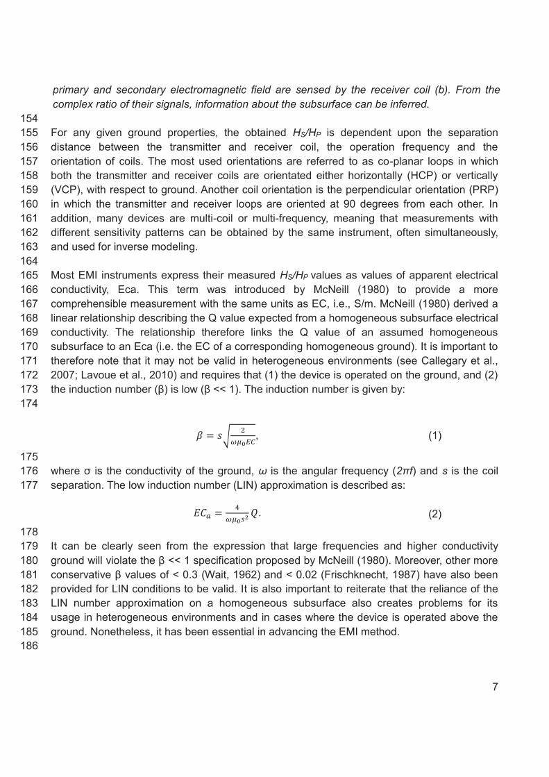
In addition to the LIN approximation, McNeill (1980) provided functions to describe the relative 188 contribution of materials below a specific depth to the overall Eca value when a device 189 operates under LIN conditions. These CS functions assume that the sensitivity of the 190 instrument is solely a function of the depth and coil separation and does not depend on the 191 subsurface EC, or the device’s operating frequency. The CS responses for VCP, HCP and 192 PRP orientations are as follows: 193 ( ) = (4 + 1) − 2 , (3) ( ) = √ , (4)

( ) = 1 − √ , (5) 194 Where z is the depth normalized by the coil separation, s. From equations 3 and 4 the 195 sensitivities for different coil separations for the CMD Mini-Explorer and CMD Explorer (GF 196 Instruments, Czech Republic), which can be operated in either VCP or HCP mode, can be 197 calculated, see Figure 2. For instance, it can be seen that measurements made with coils in 198 the VCP orientation are more sensitive to the shallow subsurface and measurements made in 199 HCP orientation are sensitive to deeper depths. These functions are commonly used by 200 manufacturers to provide information about the depth sensitivity of their instruments; i.e. the 201 rule of thumb states VCP measurements have an effective depth of 0.75 times the coil 202 separation and 1.5 times for HCP measurements. 203 204

9

Figure 2: Normalized local sensitivity pattern of the coil configurations of two multi-coils instruments: (a) CMD Mini-Explorer and (b) CMD Explorer. Each coil configuration is first determined by its orientation (VCP/HCP here) and the Tx-Rx coil separation with units of meters. The triangles on each curve corresponds to the effective depth range supplied by the manufacturer.

205 As with the LIN approximation, the CS functions have been fundamental in advancing the EMI 206 methods. Furthermore, despite the availability of inversion algorithms based on the FS 207 forward model, the use of CS forward model in EMI applications is still common. This is 208 largely due to their simplicity and speed in the inversion process compared to FS forward 209 solutions. Furthermore, although, as with the LIN approximation, the CS forward model was 210 developed for application when EMI devices are operated at ground level, several studies 211 have used it to model the response of devices operated at some elevation by re-scaling the 212 CS function (e.g. Andrade and Fisher, 2018). 213

2.3 Full Maxwell solution 214

In order to calculate a non-simplified response of the ground, in terms of HS/HP, a FS forward 215 model must be used. The model used in EMagPy relies on the assumption that 216

10

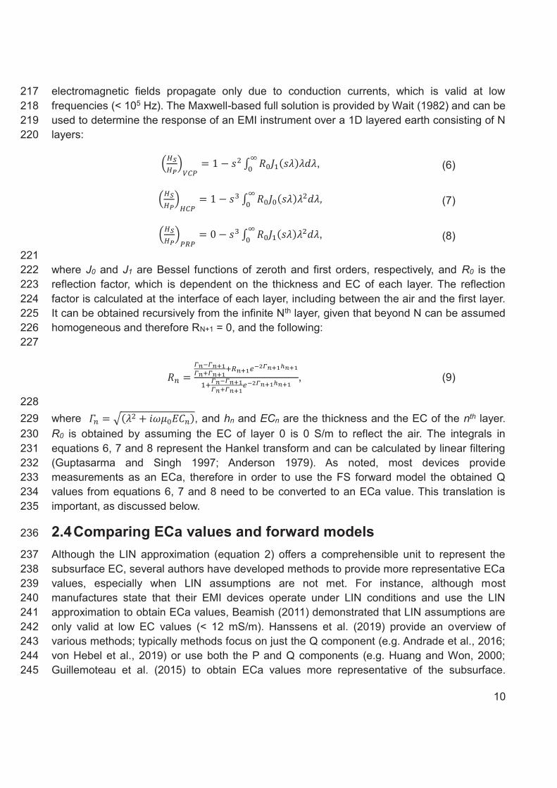
electromagnetic fields propagate only due to conduction currents, which is valid at low 217 frequencies (< 105 Hz). The Maxwell-based full solution is provided by Wait (1982) and can be 218 used to determine the response of an EMI instrument over a 1D layered earth consisting of N 219 layers: 220 = 1 − ∫ ( ) , (6)

= 1 − ∫ ( ) , (7)

= 0− ∫ ( ) , (8)

221 where J0 and J1 are Bessel functions of zeroth and first orders, respectively, and R0 is the 222 reflection factor, which is dependent on the thickness and EC of each layer. The reflection 223 factor is calculated at the interface of each layer, including between the air and the first layer. 224 It can be obtained recursively from the infinite Nth layer, given that beyond N can be assumed 225 homogeneous and therefore RN+1 = 0, and the following: 226 227

= , (9)

228 where = ( + ), and hn and ECn are the thickness and the EC of the nth layer. 229 R0 is obtained by assuming the EC of layer 0 is 0 S/m to reflect the air. The integrals in 230 equations 6, 7 and 8 represent the Hankel transform and can be calculated by linear filtering 231 (Guptasarma and Singh 1997; Anderson 1979). As noted, most devices provide 232 measurements as an ECa, therefore in order to use the FS forward model the obtained Q 233 values from equations 6, 7 and 8 need to be converted to an ECa value. This translation is 234 important, as discussed below. 235

2.4 Comparing ECa values and forward models 236

Although the LIN approximation (equation 2) offers a comprehensible unit to represent the 237 subsurface EC, several authors have developed methods to provide more representative ECa 238 values, especially when LIN assumptions are not met. For instance, although most 239 manufactures state that their EMI devices operate under LIN conditions and use the LIN 240 approximation to obtain ECa values, Beamish (2011) demonstrated that LIN assumptions are 241 only valid at low EC values (< 12 mS/m). Hanssens et al. (2019) provide an overview of 242 various methods; typically methods focus on just the Q component (e.g. Andrade et al., 2016; 243 von Hebel et al., 2019) or use both the P and Q components (e.g. Huang and Won, 2000; 244 Guillemoteau et al. (2015) to obtain ECa values more representative of the subsurface. 245

11

Because of the generally weakly magnetic subsurface in environmental cases, and the 246 characteristic instability of P measurements (Lavoue et al., 2011), in EMagPy a method akin 247 to van der Kruk et al. (2000), Andrade et al. (2016), and von Hebel et al. (2019) is used to 248 compute a more representative ECa. This is done by minimizing the absolute difference 249 between an observed Q value and a Q value for an equivalent homogeneous subsurface 250 conductivity: 251 252 − . (10)

253 The ECa value obtained from this method therefore closely matches the EC of a 254 homogeneous subsurface. As this optimization can be subject to localized minima, in EMagPy 255 it is initialized with the LIN approximation, and although this may be ambiguous at large 256 conductivities (see Hanssens et al., 2019), in the majority of cases the ground EC is 257 sufficiently low to not cause problems. 258 259 Although this method provides a more representative ECa, the key importance of inverting 260 EMI data using the FS forward model is that modeled ECa are obtained from Q using the 261 same method used to convert Q to ECa in EMI devices. For instance, although in most cases 262 devices use the LIN approximation, some EMI devices use a manufacturer calibration. For 263 example, GF Instruments use a manufacturer calibration based on a linear fit through the Q 264 values obtained at two sites of known subsurface EC. In addition, different calibrations exist 265 for when their devices are operated at ground level and 1 m, such that measurements made 266 at 1 m elevation are more representative of the true ground EC. This would mean, for 267 instance, that if ECa values using the GF Instruments 1 m calibration were converted to Q 268 using the LIN approximation they would be significantly higher than actually measured. 269 270 Furthermore, although the CS is also based on LIN assumptions, the ECa values obtained 271 from the CS forward model differ, in some cases, from the ECa obtained from LIN 272 approximation and Q values measured in the field. This means that under certain scenarios 273 use of the CS forward model could result in erroneous inversion. In this work a distinction 274 between an ECa value from equation 2 (LIN-ECa), an ECa value from equation 10 (FSEQ-275 ECa) and from the CS forward models (equations 3, 4 and 5) (CS-ECa) is made, see Fig. 3. 276 277

12

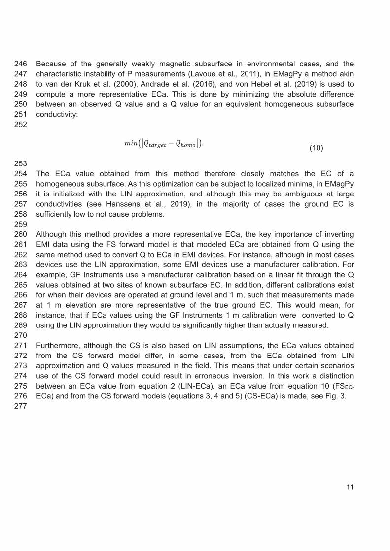
Figure 3: The different routes for obtaining ECa values. For field cases all devices obtain a Q value which is typically transformed into an ECa using either the LIN-ECa or some other manufacturer calibration (e.g. the GF instruments linear calibration). Some authors (e.g. von Hebel et al. 2019) opt to convert their field obtained Q values using a minimizing approach (FSEQ-ECa). For modeled cases there are two principle routes to obtain ECa values from a model subsurface: (1) Q values may be calculated from the FS forward model, they would then typically be converted to LIN-ECa or FSEQ-ECa, and (2) CS-ECa values can be obtained directly using the CS forward model.

278 To highlight the distinctions of ECa values defined here, and hence stress the importance of 279 their difference, they can be computed for a variety of synthetic cases. In Figure 4, FSEQ-ECa, 280 LIN-ECa and CS-ECa are calculated for the device specifications of the largest coil 281 separation (4.49 m) of the CMD Explorer operated in VCP mode above homogeneous and 282 heterogeneous subsurfaces, at ground level and at 1 m elevation. For the homogeneous 283 case, data are generated for subsurface EC of 1 to 100 mS/m in 1 mS/m increments, the 284 heterogeneous case data is generated for a two layer model with a layer 1 thickness of 0.5 m, 285 an upper layer EC of 1 to 100 mS/m in 1 m/Sm increments and a constant lower layer EC of 286 50 mS/m. 287

13

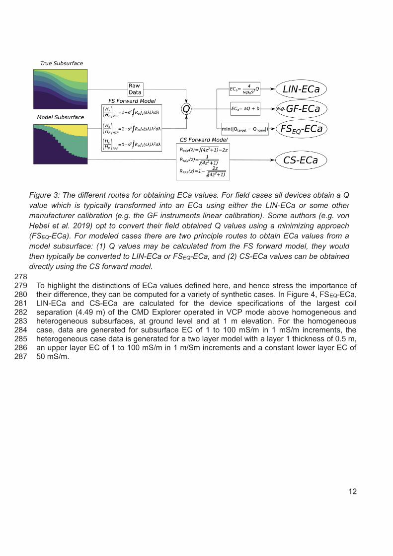
Figure 4: Differences between CS-ECa, FSEQ-ECa and LIN-ECa for a homogeneous and a heterogeneous case. (a) shows the differences over a homogeneous medium with increasing EC, (b) shows the differences over an increasing homogeneous medium when the device is operated at 1 m, (c) shows the differences over a heterogeneous medium with a fixed layer 1 thickness of 0.5 m and a fixed EC of 50 mS/m, and (d) shows the differences over a heterogeneous medium with a fixed layer 1 thickness of 0.5 m and a fixed EC of 50 mS/m when the device is operated at 1 m elevation. In all figures h is the device height above ground level.

288 Firstly, it can be seen from Fig. 4a that for a homogeneous subsurface EC when the device at 289 ground level FSEQ-ECa and CS-ECa values lie on a 1:1 line, whereas the LIN-ECa deviates 290 from this line at higher EC values. In comparison, when the device is operated at 1 m 291 elevation (Fig. 4b) FSEQ-ECa, LIN-ECa CS-ECa all show increasing deviation at higher 292 conductivities, with the FSEQ-ECa being intermediate between the higher CS-ECa and the 293 lower LIN-ECa. Furthermore, these values are broadly comparable for low conductivities (< 294 20 mS/m), for the ground level and 1 m elevation cases. When the device is operated at 295 ground level (Fig. 4c), for the heterogeneous case, the LIN-ECa is significantly lower than the 296 other two values. Furthermore, the FSEQ-ECa and CS-ECa match when the upper layer 297 conductivity is 50 mS/m (i.e. homogeneous subsurface). When the device is operated at 1 m 298 elevation (Fig. 4d) for the heterogeneous case all ECa values differ from each other across 299 the layer 1 conductivity range. 300 301

14

These observations demonstrate that under certain conditions the CS function may be 302 inappropriate to model with LIN-ECa values obtained from the field, e.g. when the subsurface 303 is strongly heterogeneous. Furthermore, it can also be noted that FSEQ-ECa is perhaps better 304 suited to modeling than the CS function and may perform reasonably in environments where 305 subsurface EC is both low and of small variability. Moreover, if FSEQ-ECa is taken as the most 306 accurate representation of the subsurface EC, it can be seen that LIN-ECa underestimates 307 the subsurface EC in the case of higher EC values and heterogeneous environments. 308 However, as noted above, so long as the translation between Q and ECa is consistent for the 309 EMI device and FS forward model, the derivation of ECa using this method is not a requisite 310 for accurate inversion. 311

2.5 Calibration of EMI data 312

In addition to considering ECa values, it is important to note that in many cases EMI devices 313 are only seen to provide qualitative measurements of conductivity because of instrument 314 calibration difficulties (Triantafilis et al. 2000; Sudduth et al. 2001; Abdu et al. 2007; Gebbers 315 et al. 2009; Nüsch et al. 2010). For instance, external influences such as presence of the 316 operator, zero-leveling procedures or field set up can influence the measurements 317 significantly. Therefore, in order to permit quantitative modeling of EMI data several authors 318 have advocated for the need of data calibration (e.g. Lavoue et al., 2009; von Hebel et al., 319 2014). Proposed calibration methods have included collection of intrusive soil samples (e.g. 320 Triantafilis et al. 2000; and Moghadas et al., 2012), use of ERT (e.g. Lavoue et al., 2010; von 321 Hebel et al., 2014) or use of measurements made at multiple elevations (e.g. Tan et al., 322 2019). 323 324 In this work the method using ERT is implemented, whereby depth-specific models of 325 electrical resistivity are used to calculate a forward EMI model response which is then paired 326 with a set of EMI measurements made along the ERT transect. Although it is possible to invert 327 ERT data with several inversion programs, the calibration implementation in EMagPy can 328 directly use ERT models produced by the sister code, ResIPy (https://gitlab.com/hkex/pyr2; 329 Blanchy et al., 2020). Clearly, there is an implicit assumption here that the ERT-derived 330 electrical conductivities are true values, and that the footprint of EMI and ERT measurements 331 does not differ significantly. 332

2.6 Inversions routines 333

2.6.1 Data and model misfit 334

In EMagPy the inverse problem can be solved using the CS or FS forward model solutions, in 335 addition the problem can be solved to produce both sharply and smoothly varying models of 336 conductivity. The sharp inversion solves the inverse problem with both conductivities and 337 depths as parameters, whereas the smooth inversion uses fixed depths and solves only for 338 conductivities. In both cases the data misfit is defined as the difference between observed 339

15

values and predicted values from the forward model solutions. As the smooth inversion 340 typically produces a model containing more EC values than measurements it requires a 341 model misfit term, which determines the smoothness of neighboring layers. In comparison, 342 the sharp inversion, although a model misfit term can be used, the inverse problem is 343 generally set such that the problem is under-determined, i.e. the number of parameters 344 (depths and conductivities) is less than the number of measurements. The total misfit is given 345 by: 346

= + , (10)

where Φd is the data misfit, Φm is the model misfit and α is a smoothing parameter 347 determining the influence of Φm on the total misfit, i.e. ordinarily this would be set to 0 for 348 sharp cases. The inversion problem can be solved by minimizing either the L1 or the L2 norm 349 cost functions for each 1D profile. The data misfit for both norms are obtained by: 350

= ∑ | − ( )|, (11)

351

= ∑ − ( ) , (12)

where N is the number of coil configurations per profile, d is the observed values and f(m) is 352 the predicted values from the forward model with parameter set, m. Similarly, the model 353 misfits for L1 and L2 norms, respectively, are obtained by: 354

= ∑ − , (13)

355 = ∑ − , (14)

where M is the number of layers in the model and ECj is the conductivity of layer j. 356

2.6.2 Optimization methods 357

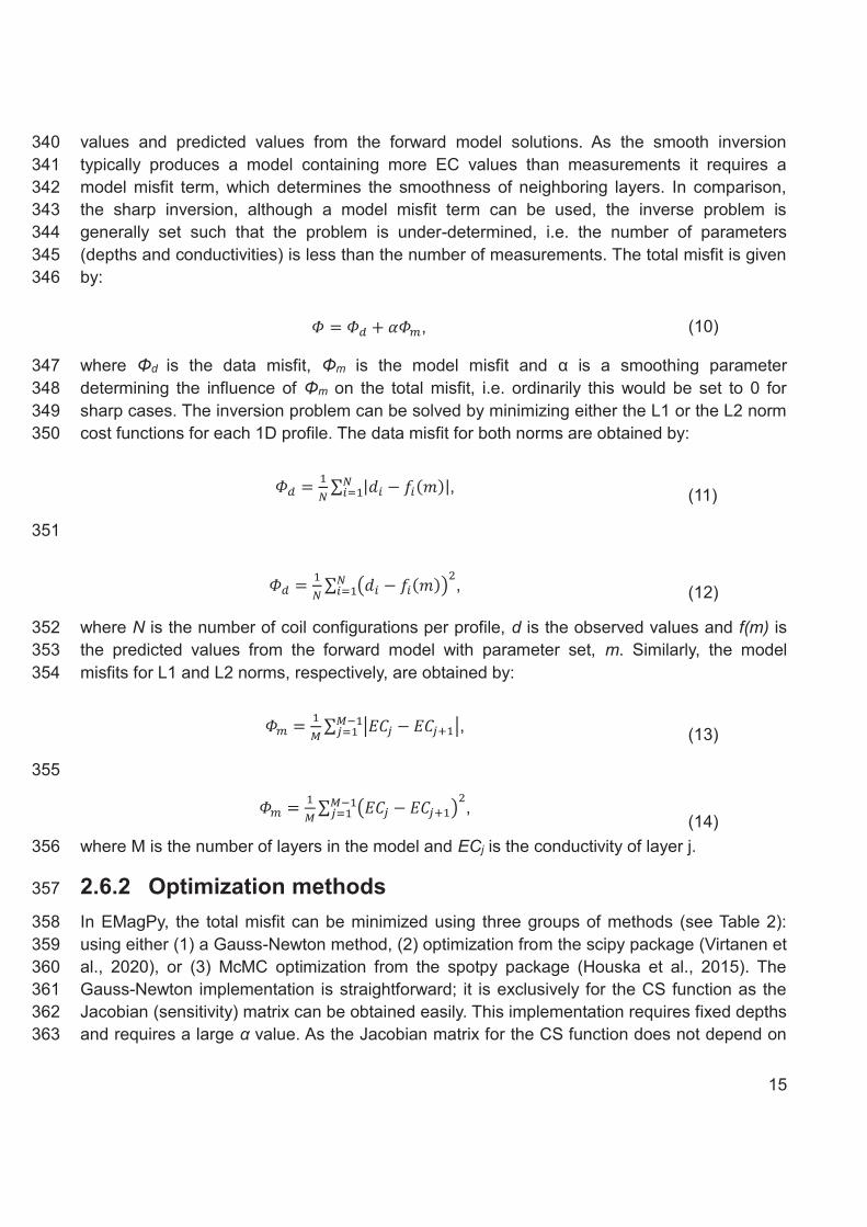
In EMagPy, the total misfit can be minimized using three groups of methods (see Table 2): 358 using either (1) a Gauss-Newton method, (2) optimization from the scipy package (Virtanen et 359 al., 2020), or (3) McMC optimization from the spotpy package (Houska et al., 2015). The 360 Gauss-Newton implementation is straightforward; it is exclusively for the CS function as the 361 Jacobian (sensitivity) matrix can be obtained easily. This implementation requires fixed depths 362 and requires a large α value. As the Jacobian matrix for the CS function does not depend on 363

16

the layer conductivity, the solution is reached in one iteration. It is therefore well suited for 364 quick inversions of smooth solutions and has the added benefit that it easily enables time-365 lapse inversion (see Whalley et al., 2017). 366

Table 2: Minimization methods employed within EMagPy. 367

Minimization method

Description Implemented features Package used

Gauss-Newton Gradient based method. CS forward model, L2 data and model misfit.

-

Nelder-Mead Simplex heuristic search method.

CS and FS forward model, L1 and L2 data

and model misfit.

scipy

L-BFGS-B Approximation of BFGS method, with bounds. This method uses

an estimate of the inverse Hessian matrix.

CS and FS forward model, L1 and L2 data

and model misfit.

scipy

Conjugate Gradient

Gradient method for non-linear problems.

CS and FS forward model, L1 and L2 data

and model misfit.

scipy

SCE-UA Shuffled Complex Evolution Algorithm McMC based method.

CS and FS forward model, L1 and L2 data

and model misfit.

spotpy

DREAM Differential Evolution Adaptive Metropolis Algorithm McMC

based method.

CS and FS forward model, L1 and L2 data

and model misfit.

spotpy

ROPE Robust Parameter Estimation McMC method

CS and FS forward model, L1 and L2 data

and model misfit.

spotpy

368

Through the optimize function from scipy, EMagPy can minimise equation 10 using the 369 Nelder-Mead (Nelder and Mead, 1965), L-BFGS-B (Byrd et al., 1995) or conjugate gradient 370 (Fletcher and Reeves, 1964) algorithms. However, it is important to note that broader range of 371 algorithms exist though the scipy package and can be implemented if needed. These 372 methods can be used for both the CS and FS forward models and are adapted to both 373 smooth and sharp inversions. Their implementation is based on the function 374 scipy.optimize.minimize() from the scipy python package that is used to minimize the 375 objective function. Each method has its own convergence criteria (see scipy documentation) 376

17

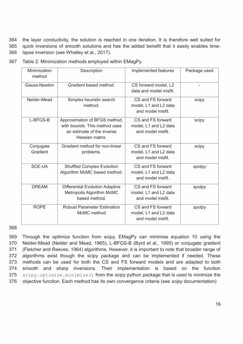
The McMC-based approach also minimizes an objective function but relies on different 377 sampling approaches to find a solution. This implementation is based on the Python spotpy 378 package (Houska et al., 2015) that provides several solvers for parameter optimization such 379 as SCE-UA (Duan et al., 1994), DREAM (Vrugt and Ter Braak, 2011) or ROPE (Bardossy et 380 al., 2008). One advantage of this approach is that it produces posterior distribution of the 381 parameters from which a model uncertainty can be estimated (Figure 5). In EMagPy, this 382 posterior distribution is based on the 10% best sample (i.e. the lowest total misfit) and the 383 error for each parameter is estimated using the standard deviation of this posterior 384 distribution. Although this method was primarily implemented to obtain sharp models of EC, it 385 can also be used for smooth models. 386

387

Figure 5: Example of a two layers, one varying depth model inverted using the McMC solver. Each subplot shows the posterior distribution of the parameters after sampling (3000 samples, 1 chain) for (a) the depth, (b) the EC of layer 1 and (c) the EC of layer 2. m is the mean and std is the standard deviation of the distribution (meters for depth and mS/m for layer1 and layer2). The red dashed line represent the true value while the green dashed line represent the best estimate (the one with the lowest misfit).

388 The quality of the inversion can be assessed visually by plotting the predicted ECa values 389 from the inverted model and the observed ECa for each profile using either showMisfit() 390 or showOne2one() methods. It is also possible to directly plot the root-mean-square error for 391 each profile on top of the inverted section using showResults(rmse=True). This makes it 392 easy to quickly identify how suitable models are for explaining the different EMI observations. 393

2.7 EMagPy capabilities 394

EMagPy has been designed to provide both a Python application programming interface (API) 395 and a graphical user interface (GUI). The Python API can be used in Python scripts or in 396 Jupyter notebooks and enables automated tasks. The GUI provides an intuitive interface for 397 the inversion and modeling of multiple datasets. 398

18

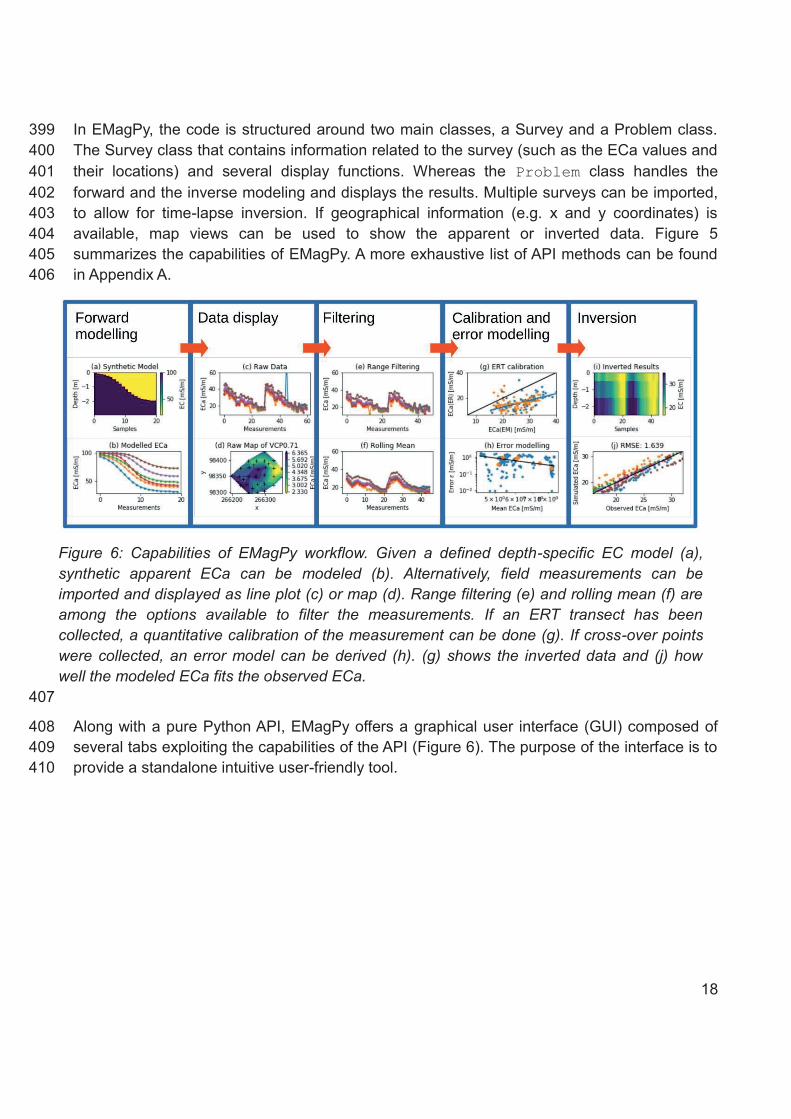
In EMagPy, the code is structured around two main classes, a Survey and a Problem class. 399 The Survey class that contains information related to the survey (such as the ECa values and 400 their locations) and several display functions. Whereas the Problem class handles the 401 forward and the inverse modeling and displays the results. Multiple surveys can be imported, 402 to allow for time-lapse inversion. If geographical information (e.g. x and y coordinates) is 403 available, map views can be used to show the apparent or inverted data. Figure 5 404 summarizes the capabilities of EMagPy. A more exhaustive list of API methods can be found 405 in Appendix A. 406

Figure 6: Capabilities of EMagPy workflow. Given a defined depth-specific EC model (a), synthetic apparent ECa can be modeled (b). Alternatively, field measurements can be imported and displayed as line plot (c) or map (d). Range filtering (e) and rolling mean (f) are among the options available to filter the measurements. If an ERT transect has been collected, a quantitative calibration of the measurement can be done (g). If cross-over points were collected, an error model can be derived (h). (g) shows the inverted data and (j) how well the modeled ECa fits the observed ECa.

407

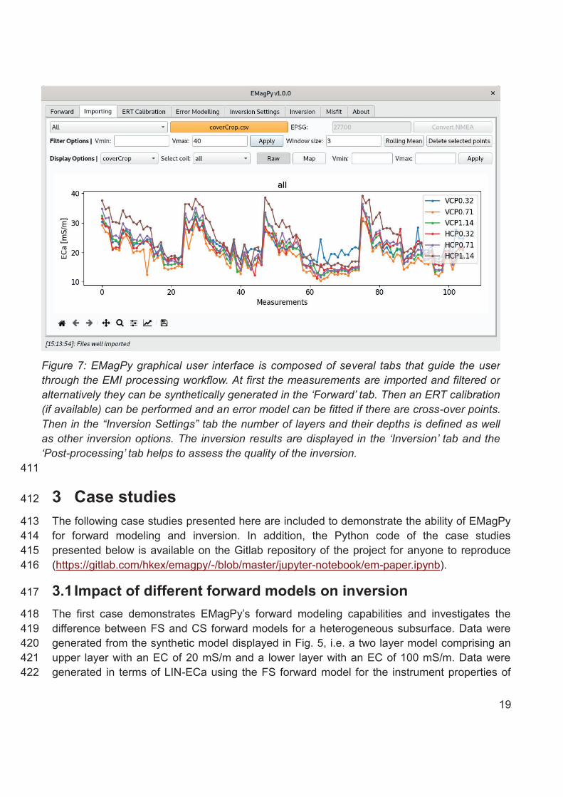
Along with a pure Python API, EMagPy offers a graphical user interface (GUI) composed of 408 several tabs exploiting the capabilities of the API (Figure 6). The purpose of the interface is to 409 provide a standalone intuitive user-friendly tool. 410

19

Figure 7: EMagPy graphical user interface is composed of several tabs that guide the user through the EMI processing workflow. At first the measurements are imported and filtered or alternatively they can be synthetically generated in the ‘Forward’ tab. Then an ERT calibration (if available) can be performed and an error model can be fitted if there are cross-over points. Then in the “Inversion Settings” tab the number of layers and their depths is defined as well as other inversion options. The inversion results are displayed in the ‘Inversion’ tab and the ‘Post-processing’ tab helps to assess the quality of the inversion.

411

3 Case studies 412

The following case studies presented here are included to demonstrate the ability of EMagPy 413 for forward modeling and inversion. In addition, the Python code of the case studies 414 presented below is available on the Gitlab repository of the project for anyone to reproduce 415 (https://gitlab.com/hkex/emagpy/-/blob/master/jupyter-notebook/em-paper.ipynb). 416

3.1 Impact of different forward models on inversion 417

The first case demonstrates EMagPy’s forward modeling capabilities and investigates the 418 difference between FS and CS forward models for a heterogeneous subsurface. Data were 419 generated from the synthetic model displayed in Fig. 5, i.e. a two layer model comprising an 420 upper layer with an EC of 20 mS/m and a lower layer with an EC of 100 mS/m. Data were 421 generated in terms of LIN-ECa using the FS forward model for the instrument properties of 422

20

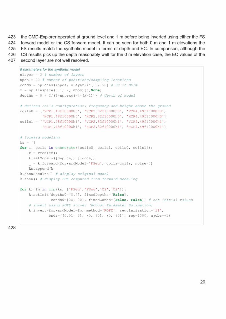
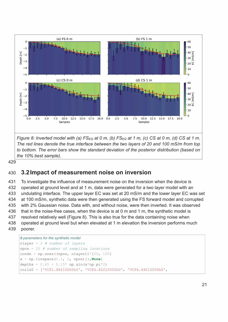
the CMD-Explorer operated at ground level and 1 m before being inverted using either the FS 423 forward model or the CS forward model. It can be seen for both 0 m and 1 m elevations the 424 FS results match the synthetic model in terms of depth and EC. In comparison, although the 425 CS results pick up the depth reasonably well for the 0 m elevation case, the EC values of the 426 second layer are not well resolved. 427

# parameters for the synthetic model nlayer = 2 # number of layers npos = 20 # number of positions/sampling locations conds = np.ones((npos, nlayer))*[10, 50] # EC in mS/m x = np.linspace(0.1, 2, npos)[:,None] depths = 0 + 2/(1+np.exp(-4*(x-1))) # depth of model # defines coils configuration, frequency and height above the ground coils0 = ['VCP1.48f10000h0', 'VCP2.82f10000h0', 'VCP4.49f10000h0', 'HCP1.48f10000h0', 'HCP2.82f10000h0', 'HCP4.49f10000h0'] coils1 = ['VCP1.48f10000h1', 'VCP2.82f10000h1', 'VCP4.49f10000h1', 'HCP1.48f10000h1', 'HCP2.82f10000h1', 'HCP4.49f10000h1'] # forward modeling ks = [] for i, coils in enumerate([coils0, coils1, coils0, coils1]): k = Problem() k.setModels([depths], [conds]) _ = k.forward(forwardModel='FSeq', coils=coils, noise=0) ks.append(k) k.showResults() # display original model k.show() # display ECa computed from forward modeling for k, fm in zip(ks, ['FSeq','FSeq','CS','CS']): k.setInit(depths0=[0.5], fixedDepths=[False], conds0=[20, 20], fixedConds=[False, False]) # set initial values # invert using ROPE solver (RObust Parameter Estimation) k.invert(forwardModel=fm, method='ROPE', regularization='l1', bnds=[(0.01, 3), (0, 80), (0, 80)], rep=1000, njobs=-1)

428

21

Figure 8: Inverted model with (a) FSEQ at 0 m, (b) FSEQ at 1 m, (c) CS at 0 m, (d) CS at 1 m. The red lines denote the true interface between the two layers of 20 and 100 mS/m from top to bottom. The error bars show the standard deviation of the posterior distribution (based on the 10% best sample).

429

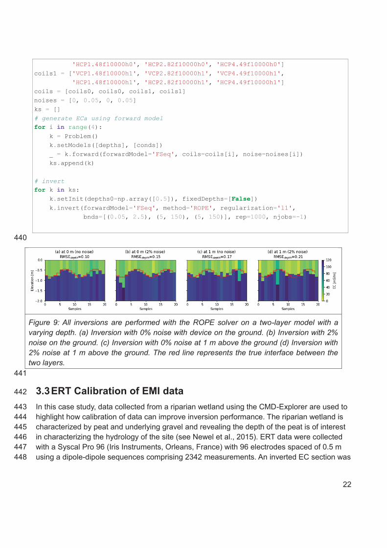
3.2 Impact of measurement noise on inversion 430

To investigate the influence of measurement noise on the inversion when the device is 431 operated at ground level and at 1 m, data were generated for a two layer model with an 432 undulating interface. The upper layer EC was set at 20 mS/m and the lower layer EC was set 433 at 100 mS/m, synthetic data were then generated using the FS forward model and corrupted 434 with 2% Gaussian noise. Data with, and without noise, were then inverted. It was observed 435 that in the noise-free cases, when the device is at 0 m and 1 m, the synthetic model is 436 resolved relatively well (Figure 8). This is also true for the data containing noise when 437 operated at ground level but when elevated at 1 m elevation the inversion performs much 438 poorer. 439

# parameters for the synthetic model nlayer = 2 # number of layers npos = 20 # number of sampling locations conds = np.ones((npos, nlayer))*[20, 100] x = np.linspace(0.1, 2, npos)[:,None] depths = 0.65 + 0.15* np.sin(x*np.pi*2) coils0 = ['VCP1.48f10000h0', 'VCP2.82f10000h0', 'VCP4.49f10000h0',

22

'HCP1.48f10000h0', 'HCP2.82f10000h0', 'HCP4.49f10000h0'] coils1 = ['VCP1.48f10000h1', 'VCP2.82f10000h1', 'VCP4.49f10000h1', 'HCP1.48f10000h1', 'HCP2.82f10000h1', 'HCP4.49f10000h1'] coils = [coils0, coils0, coils1, coils1] noises = [0, 0.05, 0, 0.05] ks = [] # generate ECa using forward model for i in range(4): k = Problem() k.setModels([depths], [conds]) _ = k.forward(forwardModel='FSeq', coils=coils[i], noise=noises[i]) ks.append(k) # invert for k in ks: k.setInit(depths0=np.array([0.5]), fixedDepths=[False]) k.invert(forwardModel='FSeq', method='ROPE', regularization='l1', bnds=[(0.05, 2.5), (5, 150), (5, 150)], rep=1000, njobs=-1)

440

Figure 9: All inversions are performed with the ROPE solver on a two-layer model with a varying depth. (a) Inversion with 0% noise with device on the ground. (b) Inversion with 2% noise on the ground. (c) Inversion with 0% noise at 1 m above the ground (d) Inversion with 2% noise at 1 m above the ground. The red line represents the true interface between the two layers.

441

3.3 ERT Calibration of EMI data 442

In this case study, data collected from a riparian wetland using the CMD-Explorer are used to 443 highlight how calibration of data can improve inversion performance. The riparian wetland is 444 characterized by peat and underlying gravel and revealing the depth of the peat is of interest 445 in characterizing the hydrology of the site (see Newel et al., 2015). ERT data were collected 446 with a Syscal Pro 96 (Iris Instruments, Orleans, France) with 96 electrodes spaced of 0.5 m 447 using a dipole-dipole sequences comprising 2342 measurements. An inverted EC section was 448

23

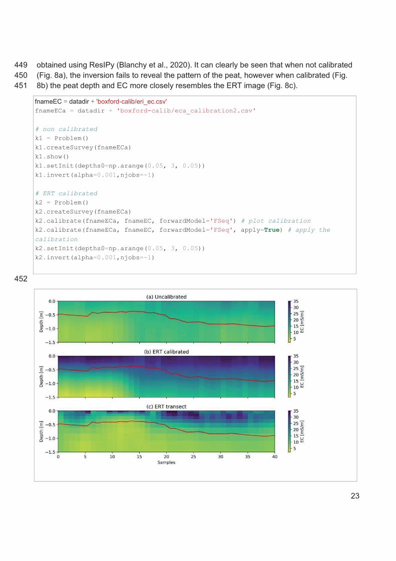
obtained using ResIPy (Blanchy et al., 2020). It can clearly be seen that when not calibrated 449 (Fig. 8a), the inversion fails to reveal the pattern of the peat, however when calibrated (Fig. 450 8b) the peat depth and EC more closely resembles the ERT image (Fig. 8c). 451

fnameEC = datadir + 'boxford-calib/eri_ec.csv' fnameECa = datadir + 'boxford-calib/eca_calibration2.csv' # non calibrated k1 = Problem() k1.createSurvey(fnameECa) k1.show() k1.setInit(depths0=np.arange(0.05, 3, 0.05)) k1.invert(alpha=0.001,njobs=-1) # ERT calibrated k2 = Problem() k2.createSurvey(fnameECa) k2.calibrate(fnameECa, fnameEC, forwardModel='FSeq') # plot calibration k2.calibrate(fnameECa, fnameEC, forwardModel='FSeq', apply=True) # apply the calibration k2.setInit(depths0=np.arange(0.05, 3, 0.05)) k2.invert(alpha=0.001,njobs=-1)

452

24

Figure 10: Smoothly inverted non-calibrated (a) and calibrated (b) EMI data with the corresponding ERT inversion (c). The red line shows the true depth of the peat intrusive penetration measurements.

453

3.4 Including prior knowledge 454

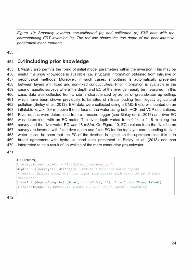
EMagPy also permits the fixing of initial model parameters within the inversion. This may be 455 useful if a priori knowledge is available, i.e. structural information obtained from intrusive or 456 geophysical methods. Moreover, in such cases, smoothing is automatically prevented 457 between layers with fixed and non-fixed conductivities. Prior information is available in the 458 case of aquatic surveys where the depth and EC of the river can easily be measured. In this 459 case, data was collected from a site is characterized by zones of groundwater up-welling, 460 which have been shown previously to be sites of nitrate loading from legacy agricultural 461 pollution (Binley et al., 2013). EMI data were collected using a CMD-Explorer mounted on an 462 inflatable kayak, 0.4 m above the surface of the water using both HCP and VCP orientations. 463 River depths were determined from a pressure logger (see Binley et al., 2013) and river EC 464 was determined with an EC meter. The river depth varied from 0.14 to 1.18 m along the 465 survey and the river water EC was 48 mS/m. On Figure 10, ECa values from the river-borne 466 survey are inverted with fixed river depth and fixed EC for the top layer corresponding to river 467 water. It can be seen that the EC of the riverbed is higher on the upstream side; this is in 468 broad agreement with hydraulic head data presented in Binley et al. (2013) and can 469 interpreted to be a result of up-welling of the more conductive groundwater. 470

471

k = Problem() k.createSurvey(datadir + 'leith/leith_dataset.csv') depths = k.surveys[0].df['depth'].values # measured water depths # setting initial model with top layer (the river) with fixed EC of 48 mS/m (measured) k.setInit(depths0=depths[:,None], conds0=[48, 20], fixedConds=[True, False]) k.invert(njobs=-1, beta=0.1) # beta > 0 will cause lateral smoothing

472

25

Figure 11: (a) ECa values measured from a CMD-Explorer on a boat along the river. (b) Inverted EC values given a fixed depth and a fixed EC of the top layer representing the river water (only the river bed conductivity is shown). (c) Hydraulic heads in the river bed from Binley et al. (2013). Upstream is at 0 m and downstream at 160 m distance.

473

3.5 Time-lapse field application 474

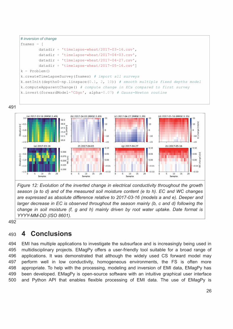
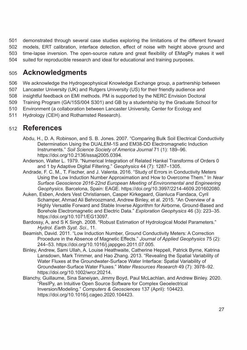
In the last case study, the capabilities to perform time-lapse EMI inversion are shown. EMI 475 measurements can be used as a proxy for soil moisture (e.g., Whalley et al., 2017). Using a 476 pedophysical relationship (Laloy et al, 2010), the change in inverted EC beneath different 477 wheat varieties can be linked to change in soil moisture. This method provides to crop 478 breeders high-throughput non-invasive below-ground information that can be important for 479 selecting resilient varieties. In this scenario, EMagPy can invert for the change in conductivity 480 using the Gauss-Newton solver using the method described in Appendix 1 of Whalley et al. 481 (2017). In this experiment ECa measurements were collected using a CMD Mini-Explorer on 482 different winter wheat plots during the growth season. At the same time, soil moisture 483 measurements were taken using neutron probe as ground truth. Note that all ECa values 484 were calibrated using an ERT array and temperature corrected. Figure 10a shows the 485 inverted EC In March 2017 while Figure 10e shows the volumetric water content measured by 486 neutron probe. Figures 10b, 10c and 10d show the change in EC, in mS/m, from this the EC 487 of 10a, and Figures 10f, 10g and 10h show the changes in water content, in relation to Figure 488 10d. Larger decreases in EC are observed at deeper depths through the growing season and 489 can be attributed to crop growth and water uptake. 490

26

# inversion of change fnames = [ datadir + 'timelapse-wheat/2017-03-16.csv', datadir + 'timelapse-wheat/2017-04-03.csv', datadir + 'timelapse-wheat/2017-04-27.csv', datadir + 'timelapse-wheat/2017-05-16.csv'] k = Problem() k.createTimeLapseSurvey(fnames) # import all surveys k.setInit(depths0=np.linspace(0.1, 2, 10)) # smooth multiple fixed depths model k.computeApparentChange() # compute change in ECa compared to first survey k.invert(forwardModel='CSgn', alpha=0.07) # Gauss-Newton routine

491

Figure 12: Evolution of the inverted change in electrical conductivity throughout the growth season (a to d) and of the measured soil moisture content (e to h). EC and WC changes are expressed as absolute difference relative to 2017-03-16 (models a and e). Deeper and larger decrease in EC is observed throughout the season mainly (b, c and d) following the change in soil moisture (f, g and h) mainly driven by root water uptake. Date format is YYYY-MM-DD (ISO 8601).

492

4 Conclusions 493

EMI has multiple applications to investigate the subsurface and is increasingly being used in 494 multidisciplinary projects. EMagPy offers a user-friendly tool suitable for a broad range of 495 applications. It was demonstrated that although the widely used CS forward model may 496 perform well in low conductivity, homogeneous environments, the FS is often more 497 appropriate. To help with the processing, modeling and inversion of EMI data, EMagPy has 498 been developed. EMagPy is open-source software with an intuitive graphical user interface 499 and Python API that enables flexible processing of EMI data. The use of EMagPy is 500

27

demonstrated through several case studies exploring the limitations of the different forward 501 models, ERT calibration, interface detection, effect of noise with height above ground and 502 time-lapse inversion. The open-source nature and great flexibility of EMagPy makes it well 503 suited for reproducible research and ideal for educational and training purposes. 504

Acknowledgments 505

We acknowledge the Hydrogeophysical Knowledge Exchange group, a partnership between 506 Lancaster University (UK) and Rutgers University (US) for their friendly audience and 507 insightful feedback on EMI methods. PM is supported by the NERC Envision Doctoral 508 Training Program (GA/15S/004 S301) and GB by a studentship by the Graduate School for 509 Environment (a collaboration between Lancaster University, Center for Ecology and 510 Hydrology (CEH) and Rothamsted Research). 511

References 512

Abdu, H., D. A. Robinson, and S. B. Jones. 2007. “Comparing Bulk Soil Electrical Conductivity Determination Using the DUALEM-1S and EM38-DD Electromagnetic Induction Instruments.” Soil Science Society of America Journal 71 (1): 189–96. https://doi.org/10.2136/sssaj2005.0394.

Anderson, Walter L. 1979. “Numerical Integration of Related Hankel Transforms of Orders 0 and 1 by Adaptive Digital Filtering.” Geophysics 44 (7): 1287–1305.

Andrade, F. C. M., T. Fischer, and J. Valenta. 2016. “Study of Errors in Conductivity Meters Using the Low Induction Number Approximation and How to Overcome Them.” In Near Surface Geoscience 2016-22nd European Meeting of Environmental and Engineering Geophysics. Barcelona, Spain: EAGE. https://doi.org/10.3997/2214-4609.201602080.

Auken, Esben, Anders Vest Christiansen, Casper Kirkegaard, Gianluca Fiandaca, Cyril Schamper, Ahmad Ali Behroozmand, Andrew Binley, et al. 2015. “An Overview of a Highly Versatile Forward and Stable Inverse Algorithm for Airborne, Ground-Based and Borehole Electromagnetic and Electric Data.” Exploration Geophysics 46 (3): 223–35. https://doi.org/10.1071/EG13097.

Bardossy, A, and S K Singh. 2008. “Robust Estimation of Hydrological Model Parameters.” Hydrol. Earth Syst. Sci., 11.

Beamish, David. 2011. “Low Induction Number, Ground Conductivity Meters: A Correction Procedure in the Absence of Magnetic Effects.” Journal of Applied Geophysics 75 (2): 244–53. https://doi.org/10.1016/j.jappgeo.2011.07.005.

Binley, Andrew, Sami Ullah, A. Louise Heathwaite, Catherine Heppell, Patrick Byrne, Katrina Lansdown, Mark Trimmer, and Hao Zhang. 2013. “Revealing the Spatial Variability of Water Fluxes at the Groundwater-Surface Water Interface: Spatial Variability of Groundwater-Surface Water Fluxes.” Water Resources Research 49 (7): 3978–92. https://doi.org/10.1002/wrcr.20214.

Blanchy, Guillaume, Sina Saneiyan, Jimmy Boyd, Paul McLachlan, and Andrew Binley. 2020. “ResIPy, an Intuitive Open Source Software for Complex Geoelectrical Inversion/Modeling.” Computers & Geosciences 137 (April): 104423. https://doi.org/10.1016/j.cageo.2020.104423.

28

Brosten, Troy R., Frederick D. Day-Lewis, Gregory M. Schultz, Gary P. Curtis, and John W. Lane. 2011. “Inversion of Multi-Frequency Electromagnetic Induction Data for 3D Characterization of Hydraulic Conductivity.” Journal of Applied Geophysics 73 (4): 323–35. https://doi.org/10.1016/j.jappgeo.2011.02.004.

Byrd, Richard H., Peihuang Lu, Jorge Nocedal, and Ciyou Zhu. 1995. “A Limited Memory Algorithm for Bound Constrained Optimization.” SIAM Journal on Scientific Computing 16 (5): 1190–1208.

Christiansen, Anders, Jesper Pedersen, Esben Auken, Niels Søe, Mads Holst, and Søren Kristiansen. 2016. “Improved Geoarchaeological Mapping with Electromagnetic Induction Instruments from Dedicated Processing and Inversion.” Remote Sensing 8 (12): 1022. https://doi.org/10.3390/rs8121022.

Corwin, D. L., and J. D. Rhoades. 1984. “Measurement of Inverted Electrical Conductivity Profiles Using Electromagnetic Induction.” Soil Science Society of America Journal 48 (2): 288–291.

Corwin, Dennis L. 2008. “Past, Present, and Future Trends in Soil Electrical Conductivity Measurements Using Geophysical Methods.” Handbook of Agricultural Geophysics, 17–44.

Dafflon, Baptiste, Susan S. Hubbard, Craig Ulrich, and John E. Peterson. 2013. “Electrical Conductivity Imaging of Active Layer and Permafrost in an Arctic Ecosystem, through Advanced Inversion of Electromagnetic Induction Data.” Vadose Zone Journal 12 (4).

Davies, Gareth, Jingyi Huang, Fernando Acacio Monteiro Santos, and John Triantafilis. 2015. “Modeling Coastal Salinity in Quasi 2D and 3D Using a DUALEM-421 and Inversion Software.” Groundwater 53 (3): 424–431.

Duan, Qingyun, Soroosh Sorooshian, and Vijai K. Gupta. 1994. “Optimal Use of the SCE-UA Global Optimization Method for Calibrating Watershed Models.” Journal of Hydrology 158 (3–4): 265–284.

Elwaseif, M., J. Robinson, F.D. Day-Lewis, D. Ntarlagiannis, L.D. Slater, J.W. Lane, B.J. Minsley, and G. Schultz. 2017. “A Matlab-Based Frequency-Domain Electromagnetic Inversion Code (FEMIC) with Graphical User Interface.” Computers & Geosciences 99 (February): 61–71. https://doi.org/10.1016/j.cageo.2016.08.016.

Farquharson, Colin G., Douglas W. Oldenburg, and Partha S. Routh. 2003. “Simultaneous 1D Inversion of Loop–Loop Electromagnetic Data for Magnetic Susceptibility and Electrical Conductivity” 68 (6): 1857–1869. https://doi.org/10.1190/1.1635038.

Frederiksen, Rasmus Rumph, Anders Vest Christiansen, Steen Christensen, and Keld Rømer Rasmussen. 2017. “A Direct Comparison of EMI Data and Borehole Data on a 1000ha Data Set.” Geoderma 303 (October): 188–95. https://doi.org/10.1016/j.geoderma.2017.04.028.

Frischknecht, F. C. 1987. “Electromagnetic Physical Scale Modeling.” Electromagnetic Methods in Applied Geophysics-Theory, 365–441.

Gebbers, Robin, Erika Lück, Michel Dabas, and Horst Domsch. 2009. “Comparison of Instruments for Geoelectrical Soil Mapping at the Field Scale.” Near Surface Geophysics 7 (3): 179–90. https://doi.org/10.3997/1873-0604.2009011.

Guillemoteau, Julien, Pascal Sailhac, Charles Boulanger, and Jérémie Trules. 2015. “Inversion of Ground Constant Offset Loop-Loop Electromagnetic Data for a Large Range of Induction Numbers.” GEOPHYSICS 80 (1): E11–21. https://doi.org/10.1190/geo2014-0005.1.

29

Guptasarma, D., and B. Singh. 1997. “New Digital Linear Filters for Hankel J0 and J1 Transforms.” Geophysical Prospecting 45 (5): 745–762.

Hanssens, Daan, Samuël Delefortrie, Christin Bobe, Thomas Hermans, and Philippe De Smedt. 2019. “Improving the Reliability of Soil EC-Mapping: Robust Apparent Electrical Conductivity (RECa) Estimation in Ground-Based Frequency Domain Electromagnetics.” Geoderma 337 (March): 1155–63. https://doi.org/10.1016/j.geoderma.2018.11.030.

Heagy, Lindsey J., Rowan Cockett, Seogi Kang, Gudni K. Rosenkjaer, and Douglas W. Oldenburg. 2017. “A Framework for Simulation and Inversion in Electromagnetics.” Computers & Geosciences 107 (October): 1–19. https://doi.org/10.1016/j.cageo.2017.06.018.

Hebel, Christian von, Sebastian Rudolph, Achim Mester, Johan A. Huisman, Pramod Kumbhar, Harry Vereecken, and Jan van der Kruk. 2014. “Three-Dimensional Imaging of Subsurface Structural Patterns Using Quantitative Large-Scale Multiconfiguration Electromagnetic Induction Data.” Water Resources Research 50 (3): 2732–48. https://doi.org/10.1002/2013WR014864.

Houska, Tobias, Philipp Kraft, Alejandro Chamorro-Chavez, and Lutz Breuer. 2015. “SPOTting Model Parameters Using a Ready-Made Python Package.” PloS One 10 (12): e0145180.

Huang, H, and I Won. 2000. “Conductivity and Susceptibility Mapping Using Broadband Electromagnetic Sensors.” Journal of Environmental and Engineering Geophysics, 12.

Huang, J., F.A. Monteiro Santos, and J. Triantafilis. 2016. “Mapping Soil Water Dynamics and a Moving Wetting Front by Spatiotemporal Inversion of Electromagnetic Induction Data,” November. https://doi.org/10.1002/2016WR019330.

Huang, J., A. Pedrera-Parrilla, K. Vanderlinden, E.V. Taguas, J.A. Gómez, and J. Triantafilis. 2017. “Potential to Map Depth-Specific Soil Organic Matter Content across an Olive Grove Using Quasi-2d and Quasi-3d Inversion of DUALEM-21 Data.” CATENA 152 (May): 207–17. https://doi.org/10.1016/j.catena.2017.01.017.

Huang, Jingyi, Alfred E. Hartemink, Francisco Arriaga, and Nathaniel W. Chaney. 2019. “Unraveling Location-Specific and Time-Dependent Interactions between Soil Water Content and Environmental Factors in Cropped Sandy Soils Using Sentinel-1 and Moisture Probes.” Journal of Hydrology 575 (August): 780–93. https://doi.org/10.1016/j.jhydrol.2019.05.075.

Jadoon, Khan Zaib, Davood Moghadas, Aurangzeb Jadoon, Thomas M. Missimer, Samir K. Al-Mashharawi, and Matthew F. McCabe. 2015. “Estimation of Soil Salinity in a Drip Irrigation System by Using Joint Inversion of Multicoil Electromagnetic Induction Measurements.” Water Resources Research 51 (5): 3490–3504. https://doi.org/10.1002/2014WR016245.

Koganti, Triven, Bhaskar Narjary, Ehsan Zare, Aslam Latif Pathan, Jingyi Huang, and John Triantafilis. 2018. “Quantitative Mapping of Soil Salinity Using the DUALEM-21S Instrument and EM Inversion Software.” Land Degradation & Development 29 (6): 1768–81. https://doi.org/10.1002/ldr.2973.

Laloy, E., M. Weynants, C.L. Bielders, M. Vanclooster, and M. Javaux. 2010. “How Efficient Are One-Dimensional Models to Reproduce the Hydrodynamic Behavior of Structured Soils Subjected to Multi-Step Outflow Experiments?” Journal of Hydrology 393 (1–2): 37–52. https://doi.org/10.1016/j.jhydrol.2010.02.017.

30

Lavoué, F., J. Van Der Kruk, J. Rings, F. André, D. Moghadas, J. A. Huisman, S. Lambot, L. Weihermüller, Jan Vanderborght, and H. Vereecken. 2010. “Electromagnetic Induction Calibration Using Apparent Electrical Conductivity Modelling Based on Electrical Resistivity Tomography.” Near Surface Geophysics 8 (6): 553–561.

Martinelli, Patricia, and María Celeste Duplaá. 2008. “Laterally Filtered 1D Inversions of Small-Loop, Frequency-Domain EMI Data from a Chemical Waste Site.” Geophysics 73 (4): F143–F149.

Martini, Edoardo, Ulrike Werban, Steffen Zacharias, Marco Pohle, Peter Dietrich, and Ute Wollschläger. 2017. “Repeated Electromagnetic Induction Measurements for Mapping Soil Moisture at the Field Scale: Validation with Data from a Wireless Soil Moisture Monitoring Network.” Hydrology and Earth System Sciences 21 (1): 495–513. https://doi.org/10.5194/hess-21-495-2017.

McNeill, J. D. 1980. Electromagnetic Terrain Conductivity Measurement at Low Induction Numbers. Geonics Limited Ontario, Canada. http://www.geonics.com/pdfs/technicalnotes/tn6.pdf.

Moghadas, Davood, Frédéric André, John H. Bradford, Jan van der Kruk, Harry Vereecken, and Sébastien Lambot. 2012. “Electromagnetic Induction Antenna Modelling Using a Linear System of Complex Antenna Transfer Functions.” Near Surface Geophysics 10 (3): 237–47. https://doi.org/10.3997/1873-0604.2012002.

Monteiro Santos, Fernando A. 2004. “1-D Laterally Constrained Inversion of EM34 Profiling Data.” Journal of Applied Geophysics 56 (2): 123–34. https://doi.org/10.1016/j.jappgeo.2004.04.005.

Nelder, John A., and Roger Mead. 1965. “A Simplex Method for Function Minimization.” The Computer Journal 7 (4): 308–313.

Nüsch, Anne-Kathrin, Peter Dietrich, Ulrike Werban, and Thorsten Behrens. 2010. “Acquisition and Reliability of Geophysical Data in Soil Science,” 4.

Pedersen, J. B., E. Auken, A. V. Christiansen, and S. M. Kristiansen. 2015. “Mapping Soil Heterogeneity Using Spatially Constrained Inversion of Electromagnetic Induction Data.” In First Conference on Proximal Sensing Supporting Precision Agriculture, 2015:1–5. European Association of Geoscientists & Engineers.

Robinson, David A., Hiruy Abdu, Inma Lebron, and Scott B. Jones. 2012. “Imaging of Hill-Slope Soil Moisture Wetting Patterns in a Semi-Arid Oak Savanna Catchment Using Time-Lapse Electromagnetic Induction.” Journal of Hydrology 416–417 (January): 39–49. https://doi.org/10.1016/j.jhydrol.2011.11.034.

Rücker, Carsten, Thomas Günther, and Florian M. Wagner. 2017. “PyGIMLi: An Open-Source Library for Modelling and Inversion in Geophysics.” Computers & Geosciences 109 (December): 106–23. https://doi.org/10.1016/j.cageo.2017.07.011.

Saey, Timothy, Jeroen Verhegge, Philippe De Smedt, Marthe Smetryns, Nicolas Note, Ellen Van De Vijver, Pieter Laloo, Marc Van Meirvenne, and Samuël Delefortrie. 2016. “Integrating Cone Penetration Testing into the 1D Inversion of Multi-Receiver EMI Data to Reconstruct a Complex Stratigraphic Landscape.” CATENA 147 (December): 356–71. https://doi.org/10.1016/j.catena.2016.07.023.

Shanahan, Peter W., Andrew Binley, W. Richard Whalley, and Christopher W. Watts. 2015. “The Use of Electromagnetic Induction to Monitor Changes in Soil Moisture Profiles beneath Different Wheat Genotypes.” Soil Science Society of America Journal 79 (2): 459. https://doi.org/10.2136/sssaj2014.09.0360.

31

Sherlock, Mark D., and Jeffrey J. McDonnell. 2003. “A New Tool for Hillslope Hydrologists: Spatially Distributed Groundwater Level and Soilwater Content Measured Using Electromagnetic Induction.” Hydrological Processes 17 (10): 1965–1977.

Sudduth, K. A., S. T. Drummond, and N. R. Kitchen. 2001. “Accuracy Issues in Electromagnetic Induction Sensing of Soil Electrical Conductivity for Precision Agriculture.” Computers and Electronics in Agriculture 31 (3): 239–264.

Tan, Xhie. 2019. “SIMULTANEOUS CALIBRATION AND INVERSION ALGORITHM FOR MULTI-CONFIGURATION ELECTROMAGNETIC INDUCTION DATA ACQUIRED AT MULTIPLE ELEVATIONS,” 55.

Triantafilis, J., G. M. Laslett, and A. B. McBratney. 2000. “Calibrating an Electromagnetic Induction Instrument to Measure Salinity in Soil under Irrigated Cotton.” Soil Science Society of America Journal 64 (3): 1009–1017.

Triantafilis, John, and S. M. Lesch. 2005. “Mapping Clay Content Variation Using Electromagnetic Induction Techniques.” Computers and Electronics in Agriculture 46 (1–3): 203–237.

Van Der Kruk, J., J. A. C. Meekes, P. M. Van Den Berg, and J. T. Fokkema. 2000. “An Apparent-Resistivity Concept for Low-Frequency Electromagnetic Sounding Techniques.” Geophysical Prospecting 48 (6): 1033–1052.

Virtanen, Pauli, Ralf Gommers, Travis E. Oliphant, Matt Haberland, Tyler Reddy, David Cournapeau, Evgeni Burovski, et al. 2020. “SciPy 1.0: Fundamental Algorithms for Scientific Computing in Python.” Nature Methods 17 (3): 261–72. https://doi.org/10.1038/s41592-019-0686-2.

von Hebel, van der Kruk, Huisman, Mester, Altdorff, Endres, Zimmermann, Garré, and Vereecken. 2019. “Calibration, Conversion, and Quantitative Multi-Layer Inversion of Multi-Coil Rigid-Boom Electromagnetic Induction Data.” Sensors 19 (21): 4753. https://doi.org/10.3390/s19214753.

Vrugt, J. A., and C. J. F. Ter Braak. 2011. “DREAM(D): An Adaptive Markov Chain Monte Carlo Simulation Algorithm to Solve Discrete, Noncontinuous, and Combinatorial Posterior Parameter Estimation Problems.” Hydrology and Earth System Sciences 15 (12): 3701–3713. https://doi.org/10.5194/hess-15-3701-2011.

Wait, James R. 1982. Geo-Electromagnetism. Academic Press. New York. Whalley, W.R., A. Binley, C.W. Watts, P. Shanahan, I.C. Dodd, E.S. Ober, R.W. Ashton, C.P.

Webster, R.P. White, and M. J. Hawkesford. 2017. “Methods to Estimate Changes in Soil Water for Phenotyping Root Activity in the Field.” Plant and Soil 415 (1–2): 407–22. https://doi.org/10.1007/s11104-016-3161-1.

Williams, B. G., and G. C. Baker. 1982. “An Electromagnetic Induction Technique for Reconnaissance Surveys of Soil Salinity Hazards.” Soil Research 20 (2): 107–18. https://doi.org/10.1071/sr9820107.

Zare, E., A. Beucher, J. Huang, A. Boman, S. Mattbäck, M. H. Greve, and J. Triantafilis. 2018. “Three-Dimensional Imaging of Active Acid Sulfate Soil Using a DUALEM-21S and EM Inversion Software.” Journal of Environmental Management 212: 99–107.

Zare, E., J. Huang, F. A. Santos, and J. Triantafilis. 2015. “Mapping Salinity in Three Dimensions Using a DUALEM-421 and Electromagnetic Inversion Software.” Soil Science Society of America Journal 79 (6): 1729–1740.

32

Appendix A 513

Table A1. Main API methods used in EMagPy. 514

Problem.show() Show apparent values as scatter plot Problem.showMap() Show spatial distribution of apparent values for given coil Problem.calibrate() Calibration of ECa value given depth-specific EC dataset Problem.invert() General inversion routine Problem.showResults() Show inversion results as a transect Problem.showSlice() Show the slice for the selected inverted layer Problem.showOne2one() Show 1:1 graph of modeled vs observed apparent EC Problem.showMisfit() Show the observed and the modeled ECa

515