Elgohary, Tarek A. and Turner, James D. (2014), "State Transition Tensor Models for the Uncertainty...

1171

AAS 13-784

STATE TRANSITION TENSOR MODELS FOR THE

UNCERTAINTY PROPAGATION OF THE TWO-BODY PROBLEM

Tarek A. Elgohary* and James D. Turner†

Several methods exist for integrating the Keplerian Motion of two gravitation-ally interacting bodies, even when gravitational perturbation terms are in-cluded. The challenge is that the equations of motion become very stiff whenthe perturbation terms are included, which forces the use of small time steps,higher-order methods, or extended precision calculations. Recently, Turner andElgohary have shown that by introducing two scalar Lagrange-like invariantsthat it is possible to integrate the two-body and two-body plus J2 perturbationterm using a recursive formulation for developing an analytic continua-tion-based power series that overcomes the limitations of standard integrationmethods. Numerical comparisons with RK12(10), and other state of the art in-tegration methods indicate performance improvements of ~ 70X, while main-taining ~mm accuracy for the orbit predictions. Extensions for J3 through J6are currently under development. With accurate trajectories available, the nextimportant theoretical development becomes extending the series-based solutionfor the state transition matrices (STM) for both the two-body and two-bodyplus J2 perturbation. STMs are useful for many celestial mechanics optimiza-tion calculations. Second and third order STM models are developed to supportuncertainty propagation investigations. The application of scalar Lagrange-likeinvariants generates highly efficient state trajectory, STM, and higher-orderSTMs models. The proposed mathematical models are expected to be broadlyuseful for celestial mechanic applications for optimization, uncertainty propa-gation, and nonlinear estimation theory.

INTRODUCTION

The development of STM models requires an accurate trajectory prediction for building the nonlinear STM ordinary differential equations. For the unperturbed two-body problem the classi-cal F&G Lagrangian coefficients provide a mapping of the initial position and velocity into cur-rent time values. Majji, Junkins, and Turner,1 based on the F&G model, have developed first- through fifth-order STM models. Unfortunately, the F&G STM-based model is not well suited for being extended for handling J2 and higher-order gravity perturbation effects. This work pre-sents an analytic series-based approach that overcomes the problems encountered for applying the F&G STM for gravity perturbations.

* Graduate Research Assistant, Aerospace Engineering, Texas A&M University, College Station, Texas, [email protected] † Research Professor, Aerospace Engineering, Texas A&M University, College Station, Texas, [email protected],Fellow AAS, Associate Fellow AIAA

1172

Continuation Methods for the Two-Body Problem

A problem of long-standing for the two-body problem has been the difficulty in developing high-order Taylor series expansions, even though the governing equations are well-defined. La-grange introduced three algebraic invariants that permit the unperturbed two-body trajectory to be expanded in a power series model.2 However, Lagrange’s analysis objective was not to develop arbitrary order time derivative models for the trajectories. Later work by Battin and others ex-tended this approach and developed recursive algorithms for propagating the Lagrange invari-ants.3, 6-8 The Lagrange invariants, however, have not been extended for handling gravity pertur-bations. This work handles both unperturbed and perturbed gravity external loads. All of the new algorithms build on Turner and Elgohary two scalar Lagrange-like invariants (i.e., f � �r r and

/2ng f �� ).4 This approach is highly efficient because the differential equations for both f and glead to bilinear equations, with no denominators, which are ideally suited for generating recur-sively-based arbitrary-order time derivatives by invoking the use of Leibniz product rule. Ordi-narily, without introducing the f and g variables, the calculations for n-th order time derivatives of the vector-valued function � � 3/2�� 3/2�r r rapidly becomes unwieldy and very complicated for coding and validating the model. Indeed, it is likely the complexity of these calculations provided La-grange with amply motivation for seeking out the development of his algebraic invariant ap-proach. Using the f and g model, there is no theoretical limit to the number of series terms that can be retained in the approximation. Numerical experiments, however, demonstrate that depend-ing on the propagation time step size and the orbit eccentricity that 8 to 15 series terms yield op-erationally useful approximations for missions operating in the LEO-GEO Theater of operations. Extended precision experiments, including Q-level and 200-500 digit calculations, support the conclusion that the integration time step for the trajectory analysis is limited by a fundamental radius of convergence issue for the series approximation.5 On-going research efforts are explor-ing the radius of convergence issue and its impact on building operationally useful tools for sup-porting space trajectory applications. Of course, f and g are just scalar kinematic variables. Tra-jectory models require that f and g are linked with the two-body problem acceleration, defined by

g�� g�� r r , where � Tx y z�r denotes the inertial relative coordinate vector that locates an object relative to the Earth, � = 398601.2 km2/sec3 is the gravitational constant. It is important to note that g�� g�� r r consists of a bilinear term involving the product of the position vector and the g scalar Lagrange-like invariant. Like the f and g variables themselves, the higher time deriv-atives for g�� g�� r r are generated by invoking Leibnitz product rule. A complete series solution is generated by recursively linking the Leibnitz product rules for f, g, and r , and recovering one derivative order for each sweep of the three Leibnitz product rules: the approach is both efficient and accurate. Calculations begin by assuming that initial values are available for ,r r,r , higher-order time derivatives are developed recursively linking Leibniz product rule for f, g, and r to recursively develop � �, , , ,f g� f g,� , ff ��,�, ,�gf, g, r r . After computing a pre-set number of terms recur-

sively, one develops the trajectory and trajectory time derivatives as the analytic continuation power series approximations,

� � � � � � � � � �

� � � � � � � �

2 3

2

/ 2! / 3!

/ 2!

t h t t h t h t h

t h t t h t h

� � � � � �

� � � � �

� � � � � �/ 2! / 3� �t h t h� � � � / 2! � �� 2 3� � / 33t h t h� � � � 2 � � / 33t h t h� � � � 2 / 2! � ��

� � � � � � � � 2 / 2t h t t h t h� � � � � � � 2 / 2h t t h t hh t t h� � � � � � �

r r r r r

r r r r (1)

1173

Only the position and velocity vectors must be analytically continued. This work extends these results to include J2 disturbance acceleration terms for the trajectory propagation, as well as developing analytic continuation power series for the STM. Numerical results are presented that compare the solution accuracy and integration time required by ODE45 and RKN1210, and the analytic power series methods developed in this work for two-body plus J2 perturbation terms.

ANALYTIC CONTINUATION SOLUTION FOR THE PERTURBED TWO-BODY PROBLEM

The trajectory model for the perturbed relative two-body problem is addressed with the fol-lowing equation of motion,

3 dr�

� � �3r�

� � 3

�r r a (2)

The disturbance acceleration term da , referring to the 2J effects, that arising from the Earth’s oblateness is defined as,

2

2 2 2 2

2 2

3 1 5 , 1 5 , 3 52

eqJ

r z x z y z zJr r r r r r r r� ��

a (3)

where, 3 2398600.4418 km s� �� is the standard gravitational parameter of the Earth, 6

2 1082.63 10J �� defines the oblateness perturbation, 6378.1370 kmeqr � is the Earth equa-torial radius.

Invariant Solution Strategy

A two-part solution strategy is presented. First, two Lagrange-Like invariants are introduced to automate the process of generating arbitrary order time derivatives for the equation of motion in Eq. (2). The first scalar Lagrange-like invariant is:

.f � r r (4)

where (.) denotes the vector inner product for the bilinear form. The n-th order time derivative of f is computed by applying Leibniz product rule as,

� � � � � �

0

nn m n m

m

nf

m�

�

� ��

� �� .r r (5)

wherenm� ��

is the standard binomial and � �m

mm

d f fdt

� . The second Lagrange-Like invariant is

given by, /2p

pg f �� (6)

1174

which is not a bilinear form, however, the first time derivative for Eq. (6) can be shown to be the

bilinear form: 02p ppfg fg� � 0p �2p p2pfg fp 2p fp

pfgfg . Evaluating the higher order time derivatives of pg , using

Leibniz product rule, and solving for the highest time derivative, one obtains,

� � � � � � � � � � � �1 1 1( 1)

1

/2 2

nn m n m m n mn

pm

np pg f g f g f g fm

� � � ��

�

��

� (7)

Note, that if the bilinear first derivative term was not used for Leibnitz product rule, that one is forced to model Eq. (6) as a composite function of the form � �p pg g f� , which is classically handled by the very complicated and celebrated Faá di Bruno mathematical identity.

From Eq. (3), it is obvious that 2Ja contains cubic and quartic terms that are not handled by

Leibnitz product rule. Theoretically, it is possible to develop multi-nominal versions of Leibnitz product rule; nevertheless, by introducing several variable transformations,

2Ja is recast in a form suitable for applying the binomial form of Leibnitz product rule for developing arbitrary-order analytic time derivative models. To this end, the first step is to define the constant

22 2

32 eqc J r�� (8)

Now Eq. (2) is re-written as

� �2 2 3

3/22 5 7 5 7 5 75 , 5 , 3 5x z x y z y z zc

r r r r r r� � � �

� � � � ��

��r = - r r r (9)

Recalling Eq. (6), Eq. (9) becomes 2

5 72

3 2 5 73

5 7

55

3 5

xg z xgg c yg z yg

zg z g�

� ��

� ��

g�r = - r (10)

New recursions are developed in Appendix C for the quartic terms appearing in Eq. (10) to

enable the use of Leibnitz Product rule. With these intermediate variable definitions the 2Ja per-

turbed acceleration is expressed in the desired bi-linear product form:

5 7

3 2 5 7

5 7

55

3 5

xg gg c yg g

zg g

��

�

��

� gr = - r (11)

The nth-order time derivative is obtained by using Leibnitz product rule, as follows:

1175

� � � � � �

� � � � � � � �

� � � � � � � �

� � � � � � � �

5 7

23 2 5 7

0 0

5 7

5

5

3 5

m n m m n m

n nn m n m m n m m n m

m m m n m m n m

x g gn n

g c y g gm m

z g g

�

� �

�

� �

� � � �

� � � �

� ��

� ��

� �r = - r (12)

The complete power series time derivative models are computed by recursively combining Eqs. (5), (7), (11)-(12), and evaluating the series for the position and velocity vectors,

� � � � � � � � � �

� � � � � � � �

2 3

2

/ 2! / 3!

/ 2!

t h t t h t h t h

t h t t h t h

� � � � � �

� � � � �

� � � � � �/ 2! / 3� �t h t h� � � � / 2! � �� 2 3� � / 33t h t h� � � � 2 � � / 33t h t h� � � � 2 / 2! � ��

� � � � � � � � 2 / 2t h t t h t h� � � � � � � 2 / 2h t t h t h� � � � � � �

r r r r r

r r r r

The two-body solution is recovered by setting 2 0c � .

STATE TRANSITION TENSORS

The development of state transition tensor models demands that previously derived recursive equations must be generalized to account for initial condition partial derivative calculations. The generalized partial derivative models for f and g are presented in Appendices A and B, respective-ly. In every case the application of Leibnitz product rule provides a systematic procedure for building all of the required partials. In this way one is left with dealing with evaluating partials for Eqs.(11) and (12). The first step in the process consists of casting the system dynamics in state-space form:

211 2

1 3 22 J

xxx x

x g ax ��

� � � � � ��

��

�� x

��

� x�� x�1x11 �11 � ��2x ��

� x�� x�x�x� ��xx

r r (13)

Two steps are required for developing the state transition tensor models. First, one evaluates the nth order time derivative of Eq. (13), leading to

� ��

� � � ��

2

1 3 2

1

20

J

nn

nm n m n

m

xx

nx x g am

� �

�

� ��

��

� ��

� �n ��

�1x1� n��

�1 ��1 �� n��2x ��x �

��

��

�� n� (14)

Second, one sequentially evaluates the state transition tensor spatial partial derivatives. The first- through third-order STTS for Eq. (13) follow as

First-Order State Transition Matrix

N-th Order time derivatives of this model are developed by applying Leibnitz product rule, as follows:

1176

� ��

� � � � � � � ��

� �

� � � � � � � � � � � � � � � �

� � � � � � � � � � � � � � � �

� � � � � � � �

2,

1, 1 ,

, 5, , 7 7 ,

, 5 5, , 7 7 ,

, 5 5,

1

2 , 2,0

5

2, 20

5 5

5 5

3 3

i

i i

i i i i

i i i i

i i

nn

nm n m m n m n

i J im

m n m m n m m n m m n m

nn m n m m n m m n m m n m

J im

m n m m n m

xx

nx x g x g am

x g x g g gn

a c y g y g g gm

z g z g

� �

� �

� �

� �

�

� � � �

� � � �

��

� ��

� � ��

� ��

� � ��

� � � � ��

� �

�

�

� �n ��

�1x1� n��

�1 ��1

,i

� ��2x ��x �

��

��

� ��

� � � � � � � �, 7 7 ,

5 5i i

m n m m n mg g� ��

� ��

(15)

Second-Order State Transition Tensor


� ��

� � � � � � � � � � � � � � � ��

� �

� � � � � � � � � � � � � � � �

� � � � � � � �

2,

, 1, 1, , 1, , 1 , 2,

, 5 , 5, , 5, 5,

, 7 , 7 ,

2,

1

20

20

5 5

ij

ij ij i j j i ij J ij

ij i j j i ij

ij i j

J ij

nn

nm n m m n m m n m m n m n

m


m n m m n m

nn

m

xx

nx x g x g x g x g am

x g x g x g x g

g g

na c

m

� � � �

� �

� � � �

�

� � � �

� �

�

� ��

� � ��

� � � �

�

� ��

� �

�

�

� �n ��

�1x� n��

�1 ��1

,ij

� ��2x ��x �

��

� ��

� � � � � � � �

� � � � � � � � � � � � � � � �

� � � � � � � � � � � � � � � �

� � � � � � � � � � � � � � � �

� � � � � � � �

, 7 , 7 ,

, 5 , 5, , 5, 5,

, 7 , 7 , , 7 , 7 ,

, 5 , 5, , 5, 5,

, 7 , 7 , ,

5 5

5 5 5 5

3 3 3 3

5 5 5

j i ij

ij i j j i ij

ij i j j i ij

ij i j j i ij

ij i j

m n m m n m




m n m m n m

g g

y g y g y g y g

g g g g

z g z g z g z g

g g

� �

� � � �

� � �

� �

� � � �

� � � �

� � � �

� �

� �

� � � �

� � �

� � � �

� � � � � � � � � �7, 7 ,

5j i ij

m n m m n mg g��

� ��

(16)

Third-Order State Transition Tensor


1177

� �

� �

� �

� � � � � � � � � � � � � �

� � � � � � � � � � � � � � � ��

,

2,

1, 1, , 1, , 1, ,

2,

1, , 1, , 1, , 1 ,

21

1 22 ,

0

2

ijk

ijk

ijk ij k ik j i jk

J ijk

jk i j ik k ij ijk

n

Jijk

n

n m m n m m n m m n mn

n

m n m m n m m n m m n mm

J

xxx g ax

x

m

x g x g x g x gna

m x g x g x g x g

a

�

��

� � � ��

� ��

� ��

� ��

��1x��

�1 ��1

,ijk

� ��2x ��x �

��

� �

� � � � � � � � � � � � � � � �

� � � � � � � � � � � � � � � �

� � � � � � � � � � � � � � � �

� � � � � �

, 5 , 5, , 5, , 5,

, 5, , 5, , 5, 5,

, 7 , 7 , , 7 , , 7 ,

, 7 , , 7

, 20

5 5 5 5

5 5

ijk ij k ik j i jk

jk i j ik k ij ijk

ijk ij k ik j i jk

jk i j




m n m m

nn

ijkm

x g x g x g x g

x g x g x g x g

g g g g

g g

nc

m

� � � �

� �

� � � �

� � � �

� � � �

�

�

� � � �

� � � �

� � � �

�

� ��

� ��

� � � � � � � � � �

� � � � � � � � � � � � � � � �

� � � � � � � � � � � � � � � �

� � � � � � � � � � � � � � � �

� �

, , 7 , 7 ,

, 5 , 5, , 5, , 5,

, 5, , 5, , 5, 5,

, 7 , 7 , , 7 , , 7 ,

, 7 ,

5 5

5 5 5 5

5

ik k ij ijk

ijk ij k ik j i jk

jk i j ik k ij ijk

ijk ij k ik j i jk

jk

n m m n m m n m




m

g g

y g y g y g y g

y g y g y g y g

g g g g

g

� �

� � � �

�

� � �

� � � �

� � � �

� � � �

� �

� � � �

� � � �

� � � ��

� � � � � � � � � � � � � � � �

� � � � � � � � � � � � � � � �

� � � � � � � � � � � �

, 7 , , 7 , 7 ,

, 5 , 5, , 5, , 5,

, 5, , 5, , 5, 5,

, 7 , 7 , , 7 , ,

5 5 5

3 3 3 3

3 3 3 3

5 5 5 5

i j ik k ij ijk

ijk ij k ik j i jk

jk i j ik k ij ijk

ijk ij k ik j

n m m n m m n m m n m



m n m m n m m n m

g g g

z g z g z g z g

z g z g z g z g

g g g

� � �

� � � �

� � � �

� � � �

� � � �

� � �

� � �

� � � �

� � � �

� � � � � � �

� � � � � � � � � � � � � ��

7,

, 7 , , 7 , , 7 ,5 5 5 5

i jk

jk i j ik k ij

m n m

m n m m n m m n m mn m

g

g g g g� � � �

�

� � ��

� ��

(17)

A key observation is that all terms above remain bilinear, this means that arbitrary order time derivative models are easily derived. As a result, all of the first- through third-order state transi-tion tensors can be recursive power series solutions coupled to the recursive solution for the state trajectories. The two-body problem state transition tensor are obtained by setting 2 0c � . From the bilinear data structure above, it is obvious that all the terms in the state and state transition tensors can be computed in a massively parallel way.

As with any power series-based approximation one must come to grips with the issues: (1) how many terms need to be retained in the approximations, (2) how large can the step-size h be made for maintaining what level of position and velocity accuracy, (3) can variable step-size al-gorithms be developed for accelerating the series approximations, and (4) what is the computa-tional performance of the series approximation when compared to other available approximation methods. The recursive nature of problem formulation is well suited for parallel implementa-tions.

1178

NUMERICAL CASE STUDIES

Two types of orbits, 2D and 3D, are presented here as numerical case studies for the analytic continuation method. Each case is integrated for one orbital period for the unperturbed and the

2J perturbed orbits. The analysis compares each case with existing numerical techniques, MATLAB ODE45 and RK1210, in terms of speed and accuracy. For the unperturbed orbit the classical F&G solution is used as the truth for accuracy calculations whereas for the perturbed orbit the methods are compared relative to each other.

Case1: 2D Orbit

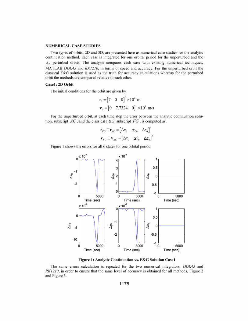
The initial conditions for the orbit are given by

� �

60

30

7 0 0 10 m

0 7.7324 0 10 m/s

T

T

� �

� �

r

v

For the unperturbed orbit, at each time step the error between the analytic continuation solu-tion, subscript AC , and the classical F&G, subscript FG , is computed as,

� �

0 0 0

0 0 0

TFG AC

TFG AC

x y z

x y z

� �

� �

r r

v v 0 0x y z0 00 x y zy0 000 0Tz

Figure 1 shows the errors for all 6 states for one orbital period.

Figure 1: Analytic Continuation vs. F&G Solution Case1

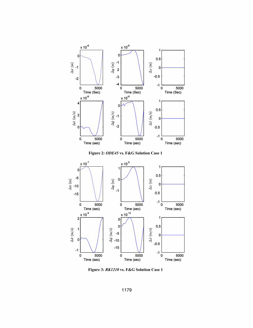
The same errors calculation is repeated for the two numerical integrators, ODE45 and RK1210, in order to ensure that the same level of accuracy is obtained for all methods, Figure 2 and Figure 3.

1179

Figure 2: ODE45 vs. F&G Solution Case 1

Figure 3: RK1210 vs. F&G Solution Case 1

1180

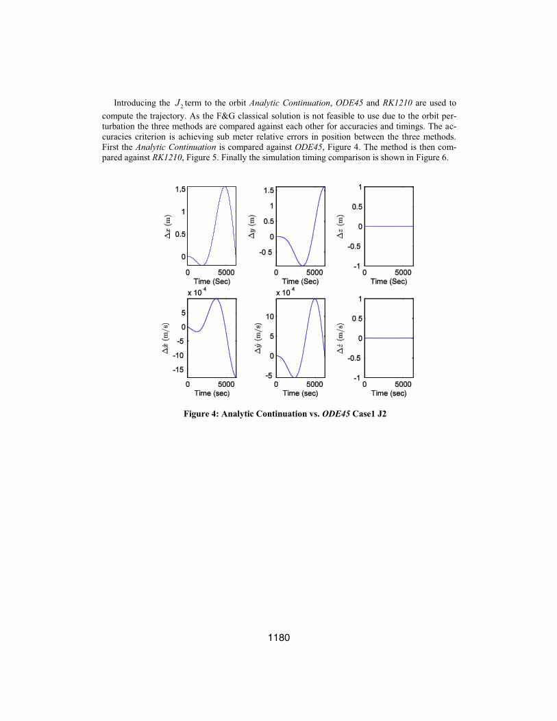
Introducing the 2J term to the orbit Analytic Continuation, ODE45 and RK1210 are used to compute the trajectory. As the F&G classical solution is not feasible to use due to the orbit per-turbation the three methods are compared against each other for accuracies and timings. The ac-curacies criterion is achieving sub meter relative errors in position between the three methods. First the Analytic Continuation is compared against ODE45, Figure 4. The method is then com-pared against RK1210, Figure 5. Finally the simulation timing comparison is shown in Figure 6.

Figure 4: Analytic Continuation vs. ODE45 Case1 J2

1181

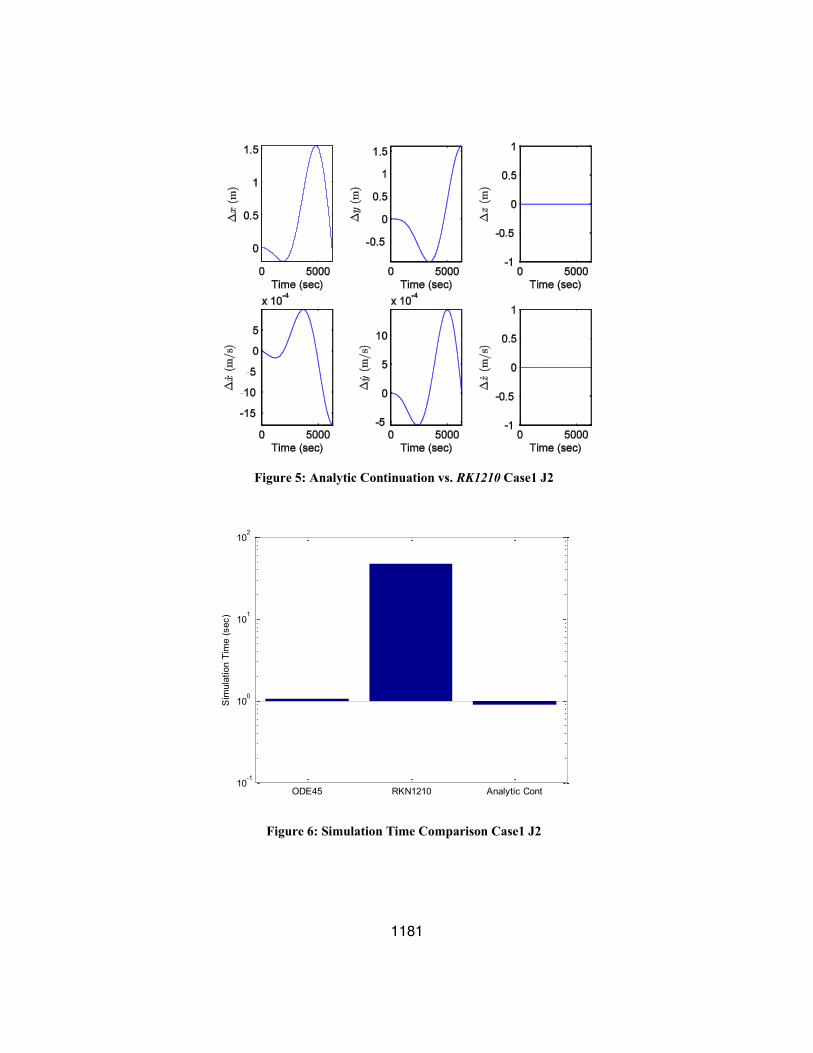
Figure 5: Analytic Continuation vs. RK1210 Case1 J2

ODE45 RKN1210 Analytic Cont10

-1

100

101

102

Sim

ulat

ion

Tim

e (s

ec)

Figure 6: Simulation Time Comparison Case1 J2

1182

For sub meter relative accuracies Analytic Continuation approach is again far more superior to RK1210, at least one order of magnitude, whereas it is slightly faster than ODE45, approximately 2X. For a fixed step size algorithm compared against highly optimized variable step size methods the speed up is quite significant and can be extended further by either introducing a variable step size technique or using parallel computing.

Case2: 3D Orbit

The initial conditions for the orbit are given by

� �

60

30

1.058 6.148 2.086 10 m

2.658 2.77 6.815 10 m/s

T

T

� � �

� � �

r

v

As in case1 for the unperturbed orbit the comparison against the classical F&G solution is shown in Figure 9.

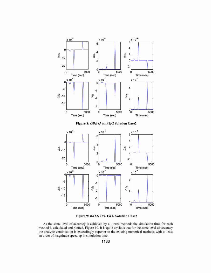
Figure 7: Analytic Continuation vs. F&G Solution Case2

The same errors calculation is repeated for the two numerical integrators, ODE45 and RK1210, used in order to ensure that the same level of accuracy is obtained for all method, Figure 8 and Figure 9.

1183

Figure 8: ODE45 vs. F&G Solution Case2

Figure 9: RK1210 vs. F&G Solution Case2

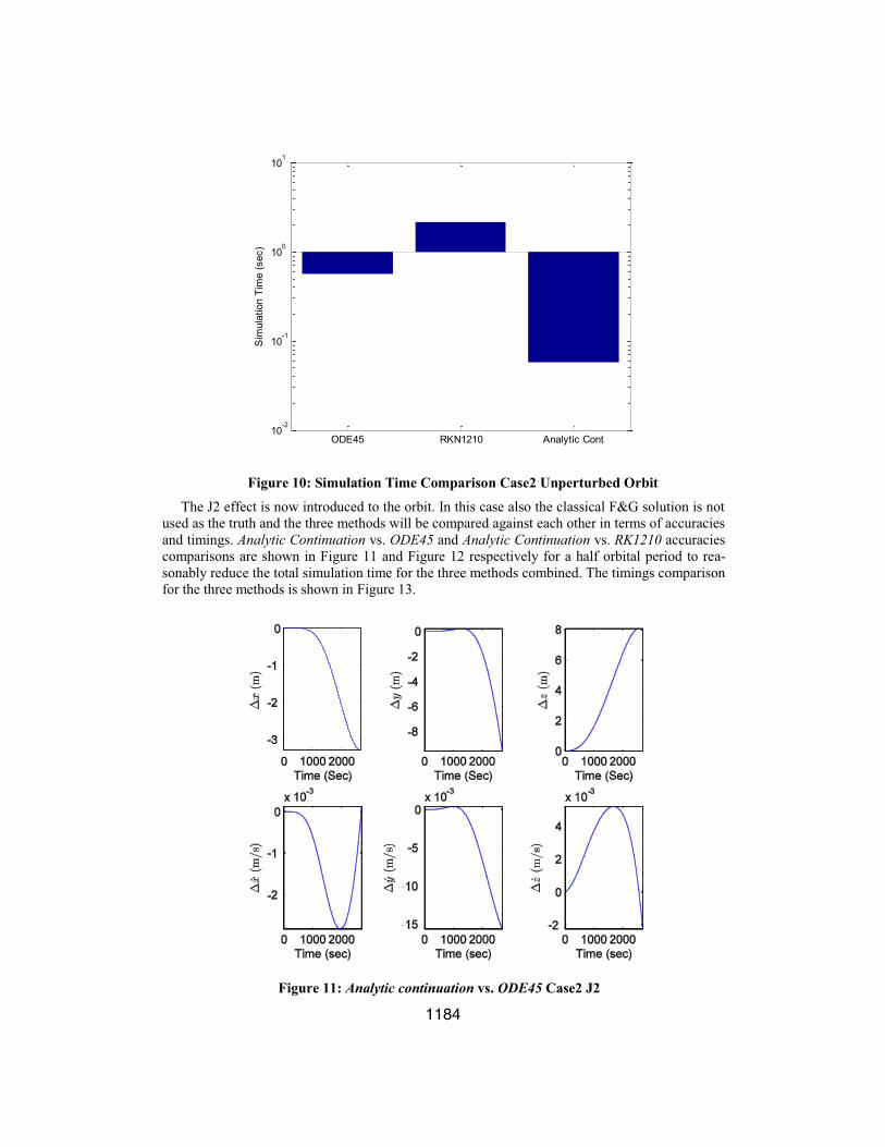
As the same level of accuracy is achieved by all three methods the simulation time for each method is calculated and plotted, Figure 10. It is quite obvious that for the same level of accuracy the analytic continuation is exceedingly superior to the existing numerical methods with at least an order of magnitude speed up in simulation time.

1184


-2

10-1

100

101

Sim

ulat

ion

Tim

e (s

ec)

Figure 10: Simulation Time Comparison Case2 Unperturbed Orbit

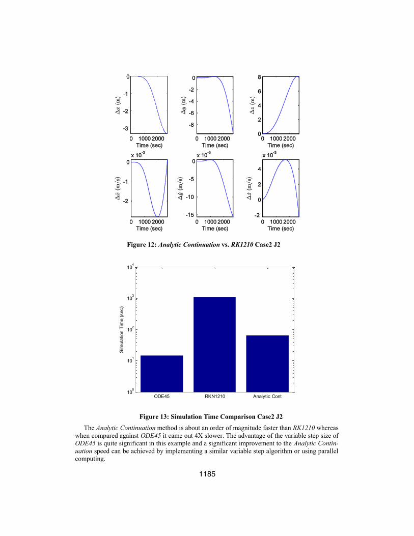
The J2 effect is now introduced to the orbit. In this case also the classical F&G solution is not used as the truth and the three methods will be compared against each other in terms of accuracies and timings. Analytic Continuation vs. ODE45 and Analytic Continuation vs. RK1210 accuracies comparisons are shown in Figure 11 and Figure 12 respectively for a half orbital period to rea-sonably reduce the total simulation time for the three methods combined. The timings comparison for the three methods is shown in Figure 13.

Figure 11: Analytic continuation vs. ODE45 Case2 J2

1185

Figure 12: Analytic Continuation vs. RK1210 Case2 J2


0

101

102

103

104

Sim

ulat

ion

Tim

e (s

ec)

Figure 13: Simulation Time Comparison Case2 J2

The Analytic Continuation method is about an order of magnitude faster than RK1210 whereas when compared against ODE45 it came out 4X slower. The advantage of the variable step size of ODE45 is quite significant in this example and a significant improvement to the Analytic Contin-uation speed can be achieved by implementing a similar variable step algorithm or using parallel computing.

1186

DISCUSSION AND CONCLUSION

The analytic continuation solution is extended to solve a broader case of problems to encom-pass the perturbed two-body problem for the Earth oblateness effects. This solution scheme can be easily extended to evaluate the higher perturbation harmonics as function of the predefined Lagrange-Like invariants. The speed and accuracy enabled by the power series solution is orders of magnitude better than the current standard numerical integrators in terms of speed while retain-ing the same accuracies.

The Analytic continuation solution technique is also used to derive the state transition tensors for the perturbed two body problem up to third order. Numerical results for perturbed and unper-turbed 2D and 3D orbits are presented. Accuracies and timings comparisons are shown against existing numerical methods, RK1210 and ODE45. For the same level of accuracy the Analytic Continuation method showed significant superiority in terms of speed over RK1210 whereas it produced very similar timings to the more optimized ODE45. As a future development variable step size can be introduced to the method and parallel computing can be easily implemented for more speed gains.

REFERENCES 1. Junkins, J. L., Majji, M., and Turner, J. D. “High Order Keplerian State Transition Tensors,”

In Proceedings of the F. Landis Markley Astronautics Symposium, 2008. AAS 08-270. 2. Lagrange, J. L. Mécanique Analytique. Paris: Gauthier-Villars, 1811.

3. Battin, R. H. An introduction to the mathematics and methods of astrodynamics, AIAA, 1999.

4. Turner, J. D., Elgohary, T., Majji, M., and Junkins, J. "High Accuracy Trajectory and Uncertainty Propogation Algorithm for Long-Term Asteroid Motion Prediction," Adventures on the interface of Mechanics and Control. Tech Science Press, 2012.

5. Elgohary, T., Turner, J. D., and Junkins, J. L. “High-Order Analytic Continuation and Numerical Stability Analysis for the Classical Two-Body Problem,” The Jer-Nan Juan Astrodynamics Symposium, 2012. AAS 12-639.

6. Brouwer, D., and Clemence, G. M. Methods of celestial mechanics, New York Academic Press, 1961 Vol. 1, 1961.

7. Hamilton, W. R. "On a general method in dynamics," Philosophical Transactions of the Royal Society Vol. 2, 1834, pp. 247-308.

8. Schaub, H., and Junkins, J. L. Analytical mechanics of space systems, AIAA, 2003.

1187

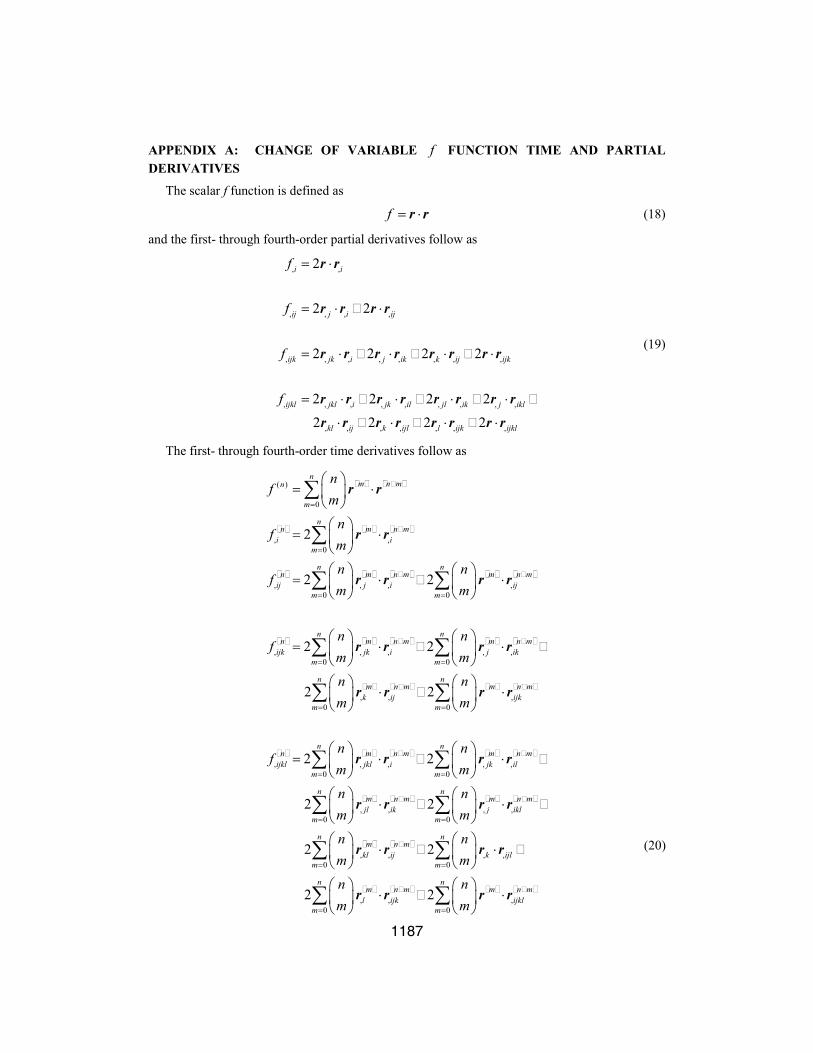
APPENDIX A: CHANGE OF VARIABLE f FUNCTION TIME AND PARTIAL DERIVATIVES

The scalar f function is defined as

f � �r r (18)

and the first- through fourth-order partial derivatives follow as

, ,

, , , ,

, , , , , , , ,

, , , , , , , , ,

, , , , , , ,

2

2 2

2 2 2 2

2 2 2 2

2 2 2 2

i i

ij j i ij

ijk jk i j ik k ij ijk

ijkl jkl i jk il jl ik j ikl

kl ij k ijl l ijk ijkl

f

f

f

f

� �

� � � �

� � � � � � � �

� � � � � � � � �

� � � � � � �

r r

r r r r

r r r r r r r r

r r r r r r r rr r r r r r r r

(19)

The first- through fourth-order time derivatives follow as

� � � �

� � � � � �

� � � � � � � � � �

� � � � � � � � � �

� � � �

( )

0

, ,0

, , , ,0 0

, , , , ,0 0

, ,0

2

2 2

2 2

2 2

nm n mn

m

nn m n m

i im

n nn m n m m n m

ij j i ijm m

n nn m n m m n m

ijk jk i j ikm m

nm n m

k ijm

nf

m

nf

m

n nf

m m

n nf

m m

n nm m

�

�

�

�

� �

� �

� �

� �

�

�

� ��

� ��

� ��

� � � ��

� � � ��

� � � ��

� ��

�

�

� �

� �

�

r r

r r

r r r r

r r r r

r r � � � �

� � � � � � � � � �

� � � � � � � �

� � � �

,0

, , , , ,0 0

, , , ,0 0

, , , ,0 0

2 2

2 2

2 2

2

nm n m

ijkm

n nn m n m m n m

ijkl jkl i jk ilm m

n nm n m m n mjl ik j ikl

m m

n nm n m

kl ij k ijlm m

n nf

m m

n nm m

n nm m

nm

�

�

� �

� �

� �

� �

�

� �

� ��

� �

� � � ��

� � � ��

� � � ��

� � � ��

�

� �

� �

� �

r r

r r r r

r r r r

r r r r

� � � � � � � �, , ,

0 02

n nm n m m n m

l ijk ijklm m

nm

� �

� �

� � ��

� � �� r r r r

(20)

1188

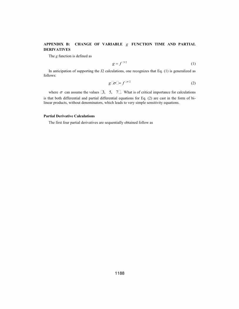
APPENDIX B: CHANGE OF VARIABLE g FUNCTION TIME AND PARTIAL DERIVATIVES

The g function is defined as 3/2g f �� (1)

In anticipation of supporting the J2 calculations, one recognizes that Eq. (1) is generalized as follows:

� � /2g f !! �� (2)

where ! can assume the values � �3, 5, 7 . What is of critical importance for calculations is that both differential and partial differential equations for Eq. (2) are cast in the form of bi-linear products, without denominators, which leads to very simple sensitivity equations.

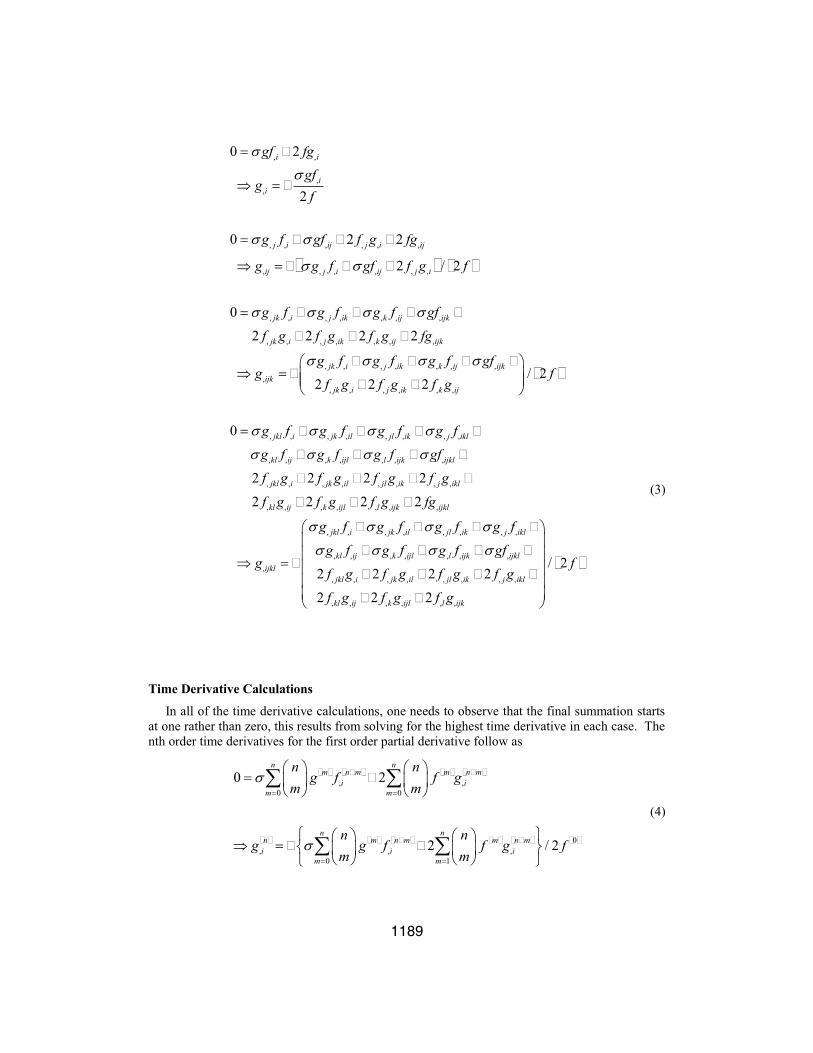
Partial Derivative Calculations

The first four partial derivatives are sequentially obtained follow as

1189

� � � �

, ,

,,

, , , , , ,

, , , , , ,

, , , , , , ,

, , , , , , ,

, , , , , , ,,

0 2

2

0 2 2

2 / 2

0

2 2 2 2

i i

ii

j i ij j i ij

ij j i ij j i

jk i j ik k ij ijk

jk i j ik k ij ijk

jk i j ik k ij iijk

gf fggf

gf

g f gf f g fg

g g f gf f g f

g f g f g f gff g f g f g fg

g f g f g f gfg

!

!

! !

! !

! ! ! !

! ! ! !

� �

� � �

� � � �

� � � � �

� � � � �

� � �

� � ��

, , , , , ,

, , , , , , , ,

, , , , , , ,

, , , , , , , ,

, , , , , , ,

/ 22 2 2

0

2 2 2 2

2 2 2 2

jk

jk i j ik k ij

jkl i jk il jl ik j ikl




ff g f g f g

g f g f g f g fg f g f g f gff g f g f g f gf g f g f g fg

! ! ! !

! ! ! !

��

� � � � �

� � � �

� � � �

� � �

� � �

, , , , , , , ,

, , , , , , ,,

, , , , , , , ,

, , , , , ,

/ 22 2 2 2

2 2 2


kl ij k ijl l ijk ijklijkl


kl ij k ijl l ijk

g f g f g f g fg f g f g f gf

g ff g f g f g f gf g f g f g

! ! ! !

! ! ! !

� � � ��

� � � ��

(3)

Time Derivative Calculations

In all of the time derivative calculations, one needs to observe that the final summation starts at one rather than zero, this results from solving for the highest time derivative in each case. The nth order time derivatives for the first order partial derivative follow as

� � � � � � � �

� � � � � � � � � � � �

, ,0 0

0, , ,

0 1

0 2

2 / 2

n nm n m m n m

i im m

n nn m n m m n mi i i

m m

n ng f f g

m m

n ng g f f g f

m m

!

!

� �

� �

� �

� �

� � � ��

� � � �

��

� � � ��

� �

� �

(4)

1190

The nth order time derivatives for the second order partial derivative follow as

� � � � � � � �

� � � � � � � �

� �

� � � � � � � �

� � � � � �

, , ,0 0

, . ,0 0

, , ,0 0

,

, . ,0 1

0

2 2

2 2

n nm n m m n mj i ij

m m

n nm n m m n m

j i ijm m

n nm n m m n mj i ij

m mnij n n

m n m mj i i

m m

n ng f g f

m m

n nf g f g

m m

n ng f g f

m mg

n nf g f g

m m

! !

! !

� �

� �

� �

� �

� �

� �

�

� �

� � � ��

� � � ��

��

� � � ��

� � � ��

��

� �

� �

� �

� � � �

� �0/ 2n mj

f�

��

(5)

The nth order time derivatives of the third order partial derivative follow as

� � � � � � � �

� � � � � � � �

� � � � � � � �

� � � � � �

, , , ,0 0

, , ,0 0

, , , ,0 0

, ,0 0

0

2 2

2 2

n nm n m m n mjk i j ik

m m

n nm n m m n mk ij ijk

m m

n nm n m m n m

jk i j ikm m

n nm n m m

k ijm m

n ng f g f

m m

n ng f g f

m m

n nf g f g

m m

n nf g f g

m m

! !

! !

� �

� �

� �

� �

� �

� �

�

� �

� � � ��

� � � ��

� ��

� ��

��

� �

� �

� �

� � � �

� �

� � � � � � � �

� � � � � � � �

� � � � � � � �

� �

,

, , , ,0 0

, , ,0 0

,

, , , ,0 0

, ,0

2

n mijk

n nm n m m n mjk i j ik

m m

n nm n m m n mk ij ijk

m mnijk

n nm n m m n m

jk i j ikm m

nm

km

n ng f g f

m m

n ng f g f

m mg

n nf g f g

m m

nf g

m

!

�

� �

� �

� �

� �

� �

� �

�

� ��

� � � ��

� ��

� �

� �

� �

� � � � � � �

� �0

,1

/ 2

nn m m n mij ijk

m

f

nf g

m� �

�

��

� ��

� (6)

The nth order time derivatives for the four-order partial derivative are given by

1191

� � � � � � � � � � � � � � � �

� � � � � � � � � � � �

, , , , , , , ,0 0 0 0

, , , , , ,0 0 0

0n n n n

m n m m n m m n m m n mjkl i jk il jl ik j ikl

m m m m

n n nm n m m n m m n mkl ij k ijl l ijk

m m m

n n n ng f g f g f g f

m m m m

n n n ng f g f g f

m m m m

! ! ! !

! ! ! !

� � � �

� � � �

� � �

� � �

� � � � � � � ��

� � � � � � � ��

� � ��

� � � �

� � � � � � �

� � � � � � � � � �

� � � � � � � � � � � �

,0

, , , , , , , ,0 0 0 0

, , , , , ,0 0 0

2 2 2 2

2 2 2 2

nm n m

ijlkm

n n n nm n m m m n m

jkl i jk il jl ik j iklm m m m

n n nm n m m n m m n m

kl ij k ijl l ijkm m m

g f

n n n nf g f g f g f g

m m m m

n n nf g f g f g

m m m

�

�

� �

� � � �

� � �

� � �

�

� � � � � � � ��

� � � � � � � ��

� � ��

�

� � � �

� � � � � � �

� �

� � � � � � � �

� � � � � � � �

� � � � � � � �

,1

, , , ,0 0

, , , ,0 0

, , , ,0 0

,

nm n m

ijklm

n nm n m m n mjkl i jk il

m m

n nm n m m n mjl ik j ikl

m m

n nm n m m n mkl ij k ijl

m m

mnijkl

nf g

m

n ng f g f

m m

n ng f g f

m m

n ng f g f

m m

nm

g

!

�

�

� �

� �

� �

� �

� �

� �

� ��

� � � ��

� � � ��

� ��

� ��

� � �

�

� �

� �

� �

� � � � � � � �

� � � � � � � �

� � � � � � � �

� � � �

, , ,0 0

, , , ,0 0

, , , ,0 0

, ,0

2

n nm n m m n ml ijk ijlk

m

n nm n m m n m

jkl i jk ilm m

n nm n m m n m

jl ik j iklm m

nm n m

kl ijm

ng f g f

m

n nf g f g

m m

n nf g f g

m m

n nf g

m

� �

� �

� �

� �

� �

� �

�

�

� ��

��

� � ��

� � � ��

� � � ��

� ��

��

� �

� �

� �

� � � � �

� � � � � � � �

� �0

, ,0

, , ,0 1

/ 2

nm n m

k ijlm

n nm n m m n m

l ijk ijklm m

f

f gm

n nf g f g

m m

�

�

� �

� �

��

� ��

�

� � (7)

1192

APPENDIX C: TRANSFORMATIONAL VARIABLES FOR J2 TRAJECTORY AND STATE TRANSITION TENSOR CALCULATIONS.

Four variables need to be introduced to allow the binomial form of Leibnitz product rule to be used for generating arbitrary order time and partial derivative models. Leibnitz product rule is used to assemble arbitrary order time derivative models for products of variables. The resulting mathematical identities are very simple to derive and code, and the basic algorithm scales to more complicated problems. The resulting algorithms are ideally suited for massive parallel implemen-tations.

Step 1: Simplify the z*z term

Variable Definition:

2 *z z z�

Arbitrary Order Time Derivative:

� � � � � �

0

2n

n m n m

m

nz z z

m�

�

� ��

� ��

Partial Derivatives and Arbitrary Order Time Derivatives:

� � � � � � � � � ��

� ��

� � � � � � � � � � � �

, , ,0

, , , , , , ,0

, , , , , , ,,

0 , , , , , ,

2

2

2

nn m n m m n mi i i

m

nn m n m m n m m n m m n mij ij i j j i ij

m

m n m m n m m n m m n mnijk ij k ik j i jkn

ijk m n m m n m m n mm jk i j ik k ij

nz z z z z

m

nz z z z z z z z z

m

z z z z z z z znz

m z z z z z z

� �

�

� � � �

�

� � � �

� � ��

� ��

� ��

� � � ��

� � � ��

� ��

�

�

� � � � �,

m n mijkz z �

� ��

(1)

Step 2: Simplify the z*z*x term:


2 * *z x z z x�


� � � � � �

0

2 2n

n m n m

m

nz x z x

m�

�

� ��

� ��


1193

� � � � � � � � � ��

� ��

� � � � � �

, , ,0

, , , , , , ,0

, , , , , , ,,

0 , , , ,

2 2 2

2 2 2 2 2

2 2 2 22

2 2

nn m n m m n mi i i

m


m


ijk m n m mm jk i j ik

nz x z x z x

m

nz x z x z x z x z x

m

z x z x z x z xnz x

m z x z x

� �

�

� � � �

�

� � � �

��

� ��

� ��

� � � ��

� � � ��

��

�

�

� � � � � � � � � � �, , ,2 2n m m n m m n mk ij ijkz x z x� � �

� ��

Step 3: Simplify the z*z*y term:


2 * *z y z z y�


� � � � � �

0

2 2n

n m n m

m

nz y z y

m�

�

� ��

� ��


� � � � � � � � � ��

� ��

� � � � � �

, , ,0

, , , , , , ,0

, , , , , , ,,

0 , , , ,

2 2 2

2 2 2 2 2

2 2 2 22

2 2

nn m n m m n mi i i

m


m


ijk m n m mm jk i j ik

nz y z y z y

m

nz y z y z y z y z y

m

z y z y z y z ynz y

m z y z y

� �

�

� � � �

�

� � � �

��

� ��

� ��

� � � ��

� � � ��

��

�

�

� � � � � � � � � � �, , ,2 2n m m n m m n mk ij ijkz y z y� � �

� ��

Step 4: Simplify the z*z*z term:


3 2*zz z�


� � � � � �

0

3 2n

n m n m

m

nz z z

m�

�

� ��

� ��


1194

� � � � � � � � � ��

� ��

� � � � � � � �

, , ,0

, , , , , , ,0

, , , , , , ,,

0 , , , ,

3 2 2

3 2 2 2 2

2 2 2 23

2 2

nn m n m m n mi i i

m


m


ijk m n m m n mm jk i j ik

nz z z z z

m

nz z z z z z z z z

m

z z z z z z z znz

m z z z z

� �

�

� � � �

�

� � � �

� ��

� ��

� ��

� � � ��

� � � ��

��

�

�

� � � � � � � � �, , ,2 2m n m m n mk ij ijkz z z z� �

� ��

Elgohary, Tarek A. and Turner, James D. (2014), "State Transition Tensor Models for the Uncertainty...

Documents

Transcript of Elgohary, Tarek A. and Turner, James D. (2014), "State Transition Tensor Models for the Uncertainty...