Appendix AElements of the Matrices for OpenholeLogging and for Logging-While-Drilling

A.1 Openhole Logging

Assuming the radius of the borehole is a. Elements in [mij]4×4 in Eq. 2.15 for theopenhole case are,

m11 = −[ na In( f a) + f In+1( f a)

], m12 = n

a Kn(pa) − pKn+1(pa),

m13 = na Kn(sa), m14 = ikz

[ na Kn(sa) − sKn+1(sa)

],

m21 = ρ f ω2 In( f a), m22 =

μ{[

2n(n−1)a2

+ 2k2z − k2s]Kn(pa) + 2p

a Kn+1(pa)},

m23 =2μ n

a

[ n−1a Kn(sa) − sKn+1(sa)

],

m24 = 2ikzμ{[

n(n−1)a2

+ s2]Kn(sa) + s

a Kn+1(sa)},

m32 =2μ n

a

[− n−1a Kn(pa) + pKn+1(pa)

],

m33 = μ{−

[2n(n−1)

a2+ s2

]Kn(sa) − 2s

a Kn+1(sa)},

m34 =2ikzμ n

a

[ 1−na Kn(sa) + sKn+1(sa)

],

m42 = 2ikzμ[ na Kn(pa) − pKn+1(pa)

],

m43 = ikzμ na Kn(sa), m44 = μ

(k2s − 2k2z

)[ na Kn(sa) − sKn+1(sa)

].

Elements not listed are zero.

© Springer Nature Switzerland AG 2020H. Wang et al., Borehole Acoustic Logging—Theory and Methods,Petroleum Engineering, https://doi.org/10.1007/978-3-030-51423-5

265

266 Appendix A: Elements of the Matrices for Openhole Logging …

Nomenclature

a Borehole radius

n The order of the multipole source, 0 for monopole, 1 for dipole, and so on

I, K Bessel functions of the first kind and second kind, respectively

kz Axial wavenumber

kf Wavenumber of the fluid, kf = ω/V f

kp Wavenumber of the P-wave in the collar, kp = ω/Vp

ks Wavenumber of the S-wave in the collar, ks = ω/Vs

f Radial wavenumber in the fluid, f =√k2z − k2f

p Radial wavenumber of the P-wave in the collar, p =√k2z − k2p

s Radial wavenumber of the S-wave in the collar, s =√k2z − k2s

ρf Fluid density

ω Angular frequency

μ Shear modulus of the formation

A.2 Acoustic Logging-While-Drilling

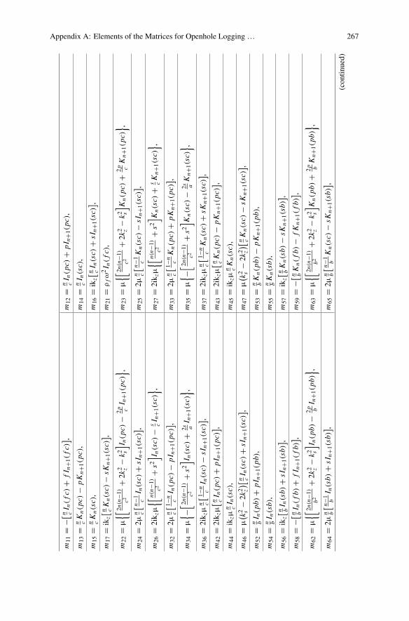
The elements of [mij]12×12 in Eq. 5.2 are listed as follows, where a and b are inner andouter radii of the collar, and c is the borehole radius. Coefficient n designates differentsource configurations, where n = 0, 1, 2, 3 are monopole, dipole, quadrupole, andhexapole, respectively. Definitions of other terms follow the equations.

Appendix A: Elements of the Matrices for Openhole Logging … 267

m11

=−[ n c

I n(fc

)+

fI n

+1(fc

)] ,m

12=

n cI n

(pc

)+

pI n

+1(pc

),

m13

=n cKn(pc

)−

pKn+

1(pc

),m

14=

n cI n

(sc ),

m15

=n cKn(sc ),

m16

=ik

z[ n cI n

(sc )

+sI

n+1(sc )

] ,

m17

=ik

z[ n cKn(sc )

−sK

n+1(sc )

] ,m

21=

ρfω2I n

(fc

),

m22

=μ

{[2n

(n−1

)

c2+

2k2 z−

k2 s

] I n(pc

)−

2p cI n

+1(pc

)} ,m

23=

μ{[

2n(n

−1)

c2+

2k2 z−

k2 s

] Kn(pc

)+

2p cKn+

1(pc

)} ,

m24

=2μ

n c

[ n−1 c

I n(sc )

+sI

n+1(sc )

] ,m

25=

2μn c

[ n−1 c

Kn(sc )

−sI

n+1(sc )

] ,

m26

=2ik z

μ{[

n (n−

1 )c2

+s2

] I n(sc )

−s cI n

+1(sc )

} ,m

27=

2ik z

μ{[

n (n−

1 )c2

+s2

] Kn(sc )

+s cKn+

1(sc )

} ,

m32

=2μ

n c

[ 1−n c

I n(pc

)−

pI n

+1(pc

)] ,m

33=

2μn c

[ 1−n c

Kn(pc

)+

pKn+

1(pc

)] ,

m34

=μ

{ −[2n

(n−1

)

c2+

s2] I n

(sc )

+2s aI n

+1(sc )

} ,m

35=

μ{ −[

2n(n

−1)

c2+

s2] K

n(sc )

−2s aKn+

1(sc )

} ,

m36

=2ik z

μn c

[ 1−n c

I n(sc )

−sI

n+1(sc )

] ,m

37=

2ik z

μn c

[ 1−n c

Kn(sc )

+sK

n+1(sc )

] ,

m42

=2ik z

μ[ n c

I n(pc

)+

pI n

+1(pc

)] ,m

43=

2ik z

μ[ n c

Kn(pc

)−

pKn+

1(pc

)] ,

m44

=ik

zμn cI n

(sc ),

m45

=ik

zμn cKn(sc ),

m46

=μ

( k2 s−

2k2 z

)[n cI n

(sc )

+sI

n+1(sc )

] ,m

47=

μ( k2 s

−2k

2 z

)[n cKn(sc )

−sK

n+1(sc )

] ,

m52

=n bI n

(pb

)+

pI n

+1(pb

),m

53=

n bKn(pb

)−

pKn+

1(pb

),

m54

=n bI n

(sb ),

m55

=n bKn(sb ),

m56

=ik

z[ n bI n

(sb )

+sI

n+1(sb )

] ,m

57=

ikz[ n b

Kn(sb )

−sK

n+1(sb )

] ,

m58

=−[ n b

I n(fb

)+

fI n

+1(fb

)] ,m

59=

−[ n bKn(fb

)−

fKn+

1(fb

)] ,

m62

=μ

{[2n

(n−1

)

b2+

2k2 z−

k2 s

] I n(pb

)−

2p bI n

+1(pb

)} ,m

63=

μ{[

2n(n

−1)

b2+

2k2 z−

k2 s

] Kn(pb

)+

2p bKn+

1(pb

)} ,

m64

=2μ

n b

[ n−1 b

I n(sb )

+sI

n+1(sb )

] ,m

65=

2μn b

[ n−1 b

Kn(sc )

−sK

n+1(sb )

] ,

(contin

ued)

268 Appendix A: Elements of the Matrices for Openhole Logging …

(contin

ued)

m66

=2ik z

μ{[

n (n−

1 )b2

+s2

] I n(sb )

−s bI n

+1(sb )

} ,m

67=

2ik z

μ{[

n (n−

1 )b2

+s2

] Kn(sb )

+s bKn+

1(sb )

} ,

m68

=ρfω2I n

(fb

),m

69=

ρfω2Kn(fb

),

m72

=2μ

n b

[ 1−n b

I n(pb

)−

pI n

+1(pb

)] ,m

73=

2μn b

[ 1−n b

Kn(pb

)+

pKn+

1(pb

)] ,

m74

=μ

{[−2

n (n−

1 )b2

−s2

] I n(sb )

+2s bI n

+1(sb )

} ,m

75=

μ{[

−2n (n−

1 )b2

−s2

] Kn(sb )

−2s bKn+

1(sb )

} ,

m76

=2ik z

μn b

[ 1−n b

I n(sb )

−sI

n+1(sb )

] ,m

77=

2ik z

μn b

[ 1−n b

Kn(sb )

+sK

n+1(sb )

] ,

m82

=2ik z

μ[ n b

I n(pb

)+

pI n

+1(pb

)] ,m

83=

2ik z

μ[ n b

Kn(pb

)−

pKn+

1(pb

)] ,

m84

=ik

zμn bI n

(sb ),

m85

=ik

zμn bKn(sb ),

m86

=μ

( k2 s−

2k2 z

)[n bI n

(sb )

+sI

n+1(sb )

] ,m

87=

μ( k2 s

−2k

2 z

)[n bKn(sb )

−sK

n+1(sb )

] ,

m98

=−[ n a

I n(fa

)+

fI n

+1(fa

)] ,m

99=

−[ n aKn(fa

)−

fKn+

1(fa

)] ,

m91

0=

n aKn( pt

a)−

ptKn+

1( pt

a) ,m

911

=n aKn( st

a) ,

m91

2=

ikzμ

[ n aKn( st

a)−

stKn+

1( st

a)],

m10

8=

ρfω2I n

(fa

),

m10

9=

ρfω2Kn(fa

),m

1010

=μt{[

2n(n

−1)

a2+

2k2 z−

k2 s

] Kn( pt

a)+

2pt aKn+

1( pt

a)},

m10

11=

2μtn a

[ n−1 a

Kn( st

a)−

stKn+

1( st

a)],

m10

12=

2ik z

μt{[

n (n−

1 )a2

+st

2] K

n( st

a)+

st aKn+

1( st

a)},

m11

10=

2μtn a

[ 1−n a

Kn( pt

a)+

ptKn+

1( pt

a)],

m11

11=

μt{[

2n(1

−n)

a−

st2] K

n( st

a)−

2st

aKn+

1( st

a)},

m11

12=

2ik z

μtn a

[1−

na

Kn( st

a)+

st aKn+

1( st

a)],

m12

10=

2ik z

μt[

n aKn( pt

a)−

ptKn+

1( pt

a)],

m12

11=

ikzμ

tn aKn( st

a) ,m

1212

=μt( kt

2 s−

2k2 z

) [n aKn( st

a)−

stKn+

1( st

a)].

Appendix A: Elements of the Matrices for Openhole Logging … 269

Elements not listed are zero.

Nomenclature

a Borehole radius

b Outer radius of the collar

c Inner radius of the collar

n The order of the multipole source, 0 for monopole, 1 for dipole, and so on

I, K Bessel functions of the first kind and second kind, respectively

kz Arial Wavenumber

kf Wavenumber of the fluid, kf = ω/V f

kp Wavenumber of the P-wave in the collar, kp = ω/Vp

ks Wavenumber of the S-wave in the collar, ks = ω/Vs

ktp Wavenumber of the P-wave in the formation, ktp = ω/V tp

kts Wavenumber of the S-wave in the formation, kts = ω/V ts

f Radial wavenumber in the fluid, f =√k2z − k2f

p Radial wavenumber of the P-wave in the collar, p =√k2z − k2p

s Radial wavenumber of the S-wave in the collar, s =√k2z − k2s

pt Radial wavenumber of the formation P-wave, pt =√k2z − kt2p

st Radial wavenumber of the formation S-wave, st =√k2z − kt2s

ρf Fluid density

ω Angular frequency

μ Shear modulus of the collar

μt Shear modulus of the formation

Appendix BFinite Difference Method

B.1 Differencing Scheme

The essence of finite difference (FD) is to replace the derivatives in the partial differ-ential equation with differences. A number of finite difference schemes, such asstaggered grid (Virieux 1986), rotated grid (Saenger and Bohlen 2004), and Lebedevformat (Lisitsa and Vishnevskiy 2010), may be used in wave equation simulation.The staggered grid is by far the most widely used scheme, and it will be used in thisbook for borehole acoustic/seismic wave propagation.

The time domain wave equation in a linear elastic medium can be expressed by,

ρ∂2

∂t2ui = τi j, j , (B.1)

τi j = Ci jklεkl, (B.2)

εi j = (ui, j + u j,i

)/2, (B.3)

where ρ is the medium density, and τ ij is the stress tensor. ui is the displacementvector. εij is the strain tensor. Cijkl is the stiffness tensor.

If the medium is isotropic,

Ci jkl = λδi jδkl + μ(δikδ jl + δilδ jk

), (B.4)

where λ and μ are Lamé constants and δi j ={

1 i = j0 i �= j

.

The staggered grid scheme was originally designed for first-order elastic waveequations. The second-order elastic wave Eqs. B.1–B.3 can be reduced to first-orderby replacing the first-order time derivate of the particle displacement with the particlevelocity as follows,

© Springer Nature Switzerland AG 2020H. Wang et al., Borehole Acoustic Logging—Theory and Methods,Petroleum Engineering, https://doi.org/10.1007/978-3-030-51423-5

271

272 Appendix B: Finite Difference Method

∂v∂t

= 1

ρ∇ · τ, (B.5a)

∂τ

∂t= c : [∇v + (∇v)T

], (B.5b)

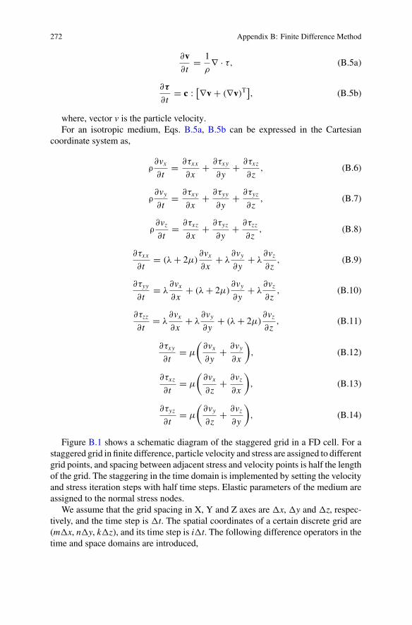
where, vector v is the particle velocity.For an isotropic medium, Eqs. B.5a, B.5b can be expressed in the Cartesian

coordinate system as,

ρ∂vx∂t

= ∂τxx

∂x+ ∂τxy

∂y+ ∂τxz

∂z, (B.6)

ρ∂vy∂t

= ∂τxy

∂x+ ∂τyy

∂y+ ∂τyz

∂z, (B.7)

ρ∂vz∂t

= ∂τxz

∂x+ ∂τyz

∂y+ ∂τzz

∂z, (B.8)

∂τxx

∂t= (λ + 2μ)

∂vx∂x

+ λ∂vy∂y

+ λ∂vz∂z

, (B.9)

∂τyy

∂t= λ

∂vx∂x

+ (λ + 2μ)∂vy∂y

+ λ∂vz∂z

, (B.10)

∂τzz

∂t= λ

∂vx∂x

+ λ∂vy∂y

+ (λ + 2μ)∂vz∂z

, (B.11)

∂τxy

∂t= μ

(∂vx∂y

+ ∂vy∂x

), (B.12)

∂τxz

∂t= μ

(∂vx∂z

+ ∂vz∂x

), (B.13)

∂τyz

∂t= μ

(∂vy∂z

+ ∂vz∂y

), (B.14)

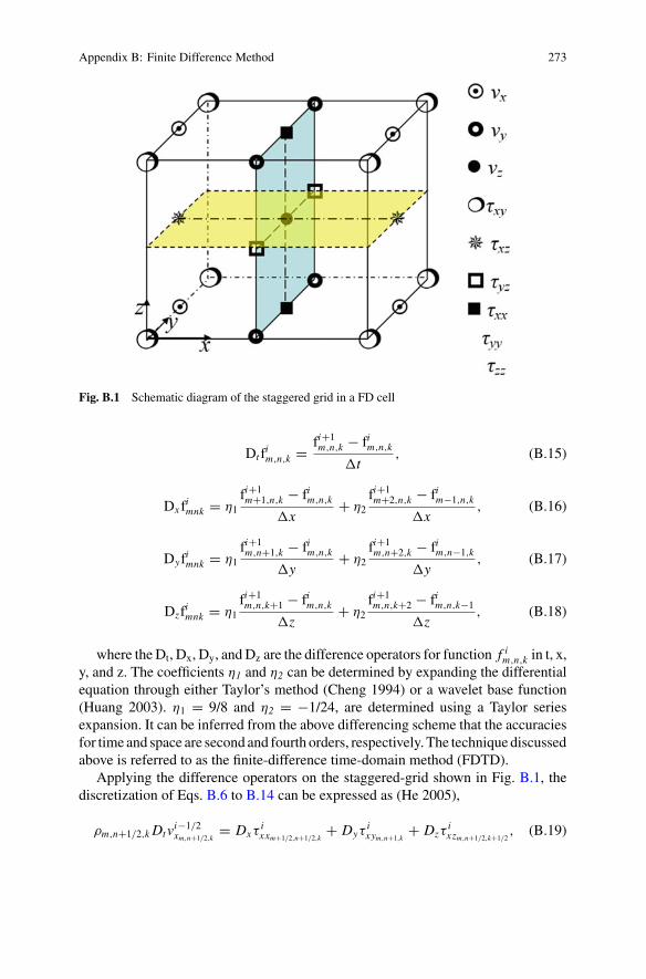
Figure B.1 shows a schematic diagram of the staggered grid in a FD cell. For astaggered grid in finite difference, particle velocity and stress are assigned to differentgrid points, and spacing between adjacent stress and velocity points is half the lengthof the grid. The staggering in the time domain is implemented by setting the velocityand stress iteration steps with half time steps. Elastic parameters of the medium areassigned to the normal stress nodes.

We assume that the grid spacing in X, Y and Z axes are x, y and z, respec-tively, and the time step is t. The spatial coordinates of a certain discrete grid are(mx, ny, kz), and its time step is it. The following difference operators in thetime and space domains are introduced,

Appendix B: Finite Difference Method 273

Fig. B.1 Schematic diagram of the staggered grid in a FD cell

Dt fim,n,k = fi+1

m,n,k − fim,n,k

t, (B.15)

Dx fimnk = η1

fi+1m+1,n,k − fim,n,k

x+ η2

fi+1m+2,n,k − fim−1,n,k

x, (B.16)

Dyfimnk = η1

fi+1m,n+1,k − fim,n,k

y+ η2

fi+1m,n+2,k − fim,n−1,k

y, (B.17)

Dzfimnk = η1

fi+1m,n,k+1 − fim,n,k

z+ η2

fi+1m,n,k+2 − fim,n,k−1

z, (B.18)

where the Dt, Dx, Dy, andDz are the difference operators for function f im,n,k in t, x,y, and z. The coefficients η1 and η2 can be determined by expanding the differentialequation through either Taylor’s method (Cheng 1994) or a wavelet base function(Huang 2003). η1 = 9/8 and η2 = −1/24, are determined using a Taylor seriesexpansion. It can be inferred from the above differencing scheme that the accuraciesfor time and space are second and fourth orders, respectively. The technique discussedabove is referred to as the finite-difference time-domain method (FDTD).

Applying the difference operators on the staggered-grid shown in Fig. B.1, thediscretization of Eqs. B.6 to B.14 can be expressed as (He 2005),

ρm,n+1/2,k Dtvi−1/2xm,n+1/2,k

= Dxτixxm+1/2,n+1/2,k

+ Dyτixym,n+1,k

+ Dzτixzm,n+1/2,k+1/2

, (B.19)

274 Appendix B: Finite Difference Method

ρm+1/2,n,k Dtvi−1/2ym+1/2,n,k

= Dxτixym+1,n,k

+ Dyτiyym+1/2,n+1/2,k

+ Dzτiyzm+1/2,n,k+1/2

, (B.20)

ρm+ 12 ,n+ 1

2 ,k+ 12Dtv

i−1/2zm+ 1

2 ,n+ 12 ,k+ 1

2

= Dxτixz

m+1,n+ 12 ,k+ 1

2

+ Dyτiyz

m+ 12 ,n+1,k+ 1

2

+ Dzτizz

m+ 12 ,n+ 1

2 ,k+1,

(B.21)

Dtτixx

m+ 12 ,n+ 1

2 ,k= (λ + 2μ)m+ 1

2 ,n+ 12 ,k Dxv

i+1/2xm+1,n+ 1

2 ,k+ λm+ 1

2 ,n+ 12 ,k Dyv

i+1/2ym+ 1

2 ,n+1,k

+ λm+ 12 ,n+ 1

2 ,k Dzvi+1/2zm+ 1

2 ,n+ 12 ,k+ 1

2

, (B.22)

Dtτiyy

m+ 12 ,n+ 1

2 ,k= λm+ 1

2 ,n+ 12 ,k Dxv

i+1/2xm+1,n+ 1

2 ,k+ (λ + 2μ)m+ 1

2 ,n+ 12 ,k Dyv

i+1/2ym+ 1

2 ,n+1,k

+ λm+ 12 ,n+ 1

2 ,k Dzvi+1/2zm+ 1

2 ,n+ 12 ,k+ 1

2

, (B.23)

Dtτizz

m+ 12 ,n+ 1

2 ,k= λm+ 1

2 ,n+ 12 ,k Dxv

i+1/2xm+1,n+ 1

2 ,k+ λm+ 1

2 ,n+ 12 ,k Dyv

i+1/2ym+ 1

2 ,n+1,k

+ (λ + 2μ)m+ 12 ,n+ 1

2 ,k Dzvi+1/2zm+ 1

2 ,n+ 12 ,k+ 1

2

, (B.24)

Dtτixzm,n+1/2,k+1/2

= μm,n+1/2,k+1/2

(Dzv

i+1/2xm,n+1/2,k+1

+ Dxvi+1/2zm+1/2,n+1/2,k+1/2

), (B.25)

Dtτiyzm+1/2,n,k+1/2

= μm+1/2,n,k+1/2

(Dzv

i+1/2ym+1/2,n,k+1

+ Dyvi+1/2zm+1/2,n+1/2,k+1/2

), (B.26)

Dtτixym,n,k

= μm,n,k

(Dyv

i+1/2xm,n+1/2,k+1

+ Dxvi+1/2ym+1/2,n,k

), (B.27)

ρm,n+1/2,k =(ρm+ 1

2 ,n+ 12 ,k + ρm− 1

2 ,n+ 12 ,k

)/2, (B.28)

ρm+1/2,n,k =(ρm+ 1

2 ,n+ 12 ,k + ρm+ 1

2 ,n− 12 ,k

)/2, (B.29)

ρm+1/2,n+1/2,k+1/2 =(ρm+ 1

2 ,n+ 12 ,k+1 + ρm+ 1

2 ,n+ 12 ,k

)/2, (B.30)

4

μm,n,k= 1

μm+1/2,n+1/2,k+ 1

μm−1/2,n+1/2,k

+ 1

μm+1/2,n−1/2,k+ 1

μm−1/2,n−1/2,k

, (B.31)

4

μm,n+1/2,k+1/2= 1

μm+1/2,n+1/2,k+ 1

μm+1/2,n+1/2,k+1

+ 1

μm−1/2,n+1/2,k+ 1

μm−1/2,n+1/2,k+1, (B.32)

4

μm+1/2,n,k+1/2= 1

μm+1/2,n+1/2,k+ 1

μm+1/2,n+1/2,k+1

+ 1

μm+1/2,n−1/2,k+ 1

μm+1/2,n−1/2,k+1, (B.33)

Appendix B: Finite Difference Method 275

The explicit difference scheme in Eqs. B.19–B.33 can be iteratively solved and isvery suitable for parallel computation.

The source is implemented by assigning the source time function at normal stressnodes (Coutant et al. 1995).

B.2 Dispersion and Stability Analysis

The essence of numerical simulation for the wave equation using the finite differencemethod is to discretize the continuous media to obtain a numerical solution. Thisgenerates numerical dispersion. Cheng (1994) suggested that at least 6–10 grids areused per wave length to avoid numerical dispersion in staggered grid finite differencesimulation.

Because the staggered grid finite difference in the time domain is explicit, certainstability conditions should be satisfied to ensure the convergence of the computationresults. Assuming Vmax is the maximum velocity for all the grids in the medium, thestability condition (Courant et al. 1967) on the discrete time and spatial steps shouldsatisfy the following relationship,

t <min(x,y,z)√3Vmax(|η1|+|η2|)

. (B.34)

B.3 Absorbing Boundary Conditions

The numerical solution of the physical problems usually involves the solution inan infinite domain as shown in Fig. B.2a, although the region of the interest isfinite. Some problems can be treated by some simple solution. For example, for aperiodic problem, a simple coordinate transformation from infinite domain (−∞,∞)to finite domain, such as (−1, 1), can be used. In most applications, including seismicwave propagation, the infinite space is usually truncated into a limited computationaldomain (as shown in Fig. B.2b). The numerical FDTD implementations includeboundaries that inevitably bring reflected energy back into the computational domain,that reflected energy contaminates the signal.

Manymethods have been developed to avoid the artificial reflections from compu-tational domain boundaries: nonreflecting plane boundary condition (Smith 1974),absorbing boundary conditions (ABCs) (Clayton and Engquist 1977; Higdon 1990),absorbing boundary layers (Cerjan et al. 1985), and transparent boundary (Zhu 1999).The most commonly used method is the perfectly matched layer (PML) (Berenger1994) that was initially developed for Maxwell’s equation. The idea of PML is toadd layers of absorbing material outside of the computational domain (as shown inFig. B.2). This material exponentially attenuates the incident energy and attenuates

276 Appendix B: Finite Difference Method

Fig. B.2 The effect of artificial boundary (Fig. 1 in Johnson [2007])

it again when it is reflected back from the outer boundary of the PML. If the layer islarge enough, the energy will be absorbed completely in the layer.

PML was introduced into seismic wave propagation simulation by Collino andTsogka (2001) and to borehole wave propagation by Wang et al. (2009, 2013a).The PML method later evolved into several different types from field-splitting PML(SPML) (Berenger 1994; Collino and Tsogka 2001) to complex frequency shiftedPML (CFS-PML) (Kuzuoglu and Mittra 1996; Komatitsch and Martin 2007). In thisbook, the CFS-PMLmethod is included in the FDTD to simulate the acoustic/seismicwave propagation in the borehole environment.

In the PMLmethod, a complex stretch factor Sj = β+d j/(α + iω) is used (Rodenand Gendney 2000) to stretch the original coordinate in the j direction in the PMLregion by jSj, where j can be x, y, or z in the Cartesian coordinate system, and α and β

are frequency-shifted factor and scaling factor, respectively. dj is a damping function,dJ = ∂γ j/∂j (γ j > 0), which is the function of space in the j direction. ω is angularfrequency. Assuming that the planewave solution of thewave equations B.5a, B.5b isexp

[−i∑

k j j], the solution can be transformed as exp

[−i∑

k j j]exp

[−∑k jγ j/ω

],

if α and β are 0 and 1, respectively (Chew and Weedon 1994; Chew and Liu 1996).In such a configuration, the incident plane wave along the j direction can be expo-nentially attenuated in the PML region (Fig. B.3d). To implement this product in thetime domain requires a convolution, which is computationally expensive.

Fig. B.3 The realization and function of PML (modified from Fig. 2 in Johnson [2007]). a Theoriginal coordinates. bThe original solution. c The new coordinates with the complex stretch factor.d The new solution with the complex stretch factor

Appendix B: Finite Difference Method 277

B.3.1 Split-Field Perfectly Matched Layer (SPML)

SPML is one of the methods which can avoid the convolution operation. Using the xdirection velocity in governing equation B.6, the expression in the frequency domainis as follows:

iωρVx = ∂txx∂x

+ ∂tyz∂y

+ ∂tzx∂z

, (B.35)

where the terms Vx, txx, tyx, and tzx are the expressions in the frequency domainof vx, τ xx, τ yx, and τ zx. With the complex stretch factor, the space derivatives ∂/∂x,∂/∂y and ∂/∂z are replaced by ∂/∂x ′ = ∂/∂x · 1/Sx , ∂/∂y′ = ∂/∂y · 1/Sy , and∂/∂z′ = ∂/∂z · 1/Sz , in the complex stretch plane, respectively. Equation B.35 canthen be expressed as follows,

iωρVx = 1

sx (x)

∂txx∂x

+ 1

sy(y)

∂tyx∂y

+ 1

sz(z)

∂tzx∂z

, (B.36)

To avoid a convolution operation in the time domain, each velocity and stresscomponent is split further into parallel and perpendicular components with respect tothe coordinate directions (Wang et al. 2009; Tao et al. 2008b; Berenger 1994; CollinoandTsogka 2001). For example,Vx can be split into three parts:Vx = Vxx+Vxy+Vxz ,and Eq. B.36 is expressed as,

iωρVxx = 1

Sx (x)

∂txx∂x

,

iωρVxy = 1

Sy(y)

∂tyx∂y

,

iωρVxz = 1

Sz(z)

∂tzx∂z

. (B.37)

The transformations into the time domain to become, (α = 0, β = 1)

∂vxx∂t

+ dxvxx = 1

ρ

∂σxx

∂x,

∂vxy∂t

+ dyvxy = 1

ρ

∂σyx

∂y,

∂vxz∂t

+ dzvxz = 1

ρ

∂σzx

∂z. (B.38)

278 Appendix B: Finite Difference Method

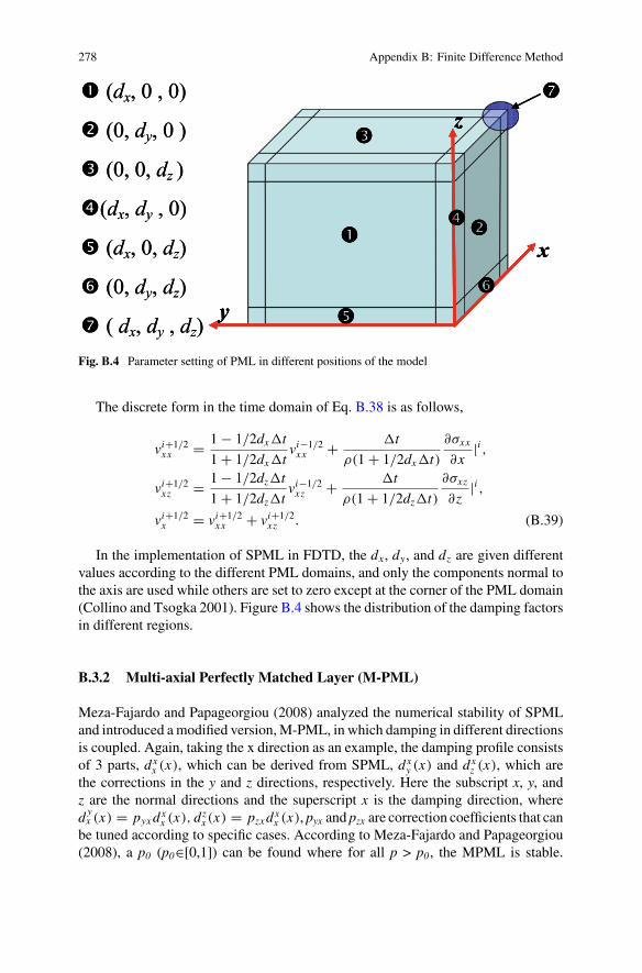
Fig. B.4 Parameter setting of PML in different positions of the model

The discrete form in the time domain of Eq. B.38 is as follows,

vi+1/2xx = 1 − 1/2dxt

1 + 1/2dxtvi−1/2xx + t

ρ(1 + 1/2dxt)

∂σxx

∂x|i ,

vi+1/2xz = 1 − 1/2dzt

1 + 1/2dztvi−1/2xz + t

ρ(1 + 1/2dzt)

∂σxz

∂z|i ,

vi+1/2x = vi+1/2

xx + vi+1/2xz . (B.39)

In the implementation of SPML in FDTD, the dx, dy, and dz are given differentvalues according to the different PML domains, and only the components normal tothe axis are used while others are set to zero except at the corner of the PML domain(Collino and Tsogka 2001). Figure B.4 shows the distribution of the damping factorsin different regions.

B.3.2 Multi-axial Perfectly Matched Layer (M-PML)

Meza-Fajardo and Papageorgiou (2008) analyzed the numerical stability of SPMLand introduced amodified version,M-PML, in which damping in different directionsis coupled. Again, taking the x direction as an example, the damping profile consistsof 3 parts, dx

x (x), which can be derived from SPML, dxy (x) and dx

z (x), which arethe corrections in the y and z directions, respectively. Here the subscript x, y, andz are the normal directions and the superscript x is the damping direction, wheredyx (x) = pyxdx

x (x), dzx (x) = pzxdx

x (x), pyx and pzx are correction coefficients that canbe tuned according to specific cases. According to Meza-Fajardo and Papageorgiou(2008), a p0 (p0∈[0,1]) can be found where for all p > p0, the MPML is stable.

Appendix B: Finite Difference Method 279

However, reflectivity increases when the stability is improved. In other words, thewave in the x direction will be damped in the x direction and will also be dampedin the other two directions (y and z). Therefore, the damping coefficients of M-PMLare:

dx = dxx (x) + dy

x (y) + dzx (z),

dy = dxy (x) + dy

y (y) + dzy(z),

dz = dxz (x) + dy

z (y) + dzz (z). (B.40)

In fact, Martin et al. (2010) made the case that the M-PML should not be consid-ered as PML because the theoretical reflection coefficient for an infinite PML is notexactly zero in this approach. It is just amodification of sponge and the reflection coef-ficients are not zeros even for differential formulation (Dmitriev and Lisitsa 2011).The M-PML is a brute-force approach that works well with media having anisotropyand high material property contrasts (Meza-Fajardo and Papageorgiou 2008).

B.3.3 Non-split Perfectly Matched Layer (NPML)

To simplify the implementation of classic PML, Wang and Tang (2003) introducedthe non-split PML (NPML), in which a trapezoidal rule is applied to calculate theconvolutions in the PML formulation. For example, Eq. B.36 can be transformedinto the time domain using inverse Fourier transforms,

ρ∂vx∂t

= F−1

(1

Sx (x)

)∗ ∂τxx

∂x+ F−1

(1

Sy(y)

)∗ ∂τyx

∂y+ F−1

(1

Sz(z)

)∗ ∂τzx

∂z,

(B.41)

where F−1(

1Sx (x)

)∗ ∂τxx

∂x = ∂τxx∂x −dx (x)

T∫

0exp[−dx (x)(T − t)] ∂τxx

∂x dt . Therefore,

the formulation of velocity in the x direction will be,

ρ∂vx∂t

= ∂σxx

∂x− dx (x)

T∫0exp[−dx (x)(T − t)]

∂σxx

∂xdt

+ ∂σyx

∂y− dy(y)

T∫0exp

[−dy(y)(T − t)]∂σyx

∂ydt

+ ∂σzx

∂z− dz(z)

T∫0exp

[−dz(z)(T − t)]∂σzx

∂zdt. (B.42)

280 Appendix B: Finite Difference Method

Taking the time step as t, the time for step i is T = it. Then the formulationB.42 becomes,

ρ∂vx∂t

= ∂σxx

∂x− dx (x)

it∫

0

exp[−dx (x)(it − t)]∂σxx

∂xdt

+ ∂σyx

∂y− dy(y)

it∫

0

exp[−dy(y)(it − t)

]∂σyx

∂ydt

+ ∂σzx

∂z− dz(z)

it∫

0

exp[−dz(z)(it − t)

]∂σzx

∂zdt. (B.43)

The time discrete form of Eq. B.43 is

vi+1/2x = vi+1/2

x + t

ρ

(∂txx∂x

+ ∂tyx∂y

+ ∂tzx∂z

),

vi+1/2x = vi+1/2

x − Pixx − Pi

yx − Pizx . (B.44)

where Pixx=dx

(x) ∫ it

0 exp[−dx

(x)(it − t

)∂txx∂x

]dt, Pi

yx=dy(y) ∫ it

0 exp[ − dy

(y)

(it − t

) ∂tyx∂y

]dt , and Pi

zx = dz(z) ∫ it

0 exp[−dz

(z)(it − t

) ∂tzx∂z

]dt .

The trapezoidal rule can be used for numerical approxima-tion of the integrations above. For example, Pi

xx = dx (x)Pi−1xx +

12tdx (x)

{exp[−tdx (x)]

∂txx∂x

∣∣(i−1) + ∂txx∂x

∣∣i}, in which the auxiliary function

is introduced to do the integration with second order time accuracy.

B.3.4 Complex Frequency-Shifted Perfectly Matched Layer(CFS-PML)

Poor damping of evanescent waves and instability for long time duration simu-lations have been reported in electromagnetic wave simulation (Berenger 1997) byFDTDwith conventional PML (Berenger 1994). To reduce the limitations of conven-tional PML, many researchers have devoted a great deal of effort on the theory andpractice of modifying PML. Kuzuoglu and Mittra (1996) analyzed the causality ofconventional PML and found that the conventional stretch factor does not preservecausality. They introduced the Complex-Frequency-Shifted (CFS) PML where theyuse a modified factor S = 1 + d/(1 + iω).

The conventional PMLmethod does not work if the wave-number is a pure imag-inary number, such as for evanescent waves or guided waves. For example, if kxis a negative imaginary number (Skelton et al. 2007), it can be replaced by kx= −ik (k is a real number). The plane wave solution in the x direction becomes

Appendix B: Finite Difference Method 281

exp(−ixkx)exp(ikxdx/ω). The factor exp(ikxdx/ω) makes the wave oscillate withoutattenuation. On the contrary, the solution of modified factor used by Kuzuogluand Mittra (1996) is exp(−i xkx ) exp

(ikωxdx/

(1 + ω2

))exp

(−kxdx/(1 + ω2

)), in

which the factor exp(−kxdx/

(1 + ω2

))can exponentially attenuate the energy with

increasing distance.In order to absorb guided waves and evanescent waves efficiently, Roden and

Gendney (2000) proposed a general stretch factor S = β + d/(α + iω) for CFS-PML, where α is a frequency-shift factor and β is a scaling factor. Komatitch andMartin (2007) used a recursive convolutional method to implement the CFS-PMLwith FDTD. Taking Eq. B.41 as an example, the inverse Fourier transform of 1/S isexpressed as,

S = F−1(1/S) = δ(t)

β− d

β2F−1

[1

α + d/β + iω

]= δ(t)

β− d

β2H(t)e−(α+d/β)t ,

(B.45)

Then Eq. B.41 becomes,

ρ∂vx∂t

= Sx ∗ ∂σxx

∂x+ Sy ∗ ∂σyx

∂y+ Sz ∗ ∂σzx

∂z, (B.46)

The recursive convolutional method, which is used to obtain Eq. (B.46), is of onlysecond-order accuracy in space and time (Martin et al. 2010). To keep PML timeaccuracy the same as that of computational domain, Zhang and Shen (2010) used theauxiliary differential equations (ADE) method to attain higher-order time accuracy.

Table B.1 compares the different PML methods to illustrate where the CFS-PMLdiffers from the others. In general, the damping profile is chosen as a polynomialfunction. Here we follow the formulation by Collino and Tsogka (2001), for dampingalong the x direction,

dx = d0(lx/L)n, (B.47)

where lx is the distance from the PML-interior interface for the location in thePML domain, n is 2, d0 is the maximum value of d which can be obtained fromCollino and Tsogka (2001, and L is the thickness of the PML layer.

Table B.1 Summary of PML methods (Wang et al. 2013)

SPML M-PML NPML CFS-PML

α 0 0 0 Non-zero

β 1 1 1 Variable

dx dxx (x) dxx (x), dyx (x), dzx (x) dxx (x) dxx (x)

Convolution No No Yes Yes

282 Appendix B: Finite Difference Method

The values ofα andβ inCFS-PMLare usually given by the following polynomials(Komatitsch and Martin 2007),

βx = 1 + (β0 − 1)(lx/L)m, (B.48)

αx = α0[1 − (lx/L)p

], (B.49)

where m and p are 2 and 1, respectively, and α0 and β0 are the maximum valuesof α and β.

B.3.5 PML Methods Used in the Numerical Simulation of Elastic WavePropagation in a Borehole

Unlike the open hole logging models, cased-hole and acoustic logging while drilling(ALWD) FDTD simulation requires very fine grids because of the thin casing or fluidannulus. Small spatial grid size requires small time step and calculation times increasewhich increases the cumulative numerical error. In addition, the high impedancecontrast (often more than 30) between the fluid and steel casing requires a high effi-ciencymethod to capture the subtle features in the late arrivals. Because of these chal-lenges, efficient computational algorithms are needed to make realistic simulationsof cased-hole and ALWD problems. Given the high material contrasts in our models,Wang et al. (2013a) evaluated the applicability of non-reflective boundary conditionsfor ALWD simulations. Different PML implementations (SPML, M-PML, NPML,and CFS-PML) were used for large material contrast models (ALWD model).

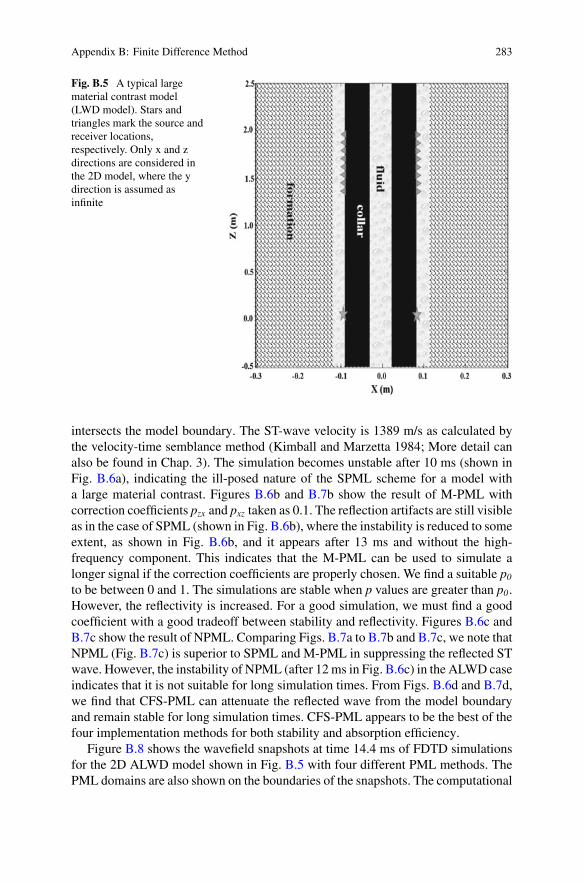
Here we show results with four different PML methods in a 2D LWD case with amonopole source. The model is shown in Fig. B.5, where only the x and z directionsare considered and y direction is assumed as infinite. Vp, Vs and density of theformation are 3927 m/s, 2455 m/s, and 2300 kg/m3, respectively. The outer radiusof the inner fluid, collar, and position of the boundary between the outer fluid andformation are 27 mm, 90 mm, and 117 mm, respectively. Collar C32 in Table 5.2 isused.

The staggered grid FDTD scheme used for testing has a fourth order accuracy inspace and 2nd order accuracy in time (Cheng 1994; Tao et al. 2008b). The modelis discretized into 123 by 334 grids along the x- and z- directions, respectively. Thegrid spacing is 9 mm, and time step is 0.9 μs. The PML layer thickness is 20 grids.The source time function of the monopole source is a Ricker wavelet with centralfrequency f c of 10 kHz. SPML parameters d0 and α0 are chosen as 1 and π f c,respectively. The total recording time of the simulated waveform is 14 ms. The arraywaveform for the entire simulation time and the first 4 ms are shown in Figs. B.6and B.7, respectively. For the case of SPML (Fig. B.7a), the drill collar wave, shear(S)- wave, and Stoneley (ST) wave can be identified from their arrival times. Also,the artificial reflection from the top boundary of the model (dashed black line) isvisible. This arrival is a ST wave reflected from the interface where the borehole

Appendix B: Finite Difference Method 283

Fig. B.5 A typical largematerial contrast model(LWD model). Stars andtriangles mark the source andreceiver locations,respectively. Only x and zdirections are considered inthe 2D model, where the ydirection is assumed asinfinite

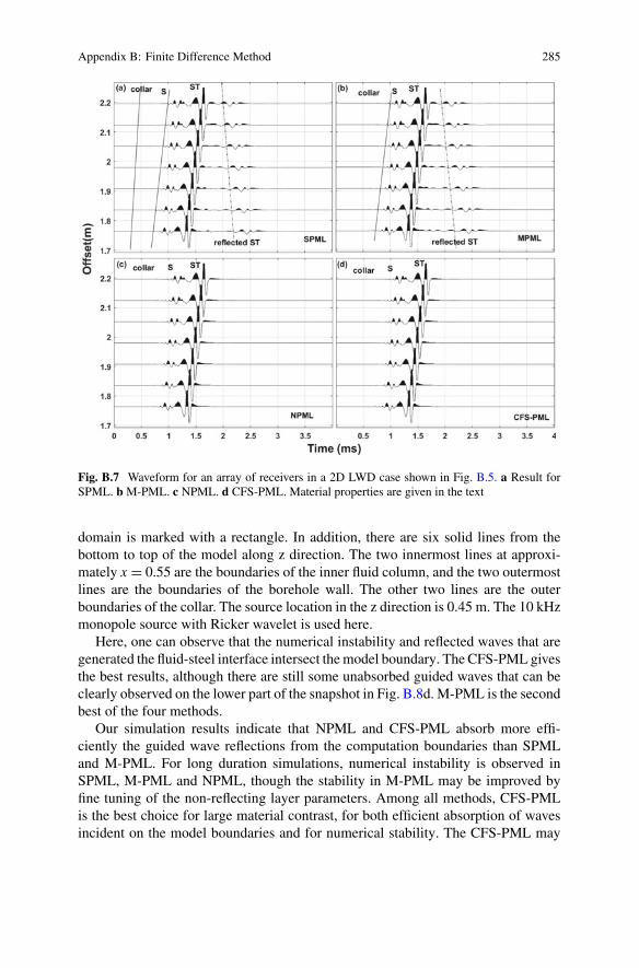
intersects the model boundary. The ST-wave velocity is 1389 m/s as calculated bythe velocity-time semblance method (Kimball and Marzetta 1984; More detail canalso be found in Chap. 3). The simulation becomes unstable after 10 ms (shown inFig. B.6a), indicating the ill-posed nature of the SPML scheme for a model witha large material contrast. Figures B.6b and B.7b show the result of M-PML withcorrection coefficients pzx and pxz taken as 0.1. The reflection artifacts are still visibleas in the case of SPML (shown in Fig. B.6b), where the instability is reduced to someextent, as shown in Fig. B.6b, and it appears after 13 ms and without the high-frequency component. This indicates that the M-PML can be used to simulate alonger signal if the correction coefficients are properly chosen. We find a suitable p0to be between 0 and 1. The simulations are stable when p values are greater than p0.However, the reflectivity is increased. For a good simulation, we must find a goodcoefficient with a good tradeoff between stability and reflectivity. Figures B.6c andB.7c show the result of NPML. Comparing Figs. B.7a to B.7b and B.7c, we note thatNPML (Fig. B.7c) is superior to SPML and M-PML in suppressing the reflected STwave. However, the instability of NPML (after 12 ms in Fig. B.6c) in the ALWD caseindicates that it is not suitable for long simulation times. From Figs. B.6d and B.7d,we find that CFS-PML can attenuate the reflected wave from the model boundaryand remain stable for long simulation times. CFS-PML appears to be the best of thefour implementation methods for both stability and absorption efficiency.

Figure B.8 shows the wavefield snapshots at time 14.4 ms of FDTD simulationsfor the 2D ALWD model shown in Fig. B.5 with four different PML methods. ThePML domains are also shown on the boundaries of the snapshots. The computational

284 Appendix B: Finite Difference Method

2 4 6 8 101.7

1.8

1.9

2

2.1

2.2

Off

set(

m)

Time (ms)

(a)

Reflection

2 4 6 8 10 12 141.7

1.8

1.9

2

2.1

2.2

Off

set(

m)

Time (ms)

(b)

Reflection

2 4 6 8 10 121.7

1.8

1.9

2

2.1

2.2

Off

set(

m)

Time (ms)

(c)

2 4 6 8 10 121.7

1.8

1.9

2

2.1

2.2

Off

set(

m)

Time (ms)

(d)

Fig. B.6 Waveform for an array of receivers in a 2D LWD case shown in Fig. B.5. a Result forSPML. b M-PML. c NPML. d CFS-PML. Material properties are given in the text. Dashed blacklines in a and b show reflections from the top of the model

Appendix B: Finite Difference Method 285

Fig. B.7 Waveform for an array of receivers in a 2D LWD case shown in Fig. B.5. a Result forSPML. bM-PML. c NPML. d CFS-PML. Material properties are given in the text

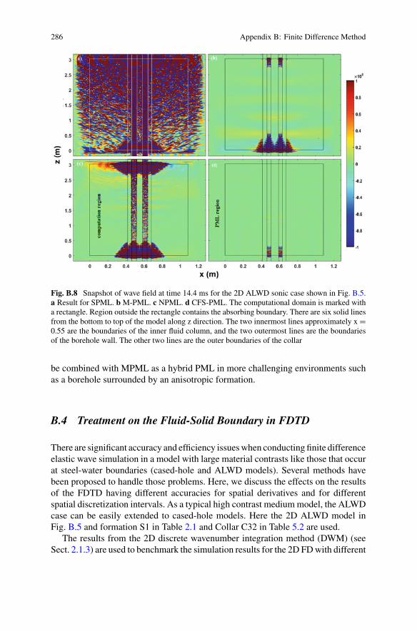
domain is marked with a rectangle. In addition, there are six solid lines from thebottom to top of the model along z direction. The two innermost lines at approxi-mately x = 0.55 are the boundaries of the inner fluid column, and the two outermostlines are the boundaries of the borehole wall. The other two lines are the outerboundaries of the collar. The source location in the z direction is 0.45 m. The 10 kHzmonopole source with Ricker wavelet is used here.

Here, one can observe that the numerical instability and reflected waves that aregenerated the fluid-steel interface intersect themodel boundary. The CFS-PML givesthe best results, although there are still some unabsorbed guided waves that can beclearly observed on the lower part of the snapshot in Fig. B.8d. M-PML is the secondbest of the four methods.

Our simulation results indicate that NPML and CFS-PML absorb more effi-ciently the guided wave reflections from the computation boundaries than SPMLand M-PML. For long duration simulations, numerical instability is observed inSPML, M-PML and NPML, though the stability in M-PML may be improved byfine tuning of the non-reflecting layer parameters. Among all methods, CFS-PMLis the best choice for large material contrast, for both efficient absorption of wavesincident on the model boundaries and for numerical stability. The CFS-PML may

286 Appendix B: Finite Difference Method

Fig. B.8 Snapshot of wave field at time 14.4 ms for the 2D ALWD sonic case shown in Fig. B.5.a Result for SPML. b M-PML. c NPML. d CFS-PML. The computational domain is marked witha rectangle. Region outside the rectangle contains the absorbing boundary. There are six solid linesfrom the bottom to top of the model along z direction. The two innermost lines approximately x =0.55 are the boundaries of the inner fluid column, and the two outermost lines are the boundariesof the borehole wall. The other two lines are the outer boundaries of the collar

be combined with MPML as a hybrid PML in more challenging environments suchas a borehole surrounded by an anisotropic formation.

B.4 Treatment on the Fluid-Solid Boundary in FDTD

There are significant accuracy and efficiency issueswhen conducting finite differenceelastic wave simulation in a model with large material contrasts like those that occurat steel-water boundaries (cased-hole and ALWD models). Several methods havebeen proposed to handle those problems. Here, we discuss the effects on the resultsof the FDTD having different accuracies for spatial derivatives and for differentspatial discretization intervals. As a typical high contrast mediummodel, the ALWDcase can be easily extended to cased-hole models. Here the 2D ALWD model inFig. B.5 and formation S1 in Table 2.1 and Collar C32 in Table 5.2 are used.

The results from the 2D discrete wavenumber integration method (DWM) (seeSect. 2.1.3) are used to benchmark the simulation results for the 2D FDwith different

Appendix B: Finite Difference Method 287

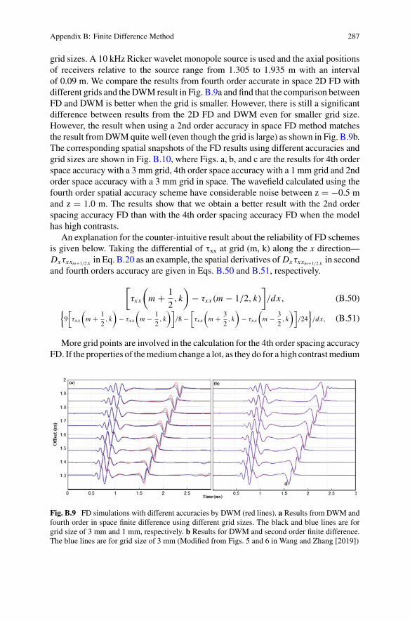
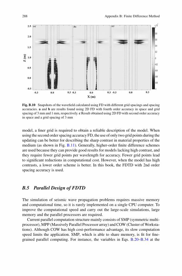
grid sizes. A 10 kHz Ricker wavelet monopole source is used and the axial positionsof receivers relative to the source range from 1.305 to 1.935 m with an intervalof 0.09 m. We compare the results from fourth order accurate in space 2D FD withdifferent grids and the DWM result in Fig. B.9a and find that the comparison betweenFD and DWM is better when the grid is smaller. However, there is still a significantdifference between results from the 2D FD and DWM even for smaller grid size.However, the result when using a 2nd order accuracy in space FD method matchesthe result fromDWMquite well (even though the grid is large) as shown in Fig. B.9b.The corresponding spatial snapshots of the FD results using different accuracies andgrid sizes are shown in Fig. B.10, where Figs. a, b, and c are the results for 4th orderspace accuracy with a 3 mm grid, 4th order space accuracy with a 1 mm grid and 2ndorder space accuracy with a 3 mm grid in space. The wavefield calculated using thefourth order spatial accuracy scheme have considerable noise between z = −0.5 mand z = 1.0 m. The results show that we obtain a better result with the 2nd orderspacing accuracy FD than with the 4th order spacing accuracy FD when the modelhas high contrasts.

An explanation for the counter-intuitive result about the reliability of FD schemesis given below. Taking the differential of τxx at grid (m, k) along the x direction—Dxτxxm+1/2,k in Eq. B.20 as an example, the spatial derivatives of Dxτxxm+1/2,k in secondand fourth orders accuracy are given in Eqs. B.50 and B.51, respectively.

[τxx

(m + 1

2, k

)− τxx (m − 1/2, k)

]/dx, (B.50)

{9

[τxx

(m + 1

2, k

)− τxx

(m − 1

2, k

)]/8 −

[τxx

(m + 3

2, k

)− τxx

(m − 3

2, k

)]/24

}/dx, (B.51)

More grid points are involved in the calculation for the 4th order spacing accuracyFD. If the properties of themediumchange a lot, as they do for a high contrastmedium

Fig. B.9 FD simulations with different accuracies by DWM (red lines). a Results from DWM andfourth order in space finite difference using different grid sizes. The black and blue lines are forgrid size of 3 mm and 1 mm, respectively. b Results for DWM and second order finite difference.The blue lines are for grid size of 3 mm (Modified from Figs. 5 and 6 in Wang and Zhang [2019])

288 Appendix B: Finite Difference Method

Fig. B.10 Snapshots of the wavefield calculated using FD with different grid spacings and spacingaccuracies. a and b are results found using 2D FD with fourth order accuracy in space and gridspacing of 3 mm and 1mm, respectively. c Result obtained using 2D FDwith second order accuracyin space and a grid spacing of 3 mm

model, a finer grid is required to obtain a reliable description of the model. Whenusing the second order spacing accuracy FD, the use of only two grid points during theupdating can be better for describing the sharp contrast in material properties of themedium (as shown in Fig. B.11). Generally, higher-order finite difference schemesare used because they can provide good results for models lacking high contrast, andthey require fewer grid points per wavelength for accuracy. Fewer grid points leadto significant reductions in computational cost. However, when the model has highcontrasts, a lower order scheme is better. In this book, the FDTD with 2nd orderspacing accuracy is used.

B.5 Parallel Design of FDTD

The simulation of seismic wave propagation problems requires massive memoryand computational time, so it is rarely implemented on a single CPU computer. Toimprove the computational speed and carry out the large-scale simulations, largememory and the parallel processors are required.

Current parallel computation structure mainly consists of SMP (symmetric multi-processor),MPP (Massively Parallel Processor array) and COW (Cluster ofWorksta-tions). Although COW has high cost-performance advantage, its slow computationspeed limits the application. SMP, which is able to share memory, is fit for fine-grained parallel computing. For instance, the variables in Eqs. B.20–B.34 at the

Appendix B: Finite Difference Method 289

Fig. B.11 Grids involved in the FD with different order spacing accuracies. The black points arethe location of discrete grids and the gray points are the positions of the obtained derivatives bydifferent spatial accuracy difference methods (Mortified from Fig. 3 in Zhang [2016])

current time step are only related to the previous time step, and the variable in acertain spatial grid is only related to the surrounding grids. Based on the recursivefeature in time domain, all the variables at a given time step can be simultaneouslyupdated.

In addition, for models requiringmassivememory that SMP is not able to provide,the coarse-grained parallel computation based onMPP can be applied. In MPP, eachnode has an independent processor and memory. The nodes communicate within aspecial network with high passband and low delay. The system is easy to expandand can run with multiple threads. Each thread has an independent address and cancommunicate with others via message delivery. The coarse-grained parallel compu-tation divides the computation area into several sub area (2D) or volume (3D) regionsbased on spatial characteristics of the model. Independent computations and data areexchanged only at the border of the regions.

290 Appendix B: Finite Difference Method

The library of SMP is OpenMP (Open Multi-Processing), which is easilyprogrammed. The library of MMP is MPI (Message Passing Interface), whichrequires the effective separation of the computational domain into several subdomains. In addition, the management of message delivery makes it relativelycomplex to program.

The simulations in this book are done by the FDTD with the OpenMP structure.FigureB.12 shows the parallel program structure based on theOpenMP. The first stepis to allocate and initialize the memory for each variable in the shared memory stack.Then, perform the time loop, and update the velocity and stress variable in the firstand last half time step, respectively. The update of all velocity or stress variables issimultaneously implemented using the parallel computation. Synchronization mustbe performed before the stress or velocity is updated to ensure that the calculation of

Fig. B.12 The structure ofthe parallel FDTD programbased on the OpenMP (modified from Fig. 2.14 inHe [2005])

Appendix B: Finite Difference Method 291

the previous time step is completed. Memory is not released until all the time stepsare computed.

The application programming interface of OpenMP includes a set of compilerdirectives, library routines, and environment variables, which can be directlyembedded into FORTRAN and C/C++ for further usage. The PARALLEL compilerdirective divides the code into serial and parallel regions and the parallel regionstarts with a compiler directive !OMP PARALLEL and ending with !OMP ENDPARALLEL. In the parallel region, the codes are implemented by multiple threads,while in serial region the codes are implemented via only one thread. The specificmarkups are responsible for assigning the task into each thread. The local variableinside the thread is assigned by a compiler directive !$OMP DO PRIVATE (namelist of local variables). This expression establishes the reproduction for all the localvariables at each thread. The values of the local variables are taken from the previoustime step but modified during the current time step and are thus not known.

B.6 Validation of the Finite Difference Code for BoreholeAcoustics

To check the validity of the FDTD method in borehole environments, the simulationresults from the FDTD andDWM (see Appendix A) in wireline and LWDmodels arecompared. The comparisons of the results from 3DFD and DWM for the fluid-filledborehole surrounded by formation F1 listed in Table 2.1, are shown in Figs. B.13and B.14. The simulation results in Figs. B.13 and B.14 are at 10 kHz for monopolecases in wireline and ALWD, respectively. The geometries of the wireline and LWDmodels are listed in Tables 2.1 and 5.2 (collar C32 used), respectively.

The solid and dashed lines are the results from the DWM and FDM, respectively.We can clearly see all themodes. For thewirelinemodel shown in Fig. B.13, it is clearto find the P, S and pR, ST, and pR Airy waves in time sequence. For the waveformsin the ALWD model shown in Fig. B.14, we see the collar, P, S, pseudo-Rayleigh(pR.), and ST waves. The amplitude of the collar wave is very small and thereforeamplified for display. In the simulation, we did not add any attenuation and thusthe amplitude of ST is very large. The results obtained using the two methods arealmost identical. These results demonstrate the applicability of the FDTD method.In this book, the wavefields in complex models that cannot be obtained using DWM,such as the eccentered drilling pipe in the ALWD case in Chap. 6 and the boreholeacoustic remote reflection image in Chap. 7, are simulated by the finite differencemethod.

292 Appendix B: Finite Difference Method

Fig. B.13 Comparisons of FDTD and DWM simulations of the wireline acoustic logging wave-forms in a fluid-filled borehole surrounded with formation F1. The waveforms are at 3 m offsetfrom a 10 kHz monopole source

Fig. B.14 Comparisons for FDTD and DWM of the ALWDwaveforms in the fluid-filled boreholesurrounded with formation F1. The waveforms are at 3 m offset from a 10 kHz monopole source.Collar C32 in Table 5.2 is used

References

Aki K, Richards PG (1980) Quantitative seismology, theory and methods. W.H. Freeman and Co.,San Francisco

Allaud LA, Martin MH (1978) Schlumberger: the history of a technique. Schlumberger Ltd.(Translated by Schwob M.)

Al Rougha HAB, Borland WH, Holderson J, Sultan AA, Chakravorty S, Al Raisi M (2005)Integration of microelectrical and sonic reflection imaging around the borehole-offshore UAE.International Petroleum Technology Conference, Doha, Qatar, 2005, Nov. 21–23

Archie GE (1942) The electrical resistivity log as an aid in determining some reservoir character-istics. Petroleum Trans AIME 146:54–62

Arditty PC, Arens G, Staron P (1981) EVA: a long spacing sonic tool for evaluation of velocities andattenuations. In: 51st annual international meeting of the society of exploration geophysicists,Los Angeles, California, United States, October 11–15, 1981

Aron J, Chang SK, Dworak R et al (1994) Sonic compressional measurements while drilling. In:SPWLA 35th annual logging symposium, paper SS

Asquith G, Krygowski D (2006) Basic well log analysis, 2nd edn. AAPGBakku SK, Fehler M, Burns D (2013) Fracture compliance estimation using borehole tube waves.Geophysics 78(4):D249–D260

Bancroft JC, Geiger HD, Margrave GF (1998) The equivalent offset method of prestack timemigration. Geophysics 63:2042–2053

Baysal E, Kosloff DD, Sherwood JWC (1983) Reverse time migration. Geophysics 48(11):1514–1524

Berenger J (1994) A perfectly matched layer for the absorption of electromagnetic waves. J ComputPhys 114(2):185–200

Berenger JP (1997) Improved PML for the FDTD solution of wave-structure interaction problems.Antennas Propag, IEEE Trans Antennas Propag 45(3):466–473

Beylkin G (1985) Imaging of discontinuities in the inverse scattering problem by inversion of acausal generalized Radon transform. J Math Phys 26:99–108

Biot MA (1952) Propagation of elastic waves in a cylindrical bore containing a fluid. J Appl Phys223:997–1005

Bleistein N, Cohen JK, Stockwell JW (2001) Mathematics of multidimensional seismic imaging,migration, and inversion. Springer

Boucher FG, Hildebrandt AB, Hagen HB (1951) New diplogging method. In: Second symposiumon subsurface geological techniques, School of Geology, University of Oklahoma, March 14–15,pp 101–110

Bouchon M, Aki K (1977) Discrete wave-number representation of seismic-source wave fields.Bull Seismolog Soc Am 67(2):259–277

Brekhovskikh LM (1960) Waves in layered media. Academic press, USA, New York, pp 1–200

© Springer Nature Switzerland AG 2020H. Wang et al., Borehole Acoustic Logging—Theory and Methods,Petroleum Engineering, https://doi.org/10.1007/978-3-030-51423-5

293

294 References

Brown HD, Grijalva VE, Raymer LL (1970) New developments in sonic wave train display andanalysis in cased holes. In: Society of petrophysicists and well-log analysts, 11th annual loggingsymposium, 3–6 May, Los Angeles, California, paper F

Byun J, Toksöz MN (2006) Effects of an off-centered tool on dipole and quadrupole logging.Geophysics 71(4):F91–F100

BrytikV, deHoopMV, van derHilst RD (2012)Elastic-wave inverse scattering based on reverse timemigration with active and passive source reflection data. In: Uhlmann G (ed) Inside out—inverseproblems. MSRI Publications, Cambridge University Press, pp 411–453

Cameron I (2013) SPE “Back to basics” bond log theory and interpretation. https://zh.scribd.com/document/238612532/Cement-Bond-Log-SPE. Accessed 25 Apr 2018

Capon J (1969)High resolution frequencywave number-spectrumanalysis. Process. IEEE57:1408–1418

Castagna JP, Batzle ML, Eastwood RL (1985) Relationships between compressional-wave andshear-wave velocities in clastic silicate rocks. Geophysics 50(4):571–581

Cawley P, Lowe MJS, Simonetti F, Chevalier C, Roosenbrand AG (2002) The variation of thereflection coefficient of extensional guided waves in pipes from defects as a function of defectdepth, axial extent, circumferential extent and frequency. Pro. Inst. Mech. Eng. C. 216(11):1131–1143

Cerjan C, Kosloff D, Kosloff R, Reshef M (1985) A nonreflecting boundary condition for discreteacoustic and elastic wave equations. Geophysics 50(4):705–708

Chabot L, Henley DC, Brown RJ, Brown RJ (2001) Single-well imaging using the full waveformof an acoustic sonic. In: SEG 71th annual meeting, expanded abstracts, pp 420–423

Chabot L, Henley DC, Brown RJ, Bancroft J C (2002) Single-well seismic imaging using fullwaveform sonic data: An update. In: SEG 72th annual meeting, 2002, Oct. 6–11

Chai X, Zhang W, Wang G, Liu J, Xu M, Liu D, Song C (2009) Application of remote explorationacoustic reflection imaging logging technique in fractured reservoir. Well Logg Technol (InChinese with English Abstract) 33:539–543

Chang SK, Everhart A (1983) Acoustic waves along a fluid filled borehole with a concentric solidlayer. J Acoust Soc Am 74(Supplement 88)

Charara M, Vershinin A, Deger E et al (2011) 3D spectral element method simulation of soniclogging in anisotropic viscoelastic media. SEG Tech Prog Expand Abstra 30(1):432–437

Chen YH, Chew WZ, Liu QH (1998) A three dimensional finite difference code for the modelingof sonic logging tools. J Acoust Soc Am 103(2):702–712

Chen T,Wang B, Zhu Z, Burns D (2010) Asymmetric source acoustic LWD for improved formationshear velocity estimation. SEG Tech Prog Expand Abstr 548–552

Cheng CH, Toksöz MN (1982) Generation, propagation and analysis of tube waves in a borehole.In: SPWLA 23th annual logging symposium, paper P

Cheng CH, Toksöz MN (1980) Modelling of full wave acoustic logs. In: Society of professionalwell log analysts annual logging symposium, 21st, paper J

Cheng CH, Toksöz MN (1981) Elastic wave propagation in a fluid-filled borehole and syntheticacoustic logs. Geophysics 46(7):1042–1053

Cheng CH, Toksöz MN, Willis ME (1982) Determination of in situ attenuation from full waveformacoustic logs. J Geophys Res 87:5477–5484

Cheng NY, Zhu Z, Cheng CH, Toksöz MN (1992) Experimental and finite difference modeling ofborehole Mach waves. Earth Resources Laboratory Industry Consortia Annual Report, 1992–10

Cheng N (1994) Borehole wave propagation in isotropic and anisotropic media: three-dimensionalfinite difference approach. PhD dissertation. MIT, Cambridge, MA, USA

Chew WC, Weedon WH (1994) A 3D perfectly matched medium from modified Maxwell’sequations with stretched coordinates: microwave Optical Tech. Letters 7:599–604

ChewWC, Liu QH (1996) Perfectly matched layers for elastodynamics: a new absorbing boundarycondition. J Comp Acoust 4:341–359

Chin WC (2014) Wave propagation in drilling, well logging and reservoir environments. Wiley

References 295

ChinWC, Zhou Y, Feng Y, Yu Q (2015) Formation testing: lowmobility pressure transient analysis.Scrivener Publishing of Wiley, Beverly, MA

Claerbout JF (1971) Toward a unified theory of reflector mapping. Geophysics 36:467–481Claerbout JF (1976) Fundamentals of geophysical data processing with applications to petroleumprospecting. McGraw-Hill Book Co., Inc., New York

Clayton R, Engquist B (1977) Absorbing boundary conditions for acoustic and elastic waveequations. Bull Seismol Soc 67:1529–1540

Close D, Cho D, Horn F, Edmondson H (2009) The sound of sonic: a historical perspective andintroduction to acoustic logging. Schlumberger Oil Field Rev 30:34–43

Coates R, Kane M, Chang C, Esmersoy C, Fukuhara M, Yamamoto H (2000) Single-wellsonic imaging: high-definition reservoir cross-sections from horizontal wells. Paper SPE 65457presented at the 2000 SPE/petroleum society of CIM international conference on horizontal welltechnology, Calgary, Alberta, 2000, Nov. 6–8

Cotes G, Xiao L, Prammer M (2000) NMR logging principles and applications. Gulf PublishingCompany, USA

Collino F, Tsogka C (2001) Application of the perfectly matched absorbing layer model to the linearelastodynamic problem in anisotropic heterogeneous media. Geophysics 66(1):294–307

CourantR, FriedrichsO,LewyH(1967)On the partial difference equations ofmathematical physics.IBM J (translated from Courant et al 1928) 11:215–234

Coutant O, Virieux J, Zollo A (1995) Numerical source implementation in a 2D finite differencescheme for wave propagation. Bull Seismol Soc Am 85(5):1507–1512

Cowles CS, Leveille JP, Hatchell PJ (1994) Acoustic multi-mode wideband logging device. U.S.Patent No. 5, 289, 433

de Hoop M, Smith H, Uhlamann G, Van der Hilst R (2009) Seismic imaging with the generalizedRadon transform: a curvelet transform perspective. Inver Prob 25:025005

Deepwater Horizon Study Group (2011) Final report on the investigation of the Macondo wellblowout, p 45. http://ccrm.berkeley.edu/pdfspapers/beapdfs/dhsgfinalreport-march2011-tag.pdf.Last accessed Apr 2019

Dmitriev M, Lisitsa V (2011) Application of M-PML reflectionless boundary conditions to thenumerical simulation of wave propagation in anisotropic media. Part I: reflectivity. Numeri AnalAppl 4:271–280

Doll HG (1949) Introduction to induction logging. Petrol Technol 1(6):148–162Dunham W (2005) The calculus gallery: materpieces from Newton to Lebesgue. PrincetonUniversity Press, p 197

Edwards GR, Gan T (2007) Detection of corrosion in offshore risers using guided ultrasonic waves.In: Proceedings of the 26th international conference on offshoremechanics and arctic engineering,June, 2007, San Diego, California, USA. OMAE 2007-29407

Ekstrom MP (1995) Dispersion estimation from borehole acoustic arrays using a modified matrixpencil algorithm. IEEE Sig Syst Comput Conf Asil 29(1):449–453

Ellefsen KJ, Daniel RB, Cheng CH (1993) Homomorphic processing of the tube wave generatedduring acoustic logging. Geophysics 58(2):1400–1406

Ellis DV, Singer JM (2007) Well logging for earth scientists. SpringerEmbree P, Burg JP, Buckus MM (1963) Wide-band velocity filtering—the pie-slice process.Geophysics 28(6):948–974

Esmersoy C, Koster K, Williams M, Boyd A, Kane M (1994) Dipole shear anisotropy logging. In:64th SEG annual meeting expanded abstracts. Los Angeles

Esmersoy C, Chang C, Tichelaar BW, Kane M, Coates RT, Quint E (1998) Acoustic imaging ofreservoir structure from a horizontal well. Leading Edge 17(7):940–946

Fletcher RP, Flower PJ, Kitchenside P (2006) Suppressing unwanted internal reflections in prestackreverse-time migration. Geophysics 71(6):E79–E82

Fortin JP,RehbinderN, StaronP (1991)Reflection imaging around awellwith the eva full-waveformtool. Log Analyst 32:271–278

296 References

Frisch GJ, GrahamWL, Griffith J (1999) Assessment of foamed-cement slurries using conventionalevaluation logs and improved interpretation methods. SPE Rocky Mountain Regional Meeting,Wyoming, America, 1999, SPE 55649

Frisch GJ, Graham WL, Griffith J (2000) A novel and economical processing technique usingconventional bond logs and ultrasonic tools for enhanced cement evaluation. In: SPWLA 41stannual logging symposium, paper EE

Frisch G, Fox P, Hospedales D, Lutchman K (2015) Using radial bond segmented waveforms toevaluate cement sheath at varying depths of investigation. Society of Petroleum Engineers, paper174829

Froelich B, Pittman D, Seeman B (1983) Cement evaluation tool—a new approach to cementevaluation. Society of Petroleum Engineers, paper 1027

Froelich B (2008) Multimode evaluation of cement behind steel pipe. J Acoust Soc Am 123:3648Geerits T, Mandal B, Schmitt D (2006) Acoustic logging-while-drilling tools having a hexapolesource configuration and associated logging methods. US Patent Published No. US20060198242A1

Gollwitzer LH, Masson JP (1982) The cement bond tool. In: SPWLA, 23rd Annual SymposiumGrosmanginM,KokeshFP,Majani P (1961)Asonicmethod for analyzing the quality of cementationof borehole casings. J Petrol Technol 13(2):165–171

Haldorsen JBU, VoskampA, Thorsen R, Vissapragada B,Williams S, FejerskovM (2006) Boreholeacoustic reflection survey for high resolution imaging. In: SEG76th annualmeeting,NewOrleans,Expanded Abstracts, pp 314–318

HardageBA (1981)An examination of tubewave noise in vertical seismic profiling data.Geophysics46:892–903

Harness PE, Sbins FL, Griffith JE (1992) New technique provides better low-density-cementevaluation. SPE 24050. Western Regional Meeting, Bakersfield, California, USA, March 1992

Havira RM (1979) Ultrasonic bond evaluation in multilayered media. J Acoust Soc Am 66:S41Hayden R, Russell C, Vereide A, Babasick P, Shaposhnikov P, May D (2011) Case studies inevaluation of cementwithwireline logs in a deepwater environment. In: Society of petrophysicistsand well log analysts 52nd annual symposium

Hayman AJ, Hutin R, Wright PV (1991) High-resolution cementation and corrosion imaging byultrasound. In: Society of petrophysicists and well log analysts 32nd annual symposium

HeX,WangX,ChenH (2017) Theoretical simulations ofwave field variation excited by amonopolewithin collar for acoustic logging while drilling. Wave Motion 72:287–302

He F (2005) The study on the simulation of the borehole acoustic reflection imaging logging tooland it’s waveform processing method. PhD thesis (In Chinese with English Abstract), ChinaUniversity of Petroleum, Beijing, China

Herold B, Marketz F, Froelich B, Edwards JE, Kuijk R, Welling R, Leuranguer C (2006) Eval-uating expandable tubular zonal and swelling elastomer isolation using wireline ultrasonicmeasurements. In: IADC/SPE Asia Pacific drilling technology conference and exhibition, paper103893

Higdon RL (1990) Radiation boundary conditions for elastic wave propagation. SIAM J NumerAnal 27(4):831–869

HilchieDW(1978)Applied openholewell log interpretation (for geologists and engineers). DouglasW. Hilchie Inc., Golden Colorado

Hirabayashi N, Torii K, Yamamoto H, Haldorsen J, Voskamp A (2010) Fracture detection usingborehole acoustic reflection survey data. SEG Tech Prog Expand Abstr 29:523–527

Hirabayashi N, Martinez GA, Wielemaker E (2016) Case Studies of borehole acoustic reflectionsurvey (BARS). In: 22nd formation evaluation symposium of Japan, September 29–30

Hornby BE, Pasternark E (2000) Analysis of full-waveform sonic data acquired in unconsolidatedgas sands. Petrophysics 41:363–374

Hornby BE (1989) Imaging of near-borehole structure using full-waveform sonic data. Geophysics54(6):747–757

References 297

Huang C, Hunter JA (1980) The correlation of “Tubewave” events with open fractures in fluid-filledboreholes, Atomic Energy of Canada Seismic downhole survey progress report—1979

Huang X (2003) Effects of tool positions on borehole acoustic measurements: a stretched grid finitedifference approach. PhD dissertation. Massachusetts Institute of Technology, Cambridge, MA,USA

Huang X, Yin H (2005) A data-driven approach to extract shear and compressional slowness fromdispersive waveform data. SEG Tech Prog Expand Abstr 2005:384–387

Ikelle LT, Amundsen L (2018) Introduction to petroleum seismology. Society of ExplorationGeophysicists

Jarrot A, Gelman A, Kusuma J (2018) Wireless digital communication technologies for drilling:communication in the bits/s regime. IEEE Signal Process Mag 35(2):112–120

Johnson HM (1962) A history of well logging. Geophysics 27(4):507–527Johnson SG (2007) Notes on perfectly matched layers (PMLs). MIT course 18.369Joyce B, Patterson D, Leggett J, Dubinsky V (2001) Introduction of a new omni-directional acousticsystem for improved real-time LWD sonic logging-tool design and field test results. In: SPWLA42nd annual logging symposium, Paper SS

Jutten J, Corrigall E (1989) Studies with narrow cement thickness lead to improved CBL inconcentric casings. J Pet Tech 1158–1192

Jutten J,HaymanA (1993)Microannulus effect on cementation logs: experiments and case histories.Society of Petroleum Engineers, paper 25377

Jutten J, Parcevaux P (1987)Relationship between cement bond log output and borehole geometricalparameters. Society of Petroleum Engineers, paper 16139

Kabir MN, Verschuur D (1995) Restoration of missing offsets by parabolic Radon transform.Geophys Prospect 43(3):347–368

Kay SM (1988) Modern spectral estimation: theory and application. Prentice Hall, p 225Kelly KR, Ward RW, Treitel S, Alford RM (1976) Synthetic seismograms: a finite-differenceapproach. Geophysics 41:2–27

Kimball CV,Marzetta TL (1984) Semblance processing of borehole acoustic array data. Geophysics49:274–281

Kimball CV (1998) Shear slowness measurement by dispersive processing of borehole flexuralmode. Geophysics 63(2):337–344

Kingsbury NG (2001) Complex wavelets for shift invariant analysis and filtering of signals. J ApplComputat Harmonic Anal 10(3):234–253

Kinoshita T, Dumont A, Hori H, Sakiyama N, Morley J, Garcia-Osuna F (2010) LWD sonic tooldesign for high-quality logs. Soc. Exp. Geophys., Tech Prog Expand Abstr 29(1):513–517

Kitsunezaki C (1980) A new method for shear wave logging. Geophysics 45:1489–1506Komatitsch D, Martin R (2007) An unsplit convolutional perfectly matched layer improved atgrazing incidence for the seismic wave equation. Geophysics 72(5):M155–M167

Kurkjian AL (1985) Numerical computation of individual far-field arrivals excited by an acousticsource in a borehole. Geophysics 50:852–866

Kurkjian A, Chang SK (1986) Acoustic multipole sources in fluid filled boreholes. Geophysics51(1):148–163

Kuzuoglu M, Mittra R (1996) Frequency dependence of the constitutive parameters of causalperfectly matched anisotropic absorbers. IEEE Microwave Guid Wave Lett 6(12):447–449

Lamb H (1917) On waves in an elastic plate. Proc R Soc London (Series A), 93(648):114–128Lang SW, Kurjian AL, McClellan JH, Morris CF, Parks TW (1987) Estimating slowness dispersionfrom arrays of sonic logging waveforms. Geophysics 52(4):530–544

Lay T, Wallace TC (1995) Modern global seismology. Academic PressLebedev NN (1972) Special functions and their applications. Dover, reprint (Translated fromRussian)

LebourgM, Fields RQ,DohCA (1956)Amethod of formation testing on logging cable. TPNo. 701-G, Fall Meeting, Society of Petroleum Engineers of A.I.M.E., Los Angeles, California, UnitedStates

298 References

Lecampion B, Quesada D, Loizzo M et al (2011) Interface debonding as a controlling mechanismfor loss of well integrity: importance for CO2 injector wells. Energy Procedia 4:5219–5226

Leggett JV, DubinskyV, PattersonD, BolshakovA (2001) Field test results demonstrating improvedreal-time data quality in an advanced LWD Acoustic system, SPE71732

Le Calvez J, Brill TM (2018) Separation of flexural and extensional modes in multi modal acousticsignals. European Patent Application, 16306114.6

LiC,YueW(2015)High-resolution adaptive beamforming for borehole acoustic reflection imaging.Geophysics 80(6):D565–D574

Li C, Yue W (2017) High-resolution Radon transforms for improved dipole acoustic imaging.Geophys Prospect 65(2):467–484

Li Y, Zhou R, Tang X, Jackson JC, Patterson DJ (2002) Single-well imaging with acoustic reflec-tion survey at Mounds, Oklahoma, USA. In: EAGE 64th conference and exhibition, paper 141,Florence, Italy, 2002, May 27–30

Li J, Tao G, Zhang K et al (2014) An effective data processing flow for the acoustic reflection imagelogging. Geophys Prospect 62(3):530–539

Li M, Tao G, Wang H et al (2016) An improved multiscale and leaky P-wave removal analysis forshear-wave anisotropy inversion with crossed-dipole logs. Petrophysics 57(3):270–293

LiW, TaoG, Torres-VerdínC (2015) Forward and backward amplitude and phase estimationmethodfor dispersion analysis of borehole sonic measurements. Geophysics 80(3):D295–D308

Li Y, Wang H, Fehler M, Fu Y (2017) Wavefield characterization of perforation shot signals in ashale gas reservoir. Phys Earth Planet Interi 267:31–40

Lisitsa V, Vishnevskiy D (2010) Lebedev scheme for the numerical simulation of wave propagationin 3D anisotropic elasticity. Geophys Prospect 58:619–635

Liu D, HuW, Chen Z (2008) SVD-TLS extending Prony algorithm for extracting UWB radar targetfeature. J Syst Eng Electron 19(2):286–291

Love AEH (1952) A treatise on the mathematical theory of elasticity, 4th edn. Dover PublicationsLuthi (2000) Geological well logs: their use in reservoir modeling. SpringerMarket J, Bilby C (2011) Introducing the first LWD cross-dipole sonic imaging service. In: SPWLA52nd annual logging symposium, paper DDD

Marple SL (1987) Digital spectral analysis: with applications. Prentice Hall PressMartin RD, Komatitsch SD, Gedney et al (2010) A high-order time and space formulation ofthe unsplit perfectly matched layer for the seismic wave equation using auxiliary differentialequations (ADE-PML). CMES 56:17–40

Matuszyk PJ, Torres-Verdin C (2011) HP-adaptive multi-physics finite-element simulation ofwireline borehole sonic waveforms. SEG Tech Prog Expand Abstr 30(1):444–448

McMechan GA (1983) Migration by extrapolation of time-dependent boundary values. GeophysProspect 31(3):413–420

Meza-FajardoKC, PapageorgiouAS (2008)Anonconvolutional, split-field, perfectlymatched layerfor wave propagation in isotropic and anisotropic elastic media: stability analysis: Bull SeismolSoc Am 98:1811–1836

Miller U (1977) Symmetry and separation of variables. Addison-WesleyMiller D, Oristaglio M, Beylkin G (1987) A new slant on seismic imaging: migration and integralgeometry. Geophysics 52(7):943–964

Miller D, Stanka FE (1999) Method of analyzing waveforms. US Patent 5859811Minear J, BirchakR,RobbinsCAet al (1995)Compressional slownessmeasurementswhile drilling.In: SPWLA 36th annual logging symposium, paper VV

Morris C, Sabbagh L,Wydrinski R, Hupp J, vanKuijk R, Froelich B (2007) Application of enhancedultrasonic measurements for cement and casing evaluation. In: SPE/IADC drilling conference,paper 105648

Nakken EI, Mjaaland S, Solstad A (1995) A new MWD concept for geological positioning ofhorizontal wells, SPE, 30454

Nolte B, Rao R, Huang X (1997) Dispersion analysis of split flexural waves. In: Borhole acousticand logging/Reservoir delineation consortia annual report, MIT

References 299

Op’t Root T, Stolk CC, de Hoop MV (2012) Linearized inverse scattering based on seismic reversetime migration. J Math Pures Appl 98(2):211–238

Paillet FL,ChengCH (1986)Anumerical investigation of headwaves and leakymodes in fluid-filledboreholes. Geophysics 51(7):1438–1449

Paillet F (1981) Predicating the frequency content of acoustic waves in boreholes. In: Society ofprofessional well log analysts annual logging symposium, 22nd, paper SS

Paillet F, Cheng C (1991) Acoustic waves in boreholes. CRC PressPardue GH, Morris RL, Gollwitzer LH, Moran JH (1963) Cement bond log—a study of cementand casing variables. J Pet Tech 5:545–555

Patterson D, Bolshakov A, Matuszyk P (2015) Utilization of electromagnetic acoustic transducersin downhole cement evaluation. In: SPWLA 56th annual logging symposium

Peng C, ToksözMN (1992) Tube wave generation at a layer boundary for an incident compressionalplane wave. MIT Earth Resources Lab Consortium Annual meeting report

Pistre V, Kinoshita T, Endo T et al (2005) A modular wireline sonic tool for measurements of3D (azimuthal, radial, and axial) formation acoustic properties. In: SPWLA 46th annual loggingsymposium, New Orleans, Louisiana, United States, June 26–29

Plona B, Sinha S, Kostek, Chang SK (1992) Axisymmetric wave propagation in fluid-loadedcylindrical shells. II: theory versus experiment. J Acoust Soc Am 92(2):1144–1155

Poletto F,Miranda F (2004) Seismicwhile drilling: fundamentals of drill-bit seismic for exploration.Elsevier Publishing

Prony R (1795) Essai experimental et analytique: L’ecole Polytech 1:24–76Qleibo M (2012) SonicScope the next generation of sonic while drilling. https://www.fesaus.org/webcast/2012/09/NTF/2_SonicScope_Schlumberger.pdf. Access 25 April 2018

Rao R, Toksöz MN (2005) Dispersive wave analysis - method and applications. Earth ResourcesLab Consortium Annual report

Reiter E (1991) Imaging of large offset ocean bottom seismic data. Ph.D. Thesis. MassachusettsInstitute of Technology, Cambridge, MA, United States

Ripley HE, Harms WW, Sutton DL, Watters LT (1981) Ultra-low density cementing compositions.J Canad Petrol 1(6):112–118

Roden JA, Gedney SD (2000) Convolutional PML (CPML): an efficient FDTD implementation ofthe CFS-PML for arbitrary media. Microwave Opti Technol Lett 27:334–338

Rose JL (1999) Ultrasonic waves in solid media. Cambridge University Press, Cambridge, UnitedKingdom, pp 1–100

Rust WM Jr (1938) A historical review of electrical prospecting methods. Geophysics 3(1):1–6Sacchi MD, Ulrych TJ (1995) High-resolution velocity gathers and offset space reconstruction.Geophysics 60(4):1169–1177

Sacchi MD, Porsani M (1999) Fast high-resolution parabolic Radon transform. 69th SEG AnnualMeeting, Expanded Abstracts 1477–1480

Saenger EH, Bohlen T (2004) Finite-difference modeling of viscoelastic and anisotropic wavepropagation using the rotated staggered grid. Geophysics 69:583–591

Sanyal SK, Meidav HT (1976) We11 Logging in the Geothermal Industry, Paper presented at the17th Annual Logging Symp. of the SPWLA, Denver, Colorado, June 1976

Schlumberge (1987) Log interpretation principles/applications. Schlumberger educational services,Houston, Texas, United States

Schmitt DP, Bouchon M (1985) Full wave acoustic logging: synthetic microseismograms andfrequency-wavenumber analysis. Geophysics 50:1756–1778

Schmitt DP (1988) Shear-wave logging in elastic formations. J Acoust Soc Am 84(6):2215–2229Selesnick IW, Baraniuk RG, Kingsbury NG (2005) The dual-tree complex wavelet transform. IEEETrans Signal Process 22(6):123–151

Shahvali A, Azin R, Zamani A (2014) Cement design for underground gas storage well completion.J Nat Gas Sci Eng 18:149–154

300 References

Shang XF (2014) Inverse scattering: theory and application to the imaging of the earth’s seismicdiscontinuities. PhD Thesis. Massachusetts Institute of Technology, Cambridge, MA, UnitedStates

Sinha BK, Zeroug S (1999) Applications of sonics and ultrasonics in geophysical prospecting. IEEEUltraso Symp 521–532

Skelton EA, Adams S, Craster R (2007) Guided elastic waves and perfectly matched layers. WaveMotion 44:573–592

Smith WD (1974) A nonreflecting plane boundary for wave propagation problems. J Comput Phys15(4):492–503

Smolen J (1996) Cased hole and production log evaluation. Pennwell Pub 161–191Song FX, Toksöz MN (2009) Model-guided geosteering for horizontal drilling. MIT, EarthResources Laboratory Industry Consortia Annual Report, 2009, 05

Song R, Liu J, Hou C, Wang K (2012) Numerical simulation of Sector Bond log and improvedcement bond image. Geophysics 77(4):95–104

StephenRA,Cardo-Casas F,ChengCH (1985) Finite-difference synthetic acoustic logs.Geophysics50:1588–1609

Stoica P, Li HB, Li J (1999) A new derivation of the APES filter. IEEE Signal Process. Lett.6(8):205–206

Stolt RH (1978) Migration by Fourier transform. Geophysics 63(1):23–48Su Y, Tang X, Xu S, Zhuang C (2015) Acoustic isolation of a monopole logging while drilling toolby combining natural stopbands of pipe extensional waves. Geophys J Int 202:439–445

Summers GC, Broding RA (1952) Continuous velocity logging. Geophysics 17(3):598–614Tang XM (1997) Predictive processing of array acoustic waveform data. Geophysics 62(6):1710–1714

Tang XM, Wang T, Patterson D (2002a) Multipole acoustic logging-while-drilling. SEG Tech ProgExpand Abstr 21(1):364–367

Tang XM, Dubinsky V, Wang T, Bolshakov A, Patterson D (2002b) Shear-velocity measurement inthe logging-while drilling environment: modeling and field evaluations. In: SPWLA 43rd annuallogging symposium, paper RR

Tang XM, Patterson D, Dubinsky V, Harrison CW, Bolshakov A (2003) Logging-while-drillingshear and compressionalmeasurements in varying environments. In: SPWLA44th annual loggingsymposium, paper II

Tang XM, Cheng CH (2004) Quantitative borehole acoustic methods. ElsevierTang X (2004) Imaging near-borehole structure using directional acoustic-wave measurement.Geophysics 69:1378–1386

Tang XM, Patterson D (2005) Analyzing and processing acoustic logging data for poorly bondedcased boreholes. In: Society of petrophysicists and well log analysts 46th annual symposium

Tang XM, Zheng Y, Vladimir D (2005) Logging while drilling acoustic measurement inunconsolidated slow formations. In: SPWLA 46th, paper R

Tang XM, Zheng Y, Patterson D (2007) Processing array acoustic-logging data to image near-borehole geologic structures. Geophysics 72(2):E87–E97

Tang XM, Li C, Patterson D (2009) A curve-fitting method for analyzing dispersion characteristicsof guided elastic waves. SEG Tech Prog Expand Abstr 461–465

Tang XM, Patterson D (2009) Single-well S-wave imaging using multicomponent dipole acoustic-log data. Geophysics 74(6):WCA211–WCA223

Tang XM, Wei Z, Su Y, Zhuang C (2013) A review on the progress and application of dipoleacoustic reflection imaging technology. Well Logg Technol (In Chinese with English Abstract)37(4):330–340

Tang X (2016) Reflection imaging away from borehole: a paradigm shift. SEG Tech Prog ExpandAbstr 4873–4877

Tang XM (2017) Acoustic characterization and imaging of shale gas fractures in horizontal wells.SEG 87th Annual Meeting, Expanded Abstracts 959–963

References 301

Tang XM, Li S, Xu S, Su Y, Zhuang C (2017) Acoustic characterization and imaging of shale gasfractures in horizontal wells: field case study in the Sichuan Basin of Southwest China.Well LoggTechnol (In Chinese with English Abstract) 41(5):501–505

TaoG,ChengCHToksözMN (1997)Measurements of shear-wave azimuthal anisotropywith cross-dipole logs. In: Industry consortia annual report of Earth Resources Laboratory at MassachusettsInstitute of Technology, 1997–10

TaoG (2006) Logging information processing and application. ChinaUniversity of PetroleumPress,Dongying, China

Tao G, He F, Yue W, Chen P (2008a) Processing of array sonic logging data with multi-scale STCtechnique. Petrol Sci 5(3):238–241

Tao G, He F, Wang B, Wang H, Chen P (2008b) Study on 3D simulation of wave fields in acousticreflection image logging. Sci China Earth Sci 51:186–194

Trad DO, Ulrych TJ, Sacchi MD (2002) Accurate interpolation with high resolution time-variantRadon transforms. Geophysics 67(2):644–656

Trad D, Ulrych T, Sacchi M (2003) Latest views of the sparse Radon transform. Geophysics68(1):386–399

Thierry S, Klieber C, Lemarenko M, Le Calvez J, Brill T, Barrou T, Hayman A, Mege F, Van OsR (2016) New-generation ultrasonic measurements for quantitative cement evaluation in heavymuds and thick-wall casings. In: Society of petroleum engineers annual technical conference andexhibition, SPE-181450-MS

Thierry S,Klieber C, LemarenkoM,Brill T, LeCalvez J,Mege F, BarrouT, LavrentievM,ConstableK (2017)Ultrasonic cement logging: expanding the operating envelope and efficiency. In: SPWLA58th annual logging symposium, Paper number: SPWLA-2017-WWWW

Tichelaar BW, van Luik KW (1995) Sonic logging of compressional-wave velocities in a very slowformation. Geophysics 60(6):1627–1633

Tixier MP, Martin M (1954) History of logging and future development. Canadian Oil Gas Indust7(8)

Toksöz MN, Johnston DH (1981) Seismic wave attenuation. Society of Exploration GeophysicistsToksöz MN, Cheng CH, Garcia G (1984a) Full waveform acoustic logging—where we are, wherewe are going. MIT Earth Resources Lab Consortium Annual meeting report

Toksöz MN, Wilkens RH, Cheng CH (1984b) Determination of shear wave velocity and attenua-tion from waveforms in low velocity formations. MIT Earth Resources Lab Consortium Annualmeeting report

Tsang L, Rader D (1979) Numerical evaluation of transient acoustic waveform due to a point sourcein a fluid-filled borehole. Geophysics 44(10):1706–1720

Tsang L (1978) Tim-harmonic solution of the elastic headwave problem incorporating the influenceof Rayleigh poles. J Acoust Soc Am 63:1302–1309

Tubman KM (1984) Full waveform acoustic logs in radially layered boreholes. PhD Thesis.Massachusetts Institute of Technology, Cambridge, MA, United States

Tubman KM, Cole SP, Cheng CH, Toksöz MN (1984) Dispersion curves and synthetic microseis-mograms in unbonded cased boreholes. Earth Resources Laboratory Industry Consortia AnnualReport, 1984–02

Van Kuijk R, Zeroug S, Froelich B, Allouche M, Bose S, Miller D, Calvez J, Schoepf V (2005) Anovel ultrasonic cased-hole imager for enhanced cement evaluation. In: International petroleumtechnology conference, paper 10546

van Kuijk R, Calvez JL, Froelich B (2006) Determination of the impedance of a material behind acasing combination two sets of ultrasonic measurements. United States Patent, NO. 7149146 B2

Varsamis GL, Wisniewski L, Arian A et al (1999) A new MWD full wave dual mode sonic tooldesign and case histories. In: SPWLA 40th annual logging symposium, paper F

Virieux J (1986) P-SV wave propagation in heterogeneous media: velocity-stress finite-differencemethod. Geophysics 51:889–901

Vogel CB (1952) A seismic velocity logging method. Geophysics 17:586–597Walker T (1968) A full-wave display of acoustic signal in cased holes. J Pet Tech 818–824

302 References

Waters KH (1978) Reflection seismology. WileyWang B, Tao G, Wang H, Li W, Tan B (2011) Extraction method of P and S reflection waves fromarray acoustic logging data. J China Univ Petrol 35(2):57–63 (in Chinese with English abstract)

Wang T, Tang X (2003) Finite-difference modeling of elastic wave propagation: a nonsplittingperfectly matched layer approach. Geophysics 68:1749–1755

Wang P, de Hoop M, van der Hilst R, Ma P, Tenorio L (2006) Imaging of structure at and near thecore mantle boundary using a generalized radon transform: 1. Construction of image gathers. JGeophys Res Solid Earth 111:B12304

Wang H, Tao G, Wang B, Li W, Zhang X (2009) Wave field simulation and data acquisition schemeanalysis for LWD acoustic tool: Chinese. J Geophys (In Chinese) 52:2402–2409

WangH,TaoG (2011)Wavefield simulation anddata-acquisition-scheme analysis forLWDacoustictools in very slow formations. Geophysics 76(3):E59–E68

WangH,TaoG,ShangX,FangX,BurnsD (2013)Stability of finite difference numerical simulationsof acoustic logging-while-drilling with different perfectly matched layer schemes. Appl Geophys10(4):384–396

Wang H, Tao G, Zhang K (2013) Wavefield simulation and analysis with the finite-element methodfor acoustic logging while drilling in horizontal and deviated wells. Geophysics 78(6):D525–D543

Wang H, Tao G, Fehler M (2015) Investigation of the high-frequency wavefield of an off-centermonopole acoustic logging-while-drilling tool. Geophysics 80(4):D329–D341

Wang H, Tao G, Shang X (2015) A method to determine the strike of interface outside of boreholeby monopole borehole acoustic reflections. J Petrol Sci Eng 133:304–312

Wang H, Tao G, Shang X (2016a) Understanding acoustic methods for cement bond logging. JAcoust Soc Am 139(5):2407–2416

Wang X, He X, Zhang X (2016) Generalized collar waves in acoustic logging while drilling. ChinPhys B 25:124316

Wang H, Fehler M, Tao G, Wei Z (2016) Investigation of collar properties on data-acquisitionscheme for acoustic logging-while-drilling. Geophysics 81(6):611–624

Wang P, Bose S, Sinha BK, Blyth M (2016d) Dipole shear anisotropy using logging-while-drillingsonic tools. In: SPWLA 57th annual logging symposium, paper PPPP

Wang H, Fehler MC, Miller D (2017) Reliability of velocity measurements made by monopoleacoustic logging-while-drilling tools in fast formations. Geophysics 82(4):D225–D233

WangH, FehlerMC (2018) The wavefield of acoustic logging in a cased-hole with a single casing—part I: a monopole tool. Geophys J Int 212(1):612–626

Wang H, Fehler M (2018) The wavefield of acoustic logging in a cased hole with a single casing—part II: a dipole tool. Geophys J Int 212(2):1412–1428

Wang H, Fehler M, Fournier A (2018) Assessing CO2 leak paths by analysis of borehole monopolewavefield modes. SEG Techn Prog Expand Abstr

Wang B, Zhang K (2019) Investigation on acoustic reflection logging of LWD using a flexible finitedifference technique. Explorat Geophys 50(2):172–180

Wei Z, Wang H (2016) Numerical simulation and field data analysis of an off-center quadrupoleacoustic wireline tool. SEG Tech Prog Expand Abstr 820–824

White JE (1965) Seismic waves, radiation, transmission and attenuation, ch. 4. McGraw-Hill, NewYork

White JE (1967) The hula log: a proposed acoustic tool. In: Transform 8th Annual LoggingSymposium Society Professor Well-Log Analysis, paper I

Whitmore ND (1983) Iterative depth imaging by backward time propagation. SEG 53rd AnnualMeeting, Expanded Abstracts, pp 382–384

Winbow GA, Chen ST, Rice JA (1991) Acoustic quadrupole shear wave logging device. US Patent:5027331

Wu PT, Darling HL, Scheibner D (1995) Low-frequency P-wave logging for improved compres-sional velocity in slow formation gas zones. SEG Tech Prog Expand Abstr 14(1):9–12

Yilmaz Ö (2001) Seismic data analysis. Society of Exploration Geophysicists, Tulsa, OK, USA

References 303

Yu S (1984) The resonance modes of elastic wave in a fluid-filled borehole in acoustic well logging.Chinese J Geophys 27(1):94–102 (In Chinese with English Abstract)

Zemanek J, Angona FA, Williams DM, Caldwell RL (1984) Continuous shear wave logging, paperU. In: 25th annual logging symposium transactions. Society of Professional Well Log Analysts

Zemanek J, Caldwell RL, Glenn E, Holcomb SV, Norton LJ, Straus A (1969) The Borehole tele-viewer—a new concept for fracture location and other types of borehole inspection. J Pet Tech25:762–774

Zeroug S, Froelich B (2003) Ultrasonic leaky-Lamb wave imaging through a highly contrastinglayer. In: IEEE ultrasonic symposium, pp 794–798

Zeroug S, Bose S, Sinha B, Liu Y, D’Angelo R (2016) Sonic and ultrasonic measurementapplications for cased oil wells. Insight 58(8):423–430

Zhang XD (1996) Modern signal processing. Tinghua University Press, BeijingZhang T, TaoG, Li J,WangB,WangH (2009) Application of the equivalent offset migrationmethodin acoustic log reflection imaging. Appl Geophys 6(4):303–310

Zhan X, Zhu Z, Chi S, Toksöz M (2010) Elimination of LWD (Logging While Drilling) tool modesusing seismoelectric data: Commun. Comput Phys 7:47–63

Zhang W, Shen Y (2010) Unsplit complex frequency-shifted PML implementation using auxiliarydifferential equations for seismic wave modeling. Geophysics 75:T141–T154

Zhang H, Xie D, Shang Z, Yang X, Wang H, Tao H (2011) Simulated various characteristic wavesin acoustic full waveform relating to cement bond on the secondary interface. J Appl Geophys73(2):139–154

Zhang K (2016) Discussion on borehole wavemodes excited by two types of acoustic logging whiledrilling sources. Mathemat Comput Sci 1(3):48–55

Zhang X, Wang X, Zhang H (2016) Leaky modes and the first arrivals in cased boreholes withpoorly bonded conditions. Sci China-Phys Mech Astron 59(2):624301

Zhang J, Xu X, Yu Q, Zhai Y, Chao Y, Ji Z (2018) Development and application of victorymulticomponent reflected shear wave imager. J Appl Acoust (In Chinese with English Abstract)37(2):268–272

Zheng H (2000) Interpretating Respon ses of cgdt casedhole gamma-density-thickness tool usingnumerical modeling techniques. Well Logg Tech 24(4):243–252

Zheng Y, Tang X (2005) Imaging near-borehole structure using acoustic logging data with pre-stackF-K migration. In: SEG 75th annual meeting, expanded abstracts, pp 360–363

Zheng Y, Hu H (2017a) Nonlinear signal comparison and high-resolution measurement of surface-wave dispersion. Bull Seismol Soc Am 107(3). https://doi.org/10.1785/0120160242

Zheng X, Hu H (2017) A theoretical investigation of acoustic monopole logging-while-drillingindividual waves with emphasis on the collar wave and its dependence on formation. Geophysics82:D1–D11

Zhu J (1999)A transparent boundary technique for numericalmodeling of elasticwaves.Geophysics64(3):963–966

Index

AAbsorbing boundary condition, 275Absorbing boundary layer, 275Absorbing material, 5, 158, 275Absorption efficiency, 283Accelerometer, 130, 131Acoustic impedance contrast, 9, 114Acoustic interface, 116, 117, 120Acoustic logging, 2–7, 9–13, 15, 16, 23, 59,

88, 94, 145, 179, 181, 220, 223, 229,246, 250, 256, 258, 260, 282, 292

Acoustic Logging-While-Drilling (ALWD),10–12, 15, 23, 129–138, 141–150,152–157, 160, 162–164, 166–169,171–173, 175–177, 179, 180, 197,198, 207, 217, 220, 223, 237, 238,266, 282, 283, 285, 286, 291, 292

Adaptive filter, 77Adaptive InterferenceCancelling (AIC), 240Airy phase, 27–29, 34, 35, 62, 96, 185, 186,

228, 242, 246Alternative phase, 66Amplification, 156, 228Amplitude and Phase Estimation (APES),

76, 77, 79Amplitude distribution, 36, 44, 51, 136Analysis, 7, 15, 57, 63, 66, 68, 72, 75, 81,

98, 138, 149, 163, 171, 185, 204, 229,234, 239, 252, 275

Analytical, 15, 17, 72, 75, 76, 81, 82, 132,143, 144, 147, 201

Anisotropy (ic), 6, 55–57, 279, 286Annulus, 9, 83, 94, 95, 99, 102, 106, 109,

110, 114, 117, 119–121, 127, 187Anti-symmetric (A) mode, 216Aperture, 239, 243

Apparent velocity, 230, 239, 241, 242, 244,247, 248, 251, 252

Applicability, 282, 291Arctangent function, 74Argillaceous carbonates, 5, 6, 252Array waveform, 5, 7, 35, 36, 40, 41, 43, 44,

48, 49, 52, 53, 55, 57, 59–62, 65, 72,73, 76, 79, 81–83, 91, 95, 98, 102–104, 106, 107, 137, 138, 141–144,146, 148–150, 154, 155, 160, 165,168, 169, 171, 174, 175, 177, 181,182, 195, 199, 205, 206, 209, 211,216, 229, 234, 241, 252, 254, 260,282

Arrival time (s), 5, 10, 39, 40, 59–61, 80, 82,85, 98, 100, 103, 107, 109, 148, 155,156, 159, 163, 172, 181–183, 199,201–203, 207, 210, 223, 225, 226,229, 230, 237, 238, 242, 246, 251,252, 283

Artificial boundary, 276Artificial reflection, 275, 283Asymmetric mode, 185, 186, 220Attenuation, 9, 10, 22, 25, 26, 28, 59, 67, 69–

71, 85, 107, 109, 112, 114, 116–118,120–122, 126, 127, 226, 281, 291

AuxiliaryDifferential Equations (ADE), 281Auxiliary function, 280Axial direction, 17, 19, 49Azimuth, 5, 23, 55, 56, 112–114, 117, 125–

128, 132, 136, 172, 179–181, 184,185, 190, 191, 193, 196, 198–208,212, 213, 215, 216, 226–229, 231,233, 236, 239, 260, 262, 263

Azimuthal coverage, 113, 129Azimuthal imaging, 117Azimuthally distributed receiver, 181, 196

© Springer Nature Switzerland AG 2020H. Wang et al., Borehole Acoustic Logging—Theory and Methods,Petroleum Engineering, https://doi.org/10.1007/978-3-030-51423-5

305

306 Index

Azimuthally distributed source, 112, 181,238

Azimuthal reflector, 237, 260Azimuthal resolution, 112, 113, 115Azimuthal variation, 198Azimuth difference, 126, 185, 186, 191, 192,

203, 207, 209, 228, 239Azimuth transducer, 112, 113, 117, 129

BBackward, 59, 66, 67, 70Bandpass filter, 80, 83, 241Bandwidth, 80, 81, 118Bayes principle, 248, 250Bed boundary, 15, 237, 238, 252, 253, 263Benchmarks, 287Borehole Acoustic Reflection Imaging

(BARI), 223, 228, 239, 240, 248,258–260, 263

Borehole Acoustic Reflection Survey(BARS), 226

Borehole axis, 29, 59, 60, 112, 117, 179, 181,183, 224, 225, 228, 229, 239, 242

Borehole compensation, 129Borehole diameter, 55, 109Borehole dimension, 239Borehole enlargement, 143, 151, 156Borehole logging, 1, 2Borehole radius, 4, 14, 26–28, 30–32, 39, 46,

49, 52, 54, 55, 58, 62, 81–83, 143,145, 151, 152, 156–158, 161, 166,170, 183, 188, 224, 266, 269

Borehole sidewall, 113Borehole stability, 286Borehole structure, 27, 223, 227, 291Borehole wall, 11–14, 20, 29, 31, 34–36, 44,

83, 95, 97, 102, 115, 135–137, 143,145, 148, 154, 155, 185, 187, 188,198, 208, 212–214, 260, 261, 285,286

Borehole washout, 29Boundary condition, 21, 88, 132, 275, 282Boundary element methods, 25Branch-cut integrations, 22, 134Branch-line integral, 22Branch point, 22, 135Brute-force approach, 279

CCalibrated gather, 258Calibration, 109, 117Caliper measurement, 114

Caprock, 262Carbonate, 5, 252, 253, 256Cartesian coordinate system, 272, 276Cased-hole, 11, 103, 104, 121, 282, 286Casing-cement interface, 97, 109, 110, 114,

126Casing eccentering, 118, 120, 122Casing flexural, 89, 102, 105Casing modes, 89, 90, 96, 98, 99, 103–105,

107, 109, 127Cauchy distribution, 250Causality, 280CBL/VDL, 107–109, 111–114C/C++, 291Cementation, 106, 122Cement Bond Log (CBL), 107–109, 111–

114Cement bond quality, 9, 10Cement coverage, 112, 117, 127Cement density, 123Cement density log, 123Cement-formation interface, 95, 97, 98, 108,

110, 120, 126Cement impedance, 122Cement loss, 15Cement thickness, 109Cement type, 109Center frequency, 24, 25, 34, 89, 108, 116,

153, 171, 252Centralized array receiver, 200Centralized tool, 136, 180, 183, 191, 193–

195, 203, 206, 207, 209Cluster of Workstations (COW), 288Coarse-grained, 289Coda, 148, 156, 199Coefficients, 18, 19, 21, 63, 65, 67–70, 75,

132, 266, 273, 279, 283Coherence, 60–62, 66, 73–75, 80, 127, 145,

149, 163, 199Coherence coefficient, 75, 77Collar, 1, 10, 15, 23, 129–141, 143–149,

151–172, 175, 177, 180, 197–199,201–203, 205, 207–217, 219, 220,237, 238, 266, 269, 282, 285, 286,291, 292

Collar body, 145, 158Collar density, 163–165, 167Collar flexural wave, 140, 147–149, 151,

152, 166–168, 177, 198, 199, 201,203, 205, 207, 209, 213, 215, 216,220

Collar flexural-wave velocity (Vfl), 133,151, 209

Index 307

Collar hexapole mode, 171Collar mode, 136, 137, 145, 153, 154, 160,

166Collar screw (quadrupole) mode, 22, 23, 88,

107, 128, 141, 153, 156, 169–171,177, 181, 214, 215

Collar S-wave velocity, 143, 162, 163Common Midpoint Stacking (CMS), 258Common Offset Gather (COG), 238, 239,

241–247, 250–253, 256–258, 261,262

Common scatter point gather, 258Common Source Gather (CSG), 65, 238,

239, 246, 247Compiler directive, 291Complex coefficient, 63, 64, 68, 77Complex contour, 22, 134Complex-Frequency-Shifted PML (CFS-

PML), 276, 280–286Complex plane, 22Complex stretch factor, 276, 277Complex stretch plane, 277Complex variable, 21Complex velocity, 26Complex wavenumber, 21Complex wavenumber plane, 22Complex window pattern, 246Computational domain, 275, 281, 285, 286,

290Conjugate transpose operator, 69Continuity, 21Continuous media, 275Contour, 184, 194Contour plot, 61, 81, 96, 98, 100, 106, 107,

143, 144, 146, 148, 149, 153–155,165, 169, 171, 186–188, 201, 206

Control factor, 31, 37, 90Convergence, 275Convolution operation, 277Coordinate transform, 275Correction coefficient, 278, 283Correction method, 51Correlogram, 61, 65, 66Cosine envelope function, 23, 25CO2 storage, 106Counter-intuitive result, 287Coupling, 21, 107, 113Covariance matrix estimation, 78Critical frequency, 134, 135Critical incident angle, 94Cross-correlation, 60, 61, 67, 76Cross-dipole, 6, 8, 9, 55, 57, 235, 236, 263

Crossline, 55, 191, 193, 194, 196, 212–214,219

Cross-plot, 72, 121Cumulative numerical error, 282Cutoff frequency, 28, 31, 33, 34, 37, 39, 41,

48–51, 53, 55, 58, 83, 89–91, 94, 99,102, 103, 140, 141, 147, 149, 151–154, 156, 160, 166–171, 174, 177,190

Cutting, 159Cylindrical coordinate, 18Cylindrical symmetry, 183

DDamping factor, 250, 278Damping function, 276Data, 1, 5–7, 10–12, 15, 39, 41, 55, 57,

59, 61–68, 70, 72–77, 79–83, 86,100, 105, 109, 113, 116, 123, 125–129, 172, 207, 214, 222, 223, 227,235–239, 241, 242, 246–261, 290

Data acquisition schemes, viData processing, 5, 15, 59, 81, 113, 223, 226,

231, 238–240, 249, 258, 263Data smoothing, 244Data transmission, 1, 7, 129Decomposition, 63–65, 70, 183, 185–197Deep water, 114Denoising, 239Density, 17, 19, 26, 39, 62, 74, 75, 84,

106–108, 113, 114, 116, 119–123,133, 162–166, 168, 175, 207–212,214–217, 266, 269, 271, 282

Depth of investigation, 44, 223Determinant, 21, 88, 132Deviated and horizontal well (borehole), vDeviated well, 262, 264Devices, 12, 1143DFD, 48, 135, 238, 291Diagonal matrix, 250Difference operator, 272, 273Difference scheme, 271, 275, 288Dip, 224, 227–229, 236, 239, 258Dipole, 6, 7, 9, 17, 22, 23, 34–37, 39–41,

47–58, 61–65, 75, 81, 88–91, 100,102–105, 127–129, 131–133, 139–141, 143, 147–150, 152–154, 166–169, 177, 181, 188, 190–194, 196,201, 203, 206, 210, 212, 214, 219,227, 231, 236, 237, 253, 256–258,262–264, 266, 269

Dipole leaky P-wave, 151

308 Index

Dipole S-wave image tool, 227, 258, 262,264

Directional receiver, 226Directional transducer, 112Direct wave, 7, 12, 20, 120, 147Discontinuity, 223, 224Discrete grid, 272, 289Discrete Wavelet Transform (DWT), 64Discrete wavenumber, 22, 25, 183, 287Discrete Wavenumber integration Method

(DWM), 287, 291, 292Discretization, 273, 286Dispersion, 15, 28, 34, 37, 39, 46, 51, 59, 61,

62, 72, 75–77, 79–82, 92, 94, 100,104, 118, 119, 134, 139, 141, 142,148, 149, 153, 154, 162, 168, 169,187, 188, 194, 201, 203, 206, 209,210, 220, 275

Dispersion analysis, 66, 82, 96, 98, 100,103, 105–107, 144, 152, 174, 175,177, 201, 203, 206, 207, 209–211,213–215, 218

Dispersion correction, 51, 149, 154, 166, 194Dispersion curve, 28, 29, 32–38, 41–43, 46–

50, 52–54, 58, 62, 66, 72, 74–76, 81,85, 88–90, 92–94, 96, 100, 103, 104,106, 107, 119, 132, 134, 135, 139–141, 143–147, 149, 151–153, 156,157, 160–164, 166–169, 171, 172,201, 203, 206, 207, 210, 213, 214

Dispersive, 5, 39, 40, 42, 55, 61, 62, 66, 79,80, 82, 96, 98, 100, 120, 142, 147–149, 151, 152, 154, 166, 168, 169,172, 181, 186, 196, 199, 207, 244

Displacement, 17, 21, 29, 92, 93, 132, 187,271

Displacement potential, 17, 19, 20Displacement vector, 271Distance, 6, 7, 9, 11, 12, 15, 28–30, 37, 44,

45, 54, 60, 67, 72, 121, 123, 129, 145,159, 183, 185, 186, 198, 201, 204,208, 209, 212, 215, 224, 225, 233,234, 239, 281, 282

Distribution angle, 132Distribution function, 25, 132Down-going, 241, 252, 253, 255, 257, 258,

261Downhole environment, 118Down sample, 63, 64Drill bit, 129–131, 217Drill collar, 1, 15, 23, 129–131, 138, 160,

197, 198, 237, 282Drilling noise, 130, 131, 156, 170, 178

Drilling safety, 129Drill pipe, 1, 130, 131Drill-rig time-saving, 129Drill string, 10, 131, 1792D time-velocity plane, 61Dual Tree Complex Wavelet Transform

(DTCWT), 63–66Duration, 28, 39, 61, 161, 280, 285

EEccentered tool, 179, 180, 185–188, 195,

207, 209, 212, 216Eccentering angle, 187, 188, 191, 193, 194,

196, 198, 219, 221Eccentering magnitude (or amount), 182,

190, 191, 215, 219, 220Eccentering parameter, 184, 186, 188, 189,

191, 192, 194–197Eccentering vector, 180, 199Edge detection, 74Edge effect, 248, 249Eigenvalue, 71Elastic properties, 162Elastic wave, 17, 271, 282, 286Electrical (log), 2Electromagnetic, 1, 280Electromagnetic wave simulation, 280Energy, 12, 13, 44, 88, 89, 119, 120, 135–

137, 143, 162, 223, 248, 275, 276,281

Energy leakage, 143Environment variable, 291Equivalent offset migration, 258Evaluation of Velocity and Attenuation

(EVA), 226Evanescent wave, 280, 281Evaporates, 5, 6Excitation amplitude, 134Excitation function, 134, 135Exponential function, 22

FFast-Fast (FF) formation, 133Fast formation, 7, 12–14, 26–29, 31, 33, 35,

36, 39–42, 46, 58, 61–63, 84, 131–133, 136, 139, 153, 157, 160, 164,175, 179, 183, 197, 198, 201, 220,239, 242–244, 247, 259–261

Field data, 6, 39, 58, 59, 61, 63, 64, 72, 81,82, 84, 85, 109, 155, 172, 173, 176,223, 252–255, 258

Filtered data, 79, 242

Index 309

FilteredFrequencySemblance (FFS), 59, 66,79, 81, 82, 96, 203

Filter window, 246Finite Difference Method (FDM), 26, 88,

275, 291Finite-Difference Time-Domain method

(FDTD), 271–273, 275, 276, 278,280, 282, 285–292

Finite element, 25Finite Impulse Response (FIR) filter, 77First arrival, 4, 10, 13, 27, 55, 96, 98–100,

102, 103, 105, 107–109, 112, 113,119, 120, 129, 141, 148, 153, 170,172, 213, 215, 216, 219, 246, 251

First arrival amplitude, 109, 112First-order elastic wave equation, 271First-order time derivate, 271Fitting function, 74Fitting method, 74F-K domain, 241–245F-K migration, 258Flexural attenuation, 7Flexural waves, 34–36, 38, 39, 47, 48, 50,

51, 55, 58, 61, 62, 65, 66, 73, 76, 81,91, 100, 102, 103, 105, 140, 147–149,151, 152, 166–168, 177, 191, 193,196, 203, 206, 207, 209, 212, 215,236, 253

Flow diagram, 239Fluid annulus, 83, 96–101, 104, 109, 120,

131, 160, 202, 237, 282Fluid channel, 94, 96, 99, 101, 102, 109, 122,

123, 126, 127Fluid circulation, 130Fluid (-) filled, 12, 26, 27, 43, 48, 52, 131,

179, 181, 182, 184, 186, 188, 189,191, 192, 194, 196, 197, 223, 228,291, 292

Fluid movement, 130Fluid pressure, 21, 35, 44, 88, 90, 102, 104,

109, 119, 120, 136, 143, 154Fluid properties, 1, 62Fluid-solid boundary, 286Fluid thickness, 99–101, 112Fluid-wave velocity, 28, 34, 42, 48, 55, 62,

112, 118, 143, 149Formation, 1–7, 9, 10, 12–15, 17, 21, 26–56,

58–66, 74, 75, 81, 83–85, 87, 91, 94–98, 100–114, 116, 119, 120, 122, 123,125–172, 174, 175, 177–179, 181–217, 220, 223–225, 227–229, 236–239, 241–247, 258–261, 263, 264,266, 269, 282, 286, 291, 292

Formation bedding, 263, 264Formation classification, 133Formation flexural wave, 55, 91, 100, 102,

105, 140, 147–149, 151, 152, 166–168, 177, 203, 206, 207, 212, 215,236

Formation hexapole mode, 171, 188Formation interface, 238, 258Formation property, 2, 6, 9, 10, 17, 32, 33,

127, 129, 133, 134, 153, 175Formation screw, or Formation quadrupole

wave, 41, 42, 58, 105, 153–156, 169,170, 194, 196, 214, 215

Formation velocity, 33, 38, 46, 50, 54, 113,127, 135, 151, 177, 178, 194, 220

Formulation, 17, 20, 279–281FORTRAN, 291Forward, 72, 73, 248–251, 259, 260Forward wavefield, 259Four component waveforms, 235Fourier transform, 20, 72, 75, 132, 279, 281Fracture, 6, 11, 15, 29, 223, 260–264Free pipe, 87, 105, 114, 128Frequency, 6, 7, 9, 13, 15, 17–22, 24–28,

31, 33, 36–44, 46–56, 58, 59, 61,63, 65–67, 70, 72–77, 79–81, 83,87, 89–92, 94, 95, 98, 99, 102–108,112–114, 116–120, 127–135, 138–156, 160, 164, 166–172, 174, 177,179, 185, 187, 188, 190, 194, 203,209, 214, 219, 237, 240, 241, 249,250, 252, 253, 266, 269, 276, 277,280–283

Frequency domain, 18–20, 59, 66, 67, 72,73, 95, 249, 250, 277

Frequency-shifted factor, 276Frequency transforms, 72, 73, 94, 240, 242,

249Frequency-wavenumber (F-K)filtering, 241,

245Frequency-wavenumber (F-K) transform,

72, 73, 131, 240, 241Full waveform, 5–7, 22, 27, 108, 113, 116–

118, 129, 145, 172, 190, 205, 207,208, 228, 234, 238, 239, 242, 244,261, 262

GGamma Ray (GR), 111, 172, 173, 176Gas reservoir, 262, 264Gas zone, 55Gaussian function, 74

310 Index

Gaussian source (s), 24Generalized Radon-Transform (GRT), 258Geo-steering, 15, 129, 217, 223, 237, 238,

258, 260Good bonding, 107, 113Good cement, 97, 103, 106, 111, 112Governing equation, 277GR-density log, 106Grooved collar, 159Grooves, 5, 158, 159Group delay, 117Group velocity, 28, 29, 34, 35, 118, 120Group velocity dispersion curve, 29, 32, 34,

35, 118Guided wave, 12, 13, 31, 74, 225, 226, 228,

233, 236, 239, 241–248, 251–253,255, 258, 261, 262, 280, 281, 285

HHankel matrix, 70Head wave, 29Hexapole, 22, 23, 171, 172, 185, 187, 266High-frequency, 42, 48, 51, 61, 65, 90, 102,

104, 105, 128, 138, 141, 142, 144,148, 149, 154, 172, 179, 283

High impedance collar, 168High-pass filter, 63High-Resolution Radon Transform (HRRT),

73, 248, 250–252, 254, 255, 257Hilbert transform, 63Histogram, 74Holomorphic processing, 66Horizontal component, 236Horizontal drilling, 15, 237, 238, 258Horizontal interface, 126, 228, 229, 236,

237, 258Horizontal plane, 229, 231, 262Hydraulic bond, 106Hyperbolic, 74, 229, 239Hyperbolic tangent function, 74

IIll-posed, 283Imaginary, 22Imaginary number, 280, 281Imaginary part, 22, 63–65Imaging, 2, 9, 11, 15, 114, 223, 226, 227,

235, 237–239, 256, 258, 259, 261–264

Imaging condition, 259Impedance, 117, 122, 135Impedance contrast, 114, 117, 239, 282

Impendence difference, 116Incidence, 12, 94, 114, 115, 118–120, 224,

239Incident angle, 12, 94, 114Incoming wave, 19, 20Industry standard casing, 83, 108Inline, 55, 190–194, 196, 219, 253, 256Inner fluid, 89, 131–133, 136, 143, 154, 282,

285, 286Inner Radius (IR), 90, 134, 160–162, 166,

167, 169–172, 269Inner radius-thickness ratio, 90Inner ST wave, 143In-situ condition, 1Instability, 280, 283, 285Integration, 21, 22, 183, 280, 287Intercept, 248Interface, 9, 10, 19, 21, 95, 108, 114–120,

122, 123, 126, 224–231, 236, 239,241, 252, 253, 258–261, 282, 283,285, 290, 291

Interface I, 107–109, 126Interface II, 108, 117Interval, 1, 5, 7, 9, 10, 35, 36, 59, 61, 72, 74,

89, 91, 113, 121, 129, 146, 150, 172,184, 186, 201, 242, 261, 286, 287

Interval transit time, 10, 129Isolator, ASO, 4, 5, 91, 158, 172Iso-offset, 6, 39Isotropic, 17, 271, 272Iterative step, 275

KKirchhoff migration, 258

LLamb wave, 92–94, 120Lamé constants, 17, 271Laplace operator, 18Leaky mode, 13, 49, 109, 119, 120, 135Leaky P-wave, 5, 35, 36, 39, 44, 46, 48, 49,

51, 55, 58, 62, 66, 83, 85, 105, 143,145, 146, 149, 151–156, 167, 168,172, 174, 179, 190, 191, 194, 196,209, 210, 244

Least Squares Radon Transform (LSRT),250

Lebedev format, 271Library routine, 291Linear chirp, 25Linear combination, 181Linear phase, 63

Index 311

Linear superposition theorem, 67, 77Line source, 25Lithologic boundary, 5, 252Lithology (lithological), 2, 5, 111, 252Logging-While-Drilling (LWD), 1, 10, 23,

129, 132, 175, 179, 223Logs, 1–3, 17, 39, 62, 83–85, 106, 107,

109–114, 160, 173, 176, 253, 262Longitudinal (L) mode, 133, 136Long time simulation, 280Low frequency component, 61Low-frequency limit, 28, 34, 41, 81, 90, 94,

105, 128, 190Low frequency source, 36, 44, 49, 105, 140,

143, 194Low-order mode, 90Low-pass filter, 105

MMach wave, 44, 45Magnetic, 2Markup, 291Massively Parallel Processor array (MPP),

288, 289Massive memory, 288, 289Material contrasts, 224, 282, 283, 286Matrix-pencil, 59, 67, 71, 174, 175, 177Maximum entropy, 248Maximum-Likelihood Method (MLM), 66Maxwell’s equation, 275Mean-square misfit error, 75Mechanical vibration, 130Media, 26, 85, 275, 279Median filtering, 240, 244, 246, 247Message deliver, 289, 290Message Passing Interface (MPI), 290Method of separation of variables, 18Micro-annulus, or Micro-debonding, 108,

114Migration, 227, 239, 256, 258–260Modal composition, 15, 185Mode, 5, 9, 13, 15, 21–23, 26–29, 31–42,

44, 46, 48–55, 58–63, 65, 70, 72, 74–82, 87–96, 98, 99, 102–105, 109, 114,118–122, 126–129, 132–135, 137–143, 147, 149, 156–158, 160–163,166–170, 172, 177, 179, 181, 183,185–199, 203, 206, 209, 210, 213,215, 220, 227, 229, 236, 241, 242,244, 247–251, 291

Mode excitation, 37, 90, 118, 134, 135, 185,206

Mode-kissing, 80Model boundary, 283, 285, 286Modeling, 7, 15, 17, 94, 113, 118, 127, 133,

223, 228, 229, 237, 246Mode order, 96, 135, 140, 142, 154, 167,

185, 187, 191, 232, 282Modified Bessel functions, 18Monopole, 5–9, 13, 14, 17, 22, 23, 27–31,

33, 35, 39–51, 53–58, 60–64, 72, 84–87, 89–91, 95, 97, 98, 102, 105, 108,109, 127, 129, 131, 133–138, 143–146, 160–164, 167, 171–175, 179,181–191, 196–198, 201, 203, 205–207, 209, 211, 214, 220, 226–228,230–232, 234, 237, 239, 242, 252–254, 260, 261, 263, 266, 269, 282,285, 287, 291, 292

Motion, 7, 29, 34, 87, 119, 137, 212Moveout, 242, 244, 247Mud circulation, 130Mud density, 26, 108, 114Muddy intercalation, 252Mud-wave velocity, 117Multi-arm mechanical calipers, 217Multi-axial Perfectly Matched Layer (M-

PML), 278, 279, 281–286Multiple scale, 63Multiple thread, 289, 291Multiple wave, 61Multiple wavefield, 83Multipole, 8, 9, 22, 23, 54, 129, 131, 179,

181, 206, 266, 269Multiscale velocity-time semblance, 240

NNear surface seismology, 72Negative time axis, 259Neutron logs, 106Noise log, 106Noise vector, 77Nonlinear filtering, 244Nonlinear least-square, 67Nonlinear problem or nonlinear process, 69Nonlinear Signal Comparison (NLSC), 76Non-orthogonal operator, 248Nonparametric spectrumestimationmethod,

59Nonreflecting plane boundary condition,

275Non-reflective boundary condition, 282Non-splitting Perfectly Matched Layer

(NPML), 279, 281–286

312 Index

Normal component, 236, 278Normal incidence, 115Normalization, 109Normal stress, 21, 35, 37, 272, 275Nuclear, 2Numerical dispersion, 275Numerical simulation, 2, 12, 24, 27, 159,

275, 282Numerical solution, 275Numerical stability, 278, 286

OObjective function, 69, 74, 78, 250Oblique line, 143, 242, 244Octupole, 23Off-centered, 15, 197Offset, 6, 33, 37–40, 45–47, 50, 51, 53, 54,

56, 60, 72, 89, 91, 110–112, 119, 135,145, 146, 150, 156, 158, 179, 181,184, 186, 199–201, 203–207, 210,212, 219, 225, 226, 228–230, 233,234, 237–239, 242, 247, 249, 252,253, 256, 258, 261, 262, 292

Offshore, 42Oil-bearing sandstone, 1Oil spill, 106Omni-directional, 112, 226Openhole, 265OpenMulti-Processing (OpenMP), 290, 291Opposite phases, 103, 203, 216, 217Optimization algorithm, 258Orientation, 55, 237Orthogonal direction, 202, 203Outer boundary, 88, 95, 97, 136, 143, 148,

154, 155, 158, 198, 199, 208, 209,212, 215, 276, 285, 286

Outer fluid, 131–133, 138, 282Outer Radius (OR), 23, 84, 90, 133, 160–

162, 166, 167, 169–172, 269, 282Outer ST wave, 143Outgoing wave, 18Out of phase, 196Over-pressure, 129

PPARALLEL compiler directive, 291Parallel computation, 275, 288–290Parallel design, 288Parameter estimation, 77, 240Parametric spectrum estimation, 59, 66, 72,

82Partial Differential Equation (PDE), 271

Partially cemented well, 95Particle displacement, 271Particle motion, 29, 32, 92, 93Particle velocity, 271, 272Peak, 61, 62, 74, 75, 78, 79, 135, 138, 142,

154Perfectly-Matched-Layer (PML), 275, 276,

278–282, 285Period equation, 92Periodic problem, 275Peripheral imaging, 6, 12, 15, 238, 256Permeability, 106Petroleum engineer, viPetrophysicist, viPhase delay, 72Phase difference, 72, 76, 219Phase shift, 67, 76Phase velocity, 28, 29, 32, 34, 35, 37, 38,

42, 43, 48, 52, 73, 75, 80–82, 94, 140,163, 168

Physical properties, 1Piezoelectric Transducers (PZTs), 129Pipe curvature, 92Pipe modes, 90Pipe thickness, 90, 92–94, 115, 119Pitch-catch method, 10, 114, 115, 118–121,

126, 127Point source, 19, 20, 22, 23, 25, 27, 103, 135,

181, 183, 236Poisson’s ratio, 38, 39, 46, 47, 50, 51, 54, 55,

58, 151–153, 156Polarity difference, 209Polarization, 8, 35, 90, 190, 212, 231, 235,

236Polarization direction, 8, 35, 212Pole, 22, 69, 71, 134, 135Polycrystalline Diamond Compact (PDC),

131Polynomial, 67, 68, 70, 281, 282Polynomial function, 281Poorly cemented well, 94, 99P-P, 120, 223–226, 229, 232, 237, 242, 246,

251PR Airy phase, 186, 228, 246Pressure, 2, 21, 37, 45, 51, 95, 105–107, 117,

135–137, 143, 147, 148, 155, 199,215, 228, 230–233

Pre-stack data, 258Pre-stack Kirchhoff migration, 258Primary (or head) waves, 12Prior knowledge, 77Probability Density Function (PDF), 74Programming interface, 291

Index 313

Projection, 61, 62, 233Prony’s method, 59, 68Propagation, 9, 12, 13, 15, 17, 18, 26, 58,

105, 113, 117, 223, 231, 239, 271,275, 276, 282, 288

Propagation direction, 18, 113, 231, 239Propagation path, 12, 13, 223, 239Prototype, 226P-S, 120, 223, 225, 226, 228–230Pseudo-Rayleigh (pR), 13, 87, 291Pulse-echo technology, 116, 118P-wave, 5, 12, 17, 20, 27, 29, 31, 34–37,

39, 40, 44, 46, 48–51, 55, 58, 62,66, 83–85, 94, 96, 98, 100, 105, 111,117, 120, 127, 128, 135, 137–139,143, 145, 146, 149, 151–157, 159–165, 167, 168, 172, 174–177, 179,183, 184, 186, 190–192, 194, 196,198, 201–203, 205, 207, 209, 210,228, 231, 244, 266, 269

P-wave impedance, 114, 121, 127P-wave velocity, or Vp, 5, 12, 26, 33, 34, 37–

39, 42, 46–49, 54, 55, 58, 60, 62, 64,66, 72, 81, 84, 85, 91, 94, 98, 99, 104,105, 119, 120, 123, 131, 133, 135,138, 139, 143, 145, 146, 149, 151,152, 154, 156, 157, 162–164, 167,168, 177, 186, 187, 194, 203–205,207, 209–212, 214–217, 282

QQuadrupole, 6, 7, 17, 22, 23, 41, 42, 51–

55, 58, 88–90, 105–107, 128, 129,131–133, 141–143, 153–158, 166,169–172, 174, 177, 181, 188, 191,194–197, 209, 210, 212–220, 266

Quality control, 74, 75Quality factor, 26, 85

RRadial direction, 20, 44, 51Radial displacement, 21, 29Radial wavenumber, 18, 266, 269Radiation, 8, 129, 132, 196, 212Radiation directivity, 8Radioactive tracer, 106Radius,radii, 4, 17, 23, 30–32, 39, 46, 49,

50, 54, 83, 85, 90, 92, 93, 119, 122,124–126, 145, 146, 151–153, 156,160–162, 166, 167, 169–172, 175,181–183, 228, 265, 266

Radon transform, 73, 240, 247–253, 258

Raw, 67, 68, 79, 239, 252, 255Ray path, 12, 121, 223, 226, 239Ray theory, 120, 224Ray tracing, 229Real axis, 22Real axis integration method, 22Real part, 64Real-time, 10, 129, 217Receiver azimuth, 5, 23, 112, 113, 126–128,

136, 172, 179, 181, 184, 185, 190,191, 196, 197, 199, 200, 202–209,213, 215, 231, 233, 260, 263

Receiver location, 23, 72, 78, 181, 237, 283Receiver offset separation, 239Receiver (s), 4–9, 19, 23, 27, 28, 31, 35,

36, 39, 56, 59–61, 65, 67, 68, 72, 79,86, 89, 91, 98, 108, 112–114, 124,126, 129, 135, 136, 150, 159, 172,179, 181, 183–185, 187–193, 195–207, 209, 210, 212, 214, 216, 217,221, 224, 226, 228, 229, 234, 235,237, 238, 242, 249, 259–261, 283

Reciprocal, 55, 61, 173Recursive convolutional method, 281Reflected wave, 119, 120, 224–229, 231,

234–239, 241–248, 250–253, 255,257, 258, 262, 283, 285

Reflecting interfaces, 19, 236, 239Reflection, 9–11, 31, 114–118, 120, 126,

223–234, 237–242, 244, 245, 252–254, 257, 258, 261, 262, 279, 283–285, 291

Reflection coefficient, 279Reflection data, 239Reflection imaging, 228, 258Reflection (wave) extraction, 252Reflector, 117, 226–229, 231, 236, 239, 241,

253, 256, 262, 263Reflector azimuth, 263Refracted P, 7, 12, 252Refracted waves, 12Reservoir, 252, 253, 256Residue, 22, 134Resistivity, 1, 3Resolution, 4, 9, 73, 75, 76, 80, 81, 111, 112,

114, 128, 248Reversed wavefield, 259, 260Reverse Time Migration (RTM), 258–261Ricker source/wavelet, 24Riemann sheet, 22Ring source, 131, 135, 171, 237, 238Rotated grid, 271Rotated measurement, 221, 271

314 Index

SSandstone, 1, 111Saturation, 2Scalar potential, 17, 19Scaling factor, 276, 281Scatter, 5, 223, 258Scattered wave, 20, 29Scattering theory, 228Schematic diagram, 9, 10, 29, 32, 64, 83, 84,

108, 115, 123, 131, 158, 180, 184,197, 225, 229, 235, 241, 246, 259,263, 272, 273

Scissors, 248, 250Screw wave (s), 51, 52, 55, 153–156, 166,

170, 194Second-order accuracy, 281Second-order elastic wave equation, 271Segmented Bond Logs (SBL), 112–114Seismic wave propagation, 17, 271, 275,

276, 288Seismologist, viSemblance method, 5, 7, 61–63, 65, 66, 82,

138, 165, 205, 239, 283Sensitivity, 17, 29, 67, 114, 118SH, 17, 18, 227, 231, 233, 235, 236, 262–264Shale, 5, 6, 42, 111, 172, 262, 264Shale gas reservoir, 262, 264Shallow, 42Shallow offshore environment, 42Shared memory stack, 290Shear attenuation, 10, 114, 118, 121, 122,

127Shear bond, 106Shear coupling, 107Shear modulus, 266, 269Shear motion, 7, 34Shear stress, 21Signal-to-NoiseRatio (SNR), 9, 76, 155, 170Silts, 42Simulation, 15, 23, 48, 135, 136, 159, 162,

164, 170, 236, 271, 275, 276, 280,282, 283, 285–288, 290–292

Simulation region, 286, 289, 290Singularity (ies), 21, 22Singular value, 71Slant stack, 248Slope, 28, 62, 72, 242, 244, 248Slotted groove, 158, 175Slow cement, 120Slow-Fast (SF) formation, 133Slow formation, 5–7, 10, 12–14, 42–44, 47–

49, 51–56, 58, 61, 62, 64, 65, 83,84, 132, 133, 143–158, 166, 168,

169, 171, 172, 175, 177, 179, 182,187, 189, 190, 192–195, 207, 208,210–212, 214–217, 220, 239, 241,244–247, 261

Slowness, 55, 61, 72, 74, 75, 173–177, 249,252, 253

Slowness Probability Density function(SPD), 75

Slowness-Time Coherence (STC), 60, 66,73, 80

Slow ST (ST2) waves, 88–90, 96, 98–101Snapshot (s), 12, 14, 15, 28, 30, 35, 44, 45,

48, 49, 51, 53, 88–90, 95, 96, 99, 102–107, 119, 120, 135, 136, 138, 139,143, 147, 148, 154, 198, 199, 208,209, 212, 215, 228, 230–233, 236,237, 285–288

Snell’s law, 12, 94, 223, 224Solid, 17, 19, 21, 26, 55, 73, 88, 94, 104, 121,

132, 134, 136, 137, 139, 141, 143,144, 147, 151, 165, 183, 190, 194,203, 209, 252, 255, 285, 286, 291

Sonic logging, 9, 12, 27, 114, 227Sonic scanner, 227Source frequency, 7, 9, 15, 26–28, 31, 33,

37–41, 43, 44, 47–56, 58, 89–92,102–107, 112, 118–120, 129, 133,139, 141, 143, 145, 146, 149–151,154–156, 160, 170, 172, 185, 190,194, 209, 237, 253

Source loading, 236Source pattern, 129Source polarization, 90, 190, 212, 235, 236Source radiation, 132Source-receiver offset, 39, 40, 45, 110, 111,

210, 225, 226, 239, 252, 253, 261Source-receiver spacing, 83, 213, 215, 217Source time function, 19, 23, 83, 85, 236,

275, 282S-P, 120, 223, 225, 226, 228–230Space accuracy, 287Space derivatives, 277Space distribution function, 25Spacing, 7, 9, 28, 108, 159, 200, 202, 206,

229, 234, 237, 252, 272, 282, 287–289

Spatial coordinate, 272Spatial derivatives, 286, 287Spectral logging, 15Spectrum, 15, 24, 59, 66–68, 72–75, 82, 116,

130, 131Spherical formulation, 20

Index 315

Split-field Perfectly Matched Layer(SPML), 276–278, 281–286

Sponge, 279S-S, 120, 223, 225, 228–230, 237Stability analysis, 275Stability condition, 275Stacking fold, 258Staggered grid, 271–273, 275, 282Standard deviation, 75Steel, 84, 85, 109, 116, 117, 119, 282, 285Stiffness tensor, 271Stoneley (ST) waves, 5, 7, 12, 13, 15, 27–29,

42, 58, 84, 133, 172, 181, 237, 283Stop band, 135Strain tensor, 271Stress potential, 132Stress tensor, 271Strike, 224, 226–229, 239Superposition, 67, 68, 77, 259, 260Surface reflection seismology, 227, 238Surface seismic surveys, 15, 223, 239Surrounding formation, 12, 14, 26, 94, 131,

134, 159SV, 17, 18, 227, 231, 233, 235, 236, 262–264SVD-TLS, 70S-wave, 5, 7, 9, 10, 12, 15, 18, 22, 26–29,

31, 33, 34, 37, 39, 41, 43, 44, 46–51, 54–56, 58, 59, 61, 62, 66, 73,81, 84, 85, 91, 94–96, 98–100, 102,105, 118, 120, 127, 128, 133, 140,142, 143, 145, 147–149, 151–154,156–158, 162–164, 166–172, 175–177, 183, 184, 186, 190, 191, 194,196, 198–201, 205, 207, 220, 223,224, 227–229, 231, 235, 236, 252,258, 262–264, 266, 269

S-wave velocity, or Vs, 5–7, 9, 10, 12, 15,26, 28, 31, 33, 34, 37, 39, 41, 43,44, 46–51, 54, 55, 58, 61, 62, 66, 73,81, 84, 91, 99, 100, 102, 105, 128,140, 142, 143, 145, 147–149, 151–154, 156, 157, 162–164, 166–172,175, 177, 186, 190, 191, 194, 196,199–201, 207, 220, 224

Sweep frequency, 25Symmetric Multiprocessor (SMP), 288–290Symmetric (S) mode, 92Synchronization, 290Synthetic, 23, 25–27, 46, 58, 59, 62, 72, 75,

82–86, 109, 110, 116, 118, 121, 138,148, 149, 153, 154, 159, 187, 188,195, 213–215, 217, 234, 236, 239,241, 242, 246, 247

TTaylor’s expansion, 273Temperature log, 106Theoretical, 7, 17, 65, 75, 94, 279Thermal neutron decay time log, 106Third acoustic interface, 116, 117, 119, 120Third Interface Echo, the (TIE), 119, 120,

126, 127Tilted tool, 180Time accuracy, 280, 281Time delay, 24, 25, 59, 61, 115, 116, 129Time-distance plot, 59Time domain, 24, 59, 72, 73, 132, 239, 242,

247, 271, 272, 275–279, 289Time loop, 290Time semblance, 63, 65, 66, 79, 138, 252,

254Time-slowness (τ-p) domain, 248Time-space domain, 241, 242, 246, 248, 249,

251, 258, 272Time step, 259, 272, 280, 282, 289–291Time window, 47, 61, 166Tool, 1, 4–10, 12, 13, 15, 16, 23, 27, 40, 42,

54–56, 62, 83–86, 91, 102, 105, 106,108, 109, 113, 114, 117, 123, 125,126, 128–130, 136–139, 143, 145,147, 148, 154–156, 159, 166, 168,169, 172, 173, 176, 177, 179–222,226, 227, 229, 235, 237, 238, 255,260, 261, 263

Tool body, 5, 91Tool design, 15Tool eccentering, 62, 109, 179, 186–198,

201–208, 210, 211, 213, 215, 216,218–220

Tool eccentricity, 108, 190, 200–202, 209Tool movement, 179Tool offset, 179, 199–203, 205–212, 214,

255Tool position, 179, 180, 217, 219–222Tool rotation, 217Tool waves, 139Torsional (T) mode, 87Total wavefield, 20, 28, 116, 242Total waveform, 246Trace equalization, 258Transducer, 9, 108, 109, 113–115, 117, 118,

129, 132, 158Transmission, 1, 5, 115, 116, 120Transmitted wave, 14, 225Transmitter, 4, 5, 10, 12, 13, 108, 112, 114,

115, 123, 224, 237Transmitter-Receiver spacing (T-R), 7, 9, 28

316 Index

Transparent boundary, 275Transpose operator, 69, 70Trapezoidal rule, 279, 280Travel time, 4, 224, 227Trough, 108Truncated boundary, 275Tsang and rader source, 24Two-way wave equation, 259

UUltralow density cement, 113Ultrasonic, 7, 9, 10, 15, 92, 94, 106, 114,

118, 120, 127, 128, 217Ultrasonic caliper, 217, 219Ultrasonic measurement, 122Ultrasonic pulse, 117, 219, 222Ultrasound scanner image method, 118Uncemented casing, 87Underground Gas Storage (UGS), 106Unit, 17, 124–126Unwrapped configuration, 113Up-going, 241, 252, 253, 255, 257, 258, 261Upper limit, 242, 244

VVariable Density Logging (VDL), 107–111,

113, 130, 131Vector (s), 17, 69, 70, 75, 179, 181, 272Velocity, 3–7, 9, 10, 12, 15, 17–19, 21, 26,

28, 29, 31–35, 37–39, 41–44, 46–55,57–67, 69, 70, 72–75, 77–82, 84–91,94–96, 98–102, 104, 105, 112, 113,117–120, 123, 127, 128, 131, 133–135, 137–158, 161–175, 177, 178,181, 182, 184–191, 194–196, 199–201, 203–211, 214, 220, 224, 226,230, 234, 239–242, 244, 247, 248,251, 252, 254, 258, 271, 272, 275,277, 279, 283, 290, 291

Velocity analysis, 57, 80, 98, 165, 186Velocity determination (measurement), 59,

62, 66, 69, 74, 96, 162, 171, 174, 175,178, 186, 239

Velocity difference, 139, 143, 148, 166, 186,239

Velocity gap, 167, 223Velocity-time semblance, 5, 7, 15, 60–64,

66, 81, 82, 96, 98, 137, 138, 140–142, 144, 146, 148–151, 153–155,163, 165, 169, 171, 181, 182, 184–189, 194, 195, 199, 200, 204, 205,

209–211, 230, 234, 239, 240, 252,283

Vertical interval, 129, 242Vertical plane, 231, 262Vertical Seismic Profile (VSP), 248Very slow formation, 48, 133, 143, 145, 152,

153, 155–158, 166, 168, 169, 171,177

WWavefield, 2, 10, 14, 15, 21, 23, 26, 28, 31,

41, 44, 45, 48, 49, 53, 86, 90, 94–96, 99, 102, 103, 105–107, 119, 120,127, 128, 131–133, 135, 137–139,143, 147–149, 153, 154, 160, 162–164, 167, 168, 171, 172, 175, 179,181, 183, 184, 186, 188–191, 193,194, 196, 207–212, 215, 228, 230–233, 236, 237, 239, 251, 258, 259,285, 287, 288, 291

Wavefield extrapolation, 259Wavefield separation, 239, 258Waveform, 5, 13, 15, 17, 21–23, 25–28, 31,

33–44, 46–62, 65–67, 72, 74–76, 83,102, 113, 114, 116, 117, 127, 134,143, 145, 163, 175, 183, 188, 196,198, 203, 206, 207, 210, 214, 219,222, 244, 248, 249, 252, 255, 258,282, 284, 285

Waveform comparison, 181, 182Waveform envelope, 114Waveform reconstruction, 65Waveform spectrum, 67, 72, 75, 116Wavefront, 44, 48, 143Waveguide, 12, 26Wavelet coefficient, 63Wavelet component, 65, 66Wavelet filter, 63Wavelet scale (or level), 65, 66, 82Wavelet transform, 63Wavenumber (s), 18, 20–22, 72, 94, 242,

266, 269Wave propagation, 13, 15, 17, 26, 58, 117,

223, 239, 275, 276, 282, 288Wave trough, 108Weighted matrix, 250Weighted Spectrum Semblance (WSS), 59,

66, 73, 75–77Weighting function, 74Wellbore stability, 14, 114Well completion, 106Well head, 29

Index 317

Well integrity, 9, 15, 128Well logging, 1Well placement, 260Well track, 258Well trajectory, 262

Wireline logging, 1, 2, 10, 15, 23, 129

XXMAC II, 227