Elementary Probability for Applications Rick Durrett, Duke U ...
163
1 Elementary Probability for Applications Rick Durrett, Duke U Version 2.4 August 20, 2021 Copyright 2020, All rights reserved.
-
Upload
khangminh22 -
Category
Documents
-
view
2 -
download
0
Transcript of Elementary Probability for Applications Rick Durrett, Duke U ...

1
Elementary Probability
for Applications
Rick Durrett, Duke U
Version 2.4
August 20, 2021
Copyright 2020, All rights reserved.

2

Contents
1 Combinatorial probability 3
1.1 Basic definitions . . . . . . . . . . . . . . . . . . . . . . . . . . . . . . . . . . 3
1.1.1 Axioms of Probability Theory . . . . . . . . . . . . . . . . . . . . . . . 4
1.1.2 Basic Properties of P(A) . . . . . . . . . . . . . . . . . . . . . . . . . . 5
1.2 Permutations and Combinations . . . . . . . . . . . . . . . . . . . . . . . . . 7
1.2.1 More than two categories . . . . . . . . . . . . . . . . . . . . . . . . . 11
1.3 Flipping Coins, the World Series, Birthdays . . . . . . . . . . . . . . . . . . . 12
1.4 Random variables, Expected value . . . . . . . . . . . . . . . . . . . . . . . . 15
1.5 Card Games and Other Urn Problems . . . . . . . . . . . . . . . . . . . . . . 18
1.6 Exercises . . . . . . . . . . . . . . . . . . . . . . . . . . . . . . . . . . . . . . 23
2 Independence 31
2.1 Conditional Probability . . . . . . . . . . . . . . . . . . . . . . . . . . . . . . 31
2.2 Geometric, Binomial and Multinomial . . . . . . . . . . . . . . . . . . . . . . 33
2.2.1 Binomial . . . . . . . . . . . . . . . . . . . . . . . . . . . . . . . . . . 34
2.2.2 Multinomial Distribution . . . . . . . . . . . . . . . . . . . . . . . . . 37
2.3 Poisson Approximation to the Binomial . . . . . . . . . . . . . . . . . . . . . 38
2.4 Probabilities of Unions . . . . . . . . . . . . . . . . . . . . . . . . . . . . . . . 43
2.4.1 Inclusion-exclusion formula . . . . . . . . . . . . . . . . . . . . . . . . 45
2.4.2 Bonferroni inequalities . . . . . . . . . . . . . . . . . . . . . . . . . . . 47
2.5 Exercises . . . . . . . . . . . . . . . . . . . . . . . . . . . . . . . . . . . . . . 49
3 Random Variables and their Distributions 57
3.1 Distributions . . . . . . . . . . . . . . . . . . . . . . . . . . . . . . . . . . . . 57
3.2 Distribution Functions . . . . . . . . . . . . . . . . . . . . . . . . . . . . . . . 61
3.2.1 For continuous random variables . . . . . . . . . . . . . . . . . . . . . 61
3.2.2 For discrete random variables . . . . . . . . . . . . . . . . . . . . . . . 63
3.3 Means and medians . . . . . . . . . . . . . . . . . . . . . . . . . . . . . . . . 65
3.4 Functions of Random Variables . . . . . . . . . . . . . . . . . . . . . . . . . . 68
3.5 Joint distributions . . . . . . . . . . . . . . . . . . . . . . . . . . . . . . . . . 71
3.5.1 Discrete distributions . . . . . . . . . . . . . . . . . . . . . . . . . . . 71
3.5.2 Continuous distributions . . . . . . . . . . . . . . . . . . . . . . . . . . 72
3.6 Exercises . . . . . . . . . . . . . . . . . . . . . . . . . . . . . . . . . . . . . . 76
3

CONTENTS 1
4 Limit Theorems 814.1 Moments, Variance . . . . . . . . . . . . . . . . . . . . . . . . . . . . . . . . . 81
4.1.1 Discrete random variables . . . . . . . . . . . . . . . . . . . . . . . . . 824.1.2 Continuous random variables . . . . . . . . . . . . . . . . . . . . . . . 84
4.2 Sums of Independent Random Variables . . . . . . . . . . . . . . . . . . . . . 854.2.1 Discrete distributions . . . . . . . . . . . . . . . . . . . . . . . . . . . 854.2.2 Continuous distributions . . . . . . . . . . . . . . . . . . . . . . . . . . 87
4.3 Variance of sums of independent r.v.’s . . . . . . . . . . . . . . . . . . . . . . 894.4 Laws of Large Numbers . . . . . . . . . . . . . . . . . . . . . . . . . . . . . . 934.5 Central Limit Theorem . . . . . . . . . . . . . . . . . . . . . . . . . . . . . . 954.6 Confidence Intervals for Proportions . . . . . . . . . . . . . . . . . . . . . . . 1004.7 Exercises . . . . . . . . . . . . . . . . . . . . . . . . . . . . . . . . . . . . . . 103
5 Conditional Probability 1095.1 The multiplication rule . . . . . . . . . . . . . . . . . . . . . . . . . . . . . . . 1095.2 Two-Stage Experiments . . . . . . . . . . . . . . . . . . . . . . . . . . . . . . 1125.3 Bayes’ Formula . . . . . . . . . . . . . . . . . . . . . . . . . . . . . . . . . . . 1185.4 Exercises . . . . . . . . . . . . . . . . . . . . . . . . . . . . . . . . . . . . . . 122
6 Markov Chains 1276.1 Definitions and Examples . . . . . . . . . . . . . . . . . . . . . . . . . . . . . 1276.2 Multistep Transition Probabilities . . . . . . . . . . . . . . . . . . . . . . . . 1326.3 Stationary Distributions . . . . . . . . . . . . . . . . . . . . . . . . . . . . . . 1356.4 Limit Behavior . . . . . . . . . . . . . . . . . . . . . . . . . . . . . . . . . . . 1406.5 Chains with absorbing states . . . . . . . . . . . . . . . . . . . . . . . . . . . 144
6.5.1 Exit distribution . . . . . . . . . . . . . . . . . . . . . . . . . . . . . . 1456.5.2 Exit Times . . . . . . . . . . . . . . . . . . . . . . . . . . . . . . . . . 1486.5.3 Gambler’s ruin* . . . . . . . . . . . . . . . . . . . . . . . . . . . . . . 151
6.6 Exercises . . . . . . . . . . . . . . . . . . . . . . . . . . . . . . . . . . . . . . 153

2 CONTENTS

Chapter 1
Combinatorial probability
1.1 Basic definitions
The subject of probability can be traced back to the 17th century when it arose out of thestudy of gambling games. As we will see, the range of applications extends beyond gamesinto business decisions, insurance, law, medical tests, and the social sciences. The stockmarket, “the largest casino in the world,” cannot do without it. The telephone network,call centers, and airline companies with their randomly fluctuating loads could not havebeen economically designed without probability theory. To quote Pierre Simon, Marquis deLaplace from several hundred years ago:
“It is remarkable that this science, which originated in the consideration of gamesof chance, should become the most important object of human knowledge . . . Themost important questions of life are, for the most part, really only problems ofprobability.”
In order to address these applications, we need to develop a language for discussing them.Euclidean geometry begins with the undefined notions of point and line. The correspond-ing basic object of probability is an experiment: an activity or procedure that producesdistinct, well-defined possibilities called outcomes. (Here and throughout the book boldface type indicates a term that is being defined.)
Example 1.1. If our experiment is to roll one die, then there are six outcomes correspondingto the number that shows on the top. The set of all outcomes in this case is 1, 2, 3, 4, 5, 6.It is called the sample space and is usually denoted by Ω (capital Omega). Symmetrydictates that all outcomes are equally likely so each has probability 1/6.
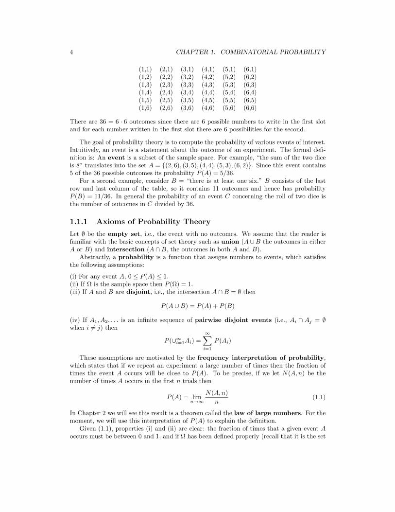
Example 1.2. Things get a little more interesting when we roll two dice. If we suppose, forconvenience, that they are red and green, then we can write the outcomes of this experimentas (m,n), where m is the number on the red die and n is the number on the green die. Tovisualize the set of outcomes it is useful to make a little table:
3
4 CHAPTER 1. COMBINATORIAL PROBABILITY
(1,1) (2,1) (3,1) (4,1) (5,1) (6,1)(1,2) (2,2) (3,2) (4,2) (5,2) (6,2)(1,3) (2,3) (3,3) (4,3) (5,3) (6,3)(1,4) (2,4) (3,4) (4,4) (5,4) (6,4)(1,5) (2,5) (3,5) (4,5) (5,5) (6,5)(1,6) (2,6) (3,6) (4,6) (5,6) (6,6)
There are 36 = 6 · 6 outcomes since there are 6 possible numbers to write in the first slotand for each number written in the first slot there are 6 possibilities for the second.
The goal of probability theory is to compute the probability of various events of interest.Intuitively, an event is a statement about the outcome of an experiment. The formal defi-nition is: An event is a subset of the sample space. For example, “the sum of the two diceis 8” translates into the set A = (2, 6), (3, 5), (4, 4), (5, 3), (6, 2). Since this event contains5 of the 36 possible outcomes its probability P (A) = 5/36.
For a second example, consider B = “there is at least one six.” B consists of the lastrow and last column of the table, so it contains 11 outcomes and hence has probabilityP (B) = 11/36. In general the probability of an event C concerning the roll of two dice isthe number of outcomes in C divided by 36.
1.1.1 Axioms of Probability Theory
Let ∅ be the empty set, i.e., the event with no outcomes. We assume that the reader isfamiliar with the basic concepts of set theory such as union (A ∪B the outcomes in eitherA or B) and intersection (A ∩B, the outcomes in both A and B).
Abstractly, a probability is a function that assigns numbers to events, which satisfiesthe following assumptions:
(i) For any event A, 0 ≤ P (A) ≤ 1.(ii) If Ω is the sample space then P (Ω) = 1.(iii) If A and B are disjoint, i.e., the intersection A ∩B = ∅ then
P (A ∪B) = P (A) + P (B)
(iv) If A1, A2, . . . is an infinite sequence of pairwise disjoint events (i.e., Ai ∩ Aj = ∅when i 6= j) then
P (∪∞i=1Ai) =
∞∑i=1
P (Ai)
These assumptions are motivated by the frequency interpretation of probability,which states that if we repeat an experiment a large number of times then the fraction oftimes the event A occurs will be close to P (A). To be precise, if we let N(A,n) be thenumber of times A occurs in the first n trials then
P (A) = limn→∞
N(A,n)
n(1.1)
In Chapter 2 we will see this result is a theorem called the law of large numbers. For themoment, we will use this interpretation of P (A) to explain the definition.
Given (1.1), properties (i) and (ii) are clear: the fraction of times that a given event Aoccurs must be between 0 and 1, and if Ω has been defined properly (recall that it is the set

1.1. BASIC DEFINITIONS 5
of ALL possible outcomes), the fraction of times something in Ω happens is 1. To explain(iii), note that if the events A and B are disjoint then
N(A ∪B,n) = N(A,n) +N(B,n)
since A∪B occurs if either A or B occurs but it is impossible for both to happen. Dividingby n and letting n→∞, we arrive at (iii).
Property (iii) implies that (iv) holds for a finite number of events, but for infinitelymany events, the last argument breaks down, and this is a new assumption. Not everyonebelieves that assumption (iv) should be used. However, without (iv) the theory of probabilitybecomes much more difficult and less useful, so we will impose this assumption and notapologize further for it. In many cases the sample space is finite so (iv) is not relevantanyway.
Example 1.3. Suppose we pick a letter at random from the word TENNESSEE. What isthe sample space Ω and what probabilities should be assigned to the outcomes?
The sample space Ω = T,E,N, S. To describe the probability it is enough to give thevalues for the individual outcomes, since (iii) implies that P (A) is the sum of the probabilitiesof the outcomes in A. Since there are nine letters in TENNESSEE the probabilities areP (T) = 1/9, P (E) = 4/9, P (N) = 2/9, and P (S) = 2/9.
1.1.2 Basic Properties of P(A)
Having introduced a number of definitions, we will now derive some basic properties ofprobabilities and illustrate their use. The first one is an obvious consequence of the frequencyinterpretation: a large set will occur more often.
Property 1. Monotonicity. If A ⊂ B, i.e., any outcome in A is also in B, then
P (A) ≤ P (B) (1.2)
Proof. A and Ac∩B are disjoint, with union B, so assumption (iii) implies P (B) = P (A) +P (Ac ∩B) ≥ P (A) by (i).
Property 2. Let Ac be the complement of A, i.e., the set of outcomes not in A, then
P (A) = 1− P (Ac) (1.3)
Proof. Let A1 = A and A2 = Ac. Then A1 ∩ A2 = ∅ and A1 ∪ A2 = Ω so (iii) impliesP (A) + P (Ac) = P (Ω) = 1 by (ii). Subtracting P (A) from each side of the equation givesthe result.
This formula is useful because sometimes it is easier to compute the probability of Ac. Foran example, consider A = “at least one six.” In this case Ac = “no six.” There are 5 · 5outcomes with no six, so P (Ac) = 25/36 and P (A) = 1 − 25/36 = 11/36, as we computedbefore.
Property 3. For any events A and B,
P (A ∪B) = P (A) + P (B)− P (A ∩B) (1.4)
Proof by picture.

6 CHAPTER 1. COMBINATORIAL PROBABILITY
PPPPPPPPPPPP
P (A)
P (B)
−P (A ∩B)
+ +
+ +
−
A
B
Intuitively, P (A) + P (B) counts A ∩B twice so we have to subtract P (A ∩B) to make thenet number of times A ∩B is counted equal to 1.
Proof. To prove this result we note that by assumption (ii)
P (A) = P (A ∩B) + P (A ∩Bc)P (B) = P (B ∩A) + P (B ∩Ac)
Adding the two equations and subtracting P (A ∩B):
P (A) + P (B)− P (A ∩B)
= P (A ∩B) + P (A ∩Bc) + P (B ∩Ac) = P (A ∪B)
which gives the desired equality.
To illustrate Property 3, let A = “the red die shows six,” and B = “the green die showssix.” In this case A ∪B = “at least one 6” and A ∩B = (6, 6), so we have
P (A ∪B) = P (A) + P (B)− P (A ∩B) =1
6+
1
6− 1
36=
11
36
The same principle applies to counting outcomes in events.
Example 1.4. A survey of 1000 students revealed that 750 owned stereos, 450 owned cars,and 350 owned both. How many own either a car or a stereo?
Given a set A, we use to |A| denote the number of points in A. The reasoning that led to(1.4) tells us that
|S ∪ C| = |S|+ |C| − |S ∩ C| = 750 + 450− 350 = 850
We can confirm this by drawing a picture:

1.2. PERMUTATIONS AND COMBINATIONS 7
400 350 100
S
C
Property 4. Monotone limits. We write An ↑ A if A1 ⊂ A2 ⊂ · · · and ∪∞i=1Ai = A. Wewrite An ↓ A if A1 ⊃ A2 ⊃ · · · and ∩∞i=1Ai = A.
IF An ↑ A or An ↓ A then P (An)→ P (A). (1.5)
Proof. Let B1 = A1 and for i ≥ 2 let Bi = Ai ∩ Aci−1. The events Bi are disjoint with∪∞i=1Bi = A so
P (A) =
∞∑i=1
P (Bi) = limn→∞
n∑i=1
P (Bi) = limn→∞
P (An)
To prove the second result let Ci = Aci . Ci ↑ C = Ac so P (Ci)→ P (C) and hence
P (Ai) = 1− P (Ci)→ 1− P (C) = P (A)
which proves the second result.
1.2 Permutations and Combinations
As usual we begin with a question:
Example 1.5. The New York State Lottery picks 6 numbers out of 59, or more precisely,a machine picks 6 numbered ping pong balls out of a set of 59. How many outcomes arethere? The set of numbers chosen is all that is important. The order in which they werechosen is irrelevant.
To work up to the solution we begin with something that is obvious but is a key step insome of the reasoning to follow.
Example 1.6. A man has 4 pair of pants, 6 shirts, 8 pairs of socks, and 3 pairs of shoes.Ignoring the fact that some of the combinations may look ridiculous, in how many ways canhe get dressed?
We begin by noting that there are 4 · 6 = 24 possible combinations of pants and shirts.Each of these can be paired with one of 8 choices of socks, so there are 192 = 24 · 8 ways of

8 CHAPTER 1. COMBINATORIAL PROBABILITY
putting on pants, shirt, and socks. Repeating the last argument one more time, we see thatfor each of these 192 combinations there are 3 choices of shoes, so the answer is
4 · 6 · 8 · 3 = 576 ways
The reasoning in the last solution can clearly be extended to more than four experiments,and does not depend on the number of choices at each stage, so we have
The multiplication rule. Suppose that m experiments are performed in order and that,no matter what the outcomes of experiments 1, . . . , k− 1 are, experiment k has nk possibleoutcomes. Then the total number of outcomes is n1 · n2 · · ·nm.
Example 1.7. How many ways can 5 people stand in line?
To answer this question, we think about building the line up one person at a time startingfrom the front. There are 5 people we can choose to put at the front of the line. Havingmade the first choice, we have 4 possible choices for the second position. (The set of peoplewe have to choose from depends upon who was chosen first, but there are always 4 peopleto choose from.) Continuing, there are 3 choices for the third position, 2 for the fourth, andfinally 1 for the last. Invoking the multiplication rule, we see that the answer must be
5 · 4 · 3 · 2 · 1 = 120
Generalizing from the last example we define n factorial to be
n! = n · (n− 1) · (n− 2) · · · 2 · 1 (1.6)
To see that this gives the number of ways n people can stand in line, notice that there aren choices for the first person, n− 1 for the second, and each subsequent choice reduces thenumber of people by 1 until finally there is only 1 person who can be the last in line.
Note that n! grows very quickly since n! = n · (n− 1)!.
1! 1 7! 5,0402! 2 8! 40,3203! 6 9! 362,8804! 24 10! 3,628,8005! 120 11! 39,916,8006! 720 12! 479,001,600
The number of ways we can put the 22 volumes of an encyclopedia on a shelf is
22! = 1.24000728× 10²¹
Here we have used our TI-83. We typed in 22 then used the MATH button to get to thePRB menu and scroll down to the fourth entry to get the ! which gives us 22! after we pressENTER.
The number of ways that cards in a deck of 52 can be arranged is
52! = 8.065817517× 1067
Before there were calculators, people used Stirling’s formula
n! ≈ (n/e)n√
2πn (1.7)
When n = 52, 52/e = 19.12973094 and√
2πn = 18.07554591 so
52! ≈ (19.12973094)52 · 18.07554591 = 8.0529× 1067

1.2. PERMUTATIONS AND COMBINATIONS 9
Example 1.8. Twelve people belong to a club. How many ways can they pick a president,vice-president, secretary, and treasurer?
Again we think of filling the offices one at a time in the order in which they were given in thelast sentence. There are 12 people we can pick for president. Having made the first choice,there are always 11 possibilities for vice-president, 10 for secretary, and 9 for treasurer. Soby the multiplication rule, the answer is
12
P
11
V
10
S
9
T= 11, 800
To compute P12,4 with the TI-83 calculator: type 12, push the MATH button, move thecursor across to the PRB submenu, scroll down to nPr on the second row, and press ENTER.nPr appears on the screen after the 12. Now type 4 and press ENTER.
Passing to the general situation, if we have k offices and n club members then the answeris
n · (n− 1) · (n− 2) · · · (n− k + 1)
To see this, note that there are n choices for the first office, n− 1 for the second, and so onuntil there are n−k+1 choices for the last, since after the last person is chosen there will ben− k left. Products like the last one come up so often that they have a name: the numberof permutations of k objects from a set of size n, or Pn,k for short. Multiplying anddividing by (n− k)! we have
n · (n− 1) · (n− 2) · · · (n− k + 1) · (n− k)!
(n− k)!=
n!
(n− k)!
which gives us a short formula,
Pn,k =n!
(n− k)!(1.8)
The last formula would give us the answer to the lottery problem if the order in whichthe numbers drawn was important. Our last step is to consider a related but slightly simplerproblem.
Example 1.9. A club has 23 members. How many ways can they pick 4 people to be ona committee to plan a party?
To reduce this question to the previous situation, we imagine making the committee mem-bers stand in line, which by (1.8) can be done in 23 · 22 · 21 · 20 ways. To get from this tothe number of committees, we note that each committee can stand in line 4! ways, so thenumber of committees is the number of lineups divided by 4! or
23 · 22 · 21 · 20
1 · 2 · 3 · 4= 23 · 11 · 7 · 5 = 8, 855
To compute C23,4 with the TI-83 calculator: type 23, push the MATH button, move thecursor across to the PRB submenu, scroll down to nCr on the third row, and press ENTER.nCr appears on the screen after the 23, now type 4 and press ENTER.
Passing to the general situation, suppose we want to pick k people out of a group of n.Our first step is to make the k people stand in line, which can be done in Pn,k ways, and

10 CHAPTER 1. COMBINATORIAL PROBABILITY
then to realize that each set of k people can stand in line k! ways, so the number of ways tochoose k people out of n is
Cn,k =Pn,kk!
=n!
k!(n− k)!=n · (n− 1) · · · (n− k + 1)
1 · 2 · · · k(1.9)
by (1.9) and (1.6). Here, Cn,k is short for the number of combinations of k thingstaken from a set of n. Cn,k is often written as
(nk
), a symbol that is read as “n choose
k.” We are now ready for the
Answer to the Lottery Problem, Example 1.5. We are choosing k = 6 objects out ofa total of n = 59 when order is not important, so the number of possibilities is
C59,6 =59!
6!53!=
59 · 58 · 57 · 56 · 55 · 54
1 · 2 · 3 · 4 · 5 · 6= 59 · 58 · 19 · 7 · 11 · 9 = 45, 057, 474
You should consider this the next time you think about spending $1 for two chances to wina jackpot that starts at $3 million and increases by $1 million each week there is no winner.
Pascal’s triangle. The number of outcomes for coin tossing problems fit together in anice pattern:
11 1
1 2 11 3 3 1
1 4 6 4 11 5 10 10 5 1
1 6 15 20 15 6 11 7 21 35 35 21 7 1
Each number is the sum of the ones on the row above on its immediate left and right. Toget the 1’s on the edges to work correctly we consider the blanks to be zeros. In symbols
Cn,k = Cn−1,k−1 + Cn−1,k (1.10)
Verbal proof. In picking k things out of n, which can be done in Cn,k ways, we may or maynot pick the last object. If we pick the last object then we must complete our set of k bypicking k − 1 objects from the first n − 1, which can be done in Cn−1,k−1 ways. If we donot pick the last object then we must pick all k objects from the first n − 1, which can bedone in Cn−1,k ways.
Analytic proof. Using the definition (1.9)
Cn−1,k−1 + Cn−1,k =(n− 1)!
(n− k)!(k − 1)!+
(n− 1)!
(n− k − 1)!k!
Factoring out the parts common to the two fractions
=(n− 1)!
(n− k − 1)!(k − 1)!
(1
n− k+
1
k
)=
(n− 1)!
(n− k − 1)!(k − 1)!
(n
(n− k)k
)=
n!
(n− k)!k!

1.2. PERMUTATIONS AND COMBINATIONS 11
which proves (1.10).
Binomial theorem. The numbers in Pascal’s triangle also arise if we take powers of(x+ y):
(x+ y)2 = x2 + 2xy + y2
(x+ y)3 = (x+ y)(x2 + 2xy + y2) = x3 + 3x2y + 3xy2 + y3
(x+ y)4 = (x+ y)(x3 + 3x2y + 3xy2 + y3)
= x4 + 4x3y + 6x2y2 + 4xy3 + y4
or in general
(x+ y)n =
n∑m=0
Cn,mxmyn−m (1.11)
To see this consider (x+ y)5 and write it as
(x+ y)(x+ y)(x+ y)(x+ y)(x+ y)
Since we can choose x or y from each parenthesis, there are 25 terms in all. If we want a termof the form x3y2 then in 3 of the 5 cases we must pick x, so there are C5,3 = (5 · 4)/2 = 10ways to do this. The same reasoning applies to the other terms, so we have
(x+ y)5 = C5,5x5 + C5,4x
4y + C5,3x3y2 + C5,2x
2y3 + C5,1xy4 + C5,0y
5
= x5 + 5x4y + 10x3y2 + 10x2y3 + 5xy4 + y5
1.2.1 More than two categories
We defined Cn,k as the number of ways of picking k objects out of n. To motivate thenext generalization we would like to observe that Cn,k is also the number of ways we candivide n objects into two groups, the first one with k objects and the second with n − k.To connect this observation with the next problem, think of it as asking: “How many wayscan we divide 12 objects into three numbered groups of sizes 4, 3, and 5?”
Example 1.10. A house has 12 rooms. We want to paint 4 yellow, 3 purple, and 5 red. Inhow many ways can this be done?
This problem can be solved using what we know already. We first pick 4 of the 12 roomsto be painted yellow, which can be done in C12,4 ways, and then pick 3 of the remaining 8rooms to be painted purple, which can be done in C8,3 ways. (The 5 unchosen rooms willbe painted red.) The answer is:
C12,4C8,3 =12!
4! 8!· 8!
3! 5!=
12!
4! 3! 5!= 27, 720
A second way of looking at the problem, which gives the last answer directly, is to firstdecide the order in which the rooms will be painted, which can be done in 12! ways, thenpaint the first 4 on the list yellow, the next 3 purple, and the last 5 red. One example is
9
Y
6
Y
11
Y
1
Y
8
P
2
P
10
P
5
R
3
R
7
R
12
R
4
R

12 CHAPTER 1. COMBINATORIAL PROBABILITY
Now, the first four choices can be rearranged in 4! ways without affecting the outcome, themiddle three in 3! ways, and the last five in 5! ways. Invoking the multiplication rule, wesee that in a list of the 12! possible permutations each possible painting thus appears 4! 3! 5!times. Hence the number of possible paintings is
12!
4! 3! 5!
The second computation is a little more complicated than the first, but makes it easierto see
Theorem 1.1. The number of ways a group of n objects to be divided into m groups of sizen1, . . . , nm with n1 + · · ·+ nm = n is
n!
n1!n2! · · ·nm!(1.12)
The formula may look complicated but it is easy to use.
Example 1.11. There are 39 students in a class. In how many ways can a professor giveout 9 A’s, 13 B’s, 12 C’s, and 5 F’s?
39!
9! 13! 12! 5!= 1.57× 10²²
1.3 Flipping Coins, the World Series, Birthdays
Even simpler than rolling a die is flipping a coin, which produces one of two outcomes, called“Heads” (H) or “Tails” (T ). If we flip two coins there are four outcomes
HTHH TH TT
heads 2 1 0probability 1/4 2/4 1/4
Flipping three coins there are eight possibilities:
HHT TTHHHH HTH THT TTT
THH HTTheads 3 2 1 0probability 1/8 3/8 3/8 1/8
If we flip a large number of coins it will be tedious to write out all the otucomes so weneed to derive some fomrulas.
Example 1.12. Suppose we flip seven coins. Compute the probability that we get 0, 1, 2,or 3 heads.
There are 27 = 128 total outcomes. There is only 1, TTTTT that gives 0 heads, so thatprobability is 1/32. There are 7 outcomes that have one heads. We could write them outbut it is better to reason that we can pick the toss for the heads to occur in
C7,1 =7!
6! 1!= 7

1.3. FLIPPING COINS, THE WORLD SERIES, BIRTHDAYS 13
Extending the last reasoning to two heads, the number of outcomes is the number of waysof picking 2 tosses for the heads to occur or
C7,2 =7!
5! 2!=
7 · 62
= 21
Likewise the number of outcomes with 3 heads is
C7,3 =7!
4! 3!=
7 · 6 · 53!
= 35
By symmetry the numbers of outcomes for 4, 5, 6, and 7 heads are 35, 21, 7, and 1. Interms of binomial coefficients this says
Cn,m =n!
m!(n−m)!= Cn,n−m (1.13)
To prove this in words: The number of ways of picking m objects out of n to take is thesame as the number of ways of choosing n − m to leave behind. Of course, one can alsocheck this directly from the formula in (1.9).
Our next problem concerns flipping four to seven coins:
Example 1.13. World Series. In this baseball event, the first team to win four gameswins the championship. Obviously, the series may last 4, 5, 6, or 7 games. Here we willcompute the probabilities of each of these outcomes. To do this, we will assume that the twoteams are equally matched and ignoring potential complicating factors like the advantage ofplaying at home or psychological factors that make the outcome of one game affect the nextone. In short, we suppose that the games are decided by tossing a fair coin to determine ifteam A or team B wins.
Four games. There are two possible ways this can happen: A wins all four games or Bwins all four games. There are 2 · 2 · 2 · 2 = 16 possible outcomes and these are 2 of them soP (4) = 2/16 = 1/8.
Five games. Here and in the next two cases we will compute the probability that A winsin the specified number of games and then multiply by 2. There are four possible outcomes
BAAAA, ABAAA, AABAA, AAABA
AAAAB is not possible since in that case the series would have ended in four games. Thereare 25 = 32 outcomes so P (5) = 2 · 4/32 = 1/4.
Six games. As we noticed in the last example, A has to win the last game. That means Bmust win exactly two of the first five games, so there are
C5,2 =5!
3!2!=
5 · 42
= 10
outcomes. Each has probability 1/26, so the probability A wins in 6 games is 10/26 and theprobability the series lasts 6 games is 2 · 10/64 = 5/16.
Seven games. In this case B must win exactly three of the first six games, so there are
C6.3 =6!
3!3!=
6 · 5 · 43!
= 20

14 CHAPTER 1. COMBINATORIAL PROBABILITY
outcomes. Each has probability 1/27, so the probability A wins in 6 games is 20/27 and theprobability the series lasts 7 games is 2 · 20/128 = 5/16.
As mentioned earlier, we are ignoring things that many fans think are important todetermining the outcomes of the games, so our next step is to compare the probabilitiesjust calculated with the observed frequencies of the duration of best of seven series in threesports. The numbers in parentheses give the number of series in our sample.
Games 4 5 6 7Probabilities 0.125 0.25 0.3125 0.3125World Series (94) 0.181 0.224 0.224 0.372Stanley Cup (74) 0.270 0.216 0.230 0.284NBA finals (57) 0.122 0.228 0.386 0.263
In statistics class you will learn that the chi-squared statistic to see if the observationsare consistent with the probabilities we have computed. The details of the test are beyondthe scope of this book so we just quote the results: the Stanley Cup data is very unusualdue to the larger than expected number of four game series. The World Series data doesnot fit the model well, but is not very unusual. On the other hand, the NBA finals datalooks like what we should expect to see. The excess of six game series can be due just tochance.
Example 1.14. Birthday problem. There are 30 people at a party. Someone wants tobet you $10 that there are two people with exactly the same birthday. Should you take thebet?
To pose a mathematical problem, we ignore Feb. 29 which only comes in leap years, andsuppose that each person at the party picks their birthday at random from the calendar.There are 36530 possible outcomes for that experiment. The number of outcomes in whichall the birthdays are different is
365 · 364 · 363 · · · 336
since the second person must avoid the first person’s birthday, the third the first two birth-days and so on until the 30th person must avoid the 29 previous birthdays. Let D be theevent that all birthdays are different. Dividing the number of outcomes in which all thebirthdays are different by the total number of outcomes, we have
P (D) =365 · 364 · 363 · · · 336
36530= 0.293684
In words, only about 29% of the time all the birthdays are different, so you will lose the bet71% of the time.
At first glance it is surprising that the probability of two people having the same birthdayis so large, since there are only 30 people compared with 365 days on the calendar. Some ofthe surprise disappears if you realize that there are (30 ·29)/2 = 435 pairs of people who aregoing to compare their birthdays. Let pk be the probability that k people all have differentbirthdays. Clearly, p1 = 1 and pk+1 = pk(365 − k)/365. Using this recursion it is easy togenerate the values of pk.
The graph shows the trends, but to get precise values a table is better:

1.4. RANDOM VARIABLES, EXPECTED VALUE 15
0
0.1
0.2
0.3
0.4
0.5
0.6
0.7
0.8
0.9
1
0 10 20 30 40 50 60
Figure 1.1: Probability of no birthday match in a group of size k
1 1.00000 11 0.85886 21 0.55631 31 0.269552 0.99726 12 0.83298 22 0.52430 32 0.246653 0.99180 13 0.80559 23 0.49270 33 0.225034 0.98364 14 0.77690 24 0.46166 34 0.204685 0.97286 15 0.74710 25 0.43130 35 0.185626 0.95954 16 0.71640 26 0.40176 36 0.167827 0.94376 17 0.68499 27 0.37314 37 0.151278 0.92566 18 0.65309 28 0.34554 38 0.135939 0.90538 19 0.62088 29 0.31903 39 0.1217810 0.88305 20 0.58856 30 0.29368 40 0.10877
1.4 Random variables, Expected value
A random variable is a real valued function defined on a probability space. Three exam-ples:
• Roll two dice and let X = the sum of the two numbers that appear.
• Flip a coin 10 times and let X = the number of Heads we get.
• Draw 13 cards out of a deck and let X = the number of Hearts we get.
The distribution of a discrete random variable is described by listing its possible valuesand giving their probabilities. In the previous section we computed the distribution of thenumber of games N to finish the world series. The distribution of the random variable isgiven by
x 4 5 6 7P (X = x) 2/16 4/16 5/16 5/16

16 CHAPTER 1. COMBINATORIAL PROBABILITY
The expected value of a discrete random value X is obtained form the formula
EX =∑x
xP (X = x) (1.14)
In words we sum over the set of possible values the value times the probability it occurs.EX is also called the mean of X. It should be clear from the definitions that
E(X + a) = EX + a E(bX) = bEX (1.15)
In words if we add 3 to a random variable we add 3 to its mean. If we multiply a randomvariable by 5 we multiply its mean by 5.
Example 1.15. Roulette. If you play roulette and bet $1 on black then you win $1 withprobability 18/38 and you lose $1 with probability 20/38, so the expected value of yourwinnings X is
EX = 1 · 18
38+ (−1) · 20
38=−2
38= −0.0526
The expected value has a meaning much like the frequency interpretation of probability: inthe long run you will lose about 5.26 cents per play.
Example 1.16. In the case of the world series
EX =2 · 4 + 4 · 5 + 5 · 6 + 5 · 7
16=
93
16= 5.8125
The interpretation of the mean is similar to the frequency interpretation of probability.Ifwe repeat our little coin flipping World Series a large number of times, the average numberof games will be close to the mean.
Example 1.17. Roll one die. Let X be the number that appears on the die. P (X =x) = 1/6 for x = 1, 2, 3, 4, 5, 6, so
EX = 1 · 1
6+ 2 · 1
6+ 3 · 1
6+ 4 · 1
6+ 5 · 1
6+ 6 · 1
6=
21
6= 3
1
2
Example 1.18. Suppose we roll two dice and let S2 be the sum of the two numbers.Consulting a table of the possible outcomes
(1,1) (2,1) (3,1) (4,1) (5,1) (6,1)(1,2) (2,2) (3,2) (4,2) (5,2) (6,2)(1,3) (2,3) (3,3) (4,3) (5,3) (6,3)(1,4) (2,4) (3,4) (4,4) (5,4) (6,4)(1,5) (2,5) (3,5) (4,5) (5,5) (6,5)(1,6) (2,6) (3,6) (4,6) (5,6) (6,6)
we see that if S2 is the sum of the two dice then P (S2 = 6) = 5/36. Realizing that theoutcomes with a given sum lie on a diagonal line we see that the distribution of the sum isgiven by
n 2 3 4 5 6 7 8 9 10 11 12P (S2 = n) 1
36236
336
436
536
636
536
436
336
236
136

1.4. RANDOM VARIABLES, EXPECTED VALUE 17
We could compute ES2 by using the definition
ES2 =2 · 1 + 3 · 2 + 4 · 3 + 5 · 4 + 6 · 5 + 7 · 6
36
+8 · 5 + 9 · 4 + 10 · 3 + 11 · 2 + 12 · 1
36=
252
36= 7
However, there is a simpler way. Let X1 be the number on the first die, and let X2 be thenumber on the second die. Since P (Xi = j) = 1/6 for j = 1, 2, . . . 6 it is clear that
EXi =1 + 2 + 3 + 4 + 5 + 6
6= 3.5
Theorem 1.2. If X1, X2, . . . Xn are any discrete random variables then
E(X1 + · · ·+Xn) = EX1 + · · ·+ EXn
This is true for the exact same reason that∫f(x) + g(x) dx =
∫f(x) dx+
∫g(x) dx
so we will not prove this.
From this it follows that if S2 is the sum of two dice then ES2 = EX1 +EX2 = 7, or moregenerally if Sk is the total of k dice then ESk = 3.5k. The same reasoning applies to Hk thenumber of heads when we flip k coins. Let Yi = 1 if the ith coin is heads and Yi = 0 if theith coin is tails. Since P (Yi = 1) = P (Yi = 0) = 1/2 we have EYi = (1/2) · 1 + (1/2) · 01/2so we have
EHk = Y1 + ·EYk = k/2
Example 1.19. The birthday problem. While it is a little tedious to compute theprobability of no birthday match in a group of n people, it is easy to compute the expectedvalue of Mn the total number of birthday matches. For 1 ≤ i < j ≤ n let Xi,j = 1 if thebirthdays of i and j match. The total number of birthday matches
Mn =∑
1≤i<j≤n
Xij
where the sum is over all i and j with i < j. The number of such pairs is Cn,2 so
EMn =Cn,2365
If n = 30 this is
EM30 =30 · 29
2· 1
365= 0.78082.
In the previous section we computed that P (M30 = 0) = 0.29368 so P (M30 > 0) = 0.70632.
Example 1.20. The birthday problem in the Senate. Since there are 100 senators itis very likely that there are two with the same birthday. By the calculations in the previousexample
EM100 =100 · 99
2· 1
365=
4950
365= 13.56

18 CHAPTER 1. COMBINATORIAL PROBABILITY
With a significant number of birthday matches it is natural to ask if there are any triplebirthdays. Let Tijk = 1 senators i, j, and k all have the same birthday.
ET100 =100 · 99 · 98
3!· 1
3652=
161, 700
133, 225= 1.213
In the 2018 Senate there were 10 double birthdays and one triple birthdays: May 3: JimRisch (Idaho), David Vitter (Louisiana), Ron Wyder (Oregon). It is difficult to computethe exact probability of no triple birthday. In Example 2.22 in Chapter 2 we will find asimple approximation, which suggests teh answer is ≈ 0.614.
Example 1.21. Fair division of a bet on an interrupted game. Pascal and Fermatwere sitting in a cafe in Paris playing the simplest of all games, flipping a coin. Each hadput up a bet of 50 francs and the first to get 10 points wins. Fermat was winning 8 pointsto 7 when he received an urgent message that a friend was sick, and he must rush to hishome town of Toulouse. The carriage man who delivered the message offered to take him,but only if he would leave immediately. Later in correspondence between the two men, theproblem arose: how should the money bet (100 francs) be divided?
In the case under consideration, it is easier to calculate the probability that Pascal(P ) wins. In order for Pascal to win by a score of 10-8 he must win three flips in arow: PPP , an event of probability 1/8. To win 10-9 he can lose one flip but not thelast one: FPPP , PFPP , PPFP , which has probability 3/16. Adding the two we seethat Pascal wins with probability 5/16 and should get that fraction of the total bet, i.e.,(5/16)(100) = 31.25.Fermat came up with the reasonable idea that the fraction of the stakesthat each receives should be equal to the probability it would have won the match.
1.5 Card Games and Other Urn Problems
A number of problems in probability have the following form.
Example 1.22. Suppose we pick 3 balls out of an urn with 12 red balls and 8 black balls.What is the probability of B2 = “We get two red balls and one black ball.”?
Almost by definition, there are
C20,3 =20 · 19 · 18
1 · 2 · 3= 5 · 19 · 3 · 17 = 1, 140
ways of picking 4 balls out of the 20. To count the number of outcomes in B2, we note thatthere are C12,2 = (12 · 11)/2 = 66 ways to choose the red balls and C8,1 = 8 ways to choosethe black balls, so the multiplication rule implies
|B2| = C12,2C8,1 = 66 · 8 = 528
It follows that P (B2) = 528/1140 = 0.4632.If we let Bk be the event that we draw k red balls then we have
k 3 2 1 0|Bk| C12,3 = 220 C12,2C8,1 = 528 C12,1C8,7 = 336 C8,3 = 56P (BK) 0.1930 0.4632 0.2947 0.0491

1.5. CARD GAMES AND OTHER URN PROBLEMS 19
Example 1.23. A deck of cards has four suits: spades ♠, hearts ♥, diamonds ♦ and clubs♣. Each suit has an ace A, king K, queen Q, jack J , 10, 9, 8, 7, 6, 5, 4, 3, 2. Suppose wedraw five cards out the deck. What is the probbability we have exactly three psaces.
The number of possible outcomes is
C52,5 = 2, 598, 960
The number of outcomes with 3 spades and 2 nonspades is
C13,3 · C39,2 =13 · 12 · 11
3!· 39 · 38
2= 211, 926
so the answer is 211, 926/2, 598, 960 = 0.8154
Poker. In the game of poker the following hands are possible; they are listed in increasingorder of desirability. In the definitions the word value refers to A, K, Q, J, 10, 9, 8, 7, 6, 5,4, 3, or 2. This sequence also describes the relative ranks of the cards, with one exception:an Ace may be regarded as a 1 for the purposes of making a straight. (See the example in(d), below.)
(a) one pair: two cards of equal value plus three cards with different valuesJ♠ J♦ 9♥ Q♣ 3♠
(b) two pair: two pairs plus another card with a different valueJ♠ J♦ 9♥ 9♣ 3♠
(c) three of a kind: three cards of the same value and two with different valuesJ♠ J♦ J♥ 9♣ 3♠
(d) straight: five cards with consecutive values5♥ 4♠ 3♠ 2♥ A♣
(e) flush: five cards of the same suitK♣ 9♣ 7♣ 6♣ 3♣
(f) full house: a three of a kind and a pairJ♠ J♦ J♥ 9♣ 9♠
(g) four of a kind: four cards of the same value plus another cardJ♠ J♦ J♥ J♣ 9♠
(h) straight flush: five cards of the same suit with consecutive valuesA♣ K♣ Q♣ J♣ 10♣
This example is called a royal flush.
To compute the probabilities of these poker hands we begin by observing that there are
C52,5 =52 · 51 · 50 · 49 · 48
1 · 2 · 3 · 4 · 5= 2, 598, 960
ways of picking 5 cards out of a deck of 52, so it suffices to compute the number of wayseach hand can occur. We will do three cases to illustrate the main ideas and then leave therest to the reader.
(d) straight: 10 · 45
A straight must start with a card that is 5 or higher, 10 possibilities. Once the values aredecided on, suits can be assigned in 45 ways. This counting regards a straight flush as astraight. If you want to exclude straight flushes, suits can be assigned in 45 − 4 ways.

20 CHAPTER 1. COMBINATORIAL PROBABILITY
(f) full house: 13 · C4,3 · 12 · C4,2
We first pick the value for the three of a kind (which can be done in 13 ways), then assignsuits to those three cards (C4,3 ways), then pick the value for the pair (12 ways), then weassign suits to the last two cards (C4,2 ways).
(b)two pair: C13,2 · C4,2 · C4,2 · 44We first pick the values for the two pair then assign suits to each of them, and pick onefinal card with a value that does not match the first two. A common incorrect answer tothis question is
13 · C4,2 · 12 · C4,2 · 44
Referring to the example above,choosing j and then 9 is counted as being different from 9and then J so this is 2 times the correct answer. Similar reasoning leads to
(a) one pair: 13 · C4,2 · C12,3 · 43
The numerical values of the probabilities of all poker hands are given in the next table.
(a) one pair .422569(b) two pair .047539(c) three of a kind .021128(d) straight .003940(e) flush .001981(f) full house .001441(g) four of a kind .000240(h) straight flush .000015
The probability of getting none of these hands can be computed by summing the values for(a) through (g) (recall that (d) includes (h)) and subtracting the result from 1. However, itis much simpler to observe that we have nothing if we have five different values that do notmake a straight or a flush. So the number of nothing hands is (C13,5− 10) · (45− 4) and theprobability of a nothing hand is 0.501177.
Example 1.24. Suppose we draw 13 cards from a deck. How many outcomes are there?How many lead to hands with 4 spades, 3 hearts, 3 diamonds, and 3 clubs? 3 spades, 5hearts, 2 diamonds, and 3 clubs?
C52,13 = 6.350135596× 10¹¹
C13,4C13,3C13,3C13,3 = 715 · (286)3 = 16, 726, 464, 040
C13,3C13,5C13,2C13,3 = 286 · 1287 · 78 · 286 = 8, 211, 173, 256
Example 1.25. Suit distributions. The last bridge hand in the previous example is saidto have a 5-3-3-2 distribution. Here, we have listed the number cards in the longest suit firstand continued in decreasing order. Permuting the four numbers we see that the example 3spades, 5 hearts, 2 diamonds, and 3 clubs is just one of 4!/2! possible ways of assigning thenumbers to suits, so the probability of a 5-3-3-2 distribution is
12 · 8, 211, 173, 256
6.350135596× 1011= 0.155
Similar computations lead to the results in the next table. We have included the numberof different permutations of the pattern to help explain why slightly unbalanced distributionshave larger probability than 4-3-3-3.

1.5. CARD GAMES AND OTHER URN PROBLEMS 21
Distribution Probability Permutations4-4-3-2 0.216 125-3-3-2 0.155 125-4-3-1 0.129 245-4-2-2 0.106 124-3-3-3 0.105 46-3-2-2 0.056 12
Example 1.26. Keno. In this game the casino picks 20 balls out of 80 numbered balls.Before the draw you may, for example pick 10 numbers and bet $1. In this case you win $1if 4 of your numbers are chosen; $2 for 5; $20 for 6; $105 for 7; $500 for 8; $5000 for 9; and$12,000 if all ten are chosen. We want to compute the expected value of the bet.
The number of possible draws is astronomically large:
C80,20 = 3.5353× 10¹⁸
The probability that k of your numbers are chosen is
pk =C10,kC70,20−k
C80,20
When k = 0 this isC70,20
C80,20=
70!60!
80!50!=
60 · 59 · · · 51
80 · 79 · · · 71= 0.045791
To compute the other probabilities it is useful to note that for 1 ≤ m ≤ n
Cn,m =n!
m!(n−m)!=n+ 1−m
m· n!
(m− 1)!(n+ 1−m)!
=n+ 1−m
m· Cn,m−1
so we have
pk = pk−1 ·11− kk
· 21− k50 + k
Writing wk for the winning when k of our numbers are drawn, using this recursion and theresult for p0 gives
k pk wk wkpk0 0.045791 01 0.179571 02 0.295257 03 0.267402 04 0.147319 1 0.1473195 0.051428 2 0.1028556 0.011479 20 0.2295887 0.001611 105 0.1697018 0.000135 500 0.0677109 6.12× 10⁻⁶ 5000 0.03060310 1.12× 10⁻⁷ 12,000 0.001347
4-10 .2120 .7486

22 CHAPTER 1. COMBINATORIAL PROBABILITY
Thus, we win something about 21.2% of the time and our average winning is a little less than75 cents, a typical expected value for Keno bets. The last column shows the contributionof the different payoffs to the expected value.
Example 1.27. Disputed elections. In a close election in a small town, 2,656 people(50.6%) voted for candidate A compared to 2,594 who voted for candidate B, a margin ofvictory of 62 votes. An investigation of the election found that 136 of the people who votedin the election should not have. Since this is more than the margin of victory, should theelection results be thrown out even though there was no evidence of fraud on the part ofthe winner’s supporters?
Like many problems that come from the real world (a court case De Martini v. Power),this one is not precisely formulated. To turn this into a probability problem we supposethat all the votes were equally likely to be one of the 136 erroneously cast and we investigatewhat happens when we remove 136 balls from an urn with 2,656 white balls and 2,594 blackballs.
In order to reverse the outcome of the election, we must have
2, 656−m ≤ 2, 594− (136−m) or m ≥ 99
This arithmetic was enough for the judge to make his decision. “ Although the successfulcandidate was elected on the strength of only 50.6% of the vote, her majority would not belost unless 99 votes i.e., 72.8% of the irregularities were cast in her favor. It taxes credulityto assume that, in so close a contest, such an extreme percentage of invalid votes wouldbe cast in one direction. In the conceded absence of fraud, a valid determination is notrendered impossible (Election Law, by the remote possibility of a changed result.”
To see how remote the possibility is, we note that the probability of removing exactlym white and 136−m black balls is
pm =C2656,mC2594,136−m
C5250,136
If one tries to evaluate this when m = 99 with your calculator you get an overflow message.Expanding the factorials we have
p99 =2656·2558
99!2594···2558
37!5250···5115
136!
=136!
99!37!· 2656 · · · 2558 · 2594 · · · 2558
5250 · · · 5152 · 5151 · · · 5115
In the last product the ratio of the term in the numerator to the one under it in thedenomainator is always close to 1/2 so the above is
≈ 136!
99!37!(1/2)136 (1.16)
which corresponds to flipping 136 coins to determine to candidate who loses the votes.The probability in (1.16) is 3.27 × 10⁻⁸. In the next section we will learn that this is thebinomial distribution and we will learn how to compute the probability B loses ≤ 37 votesis 5.13× 10⁻⁸ computer program shows the exact probability is 7.492× 10⁻⁸.
Example 1.28. Quality control. A shipment of 50 precision parts including 4 that aredefective is sent to an assembly plant. The quality control division selects 10 at randomfor testing and rejects the entire shipment if 1 or more are found defective. What is theprobability this shipment passes inspection?

1.6. EXERCISES 23
There are C50,10 ways of choosing the test sample, and C46,10 ways of choosing all goodparts so the probability is
C46,10
C50,10=
46!/36!10!
50!/40!10!=
46 · 45 · · · 37
50 · 49 · · · 41
=40 · 39 · 38 · 37
50 · 49 · 48 · 47= 0.396
Using almost identical calculations a company can decide on how many bad units they willalow in a shipment and design a testing program with a given probability of success.
Example 1.29. Capture-recapture experiments. An ecology graduate student goes toa pond and captures k = 60 beetles, marks each with a dot of paint, and then releases them.A few days later she goes back and captures another sample of r = 50, finding m = 12marked beetles and r − m = 38 unmarked. What is her best guess about the size of thepopulation of beetles?
To turn this into a precisely formulated problem, we will suppose that no beetles enter orleave the population between the two visits. With this assumption, if there were N beetlesin the pond, then the probability of getting m marked and r −m unmarked in a sample ofr would be
pN =Ck,m CN−k,r−m
CN,r
To estimate the population we will pick N to maximize pN , the so-called maximum like-lihood estimate. To find the maximizing N , we note that
Cj−1,i =(j − 1)!
(j − i− 1)!i!so Cj,i =
j!
(j − i)!i!=jCj−1,i
(j − i)
and it follows that
pN = pN−1 ·N − k
N − k − (r −m)· N − r
N
Now pN/pN−1 ≥ 1 if and only if
(N − k)(N − r) ≥ N(N − k − r +m)
that is,
N2 − kN − rN + kr ≥ N2 − kN − rN +mN
or equivalently if N ≤ kr/m. Thus the value of N that maximizes the probability pN isthe largest integer ≤ kr/m. This choice is reasonable since when N = kr/m the proportionof marked beetles in the population, k/N , equals the proportion of marked beetles in thesample, m/r. Plugging in the numbers from our example, kr/m = (60 · 50)/12 = 250, sothe probability is maximized when N = 250.
1.6 Exercises
Basic definitions
24 CHAPTER 1. COMBINATORIAL PROBABILITY
1. A man receives presents from his three children, Allison, Betty, and Chelsea. To avoiddisputes he opens the presents in a random order. What are the possible outcomes?
2. Suppose we pick a number at random from the phone book and look at the last digit.(a) What is the set of outcomes and what probability should be assigned to each outcome?(b) Would this model be appropriate if we were looking at the first digit?
3. Two students arrive late for a math final exam with the excuse that their car had a flattire. Suspicious, the professor says “each one of you write down on a piece of paper whichtire was flat. What is the probability that both students pick the same tire?
4. Suppose we roll a red die and a green die. What is the probability the number on thered die is larger (>) than the number on the green die?
5. Two dice are rolled. What is the probability (a) the two numbers will differ by 1 or less,(b) the maximum of the two numbers will be 5 or larger?
6. If we flip a coin 5 times, what is the probability that the number of heads is an evennumber (i.e., divisible by 2)?
7. The 1987 World Series was tied at two games a piece before the St. Louis Cardinals wonthe fifth game. According to the Associated Press, “The numbers of history support theCardinals and the momentum they carry. Whenever the series has been tied 2-2 the teamthat won the fifth game won the series 71% of the time.” If momentum is not a factor andeach team has a 50% chance of winning each game, what is the probaiblity that the game5 winner will win the series?
8. Two boys are repeatedly playing a game that they each have probability 1/2 of winning.The first person to win five games wins the match. What is the probability that Al will winif (a) he has won 4 games and Bobby has won 3; (b) he leads by a score of 3 games to 2?
9. 20 families live in a neighborhood. 4 have 1 child, 8 have 2 children, 5 have 3 children,and 3 have 4 children. If we pick a child at random what is the probability they come froma family with 1, 2, 3, 4 children?
10. In Galileo’s time people thought that when three dice were rolled, a sum of 9 and a sumof 10 had the same probability since each could be obtained in 6 ways:
9 : 1 + 2 + 6, 1 + 3 + 5, 1 + 4 + 4, 2 + 2 + 5, 2 + 3 + 4, 3 + 3 + 3
10 : 1 + 3 + 6, 1 + 4 + 5, 2 + 4 + 4, 2 + 3 + 5, 2 + 2 + 6, 3 + 3 + 4
Compute the probabilities of these sums and show that 10 is a more likely total than 9.
11. Suppose we roll three dice. Compute the probability that the sum is (a) 3, (b) 4, (c) 5,(d) 6, (e) 7, (f) 8 (g) 9 (h) 10.
12. In a group of students, 25% smoke cigarettes, 60% drink alcohol, and 15% do both.What fraction of students have at least one of these bad habits?
13. In a group of 320 high school graduates, only 160 went to college but 100 of the 170men did. How many women did not go to college?
14. In the freshman class, 62% of the students take math, 49% take science, and 38% takeboth science and math. What percentage takes at least one science or math course?

1.6. EXERCISES 25
15. 24% of people have American Express cards, 61% have Visa cards and 8% have both.What percentage of people have at least one credit card?
16. Suppose Ω = a, b, c, P (a, b) = 0.7, and P (b, c) = 0.6. Compute the probabilitiesof a, b, and c.
17. Suppose A and B are disjoint with P (A) = 0.3 and P (B) = 0.5. What is P (Ac ∩Bc)?
18. Given two events A and B with P (A) = 0.4 and P (B) = 0.7, what are the maximumand minimum possible values for P (A ∩B)?
Permutations and Combinations
19. How many possible batting orders are there for nine baseball players?
20. A tire manufacturer wants to test four different types of tires on three different typesof roads at five different speeds. How many tests are required?
21. 16 horses race in the Kentucky Derby. How many possible results are there for win,place, and show (first, second, and third)?
22. A school gives awards in five subjects to a class of 30 students but no one is allowed towin more than one award. How many outcomes are possible?
23. A tourist wants to visit six of America’s ten largest cities. In how many ways can shedo this if the order of her visits is (a) important, (b) not important?
24. Five businessmen meet at a convention. How many handshakes are exchanged if eachshakes hands with all the others?
25. A commercial for Glade Plug-ins says that by inserting two of a choice of 11 scents intothe device, you can make more than 50 combinations. If we exclude the boring choice oftwo of the same scent how many possibilities are there?
26. In a class of 19 students, 7 will get A’s. In how many ways can this set of students bechosen?
27. (a) How many license plates are possible if the first three places are occupied by lettersand the last three by numbers? (b) Assuming all combinations are equally likely, what isthe probability the three letters and the three numbers are different?
28. How many four-letter “words” can you make if no letter is used twice and each wordmust contain at least one vowel (A, E, I, O or U)?
29. Assuming all phone numbers are equally likely, what is the probability that all thenumbers in a seven-digit phone number are different?
30. A domino is an ordered pair (m,n) with 0 ≤ m ≤ n ≤ 6. How many dominoes are in aset if there is only one of each?
31. A person has 12 friends and will invite 7 to a party. (a) How many choices are possibleif Al and Bob are feuding and will not both go to the party? (b) How many choices arepossible if Al and Betty insist that they both go or neither one goes?
32. A basketball team has 5 players over six feet tall and 6 who are under six feet. Howmany ways can they have their picture taken if the 5 taller players stand in a row behindthe 6 shorter players who are sitting on a row of chairs?

26 CHAPTER 1. COMBINATORIAL PROBABILITY
33. The Duke basketball team has 10 women who can play guard and 12 tall women whocan play the other three positions. At the start of the game, the coach gives the refereea starting line-up that lists who will play left guard, right guard, left forward, center, andright forward. In how many ways can this be done?
34. Six students, three boys and three girls, lineup in a random order for a photograph.What is the probability that the boys and girls alternate?
35. Seven people sit at a round table. How many ways can this be done if Mr. Jones andMiss Smith (a) must sit next to each other, (b) must not sit next to each other? (Twoseating patterns that differ only by a rotation of the table are considered the same).
36. How many ways can eight rooks be put on a chess board so that no rook can captureany other rook? Or, what is the same: How many ways can eight markers be placed on an8× 8 grid of squares so that there is at most one in each row or column?
37. A BINGO card is a 5 by 5 grid. The center square is a free space and has no number.The first column is filled with five distinct numbers from 1 to 15, the second with five fromfrom 16 to 30, the middle column with four numbers from 31 to 45, the fourth with fivenumbers from 46 to 60, and the fifth with five numbers from 61 to 75. Since the object ofthe game is to get five in a row horizontally, vertically or diagonally the order is important.How many BINGO cards are there?
38. Continuing with the set-up from the previous problem, in BINGO numbers are drawnfrom 1 to 75 without replacement. When a number is called you put a marker on thatsquare. If you have five in a row horizontally, vertically or diagonally, you have a BINGO.What is the probability you will have a BINGO after (a) four numbers are called? (b) afterfive?
Multinomial Counting Problems
39. How many different ways can the letters in the following words be arranged: (a) money,(b) tattoo, (c) banana, (d) redredged, (e) statistics, (f) mississippi?
40. Ernie has 10 days to go before his mommy picks him up to take him home from college.He has 10 pairs of clean socks: 5 white, 3 brown and 2 black. How many different ways canhe wear his socks over the next 10 days assuming he wears one pair per day.
41. Twelve different toys are to be divided among 3 children so that each one gets 4 toys.How many ways can this be done?
42. A club with 50 members is going to form two committees, one with 8 members and theother with 7. How many ways can this be done (a) if the committees must be disjoint? (b)if they can overlap?
43. (a) If six dice are rolled, what is the probability that each of the six numbers will appearat least once? (b) Answer the last question for seven dice.
44. How many ways can 5 history books, 3 math books, and 4 novels be arranged on a shelfif the books of each type must be together?
45. Suppose three runners from team A and three runners from team B have a race. If allsix runners have equal ability, what is the probability that the three runners from team Awill finish first, second, and fourth?

1.6. EXERCISES 27
46. 9 boys and 7 girls are at a picnic. How many ways can we pick 4 coed teams (one boyand one girl) for a competition.
47. Eight girls show up for a ballroom dance class, but no boys do. How many ways canthe eight girls divide themselves into four pairs to practice dancing. Note: in some dancesone partner leads and the other follows, but here we assume there is no difference betweenthe roles the two dancers play.
48. Four men and four women are shipwrecked on a tropical island. How many ways canthey (a) form four male-female couples, (b) get married if we keep track of the order inwhich the weddings occur, (c) divide themselves into four unnumbered pairs, (d) split upinto four groups of two to search the North, East, West, and South shores of the island,(e) walk single-file up the ramp to the ship when they are rescued, (f) take a picture toremember their ordeal if all eight stand in a line but each man stands next to his wife?
Expected Value
49. You want to invent a gambling game in which a person rolls two dice and is paid somemoney if the sum is 7, but otherwise he loses his money. How much should you pay him forwinning a $1 bet if you want this to be a fair game, that is, to have expected value 0?
50. A bet is said to carry 3 to 1 odds if you win $3 for each $1 you bet. What must theprobability of winning be for this to be a fair bet?
51. A lottery has one $100 prize, two $25 prizes, and five $10 prizes. What should you bewilling to pay for a ticket if 100 tickets are sold?
52. In a popular gambling game, three dice are rolled. For a $1 bet you win $1 for each sixthat appears (plus your dollar back). If no six appears you lose your dollar. What is yourexpected value?
53. In a dice game the “dealer” rolls two dice, the player rolls two dice, and the player winsif his total is larger (>) than the dealer’s. What is the probability the player wins?
54. A roulette wheel has slots numbered 1 to 36 and two labeled with 0 and 00. Supposethat all 38 outcomes have equal probability. Compute the expected values of the followingbets. In each case you bet one dollar and when you win you get your dollar back in additionto your winnings. (a) You win $1 if one of the numbers 1 through 18 comes up. (b) Youwin $2 if the number that comes up is divisible by 3 (0 and 00 do not count). (c) You win$35 if the number 7 comes up.
55. In the Las Vegas game Wheel of Fortune, there are 54 possible outcomes. One is labeled“Joker,” one “Flag,” two “20,” four “10,” seven “5,” fifteen “2,” and twenty-four “1.” Ifyou bet $1 on a number you win that amount of money if the number comes up (plus yourdollar back). If you bet $1 on Flag or Joker you win $40 if that symbol comes up (plus yourdollar back). What bets have the best and worst expected value here?
56. Sic Bo is an ancient Chinese dice game played with 3 dice. One of the possibilities forbetting in the game is to bet “big.” For this bet you win if the total X is 11, 12, 13, 14, 15,16, or 17, except when there are three 4’s or three 5’s. On a $1 bet on big you win $1 plusyour dollar back if it happens. What is your expected value?
57. Five people play a game of “odd man out” to determine who will pay for the pizza theyordered. Each flips a coin. If only one person gets Heads (or Tails) while the other four get

28 CHAPTER 1. COMBINATORIAL PROBABILITY
Tails (or Heads) then he is the odd man and has to pay. Otherwise they flip again. Whatis the expected number of tosses needed to determine who will pay?
Urn Problems
58. How can 5 black and 5 white balls be put into two urns to maximize the probability awhite ball is drawn when we draw from a randomly chosen urn?
59. Two red cards and two black cards are lying face down on the table. You pick two cardsand turn them over. What is the probability that the two cards are different colors?
60. Four people are chosen at random from 5 couples. What is the probability two men andtwo women are selected?
61. You pick 5 cards out of a deck of 52. What is the probability you get exactly 2 spades?
62. Seven students are chosen at random from a class with 17 boys and 13 girls. What isthe probability that 4 boys and 3 girls are selected?
63. In a carton of 12 eggs, 2 are rotten. If we pick 4 eggs to make an omelet, what is theprobability we do not get a rotten egg?
64. An electronics store receives a shipment of 30 calculators of which 4 are defective. Sixof these calculators are selected to be sent to a local high school. What is the probabilitythat exactly one is defective?
65. A scrabble set contains 54 consonants, 44 vowels, and 2 blank tiles. Find the probabilitythat your initial draw contains 5 consonants and 2 vowels.
66. (a) How many ways can can we pick 4 students from a group of 30 to be on the mathteam? (b) Suppose there are 18 boys and 12 girls. What is the probability the team willhave 2 boys and 2 girls.
67. The following probability problem arose in a court case concerning possible discrimina-tion against black nurses. 26 white nurses and 9 black nurses took an exam. All the whitenurses passed but only 4 of the black nurses did. What is the probability we would get thisoutcome if the five nurses who failed were chosen at random?
68. A closet contains 8 pairs of shoes. You pick out 5. What is the probability of (a) nopair, (b) exactly one pair, (c) two pairs?
69. A drawer contains 10 black, 8 brown, and 6 blue socks. If we pick two socks at random,what is the probability they match?
70. A dance class consists of 12 men and 10 women. Five men and five women are chosenand paired up to dance. In how many ways can this be done?
71. Suppose we pick 5 cards out of a deck of 52. What is the probability we get at least onecard of each suit?
72. A bridge hand in which there is no card higher than a 9 is called a Yarborough after theEarl who liked to bet at 1000 to 1 that your bridge hand would have a card that was 10 orhigher. What is the probability of a Yarborough when you draw 13 cards out of a deck of52?
73. Two cards are a blackjack if one is an A and the other is a K, Q, J, or 10. (a) If you picktwo cards out of a deck, what is the probability you will get a blackjack? (b) Suppose you

1.6. EXERCISES 29
are playing blackjack against the dealer with a freshly shuffled deck. What is the probabilitythat you or the dealer will get a blackjack?
74. A student studies 12 problems from which the professor will randomly choose 6 for atest. If the student can solve 9 of the problems, what is the probability she can solve atleast 5 of the problems on the test?
75. A football team has 16 seniors, 12 juniors, 8 sophomores, and 4 freshmen. (a) If we pick5 players at random, what is the probability we will get 2 seniors and 1 from each of theother 3 classes? (b) Find an outcome with larger probability than 2− 1− 1− 1.
76. In a kindergarten class of 20 students, one child is picked each day to help serve themorning snack. What is the probability that in one week five different children are chosen?
77. An investor picks 3 stocks out of 10 recommended by his broker. Of these, six will showa profit in the next year. What is the probability the investor will pick (a) 3 (b) 2 (c) 1 (d)0 profitable stocks?
78. Four red cards (i.e., hearts and diamonds) and four black cards are face down on thetable. A psychic who claims to be able to locate the four black cards turns over 4 cards andgets 3 black cards and 1 red card. What is the probability he would get 3 or 4 black cardsif he were guessing?
79. A town council considers the question of closing down an “adult” theatre. The fivemen on the council all vote against this and the three women vote in favor. What is theprobability we would get this result (a) if the council members determined their votes byflipping a coin? (b) if we assigned the five “no” votes to council members chosen at random?
80. An urn contains white balls numbered 1 to 15 and black balls also numbered 1 to 15.Suppose you draw 4 balls. What is the probability that (a) no two have the same number?(b) you get exactly one pair with the same number? (c) you get two pair with the samenumbers?
81. A town has four TV repairmen. In the first week of September four TV sets breakand their owners call repairmen chosen at random. Find the probability that the numberof repairmen who have jobs is 1, 2, 3, 4.
82. Powerball lottery. In this lottery five balls are picked from white balls numbered1, . . . 69 and a red powerball from another urn with balls numbered 1, . . . 26. If three of thewhite numbers you picked are drawn and you get the correct power ball then we call theresult 3 + 1. Compute the probabilities of the following results for a $2 bet:
result prize odds5+1 split jackpot 1/292,201,3385+0 1 million 1/11,688,0534+1 $50,000 1/913,1294+0 $100 1/36,5253+1 $100 1/14,4943+0 $ 7 1/597.762+1 $ 7 1/701.331+1 $4 1/91.980+1 $4 1/38.22
83. Compute the probabilities of the following poker hands when we roll five six sided dice.

30 CHAPTER 1. COMBINATORIAL PROBABILITY
(a) five of a kind 0.000771(b) four of a kind, 0.019290(c) a full house, 0.038580(d) three of a kind 0.154320(e) two pair 0.231481(f) one pair 0.462962(g) no pair 0.092592
The probabilities in the list above add to 1. When we have no pair, we could have a straight:65432 or 54321. (h) compute the probabiility of a straight.
84. In seven-card stud you receive seven cards and use them to make the best poker handyou can. Ignoring the possibility of a straight or a flush the probability that the best handyou can make with your cards is
seven cards five cards(a) four of a kind, 0.001680 0.000240(b) a full house, 0.025968 0.001441(c) three of a kind 0.049254 0.021128(d) two pair 0.240113 0.047539(e) one pair 0.472839 0.422569(f) no pair 0.210150 0.507082
Verify the probabilities for seven card stud. Hint: For full house you need to consider handpatterns: 3-3-1 and 3-2-2 in addition to the more likely 3-2-1-1. For two pair you also haveto consider the possibility of three pair.
85. If we get five cards then the probability of a flush is 0.001981. The goal of this problemis to calculate the probability of a flush in seven card stud. We begin by noting that
C52,7 = 133, 484, 560
For 5 ≤ k ≤ 7, let pk be the probability we get exactly k cards of one suit when we draw 7from a deck of 52. Find p5, p6, p7. Then find the answer to our question p5 + p6 + p7.

Chapter 2
Independence
2.1 Conditional Probability
Suppose we are told that the event A with P (A) > 0 occurs. Then (i) only the part of Bthat lies in A can possibly occur, and (ii) since the sample space is now A, we have to divideby P (A) to make P (A|A) = 1. Thus the probability that B will occur given that A hasoccurred is
P (B|A) =P (B ∩A)
P (A)(2.1)
Then (i) only the part of B that lies in A can possibly occur, and (ii) since the samplespace is now A, we have to divide by P (A) to make P (A|A) = 1.
((((((((
((((A
B
B ∩A
Ac
Example 2.1. Suppose we roll two dice. Let A = “the sum is 8,” and B = “the first dieis 3.” A = (2, 6), (3, 5), (4, 4), (5, 3), (6, 2), so P (A) = 5/36. A ∩B = (3, 5), so
P (B|A) =1/36
5/36=
1
5
The same result holds if B = “The first die is k” and 2 ≤ k ≤ 6. Carrying this reasoning fur-ther, we see that given the outcome lies in A, all five possibilities have the same probability.This should not be surprising. The original probability is uniform over the 36 possibilities,so when we condition on the occurrence of A, its five outcomes are equally likely.
As the last example may have suggested, the mapping B → P (B|A) is a probability.That is, it is a way of assigning numbers to events that satisfies the axioms introduced inChapter 1.
31

32 CHAPTER 2. INDEPENDENCE
Intuitively, two events A and B are independent if the occurrence of A has no influenceon the probability of occurrence of B. Expressed in terms of conditional probability thissays
P (B) = P (B|A) =P (A ∩B)
P (A)
Rearranging we get the formal definition: A and B are independent if
P (A ∩B) = P (A)P (B)
Turning to concrete examples, in each case it should be clear that the intuitive definitionis satisfied, so we will only check the formal one.
• Flip two coins. Let A = “the first coin shows Heads,” and B = “the second coin showsHeads.” P (A) = 1/2, P (B) = 1/2, P (A ∩B) = 1/4.
• Roll two dice. Let A = “the first die shows 5,” and B = “the second die shows 2.”P (A) = 1/6, P (B) = 1/6, P (A ∩B) = 1/36.
• Pick a card from a standard deck of 52 cards. Let A = “the card is an ace,” and B =“the card is a spade.” P (A) = 1/13, P (B) = 1/4, P (A ∩B) = 1/52.
A trivial example of events that are not independent is
Example 2.2. If A and B are disjoint events that have positive probability, they are notindependent since P (A)P (B) > 0 = P (A ∩B).
A concrete example is
Example 2.3. Draw two cards from a deck. Let A = “the first card is a spade,” andB = “the second card is a spade.” Then P (A) = 1/4 and P (B) = 1/4, but
P (A ∩B) =13 · 12
52 · 51<
(1
4
)2
Sometimes it is not intuitively clear if events are independent. In this case we just have tocheck the definition.
Example 2.4. Roll two dice. Let A = “the sum of the two dice is 7,” and B = “the firstdie is 2.” A = (6, 1), (5, 2), (4, 3), (3, 4), (2, 5), (1, 6), so P (A) = 6/36. P (B) = 1/6, SinceA ∩ B = (2, 5) we do have P (A ∩ B) = 1/36 = P (A) · P (B). This only works for a sumof 7.
Independence for more than two events
There are two ways of extending the definition of independence to more than twoevents. A1, . . . , An are said to be pairwise independent if for each i 6= j, P (Ai ∩ Aj) =P (Ai)P (Aj), that is, each pair is independent. A1, . . . , An are said to be independent iffor any 1 ≤ i1 < i2 < . . . < ik ≤ n we have
P (Ai1 ∩ . . . ∩Aik) = P (Ai1) · · ·P (Aik)
2.2. GEOMETRIC, BINOMIAL AND MULTINOMIAL 33
The definition may look intimidating but it is easy to check in most situations. If we flipn coins and let Ai = “the ith coin shows Heads,” then the events Ai are independent sinceP (Ai) = 1/2 and P (Ai1 ∩ . . . ∩ Aik) = 1/2k. Likewise if we roll n dice and let Ai be theevent that the ith roll is a four, then the Ai are independent.
We have already seen an example of events that are pairwise independent but not inde-pendent:
Example 2.5. Birthdays. Let A = “Alice and Betty have the same birthday,” B =“Betty and Carol have the same birthday,” C = “Carol and Alice have the same birthday.”Each pair of events is independent but the three are not.
Since there are 365 ways two girls can have the same birthday out of 3652 possibilities (asin Example 1.14, we are assuming that leap year does not exist and that all the birthdaysare equally likely), P (A) = P (B) = P (C) = 1/365. Likewise, there are 365 ways all threegirls can have the same birthday out of 3653 possibilities, so
P (A ∩B) =1
3652= P (A)P (B)
i.e., A and B are independent. Similarly, B and C are independent and C and A areindependent, so A, B, and C are pairwise independent. The three events A, B, and C arenot independent, however, since A ∩B = A ∩B ∩ C and hence
P (A ∩B ∩ C) =1
36526=(
1
365
)3
= P (A)P (B)P (C)
The last examples is somewhat unusual. However, the moral of the story is that toshow several events are independent, you have to check more than just that each pair isindependent.
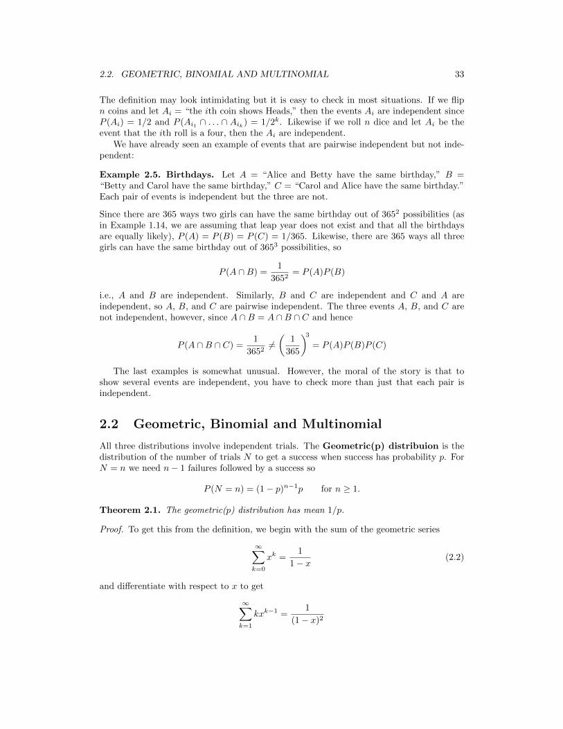
2.2 Geometric, Binomial and Multinomial
All three distributions involve independent trials. The Geometric(p) distribuion is thedistribution of the number of trials N to get a success when success has probability p. ForN = n we need n− 1 failures followed by a success so
P (N = n) = (1− p)n−1p for n ≥ 1.
Theorem 2.1. The geometric(p) distribution has mean 1/p.
Proof. To get this from the definition, we begin with the sum of the geometric series
∞∑k=0
xk =1
1− x(2.2)
and differentiate with respect to x to get
∞∑k=1
kxk−1 =1
(1− x)2
34 CHAPTER 2. INDEPENDENCE
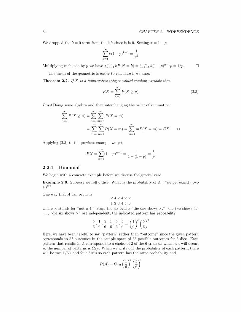
We dropped the k = 0 term from the left since it is 0. Setting x = 1− p∞∑k=1
k(1− p)k−1 =1
p2
Multiplying each side by p we have∑∞k=1 kP (N = k) =
∑∞k=1 k(1− p)k−1p = 1/p.
The mean of the geometric is easier to calculate if we know
Theorem 2.2. If X is a nonnegative integer valued random variable then
EX =
∞∑n=1
P (X ≥ n) (2.3)
Proof Doing some algebra and then interchanging the order of summation:
∞∑n=1
P (X ≥ n) =
∞∑n=1
∞∑m=n
P (X = m)
=
∞∑m=1
m∑n=1
P (X = m) =
∞∑m=1
mP (X = m) = EX
Applying (2.3) to the previous example we get
EX =
∞∑n=1
(1− p)n−1 =1
1− (1− p)=
1
p
2.2.1 Binomial
We begin with a concrete example before we discuss the general case.
Example 2.6. Suppose we roll 6 dice. What is the probability of A =“we get exactly two4’s”?
One way that A can occur is×1
4
2
×3
4
4
×5
×6
where × stands for “not a 4.” Since the six events “die one shows ×,” “die two shows 4,”. . . , “die six shows ×” are independent, the indicated pattern has probability
5
6· 1
6· 5
6· 1
6· 5
6· 5
6=
(1
6
)2(5
6
)4
Here, we have been careful to say “pattern” rather than “outcome” since the given patterncorresponds to 54 outcomes in the sample space of 66 possible outcomes for 6 dice. Eachpattern that results in A corresponds to a choice of 2 of the 6 trials on which a 4 will occur,so the number of patterns is C6,2. When we write out the probability of each pattern, therewill be two 1/6’s and four 5/6’s so each pattern has the same probability and
P (A) = C6,2
(1
6
)2(5
6
)4
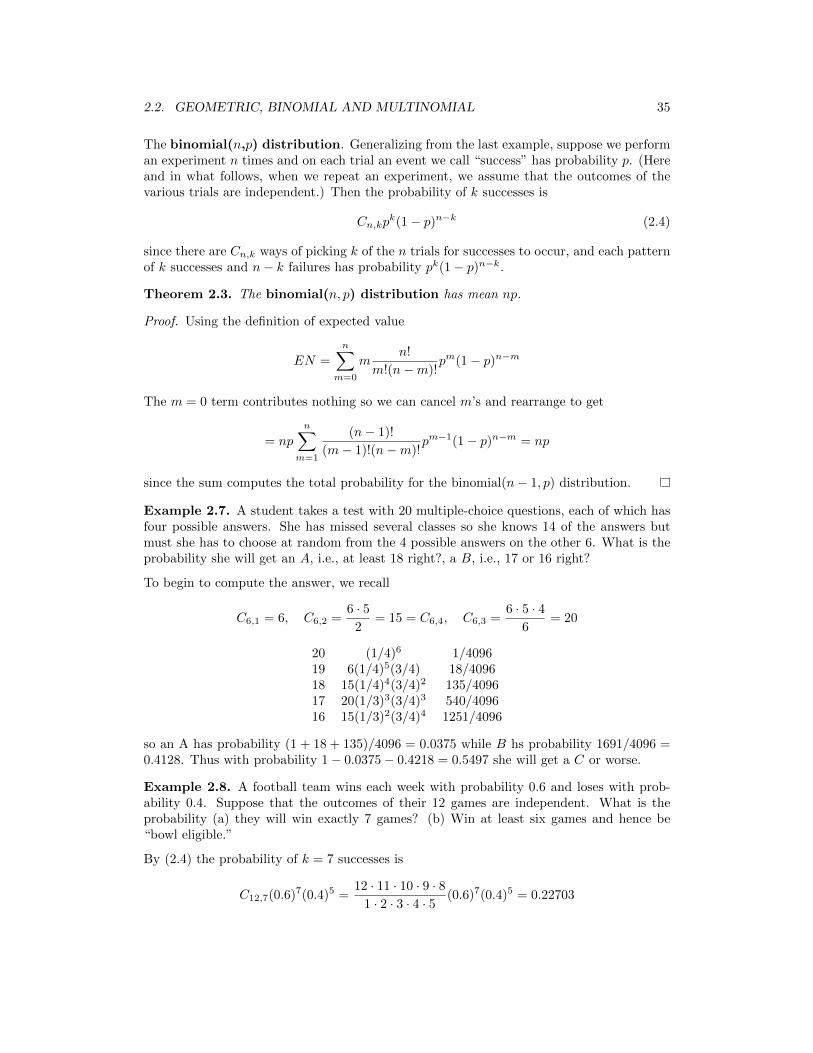
2.2. GEOMETRIC, BINOMIAL AND MULTINOMIAL 35
The binomial(n,p) distribution. Generalizing from the last example, suppose we performan experiment n times and on each trial an event we call “success” has probability p. (Hereand in what follows, when we repeat an experiment, we assume that the outcomes of thevarious trials are independent.) Then the probability of k successes is
Cn,kpk(1− p)n−k (2.4)
since there are Cn,k ways of picking k of the n trials for successes to occur, and each patternof k successes and n− k failures has probability pk(1− p)n−k.
Theorem 2.3. The binomial(n, p) distribution has mean np.
Proof. Using the definition of expected value
EN =
n∑m=0
mn!
m!(n−m)!pm(1− p)n−m
The m = 0 term contributes nothing so we can cancel m’s and rearrange to get
= np
n∑m=1
(n− 1)!
(m− 1)!(n−m)!pm−1(1− p)n−m = np
since the sum computes the total probability for the binomial(n− 1, p) distribution.
Example 2.7. A student takes a test with 20 multiple-choice questions, each of which hasfour possible answers. She has missed several classes so she knows 14 of the answers butmust she has to choose at random from the 4 possible answers on the other 6. What is theprobability she will get an A, i.e., at least 18 right?, a B, i.e., 17 or 16 right?
To begin to compute the answer, we recall
C6,1 = 6, C6,2 =6 · 5
2= 15 = C6,4, C6,3 =
6 · 5 · 46
= 20
20 (1/4)6 1/409619 6(1/4)5(3/4) 18/409618 15(1/4)4(3/4)2 135/409617 20(1/3)3(3/4)3 540/409616 15(1/3)2(3/4)4 1251/4096
so an A has probability (1 + 18 + 135)/4096 = 0.0375 while B hs probability 1691/4096 =0.4128. Thus with probability 1− 0.0375− 0.4218 = 0.5497 she will get a C or worse.
Example 2.8. A football team wins each week with probability 0.6 and loses with prob-ability 0.4. Suppose that the outcomes of their 12 games are independent. What is theprobability (a) they will win exactly 7 games? (b) Win at least six games and hence be“bowl eligible.”
By (2.4) the probability of k = 7 successes is
C12,7(0.6)7(0.4)5 =12 · 11 · 10 · 9 · 8
1 · 2 · 3 · 4 · 5(0.6)7(0.4)5 = 0.22703

36 CHAPTER 2. INDEPENDENCE
With a TI-83 calculator this probability can be found by going to the DISTR menu andusing binompdf(12,0.6,7). Here pdf is for probability density function.
(b) Let W be the number of games the team will win in the season. It would be tedious tocalculate the probability P (W ≥ 6) by adding up the probability of k = 6, 7, 8, . . . 12 gamesand adding up the answers. With a TI-83 calculator the probability of interest can be foundby going by using binomcdf(12,0.6,5) which gives the P (W ≤ 5) = 0.1582, and hence theanswer is
P (W ≥ 6) = 1− P (W ≤ 5) = 1− 0.1582 = 0.8418.
Here cdf, is for cumulative distribution function, the name for the function P (W ≤ x),which will be defined precisely and studied in Section 3.2.
Example 2.9. Tennis. In men’s tennis the winner is the first to win 3 out of 5 sets. IfRoger Federer wins a set against his opponent with probability 2/3, what is the probabilityw that he will win the match?
He can win in three sets, four or five, but he must win the last set, so
w =
(2
3
)3
+ C3,2
(2
3
)31
3+ C4,2
(2
3
)3(1
3
)2
=
(2
3
)3
(1 + 3(1/3) + 6(1/9)) =8
27· 8
3= 0.790
Example 2.10. Aces at Bridge. When we draw 13 cards out of a deck of 52, each acehas a probability 1/4 of being chosen, but the four events are not independent. How doesthe probability of drawing two aces compare with that of the binomial distribution withn = 4 and p = 1/4?
The probability of drawing two aces:
C4,2C48,11
C52,13=
6 · 48 · · · 38
11!52 · · · 40
13!
= 6 · 13 · 12 · 39 · 38
52 · 51 · 50 · 49= 0.2135
In contrast, the probability for the binomial is
C4,2(1/4)2(3/4)2 = 0.2109
Similar computations show:
aces binomial
039 · 38 · 37 · 36
52 · 51 · 50 · 49(3/4)4
1 4 · 13 · 39 · 38 · 37
52 · 51 · 50 · 494 · (1/4)(3/4)3
2 6 · 13 · 12 · 39 · 38
52 · 51 · 50 · 496 · (1/4)2(3/4)2
3 4 · 13 · 12 · 11 · 39
52 · 51 · 50 · 494 · (1/4)3(3/4)
413 · 12 · 11 · 10
52 · 51 · 50 · 49(1/4)4

2.2. GEOMETRIC, BINOMIAL AND MULTINOMIAL 37
Evaluating these expressions leads to the following probabilities:
aces binomial0 0.3038 0.31641 0.4388 0.42182 0.2134 0.21093 0.0412 0.04684 0.00264 0.00390
Example 2.11. In Bridge, each of the four players gets 13 cards from a deck of 52. In thelast 8 games, Harry had 5 hands without an ace. Should he doubt that the cards are beingshuffled properly?
By the previous problem, the number of hands in which Harry has no ace has a binomialdistribution with n = 8 and p = 0.3038. The probability of exactly 5 hands without an aceis
C8,5(0.3038)5(0.6962)3 = 0.0489
Of course if Harry had 6,7, or 8 hands without an ace he would complain, so the morerelevant thing to compute is the probability of ≥ 5 which is
1− binomcdf(8, 0.3038, 4) = 0.06097
Thus 6.1% of the time he will have five or more hands without an ace.
2.2.2 Multinomial Distribution
The arguments above generalize easily to independent events with more than two possibleoutcomes. We begin with an example.
Example 2.12. A student makes an A with probability 0.5, a B with probability 0.4, anda C with probability 0.1. In a year where she takes eight courses what is the probability of4 A’s, 3 B’s, and 1 C.
The answer is8!
4! 3! 1!(0.5)4(0.4)3(0.1)
The first factor, by (1.12), gives the number of ways to pick four courses for A’s, three coursesfor B’s, and one course for C. The second factor gives the probability of any outcome withfour A’s, three B’s, and one C. The combinatorial coefficient is 8 · 7 · 5 = 280 so the answeris 0.112.
Multinomial distribution. Generalizing from this example, we see that if we have kpossible outcomes for our experiment with probabilities p1, . . . , pk then the probability ofgetting exactly ni outcomes of type i in n = n1 + · · ·+ nk trials is
n!
n1! · · ·nk!pn1
1 · · · pnkk (2.5)
since the first factor gives the number of outcomes and the second the probability of eachone.

38 CHAPTER 2. INDEPENDENCE
Example 2.13. A baseball player gets a hit with probability 0.3, a walk with probability0.1, and an out with probability 0.6. If he bats 4 times during a game and we assume thatthe outcomes are independent, what is the probability he will get 1 hit, 1 walk, and 2 outs?
The total number of trials n = 4. There are k = 3 categories hit, walk, and out. n1 = 1,n2 = 1, and n3 = 2. Plugging in to our formula the answer is
4!
1!1!2!(0.3)1(0.1)1(0.6)2 = 0.1296
Example 2.14. The output of a machine is graded excellent 70% of the time, good 20% ofthe time, and defective 10% of the time. What is the probability a sample of size 15 has 10excellent, 3 good, and 2 defective items?
The total number of trials n = 15. There are k = 3 categories: excellent, good, anddefective. We are interested in outcomes with n1 = 10, n2 = 3, and n3 = 2. Plugging in toour formula the answer is
15!
10! 3! 2!· (0.7)10(0.2)3(0.1)2
2.3 Poisson Approximation to the Binomial
X is said to have a Poisson distribution with parameter λ, or Poisson(λ) if
P (X = k) = e−λλk
k!for k = 0, 1, 2, . . .
Here λ > 0 is a parameter. To see that the probabilities sum to 1 we recall
ex =
∞∑k=0
xk
k!(2.6)
The next figure shows the Poisson distribution with λ = 4.
Poisson(4)
0
0.05
0.1
0.15
0.2
0 1 2 3 4 5 6 7 8 9 10 11 12
Figure 2.1: Poisson distribution λ = 4
As we will now show λ is the mean of the Poisson(λ) distribution.

2.3. POISSON APPROXIMATION TO THE BINOMIAL 39
Proof. Dropping the k = 0 term since it is zero
EX =
∞∑k=1
k · e−λλk
k!
= λ
∞∑k=1
e−λλk−1
(k − 1)!= λ
since the probabilitie sin the Poisson distribution sum to 1.
Our next result explains why the Poisson distribution arises in a number of situations.
Theorem 2.4. Suppose Sn has a binomial distribution with parameters n and pn. If pn → 0and npn → λ as n→∞ then
P (Sn = k)→ e−λλk
k!(2.7)
In words, if we have a large number, n, of independent events with small probability pnthen the number that occur has approximately a Poisson distribution with mean λ = npn.The key to the proof is the following fact:
Lemma. If pn → 0 and npn → λ then as n→∞
(1− pn)n → e−λ (2.8)
Proof. Calculus tells us that if x is small then
ln(1− x) = −x− x2
2− . . .
Using this we have
(1− pn)n
= exp(n ln(1− pn))
≈ exp(−npn − np2n/2) ≈ exp(−λ)
In the last step we used the assumption that npn → λ and pn → 0 to conclude thatnpn · pn/2→ 0.
Proof of (2.7) . Since P (Sn = 0) = (1− pn)n (2.8) gives the result for k = 0. To prove theresult for k > 0, we let λn = npn and observe that
P (Sn = k) = Cn,k
(λnn
)k (1− λn
n
)n−k=n(n− 1) · · · (n− k + 1)
nk· λ
kn
k!
(1− λn
n
)n(1− λn
n
)−k→ 1 · λ
k
k!· e−λ · 1
Here n(n− 1) · · · (n− k+ 1)/nk → 1 since there are k factors in the numerator and for eachfixed j, (n− j)/n = 1− (j/n)→ 1. The last term (1− λn/n)−k → 1 since k is fixed and1− λn/n → 1.

40 CHAPTER 2. INDEPENDENCE
In some situations it is not reasonable to make the assumption that all people have equalprobabilities. For example, the number of people who go to a fast-food restaurant between12 and 1, and the number of traffic accidents in a day. With these examples in mind weformulate a more general result.
Theorem 2.5. Consider independent events Ai, i = 1, 2, . . . , n with probabilities pi =P (Ai). Let N be the number of events that occur, let λ = p1 + · · · + pn, and let Z have aPoisson distribution with parameter λ. Then, for any set of integers B,
|P (N ∈ B)− P (Z ∈ B)| ≤n∑i=1
p2i ≤ λmax
ipi
This result says that if all the pi are small then the distribution of N is close to a Poissonwith parameter λ. Taking B = k we see that the individual probabilities P (N = k)are all close to P (Z = k), but this result says more. The probabilities of events such asP (3 ≤ N ≤ 8) are close to P (3 ≤ Z ≤ 8) and we have an explicit bound on the error.
When we apply (2.7) we think, “If Sn = binomial(n, p) and p is small then Sn is approxi-mately Poisson(np).” The next example illustrates the use of this approximation and showsthat the number of trials does not have to be very large for us to get accurate answers.
Example 2.15. Suppose we roll two dice 12 times and we let D be the number of times adouble 6 appears. Here n = 12 and p = 1/36, so np = 1/3. We will now compare P (D = k)with the Poisson approximation for k = 0, 1, 2.
k = 0 exact answer:
P (D = 0) =
(1− 1
36
)12
= 0.7132
Poisson approximation: P (D = 0) = e−1/3 = 0.7165
k = 1 exact answer:
P (D = 1) = C12,11
36
(1− 1
36
)11
=
(1− 1
36
)11
· 1
3= 0.2445
Poisson approximation: P (D = 1) = e−1/3 13 = 0.2388
k = 2 exact answer:
P (D = 2) = C12,2
(1
36
)2(1− 1
36
)10
=
(1− 1
36
)10
· 12 · 11
362· 1
2!= 0.0384
Poisson approximation: P (D = 2) = e−1/3(
13
)2 12! = 0.0398
In this case the error bound in Theorem 2.5 is
12∑i=1
p2i = 12
(1
36
)2
=1
108= 0.00926
while the error for the approximation for k = 1 is 0.0057.
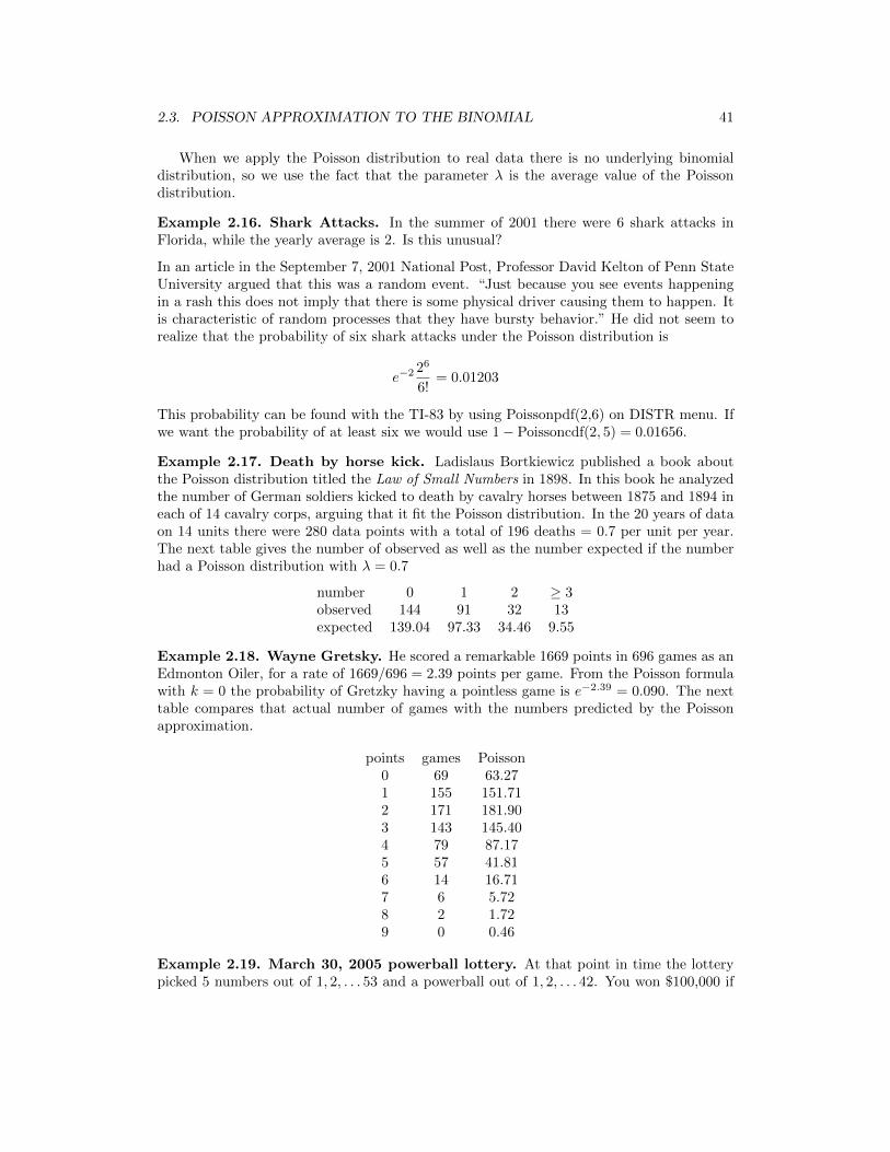
2.3. POISSON APPROXIMATION TO THE BINOMIAL 41
When we apply the Poisson distribution to real data there is no underlying binomialdistribution, so we use the fact that the parameter λ is the average value of the Poissondistribution.
Example 2.16. Shark Attacks. In the summer of 2001 there were 6 shark attacks inFlorida, while the yearly average is 2. Is this unusual?
In an article in the September 7, 2001 National Post, Professor David Kelton of Penn StateUniversity argued that this was a random event. “Just because you see events happeningin a rash this does not imply that there is some physical driver causing them to happen. Itis characteristic of random processes that they have bursty behavior.” He did not seem torealize that the probability of six shark attacks under the Poisson distribution is
e−2 26
6!= 0.01203
This probability can be found with the TI-83 by using Poissonpdf(2,6) on DISTR menu. Ifwe want the probability of at least six we would use 1− Poissoncdf(2, 5) = 0.01656.
Example 2.17. Death by horse kick. Ladislaus Bortkiewicz published a book aboutthe Poisson distribution titled the Law of Small Numbers in 1898. In this book he analyzedthe number of German soldiers kicked to death by cavalry horses between 1875 and 1894 ineach of 14 cavalry corps, arguing that it fit the Poisson distribution. In the 20 years of dataon 14 units there were 280 data points with a total of 196 deaths = 0.7 per unit per year.The next table gives the number of observed as well as the number expected if the numberhad a Poisson distribution with λ = 0.7
number 0 1 2 ≥ 3observed 144 91 32 13expected 139.04 97.33 34.46 9.55
Example 2.18. Wayne Gretsky. He scored a remarkable 1669 points in 696 games as anEdmonton Oiler, for a rate of 1669/696 = 2.39 points per game. From the Poisson formulawith k = 0 the probability of Gretzky having a pointless game is e−2.39 = 0.090. The nexttable compares that actual number of games with the numbers predicted by the Poissonapproximation.
points games Poisson0 69 63.271 155 151.712 171 181.903 143 145.404 79 87.175 57 41.816 14 16.717 6 5.728 2 1.729 0 0.46
Example 2.19. March 30, 2005 powerball lottery. At that point in time the lotterypicked 5 numbers out of 1, 2, . . . 53 and a powerball out of 1, 2, . . . 42. You won $100,000 if

42 CHAPTER 2. INDEPENDENCE
you matched the five white ball and missed the powerball, an event of probability
1
C53,5· 41
42=
1
2, 939, 677
To simplify the arithmetic let’s round the denominator to 3 million. On the date in questionabout 12,000,000 people played the lottery, so we would expect the number of $100,000winners to be approximately Poisson with mean 4. Hoever, the lottery officials were shockedto see 110 winners.
While at first criminal activity was suspected there was a simple explanation. Most of thepeople who played these numbers did so because they were in a fortune cookie manufacturedby the Wonton Food Company of Long Island City in Queens, NY. This theory is confirmedby the fact that most winners had 40 as their powerball, which was what the fortune cookierecommended.
Example 2.20. Births in Ithaca. The Poisson distribution can be used for births aswell as for deaths. There were 63 births in Ithaca, NY between March 1 and April 8, 2005,a total of 39 days, or 1.615 per day. The next table gives the observed number of birthsper day and compares with the prediction from the Poisson distribution. The agreement isgood even though it is not sensible to assume that all women in the county have an equalprobability of giving birth.
0 1 2 3 4 5 6observed 9 12 9 5 3 0 1Poisson 7.75 12.52 10.11 5.44 2.19 .71 .19
Example 2.21. Birthday problem. In the birthday problem the events Aij that i andj have the same birthday are not independent. Despite this we will use the Poisson ap-proximation and compare with the exact result. When there are k people the mean isCk,2/365 = k(k − 1)/700 and hence the Poisson approximation to the probability of nobirthday match is
exp(−k(k − 1)/700)
To see that this is reasonable note that by calculations in Example 1.14 the probability thatk people all have different birthdays is
1 ·(
1− 1
365
)·(
1− 2
365
)· · · ·
(1− k − 1
365
)using the fact that 1− x ≈ e−x we can write this as
≈ exp
− k−1∑j=1
j/365
= exp(−k(k − 1)/700)
since∑kj=1 j = k(k = 1)/2. When k = 23 the approximation is 0.49999 versus the exact
answer of 0.49270.
Example 2.22. Triple birthdays in the Senate. Using the Poisson approximation, thenumber of senators born on a given day is Binomial(100,1/365) and hence approximately

2.4. PROBABILITIES OF UNIONS 43
Poisson with mean 100/365. Using the Poisson approximation the probability that threesenators were born on July 4 is
e−100/365(100/365)3/3! = 0.002606
Using the Poisson approximation again (assuming this event for different days are inde-pendent), the number of triple birthdays is approximately Poisson(365 · 0.002606) or Pois-son(0.95119), so the probability of no triple birthday is ≈ 0.3862
2.4 Probabilities of Unions
In Section 1.1, we learned that P (A ∪ B) = P (A) + P (B) − P (A ∩ B). In this section wewill extend this formula to n > 2 events. We begin with n = 3 events:
P (A ∪B ∪ C) =P (A) + P (B) + P (C)
− P (A ∩B)− P (A ∩ C)− P (B ∩ C)
+ P (A ∩B ∩ C) (2.9)
Proof. As in the proof of the formula for two events, we have to convince ourselves that thenet number of times each part of A ∪ B ∪ C is counted is 1. To do this, we make a tablethat identifies the areas counted by each term and note that the net number of pluses ineach row is 1:
A B C A ∩B A ∩ C B ∩ C A ∩B ∩ CA ∩B ∩ C + + + − − − +A ∩B ∩ Cc + + −A ∩Bc ∩ C + + −Ac ∩B ∩ C + + −A ∩Bc ∩ Cc +Ac ∩B ∩ Cc +Ac ∩Bc ∩ C +
Example 2.23. Suppose we roll three dice. What is the probability that we get at leastone 6?
Let Ai = “we get a 6 on the ith die.” Clearly,
P (A1) = P (A2) = P (A3) = 1/6
P (A1 ∩A2) = P (A1 ∩A3) = P (A2 ∩A3) = 1/36
P (A1 ∩A2 ∩A3) = 1/216
So plugging into (2.9) gives
P (A1 ∪A2 ∪A3) = 3 · 1
6− 3 · 1
36+
1
216=
108− 18 + 1
216=
91
216
To check this answer, we note that (A1∪A2∪A3)c = “no 6” =Ac1∩Ac2∩Ac3 and |Ac1∩Ac2∩Ac3| =5 · 5 · 5 = 125 since there are five “non-6’s” that we can get on each roll. Since there are63 = 216 outcomes for rolling three dice, it follows that P (Ac1 ∩ Ac2 ∩ Ac3) = 125/216 andP (A1 ∪A2 ∪A3) = 1− P (Ac1 ∩Ac2 ∩Ac3) = 91/216.
The same reasoning applies to sets.

44 CHAPTER 2. INDEPENDENCE
Example 2.24. In a freshman dorm, 60 students read the Cornell Daily Sun, 40 read theNew York Times and 30 read the Ithaca Journal. 20 read the Cornell Daily Sun and theNew York Times, 15 read the Cornell Daily Sun and the Ithaca Journal, 10 read the NewYork Times and the Ithaca Journal, and 5 read all three. How many read at least onenewspaper?
Using our formula the answer is
60 + 40 + 30− 20− 15− 10 + 5 = 90
To check this we can draw picture using D, N , and I for the three newspapers
D
I
N
5 515
1030 10
15
To figure out the number of students in each category we work out from the middle. D∩N∩Ihas 5 students and D ∩N has 20, so D ∩N ∩ Ic has 15. In the same way we compute thatD ∩N c ∩ I has 15− 5 = 10 students and Dc ∩N ∩ I has 10− 5 = 5 students. Having foundthat 30 of students in D read at least one other newspaper, the number who read only D is60− 30 = 30. In a similar way, we compute that there are 40− 25 = 15 students who onlyread N and 30 − 20 = 10 students who only read I. Adding up the numbers in the sevenregions gives a total of 90, as we found before.
If we want to compute the number of students who read only the New York Times thiscan be done more easily using
|N ∩Dc ∩ Ic| = |N | − |N ∩D| − |N ∩ I|+ |N ∩D ∩ I|= 40− 20− 10 + 5 = 15
To check this we see how many times each region is counted by the right-hand side
|N | −|N ∩D| −|N ∩ I| |N ∩D ∩ I|N ∩Dc ∩ Ic +N ∩Dc ∩ I + −N ∩D ∩ Ic + −N ∩D ∩ I + − − +
If we add up the +1 and −1 we get 1 on the first row and 0 on the others.

2.4. PROBABILITIES OF UNIONS 45
2.4.1 Inclusion-exclusion formula
Formula (2.9) generalizes to n events:
P (∪ni=1Ai) =
n∑i=1
P (Ai)−∑i<j
P (Ai ∩Aj) +∑i<j<k
P (Ai ∩Aj ∩Ak)
· · ·+ (−1)n+1P (A1 ∩ . . . ∩An) (2.10)
In words, we take all possible intersections of one, two, . . . n events and the signs of thesums alternate. As in the case of three sets there is ana analogous formula for countint thenumber of elements in a union.
Proof. A point that is in exactly k sets is counted k times by the first sum, Ck,2 times bythe second, Ck,3 times by the third, and so on until it is counted Ck,k = 1 time by the kthterm. The net result is
Ck,1 − Ck,2 + Ck,3 . . .+ (−1)k+11
To show that this adds up to 1, we recall the Binomial theorem
(a+ b)k = ak + Ck,1ak−1b+ Ck,2a
k−2b2 + · · ·+ bk
Setting a = 1 and b = −1 we have
0 = 1− Ck,1 + Ck,2 − Ck,3 . . .− (−1)k+1
which proves the desired result.
Example 2.25. We pick 13 cards out of a deck of 52, What is the probability that we getexactly five cards of one suit?
Let Ai be the event that we get five cards of suit i. Since it is impossible to have fivecards in more than two suits (2.10) becomes
P (∪4i=1Ai) =
4∑i=1
P (Ai)−∑
1≤i<j≤4
P (Ai ∩Aj)
To find the desired probability we note that if 1 ≤ i < j ≤ 4
P (Ai) =C13,5C39,8
C52,13=
7.918× 10¹⁰
6.350× 1011= 0.12469
P (Ai ∩Aj) =C13,5C13,5C26,3
C52,13=
4.306× 10⁹
6.350× 1011= 0.00678
so taking into account the number of terms of each type we have
P(∪4i=1Ai
)= 4(0.12469)− 6(0.00678) = 0.4588
Example 2.26. We now describe a situation which is perhaps the most famous applicationof inclusion-exclusion. An absent minded professor hands tests back at random. What isthe probability of B, the event that no one of the n students gets their own test back.

46 CHAPTER 2. INDEPENDENCE
Let Ai be the event that the ith student gets their test back. P (Ai) = 1/n so
n∑i=1
P (Ai) = n · 1
n
As we compute the higher order terms a pattern develops:
−∑
1≤i<j≤n
P (Ai ∩Aj) =n(n− 1)
2!· 1
n(n− 1)=
1
2!∑1≤i<j<k≤n
P (Ai ∩Aj ∩Ak) =n(n− 1)(n− 2)
3!· 1
n(n− 1)(n− 2)=
1
3!
−∑
1≤i<j<k<`≤n
P (Ai ∩Aj ∩Ak ∩A`)
=n(n− 1)(n− 2)(n− 3)
4!· 1
n(n− 1)(n− 2)(n− 3= − 1
4!
From this we see that
P (Bn) = 1− 1
2!+
1
3!− 1
4!. . .+
(−1)n+1
n!≈ 1− e−1
where the last equality follows from the fact that ex = 1 + x + x2/2! + x3/3! + · · · . Theapproximation is very good. Since the series alternates in sign and the magnitude of theterms are decreasing,
|P (Bn)− (1− e−1)| ≤ 1/(n+ 1)!
To motivate the next topic we consider
Example 2.27. Suppose we roll a die 15 times. What is the probability that we do not seeeach of the 6 numbers at least once?
Let Ai be the event that we never see i. Since P (A1 ∩A2 . . . A6 is 0, the inclusion exclusionformula tells us that
P (∪6i=1Ai) =
6∑i=1
P (Ai)−∑
1≤i<j≤6
P (Ai ∩Aj) +∑
1≤i<j<k≤6
P (Ai ∩Aj ∩Ak)
+∑
1≤i<j<k<`≤6
P (Ai ∩Aj ∩Ak ∩A`) +∑
1≤i<j<k<`<m≤6
P (Ai ∩Aj ∩Ak ∩A` ∩Am)
Taking into account the number of terms in each sum the above
= 6(5/6)15 − 15(4/6)15 + 20(3/6)15 − 15(2/6)15 + 6(1/6)15
= 0.389433− 0.03426 + 3.05× 10⁻⁵ − 1.045× 10⁻⁶ + 1.27× 10⁻¹¹
The last two terms are very small so itis waste of effort to compute them.

2.4. PROBABILITIES OF UNIONS 47
2.4.2 Bonferroni inequalities
In brief, if you stop the inclusion-exclusion formula with a + term you get an upper bound;if you stop with a − term you get a lower bound.
P (∪ni=1Ai) ≤n∑i=1
P (Ai) (2.11)
≥n∑i=1
P (Ai)−∑i<j
P (Ai ∩Aj) (2.12)
≤n∑i=1
P (Ai)−∑i<j
P (Ai ∩Aj) +∑i<j<k
P (Ai ∩Aj ∩Ak) (2.13)
Proof. The first inequality is obvious since the right-hand side counts each outcome in∪ni=1Ai at least once. To prove the second, consider an outcome that is in exactly k sets.If k = 1, the first term will count it once and the second not at all. If k = 2 the first termcounts it 2 times and the second once, with a net total of 1. If k ≥ 3 the first term counts itk times and the second Ck,2 = k(k − 1)/2 > k times so the net number of countings is < 0.
The third formula is similar.
in k sets counted1 1 - 0 + 0 =12 2 - 1 + 0 =13 3 - 3 + 1 =1
When ≥ 4 the number of countings is
Ck,1 − Ck,2 + Ck,3 > k − k(k − 1)
2+ (k − 1)(k − 2) ≥ 0
Returning to the previous example
Example 2.28. Suppose we roll a die 15 times. What is the probability that we do not seeeach of the 6 numbers at least once?
Let Ai be the event that we never see i. Earlier we computed that
6∑i=1
P (Ai) = 6(0.064905) = 0.389433
so we haveP(∪6i=1Ai
)≤ 0.389433
Using the next term ∑i<j
P (Ai ∩Aj) = 15(0.002284) = 0.03426
and it follows that
P(∪6i=1Ai
)≥ 0.389433− 0.03426 = 0.355177

48 CHAPTER 2. INDEPENDENCE
The third term is ∑i<j<k
P (Ai ∩Aj ∩Ak) = 20(3.05× 10⁻⁵) = 0.00061
and it follows that
P(∪6i=1Ai
)≤ 0.355177 + 0.00061 = 0.355738
The upper bound and the lower bound are very close so we can stop.
Example 2.29. The Streak. In the summer of 1941, Joe DiMaggio achieved what manypeople consider the greatest record in sports, in which he had at leastone hit in each of 56games. What is the probability of this event?
A useful trick. Suppose for the moment that we know the probability p that Joe DiMaggiogets a hit in one game, and that successive games are independent. Assuming a 154-gameseason, we could let Ai be the probability that a player got hits in games i+ 1, . . . i+ 56 for0 ≤ i ≤ 98. Using (2.11) it follows that the probability of the streak is
≤ 99p56
The next sum is hard to evaluate because if i < j
P (Ai ∩Aj) =
p56pj−i if j − i < 56
p112 if j − i < 56
In words if Ai occurs, it becomes much easier for Ai+1 and other “nearby” events to occur.To avoid this problem, we will let Bi be the event the player gets no hit in game i but
has hits in games i+ 1, i+ 2, . . . , i+ 56 where 1 ≤ i ≤ 98. Ignoring the probability of havinghits in games 1, 2, . . . 56 the event of interest S = ∪98
i=1Bi, so
P (S) ≤ q ≡ 98p56(1− p)
To compute the second bound we begin by noting Bi ∩ Bj = ∅ if i < j ≤ i + 56 sinceBi requires a hit in game j while Bj requires no hit. If 56 + i < j ≤ 98 then P (Bi ∩Bj) = P (Bi)P (Bj). To simplify the arithmetic we note that in either case P (Bi ∩ Bj) ≤P (Bi)P (Bj), so ∑
1≤i<j≤98
P (Bi ∩Bj) ≤ C98,2p112(1− p)2 ≤ q2
2
This is the number we have to subtract from the upper bound to get the lower bound, sowe have
q ≥ P (S) ≥ q − q2
2(2.14)
Since q will end up being very small, the ratio of the two bounds is 1− (q/2) ≈ 1.
To compute the probability p that Joe DiMaggio gets a hit in one game,we will introduce two somewhat questionable assumptions: (i) a player gets exactly fourat bats per game (during the streak, DiMaggio averaged 3.98 at bats per game) and (ii)the outcomes of different at bats are independent with the probability of a hit being 0.325,

2.5. EXERCISES 49
Joe DiMaggio’s lifetime batting average. From assumptions (i) and (ii) it follows that theprobability
p = 1− (0.675)4 = 0.7924
and using (2.14) we have
P (S) ≈ q = 98(0.7924)56(0.2076) = 4.46× 10⁻⁵
To interpret our result, note that the probability in (2.14) is roughly 1/22,000, so even ifthere were 220 players with 0.325 batting averages, it would take 100 years for this to occuragain.
Example 2.30. A less famous streak. Sports Illustrated reports that a high schoolfootball team in Bloomington, Indiana lost 21 straight pre-game coin flips before finallywinning one. Taking into account the fact that there are approximately 15,000 high schooland college football teams, is this really surprising?
We will first compute the probability that this happens to one team some time in thedecade 1995–2004 assuming that the team plays 10 games per year. Taking a lesson fromthe previous example, we let Bi be the event that the team won the coin flip in game i butlost it in games i+ 1, . . . i+ 21. Using the reasoning that led to (2.14)
P (S) ≈ 79(1/2)22 = 1.883× 10⁻⁵
What we have computed is the probability that one particular team will have this typeof bad luck some time in the last decade. The probability that none of the 15,000 teamswill do this is
(1− 79(0.5)22)15,000 = 0.7539
i.e., with probability 0.2461 some team will have this happen to them. As a check on thelast calculation, note that (2.11) gives an upper bound of
15, 000× 1.883× 10−5 = 0.2825
2.5 Exercises
Conditional probability
1. A friend flips two coins and tells you that at least one is Heads. Given this information,what is the probability that the first coin is Heads?
2. A friend rolls two dice and tells you that there is at least one 6. What is the probabilitythe sum is at least 9?
3. Suppose we roll two dice. What is the probability that the sum is 7 given that neitherdie showed a 6?
4. Suppose you draw five cards out of a deck of 52 and get 2 spades and 3 hearts. What isthe probability the first card drawn was a spade?
5. Suppose 60% of the people subscribe to newspaper A, 40% to newspaper B, and 30% toboth. If we pick a person at random who subscribes to at least one newspaper, what is theprobability she subscribes to newspaper A?

50 CHAPTER 2. INDEPENDENCE
6. In a town 40% of families have a dog and 30% have a cat. 25% of families with a dogalso have a cat. (a) What fraction of people have a dog or cat? (b) What is the probabilitya family with a cat has a dog?
7. Two events have P (A) = 1/4, P (B|A) = 1/2, and P (A|B) = 1/3. Compute P (A ∩ B),P (B), P (A ∪B).
8. A, B, and C are events with P (A) = 0.3, P (B) = 0.4, P (C) = 0.5, A and B are disjoint,A and C are independent, and P (B|C) = 0.1. Find P (A ∪B ∪ C).
Independence
9. Suppose we draw two cards out of a deck of 52. Let A = “the first card is an Ace,” andB = “the second card is a spade.” Are A and B independent?
10. A family has three children, each of whom is a boy or a girl with probability 1/2. LetA = “there is at most 1 girl,” B = “the family has children of both sexes.” (a) Are A andB independent? (b) Are A and B independent if the family has four children?
11. Nine children are seated at random in three rows of three desks. Let A = “Al andBobby sit in the same row,” B = “Al and Bobby both sit at one of the four corner desks.”Are A and B independent?
12. Suppose we roll a red and a green die. Let A = “the red die shows a 2 or a 5,” B =“the sum of the two dice is at least 7.” Are A and B independent?
13. Roll two dice. Let A = “the sum is even,” and B = “the sum is divisible by 3,” i.e.,B = 3, 6, 9, 12. Are A and B independent?
14. Roll two dice. Let A = the larger number is 5. B = the sum is 7 or 11. Are A and Bindependent?
15. We flip three coins with probability p of heads where 0 < p < 1. Let A = the first andsecond flips are different. Let B = the second fand third flips are different. For what valuesof p are A and B independent.
16. Roll two dice. Let A = “the first die is odd,” B = “the second die is odd,” and C =“the sum is odd.” Show that these events are pairwise independent but not independent.
17. A number X is picked at random from 1, 2, . . . 100. Are the following events indepen-dent (a) A1 = X is even, B1 = X is divisible by 5. (b) A2 = X is divisible by 4, B2 = X isdivisible by 3. (c) What are the answers if X is picked at random from 1, 2, . . . 36.
18. Let A = “the sum of the two dice is a prime number,” i.e., 2, 3, 5, 7, or 11. B = “thefirst die is 2 or 6.” Are A and B independent?
19. Two students, Alice and Betty, are registered for a statistics class. Alice attends 80%of the time, Betty 60% of the time, and their absences are independent. On a given day,what is the probability (a) at least one of these students is in class, (b) exactly one of themis there?
20. Marilyn vos Savant claimed in her May 5, 2013 column that among the four digitnumbers 0000 to 9999, exactly 4000 had at least one five. Compute the number of numberswith at least one 5 by computing the probability that a randomly chosen number has no 5.

2.5. EXERCISES 51
21. At Duke, 20% of students like football (event F ) and 60% like basketball (event B).Assuming these two events are independent calculate the fraction of students who like atleast one of these sports.
22. Let A and B be two independent events with P (A) = 0.4 and P (A ∪B) = 0.64. Whatis P (B)?
23. A and B are independent events with P (A) > P (B). P (A∩B) = 0.12, P (A∪B) = 0.58.Find P (A) and P (B).
24. Three students each have probability 1/3 of solving a problem. What is the probabilityat least one of them will solve the problem?
25. Three independent events have probabilities 1/4, 1/3, and 1/2. What is the probabilityexactly one will occur?
26. Three missiles are fired at a target. They will hit it with probabilities 0.2, 0.4, and 0.6.Find the probability that the target is hit by (a) three, (b) two, (c) one, (d) no missiles.
27. Three couples that were invited to dinner will independently show up with probabilities0.9, 8/9, and 0.75. Let N be the number of couples that show up. Calculate the probabilityN = 3, 2, 1, 0.
28. In men’s tennis the first person to win three sets wins the match. Suppose Rafael Nadalhas probability of 0.6 of winning a set when he plays against Andy Murray. What is theprobability that Nadal will win the match?
29. A college student takes 4 courses a semester for 8 semesters. In each course she has aprobability 1/2 of getting an A. Assuming her grades in different courses are independent,what is the probability she will have at least one semester with all A’s?
30. When Al and Bob play tennis, Al wins a set with probability 0.7 while Bob wins withprobability 0.3. What is the probability Al will be the first to win (a) two sets, (b) threesets?
31. Chevalier de Mere made money betting that he could “roll at least one 6 in four tries.”When people got tired of this wager he changed it to “roll at least one double 6 in 24 tries”but then he started losing money. Compute the probabilities of winning these two bets.
32. Samuel Pepys wrote to Isaac Newton: “What is more likely, (a) at least one 6 in 6 rollsof one die or (b) at least two 6’s in 12 rolls?” Compute the probabilities of these events.
Binomial and Multinomial Distributions
33. A die is rolled 8 times. What is the probability we will get exactly two 3’s?
34. Mary knows the answers to 20 of the 25 multiple choice questions on the Psychology101 exam, but she has skipped several of the lectures, she must take random guesses for theother five. Assuming each question has four answers, what is the probability she will getexactly 3 of the last 5 questions right?
35. In 1997, 10.8% of female smokers smoked cigars. In a sample of size 10 female smokersWhat is the probability that (a) exactly 2 of the women smoke cigars? (b) at most 1 smokescigars.
36. A 1994 report revealed that 32.6% of U.S. births were to unmarried women. A parentingmagazine selected 30 women who gave birth in 1994 at random. (a) What is the probability

52 CHAPTER 2. INDEPENDENCE
that exactly 10 of the women were unmarried? (b) Using your calculator determine theprobability that in the sample at most 10 are unmarried.
37. 20% of all students are left-handed. A class of size 20 meets in a room with 5 left-handedand 18 right-handed chairs. Use your calculator to find the probability that each studentwill have a chair to match their needs.
38. David claims to be able to distinguish brand B beer from brand H but Alice claimsthat he just guesses. They set up a taste test with 10 small glasses of beer. David wins ifhe gets 8 or more right. What is the probability he will win (a) if he is just guessing? (b)if he gets the right answer with probability 0.9?
39. The following situation comes up the game of Yahtzee. We have three rolls of five diceand want to get three sixes or more. On each turn we reroll any dice that are not 6’s. Whatis the probability we succeed?
40. A baseball pitcher throws a strike with probability 0.5 and a ball with probability 0.5.He is facing a batter who never swings at a pitch. What is the probability that he strikesout, i.e., gets three strikes before four balls?
41. A student is taking a multiple-choice test in which each question has four possibleanswers. She knows the answers to 5 of the questions, can narrow the choices down to 2 in3 cases, and does not know anything about 2 of the questions. What is the probability shewill correctly answer (a) 10, (b) 9, (c) 8, (d) 7, (e) 6, (f) 5 questions?
42. Consider a die with 1 painted on three sides, 2 painted on two sides, and 3 painted onone side. If we roll this die ten times what is the probability we get five 1’s, three 2’s andtwo 3’s?
43. A game of bowling consists of 10 “frames” in which the bowler gets to roll the ball twice.The outcome of a frame may be a strike (all ten pins on the first try), a spare (all ten pinsknocked down in two tries), or an “open frame.” Bowler Bob gets a strike with probability0.3, a spare with probability 0.6, and an open frame with probability 0.1. His recent gamefeatured 2 strikes, 5 spares and 3 open frames. Find the probability of this outcome.
44. A baseball player gets a hit with probability 0.3, a walk with probability 0.1, and an outwith probability 0.6. If he bats 5 times during a game and we assume that the outcomesare independent, what is the probability he will get (a) 2 hits, 1 walk, and 2 outs? (b) 2hits and 3 outs?
45. A baseball player is said to “hit for the cycle” if he has a single, a double, a triple, anda home run all in one game. Suppose these four types of hits have probabilities 1/6, 1/20,1/120, and 1/24. What is the probability of hitting for the cycle if he gets to bat (a) fourtimes, (b) five times? (c) Using P (∪iAi) ≤
∑i P (Ai) shows that the answer to (b) is at
most 5 times the answer to (a). What is the ratio of the two answers?
Poisson Approximation
46. Compare the Poisson approximation with the exact binomial probabilities when (a)n = 10, p = 0.1, (b) n = 20, p = 0.05, (c) n = 40, p = 0.025.
47. An NC State player hits 3 point shots with probability 1/6. In a game against UNC heattempted 12 and made 2. (a) What is the exact Binomial probability of this event? (b)What is the Poisson approximation?

2.5. EXERCISES 53
48. Suppose that the probability of a defect in a foot of magnetic tape is 0.002. Use thePoisson approximation to compute the probability that a 1500 foot roll will have no defects.
49. Suppose 1% of a certain brand of Christmas lights is defective. Use the Poisson approx-imation to compute the probability that in a box of 25 there will be at most one defectivebulb.
50. In February 2000, 2.8% of Colorado’s labor force was unemployed. Calculate theprobability that in a group of 50 workers exactly one is unemployed.
51. An insurance company insures 3000 people, each of whom has a 1/1000 chance of anaccident in one year. Use the Poisson approximation to compute the probability there willbe at most 2 accidents.
52. Suppose that 1% of people in the population are over 6 feet 3 inches tall. What is thechance that in a group of 200 people picked at random from the population at least fourpeople will be over 6 feet 3 inches tall.
53. Use the Poisson approximation to compute the probability that you will roll at leastone double 6 in 24 trials. How does this compare with the exact answer?
54. The probability of a three of a kind in poker is approximately 1/50. Use the Poissonapproximation to compute the probability you will get at least one three of a kind if youplay 20 hands of poker.
55. In one of the New York state lottery games, a number is chosen at random between 0and 999. Suppose you play this game 250 times. Use the Poisson approximation to estimatethe probability you will never win and compare this with the exact answer.
56. If you bet $1 on number 13 at roulette (or on any other number) then you win $35 ifthat number comes up, an event of probability 1/38, and you lose your dollar otherwise.Suppose you play 70 times. Use the Poisson approximation estimate the probability that(a) you have won 0 times and lost $70, and (b) you have won 1 time and lost $34. (c) ifyou win 2 times you have won $2. Combine the results of (a) and (b) to conclude that theprobability you will have won more money than you have lost is larger than 1/2.
57. In a particular Powerball drawing 210,850,582 tickets were sold. The chance of winningthe lottery is 1 in 80,000,000. Use the Poisson approximation to estimate the probabilitythat there is exactly one winner.
58. Books from a certain publisher contain an average of 1 misprint per page. What is theprobability that on at least one page in a 300 page book there are five misprints?
59. Calls to a toll-free hotline service are made randomly at rate two per minute. Theservice has five operators, none of whom is currently busy. Use the Poisson distribution toestimate the probability that in the next minute there are < 5 calls.
60. In an average year in Ithaca there are 8 fires. Last year there were 12 fires. How likelyis it to have 12 or more fires just by chance?
61. An airline company sells 160 tickets for a plane with 150 seats, knowing that theprobability a passenger will not show up for the flight is 0.1. Use the Poisson approximationto compute the probability they will have enough seats for all the passengers who show up.

54 CHAPTER 2. INDEPENDENCE
62. There are 100 senators. (a) Use the Poisson approximation to estimate the probabilityexactly one senator has the same birthday as you. (b) What is the exact probability? Cal-culate each answers to five (or more) decimal places so you can compare the approximationwith the exact answer.
Expected value
63. In a popular gambling game, three dice are rolled. For a $1 bet you win $1 for each sixthat appears (plus your dollar back). If no six appears you lose your dollar. What is yourexpected value?
64. In blackjack the dealer gets two cards, one of which you can see and the other youcannot. When the dealer’s visible card is an Ace, she offers you the chance to take outinsurance. You can bet $1 that the her other card counts 10 (K, Q, J , 10) and hence shehas a “blackjack.” The bet has 2 : 1 odds, i.e., you win $2 (plus your dollar back) if youbet a dollar. What is the expected of this bet? Since blackjack is now played dealing froma “shoe” that contains 4 − 6 decks pretend that the new card is drawn from another deckof 52 cards.
65. Sic Bo is an ancient Chinese dice game played with 3 dice. One of the possibilities forbetting in the game is to bet “big.” For this bet you win if the total X is 11, 12, 13, 14, 15,16, or 17, except when there are three 4’s or three 5’s. On a $1 bet on big you win $1 plusyour dollar back if it happens. What is your expected value?
66. Five people play a game of “odd man out” to determine who will pay for the pizza theyordered. Each flips a coin. If only one person gets Heads (or Tails) while the other four getTails (or Heads) then he is the odd man and has to pay. Otherwise they flip again. Whatis the expected number of tosses needed to determine who will pay?
67. A man and wife decide that they will keep having children until they have one of eachsex. Ignoring the possibility of twins and supposing that each trial is independent andresults in a boy or girl with probability 1/2, what is the expected value of the number ofchildren they will have?
68. Every Sunday two children, Al and Betty take turns trying to fly their kites. Al issuccessful with probability 1/5, Betty with probability 1/3. What is the expected numberof Sundays until at least one child is successful.
69. An unreliable clothes dryer dries your clothes and takes 20 minutes with probability 0.6,buzzes for 6 minutes and does nothing with probability 0.4. If we assume that successivetrials are independent and that we patiently keep putting our money in to try to get it towork, what is the expected time we need to get our clothes dry?
70. Suppose we draw 13 cards out of a deck of 52. What is the expected value of the numberof aces we get?
71. Suppose we pick 3 students at random from a class with 10 boys and 15 girls. Let Xbe the number of boys selected and Y be the number of girls selected. Find E(X − Y ).
72. Twelve ducks fly overhead. Each of 6 hunters picks one duck at random to aim at andkills it with probability 0.6. (a) What is the mean number of ducks that are killed? (b)What is the expected number of hunters who hit the duck they aim at?

2.5. EXERCISES 55
73. 10 people get on an elevator on the first floor of a seven story building. Each gets off atone of the six higher floors chosen at random. What is the expected value of S = thenumberof stops the elevator makes?
74. Suppose Noah started with 50 pairs of animals on the ark and 10 of them died. Supposethat fate chose the 10 animals at random. What is the expected number of complete pairsthat are left? What is the probability all the deceased animals were from different species?
75. Suppose we draw 5 cards out of a deck of 52. (a) What is the expected number ofdifferent suits in our hand? For example, if we draw K♠ 3♠ 10♥ 8♥ 6♣ there are threedifferent suits in our hand. (b) Find the probability of A = we get at least one card fromeach of the four suits.
Probabilities of Unions
76. Six high school teams play each other in the Southern Tier division. Each team playsall of the other teams once. What is the probability some team has a perfect 5− 0 season?
77. Suppose you draw seven cards out of a deck of 52. What is the probability you willhave (a) exactly five cards of one suit? (b) at least five cards of one suit?
78. In a certain city 60% of the people subscribe to newspaper A, 50% to B, 40% to C,30% to A and B, 20% to B and C, and 10% to A and C, but no one subscribes to all three.What percentage subscribe to (a) at least one newspaper? (b) exactly one newspaper?, (c)only to A? (d) only to B?
79. Santa Claus has 45 drums, 50 cars, and 55 baseball bats in his sled. 15 boys will get adrum and a car, 20 a drum and a bat, 25 a bat and a car, and 5 will get three presents. (a)How many boys will receive presents? (b) How many boys will get just a drum?
80. Ten people call an electrician and ask him to come to their houses on randomly chosendays of the work week (Monday through Friday). What is the probability of A = “he hasat least one day with no jobs”?
81. We pick a number between 0 and 999, then a computer picks one at random fromthat range. Use (2.9) to compute the probability at least two of our digits will match thecomputer’s number. (Note: We include any leading zeros, so 017 and 057 have two matchingdigits.)
82. You pick 13 cards out of a deck of 52. What is the probability that you will not get acard from every suit?
83. You pick 13 cards out of a deck of 52. Let A = “you have exactly six cards in at leastone suit” and B = “you have exactly six spades.” The first Bonferroni inequality says thatP (A) ≤ 4P (B). Compute P (A) and P (A)/P (B).
84. Use the first three Bonferroni inequalities to compute an upper and a lower bound onthe probability of B = there is at least one day of the year on which exactly three peoplewere born, for a group of 60 people.
85. In the previous problem we ignored the possibility of C = four people born on thesame day. Use the first two Bonferroni inequalities to get upper and lower bounds on theprobability of C for a group of size 60.

56 CHAPTER 2. INDEPENDENCE
86. Suppose we roll two dice 6 times. Use the first three Bonferroni inequalities to computebounds on the probability of A = “we get at least one double 6.” Compare the bounds withthe exact answer 1− (35/36)6.
87. Suppose we try 20 times for an event with probability 0.01. Use the first three Bonferroniinequalities to compute bounds on the probability of at least one success.
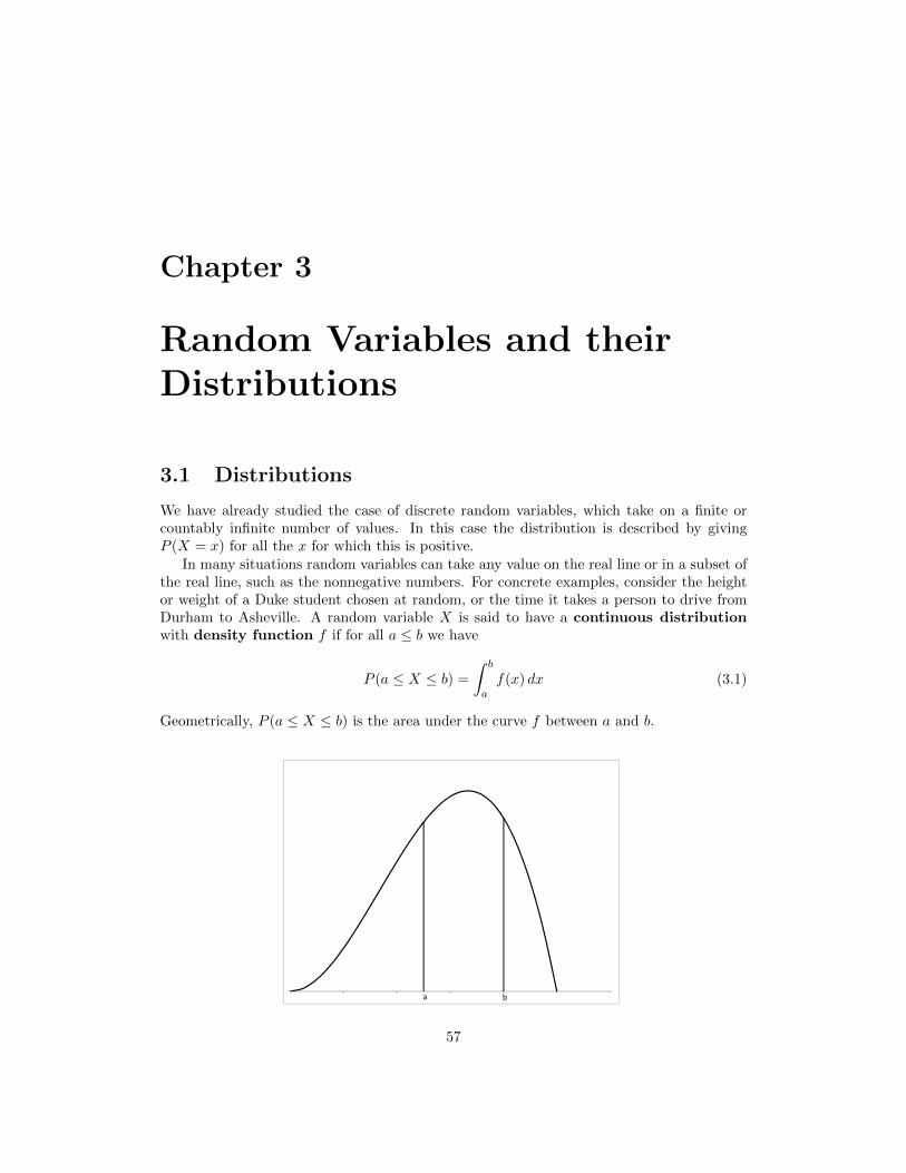
Chapter 3
Random Variables and theirDistributions
3.1 Distributions
We have already studied the case of discrete random variables, which take on a finite orcountably infinite number of values. In this case the distribution is described by givingP (X = x) for all the x for which this is positive.
In many situations random variables can take any value on the real line or in a subset ofthe real line, such as the nonnegative numbers. For concrete examples, consider the heightor weight of a Duke student chosen at random, or the time it takes a person to drive fromDurham to Asheville. A random variable X is said to have a continuous distributionwith density function f if for all a ≤ b we have
P (a ≤ X ≤ b) =
∫ b
a
f(x) dx (3.1)
Geometrically, P (a ≤ X ≤ b) is the area under the curve f between a and b.
0 0.2 0.4 0.6 0.8 1 1.2a b
57

58 CHAPTER 3. RANDOM VARIABLES AND THEIR DISTRIBUTIONS
For the purposes of understanding and remembering formulas, it is useful to think off(x) as P (X = x) even though the last event has probability zero. To explain the lastremark and to prove P (X = x) = 0, note that taking a = x and b = x + ∆x in (3.1) wehave
P (x ≤ X ≤ x+ ∆x) =
∫ x+∆x
x
f(y) dy ≈ f(x)∆x
when ∆x is small. Letting ∆x→ 0, we see that P (X = x) = 0, but f(x) tells us how likelyit is for X to be near x. That is,
P (x ≤ X ≤ x+ ∆x)
∆x≈ f(x)
In order for P (a ≤ X ≤ b) to be nonnegative for all a and b and for P (−∞ < X <∞) = 1we must have
f(x) ≥ 0 and
∫f(x) dx = 1 (3.2)
Here, and in what follows, if the limits of integration are not specified, the integration is overall values of x from −∞ to ∞. Any function f that satisfies (3.2) is said to be a densityfunction.
We are now going to give four important examples of density functions. For simplicity,we will give the values of f(x) where it is positive, and omit the phrase “0 otherwise.”
Example 3.1. Uniform distribution. Given a < b we define
f(x) =1
b− aa ≤ x ≤ b
The idea here is that we are picking a value “at random” from (a, b). That is, values outsidethe interval are impossible, and all those inside have the same probability (density).
a b
1/(b− a)
Figure 3.1: Uniform on (a, b) density function.
The area of the rectangle is (b − a) · 1/(b − a) = 1 so this is a probability density. Themost important special case occurs when a = 0 and b = 1. Random numbers generatedby a computer are typically uniformly distributed on (0, 1). Another case that comes upin applications is a = −1/2 and b = 1/2. If we take a measurement and round it off tothe nearest integer then it is reasonable to assume that the “round-off error” is uniformlydistributed on (−1/2, 1/2).
Example 3.2. Exponential distribution. Given λ > 0 we define
f(x) = λe−λx x ≥ 0
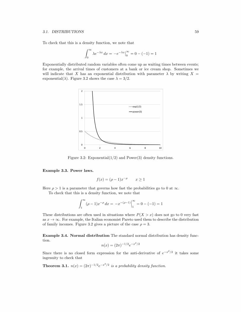
3.1. DISTRIBUTIONS 59
To check that this is a density function, we note that∫ ∞0
λe−λx dx = −e−λx∣∣∞0
= 0− (−1) = 1
Exponentially distributed random variables often come up as waiting times between events;for example, the arrival times of customers at a bank or ice cream shop. Sometimes wewill indicate that X has an exponential distribution with parameter λ by writing X =exponential(λ). Figure 3.2 shows the case λ = 3/2.
0
0.5
1
1.5
2
0 2 4 6 8 10
exp(1/2)
power(3)
Figure 3.2: Exponential(1/2) and Power(3) density functions.
Example 3.3. Power laws.
f(x) = (ρ− 1)x−ρ x ≥ 1
Here ρ > 1 is a parameter that governs how fast the probabilities go to 0 at ∞.To check that this is a density function, we note that∫ ∞
1
(ρ− 1)x−ρ dx = −x−(ρ−1)∣∣∣∞1
= 0− (−1) = 1
These distributions are often used in situations where P (X > x) does not go to 0 very fastas x→∞. For example, the Italian economist Pareto used them to describe the distributionof family incomes. Figure 3.2 gives a picture of the case ρ = 3.
Example 3.4. Normal distribution The standard normal distribution has density func-tion.
n(x) = (2π)−1/2e−x2/2
Since there is no closed form expression for the anti-derivative of e−x2/2 it takes some
ingenuity to check that
Theorem 3.1. n(x) = (2π)−1/2e−x2/2 is a probability density function.

60 CHAPTER 3. RANDOM VARIABLES AND THEIR DISTRIBUTIONS
‐3 ‐2 ‐1 0 1 2 3
Figure 3.3: The standard normal density function.
Proof. Let I =∫e−x
2/2 dx. To show that∫n(x) dx = 1 we want to show that I =
√2π.
I2 =
∫e−x
2/2 dx
∫e−y
2/2 dy =
∫∫e−(x2+y2)/2 dx dy
Changing to polar coordinates the integral becomes∫ ∞0
∫ 2π
0
e−r2/2r dθ dr = 2π
∫ ∞0
re−r2/2 dr = 2π (−r−r
2/2)∣∣∣∞0
so I2 = 2π and we have proved the desired result.
Example 3.5. Order statistics. Let U1, U2, . . . Un be independent and uniform on (0, 1).Let V1 < V2 . . . Vn be the result of putting he values U1, U2, . . . Un in increasing order. TheVk are called order statistics. Ignoring the possibility of two of the Ui landing in (x−ε, x+ε),
P (Vk ∈ (x− ε, x+ ε)) = n · 2ε · Cn−1,k−1(x− ε)k−1(1− x− ε)n−k
In words there are n ways to pick the index of the Ui to land in (x − ε, x + ε). There areCn−1,k to pick the values to be < x − ε and a probability (x − ε)k(1 − x − ε)n−1−k thatthey all land where we want them to. Dividing my 2ε and letting ε → 0 we see that thebeta(n, k) density is
n · Cn−1,k−1xk(1− x)n−1−k =
n!
(k − 1)!(n− k)!xk−1(1− x)n−k
This a special case of the beta distribution which has density
Bα,βxα−1(1− x)β−1
where α, β > 0 are real numbers, and Bα,β is a constant to make the inegral one. The orderstatistics corrsepond to α = k, β = n− k + 1.

3.2. DISTRIBUTION FUNCTIONS 61
3.2 Distribution Functions
Any random variable (discrete or contnuous) has a distribution function defined byF (x) = P (X ≤ x). However, these are the most useful in the continuous case.
3.2.1 For continuous random variables
If X has a density function f(x) then
F (x) = P (−∞ < X ≤ x) =
∫ x
−∞f(y) dy
That is, F is an antiderivative of f , and a special one F (x)→ 0 as x→ −∞ and F (x)→ 1as x→∞.
One of the reasons for computing the distribution function is explained by the nextformula. If a < b then X ≤ b = X ≤ a ∪ a < X ≤ b with the two sets on theright-hand side disjoint so
P (X ≤ b) = P (X ≤ a) + P (a < X ≤ b)
or, rearranging,
P (a < X ≤ b) = P (X ≤ b)− P (X ≤ a) = F (b)− F (a) (3.3)
The last formula is valid for any random variable. When X has density function f , it saysthat ∫ b
a
f(x) dx = F (b)− F (a)
i.e., the integral can be evaluated by taking the difference of any antiderivative at the twoendpoints.
To see what distribution functions look like, and to explain the use of (3.3), we returnto our examples.
Example 3.6. Uniform distribution. f(x) = 1/(b− a) for a ≤ x ≤ b.
F (x) =
0 x ≤ a(x− a)/(b− a) a ≤ x ≤ b1 x ≥ b
To check this, note that P (a < X < b) = 1 so P (X ≤ x) = 1 when x ≥ b andP (X ≤ x) = 0 when x ≤ a. For a ≤ x ≤ b we compute
P (X ≤ x) =
∫ x
−∞f(y) dy =
∫ x
a
1
b− ady =
x− ab− a
In the most important special case a = 0, b = 1 we have F (x) = x for 0 ≤ x ≤ 1.
Example 3.7. Exponential distribution. f(x) = λe−λx for x ≥ 0.
F (x) =
0 x ≤ 0
1− e−λx x ≥ 0

62 CHAPTER 3. RANDOM VARIABLES AND THEIR DISTRIBUTIONS
a (a+ b)/2 b
1
1/2
Uniform on [a,b]
0
Figure 3.4: Distribution function for the unifomr on [a, b].
The first line of the answer is easy to see. Since P (X > 0) = 1 we have P (X ≤ x) = 0 forx ≤ 0. For x ≥ 0 we compute
P (X ≤ x) =
∫ x
−∞f(y) dy =
∫ x
0
λe−λy dy
= −e−λy∣∣x0
= −e−λx − (−1)
Figure 3.5 shows the case λ = 1/2.Suppose X has an exponential distribution with parameter λ. If t ≥ 0 then P (X > t) =
1− P (X ≤ t) = e−λt, so if s ≥ 0 then
P (T > t+ s|T > t) =P (T > t+ s)
P (T > t)=e−λ(t+s)
e−λt= e−λs = P (T > s)
This is the lack of memory property of the exponential distribution. Given that youhave been waiting t units of time, the probability you must wait an additional s units oftime is the same as if you had not been waiting at all.
The following scaling property is useful.
If X = exponential(1) then X/λ = exponential(λ). (3.4)
To prove this note that P (X/λ > t) = P (X > λt)e−λt.
Example 3.8. Power laws. f(x) = (ρ− 1)x−ρ for x ≥ 1 where ρ > 1.
F (x) =
0 x ≤ 1
1− x−(ρ−1) x ≥ 1
The first line of the answer is easy to see. Since P (X > 1) = 1, we have P (X ≤ x) = 0 forx ≤ 1. For x ≥ 1 we compute
P (X ≤ x) =
∫ x
−∞f(y) dy =
∫ x
1
(ρ− 1)y−ρ dy
= −y−(ρ−1)∣∣∣x1
= 1− x−(ρ−1)
Figure 3.5 gives a picture of the case ρ = 3. To illustrate the use of (3.3) we note thatif ρ = 3 then
P (2 < X ≤ 4) = (1− 4−2)− (1− 2−2) =1
4− 1
16=
3
16

3.2. DISTRIBUTION FUNCTIONS 63
0
0.2
0.4
0.6
0.8
1
0 2 4 6 8 10
exp(1/2)
power(3)
Figure 3.5: Distribution functions for exponential(1/2) and power(3).
Example 3.9. Normal distribution.
n(x) = (2π)−1/2e−x2/2
does not have a closed form antiderivative, so to find P (X ≤ x) we have to use the table inthe back of the book. We will talk more about this in Chapter 3.
3.2.2 For discrete random variables
Distribution functions are somewhat messier in the discrete case.
Example 3.10. Binomial(3,1/2). Flip three coins and let X be the number of headsthat we see. The probability function is given by
x 0 1 2 3P (X = x) 1/8 3/8 3/8 1/8
In this case the distribution function can be written as
F (x) =
0 x < 0
1/8 0 ≤ x < 1
1/2 1 ≤ x < 2
7/8 2 ≤ x < 3
1 3 ≤ x
or drawn as
To check this, note for example that for 1 ≤ x < 2, P (X ≤ x) = P (X ∈ 0, 1) = 1/8+3/8.The reader should note that F is discontinuous at each possible value of X and the heightof the jump there is P (X = x). The little black dots in the figure are there to indicate thatat 0 the value is 1/8, at 1 it is 1/2, etc.
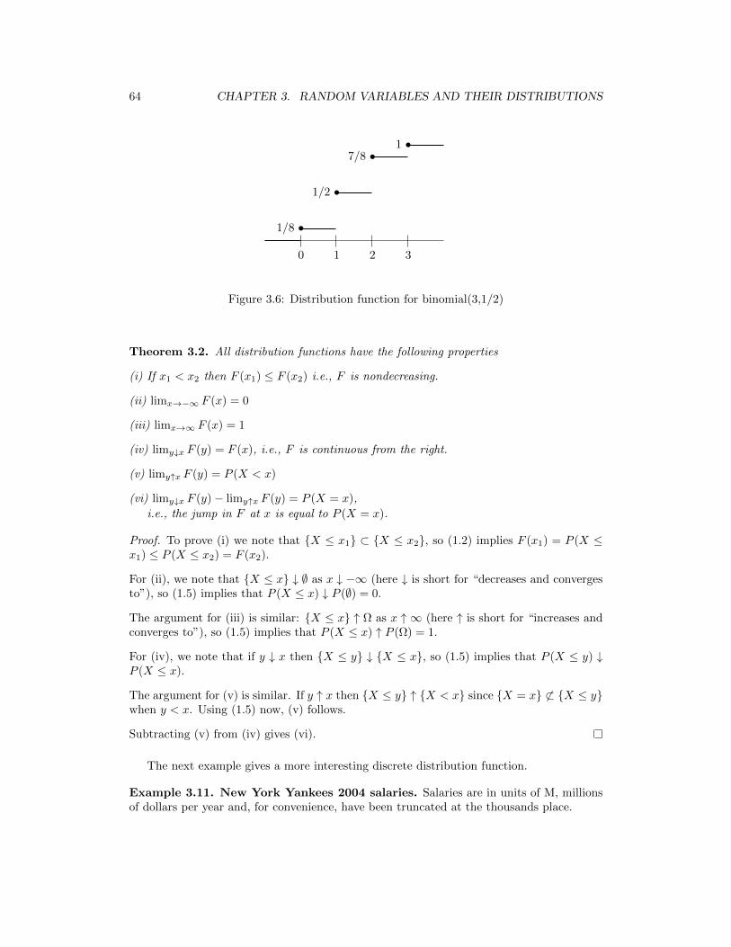
64 CHAPTER 3. RANDOM VARIABLES AND THEIR DISTRIBUTIONS
•
•
••
0 1 2 3
1/8
1/2
7/81
Figure 3.6: Distribution function for binomial(3,1/2)
Theorem 3.2. All distribution functions have the following properties
(i) If x1 < x2 then F (x1) ≤ F (x2) i.e., F is nondecreasing.
(ii) limx→−∞ F (x) = 0
(iii) limx→∞ F (x) = 1
(iv) limy↓x F (y) = F (x), i.e., F is continuous from the right.
(v) limy↑x F (y) = P (X < x)
(vi) limy↓x F (y)− limy↑x F (y) = P (X = x),
i.e., the jump in F at x is equal to P (X = x).
Proof. To prove (i) we note that X ≤ x1 ⊂ X ≤ x2, so (1.2) implies F (x1) = P (X ≤x1) ≤ P (X ≤ x2) = F (x2).
For (ii), we note that X ≤ x ↓ ∅ as x ↓ −∞ (here ↓ is short for “decreases and convergesto”), so (1.5) implies that P (X ≤ x) ↓ P (∅) = 0.
The argument for (iii) is similar: X ≤ x ↑ Ω as x ↑ ∞ (here ↑ is short for “increases andconverges to”), so (1.5) implies that P (X ≤ x) ↑ P (Ω) = 1.
For (iv), we note that if y ↓ x then X ≤ y ↓ X ≤ x, so (1.5) implies that P (X ≤ y) ↓P (X ≤ x).
The argument for (v) is similar. If y ↑ x then X ≤ y ↑ X < x since X = x 6⊂ X ≤ ywhen y < x. Using (1.5) now, (v) follows.
Subtracting (v) from (iv) gives (vi).
The next example gives a more interesting discrete distribution function.
Example 3.11. New York Yankees 2004 salaries. Salaries are in units of M, millionsof dollars per year and, for convenience, have been truncated at the thousands place.

3.3. MEANS AND MEDIANS 65
A. Rodriguez 21.726 D. Jeter 18.6M. Mussina 16 K. Brown 15.714J. Giambi 12.428 B. Williams 12.357G. Sheffield 12.029 M. Rivera 10.89J. Posada 9 J. Vazquez 9J. Contreras 9 J. Olerud 7.7H. Matsui 7 S. Karsay 6E. Loazia 4 T. Gordon 3.5P. Quantrill 3 K. Lofton 2.985J. Lieber 2.7 T. Lee 2G. White 1.925 F. Heredia 1.8R. Sierra 1 M. Cairo .9J. Falherty .775 T. Clark .75E. Wilson .7 O. Hernandez .5D. Osborne .45 C.J. Nitowski .35J. DePaula .302 B. Crosby .301
Figure 3.7 shows the distribution function of Yankees salaries. The total team salary is183.355 M. Dividing by 32 players gives a mean of 6.149 M dollars.
0
0.1
0.2
0.3
0.4
0.5
0.6
0.7
0.8
0.9
1
0 5 10 15 20 25Salary (millions of dollars)
Figure 3.7: Distribution function for Yankees salaries
3.3 Means and medians
For a discrete random variable the mean is
EX =∑x
xP (X = x)

66 CHAPTER 3. RANDOM VARIABLES AND THEIR DISTRIBUTIONS
To extend this to the continuous case we replace P (X = x) by the density function
EX =
∫xfX(x) dx
Example 3.12. Uniform distribution. Suppose X has density function f(x) = 1/(b−a)for a ≤ x ≤ b. Then
EX =
∫ b
a
x
b− adx =
x2
2(b− a)
∣∣∣∣ba
=b2 − a2
2(b− a)=a+ b
2
Notice that (a+ b)/2 is the midpoint of the interval and hence is the natural choice for theaverage value of X.
Before tackling the next example, we recall the integration by parts formula:∫ b
a
g(x)h′(x) dx = g(x)h(x)|ba −∫ b
a
g′(x)h(x) dx (3.5)
Example 3.13. Exponential distribution. Suppose X has density function
f(x) = λe−λx for x ≥ 0.
Integrating by parts with g(x) = x, h′(x) = λe−λx, so g′(x) = 1 and h(x) = −e−λx.
EX =
∫ ∞0
xλe−λx dx = −xe−λx∣∣∞0
+
∫ ∞0
e−λx dx = 0 + 1/λ
To check the last step note that −xe−λx = 0 when x = 0 and when x → ∞ −xe−λx → 0since e−λx → 0 much faster than x grows. The evaluation of the integral follows from thedefinition of the exponential desnity, which implies
∫∞0λe−λx dx = 1.
Example 3.14. Power laws. Let ρ > 1 and f(x) = (ρ− 1)x−ρ for x ≥ 1.
EX =
∫ ∞1
x(ρ− 1)x−ρ dx =ρ− 1
2− ρx2−ρ
∣∣∣∣∞1
=ρ− 1
ρ− 2
if ρ > 2. If 1 < ρ ≤ 2, EX =∞.
Example 3.15. Normal distribution. To make this example more interesting we willlook at the general normal with parameters µ and σ2 or normal(µ, σ2) introduced in (3.7):
(2πσ2)−1/2e−(x−µ)2/2σ2
By symmetry ∫(2πσ2)−1/2xe−(x−µ)2/2σ2
dx = µ
Medians. Intuitively, the median m1/2 is the point where 50% of the values are ≥ m1/2
and 50% are ≤ m1/2. It is a notion of the typical value of the distribution is not sensitive tolarge values. For example in the Yankee salaries data Alex Rodriguez’s salary contributes678,937 to the mean. Similar things would happen if we looked at salaries across the US orthe sizes of cities in a state.
When the distribution function is nice the median is where it takes the value 1/2. Thenext table computes m for our four examples and compares with the mean

3.3. MEANS AND MEDIANS 67
Exponential distribution m1/2 = (log 2)/λ. µ = 1/λUniform distribution m1/2 = (a+ b)/2 = µPower laws m1/2 = 21/(ρ−1) µ = (ρ− 1)/(ρ− 2)Normal m1/2 = µ
In the case of the exponential the mean and median differ by a constant factor. The meanand the median do not look very similar for the the power law. When ρ < 2 the mean isinfinite but the median is finite. When ρ = 4, µ = 3/2 while the median m1/2 = 1.26.
In the discrete case two unusual things can happen. In the case of the binomial(3, 1/2)distribution F (x) = 1/2 when 1 ≤ x < 2. A different type of problem exists for the uniformdistribution on 1, 2, 3. There is no place where F (x) = 1/2.
1 2 3
•
•
•
1/3
2/3
1
Figure 3.8: Distribution function for uniform on 1, 2, 3
The next definition takes care of bad cases. Suppose X has distribution function F .
m1/2 is a median for F if P (X ≤ m1/2) ≥ 1/2 and P (X ≥ m1/2) ≥ 1/2
Using this definition
• 2 is the median for the uniform on 1, 2, 3 since P (X ≤ 2) = 2/3 and P (X ≥ 2) = 2/3.
• For the binomial(3, 1/2) distribution any value m ∈ [1, 2] is a median since if m ∈ (1, 2)P (X ≤ m) = P (X ≥ m) = 1/2 while P (X ≤ 1) = 1/2 and P (X ≥ 1) = 7/8 andP (X ≤ 2) = 7/8 and P (X ≥ 2) = 1/2
• For the Yankees salaries any number between 3 and 3.5 is a median. In contrast themean is 6.49 million.
Generalizing the median, the α-percentile is the place mα where P (X ≤ mα) = α.Percentiles are commonly used when reporting values of standardized tests. For example,“my score was in the 72nd percentile on the SAT math test. These points also come up insolving optimization problems
Example 3.16. An enterprising young man sits in the lobby of a big office building sellingnewspapers. He buys papers for 15 cents and sells them for 25, but he cannot return anyunsold papers. Suppose that each day X people by papers. Compute the difference betweenbuying m papers and buy in m− 1 in order to determine the optimal number to buy.

68 CHAPTER 3. RANDOM VARIABLES AND THEIR DISTRIBUTIONS
If he buys m (or m− 1) papers his profit is
− 15m+
m−1∑k=0
25kP (X = k) + 25mP (X ≥ m)
− 15(m− 1) +
m−1∑k=0
25kP (X = k) + 25(m− 1)P (X ≥ m− 1)
In the first line the first term is his cost. The second term reflects the fact that if thedemand is k <,m he sells k papers but if k ≥ m, he sells m. The second line is similarbut we have split the two cases in a different way to make it easier to subtract the two toget −15 + 25P (X ≥ m). When this is positive buying m papers is better than m − 1, sothe optimum is the maxm : P (X ≥ m) ≥ 0.6. This is roughly the 0.4-percentile but thedistribution is discrete that isn’t quite the right answer.
3.4 Functions of Random Variables
In this section we answer the question “If X has density function f and Y = r(X), thenwhat is the density function for Y ?” Before proving a general result, we will consider anexample:
Example 3.17. Suppose X has an exponential distribution with parameter λ. What is thedistribution of Y = X2?
To solve this problem we will use the distribution function. First we recall from Example3.7 that P (X ≤ x) = 1− e−λx so if y ≥ 0 then
P (Y ≤ y) = P (X2 ≤ y) = P (X ≤ √y) = 1− e−λy1/2
Differentiating and using the chain rule (g(h(x))′ = g′(h(x))h′(x), we see that the densityfunction of Y is given by
fY (y) =d
dyP (Y ≤ y) = e−λy
1/2 λy−1/2
2for y ≥ 0
and 0 otherwise.Intuitively, this is the same as changing variables in an integral. If we set x = y1/2 and
conseqeuntly dx = (1/2)y−1/2 dy then∫ b
a
f(x) dx =
∫ b2
a2f(y1/2)(1/2)y−1/2 dy
Generalizing from the last example, we get
Theorem 3.3. Suppose X has density f and P (a < X < b) = 1. Let Y = r(X). Supposer : (a, b) → (α, β) is continuous and strictly increasing, and let s : (α, β) → (a, b) be theinverse of r, defined by r(s(y)) = y. Then Y has density
fY (y) = fX(s(y))s′(y) for y ∈ (α, β) (3.6)

3.4. FUNCTIONS OF RANDOM VARIABLES 69
Before proving this, let’s see how it applies to the last example. There X has densityf(x) = λe−λx for x ≥ 0 so we can take a = 0 and b =∞. The function r(x) = x2 is indeedcontinuous and strictly increasing on (0,∞). To find the inverse function we set y = x2 andsolve to get x = y1/2 so s(y) = y1/2. Differentiating, we have s′(y) = y−1/2/2 and plugginginto the formula, we have
g(y) = λe−λy1/2
· y−1/2/2 for y > 0
Proof of 3.3. If y ∈ (α, β) then
P (Y ≤ y) = P (r(X) ≤ y) = P (X ≤ s(y))
since r is increasing and s is its inverse. Writing F (x) for P (X ≤ x) and differentiating withrespect to y now gives
g(y) =d
dyP (Y ≤ y) =
d
dyF (s(y)) = F ′(s(y))s′(y) = f(s(y))s′(y)
by the chain rule.
Remark. The same proof works if r is decreasing but in this case
P (Y ≤ y) = P (r(X) ≤ y) = P (X ≥ s(y))
so the derivative is f(s(y))(−s′(y)). To combine the two cases into one we can write
fY (y) = f(s(y))|s′(y)|
Example 3.18. Linear transformations. Suppose X has density f(x) and Y = a+ bXwhere b > 0. r(x) = a+ bx has inverse s(y) = (y− a)/b so Y has density f((y− a)/b)/b. Toillustrate the use of this formula suppose X has the the standard normal distribution withdensity
(2π)−1/2e−x2/2
and let Y = µ+ σX where σ > 0. Our formula implies that Y has density
(2πσ2)−1/2e−(y−µ)2/2σ2
(3.7)
We call this the normal(µ, σ2) density. We know that µ is the mean. In the next chapter,we will see that σ2 is the variance.
Example 3.19. Suppose X has the standard normal distribution. Find the distribution ofY = eX . It is called the lognormal distribution since log(Y ) is normal.
r(x) = ex is increasing and maps (−∞,∞) onto (0,∞). The inverse function is s(y) = log xso using (3.6) the answer is
(2π)−1/2e−(log x)2/2 · 1/x.
This is called the lognormal distribution because log(Y ) is normally distributed

70 CHAPTER 3. RANDOM VARIABLES AND THEIR DISTRIBUTIONS
Example 3.20. Gumbel distribution. Suppose X is exponential(1). Find the desnityfunction of Y = logX.
Here, r(x) = log x is increasing on (0,∞). Its inverse function is s(y) = ey, so plugging into(3.6), the density function of Y is
fY (y) = fX(s(y))s′(y) = exp(−ey)ey y ∈ (−∞,∞)
The distribution function is G(y) = 1 − exp(−ey). For obvious reasons this is sometimescalled the double exponential distribution.
Our finaL topic is creating random variables with a specified distribution by taking afunction of the unifrom distribution. Most programming languages have built in functionsfor generating uniformly distributed random variables, so this allows us to create any dis-tribution. To begin we define the inverse of a distribuiton function. Since F (x) make takethe value y at more than one point we let
F−1(y) = minx : F (x) ≥ y
In most cases F (x) will be strictly increasing when 0 < F (x) < 1, so if 0 < y < 1 thenF−1(y) is the unique solution to F (x) = y
Theorem 3.4. Suppose the distribution function is conitnuous ands let U have uniformdistribution on (0,1). Then Y = F−1(U) has distribution function F .
Proof. A distribution function is nondecreasing, i.e., if x ≤ y then F (x) ≤ F (y). Takingx = F−1U and using the fact that F (F−1(U) = U
P (F−1(U) ≤ y) = P (F (F−1(U) ≤ F (y)) = P (U ≤ F (x)) = F (x)
since P (U ≤ y) = y for y ∈ (0, 1).
Example 3.21. For a concrete example, suppose we want to construct an exponentialdistribution with parameter λ. Setting 1 − e−λx = y and solving gives − ln(1 − y)/λ = x.So if U is uniform on (0, 1) then − ln(1−U)/λ has the desired exponential distribution. Ofcourse since 1− U is uniform on (0, 1) we could also use
r(U) = − ln(U)/λ
To check that we have achieved our goal we note that r is decreasing, and the inversefunction s(y) = e−λy. Since the density function of U is f(x) = 1 for 0 < x < 1. Using (3.6)the denity of Y = r(U) is
g(y) = 1 · |s′(y)| = λe−λy.
Theorem 3.4 has a consequence thatis useful to reduce the general case to the uniformin nonparametric statistics.
Theorem 3.5. If X has a continuous distribution function F (x) then F (X) is uniform on(0, 1).
Proof. By Theorem 3.4 F−1(U) has the same distribution as X so
P (F (X) ≤ y) = P (F (F−1(U)) ≤ y) = P (U ≤ y)
where we have used continuity to conclude F (F−1(y)) = y.

3.5. JOINT DISTRIBUTIONS 71
3.5 Joint distributions
In the next chapter we will study sums of random variables. However, before we can discussthat we need to introduce joint distributions.
3.5.1 Discrete distributions
We begin with some definitions. The joint distribution of two discrete random variablesis given by
P (X = x, Y = y)
To recover the marginal distribution of X, we sum over the possible values of Y
P (X = x) =∑y
P (X = x, Y = y) (3.8)
Similarly, to recover the marginal distribution of Y , we sum over the possible values of X
P (Y = y) =∑x
P (X = x, Y = y)
Example 3.22. An urn has 6 red, 5 blue, and 4 green balls. We draw three balls out. LetX = the number of red balls drawn and Y = the number of blue balls. If x, y ≥ 0 andx+ y ≤ 3 then 3− (x+ y) green balls were drawn so
P (X = x, Y = y) =C6,x · C5,y · C4,3−(x+y)
C15,3
The denominator is C15,3 = (15 · 14 · 13)/6 = 455. Using
C6,3 = 20 C6,2 = 15 C6,1 = 6
C5,3 = 10 C5,2 = 10 C5,1 = 5
C4,3 = 4 C4,2 = 6 C4,1 = 4
we can compute the joint distribution
Y X = 0 1 2 33 10/455 10/4552 40/455 60/455 100/4551 30/455 120/455 75/455 0 225/4550 4/455 36/455 60/455 20/455 120/445
84/455 216/455 135/455 20/455
The marginal distribution of X given in the last row is obtained by adding up the columns.The marginal distribution of Y given in the last column is obtained by adding up the rows.To check the margnal distributions note that
P (X = 1) =C6,1C9,3
C15,3=
6 · 9 · 8/2455
=216
455
P (Y = 2) =C5,2C10,1
C15,3=
10 · 5 · 4/2455
=100
455
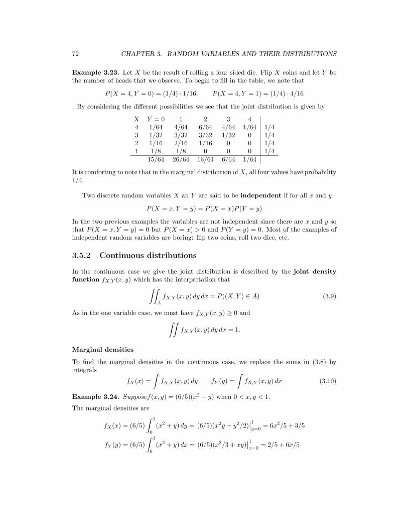
72 CHAPTER 3. RANDOM VARIABLES AND THEIR DISTRIBUTIONS
Example 3.23. Let X be the result of rolling a four sided die. Flip X coins and let Y bethe number of heads that we observe. To begin to fill in the table, we note that
P (X = 4, Y = 0) = (1/4) · 1/16, P (X = 4, Y = 1) = (1/4) · 4/16
. By considering the different possibilities we see that the joint distribution is given by
X Y = 0 1 2 3 44 1/64 4/64 6/64 4/64 1/64 1/43 1/32 3/32 3/32 1/32 0 1/42 1/16 2/16 1/16 0 0 1/41 1/8 1/8 0 0 0 1/4
15/64 26/64 16/64 6/64 1/64
It is comforting to note that in the marginal distribution ofX, all four values have probability1/4.
Two discrete random variables X an Y are said to be independent if for all x and y
P (X = x, Y = y) = P (X = x)P (Y = y)
In the two previous examples the variables are not independent since there are x and y sothat P (X = x, Y = y) = 0 but P (X = x) > 0 and P (Y = y) = 0. Most of the examples ofindependent random variables are boring: flip two coins, roll two dice, etc.
3.5.2 Continuous distributions
In the continuous case we give the joint distribution is described by the joint densityfunction fX,Y (x, y) which has the interpretation that∫∫
A
fX,Y (x, y) dy dx = P ((X,Y ) ∈ A) (3.9)
As in the one variable case, we must have fX,Y (x, y) ≥ 0 and∫∫fX,Y (x, y) dy dx = 1.
Marginal densities
To find the marginal densities in the continuous case, we replace the sums in (3.8) byintegrals
fX(x) =
∫fX,Y (x, y) dy fY (y) =
∫fX,Y (x, y) dx (3.10)
Example 3.24. Supposef(x, y) = (6/5)(x2 + y) when 0 < x, y < 1.
The marginal densities are
fX(x) = (6/5)
∫ 1
0
(x2 + y) dy = (6/5)(x2y + y2/2)∣∣1y=0
= 6x2/5 + 3/5
fY (y) = (6/5)
∫ 1
0
(x2 + y) dx = (6/5)(x3/3 + xy)∣∣1x=0
= 2/5 + 6x/5

3.5. JOINT DISTRIBUTIONS 73
To check that 6/5’s is the right constant to make the integral 1, we integrate the marginaldensities ∫ 1
0
6x2/5 + 3/5 dx = 2x3/5 + 3/5∣∣10
= 1∫ 1
0
2/5 + 6y/5 dy = 2/5 + 3y2/5∣∣10
= 1
For another example of computing marginal densities.
Example 3.25. Suppose fX,Y (x, y) = 20(y − x)3 for 0 < x < y < 1. Find the marginaldensity of X and the marginal density of Y
fX(x) =
∫ 1
x
20(y − x)3 dy = 5(y − x)4∣∣1x
= 5(1− x)4
fY (y) =
∫ y
0
20(y − x)3 dx = −5(y − x)4∣∣y0
= 5y4
Independence
As in the discrete case, X and Y are independent if the joint distribution is the product ofthe marginal distributions
fX,Y (x, y) = fX(x)fY (y).
In order for the random variables in Example 3.24 to be independent we would need
(6/5)(x2 + y) =
(2x3
5+
3
4
)(2
5+
3y2
5
)This is false when x = 0 and y = 0 In the Example 3.25 the variables are not independentsince fX,Y (0.6, 0.4) = 0 while fX(0.6) > 0 and fY (0.4) > 0.
For an example of random variables that are independent
Example 3.26. f(x, y) = 6x2y when 0 < x, y < 1.
The marginal densities are
fX(x) =
∫ 1
0
6x2y dy = 3x2y2∣∣10
= 3x2
fY (y) =
∫ 1
0
6x2y dx = 6(x3y/3)∣∣10
= 2y
fX,Y (x, y) = fX(x)fY (y) so these random variables are independent.
The next lemma makes checking independence easier
Theorem 3.6. If fX,Y (x, y) vanish outrside [a, b] × [c, d] and can be written as h(x)k(y)then X and Y are independent.

74 CHAPTER 3. RANDOM VARIABLES AND THEIR DISTRIBUTIONS
Proof. The marginal distributions are
fX(x) =
∫ d
c
h(x)k(y) dy = h(x)
∫ d
c
k(y) dy
fY (y) =
∫ b
a
h(x)k(y) dx = k(y)
∫ b
a
h(x) dy
For these random variables to be independent we need
h(x)k(y) =
(h(x)
∫ d
c
k(y) dy
)(k(y)
∫ b
a
h(x) dy
)
but this holds since
1 =
∫∫h(x)k(y) dy dx =
(∫ b
a
h(x) dy
)(∫ d
c
k(y) dy
)
In words if we can write fX,Y (x, y) as a product h(x)k(y) then there is a constant so thatfX(x) = ch(x) and fY (y) = k(y)/c and hence fX,Y (x, y) = fX(x)fY (y).
Computing probabilities
Example 3.27. Suppose two people agree to meet for coffee and each will arrive at inde-pendent randomly chosen times between 11:00 and 12:00. What is the probability of A =the first one will not have to wait more than 10 minutes for the other to arrive?
Let X1 and X2 be uniform on (0, 1) so the joint desnity is fX,Y (x, y) = 1 when 0 < x, y < 1.The answer is P (|X1−X2| < 1/6). To compute the probability it is useful to draw a picture
A
1/6
1/6
5/6
5/6
0 10
1
The central diagonal strip is the event of interest. The complement of this strip consists oftwo right triangles with each side 5/6, so the answer is 1− (5/6)2 = 11/16.

3.5. JOINT DISTRIBUTIONS 75
Example 3.28. Suppose X = exponential(λ) and Y = exponential(µ) are independent.Find P (X < Y ).
The joint density is λe−λx ·µe−µy. We want to integrate this over the region 0 < x < y <∞.∫ ∞0
dy µe−µy∫ y
0
dxλe−λx =
∫ ∞0
dyµe−µy(1− e−λy0
=
∫ ∞0
dyµe−µy − µe−(µ+λ)y = 1− µ
µ+ λ=
λ
µ+ λ
where we have used the observation that µe−µy and (µ + λ)e−(µ+λ)y integrate to 1 sincethey are exponential density functions.
Conditional densities
In the discrete case the joint distribution is P (X = x, Y = y) while the marginal distribu-tions for X and Y are given by
P (X = x) =∑y
P (X = x, Y = y)
P (Y = y) =∑x
P (X = x, Y = y)
The purpose of this section is to define the conditional distributions
P (X = x|Y = y) = P (X = x, Y = y)/P (Y = y)
P (Y = y|X = x) = P (X = x, Y = y)/P (X = x)
Example 3.29. In Example 3.23 we let X be the result of rolling a four sided die and let Ybe the number of heads that we observe when we flip X coins. By considering the differentpossibilities we see that the joint distribution is given by
X Y = 0 1 2 3 44 1/64 4/64 6/64 4/64 1/64 1/43 1/32 3/32 3/32 1/32 0 1/42 1/16 2/16 1/16 0 0 1/41 1/8 1/8 0 0 0 1/4
15/64 26/64 16/64 6/64 1/64
The condition distribution of X given that Y has
P (X = x|Y = 0) =P (X = y, Y = 0)
P (Y = 0)
In words we divide the column by the sum of the probabilities to make it sum to 1.
x 0 1 2 3P (X = x|Y = 0) 8/15 4/15 2/15 1/15
The conditional distribution of Y given that X = 3 is iis obtained by dividing the X = 3row by 1/4

76 CHAPTER 3. RANDOM VARIABLES AND THEIR DISTRIBUTIONS
y 0 1 2 3P (Y = y|X = 3) 1/8 3/8 3/8 1/8
which is the binomial distribution we used to compute the joint distribution.
The situation for continuous random variables is similar but with sums replaced by integrals.
fY |X=x(y) =fX,Y (x, y)
fX(x)fX|Y=y(y) =
fX,Y (x, y)
fY (y)
Example 3.30. In Example 3.24 f(x, y) = (6/5)(x2 + y) when 0 < x, y < 1. We calculatedthat The marginal densities are
fX(x) = 6x2/5 + 3/5 fY (y) = 2/5 + 6y/5
The conditional distributions are
fY |X=x(y) =(6/5)(x2 + y)
6x2/5 + 3/5fX|Y=y(y) =
(6/5)(x2 + y)
6/5 + y
3.6 Exercises
Discrete Distributions
1. Suppose we roll two dice and let X and Y be the two numbers that appear. Find thedistribution of |X − Y |.
2. How many children should a family plan to have so that the probability of having atleast one child of each sex is at least 0.95?
3. In a carton of six eggs two are bad. Find the distribution of the number of eggs N thatwe use before pick one that is bad.
4. We have an urn with m red balls and n blue balls. Let N be the number of balls thatwe have to draw until we get a red one. Find P (N = k) for 1 ≤ m ≤ n+ 1.
5. Suppose we roll two four sided dice with the numbers 1, 2, 3, 4 on them,and the outcomesare R1 and R2. Find the joint distribution of X = minR1, R2 and Y = R1 +R2 and thencompute the marginal distributions of X and Y .
6. Suppose we roll a six sided die repeatedly. Let Ni be the number of the roll on which wesee i for the first time. (a) Find the joint distribution of N1 and N6. (b) Find the marginaldistributions of N1. (c) The conditional distribution of N6 given N1 = i
7. Show that if X1 = geomteric(p1) and X2 = geomteric(p2) are independent then Y =minX1, X2 is geoemetric(q) where q = 1− (1− p1)(1− p2).
Density and distribution functions
8. Suppose X has density function f(x) = c(1− |x|) when −1 < x < 1.(a) What value of cmakes this a density function? (b) Find the distribution function.
9. F (x) = 3x2 − 2x3 for 0 < x < 1 (with F (x) = 0 if x ≤ 0 and F (x) = 1 if x ≥ 1)defines a distribution function. (a) Find the corresponding density function. (b) FindP (1/2 < X < 1)

3.6. EXERCISES 77
10. Let F (x) = e−1/x for x ≥ 0, F (x) = 0 for x ≤ 0. Is F a distribution function? If so,find its density function.
11. Let F (x) = 3x− 2x2 for 0 ≤ x ≤ 1, F (x) = 0 for x ≤ 0, and F (x) = 1 for x ≥ 1. Is F adistribution function? If so, find its density function.
12. Consider f(x) = c(1− x2) for −1 < x < 1, 0 otherwise. (a) What value of c should wetake to make f a density function? (b) Find the distribution function. (c) Find P (1/2 <X < 1). (d) Find EX
13. Suppose X has density function f(x) = 4x3 for 0 < x < 1, 0 otherwise. Find (a) thedistribution function, (b) P (X < 1/2), (c) P (1/3 < X < 2/3), (d) EX.
14. Suppose X has density function x−1/2/2 for 0 < x < 1, 0 otherwise. Find (a) thedistribution function, (b) P (X > 3/4), (c) P (1/9 < X < 1/4), (d) EX.
15. Suppose X has the Rayleigh density function xe−x2/2 for x ≥ 0. (a) Find the distri-
bution function. (b) P (X >√
2, (c) EX.
16. Suppose X has density f(x) = 4x(1 − x2) for 0 < x < 1. (a) Find the distributionfunction. (b) Find the median. (b) Find the mean.
17. Suppose x has density function f(x) = 12x2(1 − x) for 0 < x < 1. (a) Find thedistribution function of X, (a) P (0 < X < 1/2), and (c) EX.
18. Order statitistics were considered in Example 3.5. There it was shown that if U1, U2, . . . Unare independent uniform on (0, 1) and V1 < V2 < . . . Vn are the Ui put in increasing orderthen Vk has density
fk,n(x) =n!
(k − 1)!(n− k)!xk−1(1− x)n−k
Compute the mean EVk.
Medians, etc.
19. Suppose P (X = x) = x/21 for x = 1, 2, 3, 4, 5, 6. Find all the medians of this distribu-tion.
20. Suppose X has a Poisson distribution with λ = ln 2. Find all the medians of X.
21. Suppose X has a geometric distribution with success probability 1/4, i.e., P (X = k) =(3/4)k−1(1/4). Find all the medians of X.
22. Suppose X has density function f(x) = x/2 for 0 < x < 2, 0 otherwise. Find (a) thedistribution function, (b) the median, (c) the mean.
23. Suppose X has density f(x) = 4x(1 − x2) for 0 < x < 1. (a) Find the distributionfunction. (b) Find the median. (b) Find the mean.
24. Suppose X has the Rayleigh distribution xe−x2/2 for 0 < x < ∞. Find (a) the
distribution function, (b) the median, (c) the mean.
25. The owner of a dress store buys dresses for $50 and sells them for $125. Any unuseddresses are sold to a second-hand store at the end of the season for $25. Suppose to simplifythings that the demand for dresses is X, a random varialbe with density function f(x). Howmany dresses should the store owner buy to maximize profit.
Functions of Random Variables

78 CHAPTER 3. RANDOM VARIABLES AND THEIR DISTRIBUTIONS
26. Suppose X has density x−2 for x ≥ 1. Find the density function for Y = X2.
27. Suppose X is uniform on (0, 1). Find the density function for Y = Xα when α > 0.
28. Suppose X = exponential(λ). Show that Y = X1/α. has the Weibull distributionλαyα−1e−λy
α
.
29. Suppose thatX has the standard normal distribution. Find the distribution of Y = 1/X.
30. Suppose that X has the standard normal distribution. Find the distribution of X2.
31. Suppose X has the Rayleigh density function xe−x2/2 for x ≥ 0. . Find the distribution
of X2.
32. Suppose X1, . . . , Xn are independent and have distribution function F (x). Find thedistribution functions of (a) Y = maxX1, . . . , Xn and (b) Z = minX1, . . . , Xn
33. Suppose X1, . . . , Xn are independent exponential(λ). Show that
minX1, . . . , Xn = exponential(nλ)
34. Let U1 . . . , Un be independent and uniform on (0,1) and let V = maxU1, . . . Un. Findthe distribution function and density function for V .
Creating random variables with a given distribubtion
35. Suppose X has the powerlaw density function (ρ− 1)x−ρ for x ≥ 1 where ρ > 1. Finda function g so that if U is uniform on (0, 1), g(U) has this density function.
36. Suppose X has distribution function x/(x+ 1) for x ≥ 0, 0 otherwise. Find a functiong so that if U is uniform on [0, 1] then g(U) has this distribution function.
37. The Rayliegh distribution has density f(x) = xe−x2/2. Find a function g so that if U is
uniform on (0, 1), g(U) has this density function.
38. Suppose U uniform on (0, 1). Find a function g so that g(U) has the Weibull distributiondefined in problem 3.6.
Joint distributions: calculating probabilities
39. Suppose (X,Y ) has joint density 6xy2 for 0 < x, y < 1. Find P (X + Y < 1).
40. Suppose X and Y are independent and uniform on (0, 1). Find P (XY > z) anddifferentiate to find the density function.
41. Suppose X and Y are independent and uniform on (0, 1). Find P (Y/X ≤ z) anddifferentiate to find the density function.
42. Suppose X and Y have joint density (y − x) for 0 < x < y < 1. Compute P (Y > 2X).
43. Suppose X and Y are independent standard normals. Show that Z =√X2 + Y 2 has
the Rayleigh distribution re−r2/2.
44. Let (X,Y ) be uniform on 0 < x < y < 1. Cut the unit interval at X and Y to makethree pieces of size X, Y −X and 1 − Y . What is the probability of ∆ = the three piecescan be used to make a triangle? Note: in order to be able to make a triangle the largestpiece has to be shorter than the sum of the other two.

3.6. EXERCISES 79
45. Let A, B, and C be independent and uniform on (−1, 1). What is the probability ofE = the polynomial Ax2 + Bx + C = 0 has no real roots. Note: there are no real roots ifB2 − 4AC < 0.
46. Suppose U and V are independent uniform on (0, 1). Find E(U − V )2.
47. Suppose X and Y are independent and exponential(λ). Find E|X − Y |.
Independence, marginal and conditional distributions
48. Suppose that the joint density of X and Y is given by f(x, y) = xe−(x+y) for x, y > 0(a) Are X and Y independent? (b) Find the marginal densities of X and Y .
49. Suppose that the joint desnity of X and Y is given by f(x, y) = 24xy when x, y > 0and x + y < 1 (a) Are X and Y independent? (b) Find the marginal densities of X. (c)Thje conditional distribution of Y given X.
50. Suppose that the joint desnity of X and Y is given by f(x, y) = xe−x(1+y) when x, y > 0.(a) Are X and Y independent? (b) Find the marginal densities of X and Y .
51. Suppose X and Y have joint density fX,Y (x, y) = (6/5)(x2 + xy/2) when 0 < x, y < 1.(a) Find the marginal densities of X and Y . (b) Find P (X > Y )
52. Suppose that the joint density of X and Y is given by fX,Y (x, y) = (y − x)e−y for0 < x < y <∞. Find the marginal distributions of X and Y
53. Suppose (X,Y ) has joint density f(x, y) = 8xy for 0 < x < y < 1. (a) Find the marginaldistribution of Y . (b) Find the conditional distribution of Y given X.
54. Suppose fX,Y (x, y) = (x+ y) for 0 < x, y < 1. (a) Find the marginal distribution of X.(b) Find the conditional distribution of Y given X.
55. Suppose fX,Y (x, y) = (3/2)(xy2 +y) for 0 < x, y < 1. (a) Find the marginal distributionof X. (b) Find the conditional distribution of Y given X.
56. Suppose U1, . . . Un are independent and uniform on (0, 1). Let X = mini Ui and Y =maxi Ui. Imitate the proof in Example 3.5 to show X and Y have joint density
fX,Y (x, y) = n(n− 1)(y − x)n−2
57. Taking k = 3 in the previous problem we see that if U1, U2, U3 are independent anduniform on (0, 1). The joint density of X = minU1, U2, U3 and Y = maxU1, U2, U3 isgiven by fX,Y (x, y) = 6(y − x)or 0 < x < y < 1. (a) Find the marginal distributions of Y .(b) The conditional distribution of X given Y .
58. Let t1 and t2 be independent exponential with parameter 1. The joint density of X = t1and Y = t1 + t2 is e−y for 0 < x < y. (You do not have to prove this.) (a) Find the marginaldensities of X and Y .(b) The conditonal density of X given Y and of Y given X.
59. Let X and Y have joint distribution fX,Y (x, y) = 1/x for 0 < y < x < 1. (a) Find themarginal densities of X and Y .(b) The conditonal density of X given Y and of Y given X.

80 CHAPTER 3. RANDOM VARIABLES AND THEIR DISTRIBUTIONS
Chapter 4
Limit Theorems
4.1 Moments, Variance
In this section we will be interested in the expected values of various functions of randomvariables. The most important of these are the variance and the standard deviation whichgive an idea about how spread out the distribution is. The first basic fact we need in orderto do computations is the following, which we state without proof.
Theorem 4.1. If X has a discrete distribution then
Er(X) =∑x
r(x)P (X = x)
In the continuous case
Er(X) =
∫r(x)f(x) dx
If r(x) = xk, E(Xk) is the kth moment of X. When k = 1 this is the first moment ormean of X. If EX2 <∞ then the variance of X is defined to be
var (X) = E(X − EX)2
To illustrate this concept, we will consider some examples. But first, we need a formula thatenables us to compute the variance more easily.
var (X) = EX2 − (EX)2 (4.1)
Proof. Letting µ = EX to make the computations easier to see, we have
var (X) = E(X − µ)2 = E(X2 − 2µX + µ2) = EX2 − 2µEX + µ2
by (1.15) and the facts that E(−2µX) = −2µEX, E(µ2) = µ2. Substituting µ = EX nowgives the result.
The reader should note that EX2 means the expected value of X2 and in the proofE(X−µ)2 means the expected value of (X−µ)2. When we want the square of the expectedvalue we will write (EX)2. This convention is designed to cut down on parentheses.
81

82 CHAPTER 4. LIMIT THEOREMS
The variance measures how spread-out the distribution of X is. To begin to explain thisstatement, we will show that
var (X + a) = var (X) var (bX) = b2 var (X) (4.2)
In words, the variance is not changed by adding a constant to X, but multiplying X by amultiplies the variance by a2.
Proof. If Y = X + a then the mean of Y , µY = µX + a by (1.15), so
var (X + a) = E(X + a)− (µX + a)2 = EX − µX2 = var (X)
If Y = bX then µY = bµX by (1.15), so
var (bX) = E(bX − bµX)2 = b2E(X − µX)2 = b2 var (X)
The scaling relationship (4.2) shows that if X is measured in feet then the varianceis measured in feet2. This motivates the definition of the standard deviation σ(X) =√
var (X), which is measured in the same units as X and has a nicer scaling property:
σ(bX) = |b|σ(X) (4.3)
We get the absolute value here since√b2 = |b|.
4.1.1 Discrete random variables
Example 4.1. Roll one die and let X be the resulting number.
EX2 =1
6(1 + 4 + 9 + 16 + 25 + 36) =
91
6= 15.1666
var (X) = EX2 − (EX)2 =91
6− 49
4=
35
12= 2.91666
and σ(X) =√
var (X) = 1.7078. The standard deviation σ(X) gives the size of the “typicaldeviation from the mean.” To explain this, we note that the deviation from the mean
|X − µ| =
0.5 when X = 3, 4
1.5 when X = 2, 5
2.5 when X = 1, 6
so E|X − µ| = 1.5. The standard deviation σ(X) =√E|X − µ|2 is a slightly less intuitive
way of averaging the deviations from the mean but, as we will see later, is one that has nicerproperties.
Example 4.2. The geometric(p) distribution has variance (1− p)/p2.
Suppose N = geometric(p). That is, P (N = n) = (1 − p)n−1p for n = 1, 2, . . . and 0otherwise. To compute the variance, we begin, as in Example 2.1 by recalling the sum ofthe geometric series
∞∑n=0
xn = (1− x)−1

4.1. MOMENTS, VARIANCE 83
Differentiating this identity and noticing that the n = 0 term in the first derivative is 0 gives
∞∑n=1
nxn−1 = (1− x)−2
Differentiating again∞∑n=2
n(n− 1)xn−2 = 2(1− x)−3
Setting x = 1− p in the second formula gives
∞∑n=1
n(n− 1)(1− p)n−2 = 2p−3
Multiplying both sides by p(1− p), we have
EN(N − 1) =
∞∑n=1
n(n− 1)(1− p)n−1p =2p(1− p)
p2
From this it follows that
EN2 = EN(N − 1)+ EN =2− 2p
p2+
1
p=
(2− p)p2
var (N) = EN2 − (EN)2 =2− pp2− 1
p2=
(1− p)p2
Taking the square root we see that σ(X) =√
1− p/p.
Example 4.3. The binomial(n, p) distribution has variance np.
As in the case of the geometric, our next step is to compute
E(N(N − 1)) =
n∑m=2
m(m− 1)n!
m!(n−m)!pm(1− p)n−m
We have dropped the first two terms which contribute nothing to the sum so we can cancelto get
= n(n− 1)p2n∑
m=2
(n− 2)!
(m− 2)!(n−m)!pm−2(1− p)n−m = n(n− 1)p2
since the sum computes the total probability for the binomial(n− 2, p) distribution.
To finish up we note that
var (N) = EN2 − (EN)2 = E(N(N − 1)) + EN − (EN)2
= n(n− 1)p2 + np− n2p2 = n(p− p2) = np(1− p)
which completes the proof. In Section 4.4 we will see a much simpler proof.

84 CHAPTER 4. LIMIT THEOREMS
Example 4.4. The Poisson(λ) distribution has variance λ
As in the case of the binomial and geometric we begin by computing
E(X(X − 1)) =
∞∑k=2
k(k − 1)e−λλk
k!= λ2
∞∑k=2
e−λλk−2
(k − 2)!= λ2
From this it follows that
var (X) = EX2 − (EX)2 = E(X(X − 1)) + EX − (EX)2
= λ2 + λ− λ2
which completes the proof.
4.1.2 Continuous random variables
Example 4.5. Uniform distribution. Suppose X has density function f(x) = 1/(b− a)for a ≤ x ≤ b. We begin with the case a = 0, b = 1. The result in Example 3.12 impliesEX = 1/2.
E(X2) =
∫ 1
0
x2 dx =x3
3
∣∣∣∣10
= 1/3
var (X) = E(X2)− (EX)2 = (1/3)− (1/2)2 = 1/12
To extend to the general case we recall from that (4.2) that if Y = c+ dX then
var (Y ) = d2 var (X)
Taking c = a and d = b− a it follows that var (Y ) = (b− a)2/12
Example 4.6. Exponential distribution. To compute E(X2) we integrate by parts withg(x) = x2, h′(x) = λe−λx, so g′(x) = 2x and h(x) = −e−λx.
E(X2) =
∫ ∞0
x2 λe−λx dx = −x2e−λx∣∣∞0
+
∫ ∞0
2xe−λx dx
= 0 +2
λ
∫ ∞0
xλe−λx dx =2
λ2
by the result for EX. Combining the last two results:
var (X) =2
λ2−(
1
λ
)2
=1
λ2
To see that the answer must have the form c/λ2 let Y be exponential(1) and Z = Y/λ.
P (Z > t) = P (Y/λ > t) = P (Y > tλ) = e−λt
so Z is exponential(λ). Taking expected va;lue EZ2 = EY 2/λ2. From this we can also seethat EZm = cm/λ
m.

4.2. SUMS OF INDEPENDENT RANDOM VARIABLES 85
Example 4.7. Power laws. Let ρ > 1 and f(x) = (ρ − 1)x−ρ for x ≥ 1. E(X2) = ∞ if1 < ρ ≤ 3. If ρ > 3 we have
E(X2) =
∫ ∞1
x2(ρ− 1)x−ρ dx =ρ− 1
3− ρx3−ρ
∣∣∣∣∞1
=ρ− 1
ρ− 3
var (X) =ρ− 1
ρ− 3−(ρ− 1
ρ− 2
)2
= (ρ− 1)
[(ρ− 2)2 − (ρ− 1)(ρ− 3)
(ρ− 2)2(ρ− 3)
]=
ρ− 1
(ρ− 2)2(ρ− 3)
If, for example, ρ = 4, using the result in Example 3.14 and our new formula
EX =ρ− 1
ρ− 2=
3
2var (X) =
3
4 · 1=
3
4.
Example 4.8. Normal distribution.
n(x) = (2πσ2)−1/2e−(x−µ)2/2σ2
By (4.2) the variance is not changed if we set µ = 0. To find var (X) = EX2 we integrateby parts, see (3.5), with
g(x) = (2πσ2)−1/2x, h′(x) = xe−x2/2σ2
g′(x) = (2πσ2)−1/2 h(x) = −σ2e−x2/2σ2
to conclude ∫(2πσ2)−1/2x2e−x
2/2σ2
dx = −(2πσ2)−1/2x · σ2e−x2/2∣∣∣∞−∞
+ σ2
∫(2πσ2)−1/2e−x
2/2σ2
dx = 0 + σ2
where we have evaluated the integral by noticing that the general normal density integratesto 1.
4.2 Sums of Independent Random Variables
4.2.1 Discrete distributions
In order for X + Y = z, X must take on some value x, and Y = z − x. Summing over thepossibilities and using independence.
P (X + Y = z) =∑x
P (X = x, Y = z − x)
=∑x
P (X = x)P (Y = z − x) (4.4)
Example 4.9. Sum of three dice. Let X be the sum of two dice and Y be uniform on1, 2, . . . 6. As we have seen in Example 1.18 the distribution of X is given by

86 CHAPTER 4. LIMIT THEOREMS
0
0.02
0.04
0.06
0.08
0.1
0.12
0.14
3 4 5 6 7 8 9 10 11 12 13 14 15 16 17 18
Figure 4.1: Distribution of the sum of three dice.
2 3 4 5 6 7 8 9 10 11 12136
236
336
436
536
636
536
436
336
236
136
Using this with the fact that P (Y = y) = 1/6 for y = 1, 2, . . . 6 we have
P (X + Y = 8) =
7∑x=2
P (X = x)P (Y = 8− x)
=1 + 2 + 3 + 4 + 5 + 6
36· 1
6=
21
216
P (X + Y = 9) =2 + 3 + 4 + 5 + 6 + 5
36· 1
6=
25
216
P (X + Y = 10) =3 + 4 + 5 + 6 + 5 + 4
36· 1
6=
27
216
With some patience you can compute the entire distribution:
3, 18 4, 17 5, 16 6, 15 7, 14 8, 13 9, 12 10, 111
2163
2166
21610216
15216
21216
25216
27216
The symmetry comes from the fact that if i+j+k = m then ((7−i)+(7−j)+(7−k) = 21−m,so m and 21−m must have the same probability.
Example 4.10. Geometric distribution. Let X1, . . . Xn be independent geometric(p)and let Tn = X1 + · · ·+Xn be the time we have to wait for the nth success. Then if m ≥ n
P (Tn = m) = Cm−1,n−1pn(1− p)m−n
This is called the negative binomial distribution. To prove the formula, consider thefollowing outcome with m = 10, n = 3
F S F F F F S F F S
Any string with 3 S and 7 F has probability p3(1− p)7. For T3 = 10 the last letter must beS. The other n− 1 locations for S are chosen from the first m− 1.

4.2. SUMS OF INDEPENDENT RANDOM VARIABLES 87
Example 4.11. If X = binomial(n, p) and Y = binomial(m, p) are independent thenX + Y = binomial(n+m, p).
Proof by thinking. If X is the number of successes in the first n trials and Y is the numberof successes in the next m trials then X + Y is the number of successes in the first n + mtrials.
Proof by computation. Using (4.4)
P (X + Y = k) =
k∑j=0
P (X = j)P (Y = k − j)
=
k∑j=0
Cn,jpj(1− p)n−j · Cm,k−jpk−j(1− pm−(k−j))
= pk(1− pn+m−k)k∑j=0
Cn,jCm,k−j
= Cn+m,kpk(1− p)n+m−k
To see the last step note that if we pick k students from a class with n boys and m girlsthen for some j with 0 ≤ j ≤ k we will pick j boys (which can be done in Cn,j ways) andk − j girls (which can be done in Cm,k−j ways).
Since binomial(n, λ/n) converges to Poisson(λ) it should not be surprising that
Example 4.12. If X = Poisson(λ) and Y = Poisson(µ) are independent then X + Y =Poisson(λ+ µ).
Proof. Using (4.4)
P (X + Y = k) =
k∑j=0
P (X = j)P (Y = k − j)
=
k∑j=0
e−λλj
j!· e−µ µk−j
(k − j)!
= e−(λ+µ) 1
k!
k∑j=0
k!
j!(k − j)!λjµk−j
= e−(λ+µ) (λ+ µ)k
k!
by the binomial theorem (1.11)
4.2.2 Continuous distributions
Replacing the sums in (4.4) by integrals,the density function for the sum of two independentcontinuous random variables is
fX+Y (z) =
∫fX(x)fY (z − x) dx (4.5)

88 CHAPTER 4. LIMIT THEOREMS
Example 4.13. Uniform distribution. If X and Y are independent uniform on (0, 1)then
fX+Y (z) =
z 0 ≤ z ≤ 1
2− z 1 ≤ z ≤ 2(4.6)
Since fX and fY are 1 on (0, 1) and 0 otherwise, if 0 ≤ z ≤ 1 then
fX+Y (z) =
∫ z
0
1 dx = z
When 1 ≤ z ≤ 2, we must have X ≥ z − 1 so
fX+Y (z) =
∫ 1
1−z1 dx = 2− z
Example 4.14. Exponential distribution. We say X has a gamma distribution withparameters n and λ, and write X = gamma(n, λ) if
fX(x) =λnxn−1
(n− 1)!e−λz for x ≥ 0 (4.7)
Notice that when n = 1 this becomes the exponential density.
Theorem 4.2. If X = gamma(n, λ) and Y = exponential(λ) are independent then X+Y =gamma(n+ 1, λ)
It follows from this that
• If X1, . . . Xn are independent exponential(λ) then
X1 + · · ·+Xn = gamma(n, λ).
• If X = gamma(n, λ) and Y = gamma(m,λ) are independent then
X + Y = gamma(n+m,λ).
Proof. It follows from (4.5) and (4.7) that
fX+Y (z) =
∫ z
0
λnxn−1
(n− 1)!e−λx · λe−λ(z−x) dx
= λn+1e−z∫ z
0
xn−1
(n− 1)!dx =
λn+1zn
n!e−z
which proves the desired result.
Example 4.15. If X = normal(µ, a) and Y = normal(ν, b) are independent X + Y =normal(µ+ ν, a+ b).

4.3. VARIANCE OF SUMS OF INDEPENDENT R.V.’S 89
Proof. By considering X ′ = X−µ and Y ′ = Y −ν and noting that X+Y = X ′+Y ′+(µ+ν)it suffices to prove the result when µ = ν = 0 By (4.5) we need to evaluate∫
1√2πa
e−z2/2a 1√
2πbe−(x−z)2/2b dz
The product of the two exponentials is
exp
(− z
2
2a− z2
2b+
2xz
2b− x2
2b
)The quantity in the exponent is
−z2(a+ b) + 2axz − ax2
2ab=a+ b
2ab
(−z2 +
2a
a+ bxz − a
a+ bx2
)=a+ b
2ab
(−(z − ax
a+ bx
)2
− ab
(a+ b)2x2
)since (a2 + ab)/(a + b)2 = a/(a + b). Working backwards through our steps we need toevaluate
1√2πa
1√2πb
e−x2/2(a+b) ·
∫exp
(−a+ b
2ab
(z − ax
a+ b
)2)dz
The integrand is a constant multiple of the density of the normal with mean ax/(a+ b) andvariance ab/(a+ b) so the integral is
√2πab/(a+ b), and the expression we need to evaluate
is
=1√
2π(a+ b)e−x
2/2(a+b)
which proves the desired result.
4.3 Variance of sums of independent r.v.’s
Theorem 4.3. If X and Y are independent then
E(XY ) = EX · EY (4.8)
Proof. In the discrete case,
EXY =∑x,y
xyP (X = x)P (Y = y) =∑y
yP (Y = y)∑x
xP (X = x)
=∑y
yP (Y = y) · EX = EX · EY
In the continuous case
EXY =
∫ ∫xyfX(x)fY (y) dy dx =
∫yfY (y) dy
∫xfX(x) dx
=
∫yfY (y) dy · EX = EX · EY
Too prepare for the next proof we need to show that E|XY | < ∞ if EX2 < ∞ andEY 2 <∞. The next result takes care of this detail.

90 CHAPTER 4. LIMIT THEOREMS
Theorem 4.4. The Cauchy-Schwarz inequality
|EXY | ≤ E|XY | ≤ (EX2)1/2(EY 2)1/2 (4.9)
Proof. The first inequality is trivial. To prove the second we begin by noting that E(θ|X|−|Y |)2 ≥ 0, i.e.,
θ2EX2 − 2θE|XY |+ EY 2 ≥ 0
For this to hold for a quadratic aθ2 + bθ + c we must have
0 ≥ b2 − 4ac = 4(E|XY |)2 − 4 · EX2 · EY 2
which gives the desired result.
Theorem 4.5. If X1, . . . Xn are independent with EX2i <∞ then
var (X1 + · · ·+Xn) = var (X1) + · · ·+ var (Xn)
Proof. By (4.2) if µi = EXi and Yi = Xi − µi then
var (X1 + · · ·+Xn) = var (X1 + · · ·+Xn − (µ1 + · · ·µn))
= var (Y1 + · · ·Yn)
so it suffices to prove the result when the random variables have mean 0. In this case thevariance is the second moment, and expanding out the square gives
E(Y1 + · · ·+ Yn)2 =
n∑i=1
EY 2i + 2
∑1≤i<j≤n
E(YiYj) =
n∑i=1
var (Yi) (4.10)
since E(YiYj) = EYiEYj = 0.
Theorem 4.5 allows us to easily compute
Example 4.16. The variance of the binoomial(n, p) distribution is np.
Proof. Let Xi = 1 if the ith trial is a success, and 0 otherwise. If P (Xi = 1) = p thenSn = X1+·+Xn, is the number of successes in n trials and has a binomial(n, p) distribution.Since the Xi are independent and have the same distribution Theorem 4.5 implies thatvar (Sn) = n var (Xi).
To compute var (Xi) we note that EXi = 1·p+0·(1−p) = p and EX2i = 1·p+0·(1−p) = p
so var (Xi) = EX2i − (EXi)
2 = p− p2 = p(1− p)
We will now give a formula for the variance of a sum that does not assume independence.Letting µi = EXi and reintroducing Yi = Xi − µi into (4.10) we have
var (X1 + · · ·+Xn) =
n∑i=1
var (Xi) + 2∑
1≤i<j≤n
E[(Xi − µi)(Xj − µj)] (4.11)
Expanding out the product
E[(Xi − µi)(Xj − µj)] = E[XiXj ]− µiEXj − µjEXi + µiµj
= E[XiXj ]− µiµj

4.3. VARIANCE OF SUMS OF INDEPENDENT R.V.’S 91
Given two random variables X and Y with EX2, EY 2 <∞ the covariance is
cov (X,Y ) = E(X − EX)(Y − EY ) = E(XY )− EX · EY
Adding a to X also adds a to its mean so X − EX = (X + a) − E(X + a), and usingthe first definition it follows that
cov (X + a, Y + b) = cov (X,Y ) (4.12)
Thus the covariance, like the variance, is not effected by adding a constant. The similarityshould not be surprising since
cov (X,X) = E(X2)− (EX)2 = var (X)
From (4.11) it follows immediately that we have
Theorem 4.6. If X1, . . . Xn have EX2i <∞ then
var (X1 + · · ·+Xn) =
n∑i=1
var (Xi) + 2∑
1≤i<j≤n
cov (Xi, Xj)
If X1, . . . Xn are uncorrelated, i.e., cov (Xi, Xj) = 0 for all 1 ≤ i < j ≤ n then
var (X1 + · · ·+Xn) =
n∑i=1
var (Xi)
If the Xi are independent then they are uncorrelated. To show that random variablescan be uncorrelated without being independent we consider the following example
X Y = −1 0 11 0 0.2 0 0.20 0.3 0.2 0.3 0.8
0.3 0.4 0.3
The table gives the joint distribution of X and Y . The numbers on the edge give themarginal distributions of X and Y . In this example EX = 0.2, EY = 0.3(−1) + 0.3(1) = 0,and EXY = 0 since XY is always equal to 0. This implies
EXY = 0 = EX · EY
so X and Y are uncorrelated.
Example 4.17. Birthday problem. Given a set of n people, let Xi,j = 1 if the ith andjth persons have the same oirthday. As we have noted earlier
P (Xij = 1, Xk` = 1) = P (Xij =)P (, Xk` = 1)
so we haveE(XijXk`) = E(Xij)E(Xk`)
Using Theorem 4.6 now we see that the number of borthday coincidencea N =∑i<j Xij
has
var (N) = Cn,21
365· 364
365

92 CHAPTER 4. LIMIT THEOREMS
To illustrate the use of Theorem 4.6
Example 4.18. Hypergeometric distribution. Suppose we have an urn with n balls,m of which are red. Let Xi = 1 if we draw a red ball on the ith try. Let Rk = X1 + · · ·Xk
be the number of red balls we get when we draw from the urn k times without replacement.By
ERk = kEX1 = kp where p = m/n.
The Xi are Bernoulli(p) so var (Xi) = p(1 − p). To compute the variance using Theorem4.6 we need to compute cov (Xi, Xj). To do this we begin with
E(X1X2) = P (X1 = 1, X2 = 1) =m
n· m− 1
n− 1
so we have
cov (X1, X2) =m
n· m− 1
n− 1− m
n· mn
=m
n
((m− 1)n−m(n− 1)
n(n− 1)
)= −m
n· n−mn(n− 1)
= −p(1− p)n− 1
so it follows from Theorem 4.6 that
var (Rk) = kp(1− p)− k(k − 1)p(1− p)n− 1
= kp(1− p)[1− k − 1
n− 1
](4.13)
Note that the variance of Rk is always less that the variance of binomial(k, p), and thatvar (Rn) since at that point we have drawn all of the balls out of the urn and hence Rn = m.
Example 4.19. The elevator problem. We return to the siutation in which 10 passengersget on an elevator in a seven story building. Each indpendently chooses one of the six higherfloors. Let N be the number of floors that the elevator does NOT stop at. We want to findthe variance of N .
Let Xi = 1 if no one chooses floor i where 2 ≤ i ≤ 7.
P (Xi = 1) = (5/6)10 = 0.1615
so EN = 6(0.1615) = 0.969.
var (Xi) =
(5
6
)10[
1−(
5
6
)10]
= 0.1354
cov (X2, X3) = P (X2 = 1, X3 = 1)− P (X2 = 1)P (X3 = 1)
= (4/6)10 − (5/6)20 = −0.00874
Using Theorem 4.6 now and noting there are 6 terms in the first sum and 6 · 5 = 3) in thesecond
var (N) = 6(0.1354)− 30(0.0874 = 0.5502
If the Xi were independent the answer would be the first term swhich is 0.8124

4.4. LAWS OF LARGE NUMBERS 93
4.4 Laws of Large Numbers
Let X1, X2, . . . be independent and identically distributed (i.i.d) with Xi = µ andvar (Xi) = σ2. Let Sn = X1 + · · ·+Xn. Using Theorems 1.2 and 4.5 we have
ESn = nµ var (Sn) = nσ2 and σ(Sn) = σ√n. (4.14)
If we let Xn = Sn/n be the sample mean then using (1.15) and (4.2).
EXn = µ var (Xn) = σ2/n and σ(Xn) = σ√n. (4.15)
In statistical lingo, the first equation says that Xn is an unbiased estimator of µ. Thesecond shows that the variance of Xn tends to 0 as n → ∞. Thus we expect that if n islarge Xn is close to µ with high probability.
Theorem 4.7. Weak law of Large Numbers. Let X1, X2, . . . be i.i.d with EXi = µ andvar (Xi) = σ2. For any ε > 0, as n→∞
P (|Xn − µ| > ε)→ 0
To prove this we need some lemmas.
Lemma 4.1. If X ≤ Y and E|X|, E|Y | <∞ then EX ≤ EY .
This is similar to the calculus fact that if f ≤ g then∫ baf(x) dx ≤
∫ bag(x) dx.
Proof. If (X,Y ) has a discrete distribution then using the fact that X ≤ Y
EX =∑x,y
xP (X = x, Y = y) ≤∑x,y
yP (X = x, Y = y) = EY
The continuous case is the same with integrals instead of sums
EX =
∫∫xfX,Y (x, y) dx dy ≤
∫∫yfX,Y (x, y) dx dy = EY
To motivate the next result we begin with a little puzzle. If EX = 0 and var (X) = 6 howlarge can P (|X| ≥ 3) be?
The solution is:
−3 0 3
1/3 1/3 1/3
To explain: (i) if we have any distribution then we can make the mean 0 and not changethe variance by making it symmetric about 0. (ii) there is no reason to put any massonx : |x| > 3 because we could reduct the variance by moving all of the mass to 3. (iii)

94 CHAPTER 4. LIMIT THEOREMS
Similarly, there is no reason to put any mass on x : 0 < |x| < 3 because we could reductthe variance by moving all of the mass to 0. This means that the optimal distribution has
P (X = 3) = P (X = −3) = a P (X = 0) = 1− 2a
In order have 6 = var (X) = EX2 we want 2a · 9 = 6 or a = 1/3.
Lemma 4.2. Chebyshev’s inequality. Suppose EZ = µ and E(Z2) <∞. Then for anyz > 0
P (|Z − µ| > z) ≤ var (Z)/z2
Before we do the proof we need some notation. Given an event A we define a randomvariable called the indicator of A by
1A(ω) =
1 ω ∈ A0 ω 6∈ A
Proof. Let Y = |Z − µ| and A = Y ≥ z. Since Y ≥ 0 and Y ≥ z on A
Y 2 ≥ Y 2 · 1A ≥ z2 · 1A
Taking expected value and using Lemma 4.1
var (Z) = EY 2 ≥ z2P (A)
Diviging both sides by z2 gives the desired result.
.
Proof of Theorem 4.7. Let Z = Xn. By (4.15), EZ = µ and var (Z) = σ2/n. UsingChebyshev’s inequality now with z = ε
P (|Xn − µ| > ε) ≤ σ2
εn→ 0 (4.16)
which proves the desired result.
The weakness of Theorem 4.7 is that it shows that when n is large Xn is close to µ withhigh probability but it does not guarantee that with probability one the sequence of numbersXn converges to µ. The next result does this. Note that it only assumes E|Xi| <∞.
Theorem 4.8. Strong Law of Large Numbers. Let X1, X2, . . . be i.i.d with E|Xi| <∞and EXi = µ. Then Xn → µ as n→∞.
A corollary of this result is the frequency interpretation of probability. Let Xi = 1 if theevent A occurs on the ith trial and 0 otherwise. EXi = P (A). Theorem 4.8 implies thatXn = the fraction of times A occurs in the first n trials converges to P (A). While Theorem4.8 is nice, for practical purposes Theorem 4.7 suffices since it says that if n is large thesample mean is close to the true mean with high probability.

4.5. CENTRAL LIMIT THEOREM 95
4.5 Central Limit Theorem
At this point we know that if X1, X2, . . . are independent and have the same distributionwith mean EXi = µ and variance var (Xi) = σ2 ∈ (0,∞) then, see (4.14), the sum Sn =X1 + · · ·+Xn has mean ESn = nµ and var (Sn) = nσ2. Using (1.15) and (4.2) we see thatSn − nµ has mean 0 and variance nσ2 so
Sn − nµσ√n
has mean 0 and variance 1.
The remarkable fact, called the central limit theorem is that as n→∞ this scaled variableconverges to the standard normal distribution.
Theorem 4.9. Suppose X1, X2, . . . are independent and have the same distribution withmean EXi = µ and variance var (Xi) = σ2 ∈ (0,∞). Then for all a < b
P
(a ≤ Sn − nµ
σ√n≤ b)→∫ b
a
1√2πe−x
2/2 dx
To apply this result we need to learn how to use the normal table. If we let Φ(x) =P (χ ≤ x) be the normal distribution function then
P (a ≤ χ ≤ b) = Φ(b)− Φ(a)
The values of Φ for positive values of x are given in the table at the back of the book. BysymmetryΦ(−x) = P (χ ≤ −x) = P (χ ≥ x) = 1− Φ(x) so
P (−x ≤ χ ≤ x) = Φ(x)− (1− Φ(x)) = 2Φ(x)− 1 (4.17)
To illustrate the use of Theorem 4.9 we will use a small part of the table
x 0 1 2 3Φ(x) 0.500 0.8413 0.9772 0.9986
P (−x ≤ χ ≤ x) 0 0.6826 0.9544 0.9972
In words, for the normal distribution the probability of being within one standard deviationof the mean is 68%, within two standard deviations is 95%, and the probability of beingmore that three standard deviations away is ¡ 0.3%.We begin by considering the situation P (Xi = 1) = P (Xi = −1) which has EXi = 0 andvar (Xi) = E(X2
i ) = 1. Taking a = −1 and b = 1 and using our little table
P (−√n ≤ Sn ≤
√n) ≈ P (−1 ≤ χ ≤ 1) = 0.6826
Thus if n = 2500 = 502 our net winnings will be ∈ [−50, 50] with probability ≈ 0.6826.Since 1275−1225 = 50 this means that the number of heads will be ∈ [1225, 1275] with thatprobability. 1275/2500 = 0.51 so this corresponds to the fraction of heads ∈ [0.49, 0.51].
Using the other two values in the table, if n = 2500 our net winnings will be in [−100, 100]with probability ≈ 0.9544, and in [−150, 150] with probability ≈ 0.9972. The last resultshows that the bound from Chebyshev’s inequality can be very crude. Chebyshev tells usthat
P (|χ| ≥ 3) ≤ var (χ)
32=
1
9
while the true value of P (|χ| ≥ 3) = 1− 0.9972 = 0.0028 ≈ 1/357.Turning to a smaller value of n.

96 CHAPTER 4. LIMIT THEOREMS
Example 4.20. Suppose we flip a coin 100 times. What is the probability we get at least56 heads?
Let Xi = 1 if the ith flip is heads, 0 otherwise, and S100 = X1 + · · · + X100. EXi = 1/2and var (Xi) = 1/4 so ES100 = 50 and σ(S100) =
√100/4 = 5. To apply the central limit
theorem we write
P (S100 ≥ 56) = P
(S100 − 50
5≥ 6
5
)≈ P (χ ≥ 1.2)
= 1− P (χ ≤ 1.2) = 1− 0.8849 = 0.1151
If the question has been “What is the probability of at most 55 heads?” we would havecomputed
P (S100 ≤ 55) = P
(S100 − 50
5≤ 5
5
)≈ P (χ ≤ 1.0) = 0.8413
To see that there is a problem with what we have done note that
1 = P (S100 ≤ 55) + P (S100 ≥ 56) ≈ 0.8413 + 0.1151 = 0.9564
The solution is to regard each integer k as an interval [k − 0.5, k + 0.5] so P (S100 ≤ 55)translates into P (S100 ≤ 55.5) and P (S100 ≥ 56) becomes P (S100 ≥ 55.5). Doing this wecompute
P (S100 ≥ 55.5) = P
(S100 − 50
5≥ 5.5
5
)≈ P (χ ≥ 1.1)
= 1− P (χ ≤ 1.1) = 1− 0.8643 = 0.1357
which is a more accurate approximation of the exact probability 0.135627 than was out firstanswer 0.1151.
The correction used in the previous example is called the histogram correction becausewe think of drawing rectangles of hight P (S100 = k) and base [k − 0.5, k + 0.5] to get anapproximation of the normal density.mSee Figure 4.2.
The next example shows this is not only a device to get more accurate approximationsbut it allows us to get answers when a naive application of the central limit theorem wouldgive a nonesense answer.
Example 4.21. Suppose we flip 16 coins. What is the probability we get exactly 8 heads?
The mean number of heads in 16 tosses is 16/2 = 8 and the standard deviation is√
16/4 = 2.If we write
P (S16 = 8) = P
(S16−8
2= 0
)≈ P (χ = 0)
then we get 0 since χ has a continuous distribution. If we consider 8 to be [7.5, 8.5] then
P (7.5 ≤ S16 ≤ 8.5) = P
(0.5
2≤ S16 − 8
2≤ 0.5
2
)≈ P (−0.25 ≤ χ ≤ 0.25)
= 2P (χ ≤ 0.25)− 1 = 2(0.5987)− 1 = 0.1974
where we have used (4.17). The exact answer is
2−16 16!
8!8!= 0.1964
Similar calculations give the following results

4.5. CENTRAL LIMIT THEOREM 97
0
0.05
0.1
0.15
0.2
0.25
0 2 4 6 8 10 12 14 16
Figure 4.2: Binomial(16,0.5) compared with normal approximation.
k 8 7,9 6,10 5,11 4,12 3,13normal approx. .1974 .1747 .1209 .0656 .0279 .0092exact ans. .1964 .1746 .1221 .0666 .0277 .0085
Example 4.22. In 2007 the Boston Red Sox won 96 games and lost 66. How likely is thisresult if the games were decided by flipping coins?
If they were flipping coins the mean number of wins would be 162/2 = 81 and the standarddeviation would be
√162(0.5)(0.5) = 6.36396. The event W ≥ 96 translates into W ≥ 95.5
when we apply the histogram correction. This is 14.5 above the mean or 14.5/6.36936 = 2.28standard deviations. The normal approximation is P (χ ≥ 2.28) = 1− 0.9887 = 0.0113.
This probability is small but we must keep in mind that the Boston Red Sox are justone of 30 teams in baseball. This means that the expected number of teams with ≥ 96 winsis 0.339, so the Boston Red Sox record is not unusual for the best team in baseball. On theother hand Figure 4.3 shows that if we look at the records of all 30 teams, baseball gameoutcomes look different from flipping coins.
Example 4.23. Ipolito vs. Power. This court case considered an election where thewinning margin was 1422 to 1405 but 101 votes had to be thrown out. To reverse theelection the first candidate would have to lose at least m votes where
1422−m = 1405− (101−m) or 2m = 118
Solving gives m = 59. The fraction of people voting for the first candidate was 0.5030, sowe will simplifythe arithmetic by supposing that the votes lost by the first candidate hasthe same distribution as the number of heads when we flip 101 fair coins. Replacing ≥ 59

98 CHAPTER 4. LIMIT THEOREMS
0
0.1
0.2
0.3
0.4
0.5
0.6
0.7
0.8
0.9
1
65 69 73 77 81 85 89 93 97
Figure 4.3: The number of teams with ≤ k wins plotted versus the normal distributionfunction with mean 81 and standard deviation 6.36396.
by ≥ 58.5
P (S101 ≥ 58.5) = P
(S101 − 50.5√
101/4≥ 8
5.025
)≈ P (χ ≥ 1.59) = 1− 0.9441 = 0.0559
The judge ruled that “it does not strain the probabilities to assume a likelihood that thequestioned votes produced or could produce a change in the result.”
In Chapter 1 we considered De Martini v. Power). In a close election in a small town,2,656 people (50.6%) voted for candidate A compared to 2,594 who voted for candidateB, a margin of victory of 62 votes. An investigation revealed that 136 people vted whoshould not have. Earlier we computed that In order to reverse the outcome of the election,candidate A must lose m ≥ 99 votes. If we again suppose that the number of votes lostby candidate A has the same distribution as flipping 136 fair coins, then the mean numberof votes lost is 68 and the standard deviation is
√136/4 = 5.831. Writing m ≥ 99 as
m ≥ 98.5, 98.5 − 68 = 30.5 is 30.5/5.831 = 5.23 standard devations. Using normalcdf wesee this probability is 8.49 × 10⁻⁸, which is a little bit larger than the exact probabilityis 7.492 × 10⁻⁸ but clearly indicates that the outcome should not change if 136 randomlychosen votes are thrown out
Example 4.24. Dice. Suppose we roll a die 24 times. What is the probability that thesum of the numbers is ≥ 100.
As the figure shows the distribution of the sum of 24 dice is approximately normal (smoothcurve). To apply (4.9) we note that ES24 = 24(7/2) while σ(S24) =
√24 · 35/12 =
√70 =
8.366. Using the histogram correction we replace ≥ 100 by ≥ 99.5 and we have
P (S24 ≥ 99.5) = P
(S24 − 84√
70≥ 15.5
8.366
)≈ P (χ ≥ 1.85) = 1− P (χ ≤ 1.85) = 0.0322
compared with the exact answer 0.031760.

4.5. CENTRAL LIMIT THEOREM 99
0
0.01
0.02
0.03
0.04
0.05
60 65 70 75 80 85 90 95 100 105 110
Example 4.25. Roulette. Consider a person who plays roulette 100 times and bets $1on black each time. What is the probability they will be ahead, i.e., their net winnings are≥ 0?
The outcome of the ith play has P (Xi = 1) = 18/38 and P (Xi = −1) = 20/38. EXi =−1/19 = −0.05263 while EX2
i = 1 and var (Xi) = 1 − (1/19)2 = 0.9972 To simplify thearithetic we will use 1 instead of 0.9972. The mean of 100 plays ES100 = −5.263 while theσ(S100) =
√100 = 10. To do the histogram correction we note that after 100 plays S100 can
only take on even values, so we write S100 ≥ 0 as S100 ≥ −1. That is we place the boundaryhalf-way between −2 and 0. The rest is the same
P (S100 ≥ −1) = P
(S100 − (−5.263)
10≥ 4.263
10
)≈ P (χ ≥ 0.4263) = 1− P (χ ≤ 0.4263) = 0.33494
The exact value is 1− binomcdf(100, 18/38, 49) = 0.33431.
Example 4.26. Normal approximation to Poisson. Suppose that in Durham eachyear an average of 25 postal workers are bitten by dogs. In a recent year there were 33incidents. Is that number of unusually high?
Since dog bites are rare events and there are a large number of postmen the distributionof the number of dog bites should be approximately Poisson with mean 25. With moderncalculators we don’t have to think to solve this problem
Poissoncdf(25, 32) = 0.92854
so the probability there will be 33 or more people bitten by dogs is ≈ 0.07146. However wecan also solve the problem by using the normal to approximate the Poisson. A Poisson(25)random variable is the sum of 25 independent Poisson(1) random variables. Since it is a sumof a large number of independent random variables the distribution should be approximatelynormal with mean 25 and variance 25. Using the histogram correction with the normalapproximation
P (S25 ≥ 32.5) = P
(S25 − 25
5≤ 7.5
5
)≈ P (χ ≥ 1.5) = 1− 0.9332 = 0.0668.

100 CHAPTER 4. LIMIT THEOREMS
Example 4.27. Let Z = Poisson(16). Use the central limit theorem to approximate thethe probability Z = 16?
The mean of Z is 16, the variance is 16 so the standard deviation is 4. Using the centrallimit theorem (Z − 16)/4 is approximatelystandard normal. Replacing 16 by the interval[15.5, 16.5] the probability we want is P (15.5 ≤ Z ≤ 16.5) or
P
(−0.5
4≤ Z − 16
4≤ 0.5
4
)≈ P (−0.125 ≤ χ0.125)
= nomralcdf(−0.125, 0.125) = 0.09945
The exact value of
P (Z = 16) = e−16 (16)16
16!= 0.09922
Example 4.28. Suppose that the average weight of a man is 182 pounds with a standarddeviation of 40 pounds. A large plane can hold 200 men. What is the probability that thetotal weight of the passengers will be more than 38,000 pounds.
The expected value of S200 = 200 · 182 = 36, 400. The standard deviation is 40√
200 =565.68. These are continuous random variables so there is no histogram correction.
P (S200 ≥ 38, 000) = P
(S200 − 36, 400
565.68≥ 1600
565.68
)≈ P (χ ≥ 2.828) = 1− P (χ ≤ 2.828) = 0.00234 = 1/426.97
4.6 Confidence Intervals for Proportions
In many situations such as using a poll to forecast the outcome of an election we don’t knowthe underlying value of p so we want to use the fraction of voters in the sample to estimatep. We begin with the observation that
P (−2 ≤ χ ≤ 2) = 0.9544
If we have n independent observations that have P (Xi = 1) = p and P (Xi = 0) = 1 − pthen Xn has mean p and standard deviation
√p(1− p)/n so by the Central Limit Theorem
P
(−2 ≤ Xn − p√
p(1− p)/n≤ 2
)≈ 0.95
Changing notation so that p = Xn is our estimate for p, and doing some algebra
P
(|p− p| ≤ 2
√p(1− p)
n
)≈ 0.95
Since we observe p and want to estimate p we rewrite this as
P
(p ∈
[p− 2
√p(1− p)
n, p+ 2
√p(1− p)
n
])≈ 0.9544

4.6. CONFIDENCE INTERVALS FOR PROPORTIONS 101
where we have used p in the formula since we do not know the true value of p. We call[p− 2
√p(1− p)
n, p+ 2
√p(1− p)
n
](4.18)
a 95% confidence interval for the true value of p since if n is large the true value willlie in this interval ≈ 95% of the time. By analogy with a circle we call 2
√p(1− p)/n the
radius of the confidence interval since it is the distance from the center to the boundary.The radius represents the accuracy in using p to estimate p.
Remark. Many books replace 2 by 1.96 since P (−1.96 ≤ χ ≤ 1.96) = 0.95. We will use 2to make the arithmetic simpler and to acknowledge that this is only an approximation.
Example 4.29. During the 2015–2016 basketball season, Grayson Allen made 206 of his245 free throw attempts. Find a 95% confidence interval for his true free throw shootingpercentage.
p = 206/245 = 0.8408 so using (4.18) the 95% confidence interval is[.8408± 2
√0.8408(0.1592)
245= 0.8408± 0.0234
]= [0.8174, 0.8642]
Example 4.30. Of the first 10,000 votes cast in an election, 5,180 were for candidate A.Find a 95% confidence interval for the fraction of votes that candidate A will receive.
Plugging into eqref95CI
0.518± 2√
(.518)(.482)/10, 000 = [0.508, 0.528]
Note that this does not depend on the number of votes in the election. So if the sample isrepresentative of the overall population the outcocme can be predicted from a small fractionof the votes cast.
Example 4.31. Weldon’s dice data. An English botanist named Walter Frank RaphaelWeldon was interested in the the “pip effect” in dice – the idea that the spots on pips whichon some dice are produced by making small holes in the surface, would make the sides withmore spots lighter and more likely to come up. As he wrote in a letter to Francis Galton onFebruary 2, 1894, he threw 12 dice 26,036 times for a total of 315,672 throws. He observeda 5 or 6 come up on 106,602 throws or with probability 0.33770. A 95% confidence intervalfor the true value of p is
0.33770± 2
√0.3377 · 0.6623
315, 672= 0.33770± 0.00168 = [0.33602, 0.33938]
Figure 4.4 compares the number of 5’s and 6’s in the 26,036 throws with the binomial(12,1/3)distribution. The discrepancy is small but visible. The difference from the uniform distri-bution is not enough to be noticeable by people who play games for amusement, but itis perhaps large enough to be of concern by a casino that entertains tens of thousands ofgamblers a year. For this reason most casino use dice with no pips.

102 CHAPTER 4. LIMIT THEOREMS
0
1000
2000
3000
4000
5000
6000
7000
0 2 4 6 8 10 12
Figure 4.4: Comparison of Weldon’s 26,306 rolls of 12 dice with the binomial(12,1/3) dis-tribution.
Example 4.32. Sample size selection. Suppose that we want to forecast the result ofa close election so that the radius of the confidence interval is less than 3%. How large asample do we need?
The radius of the confidence interval is 2√p(1− p)/n. Since we don’t know p before we take
the poll, we ask the question: what is the largest possible value of f(p) = p(1− p) = p− p2
wehn p ∈ [0, 1]. Differentiating twice f ′(p) = 1−2p and f ′′(p) = −2, so the maximum valueoccurs at 1/2. The value of 2
√p(1− p)/n at p = 1/2 is 1/
√n. This is conservative but in
the context of a fairly close election is not too bad. If 0.4 ≤ p ≤ 0.6 then 2√p(1− p) ≥
2√
0.24 = 0.97979, so without much error we can suppose that the radius of the confidenceinterval is 1/
√n. To have 1/
√n = 0.03 we need
√n = 1/0.03 or n = (1/0.03)2 = 1, 111. To
be accurate within 0.01 we would need n = (1/0.01)2 = 10, 000.
Example 4.33. The Literary Digest poll. In order to forecast the outcome of the 1936election, the Literary Digest polled 2.4 million people and found that 57% would vote for AlfLandon while 43% were going to vote for Franklin Roosevelt. Use our simplified arithmeticagain, a 95% confidence interval based on this sample would be
0.57± 1√2.4× 106
= 0.57± 6.45× 10⁻⁴
but Roosevelt won getting 62% of the vote.
To explain how they made such a large error we have to look at the methods LiteraryDigest used. They sent 101 million questionnaires to people whose names came from tele-phone books and club membership lists. Since many of the 9 million unemployed did notbelong to clubs or have telephones the sample was not representative of the population asa whole.

4.7. EXERCISES 103
It is interesting to note that George Gallup who was just getting started in the pollingbusiness, predicted based on a sample of size 50,000 that Roosevelt would get 56% of thevote. A 95% confidence interval for that sample would have radius
0.56± 1√50, 000
= .56± 0.0045
The true percentage of 0.62 is outside this interval but he got much closer to the actualanswer with a much smaller sample.
4.7 Exercises
Moments, Variance
1. Can we have a random variable with EX = 3 and EX2 = 8?
2. Suppose X and Y are independent with EX = 1, EY = 2, var (X) = 3 and var (Y ) = 1.Find the mean and variance of 3X + 4Y − 5.
3. The Elm Tree golf course in Cortland, NY is a par 70 layout with 3 par fives, 5 parthrees, and 10 par fours. Find the mean and variance of par on this course.
4. Find the mean and variance of the number of games in the World Series. Recall that itis won by the first team to win four games and assume that the outcomes are determinedby flipping a coin.
5. In a group of six items, two are defective. Find the distribution of N the number ofdraws we need to find the first defective item. Find the mean and variance of N .
6. A Scrabble set has 100 tiles. he point value of a randomly chosen scrabble tile, X hasthe following distribution:
value 0 1 2 3 4 5 8 10prob. .02 .68 .07 .08 .10 .01 .02 .02
Find the mean, variance, and standard deviation.
7. Roll two dice and let Z = XY be the product of the two numbers obtained. Find themean, variance, and standard deviation of Z.
Continuous distributions
8. Suppose X has density function 6x(1− x) for 0 < x < 1 and 0 otherwise. Find the meanand variance of X.
9. Suppose X has density function x2/9 for 0 < x < 3 and 0 otherwise. Find the mean andvariance of X.
10. Suppose X has density function x−2/3/21 for 1 < x < 8 and 0 otherwise. Find themean and variance of X.
11. Suppose X has density function 30x2(1 − x)2 for 0 < x < 1. Find the mean varianceand standard deviation of X.

104 CHAPTER 4. LIMIT THEOREMS
12. Let U1, U2, U3, U4 be independent uniform on (0, 1). Let Z = max1≤i≤4 Ui. Find thedensity function for Z, EZ, var (Z), and σ(Z).
13. Let U1, U2, . . . Un be independent uniform on (0, 1). Let Z = max1≤i≤n Ui. Find thedensity function for Z, EZ, and var (Z).
14. Suppose R has the Rayleigh distribution, which has density re−r2/2 for 0 < r < ∞.
Find the mean and the variance of R.
15. Suppose X is exponential(λ). Integrate by parts and use induction to conclude EXm =m!/λm.
16. Suppose X has the standard normal distribution. By symmetry EX2k−1 = 0. Integrateby parts and use induction to conclude EX2k = (2k − 1)(2k − 3) · · · 3cdot1.
Distributions of sums of independent random variables
17. We roll two six-sided dice, one with sides 1,2,2,3,3,4 and the other with sides 1,3,4,5,6,8.What is the distribution of the sum?
18. Suppose we roll three tetrahedral dice that have 1, 2, 3, and 4 on their four sides. Findthe distribution for the sum of the three numbers.
19. Let S4 be the sum of the numbers when four six-sided dice are rolled. (a) Find themean, variance, and standard deviation of S4 (a) Find P (S4 = 9). (b) Find the value ofm that maximizes P (S4 = m) and give the value of that probability. Hint for (b) and (c):S4 = S2 + S′2 where S2 and s′2 are independent rolls of two dice.
20. (a) Let X be uniform on 1, . . . 6 (i.e., a normal die) and Y be uniform on 1, . . . , 10 oneof the unusual dice used in Dungeons and Dragons. Suppose X and Y are independent.Find the distribution of X + Y . (b) Solve the last problem when 6 is replaced by m and 10is replaced by n > m.
21. Let U1, U2, and U3 be independent and uniform on (0,1) (a) Find the density functionf for U1 +U2. (b) Find the density function g for U1 +U2 +U3. In the first case the densitywill be symmetric about 1, in the second syummetric about 3/2,
22. Let X and Y be independent and exponential(λ). Find the density function of X − Y .
23. Let X = exponential(λ) and Y = expoential(µ) be independent. Find the densityfunction of X + Y .
24. (a) Let X = unifrom on (0, 1) and Y = exponential(λ) be independent. Find the densityfunction of X+Y . (b) Generalize the last result to the case in which Y has density functionf and distribution function F .
Variance of Sums
25. In a class with 18 boys and 12 girls, boys have probability 1/3 of knowing the answerand girls have probability 1/2 of knowing the answer to a typical question the teacher asks.Assuming that whether or not the students know the answer are independent events, findthe mean and variance of the number of students who know the answer.
26. At a local high school, 12 boys and 4 girls are applying to MIT. Suppose that the boyshave a 10% chance of getting in and the girls have a 20% chance. (a) Find the mean andvariance of the number of students accepted. (b) What is more likely: 2 boys and no girlsaccepted or 1 boy and 1 girl?

4.7. EXERCISES 105
27. A basketball player hits a three point shot with probability 0.1. (a) Find the mean andthe standard deviation of N3 the number of shots he needs to make 3 of them. (b) FindP (N3 = 29).
28. Suppose we roll a die repeatedly until we see each number at least once and let R bethe number of rolls required. Find the ER, var (R), and σ(R).
29. There are 12 astrological signs: Aries, Taurus, . . . Pisces. Suppose that each sign ispresent in 1/12. Let M be the number of people we have to meet to have seen all 12 signs.Find EM , var (M), and σ(M).
30. The two previous problems are instances of the coupon collector’s problem. At varioustimes people have cards with pictures of baseball players or Pokemon. Suppose that thereare n cards and they are equally likely. Let Nn be the number we need to buy to get acomplete set. (a) Find formulas for ENn and var (En). (b) Show that ENn ∼ log n wherean ∼ bn means an/bn → 1. (c) Show that var (Nn)/n2 stays bounded. Combining (b) and(c) with Chebyshev’s inequality tells us that P (|Nn/ log n − 1| > ε) → 0 as n → ∞ butproving this is not part of the problem.
31. Four men and four women are randomly assigned to two person canoes. Find the meanand variance of N , the number of canoes with one person of each sex.
32. Suppose we draw 13 cards out of a deck of 52. What is the variance of N = the numberof aces we get? How does this compare to the variance of the binomial(4,1/2)?
33. Consider the elevator problem in which 10 people will choose randomly to get off atone of six floors. Compute the variance of the number of stops its makes by computingvar (6− S).
34. In the Noah’s ark problem there are 50 pairs of animals and 10 will die. Find thevariance of N = the number of complete pairs in the Noah’s ark problem.
35. The U.S. senate has 100 members. (a) Isgnoring February 29, what is the probabilityat least one senator is born on April 1? (b) Let N be the number of days on which at leastone student has a birthday. Find the expected value EN . (c) Find var (N). by computingvar (365−N).
36. Let X1, X2, . . . be independent continuous random variables. We say that a recordoccurs at time n if Vn > maxX1, X2, . . . Xn−1. Let Yi = 1 if a record occurs at time i.Let Rn = Y1 + · · ·+ Yn be the number of records that have occurred by time n.
Covariance
37. Suppose X takes on the values −2,−1, 0, 1, 2 with probability 1/5 each, and let Y = X2.(a) Find cov (X,Y ). (b) Are X and Y independent?
38. Let Z have the standard normal distribution. Find cov (Z,Z2).
39. Let U be uniform on (0, 1). Find cov (U2, U3).
40. Suppose (X,Y ) is uniformly distributed on 0 < x < y < 1. Find the marginal densitiesof X and Y and cov (X,Y ).
Central Limit Theorem, I. Coin Flips
41. A person bets you that in 100 tosses of a fair coin the number of Heads will differ from50 by 4 or more. What is the probability you will win this bet?

106 CHAPTER 4. LIMIT THEOREMS
42. Suppose we toss a coin 100 times. Which is bigger, the probability of exactly 50 Headsor at least 60 Heads?
43. Bill is a student at Cornell. In any given course he gets an A with probability 1/2 anda B with probability 1/2. Suppose the outcome of his courses are independent. In his fouryears at Cornell he will take 33 courses. If he can get at least 22 A’s he can graduate witha 3.666 average (or better). What is the probability he will do this?
44. For a 162 game baseball season find the approximate probability that a team with a 0.5chance of winning will win at least 87 games.
45. British Airways and United offer identical service on two flights from New York toLondon that leave at the same time. Suppose that they are competing for the same pool of400 customers who choose an airline at random. What is the probability United will havemore (>) customers than its 230 seats?
46. A probability class has 30 students. As part of an assignment, each student tosses acoin 200 times and records the number of heads. What is the probability no student getsexactly 100 heads?
47. A fair coin is tossed 2500 times. Find a number m so that the chance that the numberof heads is between 1250-m and 1250+m is approximately 2/3.
CLT, II. Biased Coins
48. Suppose we roll a die 600 times. What is the approximate probability that the numberof 1’s obtained lies between 90 and 110?
49. Suppose that each of 300 patients has a probability of 1/3 of being helped by a treatment.Find approximately the probability that more than 120 patients are helped by the treatment.
50. Suppose that 10% of a certain brand of jelly beans are red. Use the normal approxi-mation to estimate the probability that in a bag of 400 jelly beans there are at least 45 redones.
51. Basketball player Marshall Plumlee made roughly 60% of his free throws during the 2015-2016 season. Use the normal approximation to the binomial to compute the probability hemakes 18 or more free throws if he attempts 24.
52. A casino owner is concerned based on past experience that his dice show 6 too often.He makes his employees roll a die 18,000 times and they observe 3,123 sixes. What is theprobability this would occur if the die is not biased?
53. We suspect that a bridge player is cheating by putting an honor card (Ace, King, Queen,or Jack) at the bottom of the deck when he shuffles so that this card will end up in his hand.In 16 times when he dealt, the last card dealt to him was an honor on 9 occasions. Use thenormal approximation to compute the probability that in 16 deals the last card will be anhonor card at least 9 times.
54. If both parents carry one dominant (A) and one recessive gene (a) for a trait thenMendelian inheritance predicts that 1/4 of the offspring will have both recessive genes (aa)and show the recessive trait. What is the probability among 96 offspring of Aa parents wefind 30 are aa

4.7. EXERCISES 107
55. A softball player brags that he is a .300 hitter, yet at the end of the season he has gotten21 hits in 84 at bats. What is the probability that he will have ≤ 21 hits if he gets a hit ineach at bat with probability 0.3.
56. Suppose that we roll two dice 180 times and we are interested in the probability thatwe get exactly 5 double sixes. Find (a) the normal approximation, (b) the exact answer, (c)the Poisson approximation.
57. A gymnast has a difficult trick with a 10% chance of success. She tries the trick 25times and wants to know the probability she will get exactly two successes. Compute the(a) exact answer, (b) Poisson approximation, (c) normal approximation.
58. A student is taking a true/false test with 48 questions. (a) Suppose she has a probabilityp = 3/4 of getting each question right. What is the probability she will get at least 38 right?(b) Answer the last question if she knows the answers to half the questions and flips a cointo answer the other half. Notice that in each case the expected number of questions shegets right is 36.
59. To estimate the percent of voters who oppose a certain ballot measure, a survey orga-nization takes a random sample of 200 voters. If 45% of the voters oppose the measure,estimate the chance that (a) exactly 90 voters in the sample oppose the measure, (b) morethan half the voters in the sample oppose the measure.
60. An airline knows that in the long run only 90% of passengers who book a seat show upfor their flight. On a particular flight with 300 seats there are 324 reservations. Assumingpassengers make independent decisions what is the chance that the flight will be over booked?
61. Suppose that 15% of people don’t show up for a flight, and suppose that their decisionsare independent. How many tickets can you sell for a plane with 144 seats and be 99% surethat not too many people will show up?
62. A seed manufacturer sells seeds in packets of 50. Assume that each seed germinateswith probability 0.99 independently of all the others. The manufacturer promises to replace,at no cost to the buyer, any packet with 3 or more seeds that do not germinate. (a) Usethe Poisson to estimate the probability a packet must be replaced. (b) Use the normal toestimate the probability that the manufacturer has to replace more than 70 of the last 4000packets sold.
63. An electronics company produces devices that work properly 95% of the time. Thenew devices are shipped in boxes of 400. The company wants to guarantee that k or moredevices per box work. What is the largest k so that at least 95% of the boxes meet thewarranty?
CLT, III. General Distributions
64. The number of students who enroll in a psychology class is Poisson with mean 100. If theenrollment is > 120 then the class will be split into two sections. Estimate the probabilitythat this will occur.
65. On each bet a gambler loses $1 with probability 0.7, loses $2 with probability 0.2, andwins $10 with probability 0.1. Estimate the probability that the gambler will be losing after100 bets.
66. Suppose we roll a die 10 times. What is the approximate probability that the sum ofthe numbers obtained lies between 30 and 40?

108 CHAPTER 4. LIMIT THEOREMS
67. Members of the Beta Upsilon Zeta fraternity each drink a random number of beers withmean 6 and standard deviation 3. If there are 81 fraternity members, how much should theybuy so that using the normal approximation they are 93.32% sure they will not run out?
68. An insurance company has 10,000 automobile policy holders. The expected yearly claimper policy holder is $240 with a standard deviation of $800. Approximate the probabilitythat the yearly claim exceeds $2.7 million.
69. A die is rolled repeatedly until the sum of the numbers obtained is larger than 200.What is the probability that you need more than 66 rolls to do this?
70. Suppose that the checkout time at a grocery store has a mean of 5 minutes and astandard deviation of 2 minutes. Estimate the probability that a checker will serve at least49 customers during her 4-hour shift.
71. A hot dog eating champion needs 10 seconds to eat one hot dog with a standard deviationof 3 seconds. What is the probability he can eat 65 hot dogs in 10 minutes.
Confidence Intervals
72. In the 2018 season Daniel Jones completed 237 out of 395 passes for a completionpercentage of 0.605. Find a 95% confidence interval for his true completion percentaage.
73. Villanova’s 95-51 victory over Oklahoma in the 2016 NCAA semi-finals, they made 35out of 49 field goals (two point shots) or 71.43%. Find a 95% confidence interval for theprobability they will make a field goal.
74. A bank examines the records of 150 patrons and finds that 63 have savings accounts.Find a 95% confidence interval for the fraction of people with savings accounts.
75. Among 625 randomly chosen Swedish citizens, it was found that 100 had previouslybeen citizens of another country. Find a 95% confidence interval for the true proportion.
76. A sample of 2,809 hand-held video games revealed that 212 broke within the first threemonths of operation. Find a 95% confidence interval for the true proportion that break inthe first three months.
77. Suppose we take a poll of 2,500 people. What percentage should the leader have for usto be 99% confident that the leader will be the winner?
78. For a class project, you are supposed to take a poll to forecast the outcome of anelection. How many people do you have to ask so that with probability .95 your estimatewill not differ from the true outcome by more than 5%?

Chapter 5
Conditional Probability
5.1 The multiplication rule
In Section 2.1., we introduced conditional probability primarily for the purpose of definitngindependence. Here, we will study the concept in more deail. Firs,t we recall the definition.Suppose we are told that the event A with P (A) > 0 occurs. Then (i) only the part of Bthat lies in A can possibly occur, and (ii) since the sample space is now A, we have to divideby P (A) to make P (A|A) = 1. Thus the probability that B will occur given that A hasoccurred is
P (B|A) =P (B ∩A)
P (A)(5.1)
Multiplying the definition of conditional probability in (2.1) on each side by P (A) gives themultiplication rule
P (A)P (B|A) = P (B ∩A) (5.2)
Example 5.1. Alice and Bob are playing a gambling game. Each rolls one die and theperson with the higher number wins. If they tie then they roll again. If Alice just won,what is the probability she rolled a 5?
Let A = “Alice wins,” and Ri = “she rolls an i”. If we write outcomes with Alice’s rollfirst and Bob’s second, the event A
(2,1) (3,1) (4,1) (5,1) (6,1)(3,2) (4,2) (5,2) (6,2)
(4,3) (5,3) (6,3)(5,4) (6,4)
(6,5)
There are 1 + 2 + 3 + 4 + 5 = 15 outcomes in A and if we condition on A they are all equallylikely. A ∩R5 has four outcomes, so P (R5|A) = 4/15. In general, P (Ri|A) = (i− 1)/15 for1 ≤ i ≤ 6.
As the last example may have suggested, the mapping B → P (B|A) is a probability.That is, it is a way of assigning numbers to events that satisfies the axioms introduced inChapter 1. To prove this, we note that
109
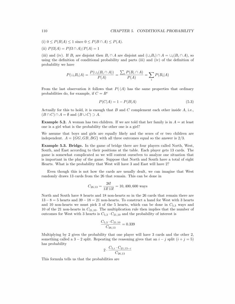
110 CHAPTER 5. CONDITIONAL PROBABILITY
(i) 0 ≤ P (B|A) ≤ 1 since 0 ≤ P (B ∩A) ≤ P (A).
(ii) P (Ω|A) = P (Ω ∩A)/P (A) = 1
(iii) and (iv). If Bi are disjoint then Bi ∩ A are disjoint and (∪iBi) ∩ A = ∪i(Bi ∩ A), sousing the definition of conditional probability and parts (iii) and (iv) of the definition ofprobability we have
P (∪iBi|A) =P (∪i(Bi ∩A))
P (A)=
∑i P (Bi ∩A)
P (A)=∑i
P (Bi|A)
From the last observation it follows that P (·|A) has the same properties that ordinaryprobabilities do, for example, if C = Bc
P (C|A) = 1− P (B|A) (5.3)
Actually for this to hold, it is enough that B and C complement each other inside A, i.e.,(B ∩ C) ∩A = ∅ and (B ∪ C) ⊃ A.
Example 5.2. A woman has two children. If we are told that her family is in A = at leastone is a girl what is the probability the other one is a girl?
We assume that boys and girls are equally likely and the sexes of er two children areindependent. A = GG,GB,BG with all three outcomes equal so the answer is 2/3.
Example 5.3. Bridge. In the game of bridge there are four players called North, West,South, and East according to their positions at the table. Each player gets 13 cards. Thegame is somewhat complicated so we will content ourselves to analyze one situation thatis important in the play of the game. Suppose that North and South have a total of eightHearts. What is the probability that West will have 3 and East will have 2?
Even though this is not how the cards are usually dealt, we can imagine that Westrandomly draws 13 cards from the 26 that remain. This can be done in
C26,13 =26!
13! 13!= 10, 400, 600 ways
North and South have 8 hearts and 18 non-hearts so in the 26 cards that remain there are13− 8 = 5 hearts and 39− 18 = 21 non-hearts. To construct a hand for West with 3 heartsand 10 non-hearts we must pick 3 of the 5 hearts, which can be done in C5,3 ways and10 of the 21 non-hearts in C21,10. The multiplication rule then implies that the number ofoutcomes for West with 3 hearts is C5,3 · C21,10 and the probability of interest is
C5,3 · C21,10
C26,13= 0.339
Multiplying by 2 gives the probability that one player will have 3 cards and the other 2,something called a 3− 2 split. Repeating the reasoning gives that an i− j split (i+ j = 5)has probability
2 · C5,i · C21,13−i
C26,13
This formula tells us that the probabilities are

5.1. THE MULTIPLICATION RULE 111
3-2 0.6784-1 0.2825-0 0.039
Thus while a 3-2 split is the most common, one should not ignore the possibility of a 4-1split.
Exercise Show that if North and South have 9 hearts then the probabilities are
2-2 0.4063-1 0.4974-0 0.095
In this case the uneven 3-1 split is more common than the 2-2 split since it can occur twoways, i.e., West might have 3 or 1.
Example 5.4. A person picks 13 cards out of a deck of 52. Let A1 = “he has at leastone Ace,” H = “he has the Ace of hearts,” and E1 = “he receives exactly one Ace.” FindP (E1|A1) and P (E1|H). Do you think these will be equal? If not then which one is larger?
Let E0 = “he has no Ace.”
p0 = P (E0) =C48,13
C52,13p1 = P (E1) =
4C48,12
C52,13
Since E1 ⊂ A1 and A1 = Ec0,
P (E1|A1) =P (E1)
P (A1)=
p1
1− p0
Since E1 ∩H means you get the Ace of Hearts and no other ace
P (E1|H) =P (E1 ∩H)
P (H)=C48,12/C52,13
1/4= p1
To compare the probabilities we observe
P (E1|A1) =p1
1− p0> p1 = P (E1|H)
Letting A2 = “he has at least two Aces and using (5.3) we have
P (A2|A1) < P (A2|H)
Intuitively, the event H is harder to achieve than A1 so conditioning on it increases ourchance of having other aces.
Conditional probabilities are the sources of many “paradoxes” in probability. One ofthese attracted worldwide attention in 1990 when Marilyn vos Savant discussed it in herweekly column in the Sunday Parade magazine.
Example 5.5. The Monty Hall problem. The problem is named for the host of thetelevision show Let’s Make A Deal in which contestants were often placed in situations likethe following: Three curtains are numbered 1, 2, and 3. Behind one curtain is a car; behindthe other two curtains are donkeys. You pick a curtain, say #1. To build some suspensethe host opens up one of the two remaining curtains, say #3, to reveal a donkey. What isthe probability you will win given that there is a donkey behind #3? Should you switchcurtains and pick #2 if you are given the chance?
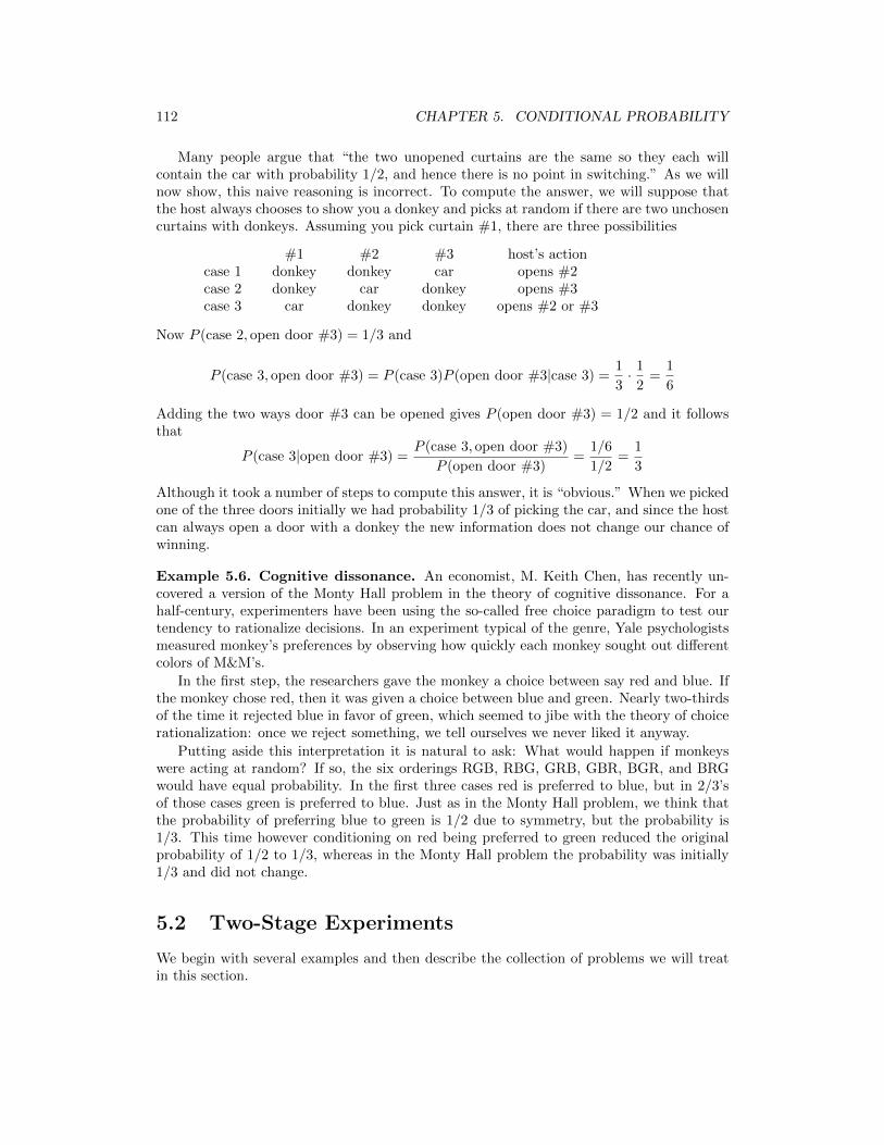
112 CHAPTER 5. CONDITIONAL PROBABILITY
Many people argue that “the two unopened curtains are the same so they each willcontain the car with probability 1/2, and hence there is no point in switching.” As we willnow show, this naive reasoning is incorrect. To compute the answer, we will suppose thatthe host always chooses to show you a donkey and picks at random if there are two unchosencurtains with donkeys. Assuming you pick curtain #1, there are three possibilities
#1 #2 #3 host’s actioncase 1 donkey donkey car opens #2case 2 donkey car donkey opens #3case 3 car donkey donkey opens #2 or #3
Now P (case 2, open door #3) = 1/3 and
P (case 3, open door #3) = P (case 3)P (open door #3|case 3) =1
3· 1
2=
1
6
Adding the two ways door #3 can be opened gives P (open door #3) = 1/2 and it followsthat
P (case 3|open door #3) =P (case 3, open door #3)
P (open door #3)=
1/6
1/2=
1
3
Although it took a number of steps to compute this answer, it is “obvious.” When we pickedone of the three doors initially we had probability 1/3 of picking the car, and since the hostcan always open a door with a donkey the new information does not change our chance ofwinning.
Example 5.6. Cognitive dissonance. An economist, M. Keith Chen, has recently un-covered a version of the Monty Hall problem in the theory of cognitive dissonance. For ahalf-century, experimenters have been using the so-called free choice paradigm to test ourtendency to rationalize decisions. In an experiment typical of the genre, Yale psychologistsmeasured monkey’s preferences by observing how quickly each monkey sought out differentcolors of M&M’s.
In the first step, the researchers gave the monkey a choice between say red and blue. Ifthe monkey chose red, then it was given a choice between blue and green. Nearly two-thirdsof the time it rejected blue in favor of green, which seemed to jibe with the theory of choicerationalization: once we reject something, we tell ourselves we never liked it anyway.
Putting aside this interpretation it is natural to ask: What would happen if monkeyswere acting at random? If so, the six orderings RGB, RBG, GRB, GBR, BGR, and BRGwould have equal probability. In the first three cases red is preferred to blue, but in 2/3’sof those cases green is preferred to blue. Just as in the Monty Hall problem, we think thatthe probability of preferring blue to green is 1/2 due to symmetry, but the probability is1/3. This time however conditioning on red being preferred to green reduced the originalprobability of 1/2 to 1/3, whereas in the Monty Hall problem the probability was initially1/3 and did not change.
5.2 Two-Stage Experiments
We begin with several examples and then describe the collection of problems we will treatin this section.

5.2. TWO-STAGE EXPERIMENTS 113
Example 5.7. The Duke basketball team is playing in a four team tournament. In the firstround they have any easy opponent that they will beat 80% of the time but if they win thatgame they will play against a tougher team where their probability of success is 0.4. Whatis the probability that they will win the tournament?
0.8
0.2
0.4
0.6
Win
Lose
HHHH
HHHH
XXXXXXXX
Win-win 0.32
Win-lose 0.48
If A and B are the events of victory in the first and second games then P (A) = 0.8 andP (B|A) = 0.4, so the probability that they will win the tournament is
P (A ∩B) = P (A)P (B|A) = 0.8(0.4) = 0.32
Example 5.8. An urn contains 5 red and 10 black balls. We draw two balls from the urnwithout replacement. What is the probability that the second ball drawn is red?
This is easy to see if we draw a picture. The first split in the tree is based on the outcomeof the first draw and the second on the outcome of the final. The outcome of the first drawdictates the probabilities for the second one. We multiply the probabilities on the edges toget probabilities of the four endpoints, and then sum the ones that correspond to Red toget the answer: 4/42 + 10/42 = 1/3.
1/3
2/3
4/14
10/14
5/14
9/14
red
black
HHHHHH
HH
XXXXXXXX
XXXXXXXX
red 4/42
black 10/42
red 10/42
black 18/42
To do this with formulas, let Ri be the event of a red ball on the ith draw and let B1 bethe event of a black ball on the first draw. Breaking things down according to the outcome

114 CHAPTER 5. CONDITIONAL PROBABILITY
of the first draw, then using the multiplication rule, we have
P (R2) = P (R2 ∩R1) + P (R2 ∩B1)
= P (R2|R1)P (R1) + P (R2|B1)P (B1)
= (1/3)(4/14) + (2/3)(5/14) = 14/42 = 1/3
From this we see that P (R2|R1) < P (R1) < P (R2|B1) but the two probabilities average togive P (R1). This calculation makes the result look like a miracle but it is not. If we numberthe 15 balls in the urn, then by symmetry each of them is equally likely to be the secondball chosen. Thus the probability of a red on the second, eighth, or fifteenth draw is alwaysthe same.
Example 5.9. Based on past experience, 70% of students in a certain course pass themidterm exam. The final exam is passed by 80% of those who passed the midterm, but onlyby 40% of those who fail the midterm. What fraction of students pass the final?
Drawing a tree as before with the first split based on the outcome of the midterm andthe second on the outcome of the final, we get the answer: 0.56 + 0.12 = 0.68
0.7
0.3
0.8
0.2
0.4
0.6
Midterm
Pass
Fail
Final
Pass 0.56
Fail 0.14
Pass 0.12
Fail 0.18
HHHHHH
HH
XXXXXXXX
XXXXXXXX
To do this with formulas, let A be the event that the student passes the final and let Bbe the event that the student passes the midterm. Breaking things down according to theoutcome of the first test, then using the multiplication rule, we have
P (A) = P (A ∩B) + P (A ∩Bc)
= P (A|B)P (B) + P (A|Bc)P (Bc)
= (0.8)(0.7) + (0.4)(0.3) = 0.68
Example 5.10. Al flips 3 coins and Betty flips 2. Al wins if the number of Heads he getsis more than the number Betty gets. What is the probability Al will win?
Let W be the event that Al wins. We will break things down according to the numberof heads Betty gets. Let Bi be the event that Betty gets i Heads, and let Aj be the eventthat Al gets j Heads. By considering the four outcomes of flipping two coins it is easy tosee that
P (B0) = 1/4 P (B1) = 1/2 P (B2) = 1/4
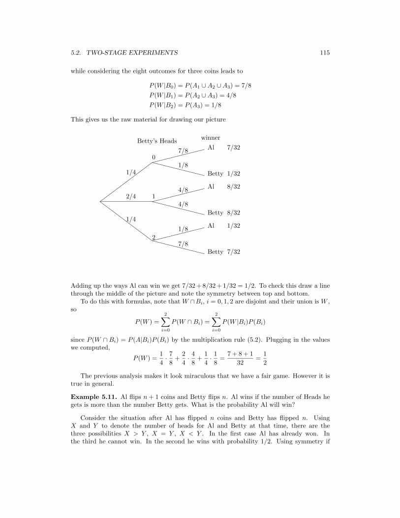
5.2. TWO-STAGE EXPERIMENTS 115
while considering the eight outcomes for three coins leads to
P (W |B0) = P (A1 ∪A2 ∪A3) = 7/8
P (W |B1) = P (A2 ∪A3) = 4/8
P (W |B2) = P (A3) = 1/8
This gives us the raw material for drawing our picture
ZZZZZZZZ
XXXXXXXX
XXXXXXXX
XXXXXXXX
1/4
2/4
1/4
07/8
1/8
14/8
4/8
2
1/8
7/8
Betty’s Heads
Betty
Al
Betty
Al
Betty
Al
winner
7/32
1/32
8/32
8/32
1/32
7/32
Adding up the ways Al can win we get 7/32 + 8/32 + 1/32 = 1/2. To check this draw a linethrough the middle of the picture and note the symmetry between top and bottom.
To do this with formulas, note that W ∩Bi, i = 0, 1, 2 are disjoint and their union is W ,so
P (W ) =
2∑i=0
P (W ∩Bi) =
2∑i=0
P (W |Bi)P (Bi)
since P (W ∩ Bi) = P (A|Bi)P (Bi) by the multiplication rule (5.2). Plugging in the valueswe computed,
P (W ) =1
4· 7
8+
2
4· 4
8+
1
4· 1
8=
7 + 8 + 1
32=
1
2
The previous analysis makes it look miraculous that we have a fair game. However it istrue in general.
Example 5.11. Al flips n + 1 coins and Betty flips n. Al wins if the number of Heads hegets is more than the number Betty gets. What is the probability Al will win?
Consider the situation after Al has flipped n coins and Betty has flipped n. UsingX and Y to denote the number of heads for Al and Betty at that time, there are thethree possibilities X > Y , X = Y , X < Y . In the first case Al has already won. Inthe third he cannot win. In the second he wins with probability 1/2. Using symmetry if

116 CHAPTER 5. CONDITIONAL PROBABILITY
P (X > Y ) = P (X < Y ) = p then P (X = Y ) = 1 − 2p, so the probability Al wins isp+ (1− 2p)/2 = 1/2.
Abstracting the structure of the last problem, let B1, . . . , Bk be a partition, that is, acollection of disjoint events whose union is Ω.
CCCCCCCC
B1 B2 B3 B4
B5
``````````````````````A
Using the fact that the sets A ∩Bi are disjoint, and the multiplication rule, we have
P (A) =
k∑i=1
P (A ∩Bi) =
k∑i=1
P (A|Bi)P (Bi) (5.4)
a formula that is sometimes called the law of total probability.The name of this section comes from the fact that we think of our experiment as occurring
in two stages. The first stage determines which of the B’s occur, and when Bi occurs in thefirst stage, A occurs with probability P (A|Bi) in the second. As the next example shows,the two stages are sometimes clearly visible in the problem itself.
Example 5.12. Roll a die and then flip that number of coins. What is the probability ofA = “we get exactly 3 Heads”?
Let Bi = “the die shows i.” P (Bi) = 1/6 for i = 1, 2, . . . , 6 and
P (A|B1) = 0 P (A|B2) = 0 P (A|B3) = 2−3
P (A|B4) = C4,3 2−4 P (A|B5) = C5,3 2−5 P (A|B6) = C6,3 2−6
So plugging into (5.4),
P (A) =1
6
1
8+
4
16+
10
32+
20
64
=
1
6
8 + 16 + 20 + 20
64
=
1
6
Example 5.13. Craps. In this game, if the sum of the two dice is 2, 3, or 12 on his firstroll, the player loses; if the sum is 7 or 11, he wins; if the sum is 4, 5, 6, 8, 9, or 10, thisnumber becomes his “point” and he wins if he “makes his point,” i.e., his number comes upagain before he throws a 7. What is the probability the player wins?
The first step in analyzing craps is to compute the probability that the player makeshis point. Suppose his point is 5 and let Ek be the event that the sum is k. There are 4

5.2. TWO-STAGE EXPERIMENTS 117
outcomes in E5 ((1, 4), (2, 3), (3, 2), (4, 1)), 6 in E7, and hence 26 not in E5 ∪ E7. Letting× stand for “the sum is not 5 or 7,” we see that
P (5) =4
36P (× 5) =
26
36· 4
36P (×× 5) =
(26
36
)24
36
From the first three terms it is easy to see that for k ≥ 0
P (× on k rolls then 5) =
(26
36
)k4
36
Summing over the possibilities, which represent disjoint ways of rolling 5 before 7, we have
P (5 before 7) =
∞∑k=0
(26
36
)k4
36=
4
36· 1
1− 2636
since∞∑k=0
xk =1
1− x(5.5)
Simplifying, we have P (5 before 7) = (4/36)/(10/36) = 4/10. Such a simple answershould have a simple explanation, and it does. Consider an urn with four balls marked5, six marked 7, and twenty-six marked with x. Drawing with replacement until we draweither a 5 or 7 is the same as drawing once from an urn with 10 balls with four balls marked5 and six marked 7.
5 5 5 5 x x x x x x x x
7 7 7 7 7 7 x x x x x x
x x x x x x x x x x x x
Another way of saying this is that if we ignore the outcomes that result in a sum other than5 or 7, we reduce the sample space from Ω to E = E5 ∪E7 and the distribution of the firstoutcome that lands in E follows the conditional probability P (·|E). Since E5 ∩ E = E5 wehave
P (E5|E) =P (E5)
P (E)=
4/36
10/36=
4
10
The last argument generalizes easily to give the probabilities of making any point:
k 4 5 6 8 9 10|Ek| 3 4 5 5 4 3P(k before 7) 3/9 4/10 5/11 5/11 4/10 3/9
To compute the probability of A = “he wins,” we let Bk = “the first roll is k,” and observethat (5.4) implies
P (A) =12∑k=2
P (A ∩Bk) =12∑k=2
P (Bk)P (A|Bk)

118 CHAPTER 5. CONDITIONAL PROBABILITY
When k = 2, 3, or 12 comes up on the first roll we lose, so
P (A|Bk) = 0 and P (A ∩Bk) = 0
When k = 7 or 11 comes up on the first roll we win, so
P (A|Bk) = 1 and P (A ∩Bk) = P (Bk)
When the first roll is k = 4, 5, 6, 8, 9, or 10, P (A|Bk) = P (k before 7) and P (A ∩Bk) is
3
36· 3
9k = 4, 10
4
36· 4
10k = 5, 9
5
36· 5
11k = 6, 8
Adding up the terms in the sum in the order in which they were computed,
P (A) =6
36+
2
36+ 2
(1
36+
4 · 236 · 5
+5 · 5
36 · 11
)=
4
18+ 2
(55 + 88 + 125
36 · 11 · 5
)=
220 + 268
18 · 11 · 5=
488
990= 0.4929 (5.6)
which is not very much less than 1/2 = 495/990.
Example 5.14. Al and Bob take turns throwing one dart to try to hit a bullseye. Alhits with probability 1/4 while Bob hits with probability 1/3. If Al goes first what is theprobability he will hit the first bullseye?
Let p be the answer. By considering one cycle of the game we see
p = 1/4 + (3/4)(1/3)(0) + (3/4)(2/3)p
In words, Al wins if he hits the bullseye on the first try. If he misses and Al hits then heloses. If they both miss then it is Al’s turn and the game starts over, so Al’s probability ofsuccess is p. Solving the equation we have p/2 = 1/4 or p = 1/2.
Back to craps. This reasoning in the last example can be used to compute the probabilityq that a player rolls a 5 before 7. By considering the outcome of the first roll q = 4/36 +(6/36)0 + (26/36)q and solving we have q = 4/10.
5.3 Bayes’ Formula
The title of the section is a little misleading since we will regard Bayes’ formula as a methodfor computing conditional probabilities and will only reluctantly give the formula after wehave done several examples to illustrate the method.
Example 5.15. Exit polls. In the California gubernatorial election in 1982, several TVstations predicted, on the basis of questioning people when they exited the polling place,that Tom Bradley, then mayor of Los Angeles, would win the election. When the votes werecounted, however, he lost to George Deukmejian by a considerable margin. What causedthe exit polls to be wrong?

5.3. BAYES’ FORMULA 119
To give our explanation we need some notation and some numbers. Suppose we choosea person at random, let B = “the person votes for Bradley” and suppose that P (B) = 0.45.There were only two candidates, so this makes the probability of voting for DeukmejianP (Bc) = 0.55. Let A = “the voter stops and answers a question about how they voted” andsuppose that P (A|B) = 0.4, P (A|Bc) = 0.3. That is, 40% of Bradley voters will respondcompared to 30% of the Deukmejian voters. We are interested in computing P (B|A) = thefraction of voters in our sample that voted for Bradley. By the definition of conditionalprobability (5.1),
P (B|A) =P (B ∩A)
P (A)=
P (B ∩A)
P (B ∩A) + P (Bc ∩A)
To evaluate the two probabilities, we use the multiplication rule (5.2)
P (B ∩A) = P (B)P (A|B) = 0.45 · 0.4 = 0.18
P (Bc ∩A) = P (Bc)P (A|Bc) = 0.55 · 0.3 = 0.165
From this it follows that
P (B|A) =0.18
0.18 + 0.165= 0.5217
and from our sample it looks as if Bradley will win. The problem with the exit poll is thatthe difference in the response rates makes our sample not representative of the populationas a whole.
Turning to the mechanics of the computation, note that 18% of the voters are for Bradleyand respond, while 16.5% are for Deukmejian and respond, so the fraction of Bradley votersin our sample is 18/(18 + 16.5). In words, there are two ways an outcome can be in A –it can be in B or in Bc – and the conditional probability is the fraction of the total thatcomes from the first way.
.18 .165
B Bc
.4.3
.45 .55
Example 5.16. Mammogram posterior probabilities. Approximately 1% of womenaged 40-50 have breast cancer. A woman with breast cancer has a 90% chance of a positivetest from a mammogram, while a woman without has a 10% chance of a false positive result.What is the probability a woman has breast cancer given that she just had a positive test?
Let B = “the woman has breast cancer” and A = “a positive test.” We want to calculateP (B|A). Computing as in the previous example,
P (B|A) =P (B ∩A)
P (A)=
P (B ∩A)
P (B ∩A) + P (Bc ∩A)

120 CHAPTER 5. CONDITIONAL PROBABILITY
To evaluate the two probabilities, we use the multiplication rule (5.2)
P (B ∩A) = P (B)P (A|B) = 0.01 · 0.9 = 0.009
P (Bc ∩A) = P (Bc)P (A|Bc) = 0.99 · 0.1 = 0.099
From this it follows that
P (B|A) =0.009
0.009 + 0.099=
9
108
or a little less than 9%. This situation comes about because it is much easier to have apositive results from a false positive for a healthy woman which has probability 0.099, thanfrom a woman with breast cancer having a positive test, which has probability 0.009.
This answer is somewhat surprising. Indeed, when ninety-five physicians were asked thisquestion “What is the probability a woman has breast cancer given that she just had apositive test?” their average answer was 75%. The two statisticians who carried out thissurvey indicated that physicians were better able to see the answer when the data waspresented in frequency format. 10 out of 1000 women have breast cancer. Of these 9 willhave a positive mammogram. However, of the remaining 990 women without breast cancer99 will have a positive test, and again we arrive at the answer 9/(9 + 99).
Example 5.17. Hemophilia. Ellen has a brother with hemophilia, but two parents who donot have the disease. Since hemophilia is caused by a recessive allele h on the X chromosome,we can infer that her mother is a carrier (that is, the mother has the hemophilia allele h onone of her X chromosomes and the healthy allele H on the other), while her father has thehealthy allele on his one X chromosome. Since Ellen received one X chromosome from herfather and one from her mother, there is a 50% chance that she is a carrier, and if so, thereis a 50% chance that her sons will have the disease. If she has two sons without the disease,what is the probability she is a carrier?
Ellen X?X0
X1Xh Mother
XhY Brother
Father X0Y
Let B be the event that she is a carrier and A be the event that she has two healthysons. Computing as in the two previous examples,
P (B|A) =P (B ∩A)
P (A)=
P (B ∩A)
P (B ∩A) + P (Bc ∩A)
To evaluate the two probabilities we use the multiplication rule (5.2). Since the probabilityof having two healthy sons when she is a carrier is 1/4, and is 1 when she is not.
P (B ∩A) = P (B)P (A|B) =1
2· 1
4=
1
8
P (Bc ∩A) = P (Bc)P (A|Bc) =1
2· 1 =
1
2

5.3. BAYES’ FORMULA 121
From this it follows that
P (B|A) =1/8
1/8 + 1/2=
1
5
Example 5.18. Three factories make 20%, 30%, and 50% of the computer chips for acompany. The probability of a defective chip is 0.04, 0.03, and 0.02 for the three factories.We have a defective chip. What is the probability it came from Factory 1?
Let Bi be the event that the chip came from factory i and let A be the event that the chip isdefective. We want to compute P (B3|A). Adapting the computation from the two previousexamples to the fact that there are now three Bi
P (B3|A) =P (B3 ∩A)
P (A)=
P (B3 ∩A)∑3i=1 P (Bi ∩A)
To evaluate the three probabilities, we use the multiplication rule (5.2)
P (B1 ∩A) = P (B1)P (A|B1) = 0.2 · (0.04) = 0.008
P (B2 ∩A) = P (B2)P (A|B2) = 0.3 · (0.03) = 0.009
P (B3 ∩A) = P (B3)P (A|B3) = 0.5 · (0.02) = 0.010
From this it follows that
P (B1|A) =P (B1 ∩A)
P (A)=
0.008
0.008 + 0.009 + 0.010=
8
27
The calculation can be summarized by the following picture. The conditional probabilityP (B3|A) is the fraction of the event A that lies in B3.
.04.03
.02
B1 B2 B3
0.2 0.3 0.5
.008 .009 .010A
We are now ready to generalize from our examples and state Bayes formula. In eachcase, we have a partition of the probability space B1, . . . , Bn, i.e., a sequence of disjointsets with ∪ni=1Bi = Ω. (In the first three examples, B1 = B and B2 = Bc.) We are givenP (Bi) and P (A|Bi) for 1 ≤ i ≤ n and we want to compute P (B1|A). Reasoning as in theprevious examples,
P (B1|A) =P (B1 ∩A)
P (A)=
P (B1 ∩A)∑i P (Bi ∩A)

122 CHAPTER 5. CONDITIONAL PROBABILITY
To evaluate the probabilities, we observe that
P (Bi ∩A) = P (Bi)P (A|Bi)
From this, it follows that
P (B1|A) =P (B1 ∩A)
P (A)=
P (B1)P (A|B1)∑ni=1 P (Bi)P (A|Bi)
(5.7)
This is Bayes formula. Even though we have numbered it, we advise you not to memorizeit. It is much better to remember the procedures we followed to compute the conditionalprobability.
5.4 Exercises
Conditional probability
1. There are two urns. Urn A has 4 red and 6 white balls, urn B has 7 red and 3 whiteballs. We pick an urn at random and pick a ball from it. Given that the ball is red what isthe probability we picked from urn A. What is the answer if we pick two balls and they areboth red?
2. An urn contains 8 red, 7 blue, and 5 green balls. You draw out two balls and they aredifferent colors. Given this, what is the probability the two balls were red and blue?
3. Two people, whom we call South and North, draw 13 cards out of a deck of 52. Southhas two Aces. What is the probability that North has (a) none? (b) one? (c) the othertwo?
4. Suppose that the number of children in a family has the following distribution
number of children 0 1 2 3 4probability 0.15 0.25 0.3 0.2 0.1
Assume that each child is independently a girl or a boy with probability 1/2 each. If afamily is picked at random what is the chance it has exactly two girls.
5. A student is taking a multiple-choice test in which each question has four possible answers.She knows the answers to 50% of the questions, can narrow the choices down to two 30% ofthe time, and does not know anything about 20% of the questions. What is the probabilityshe will correctly answer a question chosen at random from the test?
6. Plumber Bob does 40% of the plumbing jobs in a small town. 30% of the people in townare unhappy with their plumbers but 50% of Bob’s customers are unhappy with his work.If your neighbor is not happy with his plumber, what is the probability it was Bob?
7. Suppose that the probability a married man votes is 0.45, the probability a marriedwoman votes is 0.4, and the probability a woman votes given that her husband does is 0.6.What is the probability (a) both vote, (b) a man votes given that his wife does?
8. Suppose 60% of the people in a town will get exposed to flu in the next month. If you areexposed and not inoculated then the probability of your getting the flu is 80%, but if youare inoculated that probability drops to 15%. Of two executives at Beta Company, one is

5.4. EXERCISES 123
inoculated and one is not. What is the probability at least one will not get the flu? Assumethat the events that determine whether or not they get the flu are independent.
9. An ectopic preganancy is twice as likely if a woman smokes cigarettes. If 25% of womenof childbearing age are smokers, what fraction of ectopic preganancies occur to smokers?
10. Brown eyes are dominant over blue. That is, there are two alleles B and b. bb individualshave blue eyes but other combinations has brown eyes. Your parents and you have browneyes but your brother has blue. So you can infer that both of your parents are heterozy-gotes, i.e., have genetic type Bb. Given this information what is the probability you are ahomozygote.
Two-stage Experiments
11. From a signpost that says MIAMI two letters fall off. A friendly drunk puts the twoletters back into the two empty slots at random. What is the probability that the sign stillsays MIAMI?
12. Two balls are drawn from an urn with balls numbered from 1 up to 10. What is theprobability that the two numbers will differ by at least three. (≥ 3) than three?
13. You and a friend each roll two dice. What is the probability you will both have thesame two numbers?
14. Charlie draws five cards out of a deck of 52. If he gets at least three of one suit, hediscards the cards not of that suit and then draws until he again has five cards. For example,if he gets three hearts, one club, and one spade, he throws the two nonhearts away and drawstwo more. What is the probability he will end up with five cards of the same suit?
15. John takes the bus with probability 0.3 and the subway with probability 0.7. He is late40% of the time when he takes the bus but only 20% of the time when he takes the subway.What is the probability he is late for work?
16. The population of Cyprus is 70% Greek and 30% Turkish. 20% of the Greeks and 10%of the Turks speak English. What fraction of the people of Cyprus speak English?
17. You are going to meet a friend at the airport. Your experience tells you that the planeis late 70% of the time when it rains, but is late only 20% of the time when it does not rain.The weather forecast that morning calls for a 40% chance of rain. What is the probabilitythe plane will be late?
18. Two boys have identical piggy banks. The older boy has 18 quarters and 12 dimes inhis; the younger boy, 2 quarters and 8 dimes. One day the two banks get mixed up. Youpick up a bank at random and shake it until a coin comes out. What is the probability youget a quarter? Note that there are 20 quarters and 20 dimes in all.
19. Two boys, Charlie and Doug, take turns rolling two dice with Charlie going first. IfCharlie rolls a 6 before Doug rolls a 7 he wins. What is the probability Charlie wins?
20. Three boys take turns shooting a basketball and have probabilities 0.2, 0.3, and 0.5 ofscoring a basket. Compute the probabilities for each boy to get the first basket.
21. Change the second and third probabilities in the last problem so that each boy has anequal chance of winning.

124 CHAPTER 5. CONDITIONAL PROBABILITY
22. In the town of Carboro 90% of students graduate high school, 60% of high school grad-uates complete college, and 20% of college graduates get graduate or professional degrees.What fraction of students get advanced degrees?
23. What is the probability of a flush, i.e., all cards of the same suit when we draw 5 cardsout of a deck of 52?
Bayes’ Formula
24. Three bags lie on the table. One has two gold coins, one has two silver coins, and onehas one silver and one gold. You pick a bag at random, and pick out one coin. If this coinis gold, what is the probability you picked from the bag with two gold coins?
25. 1 out of 1000 births results in fraternal twins; 1 out of 1500 births results in identicaltwins. Identical twins must be the same sex but the sexes of fraternal twins are independent.If two girls are twins, what is the probability they are fraternal twins?
26. Five pennies are sitting on a table. One is a trick coin that has Heads on both sides, butthe other four are normal. You pick up a penny at random and flip it four times, gettingHeads each time. Given this, what is the probability you picked up the two-headed penny?
27. 5% of men and 0.25% of women are color blind. Assuming that there are an equalnumber of men and women, what is the probability a color blind person is a man?
28. The alpha fetal protein test is meant to detect spina bifida in unborn babies, a conditionthat affects 1 out of 1000 children who are born. The literature on the test indicates that5% of the time a healthy baby will cause a positive reaction. We will assume that the test ispositive 100% of the time when spina bifida is present. Your doctor has just told you thatyour alpha fetal protein test was positive. What is the probability that your baby has spinabifida?
29. Binary digits, i.e., 0’s and 1’s, are sent down a noisy communications channel. Theyare received as sent with probability 0.9 but errors occur with probability 0.1. Assumingthat 0’s and 1’s are equally likely, what is the probability that a 1 was sent given that wereceived a 1?
30. To improve the reliability of the channel described in the last example, we repeat eachdigit in the message three times. What is the probability that 111 was sent given that (a)we received 101? (b) we received 000?
31. A student goes to class on a snowy day with probability 0.4, but on a nonsnowy dayattends with probability 0.7. Suppose that 20% of the days in February are snowy. What isthe probability it snowed on February 7th given that the student was in class on that day?
32. A company gave a test to 100 salesman, 80 with good sales records and 20 with poorsales records. 60% of the good salesman passed the test but only 30% of the poor salesmendid. Andy passed the test. Given this, what is the probability that he is a good salesman?
33. A company rates 80% of its employees as satisfactory and 20% as unsatisfactory. Per-sonnel records indicate that 70% of the satisfactory workers had prior experience but only40% of the unsatisfactory workers did. If a person with previous work experience is hired,what is the probability they will be a satisfactory worker?
34. A golfer hits his drive in the fairway with probability 0.7. When he hits his drive inthe fairway he makes par 80% of the time. When he doesn’t he makes par only 30% of thetime. He just made par on a hole. What is the probability he hit his drive in the fairway?
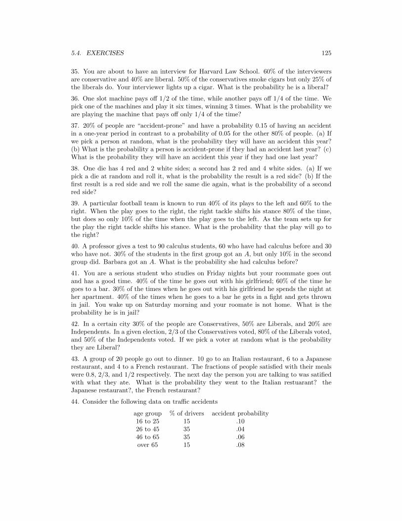
5.4. EXERCISES 125
35. You are about to have an interview for Harvard Law School. 60% of the interviewersare conservative and 40% are liberal. 50% of the conservatives smoke cigars but only 25% ofthe liberals do. Your interviewer lights up a cigar. What is the probability he is a liberal?
36. One slot machine pays off 1/2 of the time, while another pays off 1/4 of the time. Wepick one of the machines and play it six times, winning 3 times. What is the probability weare playing the machine that pays off only 1/4 of the time?
37. 20% of people are “accident-prone” and have a probability 0.15 of having an accidentin a one-year period in contrast to a probability of 0.05 for the other 80% of people. (a) Ifwe pick a person at random, what is the probability they will have an accident this year?(b) What is the probability a person is accident-prone if they had an accident last year? (c)What is the probability they will have an accident this year if they had one last year?
38. One die has 4 red and 2 white sides; a second has 2 red and 4 white sides. (a) If wepick a die at random and roll it, what is the probability the result is a red side? (b) If thefirst result is a red side and we roll the same die again, what is the probability of a secondred side?
39. A particular football team is known to run 40% of its plays to the left and 60% to theright. When the play goes to the right, the right tackle shifts his stance 80% of the time,but does so only 10% of the time when the play goes to the left. As the team sets up forthe play the right tackle shifts his stance. What is the probability that the play will go tothe right?
40. A professor gives a test to 90 calculus students, 60 who have had calculus before and 30who have not. 30% of the students in the first group got an A, but only 10% in the secondgroup did. Barbara got an A. What is the probability she had calculus before?
41. You are a serious student who studies on Friday nights but your roommate goes outand has a good time. 40% of the time he goes out with his girlfriend; 60% of the time hegoes to a bar. 30% of the times when he goes out with his girlfriend he spends the night ather apartment. 40% of the times when he goes to a bar he gets in a fight and gets thrownin jail. You wake up on Saturday morning and your roomate is not home. What is theprobability he is in jail?
42. In a certain city 30% of the people are Conservatives, 50% are Liberals, and 20% areIndependents. In a given election, 2/3 of the Conservatives voted, 80% of the Liberals voted,and 50% of the Independents voted. If we pick a voter at random what is the probabilitythey are Liberal?
43. A group of 20 people go out to dinner. 10 go to an Italian restaurant, 6 to a Japaneserestaurant, and 4 to a French restaurant. The fractions of people satisfied with their mealswere 0.8, 2/3, and 1/2 respectively. The next day the person you are talking to was satifiedwith what they ate. What is the probability they went to the Italian restuarant? theJapanese restaurant?, the French restaurant?
44. Consider the following data on traffic accidents
age group % of drivers accident probability16 to 25 15 .1026 to 45 35 .0446 to 65 35 .06over 65 15 .08

126 CHAPTER 5. CONDITIONAL PROBABILITY
Calculate (a) the probability a randomly chosen driver will have an accident this year, and(b) the probability a driver is between 46 and 65 given that they had an accident.

Chapter 6
Markov Chains
6.1 Definitions and Examples
The importance of Markov chains comes from two facts: (i) there are a large number ofphysical, biological, economic, and social phenomena that can be described in this way, and(ii) there is a well-developed theory that allows us to understand their behavior. We beginwith a famous example, then describe the property that is the defining feature of Markovchains. Throughout this chapter we will only consider Markov chains with a finite statespace.
Example 6.1. Gambler’s ruin. Consider a gambling game in which on any turn you win$1 with probability p = 0.4 or lose $1 with probability 1−p = 0.6. Suppose further that youadopt the rule that you quit playing if your fortune reaches $N . Of course, if your fortunereaches $0 the casino makes you stop.
Let Xn be the amount of money you have after n plays. I claim that your fortune, Xn
has the “Markov property.” In words, this means that given the current state, any otherinformation about the past is irrelevant for predicting the next state Xn+1. To check this,we note that if you are still playing at time n, i.e., your fortune Xn = i with 0 < i < N ,then for any possible history of your wealth in−1, in−2, . . . i1, i0
P (Xn+1 = i+ 1|Xn = i,Xn−1 = in−1, . . . X0 = i0) = 0.4
since to increase your wealth by one unit you have to win your next bet and the outcomeof the previous bets has no useful information for predicting the next outcome.
Turning now to the formal definition, we say that Xn is a discrete time Markov chainwith transition matrix p(i, j) if for any j, i, in−1, . . . i0
P (Xn+1 = j|Xn = i,Xn−1 = in−1, . . . , X0 = i0) = p(i, j) (6.1)
Equation (6.1), also called the “Markov property” says that the conditional probabilityXn+1 = j given the entire history Xn = i,Xn−1 = in−1, . . . X1 = i1, X0 = i0 is the same asthe conditional probability Xn+1 = j given only the previous state Xn = i.
In formulating (6.1) we have restricted our attention to the temporally homogeneouscase in which the transition probability
p(i, j) = P (Xn+1 = j|Xn = i)
127

128 CHAPTER 6. MARKOV CHAINS
does not depend on the time n. Intuitively, the transition probability gives the rules of thegame. It is the basic information needed to describe a Markov chain. In the case of thegambler’s ruin chain, the transition probability has
p(i, i+ 1) = 0.4, p(i, i− 1) = 0.6, if 0 < i < N
p(0, 0) = 1 p(N,N) = 1
When N = 5 the matrix is
0 1 2 3 4 5
0 1.0 0 0 0 0 01 0.6 0 0.4 0 0 02 0 0.6 0 0.4 0 03 0 0 0.6 0 0.4 04 0 0 0 0.6 0 0.45 0 0 0 0 0 1.0
but picture is perhaps more informative:
0 1 2 3 4 5
-- - -
.6 .6 .6 .6
.4 .4 .4 .4
→1
←1
Example 6.2. Ehrenfest chain. We imagine two cubical volumes of air connected by asmall hole. In the mathematical version, we have two urns in which there are a total of Nballs. At time n we pick one of the N balls at random and move it to the other urn tocreate the state at time n+ 1.
Let Xn be the number of balls in the left urn at time n. It should be clear that Xn has theMarkov property; i.e., if we want to guess the state at time n+ 1, then the current numberof balls in the left urn Xn, is the only relevant information from the observed sequence ofstates Xn, Xn−1, . . . X1, X0. To check this we note that
P (Xn+1 = i+ 1|Xn = i,Xn−1 = in−1, . . . X0 = i0) =N − iN

6.1. DEFINITIONS AND EXAMPLES 129
since to increase the number we have to pick one of the N − i balls in the other urn. Thenumber can also decrease by 1 with probability i/N . Thus the transition probability is givenby
p(i, i+ 1) =N − iN
, p(i, i− 1) =i
Nfor 0 ≤ i ≤ N
with p(i, j) = 0 otherwise. When N = 5, for example, the matrix is
0 1 2 3 4 5
0 0 5/5 0 0 0 01 1/5 0 4/5 0 0 02 0 2/5 0 3/5 0 03 0 0 3/5 0 2/5 04 0 0 0 4/5 0 1/55 0 0 0 0 5/5 0
Here we have written 1 as 5/5 to emphasize the pattern in the diagonals of the matrix.
Example 6.3. Wright–Fisher model. We consider a fixed population of N genes thatcan be one of two types: A or a. These types are called alleles. In the simplest version ofthis model the population at time n+ 1 is obtained by drawing with replacement from thepopulation at time n. In this case if we let Xn be the number of A alleles at time n, thenXn is a Markov chain with transition probability
p(i, j) =
(N
j
)(i
N
)j (1− i
N
)N−j0 ≤ i, j ≤ N
since the right-hand side is the binomial distribution for N independent trials with successprobability i/N . Note that when i = 0, p(0, 0) = 1, and when i = N , p(N,N) = 1.
time n time n+ 1
A
a
A
A
A
a
A
a
A
a
A
A
A
a
a
A
A
a
a
A
In the Gambler’s Ruin chain and the Wright-Fisher model the states 0 and N are ab-sorbing states. Once we enter these states we can never leave. The long run behavior ofthese models is not very interesting, they will eventually enter one of the absorbing statesand stay there forever. To make the Wright-Fisher model more interesting and more real-istic, we can introduce the possibility of mutations: an A that is drawn ends up being an ain the next generation with probability u, while an a that is drawn ends up being an A inthe next generation with probability v. In this case the probability an A is produced by agiven draw is
ρi =i
N(1− u) +
N − iN
v

130 CHAPTER 6. MARKOV CHAINS
i.e., we can get an A by drawing an A and not having a mutation or by drawing an a andhaving a mutation. Since the draws are independent the transition probability still has thebinomial form
p(i, j) =
(N
j
)(ρi)
j(1− ρi)N−j (6.2)
Example 6.4. Two-stage Markov chains. In a Markov chain the distribution of Xn+1
only depends on Xn. This can easily be generalized to case in which the distribution ofXn+1 only depends on (Xn, Xn−1). For a concrete example consider a basketball playerwho makes a shot with the following probabilities:
1/2 if he has missed the last two times
2/3 if he has hit one of his last two shots
3/4 if he has hit both of his last two shots
To formulate a Markov chain to model his shooting, we let the states of the process be theoutcomes of his last two shots: HH,HM,MH,MM where M is short for miss and H forhit. Noting that the first letter is Xn and the second is Xn−1 the transition probability is
HH HM MH MMHH 3/4 0 1/4 0HM 2/3 0 1/3 0MH 0 2/3 0 1/3MM 0 1/2 0 1/2
To explain suppose the state is HM , i.e., Xn = H and Xn−1 = M . In this case thenext outcome will be H with probability 2/3. When this occurs the next state will be(Xn+1, Xn) = (H,H). If he misses, an event of probability 1/3, (Xn+1, Xn) = (M,H). Tocheck the placement of 0’s note that since the first letter gets shifted to the right, if the firstletter is H then after a jump the second letter will be H.
The Hot Hand is a phenomenon known to everyone who plays or watches basketball.After making a couple of shots, players are thought to “get into a groove” so that subsequentsuccesses are more likely. Purvis Short of the Golden State Warriors describes this morepoetically as “You’re in a world all your own. It’s hard to describe. But the basket seemsto be so wide. No matter what you do, you know the ball is going to go in.”
Unfortunately for basketball players, data collected by Tversky and Gliovich (Chancevol. 2 (1989), No. 1, pages 16–21) shows that this is a misconception. The next table givesdata for the conditional probability of hitting a shot after missing the last three, missing thelast two, . . . hitting the last three, for nine players of the Philadelphia 76ers: Darryl Dawkins(403), Maurice Cheeks (339), Steve Mix (351), Bobby Jones (433), Clint Richardson (248),Julius Erving (884), Andrew Toney (451), Caldwell Jones (272), and Lionel Hollins (419).The numbers in parentheses are the number of shots for each player.

6.1. DEFINITIONS AND EXAMPLES 131
P (H|3M) P (H|2M) P (H|1M) P (H|1H) P (H|2H) P (H|3H).88 .73 .71 .57 .58 .51.77 .60 .60 .55 .54 .59.70 .56 .52 .51 .48 .36.61 .58 .58 .53 .47 .53.52 .51 .51 .53 .52 .48.50 .47 .56 .49 .50 .48.50 .48 .47 .45 .43 .27.52 .53 .51 .43 .40 .34.50 .49 .46 .46 .46 .32
In fact, the data supports the opposite assertion: after missing a player is more likely to hita shot
The first four example are meant to motivate the study. We will now introduce somesimple numerical examples that will be useful as we develop the theory. Markov chains aredescribed by giving their transition probabilities. To create a chain, we can write down anyn× n matrix, provided that the entries satisfy:
(i) p(i, j) ≥ 0, since they are probabilities.
(ii)∑j p(i, j) = 1, since when Xn = i, Xn+1 will be in some state j.
The equation in (ii) is read “sum p(i, j) over all possible values of j.” In words the last twoconditions say: the entries of the matrix are nonnegative and each row of the matrix sumsto 1.
Any matrix with properties (i) and (ii) gives rise to a Markov chain, Xn. To constructthe chain we can think of playing a board game. When we are in state i, we roll a die (orgenerate a random number on a computer) to pick the next state, going to j with probabilityp(i, j). To illustrate this we will now introduce some simple examples.
Example 6.5. Weather chain. Let Xn be the weather on day n, which we assume iseither: 1 = rainy, or 2 = sunny. Even though the weather is not exactly a Markov chain, wecan propose a Markov chain model for the weather by writing down a transition probability
1 21 .6 .42 .2 .8
The table says, for example, the probability a rainy day (state 1) is followed by a sunny day(state 2) is p(1, 2) = 0.4.
Example 6.6. Social mobility. Let Xn be a family’s social class in the nth generation,which we assume is either 1 = lower, 2 = middle, or 3 = upper. In our simple version ofsociology, changes of status are a Markov chain with the following transition probability
1 2 31 .7 .2 .12 .3 .5 .23 .2 .4 .4
Example 6.7. Brand preference. Suppose there are three types of laundry detergent,1, 2, and 3, and let Xn be the brand chosen on the nth purchase. Customers who try these
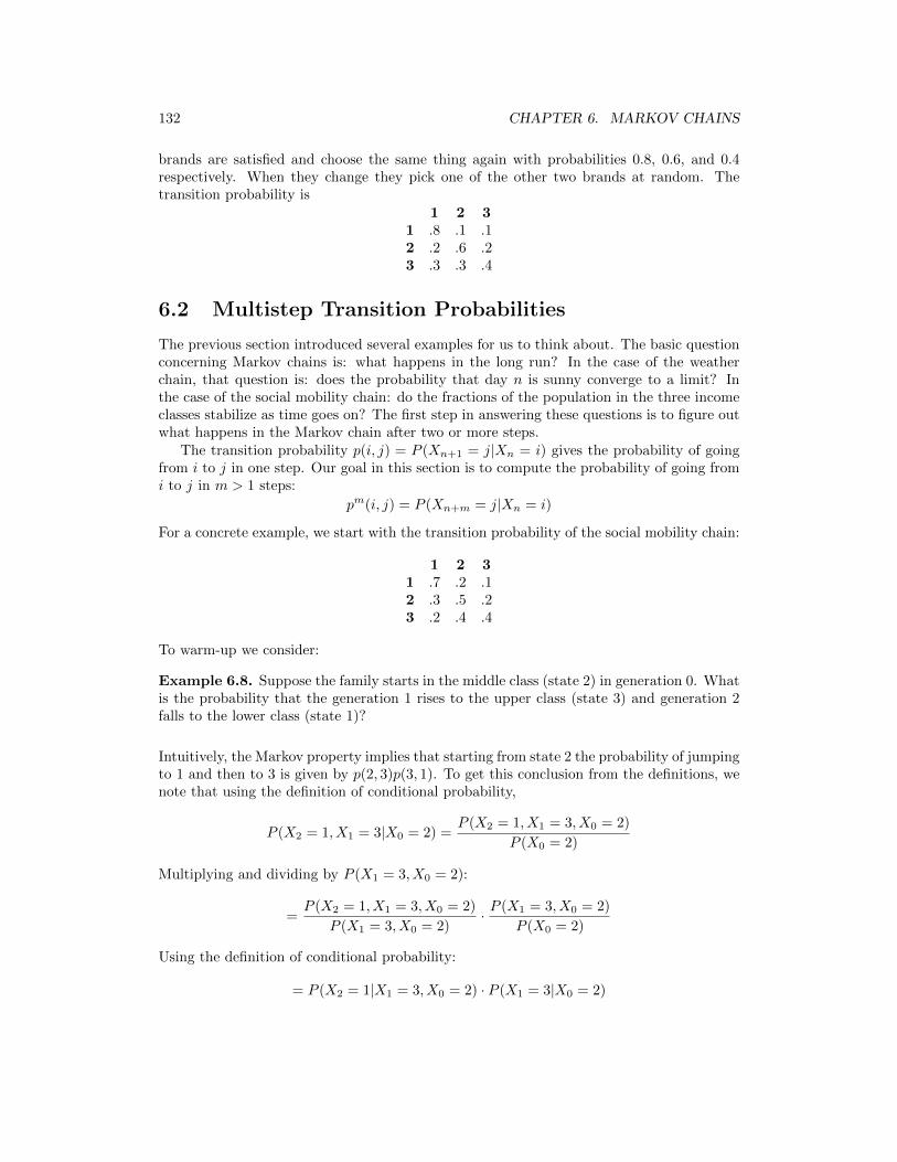
132 CHAPTER 6. MARKOV CHAINS
brands are satisfied and choose the same thing again with probabilities 0.8, 0.6, and 0.4respectively. When they change they pick one of the other two brands at random. Thetransition probability is
1 2 31 .8 .1 .12 .2 .6 .23 .3 .3 .4
6.2 Multistep Transition Probabilities
The previous section introduced several examples for us to think about. The basic questionconcerning Markov chains is: what happens in the long run? In the case of the weatherchain, that question is: does the probability that day n is sunny converge to a limit? Inthe case of the social mobility chain: do the fractions of the population in the three incomeclasses stabilize as time goes on? The first step in answering these questions is to figure outwhat happens in the Markov chain after two or more steps.
The transition probability p(i, j) = P (Xn+1 = j|Xn = i) gives the probability of goingfrom i to j in one step. Our goal in this section is to compute the probability of going fromi to j in m > 1 steps:
pm(i, j) = P (Xn+m = j|Xn = i)
For a concrete example, we start with the transition probability of the social mobility chain:
1 2 31 .7 .2 .12 .3 .5 .23 .2 .4 .4
To warm-up we consider:
Example 6.8. Suppose the family starts in the middle class (state 2) in generation 0. Whatis the probability that the generation 1 rises to the upper class (state 3) and generation 2falls to the lower class (state 1)?
Intuitively, the Markov property implies that starting from state 2 the probability of jumpingto 1 and then to 3 is given by p(2, 3)p(3, 1). To get this conclusion from the definitions, wenote that using the definition of conditional probability,
P (X2 = 1, X1 = 3|X0 = 2) =P (X2 = 1, X1 = 3, X0 = 2)
P (X0 = 2)
Multiplying and dividing by P (X1 = 3, X0 = 2):
=P (X2 = 1, X1 = 3, X0 = 2)
P (X1 = 3, X0 = 2)· P (X1 = 3, X0 = 2)
P (X0 = 2)
Using the definition of conditional probability:
= P (X2 = 1|X1 = 3, X0 = 2) · P (X1 = 3|X0 = 2)

6.2. MULTISTEP TRANSITION PROBABILITIES 133
By the Markov property (6.1) the last expression is
P (X2 = 1|X1 = 3) · P (X1 = 3|X0 = 2) = p(2, 3)p(3, 1)
Moving on to the real question:
Example 6.9. Suppose the family starts in the middle class (state 2) in generation 0. Whatis the probability that generation 2 will be in the lower class (state 1)?
To do this we simply have to consider the three possible states for generation 1 and use theprevious computation.
P (X2 = 1|X0 = 2) =
3∑k=1
P (X2 = 1, X1 = k|X0 = 2) =
3∑k=1
p(2, k)p(k, 1)
= (.3)(.7) + (.5)(.3) + (.2)(.2) = .21 + .15 + .04 = .40
There is nothing special here about the states 2 and 1 here. By the same reasoning,
P (X2 = j|X0 = i) =
3∑k=1
p(i, k) p(k, j)
The right-hand side of the last equation gives the (i, j)th entry of the matrix p is multipliedby itself.
To explain this, we note that to compute p2(2, 1) we multiplied the entries of the secondrow by those in the first column: . . .
.3 .5 .2. . .
.7 . ..3 . ..2 . .
=
. . ..40 . .. . .
If we wanted p2(1, 3) we would multiply the first row by the third column:.7 .2 .1
. . .
. . .
. . .1. . .2. . .4
=
. . .15. . .. . .
When all of the computations are done we have.7 .2 .1
.3 .5 .2
.2 .4 .4
.7 .2 .1.3 .5 .2.2 .4 .4
=
.57 .28 .15.40 .39 .21.34 .40 .26
The two step transition probability p2 = p · p. Based on this you can probably leap to
the next conclusion:
Theorem 6.1. The m-step transition probability
pm(i, j) = P (Xn+m = j|Xn = i) (6.3)
is the mth power of the transition matrix p, i.e., p · p · · · p, where there are m terms in theproduct.

134 CHAPTER 6. MARKOV CHAINS
The key ingredient in proving this is the:
Chapman–Kolmogorov equation
pm+n(i, j) =∑k
pm(i, k) pn(k, j) (6.4)
Once this is proved, (6.3) follows, since taking n = 1 in (6.4), we see that pm+1 = pm · p.
Why is (6.4) true? To go from i to j in m+ n steps, we have to go from i to some statek in m steps and then from k to j in n steps. The Markov property implies that the twoparts of our journey are independent.
••••
••••
••••
```````aaaaaaaa
aaaaaaaa
```````
i
j
time 0 m m+ n
Proof of (6.4). The independence in the second sentence of the previous explanation is themysterious part. To show this, we combine Examples 6.8 and 6.9. Breaking things downaccording to the state at time m,
P (Xm+n = j|X0 = i) =∑k
P (Xm+n = j,Xm = k|X0 = i)
Repeating the computation in Example 6.8, the definition of conditional probability implies:
P (Xm+n = j,Xm = k|X0 = i) =P (Xm+n = j,Xm = k,X0 = i)
P (X0 = i)
Multiplying and dividing by P (Xm = k,X0 = i) gives:
=P (Xm+n = j,Xm = k,X0 = i)
P (Xm = k,X0 = i)· P (Xm = k,X0 = i)
P (X0 = i)
Using the definition of conditional probability we have:
= P (Xm+n = j|Xm = k,X0 = i) · P (Xm = k|X0 = i)
By the Markov property (6.1) the last expression is
= P (Xm+n = j|Xm = k) · P (Xm = k|X0 = i) = pm(i, k)pn(k, j)
and we have proved (6.4).
Having established (6.4), we now return to computations. We begin with the weatherchain
p2 =
(.6 .4.2 .8
)(.6 .4.2 .8
)=
(.44 .56.28 .72
)

6.3. STATIONARY DISTRIBUTIONS 135
Multiplying again
p3 = p2 · p(.44 .56.28 .72
)(.6 .4.2 .8
)=
(.376 .624.312 .688
)Taking higher powers
p10 =
(.333403 .666597.333298 .666702
)p20 =
(.3333333407 .6666666597.3333333297 .6666666703
)Based on the last calculation, one might guess that as n gets large the matrix becomes closerand closer to (
1/3 2/31/3 2/3
)This is true and will be explained in the next section.
6.3 Stationary Distributions
Our first step is to consider
What happens when the initial state is random?
Breaking things down according to the value of the initial state and using the definition ofconditional probability
P (Xn = j) =∑i
P (X0 = i,Xn = j)
=∑i
P (X0 = i)P (Xn = j|X0 = i)
If we introduce q(i) = P (X0 = i), then the last equation can be written as
P (Xn = j) =∑i
q(i)pn(i, j) (6.5)
In words, we multiply the transition matrix on the left by the vector q of initial probabilities.If there are k states, then pn(x, y) is a k × k matrix. So to make the matrix multiplicationwork out right, we should take q as a 1× k matrix or a “row vector.”
For a concrete example consider the weather chain (Example 6.5) and suppose that theinitial distribution is q(1) = 0.3 and q(2) = 0.7. In this case
(.3 .7
)(.6 .4.2 .8
)=(.32 .68
)since
.3(.6) + .7(.2) = .32
.3(.4) + .7(.8) = .68

136 CHAPTER 6. MARKOV CHAINS
For a second example consider the social mobility chain (Example 6.6) and suppose thatthe initial distribution: q(1) = .5, q(2) = .2, and q(3) = .3. Multiplying the vector q by thetransition probability gives the vector of probabilities at time 1.
(.5 .2 .3
).7 .2 .1.3 .5 .2.2 .4 .4
=(.47 .32 .21
)To check the arithmetic note that the three entries on the right-hand side are
.5(.7) + .2(.3) + .3(.2) = .47
.5(.2) + .2(.5) + .3(.4) = .32
.5(.1) + .2(.2) + .3(.4) = .21
If the distribution at time 0 is the same as the distribution at time 1, then by theMarkov property it will be the distribution at all times n ≥ 1. Because of this q is called astationary distribution. Stationary distributions have a special importance in the theoryof Markov chains, so we will use a special letter π to denote solutions of the equation
π · p = π.
with πi ≥ 0 and∑j πj = 1.
To have a mental picture of what happens to the distribution of probability when onestep of the Markov chain is taken, it is useful to think that we have q(i) pounds of sand atstate i, with the total amount of sand
∑i q(i) being one pound. When a step is taken in
the Markov chain, a fraction p(i, j) of the sand at i is moved to j. The distribution of sandwhen this has been done is
q · p =∑i
q(i)p(i, j)
If the distribution of sand is not changed by this procedure q is a stationary distribution.
Example 6.10. General two state transition probability.
1 21 1− a a2 b 1− b
We have written the chain in this way so the stationary distribution has a simple formula
π(1) =b
a+ bπ(2) =
a
a+ b(6.6)
As a first check on this formula we note that in the weather chain a = 0.4 and b = 0.2which gives (1/3, 2/3) as we found before. We can prove this works in general by drawinga picture:
•1b
a+ b•2 a
a+ b
a−→←−b

6.3. STATIONARY DISTRIBUTIONS 137
In words, the amount of sand that flows from 1 to 2 is the same as the amount that flowsfrom 2 to 1 so the amount of sand at each site stays constant. To check algebraically thatthis is true:
b
a+ b(1− a) +
a
a+ bb =
b− ba+ ab
a+ b=
b
a+ bb
a+ ba+
a
a+ b(1− b) =
ba+ a− aba+ b
=a
a+ b(6.7)
Formula (6.6) gives the stationary distribution for any two state chain, so we progressnow to the three state case and consider the brand preference chain (Example 6.7). Theequation πp = π says
(π1 π2 π3
).8 .1 .1.2 .6 .2.3 .3 .4
=(π1 π2 π3
)which translates into three equations
.8π1 + .2π2 + .3π3 = π1
.1π1 + .6π2 + .3π3 = π2
.1π1 + .2π2 + .4π3 = π3
Note that the columns of the matrix give the numbers in the rows of the equations. Thethird equation is redundant since if we add up the three equations we get
π1 + π2 + π3 = π1 + π2 + π3
If we replace the third equation by π1 + π2 + π3 = 1 and subtract π1 from each side of thefirst equation and π2 from each side of the second equation we get
−.2π1 + .2π2 + .3π3 = 0
.1π1 − .4π2 + .3π3 = 0 (6.8)
π1 + π2 + π3 = 1
At this point we can solve the equations by hand or using a calcualtor.
By hand. We note that the third equation implies π3 = 1 − π1 − π2 and substitutingthis in the first two gives
.3 = .5π1 + .1π2
.3 = .2π1 + .7π2
Multiplying the first equation by .7 and adding −.1 times the second gives
1.8 = (0.35− 0.02)π1 or π1 = 18/33 = 6/11
Multiplying the first equation by .2 and adding −.5 times the second gives
−0.09 = (0.02− 0.35)π2 or π2 = 9/33 = 3/11
Since the three probabilities add up to 1, π3 = 2/11.

138 CHAPTER 6. MARKOV CHAINS
Using the TI83 calculator is easier. To begin we write (6.8) in matrix form as
(π1 π2 π3
)−.2 .1 1.2 −.4 1.3 .3 1
=(0 0 1
)If we let A be the 3 × 3 matrix in the middle this can be written as πA = (0, 0, 1). Tosolve the equation we use the inverse matrix A−1 which is the unique matrix which hasAA−1 = I, where I is the identity matrix that has 1’s on the diagonal and 0’s otherwise.Multiplying on each side by A−1 we see that
π = (0, 0, 1)A−1
which is the third row of A−1.We do not need to know linear algebra to do this because we can compute A−1 by using
our TI-83 calcular. We enter A into our calculator (using the MATRX menu and the EDITsubmenu. We then use the MATRX menu to put [A] on the computation line and thenpress the x−1 button. Reading the third row we find that the stationary distribution is
(0.545454, 0.272727, 0.181818)
Converting the answer to fractions using the first entry in the MATH menu gives
(6/11, 3/11, 2/11)
Example 6.11. Social Mobility (continuation of Example 6.6).
1 2 31 .7 .2 .12 .3 .5 .23 .2 .4 .4
Using the first two equations and the fact that the sum of the π’s is 1
.7π1 + .3π2 + .2π3 = π1
.2π1 + .5π2 + .4π3 = π2
π1 + π2 + π3 = 1
Taking the π’s from the right hand side to the left we have
−0.3π1 + .3π2 + .2π3 = 0
.2π1 +−0.5π2 + .4π3 = 0
π1 + π2 + π3 = 1
This translates into πA = (0, 0, 1) with
A =
−.3 .2 1.3 −.5 1.2 .4 1
Note that here and in the previous example, A can be obtained from p by

6.3. STATIONARY DISTRIBUTIONS 139
• Subtracting 1 from the diagonal
• then replacing the final column
The first step corresponds to moving π1 and π2 from the right-hand side to the left. Thesecond to replacing the third equation by π1 + π2 + π3 = 1.
Computing the inverse and reading the last row gives
(0.468085, 0.340425, 0.191489)
Converting the answer to fractions using the first entry in the math menu gives
(22/47, 16/47, 9/47)
Example 6.12. Ehrenfest chain (continuation of Example 6.2). Consider first thecase N = 5. As in the three previous examples, A consists of the first five columns of thetransition matrix with 1 subtracted from the diagonal, and a final column of all 1’s.
−1 1 0 0 0 1.2 −1 .8 0 0 10 .4 −1 .6 0 10 0 .6 −1 .4 10 0 0 .8 −1 10 0 0 0 1 1
The answer is given by the sixth row of A−1:
(0.03125, 0.15625, 0.3125, 0.3125, 0.15625, 0.03125)
Even without a calculator we can recognize these as
(1/32, 5/32, 10/32, 10/32, 5/32, 1/32)
the probabilities of 0 to 5 heads when we flip five coins.Based on this we can guess that in general
π(k) =
(N
k
)/2N
Proof by thinking. To determine the initial state, (a) flip N coins, with heads = in theleft urn, and tails = in the right. A transition of the chain corresponds to (b) picking acoin at random and turning it over. It is clear that the end result of (a) and (b) has all 2N
outcomes equally likely, so the state at time 1 is the same as the state at time 0.Proof by computation. For 0 < k < N we can end up in state k only by coming up fromk − 1 or down from k + 1 so
π(k − 1)p(k − 1, k) + π(k + 1)p(k + 1, k)
=
(Nk−1
)2N
· N − k + 1
N+
(Nk+1
)2N
· k + 1
N
=1
2N
((N − 1)!
(k − 1)!(N − k)!+
(N − 1)!
(k)!(N − k + 1)!
)=
1
2N
(N
k
)(k
N+N − kN
)= π(k)

140 CHAPTER 6. MARKOV CHAINS
The only way to end up at 0 is by coming down from 1 so
π(1)p(1, 0) =N
2N· 1
N= π(0)
Similarly, the only way to end up at N is by coming up from N − 1 so
π(N − 1)p(N − 1, N) =N
2N· 1
N= π(0)
Example 6.13. Basketball (continuation of Example 6.4). To find the stationarydistribution in this case we can follow the same procedure. A consists of the first threecolumns of the transition matrix with 1 subtracted from the diagonal, and a final columnof all 1’s.
−1/4 0 1/4 12/3 −1 1/3 10 2/3 −1 10 1/2 0 1
The answer is given by the fourth row of A−1:
(0.5, 0.1875, 0.1875, 0.125) = (1/2, 3/16, 3/16, 1/8)
Thus the long run fraction of time the player hits a shot is
π(HH) + π(MH) = 11/36 = 0.6875.
Notice that π(MH) = π(HM). To see why this is true look at the following simulation
HHMMM HMM HHHM HMM
In this string the state is HM four times and MH three times, since we switch from H toM four times and from M to H three times. In the long run the number of switches in tetwo directions will either be the same or differ by 1, so the limiting frequencies of HM andMH must be the same.
6.4 Limit Behavior
A stationary distribution is an equilibrium state. That is, if we start in that distribution westay in it for all time. In this section we will give conditions that guarantee that as n→∞
pn(i, j)→ π(j) as n→∞,
where π is a stationary distribution. This says that after a long time the probability ofbeing in state j is ≈ π(j) independent of the starting point. It turns out that this holds ifwe eliminate two problems. The first problem is illustrated by the following
Example 6.14. Reducible chain.
0 1 2 30 0.2 0.8 0 01 0.4 0.6 0 02 0 0 0.4 0.63 0 0 0.2 0.8

6.4. LIMIT BEHAVIOR 141
Using our formula for the stationary distribution of two state chains we see that (1/3, 2/3, 0, 0)is a stationary distribution and so is (0, 0, 1/4, 3/4). If we take the 10th power of the tran-sition matrix then to six decimal places the matrix is
0 1 2 30 1/3 2/3 0 01 1/3 2/3 0 02 0 0 1/4 3/43 0 0 1/4 3/4
The problem with this example is that is not really a four-state chain but two two-statechains in one matrix. To rule out examples like this, we need a condition.
Definition. A Markov chain is irreducible if for any x and y there is k so that pk(x, y) > 0.
In words for any states x and y it is possible to get from x to y. In the example above it isimpossible to get from 1 or 2 to 3 or 4, and vice versa. A nice consequence of irreducibilityis:
Theorem 6.2. If p is irreducible then there is a unique stationary distribution π(x) and wehave π(y) > 0 for all y.
Our next step is to consider the two state case.
Theorem 6.3. Let pn be the probability of being in state 1 after n steps. For a two stateMarkov chain with transition probability(
1− a ab 1− b
)we have ∣∣∣∣pn − b
a+ b
∣∣∣∣ =
∣∣∣∣p0 −b
a+ b
∣∣∣∣ · |1− a− b|n (6.9)
If 0 < a+ b < 2 this implies that pn → b/(a+ b) exponentially fast.
In the case of the weather chain |1− a− b| = 0.4, so the difference between pn and the limitb/(a+ b) goes to 0 faster than (0.4)n.
Proof. Using the Markov property we have for any n ≥ 1 that
pn = pn−1(1− a) + (1− pn−1)b
In words, the chain is in state 1 at time n if it was in state 1 at time n− 1 (with probabilitypn−1) and stays there (with probability 1 − a), or if it was in state 2 (with probability1−pn−1) and jumps from 2 to 1 (with probability b). Since the probability of being in state1 is constant when we start in the stationary distribution, see the first equation in (6.7):
b
a+ b=
b
a+ b(1− a) +
(1− b
a+ b
)b
Subtracting this equation from the one for pn we have
pn −b
a+ b=
(pn−1 −
b
a+ b
)(1− a) +
(b
a+ b− pn−1
)b
=
(pn−1 −
b
a+ b
)(1− a− b)

142 CHAPTER 6. MARKOV CHAINS
If 0 < a+ b < 2 then |1− a− b| < 1 and we have∣∣∣∣pn − b
a+ b
∣∣∣∣ =
∣∣∣∣pn−1 −b
a+ b
∣∣∣∣ · |1− a− b|Iterating the last equation gives the desired result.
There are two cases a = b = 0 and a = b = 1 in which |1− a− b| = 1 and hence pn(i, j)does not converge to π(i). In the first case the matrix is(
1 00 1
)so the state never changes. In this case the chain is not irreducible. In the second case thematrix is
p =
(0 11 0
)so the chain always jumps. In this case p2 = I, p3 = p, p4 = I, etc. To see that somethingsimilar can happen in a “real example,” we consider
Example 6.15. Ehrenfest chain. Consider the chain defined in Example 6.2 and forsimplicty, suppose there are three balls. In this case the transition probability is
0 1 2 30 0 3/3 0 01 1/3 0 2/3 02 0 2/3 0 1/33 0 0 3/3 0
In the second power of p the zero pattern is shifted:
0 1 2 30 1/3 0 2/3 01 0 7/9 0 2/92 2/9 0 7/9 03 0 2/3 0 1/3
To see that the zeros will persist, note that if initially we have an odd number of ballsin the left urn, then no matter whether we add or subtract one ball the result will be aneven number. Thus Xn alternates between being odd and even. To see why this preventsconvergence note that p2n+1(i, i) = 0, so we cannot have pm(i, i)→ π(i), which is positive.
The problem with the Ehrenfest chain is called periodicity. The definition of the periodof a state is a little complicated:
Definition. The period of a state i, d(i) is the greatest common divisor of Ii = n ≥ 1that have pn(i, i) > 0 is 1.
The next example explains why the definition is formulated in terms of the greatest commondivisor.

6.4. LIMIT BEHAVIOR 143
Example 6.16. Triangle and Square. The state space is −2,−1, 0, 1, 2, 3 and thetransition probability is
−2 −1 0 1 2 3−2 0 0 1 0 0 0−1 1 0 0 0 0 00 0 1/2 0 1/2 0 01 0 0 0 0 1 02 0 0 0 0 0 13 0 0 1 0 0 0
In words, from 0 we are equally likely to go to 1 or −1. From −1 we go with probabilityone to −2 and then back to 0, from 1 we go to 2 then to 3 and back to 0. The name refersto the fact that 0→ −1→ −2→ 0 is a triangle and 0→ 1→ 2→ 3→ 0 is a square.
-
?
?
6
-1 0 1
-2 3 2
1/2 1/2•
•
•
•
•
•
Noting that 3, 4 ∈ I0, we see that the period is 1. The next result shows that once wefind the period of one state we know the periods of all the states since
Lemma 6.1. If p is irreducible then all states have the same period.
If all states have period 1 then we call the chain aperiodic. From the last result we seethat
Lemma 6.2. If p is irreducible and p(x, x) > 0 then x has period 1, and hence by theprevious lemma all states have period 1.
With the key definitions made we can now state the
Convergence Theorem. If p is irreducible and aperiodic then there is a unique stationarydistribution π and for any i and j
pn(i, j)→ π(j) as n→∞ (6.10)
An easy, but important, special case is if p(i, j) > 0 for all i and j then the chain isirreducible and aperiodic. This shows that the convergence theorem applies to the Wright-Fisher model with mutation, weather chain, social mobility, and brand preference chainsthat are Examples 6.3, 6.5, 6.6, and 6.7. The Convergence Theorem does not apply tothe Gambler’s Ruin chain (Example 6.1) or the Wright-Fisher model with no mutationssince they have absorbing states and hence are not irreducible. We have already noted thatthe Ehrenfest chain (Example 6.2) does not converge since all states have period 2. Theremaining example from Section 7.1.

144 CHAPTER 6. MARKOV CHAINS
Example 6.17. Basketball chain.
HH HM MH MMHH 3/4 0 1/4 0HM 2/3 0 1/3 0MH 0 2/3 0 1/3MM 0 1/2 0 1/2
The second power of the matrix is
HH HM MH MMHH 9/16 1/6 3/16 1/12HM 1/2 2/9 1/6 1/9MH 4/5 1/6 2/9 1/6MM 1/3 1/4 1/6 1/4
so the chain is irreducible. To check aperiodicity we note that p(HH,HH) > 0 and useLemma 6.2.
Example 6.18. Period three. For another example that does not converge consider 4.Consider the following transition matrix:
1 2 3 4 5 61 0 0 1 0 0 02 1 0 0 0 0 03 0 .5 0 0 .5 04 0 .5 0 0 .5 0.5 0 0 0 0 0 16 0 0 0 1 0 0
(a) Find the stationary distribution. (b) Does the chain converge to it?
The stationary distribution is π = (1/6, 1/6, 1/6, 1/6, 1/6, 1/6) which is easily verifiedby checking that πp = π. If we draw a picture of the possible transitions of the chain wesee that if we are in 1, 6 at time 0 then we will be in 3, 4 at time 1, in 2, 5 at time 2,back in 1, 6 at time 3, etc., so all states have period three.
1
6
3
4
2
5
- -
- -
@@@R
@
@I
6.5 Chains with absorbing states
Recall that x is an absorbing state if if p(x, x) = 1. When a chain has one or more of thesestates, the asymptotic behavior is not interesting. It eventually gets stuck in one of them.The only two interesting questions are: where does it get stuck? how long does it take?

6.5. CHAINS WITH ABSORBING STATES 145
6.5.1 Exit distribution
We begin with a simple example.
Example 6.19. Two year college. At a local two year college, 60% of freshmen becomesophomores, 25% remain freshmen, and 15% drop out. 70% of sophomores graduate, 20%remain sophomores and 10% drop out. What fraction of new students eventually graduate?
We use a Markov chain with state space 1 = freshman, 2 = sophomore, G = graduate,D = dropout. The transition probability is
1 2 G D1 0.25 0.6 0 0.152 0 0.2 0.7 0.1G 0 0 1 0D 0 0 0 1
Let h(x) be the probability that a student currently in state x eventually graduates. Byconsidering what happens on one step
h(1) = 0.25h(1) + 0.6h(2)
h(2) = 0.2h(2) + 0.7
so h(2) = 0.7/0.8 = 0.875 andh(1) = 0.6
0.75h(2) = 0.7. To check these answers we will look at the sixth power powers ofthe transition probability
p6 =
1 2 G D1 0.000244 0.002161 0.697937 0.2838752 0 0.000064 0.874944 0.124492G 0 0 1 0D 0 0 0 1
Note that p6(1, D) ≈ 0.7 and p6(2, D) ≈ 0.875. The probability a student is still in collegeafter six years is only 0.000244 + 0.002161 = 2.405× 10⁻³.
Example 6.20. Tennis. In tennis the winner of a game is the first player to win fourpoints, unless the score is 4− 3, in which case the game must continue until one player winsby two points. Suppose that the game has reached the point where each player is tryingto get two points ahead to win and that the server will independently win the point withprobability 0.6. What is the probability the server will win the game if the score is tied? ifshe is ahead by one point? Behind by one point?
We formulate the game as a Markov chain in which the state is the difference of thescores. The state space is 2, 1, 0,−1,−2 with 2 (win for server) and −2 (win for opponent).The transition probability is
2 1 0 -1 -22 1 0 0 0 01 .6 0 .4 0 00 0 .6 0 .4 0-1 0 0 .6 0 .4-2 0 0 0 0 1

146 CHAPTER 6. MARKOV CHAINS
If we let h(x) be the probability of the server eventually winning when the score is x thenh(2) = 1, h(−2) = 0, and
h(1) = 0.6 + 0.4h(0)
h(0) = 0.6h(1) + 0.4h(−1)
h(−1) = 0.6h(0)
Rearranging we have
h(1)− 0.4h(0) + 0 · h(−1) = 0.6
−0.6h(1) + h(0)− 0.4h(−1) = 0
0 · h(1)− 0.6h(0) + h(−1) = 0
or in matrix form 1 −0.4 0−0.6 1 −0.4
0 −0.6 1
h(1)h(0)h(−1)
=
0.600
If we let r be the rows and columns of transition matrix corresponding to the non-absorbingstates 1, 0,−1, then the matrix on the left-hand side is (I − r) and the answer we want is h(1)
h(0)h(−1)
= (I − r)−1
0.600
To prepare for later appliications note that the column vector is p(i, 2), i.e., the probabilityof jumping to the absorbing state of interest. Inverting (I − r) we have:19/13 10/13 4/13
15/13 25/13 10/139/13 15/13 19/13
0.600
=
114/13090/13054/130
General solution. Suppose that the server wins each point with probability p. If the
game is tied then after two points, the server will have won with probability p2, lost withprobability (1 − p)2, and the game will have returned to being with probability 2p(1 − p),so h(0) = p2 + 2p(1− p)h(0). Since 1− 2p(1− p) = p2 + (1− p)2, solving gives
h(0) =p2
p2 + (1− p)2
Figure 6.1 gives the probability of winning a tied game as a function of the probability ofwinning a point.
Example 6.21. Two year college example, revisited. We will now solve the problemusing the machinery developed in the previous example. In this case
(I − r) =
(0.75 −0.6
0 0.8
)p(i, G) =
(0
0.7
)so the solution is(
h(1)h(2)
)= (I − r)−1
(0
0.7
)=
(4/3 10 5/4
)(0
0.7
)=
(0.77/8
)

6.5. CHAINS WITH ABSORBING STATES 147
0.5
0.6
0.7
0.8
0.9
1
0.5 0.6 0.7 0.8 0.9 1
Figure 6.1: Probability of winning in tennis as a function of the probability of winning apoint
Example 6.22. Wright-Fisher model. As described in Example 6.3, if we let Xn be thenumber of A alleles at time n, then Xn is a Markov chain with transition probability
p(x, y) =
(N
y
)( xN
)y (1− x
N
)N−y0 and N are absorbing states. What is the probability the chain ends up in N starting fromx?
As in the two previous examples if h(x) is the probability of getting absorbed in stateN when we start in state x then h(0) = 0, h(N) = 1, and for 0 < x < N
h(x) =∑y
p(x, y)h(y) (6.11)
In the Wright-Fisher model p(x, y) is the P (binomial(N, x/N) = y), so the expectednumber of A’s after the transition is x, i.e., the expected number of A’s remains constantin time. Taking a leap of faith we assert that the average number of A’s at the end is thesame as the number in the starting state. Since we will have N with probability h(y) and0 with probability 1− h(y) we must have
h(y) =y
N
Clearly, this function has h(0) = 0 and h(N) = 1. To check (6.11) we note that∑y
p(x, y)y
N=
x
N
since the mean of the binomial is x.The formula h(y) = y/N says that if we start with y A’s in the population then the
probability we will end with a population of all A’s (an event called “fixation” in genetics)is y/N , the fraction of the population that is A. The case y = 1 gives a famous result due toKimura. If we suppose that each individual experiences mutations at rate µ, then since thereare N individuals, new mutations occur at a total rate Nµ. Since each mutation achievesfixation with probability 1/N , the rate at which mutations become fixed is µ independentof the size of population.

148 CHAPTER 6. MARKOV CHAINS
6.5.2 Exit Times
Returning to our first two examples:
Example 6.23. Two year college. Consider the transition probability in Example 6.19.How many years on the average does it take for a freshman to graduate or dropout?
Let g(x) be the expected number of years to finish starting from x. g(G) = g(D) = 0.By considering what happens on the first step
g(1) = 1 + 0.25g(1) + 0.6g(2)
g(2) = 1 + 0.2g(2)
Here the 1 takes into account the one year that elapsed during the transition. We can solvethe equations to get
g(2) =1
0.8=
5
4g(1) =
1 + 0.6(5/4)
3/4=
7
3
so, on the average, a freshman takes 7/3 = 2.33 years to either graduate or drop out.A second approach is to rearrange our initial equation to get
0.75g(1)− 0.6g(2) = 1
0 · g(1) + 0.8g(2) = 1
The matrix on the left-hand side is the one we saw in Example 6.21, so the solution is(g(1)g(2)
)= (I − r)−1
(11
)Computing the inverse the answer is(
4/3 10 5/4
)(11
)=
(7/35/4
)To explain why this is the answer note that
(I − r)(I + r + r2 + · · · ) = (I + r + r2 + · · · )− (r + r2 + r3 + · · · ) = I
so we have (I − r)−1 = I + r + r2 + · · · . rn(i, j) is the probability of going from i to j in nsteps so we have the
Theorem 6.4. (I−r)−1(i, j) is the expected number of visits to j starting from i, includingthe visit at time 0 if j = i.
When we multiply (I − r)−1 by a column vector of all 1’s we add the entries in each row,and end up with the expected time in the state space for each starting point.
Example 6.24. Tennis. Consider the transition probability in Example 6.20. Supposethat game is tied. How many more points do we expect to see before the game ends?
Let g(x) be the expected number of points until the game ends when the score is x.Clearly, g(2) = g(−2) = 0. Writing equations as in the previous example
g(1) = 1 + 0.4g(0)
g(0) = 1 + 0.6g(1) + 0.4g(0)
g(−1) = 1 + 0.6g(0)

6.5. CHAINS WITH ABSORBING STATES 149
Rearranging we have
g(1)− 0.4g(0) + 0 · g(−1) = 1
−0.6g(1) + g(0)− 0.4g(−1) = 1
0 · g(1)− 0.6g(0) + g(−1) = 1
As in the previous example we can get to these equations by removing rows and columnsfor the absorbing states from the transition probability, to define
r =
0 .4 0.6 0 .40 .6 0
so that I − r =
1 −0.4 0−0.6 1 −0.4
0 −0.6 1
and the equaitons are (I − r)g = 1 where 1 is a column vector with three 1’s.
g = (I − r)−11 =
19/13 10/13 4/1315/13 25/13 10/139/13 15/13 19/13
111
=
33/1350/1343/13
so, on the average, a tied game requires 50/13 = 3.846 points to be completed.
General solution. To find the duration of a game starting from a tie. Divide the game intopairs of points. In each pair we will have a win by one player with probability p2 + (1− p)2
or return to a tie otherwise. Thus the number of pairs of points we need to decide the gameis 2 times a geometric with success probability p2 +(1−p)2 and the mean is 2/(p2 +(1−p)2).When p = 0.6 this is
2
0.36 + 0.16=
50
9 + 4
Example 6.25. Credit ratings. At the end of a month, a large retail store classifieseach of its customer’s accounts according to current (0), 30–60 days overdue (1), 60–90 daysoverdue (2), more than 90 days overdue (3). Their experience indicates that from onth tomonth the accounts move from state to state according to a Markov chain with transitionprobability matrix:
0 1 2 30 .9 .1 0 01 .8 0.2 02 .5 0 0 .53 .1 0 0 .9
(a) In the long run what fraction of the accounts are in each category? (b) If the customeris in state 1 what is the expected amount of time until they return to state 0?
(a) The stationary distribution is the last row of−.1 .1 0 1.8 −1 .2 1.5 0 −1 1.1 0 0 1
−1
which is π(0) = 100/122, π(1) = 10/122, π(2) = 2/122 and π(3) = 10/122.

150 CHAPTER 6. MARKOV CHAINS
If we let g(x) be the expected time to get to 0 starting from x and r be the 3 × 3matrix obtained by deleting the row and column for state 0, then as we have seen in thetwo previous examples (I − r)g = 1 where 1 is a column vector with three 1’s. In matrixform this is 1 −.2 0
0 1 −.50 0 .1
g(1)g(2)g(3)
=
111
Inverting the matrix I − r we haveg(0)
g(1)g(2)
=
1 .2 190 1 550 0 10
111
=
2.2610
To connect the two answers note that we stay in state 0 for a geometric(0.1) number of step,which has mean 10, and then it takes us an average of 2.2 units of time to return to 0, sothe fraction of time we spend in 0 in equilibrium is
10
10 + 2.2=
100
122
Example 6.26. Waiting time for coin patterns. Suppose we repeatedly flip a coinuntil we have gotten three tails in a row. What is the expected number of tosses we need?
To solve this question we define a Markov chain with states 0, 1, 2, and 3 correspondingto the number of consecutive tails we have at that point. The transition probablity is
0 1 2 30 1/2 1/2 0 01 1/2 0 1/2 02 1/2 0 0 1/23 0 0 0 1
As in the previous problems if g(x) is the expected number of tosses to get to 3 startingfrom x, and r is the 3× 3 matrix obtained by deleting the row and coumn for state 3 then(I − r)g = 1 where 1 is a column vector consisting for three 1’s. Inverting the matrix 1/2 −1/2 0
−1/2 1 −1/2−1/2 0 1
−1
=
8 4 26 4 24 2 2
so the waiting time is 8 + 4 + 2 = 14.
It is somewhat surprising that the answer is 14 rather than 8. The values of the lastthree flips (Xn−2, Xn−1, Xn) are an 8 state Markov chain in which each state has equilibriumprobability 1/8. The problem with TTT is that once we have one instance of TTT then wewill have another if the next coin is tails. Overlaps cannot happen for a pattern like TTHso as we will now show the expected waiting time is 8. Consider the Markov chain.
∅ T TT TTH∅ 1/2 1/2 0 0T 1/2 0 1/2 0
TT 0 0 1/2 1/2TTH 0 0 0 1

6.5. CHAINS WITH ABSORBING STATES 151
Inverting the matrix I − r gives 1/2 −1/2 0−1/2 1 −1/2−1/2 0 1/2
−1
=
4 2 22 2 20 0 2
so the waiting time is 8.
6.5.3 Gambler’s ruin*
Example 6.27. Consider a fair game in which you win a $1 with probability 1/2 or losea $1 with probability 1/2. In this case your fortune is a Markov chain Xn with transitionprobability p(x, x+ 1) = 1/2 and p(x, x−1) = 1/2. Find the probability h(x) that we reach$N before hitting $0 if we start with $x?
Clearly h(0) = 0 and h(N) = 1. By considering what happens on one step we see thatif 0 < x < N
h(x) = (1/2)h(x+ 1) + (1/2)h(x− 1)
Rearranging we see that
h(x+ 1)− h(x) = h(x)− h(x− 1)
or h is a line with constant slope. Since h(0) = 0 and h(N) = 1 that slope must be 1/N andh(x) = x/N . The final can be seen by using the reasoning we used for the Wright-Fishermodel. Since game is fair the average amount of money we have at the end is the same aswhat we have at the beginning so the probability of reaching N before 0 is x/N .
Example 6.28. Duration of fair games. Continuing to consider the fair game introducedin the last problem. Let τ = minn : Xn 6∈ (0, N) be the amount of time the game lasts.We claim that
Exτ = x(N − x) (6.12)
There are two ways to prove this.
Verify the guess. Let g(x) = x(N − x). Clearly, g(0) = g(N) = 0. If 0 < x < N then byconsidering what happens on the first step we have
g(x) = 1 +1
2g(x+ 1) +
1
2g(x− 1)
If g(x) = x(N − x) then the right-hand side is
= 1 +1
2(x+ 1)(N − x− 1) +
1
2(x− 1)(N − x+ 1)
= 1 +1
2[x(N − x)− x+N − x− 1] +
1
2[x(N − x) + x− (N − x+ 1)]
= 1 + x(N − x)− 1 = x(N − x)
Derive the answer. Again we begin with
g(x) = 1 + (1/2)g(x+ 1) + (1/2)g(x− 1)

152 CHAPTER 6. MARKOV CHAINS
Rearranging givesg(x+ 1)− g(x) = −2 + g(x)− g(x− 1).
Setting g(1)− g(0) = c we have g(2)− g(1) = c− 2, g(3)− g(2) = c− 4 and in general that
g(k)− g(k − 1) = c− 2(k − 1).
Using g(0) = 0 and summing we have
0 = g(N) =
N∑k=1
c− 2(k − 1) = cN − 2 · N(N − 1)
2
since, as one can easily check by induction,∑mj=1 j = m(m+1)/2. Solving gives c = (N−1).
Summing again, we see that
g(x) =
x∑k=1
(N − 1)− 2(k − 1) = x(N − 1)− x(x+ 1) = x(N − x)
Example 6.29. Unfair games. Now consider the sitautaion in which on any turn youwin $1 with probability p < 1/2 or lose $1 with probability 1− p. In this case your fortuneis a Markov chain Xn with transition probability p(x, x+ 1) = p and p(x, x− 1) = 1− p. Toanalyze this example it is convenient to introduce some notation. Tk = minn ≥ 0 : Xn = xis the time of the first visit to x. Using the new notation we want to compute
h(x) = Px(TN < T0)
be the probability that our gambler reaches the goal of $N before going bankrupt whenstarting with $x.
As in the case of a fair game, h(0) = 0 and h(1) = 1, and we consider what happens onthe first step to arrive at
h(x) = ph(x+ 1) + qh(x− 1) (6.13)
To solve this we rearrange to get p(h(x+ 1)− h(x)) = q(h(x)− h(x− 1)) and conclude
h(x+ 1)− h(x) =q
p· (h(x)− h(x− 1)) (6.14)
If we set c = h(1)− h(0) then (6.14) implies that for x ≥ 1
h(x)− h(x− 1) = c
(q
p
)x−1
Summing from x = 1 to N , we have
1 = h(N)− h(0) =
N∑x=1
h(x)− h(x− 1) = c
N∑x=1
(q
p
)x−1
Now for θ 6= 1 the partial sum of the geometric series is
N−1∑j=0
θj =1− θN
1− θ(6.15)

6.6. EXERCISES 153
To check this note that
(1− θ)(1 + θ + · · · θN−1) = (1 + θ + · · · θN−1)
− (θ + θ2 + · · · θN ) = 1− θN
Using (6.15) we see that c = (1 − θ)/(1 − θN ) with θ = q/p. Summing and using the factthat h(0) = 0, we have
h(x) = h(x)− h(0) = c
x−1∑i=0
θi = c · 1− θx
1− θ=
1− θx
1− θN
Recalling the definition of h(x) and rearranging the fraction we have
Px(TN < T0) =θx − 1
θN − 1where θ = 1−p
p (6.16)
To see what (6.16) says in a concrete example, we consider:
Example 6.30. Roulette. If we bet $1 on red on a roulette wheel with 18 red, 18 black,and 2 green (0 and 00) holes, we win $1 with probability 18/38 = 0.4737 and lose $1 withprobability 20/38. Suppose we bring $50 to the casino with the hope of reaching $100 beforegoing bankrupt. What is the probability we will succeed?
Here θ = q/p = 20/18, so (6.16) implies
P50(T100 < T0) =
(2018
)50 − 1(2018
)100 − 1
Using (20/18)50 = 194, we have
P50(T100 < T0) =194− 1
(194)2 − 1=
1
194 + 1= 0.005128
6.6 Exercises
Two state chains
1. Market research suggests that in a five year period 8% of people with cable televisionwill get rid of it, and 26% of those without it will sign up for it. Compare the predictionsof the Markov chain model with the following data on the fraction of people with cable TV:56.4% in 1990, 63.4% in 1995, and 68.0% in 2000.
2. A sociology professor postulates that in each decade 8% of women in the work force leaveit and 20% of the women not in it begin to work. Compare the predictions of his modelwith the following data on the percentage of women working: 43.3% in 1970, 51.5% in 1980,57.5% in 1990, and 59.8% in 2000.
3. A car rental company has rental offices at both Kennedy and LaGuardia airports. Assumethat a car rented at one airport must be returned to one of the two airports. If the carwas rented at LaGuardia the probability it will be returned there is 0.8; for Kennedy theprobability is 0.7. Suppose that we start with 1/2 of the cars at each airport and that each

154 CHAPTER 6. MARKOV CHAINS
week all of the cars are rented once. (a) What is the fraction of cars at LaGuardia ariportat the end of the first week? (b) at the end of the second? (c) in the long run?
4. The 1990 census showed that 36% of the households in the District of Columbia werehomeowners while the reaminder were renters. During the next decade 6% of the home-owners became renters and 12% of the renters became homeowners. (a) What percentagewere homeowners in 2000? in 2010? (b) If these trends continue what will be the long runfraction of homeowners?
5. A rapid transit system has just started operating. In the first month of operation, it wasfound that 25% of commuters are using the system while 75% are traveling by automobile.Suppose that each month 10% of transit users go back to using their cars, while 30%of automobile users switch to the transit system. (a) Compute the three step transitionprobability p3. (b) What will be the fractions using rapid transit in the fourth month? (c)In the long run?
6. A regional health study indicates that from one year to the next, 75% percent of smokerswill continue to smoke while 25% will quit. 8% of those who stopped smoking will resumesmoking while 92% will not. If 70% of the population were smokers in 1995, what fractionwill be smokers in 1998? in 2005? in the long run?
7. Census results reveal that in the United States 80% of the daughters of working womenwork and that 30% of the daughters of nonworking women work. In the long run whatfraction of women will be working?
8. Three of every four trucks on the road are followed by a car, while only one of every fivecars is followed by a truck. What fraction of vehicles on the road are trucks?
9. In a test paper the questions are arranged so that 3/4’s of the time a True answer isfollowed by a True, while 2/3’s of the time a False answer is followed by a False. You areconfronted with a 100 question test paper. Approximately what fraction of the answers willbe True?
10. When a basketball player makes a shot then he tries a harder shot the next time andhits (H) with probability 0.4, misses (M) with probability 0.6. When he misses he is moreconservative the next time and hits (H) with probability 0.7, misses (M) with probability0.3. Find the long-run fraction of time he hits a shot.
11. A university computer room has 30 terminals. Each day there is a 3% chance that agiven terminal will break and a 72% chance that a given broken terminal will be repaired.Assume that the fates of the various terminals are independent. In the long run what is thedistribution of the number of terminals that are broken.
Three or more states
12. Consider a gambler’s ruin chain with N = 4. That is, if 1 ≤ i ≤ 3, p(i, i + 1) = 0.4,and p(i, i − 1) = 0.6, but the endpoints are absorbing states: p(0, 0) = 1 and p(4, 4) = 1Compute p3(1, 4) and p3(1, 0).
13. A taxicab driver moves between the airport A and two hotels B and C according to thefollowing rules. If he is at the airport, he will go to one of the two hotels next with equalprobability. If at a hotel then he returns to the airport with probability 3/4 and goes to theother hotel with probability 1/4. (a) Find the transition matrix for the chain. (b) Suppose

6.6. EXERCISES 155
the driver begins at the airport at time 0. Find the probability for each of his three possiblelocations at time 2 and the probability he is at hotel B at time 3.
14. A person is flipping a coin repeatedly. Let Xn be the outcome of the two previous coinflips at time n, for example the state might be HT to indicate that the last flip was T andthe one before that was H. (a) compute the transition probability for the chain. (b) Findp2.
15. The town of Ithaca has a “free bikes for the people program.” You can pick up bikes atthe library (L), the coffee shop (C) or the cooperative grocery store (G) and drop them offat any of these locations. The movement of bikes can be modeled by a Markov chain
L C GL 0.5 0.1 .0.4C 0.3 0.5 0.2G 0.2 0.4 0.4
(a) What is the probability a bike from the library is at the three locations on Wednesday?(b) In the long run what fraction are at the three locations?
16. Bob eats lunch at the campus food court every week day. He either eats Chinese food,Quesadila, or Salad. His transition matrix is
C Q SC .15 .6 .25Q .4 .1 .5S .1 .3 .6
(a) He had Chinese food on Monday. What are the probabilities for his three meal choiceson Friday (four days later). (b) What are the lun run frequencies for his three meal choices.
17. A midwestern university has three types of health plans: a health maintenance organi-zation (HMO), a preferred provider organization (PPO), and a traditional fee for serviceplan (FFS). In 2000, the prcentages for the three plans were HMO:30%, PPO:25%, andFFS:45%. Experience dictates that people change plans according to the following transi-tion matrix
HMO PPO FFSHMO .85 .1 .05PPO .2 .7 .1FFS .1 .3 .6
(a) What will be the precentages for the three plans in 2001? (b) What is the long runfraction choosing each of the three plans?
18. A plant species has red, pink, or white flowers according to the genotypes RR, RW, andWW, respectively. If each of these genotypes is crossed with a pink (RW ) plant then theoffspring fractions are
RR RW WWRR .5 .5 0RW .25 .5 .25WW 0 .5 .5
What is the long run fraction of plants of the three types?

156 CHAPTER 6. MARKOV CHAINS
19. A sociologist studying living patterns in a certain region determines that the pattern ofmovement between urban (U), suburban (S), and rural areas (R) is given by the followingtransition matrix.
U S RU .86 .08 .06S .05 .88 .07R .03 .05 .92
In the long run what fraction of the population will live in the three areas?
20. In a large metropolitan area, commuters either drive alone (A), carpool (C), or takepublic transportation (T). The mode of transportation used changes from year to yearaccording to the transition probability
A C TA .8 .15 .05C .05 .9 .05S .05 .1 .85
In the long run what fraction of commuters will use the three types of transportation?
21. In a particular county voters declare themselves as members of the Republican, Demo-crat, or Green party. Voters change parties according to the transition probability:
R D GR .85 .15 0D .05 .85 .10G 0 .05 .95
In the long run what fraction of voters will belong to the three parties?
22. An auto insurance company classifies its customers in three categories: poor (P ),satisfactory (S) and excellent (E). Ratings change over time according to the followingtransition matrix
a..6 .4 0.1 .6 .30 .2 .8
What is the limiting fraction of drivers in each of these categories?
23. An individual has three umbrellas, some at her office, and some at home. If she isleaving home in the morning (or leaving work at night) and it is raining, she will take anumbrella, if one is there. Otherwise, she gets wet. Assume that independent of the past, itrains on each trip with probability 0.2. To formulate a Markov chain, let Xn be the numberof umbrellas at her current location. (a) Find the transition probability for this Markovchain. (b) Calculate the limiting fraction of time she gets wet.
24. At the beginning of each day, a piece of equipment is inspected to determine its workingcondition, which is classified as state 1 = new, 2, 3, or 4 = broken. We assume the state isa Markov chain with the following transition matrix:
1 2 3 41 .95 .05 0 02 0 .9 .1 03 0 0 .875 .125

6.6. EXERCISES 157
(a) Suppose that a broken machine requires three days to fix. To incorporate this intothe Markov chain we add states 5 and 6 and suppose that p(4, 5) = 1, p(5, 6) = 1, andp(6, 1) = 1. Find the fraction of time that the machine is working. (b) Suppose now thatwe have the option of performing preventative maintenance when the machine is in state 3,and that this maintenance takes one day and returns the machine to state 1. This changesthe transition probability to
1 2 31 .95 .05 02 0 .9 .13 1 0 0
Find the fraction of time the machine is working under this new policy.
25. Five white balls and five black balls are distributed in two urns in such a way that eachurn contains five balls. At each step we draw one ball from each urn and exchange them.Let Xn be the number of white balls in the left urn at time n. (a) Compute the transitionprobability for Xn. (b) Find the stationary distribution and show that it corresponds topicking five balls at random to be in the left urn.
Exit distributions and times
26. The Macrosoft company gives each of its employees the title of programmer (P) orproject manager (M). In any given year 70% of programmers remain in that position 20%are promoted to project manager and 10% are fired (state X). 95% of project managersremain in that position while 5% are fired. How long on the average does a programmerwork before they are fired?
27. At a nationwide travel agency, newly hired employees are classified as beginners (B).Every six months the performance of each agent is reviewed. Past records indicate thattransitions through the ranks to intermediate (I) and qualified (Q) are according to thefollowing Markov chain, where F indicates workers that were fired:
B I Q FB .45 .4 0 .15I 0 .6 .3 .1Q 0 0 1 0F 0 0 0 1
(a) What fraction of beginners eventually become qualified? (b) What is the expected timeuntil a beginner is fired or becomes qualified?
28. At a manufacturing plant, employees are classified as a recruit (R), technician (T) orsupervisor (S). Writing Q for an employee who quits we model their progress through theranks as a Markov chain with transition probability
R T S QR .2 .6 0 .2T 0 .55 .15 .3S 0 0 1 0Q 0 0 0 1
(a) What fraction of recruits eventually become a supervisor? (b) What is the expectedtime until a recruit quits or becomes supervisor?

158 CHAPTER 6. MARKOV CHAINS
29. The Markov chain associated with a manufacturing process may be described as follows:A part to be manufactured will begin the process by entering step 1. After step 1, 20% ofthe parts must be reworked, i.e., returned to step 1, 10% of the parts are thrown away, and70% proceed to step 2. After step 2, 5% of the parts must be returned to the step 1, 10%to step 2, 5% are scrapped, and 80% emerge to be sold for a profit. In short, the transitionprobability is
1 2 3 41 .2 .7 .1 02 .05 .1 .05 .83 0 0 1 04 0 0 0 1
(b) Compute the probability a part is scrapped in the production process. (c) Find theexpected time until the part is either scrapped or finished.
30. The Duke football team can Pass, Run, throw an Interception, or Fumble. Suppose thesequence of outcomes is Markov chain with the following transition matrix.
P R I FP 0.7 0.2 0.1 0R 0.35 0.6 0 0.05I 0 0 1 0F 0 0 0 1
The first play is a pass. (a) What is the expected number of plays until a fumble orinterception? (b) What is the probability the sequence of plays ends in an interception.
31. A professor has two light bulbs in his garage. When both are burned out, they arereplaced, and the next day starts with two working light bulbs. Suppose that when bothare working, one of the two will go out with probability .02 (each has probability .01 andwe ignore the possibility of losing two on the same day). However, when only one is there,it will burn out with probability .05. Letting the state be the number of burnt out lightbulbs we get a Markov chain.
0 1 20 .98 .02 01 0 .95 .052 1 0 0
(a) What is the long-run fraction of time that there is exactly one bulb working? (b) Writeand solve the usual equations to find the expected time to reach state 2 starting from state0. (c) Find the answers to (a) and (b) by noting that the amount of time spent in state 0is geometric(0.02) and the time in state 1 is geometric(0.05).
32. In Example 6.26 we considered the expected time to see TTT and TTH. Without lossof generality we can suppose that the first letter is a T . Find the expected time to see (a)THT , (b) THH.
33. A California surfer dude only says A = awesome, B = bogus, C = chill and D = dig it.

6.6. EXERCISES 159
He changes words according to the following transition matrix
A B C DA .1 .3 .2 .4B .25 .35 .3 .1C .25 .45 .1 .2D .4 .12 .16 .32
(a) Find the stationary distribution for the words he uses.(b) The surfer dude just said Bogus. What is the probability he will say Dig it before hesays Awesome.
34. To make a crude model of a forest we might introduce states 0 = grass, 1 = bushes, 2= small trees, 3 = large trees, and write down a transition matrix like the following:
0 1 2 30 1/2 1/2 0 01 1/24 7/8 1/12 02 1/36 0 8/9 1/123 1/8 0 0 7/8
The idea behind this matrix is that if left undisturbed a grassy area will see bushes grow,then small trees, which of course grow into large trees. However, disturbances such as treefalls or fires can reset the system to state 0. (a) Find the limiting fraction of land in eachof the states. (b) Compute the probability that starting from state 1, the system reachesstate 3 before hitting 0. (c) Find the expected amount to time to get to 3 starting from 0.
35. A barber has a shop with two chairs for waiting customers. We assume that customerswho come when there are three people in the shop go away. If we assume that the barbercan complete a haircut with probability 0.6 before the next person comes we arrive at thefollowing Markov chain.
0 1 2 30 0 1 0 01 0.6 0 0.4 02 0 0.6 0 0.43 0 0 0.6 0.4
(a) Find the stationary distribution. (b) Find the probability that starting from 1 the shopbecomes full before it becomes empty. (c) Find the expected time to return to state 0starting from state 1. (d) What is the relationship between the answer to (c) and π(0).
36. A warehouse has a capacity to hold four items. If the warehouse is neither full norempty, the number of items in the warehouse changes whenever a new item is produced oran item is sold. Suppose that the probability that the next event is “a new item is produced”is 2/3 and that the new event is a “sale” is 1/3.
0 1 2 3 40 1/3 2/3 0 0 01 1/3 0 2/3 0 02 0 1/3 0 2/3 03 0 0 1/3 0 2/34 0 0 0 1/3 2/3

160 CHAPTER 6. MARKOV CHAINS
Suppose there is currently one item in the warehouse. (a) What is the probability that thewarehouse will become full before it becomes empty? (b) What is the expected time toreach 0 or 4?
37. Brother-sister mating. A pair of an animals are mated and then one male and onefemale offspring are chosen to be the next pair. Ignoring the genetics details this leads tothe following Markov chain. 4 and 0 are absorbing states.
4 3 2A 2B 1 04 (AA,AA) 1 0 0 0 0 03 (AA,Aa) 1/4 1/2 1/4 0 0 02A (Aa,Aa) 1/16 1/4 1/4 1/8 1/4 1/162B (AA,aa) 0 0 1 0 0 01 (Aa,aa) 0 0 1/4 0 1/2 1/40 (aa,aa) 0 0 0 0 0 1
To explain the most complicated row, note that when Aa and Aa mate to create oneindividual then the result is AA with probability 1/4, Aa with probability 1/2, and aawith probability 1/4. Since the two individuals are independent AA,AA and aa, aa haveprobability 1/16, Aa,Aa has probability 1/4, AA, aa has probability 2 · 1/16, AA,Aa andAa, aa have probability 2 · 1/8. (a) Find h(x) the probability of ending in state 4 startingfrom x. (b) Let τ be the time that the process first enters 0 or 4. Find g(x) = Exτ .
38. Six children (Dick, Helen, Joni, Mark, Sam, and Tony) play catch. If Dick has the ballhe is equally likely to throw it to Helen, Mark, Sam, and Tony. If Helen has the ball she isequally likely to throw it to Dick, Joni, Sam, and Tony. If Sam has the ball he is equallylikely to throw it to Dick, Helen, Mark, and Tony. If either Joni or Tony gets the ball, theykeep throwing it to each other. If Mark gets the ball he runs away with it. (a) Find thetransition probability. (b) Suppose Dick has the ball at the beginning of the game. Whatis the probability Mark will end up with it? (c) What is expected time until the ball endsup in the hands of Mark, or Joni and Tony?