1

Elastic stiffness characterization using 3-D full-field deformation

obtained with optical coherence tomography and digital volume

correlation

Jiawei Fu1, Fabrice Pierron2, Pablo D Ruiz1

J.Fu2@lboro.ac.uk, F.Pierron@soton.ac.uk, P.D.Ruiz@lboro.ac.uk

1Wolfson School of Mechanical and Manufacturing Engineering, Loughborough University,

Loughborough, LE11 3TU, United Kingdom 2Faculty of Engineering and the Environment, University of Southampton, Southampton,

SO17 1BJ, United Kingdom Tel: +44(0)1509 227534 Jiawei Fu +44(0)2380 592891 Fabrice Pierron +44(0)1509 227660 Pablo D Ruiz

2

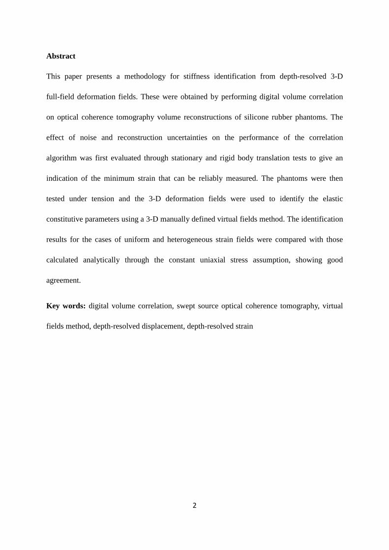
Abstract

This paper presents a methodology for stiffness identification from depth-resolved 3-D

full-field deformation fields. These were obtained by performing digital volume correlation

on optical coherence tomography volume reconstructions of silicone rubber phantoms. The

effect of noise and reconstruction uncertainties on the performance of the correlation

algorithm was first evaluated through stationary and rigid body translation tests to give an

indication of the minimum strain that can be reliably measured. The phantoms were then

tested under tension and the 3-D deformation fields were used to identify the elastic

constitutive parameters using a 3-D manually defined virtual fields method. The identification

results for the cases of uniform and heterogeneous strain fields were compared with those

calculated analytically through the constant uniaxial stress assumption, showing good

agreement.

Key words: digital volume correlation, swept source optical coherence tomography, virtual

fields method, depth-resolved displacement, depth-resolved strain

3

1. Introduction

The measurement of material deformation is necessary to assess the material mechanical

properties. A wide variety of techniques have been developed to measure the deformation of

materials under load, ranging from point-wise sensors such as the resistive strain gauge [1]

and optical fibre Bragg gratings [2] to 2-D full-field measurements including digital image

correlation (DIC) [3], the grid method [4], speckle interferometry [5], Moiré interferometry

[6]. For homogeneous and isotropic materials, these techniques usually provide enough

information to investigate their mechanical behavior. However, for materials with more

complex structures such as biological tissues and composites, surface measurements are much

less adequate to address their complete mechanical behavior since the deformation may vary

significantly between the bulk and the surface. In this case, a depth-resolved 3-D full-field

measurement of the deformation would be highly desirable.

Thanks to the development of the various tomographic techniques, digital volume

correlation (DVC) has become a popular measurement technique for depth-resolved 3-D

deformation fields. It is effectively a 3-D extension of digital image correlation (DIC), widely

applied to determine the surface deformation fields. DIC was first introduced in the early

1980s [3] and has been widely applied in many disciplines such as mechanical engineering,

material science, medical science, etc [7-11]. It basically determines the deformation field by

tracking a speckle pattern imprinted on the surface of the sample between a reference and a

deformed state. Based on the same principle, DVC was developed to measure the internal 3-D

deformation behavior of materials by tracking internal features that resemble 3-D speckle

patterns contained in the reconstructed volumes [12]. It requires sufficient speckle contrast in

4

the reconstructed volumes to ensure the correlation algorithm runs successfully. DVC has

made its way into clinical and industrial applications [13-20], where it is mainly applied on

X-ray computed tomography (X-ray CT) data of materials such as composites, metals, foams

and trabecular bones [13-16]. In all these cases the pattern contrast of the reconstructed

volume is provided by differences in X-ray absorption of the different constituents or phases

of the material. However, for soft biological tissues dominated by collagen, such as cornea,

arteries or skin, optical coherence tomography (OCT) is a more suitable technique to

reconstruct the material microstructure.

OCT is a non-invasive imaging technique that can acquire micrometer resolution,

cross-sectional images from within semitransparent, light scattering materials. It is an

interferometric technique that uses a broadband light source with short coherence length to

provide depth-resolved information of the object microstructure. The contrast of the images

encodes refractive index changes in the material (between fibres and a matrix into which they

are embedded, for example). Indeed, this rapidly developing imaging technique has already

been applied in ophthalmology, cardiology, gastroenterology and dermatology [21-24], and

many commercially available OCT systems have been developed for clinical and research

purposes [25]. With the aid of OCT, the volumetric data that represent the whole micro

structure of the scanned sample can be reconstructed. The reconstructed data can then be

utilized for structure analysis or deformation analysis using DVC. To the best of our

knowledge, this is the first time that measurements of depth-resolved deformations have been

undertaken combining OCT and DVC.

Given a constitutive model, constitutive parameters are constants that describe the

5

mechanical behavior of a material. Thanks to the development of full-field deformation

measurement techniques, several methods have been developed to identify the material

constitutive parameters. Finite element model updating (FEMU) is a widely applied approach

among these methods. It compares the experimental measurements with their numerical

counterparts obtained from a finite element model and builds up a cost function using the

difference between numerical and experimental values in terms of displacement or strain. By

minimizing the cost function with respect to the sought constitutive parameters the solution of

the problem can be reached iteratively. FEMU has already been shown to be feasible to

identify constitutive parameters in many cases such as elasticity, hyperelasticity, etc [26-28].

This approach however exhibits some shortcomings. The initial values to start the iteration

procedure, the numerical model, and the quality of the cost function for instance can all affect

the convergence time and the quality of the results. The virtual fields method (VFM) is an

alternative option for solving the identification problem [29], which is based on the principle

of virtual work and retrieves the constitutive parameters by utilizing the full-field deformation

measurements. This method is more effective than FEMU in terms of computation time since

for the latter FE model needs to be created and updated iteratively. So far, the VFM has

successfully been applied to the identification of constitutive parameters for linear elastic

materials such as composites [30-33], elasto-plasticity for metals [34-36] as well as

hyperelasticity for soft and biological materials such as artery walls [37, 38].

The aim of this study is to develop an effective methodology to investigate the internal

deformation behavior of silicone rubber phantoms under load and to identify their elastic

stiffness parameters. This methodology will eventually be applied to study the mechanical

6

properties of biological tissues such as the vertebrate eye cornea [39]. First, a brief description

of the material, the experimental setup, the experimental methods as well as the identification

theory is presented. Then, the performance of DVC coupled with OCT is evaluated through

stationary and rigid body translation tests. After that, DVC results of the tensile tests are

examined and critically discussed. Finally, the depth-resolved full-field deformation

measurement results are used to identify the material elastic stiffness parameters using VFM

and the identification results are also discussed.

2. Materials and methods

2.1 Materials

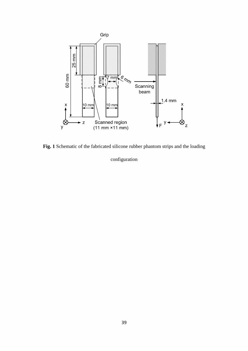
In the present study, two rectangular flat phantom strips were fabricated using silicone gel

(MM240-TV), one of them with a notch. The material comprises of two parts, a rubber base

and a hardener. They were mixed to a ratio of 10:1. The nominal Young’s modulus of the

silicone rubber is 1.88 MPa, which can change with the proportion of hardener. Since the

silicone gel does not present suitable speckle contrast for the application of DVC, copper

particles (with an average particle size of about 1 µm) were seeded into the silicone gel

mixture to provide the speckle contrast. The mixture was then put into molds and left to cure

at room temperature for approximately 24 hours. The flat strips were cut from a larger piece

using a scalpel to 104.160 ×× mm3 ( widththicknesslength ×× ). Fig. 1 shows the

rectangular and the notched phantom strips and their loading and observation configuration.

2.2 Experimental set-up and image acquisition

The experimental set-up consists of a tensile test fixture and a swept-source OCT system

(SS-OCT, Thorlabs OCS1300SS, lateral resolution 25µm, depth resolution 12µm in air). For

7

the test, the phantom strip was mounted with one end fixed to the fixture and the other end

loaded by a dead weight. At first, a dead weight of 50 g was applied as a preload to insure the

phantom strip was taut and vertical. This is a necessary step since the silicone rubber is rather

compliant. The preload state was taken as the reference state. A 10 g dead weight was then

added to the preload and considered as the deformed state, referred to as ‘load step 1’

hereafter.

For both reference and deformed states, a 3-D volume image sequence of the specimen

was acquired using the SS-OCT system. It uses a rapidly tuned narrowband light source with

central wavelength of 1325 nm and spectral bandwidth of 100 nm and records the information

with a single photo detector. The frequency of the interference signal is proportional to the

optical path difference between the sample and reference arms of an interferometer. Depth

profiles (A-scans) of the sample are obtained by evaluating the Fourier transform of the signal

for each wavelength scan. The 5-6 mm coherence length of the laser enables approximately

3 mm depth measurement. Adjacent A-scans are then synthesized to create an image in the xy

plane. Multiple adjacent 2-D images in the z-direction then form the reconstructed 3-D

volume. In the present work, a region with dimensions of 11311 ×× mm3 was scanned,

corresponding to x, y and z directions, respectively. A 3-D data volume of 10245121024 ××

voxels was obtained. The acquisition time for each 3-D volume is approximately 5 minutes. It

should be pointed out that each time, before acquiring the volume images, the specimen was

left for 10 minutes under load to accommodate significant short term viscoelastic creep.

Along the lateral scanning directions x and z, the image voxel size was determined by

dividing the 11 mm dimension by the number of corresponding 1024 voxels, which is equal to

8

10.7 µm. Regarding the through-thickness y-direction, which corresponds to optical path, the

voxel size depends on the refractive index of the medium. For the silicone rubber phantom the

voxel size inside the medium along the y-direction is 4.1 µm determined by dividing its

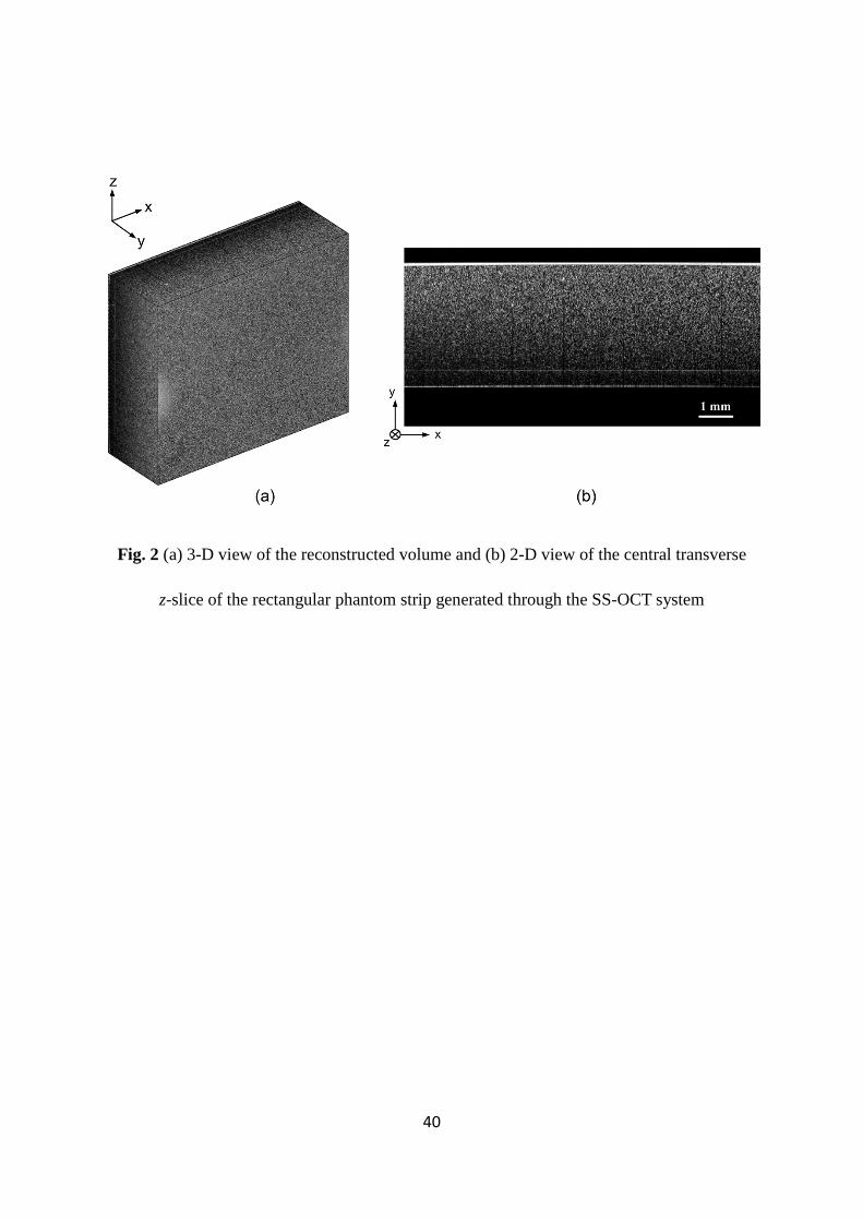
thickness 1.4 mm by the number of corresponding voxels, here 345. The reconstructed

volume and a typical central transverse z-slice ( 5121024× voxels) of the specimen are given

in Fig. 2 (a) and (b), respectively. Due to light saturation, the voxels at the top surface exhibit

very high intensity values, as can be seen from the white line at the top of the phantom in

Fig. 2(b). It should be pointed out that all the regions outside the phantom strip and the

saturated voxels at the top surface were masked out in Fig. 2(a) for a better visualization of

the 3-D reconstructed volume. The reconstructed volumes for the reference and deformed

states were recorded and DVC was then used to compute the 3-D displacement and strain

fields.

2.3 Digital volume correlation

DVC is the 3-D extension of the widely applied DIC used to measure surface deformations.

During the DVC procedure, the correlated volumes are first divided into sub-volumes. The

displacement vector of each sub-volume is determined by tracking and matching the voxels of

the sub-volumes in the reference and deformed states. This is performed by maximizing the

correlation coefficient which measures the degree of similarity of the grey level distributions

in the sub-volumes in the reference and deformed states. The best prediction of the

displacement leads to the highest degree of similarity of the grey level distributions thus the

maximal correlation coefficient (a correlation coefficient value close to 1 indicates a perfect

match). In the present study, the displacement fields were calculated using the DaVis®

9

(LaVision) software package based on a fast Fourier transform (FFT) algorithm. It evaluates a

normalized cross-correlation coefficient (NCC) defined as

( ) ( )

( )[ ] ( )[ ]∑ ∑ ∑∑ ∑ ∑∑ ∑ ∑

=22 ˆ,ˆ,ˆ,,

ˆ,ˆ,ˆ,,

zyxGzyxF

zyxGzyxFC (1)

Where ( )zyxF ,, represents the grey level at a voxel ( )zyx ,, in the sub-volume of the

reference state, while ( )zyxG ˆ,ˆ,ˆ represents the grey level at a point ( )zyx ˆ,ˆ,ˆ in the

sub-volume of the deformed state. The coordinates ( )zyx ,, and ( )zyx ˆ,ˆ,ˆ stand for the same

material point in the reference and deformed states, respectively, and are related by the 3-D

affine transformation in the form of rigid body motion combined with displacement gradients

Δzz

UΔyy

UΔxx

UUzz

Δzz

UΔy

yU

Δxx

UUyy

Δzz

UΔy

yU

Δxx

UUxx

zzzz

yyyy

xxxx

∂∂

+∂∂

+∂∂

++=

∂

∂+

∂

∂+

∂

∂++=

∂∂

+∂∂

+∂∂

++=

ˆ

ˆ

ˆ

(2)

where Ux, Uy, and Uz are the rigid body displacement components of the subset center in the x,

y and z-direction, respectively. x∆ , y∆ and z∆ , represent the distance between the subset

center and the point ( )zyx ,, . A double-pass approach was used whereby large sub-volumes

were initially used to capture large displacements. Subsequent to this, these initially

calculated displacements were used to displace smaller sub-volumes, and thus ensure the

pattern was followed and signal to noise ratio increased. Gaussian curve-fitting of the

correlation function peak was used to detect the position of the displacement with sub-voxel

resolution. The strains were then determined from the centered finite difference of the

calculated displacement fields, without any additional smoothing.

10

2.4 Evaluation of measurement performance

The DVC algorithm requires sufficient contrast in a sub-volume in order to determine a

displacement vector. The size of the sub-volumes influences the value of the correlation

coefficient and thus the displacement and strain uncertainties. In the present study, four

different sub-volume sizes were selected and compared to determine an optimal size

considering the displacement and strain spatial variation as well as the spatial resolution. A

double-pass approach used initial sub-volumes sizes 243, 483, 723 and 963 in the first pass,

followed by 123, 243, 363 and 483 in the second path and each has 50% overlap with the six

adjacent neighbors. Thus, the distance between each sub-volume centre with its immediate

neighbors is 6, 12, 18 and 24 voxels, respectively.

Prior to the tensile tests, it is necessary to evaluate the errors caused by all sources of

noise and reconstruction uncertainties. This can be done by performing DVC on two

subsequent reconstructed volumes of the stationary phantom strip. Since the stationary

specimen was not subjected to any applied force, the correlation results should show zero

displacement and strain fields over the whole field of view. This is not the case in practice due

to the influence of electronic noise in the SS-OCT system, environmental vibration, the

volume reconstruction algorithm, etc. Therefore, any non-zero results should be attributed to

the contribution of noise and other reconstruction uncertainties. The standard deviations of the

spurious strains were calculated to evaluate the resolution (uncertainty) of the strain

measurement.

Then, two reconstructed volumes were recorded after introducing a rigid body translation

of 40 µm (about 10 voxels) in the y-direction between the two volumes. This not only tests

11

the effect of all sources of noise but also tests the performance of DVC sub-voxel

interpolation (tri-linear in the present study) and accuracy of the correlation algorithm in

determining the displacement fields for a translated specimen. The same procedure of data

processing as for the stationary test was applied to the rigid body translation test and the strain

measurement resolution was computed. The above tests give an overall idea of the resolution

of the whole set-up so that the significance of the tensile test results can be better analyzed.

2.5 The virtual fields method

The virtual fields method, which is based on the principle of virtual work, was adopted to

identify the constitutive parameters of the silicone rubber phantom. This equation, provided

below, is the integral form of the equilibrium equation for the standard deformable continuous

solid model:

∫ ∫ ∫∫ ∗∗

∂

∗∗ ⋅=⋅+⋅+−V V VV

dVdVdSdV UaUbUTεσ ρ: (3)

In this equilibrium equation, σ is the actual stress tensor, ∗ε is the virtual strain tensor,

∗U is the virtual displacement vector, T is the traction vector acting on the boundary V∂

of the solid volume V , b is the volume force vector, a is the acceleration vector and ρ

is the mass per unit volume, “·” indicates vector dot product and “:” is the contracted product

for second order tensors or the matrix dot product. In this study, the phantom strip was loaded

statically and the body forces can be neglected. Therefore, their contribution to the virtual

work can be canceled out. Thus, the equilibrium equation becomes

∫ ∫∂∗∗ =⋅+−

V VdSdV 0: UTεσ (4)

This equilibrium equation is valid for any continuous and differentiable virtual displacement

field. The actual strain field and the load information are provided by the experiment. The

12

stress components can be expressed through the material constitutive parameters and the

strain components through an appropriate constitutive equation. Here, the stress and strain

components are written in columns as

{ }Txyxzyzzzyyxx σσσσσσ:σ

{ }Txyxzyzzzyyxx εεεεεε 222:ε (5)

where T is the transpose operator.

For the silicone rubber phantom, isotropic elasticity was assumed. Thus, the stress-strain

relation can be expressed as

−

−

−=

xy

xz

yz

zz

yy

xx

xyxx

xyxx

xyxx

xxxyxy

xyxxxy

xyxyxx

xy

xz

yz

zz

yy

xx

QQ

QQ

QQQQQQQQQQQ

εεεεεε

σσσσσσ

222

200000

02

0000

002

000

000000000

(6)

where xxQ and xyQ are the two stiffness components to identify, relating to the elastic

modulus E and the Poisson’s ratio ν through

( )( )( )

( )( )

−+=

−+−

=

ννν

ννν

211

2111

EQ

EQ

xy

xx

(7)

After introducing equations (5) and (6) into equation (4), the equilibrium equation becomes

( ) (

) ∫∫ ∫

∂

∗∗∗∗∗∗∗∗

∗∗∗∗∗∗∗∗

⋅=−−−+++

++++++++

Vxyxyxzxzyzyzxxyyyyxxyyzzzzyy

V xxzzzzxxV xyxyxyxzxzyzyzzzzzyyyyxxxxxx

dSdV

QdVQ

UTεεεεεεεεεεεεεε

εεεεεεεεεεεεεεεε

222

222 (8)

where ∗ijε is the virtual strain component deduced from the virtual displacement. In the

13

present study, the material is macroscopically homogeneous. Therefore, xxQ and xyQ can

be taken out of the integrals, and equilibrium equation (8) becomes

( ) (

) ∫∫ ∫

∂

∗∗∗∗∗∗∗∗

∗∗∗∗∗∗∗∗

⋅=−−−+++

++++++++

Vxyxyxzxzyzyzxxyyyyxxyyzzzzyy

V V xxzzzzxxxyxyxyxzxzyzyzzzzzyyyyxxxxxx

dSdV

QdVQ

UTεεεεεεεεεεεεεε

εεεεεεεεεεεεεεεε

222

222 (9)

Any new virtual field in the equilibrium equation leads to an equation involving the stiffness

components. Therefore, a proper choice of the virtual displacement fields enables the

identification of the unknown stiffness components xxQ and xyQ . There are different

methods for choosing virtual fields. In the present work, two manually defined polynomial

virtual fields were employed for the two sought constitutive parameters. More details about

other choices of virtual fields such as virtual fields minimizing noise effects and piecewise

virtual fields etc. can be found in [29]. The first virtual displacement field and the

corresponding virtual strain field are

( ) ;1 LxU x −=∗ ( ) ;01 =∗yU ( ) ;01 =∗

zU

;1)1( =∗xxε ;0)1( =∗

yyε ;0)1( =∗zzε ;0)1( =∗

yzε ;0)1( =∗xzε 0)1( =∗

xyε (10)

For the second virtual field

( ) ;02 =∗xU ( ) ( );2 LxxyU y −=∗ ( ) ;02 =∗

zU

;0)2( =∗xxε ( );)2( Lxxyy −=∗ε ;0)2( =∗

zzε ;0)2( =∗yzε ;0)2( =∗

xzε yLxyxy 21)2( −=∗ε (11)

where L is the length (dimension along the x-direction) of the phantom strips.

After introducing the above two virtual fields (10) and (11) into the equilibrium equation

(9), a linear equation system (12) can be formed to directly determine the sought stiffness

components xxQ and xyQ .

BAQ = (12)

14

( )

( ) ( )( ) ( )( ) ( )( )

−−+−−+−

+

∫∫∫∫

V xyzzxxV xyyy

V zzyyxx

dVyLxyLxxdVyLxyLxx

dVdV

εεεεε

εεε

22: VA

xy

xx

QQ

Q :

0:

-FL B

where F is the tension load at the position 0=x , and L− represents the virtual

displacement at the same position calculated from equation (10) for the first virtual field.

FL− represents the external virtual work done by the tension load.

It should be pointed out that due to the discrete nature of the deformation measurement,

the integrals above such as in (9) must be approximated by discrete sums. For instance, an

integral ∫ ∗

V xxxx dVεε can be approximated by ( ) ( ) ( )∑ =∗n

iii

xxi

xx v1

εε , where n is the number of data

points, ( )ixxε the actual strain xxε at data point ( )i , ( )i

xx∗ε the virtual strain ∗

xxε at data point

( )i and ( )iv the volume of each measurement point. Due to the uniaxial tension

configuration, the strain field should be dominated by low spatial frequencies. In addition, a

relatively small sub-volume size was chosen to enable a high strain spatial resolution.

Therefore, the error involved due to the discretization is small and considered as acceptable

for the current tests. Thus, matrix A in the linear equation system (12) becomes

( ) ( ) ( )( ) ( )

( ) ( )( ) ( ) ( ) ( ) ( )( ) ( )( ) ( ) ( ) ( )( ) ( ) ( )( ) ( ) ( ) ( )( ) ( )( ) ( )

−−+−−+−

+

∑∑

∑∑

==

==n

i

iixy

iiiizz

ixx

iiin

i

ixy

iiiyy

ii

n

i

iizz

iyy

n

i

iixx

vLyyxLxxvLyyxLxx

vv

i

11

1

)(

1

22:

εεεεε

εεεA

(13)

For these tests, ( )iv of each data point is constant because of the constant sub-volume size,

which is equal to nV . Therefore, ( )iv can be taken out of the sum and a sum in matrix A, for

instance, becomes

15

( ) ( ) ( )xx

n

i

ixx

n

i

iixx V

nVv εεε == ∑∑

== 11

(14)

where xxε denotes the arithmetic spatial average of xxε and V is the total volume of the

processed data. Finally, the linear equation system (12) to solve can be written as follows

( ) ( ) ( )( ) ( )

−

=

−−+−−+−+

022 VFL

QQ

yLxyLxxyLxyLxx xy

xx

xyzzxxxyyy

zzyyxx

εεεεεεεε (15)

3. Results and discussions

3.1 Strain noise analysis

A fundamental condition in image correlation techniques is that the changes in the intensity

pattern are in one-to-one correspondence with the displacements of the surface. DVC results

from OCT volume reconstructions of the reference and deformed states are likely to be

affected by a variety of factors such as: 1) electronic noise of the detectors; 2) light source

stability; 3) reconstruction algorithms; 4) contrast reduction through the sample thickness due

to material absorption, scattering, dispersion, defocusing and spectral roll-off; and 5)

strain-induced speckle decorrelation. We studied the combined effect of 1-4 by performing a

stationary test and a rigid translation of the phantoms. The effect of strain in speckle

decorrelation was explored through a numerical simulation described below.

Stationary Test

From the DVC results of the stationary test, the influence of sub-volume size was analyzed

quantitatively by comparing the standard deviations of the strain components for a central

z-slice ( )yx, for the four final sub-volume sizes. All six strain components were derived

from the centered finite differences of the spurious displacements as follows, without any

smoothing:

16

( )ijjiij UU ,,21

+=ε (16)

where the commas stand for the partial derivatives. To study the effect of sub-volume size, the

standard deviations over the whole field of view are compared in Fig. 3(a) for xxε , xyε and

yyε only, for the sake of legibility. The standard deviations of the strain components drop

from ~ 3103 −× to about 4105 −× when increasing the sub-volume size from 123 to 243. When

further increasing the sub-volume size to 363 and 483 –see Fig. 3(b), the strain fluctuations

further reduced to about 4102 −× . This is so because the larger number of features contained in

the 483 sub-volume assist the convergence of the volume correlation algorithm and enable

more accurate tracking of the sub-volume deformation. A smaller number of features in the

123 sub-volume leads to bigger tracking errors. In the case of thin specimens such as corneas

[39], or the phantoms studied in this work, 363 sub-volumes were found to be a good

compromise in terms of strain and spatial resolution. Depending on the OCT spatial sampling

rate, the speckle field may be undersampled, leading to aliasing and interpolation errors [40].

This issue will be discussed later on in the paper.

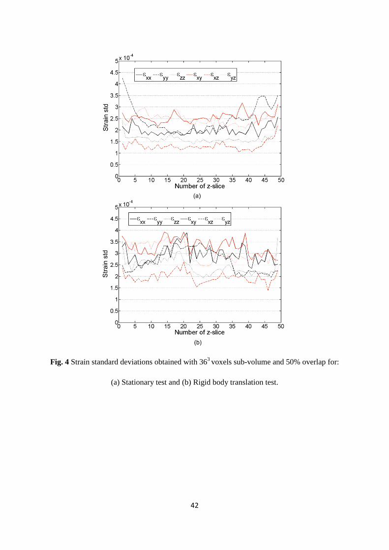
Based on the volume strain fields of the stationary test, the standard deviation of each

strain component was calculated for each z-slice and the results are plotted in Fig. 4(a). It can

be observed that the standard deviations of all the strain components generally remain stable

along the different z-slices, with a slight increase towards the ends. This is expected as the

DVC results are usually noisier near edges due to the lack of data. Although with fluctuation,

all the standard deviations are generally between 4105.1 −× and 4105.2 −× without any

smoothing, which is considered as satisfactory compared with the strain levels in the tensile

tests later on.

17

Translation test

Slightly larger values of strain standard deviation, between 4102 −× and 4105.3 −× , were

obtained for the rigid body translation test – see Fig. 4(b). This is so as extra sources of error

add to those present in the stationary test, mainly sub-voxel interpolation error as the DVC

algorithm tracks the sub-volumes between the reference and displaced states. It was observed

that lateral translations (in the xz plane) lead to strain standard deviations values between

those obtained for the stationary and the axial translation tests. These levels are still low

compared to the strain levels of approximately ~1% in the tensile tests and were thus

considered satisfactory.

Strain-induced speckle decorrelation

Due to the backscatter illumination/observation configuration, the complex 3-D point spread

function (PSF) of the OCT system has ~18 fringes across it along the axial direction (ratio

between the depth resolution, 8.3 µm, and the half wavelength of the light source in the

medium of refractive index 1.45, i.e. 1.325µm/(2×1.45)=0.457 µm). The magnitude of the

measured OCT signal corresponds to the convolution between the 3-D PSF and the scattering

particles within the phantom. This magnitude, which determines the brightness of the 3-D

speckle grain at any particular position within the sample, does not change with rigid body

motion of the sample as relative phase differences between scatterers within the 3-D PSF

remain constant. In case of strain, however, there is a limit within which the magnitude of the

speckle remains nearly unchanged and beyond which an incremental DVC approach would be

required.

In order to estimate the level of OCT speckle decorrelation due to strain, we performed a

18

2-D (on the xy plane) numerical simulation involving the following steps:

1. Generate a 2-D random distribution of scatterers such that there are many of them

(~100) inside the point spread function of the OCT system.

2. Evaluate the 2-D speckle field due to the spatial distribution of scatterers considering

the numerical aperture of the system, the central wavelength and bandwidth of the

source, and the refractive index of the medium. This was done using linear systems

theory [41, 42] by first calculating the transfer function of the OCT system, then

evaluating the complex PSF and convolving it with the scatterers. The speckle field

was oversampled to recover phase information within the PSF. In this way, the

correlation coefficient evaluation is free from under-sampling effects. We used images

of 1024×1024 pixels with a speckle size given by the dimensions of the PSF (~1024/4

pixels in the axial direction y and ~1024/2 pixels in the lateral direction x). Using the

Rayleigh resolution criteria, this leads to ~8×4=32 speckles in the simulated subset,

which compares well with the number of speckles observed on the xy face of the 363

sub-volume shown in Fig. 3(b).

3. Deform the spatial distribution of scatterers with a horizontal strain xxε from 0 to 0.5

in steps of 0.001 from 0 to 0.02 and steps of 0.05 thereafter. Poisson’s contraction in

the vertical direction was also considered, using 42.0=ν as estimated for our

phantoms in Section 3.3. For each deformation state, the intensity (magnitude) of the

corresponding speckle field was calculated.

4. Finally, the normalized cross correlation as defined in Eqn. (1) was evaluated between

the first speckle field for 0=xxε and all others in the sequence.

19

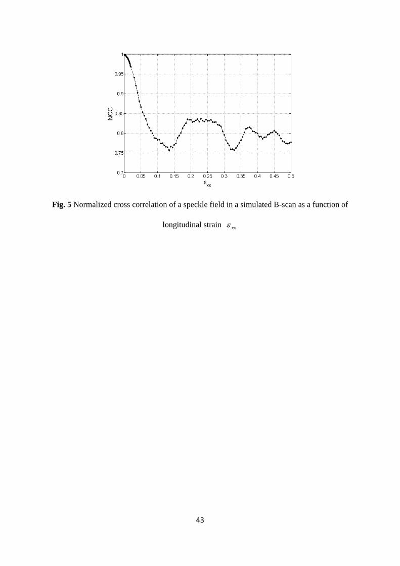
Figure. 5 shows that NCC drops to ~0.987 for %1=xxε and to ~0.961 for %2=xxε . This

latter strain corresponds to a total maximum through-thickness relative displacement of the

scatterers in the PSF of ~70nm. This is equivalent to ~1/6th of the fringe period inside the PSF

and is inversely proportional to the Poisson’s ratio. NCC drops to ~0.9 for xxε ~ 4%, which

corresponds to yyε ~1.68% using 42.0=ν . This strain level is probably a good estimate to

the maximum strain that we can measure with OCT and DVC without using an incremental

approach. Above this level, the correlation coefficient is too low to guarantee a good estimate

of displacements. When the changes in the magnitude of the interference of light scattered by

particles within the PSF are large, the speckle is said to ‘boil’, i.e. its structure changes while

only the average speckle size is preserved. Even though these results correspond to a 2-D case

(B-scan), a 3-D simulation is expected to render similar results to those reported here. Zaitsev

et al [43] have found similar results performing a numerical simulation and evaluating the

zero mean normalized cross correlation coefficient (ZMNCC) as a function of strain. They

report that speckle boiling fully decorrelates the speckle for axial strain levels of ~1.5%,

which compares well with our figure of ~1.68% mentioned above.

3.2 DVC results for tensile tests

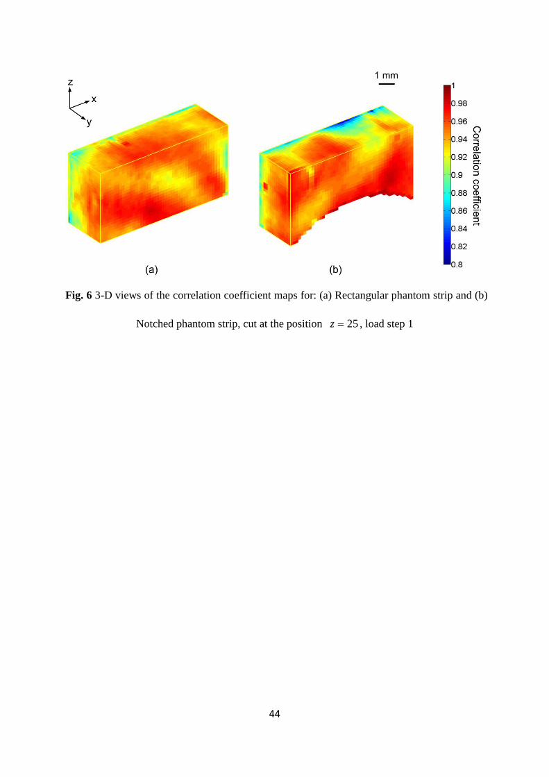
3.2.1 Correlation coefficient maps

The 3-D deformation field was measured under tension after performing DVC on the OCT

reconstructed volume data for the rectangular and notched phantom strips. As DVC was

performed using the sub-volume size of 363-voxel and 50% overlap, the reconstructed volume

of interest thus contained 501855 ×× measurement points, corresponding to the dimensions

of 104.15.10 ×× mm3. The reliability of the deformation measurements was assessed in

20

terms of the 3-D correlation coefficient maps, shown in Figs. 6 (a) and (b) for the rectangular

and notched phantom strips, respectively. In order to see the correlation coefficients within the

specimens, sub-volumes of the whole fields are represented here obtained by cutting the

volumes in the xy plane at z-slice 25. For y-slice 18 at the top of the rectangular specimen, the

mean value of the correlation coefficient is 0.95, while it is 0.92 for y-slice 1 at the bottom.

Similar results were obtained for the notched specimen: 0.95 and 0.84, respectively. This

decrease in correlation coefficient through the thickness can be attributed to a

depth-dependent speckle contrast reduction as a result of signal attenuation due to light

scattering, defocusing and spectral roll-off.

In our experiments, the maximum xxε was ~1.4% (see results for ‘load step 2’ in

Section 3.2.2) and therefore speckle boiling was not an issue. Without further analysis it

would seem prudent to consider NCC values below 0.9 as inappropriate to measure strains

with OCT and DVC.

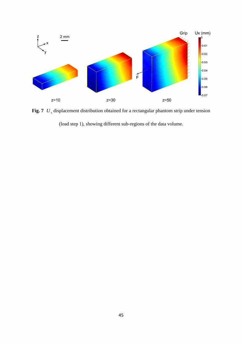
3.2.2 DVC results for rectangular phantom strip

xU displacement maps for the rectangular phantom strip, which denote the displacement

along the tension direction, are shown in Fig. 7. In Fig.7, one can see the evolution of the xU

displacement in cross sections cut at different z-slices. The absolute value of xU increases

continuously along the x-direction from the fixed side to the other, ranging from 0 to 0.07 mm,

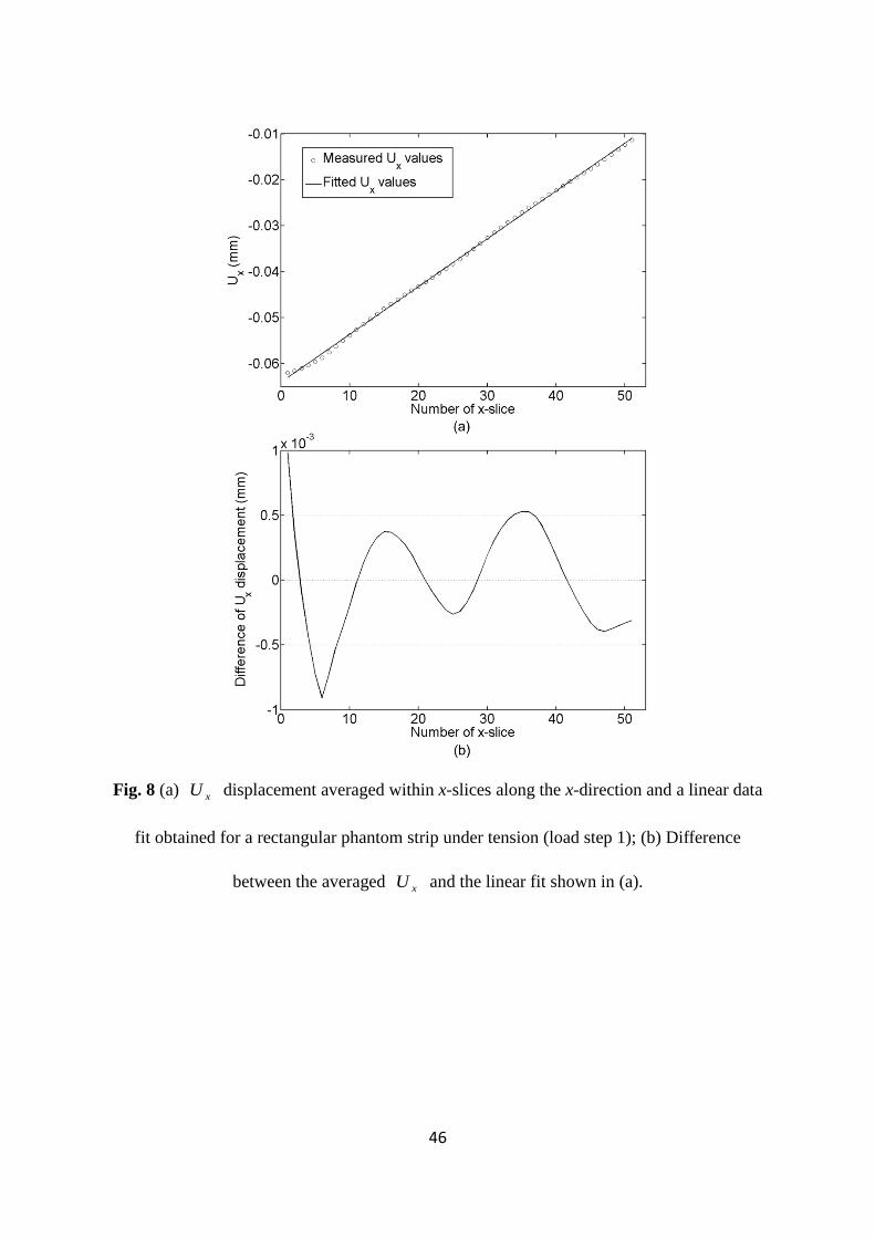
as expected from the loading configuration. Fig. 8(a) shows that the mean value of xU

evolves linearly along the x direction. Nevertheless, a sinusoidal oscillation is apparent when

the difference between the actual values and a linear fit is plotted as a function of x in

Fig. 8(b). An analysis of these displacement oscillations is provided below in this Section.

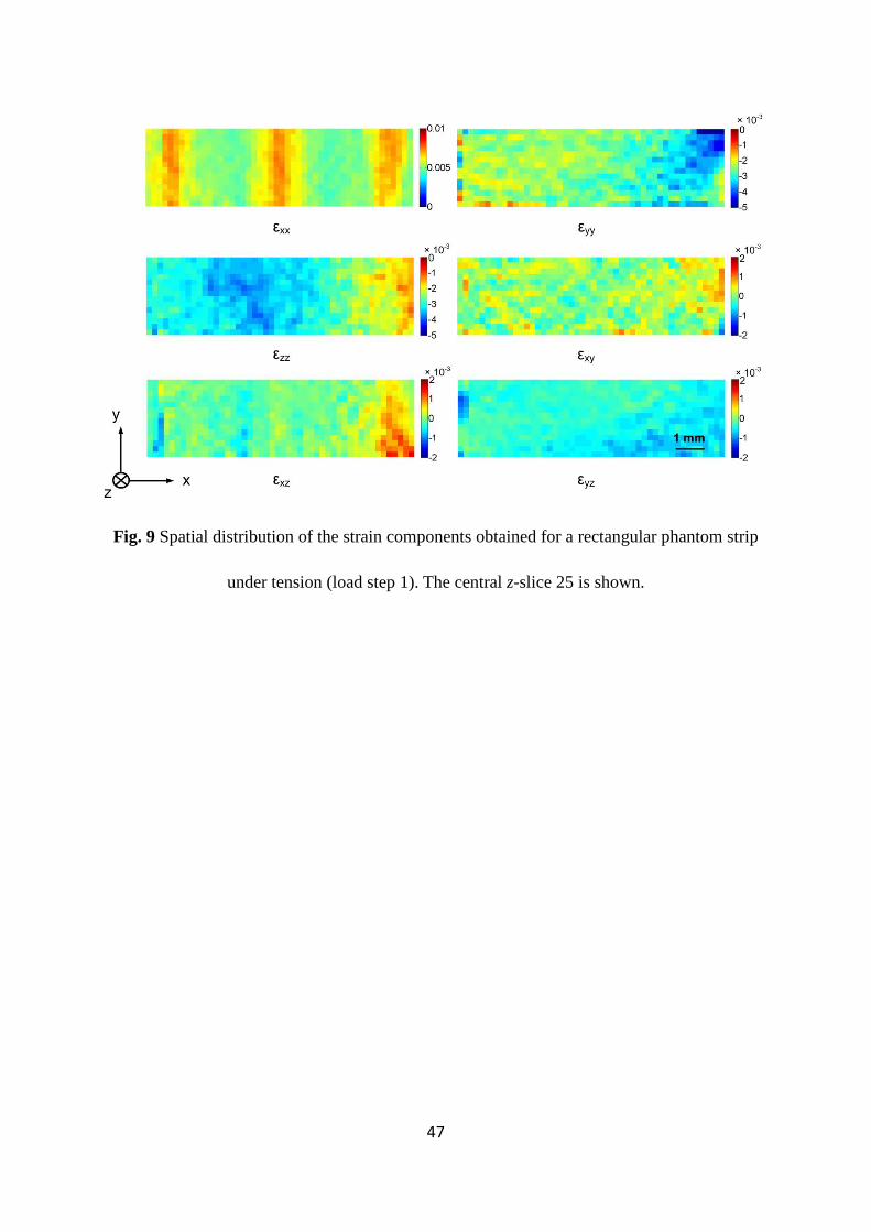
21

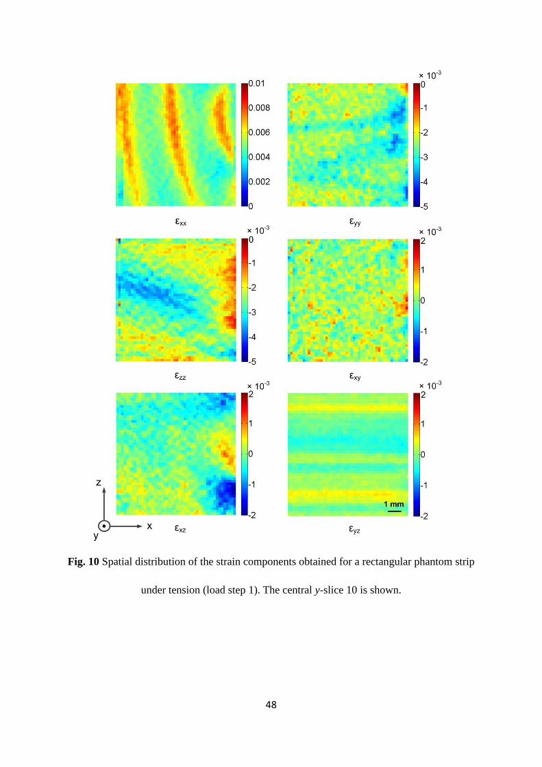
The strain maps were derived using the same procedure as for the noise analysis

(centered finite difference of the displacement data, without any smoothing). All six strain

components for central z-slice 25 and central y-slice 10 are shown in Figs. 9 and 10,

respectively. As expected from the loading configuration, the xxε strain maps for both z- and

y- slices show positive values around 0.007. Strain maps yyε and zzε show negative values

indicating a Poisson’s contraction along the corresponding directions. It is interesting to note

that zzε is very small (close to zero) at the right-hand side, where the grip prevents Poisson’s

contraction in the z- direction. Regarding yyε , it is not zero at the right-hand side because the

constraint from the grip acts only at the surface. The reason why yyε is actually larger in

magnitude may be from some material non-linearity due to the compression in the grip.

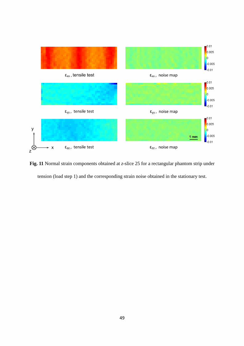
Figure 11 shows that the measured strain components are significantly larger than the

corresponding strain noise obtained for the stationary test. Since this is a pure tensile test for

the rectangular strip, all the shear strain components should be close to noise level, as

confirmed in Figs. 9 and 10. Some irregularities, however, can be seen from these strain maps.

The fringes observed in the xxε strain component in Figs. 9 and 10 could be due to either: 1)

a spatial variation of the elastic modulus, or 2) interpolation bias [40]. In the case of the FFT

based DIC algorithm used here, the period of the oscillation due to interpolation bias

corresponds to a displacement equivalent to 2 voxels [44-46]. This is consistent with 2.5

fringes observed in Fig. 8(b) for a total deformation corresponding to 5 voxels. A bias in

displacement directly leads to bias in strain, proportional to the slope of the displacement bias.

When aliasing arises due to spatial under-sampling by the SS-OCT system, the displacement

values obtained when comparing sub-volumes between reference and deformed states are

22

likely to suffer from larger interpolation errors which are further amplified when strain is

calculated. It has been shown that aliasing typically shows up as a moiré-like fringe pattern in

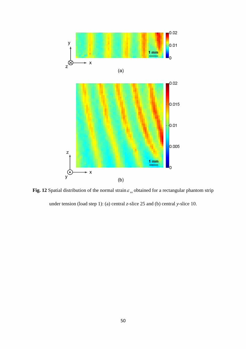
the displacement and strain fields and that it is more obvious in the latter. In order to confirm

the nature of the observed fringes, a second load step was performed on the same rectangular

phantom strip with an extra 10 g dead weight (we refer to this case as ‘load step 2’). The

strain maps showed twice as many fringes in Fig. 12, confirming that these are due to

interpolation bias in this elastic material. One way of reducing this bias is to perform

pre-smoothing on both the reference and deformed volume images using a Gaussian low-pass

filter before correlation, to reduce high spatial frequency components [47-48] or to increase

the sampling density of the OCT reconstruction.

3.2.3 Results for notched phantom strip

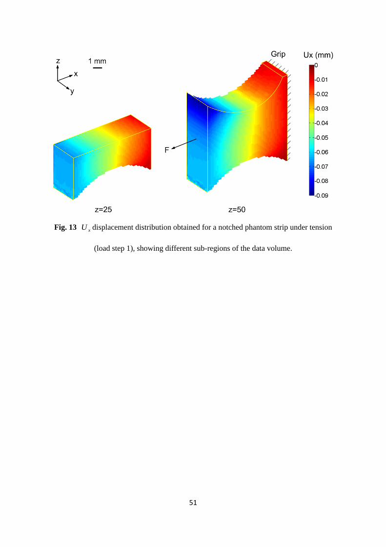
xU displacement maps for the notched phantom strip are shown in Fig. 13. One shows the

internal xU displacement in a cross section cut at central z-slice 25, while the other shows

the whole volume. It can be seen that in each z-slice the absolute value of xU increases

continuously along the x-direction from the fixed side to the other, as expected from the

loading configuration and consistent with the displacement maps for the rectangular phantom

strip as shown in Fig. 7. In Fig. 13, a slight bending of the strip can be observed from the

larger xU displacement values at the top half of the strip compared to those at the bottom

half. This is probably due to the slight geometrical asymmetry between the two notches. The

geometrical asymmetry was induced during the manufacturing process when cutting the strip

to a notched shape from a larger piece.

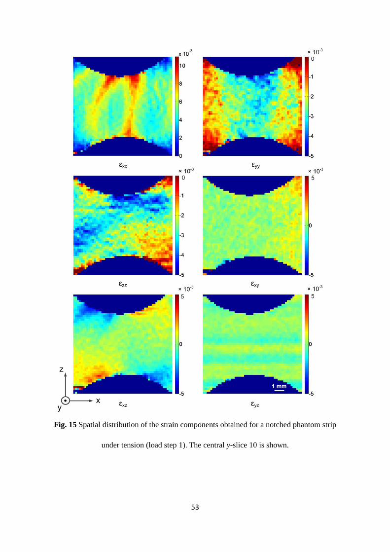
For the notched phantom strip, all six strain components for central z-slice 25 and central

23

y-slice 10 are shown in Figs. 14 and 15, respectively. The xxε strain map shows positive

values while the yyε and zzε strain maps show negative values, as expected. Larger

deformation is expected in the notched region, which can be observed in the maps of the

normal strain components in Figs. 14 and 15. In addition, strain concentration is observed

near the top notch tip of the strip for the normal strain components in Fig. 15. This is

consistent with the larger xU displacement found near the top notch in Fig. 13. The

explanation for this local strain concentration is the geometrical asymmetry of the notched

strip, which has already been stated earlier. In Fig. 15, the xzε strain map shows an

anti-symmetric shear strain distribution. Regarding the other two shear strain components,

they are close to zero. These results are consistent for this type of test. It should be pointed out

however that these results also suffer from the interpolation errors due to aliasing, especially

evident in xxε .

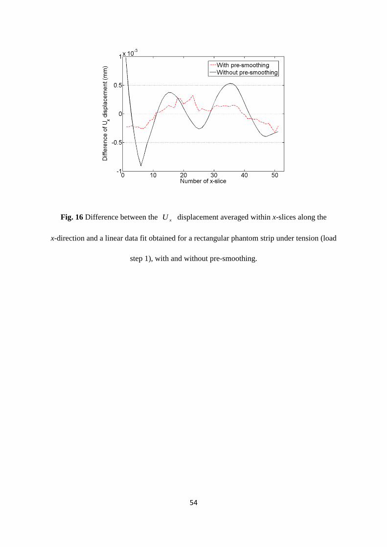
3.2.4 Bias reduction using Gaussian pre-smoothing

Pre-smoothing using a Gaussian filter has proved effective in reducing interpolation bias

[47-48]. A Gaussian filter with a kernel size of 777 ×× voxels and a standard deviation of

1.5 voxel was applied to the OCT volume reconstructions of the tensile tests prior to

correlation. In Fig. 16, for the rectangular phantom strip, the plots of the difference between

the measured and the fitted mean xU displacement of each x-slice as a function of x position

with and without pre-smoothing are compared. The difference is substantially reduced after

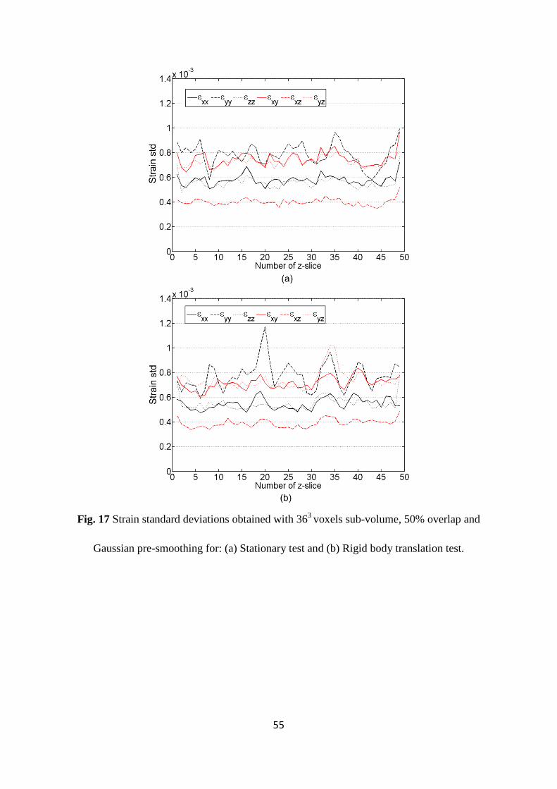
pre-smoothing, which is expected according to [47-48]. Gaussian smoothing was also applied

to the volume images of the stationary and rigid body translation tests in order to check its

influence in the strain resolution. The results show an increase in the strain standard

24

deviations with pre-smoothing, generally ranging from 4104 −× to 4108 −× , as shown in

Figs. 17 (a) and (b) for the stationary and rigid body translation tests, respectively. The reason

for this increase has been explained in [48], which states that the sum of squares of subset

intensity gradient (SSSIG) is reduced after smoothing, and the standard deviation error is

inversely proportional to the SSSIG value. In any case, these noise levels may still be

considered as acceptable compared with the strain levels of the tensile tests (about one order

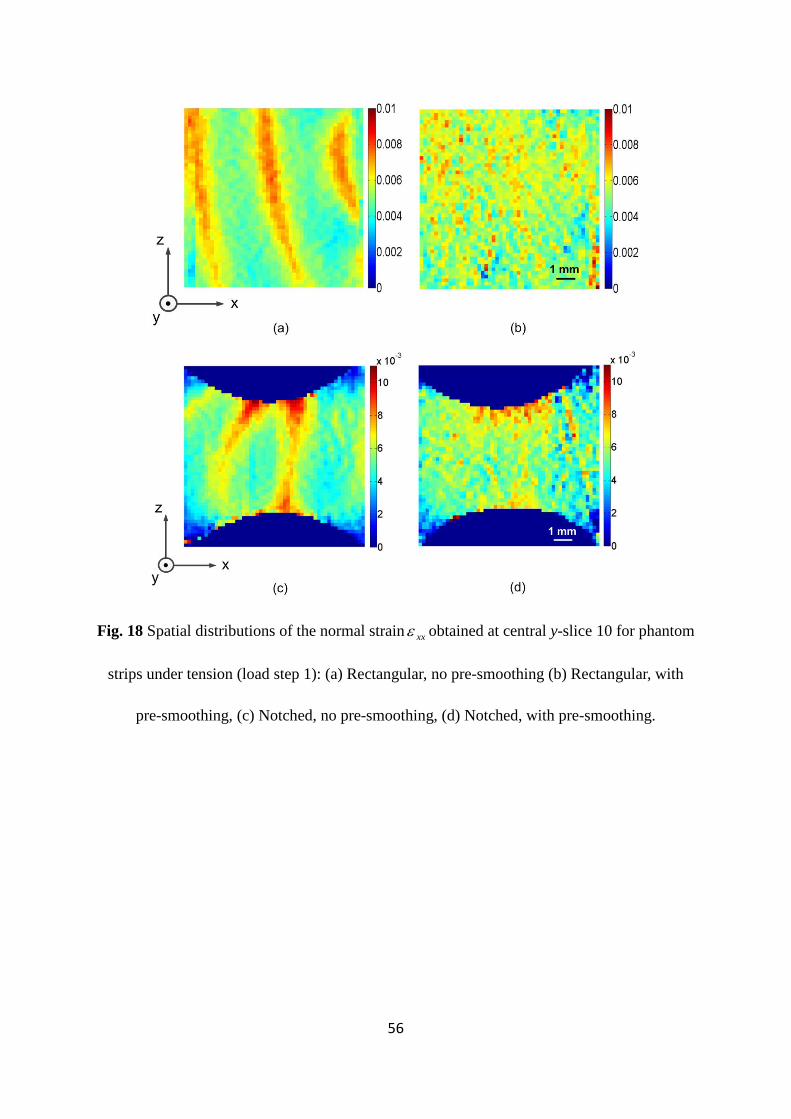
of magnitude). Fig. 18 shows the xxε strain maps with and without pre-smoothing for the

rectangular and notched phantom strips. The fringes due to interpolation bias are eliminated

after pre-smoothing.

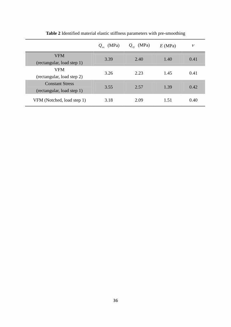
3.3 Identification results

Using the experimental strain results in the linear equation system (15), the material stiffness

components xxQ and xyQ can then be directly determined for the two tensile tests. The

identification results with and without pre-smoothing are listed in Tables 1 and 2, respectively.

From these results Young’s modulus E and Poisson’s ratio ν can be calculated through the

relations stated in equation (7). In order to provide a reference for the stiffness parameters

obtained through the VFM, Young’s modulus and Poisson’s ratio were also calculated for the

rectangular strip based on the assumption of constant uniaxial stress through the relation

−=

=

x

y

x

xE

εε

ν

εσ

(17)

where uniform stress xσ in the yz cross-section of the rectangular phantom strip was

determined through the equation AF

x =σ . F is the tension load and A is the yz cross-sectional

25

area. xε and yε are the average values of the corresponding strain components over the

whole field of view. Thus, both Young’s modulus and Poisson’s ratio can be derived and the

results are listed in Tables 1 and 2. In both tensile tests the results obtained from the VFM are

consistent with each other and also with those calculated from the constant uniaxial stress

assumption. This indicates that the 3-D VFM is an effective tool to identify the constitutive

parameters of materials with non-uniform stress/strain states when the constant uniaxial stress

assumption is no longer applicable. Moreover, the identification results with pre-smoothing

are in agreement with those without pre-smoothing when comparing Table 1 to Table 2.

It is interesting to note that when a larger preload of 115 g was used in the tensile test,

both parameters increased (E from 1.44 MPa to 1.82 MPa and ν from 0.42 to 0.48). In both

cases a load of 10 g was used.

4. Conclusions

We have shown that DVC can provide, by means of a single channel OCT system,

multicomponent displacement fields from which all the strain components required by

inversion methods such as the 3D-VFM can be evaluated. OCT+DVC has low displacement

sensitivity compared to phase-sensitive OCT elastography, and seems appropriate for strain as

large as ~1.68% (in the axial direction) at which point an incremental approach should be

used to avoid speckle decorrelation. A strain uncertainty in the order of ~4×10-4 to 8×10-4 was

observed when Gaussian pre-smoothing is used to reduce bias noise. Strain below this

uncertainty level would require an alternative approach such as phase-sensitive OCT, capable

of detecting sub-wavelength displacements with low noise. In the cases studied in this work,

one fringe across a 10 mm field of view would correspond to a relative axial displacement

26

equal to 0.45 µm and an average strain of 4.5×10-5, an order of magnitude better than the

uncertainty we report for OCT+DVC. Even though most phase-sensitive OCT elastography

systems have so far focused on phase measurements with only axial sensitivity, a new system

with sensitivity to all displacement components has been recently developed based on a

wavelength scanning OCT system using multiple illumination directions and a single

observation direction [49]. In this work, strain was evaluated with a centred finite difference

operator applied to the displacement field. No displacement smoothing was used before strain

calculation in order to achieve maximal spatial resolution with a view to further studies on

thin biological tissues such as the vertebrate eye cornea. In cases where strain accuracy is

paramount, a weighted-least squares strain estimator would be more appropriate [50].

Uniform and non-uniform 3-D strain fields measured with OCT+DVC were used to

identify the elastic stiffness components of rectangular and notched silicone rubber phantoms

using the VFM with 3-D manually defined virtual fields. The material moduli extracted from

this approach are consistent with those calculated from the constant uniaxial stress approach.

In order to test the proposed identification methodology, simple uniaxial tensile tests and

isotropic materials were used.

This is the first time that volume strain data are derived by performing DVC on OCT

reconstructed volumes. Future work will be aimed at applying this methodology to measuring

the internal 3-D full-field deformation of biological tissues under more complex loading

conditions and also identifying spatial distributions of constitutive parameters.

Acknowledgments

The authors are thankful to the China Scholarship Council and the Wolfson School of

27

Mechanical Engineering, Loughborough University, for their financial support. They are also

thankful to the reviewers for their constructive comments and insight.

References

[1] H. E. Coules, L. D. Cozzolino, P. Colegrove, S. Ganguly, S. Wen and T. Pirling, “Residual

strain measurement for arc welding and localised high-pressure rolling using resistance strain

gauges and neutron diffraction,” J. Strain. Anal. Eng. 47(8), 576-586 (2012).

[2] C. Fernández-Valdivielso, I. R. Matı́as and F. J. Arregui, “Simultaneous measurement of

strain and temperature using a fiber Bragg grating and a thermochromic material,” Sensor.

Actuat. A-Phys. 101(1-2), 107-116 (2002).

[3] T. C. Chu, W. F. Ranson, M. A. Sutton and W. H. Peters, “Applications of

digital-image-correlation techniques to experimental mechanics,” Exp. Mech. 25(3), 232-244

(1985).

[4] R. Moulart, R. Rotinat, F. Pierron and G Lerondel, “On the realization of microscopic

grids for local strain measurement by direct interferometric photolithography,” Opt. Laser.

Eng. 45(12), 1131-1147 (2007).

[5] W. An and T. E. Carlsson, “Speckle interferometry for measurement of continuous

deformations,” Opt. Laser. Eng. 40(5-6), 529-541 (2003).

[6] D. Post and W. A. Baracat, “High-sensitivity moiré interferometry-A simplified approach,”

Exp. Mech. 21(3), 100-104 (1981).

[7] B. L. Boyce, J. M. Grazier, R. E. Jones and T. D. Nguyen, “Full-field deformation of

bovine cornea under constrained inflation conditions,” Biomaterials. 29(28), 3896-3904

(2008).

28

[8] V. Libertiaux, F. Pascon and S. Cescotto, “Experimental verification of brain tissue

incompressibility using digital image correlation,” J. Mech. Behav. Biomed. 4(7), 1177-1185

(2011).

[9] Q. Z. Fang, T. J. Wang, H. G. Beom and H. P. Zhao, “Rate-dependent large deformation

behavior of PC/ABS,” Polymer. 50(1), 296-304 (2009).

[10] Y. Wang and A. M. Cuitino, “Full-field measurements of heterogeneous deformation

patterns on polymeric foams using digital image correlation,” Int. J. Solids. Struct. 39(13-14),

3777-3796 (2002).

[11] E. M. Parsons, M. C. Boyce, D. M. Parks and M. Weinberg, “Three-dimensional

large-strain tensile deformation of neat and calcium carbonate-filled high-density

polyethylene,” Polymer. 46(7), 2257-2265 (2005).

[12] B. K. Bay, T. S. Smith, D. P. Fyhrie and M. Saad, “Digital volume correlation:

three-dimensional strain mapping using X-ray tomography,” Exp. Mech. 39(3), 217-226

(1999).

[13] F. Forsberg, R. Mooser, M. Arnold, E. Hack and P. Wyss, “3-D micro-scale deformations

of wood in bending: Synchrotron radiation µCT data analyzed with digital volume

correlation,” J. Struct. Biol. 164(3), 255-262 (2008).

[14] I. Jandejsek, O. Jirousek and D. Vavrik, “Precise strain measurement in complex

materials using Digital Volumetric Correlation and time lapse micro-CT data,” Procedia. Eng.

10, 1730-1735 (2011).

[15] F. Forsberg and C. R. Siviour, “3-D deformation and strain analysis in compacted sugar

using X-ray microtomography and digital volume correlation,” Meas. Sci. Technol. 20(9), 1-8

29

(2009).

[16] N. Limodin, J. Réthoré, J. Y. Buffère, F. Hild, S. Roux, W. Ludwig, J. Rannou and A.

Gravouil, “Influence of closure on the 3-D propagation of fatigue cracks in a nodular cast iron

investigated by X-ray tomography and 3-D volume correlation,” Acta. Mater. 58(8),

2957-2967 (2010).

[17] A. Benoit, S. Guérard, B. Gillet, G. Guillot, F. Hild, D. Mitton, J.-N. Périé and S. Roux,

“3-D analysis from micro-MRI during in situ compression on cancellous bone,” J. Biomech.

42(14), 2381-2386 (2009).

[18] C. Franck, S. Hong, S. A. Maskarinec, D. A. Tirrell and G. Ravichandran,

“Three-dimensional full-field measurements of large deformations in soft materials using

confocal microscopy and digital volume correlation,” Exp. Mech. 47(3), 427-438 (2007).

[19] A. Germaneau, F. Peyruseigt, S. Mistou, P. Doumalin and J. C. Dupre, “3-D mechanical

analysis of aeronautical plain bearings: Validation of a finite element model from

measurement of displacement fields by digital volume correlation and optical scanning

tomography,” Opt. Laser. Eng. 48(6), 676-683 (2010).

[20] S. A. Maskarinec, C. Franck, D. A. Tirrell and G. Ravichandran, “Quantifying cellular

traction forces in three dimensions,” Proc. Natl. Acad. Sci. U. S. A. 106(52), 22108-22113

(2009).

[21] T. Gambichler, V. Jaedicke and S. Terras, “Optical coherence tomography in dermatology:

technical and clinical aspects,” Arch. Dermatol. Res. 303(7), 457-473 (2011).

[22] B. J. Kaluzy, J. J. Kaluzny, A. Szkulmowska, I. Gorczynska, M. Szkulmowski,

T. Bajraszewski, M. Wojtkowski and P. Targowski, “Spectral optical coherence tomography: a

30

novel technique for cornea imaging,” Cornea. 25(8), 960-965 (2006).

[23] N. Hutchings, T. L. Simpson, C. Hyun, A. A. Moayed, S Hariri, L. Sorbara and

K. Bizheva, “Swelling of the human cornea revealed by high-speed, ultrahigh-resolution

optical coherence tomography,” Invest. Ophth. Vis. Sci. 51(9), 4579-4584 (2010).

[24] A. F. Fercher, “Optical coherence tomography - development, principles, applications,”

Med. Phys. 20(4), 251-276 (2010).

[25] D. F. Kiernan, W. F. Mieler and S. M. Hariprasad, “Spectral-domain optical coherence

tomography: a comparison of modern high-resolution retinal imaging systems,” Am. J.

Ophthalmol. 149(1), 18-31 (2010).

[26] M. R. Bryant and P. J. McDonnell, “Constitutive laws for biomechanical modeling of

refractive surgery,” J. Biomech. Eng. 118(4), 473-481 (1996).

[27] K. Anderson, A. E. Sheikh and T. Newson, “Application of structural analysis to the

mechanical behaviour of the cornea,” J. R. Soc. Interface. 1(1), 3-15 (2004).

[28] T. D. Nguyen and B. L. Boyce, “An inverse finite element method for determining the

anisotropic properties of the cornea,” Biomech. Model. Mechan. 10(3), 323-337 (2011).

[29] F. Pierron and M. Grédiac, The virtual fields method, Springer, New York (2012).

[30] F. Pierron, S. Zhavoronok and M. Grédiac, “Identication of the through-thickness

properties of thick laminated tubes using the virtual fields method,” Int. J. Solids. Struct.

37(32), 4437-4453 (2000).

[31] M. Grédiac, F. Pierron and Y. Surrel, “Novel procedure for complete in-plane composite

characterization using a single T-shaped specimen,” Exp. Mech. 39(2), 142-149 (1999).

[32] M. Grédiac, F. Pierron and A. Vautrin, “The Iosipescu in-plane shear test applied to

31

composites: a new approach based on displacement field processing,” Compos. Sci. Technol.

51(3), 409-417 (1994).

[33] M Grédiac, “On the direct determination of invariant parameters governing the bending

of anisotropic plates,” Int. J. Solids. Struct. 33(27), 3969-3982 (1996).

[34] M. Grédiac and F. Pierron, “Applying the virtual fields method to the identification of

elasto-plastic constitutive parameters,” Int. J. Plasticity. 22(4), 602-627 (2006).

[35] Y. Pannier, S. Avril, R. Rotinat and F. Pierron, “Identification of elasto-plastic

constitutive parameters from statically undetermined tests using the virtual fields method,”

Exp. Mech. 46(6), 735-755 (2006).

[36] S. Avril, F. Pierron, Y. Pannier and R. Rotinat, “Stress reconstruction and constitutive

parameter identification in plane-stress elasto-plasticity problems using surface measurements

of deformation fields,” Exp. Mech. 48(4), 403-419 (2008).

[37] S. Avril, P. Badel and A. Duprey, “Anisotropic and hyperelastic identification of in vitro

human arteries from full-field optical measurements,” J. Biomech. 43(15), 2978-2985 (2010).

[38] J. H. Kim, S. Avril, A. Duprey and J. P. Favre, “Experimental characterization of rupture

in human aortic aneurysms using a full-field measurement technique,” Biomech. Model.

Mechan. 11(6), 841-853 (2012).

[39] J. Fu, M. Haghighi-Abayneh, F. Pierron and P. D. Ruiz, “Assessment of corneal

deformation using optical coherence tomography and digital volume correlation,” Conf. Proc.

SEM. 5, 155-160 (2013).

[40] M. A. Sutton, J. J. Orteu and H. W. Schreier, Image correlation for shape, motion and

deformation measurements, Springer, New York (2009).

32

[41] J. Coupland and J. Lobera, “Optical tomography and digital holography,” Meas. Sci.

Technol. 19(7), 070101(2008).

[42] P. D. Ruiz, J. M. Huntley and J. M. Coupland, “Depth-resolved imaging and

displacement measurement techniques viewed as linear filtering operations,” Exp. Mech.

51(4), 453-465(2011).

[43] V. Y. Zaitsev, L. A. Matveev, A. L. Matveyev, G. V. Gelikonov and V. M. Gelikonov,

“Elastographic mapping in optical coherence tomography using an unconventional approach

based on correlation stability,” J. Biomed. Opt. 19(2), 021107 (2014).

[44] K. Madi, G. Tozzi, Q. H. Zhang, J. Tong, A. Cossey, A. Au, D. Hollis and F. Hild,

“Computation of full-field displacements in a scaffold implant using digital volume

correlation and finite element analysis,” Med. Eng. Phys. 35 (9), 1298-1312 (2013).

[45] T. Astarita and G. Cardone, “Analysis of interpolation schemes for image deformation

methods in PIV,” Exp. Fluids. 38(2), 233-243 (2005).

[46] G. Besnard, F. Hild and S. Roux, ““Finite-element” displacement fields analysis from

digital images: application to Portevin-Le Châtelier Bands,” Exp. Mech. 46(6), 789-803

(2006).

[47] P. Lava, S. Cooreman, S. Coppieters, M. De Strycker and D. Debruyne, “Assessment of

measuring errors in DIC using deformation fields generated by plastic FEA,” Opt. Laser. Eng.

47(7-8), 747-753 (2009).

[48] B. Pan, “Bias error reduction of digital image correlation using Gaussian pre-filtering,”

Opt. Laser. Eng. 51(10), 1161-1167 (2013).

[49] S. Chakraborty and P. D. Ruiz, “Measurement of all orthogonal components of

33

displacement in the volume of scattering materials using wavelength scanning interferometry,”

J. Opt. Soc. Am. A. 29(9), 1776-1785(2012).

[50] B. F. Kennedy, S. H. Koh, R. A. McLaughlin, K. M. Kennedy, P. R. T. Munro and D. D.

Sampson, “Strain estimation in phase-sensitive optical coherence elastography,” Biomed. Opt.

Express. 3(8), 1865-1879(2012).

34

List of tables

Table 1 Identified material elastic stiffness parameters without pre-smoothing

Table 2 Identified material elastic stiffness parameters with pre-smoothing

35

Table 1 Identified material elastic stiffness parameters without pre-smoothing

xxQ (MPa) xyQ (MPa) E (MPa) ν

VFM (rectangular, load step 1)

3.45 2.44 1.44 0.41

VFM (rectangular, load step 2)

3.48 2.44 1.47 0.41

Constant Stress (rectangular, load step 1)

3.65 2.64 1.43 0.42

VFM (Notched, load step 1) 3.24 2.18 1.49 0.40

36

Table 2 Identified material elastic stiffness parameters with pre-smoothing

xxQ (MPa) xyQ (MPa) E (MPa) ν

VFM (rectangular, load step 1)

3.39 2.40 1.40 0.41

VFM (rectangular, load step 2)

3.26 2.23 1.45 0.41

Constant Stress (rectangular, load step 1)

3.55 2.57 1.39 0.42

VFM (Notched, load step 1) 3.18 2.09 1.51 0.40

37

List of figures

Fig. 1 Schematic of the fabricated silicone rubber phantom strips and the loading

configuration

Fig. 2 (a) 3-D view of the reconstructed volume and (b) 2-D view of the central transverse

z-slice of the rectangular phantom strip generated through the SS-OCT system

Fig. 3 (a) Comparison of the strain standard deviations for different sub-volume sizes,

calculated for a stationary rectangular phantom strip and (b) 3-D views of the sub-volumes

with different sizes

Fig. 4 Strain standard deviations obtained with 363 voxels sub-volume and 50% overlap for:

(a) Stationary test and (b) Rigid body translation test.

Fig. 5 Normalized cross correlation of a speckle field in a simulated B-scan as a function of

longitudinal strain xxε

Fig. 6 3-D views of the correlation coefficient maps for: (a) Rectangular phantom strip and (b)

Notched phantom strip, cut at the position 25=z , load step 1

Fig. 7 xU displacement distribution obtained for a rectangular phantom strip under tension

(load step 1), showing different sub-regions of the data volume.

Fig. 8 (a) xU displacement averaged within x-slices along the x-direction and a linear data

fit obtained for a rectangular phantom strip under tension (load step 1); (b) Difference

between the averaged xU and the linear fit shown in (a).

Fig. 9 Spatial distributions of the strain components obtained for a rectangular phantom strip

under tension (load step 1). The central z-slice 25 is shown.

38

Fig. 10 Spatial distributions of the strain components obtained for a rectangular phantom strip

under tension (load step 1). The central y-slice 10 is shown.

Fig. 11 Normal strain components obtained at z-slice 25 for a rectangular phantom strip under

tension (load step 1) and the corresponding strain noise obtained in the stationary test.

Fig. 12 Spatial distributions of the normal strain xxε obtained for a rectangular phantom strip

under tension (load step 1): (a) central z-slice 25 and (b) central y-slice 10.

Fig. 13 xU displacement distribution obtained for a notched phantom strip under tension

(load step 1), showing different sub-regions of the data volume.

Fig. 14 Spatial distributions of the strain components obtained for a notched phantom strip

under tension (load step 1). The central z-slice 25 is shown.

Fig. 15 Spatial distributions of the strain components obtained for a notched phantom strip

under tension (load step 1). The central y-slice 10 is shown.

Fig. 16 Difference between the xU displacement averaged within x-slices along the

x-direction and a linear data fit obtained for a rectangular phantom strip under tension (load

step 1), with and without pre-smoothing.

Fig. 17 Strain standard deviations obtained with 363 voxels sub-volume, 50% overlap and

Gaussian pre-smoothing for: (a) Stationary test and (b) Rigid body translation test.

Fig. 18 Spatial distributions of the normal strain xxε obtained at central y-slice 10 for phantom

strips under tension (load step 1): (a) Rectangular, no pre-smoothing (b) Rectangular, with

pre-smoothing, (c) Notched, no pre-smoothing, (d) Notched, with pre-smoothing

39

Fig. 1 Schematic of the fabricated silicone rubber phantom strips and the loading

configuration

40

Fig. 2 (a) 3-D view of the reconstructed volume and (b) 2-D view of the central transverse

z-slice of the rectangular phantom strip generated through the SS-OCT system

41

Fig. 3 (a) Comparison of the strain standard deviations for different sub-volume sizes,

calculated for a stationary rectangular phantom strip and (b) 3-D views of the sub-volumes

with different sizes

42

Fig. 4 Strain standard deviations obtained with 363 voxels sub-volume and 50% overlap for:

(a) Stationary test and (b) Rigid body translation test.

43

Fig. 5 Normalized cross correlation of a speckle field in a simulated B-scan as a function of

longitudinal strain xxε

44

Fig. 6 3-D views of the correlation coefficient maps for: (a) Rectangular phantom strip and (b)

Notched phantom strip, cut at the position 25=z , load step 1

45

Fig. 7 xU displacement distribution obtained for a rectangular phantom strip under tension

(load step 1), showing different sub-regions of the data volume.

46

Fig. 8 (a) xU displacement averaged within x-slices along the x-direction and a linear data

fit obtained for a rectangular phantom strip under tension (load step 1); (b) Difference

between the averaged xU and the linear fit shown in (a).

47

Fig. 9 Spatial distribution of the strain components obtained for a rectangular phantom strip

under tension (load step 1). The central z-slice 25 is shown.

48

Fig. 10 Spatial distribution of the strain components obtained for a rectangular phantom strip

under tension (load step 1). The central y-slice 10 is shown.

49

Fig. 11 Normal strain components obtained at z-slice 25 for a rectangular phantom strip under

tension (load step 1) and the corresponding strain noise obtained in the stationary test.

50

Fig. 12 Spatial distribution of the normal strain xxε obtained for a rectangular phantom strip

under tension (load step 1): (a) central z-slice 25 and (b) central y-slice 10.

51

Fig. 13 xU displacement distribution obtained for a notched phantom strip under tension

(load step 1), showing different sub-regions of the data volume.

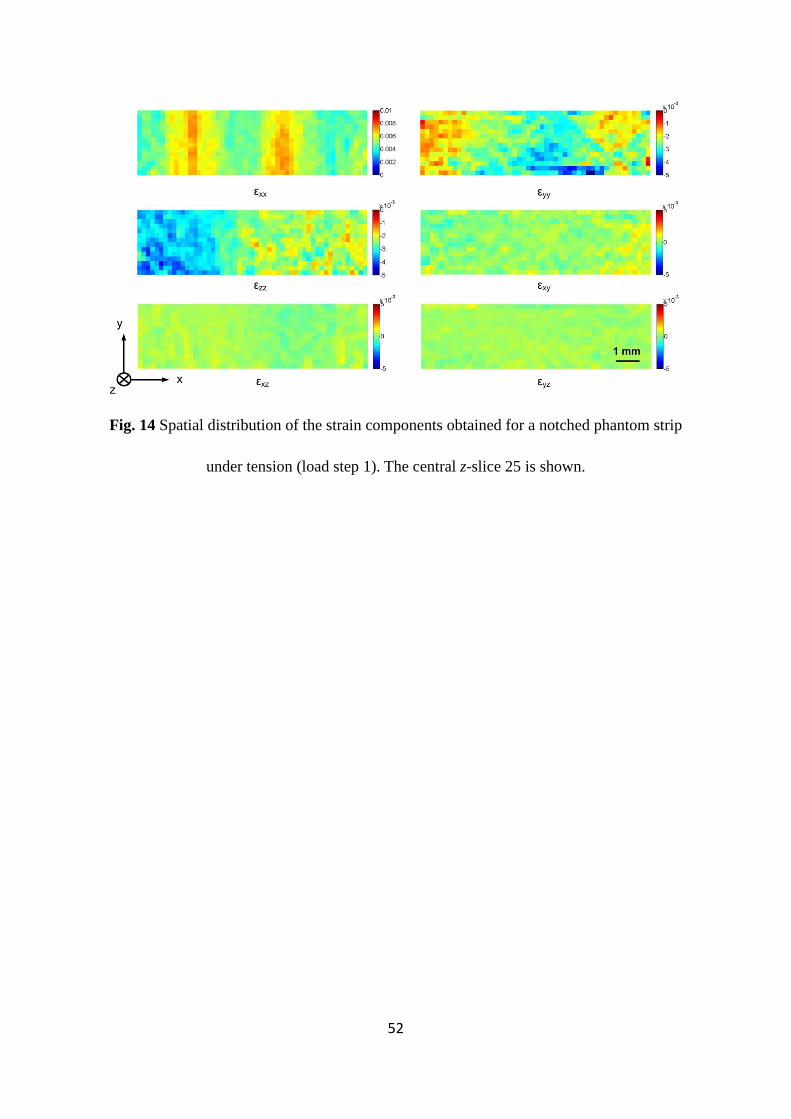
52

Fig. 14 Spatial distribution of the strain components obtained for a notched phantom strip

under tension (load step 1). The central z-slice 25 is shown.

53

Fig. 15 Spatial distribution of the strain components obtained for a notched phantom strip

under tension (load step 1). The central y-slice 10 is shown.

54

Fig. 16 Difference between the xU displacement averaged within x-slices along the

x-direction and a linear data fit obtained for a rectangular phantom strip under tension (load

step 1), with and without pre-smoothing.

55

Fig. 17 Strain standard deviations obtained with 363 voxels sub-volume, 50% overlap and

Gaussian pre-smoothing for: (a) Stationary test and (b) Rigid body translation test.

56

Fig. 18 Spatial distributions of the normal strain xxε obtained at central y-slice 10 for phantom

strips under tension (load step 1): (a) Rectangular, no pre-smoothing (b) Rectangular, with

pre-smoothing, (c) Notched, no pre-smoothing, (d) Notched, with pre-smoothing.