Analysis of interferograms of multi-layered biological samples obtained from full field optical...

Analysis of interferograms of multi-layered biologicalsamples obtained from full field optical coherence

tomography systems

Jenny Sokolovsky, Yitzhak Yitzhaky,* and Ibrahim AbdulhalimDepartment of Electro-Optics Engineering, Ben-Gurion University of the Negev, P.O. Box 653, Beer-Sheva 84105, Israel

*Corresponding author: [email protected]

Received 10 September 2012; accepted 16 October 2012;posted 18 October 2012 (Doc. ID 175923); published 6 December 2012

Several methods were developed in the past to analyze interferograms produced by optical coherencetomography, and successfully applied to simulated or animated samples. However, these techniquesdo not cope with noisy and distorted interferograms from biological tissues. In this paper, known tech-niques, including the fast Fourier transform and several variations of the continuous wavelet transform,were employed to analyze the interferogram data. However, to cope with the difficulties in biological data,pre- and post-processing procedures and adaptive thresholding were developed to provide stability androbustness. Additionally, three-dimensional structural models of the biological samples were con-structed, and revealed information like the number and locations of interfaces, the layer thicknessand pattern, and abnormalities. © 2012 Optical Society of AmericaOCIS codes: 120.3180, 170.4500, 120.2650, 110.7410.

1. Introduction

Optical coherence tomography (OCT) is aninterference-based imaging technique that is capableof producing high-resolution cross-sectional tomo-graphic imaging of a sample’s internal structure. Itis based on low-coherence interferometry, or whitelight interferometry [1,2]. OCT is a noninvasive, non-destructive technique that can be performed in situ/in vivo, and generates real time cross-section imageswith high depth and transverse resolutions. In thelast two decades, the OCT technique was developedin two aspects: new technical developments [2] andnew application expansions [1].

The full field OCT (FF-OCT) is usually based on animaging Michelson interferometer, where the illumi-nated beam is split into two beams: one is directedtoward the sample while the other toward the refer-ence mirror. After reflection, the two beams interfereand arrive to an imaging sensor (CCD/CMOS).

Microscope objectives are used to image both the re-ference and sample images on the imaging sensor(see several possible configurations in [3]). The depthscanning is facilitated by moving the reference mir-ror to change the reference path length. The inten-sity data along the depth is called interferogram orcorrelogram, and is characterized with bright anddark bands called “fringes.” Each bunch of fringescorresponds to a change in the refractive index, andtherefore contains the structural information regard-ing the scanned sample.

As for any interference intensity as a function ofthe sample depth z (“z-depth”), the interferogram ap-proximation can be expressed by a background inten-sity I0 and a series of sinusoidal interference fringesmodulated by visibility function V (also called coher-ence envelope) [4,5]:

I�z� � I0�1� V�z� cos�ϕ�z��: (1)

I0 and V depend on the system structure and thequality of the optical components, the structure ofthe sample, and spectral distribution of the light

1559-128X/12/358390-11$15.00/0© 2012 Optical Society of America

8390 APPLIED OPTICS / Vol. 51, No. 35 / 10 December 2012

source. The envelope of the fringes varies with otherfactors, such as sensitivity of the camera, the mea-sured object, and dispersion in the system. For theFF-OCT system, the envelope function depends alsoon the spatial coherence [6,7]. To investigate thestructure of a multilayered sample, the peaks of theinterferogram need to be localized. Various methodshave been developed to analyze the interferogramsignal, improve the accuracy, the speed of calcula-tion, and the immunity to noise. Most of the methodswere developed for surface profilometry application,which analyzes only the first fringe envelope createdby the surface of the sample [5]. These methods canbe divided into three approaches. One is based on thedetection of the top of the envelope, which modulatesthe interference fringes [8–10]. The second approachdetects the position of the bright or dark fringearound the envelope’s maximum [4,11,12]. This ap-proach is more sensitive to the optical path differ-ences; therefore, it requires phase measurementthat is often disturbed by the 2π ambiguity in iden-tifying the absolute fringe order. In this case, thephase is wrapped between �−π; π� and needs to be un-wrapped to recover the true continuous phase. Thethird approach combines the first two approaches byfirst detecting the envelope’s maximum and then im-plementing fine adjustments to precisely determinethe fringe peak [13].

To the best of our knowledge, detailed signal ana-lysis for thickness measurement application of biolo-gical samples was not reported in the literature, yet.These interferograms suffer from noise and distor-tions caused by the nonhomogeneity of the tissue.In this work we compare all of the aforementionedthree approaches by using the continuous wavelettransform (CWT). These approaches are comparedalso to the classical and efficient fast Fourier trans-form (FFT) envelope extraction method. In addition,we propose pre- and post-processing operations forbaseline and noise reduction, respectively. We alsoconstruct an adaptive threshold algorithm to over-come the noise variations over the sample and an al-gorithm to localize interfaces and distinguish themfrom outliers when the number of layers and theirlocations are unknown.

The rest of the paper is as follows: In Section 2 themethods employed for basic OCT signal analysis areshortly described. Section 3 presents the proposedmodifications to adapt the OCT signal analysis meth-ods to biological samples, followed by the construc-tion of the internal structure of these samples.Section 4 compares the performances of the originalmethods on ideally simulated interferogram and theperformances of proposed modifications using tworeal biological samples. Conclusions are presentedin Section 5.

2. Interferogram Analysis Techniques

This section gives a short description of the four sig-nal analysis methods employed here. These methodswere developed for interferograms of nonbiological

samples, which are significantly less noisy, and someof them for a profilometry application. The FFT [10]method is one of the pioneering methods for fringeenvelope extraction, while the other three methodswere examined by utilizing CWT [14–17].

A. FFT-based Interferogram Analysis

Chim and Kino [10] proposed to extract the envelopefunction by filtering the signal in the frequency do-main. After forward Fourier transform of the inter-ferogram signal, the zero frequency (DC) and thenegative frequencies are eliminated. Next, the abso-lute of inverse Fourier transform is calculated toobtain the fringe envelope V�z�.B. CWT-based Interferogram Analysis

All the three approaches were examined by utilizingCWT [14–17]. A wavelet with a most similar shape tothe signal’s shape is scanned along the signalwith dif-ferent scaling parameters. The output is a correlationtable between the signal and the wavelet, called sca-logram. The intensity envelope can be extracted bydetecting the magnitude of the maximum correlationcoefficient from each position along the scalogram,also called ridge. The phase can be calculated fromthe scalogram by taking arc-tangent of imaginarypart divided by real part of the coefficients.

a. Recknagel and Notni [14] and Sandoz [15] fol-low the first approach by detecting the peaks of theridge which can also be fitted to a curve (will be calledCWT ridge and CWT Gaussian fit methods).b. Sarac et al. [16] support the pure phase ap-

proach. The phase ofWavelet transform is calculated,unwrapped and linearly fitted for each scale. Theminimum of the derivative is sought in order to findthe scale at which the signal and transform phase dif-ference are close together. This method can detectonly one envelope peak per interferogram (will becalled CWT phase method).c. Tay et al. [17] follow the third approach, when

each peak extracted from the ridge is corrected bysubtracting respective phase (that is imaginary di-vided by real part of CWT at the specific scale andshift) multiplied by the central wavelength and di-vided by 2π (will be called CWT phase correctionmethod).

3. Proposed Modified Interferogram Analysis Methods

A. Mother Wavelet Selection

The success of the CWT depends on selection of amother wavelet, which should be of the same formas the signal. The OCT signal (assuming a Gaussiandistribution source) is characterized by a high-frequency sinusoidal that is modulated by Gaussian.Wavelet families which visually have a similar shapeare Paul, Morlet, complex Morlet, and Mexican hat.In this study, all these wavelets were tested. Wefound that only two wavelet families are suitable:complex Morlet and Paul. These wavelet familiesprovide a clear envelope of interferogram, while

10 December 2012 / Vol. 51, No. 35 / APPLIED OPTICS 8391

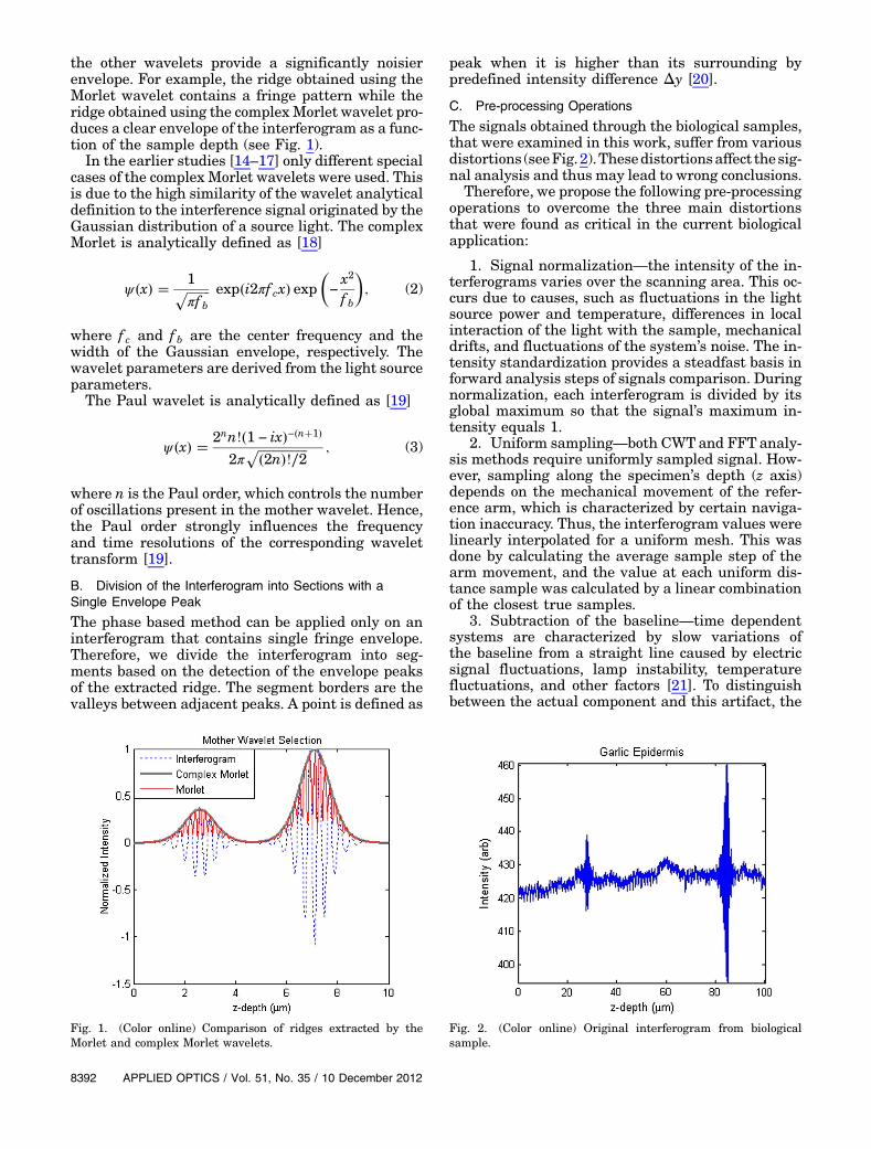
the other wavelets provide a significantly noisierenvelope. For example, the ridge obtained using theMorlet wavelet contains a fringe pattern while theridge obtained using the complexMorlet wavelet pro-duces a clear envelope of the interferogram as a func-tion of the sample depth (see Fig. 1).

In the earlier studies [14–17] only different specialcases of the complex Morlet wavelets were used. Thisis due to the high similarity of the wavelet analyticaldefinition to the interference signal originated by theGaussian distribution of a source light. The complexMorlet is analytically defined as [18]

ψ�x� � 1��πf b

p exp�i2πf cx� exp�−

x2

f b

�; (2)

where f c and f b are the center frequency and thewidth of the Gaussian envelope, respectively. Thewavelet parameters are derived from the light sourceparameters.

The Paul wavelet is analytically defined as [19]

ψ�x� � 2nn!�1 − ix�−�n�1�

2π��2n�!∕2

p ; (3)

where n is the Paul order, which controls the numberof oscillations present in the mother wavelet. Hence,the Paul order strongly influences the frequencyand time resolutions of the corresponding wavelettransform [19].

B. Division of the Interferogram into Sections with aSingle Envelope Peak

The phase based method can be applied only on aninterferogram that contains single fringe envelope.Therefore, we divide the interferogram into seg-ments based on the detection of the envelope peaksof the extracted ridge. The segment borders are thevalleys between adjacent peaks. A point is defined as

peak when it is higher than its surrounding bypredefined intensity difference Δy [20].

C. Pre-processing Operations

The signals obtained through the biological samples,that were examined in this work, suffer from variousdistortions (seeFig.2).Thesedistortionsaffect thesig-nal analysis and thus may lead to wrong conclusions.

Therefore, we propose the following pre-processingoperations to overcome the three main distortionsthat were found as critical in the current biologicalapplication:

1. Signal normalization—the intensity of the in-terferograms varies over the scanning area. This oc-curs due to causes, such as fluctuations in the lightsource power and temperature, differences in localinteraction of the light with the sample, mechanicaldrifts, and fluctuations of the system’s noise. The in-tensity standardization provides a steadfast basis inforward analysis steps of signals comparison. Duringnormalization, each interferogram is divided by itsglobal maximum so that the signal’s maximum in-tensity equals 1.

2. Uniform sampling—both CWTand FFT analy-sis methods require uniformly sampled signal. How-ever, sampling along the specimen’s depth (z axis)depends on the mechanical movement of the refer-ence arm, which is characterized by certain naviga-tion inaccuracy. Thus, the interferogram values werelinearly interpolated for a uniform mesh. This wasdone by calculating the average sample step of thearm movement, and the value at each uniform dis-tance sample was calculated by a linear combinationof the closest true samples.

3. Subtraction of the baseline—time dependentsystems are characterized by slow variations ofthe baseline from a straight line caused by electricsignal fluctuations, lamp instability, temperaturefluctuations, and other factors [21]. To distinguishbetween the actual component and this artifact, the

Fig. 1. (Color online) Comparison of ridges extracted by theMorlet and complex Morlet wavelets.

Fig. 2. (Color online) Original interferogram from biologicalsample.


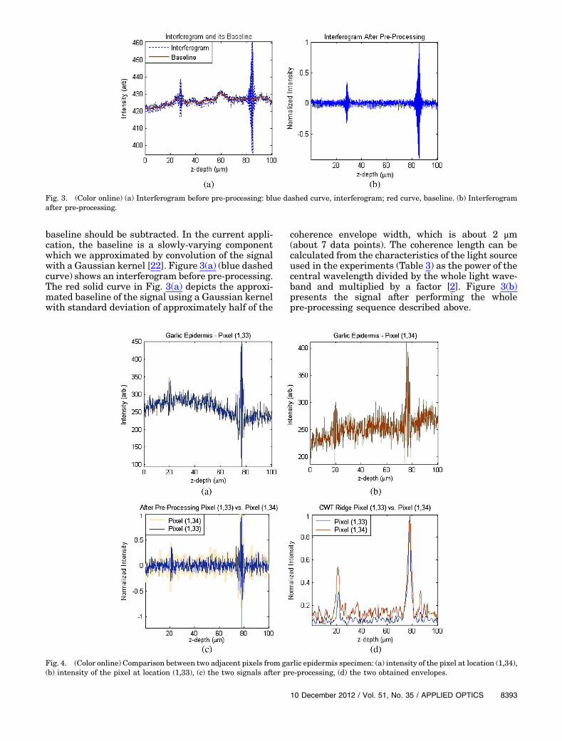
baseline should be subtracted. In the current appli-cation, the baseline is a slowly-varying componentwhich we approximated by convolution of the signalwith a Gaussian kernel [22]. Figure 3(a) (blue dashedcurve) shows an interferogram before pre-processing.The red solid curve in Fig. 3(a) depicts the approxi-mated baseline of the signal using a Gaussian kernelwith standard deviation of approximately half of the

coherence envelope width, which is about 2 μm(about 7 data points). The coherence length can becalculated from the characteristics of the light sourceused in the experiments (Table 3) as the power of thecentral wavelength divided by the whole light wave-band and multiplied by a factor [2]. Figure 3(b)presents the signal after performing the wholepre-processing sequence described above.

Fig. 3. (Color online) (a) Interferogram before pre-processing: blue dashed curve, interferogram; red curve, baseline. (b) Interferogramafter pre-processing.

Fig. 4. (Color online) Comparison between two adjacent pixels from garlic epidermis specimen: (a) intensity of the pixel at location (1,34),(b) intensity of the pixel at location (1,33), (c) the two signals after pre-processing, (d) the two obtained envelopes.


D. Adaptive Noise Elimination Thresholding

The signal analysis methods employed produce sig-nals with peaks at the locations where layers inter-face, thus, a peak detection stage is required. Thisprocess is carried out as described in Subsection 3.B,where all the points higher than their closest sur-rounding by a predefined value Δy are detected aspeaks. Therefore,Δy defines the sensitivity of the al-gorithm to the noise level. For a noisy signal, higherΔy avoids detection of the noise as peaks, while for aclean signal, smaller Δy prevents miss detection of areal peak.

In the case of the biological samples, the noise levelvaries over the scanned area. For example, Figs. 4(a)and 4(b) introduce two adjacent pixels from a garlicepidermis specimen. Figures 4(c) and 4(d) comparethe two pixels after pre-processing and after CWT,respectively. It can be seen that the noise level ofthe pixel located at coordinates (1,34) [blue curvein Fig. 4(a)] is almost twice the noise at pixel in

coordinates (1,33) (brown curve). Therefore, settingΔy to 0.2 will lead to oversensitivity of pixel (1,34),while setting it to 0.3 will lead to miss detection ofpixel (1,33) peak.

This example demonstrates the requirement thatthe parameter Δy should be adjusted to the noiselevel of each pixel in the sample.

We propose to set Δy based on the cumulative his-togram. The cumulative histogram counts the cumu-lative number of observations in all of the bins up tothe specified bin. That is, the cumulative histogramMi of a histogram mj is defined as: Mi �

Pij�1 mj,

Fig. 5. (Color online) Cumulative histograms of (a) pixel at location (1,34) and (b) pixel at location (1,33). The pink lines define the value ofΔy for each pixel according to a criterion of 90% of histogram.

Fig. 6. (Color online) Extracted envelope by FFT method withand without post-processing. Insert, magnified image of the firstpeak.

Fig. 7. (Color online) Simulated interferogram with two theore-tical layer interfaces. The inset emphasizes that there might bemiss sampling (the blue circles) of the layer interface location.

Table 1. Structure Parameters for Simulated Interferogram

Layer Width (μm) Refractive Index

First layer 2 1.3Second layer 3 1.5


wheremj is a histogram of the normalized intensitiesof the interferogram. A successful determination ofΔywas found to be the value of the normalized inten-sity where the histogram is accumulated to 0.9 of itsmaximum value (see Fig. 5). For example, for pixel(1,34), Δy equals 0.25, while for pixel (1,33), Δyequals 0.18. Such determined values match the noiselevels of these pixels [Fig. 4(d)].

E. Post-processing Operations for FFT Method

The envelope of the biological sample that is calcu-lated by taking the absolute value of the inverseFFT is very noisy (see Fig. 6 dashed blue curve).In this work we propose to accomplish the FFT anal-ysis with the following post-processing operations:

1. Noise filtering—using the same adaptivethreshold as explained in the previous section, thenoise is filtered out.

2. Smoothing—the signal above the threshold issmoothed by a convolution with a Gaussian kernel(with standard deviation σg � 3 data points in ourcase).

It can be seen in Fig. 6 (solid brown curve) thatafter the post-processing operations the envelope issignificantly smoother (compared to the dashed bluecurve in Fig. 6).

F. Identification of the Interface Location andDistinguishing Abnormalities

Each set of fringes in the interferogram correspondsto a change in the refractive index or thickness of thesample, which can be caused by either interior inter-face or by local abnormality. A concentration of out-liers can be assumed as an abnormality. Given thatthe number and location of interfaces is not pre-viously known, the algorithm first defines a global

Table 2. Summary of the Results from all the Methods Applied to the Simulated Signala

Peak Theoretical CWT-Ridge CWT-Gaussian Fit CWT-Phase CWT Phase Correction FFT

1st 2.6 2.6097 2.6121 2.6097 2.6078 2.60972nd 7.1 7.1132 7.111 7.1132 7.1148 7.0901aAll units are in micrometers. Note that complex Morlet and Paul mother wavelet provided exactly the same results, as shown in

the table.

Fig. 8. (Color online) Ridge of Paul 4 versus Paul 12 wavelet.

Fig. 9. (Color online) Ridge of complex Morlet versus Paul 12.

Table 3. Scanning Setup and Parameters for Garlic and Onion Epidermises

Garlic Epidermis [23] Onion Epidermis [24]

FF-OCT setup Michelson/Taylor LinnikLight source λc � 590 nm λc � 652 nm

Δλ � 177 nm Δλ � 196 nmSampling intervals in z axis (depth scanning) 65.9� 16 nm 89.3� 9 nm

Enface image of the top surface (200 × 200 pixels)


location of each interface based on a histogram of thelocations of the peaks detected from the wholescanned area at a certain range of depths. The histo-gram was divided into 100 bins, representing the100 μm of the sample depth. Each bin represents1 μm. This way the layer interface was about 5 μm.If a sum of counts of 5 adjacent bins is higher thanhalf of the total number of pixels in the scanned areathen the location of the highest bin is assumed as aglobal location of an interface. Thus, for each inter-ferogram, a closest peak to the location of global in-terface is defined as a local interface location whileothers are outliers. Following this analysis, it is easyto filter the outliers or the interfaces to investigatethe structure or the abnormalities of the sample,respectively. In addition, by globally localizing theinterfaces it is possible to fill missing data in theinterface surface using a local median filter.

4. Results

The performances of all the basic methods employedhere, as were proposed in the literature, werefirst examined on simulated OCT interferogram(Subsection 4.A), showing that all the basic methodsperform well when implemented to un-distorteddata. Afterward, the proposed modified methodswere examined and analyzed using two differentreal biological samples (Subsection 4.B), showingthe need and the performances of the proposedmodifications.

A. Examination of the Basic Methods with aOne-Dimensional Simulated OCT Signal

The simulation of the OCT signal (depicted in Fig. 7)is based on the model of Tomlins and Wang [2], usingthe Michelson configuration with the following sys-tem, scanning, and structure parameters (Table 1):

System parameters:

• Tr, Ts � 0.5• R � 1 (perfect mirror)

Scanning parameters:

• Source: λ0 � 0.8� 0.15 μm• Sampling step: 0.0231 μm

Based on the model of OCT signal [2], the distancebetween the peaks is equal to the layer width multi-plied by the reflection index. Therefore, in the aboveexample, the layer interfaces (see Fig. 7) should befound at: 2.6 and 7.1 μm. The inset in Fig. 7 illus-trates a zoom of the first peak that shows the possi-bility of miss-sampling of the theoretical location ofthe layer interface. For FF-OCT, and particularly forhigh NA and no index matching fluid, it was foundrecently by Safrani and Abdulhalim [7] that this isnot the case. Due to the refraction at the interface ofthe sample, the distance between the peaks corre-sponding to two consecutive interfaces becomesequal to the layer width divided by the ratio betweenthe refractive indices of the layer to that of the

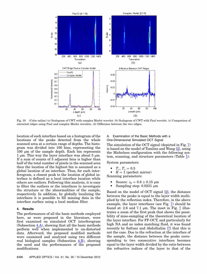
Fig. 10. (Color online) (a) Scalogram of CWT with complex Morlet wavelet. (b) Scalogram of CWT with Paul wavelet. (c) Comparison ofextracted ridges using Paul and complex Morlet wavelets. (d) Difference between the two ridges.


incidence medium. For more details the reader isreferred to [7].

All the methods provided results close to the truevalue for ideally simulated OCT signal, with devia-tion of 0.3%–0.47% (Table 2).

We found that the most suitable Paul wavelet isof order 12, since lower orders produce noisy signal(an example can be seen in Fig. 8 where order 4 iscompared to order 12). The complex Morlet andPaul wavelet of order 12 retrieve similar ridge ofthe simulated signal (see Fig. 9).

B. Experiments with Two Real Three-DimensionalBiological Specimens

Two biological samples, onion and garlic epidermis,were scanned by different FF-OCT setups and differ-ent scanning parameters (Table 3). The onion epider-mis has more than two times larger cells than garlicepidermis, which also enables an analysis of theshape of the interface [23,24].

1. Comparison Between Mother Wavelets for theReal DataAll the proposed methods based on CWT applied dif-ferent special cases of the complex Morlet wavelet. Inthis work we compared the performance of the com-plex Morlet wavelet and the Paul wavelet of order 12,also on biological samples (see Fig. 10). It can be seenthat there is a very slight difference between thefinal envelopes of the analyzed signal. However,complex Morlet requires only 7 scales while Paulrequires 15 scales [Figs. 10(a) and 10(b), respec-tively]. This directly leads to throughput differences.

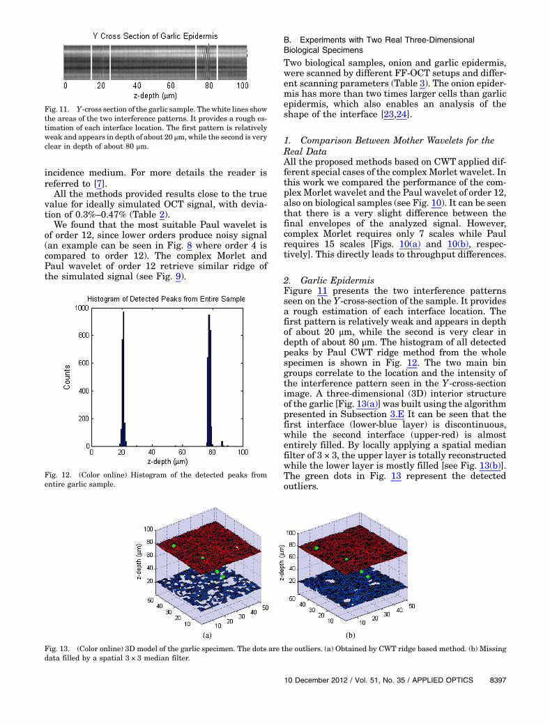
2. Garlic EpidermisFigure 11 presents the two interference patternsseen on the Y-cross-section of the sample. It providesa rough estimation of each interface location. Thefirst pattern is relatively weak and appears in depthof about 20 μm, while the second is very clear indepth of about 80 μm. The histogram of all detectedpeaks by Paul CWT ridge method from the wholespecimen is shown in Fig. 12. The two main bingroups correlate to the location and the intensity ofthe interference pattern seen in the Y-cross-sectionimage. A three-dimensional (3D) interior structureof the garlic [Fig. 13(a)] was built using the algorithmpresented in Subsection 3.E It can be seen that thefirst interface (lower-blue layer) is discontinuous,while the second interface (upper-red) is almostentirely filled. By locally applying a spatial medianfilter of 3 × 3, the upper layer is totally reconstructedwhile the lower layer is mostly filled [see Fig. 13(b)].The green dots in Fig. 13 represent the detectedoutliers.

Fig. 13. (Color online) 3D model of the garlic specimen. The dots are the outliers. (a) Obtained by CWT ridge based method. (b) Missingdata filled by a spatial 3 × 3 median filter.

Fig. 12. (Color online) Histogram of the detected peaks fromentire garlic sample.

Fig. 11. Y-cross section of the garlic sample. The white lines showthe areas of the two interference patterns. It provides a rough es-timation of each interface location. The first pattern is relativelyweak and appears in depth of about 20 μm, while the second is veryclear in depth of about 80 μm.


Fig. 14. (Color online) 3D models of the onion specimen (left column) and their corresponding histograms (right column) obtained byproposed modified methods: (a), (b) CWT ridge; (c), (d) CWT phase correction; (e), (f) CWT Gaussian fit (g), (h) CWT phase; (i), (j) FFT.


3. Onion EpidermisIn this section, all the modified methods are appliedto the onion epidermis sample. Figure 14 presents acomparison of the resulting 3D models of the onionepidermis. For a more convenient presentation andcomparison, the outliers were filtered out. A respec-tive histogram of the resulting interface depths ispresented for each modified method for an additionalaspect of the method’s performances. Unlike the pre-vious Garlic sample, in this case only one interfacewas identified. The smaller peak observed on the his-togram at about 13 μm depth results from the edgeregions of the curvatures at the interface surface.

4. Computation LoadThe proposed analysis can be divided into four parts:the pre-processing, the peak detection algorithm, theadaptive thresholding algorithm, and the distin-guishing algorithm. The dimensions of the presentedonion sample are 100 × 100 × 225 points. The follow-ing computationswere done usingMATLAB softwarewith a Gigabyte, Pentium M processor, 2 Gb RAM atWindows XP SP3. The pre-processing and the adap-tive thresholding are common to all the methods.The pre-processing algorithm computation time de-pends on the sample size and takes about 14 s, while

adaptive thresholding also depends onnumber of binsof the histogram and takes about 3 s for 100 bins.However, the peak distinguishing algorithm dependson the amount of peaks detected at the peak detectionstage. The computation time of each method and itsrespective data distinguishing algorithm are pre-sented in Table 4.

5. Conclusions for Real Biological SpecimensAccording to the comparisons presented in Fig. 14and Table 4, the performances of the modified inter-ferogram analysis methods applied to the onionspecimen can be summarized as follows:

CWT Ridge Method—is the fastest CWT method andprovides relatively smooth interface.CWT Gaussian Fit Method—according to the litera-ture [15], the Gaussian curve fitting should increasethe accuracy of the ridge method. It is clearly seenfrom the 3D model and its histogram [see Fig. 14(c)]that the interface is smoother. On the other hand,some outliers (seen at the histogram) appear due tofailures in the curve fitting.CWT Phase Method—the 3D model and its corre-sponding histogram demonstrates very noisy results.The concept of this method is to find the best match-ing scale to the total interference pattern while theridge methods define the best matching scale to eachlocation. Moreover, this is the slowest method andthe huge amount of over-detected peaks slows downalso the peak distinguishing process.CWT Phase Correction Method—requires previousknowledge of the illumination central wavelength.According to the literature [16], the phase correctionis expected to provide results that are more precisethan the ridge method. However, from the obtained3D model and its respective histogram, there is nosignificant improvement. Moreover, since the correc-tion is added to the prior detected envelope peak, thiscorrection may even increase the error if miss detec-tion occurs during the ridge extraction.

Table 4. Computation Time for Each Method Is the Sum of thePeak Detection Time and the Duration of the Distinguishing

Algorithm (at the right column)

Peak Detection (s)

ComplexMorlet

Paul12 FFT

DistinguishingAlgorithm (s)

CWT Ridge 64.02 88.12 0.29CWT Gaussian Fit 82.42 110.33 0.38CWT Phase 135.40 239.38 3.29CWT PhaseCorrection

64.25 91.70 0.47

FFT 25.87 0.87

Fig. 15. (Color online) Onion epidermis (a) 3D structural model obtained by the improved FFT method, (b) Y-cross section of the onionepidermis, showing the interface location at 8 μm, (c) XY-cross-section of the onion epidermis (100 × 100 pixels).


FFT Method—the post-processing includes smooth-ing of the signal before activating peak detectionalgorithm. Therefore, similarly to the Gaussian cor-rection method, the extracted interface is smooth. Inaddition, this is the simplest and the fastest methodamong all the tested methods. In contrast to themethods based on the CWT, there is no need to selectthe wavelet function and its parameters such asscaling or order.

Figure 15(a) shows the 3D internal structure of theonion specimen based on FFT method. The interfacelocation and curvature fits the location and curva-ture of the interface as shown in the Y-cross-sectionof the sample in Fig. 15(b). In addition, the interfacesurface pattern agrees with the cell pattern seenfrom the top view of the onion epidermis specimen(Z-cross) as shown in Fig. (15c).

5. Summary

The main novelties in this study are the modifica-tions and supplemental processing to OCT interfer-ograms analysis methods, proposed to cope with thesignal distortions induced from the nature of the bio-logical specimens. This study compared the perfor-mances of four modified interferograms analysismethods using two biological samples. It is concludedthat the FFT-based method is the simplest and fast-est one that also provides smooth interface surface.In addition, it was found that the Paul and the com-plex Morlet wavelets provide results with similarquality. Only the phase-based method was found tobe noncompatible for the current application. Theproposed algorithms enabled the building of a 3Dmodel of the interior structure that reveals the 3Dlayer structure of the biological specimen, includingthe number and thickness of the layers, the interfacepattern, and abnormalities.

The authors are thankful to Ron Friedman, LiorLeraz, and Rony Sharon for letting their experimen-tal data be made available for this study.

References1. D. Stifter, “Beyond biomedicine: a review of alternative appli-

cations and developments for optical coherence tomography,”Appl. Phys. B 88, 337–357 (2007).

2. P. H. Tomlins and R. K. Wang, “Theory, development andapplications of optical coherence tomography,” J. Phys. D38, 2519–2535 (2005).

3. I. Abdulhalim, “Theory for double beam interferometricmicroscopes and experimental verification using the Linnikmicroscope,” J. Mod. Opt. 48, 279–302 (2001).

4. P. De Groot and L. Deck, “Surface profiling by analysis ofwhite light interferograms in the spatial frequency domain,”J. Mod. Opt. 42, 389–401 (1995).

5. D. Malacara, Optical Shop Testing, 3rd ed. (Wiley, 2007).6. I. Abdulhalim, “Competence between spatial and temporal

coherence in full field optical coherence tomography and inter-ference microscopy,” J. Opt. Pure Appl. Opt. 8, 952–958 (2006).

7. A. Safrani and I. Abdulhalim, “Spatial coherence effect onlayers thickness determination in narrowband full field opti-cal coherence tomography,” Appl. Opt. 50, 3021–3027 (2011).

8. P. J. Caber, “Interferometric profiler for rough surfaces,” Appl.Opt. 32, 3438–3441 (1993).

9. S. C. Chim and G. S. Kino, “Three dimensional image realiza-tion in interference microscopy,” Appl. Opt. 31, 2550–2553(1992).

10. S. C. Chim and G. S. Kino, “Mirau correlation microscope,”Appl. Opt. 29, 3775–3783 (1990).

11. K. G. Larkin, “Efficient non linear algorithm for envelopedetection in white light interferometry,” J. Opt. Soc. Am. A13, 832–843 (1996).

12. P. Sandoz, “An algorithm for profilometry by white-lightphase-shifting interferometry,” J. Mod. Opt. 43, 1545–1554(1996).

13. M. C. Park and S. W. Kim, “Direct quadratic polynominalfitting for fringe peak detection of white light scanning inter-ferogram,” Opt. Eng. 39, 952–959 (2000).

14. R. Recknagel and G. Notni, “Analysis of white light interfer-ograms using wavelet methods,” Opt. Commun. 148, 122–128(1998).

15. P. Sandoz, “Wavelet transform as a processing tool in whitelight interferometry,” Opt. Lett. 22, 1065–1067 (1997).

16. Z. Sarac, A. Dursun, S. Yerdelen, and F. N. Ecevit, “Waveletphase evaluation of white light interferograms,” Meas. Sci.Technol. 16, 1878–1882 (2005).

17. C. J. Tay, C. Quan, and C. Li, “Investigation of a dual layerstructure using vertical scanning interferometry,”Opt. LasersEng. 45, 907–913 (2007).

18. A. Teolis, Computational Signal Processing with Wavelets(Birkhauser, 1998).

19. I. De Moortel, S. A. Munday, and A. W. Hood, “Waveletanalysis: the effect of varying basic wavelet,” Sol. Phys.222, 203–228 (2004).

20. E. Billauer, “Peakdet: peak detection using MATLAB,” http://billauer.co.il/peakdet.html.

21. Y. Kazakevich and R. Lobrutto, HPLC for PharmaceuticalScientists (Wiley, 2010).

22. A. T. Bui and R. K. Taira, Medical Imaging Informatics(Springer, 2010).

23. R. Sharon, R. Friedmann, and I. Abdulhalim, “Multilayeredscattering reference mirror for full field optical coherencetomography with application to cell profiling,” Opt. Commun.283, 4122–4125 (2010).

24. I. Abdulhalim, R. Friedman, L. Liraz, andR. Dadon, “Full fieldfrequency domain commonpath optical coherence tomographywith annular aperture,” Proc. SPIE 6627, 662719 (2007).


http://billauer.co.il/peakdet.html





Analysis of interferograms of multi-layered biological samples obtained from full field optical...

Documents

Transcript of Analysis of interferograms of multi-layered biological samples obtained from full field optical...