Morphometric Analysis of Ophthalmic Optical Coherence ...

Morphometric Analysis of Ophthalmic

Optical Coherence Tomography Images

by

Sieun LeeB.Sc. (Hons.), Simon Fraser University, 2009

Thesis Submitted in Partial Fulfillment

of the Requirements for the Degree of

Doctor of Philosophy

in the

School of Engineering Science

Faculty of Applied Sciences

c© Sieun Lee 2015

SIMON FRASER UNIVERSITY

Spring 2015

All rights reserved.

However, in accordance with the Copyright Act of Canada, this work may be

reproduced without authorization under the conditions for ”Fair Dealing”.

Therefore, limited reproduction of this work for the purposes of private study,

research, criticism, review and news reporting is likely to be in accordance

with the law, particularly if cited appropriately.

APPROVAL

Name: Sieun Lee

Degree: Doctor of Philosophy

Title: Morphometric Analysis of Ophthalmic Optical Coherence To-mography Images

Examining Committee: Chair: Dr. Andrew RawiczProfessor, School of Engineering Science

Dr. Mirza Faisal Beg Co-Senior Supervisor

Professor, School of Engineering Science

Dr. Marinko V. Sarunic Co-Senior Supervisor

Associate Professor, School of Engineering Science

Dr. Paul J. Mackenzie Supervisor

Assistant Professor, Department of Ophthalmology

and Visual Sciences, University of British Columbia

Dr. Pierre Lane Internal Examiner

Associate Professor of Professional Practice, School

of Engineering Science

Dr. J. Crawford Downs External Examiner

Professor of Ophthalmology, School of Medicine,

University of Alabama at Birmingham

Date Approved: April 14, 2015

ii

Partial Copyright Licence

iii

Abstract

Optical coherence tomography (OCT) provides in-vivo, high-resolution, cross-sectional

images of the inner structures of the eye. This dissertation outlines the construction and

application of a computational pipeline for morphometric analysis of 3D retinal and peripap-

illary OCT images for extracting clinically meaningful information based on shape features.

The images were acquired by a prototype 1060-nm swept-source OCT system and pro-

cessed to enhance the image quality. Next, retinal layers and structures in the optic nerve

head (ONH) and laminar regions were segmented. A graph-cut based, robust 3D algo-

rithm was implemented for automated segmentation of the retinal layers. The segmented

structures was measured by quantitative shape parameters, such as 3D layer thickness

and Bruch’s membrane opening (BMO) dimension.

A special focus was given to establishing anatomical correspondence across multiple

OCT images, for longitudinal or cross-sectional data, via registration. In the first approach,

retinal surfaces from two OCT images were registered by a mathematical current-based

deformation followed by spherical demons registration. In the second approach, retinal

surfaces and their signal values (ex. layer thickness) from several OCT images were jointly

varied to generate a group mean template serving as the common atlas.

In the clinical application of the pipeline, peripapillary OCT volumes of 52 myopic eyes

from normal and glaucomatous subjects were studied. Retinal layer thicknesses, and

shape features of BMO, Bruch’s membrane, and the anterior laminar region were mea-

sured and statistically analyzed. Significant differences were observed between the nor-

mal and glaucomatous groups, demonstrating glaucomatous deformation, and structural

changes correlated with myopia suggested a possible explanation to the high glaucoma

susceptibility associated with advanced myopia.

Image analysis; Image processing; Shape analysis; Optical coherence tomography;

Ophthalmology

iv

Acknowledgments

The work in this thesis could not have been possible without the constant mentor-

ship, encouragement, and guidance from my co-senior supervisors, Dr. Faisal Beg and

Dr. Marinko Sarunic, who took me on as an undergraduate student seven years ago and

personally saw through my growth as a researcher. I am also very grateful to Dr. Paul

Mackenzie for the supervision and guidance, with sharp insights of a clinician and stimu-

lating discussions. I am very thankful for my examining committee, Dr. Andrew Rawicz, Dr.

Pierre Lane, and Dr. J. Crawford Downs, for taking the time and effort to provide valuable

assessment of my work.

I am indebted to my fellow students at Biomedical Optics Research Group and Medical

Image Analysis Lab for their support and friendship. I am especially thankful to Dr. Evgeniy

Lebed, Ms. Sherry Han, and Ms. Morgan Heisler, with whom I had a chance to work closely

through various projects. I also thank the research collaborators in Canada and France for

the opportunities to benefit from their expertise and dedication.

My friends and family have stood by me throughout my graduate years. Words cannot

express my gratitude to my parents for their unwavering love and support. Lastly, I want to

thank God for giving the joy, gratitude, and deeper meaning in my life.

v

Contents

Approval ii

Partial Copyright License iii

Abstract iv

Acknowledgments v

Contents vi

List of Tables ix

List of Figures xi

1 Introduction 1

2 Background 4

2.1 The human eye . . . . . . . . . . . . . . . . . . . . . . . . . . . . . . . . . . 4

2.1.1 Retina . . . . . . . . . . . . . . . . . . . . . . . . . . . . . . . . . . . 5

2.1.2 Fovea and optic nerve head . . . . . . . . . . . . . . . . . . . . . . . 6

2.2 Glaucoma . . . . . . . . . . . . . . . . . . . . . . . . . . . . . . . . . . . . . 7

2.3 Optical coherence tomography . . . . . . . . . . . . . . . . . . . . . . . . . 9

2.4 OCT in ophthalmology . . . . . . . . . . . . . . . . . . . . . . . . . . . . . . 10

3 Image Acquisition and Preprocessing 11

3.1 Acquisition . . . . . . . . . . . . . . . . . . . . . . . . . . . . . . . . . . . . 11

3.2 Quality control and data management . . . . . . . . . . . . . . . . . . . . . 12

3.3 Preprocessing . . . . . . . . . . . . . . . . . . . . . . . . . . . . . . . . . . 14

vi

3.3.1 Motion correction . . . . . . . . . . . . . . . . . . . . . . . . . . . . . 14

3.3.2 Bounded variation image smoothing . . . . . . . . . . . . . . . . . . 19

3.4 Summary of contributions . . . . . . . . . . . . . . . . . . . . . . . . . . . . 20

4 Segmentation 22

4.1 Manual segmentation of ONH structures . . . . . . . . . . . . . . . . . . . . 22

4.2 Automated segmentation of retinal layers . . . . . . . . . . . . . . . . . . . 24

4.3 Choroid segmentation . . . . . . . . . . . . . . . . . . . . . . . . . . . . . . 26

4.3.1 Comparison of choroid segmentation in in 830 nm and 1060 nm OCT

images . . . . . . . . . . . . . . . . . . . . . . . . . . . . . . . . . . 27

4.3.2 Repeatability analysis of choroidal thickness measurements in age-

related macular degeneration . . . . . . . . . . . . . . . . . . . . . . 30


5 Retinal Surface Registration 44

5.1 Exact surface-to-surface registration . . . . . . . . . . . . . . . . . . . . . . 46

5.1.1 Methods . . . . . . . . . . . . . . . . . . . . . . . . . . . . . . . . . . 46

5.1.2 Results . . . . . . . . . . . . . . . . . . . . . . . . . . . . . . . . . . 50

5.1.3 Discussion . . . . . . . . . . . . . . . . . . . . . . . . . . . . . . . . 53

5.2 Repeatability Analysis in Longitudinal OCT Images . . . . . . . . . . . . . . 60

5.2.1 Materials and Methods . . . . . . . . . . . . . . . . . . . . . . . . . 60

5.2.2 Results . . . . . . . . . . . . . . . . . . . . . . . . . . . . . . . . . . 61

5.3 Atlas-based Shape Variability Analysis and Classification of OCT Images

using the Functional Shape (fshape) Framework . . . . . . . . . . . . . . . 75

5.3.1 Atlas Estimation . . . . . . . . . . . . . . . . . . . . . . . . . . . . . 76

5.3.2 Variability Analysis and Classification . . . . . . . . . . . . . . . . . 86

5.3.3 Experimental Results . . . . . . . . . . . . . . . . . . . . . . . . . . 91

5.3.4 Discussion . . . . . . . . . . . . . . . . . . . . . . . . . . . . . . . . 97


6 Optic Nerve Head Morphometrics in Myopic Glaucoma 101

6.1 Participants . . . . . . . . . . . . . . . . . . . . . . . . . . . . . . . . . . . . 102

6.2 Methods . . . . . . . . . . . . . . . . . . . . . . . . . . . . . . . . . . . . . . 103

vii

6.2.1 Acquisition and processing . . . . . . . . . . . . . . . . . . . . . . . 103

6.2.2 Segmentation . . . . . . . . . . . . . . . . . . . . . . . . . . . . . . . 104

6.2.3 Measurements . . . . . . . . . . . . . . . . . . . . . . . . . . . . . . 104

6.2.4 Analysis . . . . . . . . . . . . . . . . . . . . . . . . . . . . . . . . . . 107

6.3 Results . . . . . . . . . . . . . . . . . . . . . . . . . . . . . . . . . . . . . . 108

6.4 Discussion . . . . . . . . . . . . . . . . . . . . . . . . . . . . . . . . . . . . 110

6.4.1 Nerve Fiber Layer Thickness . . . . . . . . . . . . . . . . . . . . . . 111

6.4.2 Bruch’s Membrane Opening Shape . . . . . . . . . . . . . . . . . . 112

6.4.3 Peripapillary Bruch’s Membrane Shape . . . . . . . . . . . . . . . . 113

6.4.4 Choroidal Thickness . . . . . . . . . . . . . . . . . . . . . . . . . . . 115

6.5 Anterior lamina cribrosa region morphometrics . . . . . . . . . . . . . . . . 115


7 Conclusion 131

7.1 Future directions . . . . . . . . . . . . . . . . . . . . . . . . . . . . . . . . . 133

Bibliography 135

viii

List of Tables

4.1 Descriptive Statistics of the Choroidal Thickness Measured by the First Rater

(Rater 1), Second Rater (Rater 2), and the Algorithm (Auto) . . . . . . . . . 35

4.2 Intraclass Correlation and Paired Mean Difference for Choroidal Thickness

Measurement Between the Raters (Rater 1, Rater 2) and the Algorithm (Auto) 35

4.3 Intraclass Correlation and Paired Mean Difference for Choroidal Thickness

Measurement Between the Repeat Scans by the Raters (Rater 1, Rater 2)

and the Algorithm (Auto) . . . . . . . . . . . . . . . . . . . . . . . . . . . . . 37

4.4 Results of Multivariable Regression Analysis Between Drusen Area and

Choroid Thickness Measured by the Rater (Rater 1 and Rater 2) and the

Automated Algorithm (Auto) . . . . . . . . . . . . . . . . . . . . . . . . . . . 38

5.1 BMO area mean, minimum, maximum, standard deviation, and coefficient

of variation for 9 repeat measurements over 3 weeks from 6 healthy subjects. 62

5.2 BMO eccentricity mean, minimum, maximum, standard deviation, and coef-

ficient of variation for 9 repeat measurements over 3 weeks from 6 healthy

subjects. . . . . . . . . . . . . . . . . . . . . . . . . . . . . . . . . . . . . . . 63

5.3 RNFL thickness standard deviation . . . . . . . . . . . . . . . . . . . . . . . 66

5.4 Choroidal thickness standard deviation . . . . . . . . . . . . . . . . . . . . . 71

5.5 Accuracies, sensitivities, and specificities of the classification of healthy,

glaucomatous, and suspect RNFLs . . . . . . . . . . . . . . . . . . . . . . . 95

5.6 Accuracies, sensitivities, and specificities of the classification of healthy and

glaucomatous RNFLs by RNFL thickness only and RNFL posterior surface

geometry only . . . . . . . . . . . . . . . . . . . . . . . . . . . . . . . . . . . 96

5.7 Accuracies, sensitivities, and specificities of the classification of healthy,

glaucomatous, and suspect RNFLs based on unregistered RNFLs . . . . . 97

ix

6.1 Demographics and Clinical Characteristics of the Study Subjects by Group 103

6.2 Performance of the automated segmentation of peripapillary structures . . 108

6.3 Multiple Regression Analysis of Shape Parameters With Age, Axial Length,

and Mean Deviation (MD): Mean Nerve Fiber Layer Thickness, BMO Area,

BMO Eccentricity, BMO Planarity, BMO Depth, Mean BM Depth, and Mean

Choroidal Thickness . . . . . . . . . . . . . . . . . . . . . . . . . . . . . . . 119

6.4 Multiple Regression Analysis of Shape Parameters With Age, Axial Length,

and Mean Deviation (MD): Mean Nerve Fiber Layer Thickness, BMO Area,

BMO Eccentricity, BMO Planarity, BMO Depth, Mean BM Depth, and Mean

Choroidal Thickness . . . . . . . . . . . . . . . . . . . . . . . . . . . . . . . 120

x

List of Figures

1.1 OCT visualization of the optic nerve head. . . . . . . . . . . . . . . . . . . . 2

1.2 Computational pipeline of ophthalmic OCT images. . . . . . . . . . . . . . . 3

2.1 a) Schematic of the human eye. The image is from Wikimedia.org and repro-

duced here under the Creative Commons License. b) Light micrograph of a

vertical section through central human retina. The image is from Webvision

[105] and reproduced here under the Creative Commons License. . . . . . 5

2.2 a) Schematic of the optic nerve head, a reproduction from Gray’s Anatomy.

b) Ganglion cell axonal pattern. The image is from Webvision [105] and

reproduced here under the Creative Commons License. . . . . . . . . . . . 7

2.3 a) Progressive vision loss in glaucoma. Image source: National Eye In-

stitute, National Institutes of Health. b) Glaucomatous deformation in the

laminar region.1 . . . . . . . . . . . . . . . . . . . . . . . . . . . . . . . . . . 8

2.4 A simple Michelson interferometer schematic of optical coherence tomogra-

phy. (BS: beam splitter.) . . . . . . . . . . . . . . . . . . . . . . . . . . . . . 9

2.5 Ophthalmic OCT imaging of a) macular region and b) peripapillary region. . 10

3.1 Schematic of the swept-source optical coherence tomography system setup.

Source: Axsun SS Module; PC: polarization controller; BD: balanced detec-

tor; fn, focal length of the lens, where n = 1, 2, 3.[194] . . . . . . . . . . . . 12

3.2 Prototype optical coherence tomography system set up at the Eye Care

Centre, Vancouver General Hospital. . . . . . . . . . . . . . . . . . . . . . . 13

3.3 (a) Imaged region and scanning direction displayed on fundus photography.

(b) Volume reconstruction from raw data. (c) Volume visualized in 3D. . . . 14

3.4 A quick-check image of an OCT dataset. . . . . . . . . . . . . . . . . . . . . 15

xi

3.5 The first column shows the sectioning plane of the images in the second

column, and the third column illustrates motion visible in each of these im-

ages. In the first row, a B-scan (fast scan) is shown (b) in the direction of

frame acquisition (a). In the second row, an axial cross section (slow scan)

(e) orthogonal to the B-scan (as shown in (d)) displays wave-like axial mo-

tion artifact (f). In the third row, a sum-voxel en-face image in the plane (e)

displays lateral and elevation motion artifact (i) by the uneven blood vessel

boundaries and discontinuities in the image. . . . . . . . . . . . . . . . . . . 16

3.6 (a) Slow scan with maximum cross-correlation displacement profile. (b)

Same scan corrected by flattening the profile. (c) Same scan corrected by

fitting a smooth curve to the profile. The red arrows in (b) and (c) indicate

the cup depth measured in each image. (d) Volume before motion correc-

tion. The volume has been rotated that the axial axis lies vertically and the

en-face plane lies horizontally. (e) Same volume after smooth-fitting motion

correction. . . . . . . . . . . . . . . . . . . . . . . . . . . . . . . . . . . . . . 21

3.7 Example of BV smoothing . . . . . . . . . . . . . . . . . . . . . . . . . . . . 21

4.1 Example of a) automated segmentation of retinal layers and b) manual point

segmentation. . . . . . . . . . . . . . . . . . . . . . . . . . . . . . . . . . . . 23

4.2 Top: B-scan of a 1060-nm OCT macular volume. Bottom: Automated seg-

mentation of inner limiting membrane (green), Bruch’s membrane equivalent

(cyan), and estimated choroid-sclera boundary (CS-boundary). . . . . . . . 28

4.3 Macular OCT images (Left) and their segmentations (Right). Top: 830-nm

2D averaged EDI-OCT scans acquired with Cirrus SD-OCT. Middle: 830-

nm 3D scans acquired with Cirrus SD-OCT. Bottom: 1060-nm 3D scans

acquired with the prototype 1060-nm SS-OCT. . . . . . . . . . . . . . . . . 29

4.4 Segmentation of a 3D macular scan acquired with 830-nm Cirrus SD-OCT

system. . . . . . . . . . . . . . . . . . . . . . . . . . . . . . . . . . . . . . . 30

4.5 Segmentation of a 3D macular scan acquired with 1060-nm prototype SS-

OCT system. . . . . . . . . . . . . . . . . . . . . . . . . . . . . . . . . . . . 31

4.6 a) Sumvoxel projection of the macular choroid in a 1060-nm scan b) Total

retinal thickness colormap. c) Choroid thickness colormap. . . . . . . . . . 32

xii

4.7 Example of an automated subfoveal choroidal thickness measurement. Top

shows the original image. Bottom shows the segmented image. The ILM

(green), BM (blue), and choroid-sclera (CS) boundary (magenta) were seg-

mented automatically, and the choroidal thickness was measured as the ver-

tical distance between BM and CS boundary at the red dash line indicating

the foveal pit. . . . . . . . . . . . . . . . . . . . . . . . . . . . . . . . . . . . 34

4.8 Bland-Altman plots showing the interrater variability of choroidal thickness

measurements between the two manual raters (left), and between the man-

ual raters (averaged) and the automated algorithm. The dotted lines indicate

the upper and lower 95% confidence interval limits (N = 83). . . . . . . . . 36

4.9 Examples of segmentation by the first rater (red), second rater (yellow), and

the algorithm (magenta). The first and second scans show the three mea-

surements close to each other. In the third scan, the posterior choroidal

boundary is located deep with low edge strength, and the automated mea-

surement is smaller than the manual measurements. In the fourth scan a

large drusen reduces the visibility of the posterior choroidal boundary. . . . 42

4.10 Example of different choroid-sclera boundary measurements by the first

rater (red), second rater (yellow), and the algorithm (magenta). . . . . . . . 43

4.11 Repeat scans of the same fovea with different image quality. . . . . . . . . . 43

5.1 The proposed registration scheme. (a) The subject S is first brought into

close proximity with the template T by the method of surface currents φc

to produce an in-exact matching result. (b) A point-to-point correspondence

between S and T is achieved by registering φc(S) to T via spherical demons.

The end result matches the topology of the template. (c) Registration of the

four anatomical surfaces (ILM, BM, NFL and choroid) to the template by

φs(φc(Si)). . . . . . . . . . . . . . . . . . . . . . . . . . . . . . . . . . . . . . 48

5.2 3D checkerboard pattern propagation by the computed inverse mappings

Φ−1i . The top row shows the propagated checkerboard patterns of the NFL

surface while the bottom row shows the propagated checkerboard pattern

on the ILM surfaces. The surfaces shown in the first column are the NFL

and ILM surfaces of the template T . . . . . . . . . . . . . . . . . . . . . . . 51

xiii

5.3 Left column: NFL. First image: mean NFL thickness of the control group.

Second image: mean NFL thickness of the glaucomatous group. Third and

fourth images: t and p-values, respectively. Right column: choroid. First

image: mean choroidal thickness, shown in mm, of the control group. Sec-

ond image: mean choroidal thickness of the glaucomatous group. Third and

fourth images: t and p-values, respectively. . . . . . . . . . . . . . . . . . . 57

5.4 Phantom longitudinal data registration and validation. (a) Schematic depict-

ing the presence of a focal damage on the NFL and retinal thinning. Blue and

green lines represent the surfaces at time points 1 and 2, respectively. (b)

3D rendering of the phantom NFL surface at time point 2, showing the mod-

eled focal damage and retinal thinning. Colormap represents the computed

NFL thickness. (c) NFL surface at time point 1. (d) Modified NFL surface at

time point 2. The surface is translated by [0.4, 0.6, 0.2]mm, and rotated by

−10. Red rectangles highlight the modeled changes in morphometry. (e)

Surface from (d) registered to the surface from (c). Colormap represents the

differences in NFL thickness between time point 1 and registered time point

2. (f) The colormap from (e) thresholded by the intrinsic axial resolution

of the OCT system. Red represent decreased NFL thickness while green

represents increased NFL thickness. . . . . . . . . . . . . . . . . . . . . . . 58

5.5 Longitudinal analysis of NFL and choroidal thickness. Top row: Surfaces

and data from Time Point 1. Second row: Surfaces and data from Time

Point 2 (one year later). Third row: Surfaces and data from Time Point 1

registered to surfaces from Time Point 2. Fourth row: Difference in thickness

measurements from the two time points. Last row: thresholded difference in

thickness, in terms of the axial resolution of the OCT system lc (lc = 6µm).

Increased and decreased thicknesses are represented by green and red,

respectively. . . . . . . . . . . . . . . . . . . . . . . . . . . . . . . . . . . . . 59

5.6 Diurnal pattern of BMO area. . . . . . . . . . . . . . . . . . . . . . . . . . . 64

5.7 BMO area measurements over three weeks. . . . . . . . . . . . . . . . . . 65

xiv

5.8 Variability analysis of retinal nerve fiber layer (RNFL) thickness over 3 weeks.

Row 1: original RNFL thickness maps measured at 9 different time points

(t0: baseline, t1 – t8: follow-up) in 3 weeks. Row 2: follow-up RNFLs were

registered to the baseline, establishing point-to-point correspondence be-

tween each follow-up RNFL and the baseline RNFL as the common tem-

plate. In Row 2, RNFL thickness values are shown remapped onto the reg-

istered RNFLs. Row 3. Vertex-wise RNFL thickness difference between the

baseline and each follow-up RNFL. Row 4. Difference maps in Row 3 are

shown normalized by the axial coherence length of the system. . . . . . . . 66

5.9 Voxel-wise time-average and standard deviation of RNFL thickness over 3

weeks. . . . . . . . . . . . . . . . . . . . . . . . . . . . . . . . . . . . . . . . 67

5.10 Histograms of RNFL thickness standard deviation. . . . . . . . . . . . . . . 68

5.11 Cumulative distribution function plots of RNFL thickness standard deviation. 69

5.12 RNFL thickness standard deviation map overlaid on enface images. . . . . 70

5.13 Variability analysis of choroidal thickness over 3 weeks. Row 1: original

choroidal thickness maps measured at 9 different time points (t0: baseline,

t1 – t8: follow-up) in 3 weeks. Row 2: follow-up choroids were registered

to the baseline, establishing point-to-point correspondence between each

follow-up choroid and the baseline choroid as the common template. In

Row 2, choroid thickness values are shown remapped onto the registered

choroids. Row 3. Vertex-wise choroidal thickness difference between the

baseline and each follow-up choroid. Row 4. Difference maps in Row 3 are

shown normalized by the axial coherence length of the system. . . . . . . . 71

5.14 Voxel-wise time-average and standard deviation of RNFL thickness over 3

weeks. . . . . . . . . . . . . . . . . . . . . . . . . . . . . . . . . . . . . . . . 72

5.15 Histograms of RNFL thickness standard deviation. . . . . . . . . . . . . . . 73

5.16 Cumulative distribution function plots of RNFL thickness standard deviation. 74

5.17 Illustration of the algorithm principle : the estimated mean template (

x , f )isagradient−descent−basedupdateofaninitialfshape(x init,f init).

The notation (xt,f t) symbolizes the state of the template at iteration t. . . . 86

xv

5.18 (a) Aligned RNFL surfaces with RNFL thickness mapping, (b) mean tem-

plate of all RNFLs, (c) mean template of normal RNFLs only, and d) mean

template of glaucomatous RNFLs only. Note the low estimated RNFL thick-

ness of the mean glaucomatous template as compared to that of the mean

normal template. . . . . . . . . . . . . . . . . . . . . . . . . . . . . . . . . . 90

5.19 Observed RNFLs (top row) and their reconstructions from a common mean

template (bottom row). Note that the reconstruction agrees with the pattern

of the original RNFL thickness with an overall smooth and noise-reduced

profile. . . . . . . . . . . . . . . . . . . . . . . . . . . . . . . . . . . . . . . . 90

5.20 Functional convergence with gradient descent optimization. . . . . . . . . . 92

5.21 Left: Voxel-wise t-test significance map of retinal nerve fiber layer (RNFL)

thickness between normal (N = 26) and glaucomatous (N = 27) eyes, with

the red region indicating p < 0.05. Right: The same map with the log of the

p-value. . . . . . . . . . . . . . . . . . . . . . . . . . . . . . . . . . . . . . . 92

5.22 Leave-one-out cross validation accuracy with varied regularization parame-

ter ε. . . . . . . . . . . . . . . . . . . . . . . . . . . . . . . . . . . . . . . . . 94

5.23 LDA classifier for Healthy vs. Glaucoma data in A) functional residual, B)

initial momenta in x-direction, C) initial momenta in y-direction, and D) initial

momenta in z-direction. . . . . . . . . . . . . . . . . . . . . . . . . . . . . . 95

6.1 Image processing and segmentation. A B-scan is shown (a) in the original

form, (b) smoothed and edge-enhanced, and (c) segmented for inner lim-

iting membrane (ILM, magenta), posterior boundary of retinal nerve fiber

layer (NFL, purple), Bruch’s membrane (BM, green), Bruch’s membrane

opening (BMO, red), and choroid–sclera boundary (CS boundary, blue).

The CS boundary was defined as the outermost boundary of the choroidal

blood vessels, which was consistently visible in all volumes. In (d), the seg-

mented structures are displayed in 3D. Although shown here in a B-scan,

the smoothing and segmentation were performed in 3D, not frame by frame. 103

xvi

6.2 Shape parameters. (a) An example B-scan. (b) Nerve fiber layer thickness

was measured as the closest distance to ILM from each point on the poste-

rior NFL boundary. (c) Bruch’s membrane reference plane was defined as

the best-fit plane to BM points 2 mm away from the BMO center. (d) Bruch’s

membrane opening depth was measured as the normal distance between

the BM reference plane and BMO center. (e) Bruch’s membrane depth was

measured as the normal distance between each point of BM and the BM

reference plane. (f) Choroidal thickness was measured as the closest dis-

tance to BM from each point on the posterior choroid boundary. Although

shown here in a B-scan, all parameters were defined and measured in the

full 3D volume. . . . . . . . . . . . . . . . . . . . . . . . . . . . . . . . . . . 105

6.3 Sectorization. Elliptical annuli were drawn at 0.25, 0.75, 1.25, and 1.75

mm from Bruch’s membrane opening (BMO). The annuli were divided into

608 angular sectors of superior (S), nasal (N), inferior (I), and temporal (T)

and 308 angular sectors of superior-nasal (SN), inferior-nasal (IN), inferior-

temporal (IT), and superior-temporal (ST). . . . . . . . . . . . . . . . . . . . 106

6.4 Peripapillary retinal nerve fiber layer (NFL) thickness. All thickness colour

maps are in scale and right-eye orientation. The region within 0.25 mm from

Bruch’s membrane opening (BMO) was excluded. The graph plots the NFL

thickness averaged over the region between 0.25 and 1.75 mm from BMO,

with outliers in each group marked by red circles. . . . . . . . . . . . . . . . 118

6.5 Bruch’s membrane opening disc margin correspondence and planarity of

BMO. Bruch’s membrane opening points overlaid on en face images gen-

erated by summing the 3D OCT volumes in the axial direction. Red points

indicate where the BMO is posterior (into the page) to reference plane, and

green points indicate where the BMO is anterior (out of the page) to the

reference plane. . . . . . . . . . . . . . . . . . . . . . . . . . . . . . . . . . 121

6.6 Bruch’s membrane opening shape measurements. (A) Bruch’s membrane

opening area, (B) BMO eccentricity, and (C) mean BMO planarity, distributed

by (i) group and versus (ii) age, (iii) axial length, and (iv) MD. Outliers in each

group are marked by red circles in plots (i). . . . . . . . . . . . . . . . . . . 122

xvii

6.7 Peripapillary BM depth. All depth maps are in scale and right-eye orienta-

tion. The BM depth is measured with respect to the BM reference plane at

each point on BM. . . . . . . . . . . . . . . . . . . . . . . . . . . . . . . . . 123

6.8 Bruch’s membrane opening and mean BM depth measurements. (A) Bruch’s

membrane opening depth and (B) mean BM depth distributed by (i) group

and versus (ii) age, (iii) axial length, and (iv) MD (C). Intereye differences of

BMO depth and BM depth are also plotted versus intereye MD difference.

Outliers in each group are marked by red circles in plots (i). . . . . . . . . . 124

6.9 Bruch’s membrane depth sectoral analysis. (A) Sectorized group averages

of Bruch’s membrane (BM) surface depth. The colour in each sector in-

dicates the mean absolute magnitude of the normal distance between BM

and its fitted plane. Elliptical annuli are drawn at 0.25, 0.75, 1.25, and 1.75

mm from Bruch’s membrane opening (BMO). The annuli are divided into

60ngular sectors of superior (S), nasal (N), inferior (I), and temporal (T), and

30ngular sectors of superior-nasal (SN), inferior-nasal (IN), inferior-temporal

(IT), and superior-temporal (ST). (B) Average BM depth by angular sector

for the whole BM surface. (C) Average BM depth by angular sector for the

inner annulus only (0–0.25 mm distance from BMO). . . . . . . . . . . . . . 125

6.10 Peripapillary choroidal thickness. All thickness colour maps are in scale and

right-eye orientation. The region inside and within 0.25 mm from Bruch’s

membrane opening (BMO) was excluded. . . . . . . . . . . . . . . . . . . . 126

6.11 Choroidal thickness measurements. Choroidal thickness distributed by (i)

group, and versus (ii) age, (iii) axial length, and (iv) MD. . . . . . . . . . . . 127

6.12 Choroidal thickness sectoral analysis. (A) Sectorized peripapillary choroidal

thickness. Elliptical annuli are drawn at 0.25, 0.75, 1.25, and 1.75 mm

from Bruch’s membrane opening (BMO). The annuli are divided into 60

degrees angular sectors of superior (S), nasal (N), inferior (I), and tem-

poral (T), and 30 degrees angular sectors of superior-nasal (SN), inferior-

nasal (IN), inferior-temporal (IT), and superior-temporal (ST). (B) Average

choroidal thickness by angular sector. . . . . . . . . . . . . . . . . . . . . . 127

xviii

6.13 Graphical description of anterior lamina insertion points (ALIP) to Bruch’s

membrane opening (BMO) distance (left) and anterior lamina cribrosa sur-

face (ALCS) depth (right). . . . . . . . . . . . . . . . . . . . . . . . . . . . . 128

6.14 Enface projection of Bruch’s membrane openings (BMO, red) and anterior

lamina insertion points (ALIP). . . . . . . . . . . . . . . . . . . . . . . . . . 129

6.15 Saddling of the Bruch’s membrane opening (BMO) and anterior lamina in-

sertion points (ALIP). . . . . . . . . . . . . . . . . . . . . . . . . . . . . . . . 130

6.16 Multiple regression of anterior lamina insertion point (ALIP) area and depth

with axial length and mean deviation. . . . . . . . . . . . . . . . . . . . . . . 130

xix

Chapter 1

Introduction

In the past two decades, optical coherence tomography (OCT) (Figure 1.1)in ophthal-

mology and vision science has introduced a whole new level of ocular imaging capacity for

the clinicians and scientists. The noninvasive, in-vivo technology provides volumetric and

cross-sectional images of the anterior and posterior sections of the eye in high resolution.

Ocular anatomy is visualized in 3D in-vivo, complementing the conventional enface view of

the eye with an ophthalmoscope. The state of the internal tissue structures thus visualized

can be correlated with visual functions and presence and progress of diseases, and serve

as a valuable guide in clinical decision making and monitoring treatment effectiveness.

Ophthalmic OCT has also created a new class of medical images, a rich, dense source

of clinically relevant morphological information. Qualitative examination of OCT images

provides fast and intuitive understanding of in-vivo anatomy; however, a full utilization of

the the wealth of information in the highly detailed 3D images requires quantitative mea-

sures and computational techniques capable of processing and analyzing complex shape

information in a large scale. This is especially true in research investigating patterns and

trends in structural mechanisms underlying the eye’s growth, function, and pathology.

This thesis presents a comprehensive computational pipeline for ophthalmic OCT im-

ages, from image acquisition to clinically meaningful statistical inferences. The main moti-

vation for this work was glaucoma, the leading cause of irreversible blindness in the world

[8]. Glaucoma is complex, multi-factorial neuropathy in the retinal nerve fiber layer (RNFL).

The primary risk factor and treatment focus is elevated intraocular pressure (IOP), sug-

gesting pressure-induced structural damage as part of the disease mechanism. However,

the relationship between the IOP and glaucoma is yet far from clear, with large individual

1

Figure 1.1: OCT visualization of the optic nerve head.

variability. OCT can image the optic nerve head (ONH), the major site of glaucomatous

deformation, and the shape information in the images can be extracted and analyzed to

find features significant in the disease progression. Are there common shape characteris-

tics in glaucomatous ONHs, and how do these vary among individuals, and change over

time? What are the possible confounding factors that also affect the ONH anatomy? Is

there any regional pattern in glaucomatous RNFL thinning, and if so, what does it signify

in the pathogenesis? Are there shape features that distinguish eyes that are more suscep-

tible to the disease, or may explain the variability in the effectiveness of treatment? These

are some of the questions that motivated us to develop a series of tools for large-scale,

quantitative shape analysis using ophthalmic OCT images.

The thesis is organized by following chapters which also outline the computational

pipeline visualized in Figure 1.2.

Chapter 3, Acquisition and Preprocessing discusses the setup of the prototype

1060-nm swept-source OCT system used for image acquisition, and preprocessing steps

including motion correction using maximum cross correlation and bounded variation im-

age smoothing. The images were then segmented for relevant anatomical features, as

presented in Chapter 4, Segmentation, with manual segmentation of the ONH structures

and graphcut-based automated segmentation of the retinal layers. Chapter 5, Registra-

tion describes two registration methods that establishes anatomical correspondence in

comparison of retinal surfaces from different time points or subjects: surface-to-surface

exact registration of retinal surfaces based on mathematical currents, and atlas genera-

tion from multiple retinal surfaces using the fshape framework. Lastly, Chapter 6, Optic

2

Figure 1.2: Computational pipeline of ophthalmic OCT images.

Nerve Head Morphometrics in Myopic Glaucoma, presents shape measurements and

statistical analysis in myopic normal and myopic glaucomatous ONHs.

3

Chapter 2

Background

2.1 The human eye

The human visual sensory organ consists of two eyes located in the bony orbits in the

front upper part of the skull. The eye is a slightly asymmetrical globe of approximately 24

millimetres in anterior-posterior diameter among adults [167].

Eighty-five percent of the outermost coat of the eye consists of the sclera - an opaque,

collagenous tissue that protects and maintains the eye’s structural integrity. It attaches to

the surrounding muscles and connective tissues, and provides paths for blood vessels and

nerves to pass in and out of the eye. The front centre of the outer coat is the transparent

cornea, which serves both protective and refractive functions.

The anterior segment of the eye includes the cornea, iris, lens, and ciliary body, as

shown in Figure 2.1 a). The iris is an opaque layer with a hole in the centre called the pupil,

of which the the size is controlled by the muscles in the iris. As a camera’s aperture stop,

the iris regulates the amount of the light that enters the eye and effect of light diffraction

and aberration.

The lens is the eye’s principal refractive element. Its refractive power is varied by a

ring of muscle in the ciliary body. The changing refractive power of the lens allows the

eye to focus in different distances. The ciliary body contains the ciliary processes, which

produces the aqueous humour, a watery fluid filling the space between the cornea and iris

(anterior chamber) and the iris and lens (posterior chamber). Beyond the anterior segment,

majority of the optic globe is occupied by the gel-like vitreous humour.

4

Figure 2.1: a) Schematic of the human eye. The image is from Wikimedia.org and re-produced here under the Creative Commons License. b) Light micrograph of a verticalsection through central human retina. The image is from Webvision [105] and reproducedhere under the Creative Commons License.

The retina is a thin sheet-like tissue that lines the posterior two-thirds of the inner sur-

face of the eye. The light passes through the cornea, lens, and the vitreous humour, and

reaches the retina where 100 million photoreceptors receive and process the light signal.

The visual information is transmitted via the the optic nerve that exists the eye on the

posterior-nasal side and leads to the visual cortex of the brain. Between the retina and

sclera is the choroid, a vasculature layer supporting the retina.

2.1.1 Retina

The retinal layers, shown in Figure 2.1 b), represents the functional and anatomical

hierarchy of the retina, described below from the outermost to the innermost layer.

The outermost layer is the retinal pigment epithelium (RPE) between the photorecep-

tors and Bruch’s membrane of the choroid. The RPE is a single continuous layer containing

melanin pigments and transport sites of materials to and from the retina.

The photoreceptors lie in the next four layers: the outer segment, inner segment, outer

nuclear layer, and outer plexiform layer. The light-detecting photopigments of the photore-

ceptors are located in the outer segment along the posterior border of the retina. Any

5

light, therefore, must pass through the rest of the retinal tissue before it reaches the pho-

topigments. The metabolic activities of the photoreceptors occur in the inner segment

containing mitochondria.

The outer nuclear layer (ONL) contains the nuclei of the photoreceptors, separated from

the inner segment by the external limiting membrane (ELM) or outer limiting membrane

(OLM). The axons and synaptic terminal endings of the photoreceptors are in the outer

plexiform layer (OPL), which subdivides into the Henle’s fibre layer containing the axons,

and the outer synaptic layer containing the terminals.

Between the photoreceptors and the retinal ganglion cells connected to the brain, there

are two intervening pathways: vertical and lateral. In the vertical pathways, photoreceptor

signal is delivered directly to a ganglion cell via a bipolar cell. In the lateral pathways, sig-

nals from multiple photoreceptors are received by a horizontal cell and inputted to bipolar

cells, or amacrine cells connect vertical pathways by receiving inputs from bipolar cells and

other amacrine cells and outputting to bipolar cells, other amacrine cells, or ganglion cells.

The inner nuclear layer (INL) contains the nuclei of these intermediate cells. The bipolar

cell terminals, amacrine cell processes, and ganglion cell dendrites interact in the inner

plexiform layer (IPL). The cell bodies of the ganglion cells and some amacrine cells are

contained in the ganglion cell layer (GCL), and the ganglion cell axons lie in the nerve fiber

layer (NFL). Finally, the retina borders the vitreous at the inner limiting membrane (ILM).

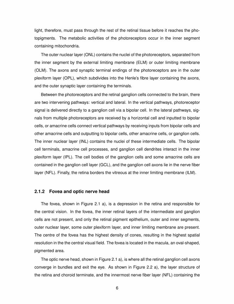
2.1.2 Fovea and optic nerve head

The fovea, shown in Figure 2.1 a), is a depression in the retina and responsible for

the central vision. In the fovea, the inner retinal layers of the intermediate and ganglion

cells are not present, and only the retinal pigment epithelium, outer and inner segments,

outer nuclear layer, some outer plexiform layer, and inner limiting membrane are present.

The centre of the fovea has the highest density of cones, resulting in the highest spatial

resolution in the the central visual field. The fovea is located in the macula, an oval-shaped,

pigmented area.

The optic nerve head, shown in Figure 2.1 a), is where all the retinal ganglion cell axons

converge in bundles and exit the eye. As shown in Figure 2.2 a), the layer structure of

the retina and choroid terminate, and the innermost nerve fiber layer (NFL) containing the

6

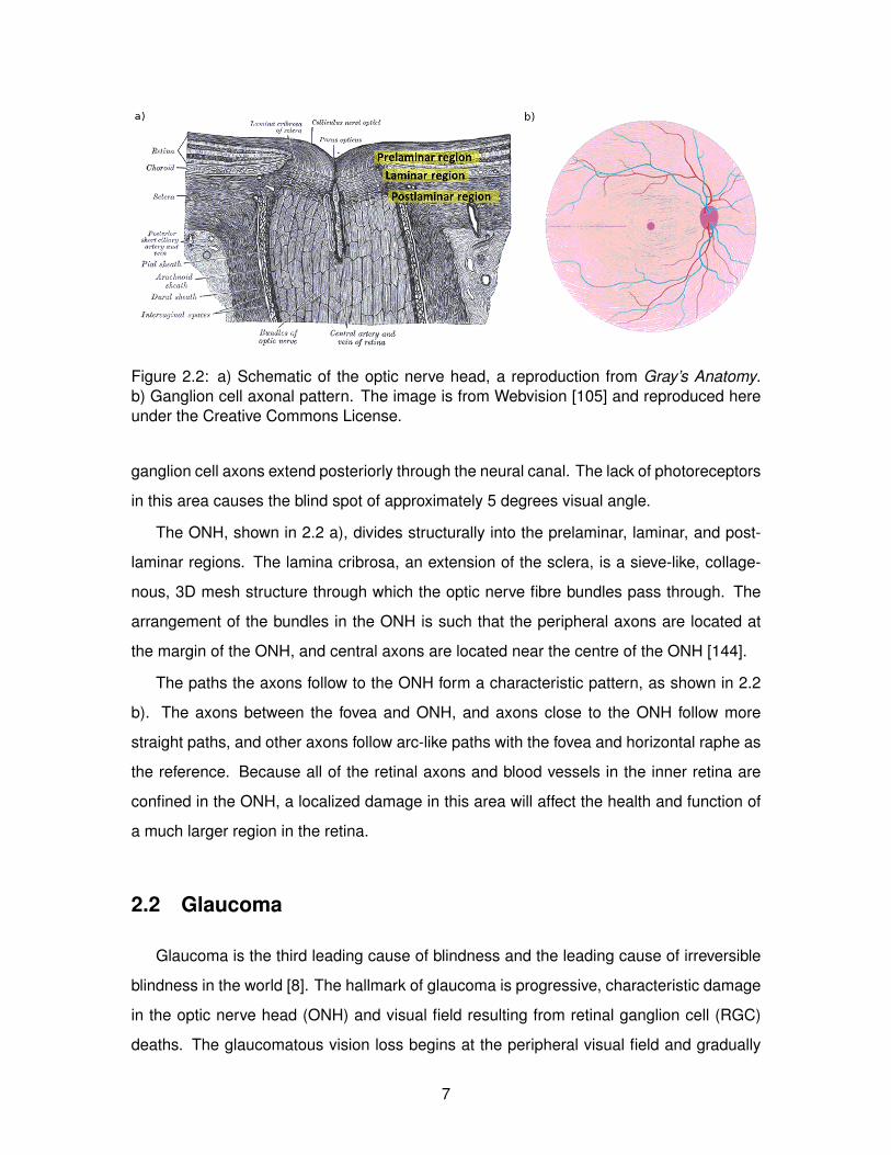
Figure 2.2: a) Schematic of the optic nerve head, a reproduction from Gray’s Anatomy.b) Ganglion cell axonal pattern. The image is from Webvision [105] and reproduced hereunder the Creative Commons License.

ganglion cell axons extend posteriorly through the neural canal. The lack of photoreceptors

in this area causes the blind spot of approximately 5 degrees visual angle.

The ONH, shown in 2.2 a), divides structurally into the prelaminar, laminar, and post-

laminar regions. The lamina cribrosa, an extension of the sclera, is a sieve-like, collage-

nous, 3D mesh structure through which the optic nerve fibre bundles pass through. The

arrangement of the bundles in the ONH is such that the peripheral axons are located at

the margin of the ONH, and central axons are located near the centre of the ONH [144].

The paths the axons follow to the ONH form a characteristic pattern, as shown in 2.2

b). The axons between the fovea and ONH, and axons close to the ONH follow more

straight paths, and other axons follow arc-like paths with the fovea and horizontal raphe as

the reference. Because all of the retinal axons and blood vessels in the inner retina are

confined in the ONH, a localized damage in this area will affect the health and function of

a much larger region in the retina.

2.2 Glaucoma

Glaucoma is the third leading cause of blindness and the leading cause of irreversible

blindness in the world [8]. The hallmark of glaucoma is progressive, characteristic damage

in the optic nerve head (ONH) and visual field resulting from retinal ganglion cell (RGC)

deaths. The glaucomatous vision loss begins at the peripheral visual field and gradually

7

Figure 2.3: a) Progressive vision loss in glaucoma. Image source: National Eye Institute,National Institutes of Health. b) Glaucomatous deformation in the laminar region.1

progresses to the centre, as shown in 2.3 a), often going unnoticed by the patient until the

damage is significant.

The major risk factor in glaucoma is elevated intraocular pressure (IOP), and the treat-

ments is often directed to the control of IOP [173, 74, 13, 66]. The pathophysiology of

glaucoma is complex and multifactorial, and the mechanisms governing the optic neu-

ropathies and their connection to IOP are yet to be fully understood, except the insult to

the RGC axons, especially within the lamina cribrosa, has been identified as one of the

central events of the disease.

A notable expression accompanying glaucomatous neuropathy is profound structural

alteration in the prelaminar, laminar, and postlaminar regions of the ONH, shown in 2.3

b) [11]. There is general posterior deformation of the peripapillary scleral flange and the

lamina cribrosa which contributes to the glaucomatous “cupping.” The prelaminar tissue

and the laminar cribrosa thickens and the neural canal expands posteriorly. In the most

severely affected eyes, the lamina cribrosa migrates out of the sclera toward the pia sheath.

1Reprinted from Experimental Eye Research, Vol. 93, Abbot Clark, David Garway-Heath, Jonathan Crow-ston, Claude F. Burgoyne, A biomechanical paradigm for axonal insult within the optic nerve head in aging andglaucoma, pp. 120-132, Copyright 2011, with permission from Elsevier.

8

Figure 2.4: A simple Michelson interferometer schematic of optical coherence tomography.(BS: beam splitter.)

2.3 Optical coherence tomography

Optical coherence tomography (OCT), first proposed in 1991 [80], is a tomographic

imaging modality based on light interference. Figure 2.4 shows a simplified description

of an OCT system: a low-coherence near-infrared beam from the source is split between

an imaging target and a reference arm with a mirror, and the light that penetrates and

subsequently backscatters from the target is interfered with the reference beam. In the

first generation of OCT systems, or time-domain OCT, the length of the reference arm

was varied, and the interference magnitude over this distance yielded a single line scan

along the depth of the target, called an A-scan. Repeating this axial scan while moving the

incidental beam transversely across the target produced a two-dimensional cross-sectional

image, or a B-scan, as shown in Figure 2.5. A full three-dimensional, volumetric image can

be generated by a series of B-scans.

In Fourier-domain OCT (FD-OCT), implemented in 1995 [46], the length of the ref-

erence arm is kept constant, and the depth and magnitude information of an A-scan is

resolved by a Fourier transformation of the interference fringes, measuring all light echoes

in the axial direction simultaneously. With the increased imaging speed [139, 138] and

greater signal-to-noise ratio [115, 32, 26], FD-OCT has become the standard in applica-

tion and research.

In the first type of FD-OCT, a low-coherence light source is used, and the interference

spectrum is measured with a spectrometer and a high-speed camera. In the second type,

known as swept-source OCT, a narrow-bandwidth light source sweeps the interference

spectrum, and the interferometer output is a function of time [38].

9

Figure 2.5: Ophthalmic OCT imaging of a) macular region and b) peripapillary region.

2.4 OCT in ophthalmology

Since its onset, OCT has been rapidly and widely adopted in ophthalmology and vision

science for several merits. The eye is a biological system designed to focus light with

minimum attenuation and scattering, and the OCT scanning beam reaches and resolves

the inner structures of the eye by the same way any visible light travels in the eye. The

power of the light source is well below the ANSI recommended level of ocular exposure of

a collimated beam [33], providing a noninvasive means of in-vivo, cross-sectional imaging

of the eye. In comparison with other in-vivo ophthalmic imaging modalities, OCT offers

a balance of image resolution, ranging from 1 to 15 µm, and tissue penetration depth of

about 2 mm. OCT is described as “filling the gap” between the ultrasound, which provides

high penetration but low resolution, and microscopy, which provides high resolution but low

penetration [38].

Ophthalmic OCT imaging can be divided into anterior, retinal (macular), and peripapil-

lary imaging, depending on the target image region (Figure 2.5). OCT images serves as a

fast and intuitive visual examination of the state of the anatomy, and as a information-rich

data source for large-scale, quantitative analysis of the shape, texture, and other anatomi-

cal features that are clinically relevant.

10

Chapter 3

Image Acquisition and Preprocessing

3.1 Acquisition

All data presented in this thesis, except when specified, were acquired using a proto-

type swept-source optical coherence tomography (SS-OCT) system with a 1060-nm wave-

length source, developed by Biomedical Optics Research Group (BORG) at Simon Fraser

University [194]. The system schematic is shown in Figure 3.1. The 1060-nm wavelength

of the source provides better penetration of the beam in the optic nerve head (ONH) and

choroidal region than the conventional 800-nm source [194]. The swept-source design al-

lows for the fast A-scan rate of 200kHz. The axial resolution of the system is approximately

6 micrometres, and the lateral resolution ranged from 12 to 20 micrometres, calculated

based on the optics of the system, scan angle, and axial lengths of individual eyes.

The image acquisition was performed at the Eye Care Centre, Vancouver General Hos-

pital, Vancouver, British Columbia, Canada. The OCT system was mounted on a standard

slit-lamp biomicroscope with an aligning stage, as shown in Figure 3.2. The subject was

seated with the head resting against the chin and forehead support to reduce motion, and

asked to focus on a fixation target. The acquisition time lasted approximately 1.6 seconds

per full 3D image volume. The image was acquired using a custom C++ and LabView

software performing a series of real-time signal processing such as dispersion compensa-

tion and fast Fourier transform, and real-time B-scan display to assist the user in image

alignment and checking the image quality.

The scan pattern was raster such that a series of B-scans was acquired to generate a

full 3D volume, as shown in Figure 3.3. A typical physical dimension of the imaged space

11

Figure 3.1: Schematic of the swept-source optical coherence tomography system setup.Source: Axsun SS Module; PC: polarization controller; BD: balanced detector; fn, focallength of the lens, where n = 1, 2, 3.[194]

was 2.8 mm in the axial direction, and 4.5 to 8 mm in the lateral directions, depending on

the lateral resolution based on the eye’s axial length. A typical voxel dimension of an image

volume was 1024 (axial) x 400 (lateral) x 400 (lateral) voxels.

3.2 Quality control and data management

Image quality control and data management are crucial part of working with a prototype

imaging system, especially as a larger number of subjects are imaged, and multiple studies

share the same datasets.

The goal of the image quality control in the data acquisition stage is to reduce, as much

as possible, artefactual variability among the images that can affect subsequent processing

and analysis. Common issues include motion-related artifact, signal-to-noise ratio, image

focus, and the position of the field-of-view relative to a reference anatomical landmark,

such as the fovea or optic nerve head. These are primarily subject-dependent, with the

age and eye condition affecting the subject’s clarity of vision and ability to focus for the

duration of image acquisition.

During the acquisition, the system user aligns the imaging location based on the real-

time B-scan and enface views in the acquisition software, and data with a large eye move-

ment or blinks are discarded. Minimum of 4-5 datasets are acquired for each eye, and after

the imaging session, visually examined through quick-check images, shown in Figure 3.4.

Data with poor quality are discarded, and the remaining data are securely transferred and

stored, in the original raw format, in a file system at Simon Fraser University with multilevel

back ups.

12

Figure 3.2: Prototype optical coherence tomography system set up at the Eye Care Centre,Vancouver General Hospital.

Proper data management, for the raw image data and associated technical and clinical

data, is important for several reasons. First, since the data is acquired from human sub-

jects, security and privacy concerns are critical. Second, a typical raw data size ranges

from 300 - 400 MB and necessitates a careful planning to save storage space. Third, the

image processing pipeline is multi-staged, flexible, and in large part automated, requiring

consistency in file format and naming convention, and directory structure. Lastly, each im-

age dataset is associated with metadata, such as OCT system parameters and subject’s

clinical information, and good organization of the raw data, metadata, and processed data

becomes essential as more than one studies are conducted over time involving the same

datasets.

13

Figure 3.3: (a) Imaged region and scanning direction displayed on fundus photography. (b)Volume reconstruction from raw data. (c) Volume visualized in 3D.

3.3 Preprocessing

The raw data, after fast Fourier transform and dispersion compensation, is built into

a 3D image volume, as shown in 3.3. The subsections below describe the subsequent

preprocessing steps: motion correction and image smoothing.

3.3.1 Motion correction

Motion in OCT images

Although the chin rest, forehead support, and fixation target reduce head and body

motion, involuntary fixational eye movements still occur. Fixational eye movements are

divided into tremor, drift, and microsaccades [125]. These movements have been charac-

terized by their general pattern, amplitude, frequency, duration, and speed, by externally

tracking the rotation angle of the eye.

Tremor is wave-like motion of high frequency (∼90 Hz) and low amplitude (less than 1

arcminute). Assuming a simple model with the centre of the eye rotation at the centre of

the eye and the average human eye diameter of 24 mm, the angular amplitude of tremor

approximately translates to less than 3.5 nm in the ONH, which is smaller than the system

axial resolution of 6 micrometres and unlikely to be detected. Drift is a gradual movement

with relatively low maximum speed of 30 arcminutes per second. This yields the maximum

displacement of 4.4 nm per frame, which would not be noticeable within a single frame.

Drift occurs between fast, twitch-like movements called microsaccades. There is a large

14

Figure 3.4: A quick-check image of an OCT dataset.

variance in characterization of this movement among different studies, and average me-

dian amplitude is 45 µm, with interval frequency between 0.4-2.6 Hz. This indicates that

microsaccades is likely the most visible source of motion artifact across multiple frames in

OCT volumetric images acquired by a raster scan pattern.

Real-time eye tracking in OCT has been implemented in prototypes [122, 150] and

the latest line of commercial systems. This involves instant adjustment of scanning beam

position to compensate for eye motion during acquisition; however, this approach entails

significant hardware modification to the standard OCT setup with additional cost, requires

regular calibration, and detects lateral motion only.

There are two considerations in characterizing the motion artifact in 3D-OCT images.

First, because the fixational eye movements are constantly present and the shape of

the ocular structures and blood vessel patterns vary in each eye, obtaining an accurate,

motion-free 3D image of the human ONH in-vivo is, technically, not possible. Second, the

motion itself has three-dimensional translational and rotational degrees of freedom and

15

Figure 3.5: The first column shows the sectioning plane of the images in the second col-umn, and the third column illustrates motion visible in each of these images. In the firstrow, a B-scan (fast scan) is shown (b) in the direction of frame acquisition (a). In the sec-ond row, an axial cross section (slow scan) (e) orthogonal to the B-scan (as shown in (d))displays wave-like axial motion artifact (f). In the third row, a sum-voxel en-face image inthe plane (e) displays lateral and elevation motion artifact (i) by the uneven blood vesselboundaries and discontinuities in the image.

varies in each eye and imaging session such that exact characterization is difficult. How-

ever, a heuristic approach can be taken based on the clinical knowledge and observation

from a large number of datasets. Based on the fixational eye movement characteristics and

qualitative examination of the images, a single frame (B-scan) acquired in 0.004 second

is approximated as an instantaneous, motion-free snapshot. The subject motion then can

be considered as motion of the frames relative to a stationary target, which is illustrated in

Figure 3.5. In an ideal case, each frame in a volume is motion-free (Figure 3.5(b)) with all

frames aligned in a row in a single orientation (Figure 3.5(c)). This is the assumption made

during the volume reconstruction of the raw data. However, an orthogonal cross -section

of an actual reconstructed volume (slow scan, Figure 3.5(d) and (e)) reveals fluctuating

artefactual peaks due to motion in the axial direction (Figure 3.5(f)) where each column in

16

Figure 3.5(d) represents a single B-scan frame. Motion in the other two directions (Figure

3.5(i)) is visible in Figure 3.5(h), a sum-voxel enface image created by summing all or-

thogonal cross-sections in the enface direction in Figure 3.5(g). Each row in Figure 3.5(h)

represents a single frame and motion in the lateral direction is seen in the small artifactual

ripples in the edges of the blood vessels. In several locations, there are abrupt discontinu-

ities in the image due to motion in the elevation direction, in which a frame either repeats

(jump forward) or skips (jump backward) several frames. This motion is particularly prob-

lematic because it is perpendicular to the frames and there is no information in the acquired

frames to interpolate for such a gap. For example, subject eye motion resulting in a verti-

cal displacement creates a discontinuity in the enface reconstructions, and the size of the

jump cannot be determined by simply observing the neighbouring frames. This problem is

intrinsic to the scanning direction and raster scan pattern.

Post-acquisition motion correction by maximum cross-correlation

Rizzo et al.[165] corrected lateral motion by matching blood vessels in the OCT en-face

sum-voxel image and motionless fundus photography using warping registration, although

this method does not address axial motion. Another widely used approach is to acquire

a small number of “fast scans” in the slow scan direction, and use these as references

for motion correction [152, 201]. However, this may introduce a new source of error if

the reference frames are not acquired at precise locations relative to the volume with the

continuous eye motion and time difference between the reference frames and the other

frames. Hu et al. [78] first automatically segmented several surfaces with strong edges

using graph-cut approach, and translated frames to flatten one of the segmented surfaces.

The automatic flattening may affect the anatomical information in the image. Both of the

latter two methods only address motion in the axial direction.

The correction method used in our pipeline is a modified version of the maximum cross

correlation technique [114], a 3D extension of a method presented in an early seminal

paper on OCT [73], which proposed correcting motion artifact in a 2D OCT image using

maximum cross-correlation of adjacent columns. In 3D OCT, each frame is approximated

as a motionless unit and translated against the next frame. The amount of displacement

which yields the maximum cross-correlation with the neighboring frame is noted. The

17

cross-correlation measures the similarity between two adjacent frames. Briefly, for a vol-

ume of N frames of a size X by Y , for each pair of frames Fn and Fn+1, n = 1 .. N − 1, a

cross-correlation vector Cn of length 2M + 1 was computed. First, Fn+1 was padded by M

pixels in the top and bottom such that the size of the padded Fn+1 was X by Y + 2M . The

mth element of Cn was then

Cn[m] =X∑i=1

Y∑j=1

Fn(i, j)Fn+1(i, j +m− 1), m = 1..M. (3.1)

The equation computes pixel-wise 2D cross-correlation between two adjacent frames as

Fn “slides up and down” relative to Fn+1 over the distance of 2M + 1

Because the frames are densely sampled in space, anatomical difference between two

consecutive frames is minimal and localized, and it does not affect the frame-to-frame

correlation significantly. The displacement of the maximum cross-correlation position, or

the index of the maximum value in C for each frame, thus captures the shift of the entire

frame due to the subject motion and the natural curvature of the eye. In Figure 3.6(a), the

maximum correlation displacement profile in white curve overlaid on a slow scan closely

follows the wave-like motion artifact. After approximating motion artifact by the maximum

correlation displacement profile, a common practice is to translate each frame such that

the profile is flattened, as shown in Figure 3.6(b) [29, 69, 24]. However, this neglects

the gradual curvature in the eye and any rapid change in topology that may contribute to

the displacement estimated by correlation. In Figure 3.6(a), the displacement profile dips

slightly near the optic cup due to its sharp slopes, and the flattening correction (Figure

3.6(b)) raises the cup bottom to compensate for this. In order to reduce such distortion as

a byproduct of correction, we fit the profile to a smooth curve instead of flattening it. This

smooth curve serves to model the natural curvature of the eye which is apparent in a single

motion-free frame. The curve is selected in an interactive setting, where the user is shown

a motion-free frame (ex. Figure 3.5(b)) and an orthogonal slice of all such frames with

the motion profile, such as in Figure 3.6(a). The user can vary a cubic-spline smoothing

parameter and see the resulting correction immediately applied to the profile and the slice,

displayed in real time. By comparing and matching the amount of curvature visible in

the motion-free frame and the slice in the orthogonal direction, the level of smoothness

for correction can be qualitatively determined. Figure 3.6 5(c) displays the result of the

correction by fitting a smooth curve with the selected fitting curve shown in white. The optic

18

cup depth (marked by red double-arrow line) in the flattened correction in Figure 3.6 5(b)

measured 20% less than that of the smooth-fitted correction, indicating flattening can alter

the ONH topology by overcompensation, and the smooth curve fitting better preserves

the variable topology. Figure 3.6 (d) and (e) compare a volume before and after motion

correction by smooth fitting, and there is noticeable improvement in the image quality after

correction.

The maximum cross-correlation technique is a relatively simple, fast, and effective mo-

tion correction method that does not require additional scans or computationally expensive

processing. One of the limitations of the maximum cross-correlation method is that the

motion in lateral direction is less resolvable due to the lack of strong vertical edges in

the frames, except in the optic cup region. In the frames that do not contain dominant

vertical structures, it is possible that the shifting position of the vertical shadows of con-

verging blood vessels is falsely classified as lateral motion. This is similar to the windowing

problem in computer vision, where positional ambiguity arises from the camera frame con-

taining only partial boundary of a continuous object while moving in a direction parallel

to the boundary. Such directionality in correction effectiveness is a common problem in

post-acquisition motion correction methods.

3.3.2 Bounded variation image smoothing

By its light-based nature, OCT images inherently consists of “speckles.” Smoothing

an OCT image can reduce the effect of speckles and image noise, and better resolve

anatomical features. However, conventional image smoothing filters, such as Gaussian,

often do not discriminate between unwanted speckle noise and structural boundaries we

wish to observe.

A variational approach[193] considers the problem as an optimization of a functional

with the antithetical constraints of i) smoothing the original image and ii) preserving certain

desired features in the same image. A minimization expression can be written as

E(I; Io) = Q(I) + λC(I, Io) (3.2)

where the first term measures the quality of the new image I, and the second term penal-

izes the distance between I and original image Io. C(I, Io) can be simply defined as the

19

L2-norm

C(I, Io) =

∫Ω|I(x)− Io(x)|2dx. (3.3)

The Q(I) term should penalize the magnitude of gradient in the image. This can be

achieved by the bounded variation norm

Q(I) =

∫|∇I|dx (3.4)

and the minimization equation 3.2 can be written as

E(I; Io) =

∫|∇I|dx+

∫Ω|I(x)− Io(x)|2dx. (3.5)

The standard gradient descent can be performed in the form of

I(n+1) = I(n) + δt

(div

(∇I(n)

|∇I(n)|

)− 2λ(I(n) − Io)

)(3.6)

The derivatives are discretized and approximated in 3D for numerical computation. Fig-

ure 3.7 shows an example of an image before and after BV smoothing. After the smoothing,

the image appears less noisy, and the anatomical structures are more clearly visible. The

bounded variation smoothing is particularly effective for OCT speckles, since it penalizes

rapidly edges, such as speckles, while preserving larger, more gradual edges, such as a

structural boundary.

3.4 Summary of contributions

The contributions described in this chapter and partially published in [114] are:

• OCT image quality control and data management.

• Axial motion correction using frame-to-frame maximum cross-correlation.

• OCT image smoothing by bounded variation optimization.

The processing steps described in this chapter were applied to all data presented in the

subsequent chapters, except when specified.

20

Figure 3.6: (a) Slow scan with maximum cross-correlation displacement profile. (b) Samescan corrected by flattening the profile. (c) Same scan corrected by fitting a smooth curveto the profile. The red arrows in (b) and (c) indicate the cup depth measured in each image.(d) Volume before motion correction. The volume has been rotated that the axial axis liesvertically and the en-face plane lies horizontally. (e) Same volume after smooth-fittingmotion correction.

Figure 3.7: Example of BV smoothing

21

Chapter 4

Segmentation

After the motion correction and smoothing described in the previous chapter, the im-

age volumes were segmented for anatomical structures. The segmentation targets were

divided into automatically-segmented retinal layer boundaries and manually-segmented

non-layer structures in the optic nerve head (ONH).

Layer boundaries and their segmentation are shown in the Figure 4.1 a). Of the par-

ticular importance are the inner limiting membrane (ILM) (anterior boundary of the retina),

Bruch’s membrane (BM)(posterior boundary of the retina), and the posterior boundary of

the choroid marking also the anterior boundary of the sclera.

In the optic nerve head (ONH) region segmentation in Figure 4.1 b), the anterior-most

retinal nerve fiber layer (NFL) is shown bending posteriorly towards the optical neural canal

to exit the eye, where all other retinal layers discontinue. Non-layer landmarks in this region

include the Bruch’s membrane opening (BMO), scleral canal wall, anterior lamina cribrosa

surface (ALCS), and anterior laminar cribrosa insertion points (ALCIP).

4.1 Manual segmentation of ONH structures

Manual segmentation was done in points, as shown in Figure 4.1 b), in 2D frames.

Amira 5.2 (FEI Company, Hillsboro, OR) was used for interactive visualization and seg-

mentation.

In raster manual segmentation, each of the B-scans from the raster acquisition pattern

is segmented. A custom Amira script displayed the volume in three slaved orthogonal

cross-sections, and on each B-scan the target structures were marked. This segmentation

22

Figure 4.1: Example of a) automated segmentation of retinal layers and b) manual pointsegmentation.

method was validated in our previous study with three different raters and sixteen eyes

[198].

In radial manual segmentation, the rater was first presented with the en-face summed

voxel projection image of the image volume, and selected two points: an approximate

centre of the optic cup and another on the outer boundary of the region of interest. This

produced a predefined number of radial slices orthogonal to the en-face plane with the

centre and width determined by the two user-selected points. The slices were spaced at a

constant angle.

There are three advantages to using radial slices for manual segmentation rather than

the original B-scans [114]. First, the user can specify the region of interest by manually

selecting the centre of the volume. Second, the radial slicing provides dense segmenta-

tion near the centre of the volume at a cost of more sparsely sampled peripheral area,

often of less importance and morphological complexity. This dense sampling at the centre

allows the rater to segment fewer frames per volume. B-scan segmentation is performed

on at least every other frame, whereas in radial segmentation, 40 slices may suffice for

approximating the centrally located optic cup. Lastly, radial slices provide more consis-

tency and control during manual segmentation, as the ONH is generally axially symmetric

23

and radial slices vary less than raster frames. 3D visualization of the result of manual

point-segmentation in radial slices is shown in Figure 4.1 b).

4.2 Automated segmentation of retinal layers

Challenges in automated OCT retinal layer segmentation include discontinuities in the

layer boundaries due to blood vessel shadowing, and lack of contrast and clarity of the

layer boundaries, which is made worse by the speckle nature of the OCT. Several groups

reported on automated segmentation of the retinal layers employing various techniques

[14, 86, 170, 3, 51, 60, 43, 52, 132, 120, 136]. One of the most successful among these

has been the 3D graph-theoretic approach developed and applied extensively by the Sonka

group in University of Iowa [67, 51, 52, 78]. The underlying key work by Li et al. [119], sum-

marized below, optimally segments surfaces in 3D by transforming the segmentation prob-

lem into a minimum s-t cut problem of a multi-dimensional arc-weighted graph. The main

advantages are that the optimality can be controlled by cost functions and built-in geomet-

ric constraints including smoothness and interrelations of multiple surfaces. Garvin et al.

[51, 52] extended this work by including regional constraints for more robust segmentation

of the retinal layers.

The algorithm begins with a multicolumn model: an image volume of the dimension X,

Y , and Z is considered as a 3D matrix I(x, y, z) and the segmented surface is N(x, y) ∈

z = 0, ..., Z − 1, with x = 0, ..., X − 1 and y = 0, ..., Y − 1 such that the surface is defined

to intersect with one voxel of each column parallel to the z-axis.

A node-weighted directed graph G = (V,E) with a node V (x, y, z) ∈ V uniquely as-

signed to each voxel I(x, y, z) ∈ I. The node cost w(x, y, z) is given by:

w(x, y, z) =

c(x, y, z) if z = 0

c(x, y, z)− c(x, y, z − 1) otherwise

The cost function for the retinal layer segmentation was given by vertical gradient of the

intensity value of each pixel.

The arcs are divided into intracolumn, intercolumn, and intersurface arc sets. The

intracolumn arc set Ea is given by

Ea = 〈V (x,y, z), V (x,y, z − 1)〉|z > 0 (4.1)

24

and the intercolumn arc set by

Er =

〈V (x,y, z), V (x+ 1,y,max(0, z −∆x))〉|x ∈ 0, ..., X − 2, z ∈ z∪

〈V (x,y, z), V (x− 1,y,max(0, z −∆x))〉|x ∈ 0, ..., X − 1, z ∈ z∪

〈V (x, y, z), V (x, y + 1,max(0, z −∆y))〉|y ∈ 0, ..., Y − 2, z ∈ z∪

〈V (x, y, z), V (x, y − 1,max(0, z −∆y))〉|y ∈ 0, ..., Y − 1, z ∈ z∪

where ∆x and ∆x are smoothness parameters such that if I(x, y, z) and I(x + 1, y, z′)

are on the surface, |z − z′| ≤ ∆x, and if I(x, y, z) and I(x, y + 1, z′) are on the surface,

|z − z′| ≤ ∆y.

The surfaces are expected not to intersect or overlap, and given surfaces N1 and N2

with graphs G1(V1, E1) and G2(V2, E2), the intersurface arc set is given by

Es =

〈V1(x,y, z), V2(x,y, z − δu)〉|z ≤ δu∪

〈V2(x,y, z), V1(x,y, z + δl)〉|z < Z − δl∪

〈V1(0, 0, δl), V2(0, 0, 0)〉

The construction of the graphs establish the following lemmas.

Lemma 1. Any k feasible surfaces in I correspond to a nonempty closed set in G with the

same total cost.

Lemma 2. Any nonempty closed set in G defines k feasible surfaces in I with the same

total cost.

Lemma 3. A minimum nonempty closed set C∗ in G specifies the optimal k surfaces in I.

C∗ in Lemma 3 can be computed by a minimum s-t cut in a related graph Gst = (V ∪

s, t, E ∪ Est), where s is a source, t is a sink, and Est is a new arc set defined as follows.

The source is connected to v/inV −, with V − denoting all nodes in G with negative costs

and arc costs −w(v). The sink is connected to v/inV +, with V + denoting all nodes in G

with nonnegative costs and arc costs w(v). A finite cost s-t cut (S, T ) of Gst has the total

cost c(S, T )

c(S, T ) = −w(V −) +∑v∈S−s

w(v) (4.2)

where w(V −) is fixed and is the cost sum of all nodes in V −. Since S − s is a closed set,

the cost of a cut (S, T ) in Gst and that of the corresponding closed set in G differ by a

25

constant. Therefore, the source set of a minimum cut in Gst corresponds to a minimum

closed set C∗ in G. The optimal k surfaces correspond to the upper envelope of C∗.

We implemented this algorithm to successfully segment retinal layers (Figure 4.1 a)),

and also the choroid, as expounded in the following subsection.

4.3 Choroid segmentation

The choroid is the layer of vasculature and connective tissue between the retina and

sclera. The critical metabolic role of the choroid in providing nutrients and removing waste

products from the retina makes it an important factor in development of retinal pathol-

ogy. Recently, interest in in-vivo visualization and quantitative analysis of the choroidal

structure has been growing with the advancement in OCT technology. However, imaging

and segmentation of the posterior surface of the choroid – choroid-sclera (CS boundary)

boundary - still remains a challenge as the light signal intensity decreases sharply be-

yond the retina due to light absorption and scattering at the retinal pigment epithelium and

among choroidal vasculature. Reliable automated measurement of the choroid therefore

requires both an acquisition system capable of resolving the CS boundary as well as a

robust segmentation algorithm.

Enhanced depth imaging (EDI) OCT [174] improves the visualization of the choroid by

positioning the spectral domain (SD) OCT closer to the eye. This pushes back the peak

signal location (zero delay) from the conventional vitreo-retinal interface towards the outer

scleral border. Since the choroid is placed closer to the zero delay, the imaging sensitivity

in the region is enhanced. In SD-OCT, the Fourier transform produces two equivalent mir-

ror images. Conventional instruments display only one of the images in which the anterior

portion of the retina is facing up in the screen. In EDI-OCT, the physical displacement of the

instrument results in the inverted mirror image being displayed. EDI-OCT has been used to

measure the choroid in normal eyes [124], high myopia [50], central serous chorioretinopa-

thy [85, 126], and AMD [123]. Additionally, OCT with a longer wavelength source [183], and

polarization-sensitive (PS) OCT [151] showed improved visualization of the choroid.

In the majority of studies, choroidal thickness has been measured manually, although

automated segmentation of the choroid-sclera interface and measurement of the choroidal

thickness have been implemented in three-dimensional 1060 nm OCT using a statistical

26

model [99], in three-dimensional 890 nm OCT using graph-cut [203, 79], and in polarization

sensitive OCT [181].

We used the 3D graph-cut algorithm, described in the previous subsection, for seg-

menting the anterior surface (Bruch’s membrane equivalent, BM) and posterior surface

(CS boundary) of the choroid. First, the inner limiting membrane (ILM) and interface be-

tween the inner and outer segment were segmented for their strong edge contrast. The

latter was smoothed, fitted to a convex hull, and redrawn by piecewise cubic interpolation

to serve as a reference layer to segment BM and limit the search region. Convex hull and

interpolation were required to handle images with retinal pigment epithelial detachments

caused by drusen, which results in reduced intensity at Bruch’s membrane equivalent.

After the BM was found, the choroid-sclera boundary was searched for in the region pos-

terior to the BM as a smooth surface with high intensity gradient. The initial choroid-sclera

boundary segmentation was smoothed and interpolated similarly as in BM, based on the

assumption that the boundary is smoothly varying and encompasses all choroidal capillar-

ies, which creates the dark/bright contrast within the choroid. An annotated B-scan and its

final segmentation result are shown in Figure 4.2.

4.3.1 Comparison of choroid segmentation in in 830 nm and 1060 nm OCT

images

For the commercial OCT system, Cirrus spectral domain OCT (SD-OCT) (software

version 6, Carl Zeiss Meditec, Inc., Dublin, CA) was used to acquire 24 3D macular scans,

all centred at the fovea. For the prototype OCT system, the in-house custom 1060-nm

swept-source OCT (SS-OCT) system described in Section 3.1 was used to acquire 10 3D

macular scans. All human imaging was conducted with ethics approval from Simon Fraser

University or the University of British Columbia, and in accordance with the guidelines

of the Declaration on Helsinki. The images were processed with motion correction and

smoothing as described in Section 3.3, and segmented using the algorithm above.

Representative OCT data and segmentation results are presented in Figure 4.3. An

830-nm 2D EDI-OCT scan with segmentation was included as a reference as it was ac-

quired by the same Cirrus SD-OCT machine used to acquire the 830-nm 3D volumes.

27

Figure 4.2: Top: B-scan of a 1060-nm OCT macular volume. Bottom: Automated seg-mentation of inner limiting membrane (green), Bruch’s membrane equivalent (cyan), andestimated choroid-sclera boundary (CS-boundary).

In the model of Cirrus SD-OCT used in this experiment the EDI function was only avail-

able in 2D. Additionally, the 2D EDI-OCT scan was averaged over 20 lines with proprietary

Selective Pixel Profiling for improved image quality, which is unavailable in 3D.

In Figure 4.3, the 830-nm 3D scan (middle) shows poorer image resolution and more

severe signal attenuation in the choroidal region compared to the 2D averaged EDI-OCT

scan (top) from the same system. We observed in one of our studies [111] that even

with averaging and EDI technique the signal intensity and sensitivity fall-off at the posterior

choroidal region was considerable, and often the CS boundary was not clearly visible.

The automated segmentation and subfoveal choroid thickness measurement for the 2D

EDI scans performed relatively well with intra-class correlation (ICC) of 0.85 with expert

raters and 0.87 between two consecutive repeat scans. For the 3D scans, the repeat scan

ICC was 0.99 for the 24 sample subjects (44 datasets in total). This implies that despite

the poorer image resolution the inherently 3D segmentation algorithm benefited from the

volumetric dataset and the smoothness constraint in the additional dimension for more

28

Figure 4.3: Macular OCT images (Left) and their segmentations (Right). Top: 830-nm2D averaged EDI-OCT scans acquired with Cirrus SD-OCT. Middle: 830-nm 3D scansacquired with Cirrus SD-OCT. Bottom: 1060-nm 3D scans acquired with the prototype1060-nm SS-OCT.

consistent result. However, the automated subfoveal choroid thickness measurement from

the 3D scans was significantly smaller than the manual and automated measurements

from the 2D EDI scans. This shows that although the automated segmentation was highly

repeatable, the 830-nm 3D scan was generally inadequate for visualizing the CS boundary

detected in the 2D EDI scan.

In the bottom row of Figure 4.3, the 1060-nm prototype SS-OCT 3D scan shows

brighter choroid region with greater amount of detail of the choroidal vasculature com-

pared with the 830-nm 3D scan. The CS boundary is also better visible and segmentable

by the automated algorithm.

Figures 4.4 and 4.5 further demonstrate the 3D segmentation of an 830-nm macular

scan (Figure 4.4) and 1060-nm macular scan (Figure 4.5). The inner limiting membrane

(green) and boundaries of the choroidal layer (cyan, magenta) are plotted as 3D surfaces.

As shown in Figure 4.3, the segmentation is consistent throughout in each volumes but

29

Figure 4.4: Segmentation of a 3D macular scan acquired with 830-nm Cirrus SD-OCTsystem.

more detailed choroidal structures and deeper CS boundary are visible in the 1060-nm

scan in comparison with the 830-nm scan.

The segmentation result can be used to flatten the volume and generate a sumvoxel

projection of the choroidal layer as shown in Figure 4.6 a). Figure 4.6 b) and c) display

an example of a total retinal thickness map and choroid thickness map generated from the

segmentation.

4.3.2 Repeatability analysis of choroidal thickness measurements in age-

related macular degeneration

The potential role of the choroid in the development of nonneovascular age-related

macular degeneration (AMD) is yet an underexplored aspect of the disease. Studies have

shown decreased blood volume and abnormal flow in eyes with nonneovascular AMD com-

pared to normal eyes [153, 63]. Berenberg et al. reported a significant association between

increased drusen extent, and decreased choroidal blood volume and flow in patients with

nonneovascular AMD [7]. The critical function of the choroid in providing nutrients to pho-

toreceptors and removing waste products from the RPE suggests any abnormalities in the

layer affecting the metabolic support may contribute to the development of AMD [62, 48].

30

Figure 4.5: Segmentation of a 3D macular scan acquired with 1060-nm prototype SS-OCTsystem.

In this section we present manual and automated measurements of subfoveal choroidal

thickness in EDI-OCT scans from patients with nonneovascular AMD. Measurement re-

peatability and correlation to drusen area were examined. Automated segmentation of

the choroidal boundaries used the graph-cut–based algorithm described in the previous

subsection 4.3.1.

Methods

A total of 88 eyes from 44 patients under the care of the retina service at University

of British Columbia (UBC) was included in the study based on the diagnosis of bilateral

nonneovascular AMD and age of 55 years or older. Participants were enrolled between

February 2012 and May 2012. We recruited patients with the full spectrum of drusen size,

including small drusen, intermediate drusen, large drusen, and drusenoid pigment ep-

ithelial detachments [31, 1]. Patients with other macular pathology, including neovascular

AMD, geographic atrophy, and macular dystrophy, were excluded. Participants with signif-

icant ocular media opacity also were excluded. Each patient underwent a full ophthalmic

examination, including biomicroscopy, best-corrected visual acuity using Snellen charts,

intraocular pressure and dilated fundus examination. For statistical analysis, Snellen acu-

ity was converted to logMAR equivalents. Informed consent was obtained from all patients,

31

Figure 4.6: a) Sumvoxel projection of the macular choroid in a 1060-nm scan b) Total retinalthickness colormap. c) Choroid thickness colormap.

and the study was approved by the Research Ethics Board at the UBC and adhered to the

tenets of the Declaration of Helsinki.

Cirrus SD-OCT (software version 6; Carl Zeiss Meditec, Inc., Dublin, CA) was used

for acquisition of two or more 3D macular cube scans (200 A-scans per B-scan, 200 B-

scans) and 2D EDI raster scans, all centred on the fovea. The wavelength of the Cirrus

machine was 830 nm, and the EDI scans used an average of 20 lines with proprietary

Selective Pixel Profiling. This is different from Heidelberg EDI-OCT, which averages 100

lines with eye tracking. The macular cube scans were acquired over a region of 6 x 6

mm and selected for minimum signal strength of 6 out of 10. For the 3D macular cube

scan, the scans with the highest signal strength were used for further analysis. For the EDI

raster scans, the two scans with the highest signal strength were used. Drusen area and

volume data in macular cube scans were obtained automatically by the Cirrus SD-OCT

software [61]. The software first segments the RPE and determines by interpolation a

virtual RPE free of deformation, referred to as the RPE floor. The drusen area and volume

are computed based on the distance between the real RPE and the virtual RPE at each

measurement data point. The algorithm ignores RPE deformation below a given threshold

to reduce noise.

For manual measurement of subfoveal choroidal thickness, two independent investiga-

tors measured the distance between Bruch’s membrane equivalent and the choroid-sclera

interface at a single point below the fovea using Cirrus SD-OCT software’s built-in caliper

32

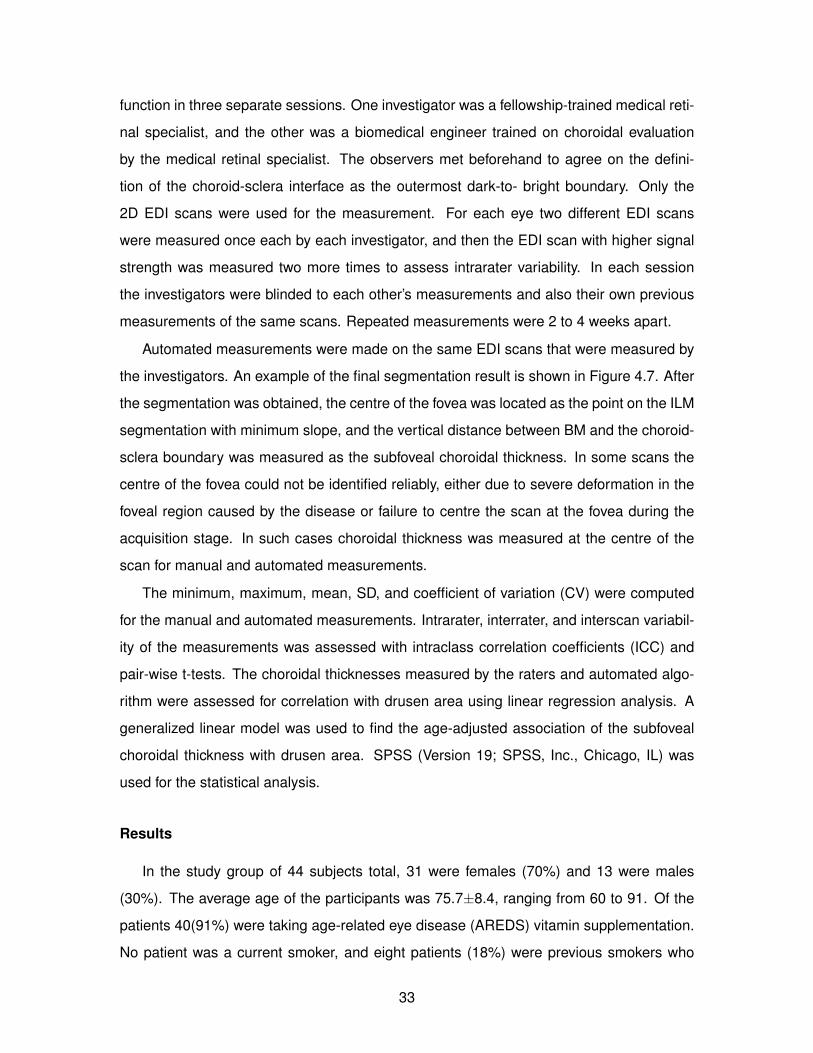
function in three separate sessions. One investigator was a fellowship-trained medical reti-

nal specialist, and the other was a biomedical engineer trained on choroidal evaluation

by the medical retinal specialist. The observers met beforehand to agree on the defini-

tion of the choroid-sclera interface as the outermost dark-to- bright boundary. Only the

2D EDI scans were used for the measurement. For each eye two different EDI scans

were measured once each by each investigator, and then the EDI scan with higher signal

strength was measured two more times to assess intrarater variability. In each session

the investigators were blinded to each other’s measurements and also their own previous

measurements of the same scans. Repeated measurements were 2 to 4 weeks apart.

Automated measurements were made on the same EDI scans that were measured by

the investigators. An example of the final segmentation result is shown in Figure 4.7. After

the segmentation was obtained, the centre of the fovea was located as the point on the ILM

segmentation with minimum slope, and the vertical distance between BM and the choroid-

sclera boundary was measured as the subfoveal choroidal thickness. In some scans the

centre of the fovea could not be identified reliably, either due to severe deformation in the

foveal region caused by the disease or failure to centre the scan at the fovea during the

acquisition stage. In such cases choroidal thickness was measured at the centre of the

scan for manual and automated measurements.

The minimum, maximum, mean, SD, and coefficient of variation (CV) were computed

for the manual and automated measurements. Intrarater, interrater, and interscan variabil-

ity of the measurements was assessed with intraclass correlation coefficients (ICC) and

pair-wise t-tests. The choroidal thicknesses measured by the raters and automated algo-

rithm were assessed for correlation with drusen area using linear regression analysis. A

generalized linear model was used to find the age-adjusted association of the subfoveal

choroidal thickness with drusen area. SPSS (Version 19; SPSS, Inc., Chicago, IL) was

used for the statistical analysis.

Results

In the study group of 44 subjects total, 31 were females (70%) and 13 were males

(30%). The average age of the participants was 75.7±8.4, ranging from 60 to 91. Of the

patients 40(91%) were taking age-related eye disease (AREDS) vitamin supplementation.

No patient was a current smoker, and eight patients (18%) were previous smokers who

33

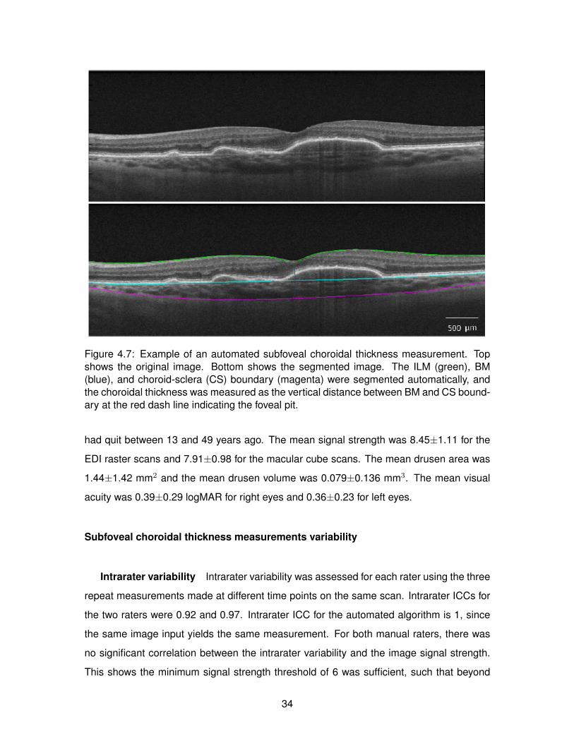
Figure 4.7: Example of an automated subfoveal choroidal thickness measurement. Topshows the original image. Bottom shows the segmented image. The ILM (green), BM(blue), and choroid-sclera (CS) boundary (magenta) were segmented automatically, andthe choroidal thickness was measured as the vertical distance between BM and CS bound-ary at the red dash line indicating the foveal pit.

had quit between 13 and 49 years ago. The mean signal strength was 8.45±1.11 for the

EDI raster scans and 7.91±0.98 for the macular cube scans. The mean drusen area was

1.44±1.42 mm2 and the mean drusen volume was 0.079±0.136 mm3. The mean visual

acuity was 0.39±0.29 logMAR for right eyes and 0.36±0.23 for left eyes.

Subfoveal choroidal thickness measurements variability

Intrarater variability Intrarater variability was assessed for each rater using the three

repeat measurements made at different time points on the same scan. Intrarater ICCs for

the two raters were 0.92 and 0.97. Intrarater ICC for the automated algorithm is 1, since

the same image input yields the same measurement. For both manual raters, there was

no significant correlation between the intrarater variability and the image signal strength.

This shows the minimum signal strength threshold of 6 was sufficient, such that beyond

34

N Minimum, µm Maximum, µm Mean, µm SD, µm CV (%)

Rater 1 83 145 521 246 63 25Rater 2 83 99 526 214 68 32

Auto 83 107 447 203 53 26

Table 4.1: Descriptive Statistics of the Choroidal Thickness Measured by the First Rater(Rater 1), Second Rater (Rater 2), and the Algorithm (Auto)

ICC 95% CI Paired Mean Difference, µm P Value

Rater 1 and rater 2 0.96 0.94− 0.98 30.56 < 0.001Rater 1 and auto 0.85 0.77− 0.90 45.51 < 0.001Rater 2 and auto 0.84 0.75− 0.89 15.39 < 0.016

Table 4.2: Intraclass Correlation and Paired Mean Difference for Choroidal Thickness Mea-surement Between the Raters (Rater 1, Rater 2) and the Algorithm (Auto)

this threshold the signal strength did not affect the measurement repeatability significantly.

The first rater showed a small, but statistically significant positive correlation between the

intrarater variability and average choroidal thickness (r = 0.27, P = 0.01), suggesting that

greater choroidal thickness was associated with greater intrarater variability. The intrarater

variability of the two raters was not correlated significantly (r = 0.16, P = 0.12) which im-

plies that there were no consistent scan features that contributed to the variability between

raters.

Interrater variability Interrater variability was assessed between the raters and the

automated algorithm. The values for the raters were averaged over the three repeated

measures to reduce the effect of intrarater variability. Of total 88 eyes, 5 for which the

difference between the average manual measurement and automated measurement was

greater than 40% were excluded from analysis as unsuccessful. Descriptive statistics, ICC

values, and paired sample t-test results are shown in Tables 4.1 and 4.2.

The ICC between the raters was 0.96, which was higher than the ICC between the

first rater and the automated algorithm (0.85), and the second rater and the automated

algorithm (0.84).

The paired t-test between the two raters indicated a statistically significant mean dif-

ference (mean difference 31 µm, P < 0.001), such that the first rater measured generally

larger choroidal thickness than the second rater. The pair-wise difference between the

raters was not correlated significantly with the choroidal thickness, drusen area, or drusen

35

Figure 4.8: Bland-Altman plots showing the interrater variability of choroidal thickness mea-surements between the two manual raters (left), and between the manual raters (averaged)and the automated algorithm. The dotted lines indicate the upper and lower 95% confi-dence interval limits (N = 83).

volume. This implies that “shadowing” of the underlying choroid by drusen did not con-

tribute significantly to variability. Correlation between the two raters was 0.93 (P < 0.001).

The paired t-test between the raters and the automated algorithm indicated a statisti-

cally significant mean differences (mean difference with the first rater 46 µm, mean differ-

ence with the second rater 15 µm, P < 0.001 for both), such that the automated algorithm

measured generally smaller choroidal thickness than both raters, but closer to the second

rater. The mean difference between the second rater and the automated algorithm was

less than that between the second and first rater. The pair-wise difference between the au-

tomated algorithm and the raters was correlated with the thickness (r = 0.70, P < 0.001),

which implies that larger choroidal thickness measurement by the manual raters has a

higher chance of yielding greater discrepancy with the automated measurement. The dif-

ference was not correlated significantly with drusen area or volume. Correlation of the

automated algorithm was 0.77 (P < 0.001) with the first rater and 0.76 (P < 0.001) with the

second rater.

Bland-Altman plots of the agreement between the raters, and between the manual

(average of the two raters) and the automated algorithm are presented in Figure 4.8.

Interscan Variability Interscan variability was assessed between two repeat scans

measurements of the same eye. Of 88 eyes, 6 eyes were excluded from analysis: 5

with largely different repeat scans, 1 with optic nerve head imaged instead of fovea. The

36

ICC 95% CI Paired Mean Difference, µm P Value

Rater 1 0.91 0.86− 0.94 -10.28 0.049Rater 2 0.96 0.94− 0.97 -10.98 0.002

Auto 0.87 0.80− 0.92 4.76 0.249

Table 4.3: Intraclass Correlation and Paired Mean Difference for Choroidal Thickness Mea-surement Between the Repeat Scans by the Raters (Rater 1, Rater 2) and the Algorithm(Auto)

result is tabulated in Table 4.3. The first rater’s interscan ICC was 0.91, the second rater’s

interscan ICC was 0.96, and the automated algorithms interscan ICC was 0.87.

However, in the paired samples t-test, the mean difference between the first and second

scan measurements was significant for the raters (p-value ¡ 0.05), but not for the algorithm.

A possible explanation is different bias in different measurement sessions by the human

raters. The raters measured the first set of scans first, and after two weeks or more mea-

sured the second set of scans. Since the scans were acquired within a minute each other,

and there was no cause for a consistent and recurring systematic difference between the

first and second scans, the significant mean difference can be attributed to the fact that

in the second session the raters tended to measure larger choroidal thickness. Since the

automated algorithm does not have such intrarater variability, the measurement difference

between the scans was not session-dependent, and the mean difference between the first

and second scans was not significant.

The interscan variability of the raters was not correlated significantly with the interscan

variability of the automated algorithm, and showed that generally there was no certain set

of scans in which the raters and algorithms had small or large interscan variability. The

interscan variability was not correlated with choroidal thickness, drusen area, or drusen

volume for all methods.

Correlation Between Choroidal Thickness and Drusen Area Drusen area was corre-

lated significantly and inversely with choroidal thickness for both raters and the algorithm

(Table 4.4) for multivariate analysis, including age, which was not a statistically significant

predictor of drusen area.

37

Outcome Predictor Beta (SE) P Model R2

Drusen area Age -0.037 (0.042) 0.38 0.12Choroid Thickness, rater 1 -0.006 (0.003) 0.05

Drusen area Age -0.031 (0.041) 0.45 0.16Choroid Thickness, rater 2 -0.007 (0.003) 0.02

Drusen area Age -0.036 (0.018) 0.84 0.26Choroid Thickness, auto -0.005 (0.002) 0.02

Table 4.4: Results of Multivariable Regression Analysis Between Drusen Area and ChoroidThickness Measured by the Rater (Rater 1 and Rater 2) and the Automated Algorithm(Auto)

Discussion

We have compared the subfoveal choroidal thickness measured by two expert raters

and an automated algorithm on EDI-OCT raster scans of nonneovascular AMD patients.

The agreement between the two raters was high, but with a statistically significant mean

difference. The agreement between the raters and the automated algorithm was less than

that between the raters, but acceptable [106]. The raters and the algorithm showed compa-

rably good repeat scan repeatability with slightly higher ICC values for the raters; however,

the raters displayed statistically significant mean difference between the first and second

scan measurements, which was not present for the automated algorithm. This may be

attributed to intrarater, or intersession, variability in manual measurement.

The raters felt it was difficult to identify confidently the choroid-sclera boundary in many

scans. However, the overall result shows high ICCs for intrarater, interrater, and interscan

repeatability among the two raters. The automated algorithm did not have intrarater vari-

ability, and had lower, but fair interrater and interscan repeatability relative to the raters.

A recent article published in IOVS presented a similar comparative analysis of a commer-

cial automated algorithm and manual graders on drusen segmentation [106]. The drusen

volume agreement was comparable between the manual graders (ICC = 0.98), and be-

tween the average of the graders and algorithm (ICC = 0.94); however, the drusen area

agreement was significantly higher between manual graders (ICC = 0.99) than between

the average of the graders and algorithm (ICC = 0.64).

The OCT scan signal strength level beyond the given threshold of 6 did not affect the

measurement. Drusen area and volume also were not correlated with measurement re-

peatability or interrater agreement for the raters and the algorithm. From observation, most

38

drusen in our study did not affect the visibility of the choroid except in a few cases. Even

when a drusen of a substantial size shadowed the choroid, the raters and the algorithm

were capable of some level of interpolation from surrounding regions where the choroid-

sclera boundary was visible.

The discrepancy between the interrater (manual) measurements, and the manual and

automated measurements was influenced by two factors: weak image intensity at the pos-

terior choroidal boundary and different definitions of the posterior choroidal boundary. A

thicker choroid implies a deeper posterior boundary where light penetration may be low,

resulting in decreased image intensity and edge clarity. Of the total 88 eyes, 6 eyes had

the choroidal thickness greater than 330 µm, and the automated segmentation was un-

successful for 4 of them (total 6 scans were categorized as unsuccessful). The value 330

µm was selected to include the cluster of unsuccessful segmentation at large choroidal

thickness. Edge clarity also is dependent on the overall image quality and the peak signal

location, which is determined at acquisition of the EDI-OCT scans. When the peak signal

location is closer to the anterior choroid and the image intensity fall off is large the anterior

blood vessels may have significantly higher contrast than the vessels near the posterior

edge of the choroid. In these cases the algorithm may falsely detect a boundary inside

the choroid resulting in a smaller thickness measurement. Unusually large drusens also

contribute to low edge clarity. Examples are shown in Figure 4.9.

One systematic factor in smaller automated measurements compared to manual mea-

surements was how the posterior choroidal boundary was defined by the raters and al-

gorithm. The algorithm searched for a relatively smooth boundary of strong dark-to-bright

contrast, which ideally corresponds to the posterior edge of the dark, large blood vessels at

the bottom of the choroid. On the other hand, the raters occasionally chose the outermost

(most posterior) edge they could identify as a smooth boundary (Figure 4.10). The thick-

ness difference between the innermost dark-to-bright boundary chosen by the algorithm

and the dark-to-bright boundary chosen by the raters could be explained physiologically by

the presence of the heavily pigmented suprachoroidal layer (lamina fusca). The thickness

of the suprachoroidal space is approximately 30 microns [182], which is close to the mean

thickness difference that we observed between the raters and algorithm.

Interscan repeatability on two consecutive scans of the same fovea was affected by

patient motion and image quality of the scans. Even when the repeat scans are imaged

39

approximately at the same location at the fovea, the amount of light penetration and the

corresponding image intensity at the choroid is low, and the visibility of choroidal structures

can be sensitive to even small changes between repeat scans. A pair of repeat scans

with a large difference in image quality, and a large interscan variability for the raters and

automated algorithm is shown in Figure 4.11.

We note the metric used in the study was the choroidal thickness below the fovea,

where the choroid tends to be the thickest, and accordingly the least visible. Also, the

choroidal thickness measurement was made on a single point and not averaged over a

region. This likely also contributed to the measurement variability and agreement for the

raters and automated algorithm.

The number and size of drusen is an important risk factor for predicting the progression

of AMD [1]. We found that choroidal thickness was correlated with drusen area, suggesting

that this may be an important parameter to follow in clinical practice and in clinical trials.

Manual and automated choroidal thickness measurements were found to correlate with

drusen area, suggesting that either would be adequate for clinical use. While manual mea-

surements tend to be less variable, obtaining these measurements can be time-consuming.

Automated measurement, thus, offers the advantage of being more applicable to a clinical

setting.

This study has presented manual and automated measurements of subfoveal choroidal

thickness in nonneovascular AMD patients using EDI-OCT scans. The manual raters

agreed with each other better than they agreed with the automated algorithm, which still

showed a fair level of agreement with the manual raters (ICC between the raters = 0.96,

ICC between the raters and the algorithm = 0.84, 0.85). All methods performed relatively

well in measurement repeatability in repeat scans. The manual measurements appeared

to be subject to possible biases in different raters and different rating sessions. The auto-

mated algorithm measurement was determined only by the given scan, but showed greater

sensitivity to image quality. As such, the manual and automated measurements of the sub-

foveal choroidal thickness in 2D EDI-OCT scans should be used with consideration. The

performance of the automated algorithm, and to some extent manual raters, is likely to

benefit from 3D or more in-depth imaging modalities, such as polarization sensitive OCT

or 1060 nm OCT.

40

The correlation of the automated choroid measurements with the drusen area was com-

parable to that of the manual measurements, indicating clinical relevance of the automated

measurements in studying the relationship between the drusen and choroid. The auto-

mated measurement showed potential for faster speed and reduced labour cost in clinical

practice and clinical trials.


The contributions described in this chapter and published in [109, 111] are:

• Manual segmentation of the ONH landmarks on radial scans.

• Implementation of automated 3D segmentation of retinal layers using graph-cut.

• Choroid segmentation

– Automated choroid segmentation in 830 nm and 1060 nm OCT images.

– Variability analysis of manual and automated subfoveal choroidal thickness mea-

surement.

The automated retinal layer segmentation tool developed here contributed to studies in

subretinal fluid detection [35], validation of radial optical coherence tomography acquisition

[107], visualization of speckle variance OCT [187], in addition to retinal surface registration

and morphometric analysis studies presented in the following chapters.

41

Figure 4.9: Examples of segmentation by the first rater (red), second rater (yellow), andthe algorithm (magenta). The first and second scans show the three measurements closeto each other. In the third scan, the posterior choroidal boundary is located deep withlow edge strength, and the automated measurement is smaller than the manual measure-ments. In the fourth scan a large drusen reduces the visibility of the posterior choroidalboundary. 42

Figure 4.10: Example of different choroid-sclera boundary measurements by the first rater(red), second rater (yellow), and the algorithm (magenta).

Figure 4.11: Repeat scans of the same fovea with different image quality.

43

Chapter 5

Retinal Surface Registration

The conventional approach to measure the anatomical difference between two OCT im-

ages is to predefine an anatomical parameter, measure it in each image, and compare the

values. Examples of such metrics are optic cup volume, cup-to-disk ratio, Bruch’s mem-

brane opening (BMO) area, retinal layer tilt, and retinal layer thicknesses representative of

the degree of cellular damage in retina due to diseases such as glaucoma [101, 87, 149,

128, 59].

Aside from the pathophysiological relevance of these parameters, there is often poor

anatomical correspondence across images, raising the question whether a particular pa-

rameter yields anatomically comparable measurements for a valid comparison between

multiple eyes. Lack of correspondence may originate from poor parameter definition, such

as in the case of the optic cup-to-disc ratio, where the cup or disk boundary often does

not correspond to a single anatomical structure within an eye or across eyes, resulting

in inconsistency among measurements [178, 160, 162, 21, 199]. Another cause for poor

inter-subject or time point correspondence can be lack of stable landmarks, such as in the

case of retinal layer thickness maps which terminate, not at an anatomical boundary, but

at the image acquisition frame.

In the latter case, in order to make any comparison or create a population or group

mean of multiple OCT images, it becomes necessary to artificially define regional corre-

spondence. This is often done based on a certain orientation and distance with gross

anatomical landmarks. In sectoral or regional retinal layer thickness analysis of macular

or peripapillary OCT scans, sectors are delimited by superior, inferior, temporal, and nasal

orientations (often simply in reference to the image frame), and distance from landmarks

44

such as the foveal pit or optic disc. However, it is unclear how the anatomical similarity

is established by these orientation and landmark distances – one may ask whether the

retinal nerve fiber layer (RNFL) thickness at a specified distance (say two millimetres) from

BMO in one eye is comparable to the RNFL thickness at the same distance from a much

larger BMO in another eye, or the distance should be adjusted according to the BMO size.

Averaging measurements over a region may somewhat mitigate the effect of this unknown

“mismatch,” but at the cost of losing measurement sensitivity and detail.

Recent studies have directly and indirectly addressed this issue in various ways. One is

to define parameters that are more anatomically consistent across multiple subjects. Sev-

eral groups confirmed the high inter-measurement variability of enface image based pa-

rameters such as the cup-to-disk ratio [178, 160, 162, 21, 199], and suggested alternatives

like BMO-based parameters as more reliable structural measurements [21]. Peripapillary

sectors were adjusted to better align to individual BMO dimensions [112], and foveal-BMO

axis has been shown, compared to the conventional superior-inferior-temporal-nasal orien-

tation by the image frame, to be less affected by acquisition factors such as the participant’s

head tilt and to have better anatomical and physiological justification [21, 71].

Registration of OCT images has been performed in 2D enface with stereo disc pho-

tography [166], and a series of repeated OCT scans were registered in both 2D [97] and

in 3D [197] in order to improve the image signal-to-noise ratio by averaging the registered

images. The voxel-wise correspondence in such application is established under the as-

sumption that the images are the same except for the acquisition modality or artifacts;

comparison of the data is not the main objective. Longitudinal OCT images of the same

eye at multiple time points have been rigidly aligned with 3D SIFT registration [140] and

with a combination of blood vessel registration and a graph-cut based A-scan matching

[141]. Many commercially available OCT systems now include techniques to track and

match the eye position in consecutive imaging sessions [53]. These methods are still lim-

ited to general alignment of the images by rigid registration, and do not direct quantify the

morphological difference between the images.

Few studies have specifically examined nonrigid cross-sectional registration of OCT

images of multiple subjects in the context of morphological comparison and group averag-

ing. In Gibson et al. [54], segmented optic cups were registered to a single template optic

45

cup, first by bringing each target into close proximity of the template via rigid and non-

rigid intensity-based volumetric registration and achieving point-to-point correspondence

by mapping the surfaces into a spherical domain and registering by spherical demons al-

gorithm [192]. The process was validated by dice coefficient of the matched cups and a

group average optic cup was created. In Chen et al. [23] registration of macular OCT scans

began first with rigid translation which aligned the foveae and subsequent A-scan affine

transformation to match ILM and Bruch’s membrane, the anterior and posterior bound-

aries of the retina, respectively. The A-scans were further deformed smoothly using radial

basis functions in order to refine the alignment of the retinal layers.

In the following sections, two methods of retinal surface registration are presented - ex-

act one-to-one retinal surface matching, and atlas generation of multiple retinal surfaces.

The segmentation algorithm described in Section 4.2 segmented the retinal layer bound-

aries, or the retinal surfaces in 3D. The segmentation output, in the form of high-density 3D

point clouds, were converted into triangular meshes using Delaunay triangulation. Sub-

sequently, at each vertex of the surfaces, we computed layer thicknesses, defined as the

closest Euclidean distance between the two surfaces corresponding to the posterior and

anterior boundaries of a retinal layer.

5.1 Exact surface-to-surface registration

5.1.1 Methods

Our proposed registration scheme consists of two parts: an in-exact, currents-based

estimation of the deformation φc, which brings the template and subject surfaces into close

proximity of each other, followed by spherical demons registration φs to produce exact

matching between the subject and template. The final deformation, a composition of φc

and φs, will be denoted by Φi = φs(φc(Si)), where Si refers to subject i.

Currents

The surfaces extracted from the segmentation algorithm described above are repre-

sented as currents [184] - objects that reside in a linear space with a computable norm.

Equipping surfaces with a computable norm allows the measurement of how ‘close’ two

surfaces are to each other.

46

Let S and T be two discretized submanifolds of Rn represented in the space of currents

via summation of the surface’s discretized elements (Dirac currents δ). That is, the surface

S is represented as S =∑

f δηfcf where f denotes the face of a triangulated surface, cf its

center, and ηf denotes the face’s normal vector. The optimal registration from S to T is

performed through minimization of the following functional:

J(vt) =

∫ 1

0‖vt‖2V︸︷︷︸

regularizer

dt+ λ ‖φ]S − T‖2H︸︷︷︸data attachment

(5.1)

where φ represents a diffeomorphism corresponding to the flow of vector fields vt at time

t = 1, and φ]S is the push-forward of S defined below.

The pull-back φ]ω of a differential 2-form ω by a mapping φ is the 2-form defined by

φ]ω(x)(u1 ∧ u2) = ω(φ(x))(dxφ ·u1 ∧ dxφ ·u2). The push-forward of φ on a current S is the

current φ]S such that for every differential 2-form ω, φ]S(ω) = S(φ]ω). In a finite, discrete

setting the data attachment term of the functional J can be written as

A =∥∥∥∑

f

δηfcf −

∑g

δηgcg

∥∥∥2

H=∑f,f

k(cf , cf )〈ηf , ηf 〉

+∑g,g

k(cg, cg)〈ηg, ηg〉 − 2∑f,g

k(cf , cg)〈ηf , ηg〉 (5.2)

where∑

f δηfcf and

∑g δ

ηgcg represent the discrete versions of φ]S and T , respectively, cf and

ηf represent the centres and normal vectors of the respective faces (triangular elements)

and k is a positive kernel defining a Reproducing Kernel Hilbert Space (RKHS) norm on

Hilbert space H. In the framework of these deformations, it has been shown [184] that the

optimal vector fields to be found from Eq. 5.1 take the form

vt(x) =N∑i=1

G(qi(t), x)αi(t), (5.3)

where qi(t) = φxi(t) are the trajectories of the surface’s vertices xi and the momentum

vectors αi(t) are the solutions to the following system of linear equations

∂

∂tqj(t) =

n∑i=1

G(qi(t), qj(t))αi(t). (5.4)

where G is a positive kernel inducing a RKHS norm on V . It turns out that, from a compu-

tational perspective, it is easier to find the deformation in terms of the momentum vectors

47

Figure 5.1: The proposed registration scheme. (a) The subject S is first brought into closeproximity with the template T by the method of surface currents φc to produce an in-exactmatching result. (b) A point-to-point correspondence between S and T is achieved byregistering φc(S) to T via spherical demons. The end result matches the topology of thetemplate. (c) Registration of the four anatomical surfaces (ILM, BM, NFL and choroid) tothe template by φs(φc(Si)).

αi(t) rather than the trajectories qi(t), which are needed to calculate vt, and thus we re-

place the functional J from Eq. 5.1 by

J(αi(t)) =

∫ 1

0

N∑i,j=1

G(qi(t), qj(t))〈αi(t), 〈αj(t)〉dt+A(qi(1)) (5.5)

For computational details on computing the variation functional J(αi(t)) we refer the

reader to [57].

Spherical Demons Registration

The currents-based registration, achieved by minimization of J , brings the template

T and subject S surfaces into close proximity of each other. However, a point-to-point

correspondence is yet to be achieved (Figure 5.1). Since the goal is to achieve a topology-

preserving and an invertible transformation, a simple projection of vertices from the trans-

formed template to subject surface is insufficient as it does not guarantee that the transfor-

mation will be invertible.

To achieve a point-to-point correspondence between S and T , we project each of the

four anatomical surfaces of S and T onto a hemispherical domain. In mapping the anatom-

ical surfaces to a hemisphere, the surfaces are first transformed to a circle-bounded planar

48

graph [202]. The boundary vertices are assigned a fixed position on the unit circle, non-

boundary (interior) vertices are expressed as a nonnegative weighted sums of their neigh-

bor vertices, and the equations are solved for new positions of the nonboundary vertices

[47]. By this construction, all nonboundary vertices lie within the unit disc. Using an in-

verse stereographic projection from point [0, 0, 1] onto a unit sphere, this disc surface can

be warped to a hemispherical surface. Finally, by mirroring this surface across the equator,

the spherical representation of surfaces are presented to the spherical registration algo-

rithm to form a point-to-point correspondence between the spherical representations of

surfaces.

Registration of the surfaces in the spherical domain is performed by the method known

as spherical demons, detailed in [190]. Briefly, spherical demons based registration of

surfaces involves applying the registration φs to φc(S) (the inexactly matched surface found

by the method of currents), where φs is found by minimizing the following functional:

(γ, φs) = arg minγ,φs‖ζ(T )− ζ(φs(φc(S)))‖2 +

1

σ2x

dist(γ, φs) +1

σ2T

Reg(γ). (5.6)

Here γ refers to a hidden transformation that acts as a prior on φs, and σ2x, σ

2T are the

tradeoff parameters to the last two terms in the objective function. The term dist(γ, φs) in

Eq. 5.6 encourages φs to be close to γ and Reg(γ) penalizes the gradient magnitude of

the displacement filed γ. For details on appropriate choices of dist(γ, φs), Reg(γ) on a

spherical domain, and on minimizing the objective function in Eq. 5.6, we refer the reader

to [191]. The authors of [190] employed cortical thickness as the function ζ to perform

the registration of cortical surfaces in the spherical domain. This method has been altered

in [54] to employ the coordinate function ζ, defined by ζ(·) = (·x, ·y, ·z) on each vertex of

(·), to register spherical representations of the ILM with a high degree of precision. In a

nutshell, maximizing the overlap of the coordinate functions for registration is essentially

akin to finding a regularized straight line correspondence between the two surfaces. The

smoothness constrain ensures that this transformation is invertible. Following the strategy

of [54], we use ζ to perform registration between two spherical representations of surfaces.

Since currents-based surface matching and the spherical demons are guaranteed to be

invertible, the combination of currents-based matching followed by spherical demons reg-

istration also produces a mapping that is smooth and invertible. With this method one can

49

now perform statistics on the vertex-wise measurements of each subject by transforming

any surface-indexed biomarker into template coordinates.

For a typical volumes consisting of approximately 100,000 vertices, the total run time

of our registration algorithm, between a template and target volume, was about 11.5 hours

on a computer with an i7 Intel CPU running at 3.50GHz and 32GB’s of memory.

5.1.2 Results

We imaged a small cohort: 3 healthy subjects and 3 glaucomatous subjects. From each

subject, we acquired volumetric OCT images of both eyes (OD and OS). Ethics review of

this study was approved by Simon Fraser University (SFU).

For each subject, we registered the four extracted surfaces: ILM, NFL, BM, and choroid,

and two different measurements: NFL thickness and choroidal thickness, to a common

template by the registration methodology described above. One of the healthy subjects

was chosen to serve as the template. Each subject was then registered to the template;

this allows us to directly compare measurements at vertices on the registered surfaces. A

schematic illustrating the proposed registration process is shown in Figure 5.1.

As it is commonly done with verification of registration algorithms when ground truth

is unavailable, we relied on a visual assessment (Figure 5.2) to evaluate the fidelity of

our proposed registration method. A 3D coloured checkerboard-texture, plotted on the

template surface T as a colormap, was propagated to the subject surfaces Si by the inverse

of the computed final surface registration Φ−1i , showing the mapping of points between the

surfaces. Fig. 5.2 shows the propagation of the checkerboard pattern to the NFL and ILM

surfaces of several subjects. One can see that the relative anatomical locations of the

different coloured patches closely match those of the template surface.

Group Differences

Since all subjects’ surfaces have been resampled into a common space, the vertices

number, arrangement and location are directly comparable. Hence, if the surface consists

of NT vertices with each having a thickness value (either NFL or choroidal), each subject’s

surface can be represented as a point in RNT dimensional space and standard dimension-

ality reduction and multivariate statistical analysis tests can be applied.

50

Figure 5.2: 3D checkerboard pattern propagation by the computed inverse mappings Φ−1i .

The top row shows the propagated checkerboard patterns of the NFL surface while thebottom row shows the propagated checkerboard pattern on the ILM surfaces. The surfacesshown in the first column are the NFL and ILM surfaces of the template T .

After establishing point-to-point correspondence between the registered surfaces, we

localized significant differences in NFL and choroidal thickness measurements across the

control and glaucomatous subject groups. This localization was carried out using the Surf-

Stat package [27], a collection of routines designed to analyze univariate and multivariate

surface data, based on linear mixed effects models and random field theory [186]. At each

vertex on the NFL and choroid surfaces, a mixed effects model was used to identify vertex-

wise differences in NFL and choroidal thickness. Clusters of vertices where the vertex-wise

differences are above a threshold (p = .001) were identified and a correction for multiple

comparisons was performed. The significance of each cluster is assessed by comparing

the extent of the cluster with an analytic distribution of cluster extents based on T-fields, as

described by [15].

Fig. 5.3 shows the t-values and clusters of p-values that contained significantly differ-

ent measurements in choroidal and NFL thickness between the two subject groups. From

the images shown in the bottom row of Fig. 5.3, we observe that there are significant

(p = .001) differences in the choroidal thickness between healthy and glaucomatous sub-

jects, occurring primarily in inferior regions of the optic nerve head. NFL thinning of the

glaucomatous group is observed to occur predominantly in the superior-temporal region,

concentrated around the blood-vessels flowing to the optic cup.

51

Longitudinal Analysis - phantom data

The surface registration framework presented in this paper allows us to not only analyze

cross-sectional group differences (Section 5.1.2) but also analyze longitudinal changes

(changes over time) for one individual subject.

In a validation of our proposed registration scheme, we generated phantom longitudinal

data by simulating changes in ONH morphometry. Simulated changes were performed

by deforming the NFL surface to model the presence of focal damage on the NFL and

retinal thinning (Figure 5.4(a)). The focal damage was modeled by creating a small circular

depression in the NFL and retinal thinning was modeled by deforming a small region of the

NFL around the BMO towards the ILM (Fig. 5.4(b)). Following these deformations, we

recomputed the new NFL thickness and applied an affine transformation to the surface,

intended to simulate artificial differences between subsequent acquisitions. The entire

surface was translated by [0.4, 0.6, 0.2]mm and rotated by applying the following rotation

matrix

R =

cos(θ) −sin(θ) 0

sin(θ) cos(θ) 0

0 0 1

, (5.7)

where θ = −10, to each vertex of the surface. The original surface, shown in Figure 5.4(c),

is referred to as time point 1, and the new, deformed surface, shown in Figure 5.4(d),

is referred to as time point 2. Using our proposed registration scheme, we registered

the surface from time point 2 to the surface from time point 1. Following the registration

process, the differences between the original and the new, simulated NFL thicknesses

are shown in Figure 5.4(e). As expected, the regions of modeled NFL thickness difference

appear as ’hot spots’ on the difference map. We note that there are other regions that show

slight differences in the registered NFL thickness, primarily in the periphery regions of the

NFL. These errors are due to the fact that the modified surface at time point 2 contains an

affine transformation relative to the surface at time point 1. In registering the two surfaces,

we applied the registration scheme as presented in Section 5.1.1, without pre-registering

with an affine registration. An accurate affine pre-registration step would likely further

improve the registration results. Finally, we thresholded the observed differences in the

NFL thickness in terms of the intrinsic axial resolution of the OCT system. The thresholded

map of the differences is shown in Figure 5.4(f). We observe differences only in the regions

52

that we have manually modified: increased NFL thickness in the region where we modeled

the focal damage, and decreased NFL thickness where we modeled retinal thinning.

Longitudinal Analysis - real data

In this experiment we tracked the changes in NFL thickness and choroidal thickness of

a 36-year-old male subject, imaged at two different time points 1 year apart. The top two

rows of Figure 5.5 show the NFL thickness and choroidal thickness of this single subject,

imaged at two time points (Time Point 1 and Time Point 2), separated by approximately one

year. The surfaces and measurements from Time Point 1 were registered to the surfaces

of Time Point 2 by the method described in Section 5.1.1. The registered surfaces and

measurements are shown in the third row of Figure 5.5. Once the homology between

the surfaces belonging to the two time points has been established, we can visualize and

study the changes in the computed NFL and choroidal thicknesses. The changes in the

computed NFL and choroidal thickness are shown in the fourth row of Figure 5.5. To better

understand the changes in NFL and choroidal thickness, we normalized the difference to

the axial resolution lc of the OCT system. The axial resolution for the system used to image

this particular subject was lc = 6µm. We observed that the NFL thickness predominantly

decreased in the region surrounding the blood vessels by 1 − 3lc. Similarly, choroidal

thickness was also found to be decreased, primarily in the inferior region around the BMO.

Few isolated regions showed an increase in choroidal thickness by 1lc.

5.1.3 Discussion

We have reported on a novel registration method capable of point-to-point comparison

between, not only intra-subject, but also inter-subject retinal OCT data. In this section we

discuss some of the limitations and goals for further improvement of this proof-of-concept

work.

In Figure 5.2, propagation of the template surface is shown for 10 target surfaces.

In each case, the optic disc is shown to serve as a strong morphological landmark that

functions as a major determinant in overall deformation. The optic disc center is commonly

used as a reference structure in rigidly aligning OCT images for retinal layer thickness

analysis by lateral translation. The result in Fig. 5.2 indicates that the proposed nonrigid

registration sufficiently handles the misalignment between the discs within the sample data

53

used in this study, and that disc alignment is an intrinsic part of the registration process

due to the role of the optic disc as a prominent shape feature. However, in the phantom

data experiment in Section 5.1.2, we observed that a global affine transformation to a test

image was not fully restored by the nonrigid registration only, and caused some regions of

slight difference in the result. Although this difference was less than the axial resolution of

the image and the rest of the simulated retinal thinning and deformation were accurately

detected, performing a 3D affine pre-registration before the nonrigid registration will likely

improve the final registration result and reduce the deformation energy for the nonrigid

registration. Further experimentation is needed to investigate how a pre-registration, such

as aligning disc centres by translation and rotation, would affect the registration accuracy.

The phantom data experiment in Section 5.1.2 demonstrated the axial-resolution level

of accuracy of the registration algorithm; however, the final accuracy and vertex-wise cor-

respondence of real data of different eyes would still depend on the accuracy and re-

peatability of the rest of the processing pipeline, in particular the layer segmentation. The

segmentation module in this study has been used in one of our studies [112] where 192

retinal layers from 50 eyes were segmented with 88-92% agreement with a trained man-

ual rater. Similar in the study, the automatically segmented surfaces in this report were

checked and corrected by a manual rater before layer thickness measurement and regis-

tration. This potentially introduces intra-rater variability to the data which may undermine

the overall vertex-wise correspondence. A detailed comparative study of retinal segmen-

tation algorithms and their influence on subsequent registration remains a topic for future

research.

We note that the registration algorithm in this study was implemented in MATLAB and

not optimized for speed. The current run time of 11.5 hours per registration may be sig-

nificantly reduced by using efficient implementations in C++, and also by exploiting the

massively-parallel architecture of a GPU. Including an affine pre-registration may also re-

duce the run time of the nonrigid registration step.

Another important question to be addressed is the effect of template choice on registra-

tion. The current algorithm registers a target set of surfaces to a template set of surfaces,

and when several eyes are thus individually registered to a single template, it establishes

a common spatial correspondence among the eyes based on the anatomy of the template

eye. Thickness at each point can be compared and averaged among the subject eyes

54

and a pseudo-mean anatomy can be also created by computing the average deformation

between the template and targets. In such way, a normative mean topology and thickness

map of healthy eyes can be generated that can serve as a reference to quantify the devi-

ation of a particular eye from the normative model. However, it is not clear whether and

how such a mean template would be affected by the choice of the initial template - more

specifically, how close the initial template is to the true mean of the averaged observations.

This effect will also likely depend on the number of total observations being averaged. We

hope to further investigate these issues in more detail and with a larger cohort, and com-

pare mean retinas generated by the same data but with different initial templates, and by

different numbers of subjects.

We demonstrated that this method can be used to localize the regions where significant

changes in morphometric measurements (NFL and choroidal thicknesses) are occurring

between healthy and glaucomatous subjects on a vertex-to-vertex basis. This offers an

advantage over having to resort to averaging measurements in localized regions, as is

commonly done in analyzing ONH morphometry [137]. The proposed registration scheme

can potentially serve as a powerful tool in computer-aided diagnosis methods that employ

classification algorithms. These classification algorithms [27, 44] typically require accurate

registrations of morphometric measurements to a common template, which our proposed

registration scheme is able to provide.

Our method is also applicable as a precursor to image intensity-based registration and

would help initialize the high-dimensional nonrigid algorithms to better avoid local mini-

mums. In addition to cross-sectional analysis, the proposed registration scheme allows

us to perform longitudinal studies of morphometric measurements, where the goal is to

study disease progression over time, or determine if the subject has converted from being

healthy to diseased between subsequent scans.

The proposed exact surface registration method is not limited to registering surfaces

extracted from OCT, and can be used for registering surfaces extracted from other imaging

modalities, such as MRI and CT. Automated diagnoses of neurodegenerative diseases,

such as Alzheimer’s, commonly rely on registering whole-brain morphometric measure-

ments such as cortical thickness and Gyrification [107] to a common template which could

be potentially achieved with the registration method proposed in this paper.

55

The proposed registration method uses several surfaces to compute deformation from

subject to template over an entire volume. This can potentially aid Tensor-Based Mor-

phometry (TBM) [116] analysis in detecting local volumetric changes that would otherwise

be impossible to detect with standard TBM analysis due to high speckle noise level in OCT

images.

56

Figure 5.3: Left column: NFL. First image: mean NFL thickness of the control group. Sec-ond image: mean NFL thickness of the glaucomatous group. Third and fourth images:t and p-values, respectively. Right column: choroid. First image: mean choroidal thick-ness, shown in mm, of the control group. Second image: mean choroidal thickness of theglaucomatous group. Third and fourth images: t and p-values, respectively.

57

Figure 5.4: Phantom longitudinal data registration and validation. (a) Schematic depictingthe presence of a focal damage on the NFL and retinal thinning. Blue and green linesrepresent the surfaces at time points 1 and 2, respectively. (b) 3D rendering of the phan-tom NFL surface at time point 2, showing the modeled focal damage and retinal thinning.Colormap represents the computed NFL thickness. (c) NFL surface at time point 1. (d)Modified NFL surface at time point 2. The surface is translated by [0.4, 0.6, 0.2]mm, androtated by −10. Red rectangles highlight the modeled changes in morphometry. (e) Sur-face from (d) registered to the surface from (c). Colormap represents the differences inNFL thickness between time point 1 and registered time point 2. (f) The colormap from (e)thresholded by the intrinsic axial resolution of the OCT system. Red represent decreasedNFL thickness while green represents increased NFL thickness.

58

Figure 5.5: Longitudinal analysis of NFL and choroidal thickness. Top row: Surfaces anddata from Time Point 1. Second row: Surfaces and data from Time Point 2 (one yearlater). Third row: Surfaces and data from Time Point 1 registered to surfaces from TimePoint 2. Fourth row: Difference in thickness measurements from the two time points. Lastrow: thresholded difference in thickness, in terms of the axial resolution of the OCT systemlc (lc = 6µm). Increased and decreased thicknesses are represented by green and red,respectively.

59

5.2 Repeatability Analysis in Longitudinal OCT Images

The registration method described in the previous section is particularly applicable for

longitudinal analysis in which images of the same eye taken over time are compared to de-

tect change. In this section, we present registration-based repeatability analysis of Bruch’s

membrane opening area, retinal nerve fibre layer (RNFL) thickness, and choroidal thick-

ness.

5.2.1 Materials and Methods

The study followed the tenets of the Declaration of Helsinki, and informed consent was

obtained from the subjects. Ethics review for the study was approved by Simon Fraser

University (SFU) and University of British Columbia (UBC).

The images were acquired at the Eye Care Centre in June and July 2014 from 6 healthy

female participants (age: 29.5 ± 3.4) without glaucoma or any other clinically significant

conditions. Each of the participants underwent a 10-2 visual field test and obtained a mean

deviation (MD) greater than -1. Both left and right eyes were imaged 9 times over 3 weeks,

with minimum 22 hours and maximum 6 days and 2 hours between consecutive scans.

All images were acquired using the custom swept-source OCT system described in

Section 3. 1.. Each image consisted of 400 B-scans, each with 400 A-scans, and 1024

pixels per A-scan. The axial resolution was 6 µm and the lateral resolution varied from 12

µm to 20 µm depending on the eye’s axial resolution. The images were centered at the

optic cup.

The images were corrected for axial motion using cross-correlation of adjacent frames,

and bounded variation smoothing was applied in 3D to reduce the effect of speckles and

enhance the edges in the image, as described in Chapter 3. Automated layer segmenta-

tion was performed for retinal nerve fiber layer (RNFL) and choroid using the 3D graph-cut

based algorithm in Section 4.2. Bruch’s membrane opening (BMO) was segmented man-

ually on 80 2D radial slices. An ellipse was fitted to the segmented BMO points. All

subsequent reference to BMO refers to this best-fit BMO ellipse. RNFL and choroid were

cropped to 0.25 mm from the BMO ellipse because the layer termination points are am-

biguous near BMO.

60

The parameters measured were BMO area and eccentricity, which are intrinsic anatom-

ical parameters unaffected by regional correspondence, and RNFL and choroid layer thick-

ness, which was measured as the closest 3D Euclidean distance from each vertex of the

posterior surface of the layer to the anterior surface. Layer thickness is an extrinsic param-

eter in that one cannot compare a thickness value from one image to another from another

image without establishing their anatomical correspondence.

Registration was performed surface-to-surface as described in the previous section,

and in this study, between posterior RNFL surfaces and between posterior choroid sur-

faces. Prior to registration, all surfaces were aligned by matching BMO centroids, and

cropped to annuli with the width of 1 mm and inwardly bound at BMO. The cropping was

performed for dimensional consistency across the surfaces, since the OCT images have

different lateral dimensions due to the eyes’ axial length, and in each image the BMO is

only approximately centered relative to the image frame.

5.2.2 Results

For repeatability analysis, the first of the 9 repeat scans for each eye was designated

as the baseline image, and the eight subsequent images were registered to the baseline

image as the common template. The assumption was that in the imaging period of 3-

weeks, for the healthy subjects, there are no clinically significant structural changes, and

any difference between the baseline and a follow-up data are either noise during the image

acquisition or processing, or temporary anatomical changes within the normal range. The

goal of the experiment was to quantify such noise floor.

BMO area

Table 5.1 and Table 5.2 summarizes the BMO area and eccentricity repeat measure-

ments over three weeks from the six healthy subjects.

Subject 2 with larger BMO area measurements showed greater standard deviation and

coefficient of variation. However, excluding Subject 2 as an outlier, the correlation between

BMO area with its standard deviation was only suggestive (p = 0.044, R = 0.65), and

coefficient of variation was not significantly correlated with BMO area (p = 0.394).

Figure 5.6 plots BMO area by the time of acquisition during the day. Each curve repre-

sents a single eye, but the points on the curve are measurements made on different days.

61

Subject Eye Mean Minimum Maximum Standard deviation Coefficient of(mm2) (mm2) (mm2) (mm2) Variance (%)

S1 OD 1.95 1.92 1.99 0.024 1.22OS 2.20 2.16 2.25 0.035 1.61

S2 OD 5.30 4.87 6.03 0.380 7.17OS 5.65 5.22 6.09 0.298 5.27

S3 OD 2.39 2.30 2.47 0.050 2.09OS 2.22 2.14 2.28 0.042 1.87

S4 OD 1.24 1.19 1.29 0.029 2.37OS 1.36 1.31 1.43 0.037 2.71

S5 OD 2.03 2.00 2.10 0.038 1.88OS 2.23 2.18 2.30 0.042 1.87

S6 OD 2.50 2.42 2.59 0.049 1.94OS 2.44 2.38 2.55 0.066 2.68

Table 5.1: BMO area mean, minimum, maximum, standard deviation, and coefficient ofvariation for 9 repeat measurements over 3 weeks from 6 healthy subjects.

The OD-OS pair of the same subject can be distinguished as two curves with the same

time points. The figure indicates there is no consistent diurnal pattern in BMO area across

the eyes, but some intereye similarity can be observed. As it can be expected from 5.1,

S2 OD-OS have much larger BMO area measurements and also much larger fluctuation

of the measurement values.

Figure 5.7 plots BMO area by the number of days from the baseline. As in Figure

5.6, each curve represents a single eye, and the OD-OS pair of the same subject can

be distinguished as two curves of the same time points. In Figure 5.6, there appears no

longitudinal trend in BMO area over three weeks, and in none of the eyes BMO area was

significantly correlated with time from baseline. As in Figure 5.6, S2 OD-OS shows the

greatest change of value over three weeks.

RNFL Thickness

The first row of Figure 5.8 shows RNFL thickness of Subject 1 OS measured over 3

weeks, with t0 as the first measurement and baseline time point, and t1 to t8 follow-up time

points. The follow-up RNFLs were registered to the baseline RNFL, establishing point-

to-point correspondence between each follow-up RNFL and the baseline RNFL, and thus

among all RNFLs with the baseline RNFL as the common template. The second row of

62

Subject Eye Mean Minimum Maximum Standard deviation Coefficient ofVariance (%)

S1 OD 1.08 1.06 1.10 0.012 1.08OS 1.08 1.01 1.12 0.032 2.94

S2 OD 1.26 1.17 1.32 0.042 3.38OS 1.21 1.12 1.25 0.040 3.28

S3 OD 1.10 1.07 1.13 0.025 2.27OS 1.07 1.05 1.10 0.019 1.75

S4 OD 1.14 1.09 1.23 0.041 3.62OS 1.10 1.05 1.14 0.029 2.64

S5 OD 1.09 1.06 1.11 0.018 1.62OS 1.07 1.04 1.09 0.017 1.56

S6 OD 1.17 1.15 1.20 0.015 1.31OS 1.24 1.22 1.27 0.016 1.30

Table 5.2: BMO eccentricity mean, minimum, maximum, standard deviation, and coeffi-cient of variation for 9 repeat measurements over 3 weeks from 6 healthy subjects.

Figure 5.8 shows the RNFL thickness of t1 to t8 mapped onto the registered RNFLs. Point-

to-point difference in RNFL thickness between the baseline and each follow up is visualized

in the third row of the same figure, and the last row shows the difference maps normalized

by the axial coherence length of the OCT system l = 6µm.

The common template registration and resulting spatial correspondence between the

images of the same eye allows for voxel-wise statistics. The left image of Figure 5.9 shows

the time average RNFL thickness of each eye over the 3-week period; even in averaging

9 images, shape details and intereye similarities are clearly preserved. The right image of

Figure 5.9 shows the time standard deviation of RNFL thickness over time. Distribution of

standard deviation values in Figure 5.9 is presented in histograms in Figure 5.10, in which

the y-axis represents the number of voxels, and x-axis voxel-wise standard deviation, and

in cumulative distribution function plots in Figure 5.11, which mark the number of voxels

with a 3-week standard deviation equal or less than the value on the x-axis. These are

summarized in Table 5.3, where the mean standard deviation is less than 10 µm for all

eyes except S4 OS, majority of eyes show 95 percentile standard deviation of less than 3

coherence lengths (18 µm), and more than 90% of the voxels have standard deviation of

less than 2 coherence lengths in most eyes.

Figure 5.12 shows the overlay of Figure 5.9 on enface overlay images. The regions

with high RNFL thickness variability correspond to the regions of intraretinal blood vessels.

63

Figure 5.6: Diurnal pattern of BMO area.

Choroidal Thickness

Similarly to Figure 5.8, the first row of Figure 5.13 shows choroidal thickness of Subject

1 OS measured over 3 weeks, with t0 as the first measurement and baseline time point,

and t1 to t8 follow-up time points. The follow-up choroids were registered to the baseline

choroid, establishing point-to-point correspondence between each follow-up choroid and

the baseline choroid, and thus among all choroids with the baseline choroid as the common

template. The second row of Figure 5.13 shows the choroidal thickness of t1 to t8 mapped

onto the registered choroids. Point-to-point difference in choroidal thickness between the

baseline and each follow up is visualized in the third row of the same figure, and the last row

shows the difference maps normalized by the axial coherence length of the OCT system

l = 6µm.

64

Figure 5.7: BMO area measurements over three weeks.

The left image of Figure 5.14 shows the time average choroidal thickness of each eye

over the 3-week period; The right image of Figure 5.14 shows the time standard deviation

of choroidal thickness over time. Distribution of standard deviation values in Figure 5.14

is presented in histograms in Figure 5.15, and in cumulative distribution function plots in

Figure 5.11. These are summarized in Table 5.4. The mean standard deviation higher for

the choroid than the RNFL data in Table 5.3 because of the layer’s vasculature structure.

65

Figure 5.8: Variability analysis of retinal nerve fiber layer (RNFL) thickness over 3 weeks.Row 1: original RNFL thickness maps measured at 9 different time points (t0: baseline, t1– t8: follow-up) in 3 weeks. Row 2: follow-up RNFLs were registered to the baseline, es-tablishing point-to-point correspondence between each follow-up RNFL and the baselineRNFL as the common template. In Row 2, RNFL thickness values are shown remappedonto the registered RNFLs. Row 3. Vertex-wise RNFL thickness difference between thebaseline and each follow-up RNFL. Row 4. Difference maps in Row 3 are shown normal-ized by the axial coherence length of the system.

Subject Eye Mean SD Medium SD SD at 95 percentile % of voxels withµm µm µm SD < 2l = 12µm

S1 OD 4.45 4.05 8.05 99.1OS 5.69 5.21 10.21 98.4

S2 OD 6.02 4.77 13.47 92.7OS 4.94 4.24 10.96 96.3

S3 OD 8.21 7.33 16.59 84.4OS 6.17 5.10 14.97 90.6

S4 OD 8.49 7.73 18.01 82.7OS 10.26 8.66 22.90 74.3

S5 OD 5.23 4.40 11.06 97.0OS 4.10 3.57 8.14 99.1

S6 OD 3.99 3.57 7.56 99.7OS 4.56 4.06 8.83 99.2

Table 5.3: RNFL thickness standard deviation

66

Figure 5.9: Voxel-wise time-average and standard deviation of RNFL thickness over 3weeks.

67

Figure 5.10: Histograms of RNFL thickness standard deviation.

68

Figure 5.11: Cumulative distribution function plots of RNFL thickness standard deviation.

69

Figure 5.12: RNFL thickness standard deviation map overlaid on enface images.70

Figure 5.13: Variability analysis of choroidal thickness over 3 weeks. Row 1: originalchoroidal thickness maps measured at 9 different time points (t0: baseline, t1 – t8: follow-up) in 3 weeks. Row 2: follow-up choroids were registered to the baseline, establishingpoint-to-point correspondence between each follow-up choroid and the baseline choroidas the common template. In Row 2, choroid thickness values are shown remapped ontothe registered choroids. Row 3. Vertex-wise choroidal thickness difference between thebaseline and each follow-up choroid. Row 4. Difference maps in Row 3 are shown normal-ized by the axial coherence length of the system.

Subject Eye Mean SD Medium SD SD at 95 percentile % of voxels withµm µm µm SD < 2l = 12µm

S1 OD 6.82 5.72 14.44 91.8OS 7.48 6.44 15.23 87.8

S2 OD 9.05 8.40 16.59 79.8OS 7.72 7.15 14.09 89.0

S3 OD 10.24 8.86 21.45 77.2OS 8.26 7.41 15.53 87.6

S4 OD 7.97 7.50 12.96 92.1OS 8.41 7.81 14.52 88.0

S5 OD 11.65 10.09 24.42 64.8OS 7.94 7.10 14.85 88.5

S6 OD 4.38 4.07 7.65 99.7OS 6.03 5.77 9.74 98.6

Table 5.4: Choroidal thickness standard deviation

71

Figure 5.14: Voxel-wise time-average and standard deviation of RNFL thickness over 3weeks.

72

Figure 5.15: Histograms of RNFL thickness standard deviation.

73

Figure 5.16: Cumulative distribution function plots of RNFL thickness standard deviation.

74

5.3 Atlas-based Shape Variability Analysis and Classification

of OCT Images using the Functional Shape (fshape) Frame-

work

The existing registration methods, including the one presented in the previous section,

register one OCT image or surface to another. In order to quantify the shape variability

among a group of OCT images using such a method, it is necessary to choose one as the

template, and the correspondence among the images is established by registering the rest

of the images to the chosen template. The choice of the template image or surface then

becomes a source of bias and influences the overall analysis result, while being often arbi-

trary and lacking in justification. This would be especially concerning in a cross-sectional

comparison where the eyes do not share the same shape features.

In this section, we propose a novel approach to analyzing variability in retinal OCT

images by the fshape framework [17]. The fshape, or functional shape, framework con-

siders a geometrical surface, such as a retinal layer surface, and functions defined on

the surface, such as retinal layer thickness, together as a single object. The “distance,”

i.e. the shape difference between two retinas, is measured by both geometry and one or

more physiological or morphological signals defined on the geometrical surface. This is a

conceptual departure from previous works in which the goal is to first establish anatomi-

cal correspondence between two eyes and then to compare the functional values at the

resulting corresponding locations.

There are several advantages to the fshape approach. First, the mathematical abstrac-

tion allows variability analysis, or comparison, beyond the frame of anatomy; given any

one or more surfaces and functional values, the fshape framework can measure the inter-

subject or inter-time point difference. This allows for combination of any number of features

- for example, ILM topology and total retinal thickness, BM topology with RNFL thickness,

or ILM and BM topology - and to investigate individually and jointly which features are

more (or less) differentiating between a disease and control group. The core of the fshape

framework is generation of a mean template of multiple fshapes. A hyper template is taken

as a simple model of a prototype fshape. This hyper template is evolved through an opti-

mization process that simultaneously minimizes i) geometric-functional distance from the

75

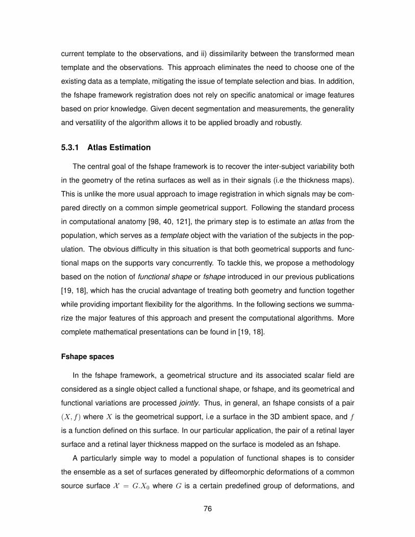
current template to the observations, and ii) dissimilarity between the transformed mean

template and the observations. This approach eliminates the need to choose one of the

existing data as a template, mitigating the issue of template selection and bias. In addition,

the fshape framework registration does not rely on specific anatomical or image features

based on prior knowledge. Given decent segmentation and measurements, the generality

and versatility of the algorithm allows it to be applied broadly and robustly.

5.3.1 Atlas Estimation

The central goal of the fshape framework is to recover the inter-subject variability both

in the geometry of the retina surfaces as well as in their signals (i.e the thickness maps).

This is unlike the more usual approach to image registration in which signals may be com-

pared directly on a common simple geometrical support. Following the standard process

in computational anatomy [98, 40, 121], the primary step is to estimate an atlas from the

population, which serves as a template object with the variation of the subjects in the pop-

ulation. The obvious difficulty in this situation is that both geometrical supports and func-

tional maps on the supports vary concurrently. To tackle this, we propose a methodology

based on the notion of functional shape or fshape introduced in our previous publications

[19, 18], which has the crucial advantage of treating both geometry and function together

while providing important flexibility for the algorithms. In the following sections we summa-

rize the major features of this approach and present the computational algorithms. More

complete mathematical presentations can be found in [19, 18].

Fshape spaces

In the fshape framework, a geometrical structure and its associated scalar field are

considered as a single object called a functional shape, or fshape, and its geometrical and

functional variations are processed jointly. Thus, in general, an fshape consists of a pair

(X, f) where X is the geometrical support, i.e a surface in the 3D ambient space, and f

is a function defined on this surface. In our particular application, the pair of a retinal layer

surface and a retinal layer thickness mapped on the surface is modeled as an fshape.

A particularly simple way to model a population of functional shapes is to consider

the ensemble as a set of surfaces generated by diffeomorphic deformations of a common

source surface X = G.X0 where G is a certain predefined group of deformations, and

76

functions defined on these shapes such that for a given X ∈ X , f is an L2 function on

the surface X (in the sense that the surface integral on X of f2 is finite). This eventually

defines a vector bundle of fshapes denoted F containing all objects of the form (X, f) with

X ∈ X , f ∈ L2(X).

In this frame, geometric-functional transformations of a given fshape (X, f) in the bun-

dle F simply consists in the combination of a deformation φ ∈ G and the addition of a resid-

ual function ζ ∈ L2(X) which gives the new fshape (Y, g).= (φ, ζ).(X, f) with Y = φ(X)

the deformed geometrical support and g = (f + ζ) φ−1 the new modified and transported

function on Y .

The main motivation of this model is that, provided the group of geometrical deforma-

tions is equipped with a certain metric dG, it becomes straightforward to measure now

distances between fshapes in F . One can simply take the minimal length of all paths

between them, which can be written as :

dF ((X, f), (Y, g))2 = inf(φ,ζ)

dG(Id, φ)2 + ‖ζ‖2L2(X)

∣∣φ(X) = Y, (f + ζ) φ−1 = g

(5.8)

Constructing relevant deformation groups and their metrics has been a wide field of study.

In this thesis, our reference model shall be the Large Diffeomorphic Metric Mapping (LD-

DMM) framework [4], where diffeomorphisms are constructed as flows of time-varying

vector fields of the 3D space belonging to a certain Hilbert space V , generally a repro-

ducing kernel Hilbert space. Given such a space V and the corresponding L2 space

of time-varying vector fields modeled on V , namely L2([0, 1], V ), one considers for any

v ∈ L2([0, 1], V ), the flow φv1 at time 1 and GV = φv1 | v ∈ L2([0, 1], V ) the associated

group of diffeomorphisms [193]. The Hilbert metric on vector fields induces in turn a Rie-

mannian metric on the group of deformations GV such that for any φ ∈ GV :

dG(Id, g)2 =

inf

∫ 1

0‖vt‖2V | v ∈ L2([0, 1], V ), φv1 = φ

(5.9)

Thus, in the LDDMM model, the optimization over φ ∈ G in (5.8) can be replaced by the

optimization on the space of time-varying deformation fields v. Combined with functional

variations, this provides fshape bundles spaces with a similar metric structure which has

several interesting properties, which are developed more thoroughly in [19].

77

Atlas formulation

Let us now consider a population of N observations (Xi, f i)i=1,..,N where the Xi’s are

the retinal surfaces and f i the corresponding thickness maps. One can introduce a gener-

ative model where the observations are obtained as geometric-functional transformations

of a common template fshape (X, f) plus some noise terms, such that:

(Xi, f i) = (φi, ζi).(X, f) + εi (5.10)

Above, (φi, ζi) are the hidden variables of transformations from the template to each sub-

ject, and εi are noise variables that must account for the fact that the observations cannot,

and in fact, should not, be obtained exactly as transformations of the template. The rea-

son is that real datasets present inter-subject variability caused by noisy irregularity in the

shape and signals, variations that do not result from the geometric-functional transforma-

tion model presented here. Defining such a noise model for textured surfaces is not trivial,

and it will be discussed further in the next subsection.

Under such a model, the purpose of atlas estimation is to recover from the observa-

tions both the template fshape (X, f) and the transformation variables (φi, ζi) which, as will

be described in a following section, enables to perform statistical analysis on population

variability or classification between different groups, for example. In a perfect noiseless

situation, this is the problem of computing a Karcher mean in the fshape bundle space F

generated from (X, f). With the presence of noise, one needs to relax the exact matching

conditions by introducing dissimilarity measures (also commonly referred as data attach-

ment terms) between two fshapes that do not necessarily belong to a common fshape

bundle. With an assumption that such a dissimilarity measure can be defined (this shall be

discussed in the next subsection) as a certain functional between the fshapes, the problem

of atlas estimation undertakes the following variational form :

(X, f, φi,∗, ζi,∗) =

arginfX,f,φi,ζi

N∑i=1

(dGV (Id, φi)2 + ‖ζi‖2L2(X)

+A((φi, ζi).(X, f), (Xi, f i))

)(5.11)

where GV is the group of geometrical deformations of the template modeled on the Hilbert

space V , and A the dissimilarity measure. The optimization is performed on the shape of

78

the template X, its mean thickness signal f in L2(X), the deformations φi (or equivalently

the deformation fields vi such that φi = φvi

1 ) and the residual signals ζi in L2(X). Each ith

observation contributes the sum of the geometric-functional transformation metric in (5.8)

and the measure of dissimilarity A between the transformed template and the observation.

The formulation above is only partly formal as it has not been specified in what space

the optimization over the template shape occurs. We refer the reader to [19] for a more

precise exposition on this topic as well as for the proof of existence of such variational

problems in a continuous setting. The following sections focus on the discrete equivalent

of the minimization problem and how it can be solved numerically.

Dissimilarity terms between fshapes

We first make a quick digression to define the dissimilarity functional A in (5.11), which

should also give some insight on interpretation of the noise variables in the generative

model of (5.10). Even in purely geometrical cases, establishing a dissimilarity measure for

practical applications is not a simple problem; one needs to establish a criterion of prox-

imity between surfaces without any point-to-point correspondence and of possibly different

topologies. In fshapes, the adjunction of signal functions defined on varying geometrical

supports presents a greater challenge.

For usual curves and surfaces, a widespread idea inherited from geometric measure

theory is to represent shapes as generalized distributions and induce metrics from these

distribution spaces. This has been consistently exploited in several past applications in

computational anatomy as in [57, 58, 40, 39, 41]. In all these examples, authors build upon

the concepts of current or varifold to embed geometrical shapes into common functional

spaces equipped with kernel-based Hilbert metrics.

Such frameworks can be naturally extended to the case of functional shapes, as suc-

cessfully demonstrated in [20] for currents and later in [19] for varifolds. The latter has

the advantage of not requiring any orientation for the shape surfaces and provides greater

robustness. In what follows, we give a brief simplified presentation of the fvarifold setting

detailed in [19].

79

In the fvarifold framework, a surface with signal is represented as a distribution of its

non-oriented normal vectors located at different positions in space and attached with cor-

responding real signal values. More precisely, any fshape (X, f) is considered as a distri-

bution µ(X,f) on the product space R3 × P (R3)×R, with P (R3) being the projective space

of all lines in R3, and is formally the sum of Diracs :

µ(X,f).=

∫Xδ(x,←→n (x),f(x))dH2(x) (5.12)

where←→n (x) denotes the (unoriented) line in P (R3) generated by the unit normal vector to

the surface X at point x, and H2 the usual 2-dimensional volume measure on the surface.

All possible fshapes are thus embedded into this common space of distributions.

As a functional space, distributions on R3×P (R3)×R can be equipped with various pos-

sible metrics or pseudo-metrics that can induce the dissimilarity criteria between fshapes.

Among these, the ones generated by positive kernels constitute a particularly interesting

category. For our purpose, positive kernels can be obtained as the product of three kernels

defined respectively on R3, P (R3) and R. If we denote them kg, kn and kf , it can be shown

we can induce a Hilbert (pseudo-) metric for any two fshapes (X, f) and (Y, g) :

〈µ(X,f), µ(Y,g)〉W ∗ =∫∫X×Y

kg(x, y).kn(←→nX(x),←→nY (y)).

kf (f(x), g(y))dH2(x)dH2(y) (5.13)

and A.= ‖µ(X,f) − µ(Y,g)‖2W ∗ = 〈µ(X,f) − µ(Y,g), µ(X,f) − µ(Y,g)〉W ∗ can be a suitable dis-

similarity term between (X, f) and (Y, g) (see [19] for an extensive presentation of the

properties of such metrics).

Depending on the choice for the kernels, various attachment terms are possible. As

apparent in (5.13), these do not assume any preliminary matching between the points

of X and Y or landmark extraction. Instead, kernel kg provides a spatial smoothness

to compare relative positions of the points on the two surfaces, and kernel kn allows to

compare relative positions of the normal vectors, while kf gives a measure of proximity

between the signal values attached to the fshapes. From now on, we shall take for kg a

Gaussian kernel on R3 of a certain scale σg, i.e.

kg(x, y) = e− |x−y|

2

σ2g .

80

A similar notion of a ’Gaussian kernel’ also exists on the more complex space P (R3) and

can be written as

kn(←→u ,←→v ) = e− 2

σ2n(1−〈−→u ,−→v 〉2)

for any unit vectors −→u and −→v generating the corresponding elements←→u ,←→v . Note that kn

is intrinsically independent of the orientations of the vectors −→u and −→v . The kernel width σn

is to be thought as a scale on the quotient sphere of unoriented unit vectors. Finally, the

last kernel kf can be also taken to be Gaussian

kf (a, b) = e− (a−b)2

σ2f

in which case (5.13) can be explicitly written as

〈µ(X,f), µ(Y,g)〉W ∗ =

∫∫X×Y

e− |x−y|

2

σ2g . e− 2

σ2n(1−〈−→nX(x),−→nY (y)〉2)

.

e− (f(x)−f(y))2

σ2f dH2(x)dH2(y) . (5.14)

The choice of Gaussian kernels is neither unique nor canonical; however, it results in

dissimilarity terms that are parameterized by three scales σg, σn and σf , allowing flexibility

and sensitiveness at various levels. Multiscale optimization can be easily facilitated by

combining different kernel values.

Discrete framework

A discrete representation of the functional surfaces is finite polyhedral surfaces with

signal values attached to each vertex. This can be expressed entirely by three matrices :

a P × 3 matrix x of the coordinates of the P vertices xk in R3, (x = (xk)1≤k≤P ), a P × 1

column vector f of the P values fk.= f(xk) ∈ R of the signal (f = (fk)1≤k≤P ), and

T × 3 connectivity matrix C that contains the list of T faces (assumed to be triangles for

simplicity) such that each row contains 3 integers corresponding to the indices of triangle

vertices.

The geometric-functional transformation on fshapes presented in 5.3.1 can be simply

translated to a discrete setting as follows. Given a discrete fshape (x,f), a diffeomorphism

φ, and a residual discrete signal ζ on the vertices of x, the transformation becomes :

(φ, ζ).(x,f) = ((φ(xk))1≤k≤P , (fk + ζk)1≤k≤P ) (5.15)

81

Note the connectivity matrix remains unchanged through the transformation. In such a

Lagrangian formulation, particles flow and transport their signals to new spatial locations.

The L2 norm of a signal ζ on a surface X in (5.8) may be approximated as

‖ζ‖2L2(X) ≈T∑l=1

f2l .|Tl| (5.16)

where for the lth triangle, |Tl| is the area of the triangle and f l is the average of the three

signal values at its vertices. This provides a Riemann sum approximation of the continuous

case. Higher order finite element approximations could be also used.

Similarly, the fvarifold-norm data attachment terms presented in 5.3.1 has a simple

discrete equivalent. The fvarifold associated with a polyhedral functional surface (x,f ,C)

can be associated with a finite sum of Diracs∑T

l=1 |Tl|.δ(xl,←→nl ,f l)

, where every triangle is

approximated by |Tl|.δ(xl,←→nl ,f l)

, xl being the barycenter, f l the mean signal value from the

three vertices, and ←→nl the unit unoriented normal vector to the triangle, obtained by the

wedge product of the two edge vectors. Now, given two discrete fshapes (x,f ,C1) and

(y, g,C2), the fvarifold data attachment term resulting from (5.14) approximates to :

A =

T1∑k=1

T1∑l=1

|Txk |.|Txl |.e− |xk−xl|

2

σ2g . e− 2

σ2n(1−〈←→nxk ,

←→nxl 〉

2). e− (fk−fl)

2

σ2f

−2

T1∑k=1

T2∑l=1

|Txk |.|Tyl |.e

− |xk−yl|2

σ2g . e− 2

σ2n(1−〈←→nxk ,

←→nyl 〉

2). e− (fk−gl)

2

σ2f

+

T2∑k=1

T2∑l=1

|T yk |.|Tyl |.e

− |yk−yl|2

σ2g . e− 2

σ2n(1−〈

←→nyk ,←→nyl 〉

2). e− (gk−gl)

2

σ2f (5.17)

The dissimilarity terms can be therefore computed based only on kernel evaluations be-

tween point positions, normal vectors, and signal values. However, this is numerically

expensive with the quadratic complexity of the number of triangles T1 and T2 of the two

surfaces. Several numerical methods can be implemented to provide fast computations

(see [18] Section 2.3.3 for a thorough discussion on the topic). For our application of

retinal surfaces, each consisting of approximately 20000 triangles, direct but massively

parallelized computations on GPU was chosen as the best trade-off between efficiency

and precision.

Lastly, we examine the discretization of the diffeomorphic transformations in the group

GV . As mentioned earlier, these can be parameterized by time-varying vector fields in

L2([0, 1], V ). This representation can be further reduced, since we are searching among

82

the optimal vector fields that link one given shape to another, or, in other words, among

geodesics in a certain Riemannian manifold of diffeomorphisms. As highlighted in re-

cent works in connection with optimal control theory, for example in [2], such geodesics

can be entirely described by the initial position and an initial momentum variable p0, and

the dynamics of the deformation is governed by a coupled system of Hamiltonian equa-

tions called the shooting equations. In the case of our discrete surfaces and V a cer-

tain RKHS of vector fields obtained by a vector kernel KV , this initial momentum can

be thought as a set of vectors p0 = (pk,0) attached to every vertex xk of the surface

for which v0(x) =∑P

k=1KV (xk, x)pk,0, and the reduced Hamiltonian undertakes the form

H(x,p) =∑n

k,l=1 pTkKV (xk, xl)pl. The shooting equations are then

x(t) = ∂pH(x(t), p(t))

p(t) = −∂xH(x(t), p(t))(5.18)

given the initial conditions x(0) = x and p(0) = p0. The resulting deformation is obtained

by flowing any initial condition x to time 1 through (5.18). An important consequence of

this is that the optimization of the template deformations φi in (5.11) can be formulated

as a minimization over initial momenta pi, all of which are made of a finite number of

vectors attached to the points of the template shape x. In addition, the energy of such a

deformation (given by the geodesic distance dGV ) can be also expressed based only on

the initial momentum p0 such that

dGV (Id, φv1)2 = H(x,p0) =

P∑k,l=1

pTk,0KV (xk, xl)pl,0. (5.19)

Numerical scheme for atlas estimation

The atlas estimation problem of (5.11) can be now formulated in the discrete setting.

The observations are N discrete fshapes given by xi, f i and the corresponding triangula-

tion matrices. The template is an fshape (x,f) given by a finite number of vertices, faces

and thickness values attached. The geometrical deformations of the template are summed

up by initial momenta variables pi, and the residual signals ζi are considered as vectors of

signal values attached to every template vertex, and thus of the same size as f . The final

83

form of the minimization functional is then as follows :

J(x,f , (pi), (ζi)).= γf .‖f‖L2 +

N∑i=1

(H(x,pi) + γζ‖ζi‖2L2

+γWA((φi, ζi).(x,f), (xi,f i))

)(5.20)

where ‖.‖L2 is given by (5.16),H(., .) by (5.19), and the dissimilarity termsA((φi, ζi).(x,f), (xi,f i))

by (5.14) and (5.15). γf , γζ and γW are strictly positive weighting coefficients leading to

different balance between the terms. Note that the additional presence of ‖f‖L2 (com-

pared to (5.11)) is to provide more regularity to the estimated template signal and it is also

a condition to guarantee the existence of solutions as explained in detail in [19].

Eventually, we are led to the problem of joint minimization with respect to all (finite-

dimensional) variables x,f , (pi), (ζi). This is still a very high-dimensional space since

each variable is roughly of dimension P , the number of template vertices, and the func-

tional J , essentially through the data attachment terms, fails from having any nice convexity

property. A reasonable approach to perform the actual optimization is a standard adaptive

step gradient descent on all variables simultaneously at each step. For this, one needs

to specify an initialization of the template fshape, denoted as xinit,f init, where the shape

given by xinit and its triangulation matrix should give a crude estimation of the observa-

tions, for instance, in global topology. Input initialization for the momenta and residual

signals pi and ζi is also needed, and it is often sufficient to set pi = 0 and ζi = 0. From

the expressions given above, computation of the gradient with respect to the variables

f = (fk)k=1,..,P and ζi = (ζik)k=1,..,P is quite straightforward and detailed in [19]. The gra-

dient with respect to the template position x and the momenta pi is slightly more involved.

‖f‖L2 , ‖ζi‖L2 and H(x,pi) can be easily differentiated with respect to x and pi, but the

dissimilarity metrics A((φi, ζi).(x,f), (xi,f i)) depends a priori on the deformed version

of the template, i. e. xi .= φi(x), f

i .= f + ζi. Each deformation φi is itself obtained

from x and pi by flowing forward in time the Hamiltonian equations (5.18). It has been

demonstrated in [40, 2] that the gradient of A((φi, ζi).(x,f), (xi,f i)) with respect to pi and

x can be computed by flowing backward in time the adjoint Hamiltonian system along the

trajectory of x and p :

Q(t) = −(∂2x,pH(x(t), p(t)))∗Q(t)

+(∂2x,qH(x(t), p(t)))∗P (t)

84

Algorithm 1 Atlas estimation on functional shapes

Require: N functional shapes (xi,f i), initialization of the template fshape (x = xinit,f =f init) and the gradient descent step δ.

1: set pi = 0 and ζi = 0 for all i ∈ 1, .., N.2: while Convergence do3: for i=1,..,N do4: Flow (x,f) by forward integration with pi and store the deformed template at time

1 (xi, fi).

5: Compute the gradients of ‖f‖L2 , H(x,pi), ‖ζi‖2L2 with respect to x, f , pi and ζi.

6: Compute the fvarifold representations of (xi,f i) and (xi, fi).

7: Compute the gradient ∇xiA((xi, fi), (xi,f i)) with respect to the final point config-

uration.8: Apply the backward integration of (5.20) and deduce ∇xA((xi, f

i), (xi,f i)) and

∇piA((xi, fi), (xi,f i)).

9: end for10: Update variables :

x← x+ δ∇xJ

f ← f + δ∇fJ

pi ← pi + δ∇piJ

ζi ← ζi + δ∇ζiJ

11: Compute new functional J(x,f , (pi), (ζi)) and possibly adapt step δ by line search.12: end while13: return template functional shape (x,f), N initial momenta (pi) and functional residu-

als (ζi).

P (t) = −(∂2p,pH(x(t), p(t)))∗Q(t)

+(∂2x,pH(x(t), p(t)))∗P (t) (5.21)

where the adjoint variablesQ and P are set with the end-time conditionsQ(1) = −∇xiA((xi, fi), (xi,f i))

and P (1) = 0. Then the gradients are∇xA((xi, fi), (xi,f i)) = −Q(0) and∇piA((xi, f

i), (xi,f i)) =

−P (0).

85

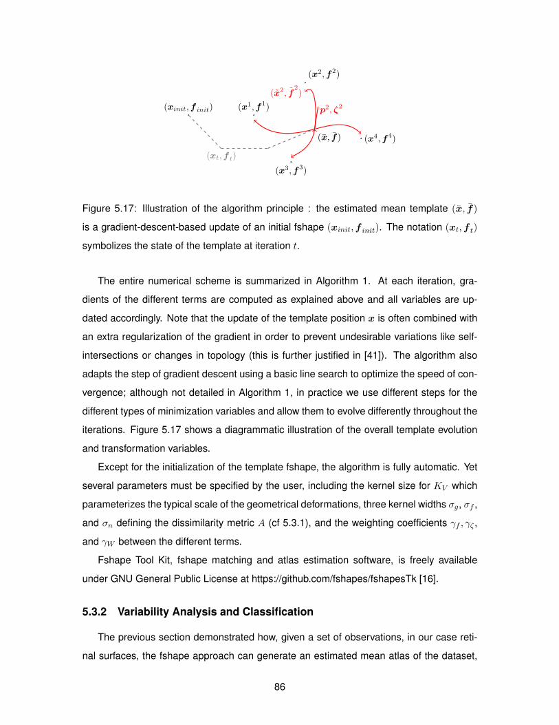
(xinit,f init)

(x, f)

(x1,f1)

(x2,f2)

(x2, f2)

(x3,f3)

(x4,f4)

(xt,f t)

p2, ζ2

Figure 5.17: Illustration of the algorithm principle : the estimated mean template (x, f)

is a gradient-descent-based update of an initial fshape (xinit,f init). The notation (xt,f t)

symbolizes the state of the template at iteration t.

The entire numerical scheme is summarized in Algorithm 1. At each iteration, gra-

dients of the different terms are computed as explained above and all variables are up-

dated accordingly. Note that the update of the template position x is often combined with

an extra regularization of the gradient in order to prevent undesirable variations like self-

intersections or changes in topology (this is further justified in [41]). The algorithm also

adapts the step of gradient descent using a basic line search to optimize the speed of con-

vergence; although not detailed in Algorithm 1, in practice we use different steps for the

different types of minimization variables and allow them to evolve differently throughout the

iterations. Figure 5.17 shows a diagrammatic illustration of the overall template evolution

and transformation variables.

Except for the initialization of the template fshape, the algorithm is fully automatic. Yet

several parameters must be specified by the user, including the kernel size for KV which

parameterizes the typical scale of the geometrical deformations, three kernel widths σg, σf ,

and σn defining the dissimilarity metric A (cf 5.3.1), and the weighting coefficients γf , γζ ,

and γW between the different terms.

Fshape Tool Kit, fshape matching and atlas estimation software, is freely available

under GNU General Public License at https://github.com/fshapes/fshapesTk [16].

5.3.2 Variability Analysis and Classification

The previous section demonstrated how, given a set of observations, in our case reti-

nal surfaces, the fshape approach can generate an estimated mean atlas of the dataset,

86

along with the geometrical and functional distances from the template to each of the ob-

servations. A group average retina in itself is useful for purposes such as qualitative and

quantitative group comparisons. The shape and signal distances of individual observations

can serve as metrics for inter-eye variability.

Augmenting the fshape framework with a classification module is thus a natural ex-

tension with several merits. On experimental data with confirmed diagnosis, automated

classification can demonstrate the mean template-based variability of retinas has indeed

anatomical and clinical relevance. Furthermore, a classification module can determine

whether a particular anatomical feature, thickness or topology of a layer, is significantly

correlated with a disease. This can lead to better understanding of the structural mani-

festation of the disease in terms of cause or effect. Lastly, automated classification is an

example of the fshape framework application that can directly assist in clinical decision

making.

The initial momenta (pi) and functional residuals (ζi) in 5.3.1, representing the retinal

layer surface topology and associated retinal layer thickness respectively, are used for clas-

sification. Two classificaiton methods were tested: a set of Weka 3 software modules [68]

performing feature selection based on information gain followed by a support vector ma-

chine classification (InfoGainSVM), and a tunable variation of linear discriminant analysis

(LDA) classifier. The LDA classifier is described in the following subsections.

Regularized LDA on Hilbert space valued dataset

LDA is a classic linear classification method that may be viewed as a weighted principal

component analysis (see chapter 4 of [70] for an introduction). We discuss hereafter the

particular case in which the data points x1, · · · , xN belong to a separable Hilbert space H

of a possibly infinite dimension. As mentioned, in our particular application, the xi’s will be

functional residuals and/or the geometrical initial momenta.

Within- and between-class scatter operators We assume that the N observations at

hand are divided into K classes C1, · · · , Ck such that 1, · · · , N =⋃Kk=1Ck. The mean of

the k-th class is xk = 1Nk

∑i∈Ck xi where Nk = Card(Ck). Let us define the within-class

scatter operator Sw : H → H

87

Sw(·) =1

N

K∑k=1

∑i∈Ck

〈xi − xk, ·〉H (xi − xk)

and the between-class scatter operator Sb : H → H

Sb(·) =1

N

K∑k=1

Nk〈xk − x, ·〉H (xk − x) .

In the case where H is of finite dimension, the matrix associated to the operator Sw (or Sb)

is the standard within-class (or between-class) scatter matrix.

Finite dimensional representation We denote H0 = Span (xi, . . . , xN ) ⊂ H and q =

dim(H0). In our framework, H is high (or infinite) dimensional, and, in practice, q equals to

N . We then denote fH0 : H0 → H0 the restriction to H0 of any linear mapping f : H → H

such that f(H0) ⊂ H0. In particular, we may consider the restrictions Sw,H0 and Sb,H0 of

the scatter operators Sw and Sb, respectively.

Let us now choose an arbitrary isometric linear mapping L : H0 → Rq in order to get a

finite representation of the data

xi = Lxi ∈ Rq.

By definition we have ‖xi‖Rq = ‖xi‖H . From now on, we will work with this new represen-

tation of the data and we may consider their corresponding scatter operators Sw, Sb : Rq →

Rq defined as,

Sw = LSw,H0L† and Sb = LSb,H0L

†,

where L† : Rq → H0 is given by 〈L†a, x〉H = 〈a, Lx〉Rq for any x ∈ H0 and a ∈ Rq.

When the xi’s form a basis of H0, an effective way to build an isometric mapping L is

to introduce the mapping γ(x) = (〈x, xi〉H)Ni=1 for any x ∈ H0 and the Gram matrix G =

[〈xi, xj〉H ]Ni,j=1 ∈ RN×N . It is then easy to check that the linear mapping Lx = G−12γ(x) is

isometric.

Discriminant axes in the finite dimensional space In our framework, the within-class

scatter operator Sw may not be invertible in general. We consider the following regulariza-

tion of the within-class scatter operator

Sεw = Sw + εIdRq , (5.22)

88

where ε > 0 is a regularization parameter which has to be calibrated by the user as de-

scribed below.

The discriminant spaces of the LDA are given by the eigendecomposition of

Aε = (Sεw)−1Sb.

The number of non-vanishing eigenvalues is limited by the rank of Sb which is less than

K − 1. In general, we have the K − 1 corresponding unit eigenvectors u1, . . . , uK−1 ∈ Rq

that will be used to derive the discriminant axes in H.

Classification with regularized LDA The rationale behind the isometric dimension re-

duction is that the unit vectors

u` = L†u` ∈ H0, ` = 1, . . . ,K − 1

are the eigenvectors corresponding to the non-vanishing eigenvalues of AεH0= (Sw,H0 +

εIdH0)−1Sb,H0 , as in [49]. This classic trick avoids numerical issues as the matrix inversion

is performed in the small dimensional space Rq.

Then, given a new observation y ∈ H we use directly the discriminant axes u1, . . . , uK−1

to define a classification rule. For instance, when K = 2 (a two-class classifier) we have

u1 ∝ (Sεw)−1(x1 − x2) where the ∝ symbol means “collinear to”. The discriminant rule is

then a threshold on y → 〈u1, y − x〉H .

Calibration of the regularization parameter The regularization parameter ε > 0 can be

optimized with a leave-p-out cross-validation (CV) procedure. Note that we do not need

to compute the Gram matrix G appearing in the definition of the isometric mapping L at

each stage of the CV. This is very helpful since the operation may be costly depending on

the magnitude of N . Instead, the N ×N “full” Gram matrix Gf with all the observations is

computed once, and the (N − p)× (N − p) Gram matrices G are obtained by deleting the

p rows and columns of Gf corresponding to the p left-out observations.

In our simulations, surprisingly small values of the regularization parameter ε, ranging

from 0.001 to 1, generally yielded better CV results. We provide below a short analysis on

the LDA behaviour for small values of ε.

Let H1 ⊂ H0 be the linear subspace of H defined by

H1 = Sw(H) = Span xi − xk|1 ≤ k ≤ K, i ∈ Ck

89

Figure 5.18: (a) Aligned RNFL surfaces with RNFL thickness mapping, (b) mean templateof all RNFLs, (c) mean template of normal RNFLs only, and d) mean template of glauco-matous RNFLs only. Note the low estimated RNFL thickness of the mean glaucomatoustemplate as compared to that of the mean normal template.

Figure 5.19: Observed RNFLs (top row) and their reconstructions from a common meantemplate (bottom row). Note that the reconstruction agrees with the pattern of the originalRNFL thickness with an overall smooth and noise-reduced profile.

Denoting pH⊥1 : H → H the linear projection onto the linear space orthogonal to H1, it can

be shown that

limε→0

ε(Sεw)−1Sb = pH⊥1Sb.

The limit is taken here in the sense of the operator norm ‖f‖ = maxx,‖x‖H=1 ‖fx‖H

for any linear f : H → H. This indicates when the chosen ε > 0 is small, discriminant

information is found orthogonal to the within-class variations. In particular, when K = 2

and ε vanishes, the discriminant axis is u1 ∝ pH⊥1 (x1 − x2).

90

5.3.3 Experimental Results

Peripapillary OCT images from 53 eyes with confirmed diagnosis from 10 controls, 10

bilateral glaucoma patients, and 7 unilateral glaucoma patients were included in the exper-

iment. Written consent forms were obtained from all participants and ethics review was

approved by the Office of Research Ethics at Simon Fraser University (SFU) and the Re-

search Ethics Board of the University of British Columbia (UBC). In addition to OCT imag-

ing, all participants were subject to a battery of standard tests, including dilated stereo-

scopic examination of the optic nerve, stereo disc photography analysis and visual field

abnormality check, to ensure there was no other pathology present. The acquired im-

ages were smoothed, segmented, and measured for retinal layer thickness as described

in Chapter 3 and 4.

Mean template generation

The mean templates of retinal nerve fiber layer (RNFL) posterior surfaces and associ-

ated RNFL thickness maps were generated as described in Section 5.3.1. The surfaces

were aligned at the BMO centroid prior to the mean template generation, as shown in in

Fig. 5.18 (a). The physical dimensions of the images vary as the imaging field of view

changes depending on the axial length of the eye. Fig. 5.18 (b), (c), and (d) respec-

tively show the mean templates generated from all eyes (N = 53), bilaterally normal eyes

(N = 20), and glaucomatous eyes (N = 26). Qualitatively, the normal mean template in

Fig. 5.18 (c) displays the characteristic hourglass pattern in RNFL thickness, whereas the

glaucomatous mean template in Fig. 5.18 (d) show much thinner RNFL thickness overall,

with superior peripapillary RNFL slightly more preserved compared to the inferior region.

Fig. 5.19 shows the observed RNFL surfaces (top row) and their approximations (bot-

tom row) from a common mean template of 53 RNFLS in Fig. 5.18 (b). As described in the

previous section, the ith approximation is a deformed version of the template, such that

xi.= φi(x), f

i .= f+ζi. The salient shape features are reproduced, in particular the RNFL

thickness pattern and the BMO location and size. The level of detail in approximation can

be tuned by user specified parameters including kernel sizes for geometric deformation

and dissimilarity metric, and runtime parameters in the gradient descent optimization.

91

Figure 5.20: Functional convergence with gradient descent optimization.

Figure 5.21: Left: Voxel-wise t-test significance map of retinal nerve fiber layer (RNFL)thickness between normal (N = 26) and glaucomatous (N = 27) eyes, with the red regionindicating p < 0.05. Right: The same map with the log of the p-value.

Fig. 5.20 shows the convergence of the minimization functional (5.20) in computing the

mean template of 53 RNFLs in Fig. 5.18 (b) with the adaptive gradient descent optimization

process in Section 5.3.1. In the actual computation, the algorithm was run with three sets of

different kernel sizes for σg, σf , and σn. This allowed refinement of the result by reducing

the kernel sizes at successive runs with each ending at either reaching the predefined

maximum number of iterations per run or minimum change of the functional value with the

given set of parameters.

In Fig. 5.20, the first run begins at Iteration 0 with the functional value at 1.34 × 104

and ends at Iteration 40 with the energy reduced to 2.47 × 103. The second run begins at

Iteration 41 with a new set of kernel sizes and the starting functional evaluated at 1.28 ×

103. This run ends at Iteration 44 because ∆J becomes less than the preset minimum of

10−4. The third run begins at Iteration 45, again with smaller kernel sizes, and the energy

stabilizes around 6.94× 102.

92

T-test between healthy and glaucomatous RNFL thickness residuals

The mean templates of the normal (c) and glaucomatous (d) RNFLs in Fig. 5.18 qual-

itatively show the difference between the two groups. In order to identify the spatial loca-

tions of the thickness difference, a vertex-wise t-test was performed using the functional

(thickness) residual ζi, the vertex-wise thickness offset between the template and its ap-

proximation of the ith observation. The t-test compared the means of the residuals of 26

normal RNFLs and 27 glaucoma RNFLs at each voxel on the mean template of all RNFLs

in Fig. 5.18 (b).

The result is shown in Fig. 5.21. On the left, the voxels with p-values less than 0.05

are marked in red and indicate the regions with statistically significant RNFL thickness dif-

ference between the normal and glaucomatous RNFLs. Most of the peripapillary region

shows significance, except at the image boundaries, where the f-shape correspondence

may be less reliable due to the different imaging field of view size, and in the region immedi-

ately temporal to BMO. More interesting pattern is shown in the right image, which displays

the log of the p-value. Cooler colors indicate smaller p-values and greater statistical sig-

nificance across the multiple RNFLs. The figure shows that glaucomatous thinning occurs

most distinctly in the inferior-temporal region of the RNFL, which agrees with previous stud-

ies [146, 135, 9, 101, 200] that the inferior peripapillary region is the most distinguishing

between normal and glaucomatous eyes, especially in the early stage of the disease. Un-

like the previous studies, however, our analysis shows full spatial detail without averaging

in sectors, and reveals a clear pattern of statistical significance that resembles the charac-

teristic thickness pattern of a healthy RNFL. The result suggests that the most significant

amount of glaucomatous thinning, or the earliest of the thinning, may occur along the RNFL

ridges where the RNFL is naturally the thickest.

Classification

As described in Section 5.3.2, classification experiments were performed using Weka

InfoGainSVM and LDA classifiers, on the momenta pi, which represents the vertex-wise

geometric deformation of the template to the ith observation, and functional residuals

ζi, the vertex-wise thickness offset between the template and the approximation of the

93

Figure 5.22: Leave-one-out cross validation accuracy with varied regularization parameterε.

ith retina. For each experiment, the LDA classifier was trained by leave-one-out cross-

validation, with the best-performing regularization parameter ε chosen from values by test-

ing 0.001 to 1 as shown in Fig. 5.22.

Healthy vs. Glaucoma Age-matched (59.6 ± 6.7) normal (N = 10) and glaucomatous

(N = 18) RNFLs were classified with the result in Table 5.5. Both Weka and LDA mod-

els yielded high classification rates, with the LDA model classifying a test sample drawn

from the data 144 times with no error. The result indicates that the fshape metrics of

the peripapillary RNFL posterior surface and RNFL thickness can be used to predict the

clinical diagnosis of glaucoma with high accuracy, and confirms the connection between

vision loss that bases glaucoma diagnosis, and characteristic morphological changes in

the RNFL.

Healthy vs. Suspect Glaucoma is generally bilateral, affecting both eyes of the patient,

and often asymmetric, such that the affected fellow eyes exhibit different degrees of sever-

ity. In unilateral primary glaucoma in which only one eye is diagnosed with glaucoma, the

healthy fellow eye is at a greater risk of developing glaucoma in the future than healthy

eyes of bilaterally normal subjects [104, 180]. Based on this, we labeled 7 healthy fel-

low eyes from unilateral glaucoma cases as suspect, and attempted to detect these from

healthy eyes of bilaterally nonglaucomatous subjects. The classification result of the bilat-

erally healthy eyes (N = 19, mean age: 43.4± 14.8) and suspect eyes (N = 7, mean age:

57.1± 12.4) are shown in Table 5.5.

94

Method Accuracy (%) Sensitivity (%) Specificity (%)

Healthy vs. GlaucomaWeka 94.23 94 90LDA 100.00 100.00 100.00

Healthy vs. SuspectWeka 83.10 83 76LDA 91.67 88.89 92.59

Table 5.5: Accuracies, sensitivities, and specificities of the classification of healthy, glauco-matous, and suspect RNFLs

Figure 5.23: LDA classifier for Healthy vs. Glaucoma data in A) functional residual, B)initial momenta in x-direction, C) initial momenta in y-direction, and D) initial momenta inz-direction.

That both models appear to distinguish the suspect eyes from the bilaterally healthy

eyes is noteworthy, considering that the suspect eyes are prediagnosis and without func-

tional loss or other conventional clinical features of glaucoma. As expected, the classifi-

cation rates are lower than those between confirmed glaucomatous eyes and bilaterally

healthy eyes in the previous experiment, but still high, particularly with the LDA model

of 88.89% sensitivity and 92.59% specificity. The result suggests the fshape metrics may

capture some subtle morphological changes in the RNFL that precedes vision loss in glau-

coma.

In LDA classification, an intuitive way to understand the result is to visualize the classi-

fier, or the direction that yields the maximum between-class variance. The LDA classifier

for the Healthy vs. Glaucoma dataset is visualized in Fig. 5.23 on the mean template

95


Healthy vs. Glaucoma, RNFL thickness onlyWeka 93.99 94 97LDA 100.00 100.00 100.00

Healthy vs. Glaucoma, RNFL posterior surface geometry onlyWeka 81.43 81 70LDA 81.94 84.04 78.00

Table 5.6: Accuracies, sensitivities, and specificities of the classification of healthy andglaucomatous RNFLs by RNFL thickness only and RNFL posterior surface geometry only

RNFL, in functional residual (RNFL thickness), and x, y, and z coordinates of initial mo-

menta representing the template deformation. The relative magnitude can be interpreted

as the degree of contribution to the classification, and it can be seen that RNFL thickness

was a more decisive factor in the classification of healthy and glaucomatous eyes than

posterior RNFL surface geometry. The map in Fig. 5.23 A, which is the spatial pattern

of classification contribution of RNFL thickness residual, is similar to the right image of

Fig. 5.21, which is the statistical significance map of the group difference between the two

classes. This confirms that the LDA classification was the most influenced by the regions

where there are the most significant difference between the healthy and glaucomatous

eyes.

RNFL thickness vs. RNFL surface geometry In order to compare the discriminating

power of RNFL thickness against RNFL posterior surface geometry, and to confirm what

was shown in Fig. 5.23, we repeated the Healthy vs. Glaucomatous classification with

RNFL functional residual (RNFL thickness) and initial momenta (RNFL posterior surface

geometry) separately. The result is summarized in Table 5.6.

As expected from Fig. 5.23, the classification result with RNFL thickness only is com-

parable to that with both RNFL thickness and geometry, and superior to the result with

RNFL geometry only. However, it is interesting to note that posterior RNFL surface without

the thickness information appears to still discriminate the healthy and glaucomatous eyes

to some degree. This, along with the characteristic pattern in Fig. 5.21, suggests that the

magnitude of RNFL thinning in glaucoma is not uniform across the peripapillary region,

and the surface topology is altered along with the overall reduction in tissue volume.

96


Healthy vs. Glaucoma, unregistered RNFLWeka 84.52 85 79LDA 95.83 98.13 89.19

Healthy vs. Suspect, unregistered RNFLWeka 74.29 74 47LDA 89.58 80.00 74.31

Table 5.7: Accuracies, sensitivities, and specificities of the classification of healthy, glauco-matous, and suspect RNFLs based on unregistered RNFLs

Classification with unregistered RNFLs The above classifications for Healthy vs. Glau-

coma and Healthy vs. Suspect were repeated with the same eyes, but instead of the fshape

metrics of the RNFL thickness residual and initial momenta, the original RNFL thickness

and RNFL posterior surface point coordinates were used. The result in Table 5.7 shows

relatively high classification success rates, but compared to the results in Table 5.5, all

accuracies, sensitivities, and specificities are consistently lower for both Weka and LDA

models. The specificity values are especially lower, indicating that the fshape metrics were

able to reduce the number of false positive classifications with the unregistered original

data.

5.3.4 Discussion

We present a novel application of the powerful fshape framework that can simulta-

neously compute the variability in shape and associated signals in retinal optical coher-

ence tomography (OCT) images. Fshape-based analysis and classification was performed

on healthy and glaucomatous peripapillary retinal nerve fiber layers (RNFL). The fshape

framework enabled creation of a mean atlas RNFL surface and RNFL thickness from mul-

tiple eyes, and quantification of the difference among the observed RNFLs with the mean

template as the reference. This approach is a compelling and complementary improvement

to the conventional sector analysis of the retina, and it has a potential for broad applica-

tion in studying longitudinal changes and cross-sectional differences in both anatomy and

physiological signals. Below we discuss few of the details involved in successfully applying

the algorithm for OCT data.

The fshape framework extracts the shape and signal variability in a given data, but

prior knowledge of the cause of the variability is important in preprocessing the data and

97

interpretation of the result. For example, there were several artifactual shape discrepancies

in the original OCT images used in this thesis. The image field-of-view size varied for

each retina due to the eye’s axial length. Bruch’s membrane opening (BMO) was only

approximately centered relative to the image frame, and the axial position of the RNFL

relative to the image frame varied. Since we were specifically interested in shape variability

due to pathology, the input data was preprocessed prior to the fshape pipeline in order to

reduce such unwanted noise and to minimize its effect in the result. Before the experiment,

it was confirmed that there was no correlation between presence or severity of glaucoma

and the subject’s axial lengths or the relative BMO position. The surfaces were therefore

aligned at the BMO center, as shown in Fig. 5.18 a), to bring them as close as possible

with each other without altering the surface topology. Additionally, RNFL within 0.25 mm

from BMO was excluded, because the exact termination point of the layer in the region

is often ambiguous. The input surfaces were then concentric with respect to BMO and

centrally overlapping, but the outer edges were mismatched due to the differing image

size, which is visible in Fig. 5.18 a). Whereas BMO is a true anatomical structure and a

valid registration landmark, the image boundary is purely artificial except in its relation to

the subject’s axial length. We were therefore wary that a mean template and estimated

momenta at the boundary region would be affected by this mismatch. This may also have

confounded the classification as the momenta and functional residuals at the boundary

have less spatial correspondence across the eyes. However, the regions near the outer

boundary also make the least contribution to the classification of healthy and glaucomatous

eyes, as it can be seen in Fig. 5.21 and 5.23. One way to possibly mitigate the boundary

effect is to crop the images, for example, to the largest commonly overlapping region. The

disadvantage is that this could waste a significant amount of data, and the cropping must

be done in a way that does not introduce artificial bias.

Choosing a good initial hyper template is also important in the computation and quality

of the final mean template. The hyper template must be topologically equivalent to the

observations, and as unbiased as possible. An implicit assumption is that the observations

from which a mean template is generated are topologically similar. Retinal layer surfaces in

OCT images can be modeled in relatively simple shapes; a surface from the macular region

is a 3D planar surface, and a surface from the peripapillary region with optic cup in the

center is a 3D planar surface with a hole in the center. In these cases, a prototype template

98

can be generated without difficulty, and even incorporate simple pre-measurements such

as the average width and length of the observed layers. However, complex structures like

lamina cribrosa can pose a greater challenge in choosing a suitable hyper template.

A potential application of the fshape framework is to create population-based normative

atlases of the retina using large data cohorts. Statistical distribution of the retinal morphol-

ogy in healthy subjects can be computed voxel-wise on the atlas. A test subject’s retina can

then be compared to the atlas to quantify its deviation from the healthy mean, and assess

the disease risk or severity based on the population statistics. Such comparison of a tar-

get subject to an existing atlas would require matching. In matching of a template fshape

(X, f) and a target fshape Xt, f t, the purpose is for the template to approximate the target

as closely as possible, and to obtain the distance between the two by the deformation φt

and functional residual ζt of the approximation. This is written as the minimization of the

functional

(φt, ζt) = arginfφt,ζt

dGV (Id, φt)2 + ‖ζt‖2

L2(X)

+A((φt, ζt).(X, f), (Xt, f t))

and similarly to Eq. 5.11, GV is the the group of geometrical deformations of the template

on the Hilbert space V , and A is the dissimilarity measure between the target and the tem-

plate approximation. Unlike the atlas estimation, the optimization in matching is performed

only on φt and ζt which can be done exactly as explained in Section 5.3.1. Such matching

would also allow one to directly compare one mean template to another.

Future work will include a comprehensive investigation of the optic nerve and macular

morphology in a larger data using the fshape and classification modules presented here.

The goal is to better detect and understand the shape changes or differences correlated to

diseases such as glaucoma. In this report only RNFL was examined, but any other retinal

layer can be similarly analyzed, in any combination of layers, surface topology, thickness,

etc. Shape and signal from multiple eyes will be made comparable by a common atlas, and

significance of a metric, region, or anatomical structure can be tested by statistical analysis

including the classification modules above. In this work the mean template generation

and classification process yielded convincing results despite of the mismatch between the

RNFL sizes and relative BMO locations. Another direction of future research is to apply the

fshape framework to structures like lamina cribrosa, which is not only more topologically

99

complex but also much less consistently visible across eyes than retinal layers. It may be

possible that the combined framework can extract common shape information from multiple

lamina cribrosa images with varying and limited visibility.


The contributions described in this chapter and published in [113] and submitted for

publication in IEEE Transactions on medical Imaging:

• Surface-to-surface registration of retinal surfaces by current-based approximation fol-

lowed by spherical demons registration.

• Repeatability analysis of BMO shape and RNFL and choroidal thickness in healthy

subjects using the surface-to-surface registration.

• Atlas-based shape analysis and classification of retinal surfaces using the fshape

framework

A manuscript is in preparation for publication on the repeatability analysis.

100

Chapter 6

Optic Nerve Head Morphometrics in Myopic

Glaucoma

The pathophysiology of glaucoma, although not fully understood, involves damage to

the retinal ganglion cell axons at the level of the lamina cribrosa [156, 155, 5]. Uncon-

trolled intraocular pressure (IOP) likely triggers several parallel, but interacting, mecha-

nisms including direct axonal damage, disturbances in neuro-metabolism and microvas-

cular supply, glial activation, and extensive remodeling of the connective tissues of the

lamina cribrosa and surrounding tissues throughout the development and progression of

glaucoma [154, 131, 75, 13, 28, 145, 168, 169, 30, 64, 65, 185]. The peripapillary tissues

that surround the optic nerve itself have also been implicated as possible contributors to

glaucomatous changes, both in experimental and modeling studies [36]. Atrophic features

of the peripapillary tissues which appear to be associated with glaucoma can include thin-

ning of the peripapillary scleral tissue [189], and loss of almost all retinal and deeper layers

separating the subarachnoid space from the vitreous cavity [37].

Myopia presents unique challenges for the management of glaucoma. Population-

based studies have indicated a greater prevalence of glaucoma in myopes [133, 188]. The

shallow cupping and pale neuro-retinal rim of high myopia make optic nerve head assess-

ment difficult. Myopic individuals can show abnormal results on structural and functional

testing because normal databases are composed of individuals with low refractive error

[45, 134]. Coexisting pathologies, particularly myopic degeneration, cloud interpretation

of visual field changes in advanced glaucoma. Cup-to-disk ratio and retinal nerve fiber

layer (RNFL) thickness measured by commercial optical coherence tomography (OCT)

101

and confocal scanning laser ophthalmoscopy (CSLO) were shown to be less effective in

discriminating glaucomatous and nonglaucomatous subjects with high myopia [130], with

several studies reporting RNFL thinning associated with myopia [81, 102, 171]. There are

theoretical grounds to suggest that myopic eyes may be more sensitive to a given IOP as

a result of the larger globe size and thinner, more compliant tissues [142, 172, 182].

In studies comparing highly myopic glaucomatous eyes to non-highly myopic glauco-

matous eyes, the former showed significant histological difference in the peripapillary re-

gion including elongation and thinning of the scleral flange [96]. Comparison of colour

stereo optic disc photography showed more pronounced optic nerve damage, larger and

more elongated optic discs, and shallower optic cups in myopic glaucomatous eyes [91,

92, 34].

To further understand the features of the myopic optic nerve in glaucoma, we have

imaged the optic nerve and surrounding peripapillary tissues in myopes, both with and

without glaucoma, and performed quantitative shape measurement and analysis.

6.1 Participants

A total of 27 subjects were recruited for this study: 5 young healthy controls (10 eyes,

mean age = 29.8 ± 3.6), 5 older healthy controls (10 eyes, mean age = 57.0 ± 4.4), 7

patients with unilateral glaucoma (14 eyes, mean age = 57.2 ± 12.4), and 10 patients

with bilateral open-angle glaucoma (19 eyes, mean age = 55.7 ± 12.6). Ethics review for

this study was approved from Simon Fraser University (SFU) and from the University of

British Columbia (UBC). The study was conducted in accordance with the guidelines of the

Declaration of Helsinki, and informed consent form was obtained from each participant.

All participants had axial lengths greater than 24 mm. A diagnosis of open-angle glau-

coma was made clinically by a fellowship-trained glaucoma specialist based on full exam-

ination including dilated stereoscopic examination of the optic nerve, analysis of stereo

disc photography, and typical reproducible Humphrey SITA-Standard white on white visual

field abnormality. No reference to OCT images was made for the purposes of categorizing

subjects for the study. Severity of glaucomatous visual field loss was quantified by Visual

Field Mean Deviation (MD) values. Participant demographics are tabulated in Table 6.1.

102

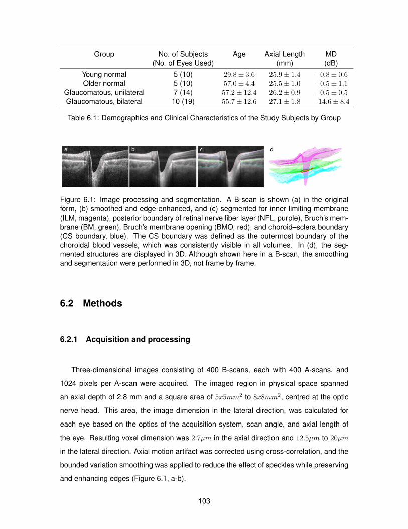
Group No. of Subjects Age Axial Length MD(No. of Eyes Used) (mm) (dB)

Young normal 5 (10) 29.8± 3.6 25.9± 1.4 −0.8± 0.6Older normal 5 (10) 57.0± 4.4 25.5± 1.0 −0.5± 1.1

Glaucomatous, unilateral 7 (14) 57.2± 12.4 26.2± 0.9 −0.5± 0.5Glaucomatous, bilateral 10 (19) 55.7± 12.6 27.1± 1.8 −14.6± 8.4

Table 6.1: Demographics and Clinical Characteristics of the Study Subjects by Group

Figure 6.1: Image processing and segmentation. A B-scan is shown (a) in the originalform, (b) smoothed and edge-enhanced, and (c) segmented for inner limiting membrane(ILM, magenta), posterior boundary of retinal nerve fiber layer (NFL, purple), Bruch’s mem-brane (BM, green), Bruch’s membrane opening (BMO, red), and choroid–sclera boundary(CS boundary, blue). The CS boundary was defined as the outermost boundary of thechoroidal blood vessels, which was consistently visible in all volumes. In (d), the seg-mented structures are displayed in 3D. Although shown here in a B-scan, the smoothingand segmentation were performed in 3D, not frame by frame.

6.2 Methods

6.2.1 Acquisition and processing

Three-dimensional images consisting of 400 B-scans, each with 400 A-scans, and

1024 pixels per A-scan were acquired. The imaged region in physical space spanned

an axial depth of 2.8 mm and a square area of 5x5mm2 to 8x8mm2, centred at the optic

nerve head. This area, the image dimension in the lateral direction, was calculated for

each eye based on the optics of the acquisition system, scan angle, and axial length of

the eye. Resulting voxel dimension was 2.7µm in the axial direction and 12.5µm to 20µm

in the lateral direction. Axial motion artifact was corrected using cross-correlation, and the

bounded variation smoothing was applied to reduce the effect of speckles while preserving

and enhancing edges (Figure 6.1, a-b).

103

6.2.2 Segmentation

Inner limiting membrane (ILM), the posterior boundary of nerve fiber layer (NFL), Bruch’s

membrane (BM), Bruch’s membrane opening (BMO), and the choroid–sclera boundary

(CS boundary) were segmented for this study (Figure 6.1 c). The automated segmenta-

tion result was examined and corrected by a trained research engineer using a custom

script in Amira (version 5.2; Visage Imaging, San Diego, CA, USA). Segmented surfaces

were overlaid on the original grayscale image and viewed simultaneously in three separate

orthogonal planes for better visualization of the structural boundaries obscured by blood

vessel shadows. The rater was able to scroll back and forth through the volume in any one

of the three orientation views while the other two orthogonal views and location pointers

were slaved and updated accordingly.

Bruch’s membrane opening was defined as the termination point of the high-reflectance

BM/retinal pigment epithelium (RPE) complex on the OCT image (Figure 6.1 c). This

corresponds to a pigmented and thus clinically identifiable structure, or a nonpigmented

and thus clinically invisible structure [161, 22]. The BMO was segmented manually by a

trained research engineer on 40 radial slices extracted from the volume, intersecting at the

approximated center of the BMO and spaced at a constant angle of 4.5 degrees.

6.2.3 Measurements

Seven shape characteristics were defined and measured on the segmented ILM, NFL,

BM, BMO, and CS boundary: NFL thickness, BMO area, BMO eccentricity, BMO planarity

[175], BMO depth, BM depth, and choroidal thickness. The parameters are graphically

described in Figure 6.2.

Nerve fiber layer thickness was measured at each pixel of the posterior NFL surface as

the closest distance to the ILM surface. The NFL within 0.25 mm from BMO was excluded

because near and inside BMO, NFL changes into vertical fiber bundles. For statistical

analysis, NFL thickness was averaged over an elliptical annulus, inwardly bounded at 0.25

mm from BMO and outwardly bounded at 1.75 mm from BMO. This provided a level of

anatomical consistency in averaging measurements over multiple eyes with different image

and BMO sizes.

104

Figure 6.2: Shape parameters. (a) An example B-scan. (b) Nerve fiber layer thickness wasmeasured as the closest distance to ILM from each point on the posterior NFL boundary.(c) Bruch’s membrane reference plane was defined as the best-fit plane to BM points 2mm away from the BMO center. (d) Bruch’s membrane opening depth was measuredas the normal distance between the BM reference plane and BMO center. (e) Bruch’smembrane depth was measured as the normal distance between each point of BM andthe BM reference plane. (f) Choroidal thickness was measured as the closest distance toBM from each point on the posterior choroid boundary. Although shown here in a B-scan,all parameters were defined and measured in the full 3D volume.

To quantify the BMO shape, an ellipse was fitted to the segmented BMO points by

first finding the best-fit plane using principal component analysis (PCA) [90] and fitting

an ellipse to the projection of the BMO points on the plane by least-squares criterion.

Bruch’s membrane opening area and BMO eccentricity were calculated from the fitted

ellipse. Bruch’s membrane opening planarity, or how much the BMO deviates from a plane,

was measured as the mean of the normal distance between the segmented BMO points

and its best-fit plane.

For the BM shape parameters, BMO depth and BM depth, a BM reference plane [175]

was first established by selecting points on BM along a circle 2 mm from the center of

the BMO and fitting a plane with PCA. Bruch’s membrane opening depth was measured

as the normal distance from the BMO center to the BM reference plane and reflects the

posterior depth of BMO with respect to the BM reference plane. Bruch’s membrane depth

was defined as the normal distance from each pixel of the BM surface to the BM reference

plane. For statistical analysis, BM depth was averaged over an elliptical annulus, inwardly

bounded at BMO and outwardly bounded at 1.75 mm from BMO. Furthermore, BM depth

105

Figure 6.3: Sectorization. Elliptical annuli were drawn at 0.25, 0.75, 1.25, and 1.75 mmfrom Bruch’s membrane opening (BMO). The annuli were divided into 608 angular sectorsof superior (S), nasal (N), inferior (I), and temporal (T) and 308 angular sectors of superior-nasal (SN), inferior-nasal (IN), inferior-temporal (IT), and superior-temporal (ST).

was averaged in regional sectors as shown in Figure 6.3. Four elliptical annuli, with the

innermost boundary of the BMO ellipse and consecutive boundaries at 0.25, 0.75, 1.25,

and 1.75 mm from the BMO ellipse, were drawn. Elliptical annuli with fixed distances from

the BMO ellipse were chosen over concentric circles centred at the BMO center because

of considerable variability in size and eccentricity of BMO among individuals. The annuli

were also divided into eight angular sectors: nasal, superior, temporal, inferior (60 degrees

each) and superior-nasal, inferior-nasal, inferior-temporal, and superior-temporal (30 de-

grees each). Such sectorization allowed generating comparable group means for different

regions (e.g., superior versus inferior, nasal versus temporal) as well as aggregating mea-

surements of multiple eyes without losing all regional information.

Choroidal thickness was measured at each pixel of the posterior choroid boundary (CS

boundary) as the closest distance to the BM surface. The choroid within 0.25 mm from

BMO was excluded because choroid termination near sclera canal was often unclear and

indistinguishable. Similarly to BM depth, for statistical analysis, choroidal thickness was

averaged in the elliptical annulus and regional sectors as described above.

106

6.2.4 Analysis

Subjects were divided into four groups: young normal (five subjects, 10 eyes, mean age

= 29.8±3.6 years), older normal (five subjects, 10 eyes, mean age = 57.0±4.4), glaucoma

suspect (seven subjects, seven eyes, mean age = 57.2±12.4), and glaucoma (17 subjects,

26 eyes, mean age = 55.7± 12.6). The suspect group consisted of the apparently normal

contralateral eyes of the patients with unilateral glaucoma [103, 179]. For all analysis and

graphical presentation, left eyes were flipped horizontally into right-eye orientation.

Nerve fiber layer thickness, BM depth, and choroidal thickness were mapped on two-

dimensional (2D) en face colour maps. Bruch’s membrane depth and choroidal thickness

were further plotted in the regional sectors described in the previous section. All seven

shape characteristics (NFL thickness, BMO area, BMO eccentricity, BMO planarity, BMO

depth, BM depth, choroidal thickness) were scatter plotted and compared between groups

and against age, axial length, and MD. For BM depth and choroidal thickness, regional

sectors were also compared by averaging measurements in each sector for all eyes in each

group. Multiple linear regression was performed on the shape parameters against age,

axial length, and MD. For the regression, only the right eye of each subject was selected to

avoid artificial reinforcement of a trend due to intereye correlation. Outliers were excluded

from the regression by a threshold of two standard deviations. IBM SPSS Statistics Version

19 (IBM Corp., Armonk, NY, USA) was used to perform multiple linear regression on each

of the seven dependent variables against the three independent variables, as the following

equation:

Shape Parameter (e.g. BMO Area) = α+β1∗Age+β2∗Axial length+β3∗Mean deviation

Regression was performed with all eyes and repeated for two subsets: normal eyes

(young normal and older normal, 10 subjects) and older eyes (all subjects age 50 or older,

18 subjects). Lastly, multiple regression was performed on intereye difference of the shape

parameters with intereye difference of axial length and MD.

107

ILM NFL BM CS Boundary

Corrected region, % 8.0± 12.3 8.6± 10.5 7.8± 8.8 12.2± 15.3Mean correction, pixels 28.6± 31.0 7.6± 12.2 7.4± 13.4 18.6± 12.5Mean correction, mm 0.077± 0.084 0.020± 0.033 0.020± 0.036 0.050± 0.033

Table 6.2: Performance of the automated segmentation of peripapillary structures

6.3 Results

Out of 53 eyes, three eyes from two subjects were excluded from NFL and choroid

analysis because the layer boundaries could not be segmented with confidence, either au-

tomatically or manually. Table 6.2 summarizes the performance of the automated segmen-

tation by (1) percentage of correction, calculated by dividing the number of corrected pixels

by the total number of pixels (400 x 400 pixels), and (2) amount of correction, calculated

by the difference between the automated segmentation and manual correction averaged

over all corrected pixels. Out of 202 automatically segmented surfaces, 10 surfaces (three

ILM, two posterior NFL boundary, two BM, three CS boundary) from six volumes had a

manual correction rate greater than 50% and were categorized as unsuccessful. These

cases were attributed to severe pathological deformation, image artifact, and poor image

contrast.

Figure 6.4 illustrates the NFL thickness mapping for all subjects by group and demon-

strates the characteristic hourglass pattern of thicker NFL in superior and nasal regions

relative to temporal and nasal regions. The accompanying scatter plot shows the distri-

bution of mean NFL thickness, averaged over the region between 0.25 and 1.75 mm from

BMO, between groups. As expected, NFL thickness decreases in the glaucomatous group.

In multiple regression (Table 6.3), NFL thickness was significantly correlated with MD, and

the intereye difference in NFL thickness was significantly correlated with the intereye dif-

ference in MD (Table 6.4).

Figure 6.5 illustrates the delineated BMO points overlaid on the sum-voxel, en face view

of the image volumes for all subjects. Red points indicate where the BMO is positioned

posterior (into the page) to its plane (best-fit plane to all BMO points), and green points

indicate where the BMO is positioned anterior (out of the page) to the plane. The variable

correspondence between the BMO, delineated from 3D OCT image, and clinical disc mar-

gin can be seen. In Figure 6.6, three BMO shape parameters (area, eccentricity, mean

108

planarity) are plotted by group and against age, axial length (AL), and MD. In multiple re-

gression of the same parameters with age, AL, and MD (Table 6.3), all three parameters

of BMO area, eccentricity, and planarity were significantly correlated with AL.

Figure 6.7 illustrates BM depth with respect to the BM reference plane at every point

across the whole BM for each subject. Warm colours, or positive distance values, indicate

that the BM surface is posterior to the reference plane; cool colours, or negative distance

values, indicate that the BM surface is anterior to the reference plane. In Figure 6.8, BMO

depth and mean BM depth are plotted by group and against age, AL, and MD. Bruch’s

membrane opening depth captures the degree of posterior deviation of BM at BMO. A

larger BMO depth reflects a greater degree of steepness between from the BM reference

plane and BMO. Mean BM depth is the mean of the absolute BM depth value, averaged

over the region between BMO and 1.75 mm from BMO, and reflects the degree to which the

overall BM shape deviates from a plane. A larger mean BM depth indicates a less planar

BM, while a smaller mean BM depth indicates a flatter BM. In multiple regression of BMO

depth and mean BM depth with age, AL, and MD (Table 6.3), some correlation existed

between BM depth and AL and MD. More significant correlations were observed between

the intereye difference of BMO depth and intereye MD difference, and also between the

intereye difference in mean BM depth and intereye MD difference.

Figure 6.9 presents the sectoral analysis of BM depth with sectors divided by both radial

distance from BMO and angular sectors. In Figure 6.9A, BM depth is shown averaged in

each sector across each group. A greater overall BM depth, indicating a greater degree of

global deviation from a plane, can be seen in the older normal and glaucomatous groups

compared with the young normal group. In Figures 6.9 B and C, BM depth is plotted by

angular sectors only, starting from temporal and proceeding clockwise to inferior-temporal

region. In Figure 6.9 B, all BM depth points in the same angular sectors were averaged,

each sector extending from BMO to 1.75 mm from BMO. In Figure 6.9 C, only the BM

depth points between BMO and 0.25 mm from BMO were averaged by angular sectors.

In both cases, BM depth is smaller in young normal eyes compared to older normal and

glaucomatous eyes, with a general pattern of smaller BM depth in the nasal region.

109

Figure 6.10 illustrates choroidal thickness at every point across the whole choroid for

each subject. Compared to NFL thickness or BM depth, there is a larger individual variabil-

ity in the magnitude and spatial pattern of choroidal thickness. There is, however, visible

similarity between fellow eyes. The young normal group generally exhibited thicker choroid.

In Figure 6.11, mean choroidal thickness, averaged over the region between 0.25 and

1.75 mm from BMO, is plotted by group and against age, AL, and MD. In multiple regression

with age, AL, and MD (6.3), choroidal thickness was significantly correlated with age, and

within the age-matched group (50+), also with axial length.

Figure 6.12 presents the sectoral analysis of choroidal thickness, similarly to Figure

6.9 for BM depth. In Figure 6.12, all groups display the thickest choroid in the superior or

superiornasal sector and the thinnest choroid in the inferior sector.

6.4 Discussion

In this study we have examined RNFL thickness, BMO shape, BM planarity, and choroidal

thickness in myopic subjects both with and without glaucoma. Most patients had asymmet-

ric glaucoma, which allowed us to also compare the intereye difference in the degree of

glaucoma and axial length with the intereye difference in the shape parameters, thus con-

trolling for large intersubject differences. We found that the dimension and shape of BMO

tended to change with axial length but not with age or degree of glaucoma. Peripapillary

BM position was associated with distance from BMO such that BM was more posterior

closer to BMO. Large variability in BM depth was noted between subjects; but within sub-

jects, our analysis revealed an association between degree of glaucoma and BM depth.

Finally, choroidal thickness appeared to decrease with age but not with the presence of

glaucoma.

In displaying images in en face view and NFL thickness, BM depth, and choroid thick-

ness colour maps, we chose to use the same size scale for all images rather than scaling

the images to the same presentation size. Differences in scan size were due to the axial

length differences between the eyes, and a common scale allowed a truer, in-scale vi-

sual comparison, including that of varying BMO size and level of BM stiffness among the

subjects.

110

In the sectoral analysis, the sectors were divided by angles measured with reference

to the acquired image frame. A more anatomically consistent approach would be using

the axis between the center of the BMO and fovea (foveal–BMO axis), which aligns with

the direction of the nerve fiber bundles[72]. It has been shown that there is intrasubject

and intersubject variability in the correspondence between the acquired image frame and

the foveal–BMO axis [22, 148]; using the foveal–BMO axis in future studies will reduce the

effect of individual variability and result in more anatomically equivalent and comparable

sectors across multiple individuals.

The eyes that were grouped as “suspect” in this study were the normal-appearing fellow

eyes of subjects with glaucoma. No reference to OCT imaging was made during diagnosis.

Outliers in the dataset were included in the scatter plots but excluded from the mul-

tivariate regression analyses. The most extreme example was a glaucomatous eye with

axial length of 31.3 mm, which was also a full millimetre longer than that of its fellow (glau-

comatous) eye. At such extreme axial lengths of pathologic myopia, different mechanisms

may be at play than generally seen in the rest of the dataset. With the exception of this

eye, our axial lengths were between 24 and 30 mm, and the results are applicable only to

this range.

6.4.1 Nerve Fiber Layer Thickness

In nonmyopic eyes, characteristic ONH features are more apparent. In myopic eyes,

however, the myopic tilt, shallow laminar position, decreased contrast of neuroretinal rim

tissues, and peripapillary degenerative changes can make preperimetric glaucoma detec-

tion more difficult. Optical coherence tomograpy imaging of the NFL can be particularly

beneficial in these patients.

As expected, we observed decreasing NFL thickness in subjects with glaucoma and

significant negative correlations between NFL thickness and severity of glaucoma quanti-

fied by MD (Figure 6.4; Table 6.3). These findings agree with a large body of research on

NFL in glaucoma [100, 88, 129, 6] and provided an internal control for imaging, segmen-

tation, and analysis method in our study. Among the studies on NFL thickness of normal

myopic subjects, Bendschneider et al.[6] and Budenz et al.[10] found significant correla-

tions in NFL thickness with both age and axial length, whereas Leung et al. [118] and

Rauscher et al.[159] reported no correlation with age but with axial length. In age-matched

111

studies, several groups [81, 102, 171] reported significant correlation between NFL thick-

ness and axial length, while the last saw large variability in the correlation depending on

the quadrant, with the inferior quadrant showing the highest correlation and the temporal

quadrant showing the weakest correlation. Hoh et al.[77] found no significant correlation

between NFL thickness and axial length among 132 young males. Our measurement of

NFL thickness was not correlated with age or axial length. The varying results of previous

studies possibly indicate that age and axial length, compared to MD, are more subtle and

easily confounded factors; and the small sample size and presence of glaucoma patients

in this study likely made it difficult to detect meaningful influence by age or axial length.

6.4.2 Bruch’s Membrane Opening Shape

We quantified BMO shape by three parameters: area, eccentricity, and planarity. Figure

6.5 illustrates the large variability in BMO shape between myopic patients with and without

glaucoma. The figure also demonstrates the large variability in the correspondence be-

tween the clinical disc margin and BMO between myopic patients, again with and without

glaucoma. This supports an increasing body of evidence that the clinical disc margin is clin-

ically heterogeneous, even within an individual eye [161, 22, 199, 178, 162, 176, 177],and

suggests that similar issues also exist in myopes.

We observed larger BMO area with increasing axial length (Figure 6.6A; Table 6.3).

This finding is not artifactual since the pixel dimension was corrected for axial length, and

it is consistent with previous studies showing increasing disc area with increasing axial

length [93, 117, 143]. We also noted a small but significant (P < 0.05) negative correlation

between age and BMO size. This may represent type I error in our population and needs to

be further investigated. However, if confirmed, we speculate that this could reflect the pre-

sumed greater compliance of younger tissues, resulting in outward expansion of BMO as

seen in nonhuman primate (NHP) experimental glaucoma [5, 55, 175, 56]. Bruch’s mem-

brane opening eccentricity increased with increasing axial length; that is, as axial length

increased, the BMO tended away from a circular to a more elliptical shape (Figure 6.6

B; Table 6.3). Regarding the orientation of the BMO ellipse, or the direction of its major

axis, 61%, or 32 out of a total 52 BMOs, were oriented in the nasal-temporal direction;

23%, or 12 BMOs, were oriented in the superiornasal– inferior-temporal direction. Seven

BMOs were oriented in the superior-temporal–inferior-nasal direction, and only 1 BMO was

112

oriented in the superior-inferior direction. This pattern can be seen in Figure 6.5. Bruch’s

membrane opening planarity (by which we measure how much BMO deviates from a plane)

also appeared to increase slightly with axial length (Figure 6.6 C; Table 6.3). Bruch’s mem-

brane opening planarity can be related to a small but consistent saddle configuration of

BMO we observed (Figure 6.5). In this saddle configuration, BMO tended to be posteriorly

displaced along its long axis and anteriorly displaced along its short axis. Furthermore,

BMO planarity was indeed correlated with BMO eccentricity (Pearson correlation = 0.613,

P = 0.001), such that a more elliptical BMO was correlated to more deviation from a plane.

It should be noted this BMO saddling is small in magnitude ( 0.03 mm on average) relative

to the length of BMO ( 1 mm on average), and BMO is still a relatively planar structure. We

are unsure whether the BMO saddling is a feature unique to myopes, how it reflects under-

lying stresses and strains on BM, or whether it corresponds to local variability in deep ONH

morphology such as the recently reported horizontal laminar ridge [147]. We are currently

analyzing the 3D morphology of BM in more detail in a greater number of subjects and

hope to investigate these questions in future studies.

In summary, BMO appeared to become larger, more elliptical, and less planar with in-

creasing axial length. No relationship was seen between glaucoma severity (as measured

by MD) and BMO shape, which agrees with previous studies [157, 76]. The change in

BMO shape associated with longer axial length in this study may be a ramification of global

structural change in myopia, including elongation of the eye due to growth and remodeling

mechanism driven by visual error signal.

6.4.3 Peripapillary Bruch’s Membrane Shape

All eyes showed increasing posterior deformation of BM with increasing proximity to

BMO (Figures 6.7, 6.9B). Within the same subject, there appeared to be a good inter-

eye correspondence in the degree of posterior deformation. In BMO depth and mean BM

depth, no significant group difference was observed between the nonglaucomatous and

glaucomatous eyes (Figures 6.8A, 6.8A). However, a significant correlation existed be-

tween the intereye differences of BMO depth and mean BM depth with the intereye MD dif-

ference (Figure 6.8C; Table 6.4), suggesting that when intersubject variance is partitioned,

greater BMO depth and BM depth are associated with a greater degree of glaucomatous

113

damage. Similar change was also observed in a longitudinal study of experimental glau-

coma in NHPs [175]. These data are illustrated in a sectoral analysis in Figure 6.9, which

presents, with small but consistent associations with the presence of glaucoma, a visible

BM depth increase with age. The statistical significance of the group mean difference be-

tween the young normal (n = 5) and older normal subjects (n = 5) was 0.084 with the

right eyes and 0.037 with the left eyes, suggesting a relationship that would possibly be

more apparent with a larger dataset. Taken together, the results suggest that in the myopic

subjects under study, despite the large intersubject variability in BM position, there is an

association of BM depth with age and a smaller but consistent association with degree of

glaucoma. Axial length was also correlated with BM depth among the older, age-matched

normal and glaucoma subset of the data. The exact shape and regional pattern of this devi-

ation requires further investigation to analyze the slope, change of slope (bending/bowing),

and differences and similarities in the effect of myopia and effect of glaucoma.

The increase in BM depth may be a direct mechanical result of increased IOP or a

secondary deformation resulting from tissue remodeling of deeper structures, such as the

lamina cribrosa and peripapillary sclera, in a complex interplay of aging, myopia, and glau-

coma. The peripapillary sclera was shown to become posteriorly deformed and displaced

in early glaucomatous monkey ONH [189], and the peripapillary scleral thickness near the

scleral canal and optic nerve meninges was shown to decrease significantly with increas-

ing axial length [163]. Posterior cupping of the lamina cribrosa (LC) and posterior migration

of the laminar insertion in the connective tissue remodeling in response to elevated IOP in

glaucoma [30, 189, 12] may also influence posterior deformation of BM. Ocular elongation

and IOP both influence ONH remodeling, and it is an important challenge to understand

the combined impact and mechanism, particularly in the context of higher glaucoma sus-

ceptibility among people with advanced myopia.

Myopia, especially high myopia, has been a complicating factor in glaucoma in that it

is associated with structural changes in the peripapillary region. Optic disc area and area

of the peripapillary region with chorioretinal atrophy were correlated with degree of myopia

along with disc elongation [143, 93, 83, 25, 158, 94], and the LC was shown to be thinner

in highly myopic eyes than in non-highly myopic eyes [95]. In highly myopic glaucomatous

eyes, compared to non-highly myopic glaucomatous eyes, optic disc area, elongation, cup

length, and peripapillary atrophy were significantly larger [92, 34] LC was thinner [95], and

114

rim loss was greater. In our study of myopic glaucomatous subjects, we aimed to observe,

in relation to myopia and glaucoma, not only the changes in RNFL but also their effect on

Bruch’s membrane and the opening. These are relatively robust structures not directly sub-

ject to glaucomatous atrophy, and thus better indicators of mechanical or pressure-related

deformation associated with both myopia and glaucoma. A recent study by Johnstone et

al. [89] suggests posterior migration of BMO with age in relation to age-related choroidal

thinning. This questions the appropriateness of the BMO as a reference structure in shape

measurement. However, in establishing the reference plane in this study, we used BM

points 2 mm outward from the BMO centroid [175]. A typical model of ONH deformation in

glaucoma, originating from the LC region and including cupping, also suggests that the BM

may be more mechanically stable at its peripheral region than at its opening. In summary,

our study demonstrated large differences between myopic subjects in peripapillary mea-

surements with smaller but consistent peripapillary changes associated with glaucoma.

6.4.4 Choroidal Thickness

Thinner mean choroidal thickness was associated with increased age, and also with

axial length among older, age-matched subjects (Table 6.3). Mean deviation was not a

significant factor in choroidal thickness. These results are in agreement with several stud-

ies that have reported macular choroidal thinning with both age [84] and high myopia [50].

Maul et al. [127] found that peripapillary choroidal thickness was associated with age, axial

length, central corneal thickness, and also diastolic ocular profusion pressure in glaucoma

suspects and patients. In recent studies, choroidal thickness was not correlated with glau-

comatous damage [127, 42, 164]. In our sectoral analysis (Figure 6.12), we observed a

regional pattern of the thickest choroid at superior or superior-nasal region and the thinnest

in inferior region.

6.5 Anterior lamina cribrosa region morphometrics

32 eyes from 17 of the myopic participants (7 normal, 4 unilateral glaucoma, 6 bilateral

glaucoma) were additionally segmented for anterior lamina insertion points (ALIP), and

anterior lamina cribrosa surface (ALCS). Area, eccentricity, and planarity of ALIP were

measured by ellipse-fitting. The height, skew, and length of the anterior scleral canal were

115

characterized by vertical, horizontal, and normal distances between BMO and ALIP. ALCS

depth was measured from a reference plane fit to ALIP. Multiple regression analysis was

performed to assess the effect of age, axial length (AL), and mean deviation (MD). Right

eyes (OD, N = 17, 10 normal, 7 glaucomatous) and left eyes (OS, N = 15, 8 normal, 7

glaucomatous) were analyzed separately, along with intereye difference.

Figure 6.14 shows the enface images and overlaid with BMO (red) and ALIP (blue).

ALIPs are larger than BMOs (OD: p = 0.0007, OS: p = 0.0015) and positioned nasally from

BMO and more centrally relative to the retinal blood vessels. ALIPs were also generally

elongated in the nasal-temporal direction; the canal was consistently skewed toward the

nasal direction. Figure 6.16 display the saddle-like topology of the ALIP found in several

cases.

The ALIP area was positively correlated with AL (OD: p = 0.0007, OS: p = 0.0270).

The vertical, horizontal, and normal distance between BMO and ALIP centroids were not

significantly correlated with any factor. ALCS depth was correlated with MD (OD: p =

0.0001, OS: p = 0.0026), and with AL (OD: p = 0.0012), and in inter-eye difference, with MD

only (p = 0.014). ALCS depth was also correlated with Bruch’s membrane depth measured

in the previous section (OD: p = 0.003, OS: p = 0.043). The intereye difference of ALCS

depth was also correlated with the intereye difference of BM depth (p = 0.001). The results

are plotted in 6.16.

In conclusion, the posterior bowing of the ALCS was more prominent and significant

than overall posterior migration represented by the ALIP position relative to BMO. ALCS

shape may be affected by axial length; this is more apparent among normal subjects.

Lastly, BM ”bowing” or depth (distance of BM surface from a reference plane) was corre-

lated with ALCS depth.


The contributions described in this chapter and published in [196, 195, 108, 112] are:

• ONH morphometrics of myopic glaucoma

– Measurement of RNFL thickness, choroid thickness, BM bowing, BMO dimen-

sion, scleral canal dimension, and ALCS depth

– Group comparison between normal, suspect, and glaucomatous subjects

116

– Multiple regression of the shape parameters with age, axial length, and MD

117

Figure 6.4: Peripapillary retinal nerve fiber layer (NFL) thickness. All thickness colour mapsare in scale and right-eye orientation. The region within 0.25 mm from Bruch’s membraneopening (BMO) was excluded. The graph plots the NFL thickness averaged over the regionbetween 0.25 and 1.75 mm from BMO, with outliers in each group marked by red circles.

118

Part Corr. Coeff. (P-values)

n R F(Sig.) Age AL MD

Mean nerve fiber layer thicknessAll data 25 .92 38.55 (<.001) - - .89 (<.001)Normal, YN, and ON - - - - - -Age-matched, 50+ 16 .86 11.95 (.001) - - .75 (<.001)

BMO areaAll data 25 .71 7.18 (.002) -.34 (.038) .69 (<.001) -Normal, YN, and ON 10 .86 5.47 (.038) - .83 (.008) -Age-matched, 50+ 16 .78 6.13 (.009) -.45 (.030) .59 (.007) -

BMO eccentricityAll data 26 .59 3.94 (.022) - .42 (.025) -Normal, YN, and ON 10 .80 3.54 (.088) - .59 (.053) -Age-matched, 50+ - - - - - -

BMO planarityAll data 25 .69 6.70 (.002) - .40 (.019) -Normal, YN, and ON - - - - - -Age-matched, 50− - - - - - -

BMO depthAll data - - - - - -Normal, YN, and ON - - - - - -Age-matched, 50+ - - - - - -

Mean BM depthAll data - - - - - -Normal, YN, and ON - - - - - -Age-matched, 50+ 16 .67 3.30 (.058) - .62 (.014) -0.49 (.040)

Mean choroidal thicknessAll data 24 .75 8.82 (.001) -.59 (.001) - -Normal, YN, and ON 10 .84 4.92 (.047) -.81 (.010) - -Age-matched, 50+ 16 .76 5.59 (.012) -.56 (.011) -.45 (.034)

Table 6.3: Multiple Regression Analysis of Shape Parameters With Age, Axial Length, andMean Deviation (MD): Mean Nerve Fiber Layer Thickness, BMO Area, BMO Eccentricity,BMO Planarity, BMO Depth, Mean BM Depth, and Mean Choroidal Thickness

119

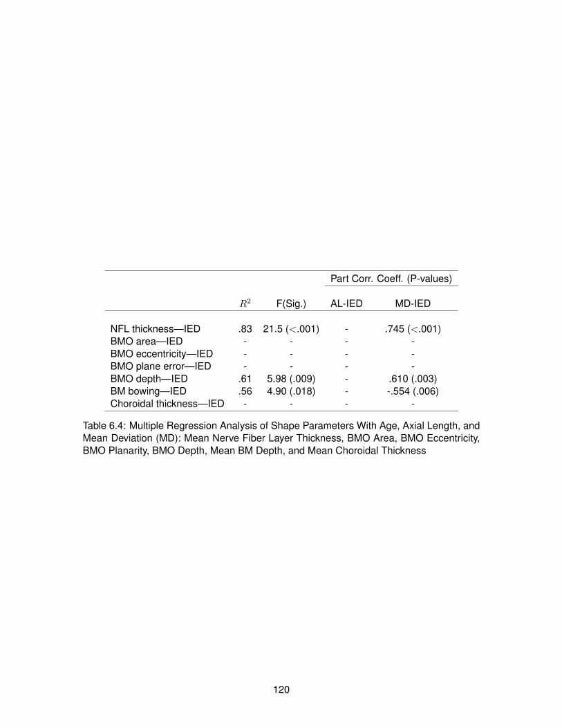
Part Corr. Coeff. (P-values)

R2 F(Sig.) AL-IED MD-IED

NFL thickness—IED .83 21.5 (<.001) - .745 (<.001)BMO area—IED - - - -BMO eccentricity—IED - - - -BMO plane error—IED - - - -BMO depth—IED .61 5.98 (.009) - .610 (.003)BM bowing—IED .56 4.90 (.018) - -.554 (.006)Choroidal thickness—IED - - - -

Table 6.4: Multiple Regression Analysis of Shape Parameters With Age, Axial Length, andMean Deviation (MD): Mean Nerve Fiber Layer Thickness, BMO Area, BMO Eccentricity,BMO Planarity, BMO Depth, Mean BM Depth, and Mean Choroidal Thickness

120

Figure 6.5: Bruch’s membrane opening disc margin correspondence and planarity of BMO.Bruch’s membrane opening points overlaid on en face images generated by summing the3D OCT volumes in the axial direction. Red points indicate where the BMO is posterior(into the page) to reference plane, and green points indicate where the BMO is anterior(out of the page) to the reference plane.

121

Figure 6.6: Bruch’s membrane opening shape measurements. (A) Bruch’s membraneopening area, (B) BMO eccentricity, and (C) mean BMO planarity, distributed by (i) groupand versus (ii) age, (iii) axial length, and (iv) MD. Outliers in each group are marked by redcircles in plots (i).

122

Figure 6.7: Peripapillary BM depth. All depth maps are in scale and right-eye orientation.The BM depth is measured with respect to the BM reference plane at each point on BM.

123

Figure 6.8: Bruch’s membrane opening and mean BM depth measurements. (A) Bruch’smembrane opening depth and (B) mean BM depth distributed by (i) group and versus (ii)age, (iii) axial length, and (iv) MD (C). Intereye differences of BMO depth and BM depthare also plotted versus intereye MD difference. Outliers in each group are marked by redcircles in plots (i).

124

Figure 6.9: Bruch’s membrane depth sectoral analysis. (A) Sectorized group averagesof Bruch’s membrane (BM) surface depth. The colour in each sector indicates the meanabsolute magnitude of the normal distance between BM and its fitted plane. Elliptical annuliare drawn at 0.25, 0.75, 1.25, and 1.75 mm from Bruch’s membrane opening (BMO). Theannuli are divided into 60ngular sectors of superior (S), nasal (N), inferior (I), and temporal(T), and 30ngular sectors of superior-nasal (SN), inferior-nasal (IN), inferior-temporal (IT),and superior-temporal (ST). (B) Average BM depth by angular sector for the whole BMsurface. (C) Average BM depth by angular sector for the inner annulus only (0–0.25 mmdistance from BMO).

125

Figure 6.10: Peripapillary choroidal thickness. All thickness colour maps are in scale andright-eye orientation. The region inside and within 0.25 mm from Bruch’s membrane open-ing (BMO) was excluded.

126

Figure 6.11: Choroidal thickness measurements. Choroidal thickness distributed by (i)group, and versus (ii) age, (iii) axial length, and (iv) MD.

Figure 6.12: Choroidal thickness sectoral analysis. (A) Sectorized peripapillary choroidalthickness. Elliptical annuli are drawn at 0.25, 0.75, 1.25, and 1.75 mm from Bruch’s mem-brane opening (BMO). The annuli are divided into 60 degrees angular sectors of superior(S), nasal (N), inferior (I), and temporal (T), and 30 degrees angular sectors of superior-nasal (SN), inferior-nasal (IN), inferior-temporal (IT), and superior-temporal (ST). (B) Aver-age choroidal thickness by angular sector.

127

Figure 6.13: Graphical description of anterior lamina insertion points (ALIP) to Bruch’smembrane opening (BMO) distance (left) and anterior lamina cribrosa surface (ALCS)depth (right).

128

Figure 6.14: Enface projection of Bruch’s membrane openings (BMO, red) and anteriorlamina insertion points (ALIP).

129

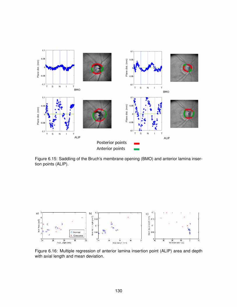
Figure 6.15: Saddling of the Bruch’s membrane opening (BMO) and anterior lamina inser-tion points (ALIP).

Figure 6.16: Multiple regression of anterior lamina insertion point (ALIP) area and depthwith axial length and mean deviation.

130

Chapter 7

Conclusion

In this thesis, we have presented a comprehensive computational pipeline for process-

ing, segmentation, registration, and morphometric analysis of retinal and peripapillary op-

tical coherence tomography.

In Chapter 3, the image acquisition and preprocessing steps were described, with fo-

cus on motion correction and image smoothing. The involutary microsaccadic movement

of the eye creates axial and lateral motion artefacts in OCT images. A simple and effec-

tive method to remove the wave-like axial motion artefact is to first obtain an approximated

motion profile by finding the axial translation of the maximum cross-correlation between

adjacent frames. The profile was smoothed by curve-fitting, and the frame positions were

adjusted according to the smoothing. The image volume was additionally enhanced by

3D bounded variation image smoothing, which optimizes a functional that balances the

smoothness of the image and faithfulness to the original image. This resulted in smooth-

ing the image speckles while preserving and visually enhancing the edges of anatomical

structures.

In Chapter 4, manual and automated segmentation methods were presented. Non-

layer features in the optic nerve head (ONH), such as the Bruch’s membrane opening

(BMO) and anterior laminar insertion points (ALIP), were point-segmented manually on

radial scans extracted from the original 3D volume. Retinal layers were segmented au-

tomatically using a graph-cut based method, which transformed the image volume into a

node-weighted directed graph such that the cut of the associated arc-weighted graph cor-

responded to the optimal 3D surfaces in the volume. A cost function involving the vertical

intensity gradient yielded successful segmentation of the horizontal layer structure of the

131

retina. We applied the automated segmentation to segment the choroid, the vasculature

layer posterior to the retina of which the posterior boundary is often unclear due to light

absorbtion and scattering. Choroid from 830-nm OCT images, 1060-nm OCT images,

and enhanced-depth imaging (EDI) OCT images were segmented. Measurement of the

subfoveal choroidal thickness from automated segmentation was compared with those of

expert human raters, and demonstrated solid performance with potential for clinical appli-

cation.

In Chapter 5, we presented two registration methods of retinal surfaces - surface-to-

surface exact registration, and atlas template generation from multiple surfaces. Reg-

istration establishes anatomical correspondence for comparing multiple retinal surfaces.

The first method brings two surfaces in close proximity by mathematical current measure,

and achieves one-to-one spatial correspondence between the surfaces through spherical

demons registration. We applied this technique to measure repeatability of retinal nerve

fibre layer (RNFL) and choroidal thickness maps, which showed high repeatability relative

to the image axial coherence length; the RNFL thickness was more variable in the regions

of retinal blood vessels, and the choroidal thickness was in average more variable than the

RNFL thickness, suggesting blood flow affects the layer thickness measurement.

The second method uses the fshape framework, in which a geometrical surface in 3D

and signals mapped onto the surface are considered as a single object of fshape. In order

to obtain the mean atlas of multiple fshapes, a simple initial hyper template is chosen, and

its geometrical deformation and signal residuals are varied simultaneously to minimize the

template’s deformation distance to its approximation to each of the observed fshapes, and

the dissimilarity between each of the template’s approximation and the corresponding ob-

servation. The observed fshapes are compared via the distances to the common mean

template (atlas) from their estimated fshapes. Using this framework, we generated mean

RNFL surfaces and thickness maps for normal and glaucomatous eyes and visualized the

discriminative power over the peripapillary region between the normal and glaucomatous

RNFLs. Additionally, automated classification was performed by a linear discriminant anal-

ysis (LDA) method, and info-gain based support vector machine (SVM) method, and both

yielded high automated classification rate between normal and glaucomatous groups and

between normal and glaucoma-suspect groups based on the RNFL fshape measures.

132

In Chapter 6, a comprehensive ONH shape analysis of myopic glaucoma was pre-

sented. We acquired 52 eye images from young normal, older normal, glaucoma-suspect,

and glaucoma groups, which were processed, segmented, and measured for features such

as the RNFL thickness, choroidal thickness, BMO dimension, Bruch’s membrane (BM)

bowing, scleral canal dimension, and anterior lamina cribrosa surface (ALCS) depth. Multi-

ple regression was performed to assess the correlation of the shape parameters to the sub-

jects’ age, degree of myopia measured by the eye’s axial length, and degree of glaucoma

severity measured by the mean deviation (MD), which in turn indicates the amoutn of visual

field loss. From the results, we found that along with the MD value, axial length affected the

ONH morphology significantly and may be a confounding factor in glaucoma development,

which also possibly explain the high susceptibility of glaucoma among those with advanced

myopia. Severe glaucoma (large MD magnitude) was associated with greater BM bowing

and ALCS depth, confirming the posterior deformation of glaucomatous ONH in-vivo.

The contributions of this thesis are published in [196, 114, 195, 111, 109, 112, 113]

and submitted for publication in [110]. A manuscript on the repeatability study in Chapter

5, and the anterior laminar region morphometrics in Chapter 6, are under preparation.

7.1 Future directions

The future directions of the work presented in this thesis are discussed in individual

sections in more detail.

One direction is more extensive application of the tools presented here in clincal stud-

ies. The repeatability study in Section 5.2 can be applied to longitudinal data over longer

periods of time in glaucomatous eyes to track change; in particular, the RNFL and other

retinal layers can be monitored for further tissue loss after treatement. The fshape atlas-

based variability analysis in Section 5.3 can be applied to a larger dataset with various

features, focusing on confirming the regional pattern of RNFL thinning in glaucoma, and

testing other layers, such as the choroid, for changes with glaucoma progression. The

application of the morphometric tools in this thesis is not limited to glaucoma studies, and

can be extended to other eye diseases involving structural changes.

One of the more immediate methodoligcal improvements in the pipeline is including the

retinal blood vessels as a reference structure. We are currently investigating automated

133

segmentation of the retinal blood vessels to perform pre-registration alignment of longitudi-

nal data, and to mark the regions with more variable retinal layer thickness measurements.

Automated segmentation of the Bruch’s membrane opening (BMO) is another potential

future project. Accurate automated BMO segmentation is challenging largely due to the

heavy blood-vessel shadowing near the optic cup surface. However, since our morphome-

tric measurements are largely based on the best-fit ellipse of the BMO, and the manual

segmentation of the BMO is limited in measurement repeatability, it may suffice for the

machine to approximate the BMO than aiming to mark the exact location.

An important physiological parameter not considered in the thesis is the intraocular

pressure (IOP), and it is not clear how much the shape measurements presented in the

thesis would be affected by the change in IOP. Our group is currently revising the image

acquisition protocol such that IOP measurement can be obtained for each imaging subject.

In ONH morphometrics, one of the future projects is improved characterization of the

Bruch’s membrane bowing. Although the BM depth in Chapter 6 quantifies the crude

“flatness” of the BM surface, a more detailed analysis may reveal topological characteristics

that better distinguishes myopia-related, glaucoma-related, or age-related deformations.

Another shape parameter to be considered is the myopic tilt [82] of the optic disk, which

may affect the BM bowing measurement.

134

Bibliography

[1] Age Related Eye Disease Research Group. A randomized, placebo-controlled, clini-

cal trial of high-dose supplementation with vitamins C and E, beta carotene, and zinc

for age-related macular degeneration and vision loss: AREDS report no. 8. Archives

of ophthalmology, 119(10):1417–36, October 2001. 31, 40

[2] S. Arguillere, E. Trelat, A. Trouve, and L. Younes. Shape deformation analysis from

the optimal control viewpoint. arXiv:1401.0661, Jan 2014. 83, 84

[3] Ahmet Murat Bagci, Mahnaz Shahidi, Rashid Ansari, Michael Blair, Norman Paul

Blair, and Ruth Zelkha. Thickness profiles of retinal layers by optical coherence

tomography image segmentation. American journal of ophthalmology, 146(5):679–

87, November 2008. 24

[4] M. F. Beg, M. I. Miller, A. Trouve, and L. Younes. Computing large deformation metric

mappings via geodesic flows of diffeomorphisms. International journal of computer

vision, 61(139-157), 2005. 77

[5] Anthony J Bellezza, Christopher J Rintalan, Hilary W Thompson, J Crawford Downs,

Richard T Hart, and Claude F Burgoyne. Deformation of the lamina cribrosa and an-

terior scleral canal wall in early experimental glaucoma. Investigative ophthalmology

& visual science, 44(2):623–37, February 2003. 101, 112

[6] Delia Bendschneider, Ralf P Tornow, Folkert K Horn, Robert Laemmer, Christo-

pher W Roessler, Anselm G Juenemann, Friedrich E Kruse, and Christian Y Mardin.

Retinal nerve fiber layer thickness in normals measured by spectral domain OCT.

Journal of glaucoma, 19(7):475–82, September 2010. 111

[7] Thomas L Berenberg, Tatyana I Metelitsina, Brian Madow, Yang Dai, Gui-Shuang

Ying, Joan C Dupont, Lili Grunwald, Alexander J Brucker, and Juan E Grunwald. The

135

association between drusen extent and foveolar choroidal blood flow in age-related

macular degeneration. Retina (Philadelphia, Pa.), 32(1):25–31, January 2012. 30

[8] Rupert R A Bourne, Gretchen A Stevens, Richard A White, Jennifer L Smith, Seth R

Flaxman, Holly Price, Jost B Jonas, Jill Keeffe, Janet Leasher, Kovin Naidoo, Konrad

Pesudovs, Serge Resnikoff, and Hugh R Taylor. Causes of vision loss worldwide,

1990-2010: a systematic analysis. The Lancet. Global health, 1(6):e339–49, De-

cember 2013. 1, 7

[9] Christopher Bowd, Linda M Zangwill, Charles C Berry, Eytan Z Blumenthal, Cris-

tiana Vasile, Cesar Sanchez-Galeana, Charles F Bosworth, Pamela A Sample, and

Robert N Weinreb. Detecting early glaucoma by assessment of retinal nerve fiber

layer thickness and visual function. Investigative Ophthalmology & Visual Science,

42(9):1993–2003, 2001. 93

[10] Donald L Budenz, Douglas R Anderson, Rohit Varma, Joel Schuman, Louis Cantor,

Jonathan Savell, David S Greenfield, Vincent Michael Patella, Harry A Quigley, and

James Tielsch. Determinants of normal retinal nerve fiber layer thickness measured

by Stratus OCT. Ophthalmology, 114(6):1046–52, June 2007. 111

[11] Claude F Burgoyne. A biomechanical paradigm for axonal insult within the optic

nerve head in aging and glaucoma. Experimental eye research, 93(2):120–32, Au-

gust 2011. 8

[12] Claude F Burgoyne and J Crawford Downs. Premise and prediction-how optic nerve

head biomechanics underlies the susceptibility and clinical behavior of the aged optic

nerve head. Journal of glaucoma, 17(4):318–28, January. 114

[13] Claude F Burgoyne, J Crawford Downs, Anthony J Bellezza, J-K Francis Suh, and

Richard T Hart. The optic nerve head as a biomechanical structure: a new paradigm

for understanding the role of IOP-related stress and strain in the pathophysiology

of glaucomatous optic nerve head damage. Progress in retinal and eye research,

24(1):39–73, January 2005. 8, 101

136

[14] Delia Cabrera Fernandez, Harry M. Salinas, and Carmen A. Puliafito. Automated

detection of retinal layer structures on optical coherence tomography images. Optics

Express, 13(25):10200, December 2005. 24

[15] J. Cao. The size of the connected components of excursion sets of χ2, t and F fields.

Advances in Applied Probability, 31(3):579–595, September 1999. 51

[16] B Charlier, N Charon, and A Trouve. Fshapes tool kit, December 2014. 86

[17] Benjamin Charlier, Nicolas Charon, and Alain Trouve. The fshape framework for the

variability analysis of functional shapes. April 2014. 75

[18] N. Charon. Analysis of geometric and functional shapes with extensions of currents.

Application to registration and atlas estimation. PhD thesis, ENS Cachan, 2013. 76,

82

[19] N. Charon, B. Charlier, and A. Trouve. The fshape framework for the variability

analysis of functional shapes. ArXiv:1404.6039, Apr 2014. 76, 77, 79, 80, 84

[20] N. Charon and A. Trouve. Functional currents : a new mathematical tool to model

and analyse functional shapes. JMIV, 48(3):413–431, 2013. 79

[21] Balwantray C. Chauhan and Claude F. Burgoyne. From clinical examination of the

optic disc to clinical assessment of the optic nerve head: A paradigm change. Am.

J. Ophthalmol., 156(2):218–227, August 2013. 44, 45

[22] Balwantray C Chauhan and Claude F Burgoyne. From clinical examination of the op-

tic disc to clinical assessment of the optic nerve head: a paradigm change. American

journal of ophthalmology, 156(2):218–227.e2, August 2013. 104, 111, 112

[23] Min Chen, Andrew Lang, Howard S. Ying, Peter A. Calabresi, Jerry L. Prince, and

Aaron Carass. Analysis of macular OCT images using deformable registration.

Biomed. Opt. Express, 5(7):2196–2214, Jul 2014. 46

[24] Yueli Chen, Laurel N. Vuong, Jonathan Liu, Joseph Ho, Vivek J. Srinivasan, Iwona

Gorczynska, Andre J. Witkin, Jay S. Duker, Joel Schuman, and James G. Fuji-

moto. Three-dimensional ultrahigh resolution optical coherence tomography imaging

of age-related macular degeneration. Optics Express, 17(5):4046, March 2009. 18

137

[25] E Chihara and K Chihara. Covariation of optic disc measurements and ocular param-

eters in the healthy eye. Graefe’s archive for clinical and experimental ophthalmol-

ogy = Albrecht von Graefes Archiv fur klinische und experimentelle Ophthalmologie,

232(5):265–71, May 1994. 114

[26] Michael Choma, Marinko Sarunic, Changhuei Yang, and Joseph Izatt. Sensitivity ad-

vantage of swept source and Fourier domain optical coherence tomography. Optics

Express, 11(18):2183, September 2003. 9

[27] Moo K Chung, Keith J Worsley, Brendon M Nacewicz, Kim M Dalton, and Richard J

Davidson. General multivariate linear modeling of surface shapes using SurfStat.

NeuroImage, 53(2):491–505, November 2010. 51, 55

[28] George A Cioffi. Ischemic model of optic nerve injury. Transactions of the American

Ophthalmological Society, 103:592–613, January 2005. 101

[29] Rogerio A Costa, Mirian Skaf, Luiz A S Melo, Daniela Calucci, Jose A Cardillo,

Jarbas C Castro, David Huang, and Maciej Wojtkowski. Retinal assessment using

optical coherence tomography. Progress in retinal and eye research, 25(3):325–53,

May 2006. 18

[30] J Crawford Downs, Michael D Roberts, and Ian A Sigal. Glaucomatous cupping of

the lamina cribrosa: a review of the evidence for active progressive remodeling as a

mechanism. Experimental eye research, 93(2):133–40, August 2011. 101, 114

[31] Catherine Cukras, Elvira Agron, Michael L Klein, Frederick L Ferris, Emily Y Chew,

Gary Gensler, and Wai T Wong. Natural history of drusenoid pigment epithelial

detachment in age-related macular degeneration: Age-Related Eye Disease Study

Report No. 28. Ophthalmology, 117(3):489–99, March 2010. 31

[32] Johannes F. de Boer, Barry Cense, B. Hyle Park, Mark C. Pierce, Guillermo J. Tear-

ney, and Brett E. Bouma. Improved signal-to-noise ratio in spectral-domain com-

pared with time-domain optical coherence tomography. Optics Letters, 28(21):2067,

November 2003. 9

[33] Francois C Delori, Robert H Webb, and David H Sliney. Maximum permissible expo-

sures for ocular safety (ANSI 2000), with emphasis on ophthalmic devices. Journal

138

of the Optical Society of America. A, Optics, image science, and vision, 24(5):1250–

65, May 2007. 10

[34] A Dichtl, J B Jonas, and G O Naumann. Histomorphometry of the optic disc in highly

myopic eyes with absolute secondary angle closure glaucoma. The British journal

of ophthalmology, 82(3):286–9, March 1998. 102, 114

[35] Weiguang Ding, Mei Young, Serge Bourgault, Sieun Lee, David A Albiani, Andrew W

Kirker, Farzin Forooghian, Marinko V Sarunic, Andrew B Merkur, and Mirza Faisal

Beg. Automatic detection of subretinal fluid and sub-retinal pigment epithelium fluid

in optical coherence tomography images. Conference proceedings : ... Annual Inter-

national Conference of the IEEE Engineering in Medicine and Biology Society. IEEE

Engineering in Medicine and Biology Society. Annual Conference, 2013:7388–91,

January 2013. 41

[36] J Crawford Downs, J-K Francis Suh, Kevin A Thomas, Anthony J Bellezza, Richard T

Hart, and Claude F Burgoyne. Viscoelastic material properties of the peripapillary

sclera in normal and early-glaucoma monkey eyes. Investigative ophthalmology &

visual science, 46(2):540–6, February 2005. 101

[37] J Crawford Downs, Hongli Yang, Christopher Girkin, Lisandro Sakata, Anthony

Bellezza, Hilary Thompson, and Claude F Burgoyne. Three-dimensional histomor-

phometry of the normal and early glaucomatous monkey optic nerve head: neural

canal and subarachnoid space architecture. Investigative ophthalmology & visual

science, 48(7):3195–208, July 2007. 101

[38] Wolfgang Drexler and James G. Fujimoto, editors. Optical Coherence Tomography.

Biological and Medical Physics, Biomedical Engineering. Springer Berlin Heidelberg,

Berlin, Heidelberg, 2008. 9, 10

[39] S. Durrleman, P. Fillard, X. Pennec, Alain Trouve, and Nicholas Ayache. Registration,

atlas estimation and variability analysis of white matter fiber bundles modeled as

currents. NeuroImage, 55(3):1073–1090, 2010. 79

139

[40] S. Durrleman, X. Pennec, Alain Trouve, and Nicholas Ayache. A forward model to

build unbiased atlases from curves and surfaces. Proc. of the International Work-

shop on the Mathematical Foundations of Computational Anatomy, 2008. 76, 79,

84

[41] S. Durrleman, M. Prastawa, N. Charon, J.R Korenberg, S. Joshi, G. Gerig, and

A. Trouve. Deformetrics : morphometry of shape complexes with space deforma-

tions. Neuroimage, 101:35–49, 2014. 79, 86

[42] Joshua R Ehrlich, Jeffrey Peterson, George Parlitsis, Kristine Y Kay, Szilard Kiss,

and Nathan M Radcliffe. Peripapillary choroidal thickness in glaucoma measured

with optical coherence tomography. Experimental eye research, 92(3):189–94,

March 2011. 115

[43] Tapio Fabritius, Shuichi Makita, Masahiro Miura, Risto Myllyla, and Yoshiaki Yasuno.

Automated segmentation of the macula by optical coherence tomography. Optics

express, 17(18):15659–69, August 2009. 24

[44] Yong Fan, Dinggang Shen, Ruben C Gur, Raquel E Gur, and Christos Davatzikos.

COMPARE: classification of morphological patterns using adaptive regional ele-

ments. IEEE transactions on medical imaging, 26(1):93–105, January 2007. 55

[45] R D Fechtner. Review of normative database construction in available oct models

highlighting differences. In FDA/American Glaucoma Society Workshop on the Va-

lidity, Reliability, and Usability of Glaucoma Imaging Devices, 2012; Silver Spring,

MD. 101

[46] A.F. Fercher, C.K. Hitzenberger, G. Kamp, and S.Y. El-Zaiat. Measurement of in-

traocular distances by backscattering spectral interferometry. Optics Communica-

tions, 117(1-2):43–48, May 1995. 9

[47] Michael S. Floater. Mean value coordinates. Computer Aided Geometric Design,

20(1):19–27, March 2003. 49

[48] E Friedman. A hemodynamic model of the pathogenesis of age-related macular

degeneration. American journal of ophthalmology, 124(5):677–82, November 1997.

30

140

[49] Jerome H. Friedman. Regularized discriminant analysis. Journal of the American

Statistical Association, 84(405):pp. 165–175, 1989. 89

[50] Takamitsu Fujiwara, Yutaka Imamura, Ron Margolis, Jason S Slakter, and Richard F

Spaide. Enhanced depth imaging optical coherence tomography of the choroid in

highly myopic eyes. American journal of ophthalmology, 148(3):445–50, September

2009. 26, 115

[51] Mona K Garvin, Michael D Abramoff, Randy Kardon, Stephen R Russell, Xiaodong

Wu, and Milan Sonka. Intraretinal layer segmentation of macular optical coherence

tomography images using optimal 3-D graph search. IEEE transactions on medical

imaging, 27(10):1495–505, October 2008. 24

[52] Mona Kathryn Garvin, Michael David Abramoff, Xiaodong Wu, Stephen R Russell,

Trudy L Burns, and Milan Sonka. Automated 3-D intraretinal layer segmentation of

macular spectral-domain optical coherence tomography images. IEEE transactions

on medical imaging, 28(9):1436–47, September 2009. 24

[53] Andrea Giani, Marco Pellegrini, Alessandro Invernizzi, Mario Cigada, and Giovanni

Staurenghi. Aligning scan locations from consecutive spectral-domain optical coher-

ence tomography examinations: A comparison among different strategies. Invest.

Ophthalmol. Vis. Sci., 53(12):7637–7643, 2012. 45

[54] E. Gibson, Mei Young, M.V. Sarunic, and M.F. Beg. Optic nerve head registration

via hemispherical surface and volume registration. Biomedical Engineering, IEEE

Transactions on, 57(10):2592–2595, Oct 2010. 45, 49

[55] Michael J A Girard, J-K Francis Suh, Michael Bottlang, Claude F Burgoyne, and

J Crawford Downs. Scleral biomechanics in the aging monkey eye. Investigative

ophthalmology & visual science, 50(11):5226–37, November 2009. 112

[56] Michael J A Girard, J-K Francis Suh, Michael Bottlang, Claude F Burgoyne, and

J Crawford Downs. Biomechanical changes in the sclera of monkey eyes exposed to

chronic IOP elevations. Investigative ophthalmology & visual science, 52(8):5656–

69, July 2011. 112

141

[57] J. Glaunes, A. Trouve, and L. Younes. Diffeomorphic matching of distributions: a

new approach for unlabelled point-sets and sub-manifolds matching. In Proceedings

of the 2004 IEEE Computer Society Conference on Computer Vision and Pattern

Recognition, 2004. CVPR 2004., volume 2, pages 712–718. IEEE, 2004. 48, 79

[58] J. Glaunes and M. Vaillant. Surface matching via currents. Proceedings of Infor-

mation Processing in Medical Imaging (IPMI), Lecture Notes in Computer Science,

3565(381-392), 2006. 79

[59] Alberto O. Gonzalez-Garcıa, Gianmarco Vizzeri, Christopher Bowd, Felipe A.

Medeiros, Linda M. Zangwill, and Robert N. Weinreb. Reproducibility of RTVue

retinal nerve fiber layer thickness and optic disc measurements and agreement

with Stratus optical coherence tomography measurements. Am. J. Ophthalmol.,

147(6):1067–1074, June 2009. 44

[60] Erich Gotzinger, Michael Pircher, Wolfgang Geitzenauer, Christian Ahlers, Bernhard

Baumann, Stephan Michels, Ursula Schmidt-Erfurth, and Christoph K. Hitzenberger.

Retinal pigment epithelium segmentation by polarization sensitive optical coherence

tomography. Optics Express, 16(21):16410, September 2008. 24

[61] Giovanni Gregori, Fenghua Wang, Philip J Rosenfeld, Zohar Yehoshua, Ninel Z Gre-

gori, Brandon J Lujan, Carmen A Puliafito, and William J Feuer. Spectral domain

optical coherence tomography imaging of drusen in nonexudative age-related mac-

ular degeneration. Ophthalmology, 118(7):1373–9, July 2011. 32

[62] J E Grunwald, S M Hariprasad, J DuPont, M G Maguire, S L Fine, A J Brucker,

A M Maguire, and A C Ho. Foveolar choroidal blood flow in age-related macular

degeneration. Investigative ophthalmology & visual science, 39(2):385–90, February

1998. 30

[63] Juan E Grunwald, Tatyana I Metelitsina, Joan C Dupont, Gui-Shuang Ying, and

Maureen G Maguire. Reduced foveolar choroidal blood flow in eyes with increasing

AMD severity. Investigative ophthalmology & visual science, 46(3):1033–8, March

2005. 30

142

[64] Rafael Grytz, Christopher A Girkin, Vincent Libertiaux, and J Crawford Downs. Per-

spectives on biomechanical growth and remodeling mechanisms in glaucoma(). Me-

chanics research communications, 42:92–106, July 2012. 101

[65] Rafael Grytz, Ian A Sigal, Jeffrey W Ruberti, Gunther Meschke, and J Crawford

Downs. Lamina Cribrosa Thickening in Early Glaucoma Predicted by a Microstruc-

ture Motivated Growth and Remodeling Approach. Mechanics of materials : an

international journal, 44:99–109, January 2012. 101

[66] Li Guo, Stephen E Moss, Robert A Alexander, Robin R Ali, Frederick W Fitzke, and

M Francesca Cordeiro. Retinal ganglion cell apoptosis in glaucoma is related to

intraocular pressure and IOP-induced effects on extracellular matrix. Investigative

ophthalmology & visual science, 46(1):175–82, January 2005. 8

[67] Mona Haeker, Xiaodong Wu, Michael Abramoff, Randy Kardon, and Milan Sonka.

Incorporation of regional information in optimal 3-D graph search with application for

intraretinal layer segmentation of optical coherence tomography images. Informa-

tion processing in medical imaging : proceedings of the ... conference, 20:607–18,

January 2007. 24

[68] Mark Hall, Eibe Frank, Geoffrey Holmes, Bernhard Pfahringer, Peter Reutemann,

and Ian H Witten. The WEKA data mining software: an update. ACM SIGKDD

explorations newsletter, 11(1):10–18, 2009. 87

[69] Masanori Hangai, Yumiko Ojima, Norimoto Gotoh, Ryo Inoue, Yoshiaki Yasuno,

Shuichi Makita, Masahiro Yamanari, Toyohiko Yatagai, Mihori Kita, and Nagahisa

Yoshimura. Three-dimensional imaging of macular holes with high-speed optical

coherence tomography. Ophthalmology, 114(4):763–73, April 2007. 18

[70] Trevor Hastie, Robert Tibshirani, and Jerome Friedman. The Elements of Statistical

Learning (2nd edition). Springer Series in Statistics. Springer New York Inc., 2009.

87

[71] Lin He, Ruojin Ren, Hongli Yang, Christy Hardin, Luke Reyes, Juan Reynaud, Stu-

art K. Gardiner, Brad Fortune, Shaban Demirel, and Claude F. Burgoyne. Anatomic

143

vs. acquired image frame discordance in spectral domain optical coherence tomog-

raphy minimum rim measurements. PLoS ONE, 9(3):e92225, March 2014. 45

[72] Lin He, Ruojin Ren, Hongli Yang, Christy Hardin, Luke Reyes, Juan Reynaud, Stu-

art K Gardiner, Brad Fortune, Shaban Demirel, and Claude F Burgoyne. Anatomic

vs. acquired image frame discordance in spectral domain optical coherence tomog-

raphy minimum rim measurements. PloS one, 9(3):e92225, January 2014. 111

[73] M R Hee, J A Izatt, E A Swanson, D Huang, J S Schuman, C P Lin, C A Puliafito,

and J G Fujimoto. Optical coherence tomography of the human retina. Archives of

ophthalmology, 113(3):325–32, March 1995. 17

[74] Anders Heijl. Reduction of Intraocular Pressure and Glaucoma Progression.

Archives of Ophthalmology, 120(10):1268, October 2002. 8

[75] M R Hernandez. The optic nerve head in glaucoma: role of astrocytes in tissue

remodeling. Progress in retinal and eye research, 19(3):297–321, May 2000. 101

[76] Esther M Hoffmann, Linda M Zangwill, Jonathan G Crowston, and Robert N Wein-

reb. Optic disk size and glaucoma. Survey of ophthalmology, 52(1):32–49, January

2007. 113

[77] Sek-Tien Hoh, Marcus C C Lim, Steve K L Seah, Albert T H Lim, Sek-Jin Chew,

Paul J Foster, and Tin Aung. Peripapillary retinal nerve fiber layer thickness varia-

tions with myopia. Ophthalmology, 113(5):773–7, May 2006. 112

[78] Zhihong Hu, Michael D Abramoff, Young H Kwon, Kyungmoo Lee, and Mona K

Garvin. Automated segmentation of neural canal opening and optic cup in 3D spec-

tral optical coherence tomography volumes of the optic nerve head. Investigative

ophthalmology & visual science, 51(11):5708–17, November 2010. 17, 24

[79] Zhihong Hu, Xiaodong Wu, Yanwei Ouyang, Yanling Ouyang, and Srinivas R. Sadda.

Semiautomated segmentation of the choroid in spectral- domain optical coher-

ence tomography volume scans. Investigative Ophthalmology and Visual Science,

54(3):1722–1729, March 2013. 27

144

[80] D Huang, E. Swanson, C. Lin, J. Schuman, W. Stinson, W Chang, M. Hee, T Flotte,

K Gregory, C. Puliafito, and al. Et. Optical coherence tomography. Science,

254(5035):1178–1181, November 1991. 9

[81] Son C Huynh, Xiu Ying Wang, Elena Rochtchina, and Paul Mitchell. Peripapillary

retinal nerve fiber layer thickness in a population of 6-year-old children: findings by

optical coherence tomography. Ophthalmology, 113(9):1583–92, September 2006.

102, 112

[82] Young Hoon Hwang, Chungkwon Yoo, and Yong Yeon Kim. Myopic optic disc tilt and

the characteristics of peripapillary retinal nerve fiber layer thickness measured by

spectral-domain optical coherence tomography. Journal of glaucoma, 21(4):260–5,

January. 134

[83] S M Hyung, D M Kim, C Hong, and D H Youn. Optic disc of the myopic eye: rela-

tionship between refractive errors and morphometric characteristics. Korean journal

of ophthalmology : KJO, 6(1):32–5, June 1992. 114

[84] Yasushi Ikuno, Kana Kawaguchi, Takeyoshi Nouchi, and Yoshiaki Yasuno. Choroidal

thickness in healthy Japanese subjects. Investigative ophthalmology & visual sci-

ence, 51(4):2173–6, April 2010. 115

[85] Yutaka Imamura, Takamitsu Fujiwara, Ron Margolis, and Richard F Spaide. En-

hanced depth imaging optical coherence tomography of the choroid in central serous

chorioretinopathy. Retina (Philadelphia, Pa.), 29(10):1469–73, January. 26

[86] Hiroshi Ishikawa, Daniel M Stein, Gadi Wollstein, Siobahn Beaton, James G Fuji-

moto, and Joel S Schuman. Macular segmentation with optical coherence tomogra-

phy. Investigative ophthalmology & visual science, 46(6):2012–7, June 2005. 24

[87] Glenn J. Jaffe and Joseph Caprioli. Optical coherence tomography to detect and

manage retinal disease and glaucoma. Am. J. Ophthalmol., 137(1):156–169, Jan-

uary 2004. 44

[88] Glenn J Jaffe and Joseph Caprioli. Optical coherence tomography to detect

and manage retinal disease and glaucoma. American journal of ophthalmology,

137(1):156–69, January 2004. 111

145

[89] John Johnstone, Massimo Fazio, Kulawan Rojananuangnit, Brandon Smith, Mark

Clark, Crawford Downs, Cynthia Owsley, Michael J A Girard, Jean Martial Mari, and

Christopher A Girkin. Variation of the axial location of Bruch’s membrane opening

with age, choroidal thickness, and race. Investigative ophthalmology & visual sci-

ence, 55(3):2004–9, March 2014. 115

[90] I.T. Jolliffe. Principal Component Analysis. Springer Science & Business Media,

2002. 105

[91] J B Jonas and W M Budde. Optic nerve damage in highly myopic eyes with chronic

open-angle glaucoma. European journal of ophthalmology, 15(1):41–7, January

2005. 102

[92] J B Jonas and A Dichtl. Optic disc morphology in myopic primary open-angle glau-

coma. Graefe’s archive for clinical and experimental ophthalmology = Albrecht von

Graefes Archiv fur klinische und experimentelle Ophthalmologie, 235(10):627–33,

October 1997. 102, 114

[93] J B Jonas, G C Gusek, and G O Naumann. Optic disc, cup and neuroretinal rim size,

configuration and correlations in normal eyes. Investigative ophthalmology & visual

science, 29(7):1151–8, July 1988. 112, 114

[94] Jost B Jonas. Optic disk size correlated with refractive error. American journal of

ophthalmology, 139(2):346–8, February 2005. 114

[95] Jost B Jonas, Eduard Berenshtein, and Leonard Holbach. Lamina cribrosa thickness

and spatial relationships between intraocular space and cerebrospinal fluid space in

highly myopic eyes. Investigative ophthalmology & visual science, 45(8):2660–5,

August 2004. 114

[96] Jost B Jonas, Shefali B Jonas, Rahul A Jonas, Leonard Holbach, and Songhomitra

Panda-Jonas. Histology of the parapapillary region in high myopia. American journal

of ophthalmology, 152(6):1021–9, December 2011. 102

146

[97] Thomas Martini Jørgensen, Jakob Thomadsen, Ulrik Christensen, Wael Soliman,

and Birgit Sander. Enhancing the signal-to-noise ratio in ophthalmic optical coher-

ence tomography by image registration—method and clinical examples. J. Biomed.

Opt., 12(4):041208, August 2007. 45

[98] S. Joshi, B. Davis, M. Jomier, and G. Gerig. Unbiased diffeomorphic atlas construc-

tion for computational anatomy. NeuroImage, 23:S151–S160, 2004. 76

[99] Vedran Kajic, Marieh Esmaeelpour, Boris Povazay, David Marshall, Paul L Rosin,

and Wolfgang Drexler. Automated choroidal segmentation of 1060 nm OCT in

healthy and pathologic eyes using a statistical model. Biomedical optics express,

3(1):86–103, January 2012. 27

[100] Akiyasu Kanamori, Makoto Nakamura, Michael F T Escano, Ryu Seya, Hidetaka

Maeda, and Akira Negi. Evaluation of the glaucomatous damage on retinal nerve

fiber layer thickness measured by optical coherence tomography. American journal

of ophthalmology, 135(4):513–20, April 2003. 111

[101] Akiyasu Kanamori, Makoto Nakamura, Michael F.T Escano, Ryu Seya, Hidetaka

Maeda, and Akira Negi. Evaluation of the glaucomatous damage on retinal nerve

fiber layer thickness measured by optical coherence tomography. Am. J. Ophthal-

mol., 135(4):513–520, April 2003. 44, 93

[102] Shin Hee Kang, Seung Woo Hong, Seong Kyu Im, Sang Hyup Lee, and Myung Douk

Ahn. Effect of myopia on the thickness of the retinal nerve fiber layer measured

by Cirrus HD optical coherence tomography. Investigative ophthalmology & visual

science, 51(8):4075–83, August 2010. 102, 112

[103] M A Kass, A E Kolker, and B Becker. Prognostic factors in glaucomatous visual field

loss. Archives of ophthalmology, 94(8):1274–6, August 1976. 107

[104] MA Kass, AE Kolker, and B Becker. Prognostic factors in glaucomatous visual field

loss. Archives of Ophthalmology, 94(8):1274–1276, 1976. 94

[105] Helga Kolb. Simple Anatomy of the Retina. University of Utah Health Sciences

Center, January 2012. xi, 5, 7

147

[106] J R Landis and G G Koch. The measurement of observer agreement for categorical

data. Biometrics, 33(1):159–74, March 1977. 38

[107] Evgeniy Lebed, Sieun Lee, Marinko V Sarunic, and Mirza Faisal Beg. Rapid ra-

dial optical coherence tomography image acquisition. Journal of biomedical optics,

18(3):036004, March 2013. 41, 55

[108] S. Lee, S. X. Han, M. Young, P. J. Mackenzie, M. F. Beg, and M. V. Sarunic. Op-

tic nerve head and peripapillary morphometrics in myopic glaucoma. presented at

Association of Research in Vision and Ophthalmology (ARVO), Orlando, FL, May,

2014. 116

[109] Sieun Lee, Mirza F. Beg, and Marinko V. Sarunic. Segmentation of the macular

choroid in OCT images acquired at 830nm and 1060nm. In B. Bouma and R. Leit-

geb, editors, Optical Coherence Tomography and Coherence Techniques VI, volume

8802, page 88020J, Munich, 2013. Optical Society of America. 41, 133

[110] Sieun Lee, Nicolas Charon, Benjamin Charlier, Karteek Popuri, Evgeniy Lebed,

Pradeep Reddy Ramana, Marinko V. Sarunic, Alain Trouve, and Mirza Faisal Beg.

Atlas-based shape analysis and classification of retinal optical coherence tomogra-

phy images using the functional shape (fshape) framework. IEEE TRANSACTIONS

ON MEDICAL IMAGING, 2015. submitted for publication. 133

[111] Sieun Lee, Nader Fallah, Farzin Forooghian, Ashley Ko, Kaivon Pakzad-Vaezi, An-

drew B Merkur, Andrew W Kirker, David A Albiani, Mei Young, Marinko V Sarunic,

and Mirza Faisal Beg. Comparative analysis of repeatability of manual and auto-

mated choroidal thickness measurements in nonneovascular age-related macular

degeneration. Investigative ophthalmology & visual science, 54(4):2864–71, April

2013. 28, 41, 133

[112] Sieun Lee, Sherry X. Han, Mei Young, Mirza Faisal Beg, Marinko V. Sarunic, and

Paul J. Mackenzie. Optic nerve head and peripapillary morphometrics in myopic

glaucoma. Invest. Ophthalmol. Vis. Sci., 55(7):4378–4393, July 2014. 45, 54, 116,

133

148

[113] Sieun Lee, Evgeniy Lebed, Marinko V Sarunic, and Mirza Faisal Beg. Exact surface

registration of retinal surfaces from 3-d optical coherence tomography images. IEEE

transactions on bio-medical engineering, 62(2):609–17, February 2015. 100, 133

[114] Sieun Lee, Mei Young, Marinko V. Sarunic, and Mirza Faisal Beg. End-to-end

Pipeline for Spectral Domain Optical Coherence Tomography and Morphometric

Analysis of Human Optic Nerve Head. Journal of Medical and Biological Engineer-

ing, 31(2):111–119, April 2011. 17, 20, 23, 133

[115] R. Leitgeb, C. Hitzenberger, and Adolf Fercher. Performance of fourier domain vs

time domain optical coherence tomography. Optics Express, 11(8):889, April 2003.

9

[116] Alex D Leow, Igor Yanovsky, Neelroop Parikshak, Xue Hua, Suh Lee, Arthur W Toga,

Clifford R Jack, Matt A Bernstein, Paula J Britson, Jeffrey L Gunter, Chadwick P

Ward, Bret Borowski, Leslie M Shaw, John Q Trojanowski, Adam S Fleisher, Danielle

Harvey, John Kornak, Norbert Schuff, Gene E Alexander, Michael W Weiner, and

Paul M Thompson. Alzheimer’s disease neuroimaging initiative: a one-year follow up

study using tensor-based morphometry correlating degenerative rates, biomarkers

and cognition. NeuroImage, 45(3):645–55, April 2009. 56

[117] Christopher Kai-Shun Leung, Arthur Chak Kwan Cheng, Kelvin Kam Lung Chong,

King Sai Leung, Shaheeda Mohamed, Charles Sing Lok Lau, Carol Yim Lui Cheung,

Geoffrey Chin-Hung Chu, Ricky Yiu Kwong Lai, Calvin Chi Pui Pang, and Dennis

Shun Chiu Lam. Optic disc measurements in myopia with optical coherence tomog-

raphy and confocal scanning laser ophthalmoscopy. Investigative ophthalmology &

visual science, 48(7):3178–83, July 2007. 112

[118] Christopher Kai-Shun Leung, Shaheeda Mohamed, King Sai Leung, Carol Yim-Lui

Cheung, Sylvia Lai-wa Chan, Daphne Ka-yee Cheng, August Ki-cheung Lee, Glo-

ria Yuk-oi Leung, Srinivas Kamalakara Rao, and Dennis Shun Chiu Lam. Retinal

nerve fiber layer measurements in myopia: An optical coherence tomography study.

Investigative ophthalmology & visual science, 47(12):5171–6, December 2006. 111

149

[119] Kang Li, Xiaodong Wu, Danny Z Chen, and Milan Sonka. Optimal surface segmenta-

tion in volumetric images–a graph-theoretic approach. IEEE transactions on pattern

analysis and machine intelligence, 28(1):119–34, January 2006. 24

[120] Shijian Lu, Carol Yim-lui Cheung, Jiang Liu, Joo Hwee Lim, Christopher Kai-shun

Leung, and Tien Yin Wong. Automated layer segmentation of optical coherence

tomography images. IEEE transactions on bio-medical engineering, 57(10):2605–8,

October 2010. 24

[121] J. Ma, M. I. Miller, and L. Younes. A Bayesian generative model for surface template

estimation. Journal of Biomedical Imaging, 2010:16, 2010. 76

[122] Gopi Maguluri, Mircea Mujat, B H Park, K H Kim, Wei Sun, N V Iftimia, R D Fer-

guson, Daniel X Hammer, Teresa C Chen, and Johannes F de Boer. Three dimen-

sional tracking for volumetric spectral-domain optical coherence tomography. Optics

express, 15(25):16808–16817, December 2007. 15

[123] Varsha Manjunath, Jordana Goren, James G Fujimoto, and Jay S Duker. Analysis

of choroidal thickness in age-related macular degeneration using spectral-domain

optical coherence tomography. American journal of ophthalmology, 152(4):663–8,

October 2011. 26

[124] Ron Margolis and Richard F Spaide. A pilot study of enhanced depth imaging optical

coherence tomography of the choroid in normal eyes. American journal of ophthal-

mology, 147(5):811–5, May 2009. 26

[125] Susana Martinez-Conde, Stephen L Macknik, and David H Hubel. The role of fixa-

tional eye movements in visual perception. Nature reviews. Neuroscience, 5(3):229–

240, March 2004. 14

[126] Ichiro Maruko, Tomohiro Iida, Yukinori Sugano, Akira Ojima, Masashi Ogasawara,

and Richard F Spaide. Subfoveal choroidal thickness after treatment of central

serous chorioretinopathy. Ophthalmology, 117(9):1792–9, September 2010. 26

[127] Eugenio A Maul, David S Friedman, Dolly S Chang, Michael V Boland, Pradeep Y

Ramulu, Henry D Jampel, and Harry A Quigley. Choroidal thickness measured by

150

spectral domain optical coherence tomography: factors affecting thickness in glau-

coma patients. Ophthalmology, 118(8):1571–9, August 2011. 115

[128] Felipe A. Medeiros, Linda M. Zangwill, Christopher Bowd, Roberto M. Vessani,

Remo Susanna Jr, and Robert N. Weinreb. Evaluation of retinal nerve fiber layer, op-

tic nerve head, and macular thickness measurements for glaucoma detection using

optical coherence tomography. Am. J. Ophthalmol., 139(1):44–55, January 2005. 44

[129] Felipe A Medeiros, Linda M Zangwill, Christopher Bowd, Roberto M Vessani, Remo

Susanna, and Robert N Weinreb. Evaluation of retinal nerve fiber layer, optic nerve

head, and macular thickness measurements for glaucoma detection using optical

coherence tomography. American journal of ophthalmology, 139(1):44–55, January

2005. 111

[130] Gustavo B Melo, Rodrigo D Libera, Aline S Barbosa, Lia M G Pereira, Larissa M Doi,

and Luiz A S Melo. Comparison of optic disk and retinal nerve fiber layer thickness

in nonglaucomatous and glaucomatous patients with high myopia. American journal

of ophthalmology, 142(5):858–60, November 2006. 102

[131] D S Minckler, A H Bunt, and G W Johanson. Orthograde and retrograde axoplasmic

transport during acute ocular hypertension in the monkey. Investigative ophthalmol-

ogy & visual science, 16(5):426–41, May 1977. 101

[132] Akshaya Mishra, Alexander Wong, Kostadinka Bizheva, and David A Clausi. Intra-

retinal layer segmentation in optical coherence tomography images. Optics express,

17(26):23719–28, December 2009. 24

[133] P Mitchell, F Hourihan, J Sandbach, and J J Wang. The relationship between glau-

coma and myopia: the Blue Mountains Eye Study. Ophthalmology, 106(10):2010–5,

October 1999. 101

[134] G V Moraes. How does construction and statistical modeling within oct nor-

mative databases compare with standard automated perimetry databases? In

FDA/American Glaucoma Society Workshop on the Validity, Reliability, and Usability

of Glaucoma Imaging Devices, 2012; Silver Spring, MD. 101

[135] J.C. Morrison and I.P. Pollack. Glaucoma: Science and Practice. Thieme, 2011. 93

151

[136] Jean-Claude Mwanza, Jonathan D Oakley, Donald L Budenz, Robert T Chang,

O’Rese J Knight, and William J Feuer. Macular ganglion cell-inner plexiform layer:

automated detection and thickness reproducibility with spectral domain-optical co-

herence tomography in glaucoma. Investigative ophthalmology & visual science,

52(11):8323–9, January 2011. 24

[137] Jean-Claude Mwanza, Fouad E Sayyad, and Donald L Budenz. Choroidal thick-

ness in unilateral advanced glaucoma. Investigative ophthalmology & visual science,

53(10):6695–701, January 2012. 55

[138] N. A. Nassif, B. Cense, B. H. Park, M. C. Pierce, S. H. Yun, B. E. Bouma, G. J.

Tearney, T. C. Chen, and J. F. de Boer. In vivo high-resolution video-rate spectral-

domain optical coherence tomography of the human retina and optic nerve. Optics

Express, 12(3):367, 2004. 9

[139] Nader Nassif, Barry Cense, B. Hyle Park, Seok H. Yun, Teresa C. Chen, Brett E.

Bouma, Guillermo J. Tearney, and Johannes F. de Boer. In vivo human retinal imag-

ing by ultrahigh-speed spectral domain optical coherence tomography. Optics Let-

ters, 29(5):480, 2004. 9

[140] Meindert Niemeijer, Mona K Garvin, Kyungmoo Lee, Bram van Ginneken, Michael D

Abramoff, and Milan Sonka. Registration of 3D spectral OCT volumes using 3D

SIFT feature point matching. In SPIE Medical Imaging, pages 72591I–72591I. Inter-

national Society for Optics and Photonics, 2009. 45

[141] Meindert Niemeijer, Kyungmoo Lee, Mona K. Garvin, Michael D. Abramoff, and Milan

Sonka. Registration of 3D spectral OCT volumes combining ICP with a graph-based

approach. volume 8314, pages 83141A–83141A–9, 2012. 45

[142] Hideki Nomura, Fujiko Ando, Naoakira Niino, Hiroshi Shimokata, and Yozo Miyake.

The relationship between intraocular pressure and refractive error adjusting for age

and central corneal thickness. Ophthalmic and Physiological Optics, 24(1):41–45,

January 2004. 102

152

[143] C Oliveira, N Harizman, C A Girkin, A Xie, C Tello, J M Liebmann, and R Ritch.

Axial length and optic disc size in normal eyes. The British journal of ophthalmology,

91(1):37–9, January 2007. 112, 114

[144] Clyde W. Oyster. The Human Eye: Structure and Function. Sinauer Associates,

2006. 7

[145] Mona Pache and Josef Flammer. A sick eye in a sick body? Systemic findings in

patients with primary open-angle glaucoma. Survey of ophthalmology, 51(3):179–

212, January 2006. 101

[146] Rajul S. Parikh, Shefali Parikh, G. Chandra Sekhar, Rajesh S. Kumar, S. Prabakaran,

J. Ganesh Babu, and Ravi Thomas. Diagnostic capability of optical coherence to-

mography (Stratus OCT 3) in early glaucoma. Ophthalmology, 114(12):pp. 2238–

2243, 2007. 93

[147] Sung Chul Park, Saman Kiumehr, Christopher C Teng, Celso Tello, Jeffrey M Lieb-

mann, and Robert Ritch. Horizontal central ridge of the lamina cribrosa and regional

differences in laminar insertion in healthy subjects. Investigative ophthalmology &

visual science, 53(3):1610–6, March 2012. 113

[148] Nimesh B Patel, Joe L Wheat, Aldon Rodriguez, Victoria Tran, and Ronald S Har-

werth. Agreement between retinal nerve fiber layer measures from Spectralis and

Cirrus spectral domain OCT. Optometry and vision science : official publication of

the American Academy of Optometry, 89(5):E652–66, May 2012. 111

[149] Lelia A. Paunescu, Joel S. Schuman, Lori Lyn Price, Paul C. Stark, Siobahn Beaton,

Hiroshi Ishikawa, Gadi Wollstein, and James G. Fujimoto. Reproducibility of nerve

fiber thickness, macular thickness, and optic nerve head measurements using Stra-

tus OCT. Invest. Ophthalmol. Vis. Sci., 45(6):1716–1724, June 2004. 44

[150] Michael Pircher, Bernhard Baumann, Erich Gotzinger, Harald Sattmann, and

Christoph K. Hitzenberger. Simultaneous SLO/OCT imaging of the human retina

with axial eye motion correction. Optics Express, 15(25):16922, 2007. 15

153

[151] Michael Pircher, Erich Gotzinger, Oliver Findl, Stephan Michels, Wolfgang

Geitzenauer, Christina Leydolt, Ursula Schmidt-Erfurth, and Christoph K Hitzen-

berger. Human macula investigated in vivo with polarization-sensitive optical coher-

ence tomography. Investigative ophthalmology & visual science, 47(12):5487–94,

December 2006. 26

[152] Benjamin Potsaid, Iwona Gorczynska, Vivek J. Srinivasan, Yueli Chen, James Jiang,

Alex Cable, and James G. Fujimoto. Ultrahigh speed Spectral / Fourier domain OCT

ophthalmic imaging at 70,000 to 312,500 axial scans per second. Optics Express,

16(19):15149, September 2008. 17

[153] Constantin J Pournaras, Eric Logean, Charles E Riva, Benno L Petrig, Stephane R

Chamot, Gabriel Coscas, and Gisele Soubrane. Regulation of subfoveal choroidal

blood flow in age-related macular degeneration. Investigative ophthalmology & visual

science, 47(4):1581–6, April 2006. 30

[154] H Quigley and D R Anderson. The dynamics and location of axonal transport block-

ade by acute intraocular pressure elevation in primate optic nerve. Investigative

ophthalmology, 15(8):606–16, August 1976. 101

[155] H A Quigley, E M Addicks, W R Green, and A E Maumenee. Optic nerve damage

in human glaucoma. II. The site of injury and susceptibility to damage. Archives of

ophthalmology, 99(4):635–49, April 1981. 101

[156] H A Quigley, R M Hohman, E M Addicks, R W Massof, and W R Green. Morphologic

changes in the lamina cribrosa correlated with neural loss in open-angle glaucoma.

American journal of ophthalmology, 95(5):673–91, May 1983. 101

[157] H A Quigley, R Varma, J M Tielsch, J Katz, A Sommer, and D L Gilbert. The relation-

ship between optic disc area and open-angle glaucoma: the Baltimore Eye Survey.

Journal of glaucoma, 8(6):347–52, December 1999. 113

[158] R S Ramrattan, R C Wolfs, J B Jonas, A Hofman, and P T de Jong. Determinants

of optic disc characteristics in a general population: The Rotterdam Study. Ophthal-

mology, 106(8):1588–96, August 1999. 114

154

[159] Frederick M Rauscher, Navneet Sekhon, William J Feuer, and Donald L Budenz.

Myopia affects retinal nerve fiber layer measurements as determined by optical co-

herence tomography. Journal of glaucoma, 18(7):501–5, September 2009. 111

[160] Alexandre S. C. Reis, Neil O’Leary, Hongli Yang, Glen P. Sharpe, Marcelo T. Nicolela,

Claude F. Burgoyne, and Balwantray C. Chauhan. Influence of clinically invisible, but

optical coherence tomography detected, optic disc margin anatomy on neuroretinal

rim evaluation. Invest. Ophthalmol. Vis. Sci., 53(4):1852–1860, April 2012. 44, 45

[161] Alexandre S C Reis, Neil O’Leary, Hongli Yang, Glen P Sharpe, Marcelo T Nicolela,

Claude F Burgoyne, and Balwantray C Chauhan. Influence of clinically invisible, but

optical coherence tomography detected, optic disc margin anatomy on neuroretinal

rim evaluation. Investigative ophthalmology & visual science, 53(4):1852–60, April

2012. 104, 112

[162] Alexandre S.C. Reis, Glen P. Sharpe, Hongli Yang, Marcelo T. Nicolela, Claude F.

Burgoyne, and Balwantray C. Chauhan. Optic disc margin anatomy in patients with

glaucoma and normal controls with spectral domain optical coherence tomography.

Ophthalmology, 119(4):738–747, April 2012. 44, 45, 112

[163] Ruojin Ren, Ningli Wang, Bin Li, Liaoqing Li, Fei Gao, Xiaolin Xu, and Jost B Jonas.

Lamina cribrosa and peripapillary sclera histomorphometry in normal and advanced

glaucomatous Chinese eyes with various axial length. Investigative ophthalmology

& visual science, 50(5):2175–84, May 2009. 114

[164] Jin Young Rhew, Yun Taek Kim, and Kyu Ryong Choi. Measurement of subfoveal

choroidal thickness in normal-tension glaucoma in Korean patients. Journal of glau-

coma, 23(1):46–9, January 2014. 115

[165] Susanna Ricco, Mei Chen, Hiroshi Ishikawa, Gadi Wollstein, and Joel Schuman.

Correcting motion artifacts in retinal spectral domain optical coherence tomography

via image registration. Medical image computing and computer-assisted intervention

: MICCAI ... International Conference on Medical Image Computing and Computer-

Assisted Intervention, 12(Pt 1):100–7, January 2009. 17

155

[166] Susanna Ricco, Mei Chen, Hiroshi Ishikawa, Gadi Wollstein, and Joel Schuman.

Correcting motion artifacts in retinal spectral domain optical coherence tomography

via image registration. In Med. Image. Comput. Assist. Interv. (MICCAI’09) Part I,

pages 100–107, London, UK, September 2009. 45

[167] Paul Riordan-Eva and Emmett Cunningham. Vaughan & Asbury’s General Ophthal-

mology, 18th Edition. McGraw Hill Professional, 2011. 4

[168] Michael D Roberts, Vicente Grau, Jonathan Grimm, Juan Reynaud, Anthony J

Bellezza, Claude F Burgoyne, and J Crawford Downs. Remodeling of the connec-

tive tissue microarchitecture of the lamina cribrosa in early experimental glaucoma.

Investigative ophthalmology & visual science, 50(2):681–90, February 2009. 101

[169] Michael D Roberts, Ian A Sigal, Yi Liang, Claude F Burgoyne, and J Crawford

Downs. Changes in the biomechanical response of the optic nerve head in early

experimental glaucoma. Investigative ophthalmology & visual science, 51(11):5675–

84, November 2010. 101

[170] Marco Ruggeri, Hassan Wehbe, Shuliang Jiao, Giovanni Gregori, Maria E. Jock-

ovich, Abigail Hackam, Yuanli Duan, and Carmen a. Puliafito. In vivo three-

dimensional high-resolution imaging of rodent retina with spectral-domain optical co-

herence tomography. Investigative Ophthalmology and Visual Science, 48(4):1808–

1814, April 2007. 24

[171] Giacomo Savini, Piero Barboni, Vincenzo Parisi, and Michele Carbonelli. The influ-

ence of axial length on retinal nerve fibre layer thickness and optic-disc size mea-

surements by spectral-domain OCT. The British journal of ophthalmology, 96(1):57–

61, January 2012. 102, 112

[172] Ian A Sigal, John G Flanagan, and C Ross Ethier. Factors influencing optic nerve

head biomechanics. Investigative ophthalmology & visual science, 46(11):4189–99,

November 2005. 102

[173] Alfred Sommer. Relationship Between Intraocular Pressure and Primary Open An-

gle Glaucoma Among White and Black Americans. Archives of Ophthalmology,

109(8):1090, August 1991. 8

156

[174] Richard F Spaide, Hideki Koizumi, Maria C Pozzoni, and Maria C Pozonni. Enhanced

depth imaging spectral-domain optical coherence tomography. American journal of

ophthalmology, 146(4):496–500, October 2008. 26

[175] Nicholas G Strouthidis, Brad Fortune, Hongli Yang, Ian A Sigal, and Claude F Bur-

goyne. Longitudinal change detected by spectral domain optical coherence tomog-

raphy in the optic nerve head and peripapillary retina in experimental glaucoma. In-

vestigative ophthalmology & visual science, 52(3):1206–19, March 2011. 104, 105,

112, 114, 115

[176] Nicholas G Strouthidis, Jonathan Grimm, Galen A Williams, Grant A Cull, David J

Wilson, and Claude F Burgoyne. A comparison of optic nerve head morphology

viewed by spectral domain optical coherence tomography and by serial histology.

Investigative ophthalmology & visual science, 51(3):1464–74, March 2010. 112

[177] Nicholas G Strouthidis, Hongli Yang, J Crawford Downs, and Claude F Burgoyne.

Comparison of clinical and three-dimensional histomorphometric optic disc margin

anatomy. Investigative ophthalmology & visual science, 50(5):2165–74, May 2009.

112

[178] Nicholas G. Strouthidis, Hongli Yang, Juan F. Reynaud, Jonathan L. Grimm, Stu-

art K. Gardiner, Brad Fortune, and Claude F. Burgoyne. Comparison of clinical and

spectral domain optical coherence tomography optic disc margin anatomy. Invest.

Ophthalmol. Vis. Sci., 50(10):4709–4718, October 2009. 44, 45, 112

[179] R Susanna, S M Drance, and G R Douglas. The visual prognosis of the fellow eye

in uniocular chronic open-angle glaucoma. The British journal of ophthalmology,

62(5):327–9, May 1978. 107

[180] R Susanna, SM Drance, and GR Douglas. The visual prognosis of the fellow eye

in uniocular chronic open-angle glaucoma. The British Journal of Ophthalmology,

62(5):327–329, 1978. 94

[181] Teresa Torzicky, Michael Pircher, Stefan Zotter, Marco Bonesi, Erich Gotzinger, and

Christoph K Hitzenberger. Automated measurement of choroidal thickness in the

157

human eye by polarization sensitive optical coherence tomography. Optics express,

20(7):7564–74, March 2012. 27

[182] William B. Trattler, Peter K. Kaiser, and Neil J. Friedman. Review of Ophthalmology:

Expert Consult - Online and Print. Elsevier Health Sciences, 2012. 39, 102

[183] A. Unterhuber, B. Povazay, B. Hermann, H. Sattmann, A. Chavez-Pirson, and

W. Drexler. In vivo retinal optical coherence tomography at 1040 nm - enhanced

penetration into the choroid. Optics Express, 13(9):3252, May 2005. 26

[184] Marc Vaillant and Joan Glaunes. Information Processing in Medical Imaging, volume

3565 of Lecture Notes in Computer Science. Springer Berlin Heidelberg, Berlin,

Heidelberg, July 2005. 46, 47

[185] Bo Wang, Jessica E Nevins, Zach Nadler, Gadi Wollstein, Hiroshi Ishikawa,

Richard A Bilonick, Larry Kagemann, Ian A Sigal, Ireneusz Grulkowski, Jonathan J

Liu, Martin Kraus, Chen D Lu, Joachim Hornegger, James G Fujimoto, and Joel S

Schuman. In vivo lamina cribrosa micro-architecture in healthy and glaucomatous

eyes as assessed by optical coherence tomography. Investigative ophthalmology &

visual science, 54(13):8270–4, December 2013. 101

[186] K J Worsley, J Cao, T Paus, M Petrides, and A C Evans. Applications of random

field theory to functional connectivity. Human brain mapping, 6(5-6):364–7, January

1998. 51

[187] J. Xu, S. Han, S. Lee, M. Cua, M. Young, A. merkur, A. Kirker, D. Albiani,

F. Forooghian, P. Mackenzie, and M. V. Sarunic. Real-time acquisition and display of

flow contrast in macula and onh with speckle variance oct. presented in the annual

meeting of Association of Research in Vision and Ophthalmology (ARVO), Orlando,

FL, May. 41

[188] Liang Xu, Yaxing Wang, Shuang Wang, Yun Wang, and Jost B Jonas. High myopia

and glaucoma susceptibility the Beijing Eye Study. Ophthalmology, 114(2):216–20,

March 2007. 101

[189] Hongli Yang, J Crawford Downs, Christopher Girkin, Lisandro Sakata, Anthony

Bellezza, Hilary Thompson, and Claude F Burgoyne. 3-D histomorphometry of the

158

normal and early glaucomatous monkey optic nerve head: lamina cribrosa and peri-

papillary scleral position and thickness. Investigative ophthalmology & visual sci-

ence, 48(10):4597–607, October 2007. 101, 114

[190] B T Thomas Yeo, Mert Sabuncu, Tom Vercauteren, Nicholas Ayache, Bruce Fischl,

and Polina Golland. Spherical demons: fast surface registration. Medical image

computing and computer-assisted intervention : MICCAI ... International Conference

on Medical Image Computing and Computer-Assisted Intervention, 11(Pt 1):745–53,

January 2008. 49

[191] B T Thomas Yeo, Mert R Sabuncu, Tom Vercauteren, Nicholas Ayache, Bruce Fischl,

and Polina Golland. Spherical demons: fast diffeomorphic landmark-free surface

registration. IEEE transactions on medical imaging, 29(3):650–68, March 2010. 49

[192] B.T.T. Yeo, M.R. Sabuncu, T. Vercauteren, N. Ayache, B. Fischl, and P. Golland.

Spherical demons: Fast diffeomorphic landmark-free surface registration. Medical

Imaging, IEEE Transactions on, 29(3):650–668, March 2010. 46

[193] L. Younes. Shapes and diffeomorphisms. Springer, 2010. 19, 77

[194] Carolyn Mei Young. High-speed volumetric in vivo medical imaging for morphometric

analysis of the human optic nerve head. PhD thesis, November 2011. xi, 11, 12

[195] M. Young, S. Lee, M. F. Beg, P. J. Mackenzie, and M. V. Sarunic. High speed mor-

phometric imaging of the optic nerve head with 1um oct. presented at Association

of Research in Vision and Ophthalmology (ARVO), Fort Lauderdale, FL, May 1-5,

2011. 116, 133

[196] M. Young, S. Lee, E. Gibson, K. Hsu, M. F. Beg, P. J. Mackenzie, and M. V. Sarunic.

Morphometric analysis of the optic nerve head with optical coherence tomography.

In Joseph A. Izatt, James G. Fujimoto, and Valery V. Tuchin, editors, Proceedings of

SPIE - The International Society for Optical Engineering, pages 75542L–75542L–6,

February 2010. 116, 133

[197] Mei Young, Evgeniy Lebed, Yifan Jian, Paul J. Mackenzie, Mirza Faisal Beg, and

Marinko V. Sarunic. Real-time high-speed volumetric imaging using compressive

159

sampling optical coherence tomography. Biomed. Opt. Express, 2(9):2690–2697,

Sep 2011. 45

[198] Mei Young, Sieun Lee, Mahmoud Rateb, Mirza F Beg, Marinko V Sarunic, and Paul J

Mackenzie. Comparison of the clinical disc margin seen in stereo disc photographs

with neural canal opening seen in optical coherence tomography images. Journal of

glaucoma, 23(6):360–7, August 2014. 23

[199] Mei Young, Sieun Lee, Mahmoud Rateb, Mirza F. Beg, Marinko V. Sarunic, and

Paul J. Mackenzie. Comparison of the clinical disc margin seen in stereo disc pho-

tographs with neural canal opening seen in optical coherence tomography images.

J. Glaucoma, 23(6):360–367, August 2014. 44, 45, 112

[200] Linda M Zangwill, Christopher Bowd, Charles C Berry, Julia Williams, Eytan Z Blu-

menthal, Cesar A Sanchez-Galeana, Christiana Vasile, and Robert N Weinreb. Dis-

criminating between normal and glaucomatous eyes using the Heidelberg retina to-

mograph, GDx nerve fiber analyzer, and optical coherence tomograph. Archives of

ophthalmology, 119(7):985–993, 2001. 93

[201] Robert J. Zawadzki, Alfred R. Fuller, Stacey S. Choi, David F. Wiley, Bernd Hamann,

and John S. Werner. Correction of motion artifacts and scanning beam distortions

in 3D ophthalmic optical coherence tomography imaging. In Fabrice Manns, Per G.

Soederberg, Arthur Ho, Bruce E. Stuck, and Michael Belkin, editors, Biomedical

Optics (BiOS) 2007, pages 642607–642607–11. International Society for Optics and

Photonics, February 2007. 17

[202] R. Zayer, C. Rossl, and H.-P. Seidel. Discrete tensorial quasi-harmonic maps. In

International Conference on Shape Modeling and Applications 2005 (SMI’ 05), vol-

ume 0, pages 276–285, Los Alamitos, 2005. IEEE Comput. Soc. 49

[203] Li Zhang, Kyungmoo Lee, Meindert Niemeijer, Robert F Mullins, Milan Sonka, and

Michael D Abramoff. Automated segmentation of the choroid from clinical SD-OCT.

Investigative ophthalmology & visual science, 53(12):7510–9, November 2012. 27

160

Morphometric Analysis of Ophthalmic Optical Coherence ...

Documents

Transcript of Morphometric Analysis of Ophthalmic Optical Coherence ...