GEOPHYSICS, VOL. 63, NO. 5 (SEPTEMBER-OCTOBER 1998); P. 1685–1695, 8 FIGS.

Elastic reverse time migration of marine walkawayvertical seismic profiling data

Ketil Hokstad∗, Rune Mittet‡, and Martin Landrø∗∗

ABSTRACT

Walkaway vertical seismic profiling (VSP) acquisitionwith three-component geophones allows for direct mea-surement of compressional as well as shear energy. Thismakes full elastic reverse time migration an attractivealternative for imaging data.

We present results from elastic reverse time migrationof a marine walkaway VSP acquired offshore Norway.The reverse time migration scheme is based on a high-order finite-difference solution to the two-way elasticwave equation. Depth images of the subsurface are con-structed by correlation of forward- and back-propagatedelastic wavefields. In the walkaway VSP configuration,the number of shots is much larger than the numberof geophone levels. Using processing methods operat-ing in the shot/receiver domain, it is advantageous touse the reciprocal relationship between the walkawayVSP and the reverse VSP configurations. We do thisby imaging each component of each geophone level asa reverse VSP common shot gather. The final images

are constructed by stacking partial images from eachlevel.

The depth images obtained from the vertical compo-nents reveal the major characteristics of the geologicalstructure below geophone depth. A graben in the baseCretaceous unconformity and a faulted coal layer canbe identified. The horizontal components are more dif-ficult to image. Compared to the vertical components,the horizontal component images are more corrupted bymigration artifacts. This is because the horizontal com-ponent images are more sensitive to aperture effects andto the shear-wave velocity macromodel. When convertedto two-way time, the migration results tie well with thesurface seismic section.

Comparison of fully elastic and acoustic reverse timemigration shows that the vertical component is domi-nantly PP-reflected events, whereas the horizontal com-ponents get important contributions from PS-convertedenergy. The horizontal components also provide higherresolution because of the shorter wavelength of the shearwaves.

INTRODUCTION

In a 2-D walkaway vertical seismic profiling (VSP) survey,a moving source is fired at typically 200 positions along thesurvey line, and data are recorded at a few depth levels withstationary downhole geophones. For migration schemes wherethe modeling of each shot is part of the migration process, andfor other processing algorithms operating in the shot-receiverdomain, the large number of shots is a problem. Using suchtypes of algorithms, reverse VSP data, acquired with a down-hole source, can be processed much more efficiently.

The walkaway VSP and reverse VSP configurations arelinked through the principle of reciprocity. If the variations in

Manuscript received by the Editor November 8, 1996; revised manuscript received December 19, 1997.∗IKU Petroleum Research, N-7034 Trondheim, Norway, and Norwegian University of Science and Technology, N-7034 Trondheim, Norway; E-mail:ketil.hokstad@iku.sintef.no.‡Formerly IKU Petroleum Research; presently Sting Research, Rosenborg Gt. 17, N-7014 Trondheim, Norway; E-mail: konrumi@statoil.no.∗∗Formerly IKU Petroleum Research; presently Statoil Research Centre Postuttak, N-7005 Trondheim, Norway; E-mail: mlan@statoil.no.c© 1998 Society of Exploration Geophysicists. All rights reserved.

the source signal from shot to shot are small, a walkaway VSPexperiment can be transformed into the reverse VSP configu-ration for processing purposes. Marine walkaway VSP data areusually acquired with small air-gun arrays with approximatelyspherical radiation characteristics for seismic wavelengths, andthree components of displacement velocity are measured at thegeophone. A reciprocity relation, which accounts for directiv-ity characteristics at the source and receiver side and which isvalid in the fully elastic case, has been presented by Mittet andHokstad (1995). This relation forms a theoretical basis for theapplication of reciprocity in marine walkaway VSP processing.

In this paper, we present the results from 2-D elastic reversetime migration of a marine walkaway VSP data set from the

1685

1686 Hokstad et al.

North Sea. The geology below the walkaway VSP line is rela-tively simple in the crossline direction. Therefore the data setis well suited for 2-D data processing.

The reverse time migration scheme is founded on nonlinearinversion theory (Tarantola, 1984; Mora, 1987; Mittet et al.,1994). It is based on a coarse-grid, finite-difference solution tothe two-way, isotropic, elastic wave equation (Holberg, 1987;Mittet et al., 1988). We construct depth images of the subsur-face by displaying elastic gradients that are computed by corre-lating forward-propagated fields with back-propagated resid-ual fields. This imaging condition is equivalent to Claerbout’s(1971) principle. Because the migration scheme is fully elastic,we do not need to separate P- and S-waves. We avoid the sim-plifying assumptions regarding the earth, which underlie mostmethods for accomplishing this. Reverse time migration of re-verse VSP data has been presented by Chen and McMechan(1991, 1992).

One of the motivations for performing the work presentedhere was to test processing methods and algorithms beforeextending the methodology to 3-D. The first results from ap-plication of the scheme to real 3-D walk-away VSP data havebeen presented by Mittet et al. (1997b).

DATA ACQUISITION

The walkaway VSP data were acquired in a slightly devi-ated well offshore Norway in 1992. The deviated well coincideswith a vertical well for the upper 2000 m. Two walkaway VSPlines running approximately east–west were acquired. The to-tal length of the lines was 4.9 and 6.0 km, respectively. Theseismic source was a cluster of 3× 200 in.3 air guns. The geo-phones were located approximately 3.0 km below mean sealevel. For each of the lines, data were recorded with a five-shuttle, three-component tool, giving ten common geophonegathers. The bottom common geophone gather (level 1) wascorrupted by noise and was discarded in the processing.

APPLICATION OF RECIPROCITY IN WALKAWAYVSP PROCESSING

The walkaway VSP and reverse VSP configurations arelinked by the principle of reciprocity. For the scalar wave equa-tion, the application of reciprocity is straightforward: Sourceand receiver positions can be interchanged without changingthe wavefield. In a marine walkaway VSP experiment, sourceswith an approximately spherical symmetry are fired in the wa-ter layer and displacement velocity, which is a vector quantity,is recorded with multicomponent geophones. The reciprocityequation relating the walkaway VSP and reverse VSP configu-rations must properly account for the directivity properties onthe source as well as the receiver side.

For the general elastic case, Mittet and Hokstad (1995) showthat the reciprocity transformation relating displacement ve-locity vi measured in a walkaway VSP experiment to pseudo-pressure 9 measured in a reverse VSP can be expressed as

9(xs|xg, t;ei ) = −M(xs) vi (xg|xs, t)ei , (1)

where i = x, y, or z; M(xs) is the bulk modulus in water; andvi (xg|xs, t) is the i -component of the elastic displacement veloc-ity vector recorded in a marine walkaway VSP with a monopolesource located at xs in the water layer. The value 9(xs|xg, t;ei )

is the acoustic pseudo-pressure recorded at xs in a marinereverse VSP experiment with a directive source in the direc-tion of the unit vector ei located at xg in an elastic subsurface.The dot above 9 denotes differentiation with respect to time.Synthetic tests have shown that this reciprocity relation is veryaccurate for both traveltimes and amplitudes.

From a practical point of view, the elastic reciprocity trans-formation is very simple. It amounts to a reinterpretation ofthe WVSP common receiver gathers as RVSP common shotgathers for each component of the displacement vector. Simul-taneously, the source contribution is changed from sphericallysymmetric to directional.

In walkaway VSP modeling and processing using an acousticwave equation, the directional sources should be interpretedas dipole source distributions because true directional bodyforces can be generated only when the shear modulus is notzero.

PREPROCESSING

Figure 1 shows the processing sequence applied to image thewalkaway VSP data. The processing sequence is relatively sim-ple and deviates from standard practice in the industry. There-fore, we will discuss the various steps of the sequence. In view ofthe reciprocity relation given above, we shall interchangeablyspeak of the data set as walkaway VSP or reverse VSP data,

FIG. 1. Walkaway VSP processing sequence.

Elastic RTM of Walkaway VSP Data 1687

depending on the most convenient configuration for each pro-cessing step.

Rotation of geophone components

The local deviation angle of the well at geophone depth isapproximately 10◦, and the acute angle between the surveyline and the projection of the well onto the horizontal planeis approximately 25◦. Using the iterative method presented byHokstad (1995), we estimated the orientation of the geophoneaxis for each shot in the survey. In the walkaway VSP configu-ration, the geophone is stationary in the well for all shots alongthe survey line. If the main assumption of the angle estima-tion scheme—lateral invariance of the subsurface in the cross-line direction—is fulfilled, the computed rotation angles will beequal for all shots. For the real walkaway VSP data, we foundslight variations from shot to shot. For each geophone level,the estimated angles were averaged over the shots, excludingthe small offsets. Using the estimated angles, we rotated thegeophone components into alignment with a reference framedefined by the in-line direction and the vertical.

Water bottom multiple attenuation

The removal of all types of free surface multiples, withoutmaking any assumptions about horizontal layering, is a de-manding task. A method for accomplishing this in the generalelastic case has been developed (Fokkema and Van den Berg,1990; Wapenaar et al., 1990). This method, however, is not ap-plicable to walkaway or reverse VSP data because it requiresfull reciprocity in the data set, i.e., each receiver position mustbe a source position at least once. A less ambitious and morerealistic goal is to attenuate the multiple reflections generatedby the free surface and the water bottom, which are the mostimportant because of the usually relatively large reflection co-efficient of the water bottom. To achieve this, we have adapteda scheme proposed by Wiggins (1988) to be applicable to walk-away VSP data.

The water-bottom multiple attenuation scheme is formu-lated according to the reverse VSP configuration. First, weseparate each reverse VSP common shot gather into up- anddown-going waves right below the air–water surface. The wave-field separation is performed in the frequency-wavenumberdomain. In the walkaway VSP configuration, this amounts toa source deghosting. Second, we extrapolate the common shotgathers down to the water bottom with the Kirchhoff inte-gral. Third, the water-bottom multiples are predicted and sub-tracted from the data. The multiple reflections are computedby convolving the down-going waves with a short spatial andtemporal convolution operator that approximates the water-bottom reflectivity. The convolution operator is linear and canbe computed by solving a least-squares optimization problem,equivalent to the design of a Wiener filter. We used convolutionoperators where the half-lengths in the space and time direc-tions were Lx = 2 and Lt = 8, respectively. Finally, the up-goingwavefield is extrapolated back to hydrophone depth. At thefinal step, the data can be extrapolated to the finite-differencegrid.

For our walkaway VSP data set, the air-gun bubble periodand the water-bottom multiple period are close to equal, whichmeans bubble oscillations and multiple reflections interfere in

time. A weakness of Wiggins’ method is that it is not fullyeffective when events in the data interfere.

Trace interpolation

The spatial sampling of the raw common geophone gatherswas highly irregular. The average trace spacing was 29 and34 m for the two passes with the vessel, respectively. The shotinterval varied from a maximum of 160 m (pass 1) and 240 m(pass 2) at zero offset, where the rig interfered with the vessel,down to a minimum of 7 m. In a migration scheme where thewave propagation is based on finite differences, the velocityand density macromodel is discretized on a regular grid. Thedata must be interpolated to coincide with the nodes of thegrid.

The irregular spatial sampling of the data excludes mostinterpolation algorithms working in the Fourier or τ–p do-mains. We tested two different interpolation methods: purecubic spline interpolation and a combination of cubic splinesand interpolation with the Kirchhoff integral. The spline inter-polation was done in two steps. First, we interpolated across thezero-offset gap to a trace interval approximately equal to theaverage trace interval. In this step, we low-pass filtered a copyof the data, with the high-cut wavenumber defined by the sizeof the gap, and interpolated using only the low wavenumberpart of the spectrum. The interpolated traces were then mergedinto the gap in the unfiltered data. Second, we interpolatedthe resulting data to a regular trace spacing of 12.5 m. To en-hance the performance of the spline interpolation, we applieda simple constant-velocity NMO to flatten major events beforeinterpolation. After interpolation, the NMO was removed.

When performing trace interpolation with the Kirchhoff in-tegral, the second spline interpolation step was replaced bywavefield extrapolation using the Kirchhoff integral. With thisapproach, the trace interpolation can be integrated with themultiple attenuation method discussed in the previous subsec-tion. At the final step of the multiple attenuation algorithm,the wavefield is extrapolated from the water bottom back tohydrophone depth. We can then extrapolate the wavefield tospatial locations coinciding with the regular grid.

From a theoretical point of view, interpolation with theKirchhoff integral is the more attractive method because itis based on the acoustic wave equation. Cubic splines are apurely mathematical device; when using splines to interpolateseismic data, we make some assumptions that are not alwaysvalid. We have, however, experienced in tests with both realand synthetic data that the combined process of trace interpo-lation and migration is very stable and that the choice betweenthe two methods is unimportant.

Coupling factor estimation and compensation

During acquisition of a walkaway VSP, the coupling betweenthe well and the tool may change and the source characteristicscan vary slightly from shot to shot. This should be compensatedfor in the data processing. When the wave propagation is gov-erned by a linear wave equation, the effects of the well-toolcoupling and the amplitude variations of the source can becombined into effective coupling factors. In the case of realdata, the effective coupling factors also give approximate com-pensation for various effects not accounted for elsewhere in

1688 Hokstad et al.

the processing, such as the amplitude loss attributable to ab-sorption and 3-D geometrical spreading for the first arrival.

For each trace in a gather, we define the effective couplingfactor as the ratio of the rms energy in real and syntheticdata:

armsi (x) =

√√√√√√√∫

dt[vobs

i (xg, t)]2∫

dt[vmod

i (xg, t)]2. (2)

Here, vobsi (x, t) and vmod

i (xg, t) are measured and modeled com-ponents of displacement velocity. The synthetic data were mod-eled in a smooth macrovelocity model. Compensation for theeffective coupling factors is achieved by multiplying each traceby the inverse of equation (2).

3-D geometrical spreading correction

A single real walkaway VSP line is an experiment with 2-Dmeasurement and 3-D wave propagation. The wave propaga-tion in the reverse time migration scheme is 2-D, as is the imple-mentation of the preprocessing algorithms that we used. The3-D geometrical spreading in the real data should be accountedfor in the processing. The 3-D to 2-D geometrical spreading cor-rection can be applied accurately only for horizontally layeredmedia and data sets with cylinder symmetry. In the case of realdata, such an assumption will be violated. For a split-spreadwalkaway VSP data set, the cylinder symmetrical assumptionintroduces additional difficulties because contributions fromnegative offsets are wrapped over to the positive offsets, andvice versa. We tried to use the geometrical spreading correctionpresented by Amundsen (1993), treating positive and negativeoffsets separately. This method, however, was rejected becausethe cylinder symmetry assumption introduced spatial discon-tinuity in the data at zero offset and because the data becametoo corrupted by aperture effects. We ended up using no cor-rection for 3-D effects other than what we obtained throughthe compensation for effective coupling factors. This seems tobe sufficient, though not optimal, for walkaway VSP imagingover a wide range of offsets and arrival times.

Source wavelet estimation

In standard VSP processing, spiking or waveshaping decon-volution is usually applied to the data to remove the sourcesignature from the data. We have taken another approach—namely, to model the full waveform in the data as part of themigration process.

The RTM scheme we use requires an estimate of the sourcetime function of the air-gun cluster as input. To estimate thesource time function, including air-gun bubble oscillations,we used a source modeling program that solves a modifiedKirkwood–Bethe equation (Landrø and Sollie, 1992). Near-field measurements of the cluster were used to calibrate thesource modeling. To account for the pulse modification duringpropagation from absorption, we applied a filter to the wavelet.This filter was designed so we got a reasonably good fit betweenthe waveforms in the modeled and measured first arrivals ofthe walkaway VSP data set.

MACROMODEL CONSTRUCTION

A major concern in seismic depth migration is the construc-tion of good density and velocity macromodels. For walkawayVSP data, the standard velocity analysis methods used with sur-face seismic data are not directly applicable. The macromodelwe used in the walkaway VSP migration is a synthesis of in-formation obtained in various ways. We started from a modelsuggested by the contractor who had processed this data set.The contractor’s P-wave velocity and density models were de-fined by identifying the log responses at formation boundarieson the calibrated sonic log. The geometry of the model awayfrom the well was based on surface seismic data in the area.The S-wave velocity model was computed from the P-wavevelocity model using a constant vP/vS-ratio of 1.7.

We performed a few finite-difference forward modeling op-erations in the macromodel. After each modeling operation,the upper part of the P-wave velocity profile (above the geo-phones) was modified systematically to give a gradually bet-ter match between first-arrival traveltimes in real and mod-eled data. To compensate empirically for P-wave anisotropy, aplane layer in the overburden was replaced by a laterally vari-ant syncline-shaped layer, thereby reducing the traveltime ofrays arriving at large offsets.

The iteration-by-hand procedure outlined above is less ap-plicable for adjusting the S-wave model and the P-wave modelbelow the geophones. To improve this part of the model, we in-corporated P- and S-wave velocities which had been estimatedby G. Jackson (formerly at Elf UK) using the WishingWellsoftware.

When choosing the node spacing in the finite-difference grid,the frequency content in the data and the minimum nonzerovelocity in the macromodel must be taken into account. Thisis necessary to avoid significant numerical dispersion in thewave propagation. With a maximum frequency of approxi-mately 70 Hz, the node spacing in the x- and z-directions wasset to 1x= 12.5 m and 1z= 6.25 m. Before the reverse timemigration, we filtered the macromodel below the water bottomto get smooth density and velocity profiles. The water bottomwas not smoothed to preserve the discontinuity at the liquid–solid interface. The spatial low-pass filter removes informationabove 10% of the Nyquist wavenumber. The filter operates onslowness to preserve the traveltimes. To simulate a water layerextending to infinity in the negative z-direction, we put an ab-sorbing buffer with a width of 30 grid points at the top of themacromodel.

REVERSE TIME MIGRATION

The walkaway VSP data were imaged using a fully elasticreverse time migration scheme, which is based on nonlinear in-version theory (Tarantola, 1984; Mora, 1987; Mittet et al., 1994;Mittet et al., 1997a). The mathematical details are given in theAppendix. Using an elastic migration scheme, P- and S-energyis imaged in a single step, and no P/S-separation is required inpreprocessing the data. In the migration of the walkaway VSPdata, we use the reciprocal relationship between the walkawayand reverse VSP configurations: each component of displace-ment velocity is processed as reverse VSP pseudo-pressuresas defined in equation (1). The vertical and horizontal compo-nents are imaged separately.

Elastic RTM of Walkaway VSP Data 1689

Migration consists of two steps: wavefield extrapolation andimaging. We perform wavefield extrapolation, forward andbackward in time, by a high-order finite-difference solution tothe two-way elastic wave equation. The scheme is second or-der in time, and spatial derivatives are computed by the high-order operators proposed by Holberg (1987). The operatorhalf-lengths in the x- and z-directions were Lx = Lz= 8.

The elastic depth images are constructed by displaying thegradients of the density and Lame parametersλ andµ. The gra-dients are computed by correlation of forward- and backward-modeled wavefields as shown in equations (A-4) and (A-5).When the wavefield extrapolation is performed in a smoothmacromodel, this imaging condition becomes equivalent to

FIG. 2. Surface seismic section from the area of interest. The solid line is the well.

Claerbout’s U /D principle (Claerbout, 1971). To improve theS/N ratio, the partial images from each shot are stacked to givethe final image. The gradient with respect to the Lame param-eter λ is constructed from local P-energy only and is denotedP-image in the following. The density gradient generally getscontributions from both local P- and S-energy. It is sensitive toboth PP-reflections and PS-conversions on the reflectors. It iscalled P&S-image in the following. The gradient with respectto µ duplicates the information in the density gradient and isnot shown.

Figure 2 shows the surface seismic section for the area ofinterest. Two major reflectors are present within the zonecovered by the walkaway VSP survey: the base Cretaceous

1690 Hokstad et al.

unconformity is found immediately below 2.9 s two-way time,and a dipping coal marker intersects the well between 3.0 and3.1 s two-way time. The coal marker is faulted, with a fault planeintersecting the well at approximately 3700 m. A Jurassic reser-voir is located between the base Cretaceous unconformity andthe coal layer.

Elastic reverse time migration

Figure 3 shows the P- and P&S-images obtained from thez-component of a single geophone level (level 8). The refer-ence frame is relative to the wellhead. Figure 4 shows the im-ages obtained by stacking the partial images obtained from thez-components at all nine levels. On the elastic z-componentimages, we can identify the base Cretaceous unconformity at3.6 km, with a graben starting at approximately x' 0. The dip-ping reflector at 3.8 km is the coal marker. The coal markeris faulted, with the fault plane intersecting the well at approx-imately 3.7 km. Below the coal marker, at the right side ofthe well, the geology is probably complex, and there may beadditional faults in this region. Comparing Figures 3 and 4,

FIG. 3. Elastic reverse time migration of a single z-component(level 8) for (a) P-image and (b) P&S-image.

we observe the images are improved by using all availablegeophone levels when imaging the walkaway VSP data. TheS/N ratio is improved by stacking the partial images. Coherentevents add constructively, whereas artifacts and random noiseare attenuated.

The x-components are more difficult to image because theyare very sensitive to the S-wave velocity model and finite aper-ture. Figure 5 shows the P- and P&S-images obtained by stack-ing the x-component partial images from all geophone levels.Compared to the z-component, the x-component images aremore corrupted by migration smiles and artifacts. The baseCretaceous unconformity and the coal marker can, however,be recognized.

To compare the walkaway VSP images with the surfaceseismic section (Figure 2), we transformed the P&S-imagesfrom the x- and z-components to two-way traveltime us-ing the P-wave velocity macromodel. Figures 6 and 7 showthe P&S-images (Figures 4 and 5) transformed to two-waytime and merged into the surface seismic section. The walka-way VSP images tie well with major reflectors at the surfaceseismics.

FIG. 4. Elastic reverse time migration of nine z-components for(a) P-image and (b) P&S-image.

Elastic RTM of Walkaway VSP Data 1691

Acoustic reverse time migration

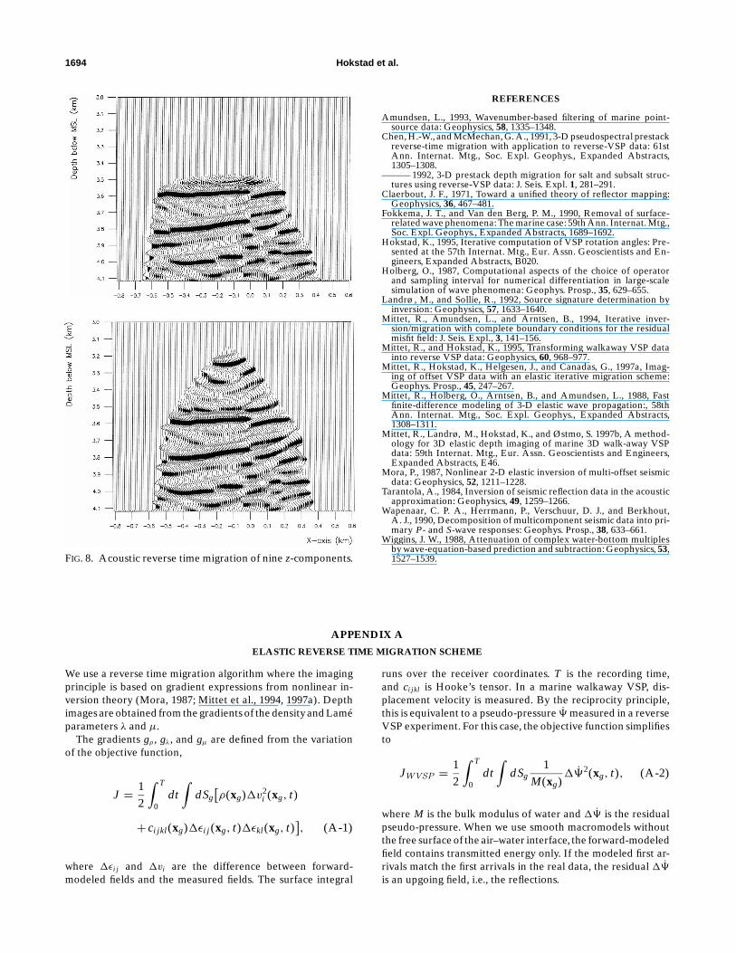
For comparison, the walkaway VSP data were migrated us-ing an acoustic macromodel as well, setting the S-wave veloci-ties to zero. The result from acoustic reverse time migration ofthe z-components is shown in Figure 8. Comparing with Fig-ure 4, we observe that, for the z-components, the result is notsignificantly degraded by migration in the acoustic approxi-mation.

Acoustic migration of the x-components gives meaninglessresults, as expected, because the x-components contains con-siderable amounts of PS-conversions.

DISCUSSION

The P-images are obtained by correlating local P-energyat each node of the finite-difference grid within the region ofinterest. Correspondingly, the P&S-images are in general ob-tained by correlating both local P- and S-energy. The surfaceseismics (Figure 2) indicate the overburden is close to plane lay-ered and the target zone for the walkaway VSP survey consistsof possibly faulted but otherwise small dipping layers. Fault-plane reflections fall outside the aperture of the walkaway

FIG. 5. Elastic reverse time migration of nine x-components.(Top) P-image; (bottom) P&S-image.

VSP experiment. Therefore, it is reasonable to suspect that thez-components of the walkaway VSP data are dominated byPP-reflections recorded at small and intermediate offsets. PS-converted energy propagating at large angles from the verticalgive minor contributions to the z-components. This is con-firmed by the images obtained by acoustic reverse time migra-tion. From a reverse VSP point of view, this can be understoodfrom the radiation characteristics of directional sources. Witha force in the z-direction, P-energy is radiated within a fanaround the vertical axis, whereas S-energy is radiated within afan around the x-axis.

The P- and P&S-images obtained from the x-componentsare nearly complementary. This also may be understood fromthe radiation characteristics of direction forces. For a reverseVSP shot with a force in the x-direction, P-energy is radiatednear the horizontal plane, whereas S-energy is radiated nearthe vertical direction. Consequently, the x-component receivesPS-conversions at small offsets and PP-reflections at large off-sets. The PP image from the x-component vanishes at smalloffsets, as do the PP reflected and transmitted waves on thex-component in walkaway VSP data. The S-waves have lowervelocity and shorter wavelength than the P-waves. Therefore,PS-converted energy may resolve detail on a smaller scale nearthe well. Comparing the x- and z-component images (e.g., Fig-ures 6 and 7), we see this is the case.

CONCLUSIONS

We have presented the results obtained from elastic reversetime migration of marine walkaway VSP data. In the areawhere the walkaway VSP survey was completed, the geology isfairly simple in the cross-line direction. Therefore, it is possibleto obtain good results from 2-D processing.

We imaged the x- and z-components separately by usingthe reciprocal relationship between the walkaway and re-verse VSP configurations. The depth images obtained from thez-components reveal the major characteristics of the geologicalstructure below geophone depth. The base Cretaceous uncon-formity with a graben at 3.6 km depth and the faulted coalmarker at 3.8 km can be identified on the z-component images.After transformation to the two-way time domain, the elasticimages tie well with the surface seismic section. A numeri-cal test using acoustic reverse time migration showed that thez-component images were not significantly degraded by acous-tic approximation. This indicates the events recorded on thez-components are dominantly PP-reflections.

Compared to the z-component images, the images obtainedfrom the x-component are more corrupted by migration smilesand artifacts. However, when interpreted together with thez-component images, they provide some information. On thex-component P-images, continuous reflectors are imaged far-ther away from the well. The x-component P&S-images getimportant contributions from PS-converted energy recorded atsmall offsets, resolving details near the well. The x-componentimages are sensitive to the S-wave velocity macromodel belowgeophone depth.

Currently, we are working on 3-D elastic RTM of a 3-Dmarine WVSP. The real data example presented in this paperdemonstrates that full elastic RTM is an attractive alternativefor imaging of WVSP data, and that both P- and S-energy canbe used in the construction of the depth images.

1692 Hokstad et al.

FIG. 6. Elastic reverse time migration of nine z-components. The P&S depth image is transformed to two-way traveltime andmerged into the surface seismic section.

Elastic RTM of Walkaway VSP Data 1693

ACKNOWLEDGMENTS

We thank the participants of the 3-D VSP project, ElfPetroleum Norge AS, Norsk Agip A/S, Norsk Hydro a.s.,Norwegian Petroleum Directorate, Statoil and TOTAL NorgeA.S., for financial support and for permission to publish the re-sults. Furthermore, we thank Lasse Amundsen (Statoil), Eivind

FIG. 7. Elastic reverse time migration of nine x-components. The P&S depth image is transformed to two-way traveltime andmerged into the surface seismic section.

Berg (S&B Geophysical, formerly Statoil), Arild Haugen(NPD), Philippe Julien (TOTAL), Peter Macalister-Hall (TO-TAL), Jean-Marc Mougenot (Elf), and Steen Petersen (NorskHydro) for discussions. We thank Elf Petroleum Norge a.s.,for permission to use the real data, and we are grateful toGeoffrey Jackson, formerly of Elf Geoscience Research Cen-tre, for giving us the results from his velocity analysis.

1694 Hokstad et al.

FIG. 8. Acoustic reverse time migration of nine z-components.

APPENDIX A

ELASTIC REVERSE TIME MIGRATION SCHEME

We use a reverse time migration algorithm where the imagingprinciple is based on gradient expressions from nonlinear in-version theory (Mora, 1987; Mittet et al., 1994, 1997a). Depthimages are obtained from the gradients of the density and Lameparameters λ and µ.

The gradients gρ , gλ, and gµ are defined from the variationof the objective function,

J = 12

∫ T

0dt∫

dSg[ρ(xg)1v2

i (xg, t)

+ ci jkl (xg)1εi j (xg, t)1εkl(xg, t)], (A-1)

where 1εi j and 1vi are the difference between forward-modeled fields and the measured fields. The surface integral

runs over the receiver coordinates. T is the recording time,and ci jkl is Hooke’s tensor. In a marine walkaway VSP, dis-placement velocity is measured. By the reciprocity principle,this is equivalent to a pseudo-pressure 9 measured in a reverseVSP experiment. For this case, the objective function simplifiesto

JWVSP = 12

∫ T

0dt∫

dSg1

M(xg)192(xg, t), (A-2)

where M is the bulk modulus of water and 19 is the residualpseudo-pressure. When we use smooth macromodels withoutthe free surface of the air–water interface, the forward-modeledfield contains transmitted energy only. If the modeled first ar-rivals match the first arrivals in the real data, the residual 19is an upgoing field, i.e., the reflections.

REFERENCES

Amundsen, L., 1993, Wavenumber-based filtering of marine point-source data: Geophysics, 58, 1335–1348.

Chen, H.-W., and McMechan, G. A., 1991, 3-D pseudospectral prestackreverse-time migration with application to reverse-VSP data: 61stAnn. Internat. Mtg., Soc. Expl. Geophys., Expanded Abstracts,1305–1308.

——— 1992, 3-D prestack depth migration for salt and subsalt struc-tures using reverse-VSP data: J. Seis. Expl. 1, 281–291.

Claerbout, J. F., 1971, Toward a unified theory of reflector mapping:Geophysics, 36, 467–481.

Fokkema, J. T., and Van den Berg, P. M., 1990, Removal of surface-related wave phenomena: The marine case: 59th Ann. Internat. Mtg.,Soc. Expl. Geophys., Expanded Abstracts, 1689–1692.

Hokstad, K., 1995, Iterative computation of VSP rotation angles: Pre-sented at the 57th Internat. Mtg., Eur. Assn. Geoscientists and En-gineers, Expanded Abstracts, B020.

Holberg, O., 1987, Computational aspects of the choice of operatorand sampling interval for numerical differentiation in large-scalesimulation of wave phenomena: Geophys. Prosp., 35, 629–655.

Landrø , M., and Sollie, R., 1992, Source signature determination byinversion: Geophysics, 57, 1633–1640.

Mittet, R., Amundsen, L., and Arntsen, B., 1994, Iterative inver-sion/migration with complete boundary conditions for the residualmisfit field: J. Seis. Expl., 3, 141–156.

Mittet, R., and Hokstad, K., 1995, Transforming walkaway VSP datainto reverse VSP data: Geophysics, 60, 968–977.

Mittet, R., Hokstad, K., Helgesen, J., and Canadas, G., 1997a, Imag-ing of offset VSP data with an elastic iterative migration scheme:Geophys. Prosp., 45, 247–267.

Mittet, R., Holberg, O., Arntsen, B., and Amundsen, L., 1988, Fastfinite-difference modeling of 3-D elastic wave propagation:, 58thAnn. Internat. Mtg., Soc. Expl. Geophys., Expanded Abstracts,1308–1311.

Mittet, R., Landrø, M., Hokstad, K., and Østmo, S. 1997b, A method-ology for 3D elastic depth imaging of marine 3D walk-away VSPdata: 59th Internat. Mtg., Eur. Assn. Geoscientists and Engineers,Expanded Abstracts, E46.

Mora, P., 1987, Nonlinear 2-D elastic inversion of multi-offset seismicdata: Geophysics, 52, 1211–1228.

Tarantola, A., 1984, Inversion of seismic reflection data in the acousticapproximation: Geophysics, 49, 1259–1266.

Wapenaar, C. P. A., Herrmann, P., Verschuur, D. J., and Berkhout,A. J., 1990, Decomposition of multicomponent seismic data into pri-mary P- and S-wave responses: Geophys. Prosp., 38, 633–661.

Wiggins, J. W., 1988, Attenuation of complex water-bottom multiplesby wave-equation-based prediction and subtraction: Geophysics, 53,1527–1539.

Elastic RTM of Walkaway VSP Data 1695

The variation of the objective function is

δJ =∫

d3x[gρ(x)δρ + gλ(x)δλ+ gµ(x)δµ], (A-3)

where the equations for the gradients are

gρ(x) = −∫ T

0dt[∂tv

modi (x, t)

]∂t1vi (x, t),

(A-4)

gλ(x) =∫ T

0dt[∂tε

modi i (x, t)

]∂t1ε j j (x, t),

and

gµ(x) = 2∫ T

0dt[∂tε

modi j (x, t)

]∂t1εi j (x, t).

Here, εmodi j and vmod

i are forward-modeled strain and displace-ment velocity fields, and1εi j and1vi are the back-propagateddifference between forward-modeled fields and the measuredfields. We define the corresponding preconditioned gradientsby

gη(x) = B(x)gη(x), (A-5)

where η= ρ, λ, or µ and B−1(x) is proportional to the averageenergy of the forward-modeled field in position x. In an in-version scheme, the preconditioning function B(x) is an ap-proximation to the diagonal part of the inverse Hessian tensor.For migration purposes, B(x) can be viewed as a geometricalspreading correction.

The back-propagation of the residual fields is equivalentto reverse time migration of the upgoing reflected wave-field. The imaging condition, computed by correlation ofback-propagated (upgoing) and forward-modeled (downgo-ing) fields, is equivalent to Claerbout’s imaging principle. Theforward modeling and back-propagation both proceed in thesmooth background model where the only spatially localizedreflectors are the sea bottom and, if present, the free surface.

The migration images are constructed by displaying the pre-conditioned gradients. For a multishot experiment, the imagesare

Iη(x) = F{∑

s

gsη(x)

}, (A-6)

where η= ρ, λ, or µF is a filter, and the sum runs over shots.