EITN90 Radar and Remote SensingLecture 6: Target fluctuation models

Daniel Sjoberg

Department of Electrical and Information Technology

Spring 2020

Outline

1 Radar cross section of simple targets

2 Radar cross section of complex targets

3 Statistical characteristics of the RCS of complex targets

4 Target fluctuation models

5 Doppler spectrum of fluctuating targets

6 Conclusions

2 / 37

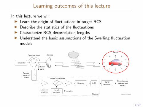
Learning outcomes of this lecture

In this lecture we willI Learn the origin of fluctuations in target RCSI Describe the statistics of the fluctuationsI Characterize RCS decorrelation lengthsI Understand the basic assumptions of the Swerling fluctuation

models

Transmitter T/R

Transmit signal Antenna

Target

Receiverprotector

switch

Receivesignal

Low noiseamplifier

Mixer/Preamplifier

Localoscillator

IF amplifier

Detector A/DSignal

processor

Detection andmeasurement

results

(Adapted from Fig. 1-1)Receiver

3 / 37

Outline

1 Radar cross section of simple targets

2 Radar cross section of complex targets

3 Statistical characteristics of the RCS of complex targets

4 Target fluctuation models

5 Doppler spectrum of fluctuating targets

6 Conclusions

4 / 37

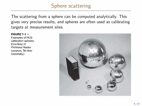
Sphere scattering

The scattering from a sphere can be computed analytically. Thisgives very precise results, and spheres are often used as calibratingtargets at measurement sites.

5 / 37

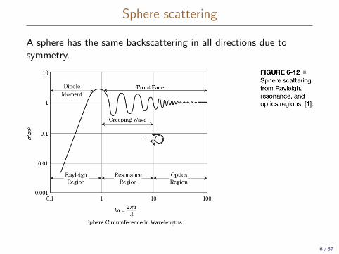
Sphere scattering

A sphere has the same backscattering in all directions due tosymmetry.

6 / 37

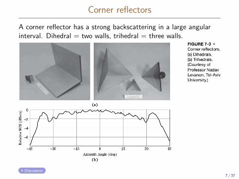
Corner reflectors

A corner reflector has a strong backscattering in a large angularinterval. Dihedral = two walls, trihedral = three walls.

Discussion7 / 37

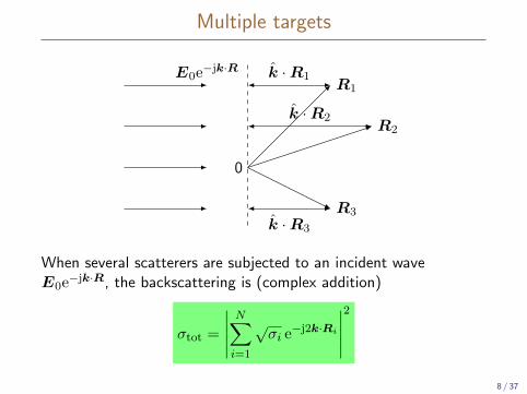
Multiple targets

0

R1

R2

R3

k ·R1

k ·R2

k ·R3

E0e−jk·R

When several scatterers are subjected to an incident waveE0e−jk·R, the backscattering is (complex addition)

σtot =

∣∣∣∣∣N∑i=1

√σi e−j2k·Ri

∣∣∣∣∣2

8 / 37

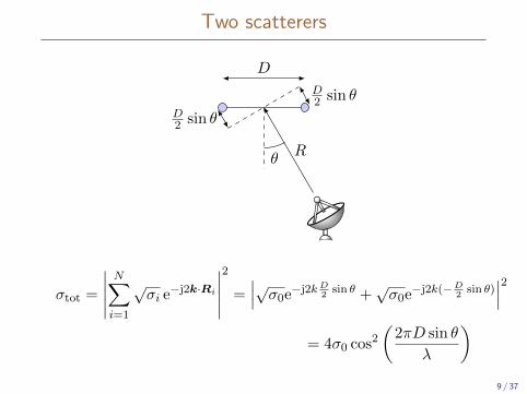
Two scatterers

R

D

θ

D2 sin θ

D2 sin θ

σtot =

∣∣∣∣∣N∑i=1

√σi e−j2k·Ri

∣∣∣∣∣2

=∣∣∣√σ0e−j2kD

2sin θ +

√σ0e−j2k(−D

2sin θ)

∣∣∣2= 4σ0 cos2

(2πD sin θ

λ

)9 / 37

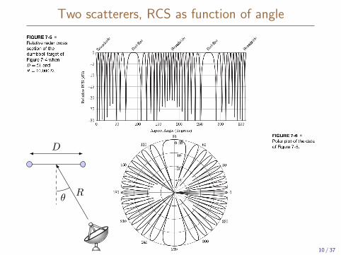
Two scatterers, RCS as function of angle

R

D

θ

10 / 37

Outline

1 Radar cross section of simple targets

2 Radar cross section of complex targets

3 Statistical characteristics of the RCS of complex targets

4 Target fluctuation models

5 Doppler spectrum of fluctuating targets

6 Conclusions

11 / 37

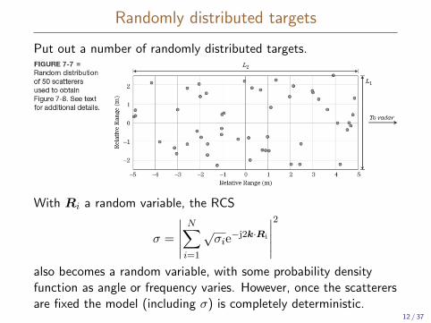
Randomly distributed targets

Put out a number of randomly distributed targets.

With Ri a random variable, the RCS

σ =

∣∣∣∣∣N∑i=1

√σie−j2k·Ri

∣∣∣∣∣2

also becomes a random variable, with some probability densityfunction as angle or frequency varies. However, once the scatterersare fixed the model (including σ) is completely deterministic.

12 / 37

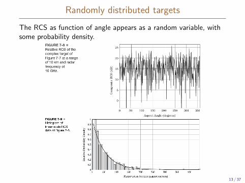
Randomly distributed targets

The RCS as function of angle appears as a random variable, withsome probability density.

13 / 37

Outline

1 Radar cross section of simple targets

2 Radar cross section of complex targets

3 Statistical characteristics of the RCS of complex targets

4 Target fluctuation models

5 Doppler spectrum of fluctuating targets

6 Conclusions

14 / 37

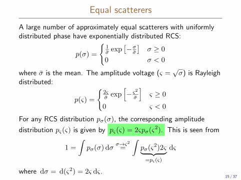
Equal scatterers

A large number of approximately equal scatterers with uniformlydistributed phase have exponentially distributed RCS:

p(σ) =

1σ exp

[−σσ

]σ ≥ 0

0 σ < 0

where σ is the mean. The amplitude voltage (ς =√σ) is Rayleigh

distributed:

p(ς) =

2ςσ exp

[− ς2

σ

]ς ≥ 0

0 ς < 0

For any RCS distribution pσ(σ), the corresponding amplitude

distribution pς(ς) is given by pς(ς) = 2ςpσ(ς2). This is seen from

1 =

∫pσ(σ) dσ

σ→ς2=

∫pσ(ς2)2ς︸ ︷︷ ︸

=pς(ς)

dς

where dσ = d(ς2) = 2ς dς.15 / 37

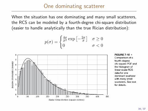
One dominating scatterer

When the situation has one dominating and many small scatterers,the RCS can be modeled by a fourth-degree chi-square distribution(easier to handle analytically than the true Rician distribution):

p(σ) =

4σσ2 exp

[−2σ

σ

]σ ≥ 0

0 σ < 0

16 / 37

17 / 37

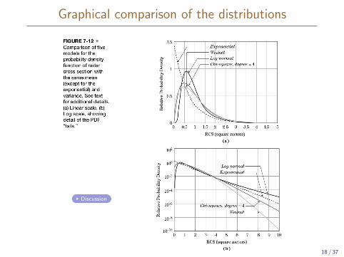
Graphical comparison of the distributions

Discussion

18 / 37

Matlab demo (see http://radarsp.com)

19 / 37

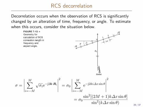
RCS decorrelation

Decorrelation occurs when the observation of RCS is significantlychanged by an alteration of time, frequency, or angle. To estimatewhen this occurs, consider the situation below.

σ =

∣∣∣∣∣M∑

i=−M

√σie−j2k·Ri

∣∣∣∣∣2

= σ0

∣∣∣∣∣M∑

i=−Me−j2ki∆x sin θ

∣∣∣∣∣2

= σ0sin2[(2M + 1)k∆x sin θ]

sin2(k∆x sin θ)20 / 37

RCS decorrelation

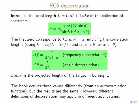
Introduce the total length L = (2M + 1)∆x of the collection ofscatterers:

σ = σ0sin2(kL sin θ)

sin2(k∆x sin θ)

The first zero corresponds to kL sin θ = π, implying the correlationlengths (using k = 2π/λ = 2πf/c and sin θ ≈ θ for small θ)

∆f =c

2L sin θ(frequency decorrelation)

∆θ =λ

2L(angle decorrelation)

L sin θ is the projected length of the target in boresight.

The book derives these values differently (from an autocorrelationfunction), but the results are the same. However, differentdefinitions of decorrelation may apply in different applications.

21 / 37

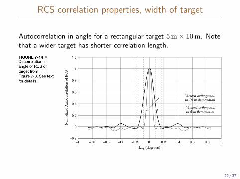
RCS correlation properties, width of target

Autocorrelation in angle for a rectangular target 5 m× 10 m. Notethat a wider target has shorter correlation length.

22 / 37

RCS correlation properties, frequency agility

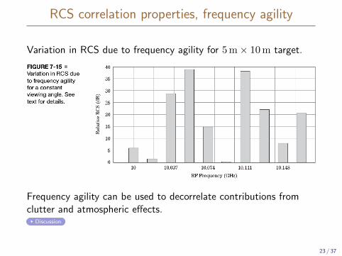
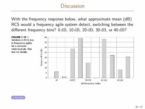
Variation in RCS due to frequency agility for 5 m× 10 m target.

Frequency agility can be used to decorrelate contributions fromclutter and atmospheric effects.

Discussion

23 / 37

Outline

1 Radar cross section of simple targets

2 Radar cross section of complex targets

3 Statistical characteristics of the RCS of complex targets

4 Target fluctuation models

5 Doppler spectrum of fluctuating targets

6 Conclusions

24 / 37

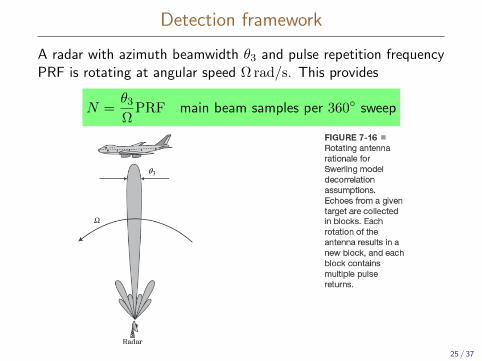
Detection framework

A radar with azimuth beamwidth θ3 and pulse repetition frequencyPRF is rotating at angular speed Ω rad/s. This provides

N =θ3

ΩPRF main beam samples per 360 sweep

25 / 37

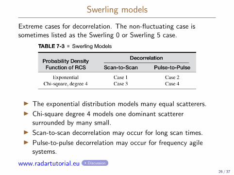
Swerling models

Extreme cases for decorrelation. The non-fluctuating case issometimes listed as the Swerling 0 or Swerling 5 case.

I The exponential distribution models many equal scatterers.

I Chi-square degree 4 models one dominant scatterersurrounded by many small.

I Scan-to-scan decorrelation may occur for long scan times.

I Pulse-to-pulse decorrelation may occur for frequency agilesystems.

www.radartutorial.eu Discussion

26 / 37

Different decorrelations, scan or pulse

27 / 37

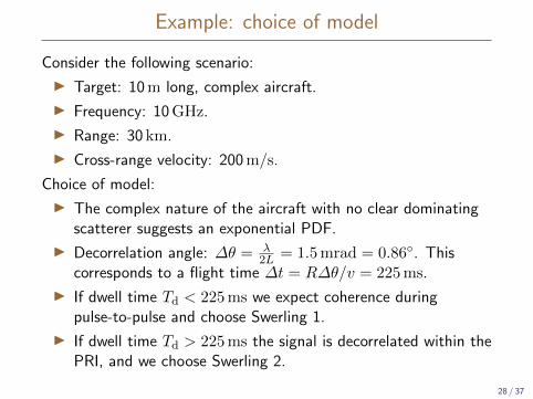
Example: choice of model

Consider the following scenario:

I Target: 10 m long, complex aircraft.

I Frequency: 10 GHz.

I Range: 30 km.

I Cross-range velocity: 200 m/s.

Choice of model:

I The complex nature of the aircraft with no clear dominatingscatterer suggests an exponential PDF.

I Decorrelation angle: ∆θ = λ2L = 1.5 mrad = 0.86. This

corresponds to a flight time ∆t = R∆θ/v = 225 ms.

I If dwell time Td < 225 ms we expect coherence duringpulse-to-pulse and choose Swerling 1.

I If dwell time Td > 225 ms the signal is decorrelated within thePRI, and we choose Swerling 2.

28 / 37

Outline

1 Radar cross section of simple targets

2 Radar cross section of complex targets

3 Statistical characteristics of the RCS of complex targets

4 Target fluctuation models

5 Doppler spectrum of fluctuating targets

6 Conclusions

29 / 37

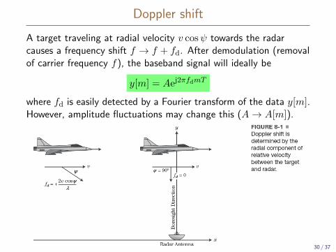
Doppler shift

A target traveling at radial velocity v cosψ towards the radarcauses a frequency shift f → f + fd. After demodulation (removalof carrier frequency f), the baseband signal will ideally be

y[m] = Aej2πfdmT

where fd is easily detected by a Fourier transform of the data y[m].However, amplitude fluctuations may change this (A→ A[m]).

30 / 37

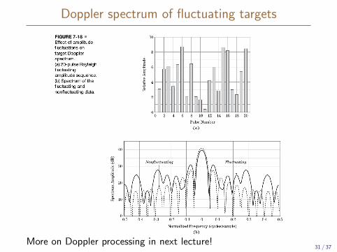
Doppler spectrum of fluctuating targets

More on Doppler processing in next lecture!31 / 37

Outline

1 Radar cross section of simple targets

2 Radar cross section of complex targets

3 Statistical characteristics of the RCS of complex targets

4 Target fluctuation models

5 Doppler spectrum of fluctuating targets

6 Conclusions

32 / 37

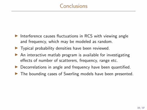
Conclusions

I Interference causes fluctuations in RCS with viewing angleand frequency, which may be modeled as random.

I Typical probability densities have been reviewed.

I An interactive matlab program is available for investigatingeffects of number of scatterers, frequency, range etc.

I Decorrelations in angle and frequency have been quantified.

I The bounding cases of Swerling models have been presented.

33 / 37

Discussion

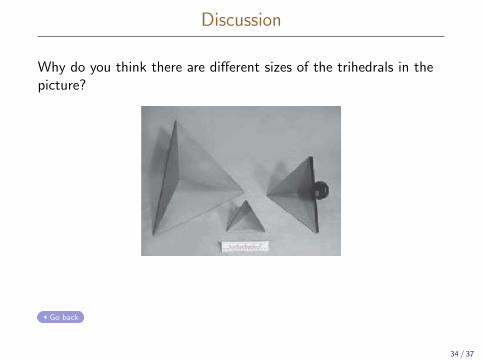
Why do you think there are different sizes of the trihedrals in thepicture?

Answer: What matters is the size of the scatterer in terms ofwavelengths. The different sizes target different wavelengths.

Go back

34 / 37

Discussion

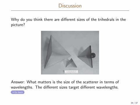
Why do you think there are different sizes of the trihedrals in thepicture?

Answer: What matters is the size of the scatterer in terms ofwavelengths. The different sizes target different wavelengths.

Go back

34 / 37

Discussion

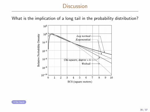
What is the implication of a long tail in the probability distribution?

Answer: with a long tail (slow decrease), there is a higherprobability for extreme events.

Go back

35 / 37

Discussion

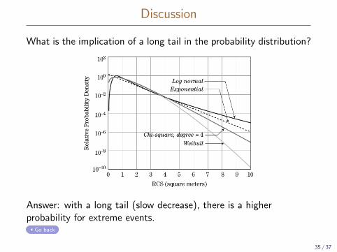
What is the implication of a long tail in the probability distribution?

Answer: with a long tail (slow decrease), there is a higherprobability for extreme events.

Go back

35 / 37

Discussion

With the frequency response below, what approximate mean (dB)RCS would a frequency agile system detect, switching between thedifferent frequency bins? 0 dB, 10 dB, 20 dB, 30 dB, or 40 dB?

Answer: Around 20 dB (more exactly 18 dB).

Go back

36 / 37

Discussion

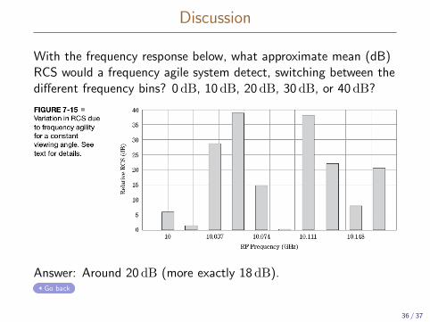
With the frequency response below, what approximate mean (dB)RCS would a frequency agile system detect, switching between thedifferent frequency bins? 0 dB, 10 dB, 20 dB, 30 dB, or 40 dB?

Answer: Around 20 dB (more exactly 18 dB).Go back

36 / 37

Discussion

With a decorrelation time of ∆T , pulse repetition interval PRI,and dwell time Td = npPRI, what is the condition for a Swerling 1situation (scan-to-scan decorrelation), and a Swerling 2 situation(pulse-to-pulse decorrelation)?

Answer:

I Swerling 1: Td > ∆T (or NTd > ∆T , with N being thenumber of scan positions for a search radar)

I Swerling 2: PRI > ∆T

Go back

37 / 37

Discussion

With a decorrelation time of ∆T , pulse repetition interval PRI,and dwell time Td = npPRI, what is the condition for a Swerling 1situation (scan-to-scan decorrelation), and a Swerling 2 situation(pulse-to-pulse decorrelation)?

Answer:

I Swerling 1: Td > ∆T (or NTd > ∆T , with N being thenumber of scan positions for a search radar)

I Swerling 2: PRI > ∆T

Go back

37 / 37