Radar Equations for Modern Radar 53-76

CHAPTER 2

The Search Radar Equation

The radar equations presented in Chapter 1 give thedetection range of an existing or proposed radar forwhich the major parameters are known. They can be usedto test different sets of parameters and to compare theresults of competing radar designs for a given task,determining which best meets requirements such as therange at which a specified detection performance isavailable given the available beam dwell time andinvestment in equipment and input power.

The search radar equation is a modification of the basicequation that allows one to avoid the process ofgenerating many alternative designs and testing them tosee which can meet a specified objective. It providesan estimate of the mini-mum radar size, as measured bythe product of average transmitter power Pav andreceiving antenna aperture area A, that can search agiven volume of three-dimensional space with aspecified level of detection performance.Alternatively, it can define the volume that can besearched by a radar of specified size while providing aspecified level of detection performance. Neither thewavelength nor the waveform need be known to obtainthese estimates, and hence it is unneces-sary topostulate details such as the signal processing methodsor the resolution properties of the radar until a laterstage in the synthesis or analysis of the radar design.

The search radar equation originated in a 1948 studyby Edward Barlow and his associates at Sperry GyroscopeCompany that was presented in a classified report. Thatreport has apparently never been declassified, but the

derivation of the equation was presented in and it hassubsequently seen wide use. For example, it providesthe basis for the definition of a class of radars whosesiting was limited by the (now defunct) U.S.-RussianABM Treaty to locations on the periphery of the usingcountry, looking outward. It serves as a reference forquick evaluation and comparison of proposed radardesigns and systems on which available data arelimited.

33

34 Radar Equations for Modern Radar

2.1 DERIVATION OF THE SEARCH RADAR EQUATION

The search radar equation is derived from an idealizedmodel of the search process. An angular sector is to besearched in a specified period of time by atransmitting beam that may either scan the sector orilluminate it continuously, while one or more receivingbeams recover and integrate the energy of resultingtarget echoes. Free space propagation is assumed. Acombined search loss factor is included to account fordepartures from the idealized model of the radar andenvironment. Steps in derivations of the equations areas follows.

Search Sector. The first step in derivation of thesearch radar equation is to establish an idealizedmodel of the search sector, specified as a solid angle ssteradians, within which the radar resources of timeand energy are to be confined. The solid angle s isnormally specified in terms of the width Am of theazimuth sector and the upper and lower limits m and 0of the elevation sector:

where Am is in radians. Note that the elevation anglem is positive for a surface based radar, for whichnormally 0 0. For a radar elevated above thesurface, either or both angles can be negative, theonly requirement being that m > 0.

Transmitting Beam Sector. The transmitting beam ismodeled as rectangular in shape with uniform gain overa beam sector bt s given by

whereattmaxtminet

= azimuth width of transmitting beam (rad); = elevation of upper edge of transmitting beam

(rad); = elevation of lower edge of transmitting beam

(rad);

= tma x tmin = elevation width of transmittingbeam (rad).

The transmitting beamwidths are either matched to thesearch sector or made small enough that the radar canscan the sector s with no overlap between adjacentbeams or excursion beyond the sector. The latter caseis normally assumed, justifying the small angleapproximation in (2.2). The solid angle b of the beamis related to the gain Gt of the idealized transmittingantenna by a simple expression, based on the assumptionthat the transmitted energy is confined to anduniformly distributed within the rectangular shapedbeam:

bt

at

et

4

steradians (2.3)Gt

The Search Radar Equation 35

where 4 is the solid angle of a sphere surrounding theradar, over which an isotropic antenna would spread theradiated power. Equation (2.3) states the fact that thegain Gt of an antenna varies inversely with the solidangle of its beam. We consider later the limitation onthe gain that can be produced by a practical antenna,requiring replacement of the factor 4 by 4/Ln 10.75from [3, p. 334].

Search Frame Time. Targets in the search sector are tobe detected with specified probability within a searchframe time ts. This allows expression of the observation(or dwell) time to in each transmitting beam position as

to

t s

t s

bt 4ts sec (2.4)

nbt s Gt s

where nbt = s/bt is the number of transmitting beampositions in the search sector.1

Coherent Integration. The idealized radar performscoherent integration of the echo energy received in theperiod to, during which the transmitted energy is

Et

P

av

to

4Pav ts

J (2.5)Gt s

Further Assumptions. The following assumptions alsoapply to the idealized search radar and process:

The gain of the ideal receiving antenna is given by(1.5), with the receiving aperture equal to thephysical area2 of the receiving antenna, Ar = A:

Gr

4A(2.6) 2

The target cross section is a constant , located onthe axes of the nearest transmitting and receiving beams, at broadside tothe antenna array if one is used. The basic steady-target detectability factor D0(1) for this case isas given by Rice [4] (see Section 4.2).

Free-space paths give pattern-propagation factors Ft

= Fr = 1.

The system noise temperature Ts = T0 = 290K.

1 For electronically scanned array antennas, broadening of the beamat angles off broadside reduces the number of beams required toscan a given sector.

2 We use here the physical aperture A rather than the effectivereceiving aperture Ar appearing in some discussions, to base theequation on a truly ideal reference.


All losses relative to the ideal are lumped into a search loss factor Ls.

Search Radar Range. With these assumptions, the maximumdetection range from (1.18) becomes

1 4

Rm Pav t s A m (2.7) 4 s kT0 D0 1Ls

The three dimensional search volume is defined bythe angular sector s and the maximum range Rm. Thetransmitting antenna gain and number of beamstransmitted into the search sector cancel out of theequation, leaving the energy density per unit solidangle Pavts/s (in J/steradian) as the transmitterillumination density in the search sector. As long asthe echo energy is collected efficiently by thereceiving aperture A, it makes no difference whetherthe energy appears in short periods to << ts from atransmitting antenna with high Gt, or any longer periodwith lower Gt , approaching the limiting case ofcontinuous low gain illumination of the full sector forts seconds by a nonscanning transmission: bt = s, nbt =1. If the transmitting beam scans the sector, thereceiving beam must follow it to receive all the echoenergy incident on the receiving aperture from theillumination of each beam position. If the transmittingbeam illuminates a solid angle bt greater than that ofa single receiving beam (i.e., the transmittingaperture is smaller than A), then multiple receivingbeams must be formed in parallel to collect the echoenergy returned to the receiving antenna. Receivingaperture effi-ciency a < 1.0 for requires that thecorresponding loss factor L = 1/a be included in thesystem loss factor. If coherent integration is notperformed over the observation time to, a correspondingnoncoherent integration loss must be included in Ls.

Power-Aperture Required for Search. Inversion of (2.7) tosolve for the power-aperture product Pav A required to meet asearch specification gives

Pav A

4s Rm4 kT0 D0

1Ls W m2 (2.8)ts

The task assigned to the search radar determines five of the terms in (2.8):

s, Rm, D0, ts, and .

The factors 4, k and T0 are constants. Only Pav and Aon the left side and Ls on the right side are controlledby decisions of the radar designer. The challenge inapplying the search radar equation is to define theappropriate search sector s and estimate the lossesthat enter into Ls. These steps are critical to use ofthe equation,

37since the idealized assumptions made in its derivationrequire that s be carefully defined and that manylosses, usually totaling 20 dB or more, be identifiedand quantified.

2.2 SEARCH SECTORS FOR 2-D AIR SURVEILLANCE

Air surveillance radars are described as two-dimensional (2-D) when their output data are range andazimuth, and three-dimensional (3-D) when range,azimuth, and elevation data are provided. Both typessearch within the three-dimensional space used in thesearch radar equation.

2.2.1 Elevation Coverage in 2-D Surveillance

The 2-D air surveillance radar coverage pattern inelevation can seldom be defined simply in terms of themaximum and minimum elevation angles m and 0 used in(2.1). Requirements typically follow one of the curvesplotted in Figure 2.1.

= 45°

km cs

in c

Altit

ude c 1.s

c 5

Constantaltitude = 2.8°

1

csc2Hm = 10 km

mn

a

F de

liza

e

Id

Rm = 170 km

Slant range in km

Figure 2.1 Typical vertical coverage requirement options for 2-D air surveillance radar.


Air surveillance coverage is customarily specifiedin terms of the maximum altitude Hm of intended targetsand required detection range Rm, over the full 360azimuth sector. The elevation coverage of the idealizedbeam, which is rectangular in angle space, is shown bysolid lines as a right triangle. Its lower side extendshorizontally (at zero elevation) from the radar torange Rm; the right side extends vertically from thatpoint to an altitude Hm above the curved Earth; and thehypotenuse is a straight line returning from that pointto the radar. The elevation beamwidth 1 (2.8 in theexample shown) is expressed as

H

mR

m arcsin rad (2.9)

1

Rm2k

e a

e where

Hm =maximum target altitude (m);

ke = 4/3 = Earth’s radius factor;

ae =6,378,000m = Earth’sradius.

The minimum and maximum elevations for use in (2.1) are0 = 0 and m = 1. The maximum-altitude target isdetected the at range Rm, but at shorter ranges it liesabove the idealized beam. This is far from ideal in thepractical sense. One of the five other patterns shownwill typically be used in practice, with appropriateentries in the search radar equation as describedbelow.

2.2.2 Fan-Beam Pattern for 2-D Surveillance

In fan-beam 2-D radar the elevation beam patterns fortransmitting and receiving are matched to the requiredelevation search sector. A possible fan beam contour,shown in Figure 2.1 as a dashed curve, approximates theidealized triangle, but its half-power beamwidth hasbeen adjusted to e 1.51 to include the point Rm,Hm. This moves the upper shoulder of its pattern abovethe hypotenuse of the triangle and extends the beampeak beyond Rm. Targets at altitude Hm still lie above

the beam at R < 0.9Rm, so detection at maximum altitudeis only possible in a narrow range interval near Rm.Even this small departure of the fan beam from theideal-ized coverage triangle requires the followingadjustments of entries in the search radar equation.An elevation beamshape loss Lpe = e/1 1.5 = 1.76 dBis included as a component of Ls to account for theincrease in beamwidth of the 2-D radar antenna. Thisresults from inability to synthesize the square-endedbeam corresponding to the idealized triangular patternshown in Figure 2.1, thus violating the assumption thatthe transmitted energy is uniform from 0 to 1, as usedin defining s. This loss is reduced if the apertureheight h is large enough to permit the full-rangecoverage pattern to be synthesized by com-

The Search Radar Equation 39bining two or more narrow elevation beams toapproximate a square-ended beam (see Section 10.1.4). The elevation beamshape loss included in Ls issquared, to account also for the reduction ineffective receiving aperture area Ar = A/Lpe. Thetwo-way loss L2pe in the search radar equationreplaces the beamshape loss Lp = 1.24 dB used in theconventional radar equation to give the reduction inaverage two-way gain for targets distributed overthe elevation beamwidth (see Section 5.2).

The search solid angle s for fan-beam 2-D radar iscalculated using m = 1 and 0 = 0 in (2.1).

2.2.3 Cosecant-Squared Pattern for 2-D Surveillance

Another curve in Figure 2.1 shows a cosecant-squaredelevation beam pattern. Here the mainlobe extends fromzero elevation to 1 at range Rm, but coveragecontinues along a horizontal line from that point to anupper elevation limit 2. Above 2 is a cone of silence inwhich coverage is lost. The idealized antenna gain as afunction of elevation angle is

G

G ,

0

m 1

G

csc2 ,

(2.10)

m csc2 1 2

1 0, 2

where Gm is the gain required to achieve detection at Rm.

The search sector specified in the search radarequation can be adjusted for an idealized csc2 patternby using an equivalent value of upper elevation givenby [5, p. 315, Eq. (7.4)]:

sin

L 2 1

rad (2.11)m csc 1 1

sin2

where Lcsc is the pattern loss in gain for the csc2coverage compared to the fan beam with half-power width1. This loss approaches a maximum of 3 dB for 2 >> 1.Use of the equivalent upper elevation angle incalculating s accounts for the transmitted energydensity over the search sector, but a secondapplication of Lcsc is needed to reflect the reductionin effective receiving aperture. Thus, entries in thesearch radar equation must be adjusted for the csc2pattern as follows:


The required search solid angle s is increased byLcsc, relative to the fan beam radar, to allow fordiversion of transmitted energy into the uppershoulder of the pattern.

The Lcsc in effective receiving aperture is includedin Ls.

The elevation beamshape loss Lpe remains as listed inSection 2.2.2.

2.2.4 Coverage to Constant Altitude

Even with its extension above 1, the csc2 pattern doesnot quite meet the required altitude coverage toaltitude Hm at ranges within Rm, because 1 from (2.9)has been reduced by the Earth’s curvature relative tothe angle that would apply over a flat Earth. A slightadjustment to (2.10) can preserve coverage to thatlabeled “constant altitude” in Figure 2.1. Theresulting losses in on-axis gain for the csc2 andconstant altitude patterns are shown in Figure 2.2,along with data for two other types of enhanced uppercoverage, discussed below. The pattern loss due to theuse of csc2 or other patterns with elevation coverageextended at ranges within Rm will be denoted here by Lcscregardless of the exponent of the csc function used orthe adjustment for coverage to constant targetaltitude. All the plots in Figure 2.2 are calculatedfor a maximum elevation coverage angle 2 = 45, butthere is negligible change as that angle varies from30 to 60. The factor Lcsc appears both as an increasein s (for transmitting) and in Ls (for receiving).

Patte

rn lo

ss in

dB

8

7

6

5 Const ant

H = 10 kmt

4

3csc2

2 0 1 2 3

csc

csc 3/

2

.

4 5 6 7 8 9 10

Full-range sector width in degFigure 2.2 Pattern loss Lcsc for csc2 and other patterns with extended

upper coverage, as a function of full-range elevation sector width1.

2.2.5 Enhanced Upper Coverage for 2-D SurveillanceRadar

When sensitivity time control (STC) is used in a 2-D surveillance radar with a csc2 or constant-altitude pattern, the detection range is reduced on targets at ranges


where STC is applied. To avoid this, an antenna patternwith enhanced upper coverage is used [6]. Two suchcurves are shown in Figure 2.1, corresponding togains varying as csc3/2 and csc . Figure 2.2 includesplots of loss Lcsc for these two cases. For the csc pattern the equivalent upper elevation is given by

sin 2

L 1 ln

rad (2.12)

m csc 1 sin

1

1

As with csc2 coverage, both s and Ls are increased inthe search radar equation to account for the extendedcoverage, and the elevation beamshape loss Lpe is alsoapplied.

2.2.6 Reflector Antenna Design for 2-D SurveillanceRadar

Reflector antennas for csc2 or other enhanced uppercoverage are designed in either of two ways: (1)reflector area is added at the top or bottom of theparabolic surface, deviating from the parabola todivert that energy into the upper coverage region andilluminated by a broadened horn pattern; or (2)multiple feed horns are stacked one above the other,fed from a power divider whose coupling is adjusted toprovide the desired pattern shape. Option (1) increasesthe physical aperture A but reduces the effective areaAr relative to a simple paraboloid, increasing the lossby the factor Lcsc relative to the fan beam (and by agreater factor relative to the increased area A).Option (2) uses the aperture height required for themainlobe of width 1, but reduces its effective areaby Lcsc. In both cases there is an increase in receivingaperture loss included in Ls, in addition to that causedby illumination tapers applied for sidelobe reductionin both coordinates and by spill-over and feedblockage.

2.2.7 Array Antennas for 2-D Surveillance Radar

There are also two design approaches available forelectrically fixed array antennas with csc2 or otherenhanced upper coverage: (1) rows of radiators areadded at the top or bottom of the array, for which theamplitudes and phases are adjusted to form the desiredupper coverage; or (2) the number of element rows ischosen for an elevation beamwidth 1, and multiplefeed lines are coupled to each row with complex weightsthat generate the radiated field contributions requiredfor the upper coverage. The two methods are equivalentto those discussed for reflectors, and the same lossconsiderations apply. Active arrays are seldom used in2-D ra-dars, but if this is done the first option maybe required to avoid distortion caused by saturation ofpower amplifiers with variation in the amplitude ofexcitation.


2.2.8 Example of Required Power-Aperture Product for 2-D Radar

The search radar equation can be applied to estimatethe power-aperture products required for each coveragecurve of Figure 2.1. Typical parameters common to allcoverage options are shown in Table 2.1. To compareresults for a specific choice of radar band, thewavelength has been assumed as 0.23m (L-band), and theaperture dimensions calculated based on a beamwidthconstant K = aw/ = 1.1. The upper coverage is assumedto be obtained by manipulation of the illumination overthe aperture height h = 5.2m needed to obtain e =1.51.

Table 2.1 Parameters Common to Example 2-D Search Radar

Target cross section System noise temperature Ts

Search loss Ls (excluding Lpe, Lcsc) Azimuth sector Am

Maximum full-range elevation 1

Wavelength Aperture width w Aperture area A

m2 1.0K 500dB 20deg 360deg 2.8

m0.23

m 9.7m2 50

Frame time ts s 6Detectability factorD0(1) dB 12Maximum range Rm km 170Minimum elevation 0 deg 0Maximum target altitude Hm km 10Azimuth beamwidth a deg 1.5Aperture height h m 5.2

Table 2.2 shows the results of applying (2.8) to theparameters shown in Table 2.1. The required power-aperture product increases as more power is divertedinto the upper coverage. The increased requirementshown in the last two columns is attributable to theenhanced upper coverage made necessary by theapplication of STC to avoid receiver saturation fromclutter and false alarms from small moving targets atshort range.

Table 2.2 Results from Search Radar Equation

Requirement UnitElevation pattern

Fan csc2 Const. H csc1.5 cscMaximum elevation 2 deg 2.8 45 45 45 45Elevation beamshape loss Lpe dB 1.76 1.76 1.76 1.76 1.76Pattern loss Lcsc dB 0.0 2.86 3.42 3.98 5.65Effective elevation sector m deg 4.2 5.4 6.2 7.0 10.3Solid angle of sectors sterad 0.31 0.59 0.67 0.77 1.13Power-aperture product kW·m2 7.66 28.6 37.1 47.9 103.3Average power Pav W 153 570 740 956 2,063


2.3 THREE-DIMENSIONAL AIR SURVEILLANCE

This section considers air surveillance conducted byradars that scan mechanically in azimuth, withelevation coverage provided by stacked beams thatoperate in parallel to cover the elevation sector or asingle beam that scans the sector. Elec-tronic scan inboth coordinates, using a mechanically fixed array, isdiscussed in Section 2.4.

2.3.1 Stacked-Beam 3-D Surveillance Radars

The stacked-beam 3-D radar uses a single transmittingpattern similar to that of the 2-D radar. Multiple,narrow receiving beams are stacked one above the other,within the transmitted beamwidth, to cover theelevation sector. The equivalent upper elevation anglem used in the search radar equation is given inSections 2.2.1–2.2.5. The gains of the receiving beamsare selected independently, giving flexibility inapportioning of transmitting and receiving gains overthe elevation sector. To obtain the equivalent of thecsc2 2-D coverage, for example, one of the followingapproaches may be used:

Receiving beams use the gain of the full aperture,allowing the transmitting pattern to follow a csc4

pattern that minimizes the loss Lcsc. Receiving beamwidths vary with elevation so thatboth transmitting and re-ceiving gains follow thecsc2 envelope, with losses as given in Section2.2.3.

The transmitting pattern is csc2, while receivingbeams following the csc1.5 or csc envelope toovercome the STC effect discussed in Section 2.2.5,while providing consistent height accuracy in theupper coverage.

The first method is seldom used because it requires thelargest number of receiv-ing channels. The second usesfewer channels but the broad beamwidths at highelevations increase losses and compromise the accuracyof height measurement.

The elevation beamshape loss Lpe applies to thetransmitting antenna of a stacked-beam 3-D radar whenthe full-range coverage sector is provided by a sin-glebeam (i.e., when the aperture height h K/1). Theloss is reduced when two or more beams are combined toapproach a square-ended beam. For the stacked receivingbeams Lpe Lp = 1.24 dB, and Lcsc is based on thereceiving gain profile applied to the upper coverage.

2.3.2 Scanning-Beam 3-D Surveillance Radars

The scanning-beam 3-D radar has achieved wide use sincedevelopment of the electronically scanned array (ESA).The basic problem is to cover all elevation beams insuccession during the time of antenna scan through theazimuth beam-


width (the azimuth dwell time toa). Electronic scanning iscombined with variation in elevation beamwidth,transmitted energy, and pulse repetition interval as afunction of beam elevation, in order to cover theelevation sector within that time. As a result, thefull aperture A is brought to bear only on lowerelevation portions of the search sector. The equivalentupper elevation calculated in Sections 2.2.1– 2.2.5accounts for the additional energy transmitted into theupper coverage, and the loss Lcsc approximately measuresof the effect of the coverage extension on effectivereceiving aperture. The azimuth spacing betweenelevation scans often leads to increased beamshapelosses relative to other types of surveillance radar(see Sections 2.4.2 and Chapter 5).

The elevation beamshape loss Lpe applies to thetransmitting antenna of a scanning-beam 3-D radar whenthe full-range coverage sector is provided by a singlebeam, but is reduced when two or more beams arecombined to form a square-ended beam. The loss Lpe isthe net beamshape loss Lpn for the scanned receiving beams(see Sections 5.3.5, 5.4.6, and 5.5.6), and Lcsc isbased on the re-ceiving gain profile applied to theupper coverage.

2.3.3 Search Losses in 3-D Surveillance Radar

The class of 3-D surveillance radars discussed aboverotate mechanically to cover the azimuth sector. Thenet azimuth beamshape loss Lpn is that calculated forthe search radar equation but with a smaller number ofsamples per beamwidth for scanning-beam types, becauseof the need to cover many elevation beam positionsduring the azimuth dwell time. This increases theazimuth beamshape loss, espe-cially for high values ofPd (see Chapter 5). In elevation, the specified Pd isre-quired at range Rm on targets averaged overelevations 0 1, considering the pattern-propagation factor within the elevation mainlobe. Toavoid too deep a drop in Pd near the horizon, the axisof the lowest beam is normally placed below 1/2. Instacked-beam systems this may require a half-power

transmitting beam-width greater than 1, as discussedin Section 2.2.2. Other search loss components are asdiscussed in Section 2.6.

2.4 SURVEILLANCE WITH MULTIFUNCTION ARRAY RADAR

The multifunction array radar (MFAR) can perform searchas well as tracking and fire control functions, usingone or more planar array faces. Each face may be servedby an individual transmitter, or a common transmittermay be switched among faces. Allocation of radarresources in transmitted energy and time is var-iedunder software control according to the defensestrategy or in response to the threat and environmentalconditions. In place of a fixed search volume, as de-scribed in Section 2.2, the MFAR search coverage iscommonly divided into sev-


eral sectors, i = 1, 2, … m, with different values ofRmi, angle limits, and frame times tsi, and each sectoris allocated some fraction of the resources. Toestablish requirements for the search fraction of thepower-aperture product, the search ra-dar equation isapplied separately to each sector, and often to morethan one threat condition. For example, there may be a“normal” condition under which a major fraction of theresources is assigned to the search function, and oneor more “bat-tle management” conditions requiringdiversion of search resources to fire control.

2.4.1 Example of MFAR Search Sectors

A typical search allocation for the normal condition(clear air, low engagement rate) is 50% of the totalresources. An example of vertical coverage sectors fora long-range surface-to-air missile (SAM) system foruse against aircraft is shown in Figure 2.3. Therequirements on each of m = 3 sectors are listed inTable 2.3. Within each sector, the narrow MFAR beamperforms a raster scan with beams spaced byapproximately 3, the half-power beamwidth (3 = 1.4 atbroadside).

Altit

ude

in k

m

Figure 2.3

High-elevation sector

Long-range sector

Horizon sector

Slant range in km

Example of vertical coverage sectors for MFAR air defenseradar.

The example assumes that a single array face isused, with azimuth sectors that are within the scancapability of typical array designs. The long-range andhorizon sectors use a csc2 envelope, slightly modifiedto preserve coverage up to the maximum target altitudeof the sector. The high-elevation sector is specifiedto provide coverage to the maximum target altitude atelevations above the long-range sector, withoutoverlapping that coverage. The horizon search sectorover-laps the long-range sector, and uses a highrevisit rate to guard against low-


Table 2.3 Example of MFAR Search Sectors

Requirement UnitSector

Long-Range High-Elevation Horizon

Maximum range Rm i km 170 89 85Maximum target altitude Hm i km 30 30 3Maximum range Rh i at Hm i km 85 42 4

Maximum elevation 2 i deg 20 45 45

Minimum elevation 0 i deg 0 20 0Azimuth sector Am i deg 90 120 120Effective elevation sector m deg 14.6 10.2 3.7Solid angle of sector s i steradian 0.26 0.37 0.13Frame time ts i s 10 5 1

Dwells per s 38 108 196

Pulses per dwell n 3 3 3Average dwell time ntr i ms 4.2 2.5 0.31Sector time fraction TF i 0.159 0.266 0.060Total search time fraction TF

0.485

altitude threats that might be masked by terrain untilthey pop up at relatively short range. Its angularextent is minimized to avoid an excessive timeallocation. Each dwell is assumed to use three pulses,providing frequency diversity or alter-nativelysupporting moving-target indication (MTI).

2.4.2 Advantages and Disadvantages of MFAR Search

An advantage of the MFAR search mode is that tracks canbe initiated using vali-dation and multiple track-initiation dwells immediately following the firstdetec-tion, even when that detection results from a lowsignal-to-noise ratio with result-ing low single-scanPd. The range of track initiation is that for which thecumula-tive probability of detection Pc, rather than single-scan

Pd, reaches the desired level [7]. This rapid-validationapproach is a form of sequential detection [8].

Disadvantages in MFAR search are scan loss and theneed to share radar re-sources among the searchsectors, including validation dwells and other radarfunctions. A further disadvantage is that the frequencyband must be chosen to accommodate both search andtracking functions, and in general is too high foroptimum search and too low for optimum tracking. Thesharing of resources is best expressed by applying(2.7) separately to each search sector, using only thefraction of average power allocated to that sector.Similarly, (2.8) will yield the


required product of receiving aperture and the averagepower that must be allocat-ed to the sector.

MFAR design normally holds the peak power constant,but permits adjust-ment of transmitted energy per beamthrough changes in pulsewidth. The same aperture isused for all sectors, but its effective value can bevaried by defocusing, to reduce the allocated searchtime at the expense of increased energy per beam.

MFAR beam broadening and pattern losses L and Lcscare calculated in the same way as for a scanning-beam3-D radar. For the coverage shown in Figure 2.3 it canbe assumed that Lpe = Lp = 1.24 dB for the long-rangeand high-altitude sec-tors, because the detectionenvelope of the narrow scanning beam can be closelymatched to the required coverage. For the low-altitudesector, Lpe 1.5 = 1.76 dB because the beamwidth isapproximately equal to the sector width.

2.4.3 Example of Search Radar Equation for MFAR

As an example of using the search radar equation, assume that the terms common to the three regions shownin Figure 2.3 are as follows:

Target cross section = 1.0 m2; Detectabilityfactor D0(1) = 15 dB; Search loss Ls = 20 dB;Array aperture A = 1.6 m2.

The system temperature, search loss, and otherparameters vary as shown in Table 2.4. Other values inthe table are obtained from (2.8) and Table 2.3. Theexample array aperture assumes an X-band radar withbroadside beamwidth of 1.4, a broadening factor givenby the secant of the off-broadside angle, and use of afo-cused beam throughout the coverage.

Note that the average powers given by application of(2.8) are averaged over the entire operating time ofthe radar. The power averaged over a single sector isgiven by Pav i/TF i for sector i, and that averaged over thesearch time fraction is Pav /TF = 11.5 kW. A transmitterrated for 10 kW average power would be ade-quate,provided that individual dwells up to 25.3 kW for 2

ms could be support-ed for the horizon sector.In this example, the fact that the high-elevation

sector consumes the largest time fraction while usingthe least average power suggests that it would beappro-priate to defocus the beamwidths in that sector.Table 2.5 shows the result of in-creasing bothbeamwidths by a factor of two. The time allocated forsearch is re-duced, average power in the three searchsectors is more uniform, but over the reduced searchtime fraction it averages twice that for the originalallocations. Use of the search radar equation, however,makes this type of trade-off a simple exer-cise.

48Radar Equations for Modern Radar

Table 2.4 Example of MFAR Power Calculation



Maximum range Rm i km 170 89 85Solid angle of sector s i

steradian 0.34 0.21 0.09

Frame time ts i s 10 5 1Sector time fraction TF i 0.159 0.266 0.060System temperature Ts i K 350 300 400Search loss Ls i (excluding Lps, Lcsc) dB 20 18 22Elevation beamshape lossLpe dB 1.24 1.24 1.76Pattern loss Lcsc dB 1.19 0.0 1.57

Product Pav i A W-m2 5,500 252 1,650Average power Pav i kW 3.44 0.16 1.03Average power Pav

i/TF i W 16.5 1.0 25.3Total search average power Pav W 4.6Total search time fraction TF

0.40

Average power during search W

11.5

Table 2.5 MFAR Power Calculation with Defocusing in High-Elevation Sector



Sector time fraction TF i 0.159 0.038 0.060

Average power Pav i kW 3.44 5.11 1.03Average power Pav

i/TF i kW 16.5 16.6 25.3Total search average power Pav kW 5.1Total search time fraction TF

0.287

Average power during search kW 17.8

2.5 THE SEARCH FENCE

The search fence is a narrow coverage region, usuallyin elevation, through which a target must pass to entera defended area. Warning of a target entering the de-fended area is obtained using minimum resources, andsubsequent tracking is as-signed either to the trackingmode of the radar that provides the fence or to a sepa-rate radar. An example of the search fence is the scanof a narrow elevation sector for detection of ballistictargets as they rise above the launch site or the radarhori-zon. An early application of the technique was inlocation of hostile mortar or


artillery sites, near the end of World War II. It hassubsequently been applied in the Ballistic MissileEarly Warning System (BMEWS) designed to alert theUnit-ed States to attack by intercontinental missiles.

2.5.1 Search Sector for the Fence

The geometry of a ballistic missile search fence isshown in Figure 2.4. Most search fence applicationsrequire coverage of a limited azimuth sector Am,typical-ly 60–180. rather than the 360 coverage usedin air surveillance. The minimum elevation is typicallynear zero, to minimize the delay between target launchand detection, although it may be set at 1–2 to reduceatmospheric attenuation in missile defense or surfaceclutter in hostile battery location.

Target trajectory

vt Vz

Radar

Figure 2.4 Ballistic missile search fence.

The available search frame time is determined by themaximum vertical ve-locity vz of the expected targets,the number of scans nsc required for reliable de-tection, and the elevation sector width:

ts

Rm s (2.13)

n n v

zsc e sc

where

ts =frame time (s);

= m 0 = elevation width of fence (rad);e = maximum target elevation rate (rad/s);vz =

maximum vertical component of target velocity (m/s) with respect to

the plane tangent to the surface at the radar site;

Rm =maximum range (m) at which targets can enter the fence.

The required number of scans is usually set to nsc 2,with a high probability of detection on each scan,since there will not be another opportunity fordetection after the target rises above the fence.


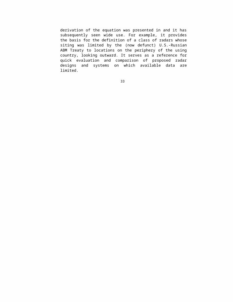
Substituting (2.13) into (2.8), we obtain the search-fence equation:

Pav A

4 Am Rm3 nsc v z kTs D0

1Ls W m2 (2.14)

Note that the power-aperture product depends on thecube, rather than the fourth power of range, becausetargets at longer range have smaller elevation rates,al-lowing larger frame times.

2.5.2 Example ICBM Fence

For example, assume an ICBM search fence for theconditions shown in Table 2.6. The target for this caseis an ICBM launched from a site 2,600 km from theradar, which is deployed halfway between the defendedarea and the launch site.

Table 2.6 ICBM Search FenceAzimuth sector Am deg 90 Maximum range Rm km 2,000

Number of scans nsc 2Elevation beamwidthe deg 2.0

System noise temperature Ts K 400

Detectability factor D0(1) dB 15

Search loss Ls dB 15Target cross section m2 1

Target vertical velocity vz km/s 3.9

At the end of its boost phase, the ICBM is 600 kmdownrange with 250 km altitude and a velocity vt = 7km/s directed 16 above the horizontal at that point,2,000 km from the radar. The tangent plane at the radaris tilted by some 18 from the horizontal at thetarget. The elevation angle of the velocity vector fromthe radar plane is 34, and the vertical velocitycomponent is 3.9 km/s, resulting in an elevation ratee = 0.11/s. Assuming the two scans must be obtainedduring the passage of the target through the scansector, the time per scan is ts = 9s. The re-quiredpower-aperture product from (2.14) is

Pav A 47 106 W m2

If the early warning radar operates at 450 MHz ( =0.67m) with a circular re-flector antenna, its diameterDa = 23m, and its area A = 412m2. The resulting aver-age power requirement is Pav = 114 kW. If subsequenttracking tasks are assigned to the same radar, therequired power is increased.


2.6 SEARCH LOSSES

The apparent simplicity of the search radar equation isthe result of the many as-sumptions imposed on theidealized system. This approach leads, however, to therequirement that the system loss factor Ls accommodatemany nonideal factors that characterize actual radarsystems and environmental conditions.

In Chapter 1, separate factors are included in therange equation for reduc-tions in available energyratio at the antenna output and increases in requireden-ergy ratio for the specified detection performance.The search loss factor Ls in-cludes both sets offactors, along with others that are unique to thesearch radar equation. The losses, includingreciprocals of the range-dependent factors F 2

rdr, aresummarized here.

2.6.1 Reduction in Available Energy Ratio

Components of Ls that reduce the available energy ratio are as follows: Elevation Beamshape Loss Lpe. This loss results fromobtaining the coverage to range Rm up to elevationangle 1 using a fan beam rather than the idealizedsquare-ended triangular beam (see Section 2.2.2).

Pattern Loss Lcsc. The loss results from extendingelevation coverage above 1 at ranges R < Rm. (seeSection 2.2.3).

Antenna Dissipative Loss La. This loss adjusts theidealized antenna gains used in (2.3) and (2.6),which are actually the directivities Dt and Dr of theantennas, to the actual power gains Gt. and Gr (seeSection 10.1.5).

Pattern Constant Ln. This loss adjusts the gain-beamwidth relationship of the idealized transmitting beam assumed in deriving(2.3) to correspond to the value achievable inactual antennas. Ln = 1.16–1.28 (0.64–1.07 dB)applies to rectangular and elliptical apertures with

illumination varying from uniform to low-sidelobetapers. Reflector and lens antennas typically havean additional loss of 0.6–1.0 dB from spillover and(in reflectors) from blockage (see Sec-tion 10.1.5).

Receiving Aperture Efficiency a. The ideal gain Gr appearingin (2.6) applies to a uniformly illuminated apertureunder ideal conditions, but must be re-duced forfactors that result from tapered illumination,blockage of the path into space, spillover in space-fed antennas, and tolerances in construction thatcause departures from a radiated plane wave (seeSection 10.1.5).

Receiving Noise Loss Lrec. The temperature T0 = 290K is usedto establish the noise spectral density in (2.7). The loss thataccounts for the actual system noise temperature Ts(see Chapter 6) is defined as


Lrec Ts T0 , where Ts is averaged over the search sector.

Transmission Line Loss Lt (see Section 10.1.1). Atmospheric Attenuation L. For use in the search radarequation this loss (see Chapter 7) is calculated by averaging theattenuation over the two-way path to the limits ofthe search sector.3

Polarization Loss Lpol. This loss is the reciprocal of thepolarization factor Fp

2 introduced in (1.23) to describethe reduced received energy resulting from mismatch ofthe received polarization to that of the echo from atarget cross section when illuminated by thetransmitting antenna (see Section 10.1.1).

Range-Dependent Response Loss Lrdr. This loss is thereciprocal of the range-dependent response factorFrdr (see Sections 1.6.2 and 10.1.2).

2.6.2 Increase in Required Energy Ratio

The product kT0D0(1) in (2.8) represents the minimumrequired energy ratio for detection on a steady targetusing a single coherently integrated sample of the re-ceived signal, for an idealized receiving system in aroom-temperature environ-ment. Factors in the radarthat increase the required energy ratio and must be in-cluded in Ls are listed below.

Integration Loss Li (see Section 4.4.3).

Fluctuation Loss Lf (see Section 4.4.5).

Matching Factor M (see Section 10.2.3).

Beamshape Loss Lpe (see Section 2.2.2 and Chapter 5).

Miscellaneous Signal Processing Loss Lx (see Sections 1.3.1and 10.2.5).

Scan Sector Loss Lsector (see Section 10.2.1).

Scan Distribution Loss Ld (see Section 10.1.4).

2.6.3 Summary of Losses

The losses listed in Section 2.6.1 include ten factors(some of them consisting of contributions from severalcomponents), that reduce the available energy ratio.Those can be grouped into a single value L1, as usedpreviously in (1.7) to repre-sent the RF loss in energyratio at the antenna output, as listed in the firstpart of Table 2.7. Four components of Lrdr are listedseparately. A further seven losses

3 Strictly speaking, the fraction of energy 1/L after attenuation isaveraged over the elevation sector, and the attenuation calculatedas the reciprocal of that average.


Table 2.7 Search Loss for Typical Air Surveillance Radar Systems

Loss Component SymbolLoss in dB

2-D System 3-D AESA

Elevation beamshapeloss Lpe 1.8 1.8

Pattern (csc2) loss Lcsc 2.2 2.2Antenna dissipative Lat + Lar 0.8 0.8Pattern constant Ln 1.4 0.4

Antenna efficiency L 1.8 0.9

Receiving noise Lrec 2.7 -0.1

Transmission line Lt 0.8 0.2Atmospheric attenuation L 1.5 1.5

Polarization Lpol 0.0 0.0

Lens Llens 1.0 1.0

STC Lstc 0.0 0.0

Frequency diversity Lfd 0.0 0.0

Eclipsing Lecl 0.0 0.0

Subtotal L1 L1 14.00 8.70

Integration Li 2.0 1.0

Fluctuation Lf 1.5 1.5

Matching factor M 1.0 1.0Azimuth beamshape Lp0 1.3 1.3

Miscellaneous Lx 4.0 3.0

Scan sector Lsector 0.0 1.5

Scan distribution Ld 0.0 0.0

Subtotal L2 L2 9.8 9.3

Total Ls Ls 23.80 18.00

that increase the required energy ratio, listed inSection 2.6.2, can be grouped into a value L2, alsolisted in the table.

Estimates of loss are shown for two typical systems:a mechanically scanning 2-D radar with the constant-altitude coverage shown in Figure 2.1, and an activeelectronically scanned array (AESA) that covers the

same elevation coverage in an azimuth sector 45 frombroadside. No attempt has been made to detail the timebudget for the AESA, and the loss estimates areapproximate for both sys-tems, but the total losses arerealistic for both systems, relative to the resultspre-dicted for a given product of average power Pav andphysical receiving aperture A.


The total search loss is normally in the order of 20dB, reducing the detection range to about one-third ofthat available in a “perfect” radar with the same prod-uct of average power and physical aperture. Themechanically scanned system estimates shown in Table2.7 total almost 24 dB, while the AESA system total is18 dB, in spite of the minimal RF losses within theradar. More accurate evalua-tions are possible onlywhen the radar parameters are defined in much greaterde-tail than is usual in early phases of a radardevelopment or procurement. When considering using thesearch radar equation in a particular application,however, it is possible to use results from a number ofradars that have been developed for similarapplications, and to estimate the minimum Lsmin that canbe expected. Sub-stituting Lsmin in the search radarequation provides a starting point for estimating theminimum size of the radar that will be required. Whenthat process leads to a specific radar design, theapplicable loss components may then be determined torefine the calculation.

References[1] Barlow, E., “Radar System Analysis,” Sperry Gyroscope Company Report

No. 5223-1109, June 1948.

[2] Barton, D. K., Radar System Analysis, Englewood Cliffs, NJ: Prentice-Hall, 1964; Dedham, MA: Artech House, 1976.

[3] Barton, D. K. and H. R. Ward, Handbook of Radar Measurement,Englewood Cliffs, NJ: Pren-tice-Hall, 1969; Dedham, MA: ArtechHouse, 1984.

[4] Rice, S. O., “Mathematical Analysis of Random Noise,” Bell Sys. Tech.J., Vol. 23, No. 3, July 1944, pp. 282–332 and Vol. 24, No. 1,January 1945, pp. 461–556. Reprinted: Selected Papers on Noise andStochastic Processes, (N. Wax, ed.), New York: Dover Publ. 1954.

[5] D. K. Barton, Radar System Analysis and Modeling, Norwood, MA: ArtechHouse, 2005.

[6] Shrader, W. W., “Antenna Considerations for Surveillance RadarSystems,” Proc. 7th IRE East Coast Conf. on Aero. and Navig. Electronics,Baltimore, MD, October 1960.

[7] Barton, D. K., “Maximizing Firm-Track Range on Low-ObservableTargets,” IEEE Int. Conf. Radar-2000, Washington, DC, May 812, 2000,pp. 2429.

[8] IEEE Standard 100, The Authoritative Dictionary of IEEE Standards Terms, 7thed., New York: IEEE Press, 2000.

Radar Equations for Modern Radar 53-76

Documents

Transcript of Radar Equations for Modern Radar 53-76