Stat ComputDOI 10.1007/s11222-014-9541-6

Efficient local updates for undirected graphical models

Francesco Stingo · Giovanni M. Marchetti

Received: 3 March 2014 / Accepted: 30 October 2014© Springer Science+Business Media New York 2014

Abstract We present a new Bayesian approach for undi-rected Gaussian graphical model determination. We providesome graph theory results for local updates that facilitate afast exploration of the graph space. Specifically, we showhow to locally update, after either edge deletion or inclusion,the perfect sequence of cliques and the perfect eliminationorder of the nodes associated to an oriented, directed acyclicversion of a decomposable graph. Building upon the decom-posable graphical models framework, we propose a moreflexible methodology that extends to the class of nondecom-posable graphs. Posterior probabilities of edge inclusion areinterpreted as a natural measure of edge selection uncertainty.When applied to a protein expression data set, the model leadsto fast estimation of the protein interaction network.

Keywords Graphical model determination ·Local updates · Markov chain Monte Carlo ·Mixture priors · Perfect elimination order

1 Introduction

The purpose of this paper is to introduce a new modellingapproach for undirected Gaussian graphical model determi-nation. A full Bayesian approach provides a clear measureof uncertainty on the estimated network structures and has

F. Stingo (B)Department of Biostatistics, The University of TexasMD Anderson Cancer Center, Houston, TX, USAe-mail: fstingo@mdanderson.org

G. M. MarchettiDipartimento di Statistica, Informatica, Applicazioni “G.Parenti”,University of Florence, 50134 Florence, Italye-mail: giovanni.marchetti@disia.unifi.it

been implemented for both decomposable and unrestrictedgraphical models. For decomposable models, efficient sto-chastic search procedures based on hyper-inverse Wishartpriors can be implemented. This approach allows us to explic-itly obtain the marginal likelihoods of the graph, as first notedby Clyde and George (2004). Jones et al. (2005) describedhow to perform Bayesian variable selection for both decom-posable and nondecomposable undirected Gaussian graph-ical models in a high-dimensional setting, underlining thecomputational difficulties for the latter case; see also Rover-ato (2002) and Dobra et al. (2004). Scott and Carvalho (2008)proposed a feature-inclusion stochastic search algorithm thatuses online estimates of edge-inclusion probabilities to guideBayesian model determination in decomposable Gaussiangraphical models. They showed the greater speed and sta-bility of their approach compared with Markov chain MonteCarlo and lasso approaches. However, decomposable mod-els are a small subset of all possible graphs, and it is notalways appropriate to restrict the model space to this sub-class. Exploiting the theoretical properties of the G-Wishartprior shown in Atay-Kayis and Massam (2005), Dobra et al.(2012) proposed efficient Bayesian methods for undirectedGaussian graphical model determination. From a computa-tional standpoint, the main difference between decompos-able and unrestricted Gaussian graphical models is the waythe normalizing constant of the marginal likelihoods is com-puted. For decomposable graphs, it is analytically calculated;whereas similar computations for nondecomposable graphsraise significant numerical challenges. Dobra et al. (2012)proposed approaches that avoid the computation of poste-rior normalizing constants that result in Markov chain MonteCarlo methods for sampling over the joint space of graphs andprecision matrices. This method has been further improvedby Wang and Li (2012) by the implementation of an exchangealgorithm that bypasses the evaluation of prior normalizing

123

Stat Comput

constants in a carefully designed Markov chain Monte Carlosampling scheme.

In this paper we describe a new approach to Bayesianmodel determination in Gaussian graphical models. Themodel we propose allows for greater flexibility in the priorspecification and reduces the computational complexity atthe same time. Our approach builds upon the decompos-able Gaussian graphical model framework. Posterior infer-ence on decomposable Gaussian graphical models has beenmade easier by several graph theory results: Frydenbergand Lauritzen (1989) and Giudici and Green (1999) showedhow to efficiently check, through local computation, whetherdecomposability is preserved when a simple perturbation ofthe graph occurs from adding or removing an edge. Recentadvancements in graph theory for decomposable graphs(Ibarra 2008; Green and Thomas 2013) have led to the con-struction of efficient samplers that directly target the junctiontrees associated with the decomposable graph. We assess theperformance of our proposed model on simulated data andthen investigate its application to the analysis of a proteinco-expression network.

2 Basic concepts on graphical models

2.1 Gaussian graphical models

A Gaussian undirected graph model is a family of multivari-ate normal distributions for p variables X = (X1, . . . , X p)

T

∼ Np(0, �) with zero mean, positive definite covariancematrix �, defined by a set of zero restrictions ωi j = 0 on theelements of concentration matrix Ω = �−1 = (ωi j ). Eachrestriction ωi j = 0 is equivalent to a conditional indepen-dence of Xi and X j given the remaining variables, writtenas X j ⊥⊥ X j | XV \i j . This model, introduced by Dempster(1972) with the name of covariance selection model, is char-acterized by an undirected graph G = (V, E), with a setV = {1, . . . , p} of nodes associated with the variables, anda set of edges E = {{i, j}:ωi j �= 0} such that the missingedges in the graph represent the assumed conditional inde-pendences between pairs of variables.

If a random sample of n iid observations X (1), . . . , X (n)

from Np(0,Ω) is available, the likelihood function is

L(Ω|S) ∝ (det Ω)n/2 exp

{−1

2tr(ΩS)

}, (1)

where Ω belongs to the cone PG of positive definite p × pmatrices such that ωi j = 0 whenever {i, j} �∈ E}, andS = ∑n

t=1 X (t)(X (t))T is the sample sum-of-products matrix.The parameter space PG has a complex structure but in thespecial situation of decomposable graphs explained belowin Sect. 2.2 it can be simplified considerably using an alter-native parameterization based on the triangular decomposi-tion of Ω . In general, given any positive definite matrix Ω ,

there exists a unique triangular decomposition (see Wermuth1980),

Ω = (I − Γ )TΔ−1(I − Γ ), (2)

where Γ = (γi j ) is an upper triangular matrix and Δ is adiagonal matrix with positive diagonal entries δi i . The para-meters γi j = βi j. j+1,...,p with i < j are linear regressioncoefficients of Xi on X j conditionally on X j+1, . . . , X p,and δi i = σi i.i+1,...p are the conditional variances of Xi

given Xi+1, . . . , X p. Then, (Γ,�) is a smooth reparame-trization of Ω dependent on the specific ordering of thevariables, but with variation independent components; seeRoverato (2000). This riparametrization is advantageous fordecomposable graphical models because in this case, if thevariables are suitably ordered as explained below, the zerorestrictions on the concentrations are exactly equivalent tothe corresponding restrictions on the regression coefficientsωi j = 0 ⇐⇒ γi j = 0. Therefore, given the upper triangu-lar structure of the matrix Γ , the joint density of a Gaussiandecomposable graph model can be factorized into a sequenceof univariate regressions.

2.2 Decomposable graphs and junction trees

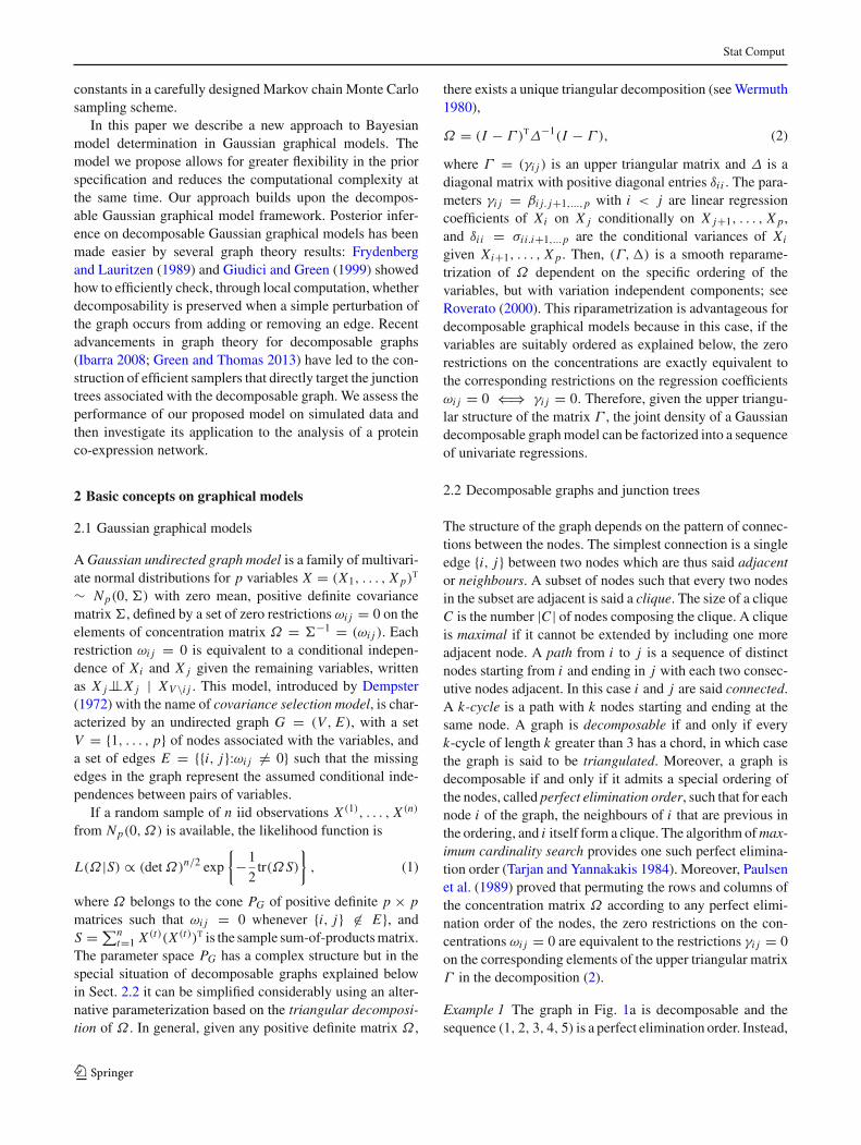
The structure of the graph depends on the pattern of connec-tions between the nodes. The simplest connection is a singleedge {i, j} between two nodes which are thus said adjacentor neighbours. A subset of nodes such that every two nodesin the subset are adjacent is said a clique. The size of a cliqueC is the number |C | of nodes composing the clique. A cliqueis maximal if it cannot be extended by including one moreadjacent node. A path from i to j is a sequence of distinctnodes starting from i and ending in j with each two consec-utive nodes adjacent. In this case i and j are said connected.A k-cycle is a path with k nodes starting and ending at thesame node. A graph is decomposable if and only if everyk-cycle of length k greater than 3 has a chord, in which casethe graph is said to be triangulated. Moreover, a graph isdecomposable if and only if it admits a special ordering ofthe nodes, called perfect elimination order, such that for eachnode i of the graph, the neighbours of i that are previous inthe ordering, and i itself form a clique. The algorithm of max-imum cardinality search provides one such perfect elimina-tion order (Tarjan and Yannakakis 1984). Moreover, Paulsenet al. (1989) proved that permuting the rows and columns ofthe concentration matrix Ω according to any perfect elimi-nation order of the nodes, the zero restrictions on the con-centrations ωi j = 0 are equivalent to the restrictions γi j = 0on the corresponding elements of the upper triangular matrixΓ in the decomposition (2).

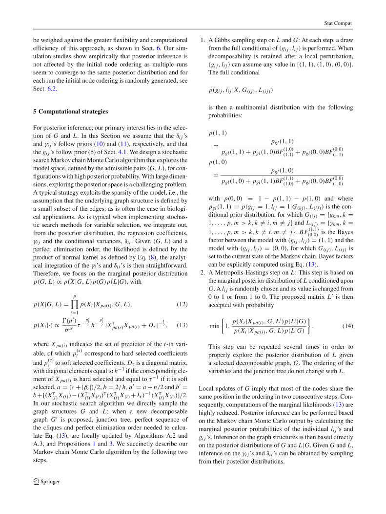
Example 1 The graph in Fig. 1a is decomposable and thesequence (1, 2, 3, 4, 5) is a perfect elimination order. Instead,

123

Stat Comput

(2, 3, 1, 4, 5) is not because 1 and its neighbours 2, 3 thatprecede 1 in the sequence do not form a clique. Thus, theGaussian graphical model can be parametrized by Ω andthe restrictions ω23 = ω24 = ω34 = 0 and ωi5 = 0 fori = 1, . . . , 4 or equivalently by a set of recursive regressions

X1 = γ12 X2 + γ13 X3 + γ14 X4 + ε1

Xi = εi , i = 2, . . . , 5, with ε = (εi ) ∼ N5(0,�).

Thus the essential prerequisites to get an equivalent regres-sion parameterization of a Gaussian graphical model are that(a) the graph is decomposable and (b) that the concentrationmatrix is permuted according to a perfect elimination order.Every decomposable graph has a junction tree representa-tion. A junction tree is a connected graph whose nodes are themaximal cliques of the decomposable graph, with no cycles,and with the so-called running intersection property meaningthat given any two maximal cliques C and K and consideringtheir common nodes C ∩ K , then all the cliques along theunique path between C and K must contain C ∩ K . Oftenhereafter we use the term clique of a junction tree to mean amaximal clique of the decomposable graph. The edges of thejunction tree are labeled by the intersections of the adjacentcliques at the endpoints, called the separators. The edges eof a junction tree have attached a weight w(e) equal to thesize |C ∩ K | of the separator. A graph is decomposable ifand only if it can be represented by a junction tree. This rep-resentation is not unique: see Thomas and Green (2009) foralgorithms to find equivalence classes of junction trees. Bylisting the nodes in a perfect elimination order we visit thecliques of the junction tree consecutively. On the other handone can always reconstruct a perfect elimination order froma junction tree as follows: define with no loss of generalityany clique, say C1, as a root of the junction tree and thendefine a partial order C K between cliques C and K if andonly if the unique path from the root C1 to K intercepts C .Any sequence (C1, . . . , Ck) of the cliques that respects thispartial order is said to be a perfect sequence of the cliques.From the perfect sequence of cliques, the perfect elimina-tion order of the nodes is obtained by first taking the nodesin C1 in any order, then the nodes in C2\C1 in any order,then those in C3\(C1 ∪ C2) and so on, until all the variablesare selected, and finally by reversing the obtained sequence.Notice that while here perfect sequences of cliques are gener-ated from a junction tree, they can be defined independently;see Lauritzen (1996).

Example 2 One possible junction tree associated with thedecomposable graph of Fig. 1a is shown in Fig. 1b. Thecliques are shown as ovals and the separators as rectangles.The original graph is disconnected and thus the separatorbetween cliques {1, 3} and {5} is the empty set. As the vari-able 1 is common to the cliques C = {1, 2} and K = {1, 4},then by the running intersection property any clique on the

2 4

3

1 5

12 1 13 1 14

5

(b)(a)

Fig. 1 a An undirected graph in five nodes. b One possible associatedjunction tree

path between C and K contains variable 1. Taking as root ofthe junction tree C1 = {5}, a perfect sequence of cliques isC1, C2 = {1, 5}, C3 = {1, 3}, C4 = {1, 2}, from which weget the sequence (5, 4, 3, 2, 1) that reversed gives the perfectelimination order (1, 2, 3, 4, 5).

2.3 Graphical model determination and single edgeperturbations of the graph

Bayesian graphical model determination is commonly per-formed by running a Markov chain whose states have theform of a graph G = (gi j ) and a vector of parameters (in ourcase, γ,�), with gi j = 1 if edge {i, j} is part of graph G,and gi j = 0 otherwise. The computational strategy is oftenbased on sequential random choices of pairs of distinct nodes;if they are currently connected, the algorithm proposes theedge removal, otherwise it proposes an edge addition. If thesearch is limited to the space of decomposable graphs, then,the junction tree representation of the graph permits a fastcheck that the edge perturbation is legal, i.e., yields a graphG ′ that is still decomposable. Given an edge e = {a, b} anda junction tree J of G, the verification is based on the twofollowing results.

(i) G ′ = G − e is decomposable if and only if there isa unique maximal clique C∗ containing both a and b;see Grone et al. (1984) and Frydenberg and Lauritzen(1989).

(ii) G ′ = G + e is decomposable if and only if a is con-tained in a maximal clique Ca and b is contained in amaximal clique Cb adjacent in the junction tree J or inan equivalent junction tree T ; Giudici and Green (1999).

Checking condition (i) is straightforward. Checking (ii) ismore involved and requires information about the junctiontree J . The following algorithm (Ibarra 2008) is availableand used in our procedure.

A.1 Verify whether adding edge {a, b} is legal.

(1) Find the closest cliques Ca and Cb in J such that a ∈ Ca

and b ∈ Cb.(2) If they are adjacent in J , accept the edge addition and

return the junction tree T = J .

123

Stat Comput

C1

Ca

Ce2

CbCR

Cd

CL

Ct

e

C1

Ca

Ce2

CbCR

Ct

CL

Cd

TJ

Fig. 2 Left a junction tree J with root clique C1. The minimum weightedge on the unique path between Ca and Cb is denoted by e. Right Theequivalent directed junction tree T obtained after removing e and addingan edge between Ca and Cb. The path from the endpoint Cb to Ce2 isinverted

(3) Otherwise, find the edge u with minimum-weight edgew(u) on the path between Ca and Cb in J and if w(u) =|Ca ∩ Cb|, then accept the edge {a, b} and return thejunction tree T = J − u + {Ca, Cb}. Otherwise, rejectthe edge {a, b}.

The condition of step 3 is in fact necessary and sufficientfor the existence of a junction tree T equivalent to J , withadjacent cliques Ca and Cb. An example of a junction treeupdate, as described in step 3, is given in Fig. 2.

After a proposal is accepted, a new graph G ′ is obtainedand the appropriate changes to the parameters (Γ,�) of themodel must be carried out. Therefore the information aboutthe the perfect elimination order has to be updated. Thiscan be done globally, by running (for example) the max-imum cardinality search algorithm after each move. How-ever, this strategy is inefficient because significant gains canbe achieved by local updates.

In this paper, building upon results from Ibarra (2008),we show that an updated perfect elimination order can beobtained by fast local updates of the perfect sequence ofcliques and a parallel local update of the junction tree. Ina recent paper by Green and Thomas (2013, Fig. 3) localupdates are proposed as well. However, while both Ibarra

GG ′

f e d

g a b c

f e d

g a b c

JJ ′

ag abe

aef bde

bc ag

aef bde

bc

Fig. 3 Left a decomposable graph G and below, an associated junctiontree. Right the decomposable graph G ′ obtained by removing the edge{a, b} and below, the associated junction tree

(2008) and Green and Thomas (2013) are interested in localupdates of the junction tree, our focus are local updates ofthe perfect elimination order. This order affects the likelihoodin the parametrization based on recursive regression and isthe central object in our approach. In spite of the similarities,the algorithms to update the perfect elimination order requiresome results that are summarized in the following Sect. 3 andproved in the appendix. These results have some interest intheir own because, to our knowledge, there are no dynamicalgorithms for directly updating the perfect elimination orderafter an edge perturbation.

In the algorithms of next section the following two results(Ibarra 2008) are used to update the clique set after a pertur-bation.

(a) After edge removal: C∗ in (i) may be split in two cliquesCa = C∗\{b} and Cb = C∗\{a}. Moreover, Ca is amaximal clique in G ′ if and only if there are no maximalcliques C adjacent to C∗ in the junction tree J , contain-ing a and such that C ∩ C∗ = Ca . A similar conditionholds for Cb.

(b) After edge insertion: C∗ = (Ca ∩ Cb) ∪ {a, b} is a newmaximal clique in G ′ = G + {a, b}. Moreover, Ca is amaximal clique in G ′ if and only if |Ca | > |Ca ∩Cb|+1.A similar condition holds for Cb.

3 Dynamic update of the perfect sequence of cliques

Let G be a decomposable graph with junction tree J andlet (C1, . . . , C j , . . . , Ck) be a perfect sequence of the max-imal cliques of G. Recall that from this sequence a perfectelimination order follows straightforwardly as explained inthe previous section. In this section we give the details onthe local updates of the perfect order of the maximal cliques,after edge removal or edge addition. We shall prove that thelocal updates are possible directly from the perfect sequenceof the cliques, once it is checked that the move is legal. Asthe check requires the junction tree, the junction tree itselfmust be updated and we shall see that this can be done locally,without recalculating the full junction tree that would requirethe global maximum cardinality search algorithm.

3.1 Local updates after edge removal

From the result of Sect. 2.3(a) after removing the edge e ={a, b} the maximal clique C∗ is split in two cliques Ca and Cb.Then, according to Lauritzen (1996, Lemma 2.20) a perfectsequence of cliques for G ′ is obtained by first choosing a asthe endpoint of e that comes first in the perfect numberingof the nodes, and then replacing C∗ in the sequence withthe two sets Ca and Cb. However, this simple rule is notenough to achieve a perfect ordering of the maximal cliques

123

Stat Comput

of G ′ because, in general, Ca or Cb can lose the property ofmaximality.

Example 3 Consider the decomposable graph G in Fig. 3and its junction tree J , and let (ag, abe, bde, bc, ae f ) bea perfect ordering of the cliques. After removing the edge{a, b}, we find the new decomposable graph G ′, the two sub-sets Ca = {a, e} and Cb = {b, e} and the perfect sequence ofcliques (ag, ae, be, bde, bc, ae f ). However, looking at theupdated junction tree J ′, we see that a perfect sequence of(maximal) cliques is (ag, ae f, bde, bc).

Following Lauritzen (1996), hereafter we assume that ais the endpoint of e that comes first in the perfect number-ing of the nodes. Then, let S = (C1, . . . , Ca, Cb, . . . , Ck)

be the perfect sequence of sets before the edge is removed.The updated perfect sequence of cliques, is obtained by thefunction Update(S, Ca) returning⎧⎪⎨⎪⎩

S if Ca is a maximal clique in G

S\Ca if there is a C Ca : Ca ⊆ C

S with Ca replaced by C if there is a C � Ca : Ca ⊆ C.

Moreover, we denote the updating of S with respect to Ca andCb by Update(S, Ca, Cb). Then the following propositionproved in the Appendix holds.

Proposition 1 Given a perfect sequence of sets (C1, . . . ,

C∗, . . . , Ck) of the cliques of the decomposable graph G,where C∗ is the unique clique containing an edge {a, b},then a perfect sequence S ′ of the cliques of the graphG ′ = G − {a, b} is obtained by

S ′ = Update(S, Ca, Cb), (3)

where S = (C1, . . . , Ca, Cb, . . . , Ck) is obtained by replac-ing C∗ with Ca, Cb.

The proof in of Proposition 1 in the Appendix is based onthe three sets

Na ={C ∈ ne(C∗) | a ∈ C}, Nb ={C ∈ ne(C∗) | b ∈ C},N ab ={C ∈ ne(C∗) | a, b /∈ C}. (4)

The three subsets are clearly a partition of the neighbours ofC∗ in J ; see also Ibarra (2008). The proof of the Propositionimplies as a by-product the following algorithm to locallyupdate J into a new junction tree J ′.

A.2. Local junction tree update after edge removal

(1) Modify J by replacing node C∗ by Ca and Cb and addan edge {Ca, Cb}.

(2) For each clique C ∈ Na , replace the edge {C, C∗} withan edge {C, Ca}. For each clique C ∈ Nb, replace theedge {C, C∗} with an edge {C, Cb}. For each clique N ab,

replace the edge {C, C∗} with {C, Ca} or {C, Cb}, choos-ing arbitrarily. The resulting tree has the running inter-section property.

(3) If Ca and Cb are both maximal in G ′, return the previoustree as J ′.Else if Ca is not maximal, for C ∈ Na if Ca ⊂ C thencontract {Ca, C} and replace Ca with C .Else if Cb is not maximal, for C ∈ Nb if Cb ⊂ C thencontract {Cb, C} and replace Cb with C .Return the resulting tree as the updated junction tree J ′.

3.2 Local updates after edge addition

Let e = {a, b} be the new edge to be added. If the edgeaddition is legal, we have two cases:

(1) either J has the property (ii) of Sect. 2., i.e., the twocliques Ca and Cb containing the endpoints of e areadjacent in J ,

(2) or J has been transformed into an equivalent junctiontree T with that property, by algorithm A.1.

In case (1), the perfect sequence of cliques (C1, . . . , Ca, . . . ,

Cb, . . . , Ck) can always be rearranged to have Cb rightafter Ca , thus obtaining an equivalent perfect sequence(C1, . . . , Ca, Cb, . . . , Ck). Then there is a simple rule forlocal updates of this rearranged perfect sequence of cliques.

Proposition 2 If (C1, . . . , Ca, Cb, . . . , Ck) is a perfectsequence of cliques of G, and if the two cliques, Ca andCb such that a ∈ Ca and b ∈ Cb, are adjacent in J and aprecedes b in the node ordering, then a perfect ordering ofcliques of G ′ = G + {a, b} is obtained from

(C1, . . . , Ca, C∗, Cb, . . . , Ck), (5)

with C∗ = (Ca ∩ Cb) ∪ {a, b}, after removing Ca and Cb

from the sequence if they are subsets of C∗.

The proof of Proposition 2 is in the Appendix. The associatedalgorithm to update the junction tree is the following.

A.3 Local junction tree update after edge addition

(1) Modify J by including the new maximal clique C∗ =(Ca ∩ Cb) ∪ {a, b}, removing the edge {Ca, Cb} andadding the new edges {Ca, C∗} and {C∗, Cb}, each withweight |Ca ∩ Cb| + 1.

(2) If both Ca and Cb are maximal cliques, return the pre-vious updated tree as J ′. Else If Ca is not maximal inG ′, remove the node Ca from J ′ and contract the edge{Ca, C∗}.Else if Cb is not a maximal in G ′, remove the node Cb

from J ′ and contract the edge {Cb, C∗}.

123

Stat Comput

In case (2), the junction tree has been modified (locally) byalgorithm A.1 and thus in order to use Proposition 2 theoriginal perfect sequence of cliques of J must be modifiedas well. Proposition 3 describes the transformation. First,we define Ca and Cb as follows. Let e = {Ce1, Ce2} bethe minimum-weight edge of algorithm A.1, with the cliqueCe1 preceding Ce2 in the perfect sequence. Let d(x, y) bethe number of nodes on the path between two cliques xand y in the junction tree J . Let C ′

a = Ca, C ′b = Cb if

d(Ca, Ce1) < d(Ca, Ce2), and C ′a = Cb, C ′

b = Ca other-wise.

Proposition 3 Given a perfect sequence of the cliques of G

(C1, . . . , Ca, . . . , Cb, . . . , Ck), (6)

a perfect sequence of the cliques after the transformation ofJ into T of Algorithm A.1 is

(CL , C ′a, C ′

b, Ct , Cd , CR), (7)

where the clique sets, if not empty, are defined as

CL is the sequence of all the cliques preceding C ′a and

excluding the cliques in Ce2 ∪ de(Ce2), where de(Ce2)

denotes the set of descendants of Ce2 ;Ct is the sequence of the cliques on the path from C ′

b to Ce2

following a reverse order with respect to sequence (6);Cd is the sequence of all the descendants of Ct and of C ′

b,ordered as in (6); andCR is the sequence of all the cliques that follow C ′

a,excluding the cliques in Ce2 ∪ de(Ce2).

The proof of Proposition 3 is in the Appendix. As a last step,the perfect sequence of the cliques is updated sequentiallyby applying Propositions 3 and 2.

3.3 Numerical experiments

In this simulation, we illustrate the computational effi-ciency of the local updates approach, described in Sect.3, in comparison to the maximum cardinality search algo-rithm. Specifically, we compare the computational efficiencyof the the Matlab function maxCardinalitySearch witha Matlab implementation of our local updates approach.maxCardinalitySearch, from the PMTK3 toolkit, can beconsidered one of computational most efficient imple-mentations of the maximum cardinality search algorithm.Note that our local updates yield an update of junctiontree, perfect sequence of the cliques and perfect elimi-nation order whereas maxCardinalitySearch returns themaximal cliques of the graph, in an order that satisfiesrunning intersection property, but does not provide ajunction tree representation of the graph. We randomlygenerated 10,000 decomposable graphs with p nodes by

100 200 300 400 500

05

1015

2025

3035

Number of nodes

time(

MC

S)/

time(

loca

l)

Fig. 4 Local versus global updates: computational efficiency as a func-tion of the number of nodes in the graph

adding/deleting one edge to/from the decomposable graphgenerated at the previous step. We repeated this experimentfor p = 20, 50, 100, 200, 300, 400, 500. For each decom-posable graph we derived junction tree, perfect sequenceof the cliques and perfect elimination order via our localupdates and a perfect elimination order via the maxCar-dinalitySearch function. Figure 4 compares the computa-tional efficiency of the aforementioned approaches as a func-tion of the number of nodes in the graph. Specifically, they-axis represents the ratio between the total time neededby the MCS algorithm to perform all the proposed updatesand the time needed by our approach to perform the sametasks (time(MCS)/time(local)). Clearly, the loss of compu-tational efficiency of the maximum cardinality search algo-rithm respect to our approach follows an exponential trendand highlights the computational advantages of the pro-posed method when local moves in the graph space areperformed.

4 Bayesian model

4.1 A Bayesian approach for decomposable graphs

We define a probabilistic framework for undirected graphmodels based on p random variables, X = (X1, . . . , X p)

T,where p can be possibly larger than the sample size n undera Gaussian model, with X ∼ N (0,Ω−1) and a decompos-able structure of zero restrictions on Ω . In Sect. 4.2, weextend our methodology to nondecomposable graph struc-tures. As shown in Sect. 2.1, a decomposable Gaussian graph-ical model is equivalent to a system of linear regression equa-tions where each regression coefficient βi j. j+1,...,p coincideswith an element γi j of the upper triangular matrix Γ , andwhere the variable ordering is derived by the perfect elimi-

123

Stat Comput

nation scheme of the nodes of the graph. Given a decompos-able graph G, the likelihood (1) is a function of the regressioncoefficients γi j and the conditional variances δi i , and can bedefined as the product of the pdf of p random variables

Xi =p∑

j=1

γi j X j + ε j , ε j ∼ N (0, δi i ), i = 1, . . . , p,

(8)

where the γi j ’s are non-zero if {i, j} is part of graph G andif node j precedes node i in the perfect elimination order.We use X pa(i) to indicate the set of predictor of the i-thvariable in Eq. (8). The reparameterization of decompos-able Gaussian graphical models as a system of linear regres-sions brings several advantages. The regression coefficientsare variation independent; whereas the elements of the con-centration matrix Ω are not. Priors on Ω have to be definedon a subset of the cone of the positive definite matrices PG

defined by G, such as the G-Wishart distributions; whereasthe parameter space of Γ is R

|E |. Alternative approachesto the G-Wishart distribution, like the Bayesian graphicallasso (Wang 2012) or similar priors marginally defined onthe elements of the precision matrix, have substantial com-putational disadvantages since the positive definiteness of Ω

has to be checked at each step of the optimization/samplingalgorithm. From standard distribution theory, the distribu-tions of γi j and δi i are functions of the elements of theconcentration matrix Ω; see Dawid and Lauritzen (1993)and Dobra et al. (2004), among others. An inverse Wishartprior on � ∼ Inv-Wishart(c, h−1 I ), with I being an identitymatrix of the same dimension of �, implies that

γi j ∼ N (0, h δi i ) (9)

δi i ∼ Inv-Ga((c + |βi |)/2, 2h), (10)

where |βi | is the number of covariates in equation i , and hand c are hyperparamters to be set to a fixed value. Withinour model framework we can specify any prior distributionp(G) on the graph space. Among the most commonly usedover the set of decomposable graphs, we can mention

(a) the uniform prior p(G) ∝ 1;(b) the prior that assumes the edge inclusion probability to

be all equal to p1 ∈ (0, 1); and(c) the prior by Armstrong et al. (2009), which gives equal

probability to the size, defined as the number of selectededges, of the graph and equal probability to graphs ofeach size.

Prior (a) gives more probability to graphs of a medium sizeand can be seen as a special case of prior (b), with p1 = 0.5;whereas smaller values of p1 favour sparse graphs. Prior (c)can be used when there is strong prior information about theexpected size of the graph. All the described priors have to

be normalized since every nondecomposable graph has zeroprobability.

4.2 An approximate approach for nondecomposable graphs

In this section, we propose a probabilistic framework thatgeneralizes the modeling approach proposed in Sect. 4.1 inorder to learn the structure of nondecomposable Gaussiangraphical models. We introduce a p × p symmetric binarymatrix L that induces a double selection prior for the soft andhard selection of edges. An edge is said to be hard selectedif it is both part of the edge set G and li j = 1; whereas anedge is soft selected if gi j = 1 and li j = 0. The matrixL can assume any value on the model space of the unre-stricted graphs with p nodes, as as long as this graph is a sub-graph of G. The graph space can be then defined by all pairs(G, L) such that G is an adjacency matrix of a decomposablegraph and L is an adjacency matrix of a (unrestricted) sub-graph of G. Following the approach of George and McCul-loch (1993), we introduce a soft/hard selection prior definedas a two-component mixture distribution on the regressioncoefficients

(γi j |gi j = 1, li j ) ∼ li j N (0, hδi i ) + (1 − li j )N (0, τδi i ),

(11)

with τ set to a very small value, such that the first componentin the mixture puts most of its mass on values close to zero(George and McCulloch 1993), and h being a hyperparameterto be specified. This approach encourages the soft selectionof decomposable graphs that contain both edges supported bythe data and an additional set of edges that makes the graphdecomposable. Edges supported by the data are identifiedthrough the mixture prior (11). The model specification iscompleted by using conjugate inverse-Gamma priors on theδi i ’s and by using independent Bernoulli (p2) priors on theli j ’s, with p2 being the prior probability of labeling {i, j} asan hard edge, given {i, j} ∈ G; p2 can be set to a value thatfavors sparse graphs.

As introduced in Sect. 2.1, from a decomposable graphwe can usually derive more than one perfect eliminationorder. Each perfect elimination order explicitly defines adirected acyclic graph (DAG); prior distributions (9)–(10)fall in the invariant class characterized by Geiger and Heck-erman (2002), implying that two independence-equivalentDAGs, i.e. two DAGs defined by two alternative perfect elim-ination orders of the same undirected graph, are assigned thesame marginal likelihood, see also Andersson et al. (1997).However prior (11), unless all li j = 1, does not fall in thisinvariant class, and then two independence-equivalent DAGsmay not be assigned the same marginal likelihood. This isan undesired property of prior (11), and we then considerour approach approximate; however, this deficiency must

123

Stat Comput

be weighed against the greater flexibility and computationalefficiency of this approach, as shown in Sect. 6. Our sim-ulation studies show empirically that posterior inference isnot affected by the initial node ordering as multiple runsseem to converge to the same posterior distribution and foreach run the initial node ordering is randomly generated, seeSect. 6.2.

5 Computational strategies

For posterior inference, our primary interest lies in the selec-tion of G and L . In this Section we assume that the δi j ’sand γi j ’s follow priors (10) and (11), respectively, and thatthe gi j ’s follow prior (b) of Sect. 4.1. We design a stochasticsearch Markov chain Monte Carlo algorithm that explores themodel space, defined by the admissible pairs (G, L), for con-figurations with high posterior probability. With large dimen-sions, exploring the posterior space is a challenging problem.A typical strategy exploits the sparsity of the model, i.e., theassumption that the underlying graph structure is defined bya small subset of the edges, as is often the case in biologi-cal applications. As is typical when implementing stochas-tic search methods for variable selection, we integrate out,from the posterior distribution, the regression coefficients,γi j and the conditional variances, δi i . Given (G, L) and aperfect elimination order, the likelihood is defined by theproduct of normal kernel as defined by Eq. (8), the analyt-ical integration of the γi ’s and δi i ’s is then straightforward.Therefore, we focus on the marginal posterior distributionp(G, L) ∝ p(X |G, L)p(G)p(L|G), with

p(X |G, L) =p∏

i=1

p(Xi |X pa(i), G, L), (12)

p(Xi |·) ∝ �(a′)b′a′ τ− pc

i2 h− ps

i2 |X T

pa(i) X pa(i) + Dτ |− 12 , (13)

where X pa(i) indicates the set of predictor of the i-th vari-

able, of which p(s)i correspond to hard selected coefficients

and p(c)i to soft selected coefficients. Dτ is a diagonal matrix,

with diagonal elements equal to h−1 if the corresponding ele-ment of X pa(i) is hard selected and equal to τ−1 if it is softselected, a = (c + |βi |)/2, b = 2/h, a′ = a + n/2 and b′ =b+[(X T

(i) X(i))−(X T(i) X(i))

T(X T(i) X(i) + Iτ )−1(X T

(i) X(i))]/2.In our stochastic search algorithm we directly sample thegraph structures G and L; when a new decomposablegraph G ′ is proposed, junction tree, perfect sequence ofthe cliques and perfect elimination order needed to calcu-late Eq. (13), are locally updated by Algorithms A.2 andA.3, and Propositions 1 and 3. We succinctly describe ourMarkov chain Monte Carlo algorithm by the following twosteps.

1. A Gibbs sampling step on L and G: At each step, a drawfrom the full conditional of (gi j , li j ) is performed. Whendecomposability is retained after a local perturbation,(gi j , li j ) can assume any value in {(1, 1), (1, 0), (0, 0)}.The full conditional

p(gi j , li j |X, G(i j), L(i j))

is then a multinomial distribution with the followingprobabilities:

p(1, 1)

= pgl(1, 1)

pgl(1, 1) + pgl(1, 0)BF(1,0)(1,1) + pgl(0, 0)BF(0,0)

(1,1)

p(1, 0)

= pgl(1, 0)

pgl(1, 0) + pgl(1, 1)BF(1,1)(1,0) + pgl(0, 0)BF(0,0)

(1,0)

with p(0, 0) = 1 − p(1, 1) − p(1, 0) and wherepgl(1, 1) ≡ p(gi j = 1, li j = 1|G(k j), L(i j)) is the con-ditional prior distribution, for which G(i j) = {gkm, k =1, . . . , p, m > k, k �= i, m �= j} and L(i j) = {γkm, k =1, . . . , p, m > k, k �= i, m �= j}. B F (1,1)

(0,0) is the Bayesfactor between the model with (gi j , li j ) = (1, 1) and themodel with (gi j , li j ) = (0, 0), for which G(i j), L(i j) isset to the current state of the Markov chain. Bayes factorscan be explicitly computed using Eq. (13).

2. A Metropolis-Hastings step on L: This step is based onthe marginal posterior distribution of L conditioned uponG. A li j is randomly chosen and its value is changed from0 to 1 or from 1 to 0. The proposed matrix L ′ is thenaccepted with probability

min

{1,

p(Xi |X pa(i), G, L ′)p(L ′|G)

p(Xi |X pa(i), G, L)p(L|G)

}. (14)

This step can be repeated several times in order toproperly explore the posterior distribution of L givena selected decomposable graph, G. The ordering of thevariables and the junction tree do not change with L .

Local updates of G imply that most of the nodes share thesame position in the ordering in two consecutive steps. Con-sequently, computations of the marginal likelihoods (13) arehighly reduced. Posterior inference can be performed basedon the Markov chain Monte Carlo output by calculating themarginal posterior probabilities of the individual li j ’s andgi j ’s. Inference on the graph structures is then based directlyon the posterior distributions of G and L|G. Given G and L ,inference on the γi j ’s and δi i ’s can be obtained by samplingfrom their posterior distributions.

123

Stat Comput

6 Applications

6.1 Simulation studies: first scenario

We investigated the performance of our model using sim-ulated data and scenarios that mimic the characteristics ofthe real data that motivated the development of the model.We focused on situations where most of the edges are miss-ing and tested the ability of our method to discover rel-evant edges in the presence of a large number of poten-tially false-positive links. The simulation comprised a totalof p = 6, 20, 35, and 50 variables observed for a relativelysmall number of observations, n = 50. With p = 50, thereare 1,225 possible edges. Our goal is to show that the pro-posed methodology is able to efficiently explore the modelspace composed by 2p(p−1)/2 graphs, and select the edgesbest supported by the data. Throughout Sect. 6, we com-pare our approach with the method proposed by Wang andLi (2012), in terms of both network selection and computa-tional time. The methodology and computational strategiesproposed by Wang and Li (2012) build upon the approachproposed by Dobra et al. (2012) and can be considered tobe state of the art in terms of Bayesian approaches to high-dimensional networks. Following Wang and Li (2012), wegenerated n samples from a zero mean normal distributionthat defines a proper distribution over the circular graph withedge set E = {(i, i + 1) : 1 ≤ i ≤ p − 1} ∪ (1, p). We setthe nonzero elements of the precision matrix to wk j = 0.5for |k − j | = 1 and w1p = wp1 = 0.4. The circulargraph is a cordless cycle of length p; hence, we tested ourapproach on a graph that is not close to a decomposableone. To assess uncertainty about our estimation results, weperformed inference for 50 simulated data sets, generatedusing the same procedure as above. We report the resultsobtained by choosing, when possible, hyperparameters that

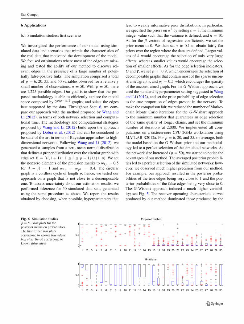
lead to weakly informative prior distributions. In particular,we specified the priors on σ 2 by setting c = 3, the minimuminteger value such that the variance is defined, and h = 10.As for the β vectors of regression coefficients, we set theprior mean to 0. We then set τ to 0.1 to obtain fairly flatpriors over the region where the data are defined. Larger val-ues of h would encourage the selection of only very largeeffects; whereas smaller values would encourage the selec-tion of smaller effects. As for the edge selection indicators,G and γ, we set p1 = 0.9, which encourages the selection ofdecomposable graphs that contain most of the sparse uncon-strained graphs, and p2 = 0.5, which encourages the sparsityof the unconstrained graph. For the G-Wishart approach, weused the standard hyperparameter setting suggested in Wangand Li (2012), and set the prior probability of edge selectionto the true proportion of edges present in the network. Tomake the comparison fair, we reduced the number of Markovchain Monte Carlo iterations for the G-Wishart approachto the minimum number that guarantees an edge selectionof the same quality of longer chains, and set the minimumnumber of iterations at 2,000. We implemented all com-putations on a sixteen-core CPU 2GHz workstation usingMATLAB R2012a. For p = 6, 20, and 35, on average, boththe model based on the G-Wishart prior and our methodol-ogy led to a perfect selection of the simulated networks. Asthe network size increased (p = 50), we started to notice theadvantages of our method. The averaged posterior probabili-ties led to a perfect selection of the simulated networks; how-ever, we observed much higher precision from our method.For example, our approach resulted in the posterior proba-bilities of the true edges being very close to 1 and the pos-terior probabilities of the false edges being very close to 0.The G-Wishart approach induced a much higher variabil-ity; see Fig. 5. The receiver operating characteristic curvesproduced by our method dominated those produced by the

Fig. 5 Simulation studiesp = 50. Box plots for theposterior inclusion probabilities.The first fifteen box plotscorrespond to known true edges;box plots 16–30 correspond toknown false edges

0

0.5

1

1 2 3 4 5 6 7 8 9 10 11 12 13 14 15 16 17 18 19 20 21 22 23 24 25 26 27 28 29 30

Proposed method

0

0.5

1

1 2 3 4 5 6 7 8 9 10 11 12 13 14 15 16 17 18 19 20 21 22 23 24 25 26 27 28 29 30

G−Wishart

123

Stat Comput

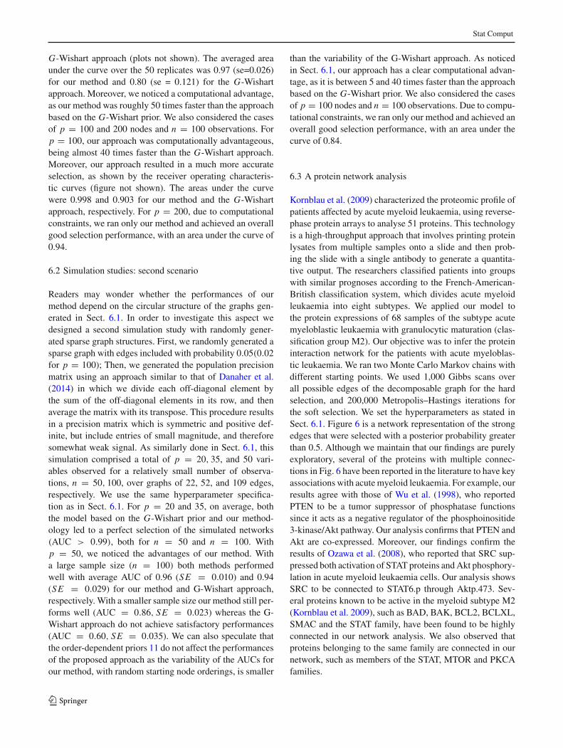
G-Wishart approach (plots not shown). The averaged areaunder the curve over the 50 replicates was 0.97 (se=0.026)for our method and 0.80 (se = 0.121) for the G-Wishartapproach. Moreover, we noticed a computational advantage,as our method was roughly 50 times faster than the approachbased on the G-Wishart prior. We also considered the casesof p = 100 and 200 nodes and n = 100 observations. Forp = 100, our approach was computationally advantageous,being almost 40 times faster than the G-Wishart approach.Moreover, our approach resulted in a much more accurateselection, as shown by the receiver operating characteris-tic curves (figure not shown). The areas under the curvewere 0.998 and 0.903 for our method and the G-Wishartapproach, respectively. For p = 200, due to computationalconstraints, we ran only our method and achieved an overallgood selection performance, with an area under the curve of0.94.

6.2 Simulation studies: second scenario

Readers may wonder whether the performances of ourmethod depend on the circular structure of the graphs gen-erated in Sect. 6.1. In order to investigate this aspect wedesigned a second simulation study with randomly gener-ated sparse graph structures. First, we randomly generated asparse graph with edges included with probability 0.05(0.02for p = 100); Then, we generated the population precisionmatrix using an approach similar to that of Danaher et al.(2014) in which we divide each off-diagonal element bythe sum of the off-diagonal elements in its row, and thenaverage the matrix with its transpose. This procedure resultsin a precision matrix which is symmetric and positive def-inite, but include entries of small magnitude, and thereforesomewhat weak signal. As similarly done in Sect. 6.1, thissimulation comprised a total of p = 20, 35, and 50 vari-ables observed for a relatively small number of observa-tions, n = 50, 100, over graphs of 22, 52, and 109 edges,respectively. We use the same hyperparameter specifica-tion as in Sect. 6.1. For p = 20 and 35, on average, boththe model based on the G-Wishart prior and our method-ology led to a perfect selection of the simulated networks(AUC > 0.99), both for n = 50 and n = 100. Withp = 50, we noticed the advantages of our method. Witha large sample size (n = 100) both methods performedwell with average AUC of 0.96 (SE = 0.010) and 0.94(SE = 0.029) for our method and G-Wishart approach,respectively. With a smaller sample size our method still per-forms well (AUC = 0.86, SE = 0.023) whereas the G-Wishart approach do not achieve satisfactory performances(AUC = 0.60, SE = 0.035). We can also speculate thatthe order-dependent priors 11 do not affect the performancesof the proposed approach as the variability of the AUCs forour method, with random starting node orderings, is smaller

than the variability of the G-Wishart approach. As noticedin Sect. 6.1, our approach has a clear computational advan-tage, as it is between 5 and 40 times faster than the approachbased on the G-Wishart prior. We also considered the casesof p = 100 nodes and n = 100 observations. Due to compu-tational constraints, we ran only our method and achieved anoverall good selection performance, with an area under thecurve of 0.84.

6.3 A protein network analysis

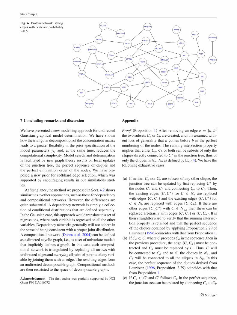
Kornblau et al. (2009) characterized the proteomic profile ofpatients affected by acute myeloid leukaemia, using reverse-phase protein arrays to analyse 51 proteins. This technologyis a high-throughput approach that involves printing proteinlysates from multiple samples onto a slide and then prob-ing the slide with a single antibody to generate a quantita-tive output. The researchers classified patients into groupswith similar prognoses according to the French-American-British classification system, which divides acute myeloidleukaemia into eight subtypes. We applied our model tothe protein expressions of 68 samples of the subtype acutemyeloblastic leukaemia with granulocytic maturation (clas-sification group M2). Our objective was to infer the proteininteraction network for the patients with acute myeloblas-tic leukaemia. We ran two Monte Carlo Markov chains withdifferent starting points. We used 1,000 Gibbs scans overall possible edges of the decomposable graph for the hardselection, and 200,000 Metropolis–Hastings iterations forthe soft selection. We set the hyperparameters as stated inSect. 6.1. Figure 6 is a network representation of the strongedges that were selected with a posterior probability greaterthan 0.5. Although we maintain that our findings are purelyexploratory, several of the proteins with multiple connec-tions in Fig. 6 have been reported in the literature to have keyassociations with acute myeloid leukaemia. For example, ourresults agree with those of Wu et al. (1998), who reportedPTEN to be a tumor suppressor of phosphatase functionssince it acts as a negative regulator of the phosphoinositide3-kinase/Akt pathway. Our analysis confirms that PTEN andAkt are co-expressed. Moreover, our findings confirm theresults of Ozawa et al. (2008), who reported that SRC sup-pressed both activation of STAT proteins and Akt phosphory-lation in acute myeloid leukaemia cells. Our analysis showsSRC to be connected to STAT6.p through Aktp.473. Sev-eral proteins known to be active in the myeloid subtype M2(Kornblau et al. 2009), such as BAD, BAK, BCL2, BCLXL,SMAC and the STAT family, have been found to be highlyconnected in our network analysis. We also observed thatproteins belonging to the same family are connected in ournetwork, such as members of the STAT, MTOR and PKCAfamilies.

123

Stat Comput

Fig. 6 Protein network: strongedges with posterior probability>0.5

ACTB

AKT

AKT.p308

AKT.p473

BAD

BAD.p112

BAD.p136

BAD.p155

BAK

BCL2

BCLXL

CCND1

ERK2

ERk2.p

GSK3

MCL1

MEK

MEK.p

MTOR

MTOR.p

NRP1

P70S6K

P70S6K.p

PKCA

PKCA.p

PTEN

PTEN.p

S6

S6RP.p240

S6.p235

SMAC

SRC

SRC.p527

SSBP2

STAT1.p

STAT3.p705

STAT5.p431

STAT6.p

SURVIVIN

TP27

TP38.p

XIAP

7 Concluding remarks and discussion

We have presented a new modelling approach for undirectedGaussian graphical model determination. We have shownhow the triangular decomposition of the concentration matrixleads to a greater flexibility in the prior specification of themodel parameters γi j and, at the same time, reduces thecomputational complexity. Model search and determinationis facilitated by new graph theory results on local updatesof the junction tree, the perfect sequence of cliques andthe perfect elimination order of the nodes. We have pro-posed a new prior for soft/hard edge selection, which wassupported by encouraging results in our simulations stud-ies.

At first glance, the method we proposed in Sect. 4.2 showssimilarities to other approaches, such as those for dependencyand compositional networks. However, the differences arequite substantial. A dependency network is simply a collec-tion of conditional distributions that are defined separately.In the Gaussian case, this approach would translate to a set ofregressions, where each variable is regressed on all the othervariables. Dependency networks generally will not cohere inthe sense of being consistent with a proper joint distribution.A compositional network (Dobra et al. 2004) can be definedas a directed acyclic graph, i.e., as a set of univariate modelsthat implicitly defines a graph. In this case each composi-tional network is triangulated by replacing all arrows withundirected edges and marrying all pairs of parents of any vari-able by joining them with an edge. The resulting edges forman undirected decomposable graph. Compositional methodsare then restricted to the space of decomposable graphs.

Acknowledgment The first author was partially supported by NCIGrant P30 CA016672.

Appendix

Proof (Proposition 1) After removing an edge e = {a, b}the two subsets Ca or Cb are created, and it is assumed with-out loss of generality that a comes before b in the perfectnumbering of the nodes. The running intersection propertyimplies that either Ca, Cb or both can be subsets of only thecliques directly connected to C∗ in the junction tree, thus ofonly the cliques in Na, Nb as defined by Eq. (4). We have thefollowing exhaustive cases.

(a) If neither Ca nor Cb are subsets of any other clique, thejunction tree can be updated by first replacing C∗ bythe nodes Ca and Cb and connecting Ca to Cb. Then,the existing edges {C, C∗} for C ∈ Na are replacedwith edges {C, Ca} and the existing edges {C, C∗} forC ∈ Nb are replaced with edges {C, Cb}. If there areother edges {C, C∗} with C ∈ N ab then these can bereplaced arbitrarily with edges {C, Ca} or {C, Ca}. It isthen straightforward to verify that the running intersec-tion property is retained and that the perfect sequenceof the cliques obtained by applying Proposition 2.29 ofLauritzen (1996) coincides with that from Proposition 1.

(b) If Ca ⊂ C , where C precedes Ca in the sequence, then inthe previous procedure, the edge {C, Ca} must be con-tracted and Ca must be replaced by C . Thus, C willbe connected to Cb and to all the cliques in Na , andCb will be connected to all the cliques in Nb. In thiscase, the perfect sequence of the cliques derived fromLauritzen (1996, Proposition. 2.29) coincides with thatfrom Proposition 1.

(c) If Ca ⊂ C ′ and C ′ follows Ca in the perfect sequence,the junction tree can be updated by connecting Ca to Cb

123

Stat Comput

and to all the other cliques in Na , and connecting Cb to allthe cliques in Nb. In this case, the perfect sequence of thecliques derived from Lauritzen (1996, Proposition. 2.29)coincides with that from Proposition 1.

(d) If Ca ⊂ C and Cb ⊂ C ′, where C precedes Ca andC ′ follows Ca in the perfect sequence, the junction treecan be updated by connecting C to Cb and to all theother cliques in Na , and connecting Cb to all the othercliques in Nb. In this case, the perfect sequence of thecliques derived from Lauritzen (1996, Proposition 2.29)coincides with that from Proposition 1.

(e) When Ca and Cb are subsets of cliques C ′ and C ′′,respectively, following Ca in the perfect sequence, thejunction tree can be updated by connecting Ca to Cb andto all the other cliques in Na , and connecting Cb to allthe other cliques in Nb. Then the perfect sequence of thecliques derived from Lauritzen (1996, Proposition 2.29)coincides with that from Proposition 1. ��

Proof (Proposition 2) At the end of Algorithm 3, we havethree possible cases:

Case Are Ca, Cb in G ′? Edge in J Edge in J ′

(a) Yes, yes {Ca, Cb} {Ca, C∗} and {C∗, Cb}(b) No, yes yes, no {Ca, Cb} {Ca, C∗} or {C∗, Cb}(c) No, no {Ca, Cb} none

In case (a), if Ca and Cb are both maximal cliques in G ′,the new junction tree J ′ has a new node C∗ on the directedpath between Ca and Cb. Therefore, the perfect sequence ofthe cliques is given in Eq. (5). In case (b), if only one of Ca

or Cb is a maximal clique in G ′, the sequence (5) is reducedby possibly removing either Ca or Cb. Finally, in case (a),both Ca and Cb are removed. ��Proof (Proposition 3) In the junction tree T , all the cliquesin Ct and Cd are separated from all the remaining cliques byC ′

b. Then the cliques in CL are the first in the new perfectsequence, since they belong to a subtree of T that remainsunchanged after the update. By definition, C ′

a and C ′b can be

the next two cliques in the sequence. Then the set of cliquesin Ct is a subpath between C ′

b and one of the leaves of Tand must be in reverse order with respect to that in (6); seeFig. 2. Next, by the definition of descendants, the cliquesin Cd can immediately follow Ct in the same ordering asthat of (6). Clearly, the descendants de(Cti ) of each cliqueCti ∈ Ct must be ordered as in (6) since the subtree that con-nects them remains unchanged after updating J ; whereas theordering between de(Cti ) is arbitrary since they are sepa-rated by Ct . Finally, the cliques in CR also belong to a sub-tree of T that remains unchanged after the tree update, and

they are separated, in T , from the cliques in Ct and Cd byC ′

a . ��

References

Andersson, S., Madigan, D., Perlman, M.: A characterization of Markovequivalence classes for acyclic garphs. Ann. Stat. 25, 505541(1997)

Armstrong, H., Carter, C., Wong, K., Kohn, R.: Bayesian covariancematrix estimation using a mixture of decomposable graphical mod-els. Stat. Comput. 19, 303–316 (2009)

Atay-Kayis, A., Massam, H.: The marginal likelihood for decomposableand non-decomposable graphical gaussian models. Biometrika 92,317–335 (2005)

Clyde, M., George, E.: Model uncertainty. Statistical Science 19(1),81–94 (2004)

Danaher, P., Wang, P., Witten, D.: The joint graphical lasso for inversecovariance estimation across multple classes. J. R. Stat. Soc. 76(2),373–397 (2014)

Dawid, A.P., Lauritzen, S.: Hyper Markov laws in the statistical analy-sis of decomposable graphical models. Ann. Stat. 3, 1272–1317(1993)

Dempster, A.P.: Covariance selection. Biometrics 28, 157–175 (1972)Dobra, A., Jones, B., Hans, C., Nevins, J., West, M.: Sparse graphical

models for exploring gene expression data. J. Multivar. Anal. 90,196–212 (2004)

Dobra, A., Lenkoski, A., Rodriguez, A.: Bayesian inference for generalgaussian graphical models with application to multivariate latticedata. J. Am. Stat. Assoc. 106, 1418–1433 (2012)

Frydenberg, M., Lauritzen, S.: Decomposition of maximum likelihoodin mixed graphical interaction models. Biometrika 76(3), 539–55(1989)

Geiger, D., Heckerman, D.: Parameter priors for directed acyclic graph-ical models and the characterization of several probability distrib-utions. Ann. Stat. 5, 14121440 (2002)

George, E., McCulloch, R.: Variable selection via Gibbs sampling. J.Am. Stat. Assoc. 88, 881–889 (1993)

Giudici, P., Green, P.: Decomposable graphical Gaussian model deter-mination. Biometrika 86(4), 785–801 (1999)

Green, P., Thomas, A.: Sampling decomposable graphs using a markovchain on junction trees. Biometrika 100(1), 91–110 (2013)

Grone, R., Johnson, C.R., Sà, E.M., Wolkowicz, H.: Positive definitecompletion of partial Hermitian matrices. Linear Algebra Appl.58, 109–124 (1984)

Ibarra, L.: Fully dynamic algorithms for chordal graphs and split graphs.ACMM Trans. Algorithms 40(1), 40 (2008)

Jones, B., Carvalho, C., Dobra, A., Hans, C., Carter, C., West, M.: Exper-iments in stochastic computation for high-dimensional graphicalmodels. Stat. Sci. 20(4), 388–400 (2005)

Kornblau, S., Tibes, R., Qiu, Y., Chen, W., Kantarjian, H., Andreeff,M., Coombes, K., Mills, G.: Functional proteomic profiling ofaml predicts response and survival. Blood 113, 154–164 (2009)

Lauritzen, S.: Graphical Models. Claredon Press, Oxford (1996)Ozawa, Y., Williams, A., Estes, M., Matsushita, N., Boschelli, F., Jove,

R., List, A.: Src family kinases promote AML cell survival throughactivation of signal transducers and activators of transcription(STAT). Leuk. Res. 32(6), 893–903 (2008)

Paulsen, V., Power, S., Smith, R.: Schur products and matrix comple-tions. J. Funct. Anal. 85, 151–178 (1989)

Roverato, A.: Cholesky decomposition of a hyper-inverse Wishartmatrix. Biometrika 87, 99–112 (2000)

Roverato, A.: Hyper-inverse Wishart distribution for non-decomposablegraphs and its application to bayesian inference for Gaussiangraphical models. Scand. J. Stat. 29, 391–411 (2002)

123

Stat Comput

Scott, J., Carvalho, C.: Feature-inclusion stochastic search for Gaussiangraphical models. J. Comput. Graphical Stat. 17, 790–808 (2008)

Tarjan, R., Yannakakis, M.: Simple linear-time algorithms to testchordality of graphs, test acyclicity of hypergraphs, and selec-tively reduce acyclic hypergraphs. SIAM J. Comput. 13, 566–579(1984)

Thomas, A., Green, P.: Enumerating the decomposable neighbors of adecomposble graph under a simple perturbation scheme. Comput.Stat. Data Anal. 53, 1232–1238 (2009)

Wang, H.: Bayesian graphical lasso models and efficient posterior com-putation. Bayesian Anal. 7(4), 867–886 (2012)

Wang, H., Li, Z.: Efficient Gaussian graphical model determinationunder G-Wishart prior distributions. Electron. J. Stat. 6, 168–198(2012)

Wermuth, N.: Linear recursive equations, covariance selection, and pathanalysis. J. Am. Stat. Assoc. 75(372), 963–972 (1980)

Wu, X., Senechal, K., Neshat, M., Whang, Y., Sawyers, C.: ThePTEN/MMAC1 tumor suppressor phosphatase functions as a neg-ative regulator of the phosphoinositide 3-kinase/Akt pathway.PNAS 95(15), 587–591 (1998)

123