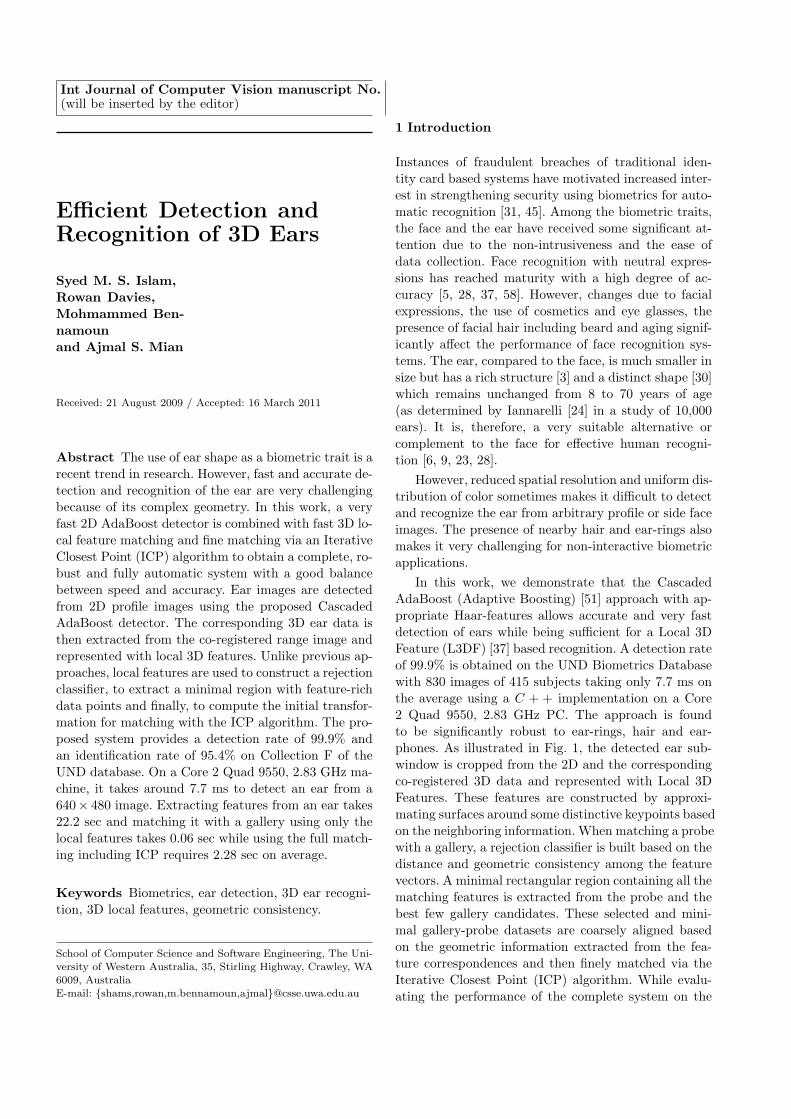
Int Journal of Computer Vision manuscript No.(will be inserted by the editor)

Efficient Detection andRecognition of 3D Ears

Syed M. S. Islam,Rowan Davies,Mohmammed Ben-namounand Ajmal S. Mian

Received: 21 August 2009 / Accepted: 16 March 2011

Abstract The use of ear shape as a biometric trait is arecent trend in research. However, fast and accurate de-tection and recognition of the ear are very challengingbecause of its complex geometry. In this work, a veryfast 2D AdaBoost detector is combined with fast 3D lo-cal feature matching and fine matching via an IterativeClosest Point (ICP) algorithm to obtain a complete, ro-bust and fully automatic system with a good balancebetween speed and accuracy. Ear images are detectedfrom 2D profile images using the proposed CascadedAdaBoost detector. The corresponding 3D ear data isthen extracted from the co-registered range image andrepresented with local 3D features. Unlike previous ap-proaches, local features are used to construct a rejectionclassifier, to extract a minimal region with feature-richdata points and finally, to compute the initial transfor-mation for matching with the ICP algorithm. The pro-posed system provides a detection rate of 99.9% andan identification rate of 95.4% on Collection F of theUND database. On a Core 2 Quad 9550, 2.83 GHz ma-chine, it takes around 7.7 ms to detect an ear from a640× 480 image. Extracting features from an ear takes22.2 sec and matching it with a gallery using only thelocal features takes 0.06 sec while using the full match-ing including ICP requires 2.28 sec on average.

Keywords Biometrics, ear detection, 3D ear recogni-tion, 3D local features, geometric consistency.

School of Computer Science and Software Engineering, The Uni-versity of Western Australia, 35, Stirling Highway, Crawley, WA6009, AustraliaE-mail: {shams,rowan,m.bennamoun,ajmal}@csse.uwa.edu.au

1 Introduction

Instances of fraudulent breaches of traditional iden-tity card based systems have motivated increased inter-est in strengthening security using biometrics for auto-matic recognition [31, 45]. Among the biometric traits,the face and the ear have received some significant at-tention due to the non-intrusiveness and the ease ofdata collection. Face recognition with neutral expres-sions has reached maturity with a high degree of ac-curacy [5, 28, 37, 58]. However, changes due to facialexpressions, the use of cosmetics and eye glasses, thepresence of facial hair including beard and aging signif-icantly affect the performance of face recognition sys-tems. The ear, compared to the face, is much smaller insize but has a rich structure [3] and a distinct shape [30]which remains unchanged from 8 to 70 years of age(as determined by Iannarelli [24] in a study of 10,000ears). It is, therefore, a very suitable alternative orcomplement to the face for effective human recogni-tion [6, 9, 23, 28].

However, reduced spatial resolution and uniform dis-tribution of color sometimes makes it difficult to detectand recognize the ear from arbitrary profile or side faceimages. The presence of nearby hair and ear-rings alsomakes it very challenging for non-interactive biometricapplications.

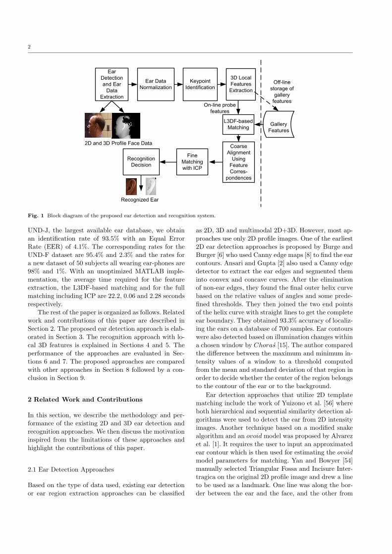
In this work, we demonstrate that the CascadedAdaBoost (Adaptive Boosting) [51] approach with ap-propriate Haar-features allows accurate and very fastdetection of ears while being sufficient for a Local 3DFeature (L3DF) [37] based recognition. A detection rateof 99.9% is obtained on the UND Biometrics Databasewith 830 images of 415 subjects taking only 7.7 ms onthe average using a C + + implementation on a Core2 Quad 9550, 2.83 GHz PC. The approach is foundto be significantly robust to ear-rings, hair and ear-phones. As illustrated in Fig. 1, the detected ear sub-window is cropped from the 2D and the correspondingco-registered 3D data and represented with Local 3DFeatures. These features are constructed by approxi-mating surfaces around some distinctive keypoints basedon the neighboring information. When matching a probewith a gallery, a rejection classifier is built based on thedistance and geometric consistency among the featurevectors. A minimal rectangular region containing all thematching features is extracted from the probe and thebest few gallery candidates. These selected and mini-mal gallery-probe datasets are coarsely aligned basedon the geometric information extracted from the fea-ture correspondences and then finely matched via theIterative Closest Point (ICP) algorithm. While evalu-ating the performance of the complete system on the

2

Keypoint

Identification

3D Local

Features

Extraction

L3DF-based

Matching

Fine

Matching

with ICP

Coarse

Alignment

Using

Feature

Corres-

pondences

Gallery

Features

Off-line

storage of

gallery

featuresOn-line probe

features

Recognized Ear

Ear Data

Normalization

Ear

Detection

and Ear

Data

Extraction

Recognition

Decision

2D and 3D Profile Face Data

Fig. 1 Block diagram of the proposed ear detection and recognition system.

UND-J, the largest available ear database, we obtainan identification rate of 93.5% with an Equal ErrorRate (EER) of 4.1%. The corresponding rates for theUND-F dataset are 95.4% and 2.3% and the rates fora new dataset of 50 subjects all wearing ear-phones are98% and 1%. With an unoptimized MATLAB imple-mentation, the average time required for the featureextraction, the L3DF-based matching and for the fullmatching including ICP are 22.2, 0.06 and 2.28 secondsrespectively.

The rest of the paper is organized as follows. Relatedwork and contributions of this paper are described inSection 2. The proposed ear detection approach is elab-orated in Section 3. The recognition approach with lo-cal 3D features is explained in Sections 4 and 5. Theperformance of the approaches are evaluated in Sec-tions 6 and 7. The proposed approaches are comparedwith other approaches in Section 8 followed by a con-clusion in Section 9.

2 Related Work and Contributions

In this section, we describe the methodology and per-formance of the existing 2D and 3D ear detection andrecognition approaches. We then discuss the motivationinspired from the limitations of these approaches andhighlight the contributions of this paper.

2.1 Ear Detection Approaches

Based on the type of data used, existing ear detectionor ear region extraction approaches can be classified

as 2D, 3D and multimodal 2D+3D. However, most ap-proaches use only 2D profile images. One of the earliest2D ear detection approaches is proposed by Burge andBurger [6] who used Canny edge maps [8] to find the earcontours. Ansari and Gupta [2] also used a Canny edgedetector to extract the ear edges and segmented theminto convex and concave curves. After the eliminationof non-ear edges, they found the final outer helix curvebased on the relative values of angles and some prede-fined thresholds. They then joined the two end pointsof the helix curve with straight lines to get the completeear boundary. They obtained 93.3% accuracy of localiz-ing the ears on a database of 700 samples. Ear contourswere also detected based on illumination changes withina chosen window by Choras [15]. The author comparedthe difference between the maximum and minimum in-tensity values of a window to a threshold computedfrom the mean and standard deviation of that region inorder to decide whether the center of the region belongsto the contour of the ear or to the background.

Ear detection approaches that utilize 2D templatematching include the work of Yuizono et al. [56] whereboth hierarchical and sequential similarity detection al-gorithms were used to detect the ear from 2D intensityimages. Another technique based on a modified snakealgorithm and an ovoid model was proposed by Alvarezet al. [1]. It requires the user to input an approximatedear contour which is then used for estimating the ovoid

model parameters for matching. Yan and Bowyer [54]manually selected Triangular Fossa and Incisure Inter-tragica on the original 2D profile image and drew a lineto be used as a landmark. One line was along the bor-der between the ear and the face, and the other from

3

the top of the ear to the bottom. The authors foundthis method suitable for PCA-based and edge-basedmatching. The Hough Transform can extract shapeswith properties equivalent to template matching andwas used by Arbab-Zavar and Nixon [3] to detect theelliptical shape of the ear. The authors successfully de-tected the ear region in all of the 252 profile images ofa non-occluded subset of the XM2V TS database. Forthe UND database, they first detected the face regionusing skin detection and the Canny edge operator fol-lowed by the extraction of the ear region using theirproposed method with a success rate of 91%. They alsointroduced synthetic occlusions vertically from top tobottom on the ear region of the first dataset and ob-tained around 93% and 90% detection rates for 20% and30% occlusion respectively. Recently, Gentile et al. [19]used AdaBoost [51] to detect the ear from a profile faceas part of their multi-biometric approach for detectingdrivers’ profiles in a security checkpoint. In an exper-iment with 46 images from 23 subjects, they obtainedan ear detection rate of 97% with seven false positivesper image. They did not report the efficiency of theirsystem.

Approaches using only 3D or range data includeYan and Bowyer’s two-line based landmarks and 3Dmasks [54], Chen and Bhanu’s 3D template matching[10] and the ear-shape-model based approach [12]. Sim-ilar to their 2D technique [54] mentioned above, Yanand Bowyer [54] drew two lines on the original range im-age to find the orientation and scaling of the ear. Theyrotated and scaled a mask accordingly and applied iton the original image to crop the 3D ear data in anICP-based matching approach. Chen and Bhanu [10]combined template matching with average histogramto detect ears. They achieved a 91.5% detection ratewith about 3% False Positive Rate (FPR). In [12], theyrepresented an ear shape model by a set of discrete 3Dvertices on the ear helix and anti-helix parts and alignedthe model with the range images to detect the ear parts.With this approach, they obtained 92.5% detection ac-curacy on the University of California, Riverside (UCR)ear dataset with 312 images and an average detectiontime of 6.5 sec on a 2.4 GHz Celeron CPU.

Among the multimodal 2D+3D approaches, Yan andBowyer [55] and Chen and Bhanu [13] are prominent. Inthe first approach, the ear region was initially locatedby taking a predefined sector from the nose tip. Thenon-ear portion was then cropped out from that sectorusing a skin detection algorithm and the ear pit wasdetected using Gaussian smoothing and curvature esti-mation algorithms. An active contour algorithm was ap-plied to extract the ear contour. Using the color and thedepth information separately for the active contour, ear

detection accuracies of 79% and 85% respectively wereobtained. However, using both 2D and 3D information,ears from all the profile images were successfully ex-tracted. Thus, the system is automatic but dependshighly on the accuracy of detection of nose tip and earpit and it fails when the ear pit is not visible. Chenand Bhanu [13] also used both color and range imagesto extract ear data. They used a reference ear shapemodel based on the helix and anti-helix curves and theglobal-to-local shape registration. They obtained 99.3%and 87.7% detection rates while tested on the UCR eardatabase of 902 images from 155 subjects and on 700images of the UND database, respectively. The detec-tion time for the UCR database is reported as 9.5 secwith a MATLAB implementation on a 2.4 GHz CeleronCPU.

2.2 Ear Recognition Approaches

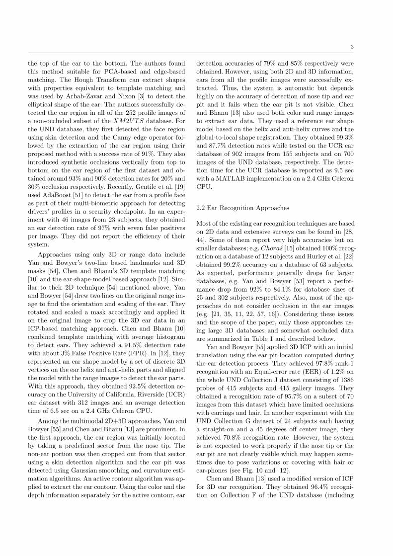
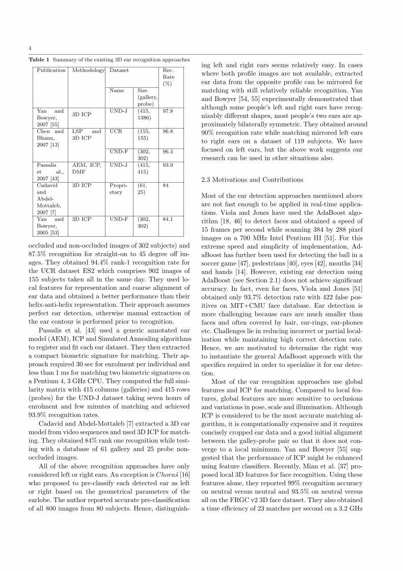
Most of the existing ear recognition techniques are basedon 2D data and extensive surveys can be found in [28,44]. Some of them report very high accuracies but onsmaller databases; e.g. Choras [15] obtained 100% recog-nition on a database of 12 subjects and Hurley et al. [22]obtained 99.2% accuracy on a database of 63 subjects.As expected, performance generally drops for largerdatabases, e.g. Yan and Bowyer [53] report a perfor-mance drop from 92% to 84.1% for database sizes of25 and 302 subjects respectively. Also, most of the ap-proaches do not consider occlusion in the ear images(e.g. [21, 35, 11, 22, 57, 16]). Considering these issuesand the scope of the paper, only those approaches us-ing large 3D databases and somewhat occluded dataare summarized in Table 1 and described below.

Yan and Bowyer [55] applied 3D ICP with an initialtranslation using the ear pit location computed duringthe ear detection process. They achieved 97.8% rank-1recognition with an Equal-error rate (EER) of 1.2% onthe whole UND Collection J dataset consisting of 1386probes of 415 subjects and 415 gallery images. Theyobtained a recognition rate of 95.7% on a subset of 70images from this dataset which have limited occlusionswith earrings and hair. In another experiment with theUND Collection G dataset of 24 subjects each havinga straight-on and a 45 degrees off center image, theyachieved 70.8% recognition rate. However, the systemis not expected to work properly if the nose tip or theear pit are not clearly visible which may happen some-times due to pose variations or covering with hair orear-phones (see Fig. 10 and 12).

Chen and Bhanu [13] used a modified version of ICPfor 3D ear recognition. They obtained 96.4% recogni-tion on Collection F of the UND database (including

4

Table 1 Summary of the existing 3D ear recognition approaches

Publication Methodology Dataset Rec.Rate(%)

Name Size(gallery,probe)

Yan andBowyer,2007 [55]

3D ICPUND-J (415,

1386)97.8

Chen andBhanu,2007 [13]

LSP and3D ICP

UCR (155,155)

96.8

UND-F (302,302)

96.4

Passaliset al.,2007 [43]

AEM, ICP,DMF

UND-J (415,415)

93.9

CadavidandAbdel-Mottaleb,2007 [7]

3D ICP Propri-etary

(61,25)

84

Yan andBowyer,2005 [53]

3D ICP UND-F (302,302)

84.1

occluded and non-occluded images of 302 subjects) and87.5% recognition for straight-on to 45 degree off im-ages. They obtained 94.4% rank-1 recognition rate forthe UCR dataset ES2 which comprises 902 images of155 subjects taken all in the same day. They used lo-cal features for representation and coarse alignment ofear data and obtained a better performance than theirhelix-anti-helix representation. Their approach assumesperfect ear detection, otherwise manual extraction ofthe ear contour is performed prior to recognition.

Passalis et al. [43] used a generic annotated earmodel (AEM), ICP and Simulated Annealing algorithmsto register and fit each ear dataset. They then extracteda compact biometric signature for matching. Their ap-proach required 30 sec for enrolment per individual andless than 1 ms for matching two biometric signatures ona Pentium 4, 3 GHz CPU. They computed the full simi-larity matrix with 415 columns (galleries) and 415 rows(probes) for the UND-J dataset taking seven hours ofenrolment and few minutes of matching and achieved93.9% recognition rates.

Cadavid and Abdel-Mottaleb [7] extracted a 3D earmodel from video sequences and used 3D ICP for match-ing. They obtained 84% rank one recognition while test-ing with a database of 61 gallery and 25 probe non-occluded images.

All of the above recognition approaches have onlyconsidered left or right ears. An exception is Choras [16]who proposed to pre-classify each detected ear as leftor right based on the geometrical parameters of theearlobe. The author reported accurate pre-classificationof all 800 images from 80 subjects. Hence, distinguish-

ing left and right ears seems relatively easy. In caseswhere both profile images are not available, extractedear data from the opposite profile can be mirrored formatching with still relatively reliable recognition. Yanand Bowyer [54, 55] experimentally demonstrated thatalthough some people’s left and right ears have recog-nizably different shapes, most people’s two ears are ap-proximately bilaterally symmetric. They obtained around90% recognition rate while matching mirrored left earsto right ears on a dataset of 119 subjects. We havefocused on left ears, but the above work suggests ourresearch can be used in other situations also.

2.3 Motivations and Contributions

Most of the ear detection approaches mentioned aboveare not fast enough to be applied in real-time applica-tions. Viola and Jones have used the AdaBoost algo-rithm [18, 46] to detect faces and obtained a speed of15 frames per second while scanning 384 by 288 pixelimages on a 700 MHz Intel Pentium III [51]. For thisextreme speed and simplicity of implementation, Ad-aBoost has further been used for detecting the ball in asoccer game [47], pedestrians [40], eyes [42], mouths [34]and hands [14]. However, existing ear detection usingAdaBoost (see Section 2.1) does not achieve significantaccuracy. In fact, even for faces, Viola and Jones [51]obtained only 93.7% detection rate with 422 false pos-itives on MIT+CMU face database. Ear detection ismore challenging because ears are much smaller thanfaces and often covered by hair, ear-rings, ear-phonesetc. Challenges lie in reducing incorrect or partial local-ization while maintaining high correct detection rate.Hence, we are motivated to determine the right wayto instantiate the general AdaBoost approach with thespecifics required in order to specialize it for ear detec-tion.

Most of the ear recognition approaches use globalfeatures and ICP for matching. Compared to local fea-tures, global features are more sensitive to occlusionsand variations in pose, scale and illumination. AlthoughICP is considered to be the most accurate matching al-gorithm, it is computationally expensive and it requiresconcisely cropped ear data and a good initial alignmentbetween the galley-probe pair so that it does not con-verge to a local minimum. Yan and Bowyer [55] sug-gested that the performance of ICP might be enhancedusing feature classifiers. Recently, Mian et al. [37] pro-posed local 3D features for face recognition. Using thesefeatures alone, they reported 99% recognition accuracyon neutral versus neutral and 93.5% on neutral versusall on the FRGC v2 3D face dataset. They also obtaineda time efficiency of 23 matches per second on a 3.2 GHz

5

Pentium IV machine with 1GB RAM. In this paper, weadapt these features for the ear and use them for coarsealignment as well as for rejecting a large number of falsematches. We also use L3DFs for extracting a minimalset of datapoints to be used in ICP.

The specific contributions of this paper are as fol-lows:

(1) A fast and fully automatic ear detection approachusing cascaded AdaBoost classifiers trained withthree new features and a rectangular detection win-dow. No assumption is made about the localizationof the nose or the ear pit.

(2) The local 3D features are used for ear recognitionin a more accurate way than originally proposedin [37] for the face including an explicit secondround of matching based on geometric consistency.L3DFs are used not only for coarse alignment butalso for rejecting most false matches.

(3) A novel approach for extracting minimal feature-rich data points for the final ICP alignment is pro-posed which significantly increases the time effi-ciency of the recognition system.

(4) Experiments are performed on a new database ofprofile images with ear-phones along with the largestpublicly available dataset of the UND and highrecognition rates are achieved without an explicitextraction of the ear contours.

3 Automatic Detection and Extraction of EarData

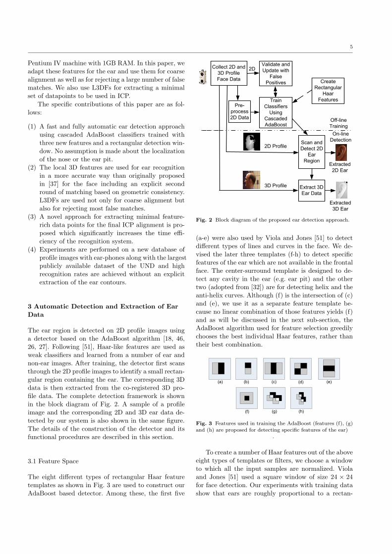
The ear region is detected on 2D profile images usinga detector based on the AdaBoost algorithm [18, 46,26, 27]. Following [51], Haar-like features are used asweak classifiers and learned from a number of ear andnon-ear images. After training, the detector first scansthrough the 2D profile images to identify a small rectan-gular region containing the ear. The corresponding 3Ddata is then extracted from the co-registered 3D pro-file data. The complete detection framework is shownin the block diagram of Fig. 2. A sample of a profileimage and the corresponding 2D and 3D ear data de-tected by our system is also shown in the same figure.The details of the construction of the detector and itsfunctional procedures are described in this section.

3.1 Feature Space

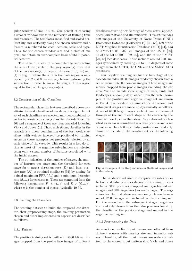
The eight different types of rectangular Haar featuretemplates as shown in Fig. 3 are used to construct ourAdaBoost based detector. Among these, the first five

On-line

Detection

Off-line

Training

2D

3D Profile

2D Profile

Extract 3D

Ear Data

Scan and

Detect 2D

Ear

Region

Collect 2D and

3D Profile

Face Data

Validate and

Update with

False

Positives Create

Rectangular

Haar

FeaturesPre-

process

2D Data

Train

Classifiers

Using

Cascaded

AdaBoost

Extracted

2D Ear

Extracted

3D Ear

Fig. 2 Block diagram of the proposed ear detection approach.

(a-e) were also used by Viola and Jones [51] to detectdifferent types of lines and curves in the face. We de-vised the later three templates (f-h) to detect specificfeatures of the ear which are not available in the frontalface. The center-surround template is designed to de-tect any cavity in the ear (e.g. ear pit) and the othertwo (adopted from [32]) are for detecting helix and theanti-helix curves. Although (f) is the intersection of (c)and (e), we use it as a separate feature template be-cause no linear combination of those features yields (f)and as will be discussed in the next sub-section, theAdaBoost algorithm used for feature selection greedilychooses the best individual Haar features, rather thantheir best combination.

(a) (b)

(h)(g)

(d)(c)

(f)

(e)

Fig. 3 Features used in training the AdaBoost (features (f), (g)and (h) are proposed for detecting specific features of the ear)

.

To create a number of Haar features out of the aboveeight types of templates or filters, we choose a windowto which all the input samples are normalized. Violaand Jones [51] used a square window of size 24 × 24for face detection. Our experiments with training datashow that ears are roughly proportional to a rectan-

6

gular window of size 16 × 24. One benefit of choosinga smaller window size is the reduction of training timeand resources. The templates are shifted and scaled hor-izontally and vertically along the chosen window and afeature is numbered for each location, scale and type.Thus, for the chosen window size and a shift of onepixel, we obtain an over-complete basis of 96413 poten-tial features.

The value of a feature is computed by subtractingthe sum of the pixels in the grey region(s) from thatof the dark region(s) (except in the case of (c), (e) and(f) in Fig. 3, where the sum in the dark region is mul-tiplied by 2, 2 and 8 respectively before performing thesubtraction in order to make the weight of this regionequal to that of the grey region(s)).

3.2 Construction of the Classifiers

The rectangular Haar-like features described above con-stitute the weak classifiers of our detection algorithm. Aset of such classifiers are selected and then combined to-gether to construct a strong classifier via AdaBoost [18,46] and a sequence of these are then cascaded followingViola and Jones [51]. Thus, each strong classifier in thecascade is a linear combination of the best weak clas-sifiers, with weights inversely proportional to trainingerrors on those examples not previously rejected by anearly stage of the cascade. This results in a fast detec-tion as most of the negative sub-windows are rejectedusing only a small number of features associated withthe initial stages.

The optimization of the number of stages, the num-ber of features per stage and the threshold for eachstage for a target detection rate (D) and false posi-tive rate (Ft) is obtained similar to [51] by aiming fora fixed maximum FPR (fm) and a minimum detectionrate (dmin) for each stage. These are computed from thefollowing inequalities: Ft < (fm)n and D > (dmin)n,where n is the number of stages, typically 10-50.

3.3 Training the Classifiers

The training dataset to build the proposed ear detec-tor, their preprocessing stage, the training parameterschosen and other implementation aspects are describedas follows.

3.3.1 Dataset

The positive training set is built with 5000 left ear im-ages cropped from the profile face images of different

databases covering a wide range of races, sexes, appear-ances, orientations and illuminations. This set includes429 images of the University of Notre Dame (UND)Biometrics Database (Collection F) [49, 55], 659 of theNIST Mugshot Identification Database (MID) [41], 573of XM2VTSDB [36], 201 images of the USTB [50],15 of the MIT-CBCL [52, 39], and 188 of the UMIST[20, 48] face databases. It also includes around 3000 im-ages synthesized by rotating -15 to +15 degrees of someimages from the USTB, the UND and the XM2VTSDBdatabases.

Our negative training set for the first stage of thecascade includes 10,000 images randomly chosen from aset of around 65,000 non-ear images. These images aremostly cropped from profile images excluding the eararea. We also include some images of trees, birds andlandscapes randomly downloaded from the web. Exam-ples of the positive and negative image set are shownin Fig. 4. The negative training set for the second andsubsequent stages are made up dynamically as follows.A set of 6000 large images without ears are scannedthrough at the end of each stage of the cascade by theclassifier developed in that stage. Any sub-window clas-sified as an ear is considered as a false positive and a setof not more than 5000 such false positives are randomlychosen to include in the negative set for the followingstages.

Fig. 4 Examples of ear (top) and non-ear (bottom) images usedin the training.

The validation set used to compute the rates of de-tection and false positives during the training processincludes 5000 positives (cropped and synthesized earimages) and 6000 negatives (non-ear images). The neg-atives for the first stage are randomly chosen from aset of 12000 images not included in the training set.For the second and the subsequent stages, negativesare randomly chosen from the false positives found bythe classifier of the previous stage and unused in thenegative training set.

3.3.2 Preprocessing the Data

As mentioned earlier, input images are collected fromdifferent sources with varying size and intensity val-ues. Therefore, all the input images are scale normal-ized to the chosen input pattern size. Viola and Jones

7

reported a square input pattern of size 24 × 24 as themost suitable for detecting frontal faces [51]. Consider-ing the shape of the ear, we instead use a rectangularpattern of size 16× 24.

The variance of the intensity values of images arealso normalized to minimize the effect of lighting. Sim-ilar normalization is performed for each sub-windowscanned during testing.

3.3.3 Training the Cascade

In order to train the cascade, we choose Ft = 0.001and D = 0.98. However, to quickly reject most of thefalse positives using a small number of features, we de-fine the first four stages to be completed with 10, 20,60 and 80 features. We also performed validation afteradding ten features for the first ten stages and then,adding of 25 for the remaining stages. The detectionand false positive rates computed during the validationof each stage follow a gradual decrease to the target.The training finishes at stage 18 with a total of 5035rectangular features including 1425 features in the laststage.

3.3.4 Training Time

The training process involved a huge amount of com-putation due to the large training set and also for thevery low target FPR, taking several weeks on a singlePC. To speed up the process, we distributed the jobover a network of around 30 PCs. For this purpose, weused MATLABMPI which is a MATLAB implemen-tation of the Message Passing Interface (MPI) standardthat allows any MATLAB program to exploit multi-ple processors [33]. It helped in reducing the trainingtime to an order of days. An optimized C or C + +implementation would reduce this time, but since thistraining never needs to be done again, our MATLABimplementation was sufficient.

3.4 Ear Detection with the Cascaded Classifiers

The trained classifiers of all the stages are used to buildthe ear detector in a cascaded manner. The detector isscanned over a test profile image in different sizes andlocations. A classifier in the cascade is only used whena sub-window in the test image is detected as positive(ear) by the classifier of the previous stage and acceptedfinally only when it passes through all of them.

To detect various sizes of ears, instead of resizing thegiven test image, we scale up the detector along withthe corresponding features and use an integral imagecalculation. The approach is similar to that of Viola

and Jones [51] who also illustrated this to be more time-efficient than the conventional pyramid approach.

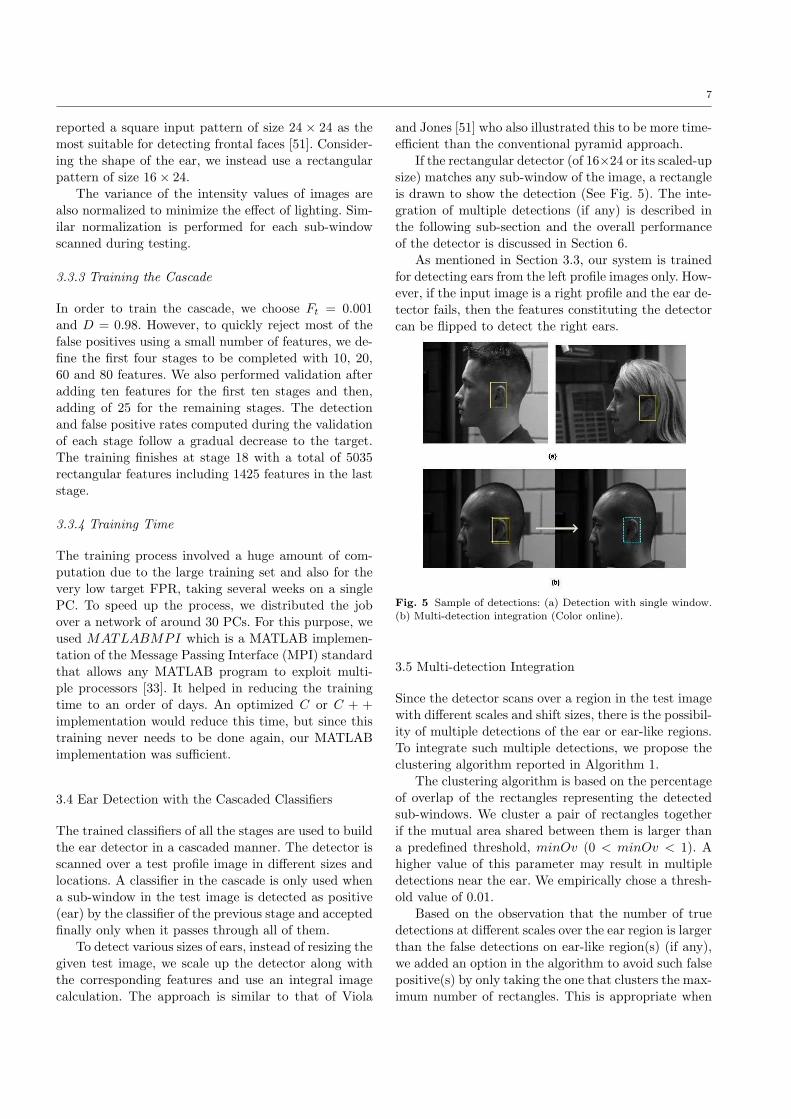
If the rectangular detector (of 16×24 or its scaled-upsize) matches any sub-window of the image, a rectangleis drawn to show the detection (See Fig. 5). The inte-gration of multiple detections (if any) is described inthe following sub-section and the overall performanceof the detector is discussed in Section 6.

As mentioned in Section 3.3, our system is trainedfor detecting ears from the left profile images only. How-ever, if the input image is a right profile and the ear de-tector fails, then the features constituting the detectorcan be flipped to detect the right ears.

Fig. 5 Sample of detections: (a) Detection with single window.(b) Multi-detection integration (Color online).

3.5 Multi-detection Integration

Since the detector scans over a region in the test imagewith different scales and shift sizes, there is the possibil-ity of multiple detections of the ear or ear-like regions.To integrate such multiple detections, we propose theclustering algorithm reported in Algorithm 1.

The clustering algorithm is based on the percentageof overlap of the rectangles representing the detectedsub-windows. We cluster a pair of rectangles togetherif the mutual area shared between them is larger thana predefined threshold, minOv (0 < minOv < 1). Ahigher value of this parameter may result in multipledetections near the ear. We empirically chose a thresh-old value of 0.01.

Based on the observation that the number of truedetections at different scales over the ear region is largerthan the false detections on ear-like region(s) (if any),we added an option in the algorithm to avoid such falsepositive(s) by only taking the one that clusters the max-imum number of rectangles. This is appropriate when

8

only one ear needs to be detected which is the case formost recognition applications.

An example of integrating three detection windowsis illustrated in Fig. 5(b). Each of the detections isshown by a rectangle in yellow lines while the integrateddetection window is shown by a rectangle in bold dottedcyan lines.

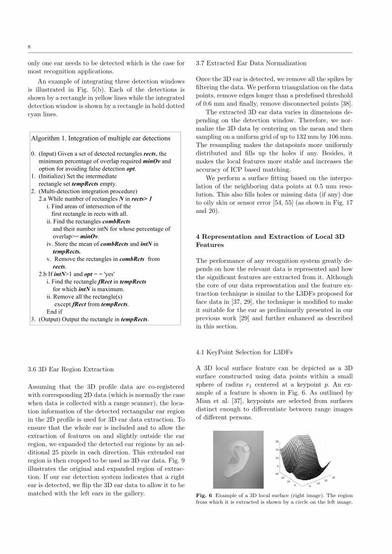
Algorithm 1. Integration of multiple ear detections

0. (Input) Given a set of detected rectangles rects, the

minimum percentage of overlap required minOv and

option for avoiding false detection opt.

1. (Initialize) Set the intermediate

rectangle set tempRects empty.

2. (Multi-detection integration procedure)

2.a While number of rectangles N in rects> 1

i. Find areas of intersection of the

first rectangle in rects with all.

ii. Find the rectangles combRects

and their number intN for whose percentage of

overlap>= minOv.

iv. Store the mean of combRects and intN in

tempRects.

v. Remove the rectangles in combRcts from

rects.

2.b If intN>1 and opt = = 'yes'

i. Find the rectangle fRect in tempRects

for which intN is maximum.

ii. Remove all the rectangle(s)

except fRect from tempRects.

End if

3. (Output) Output the rectangle in tempRects.

3.6 3D Ear Region Extraction

Assuming that the 3D profile data are co-registeredwith corresponding 2D data (which is normally the casewhen data is collected with a range scanner), the loca-tion information of the detected rectangular ear regionin the 2D profile is used for 3D ear data extraction. Toensure that the whole ear is included and to allow theextraction of features on and slightly outside the earregion, we expanded the detected ear regions by an ad-ditional 25 pixels in each direction. This extended earregion is then cropped to be used as 3D ear data. Fig. 9illustrates the original and expanded region of extrac-tion. If our ear detection system indicates that a rightear is detected, we flip the 3D ear data to allow it to bematched with the left ears in the gallery.

3.7 Extracted Ear Data Normalization

Once the 3D ear is detected, we remove all the spikes byfiltering the data. We perform triangulation on the datapoints, remove edges longer than a predefined thresholdof 0.6 mm and finally, remove disconnected points [38].

The extracted 3D ear data varies in dimensions de-pending on the detection window. Therefore, we nor-malize the 3D data by centering on the mean and thensampling on a uniform grid of up to 132 mm by 106 mm.The resampling makes the datapoints more uniformlydistributed and fills up the holes if any. Besides, itmakes the local features more stable and increases theaccuracy of ICP based matching.

We perform a surface fitting based on the interpo-lation of the neighboring data points at 0.5 mm reso-lution. This also fills holes or missing data (if any) dueto oily skin or sensor error [54, 55] (as shown in Fig. 17and 20).

4 Representation and Extraction of Local 3DFeatures

The performance of any recognition system greatly de-pends on how the relevant data is represented and howthe significant features are extracted from it. Althoughthe core of our data representation and the feature ex-traction technique is similar to the L3DFs proposed forface data in [37, 29], the technique is modified to makeit suitable for the ear as preliminarily presented in ourprevious work [29] and further enhanced as describedin this section.

4.1 KeyPoint Selection for L3DFs

A 3D local surface feature can be depicted as a 3Dsurface constructed using data points within a smallsphere of radius r1 centered at a keypoint p. An ex-ample of a feature is shown in Fig. 6. As outlined byMian et al. [37], keypoints are selected from surfacesdistinct enough to differentiate between range imagesof different persons.

510

1520

510

1520

5

10

15

20

Fig. 6 Example of a 3D local surface (right image). The regionfrom which it is extracted is shown by a circle on the left image.

9

Nearest Neighbour Error (mm)Cumulative % of Repeatability

(a) (b)

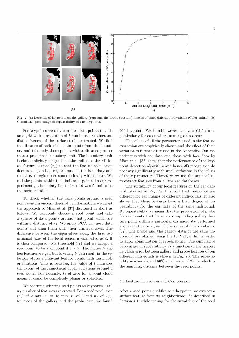
Fig. 7 (a) Location of keypoints on the gallery (top) and the probe (bottom) images of three different individuals (Color online). (b)Cumulative percentage of repeatability of the keypoints.

For keypoints we only consider data points that lieon a grid with a resolution of 2 mm in order to increasedistinctiveness of the surface to be extracted. We findthe distance of each of the data points from the bound-ary and take only those points with a distance greaterthan a predefined boundary limit. The boundary limitis chosen slightly longer than the radius of the 3D lo-cal feature surface (r1) so that the feature calculationdoes not depend on regions outside the boundary andthe allowed region corresponds closely with the ear. Wecall the points within this limit seed points. In our ex-periments, a boundary limit of r + 10 was found to bethe most suitable.

To check whether the data points around a seedpoint contain enough descriptive information, we adoptthe approach of Mian et al. [37] discussed in short asfollows. We randomly choose a seed point and takea sphere of data points around that point which arewithin a distance of r1. We apply PCA on those datapoints and align them with their principal axes. Thedifference between the eigenvalues along the first twoprincipal axes of the local region is computed as `. Itis then compared to a threshold (t1) and we accept aseed point to be a keypoint if ` > t1. The higher t1 theless features we get, but lowering t1 can result in the se-lection of less significant feature points with unreliableorientations. This is because, the value of ` indicatesthe extent of unsymmetrical depth variations around aseed point. For example, t1 of zero for a point cloudmeans it could be completely planar or spherical.

We continue selecting seed points as keypoints untilnf number of features are created. For a seed resolution(rs) of 2 mm, r1 of 15 mm, t1 of 2 and nf of 200,for most of the gallery and the probe ears, we found

200 keypoints. We found however, as low as 65 featuresparticularly for cases where missing data occurs.

The values of all the parameters used in the featureextraction are empirically chosen and the effect of theirvariation is further discussed in the Appendix. Our ex-periments with ear data and those with face data byMian et al. [37] show that the performance of the key-point detection algorithm and hence 3D recognition donot vary significantly with small variations in the valuesof these parameters. Therefore, we use the same valuesto extract features from all the ear databases.

The suitability of our local features on the ear datais illustrated in Fig. 7a. It shows that keypoints aredifferent for ear images of different individuals. It alsoshows that these features have a high degree of re-peatability for the ear data of the same individual.By repeatability we mean that the proportion of probefeature points that have a corresponding gallery fea-ture point within a particular distance. We performeda quantitative analysis of the repeatability similar to[37]. The probe and the gallery data of the same in-dividual are aligned using the ICP algorithm in orderto allow computation of repeatability. The cumulativepercentage of repeatability as a function of the nearestneighbor error between gallery and probe features of tendifferent individuals is shown in Fig. 7b. The repeata-bility reaches around 80% at an error of 2 mm which isthe sampling distance between the seed points.

4.2 Feature Extraction and Compression

After a seed point qualifies as a keypoint, we extract asurface feature from its neighborhood. As described inSection 4.1, while testing for the suitability of the seed

10

point we take a sphere of data points with a radius of r1

from that seed point and align them to their principalaxes. We use these rotated data points to construct the3D local surface feature. Similar to [37], the principaldirections of the local surface are used as the 3D coor-dinates to calculate the features. Since the coordinatebasis is defined locally based on the shape of the sur-face, the computed features are mostly pose invariant.However, large changes in viewpoints can cause differ-ent points of the ear to occlude and cause perturbationsin the local coordinate basis.

We fit a 30×30 uniformly sampled 3D surface (witha resolution of 1 mm) to these data points. In orderto avoid boundary effects, we crop the inner region of20×20 datapoints and store it as a feature (see Fig. 6).

For surface fitting, we use a publicly available sur-face fitting code [17]. The motivation behind the selec-tion of this algorithm is that it builds a surface overthe complete lattice approximating (rather than inter-polating) and extrapolating smoothly into the corners.Therefore, it is less sensitive to noise, outliers and miss-ing data.

In order to reduce computational time and memorystorage and to make features more robust to noise, weapply PCA on the whole gallery feature set as in [37],after centering on the mean. The top 11 eigenvectorsare then used to project gallery and probe features intovectors of dimension 11. Unlike [37], we do not normal-ize the variance of the dimensions, nor the size of thefeatures. Instead, we preserve as much as possible of theoriginal geometry in the features.

5 L3DF Based Matching Approach

In this Section, our method of matching gallery andprobe datasets is described. We establish correspon-dences between extracted L3DFs [29] similar to Mianet al. [37] for face. However, we use geometric consis-tency checks [25] to refine the matching and to calculateadditional similarity measures. We use the matching in-formation to reject a large number of false gallery can-didates and to coarsely align the remaining candidatesprior to the application of a modified version of ICPalgorithm for fine matching. The complete matchingalgorithm is formulated in Algorithm 2 and discussedas follows.

5.1 Finding Correspondence Between CandidateFeatures

The similarity between two features is calculated asthe Root Mean Square (RMS) distance between cor-responding points on the 20 × 20 grid generated when

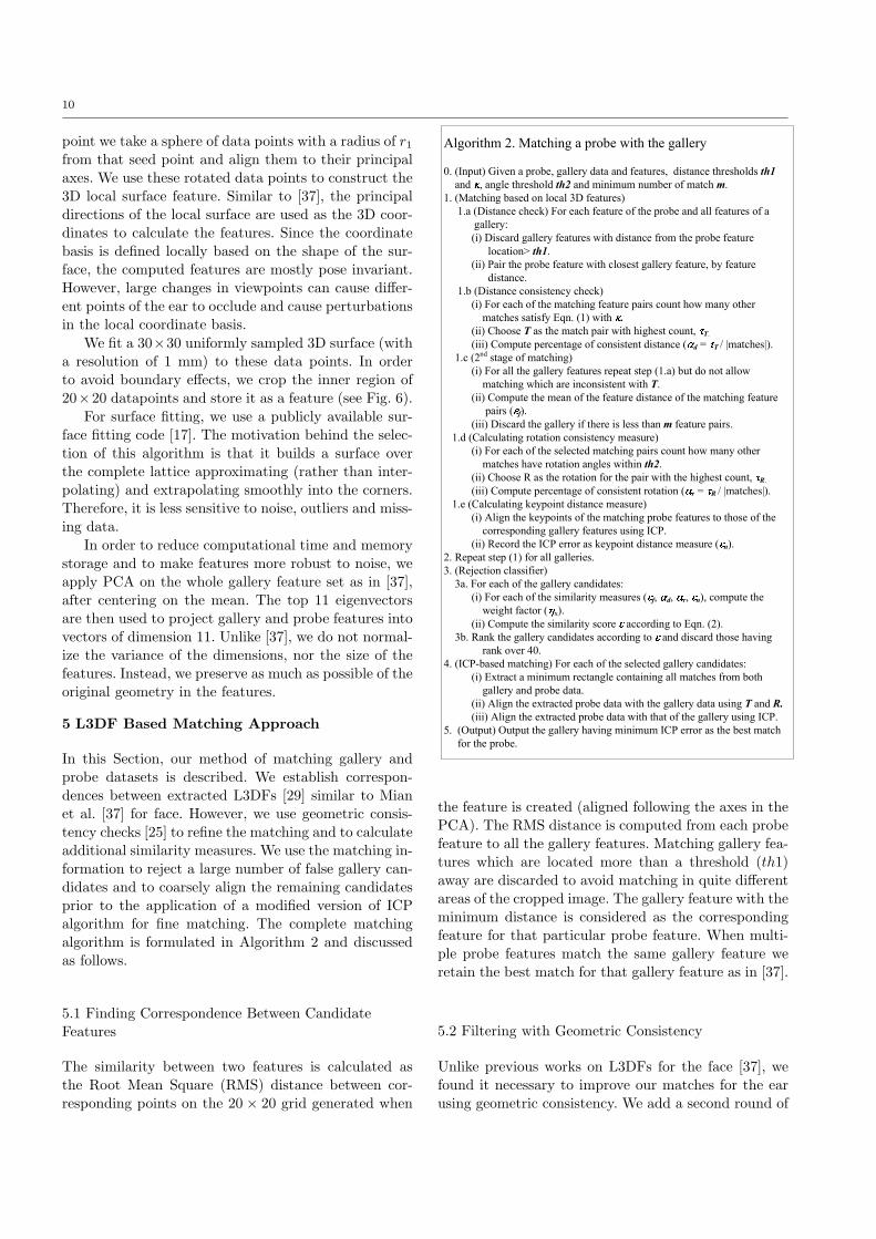
Algorithm 2. Matching a probe with the gallery

0. (Input) Given a probe, gallery data and features, distance thresholds th1

and , angle threshold th2 and minimum number of match m.

1. (Matching based on local 3D features)

1.a (Distance check) For each feature of the probe and all features of a

gallery:

(i) Discard gallery features with distance from the probe feature

location> th1.

(ii) Pair the probe feature with closest gallery feature, by feature

distance.

1.b (Distance consistency check)

(i) For each of the matching feature pairs count how many other

matches satisfy Eqn. (1) with .

(ii) Choose T as the match pair with highest count, T.

(iii) Compute percentage of consistent distance ( d = T / |matches|).

1.c (2nd stage of matching)

(i) For all the gallery features repeat step (1.a) but do not allow

matching which are inconsistent with T.

(ii) Compute the mean of the feature distance of the matching feature

pairs ( f).

(iii) Discard the gallery if there is less than m feature pairs.

1.d (Calculating rotation consistency measure)

(i) For each of the selected matching pairs count how many other

matches have rotation angles within th2.

(ii) Choose R as the rotation for the pair with the highest count, R. (iii) Compute percentage of consistent rotation ( r = R / |matches|).

1.e (Calculating keypoint distance measure)

(i) Align the keypoints of the matching probe features to those of the

corresponding gallery features using ICP.

(ii) Record the ICP error as keypoint distance measure ( n).

2. Repeat step (1) for all galleries.

3. (Rejection classifier)

3a. For each of the gallery candidates:

(i) For each of the similarity measures ( f, d, r, n), compute the

weight factor ( x).

(ii) Compute the similarity score according to Eqn. (2).

3b. Rank the gallery candidates according to and discard those having

rank over 40.

4. (ICP-based matching) For each of the selected gallery candidates:

(i) Extract a minimum rectangle containing all matches from both

gallery and probe data.

(ii) Align the extracted probe data with the gallery data using T and R.

(iii) Align the extracted probe data with that of the gallery using ICP.

5. (Output) Output the gallery having minimum ICP error as the best match

for the probe.

the feature is created (aligned following the axes in thePCA). The RMS distance is computed from each probefeature to all the gallery features. Matching gallery fea-tures which are located more than a threshold (th1)away are discarded to avoid matching in quite differentareas of the cropped image. The gallery feature with theminimum distance is considered as the correspondingfeature for that particular probe feature. When multi-ple probe features match the same gallery feature weretain the best match for that gallery feature as in [37].

5.2 Filtering with Geometric Consistency

Unlike previous works on L3DFs for the face [37], wefound it necessary to improve our matches for the earusing geometric consistency. We add a second round of

11

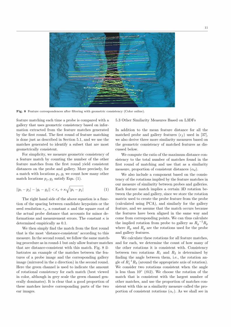
Fig. 8 Feature correspondences after filtering with geometric consistency (Color online).

feature matching each time a probe is compared with agallery that uses geometric consistency based on infor-mation extracted from the feature matches generatedby the first round. The first round of feature matchingis done just as described in Section 5.1, and we use thematches generated to identify a subset that are mostgeometrically consistent.

For simplicity, we measure geometric consistency ofa feature match by counting the number of the otherfeature matches from the first round yield consistentdistances on the probe and gallery. More precisely, fora match with locations pi, gi we count how many othermatch locations pj , gj satisfy Eqn. (1).

||pi − pj | − |gi − gj || < rs + κ√|pi − pj | (1)

The right hand side of the above equation is a func-tion of the spacing between candidate keypoints or theseed resolution rs, a constant κ and the square root ofthe actual probe distance that accounts for minor de-formations and measurement errors. The constant κ isdetermined empirically as 0.1.

We then simply find the match from the first roundthat is the most ‘distance-consistent’ according to thismeasure. In the second round, we follow the same match-ing procedure as in round-1 but only allow feature matchesthat are distance-consistent with this match. Fig. 8 il-lustrates an example of the matches between the fea-tures of a probe image and the corresponding galleryimage (mirrored in the z direction) in the second round.Here the green channel is used to indicate the amountof rotational consistency for each match (best viewedin color, although in grey scale the green channel gen-erally dominates). It is clear that a good proportion ofthese matches involve corresponding parts of the twoear images.

5.3 Other Similarity Measures Based on L3DFs

In addition to the mean feature distance for all thematched probe and gallery features (εf ) used in [37],we also derive three more similarity measures based onthe geometric consistency of matched features as dis-cussed below.

We compute the ratio of the maximum distance con-sistency to the total number of matches found in thefirst round of matching and use that as a similaritymeasure, proportion of consistent distances (αd).

We also include a component based on the consis-tency of the rotations implied by the feature matches inour measure of similarity between probes and galleries.Each feature match implies a certain 3D rotation be-tween the probe and gallery, since we store the rotationmatrix used to create the probe feature from the probe(calculated using PCA), and similarly for the galleryfeature, and we assume that the match occurs becausethe features have been aligned in the same way andcome from corresponding points. We can thus calculatethe implied rotation from probe to gallery as Rg

−1Rp

where Rp and Rg are the rotations used for the probeand gallery features.

We calculate these rotations for all feature matches,and for each, we determine the count of how many ofthe other rotations it is consistent with. Consistencybetween two rotations R1 and R2 is determined byfinding the angle between them, i.e., the rotation an-gle of R−1

1 R2 (around the appropriate axis of rotation).We consider two rotations consistent when the angleis less than 10◦ (th2). We choose the rotation of thematch that is consistent with the largest number ofother matches, and use the proportion of matches con-sistent with this as a similarity measure called the pro-portion of consistent rotations (αr). As we shall see in

12

Section 7, this measure is the strongest among the mea-sures used prior to applying ICP in our ear recognitionexperiments and fusing with the other measures pro-vides only a modest but worthwhile improvement. Wealso use the rotation with the highest consistency forICP coarse alignment as described in Section 5.6.

Lastly, we develop another similarity measure calledkeypoint distance measure (εn) based on the distancebetween the keypoints of the corresponding features. Tocompute it, we apply ICP only on the keypoints (notthe whole dataset) of the matched features (obtainedin the second round of matching). This corresponds tothe ‘graph node error’ described in Mian et al. [37] forthe face.

5.4 Building a Rejection Classifier

As in [37], the similarity measures (εf , αr, αd and εn)computed in the previous sub-section are first normal-ized on the scale from 0 to 1 and then combined usinga confidence weighted sum rule as shown in Eqn. (2).

ε = ηf εf + ηr(1− αr) + ηd(1− αd) + ηnεn (2)

The weight factors (ηf ,ηr,ηd,ηn) are dynamically com-puted individually for each probe during recognition asthe ratio between the minimum and second minimumvalues, taken relative to the mean value of the similaritymeasure for that probe [37]. Therefore, the weights re-flect the relative importance of the similarity measuresfor a particular probe based on the confidence in eachof them. Note that the second and the third similaritymeasures (αr and αd) are subtracted from unity beforemultiplication with the corresponding weight factor asthese have a polarity opposite to other measures (thehigher the values the better is the result).

We observe that the combination of these similaritymeasures provides an acceptable recognition rate andmost of the misclassified images are matched withinthe rank of 40 (see Section 7.7). Therefore, unlike [37],we use this combined classifier as a rejection classifierto discard the huge number of bad candidates retain-ing only the best 40 identities (sorted according to thisclassifier) for fine matching using ICP as described inthe following sections.

5.5 Extraction of a Minimal Rectangular Area

We extract a reduced rectangular region (containingall the matching features) from the originally detectedgallery and probe ear data. This region is identifiedusing the minimum and maximum co-ordinate valuesof the matched L3DFs. Fig. 9 illustrates this region

in comparison with other extraction windows (see Sec-tion 3.6).

Extended extraction window

used for feature extraction

Original detection window

Minimal extraction window

used for ICP

Fig. 9 Extraction of a minimal rectangular area containing allthe matching L3DFs.

L3DFs do not match from regions with occlusionor excessive missing data. By selecting a sub-windowwhere the L3DFs matches, such regions are generallyexcluded. Besides, this smaller but feature-rich regionreduces the processing time as described in Section 7.6.

5.6 Coarse Alignment of Gallery-Probe Pairs

The input profile images of the gallery and the probemay have pose (rotation and translation) variations.To minimize the effect of such variations, we apply thetransformation in Eqn. (3) to the minimal rectangulararea of the probe dataset.

P ′ = RP + t (3)

where, P and P ′ are the probe dataset before andafter the coarse alignment. We use the translation (t)corresponding to the matched pair with the maximumdistance consistency and the rotation (R) correspond-ing to the matched pair with the largest cluster of con-sistent rotations for this alignment. Our results show abetter performance with this approach compared to analternative of minimizing the sum of squared distancebetween points in the feature matches.

5.7 Fine Alignment with the ICP

The Iterative Closest Point (ICP) algorithm [4] is con-sidered to be one of the most accurate algorithms forregistration of two clouds of data points provided thedatasets are roughly aligned. We apply a modified ver-sion of ICP as described in [38]. The computationalexpense of ICP is minimized using the minimal rectan-gular area as described in Section 5.5. The final decisionregarding the matching is made based on the results ofICP.

13

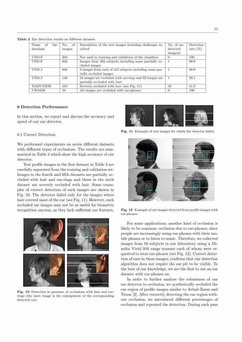
Table 2 Ear detection results on different datasets

Name of thedatabase

No. ofimages

Description of the test images including challenges in-volved

No. of un-detectedimage(s)

Detectionrate (%)

UND-F 203 Not used in training and validation of the classifiers 0 100

UND-F 942 Images from 302 subjects including some partially oc-cluded images

1 99.9

UND-J 830 2 images from each of 415 subjects including some par-tially occluded images

1 99.9

UND-J 146 54 images are occluded with earrings and 92 images arepartially occluded with hair

1 99.1

XM2VTSDB 104 Severely occluded with hair (see Fig. 11) 50 51.9

UWADB 50 All images are occluded with ear-phones 0 100

6 Detection Performance

In this section, we report and discuss the accuracy andspeed of our ear detector.

6.1 Correct Detection

We performed experiments on seven different datasetswith different types of occlusions. The results are sum-marized in Table 2 which show the high accuracy of ourdetector.

Test profile images in the first dataset in Table 2 arecarefully separated from the training and validation set.Images in the fourth and fifth datasets are partially oc-cluded with hair and ear-rings and those in the sixthdataset are severely occluded with hair. Some exam-ples of correct detection of such images are shown inFig. 10. The detector failed only for the images wherehair covered most of the ear (see Fig. 11). However, suchoccluded ear images may not be as useful for biometricrecognition anyway, as they lack sufficient ear features.

Fig. 10 Detection in presence of occlusions with hair and ear-rings (the inset image is the enlargement of the correspondingdetected ear).

Fig. 11 Example of test images for which the detector failed.

Fig. 12 Example of ear images detected from profile images withear-phones.

For some applications, another kind of occlusion islikely to be common: occlusion due to ear-phones, sincepeople are increasingly using ear-phones with their mo-bile phones or to listen to music. Therefore, we collectedimages from 50 subjects in our laboratory using a Mi-nolta Vivid 910 range scanner each of whom were re-quested to wear ear-phones (see Fig. 12). Correct detec-tion of ears in these images, confirms that our detectionalgorithm does not require the ear pit to be visible. Tothe best of our knowledge, we are the first to use an eardataset with ear-phones on.

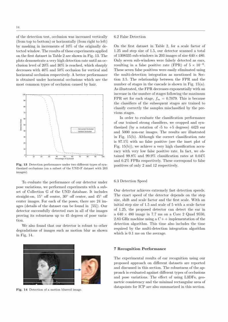
In order to further analyze the robustness of ourear detector to occlusion, we synthetically occluded theear region of profile images similar to Arbab-Zavar andNixon [3]. After correctly detecting the ear region with-out occlusion, we introduced different percentages ofocclusion and repeated the detection. During each pass

14

of the detection test, occlusion was increased vertically(from top to bottom) or horizontally (from right to left)by masking in increments of 10% of the originally de-tected window. The results of these experiments appliedon the first dataset in Table 2 are shown in Fig. 13. Theplots demonstrate a very high detection rate until an oc-clusion level of 20% and 30% is reached, which sharplydecreases with 40% and 50% occlusion for vertical andhorizontal occlusion respectively. A better performanceis obtained under horizontal occlusions which are themost common types of occlusion caused by hair.

0 10 20 30 40 50 60 70 80 90 1000

10

20

30

40

50

60

70

80

90

100

Det

ectio

n R

ate

Percentage of Occlusion

Horizontal OcclusionVertical Occlusion

Fig. 13 Detection performance under two different types of syn-thesized occlusions (on a subset of the UND-F dataset with 203images).

To evaluate the performance of our detector underpose variations, we performed experiments with a sub-set of Collection G of the UND database. It includesstraight-on, 15◦ off center, 30◦ off center, and 45◦ offcenter images. For each of the poses, there are 24 im-ages (details of the dataset can be found in [55]). Ourdetector successfully detected ears in all of the imagesproving its robustness up to 45 degrees of pose varia-tion.

We also found that our detector is robust to otherdegradations of images such as motion blur as shownin Fig. 14.

Fig. 14 Detection of a motion blurred image.

6.2 False Detection

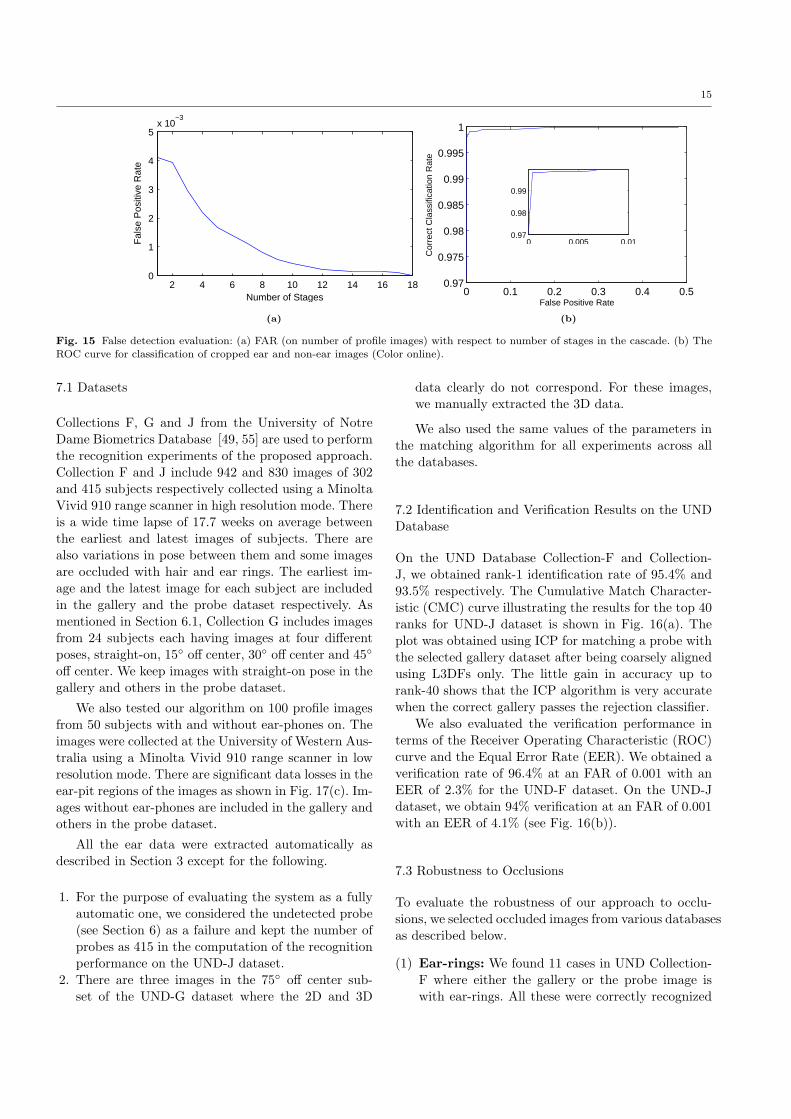
On the first dataset in Table 2, for a scale factor of1.25 and step size of 1.5, our detector scanned a totalof 1308335 sub-windows in 203 images of size 640×480.Only seven sub-windows were falsely detected as ears,resulting in a false positive rate (FPR) of 5 × 10−6.These seven false positives were easily eliminated usingthe multi-detection integration as mentioned in Sec-tion 3.5. The relationship between the FPR and thenumber of stages in the cascade is shown in Fig. 15(a).As illustrated, the FPR decreases exponentially with anincrease in the number of stages following the maximumFPR set for each stage, fm = 0.7079. This is becausethe classifiers of the subsequent stages are trained toclassify correctly the samples misclassified by the pre-vious stages.

In order to evaluate the classification performanceof our trained strong classifiers, we cropped and syn-thesized (by a rotation of -5 to +5 degrees) 4423 earand 5000 non-ear images. The results are illustratedin Fig. 15(b). Although the correct classification rateis 97.1% with no false positive (see the inset plot ofFig. 15(b)), we achieve a very high classification accu-racy with very low false positive rate. In fact, we ob-tained 99.8% and 99.9% classification rates at 0.04%and 0.2% FPRs respectively. These correspond to falsepositives of only 2 and 12 respectively.

6.3 Detection Speed

Our detector achieves extremely fast detection speeds.The exact speed of the detector depends on the stepsize, shift and scale factor and the first scale. With aninitial step size of 1.5 and scale of 5 with a scale factorof 1.25, the proposed detector can detect the ear ina 640 × 480 image in 7.7 ms on a Core 2 Quad 9550,2.83 GHz machine using a C ++ implementation of thedetection algorithm. This time also includes the timerequired by the multi-detection integration algorithmwhich is 0.1 ms on the average.

7 Recognition Performance

The experimental results of ear recognition using ourproposed approach on different datasets are reportedand discussed in this section. The robustness of the ap-proach is evaluated against different types of occlusionsand pose variations. The effect of using L3DFs, geo-metric consistency and the minimal rectangular area ofdatapoints for ICP are also summarized in this section.

15

2 4 6 8 10 12 14 16 180

1

2

3

4

5x 10

−3

Number of Stages

Fal

se P

ositi

ve R

ate

0 0.1 0.2 0.3 0.4 0.50.97

0.975

0.98

0.985

0.99

0.995

1

Cor

rect

Cla

ssifi

catio

n R

ate

False Positive Rate

0 0.005 0.010.97

0.98

0.99

(a) (b)

Fig. 15 False detection evaluation: (a) FAR (on number of profile images) with respect to number of stages in the cascade. (b) TheROC curve for classification of cropped ear and non-ear images (Color online).

7.1 Datasets

Collections F, G and J from the University of NotreDame Biometrics Database [49, 55] are used to performthe recognition experiments of the proposed approach.Collection F and J include 942 and 830 images of 302and 415 subjects respectively collected using a MinoltaVivid 910 range scanner in high resolution mode. Thereis a wide time lapse of 17.7 weeks on average betweenthe earliest and latest images of subjects. There arealso variations in pose between them and some imagesare occluded with hair and ear rings. The earliest im-age and the latest image for each subject are includedin the gallery and the probe dataset respectively. Asmentioned in Section 6.1, Collection G includes imagesfrom 24 subjects each having images at four differentposes, straight-on, 15◦ off center, 30◦ off center and 45◦

off center. We keep images with straight-on pose in thegallery and others in the probe dataset.

We also tested our algorithm on 100 profile imagesfrom 50 subjects with and without ear-phones on. Theimages were collected at the University of Western Aus-tralia using a Minolta Vivid 910 range scanner in lowresolution mode. There are significant data losses in theear-pit regions of the images as shown in Fig. 17(c). Im-ages without ear-phones are included in the gallery andothers in the probe dataset.

All the ear data were extracted automatically asdescribed in Section 3 except for the following.

1. For the purpose of evaluating the system as a fullyautomatic one, we considered the undetected probe(see Section 6) as a failure and kept the number ofprobes as 415 in the computation of the recognitionperformance on the UND-J dataset.

2. There are three images in the 75◦ off center sub-set of the UND-G dataset where the 2D and 3D

data clearly do not correspond. For these images,we manually extracted the 3D data.

We also used the same values of the parameters inthe matching algorithm for all experiments across allthe databases.

7.2 Identification and Verification Results on the UNDDatabase

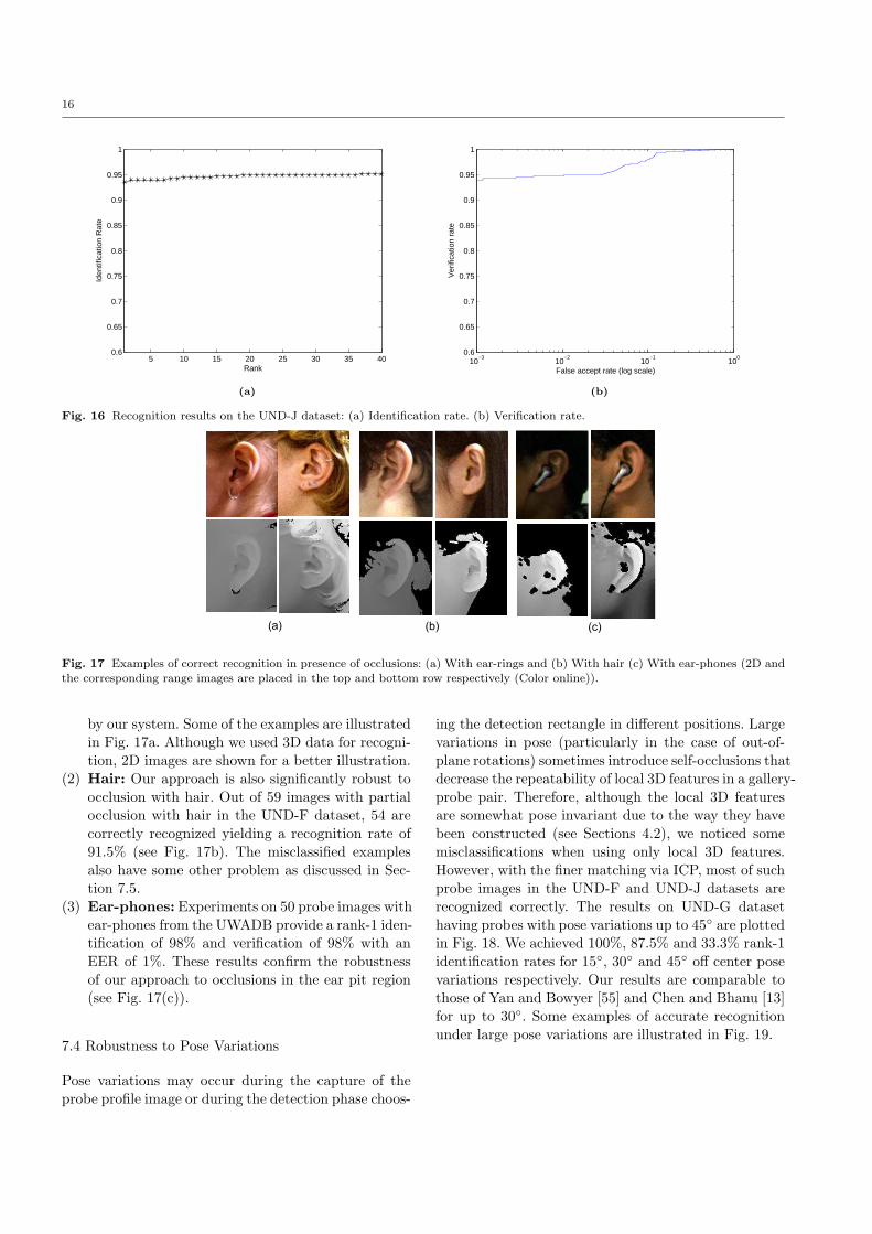
On the UND Database Collection-F and Collection-J, we obtained rank-1 identification rate of 95.4% and93.5% respectively. The Cumulative Match Character-istic (CMC) curve illustrating the results for the top 40ranks for UND-J dataset is shown in Fig. 16(a). Theplot was obtained using ICP for matching a probe withthe selected gallery dataset after being coarsely alignedusing L3DFs only. The little gain in accuracy up torank-40 shows that the ICP algorithm is very accuratewhen the correct gallery passes the rejection classifier.

We also evaluated the verification performance interms of the Receiver Operating Characteristic (ROC)curve and the Equal Error Rate (EER). We obtained averification rate of 96.4% at an FAR of 0.001 with anEER of 2.3% for the UND-F dataset. On the UND-Jdataset, we obtain 94% verification at an FAR of 0.001with an EER of 4.1% (see Fig. 16(b)).

7.3 Robustness to Occlusions

To evaluate the robustness of our approach to occlu-sions, we selected occluded images from various databasesas described below.

(1) Ear-rings: We found 11 cases in UND Collection-F where either the gallery or the probe image iswith ear-rings. All these were correctly recognized

16

5 10 15 20 25 30 35 400.6

0.65

0.7

0.75

0.8

0.85

0.9

0.95

1

Rank

Iden

tific

atio

n R

ate

10−3

10−2

10−1

100

0.6

0.65

0.7

0.75

0.8

0.85

0.9

0.95

1

False accept rate (log scale)

Ver

ifica

tion

rate

(a) (b)

Fig. 16 Recognition results on the UND-J dataset: (a) Identification rate. (b) Verification rate.

(a) (b) (c)

Fig. 17 Examples of correct recognition in presence of occlusions: (a) With ear-rings and (b) With hair (c) With ear-phones (2D andthe corresponding range images are placed in the top and bottom row respectively (Color online)).

by our system. Some of the examples are illustratedin Fig. 17a. Although we used 3D data for recogni-tion, 2D images are shown for a better illustration.

(2) Hair: Our approach is also significantly robust toocclusion with hair. Out of 59 images with partialocclusion with hair in the UND-F dataset, 54 arecorrectly recognized yielding a recognition rate of91.5% (see Fig. 17b). The misclassified examplesalso have some other problem as discussed in Sec-tion 7.5.

(3) Ear-phones: Experiments on 50 probe images withear-phones from the UWADB provide a rank-1 iden-tification of 98% and verification of 98% with anEER of 1%. These results confirm the robustnessof our approach to occlusions in the ear pit region(see Fig. 17(c)).

7.4 Robustness to Pose Variations

Pose variations may occur during the capture of theprobe profile image or during the detection phase choos-

ing the detection rectangle in different positions. Largevariations in pose (particularly in the case of out-of-plane rotations) sometimes introduce self-occlusions thatdecrease the repeatability of local 3D features in a gallery-probe pair. Therefore, although the local 3D featuresare somewhat pose invariant due to the way they havebeen constructed (see Sections 4.2), we noticed somemisclassifications when using only local 3D features.However, with the finer matching via ICP, most of suchprobe images in the UND-F and UND-J datasets arerecognized correctly. The results on UND-G datasethaving probes with pose variations up to 45◦ are plottedin Fig. 18. We achieved 100%, 87.5% and 33.3% rank-1identification rates for 15◦, 30◦ and 45◦ off center posevariations respectively. Our results are comparable tothose of Yan and Bowyer [55] and Chen and Bhanu [13]for up to 30◦. Some examples of accurate recognitionunder large pose variations are illustrated in Fig. 19.

17

0 15 30 450.2

0.4

0.6

0.8

1

Off center Pose Variation (in Degrees)

Ran

k−1

Iden

tific

atio

n R

ate

1 2 4 6 8 10 12 14 16 18 20 22 240.2

0.4

0.6

0.8

1

Rank

Iden

tific

atio

n R

ate

30 degrees off center45 Degree Off center

(a) (b)

Fig. 18 Recognition results on the UND-G dataset: (a) Identification rate for different off center pose variations. (b) CMC curves for30◦ and 45◦ off center pose variations.

(a) (b)

(c) (d)

Fig. 19 Examples of correct recognition of four gallery-probepairs with pose variations (Color online).

7.5 Analysis of the Failures

Most of the misclassifications that occurred in all ourexperiments involve missing data (inside or very closeto the ear contour) in either the gallery or the probe im-age. The remaining ones involve large out-of-plane posevariations and/or occlusions with hair. Some examplesare illustrated in Fig. 20.

(a) (b)

Fig. 20 Examples of failures: (a) Two probe images with missingdata. (b) A gallery-probe pair with a large pose variation.

7.6 Speed of Recognition

On a Core 2 Quad 9550, 2.83 GHz machine, an un-optimized MATLAB implementation of our feature ex-traction algorithm requires around 22.2 sec to extractlocal 3D features from a probe ear image. A similar im-plementation of our algorithm for matching 200 L3DFsof a probe with those in a gallery requires 0.06 sec onaverage. This includes 0.02 sec required by the compu-tation of geometric consistency measures. For the fullalgorithm, including L3DF as rejection classifier, fol-lowed by coarse alignment and ICP on a minimal rect-angle, the average time to match a probe-gallery pair inthe identification case is 2.28 sec on the UND dataset.Timing for different combinations of our recognition al-gorithms are given in Table 3.

7.7 Evaluation of L3DFs, Geometric ConsistencyMeasures and Minimal Rectangular Area of Dataset

We obtain improved accuracy and efficiency using thelocal 3D feature based rejection classifier and extract-ing the minimal rectangular area prior to the applica-tion of ICP. The improvements are summarized in Ta-ble 3 where numbers within parenthesis following thedatabase name are the number of images in the galleryand probe set respectively.

Results in the first row in the above-mentioned tableare computed using the same ICP implementation as inour final approach but without using L3DFs and corre-sponding minimal rectangular area of data points. Thewider detection window with hair and outliers and theabsence of proper initial transformation caused ICP toyield very poor results compared to our approach withL3DFs. In all the cases, our method is significantly moreefficient than the raw ICP algorithm.

As shown in Table 3, using geometric consistencymeasures improved the accuracy of identification sig-

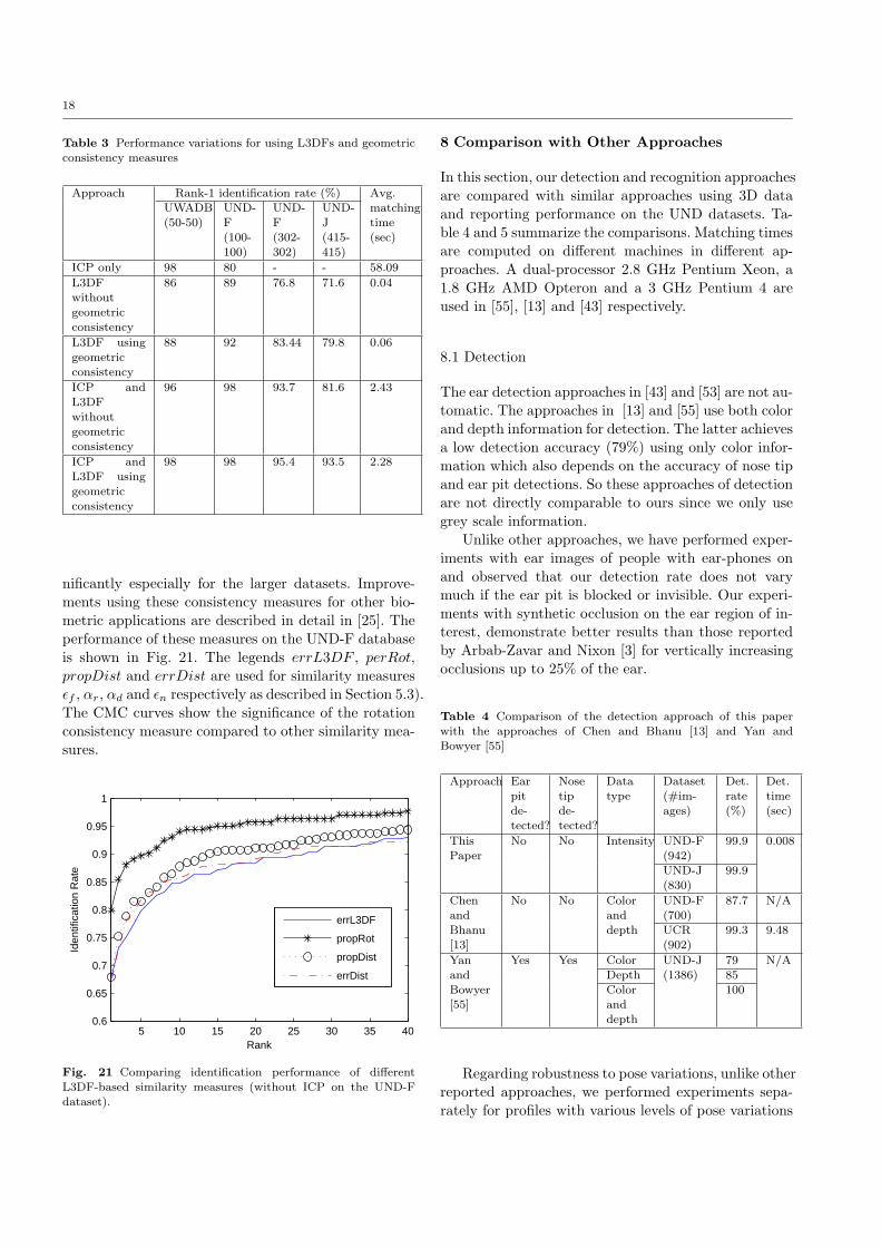
18

Table 3 Performance variations for using L3DFs and geometricconsistency measures

Approach Rank-1 identification rate (%) Avg.UWADB(50-50)

UND-F(100-100)

UND-F(302-302)

UND-J(415-415)

matchingtime(sec)

ICP only 98 80 - - 58.09

L3DFwithoutgeometricconsistency

86 89 76.8 71.6 0.04

L3DF usinggeometricconsistency

88 92 83.44 79.8 0.06

ICP andL3DFwithoutgeometricconsistency

96 98 93.7 81.6 2.43

ICP andL3DF usinggeometricconsistency

98 98 95.4 93.5 2.28

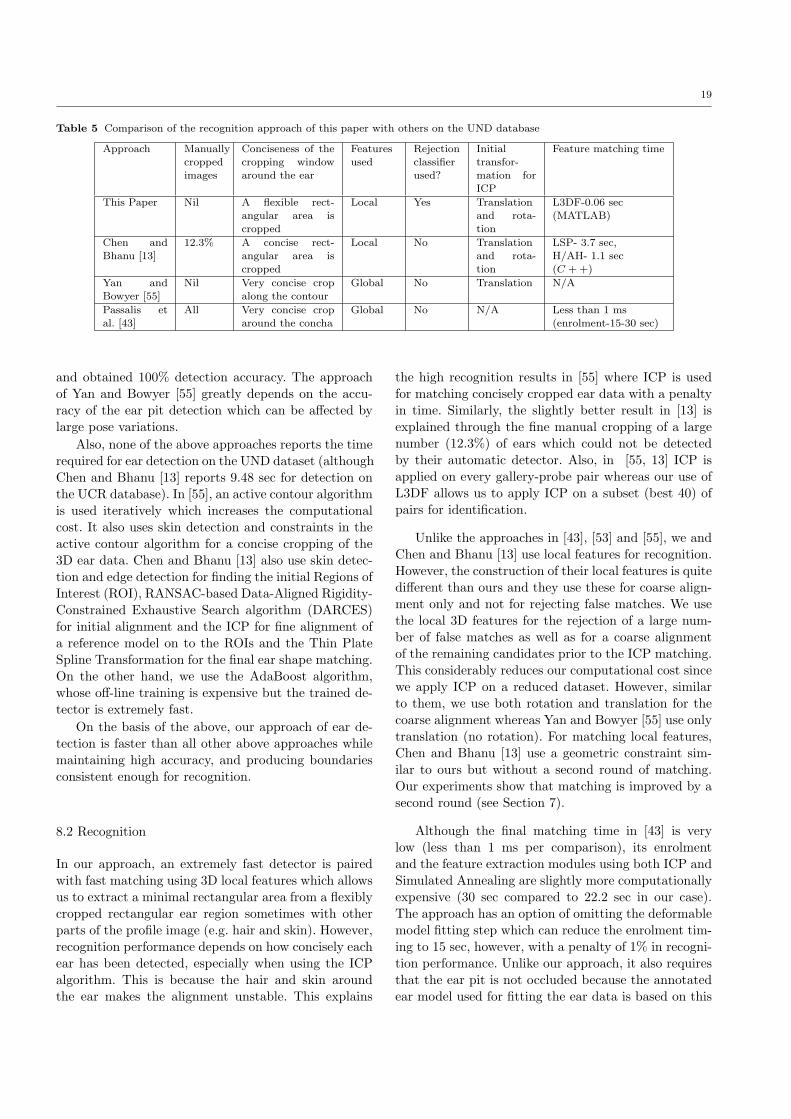
nificantly especially for the larger datasets. Improve-ments using these consistency measures for other bio-metric applications are described in detail in [25]. Theperformance of these measures on the UND-F databaseis shown in Fig. 21. The legends errL3DF , perRot,propDist and errDist are used for similarity measuresεf , αr, αd and εn respectively as described in Section 5.3).The CMC curves show the significance of the rotationconsistency measure compared to other similarity mea-sures.

5 10 15 20 25 30 35 400.6

0.65

0.7

0.75

0.8

0.85

0.9

0.95

1

Rank

Iden

tific

atio

n R

ate

errL3DF

propRot

propDist

errDist

Fig. 21 Comparing identification performance of differentL3DF-based similarity measures (without ICP on the UND-Fdataset).

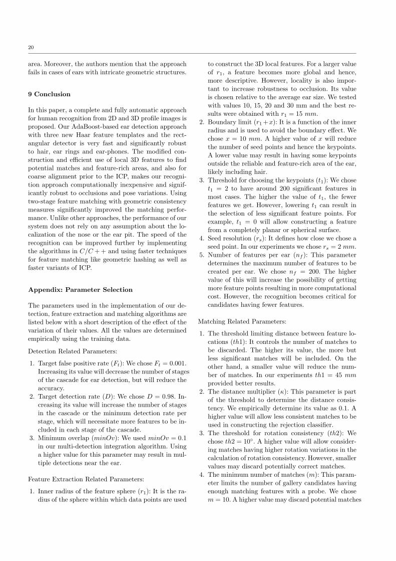
8 Comparison with Other Approaches

In this section, our detection and recognition approachesare compared with similar approaches using 3D dataand reporting performance on the UND datasets. Ta-ble 4 and 5 summarize the comparisons. Matching timesare computed on different machines in different ap-proaches. A dual-processor 2.8 GHz Pentium Xeon, a1.8 GHz AMD Opteron and a 3 GHz Pentium 4 areused in [55], [13] and [43] respectively.

8.1 Detection

The ear detection approaches in [43] and [53] are not au-tomatic. The approaches in [13] and [55] use both colorand depth information for detection. The latter achievesa low detection accuracy (79%) using only color infor-mation which also depends on the accuracy of nose tipand ear pit detections. So these approaches of detectionare not directly comparable to ours since we only usegrey scale information.

Unlike other approaches, we have performed exper-iments with ear images of people with ear-phones onand observed that our detection rate does not varymuch if the ear pit is blocked or invisible. Our experi-ments with synthetic occlusion on the ear region of in-terest, demonstrate better results than those reportedby Arbab-Zavar and Nixon [3] for vertically increasingocclusions up to 25% of the ear.

Table 4 Comparison of the detection approach of this paperwith the approaches of Chen and Bhanu [13] and Yan andBowyer [55]

Approach Earpitde-tected?

Nosetipde-tected?

Datatype

Dataset(#im-ages)

Det.rate(%)

Det.time(sec)

ThisPaper

No No Intensity UND-F(942)

99.9 0.008

UND-J(830)

99.9

Chenand

No No Colorand

UND-F(700)

87.7 N/A

Bhanu[13]

depth UCR(902)

99.3 9.48

Yan Yes Yes Color UND-J 79 N/Aand Depth (1386) 85Bowyer[55]

Coloranddepth

100

Regarding robustness to pose variations, unlike otherreported approaches, we performed experiments sepa-rately for profiles with various levels of pose variations

19

Table 5 Comparison of the recognition approach of this paper with others on the UND database

Approach Manuallycroppedimages

Conciseness of thecropping windowaround the ear

Featuresused

Rejectionclassifierused?

Initialtransfor-mation forICP

Feature matching time

This Paper Nil A flexible rect-angular area iscropped

Local Yes Translationand rota-tion

L3DF-0.06 sec(MATLAB)

Chen andBhanu [13]

12.3% A concise rect-angular area iscropped

Local No Translationand rota-tion

LSP- 3.7 sec,H/AH- 1.1 sec(C + +)

Yan andBowyer [55]

Nil Very concise cropalong the contour

Global No Translation N/A

Passalis etal. [43]

All Very concise croparound the concha

Global No N/A Less than 1 ms(enrolment-15-30 sec)

and obtained 100% detection accuracy. The approachof Yan and Bowyer [55] greatly depends on the accu-racy of the ear pit detection which can be affected bylarge pose variations.

Also, none of the above approaches reports the timerequired for ear detection on the UND dataset (althoughChen and Bhanu [13] reports 9.48 sec for detection onthe UCR database). In [55], an active contour algorithmis used iteratively which increases the computationalcost. It also uses skin detection and constraints in theactive contour algorithm for a concise cropping of the3D ear data. Chen and Bhanu [13] also use skin detec-tion and edge detection for finding the initial Regions ofInterest (ROI), RANSAC-based Data-Aligned Rigidity-Constrained Exhaustive Search algorithm (DARCES)for initial alignment and the ICP for fine alignment ofa reference model on to the ROIs and the Thin PlateSpline Transformation for the final ear shape matching.On the other hand, we use the AdaBoost algorithm,whose off-line training is expensive but the trained de-tector is extremely fast.

On the basis of the above, our approach of ear de-tection is faster than all other above approaches whilemaintaining high accuracy, and producing boundariesconsistent enough for recognition.

8.2 Recognition

In our approach, an extremely fast detector is pairedwith fast matching using 3D local features which allowsus to extract a minimal rectangular area from a flexiblycropped rectangular ear region sometimes with otherparts of the profile image (e.g. hair and skin). However,recognition performance depends on how concisely eachear has been detected, especially when using the ICPalgorithm. This is because the hair and skin aroundthe ear makes the alignment unstable. This explains

the high recognition results in [55] where ICP is usedfor matching concisely cropped ear data with a penaltyin time. Similarly, the slightly better result in [13] isexplained through the fine manual cropping of a largenumber (12.3%) of ears which could not be detectedby their automatic detector. Also, in [55, 13] ICP isapplied on every gallery-probe pair whereas our use ofL3DF allows us to apply ICP on a subset (best 40) ofpairs for identification.

Unlike the approaches in [43], [53] and [55], we andChen and Bhanu [13] use local features for recognition.However, the construction of their local features is quitedifferent than ours and they use these for coarse align-ment only and not for rejecting false matches. We usethe local 3D features for the rejection of a large num-ber of false matches as well as for a coarse alignmentof the remaining candidates prior to the ICP matching.This considerably reduces our computational cost sincewe apply ICP on a reduced dataset. However, similarto them, we use both rotation and translation for thecoarse alignment whereas Yan and Bowyer [55] use onlytranslation (no rotation). For matching local features,Chen and Bhanu [13] use a geometric constraint sim-ilar to ours but without a second round of matching.Our experiments show that matching is improved by asecond round (see Section 7).

Although the final matching time in [43] is verylow (less than 1 ms per comparison), its enrolmentand the feature extraction modules using both ICP andSimulated Annealing are slightly more computationallyexpensive (30 sec compared to 22.2 sec in our case).The approach has an option of omitting the deformablemodel fitting step which can reduce the enrolment tim-ing to 15 sec, however, with a penalty of 1% in recogni-tion performance. Unlike our approach, it also requiresthat the ear pit is not occluded because the annotatedear model used for fitting the ear data is based on this

20

area. Moreover, the authors mention that the approachfails in cases of ears with intricate geometric structures.

9 Conclusion

In this paper, a complete and fully automatic approachfor human recognition from 2D and 3D profile images isproposed. Our AdaBoost-based ear detection approachwith three new Haar feature templates and the rect-angular detector is very fast and significantly robustto hair, ear rings and ear-phones. The modified con-struction and efficient use of local 3D features to findpotential matches and feature-rich areas, and also forcoarse alignment prior to the ICP, makes our recogni-tion approach computationally inexpensive and signif-icantly robust to occlusions and pose variations. Usingtwo-stage feature matching with geometric consistencymeasures significantly improved the matching perfor-mance. Unlike other approaches, the performance of oursystem does not rely on any assumption about the lo-calization of the nose or the ear pit. The speed of therecognition can be improved further by implementingthe algorithms in C/C + + and using faster techniquesfor feature matching like geometric hashing as well asfaster variants of ICP.

Appendix: Parameter Selection

The parameters used in the implementation of our de-tection, feature extraction and matching algorithms arelisted below with a short description of the effect of thevariation of their values. All the values are determinedempirically using the training data.

Detection Related Parameters:

1. Target false positive rate (Ft): We chose Ft = 0.001.Increasing its value will decrease the number of stagesof the cascade for ear detection, but will reduce theaccuracy.

2. Target detection rate (D): We chose D = 0.98. In-creasing its value will increase the number of stagesin the cascade or the minimum detection rate perstage, which will necessitate more features to be in-cluded in each stage of the cascade.

3. Minimum overlap (minOv): We used minOv = 0.1in our multi-detection integration algorithm. Usinga higher value for this parameter may result in mul-tiple detections near the ear.

Feature Extraction Related Parameters:

1. Inner radius of the feature sphere (r1): It is the ra-dius of the sphere within which data points are used

to construct the 3D local features. For a larger valueof r1, a feature becomes more global and hence,more descriptive. However, locality is also impor-tant to increase robustness to occlusion. Its valueis chosen relative to the average ear size. We testedwith values 10, 15, 20 and 30 mm and the best re-sults were obtained with r1 = 15 mm.

2. Boundary limit (r1 +x): It is a function of the innerradius and is used to avoid the boundary effect. Wechose x = 10 mm. A higher value of x will reducethe number of seed points and hence the keypoints.A lower value may result in having some keypointsoutside the reliable and feature-rich area of the ear,likely including hair.

3. Threshold for choosing the keypoints (t1): We choset1 = 2 to have around 200 significant features inmost cases. The higher the value of t1, the fewerfeatures we get. However, lowering t1 can result inthe selection of less significant feature points. Forexample, t1 = 0 will allow constructing a featurefrom a completely planar or spherical surface.

4. Seed resolution (rs): It defines how close we chose aseed point. In our experiments we chose rs = 2 mm.

5. Number of features per ear (nf ): This parameterdetermines the maximum number of features to becreated per ear. We chose nf = 200. The highervalue of this will increase the possibility of gettingmore feature points resulting in more computationalcost. However, the recognition becomes critical forcandidates having fewer features.

Matching Related Parameters:

1. The threshold limiting distance between feature lo-cations (th1): It controls the number of matches tobe discarded. The higher its value, the more butless significant matches will be included. On theother hand, a smaller value will reduce the num-ber of matches. In our experiments th1 = 45 mm

provided better results.2. The distance multiplier (κ): This parameter is part

of the threshold to determine the distance consis-tency. We empirically determine its value as 0.1. Ahigher value will allow less consistent matches to beused in constructing the rejection classifier.

3. The threshold for rotation consistency (th2): Wechose th2 = 10◦. A higher value will allow consider-ing matches having higher rotation variations in thecalculation of rotation consistency. However, smallervalues may discard potentially correct matches.

4. The minimum number of matches (m): This param-eter limits the number of gallery candidates havingenough matching features with a probe. We chosem = 10. A higher value may discard potential matches

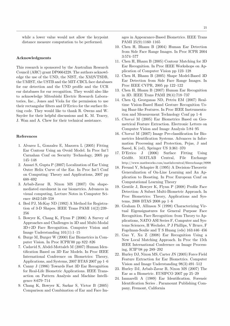
21

while a lower value would not allow the keypointdistance measure computation to be performed.

Acknowledgments

This research is sponsored by the Australian ResearchCouncil (ARC) grant DP0664228. The authors acknowl-edge the use of the UND, the NIST, the XM2VTSDB,the UMIST, the USTB and the MIT-CBCL face databasesfor ear detection and the UND profile and the UCRear databases for ear recognition. They would also liketo acknowledge Mitsubishi Electric Research Labora-tories, Inc., Jones and Viola for the permission to usetheir rectangular filters and D’Errico for the surface fit-ting code. They would like to thank R. Owens and W.Snyder for their helpful discussions and K. M. Tracey,J. Wan and A. Chew for their technical assistance.

References

1. Alvarez L, Gonzalez E, Mazorra L (2005) FittingEar Contour Using an Ovoid Model. In Proc Int’lCarnahan Conf on Security Technology, 2005 pp145–148

2. Ansari S, Gupta P (2007) Localization of Ear UsingOuter Helix Curve of the Ear. In Proc Int’l Confon Computing: Theory and Applications, 2007 pp688–692

3. Arbab-Zavar B, Nixon MS (2007) On shape-mediated enrolment in ear biometrics. Advances invisual computing, Lecture Notes in Computer Sci-ence 4842:549–558

4. Besl PJ, McKay ND (1992) A Method for Registra-tion of 3-D Shapes. IEEE Trans PAMI 14(2):239–256

5. Bowyer K, Chang K, Flynn P (2006) A Survey ofApproaches and Challenges in 3D and Multi-Modal3D+2D Face Recognition. Computer Vision andImage Understanding 101(1):1–15

6. Burge M, Burger W (2000) Ear Biometrics in Com-puter Vision. In Proc ICPR’00 pp 822–826

7. Cadavid S, Abdel-Mottaleb M (2007) Human Iden-tification Based on 3D Ear Models. In Proc IEEEInternational Conference on Biometrics: Theory,Applications, and Systems, 2007 BTAS 2007 pp 1–6

8. Canny J (1986) Towards Fast 3D Ear Recognitionfor Real-Life Biometric Applications. IEEE Trans-action on Pattern Analysis and Machine Intelli-gence 8:679–714

9. Chang K, Bowyer K, Sarkar S, Victor B (2005)Comparison and Combination of Ear and Face Im-

ages in Appearance-Based Biometrics. IEEE TransPAMI 25(9):1160–1165

10. Chen H, Bhanu B (2004) Human Ear Detectionfrom Side Face Range Images. In Proc ICPR 20043:574–577

11. Chen H, Bhanu B (2005) Contour Matching for 3DEar Recognition. In Proc IEEE Workshops on Ap-plication of Computer Vision pp 123–128

12. Chen H, Bhanu B (2005) Shape Model-Based 3DEar Detection from Side Face Range Images. InProc IEEE CVPR, 2005 pp 122–122

13. Chen H, Bhanu B (2007) Human Ear Recognitionin 3D. IEEE Trans PAMI 29(4):718–737

14. Chen Q, Georganas ND, Petriu EM (2007) Real-time Vision-Based Hand Gesture Recognition Us-ing Haar-like Features. In Proc IEEE Instrumenta-tion and Measurement Technology Conf pp 1–6

15. Choras M (2005) Ear Biometrics Based on Geo-metrical Feature Extraction. Electronic Letters onComputer Vision and Image Analysis 5:84–95

16. Choras M (2007) Image Pre-classification for Bio-metrics Identification Systems. Advances in Infor-mation Processing and Protection, Pejas, J andSaeed, K (ed), Springer US 3:361–370

17. D’Errico J (2006) Surface Fitting UsingGridfit. MATLAB Central, File Exchangehttp://www.mathworks.com/matlabcentral/fileexchange/8998

18. Freund Y, Schapire R (1995) A Decision-TheoreticGeneralization of On-Line Learning and An Ap-plication to Boosting. In Proc European Conf onComputational Learning Theory

19. Gentile J, Bowyer K, Flynn P (2008) Profile FaceDetection: A Subset Multi-Biometric Approach. InProc Biometrics: Theory, Applications and Sys-tems, 2008 BTAS 2008 pp 1–6

20. Graham D, Allinson N (1998) Characterizing Vir-tual Eigensignatures for General Purpose FaceRecognition. Face Recognition: from Theory to Ap-plications, NATO ASI Series F, Computer and Sys-tems Sciences, H Wechsler, P J Phillips, V Bruce, FFogelman-Soulie and T S Huang (eds) 163:446–456

21. Guo Y, Xu Z (2008) Ear Recognition Using aNew Local Matching Approach. In Proc the 15thIEEE International Conference on Image Process-ing, ICIP’08 pp 289–292

22. Hurley DJ, Nixon MS, Carter JN (2005) Force FieldFeature Extraction for Ear Biometrics. ComputerVision and Image Understanding 98(3):491–512

23. Hurley DJ, Arbab-Zavar B, Nixon MS (2007) TheEar as a Biometric. EUSIPCO 2007 pp 25–29

24. Iannarelli A (1989) Ear Identification. ForensicIdentification Series . Paramount Publishing Com-pany, Fremont, California

22

25. Islam S, Davies R (2009) Refining Local 3D Fea-ture Matching through Geometric Consistency forRobust Biometric Recognition. Proc Digital ImageComputing: Techniques and Applications (DICTA)pp 513–518

26. Islam S, Bennamoun M, Davies R (2008) Fast andFully Automatic Ear Detection Using CascadedAdaBoost. In Proc IEEE Workshop on Applicationof Computer Vision pp 1–6

27. Islam S, Bennamoun M, Mian A, Davies R (2008) AFully Automatic Approach for Human Recognitionfrom Profile Images Using 2D and 3D Ear Data.Proc 3DPVT pp 131–141

28. Islam S, Bennamoun M, Owens R, Davies R (2008)Biometric Approaches of 2D-3D Ear and Face: ASurvey. Advances in Computer and InformationSciences and Engineering, T Sobh(ed), SpringerNetherlands pp 509–514

29. Islam S, Davies R, Mian A, Bennamoun M (2008)A Fast and Fully Automatic Ear Recognition Ap-proach Based on 3D Local Surface Features. JBlanc-Talon et al (Eds): ACIVS 2008, LNCS 5259,Springer, Heidelberg pp 1081–1092

30. Jain AK, Ross A, Prabhakar S (2004) An introduc-tion to biometric recognition. IEEE Trans Circuitsand Systems for Video Technology 14(1):4–20

31. Jain AK, Ross A, Pankanti S (2006) Biometrics: ATool For Information Security. IEEE Trans Infor-mation Forensics and Security 1(2):125–143

32. Jones M, Viola P (2003) Fast Multi-view Face De-tection. Technical Report TR2003-96, MERL

33. Kepner J (2004) MatlabMPI. Journal of Paralleland Distributed Computing 64(8):997–1005

34. Lienhart R, Liang L, Kuranov A (2003) A DetectorTree of Boosted Classifiers for Real-Time ObjectDetection and Tracking. In Proc the Int’l Conf onMultimedia and Expo, 2003 ICME ’03 2:277–280

35. Lu L, Zhang X, Zhao Y, Jia Y (2007) Human Iden-tification Based on 3D Ear Models. In Proc Inter-national Conference on Innovative Computing, In-formation and Control, 2006 ICICIC ’06 3:353–356

36. Messer K, Matas J, Kittler J, Luettin J,Maitre G (1999) XM2VTSbd: The ExtendedM2VTS Database. In Proc the 2nd Conf on Au-dio and Video-base Biometric Personal Verifica-tion, Springer Verlag, New York pp 1–6, URLhttp://www.ee.surrey.ac.uk/Research/VSSP/xm2vtsdb

37. Mian A, Bennamoun M, Owens R (2008) KeypointDetection and Local Feature Matching for Tex-tured 3D Face Recognition. International Journalof Computer Vision 79(1):1–12

38. Mian AS, Bennamoun M, Owens R (2007) AnEfficient Multimodal 2D-3D Hybrid Approach to

Automatic Face Recognition. IEEE Trans PAMI29(11):1927–1943

39. MIT-CBCL (2004) MIT-CBCL Face RecognitionDatabase.http://cbcl.mit.edu/software-

datasets/heisele/facerecognition-database.html

40. Monteiro G, Peixoto P, Nunes U (2006) Vision-Based Pedestrian Detection using Haar-Like fea-tures. Robotica 2006-Scientific meeting of the 6thRobotics Portuguese Festival,Portugal

41. NIST-MID (1994) NIST Mugshot IdentificationDatabase (MID).http://www.nist.gov/srd/nistsd18.htm

42. Niu Z, Shan S, Yan S, Chen X, Gao W (2006) 2DCascaded AdaBoost for Eye Localization. In ProcICPR 2006 2:1216–1219

43. Passalis G, Kakadiaris I, Theoharis T, Toderici G,Papaioannou T (2007) Towards Fast 3D Ear Recog-nition for Real-Life Biometric Applications. In ProcIEEE Conference on Advanced Video and SignalBased Surveillance, 2007 AVSS 2007 3:39–44

44. Pun KH, Moon YS (2004) Recent Advances in EarBiometrics. In Proc IEEE Int’l Conf on AutomaticFace and Gesture Recognition pp 164–169

45. Ross A, Jain AK (2004) Multimodal Biometrics:An Overview. In Proc European Signal ProcessingConf pp 1221–1224

46. Simard P, Bottou L, Haffner P, LeCun Y (1999)A Fast Convolution Algorithm for Signal Process-ing and Neural Networks, M. Kearns, S. Solla, andD. Cohn (Eds.). Advances in Neural InformationProcessing Systems, 11:571– 577

47. Treptow A, Zell A (2004) Real-time Object Track-ing for Soccerrobots without Color Information.Robotics and Autonomous Systems 48(1):41–48

48. UMIST (2002) The UMIST Face Database.http://images.ee.umist.ac.uk/danny/database.html

49. UND (2005) University of Notre Dame BiometricsDatabase.http://www.nd.edu/ cvrl/CVRL/Data Sets.html

50. USTB (2002) USTB Ear Database.http://www.en.ustb.edu.cn/resb/

51. Viola P, Jones M (2004) Robust Real-TimeFace Detection. Int’l Journal of Computer Vision57(2):137–154

52. Weyrauch B, Huang J, Heisele B, Blanz V (2004)Component-Based Face Recognition with 3D Mor-phable Models. In: First IEEE Workshop on FaceProcessing in Video, Washington, D.C.

53. Yan P, Bowyer KW (2005) Ear Biometrics Using2D and 3D Images. In Proc CVPR pp 121–121

54. Yan P, Bowyer KW (2005) Empirical Evaluation ofAdvanced Ear Biometrics. In Proc CVPR pp 41–41

23

55. Yan P, Bowyer KW (2007) Biometric Recogni-tion Using 3D Ear Shape. IEEE Trans PAMI29(8):1297–1308

56. Yuizono T, Wang Y, Satoh K, Nakayama S (2002)Study on Individual Recognition for Ear Images byUsing Genetic Local search. In Proc Congress onEvolutionary Computation pp 237–242

57. Zhang HJ, Mu ZC, Qu W, Liu LM, Zhang CY(2005) A Novel Approach for Ear RecognitionBased on ICA and RBF Network. In Proc Int’lConf on Machine Learning and Cybernetics, 2005pp 4511–4515

58. Zhao W, Chellappa R, Rosenfeld A, Phillips P(2003) Face Recognition: A Literature Survey.ACM Computing Surveys pp 399–458