Recognition of Human Body Posture from a Cloud of 3D Data Points using Wavelet Transform...

Pattern Recognition Letters 26 (2005) 663–677

www.elsevier.com/locate/patrec

A discriminative 3D wavelet-based descriptors: Applicationto the recognition of human body postures

Naoufel Werghi

College of Information Technology, Dubai University College, P.O. Box 14143, Dubai, United Arab Emirates

Received 22 October 2003; received in revised form 31 August 2004

Abstract

This paper deals with the recognition of human body postures from a cloud of 3D points acquired by a human body

scanner. Motivated by finding a representation that embodies a high power of discrimination between posture classes, a

new type of 3D shape descriptors is suggested, namely wavelet transform coefficients (WC). These features can be seen

as an extension to 3D of the 2D wavelet shape descriptors developed by (Shen, D., Ip, H.H.S., 1999. Pattern Recog-

nition, 32, 151–165). The WC is compared with other 3D shape descriptors, within a Bayesian classification framework.

Experiments with real scan data show that the WC outperforms other standard 3D shape descriptors in terms of dis-

crimination power and classification rate.

� 2004 Elsevier B.V. All rights reserved.

Keywords: 3D Human body scan data; 3D Human posture recognition; 3D Shape descriptors; Wavelet transform; Bayesian

classification

1. Introduction

The emergence of 3D imaging technology that

enables full scanning of the human body surface

with reasonable measurement accuracy and

acceptable computational cost is a recent phenom-enon. This advance facilitates the exploitation of

the human body form in various areas such as

anthropometrical research (e.g., Jones and Rioux,

0167-8655/$ - see front matter � 2004 Elsevier B.V. All rights reserv

doi:10.1016/j.patrec.2004.09.018

E-mail address: [email protected]

1997; Paquet et al., 2000), clothing design (e.g.,

Jones et al., 1995; Pargas et al., 1996; Dekker

et al., 1998; Cordier et al., 2003) and virtual human

animation (e.g., Sun et al., 2001; Starck et al.,

2002). The raw data delivered by the human body

scanner requires substantial main memory andback-up storage resources but it contains too little

semantic information to be useful for potential

applications. The recognition of body posture

has a major role in many applications requiring

automatic processing of the scanner data. Auto-

matic segmentation techniques of the human body

ed.

mailto:[email protected]

664 N. Werghi / Pattern Recognition Letters 26 (2005) 663–677

scanner data usually use prior information on the

human body posture (e.g., Dekker et al., 1998;

Cordier et al., 2003; Xiao et al., 2003). Applica-

tions that exploit scanned human body data in

TV and cinema production involve the fitting ofa generic model to the scanned data to obtain a

realistic model that, for instance, can be integrated

into a movie sequence. Here, the identification of

the posture from the scanner data is useful as a

good initialization for iterative techniques that

may be involved in the fitting algorithm, in partic-

ular to guarantee and accelerate the convergence

of the algorithm.The work presented in this paper describes a

method of recognizing human body postures from

3D scanner data by adopting a model-based ap-

proach. The problem is stated as follows. Given

a set of posture models and a query posture, find

which posture model corresponds to the query

posture. The paradigm followed to solve this prob-

lem is built upon three premises: representation,feature extraction and classification. The emphasis

in this paper is on representation and feature

extraction.

2. Representation

In shape recognition techniques, objects arerepresented by numerical features, which are

grouped into vectors, to remove data redundancy

and reduce data dimension. The data we deal with

consist of scattered 3D points that represent the

surface shape of the human body. Most of the

human body scanners provide a complete data set

that covers the entire body surface. This encour-

ages investigation of global features that can beexploited in 3D shape identification. Moments as

global 2D shape features have been used exten-

sively in image analysis and description. Attention

has been mainly oriented towards moments that

are invariant with respect to translation, rotation

and scale. Such moments were first proposed by

Hu (1962). After that, a variety of moments were

developed. Examples include, statistical moments(Chim et al., 1999), orthogonal moments, such as

Legendre moments, Fourier–Mellin moments,

Zernike moments and pseudo-Zernike moments.

It has been shown that orthogonal moments are

less redundant, less sensitive to noise and more

informative than geometrical moments (Teague,

1980). A good survey of 2D moments can be found

in (Teh and Chin, 1988) and (Belkassim et al.,1991). However, less study has been done of the

3D case. One reason for this is that most of the

3D imaging devices do not provide a complete

data set in terms of surface coverage. Being sensi-

tive to missing data and occlusions, global features

are not suitable for such cases. Nevertheless, there

have been some attempts to define frameworks for

the construction of 3D moments. Sadjadi andHall (1980) pioneered the development of 3D geo-

metric moment invariants. Their framework built

a family of three invariant moments with degrees

up to the second order. Using complex moments,

Lo and Don (1989) constructed a family of 12

invariant moments with orders up to the third de-

gree. Their moments were mainly used to estimate

3D transformations and their performance wasnot assessed for classification. In addition, these

moments are not derived from a family of

orthogonal functions, and they are therefore sub-

ject to correlation and redundancy. Motivated

rather by computational efficiency, Sheynin and

Tuzikov (2001) proposed a computational frame-

work for the calculation of Cartesian moments.

However, their approach is restricted to polyhe-dral objects. The desirable properties of orthogo-

nal moments, in terms of sensitivity to noise and

information redundancy, motivated the develop-

ment of families of orthogonal 3D moments.

Examples include 3D Zernike moments (Cantera-

kis, 1997) and 3D Haar moments (Schael, 1997).

These efforts, however, did not provide experimen-

tal frameworks for testing these moments. 3Dshape descriptors based on the 3D discrete Fourier

Transform were proposed by Vranic and Saupe

(2001) for model retrieval applications. However,

the discriminative power of this type of feature

was not assessed.

In this work, we present a new family of 3D

shape descriptors, namely the wavelet-based

descriptors. The performance of these features isevaluated and compared with 3D Zernike mo-

ments and 3D Fourier descriptors. In a previous

study Werghi and Xiao (2002), it was shown that

N. Werghi / Pattern Recognition Letters 26 (2005) 663–677 665

3D geometric moments proposed by Lo et al.

(1998) are far less powerful than the wavelet-based

3D shaped descriptors in terms of their discrimina-

tive capabilities.

2.1. Wavelet-based representation

The wavelet was introduced by Morlet and

Grossman (1984) as a time-scale analysis tool for

non-stationary signals. It was further developed

by many authors (e.g., Mallat, 1989; Daubechies,

1990; Meyer, 1997; Jaffard et al., 2001) and rapidly

found applications in many areas. A wavelet func-tion is a function that is well localized in the space

and frequency domains. From a mother function

w(r), a family of wavelet functions

wa;bðrÞ ¼1

aw

r � ba

� �; a > 0

is derived. This family is obtained by shifting the

wavelet mother by b (the shifting parameter) and

by dilating (stretching) it with a (the scaling

parameter). The wavelet transform at the scale a

and shift b isZ 1

�1f ðrÞwa;bðrÞdr

The wavelet transform embodies information

about the regularity and the spectrum of the fre-

quency around the position b at the scale a. Fromthis perspective, it is a local operator. However, by

varying the parameter b along the domain of the

function f(r), a global description of the function

can be obtained. Consider f(r,h,/), a 3D binary

representation for the cloud of 3D data points in

spherical coordinates, which in its discrete form,

can be seen as spherical voxel representation of

the 3D data.In order to analyse the distribution of the cloud

of points over the space (r,h,/), the following

function is used:

F ðrÞm;n ¼Z 2p

0

Z p

0

f ðr; h;/ÞUm;nðh;/Þr2 sin hdhd/;

0 6 m 6 n ð1Þ

This function integrates the distribution

f(r,h,/)Um,n(h,/) over the sphere of radius r.

Um,n, 0 6 m 6 n are the set of spherical harmonics

of order m and n. These functions are defined on

the unit sphere and form an orthogonal family

(Ferrers, 1877). Their expression is Um,n =

ejm/Vn(h), where Vn(h) is a polynomial functionof order n in cosh and sinh.

F(r)m,n 0 6 m 6 n, represent the projections of

the distribution f(r,h,/) over the space of the

spherical harmonics. Therefore, they describe the

spectrum of f(r,h,/) with respect to h and /. Tomake the description of the distribution complete,

we must also analyse the set F(r)m,n in terms of

the radius r. For this, we propose wavelet-basedanalysis in which the function F(r)m,n is projected

on an orthogonal family of wavelet functions.

The set of projections forms a unique representa-

tion of F(r)m,n and therefore of the distribution

f(r,h,/). From that set, a group of features are

selected according to the criteria described in Sec-

tion 3.1.

Consider the projections of F(r)m,n on the familyof wavelet functions wa,b.

Cm;na;b ¼

Z 1

0

F ðrÞm;nwa;bðrÞdr

¼Z 1

0

Z 2p

0

Z p

0

f ðr; h;/Þwa;bðrÞejm/V nðhÞr2

� sin hdhd/dr ð2Þ

Cm;na;b , also called the wavelet transform coefficients,

represent according to (2) the projections of the

distribution f(r,h,/) on the orthogonal family

Lm;na;b ¼ wa;bðrÞUm;nðh;/Þ. It can be shown that:

hLm;na;b ; ðL

m0 ;n0

a0 ;b0 Þi ¼ Kdaa0dbb0dmm0dnn0 , where * denote

the complex conjugate, d is the Kroneker symbol

(dij = 1 if i = j, 0 otherwise) and K is a constant.

Therefore, the coefficients Cm;na;b can be seen as a

special type of 3D moments derived from the

orthogonal family Lm;na;b . The orthogonal wavelet

family we used is built with the Meyer�s wavelet

(Meyer, 1997). In addition to their orthogonality,

Meyer�s wavelet family exhibit high regularity in

both the space and frequency domains. Because

Cm;na;b is a complex entity, the feature considered

here is rather its norm defined asffiffiffiffiffiffiffiffiffiffiffiffiffiffiffiffiffiffiffiffiffiffiffiffiffiffiffiffiffiffihCm;n

a;b ; ðCm0;n0

a0;b0 Þi

q.


2.2. Feature invariance

For translation and scale invariance, the human

body scan data is first rasterized into a voxel grid.

Then the centre of mass of the scan data is alignedwith the centre of the grid. The scale invariance is

obtained by scaling the 3D points� coordinates sothat the data volume defined by the moment

m000 ¼P

x

Py

Pzf ðx; y; zÞ is equal to V0, where

V0 is a predetermined value.

For the rotational invariance, we must know

that, within the scanner device, the rotation of the

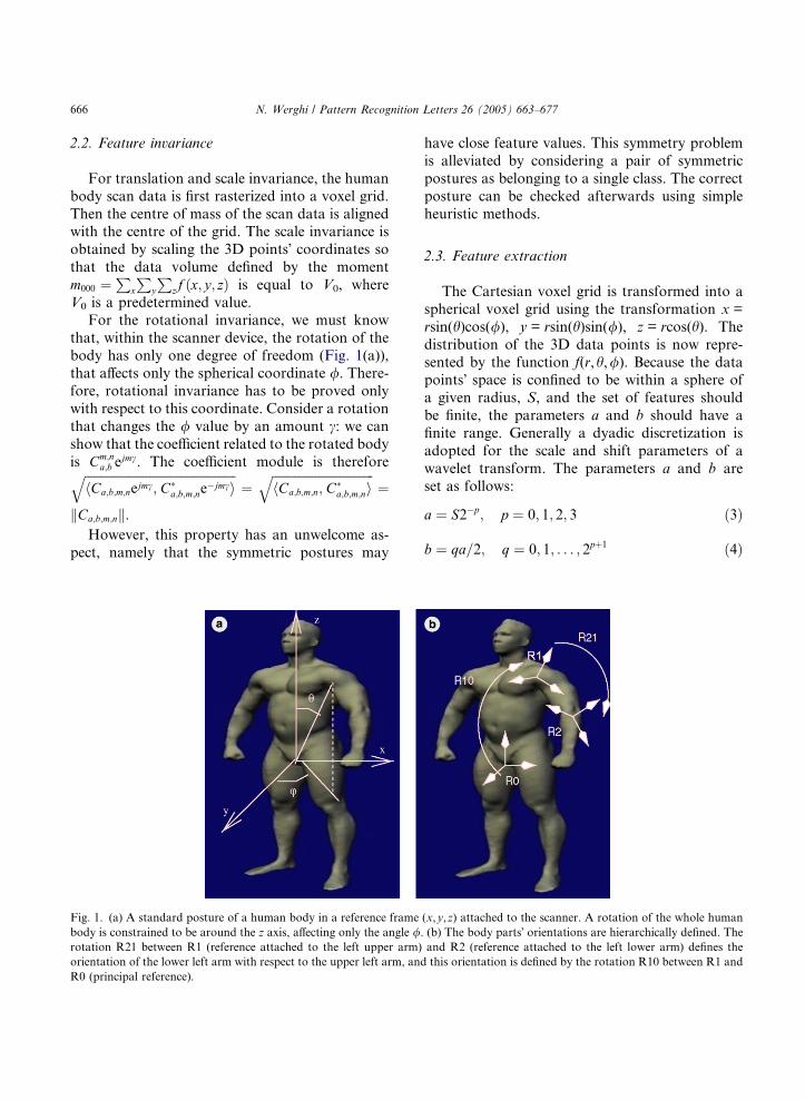
body has only one degree of freedom (Fig. 1(a)),that affects only the spherical coordinate /. There-fore, rotational invariance has to be proved only

with respect to this coordinate. Consider a rotation

that changes the / value by an amount c: we can

show that the coefficient related to the rotated body

is Cm;na;b e

jmc. The coefficient module is thereforeffiffiffiffiffiffiffiffiffiffiffiffiffiffiffiffiffiffiffiffiffiffiffiffiffiffiffiffiffiffiffiffiffiffiffiffiffiffiffiffiffiffiffiffiffiffiffiffiffihCa;b;m;nejmc; C

a;b;m;ne�jmci

q¼

ffiffiffiffiffiffiffiffiffiffiffiffiffiffiffiffiffiffiffiffiffiffiffiffiffiffiffiffiffiffiffiffiffihCa;b;m;n; C

a;b;m;ni

q¼

kCa;b;m;nk.However, this property has an unwelcome as-

pect, namely that the symmetric postures may

Fig. 1. (a) A standard posture of a human body in a reference frame

body is constrained to be around the z axis, affecting only the angle /.rotation R21 between R1 (reference attached to the left upper arm)

orientation of the lower left arm with respect to the upper left arm, and

R0 (principal reference).

have close feature values. This symmetry problem

is alleviated by considering a pair of symmetric

postures as belonging to a single class. The correct

posture can be checked afterwards using simple

heuristic methods.

2.3. Feature extraction

The Cartesian voxel grid is transformed into a

spherical voxel grid using the transformation x =

rsin(h)cos(/), y = rsin(h)sin(/), z = rcos(h). The

distribution of the 3D data points is now repre-

sented by the function f(r,h,/). Because the datapoints� space is confined to be within a sphere of

a given radius, S, and the set of features should

be finite, the parameters a and b should have a

finite range. Generally a dyadic discretization is

adopted for the scale and shift parameters of a

wavelet transform. The parameters a and b are

set as follows:

a ¼ S2�p; p ¼ 0; 1; 2; 3 ð3Þ

b ¼ qa=2; q ¼ 0; 1; . . . ; 2pþ1 ð4Þ

(x,y,z) attached to the scanner. A rotation of the whole human

(b) The body parts� orientations are hierarchically defined. The

and R2 (reference attached to the left lower arm) defines the

this orientation is defined by the rotation R10 between R1 and


The scaling parameter a takes the values S, S/2,

S/4, S/8, as scales below S/8 cover a very reduced

space that reveals little significant information.

The shifting parameter b is varied in proportion

to the scale parameter and within the range[0,S]. This makes 34 pairs (a,b).

The first four spherical harmonic functions are

used, namely, U0,0 = 1, U0,1 = cosh, U1,1 = ej/sinh,and U1,2 = �3ej/sinhcosh. This gives a total num-

ber of wavelet features (WC) Cm;np;q of 34 · 4 = 136.

However, this number will be reduced by removing

the redundant features as described in the Section

3.1.Computation of the wavelet coefficients is imple-

mented using the Matlab Wavelet package. First,

the function F(r)m,n (1) is calculated by means of

a standard integral discretization technique. Then,

the wavelet transform (2) is calculated using the

Matlab cwt function, which approximates the con-

tinuous wavelet transform. More details can be

found in the Matlab documentation.

2.4. 3D Zernike coefficient features

Zernike moments have been extensively used in

2D image analysis for their good performance with

regard to noise resilience, information redundancy

and reconstruction capability (Teh and Chin,

1988; Khotanzad and Hong, 1990). This was amotivation to put them into our trial and compare

them with the wavelet features.

2D Zernike moments are obtained by projecting

the image function on the Zernike polynomials,

which form a complete orthogonal basis. These

functions are complex polynomials defined over

the unit disk by

zp;lðrÞ ¼ Rp;lðrÞejlh ð5Þ

where the radial function Rp,l(r) is defined for p

and l integers with p P l P 0 by

Rp;lðrÞ¼

Pðp�lÞ=2t¼0

ð�1Þtðp� tÞ!t! 1

2ðpþlÞ� t

� �! 1

2ðp�lÞ� t

� �!rp�2t

if p� l even

0

if p� l odd

8>>>>>><>>>>>>:

The first few non-zero polynomials are as follows:

R0;0 ¼ 1; R2;2 ¼ r2; R4;0 ¼ 6r4 � 6r2 þ 1

R1;1 ¼ r; R3;1 ¼ 3r2 � 2r; R4;2 ¼ 4r4 � 3r2

R2;0 ¼ 2r2 � 1; R3;3 ¼ r3; R4;4 ¼ r4

The extension of the Zernike functions to the 3D

case is obtained by substituting the angular expo-nential function in (5) with the spherical harmon-

ics Umn ðh;/Þ

zm;np;l ¼ Rp;lUm;nðh;/Þ ð6Þ

zm;np;l form a family of orthogonal functions. Indeed,

it can be easily shown that hzm;np;l ; ðzm0;n0

p0;l0 Þi ¼

Kdp;p0dl;l0dm;m0dn;n0 . By projecting the data distribu-

tion f(r,h,/) on the basis zm;np;l , we obtain a set of

coefficients, called 3D Zernike coefficient features

(ZC), expressed by

Zm;np;l ¼ hF ðr; h;/Þ; zm;np;l i

¼Z 1

0

Z p

0

Z 2p

0

F ðr; h;/ÞZm;np;l sin hd/dhdr

ð7Þ

Like the wavelet features, the Zernike features areinvariant with respect to a tilt rotation affecting the

angle /. By combining the first four spherical har-

monics U0,0,U0,1,U1,1,U1,2 with the first 36 non-

zero polynomials, Rp,l, 144 Zernike features are

obtained. From this collection, the best discrimi-

native features are selected using the technique de-

scribed in Section 3.1.

The computation of the Zernike features wasimplemented using the Matlab package. The inte-

grals in (7) are simply replaced by summations.

The explicit forms of the Zernike polynomials

make the discretization of that expression trivial.

2.5. 3D Fourier coefficients

In Cartesian coordinates, the 3D Fourier trans-

form coefficients (FC) of a 3D discrete function

F(i, t,k) defined over the voxel grid of size N

(�N/2 i, t,k N/2), are expressed as


FCuvw ¼ 1ffiffiffiffiffiffiN 3

pXi¼N=2�1

i¼�N=2

Xt¼N=2�1

t¼�N=2

Xk¼N=2�1

k¼�N=2

F ði; t; kÞ

� e�j2pN ðiuþtvþkwÞ:

Theoretically the frequency parameters u, v, w

have unlimited range, but in practice they are

bounded in �K 6 u,v,w 6 K, where K depends

on some prior assumption on the spectrum of the

function F(i, t,k). Because in our application pos-

ture changes are inferred by the movements of

body limbs, and given that each limb occupies alarge area of the posture space (approximately

one sixth of the whole space), the spectrum of

the posture data distribution is concentrated in

the low frequencies. Based on this, K was set to 3.

Because we are interested in the norm of the

Fourier coefficients, and taking into account the

fact that the coefficients FCuvw occur in complex

conjugate pairs (except for FC000), the number ofFC features is ((2K + 1)3 + 1)/2, thus forming a

vector of 172 features for K = 3. Note also that

the FC coefficients are not invariant with respect

to rotation. Approaches utilizing the Fourier

transform must first align the data to the canonical

reference, defined by the principal axes.

3. The classification

The classification problem is stated as follows.

Given a set of posture classes C1, . . . ,CN and given

a query posture Q, to which class does the posture

Q belong? The query posture is represented by an

observation feature vector of dimension d,

X = [x1,x2, . . . ,xd]. For each class Ci, consider thediscriminative functions di(X). The observed fea-

ture vector is associated with the class Ci if

di(X) > dj(X) for all j5 i. The optimal discrimina-

tive function, in Bayes� sense, is that defined as

the posteriori conditional probability function

P(CijX), expressed according to Bayes� rule by

P ðCijX Þ ¼ P ðX jCiÞPðCiÞP ðX Þ . Because any monotonically

increasing function of P(CijX) leads to identical

classification, the following function is preferred:

di(X) = ln(P(XjCi)P(Ci)). This expresses the sepa-ration distance as the logarithm of the product

of the likelihood of the class Ci with respect to X

and the prior probability function P(Ci). Assuming

that P(XjCi) is a normal distribution Nðli;RiÞ de-fined by pðX jCiÞ¼ 1

2pjRi j1=2exp½� 1

2ðX �liÞ

TR�1i ðX�

liÞ� and that all the classes have equal prior

probability, the expression of the discriminative

function can be brought to

diðX Þ ¼ � 1

2ðX � liÞ

TR�1i ðX � liÞ �

1

2ln jRij ð8Þ

The statistics (li,Ri) of a class Ci are obtained from

a training process using the standard EM tech-

nique (Redner and Walker, 1984).

3.1. Selection of discriminative features

Naturally, not all the features contribute effec-

tively to the classification. To avoid redundancy,

only features having reasonable discriminative

power are selected. The discriminative power is as-

sessed by the interclass distance defined as a metricfor measuring the separation between two classes.

A selection criterion based on that metric is there-

fore utilized in the search for the optimal set of fea-

tures. Feature selection has been the subject of

intensive work in the literature (Fukunaga,

1990). There are two main categories of technique:

the first operates on feature vectors, the second

treats each feature individually. We adopted atechnique belonging to the second category. It is

sub-optimal but relatively efficient. The selection

algorithm is as follows: given a set of features

{x1,x2, . . . ,xh} and given a selection criterion J,

(1) compute the selection criterion value J(k) for

each feature xk, k = 1, . . . ,h;(2) rank the features in descending order with

respect to J; and

(3) select the top-ranked features.

There are various schemes for determining the

optimal number of features to be selected. One

method consists in rejecting the features for which

the discriminative power criterion is below a cer-

tain lower bound (e.g., the minimum value of theseparation distance between two classes). The opti-

mal number can also be determined by means of

training trials, in which the number of features is

gradually increased until it reaches a value beyond


which the classification performance does not im-

prove. Section 4.2 will describe experiments illus-

trating this method.

3.2. The interclass distance

The selection criterion is closely related to the

classification method and therefore it should be

defined in the same framework. The interclass dis-

tance between two classes Ci and Cj having condi-

tional probability density functions P ðxk;CiÞ ¼Nðlk

i ; rki Þ and P ðxk;CjÞ ¼ Nðlk

j ; rkj Þ with respect

to the feature xk can be evaluated by the followingprobabilistic separation:

dkij ¼

1

2

rkj

rkiþrk

i

rkj�2

!þ1

2ðlk

i �lkj Þ

2 1

ðrki Þ

2þ 1

ðrkj Þ

2

!

ð9Þ

This expression indicates that the larger the differ-

ence between the means with respect to the vari-

ances, the wider the separation between the two

20 40 60 80 100 1200123456789

10x 105

Wavelet Feature

Dis

crim

inat

ive

pow

er

20 40 600

0.5

1

1.5

2

2.5x 106

Zernike

Dis

crim

inat

ive

pow

er

(a) (b)

20 40 60 80 100 1200

102030405060708090

100

Wavelet Feature

Dis

crim

inat

ive

pow

er d

ecre

ase

%

20 40 600

102030405060708090

100

Zernike

Dis

crim

inat

ive

pow

er d

ecre

ase

%

(d) (e)

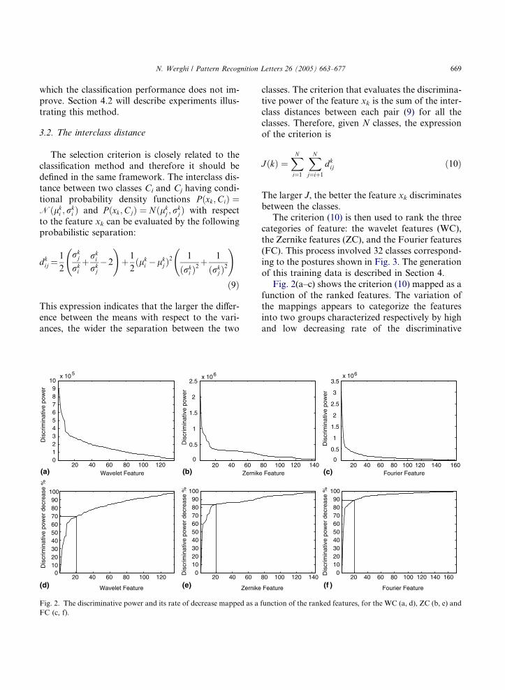
Fig. 2. The discriminative power and its rate of decrease mapped as a

FC (c, f).

classes. The criterion that evaluates the discrimina-

tive power of the feature xk is the sum of the inter-

class distances between each pair (9) for all the

classes. Therefore, given N classes, the expression

of the criterion is

JðkÞ ¼XNi¼1

XNj¼iþ1

dkij ð10Þ

The larger J, the better the feature xk discriminates

between the classes.The criterion (10) is then used to rank the three

categories of feature: the wavelet features (WC),

the Zernike features (ZC), and the Fourier features

(FC). This process involved 32 classes correspond-

ing to the postures shown in Fig. 3. The generation

of this training data is described in Section 4.

Fig. 2(a–c) shows the criterion (10) mapped as a

function of the ranked features. The variation ofthe mappings appears to categorize the features

into two groups characterized respectively by high

and low decreasing rate of the discriminative

80 100 120 140 Feature

20 40 60 80 100 120 140 1600

0.5

1

1.5

2

2.5

3

3.5x 106

Fourier Feature

Dis

crim

inat

ive

pow

er

(c)

80 100 120 140

Feature

20 40 60 80 100 120 140 1600

102030405060708090

100

Fourier Feature

Dis

crim

inat

ive

pow

er d

ecre

ase

%

(f )

function of the ranked features, for the WC (a, d), ZC (b, e) and

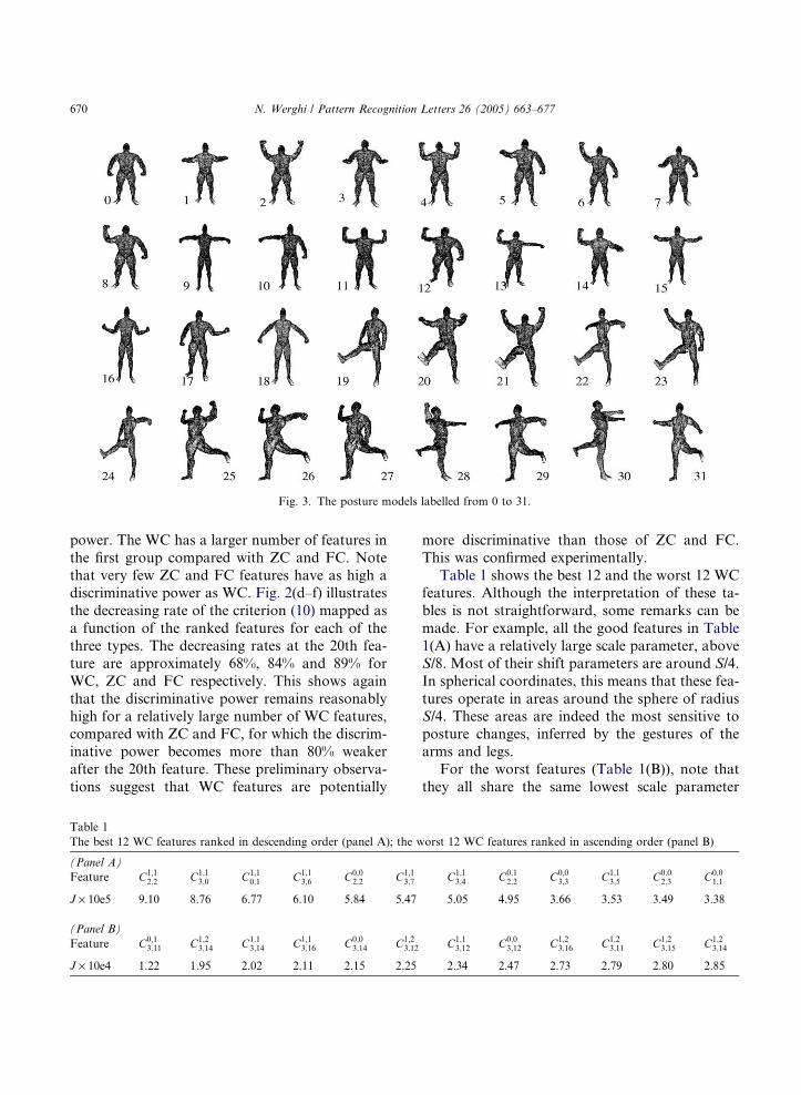
Fig. 3. The posture models labelled from 0 to 31.


power. The WC has a larger number of features in

the first group compared with ZC and FC. Note

that very few ZC and FC features have as high adiscriminative power as WC. Fig. 2(d–f) illustrates

the decreasing rate of the criterion (10) mapped as

a function of the ranked features for each of the

three types. The decreasing rates at the 20th fea-

ture are approximately 68%, 84% and 89% for

WC, ZC and FC respectively. This shows again

that the discriminative power remains reasonably

high for a relatively large number of WC features,compared with ZC and FC, for which the discrim-

inative power becomes more than 80% weaker

after the 20th feature. These preliminary observa-

tions suggest that WC features are potentially

Table 1

The best 12 WC features ranked in descending order (panel A); the w

(Panel A)

Feature C1;12;2 C1;1

3;0 C1;10;1 C1;1

3;6 C0;02;2 C1;1

3;7

J · 10e5 9.10 8.76 6.77 6.10 5.84 5.47

(Panel B)

Feature C0;13;11 C1;2

3;14 C1;13;14 C1;1

3;16 C0;03;14 C1;2

3;12

J · 10e4 1.22 1.95 2.02 2.11 2.15 2.25

more discriminative than those of ZC and FC.

This was confirmed experimentally.

Table 1 shows the best 12 and the worst 12 WCfeatures. Although the interpretation of these ta-

bles is not straightforward, some remarks can be

made. For example, all the good features in Table

1(A) have a relatively large scale parameter, above

S/8. Most of their shift parameters are around S/4.

In spherical coordinates, this means that these fea-

tures operate in areas around the sphere of radius

S/4. These areas are indeed the most sensitive toposture changes, inferred by the gestures of the

arms and legs.

For the worst features (Table 1(B)), note that

they all share the same lowest scale parameter

orst 12 WC features ranked in ascending order (panel B)

C1;13;4 C0;1

2;2 C0;03;3 C1;1

3;5 C0;02;3 C0;0

1;1

5.05 4.95 3.66 3.53 3.49 3.38

C1;13;12 C0;0

3;12 C1;23;16 C1;2

3;11 C1;23;15 C1;2

3;14

2.34 2.47 2.73 2.79 2.80 2.85


value, namely (S/8), and that most of them have a

relatively large shift parameter value close to S.

This indicates that these features operate at a

low scale, in the very periphery of the scan data

space; therefore, they embed poor informationabout the posture.

4. Experiments

A series of experiments was conducted to assess

the performance of the WC, ZC and FC features

in terms of power discrimination and classificationrate. The experimental data consists of 32 different

posture models. This set was generated as follows:

a real 3D human body scan collected from the

Cyberware website (http://www.cyberware.com)

was fitted to a hierarchical jointed structure model

satisfying the kinematics constraints of the human

body. In this model, a body segment location (po-

sition and orientation) is defined relative to theupper segment in the body hierarchy. For exam-

ple, the position and orientation of the right lower

arm are defined with respect to a reference at-

tached to the right upper arm (Fig. 1(b)). The rel-

ative orientations of the human body segments

define the parameters that control the posture.

By varying these parameters, a variety of postures

with a reasonable human appearance was ob-tained, and 32 different posture models were gener-

ated (Fig. 3). The statistical characteristics of the

posture models were determined as follows. For

each posture, 30 training data sets were generated,

the posture parameters of each sample were per-

turbed with Gaussian noise and the full data set

was rotated randomly around the z axis, thus

affecting the / coordinate. The mean and the var-

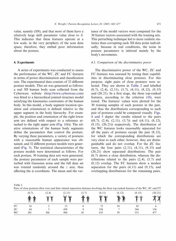
Table 2

Pairs of close postures (first row) and their related separation distance

(0,7) (2,4) (2,11) (3,7)

FC 16 2 13 0

ZC 64 3 438 8

WC 201 306 984 45

iance of the model vectors were computed for the

30 feature vectors associated with the training sets.

This perturbing technique led to more realistic sta-

tistics than corrupting each 3D data point individ-

ually, because in real conditions, the noise inposture parameters is inferred mainly by the

body�s movements.

4.1. Comparison of the discriminative power

The discriminative power of the WC, ZC and

FC features was assessed by testing their capabil-

ities in discriminating close postures. For thispurpose, eight pairs of close postures were se-

lected. They are shown in Table 2 and labelled

(0,7), (2,4), (2,11), (3,7), (4,11), (8,12), (9,15)

and (20,21). In a first stage, the three top-ranked

features, according to the criterion (10), were

tested. The features� values were plotted for the

30 training samples of each posture in the pair,

and thus the distributions corresponding to eachpair of postures could be compared visually. Figs.

4 and 5 depict the results related to the pairs

((0,7), (2,4), (2,11), (3,7)) and ((4, 11), (8,12),

(9,15), (20,21)) respectively. The distribution of

the WC features looks reasonably separated for

all the pairs of postures except the pair (8,12),

for which the corresponding distributions are

very close to each other; however, they are distin-guishable and do not overlap. For the ZC fea-

tures, the four pairs (2,11), (4,11), (9,15) and

(20,21) show separated distributions. The pair

(0,7) shows a close distribution, whereas the dis-

tributions related to the pairs (2,4), (3,7) and

(8,12) overlap. The FC features show a modest

separation for the pairs (4,11) and (9,15), and

overlapping distributions for the remaining pairs.

involving the three top-ranked features of the WC, ZC and FT

(4,11) (8,12) (9,15) (20,21)

72 54 82 6

356 7 544 136

635 39 533 477

http://www.cyberware.com

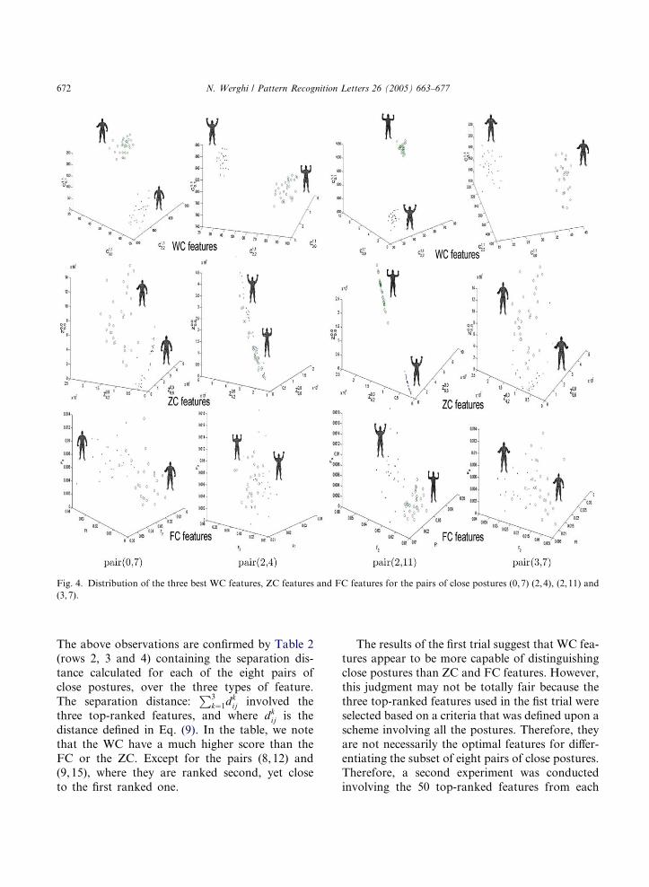
Fig. 4. Distribution of the three best WC features, ZC features and FC features for the pairs of close postures (0,7) (2,4), (2,11) and

(3,7).


The above observations are confirmed by Table 2(rows 2, 3 and 4) containing the separation dis-

tance calculated for each of the eight pairs of

close postures, over the three types of feature.

The separation distance:P3

k¼1dkij involved the

three top-ranked features, and where dkij is the

distance defined in Eq. (9). In the table, we note

that the WC have a much higher score than the

FC or the ZC. Except for the pairs (8,12) and(9,15), where they are ranked second, yet close

to the first ranked one.

The results of the first trial suggest that WC fea-tures appear to be more capable of distinguishing

close postures than ZC and FC features. However,

this judgment may not be totally fair because the

three top-ranked features used in the fist trial were

selected based on a criteria that was defined upon a

scheme involving all the postures. Therefore, they

are not necessarily the optimal features for differ-

entiating the subset of eight pairs of close postures.Therefore, a second experiment was conducted

involving the 50 top-ranked features from each

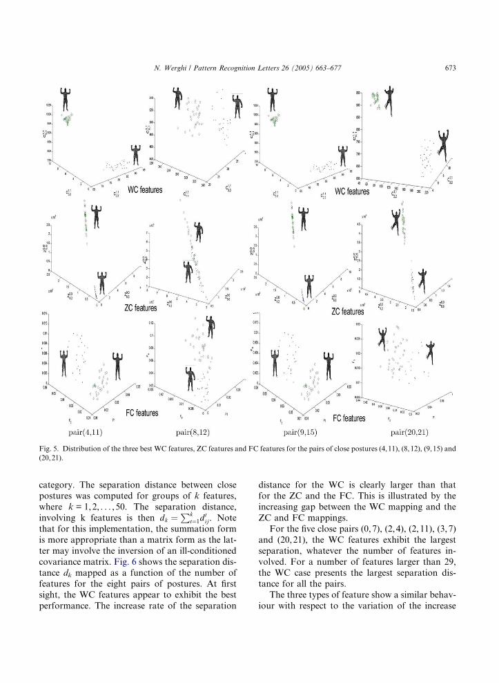
Fig. 5. Distribution of the three best WC features, ZC features and FC features for the pairs of close postures (4,11), (8,12), (9,15) and

(20,21).


category. The separation distance between closepostures was computed for groups of k features,

where k = 1,2, . . . , 50. The separation distance,

involving k features is then dk ¼Pk

t¼1dtij. Note

that for this implementation, the summation form

is more appropriate than a matrix form as the lat-

ter may involve the inversion of an ill-conditioned

covariance matrix. Fig. 6 shows the separation dis-

tance dk mapped as a function of the number offeatures for the eight pairs of postures. At first

sight, the WC features appear to exhibit the best

performance. The increase rate of the separation

distance for the WC is clearly larger than thatfor the ZC and the FC. This is illustrated by the

increasing gap between the WC mapping and the

ZC and FC mappings.

For the five close pairs (0,7), (2,4), (2,11), (3,7)

and (20,21), the WC features exhibit the largest

separation, whatever the number of features in-

volved. For a number of features larger than 29,

the WC case presents the largest separation dis-tance for all the pairs.

The three types of feature show a similar behav-

iour with respect to the variation of the increase

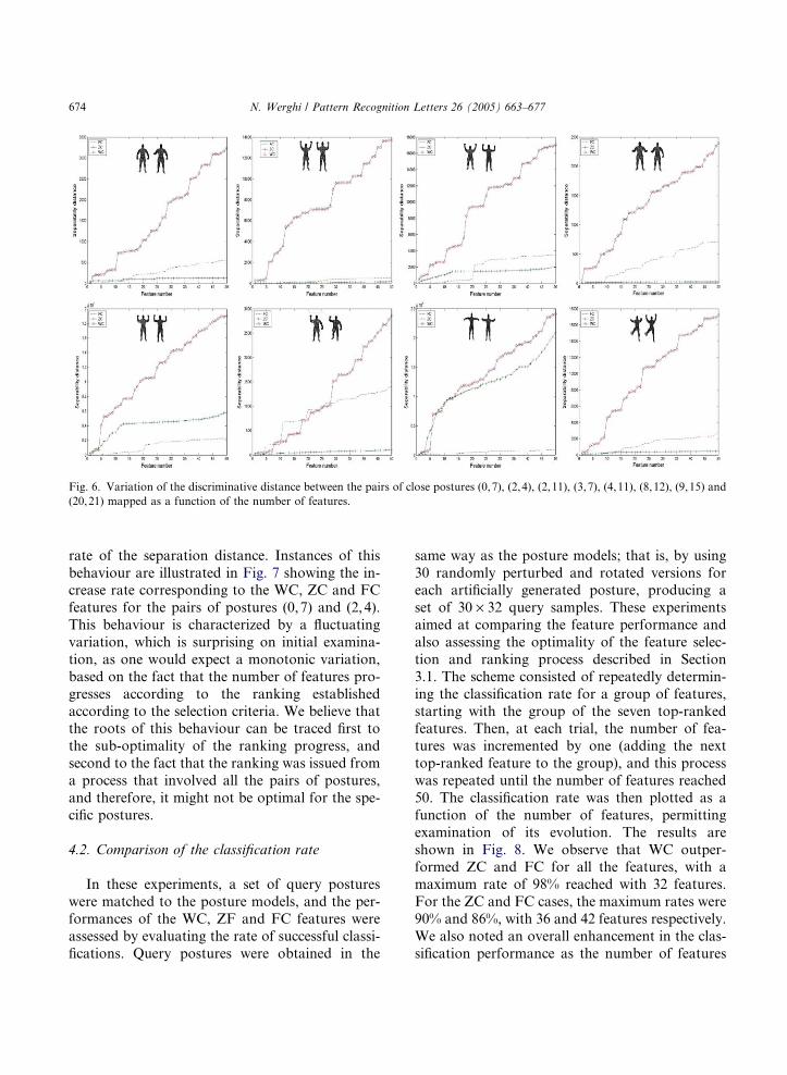
Fig. 6. Variation of the discriminative distance between the pairs of close postures (0,7), (2,4), (2,11), (3,7), (4,11), (8,12), (9,15) and

(20,21) mapped as a function of the number of features.


rate of the separation distance. Instances of this

behaviour are illustrated in Fig. 7 showing the in-crease rate corresponding to the WC, ZC and FC

features for the pairs of postures (0,7) and (2,4).

This behaviour is characterized by a fluctuating

variation, which is surprising on initial examina-

tion, as one would expect a monotonic variation,

based on the fact that the number of features pro-

gresses according to the ranking established

according to the selection criteria. We believe thatthe roots of this behaviour can be traced first to

the sub-optimality of the ranking progress, and

second to the fact that the ranking was issued from

a process that involved all the pairs of postures,

and therefore, it might not be optimal for the spe-

cific postures.

4.2. Comparison of the classification rate

In these experiments, a set of query postures

were matched to the posture models, and the per-

formances of the WC, ZF and FC features were

assessed by evaluating the rate of successful classi-

fications. Query postures were obtained in the

same way as the posture models; that is, by using

30 randomly perturbed and rotated versions foreach artificially generated posture, producing a

set of 30 · 32 query samples. These experiments

aimed at comparing the feature performance and

also assessing the optimality of the feature selec-

tion and ranking process described in Section

3.1. The scheme consisted of repeatedly determin-

ing the classification rate for a group of features,

starting with the group of the seven top-rankedfeatures. Then, at each trial, the number of fea-

tures was incremented by one (adding the next

top-ranked feature to the group), and this process

was repeated until the number of features reached

50. The classification rate was then plotted as a

function of the number of features, permitting

examination of its evolution. The results are

shown in Fig. 8. We observe that WC outper-formed ZC and FC for all the features, with a

maximum rate of 98% reached with 32 features.

For the ZC and FC cases, the maximum rates were

90% and 86%, with 36 and 42 features respectively.

We also noted an overall enhancement in the clas-

sification performance as the number of features

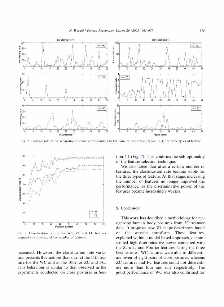
Fig. 7. Increase rate of the separation distance corresponding to the pairs of postures (0,7) and (2,4) for three types of feature.

Fig. 8. Classification rate of the WC, ZC and FC features

mapped as a function of the number of features.


increased. However, the classification rate varia-

tion presents fluctuations that start at the 11th fea-

ture for the WC and at the 10th for ZC and FC.

This behaviour is similar to that observed in theexperiments conducted on close postures in Sec-

tion 4.1 (Fig. 7). This confirms the sub-optimality

of the feature selection technique.

We also noted that after a certain number of

features, the classification rate became stable for

the three types of feature. At that stage, increasing

the number of features no longer improved theperformance, as the discriminative power of the

features became increasingly weaker.

5. Conclusion

This work has described a methodology for rec-

ognizing human body postures from 3D scannerdata. It proposes new 3D shape descriptors based

on the wavelet transform. These features,

exploited within a model-based approach, demon-

strated high discriminative power compared with

the Zernike and Fourier features. Using the three

best features, WC features were able to differenti-

ate seven of eight pairs of close postures, whereas

ZC features and FC features could not differenti-ate more than four and one respectively. The

good performance of WC was also confirmed for


a larger number of features. The mapping of the

separation distance as a function of the number

of features shows that WC has the highest increase

rate, well above those of FC and ZC. The experi-

ments conducted on a set of 32 posture modelsconfirmed the high performance of the WC, which

achieved a top rate of 98% compared with 90%

and 86% for the ZC and the FC respectively.

Naturally, the set of posture models can be

enriched by a greater variety of postures. The

method we adopted remains very applicable. How-

ever, a question may arise as to the number of dif-

ferent postures that can be recognized. We believethat this is linked first, to what extent the recogni-

tion process can differentiate between close pos-

tures, and second, to the ability to set a metric to

measure the closeness of the postures. The para-

metric description of the posture in terms of the

orientation of each body segment can be used for

that purpose. What remains is to determine the

minimum changes in posture parameters thatwould produce a distinguishable new posture.

We are currently investigating this.

References

Belkassim, S.O. et al., 1991. Pattern recognition with moment

invariants: A comparative study and new results. Pattern

Recognition 24 (12), 1117–1138.

Canterakis, N., 1997. Fast 3D Zernike moments and invariants.

Tech. Report 5/97, Institute of Informatics, University of

Freiburg, Germany.

Chim, Y. et al., 1999. Character recognition using statistical

moments. Image Vision Comput. 17 (3–4), 299–307.

Cordier, H., Seo, H., Magnenat-Thalmann, N., 2003. Made-to-

measure technologies for an online clothing store. Comput.

Graphics Appl. (January–February), 38–48.

Daubechies, I., 1990. The wavelet transform, time-frequency

localization and signal analysis. IEEE Trans. Info. Theory

36 (5), 961–1005.

Dekker, L., Khan, S., West, E., Buxton, B., 1998. Models for

understanding the 3D human body form. In: Proc. IEEE

Workshop on Model-Based 3D Image Anal., Bombay,

India, pp. 65–74.

Ferrers, N.M., 1877. An elementary treatise in spherical

harmonics. MacMillan.

Fukunaga, K., 1990. Introduction to statistical pattern recog-

nition, second ed. Academic Press, New York.

Hu, M., 1962. Visual pattern recognition by moment invariants.

IRE Trans. Inform. Theory IT-8, 179–187.

Jaffard, S., Meyer, Y., Dyan, R., 2001. Wavelets: Tools for

Science and Technology. SIAM, Philadelphia.

Jones, P.R.M., Rioux, M., 1997. Three dimensional surface

anthropometry: Applications to human body. Optics Lasers

Eng. 28 (2), 89–117.

Jones, P., Li, P., Brook-Wavel, K., West, G., 1995. Format of

human body modelling from 3D body scanning. Int. J.

Cloth. Sci. 7 (1), 7–16.

Khotanzad, A., Hong, Y.H., 1990. Invariant image recognition

by Zernike moments. IEEE Trans. Pattern Anal. Machine

Intell. 12 (5), 489–797.

Lo, C., Don, H., 1989. 3-D Moment forms: Their construction

and application to object identification and positioning.

IEEE Trans. Pattern Anal. Machine Intell 11 (10), 1053–

1064.

Mallat, S., 1989. A theory for multiresolution signal decompo-

sition: The wavelet representation. IEEE Trans. Pattern

Anal. Machine Intell 11 (7), 674–693.

Meyer, Y., 1997. Wavelets and operatorsCambridge Studies in

Advanced Mathematics, Vol. 37. Cambridge University

Press.

Morlet, J.M, Grossman, A., 1984. Decomposition of Hardy

functions into square integrable wavelets of constant shape.

SIAM J. Math. Anal. 15 (4), 723–736.

Paquet, E., Robinette, K.M., Rioux, M., 2000. Management of

three-dimensional and anthropometric databases: Alexan-

dria and Cleopatra. J. Electron. Imaging 9, 421–431.

Pargas, R., Staples, N., Davis, J., 1996. Automatic measure-

ment extraction for apparel for three-dimensional body

scan. J. Optics Laser Eng. 28 (PT2), 157–172.

Redner, R., Walker, H., 1984. Mixture densities, maximum

likelihood and the EM algorithm. SIAM Rev. 26 (2), 195–

239.

Sadjadi, F.A., Hall, E.L., 1980. Three-dimensional moment

invariants. IEEE Trans. Pattern Anal. Machine Intell. 2 (2),

127–135.

Schael, M., 1997. Invariant 3D features. Tech. Report 4/97,

Institute of Informatics, Albert-Ludwigs-Universitat

Freiburg.

Sheynin, S.S., Tuzikov, A.V., 2001. Explicit formulae for

polyhedra moments. Pattern Recognition Lett. 22 (10),

1103–1109.

Sun, W., Hilton, A., Smith, R., Illingworth, J., 2001. Layered

animation of captured data. Internat. J. Comput. Graphics

17 (8), 457–474.

Starck, J., Collins, G., Smith, R., Hilton, A., Illingworth, J.,

2002. Animated statues. J. Machine Vision Appl. 14 (4),

248–259.

Teague, M., 1980. Image analysis via the general theory of

moments. J. Opt. Soc. Amer. 70 (8), 920–930.

Teh, C.H., Chin, R.T., 1988. On image analysis by the methods

of moments. IEEE Trans. Pattern Anal. Machine Intell. 10,

496–513.

Vranic, D.V., Saupe, D., 2001. 3D shape descriptor based on

3D Fourier transform. In: Proc. EURASIP Conf. Digital

Signal Process. Multimedia Commun. Services (ECMCS

2001) Budapest, Hungary, pp. 271–274.


Werghi, N., Xiao, Y., 2002. Wavelet moments for recognizing

human body posture from 3D scans. In: Proc. Internat.

Conf. Pattern Recognition, Quebec City, Canada, pp. 123–

126.

Xiao, Y., Werghi, N., Siebert, P., 2003. A discrete Reeb graph

approach for the segmentation of human body scans. In:

Proc. Internat. Conf. 3D Digital Imag. Model., Alberta,

Canada, pp. 378–385.

Recognition of Human Body Posture from a Cloud of 3D Data Points using Wavelet Transform...

Documents

Transcript of Recognition of Human Body Posture from a Cloud of 3D Data Points using Wavelet Transform...