Efficiency Discounted Exponential Growth (EDEG) Approach to Modeling the Power Progression of a...

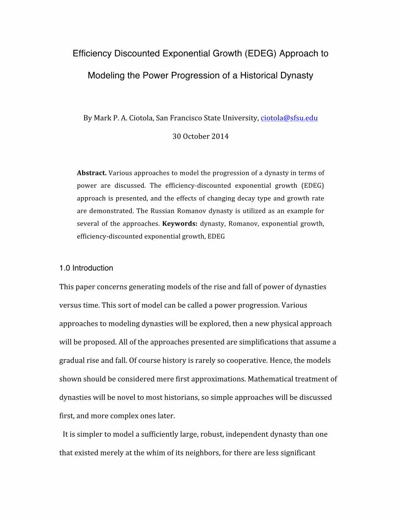
Efficiency Discounted Exponential Growth (EDEG) Approach to

Modeling the Power Progression of a Historical Dynasty

By Mark P. A. Ciotola, San Francisco State University, [email protected]

30 October 2014

Abstract. Various approaches to model the progression of a dynasty in terms of

power are discussed. The efficiency-‐discounted exponential growth (EDEG)

approach is presented, and the effects of changing decay type and growth rate

are demonstrated. The Russian Romanov dynasty is utilized as an example for

several of the approaches. Keywords: dynasty, Romanov, exponential growth,

efficiency-‐discounted exponential growth, EDEG

1.0 Introduction

This paper concerns generating models of the rise and fall of power of dynasties

versus time. This sort of model can be called a power progression. Various

approaches to modeling dynasties will be explored, then a new physical approach

will be proposed. All of the approaches presented are simplifications that assume a

gradual rise and fall. Of course history is rarely so cooperative. Hence, the models

shown should be considered mere first approximations. Mathematical treatment of

dynasties will be novel to most historians, so simple approaches will be discussed

first, and more complex ones later.

It is simpler to model a sufficiently large, robust, independent dynasty than one

that existed merely at the whim of its neighbors, for there are less significant

dependencies, and thus can be approximated as a substantially isolated system. So

we will utilize Russia’s Romonov dynasty as an example. Widely accepted start and

end dates are 1613 and 1917 (Mazour and Peoples 1975). Peter the Great and

Catherine the Great were the two important rulers of the Romanov dynasty, and the

Russian Empire gained much of its most valuable territory by the end of Catherine’s

reign. The Romanov dynasty was big, robust and essentially independent. It fought

wars, but it generally was not under serious threat of extinction. Even Napoleon

could not conquer Russia, but rather Russia nearly conquered Napoleon. This

dynasty was reasonably long-‐lived, rather than just a quick, “flash-‐in-‐the-‐pan”

empire.

1.1 Straight line

The simplest approach to model the power progression of a dynasty is a

combination of two linear models. This requires start and end years of the dynasty,

and its peak year as input parameters. For a single dynasty, the magnitude of the

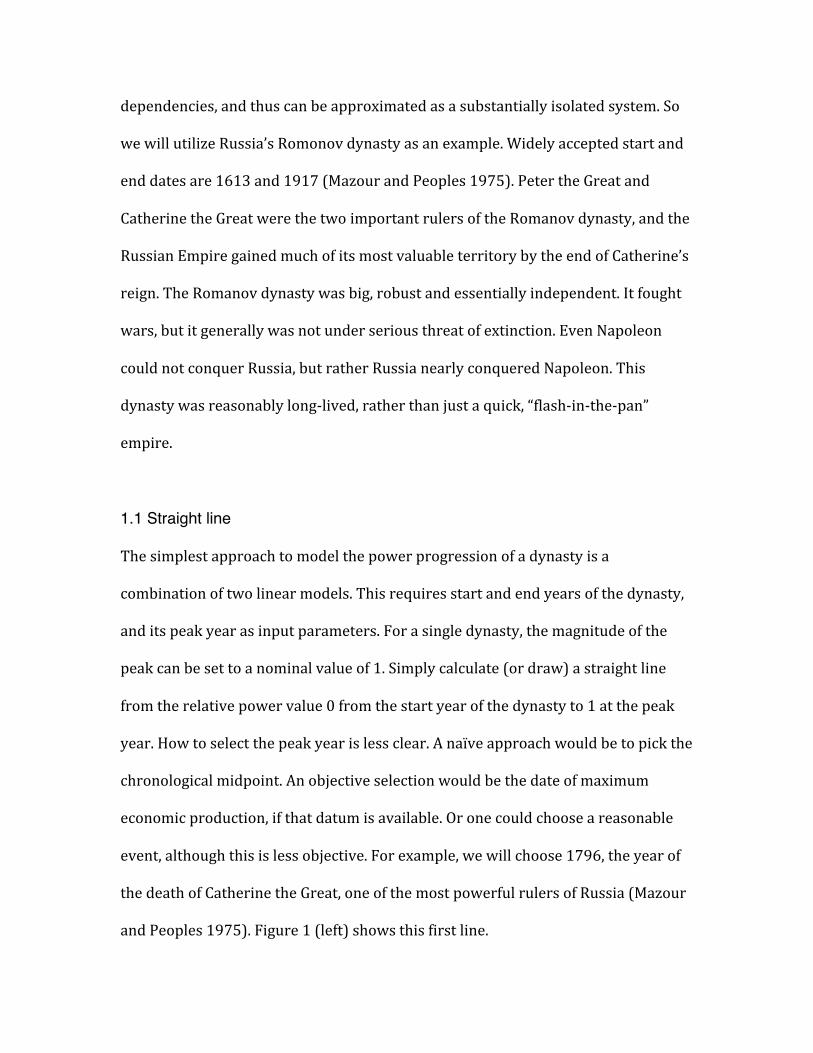
peak can be set to a nominal value of 1. Simply calculate (or draw) a straight line

from the relative power value 0 from the start year of the dynasty to 1 at the peak

year. How to select the peak year is less clear. A naïve approach would be to pick the

chronological midpoint. An objective selection would be the date of maximum

economic production, if that datum is available. Or one could choose a reasonable

event, although this is less objective. For example, we will choose 1796, the year of

the death of Catherine the Great, one of the most powerful rulers of Russia (Mazour

and Peoples 1975). Figure 1 (left) shows this first line.

Next, calculate a straight line from magnitude 1 at the peak year to magnitude 0 at

the end year, involving the slope and vertical-‐intercept, shown on Figure 1 (right).

This model has several disadvantages among which it is discontinuous at its peak

and assumes linear growth and decay. Further, it tells us little about what

underlying causes and factors may be.

FIGURE 1: Line from start to peak year, where peak is death of Catherine the Great (left); Linear model of entire dynasty (right).

1.2 Inverted quadratic function

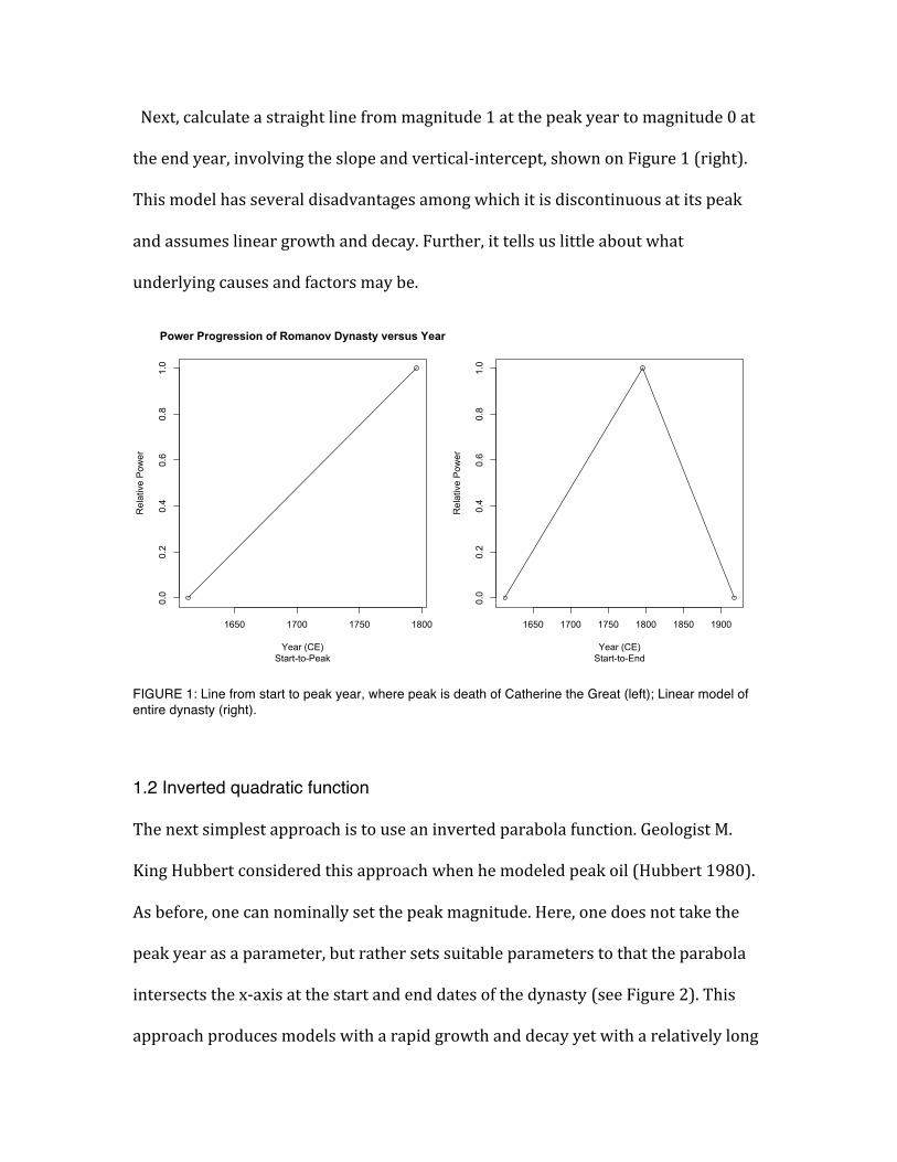
The next simplest approach is to use an inverted parabola function. Geologist M.

King Hubbert considered this approach when he modeled peak oil (Hubbert 1980).

As before, one can nominally set the peak magnitude. Here, one does not take the

peak year as a parameter, but rather sets suitable parameters to that the parabola

intersects the x-‐axis at the start and end dates of the dynasty (see Figure 2). This

approach produces models with a rapid growth and decay yet with a relatively long

1650 1700 1750 1800

0.0

0.2

0.4

0.6

0.8

1.0

Power Progression of Romanov Dynasty versus Year

Start-to-PeakYear (CE)

Rel

ativ

e P

ower

1650 1700 1750 1800 1850 1900

0.0

0.2

0.4

0.6

0.8

1.0

Start-to-EndYear (CE)

Rel

ativ

e P

ower

period of relative stability in the midst. A chief disadvantage is that the symmetry of

this function forces one to assume a peak year in the mid-‐point of the dynasty’s life.

Also, this model tells us very little about underlying causes.

FIGURE 2: Inverted parabola with endpoints at 1613 and 1917.

1.3 Normal distribution

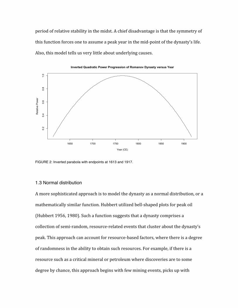
A more sophisticated approach is to model the dynasty as a normal distribution, or a

mathematically similar function. Hubbert utilized bell-‐shaped plots for peak oil

(Hubbert 1956, 1980). Such a function suggests that a dynasty comprises a

collection of semi-‐random, resource-‐related events that cluster about the dynasty’s

peak. This approach can account for resource-‐based factors, where there is a degree

of randomness in the ability to obtain such resources. For example, if there is a

resource such as a critical mineral or petroleum where discoveries are to some

degree by chance, this approach begins with few mining events, picks up with

1650 1700 1750 1800 1850 1900

0.2

0.4

0.6

0.8

1.0

Inverted Quadratic Power Progression of Romanov Dynasty versus Year

Year (CE)

Rel

ativ

e P

ower

growth, then levels off with the difficulty of finding new deposits (Ciotola 1995). A

chief disadvantage is that this model forces symmetry upon the dynasty’s rise and

fall. Another disadvantage is that one must literally begin with the peak and work to

the endpoints. It provides no readily apparent means to a priori simulate the

emergence of a dynasty.

The normal distribution approach also requires selecting a standard deviation

value. Since the vertical axis represents power, and the area under the plot

represents cumulative power, then one can set a standard deviation to produce the

corresponding percentage of cumulative power. One can also determine the ratio of

peak-‐to-‐start power, and use that to set the end-‐points. Note that a smaller standard

deviation results in a sharper peak, whereas a greater one produces models that

approach an inverted parabola (see Figure 3). This characteristic can be used to

reject particular models based on available evidence.

FIGURE 3: Normal distributions with range of standard deviations.

1650 1700 1750 1800 1850 1900

0.0

0.1

0.2

0.3

0.4

Standard Deviation = (1/16) * lifetimeYear (CE)

Rel

ativ

e P

ower

1650 1700 1750 1800 1850 1900

0.0

0.1

0.2

0.3

0.4

Romanov Dynasty Normal Distribution Progression


Rel

ativ

e P

ower

1650 1700 1750 1800 1850 1900

0.15

0.20

0.25

0.30

0.35

0.40


Rel

ativ

e P

ower

1.4 Maxwell-Boltzmann distribution

The Maxwell-‐Boltzmann distribution rises quickly then declines slowly. (It is

possible to alter this distribution so that the opposite occurs). This distribution

involves a quadratic function leading to a rise, and exponential decay leaving to a

fall. So it is a qualitatively reasonable candidate to model the progression of a

dynasty. The Maxwell-‐Boltzmann distribution has most of the advantages of the

normal distribution, and it allows asymmetry. Disadvantages may include that this

model is less simple both conceptually and mathematically, and requires more

parameters than the approaches discussed above. An initial attempt to model the

rise and fall (Ciotola 1995) of the Colorado San Juan mining region is shown in

Figure 4. The parameters were adjusted to fit several data points provided by a

historical account of the region by D. Smith (1982).

FIGURE 4: Maxwell-Boltxmann distribution for mining production versus year in San Juans region, with

vertical axis represents millions of $US.

2.0 Efficiency Discounted Exponential Growth (EDEG) Approach

The efficiency-‐discounted exponential growth (EDEG) approach is relatively new. A

few rough simulations were conducted earlier (Ciotola 2009, 2010), but this paper

presents a more refined approach for generating dynasty models. EDEG produces a

model based on two mathematically simple components, but allows the addition of

other, more sophisticated components. By developing a fundamental approach to

modeling the rise and fall of dynasties, it is possible to accept or reject models based

upon both qualitative historical evidence and quantitative historical data.

Historical dynasties are consumers of energy and producers of power, so models in

terms of such quantities are inherently fundamental in that they can be derived

directly from the laws of physics and expressed in physical quantities. Such models

are not theories of everything, but rather describe certain types of broad macro-‐

historical phenomena rather than the intricate workings of the interactions of

individual people.

The term energy is meant in the physical sense here. There are several possible

measures of the physical energy of a dynasty, such as population governed or grain

production. Each of these is translatable into physical units of energy. For example,

the quantity of people multiplied by the mean Calorie diet per person will result in

an amount in units of energy. These figures can be estimated for most dynasties

over their lifespans, albeit with differing degrees on uncertainty. The proportion of

this energy that rulers of the dynasty actually have at their disposal is beyond the

scope of this paper, but should be considered for improved accuracy.

Power is a physical term. It refers to energy expended per unit of time. Yet it also

has meaning within social and political contexts, and will be discussed in both

senses. Absolute power would generally be presented in physical units of power

such as Watts. However, it is possible to express any type of power in terms of

proportions, such as the ratio of power at a dynasty’s peak to its start date. Such a

ratio can apply to physical, political or even military power. So the EDEG approach

can be utilized to model any type of power. In fact, the EDEG approach provides a

framework to explore the question of how political and physical power are related.

2.1 Origins of Efficiency Discounted Exponential Growth (EDEG)

This author’s original efforts at modeling dynasties were heavily influenced by

M. King Hubbert’s attempts to model peak oil. The author originally used the

normal distribution approach (Ciotola, 2001) discussed by Hubbert, but this

approach was not sufficiently broad in that few historical dynasties utilized

petroleum in major quantities, nor did Hubbert’s attempts involve a driving

tendency for history. The author began some related models for French and Spanish

dynasties (2009) and more fully developed EDEG for petroleum modeling (Ciotola

2010).

2.2 Exponential Growth

It is noticed that systems in both nature and human society often grow

exponentially (Ciotola 2001; Annila 2010). Exponential growth essentially means

that a system’s present growth is proportional to its present magnitude. For

example, if a doubling of population (say of mice) is involved, then 10 mice will

become 20 mice, while 20 mice will become 40 mice. A formula for exponential

growth is:

y = ekt

where y is the output, k is the growth rate, and t represents time.

Sources of growth can include geographic expansion, infrastructure improvements

and trade expansion. It will be assumed that dynasties will strive to grow

exponentially. (This paper does not attempt to prove this assertion, but rather it is a

rebuttable presumption). If so, this certainly explains the rise of a dynasty. There is

a minor distinction between exponential growth and compounded growth.

Exponential growth essentially involves continuous compounding which produces a

larger effective growth rate than discrete compounding. It is similar to the

difference of quarterly versus daily compounding of a bank savings account. This

effect is less significant at small growth rates but more so at very large rates. For the

growth rates that we will consider, the effect is negligible compared to the other

sources of uncertainty that exist.

The Romanov dynasty with various growth rates is shown in Figure 5. The plot

shapes appear similar, except that a greater rate produces a “sharper” corner. Also,

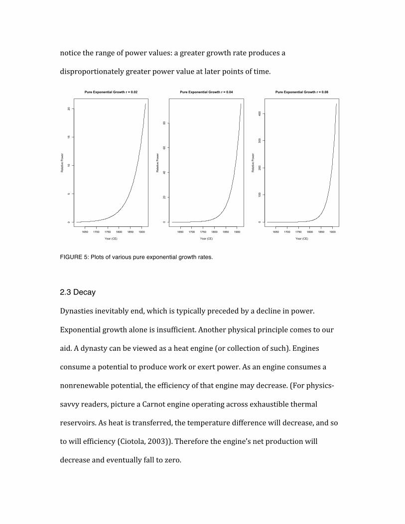
notice the range of power values: a greater growth rate produces a

disproportionately greater power value at later points of time.

FIGURE 5: Plots of various pure exponential growth rates.

2.3 Decay

Dynasties inevitably end, which is typically preceded by a decline in power.

Exponential growth alone is insufficient. Another physical principle comes to our

aid. A dynasty can be viewed as a heat engine (or collection of such). Engines

consume a potential to produce work or exert power. As an engine consumes a

nonrenewable potential, the efficiency of that engine may decrease. (For physics-‐

savvy readers, picture a Carnot engine operating across exhaustible thermal

reservoirs. As heat is transferred, the temperature difference will decrease, and so

to will efficiency (Ciotola, 2003)). Therefore the engine’s net production will

decrease and eventually fall to zero.

1650 1700 1750 1800 1850 1900

05

1015

20

Pure Exponential Growth r = 0.02

Year (CE)

Rel

ativ

e P

ower

1650 1700 1750 1800 1850 1900

020

4060

80


Year (CE)

Rel

ativ

e P

ower

1650 1700 1750 1800 1850 1900

0100

200

300

400


Year (CE)

Rel

ativ

e P

ower

Likewise, as the dynasty progresses, non-‐renewable resources will be consumed,

and efficiency will decrease. There will still be production until the end, but there

will be a lower return on investment, so to speak. Causes of decay can include

overuse of agricultural land leading to nutrient depletion, the build-‐up of toxins in

the environment, depletion of old growth forests, and even running low on social

goodwill.

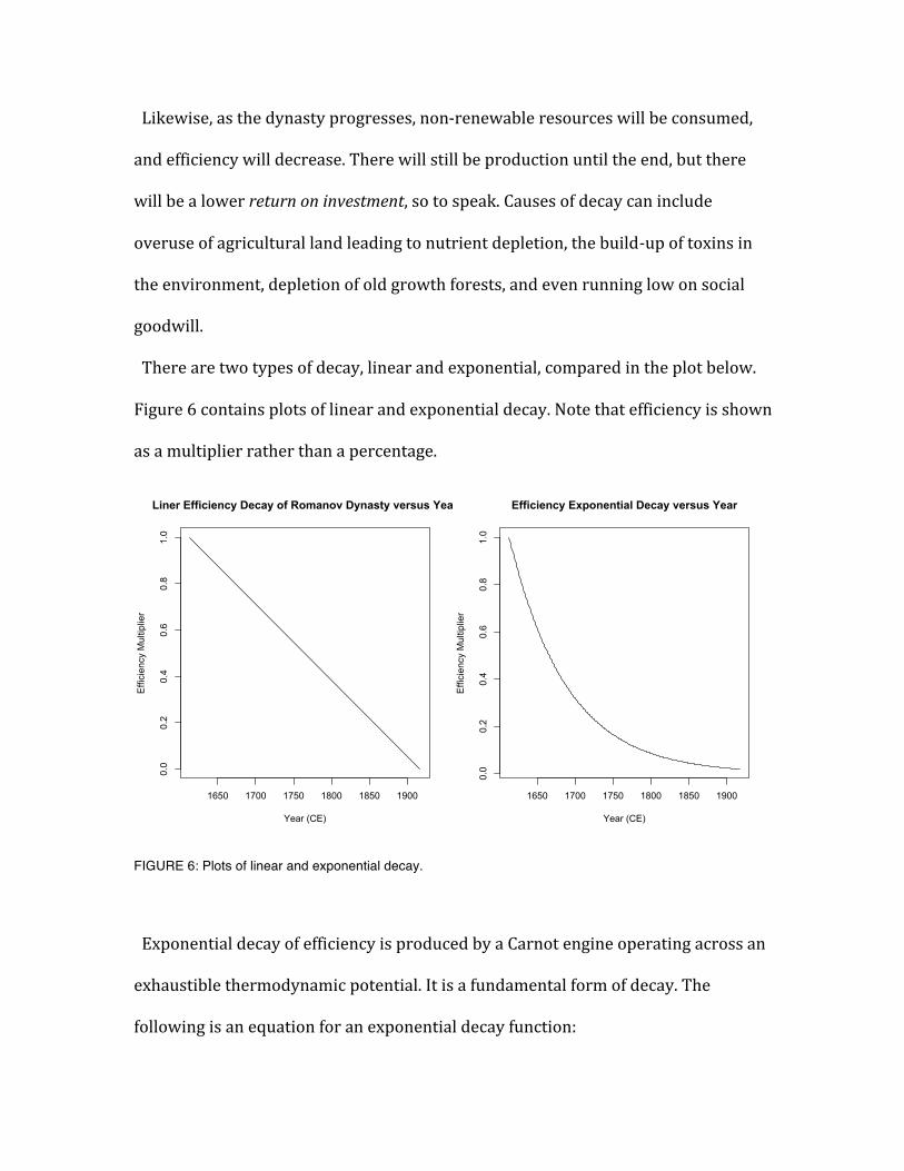
There are two types of decay, linear and exponential, compared in the plot below.

Figure 6 contains plots of linear and exponential decay. Note that efficiency is shown

as a multiplier rather than a percentage.

FIGURE 6: Plots of linear and exponential decay.

Exponential decay of efficiency is produced by a Carnot engine operating across an

exhaustible thermodynamic potential. It is a fundamental form of decay. The

following is an equation for an exponential decay function:

1650 1700 1750 1800 1850 1900

0.0

0.2

0.4

0.6

0.8

1.0

Liner Efficiency Decay of Romanov Dynasty versus Yea

Year (CE)

Effi

cien

cy M

ultip

lier

1650 1700 1750 1800 1850 1900

0.0

0.2

0.4

0.6

0.8

1.0

Efficiency Exponential Decay versus Year

Year (CE)

Effi

cien

cy M

ultip

lier

y = e-‐kt ,

where y is the output, k is a constant of proportionality, and t represents time. This

appears nearly identical to the exponential growth function, except that the

exponent is negative. However, there are two disadvantages of exponential decay

within the context of modeling dynasties. First, it is slightly difficult to set up. For

example, exponential decay has an infinitely long tail. While this allows for

mathematical immortality, most of the tail is superfluous in the context of a dynasty

of limited lifetime. Second, it may not provide the most consistent models with

observations.

A linear approach is simpler to set up. Importantly, it also provides some reflection

of efficiencies achieved through centralization and economies of scale as the dynasty

progresses. It has unambiguous beginning and end points. Efficiency cannot be

greater than one, and is typically no lower than zero. Therefore, as a first

approximation, one can set the efficiency to 100% at the start date of the dynasty

and 0% at the end year (except that the math is simpler if the value 1 is used for

100%). Using a value of 0 for ending efficiency ensures that the dynasty actually

does end by its historical end date. Although physical efficiency is typically lower

than 100% for real life heat engines, 1 provides an easy starting point that also

produces the correct shape of curve. The following is an example of linear decay

function:

efficiency = 1 – ((year – start year)/(end year – start year)).

As the year increases, efficiency will decrease. Using a lower initial efficiency

reduces the magnitude of production increase for the dynasty compared to its initial

production. It also flattens out the curve. Using a value of zero for ending efficiency

ensures that the dynasty actually does end by its historical end date. It is possible to

use a value other than zero for the ending efficiency, but then some other factor

must be used to end the dynasty.

2.4 Efficiency-Discounted Exponential Growth (EDEG)

We still need to go a step further. So now we bring exponential growth and declining

efficiency together. We need to use the decay to discount exponential growth, just a

little in the beginning, then completely at the end. The following is an example of an

EDEG equation:

y = exponential growth function * efficiency function,

where * is a multiplication symbol. Substituting in our functions (utilizing linear

decay):

Y = ekt *(1 – (t/(end year – start year))).

Y = ek(year – start year) *(1 – ((year – start year)/(end year – start year))).

This produces a steady rise, a level period and a slightly faster decay. So by

discounting exponential growth by decreasing efficiency, we then have a rise and

fall pattern that is consistent with the rise and fall of a dynasty.

2.5 Application

Let us apply the EDEG approach to the Romanov dynasty. Let us assume a

conservative 1% growth rate. Let us further assume linear decay from 100% to 0%

efficiency. A simulation has been written in the Ruby programming language. This

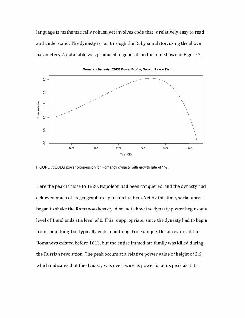
language is mathematically robust, yet involves code that is relatively easy to read

and understand. The dynasty is run through the Ruby simulator, using the above

parameters. A data table was produced to generate in the plot shown in Figure 7.

FIGURE 7: EDEG power progression for Romanov dynasty with growth rate of 1%.

Here the peak is close to 1820. Napoleon had been conquered, and the dynasty had

achieved much of its geographic expansion by them. Yet by this time, social unrest

began to shake the Romanov dynasty. Also, note how the dynasty power begins at a

level of 1 and ends at a level of 0. This is appropriate, since the dynasty had to begin

from something, but typically ends in nothing. For example, the ancestors of the

Romanovs existed before 1613, but the entire immediate family was killed during

the Russian revolution. The peak occurs at a relative power value of height of 2.6,

which indicates that the dynasty was over twice as powerful at its peak as it its

1650 1700 1750 1800 1850 1900

0.0

0.5

1.0

1.5

2.0

2.5

Romanov Dynasty: EDEG Power Profile, Growth Rate = 1%

Year (CE)

Pow

er (r

elat

ive)

beginning. Remember, this model is merely a hypothesis that is either valid or

invalid for a particular level of uncertainty.

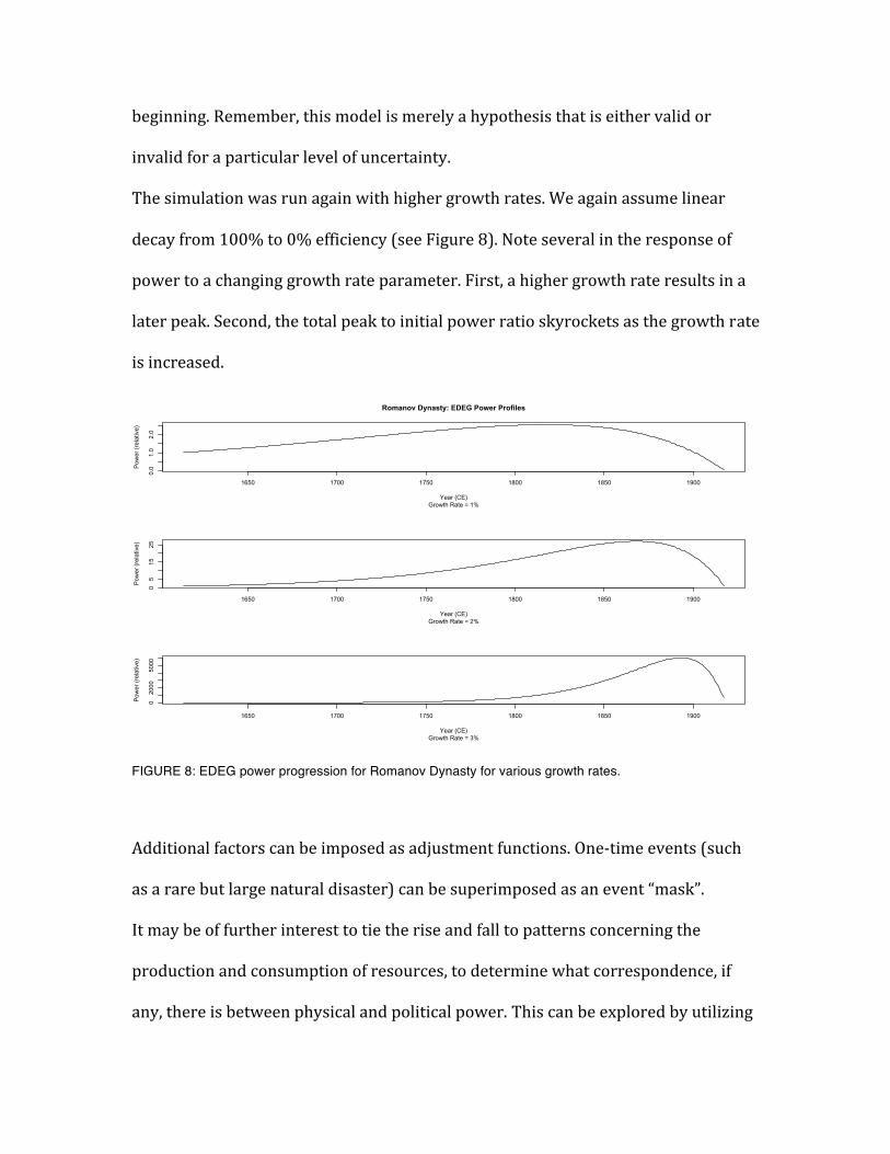
The simulation was run again with higher growth rates. We again assume linear

decay from 100% to 0% efficiency (see Figure 8). Note several in the response of

power to a changing growth rate parameter. First, a higher growth rate results in a

later peak. Second, the total peak to initial power ratio skyrockets as the growth rate

is increased.

FIGURE 8: EDEG power progression for Romanov Dynasty for various growth rates.

Additional factors can be imposed as adjustment functions. One-‐time events (such

as a rare but large natural disaster) can be superimposed as an event “mask”.

It may be of further interest to tie the rise and fall to patterns concerning the

production and consumption of resources, to determine what correspondence, if

any, there is between physical and political power. This can be explored by utilizing

1650 1700 1750 1800 1850 1900

0.0

1.0

2.0

Romanov Dynasty: EDEG Power Profiles

Growth Rate = 1%Year (CE)

Pow

er (r

elat

ive)

1650 1700 1750 1800 1850 1900

05

1525


Pow

er (r

elat

ive)

1650 1700 1750 1800 1850 1900

02000

5000


Pow

er (r

elat

ive)

actual physical energy data to produce a model of physical power, and then

comparing that model with evidence of political power versus time. With the wealth

of historical data being gathered in anthropological data warehouses, and other “big

data” facilities, this may be accomplished with increasing validity.

3.0 Discussion and Future Directions

This presentation of the EDEG approach is more of a barebones beginning than a

complete end. It raises more questions than it answers, but it enables a broad

framework to answer these questions. This framework acts as a unifying skeleton to

link the humanistic elements of history with the quantitative constraints of the

physical universe.

The power of such a framework should not be underestimated. It is possible to

gather quantitative data (or quantify qualitative evidence), perform statistical

analysis and accept or disprove hypotheses. Yet such results, while often important,

are merely empirical. They are often hard to use to constrain or illustrate each

other. In a unified framework, all results act to constrain all other results. When we

learn about one thing, we necessarily learn something about everything else. This is

where the physical sciences have derived much of their strength.

There are many immediately apparent improvements to improve the value of the

EDEG approach. One improvement would be to better understand efficiency decay.

Another improvement would be to start using actual data of physical energy, to the

extent such data is available. Another improvement will be to separate the power

level of the underlying society from that of the dynasty. For example, Russia did not

disappear upon the death of the Romanov dynasty. On the contrary, it is still one of

the most powerful societies on Earth. The brings up the need to be able to model the

emergence of a series of dynasties in a way that connects and constrains each

dynasty, such as concerning relative strength and timing of emergence. Further,

there needs to be a way to compare co-‐existing dynasties and model their

interaction within this framework. While the EDEG approach suggests possible

means, the devil will be in the details.

REFERENCES

Annila, A. and S. Salthe. 2010. Physical foundations of evolutionary theory. J. Non-‐

Equilib. Thermodyn. 35:301–321.

Ciotola, M. 1997. San Juan Mining Region Case Study: Application of Maxwell-‐

Boltzmann Distribution Function. Journal of Physical History and Economics 1.

Ciotola, M. 2001. Factors Affecting Calculation of L, edited by S. Kingsley and R.

Bhathal. Conference Proceedings, International Society for Optical Engineering (SPIE)

Vol. 4273.

Ciotola, M. 2003. Physical History and Economics. San Francisco: Pavilion Press.

Ciotola, M. 2009. Physical History and Economics, 2nd Edition. San Francisco: Pavilion

of Research & Commerce.

Ciotola, M. 2010. Modeling US Petroleum Production Using Standard and Discounted

Exponential Growth Approaches.

Gibson, C. 1966. Spain in America. New York: Harper and Row.

Hewett, D. F. 1929. Cycles in Metal Production, Technical Publication 183. New York:

The American Institute of Mining and Metallurgical Engineers.

M. King Hubbert.1956. Nuclear Energy And The Fossil Fuels. Houston, TX: Shell

Development Company, Publication 95.

Hubbert, M. K. 1980. "Techniques of Prediction as Applied to the Production of Oil

and Gas." Presented to a symposium of the U.S. Department of Commerce,

Washington, D.C., June 18-‐20.

Mazour, A. G., and J. M. Peoples. 1975. Men and Nations, A World History, 3rd Ed. New

York: Harcourt, Brace, Jovanovich.

Schroeder, D. V. 2000. Introduction to Thermal Physics. San Francisco: Addison

Wesley Longman.

Smith, D. A. 1982. Song of the Drill and Hammer: The Colorado San Juans, 1860–1914.

Colorado School of Mines Press.

Efficiency Discounted Exponential Growth (EDEG) Approach to Modeling the Power Progression of a...

Documents

Transcript of Efficiency Discounted Exponential Growth (EDEG) Approach to Modeling the Power Progression of a...