HAL Id: tel-03602509https://tel.archives-ouvertes.fr/tel-03602509

Submitted on 9 Mar 2022

HAL is a multi-disciplinary open accessarchive for the deposit and dissemination of sci-entific research documents, whether they are pub-lished or not. The documents may come fromteaching and research institutions in France orabroad, or from public or private research centers.

L’archive ouverte pluridisciplinaire HAL, estdestinée au dépôt et à la diffusion de documentsscientifiques de niveau recherche, publiés ou non,émanant des établissements d’enseignement et derecherche français ou étrangers, des laboratoirespublics ou privés.

Etude théorique des réponses évolutives au changementclimatique : effets de l’homogamie et des fluctuations de

l’intensité de la sélectionClaire Godineau

To cite this version:Claire Godineau. Etude théorique des réponses évolutives au changement climatique : effets del’homogamie et des fluctuations de l’intensité de la sélection. Sciences agricoles. Université Mont-pellier, 2021. Français. �NNT : 2021MONTG065�. �tel-03602509�

THÈSE POUR OBTENIR LE GRADE DE DOCTEUR DE L’UNIVERSITÉ DE MONTPELLIER

En Science de l’évolution et de la biodiversité

École doctorale GAIA - Écologie, Évolution, Ressources Génétiques, Paléobiologie (EERGP)

Unité de recherche 5554 - ISEM

Présentée par Claire GODINEAULe 25 novembre 2021

Sous la direction de Ophélie RONCE, Céline DEVAUX et Matthieu ALFARO

Devant le jury composé de

Patrice DAVID, Directeur de Recherche, CEFE

Céline DEVAUX, Maitre de Conférences, Université de Montpellier

Anne DUPUTIE, Maitre de Conférences, Université de Lille

Michael KOPP, Professeur, Université d’Aix-Marseille

John PANNELL, Professeur, Université de Lausanne

Ophélie RONCE, Directrice de Recherche, ISEM

Président du jury

Membre du jury

Membre du jury

Rapporteur

Rapporteur

Directrice de thèse

Etude théorique des réponses évolut ives au changement c l imat ique : effets de l ’homogamie et des f luctuat ions de

l ’ intensité de la sélect ion

Résumé

Les précédentes études théoriques de l’adaptation de populations à un changement

environnemental ont identifié la variance génétique comme un élément clef. Le changement

climatique contemporain a ravivé l’intérêt de ces études qui tentent maintenant d’intégrer la

complexité du vivant et du changement climatique. Des évolutions rapides des dates de floraison

ont été documentées chez plusieurs espèces en lien avec le changement climatique.

L’appariement entre des individus qui se ressemblent – homogamie – est fréquent, et obligatoire

pour la date de floraison, la sélection naturelle peut être différente sur les fonctions mâles et

femelles et l’intensité de la sélection entre années diffère selon la durée des saisons. Ces

caractéristiques sont généralement ignorées par la théorie sur l’adaptation à un environnement

changeant. Dans un premier chapitre, nous avons évalué si l’homogamie peut être responsable

des réponses évolutives rapides des phénologies de floraison au changement climatique. Un

modèle individu-centré de génétique quantitative simule un changement climatique et

l’évolution des dates moyennes de floraison individuelle dans une population isolée. Dans la

plupart des scénarios, malgré ses effets négatifs sur le polymorphisme génétique, l’homogamie

maintient plus de variance génétique dans un environnement changeant que la panmixie, et

permet ainsi aux populations de mieux suivre le changement climatique et d’avoir une valeur

sélective plus grande. Un modèle analytique, basé sur le modèle infinitésimal d’héritabilité des

traits, confirme ces résultats. Le deuxième chapitre intègre deux éléments supplémentaires,

fréquents dans les populations de plantes et d’animaux : la sélection naturelle sexe-spécifique et

le dimorphisme sexuel. Le modèle analytique construit est une extension du précédent, et

généralise les résultats en incluant le dimorphisme sexuel, et deux modes courants d’homogamie:

la préférence homogame des femelles pour certains phénotypes mâles, et, l’homogamie

temporelle pour la date de floraison. Le modèle montre que (i) l’homogamie produit de la

sélection sexuelle qui intensifie l’effet de la sélection naturelle sur les femelles et diminue celui

de la sélection naturelle sur les mâles; (ii) en présence d’un fort dimorphisme sexuel, cette

sélection sexuelle engendre une sélection directionnelle sur les mâles, et peut conduire à une

évolution de valeurs de traits en dehors de l’intervalle défini par les optimums mâles et femelles;

(iii) dans certaines conditions, la mal-adaptation des femelles peut être plus petite dans un

environnement changeant que constant, en homogamie comme en panmixie ; (iv) l’homogamie

facilite l’adaptation des femelles à un climat changeant, seulement si la sélection sur les femelles

est plus forte que celle sur les mâles, et/ou le dimorphisme sexuel n’est pas trop fort et/ou le

changement climatique est rapide. La robustesse de ces résultats a été testée à l’aide d’un modèle

individu-centré. Le troisième chapitre étudie les effets des fluctuations de l’intensité de la

sélection sur les réponses génétiques à long terme des populations. Nous avons utilisé des

approximations analytiques et une exploration numérique du modèle infinitésimal. Les

fluctuations de l’intensité de la sélection sont modélisées par des fluctuations de la largeur de la

fonction de sélection supposée Gaussienne. Ces fluctuations augmentent l’intensité moyenne de

la sélection, et diminuent la variance génétique et le retard adaptatif des populations. Les

fluctuations ont un coût démographique et diminuent le taux de croissance à long-terme des

populations dans la plupart des scénarios. L’ensemble de ces résultats suggère que (i)

2

l’homogamie ne facilite les réponses évolutives au changement climatique que dans certaines

conditions seulement, (ii) des réponses évolutives rapides ne sont pas nécessairement un gage

d’atténuation des conséquences démographiques du changement climatique.

Mots clés : modélisation, environnement changeant, adaptation, génétique quantitative,

sélection sexuelle, phénologie

3

Abstract

Previous theory on adaptation to a changing environment has identified genetic variance

as a key factor. Contemporary climate change renews the interest for such studies, which now

attempt to include the complexity of life and climate change. Rapid evolution of flowering

time has been documented in several species as a response to climate change. Assortative

mating, i.e. mating restricted to individuals with similar phenotypes, is frequent and obligate for

flowering time, the intensity of natural selection can differ between sexes, and the intensity of

stabilizing selection on flowering can vary with the duration of seasons, and which fluctuates

across years. These features are however largely ignored by extent theory on adaptation to

changing environments. In a first chapter, we have studied the effects of assortative mating for

flowering date on evolutionary responses to climate change, with the aim to evaluate whether

assortative mating, compared to random mating, can explain fast evolutionary responses of

flowering phenology to climate change. To this end, an individual-based quantitative genetics

model simulates climate change and the evolution of mean individual flowering date in an

isolated population. In most scenarios, and despite its negative effect on genetic polymorphism,

assortative mating maintains higher genetic variance at equilibrium than random mating, and

therefore allows populations to better track climate change and to have a better fitness. An

analytic model, based on the infinitesimal model of trait heritability, confirms those results. The

second chapter integrates more elements of realism, common in plant and animal populations:

sex-specific natural selection and sexual dimorphism. The analytical model is an extension of

the previous one, and generalizes results by including sexual dimorphism, and two frequently

observed types of assortative mating in animals and plants: assortative preference of females

for male phenotypes, and temporal assortative mating for flowering date. The model shows that

(i) assortative mating generates sexual selection, which increases the effect of natural selection

on females and decreases the effect of natural selection on males, (ii) when sexual dimorphism

is large, assortative mating further generates directional sexual selection on male phenotypes,

which can lead to the evolution of trait values overshooting the interval between the male and

female optima; (iii) in some conditions, which occur both under random and assortative mating,

female maladaptation can be smaller in a changing environment than in a constant environment;

(iv) assortative mating can help populations to better track climate change than random mating,

when selection on females is stronger than that on males and/or sexual dimorphism is not too

large, and/or climate change is fast enough. The robustness of results has been tested with an

individual-based model. The third chapter studies the effects of the fluctuations of the strength

of selection on the long-term responses of populations. To this end, we have used both analytical

approximations and a numerical exploration of the infinitesimal model. Fluctuations in the

strength of selection are modeled by fluctuations of the width of the fitness function assumed to

be Gaussian. Such fluctuations increase the mean strength of selection and therefore decrease

genetic variance and adaptive lag. Fluctuations of the strength of selection however have a

demographic cost, and decrease the long-run growth rate of populations in most cases. Taken

together, these results suggest that: (i) assortative mating improves adaptation to climate change

4

only under specific circumstances, (ii) rapid evolutionary responses to climate change do not

necessarily mitigate its negative consequences on demography.

Keywords: modelling, changing environment, adaptation, quantitative genetics, sexual

selection, phenology

5

Remerciements

Le périple de la thèse touche déjà à sa fin ! Je souhaite remercier toutes les personnes qui

m’ont accompagnée et guidée sur ce sinueux chemin. Je suis très heureuse d’avoir vécu cette

aventure à vos côtés !

Je remercie mes encadrants, Ophélie, Céline et Matthieu de m’avoir fait confiance pour

mener ce projet. Ophélie et Céline, je tiens à vous remercier pour votre grande patience et votre

flexibilité. Vous avez su apprivoiser mon esprit peu synthétique qui transforme n’importe quel

mind map en véritable toile d’araignée. Je me suis bien souvent empêtrée dans ces toiles mais

vous avez toujours su me remettre sur le droit chemin. Même après plus de trois ans à parler

d’homogamie et de sélection variable, les échanges avec vous sont toujours aussi stimulants ! Je

tiens aussi à vous remercier pour m’avoir poussée à me dépasser tout au long de ces trois années.

Cela n’a pas été de tout repos mais aujourd’hui je peux dire que la troisième année a été la

meilleure ! Merci de m’avoir permis de travailler à distance au cours des différents confinements.

Céline je te remercie pour ton écoute et pour m’avoir permis de remettre les choses en perspective

dans les périodes de creux. Ophélie je te remercie de m’avoir invitée à Vancouver et de m’avoir

accueillie si chaleureusement dans ta famille. Cette étape aura été cruciale pour façonner la

doctorante que je suis aujourd’hui.

Je remercie aussi ceux qui m’ont mise sur le chemin de la thèse : mes encadrantes de

master 2, Céline et Ophélie, ainsi que l’ensemble de l’URFM qui m’a accueillie durant une

année. Je tiens à remercier particulièrement François : ta grande bienveillance, ton écoute et les

collaborations m’ont donné confiance en mes capacités à réaliser une thèse. Je remercie aussi

Eric, Caroline et Nicolas dont les conseils ont été précieux.

Je souhaite remercier les membres du jury pour avoir évalué mon travail : Michael

Kopp et John Pannell en qualité de rapporteurs et Patrice David et Anne Duputié en qualité

d’examinateurs.

Je remercie les membres de mon comité de thèse pour leur écoute attentive et leurs

conseils : Patrice David, Nicolas Galtier, Emmanuelle Porcher, Gaël Raoul et Laurène Gay.

Je voudrais remercier Gwenaël et Matthieu pour nos échanges sur les modèles de

dispersion dans des populations structurées en âge. Je suis contente d’avoir initié ce projet avec

vous.

Je remercie Matthieu Fontaine pour sa contribution au troisième chapitre de cette thèse.

C’était un plaisir d’encadrer un étudiant avec une telle envie d’apprendre la modélisation.

Merci aux gestionnaires et au service informatique. En particulier je voudrais remercier

Florence et Yannick, toujours disponibles et de bonne humeur pour aider les doctorants.

6

Je tiens à remercier à l’ensemble de l’équipe Evo Démo qui a partagé avec moi ces trois

années (et même plus !). Juliette, je suis heureuse d’avoir vécu avec toi cette expérience de

thésarde ! Agnès, je te remercie pour ton coaching. Je remercie aussi Guillaume pour ces

échanges si passionnants et une retraite rédactionnelle tombée à pic. Jeanne, je te remercie de

partager si facilement ton expérience de jeune chercheuse.

Un grand merci aux amies du labo : Elodie, Claire, Juju, Cass, Marie, Juliette et Sophie

pour tous les moments de rigolade qui ont égayé cette thèse. Merci de m’avoir épaulée tout au

long de ces années !

Je tiens aussi à remercier l’équipe d’anciens thésards. Violette je te remercie pour ton

grand soutien, tes encouragements et ton humour qui rend les choses plus légères. Merci à mon

fidèle ami Joffrey, nous arrivons au bout du périple presque en même temps ! Merci aussi à

Josselin, Maxime, Cathleen et Valentin pour vos encouragements.

Un grand merci à ma Marianne et à ma soeur pour votre écoute et votre soutien infaillible.

Merci pour tout le réconfort que vous m’avez apporté au cours de ces trois années et pour m’avoir

aidée à garder les pieds sur terre. Je remercie ma soeur pour avoir partagé des confinements

très studieux, pour m’avoir installé un super bureau à la meilleure place de la maison et pour les

soirées de co-working à distance.

Je souhaite enfin remercier ma famille pour être toujours présente, pour m’encourager et

pour m’avoir donné les moyens de réaliser mes ambitions. Papa, maman, papi, mamie, Jeanne :

mille mercis !!!

7

Contents

1 Introduction 13

1.1 Les réponses au changement climatique . . . . . . . . . . . . . . . . . . . . . . . 14

1.1.1 Migration . . . . . . . . . . . . . . . . . . . . . . . . . . . . . . . . . . . . 14

1.1.2 Réponses évolutives et plastiques . . . . . . . . . . . . . . . . . . . . . . . 14

1.1.3 Changements de phénologie . . . . . . . . . . . . . . . . . . . . . . . . . . 15

1.2 Comprendre et prédire les réponses évolutives : apport des modèles de sauvetage

évolutif . . . . . . . . . . . . . . . . . . . . . . . . . . . . . . . . . . . . . . . . . 15

1.2.1 Déplacement ponctuel de l’optimum . . . . . . . . . . . . . . . . . . . . . 16

1.2.2 Déplacement graduel et constant de l’optimum . . . . . . . . . . . . . . . 16

1.2.3 Fluctuations de l’optimum . . . . . . . . . . . . . . . . . . . . . . . . . . . 17

1.2.4 Preuves empiriques de sauvetage évolutif . . . . . . . . . . . . . . . . . . 18

1.3 Homogamie . . . . . . . . . . . . . . . . . . . . . . . . . . . . . . . . . . . . . . . 18

1.3.1 Différents types d’homogamie . . . . . . . . . . . . . . . . . . . . . . . . . 18

1.3.2 Effets de l’homogamie sur les réponses évolutives . . . . . . . . . . . . . . 19

1.4 Effet de la sélection sexe-spécifique sur la phénologie de floraison . . . . . . . . . 20

1.5 Objectifs de la thèse . . . . . . . . . . . . . . . . . . . . . . . . . . . . . . . . . . 20

1.5.1 Effet de l’homogamie sur les réponses évolutives de la phénologie de

floraison au changement environnemental . . . . . . . . . . . . . . . . . . 21

1.5.2 Effet combiné de l’homogamie et de la sélection sexe-spécifique sur les

réponses évolutives . . . . . . . . . . . . . . . . . . . . . . . . . . . . . . . 21

1.5.3 Effet des fluctuations de la durée de la saison favorable à la floraison sur

les réponses évolutives . . . . . . . . . . . . . . . . . . . . . . . . . . . . . 21

Bibliographie 23

2 Chapitre 1 : Assortative mating can help adaptation of flowering time to a changing

climate: Insights from a polygenic model 29

2.1 Main text . . . . . . . . . . . . . . . . . . . . . . . . . . . . . . . . . . . . . . . . 29

2.2 Appendix 1 . . . . . . . . . . . . . . . . . . . . . . . . . . . . . . . . . . . . . . . 48

3 Chapitre 2 : Combined effects of assortative mating and sex-specific natural

selection on adaptation of a sexually dimorphic trait to environmental change 71

3.1 Introduction . . . . . . . . . . . . . . . . . . . . . . . . . . . . . . . . . . . . . . . 73

3.1.1 Assortative mating facilitates adaptation in a changing environment in the

absence of sex-specific selection . . . . . . . . . . . . . . . . . . . . . . . . 73

8

3.1.2 Sex-specific natural selection under random mating and environmental

change . . . . . . . . . . . . . . . . . . . . . . . . . . . . . . . . . . . . . . 73

3.1.3 Sexual selection interacts with natural selection . . . . . . . . . . . . . . . 74

3.1.4 Aims of the study . . . . . . . . . . . . . . . . . . . . . . . . . . . . . . . . 74

3.2 Methods . . . . . . . . . . . . . . . . . . . . . . . . . . . . . . . . . . . . . . . . . 75

3.2.1 Analytical model . . . . . . . . . . . . . . . . . . . . . . . . . . . . . . . . 76

3.2.1.1 Mating patterns . . . . . . . . . . . . . . . . . . . . . . . . . . . 76

3.2.1.2 Genetic architecture . . . . . . . . . . . . . . . . . . . . . . . . . 77

3.2.1.3 Sex-specific selection and environmental change . . . . . . . . . 77

3.2.1.4 Sex-specific trait expression . . . . . . . . . . . . . . . . . . . . . 79

3.2.1.5 Metrics recorded . . . . . . . . . . . . . . . . . . . . . . . . . . . 79

3.2.1.5.1 Distribution of breeding values after natural selection

and reproduction . . . . . . . . . . . . . . . . . . . . . . 79

3.2.1.5.2 Mismatch of the population mean breeding value to the

female optimum . . . . . . . . . . . . . . . . . . . . . . 80

3.2.2 Individual-based model . . . . . . . . . . . . . . . . . . . . . . . . . . . . 80

3.2.2.1 Genetic architecture . . . . . . . . . . . . . . . . . . . . . . . . . 81

3.2.2.2 Matings . . . . . . . . . . . . . . . . . . . . . . . . . . . . . . . . 81

3.2.2.3 Metrics recorded . . . . . . . . . . . . . . . . . . . . . . . . . . . 81

3.2.3 Parameter choice . . . . . . . . . . . . . . . . . . . . . . . . . . . . . . . . 82

3.3 Results . . . . . . . . . . . . . . . . . . . . . . . . . . . . . . . . . . . . . . . . . . 82

3.3.1 Mismatch to the female optimum under a constant environment . . . . . . 83

3.3.1.1 Sexual selection shifts the evolutionary optimum towards the

female optimum . . . . . . . . . . . . . . . . . . . . . . . . . . . 83

3.3.1.2 Sex-specific selection shifts the evolutionary optimum . . . . . . 85

3.3.1.3 Sex-specific trait expression modifies the effect of sexual selection 86

3.3.1.4 Sexual selection modifies the effect of the sex-specific natural

selection on the adaptive lag . . . . . . . . . . . . . . . . . . . . 87

3.3.2 Total mismatch to the female optimum . . . . . . . . . . . . . . . . . . . . 89

3.3.2.1 Environmental change can decrease the mismatch to the female

optimum . . . . . . . . . . . . . . . . . . . . . . . . . . . . . . . 89

3.3.2.2 Parameter range for which assortative mating helps to track the

female optimum . . . . . . . . . . . . . . . . . . . . . . . . . . . 90

3.3.3 Genetic variance . . . . . . . . . . . . . . . . . . . . . . . . . . . . . . . . 92

3.3.3.1 Expected effects on genetic variance . . . . . . . . . . . . . . . . 92

3.3.3.2 Genetic and genic variance in the simulations . . . . . . . . . . . 93

3.3.3.3 Changes in the genic variance do not affect qualitatively the

predictions for the mismatch to the female optimum . . . . . . . 95

3.4 Discussion . . . . . . . . . . . . . . . . . . . . . . . . . . . . . . . . . . . . . . . . 95

3.4.1 Main results . . . . . . . . . . . . . . . . . . . . . . . . . . . . . . . . . . . 95

3.4.2 Effects of sex-specific natural selection on maladaptation . . . . . . . . . . 96

9

3.4.2.1 Assortative mating decreases the maladaptation under constant

environment . . . . . . . . . . . . . . . . . . . . . . . . . . . . . 96

3.4.2.2 Beneficial effects of a changing environment . . . . . . . . . . . 96

3.4.3 In most cases, sex-specific trait expression does not help adaptation . . . . 97

3.4.4 Combined effects of sexual and sex-specific natural selection on genetic

variance . . . . . . . . . . . . . . . . . . . . . . . . . . . . . . . . . . . . . 97

3.4.5 Comparison of the types of assortative mating . . . . . . . . . . . . . . . . 98

3.4.6 Potential demographic consequences . . . . . . . . . . . . . . . . . . . . . 99

3.5 Conclusion . . . . . . . . . . . . . . . . . . . . . . . . . . . . . . . . . . . . . . . 99

Bibliography 101

3.1 Appendix 2 . . . . . . . . . . . . . . . . . . . . . . . . . . . . . . . . . . . . . . . 103

3.1.1 Joint distribution of breeding and phenotypic values under assortative

female preference . . . . . . . . . . . . . . . . . . . . . . . . . . . . . . . 103

3.1.1.1 Initial conditions . . . . . . . . . . . . . . . . . . . . . . . . . . . 104

3.1.1.2 Joint distribution of breeding and phenotypic values in the

offspring generation . . . . . . . . . . . . . . . . . . . . . . . . . 104

3.1.1.3 Natural selection . . . . . . . . . . . . . . . . . . . . . . . . . . . 105

3.1.1.4 Sexual selection . . . . . . . . . . . . . . . . . . . . . . . . . . . 106

3.1.1.5 Joint distribution of breeding and phenotypic values after natural

selection . . . . . . . . . . . . . . . . . . . . . . . . . . . . . . . 106

3.1.1.6 Selection function on males to mate with a given female with

phenotype x . . . . . . . . . . . . . . . . . . . . . . . . . . . . . 108

3.1.1.7 Probability that a male has breeding value gm given the phenotype

x of a female in a pair of parents . . . . . . . . . . . . . . . . . . 108

3.1.1.8 Probability that a male has breeding value gm and that a female

has breeding value gf in a pair of parents . . . . . . . . . . . . . 109

3.1.1.9 Distribution of breeding and phenotypic values in the offspring

generation . . . . . . . . . . . . . . . . . . . . . . . . . . . . . . 109

3.1.1.10 Mismatch to the female optimum at equilibrium . . . . . . . . . 110

3.1.2 Joint distribution of breeding and phenotypic values under random mating 112

3.1.3 Joint distribution of breeding and phenotypic values under temporal

assortative mating . . . . . . . . . . . . . . . . . . . . . . . . . . . . . . . 112

3.1.3.1 Competition between males with different fitness . . . . . . . . . 113

3.1.3.2 Competition between males with the same fitness . . . . . . . . . 114

Bibliography 117

4 Chapitre 3 : Fluctuations in selection strength affect the long-term response to

climate change 119

4.1 Introduction . . . . . . . . . . . . . . . . . . . . . . . . . . . . . . . . . . . . . . . 120

4.1.1 Fluctuating selection and its impacts on evolution . . . . . . . . . . . . . . 120

4.1.2 Measuring fluctuating selection . . . . . . . . . . . . . . . . . . . . . . . . 121

10

4.1.3 How can theory clarify the role of the fluctuating selection ? . . . . . . . . 121

4.1.4 Demographic consequences of fluctuating selection . . . . . . . . . . . . . 122

4.1.5 Questions, methods and main results . . . . . . . . . . . . . . . . . . . . . 122

4.2 Methods . . . . . . . . . . . . . . . . . . . . . . . . . . . . . . . . . . . . . . . . . 123

4.2.1 Genetic architecture . . . . . . . . . . . . . . . . . . . . . . . . . . . . . . 123

4.2.2 Fluctuating selection . . . . . . . . . . . . . . . . . . . . . . . . . . . . . . 123

4.2.3 Adaptive lag . . . . . . . . . . . . . . . . . . . . . . . . . . . . . . . . . . . 123

4.2.4 Population mean fitness and fitness loads . . . . . . . . . . . . . . . . . . 124

4.2.5 Distribution of breeding values in the offspring generation . . . . . . . . . 124

4.2.6 Analytical approximations . . . . . . . . . . . . . . . . . . . . . . . . . . . 125

4.2.7 Numerical investigation . . . . . . . . . . . . . . . . . . . . . . . . . . . . 125

4.3 Results . . . . . . . . . . . . . . . . . . . . . . . . . . . . . . . . . . . . . . . . . . 126

4.3.1 Reference case with a constant fitness width . . . . . . . . . . . . . . . . . 126

4.3.2 Results with variation in the fitness width . . . . . . . . . . . . . . . . . . 127

4.3.2.1 Strength of selection . . . . . . . . . . . . . . . . . . . . . . . . . 127

4.3.2.2 Genetic variance at equilibrium . . . . . . . . . . . . . . . . . . . 129

4.3.2.3 Adaptive lag . . . . . . . . . . . . . . . . . . . . . . . . . . . . . 130

4.3.2.4 Evolutionary load . . . . . . . . . . . . . . . . . . . . . . . . . . 131

4.3.2.5 Variance load . . . . . . . . . . . . . . . . . . . . . . . . . . . . . 132

4.3.2.6 Geometric mean fitness . . . . . . . . . . . . . . . . . . . . . . . 134

4.4 Discussion . . . . . . . . . . . . . . . . . . . . . . . . . . . . . . . . . . . . . . . . 134

4.4.1 Main results . . . . . . . . . . . . . . . . . . . . . . . . . . . . . . . . . . . 134

4.4.2 The geometric mean fitness is affected directly and indirectly by the

variation in the fitness width . . . . . . . . . . . . . . . . . . . . . . . . . 135

4.4.3 Interaction between the mean and the variation in the fitness width . . . . 135

4.4.4 Measuring the position of the population in the fitness landscape . . . . . 136

4.4.5 Phenotypic plasticity and bet-hedging as strategies to cope with fluctuations

of the selection strength? . . . . . . . . . . . . . . . . . . . . . . . . . . . 136

4.4.6 Usefulness of an individual-based model . . . . . . . . . . . . . . . . . . . 137

4.4.7 Possible extensions of the model . . . . . . . . . . . . . . . . . . . . . . . 138

4.4.8 Conclusion . . . . . . . . . . . . . . . . . . . . . . . . . . . . . . . . . . . 138

Bibliography 139

4.1 Appendix 3 . . . . . . . . . . . . . . . . . . . . . . . . . . . . . . . . . . . . . . . 142

4.1.1 Figures . . . . . . . . . . . . . . . . . . . . . . . . . . . . . . . . . . . . . 142

4.1.2 Preliminary results from Matthieu Fontaine . . . . . . . . . . . . . . . . . 144

4.1.3 Analytical approximations . . . . . . . . . . . . . . . . . . . . . . . . . . . 146

4.1.3.1 Approximation for the strength of selection . . . . . . . . . . . . 146

4.1.3.2 Approximation for the adaptive lag . . . . . . . . . . . . . . . . . 146

4.1.3.3 Approximation for the mean fitness . . . . . . . . . . . . . . . . 147

4.1.3.3.1 Approximation for the variance load . . . . . . . . . . . 148

4.1.3.3.2 Approximation for the evolutionary load . . . . . . . . . 149

4.1.3.4 Approximation for the genetic variance . . . . . . . . . . . . . . 149

11

5 Discussion 151

5.1 Résultats principaux . . . . . . . . . . . . . . . . . . . . . . . . . . . . . . . . . . 151

5.1.1 Effets de l’homogamie sur les réponses évolutives à la sélection . . . . . . 151

5.1.2 Effets de l’homogamie sur la structure de la variance génétique . . . . . . 152

5.1.3 Effets de l’homogamie sur l’adaptation . . . . . . . . . . . . . . . . . . . . 154

5.1.4 Effets des fluctuations de l’intensité de la sélection . . . . . . . . . . . . . 155

5.2 Comment connecter ces résultats théoriques à des résultats empiriques? . . . . . 156

5.3 Perspectives . . . . . . . . . . . . . . . . . . . . . . . . . . . . . . . . . . . . . . . 157

5.3.1 Effet de l’autofécondation sur les réponses évolutives au changement

climatique . . . . . . . . . . . . . . . . . . . . . . . . . . . . . . . . . . . . 157

5.3.1.1 Environnement constant . . . . . . . . . . . . . . . . . . . . . . . 157

5.3.1.2 Environnement changeant . . . . . . . . . . . . . . . . . . . . . . 158

5.3.2 Effet des variations de la taille de population sur les réponses évolutives au

changement climatique . . . . . . . . . . . . . . . . . . . . . . . . . . . . 158

5.3.3 Effet des stades de vie sur les réponses évolutives au changement climatique159

5.4 Conclusion générale . . . . . . . . . . . . . . . . . . . . . . . . . . . . . . . . . . 160

Bibliographie 163

12

1Introduction

Le changement climatique contemporain se traduit notamment par une augmentation des

températures et de leur fluctuation entre années ainsi qu’une augmentation de la fréquence et de

l’intensité des épisodes de précipitation ou sécheresse (IPCC, 2014). Le changement climatique

modifie dans le temps et l’espace les conditions abiotiques favorables aux espèces, appelées niche

climatique. Par exemple, la date de ponte maximisant la valeur sélective des mésanges est de

plus en plus précoce (Charmantier et al., 2008). Le changement climatique modifie aussi la

durée des saisons de croissance des plantes. Celle-ci augmente car le printemps arrive plus tôt

et l’hiver plus tard (Anderson et al., 2012 ; Bradshaw et Holzapfel, 2008). Les sécheresses en

fin de saison peuvent également écourter les saisons de croissance (Hamann et al., 2018). Le

changement climatique renforce ainsi la nécessité de comprendre les réponses des populations

naturelles à la sélection pour mieux comprendre ses conséquences sur les populations. Parmi les

réponses au changement climatique, les changements de phénologie, c’est-à-dire les changements

de temporalité des évènements répétés dans le cycle de vie des organismes comme la floraison, la

migration ou la ponte, sont parmi les plus fréquemment observés (Parmesan, 2007 ; Parmesan et

Yohe, 2003). En particulier les dates de floraison présentent des réponses rapides au changement

climatique. Les dates de floraison sont des traits polygéniques sous homogamie temporelle puisque

les appariements ne peuvent se produire qu’entre individus ayant des floraisons chevauchantes.

L’homogamie crée des associations positives entre effets alléliques augmentant la variance

génétique (Crow et Felsenstein, 1968 ; Crow et Kimura, 1970 ; Devaux et Lande, 2008 ; Wright,

1921). L’homogamie pourrait donc expliquer les réponses rapides des phénologies de floraison au

changement climatique. La phénologie de floraison a aussi la particularité d’être dimorphique car

les floraisons mâles et femelles sont souvent décalées dans le temps (Lloyd et Webb, 1986). Ces

différences de floraison entre sexes peuvent être causées par une sélection différente entre les

sexes. La sélection sexe-spécifique pourrait contraindre les réponses des phénologies de floraison

au changement environnemental. Les réponses des phénologies de floraison au changement

environnemental pourraient aussi être contraintes par les fluctuations de la durée de la période

favorable à la floraison, accentuées par les effets du changement climatique sur les températures

et les précipitations (IPCC, 2014). Au cours de cette thèse nous souhaitons comprendre les effets

de l’homogamie, de la sélection sexe-spécifique et des fluctuations de la période favorable à la

floraison sur les réponses évolutives des phénologies de floraison.

13

1.1 Les réponses au changement climatique

Le changement climatique menace d’extinction les populations naturelles en modifiant

leur niche climatique (Román-Palacios et Wiens, 2020 ; Urban, 2015). Les espèces peuvent éviter

l’extinction selon trois voies non mutuellement exclusives : migrer pour suivre le déplacement

de leur niche climatique dans l’espace, modifier la temporalité des évènements du cycle de vie

pour suivre le déplacement de leur niche climatique dans le temps, ou s’adapter aux nouvelles

conditions (Bellard et al., 2012 ; Parmesan, 2006). Deux mécanismes déterminent les réponses à

la sélection : la plasticité et l’évolution génétique.

1.1.1 Migration

Le changement climatique déplace les conditions favorables aux espèces vers les pôles ou

vers les sommets (Lenoir et al., 2008). Les preuves que les espèces peuvent suivre le déplacement

de leur niche sont nombreuses bien que la migration ne soit pas toujours suffisante pour suivre

le déplacement de la niche (Devictor et al., 2012 ; Lenoir et al., 2008 ; Lenoir et al., 2020). Les

aires de distributions des espèces terrestres suivent le déplacement de la niche écologique et

se déplacent en moyenne a une vitesse de 1.11 km/an (±0.96) vers les pôles et de 1.78 km/an

(±0.41) vers les sommets (Lenoir et al., 2020). Les aires de distribution des espèces marines

se déplacent plus rapidement, probablement car les activités humaines contraignent moins le

suivi des changements environnementaux (Lenoir et al., 2020). Les réponses au déplacement des

niches climatiques peuvent impliquer des changements de la position de l’aire de distribution

dans sa globalité (Lenoir et al., 2008). Quand les changements d’aire de distribution ne suffisent

pas à suivre le changement rapide de la niche climatique, les populations peuvent décliner à

leur marge la plus distante de l’optimum. Par exemple, les populations de pingouin Adélie en

Antartique déclinent à leur marge nord car l’augmentation de la température de surface des

océans diminue la quantité de ressources et la qualité des sites de ponte (Cimino et al., 2016).

1.1.2 Réponses évolutives et plastiques

Une étude récente estime que les changements d’aire de distribution sont insuffisants et

pourraient conduire à l’extinction de 57 à 70% des espèces (Román-Palacios et Wiens, 2020).

Cependant, l’impact des déplacements de la niche climatique peut être réduit si les espèces

s’adaptent aux nouvelles conditions climatiques locales. La plasticité phénotypique est un

mécanisme par lequel un génotype peut ajuster son phénotype en fonction de l’environnement.

Elle a été particulièrement étudiée car elle permet de répondre rapidement (à l’échelle d’une

génération) à un changement environnemental rapide comme celui causé par le changement

climatique. Cependant, plusieurs études suggèrent que la plasticité phénotypique seule n’est pas

suffisante pour suivre les changements environnementaux (Etterson, 2004 ; Loeuille, 2019 ;

Phillimore et al., 2010). L’évolution génétique peut favoriser une réponse à plus long terme. Bien

que l’évolution génétique soit difficile à distinguer de la plasticité (Hoffmann et Sgrò, 2011 ;

Merilä et Hendry, 2014), plusieurs études mettent en évidence des réponses évolutives

14

(Anderson et al., 2012 ; Etterson, 2004 ; Franks et al., 2014 ; Merilä et Hendry, 2014 ; Pulido et

Berthold, 2010 ; Réale et al., 2003). Par exemple, chez le thym commun (Thymus vulgaris), la

fréquence des génotypes sensibles au froid augmente en réponse à la diminution de la fréquence

des épisodes de froid extrême (Thompson et al., 2013). Les réponses évolutives peuvent ainsi

permettre aux populations d’échapper à l’extinction quand la diversité génétique des traits liés au

climat est suffisante (Franks et al., 2007 ; Hamann et al., 2018 ; Jump et al., 2008 ; Thompson

et al., 2013). C’est ce que l’on appelle le sauvetage évolutif (Carlson et al., 2014 ; Gomulkiewicz

et Holt, 1995).

1.1.3 Changements de phénologie

On estime que 59% des espèces présentent des changements de leur phénologie et que

les phénologies avancent en moyenne de 2.3 jours par décennie (Parmesan et Yohe, 2003). Les

changements de la phénologie de floraison sont particulièrement bien renseignés (Parmesan,

2006). Ces changements sont probablement causés par un avancement du début de la saison de

croissance sous l’effet du changement climatique (Anderson et al., 2012 ; Bradshaw et Holzapfel,

2008 ; Parmesan, 2006). Par exemple un suivi long terme montre un avancement de la date de

floraison de 0.2 à 0.5 jour par génération en réponse à l’augmentation des températures et à la

fonte des neiges plus précoce (Anderson et al., 2012). Une fin de saison plus précoce, causée

par exemple par la sécheresse, favorise aussi des floraisons précoces permettant de maturer les

graines avant que les conditions environnementales deviennent létales (Hamann et al., 2018).

Cependant, les réponses de la phénologie de floraison au changement climatique peuvent être

limitées par les interactions biotiques (Loeuille, 2019). Par exemple, si la date de floraison des

plantes d’une population avance plus rapidement que la date d’émergence de ses pollinisateurs

(Kehrberger et Holzschuh, 2019) alors l’avancement des dates de floraison est limité par l’absence

de pollinisateurs pour les plantes les plus précoces. Les réponses des phénologies au changement

climatique sont plastiques et/ou génétiques (Anderson et al., 2012 ; Charmantier et Gienapp,

2014 ; Franks et al., 2014 ; Hamann et al., 2018 ; Merilä et Hendry, 2014 ; Ramakers et al., 2019 ;

Réale et al., 2003). La plupart des exemples de réponses évolutives au changement climatique

concernent les phénologies de floraison (Merilä et Hendry, 2014). Par exemple, Hamann et al.

(2018) met en évidence une réponse évolutive rapide du début de floraison en utilisant une

approche par résurrection chez Brassica rapa. La date de début de floraison avance en moyenne

de trois jours en 18 générations en réponse aux changements d’aridité et de précipitations.

Ces réponses sont souvent adaptatives c’est-à-dire qu’elles augmentent la valeur sélective des

individus (Møller et al., 2008 ; Radchuk et al., 2019).

1.2 Comprendre et prédire les réponses évolutives :

apport des modèles de sauvetage évolutif

Plusieurs modèles de génétique quantitative ont étudié les conditions de persistance

d’une population soumise à un environnement changeant et mimant le changement climatique

15

(Bürger et Lynch, 1995 ; Charlesworth, 1993 ; Lande et Shannon, 1996 ; Lynch et al., 1991). Ces

modèles supposent un trait soumis à la sélection stabilisante de forme Gaussienne : il existe une

valeur phénotypique optimale et les individus qui en dévient ont une reproduction ou une survie

plus faible. La valeur sélective des individus déviant de l’optimum diminue d’autant plus vite

que la fonction de sélection est étroite. Différentes situations biologiques ont été explorées par

déplacement de l’optimum au cours du temps. En revanche, les modèles supposent une largeur

de la fonction de sélection constante.

1.2.1 Déplacement ponctuel de l’optimum

La théorie s’est initialement intéressée à un déplacement ponctuel de l’optimum

correspondant par exemple à l’invasion d’un nouvel environnement (Gomulkiewicz et Holt,

1995). Dans ce nouvel environnement, la population n’est pas à son optimum et son taux de

croissance diminue (fig 1.1). Dans le même temps, la sélection favorise l’augmentation en

fréquence des allèles avantageux et élimine les allèles désavantageux. Pour les populations

initialement trop maladaptées, la sélection des allèles avantageux ne suffit pas à compenser la

diminution de la taille de population. Une taille de population initialement grande offre plus de

diversité génétique et plus de temps pour que le sauvetage évolutif se produise.

Figure 1.1: Taille de population (courbe noire) et fréquence des allèles adaptés (courbe bleue) au cours dutemps. Le changement de l’environnement diminue le taux de croissance initial et la population commenceà décliner. La sélection naturelle favorise les allèles adaptés qui augmentent en fréquence. Le taux decroissance de la population peut augmenter à nouveau. En dessous d’une certaine taille de population,l’extinction par stochasticité démographique est probable (ligne rouge). Plus la population passe de tempssous cette limite et plus la probabilité d’extinction augmente. Figure adaptée à partir de Loeuille 2019.

1.2.2 Déplacement graduel et constant de l’optimum

Certains modèles ont aussi étudié un optimum se déplaçant chaque génération à un taux

constant pour modéliser des tendances globales comme l’augmentation des températures (Bürger,

1999 ; Bürger et Lynch, 1995 ; Charlesworth, 1993 ; Lynch et al., 1991 ; Matuszewski et al., 2015 ;

Pease et al., 1989). Le gradient de sélection sur le trait augmente quand l’optimum commence à se

déplacer. La population répond au déplacement de l’optimum avec un retard jusqu’à atteindre un

16

régime asymptotique où le phénotype moyen change aussi vite que le déplacement de l’optimum

mais conserve toujours un retard adaptatif (Lynch et al. 1991 ; fig 1.2). Le retard adaptatif est

d’autant plus grand que le changement environnemental est rapide, que la sélection stabilisante

sur le trait est faible et que la variance génétique dans la population est faible (Bürger et Lynch,

1995 ; Charlesworth, 1993 ; Lande et Shannon, 1996 ; Lynch et al., 1991). Cependant, si la

vitesse de changement de l’environnement est trop rapide, la diversité génétique initiale peut

être insuffisante pour répondre au changement environnemental. Le retard du phénotype moyen

à l’optimum augmente, le taux de croissance de la population diminue et la population s’éteint

(Bürger et Lynch, 1995 ; Charlesworth, 1993 ; Lynch et al., 1991). On peut ainsi définir une

vitesse critique du changement environnemental au-delà de laquelle le risque d’extinction de la

population est élevé (Lynch et al. 1991). Des modèles plus récents ont distingué le rôle de la

variance génétique pré-existante et des mutations de novo dans les réponses évolutives (Anciaux

et al., 2018 ; Matuszewski et al., 2015).

Figure 1.2: Réponse du phénotype moyen (z) à un changement graduel et constant du phénotype optimal(θ). La population est en retard sur son optimum jusqu’à atteindre un régime asymptotique où le phénotypemoyen change aussi vite que le déplacement de l’optimum mais conserve toujours un retard adaptatif.Figure adaptée à partir de Lynch et al. 1991.

1.2.3 Fluctuations de l’optimum

Les modèles de génétique quantitative ont aussi considéré la stochasticité

environnementale (Bürger et Lynch, 1995 ; Charlesworth, 1993 ; Lande et Shannon, 1996 ; Lynch

et al., 1991). L’optimum fluctue autour d’une valeur constante ou d’une tendance linéaire

illustrant par exemple les variations interannuelles de la température autour d’une tendance

générale à l’augmentation. Dans un tel environnement, le risque d’extinction augmente avec

l’intensité des fluctuations de l’optimum (Bürger et Lynch, 1995). Répondre à la sélection une

génération donnée augmente le retard du phénotype moyen à l’optimum à la génération

suivante quand les fluctuations de l’optimum sont faibles à modérées et non autocorrélées (bruit

blanc). Répondre à la sélection fluctuante augmente donc la valeur sélective moyenne de la

population à une génération donnée mais diminue la valeur sélective moyenne de la population

à la génération suivante. En moyenne sur plusieurs générations, les populations avec peu de

17

variance génétique ont alors une meilleure valeur sélective que les populations avec une forte

variance génétique (Charlesworth, 1993 ; Lande et Shannon, 1996). En revanche la variance

génétique limite le retard à l’optimum quand les fluctuations de l’optimum sont fortes. La valeur

sélective moyenne de la population augmente donc avec la variance génétique (Charlesworth,

1993). La variance génétique facilite aussi le suivi d’un optimum aux fluctuations cycliques ou

autocorrélées (Charlesworth, 1993 ; Lande et Shannon, 1996 ; Lynch et al., 1991).

1.2.4 Preuves empiriques de sauvetage évolutif

L’ensemble de ces modèles montre la pertinence de la variabilité génétique du trait

sous sélection pour quantifier le potentiel évolutif et la persistance des populations dans un

environnement changeant. La théorie du sauvetage évolutif est validée par plusieurs données

expérimentales (numéro spécial Gonzalez et al., 2013 et revue Carlson et al., 2014). Le sauvetage

évolutif est plus difficile à mettre en évidence dans les populations naturelles car les interactions

biotiques brouillent le signal du sauvetage évolutif (Carlson et al., 2014). On peut néanmoins

citer l’exemple de l’évolution de la résistance à la maladie du tournis (Myxobolus cerebralis)

chez les populations de truites arc-en-ciel (Oncorhynchus mykiss). Cette maladie a entraîné un

déclin rapide des populations de truites jusqu’à l’évolution de génotypes résistants à la maladie

favorisant le rétablissement des populations (Miller et Vincent, 2008).

1.3 Homogamie

La théorie classique du sauvetage évolutif suppose des appariements panmictiques.

Cependant, de nombreux traits quantitatifs sont sous homogamie c’est-à-dire que les

appariements se produisent entre individus exprimant des phénotypes similaires (Janicke et al.,

2019 ; Jiang et al., 2013).

1.3.1 Différents types d’homogamie

Les mécanismes conduisant à l’homogamie peuvent être classifiés en deux types :

l’homogamie par préférence (aussi appelé "Preference/Trait Rules") et l’homogamie par

concordance (aussi appelé "Matching Rules" ; Kopp et al., 2018). L’homogamie par préférence se

caractérise souvent par une fonction de préférence d’un sexe pour les valeurs phénotypiques de

l’autre sexe (Kopp et al., 2018 pour une revue, Rodríguez et al., 2013 et Neelon et al., 2019 pour

des estimations empiriques, Sachdeva et Barton, 2017 pour un modèle). Un cas particulier

d’homogamie par concordance est l’homogamie par regroupement (appelé "grouping" ; Kopp

et al., 2018). A la différence des autres mécanismes, l’homogamie par regroupement n’implique

pas de choix. C’est uniquement la valeur du trait qui définit des groupes au sein desquels les

appariements sont aléatoires. Les regroupements peuvent avoir lieu dans l’espace ou dans le

temps. Par exemple, certains insectes choisissent une plante hôte sur laquelle ils se reproduiront.

Les individus qui s’apparient ont donc le même phénotype pour le choix de la plante hôte et le

regroupement est spatial. Chez les plantes, la date de floraison implique un regroupement dans

18

le temps des individus qui s’apparient : les plantes qui fleurissent tôt (ou tard) s’apparient plus

fréquemment avec d’autres plantes qui fleurissent tôt (ou tard). L’intensité de l’homogamie

augmente avec la variance des dates de floraison dans la population et diminue avec la durée des

floraisons individuelles (fig 1.3 ; Fox, 2003 ; Weis et al., 2014 ; Weis et al., 2005).

Figure 1.3: Exemples de calendrier d’ouverture des fleurs au cours de la saison. Chaque courbe indiquele nombre de fleurs ouvertes par jour au cours de la saison. Un exemple de référence (a) est comparéavec un scénario où l’écart-type des dates de floraison entre individus augmente (b) ou avec une floraisonindividuelle plus courte (c). Dans ces deux scénarios, l’homogamie augmente par rapport à l’exemple deréférence car le chevauchement des floraisons individuelles diminue. Figure adaptée de Weis et al. 2014.

1.3.2 Effets de l’homogamie sur les réponses évolutives

L’homogamie affecte la variance génétique et les réponses à la sélection. En effet

l’homogamie, en associant des individus avec des phénotypes similaires, crée des associations

positives entre effets alléliques similaires (Crow et Felsenstein, 1968 ; Crow et Kimura, 1970 ;

Wright, 1921). L’homogamie induit aussi de la sélection sexuelle car les phénotypes rares ont un

succès reproducteur plus faible (Fox, 2003 ; Kirkpatrick et Nuismer, 2004 ; Weis et al., 2005). La

sélection sexuelle s’ajoute à la sélection naturelle stabilisante et augmente l’intensité totale de la

sélection sur les traits sous homogamie par rapport à la panmixie. L’intensité de la sélection

stabilisante diminue la variance génique mesurant le polymorphisme génétique à l’équilibre de

liaison et de Hardy-Weinberg. L’homogamie a donc des effets antagonistes sur la variance

génétique : elle augmente la variance génétique via son effet positif sur les associations

génétiques mais diminue la variance génétique via son effet négatif sur la variance génique. Les

effets de l’homogamie sur la diversité génétique ont été particulièrement étudiés dans le cadre de

la spéciation (Devaux et Lande, 2008 ; Kirkpatrick et Nuismer, 2004 ; Kopp et al., 2018 ;

Sachdeva et Barton, 2017 ; Smadja et Butlin, 2011). Sous sélection stabilisante, les effets positifs

et négatifs de l’homogamie sur la variance génétique se compensent (Lande, 1977). Les

19

associations positives entre effets alléliques facilitent les réponses évolutives à la sélection

directionnelle (voir Fox, 2003 ; O’Donald, 1960 ; Weis et al., 2005 pour des modèles et Baker,

1973 ; de Lange, 1974 ; Shepherd et Kinghorn, 1994 ; Smith et Hammond, 1987 ; Tallis et

Leppard, 1987 pour des résultats de sélection artificielle). Cependant, les effets de l’homogamie

sur les réponses évolutives à un environnement changeant ne sont pas connus. Si l’homogamie

favorisait les réponses évolutives au changement environnemental alors elle pourrait être utilisée

comme un levier d’action dans les populations en déclin.

1.4 Effet de la sélection sexe-spécifique sur la phénologie

de floraison

La sélection sexe-spécifique est fréquente dans les populations naturelles (Cox et Calsbeek,

2009 ; de Lisle et al., 2018). Elle induit un conflit entre les réponses des traits mâles et femelles car

la population ne peut pas être à la fois à l’optimum mâle et à l’optimum femelle (Bonduriansky et

Chenoweth, 2009). La sélection sexe-spécifique fait donc émerger un phénotype optimal, distinct

des optimums mâle et femelle, maximisant la valeur sélective de la population (Lande, 1980). La

sélection sexuelle augmente la contrainte sur les réponses évolutives des populations dans un

environnement constant (Lande, 1980). Cette sélection sexuelle, qui est notamment générée par

l’homogamie pour la date floraison, déplace l’optimum des mâles de leur pic de valeur sélective

(Lande, 1980). Les réponses des mâles sont donc un compromis entre la sélection naturelle et la

sélection sexuelle. Le conflit entre les réponses des sexes peut être atténué par la diminution des

corrélations génétiques entre les traits mâle et femelle faisant ainsi apparaître un dimorphisme

sexuel (Bonduriansky et Chenoweth, 2009 ; Lande, 1980 ; Poissant et al., 2010 ; Rhen, 2000). Les

effets de la sélection sexe-spécifique dans le cadre du changement environnemental restent peu

étudiés. Connallon et Hall (2016) montre que le changement environnemental, en déplaçant les

optimums mâle et femelle, peut aligner la direction de la sélection sur les traits mâles et femelles.

La réponse de chaque sexe est alors moins contrainte par la réponse de l’autre sexe que dans un

scénario où la sélection sur les sexes est opposée. La phénologie de floraison est un trait sous

homogamie qui présente fréquemment une différence entre les dates de floraison mâle et femelle

(Lloyd et Webb, 1986). Cette asynchronie de floraison peut évoluer en réponse au conflit entre

les sexes générés par la sélection sexe-spécifique. Les réponses évolutives de la phénologie de

floraison pourraient ainsi être contraintes par la sélection sexe-spécifique et la sélection sexuelle.

1.5 Objectifs de la thèse

Cette thèse vise à approfondir la compréhension des réponses évolutives de la phénologie

de floraison au changement environnemental en utilisant une approche exclusivement théorique

basée sur des observations empiriques. Pour cela, nous nous appuyons sur la littérature théorique

des réponses évolutives au changement climatique pour identifier l’effet (i) de l’homogamie, (ii) de

20

la sélection sexe-spécifique et (iii) des fluctuations de la durée de la période favorable à la floraison

sur les réponses évolutives de la phénologie de floraison au changement environnemental.

1.5.1 Effet de l’homogamie sur les réponses évolutives de la phénologie de floraison

au changement environnemental

Le premier chapitre cherche à comprendre si l’homogamie temporelle pour la date de

floraison, via ses effets sur la variance génétique, peut expliquer les réponses rapides de la

phénologie de floraison au changement environnemental. Nous utilisons deux modèles

complémentaires de génétique quantitative pour identifier les effets de l’homogamie temporelle

pour la date de floraison sur la variance génétique dans un environnement changeant par

rapport à la panximie. Le premier modèle est un modèle analytique supposant une taille de

population infinie et un grand nombre de loci déterminant la date floraison. La variance génique

est constante de telle sorte que la variance génétique évolue sous l’effet des changements

d’associations entre effets alléliques. Le second modèle est un modèle individu-centré supposant

une taille de population finie, un nombre de loci déterminant la date de floraison limité et une

variance génique non constante. Les résultats montrent que l’homogamie temporelle pourrait

expliquer les réponses rapides des phénologies de floraison au changement environnemental. Ce

chapitre a fait l’objet d’une publication dans "Journal of Evolutionary Biology" dans le numéro

spécial intitulé "Assortative mating for labile traits and its fitness consequences in the wild". Cette

publication est présentée dans le premier chapitre.

1.5.2 Effet combiné de l’homogamie et de la sélection sexe-spécifique sur les

réponses évolutives

Dans le deuxième chapitre, nous avons testé la robustesse des conclusions du premier

chapitre à la sélection sexe-spécifique. Pour cela, nous avons introduit la sélection sexe-spécifique

au modèle analytique précédent et généralisé les résultats en comparant différentes hypothèses

sur la façon de modéliser l’homogamie. Dans le prolongement de la littérature théorique sur

la sélection sexe-spécifique en environnement constant, nous avons également introduit le

dimorphisme sexuel comme un facteur pouvant moduler les conflits sexuels. Les prédictions du

modèle analytique sont comparées à des simulations individu-centrées supposant une variance

génique non constante. Les résultats, présentés dans le deuxième chapitre, montrent que la

gamme de paramètres dans laquelle l’homogamie facilite le suivi de l’environnement par rapport

à la panmixie est plus restreinte que celle identifiée dans le chapitre précédent. Le second chapitre

sera très prochainement soumis pour publication dans un journal scientifique.

1.5.3 Effet des fluctuations de la durée de la saison favorable à la floraison sur les

réponses évolutives

Les modèles de génétique quantitative des réponses évolutives au changement

environnemental simulent souvent l’augmentation des températures et leurs fluctuations

inter-annuelles par un optimum phénotypique mobile. Cependant, ces modèles supposent une

21

largeur constante de la fonction de sélection. Dans le troisième chapitre, nous avons modélisé les

fluctuations de la durée de la saison favorable à la floraison en laissant la largeur de la fonction

de sélection varier entre années. Nous avons développé des attendus analytiques pour mieux

comprendre l’effet des fluctuations de la durée de la saison favorable à la floraison sur les

réponses évolutives et le taux de croissance à long-terme des populations. Les résultats, présentés

dans le troisième chapitre, suggèrent que les prédictions de l’adaptation des populations au

changement climatique pourraient être améliorées en prenant en compte les fluctuations de la

largeur de la fonction de sélection.

22

Bibliographie

Anciaux, Y., Chevin, L.-M., Ronce, O. & Martin, G. (2018). Evolutionary rescue over a fitness landscape.Genetics, 209(1), 265-279. https://doi.org/10.1534/genetics.118.300908

Anderson, J. T., Inouye, D. W., McKinney, A. M., Colautti, R. I. & Mitchell-Olds, T. (2012). Phenotypicplasticity and adaptive evolution contribute to advancing flowering phenology in response toclimate change. Proceedings. Biological sciences, 279(1743), 3843-3852.

Baker, R. J. (1973). Assortative mating and artificial selection. Heredity, 31(2), 231-238.Bellard, C., Bertelsmeier, C., Leadley, P., Thuiller, W. & Courchamp, F. (2012). Impacts of climate change

on the future of biodiversity. Ecology Letters, 15(4), 365-377. https://doi.org/10.1111/j.1461-0248.2011.01736.x

Bonduriansky, R. & Chenoweth, S. F. (2009). Intralocus sexual conflict. Trends in Ecology & Evolution,24(5), 280-288. https://doi.org/10.1016/j.tree.2008.12.005

Bradshaw, W. E. & Holzapfel, C. M. (2008). Genetic response to rapid climate change : it’s seasonaltiming that matters. Molecular Ecology, 17(1), 157-166. https ://doi .org/10.1111/j .1365-294X.2007.03509.x

Bürger, R. (1999). Evolution of genetic variability and the advantage of sex and recombination in changingenvironments. Genetics, 153(2), 1055-1069. https://doi.org/10.1093/genetics/153.2.1055

Bürger, R. & Lynch, M. (1995). Evolution and extinction in a changing environment : a quantitative-geneticanalysis. Evolution, 1(49), 151-163.

Carlson, S. M., Cunningham, C. J. & Westley, P. A. H. (2014). Evolutionary rescue in a changing world

(T. 29). https://doi.org/10.1016/j.tree.2014.06.005Charlesworth, B. (1993). The evolution of sex and recombination in a varyin. Journal of Heredity, 84(5),

345-350.Charmantier, A. & Gienapp, P. (2014). Climate change and timing of avian breeding and migration :

evolutionary versus plastic changes. Evolutionary applications, 7(1), 15-28. https://doi.org/10.1111/eva.12126

Charmantier, A., McCleery, R. H., Cole, L. R., Perrins, C., Kruuk, L. E. B. & Sheldon, B. C. (2008). Adaptivephenotypic plasticity in response to climate change in a wild bird population. Science, 320(5877),800-803. https://doi.org/10.1126/science.1157174

Cimino, M. A., Lynch, H. J., Saba, V. S. & Oliver, M. J. (2016). Projected asymmetric response of adéliepenguins to antarctic climate change. Scientific Reports, 6(1), 28785. https://doi.org/10.1038/srep28785

Connallon, T. & Hall, M. D. (2016). Genetic correlations and sex-specific adaptation in changingenvironments. Evolution, 70(10), 2186-2198. https://doi.org/10.1111/evo.13025

Cox, R. M. & Calsbeek, R. (2009). Sexually antagonistic selection, sexual dimorphism, and the resolutionof intralocus sexual conflict. The American Naturalist, 173(2), 176-187. https://doi.org/10.1086/595841

23

Crow, J. F. & Felsenstein, J. (1968). The effect of assortative mating on the genetic composition of apopulation. Eugenics Quaterly, 15(2), 85-97.

Crow, J. F. & Kimura, M. (1970). An introduction to population genetics theory. Population (French Edition),26(5), 977. https://doi.org/10.2307/1529706

de Lange, A. O. (1974). A simulation study of the effects of assortative mating on the response to selection.Proceedings of the 1st World Congress on Genetics Applied to Livestock Production, 3, 421-425.

de Lisle, S. P., Goedert, D., Reedy, A. M. & Svensson, E. I. (2018). Climatic factors and species rangeposition predict sexually antagonistic selection across taxa. Philosophical transactions of the Royal

Society of London. Series B, Biological sciences, 373(1757). https://doi.org/10.1098/rstb.2017.0415Devaux, C. & Lande, R. (2008). Incipient allochronic speciation due to non-selective assortative mating by

flowering time, mutation and genetic drift. Proceedings. Biological sciences, 275(1652), 2723-2732.https://doi.org/10.1098/rspb.2008.0882

Devictor, V., van Swaay, C., Brereton, T., Brotons, L., Chamberlain, D., Heliölä, J., Herrando, S., Julliard, R.,Kuussaari, M., Lindström, Å., Reif, J., Roy, D. B., Schweiger, O., Settele, J., Stefanescu, C., vanStrien, A., van Turnhout, C., Vermouzek, Z., WallisDeVries, M., . . . Jiguet, F. (2012). Differencesin the climatic debts of birds and butterflies at a continental scale. Nature Climate Change, 2(2),121-124. https://doi.org/10.1038/nclimate1347

Etterson, J. R. (2004). Evolutionary potential of chamaecrista fasciculata in relation to climate change.i. clinal patterns of selection along an environmental gradient in the great plains. Evolution ;

international journal of organic evolution, 58(7), 1446-1458. https://doi.org/10.1111/j.0014-3820.2004.tb01726.x

Fox, G. A. (2003). Assortative mating and plant phenology : evolutionary and practical consequences.Evolutionary Ecology Research, 5, 1-18.

Franks, S. J., Sim, S. & Weis, A. E. (2007). Rapid evolution of flowering time by an annual plant in responseto a climate fluctuation. Proceedings of the National Academy of Sciences, 104(4), 1278-1282.

Franks, S. J., Weber, J. J. & Aitken, S. N. (2014). Evolutionary and plastic responses to climate change interrestrial plant populations. Evolutionary applications, 7(1), 123-139. https://doi.org/10.1111/eva.12112

Gomulkiewicz, R. & Holt, R. D. (1995). When does evolution by natural selection preventextinction&#x003f ; Evolution, 1(49), 201-207.

Gonzalez, A., Ronce, O., Ferriere, R. & Hochberg, M. E. (2013). Evolutionary rescue : an emerging focus atthe intersection between ecology and evolution. Philosophical Transactions of the Royal Society B :

Biological Sciences, 368(1610), 20120404. https://doi.org/10.1098/rstb.2012.0404Hamann, E., Weis, A. E. & Franks, S. J. (2018). Two decades of evolutionary changes in brassica rapa in

response to fluctuations in precipitation and severe drought. Evolution ; international journal of

organic evolution, 72(12), 2682-2696. https://doi.org/10.1111/evo.13631Hoffmann, A. A. & Sgrò, C. M. (2011). Climate change and evolutionary adaptation. Nature, 470(7335),

479-485. https://doi.org/10.1038/nature09670IPCC. (2014). Impacts of 1.5°c impact of 1.5c of global warming on natural and human systems. Récupérée,

à partir de https://www.ipcc.ch/site/assets/uploads/sites/2/2019/06/SR15_Chapter3_Low_Res.pdf

Janicke, T., Marie-Orleach, L., Aubier, T. G., Perrier, C. & Morrow, E. H. (2019). Assortative mating inanimals and its role for speciation. The American Naturalist, 194(6), 865-875. https://doi.org/10.1086/705825

Jiang, Y., Bolnick, D. I. & Kirkpatrick, M. (2013). Assortative mating in animals. The American Naturalist,181(6).

Jump, A. S., PEÑUELAS, J., RICO, L., RAMALLO, E., ESTIARTE, M., MARTÍNEZ-IZQUIERDO, J. A. &LLORET, F. (2008). Simulated climate change provokes rapid genetic change in the mediterranean

24

shrub fumana thymifolia. Global Change Biology, 14(3), 637-643. https://doi.org/10.1111/j.1365-2486.2007.01521.x

Kehrberger, S. & Holzschuh, A. (2019). Warmer temperatures advance flowering in a spring plant morestrongly than emergence of two solitary spring bee species. PLOS ONE, 14(6), e0218824. https://doi.org/10.1371/journal.pone.0218824

Kirkpatrick, M. & Nuismer, S. L. (2004). Sexual selection can constrain sympatric speciation. Proceedings.

Biological sciences, 271(1540), 687-693. https://doi.org/10.1098/rspb.2003.2645Kopp, M., Servedio, M. R., Mendelson, T. C., Safran, R. J., Rodríguez, R. L., Hauber, M. E., Scordato, E. C.,

Symes, L. B., Balakrishnan, C. N., Zonana, D. M. & van Doorn, G. S. (2018). Mechanisms ofassortative mating in speciation with gene flow : connecting theory and empirical research. The

American Naturalist, 191(1), 1-20. https://doi.org/10.1086/694889Lande, R. (1977). The influence of the mating system on the maintena. Genetics, 86(2), 485-498.Lande, R. (1980). Sexual dimorphism, sexual selection, and adaptation in polygenic characters. Evolution,

(34(2)), 292-305.Lande, R. & Shannon, S. (1996). The role of genetic variation in adaptation and population persistence in

a changing environment. Evolution, 50(1), 434-437.Lenoir, J., Gégout, J. C., Marquet P.A., de Ruffray P. & Brisse, H. (2008). A significant upward shift in

plant species optimum elevation during the 20th century. Science (New York, N.Y.), 320(5884),1768-1771. https://doi.org/10.1126/science.1157704

Lenoir, J., Bertrand, R., Comte, L., Bourgeaud, L., Hattab, T., Murienne, J. & Grenouillet, G. (2020).Species better track climate warming in the oceans than on land. Nature Ecology & Evolution, 4(8),1044-1059. https://doi.org/10.1038/s41559-020-1198-2

Lloyd, D. G. & Webb, C. J. (1986). The avoidance of interference between the presentation of pollenand stigmas in angiosperms i. dichogamy. New Zealand Journal of Botany, 24(1), 135-162.https://doi.org/10.1080/0028825X.1986.10409725

Loeuille, N. (2019). Eco-evolutionary dynamics in a disturbed world : implications for the maintenance ofecological networks. F1000Research, 8. https://doi.org/10.12688/f1000research.15629.1

Lynch, M., Gabriel, W. & Wood, M. (1991). Adaptive and demographic responses of plankton populationsto environmental change. Limnology and Oceanography, 36(1301-1312).

Matuszewski, S., Hermisson, J. & Kopp, M. (2015). Catch me if you can : adaptation from standing geneticvariation to a moving phenotypic optimum. Genetics, 200(4), 1255-1274. https://doi.org/10.1534/genetics.115.178574

Merilä, J. & Hendry, A. P. (2014). Climate change, adaptation, and phenotypic plasticity : the problem andthe evidence. Evolutionary applications, 7(1), 1-14. https://doi.org/10.1111/eva.12137

Miller, M. P. & Vincent, E. R. (2008). Rapid natural selection for resistance to an introduced parasiteof rainbow trout. Evolutionary applications, 1(2), 336-341. https://doi.org/10.1111/j.1752-4571.2008.00018.x

Møller, A. P., Rubolini, D. & Lehikoinen, E. (2008). Populations of migratory bird species that did not showa phenological response to climate change are declining. Proceedings of the National Academy of

Sciences, 105(42), 16195-16200. https://doi.org/10.1073/pnas.0803825105Neelon, D. P., Rodríguez, R. L. & Höbel, G. (2019). On the architecture of mate choice decisions : preference

functions and choosiness are distinct traits. Proceedings of the Royal Society B : Biological Sciences,286(1897), 20182830. https://doi.org/10.1098/rspb.2018.2830

O’Donald, P. (1960). Assortative mating in a population in which two alleles are segregating. Heredity,15(4), 389-396.

Parmesan, C. (2006). Ecological and evolutionary responses to recent climate change. Annual Review of

Ecology, Evolution, and Systematics, 37(1), 637-669. https://doi.org/10.1146/annurev.ecolsys.37.091305.110100

25

Parmesan, C. (2007). Influences of species, latitudes and methodologies on estimates of phenologicalresponse to global warming. Global Change Biology, 13(9), 1860-1872. https://doi.org/10.1111/j.1365-2486.2007.01404.x

Parmesan, C. & Yohe, G. (2003). A globally coherent fingerprint of climate change impacts across naturalsystems. Nature, 421(6918), 37-42. https://doi.org/10.1038/nature01286

Pease, C. M., Lande, R. & Bull, J. J. (1989). A model of population growth, dispersal and evolution in achanging environment. Ecology, 70(6), 1657-1664. https://doi.org/10.2307/1938100

Phillimore, A. B., Hadfield, J. D., Jones, O. R. & Smithers, R. J. (2010). Differences in spawning datebetween populations of common frog reveal local adaptation. Proceedings of the National Academy

of Sciences, 107(18), 8292-8297. https://doi.org/10.1073/pnas.0913792107Poissant, J., Wilson, A. J. & Coltman, D. W. (2010). Sex-specific genetic variance and the evolution of

sexual dimorphism : a systematic review of cross-sex genetic correlations. Evolution, 64(1), 97-107.https://doi.org/10.1111/j.1558-5646.2009.00793.x

Pulido, F. & Berthold, P. (2010). Current selection for lower migratory activity will drive the evolution ofresidency in a migratory bird population. Proceedings of the National Academy of Sciences, 107(16),7341-7346. https://doi.org/10.1073/pnas.0910361107

Radchuk, V., Reed, T., Teplitsky, C., van de Pol, M., Charmantier, A., Hassall, C., Adamík, P., Adriaensen, F.,Ahola, M. P., Arcese, P., Miguel Avilés, J., Balbontin, J., Berg, K. S., Borras, A., Burthe, S., Clobert,J., Dehnhard, N., de Lope, F., Dhondt, A. A., . . . Kramer-Schadt, S. (2019). Adaptive responsesof animals to climate change are most likely insufficient. Nature Communications, 10(1), 3109.https://doi.org/10.1038/s41467-019-10924-4

Ramakers, J. J. C., Gienapp, P. & Visser, M. E. (2019). Phenological mismatch drives selection on elevation,but not on slope, of breeding time plasticity in a wild songbird. Evolution ; international journal of

organic evolution, 73(2), 175-187. https://doi.org/10.1111/evo.13660Réale, D., McAdam, A. G., Boutin, S. & Berteaux, D. (2003). Genetic and plastic responses of a northern

mammal to climate change. Proceedings. Biological sciences, 270(1515), 591-596. https://doi.org/10.1098/rspb.2002.2224

Rhen, T. (2000). Sex-limited mutations and the evolution of sexual dimorphism. Evolution ; international

journal of organic evolution, 54(1), 37-43. https://doi.org/10.1111/j.0014-3820.2000.tb00005.xRodríguez, R. L., Hallett, A. C., Kilmer, J. T. & Fowler-Finn, K. D. (2013). Curves as traits : genetic and

environmental variation in mate preference functions. Journal of evolutionary biology, 26(2),434-442. https://doi.org/10.1111/jeb.12061

Román-Palacios, C. & Wiens, J. J. (2020). Recent responses to climate change reveal the drivers of speciesextinction and survival. Proceedings of the National Academy of Sciences, 117(8), 4211-4217.https://doi.org/10.1073/pnas.1913007117

Sachdeva, H. & Barton, N. H. (2017). Divergence and evolution of assortative mating in a polygenic traitmodel of speciation with gene flow. Evolution ; international journal of organic evolution, 71(6),1478-1493. https://doi.org/10.1111/evo.13252

Shepherd, R. K. & Kinghorn, B. P. (1994). A deterministic multi-tier model of assortative mating followingselection. Genetics Selection Evolution, 26(6), 495. https://doi.org/10.1186/1297-9686-26-6-495

Smadja, C. M. & Butlin, R. K. (2011). A framework for comparing processes of speciation in the presenceof gene flow. Molecular Ecology, 20(24), 5123-5140. https://doi.org/10.1111/j.1365-294X.2011.05350.x

Smith, S. & Hammond, K. (1987). Assortative mating and artificial selection : a second appraisal. Genetique,

selection, evolution, 19(2), 181-196. https://doi.org/10.1186/1297-9686-19-2-181Tallis, G. M. & Leppard, P. (1987). The joint effects of selection and assortative mating on a single polygenic

character. Theoretical and Applied Genetics, 75(1), 41-45. https://doi.org/10.1007/BF00249140

26

Thompson, J., Charpentier, A., Bouguet, G., Charmasson, F., Roset, S., Buatois, B., Vernet, P. & Gouyon,P.-H. (2013). Evolution of a genetic polymorphism with climate change in a mediterraneanlandscape. Proceedings of the National Academy of Sciences, 110(8), 2893-2897. https://doi.org/10.1073/pnas.1215833110

Urban, M. C. (2015). Climate change. accelerating extinction risk from climate change. Science (New York,

N.Y.), 348(6234), 571-573. https://doi.org/10.1126/science.aaa4984Weis, A. E., Nardone, E. & Fox, G. A. (2014). The strength of assortative mating for flowering date and

its basis in individual variation in flowering schedule. Journal of evolutionary biology, 27(10),2138-2151. https://doi.org/10.1111/jeb.12465

Weis, A. E., Winterer, J., Vacher, C., Kossler, T. M., Young, C. A. & LeBuhn, G. L. (2005). Phenologicalassortative mating in flowering plants : the nature and consequences of its frequency dependence.Evolutionary Ecology Research, 7, 161-181.

Wright, S. (1921). Systems of mating. iii. assortative mating based on somatic resemblance. Genetics, 6(2),144.

27

2Chapitre 1 : Assortative mating can help

adaptation of flowering time to a

changing climate: Insights from a

polygenic model

2.1 Main text

29

J Evol Biol. 2021;00:1–18. |wileyonlinelibrary.com/journal/jeb

|

A change in phenology, which is the timing of recurrent events in the

life cycle, is a common response of plant and animal species to cur-

rent climate change (Merilä & Hendry, 2014; Parmesan & Yohe, 2003).

In particular, flowering time has advanced for many plant popula-

tions of temperate zones (Anderson et al., 2012; Franks et al., 2007,

2014; Hamann et al., 2018; Inouye, 2008; Morin et al., 2007) and

these changes are partly due to rapid genetic evolution (Ashworth

et al., 2016; Franks et al., 2007, 2014; Hamann et al., 2018;

| |DOI: 10.1111/jeb.13786

| |

This is an open access article under the terms of the Creative Commons Attribution- NonCommercial- NoDerivs License, which permits use and distribution in

any medium, provided the original work is properly cited, the use is non- commercial and no modifications or adaptations are made.

© 2021 The Authors. Journal of Evolutionary Biology

Ophélie Ronce and Céline Devaux are contributed equally to this work.

1Institut des Sciences de l'Évolution,

Montpellier, France

2

Claire Godineau, Ophélie Ronce, and Céline

Devaux, Institut des Sciences de l'Évolution,

Montpellier, France.

Agence Nationale de la Recherche, Grant/

Studies

Several empirical studies report fast evolutionary changes in flowering time in re-

sponse to contemporary climate change. Flowering time is a polygenic trait under as-

sortative mating, since flowering time of mates must overlap. Here, we test whether

assortative mating, compared with random mating, can help better track a changing

climate. For each mating pattern, our individual- based model simulates a popula-

tion evolving in a climate characterized by stabilizing selection around an optimal

analytical predictions from a quantitative genetics model for the expected genetic

variance at equilibrium, and its components, the lag of the population to the optimum

and random mating, and to our simulation results. Assortative mating, compared with

random mating, has antagonistic effects on genetic variance: it generates positive as-

sociations among similar allelic effects, which inflates the genetic variance, but it de-

creases genetic polymorphism, which depresses the genetic variance. In a stationary

environment with substantial stabilizing selection, assortative mating affects little

the genetic variance compared with random mating. In a changing climate, assorta-

tive mating however increases genetic variance compared to random mating, which

diminishes the lag of the population to the optimum, and in most scenarios translates

into a fitness advantage relative to random mating. The magnitude of this fitness

advantage depends on the extent to which genetic variance limits adaptation, being

larger for faster environmental changes and weaker stabilizing selection.

fitness, genetic variance, lag, nonrandom mating, phenology, quantitative genetics

30

| GODINEAU ET AL.

Lustenhouwer et al., 2018). For example, the resurrection ecology

approach used by Hamann et al. (2018) showed that breeding values

for flowering onset advanced by an average of three days in 18 gen-

erations. In fact, most cases of genetic responses to climate warm-

ing concern phenology, and especially flowering time (see the special

likely affected by assortative mating, that is the positive correlation

between mates for flowering time. Assortative mating is obligate in

plants, but the phenotypic correlation between mates can range from

low to high values, for example 0.05– 0.63 within the same old- field

-

ering phenologies of different individuals in the population (Devaux

pattern in plants can contribute to the rapid observed evolution of

flowering time in response to a warming climate.

Available quantitative genetics theory on evolutionary re-

sponses to environments changing in time mostly assumes

asexual reproduction or sexual reproduction with random mat-

the limits to adaptation to a changing climate. Most models assume

stabilizing selection on traits with an optimal value that changes

directionally and fluctuates through time. They predict that the

population evolves to track the moving optimum, but with some

lag. Higher genetic variance for the adaptive traits accelerates the

response to selection, decreases the lag of the population to the

optimum, which translates into an increased population mean fit-

ness when temporal changes in the optimum are predictable and

the lag is not too small (e.g. for a sudden shift in the optimum in

variance depresses population mean fitness in constant environ-

ments, because more individuals depart from the optimal pheno-

environments because an increased response to selection can move

the mean population trait away from the optimum in the next se-

theoretical models can be easily extended for adaptive traits under

assortative mating is however yet unclear.

Assortative mating has antagonistic effects on the evolution of

the genetic variance for adaptive traits. The genetic variance for a

polygenic trait can be partitioned into: (a) the genic variance, which is

reflecting the polymorphism at each locus, (b) covariances in allelic

effects within and across loci that can be either positive or negative

associations (covariances) among alleles of similar effects on the

trait, both among and within loci, which inflates the genetic variance

Assortative mating can however decrease the polymorphism main-

tained at mutation- selection equilibrium at each locus, that is the

genic variance. It does so because it decreases the reproductive suc-

cess of individuals with a rare phenotype, which generates stabiliz-

random mating, assortative mating can therefore either increase

Nuismer, 2004). A number of studies have found that the predicted

genetic variance is higher under assortative than under random mat-

positive effects of assortative mating on associations among allelic

effects often dominate the negative effects of depressing genic vari-

-

ing on the equilibrium genetic variance for a trait under constant or

fluctuating stabilizing selection, suggesting a perfect compensation

of its antagonistic effects on the components of genetic variance.

Predictions for the antagonistic effects of assortative mating on the

genetic variance for a polygenic trait are however lacking when the

optimal trait changes with a trend through time, as imagined under

climate change.

As a consequence of its effect on the evolution of the genetic

variance, assortative mating can either facilitate, or constrain,

the response to disruptive selection, the evolution of genetic di-

vergence in spatially heterogeneous environments, and sympat-

facilitate the response to directional selection, because higher

homozygosity increases the genetic variance exposed to selection

biallelic locus determining the trait in a population subject to direc-

tional selection. Quantitative genetics models for polygenic traits

predict that assortative mating can increase genetic responses to

specific forms of artificial selection, but only if heritability is high

These predictions about response to selection remain to be tested

for polygenic traits under natural stabilizing selection with an opti-

mum varying in time.

Our goal was to test the ideas that (a) assortative mating for a

polygenic trait increases genetic variance in a changing climate de-

spite its antagonistic effects on the genic variance and the associa-

tions among allelic effects and (b) an increased genetic variance then

and genetic variance, lag to the optimum, and mean fitness of an

isolated population, under either random or assortative mating, and

in different scenarios of environmental change affecting the optimal

value for a polygenic trait. The evolving trait under assortative mat-

ing is flowering time, and the strength of assortative mating evolves 31

|GODINEAU ET AL.

with the degree of overlap in flowering among individuals in the pop-

effects are shaped by drift, mutation, selection and the mating pat-

tern. To better understand the mechanisms explaining the effects of

assortative mating on the evolutionary responses of flowering time

to climate change, we compare our simulation results with analytical

predictions. First, we extend to the case of assortative mating the

and mean fitness in a changing environment. Second, we adapt the

associations among allelic effects to our scenarios of selection and

assortative mating for flowering time. Our simulations and analytical

model both confirm that assortative mating can help adaptation of

flowering time to a changing climate through its positive effect on

the evolution of the genetic variance. This adaptive advantage of as-

sortative mating can however be small and increases with the speed

of climate change.

|

Our individual- based model assumes discrete and nonoverlapping

model the evolution of peak flowering time, which is under as-

sortative mating because flowering must overlap between mates.

Flowering time is assumed to be under stabilizing selection around

an optimal time, which varies with climate and thus among years. For

comparison, we also consider a scenario with adaptation to climate

change for a trait under random mating. All notations are defined in

Table 1.

|

The plant is annual, bears hermaphroditic flowers, with synchronous

male (pollen release) and female (stigmate receptivity) phase. The

that flowers are open for a single day, but the reasoning would be the

same for different flower longevities (be it hours or days), as long as

number of ovules and thus a large number of seeds. The reproductive

success of mothers does not depend on access to mates (no pollen

limitation or interference). A flower can only be fertilized by a pollen

grain emitted by a flower open the same day. Pollen grains compete

time is genetically variable and can thus be different among plants;

in contrast we assume that the duration of flowering is the same

for all plants. The distribution of open flowers through days for all

plants is approximately Gaussian with a constant variance α2

-

quence for the number of open flowers per day: {1,2,2,3,4,3,2,2,1}

(Table 2), corresponding to α2 = 4.5. The peak flowering date Zj (in-

teger number) for individual j can be positive or negative, describing,

respectively, later or earlier flowering compared with an arbitrary

reference date set to 0 in year 0. The strength of assortative mating

for peak flowering date is measured by the phenotypic correlation

between mates:

with Zx and Zy respectively, the peak flowering dates of a

mother and a father mating together and contributing to the next

generation.

In our model with constant duration of flowering, the strength

of assortative mating is solely affected by the spread, that is vari-

ance, in peak flowering dates among plants. Relaxing this assump-

tion by making duration of flowering variable among individuals,

but with identical mean duration and spread of flowering dates,

would not affect the strength of assortative mating. As variance

of flowering time evolves in our model, so does the strength of

assortative mating across years. Note that, even if mating among

flowers is strictly assortative between days, it is random among

flowers within days.

|

The number of viable seeds produced by a flower depends on the day

viable seeds because of frost, whereas late flowers may not have

enough time to mature their seeds (Chuine, 2010; Inouye, 2008;

i, the probability that a fer-

tilized ovule will turn into a viable seed is maximal at time θi (real

number) within the year; this optimal flowering time can vary across

years. Seed viability declines as a Gaussian function with distance

to the optimal flowering time θi ω2 the width of

this Gaussian function remains constant through years. The female

fitness wij of a plant j in year i is measured by summing, over all days

in the year, its number of open flowers multiplied by the probability

that each will produce viable seeds.

A new generation of N plants (N = 1,000) is formed by randomly

sampling N fertilized ovules among all flowers open in the year, ac-

ovules is then paired to a pollen grain sampled at random among all

flowers open the same day as the flower bearing the ovule.

|

This expected phenotypic value zj of a plant j is defined by:

with gj the breeding value, and ej the micro- environmental effect for

peak flowering time associated with plant j, drawn from a Normal dis-

tribution N(0,Ve = 4). Note that peak flowering time is not plastic in

our model (but see Discussion).

(1)� =

cov(Zx,Zy)√

Var(Zx)Var(Zy)

(2)zj = gj + ej

32

| GODINEAU ET AL.

The actual peak flowering date of individual j in the simulations

is an integer value Zj obtained by rounding the expected phenotypic

value zj (real number) up or down to the next integer, depending on

to the fractional part of zj.

The breeding value for peak flowering time is determined by L

additive and freely recombining loci:

(3)gj =∑

Ll= 1(axjl + ayjl)

List of symbols with their description

Zj Peak flowering date (integer) for plant j (x for mother and y for father)

ZiPopulation mean peak flowering date in year i

zj Peak flowering time (real) for plant j

ej Micro- environmental effect for plant j drawn from a Normal distribution N(0,Ve)

Ve

gj j

gi Population mean breeding value of peak flowering time in year i

Vgi Genetic variance for peak flowering time in year i measured in the simulations before selection

Vg

V[gi] gi the mean breeding value in generation i

VLEi i measured in the simulations before

selection

VLE

L Number of loci determining peak flowering time

Le

� l Standard deviation in allelic effects for locus l

axjl (resp.ayjl) Maternal (resp. paternal) allelic effect at locus l for plant j

axl(resp. ayl) Maternal (resp. paternal) mean allelic effect at locus l

al Population mean allelic effect at locus l

� Allelic mutation rate

U Genomic mutation rate

Vm Mutational variance for peak flowering time

h2 Heritability of peak flowering time

�2 Individual variance for flowering time, which links to the duration of flowering for individual plants

� Phenotypic correlation between mates

�i Optimal flowering time in year i

!2

k Speed of the optimum change per generation

"i Deviation of the optimal flowering time in year i drawn from a Normal distribution N(0,V�)

V�

wij Female fitness of a plant j in year i

wi Population mean fitness in year i

w

�i Phenotypic lag of the population to the optimal flowering time measured in year i in the simulations

�

N Population size

Ne

Vs

V

sn Strength of natural selection on breeding values for peak flowering time

ss Strength of sexual selection on breeding values for peak flowering time

33

|

GO

DIN

EA

U E

T A

L.

Parameter values for all scenarios tested, with corresponding literature references for the number of loci L, the individual variance in flowering time �2 (in days2), the width of the Gaussian function for stabilizing selection !2 (in days2), the speed of the optimum change k (in days/generation), the variance in the fluctuations in the optimum V

� (in days2), the genomic

mutation rate U, and the mutational variance Vm (in days2)

L α !2 k V

�U V

m

Reference 5 (Putterill

et al., 2004)

4.5 (Primack et al., 2004) 400 (Gauzere et al., 2020)

et al., 2018)

100 (Gauzere et al., 2020) 0.1 (Russell

Constant environment 0, 20, 50, 100, 400, 1,000,

10,000, 100,000, infinite

0 0

Constant environment and

higher number of loci

50 0, 20, 50, 100, 400, 1,000,

10,000, 100,000, infinite

0 0

Stationary environment 0

No fluctuations 0

22.7

Higher number of loci 50

Stronger stabilizing selection 50

Rarer mutations of smaller

effects, higher number of

loci and stronger stabilizing

selection

50 50 0.01 0.004

34

| GODINEAU ET AL.

with axjl (resp. ayjl) the maternal (resp. paternal) allelic effect at locus l

for plant j.

Mutations occur at rate � = U∕(2L) per allele with U the genomic

mutation rate, whereas the mutational effects are sampled in a

Normal distribution N(0,Vm∕U) with Vm the mutational variance for

the evolving trait introduced by mutation each generation.

|

time. The (additive) genetic variance Vgi of the trait in year i among

plants before selection is measured in the simulations by:

with axjl (resp. ayjl) the maternal (resp. paternal) allelic effect at locus l for

plant j, and gi the population mean breeding value of the trait in year i.

VLE, that is genetic variance at

VLE is a measure of genetic

polymorphism for loci affecting peak flowering time and is defined

in year i as:

with axl (resp. ayl) the population mean of maternal (resp. paternal) al-

lelic effects at locus l in year i.

To measure the (mal)adaptation of the population, we also record

in each year the population mean fitness wi, as well as the pheno-

typic lag of the population mean flowering date Zi to the optimal

flowering time �i, �i = Zi − �i

that the optimal flowering time decreases across years in our scenar-

ios mimicking climate change (as in Franks et al., 2007). In this case,

the population lag �i is expected to be on average positive whenever

the population lags behind the optimal flowering time.

|

Climate change is characterized by a trend of increasing temperature

with strong fluctuations of temperature between years (IPCC, 2007)

and is modelled here with the following changes in the optimal flow-

ering time:

where k < 0 measures the speed of the optimum change (day/year)

and "i is sampled independently for each year i in a Normal distribu-

tion N(0,V�). The initial optimal flowering time �0 is, without loss of

generality, set to 0. The variance V� here scales the amplitude of the

stochastic fluctuations in optimal flowering time across years.

Several scenarios (Table 2) are compared to understand the ef-

fects of assortative mating on adaptation: (a) scenarios in which peak

flowering time is neutral (i.e. !2 is infinitely large), (b) scenarios with

stabilizing selection in a constant environment (k = 0 and V�= 0), (c)

scenarios with uncorrelated fluctuations around a constant optimal

flowering time in a stationary environment (k = 0 and V�> 0), (d)

scenarios with a linear trend through years in the optimal flowering

time with no fluctuations (k < 0 and V�= 0) and finally (e) scenarios

including both a linear trend and fluctuations in the optimal flower-

ing time (k < 0 and V�> 0

genotypes of plants at the start of each simulation depend on the sce-

nario. Simulations with no selection (neutral scenario) last for 10,000

generations and start with a monomorphic population with all allelic

effects set to 0 (corresponding to �0). For scenarios with constant sta-

bilizing selection (k = 0 and V�= 0), each replicate lasts for 2,000 gen-

erations and starts with the genotypes of individuals recorded at the

last generation of one of the 10 replicated populations in the neutral

scenario. For scenarios with environmental change (k < 0 or V�> 0),

each simulation lasts 2,000 generations and starts with the genotypes

of individuals recorded at the last generation of one of the 10 rep-

licated populations obtained under the same and constant strength

of stabilizing selection. Population genetic variance Vgi, genic variance

VLEi, lag �i and mean fitness wi are averaged over the last 1,000 gener-

ations of each simulation (and the last 6,000 generations for the neu-

tral scenario), and over the 10 replicate simulations. Averaging over

generations allows discarding expected fluctuations due to random

genetic drift and random fluctuations of the optimal flowering time.

approximately reached equilibrium, as indicated by its small average

metrics, based on their variance among the 10 replicate simulations.

|

the genomic mutation rate and the mutational variance correspond

to published empirical estimates for flowering time (Table 2; see

also references in Devaux & Lande, 2008). This parameter choice

assumes that mutations are frequent with small effects on the trait

and fitness, a situation for which we expect allelic effects to be

distributed as a Gaussian at each locus (see comparison to analyti-

-

lection on flowering time and how it changes with climate change

are hard to obtain. The default values for the width of the fitness

function and the amplitude of the fluctuations among years in the

optimal time are similar to the predictions obtained from a mecha-

nistic model (Gauzere et al., 2020) that simulates variation in natural

selection on plant spring phenology along climatic gradients. The

range of values for the speed of the optimum change originates from

observed change in breeding values for flowering date in annual

(4)Vgi =1

N

∑

Nj= 1

(

∑

Ll= 1(axjl + ayjl) − gi

)2

(5)VLEi =1

N

∑

Nj= 1

[

∑

Ll= 1(axjl − axl)

2+ (ayjl − ayl)

2]

(6)�i = �0 + k × i + "i

35

|GODINEAU ET AL.

plant populations subject to increasing drought (Franks et al., 2007;

-

tion in a constant environment and the amplitude of the stochastic

fluctuations around the optimal flowering time in fluctuating but sta-

-

clusions when increasing the number of loci affecting the trait, but

keeping the same input of phenotypic variance through mutation

per generation, both in a constant and changing climate (Table 2). In

the climate change scenarios, we increase the strength of stabilizing

selection and we test for the effects of variation in the mutational

parameters by combining increased strength of selection, increased

number of loci and rarer mutations of larger effects, a situation for

which we expect the Stochastic House of Card approximation to

better describe the genetic variance than does the Gaussian model

-

ing by extending the duration of flowering for each plant: each plant

produces 40 flowers over 21 days with the following sequence for

the number of open flowers per day {1,1,1,1,1,2,2,3,3,3,4,3,3,3,2,2,1

,1,1,1,1} and corresponding to �2 = 22.7. All combinations of param-

eters tested are summarized in Table 2.

|

Our analytical predictions (see next section and Appendix S1 for their

derivations) suggest that under assortative mating for flowering time

the response to selection acting only on the female fitness equals

that of a population under random mating with the same genetic var-

iance, but with selection acting on both the female and male fitness.

Assortative mating indeed generates indirect (sexual) selection on

flowering time through the male fitness: plants flowering closer to,

rather than further from, the optimal time that maximizes maternal

fitness (seed viability) also sire more offspring as fathers, because

they mate preferentially with more fecund mothers. Indirect selec-

tion on the male fitness due to sexual selection through assortative

mating, under this selection scheme is exactly equal to direct selec-

tion on the female fitness (see Appendix S1). This result conveniently

allows disentangling different effects of assortative mating on the

evolution of flowering time in which natural selection acts directly,

and only, on the female fitness to simulations under random mating

and the same selection on both the male and female fitness, we can

contrast situations for which the same level of genetic variance is ex-

pected to induce the same response to selection under both assorta-

tive and random mating. Through this comparison, we can therefore

test the idea that assortative mating accelerates adaptive responses

through its effect on the evolution of the genetic variance.

To simulate scenarios of random mating, we assume that a given

flower can be fertilized by any pollen grain emitted by flowers open

varies with days within years, with the same optimal flowering time

that maximizes both pollen production and seed viability. Mothers

and fathers of the next generation are drawn independently, but

randomly according to the same selection function, and then paired

randomly, that is independently of day. Apart from the mating pattern

and the direct selection acting on the male fitness, all other aspects

of the simulations are identical in scenarios of random and assortative

changing environments by comparing the genetic variance, the lag of

the population and the population mean fitness under random and

assortative mating for each scenario of environmental change.

|

To validate the simulation model, results are compared with previ-

ous analytical predictions about the genetic variance at equilibrium

are not aware of similar, closed- form, analytical predictions for the

genetic variance in a changing environment.

-

lations is compared with its expectation at mutation- random genetic

with Ne the effective population size expected to equal N the census

population size.

Under assortative mating, the expected genetic variance (Devaux

& Lande, 2008) is:

with h2 = Vg∕(Ve + Vg) the heritability of the trait, � the strength of as-

VLE the genic variance at linkage equilib-

rium and Le the effective number of loci for the quantitative trait,

Le =(∑

L

l= 1� l

)2∕(∑

L

l= 1�2

l

)

with

� l =

√

(

∑

Nj= 1(axjl − al)

2 +∑

Nj= 1(ayjl − al)

2

)

∕2N the standard devia-

tion in allelic effects for locus l

and al the population mean allelic effect at locus l.

stabilizing selection in a constant environment

at equilibrium with Gaussian stabilizing selection, random mating,

mutation and random genetic drift are approximations that depend

(7)Vg = VLE = 2NeVm

(8)Vg =VLE

1 − h2�(

1 −1

2Le

)

36

| GODINEAU ET AL.

on assumptions about the mutation regime. The distribution of al-

lelic effects at each locus is expected to be approximately Gaussian

with Vs the variance of the Gaussian fitness function relating fitness

and breeding values for the trait.

Assuming that allelic effects are normally distributed at each

locus and neglecting linkage disequilibrium in a randomly mating

polygenic trait should be well approximated by:

have large effects on the quantitative trait, the genetic variance

is predicted by the Stochastic House of Cards approximation

to be accurate when:

-

stant environment with random mating, varying the strength of sta-

bilizing selection over a large range; in Figure 1, we show only the

estimate Vs in our simulations assuming that the distribution of flow-

ers through days for any individual plant is exactly Gaussian with

variance �2 (see Appendix S1 and Table 2): Vs = Ve + !2+ �2 -

pect the genetic variance to converge towards neutral expectations

!2, and thus Vs, are very large

of !2 in a constant environment to test for this prediction (Table 2).

|

to the optimum and population mean fitness

finite, and the optimum fluctuates around a linear trend, as in our

simulations, the lag of the mean phenotype to the optimum fluctu-

ates from generation to generation. Yet, the expected value of this

lag � after a large number of generations in a changing environment

can be predicted as:

with sn = Vg∕(

Vg + Vs)

a measure of the strength of stabilizing selection

on the trait (see Appendix S1).

a constant genetic variance and that the distribution of breeding val-

ues and phenotypic values are Gaussian. In Appendix S1, we show

that the same prediction holds under (a) assortative mating, (b) the

specific assumptions of our individual- based model of flowering time

and (c) a Gaussian distribution of phenotypes and breeding values

(which is a good approximation in our simulations, both under ran-

the optimum, knowing the genetic variance for the adaptive trait,

lag averaged over the last 1,000 generations and the 10 replicate

simulations in a changing environment, whereas replacing the ge-

netic variance Vg by its averaged value over the last 1,000 genera-

tions and the 10 replicate simulations.

w, the expected population mean fitness asymptotically reached in a

changing environment, and the population genetic variance Vg:

with V = Vg + Vs + V� + V[

gi]

, V[gi] the variance, among realizations of

the stochastic evolutionary trajectories, in gi the mean breeding value

in generation i, and again sn = Vg∕(

Vg + Vs)

.

To compare w with the measured population mean fitness, we

Vg by its averaged value

over the last 1,000 generations and the 10 replicate simulations. V[gi]

caused by random genetic drift and environmental fluctuations in

selection is replaced by the variance among the 10 replicate popula-

tions in Zi in generation i averaged over the last 1,000 generations.

V[gi] could be different between random and assortative mating,

but the measured difference between mating patterns is here small

(see Figure S1); to make the figures more readable, predictions of

under assortative and random mating under environmental change

Vm

U< 9�Vs,

(10)Vg(G) =L

2Ne

(

√

Vs

√

16N2e�Vm

U+ Vs − Vs

)

(11)Vg (SHC) =2NeVm

1 +VmNe

U Vs

(12)Vm

U> 20�Vs

(13)� = E[

gi − �i

]

→

i→∞

−k

sn

(14)w = E[

wi

]

→

i→∞

√

!2

Ve−

k2

2s2nV

37

|GODINEAU ET AL.

genetic variance at equilibrium in our simulations, that is the relative

contribution of genic variance to genetic variance. The infinitesi-

mal model assumes that, conditional on the breeding values of the

male and female parents, the distribution of breeding values in the

family is distributed as a Gaussian, with a mean equal to the aver-

aged breeding values of the two parents and with a fixed variance

equal to half the genic variance in the population. The infinitesimal

model should approximate well this distribution when the evolving

trait is controlled by a large number of loci, each of small additive

the distribution of breeding values in the population is Gaussian

and further assume that the population is large enough to neglect

(2017) about the effect of assortative mating on the evolution of

the genetic variance to fit the assumptions of our individual- based

simulations for the evolution of flowering time. Derivations of these

analytical predictions under assortative mating are presented in

Appendix S1. The predicted structure of the genetic variance for

flowering time under assortative mating is measured by the ratio of

genic to genetic variance and is predicted to be, for all scenarios of

environmental change:

where ss = Vg∕(

Vg + Ve + �2)

is a measure of the strength of sexual

selection.

This ratio varies between 0 and 2 in the case of assortative

mating.

In comparison, with random mating, this ratio is:

and which varies between 1 and 2.

VLE∕Vg is close to one, associations among allelic ef-

fects within and across loci make a small contribution to the

genetic variance, as expected under random mating and weak

VLE∕Vg is larger than one, negative associations

among allelic effects depress the genetic variance below the

VLE∕Vg is smaller than one, positive associa-

tions among allelic effects inflate the genetic variance above the

genic variance. Note that our analytical model makes no predic-

tion about the genic variance at equilibrium VLE, whereas VLE can

sn and ss

the genetic variance Vg by its averaged value over the last 1,000

15 and 16 to compare the predicted structure of the genetic vari-

ance to that measured in the simulations with the ratio VLE∕Vg. Due to the assumptions of the infinitesimal model, we expect

these predictions to be more accurate when the number of loci

is large.

|

|

The mean overlap of flowering times among plants decreases with

increased variance in peak flowering dates among plants, that is

spread of peak flowering dates within the year, and with decreased

duration of flowering for individual plants �2

duration for each plant is constant in our simulations, assortative

mating, as measured by the phenotypic correlation of peak flower-

ing dates among mates, varies with the evolving genetic variance

for flowering times. In the simulations with assortative mating, the

strength of assortative mating thus ranges from 0.45 to 1 when

�2= 4.5 �

2= 22.7 (Table S1). As ex-

pected, the measured strength of assortative mating is null in the

simulations with random mating (results not shown).

|

Overall, the genetic variances in the simulations with a constant

environment match well their analytical predictions at equilibrium

code for the model.

and solid lines in Figure 1), the genetic variance for a neutral trait is

much larger under assortative than under random mating (Figure 1).

For both mating patterns, the genetic variance decreases with in-

creased stabilizing selection (lower !2). For weak stabilizing selection

(i.e. strength of natural selection sn < 0.01

variance remains higher under assortative than under random mat-

ing (Figure 1). For moderate stabilizing selection (0.01 ≤ sn ≤ 0.1),

the difference in genetic variance between the two mating patterns

vanishes (Figure 1). For stronger stabilizing selection (0.1 < sn), the

genetic variance in the simulations is slightly smaller under assorta-

tive than under random mating (Figure 1b).

|

Random fluctuations in the optimum have a weak effect on the evo-

lution of the genetic variance, under both assortative and random

mating (Figure 2). An optimum moving at a constant speed across

generations however has noticeable effects on the evolution of the

genetic variance (Figure 3). For all scenarios with a directional change

-

sortative than under random mating (Table S1). For both random and

(15)VLE

Vg= 1 + 2sn − ss

(16)VLE

Vg= 1 + sn,

38

| GODINEAU ET AL.

assortative mating, the genetic variance peaks at some intermediate

speed of the optimum change, but this peak is higher and reached for

faster optimum change under assortative than under random mating

(Figure 3).

|

Our analytical predictions for the ratio VLE∕Vg of the genic to the

model of trait inheritance match relatively well the simulation re-

sults, but as expected, with more accuracy when the number of loci

determining the trait is larger (Figure S2).

The structure of the total genetic variance depends on the mat-

ing pattern. Under random mating, the genetic variance is essentially

composed of genic variance (Figures 1, 3 and Figure S2), as shown by

the ratio VLE∕Vgpredictions in Appendix S1). The genetic variance is indeed slightly

smaller than the genic variance because of weak negative genetic as-

sociations between allelic effects within and across loci generated by

stabilizing selection (Figure S2). The contribution of these negative

genetic associations increases, as predicted, with increased strength

of stabilizing selection, but remains small in all simulations (Figures 1,

3 and Figure S2). In contrast, VLE∕Vg is smaller than one in popula-

tions under assortative mating (Figure S2); the genetic variance is

then larger than the genic variance because of positive genetic asso-

ciations among allelic effects both within and among loci generated

by assortative mating. The contribution of those associations can be

large under assortative mating but it decreases, as predicted, with in-

creased strength of stabilizing selection (Figures 1, 3 and Figure S2).

Interestingly, the structure of the genetic variance is more sensitive

to the strength of stabilizing selection under assortative than random

contribution of positive genetic associations among allelic effects to

the genetic variance is smaller when the duration of individual flow-

ering phenology is longer (�2 = 22.7) and assortative mating is weaker

(� ∼ 0.3, compare squares and circles in Figure S2).

The speed of change and the fluctuations of the optimum barely

affect the structure of the genetic variance as reflected by VLE∕Vg

and 16). The genic variance VLE is however always lower under assor-

tative than under random mating (Figures 1 and 3), but the differ-

ence in VLE between the mating patterns shrinks with faster change

in the optimum (Figure 3). For both random and assortative mating,

the genic variance VLE peaks at the same speed of the optimum

change as does the genetic variance (Figure 3).

Mean genic (triangles, right y- axis) and genetic (circles, left y- axis) variance under assortative (filled symbols) versus random (open symbols) mating as a function of !2, the width of the Gaussian function for stabilizing selection in a constant environment, and for (a) the reference genetic architecture or (b) a higher number of loci (Table 2). Symbols are means over the 10 replicate simulations whereas vertical bars are

the inter- simulation variance. Predictions for the neutral case (infinite !2) are represented by the bold dashed line for

8); the thin dashed line represents the prediction for random mating only from

Dark grey corresponds to sn > 0.1, grey to 0.01 ≤ sn ≤ 0.1 and white to sn < 0.01

39

|GODINEAU ET AL.

|

k = 0), the average lag

of the population to the optimum is null in the simulations (results

-

ment, the expected population mean fitness w is predicted to de-

crease with higher genetic variance Vg, amplitude of the fluctuations

V� in the optimum, stochastic variations in mean breeding value V[gi]

mean fitnesses in the simulations match closely these analytical pre-

dictions (Figure 2). Genetic variance is weakly affected by the mating

pattern in a stationary environment; consequently, for a given V�,

the population mean fitness is similar under assortative and random

mating (Figure 2 and Table S1).

|

The lag of the population to the optimum is predicted to de-

crease nonlinearly with higher genetic variance VgIn particular, when the genetic variance is already high relative to

Vs = Ve + !2+ �2, it has little effect on the lag. For a given genetic

variance, the lag is expected to increase with faster optimum change

and weaker stabilizing selection (higher !2). For both random and

assortative mating, the lags measured in the simulations match well

their analytical predictions (Figure 4). The quality of the fit varies,

but maximal differences are ~ ~

under assortative mating (Figure 4). These differences are consistent

with those mentioned— for random mating only— in the discussion of

The predicted relationship between the population mean fitness

and the genetic variance is nonmonotonic in a changing environment

results in a large lag to the optimum; in this case, a larger genetic

variance greatly decreases the lag, as well as greatly increases the

mean fitness. As the lag to the optimum shrinks and is less sensitive

to the genetic variance, the beneficial effect of a larger genetic vari-

ance on population mean fitness is decreased. For a very small lag to

the optimum, the population mean fitness eventually decreases with

larger genetic variance, as in a stationary environment. Fit between

predictions and measured fitness in the simulations varies but mis-

matches remain small (Figure 5).

The higher genetic variance observed in the simulations under

assortative mating compared to random mating allows populations

to better track the optimum, as the lag to the optimum is always

smaller under assortative than under random mating (Figure 4 and

Table S1). In most scenarios with a directional change in the op-

timum, the smaller lag for populations under assortative mating

results in higher population mean fitness, compared with random

mating (Figure 5). This fitness advantage increases with faster opti-

mum change (Figure 5 and Table S1). These conclusions are generally

robust to changes in the strength of assortative mating and stabi-

lizing selection, the number of loci and the mutational input in the

trait, but the sizes of the lag and the fitness advantage of assortative

mating compared with random mating vary (Figures 4 and 5): this

The size of the fitness advantage of assortative mating compared

with random mating depends on whether genetic variance under

random mating strongly limits adaptation (Figure 5 and Table S1).

For example, under strong stabilizing selection, the lag to the opti-

mum is small even for small genetic variance, and assortative mating

provides a modest advantage in adaptation to a changing environ-

ment compared to random mating (Figures 4e,f, 5e,f and Table S1).

loci determining the trait, and when the optimum changes slowly,

an increase in genetic variance actually depresses population mean

be smaller in populations under assortative compared with random

Table S1).

|

Rapid evolutionary changes in flowering phenology in response

to climate change have been repeatedly reported (Ashworth

et al., 2016; Franks et al., 2007, 2014; Hamann et al., 2018;

Population mean fitness as a function of genetic variance under assortative (filled symbols) or random (open symbols) mating for a stationary environment with !2 = 400. A line is the expected relationship between fitness and genetic variance

for a given variance of the optimum V�. Symbols are means over the

10 replicate simulations. Horizontal and vertical bars are confidence

intervals for population mean fitness decreases as variance of the optimum V

� decreases and can be smaller than the symbol. Colours

of symbols and lines change with the variance of the optimum V�

40

| GODINEAU ET AL.

whether assortative mating for traits affecting flowering phenol-

ogy could be responsible for these observations. Our simulations

show that assortative mating has antagonistic effects on the evolu-

tion of the genetic variance whenever there is stabilizing selection:

compared with random mating, assortative mating depresses the

level of genetic polymorphism at each locus (i.e. the genic variance)

but generates positive genetic associations among allelic effects

both among and within loci. In a stationary environment with sub-

stantial stabilizing selection, the genetic variance at equilibrium is

comparable between random and assortative mating, and assor-

environment changes with a trend, genetic variance is larger under

assortative than under random mating and this reduces the lag

of the population to the optimum and improves its mean fitness,

-

plaining these patterns, and the implications for our understand-

ing of adaptive responses of flowering time and other traits to

climate change.

|

Our simulations and analytical model show that genic variance

composes a smaller part of genetic variance under assortative than

under random mating, especially when stabilizing selection is weak

and assortative mating is strong. Such results are consistent with

contribution of genic to genetic variance is little affected by the

variance under assortative mating is much larger than genic variance,

because it is mainly composed of positive associations between al-

lelic effects both across (positive linkage disequilibrium) and within

(heterozygote deficit) loci. For random mating, genic variance can

be larger than genetic variance because of negative associations

Mean genic (triangles; right y- axis) and genetic (circles; left y- axis) variance as a function of the absolute speed of the optimum change k (days per generation), under assortative (filled symbols) and random (open symbols) mating for (a) the reference case, (b) no fluctuations in the optimum (V

�= 0), (c)

weaker assortative mating � (�2 = 22.7), (d) higher number of loci L (L = 50), (e) stronger stabilizing selection with lower !2 (!2 = 50) and (f) rarer mutations of

smaller effects, higher L and lower !2 (U = 0.01; Vm = 0.004; L = 50; !2 = 50; see Table 2)

rarer mutations of smaller

effects, higher and lower 2

lower 2

lower higher

no fluctuation(a) reference (b)

(c) (d)

(e) (f)

41

|GODINEAU ET AL.

mating also generates stabilizing sexual selection by favouring fa-

thers with flowering times most similar to that of the most fecund

mothers. This stabilizing sexual selection adds up to stabilizing

natural selection and reduces the contribution of positive asso-

that positive effects of assortative mating dominate its negative ef-

fects on the relative contribution of these associations when assor-

tative mating is strong compared with stabilizing natural selection,

also found that assortative mating generates additional stabilizing

selection, which is caused in their model by the limited mating po-

tential for individual with rare phenotypes, and that sexual stabiliz-

ing selection constrains the contribution of positive associations to

the genetic variance.

If genic variance were constant and comparable for the two

mating patterns, as assumed in our analytical model, in all scenarios

genetic variance would be higher under assortative than under ran-

-

tion is however not observed in the simulations. Genic variance in

the simulations is smaller under assortative than under random mat-

ing and is affected by the scenario of optimum change (Figures 1 and

3). Fully understanding the evolution of genetic variance under as-

sortative mating thus requires understanding the evolution of genic

variance. Mechanisms explaining the evolution of genic variance

under assortative mating in constant and changing environments are

discussed in the next sections below.

|

The lower genic variance under assortative than random mating

observed in the simulations with a constant environment likely

Lag of the population to the optimum under assortative (filled symbols) and random mating (open symbols) as a function of the genetic variance for (a) the reference case, (b) no fluctuations in the optimum (V

�= 0), (c) weaker assortative

mating � (�2 = 22.7), (d) higher number of loci L (L = 50), (e) stronger stabilizing selection with lower !2 (!2 = 50) and (f) rarer mutations of smaller effects, higher L and lower !2 (U = 0.01; Vm = 0.004; L = 50; !2 = 50; see Table 2). A line is the expected relationship between lag and genetic variance under random mating

13) for a given absolute speed of the optimum change k. The same prediction holds for assortative mating. Symbols are means over the 10 replicate simulations. Horizontal and vertical bars are

inter- simulation variance. Colours of lines and symbols change with the absolute speed of the optimum change k. Note the differences in scales for the y- axes and the x- axes among panels

rarer mutations of smaller

effects, higher and lower 2

lower 2

lower higher

no fluctuation(a) reference (b)

(c) (d)

(e) (f)

42

| GODINEAU ET AL.

results from the additional stabilizing sexual selection on males

that decreases the level of polymorphism at mutation– selection–

that the part of the genetic variance due to associations among

polymorphism depresses both components of the genetic vari-

ance. In a constant environment with strong stabilizing selection

(sn > 0.1 -

ing is slightly smaller than that under random mating (Figure 1b),

because the negative effects of assortative mating on genic vari-

ance are not entirely compensated by its positive effects on as-

sociations among allelic effects. For moderate stabilizing selection

(0.01 ≤ sn ≤ 0.1), the genetic variance under assortative mating is

similar to that under random mating, showing that negative and

positive effects of assortative mating balance each other. The

same conclusion holds in a stationary environment in which the

optimum fluctuates around a constant value across generations.

that assortative mating does not affect the genetic variance at

mutation- selection equilibrium, as long as assortative mating and

linkage disequilibrium are not too strong, and stabilizing selection

is not too weak. In a constant environment, the genetic variance

under assortative mating is much larger than that under random

mating only when stabilizing selection is weak (sn < 0.01) and thus

mean fitness in a constant or stationary environment is little af-

fected by the mating pattern, either because the genetic variances

are comparable between the two mating patterns (when selection

is moderate), or because the load due to stabilizing selection is very

small when selection is weak.

|

In a changing environment, the genetic variance is systemati-

cally larger, and the genic variance smaller, under assortative than

under random mating. Genic and genetic variances peak at dif-

ferent speeds of the optimum change for random and assortative

mating (Figure 3). The bell- shaped relationship between genetic

variance and speed of the optimum change has already been de-

environments has been interpreted as resulting from increasing

assortative mating, this increase of genic variance is amplified

by the production of positive associations among allelic effects,

resulting in larger genetic variance than under random mating.

The decline in genic variance for rapidly changing environments

and random mating is interpreted as a consequence of increased

random genetic drift in declining populations lagging far behind

population size may then be affected by the lag to the optimal

value, which is larger under random than under assortative mat-

ing (see next section); it could explain that the genetic variance

declines for slower change in the optimum for random mating than

it does for assortative mating.

|

In a constantly changing environment with a linear trend, previ-

ous theory predicts that populations track the moving optimum,

larger for faster environmental change, but also when weaker stabi-

lizing selection or lower genetic variance decreases the response to

selection. Our analytical model for flowering time with assortative

mating shows that selection acting on female fecundity generates

indirect selection on male fitness (additional stabilizing sexual selec-

tion). Interestingly in this model, the equilibrium lag has the same

expression and dependence on genetic variance as in a model with

random mating and direct selection on both male and female fitness

is systematically higher under assortative than under random mat-

ing in a directionally changing environment in our simulations, this

trait under assortative mating than for a trait under random mat-

ing; our simulation results match this prediction very well (Figure 4).

This finding thus generalizes to a polygenic trait the conclusion that

temporal assortative mating accelerates response to directional se-

models.

The difference in lag between random and assortative mating

is often small whenever the lag is already small, that is when the

optimum change is slow, genetic variance is large or stabilizing se-

lection is strong (Figure 4 and Table S1). Previous analytical models

of artificial directional selection on a quantitative trait predict that

assortative mating has small effects on the genetic response to se-

lection compared to random mating, when selection is strong, but,

-

tative mating compared with random mating was also found to

be small in experiments of artificial selection, and significant only

There is an optimal genetic variance that maximizes population

mean fitness in a changing environment (Figure 5). On one hand,

mean fitness increases with genetic variance because increased

genetic variance reduces the lag between the mean phenotype

43

|GODINEAU ET AL.

population mean fitness decreases as genetic variance increases,

because of a load induced by individuals deviating from the op-

scenarios of environmental change explored, the beneficial ef-

fects of assortative mating compared with random mating dom-

inate the evolution of population mean fitness. The difference in

population mean fitness between assortative and random mating

increases with faster optimum change and weaker stabilizing se-

lection (Figure 5). In a rapidly warming climate with a longer fa-

thus weaker stabilizing selection, the fitness advantage conferred

by assortative mating compared to random mating could be large,

and critical to population persistence. In the scenarios for which

genetic variance does not limit adaptation, and the lag is already

small under random mating, the beneficial effects of assortative

mating on mean fitness can be small.

|

Flowering time is typically a plastic trait, responsive to temperature

(Anderson et al., 2012; Nicotra et al., 2010). This plasticity is par-

tially adaptive, helping flowering time to get closer to the optimum

(Donohue et al., 2000; Franks et al., 2014), and plasticity can evolve

explicitly such plastic responses, but our conclusions should still hold

if we assume partially adaptive plastic responses to environmental

cues indicative of optimal phenotypes, with no genetic variation for

the slope of the reaction norm (making flowering of all genotypes

respond similarly to the cue). Such a change simply amounts to res-

caling the optimal value for the trait and interpreting it as the optimal

breeding value (rather than the optimal phenotypic value) for flower-

ing time.

Our model of flowering time evolution assumes temporal

assortative mating, the same flowering duration for all plants,

Population mean fitness under assortative (filled symbols) and random mating (open symbols) as a function of the genetic variance for (a) the reference case, (b) no fluctuations in the optimum (V

�= 0), (c) weaker assortative

mating � (�2 = 22.7), (d) higher number of loci L (L = 50), (e) stronger stabilizing selection with lower !2 (!2 = 50) and (f) rarer mutations of smaller effects, higher L and lower !2 (U = 0.01; Vm = 0.004; L = 50; !2 = 50; see Table 2). A line is the expected relationship between fitness and genetic variance under random

of the optimum change k. The expected relationship between fitness and genetic variance under assortative mating is not displayed because the difference among predicted fitness under random and assortative mating is very small. Symbols are means over the 10 replicate simulations. Horizontal and vertical bars

on the inter- simulation variance. Colours of lines and symbols change with the absolute speed of the optimum change k. Note the differences in scales for the y- axes and the x- axes among panels

rarer mutations of smaller

effects, higher and lower 2

lower 2

lower higher

no fluctuation(a) reference (b)

(c) (d)

(e) (f)

44

| GODINEAU ET AL.

synchronous male and female flowering, female fitness varying

through time within years and no direct selection on male flow-

ering. Under these assumptions, our analytical derivations high-

light that the response to sexual selection on fathers is exactly

S20, Appendix S1). The same prediction would hold if selection on

and see discussion in Appendix S1), since fathers compete to ac-

cess mates only with other fathers flowering at the same time.

Although we expect the fitness advantage of assortative mating

in a changing environment to hold for reproductive time in animals

corals: Tomaiuolo et al., 2007), we believe that changing the type

of assortative mating, the life history traits affected by selection

and the difference in phenology between male and female organs

could however alter our quantitative conclusions about the lag to

the optimum and the genetic variance maintained under assorta-

tive mating. Temporal assortative mating, in which males compete

only with those flowering at the same time, was claimed to main-

tain higher genetic variance for flowering time than for traits under

|

Climate change is expected to affect individual flowering phenolo-

gies and their distributions in populations (Anderson et al., 2012;

Franks et al., 2007, 2014; Hamann et al., 2018; Inouye, 2008; Morin

et al., 2007) and thus to affect the strength of assortative mating

Results here suggest that decreasing the strength of assortative

mating, for example by lengthening individual flowering duration,

would rapidly decrease genetic variance by shrinking positive as-

sociations among allelic effects, but would eventually maintain

increased genetic polymorphism for flowering time. In contrast,

increasing assortative mating, for example by shortening individual

flowering duration, would rapidly increase genetic variance by creat-

term, increased assortative mating would depress genetic polymor-

phism. In the context of evolutionary rescue, in which a population

avoid extinction by adapting to a stressful environment causing its

the short term by increasing assortative mating over a few genera-

tions should be greatly beneficial.

|

Assortative mating increases genetic responses of flowering time to

climate change as compared to a trait under random mating. This

mating pattern in plants may explain why fast genetic evolution

of flowering time has been repeatedly measured in response to a

warming climate, whereas empirical evidence for genetic adaptation

to climate change remains in general rare (Merilä & Hendry, 2014).

The fitness advantage conferred by assortative mating for flower-

ing time compared with random mating in an isolated population

is explained by the increase of the population genetic variance in

scenarios of climate change tested here. The magnitude of this fit-

ness advantage is however quite variable and can be small in some

scenarios, casting doubt on the general ability of assortative mat-

ing for flowering time to rescue populations from extinction in a

changing climate. Our results also suggest that theory on adaptive

responses to selection under random mating could be used for traits

under assortative mating to predict the fate of natural populations,

as done by Gienapp et al. (2013) for the evolution of laying date in

birds under different scenarios of climate change. This would allow

knowing whether genetic variance limits adaptation, without having

to know the strength of assortative mating.

Nationale de la Recherche through a grant to OR and CD (ANR-

Institute for Advanced Studies, supporting the visit of OR and CG

thank Niels Dingemanse and two anonymous reviewers for their

helpful comments on the manuscript.

The authors have no conflict of interest to declare.

All authors designed the study, contributed to the interpretation of

results and CG wrote the paper with the contribution from CD and

OR. CD and CG wrote the simulation script and CG run simulations.

OR wrote the analytical model with the contribution from CD and

CG.

The script (.cdf) simulating the evolution of populations under assor-

tative and random mating is available at: https://doi.org/10.5061/

dryad.zs7h4 4j85. Please contact the corresponding author for the

notebook (.nb).

45

|GODINEAU ET AL.

Claire Godineau https://orcid.org/0000-0002-4753-4208

Olds, T. (2012). Phenotypic plasticity and adaptive evolution contrib-

ute to advancing flowering phenology in response to climate change.

Proceedings of the Royal Society B: Biological Sciences, 279(1743),

-

tive evolution in Raphanus raphanistrum Evolutionary

Applications, 9

Heredity,

31

Ciais, P., Piao, S., & Tucker, C. (2013). Large- scale variations in the

vegetation growing season and annual cycle of atmospheric CO2 at

Global Change Biology,

19(10), 3167– 3183. https://doi.org/10.1111/gcb.12283

model: Definition, derivation, and implications. Theoretical Population

Biology, 118, 50– 73. https://doi.org/10.1016/j.tpb.2017.06.001

Heredity, 10

-

ity. The American Naturalist, 105

org/10.1086/282718

The mathematical theory of quantitative genetics.

Oxford University (Clarendon) Press.

sex and recombination in changing environments. Genetics, 153(2),

-

vironment: A quantitative- genetic analysis. Evolution, 49(1), 151– 163.

on the genetic change due to linear index selection in Tribolium.

Journal of Animal Breeding and Genetics, 111

varying environment. Journal of Heredity, 84(5), 345– 350. https://doi.

Philosophical Transactions of the Royal Society B: Biological Sciences,

365

models of the selection of barriers to interbreeding between subspe-

cies. Heredity, 25

the genetic composition of a population. Eugenics Quarterly, 15(2),

An introduction to population genetics

theory

mating on the response to selection. Proceedings of the 1st World

Congress on Genetics Applied to Livestock Production, 3, 421– 425.

Devaux, C., & Lande, R. (2008). Incipient allochronic speciation due to

non- selective assortative mating by flowering time, mutation and

genetic drift. Proceedings of the Royal Society B: Biological Sciences,

275

site- dependent selection on shade- avoidance responses in impatiens

capensis. Evolution, 54

j.0014- 3820.2000.tb012 40.x

and practical consequences. Evolutionary Ecology Research, 5(1),

1– 18.

-

ing time by an annual plant in response to a climate fluctuation.

Proceedings of the National Academy of Sciences, 104(4), 1278– 1282.

-

tic responses to climate change in terrestrial plant populations.

Evolutionary Applications, 7

eva.12112

by allochrony in a seabird. Proceedings of the National Academy

of Sciences, 104

pnas.07004 46104

in Drosophila melanogaster. Journal of Animal Breeding and Genetics,

109

gradients and the adaptive value of plasticity. A case study on tree

phenology. Evolution Letters, 4

-

Philosophical Transactions of the Royal Society B: Biological Sciences,

368

Evolution, 49(1), 201– 207. https://doi.

-

ary changes in Brassica rapa in response to fluctuations in precipita-

tion and severe drought. Evolution, 72

org/10.1111/evo.13631

-

age, and floral abundance of montane wildflowers. Ecology, 89(2),

IPCC (2007). Climate change 2007: The physical science basis summary

for policymakers. Energy & Environment, 18(3– 4), 433– 440. https://

sympatric speciation. Proceedings of the Royal Society of London. Series

B: Biological Sciences, 271

rspb.2003.2645

whitefishes in the Allegash basin. Evolution, 33(1Part2), 478– 485.

traits: Theoretical perspectives. Evolutionary Applications, 7

Zonana, D. M., & van Doorn, G. S. (2018). Mechanisms of assorta-

tive mating in speciation with gene flow: Connecting theory and

empirical research. The American Naturalist, 191(1), 1– 20. https://doi.

-

nance of genetic variability in polygenic characters. Genetics, 86(2),

-

tion and population persistence in a changing environment. Evolution,

46

| GODINEAU ET AL.

50

04.x

-

leles. II. Centripetal selection, mutation, and isoallelic variation.

Genetics, 66(1), 165– 186.

expansion with recent climate change. Global Change Biology, 24(2),

Genetics Research,

51(2), 137– 148. https://doi.org/10.1017/S0016 67230 0024150

-

graphic responses of plankton populations to environmental

change. Limnology and Oceanography, 36(7), 1301– 1312. https://doi.

mutation. Evolution, 40

Biotic interactions and global change. Sinauer Associates.

in Drosophila melanogaster. Genetical Research, 4

-

notypic plasticity: The problem and the evidence. Evolutionary

Applications, 7(1), 1– 14. https://doi.org/10.1111/eva.12137

-

-

Ecology, 88

-

ing climate. Trends in Plant Science, 15

are segregating. Heredity, 15

-

ical characters in Lythrum salicaria L. (lythraceae). Evolution, 51(1),

Parmesan, C., & Yohe, G. (2003). A globally coherent fingerprint of cli-

mate change impacts across natural systems. Nature, 421

42. https://doi.org/10.1038/natur e01286

D. (2004). Herbarium specimens demonstrate earlier flowering times

American Journal of Botany, 91(8),

genetic control of flowering time. BioEssays, 26(4), 363– 373. https://

doi.org/10.1002/bies.20021

-

ing quantitative characters in long- time inbred lines of maize 1. Crop

Science, 3

-

tative mating in a polygenic trait model of speciation with gene flow:

Divergence and evolution of assortative mating. Evolution, 71(6),

Servedio, M. R. (2016). Geography, assortative mating, and the ef-

fects of sexual selection on speciation with gene flow. Evolutionary

Applications, 9

-

tic multi- tier model of assortative mating following selec-

tion. Genetics Selection Evolution, 26

-

paring processes of speciation in the presence of gene

flow. Molecular Ecology, 20(24), 5123– 5140. https://doi.

-

lection: A second appraisal. Génétique Sélection Évolution, 19(2), 181–

under assortative mating in mice. Genetical Research, 11(2), 171– 178.

https://doi.org/10.1017/S0016 67230 0011332

assortative mating on a single polygenic character. Theoretical and

Applied Genetics, 75

Tomaiuolo, M., Hansen, T. F., & Levitan, D. R. (2007). A theoretical in-

vestigation of sympatric evolution of temporal reproductive isolation

as illustrated by marine broadcast spawners. Evolution, 61(11), 2584–

selection balance: Lerch’s zeta meets the abdominal bris-

tle. Theoretical Population Biology, 25

I., & Delzon, S. (2011). Assessing the effects of climate change on

Agricultural and Forest

Meteorology, 151

rmet.2011.03.003

mating for flowering date and its basis in individual variation in flow-

ering schedule. Journal of Evolutionary Biology, 27(10), 2138– 2151.

https://doi.org/10.1111/jeb.12465

G. L. (2005). Phenological assortative mating in flowering plants: The

nature and consequences of its frequency dependence. Evolutionary

Ecology Research, 7(2), 161– 181.

-

tems and selection on pupa weight in Tribolium. Genetical Research,

6(3), 341– 351. https://doi.org/10.1017/S0016 67230 0004237

somatic resemblance. Genetics, 6(2), 144– 161.

Additional supporting information may be found online in the

Supporting Information section.

Godineau C, Ronce O, Devaux C.

Assortative mating can help adaptation of flowering time to a

changing climate: Insights from a polygenic model. J Evol Biol.

2021;00:1– 18. https://doi.org/10.1111/jeb.13786

47

2.2 Appendix 1

48

1

SUPPORTING INFORMATIONS 1

Table S1: Parameter values and metrics measured in the simulations under assortative (AM) and random (RM) mating. Number of loci !, individual 2

variance in flowering time "# (in $%&'#), width of the Gaussian function for stabilizing selection (# (in $%&'#), speed of the optimum change * (in 3 $%& +,-,.%/01-2 ), variance in the fluctuations of the optimum 34 (in $%&'#), genomic mutation rate 5, and mutational variance 36 (in $%&'#); grey cells 4

correspond to the same value as for the reference case (first line). Mean phenotypic correlation among mates 7 measured under AM, differences between RM 5

and AM in genetic variance ($38), lag ($9), and population mean fitness ($:;) scaled by the corresponding value for RM; advantages for AM correspond to 6

positive values for $38 and $:;, but negative values for<$9. * indicates that for * = >, lags 9 are close to zero compared to (#, such that $9 can be artificially 7

large and are thus not reported. 8

case number of loci !

individual variance

in flowering

time "#

width of the

Gaussian fitness

function (#

speed of the

optimum change *

variance in the

fluctuations of the

optimum 34

genomic mutation

rate 5

mutational variance 36

phenotypic correlation

among mates

under AM 7?@

differences between RM and AM in

genetic variance $38 (%)

differences between RM and

AM in lag $9 (%)

differences between RM and AM in

population mean fitness $:;(%)

reference 5 4.5 400

0

100 0.1 0.04

0.75 -1.2 * 0.0

-0.1 0.78 12.1 -10.1 0.2

-0.2 0.78 47.1 -30.1 4.5

-0.3 0.77 54.9 -33.9 15.9

-0.4 0.75 55.8 -34.3 42.0

-0.5 0.73 53.0 -34.0 98.5

constant environment

20

0 0

0.45 -2.5 * 0.1

50 0.56 -3.3 * 0.1

100 0.63 -6.8 * 0.2

400 0.74 -0.4 * 0.0

1000 0.80 -2.8 * 0.0

10000 0.92 35.8 * -0.1

100000 0.95 54.8 * -0.1

infinite 0.97 317.2 * 0.0

9

49

2

10

case

number of loci !

individual variance

in flowering

time "#

width of the

Gaussian fitness

function (#

speed of the

optimum change *

variance in the

fluctuations of the

optimum 34

genomic mutation

rate 5

mutational variance 36

phenotypic correlation

among mates

under AM 7?@

differences between RM and AM in

genetic variance $38 (%)

differences between RM and

AM in lag $9 (%)

differences between RM and AM in

population mean fitness $:;(%)

constant environment and higher number of loci

50

20

0 0

0.53 -19.1 * 1.7

50 0.65 -25.8 * 1.9

100 0.73 -22.5 * 1.3

400 0.83 -23.9 * 0.8

1000 0.89 -15.3 * 0.3

10000 0.96 51.2 * -0.2

100000 0.99 359.2 * -0.1

infinite 1.00 2623.8 * 0.0

stationary environment 0

0 0.74 -0.4 * 0.0 5 0.74 -6.5 * 0.0

25 0.74 -6.0 * 0.1 100 0.75 -1.2 * 0.1 400 0.75 -0.1 * 0.1 900 0.75 4.7 * -0.4

no fluctuations

0

0

0.74 -0.4 * 0.0

-0.1 0.76 22.1 -12.8 0.2

-0.2 0.77 48.8 -30.3 5.1

-0.3 0.75 64.0 -37.2 22.6

-0.4 0.73 53.8 -33.7 50.1

-0.5 0.72 59.0 -35.9 134.7

weaker assortative mating 22.7

0

0.38 -3.1 * -0.2

-0.1 0.39 11.8 -9.2 0.1

-0.2 0.36 15.7 -13.3 2.3

-0.3 0.35 25.6 -18.4 10.1

-0.4 0.34 24.9 -18.8 25.6

-0.5 0.33 25.1 -18.3 51.6

11

50

3

case number of loci !

individual variance

in flowering

time "#

width of the

Gaussian fitness

function (#

speed of the

optimum change *

variance in the

fluctuations of the

optimum 34

genomic mutation

rate 5

mutational variance 36

phenotypic correlation

among mates

under AM 7?@

differences between

RM and AM in genetic variance $38 (%)

differences between

RM and AM in lag $9 (%)

differences between

RM and AM in

population mean fitness $:;(%)

higher number of loci 50

0

0.83 -16.0 * 0.5

-0.1 0.87 24.7 -3.4 -0.5

-0.2 0.89 48.2 -20.7 -0.7

-0.3 0.90 64.2 -32.7 -0.4

-0.4 0.90 85.3 -41.4 0.8

-0.5 0.90 89.5 -42.6 2.5

stronger stabilizing selection

50

0

0.58 0.2 * 0.6

-0.1 0.60 4.3 -2.5 0.8

-0.2 0.60 6.6 -5.8 0.0

-0.3 0.61 8.5 -5.8 1.5

-0.4 0.61 15.6 -11.9 2.5

-0.5 0.60 16.9 -12.7 4.2

rarer mutations of smaller effects. higher number of

loci and stronger stabilizing selection

50 50

0

0.01 0.004

0.51 -12.0 * 0.1

-0.1 0.60 7.2 -0.2 0.7

-0.2 0.61 24.2 -15.3 0.8

-0.3 0.60 13.2 -9.6 0.8

-0.4 0.60 11.8 -7.5 3.1

-0.5 0.59 6.8 -3.4 1.1

12

51

4

13

Figure S1: Among population variance in mean trait under assortative (filled symbols) and random 14

(open symbols) mating as a function of the absolute speed of the optimum change per generation *, for 15

(a) the reference case, (b) no fluctuations of the optimum (34 = ><), (c) weaker assortative mating 7 16

("# = AABC), (d) higher number of loci ! (! = C>), (e) lower (# and thus increased stabilizing selection 17

((# = C>), (f) rarer mutations of smaller effects, higher ! and lower (# (5 = >B>D, 36 = >B>>>E, ! = C>, 18 (# = C>, see Table 2). This variance is the average (over the last 1000 generations) variance of the 19

mean trait F among the 10 replicate populations. It depends on the speed of the optimum change and 20

is little affected by the mating pattern. Vertical bars correspond to confidence interval at 95% based on 21

the inter-population variance.22

52

5

23

Figure S2: Observed (measured) versus predicted ratio of the genic to the genetic variance 3GH 382 ; note 24

that 38 measured in the simulated populations is used to compute the strength of stabilizing selection 25

and heritability in the predicted ratio 3GH 382 <(eqn 15 and eqn 16). Filled or open symbols for assortative 26

or random mating, respectively; squares for number of loci ! = C and low assortative mating ("# = AABI 27

days²), circles for number of loci ! = C and strong assortative mating ("# = EBC days²), and triangles for 28

number of loci ! = C> and strong assortative mating ("# = EBC days²). Colours correspond to different 29

widths of the Gaussian function for stabilizing selection (#. Estimates for simulations with different 30

speeds of the optimum change are indicated with the same symbol and colour; note that they overlap 31

in many instances and hide that 3GH 382 J D for assortative mating. Black line for K = & and grey dashed 32

lines for 3GH = 38. 33

53

6

Table S2: List of symbols for the Appendix S1 with their description 34

Symbol Description F (K or &) phenotypic value (for females or males) drawn from a Normal distribution of expectation FL and variance 3M = 38 N 3O , micro-environmental effect drawn from a Normal distribution of null expectation and variance 3O + breeding value drawn from a Normal distribution of expectation +L and variance 38 +LP6Q (or +LPRQ ) population mean breeding value of mothers (or potential fathers in the pollen pool) after natural selection in year 0 386Q (or 38RQ ) genetic variance among potential mothers (or fathers) in the population after natural selection in year 0 S1T6Q U+V F) covariance between breeding +<and phenotypic F values among selected mothers .8WVMW regression coefficient of the breeding value over the phenotypic value, in males XPU+V F) joint distribution of breeding + and phenotypic<F values in year 0 with mean YZ and variance [ XP6Q U+6V K) joint distribution of breeding +6 and phenotypic K values in year 0 for mothers after natural selection XPU+V\) marginal distribution of genotypes + in the population in year 0 XPU\V F) marginal distribution of phenotypes F in the population in year 0 ]PU/) probability to produce viable seeds at day / and year 0 with optimum ^P and width (# :PUK) total female fitness in year 0 of a plant with peak flowering time K :;P6 population mean fitness of mothers in year 0 _` a measure of the strength of natural selection on peak flowering time _a a measure of the strength of sexual selection on peak flowering time _6 a measure of the strength of natural selection on reproductive phenologies of individual mothers '` a measure of the strength of natural selection on breeding values for peak flowering time 'a a measure of the strength of sexual selection on breeding values for peak flowering time 'b a measure scaling the ratio of genic to genetic variance, which depends on both natural and sexual selection cU/|F) flowering phenology at day / of a plant with peak flowering time F cdP6U/|K) reproductive phenology at day / of a plant with peak flowering time K ePU&|K) probability that a plant with peak flowering time & mates with, and sires, an offspring of a mother with peak flowering time K fg+h+6 V +Ri probability that an offspring has a breeding value + given the breeding values +6 and +R of its mother and father jUF|+) conditional distribution of phenotypes F given the breeding values + kPU+6 V +R) joint distribution of breeding values +6 for mothers and +R for fathers of the same offspring in year 0 lPg+RhKi probability that the father has the genotype +R given the phenotype K of the mother in year 0 mPg+Rh&i probability that, in year 0, a father has a breeding value +R given its phenotype &

35

54

7

Appendix S1: Changes in genetic variance and mean flowering time under the 36

infinitesimal model with a Gaussian distribution of breeding values 37

We derive predictions for the deterministic changes across generations in mean and 38

variance in flowering time, assuming a Gaussian distribution of breeding values and 39

phenotypes, and an infinitesimal model of trait inheritance. We use these equations to 40

predict at equilibrium and for several patterns of environmental changes: (i) the mean 41

lag of the population to the optimal flowering time, given its genetic variance, (ii) the 42

population mean fitness, given its genetic variance, (iii) the level of genetic variance in 43

flowering time, given the genic variance (the genetic variance at linkage and Hardy-44

Weinberg equilibrium) in the population. We here make the same assumptions about 45

patterns of selection on flowering time as in our individual-based simulations, and build 46

on the model in the Appendix S4 of Sachdeva & Barton (2017) by including the 47

following new components: (i) partial heritability of the phenotype, (ii) temporal 48

assortative mating, (iii) different effects of selection on male and female fitness, (iv) 49

fitness of mothers varying with time within a year, and (v) changes in selection across 50

years. Our derivations also extend to a scenario of temporal assortative mating the 51

predictions from Bürger & Lynch (1995) for the lag and the population mean fitness 52

obtained under random mating in a changing environment. 53

In our model, individuals are hermaphrodite, male and female flowering are 54

synchronous within individuals, each generation is completed within a single year, and 55

climatic conditions within that year determine the optimal flowering time, which varies 56

across years. In the following, we derive the changes from one generation to the next 57

in the distribution of the breeding values for peak flowering time due to (i) natural 58

selection on seed viability, (ii) sexual selection generated by assortative mating 59

between mates, and (iii) recombination. If we assume that the distributions of breeding 60

55

8

and phenotypic values are initially Gaussian, under the assumptions of our model and 61

the infinitesimal model of trait inheritance, we show that these distributions remain 62

Gaussian through the life cycle and in the next generation. Natural and sexual selection 63

have distinct effects on the fitness of mother and father individuals that contribute to 64

the next generation: the distribution of breeding and phenotypic values of peak 65

flowering time can thus differ between mothers and fathers of the next generation; 66

changes in these distributions are thus derived separately. We use the indices m and 67

f throughout the derivations to denote mothers and fathers, respectively. All notations 68

and their description are summarized in Table 1 and S2. 69

70

Effective female reproductive phenology 71

The flowering phenology of an individual is described by the number of flowers it opens 72

each day / within a year; this number is assumed to be distributed through time as a 73

Gaussian function with peak flowering time F (phenotypic value consisting of a real 74

number) and variance "#. The proportion of open flowers on day t for an individual with 75

peak flowering time F is then: 76

cU/|F) = no#pqr ,s<Utuv)rrwr S1 77

where " scales the duration of the individual flowering phenology. If each individual 78

flowers for a longer time (" is larger), chances that flowering will overlap between 79

individuals with different peak flowering times are higher and assortative mating will be 80

weaker. 81

As in the individual-based simulations, each flower produces a different number 82

of viable seeds depending on the day / it is open and pollinated. The optimal flowering 83

time that maximizes the number of viable seeds per flower can vary between years; 84

this number of viable seeds is proportional to: 85

56

9

]PU/) = ,s<gtuxyirrzr S2 86

where P is the optimal flowering time in year 0 and ( is related to the duration of the 87

favourable flowering season, which is here assumed to be constant across years. 88

Given its flowering phenology<cU/|K), an individual plant with a peak flowering 89

time K has a total female fitness proportional to the total number of seeds it produces 90

in year 0, which depends on K : 91

:PUK) = {]PU/)cU/|K)$/ = } ~r~r�qr ,s< g�uxyir

rgwr�zri S3 92

93

Eqn S3 can be derived using results about products of Gaussian functions. The 94

variation in seed production per flower with day / within years affects the reproductive 95

phenology of a mother contributing to the next generation, i.e. modifies the effective 96

reproductive phenology. Let cdP6U/|K) be the distribution of viable seeds through days 97

/ produced by a mother with peak flowering time K in year 0: 98

cdP6U/|K) = �yU�)�U/|K)�yU�) S4 99

This function cdP6U/|K) has also a Gaussian shape with mean and variance: 100

��d y�U/|K) = K N _6U P � K) S5 101

3�d y�U/|K) = "#UD � _6) S6 102

with _6 = qr~r�qr a measure of the strength of the effect of natural selection on the 103

individual reproductive phenology of mothers. 104

Variation through days / in the number of viable seeds per flower thus results in 105

(i) a shift in the effective peak of reproduction away from the flowering peak of the 106

mother and closer to the optimal flowering time (eqn S5), and (ii) a reduction in the 107

57

10

duration of the effective reproduction for the mother plant compared to the duration of 108

its flowering (eqn S6). 109

As in our individual-based simulations, we assume that the quantity and quality 110

of pollen emitted by a single flower does not change with days within years. 111

112

Effect of natural selection on the distributions of breeding values and 113

phenotypes 114

Peak flowering time is a quantitative trait, such that the phenotypic value F of an 115

individual is the sum of its breeding value and a random environmental effect: 116

F = + N , S7 117

118

We assume a Gaussian distribution of breeding values for peak flowering time in the 119

population in year 0, with mean +LP and variance 38B< We also assume that the genetic 120

variance 38 for peak flowering time has reached equilibrium in the population and is 121

constant across years, but it varies within a year as a result of natural selection, 122

assortative mating and recombination. At birth, environmental effects are distributed 123

as a Gaussian with mean 0 and variance 3O. We therefore have a joint Gaussian 124

distribution of phenotypic and breeding values, with a probability density function 125

XPU+V F), with mean �Z = �+LP+LP� and variance-covariance matrix [ = �38 3838 38 N 3O� at the 126

beginning of year 0. Under these assumptions and using results about the product of 127

Gaussian functions, the mean fitness of mothers in the population is (see also e.g. 128

Bürger & Lynch, 1995; Cotto & Chevin, 2020): 129

:;P6 = {:PUF)XPU\V F)$F = } ~r������~r�qr ,s<gv�yuxyirrg������zr�wri S8 130

58

11

with XPU\V F) = {XPU+V F)$+ the marginal distribution of phenotypic values F in the 131

population in year 0B 132

Recall that we assume that all males contribute equally to the pollen pool. After 133

natural selection, the joint distribution of breeding and phenotypic values for peak 134

flowering time is Gaussian for both mothers (XP6Q U+V F))<and potential fathers (XPRQ U+V F)) 135

contributing to the next generation, but they have different means and variances. 136

These means and variances can be computed from linear and quadratic selection 137

gradients, as classically done in quantitative genetics models assuming a Gaussian 138

distribution of phenotypes and breeding values (see proof 1 at the end of the 139

Appendix). Let _` = �����������~r�qr be a measure of the strength of stabilizing selection 140

on peak flowering time, and l# = 38 g38 N 3Oi2 the heritability of the trait. We find that, 141

after natural selection, the mean breeding value of mothers among parents in the next 142

generation is: 143

+LP6Q = +LP N l#_`U P � FLP) 144

Noting that, initially, FLP = +LP, the mean breeding value of mothers is: 145

+LP6Q = +LP N l#_`U P � +LP) S9 146

The variance of breeding values among mothers is: 147

386Q = 38UD � l#_`) S10 148

The mean phenotypic value and phenotypic variance of mothers are: 149

FLP6Q = +LP N _`U P � +LP) S11 150

3M6Q = g38 N 3OiUD � _`) S12 151

The covariance of breeding and phenotypic values among selected mothers is: 152

S1T6Q U+V F) = 38UD � _`) S13 153

For potential fathers in the pollen pool, we have: 154

+LPRQ = FLPRQ = +LP, 38RQ = 38, 3MRQ = 38 N 3O, and S1TRQU+V F) = 38 155

59

12

Assortative mating through flowering phenology 156

Mating occurs at random between flowers that are open on the same day. Competition 157

between potential fathers for access to mothers thus occurs within days. The 158

probability that a plant with peak flowering time & sires an offspring of a mother with 159

peak flowering time K is: 160

ePU&|K) = {cdP6U/|K) �yU\V�)�g/h&i{�yU\VM)�U/|F)�M $/ S14 161

where XPU\V F) = { XPU+V F)$+ is the marginal distribution of phenotypes F among plants 162

in the population in year 0. The term cdP6U/|K) describes the proportion of all seeds 163

mothered by a plant with peak flowering time K that is fertilized on day /. The fraction 164

describes the probability that a father with phenotype & fertilizes any of these seeds. 165

The denominator describes that all fathers with open flowers on that day / are in 166

competition for pollinating the open flowers of the mother. Plants with more open 167

flowers on that day </ have a higher chance to sire the seeds fertilized on that day. 168

Note that eqn S14 would also hold if the quantity or quality of pollen emitted by a 169

flower depended on days within years, considering that all flowers open on the same 170

day emitted the same quantity and quality of pollen. The dependence of the male 171

fitness with days would appear in both the numerator and denominator of the fraction 172

in eqn S14 and would thus cancel out. Therefore, the results below not only apply to 173

the case of no direct natural selection on male flowering phenology, but also to a case 174

with selection on male fitness similar to that assumed for female fitness, which gives 175

more generality to our conclusions. Ultimately, this is due to the fact that the seeds 176

produced by all mothers along all days within the year compete to establish in the 177

population, and form the next generation, while pollen grains compete to pollinate 178

flowers only with other pollen grains emitted on the same day. The total pollen 179

production of a plant over the whole year becomes irrelevant whenever competition for 180

60

13

mates occurs only within a single day and male fitness varies with day. Results would 181

however differ if pollen production per flower would differ among plants that flower on 182

the same day. 183

Given that the distribution of peak flowering times among fathers is Gaussian, 184

using results about Gaussian function products, we can show that ePU&|K) has a 185

Gaussian shape with mean and variance: 186

��yU&|K) = +LP N _aUK N _6U P � K) � +LP) S15 187

3�y<U&|K) = < g38 N 3OiUD � _a)gD N _aUD � _6)i S16 188

with _a = �����������qr a measure of the strength of sexual selection acting on peak 189

flowering times of the fathers. 190

Increasing "# increases the duration of flowering and thus the overlap in 191

flowering among individuals. As a consequence increasing "# decreases the strength 192

of sexual selection _a. Fathers mated with mothers with a given flowering time have a 193

mean flowering time shifted towards the peak of the effective reproductive phenology 194

of the mothers (eqn S15). The variance in peak flowering time among those fathers 195

mated with a mother with a given peak flowering time is furthermore reduced by sexual 196

selection _a (eqn S16). This effect is stronger when the duration of flowering is shorter 197

(i.e. _a is larger) and when the duration of the effective reproduction of mothers is even 198

shorter due to natural selection (i.e. when _6 is larger). For comparison, in the absence 199

of natural selection on seed viability (i.e. with _6 = >), we would have 3�y<U&|K) = < U38 N200

3O)UD � _a#). 201

202

Distribution of breeding values in the offspring generation 203

The infinitesimal model assumes that, conditional on the breeding value of the father 204

and mother parents, the distribution of breeding values in the family is distributed as a 205

61

14

Gaussian, with a mean equal to the averaged breeding values of the two parents, and 206

a fixed variance equal to half the genic variance in the population 3GH A2 . The 207

infinitesimal model approximates well the distribution of breeding values within a family 208

when the evolving trait is controlled by a large number of loci, each of small additive 209

effects (Bulmer, 1980; Tufto, 2000 and see a review in Barton et al. 2017). The 210

probability that an offspring has a breeding value + given the breeding values +R and 211

+6 of its father and mother, respectively, is then: 212

fg+h+6V +Ri = n�p��� ,s��u����Wr �r

��� S17 213

At the scale of the population, we obtain the joint distribution of breeding and 214

phenotypic values of all offspring in the next generation as: 215

XP�nU+V F) = jUF|+)�fg+h+6V +RikPU+6V +R) $+R$+6 S18 216

where jUF|+) is the probability that the offspring has phenotype F given its breeding 217

value + (which is distributed as a Gaussian centered on + with variance 3O), and 218

kPU+6V +R) is the joint distribution of the breeding values of the mother and father of the 219

same offspring in year 0B With assortative mating, the breeding values of parents 220

covary. 221

After integration (see proof 2 at the end of the Appendix), we obtain that the joint 222

distribution of breeding and phenotypic values in the next generation is Gaussian with 223

mean breeding and phenotypic values as: 224

+LP�n = FLP�n = n#+LP6Q N n# �+LPRQ N l#_agFLP6Q N _6U P � FLP6Q ) � FLPRQ i� S19 225

The mean breeding values of offspring is the average of the breeding values of mothers 226

(first term) and fathers (second term) after natural and sexual selection. The sexual 227

selection term (in factor of _a) only affects the mean breeding value of fathers, and 228

depends on the difference between the mean flowering peak of potential fathers (FLPRQ ) 229

62

15

and the time at which a maximal number of viable seeds will be produced by mothers 230

(as given by FLP6Q N _6U P � FLP6Q )). We show in proof 2 at the end of the Appendix that, 231

once we replace mean breeding and phenotypic values of fathers and mothers after 232

natural selection, eqn S19 can be rearranged as: 233

+LP�n = FLP�n = n# g+LP N l#_`U P � +LP)i N n# g+LP N l#_`U P � +LP)i S20 234

Eqn S20 shows that indirect selection on fathers due to sexual selection through 235

temporal assortative mating, under our selection scheme, results in a selection 236

response in fathers (second term) exactly equal to the selection response in mothers 237

(first term), despite the fact that we have no natural selection affecting male fitness. 238

We thus have at the beginning of the next year: 239

+LP�n = +LP N '`U P � +LP) with '` = l#_` S21 240

The change in mean breeding values is therefore the same as under random mating 241

with the same selection on male and female fitness, although here mating is assortative 242

and natural selection only acts on female fitness. Note that this conclusion would not 243

necessarily hold with other forms of selection on flowering time (e.g. if flowering time 244

affected the total fecundity of females, but not the distribution of viable seeds during a 245

female reproductive season, results not shown). 246

247

Evolutionary lag and mean fitness at equilibrium 248

Eqn S21 is the same as eqn 4 in Bürger & Lynch (1995), which was derived under the 249

assumption of random mating. As in our individual-based simulations, Bürger & Lynch 250

(1995) consider a population evolving in an environment in which the optimal 251

phenotype fluctuates stochastically around a linear trend through generations. They 252

assume constant genetic variance and constant strength of stabilizing selection around 253

the optimum. The similarity of eqn S21 with their result for the expected change in 254

63

16

breeding values across generations allows the use of their predictions for the expected 255

asymptotic lag of the population (between mean and optimal phenotype; equation 8b 256

in Bürger & Lynch, 1995) and for the expected population mean fitness, once in its 257

asymptotic regime (equation 9 in Bürger & Lynch, 1995). 258

As in the individual-based simulations (and as in Bürger & Lynch, 1995), we 259

assume that P = * × 0 N �P, with �P drawn in a Gaussian distribution with mean > and 260

variance 34. We can then predict that the expected asymptotic lag for peak flowering 261

time in our model is the same as the one in a randomly mating population with selection 262

acting both on male and female fitness, given the genetic variance at equilibrium: 263

9 = ��+LP �  ¡¢ P£¤¥¦§ s¨a© S22 264

In the asymptotic regime, the lag fluctuates around this expected value among different 265

stochastic realizations of the evolutionary trajectories. 266

The expected mean population fitness is predicted to be: 267

:; = ��:;P¢ P£¤¥¦§ }~r�d ,s ªrr«©r�d S23 268

with 3¬ = 38 N 3O N "# N (# N 34 N 3�+LP¢, and 3�+LP¢ the variance, among realizations of 269

the stochastic evolutionary trajectories, in the mean breeding value in year 0. 270

271

Genetic variance at equilibrium 272

By integrating eqn S18 we also find the genetic variance among the offspring in the 273

next generation (see proof 2 at the end of the Appendix): 274

38­ = ���# N ���®¯ N ��W®¯ � °±��vW® s�²y<U�|�)�¯ N °±³«rUns³�)r�v�®¯ N °±³«Uns³�)�v�®# S24 275

Sexual selection _a decreases the genetic variance in fathers contributing to the next 276

generation, as shown by the fourth negative term, which depends on the difference in 277

phenotypic variance among fathers before and after sexual selection. Yet, assortative 278

64

17

mating also inflates the genetic variance (due to positive genetic correlations between 279

mates), as shown by the last two positive terms in the sum, and which depend on the 280

phenotypic variance among mothers. In the absence of sexual selection (_a = >) and 281

as expected, the genetic variance in the next generation is simply 38­ = ���# N ���®¯ N ��W®¯ . 282

Replacing 3�y<U&|K) and the variances after selection by their values (eqn S10, 283

S12, and S16), and noting that _aU_` N UD � _`)_6) = _`, we find the genetic variance 284

in the next generation: 285

38­ = ���# N ��# UD � 'b) with<'b = l#UA_` � _a) S25 286

For comparison, the change in genetic variance under random mating and selection 287

on male and female fitness is: 288

38­ = ���# N ��# UD � '`) S26 289

Assortative mating for flowering time in our model has therefore antagonistic effects 290

on the evolution of the genetic variance: the first positive term in 'b suggests that 291

assortative mating enhances the effect of natural stabilizing selection of decreasing 292

the genetic variance, by doubling its intensity in comparison to random mating with 293

selection on both sexes (A_`); the second negative term in 'b, which depends directly 294

on the strength of sexual selection (_a), suggests an effect of assortative mating of 295

increasing genetic variance. 296

At equilibrium, we have 38­ = 38 and thus the part of the genetic variance made of 297

genic variance (the genetic variance at linkage equilibrium) is: 298

����� = D N 'b S27 299

This equation defines the genetic variance only implicitly as 'b also depends on 38. It 300

however suggests that the structure of the genetic variance (the fraction of the total 301

genetic variance made of genic variance) should be similarly shaped by the strength 302

65

18

of natural and sexual selection independently of the scenario for the environmental 303

change. With random mating and selection on male and female fitness this ratio 304

equals: 305

����� = D N '` S28 306

As '` is strictly positive, the ratio is always above one under random mating and 307

stabilizing selection: the genic variance exceeds the genetic variance, because of the 308

negative associations between allelic effects generated by stabilizing selection. 309

Conversely under assortative mating, 'b can become negative, which predicts that the 310

genetic variance can be larger than the genic variance, because of the positive 311

associations between allelic values across and within loci. The coefficient 'b is negative 312

when 38 N 3O N "# J (#, which happens if (i) the duration of the favorable flowering 313

season, as scaled by (#, is long and natural selection on flowering time not very strong, 314

and (ii) the duration of individual flowering, as scaled by "#, is short and sexual 315

selection is strong. 316

66

19

Proof 1: 317

To derive eqn S9-13, we use the following results (see e.g. Cotto & Chevin, 2020) for 318

the means �ZQ and variance-covariance matrix [´ after an episode of selection: 319

�ZQ=µZN[<¶Z with ¶Z = ·¸¹º<U�; y)¸8�y¸¹º<U�; y)¸MLy» and [Q = [ N [¼½Z[ with ½Z = ·¸

r¹º<U�; y)¸8�yr ¸r¹º<U�; y)¸MLy¸8�y¸r¹º<U�; y)¸MLy¸8�y ¸r¹º<U�; y)¸MLyr». 320

321

Proof 2: 322

We can rewrite eqn S18 as: 323

XP�nU+V F) = jUF|+)XP�nU+V\) 324

with the marginal distribution of breeding values in the offspring generation given as: 325

XP�nU+V\) = ¾fg+h+6V +RikPU+6V +R)$+R $+6 326

where fg+h+6V +Ri is the probability that an offspring has a breeding value + given the 327

breeding values +6 and +R of its mother and father, and kPU+6V +R) is the joint 328

distribution of the breeding values of the mothers and fathers of the same offspring in 329

year 0B Under assortative mating,<kPU+6V +R) can be written as: 330

kPg+6V +Ri = ¿XP6Q U+6V K)lP U+R|K)$K!331

where XP6Q U+6V K) is the probability that a mother after natural selection has breeding 332

value +6 and phenotypic value K (see eqn S9 to S12 for moments of this joint 333

distribution of breeding and phenotypic values), and lPg+RhKi is the probability that a 334

father has the genotype +R given the phenotype K of a mother in a pair of parents. The 335

latter probability is given by: 336

lPg+RhKi = ¿mPg+Rh&iePU&|K)$& 337

67

20

where ePU&|K) is the probability that a plant with a peak flowering time & sires an 338

offspring of a mother with a peak flowering time K (see eqn S14), and mPg+Rh&i is the 339

probability that, in year 0, a father has a breeding value +R given its phenotype &. The 340

conditional distribution mPg+Rh&i has a Gaussian shape with mean and variance for 341

fathers: 342

�ÀyU+R|&) = +LPRQ N .8WVMWg& � FLPRQ i 343

3ÀyU+R|&) = 38RQ � .8WVMW# 3MRQ 344

where .8WVMW is the regression coefficient of the breeding values over the phenotypic 345

values in potential fathers, which is also more simply the heritability: 346

.8WVMW = S1TRQU+V F)3MRQ = 383M = l# 347

Given that ePU&|K) has also a Gaussian shape, using results about the product of 348

Gaussian functions, we can show that lPg+RhKi also corresponds to the probability 349

density function of a Gaussian distribution with mean and variance: 350

�°yg+RhKi = +LPRQ N l#U��yU&|K) � FLPRQ ) 351

3°yg+RhKi = 38RQ � l¯3MRQ N l¯3�y<U&|K), 352

which, after replacing the mean and variance in ePU&|K) by their expression in eqn S15 353

and S16, become: 354

�°yg+RhKi = +LP N l#_aU_6 P N KUD � _6) � +LP) 355

3°yg+RhKi = 38 �D � l#gD � UD � _a)UD N UD � _6)_a)i� 356

Using results about the product of Gaussian functions with similar reasoning to 357

compute kPg+6V +Ri and XP�nU+V\),<we finally find that the distribution of offspring 358

breeding values in the next generation is Gaussian with a mean and variance equal to: 359

+LP�n = DA+LP6Q N DA g+LP N l#_aU_6 P N FLP6Q UD � _6) � +LP)i 360

68

21

38­ = 3GHA N 386QE N 38RQE � l¯g3MRQ � 3�y<U&|K)iE N l¯_a#UD � _6)#3M6QE N l¯_aUD � _6)3M6QA 361

If there is no direct natural selection on male fitness and only natural selection on 362

female fitness, one can replace the means and variances in breeding values and 363

phenotypic values in mothers after selection by their expressions (eqn S9-12) and 364

obtain: 365

+LP�n = n# g+LP N l#_`U P � +LP)i N n# g+LP N l#_aU_` N UD � _`)_6)U P � +LP)i 366

38­ = 3GHA N 38A � l#38A N l#38UD � _a)UD N UD � _6)_a)E N l#38UD � _`)UD N UD � _6)_a)#E 367

Note that, when replacing the selection coefficients by their values we have 368

_aU_` N UD � _`)_6) = _` and thus: 369

+LP�n = FLP�n = n# g+LP N l#_`U P � +LP)i N n# g+LP N l#_`U P � +LP)i, 370

or 371

+LP�n = +LP N '`U P � +LP) with '` = l#_` 372

and 373

38­ = 3GHA N 38A UD � 'b) 374

with 'b = l#UA_` � _a) = A'` � 'a with 'a = l#_a 375

376

REFERENCES 377

Barton, N. H., Etheridge, A. M., & Véber, A. (2017). The infinitesimal model: Definition, derivation, and 378

implications. Theoretical Population Biology, 118, 50–73. 379

https://doi.org/10.1016/j.tpb.2017.06.001 380

Bulmer, M. G. (1980). The mathematical theory of quantitative genetics. Clarendon Press. 381

https://www.cabdirect.org/cabdirect/abstract/19810155621 382

Bürger, R., & Lynch, M. (1995). Evolution and extinction in a changing environment: A quantitative-383

genetic analysis. Evolution, 49(1), 151–163. https://doi.org/10.1111/j.1558-384

5646.1995.tb05967.x 385

Cotto, O., & Chevin, L.-M. (2020). Fluctuations in lifetime selection in an autocorrelated environment. 386

Theoretical Population Biology, 134, 119–128. https://doi.org/10.1016/j.tpb.2020.03.002 387

69

22

Sachdeva, H., & Barton, N. H. (2017). Divergence and evolution of assortative mating in a polygenic 388

trait model of speciation with gene flow: DIVERGENCE AND EVOLUTION OF ASSORTATIVE 389

MATING. Evolution, 71(6), 1478–1493. https://doi.org/10.1111/evo.13252 390

Tufto, J. (2000). Quantitative genetic models for the balance between migration and stabilizing 391

selection. Genetical Research, 76(3), 285–293. https://doi.org/10.1017/S0016672300004742 392

70

3Chapitre 2 : Combined effects of

assortative mating and sex-specific

natural selection on adaptation of a

sexually dimorphic trait to environmental

change

CLAIRE GODINEAU, OPHÉLIE RONCE AND CÉLINE DEVAUX

71

Abstract

Assortative mating is common in plant and animal natural populations. It can facilitate

adaptation to environmental change, as it can increase genetic variance compared to random

mating. In contrast, sex-specific natural selection, which is also frequent in natural populations,

can hamper population adaptation. In particular, intersexual conflict in selection may cause the

mean phenotype in the population to depart from that maximizing female fitness with potential

demographic consequences in species where male fitness does not limit the population growth.

The combined effects of assortative mating and sex-specific natural selection on evolutionary

responses remain unexplored under environmental change, and are here studied. We built an

analytical model based on the infinitesimal model of trait inheritance to evaluate the combined

effect of sex-specific natural selection, sexual selection and sex-specific trait expression on the

genetic responses in a changing environment. We model and compare predictions for (i) the

genetic variance and (ii) the mismatch of the population mean breeding value to the female

optimum, for traits under (a) female preference, (b) temporal assortative mating, and (c)

random mating. Analytical predictions are validated by an individual-based model, which relaxes

the assumption of an infinite number of loci and infinite population size. We showed that the

mismatch of the population mean breeding value to the female optimum is composed of two parts:

(i) a mismatch caused by sex-specific natural selection, sex-specific trait expression and sexual

selection in a constant environment, and (ii) an adaptive lag caused by environmental change.

Sex-specific trait expression combined with sexual selection generated by assortative mating

induces a runaway of the mean breeding value, constrained by natural selection, which can lead

to the evolution of trait values overshooting the interval between the male and female optima. In

some conditions, which occur both under random and assortative mating, female maladaptation

can be smaller in a changing environment than in a constant environment. Assortative mating

can help populations to better track climate change than random mating, when selection on

females is stronger than that on males and/or sexual dimorphism is not too large, and/or climate

change is fast enough. The robustness of results has been tested with an individual-based model.

It is therefore important to take into account sex-specific responses of traits under assortative

mating to improve our understanding of the adaptation of populations to environmental change.

72

3.1 Introduction

3.1.1 Assortative mating facilitates adaptation in a changing environment in the

absence of sex-specific selection

Assortative mating for a trait, which is measured by the phenotypic correlation for this

trait between mates, is common in natural populations (see reviews in Jiang et al., 2013 and

Janicke et al., 2019). Assortative mating has antagonistic effects on the genetic variance of

populations. It increases genetic variance by creating positive associations among allelic effects

within and among loci (Crow and Felsenstein, 1968; Crow and Kimura, 1970; Devaux and Lande,

2008; Fox, 2003; Weis et al., 2005; Wright, 1921). It also induces variation in the reproductive

success of males, and favors males with phenotypes that resemble the phenotype of most common

and/or successful females in the population. Stabilizing sexual selection generated by assortative

mating adds to stabilizing natural selection, which decreases genetic polymorphism and therefore

genetic variance (Godineau et al., 2021; Kirkpatrick and Nuismer, 2004). The size of positive

and negative effects of assortative mating on the genetic variance under stabilizing selection

depends on the strength of selection (Godineau et al., 2021; Lande, 1977). The positive effects

of assortative mating on genetic variance generally exceed the negative ones under directional or

disruptive selection (Crosby, 1970; Devaux and Lande, 2008; Fox, 2003; Godineau et al., 2021;

Sachdeva and Barton, 2017; Weis et al., 2005). The positive effects of assortative mating on

genetic variance were recently shown to help populations track environmental change, increasing

their mean fitness in a model for the evolution of flowering time under climate change (Godineau

et al., 2021). Those effects of assortative mating on evolutionary responses to environmental

change however have been studied in the absence of sex-specific natural selection, although it

is frequent in natural populations (Cox and Calsbeek, 2009; de Lisle et al., 2018). Sex-specific

natural selection can generate conflicts between sexes and impede evolutionary responses to

a changing environment (Connallon and Hall, 2016; Lande, 1980). We here investigated the

combined effects of assortative mating and sex-specific selection on adaptation to a constant or

changing environment.

3.1.2 Sex-specific natural selection under random mating and environmental change

Males and females experience different selection strength and optima under sex-specific

natural selection. When sex-specific natural selection appears on a trait that is perfectly correlated

between sexes and shows no sex-specific expression, males and females have the same phenotype

and neither males nor females can simultaneously be at their optimum (Bonduriansky and

Chenoweth, 2009). The selection is antagonistic because selection on males and on females

is in opposite direction. There is a conflict between sexes to reach their own optimum and

the evolutionary trajectory of the trait under sex-specific natural selection is thus constrained

by a trade-off between selection on males and females (Lande, 1980). A reduced genetic

correlation between males and females can solve the conflict between sexes (Bonduriansky and

Chenoweth, 2009). Male and female traits are then free to evolve towards their respective

73

optimum (Bonduriansky and Chenoweth, 2009; Lande, 1980; Poissant et al., 2010; Rhen, 2000).

An alternative way to solve sexual conflicts is to evolve sex-specific trait expression, which is a

form of plasticity where the same genotype results in different phenotypic values in males and

females. Traits (such as size in many animals) showing sex-specific expression despite being

genetically correlated between sexes are very common (Cox and Calsbeek, 2009). When conflicts

caused by sex-specific natural selection are only partially solved, because of genetic constraints

and imperfect plasticity, the mismatch between the female optimum and the phenotypes of

females is likely to contribute to a genetic load. This genetic load depresses the population

growth rate, and impacts the demography and persistence of the population in a changing

environment. Female fitness, and not male fitness, indeed constrains demography in populations

in which male gametes are sufficiently abundant to fertilize all female gametes, and in which

parental care is provided mostly by females.

In a model of sex-specific adaptation to environmental change, Connallon and Hall (2016)

showed that in many instances signals of antagonistic selection between sexes may vanish in

a changing environment. Continuously changing environment can also maintain antagonistic

sex-specific selection and prevent the resolution of conflicts, on the contrary to a constant

environment in which conflicts can be solved (Connallon and Hall, 2016). A recent model

of sex-specific selection on a single bi-allelic locus under environmental change suggests that

environmental change maintains more genetic variance than a constant environment, especially

when stabilizing selection is strong (Connallon et al., 2019).

3.1.3 Sexual selection interacts with natural selection

Those models of sex-specific selection do not consider the effect of sexual selection,

although it can modify the selection on males. Lande (1980) indeed shows that the phenotype of

males at equilibrium is shifted away from the adaptive peak by sexual selection generated by

assortative mating, even in the absence of genetic correlation between sexes. Our previous study

investigated the effect of sexual selection, through temporal assortative mating for flowering time,

on the evolutionary responses under environmental change (Godineau et al., 2021). Despite

the absence of natural selection on males, we found that assortative mating generated indirect

selection on males, of the same strength as natural selection on female fitness.

3.1.4 Aims of the study

Here we investigate how assortative mating modifies sex-specific natural selection and

thus affects the evolutionary responses of a trait with sex-specific expression under environmental

change. We develop an analytical model for the evolution of a quantitative trait based on

the infinitesimal model of trait inheritance, under assortative mating and sex-specific natural

selection, i.e. with different male and female optima, and with different levels of sexual conflicts,

i.e. different values of sex-specific trait expression. We assume a single population of infinite

size and a constant genic variance, i.e. the genetic variance at linkage and Hardy-Weinberg

equilibrium, and thus assume that the evolution of the genetic variance for the trait results

74

only from changes in associations between allelic effects within and among loci. We focused

on female maladaptation, which often constrains more population demography than does male

maladaptation. We evaluate both the mismatch of the population mean breeding value to the

female optimum, and the genetic variance at equilibrium for three types of mating: female

assortative preference, temporal assortative mating, and random mating. We show that this

mismatch is composed of two parts: (i) a mismatch caused by sex-specific natural selection,

sex-specific trait expression and sexual selection in a constant environment, and (ii) an adaptive

lag caused by environmental change. We validate our analytical results using an individual-based

model with a finite and constant population size, a limited number of loci and in which the genic

variance evolves. The mismatch and the genetic variance in the simulated populations fit the

predictions of the analytical model.

3.2 Methods

We develop an analytical model (based on the model in the Appendix S1 of Godineau

et al., 2021) for the evolution of a quantitative trait under assortative mating, sex-specific natural

selection and sex-specific trait expression, similar to flowering time in species for which male

and female flowering phenology differ. We compare the effects on genetic adaptation of female

assortative preference (preference for males resembling them), which is assumed in models of

assortative mating (e.g. Sachdeva and Barton, 2017), temporal assortative mating, which is

typical for reproductive time (Devaux and Lande, 2008; Fox, 2003; Godineau et al., 2021; Morbey

and Ydenberg, 2001; Weis et al., 2005), and random mating. This allows disentangling the

effects of sex-specific natural selection and sexual selection generated by assortative mating on

genetic responses. We model both a constant and a changing environment, defined by the optimal

trait values, which maximize female and male fitness, shifting at the same and constant speed

k < 0 over time for both males and females. We use an analytical model for the deterministic

change over time of a quantitative trait based on the infinitesimal model of trait inheritance. This

model assumes an isolated population of infinite size, a large number of loci and a constant genic

variance (i.e. the genetic variance at linkage and Hardy-Weinberg equilibrium and a measure of

genetic polymorphism). For the sake of simplicity, we will describe the life cycle of a dioecious

population with separated sexes but the model can also apply to hermaphroditic organisms

for which the female trait (e.g. the date of stigmate receptivity) and the male trait (e.g. the

date of pollen release) are perfectly genetically correlated, and affect respectively the male and

female fitness components. Natural selection, mating and recombination occur successively

within a generation. Generations are non-overlapping and occur within a year. The reproductive

success of females is not limited by their access to males, and the population growth rate is thus

measured by the mean fitness of females in the population. Females compete with all others in the

population regardless of the mating pattern. The siring success of a male depends on its fitness,

but also on the probability to mate with many and very fit females. With assortative mating, this

mating probability depends on the female phenotypic distribution and their degree of choosiness,

as well as the intensity of male-male competition, which also varies with the female phenotype.

A population is expected to produce more offspring and to be less subject to extinction whenever

75

its mean phenotype is closer to the female optimum compared to a population with a mean

phenotype more distant to the female optimum. We therefore measure genetic adaptation by

the mismatch, at equilibrium, of the population mean breeding value to the optimum for the

female trait. The robustness of the analytical results is tested with an individual-based model in

which the genic variance evolves, the number of loci is limited, the population size is finite and

constant, and the organisms are all hermaphroditic.

3.2.1 Analytical model

We derive predictions for the deterministic changes across generations in the mean and

variance of a trait for individuals with separate sexes, assuming a Gaussian distribution of

breeding and phenotypic values, and an infinitesimal model of trait inheritance. The details of

the model are provided in the Appendix.

3.2.1.A Mating patterns

Assortative mating is first modeled by the preference of females for male phenotypes

similar to their own phenotype (i.e. trait value). The relative siring success of a male with

phenotype y that mates with a female with phenotype x is:

ψP (y|x) = A(y|x)wm(y)∫∫

pm(gm, z)wm(z)A(z|x)dgmdz(3.1)

with pm(gm, z) the joint distribution of breeding and phenotypic values of males before natural

selection and reproduction, A(y|x) the preference function of a female with phenotype x for

males centered on x and with a preference range α2 such as:

A(y|x) = exp(−(x − y)2

2α2) (3.2)

and wm(y) the quantity of viable gametes produced by a male with phenotype y such as:

wm(z) = exp(−(z − θm)2

2ω2m

) (3.3)

The strength of stabilizing selection applying on the male phenotypes to match the female

phenotype x increases with the strength of the assortment measured as 1/α2 (first term of eqn

3.1). The relative siring success of a male increases with its fitness and is measured by its relative

fitness compared to the other males in the population and by the female preference (the ratio in

eqn 3.1).

Assortative mating is also modelled for traits linked to reproductive time, and is thus

temporal: mating occurs only if the reproductive period of both males and females overlap (e.g.

76

overlap in flowering phenologies). The relative siring success of a male with phenotype y that

mates with a female with phenotype x within a year is then:

ψT (y|x) =

∫φf (t|x)φm(t|y)

wm(y)∫∫pm(gm, z)wm(z)φm(t|z)dgmdz

dt (3.4)

with φf (t|x) and φm(t|y) the proportion of female (respectively male) gametes produced at time

t, given the phenotype x (respectively y) of the female (respectively male), which declines as a

Gaussian function with mean x (and respectively y) and width α2.

The relative siring success of a male with phenotype y that mates with a female with

phenotype x at a given time t under temporal assortative mating depends on the number of

gametes produced by the female and the male at time t within the year (first two terms), and the

fitness of the male compared to the other males in the gamete pool at time t in the population

(third term in eqn 3.4). In other words, the relative siring success depends on the quality of the

male and the overlap between its reproductive period and the reproductive period of a female at

time t compared to the other males. In contrast to female preference, competition between males

for the access to a particular female varies with time.

Under random mating, females can mate with any male in the population and individuals

(males and females) compete with all others of the same sex in the population to produce

offspring. The success of a mating depends only on the fitness of the mates.

3.2.1.B Genetic architecture

We assume a single quantitative trait determined by a large number of loci with additive

effects. The distribution of breeding values is Gaussian with mean g and variance Vg, while

environmental effects are distributed as a Gaussian with mean e = 0 and variance Ve. The

phenotype (trait value) of a female is determined by the sum of its breeding value and its

environmental effect, z = g + e. The phenotype of a male depends on sex-specific trait expression

δ with z = g + e + δ. Under these assumptions, at the beginning of each generation, female

(respectively male) phenotypes are distributed as a Gaussian with mean zf = g (respectively

zm = g + δ) and variance Vz = Vg + Ve. We use an infinitesimal model of trait inheritance

assuming that, conditional on the breeding value of the father and the mother, the distribution of

breeding values of the offspring in any family is distributed as a Gaussian with mean value equal

to the average breeding values of the two parents, and a variance equal to half the genic variance

VLE . Here the genic variance is assumed to be constant, and the genetic variance can thus only

evolve through changes in negative or positive associations among allelic effects.

3.2.1.C Sex-specific selection and environmental change

Natural selection is sex-specific and affects fertility (i.e. the production of gametes) or

survival. The male and female fitness decline with the distance to the optimal phenotype as a

Gaussian function. The (optimal) phenotype that maximizes female fitness θf is different from

77

the one that maximizes male fitness θm, and the width of the selection function on the female

fitness ωf can be different from that on the male fitness ωm (e.g. fig 3.1a). The widths of selection

functions are constant over time. In a constant environment, the optimal phenotypes for males

and females are constant, while in a changing environment, the optimal phenotypes change with

a decreasing linear trend over generation and at the same speed k < 0. This environmental

change can depict optimal flowering date for plants (Franks et al. 2007, Hamman et al. 2018).

Male and female fitness are therefore year-specific even if, in the following, the year dependency

in the equations is ignored for readability.

Figure 3.1: Position of the evolutionary optimum for breeding values compared to male and femaleoptimal phenotypes, under random (first column) versus assortative mating (second column). The sex-specific phenotypic expression is absent (first row), smaller than the difference between the male andfemale optimal phenotypes (second row) or equal to the difference between the male and female optima(last row). Filled Gaussian distributions are the phenotypic distributions of female (pink) and male (blue)traits. The pink and blue Gaussian curves show natural selection acting on female and male fertility,respectively. The dashed blue Gaussian curve is the result of both natural and sexual selection on males.The mean breeding value of the population is assumed to be at its evolutionary optimum. The filled pink(blue) arrow is the selection gradient on female (male) traits after natural (and sexual) selection. Theselection gradient is measured on the mean phenotype but its effect is on the mean breeding value, whichis shifted from the mean male phenotype due to sex-specific trait expression. The effect on the meanbreeding value of the selection gradient on males is represented by an empty blue arrow. The length of thearrows indicates the part of the selection gradient caused by a shift from the optimal phenotype, whiletheir thickness indicates the part of the selection gradient caused by the strength of natural and/or sexualselection.

78

3.2.1.D Sex-specific trait expression

Sex-specific trait expression, denoted δ, shifts the male phenotype away from its breeding

value, and it is constant over time; sex-specific trait expression modeled here is thus similar to

constant phenotypic plasticity. For example, body size frequently differs between sexes, and

is under sex-specific selection (Shine, 1989). For hermaphroditic individuals, an example is

dichogamy, i.e. the temporal shift between pollen release and stigma receptivity. We here explore

value of δ that should attenuate sexual conflicts, with the male phenotypes being closer to their

optimal value, i.e. for θm − θf ≥ δ ≥ 0 if θm > θf or θm − θf ≤ δ ≤ 0 if θm < θf .

3.2.1.E Metrics recorded

3.2.1.5.a Distribution of breeding values after natural selection and reproduction

We derive the joint distribution of phenotypic and breeding values after natural selection

and reproduction. This derivation requires successive integrations presented in the Appendix,

and involves the probability that a father has breeding value gm given the phenotype x of the

mother and the probability that an offspring has a breeding value g given the breeding values gm

and gf of its father and mother. Given the joint distribution of phenotypic and breeding values of

the parents, pf (gf , x) and pm(gm, y), one can find the joint distribution after natural selection

p′

f (gf , x) and pm′(gm, y) and the joint distribution after natural selection and reproduction

p′′

f (gf , x) and pm′′(gm, y). The mean breeding value after natural selection and reproduction g′′

are presented in table 3.1. The strength of natural selection on females and males is measured

as:

Snf =Vz

Vz + ω2f

(3.5)

and

Snm =Vz

Vz + ω2m

(3.6)

The strength of sexual selection on males is measured as:

Ss =Vz(1 − Snm)

Vz(1 − Snm) + α2(3.7)

The genetic variance after natural and sexual selection V ′′

g is:

V ′′

g =VLE

2+

Vg

2(1 − h2S∗

. ) (3.8)

with S∗

. presented in table 3.2 and varying with the mating pattern. Note that the first term

on the right side of eqn 3.8 is constant under the assumption of the infinitesimal model of trait

inheritance, and that the second term is determined by the stabilizing effect of both natural and

sexual selection on the trait and by the genetic associations among allelic effects generated by

the mating pattern.

79

At equilibrium the genetic variance is constant (V ′′

g = Vg) and is:

Vg =VLE

1 + h2S∗

.

(3.9)

Table 3.1: Mean breeding value after natural and sexual selection. The expression of the mean breedingvalue is the same under assortative female preference and temporal assortative mating for a given geneticvariance. A indicates assortative mating while R indicates random mating.

assortativemating: femalepreference ortemporalassortativemating

g′′

A = g +h2

2[Snf (θf − g)(1 + Ss) + Snm(θm − g − δ)(1 − Ss) − δ Ss]

(3.10)

random mating g′′

R = g +h2

2[Snf (θf − g) + Snm(θm − g − δ)] (3.11)

Table 3.2: S∗

. under all mating patterns. P indicates female preference, T temporal assortative matingand R random mating.

female preference S∗

P =Snf (1 + Ss)2 + Snm(1 − Ss) − Ss(1 + Ss)

2(3.12)

temporal assortative mating S∗

T =Snf (1 + Ss)2 + Snm(1 − S2

s ) − 2Ss

2(3.13)

random mating S∗

R =Snf + Snm

2(3.14)

3.2.1.5.b Mismatch of the population mean breeding value to the female optimum

As female maladaptation is a predictor of threats on the population growth rate, we

evaluate the mismatch M of the population mean breeding value g, not to both the male and

female optima, but only to the female optimum θf with:

M = θf − g (3.15)

3.2.2 Individual-based model

The predictions of the mismatch to the female optimum and the genetic variance obtained

by the analytical model are compared to results of simulations from an individual-based model

(modified from Godineau et al. 2021). This model is built with the same assumptions as for the

80

analytical model except that (i) population size is finite and constant (N = 1000), (ii) the number

of loci determining the quantitative trait is limited (L = 5), (iii) both the genic and genetic

variances for the trait can vary over generations/years, (iv) the individuals are all hermaphroditic,

and (vi) mutation and segregation of loci are explicitly modeled.

3.2.2.A Genetic architecture

Mutations occur at a rate µ = U/2L with L the number of loci for both the female and

male traits, and U = 0.1 the genomic mutation rate. The effects of mutations are sampled in a

Normal distribution of null expectation and variance equal to the mutational variance introduced

by mutation each generation Vm = 0.04.

3.2.2.B Matings

Regardless of the mating pattern, N females are sampled in the population according to

their fitness. Under random mating, N males are sampled in the population according to their

fitness and then randomly paired with the females. Under female preference, the probability for

a male to mate with a given female is the product of its fitness and the preference function of

the female. Under temporal assortative mating, the probability for a male to mate with a given

female at time t is proportional to the product of the quantity of its gametes produced at time t

and its fitness defined by its trait value.

3.2.2.C Metrics recorded

We record the mismatch of the population mean breeding value to the female optimum as

M with eqn 3.15.

The genetic variance Vg is measured before selection as:

Vg =1

N

N∑

j=1

(L∑

l=1

(axjl + ayjl) − g)2 (3.16)

with axjl (resp. ayjl) the maternal (resp. paternal) allelic effect at locus l for individual j and g

the population mean breeding value of the trait.

The genic variance, a measure of genetic polymorphism, of the trait is measured as:

VLE =1

N

N∑

j=1

(L∑

l=1

(axjl − axl)2 + (ayjl − ayl)

2) (3.17)

with axl (resp. ayl) the population mean maternal (resp. paternal) allelic effect at locus l.

Simulations last for 3 000 generations. In a constant environment, simulations start with

allelic effects sampled in a Normal distribution of null expectation and variance equal to four. In

a changing environment, simulations start with the genotypes of the last generation produced

81

under constant environment. The average change of the genetic variance per generation over the

last 1 000 generations is small (from −0.03 to 0.05%) and we thus assume that the population has

reached an equilibrium. Mismatch to the female optimum and genetic and genic variances are

averaged over the last 1 000 generations to discard expected fluctuations due to random genetic

drift. We did not replicate simulations because results fit well their expectation.

3.2.3 Parameter choice

We use the same parameter values for the sex-specific trait expression and sex-specific

selection in the analytical and the individual-based models. We compare three ratios of the width

of the natural selection function on males to that on females and keep their harmonic mean

constant to 100 with ω2m

ω2f

= 30060 ; 100

100 ; 60300 . We also compare three absolute differences between

the female and male optimal phenotypes: |θm − θf | = 0, 3, 10 and up to four absolute values for

sex-specific phenotypic expression: |δ| = 0, 1, 2, 3. The speeds of the environmental change tested

here are k = 0, −0.1, −0.2, −0.3, −0.4, −0.5. The female preference ranges α2 are set to 4.5, 10,

20 and 50.

3.3 Results

We derive, from the analytical model, the mismatch of the mean breeding value of the

population (g) to the phenotype maximizing the female fitness (θf ), i.e. a measure of the

adaptation of the population when the population growth rate is assumed to be driven only

by females. We show that, for a given amount of genetic variance, the mean breeding value

at equilibrium, and thus the mismatch to the female optimum, is the same under temporal

assortative mating (A) and female preference (P ), but differs from that under random mating

(R, 3.10 and 3.11). The mismatch to the female optimum for mating pattern (.) is:

M. = M.0 + M.k = (θf − θ.) +k

h2s.(3.18)

with M.0 = θf − θ. = θf − g. the mismatch under constant environment, θ. the evolutionary

optimum for breeding values, and M.k = kh2s.

the mismatch between the mean breeding value of

the population and the evolutionary optimum under a changing environment.

This mismatch to the female optimum depends on the balance between the two parts it is

composed of (eqn 3.18 and fig 3.2). The first part M.0 is caused by sex-specific trait expression,

sex-specific selection and sexual selection in a constant environment; it accounts for the deviation

from the female optimal phenotype θf of the evolutionary optimum θ, which corresponds to

the population breeding value that maximizes the population mean fitness. The second part

M.k is caused by the shift through years, at the same speed k, of the optimal female and male

phenotypes, and is called the adaptive lag. Below we show that the mating patterns quantitatively

affect both parts of the mismatch to the female optimum. We first describe specific cases (e.g. no

sex-specific trait expression or equal strength of selection on both males and females) to help

82

understand what drives the mismatch to the female optimum. Recall that we address only cases

for which the sex-specific trait expression does not evolve, is smaller and of the same sign than

the difference between the optimal values for males and females.

3.3.1 Mismatch to the female optimum under a constant environment

At equilibrium and in a constant environment, the evolutionary optimum for the population

mean breeding value is for the two types of assortative mating modelled here:

θA =1

2sA(Snf (1 + Ss)θf + Snm(1 − Ss)(θm − δ) − Ssδ) (3.19)

with the optimal breeding value of males corresponding to θm − δ, and

sA =Snf (1 + Ss) + Snm(1 − Ss)

2(3.20)

The mismatch to the female optimum under a constant environment and assortative

mating thus becomes:

MA0 =Snm(1 − Ss)

(θf − (θm − δ)

)+ Ssδ

Snf (1 + Ss) + Snm(1 − Ss)(3.21)

If the strength of sexual selection Ss (eqn 3.7) tends towards zero (i.e. α2 → ∞), we

obtain the evolutionary optimum for the population mean breeding value under random mating :

θR =1

2sR(Snf θf + Snm(θm − δ)) (3.22)

with

sR =Snf + Snm

2(3.23)

Note that sR is also referred as S∗

R (eqn 3.14).

The mismatch under random mating then becomes:

MR0 =Snm

(θf − (θm − δ)

)+ Ssδ

Snf + Snm(3.24)

3.3.1.A Sexual selection shifts the evolutionary optimum towards the female optimum

With no sex-specific trait expression (δ = 0) and the same strength of selection on males

and females (Snf = Snm or equivalently w2f = w2

m), the evolutionary optimum under random

mating is equidistant from the optimal phenotypes that maximize the fitness of males and females

(hereafter called male and female optima; fig 3.1a and eqn 3.22). The selection gradient on males

is opposite to the selection gradient on females, thus signaling a sexual conflict (Chapman 2003;

83

Figure 3.2: Effect of a changing environment on the mismatch to the female optimum in several scenarios.This is a schematic representation to aid interpretation of eqn 3.18 (not actual numerical results from themodel). The male optimal phenotype (blue line) is larger (first column) or smaller (second column) thanthe female optimal phenotype (pink line). Optima are first constant and then decrease at the same andconstant speed over years. The evolutionary optimum for breeding values (solid black line) depends onthe mating pattern, the sex-specific trait expression, the relative position of female and male optima, andthe strength of selection on the two sexes. The shift of the evolutionary optimum from the female optimumin a constant environment is indicated by arrow 1. Environmental change results in the population meanbreeding value lagging behind this shifting optimum (indicated by arrow 2). Rows illustrate scenarios forwhich (a and b) the evolutionary optimum is located at equal distance to the female and male optimalphenotypes, for example under random mating (Ss = 0), null sex-specific trait expression (δ = 0) andthe same strength of selection on both sexes (Snf = Snm; see fig 3.1a for illustration), (c and d) theevolutionary optimum is closer to the female than the male optimum, for example under assortativemating (Ss Ó= 0), and a small sexual dimorphism (see fig 3.1 c and d for illustration), or (e and f) theevolutionary optimum overshoots the female optimal phenotype, for example under assortative mating(Ss Ó= 0) and with a large sex-specific trait expression (see fig 3.1f for illustration).

84

Cox and Calsbeek, 2009; Connallon and Hall, 2018). The evolutionary optimum under assortative

mating is displaced towards the female optimum (fig 3.1b and 3.3a), as θA =(1+Ss)θf +(1−Ss)θm

2 .

Sexual selection generated by assortative mating weakens the effect of selection on males while

it strengthens the effect of selection on females (eqn 3.19). The resulting mismatch under

assortative mating is MA0 = (1 − Ss)MR0, and thus the size of the mismatch is smaller under

assortative than under random mating (|MA0| < |MR0|); in other words, the evolutionary

optimum is always closer to the female optimum under assortative than under random mating in

this scenario.

3.3.1.B Sex-specific selection shifts the evolutionary optimum

With no sex-specific trait expression (δ = 0), stronger natural selection on one sex

(Snm Ó= Snf ) shifts the evolutionary optimum under random mating towards the optimum for

this sex, as MR0 = Snm

(Snm+Snf )(θf − θm) (eqn 3.24). When natural selection is stronger on males

than on females, the displacement of the evolutionary optimum towards the male optimum is

constrained under assortative mating by sexual selection on males. In contrast, when natural

selection is stronger on females than on males, the displacement of the evolutionary optimum

towards the female optimum is amplified by sexual selection under assortative mating. The

mismatch under assortative mating when natural selection on females differs from that on males

is MA0 =(Snf +Snf )(1−Ss)

Snf (1+Ss)+Snm(1−Ss)MR0, and thus always smaller, in size, than that under random

mating.

Figure 3.3: Position at equilibrium of the population mean breeding value compared to male and femaleoptima (respectively light blue and light pink) under a constant environment (k = 0) as a function of thestrength of assortment ( 1

α2 ) and for different ratios of ω2m/ω2

f without (a) or with (b) sex-specific traitexpression δ. In a constant environment, the population mean breeding value is equal to the evolutionaryoptimum (g = θ). Points are predictions under random mating (1/α2 → 0; eqn 3.22), while lines are

predictions under assortative mating (eqn 3.19). Parameter values are: Vg = 5, Ve = 4,ω2

f ω2

m

ω2

f+ω2

m= 100.

85

3.3.1.C Sex-specific trait expression modifies the effect of sexual selection

Independently of mating pattern, sex-specific trait expression (δ = zm − g Ó= 0) moves the

optimal breeding value for males (θm − δ) away from their optimal phenotype (θm), and in the

direction of the female optimal phenotype (compare dark blue for θm − δ and light blue for the

θm in fig 3.3b; eqn 3.19 and 3.22). The position of the evolutionary optimum is affected by the

positions of the optimal breeding value for females θf and males θm − δ; again it depends on the

relative strength of natural selection on males and females, and under assortative mating on the

effects of sexual selection (eqn 3.19 and 3.22).

Under assortative mating a runaway process emerges from the interaction between

sex-specific trait expression and sexual selection. For example when θf < θm and δ > 0, males

accessing the fittest females have a smaller breeding value than these females, but their

phenotypes match; their offspring have therefore a smaller breeding value than the females, and

as a result the mean breeding value in the next generation declines. This runaway process

mediated by sexual selection can lead the mean breeding value to overshoot the female optimum.

This runaway is stopped by natural selection when both the mean phenotype of females and

males depart from their optimum sufficiently to oppose the effect of sexual selection.

There is an optimal value of the sex-specific trait expression for which the mismatch in a

constant environment can be null. Under random mating, the optimal value for the sex-specific

trait expression is

δR = θm − θf (3.25)

the sign of which depends on the position of θm compared to θf .

Note that δR corresponds actually to the largest possible value of δ in our model, such that

any deviation of δ from this value moves the evolutionary optimum under random mating away

from the female optimum (fig 3.4). In other words, the sexual conflict is solved under random

mating at δ = δR and the evolutionary optimum thus equals the female optimal trait (fig 3.4).

When |δ| < |δR|, the position of the evolutionary optimum between the optimal breeding values

for females θf and males (θm − δ) depends on the relative strength of natural selection on males

and females.

Under assortative mating, the value of δ that cancels out the mismatch is :

δA =Snm(1 − Ss)(θm − θf )

Snm(1 − Ss) + Ss(3.26)

Independently of the relative position of θm to θf , δA is always smaller than the maximal

value of δ, i.e. the difference between the male and female optima. Therefore, the mismatch

under assortative can be either negative or positive depending on the value of δ compared to

δA. For example, if the optimal flowering time of females is earlier than for males, the mean

breeding value of the population is later than the female optimum but earlier than the male

86

Figure 3.4: Mismatch in a constant environment under assortative (green arrows) or random (orangearrows) mating for several values of the sex-specific trait expression (black arrows). The initial point ofblack arrows indicates the position of the optimal breeding value for males (θm − δ), while the initial pointof the orange and green arrows shows the position of the respective evolutionary optima. Null values areindicated by a point. Gaussian distributions correspond to the selection functions on males (blue) andfemales (pink) with equal widths (ω2

f = ω2m).

optimum when δ < δA (fig 3.4). The mean breeding value of the population is earlier than the

male and female optima when δ > δA. Whenever |δ| > |δA| the runaway process emerging under

assortative mating makes the evolutionary optimum for the population mean breeding value go

beyond the range defined by θm and θf and in the direction of the female optimum.

We can also define a critical value for the sex-specific trait expression for which the

size of the mismatch under assortative mating equals that under random mating in a constant

environment, |MA0| = |MR0|(fig 3.4):

δ∗

c =2Snm(Snf + Snm(1 − Ss))(θm − θf )

2Snm(Snf + Snm(1 − Ss)) + Ss(Snf + Snm)(3.27)

with |δA| < |δ∗

c | < |δ|.

When |δ| > |δc|, the mismatch under assortative mating in a constant environment is in

size smaller than that under random mating, i.e. the evolutionary optimum is closer to the female

optimum, independently of its position relative to the female optimum θf (fig 3.4).

3.3.1.D Sexual selection modifies the effect of the sex-specific natural selection on the

adaptive lag

Recall that the evolutionary optimum shifts at the same speed than male and female

optima. The population mean breeding value lags behind the evolutionary optimum with an

asymptotic regime (Lande and Shannon, 1996; Lynch et al., 1991); it is under assortative mating

87

MAk = kh2sA

while under random mating it is MRk = kh2sR

(eqn 3.18). With no sex-specific

selection or sex-specific trait expression, note that the expression of the adaptive lag under

random mating equals that of Lande and Shannon (1996).

The adaptive lag is only affected by k, and the strength of sexual and/or natural selection

on males and females, but not by sex-specific trait expression or the difference between the

female and male optima. The adaptive lag under both assortative and random mating decreases

with increased mean strength of natural selection on female and male fitness (fig 3.5). Adaptive

lags reported in fig 3.5 for random mating are almost identical because of the constant harmonic

mean of the widths of the selection functions leading to very similar mean strength of natural

selection. The adaptive lag under assortative mating becomes independent of the strength of

sexual selection when natural selection is as strong on males as on females. When the strength of

natural selection is sex-specific, sexual selection generated by assortative mating again amplifies

the effect of natural selection on females and weakens the effect of natural selection on males

on sA (eqn 3.20). One can note that sA = sR + Ss

2 (Snf − Snm), and sA > sR if Snf > Snm. The

adaptive lag, all else being equal (i.e. h2 and k) is thus smaller (resp. larger) under assortative

than under random mating when natural selection is stronger (resp. weaker) on females (resp.

males) than on males (resp. females; fig 3.5). As we model k < 0, the adaptive lag is negative

and can make the mismatch under a changing environment smaller than the mismatch under

constant environment (fig 3.2).

Figure 3.5: Adaptive lag as a function of the strength of the assortment for three ratios of ω2

m

ω2

f

, and thus

three strengths of natural selection on females compared to males. The evolutionary optimum is assumedto be at the female optimum such that the mismatch to the female optimum is only caused by the shift

through years of the optima. Parameter values are: Vg = 5, Ve = 4,ω2

f ω2

m

ω2

f+ω2

m= 100, k = −0.2.

88

3.3.2 Total mismatch to the female optimum

3.3.2.A Environmental change can decrease the mismatch to the female optimum

Environmental change defined by k < 0 can decrease the mismatch compared to that

under constant environment when the latter is positive. In that case, there is an optimal speed of

the environmental change k for which the mismatch to the female optimum is zero; it is under

assortative mating:

kA = h2sA(θA − θf ) = −1

2h2(Snm(1 − Ss)(θf − (θm − δ) + Ssδ) (3.28)

and under random mating (for which α2 → ∞ and thus Ss → 0) :

kR = h2sR(θR − θf ) = −1

2h2Snm(θf − (θm − δ)) (3.29)

Note that for both mating patterns, k is a linear function of the sex-specific trait expression

δ, and that kA can be expressed as kA = (1 − Ss)kR − 12h2Ssδ.

Figure 3.6: Optimal speed of the environmental change as a function of the strength of preference(measured as 1/α2) for different strengths of the sex-specific trait expression when θm > θf (a) or θm < θf

(b). The optimal speed of the environmental change is indicated by points under random mating (eqn3.29) and lines under assortative mating (eqn 3.28). Note the differences in scales for the y-axes amongplots. Parameter values are: θf = 0, θm = 3 for (a) or θm = −3 for (b), Vg = 5, Ve = 4, and ω2

m = 100.

The effects of sex-specific trait expression, natural selection on males, and sexual selection

on the optimal speed depend on whether the male optimum is larger or smaller than the female

optimum. With no sex-specific trait expression (δ = 0), the optimal speed of the environmental

change is negative for both random and assortative mating when θm < θf (fig 3.6b), but positive,

and thus impossible according to our assumption when θm > θf (fig 3.6a). Increased sexual

selection (through Ss or 1/α2) cancels out the mismatch under assortative mating for slower

environmental change than for random mating (fig 3.6). Sex-specific trait expression expands

the possible (negative) values for the optimal speed of the environmental change for assortative

89

mating only and only when θm > θf . In situations where assortative mating causes large

mismatch and female maladaptation already in a constant environment (due to the runaway

process described above), there is a larger potential for environmental change to mitigate this

mismatch. In particular it can happen in a warming climate, in which earlier flowering is favored

(k < 0), when female flowering period is too early in a constant environment, and males flower

later than do females.

3.3.2.B Parameter range for which assortative mating helps to track the female optimum

We can define conditions, i.e. in terms of speed of the environmental change for a given

sex-specific trait expression or vice versa, for which the size of the mismatch under assortative

mating equals the size of the mismatch under random mating. For both ranking of θm to θf , the

critical speed of the environmental change allowing |MA| = |MR| is :

k∗

c1 = − h2

2(Snf (2 + Ss) + Snm(2 − Ss))

(2Snm(Snf +Snm(1−Ss))(θf −(θm−δ))+δSs(Snf +Snm)

)

(3.30)

and when θm > θf and Snf < Snm, or, when θm < θf and Snf > Snm, there is a second critical

speed :

k∗

c2 = − h2

2(Snf − Snm)

(2Snf Snm(θf − (θm − δ)) − (Snf + Snm)δ

)(3.31)

These critical speeds of the environmental change help to define combinations of

parameters for which |MA| < |MR|; those conditions strongly depend on whether the optimal

value is greater for males or females and the relative strength of natural selection on males and

females. With no sex-specific trait expression, and regardless of the ranking of optima, stronger

selection on females than males expands the range of possible speeds of the environmental

change for which the mismatch under assortative mating is smaller than that under random

mating.

The same patterns hold whenever δ Ó= 0: stronger selection on females than on males, and

k of the opposite sign as (θm − θf ) both allow the mismatch to the female optimum to be smaller

for assortative mating compared to random mating for a large range of speeds of environmental

change (fig 3.7 a and b). Increased sex-specific trait expression increases the range of speeds

of the environmental change for which the mismatch under assortative mating is smaller than

that random mating when θm > θf and Snm > Snf (fig 3.7d). Otherwise the sex-specific trait

expression (in absolute value) decreases the range of speeds of the environmental change for

which the mismatch under assortative mating is smaller than that random mating (fig 3.7a, b

and d).

Note that the mismatch under assortative mating can be either positive or negative, and

that above a critical value for the sex-specific trait expression, |δ| > |δ∗

c | (eqn 3.27), the runaway

evolution of the population mean breeding values under assortative mating generated by sexual

selection makes the size of the mismatch larger than that under random mating. When selection

90

Figure 3.7: Range of speed of the environmental change k < 0 and sex-specific trait expression δ for whichthe size of the mismatch under assortative mating is smaller than that under random mating, |MA| < |MR|(shaded area). This is a schematic representation to aid interpretation (not actual numerical results fromthe model). Green or orange lines correspond to optimal speeds of the environmental change cancelingthe mismatch under assortative (kA in eqn 3.28) and random mating (kR in eqn 3.29), respectively.Note that when θm > θf , kR = 0 only when δ = θm − θf . The red lines show critical speeds of theenvironmental change k∗

c1 and k∗

c2, respectively, for which |MA| = |MR| (eqn 3.30 and eqn 3.31). Theslope of green, orange and red lines can change quantitatively but their relative ranking remains the samefor all parameter values. Columns and rows are defined for several combination of strength of naturalselection and ranking of female to male optimum.

91

on females is stronger than that on males and θm > θf , the beneficial effect of assortative mating

on the adaptive lag dominates its detrimental effects on the mismatch in a constant environment

when the mismatch due to runaway in a constant environment is not too large (δ not large) and

the adaptive lag is very large (k << 0; fig 3.7b). Conversely if selection on males is stronger than

on females and θm < θf , assortative mating makes the adaptive lag larger and helps adaptation

to the female optimum only when the mismatch due to runaway in a constant environment is not

too large (δ not large in absolute value) and the adaptive lag is small (k < 0; fig 3.7c).

3.3.3 Genetic variance

Recall that the analytical model only predicts genetic variance that scales to constant genic

variance. Analytical predictions for the genetic variance differs between mating patterns (eqn

3.9 and table 3.2). For all mating patterns, the genetic variance is expected to increase with

increased genic variance but to not be affected by sex-specific trait expression or the difference

between female and male optima. Below we present how the genetic variance is affected by

selection and mating patterns, and compare its prediction, for a fixed genic variance, to its value

obtained with an individual-based model in which genic and genetic variance can both evolve.

Figure 3.8: Genetic variance as a function of the genic variance for random mating (a), female preference(b) and temporal assortative mating (c). Lines are analytical predictions, assuming constant genic variance,and points are simulated values with evolving genic variance. The scale color indicates the ratio of thewidths of the selection function. Symbols indicate the value for the sex-specific trait expression. Predictionsabove (resp. below) the grey line Vg = VLE helps to visualize when associations among allelic effects arepositive (resp. negative). Parameters values are: k = 0, θf = 0, θm = 10 for δ = 0 and δ = 3 or θm = −10

for δ = −3,ω2

f ω2

m

ω2

f+ω2

m= 100, α2 = 4.5.

3.3.3.A Expected effects on genetic variance

The structure of the genetic variance under random mating is only affected by the mean

strength of natural selection on females and males (eqn 3.9). As we choose parameter values

to getω2

fω2

m

ω2f

+ω2m

exactly constant, the mean strength of selection under random mating is almost

constant and the genetic variance is only very slightly affected by the ratios of the selection

widths tested here (compare lines on fig 3.8a). The predicted genetic variance is lower than the

92

genic variance indicating negative associations among allelic effects selected by the stabilizing

selection.

The genetic variance at equilibrium under assortative mating increases as S∗

P and S∗

T

decrease (eqn 3.9, 3.12 and 3.13). For a fixed genic variance, the genetic variance at equilibrium

under temporal assortative mating is always expected to be higher than under female preference

as S∗

T = S∗

P − Ss(1−Ss)(1−Snm)2 . As a result, for a fixed genic variance, even if the mismatch of

the population mean breeding value to the female optimum has the same expression for both

types of assortative mating, this mismatch is expected to be smaller under temporal assortative

mating than under female preference. For a fixed genic variance, the genetic variance under

random mating is smaller than that under temporal assortative mating if Snf < SnmSs+2Ss+2 and

under female preference if Snf < Snm+Ss+1Ss+2 . Note that when the strength of natural selection is

the same on males and females, the genetic variance is expected to be the smallest under random

mating.

For a fixed genic variance, the genetic variance under assortative mating is expected

smaller when natural selection on females is stronger than on males (eqn 3.12, 3.13 and fig

3.8b and c). The effect of sexual selection on S∗

P and S∗

T depends on the type of assortative

mating (eqn 3.12 and 3.13). The strength of sexual selection amplifies the effect of the strength

of natural selection on females on S∗

P and S∗

T . It also lowers the effect of the strength of natural

selection on males on S∗

P and S∗

T but to a lesser extent for female preference than for temporal

assortative mating (compare the second term in the numerator of eqn 3.12 with 3.13). However,

S∗

T is also more decreased by sexual selection than S∗

P (compare the last term in the numerator of

eqn 3.12 with 3.13 and fig 3.8b with c). The genetic variance under female preference is expected

lower than under temporal assortative mating (eqn 3.12 and 3.13). The genetic variance is not

always adaptive as it can increase or decrease the absolute value of the mismatch to the female

optimum (fig 3.9 and 3.10).

3.3.3.B Genetic and genic variance in the simulations

For the explored range of parameters, simulations fit well the predictions for the mismatch

to the female optimum (fig 3.9 and 3.10). Simulations deviate slightly from predictions for

genetic variance, especially for temporal assortative mating (fig 3.8). As expected, the genetic

variance increases with the strength of the assortment (i.e. 1/α2; fig 3.9). Female preference

and temporal assortative mating can decrease the genic variance in the simulated populations

compared to random mating (compare points in fig 3.8) but these mating patterns also generate

positive associations among similar allelic effects, and more for temporal assortative mating

than female preference (fig 3.8b and c). The positive effect on associations does not always

compensate for the loss of genic variance for the female assortative preference model; in most

cases, positive effects of associations however exceeds the loss of genic variance in the case of

temporal assortative mating, resulting in higher variance than with random mating

93

Figure 3.9: Mismatch of the population mean breeding value as a function of the genetic variance forseveral strengths of the assortment ( 1

α2 ; colour gradient). Lines are analytical predictions under assortative(solid) or random (dashed) mating, while symbols show values obtained in the simulated populationsunder female preference (filled circle), temporal assortative mating (filled triangle) and random mating(empty circle). Parameter values are δ = 1, θm = 3, θf = 0, k = 0, ω2

f = ω2m = 100.

Figure 3.10: Mismatch of the population mean breeding value as a function of the genetic variance fordifferent speeds of the environmental change, k (colour gradient). See fig 3.9 for symbols.

94

Also contrary to predictions, genetic variance, as well as genic variance, are both increased

by increased sex-specific trait expression (fig 3.8b and c). As previously found (Bürger and Lynch,

1995 for random mating; and Godineau et al., 2021 for temporal assortative mating with no

sex-specific trait expression), both genic and genetic variances are bell-shaped with increased

speed of the environmental change (fig 3.10).

3.3.3.C Changes in the genic variance do not affect qualitatively the predictions for the

mismatch to the female optimum

Despite the effects of the mating pattern on the genic variance in the simulations,

predictions for the mismatch to the female optimum are qualitatively correct (fig 3.9 and 3.10).

Indeed, the difference, for a given genic variance, between the mismatch to the female optimum

under the two types of assortative mating is maintained when the genic variance evolves in

simulations. For example, when the mismatch under assortative mating is predicted smaller in

absolute value than under random mating, the mismatch simulated under assortative mating is

still smaller than under random mating despite the evolution of the genic variance.

3.4 Discussion

3.4.1 Main results

Evolutionary responses under assortative mating have been mostly studied with no sex-

specific natural selection (Crosby, 1970; Devaux and Lande, 2008; Fox, 2003; Godineau et

al., 2021; Kirkpatrick and Nuismer, 2004; Lande, 1977; Sachdeva and Barton, 2017; Weis

et al., 2005), although sex-specific natural selection is frequent in natural populations (Cox and

Calsbeek, 2009; de Lisle et al., 2018). For example, assortment for flowering time is assortative

and male and female flowering are often distinct (Lloyd and Webb, 1986). Sex-specific natural

selection being a common cause of sexual dimorphism (Cox and Calsbeek, 2009) it could explain

the sexual dimorphism for flowering time. We investigated here how sex-specific natural selection

affects both the mismatch of the population mean breeding value to the female optimum, and

the genetic variance of a quantitative trait under random or assortative mating, in a changing

environment and under different levels of sex-specific trait expression. This mismatch depends on

the compensation between the mismatch caused by sex-specific natural selection, sex-specific trait

expression and sexual selection in a constant environment, and an adaptive lag, the size of which

varies with the strength of both natural and sexual selection. Assortative mating generates sexual

selection that weakens the effect of natural selection on males and strengthens it on females, such

that the population mean breeding value is more shifted towards the female optimum, compared

to random mating. Combined with sex-specific trait expression, assortative mating induces a

runaway process, constrained by natural selection, which can lead to the evolution of trait values

overshooting the interval between the male and female optima. Female maladaptation can be

smaller in a changing environment than in a constant environment regardless of the mating

pattern. Stronger selection on females than that on males, small sexual dimorphism and fast

95

climate change help populations under assortative mating to better track climate change than

random mating when the female optimal flowering time is earlier than the male optimal flowering

time. We discuss below the separate and combined effects of sex-specific natural selection, sexual

selection, sex-specific trait expression on the mismatch to the female optimum, and on the genetic

variance. We also discuss the effect of the type of assortative mating on the mismatch to the

female optimum, and on the genetic variance and the demographic consequences of these results.

3.4.2 Effects of sex-specific natural selection on maladaptation

3.4.2.A Assortative mating decreases the maladaptation under constant environment

With no sex-specific trait expression, sex-specific natural selection induces maladaptation

of both sexes in a constant environment, as the population mean fitness results from a trade-off

between natural selection on females and natural selection on males, and males and females

cannot be simultaneously at their optimum. This process occurs for all mating patterns but is

quantitatively affected by mating pattern. The optimal phenotype for males under sex-specific

natural selection and assortative mating is a trade-off between natural selection and sexual

selection. Indeed, the optimal phenotype for males is a trade-off between the male optimum from

natural selection and the phenotype that should allow access to the selected females. Sexual

selection generated by assortative mating therefore impedes males to reach their optimum from

natural selection (Lande, 1980). Sexual selection generated by assortative mating affects the

evolutionary optimum for the population mean breeding value because it increases the effect

of the strength of natural selection on females and decreases it on males. Sexual selection thus

shifts the evolutionary optimum away from that under random mating and in the direction of the

female optimum. This shift is larger when natural selection is stronger on females than males. As

we measure adaptation only through the mismatch of the population mean breeding value to the

female optimum, combined effects of assortative mating and sex-specific natural selection in a

constant environment allows better adaptation of populations compared to random mating when

sex-specific trait expression is null.

As adaptation critically depends on the relative strength of selection on sexes, measuring

only female fitness components, as usually done in animals or plants (but see, Austen and Weis,

2016 and Tonnabel et al., 2019 for estimates of male fitness components), most probably do

not estimate accurately maladaptation of populations. The same claim was made by Cotto et al.

(2019), who found that fecundity and survival affect the evolutionary optimum of populations

structured in life stages, and therefore that estimates of all fitness components could improve

predictions of maladaptation.

3.4.2.B Beneficial effects of a changing environment

We found here, as in the classical theory on adaptation to environmental change under

random mating (Lande and Shannon, 1996; Lynch et al., 1991), that the population mean

breeding value reaches an asymptotic regime at equilibrium, lagging behind the value that

96

maximizes population fitness. Environmental change, i.e. a shift at the same speed of the male

and female optima through years, combined with sex-specific selection and when sex-specific trait

expression is null, inevitably brings the population mean breeding value closer to one optimum

but further from the other one. When environmental change goes in the opposite direction as the

mismatch under a constant environment, there should be an optimal speed of the environmental

change k Ó= 0 that can make the population mean breeding value be at the female optimum.

Those optimal speeds actually depend linearly on the sex-specific trait expression.

The adaptive lag induced by environmental change under random mating is proportional

to the mean strength selection on the two sexes. Sexual selection generated by assortative mating

modifies the effect of sex-specific natural selection on the adaptive lag induced by environmental

change. The effect of assortative mating on the adaptive lag can compensate or add to its effect

on the mismatch in a constant environment. Populations under assortative mating can sustain a

faster environmental change than can populations under random mating (fig 3.7).

3.4.3 In most cases, sex-specific trait expression does not help adaptation

Recall that sex-specific trait expression can not evolve here, and cannot exceed the

difference between the female and male optima for fitness. We restricted our analysis to perfect

genetic correlations between female and male phenotypes, although under sex-specific selection it

should decrease and each sex should evolve towards its optimum (Bonduriansky and Chenoweth,

2009). Note also than in plants, sex-specific trait expression can evolve for other reasons than sex-

specific natural selection, such as to avoid selfing (Lloyd and Webb, 1986). For all mating patterns,

sex-specific trait expression moves the male breeding values away from the male phenotypes

but in the direction of the female optimal value for the trait. For populations under random

mating, the breeding value of the males never overshoots the breeding values of the females.

For populations under assortative mating, and because of competition for access to females, the

male breeding values can overshoot the female breeding values. Combination of sex-specific trait

expression and the sexual selection generates a runaway of the population mean breeding value,

which is constrained by the strength of natural selection. Sex-specific trait expression therefore

can decrease the adaptation of populations under assortative mating compared to random mating

in a constant environment. Increased sex-specific trait expression increases the range of speeds

of the environmental change for which the mismatch under assortative mating is smaller than

that random mating only when the optimal flowering date for males is later than for females and

natural selection on males is stronger than on females.

3.4.4 Combined effects of sexual and sex-specific natural selection on genetic

variance

Classical theory of adaptation to directional selection with no sex-specific selection (Kopp

and Matuszewski, 2014; Lande and Shannon, 1996) predicts that increased genetic variance

decreases the lag of the population mean breeding value to the optimum. In contrast, under

sex-specific selection in a changing environment the genetic variance is not always adaptive

97

as it can increase or decrease the absolute value of the mismatch to the female optimum (fig

3.10). The analytical model suggests that, sexual selection generated by assortative mating

increases the effect of selection on females and decreases the effect of selection on males. As a

result, for a given genic variance, the increase of genetic variance through positive associations

among allelic effects under assortative mating is larger when selection on males is stronger than

that on females. In line with previous studies (Godineau et al., 2021; Kirkpatrick and Nuismer,

2004), simulations show that sexual selection generated by assortative mating decreases the

genic variance compared to random mating. The genetic variance under assortative mating

in simulations performed can be higher or lower than under random mating in a constant or

changing environment. This suggests that the positive effect of assortative mating on genetic

associations does not always compensate its negative effect on the genic variance.

The effect of the sex-specific trait expression on the genetic variance is unclear. The

analytical model predicts it has no effect, while it has effects on both the genetic and genic

variance in the simulations (fig 3.8). Also, in the simulations the speed of the environmental

change affects the genetic variance through its effect on the genic variance, as previously found

for population with no sex-specific selection under random mating (Bürger and Lynch, 1995) or

assortative mating (Godineau et al., 2021).

3.4.5 Comparison of the types of assortative mating

We modelled assortative mating through female assortative preference, often assumed

in models (e.g. Sachdeva and Barton, 2017) or through temporal assortative mating typical for

flowering time. Indeed, there is an expected correlation for flowering time because mates must

have overlapping flowering periods (Devaux and Lande, 2008; Fox, 2003; Godineau et al., 2021;

Weis et al., 2005). We thus decided to compare and discuss the effect of the mechanisms of

mating on genetic responses to environmental change under commonly observed sex-specific

selection.

We found that the genetic response to selection for temporal assortative mating is the

same than that under female preference, for a given genetic variance. Under female preference,

the siring success of a male with a given female depends only on how much its phenotype match

the phenotype of the female relative to the other males. Under temporal assortative mating,

the siring success of a male with a given female depends on how much, at a given time, its

reproductive phenology overlaps with that of the female relative to the other males. For both type

of assortative mating, all males compete for the access to females and their siring success depends

on that of the other males in the population. The siring success of males is thus under soft

selection (Wallace 1975; Bell et al. 2021), even if under temporal assortative mating there are

different "effective" pollen pools for each female, but also for a given female, different effective

pollen pools for each time interval.

The variation of the competition over time could contribute to maintain higher genetic

variance under temporal assortative mating than female preference. Indeed, we found that

98

temporal assortative mating maintains higher genetic variance than female preference, and

thus the genetic response under temporal assortative mating is higher than that under female

preference. Fox (2003) previously discussed the ability of temporal assortative to maintain

higher genetic variance than other types of assortative mating. The analytical model predicts that

temporal assortative mating produces more positive genetic associations than female preference

(eqn 3.8 and table 3.2). The genic variance in the simulated populations is in addition less

decreased under temporal assortative mating than it is under the female preference. The negative

effects of the female preference on the genic variance often exceeds its positive effect on genetic

associations such that genetic variance can be smaller than that under random mating, but it is

less common for temporal assortative mating in a changing environment.

Taken together these results suggest that the mechanism of assortative mating affects the

genetic responses and the genetic variance at equilibrium in population under a constant or

changing environment. Knowing and understanding what drives assortative mating can help to

predict population fate to changing environments.

3.4.6 Potential demographic consequences

We studied here the mismatch of the population mean breeding value to the female

optimum because we assumed that the contribution of females to the growth rate is larger than

that of males. This assumption is common (Harts et al., 2014) while males are sometimes found

to influence the growth rate (Rankin and Kokko, 2007), such for Allee effects (Berec et al., 2001)

or biparental care (Cockburn, 2006). Connallon and Hall (2016) similarly suggested that the

persistence of populations can be increased by the genetic correlations that facilitate track a

directional change in the female optimum. We showed here that sexual selection, generated

by assortative mating, combined with sex-specific natural selection can help adaptation to

environmental change in populations in which only females limit the population growth rate.

Whether environmental changes favor phenotypes that are more female-like or male-like should

influence the time to extinction or the time to evolutionary rescue.

3.5 Conclusion

Using a theoretical approach, we showed that assortative mating, by generating sexual

selection, weakens the effect of natural selection on males and strengthens the effect of natural

selection on females on the mismatch to the female optimum. Combination of assortative mating

and sex-specific selection can facilitate, compared to random mating, adaptation to a changing

environment depending on the speed of the environmental change, sex-specific trait expression,

whenever selection on females is stronger than selection on males and whether the male optimum

is higher or lower than the female optimum. Results suggest that we need to estimate male and

female components of fitness and the mechanisms that drive assortative mating to provide sound

predictions of adaptation to environmental change for many populations. Empirical measures

of genetic responses of traits under assortative mating combined with estimates of sex-specific

99

natural selection are still scarce but would strongly help to understand and then quantify of

adaptation in a changing environment.

100

Bibliography

Austen, E. J., & Weis, A. E. (2016). Estimating selection through male fitness: three complementarymethods illuminate the nature and causes of selection on flowering time. Proceedings. Biological

sciences, 283(1825), 20152635. https://doi.org/10.1098/rspb.2015.2635Berec, L., Boukal, D. S., & Berec, M. (2001). Linking the allee effect, sexual reproduction, and temperature-

dependent sex determination via spatial dynamics. The American naturalist, 157(2), 217–230.https://doi.org/10.1086/318626

Bonduriansky, R., & Chenoweth, S. F. (2009). Intralocus sexual conflict. Trends in Ecology & Evolution,24(5), 280–288. https://doi.org/10.1016/j.tree.2008.12.005

Bürger, R., & Lynch, M. (1995). Evolution and extinction in a changing environment: a quantitative-geneticanalysis. Evolution, 1(49), 151–163.

Cockburn, A. (2006). Prevalence of different modes of parental care in birds. Proceedings of the Royal

Society B: Biological Sciences, 273(1592), 1375–1383. https://doi.org/10.1098/rspb.2005.3458Connallon, T., & Hall, M. D. (2016). Genetic correlations and sex-specific adaptation in changing

environments. Evolution, 70(10), 2186–2198. https://doi.org/10.1111/evo.13025Connallon, T., Sharma, S., & Olito, C. (2019). Evolutionary consequences of sex-specific selection in

variable environments: four simple models reveal diverse evolutionary outcomes. The American

naturalist, 193(1), 93–105. https://doi.org/10.1086/700720Cotto, O., Sandell, L., Chevin, L.-M., & Ronce, O. (2019). Data from: maladaptive shifts in life history in a

changing environment. The American naturalist, 194(4), 558–573.Cox, R. M., & Calsbeek, R. (2009). Sexually antagonistic selection, sexual dimorphism, and the resolution

of intralocus sexual conflict. The American Naturalist, 173(2), 176–187. https://doi.org/10.1086/595841

Crosby, J. L. (1970). The evolution of genetic discontinuity: computer models of the selection of barriersto interbreeding between subspecies. Heredity, 25(2), 253–297. https://doi.org/10.1038/hdy.1970.30

Crow, J. F., & Felsenstein, J. (1968). The effect of assortative mating on the genetic composition of apopulation. Eugenics Quaterly, 15(2), 85–97.

Crow, J. F., & Kimura, M. (1970). An introduction to population genetics theory. Population (French

Edition), 26(5), 977. https://doi.org/10.2307/1529706de Lisle, S. P., Goedert, D., Reedy, A. M., & Svensson, E. I. (2018). Climatic factors and species range

position predict sexually antagonistic selection across taxa. Philosophical transactions of the Royal

Society of London. Series B, Biological sciences, 373(1757). https://doi.org/10.1098/rstb.2017.0415Devaux, C., & Lande, R. (2008). Incipient allochronic speciation due to non-selective assortative mating by

flowering time, mutation and genetic drift. Proceedings. Biological sciences, 275(1652), 2723–2732.https://doi.org/10.1098/rspb.2008.0882

Fox, G. A. (2003). Assortative mating and plant phenology: evolutionary and practical consequences.Evolutionary Ecology Research, 5, 1–18.

101

Godineau, C., Ronce, O., & Devaux, C. (2021). Assortative mating can help adaptation of flowering timeto a changing climate: insights from a polygenic model. Journal of evolutionary biology, 1–18.https://doi.org/10.1111/jeb.13786

Harts, A. M. F., Schwanz, L. E., & Kokko, H. (2014). Demography can favour female-advantageous alleles.Proceedings. Biological sciences, 281(1790). https://doi.org/10.1098/rspb.2014.0005

Janicke, T., Marie-Orleach, L., Aubier, T. G., Perrier, C., & Morrow, E. H. (2019). Assortative mating inanimals and its role for speciation. The American Naturalist, 194(6), 865–875. https://doi.org/10.1086/705825

Jiang, Y., Bolnick, D. I., & Kirkpatrick, M. (2013). Assortative mating in animals. The American Naturalist,181(6).

Kirkpatrick, M., & Nuismer, S. L. (2004). Sexual selection can constrain sympatric speciation. Proceedings.

Biological sciences, 271(1540), 687–693. https://doi.org/10.1098/rspb.2003.2645Kopp, M., & Matuszewski, S. (2014). Rapid evolution of quantitative traits: theoretical perspectives.

Evolutionary applications, 7(1), 169–191. https://doi.org/10.1111/eva.12127Lande, R. (1977). The influence of the mating system on the maintena. Genetics, 86(2), 485–498.Lande, R. (1980). Sexual dimorphism, sexual selection, and adaptation in polygenic characters. Evolution,

(34(2)), 292–305.Lande, R., & Shannon, S. (1996). The role of genetic variation in adaptation and population persistence in

a changing environment. Evolution, 50(1), 434–437.Lloyd, D. G., & Webb, C. J. (1986). The avoidance of interference between the presentation of pollen

and stigmas in angiosperms i. dichogamy. New Zealand Journal of Botany, 24(1), 135–162.https://doi.org/10.1080/0028825X.1986.10409725

Lynch, M., Gabriel, W., & Wood, M. (1991). Adaptive and demographic responses of plankton populationsto environmental change. Limnology and Oceanography, 36(1301-1312).

Morbey, Y. E., & Ydenberg, R. C. (2001). Protandrous arrival timing to breeding areas: a review. Ecology

Letters, (4), 663–673.Poissant, J., Wilson, A. J., & Coltman, D. W. (2010). Sex-specific genetic variance and the evolution of

sexual dimorphism: a systematic review of cross-sex genetic correlations. Evolution, 64(1), 97–107.https://doi.org/10.1111/j.1558-5646.2009.00793.x

Rankin, D. J., & Kokko, H. (2007). Do males matter? the role of males in population dynamics. Oikos,116(2), 335–348. https://doi.org/10.1111/j.0030-1299.2007.15451.x

Rhen, T. (2000). Sex-limited mutations and the evolution of sexual dimorphism. Evolution; international

journal of organic evolution, 54(1), 37–43. https://doi.org/10.1111/j.0014-3820.2000.tb00005.xSachdeva, H., & Barton, N. H. (2017). Divergence and evolution of assortative mating in a polygenic trait

model of speciation with gene flow. Evolution; international journal of organic evolution, 71(6),1478–1493. https://doi.org/10.1111/evo.13252

Shine, R. (1989). Ecological causes for the evolution of sexual dimorphism: a review of the evidence. The

Quarterly review of biology, 64(4), 419–461. https://doi.org/10.1086/416458Tonnabel, J., David, P., & Pannell, J. R. (2019). Do metrics of sexual selection conform to bateman’s

principles in a wind-pollinated plant? Proceedings of the Royal Society B: Biological Sciences,286(1905), 20190532. https://doi.org/10.1098/rspb.2019.0532

Weis, A. E., Winterer, J., Vacher, C., Kossler, T. M., Young, C. A., & LeBuhn, G. L. (2005). Phenologicalassortative mating in flowering plants: the nature and consequences of its frequency dependence.Evolutionary Ecology Research, 7, 161–181.

Wright, S. (1921). Systems of mating. iii. assortative mating based on somatic resemblance. Genetics, 6(2),144.

102

3.1 Appendix 2

3.1.1 Joint distribution of breeding and phenotypic values under assortative female

preference

We derive predictions for the deterministic changes across generations in the mean and

variance of a trait for individuals with separate sexes, assuming a Gaussian distribution of

breeding and phenotypic values, and an infinitesimal model of trait inheritance. Note that the

model should also apply to hermaphroditic individuals in which a female trait (e.g. the date of

stigmate receptivity) and the male trait (e.g. the date of pollen release) are perfectly genetically

correlated and affect respectively the male and female fitness components.The model is an

extension of the model in the Appendix S1 of Godineau et al., 2021: it here includes sex-specific

trait expression and sex-specific selection for three types of mating patterns. From the predictions

of the model, we obtain the mismatch at equilibrium of the population mean breeding value to

the female optimum, given the genetic variance, in a constant or a changing environment. The

model is an extension of the model in the Appendix S1 of Godineau et al., 2021, which here

includes sex-specific trait expression and sex-specific selection. We describe below the equations

for changes along the life cycle in the joint distribution of breeding and phenotypic values under

female preference, given the genic variance for the evolving trait (the genetic variance at linkage

and Hardy Weinberg equilibrium). We compare in the next sections these changes for traits under

random mating and temporal assortative mating.

If we assume that the joint distribution of breeding and phenotypic values is a bivariate

Gaussian, under the assumptions of our model with Gaussian fitness functions and the

infinitesimal model of trait inheritance, we show that these distributions remain Gaussian

through the life cycle and in the next generation. The infinitesimal model assumes that,

conditional on the breeding value of the father and mother, the distribution of breeding values in

the full-sib family is distributed as a Gaussian, with a mean equal to the average breeding values

of the two parents, and a fixed variance equal to half the genic variance in the population. The

infinitesimal model approximates well the distribution of breeding values within a family when

the evolving trait is controlled by a large number of loci, each of small additive effects (Bulmer,

1980; Tufto, 2000 and see a review in Barton et al., 2017).

Each generation is completed within a single year. Climatic conditions within that year

determine the optimal phenotypes for the male and female traits, which are either constant

or change linearly across years. The mean phenotype of males can be different from that of

females because of sex-specific trait expression. This sex-specific trait expression is constant over

generations (the degree of sexual dimorphism does not evolve and is the same for all individuals).

In the following, we derive the changes from one generation to the next in the distribution of the

breeding and phenotypic values due to (i) natural selection on females and males, (ii) sexual

selection generated by assortative mating between mates, and (iii) recombination. Changes in

the distribution of breeding and phenotypic values are derived separately in males and females.

103

We use the indices f and m throughout the derivations to denote females and males, respectively

(note that this notation is different from that in the appendix of Godineau et al. (2021) in which

indices f and m denote fathers and mothers).

3.1.1.A Initial conditions

We assume a single quantitative trait determined by a large number of loci. Breeding

values are distributed, before natural selection and reproduction, as a Gaussian with mean g and

variance Vg in each sex. Environmental effects are distributed as a Gaussian with mean e = 0 and

variance Ve, regardless of the sex.

At the beginning of a generation, the joint Gaussian distribution of breeding and

phenotypic values for females has a probability density function pf (g, z), with means, variances

and covariance:

µf =

(g

g

)(S1)

Σf =

(Vg Vg

Vg Vz

)(S2)

The phenotype of a male depends on sex-specific trait expression (a special form of

phenotypic plasticity) such that a male with a breeding value g has phenotype zm = g +e+δ. The

joint Gaussian distribution of breeding and phenotypic values for males is a probability density

function pm(g, z), with means, variances and covariance:

µm =

(g

g + δ

)(S3)

Σm = Σf (S4)

3.1.1.B Joint distribution of breeding and phenotypic values in the offspring generation

Natural selection is sex-specific, and the optimal phenotypes for males and females shift

over years at the same speed. The joint distribution of breeding and phenotypic values changes

over years because of natural selection. Given the joint distribution of breeding and phenotypic

values in a given generation p(z, g), we derive the joint distribution of breeding and phenotypic

values, after natural selection and reproduction, in the offspring generation for females p′′

f (z, g)

and males p′′

m(z, g). We below ignore the time dependency in equations to simplify the notation,

but one should keep in mind that male and female fitness are year-specific. The general derivation

for the joint distribution of breeding and phenotypic values in the offspring generation is presented

here and then more details are presented in the next sections. Also for simplicity and in the

following we call the potential fathers and mothers of the new generation males and females.

104

The joint distribution of phenotypic and breeding values of females in the offspring

generation is:

p′′

f (z, g) = ηf (z|g)p′′(g) (S5)

with ηf (z|g) the probability that a female offspring has phenotype z given its breeding value g,

which is distributed as a Gaussian centered on g with variance Ve, and p′′(g) the distribution of

breeding values g in the offspring generation.

Similarly, the distribution of phenotypic and breeding values of males in the offspring

generation is:

p′′

m(z, g) = ηm(z|g)p′′(g) (S6)

with ηm(z|g) the probability that a male offspring has phenotype z given its breeding value g,

which is distributed as a Gaussian centered on g + δ with variance Ve.

The distribution of breeding values g in the offspring generation is the same for the two

sexes:

p′′(g) =

∫∫R(g|gf , gm)ϕ(gf , gm)dgmdgf (S7)

where R(g|gf , gm) the probability that an offspring has breeding value g given the breeding

values gm and gf of its father and mother, respectively, and according to the infinitesimal model

of trait inheritance, is:

R(g|gf , gm) =1√

πVLE

e−

(g−

gm+gf2 )2

VLE (S8)

with VLE the genic variance of the population.

and where ϕ(gf , gm) the probability that a male has breeding value gm and that a female has

breeding value gf in a pair of parents is:

ϕ(gf , gm) =

∫pf (gf , x)wf (x)

∫pm(gm, y)wm(y|x)dydx (S9)

with wf (x) the relative fitness of a female with phenotype x, and wm(y|x) the relative siring

success of a male with phenotype y that mates with a female with phenotype x.

3.1.1.C Natural selection

Natural selection on phenotypes is sex-specific and affects a fitness component such as

fertility (i.e. the production of gametes) or survival. For a given year, the trait maximizing the

female (respectively male) fitness is θf (resp. θm) and the female (resp. male) fitness declines

with distance to θf (resp. θm) as a Gaussian function of width ω2f (resp. ω2

m).

The fitness of a female with phenotype z is:

wf (z) = exp(−(z − θf )2

2ω2f

) (S10)

105

The fitness of a male with phenotype z is:

wm(z) = exp(−(z − θm)2

2ω2m

) (S11)

Note that sex-specific selection induces a sexual conflict between the sexes to reach their own

optimum trait value (Bonduriansky and Chenoweth, 2009). Sex-specific expression can decrease

this conflict by moving the male phenotypes closer to their optimum; in mathematical terms

it means that we explore values for the constant δ such as θm − θf ≥ δ ≥ 0 if θm > θf , or,

θm − θf ≤ δ ≤ 0 if θm < θf .

3.1.1.D Sexual selection

Females have a preference for males with a similar phenotype to their own. The preference

function of a female with phenotype x for males is:

A(y|x) = exp(−(x − y)2

2α2) (S12)

with α2 the preference range of females for male phenotypes. 1/α2 measure the strength of the

assortment.

A given female competes with other females of the population to mate. Its relative fitness

then is:

wf (x) =wf (x)∫∫

pf (z, gf )wf (z)dgf dz(S13)

A given male competes with other males of the population to mate with a given female.

Its relative siring success depends on the preference function of this female such as:

wm(y|x) =wm(y)A(y|x)∫∫

pm(z, gm)wm(z)A(z|x)dgmdz(S14)

3.1.1.E Joint distribution of breeding and phenotypic values after natural selection

The joint distribution of breeding and phenotypic values for females after natural selection

(indicated in the following by a prime) is computed by using mathematical properties of the

product of a bivariate Gaussian distribution (i.e. pf (g, x)) with a univariate Gaussian distribution

(i.e. wf (x)), such that:

p′

f (g, x) =pf (g, x) × wf (x)

wf(S15)

with wf constant and equal to:

wf =ω2

f√(Vz + ω2

f )exp

−(zf − θf )2

2(Vz + ω2f )

(S16)

106

p′

f (g, x) is a bivariate Gaussian with means, variances and covariance:

g′

f = gf + h2Snf (θf − zf ) = g + h2Snf (θf − g) (S17)

V′

gf = Vg(1 − h2Snf ) (S18)

z′

f = zf + Snf (θf − zf ) = g + Snf (θf − g) (S19)

V′

zf = Vz(1 − Snf ) (S20)

Cov′

f (g, z) = Vg(1 − Snf ) (S21)

with Snf a coefficient that measures the strength of the natural selection on females:

Snf =Vz

Vz + ω2f

(S22)

Similarly for males, the joint distribution of breeding and phenotypic values after natural

selection (indicated in the following by a prime) is computed by using the same result on the

product of a bivariate Gaussian distribution with a univariate Gaussian distribution such that:

p′

m(g, y) =pm(g, y) × wm(y)

wm(S23)

with wm a constant equal to:

wm =ω2

m√(Vz + ω2

m)exp

−(zm − θm)2

2(Vz + ω2m)

(S24)

p′

m(g, y) is a bivariate Gaussian with means, variances and covariance:

g′

m = gm + h2 Snm(θzm − zm) = g + h2Snm((θm − δ) − g) (S25)

V′

gm = Vg(1 − h2Snm) (S26)

z′

m = zm + Snm(θzm − zm) = g + δ + Snm((θm − δ) − g) (S27)

V′

zm = Vz(1 − Snm) (S28)

Cov′

m(g, z) = Vg(1 − Snm) (S29)

107

with Snm a coefficient that measures the strength of the natural selection on males:

Snm =Vz

Vz + ω2m

(S30)

and (θm − δ) the optimal breeding value of males, which is shifted by sex-specific trait expression

from the optimal phenotype θm.

The strength of the natural stabilizing selection on females (or males) reduces the deviation

of both the population mean breeding value and the mean phenotype of females to the female

optimum (or the male optimum for the breeding value (θm − δ)). The strength of the natural

stabilizing selection on females (or males) also reduces their genetic and phenotypic variances,

as well as the covariances between them.

3.1.1.F Selection function on males to mate with a given female with phenotype x

We define the numerator of the relative siring success of males i.e. such as w∗

m(z|x) =

wm(y)A(y|x). One can also write w∗

m(z|x) as:

w∗

m(z|x) = W ∗

m(x) ∗ exp(−(z − θ∗

m(x))2

2ω∗

m

)(S31)

with W ∗

m(x) a constant and

θ∗

m = θmγ + x(1 − γ) (S32)

with γ = α2

α2+ω2m

, and

ω2∗

m = ω2mγ (S33)

The optimum phenotype for males is close to the one favored by natural selection when the

female preference is weak (and α2 is large); conversely the success of a male depends mostly

on its resemblances to the female when natural selection on male fitness is weak (and ω2m is

large). Selection on male siring success is less intense when the natural selection on males and

the female preference are weak.

3.1.1.G Probability that a male has breeding value gm given the phenotype x of a female in a

pair of parents

To compute ϕ(gf , gm) (eqn S9), we proceed in several steps. We first define the probability

that a male has breeding value gm given the phenotype x of a female in a pair of parents (second

integral in eqn S9):

χ(gm|x) =

∫pm(y, gm)w(y|x)dy (S34)

By using the results on the product of Gaussian distributions, one can find that this

distribution has a Gaussian form with expectation and variance:

EχP(gm|x) = gm + h2S∗

m(θ∗

m(z|x) − zm) (S35)

108

Vχ(gm|x) = Vg(1 − h2S∗

m) (S36)

with S∗

m = Vz

Vz+α2(1−γ)= Vz

Vz+ω2∗

mthe strength of the selection on males around phenotype x of a

given female. This strength of the selection is caused by successive natural and sexual selection.

S∗

m is always stronger than natural selection on males Snm.

3.1.1.H Probability that a male has breeding value gm and that a female has breeding value

gf in a pair of parents

The probability that a male has the breeding value gm given the breeding value gf of a

female in a pair of parents, denoted ϕ(gf , gm) (eqn S9), has a Gaussian form with expectations,

variances and covariance:

Eϕ(gf ) = g′

f (S37)

Eϕ(gm) = g + h2S∗

m(θmγ + z′

f (1 − γ) − zm) (S38)

Vϕ(gf ) = V ′

gf (S39)

Vϕ(gm) = Vg(1 − h2Sm) (S40)

Covϕ(gf , gm) = h2VgS∗

m(1 − γ)(1 − Snf ) (S41)

with the variance of the breeding values of potential males in a pair of parents Sm is:

Sm = S∗

m

(1 − S∗

m(1 − γ)2(1 − Snf ))

(S42)

3.1.1.I Distribution of breeding and phenotypic values in the offspring generation

By computing p′′(z, g), in eqn S6, with the intermediate results from eqn S7 and S9, one

finds that the distribution of breeding values in the offspring generation is a bivariate Gaussian

with expectation and variance:

g′′

=Eϕ(gf )

2+

Eϕ(gm)

2

= g +h2

2

(Snf (θf − g) + S∗

mθmγ + S∗

mz′

f (1 − γ) − S∗

mzm(1 − γ) − S∗

mzmγ) (S43)

V′′

g =VLE

2+

Vϕ(gf )

4+

Vϕ(gm)

4+

Covϕ(gf , gm)

2

=VLE

2+

Vg

2

(1 − h2 Snf + S∗

m(1 − γ) + S∗

mγ − S∗

m2(1 − γ)2(1 − Snf ) − 2S∗

m(1 − γ)(1 − Snf ))

2

)

(S44)

109

Stabilizing selection decreases the genetic variance in the offspring generation through

the second and third terms in eqn S44, whereas positive associations among allelic effects among

and within loci increases the genetic variance in the offspring generation through the last positive

term.

One can note that S∗

m(1 − γ) = V′

zm

V′

zm+α2 , which is a measure of the intensity of stabilizing

sexual selection acting on males, denoted Ss. When also noting that S∗

mγ = Snm(1 − Ss), eqn 11

and S44 simplify to :

g′′ = g +h2

2[Snf (θf − g)(1 + Ss) + Snm(θm − g − δ)(1 − Ss) − δ Ss] (S45)

V′′

g =V LE

2+

Vg

2(1 − h2 S∗) (S46)

with

S∗ =Snf (1 + Ss)2 + Snm(1 − Ss) − Ss(1 + Ss)

2(S47)

The strength of sexual selection amplifies the effect of the strength of natural selection on

females (first term in S∗), and weakens the strength of natural selection on males on the genetic

variance at equilibrium (second term in eqn S47). The last term in S∗, caused by sexual selection,

decreases S∗.

3.1.1.J Mismatch to the female optimum at equilibrium

At equilibrium, the mean breeding value (eqn S45) in a constant environment is constant

(g − g′′ = 0) and is:

g =1

2s(Snf (1 + Ss)θf + Snm(1 − Ss)(θm − δ) − δSs) (S48)

with:

s =Snf (1 + Ss) + Snm(1 − Ss)

2(S49)

In a constant environment, the population mean breeding value is at its evolutionary optimum,

i.e. the phenotype that maximizes the mean population fitness:

θ = g =1

2s(Snf (1 + Ss)θf + Snm(1 − Ss)(θm − δ) − δSs) (S50)

The evolutionary optimum for the population mean breeding value depends on the trade-off

between males and females caused by sex-specific selection, and sex-specific trait expression.

Sexual selection selects males that are most similar to females. The strength of sexual selection

thus increases the contribution of natural selection on females (first term in the brackets in eqn

S50), and decreases the contribution of natural selection on males (second term in the brackets in

eqn S50). With no sex-specific trait expression (δ = 0) and equal strength of natural selection on

males and females, the strength of sexual selection therefore shifts the evolutionary optimum in

the direction of the female optimum. The sex-specific trait expression shifts the optimal breeding

110

value of males (θm − δ) in the direction of females because here we assume that θm − θf ≥ δ ≥ 0

if θm > θf , or, θm − θf ≤ δ ≤ 0 if θm < θf . The last term in brackets in eqn S50 indicates that

the strength of sexual selection shifts the evolutionary in the direction of the female optimum.

δ > θm − θf if θf < θm (or when δ < θm − θf if θf > θm) if sexual selection is strong and

sex-specific trait expression is large. The mismatch of the evolutionary optimum to the female

optimum therefore changes sign because the evolutionary optimum shifts beyond the female

optimum.

The evolutionary optimum and the population mean breeding value in a constant

environment are distinct from the male and female optima in most cases (S50). One can define

the mismatch of the population to the female or the male optimum. We here focus on the

mismatch to the female optimum because in nature it is common that males do not limit

reproduction, and that the contribution of females to the population growth rate is higher than

that of males (“female demographic dominance”; Crowley 2000; Harts et al. 2014). Conditions

decreasing the mismatch of the population mean breeding value to the female optimum can thus

increase the probability of persistence of the population. This mismatch in a constant

environment is:

θf − g = θf − θ (S51)

In a changing environment with both male and female optima shifting over time at the

same speed k, the population mean breeding value progressively lags behind the evolutionary

optimum until it reaches an asymptotic regime (Lynch and Lande 1993, Lande and Shannon,

1996). In this asymptotic regime, g − g′′ = k. From eqn 11 the population mean breeding value

is:

g = θ − k

h2s(S52)

The mismatch of the mean breeding value to the female optimum in the asymptotic regime

thus is:

θf − g = (θf − θ) +k

h2s(S53)

The mismatch to the female optimum is composed of two parts: the first part is caused by the

shift of the evolutionary optimum to the female optimum (θf − θ) in a constant environment

because of sexual selection and sex-specific natural selection; the second part is caused by the

shift at the same speed through time of the male and female optima, and is called the adaptive

lag ( k

h2s). Note that the adaptive lag has the same form than in the classical theory of adaptation

to environmental change with no sex-specific trait expression and under random mating if one

substitutes s by s = Vz

Vz+ω2 (Lande and Shannon, 1996) and is caused by the deviation of the

mean trait to the evolutionary optimum.

111

3.1.2 Joint distribution of breeding and phenotypic values under random mating

The relative siring success of a male with phenotype y is independent of the phenotype

x of the female under random mating. The distribution of offspring breeding and phenotypic

values after natural selection and reproduction under random mating has a Gaussian form with

mean and variance:

g′′ = z′

f = g +h2

2[Snf (θf − g) + Snm(θm − g − δ)] (S54)

V′′

g =V LE

2+

Vg

2(1 − h2S∗) (S55)

with

S∗ =Snf + Snm

2(S56)

The mismatch of the mean breeding value to the female optimum in a constant

environment and at equilibrium is:

θf − g = θf − θ (S57)

with the evolutionary optimum for the breeding value:

θ =1

2s(Snf θf + Snm(θm − δ)) (S58)

with:

s =Snf + Snm

2(S59)

Note that the position of the evolutionary optimum depends on the mean of strength of natural

selection on females and males. Sex-specific trait expression shifts the optimal breeding value of

males (θm − δ) in the direction of the female optimum. The evolutionary optimum is equidistant

of the optimal breeding value (phenotype) of females and the optimal breeding value of males

when the strength of natural selection is the same on both sexes. The mean breeding value is at

the female optimum when δ = θm − θf .

In a changing environment, similarly to assortative mating by female preference, the

mismatch to the female optimum in a constant environment and in the asymptotic regime is:

θf − g = θf − θ +k

h2s(S60)

3.1.3 Joint distribution of breeding and phenotypic values under temporal assortative

mating

We also study a scenario with an individual distribution of the fertility. For example

in plants, the individual distribution of male and female gametes is defined by the individual

112

distribution of open flowers through days within a year. In birds the individual distribution of

gametes is defined by the individual distribution of migration dates over years. The distributions

of the number of gametes produced over time for females and males, respectively denoted φm(t|x)

and φf (t|y), decline as Gaussian functions with mean x or y and width α2. Individuals can mate

only if their gamete distribution overlap.

In the following we study two extreme scenarios: (i) a given male competes for the access

to the fittest females with males having different fitness, and (ii) a given male competes for the

access to the fittest females with males that have the same fitness. This last scenario connects

to that in Godineau et al., 2021; in which we show in a model with no sex-specific selection

and sex-specific trait expression, that competition between males within a time window cancels

natural selection on males because males that compete for access to the fittest females have same

fitness. We also found that, given a constant genetic variance, the adaptive lag is the same under

temporal assortative mating and random mating.

3.1.3.A Competition between males with different fitness

The relative mating success between a male with phenotype y and a female with phenotype

x is:

wm(y|x) =

∫φf (t|x)

wm(y)φm(t|y)∫∫pm(gm, z)wm(z)φm(t|z)dgmdz

dt (S61)

The distribution of offspring breeding values after natural selection and reproduction is

obtained by replacing eqn S61 in eqn S6. The distribution of offspring breeding values has a

Gaussian form with mean and variance:

g′′ = g′′ = g +h2

2[Snf (θf − g)(1 + Ss) + Snm(θm − g − δ)(1 − Ss) − δ Ss] (S62)

V′′

g =V LE

2+

Vg

2

[1 − h2 S∗

](S63)

with:

S∗ =Snf (1 + Ss)2 + Snm(1 − S2

s ) − 2Ss

2(S64)

Note that the population mean breeding value after natural selection and reproduction is the same

than under female preference (eqn S45 and S62). As a result, the mismatch of the population

mean breeding value to the female optimum at equilibrium and for a given genetic variance, is

the same than under female preference (eqn S51 and S53).

113

3.1.3.B Competition between males with the same fitness

When the quality of gametes depends on time regardless of x or y, the distribution of the

quality of gametes at time t is:

vf (t) = exp

(−(t − θf )2

2σ2f

)(S65)

vm(t) = exp

(−(t − θm)2

2σ2m

)(S66)

with σ2f and σ2

m the width of the fitness function on the female and male fertility over time.

The individual fitness of females and males is then:

wf (xf ) =

∫vf (t)φf (t|xf )dt =

√√√√ σ2f

α2 + σ2f

exp

(−(xf − θf )2

2(α2 + σ2f )

)(S67)

wm(ym) =

∫vm(t)φm(t|ym)dt =

√σ2

m

α2 + σ2m

exp

(−(ym − θm)2

2(α2 + σ2m)

)(S68)

In order to compare the strength of selection on females and males among types of temporal

assortative mating, we assume that ω2f = α2 + σ2

f and ω2m = α2 + σ2

m such that when the quality

of gametes is variable through time within year, the individual fitness of females and males can

be written as:

wf (xf ) =

√√√√ σ2f

ω2f

exp

(−(xf − θf )2

2ω2f

)(S69)

wm(ym) =

√σ2

m

ω2m

exp

(−(ym − θm)2

2ω2m

)(S70)

The relative mating success between a male with phenotype y and a female with phenotype

x is:

wm(y|x) =

∫φf (t|x)

φm(t|y)∫∫pm(gm, z)φm(t|z)dgmdz

dt (S71)

with the proportion of offspring of a female with phenotype x conceived at time t:

φf (t|x) =φf (t|x)vf (t, x)

wf (x)(S72)

The distribution of offspring breeding values after natural selection and reproduction is

obtained by replacing eqn S71 in eqn S6. The distribution of offspring breeding values has a

Gaussian form with mean and variance:

g′′ = g +h2

2[2Snf (θf − g) − δSs] (S73)

114

V′′

g =V LE

2+

Vg

2(1 − h2 S∗) (S74)

with:

S∗ =1

2

(Snf

(2 + h2 + h4

)+ Snm (1 − Ss(γ(1 − Ss) + Ss)) + 2Ss(γ − 1)

+ h2(Ss γ(Ss(1 − γ) − 1) − h2Ss γ(Ss(1 − γ) + 1))

) )(S75)

With no sex-specific trait expression, the genetic response depends only on natural selection

on females as previously found in Godineau et al. (2021) in a model with no sex-specific selection

or sex-specific trait expression. The genetic response is different from that under random mating

because of the sex-specific selection.

The mismatch to the female optimum at equilibrium and in a constant environment is:

θf − g = θf − θ (S76)

with the evolutionary optimum for the breeding value:

θ = θf − δSs

2Snf(S77)

In a changing environment, the mismatch to the female optimum at equilibrium is:

θf − g = θf − θ +k

h2Snf(S78)

115

Bibliography

Barton, N. H., Etheridge, A. M., & Véber, A. (2017). The infinitesimal model: definition, derivation, andimplications. Theoretical Population Biology, 118, 50–73. https://doi.org/10.1016/j.tpb.2017.06.001

Bonduriansky, R., & Chenoweth, S. F. (2009). Intralocus sexual conflict. Trends in Ecology & Evolution,24(5), 280–288. https://doi.org/10.1016/j.tree.2008.12.005

Bulmer, M. G. (1980). The mathematical theory of quantitative genetics. Biometrics, 43(1), 258. https://doi.org/10.2307/2531982

Godineau, C., Ronce, O., & Devaux, C. (2021). Assortative mating can help adaptation of flowering timeto a changing climate: insights from a polygenic model. Journal of evolutionary biology, 1–18.https://doi.org/10.1111/jeb.13786

Lande, R., & Shannon, S. (1996). The role of genetic variation in adaptation and population persistence ina changing environment. Evolution, 50(1), 434–437.

Tufto, J. (2000). Quantitative genetic models for the balance between migration and stabilizing selection.Genetical research, 76(3), 285–293. https://doi.org/10.1017/S0016672300004742

117

4Chapitre 3 : Fluctuations in selection

strength affect the long-term response to

climate change

CLAIRE GODINEAU, CÉLINE DEVAUX AND OPHÉLIE RONCE

Abstract

There is plenty of empirical evidence of fluctuating selection and fluctuations of the strength of

selection in natural populations. Theory has historically been used to understand the effect of

fluctuating selection on adaptation, but not the effects of variation in the strength of selection.

For example variation in the width of a Gaussian selection function has not yet been studied,

despite predicted enhanced variation in the width of the fitness function due to human activities.

Here, we derived analytical approximations and used a numerical investigation to evaluate the

effects of the variance in the width of a Gaussian fitness function on the long-run responses of

populations to climate change. The variation in the width of the fitness function increases the

mean strength of selection, and thus decreases both the adaptive lag and the genetic variance of

populations. The evolutionary and variance loads are also affected, positively or negatively, by

the variation in the width of the fitness function through direct and indirect pathways through

the genetic variance and the mean and variance of lag. The variance in the width of the fitness

function has mostly negative effects on the long-run growth rate. Our study highlights that the

positive effect of the variation in the width of the fitness function on rapid evolutionary responses

to climate change does not necessarily mitigate its negative consequences on demography.

119

4.1 Introduction

4.1.1 Fluctuating selection and its impacts on evolution

There is empirical evidence of fluctuating selection in natural populations (Ehrlén and Valdés,

2020; Grant and Grant, 2002; McAdam et al., 2018; Nosil et al., 2018; Reimchen and Nosil,

2002; van Buskirk and Smith, 2021), some of which has become textbook example such as

fluctuating selection on body size or beak shape of Darwin’s Finches (Grant and Grant, 2002).

Based on a 30 years study, Grant and Grant (2002) highlights that body size and beak shape of

Darwin’s Finches respond to changes in the direction of selection, which is caused by variation in

their food resource due to rain and drought. Another long-term survey shows that fluctuations

in the strength of directional selection on flowering time (Ehrlén and Valdés, 2020) are linked

to climate: increased minimum spring temperature and decreased spring precipitation both

increase the strength of selection for early flowering. Climate also induces variations in the

density of predators (Reimchen and Nosil, 2002) or variations in the colour of plants for cryptic

insects (Nosil et al., 2018). Those variations can cause fluctuating selection on phenotypes of

prey and cryptic insects. Climate therefore is an important source of fluctuating selection in

nature. Fluctuating selection has strong consequences on the evolution of populations: it can

maintain phenotypic diversity (Bull, 1987; Lande and Shannon, 1996; Tufto, 2015) and generate

phenotypic variation by favouring the evolution of mechanisms such as bet hedging and/or

phenotypic plasticity (Bull, 1987; Gavrilets and Scheiner, 1993; Gillespie, 1974; Tufto, 2015).

Fluctuating selection can also connect micro- and macro-evolution by explaining how populations

can rapidly respond to environmental change despite evolutionary stasis at geological time scale

(Uyeda et al., 2011). Fluctuating selection received also attention because of its demographic

consequences (Lande, 1993; Lande et al., 2003; Sæther and Engen, 2015). Indeed fluctuating

selection, in combination with demographic stochasticity, affects the long-run growth rate of

populations, which is an indicator of the extinction risk of populations (Lande, 1993). Theoretical

studies of the effects of fluctuating selection on evolution commonly assume a fitness function

with a Gaussian form and an optimal phenotype that maximises fitness and that varies over time

but a constant width for such fitness function (Bürger and Lynch, 1995; Chevin et al., 2015;

Lande and Shannon, 1996; Lynch et al., 1991; Lynch et al., 1993, but see Revell, 2007 for

variation of the selection strength). Models therefore assume that the strength of stabilising

selection does not vary with time, only the position of the optimum does. There are many reasons

to expect the strength of stabilising selection to vary with climate, for instance phenology should

be under weaker selection in years where the favourable season is long compared to when it is

short. Increased temperature increases the duration of seasons by advancing the beginning of the

growing season of plants and delaying its end, except when an extreme drought shortens the

season (Anderson et al., 2012; Bradshaw and Holzapfel, 2008; Hamann et al., 2018; Parmesan,

2006). Anthropogenic activities can increase variation in the duration of seasons through their

effects on temperature and precipitation regimes (IPCC, 2014). We here study the effects of

120

the variation of the width of the fitness function on the evolution of populations adapting to a

fluctuating and warming climate.

4.1.2 Measuring fluctuating selection

Selection is frequently quantified by selection coefficients (see Bell, 2010 for a review) or selection

gradients (Lande and Arnold, 1983, see reviews in Kingsolver et al., 2012; Kingsolver and Pfennig,

2007; Morrissey and Hadfield, 2012; Siepielski et al., 2009). Linear coefficients in gradients

of selection measure how selection relates the population mean phenotype to the population

mean fitness, whereas quadratic coefficients in the empirical relationship between phenotypes

and fitness measures how variance of the trait and covariance with others measured translate

into population mean fitness (Brodie et al., 1995). The quadratic gradient of selection indicates

if the relationship between the fitness and phenotypes is concave or convex (Lande and Arnold,

1983). Sufficient phenotypic variation is thus required to estimate selection gradients in natural

populations. Meta-analyses highlight the difficulties to detect significant fluctuating selection in

linear and quadratic terms of selection because of large sampling errors in estimates (Kingsolver

et al., 2012; Kingsolver and Pfennig, 2007; Morrissey and Hadfield, 2012; Siepielski et al., 2009).

This suggests that, in most cases, we probably need more data of better quality (i.e. with smaller

sampling error) to clearly detect fluctuating selection (de Villemereuil et al., 2020; Haller and

Hendry, 2014; Kingsolver and Pfennig, 2007; Morrissey and Hadfield, 2012). When fluctuating

selection is detected, it is difficult to define whether fluctuations are caused by variation in

the optimum and/or variation in the width of the selection function (Chevin et al., 2015). A

recent study however shows that fluctuations among years in the severity of disturbance and the

intensity of biotic interactions change the curvature of selection on pool location and hatching

date of a frog species (van Buskirk and Smith, 2021).

4.1.3 How can theory clarify the role of the fluctuating selection ?

Theory can complement empirical data to understand the effects of fluctuating selection on the

fate of populations. A Gaussian function of selection with a given optimal phenotype and a given

width is classically assumed (see a review in Kopp and Matuszewski, 2014). This hypothesis is

consistent with empirical data (de Villemereuil et al., 2020). The optimum can change linearly

and/or fluctuate over time whereas the fitness width is always assumed constant (Kopp and

Matuszewski, 2014 but see Revell, 2007). In a constant environment, even when the mean

phenotype in the population matches the optimum, in the presence of phenotypic variance

around this mean, the deviation of individual phenotypes from the optimum induces a loss in

the population mean fitness, which is called a variance load (Lande and Shannon, 1996). The

variance load increases with the phenotypic variance and the inverse of the fitness width, i.e. the

strength of stabilising selection. In a changing environment, the deviation of the mean phenotype

to the optimum also induces a loss in the population mean fitness called the evolutionary load

(Lande and Shannon, 1996). A narrow fitness function limits the deviation of the mean phenotype

to the moving optimum. When the optimum fluctuates with little temporal autocorrelation or

in complete unpredictable manner, genetic response to selection a given generation can be

121

maladaptive at the next generation (Lande and Shannon, 1996). A fluctuating optimum impacts

both the variance and evolutionary loads and the resulting population mean fitness. Theoretical

studies including variation in the width of the fitness function however are scarce (but see Revell,

2007). In a study with several selection episodes over a generation, a recent study showed that

the total strength of selection over this generation is similar to a harmonic mean of the width of

the fitness function (Cotto and Chevin, 2020).

4.1.4 Demographic consequences of fluctuating selection

Population mean fitness w(t) at time t defines the instantaneous growth rate of the population

r(t) = ln(w(t)). The population size in the next time step increases if the growth rate is positive,

is constant if the growth rate is null, and decreases if the growth rate is negative (Lande,

1993). However demographic and environmental stochasticity induce temporal variations in the

population mean fitness (Lande, 1993). Beyond having the best population growth rate at a given

time, the most important for population persistence is to have the best population growth rate

over a long time. For example, a population with a high population growth rate in good years

and a low population growth rate in bad years would be more prone to extinction in bad years

than a population with an almost constant population growth rate. Evolution therefore does not

maximise the arithmetic population mean fitness, but instead, the population geometric mean

fitness (i.e. the geometric mean of growth rates; Sæther and Engen, 2015), which measures the

long-run growth rate of the population (Lewontin and Cohen, 1969). For a given population, the

geometric mean fitness depends on the temporal expectation of the logarithm of its mean fitness

exp(Et[ln(w(t))]). Strategies reducing the temporal variance of the population mean fitness over

time decrease the negative effect of fluctuating selection in the population mean fitness and

can thus be selected; such strategies include phenotypic plasticity and bet-hedging (Bull, 1987;

Gavrilets and Scheiner, 1993; Gillespie, 1974; Tufto, 2015).

4.1.5 Questions, methods and main results

We here investigate how variation in the width of the fitness function affects the strength of

selection, the genetic variance at equilibrium, the evolutionary load, the variance load, and

the geometric mean fitness of populations. Based on the classical literature of adaptation to a

changing environment, we use a selection function with a Gaussian form. We here assume that

the width of this function fluctuates across years/generations. In years with strong selection,

we expect based on previous theory that the genetic variance decreases, but the population

better tracks its optimum. More selective deaths should also occur in years with strong selection.

Conversely, in years with weak selection, the population mean phenotype may lag further from

the optimum, the genetic variance is less depleted by selection and the mean fitness should

be higher. Whether these effects just compensate each other over time when the strength of

stabilising selection varies randomly across years is however hard to predict a priori. We therefore

use a model to clarify our expectations in this regard. We develop analytical approximations,

assuming a constant genetic variance across years, for the strength of selection, the genetic

variance at equilibrium, the evolutionary load, the variance load, and the geometric mean fitness

122

of populations. We compare those analytical approximations with a numerical investigation of

an infinitesimal model of trait inheritance where the genetic variance evolves and fluctuates

across years. We find that the variation in the width of the fitness function increases the mean

strength of selection and thus facilitates evolutionary responses. It also increases or decreases

the evolutionary and variance loads through direct and indirect pathways. In most cases, the

variance in the width of the fitness function has negative effects on the long-run growth rate.

4.2 Methods

4.2.1 Genetic architecture

We assume a single quantitative trait determined by a large number of loci. In generation t,

the distribution of breeding values for the trait in the population is a Gaussian with mean g(t)

and variance Vg(t). At birth, environmental effects are distributed as a Gaussian with mean 0

and variance Ve. The phenotypic value of an individual is the sum of its breeding value g and a

random environmental effect e:

z = g + e (1)

Under these assumptions, the distribution of the trait in the population in generation t, denoted

pz(t), is also a Gaussian with mean z(t) = g(t) and variance Vz(t) = Vg(t) + Ve.

4.2.2 Fluctuating selection

Selection acts on the survival or fecundity of individuals. Fitness varies over years and has a

Gaussian form with optimum θ(t) and width ω2(t), hereafter called fitness width. The fitness of

an individual with phenotype z in generation t is:

wz(t) = exp

(−(z − θ(t))2

2ω2(t)

)(2)

The fitness of an individual increases with the fitness width ω2(t) and the match between its

phenotype z and the optimum θ(t). The optimum can randomly fluctuates over years and can

increase with a linear trend. The fitness width randomly fluctuates over years (i.e. white noise)

and independently from the optimum.

4.2.3 Adaptive lag

The mal-adaptation of the population is measured by the lag of the population mean phenotype

to the optimal phenotype (Lande and Shannon, 1996) in generation t as:

l(t) = z(t) − θ(t) (3)

123

4.2.4 Population mean fitness and fitness loads

Using results on the product of two Gaussian functions and our assumption of a Gaussian

distribrution of phenotypes, the population mean fitness in generation t is:

w(t) =

∫wz(t)pz(t)dz =

√ω2(t)

ω2(t) + Vz(t)exp

(− (z(t) − θ(t))2

2(ω2(t) + Vz(t))

)(4)

When the mean phenotype is at the optimum and that there is no phenoypic variance, the

maximal fitness is equal to one. The fitness load is the expected loss of mean Malthusian fitness

due to genetic and evolutionary factors (Lande and Shannon, 1996) such as:

L(t) = log(wmax) − log(w(t)) = log(wmax) − 1

2log

(ω2(t)

ω2(t) + Vz(t)

)+

(z(t) − θ(t))2

2(ω2(t) + Vz(t))(5)

The loss of fitness caused by the phenotypic variance is measured by the variance load

(Lande and Shannon, 1996) such as:

Lv(t) = −1

2log

(ω2(t)

ω2(t) + Vz(t)

)= −1

2log

(ω2(t)γ(t)

)(6)

with the strength of selection measured as:

γ(t) =1

Vz(t) + ω2(t)(7)

The loss of fitness caused by the deviation of the mean phenotype to the optimal phenotype

is measured by the evolutionary load (Lande and Shannon, 1996) such as:

Le(t) =(z(t) − θ(t))2

2(ω2(t) + Vz(t))=

1

2l(t)2γ(t) (8)

The geometric mean fitness is a measure of the long-run growth rate of the population

(Lewontin and Cohen, 1969) and is:

w∗ = exp (Et[log(w(t))]) (9)

4.2.5 Distribution of breeding values in the offspring generation

We use an infinitesimal model of trait inheritance to derive predictions for the changes over

generations in the mean breeding value and in the genetic variance. Given the breeding values of

parents, the infinitesimal model assumes that the distribution of breeding values in the family is

distributed as a Gaussian, with mean equal to the average breeding value of the two parents. The

genetic variance of the family is constant and equal to half the genic variance in the population

VLE (i.e. the genetic variance at linkage and Hardy Weinberg equilibrium). The probability that

124

an offspring has breeding value g given the breeding value gf and gm of its father and its mother

respectively is:

R(g|gf , gm) =1√

πVLE

exp

(−(g − gf +gm

2 )2

VLE

)(10)

The distribution of the breeding values in the offspring generation after natural selection

and reproduction (Barton et al., 2017) is a Gaussian with mean and variance:

g(t + 1) = g(t) + Vg(t)γ(t)(θ(t) − g(t)) (11)

Vg(t + 1) =VLE

2+

Vg(t)

2(1 − Vg(t)γ(t)) (12)

4.2.6 Analytical approximations

We derive approximations for the temporal expectation of (i) the genetic variance, (ii) the

strength of selection, (iii) the adaptive lag, (iv) the fitness loads and (v) the geometric mean

fitness (eqn 12, 7, 3, 6, 8, 9). The genetic variance is assumed to have reached an equilibrium

and to slightly fluctuate around its equilibrium such that Vg(t) = Vg = Et[Vg(t)]. The population

is also assumed to be in a stationary equilibrium such that the average change in the phenotypes

over time is equal to the average speed of the environmental change.

The deviation of the fitness width in generation t to its expectation, denoted δ(t), is small

such that δ(t) = ω2(t) − E[ω2(t)] ≈ 0. We use a Taylor series around δ(t) = 0 to the order 2 for

the strength of selection, the evolutionary load and the variance load (eqn 7, 6, 8).

4.2.7 Numerical investigation

We then test the robustness of the analytical approximations to an evolving genetic variance by

comparing approximations with simulations by a recurrence over time on the mean breeding

value and the genetic variance (eqn 11, 12). The optimum increases with a linear trend and

randomly fluctuates over years:

θ(t + 1) = θ(0) + k × t + ǫ(t) (13)

with θ(0) the initial optimum, k the speed of change of the optimum (hereafter called speed of

the environmental change) and set to 0.05, 0.1, 0.15 or 0.2, and ǫ(t) the random deviation of

the optimum to the linear trend in generation t sampled in a Normal distribution with mean

0 and variance Vθ = 0, 3 or 10 (i.e. white noise). The fitness width ω2(t) randomly fluctuates

over years (i.e. white noise) and independently from the optimum. We ensure that the sampled

fitness width are strictly positive by sampling in a LogNormal distribution with mean Et[ω2(t)]

and variance Vt[ω2(t)]. The temporal expectation of the fitness width Et[ω

2(t)] is 20, 50 or 100.

The variance of the fitness width Vt[ω2(t)] takes values in range of integers from 0 to 500 (see

125

fig 1 for an example of environmental change). Simulations last for 10 000 generations. The

strength of selection, the adaptive lag, the geometric mean fitness, fitness loads and the genetic

variance are averaged over the last 9 000 generations. We thus ensure to measure metrics when

the population has reached a stationary equilibrium such that the slope of the genetic variance

over time is quasi null (from −8 × 10−5 to 7.9 × 10−5).

Figure 1: Example of variation of the optimum (solid green line) and the fitness width (green shaded area)over 50 generations. The dashed green line indicates the linear trend of the optimum. The middle panelrepresents the Gaussian fitness function at the 27th generation indicated by the first black dashed line onthe left panel. The right panel represents the Gaussian fitness function at the 48th generation indicatedby the second black dashed line on the left panel. Parameter values are: V [ω2(t)] = 200, E[ω2(t)] = 20,k = 0.1, Vθ = 3.

4.3 Results

4.3.1 Reference case with a constant fitness width

We first recall the predictions for the strength of selection, the adaptive lag, the evolutionary

load and the variance load with a constant fitness width such as ω2 = Et[ω2(t)] (derivations in

the Appendix 3). The genetic variance is assumed to be at equilibrium such that Vg(t) = Vg =

Et[Vg(t)]. To simplify the expressions below, Et[Vg(t)] is denoted as Vg. In a such scenario, the

strength of selection is:

γc =1

Vg + Ve + ω2(14)

Increased genetic variance at equilibrium and increased fitness width decreases the strength of

stabilising selection.

The temporal expectation of the adaptive lag is:

Et[lc(t)] =k

Vgγc=

k(Vg + Ve + ω2)

Vg(15)

126

Increased speed of the environmental change k and increased fitness width both increase the

adaptive lag, while increased strength of selection and increased genetic variance decrease the

adaptive lag.

The temporal expectation of the evolutionary load, as defined by Lande and Shannon

(1996), is:

Et[Lec(t)] =1

2(Vt[lc(t)] + Et[lc(t)]

2)γc (16)

The strength of selection, the temporal mean and variance of the adaptive lag increase the

evolutionary load.

The temporal expectation of the variance load, as defined by Lande and Shannon (1996),

is:

Et[Lvc(t)] =1

2log(

1

ω2γc) =

1

2log(

Vg + Ve + ω2

ω2) (17)

Increased strength of selection decreases the variance load. The genetic variance increases the

variance load whereas the fitness width decreases the variance load.

Interestingly, the strength of selection γc is a key factor in the prediction of the adaptive

lag and the two fitness loads.

4.3.2 Results with variation in the fitness width

4.3.2.A Strength of selection

The temporal expectation for the strength of selection for a constant genetic variance (eqn 7; see

Appendix 3 for the derivation) is:

Et[γ(t)] ≈ 1

Et[ω2(t)] + Vg + Ve+

Vt[ω2(t)]

(Et[ω2(t)] + Vg + Ve

)3 ≈ γc(1 + Vt[ω2(t)]γ2

c ) (18)

The relation between the strength of selection and the fitness width is concave (fig 2).

As a consequence, the temporal expectation for the strength of selection with variation of the

fitness width is higher than the strength of selection with a constant fitness width (eqn 14). This

indicates that years of strong selection have a stronger impact on the strength of selection than

do years of low selection.

The variation in the fitness width Vt[ω2(t)] increases the expectation for the strength of

selection compared to a constant fitness width (see the second term in brackets on the right

hand side of eqn 18 and fig 2). When selection is weak on average, the variation in the fitness

width has little effect on the strength of selection (see the denominator of the second term on the

middle equation in eqn 18). The predicted pattern is robust to evolving genetic variance (fig 3).

The quality of the prediction however decreases with the variation in the fitness width (fig S2).

The deviation of the analytical investigation from its simulated value increases with decreased

127

Figure 2: Strength of selection as a function of the fitness width. The temporal expectation for thestrength of the selection with variation in the fitness width Et[γ(t)] is higher than the strength of theselection with a constant fitness width γc. This effect is caused by the curvature of the relation betweenthe strength of selection and the fitness width.

Figure 3: Strength of selection averaged over time in simulations as a function of the variation in thefitness width. The colour of symbols indicates the average fitness width.

128

average fitness width, and is probably caused by the violation of the hypothesis that the variation

in fitness width is small.

4.3.2.B Genetic variance at equilibrium

When genetic variance slightly fluctuates around its equilibrium, we find that the temporal

expectation of the genetic variance (eqn 12; see Appendix for derivation) is approximated by:

Et[Vg(t)] ≈ −1 +√

1 + 4VLEE[γ(t)]

2E[γ(t)](19)

The average strength of selection Et[γ(t)] decreases the average genetic variance. The

variation in the fitness width thus decreases the genetic variance through its positive effect on the

strength of selection. When selection is weak on average, the variation in the fitness width has

little effect on the genetic variance. We have also showed previously that the genetic variance

decreases the average strength of selection Et[γ(t)]. Those results suggest a negative feedback

between the genetic variance and the strength of selection.

Figure 4: Genetic variance averaged over time in simulations at equilibrium as a function of the variationin the fitness width. The colour of symbols indicates the average fitness width.

In simulations, the coefficient of variation of the genetic variance around its equilibrium

value is small (< 0.72%), indicating that the fluctuations of the genetic variance around its

equilibrium are small (see also fig S1 for an example of temporal dynamic of the genetic

variance). The predicted pattern is robust to evolving genetic variance (fig 4). Simulated genetic

variances are very well predicted by approximations (prediction error ranging from −0.32 to

0.008%; fig S3). The quality of the prediction slightly decreases with the variation in the fitness

width, and with decreased average width of fitness. This is probably caused by the deviation of

the hypothesis that the genetic variance slightly fluctuates.

129

4.3.2.C Adaptive lag

Assuming that the mean phenotype slightly fluctuates, the temporal expectation for the adaptive

lag (eqn 3; see Appendix for derivation) is:

Et[l(t)] ≈ k

VgE[γ(t)](20)

Interestingly, the expectation for the adaptive lag Et[l(t)] is explained by the expectation

of the strength of selection (eqn 18 and fig 5). The variation in the fitness width decreases

the adaptive lag through its positive effect on the strength of selection. The speed of the

environmental change increases the adaptive lag. With no fluctuation of the optimum, the

prediction fits well the simulated values (error prediction ranging from −0.55 to 0.03% ; fig S4).

The quality of the prediction however decreases with increased fluctuations of the optimum

(error prediction ranging from −55.7 to 23.3% ; fig S4). This may be caused by the violation of

the hypothesis that the mean phenotype slightly fluctuates.

Figure 5: Adaptive lag averaged over time in simulations as a function of the variation in the fitness width.The colour of symbols indicates the speed of the environmental change. The optimum does not fluctuatearound its trend. Results presented for E[ω2(t)] = 20.

As the evolutionary load (eqn 16) depends on the variance of the adaptive lag, we also

investigated the effect of the variation in the fitness width on the variance of the adaptive lag.

This effect depends on the variance of the optimum of the selection function and the average

width of the fitness function (fig 6). When the optimum shifts at a constant speed with no

fluctuation, the variation in the fitness width slightly increases the variance of the adaptive lag

(fig 6a). When the optimum fluctuates around a trend, the effect of the variation in the fitness

width on the variance of the adaptive lag depends on the average fitness width (fig 6b). Indeed,

the variance of the adaptive lag increases (respectively decreases) with increased variation in the

fitness width when the average fitness width is low (respectively high).

130

Figure 6: Variance over time in the simulations for the adaptive lag as a function of the variation in thefitness width. The colour of symbols indicates the average fitness width. The optimum is constant (a) orfluctuating (b). Note the difference in scales for y-axes.

4.3.2.D Evolutionary load

Assuming slight variation in the fitness width, the temporal expectation for the evolutionary load

(eqn 8; see Appendix for derivation) is:

Et[Le(t)] ≈ Lec

(1 + Vt[ω

2(t)]γ2c

)(21)

Variation in the fitness width increases the evolutionary load compared to a constant

fitness width (eqn 21). The strength of selection with a constant fitness width increases the

positive effect of the variation in the fitness width on the evolutionary load. One can also write

the evolutionary load as:

Et[Le(t)] ≈ Vt[l(t)] + Et[l(t)]2

2(Et[ω2(t)] + Vg + Ve

)(1 +

Vt[ω2(t)]

(Et[ω2(t)] + Vg + Ve

)2

)(22)

The average and the variance of the adaptive lag increase the evolutionary load (eqn 22).

The variation in the fitness width has therefore an indirect negative effect through the average

adaptive lag and an indirect positive or negative effect through the variance of the adaptive lag

(fig 7). The genetic variance decreases the evolutionary load and the variation in the fitness width

has therefore an indirect positive effect on the evolutionary load through the genetic variance.

The effect of Vt[ω2(t)] on the expectation of the evolutionary load thus depends on which of its

positive or negative effect dominates the other.

The numerical investigation suggests that the indirect negative effect of the variation

in the fitness width on the evolutionary load dominates when the optimum does not fluctuate

around its trend (fig 8a). In contrast, the positive effect of the variation in the fitness width on

131

Figure 7: Direct and indirect pathways through which the variation in the fitness width affects thetemporal expectation of the components of the model. Positive effects are indicated by green arrows andnegative effects are indicated by red arrows. The grey arrow indicates an effect that can be positive ornegative depending on the parameter range.

the evolutionary load dominates when the optimum fluctuates (fig 8b). The quality of predictions

however decreases with the variation in the strength of selection (prediction error ranging from

−22.1 to 1.4%; fig S5). The deviation of the analytical approximation from its simulated value

increases with decreased average fitness width, and is probably caused by the violation of the

hypothesis that the variation in fitness width is slight.

4.3.2.E Variance load

Assuming slight variation in the fitness width, the temporal expectation for the variance load

(eqn 6; see Appendix for derivation) is:

Et[Lv(t)] ≈ Lvc + Vt[ω2(t)]γ2

c

Vz

(2Et[ω

2(t)] + Vz

)

4Et[ω2(t)]2(23)

The variation in the fitness width increases the expectation for the variance load Et[Lv(t)]

compared to a constant fitness width (eqn 23). The strength of selection with a constant fitness

width increases the positive effect of the variation in the fitness width on the variance load (see

the second term in eqn 23). One can also write the variance load as:

Et[Lv(t)] ≈ 1

2log

(Et[ω2(t)] + Vz

Et[ω2(t)]

)+ Vt[ω

2(t)]Vz

(2Et[ω

2(t)] + Vz

)

4Et[ω2(t)]2(Et[ω2(t)] + Vz

)2 (24)

132

Figure 8: Evolutionary load (a and b), variance load (c and d), and geometric mean fitness (e and f)averaged over time in the simulations as a function of the variation in the fitness width. Left panelscorrespond to a constant optimum while right panels correspond to a fluctuating optimum such as Vθ = 10.The colour of symbols indicates the average fitness width. The size of symbols indicates the speed of theenvironmental change. Note the difference in scales for y-axes.

133

Genetic variance increases the variance load (see the numerator of the last term in eqn

24). We previously found that the variation in the fitness width decreases the genetic variance.

As a result, the variation in the fitness width indirectly decreases the variance load through the

genetic variance (eqn 19). The effect of Vt[ω2(t)] on the expectation of the variance load thus

depends on which of its positive or negative effect dominates the other.

The numerical investigation suggests that the direct positive effect of the variation in the

fitness width on the variance load dominates its indirect negative effect (fig 8c and d). The quality

of the prediction however decreases with the variation in the strength of selection (prediction

error ranging from −16.9 to 1.1%; fig S6). The deviation of the analytical approximation from its

simulated value increases with decreased average fitness width, and is probably caused by the

violation of the hypothesis that the variation in fitness width is slight.

4.3.2.F Geometric mean fitness

The geometric mean fitness (eqn 9) is:

w∗ = exp (−E[Lv(t)] − E[Le(t)]) (25)

The expectation of both fitness loads decreases the geometric mean fitness. The variation in the

fitness width can have positive or negative effect on the fitness loads (eqn 24 and 22). The effect

of the variation in the fitness width depends thus on which load dominates the other.

In our numerical investigation, the variation in the fitness width decreases the geometric

mean fitness in most cases (fig 8e and f). Indeed, with a constant optimum, the variance load is

larger than the evolutionary load and the positive effect of the variation in the fitness width on

the variance load therefore dominates its negative effect on the evolutionary load. As a result,

the variation in the fitness width decreases the geometric mean fitness (fig 8e), except when the

environmental change is fast and the average fitness width is low. In that case, the negative effect

of the variation in the fitness width on the evolutionary load dominates its positive effect on the

variance load. The variation in the fitness width therefore increases the geometric mean fitness

(fig 8e). With fluctuations in the optimum, the positive effect of the variation in the fitness width

on the two fitness loads decreases the geometric mean fitness (fig 8f).

4.4 Discussion

4.4.1 Main results

Despite an historical strong interest in understanding the effect of fluctuating selection on

adaptation, the effect of the variation in the fitness width remains undetermined. However,

empirical data suggest that the fitness width fluctuates over time (van Buskirk and Smith, 2021)

134

and its variation could increase with human activities (IPCC, 2014). Here, we derived analytical

approximations and used a model of evolution of breeding values to investigate the effects of

the variation in the fitness width on the evolutionary responses and the long-run growth rate

of populations. We found that variation in the fitness width increases the strength of selection

and decreases the genetic variance. Evolutionary and variance loads are both affected by the

variation in the fitness width through direct and indirect pathways through the genetic variance

and the mean and variance of lag. The strength of selection is a key element to understand the

indirect effect of the variation in the fitness width on the evolutionary and variance loads as it

defines the genetic variance and the mean lag. The effect of the variation in the fitness width on

the geometric mean fitness is negative, except when the environmental change is fast and the

average fitness width is high.

4.4.2 The geometric mean fitness is affected directly and indirectly by the variation in

the fitness width

We found that the variation in the fitness width has direct and indirect effects on the geometric

mean fitness. The variation in the fitness width increases directly the evolutionary and variance

fitness loads compared to a constant width for the selection function (Lande and Shannon, 1996).

Fitness loads are also indirectly affected by the variation in the fitness width through the strength

of selection. The variation in the fitness width, through the mean adaptive lag, has a negative

effect on the evolutionary load. It also has positive or negative effect on the evolutionary load

through the variance of the adaptive lag. Through its effect on the genetic variance, the variation

in the fitness width has a positive effect on the evolutionary load and a negative effect on the

variance load. The mean and the variation in the fitness width, the genetic variance, the variance

of the adaptive lag and the variance of the optimum define if the variation in the fitness width

has a positive or a negative effect on the evolutionary load. The mean and the variation in the

fitness width, as well as the genetic variance, define which of the positive or the negative effect

on the variance load of the variation in the fitness width dominates the others. The effects of the

variation in the fitness width on the fitness loads, and consequently on the long-run growth rate

are therefore non-trivial and deserve to be included in future studies to improve the quality of

predictions.

4.4.3 Interaction between the mean and the variation in the fitness width

The mean width of the selection function modulates the effect of the variation in the fitness

width on the geometric mean fitness. Studies on the thermal tolerance of species show similar

interaction between the mean and variance of optimal temperature in responses to climate

change (Kingsolver et al., 2013; Vasseur et al., 2014). Increased mean temperature could

decrease the fitness of tropical species already experiencing temperature close to their optimum

(Kingsolver et al., 2013). In mid-latitudes, increased mean temperature could have positive effect

on fitness (Kingsolver et al., 2013; Vasseur et al., 2014). The relationship between temperature

and performance, steeply falling once the optimal temperature is surpassed, induces that extreme

events have strong negative effects on the performance of species and can have greater effects

135

than does the mean temperature (Vasseur et al., 2014). We found that for most interactions

between the mean and the variation in the fitness width, the average fitness width decreases the

effect of the variation in the fitness width. Climate change would therefore amplify the effects of

the variation in the fitness width when it decreases the growing season.

4.4.4 Measuring the position of the population in the fitness landscape

Fitness loads depend on the genetic variance and their interaction with the mean and the variation

in the fitness width. Measuring the genetic variance is thus essential to predict the long-run

growth rate of natural populations. The evolutionary load also depends on the linear trend of the

optimum and its fluctuations. Predicting the fate of populations requires therefore to have a deep

knowledge of the fitness landscape (optimum and width), its temporal changes (linear trend of

the optimum and its fluctuations and the variation in the fitness width), and the position of the

population in this fitness landscape.

However, previous studies have highlighted the difficulties in measuring selection and its

fluctuations (Chevin and Haller, 2014; Haller and Hendry, 2014; Kingsolver and Pfennig, 2007).

In most cases, sampling error does not allow precisely measuring the fluctuations of the selection

(de Villemereuil et al., 2020; Morrissey and Hadfield, 2012). Those difficulties in measuring

fluctuating selection can explain the current gap between empirical and theoretical results. For

example, Chevin and Haller (2014) shows that measuring the directional selection gradient is

not enough to estimate the fluctuations of the optimum.

Even if currently all empirical measures are not available to predict the long-run growth

rate of populations, relationships that are theoretically identified could be used to explore a

range of values for the unknown variables. In some cases, favourable conditions for the long-run

growth rate could be identified. Laboratory experiments also constitute a promising possibility to

connect theoretical and empirical results, because they allow replication in controlled conditions

and a large number of generations when using short lived organisms (Rescan et al., 2020).

4.4.5 Phenotypic plasticity and bet-hedging as strategies to cope with fluctuations of

the selection strength?

The mean and the variance of the adaptive lag are the two ways by which the variation in

the fitness width can decrease the evolutionary load and increase the long-run growth rate.

Fluctuating selection can favour the evolution of phenotypic plasticity and/or bet-hedging (Bull,

1987; Gavrilets and Scheiner, 1993; Gillespie, 1974; Tufto, 2015). Phenotypic plasticity is

expected to evolve when the environment is partially predictable (i.e. auto-correlated fluctuations

of the optimum; Chevin, 2013; Tufto, 2015). Adaptive phenotypic plasticity can facilitate the

track of the optimum and thus decrease the mean and the variance of the adaptive lag compared

to genetic responses alone. Phenotypic plasticity could thus increase negative effects of the

variation in the fitness width on the geometric mean fitness. However, the variation in the

fitness width could also decrease the genetic variance for phenotypic plasticity. How phenotypic

136

plasticity could affect the long-run growth rate in an environment with variance in the width of

the selection function is thus an open question.

Bet-hedging allows decreasing the environmental variance of the fitness. Two main forms

of bet-hedging are traditionally explored even if intermediate forms probably exist. Diversifying

bet-hedging, also called "don’t put all your eggs in one basket", is a strategy by which a genotype

produces offspring with a variety of specialised phenotypes, for example to good or bad years.

In this way, even if the fluctuations of the environment are unpredictable, a part of offspring

will perform well the next year. Diversifying bet-hedging is expected to evolve when the auto-

correlation of the environment is low and that the variance of the adaptive lag is larger than that

of the optimum (Tufto, 2015). We found that strong fluctuations of the optimum can lead to

a variance of the adaptive lag larger than that of the optimum, in which case diversifying bet-

hedging could eventually emerge in an environment with variance in the width of the selection

function. An alternative strategy is conservative bet-hedging, also called "always play it safe".

This is a strategy by which a genotype produces a mostly constant phenotype instead of producing

very good phenotypes in good years and very bad phenotypes in bad years. This strategy would

decrease or increase the mean and the variance of the adaptive lag, and thus have positive or

negative effects on the long-run growth rate.

4.4.6 Usefulness of an individual-based model

We here ignored demographic stochasticity and random genetic drift by using an analytical

model with an infinite population size, while an individual-based model with a finite population

size would allow to take into account of both. Demographic stochasticity could enhance the

probability of extinction by increasing the effect of the environmental stochasticity during extreme

selection events (Lande, 1993; Melbourne and Hastings, 2008).

The infinitesimal model assumes that the genic variance, a measure of the genetic

polymorphism, is constant over time. Our numerical investigation, based on the infinitesimal

model, showed that the evolution of genetic associations among allelic effects does not affect the

patterns predicted by the analytical predictions. The robustness of the results should be tested by

letting evolve the genic variance and genetic associations among allelic effects in an

individual-based model.

Matthieu Fontaine during his internship on this project, used an individual-based model

based on the same assumptions as those in this study, except for the sampling of temporal series

of fitness width. Despite this difference, the average strength of selection increases with the

variation in the fitness width. He showed that the adaptive lag decreases with the average

strength of selection (fig S7). He also showed that the relationship between the arithmetic mean

fitness in a changing environment and the average strength of selection is non-linear (fig S8).

Those results are consistent with our predictions, and suggest that our predictions are robust

to random genetic drift, evolution of the genic variance and the distribution in which temporal

series of fitness width are sampled.

137

We found here that the fluctuations of the genetic variance around its equilibrium value

are very low and slightly increase with the variation in the fitness width. In a model with a

bivariate selection, Revell (2007) showed that the G matrix is less stable when the correlation

coefficient of the fitness surface takes moderate values. The difference between our results and

those of Revell (2007) may come from our assumptions of a constant genic variance and/or an

infinite population size. The use of an individual-based model relaxing these hypothesis could

reconcile these results.

4.4.7 Possible extensions of the model

We here have used a simple approach to explore the effects of the variation in the fitness width

on the long-run growth rate. This step was necessary to better understand the complex effects of

the variation in the fitness width on the long-run growth rate. One can increase the realism of

the model by exploring the effects of a correlation between the variation of the optimum and the

width of the selection function. For example, warm years could lead to earlier optimal flowering

date because of earlier snow melt (Anderson et al., 2012). It could also advance the beginning of

the season and delay the end of the season at high elevation, or advance the end of the season

because of increased drought at low elevation (Anderson and Wadgymar, 2020).

We here studied the effects of a single episode of selection in a given generation. However,

Cotto and Chevin (2020) showed that several episodes of fluctuating selection within a generation

also induce an additional load. This load could add to or interact with the loads identified in our

study.

4.4.8 Conclusion

In the context of the current climate change that increases the magnitude and the frequency of

extreme events, studying the effects of the variation in the fitness width on the long-run growth

rate is essential. We showed that the variation in the fitness width has non-trivial effects on the

long-run growth rate. The variance and the mean of the width of the selection function both

interact to define the long-run growth rate. Including the variation in the fitness width could

therefore improve future predictions on the fate of populations. Connecting those results with

empirical data is not straightforward and probably require time to acquire new data.

138

Bibliography

Anderson, J. T., Inouye, D. W., McKinney, A. M., Colautti, R. I., & Mitchell-Olds, T. (2012). Phenotypicplasticity and adaptive evolution contribute to advancing flowering phenology in response toclimate change. Proceedings. Biological sciences, 279(1743), 3843–3852.

Anderson, J. T., & Wadgymar, S. M. (2020). Climate change disrupts local adaptation and favours upslopemigration. Ecology Letters, 23(1), 181–192. https://doi.org/10.1111/ele.13427

Barton, N. H., Etheridge, A. M., & Véber, A. (2017). The infinitesimal model: definition, derivation, andimplications. Theoretical Population Biology, 118, 50–73. https://doi.org/10.1016/j.tpb.2017.06.001

Bell, G. (2010). Fluctuating selection: the perpetual renewal of adaptation in variable environments.Philosophical Transactions of the Royal Society B: Biological Sciences, 365(1537), 87–97. https://doi.org/10.1098/rstb.2009.0150

Bradshaw, W. E., & Holzapfel, C. M. (2008). Genetic response to rapid climate change: it’s seasonaltiming that matters. Molecular Ecology, 17(1), 157–166. https://doi .org/10.1111/j .1365-294X.2007.03509.x

Brodie, E. D., Moore, A. J., & Janzen, F. J. (1995). Visualizing and quantifying natural selection. Trends in

ecology & evolution, 10(8), 313–318. https://doi.org/10.1016/S0169-5347(00)89117-XBull, J. J. (1987). Evolution of phenotypic variance. Evolution, (41), 303–315.Bürger, R., & Lynch, M. (1995). Evolution and extinction in a changing environment: a quantitative-genetic

analysis. Evolution, 1(49), 151–163.Chevin, L.-M. (2013). Genetic constraints on adaptation to a changing environment. Evolution, 67(3),

708–721. https://doi.org/10.1111/j.1558-5646.2012.01809.xChevin, L.-M., & Haller, B. C. (2014). The temporal distribution of directional gradients under selection

for an optimum. Evolution, 68(12), 3381–3394. https://doi.org/10.1111/evo.12532Chevin, L.-M., Visser, M. E., & Tufto, J. (2015). Estimating the variation, autocorrelation, and environmental

sensitivity of phenotypic selection. Evolution, 69(9), 2319–2332. https://doi.org/10.1111/evo.12741

Cotto, O., & Chevin, L.-M. (2020). Fluctuations in lifetime selection in an autocorrelated environment.Theoretical Population Biology, 134, 119–128. https://doi.org/10.1016/j.tpb.2020.03.002

de Villemereuil, P., Charmantier, A., Arlt, D., Bize, P., Brekke, P., Brouwer, L., Cockburn, A., Côté, S. D.,Dobson, F. S., Evans, S. R., Festa-Bianchet, M., Gamelon, M., Hamel, S., Hegelbach, J., Jerstad, K.,Kempenaers, B., Kruuk, L. E. B., Kumpula, J., Kvalnes, T., . . . Chevin, L.-M. (2020). Fluctuatingoptimum and temporally variable selection on breeding date in birds and mammals. Proceedings

of the National Academy of Sciences of the United States of America, 117(50), 31969–31978.https://doi.org/10.1073/pnas.2009003117

Ehrlén, J., & Valdés, A. (2020). Climate drives among-year variation in natural selection on flowering time.Ecology Letters, 23(4), 653–662. https://doi.org/10.1111/ele.13468

139

Gavrilets, S., & Scheiner, S. M. (1993). The genetics of phenotypic plasticity. v. evolution of reactionnorm shape. Journal of Evolutionary Biology, 6(1), 31–48. https://doi.org/10.1046/j.1420-9101.1993.6010031.x

Gillespie, J. H. (1974). Natural selection for within-generation variance in offspring number. Genetics,76(3), 601–606. https://doi.org/10.1093/genetics/76.3.601

Grant, P. R., & Grant, B. R. (2002). Unpredictable evolution in a 30-year study of darwin’s finches. Science,296(5568), 707–711. https://doi.org/10.1126/science.1070315

Haller, B. C., & Hendry, A. P. (2014). Solving the paradox of stasis: squashed stabilizing selection and thelimits of detection. Evolution, 68(2), 483–500. https://doi.org/10.1111/evo.12275

Hamann, E., Weis, A. E., & Franks, S. J. (2018). Two decades of evolutionary changes in brassica rapa inresponse to fluctuations in precipitation and severe drought. Evolution; international journal of

organic evolution, 72(12), 2682–2696. https://doi.org/10.1111/evo.13631IPCC. (2014). Impacts of 1.5°c impact of 1.5c of global warming on natural and human systems. Retrieved,

from https://www.ipcc.ch/site/assets/uploads/sites/2/2019/06/SR15_Chapter3_Low_Res.pdfKingsolver, J. G., Diamond, S. E., & Buckley, L. B. (2013). Heat stress and the fitness consequences of

climate change for terrestrial ectotherms. Functional Ecology, 27(6), 1415–1423. https://doi.org/10.1111/1365-2435.12145

Kingsolver, J. G., Diamond, S. E., Siepielski, A. M., & Carlson, S. M. (2012). Synthetic analyses of phenotypicselection in natural populations: lessons, limitations and future directions. Evolutionary Ecology,26(5), 1101–1118. https://doi.org/10.1007/s10682-012-9563-5

Kingsolver, J. G., & Pfennig, D. W. (2007). Patterns and power of phenotypic selection in nature. BioScience,57(7), 561–572. https://doi.org/10.1641/B570706

Kopp, M., & Matuszewski, S. (2014). Rapid evolution of quantitative traits: theoretical perspectives.Evolutionary applications, 7(1), 169–191. https://doi.org/10.1111/eva.12127

Lande, R. (1993). American society of naturalists. The American Naturalist, 142(6), 911–927. https://doi.org/10.1086/284618

Lande, R., & Arnold, S. J. (1983). The measurement of selection on correlated characters. Evolution, 37(6),1210–1226.

Lande, R., Engen, S., & SAETHER, B.-E. (2003). Stochastic population dynamics in ecology andconservation (Oxford Univeristy Press, Ed.).

Lande, R., & Shannon, S. (1996). The role of genetic variation in adaptation and population persistence ina changing environment. Evolution, 50(1), 434–437.

Lewontin, R. C., & Cohen, D. (1969). On population growth in a randomly varying environment. Proceedings

of the National Academy of Sciences, 62(4), 1056–1060.Lynch, M., Gabriel, W., & Wood, M. (1991). Adaptive and demographic responses of plankton populations

to environmental change. Limnology and Oceanography, 36(1301-1312).Lynch, M., Lande, R., Kareiva, P. M., Kingsolver, J. G., & Huey, R. B. (1993). Biotic interactions and global

change (Sinauer Associates).McAdam, A., Boutin, S., Dantzer, B., & Lane, J. (2018). Seed masting causes fluctuations in optimum litter

size and lag load in a seed predator.Melbourne, B. A., & Hastings, A. (2008). Extinction risk depends strongly on factors contributing to

stochasticity. Nature, 454(7200), 100–103. https://doi.org/10.1038/nature06922Morrissey, M. B., & Hadfield, J. D. (2012). Directional selection in temporally replicated studies is

remarkably consistent. Evolution, 66(2), 435–442. https://doi.org/10.1111/j.1558-5646.2011.01444.x

Nosil, P., Villoutreix, R., de Carvalho, C. F., Farkas, T. E., Soria-Carrasco, V., Feder, J. L., Crespi, B. J., &Gompert, Z. (2018). Natural selection and the predictability of evolution in timema stick insects.Science, 359(6377), 765–770. https://doi.org/10.1126/science.aap9125

140

Parmesan, C. (2006). Ecological and evolutionary responses to recent climate change. Annual Review of

Ecology, Evolution, and Systematics, 37(1), 637–669. https://doi.org/10.1146/annurev.ecolsys.37.091305.110100

Reimchen, T. E., & Nosil, P. (2002). Temporal variation in divergent selection on spine number in threespinestickleback. Evolution, 56(12), 2472–2483. https://doi.org/10.1111/j.0014-3820.2002.tb00172.x

Rescan, M., Grulois, D., Ortega-Aboud, E., & Chevin, L.-M. (2020). Phenotypic memory drives populationgrowth and extinction risk in a noisy environment. Nature ecology & evolution, 4(2), 193–201.https://doi.org/10.1038/s41559-019-1089-6

Revell, L. J. (2007). The g matrix under fluctuating correlational mutation and selection. Evolution, 61(8),1857–1872. https://doi.org/10.1111/j.1558-5646.2007.00161.x

Sæther, B.-E., & Engen, S. (2015). The concept of fitness in fluctuating environments. Trends in ecology &

evolution, 30(5), 273–281. https://doi.org/10.1016/j.tree.2015.03.007Siepielski, A. M., DiBattista, J. D., & Carlson, S. M. (2009). It’s about time: the temporal dynamics of

phenotypic selection in the wild. Ecology Letters, 12(11), 1261–1276. https://doi.org/10.1111/j.1461-0248.2009.01381.x

Tufto, J. (2015). Genetic evolution, plasticity, and bet-hedging as adaptive responses to temporallyautocorrelated fluctuating selection: a quantitative genetic model. Evolution, 69(8), 2034–2049.https://doi.org/10.1111/evo.12716

Uyeda, J. C., Hansen, T. F., Arnold, S. J., & Pienaar, J. (2011). The million-year wait for macroevolutionarybursts. Proceedings of the National Academy of Sciences, 108(38), 15908–15913. https://doi.org/10.1073/pnas.1014503108

van Buskirk, J., & Smith, D. C. (2021). Ecological causes of fluctuating natural selection on habitat choicein an amphibian. Evolution, 75(7), 1862–1877. https://doi.org/10.1111/evo.14282

Vasseur, D. A., DeLong, J. P., Gilbert, B., Greig, H. S., Harley, C. D. G., McCann, K. S., van Savage, Tunney,T. D., & O’Connor, M. I. (2014). Increased temperature variation poses a greater risk to speciesthan climate warming. Proceedings of the Royal Society B: Biological Sciences, 281(1779), 20132612.https://doi.org/10.1098/rspb.2013.2612

141

4.1 Appendix 3

4.1.1 Figures

Figure S1: Temporal dynamic of the genetic variance for V [ω2(t)] = 500, E[ω2(t)] = 100, V [θ(t)] = 10and k = 0.2. The red line indicates the equilibrium value for the genetic variance. The fluctuations of thegenetic variance around its equilibrium value are on mean lower than 0.72%.

Figure S2: Error of the predicted strength of selection, measured in percentage, as a function of thevariation in the fitness width. The colour of the symbols indicates the average fitness width.

142

Figure S3: Error of the predicted genetic variance, measured in percentage, as a function of the variationin the fitness width. The colour of the symbols indicates the average fitness width.

Figure S4: Error of the predicted mean adaptive lag, measured in percentage, as a function of the variationin the fitness width. The colour of the symbols indicates the average fitness width.

Figure S5: Error of the predicted mean evolutionary load, measured in percentage, as a function of thevariation in the fitness width. The colour of the symbols indicates the average fitness width.

143

Figure S6: Error of the predicted mean variance load in percentage as a function of the variation in thefitness width. The colour of the symbols indicates the average fitness width.

4.1.2 Preliminary results from Matthieu Fontaine

Matthieu Fontaine did a first year master internship on this project. He used an individual-

based model developed on the same assumptions as those in this study, except for the definition of

the strength of selection and the sampling of temporal series of the fitness width. The strength of

selection was defined as s(t) = Vg(t)γ(t). The temporal series of the fitness width were sampled in

a Normal distribution, assuming a minimal limit to avoid null or negative fitness width. Matthieu

measured in simulations, among other metrics, the adaptive lag and the arithmetic population

mean fitness.

He found a decreasing relation between the adaptive lag and the strength of selection (fig

S7). He also found a non-linear relation between the arithmetic mean fitness of the population

and the strength of selection, measured as s(t) (fig S8).

144

Figure S7: Mean adaptive lag as a function of the strength of selection. The colour of symbols indicatesthe variation of the fitness width. The size of the symbols indicates the mean fitness width. The dashedline corresponds to the prediction k/Et[s(t)]. Figure adapted from the master thesis of Matthieu Fontaine.

Figure S8: Arithmetic mean fitness of the population as a function of the strength of selection. The colourof the symbols indicates the variation of the fitness width. The size of the symbols indicates the meanfitness width. The shape of the symbols indicates the speed of the environmental change. Figure adaptedfrom the master thesis of Matthieu Fontaine.

145

4.1.3 Analytical approximations

4.1.3.A Approximation for the strength of selection

The strength of selection around the optimum is defined as:

γ(t) =1

Vg(t) + Ve + ω2(t)(S1)

where Vg(t) is the genetic variance at time t, and ω2(t) is the width of the fitness function at time

t.

The genetic variance is assumed to be at equilibrium such as Vg(t) = Vg = Et[Vg(t)]. To

simplify the expressions below, Et[Vg(t)] is denoted as Vg.

With a constant fitness width, the fitness width is assumed to be constant such that

ω2(t) = Et[ω2(t)]. The strength of selection is then:

γc =1

Vg + Ve + Et[ω2(t)](S2)

Now we assume that the fitness width varies, and that the deviation of the width of

the selection function at generation t to its expectation, denoted δ(t), is small such that δ(t) =

ω2(t) − Et[ω2(t)] ≈ 0. We use a Taylor series around δ(t) = 0 to the order 2 to approximate the

strength of selection as:

γδ(t)(t) ≈ 1

Et[ω2(t)] + Vg + Ve− δ(t)

(Et[ω2(t)] + Vg + Ve)2+

δ(t)2

(Et[ω2(t)] + Vg + Ve)3+o(δ(t))3 (S3)

The temporal expectation for the strength of selection is:

Et[γδ(t)(t)] ≈ 1

Et[ω2(t)] + Vg + Ve+

Et[δ(t)]

(Et[ω2(t)] + Vg + Ve)2+

Et[δ(t)2]

(Et[ω2(t)] + Vg + Ve)3(S4)

By replacing Et[δ(t)2] = Vt[ω2(t)] + Et[δ(t)]2 and recalling that Et[δ(t)] = 0, one can also

write:

Et[γδ(t)(t)] ≈ γc(1 + V [ω2(t)]γ2c ) (S5)

4.1.3.B Approximation for the adaptive lag

With a constant fitness width, the mean phenotype in the offspring generation is:

z(t + 1) = z(t) + Vg(t)γc

(θ(t) − z(t)

)

= z(t) + Vg(t)γclc(t)(S6)

146

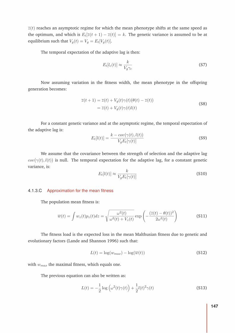
z(t) reaches an asymptotic regime for which the mean phenotype shifts at the same speed as

the optimum, and which is Et[z(t + 1) − z(t)] = k. The genetic variance is assumed to be at

equilibrium such that Vg(t) = Vg = Et[Vg(t)].

The temporal expectation of the adaptive lag is then:

Et[lc(t)] ≈ k

Vgγc(S7)

Now assuming variation in the fitness width, the mean phenotype in the offspring

generation becomes:

z(t + 1) = z(t) + Vg(t)γ(t)(θ(t) − z(t)

)

= z(t) + Vg(t)γ(t)l(t)(S8)

For a constant genetic variance and at the asymptotic regime, the temporal expectation of

the adaptive lag is:

Et[l(t)] =k − cov

(γ(t), l(t)

)

VgEt[γ(t)](S9)

We assume that the covariance between the strength of selection and the adaptive lag

cov(γ(t), l(t)

)is null. The temporal expectation for the adaptive lag, for a constant genetic

variance, is:

Et[l(t)] ≈ k

VgEt[γ(t)](S10)

4.1.3.C Approximation for the mean fitness

The population mean fitness is:

w(t) =

∫wz(t)pz(t)dz =

√ω2(t)

ω2(t) + Vz(t)exp

(−(z(t) − θ(t))2

2ω2(t)

)(S11)

The fitness load is the expected loss in the mean Malthusian fitness due to genetic and

evolutionary factors (Lande and Shannon 1996) such that:

L(t) = log(wmax) − log(w(t)) (S12)

with wmax the maximal fitness, which equals one.

The previous equation can also be written as:

L(t) = −1

2log

(ω2(t)γ(t)

)+

1

2l(t)2γ(t) (S13)

147

The first term on the right hand side is the loss in fitness caused by genetic variance, called the

variance load and denoted Lv(t) = −12 log

(ω2(t)γ(t)

), while the second term is the loss in fitness

caused by the evolutionary lag, called the evolutionary load and denoted Le(t) = 12 l(t)2γ(t). In

the following we present an approximation for these two fitness loads.

4.1.3.3.a Approximation for the variance load

With a constant fitness width and a constant genetic variance, the temporal expectation of

the variance load is:

Et[Lvc(t)] = −1

2log

(Et[ω

2(t)]γc

)(S14)

Now assuming variation in the fitness width and that the deviation of the fitness width at

generation t to its expectation, denoted δ(t), is small such that δ(t) = ω2(t) − E[ω2(t)] ≈ 0. We

use a Taylor series around δ(t) = 0 to the order 2 to approximate the variance load:

Lv(t) ≈ 1

2log

(Et[ω2(t)] + Vz

Et[ω2(t)]

)− δ(t)Vz

2(Et[ω2(t)]

(Et[ω2(t)] + Vz

))

+δ2(t)Vz

(2Et[ω

2(t)] + Vz

)

4Et[ω2(t)]2(Et[ω2(t)] + Vz

)2 + o(δ(t))3 (S15)

The temporal expectation for the variance load is:

Et[Lv(t)] ≈ 1

2log

(Et[ω2(t)] + Vz

Et[ω2(t)]

)− Et[δ(t)]Vz

2(Et[ω2(t)]

(Et[ω2(t)] + Vz

))

+Et[δ

2(t)]Vz

(2Et[ω

2(t)] + Vz

)

4Et[ω2(t)]2(Et[ω2(t)] + Vz

)2 (S16)

By replacing Et[δ(t)2] = Vt[ω2(t)] + Et[δ(t)]2 and recalling that Et[δ(t)] = 0, one can also

write:

Et[Lv(t)] ≈ 1

2log

(Et[ω2(t)] + Vz

Et[ω2(t)]

)+

Vt[ω2(t)]Vz

(2Et[ω

2(t)] + Vz

)

4Et[ω2(t)]2(Et[ω2(t)] + Vz

)2 (S17)

and finally the variance load is:

Et[Lv(t)] ≈ Lvc + Vt[ω2(t)]γ2

c

Vz

(2Et[ω

2(t)] + Vz

)

4Et[ω2(t)]2(S18)

148

4.1.3.3.b Approximation for the evolutionary load

With a constant fitness width and a constant genetic variance, the temporal expectation of

the evolutionary load is:

Et[Lec(t)] =1

2Et[l

2c (t)]γc =

1

2(Vt[lc(t)] + Et[lc(t)]

2)γc (S19)

Now assuming variation in the fitness width, and that the deviation of the fitness width at

generation t to its expectation is small, and using a Taylor series around δ(t) = 0 to the order 2,

one can approximate the evolutionary load as:

Le(t) ≈ l2(t)

2(Et[ω2(t)] + Vz

) − l2(t)δ(t)

2(Et[ω2(t)] + Vz

)2

+l2(t)δ(t)2

2(Et[ω2(t)] + Vz

)3 + o(δ(t))3 (S20)

The temporal expectation for the evolutionary load is:

Et[Le(t)] ≈ Et[l2(t)]

2(Et[ω2(t)] + Vz

) − Et[l2(t)δ(t)]

2(Et[ω2(t)] + Vz

)2 +Et[l

2(t)δ(t)2]

2(Et[ω2(t)] + Vz

)3 (S21)

Et[Le(t)] ≈ Et[l2(t)]

2(Et[ω2(t)] + Vz

) − Et[l2(t)]Et[δ(t)]

2(Et[ω2(t)] + Vz

)2 +Et[l

2(t)]Et[δ(t)2]

2(Et[ω2(t)] + Vz

)3 (S22)

By replacing Et[δ(t)2] = Vt[ω2(t)] + Et[δ(t)]2 and recalling that Et[δ(t)] = 0, one can also

write:

Et[Le(t)] ≈ Et[l2(t)]

2(Et[ω2(t)] + Vz

)(1 +

Vt[ω2(t)]

(Et[ω2(t)] + Vz

)2

)(S23)

and thus find the evolutionary load:

Et[Le(t)] ≈ Lec

(1 + Vt[ω

2(t)]γ2c

)(S24)

4.1.3.D Approximation for the genetic variance

We first assume a constant fitness width. From the infinitesimal model of trait inheritance,

the genetic variance after natural selection and random mating and with a constant fitness width

is:

Vg(t + 1) =VLE

2+

Vg(t)

2

(1 − Vg(t)γc(t)

)(S25)

with γc(t) = 1Vg(t)+Ve+Et[ω2(t)]

.

149

The temporal expectation of the genetic variance is:

Et[Vg(t + 1)] =VLE

2+

Et[Vg(t)]

2−

Et[V2

g (t)γc(t)]

2

=VLE

2+

Et[Vg(t)]

2−

Et[V2

g (t)]Et[γc(t)]

2−

cov(V 2g (t), γc(t))

2

(S26)

We assume that the fluctuations of the genetic variance are small such that E[Vg(t + 1) −Vg(t)] ≈ 0 and thus cov(V 2

g (t), γc(t)) ≈ 0. The temporal expectation of the genetic variance

simplifies to:

Et[Vg(t)] ≈ VLE + Et[V2

g (t)]Et[γc(t)] (S27)

One can derive the roots of the previous equation and find:

Et[Vg(t)] ≈ −1 +√

1 + 4VLEE[γc(t)]

2E[γc(t)](S28)

Now we assume variation in the fitness width. Again from the infinitesimal model of trait

inheritance, the genetic variance after natural selection and random mating, assuming variation

in the fitness width, is:

Vg(t + 1) =VLE

2+

Vg(t)

2

(1 − Vg(t)γ(t)

)(S29)

With the same reasoning than in the previous section, one can find the temporal

expectation for the genetic variance:

Et[Vg(t)] ≈ −1 +√

1 + 4VLEE[γ(t)]

2E[γ(t)](S30)

150

5Discussion

La phénologie de floraison est un trait pour lequel des réponses évolutives rapides au changement

climatique sont observées empiriquement (Parmesan, 2006 ; Parmesan et Yohe, 2003). Au cours

de cette thèse nous avons cherché à identifier les facteurs favorisant ou limitant les réponses

évolutives de la phénologie de floraison au changement climatique. Nous avons dans un premier

temps cherché à comprendre si l’homogamie pour la date de floraison pouvait expliquer les

réponses évolutives rapides observées dans les populations naturelles. Dans un second temps,

nous avons pris en compte l’effet de la sélection sexe-spécifique sur les réponses évolutives.

La sélection sexe-spécifique est fréquente dans les populations naturelles et pourrait expliquer

le dimorphisme sexuel observé pour la date de floraison, mais aussi contraindre les réponses

évolutives de la date de floraison. Enfin nous avons étudié les effets des fluctuations de la durée

de la saison de floraison, accentuées par le changement climatique, sur les réponses évolutives.

Ci-dessous je résume les résultats principaux des différents axes. Je propose ensuite quelques

connections possibles avec les données empiriques et quelques perspectives.

5.1 Résultats principaux

5.1.1 Effets de l’homogamie sur les réponses évolutives à la sélection

Je rappelle ici les différents patrons d’appariement que nous avons étudiés et les

hypothèses sous-jacentes avant de discuter de l’effet de ces patrons d’appariement sur les

réponses évolutives (i.e. les changements de génotype moyen entre générations). Nous avons

comparé les réponses évolutives à la sélection pour des populations homogames ou panmictiques.

Nous avons également comparé deux mécanismes d’homogamie : l’homogamie par préférence

femelle et l’homogamie temporelle. L’homogamie par préférence femelle suppose que les

femelles sélectionnées s’apparient avec des mâles ayant un phénotype qui leur ressemble. Elle est

modélisée par une fonction de préférence de forme Gaussienne dont la largeur affecte l’intensité

de la corrélation entre les partenaires. Sous homogamie temporelle, la production de gamètes est

distribuée au cours de la saison. Par exemple chez les plantes, la distribution des gamètes mâles

et femelles est définie par la distribution des fleurs ouvertes au cours de la saison. Nous avons

étudié deux scénarios extrêmes d’homogamie temporelle. Dans le premier chapitre, nous avons

supposé que la qualité des gamètes d’un individu varie au cours du temps et ce indépendemment

du phénotype de l’individu. La fertilité d’un individu varie donc au cours de la saison à la fois

151

parce que le nombre de gamètes produits change avec le nombre de fleurs ouvertes et parce que

la qualité de ces gamètes change. A un instant donné, tous les gamètes de la population ont

cependant la même qualité. Dans la suite de la discussion, ce scénario d’homogamie est appelé

"homogamie temporelle à qualité variable". Dans le deuxième chapitre, nous avons supposé que

la qualité des gamètes d’un individu dépend uniquement de son phénotype et qu’elle était

constante au cours de la saison. La fertilité d’un individu varie alors au cours de la saison

uniquement parce que le nombre de gamètes produits varie. A un instant donné, les gamètes de

la population ont des qualités différentes dépendant du phénotype de l’individu qui les a

produits. Dans la suite de la discussion, ce scénario d’homogamie est appelé "homogamie

temporelle à qualité constante". Un élément clé pour comprendre les points communs et les

différences de réponses évolutives entre patrons d’appariement est la compétition entre les

mâles.

Dans le premier chapitre, nous avons montré que la variation du nombre et de la qualité

des gamètes au cours de la saison modifie la fertilité efficace des individus. La fertilité efficace

maximale d’un individu est déplacée vers la date de floraison maximisant la qualité des gamètes

et est donc différente de son pic de production de gamètes. La période de floraison efficace pour

un individu est plus petite que la période de floraison. Le succès reproducteur relatif d’un mâle est

indépendant de la qualité de ses gamètes car, à un instant donné, tous les mâles en compétition

ont la même qualité de gamètes. Le succès reproducteur relatif d’un mâle dépend alors de la

proportion de gamètes produits à cet instant par rapport aux autres mâles de la population et

de la fertilité efficace de la femelle à cet instant. La réponse des mâles à la sélection sexuelle

induite par l’homogamie est identique à la réponse des femelles à la sélection naturelle, suggérant

que la sélection naturelle sur les mâles est totalement substituée par la sélection naturelle sur

les femelles. Pour une variance génétique donnée, la réponse à la sélection sous homogamie

temporelle à qualité variable est donc identique à celle sous panmixie. Rappelons que dans ce

modèle l’intensité de la sélection sur les sexes est identique et que le dimorphisme sexuel est nul.

Dans le deuxième chapitre, nous avons comparé la réponse à la sélection sous préférence

femelle avec celle sous homogamie temporelle à qualité constante. Bien que la compétition entre

mâles se produise à différentes échelles, i.e. une femelle pour la préférence, ou un instant donné

pour l’homogamie temporelle, le succès reproducteur d’un mâle dépend de celui des autres mâles

de la population. Ce point commun pourrait expliquer pourquoi, pour une variance génétique

donnée, la réponse à la sélection sous homogamie temporelle à fertilité constante est identique

à celle sous préférence femelle. Nous avons également montré que la réponse à la sélection

sous préférence femelle (ou homogamie temporelle à qualité constante) peut être plus petite ou

plus grande que celle sous panmixie selon l’intensité de la sélection sur les sexes, la vitesse du

changement environnemental et le degré de dimorphisme sexuel.

5.1.2 Effets de l’homogamie sur la structure de la variance génétique

En combinant l’utilisation de modèles théoriques aux hypothèses complémentaires, nous

avons montré les effets antagonistes de l’homogamie sur les composantes de la variance

152

génétique. Le modèle analytique est basé sur le modèle infinitésimal d’héritabilité du trait qui

suppose une variance génique constante, une taille de population infinie et un grand nombre de

locus déterminant le trait. Les prédictions de ce modèle ont permis de contraster les effets des

patrons d’appariement sur les associations entre effets alléliques. Sous panmixie, l’intensité de la

sélection stabilisante génère des associations négatives entre effets alléliques (Bulmer effect ;

Bulmer, 1971), diminuant ainsi la variance génétique. Sous homogamie, la corrélation entre les

phénotypes des partenaires associe des allèles à effets similaires sur le phénotype, et augmente la

variance génétique. L’effet positif de l’homogamie sur les associations alléliques est plus fort

quand la sélection naturelle stabilisante sur les femelles est moins forte que celle sur les mâles.

L’homogamie induit aussi une différence de succès reproducteur entre mâles, produisant de la

sélection sexuelle. Cette sélection sexuelle s’ajoute à la sélection naturelle stabilisante et

augmente l’intensité de la sélection stabilisante sur le trait. Nous avons utilisé un modèle

individu-centré qui laisse évoluer le polymorphisme génétique afin de comprendre les effets de la

sélection sexuelle sur celui-ci. Ce modèle suppose une taille finie de population et un nombre

limité de locus déterminant le trait. Les simulations montrent que la sélection sexuelle produite

par l’homogamie diminue le polymorphisme génétique. En lien avec les travaux de Kirkpatrick et

Nuismer (2004), nous avons montré que les effets positifs de l’homogamie sur les associations

entre allèles peuvent compenser ou non ses effets négatifs sur le polymorphisme génétique. Dans

le premier chapitre, nous avons mis en évidence que l’effet négatif de l’homogamie sur le

polymorphisme génétique maintient moins de variance génétique que sous panmixie quand la

sélection stabilisante est forte. A l’inverse, quand la sélection stabilisante est faible, l’effet positif

de l’homogamie sur les associations positives entre effets alléliques augmente la variance

génétique par rapport à celle maintenue sous panmixie. Nos résultats permettent de connecter

les attendus théoriques précédemment obtenus en absence de sélection et sous sélection

stabilisante. La diminution des effets positifs de l’homogamie sur la variance génétique avec

l’intensité de la sélection stabilisante explique pourquoi les études théoriques en absence de

sélection prédisent un fort effet de l’homogamie sur la variance génétique (Crow et Felsenstein,

1968 ; Crow et Kimura, 1970 ; Devaux et Lande, 2008 ; S. Wright, 1921) tandis qu’une étude sous

sélection stabilisante prédit une absence d’effet de l’homogamie (Lande, 1977). Nos résultats

permettent également d’expliquer pourquoi les études empiriques sous sélection directionnelle

artificielle trouvent un effet faible, voire nul, de l’homogamie sur les réponses génétiques (Breese,

1956 ; Campo et Gil, 1994 ; Garcia et Sanchez, 1992 ; McBride et Robertson, 1963 ; Sutherland

et al., 1968 ; Wilson et al., 1965). Les simulations montrent aussi que la vitesse de changement

environnemental modifie la variance génétique et le polymorphisme génétique. Cependant, la

variance génétique dans les populations homogames est généralement supérieure à celle des

populations panmictiques dans notre modèle quand l’environnement change.

Dans le chapitre 2, nous avons montré qu’une plus forte sélection naturelle sur les femelles

que sur les mâles diminue l’effet de l’homogamie sur les associations entre effets alléliques. La

variance génétique dépend aussi du type d’appariement. La variance génétique sous homogamie

temporelle est supérieure à celle sous panmixie, du moins dans la gamme de paramètres simulée.

En revanche, la variance génétique sous préférence femelle peut être inférieure à celle sous

panmixie suggérant que l’effet négatif de la préférence femelle sur le polymorphisme génétique

153

peut dépasser son effet positif sur les associations entre effets alléliques. Pour une valeur de

polymorphisme génétique donnée, l’homogamie temporelle produit plus d’associations positives

que la préférence femelle. L’homogamie temporelle maintient aussi plus de polymorphisme

génétique que la préférence femelle. La variance génétique sous homogamie temporelle est donc

supérieure à celle sous préférence femelle. La distribution individuelle des gamètes en homogamie

temporelle pourrait expliquer cette différence de variance génétique. L’annexe du chapitre 2

définit la variance génétique des mâles accédant à une femelle donnée. Cette variance est plus

petite que celle des mâles accédant à la reproduction à l’échelle de la population. En effet la

distribution des phénotypes des femelles implique que la variance des mâles qui se reproduisent

est supérieure à celle d’une population dans laquelle il y aurait un unique phénotype femelle.

De manière similaire, on peut supposer que la distribution individuelle des gamètes au cours

de la saison augmente la variance phénotypique des mâles accédant à une femelle donnée. A

l’échelle de la population, il est probable que la distribution individuelle des gamètes augmente

la variance génétique des pères et donc augmente la variance génétique à la génération suivante.

Les données empiriques montrent que les phénologies de floraison répondent au changement

climatique par des réponses à la fois évolutives et plastiques (Anderson et al., 2012 ; Franks

et al., 2014 ; Hamann et al., 2018) tandis que chez les animaux les réponses des phénologies

de reproduction semblent majoritairement plastiques (Charmantier et Gienapp, 2014 ; Gienapp

et al., 2008 mais voir aussi Réale et al., 2003). Il pourrait être intéressant d’explorer si la plus

grande variance génétique maintenue sous homogamie temporelle pour la date de floraison que

sous préférence femelle, commune chez les animaux, peut expliquer les différences de rôles entre

réponses plastiques et évolutives chez les plantes et les animaux.

5.1.3 Effets de l’homogamie sur l’adaptation

L’homogamie temporelle réduit le retard des populations à l’optimum par rapport à la

panmixie. En effet, bien que les réponses à la sélection directionnelle sont attendues équivalentes

sous homogamie temporelle à qualité variable et panmixie pour une variance génétique donnée,

l’augmentation de la variance génétique sous homogamie diminue le retard adaptatif.

L’homogamie diminue donc le fardeau évolutif par rapport à la panmixie. L’augmentation de

variance génétique sous homogamie augmente en revanche le fardeau de variance. Dans la

plupart des scénarios étudiés dans le chapitre 1, la diminution du fardeau de retard dépasse

l’augmentation du fardeau variance, augmentant ainsi la valeur sélective moyenne des

populations homogames. L’homogamie peut donc expliquer, au moins en partie, les réponses

évolutives rapides des phénologies de floraison au changement climatique.

Dans le deuxième chapitre, la sélection sexe-spécifique empêche les mâles et les femelles

d’être simultanément à leur optimum et fait émerger un optimum évolutif maximisant la valeur

sélective de la population. Cet optimum évolutif dépend de la position relative des optimums

mâles et femelles, de l’intensité de la sélection sur chaque sexe, du dimorphisme sexuel et de la

sélection sexuelle. Nous avons choisi de mesurer l’adaptation par rapport aux femelles qui sont

souvent plus limitantes pour la reproduction que ne le sont les mâles (Harts et al., 2014). Nous

avons décomposé la déviation de la valeur génétique moyenne de la population à l’optimum

154

femelle en deux parties. La première partie est causée par la déviation de la valeur génétique

moyenne de la population à l’optimum femelle en environnement constant. La sélection sexuelle

générée par l’homogamie augmente l’effet de la sélection naturelle sur les femelles et diminue

l’effet de la sélection naturelle sur les mâles. En absence de dimorphisme sexuel, la sélection

sexuelle et une plus forte sélection sur les femelles que sur les mâles diminue la déviation de la

valeur génétique moyenne de la population par rapport à l’optimum femelle. La deuxième partie

de la déviation à l’optimum femelle correspond à la déviation de la valeur génétique moyenne

de la population à l’optimum évolutif en environnement changeant. Cette part de la déviation

à l’optimum femelle est ainsi comparable au retard évolutif mesuré dans le premier chapitre.

Nous avons montré que le retard évolutif est plus petit (en valeur absolue) sous homogamie

qu’en panmixie quand la sélection sur les femelles est plus forte que celle sur les mâles. En

revanche le retard est plus grand (en valeur absolue) sous homogamie qu’en panmixie quand

la sélection sur les femelles est plus faible que celle sur les mâles. En absence de dimorphisme

sexuel, la sélection sexe-spécifique et la vitesse du changement environnemental définissent les

conditions pour lesquelles la valeur absolue de la déviation de la valeur génétique moyenne de la

population à l’optimum femelle est inférieure en homogamie par rapport à celle en panmixie. La

sélection sexe-spécifique limite les conditions pour lesquelles l’homogamie aide l’adaptation à un

environnement changeant.

Le dimorphisme sexuel est une réponse très fréquente pour résoudre les conflits entre sexes

engendrés par la sélection sexuelle et/ou la sélection naturelle sexe-spécifique (Cox et Calsbeek,

2009 ; de Lisle et al., 2018). De plus, pour les phénologies de floraison, le dimorphisme sexuel est

aussi sélectionné pour éviter l’autofécondation (Lloyd et Webb, 1986). Sous les hypothèses de

notre modèle, le dimorphisme sexuel déplace le phénotype des mâles de leur valeur génétique.

Sous homogamie, le dimorphisme sexuel entraîne l’optimum évolutif de la population dans la

direction des femelles. Dans une large gamme de paramètres, l’optimum évolutif peut même

dépasser l’optimum femelle. La déviation de la valeur génétique moyenne de la population à

l’optimum femelle change alors de signe et peut devenir supérieure à celle sous panmixie. Nous

avons montré que le dimorphisme sexuel limite l’adaptation des populations sous homogamie

par rapport à celles sous panmixie sauf quand l’optimum de floraison mâle est plus tardif que

l’optimum femelle et que la sélection sur les mâles est plus forte que celle sur les femelles.

5.1.4 Effets des fluctuations de l’intensité de la sélection

La plupart des modèles de génétique quantitative d’adaptation au changement

environnemental supposent une fonction de sélection de forme Gaussienne avec un optimum

mobile et une largeur constante (voir la revue de Kopp et Matuszewski, 2014). Dans le troisième

chapitre, nous avons montré que les fluctuations de la largeur de la fonction de sélection

augmentent l’intensité de la sélection par rapport à une largeur constante de la fonction de

sélection. L’augmentation de l’intensité de la sélection diminue la variance génétique et le retard

adaptatif.

155

En lien avec la littérature classique (Lande et Shannon, 1996, voir aussi la revue de Kopp

et Matuszewski, 2014), nous avons décomposé la diminution de la valeur sélective par rapport

à la valeur sélective maximale en un fardeau de variance et un fardeau évolutif. Nous avons

estimé les effets des fluctuations de la largeur de la sélection sur le taux de croissance à long

terme des populations en mesurant la moyenne géométrique des valeurs sélectives au cours du

temps. Nous montrons que les fluctuations de la largeur de la sélection augmentent directement

le fardeau de variance et le fardeau évolutif. Ces fardeaux sont aussi affectés indirectement

par les fluctuations de la largeur de la sélection via différentes voies. Les fluctuations de la

largeur de la sélection ont un effet indirect négatif sur le fardeau de variance via la variance

génétique. Le fardeau évolutif augmente avec la moyenne et la variance du retard adaptatif et

diminue avec la variance génétique. Les fluctuations de la largeur de la sélection ont donc un

effet indirect sur le fardeau évolutif via la variance génétique et le retard adaptatif. L’intensité

de la sélection est un élément clé pour comprendre les effets indirects des fluctuations de la

largeur de la sélection sur les fardeaux de variance et évolutif puisqu’elle détermine la variance

génétique et le retard adaptatif. Les simulations mettent en évidence un effet des fluctuations de

la largeur de la sélection sur la variance du retard adaptatif. L’effet des fluctuations de la largeur

de la sélection sur les fardeaux résultent donc d’effets direct et indirect ayant des signes opposés.

L’exploration numérique suggère que les fluctuations de l’intensité de la sélection diminuent la

moyenne géométrique des valeurs sélectives sauf quand l’environnement change rapidement et

que la force moyenne de la sélection est faible. Les fluctuations de l’intensité de la sélection ont

donc un coût démographique qui pourrait aggraver le déclin des populations.

5.2 Comment connecter ces résultats théoriques à des

résultats empiriques?

L’objectif de ces travaux de thèse était de fournir des prédictions explicatives aux réponses

évolutives au changement climatique. En nous basant sur des observations empiriques, nous

avons utilisé une approche théorique pour affiner la compréhension des réponses évolutives au

changement climatique. Il serait maintenant intéressant de vérifier si les données empiriques

appuient ou réfutent nos prédictions.

Nos résultats suggèrent que l’adaptation des populations naturelles peut être prédite

si nous avons accès à des estimations des paysages de valeurs sélectives au cours du temps.

Cependant les mesures empiriques de la sélection présentent plusieurs limites. Parmi ces limites,

l’erreur d’échantillonnage représente une part importante de la variance des estimations et rend

difficile l’interprétation des fluctuations temporelles de la sélection (Morrissey et Hadfield, 2012 ;

Siepielski et al., 2009). Les données actuelles ne sont aussi peut-être pas suffisantes pour estimer

la sélection avec suffisamment de précision (de Villemereuil et al., 2020 ; Haller et Hendry,

2014 ; Kingsolver et Pfennig, 2007 ; Morrissey et Hadfield, 2012). Enfin, les études considèrent

souvent une seule composante de la valeur sélective plutôt que l’ensemble des composantes de

valeur sélective (Kingsolver et Pfennig, 2007). De nouvelles méthodes telles que la méthode

156

aster permettent désormais des estimations plus précises des fonctions de sélection (Shaw et

Geyer, 2010 ; Shaw et al., 2008). Ces méthodes pourraient ainsi faciliter les connections entre les

résultats théoriques et empiriques.

Nous avons ici souhaité fournir des prédictions généralistes des conditions favorisant ou

contraignant l’adaptation des populations au changement climatique. Nous pourrions maintenant

envisager de paramétrer les modèles avec des estimations spécifiques à une espèce donnée pour

prédire ses réponses au changement climatique et guider les stratégies de gestion. Cependant

une difficulté est que l’ensemble des informations nécessaires pour paramétrer les modèles sont

rarement disponibles. Une possibilité serait néanmoins d’explorer une gamme de valeurs réalistes

pour les paramètres auxquels nous n’avons pas accès et de réaliser une analyse de sensibilité des

résultats. Les conditions favorisant l’adaptation de cette espèce en particulier pourraient ainsi

être identifiées.

5.3 Perspectives

5.3.1 Effet de l’autofécondation sur les réponses évolutives au changement

climatique

Nous avons vu que l’homogamie associe des individus aux phénotypes similaires associant

ainsi des allèles à effets similaires sur les phénotypes. Les associations positives entre allèles

augmentent la variance génétique favorisant dans certains cas les réponses évolutives au

changement climatique. L’autofécondation crée aussi des associations positives fortes entre

allèles, mais sur l’ensemble du génome. Il serait donc intéressant de faire un parallèle entre les

effets de l’homogamie et de l’autofécondation sur les réponses évolutives au changement

climatique.

5.3.1.A Environnement constant

Les effets de l’autofécondation sur la variance génétique ont été étudiés historiquement

pour comprendre les transitions entre l’autofécondation, l’allofécondation et les systèmes mixtes

(Lande et Schemske, 1985 ; Schemske et Lande, 1985 ; S. I. Wright et al., 2013). L’autofécondation

agit sur la variance génétique avec des mécanismes différents de ceux de l’homogamie. D’une part,

en absence de sélection, l’autofécondation augmente l’homozygotie en associant des génotypes

identiques. Les allèles délétères sont alors exposés à la sélection et l’effet positif de l’augmentation

de l’homozygotie est compensé par la purge des allèles délétères (Lande, 1977). La sélection

stabilisante favorise les associations entre effets alléliques opposés sur le phénotype (Bulmer,

1971). La variance génétique est ainsi réduite mais le polymorphisme génétique est maintenu.

L’autofécondation favorise ces associations négatives entre allèles en réduisant la recombinaison

et diminue l’efficacité de la sélection. Dans son modèle d’évolution de la variance génétique d’un

trait polygénique soumis à la mutation et à la sélection stabilisante, Lande (1977) montre que

les effets positifs et négatifs de l’autofécondation se compensent. La variance génétique sous

157

autofécondation n’est donc pas différente de celle sous panmixie. Lande et Porcher (2015) ont

étendu la gamme de taux d’autofécondation étudiée et ont identifié un taux d’autofécondation

seuil au-dessus duquel, la variance génétique des populations autofécondantes est inférieure à

celle des populations panmictiques. Les données empiriques confirment que l’autofécondation

diminue la variance génétique par rapport à la panmixie (voir Clo et al., 2019 pour une méta-

analyse).

5.3.1.B Environnement changeant

Les effets de l’autofécondation sur les réponses évolutives au changement

environnemental ont été moins étudiés. L’autofécondation peut accélérer la réponse à la

sélection par rapport à l’allofécondation, au moins dans les premières générations suivant un

changement de l’environnement (Noël et al., 2017). Dans une étude récente, Clo et al. (2020)

utilise des simulations individu-centré supposant une fonction de sélection de forme Gaussienne

dont l’optimum change ponctuellement. Les auteurs montrent que les associations négatives

entre effets alléliques générées par l’autofécondation permettent de stocker le polymorphisme

génétique quand le taux de mutation est élevé. Le polymorphisme génétique peut alors être

mobilisé suite à un changement ponctuel de l’environnement. Les populations autofécondantes

(taux d’autofécondation < 1) peuvent ainsi s’adapter aussi bien que les populations

allofécondantes. L’autofécondation est donc un régime de reproduction qui présente des

propriétés intéressantes dans le cadre du changement climatique. Il serait pertinent de comparer

les effets de l’autofécondation et de l’homogamie sur les réponses évolutives à un changement

soutenu de l’environnement. Les conditions dans lesquelles l’homogamie favorise plus ou moins

les réponses évolutives par rapport à l’autofécondation pourraient ainsi être déterminées.

En particulier, on peut s’attendre à ce que les épisodes de forte sélection annulent les

effets positifs de l’homogamie sur la variance génétique. Suite à des épisodes de forte sélection,

l’homogamie, par son effet sur les associations positives en effets alléliques, pourrait favoriser le

regain rapide de variance génétique si le polymorphisme génétique est suffisant. En revanche,

si les épisodes de forte sélection sont trop fréquents, les effets négatifs de l’homogamie sur le

polymorphisme pourraient s’ajouter à ceux des fluctuations de l’environnement et compromettre

l’adaptation. Dans cette situation, l’autofécondation protégeant le polymorphisme génétique

pourrait être plus avantageuse que l’homogamie.

5.3.2 Effet des variations de la taille de population sur les réponses évolutives au

changement climatique

Au cours de cette thèse, nous nous sommes intéressées aux conditions dans lesquelles la

variance génétique peut faciliter les réponses au changement climatique en supposant une taille

de population très grande ou constante. Les méta-analyses des données empiriques identifient la

taille de population comme étant l’un des principaux facteurs d’extinction (O’Grady et al., 2004).

La théorie s’est ainsi attachée à clarifier l’effet de la stochasticité sur la taille de population sur

le risque d’extinction (Lande, 1993 ; Lande et al., 2003 ; Melbourne et Hastings, 2008 ; Sæther

158

et Engen, 2015). La stochasticité de la taille de population peut être d’origine démographique

ou environnementale. La stochasticité environnementale est causée par les fluctuations de la

probabilité de mortalité et de reproduction de tous les individus de la population (Lande, 1993).

La stochasticité environnementale agit donc sur l’ensemble de la population quelle que soit

sa taille et représente un risque important d’extinction pour les populations. La stochasticité

démographique est causée par la variation de la probabilité de survie et de reproduction entre

individus d’un même génotype (Lande, 1993). Lorsque la taille de population initiale est grande,

la stochasticité démographique a peu d’effet sur la taille de population à la génération suivante

(Lande 1993). Cependant, quand la taille de population initiale est faible à modérée, les effets

de la stochasticité démographique sur le risque d’extinction s’ajoutent à ceux de la stochasticité

environnementale. En effet, dans les petites populations la diversité génétique est plus faible que

dans les grandes populations, limitant ainsi la réponse évolutive au changement environnemental.

De plus, la dérive génétique est plus forte dans les petites populations que dans les grandes

populations. Des allèles bénéfiques pour les réponses au changement environnemental sont alors

plus facilement perdus. Les stochasticités démographique et environnementale ont donc des effets

synergiques sur le risque d’extinction et ne pas prendre en compte les effets de la stochasticité

démographique peut conduire à sous-estimer le risque d’extinction (Bürger et Lynch, 1995 ;

Melbourne et Hastings, 2008). Une extension possible aux travaux de cette thèse serait de laisser

la taille de population varier afin de déterminer si nos conclusions sur les effets de l’homogamie

et des fluctuations de l’intensité de la sélection sont robustes à la stochasticité démographique.

5.3.3 Effet des stades de vie sur les réponses évolutives au changement climatique

Comme la plupart des études théoriques, nous avons considéré l’adaptation d’une espèce

avec un cycle de vie très simplifié. Cependant, la plupart des organismes présentent un cycle

de vie à plusieurs stades. Le réalisme de nos modèles pourrait donc être amélioré en prenant

en compte des cycles de vie à plusieurs stades. Les effets de la complexité des cycles de vie sur

l’adaptation ont été étudiés pour des populations à reproduction panmictique (Cotto et Chevin,

2020 ; Cotto et Ronce, 2014 ; Cotto et al., 2019 ; Marshall et al., 2016). Ces modèles ont pris

en compte les variations de la sélection entre stades de vie et montrent qu’un cycle de vie à

plusieurs stades peut contraindre ou faciliter les réponses évolutives. Les stades juvéniles sont

souvent soumis à de plus fortes pressions de sélection que les stades âgés (Przeslawski et al.,

2015). Les réponses des stades juvéniles sont donc attendues différentes de celles des stades

adultes (Cotto et Ronce, 2014). De plus, les réponses des stades ne sont pas indépendantes :

l’évolution des stades juvéniles influence l’évolution des stades plus âgés (Marshall et al., 2016).

Les différences d’intensité de sélection entre stades peuvent faciliter ou contraindre l’adaptation

selon notamment les corrélations génétiques entre stades de vie, la variance génétique et la

plasticité de chaque stade (Marshall et al., 2016). Cotto et Chevin (2020) modélise une population

soumise à plusieurs épisodes de sélection fluctuante au cours d’une génération. A l’aide d’un

modèle d’évolution d’un trait polygénique, les auteurs montrent que les dynamiques évolutives

dépendent d’un optimum intégratif correspondant à une somme des optimums pondérée par la

contribution de chaque épisode de sélection à la sélection totale. L’intensité de la sélection est

159

quant à elle proportionnelle à une moyenne harmonique des largeurs de fonctions de sélection.

Les fluctuations intra-génération de la sélection résultent en l’élimination sélective d’individus.

Dans le chapitre 3 nous avons montré que les variations de l’intensité de la sélection entre années

peuvent aussi aggraver le déclin des populations. Il serait intéressant de comparer la part de la

variation de l’intensité de la sélection entre années (chapitre 3) et entre stades de vie dans les

changements de taux de croissance à long terme des populations.

Chez certains organismes comme les plantes ou les coraux, la phase de dispersion se

produit uniquement au stade de gamète et au stade juvénile (i.e. graine ou larve). Au delà

du fait que les phases juvénile et adulte ne subissent pas les mêmes pressions de sélection,

la phase fixée peut contraindre les changements rapides d’aire de distribution et les réponses

évolutives (Aguilée et al., 2016 ; Cotto et al., 2017). Chez les plantes, la phase de dispersion

est étroitement liée à la phénologie de floraison et l’homogamie pour la date de floraison peut

agir comme un filtre aux flux de gènes (Soularue et Kremer, 2012). L’homogamie pourrait

ainsi avoir des conséquences non négligeables sur les changements d’aire de distribution et les

changements de niche écologique dans un climat changeant. Il serait intéressant d’étudier les

effets de l’homogamie sur les changements d’aire de distribution des plantes.

5.4 Conclusion générale

Au cours de cette thèse, nous avons utilisé une approche théorique pour tenter d’améliorer

le réalisme des modèles d’adaptation des phénologies de floraison au changement climatique.

Nous avons montré que la sélection sexuelle engendrée par l’homogamie affecte les conflits de

sélection entre mâles et femelles. La sélection sexuelle et la sélection naturelle sexe-spécifique,

en absence de dimorphisme sexuel, déplacent la valeur génétique moyenne de la population

en direction de l’optimum des femelles en environnement constant. Dans un environnement

changeant, il existe une gamme de vitesse de changement environnemental, variant avec la

sélection sexe-spécifique, pour laquelle l’homogamie facilite l’adaptation à l’optimum femelle par

rapport à la panmixie. Le dimorphisme sexuel peut entraîner la valeur génétique moyenne de

la population au-delà de l’optimum femelle, et ainsi augmenter ou diminuer la déviation de la

valeur génétique moyenne de la population par rapport à l’optimum femelle. Le dimorphisme

sexuel diminue souvent la gamme de vitesses de changement environnemental pour laquelle

l’homogamie facilite l’adaptation à l’optimum femelle par rapport à la panmixie. Nous avons aussi

montré que la sélection sexuelle a des effets antagonistes sur la variance génétique : elle s’ajoute

à la sélection stabilisante et diminue le polymorphisme génétique mais elle augmente aussi les

associations positives entre effets alléliques. Les associations positives sont moins importantes

quand la sélection sur les femelles est plus forte que celle sur les mâles. Dans de nombreux

cas, les effets positifs de l’homogamie dominent ses effets négatifs et l’homogamie augmente la

variance génétique par rapport à la panmixie. La manière de modéliser l’homogamie affecte la

compétition entre les mâles et la variance des mâles accédant la reproduction. Enfin nous avons

montré que les fluctuations de la durée de la saison de floraison, accentuées par le changement

climatique, diminuent la variance génétique et le retard adaptatif. Les fluctuations de la durée de

160

la saison de floraison impliquent dans de nombreux cas un coût démographique qui compromet

le taux de croissance à long terme des populations.

161

Bibliographie

Aguilée, R., Raoul, G., Rousset, F. & Ronce, O. (2016). Pollen dispersal slows geographical range shiftand accelerates ecological niche shift under climate change. Proceedings of the National Academy

of Sciences of the United States of America, 113(39), E5741-8. https://doi.org/10.1073/pnas.1607612113

Anderson, J. T., Inouye, D. W., McKinney, A. M., Colautti, R. I. & Mitchell-Olds, T. (2012). Phenotypicplasticity and adaptive evolution contribute to advancing flowering phenology in response toclimate change. Proceedings. Biological sciences, 279(1743), 3843-3852.

Breese, E. L. (1956). The genetical consequences of assortative mating. Heredity, 10(3), 323-343. https://doi.org/10.1038/hdy.1956.30

Bulmer, M. G. (1971). The effect of selection on genetic variability. The American naturalist, 105(943),201-211. https://doi.org/10.1086/282718

Bürger, R. & Lynch, M. (1995). Evolution and extinction in a changing environment : a quantitative-geneticanalysis. Evolution, 1(49), 151-163.

Campo, J. L. & Gil, M. G. (1994). The effects of assortative mating on the genetic change due to linearindex selection in tribolium. Journal of animal breeding and genetics = Zeitschrift fur Tierzuchtung

und Zuchtungsbiologie, 111(1-6), 213-219. https://doi.org/10.1111/j.1439-0388.1994.tb00460.xCharmantier, A. & Gienapp, P. (2014). Climate change and timing of avian breeding and migration :

evolutionary versus plastic changes. Evolutionary applications, 7(1), 15-28. https://doi.org/10.1111/eva.12126

Clo, J., Gay, L. & Ronfort, J. (2019). How does selfing affect the genetic variance of quantitative traits ? anupdated meta-analysis on empirical results in angiosperm species. Evolution ; international journal

of organic evolution, 73(8), 1578-1590. https://doi.org/10.1111/evo.13789Clo, J., Ronfort, J. & Abu Awad, D. (2020). Hidden genetic variance contributes to increase the short-term

adaptive potential of selfing populations. Journal of Evolutionary Biology, 33(9), 1203-1215.https://doi.org/10.1111/jeb.13660

Cotto, O. & Chevin, L.-M. (2020). Fluctuations in lifetime selection in an autocorrelated environment.Theoretical Population Biology, 134, 119-128. https://doi.org/10.1016/j.tpb.2020.03.002

Cotto, O. & Ronce, O. (2014). Maladaptation as a source of senescence in habitats variable in space andtime. Evolution, 68(9), 2481-2493. https://doi.org/10.1111/evo.12462

Cotto, O., Sandell, L., Chevin, L.-M. & Ronce, O. (2019). Data from : maladaptive shifts in life history in achanging environment. The American naturalist, 194(4), 558-573.

Cotto, O., Wessely, J., Georges, D., Klonner, G., Schmid, M., Dullinger, S., Thuiller, W. & Guillaume, F.(2017). A dynamic eco-evolutionary model predicts slow response of alpine plants to climatewarming. Nature Communications, 8(1), 15399. https://doi.org/10.1038/ncomms15399

Cox, R. M. & Calsbeek, R. (2009). Sexually antagonistic selection, sexual dimorphism, and the resolutionof intralocus sexual conflict. The American Naturalist, 173(2), 176-187. https://doi.org/10.1086/595841

163

Crow, J. F. & Felsenstein, J. (1968). The effect of assortative mating on the genetic composition of apopulation. Eugenics Quaterly, 15(2), 85-97.

Crow, J. F. & Kimura, M. (1970). An introduction to population genetics theory. Population (French Edition),26(5), 977. https://doi.org/10.2307/1529706

de Lisle, S. P., Goedert, D., Reedy, A. M. & Svensson, E. I. (2018). Climatic factors and species rangeposition predict sexually antagonistic selection across taxa. Philosophical transactions of the Royal

Society of London. Series B, Biological sciences, 373(1757). https://doi.org/10.1098/rstb.2017.0415Devaux, C. & Lande, R. (2008). Incipient allochronic speciation due to non-selective assortative mating by

flowering time, mutation and genetic drift. Proceedings. Biological sciences, 275(1652), 2723-2732.https://doi.org/10.1098/rspb.2008.0882

de Villemereuil, P., Charmantier, A., Arlt, D., Bize, P., Brekke, P., Brouwer, L., Cockburn, A., Côté, S. D.,Dobson, F. S., Evans, S. R., Festa-Bianchet, M., Gamelon, M., Hamel, S., Hegelbach, J., Jerstad, K.,Kempenaers, B., Kruuk, L. E. B., Kumpula, J., Kvalnes, T., . . . Chevin, L.-M. (2020). Fluctuatingoptimum and temporally variable selection on breeding date in birds and mammals. Proceedings

of the National Academy of Sciences of the United States of America, 117(50), 31969-31978.https://doi.org/10.1073/pnas.2009003117

Franks, S. J., Weber, J. J. & Aitken, S. N. (2014). Evolutionary and plastic responses to climate change interrestrial plant populations. Evolutionary applications, 7(1), 123-139. https://doi.org/10.1111/eva.12112

Garcia, C. & Sanchez, L. (1992). Assortative mating and selection response in drosophila melanogaster.Journal of animal breeding and genetics = Zeitschrift fur Tierzuchtung und Zuchtungsbiologie,109(1-6), 161-167. https://doi.org/10.1111/j.1439-0388.1992.tb00393.x

Gienapp, P., Teplitsky, C., Alho, J. S., Mills, J. A. & Merilä, J. (2008). Climate change and evolution :disentangling environmental and genetic responses. Molecular Ecology, 17(1), 167-178. https://doi.org/10.1111/j.1365-294X.2007.03413.x

Haller, B. C. & Hendry, A. P. (2014). Solving the paradox of stasis : squashed stabilizing selection and thelimits of detection. Evolution, 68(2), 483-500. https://doi.org/10.1111/evo.12275

Hamann, E., Weis, A. E. & Franks, S. J. (2018). Two decades of evolutionary changes in brassica rapa inresponse to fluctuations in precipitation and severe drought. Evolution ; international journal of

organic evolution, 72(12), 2682-2696. https://doi.org/10.1111/evo.13631Harts, A. M. F., Schwanz, L. E. & Kokko, H. (2014). Demography can favour female-advantageous alleles.

Proceedings. Biological sciences, 281(1790). https://doi.org/10.1098/rspb.2014.0005Kingsolver, J. G. & Pfennig, D. W. (2007). Patterns and power of phenotypic selection in nature. BioScience,

57(7), 561-572. https://doi.org/10.1641/B570706Kopp, M. & Matuszewski, S. (2014). Rapid evolution of quantitative traits : theoretical perspectives.

Evolutionary applications, 7(1), 169-191. https://doi.org/10.1111/eva.12127Lande, R. (1977). The influence of the mating system on the maintena. Genetics, 86(2), 485-498.Lande, R. (1993). American society of naturalists. The American Naturalist, 142(6), 911-927. https :

//doi.org/10.1086/284618Lande, R., Engen, S. & SAETHER, B.-E. (2003). Stochastic population dynamics in ecology and conservation

(Oxford Univeristy Press, Éd.).Lande, R. & Porcher, E. (2015). Maintenance of quantitative genetic variance under partial self-fertilization,

with implications for evolution of selfing. Genetics, 200(3), 891-906. https://doi.org/10.1534/genetics.115.176693

Lande, R. & Schemske, D. W. (1985). The evolution of self-fertilization and inbreeding depression in plants.i. genetic models. Evolution, 39(1), 24-40. https://doi.org/10.1111/j.1558-5646.1985.tb04077.x

Lande, R. & Shannon, S. (1996). The role of genetic variation in adaptation and population persistence ina changing environment. Evolution, 50(1), 434-437.

164

Lloyd, D. G. & Webb, C. J. (1986). The avoidance of interference between the presentation of pollenand stigmas in angiosperms i. dichogamy. New Zealand Journal of Botany, 24(1), 135-162.https://doi.org/10.1080/0028825X.1986.10409725

Marshall, D. J., Burgess, S. C. & Connallon, T. (2016). Global change, life-history complexity and thepotential for evolutionary rescue. Evolutionary applications, 9(9), 1189-1201. https://doi.org/10.1111/eva.12396

McBride, G. & Robertson, A. (1963). Selection using assortative mating in drosophila melanogaster.Genetical Research, 4(3), 356-369. https://doi.org/10.1017/s001667230000375x

Melbourne, B. A. & Hastings, A. (2008). Extinction risk depends strongly on factors contributing tostochasticity. Nature, 454(7200), 100-103. https://doi.org/10.1038/nature06922

Morrissey, M. B. & Hadfield, J. D. (2012). Directional selection in temporally replicated studies isremarkably consistent. Evolution, 66(2), 435-442.https://doi.org/10.1111/j.1558-5646.2011.01444.x

Noël, E., Jarne, P., Glémin, S., MacKenzie, A., Segard, A., Sarda, V. & David, P. (2017). Experimentalevidence for the negative effects of self-fertilization on the adaptive potential of populations.Current biology : CB, 27(2), 237-242. https://doi.org/10.1016/j.cub.2016.11.015

O’Grady, J. J., Reed, D. H., Brook, B. W. & Frankham, R. (2004). What are the best correlates of predictedextinction risk ? Biological Conservation, 118(4), 513-520. https://doi.org/10.1016/j.biocon.2003.10.002

Parmesan, C. (2006). Ecological and evolutionary responses to recent climate change. Annual Review of

Ecology, Evolution, and Systematics, 37(1), 637-669. https://doi.org/10.1146/annurev.ecolsys.37.091305.110100

Parmesan, C. & Yohe, G. (2003). A globally coherent fingerprint of climate change impacts across naturalsystems. Nature, 421(6918), 37-42. https://doi.org/10.1038/nature01286

Przeslawski, R., Byrne, M. & Mellin, C. (2015). A review and meta-analysis of the effects of multipleabiotic stressors on marine embryos and larvae. Global Change Biology, 21(6), 2122-2140. https://doi.org/10.1111/gcb.12833

Réale, D., McAdam, A. G., Boutin, S. & Berteaux, D. (2003). Genetic and plastic responses of a northernmammal to climate change. Proceedings. Biological sciences, 270(1515), 591-596. https://doi.org/10.1098/rspb.2002.2224

Sæther, B.-E. & Engen, S. (2015). The concept of fitness in fluctuating environments. Trends in ecology &

evolution, 30(5), 273-281. https://doi.org/10.1016/j.tree.2015.03.007Schemske, D. W. & Lande, R. (1985). The evolution of self-fertilization and inbreeding depression in

plants. ii. empirical observations. Evolution, 39(1), 41-52. https://doi.org/10.1111/j.1558-5646.1985.tb04078.x

Shaw, R. G. & Geyer, C. J. (2010). Inferring fitness landscapes. Evolution, 64(9), 2510-2520. https ://doi.org/10.1111/j.1558-5646.2010.01010.x

Shaw, R. G., Geyer, C. J., Wagenius, S., Hangelbroek, H. H. & Etterson, J. R. (2008). Unifying life-historyanalyses for inference of fitness and population growth. The American Naturalist, 172(1), E35-47.https://doi.org/10.1086/588063

Siepielski, A. M., DiBattista, J. D. & Carlson, S. M. (2009). It’s about time : the temporal dynamics ofphenotypic selection in the wild. Ecology Letters, 12(11), 1261-1276. https://doi.org/10.1111/j.1461-0248.2009.01381.x

Soularue, J.-P. & Kremer, A. (2012). Assortative mating and gene flow generate clinal phenologicalvariation in trees. BMC evolutionary biology, 12, 79. https://doi.org/10.1186/1471-2148-12-79

Sutherland, T. M., Biondini, P. E. & Haverland, L. H. (1968). Selection under assortative mating in mice.Genetical Research, 11(2), 171-178. https://doi.org/10.1017/s0016672300011332

165

Wilson, S. P., Kyle, W. H. & Bell, A. E. (1965). The effects of mating systems and selection on pupa weightin tribolium. Genetical Research, 6(3), 341-351. https://doi.org/10.1017/s0016672300004237

Wright, S. (1921). Systems of mating. iii. assortative mating based on somatic resemblance. Genetics, 6(2),144.

Wright, S. I., Kalisz, S. & Slotte, T. (2013). Evolutionary consequences of self-fertilization in plants.Proceedings. Biological sciences, 280(1760), 20130133. https://doi.org/10.1098/rspb.2013.0133

Layout modified from Latex Style "UCPH Thesis" Copyright 2019 M. Roald-Arbøl

166