Poincaré on clocks in motion - HAL-SHS - Archives-Ouvertes.fr
Upload
khangminh22Category
view
0download
0
HAL Id: tel-02917985https://tel.archives-ouvertes.fr/tel-02917985
Submitted on 20 Aug 2020
HAL is a multi-disciplinary open accessarchive for the deposit and dissemination of sci-entific research documents, whether they are pub-lished or not. The documents may come fromteaching and research institutions in France orabroad, or from public or private research centers.
L’archive ouverte pluridisciplinaire HAL, estdestinée au dépôt et à la diffusion de documentsscientifiques de niveau recherche, publiés ou non,émanant des établissements d’enseignement et derecherche français ou étrangers, des laboratoirespublics ou privés.
Modeling the kinetic behaviour, mixing and localtransfer pheonmena and biologicial populationheterogeneity effects in industrial fermenters
Maxime Pigou
To cite this version:Maxime Pigou. Modeling the kinetic behaviour, mixing and local transfer pheonmena and biologicialpopulation heterogeneity effects in industrial fermenters. Biotechnology. INSA de Toulouse, 2018.English. NNT : 2018ISAT0038. tel-02917985

THESETHESEEn vue de l’obtention du
DOCTORAT DE L’UNIVERSITE DE TOULOUSEDelivre par :
l’Institut National des Sciences Appliquees de Toulouse (INSA de Toulouse)
Presentee et soutenue le 08/10/2018 par :Maxime PIGOU
Modelisation du comportement cinetique, des phenomenes demelange, de transfert locaux et des effets d’heterogeneite de
population dans les fermenteurs industriels.
JURYFrank DELVIGNE Liege University RapporteurRodney O. FOX Iowa State University RapporteurMartine MEIRELES Centre National de la Recherche Scientifique ExaminateurRalf TAKORS University of Stuttgart ExaminateurAngelique DELAFOSSE Liege University ExaminateurMarie-Isabelle PENET Sanofi Chimie ExaminateurGeoffrey LARONZE Sanofi Chimie InviteJerome MORCHAIN INSA de Toulouse Co-directeurPascal FEDE Universite Paul Sabatier Co-directeur
Ecole doctorale et specialite :MEGEP : Genie des procedes et de l’Environnement
Unites de Recherche :Laboratoire d’Ingenierie des Systemes Biologiques et des ProcedesInstitut de Mecanique des Fluides de Toulouse
Directeurs de These :Jerome MORCHAIN et Pascal FEDE
Rapporteurs :Frank DELVIGNE et Rodney O. FOX

i
The work described in the present manuscript has been conducted at
Laboratoire d’Ingenierie des Systemes Biologiques et des ProcedesUMR 5504 INSA, CNRSUMR 792 INSA, INRA135 Avenue de Rangueil31077 Toulouse Cedex 4, France
and
Institut de Mecanique des Fluides de ToulouseUMR 5502 CNRS, INPT, UPS2 Allee du Professeur Camille Soula31400 Toulouse, France
with the financial support and under the supervision of
Sanofi Chimie9 Quai Jules Guesde94400 Vitry-sur-Seine cedex, France
and
Sanofi Chimie20 Avenue Raymond Aron92165 Antony cedex, France


R E S U M E
Les biotechnologies sont un champ d’application majeur pour les travaux de rechercheactuels et a venir [Noorman and Heijnen, 2017; Camarasa et al., 2018]. Elles sont actuelle-ment appliquees aux productions industrielles de composes chimiques, de bio-carburantset bio-plastiques, ou de molecules a forte valeur ajoutee. La diversite naturelle des micro-organismes nous laisse esperer de nouvelles applications industrielles dans un futur proche,et pourrait aider a la lutte contre les crises environnementales et energetiques.
De la decouverte de nouvelles voies de production a leurs applications industrielles,plusieurs etapes d’ingenierie sont requises pour permettre le passage d’echelle. Ce tra-vail peut etre facilite par la modelisation et la simulation predictive des bioreacteurs.Differentes approches ont ete developpees dans cet objectif, mais les modeles obtenusechouent generalement a reproduire les observations experimentales a differentes echelles[Enfors et al., 2001]. Cela s’explique par l’utilisation d’hypotheses qui, bien que validesaux echelles de culture en laboratoire, ne s’appliquent pas aux echelles industrielles. Ledefi principal aborde par ce travail est de s’affranchir de ces hypotheses afin d’ameliorerles modeles tout en assurant un cout numerique plus faible que les approches usuelles.
Cette these se concentre sur le developpement d’une structure de modele pour lesfermenteurs industriels, en visant un usage d’ingenierie. Ce travail se base sur deuxpostulats : (i) par leur taille, les fermenteurs industriels sont heterogenes; (ii) par leurnature, les micro-organismes sont des systemes dynamiques. Ces considerations induisentplusieurs consequences. La principale est que les micro-organismes vont se differencierles uns des autres. La seconde est qu’ils seront en desequilibre avec leur environnement,entraınant des baisses de performance a l’echelle du procede. Pour integrer l’ensemblede ces aspects dans une unique structure de modele, tout en permettant des simula-tions rapides d’un fermenteur, l’approche proposee couple (i) un modele metaboliquedynamique pour decrire le comportement des cellules, (ii) un modele de bilan de popu-lation pour suivre l’heterogeneite biologique et (iii) un modele de compartiments pourdecrire l’hydrodynamique.
Un resultat majeur a ete le developpement d’une structure de modele metabolique, quia ete confrontee avec succes a de nombreuses donnees experimentales, tout en preservantun cout numerique significativement faible. Cette structure a ete appliquee a deux micro-organismes, Escherichia coli et Saccharomyces cerevisiae. Une comparaison de plusieursmethodes permettant de traiter les equations de bilans de population a ete menee entermes de stabilite, precision et performances a conduit a la selection de la methodeetendue de quadrature des moments. Une amelioration majeure de cette methode a eteidentifiee, permettant un gain de stabilite et de performances, en reduisant son cout d’unfacteur 10. L’hydrodynamique gaz-liquide d’un fermenteur industriel a ete obtenue parMecanique des Fluides Numerique (CFD) et des outils supplementaires ont ete developpespour extraire des modeles de compartiments a partir des simulations CFD. Finalement,le couplage des modeles metaboliques, de bilan de population et de compartiments a eteillustre par la simulation d’une configuration industrielle.
Mots cles : bioreacteur, modelisation, simulation, bilan de population, metabolisme, scale-up,CFD, modele de compartiments, micro-melange
iii


S U M M A RY
Biotechnologies form a significant field for current and upcoming research [Noorman andHeijnen, 2017; Camarasa et al., 2018]. They are currently applied to industrial productionof chemicals, bio-fuels or high-value molecules. The natural –massive– diversity of micro-organisms is expected to unlock new industrial applications in a near future, and couldhelp facing the environmental and energetic crises.
Between the lab discovery of new interesting pathways to their industrial application,multiple engineering stages are required to scale-up the process efficiently. In this context,the predictive modelling and simulation of bioreactors facilitates the scale-up procedureof new processes, and can be applied to existing systems to improve their performances.Attempts to produce such predictive models exist, but proposed approaches usually donot fit experimental results at different scales simultaneously [Enfors et al., 2001]. Thiscan be explained by the use of modelling hypotheses that, while being valid at lab-scale,tend to be inaccurate in large-scale heterogeneous systems. Removing the need for thesehypotheses while keeping the model complete, yet simple enough to allow fast simulations,is a challenge that this thesis attempts to tackle.
This PhD thesis focuses on developing a modelling framework for fermenter simulations,aiming at engineering applications. This work is based on two premises: (i) due to theirsize, industrial fermenters are heterogeneous; (ii) due to their nature, micro-organisms aredynamic systems. Coupling these considerations leads to a variety of consequences. Themain one is that cells will tend to differentiate one from another, hence inducing biologicalheterogeneity at a population scale. The second one is that micro-organisms will be atdisequilibrium with their environment, which induces loss in process performances. Toembrace all of these aspects in a modelling framework, while allowing for fast simulations,we chose to couple (i) a dynamic metabolic model for cell behaviour, (ii) a populationbalance model to track biological heterogeneity and (iii) a compartment model to describethe fermenter hydrodynamics.
A significant achievement has been the development of a metabolic model structurewhich has shown to be accurate against numerous experimental data sets, while having asignificantly low numerical cost. This structure has been applied to two micro-organisms:Escherichia coli and Saccharomyces cerevisiae. Multiple numerical methods exist to treatPopulation Balance Equations. They have been compared in terms of stability, accuracyand performances, which led to the selection of the Extended Quadrature Method ofMoments (EQMOM). We happened to identify a major improvement to this method,which led to a further increase of its performances and stability, by reducing its costby a factor 10. Computational Fluid Dynamics (CFD) has been used to access thegas-liquid hydrodynamics of an actual industrial fermenter. Tools have been developedto post-process CFD results and obtain compartment models. Finally, the coupling ofcompartment, population balance and metabolic models for engineering application hasbeen illustrated on an industrial fermenter.
Keywords: bioreactor, modelling, simulation, population balance, metabolism, scale-up, CFD,compartment model, micro-mixing
v

C O N F I D E N T I A L I T Y N O T I C E
For confidentiality reasons, the complete thesis cannot be made fully available. Thecurrent version is incomplete; this confidentially safe version comes with following modi-fications of the original manuscript:
• details about an industrial fermenter geometry and operating conditions were dis-carded;
• simulation results were normalized or changed to arbitrary units;
• content of Appendix D has been completely removed.
Despite these modifications, this manuscript version remains faithful to the original thesis.Observations, discussions and analysis were left untouched.
vii


R E M E RC I E M E N T S
Le travail de these decrit dans ce manuscrit est l’aboutissement de plusieurs anneespassees au sein du Hall GPE sur le campus de l’INSA de Toulouse. J’ai rejoint cetteecole debut 2011 en tant qu’etudiant Ingenieur et j’y ai rencontre d’une part celui quiallait ensuite etre mon maıtre de stage puis mon directeur de these, et d’autre part celleavec qui je vis maintenant depuis 6 ans. Il est connu que le temps semble passer viteen bonne compagnie, et depuis 2011, le temps est passe vite, tres vite! J’ai fait de tresbelles rencontres, et maintenant que je sais que je resterai encore de nombreuses anneessur Toulouse, je sais que je ne perdrai pas de vue la majorite de celles et ceux que j’ai pucotoyer, en particulier durant ma these.
Avant de commencer a travailler sur cette these, j’ai discute avec plusieurs doctorants etleur principal conseil etait “Choisis bien tes directeurs de these, davantage que le sujet”. Ace niveau la, j’ai eu de la chance. La chance de rencontrer Jerome Morchain, avec qui j’aicommence a travailler lors d’un projet d’initiation a la recherche qui a ensuite debouchesur tout le debut de ma carriere : stage, contrat d’ingenieur, puis these sur un sujetcorrespondant parfaitement a ma formation. Jerome, tu as ete pour moi un exemple, unmentor, et l’image de ce que devrait etre tout directeur de these : implique tout en laissantbeaucoup de libertes ; tres humain la ou certains ont bien moins de consideration enversleurs doctorants ; et tres actif pour faciliter l’insertion professionnelle de tes thesards enleur ouvrant ton reseau. Pour cela, pour les bonnes soirees passees au travers de nombreuxcongres, pour ces journees de brainstorming intensif, et pour la place importante que tum’as laissee au sein de ton projet de recherche, je te remercie tres sincerement. J’espereque nous continuerons a collaborer encore longtemps !
Le fait que ma these ait ete co-encadree par deux laboratoires et un partenaire in-dustriel aurait pu etre une source de complication, mais cela s’est au final extremementbien deroule. Du cote IMFT, Pascal Fede m’aura apporte un regard de non-biologistesur ce travail avec une expertise en mecanique des fluides multiphasique et une rigueurmathematique autrement manquante dans mes ecrits. Pascal, merci de m’avoir ou-vert les portes de l’IMFT ce qui aura –a terme– debouche sur mon poste actuel, et dem’avoir accueilli dans ton bureau a une periode de ma these ou j’avais besoin de changerd’environnement. Avec toi aussi j’espere continuer a collaborer longtemps.
Du cote industriel, j’ai egalement pu profiter d’un encadrement tres humain, dontl’objectif etait d’amener le projet aussi loin que possible et sans perdre de vue lesthematiques industrielles ; sans jamais etre contraignant, toujours en etant constructifs.J’ai beneficie d’un veritable interet pour ce travail a toutes les echelles de la recherchechez Sanofi. Je tiens en particulier a remercier mes interlocuteurs directs, a savoir Ge-offrey Laronze, Marie-Isabelle Penet et Marine Bertin. Vous avez porte ce projet dethese et m’avez permis de travailler durant ces quelques annees sur des thematiques nousinteressant tous profondement. Nos frequents echanges, par teleconference ou en face-a-face, ont toujours ete productifs, constructifs, et se sont deroules dans la bonne humeur.Travailler avec vous a ete pour moi une tres bonne experience ; j’espere que vous partagezcet avis et que les collaborations vont pouvoir se poursuivre sur la lignee de cette premierethese.
ix

x
Cette these s’est deroule en parallele de plusieurs projets partageant des thematiquescommunes. Cela a ete la source de discussions interessantes, et parfois critiques pourla poursuite de mon travail, ainsi que d’echanges qui ont permis a mon travail d’allerbien plus loin que ce que j’aurais ete capable d’effectuer de maniere isolee. Dans cecadre, je tiens a remercier en particulier Bastien Polizzi, alors post-doctorant dans lecadre de la chaire d’attractivite BIREM, dont l’aide sur le developpement d’un code depost-traitement de resultats de CFD a debloque l’ensemble des resultats decrits dans leschapitres IV et V. Bastien, merci de m’avoir consacre du temps et de m’avoir debloquedans une periode ou tu avais d’autres priorites. Merci egalement pour les nombreux re-tours que tu m’as fait sur mes developpements et mes presentations. Je te souhaite unebonne continuation et j’espere que nos chemins professionnels se recroiseront. Je tiensegalement a remercier Guillaume Jambon qui, par le biais d’un projet qui n’a pas pu allera son terme, m’a apporte la vision critique de quelqu’un n’etant pas de mes thematiquesscientifiques. Cela m’a aide a remettre en question des certitudes personnelles non jus-tifiees et a donc limiter les biais dans ma demarche scientifique.
Bien que cela ne transparait que peu dans ce manuscrit, une partie non negligeabledu temps consacre a ma these a porte sur la realisation de simulations en mecanique desfluides numeriques, en utilisant le logiciel NEPTUNE CFD. Je tiens donc a remercier ceuxqui m’ont aide sur l’utilisation de cet outil, tout d’abord Lokman Bennani qui m’a formea l’utilisation du logiciel, et ensuite Herve Neau pour son aide tout au long de ma these.Herve, non seulement tu as repondu a mes nombreuses demandes concernant Neptune,mais tu m’as egalement fait decouvrir le metier d’Ingenieur en Calcul Scientifique. Tum’as entendu lorsque des ma deuxieme annee de these je t’ai dit etre interesse par cemetier, et voila que deux ans plus tard j’ai le plaisir de travailler quotidiennement avectoi. A toi Herve, mais egalement a l’ensemble du service CoSiNus, a savoir Alexei Stoukov,Annaıg Pedrono et Pierre Elyakime : merci de m’avoir accueilli dans votre equipe et dem’avoir aide a preparer et a obtenir le concours grace auquel je suis assure de vous cotoyerces prochaines annees !
Pour arriver jusque la, j’ai eu de la chance. La chance de rencontrer d’une part ceuxqui, tout au long de ma formation, m’ont laisse l’opportunite de faire mes preuves, m’ontforme et m’ont guide, jusqu’a ma position actuelle. La chance d’autre part de rencontrerceux qui ont fait de ces annees de these une periode si agreable de ma vie et qui aurontcree cette ambiance chaleureuse propre au Hall GPE. La liste de ces personnes est longueet je vais en oublier quelques-un, qu’ils ne m’en veuillent pas. Merci a Sylvie Besses, lehasard aura voulu que d’Angers a Toulouse, je fasse une ecole d’ingenieurs et une thesea quelques pas de la ou vous avez fait vos propres etudes. Merci a Patrice Davodeau,je n’ai pas oublie notre conversation. Merci a Annie Leuridan et Laurent Bonaventure,cette annee passee sur Nantes fut intense, mais vous m’avez donne les outils qui m’ontpermis de poursuivre, merci de m’avoir fait confiance et d’avoir ouvert les portes del’ATS a une formation jusque la inconnue ! Merci Aras Ahmadi pour l’ensemble de nosnombreuses discussions, l’une d’entre elle ayant eu un impact particulierement importantsur les developpements que j’ai realises (POO), et pour ton expertise sur les questionsd’optimisation qui m’aura fortement depanne dans mes derniers mois de these. MerciAlain Line, tu seras parvenu a me faire aimer la mecanique (des fluides, tout du moins),merci pour ton regard sur les aspects de simulation CFD que j’ai rencontres dans mathese. Merci a Arnaud Cockx, pour l’organisation que tu as donne a l’equipe TIM,permettant aux doctorants de participer activement a la vie de l’equipe, tu m’as permisd’experimenter a petite echelle un role de support informatique et cela se sera montre

xi
decisif pour mes choix d’orientation de carriere ! Finalement, merci a Maria AuroraFernandez pour avoir ete une directrice de departement a l’ecoute de ses etudiants, et pourm’avoir permis de realiser mon stage de fin d’etude au Hall GPE –contre l’avis irrationnelet injustifie de la responsable des stages de 5A–, ce stage a ete le commencement de macarriere et m’a mene a mon poste actuel, et je n’aurais pas voulu qu’il en soit autrement.Pour cela et pour le reste, merci!
Il me reste a remercier chaleureusement tous ceux qui, par leur sourire, leur bonnehumeur, leurs discussions, ont rendu le quotidien au Hall GPE si agreable! Tout d’abord,Daniel, Nour et Arezki : partager un bureau avec vous a ete une formidable experiencea coups de luttes feministes (?...), d’entraide au branchement de cables (par post-it in-tercales), et de tentatives de reorganisation du mobilier (je maintiens qu’il y avait debonnes idees ! Bien que le passage puisse etre legerement bloque...). Ensuite, il y al’ensemble de la vague des nouveaux doctorants de fin 2014 - debut 2015 : David (monco-gestionnaire de KFet’), Naıla, Elsa (responsable de l’evenementiel), Angelica (qui aurareleve avec succes le defi “entre parent-these”) et Paul. Ne pas oublier ceux qui etaientdeja dans les murs –Ana, Allan– et ceux qui allaient arriver peu apres –Vincent G., Noemie(specialiste de la fameuse Noemiade, melange incertain de spontaneite et de raisonnementsincomprehensiblement coherents, mais elle ne serait pas d’accord avec cette definition...),Flavie, Ibrahima– ou beaucoup plus recemment –Dylan, Gaelle, Ryma, Alexandre–. Ane citer que les (post-)doctorants, je risque de laisser l’image erronee d’un Hall GPE oules non-permanents contractuels sont mis a part, alors que la secte des cruciverbistes estouverte a tous ! Plus serieusement, mes meilleurs souvenirs de ces dernieres annees serontceux de la KFet’ ou, midis apres midis, des liens se forgent entre deux equipes, entre (post-)doctorants, enseignants et/ou chercheurs et technicien(ne)s, autour de mots-fleches, decafe, de patisseries, de cafe, de discussions animees et de cafe. Je tiens d’ailleurs a im-mortaliser par ecrit la premiere phrase de celui qui etait alors mon directeur de stagelorsque j’ai rejoint le Hall GPE : “la recherche, c’est avant tout 50% de cafe, et 50% decafet’ ” (Jerome Morchain, Fev. 2014). Tout cela pour dire : Aurore, Nathalie, Manon,Colette, Claude, Jose, Nicolas, a tous ceux cites precedemment, et a tous ceux que j’aimalheureusement oublie de citer, merci pour ces moments ! Merci egalement de con-tinuer a m’accueillir alors que j’ai maintenant quitte officiellement le LISBP depuis denombreux mois, le sevrage risque de prendre encore quelques annees, et pourrait ne jamaisetre complet !...
Si j’ai pu, apres un BAC technologique et un BTS, poursuive mes etudes si loin, c’estpour beaucoup grace au soutien de ma famille. D’une part de mon pere, qui aura soutenumes choix qui m’auront conduit a ce parcours atypique, et aura fait des sacrifices entreautre pour me permettre d’aller au bout de ces choix : je ne te le dis jamais assez, merci !D’autre part a ma grand-mere, dont le hasard veut qu’elle ait travaille sur le site industrielde Vitry-sur-Seine ou se situe actuellement l’activite chez Sanofi en lien avec ma these,et que j’ai donc pu visiter a quelques reprises ces dernieres annees. Merci de m’avoirtoujours soutenu et d’avoir eveille en moi une fascination pour les sciences !
On dit de toujours garder le meilleur pour la fin, et le meilleur qui me soit arrivedepuis mon installation sur Toulouse porte le prenom de Marine. Merci de partager mavie depuis 6 ans, a l’heure ou j’ecris ces lignes. Merci de supporter mes geekeries, mes di-vagations, mes expressions un tantinet desuettes et ma memoire defaillante. Merci d’avoirsupporte sans (trop) broncher le doctorant en fin de these, en redaction, en preparationde soutenance (cumule a un concours) que j’ai ete. Je serai la pour te soutenir lorsqueviendra ton tour, et pour ce qui viendra ensuite.


N O TAT I O N S
Roman symbols
Symbol Description Unita? Specific gas-liquid transfer area m2/m3
a Gas-liquid transfer area per gas volume unit m2/m3G
C Vector of mass concentrations kg/m3
d32 Bubble Sauter diameter mdb Bubble diameter mD Dilution rate s−1
D Diffusion/dispersion coefficient m2/sf Specific consumption or production molar transfer rate mol/kgX · s~g Gravity acceleration m/s2
H Gas solubility, Henry constant kgL/kgGH Shannon entropyJ Jacobi matrixkL Vector of volumetric reaction rates kg/m3 · sK Biological affinity constant kg/m3
LKi Biological inhibition constant kg/m3
Lm Maintenance rate molG/kgX · sm Moment of a number density functionmp Particle mass kgX~M Momentum exchange rate kg/m2 · s2
M Molar mass of chemical species kg/moln Concentration density function of cell properties distributionnb Number density function of bubble size distributionNcell Number of biological cellsp Vector of biological propertiesP Pressure Paq Specific reaction or metabolic-mode rate mol/kgX · sr Vector of specific reaction rate kg/kgX · sR Vector of volumetric reaction rates kg/m3 · st Time sT Characteristic time-scale of phenomena s~u Velocity m/sV Volume m3
~x Vector of location mY Conversion yield mol/mol
xiii

xiv Subscripts and superscripts
Greek symbols
Symbol Description Unitα Local phase fraction m3
k/m3
β Probability Density Function of property redistributionκ Kernel Density Functionµ Dynamic fluid viscosity Pa · sµ Biological growth-rate kgX/kgX · sϕ Specific consumption or production mass transfer rate kg/kgX · sΦ Volumetric mass transfer rate kg/m3 · sπ Orthogonal polynomialρ Phase density kg/m3
σ Glycolytic stressτ Stress tensor Paζ Adaptation rate of biological properties
Subscripts and superscripts
Symbol Descriptionx@p Particle or individual attached variablex∗ Variable defined at equilibrium with environmentx(a) Actual (realised) output of biological modelx(b) Biological phase attached variablex(e) Environment attached variablex(g) Global variable accounting for biological and environmental conditionsx(max)/xmax Maximum possible valuex Population mean value〈x〉 Volumetric mean valuex Time mean value
Tensors and operators
Tensors are denoted by a bold font in mathematical notations, e.g. C. This manuscriptrefers to vectors and operators defined either in the geometrical space, e.g. ~x and ~∇, orin a space of individual-scale properties as defined under the framework of PopulationBalance Models, e.g. x and ∇. On top of classical vectorial notations (dot-product~a ·~b, cross-product ~a×~b, tensor-product ~a⊗~b), this manuscript makes use of Hadamardoperators for element-wise products (A B) and element-wise divisions (AB).

Abbreviations xv
Abbreviations
ATP Adenosine TriPhosphateBSD Bubble Size DistributionCDF Concentration Density FunctionCFD Computational Fluid DynamicsCFL Courant-Friedrichs-LewyCFU Colony-Forming UnitsCMA Compartment Model ApproachDNS Direct Numerical SimulationEQMOM Extended Quadrature Method of MomentsFBP Fructose-1,6-BiPhosphateFLOP Floating-Point OperationsGLIM Generalized Large-Interface ModelG6P Glucose-6-PhosphateHMMC High-order Moment conserving Method of ClassesKDEM Kernel Density Element MethodKDF Kernel Density FunctionLES Large-Eddies SimulationLHS Left-Hand SideMRF Multiple Reference FramesNDF Number Density FunctionODE Ordinary Differential EquationPBE Population Balance EquationPBM Population Balance ModelPDE Partial Differential EquationPDF Probability Density FunctionPIV Particle Image VelocimetryPOD Proper Orthogonal DecompositionPTS PhosphoTransferase SystemQMOM Quadrature Method of MomentsRANS Reynolds-Averaged Navier-StokesRHS Right-Hand SideRTD Residential Time DistributionTSM Two-Size Moment

C O N T E N T S
Resume iii
Summary v
I context, state of the art and objectives 1I.1 Bioreactors in current economy . . . . . . . . . . . . . . . . . . . . . . . 1I.2 Challenges for operating robust large-scale bioprocesses . . . . . . . . . . 1I.3 Using bioprocesses simulation to improve their robustness . . . . . . . . . 2I.4 Challenges in bioreactors modelling . . . . . . . . . . . . . . . . . . . . . 3
I.4.1 Describing large-scale hydrodynamics... . . . . . . . . . . . . . . . 3I.4.2 ... as well as single-cell functioning ... . . . . . . . . . . . . . . . . 3I.4.3 ... among billions of different cells. . . . . . . . . . . . . . . . . . 4
I.5 Bioreactors as three phases systems . . . . . . . . . . . . . . . . . . . . . 5I.5.1 Euler-Euler treatment of gas and liquid phases . . . . . . . . . . . 6I.5.2 Lagrangian description of micro-organisms . . . . . . . . . . . . . 8I.5.3 Population Balance Equation for biological phase . . . . . . . . . 9
I.6 Usual modelling closures for bioreactors . . . . . . . . . . . . . . . . . . . 10I.6.1 Gas-liquid mass transfer . . . . . . . . . . . . . . . . . . . . . . . 10I.6.2 Phase-fractions and velocity fields . . . . . . . . . . . . . . . . . . 12I.6.3 Biological behaviour . . . . . . . . . . . . . . . . . . . . . . . . . 14
I.7 Handling the PBE in a Eulerian transport scheme . . . . . . . . . . . . . 18I.7.1 Sectional methods . . . . . . . . . . . . . . . . . . . . . . . . . . . 18I.7.2 Moment methods . . . . . . . . . . . . . . . . . . . . . . . . . . . 20I.7.3 Unsegregated models . . . . . . . . . . . . . . . . . . . . . . . . . 21
I.8 Overview of current state-of-the-art . . . . . . . . . . . . . . . . . . . . . 21I.9 Proposed approach, thesis goals and outline . . . . . . . . . . . . . . . . 24
II Metabolism modelling 27Resume . . . . . . . . . . . . . . . . . . . . . . . . . . . . . . . . . . . . . . . 27Summary . . . . . . . . . . . . . . . . . . . . . . . . . . . . . . . . . . . . . . 29II.1 Objectives and constraints of the biological modelling . . . . . . . . . . . 31II.2 Proposed metabolic model structure . . . . . . . . . . . . . . . . . . . . . 32
II.2.1 Inspiration from a decision-tree model by Xu et al. [1999] . . . . . 32II.2.2 Brief description of the model structure . . . . . . . . . . . . . . . 34
II.3 Application to a simple micro-organism: Escherichia coli . . . . . . . . . 38II.3.1 General presentation . . . . . . . . . . . . . . . . . . . . . . . . . 38II.3.2 Elementary metabolic modes, limitations and global rates . . . . . 39II.3.3 Discussion . . . . . . . . . . . . . . . . . . . . . . . . . . . . . . . 48
II.4 Application to Saccharomyces cerevisiae . . . . . . . . . . . . . . . . . . 50II.4.1 General presentation . . . . . . . . . . . . . . . . . . . . . . . . . 50II.4.2 Metabolic network . . . . . . . . . . . . . . . . . . . . . . . . . . 50II.4.3 Elementary modes . . . . . . . . . . . . . . . . . . . . . . . . . . 53II.4.4 Cell dynamics . . . . . . . . . . . . . . . . . . . . . . . . . . . . . 58
xvii
xviii Contents
II.4.5 Mode limitations . . . . . . . . . . . . . . . . . . . . . . . . . . . 64II.4.6 Mode rates computation . . . . . . . . . . . . . . . . . . . . . . . 64
II.5 Challenging the model developed for S. cerevisiae . . . . . . . . . . . . . 66II.5.1 Comparison data . . . . . . . . . . . . . . . . . . . . . . . . . . . 66II.5.2 Model fitting strategy . . . . . . . . . . . . . . . . . . . . . . . . 66II.5.3 Comparison results . . . . . . . . . . . . . . . . . . . . . . . . . . 68
II.6 Conclusion . . . . . . . . . . . . . . . . . . . . . . . . . . . . . . . . . . . 71
III Population balances for biological systems 73Resume . . . . . . . . . . . . . . . . . . . . . . . . . . . . . . . . . . . . . . . 73Summary . . . . . . . . . . . . . . . . . . . . . . . . . . . . . . . . . . . . . . 75III.1 Introduction . . . . . . . . . . . . . . . . . . . . . . . . . . . . . . . . . . 77III.2 Considered Population Balance Equations . . . . . . . . . . . . . . . . . 79
III.2.1 A generic 1D population balance model on growth-rate . . . . . . 79III.2.2 Modelling S. cerevisiae dynamics . . . . . . . . . . . . . . . . . . 82
III.3 Applying sectional and moment methods to E. coli Population BalanceEquation (PBE) . . . . . . . . . . . . . . . . . . . . . . . . . . . . . . . . 83III.3.1 Sectional methods . . . . . . . . . . . . . . . . . . . . . . . . . . . 84III.3.2 Methods of moments . . . . . . . . . . . . . . . . . . . . . . . . . 85
III.4 Numerical methods providing closure for moment formulations . . . . . . 86III.4.1 Quadrature Method Of Moments . . . . . . . . . . . . . . . . . . 87III.4.2 Extended Quadrature Method of Moments . . . . . . . . . . . . . 88III.4.3 Maximum-Entropy Method . . . . . . . . . . . . . . . . . . . . . 89
III.5 Comparison of numerical methods . . . . . . . . . . . . . . . . . . . . . . 90III.5.1 Comparison methodology . . . . . . . . . . . . . . . . . . . . . . 91III.5.2 Comparison results . . . . . . . . . . . . . . . . . . . . . . . . . . 92III.5.3 Conclusion . . . . . . . . . . . . . . . . . . . . . . . . . . . . . . . 97
III.6 Improving the Extended Quadrature Method of Moments . . . . . . . . . 98III.6.1 Developments background . . . . . . . . . . . . . . . . . . . . . . 98III.6.2 Description of EQMOM moment-inversion procedures . . . . . . . 99III.6.3 Measuring the performance gains . . . . . . . . . . . . . . . . . . 102
III.7 Reducing the 5-D Population Model to a 1-D treatment . . . . . . . . . . 106III.8 Conclusion . . . . . . . . . . . . . . . . . . . . . . . . . . . . . . . . . . . 107
IV Modelling large-scale hydrodynamics 109Resume . . . . . . . . . . . . . . . . . . . . . . . . . . . . . . . . . . . . . . . 109Summary . . . . . . . . . . . . . . . . . . . . . . . . . . . . . . . . . . . . . . 111IV.1 Introduction . . . . . . . . . . . . . . . . . . . . . . . . . . . . . . . . . . 113IV.2 Production-scale fermenter . . . . . . . . . . . . . . . . . . . . . . . . . . 114
IV.2.1 System geometry . . . . . . . . . . . . . . . . . . . . . . . . . . . 114IV.2.2 Operating conditions . . . . . . . . . . . . . . . . . . . . . . . . . 115
IV.3 Computational Fluid Dynamics (CFD) simulations . . . . . . . . . . . . 116IV.3.1 Goal and constraint on bioreactor hydrodynamic computations . . 116IV.3.2 Simplifying the hydrodynamics modelling . . . . . . . . . . . . . . 116IV.3.3 Momentum exchange between phases . . . . . . . . . . . . . . . . 118IV.3.4 Geometry meshing . . . . . . . . . . . . . . . . . . . . . . . . . . 120
IV.4 Time-scale analysis . . . . . . . . . . . . . . . . . . . . . . . . . . . . . . 120IV.5 From CFD to Compartment Models . . . . . . . . . . . . . . . . . . . . . 122

Contents xix
IV.5.1 State of the art, constraints and selected approach . . . . . . . . . 122IV.5.2 Numerical integrations . . . . . . . . . . . . . . . . . . . . . . . . 123IV.5.3 Cleaning error from circulation map . . . . . . . . . . . . . . . . . 129IV.5.4 Conclusion and outlooks on the compartmentalization process . . 132
IV.6 Conclusion . . . . . . . . . . . . . . . . . . . . . . . . . . . . . . . . . . . 133
V Simulation of an industrial fermenter 137Resume . . . . . . . . . . . . . . . . . . . . . . . . . . . . . . . . . . . . . . . 137Summary . . . . . . . . . . . . . . . . . . . . . . . . . . . . . . . . . . . . . . 139V.1 Introduction . . . . . . . . . . . . . . . . . . . . . . . . . . . . . . . . . . 141V.2 Summary of developed model . . . . . . . . . . . . . . . . . . . . . . . . 141
V.2.1 Mass balance equations . . . . . . . . . . . . . . . . . . . . . . . . 142V.2.2 Compartment models for industrial fermenters . . . . . . . . . . . 142V.2.3 Population Balance Equations tracking biological heterogeneity . 143V.2.4 Metabolic model for S. cerevisiae . . . . . . . . . . . . . . . . . . 144V.2.5 Mass transfer between gas and liquid phases . . . . . . . . . . . . 145V.2.6 Mass transfer toward the biological phase . . . . . . . . . . . . . . 146V.2.7 Short summary . . . . . . . . . . . . . . . . . . . . . . . . . . . . 149
V.3 Simulations description . . . . . . . . . . . . . . . . . . . . . . . . . . . . 150V.3.1 A pseudo-stationary fedbatch culture . . . . . . . . . . . . . . . . 150V.3.2 Assessed variables . . . . . . . . . . . . . . . . . . . . . . . . . . . 152V.3.3 Numerical tool . . . . . . . . . . . . . . . . . . . . . . . . . . . . 153
V.4 Simulation results and analysis . . . . . . . . . . . . . . . . . . . . . . . 153V.4.1 Concentration fields presentation . . . . . . . . . . . . . . . . . . 153V.4.2 Quantifying metabolic dysfunction . . . . . . . . . . . . . . . . . 153V.4.3 Reducing metabolic dysfunction: energy or design? . . . . . . . . 156V.4.4 Numerical cost . . . . . . . . . . . . . . . . . . . . . . . . . . . . 160
V.5 Conclusion . . . . . . . . . . . . . . . . . . . . . . . . . . . . . . . . . . . 161
VI outlooks and conclusions 163VI.1 Introduction . . . . . . . . . . . . . . . . . . . . . . . . . . . . . . . . . . 163VI.2 Outlooks . . . . . . . . . . . . . . . . . . . . . . . . . . . . . . . . . . . . 163
VI.2.1 Metabolic modelling . . . . . . . . . . . . . . . . . . . . . . . . . 163VI.2.2 Biological heterogeneity . . . . . . . . . . . . . . . . . . . . . . . 165VI.2.3 Large-scale hydrodynamics . . . . . . . . . . . . . . . . . . . . . . 168VI.2.4 Simulation of industrial fermenters . . . . . . . . . . . . . . . . . 169
VI.3 General conclusion . . . . . . . . . . . . . . . . . . . . . . . . . . . . . . 170
Bibliography 173
Appendices 182
A investigating the interaction between physical and bi-ological heterogeneities in bioreactors using compart-ment, population balance and metabolic models 183
B an assessment of methods of moments for the simulationof population dynamics in large-scale bioreactors 201

xx Contents
C new developments of the extended quadrature methodof moments to solve population balance equations 217
D coupled simulation results 245

IC O N T E X T , S TAT E O F T H E A RT A N D O B J E C T I V E S
I.1 Bioreactors in current economy
Biotechnologies refer to “any technological application that uses biological systems, livingorganisms, or derivatives thereof, to make or modify products or processes for specific use”[United Nations, 1992]. This broad definition encompasses a large-variety of applicationsin most fields of current industries, classified through so-called colors of biotechnologies.Green biotechnologies refer to agriculture use, blue to marine applications, red to healthand pharmaceutical applications, white to industrial productions, and so on [Kafarski,2012]. The global market size for biotechnologies was estimated at approximately USD330 billion in 2015 and could reach up to USD 775 billion by 2024. This impressiveexpected growth can be attributed to recent breakthroughs in experimental capabilities tointeract with biological systems, from fast and affordable genome sequencing to targetedgenome edition [e.g. CRISPR-Cas9, Bolotin et al., 2005]. These experimental advancesalso benefit from a context of fossil fuels depletion to which biotechnologies are expectedto provide an answer through biofuel, biogas or bio-material productions.
Whilst biotechnologies are not new and can be traced back to alcoholic beverage pro-ductions in all known civilisations, a major challenge for current industries is “to movefrom traditional methods towards more standardized industrial processes” [Noorman andHeijnen, 2017]. Most current productions occur in large-scale bioreactors: large mixedculture tanks, possibly aerated, in which a substrate is converted by a biological pop-ulation into a product of interest. These products can be specific high value molecules(hormone, pharmaceuticals, ...), solvants, biopolymers, biofuels, biogas or even food ingre-dients. Considering the high volume or high value productions in each of these markets,any improvement to bioreactor processes will have significant financial impact. Doingso will require to understand local phenomenon occurring in such systems, and to cou-ple these understandings of elementary phenomenon to predict the large-scale behaviourof the process. This, by itself, constitutes an exciting challenge for both academic andindustrial communities.
I.2 Challenges for operating robust large-scale bioprocesses
When designing a bioprocess, the first steps consist in identifying a micro-organismthat converts an available substrate into the targeted molecule, either naturally, or af-ter metabolic engineering. This organism is then tested in lab-scale cultures in flasksor litre-scale bioreactors, and optimal culture conditions are then determined (pH, oxy-
1

2 context, state of the art and objectives
gen/substrate concentrations, temperature, . . . ). However, when scaling-up these cul-tures to industrial scales, conversion yield loss are usually observed.
Enfors et al. [2001] pointed out the existence of large-scale gradients as the main ex-planation for this difference of behaviour between lab-scale and industrial-scale cultures.Indeed, in litter-scale reactor, the mixing is fast enough to ensure homogeneous conditionsin terms of pH, temperature, substrate or oxygen concentrations, . . . Therefore, when se-lecting micro-organisms for their high conversion performances in lab-scale cultures, theselection is biased in that chosen organisms perform well, but under tightly controlled con-ditions. To reach high production rates, industrial bioreactors are high volume systems.However, the higher the volume, the higher the mixing time. Therefore, it is usually notpossible to replicate the perfectly controlled homogeneous conditions of lab-scale culturesinto production-scale bioreactors, where gradients will then appear.
Cells travelling in an heterogeneous environment will experience fluctuations, of pH,temperature, concentration and so on. They will undergo periodic starvation and over-feeding [Ferenci, 2001], they will face aerobic and anaerobic conditions every few secondsor minutes, or switch between nitrogen and carbonaceous limitations [Loffler et al., 2017].These conditions will be drastically different from tightly controlled lab-scale culturesin which the strain has been selected. This is known to cause undesired metabolic ef-fect through the activation of unproductive biological reactions [Neubauer et al., 1995;Brand et al., 2018] as the natural objective of micro-organisms is survival, not industrialproduction.
I.3 Using bioprocesses simulation to improve their robustness
As soon as large-scale bioreactors are considered, one has to admit that gradients willalways appear in these systems; that cells will have to travel in these gradients andthat their metabolism will be disturbed by these environmental fluctuations. In silico“experimentations” –or simulations– of bioreactors are useful to assess these nefariouseffects. They can also become tools to design bioprocesses or optimise mixing, feedingstrategy or other operating conditions in order to reduce unwanted large-scale effects andimprove production yields. The use of simulation tools is expected to replace the useof empirical scale-up criteria that are, for now, used to design industrial bioprocesses[Takors, 2012].
A prerequisite to bioreactors simulations is the definition of a model, which sums upto a closed set of equations describing the dynamic evolution of a biological culture, andthe use of suitable numerical methods to solve these equations. The basis of most modelsare local mass balance equations such as
∂C(~x, t)∂t
+ ~u(~x, t) · ~∇C(~x, t)− ~∇ ·(D~∇C(~x, t)
)= R(C(~x, t)) (I.1)
with ~x and t the location and time, ~u the local fluid velocity and C a vector of concentra-tions of dissolved species that are convected and dispersed/diffused by the fluid motion.This equation describes the evolution of local concentrations in an elementary volume offluid in which some reactions occur.
If only chemical reactions were considered, the Right-Hand Side (RHS) term would bea sink or source term that could be attributed to these reactions and could be directlycomputed from thermodynamics and kinetic laws. In the case of bioreactors, these reac-

I.4 challenges in bioreactors modelling 3
tion terms must account for the contribution of each viable micro-organism to the overallobserved local reaction rate.
Up to now, very few works attempted to perform large-scale simulations of bioreactors,and even less managed to use these simulations as decision assisting tools. Therefore,there is still room left for the emergence of engineering tools that will help the decisionmaking process. One goal of this thesis is to provide a simulation framework that al-lows performing simulations of large-scale biological systems, in a reasonable amount ofcomputation time, to pave the way for the development of such tools.
I.4 Challenges in bioreactors modelling
To start, we shall explain what still limits the emergence of engineering tools based onbioreactor simulations. Bioreactors are large tanks, usually aerated through gas injection,mixed by one or multiple impellers, in which micro-organisms are cultivated. This impliesthat interactions occur continuously at multiples length and time scales. Even thoughEq. (I.1) is an over-simplification of a bioreactor model, it still emphasize the fact thattwo aspects are core to the modelling: physical transport on the Left-Hand Side (LHS),and bioreactions on the RHS. Both aspects must therefore be dealt with and will bringcomplementary challenges to the modelling of bioprocesses.
I.4.1 Describing large-scale hydrodynamics...
In terms of transport, a complete model must be able to describe the velocity field withinthe reactor. This can be done either by enforcing a circulation flow through so-calledCompartment Models [Delafosse et al., 2014; Vrabel et al., 1999] or by solving equationsof fluid mechanics, namely Navier-Stokes equations, for multiphase flows. Bioreactorsare three-phases systems, with a liquid culture medium, gas bubbles for aeration, and abiological phase made of micrometric living particles.
Numerous works focus on the simulation of gas-liquid stirred systems using Computa-tional Fluid Dynamics (CFD) [Schutze and Hengstler, 2006; Moilanen et al., 2008; Zhanget al., 2009; Elqotbi et al., 2013]. Due to the low Stokes number of micro-organisms,biological cells follow the same trajectories as fluid-particle which explains why two-phases simulations are sufficient to describe hydrodynamics in bioreactors [Delafosse,2008; Linkes et al., 2014]. In these simulations, the liquid phase is actually a mixturerepresentation of both liquid and biological phases, and one can integrate the rheologicaleffects of biomass on the properties of that mixture phase [Bezzo et al., 2003; Moilanenet al., 2007; Laupsien, 2017].
I.4.2 ... as well as single-cell functioning ...
Despite the modelling difficulties tied to CFD approaches, the hydrodynamic descriptionmight not be the most challenging aspect of bioreactors modelling. The simple, almostnaive, reaction term R(C(~x, t)) in Eq. (I.1) encompasses a wide variety of phenomenawhose modelling is all but straightforward.
First, at the smallest scales, bioreactions occur within each viable micro-organism.These living systems uptake some substrates from their environment (i.e. sugars, oxygen,
4 context, state of the art and objectives
ammonium, organic molecules, ...) and process them through metabolic pathways toproduce new cells, energy, and multiple by-products.
Internal metabolic –or reactive– pathways a cell is capable-of may differ between strains,but also between individuals of the same strain. Numerous modern experimental tools areused nowadays to investigate this wide variety of living systems, to understand and evenpredict the internal interactions, reactions and regulations that occur in each cell. Thesetools are usually gathered within the `omics family: fluxomics, metabolomics, proteomics,genomics, . . . [Winter and Kromer, 2013].
Thanks to recent progresses in experimental capabilities, databases and models start toemerge to describe the overall functioning of cells for strains commonly used in industrialbioprocesses. Orth et al. [2011] propose such a model for the bacteria Escherichia coli bydescribing 1366 genes, 2251 reactions between 1366 metabolites and numerous transportsand interactions. Similarly, Heavner et al. [2012, 2013] provide incremental updates of aconsensus yeast model for Saccharomyces cerevisiae that, in its version 6, described 900genes, 1458 metabolites and 1888 possibles reactions between these.
For reactions to take place within a cell, substrates must first be up-taken from theculture medium. A particularity of biological system is that they manage to preventthermodynamic equilibrium at the liquid-biological phases interface through the expenseof energy. Transport between this two phases is regulated by the biological membraneand by the activation –or deactivation– of different transporters Ferenci [1996, 1999];Gosset [2005]. The state of these transporters evolves along a cell’s trajectory due tocomplex regulation mechanisms that respond to fluctuations of external (pH, concen-trations, light, temperature, ...) and internal (metabolite concentrations, storages, ...)signals [e.g. Schlegel et al., 2002]. Tracking the state of these transporters appears to berequired to predict the overall reaction terms in Eq. (I.1).
Overall, micro-organisms can be seen as reactive particles in heterogeneous catalysissystems. In order for the reaction to occur, substrate must first be brought near a cellmembrane through external transport. Due to the size of micro-organisms, the descriptionof this external transport cannot be done directly by solving fluid-dynamics equations.Indeed, this would require to solve all scales of turbulence up to the Kolmogorov andBatchelor length-scales (1 to 10 µm under commonly observed mixing rates in bioreactors,Delafosse [2008]). This would roughly require discretizing the whole volume of a 100m3
bioreactor into 1017 to 1020 volume elements. To give an idea of the infeasibility of sucha computation, as of November 2017, the super computer with the biggest memory could“only” hold approximately 1.7 1015 bytes of information. But even if such a simulationwas feasible, it would not be relevant if the same level of accuracy cannot be met whendescribing the behaviour of micro-organisms. In particular, no model is able to predictaccurately the impact of short term fluctuations (≈ 1µs) in a cell environment on itsmetabolic behaviour. A more standard chemical engineering approach will make use ofclosure laws based on the comparison of characteristic times of micromixing and reaction.This approach will be sufficient for the overall modelling of bioreactions in a fluid particle.
I.4.3 ... among billions of different cells.
One last source of complexity for the modelling of bioreactors is yet to be considered. Asstated previously, micro-organisms respond to environmental fluctuations through regu-

I.5 bioreactors as three phases systems 5
lation and dynamic evolution of internal concentrations of numerous metabolites. Fromone cell to an other, fluctuations will differ, and thus cells will differentiate in response tothis so-called extrinsic noise [Delvigne and Goffin, 2014]. Moreover, cells may differenti-ate spontaneously due to stochastic noise in the occurrence of internal reactions throughmolecular crowding [Klumpp et al., 2013] or due to the uneven distribution of cellularcontent during cell division or budding. This stochastic differentiation is referred to asintrinsic noise, and ensures that biological heterogeneity exists, even in well controlledenvironments.
If this heterogeneity did not exist, the term R(C) in Eq. (I.1) could be written assimply as
R(C) = Ncell r(C) (I.2)
with Ncell the number of cell in a volume of liquid, and r the consumption and productionrates of a single cell.
Due to the biological heterogeneity, one must introduce a vector of cell properties, p,that will impact the metabolism and thus the rates of consumption and production. Thisvector may contain information such as its mass, size, age, internal concentrations ofmetabolites or other variables of interest. This vector is different between cells, and thusthe source/sink term in Eq. (I.1) must be written
R(C) =Ncell∑i=1r(C, pi) (I.3)
The introduction of this state vector comes with multiple modelling difficulties. Gath-ering experimental data at the scale of a biological population is still a difficult task.Few works ensure a stringent control of cells environment through microfluidics to accesscell-attached properties [Yasuda, 2011; Nobs and Maerkl, 2014] and an other currentlydevelopped approach is the use of flow cytometry to access cell-scale information [Brog-naux et al., 2013]. Modelling the evolution of these variables is then a challenge due tothe limited accessibility to experimental data.
Moreover, even if one can predict the evolution of a micro-organism state over time,hardly no information is usually available about the distribution of biological state at thebeginning of a biological culture.
Finally, a simulation tool based on a model that account for the varying biological stateshould be able to describe the variety of internal properties among a biological population.Note that a cell concentration of 109 Colony-Forming Units (CFU) per millilitre is quiteusual. If one aims at performing fast simulations of bioreactors while accounting forbiological heterogeneity, a strong focus must be made on keeping track of the diversityamong such a large population, without following each individual isolatedly.
I.5 Bioreactors as three phases systems
At the most fundamental level of description, bioreactors are three-phases systems:

6 context, state of the art and objectives
• an aqueous liquid phase, constituted by the culture medium which carries otherphases;
• a gaseous phase, usually bubbles of air or pure oxygen, meant to transfer oxygento the culture medium and possibly to strip carbon dioxide or volatile compoundsfrom it;
• a biological phase which catalyses reactions of interest within a high number ofmicro-organisms.
Each of these phases carries dissolved matter, and they all exchange momentum , mat-ter and heat. The description of these transport and transfer phenomenon are core tothe modelling of bioreactors, in particular when considering the transfer of substratesand products between the culture medium and micro-organisms. Therefore, a completemodelling of these systems must account for all three phases.
I.5.1 Euler-Euler treatment of gas and liquid phases
Large-scale gas-liquid systems are often modelled using the Euler-Euler description inwhich both phases are considered as inter-penetrating continua. This approach solveslocal volumetric phase fractions αk and velocities velocity ~uk by formulating continuityand momentum balance equations on each phase.
This Euler-Euler approach is especially suited to described homogeneous phases. Thegas phase is actually dispersed, bubble size is not monodispersed and gas concentrationmay differ from one bubble to another. But overall, thanks to coalescence and breakagein stirred bioreactors, it can be considered that the gas phase is almost homogeneous sothat one does not need to describe concentration heterogeneity between close bubbles.
Many authors have gathered experimental data about bubble-size distributions in ag-itated tank [Barigou and Greaves, 1992; Machon et al., 1997; Alves et al., 2002] andothers have used this data to model breakage, coalescence and transport phenomena overbubble populations [Ribeiro and Lage, 2004; Laakkonen et al., 2007; Buffo et al., 2012;Yang and Xiao, 2017]. Despite the relevancy of these models for large-scale bioreactors,no particular focus was made during this work on the gas-liquid aspect of the overallmodelling.
Overall, the Euler-Euler treatment of gas and liquid phases can be summed up to threeequations for each phase.
Continuity equations are
∂αGρG∂t
+ ~∇ · (αGρG~uG) = 0 (I.4)∂αLρL∂t
+ ~∇ · (αLρL~uL) = 0 (I.5)
where
• k ∈ G,L,B designates respectively the gas, liquid and biological phase;
• αk designates the volumetric phase fraction (m3k/m
3), ∑k αk = 1;
• ρk is the phase density (kgk/m3k);

I.5 bioreactors as three phases systems 7
• ~uk is the local velocity of phase k (m/s).
Momentum conservation equations are
∂αGρG~uG∂t
+ ~∇ · (αGρG~uG ⊗ ~uG) = αG(ρG~g − ~∇P
)+ ~∇ · τG + ~MG (I.6)
∂αLρL~uL∂t
+ ~∇ · (αLρL~uL ⊗ ~uL) = αL(ρL~g − ~∇P
)+ ~∇ · τL + ~ML (I.7)
where
• ~g is the body acceleration which only encompasses gravity in bioreactors (m/s2);
• P is the local pressure, shared by all phases (Pa);
• τk is the stress tensor of phase k (Pa) ;
• ~Mk represents momentum exchange between phases (kgk/m2.s2).
Finally, both gas and liquid phases carry numerous dissolved species (substrate, oxygen,. . . ) whose concentrations are tracked by the following mass balance equations:
∂αGCG
∂t+ ~∇ ·
(αGCG~uG − ~∇ (αGDG CG)
)= αGRG + ΦLG + ΦBG (I.8)
∂αLCL
∂t+ ~∇ ·
(αLCL~uL − ~∇ (αLDL CL)
)= αLRL + ΦGL + ΦBL (I.9)
where
• Ck is a vector of concentrations carried by phase k (kg/m3k);
• Dk is the vector of diffusion/dispersion rates of species carried by phase k (m2/s);
• Rk is a source or sink term related to chemical reactions occurring in phase k(kg/m3
k.s);
• Φkk′ is the rate of mass transfer from phase k to phase k′ (kg/m3.s).
In most bioreactors, no significant chemical reaction occur in gas and liquid phases,except for acid-base reactions which play a role in the pH of the culture medium. Wechoose not to cover this last aspect, hence in this manuscript RG = 0 and RL = 0.Similarly, gaseous compounds usually dissolved into the liquid phase and do not transferdirectly from the gas phase to micro-organisms which implies that ΦBG = 0.
All reactions of interest occur within micro-organisms. Therefore, a strong focus mustbe made on mass transfer between liquid and biological phases. While mass transferbetween gas and liquid phases can be deduced from thermodynamic laws (see I.6.1), bi-ological systems have the unique capability of preventing thermodynamic equilibrium.Micro-organisms are indeed able to dynamically regulate the flow of matter through theirmembrane, at the expense of energy, in order to improve assimilation in poor environ-ments [Ferenci, 1996], and to reduce assimilation in too rich environments. The modellingof ΦBL will then be a crucial aspect and will require to accurately describe the biologicalphase.

8 context, state of the art and objectives
Opposite to the gas phase, micro-organism do not undergo coalescence or breakage and,as explained previously, they tend to differentiate from one another due to environmentalfluctuations or to internal stochastic noise [Klumpp et al., 2013]. Thus, the biologicalphase must be modelled as a heterogeneous particulate phase. i.e. each particle has itsown set of properties that impacts the computation of ΦBL, and these properties differbetween particles .
Note that Eqs. (I.4) and (I.5) are only valid under the assumption that the gas-liquidmass-transfer (ΦGL) has a negligible impact of phase volumes. This mass transfer shouldbe integrated, for instance if all oxygen is transferred from air to the liquid phase inducinga 21% loss of volume in the gas phase.
I.5.2 Lagrangian description of micro-organisms
At its fundamental level, a Lagrangian treatment of a dispersed phase consists in a track-ing of trajectories of numerous particles. In the present context of bioreactors modelling,micro-organisms can be modelled as Lagrangian particles whose trajectories follow liquidstreamlines considering that they are non-inertial particles. This is verified by compar-ing their characteristic relaxation time, estimated around ≈ 10µs by Delafosse [2008],against smallest turbulence time-scales, estimated by the same author to be around a fewmilliseconds.
Along with each particle trajectory, one solves a set of ordinary differential equationsthat defines the evolution of particle-attached properties. Therefore, the Lagrangianapproach sums up to a trajectory equation, and a property evolution equation, attachedto each particle:
∂~x@p
∂t= ~uL(~x@p) (I.10)
∂p@p
∂t= ζ (p@p,CL(~x@p)) (I.11)
where
• subscript @p designates variables attached to a Lagrangian particle;
• ~x@p is the location of a particle;
• p@p is the vector of biological properties attached to a particle;
• ζ is the rate of evolution of p@p ([unit of p]/s).
Under this formalism, local transfer rates from liquid to cells is given by
ΦBL(~x, t) =∑i
Dp(~x, t)mpϕ (p@pi ,CL(~x, t)) (I.12)
where
• the summation is performed over Lagrangian particle strictly located at ~x;
• ϕ is the vector of specific consumption/production rates (kg/kgcell · s);
• Dp is the local particle density (particle/m3L).
I.5 bioreactors as three phases systems 9
• mp is the unitary particle mass (kgcell)
In order to reach high accuracies, this approach requires a high number of particles, sothat high local particle density is obtained in every location of the considered bioreactor.Without this high density, no statistical convergence can be met and the evaluation ofΦBL will be skewed. This high density can be reached for small-scale reactors, but is yetto be seen in large-scale simulations.
Currently, the best work in terms of Lagrangian simulations for bioreactors made useof Lagrangian particles to record environmental perturbations seen by micro-organismsalong their trajectory [Haringa et al., 2016]. However, this work did not consider the gasphase, and did not resolve the consumption of substrate using Lagrangian particles. Con-centration fields where resolved using a kinetic model which did not account for biologicalheterogeneity. These simulations are then useful to assess the effect of environmental per-turbation on biological populations in large-scale fermenters, but are not yet used forpredictive modelling and simulation of bioreactors.
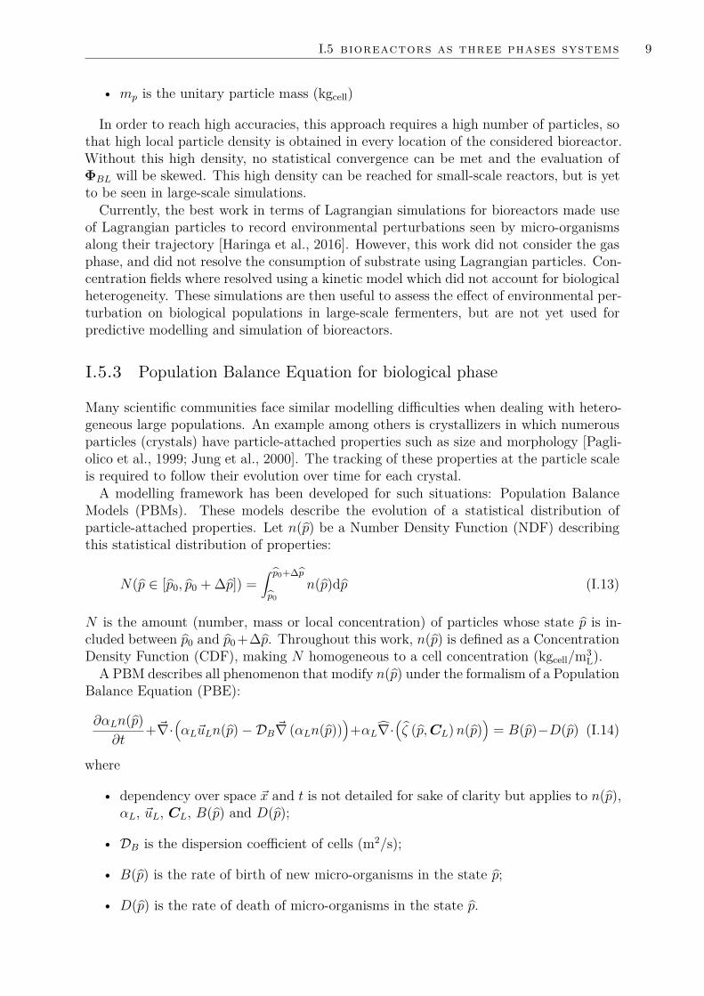
I.5.3 Population Balance Equation for biological phase
Many scientific communities face similar modelling difficulties when dealing with hetero-geneous large populations. An example among others is crystallizers in which numerousparticles (crystals) have particle-attached properties such as size and morphology [Pagli-olico et al., 1999; Jung et al., 2000]. The tracking of these properties at the particle scaleis required to follow their evolution over time for each crystal.
A modelling framework has been developed for such situations: Population BalanceModels (PBMs). These models describe the evolution of a statistical distribution ofparticle-attached properties. Let n(p) be a Number Density Function (NDF) describingthis statistical distribution of properties:
N(p ∈ [p0, p0 + ∆p]) =∫ p0+∆p
p0n(p)dp (I.13)
N is the amount (number, mass or local concentration) of particles whose state p is in-cluded between p0 and p0 +∆p. Throughout this work, n(p) is defined as a ConcentrationDensity Function (CDF), making N homogeneous to a cell concentration (kgcell/m3
L).A PBM describes all phenomenon that modify n(p) under the formalism of a Population
Balance Equation (PBE):
∂αLn(p)∂t
+~∇·(αL~uLn(p)−DB ~∇ (αLn(p))
)+αL∇·
(ζ (p,CL)n(p)
)= B(p)−D(p) (I.14)
where
• dependency over space ~x and t is not detailed for sake of clarity but applies to n(p),αL, ~uL, CL, B(p) and D(p);
• DB is the dispersion coefficient of cells (m2/s);
• B(p) is the rate of birth of new micro-organisms in the state p;
• D(p) is the rate of death of micro-organisms in the state p.

10 context, state of the art and objectives
This PBE shares a similar structure with Eq. (I.9). The second term on the LHSaccounts for the transport of cells thank to their carrying fluid, and is analogous to thetrajectory equation under a Lagrangian treatment of the biological phase (Eq. (I.10)).Source and sink terms are on the RHS to describe new-cell formation through cell division,or their possible death, just like reaction or transfer terms describe added or removeddissolved species in Eq. (I.9).
The major difference between Eqs. (I.9) and (I.14) comes from the fact that the NDFdoes not only depends on location ~x and time t, but also on p. Under the PBM formalism,p must be seen as a location, not in the physical space, but in the space of biologicalproperties. Therefore, the evolution of cell’s properties in the Lagrangian approach (Eq.(I.11)) is now described as a transport term in the internal properties space, with avelocity ζ(p,CL), in the third term on the LHS of the PBE.
Provided some numerical methods to transform the PBE into a set of equation thatexactly match the formalism of (I.9), this approach is directly compatible with a Eulerianmultiphase modelling. In particular, under this formalism, the overall mass transfer-ratebetween the liquid and biological phases can be written
ΦBL(~x, t) =∫
Ωpn(p, ~x, t)ϕ (p,CL(~x, t)) dp (I.15)
where ϕ is the specific rate of bioreactions (kg/kgcell · s). The overall accuracy of thismethod depends on how accurate the NDF resolution is.
I.6 Usual modelling closures for bioreactors
The description given in I.5 of elementary equation sets for bioreactor modelling is meantto be as generic as possible. All existing work about bioreactor models and simulationscan be integrated under this formalism provided some closures or model reductions. Suchusual closures or approach are detailed hereafter, to lay the foundations of discussionsabout the degree of accuracy that should be used on each aspect of the overall modelling.
I.6.1 Gas-liquid mass transfer
Equations (I.8) and (I.9) both describe the transfer of matter between liquid and gasphases through the terms ΦGL and ΦLG. This mass transfer occur at the gas-liquidinterface. The transfer of oxygen or carbon dioxide is usually limited by a resistancein the liquid film. Therefore, the gas-liquid mass transfer of one of these compound isusually modelled as
ΦGL = kLa∗(HCG − CL) (I.16)
where
• kL is the liquid-film resistance to transfer (m/s);
• a∗ is the specific transfer area (m2/m3);
• H is the solubility (kgL/kgG).

I.6 usual modelling closures for bioreactors 11
H is a thermodynamic equilibrium constant illustating the linear relationship betweenliquid and gas phase concentrations (or partial pressure) of a compound at rest as de-scribed by Henry’s law [Sander, 2015]. Its value mainly depends on temperature and onthe composition of both phases.
The transfer resistance, kL, is related to convection and diffusion phenomena in theliquid film. Numerous correlation are available in literature to estimate its value forbubbles in water. These correlations usually take the following form:
Sh = a+ bRec + Scd (I.17)
with
Sh = kL dbD
, Re = ρL db |~uL|µL
, Sc = µLρL D
(I.18)
where
• Sh, Re and Sc respectively designate the dimensionless Sherwood, Reynolds andSchmidt numbers;
• db is the bubble diameter (m);
• D is the dissolved gas molecular diffusivity (m2/s);
• µL is the liquid dynamic viscosity (Pa · s);
• a, b, c and d are the correlation fitting parameters.
As shown in the definition of dimensionless numbers, the resistance kL is dependent onthe bubble diameter db. Numerous experimental analysis show that their exists a BubbleSize Distribution (BSD) in stirred aerated reactors. Let nb(d) be that distribution in avolume of reference V . It is possible to express the specific gas-liquid transfer area fromthat distribution:
[specific area] = [total bubble area in V][total bubble volume in V] ×
[total bubble volume in V]V
which numerically translates into
a∗ = aαG (I.19)
with a the specific area expressed per unit of gas volume (m2/m3G):
a =∫
Ωdb πd2bnb(db)ddb∫
Ωdbπ6d
3bnb(db)ddb
= 6d32
(I.20)
d32 is known as the Sauter diameter and is an integral property of the BSD.If the BSD is resolved, the kL value used in Eq. (I.16) should be a mean value over all
bubbles:
kL =∫
Ωdb kL(db)nb(db)ddb∫Ωdb nb(db)ddb
(I.21)

12 context, state of the art and objectives
I.6.2 Phase-fractions and velocity fields
All local equations (Eqs. (I.4-I.9), (I.10) and (I.14)) require the knowledge of local phasefractions and velocities. These informations could be accessed locally by experimentalmeasurements based, for instance, on Particle Image Velocimetry (PIV) and ombroscopymethods. However, these methods are limited to small set-ups and would be impracticalon large-scale bioreactors. In particular, they require transparent vessels and fluids whichis not applicable to industrial fermenters.
For now, experimental measurements are applied to small-scale systems using modelfluids [Laupsien, 2017]. These measures are then used to improve existing hydrodynamicmodel and to perform large-scale simulation of hydrodynamics, by solving numericallythe fluid mechanics equations given in Eqs. (I.4-I.7).
CFD-RANS approach
The Euler-Euler modelling of gas-liquid systems has been presented previously (see Eqs.(I.4)-(I.9)) and consists in considering that both phases are interpenetrated continuousphases each characterised by its own velocity ~uk and local phase fraction αk. To solvethese variables over time and space, CFD software apply some numerical methods, suchas the finite-volume or finite-element methods, to degenerate Navier-Stokes equations intoa set of discrete integrable equations. However, due to their strong non-linearities, theseequations can not be directly resolved as soon as large turbulent systems are considered.Bioreactors will then be modelled using the Reynolds-Averaged Navier-Stokes (RANS)approach in which velocity and local fractions are split into a mean and a fluctuatingcomponent:
~uk(~x, t) = ~Uk(~x) + ~u′k(~x, t) (I.22)αk(~x, t) = αk(~x, t) + α′k(~x, t) (I.23)
Injecting these decompositions into momentum conservation equations (Eqs. (I.6)-(I.7)),leads to following equations for conservation of the mean local momentum:
∂αGρG~uG∂t
+ ~∇ · (αGρG~uG ⊗ ~uG) = αG(ρG~g − ~∇P
)+ ~∇ · (τG + τ ′G) + ~MG (I.24)
∂αLρL~uL∂t
+ ~∇ · (αLρL~uL ⊗ ~uL) = αL(ρL~g − ~∇P
)+ ~∇ · (τL + τ ′L) + ~ML (I.25)
where τ ′k are Reynolds stress tensors, defined as
τ ′kij = ρku′kiu′kj (I.26)
which represent the mean effect of velocity fluctuations on the dispersion of momentum.Under RANS approaches, these fluctuations are not resolved. Therefore, the Reynoldsstress tensors will need to be modelled by introducing conserved turbulence characterisingvariables. Multiple models have been developed for that purpose [Couderc et al., 2008]and the most commonly applied, though not the most accurate, is the two-equations k−εmodel first proposed by Launder and Spalding [1972]. This model resolves the turbulentkinetic energy k (J/kg) and the rate of viscous dissipation of that energy ε (W/kg).

I.6 usual modelling closures for bioreactors 13
Closure for momentum transfer between liquid and gas phase
In Eqs. (I.24)-(I.25), terms ~Mk represent the interfacial transfer of momentum betweengas and liquid phases. Here, we only consider momentum exchange between a dispersedgas phase (i.e. bubbles) and a surrounding liquid. When transferred from phase A,momentum will either be received by phase B, or will be used to extend the interfacialarea. When this area is left unchanged, one can model the momentum transfer as
~MG = − ~ML = ~fB + ~fD + ~fVM + ~fL (I.27)
with
• ~fB: buoyancy force resulting from body and gravitational forces,
~fB = (ρG − ρL)~g (I.28)
• ~fD: drag force resulting from pressure and viscous effects on the gas-liquid interface,usually modelled as
~fD = FD(~uL − ~uG) with FD = 18µLd2b
CDReb24 (I.29)
for spherical bubbles of diameter db of Reynolds number Re = ρLdb|~uG−~uL|µL
. CD isthe bubble drag coefficient.
• ~fVM : virtual (or added) mass force. This is the force required to accelerate thefluid surrounding a bubble, modelled as
~fVM = CVMρL
(∂~uL∂t− ∂~uG
∂t
)(I.30)
with CVM = 0.5 the virtual mass coefficient.
• ~fL: lift force due to the unbalanced distribution of pressure and viscous constraintson the gas-liquid interface modelled as:
~fL = CLρLαG(~uL − ~uG)× (~∇× ~uL) (I.31)
with CL the lift force coefficient.
See Couderc et al. [2008], Laupsien [2017] and ANSYS Fluent [2015] for further referenceson these models and for closures for drag, virtual mass and lift force coefficients. Thesetopic are vast and the development of models suiting the properties of culture broth(rheology, gas-liquid interface contamination, . . . ) are still on-going. However, this doesnot constitute a core topic of this thesis.
Reducing the spatial resolution: compartment approaches
While CFD simulations form the current trend for hydrodynamic description of reactors,they have not always been as widely available as today. Chemical engineers then devel-oped other approaches to describe the transport in heterogeneous systems that are stillrelevant nowadays including mainly the Compartment Model Approach (CMA).

14 context, state of the art and objectives
Figure I.1: Compartmental representation of macroscopic flow patterns in a 22 m3 fed-batch bioreactor [Pigou and Morchain, 2015]. Model from Vrabel et al. [1999].
In these models, the reactor volume is split into a low number of sub-volumes (i.e. thecompartments, or zones) assumed to be homogeneous. The transport is then describedby defining the volume flow-rates of each phase between adjacent compartments. Thesemodels can be deduced from experimental observations [Reuss, 1991; Mayr et al., 1993;Vrabel et al., 1999; Zahradnık et al., 2001] or from CFD simulations [Bezzo et al., 2003;Le Moullec et al., 2010; Delafosse et al., 2014; Zhao et al., 2016]. An example of such acompartment-based model is illustrated in Fig. I.1.
I.6.3 Biological behaviour
Once biological heterogeneity is tackled through Lagrangian or PBE approach, one stillneeds to define how a cell, in the state p and in an environment characterized by concen-trations CL, will behave. This question encompasses two aspects:
• What will be the rates of consumption of substrates and production of (by-)products?i.e. How to compute ϕ(p,CL) in Eqs. (I.12) and (I.15)?
• How will evolve the cell’s properties? i.e. How to compute ζ(p,CL) in Eqs. (I.11)and (I.14)?
Both aspects must be considered together, and answers will strongly depend on whichcell properties are tracked in p. Thereafter are listed some examples of approaches tomodel this overall biological behaviour. In terms of metabolism, two distinctions arepossible:
• kinetic/metabolic model
• structured/unstructured model
Kinetic models will be constant conversion yields model and can usually be summedup to a simple pseudo-reaction, for instance:
YSXS + YOXO2X−→ X + YPXP (I.32)

I.6 usual modelling closures for bioreactors 15
with S: substrate, O2: oxygen, X: biomass and P : product. YAB is the conversionyield of A into B. These simple models do not account for the actual complexity ofmetabolic networks. They rely on the hypothesis of balanced growth with constantbiomass composition over time and act as black box models of the internal cell functioning.
On the opposite side, metabolic models rely on a description of the metabolic net-work and let substrates flow through different pathways depending on current internaland external conditions. Therefore, depending on which pathways are activated and ontheir respective efficiency for substrate conversion, a metabolic model will exhibit varyingglobal conversion yields.
The structured aspect of metabolism modelling relates to whether the model trackscell attached quantities. These can be composition/internal concentrations, physiologyparameters (mass, size, age, . . . ), or variable without physically defined definition (cyber-netic variables, Tartakovsky et al. [1997]). These are the quantities that can be trackedthrough Population Balance approaches detailed previously.
If a model is structured and tracks some cell-attached properties, these informationcan be used to determine the rates of reactions described through kinetic or metabolicapproaches. If the model is unstructured, only external information (i.e. environmentalconcentrations) are used to model these rates. Hereafter are four examples illustratingeach association of the kinetic/metabolic and structured/unstructured modelling.
unstructured kinetic model A simple unstructured kinetic model can bebased on the previous pseudo-reaction (Eq. (I.32)). The growth rate is often definedusing Monod-type law [Monod, 1952]:
µ = µmaxS
S +KS
O
O +KO
(I.33)
with S and O the liquid phase concentrations of substrate and oxygen, KS and KO therespective affinities of the cell toward these compounds, and µmax the maximum growthrate. Chapter II discusses the applicability of this law.
Once the growth-rate µ (gX/gX · h) is determined from environmental conditions (hencethe unstructured nature of the model), the volumetric consumption or production rates ofS, O2, X and P (Ri expressed in gi/L.h) can be computed by considering stoichiometryfrom Eq. (I.32):
RS = −YSXµX (I.34)RO2 = −YOXµX (I.35)RX = µX (I.36)RP = YPXµX (I.37)
unstructured metabolic model Xu et al. [1999] propose a metabolic modeldescribing the behaviour of Escherichia coli using either glucose or acetate as a carbonsource, and able to switch between oxidative and fermentative energy production modes.This model will be further detailed in Chapter II and is illustrated in Fig. I.2.
In an environment characterised by moderate glucose and oxygen availability, thismodel will predict a behaviour summed-up by the pseudo-reaction:
YSXS + YOXO → X (I.38)
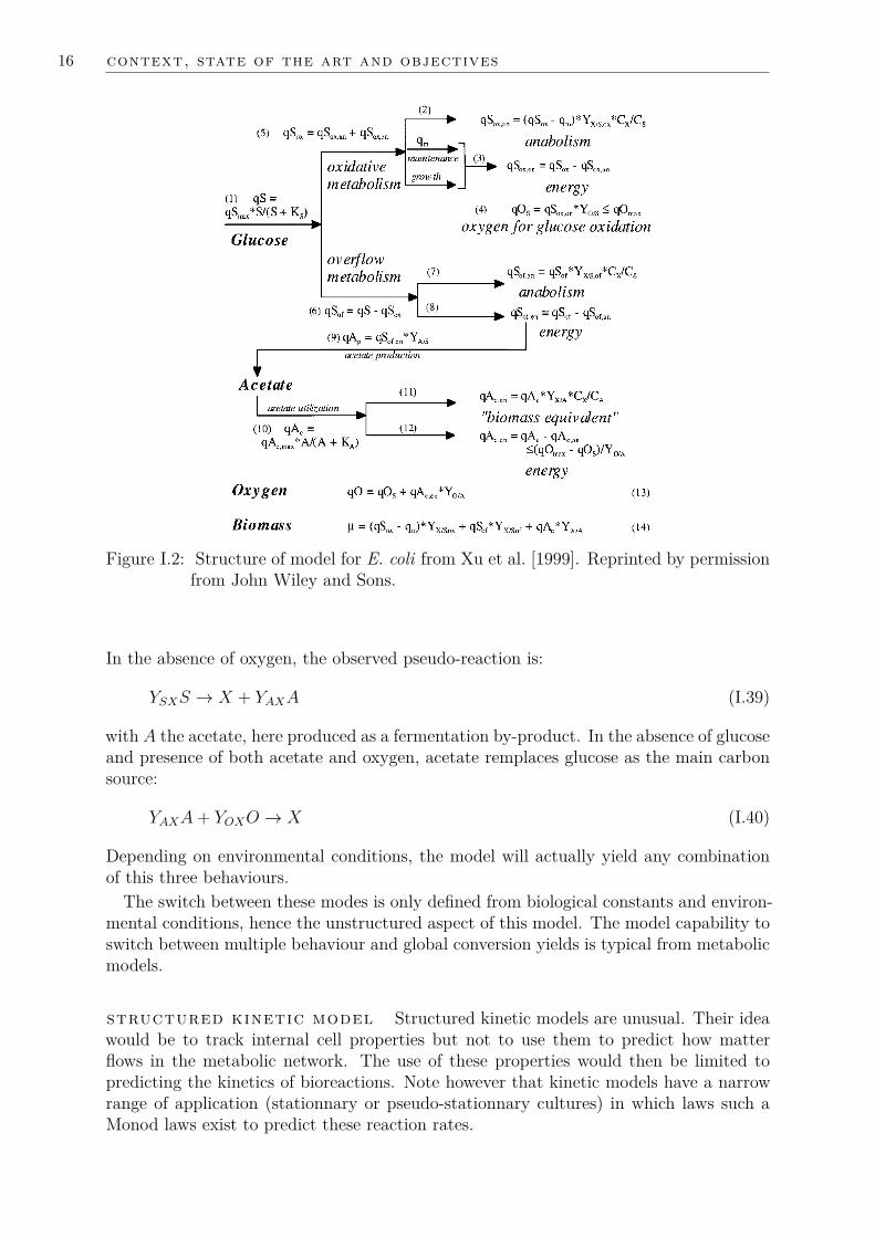
16 context, state of the art and objectives
Figure I.2: Structure of model for E. coli from Xu et al. [1999]. Reprinted by permissionfrom John Wiley and Sons.
In the absence of oxygen, the observed pseudo-reaction is:
YSXS → X + YAXA (I.39)
with A the acetate, here produced as a fermentation by-product. In the absence of glucoseand presence of both acetate and oxygen, acetate remplaces glucose as the main carbonsource:
YAXA+ YOXO → X (I.40)
Depending on environmental conditions, the model will actually yield any combinationof this three behaviours.
The switch between these modes is only defined from biological constants and environ-mental conditions, hence the unstructured aspect of this model. The model capability toswitch between multiple behaviour and global conversion yields is typical from metabolicmodels.
structured kinetic model Structured kinetic models are unusual. Their ideawould be to track internal cell properties but not to use them to predict how matterflows in the metabolic network. The use of these properties would then be limited topredicting the kinetics of bioreactions. Note however that kinetic models have a narrowrange of application (stationnary or pseudo-stationnary cultures) in which laws such aMonod laws exist to predict these reaction rates.

I.6 usual modelling closures for bioreactors 17
To formulate a structured kinetic model, one could simply track an internal cell glucoseconcentration Sin whose evolution could be dictated by
∂Sin∂t
= 1τS
(S − Sin) (I.41)
with τS the characteristic time of substrate assimilation, and then base the Monod lawon this internal concentration
µ = µmaxSin
Sin +KS
O
O +KO
(I.42)
Doing so would induce a delay in the answer of a cell in terms of growth rates followinga sudden change in its environment glucose concentration.
structured metabolic model Structured metabolic models form the vast ma-jority of current cell modelling. They describe internal properties of cells and use thatinformation to predict which metabolic pathways are activated and at which rates. Theycan account for internal metabolic regulations, for lack or excess of metabolites, and forcell-cycle effects.
Quantities that can be tracked are
• Internal concentrations [Reuss, 1991; Rizzi et al., 1997; Lei et al., 2001; Lapin et al.,2004; Matsuoka and Shimizu, 2013]
• Physiology quantities such as age, mass, size, ... [Hatzis et al., 1995; Mantzariset al., 1999; Robert et al., 2014]
• Cybernetic variables [Sweere et al., 1988; Abulesz and Lyberatos, 1989; Morchainet al., 2013]
• Sub-population fractions [Le Moullec et al., 2010]
In particular, internal concentration based metabolic models can benefit from recentadvances in metabolic flux analysis [Noh et al., 2007; Kajihata et al., 2015].
Bioreaction rates in structured metabolic models can be computed by different ways,the most common being:
• Use of kinetic expressions based on internal concentrations.
• Optimization algorithm aiming a maximizing one rate or yield, usually the growthrate [Varma and Palsson, 1994; Orth et al., 2011]
• Decision-tree based closure [Sweere et al., 1988]
The evolution of biological properties directly depends on their definitions. Age in-creases naturally over-time and is reset to 0 at cell-division. Cell mass or internal concen-trations evolution can be modelled through mass balances. The evolution of cyberneticvariables is usually more tricky as their definition and physical meaning is not direct.Their evolution will be modelled on a per-variable manner.

18 context, state of the art and objectives
I.7 Handling the PBE in a Eulerian transport scheme
Whereas many authors already attempted using Population Balance Modelling for thesimulation of bioreactors, few works actually made use of PBE in conjunction with atransport scheme for fermenters. Example of such attempts are Heins et al. [2015] whotransported a PBM developed by Lencastre Fernandes et al. [2012] in a two-compartmentsset-up. An other example actually preceded the current PhD thesis and was presentedin Pigou and Morchain [2015]. In this work, a PBM was applied to the simulation of a22m3 fermenter using a metabolic model for E. coli derived from the work of Xu et al.[1999].
One of the main reason this coupling is hardly ever considered is because of the needfor numerical methods to make the PBE (Eq. (I.14)) compatible with the generic localtransport equation (Eq. (I.9)). Such methods already exist and were applied by numer-ous scientific communities for whom the coupling of PBEs with a transport scheme isespecially required.
Overall, all methods will consist in forming a vector P (~x, t) from which one can de-duce an approximation n(p, ~x, t) of n(p, ~x, t). P (~x, t) will be referred to as a vector ofpopulation-scale biological properties, opposed to p which is the vector of cell-scale bi-ological properties. By construction, P (~x, t) will be transportable in the Euler-Eulerframework of gas-liquid description:
∂αLP (~x, t)∂t
+ ~∇ ·(αL~uLP −DB ~∇(αLP )
)= S(P ,CL) (I.43)
where S(P ,CL) is the overall source or sink term which accounts for all phenomenonthat modify the distribution in the space of internal properties: transport in the internalspace, birth and death of cells in a specific state p.
Two main approaches will be detailed hereafter, and illustrated with the example of aone dimensional PBE whose cell-scale biological property is the cell age, p = a:
∂αLn(a)∂t
+ ~∇·(αL~uLn(a)−DB ~∇(αLn(a))
)+αL
∂(ζa(a,CL)n(a))∂a
= B(a)−D(a) (I.44)
where
• ζa is the rate of age increase over time, therefore ζa = 1 s/s;
• B(a) is the rate of formation of new cells whose age is a. All cells are born witha age a = 0 so that B(a) = Γbδ(a) with Γb the rate of formation of new cells(kgcell/m3
L · s) and δ the Dirac delta function;
• D(a) is the rate of death of cells of age a with D(a) = Γd(a)n(a) with Γd(a) thespecific rate of death (kgcell/kgcell · s).
I.7.1 Sectional methods
This first category of approach to solve the PBE in a Eulerian transport scheme hasmultiple designation: sectional methods [Nguyen et al., 2016], pivot methods [Kumarand Ramkrishna, 1996a,b] or class methods [Alopaeus et al., 2006, 2007, 2008; Morchainet al., 2013].

I.7 handling the pbe in a eulerian transport scheme 19
Figure I.3: Illustration of a continuous Number Density Function of age distribution andassociated 20-classes discretization.
This approach consists in discretizing the space of biological properties into numerous“sections” or “classes”. Under this formalism, P is a vector whose values are the concen-trations of cells which belong to each section. For each section, one attaches a “pivot” piand all cells within that section are assumed to be actually located at that pivot in thespace of internal properties. For the cell-age distribution example, Fig. I.3 illustrates theapplication of this discretization to an arbitrary distribution.
Let P = [N1, N2, . . . , N20]T . In this 1D example, one must perform integrations ofthe PBE on the support of each class to obtain the law of evolution of P . For instance,the evolution of N10 is given by integrating each term of the PBE from Eq. (I.44) overa ∈
[a10−1/2; a10+1/2
]:
∂αLN10
∂t+~∇·
(αL~uLN10 −DB ~∇(αLN10)
)=∫ a10+1/2
a10−1/2
(B(a)−D(a))da−[ζa(a,CL)n(a)]a10+1/2
a10−1/2
(I.45)
The third term of the LHS is the flux of cells between the 10−th class and its surroundingclasses.
n(a) can be approximated from P as a discrete distribution where all cells are consid-ered to be located at the pivot of their class, or as a uniform by part distribution. Byincreasing the number of classes, the error between n(a) and its approximation decreases.
Variants of this method aims at higher accuracy by solving multiple values in eachsection such as the Two-Size Moment (TSM) sectional method [Nguyen et al., 2016] andHigh-order Moment conserving Method of Classes (HMMC) [Alopaeus et al., 2006, 2007,2008].

20 context, state of the art and objectives
I.7.2 Moment methods
Moments are integral properties of a NDF. The k − th order integer moment of a mono-variable NDF such as n(a) is defined as
mk =∫
Ωaakn(a)da (I.46)
where
• m0 is the total amount of individual; here the total concentration of cells whatevertheir age;
• m1 is related to the population mean age a by m1 = am0;
• m2 holds information about the standard deviation σa of the age distribution: σa =√m2m0−2m2
1m0
Higher order moments are related to age distribution skewness, kurtosis, flatness, andother descriptors of the distribution shape.
Methods of moments, applied to a PBE, will track moments of the NDF whose evolutionis described by that PBE. Let P = [m0,m1, . . . ,mN−1]T be the vector of the first Ninteger moments of n(a). The moment equations, which describes the evolution of eachelement of P , is obtained by multiplying all terms of the PBE (here Eq. (I.44)) by ak
and integrating over the space of definition of a, Ωa:
∂αLmk
∂t+ ~∇ ·
(αL~uLmk −DB ~∇ (αLmk)
)+[akζan(a)
]∂Ωa
−∫
Ωakak−1ζan(a)da =
∫Ωaak(B(a)−D(a))da (I.47)
where the third term on the LHS represent the flux of cells, weighted by ak, at the limitsof the space of age definition. As the ageing process will not allow cells to go out out thespace of age, this term is necessarily null.
After a reorganization of terms, and an expansion of B(a) and D(a) definitions, oneobtains the following moment equations:
∂αLm0
∂t+ ~∇ ·
(αL~uLm0 −DB ~∇ (αLm0)
)= Γb −
∫Ωa
Γd(a)n(a)da (I.48)
∂αLmk
∂t+ ~∇ ·
(αL~uLmk −DB ~∇ (αLmk)
)= kζamk−1 −
∫ΩaakΓd(a)n(a)da, (I.49)
k ∈ 1, . . . , N − 1
If Γd(a) is not defined as a polynomial of a, the integral term on the RHS of Eqs. (I.48)and (I.49) will not be closed in terms of moments of n(a). Moreover, even if Γd(a) isindeed a polynomial but is not constant, the volution of mk will depend on higher ordermoments such as mk+1 which leads to an unclosed set of equations. For these reasons,numerical methods to estimate unknown integral properties of n(a) from its resolvedmoments are usually required. Examples of such methods are the Quadrature Methodof Moments (QMOM) [Marchisio et al., 2003a], the Extended Quadrature Method ofMoments (EQMOM) [Yuan et al., 2012] and the Maximum Entropy method [Mead and
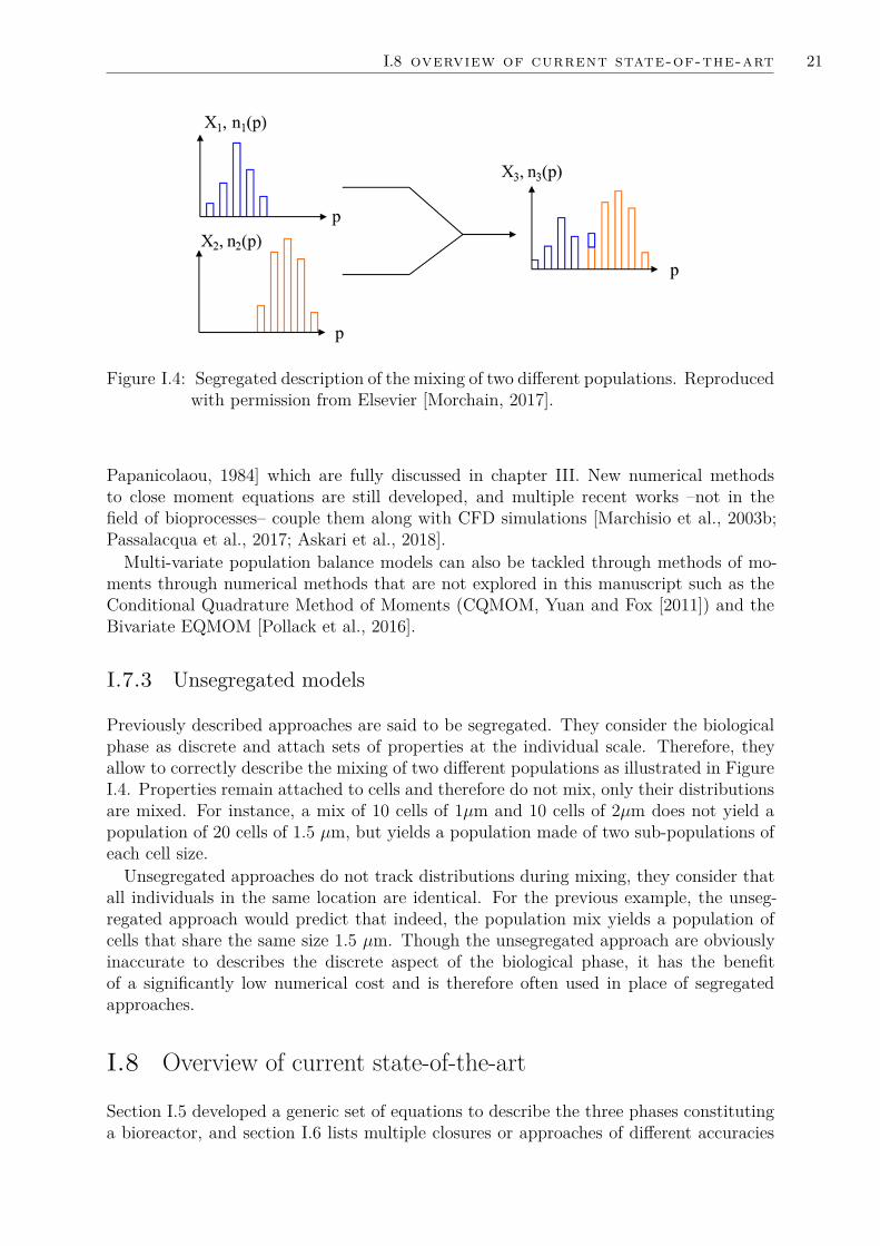
I.8 overview of current state-of-the-art 21
Figure I.4: Segregated description of the mixing of two different populations. Reproducedwith permission from Elsevier [Morchain, 2017].
Papanicolaou, 1984] which are fully discussed in chapter III. New numerical methodsto close moment equations are still developed, and multiple recent works –not in thefield of bioprocesses– couple them along with CFD simulations [Marchisio et al., 2003b;Passalacqua et al., 2017; Askari et al., 2018].
Multi-variate population balance models can also be tackled through methods of mo-ments through numerical methods that are not explored in this manuscript such as theConditional Quadrature Method of Moments (CQMOM, Yuan and Fox [2011]) and theBivariate EQMOM [Pollack et al., 2016].
I.7.3 Unsegregated models
Previously described approaches are said to be segregated. They consider the biologicalphase as discrete and attach sets of properties at the individual scale. Therefore, theyallow to correctly describe the mixing of two different populations as illustrated in FigureI.4. Properties remain attached to cells and therefore do not mix, only their distributionsare mixed. For instance, a mix of 10 cells of 1µm and 10 cells of 2µm does not yield apopulation of 20 cells of 1.5 µm, but yields a population made of two sub-populations ofeach cell size.
Unsegregated approaches do not track distributions during mixing, they consider thatall individuals in the same location are identical. For the previous example, the unseg-regated approach would predict that indeed, the population mix yields a population ofcells that share the same size 1.5 µm. Though the unsegregated approach are obviouslyinaccurate to describes the discrete aspect of the biological phase, it has the benefitof a significantly low numerical cost and is therefore often used in place of segregatedapproaches.
I.8 Overview of current state-of-the-art
Section I.5 developed a generic set of equations to describe the three phases constitutinga bioreactor, and section I.6 lists multiple closures or approaches of different accuracies
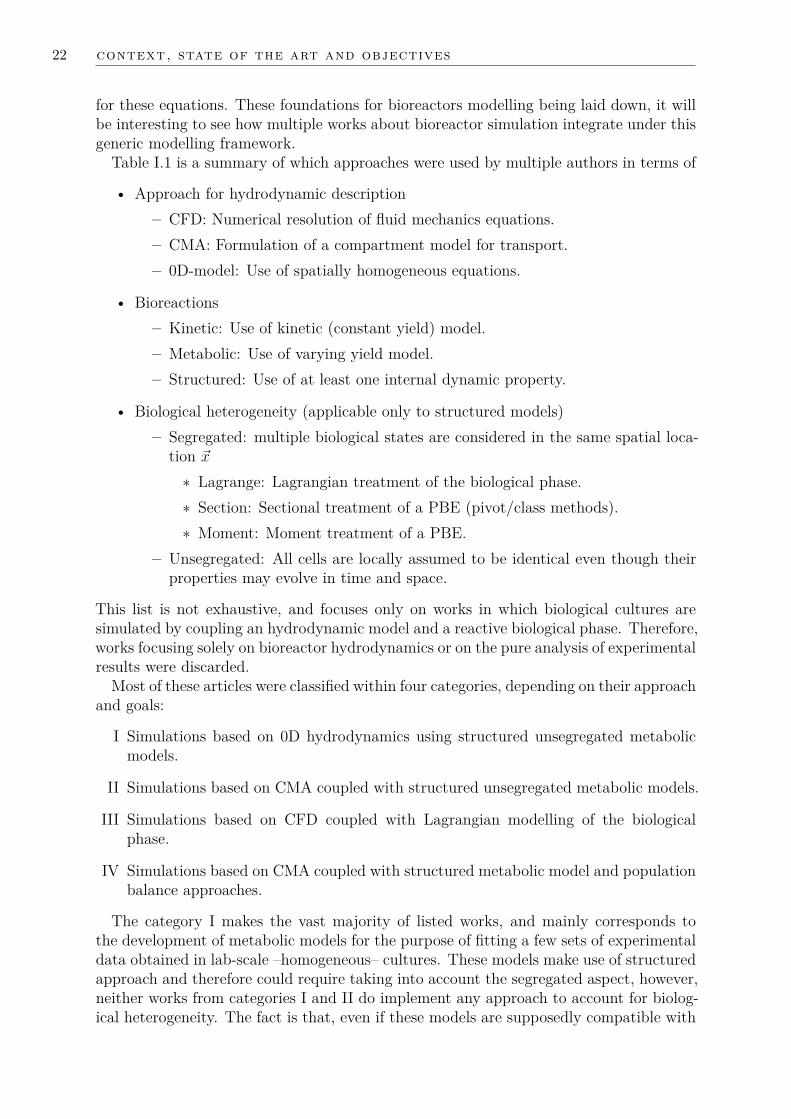
22 context, state of the art and objectives
for these equations. These foundations for bioreactors modelling being laid down, it willbe interesting to see how multiple works about bioreactor simulation integrate under thisgeneric modelling framework.
Table I.1 is a summary of which approaches were used by multiple authors in terms of
• Approach for hydrodynamic description– CFD: Numerical resolution of fluid mechanics equations.– CMA: Formulation of a compartment model for transport.– 0D-model: Use of spatially homogeneous equations.
• Bioreactions– Kinetic: Use of kinetic (constant yield) model.– Metabolic: Use of varying yield model.– Structured: Use of at least one internal dynamic property.
• Biological heterogeneity (applicable only to structured models)– Segregated: multiple biological states are considered in the same spatial loca-
tion ~x∗ Lagrange: Lagrangian treatment of the biological phase.∗ Section: Sectional treatment of a PBE (pivot/class methods).∗ Moment: Moment treatment of a PBE.
– Unsegregated: All cells are locally assumed to be identical even though theirproperties may evolve in time and space.
This list is not exhaustive, and focuses only on works in which biological cultures aresimulated by coupling an hydrodynamic model and a reactive biological phase. Therefore,works focusing solely on bioreactor hydrodynamics or on the pure analysis of experimentalresults were discarded.
Most of these articles were classified within four categories, depending on their approachand goals:
I Simulations based on 0D hydrodynamics using structured unsegregated metabolicmodels.
II Simulations based on CMA coupled with structured unsegregated metabolic models.
III Simulations based on CFD coupled with Lagrangian modelling of the biologicalphase.
IV Simulations based on CMA coupled with structured metabolic model and populationbalance approaches.
The category I makes the vast majority of listed works, and mainly corresponds tothe development of metabolic models for the purpose of fitting a few sets of experimentaldata obtained in lab-scale –homogeneous– cultures. These models make use of structuredapproach and therefore could require taking into account the segregated aspect, however,neither works from categories I and II do implement any approach to account for biolog-ical heterogeneity. The fact is that, even if these models are supposedly compatible with

I.8 overview of current state-of-the-art 23
Table I.1: Overview of existing work on bioreactor simulation.
ReferenceHydrodynamics Bioreactions Heterogeneity
Category0D CMA CFD Kinetic Metabolic Structured Segregated Un-segregatedLagrange Section Moment
Young et al. [1970] X - - X - - - - - -Sweere et al. [1988] X - - X - - - - - -
Reuss [1991] X - - - X X - - - X INielsen and Villadsen [1992] X - - - X X - - - X I
Bellgardt [1994] X - - X - X - - - -Varma and Palsson [1994] X - - - X X - - - X I
Hatzis et al. [1995] X - - - - X X - - -Rizzi et al. [1997] X - - - X X - - - XXu et al. [1999] X - - - X - - - - -
Vrabel et al. [1999] X X - - X - - - - - IILei et al. [2001] X - - - X X - - - X I
Mantzaris et al. [2001] X - - X - - - X - -Vrabel et al. [2001] X X - - X - - - - X II
Chassagnole et al. [2002] X - - - X - - - - XBezzo et al. [2003] - X X - X - - - - - II
Gerdtzen et al. [2004] X - - - X X - - - X IRodrıguez et al. [2004] X - - - X X - - - X I
Lapin et al. [2004] - - X X X X X - - - IIIHristov et al. [2004] - X - X - - - - - -
Hjersted and Henson [2006] X - - - X X - - - X ILaakkonen et al. [2006] - X X X - - - - - -
Lapin et al. [2006] - - X - X X X - - - IIIMorchain and Fonade [2009] X - - - X X - - - X I
Meadows et al. [2010] X - - - X X - - - X ILe Moullec et al. [2010] - X X - X X - - - X II
Lencastre Fernandes et al. [2012] X - - X - X - - - -Elqotbi et al. [2013] X - X X - - - - - -
Matsuoka and Shimizu [2013] X - - - X X - - - X IMorchain et al. [2013] X - - X - X - X - -Morchain et al. [2014] - - X X - X - X - -Goldrick et al. [2015] X - - - X X - - - X I
Heins et al. [2015] - X - X - X - X - - IVPigou and Morchain [2015] X X - - X X - X - - IV
Haringa et al. [2016] - - X - - X X - - - IIIOrdonez et al. [2016] X - - - X X - - - X I
Farzan and Lerapetritou [2017] - - X X X X - - - X IIIKuschel et al. [2017] - - X - - X X - - - IIIBrand et al. [2018] X - - - X X - - - X I
segregation by their structured nature, they are usually not designed with this consider-ation in mind. They may therefore have a prohibitive complexity through the use of ahigh number of internal variables, or the parameter identification might have been flawedby assuming that all cells are identical in a lab-scale system while they may actuallydifferentiate through stochastic processes [Delvigne et al., 2014].
First attempts to account for cell’s history and exposure to different environmentalfluctuations were carried out through the Euler-Lagrange framework using CFD simu-lations (see category III). Developments related to this approach are still ongoing andfor now the Lagrangian method is used to characterise environmental fluctuations alongcell’s trajectories rather than to predict their effect of biological heterogeneity and reversecoupling on concentration field gradients. For instance, Haringa et al. [2016] tracked thesignal of substrate concentration fluctuations in a large-scale fermenter using Lagrangianparticles, but for the “prediction” of concentration fields evolutions, they relied on anunstructured kinetic model.
Finally, some attempts are being made to couple the biological heterogeneity withintermediate hydrodynamic resolutions (category IV). On that regard, developments ofCMA models from CFD is an interesting topic that has been considered by numerous

24 context, state of the art and objectives
authors classified in category II (all those for which both CMA and CFD approaches areticked), and is also investigated in papers not referenced here (i.e. Delafosse et al. [2015]).
Bailey [1998]’s classification is at the origin of (un)segregated and (un)structured clas-sifications of biological models. Table I.2, excerpted from Zieringer and Takors [2018]summarizes pros and cons of these categories. From these, it is easily understood whythe majority of developments on bioreactor simulation relies on unsegregated descrip-tions, due to the mathematical complexity on segregated approaches. However, it is alsoclear that structured segregated models will be required for the simulation of industrialfermenters.
Table I.2: Partial reproduction of the summary of pros and cons of (un)segregated and(un)structured approaches for biological models listed by Zieringer and Takors[2018].
Model class Application Advantages DisadvantagesStructured Systems in transient state Cellular compartmentation Biological knowledgeUnstructured Steady-state systems Easy to build Only penomenological cell descriptionSegregated Heterogeneous, individual cell systems More representative and informative Difficult to handle mathematicallyUnsegregated Systems with average cell description Easy to build for a large number of cells Average cell description
I.9 Proposed approach, thesis goals and outline
The main goal of this PhD thesis is to develop a model structure that encompassesall aspects of bioreactors modelling while keeping a low numerical cost. This modelstructure is applied to the simulation of an industrial fermenter in which the baker yeast,Saccharomyces cerevisiae, is cultivated.
In order to reach all-coupling simulations of bioreactors, it is necessary to develop amodelling strategy and to focus on each aspect of the overall model to ensure that lowestpossible numerical costs are achieved while not sacrificing accuracy. Indeed, aiming atlow numerical cost will be useless if each part of the model is not accurate enough toobtain an overall predictive model. Therefore, along this thesis, discussions about thetrade-off between numerical cost and accuracy will be a common thread.
Considering all previously detailed aspects, the proposed modelling strategy is as follow:
1. First, define a structured metabolic for the considered micro-organism. This defini-tion should answer the following questions:
• What are chemical species that are used as source of matter/energy, and/orare produced by the considered strain? This step consists in defining CL.
• What is the minimal list of biological properties that should be tracked foreach cell to determine its behaviour? Examples would be age, size, internalconcentrations, storage level, or others... This step consists in defining p
• What mathematical model allows predicting the rates of consumption or pro-duction of chemical species for a cell defined by p in an environment char-acterized by concentrations CL? This steps consists in defining closure forϕ(p,CL).
• Along with the definition of ϕ(p,CL), what mathematical model gives theevolution of cell-attached properties for a cell defined by p in an environment

I.9 proposed approach, thesis goals and outline 25
characterized by concentrations CL? This step consists in defining closure forζ(p,CL).
2. Define how to model biological heterogeneity• Based on p definition chose the most suited numerical method by weighting
accuracy against numerical cost.
3. Define how to describe large-scale hydrodynamics• Arbitrate about the implementation of biological models within CFD or CMA
frameworks by considering hydrodynamic and biological time-scales as well asnumerical cost.
These steps actually draw the structure of this PhD thesis. Chapter II focuses onthe metabolism modelling. In particular, this chapter details a modular and numericallyefficient model structure. This structure is first applied to a bacteria, E. coli, to illustrateits application to a simple micro-organism. Then, the same structure is applied to S.cerevisiae to prepare large-scale simulations of an industrial fermenter cultivating thisspecie. Both models are compared to, and validated against, experimental data availablethroughout the literature.
In this work, the PBM approach is considered to be the key element that allows large-scale simulations of bioreactors. Chapter III makes a strong focus on this aspect bycomparing both sectional and moment methods to solve 1D population balance mod-els. Studying the core principles of moment methods led to a major improvements ofa numerical method used to close equations in monovariate moment approaches. Theseimprovements of the numerical method are described too in this chapter.
In order to illustrate the coupling of metabolic models and population balances withhydrodynamics, Chapter IV focuses on performing numerical simulations of the gas-liquidhydrodynamics of an actual industrial fermenter. To further exploit these CFD simulationresults, Chapter IV details how to produce a compartment model from highly resolvedCFD results.
Finally, Chapter V couples developments from Chapter II to IV to perform the simu-lation of industrial biological cultures and show the capabilities and applications of theproposed modelling framework.
Table I.3: Approaches used in following Chapters.
ReferenceHydrodynamics Bioreactions Heterogeneity
Category0D CMA CFD Kinetic Metabolic Structured Segregated Un-segregatedLagrange Section Moment
Chapter II X - - - X X - - - X IChapter III X X - - X X - X X - IVChapter IV - X X - - - - - - -Chapter V - X - - X X - - X - IV
Table I.3 is based on the same structure than Table I.1, but summarizes which ap-proaches are developed in the current work. First, Chapter II focuses on developing alow-cost metabolic model structure and relies on homogeneous non-segregated simula-tions. Note that this model structure is designed for upcoming coupling with segregatedapproaches. These are developed in Chapter III were numerical methods to solve Pop-ulation Balance Equation are investigated. This chapter implements both homogeneous

26 context, state of the art and objectives
and compartment model approaches to assess numerical methods in terms of accuracy,stability and performances. In order to not be bound to Compartment Models availablefrom the literature, and to make possible the use of this work for any bioreactor, ChapterIV focuses on the use of CFD simulations to formulate Compartment Models. Finally,Chapter V illustrates the coupling of developments from all three previous chapters toperform the predictive simulation of a large-scale fedbatch culture, and underlines howthis tool can be used for engineering purposes.

IIM O D E L I S AT I O N D U M E TA B O L I S M E
Resume
La principale complexite associee a la modelisation d’un bioreacteur industriel provientde la description de la phase biologique. Les micro-organismes ne sont pas des particulesinertes ou catalysant de simples reactions chimiques, mais sont des systemes vivants et dy-namiques dotes par leur evolution Darwinienne de capacite de regulation et d’adaptationaux perturbations dans leur environnement. Ils sont donc capables de selectionner demaniere preferentielle leurs substrats, de reguler leur assimilation en s’affranchissant desequilibres thermodynamiques au prix d’une depense energetique, et d’orienter la matiereassimilee vers de multiples voies metaboliques par le biais de regulations internes forte-ment couplees.
Ce premier chapitre de developpements se focalise sur la modelisation de ces aspects,dans la continuite de tres nombreux travaux sur ce sujet enrichissant la litterature depuisplusieurs decennies. Ces travaux tombent generalement soit dans un exces de simplicite ennegligeant de nombreuses dynamiques cellulaires, soit dans un exces de complexite en cher-chant a decrire les echelles les plus fines. Il va de soi qu’aucune de ces deux modelisationslimites ne peuvent etre envisagees pour la simulation predictive de bioreacteurs industriels.Quelques modeles se situant a un niveau intermediaire de complexite existent, mais ilsn’ont en general pas ete penses ni construits en vue d’un couplage avec le transport dela phase biologique dans un systeme heterogene.
Nous chercherons a integrer les dynamiques biologiques, les regulations des flux etl’orientation de la matiere entre differentes voies metaboliques dans un modele de faiblecout numerique. Cela permettra le couplage avec des approches aussi bien Lagrangienneque de Bilan de Population pour prendre en consideration la diversite biologique, c’est-a-dire le fait que les micro-organismes peuvent se differencier suite a des perturbationsenvironnementales ou stochastiques. Il sera alors possible d’envisager des simulations decultures biologiques aux echelles industrielles pour un cout numerique raisonnable.
Ce chapitre propose essentiellement une structure de modele metabolique. Cette struc-ture, derivee du travail de Xu et al. [1999] et des approches de reduction de reseaux dereactions metaboliques par la definition de modes metaboliques, permettra effectivementd’integrer les dynamiques, les regulations et les differentes orientations de la matiere,sans faire appel a des procedures couteuses d’optimisation. La mise en œuvre de cettestructure est illustree d’une part pour la modelisation d’Escherichia coli, et d’autre partpour decrire les comportements dynamiques de Saccharomyces cerevisiae. En partic-ulier ce dernier modele, qui sera utilise par la suite dans le Chapitre V, est teste surplusieurs jeux de donnees experimentales obtenus par differentes equipes de chercheurs,pour plusieurs souches sauvages de la levure, et sur des modes de culture distincts. La
27

28 modelisation du metabolisme
confrontation massive a differents jeux de donnees experimentales constitue un test severepour un modele. A notre connaissance, c’est la premiere fois qu’un modele metaboliquede si faible cout numerique est confronte a autant de donnees experimentales.

IIM E TA B O L I S M M O D E L L I N G
Summary
The main challenge in the modelling of industrial bioreactors comes from the depictionof the biological phase. Micro-organisms are not inert particles or catalysts for simplechemical reactions. These are living and dynamic systems which, through Darwinianevolution, obtained regulation and adaptation capabilities to face environmental pertur-bations. They are then able to select preferential substrates, regulate their assimilation byover-coming thermodynamic equilibrium at the expense of energy, and to channel assim-ilated matter toward multiple metabolic pathways through internal and tightly coupledregulations.
This first development chapter focuses on modelling these aspects, in the continuationof numerous works which covered this topic over the last decades. These works tendedto fall either in an oversimplification excess, by neglecting most of cell dynamics, or in acomplexity excess by attempting to describe smallest scales. It is obvious that both ofthese limit modelling approaches may not be considered to perform predictive simulationsof large-scale fermenters. Some models lie at an intermediary level of complexity, but thesewere not designed by anticipating their coupling with the transport of the biological phasein an heterogeneous system.
This chapter describe how to integrate biological dynamics, flux regulation and thechannelling of matter through multiple metabolic pathways in a low numerical cost model.This low-cost permits the integration of this model under Lagrangian or Population Bal-ance modellings to account for biological diversity, i.e. the fact that micro-organisms willdifferentiate due to environmental or stochastic perturbations. This shall allow the sim-ulation of industrial-scale biological cultures with a reasonable and tractable numericalcost.
This chapter mainly describes a structure proposal for metabolic models. This struc-ture, derived from the work of Xu et al. [1999] and from metabolic-mode approaches formetabolic networks reduction, describes indeed dynamics, regulations and matter chan-nelling with an especially low numerical cost. This structure is applied to the modellingof Escherichia coli and to the description of dynamic behaviours of Saccharomyces cere-visiae. In particular the model developed for this yeast, which will be used in ChapterV, is challenged against numerous experimental data sets produced by multiple researchteams with different wild strains and culture modes. Challenging a model against suchdifferent data sets is quite a severe test. To the best of our knowledge, this is the firstattempt to produce such a low-cost metabolic model that fits so many experimental datasets.
29


IIM E TA B O L I S M M O D E L L I N G
II.1 Objectives and constraints of the biological modelling
In the proposed modelling framework, the metabolic model serves to predict the masstransfer rates between the liquid and the biotic phase. The starting point is the knowledgeof the cell state and the concentrations in the surrounding liquid. To develop metabolicmodels, two questions must be tackled. (i) What limits the reaction rates? (ii) Throughwhich pathways will the matter be transformed? This notion of pathways encompassesthe need to define reaction stoichiometry, but also energetic cost of the conversion.
At the most fundamental levels, biological reactions depend on oxidative reactionsof carbonaceous reduced matter (sugars, fat). Just like in combustion, these reactionsrelease energy, part of it as heat, but most of this chemical energy will be used by theliving system to produce highly complex biomolecules, new cells, to interact with theenvironment by controlling flux at the membrane level, or even by using this energy tomove toward more favourable environments.
In combustion, energy is only released as heat in fast reactions, whose time-scalescan be as low as nanoseconds [Caudal et al., 2013]. The need for biological system tocontrol the release of energy implies that they must be able to limit and control the rateof bioreactions. Some of these limitations occur naturally, for instance due to limitingdiffusive transport within a cell cytoplasm. Cells also actively regulate their internalreaction rates by decreasing the concentrations of some enzymes, or by limiting fluxes atthe membrane level at the expense of energy. For these reasons, even in rich environment,bioreactions will never be as fast as combustion.
If limitations do not come from internal reaction rates, or from limiting cross-membranetransfer, the limitation will be external to the cell. It is indeed straightforward to un-derstand that cells without internal reserves cannot perform any reaction in a depletedenvironment where no substrate is available.
Both internal and external limitations will have to be considered when designing abiological model for large-scale simulation. Indeed, in such systems, the environment willbe rich in substrate near the feeding point but might be depleted in other parts of thereactor. Similarly, oxygen will be highly available near the bubble spargers where gas isstill rich, but may be limited elsewhere if the oxygen transfer rate is insufficient comparedto the overall biological needs. Consequently, due to this possibly cyclic environmentalavailabilities, the proposed model will need to handle both sources of limitations.
If the biological reaction could be summed up to
Glucose + Oxygen→ Cells
31

32 metabolism modelling
the rate of this reaction would simply be the limiting value between the possible as-similation rates of glucose and oxygen, and the maximum production rate of new cells.Unfortunately, the chemistry of living systems is much more complicated than that.
This chapter will detail proposed models for a bacteria, Escherichia coli, and for ayeast, Saccharomyces cerevisiae. Both of these micro-organisms are said to be optionalaero-anaerobic. This implies that they are both able to grow either with, or without,oxygen. If oxygen is present, cells produce energy from oxidative catabolism, i.e. en-ergy producing pathway, whose final electron receiver is oxygen. These pathways areanalogous to full combustion of organic matter in presence of oxygen. On the opposite,if no oxygen is available, fermentative catabolism still allows producing energy. Thesepathways lead to the formation of some by-products (alcohol or acid compounds) justlike partial combustion.
The proposed models will then have to be able to switch between these two modesof energy production depending on oxygen availability, but complexity goes on. Whileglucose is the preferential source of carbon and energy for these micro-organisms, theyare also able to grow on other carbonaceous substrate. In particular, by-products fromfermentative catabolism are still reduced carbon matter and can be assimilated again inoxygen-rich environments, both for energy and new cell productions.
Moreover, the model will be used in large-scale where the biomass undergoes both(i) short-term perturbations such as sudden expositions to high substrate concentrationswhen cells pass by the feeding point, as well as (ii) long term modifications of the overallenvironment, for instance if the oxygen supply becomes limiting due to increasing biomassconcentration over time.
Due to the last aspect, the metabolic model must be able to switch between multiplemodes and must behave well both in long-term steady situations and in dynamic envi-ronments. The model construction will have to account for these aspects, and must bechallenged against both steady and dynamically changing experimental conditions.
Finally, one must keep in mind that this model will be used for long-term large-scalesimulations. This model will be called in each volume of reference solved by the hydrody-namic part of the overall model, and for each biological state considered in the biologicalheterogeneity part of the whole model. The numerical cost of the biological model mustthen be maintained as low as possible and can not rely on expensive computations.
II.2 Proposed metabolic model structure
II.2.1 Inspiration from a decision-tree model by Xu et al. [1999]
Foundations of the proposed structure come from Xu et al. [1999] who developed a simplemodel for E. coli. This model describes growth of this bacteria in anaerobic conditions,where glucose could be fermented producing energy as well as acetate as a by-product;and in aerobic conditions where both glucose and acetate could be used as main carbonsource along with an oxidative energy production. This model is illustrated on Fig. II.1and relies on two simple yet powerful ideas:
1. Growth is limited by some maximum fluxes of matter (glucose, acetate, oxygen).
2. Available matter will first be directed toward high-yield and/or high-affinity metabolicmodes, only leftovers will be directed toward other modes.

II.2 proposed metabolic model structure 33
Figure II.1: Structure of model for E. coli from Xu et al. [1999]. Reprinted by permissionfrom John Wiley and Sons.
The first idea allows describing the overall metabolism only in terms of flux of matterand energy. As energy is produced from biochemical reactions, all fluxes are coupledthrough mass and energy balances. For instance, if the flux of glucose and oxygen thatis processed by a cell is known, one can deduce the associated flux of energy-carryingmetabolites produced through the oxidative pathway.
The second idea comes as a replacement for a commonly used approach when solvingmetabolic models. Most models based on an extensive description of a metabolic net-work rely on constraint-based flux optimization to deduce an internal cell composition,and matter orientation between metabolic pathways, from environmental composition.Examples are the YEAST model for S. cerevisiae [Heavner et al., 2012, 2013], and theiJO1366 model for E. coli [Orth et al., 2011]. The flux optimization usually aims atidentifying the cell state that maximizes growth.
Instead of performing expensive optimization computations, the E. coli model from Xuet al. [1999] enforces that matter will be used in priority within efficient growth modes,sorted in the following order:
1. Growth on glucose with oxidative energy production;
2. Growth on glucose with fermentative energy production;
3. Growth on acetate with oxidative energy production.
Obviously, if no oxygen is available, only the mode 2 will be activated. Similarly, a lackof glucose in presence of acetate will only activate the mode 3. Overall, this approach

34 metabolism modelling
ensures that the most efficient metabolic mode is used when associated substrates areavailable. This indirectly allows the model to maximize growth, without actually relyingon expensive optimization algorithms. Note that if a strain has been engineered so that ittends to maximize an other process than growth, this can still be accounted for by simplysorting metabolic modes differently. This approach is not limited to strains maximizinggrowth.
Therefore, the model from Xu et al. [1999] does integrate two of the three constraintsthat we are interested in. The computation of reaction rates is fast as no specific expen-sive algorithm is involved. Moreover, by construction, it allows describing multiple cellfunctioning modes.
This model structure removes the need for solving numerous intracellular concentra-tions and for computing reaction rates using over-parametrized kinetic expressions basedon all these internal concentrations. Such models would be the one from Rizzi et al. [1997],or those applied to metabolic flux analysis [Matsuoka and Shimizu, 2013]. The high num-ber of dynamics tracked by these models, i.e. number of internal concentrations, makethem hardly compatible with heterogeneous bioreactor modelling. While simplifying thecomputation of bioreaction rates, it is crucial to observe that this computation dependson the prior knowledge of some key fluxes. This approach then only reduces the numberof degrees of liberty of the system to be solved. In the present case of Xu et al. [1999],the glucose uptake rate and the maximum respiration rate have to be known. The firstone is modelled as a function of two constant cell properties qSmax and KS along with theglucose concentration (see Eq. (1) in Fig. II.1) and a similar modelling is proposed bythe authors for the oxygen consumption rate. It is reasonable to question these closurelaws with at least two ideas in mind: do all cells share the same state and will uptake atthe same rates in the same environment? Also, some closure laws have to be defined forsome fluxes, but which ones are the most relevant?
II.2.2 Brief description of the model structure
The model from Xu et al. [1999] lacks the integration of dynamics variables. A first at-tempt of integrating this aspect was done in work preceding this PhD thesis [Pigou andMorchain, 2015]. The proposal was to associate a growth capability to micro-organismswhich would evolve over time. Metabolic modes aiming at growth, i.e. new cell produc-tion, could be limited by this growth capability even if sufficient nutrients were avail-able. If a strong disequilibrium occurred between glucose consumption, and glucoserequirements for growth, the excess glucose would be diverted into the well-known over-flow metabolism which induces acetate production when E. coli is suddenly exposed tohigh glucose concentrations [Xu et al., 1999; Matsuoka and Shimizu, 2013; Yamane andShimizu, 1984]. This initial model was fully detailed in Pigou and Morchain [2015] andkept a structure similar to Xu et al. [1999]. Here, we further improve upon this previouswork by defining a procedure to define metabolic models. Overall, the design of thesemodels will rely on:
1. Identifying self-sufficient metabolic modes that can be observed in experimentalcultures.

II.2 proposed metabolic model structure 35
2. Sorting metabolic modes by order of priority. A general rule would be to prioritizegrowth-mode with high yield efficiency (substrate affinity, more efficient energeticproduction, ...).
3. Identifying what can limit the rate of each mode.
The model structure will be more easily explained through application examples to il-lustrate each of these three basis aspects, and how their combination makes the modelstructure suitable for dynamic simulations of industrial fermenters. Nevertheless, we startwith a short generic explanation of the proposed structure.
Metabolic modes
The concept of metabolic modes is usually associated to the model reduction of complexmetabolic networks through linear analysis by identifying limits of a convex hyper-volumeof admissible metabolic flux. This approach is extensively detailed by Trinh et al. whosesummary figure is reproduced in Fig. II.2. Readers interested in these model reductionapproaches should refer to their article [Trinh et al., 2008].
In short, metabolic modes are elementary functionings of a cell and each modes de-scribes the transformation of some input matter (substrates, oxygen, . . . ) into someoutput matter (products, by-products, new cells, . . . ). One property of these modes isthat, taken individually, they appear as constant stoichiometry bioreactions. All pos-sible thermodynamically admissible metabolic behaviours can be expressed as a linearcombination of these elementary modes.
The way metabolic modes are combined evolves over time due to (i) the evolutionof environmental concentrations and (ii) the evolution of biological capabilities to pro-cess matter through each possible pathway. These changing combinations of elementarymodes explain how the overall conversion yields of matter by cells may change fromone experimental condition to another, even though underlying stoichiometry does notactually change.
The usual approach consists in deducing metabolic elementary modes from a detailedmetabolic network, coupled to thermodynamic constraints over this network [Trinh et al.,2008]. Highly detailed metabolic network models exist for E. coli[Orth et al., 2011] and S.cerevisiae[Heavner et al., 2012, 2013] and model reduction methods could be applied tothem [Gerdtzen et al., 2004]. However, we choose to manually design simplified metabolicmodels instead of reducing complex ones. This was decided in order to ensure a low-cost final model, and to only account for selected metabolic features. Doing so allowsfor keeping the model complexity low which improves the identifiability of the modelparameters.
Therefore, we propose to manually define metabolic modes to list, in an exhaustivemanner, all metabolic features of interest of the considered strain. Such features couldbe:
• capability to grow using glucose and oxygen only, i.e. oxidative glucose-basedgrowth;
• capability to grow using only glucose and producing acetate as a by-product, i.e.fermentative glucose-based growth;
• . . .

36 metabolism modelling
Figure II.2: Illustration of elementary mode analysis of metabolic networks. Reprinted bypermission from Springer Customer Service Centre GmbH: Springer Nature,Applied Microbiology and Biotechnology, Elementary mode analysis: a usefulmetabolic pathway analysis tool for characterizing cellular metabolism, Trinh,Wlaschin and Srienc, COPYRIGHT (2008). License number 4355340054177.

II.2 proposed metabolic model structure 37
Selected metabolic modes must be non-colinear, meaning that no mode should be a linearcombination of others.
Modes prioritization
Once metabolic modes are defined, the challenge is to determine how much each ele-mentary mode is activated, based on environmental substrate availabilities, and internalbiological limits. On that regard, we keep the approach from Xu et al. [1999] by giv-ing a higher priority to metabolic modes that make use of high-affinity substrates andhigh-efficiency energetic pathways.
Each mode makes use of resources, and the reaction rate associated to a mode will belimited by resources availability. These may be substrate resources, reactive resources,and/or transport resources. For instance, an elementary mode that describes growthusing glucose and oxidative catabolism may be limited by:
• External transport limitation due to turbulence, mixing, external concentrations,...
– Maximum glucose uptake rate allowed by the environment ϕ(e)G (kgG/kgX · h).
– Maximum oxygen uptake rate allowed by the environment ϕ(e)O (kgO/kgX · h).
• Internal bioreaction rate limitations due to enzyme content, induction or repressionof pathways, ...
– Limit on glucose utilization (maximum rate of glycolysis for instance).– Maximum rate of respiratory chain for oxidative energy production.– Maximum rate of any sub-reaction required to produce new cell building
blocks.– . . .
• Mass transfer limitations due to insufficient membrane transporters, repression ofthese transporters, ...
– Maximum transport rate of glucose through the biological membrane– Possible transports between cytoplasm and mitochondria in eukaryotic cells.– . . .
These resource limits are shared by all metabolic modes. Hence, the resulting linearcombination of metabolic modes cannot use more resources than those available. There-fore, in order to respect this constraint, and to account for the mode prioritization, theresolution of metabolic model will consist in
• Computing available resources– Maximum mass transfer/transport rates of S: ϕ(max)
S (kgS/kgX · h)
– Maximum rate of i-th reaction in the metabolic network: q(max)i (moli/kgX · h)
• Maximizing the rate of each metabolic mode, one by one, in their priority order,while always respecting global constraints
1. Identify limiting resource for mode A;
38 metabolism modelling
2. Set rate of mode A such that its limiting resource is depleted;3. Compute remaining resources for mode B;4. Identify limiting resource for mode B;5. Set rate of mode B such that its limiting resource is depleted;6. Compute remaining resources for mode C;7. . . .
The main benefit of this structure is its low numerical cost. The dynamic aspect ofthis model comes from how one computes available resources. If these resources areonly defined in terms of external concentrations, the output of the metabolic modelwill be entirely controlled by the environment (unstructured modelling). The preferredapproach will be to track some dynamic biological properties and use them to computethese resources, then the model will behave in a dynamic way and the “memory” of cellswill affect their metabolic behaviour. Some dynamic properties could be
• Internal concentrations, or storage quantities;
• Number and/or activity of membrane transporters (porines, PTS, ...);
• Non-biochemical properties of cells such as age, mass, length, number of bud scarsfor yeasts, ...
• Reactive capabilities, either expressed in terms of enzyme concentrations, or interms of maximum achievable reaction rates.
Instead of tracking all possible dynamic properties, following model developmentswill focus on (i) identifying what dynamic behaviours are of interest, (ii) listing whichmetabolic pathways and elementary modes are necessary to describe them, and (iii) defin-ing which biological properties are required to account for these dynamics. The goal willbe to obtain models that exhibit correct behaviours in lab-scale dynamic cultures, whilekeeping the model size as low as possible in terms of elementary modes and dynamicvariables.
II.3 Application to a simple micro-organism: Escherichia coli
II.3.1 General presentation
Escherichia coli is a well-known bacteria whose genome sequence is known since 1997[Blattner et al.]. This micro-organism has multiple industrial uses through the intro-duction of heterologous metabolism pathways. It is mainly known for its historic usein therapeutic insulin production, but is also used for the production of amino acids,monomers (1, 3-Propanediol, 1, 4-Butanediol), other protein therapeutics, organics acids,and so on [Theisen and Liao, 2016].
As stated in introduction (II.1), this bacteria is optional aero-anaerobic, meaning thatit can produce energy using either oxidative of fermentative pathways. It is able to useglucose as a primary source of carbon and energy, and produces multiple organic acids,the main one being acetate, when using fermentative pathways. These acids can also

II.3 application to a simple micro-organism: Escherichia coli 39
serve as carbon source when sugars are depleted and oxygen is available. Finally, E. coliis known to produce acetate when exposed to significantly high glucose concentrations,this is known as the overflow metabolism. This phenomenon has been extensively studiedover the last decades as this acetate production inhibits growth, but also diverts glucosefrom metabolic pathways of industrial interest and therefore affects the conversion yieldof the process [Xu et al., 1999; Anane et al., 2017]. All of these metabolic aspects areconsidered in the following model.
II.3.2 Elementary metabolic modes, limitations and global rates
Metabolic network
The basis of metabolic models is the considered metabolic network which sums up allbioreactions. Here, the considered network is kept close to the one illustrated in Fig. II.1and is illustrated in Fig. II.3. This network consists in following bioreactions:
G+ YEGEq
(G)r1−−→ YXGX (r1)
A+ YEAEq
(A)r1′−−→ YXAX (r′1)
G+ YOGOq
(G)r2−−→ Y
(o)EGE (r2)
A+ YOAOq
(A)r2′−−→ Y
(o)EAE (r′2)
G+q
(G)r3−−→ Y
(f)EGE + YAGA (r3)
Gq
(G)r4−−→ YAGA (r4)
Gq
(G)r5−−→ ∅ (r5)
with G: Glucose, A: Acetate, O: Oxygen, X: Cells/Biomass and E: Adenosine TriPhos-phate, an energy-carrying molecule. Yij are molar conversion yields (moli/molj), and q(j)
i
the specific reaction rates of reaction i, expressed in terms of processed quantity of j(molj/kgX · h).r1 represents the production of new cells using glucose and energy. r2 and r3 are
reactions for glucose-based production of energy, respectively through oxidative and fer-mentative catabolism. r4 is the dissimilation of excess glucose into acetate through theoverflow metabolism. r′1 and r′2 are acetate-based reactions for cell production and energyproduction through an oxidative pathway.
Reaction r5 was not explicitly described in the model from Pigou and Morchain [2015].It corresponds to a use of glucose for unproductive processes generally referred to asmaintenance processes [Hempfling and Mainzer, 1975]. Usually, maintenance is associatedto a use of energy through ATP consumption [Meadows et al., 2010]. However, the modeldescribed in Pigou and Morchain [2015] (Appendix A) made use of Pirt’s law [1965] toaccount for the effect of maintenance on the conversion yield of glucose into biomass,YXG. This was done by varying this yield depending on the performed growth rate. Byseparating maintenance into a different reaction, YXG is now a model constant. The factthat reaction r5 uses glucose in place of ATP is related to the definition of the maintenance

40 metabolism modelling
𝑟3
Glucose
Cells
Oxygen
ATP
ATP Acetate
Glucose
Oxygen Acetate
Cells
𝑟1
𝑟2
𝑟4
𝑟1′
𝑟2′
𝜑𝑋
𝜑𝐺
𝜑𝑂
𝜑𝐴
Figure II.3: Simplified metabolic network considered for E. coli modelling.
rate in Pirt’s law, expressed as a consumption of substrate (molG/gX · h). This was kepthere to prevent the current model and the one described in Appendix A from differing.
Elementary modes
The E. coli model will associate previously defined bioreactions into the five followingelementary modes:
A. Maintenance
B. Oxidative growth on glucose
C. Fermentative growth on glucose
D. Overflow
E . Oxidative growth on acetate
These modes are here sorted by their order of priority. Indeed, maintenance correspondsto the highest needs of a cell to ensure its minimal functioning. Glucose will then beoriented toward this mode in priority. Then come modes related to growth using thehighest affinity substrate: glucose. Priority is given to the oxidative growth as its efficientenergy-producing pathway allows for highest yields of conversion. If not all glucose isused for growth, leftovers are directed into the overflow metabolism. This is the non-equilibrium metabolism that was not present in Xu et al. [1999] model. Finally, a modeenables growth on acetate using an oxidative energy producing pathway.
All five modes are illustrated in Fig. II.4. Let q(j)i be the rate of mode i ∈ A,B, C,D, E
(molj/kgX · h), ϕ(i)j be the mass rate of production of j ∈ G,A,O,X by the mode i
(kgj/kgX · h), and f(i)j be the molar rate of production of j (molj/kgX · h). Note that
ϕ(i)j = Mjf
(i)j (II.1)
with Mj the molar mass of j (kgj/molj). Biomass is represented by the typical chemicalformula C5H7NO2.

II.3 application to a simple micro-organism: Escherichia coli 41
Glucose Glucose 𝜑𝐺
Mode A
Glucose
Cells
Oxygen
ATP Glucose
Oxygen
Cells
𝑟1
𝑟2
𝜑𝑋
𝜑𝐺
𝜑𝑂
Mode B
𝑟3
Glucose
Cells
ATP
Acetate
Glucose
Acetate
Cells
𝑟1
𝜑𝑋
𝜑𝐺
𝜑𝐴
Mode C
Glucose
Acetate
Glucose
Acetate
𝑟4
𝜑𝐺
𝜑𝐴
Mode D
Cells
Oxygen
ATP Acetate
Oxygen Acetate
Cells
𝑟1′
𝑟2′
𝜑𝑋
𝜑𝑂
𝜑𝐴
Mode E
Figure II.4: Elementary modes for E. coli metabolic modelling.

42 metabolism modelling
Table II.1: Stoichiometry of elementary modes for E. coli metabolic model: consumptionand production rates.
Mode, i Mode rate, q(j)i f
(i)G /q
(j)i f
(i)A /q
(j)i f
(i)O /q
(j)i f
(i)X /q
(j)i
(molj/kgX · h) (molG/molj) (molA/molj) (molO/molj) (molX/molj)A q
(G)A −1 0 0 0
B q(G)B −1 0 − YEGYOG
YEG+Y (o)EG
YXGY(o)EG
YEG+Y (o)EG
C q(G)C −1 YAGYEG
YEG+Y (f)EG
0 YXGY(f)EG
YEG+Y (f)EG
D q(G)D −1 YAG 0 0
E q(A)E 0 −1 − YEAYOA
YEA+Y (o)EA
YXAY(o)EA
YEA+Y (o)EA
Table II.2: Stoichiometry of elementary modes for E. coli metabolic model: reaction rates.Values are ratios between reaction rates and mode rates (mol/mol).
Reaction rate, q(j)i (molj/kgX · h)
q(G)r1 q(G)
r2 q(G)r3 q(G)
r4 q(G)r5 q
(A)r1′ q
(A)r2′
Mod
era
te,q
(j)
i(m
olj/
kgX·h
)
q(G)A 0 0 0 0 1 0 0
q(G)B
Y(o)EG
YEG + Y(o)EG
YEG
YEG + Y(o)EG
0 0 0 0 0
q(G)C
Y(f)EG
YEG + Y(f)EG
0 YEG
YEG + Y(f)EG
0 0 0 0
q(G)D 0 0 0 1 0 0 0
q(A)E 0 0 0 0 0 Y
(o)EA
YEA + Y(o)EA
YEA
YEA + Y(o)EA
Though this would be feasible through the use of dynamic variables, we will not describethe accumulation of intracellular matter. Therefore, one can easily access the overallstoichiometry of each mode by formulating mass and energy balances over intracellularcontent. This leads to the stoichiometry table in Tab. II.1 where the consumption and/orproduction rates ϕ(i)
j are expressed in terms of mode rates q(j)i , and to Tab. II.2 which
details the activity level of each reaction for all modes.It is crucial to observe that the strength of this modelling approach lies in its ability
to detect if some substrate is available for side reactions. This ability comes from the apriori knowledge of both the uptake rate and the maximum glucose utilization rate forgrowth. It is worth explaining this feature in some more details because it is also tightlyrelated to the dynamic capabilities of the metabolic model.
Growth-rate dynamics
The model proposed in Pigou and Morchain [2015] (article available in Appendix A) isbased on the idea that growth-rate is a dynamic property of cells. By tracking the growthcapability of a cell, one is able to define its needs in terms of glucose consumption. Onthe other hand, it has been observed that glucose uptake is not directly correlated to

II.3 application to a simple micro-organism: Escherichia coli 43
growth-rate [Natarajan and Srienc, 2000] as their “reactivity” [Leegwater et al., 1982]allows them to dynamically adapt their uptake capacity in response to environmentalfluctuations in substrate availability [Ferenci, 1996]. Therefore, by (i) tracking growthcapability and (ii) modelling glucose uptake, one will be able to measure a disequilibriumbetween glucose needs and uptake, which will condition the activation of the overflowmetabolism if glucose is in excess.
This notion of a dynamic growth-rate is often not considered for the modelling of biore-actors. Instead, one often assume a local equilibrium between a cell and its environmentby making use of equilibrium kinetics that usually follow the [Monod, 1952], alreadypresented in I.6.3:
µ∗ = µmaxG∗
G∗ +KG
(II.2)
where µ∗ and G∗ are steady-state –at equilibrium– growth-rate and glucose concentration,µmax is the maximum mean growth-rate observed at the population level, and KG is theaffinity for glucose (kgG/m3
L). Other terms can be added to this law to account foraffinity toward other substrates and/or for inhibition by some compounds. These lawsare deduced from experimental observations as detailed hereafter.
Using Monod kinetics law to model steady-state conditions from the point of viewof a cell is a valid approach. However, large-scale bioreactors are heterogeneous, anda cell travelling in concentration gradients will experience dynamic fluctuations in itssurrounding environment. Using Monod kinetics in these systems would then be anover-simplification “by allowing instantaneous adaptation of the cell to the abiotic envi-ronment” [Silveston et al., 2008].
This is perfectly illustrated by the experimental response of a chemostat system to adilution-rate shift-up. Chemostats are continuous homogeneous lab-scale cultures char-acterized by their dilution rate D = Q/V (h−1) with V their volume (m3) and Q the flowrate passing through the reactor (m3/h). A simple mass balance on such a system showsthat at steady state, the dilution rate of a chemostat matches the mean growth rate of abiological population (µ = D at steady-state).
As illustrated in Fig. II.5, if one suddenly increases the dilution rate from D to D′ ina chemostat culture, the biomass concentration first decreases (meaning that µ < D′),then increases (µ > D′) to finally reach a new equilibrium (µ = D′). This experimentallyproves that the growth-rate is indeed a dynamic variable.
This problematic of whether Monod models can be applied to dynamic chemostatcultures was actually fully investigated half a century ago [Young et al., 1970]. Theconclusion of these authors was that inducing a delay in the evolution of growth-rate wasnecessary to achieve a reasonable fitting with experimental data.
Let µc@p be the glucose-based growth-rate of a cell, whose evolution is described as
∂µc@p∂t
= ζµ(µc@p,CL) (II.3)
Chapter III will detail how such a biological property can be tracked over an entirebiological population. ζµ(µc,CL) will be defined in such a way that µc will evolve over-

44 metabolism modelling
0.0
1.0
2.0
3.0
4.0
5.0
6.0
7.0
0.0
1.0
2.0
3.0
4.0
5.0
6.0
7.0
26.5 28.5 30.5 32.5 34.5 36.5 38.5
Glu
cose
(g G
/L)
Bio
mas
s (g
X/L
)
Time (h)
Biomass
Glucose
𝜇 = 𝐷 𝜇 < 𝐷′ 𝜇 > 𝐷′ 𝜇 = 𝐷′
Figure II.5: Experimental measurements of biomass and glucose concentrations in achemostat culture after a dilution rate shift-up [Katterer et al., 1986]. Dashed-lines: modelling with dynamic growth-rate. Dotted-lines: modelling withequilibrium growth-rate.
time toward µ∗ (computed from CL). The following model was proposed by Morchainand Fonade [2009]:
ζµ(µc@p,CL) =( 1T
+ µc@p
)(µ∗(CL)− µc@p) (II.4)
This formulation implies that all cells will adapt their growth rate to eventually reachµ∗(CL) but that fastest growing cells will be able to adapt their growth machinery faster.The question is then to identify the time-scale T and the equilibrium law µ∗(CL).
This delay between an environmental change and the biological answer in terms ofgrowth rate has been observed on Candida tropicalis and Trichosporon cutaneum byKatterer et al. [1986], on Azobacter vinelandi and Saccharomyces cerevisiae [Young et al.,1970], and on Lactococcus lactis [Adamberg et al., 2009]. Each time, the time-scale ofthat delay was about an hour. This seems to imply that producing the growth-relatedcellular machinery is as complex and slow as producing new cells, considering that thecharacteristic time of growth is about an hour too. Therefore, T ≈ 1h and can be iden-tified through dilution-rate shift-up experiments [Katterer et al., 1986] or in accelerostatcultures [Adamberg et al., 2009].
A subtlety implemented in Pigou and Morchain [2015] was the use of different time-scales Tu and Td depending on whether the growth-rate adaptation was performed upward(µc < µ∗) or downward (µc > µ∗). This was necessary for fitting the modelling toexperimental data in large-scale bioreactors and implied that upward adaptation is afaster phenomenon than downward adaptation.

II.3 application to a simple micro-organism: Escherichia coli 45
The notion of equilibrium, and thus the Monod law (Eq. (II.2)), can be analysedexperimentally in chemostat cultures. A simple mass balance on the biomass over achemostat will be
∂XT
∂t=(µ− Q
V
)XT (II.5)
whereXT =∫Ωµ n(µc)dµc is the total biomass concentration (kgX/m3), µ is the population
mean growth-rate and V the reactor volume. At steady-state, one can easily observe thatµ = Q/V = D with D being the chemostat dilution rate. Therefore, by controlling thefeeding flow rate Q, one can enforce a growth-rate at steady-state.
By doing so, it is possible to experimentally observe an equilibrium law between abiological population mean growth-rate and the residual substrate concentration. Anexample is given in Fig. II.6 from Schmideder et al. [2015] where lab-scale bioreactorswere used to access steady-state kinetics of E. coli on glucose. Parameters of the Monodlaw can be extracted from such experiments. µmax is the maximum growth rate achievableby the population. For high dilution rates, D > µmax, the population can not growth fastenough and is flushed out of the reactor. This allows identifying µmax as the maximumdilution rate at which biomass is still present (≈ 0.52h−1 in Fig. II.6).
Figure II.6: State of equilibrium between a E. coli population and its environment inmilliliter-scale chemostat cultures [Schmideder et al., 2015].
Mode limitations
Pigou and Morchain [2015] detailed a procedure to compute reaction rates q(G)r1 , q(G)
r2 , ...from environment concentrations GL, AL and OL and the glucose-based growth capabil-ity µc@p (see Appendix A of that article for full details of the initial procedure). Here,the goal is to define the maximum consumption rates or reaction rates, i.e. available re-sources, such that the metabolic mode-based model will behave in a similar manner thanthe decision-tree model detailed in Pigou and Morchain [2015]. As far as consumptionrate are concerned, they can be limited either by biological limits, e.g. insufficient mem-brane transporters, or by environmental limits, e.g. depleted environment or insufficientmicromixing. The model from Pigou and Morchain [2015] did not explicitly consider bothaspects. In terms of notations, environmental limits are noted ϕ
(e)i , biological limits ϕ(b)
i
and global limits ϕ(g)i (kgi/kgX · h).

46 metabolism modelling
First, the maintenance elementary mode will be limited by the maintenance rate m ini-tially defined in Pirt’s law as the quantity of glucose required for maintenance operations(molG/kgX · h). This will simply translate into a limit reaction rate for reaction r5
q(g)r5 = m (II.6)
Models from Xu et al. [1999] and Pigou and Morchain [2015] both used the sameformulation for a maximal oxygen consumption rate:
ϕ(g)O = ϕ
(max)O
O
O +KO
K(O)i,A
A+K(O)i,A
(II.7)
with ϕ(max)O the maximum achievable oxygen consumption rate, KO the affinity constant
of E. coli toward oxygen, and K(O)i,A the inhibition constant of oxygen uptake by acetate.
Equilibrium growth rates on glucose and acetate are defined by following Monod laws:
µ∗G = µ(max)G
G
G+KG
O
O +KO
Ki,A
A+Ki,A
(II.8)
µ∗A = µ(max)A
A
A+KA
O
O +KO
Ki,G
G+Ki,G
(II.9)
Elementary modes leading to cell-production might be limited by growth capabilities,defined as maximum reaction rates for reactions r1 and r′1. In accordance with the modelfrom Pigou and Morchain [2015], these maximum growth reaction rates are defined fromcell-attached growth capability µc@p and from equilibrium growth rates µ∗G and µ∗A:
q(g)r1 = min (µc@p, µ∗G)
MXYXG(II.10)
q(g)r′1
= min (µc@p −min (µc@p, µ∗G) , µ∗A)MXYXA
(II.11)
The underlying idea is simply that cells grow as fast as their internal capabilities allowthem to, unless their environment is limiting them.
The last limitation introduced in Pigou and Morchain [2015] is related to glucose con-sumption. Considering that glucose uptake systems are quickly regulated compared tothe adaptation of growth capabilities [Ferenci, 1996; Quedeville et al., 2018], we assumedthat all cells will assimilate as much glucose as a cell at equilibrium with its environment.Therefore, ϕ(g)
G is defined as the total glucose consumption rate of a cell characterizedby µc@p = µ∗G with null mode rates for overflow and acetate-based growth elementarymetabolic modes (q(G)
D = 0 and q(A)E = 0).
Mode rates computation
Once metabolic modes are defined in terms of stoichiometry and priority ranks, alongwith maximum available resources, computing actual mode rates q(j)
i is straightforward.To summarize, available resources are:
• Consumption rates– of oxygen: ϕ(g)
O (kgO/kgX · h) or f (g)O = ϕ
(g)O /MO (molO/kgX · h);

II.3 application to a simple micro-organism: Escherichia coli 47
– of glucose: ϕ(g)G (kgG/kgX · h) or f (g)
G = ϕ(g)G /MG (molG/kgX · h).
• Reaction rates– of glucose-based growth: q(g)
r1 (molG/kgX · h);
– of acetate-based growth: q(g)r′1
(molA/kgX · h);
– of maintenance: q(g)r5 (molG/kgX · h).
This process of computing mode rates simply consists in following operations
1. Compute mode A rate by considering limits in maintenance rate (q(g)r5 ) and glucose
availability f (g)G ,
q(G)A = min
(q(g)r5 ; f (g)
G
)2. Compute resources left for modes B to E by decreasing glucose availability,
f(g)G ← f
(g)G − q
(G)A
3. Compute mode B rate by considering limits in glucose-based growth reaction rateq(g)r1 , glucose availability f (g)
G and oxygen availability f (g)O ,
q(G)B = min
YEG + Y(o)EG
Y(o)EG
q(g)r1 ; f (g)
G ; YEG + Y(o)EG
YEGYOGf
(g)O
4. Compute resources left for modes C to E by decreasing glucose and oxygen avail-
abilities, as well as glucose-based growth capability,
f(g)G ← f
(g)G − q
(G)B
f(g)O ← f
(g)O −
YEGYOG
YEG + Y(o)EG
q(G)B
q(g)r1 ← q(g)
r1 −Y
(o)EG
YEG + Y(o)EG
q(G)B
5. Compute mode C rate by considering limits in glucose based growth reaction rateq(g)r1 and glucose availability f (g)
G ;
q(G)C = min
YEG + Y(f)EG
Y(f)EG
q(g)r1 ; f (g)
G
6. Compute resources left for modes D and E by decreasing glucose availability,
f(g)G ← f
(g)G − q
(G)C
7. Compute mode D rate by considering only glucose availability f (g)G ,
q(G)D = f
(g)G (II.12)
48 metabolism modelling
8. Compute mode E rate by considering limits in acetate-based growth reaction rateq
(g)r1′ and oxygen availability f (g)
O ,
q(A)E = min
YEA + Y(o)EA
Y(o)EA
q(g)r1′ ;
YEA + Y(o)EA
YEAYOAf
(g)O
Overall bioreaction rates
Once mode rates are known, the actual growth-rate, substrate consumption rates, and(by-)product production rates are simply given by a linear combination of mode ratesbased on stoichiometry coefficients from Tab. II.1. These actual rates are denoted by theupper-script (a):
µ(a) = YXGY
(o)EG
YEG + Y(o)EG
q(G)B + YXGY
(f)EG
YEG + Y(f)EG
q(G)C + YXAY
(o)EA
YEA + Y(o)EA
q(A)E
MX
ϕ(a)G = −
(q
(G)A + q
(G)B + q
(G)C + q
(G)D
)MG
ϕ(a)A =
(YAGYEG
YEG + Y(f)EG
q(G)C + YAGq
(G)D − q
(A)E
)MA
ϕ(a)O = −
(YEGYOG
YEG + Y(o)EG
q(G)B + YEAYOA
YEA + Y(o)EA
q(A)E
)MO
II.3.3 Discussion
This E. coli model mainly serves as an illustration of the metabolic mode based structure,by reusing and restructuring developments published prior to this PhD thesis where themodel predictions were challenged against experimental data [Pigou and Morchain, 2015].This model was voluntarily kept simple by only describing a slow cell dynamic, the growth-rate adaptation, to show the interest of coupling such simple metabolic models withbiological properties tracking. It will be shown hereafter, in Section II.4, that adding afew dynamics, while preserving this model structure, allows representing more advancedmetabolic behaviour, here in the case of the baker’s yeast Saccharomyces cerevisiae.
The most important aspect of the proposed model is its low numerical cost. Manyquantities can be precomputed, the numerical cost is then mainly related to (i) thecomputation of available resources, (ii) the computation of the maximum mode rate foreach mode, which was shown to simply consist in the identification of the most limitingrate and (iii) the computation of resources left for ulterior modes.
This simple order of computations, consisting only in multiplications, addition, andcalls to the min function, allows for fast computations. In particular, if this model must becalled numerous times –which will be the cased in Chapter V for large-scale simulations–it is important to note that such a model structure is compatible with vectorization. Thiscan be done either in [MATLAB, 2016] using vectorization notations, or more broadlyusing instruction sets available in last generation processors (SSE, AVX, ...), to furtheraccelerate computations of the metabolic behaviour.
In addition to its low cost and possible computation speed-ups allowed by the com-putation procedure simplicity, a major feature of this model structure is its facilitatedmodularity. For instance, one could easily implement a mortality phenomenon that would
II.3 application to a simple micro-organism: Escherichia coli 49
be triggered if maintenance requirements are not fulfilled. Doing so would simply requirea supplementary reaction that would describe cell death:
Xq
(X)r6−−→ ∅ (r6)
A new mode, say F , would trigger death to a rate proportional to the unsatisfied mainte-nance rate, q(g)
r5 . If maintenance requirements are fulfilled by mode A, q(g)r5 = 0 for modes
B to F and therefore no death occurs. Otherwise, cell death is triggered.This modularity comes from the fluency of adding or removing metabolic modes with-
out influencing much other aspects of the model, but also from the easiness of addingdynamics of interest. For instance, we defined the glucose uptake limit, ϕ(g)
G , directlyfrom a cell equilibrium state and thus we assumed that glucose uptake is instantaneouslyadapted to environmental fluctuations. It can be experimentally shown that the uptakerate of glucose after a sudden exposure to high concentrations induces a quick regula-tion of membrane transporters to limit the influx of glucose [Sunya et al., 2012]. This isexplained by Ferenci [1996] through the coexistence of two membrane transporter fami-lies, (i) porines which are passive transport systems, based on natural diffusivity throughprotein channel and (ii) the PhosphoTransferase System (PTS) which is an active (i.e.energy consuming) transport system [Chassagnole et al., 2002]. Activities and number ofboth transporters can be regulated with a time-scale of a few seconds to a few minutes,which induces a short-term dynamic response of glucose uptake capabilities after environ-mental perturbations. If one models dynamics of these transporter systems, it is possibleto derive ϕ(g)
G from this cell-attached information and therefore improve the overall modelto short-term perturbations. Actually, this work has been started in a project parallelto this PhD thesis, but needs few refinements before coupling it with current metabolicmodel [Quedeville et al., 2018].
Summing-up steps required for the definition of a mode-based metabolic model, oneneeds to
1. list reactions defining the metabolic network and their respective stoichiometry;
2. define metabolic modes as self-sufficient combinations of elementary reactions;
3. define the order of priority of elementary modes;
4. identify and quantify substrate uptake, and reactive, resources that may limit therate associated to each mode.
Once the networks and modes are defined in terms of stoichiometry matrices, and closuresare provided for limiting resource, the computation of mode rates is straightforward andnumerically efficient.
A final aspect of interest lies in the choice of cell-attached dynamic variables. Usualapproaches consist in tracking cell-size, mass or age [Fredrickson and Tsuchiya, 1963;Hatzis et al., 1995; Heins et al., 2015] while we propose to track the growth-rate. Therational behind this choice is that from this growth-rate, it is easy to deduce reactiveand transfer flux in the metabolic network. Here, the growth-rate is associated to thecapability of cells to process substrate to form new cells, which is sufficient informationto deduce the activation rate of growth-related metabolic modes. If we tracked physicalcell properties (age, mass, . . . ), more disputable closures would be required to deduce therates of metabolic modes from these quantities.
50 metabolism modelling
II.4 Application to Saccharomyces cerevisiae
II.4.1 General presentation
Saccharomyces cerevisiae is one of the most employed strain for industrial productionpurposes [Theisen and Liao, 2016]. Thanks to its versatility, this micro-organism isemployed both for (i) high-quantity low-value productions such as xylose-based biofuel[Kim et al., 2013] and for (ii) low-quantity high-value productions such as pharmaceuticalmolecules [Paddon and Keasling, 2014].
Industrial cultures of S. cerevisiae are subjected to the Glucose –or Crabtree– effect.Indeed, like E. coli, S. cerevisiae is an optional aero-anaerobic micro-organism. There-fore, it is expected to produce energy through oxidative pathways in presence of oxygen,and through fermentative pathways in anaerobic conditions. However, the Crabtree effectleads to the production of ethanol, showing that fermentative metabolism is active, evenin presence of dissolved oxygen. This phenomenon is known to occur when the culturemedium is rich in glucose, but with triggering concentrations varying between experimen-tations. This ethanol production is often undesired and detrimental due to the inhibitoryeffect of this by-product on growth, and the yield-loss resulting from the diversion of themain substrate toward ethanol producing pathways.
Just as E. coli which grows on both glucose and acetate, S. cerevisiae can use multiplecarbon sources. It will be shown hereafter that glucose, ethanol and acetate are allpossible carbon sources for this yeast.
Finally, the growth rate dynamics that were observed on E. coli are actually general-izable to most micro-organisms, including the baker’s yeast. Therefore, these dynamicswill be considered too for the modelling of this strain.
Many experimental data for S. cerevisiae cultures are available in the literature. Theproposed model will rely on these observations and will be designed to fit, at least quali-tatively, with observed tendencies, as well as quantitatively when possible.
II.4.2 Metabolic network
The metabolic modelling will be dedicated to wild strains of S. cerevisiae and will focuson the central carbon metabolism. The specificity of this metabolism in S. cerevisiae com-pared to E. coli is the fact that the oxidative metabolism occurs in mitochondria whosemain purpose is to produce energy, mainly Adenosine TriPhosphate (ATP) molecules,through the oxidation of co-enzymes that are reduced by other parts of the metabolism.
The central carbon metabolism has been modelled by Rizzi et al. [1997] who consideredthe metabolic network illustrated in Fig. II.7. However, closure for their model wasobtained by tracking up to 15 internal concentrations, while we attempt to significantlylimit the number of biological properties.
Therefore, we based our metabolic network on a more simple one, from Pronk et al.[1996], where main pathways are simplified into a few global reactions. Their minimalisticmetabolic network is given in Fig. II.8, and the version we used, with associated reactionsand trans-membrane mass transfers is illustrated in Fig. II.9.
Considered reactions are listed in Tab. II.3. Most reactions and isolated pathways havewell defined stoichiometry. In these cases, coefficients directly appear in reaction formulas.Cell production (reaction r10) is not an actual reaction so stoichiometry coefficients in

II.4 application to Saccharomyces cerevisiae 51
Figure II.7: Structure of the metabolic network considered for S. cerevisiae modellingby Rizzi et al. [1997]. Reprinted by permission from John Wiley and Sons:Biotechnology & Bioengineering, In vivo analysis of metabolic dynamics inSaccharomyces cerevisiae: II. Mathematical model, Rizzi, Baltes, Theobaldand Reuss, COPYRIGHT (1997).

52 metabolism modelling
Figure II.8: Illustration of the central carbon metabolism of S. cerevisiae as detailedby Pronk et al. [1996]. Reprinted by permission from John Wiley andSons: YEAST, Pyruvate Metabolism in Saccharomyces cerevisiae, Pronk,Yde Steensma and Van Dijken, COPYRIGHT (1996).
Glc Glc Pyr 𝜑𝑃
Acet
EtOH
ATP
𝜑𝐺
Cytoplasm
Mitochondria Cells
Cells
𝜑𝐸
𝜑𝐴
𝜑𝑂 Oxy Oxy
𝜑𝑋
𝜑𝐶
𝑟1
𝑟2
𝑟3 AcAl EtOH
𝑟4
𝑟5 Ac-CoA Acet
𝑟8
𝑟9
Pyr
Ac-CoA
TCA
NADH
𝑟7
𝑟6
Figure II.9: Simplified metabolic network considered for S. cerevisiae modelling.

II.4 application to Saccharomyces cerevisiae 53
Table II.3: Detail of reactions used in the metabolic network from Fig. II.9.Reaction Formula Descriptionr1a GLC + ATP qr1a−−→ F6P Glycolysis Ir1b F6P + ATP
qr1b−−→ 2G3P Glycolysis IIr1c G3P qr1c−−→ Pyr + NADH + 2ATP Glycolysis IIIr2 Pyr qr2−→ AcAl Pyruvate decarboxylationr3 EtOH qr3−→ AcAl + NADH Ethanol dehydrogenationr′3 EtOH qr3′−−→ AcAl + NADPH Ethanol dehydrogenationr4 AcAl qr4−→ Acet + NADH Acetaldehyde dehydrogenationr5 Acet + ATP qr5−→ AcCoA Acetate utilizationr6 Pyr qr6−→ AcCoA + NADH Pyruvate dehydrogenationr7 AcCoA qr7−→ 3.6NADH + ATP TriCarboxylic Acid cycler8 2NADH + Oxy qr8−→ 5ATP Respiratory chainr9 3GLC qr9−→ 6NADPH + G3P + 2F6P Pentose-Phosphate Pathwayr10 YCXAcCoA + YEXATP + YNXNADPH qr10−−→ X Cell production
this reaction will be fitting parameters, and are allowed to differ from one elementarymode to another. Note that reactions formulas given in this table are simplifications ofactual reactions, and only describe elements on which we will formulate mass balancesto determine each mode global stoichiometry. For instance, we only describe reduced co-enzymes (NADH and NADPH) and not their oxidized counterpart, as their mass balancesare symmetric.
II.4.3 Elementary modes
Mode definition
The choice of elementary modes comes from the analysis of experimental data available inthe literature. What defines a mode is the list of its “reactant” (substrates, oxygen, . . . ),and the list of its “products” (cells, by-product or product of industrial interest). Manydata sets were used to define the following list of metabolic modes, but those representedin Fig. II.10 are sufficient to exhibit most of the following modes:
G1. Oxidative growth on glucose.
Y(G1)GX GLC + Y
(G1)OX Oxy
q(X)G1−−→ X
G2. Fermentative growth on glucose.
Y(G2)GX GLC
q(X)G2−−→ X + Y
(G2)EX EtOH

54 metabolism modelling
(a) Aerobic batch culture of S. cerevisiaeCBS8066 after addition of excess glucose inthe culture medium.
(b) Anaerobic batch culture of S. cere-visiae CBS8066 after addition of ex-cess glucose in the culture medium.
Figure II.10: van Dijken and Scheffers, Redox balances in the metabolism of sugars byyeasts, FEMS Microbiology Reviews, 1986, volume 32, issue 3, p. 199-224,by permission of Oxford University Press.
E1. Oxidative growth on ethanol.
Y(E1)EX EtOH + Y
(E1)OX Oxy
q(X)E1−−→ X
E2. Oxidation of ethanol.
EtOH + Y(E2)OE Oxy
q(E)E2−−→ Y
(E2)AE Acet
A1. Oxidative growth on acetate.
Y(A1)AX Acet + Y
(A1)OX Oxy
q(X)A1−−→ X
The culture illustrated in Fig. II.10a is split into four phases, in which different modesare, or can be, activated. In phase I, the fact that ethanol and cells are produced alongwith glucose consumption indicates that mode G2 is activated, moreover, the production ofacetate indicated that mode E2 is activated too. The fact that no cell is produced in phaseII once glucose is depleted tends to indicate that growth only happens through glucoseconsumption in phase I. In absence of data about oxygen consumption, the possibility thatmode G1 is activated during this first culture phase cannot be confirmed nor discarded.In phase II, glucose is depleted and no growth is observed but ethanol is converted intoacetate, which implies that only mode E2 is activated. In phase III, acetate keeps beingoxidized by mode E2 and growth is observed but it is not clear whether it should beattributed to either mode E1, A1 or a combination of both.
In Fig. II.10b, the anaerobic conditions ensure that modes G1, E1, E2 and A1 are dis-abled. Therefore, only mode G2 can explain the observed growth and ethanol productionin phase I. The steady conditions in phase II confirm that the metabolism of S. cerevisiaecannot process ethanol in the absence of oxygen.

II.4 application to Saccharomyces cerevisiae 55
None of these observed phases of culture prove the existence of mode G1, but it is knownthat in aerobic continuous cultures of S. cerevisiae, and at low dilution rate, growth ispossible on glucose by consuming oxygen, and without the production of ethanol or otherfermentation by-products [Postma et al., 1989].
Stoichiometry coefficients for each mode are computed from mass balance equations onall species that appear in reactions described in Tab. II.3. These mass balance equationsdiffer from one mode to another depending on which reactions are activated per mode asillustrated in Fig. II.11.
Glc Glc Pyr 𝜑𝑃
ATP
𝜑𝐺
Cytoplasm
Mitochondria Cells
Cells
𝜑𝑂 Oxy Oxy
𝜑𝑋
𝑟1
𝑟2
AcAl
𝑟4
𝑟5 Ac-CoA Acet
𝑟8
𝑟9
Pyr
Ac-CoA
TCA
NADH
𝑟7
𝑟6
Glc Glc Pyr
EtOH
ATP
𝜑𝐺
Cytoplasm Cells
Cells
𝜑𝐸
𝜑𝑋
𝑟1
𝑟2
𝑟3 AcAl EtOH
𝑟4
𝑟5 Ac-CoA Acet
𝑟9
EtOH
ATP
Cytoplasm
Mitochondria Cells
Cells
𝜑𝐸 𝜑𝑂 Oxy Oxy
𝜑𝑋
𝜑𝐶
𝑟3 AcAl EtOH
𝑟4
𝑟5 Ac-CoA Acet
𝑟8
Ac-CoA
TCA
NADH
𝑟7
𝑟3′
Acet
EtOH
ATP
Cytoplasm
Mitochondria
𝜑𝐸
𝜑𝐴
𝜑𝑂 Oxy Oxy 𝑟3
AcAl EtOH
𝑟4
Acet
𝑟8 NADH
Acet
ATP
Cytoplasm
Mitochondria Cells
Cells
𝜑𝐴
𝜑𝑂 Oxy Oxy
𝜑𝑋
𝜑𝐶
𝑟5 Ac-CoA Acet
𝑟8
Ac-CoA
TCA
NADH
𝑟7
Figure II.11: Elementary modes for S. cerevisiae metabolic modelling.
As stoichiometry coefficients for anabolism (reaction r10) are undefined, the globalstoichiometry of modes will be parametrized by yields YCX , YEX and YNX . We detailhereafter the computation of stoichiometry parameters for mode G1 by showing the un-derlying linear system associated to this mode. The same approach has been applied toall modes but only final results are shown for sake of clarity.
Stoichiometry of mode G1
As shown in Fig. II.11, the mode corresponding to oxidative growth on glucose makesuse of reactions r1, r2, r3 r4, r5, r6, r7, r8, r9 and r10, and requires the transfer of glucose

56 metabolism modelling
and oxygen from the environment to the cell, and of pyruvate between the cytoplasm andthe mitochondria. Therefore, we aim at identifying the rate of each of these reactionsand transfers from the overall rate of the mode, q(X)
G1 (molX/gX · h). By assuming thatmetabolites do not accumulate in cells, and considering stoichiometry of reactions (seeII.3), one can formulate mass balances on GLC, ATP, F6P, G3P, NADH, AcAl, Acet,Oxy, NADPH, biomass (X), Pyr and AcCoA. Note that these last two metabolites arelocated both in cytoplasm and in mitochondria. These mass balances are summed up inthe following linear system
−1 · · · · · · · · −3 · −1 · · ·−1 −1 2 · · −1 · 1 5 · −Y
(G1)EX · · · ·
1 −1 · · · · · · · 2 · · · · ·· 2 −1 · · · · · · 1 · · · · ·· · 1 −1 · · · · · · · · · −1 ·· · 1 · 1 · 1 3.6 −2 · · · · · ·· · · 1 −1 · · · · · · · · · ·· · · · 1 −1 · · · · · · · · ·· · · · · 1 · · · · −Y
(G1)CX · · · ·
· · · · · · · · −1 · · · −1 · ·· · · · · · · · · 6 −Y
(G1)NX · · · ·
· · · · · · · · · · 1 · · · −1· · · · · · −1 · · · · · · 1 ·· · · · · · 1 −1 · · · · · · ·· · · · · · · · · · · · · · 1
×
q(G1)r1a
q(G1)r1b
q(G1)r1c
q(G1)r2
q(G1)r4
q(G1)r5
q(G1)r6
q(G1)r7
q(G1)r8
q(G1)r9
q(G1)r10
f(G1)G
f(G1)O
f(G1)P
f(G1)X
=
00000000000000
q(X)G1
Mass transfer rates fi (moli/gX · h) are defined such that a positive value correspondsto matter leaving the cytoplasm. This linear system has been inverted using MATLAB[2016] symbolic toolbox, which leads to following reaction and mass transfer rates:
q(G1)r1a
q(G1)r1b
q(G1)r1c
q(G1)r2
q(G1)r4
q(G1)r5
q(G1)r6
q(G1)r7
q(G1)r8
q(G1)r9
f(G1)G
f(G1)O
f(G1)P
= Y(G1)EX q
(X)G1
1/321/321/16
000
1/161/167/40
0−1/32−7/401/16
+Y(G1)CX q
(X)G1
11/3211/3211/16
111
−5/16−5/16
1/80
−11/32−1/8−5/16
+Y(G1)NX q
(X)G1
−83/192−19/192−1/32
000
−1/32−1/32−7/80
1/6−13/192
7/80−1/32
and by definition q(G1)r10 = f
(G1)X = q
(X)G1 . Overall yields of this modes are simply given by
Y(G1)GX = −f (G1)
G /f(G1)X and Y
(G1)OX = f
(G1)O /f
(G1)X

II.4 application to Saccharomyces cerevisiae 57
The model will describe limits over some of these reaction and mass transfer ratesand these stoichiometry coefficients will allow determining the limiting factor for modeG1. The same approach, based on linear systems, has been applied to determine thestoichiometry of other modes.
Stoichiometry of mode G2
The mode G2 which describes fermentative growth on glucose activates reactions r1, r2,r3, r4, r5, r9 and r10. It consumes a single substrate, glucose, and produces ethanol as afermentation by-product. Rates of these reactions and mass transfers can be expressedfrom the rate of cell production by this mode, q(X)
G2 (molX/gX · h). The procedure isidentical to the one used for mode G1 and considers mass balances on GLC, ATP, F6P,G3P AcAl, Acet, NADPH, biomass (X), Pyr, EtOH and AcCoA. Note that a massbalance on NADH would be a linear combination of mass balances on Pyr and AcAlwhich explains why it is not considered. Overall, we obtain following reaction and transferrates:
q(G2)r1a
q(G2)r1b
q(G2)r1c
q(G2)r2
q(G2)r3
q(G2)r4
q(G2)r5
q(G2)r9
f(G2)G
f(G2)E
= Y(G2)EX q
(X)G2
1/21/211−1000−1/2−1
+ Y(G2)CX q
(X)G2
1/21/2110110−1/2
0
+ Y(G2)NX q
(X)G2
−2/3−1/3−1/2−1/21/200
1/6−1/61/2
and q(G2)
r10 = f(G2)X = q
(X)G2 .
Stoichiometry of mode E1
Mode E1 describes the oxidative growth on ethanol. It requires reactions r3, r′3, r4, r5, r7,r8, r10, consumes both ethanol and oxygen, and AcCoA produced in cytosol is transferredto mitochondria to enter the TriCarboxylic Acid Cycle. By formulating mass balances aspreviously, we obtain following rates parametrized by the mode rate q(X)
E1 (molX/gX · h):
q(E1)r3
q(E1)r′3
q(E1)r4
q(E1)r5
q(E1)r7
q(E1)r8
f(E1)E
f(E1)O
f(E1)C
= Y(E1)EX q
(X)E1
1/140
1/141/141/141/5−1/14−1/5−1/14
+ Y
(E1)CX q
(X)E1
5/70
5/75/7−2/71/5−5/7−1/52/7
+ Y
(E1)NX q
(X)E1
−23/281
5/285/285/28
0−5/28
0−5/28
and q(E1)r10 = f
(E1)X = q
(X)E1 .
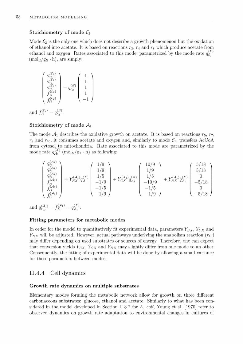
58 metabolism modelling
Stoichiometry of mode E2
Mode E2 is the only one which does not describe a growth phenomenon but the oxidationof ethanol into acetate. It is based on reactions r3, r4 and r8 which produce acetate fromethanol and oxygen. Rates associated to this mode, parametrized by the mode rate q(E)
E2
(molE/gX · h), are simply:
q(E2)r3
q(E2)r4
q(E2)r8
f(E2)A
f(E2)O
= q(E)E2
1111−1
and f
(E2)E = q
(E)E2 .
Stoichiometry of mode A1
The mode A1 describes the oxidative growth on acetate. It is based on reactions r5, r7,r8 and r10, it consumes acetate and oxygen and, similarly to mode E1, transfers AcCoAfrom cytosol to mitochondria. Rate associated to this mode are parametrized by themode rate q(X)
A1 (molX/gX · h) as following:
q(A1)r5
q(A1)r7
q(A1)r8
f(A1)A
f(A1)O
f(A1)C
= Y
(A1)EX q
(X)A1
1/91/91/5−1/9−1/5−1/9
+ Y
(A1)CX q
(X)A1
10/91/91/5−10/9−1/5−1/9
+ Y
(A1)NX q
(X)A1
5/185/18
0−5/18
0−5/18
and q(A1)r10 = f
(A1)X = q
(X)A1 .
Fitting parameters for metabolic modes
In order for the model to quantitatively fit experimental data, parameters YEX , YCX andYNX will be adjusted. However, actual pathways underlying the anabolism reaction (r10)may differ depending on used substrates or sources of energy. Therefore, one can expectthat conversion yields YEX , YCX and YNX may slightly differ from one mode to an other.Consequently, the fitting of experimental data will be done by allowing a small variancefor these parameters between modes.
II.4.4 Cell dynamics
Growth rate dynamics on multiple substrates
Elementary modes forming the metabolic network allow for growth on three differentcarbonaceous substrates: glucose, ethanol and acetate. Similarly to what has been con-sidered in the model developed in Section II.3.2 for E. coli, Young et al. [1970] refer toobserved dynamics on growth rate adaptation to environmental changes in cultures of

II.4 application to Saccharomyces cerevisiae 59
S. cerevisiae. Therefore, we will attach three biological properties to cells to account fortheir growth capability on each substrate:
• µG@p: growth capability on glucose (gX/gX · h);
• µE@p: growth capability on ethanol (gX/gX · h);
• µA@p: growth capability on acetate (gX/gX · h).We model the adaptation rate of all three growth rate capabilities with a similar adapta-tion law:
∂µk@p
∂t= ζµk (µk@p,CL) = 1
Tµk(µ∗k(CL)− µk@p), k ∈ G,E,A (II.13)
This first-order adaptation law was chosen, instead of the second-order law used for E.coli (see Eq. (II.4)), to limit the number of parameters in the model, and facilitateparameter identification. It will be shown in Section II.5, that this law allows for asatisfactory enough fitting of the model against experimental data. These adaptation lawsstill require the definition of an equilibrium growth rate for each substrate. We definedthese, using Monod-like kinetic laws, by considering that growth on glucose is slightlyinhibited by both ethanol and acetate, and that growth based on these by-products isstrongly inhibited by glucose which is the preferential carbon source. Equilibrium lawsare then given by
µ∗G(CL) = µ(max)G
G
G+KG
K(G)i,E
E +K(G)i,E
K(G)i,A
A+K(G)i,A
µ∗E(CL) = µ(max)E
E
E +KE
K(G)i,G
G+K(G)i,G
µ∗A(CL) = µ(max)A
A
A+KA
K(A)i,G
G+K(A)i,G
K(A)i,E
E +K(A)i,E
Time-scales associated to the adaptation of each growth rate, TµG , TµE and TµA , willhave a similar order of magnitude than the time-scale used in the E. coli model, aboutan hour. These time-scales are allowed to slightly differ between substrates.
Crabtree effect: adapting the oxidative capacity
Once growth-rate dynamics are tackled, the main dynamic effect to be considered about S.cerevisiae is the Crabtree effect. As already stated, this effect consists in the productionof ethanol, which is a fermentative pathway by-product, under aerobic conditions. Pronket al. [1996] actually differentiate two phenomenon, the long-term Crabtree effect and theshort-term Crabtree effect, each having distinct origins.
The long-term effect corresponds to the production of ethanol in culture at high growth-rate, no matter the residual glucose concentration. It can be observed by tracking oxygenconsumption, carbon dioxide production, and sugar to cell conversion yield against in-creasing dilution rates in chemostat cultures as shown in Fig. II.12.
At low growth rates (µ < 0.3h−1), oxygen consumption increases almost linearly withthe growth-rate. The respiratory quotient (molar ratio between carbon dioxide produc-tion and oxygen consumption) is near 1.0 which denotes an exclusive use of oxidative

60 metabolism modelling
Figure II.12: Illustration of long-term Crabtree effect in chemostat cultures. (left) Spe-cific oxygen consumption rate. Reproduced with permission of MicrobiologySociety via Copyright Clearance Center [Barford and Hall, 1979]. (right)Respiratory quotient and conversion yield of glucose [van Dijken and Schef-fers, 1986].
pathways. Once the dilution –and growth– rates reach the critical value of 0.3h−1, oxy-gen consumption reaches a plateau, and the respiratory quotient starts increasing linearlywith the growth-rate. This RQ increase can be attributed to the use of fermentative path-ways. This also explains the associated drop in glucose conversion yield, as fermentativepathways are less efficient than oxidative ones. Similar results have been observed byPetrik et al. [1983] and Rieger et al. [1983].
Overall, the long-term Crabtree effect can be attributed to a limiting oxidative capacitywhich cannot exceed the capacity required to grow at a critical rate µcrit ≈ 0.3h−1. Thesteady-state data shown in Fig. II.12 are however not sufficient to determine whether theoxidative capacity is a dynamic property of cells. Indeed, the capacity could always beat its peak value, and would be under-solicited at low growth-rate. Another hypothesiswould be that cells dynamically adapt their capacity at low growth-rates.
It has been assumed that the oxidative capacity is indeed a dynamic property of cells.While growth-rate dynamics denotes the adaptation of cells to varying substrate avail-ability, the adaptation of oxidative capacity will denote the adaptation of cells to varyingenergy production requirements. This assumption is in-line with the modelling of Scere-visiae by Sweere et al. [1988] where a dynamic oxidative capacity was considered too.
Assessing whether this assumption is correct is difficult due to a lack of experimentalevidence. Indeed, due to the short-term Crabtree effect which prevents an efficient use ofoxidative pathways, one cannot observe whether the oxidative capacity is a limiting factorafter a sudden increase of dilution-rate in chemostat culture. A possibility would be toperform anaerobic chemostat culture at moderate growth-rate and to observe whetherswitching to aerobic conditions allows an instantaneous use of oxygen resources.
For now, we will describe the evolution of a cell-attached property ϕ(b)O@p (gO/gX · h)
which is the maximum amount of oxygen that can be processed by cells in the respiratorychain to produce energy. This variable will evolve toward an equilibrium capacity whichdepends on the equilibrium growth-rate associated to the environment. This equilibriumcapacity is modelled against experimental data illustrated in Fig. II.13 by
ϕ∗O =ϕ
(max)O
µ∗GµOlimG
if µ∗G ≤ µOlimG
ϕ(max)O otherwise
(II.14)

II.4 application to Saccharomyces cerevisiae 61
0
2
4
6
8
10
12
0 0,1 0,2 0,3 0,4 0,5 0,6
Mea
n o
xyge
n u
pta
ke r
ate,
ϕO
(m
mo
lO/g
X.h
)
Dilution rate (h-1)
Sweere et al. (1988)Strain CBS 8066
Rieger et al (1982)Strain H1022
Flikweert et al. (1999)Strain CEN-PK113-7D
Barford et al. (1979)Strain 248 UNSW 703100
Figure II.13: Experimentally measured specific oxygen consumption rate in chemostatcultures at equilibrium.
Figure II.14: Concentrations of ethanol (), acetate () and glycerol (4) after a dilution-rate shift-up (0.05 to 0.15 h−1) in a glucose-fed chemostat culture of S.cerevisiae. Reproduced by permission of Oxford University Press [Guillouet al., 2004].
with µOlimG the minimal growth-rate at which the long-term Crabtree effect occurs and
ϕ(max)O the corresponding oxidative capacity. The cell capacity ϕ
(b)O@p will evolve toward
this equilibrium value at the following rate:
∂ϕ(b)O@p
∂t= ζϕO = 1
TϕO
(ϕ∗O − ϕ
(b)O@p
)(II.15)
Sweere et al. [1988] also modelled S. cerevisiae by introducing a dynamic oxidative ca-pacity. This property evolved with a time-scale of 1.8h.
On top of the long-term Crabtree effect, which is simply described by the observedplateau in specific oxygen consumption in Fig. II.12, the critical dynamic behaviour forS. cerevisiae modelling is the short-term Crabtree effect. This effect corresponds to theproduction of ethanol by S. cerevisiae, in aerobic cultures, after a sudden exposition tohigh glucose concentrations. This is illustrated in Fig. II.14 where ethanol is producedin a chemostat culture after a dilution-rate shift-up.

62 metabolism modelling
Figure II.15: Intracellular concentration in Glucose-6-Phosphate (G6P), Fructose-6-Phosphate (F6P) and Fructose-1,6-BiPhosphate (FBP), after a glucose pulsein chemostat culture of S. cerevisiae. Reproduced by permission of John Wi-ley and Sons [Theobald et al., 1997].
The short-term Crabtree effect is usually attributed to a saturation of the respiratorychain, which induces an overflow at the pyruvate node in the metabolic network, andresults in a diversion of carbon toward ethanol production [Pronk et al., 1996]. Morerecently, Rosas-Lemus et al. [2014] isolated mitochondria from both Crabtree-positiveand Crabtree-negative yeasts and could measure their activity when exposed to differentconditions. In particular, they observed that one metabolite of the glycolysis pathway,the Fructose-1,6-BiPhosphate (FBP), closes mitochondrial unspecific channels which areresponsible for most mass-transfers between cytoplasm and mitochondria.
Theobald et al. [1997] measured intracellular concentrations of multiple metabolites,including FBP, in S. cerevisiae right after a glucose pulse in chemostat culture. Theirmost interesting result to understand the short-term Crabtree effect is shown in Fig.II.15 where one can observe that after the pulse, glucose is assimilated and consequentlyconverted into G6P , F6P and then FBP. As long as the environment remains rich inglucose, the intracellular concentration of FBP remains at high levels, which shows thatthe conversion of FBP by the fructose-bisphosphate aldolase is a limiting reaction in theglycolysis pathway.
Coupling measurements of intracellular concentrations after a glucose pulse [Theobaldet al., 1997] with the observation of isolated mitochondria by Rosas-Lemus et al. [2014]allows inferring a probable cause for the short-term Crabtree effect: if a cell is suddenlyexposed to high glucose concentrations, this substrate will enter the cytoplasm but thecellular machinery will not be sufficient to process efficiently this high substrate quantity.Therefore, FBP will accumulate which will close mitochondria unspecific channels andprevent part of the pyruvate to enter the TriCarboxylic Acid cycle which reduces theenergetic efficiency of the cell by under-using the respiratory chain. As pyruvate accumu-lates, and the use of oxidative pathways is diminished, some of that pyruvate is divertedtoward the fermentative pathway which explains the ethanol production.

II.4 application to Saccharomyces cerevisiae 63
Overall, this short-term Crabtree dynamics can be described by considering that (i) inglucose-rich environments, some metabolites accumulate quickly –within a few seconds(Fig. II.15)– in cells which reduces the use of oxidative metabolic modes and (ii) inenvironments with non-excessive glucose concentrations, these metabolites are processedand the respiratory capacity can be fully exploited once again. The time-scale associatedto the return to standard cell functioning is not clearly identifiable from previous resultsand will be a fitting parameters of the model.
Instead of quantitatively track intracellular concentrations to determine whether theshort-term Crabtree effect occurs, we chose to track an adimensional quantity, σ@p ∈ [0, 1]which we refer to as the glycolytic stress. If σ@p = 0, cells are unstressed and the oxidativecapacity can be fully exploited. Otherwise, oxidative modes will be inhibited.
Stress evolution is modelled by the following law:
∂σ@p
∂t= ζσ = κσ
T(u)σ
(1− σ)− (1− κσ)T
(d)σ
σ (II.16)
κσ is a variable close to 1 in stressful environment and close to 0 in unstressing envi-ronments. Therefore, the first term on the Right-Hand Side (RHS) describes the stressincrease with a time-scale T (u)
σ ≈ 1s and the second term describe stress recovery over alonger time-scale T (d)
σ ≈ 1min. It was decided to characterise the stressfulness of an en-vironment by comparing the difference between a cell’s growth capacity on glucose µG@pwith the equilibrium growth-rate µ∗G(CL) against a threshold value δµσ:
κσ =(
11 + exp (−50 (µ∗G − µG@p − δµσ))
)2
≈
0 if µ∗G − µG@p < δµσ
1 otherwise(II.17)
µG@p is here taken as an estimate of a cell’s capability to process glucose, and µ∗G a roughestimate of the glucose uptake rate. Therefore, the difference µ∗G − µG@p is a measureof the disequilibrium between a cell and its environments. The introduced thresholdvalue δµσ reflects the fact that small scale disequilibriums are indeed dumped by minormetabolic adjustments whereas larger disequilibrium are stressful and will turn into majormetabolic perturbations.
Observing conversion yields and respiration rates under active Crabtree-effect, we couldnotice that oxidative modes are not entirely inhibited by this effect. Overall, after asignificant stressing event (glucose pulse, dilution rate shift-up), respiration is reducedby approximately 60% compared to the oxygen consumption rate preceding the event.Therefore, we compute an inhibition factor ki,σ by
ki,σ =k
(min)i,σ
k(min)i,σ +
(1− k(min)
i,σ
)σ@p
(II.18)
with k(min)i,σ = 0.4. The computation of rates associated to each mode will still be based
on the identification of the limiting factor, but afterwards, the rate of oxidative modeswill be multiplied by ki,σ. Doing so, if a cell is fully stressed (σ@p ≈ 1), oxidative modeswill be slowed down by 60%. Otherwise, these mode rates will be left almost unchanged.

64 metabolism modelling
II.4.5 Mode limitations
Similarly to the E. coli model developed in Section II.3, the rates of metabolic modesin the S. cerevisiae model will be computed by defining available resources which, oncedepleted, will limit metabolic mode rates. We recall here that generally speaking, theuptake rates ϕ(g) (g/gX · h) is either limited by the availability in the environment ϕ(e)
or by the cell capability to import the substrates ϕ(b). None of these limits is actuallyconstant in industrial bioprocessed but in this section, it will be assumed the ϕ(g) = ϕ(b),i.e. that the environment is not limiting. The modelling of ϕ(e) and its combination withϕ(b) to compute ϕ(g) is an aspect that will be developed in Chapter V.
Biological limits on carbonaceous substrate uptake-rates will simply be defined as bi-ological constants, ϕ(b)
G,E,A = ϕ(max)G,E,A, which will be fitting parameters for the model.
Limits on oxygen consumption rate is defined by the cell-attached biological propertyϕ
(g)O = ϕ
(b)O@p.
Cell-attached growth capabilities µG@p, µE@p and µA@p form limits on cell productionrates for growth modes. It is known that fermentative growth is slower than oxidativegrowth on glucose, µ(max,o)
G > µ(max,f)G . In order to account for this, while only attaching a
single glucose-based growth capability µG@p to cells, the maximum growth rate on glucosethrough fermentation is set to a fraction of the maximum value for oxidative growth. Thisaspect will clearly appear hereafter in the computation of the rate for mode G2. Note thatthis approach makes the implicit assumption that a cell fully adapted to oxidative growthon glucose will be instantaneously able to grow a full efficiency in a fermentative mode isoxygen is suddenly depleted. This is not an accurate description of the switch betweenoxidative and fermentative growths, but it allows limiting the number of cell-attacheddynamic properties.
II.4.6 Mode rates computation
Available resources available for S. cerevisiae metabolic modes are:
• Consumption/uptake rates– of glucose: ϕ(g)
G (kgG/kgX · h) or f (g)G = ϕ
(g)G /MG (molG/kgX · h);
– of ethanol: ϕ(g)E (kgE/kgX · h) or f (g)
E = ϕ(g)E /ME (molE/kgX · h);
– of acetate: ϕ(g)A (kgA/kgX · h) or f (g)
A = ϕ(g)A /MA (molA/kgX · h);
– of oxygen: ϕ(g)O (kgO/kgX · h) or f (g)
O = ϕ(g)O /MO (molO/kgX · h).
• Growth capabilities– on glucose µ(g)
G = µG@p (kgX/kgX · h);
– on ethanol µ(g)E = µE@p (kgX/kgX · h);
– on acetate µ(g)A = µA@p (kgX/kgX · h);
Stoichiometry of modes has been defined previously (see Section II.4.3) and here, we willonly make use of global conversion yields associated to each mode. Note however thatthese yields actually depend on stoichiometric coefficients associated to the anabolismreaction which will be fitting parameters in Section II.5.
Steps for the computation of mode rates are

II.4 application to Saccharomyces cerevisiae 65
1. Compute the inhibition factor of oxidative modes by glycolytic stress ki,σ.
2. Compute mode G1 rate considering inhibition by stress and limits in oxygen andglucose uptake rates (f (g)
O and f(g)G ) and glucose-based growth capacity µ(g)
G ,
q(X)G1 = ki,σ min
f(g)O
Y(G1)OX
; f(g)G
Y(G1)GX
; µ(g)G
MX
3. Compute remaining resources for modes G2, E1, E2 and A1,
f(g)O ← f
(g)O − Y
(G1)OX q
(X)G1
f(g)G ← f
(g)G − Y
(G1)GX q
(X)G1
µ(g)G ← µ
(g)G −MXq
(X)G1
4. Compute mode G2 rate considering limits in glucose uptake rate f (g)G and glucose-
base growth capacity µ(g)G corrected for fermentative growth,
q(X)G2 = min
f(g)G
Y(G2)GX
; µ(max,f)G
µ(max,o)G
µ(g)G
MX
5. Compute mode E1 rate considering the stress level, upper bounds on uptake ratesfor oxygen and ethanol (f (g)
O and f(g)E ) and the limited growth capacity on ethanol
µ(g)E ,
q(X)E1 = ki,σ min
f(g)O
Y(E1)OX
; f(g)E
Y(E1)EtX
; µ(g)E
MX
6. Compute resources available for modes E2 and A1,
f(g)O ← f
(g)O − Y
(E1)OX q
(X)E1
f(g)E ← f
(g)E − Y
(E1)EX q
(X)E1
7. Compute mode E2 rate considering limits in oxygen and ethanol uptake rates (f (g)O
and f(g)E ),
q(E)E2 = min
f(g)O
Y(E2)OE
; f (g)E
8. Compute resources available for mode A1,
f(g)O ← f
(g)O − Y
(E2)OE q
(E)E2

66 metabolism modelling
9. Compute mode A1 rate considering the stress level, upper bounds on uptakes ratesfor oxygen and acetate (f (g)
O and f(g)A ) and the limited growth capacity on acetate
µ(g)A ,
q(X)A1 = ki,σ min
f(g)O
Y(A1)OX
; f(g)A
Y(A1)AX
; µ(g)A
MX
Once mode rates are computed through this straightforward procedure, actual con-sumption/production and growth rates are computed by
µ(a) =(q
(X)G1 + q
(X)G2 + q
(X)E1 + q
(X)A1
)MX
ϕ(a)G = −
(Y
(G1)GX q
(X)G1 + Y
(G2)GX q
(X)G2
)MG
ϕ(a)E =
(Y
(G2)EX q
(X)G2 − Y
(E1)EX q
(X)E1 − q
(E)E2
)ME
ϕ(a)A =
(Y
(E2)AE q
(E)E2 − Y
(A1)AX q
(X)A1
)MA
ϕ(a)O = −
(Y
(G1)OX q
(X)G1 + Y
(E1)OX q
(X)E1 + Y
(A1)OX q
(X)A1
)MG
II.5 Challenging the model developed for S. cerevisiae
II.5.1 Comparison data
The model described previously is meant to reproduce the behaviour of a wild S. cerevisiaestrain in steady environment but also in dynamic situations. Therefore, we attemptedto fit the model against multiple experimental data sets coming from different culturemodes. To do so, we extracted data points from the literature for experiments usingdifferent wild strains of S. cerevisiae. A summary of these data sets is given in Table II.4.
Table II.4: References for data sets used to fit the S. cerevisiae model.Source Strain Culture modeFlikweert et al. [1999] CEN-PK113-7D Steady-state chemostat
Glucose pulse in chemostatBarford and Hall [1979] 248 UNSW703100 Steady-state chemostatvan Dijken and Scheffers [1986] CBS 8066 Aerobic batch cultures
Anaerobic batch cultureSweere et al. [1988] CBS 8066 Glucose pulse in chemostat
II.5.2 Model fitting strategy
For now, the model has only been described qualitatively and only order of magnitudeswere given for the model parameters. All model parameters were fitted manually againstpreviously listed data sets. This was done by iterating over two fitting steps:

II.5 challenging the model developed for S. cerevisiae 67
1. Fit parameters that only have an impact on steady-state behaviour (conversionyields, affinity/inhibition constants, maximum kinetic rates, ...) against steady-state chemostat data.
2. Fit parameters that have an impact on dynamic behaviour (adaptation rates ofbiological properties, order of magnitude of short-term Crabtree effect, . . . ).
Final model parameters are listed in Table II.5.
Table II.5: List of fitted parameters for S. cerevisiae model.Kinetic parameters Mode yieldsSymbol Value Symbol Valueµ
(max,o)G 0.49 h−1 Y
(G1)EX 16.02 molATP/molX
µ(max,f)G 0.37 h−1 Y
(G2)EX 12.02 molATP/molX
µ(max)E 0.12 h−1 Y
(E1)EX 16.02 molATP/molX
µ(max)A 0.20 h−1 Y
(A1)EX 18.02 molATP/molX
ϕ(max)O 8.90 molO/kgX · h Y
(G1)CX 2.77 molAcCoA/molX
ϕ(max)G 19.86 molG/kgX · h Y
(G2)CX 3.02 molAcCoA/molX
ϕ(max)E 3.87 molE/kgX · h Y
(E1)CX 2.52 molAcCoA/molX
ϕ(max)A 4.13 molA/kgX · h Y
(A1)CX 3.02 molAcCoA/molXY
(G1)NX 29.4 mmolNADPH/molX
Affinity/Inhibition constants Y(G2)NX 29.4 mmolNADPH/molX
Symbol Value Y(E1)NX 29.4 mmolNADPH/molX
KG 41.37 gG/m3L Y
(A1)NX 29.4 mmolNADPH/molX
K(G)i,E 40.0 kgE/m3
L Y(E2)AE 0.5 molA/molE
K(G)i,A 6.0 kgA/m3
LKE 561.8 gE/m3
L ConstantsK
(E)i,G 10 gG/m3
L Symbol ValueKA 450.6 gE/m3
L MG 180.2 gG/molGK
(A)i,G 2.0 gG/m3
L ME 46.0 gE/molEK
(A)i,E 2.0 gE/m3
L MA 59.0 gA/molAMO 32.0 gO/molO
Dynamics time-scales MX 113.1 gX/molXSymbol ValueTµG 2.5 h DiverseTµE 3.5 h Symbol ValueTµA 0.4 h µOlimG 0.31 h−1
TϕO 1.6 h δµσ 0.2 h−1
T (u)σ 3 s k
(min)i,σ 0.4
T (d)σ 120 s

68 metabolism modelling
0
0,1
0,2
0,3
0,4
0,5
0,6
0 0,1 0,2 0,3 0,4 0,5
Y XG
(gX/g
G)
Dilution rate D (h-1)
(a)
0
2
4
6
8
10
12
0 0,2 0,4 0,6
qO
2(m
mo
l O/g
X.h
)
Dilution rate D (h-1)
(b)
0
1
2
3
4
5
6
0 0,2 0,4 0,6
RQ
(m
ol C
O2/m
ol O
2)
Dilution rate D (h-1)
(c)
Figure II.16: Comparison of model predictions against experimental steady-state chemo-stat measurements. Data from Flikweert et al. [1999]. N Data fromBarford and Hall [1979]. (a) Conversion yield of glucose to cell. (b) Specificoxygen consumption rate. (c) Respiratory quotient.
II.5.3 Comparison results
Steady-state comparison
First, the model has been assessed by simulating glucose-fed chemostat culture at multipledilution rates. The culture state was considered steady with the stopping criterion∣∣∣∣∣
∣∣∣∣∣(∂C
∂t
)C
∣∣∣∣∣∣∣∣∣∣ < 10−3h−1 (II.19)
i.e. when concentrations would vary by less than 0.1% over an hour. At this steady-state, we extracted from the mode rates the global conversion yield of glucose into cell,the specific oxygen consumption rate and the respiratory quotient RQ. The latter is themolar ratio between rates of produced carbon dioxide and consumed oxygen. This is ametrics often used to assess the well functioning of a culture as this ratio is close to 1 ifthe metabolic is fully oxidative, and significantly increases when fermentative pathwaysare active. Results are illustrated in Fig. II.16 and clearly show correct tendencies as wellas the switch of metabolism occurring around D = 0.31h−1 = µOlim
G due to the long-termCrabtree effect.
Dynamic simulations
van Dijken and Scheffers [1986] have performed lab-scale cultures of S. cerevisiae whichare of particular interest for the development of our model. They performed batch cul-tures, but with the particularity that these batch cultures directly follow pre-culture inchemostat. As explained in Section II.3, chemostat cultures allow for enforcing a specificgrowth-rate over a biological population. As batch culture are highly sensitive to initialcondition, having performed these chemostat pre-culture helps us defining the initial stateof the biological population. Note that this knowledge of initial state is often missing.Therefore, we will focus the fitting of the model on data sets from these authors havinga great confidence in their exploitability.
Three data sets corresponding to three batch culture are actually available. The ex-perimental data and corresponding simulations are shown in Fig. II.17. Sub-figures (a)

II.5 challenging the model developed for S. cerevisiae 69
0
0,5
1
1,5
2
2,5
3
3,5
4
0
2
4
6
8
10
0 2 4 6 8 10
Eth
ano
l (g E
/L)
Glu
cose
(g G
/L)
t (h)
(a)
0
1
2
3
4
5
6
0
0,2
0,4
0,6
0,8
1
1,2
1,4
1,6
1,8
0 2 4 6 8 10
Bio
mas
s(g
X/L
)
Ace
tate
(gA/L
)
t (h)
(b)
0
0,5
1
1,5
2
2,5
3
0
2
4
6
8
10
12
0 2 4 6 8 10
Eth
ano
l (g E
/L)
Glu
cose
(g G
/L)
t (h)
(c)
0
0,5
1
1,5
2
2,5
3
3,5
4
2
2,5
3
3,5
4
4,5
5
5,5
6
0 2 4 6 8 10
Bio
mas
s(g
X/L
)
Ace
tate
(gA/L
)
t (h)
(d)
0
0,5
1
1,5
2
2,5
3
3,5
4
0
1
2
3
4
5
6
7
8
9
0 0,5 1 1,5 2 2,5 3 3,5
Eth
ano
l (g E
/L)
Glu
cose
(g G
/L)
t (h)
(e)
3
3,4
3,8
4,2
4,6
5
0
0,2
0,4
0,6
0,8
1
0 0,5 1 1,5 2 2,5 3 3,5
Bio
mas
s(g
X/L
)
Ace
tate
(gA/L
)
t (h)
(f)
Figure II.17: Comparison of model predictions with batch culture following pre-cultivation in chemostat from van Dijken et al. [2000]. (a) and (b): precul-ture at dilution rate 0.1h−1. Aerobic batch culture. (c) and (d): precultureat dilution rate 0.2h−1. Aerobic batch culture. (e) and (f) preculture atdilution rate 0.1h−1. Anaerobic batch culture.
and (b) correspond to an aerobic batch culture with a pre-culture dilution rate set toD = 0.1h−1. Sub-figures (c) and (d) are similar but with an higher pre-culture dilutionrate set to D = 0.2h−1. Finally, sub-figures (e) and (f) correspond to an anaerobic batchculture with a pre-culture dilution rate of D = 0.1h−1.
Overall, all metabolic modes play their role in different phases of theses cultures asshown previously in Fig. II.10. Therefore, we could adjust conversion yield but alsotime-scales for biological properties adaptation over these data sets. Following this, wecould attempt reproducing chemostat cultures disturbed by glucose pulses by Flikweertet al. [1999] (see Fig. II.18) and Sweere et al. [1988] (see Fig. II.19). Due to the use ofdifferent strains of S. cerevisiae, the imperfect fitting is not surprising. However, maintendencies seem to be well reproduced and the use of automated fitting tool in place ofa manual adjustment of model parameters could certainly yield even better agreement.

70 metabolism modelling
0 2 4 6 8time (h)
0
2
4
6
8
10
Glu
cose
, CG
(g
G/L
)
0 2 4 6 8time (h)
0
0.5
1
1.5
2
2.5
3
Eth
anol
, CE
(g
E/L
)
0 2 4 6 8time (h)
0
0.5
1
1.5
2
Ace
tate
, CE
(g
E/L
)
Figure II.18: Comparison of model predictions with glucose pulse experiment in chemo-stat culture by Flikweert et al. [1999]. Dilution rate: 0.10h−1.
0 2 4 6 8time (h)
0
2
4
6
8
10
Glu
cose
, CG
(g
G/L
)
0 2 4 6 8time (h)
0
1
2
3
4
Eth
anol
, CE
(g
E/L
)
0 2 4 6 8time (h)
0
0.5
1
1.5
Ace
tate
, CE
(g
E/L
)
0 2 4 6 8time (h)
2
3
4
5
6
Bio
mas
s, C
X (
gX
/L)
Figure II.19: Comparison of model predictions with glucose pulse experiment in chemo-stat culture by Sweere et al. [1988]. Dilution rate: 0.08h−1.

II.6 conclusion 71
II.6 Conclusion
This chapter focused on developing a low-cost structure for metabolic models which canaccount for dynamic biological properties and multiple metabolic modes. This work isactually the continuation of a Master thesis where a simple metabolic model for E. coli byXu et al. [1999] was derived to account for a dynamic growth capability and disequilibriumbetween a cell and its environment [Pigou and Morchain, 2015]. Principles underlyingthese first models have been reapplied under a better organized formalism, based on ametabolic mode definition and a simple methodology to compute rates of these modes.This was mainly done by selecting key metabolic fluxes and by providing simple closurelaws to estimate them. This in turn allows computing all fluxes and thus consumptionand production rates.
The proposed structure has been illustrated on two standard micro-organisms in indus-trial bio-processes: Escherichia coli and Saccharomyces cerevisiae. The first one mainlyserved as an illustration of the structure. The second one will be used in Chapter V toperform large-scale simulations of an industrial bioreactor.
The S. cerevisiae model has been challenged against multiple experimental data sets,originating from multiple labs and research teams. A preliminary fitting has been per-formed manually which yields a satisfactory match between simulations and experimentalresults. An ulterior step would be to improve numerically the fitting while also assessingthe model sensitivity to its parameters through an optimization based procedure [Sanchezet al., 2014]. For now, the proposed model is a proof-of-concept which illustrates thatthe proposed structure can indeed reproduce observed tendencies over a wide range ofculture modes even in dynamic conditions. Note that this is done using a low number offloating-point operations (flop), about 140 flop, and a limited number of parameters too(35 different parameters in Table II.5). To give a sense of comparison, Rizzi et al. [1997]proposed a intracellular concentrations-based model tracking 15 metabolites concentra-tions which required fitting 87 model parameters and relied on at least 330 floating-pointoperations. This model did not handle long-term cultures as the growth-rate was a con-stant model parameter.


IIIB I L A N S D E P O P U L AT I O N A P P L I Q U E S AU X S Y S T E M E SB I O L O G I Q U E S
Resume
Afin de predire le comportement des bioreacteurs aux echelles de pilotes de laboratoireet de procedes industriels, tout en preservant un meme modele, l’element cle est deconsiderer les micro-organismes comme des systemes dynamiques. Suivre leurs proprietesdynamiques est alors un prerequis pour une modelisation precise des fermenteurs.
Dans le Chapitre II, des modeles metaboliques sont presentes pour Escherichia coli etSaccharomyces cerevisiae et sont bases sur la definition de variables dynamiques directe-ment liees aux vitesses de reactions internes. Les variables alors choisies sont les capacitesde croissance, de mobilisation des voies oxydatives, et le stress glycolitique. Ces variablesont ete selectionnees car directement utilisables pour predire l’orientation des flux dematieres entre les modes metaboliques elementaires du modele. Ces choix de variablesetaient donc justifies par leur couplage avec la structure de modele metabolique proposee.Cependant, de nombreux auteurs ont considere d’autres quantites attachees aux cellulestelles que leur age, masse, taille, . . . Au dela du choix de ces variables, le principal defiest de suivre ces quantites a l’echelle d’une population biologique.
Pour resoudre la diversite de ces variables sur l’ensemble de la population de micro-organismes, et grace au nombre important d’individu, il va etre possible d’appliquerdes approches statistiques. Au lieu de suivre les proprietes attachees a chaque celluleprise individuellement, nous proposons d’appliquer la modelisation par bilan de popu-lation, dont le principe est de resoudre l’evolution spatiale et temporelle d’une distri-bution statistique. Le formalisme des bilans de population se couple parfaitement avecles modeles metaboliques presentes en Chapitre II, mais aussi avec les descriptions del’hydrodynamique qui seront detaillees en Chapitre IV. Cependant, cette approche peutse reveler numeriquement couteuse selon la methode choisie pour resoudre l’Equation deBilan de Population.
Ce chapitre vise principalement a identifier la methode la plus adaptee pour resoudreles equations de bilan de population appliquees a la modelisation des bioreacteurs. Deuxcategories de methodes sont considerees : methodes des classes et methodes des moments.La methode des classes a deja ete appliquee a la modelisation des bioreacteurs avant cetravail de these [Pigou and Morchain, 2015]. Appliquer les methodes aux moments a lamodelisation des fermenteurs est cependant un element nouveau propose au cours de cetravail.
Une premiere partie de ce chapitre presente (i) une variante des methodes des classes,dite de pivots-fixes et (ii) des methodes de quadratures des moments afin de fermerle jeu d’equations obtenu dans la formulation aux moments : la methode de Quadra-
73

74 bilans de population appliques aux systemes biologiques
ture des Moments (QMOM), sa version etendue (EQMOM) et l’approche du Maximumd’Entropie. Une seconde partie se concentre sur la comparaison de ces methodes en ter-mes de precision, de stabilite et de performance. Cette comparaison a ete publiee dansChemical Engineering Science [Pigou et al., 2017]. Au cours de ce travail, EQMOM aete identifiee comme repondant aux besoins associes a la simulation des bioreacteurs. Letravail d’implementation de methodes pour leur comparaison nous a permis d’identifierune amelioration majeure qu’il etait possible d’apporter a EQMOM. Une troisieme par-tie de ce chapitre decrit brievement cette amelioration, et se concentre sur la mesure desgains qu’elle apporte. En particulier, il est montre que le cout numerique d’EQMOMa ete reduit d’un facteur 5 a 30. L’ensemble des details relatifs a cette nouvelle versiond’EQMOM ont ete publies dans le Journal of Computational Physics [Pigou et al., 2018a].

IIIP O P U L AT I O N B A L A N C E S FO R B I O L O G I C A L S Y S T E M S
Summary
In order to use similar models to predict the behaviour of bioreactors at both lab-scaleand industrial scale, the key consideration is that micro-organisms are dynamic systems.Tracking their dynamic properties is therefore a prerequisite for an accurate modelling offermenters.
In Chapter II, metabolic models are developed for Escherichia coli and Saccharomycescerevisiae and are based on the definition of dynamic variables directly related to internalreaction rates. Chosen variables were growth capabilities, oxidative capacity and gly-colytic stress. These variables were selected as they directly contain information usefulfor orienting matter between elementary metabolic modes. These variable choices werethen motivated by the proposed metabolic model structure. However, many authors haveconsidered other quantities such as cell age, mass, size, budding index, . . . Beyond thisvariable choice, the main numerical challenge is to track these quantities over a largebiological population.
To track the diversity of these variables among whole biological populations, one canbenefit from the high number of cells to apply statistical approaches. Instead of trackingthese properties cell-by-cell, we propose to make use of the Population Balance Modelling(PBM) approach which tracks statistical distributions over time and space. The PBMformalism can be perfectly coupled with metabolic models as proposed in Chapter II,and with hydrodynamic framework that will be discussed in Chapter IV. However, thisapproach can be computationally expensive depending on the method used to solve thePopulation Balance Equation.
This chapter aims at identifying the best suited method to handle Population Balancesfor the simulation of large-scale bioreactors. Two categories of methods are considered:methods of classes and methods of moments. The class method has already been used inthe context of bioreactor modelling before this PhD thesis [Pigou and Morchain, 2015]however this problem is an original application case for method of moments that havebeen mainly developed in other chemical engineering fields.
The first part of this chapter introduces (i) the fixed-pivot method which is one variantof methods of classes and (ii) quadrature methods used to close the set of equations in mo-ment formulation, namely the Quadrature Method of Moments (QMOM), its Extendedversion (EQMOM) and the Maximum-Entropy approach. The second part focuses oncomparing these methods in terms of accuracy, stability and performance. This compar-ison has been published in Chemical Engineering Science [Pigou et al., 2017]. Finally,over the course of this work, EQMOM was found to be a method suiting the goal ofbioreactor simulations, and we happened to identify a major improvement in the basis of
75

76 population balances for biological systems
this method. These improvements are quickly presented in a third part, and are shownto significantly reduce the numerical cost of EQMOM by a factor ranging between 5 and30. Full details of this new EQMOM version were published in Journal of ComputationalPhysics [Pigou et al., 2018a].

IIIP O P U L AT I O N B A L A N C E S FO R B I O L O G I C A L S Y S T E M S
III.1 Introduction
Bioreactors are heterogeneous systems and so are biological populations. This fact iswell documented [Delvigne and Goffin, 2014; Heins et al., 2015; Simen et al., 2017] andconstitutes the main challenge in bioreactor modelling. The proposed modelling frame-work accounts for this by associating a vector of biological properties, p, to cells. Theseproperties evolve along cell’s trajectories, and influence their metabolic behaviour.
In chapter II, two biological models have been detailed. The first one describing E. coliconsiders a single biological property, the cell’s growth capability µc, hence p = µc. Thesecond model describes the behaviour of S. cerevisiae and requires multiple dynamic vari-ables, namely the specific growth capability associated to each carbon substrate (glucose,ethanol and acetate), the unstressed oxidative capacity, and the glycolytic stress, hencep =
[µG, µE, µA, ϕ
(b)O , σ
]T. These models are defined at the cell-scale. They take as
input the vector of biological properties p and the vector of concentrations in the liquidenvironment of a cell, CL. From these inputs, both models yield (i) a vector of specificconsumption/production rates r(p,CL) which will be source/sink terms in mass balanceequations of dissolved species, as well as (ii) rates of evolution of biological propertiesζ(p,CL).
The cell-scale behaviour being modelled, the remaining challenge is to describe thisbiological behaviour at the scale of the whole population, in a numerically tractable way.As stated in chapter I, these questions are not new and arise in many engineering fields.Suitable modelling frameworks have already been developed to tackle these problems, andthe challenge is mainly to transpose and adapt them to the modelling of heterogeneousbioreactors.
The modelling of heterogeneous population will be handled by Population BalanceModels (PBMs). They are based on Population Balance Equations (PBEs) which tracka statistical distribution n(p) of heterogeneous properties in space and time. PBEs allowtaking into account all phenomena that influence the statistical distribution. The cell-scale evolution of biological properties, modelled through the term ζ(p,CL), will be atransport term in the space of biological properties, which is the support of the NumberDensity Function (NDF) n(p). The fact that new cells are formed by cell-division (forbacteria) or budding (for yeasts) and that these new cells can have properties differingfrom their mothers cells can also be taken into account, as soon as one describes theprobability that a mother of properties p′ will produce a daughter cell of properties p.This will be referred to as the redistribution probability law β(p, p′).
This chapter focuses on how to handle the PBE in a way compatible with other aspectsof a bioreactor modelling. The core question is: how to track n(p) in a numerically efficient
77

78 population balances for biological systems
way? For the modelling of bioreactors, having access to this distribution is of interest asit allows estimating local rates of consumption or production of dissolved species (glucose,acetate, oxygen, ...):
R (n(µ),CL) =∫
Ωpn(p)r(p,CL)dp (III.1)
Approaches developed hereafter will not directly track n(p) but will yield approximationsof this reaction term.
A generic PBE compatible with models developed in chapter II is
∂n(p)∂t
+ ∇ ·(ζ(p,CL)n(p)
)=∫
Ωpµ(p′,CL)β(p, p′)n(p′)dp′ (III.2)
Spatial convection and dispersion terms must be added on the Left-Hand Side (LHS),refer to Eq. (I.14) for the complete PBE. A supplementary term on the Right-Hand Side(RHS) could account for cell death, but this has not been considered in this work. SpecificPBEs for E. coli and S. cerevisiae, based on models from Chapter II, will be detailed inSection III.2.
As explained in Chapter I, PBEs are not directly compatible with mass balance equa-tions as described in classical Euler-Euler gas-liquid modelling and simulation frameworks(see Eq.(I.9)), due to the transport term in the space of cell’s properties. Both sectionaland moment methods can be applied to transform a PBE into a set a equations havingthe expected structure. This is presented in Section III.3 in the case of developed PBEs.
When moment methods are applied to a PBE, some integral terms may not be for-mulated directly in terms of moments. For bioreactors, and in particular if one uses themetabolic model structure developed in Chapter II, this situation will occur. Therefore,supplementary numerical methods will be required to provide closure for these integralterms. Some of these methods were assessed by John et al. [2007] and Lebaz et al. [2016].Supplementary comparisons have been performed, aiming in particular toward the sim-ulation of bioreactors. Methods first detailed in Section III.4 are then compared to thesectional method as presented in Section III.5 which sums up an article published inChemical Engineering Science [Pigou et al., 2017, accessible in Appendix B].
Numerous readings while implementing these methods, in particular of Chihara [1978],Dette and Studden [1997], and Nguyen et al. [2016], allowed identifying –almost byserendipity– a way to improve an already efficient method, the Extended QuadratureMethod of Moments (EQMOM). This led to an article [Pigou et al., 2018a, accessible inAppendix C] whose main developments and results are summed up in Section III.6. Notethat these improvements are not specific to the study-case of a bioreactor modelling, andcan benefit all communities using moment methods for one-dimension PBMs.
Most developments presented in this chapter are related to one-dimensional PBMs andare thus applied to the PBE related to E. coli for sake of illustration. However, themodelling of S. cerevisiae as presented in Chapter II requires five dynamic biologicalproperties. Therefore, Section III.7 describes the trade-off that is applied to considerthese five variables while using only numerical methods for 1D PBEs.

III.2 considered population balance equations 79
III.2 Considered Population Balance Equations
III.2.1 A generic 1D population balance model on growth-rate
As stated in Chapter II, this PhD thesis is the continuation of a worked started with themodelling of large-scale cultures of E. coli. This preliminary work integrated the use ofa Population Balance Model based on the growth capability p = µc of a cell, i.e. thegrowth rate a cell can achieve if substrates are sufficiently available in the environment.This PBM was first proposed by Morchain et al. [2013, 2014] and takes the followingform:
∂n(µc)∂t
+ ∂
∂µc(n(µc)ζµ(µc,CL)) =
∫Ωµµ(µ′c,CL)n(µ′c)β(µc, µ′c)dµ′c (III.3)
with µ(µ′c,CL) being the growth rate achieved by a cell based on its growth capabilitiesand on the substrate availability in its environment. ζµ(µc,CL) is the rate of evolutionof the growth rate, and β(µ, µ′) is the probability density function that a mother cell ofgrowth capability µ′ will yield a daughter cell of growth capability µ.
The computation of µ(µc,CL) was detailed in Chapter II.3. Over the course of thiswork, various proposal were made for the terms ζµ(µc,CL) and β(µ, µ′). They are detailedhereafter.
Dynamics of growth-rate adaptation
Growth-rate adaptation corresponds to the second LHS term in Eq. (III.3) where ζµ(µc,CL)is the rate of adaptation of a cell’s growth rate. This notion of a dynamic growth-rate hasbeen fully detailed in Chapter II for the specific case of E. coli, but is actually applicableto a variety of other micro-organisms (see Section II.3).
The proposed model for growth-rate adaptation to an environment is based on thefact that, in constant environments, the mean growth-rate of a population reaches anequilibrium value that usually follows the Monod [1952] law, already presented in I.6.3:
µ∗ = µmaxG∗
G∗ +KG
(III.4)
where µ∗ and G∗ are steady-state –at equilibrium– growth-rate and glucose concentration,µmax is the maximum mean growth-rate achievable by the population, and KG is theaffinity of the cell with glucose (kgG/m3
L). Other terms can be added to this law toaccount for affinity toward other substrates and/or for inhibition by some compounds.
In unsteady environments, it can be observed that growth-rate evolves dynamicallyand requires a few hours to reach a new equilibrium. Therefore, the following model wassuggested by Morchain and Fonade [2009]:
ζµ(µc,CL) =( 1T
+ µc
)(µ∗(CL)− µc) (III.5)
with T the time-scale of adaptation (≈ 1h) and µ∗(CL) the Monod law adapted to theconsidered micro-organism.

80 population balances for biological systems
Redistribution of growth rate at cell-division
The redistribution of growth-rate when new cells are formed, let it be by cell division orbudding, is modelled through the probability density function β(µc, µ′c) which representsthe probability that a new cell will have a growth-rate µc if its mother cell is characterisedby a growth-rate µ′c.
The simplest approach is to assume that the growth-rate is inherited at cell division,therefore
β(µc, µ′c) = δ(µc, µ′c) (III.6)
where δ is the Dirac delta distribution, that can be defined by its sifting property∫f(x)δ(x, x′)dx = f(x′) (III.7)
Though being a simple approach, which in particular prevents the need for integral termon the RHS of Eq. (III.3), this model is not supported by experimental measurements.
The choice of the growth rate as a discriminating factor between individuals facilitatesthe computation of reaction rates as shown in Chapter II. However, the growth rate isa variable that is more easily attached to a population rather than to individuals. Thiscan reveal to be problematic if one must produce a Probability Density Function (PDF)defining the growth-rate of a daughter cell based on the growth rate of its mother cell, asone requires the knowledge of cell-attached growth-rates.
The growth-rate has two definitions depending on whether one considers the totalmass of the biological population, or the total number of cells. In terms of mass, itis defined as the rate of population mass increase, hence µ being defined with a unitkgbiomass/kgbiomass · h. It is also well-known that the growth rate can be defined by thepopulation doubling time µ = ln(2)/τ where τ is the time required to double the numberof cells in the population. As thoroughly analysed by Quedeville et al. [2018], these twodefinitions only match when cells mean-mass remains constant. This only happens insteady-state culture (chemostat) or during exponential growth in batch cultures.
The number based definition of µ may give access to cell-attached growth-rate if oneconsiders that the population doubling time is relatable to the cell division-time –if oneconsider bacteria exhibiting cell division– or budding-time if one considers budding yeast.The modelling of the probability density function β(µc, µ′c) can then be based on experi-mental data that follow the division time along cells lineage in a steady environment.
Such experimental data are not widely available but Yasuda [2011] did perform suchlineage analysis on E. coli cultures. Similar analysis were also conducted by Nobs andMaerkl [2014] on Schyzosaccharomyces pombe. This yeast exhibits a rod-shape and cell-division similar to E. coli. These authors developed microfluidic devices allowing for thevisually monitored culture of micro-organisms in chemostat conditions, using perfusedfeeding. Camera and image processing tool were then used to track individual cellsover-time which gives access to statistically significant measures of doubling times alonglineages. As demonstrated in Morchain et al. [2016], we could post-process these datato model the redistribution β(µc, µ′c). The proposed model is given by the followingskew-normal distribution:
β(µc, µ′c) = 1σ√
2πexp
(−(µc − l)2
2σ2
)(1 + erf
(α(µc − l)σ√
2π
))(III.8)
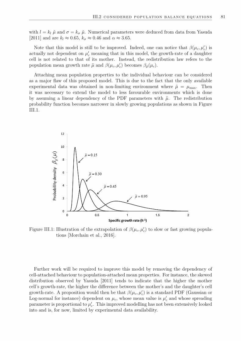
III.2 considered population balance equations 81
with l = kl µ and σ = kσ µ. Numerical parameters were deduced from data from Yasuda[2011] and are kl ≈ 0.65, kσ ≈ 0.46 and α ≈ 3.65.
Note that this model is still to be improved. Indeed, one can notice that β(µc, µ′c) isactually not dependent on µ′c meaning that in this model, the growth-rate of a daughtercell is not related to that of its mother. Instead, the redistribution law refers to thepopulation mean growth rate µ and β(µc, µ′c) becomes βµ(µc).
Attaching mean population properties to the individual behaviour can be consideredas a major flaw of this proposed model. This is due to the fact that the only availableexperimental data was obtained in non-limiting environment where µ = µmax. Thenit was necessary to extend the model to less favourable environments which is doneby assuming a linear dependency of the PDF parameters with µ. The redistributionprobability function becomes narrower in slowly growing populations as shown in FigureIII.1.
Figure III.1: Illustration of the extrapolation of β(µc, µ′c) to slow or fast growing popula-tions [Morchain et al., 2016].
Further work will be required to improve this model by removing the dependency ofcell-attached behaviour to population-attached mean properties. For instance, the skeweddistribution observed by Yasuda [2011] tends to indicate that the higher the mothercell’s growth-rate, the higher the difference between the mother’s and the daughter’s cellgrowth-rate. A proposition would then be that β(µc, µ′c) is a standard PDF (Gaussian orLog-normal for instance) dependent on µc, whose mean value is µ′c and whose spreadingparameter is proportional to µ′c. This improved modelling has not been extensively lookedinto and is, for now, limited by experimental data availability.

82 population balances for biological systems
III.2.2 Modelling S. cerevisiae dynamics
Biological properties
As detailed previously in Chapter II, we model the metabolic behaviour of S. cerevisiaeby considering five dynamic biological properties attached to each cell:
• µ(b)G : maximum rate of glucose-based growth in non-limiting aerobic environment
(gX/gX · h).
• µ(b)E : maximum rate of ethanol-based growth in non-limiting environment (gX/gX · h).
• µ(b)A : maximum rate of acetate-based growth in non-limiting environment (gX/gX · h).
• ϕ(b)O : maximum oxygen consumption rate (gO/gX · h).
• σ: cell glycolytic stress (no unit, normalized between 0 and 1).
The three maximum growth rates and the maximum oxygen consumption rate areproperties that slowly change over time in order to reach values of equilibrium with theenvironment:
∂µ(b)G,E,A
∂t= ζµG,E,A = 1
TµG,E,A
(µ∗G,E,A − µG,E,A
)(III.9)
∂ϕ(b)O
∂t= ζϕO = 1
TϕO
(ϕ∗O − ϕ
(b)O
)(III.10)
where star values are population mean rates that are experimentally observed in a steadyenvironment. Time constants TµG,µE ,µA,ϕO have an order or magnitude of an hour.
The stress σ is a variable which keeps track of whether a cell has been exposed to highglucose concentrations recently. If not, σ ≈ 0 which will imply in the metabolic modelthat the short-term Crabtree effect is not active. If the cell has indeed been recentlyexposed to high glucose concentrations (stressing environment), σ ≈ 1 and the short-term Crabtree effect is triggered. Therefore, the evolution of this variable is described bytwo mutually exclusive terms:
∂σ
∂t= ζσ = κσ
T(u)σ
(1− σ)− (1− κσ)T
(d)σ
σ (III.11)
where κσ ∈ [0, 1] qualifies the stressfulness of the environment, T (u)σ is the time constant
of stress increase in stressful environments (≈ 1s) and T (d)σ is the characteristic time for
a return to unstressed metabolic behaviour (≈ 100s).Closures for µ∗G,E,A and ϕ∗O were defined in Chapter II and are based on the vector of
liquid-phase concentrations CL = [CG, CE, CA, CO]. κσ computation also relies on CL
but also on the value of µG.
Population Balance Equation
In order to track these properties and their respective evolution, not at a cell-scale, butat the population scale, a multivariate population balance model can be formulated. Letp = [µ(b)
G , µ(b)E , µ
(b)A , ϕ
(b)O , σ] be the vector of biological properties of a cell, and n(p) the

III.3 applying sectional and moment methods to E. coli PBE 83
Number Density Function which represents the statistical distribution of these propertiesover the biological population. A Population Balance Equation tracking the evolution ofn(p) is
∂n(p)∂t
+∑
i∈G,E,A
(∂
∂µ(b)i
(n(p)ζµi(p,CL)))
+ ∂
∂ϕ(b)O
(n(p)ζϕO(p,CL)
+ ∂
∂σ(n(p)ζσ(p,CL) =
∫Ωpµ(a)(p′,CL)n(p′)β(p, p′)dp′ (III.12)
or, more simply by defining ζ = [ζµG , ζµE , ζµA , , ζϕO , ζσ]T :
∂n(p)∂t
+ ∇ ·(ζ(p,CL)n(p)
)=∫
Ωpµ(a)(p′,CL)n(p′)β(p, p′)dp′ (III.13)
Redistribution term
The RHS of (III.12) is analogous to the RHS of (III.3) and represents the distributionof biological properties when new cell are formed. We did not attempt to provide a finedescription for this term as the difficulty of finding relevant experimental data observedfor E. coli is worsened by the multi-dimensionality of the current S. cerevisiae modelling.
Therefore we applied an inheritance assumption by making daughter cells identical totheir mother. This is modelled by defining the transition distribution β(p, p′) as a 5DDirac distribution:∫
Ωpf(p′)β(p, p′)dp′ = f(p) (III.14)
which yields∫Ωpµ(a)(p′,CL)n(p′)β(p, p′)dp′ = µ(a)(p,CL)n(p) (III.15)
III.3 Applying sectional and moment methods to E. coli PBE
As stated previously, Population Balance Equations have a structure that is not directlycompatible with mass balance equations in Eulerian modelling framework. To allowcompatibility between the Population Balance Model framework with simulation softwarebased on local mass balances, both sectional and moment methods can be applied toreplace the PBE by a set of local mass balance equations.
Here, the focus is made on applying these methods on one-dimensional PBEs. Methodsfor higher order PBEs were not investigated in this PhD and are being tackled in an otherongoing project. Therefore, following sections illustrate the use of both sectional andmoment methods on the 1D PBE associated to the modelling of E. coli (see Eq. (III.3)).This PBE is here recalled with an explicit convection term:
∂n(µc)∂t
+~∇·(~uLn(µc))+ ∂
∂µc(n(µc)ζµ(µc,CL)) =
∫Ωµµ(µ′c,CL)n(µ′c)β(µc, µ′c)dµ′c (III.16)

84 population balances for biological systems
III.3.1 Sectional methods
Sectional methods, also referred to as class methods or pivot methods, consist in a dis-cretization of the support of a continuous NDF.
In the considered case of the PBE describing the evolution of the growth-rate of E. coli,the considered support is µc ∈ [0, µlim[ where µlim is the maximum growth-rate achievableby a single cell. µlim must not be confused with the maximum growth-rate µmax as seenin the Monod kinetic law (see Eq. (III.4)). µmax is the maximum growth-rate that canbe observed at the population scale. This value is only a mean value, meaning that thereexists cells that grow at a higher rate than µmax. Experimental results have indeed shownthat at the cell-scale, some cells grow and divide at a higher rate indeed, hence µlim > µmax.In the proposed model, such individuals whose growth rate is higher than µmax appearthank to the modelling of the cell-division redistribution function β(µc, µ′c) which cantheoretically generate cells with infinitely high growth-rate but with low probability. Weset µlim = 2.2µmax considering that the probability to generate individuals such thatµc > 2.2µlim is negligible (< 0.07%).
We considered the simplest of sectional methods consistent with the bounded support,that is the fixed pivot method using regular grid [Kumar and Ramkrishna, 1996a]. In thisapproach, the support Ωµ = [0, µlim[ is discretized into Nclass intervals of same lengths.Bounds of the i-th interval, or class, are defined as
µi−1/2 = (i− 1) µlim
Nclass
µi+1/2 = iµlim
Nclass
with i ∈ 1, . . . ,Nclass. All cells whose property lies within the bounds of the i-th class,for which µc ∈ [µi−1/2, µi+1/2[, are assumed to share the same property µi defined as themean class property:
µi = (i− 1/2) µlim
Nclass
An illustration of this discretization is given in Fig. III.2 for Nclass = 10.
µ1/2 µ3/2 µ5/2 µ7/2 µ9/2 µ11/2 µ13/2 µ15/2 µ17/2 µ19/2 µ21/2
0 µlim
µ1 µ2 µ3 µ4 µ5 µ6 µ7 µ8 µ9 µ10
Figure III.2: Example of NDF support discretization in regular grid fixed pivot technique.
Let Ni be the amount of cells in the i-th class (kgX/m3L). The mass balance equation
on Ni is obtained by integrating Eq. (III.16) over [µi−1/2, µi+1/2[ which leads to
∂Ni
∂t+ ~∇·(~uLNi) = − [n(µc)ζµ(µc,CL)]µi+1/2
µi−1/2+Nclass∑j=1
(µ(µj,CL)Nj
∫ µi+1/2
µi−1/2
β(µc, µj)dµc)
(III.17)

III.3 applying sectional and moment methods to E. coli PBE 85
The first term on the RHS is the net flux of cell moving between adjacent classes due togrowth-rate adaptation. The second term on the RHS is the rate of production of new cellswhose growth-rate is located in the i-th interval. This second term is already closed andonly requires the analytical or numerical (pre)computation of integrals
∫ µi+1/2µi−1/2
β(µc, µj)dµcfor each pair of classes.
The first term is not directly accessible from N = [N1, . . . , NNclass ]T as is requires theknowledge of the values n(µc) not at the pivot locations µi, but at the interval boundariesµi±1/2. The following transport scheme was then used by Morchain et al. [2013] as it allowspreserving the positivity of N elements [Kumar and Ramkrishna, 1997]:
− [n(µc)ζµ(µc,CL)]µi+1/2µi−1/2
≈ 1∆µ
[Ni−1ζ
uµ(µi−1,CL) +Ni+1ζ
dµ(µi+1,CL)−Ni|ζµ(µi,CL)|
](III.18)
where
ζuµ(µc,CL) =ζµ(µc,CL) if µc < µ∗(CL)
0 otherwise
ζdµ(µc,CL) =−ζµ(µc,CL) if µc > µ∗(CL)
0 otherwise
This first scheme is applicable here because all cells move toward the same µ∗(CL) value.The fixed pivot method lies in the family of finite volume methods to solve partial
derivative equations. It is then also possible to apply the well-known Rusanov schemewhich is suited for transport terms in finite-volume approaches and ensures an accurate,conservative and non-oscillatory solution1.
Under that formalism, the computation of bioreaction rates over the population is givenby a sum over all classes:
R(N ,CL) =Nclass∑i=1
Nir(µi,CL) (III.19)
III.3.2 Methods of moments
Methods of moments do not track directly local values of the NDF but resolve a finiteset of its moments mN = [m0,m1, . . . ,mN ]T with
mk =∫
Ωµµkcn(µc)dµc (III.20)
While defining a cut-off value µlim was required for the sectional method, this is notrequired any more for moment methods, therefore Ωµ = [0,+∞[.
1 The application of Rusanov scheme for the closure of mass-balance equations when applying the sectionalmethod was suggested by Dr. Bastien POLIZZI.

86 population balances for biological systems
Multiplying each term of Eq. (III.16) by µkc , k ∈ 0, . . . , N and integrating over Ωµ
yields
∂m0
∂t+~∇· (~uLm0) =
∫Ωµµ(µ′c,CL)n(µ′c)β(µc, µ′c)dµ′c (III.21)
∂mk
∂t+~∇· (~uLmk) = k
∫Ωµµk−1c n(µc)ζµ(µc,CL)dµc+∫∫
Ωµµkcµ(µ′c,CL)n(µ′c)β(µc, µ′c)dµ′cdµc (III.22)
The total amount of cells m0 is not affected by the adaptation of growth-rate, but only bythe total number of newly created cells (RHS of Eq (III.21)). Both the adaptation andthe formation of new cells will affect higher order moments, and therefore the shape ofthe growth-rate distribution. The first term on the RHS of Eq. (III.22) can be expressedin terms of moments if one considers the model for ζµ(µc,CL) given in Eq. (III.5):
∫Ωµµk−1c n(µc)ζµ(µc,CL)dµc = µ∗(CL)
Tmk−1 +
(µ∗(CL)− 1
T
)mk −mk+1 (III.23)
Note however that this closure is not possible if T depends on µc and C. This was thecase in the modelling from Pigou and Morchain [2015] where two different characteristictimes Tu and Td are used as explained previously (see Section III.2.1).
For the modelling of bioreactors, one should expect unclosed integral terms when meth-ods of moments are applied. For the currently considered PBE, these unclosed terms aremainly related to the fact that biological reaction rates cannot be directly expressed interms of moments of n(µc). This is the case for the cell-division integral terms in momentequations (see Eqs. (III.21) and (III.22)), but also for the reaction rates in dissolvedspecies mass balance equations
R(n,CL) =∫
Ωµn(µc)r(µc,CL)dµc (III.24)
which cannot be expressed directly in terms of moments of the distribution n(µc), atleast because, under the formalism proposed in Chapter II, elements of r(µc,CL) are notcontinuously differentiable with respect to µc.
III.4 Numerical methods providing closure for moment formula-tions
As shown previously, moment equations do not form a closed system for the consideredcase of bioreactors modelling. Numerous integral terms appear in this formulation, andtheir closure requires the knowledge of the raw distribution n(µc), which is not accessiblefrom only a finite set of its moments. Therefore, a numerical method is required toprovide closure by approximating integral properties of the distribution when only fewmoments of that distribution are known.
III.4 numerical methods providing closure for moment formulations 87
Multiple numerical methods exist to tackle this issue. All of these methods propose anapproximation n(µc) of n(µc) as well as a quadrature rule such that
∫Ωµf(µc)n(µc)dµc ≈
Nnode∑i=1
wif(ξi) (III.25)
where wi are the weights of the quadrature, ξi its nodes, and Nnode the number of quadra-ture nodes. These weights and nodes are computed from moments mN = [m0, . . . ,mN ]Tof n(µc) in such a way that the quadrature rule (Eq. (III.25)) correctly reproduces thesemoments, i.e. yields exact results if f(µc) = µkc , k ∈ 0, . . . , N.
John et al. [2007] and Lebaz et al. [2016] assessed multiple moment-based closuremethods and noticed that the following ones were either inaccurate or unstable for theirrespective test-cases:
• The Kernel Density Element Method [Athanassoulis and Gavriliadis, 2002]
• The Spline Method [John et al., 2007]
For these reasons, these two methods were not furthermore considered for the simulationof bioreactors. Hereafter are detailed other existing methods that have been consideredduring this work to hopefully provide low-cost, stable and accurate closures. Thesemethods will be compared in section III.5 to the class method.
III.4.1 Quadrature Method Of Moments
The Quadrature Method of Moments was first proposed by McGraw [1997] to provideclosure in moment-evolution equations in the modelling of aerosol size distributions. Itis derived from the theory of orthogonal polynomial [Chihara, 1978] which serves as abasis for Gauss-quadratures whose main purpose is to provide approximations of integralterms in general.
Using an even number 2P of moments, Quadrature Method of Moments (QMOM)yields a P nodes quadratures. Its weights wP and nodes ξP are obtained by computingeigenvalues and normalized eigenvectors of a P × P tridiagonal symmetric matrix whoseelements are deduced from m2P−1. Exact details of this computation are given in SectionIII.6.
In a sense, one can consider that QMOM yields an approximation of n(µc) defined by
n(µc) =P∑i=1
wiδ(µc, ξi) (III.26)
where δ is the Dirac delta distribution defined in Eq. (III.7).This approximation is discontinuous whereas n(µc) is expected to be a continuous
distribution. Therefore, QMOM cannot be used to estimate point-wise values of n(µc)and must be restricted to situations where only integral properties are required. Whenapplying QMOM, the generic quadrature rule from Eq. (III.25) becomes
∫Ωµf(µc)n(µc)dµc ≈
P∑i=1
wif(ξi) (III.27)

88 population balances for biological systems
III.4.2 Extended Quadrature Method of Moments
[Yuan et al., 2012] introduced the EQMOM as a generalisation of bi-Gaussian approxi-mations of NDFs proposed by Chalons et al. [2010]. EQMOM approximates a NDF as aconvex mixture of Kernel Density Functions (KDFs) of the same parametric family:
n(µc) =P∑i=1
wiκ(µc, ξi, σ) (III.28)
where κ(µ, ξ, σ) is a probability density function, referred to as the EQMOM kernel, whoselocation parameter is ξ and shape parameter is σ. Over the past few years, multiplekernels were found to be compatible with the method:
• Gaussian kernel [Chalons et al., 2010; Marchisio and Fox, 2013];
κG(µ, ξ, σ) = 1σ√
2πexp
(−(µ− ξ)2
2σ2
)(III.29)
• Laplace kernel [Pigou et al., 2018a]
κλ(µ, ξ, σ) = 12σ exp
(−|µ− ξ|
σ
)(III.30)
• Log-Normal kernel [Madadi-Kandjani and Passalacqua, 2015]:
κL(µ, ξ, σ) = 1σµ√
2πexp
(−(log(µ)− log(ξ))2
2σ2
)(III.31)
• Gamma kernel [Yuan et al., 2012]:
κΓ(µ, ξ, σ) = µ(l−1) exp(−µ/σ)Γ(l)σl with l = ξ
σand Γ(x) =
∫ +∞
0tx−1e−tdt (III.32)
• Weibull kernel [Pigou et al., 2018a]:
κW (µ, ξ, σ) = 1σξ
(µ
ξ
) 1−σσ
exp−(µ
ξ
)1/σ (III.33)
• Beta kernel [Yuan et al., 2012]:
κβ(µ, ξ, σ) = µ(l−1)(1− µ)(m−1)
B(l,m) with l = ξ
σ,m = 1− ξ
σ
and B(l,m) =∫ 1
0x(l−1)(1 − x)(m−1)dx (III.34)
The core of this method is the moment-inversion procedure which is an iterative processwhose goal is to identify values of the weights wP , nodes ξP and shape parameter σ froman odd number of moments 2P + 1. This procedure was first developed by Yuan et al.

III.4 numerical methods providing closure for moment formulations 89
[2012] and has been further improved by Nguyen et al. [2016]. An even more efficientmoment-inversion procedure has been identified during the course of this work and isdetailed in section III.6.
For all kernels, it is possible to establish a quadrature rule such that
∫Ωµf(µ)κ(µ, ξ, σ)dµ ≈
Q∑j=1
ωj(ξ, σ)f(λj(ξ, σ)) (III.35)
with ωQ(ξ, σ) = [ω1(ξ, σ), . . . , ω(ξ, σ)Q] and λQ(ξ, σ) = [λ1(ξ, σ), . . . , λQ(ξ, σ)] the weightsand nodes of this Q-nodes quadrature rule. Therefore, when using EQMOM, integralterms over the population n(µc) can be approximated by
∫Ωµf(µc)n(µc)dµ ≈
P∑i=1
Q∑j=1
wiωj(ξi, σ)f (λj(ξi, σ)) (III.36)
More importantly, EQMOM yields a continuous approximation of n(µc) from its momentswhich allows approximating point-wise values of this distribution. This is not possiblewith QMOM which only yields discrete distributions.
III.4.3 Maximum-Entropy Method
The Maximum-Entropy method was assessed by Lebaz et al. [2016] and favorably selectedwhen compared to Kernel Density Element Method (KDEM) and Spline Methods for themodelling of a depolymerization process. This method was introduced by Mead andPapanicolaou [1984] and has been further improved by Tagliani [1999, 2001]. Its coreidea is to select, between all NDFs whose first moments are given by mN , the one whoseShannon entropy is the highest.
The Shannon entropy of a NDF p(x) defined on Ωx = [0, 1] is defined as
H[p] = −∫ 1
0p(x) log p(x)dx (III.37)
and is a measure of the amount of information required to define p(x).Solving the Moment Maximum-Entropy problem requires identifying the NDF p(x) of
highest Shannon Entropy under the constraints∫ 1
0xkp(x)dx = m′k k ∈ 0, . . . , N,m′0 = 1 (III.38)
with m′N moments of p(x).Mead and Papanicolaou [1984] and Tagliani [1999] show that the solution to this prob-
lem is a NDF whose expression takes the following form:
p(x) = exp(−
N∑i=0
λixi
)(III.39)
which is the exponential of a polynomial function. The core procedure of the Maximum-Entropy approach then lies in the identification of polynomial coefficients λN = [λ0, . . . , λN ].

90 population balances for biological systems
It is shown that the researched λN values minimize the convex function Γ(λN) definedas [Mead and Papanicolaou, 1984]
Γ(λN) =N∑i=1
λim′i + log
(∫ 1
0exp
(−
N∑i=1
λixi
)dx)
(III.40)
and whose Jacobian and Hessian matrices are easily expressed in terms of the followingintegrals [Abramov, 2007]
m′k =∫ 1
0xk exp
(−
N∑i=0
λixi
)dx k ∈ 0, . . . , 2N (III.41)
Finding the Maximum Entropy reconstruction from a moment set mN is then equiva-lent to finding the minimum of Γ(λN). This is feasible by applying the Newton-Raphsoniterative procedure to identify the root of the Jacobian matrix of this function. Notehowever that each iteration of this procedure requires 2N numerical integrations (seeEq. (III.41)) and that the accuracy and stability of the method depends on the accuracyof these numerical integrations. Vie et al. [2013] then suggested the use of an adaptivequadrature rule. The basics of this adaptive quadrature is to split the interval [0, 1] intomultiple sub-intervals depending on the values of intermediary reconstructions, and thenuse a Gauss-Legendre quadrature on each on these sub-intervals.
Hitherto, the method has only been presented for a NDF p(x) defined on Ωx = [0, 1].We must then transform our problem of reconstructing the NDF n(µc) on Ωµ = [0, µlim]to reach the expected formalism. This is done by a simple variable change
p(x) = n(x ∗ µlim) (III.42)
which implies the following relation between moments mN of n(µc) and moments m′N ofp(x):
m′k = µ−(k+1)lim
k∑i=0
k!i!(k − i)!mk−j (III.43)
Among methods compared in this work (QMOM, EQMOM and ME), the MaximumEntropy approach can be seen as the most –mathematically speaking– elegant. Its coreprinciple is to “extract” as much information as possible from the known moments, anddoes not requires any hypothesis about an expected shape of the raw NDF.
III.5 Comparison of numerical methods
As detailed in an article published before the current PhD work [Pigou and Morchain,2015], we performed simulations of a large-scale bioreactor, using the model for E. coliwhich inspired the formulation of metabolic models proposed in Chapter II, the Popu-lation Balance Model presented previously (see Section III.2.1), and the CompartmentModel from Vrabel et al. [1999]. These simulations relied on the use of the class methodto solve the Population Balance Equation.
Accuracy was obtained through the use of 100 classes while 80 of them containedvirtually no cell. This is a usual drawback of sectional methods which implies that most

III.5 comparison of numerical methods 91
of the memory allocated to the tracking of the biological-population state holds no usefulinformation. This explains why we considered the use of methods of moments, in orderto make a better use of allocated memory. Less tracked variables implies both less usedmemory, and also less mass balance equations to be solved, which can be of significantinterest in particular when the biological modelling (metabolic model coupled with thePBM) is embedded in Computational Fluid Dynamics (CFD) simulations.
These gains expected from a switch toward methods of moments come with the neces-sity to use quadrature methods as presented previously. This implies an expected loss ofaccuracy difficult to estimate a priori. Therefore, estimating the accuracy of quadraturemethods compared to the class method is a prerequisite to their use in large-scale simula-tions. As far as the class method is concerned, increasing the number of classes to assessthe sensibility of results to that number, and to tightly control the method accuracy, isstraightforward.
An other key element of comparison is the numerical cost associated to each method. Asalready stated, the class method requires solving coupled mass balance equations over allclasses, as well as one call to the metabolic model for each class that holds non negligiblequantity of micro-organisms. Moreover, the discretization of the biological propertiesspace induces a stringent constraint on the simulation time-step analogous to the Courant-Friedrichs-Lewy (CFL) condition, well known to CFD-software users [Courant et al., 1928].On the other side, each quadrature method presented in section III.4 comes with differentnumerical costs related to
• varying number of resolved moments;
• the computation of the quadrature rule;
• a varying number of calls to the metabolic model depending on the size of theproduced quadrature rule.
Finally, stability will also be a concern. For the class method, stability is ensuredby using low-order transport schemes as detailed previously (see III.3.1). Stability ismore difficult to achieve for methods of moments where time-integration can producenon-realisable moment sets, i.e. vector of moments that cannot be associated to any well-defined NDF [Vikas et al., 2011], or if a quadrature method fails to produce an accuratequadrature rule.
Over the course of this work, a strong focus has been made on comparing the classmethod with all three considered quadrature methods (QMOM, EQMOM and the Max-imum entropy approach latter referred to as MaxEnt) on each of these aspects: memoryuse, numerical cost and stability. This is detailed hereafter by first explaining the com-parison methodology and then the observed results. Full details of this comparison canbe found in Pigou et al. [2017].
III.5.1 Comparison methodology
In order to assess methods of moment against the class method, two biological cultureshave been simulated. They are both shortly described hereafter and have been fullydetailed in Pigou et al. [2017].
The first simulation set-up allowed assessing the stability of all methods for the simu-lation of a stressed homogeneous system, and to measure the dependency of results onthe number of resolved moments.
92 population balances for biological systems
The second simulation set-up is that of a large-scale fedbatch culture already simulatedin Pigou and Morchain [2015] using the class method and whose results are reproducedusing moment methods. This allows to assess the accuracy and stability of these methodsin heterogeneous systems.
Stressed chemostat culture
The first simulation case corresponds to experimental results shown previously in ChapterII, Fig. II.5, from Katterer et al. [1986]. It is a chemostat culture started with a dilutionrate D = 0.10h−1 which is suddenly shifted toward a higher dilution rate D′ = 0.42h−1.In this set-up, the bioreactor can be considered as homogeneous, and the biological popu-lation only experiences a single environmental perturbation. This allows for a comparisonof methods in a tightly controlled set-up. The time integration was performed by a first-order explicit Euler method with a fixed time-step, shared by all methods, chosen so thatall results are independent from that time-step.
In order for these simulations to quantitatively compare against experimental resultsfrom Katterer et al. [1986], constants of the E. coli metabolic model from Pigou andMorchain [2015] have been changed to match the conversion yields of Candida tropicalis.
Large-scale fedbatch culture
Vrabel et al. [2001] performed simulations of a large-scale (22m3) fedbatch culture of E.coli using the metabolic model from Xu et al. [1999] and the hydrodynamic CompartmentModel Approach developed by Vrabel et al. [1999]. We reproduced these simulations asdetailed in Pigou and Morchain [2015] by integrating the Population Balance Model forthe dynamic adaptation of E. coli growth-rate as detailed previously (see III.2.1) using theclass method to solve the PBE. Please refer to Pigou and Morchain [2015]; Pigou et al.[2017] for a full presentation of the hydrodynamic modelling by Compartment ModelApproach (CMA).
We reproduced these simulations by using moment methods (QMOM, EQMOM andMaxEnt) with a number of moment based on results from the simulation of the stressedchemostat culture.
III.5.2 Comparison results
Stressed chemostat cuture
Fig. III.3 sums-up simulation results for biomass and glucose concentrations for eachmethod and different orders of resolution. The first observation is that all methodsmanage to correctly reproduce the overall dynamics of the system. This dynamics ismainly related to the accuracy of the PBE treatment which describes the growth-ratedynamic evolution (see Eq. (III.16)). In particular, the moment equation (Eq. (III.22))of the last resolved moment mN−1 requires the knowledge of the unknown moment mN .The predicted dynamics will then depend on the approximation of this unknown momentfrom the quadrature rule yield by each method. An analysis conducted on this aspecthas shown that all methods and order correctly predicted this unknown moment withless than 0.2% of relative error. This implies that all moment method correctly predictthe dynamics indeed.

III.5 comparison of numerical methods 93
25 30 35 40 45
t (h)
4
5
6
7
Biomass
(gX/L)
0
1
2
3
Glucose
(gG/L)
(a) Class method
100 classes
400 classes
25 30 35 40 45
t (h)
4
5
6
7
Biomass
(gX/L)
0
1
2
3
Glucose
(gG/L)
(b) QMOM method
N=4
N=6
N=8
N=10
25 30 35 40 45
t (h)
4
5
6
7
Biomass
(gX/L)
0
1
2
3
Glucose
(gG/L)
(c) Gaussian EQMOM method
N=3
N=5
N=7
25 30 35 40 45
t (h)
4
5
6
7
Biomass
(gX/L)
0
1
2
3
Glucose
(gG/L)
(d) MaxEnt method
N=3
N=5
N=6
N=7
Figure III.3: Comparison of experimental data from Katterer et al. [1986] against simula-tion results from each method. For methods of moments, N is the numberof resolved moments.
Clearly, all methods yield accurate approximate of unknown moment. A more sensi-tive variable will be the acetate production. As stated in Chapter II, Section II.3, themetabolic model for E. coli predicts that cells whose growth-rate µc is lower than theequilibrium growth rate µ∗ will produce acetate through the overflow metabolism. Here,we reused this model by only changing some conversion yields to fit experimental data interms of glucose and biomass concentration (see Fig. III.3) but this overflow metabolismis still enabled. Since acetate production is closely related to the shape of the distribu-tion n(µc), the acetate concentration should be sensitive to methods order and accuracy.Predicted evolutions of these concentrations are given in Fig. III.4.
Let AM(t) be the evolution of acetate concentration as predicted by moment methods,and AC(t) the same evolution as predicted by the class method with 400 classes. Fig.III.5 summarizes the error between moment methods against the class method with
ε =∫ tft0 |AM(t)− AC(t)|dt∫ tf
t0 AC(t)dt(III.44)
with t0 = 25h and tf = 45h. This figure shows that in terms of accuracy, MaxEntis the more accurate method, even with as low as 3 moments, for the prediction ofacetate production in this stressed chemostat culture. EQMOM and MaxEnt share similaraccuracy as soon as 5 moments are tracked. Finally, QMOM requires twice as manymoments as other methods to reach a similar accuracy of 5%.
While performing these simulations, we noticed stability issues with MaxEnt as soon as7 moments were used. Stability could still be maintained at the cost of extra operations asdetailed in Pigou et al. [2017] but no more than 7 moments could be tracked. In terms of

94 population balances for biological systems
0 20 40
0
1
2
3
4
N=4
N=6
N=8
N=10
0 20 40
0
1
2
3
4
N=3
N=5
N=7
0 20 40
0
1
2
3
4
N=3
N=5
N=6
N=7
Figure III.4: Evolution of acetate concentrations as predicted by each moment method.Black dash-dotted line: results from class method using 400 classes.
0.0%
2.0%
4.0%
6.0%
8.0%
10.0%
12.0%
3 4 5 6 7 8 9 10
Re
lati
ve e
rro
r ε
N
QMOM
EQMOM
MaxEnt
Figure III.5: Relative error on acetate concentration predictions for all methods and or-ders. The 400 classes method serves as a reference.
numerical costs, Fig. III.6 details the run-time associated with each method. The QMOMmethod appears twice in this figure because two different algorithms were tested to per-form the quadrature computation (PDA: Product Difference Algorithm, WA: WheelerAlgorithm, also referred to as Chebyshev Algorithm is Section III.6). The “Blank” mea-surement corresponds to simulations were reaction terms were not computed in order toisolate bioreaction and population balance related computations from other tasks per-formed by the simulation software. A complete analysis of these run-times is provided inPigou et al. [2017], main observations are:
• Overall, all method have a similar order of magnitude in term of associated run-timeeven though this numerical cost has different sources for each method.
• The cost associated to the class method mainly comes from calling the metabolicmodel for each class, as well as computing the redistribution term by integrating askew-normal distribution over each class (see Eq. (III.8)).

III.5 comparison of numerical methods 95
Bla
nk
Cla
ss 1
00
Cla
ss 4
00
QM
OM
4 P
DA
QM
OM
6 P
DA
QM
OM
8 P
DA
QM
OM
10 P
DA
QM
OM
4 W
A
QM
OM
6 W
A
QM
OM
8 W
A
QM
OM
10 W
AEQ
MO
M 3
EQ
MO
M 5
EQ
MO
M 7
ME 3
ME 4
ME 5
ME 7
0
0.5
1
1.5
2
2.5
3
3.5
Ru
nti
me
(ms/
tim
este
p)
Figure III.6: Mean run-time per time-step for each tested method and order (ms/ts) (±standard-deviation measured on 20 simulations).
• The iterative process underlying the MaxEnt approach often converges in a single it-eration, but this increases up to 10 iteration by time-step right after the dilution-rateshift-up. Simulating the next few hours following this shift significantly increasesthe mean observed run-time for this method, but it should be quite fast if used insystems with minor perturbations.
• QMOM has a computational cost hardly dependent on the method order and is thefastest method as it yield the lower number of quadrature nodes.
• Analytical solutions were used for 3 and 5 moments with EQMOM which explainsthe significant increase in numerical cost for N = 7.
One surprising aspect in this comparison of run-time is the low difference between the classmethod and QMOM. One would expect a significantly lower cost for QMOM compared tothe class method which is not visible here. This observation has been latter linked to theuse of a simulation software based on Oriented Object Programming in MATLAB [2016]which happened to be badly optimized. The transfer of data between the time integrationroutine and modelling blocks (code for quadrature computations, for metabolic modelcomputations, ...) significantly slowed down the simulations. Therefore, all previouscomparisons only have a qualitative value but not a quantitative one. A better approachwould have been to compare the number of required Floating-Point Operations per time-step but this is a less accessible metrics. The key element of comparison will then bestability and accuracy of quadrature methods.
Large-scale fedbatch culture
Initial simulations of a homogeneous system led to the selection of EQMOM and MaxEntwith N = 5 as well as QMOM with N = 10 to perform simulations of a 22m3 heteroge-neous fedbatch culture. Figure III.7 details the volumetric means of glucose, biomass andacetate concentrations, as well as local acetate production/consumption rates, at threedifferent heights referred to as top, middle and bottom. Once again, all moment methods

96 population balances for biological systems
0 10 20 30 40
Time (h)
0
0.05
0.1
0.15
0.2
CG(g
G.L
−1)
(a)
0 10 20 30 40
Time (h)
0
5
10
15
20
25
30
35
40
XTotal(g
X.L
−1)
(b)
0 10 20 30 40
Time (h)
0
0.1
0.2
0.3
0.4
CA(g
A.L
−1)
(c)
0 10 20 30 40
Time (h)
-0.1
-0.05
0
0.05
0.1
0.15
0.2
0.25
0.3
r A(g
A.g
−1
X.h
−1)
(d)
Class (100)
MaxEnt (N=5)
QMOM (N=10)
EQMOM (N=5)
〈·〉top
〈·〉middle
〈·〉bottom
Figure III.7: Simulation results for the different population balance methods in the het-erogeneous fedbatch culture. (a) Glucose concentration, (b) Total biomassconcentration, (c) Acetate concentration and (d) Acetate specific productionrate.

III.5 comparison of numerical methods 97
Bla
nk
Cla
ss 1
00
Cla
ss 2
00
Cla
ss 4
00
QM
OM
4Q
MO
M 6
QM
OM
8Q
MO
M 1
0EQ
MO
M 3
EQ
MO
M 5
EQ
MO
M 7
ME 3
ME 4
ME 5
0
5
10
15
20
25
30
Ru
nti
me
(ms/
tim
este
p)
Figure III.8: Mean run-time per time-step for each method (ms/time-step ± standarddeviation measured on 5 simulations per method and order).
closely match the results obtained with the class method. This confirms that 5 momentsare sufficient to account for biological heterogeneity with the proposed modelling.
In terms of stability and numerical cost, Fig. III.8 is similar to Fig. III.6 by showingrun-times per time-step for each method. The analysis of these run-times is similar tothe homogeneous chemostat with the only noticeable change being that the Maximumentropy approach could not be tested with more than 5 moments due to stability issues,and its numerical cost is here significantly higher than that of QMOM and analyticalEQMOM.
III.5.3 Conclusion
Overall, all tested quadrature methods gave satisfactory accuracy compared to the classmethod, but required significantly less resolved variables. In terms of tracked moments,EQMOM and MaxEnt make a better use of the information embedded within the firstfew integer moments than QMOM which leads to a good accuracy with as few as 3 to 5moments. Meanwhile, QMOM required twice as much moments as the other methods toreach similar accuracy. Little time after these developments were published [Pigou et al.,2017], an other group performed a similar analysis by comparing QMOM, MaxEnt and apolynomial closure method [Muller et al., 2017]. They observed too the lack of accuracyof QMOM at equivalent number of resolved moments compared to other methods.
A key observation was the lack of stability related to the Maximum Entropy approach.This had already been observed by Vie et al. [2013] and has been confirmed to be a majordrawback of this method for simulations of large-scale bioreactors. Therefore, MaxEnthas been discarded from future use in this context.
QMOM and EQMOM shared similar computational costs, but EQMOM required lessresolved moments. This implies lower cost for the resolution of coupled mass-balanceequations, especially if the PBM is used within a CFD framework, but this also improvesthe simulation stability. Indeed, the resolution of high order moment sets may lead moreeasily to the appearance of unrealisable moment sets which would constitute a strong

98 population balances for biological systems
source of instability. Therefore, EQMOM seems to be the most relevant choice for theresolution of Population Balance Equations in the context of large-scale bioreactors.
III.6 Improving the Extended Quadrature Method of Moments
III.6.1 Developments background
While performing simulations presented previously when comparing methods to solvePBEs, all variants of EQMOM were tested even though only results based on Gauss-EQMOM have been presented. This is due to instabilities that have been observed forthe Log-normal, Gamma and Beta variations. These instabilities led to failures in thequadrature computation when these kernels were used for the EQMOM moment-inversionprocedure, only the Gauss kernel did not fail.
Using a mixture of Gaussian kernels –defined on R– to approximate a NDF definedon Ωµ = [0, µlim] or Ωµ = [0,+∞[ obviously presents an intrinsic weakness, and actuallyled to the appearance of some quadrature nodes with negative growth-rate in resultspresented previously (see III.5.2). This was corrected by truncating and renormalizing theapproximated NDF over Ωµ for the integration of bioreaction rates over the population,this approach was however unsatisfactory.
Results from Pigou et al. [2017] show that 5 moments are sufficient for accurate simu-lations of large-scale bioreactors when EQMOM is used to provide closure. Consequently,an attempted approach to prevent instabilities was to develop analytical solutions for2-nodes EQMOM reconstructions for other kernels. Such an analytical solution was onlydescribed for the Gauss kernel by Chalons et al. [2010] and supplementary analyticalsolutions have been identified for Gamma, Laplace and Log-normal kernels. The iden-tification of Laplace and Weibull distributions as kernels compatible with the EQMOMmethod happened simultaneously with these analytical solution developments.
Unfortunately, using analytical solutions for the Log-normal and Gamma kernels didnot provide an efficient response to the previously observed stability issues. The explana-tion for this came from Nguyen et al. [2016]: the EQMOM reconstruction may happennot to be defined, it may be possible that the last moment may not be conserved by anEQMOM approximation. Nguyen et al. [2016] then proposed a new EQMOM moment-inversion procedure which
• is more stable than previous ones by adding a realisability check at each iterationof the procedure;
• makes use of a faster root-finding algorithm compared to previous implementations,namely the Ridder’s method;
• switches from a root-finding algorithm toward a minimization algorithm if no EQ-MOM reconstruction exists.
If we identified these recent improvements of EQMOM sooner, this would have had animpact on the article presenting the method comparison [Pigou et al., 2017] by
1. allowing the use of LogN-EQMOM or Gamma-EQMOM in place of Gauss-EQMOM;
2. improving the stability even for higher number of moments;

III.6 improving the extended quadrature method of moments 99
3. reducing the numerical cost observed for EQMOM.
However, the strong focus made on EQMOM to tackle these instabilities, coupled withmultiple readings associated to the mathematical fundamentals of Gauss-Quadrature,orthogonal polynomial and moment theories [Chihara, 1978; Dette and Studden, 1997;Gautschi, 2004], led to the identification of a whole new EQMOM moment-inversionprocedure of significantly lower numerical cost. Main aspects of this new procedure arelaid out hereafter, followed by quantification of gains provided by these new developments.
III.6.2 Description of EQMOM moment-inversion procedures
The new EQMOM moment-inversion procedure has been fully detailed in Pigou et al.[2018a] and Pigou et al. [2018b]. Main ideas are summarized hereafter but please referto these articles for complete explanations.
Gauss quadratures - QMOM
First, EQMOM is based on the Quadrature Method of Moments or more generally onGaussian quadratures whose basics are at the core of the new procedure and need to bereminded. Let n(µ) be a NDF defined on a support Ωµ whose first N+1 integer momentsare mN = [m0, . . . ,mN ]T with
mk =∫
Ωµµkn(µ)dµ (III.45)
A P-nodes Gauss-quadrature associated with the NDF n(µ) is defined by its weights wP
and nodes ξP such that∫
Ωµµkn(µ)dµ = mk =
P∑i=1
wiξki ∀k ∈ 0, . . . , 2P − 1 (III.46)
The computation of wP and ξP constitutes the core of QMOM and is a two steps process.It is well-known from the theory of orthogonal polynomials [Gautschi, 2004] that anyNDF is associated to a sequence of monic orthogonal polynomials denoted πk –with k theorder of the polynomial– such that∫
Ωµπi(µ)πj(µ)n(µ)dµ = 0 for i 6= j. (III.47)
These polynomials satisfy a three-terms recurrence relation
πk+1(µ) = (µ− ak)πk(µ)− bkπk−1(µ) (III.48)

100 population balances for biological systems
with ak and bk the recurrence coefficients specific to the NDF n(µ), π−1(µ) = 0 andπ0(µ) = 1. Let Jn be the n×n Jacobi matrix associated to n(µ). This is a tridiagonalmatrix defined as
Jn =
a0
√b1 0
√b1 a1
. . .. . . . . . √
bn−10
√bn−1 an−1
(III.49)
Weights and nodes of the quadrature rule from Eq. (III.46) are obtained from spectralproperties of JP . Nodes ξP are the eigenvalues of JP and weights are given by
wi = m0v21,i (III.50)
where v1,i is the first component of the normalised eigenvector belonging to the eigenvalueξi. QMOM and Gauss-quadratures then rely on
1. the computation of recurrence coefficients aP−1 = [a0, . . . , aP−1]T and bP−1 =[b1, . . . , bP−1]T from m2P−1;
2. the computation of eigenvalues and eigenvectors of JP .
The first step is easily performed using the Chebyshev algorithm [Wheeler, 1974]. Thesecond step can be tackled using Francis or Jacobi algorithms [Ford, 2015], but thesehave a high numerical cost. The following improvements of EQMOM are actually mainlyrelated to reducing the number of call to these algorithms to one single call as furtherexplained hereafter.
Moment-inversion procedure
EQMOM is a method that approximates a NDF n(µ) from its first 2P+1 integer momentsm2P as
n(µ) ≈ n(µ) =P∑i=1
wiκ(µ, ξi, σ) (III.51)
The goal of the EQMOM moment-inversion procedure is to identify the weights wP =[w1, . . . , wP ]T , the nodes ξP = [ξ1, . . . , ξP ]T and the shape parameter σ from the first2P + 1 integer moments m2P of n(µ), under the constraint m2P = m2P with m2P themoments of n(µ).
Yuan et al. [2012] noticed a linear relationship mn = An(σ) ·m∗n with
n∗(µ) =P∑i=1
wiδ(µ, ξi), m∗n =
m∗0m∗1...m∗n
, m∗k =∫
Ωµµkn∗(µ)dµ (III.52)
where δ(µ, ξ) is the Dirac distribution defined in Eq. (III.7). An(σ) is a lower-triangular(n+1)×(n+1) matrix whose elements depend on the chosen EQMOM kernel. By defi-nition of Gauss quadrature, if one applies QMOM to the vector m∗2P−1, the returned

III.6 improving the extended quadrature method of moments 101
weights and nodes will be wP and ξP . Therefore, if σ is known, computing wP and ξPis only a matter of (i) computing m∗2P−1 = A−1
2P−1 ×m2P−1 and (ii) extract wP and ξPby computing a Gauss quadrature based on m∗2P−1. The challenge is then to identify thevalue of the shape parameter σ.
The initial approach developed by Yuan et al. [2012] and latter improved by Nguyenet al. [2016] formulates a scalar non-linear function D2P (s), whose root is the shapeparameter, D2P (σ) = 0. The computation of that function is as follow:
1. Compute m∗2P−1(s) = A−12P−1(s)×m2P−1;
2. Apply the QMOM method to m∗2P−1(s):a) Apply the Chebyshev algorithm to m∗2P−1 to access recurrence coefficientsaP−1(s) and bP−1(s);
b) Compute eigen-properties of JP (s) to access wP and ξP .
3. Compute m2P (s) = ∑Pi=1wi
∫Ωµ µ
2P δσ(µ, ξi)dµ;
4. Compute D2P (s) = m2P − m2P (s).By construction, and for any s value, the resulting vectors wP and ξP will verify m2P−1 =m2P−1, but only the specific value s = σ will yield m2P = m2P , hence D2P (σ) = 0.Finding σ can then be done by using a root-finding algorithm such as dichotomic orsecant-bounded methods, or the more efficient Ridder’s method as suggested by Nguyenet al. [2016].
One can notice in this initial approach that it is necessary to compute eigenvalues andeigenvectors of JP (s) for each tested s value, which is an expensive operation. We thenpropose a new method which allows identifying σ at a lower numerical cost.
The new moment-inversion algorithm is based on the fact that, by construction,m∗2P (σ)is the vector of the first 2P + 1 moments of a convex mixture of P Dirac distributions. Itis well known that such a moment set has a very specific property: it is strictly located onthe boundary of the realisable moment spaceM2P . This space is the set of all moment setsm2P induced by all possible NDFs defined on Ωµ. Therefore, identifying σ is equivalentto finding s such that m∗2P (s) is located on the boundary of M2P . By construction, ifs < σ, m∗2P (s) will be within this space, and otherwise, if s > σ, m∗2P (s) will be outsideof the realisable moment space. The question is then to determine whether of momentset is realizable, which actually comes at really low cost.
If the support of the NDF is Ωµ = R, it is known that the realisability of a momentset m2P if equivalent to the positivity of the recurrence coefficients bP defined previously[Chihara, 1978; Favard, 1935]. If the support is the positive half-line Ωµ =]0,+∞[, therealisability can be checked by the positivity of elements of ζ2P = [ζ1, . . . , ζ2P ]T definedby
ζ2k = bkζ2k−1
, ζ2k+1 = ak − ζ2k (III.53)
with ζ1 = a0 = m1/m0 [Shohat and Tamarkin, 1943]. Finally, if the support is thebounded segment Ωµ =]0, 1[, a moment set is realisable if each of its canonical momentsp2P = [p1, . . . , p2P ]T is located in ]0, 1[ with
pk = ζk1− pk−1
, p1 = m1/m0 (III.54)
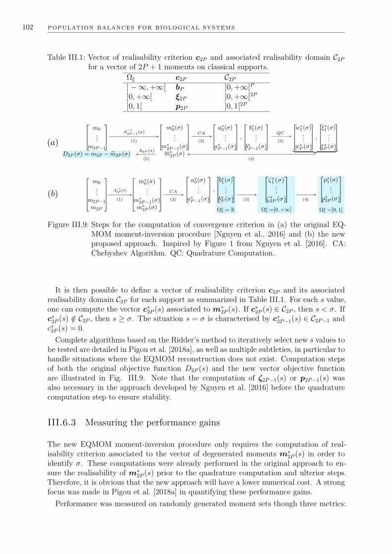
102 population balances for biological systems
Table III.1: Vector of realisability criterion c2P and associated realisability domain C2Pfor a vector of 2P + 1 moments on classical supports.
Ωξ c2P C2P]−∞,+∞[ bP ]0,+∞[P]0,+∞[ ξ2P ]0,+∞[2P]0, 1[ p2P ]0, 1[2P
Figure III.9: Steps for the computation of convergence criterion in (a) the original EQ-MOM moment-inversion procedure [Nguyen et al., 2016] and (b) the newproposed approach. Inspired by Figure 1 from Nguyen et al. [2016]. CA:Chebyshev Algorithm. QC: Quadrature Computation.
It is then possible to define a vector of realisability criterion c2P and its associatedrealisability domain C2P for each support as summarized in Table III.1. For each s value,one can compute the vector c∗2P (s) associated to m∗2P (s). If c∗2P (s) ∈ C2P , then s < σ. Ifc∗2P (s) /∈ C2P , then s ≥ σ. The situation s = σ is characterised by c∗2P−1(s) ∈ C2P−1 andc∗2P (s) = 0.
Complete algorithms based on the Ridder’s method to iteratively select new s values tobe tested are detailed in Pigou et al. [2018a], as well as multiple subtleties, in particular tohandle situations where the EQMOM reconstruction does not exist. Computation stepsof both the original objective function D2P (s) and the new vector objective functionare illustrated in Fig. III.9. Note that the computation of ζ2P−1(s) or p2P−1(s) wasalso necessary in the approach developed by Nguyen et al. [2016] before the quadraturecomputation step to ensure stability.
III.6.3 Measuring the performance gains
The new EQMOM moment-inversion procedure only requires the computation of real-isability criterion associated to the vector of degenerated moments m∗2P (s) in order toidentify σ. These computations were already performed in the original approach to en-sure the realisability of m∗2P (s) prior to the quadrature computation and ulterior steps.Therefore, it is obvious that the new approach will have a lower numerical cost. A strongfocus was made in Pigou et al. [2018a] in quantifying these performance gains.
Performance was measured on randomly generated moment sets though three metrics:

III.6 improving the extended quadrature method of moments 103
• Number of Floating-Point Operations (FLOP) required for the whole moment-inversion procedure;
• Number of tested s values before convergence is reached and σ is identified;
• CPU runtime for each call to the procedure.
Both the original and new approaches have been implemented in MATLAB [2016]. Allsource codes used for these comparisons are available as Supplementary Data of Pigouet al. [2018a] along with the complete methodology.
In terms of computational cost, Table III.2 details the reduction of required FLOPper call to the moment-inversion procedure for five kernels, out of the six available. Itis shown that the higher the order of the reconstruction, the more significant the gainprovided by the new procedure, ranging from about 60% for P = 2 up to 92% for P = 5.This significant improvement of EQMOM can be attributed to two phenomena.
Table III.2: Gain in FLOP when using the new EQMOM moment-inversion procedure.P = 2 P = 3 P = 4 P = 5
Gauss 59.1%±12.3% 84.2%±3.5% 87.9%±2.5% 88.0%±13.1%Laplace 64.2%±10.7% 87.5%±2.7% 91.0%±1.7% 91.6%±8.9%Log-normal 58.9%±20.0% 85.6%±5.8% 89.1%±4.3% 93.3%±3.5%Gamma 58.2%±18.8% 82.1%±7.3% 85.7%±6.8% 91.6%±5.4%Weibull 67.7%±15.1% 87.4%±5.1% 90.0%±4.2% 94.2%±3.6%
The first one is detailed in Table III.3 which presents the reduction in the number ofiterations to reach the convergence on σ. This reduction is mainly due to the fact thatin the moment-inversion procedure proposed by Nguyen et al. [2016], if a moment setm∗2P−1(s) happens not to be realisable, the objective function D2P (s) is set to an arbi-trarily high negative value such as −10100. Using arbitrary value in root-search algorithmslows down the convergence as it leads to a non optimal choice for the next tested value.On the opposite, the way the new procedure makes use of all elements of c2P (s), oneafter the other, prevents the need of such arbitrary values and therefore allows reachinga converged state in a few iterations.
Table III.3: Reduction in number of tested s values when using the new EQMOM moment-inversion procedure.
P = 2 P = 3 P = 4 P = 5Gauss 8.6%±27.7% 40.9%±17.7% 54.2%±12.8% 53.0%±55.2%Laplace 8.6%±28.3% 41.1%±17.6% 54.3%±12.7% 53.2%±54.4%Log-normal 8.8%±45.9% 21.9%±32.8% 30.5%±27.0% 49.5%±23.8%Gamma 15.5%±38.2% 24.7%±31.1% 34.9%±30.1% 57.2%±24.9%Weibull 26.3%±35.0% 27.2%±30.2% 32.4%±28.1% 54.0%±25.8%
The second reason for the net decrease of computational cost was expected and isrelated to the fact that in the former approach, the quadrature computation is performedin almost each iteration loop. More specifically, this step is called if m∗2P−1(s) is happensto be realisable. In the new approach, the quadrature computation is not required anymore to identify σ. It is only performed once when σ is identified to obtain wP and ξP .

104 population balances for biological systems
We could not find a moment set for which the former approach was faster than the newone. Note that only randomly generated sets were used for the comparison. Therefore,the benefits of this new EQMOM version are beyond the specific application case ofbioreactors modelling and should benefit all communities using this method.
Moreover, we observed an unexpected yet appreciable feature of the new approach: itsstable –bounded– numerical cost. Figs. III.10 and III.11 show the raw and normalizeddistributions of floating point cost for the Gauss and Log-normal kernels with P = 4. Inboth example, the raw distribution shows a lower numerical cost for the new approachas stated previously. Normalized distribution shows that the standard-deviation of thedistribution of numerical costs is lower for the new approach. This is shown on twoexamples but this has been observed for all kernels and orders. This lower variance innumerical cost is especially marked for EQMOM kernels defined on Ωµ =]0,+∞[. Thefact that the numerical cost is more consistent from one moment set to another will beparticularly beneficial to facilitate load-balancing in highly parallelized simulations, forinstance for PBE-CFD coupling.

III.6 improving the extended quadrature method of moments 105
Figure III.10: Distribution of numerical cost (FLOP) over 104 calls to moment-inversionprocedures with Gauss-EQMOM and P = 4.
Figure III.11: Distribution of numerical cost (FLOP) over 104 calls to moment-inversionprocedures with LogN-EQMOM and P = 4.

106 population balances for biological systems
III.7 Reducing the 5-D Population Model to a 1-D treatment
This chapter mainly focused on numerical methods that suit mono-dimensional Popu-lation Balance Models. However, Chapter V will describe the simulation of industrialcultures of S. cerevisiae, whose metabolism is described by accounting for five dynamicbiological properties (see Eq. (III.12)). Accounting for multi-variate PBEs for biologicalsystems is actually one of the goal of a project carried out by Quedeville et al. [2018] inparallel to this PhD thesis. For now, we will need to simplify the treatment of the 5DPBE in order to be able to apply 1D methods.
We propose to simplify the PBE treatment by analysing the involved time-scales. ThePBM allows tracking the two-way coupling between physical (concentration) heterogene-ity with biological heterogeneity. Therefore, we propose to first analyse time-scales asso-ciated to concentration fluctuations as perceived by micro-organism against time-scalesassociated to the evolution of their biological properties.
We first remind that, in industrial bioreactors, order of magnitudes for meso and macro-mixing time scales are respectively about 0.1 to 1s and 10 to 100s [Delafosse, 2008]. Thefirst four biological properties described in the S. cerevisiae metabolic model (µ(b)
G , µ(b)E ,
µ(b)A and ϕ
(b)O ) evolve over time with a characteristic time-scale T ≈ 1h (see Table II.5).
Therefore, we can infer from these time-scales that the slow biological regulations thatoccur to adapt these biological properties will act as a low-pass filter. The distributionsof growth and oxidative capacities will be mainly homogeneous in a large fermenter.
Moreover, Chapter V will focus on the simulation of substrate-limited fedbatch cultures.In short, this implies that while glucose concentration will locally be high at the feedingpoint, most of the fermenter volume will be depleted in terms of glucose. Therefore,most of the time cells will be in a poor environment and will go through high-glucoseconcentration areas every few minutes (circulation time) for a few seconds (mean residencetime in the feeding area). In these conditions, we can expect the distribution of growthcapability on glucose µ(b)
G to be nearly monodispersed at low values.The conclusion of this first analysis is that, whilst growth and oxidative capabilities
are dynamic properties, it is most likely not required to track their distribution in timeand space. The tracking of mean population values might be sufficient.
On the other side, the glycolytic stress σ is a peculiar property. In Chapter II, wemodelled its evolution such that
• in stressing (high glucose concentration) environment, the stress increases with atime-scale T (u)
σ ≈ 1s;
• in non-stressing environment, the cell recovers from stress with a time-scale T (d)σ ≈
1min.
Therefore, while other properties are almost unresponsive to the occasional exposition tohigh glucose concentrations in the feeding area, the stress σ will be strongly impacted.A cell travelling in a substrate-limited fedbatch culture will be exposed to the stressingenvironment of the feeding area for a few second which will be sufficient for its stress levelto increase significantly. Multiple passes through this area are separated, in mean, by thefermenter circulation time (≈ 1min) which allows for a recovery from previous stressingevents. Depending on trajectories of each cell, areas where recently stressed cells will

III.8 conclusion 107
cross the path of unstressed micro-organisms will exist. Therefore we can a priori expecta strong effect of the stress heterogeneity over the biological population.
To account for the dynamic evolution of mean growth and oxidative capabilities, alongwith the stress heterogeneity, we may simply track uncoupled moments of the distributionn(p). Let theses moments be defined as
mk1,k2,k3,k4,k5 =∫
ΩµG
∫ΩµE
∫ΩµA
∫ΩϕO
∫Ωσµk1G µ
k2E µ
k3A ϕ
k4O σ
k5dσdϕOdµAdµEdµG. (III.55)
We will track following moments of the distribution
M =
m0,0,0,0,0m1,0,0,0,0m0,1,0,0,0m0,0,1,0,0m0,0,0,1,0m0,0,0,0,1
...m0,0,0,0,Nmσ
=
XL
µ(b)G XL
µ(b)E XL
µ(b)A XL
ϕ(b)O XL
σXL...
m0,0,0,0,Nmσ
(III.56)
with Nmσ the number of moments tracked along the stress direction to account for theheterogeneity of σ.
From these moments, we will produce a quadrature rule formed by weights wQ =[w1, . . . , wQ] and vectors of properties pQ = [p1, . . . , pQ] such that
∫Ωpf(p)n(p)dp ≈
Q∑i=1
wif(pi). (III.57)
Vectors of properties pi are defined as
pi =
µ(b)G
µ(b)E
µ(b)A
ϕ(b)O
σi
=
m1,0,0,0,0/m0,0,0,0,0m0,1,0,0,0/m0,0,0,0,0m0,0,1,0,0/m0,0,0,0,0m0,0,0,1,0/m0,0,0,0,0
σi
(III.58)
and wQ and σQ = [σ1, . . . , σQ] are the weights and nodes of a quadrature formed from thevector of moments [m0,0,0,0,0,m0,0,0,0,1, . . . ,m0,0,0,0,Nmσ ] using either QMOM or EQMOMmethod.
III.8 Conclusion
In order to account for the heterogeneity of cell-attached properties in the modelling ofbioreactors, the Population Balance Model approach has been selected to facilitate thecoupling with the classical mass-balance based modelling framework of reactors in chem-ical engineering. PBMs are compatible both with Computational Fluid Dynamics, CMA

108 population balances for biological systems
and 0D hydrodynamic model which makes this approach compatible with the modellingof all bioreactor scales.
Population Balance Equations can be solved using either sectional –or class– methodsor moment methods. The former are more intuitive and constitute a direct resolutionof the equation, at the cost of high number of resolved variables. Therefore, methodsof moments have been assessed in order to significantly reduce the size of simulations.Multiple methods to provide closure in moment formulations have been implementedand tested against the class method, these were QMOM, EQMOM and the MaximumEntropy approach. MaxEnt was found to be the most accurate of all methods, but itslack of stability makes this numerical method unsuited for the simulation of large-scalebiological cultures where any numerical failure compromises the integrity of the wholesimulation. QMOM is the fastest of all three methods, but requires twice has muchresolved moments as EQMOM to reach a similar accuracy and cannot provide point-wiseevaluation of the NDF. Therefore, EQMOM has been favourably selected as the bestsuited method. Its proved to be accurate and stable with a reasonable numerical cost.
EQMOM has been developed quite recently [Yuan et al., 2012] and has been improvedover time [Madadi-Kandjani and Passalacqua, 2015; Nguyen et al., 2016; Passalacquaet al., 2017]. Using this method and researching the mathematical fundamentals of meth-ods of moments led to the discovery of a new procedure to solve the EQMOM moment-inversion problem. This implies that a new version of EQMOM is now available to whommay be interested in faster computations based on this method [Pigou et al., 2018a].
While Chapter II focused on modelling bioreaction rates for E. coli and S. cerevisiae,the current Chapter detailed Population Balance Equations for both micro-organisms.Thanks to these, and to the selection of suited numerical methods, previously developedmetabolic models can now be applied in dynamic heterogeneous systems at reasonablecomputational costs.

IVM O D E L I S AT I O N D E L ’ H Y D RO DY N A M I Q U E AU X G R A N D E SE C H E L L E S
Resume
Les Chapitres II et III se sont concentres sur la modelisation de la phase biologique.Desormais, des modeles sont disponibles pour decrire le comportement metabolique demicro-organismes soumis a des perturbations, ainsi que des methodes numeriques pourintegrer ces comportements a l’echelle d’une population. Afin d’appliquer ces modeles a lasimulation de fermenteurs industriels, un aspect manquant est celui de l’hydrodynamiquede ces systemes. Savoir comment les phases gaz et liquide circulent dans un bioreacteurest en effet un pre-requis pour predire le transport des especes dissoutes (substrats, sous-produits, . . . ), le taux de transfert des especes gazeuses (oxygene, dioxyde de carbone,. . . ) et le transport de la phase biologique.
Appliquer directement des methodes experimentales sur les bioreacteurs industrielspour obtenir les champs de vitesses et la distribution spatiale des deux phases sembledifficile, voire impossible, et serait particulierement onereux. L’outil alors le plus adapteest la Mecanique des Fluides Numerique (CFD) qui permet de predire l’hydrodynamiquedans les systemes de grande echelle, seulement a partir de leur geometrie, des conditionsoperatoires, et du choix de modeles adaptes a la description de cuve agitee gaz-liquide. Aucours de ce travail, deux logiciels de CFD ont ete mis en œuvre. La suite applicative AN-SYS Workbench a ete utilisee pour definir la geometrie d’un fermenteur industriel, pourgenerer des maillages, et pour effectuer des simulations sous ANSYS Fluent basees surune approche pseudo-stationnaire. NEPTUNE CFD, un logiciel developpe par les princi-paux acteurs de l’industrie nucleaire civile francaise (CEA, EDF, FRAMATOME, IRSN),a ete utilise pour effectuer des simulations plus avancees. Celles-ci sont basees sur uneapproche instationnaire a maillage tournant en integrant de nouvelles modelisations pourdecrire les interactions gaz/liquide, en particulier a fort taux de gaz. Le cout numeriqueimportant de ces simulations instationnaires a necessite la mise en oeuvre de calculshaute performance sur supercalculateurs. Cela peut, d’une certaine maniere, sembler encontradiction avec l’objectif principal de cette these de parvenir a simuler des culturesbiologiques industrielles de maniere rapide et peu couteuse.
Apres avoir detaille le fermenteur industriel a simuler et les simulations CFD associees,ce chapitre developpe une analyse de temps caracteristiques. Il est ainsi montre que,bien qu’une resolution spatiale fine soit requise pour les simulations CFD, le couplage del’hydrodynamique avec la modelisation de la phase biologique ne requiert pas une telleresolution. Au contraire, une description spatiale fine engendrerait des couts computa-tionels prohibitifs et contraindrait fortement les pas de temps utilises pour les simulations.Ainsi, nous proposons d’effectuer le couplage des modeles biologiques (metabolique et bi-
109

110 modelisation de l’hydrodynamique aux grandes echelles
lan de population) avec l’hydrodynamique dans une approche par compartiments. Laderniere section de ce Chapitre se concentre donc sur la methodologie employee pourdeduire un modele de compartiments a partir des resultats de simulations CFD. Cettemethodologie, basee sur l’exploitation de donnees au format Ensight Gold exportable parANSYS Fluent et NEPTUNE CFD, est developpee pour integrer les champs de vitesseaux frontieres entre les compartiments, et les champs scalaires (fractions volumiques,variables caracteristiques de la turbulence) sur le volume de chaque compartiment. Lorsde l’implementation de cette methodologie, nous avons observe une erreur residuelle nonnegligeable qui, non resolue, induit un schema de transport non conservatif. Des lors, nousproposons une procedure basee sur une optimisation multi-variables et multi-objectifspour corriger cette erreur et obtenir une modelisation conservative de l’hydrodynamiquedes bioreacteurs industriels.
IVM O D E L L I N G L A RG E - S C A L E H Y D RO DY N A M I C S
Summary
Chapters II and III focused on the description of the biological phase. Now models areavailable to describe the metabolic behaviour of micro-organisms subjected to perturba-tions along with numerical method to integrate these behaviours at the population-scale.In order to integrate these models in simulations of industrial fermenters, the remainingaspect is that of hydrodynamics. Knowing how gas and liquid phases flow in the systemis indeed required to predict the transport of dissolved species (substrates, by-products,. . . ), the local transfer rate of gases (oxygen, carbon dioxide, . . . ) and the transport ofthe biological phase.
Using directly experimental methods in industrial fermenters to obtain the knowledgeof fluid velocities and spatial distribution of both phases is difficult, if not impossible,and would be prohibitively expensive. The most suited tool is the Computational FluidDynamics which allows predicting large-scale hydrodynamics solely from the system ge-ometry, operating conditions, and the choice of suitable models to describe gas-liquidturbulent flows in a stirred tank reactor. Over the course of this work, two CFD softwarehave been used. The ANSYS Workbench tool-suite has been employed to define thesystem geometry, generate meshes, and to perform pseudo-stationary simulations usingANSYS Fluent. NEPTUNE CFD, a software developed by the main actors of Frenchcivil nuclear industry (CEA, EDF, FRAMATOME, IRSN), has been used to performmore detailed simulations. They used an unsteady moving-mesh approach and new mod-els for the description of gas-liquid interaction at high gas flow rates. The numericalcost of these unsteady simulations required the use of supercomputing resources, whichsomehow contradicts the goal of performing fast –low-cost– simulations for industrialfermentations.
After having detailed the considered industrial set-up and associated CFD simulations,the current Chapter develops a time-scale analysis. While fine CFD simulations are re-quired to access hydrodynamics in industrial bioreactors, it is shown that the couplingwith biological models does not require the spatial resolution of CFD simulations. Ac-tually, this spatial resolution would induce a prohibitively high computational cost andwould enforce a limiting time-step for simulations. Therefore, we propose to perform thecoupling of biological (metabolic and population balance) models with a CompartmentModel.
The last part of this Chapter then focuses on describing how to obtain a compartmentmodel starting from CFD results. A methodology, based on the Ensight Gold file formatwhich can be exported from both ANSYS Fluent and NEPTUNE CFD, is developedto integrate velocity field over contours of compartments, and phase fraction fields over
111

112 modelling large-scale hydrodynamics
compartment volumes. When implementing this methodology, we noticed non negligibleresidual error on obtained compartment models. If not resolved, this would lead to non-conservative transport schemes. Therefore, a procedure based on multi-objectives multi-parameter optimisation is proposed to fix this residual error and enforce a conservativehydrodynamic model for large-scale bioreactors.

IVM O D E L L I N G L A RG E - S C A L E H Y D RO DY N A M I C S
IV.1 Introduction
The modelling of bioreactors has often been limited to either homogeneous descriptionsof the system where no gradient are considered, or to heterogeneous descriptions wherebiological complexity is left apart (see I.8). Only few attempts were made to handle bothbiological heterogeneity and metabolic complexity within a unified modelling frameworkthat could be applied to all bioreactor scales.
In order to achieve this goal, the Euler-Euler-PBE gas-liquid modelling frameworkhas been selected. It allows integrating biological heterogeneity described by PopulationBalance Equations (PBEs) (see Chapter III) and metabolic models (see Chapter II) assource/sink terms in mass balance equations. Depending on the scale of the reactor, andon the comparison between mixing and reaction/transfer/adaptation characteristic times,the system will either be homogeneous or heterogeneous with large-scale or local-scalegradients. Depending on the situation, the conservation equations will require to bewritten over control volumes defined with different length scales. Let Ck be a vector ofquantities expressed per unit of volume of the phase k, mass balance equations on thisquantity can be:
• For homogeneous systems of volume V
∂〈αk〉VCk
∂t= Sk (IV.1)
• For heterogeneous systems with large-scale gradients, modelled by CompartmentModel Approach (CMA)
∂〈αk,i〉ViCk,i
∂t=
NC∑j=1
Q(k)j,i Ck,j −Ck,i
NC∑j=1
Q(k)i,j + Sk,i (IV.2)
• For heterogeneous systems with short-range gradients, approached by Computa-tional Fluid Dynamics (CFD)
∂αkCk
∂t+ ~∇ ·
(αkCk~uk − ~∇ (αkDk Ck(~x, t))
)= Sk (IV.3)
αk is the local phase fraction and 〈αk〉 is its mean value over a control volume. Subscriptsi and j denote variables attached to the i-th or j-th compartment in a compartmentalapproach with NC compartments.
113

114 modelling large-scale hydrodynamics
Elements of Ck may correspond to liquid-phase concentrations of oxygen, glucose, ac-etate, . . . (kg/m3
L), to gas-phase concentrations of oxygen, carbon dioxide, or other gaseouscompounds (kg/m3
G) but also, for the treatment of PBEs to class-attached biomass con-centrations (kgX/m3
L) or to moments of the distribution of biological properties (unitdepending on moment order and property unit). The compatibility of models and nu-merical methods developed in Chapters II and III, with these transport equations, isthen straightforward. Sk is the vector of source/sink terms associated to each quantitytracked in Ck and can account for mass transfer, reaction, or adaptation/redistributionof biological properties as defined in previous chapters.
Note that the homogeneous modelling is a simplification of a compartment model witha single compartment (or actually, that CMA is an extension of homogeneous models).Therefore, in this chapter we only consider CMA and CFD approaches. Therefore, twoquestions arise when a specific bioreactor has to be simulated:
• Which approach should be selected between CMA and CFD for the coupling oftransport with bioreaction?
• How to access phase presence and velocity fields (αk(x) and ~uk(x) for CFD, εk,i andQ
(k)i,j for CMA)?
As part of this project and in relation with industrial interests of Sanofi, a specificapplication case was selected for the whole modelling framework and simulation work-flow. The presentation of this application will drive the current chapter by illustratingthe specific questions that occurred and how they have been tackled to obtain a large-scalehydrodynamics modelling.
First, the industrial bioreactor is briefly described in section IV.2 along with operatingconditions. Considering the size of the system, and the culture mode, it will be made clearthat the bioreactor will never be strictly homogeneous and that heterogeneity must beaccounted for. Therefore, CMA or CFD description of transport will be required, whichin turn requires the description of velocity fields. As no sufficient experimental data isavailable on that industrial geometry, numerical computations of velocity fields are a re-quirement. CFD simulations are thus presented in section IV.3. Section IV.4 focuses ondetermining whether the high spatial accuracy achieved in CFD simulations is requiredfor the coupling with biological models. A comparison of time-scales associated to the bio-logical phase and to the CFD transport scheme will show that the CMA approach is moreefficient to perform the coupling between transport and biological reactions/adaptation.Therefore a methodology for converting CFD results into Compartment Models is pre-sented in section IV.5.
IV.2 Production-scale fermenter
IV.2.1 System geometry
The study of bioreactor modelling and simulation has been applied to an industrial-scalefermenter of undisclosed volume. This vessel is equipped with three turbines, whosespecifications may not be disclosed for confidentiality reasons. The bottom impeller is a6-blade radial turbine, responsible for gas dispersion. The other two impellers are 3-bladeturbines leading to an hybrid radial and pumping-up axial flow, whose goal is to favour

IV.2 production-scale fermenter 115
Figure IV.1: Simplified geometry of the considered industrial large-scale bioreactor. 6-blade Rushton turbines are displayed in place of actual turbines.
large-scale mixing and gas dispersion. Central vortex is prevented by three baffles. Anincomplete geometry, where actual impellers are replaced by Rushton turbines, is shownin Fig. IV.1. The fermenter dimensions are undisclosed. Gas is injected at undisclosedlocation.
IV.2.2 Operating conditions
The goal of the study and of simulations presented in Chapter V is to assess the effect ofstirring speed and gas flow rate on observed metabolic dysfunctions of the baker yeast (seeChapter II). Therefore, CFD computations will be performed for two sets of operatingconditions summed up in Table IV.1.
Table IV.1: Operating conditions to be simulated. Normalized by Operating Condition 1for confidentiality reasons.
Operating condition 1 Operating condition 2Impeller rotation speed 1 1.4Gas flow rate 1 1.85Liquid volume 1 1
This fermenter is used for fedbatch cultures. This implies that the liquid volumeincreases over-time during the course of the fermentation process which spans severaldays. Instead of solving hydrodynamics over such a long period, it has been decidedto perform pseudo-stationary simulations of the overall system at an operating point
116 modelling large-scale hydrodynamics
corresponding to an undisclosed liquid volume. This point corresponds to a specific timein the fedbatch process, associated to a specific biomass concentration and substratefeeding rates which will be used for simulations in Chapter V.
IV.3 CFD simulations
IV.3.1 Goal and constraint on bioreactor hydrodynamic computations
Leaving aside all biological considerations and on a strictly hydrodynamics point of view,the numerical simulation of industrial fermenters poses multiple challenges.
The first one comes from the geometric complexity of these systems. In order tomonitor the process, to control temperature and pH or to allow injection of gas andliquid sources of feeding material, bioreactors are filled with numerous apparatus whichcan locally affect the circulation of fluids.
The second aspect is the presence of macro-instabilities. Large-scale bioreactors areoperated in turbulent flow regime which implies small scales for velocity fluctuations,while the overall system is large. The continuous stirring also induces periodic fluctuationsof velocity fields associated to the cyclic movement of turbines. Solving simultaneouslysmall and large scales poses a numerical challenge.
A third source of complexity originates from physical properties of culture broth. Thepresence of high cell concentrations increases the fluid viscosity. This viscosity is evenmore significantly increased locally around the glucose feeding point if concentrated syrupis directly injected in the system. Moreover, the numerous chemical and biological speciesin the culture broth influence the gas-liquid surface tension.
Finally, a fourth challenge comes from the gas-liquid aspect of these systems. Indeed,high gas flow rates applied to the considered fermenter prevent the use of spargers todisperse gas in the system. Instead, an exhaust-pipe injects the gas and the bottomturbine is responsible for breaking gas pockets into dispersed bubbles. This implies thata correct description of the gas-liquid hydrodynamics requires handling both a continuousgas phase under the bottom turbine, a dispersed gas phase carried by the liquid, as wellas breakage and coalescence phenomenon which will affect the distribution of bubble sizesand shapes. Note that breakage and coalescence will be impacted by the local evolutionsof viscosity and surface tensions as pointed out in the third consideration.
Overall, bioreactor hydrodynamics is a complex topic indeed. Nevertheless, a per-fect description of these complexities will not be required for the upcoming coupling oftransport by fluids with biological reactions. The hydrodynamic description will then besimplified by estimating whether each aspect is expected to have a significant effect on theoverall coupling. Said otherwise, we will only describe phenomenon whose consequencesare perceived by the biological modelling, both in terms of metabolism and of biologicaladaptation.
IV.3.2 Simplifying the hydrodynamics modelling
This thesis is not focused on performing complex –state-of-the-art– simulations of in-dustrial fermenters hydrodynamics. All previously listed aspects do have an impact onoverall bioreactor performances, but quantifying these impacts requires describing all phe-

IV.3 CFD simulations 117
nomenon, including biological-phase related aspects, with the same high accuracy andat the expense of inaccessible numerical cost. Therefore, we focused on obtaining roughhydrodynamics, both in terms of velocity field and in terms of spatial distribution of thegas phase.
Having the correct order of magnitude for these variables (velocities and phase fractions)will yield correct meso and macro-mixing times, as well as local oxygen transfer rate.These in turn will impact the biological model, and allow a reverse coupling between large-scale gradient/local substrate availabilities, biological state and metabolic behaviours.
To facilitate CFD simulations while preserving meso/macro-mixing time-scales, thefermenter geometry has been simplified to its bare minimum. All small elements thatonly slightly disturb the flow have been removed from the geometry as they only inducelocal perturbations that do not significantly influence macromixing and gradients. Fig.IV.1 illustrates which elements were kept: vessel walls, the three baffles, and the agitatorshaft. Baffles and turbine blades were even more simplified by describing them using athin-wall approach, therefore their thickness was not described, which allows for a slightlycoarser meshing and improves the mesh quality in terms of aspect ratios.
In terms of turbulent velocity fluctuations, solving them would require performingDirect Numerical Simulations (DNSs) where all scales of turbulence are resolved, downto the Kolmogorov scale, or at least Large-Eddies Simulations (LESs) where only thesmallest –sub-grid– scales are modelled. However, the size of the industrial fermenterprevents such simulations due to a prohibitive numerical cost. This will not be a majorissue, considering that an accurate description of turbulent velocity fluctuations is notrequired in the first place. Indeed, the biological model only responds to potential lackof substrate due to micro-mixing limitations, and not to actual velocity fluctuations.Evaluating the flux of substrate available through micro-mixing is feasible using integralproperties of turbulence, such as the kinetic turbulent energy k and the dissipation rateof that energy ε, in the k−ε Reynolds-Averaged Navier-Stokes (RANS) approach.
It is known that in stirred vessels, the instantaneous velocity field U(~x, t) can be de-composed into a mean value u(~x), a periodic perturbation associated to agitation u(~x, t)and chaotic fluctuations associated to turbulence u′(~x, t) [Escudie and Line, 2004].
U(~x, t) = u(~x) + u(~x, t) + u′(~x, t) (IV.4)
It is clear that the mean velocity will strongly impact meso and macro-mixing and there-fore large-scale gradients. As stated previously, smallest scales of turbulent fluctuationsare related to micro-mixing and will have an impact on substrate consumption by micro-organisms and this aspect will be modelled using variables of the k−ε approach in ChapterV. However, the need for describing periodic fluctuations u(~x, t) is more difficult to assessbeforehand. For sake of simplicity, we first used in ANSYS Fluent [2015] the MultipleReference Frames (MRF) approach which consists in discarding these periodic fluctua-tions, in line with the approach used by Haringa et al. [2016] among other examples.Other simulations using a rotating mesh approach have been performed under an othersoftware, NEPTUNE CFD [2016], in order to account for these periodic fluctuations ofvelocity fields.
Part of this section is edited out for confidentiality reasons.Due to the breakage of large gas caps, and to classical breakage and coalescence of
dispersed bubbles, strongly poly-dispersed Bubble Size Distributions (BSDs) are expectedin industrial fermenters. Despite the fact that models are available to track this BSD

118 modelling large-scale hydrodynamics
Figure IV.2: Illustration of differences between dispersed gas model and GeneralizedLarge-Interface Model (GLIM) on simple 2D CFD simulations performedunder Neptune CFD. (a) Initial conditions. The green arrow indicates thesource and direction of gas injection. (b) Dispersed model. (c) GLIM model.
through a Population Balance Model approach [Laakkonen et al., 2007; Li et al., 2018],or to resolve the transport of the interfacial area, we did not integrate these in oursimulations. Instead, we performed simulations by enforcing a constant bubble diameter.
IV.3.3 Momentum exchange between phases
For interaction modelling between gas and liquid phases, we followed general guidelinesof ANSYS Fluent [2015] user guide for bubbly flows. Drag was described using the uni-versal drag laws for bubble-liquid flows [Kolev, 2007]. This law is applicable to mostgas-flow regimes, and even to non-spherical bubbles, under the condition that the hy-draulic diameter of the flow domain is significantly larger than the characteristic size ofthe dispersed phase, which is here the case. The lift force is modelled using the variant ofTomiyama [1998] law proposed by Frank et al. [2004]. For stability reasons, virtual massforce modelling was not enabled in performed simulations.
For simulations that ran under NEPTUNE CFD [2016], we made use of the Gener-alized Large-Interface Model [Merigoux et al., 2016] which is designed to describe flowswhere a phase exists both as continuous pockets and dispersed bubbles [Mer et al., 2018].This model detects large gas-liquid interfaces by comparing gas fraction gradients to athreshold value and by adding a special treatment at the interface location. This ensurespreserving the consistency of these large interfaces (large pockets or free surface) whichis otherwise lost when using purely dispersed models. This is illustrated in Fig. IV.2where a simple 2D set-up is simulated using either dispersed or GLIM modelling. Thefree surface consistency is quickly lost using the dispersed modelling (Fig. IV.2b). Thegas pockets predicted by GLIM can be dispersed by turbulent flow which is consistentwith experimental observations of aerated bioreactors [Moilanen et al., 2008].

IV.3 CFD simulations 119
Figure IV.3: (a) Mesh of stator zone, discretized using ≈ 300000 hexahedral elements.Green surfaces represent two out of three thin-wall baffles. (b) Sectionalview of rotor zone mesh, discretized using ≈ 1000000 tetrahedral and prismelements.

120 modelling large-scale hydrodynamics
IV.3.4 Geometry meshing
The same mesh has been used on both ANSYS Fluent [2015] and NEPTUNE CFD [2016].In order for it to be compatible with MRF as well as rotating-mesh approaches, two zoneswere defined: a rotor encompassing the agitator shaft, and a stator. These meshes are il-lustrated on Fig. IV.3. The stator zone could be entirely meshed by hexahedral elements.The complex geometry of impellers prevented such a regular meshing and therefore re-quired an unstructured tetrehadron-based meshing. Zones in-between impellers weremeshed using prism elements. A similar quadrangle-based mesh was enforced on thecontact surface between rotor and stator meshes.
IV.4 Time-scale analysis
As stated previously, the instantaneous velocity field U(~x, t) can be decomposed into amean value u(~x), a periodic fluctuation u(~x, t) and a chaotic fluctuations u′(~x, t).
Turbulent fluctuations are filtered by the RANS approach which is closed by applyingthe k−ε model for the transport and dissipation of turbulent kinetic energy. Moreover,the periodic perturbation is filtered out too by the MRF approach which models thesystem as pseudo-stationary. Therefore, smallest time-scales of the hydrodynamics havenot been resolved by previously described CFD simulations. Chapter V describes howmicromixing and turbulent fluctuations can be accounted for in the coupling of transportwith biological reaction.
If only mean velocity fields have been solved, and therefore only meso and macro-mixing are well described by these fields, one can wonder whether the resolution of the“fine” mesh used for CFD simulations is still required for the coupling of transport withmetabolic and population balance models described in Chapters II and III. The smallesttime-scale associated to these models is the one associated to the increase of glycolyticstress, σ, if cells are exposed to environment rich in terms of glucose concentration. Thistime-scale was identified to be around 3 seconds. Therefore, in order to correctly resolvethe biological model, the simulation time-step does not need to be significantly lower thanthat value.
If the coupling of transport and biological model is directly performed with transportdescribed by a finite-volume scheme using the CFD mesh, the time integration will haveto respect the CFL condition [Courant et al., 1928]. Let ci be the Courant numberassociated to the i-th volume element of the mesh, i ∈ 1, . . . , Nmesh:
ci = |~u(~xi)|δtδxi
(IV.5)
with ~u(~xi) the velocity of a phase at the center of the i-th volume element, δt the simula-tion time-step, and δxi the characteristic length of the volume element. It is well knownthat the stability of the transport scheme requires that
maxi
ci ≤ 1
Having obtained a pseudo-stationary velocity field for each phase through the RANS-MRF approach, it is possible to deduce from this stability condition a maximum time-step δtmax that should be used to perform coupled simulations within the CFD framework.
IV.4 time-scale analysis 121
This maximum time-step has been measured using ANSYS Fluent built-in post-processingtools. The characteristic length δxi was approximated by the cubic root of the i-thcell’s volume. Obtained maximum time-steps are 2.0ms and 1.5ms for the two operatingconditions presented in Section IV.2.
The time-scale associated to numerical stability of the transport terms is significantlylower than the smallest time-scale associated to other aspects of bioreactor modelling.Therefore, keeping the spatial accuracy of CFD simulations is not a requirement to per-form coupled simulations of transport with transfer, reaction, and biological adaptation.It will be more efficient to compute a Compartment Model from CFD results as it willallow to significantly reduce the numerical cost on two aspects.
Typical number of compartments in Compartment Model Approach range from dozens[Vrabel et al., 1999] to thousands [Delafosse et al., 2014]. This is significantly lower thanthe number of volume-elements used for CFD simulations, which was here of 1.2 millioncells. Therefore, a compartment model yields a much lower number of resolved vari-ables, hence limited memory requirements, and decreases the numerical cost by reducingthe number of calls to the metabolic model (Chapter II) and to numerical methods asQuadrature Method of Moments (QMOM) or Extended Quadrature Method of Moments(EQMOM) for the resolution of PBEs (Chapter III).
Moreover, the modelling will be used to perform simulations of long-term biologicalcultures. Whether these simulations span a whole culture (hours/days of simulated time),or attempt to identify a steady or pseudo-stationary state as shown in Chapter V, it will benecessary to simulate multiple hours of the system. The simulation of 10h of culture with atime-step limited by the Courant condition of δtmax ≈ 2.0ms would require ≈ 1.8 109 time-steps. Though being clearly infeasible, we still attempted to perform these simulationsin order to estimate the numerical cost that would be required. These simulations ran ona computing cluster using 240 allocated CPU cores using the software NEPTUNE CFD[2016] without accounting for biological heterogeneity (unsegregated approach, see I.6.3),and by disabling the resolution of RANS and k−ε equations, therefore using a frozen flowapproach. Only mean values for biological properties were tracked, and the metabolicmodel was called once per mesh volume-element. This over-simplified modelling, and theuse of significant computing resources, still yield a mean computation time of 1.5s pertime-step. A 10h long simulation would then require about a year of computations. It istherefore obvious that handling the transport of species carried by each phase within theframework of CFD simulations is not reasonable, if particular if one expect quick answerfrom simulations for an engineering application, and even more if the complete modelling,integrating biological heterogeneity, is considered.
For all previously detailed reasons, the Compartment Model Approach will be usedto perform coupled simulations in Chapter V. The lower number of compartments com-pared to the number of mesh elements will decrease both memory and numerical costs.Moreover, the higher volume of compartments will allow to relax the Courant conditionto higher stable time-steps, thus significantly reducing the total number of time-steps re-quired. Following sections therefore focus on the computation of a suitable CompartmentModel from CFD results.

122 modelling large-scale hydrodynamics
IV.5 From CFD to Compartment Models
IV.5.1 State of the art, constraints and selected approach
The idea of degrading results of CFD simulations to obtain compartment models andassociated flow maps is certainly not new [Bezzo et al., 2003]. It has been successfullyapplied to waste-water treatment [Le Moullec et al., 2010] and to bioreactor modelling inprevious works [Delafosse et al., 2010, 2014; Nauha et al., 2018].
Two main approaches exist to perform the compartmentalization of CFD results. Thefirst one consists in identifying sub-volumes in which some parameters are near constantthrough either stochastic or more usually deterministic methods. This approach leadsto compartments of homogeneous turbulence or gas fraction for instance. However, theshape of these compartments will tend to be irregular and will strongly differ betweenoperating conditions.
The second approach to obtain a compartment model from CFD is the manual zoningwhere geometric bounds of each compartment are defined by-hand. For the simulationof bioreactors, having regular compartments seems to be a more interesting option fortwo reasons. The first one is the easier comparison of simulation results when operatingconditions are modified. For instance, assessing the effect of stirring speed or aerationrate on the overall culture is easier if one is sure that the compartmentalization wasperformed in exactly the same way between simulations (see Chapter V). The secondreason why manual zoning might be more interesting is related to an unexplored idea. Ifone wants to integrate varying operating conditions or fluid properties over time such asa liquid viscosity depending on the biomass concentration, or on a product concentration(i.e. xanthan production), the approach would consist in
• performing CFD simulations for multiple conditions;
• computing compartment models associated to each CFD simulation;
• dynamically compute a compartment model as a convex mixture of previously de-fined models.
The last step is by far easier and less error prone if compartment models are defined ona regular –manual– zoning.
Note that Delafosse et al. [2010] obtained a better agreement in terms of mixing timebetween CFD simulations and manual zoning than when automatic zoning was used. Thismanual zoning approach has also been favourably selected by Delafosse et al. [2014] andNauha et al. [2018]. For all these reasons, this will be the retained approach for followingdevelopments. The question is then to determine the technical solution for computingthe compartment model from CFD results.
By CFD results, we imply results coming from simulation performed either on AN-SYS Fluent or on NEPTUNE CFD. These could be single-phase simulations or, moregenerally for aerated bioreactors, gas-liquid simulations. While we initially aimed atgenerating transient compartment model based on time-resolved hydrodynamics, onlypseudo-stationary hydrodynamics are handled by following developments.
To handle results coming from both software, ANSYS Fluent and NEPTUNE CFD,the selected approach has been to create a code able to read and post-process files in theEnsight Gold format. Both software can export simulation results in this format, and a
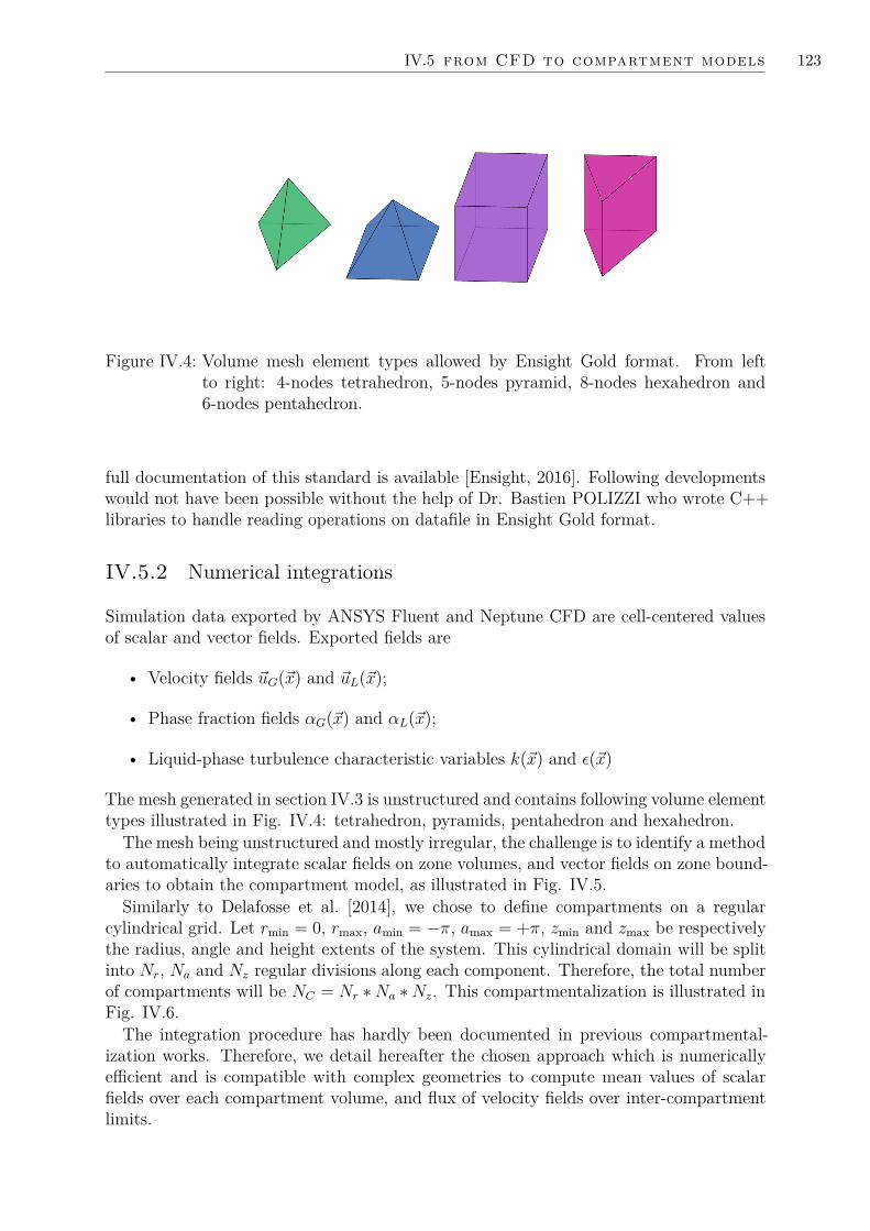
IV.5 from CFD to compartment models 123
Figure IV.4: Volume mesh element types allowed by Ensight Gold format. From leftto right: 4-nodes tetrahedron, 5-nodes pyramid, 8-nodes hexahedron and6-nodes pentahedron.
full documentation of this standard is available [Ensight, 2016]. Following developmentswould not have been possible without the help of Dr. Bastien POLIZZI who wrote C++libraries to handle reading operations on datafile in Ensight Gold format.
IV.5.2 Numerical integrations
Simulation data exported by ANSYS Fluent and Neptune CFD are cell-centered valuesof scalar and vector fields. Exported fields are
• Velocity fields ~uG(~x) and ~uL(~x);
• Phase fraction fields αG(~x) and αL(~x);
• Liquid-phase turbulence characteristic variables k(~x) and ε(~x)
The mesh generated in section IV.3 is unstructured and contains following volume elementtypes illustrated in Fig. IV.4: tetrahedron, pyramids, pentahedron and hexahedron.
The mesh being unstructured and mostly irregular, the challenge is to identify a methodto automatically integrate scalar fields on zone volumes, and vector fields on zone bound-aries to obtain the compartment model, as illustrated in Fig. IV.5.
Similarly to Delafosse et al. [2014], we chose to define compartments on a regularcylindrical grid. Let rmin = 0, rmax, amin = −π, amax = +π, zmin and zmax be respectivelythe radius, angle and height extents of the system. This cylindrical domain will be splitinto Nr, Na and Nz regular divisions along each component. Therefore, the total numberof compartments will be NC = Nr ∗Na ∗Nz. This compartmentalization is illustrated inFig. IV.6.
The integration procedure has hardly been documented in previous compartmental-ization works. Therefore, we detail hereafter the chosen approach which is numericallyefficient and is compatible with complex geometries to compute mean values of scalarfields over each compartment volume, and flux of velocity fields over inter-compartmentlimits.

124 modelling large-scale hydrodynamics
8 16 24 32 40
7 15 23 31 39
6 14 22 30 38
5 13 21 29 37
4 12 20 28 36
3 11 19 27 35
2 10 18 26 34
1 9 17 25 33
𝜀𝐿,8 𝜀𝐿,16 𝜀𝐿,24 𝜀𝐿,32 𝜀𝐿,40
𝜀𝐿,7 𝜀𝐿,15 𝜀𝐿,23 𝜀𝐿,31 𝜀𝐿,39
𝜀𝐿,6 𝜀𝐿,14 𝜀𝐿,22 𝜀𝐿,30 𝜀𝐿,38
𝜀𝐿,5 𝜀𝐿,13 𝜀𝐿,21 𝜀𝐿,29 𝜀𝐿,37
𝜀𝐿,4 𝜀𝐿,12 𝜀𝐿,20 𝜀𝐿,28 𝜀𝐿,36
𝜀𝐿,3 𝜀𝐿,11 𝜀𝐿,19 𝜀𝐿,27 𝜀𝐿,35
𝜀𝐿,2 𝜀𝐿,10 𝜀𝐿,18 𝜀𝐿,26 𝜀𝐿,34
𝜀𝐿,1 𝜀𝐿,9 𝜀𝐿,17 𝜀𝐿,25Manualzoning
scalar fieldintegration
velocity fieldintegration
Figure IV.5: Steps of the compartmentalization procedure of CFD results.
Figure IV.6: Compartmentalization of the industrial geometry. (left) top view, (middle)side view, (right) interior view.

IV.5 from CFD to compartment models 125
Figure IV.7: Illustration of splitting procedure to 2D meshes. Note that the initial mesh(left-hand side) contains both triangles and quadrangles, some of them lo-cated in multiple compartments. The final mesh (right-hand side) containsonly triangles strictly located within a single compartment.
Mesh splitting
Some authors used natural limits of mesh elements to perform the integration of fields.This was done by identifying neighbour cells whose center lie in different compartments,and then integrating vector fields over the facet joining these cells. While being seeminglystraightforward, this approach has a main numerical drawbacks: it requires the knowledgeof the mesh associativity, i.e. which mesh elements are connected by shared verticesand facets. This information is not directly available in Ensight Gold geometry files.Associativity can be reconstructed at moderate cost if the whole geometry is meshed in aunique block (or “part’ is the Ensight Gold format terminology), but the cost significantlyincreases when multiples parts constitute the complete mesh. As explained in SectionIV.3.4, the simulation of stirred reactors requires to mesh independently rotor and statorzones, which translates as two different parts when data is exported to Ensight Goldformat. Moreover, the accuracy of this approach can be questioned as soon as the meshis strongly irregular.
In order to obtain low-cost and accurate compartmentalization even for complex geom-etry, we chose to perform a mesh splitting. The basic idea is to split each mesh-elementlocated on a compartment limit into multiple sub-elements whose vertices are all locatedinto a single compartment or strictly on a compartment limit. This is illustrated in Fig.IV.7 for a 2D-mesh where at-limit elements are split into sub-elements strictly located ineach compartment. This idea is easily generalizable to 3D-meshes too by splitting volumemesh elements into sub-elements.
To facilitate the splitting operation of mesh-elements by surfaces that limit compart-ments, we first reduce all types of elements to tetrahedron. This is illustrated by Fig.IV.8 for element types handled by the Ensight Gold format shown in Fig. IV.4. Indeed,splitting in two a hexahedron, pentahedron or pyramid can yield complex shapes, how-ever a tetrahedron can only be split by a plane into sub-elements that are tetrahedrons,pyramids or pentahedrons. These elements can in turn be re-divided into tetrahedronsallowing for an easy iterative procedure.

126 modelling large-scale hydrodynamics
Figure IV.8: Splitting of volume elements from Fig. IV.4 into tetrahedrons.
Therefore, one only needs to
1. define how to split pyramids, pentahedrons and hexahedrons into tetrahedron;
2. identify tetrahedrons which are located in multiple compartments;
3. compute coordinates of sub-parts of the tetrahedron which are located in eachcompartment.
The first step is straightforward and is illustrated by Fig. IV.8. The second step iseasily done by checking whether all vertices of a tetrahedron are located in the samecompartment. If at least one vertex is in a different compartment than others, thenthe tetrahedron needs to be split into two sub-volumes. Finally, the third step is only amatter of detecting which edges cross the compartment limits, computing the intersectioncoordinates and forming sub-elements.
Note that in this approach, one only needs to know coordinates of vertices for eachinitial mesh element. This information is directly available in geometry files in EnsightGold format. Iterating over mesh elements, and splitting them into sub-volumes is onlya matter of simple linear algebra and computations of edge/surface intersections.
These steps have been implemented into a non-optimized and unparallelized C++ code.When applied to the industrial bioreactor mesh, with a 432 compartments (Nr = 6,Na = 6, Nz = 12) model as shown in Fig. IV.6, the mesh splitting procedure onlyrequired about 3 seconds on a mid-end desktop while an associativity based approachrequired multiple minutes, which illustrates the efficiency of this approach.
After the mesh-splitting step, all facets located at the limit between compartmentsare triangles and should have been identified. Similarly, all volumes elements should betetrahedrons fully located in each compartment. Therefore, integrating vector and scalarfields will easily be done as explained hereafter.
As illustrated in Fig. IV.5, applying the manual zoning on a complex geometry can yieldcompartments that do not contain any volume element (compartment n°33) or partiallyfilled compartments (n°1, 9, 17, 25 and 34). Therefore, the actual volume of compartmentswill not be defined by their geometric boundaries shown in Fig. IV.6, but will ratherbe the sum of elementary volumes of each tetrahedron contained in each compartment.By automatically discarding empty compartments, the developed compartmentalizationapproach can be applied to any complex geometry.
IV.5 from CFD to compartment models 127
Integrating scalar fields
Let NT,i be the number of tetrahedrons in the i-th compartment (i ∈ 1, . . . , NC), VT,i,jthe volume of the j-th tetrahedron associated to that compartment (j ∈ 1, . . . , NT,i),and ST,i,j the value of a scalar field at the center of this tetrahedron.
The total volume of the i-th compartment, Vi, is simply defined as the sum of elemen-tary tetrahedron volumes:
Vi =NT,i∑j=1
VT,i,j (IV.6)
Let 〈Si〉 be the volumetric mean value of the scalar field in the i-th compartment, it isdefined as
〈Si〉 = 1Vi
NT,i∑j=1
ST,i,jVT,i,j (IV.7)
One main drawback of manual zoning approach is that created compartments mightbe strongly spatially heterogeneous in terms of some scalar fields. If one cannot afford tolose this heterogeneity information because it has a significant impact on other aspectsof the modelling, approaches developed in Chapter III can be reapplied here. Indeed,it has been observed that methods of moments are efficient when one wants to describeheterogeneous systems by storing only few information. Let MS,N,i = [MS,0,i, . . . ,MS,N,i]be moments of the volumetric distribution vi(S) where
∫ S2S1vi(S)dS is the sub-volume of
compartment i associated to scalar values in-between S1 and S2. These moments can becomputed by:
MS,k,i =∫ Smax
SminSkv(S)dS ≈
NT,i∑j=1
SkT,i,jVT,i,j (IV.8)
where Si,min = minj ST,i,j and Si,max = maxj ST,i,j are limits of S values observed in thei-th compartment. Note that MS,0,i = Vi and MS,1,i = Vi〈Si〉.
Using first few moments of v(S), one can precompute a quadrature rule such that eachnodes of this rule is a sub-volume of the i-th compartment associated to a discrete valueof the scalar field S. This gives access to sub-grid –or sub-compartment– heterogeneityand helps circumventing the drawback of manual zoning.
The moment approach is suggested as it allows gathering most of heterogeneity in-formation within a few numerical values, but it is not strictly speaking required as thevolumetric distribution vi(S) is known thank to the small-scale CFD meshing. Therefore,if multiple uncorrelated heterogeneous fields, say S(1) and S(2), coexist in a compartment,is is possible to directly post-process the multivariate distribution vi(S(1), S(2)) to obtaina sub-compartment quadrature.
These developments about sub-grid heterogeneity have not been applied, due to timelimitations in the overall project. However, it is worth noting that when done right, thecompartmentalization process can retain most of useful information obtained through theexpensive CFD computations without even using a high number of compartments.
As stated previously, we exported from CFD simulations multiple scalar fields: localphase fractions αG and αL and liquid-phase turbulent variables k and ε. Therefore, we

128 modelling large-scale hydrodynamics
directly integrated fields of local phase fractions to obtain phase volumes VG,i and VL,i,and we computed mean turbulence variables 〈k〉i and 〈ε〉i:
VG,i =NT,i∑j=1
αGT,i,jVTi,j (IV.9)
VL,i =NT,i∑j=1
αLT,i,jVTi,j (IV.10)
〈k〉i = 1VL,i
NT,i∑j=1
αLT,i,jkT,i,jVTi,j (IV.11)
〈ε〉i = 1VL,i
NT,i∑j=1
αLT,i,jεT,i,jVTi,j (IV.12)
Integrating vector fields
For the simulation of bioreactors, we are interested in computing the flow of each phasethrough all faces delimiting compartments, to obtain the volumetric flow rates, Q(k)
i,j ,required in Eq. (IV.2).
Let S be the surface separating the i-th and j-th compartments and ~n the vectornormal to that surface, oriented toward the j-th compartment. In order to account forthe fact that phases can flow in both directions across the surface, which introduce back-mixing between compartments, we will distinguish two volumetric flow-rates Q(k)
i,j andQ
(k)j,i defined as
Q(k)i,j =
∫∫Sαk max (0, ~uk · ~n) dS
Q(k)j,i =
∫∫Sαk max (0,−~uk · ~n) dS
with αk the local phase fraction of phase k ∈ G,L, and ~uk its velocity.Using the manual zoning described previously, surfaces delimiting compartments are
defined at constant radius, angle or height. Therefore, the normal vector of these surfaceare defined as one of the basis vector of a cylindrical coordinate system. Let c ∈ r, a, zbe the constant cylindrical coordinate of the surface S, previous definitions of Q(k)
i,j andQ
(k)j,i can be simplified into
Q(k)i,j =
∫∫Sαk max (0, uk,c) dS
Q(k)j,i =
∫∫Sαk max (0,−uk,c) dS
where uk,c ∈ uk,r, uk,a, uk,z is the component of the phase velocity orthogonal to thesurface S. Vector fields are defined in terms of Cartesian coordinates in Ensight Goldformat, ~uk = [uk,x, uk,y, uk,z]T , and from these values, one can easily deduce componentsin terms of a cylindrical coordinate basis uk,r and uk,a; uk,z is left unchanged betweenCartesian and Cylindrical coordinate basis.
r =√x2 + y2 uk,r = cos(a)uk,x + sin(a)uk,y

IV.5 from CFD to compartment models 129
a = tan−12 (y, x) uk,a = −sin(a)uk,x + cos(a)uk,y
where tan−12 is the generalization of the tan−1 function which yields angle in-between −π
and +π depending on the quadrant in which the point of coordinates (x, y) is located.Thank to this simplification allowed by a cylindrical manual zoning, the approximation
of flow-rates is straightforward. LetNt be the number of triangles associated to the surfaceS following the mesh-splitting operation, αtn,k and utn,k,c variables attached to the n-thtriangle (n ∈ 1, . . . , Nt) and Stn its surface. Flow rates are simply approximated as:
Q(k)i,j ≈
Nt∑n=1
αtn,k max (0, utn,k,c)Stn
Q(k)i,j ≈
Nt∑n=1
αtn,k max (0,−utn,k,c)Stn
The remark formulated on the integration of scalar fields is also applicable here forvelocity fields: one could track the distribution of velocity over the surface, for instance bytracking the moments of that distribution. However, this seems less relevant for multiplereasons. The first one is that, as detailed hereafter (see IV.5.3), when performing theintegration of velocity fields, we noticed non negligible error on computed flows. If thefirst-order integration is vitiated with manifest error, one could question the accuracy ofhigher order information about the velocity distribution on the surface. Moreover, theintegration of weighted velocity fields αk~uk only accounts for mean velocity fields as ~ukis here defined as the Reynolds averaged velocity, and a pseudo-stationary –the MRF–approach was used in ANSYS Fluent. As previously suggested, integrating periodic andturbulent fluctuations of velocity fields in the compartment model might be of priorinterest before considering the tracking of high order information on the mean velocitydistribution on inter-compartment surfaces.
IV.5.3 Cleaning error from circulation map
Flows between compartments are more easily handled if stored into a circulation matrix.Consider the simplified compartment model illustrated in Fig. IV.9. The matrix M isthe circulation matrix associated to this simple compartment model and contains flowsbetween compartments. The flow on the i-th row and j-th column is the volumetric flowrate going from the i-th compartment to the j-th. Note that this value contains onlypositive values, or null values for unconnected compartments. This matrix M is definedfor both phases but following observations and developments can be applied similarly toeach phase. Therefore, the phase dependency does not appear in following notations.
The integration methodology developed in Section IV.5.2 was applied to steady-statevelocity and scalar fields. Therefore, phases should not accumulate into compartmentsand inflows associated to each compartment should balance outflows. Let F (in)
i andF
(out)i be the total inflow and outflow associated to the i-th compartment, these can be
computed by summing all elements on the i-th column or row of M :
F(in)i =
NC∑j=1
Mj,i, F(out)i =
NC∑j=1
Mi,j (IV.13)
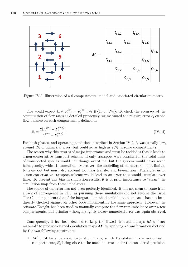
130 modelling large-scale hydrodynamics
3 6
2 5
1 4
𝑄1,2 𝑄1,4
𝑄2,1 𝑄2,3 𝑄2,5
𝑄3,2 𝑄3,6
𝑄4,1 𝑄4,5
𝑄5,2 𝑄5,4 𝑄5,6
𝑄6,3 𝑄6,5
𝑀 =
Figure IV.9: Illustration of a 6 compartments model and associated circulation matrix.
One would expect that F (in)i = F
(out)i , ∀i ∈ 1, . . . , NC. To check the accuracy of the
computation of flow rates as detailed previously, we measured the relative error ei on theflow balance on each compartment, defined as
ei = 2|F (in)i − F (out)
i |F
(in)i + F
(out)i
(IV.14)
For both phases, and operating conditions described in Section IV.2, ei was usually low,around 1% of numerical error, but could go as high as 25% in some compartments.
The reason why this error is of major importance and must be tackled is that it leads toa non-conservative transport scheme. If only transport were considered, the total massof transported species would not change over-time, but the system would never reachhomogeneity, which is unrealistic. Moreover, the modelling of bioreactors is not limitedto transport but must also account for mass transfer and bioreaction. Therefore, usinga non-conservative transport scheme would lead to an error that would cumulate overtime. To prevent any bias in simulation results, it is of prior importance to “clean” thecirculation map from these imbalances.
The source of the error has not been perfectly identified. It did not seem to come froma lack of convergence in CFD as pursuing these simulations did not resolve the issue.The C++ implementation of the integration method could be to blame as it has not beendirectly checked against an other code implementing the same approach. However thesoftware Ensight has been used to manually compute the flow rate imbalance over a fewcompartments, and a similar –thought slightly lower– numerical error was again observed.
Consequently, it has been decided to keep the flawed circulation maps M as “rawmaterial” to produce cleaned circulation maps M ′ by applying a transformation dictatedby the two following constraints:
1. M ′ must be a balanced circulation maps, which translates into errors on eachcompartments, e′i, being close to the machine error under the considered precision.

IV.5 from CFD to compartment models 131
2. M ′ should be as close as possible to M . A metric could be to minimize ‖M −M ′‖while respecting the first constraint.
The first constraint makes M ′ suitable for a coupling with transfer and bioreactionswithout cumulating numerical error over time. The second constraint ensures that thecirculation of matter as predicted by CFD computations is conserved, as much as possible,even if one has to arbitrarily modify the circulation map M .
Let Q′ij be the cleaned flow rates forming the matrix M ′ and wij the correction weightssuch that Q′ij = wijQij. This simply translates into M ′ = W M . The problemof identifying the matrix of correction weights W ∈ RN2
C+ under the previously defined
two constraints can be translated into the following multi-objective and multi-parameteroptimization problem:
minimizeW∈R
N2C
+
(1− wij)2, (i, j) ∈ 1, . . . , NC2
subject toNC∑j=1
(wijQij − wjiQji) = 0, i ∈ 1, . . . , NC
The optimization goal “minimize (1−wij)2” translates the second constraint of chang-ing M as less as possible by trying to keep correction weights as close as possible from 1.This is done under the constraint that corrected flows must satisfy the balance of flowson all compartments.
This optimization system can easily be solved using the “fmincon” function available inMATLAB [2016] optimization toolbox. This function uses a deterministic linear approachto find a minimum to the problem, under specified constraints. Note that Jacobianmatrices associated to the vector of minimization objectives, and to the vector of equalityconstraints, are easily expressed in terms of wij values which facilitates the identificationof a minimum.
The computation time associated to the minimization process was about a few minutes.Correction weights identified through this optimization process led to circulation matricesM ′ for each phase and operating condition that were balanced with an absolute error onflow balances always lower than 1.8 10−15, which is only 8 time the machine error underdouble precision. Note that this value is the maximum observed error, but for mostcompartments, this error was even lower. Therefore, the balance constraint is indeedabided to, thank to the resolution of the constrained minimization problem.
Even though circulation matrix M ′ complies with the balance constraint, the highdimension of the problem prevents ensuring that the identified minimum is global andnot only local. Therefore, there may exist a better solution to the problem than theone identified. As illustrated if Fig. IV.10, for all cases the correction weights were keptclose to 1, with a standard deviation of only 4.5%. Highest corrections were around 15%which we considered to be sufficiently low to maintain macro and meso-mixing times, andmain circulation loops, during the correction process. Therefore, we did not attempt toimprove the correction by verifying whether the identified minimum is global, or onlylocal. If needed, it will be more efficient to improve the numerical integration of flowsin order for M to be closer from a balanced circulation matrix, rather than trying toidentify the extrema of a high dimension optimization problem.

132 modelling large-scale hydrodynamics
0.8 0.85 0.9 0.95 1 1.05 1.1 1.15 1.2
Weights wij
0
50
100
150
200
Nu
mb
er
of
we
igh
t o
ccu
ren
ce
s Liquid, op. cond. 1
Gas, op. cond. 1
Liquid, op. cond. 2
Gas, op. cond. 2
Figure IV.10: Distribution of correction weights wij on compartment models associatedto each phase and operating conditions described in section IV.2.
IV.5.4 Conclusion and outlooks on the compartmentalization process
Using previous developments and pseudo-stationnary simulation results from ANSYSFluent [2015], the production of a conservative compartment model is a simple two-stepprocess:
1. Use the developed C++ tool to integrate scalar and vector fields over compartments.
2. “Clean” the obtained circulation maps by solving a multi-dimensional optimisationproblem.
For now, the second step was performed using MATLAB [2016] and functions available inits optimisation toolbox, but certainly libraries are available to integrate this step directlyin the C++ tool. Obtaining a compartment model now simply consists in defining thenumber of compartments along each direction.
For arbitrary reasons, we decided to fix the number of orthoradial divisions to Na = 6,by simply considering the number of baffles (three) and blades for bottom and top turbines(respectively six and three blades). From there, we defined the number of radial divisionsNr = 6 and axial divisions Nz = 12 to preserve similar compartment lengths along eachdirection. After the compartmentalization process, we measured the mean residentialtime associated to each compartment. Obtained min and max values are 0.281s and 4.31sfor a operation condition 1, and 0.196s and 3.08s for operating conditions 2 (see TableIV.1). These values being of the same order of magnitude than the smallest time-scaleassociated to the biological model (τ (u)
σ = 3s), we considered this compartmentalizationto be sufficient.
Developments related to the compartmentalization process came late over the courseof this PhD thesis. After obtaining a conservative compartment model, focus was quicklyshifted toward coupled simulations presented in Chapter V. Therefore, some aspectswould still require supplementary work. The first aspect, which would not need much

IV.6 conclusion 133
investment, would be to assess the sensitivity of coupled simulations to the number ofdivisions by increasing and decreasing the total number of compartments. The secondaspect lies in the exploitation of CFD results from NEPTUNE CFD [2016].
NEPTUNE CFD [2016] was used to perform unsteady simulations of the fermenterhydrodynamics. The simulated time of transient hydrodynamic cannot be directly usedto perform simulation spanning a whole fermentation culture (several days). Fields ofvelocity, phase fractions and turbulence variables evolve through time and space and canbe decomposed into mean fields, periodic fields, and noise fields. Exploiting them toobtain a unstationary compartment model would require to filter out noise fields and toensure the periodicity of field by enforcing a cyclic pattern over a short period of timethat would be repeated to span days of fermentation culture. This work might requirecoupling Proper Orthogonal Decomposition (POD) of these fields [Bergmann, 2004; Lineet al., 2013] with Fourier transform. These are only raw ideas and would require maybea year of dedicated work. In particular, we already observed an unbalance of phasemass balances with stationary CFD results. This problem will necessarily occur againwith unsteady hydrodynamics, and will be more difficult to tackle considering that theprevious constraint on circulation maps,
NC∑j=1
Qij −Qji = 0, i ∈ 1, . . . , NC,
would becomeNC∑j=1
Qij(t)−Qji(t) = Vi∂〈αi〉(t)∂t
, i ∈ 1, . . . , NC
which is not a simple scalar problem any-more. A first step would then be to attemptthese developments on liquid-only CFD simulation results. Therefore, the exploitationof the simulation results database from NEPTUNE CFD [2016] to obtain compartmentmodels has not been tackled. This database is kept for ulterior exploitation.
IV.6 Conclusion
Large-scale bioreactor always tend to be heterogeneous. This fact is particularly truefor the substrate-limited fedbatch culture which constitutes the application example ofthe overall modelling framework developed over this thesis. To account for spatial het-erogeneity and gradients, one needs to model the transport of species carried by bothphases. This, in turns, requires the knowledge of fluid velocities and spatial distributionof both phases.
In order to access hydrodynamics information, Computational Fluid Dynamics is themost suited tool as it gives a good idea of organised flow structures, associated mixingtimes and gas dispersion, without other knowledge than the system geometry and op-erating conditions. Therefore, the considered bioreactor has been simulated using twosoftware and different approaches to account for the rotating agitator shaft, and to de-scribe the gas phase.
ANSYS Fluent has been used to perform pseudo-stationary simulations using the MRFapproach. By virtually adding source terms to momentum conservation equation associ-

134 modelling large-scale hydrodynamics
ated to centrifugal and Coriolis pseudo-forces in an rotating area, this modelling approachis used to describe the effect of agitators without actually obtaining a transient hydrody-namics. In these simulations, the gas injection had to be simplified by not describing acontinuous gas phase at its injection point, to ensure computation stability.
NEPTUNE CFD was used to perform more detailed simulations, by accounting bothfor the transient –periodic– effect of agitators on velocity fields through a moving-meshapproach, and for the presence of both continuous and dispersed gas-phase using theGeneralized Large-Interface Model [Coste, 2013; Merigoux et al., 2016]. Though beingavailable for future developments related to this work, these simulation results have notbeen further exploited due to difficulties associated to the formulation of dynamic com-partment models.
CFD is a powerful tool to obtain large-scale hydrodynamics, and both used softwareallow the resolution of mass balance equation of species carried by phases. These equa-tions could account for source/sink terms in order to model bioreactions as well as theevolution of biological properties. Therefore, it could have been possible to integrate mod-els from Chapters II and III into CFD simulations. However, it has been observed thatperforming this coupling within the CFD simulation framework is actually infeasible dueto prohibitively expensive computations. This numerical cost comes from two origins: (i)the high number of mesh cells in which all variables must be resolved, and for which themetabolic model must be computed multiple times due to biological heterogeneity; (ii)the Courant condition [Courant et al., 1928] which enforces a small time-step to ensurethe stability of the transport scheme, while simulations must span dozens of hours ofbiological culture. Therefore, the use of Compartment Model Approach seems to be amore interesting choice to perform the coupling of species transport with other aspectsof the modelling.
Multiple works already focused on using CFD simulation results to form compartmentmodels. Two main methodologies exist: (i) the automatic zoning, which aims towardhomogeneous compartments in terms of some variables (i.e. turbulent kinetic energy),and (ii) the manual zoning where compartments are defined by setting arbitrary geomet-ric boundaries. The second option has been favoured as it will simplify the comparisonbetween different operating conditions, and was found not to produce significantly differ-ent results compared to the automatic zoning [Delafosse et al., 2010]. Moreover, manualzoning is a requirement if one aims at producing dynamic compartment models.
As CFD simulations ran using two different software and with a complex geometryand associated meshing, specific developments were required to perform the integrationof scalar and vector fields over the manually defined compartmentalization. Both ANSYSFluent and NEPTUNE CFD can export results in the same –documented– Ensight Goldformat which enabled the development of a common tool to perform these integrations.An approach based on mesh refinement –or splitting– has been proposed and successfullyapplied to pseudo-stationary CFD results originating from ANSYS Fluent. Numericalerror led to a non-conservative compartment model but this could be easily solved bya simple optimization-based correction of the circulation map. The formulation of thisoptimization problem was facilitated by the pseudo-steady state associated to the MRFapproach. While the use of the same integration tool could be directly applied to unsteadyCFD results from Neptune CFD, the fact that local phase fractions evolve over timecomplicates the post-integration correction of computed flow to obtain a conservativecompartment model. This task has not been tackled over the course of this work and isleft for future developments.

IV.6 conclusion 135
Overall, through the use of numerical tools, it has been possible to obtain a conserva-tive gas-liquid compartment model for multiple operation conditions on an industrial fer-menter. Through Chapter II to IV, all scales of interest for the description of bioreactorshave been modelled, using matched accuracy. Simulation coupling transport, biologicalheterogeneity and dynamic metabolism are therefore accessible as it will be demonstratedin the following chapter.


VS I M U L AT I O N D ’ U N B I O R E AC T E U R I N D U S T R I E L
Resume
En couplant les developpements issus des Chapitres precedents, en particulier le modelemetabolique pour S. cerevisiae (Chapitre II), la resolution d’une equation de bilan depopulation par la methode EQMOM (Chapitre III) et les modeles de compartimentsd’un bioreacteur industriel (Chapitre IV), il est desormais possible de realiser la simula-tion de cultures industrielles et d’illustrer les capacites de la structure proposee pour lamodelisation des bioreacteurs. Ces simulations sont le sujet principal de ce Chapitre.
Dans un premier temps, les modeles et methodes numeriques precedemment developpessont resumes afin de souligner en quoi leur usage couple induit une modelisation fermeedes bioreacteurs integrant les aspects listes au Chapitre I : fonctionnement cellulaireinterne, gradients aux grandes echelles et leur couplage bidirectionnel au travers del’heterogeneite biologique. De plus, la maniere dont est modelisee l’articulation entrelimitations biologiques et environnementales est detaillee ici, et s’appuie sur des con-siderations abordees dans les Chapitres precedents.
Le systeme simule est un fermenteur industriel operant en culture fedbatch. Ces cul-tures sont parmis les plus difficiles a simuler car leurs comportements sont sensibles aussibien aux conditions initiales du systeme qu’aux conditions operatoires tout au long de laculture. Afin de se defaire de ces sensibilites, nous simulerons un etat pseudo-stationnairede la culture. Ces simulations visent a quantifier l’effet des conditions operatoires demelange et d’injection de gaz, ainsi que l’importance de la strategie d’injection du sub-strat, sur l’apparition de comportements metaboliques indesirables, i.e. les productionsd’ethanol et d’acetate.
Il est ainsi montre que dans des conditions operatoires de reference, ethanol et acetatesont produits en consequence (i) d’un transfert gaz-liquide d’oxygene insuffisant et (ii)d’un dysfonctionnement metabolique attribue a l’effet Crabtree. En multipliant lespoints d’injection du substrat principal, nous montrons que la production d’ethanol peutetre reduite de 48% sans cout energetique supplementaire. En augmentant la depenseenergetique par un melange plus rapide et un debit de gaz injecte plus eleve, la productiond’ethanol peut etre entierement inhibee. Ces simulations, servant de preuves de concepta la mise en œuvre de la modelisation proposee des bioreacteurs, montrent l’interet dedisposer de tels outils facilitant les prises de decision sur les problematiques d’ingenierie.
137


VS I M U L AT I O N O F A N I N D U S T R I A L F E R M E N T E R
Summary
By coupling developments from previous Chapters, namely the S. cerevisiae metabolicmodel from Chapter II, the resolution of the population balance using EQMOM as de-tailed in Chapter III and the compartment models from Chapter IV, it is now possible toperform simulations of an industrial fermenter to show the capabilities of the proposedbioreactor modelling framework. These simulations are the core topic of this Chapter.
Previously detailed models and numerical methods are first summarized to underlinehow their conjoint use form a closed bioreactor model that accounts for all aspects listedin Chapter I: inner cell functioning, large-scale gradients, and their two-way couplingthrough biological heterogeneity. Moreover, the articulation between biological and envi-ronmental metabolic limitations is discussed here as this aspect requires considerationsfrom all three previous Chapters.
The simulated system is an industrial fermenter used in fedbatch culture mode. Thesecultures are the most difficult to simulate as their courses depend both on initial condi-tions and operating conditions over time. In order to discard any effect of initial condi-tions, we choose to simulate a pseudo-stationary state of the system. These simulationsaim at quantifying the effect of mixing and gas-flow rate operating conditions, as wellas the importance of the substrate injection strategy, on the occurrence of undesiredmetabolic behaviours, i.e. the productions of ethanol or acetate.
It is shown that under reference operating conditions, ethanol and acetate are producedas a consequence of both (i) poor gas-liquid mass transfer of oxygen and (ii) metabolicdysfunction due to the Crabtree effect. By changing the substrate injection design, weshow that the ethanol production can be reduced by 48% at no extra energetic cost. Byincreasing the energetic expense through faster mixing and higher gas-flow rates, thisethanol production can be entirely prevented. These proof-of-concept simulations of alarge-scale bioreactor show the interest of such a decision-assisting tool for engineeringpurposes.
139


VS I M U L AT I O N O F A N I N D U S T R I A L F E R M E N T E R
V.1 Introduction
The simulation of all phenomenon in bioreactors is a challenging topic, and will requirea computational power that will probably not be accessible within the next few yearsor even decades. However, as it has been thoroughly discussed throughout this thesis,describing all details of these phenomenon is not actually required, which allows for asimplified yet complete enough modelling of industrial fermenters. This Chapter will focuson demonstrating that, indeed, accurate enough simulations of large-scale fermenters canbe performed, at reasonable numerical cost, to obtain an engineering assisting tool. Doingso will require to integrate developments of previous three Chapters.
Chapters II, III and IV focused on the development or applications of models andnumerical methods that, when coupled, yield a bioreactor model complete enough to ac-count simultaneously for large-scale gradients, biological heterogeneity, and metabolismcomplexity. More specifically, Chapter IV presented the methodology used to obtain agas-liquid hydrodynamic model of an actual industrial fermenter. Chapter III focusedon numerical methods to efficiently account for biological heterogeneity in terms of somedynamic parameters whose effect on metabolism is non negligible. Finally, Chapter II de-tailed a structure for metabolic models that can account for most cell behaviour observedexperimentally, but at a very low numerical cost. Section V.2 sums-up these models,methods, and the way they can easily be used together.
Developed models will be applied to the simulation of a the culture of S. cerevisiae, inthe bioreactor presented in Chapter IV. Section V.3 details these simulations in terms ofculture mode, operating conditions, and simulation tool. Section V.4 presents results ofthese simulations and underlines how these could be used for engineering purposes.
V.2 Summary of developed model
Chapter I details most approaches that can be used to model bioreactors. We selectedthose that appeared to be the most numerically efficient, while being accurate enough, toobtain a model that do not neglect spatial nor biological heterogeneities, and accounts formetabolic consequences of these heterogeneities. Hereafter, these approaches are brieflyreminded to clarify which set of equations is solved, and which closures are used. Somemodelling aspects, related to limitations of mass transfer between phases have not beenparticularly considered in previous Chapters and will be detailed in this section.
141

142 simulation of an industrial fermenter
V.2.1 Mass balance equations
Simulations detailed in Section V.4 are about fedbatch cultures of S. cerevisiae in anindustrial-scale gas-liquid fermenter. The model developed for this yeast in Chapter IIaccounts for four species dissolved in the liquid phase that can be ingested or producedby cells: glucose, ethanol, acetate and oxygen. Out of these, only oxygen also exists inthe gas phase. It has been explained in Chapter IV that spatial heterogeneity will beaccounted for by a Compartment Model Approach, and in chapter III that biologicalheterogeneity will be tracked using moment methods applied to a 5 variables PopulationBalance Equation (PBE).
Therefore, simulations will track three vectors: liquid-phase concentrations CL =[GL, EL, AL, OL]T , gas-phase concentrations CG = [OG] and moments of biological-phase properties distribution M , in each compartment of the hydrodynamic model:
∂εL,iViCL,i(t)∂t
=NC∑j=1
Q(L)j,i CL,j(t)−CL,i(t)
NC∑j=1
Q(L)i,j + ΦBL,i + ΦGL,i (V.1)
∂εG,iViCG,i(t)∂t
=NC∑j=1
Q(G)j,i CG,j(t)−CG,i(t)
NC∑j=1
Q(G)i,j + ΦLG,i (V.2)
∂εL,iViMi(t)∂t
=NC∑j=1
Q(L)j,i Mj(t)−Mi(t)
NC∑j=1
Q(L)i,j +Zi (V.3)
All terms appearing in these balance equations are detailed hereafter.
V.2.2 Compartment models for industrial fermenters
The transport of dissolved or biological species by gas and liquid phases is described bya Compartment Approach. This model describes the industrial fermenter as NC = 432compartments as described in Chapter IV and illustrated in Fig. IV.6 through a manualzoning approach.
This models defines Vi as the i-th compartment volume (m3); εL,i and εG,i respectivelythe liquid and gas phase fraction (m3
L/m3 and m3G/m3); Q(L)
i,j and Q(G)i,j the volumetric
flow rate from the i-th to the j-th compartment for the liquid and gas phases (m3L/s and
m3G/s).
Chapter IV detailed how these model parameters could be obtained from a pseudo-stationary Computational Fluid Dynamics (CFD) simulation of the industrial fermenter.Therefore, for upcoming simulations, these parameters will be kept constant over time.Further work will be required to obtain transient compartment models. Note that inthe compartmentalization process, fields of turbulent kinetic energy k (J/kgL) and itsdissipation rate ε (W/kgL) were post-processed so that following models may access kiand εi in each compartment if required. This will be of particular interest in models forinter-phase mass transfer limitation.

V.2 summary of developed model 143
V.2.3 Population Balance Equations tracking biological heterogeneity
The metabolic model described in Chapter II and briefly recalled hereafter accounts forfive cell-attached dynamic variables:
• µ(b)G : glucose-based growth capability (gX/gX · h);
• µ(b)E : ethanol-based growth capability (gX/gX · h);
• µ(b)A : acetate-based growth capability (gX/gX · h);
• ϕ(b)O : oxidative capability (molO/gX · h);
• σ: glycolytic stress.
Let p = [µ(b)G , µ
(b)E , µ
(b)A , ϕ
(b)O , σ]T be the vector of these properties, and ni(p) the sta-
tistical distribution of these properties over cells located in the i-th compartment. Thisdistribution is defined such that∫
Ωpni(p)dp = XL,i (V.4)
where XL,i is the biomass concentration (kgX/m3L) in the i-th compartment.
A PBE tracking ni(p) is
∂εL,iVini(p, t)∂t
+ εL,iVi∇ ·(ζ(p,CL,i)n(p)
)=
NC∑j=1
(Q
(L)j,i nj(p, t)− ni(p, t)Q
(L)i,j
)+∫
ΩprX(p′,CL,i)β(p, p′)n(p′)dp′ (V.5)
where ζ(p,CL,i) is the vector of adaptation rates of biological properties, rX(p,CL) is theactual growth rate of cells of properties p in a liquid environment of composition CL, andβ(p, p′) the probability that a cell of properties p′ yields a daughter cell of properties p.The modelling of ζ(p,CL,i) and rX(p,CL) is handled hereafter by the metabolic model.
Due to a lack of experimental data, β(p, p′) will simply be defined as a 5-dimensionalDirac distribution∫
Ωpf(p′)β(p, p′)dp′ = f(p) (V.6)
which implies that daughter cells inherit properties of their mother.The use of moment methods has been selected in Chapter III for their efficiency. Let
moments of n(p) be defined as
mk1,k2,k3,k4,k5 =∫
ΩµG
∫ΩµE
∫ΩµA
∫ΩΦO
∫Ωσµk1G µ
k2E µ
k3A ϕ
k4O σ
k5n(p)dσdϕOdµAdµEdµG (V.7)

144 simulation of an industrial fermenter
Due to the fact that only monovariate numerical methods were considered in Chapter III,only following uncoupled moments will be resolved:
M =
m0,0,0,0,0m1,0,0,0,0m0,1,0,0,0m0,0,1,0,0m0,0,0,1,0m0,0,0,0,1
...m0,0,0,0,Nmσ
=
XL
µGXL
µEXL
µAXL
ϕOXL
σXL...
m0,0,0,0,Nmσ
(V.8)
with Nmσ the number of moments resolved along the stress dimension of the distribution.x denotes a population mean variable. The rational behind the choice of these momentshas been detailed in Section III.7.
The Extended Quadrature Method of Moments (EQMOM) will be applied on momentsm0,0,0,0,k5 , k5 ∈ 0, . . . , Nmσ to obtain a quadrature rule wQ = [w1, . . . , wQ]T , σQ =[σ1, . . . , σQ]T , such that
∫Ωpf(p)n(p)dp ≈
Q∑j=1
wjf(pj) (V.9)
with pj = [µG µE µA ΦO σj]T .
V.2.4 Metabolic model for S. cerevisiae
The metabolic model of S. cerevisiae allows the computation of rCL , rX and ζ, consideringbiological properties p and the environment composition CL, with
rCL(p,CL) =
rG(p,CL)rE(p,CL)rA(p,CL)rO(p,CL)
, ζ(p,CL) =
ζµG(p,CL)ζµE(p,CL)ζµA(p,CL)ζΦO(p,CL)ζσ(p,CL)
(V.10)
ri is the rate of consumption or production of i ∈ G,E,A,O,X (kgi/kgX · h), and ζithe rate of adaptation of the biological property i ∈ µG, µe, µA,ΦO, σ ([unit of i]/h).The model structure proposed in Chapter II performs these computations at very lownumerical cost, between 135 and 150 floating-point operations by set of biological andenvironmental properties (p,CL).
ζ(p,CL) and rX(p,CL) are directly used in the moment-tracking equation. Couplingthe quadrature rule in Eq. (V.9) with rCL(p,CL) yields the mass transfer rate from liquidphase to biological phase, ΦLB,i in Eq. (V.1):
ΦLB,i =∫
ΩprCL(p,CL,i)ni(p)dp ≈
Q∑j=1
wi,jrCL(pi,j,CL,i) (V.11)

V.2 summary of developed model 145
with wi,j and pi,j the quadrature weights and nodes computed from moments Mi, j ∈1, . . . , Q.
V.2.5 Mass transfer between gas and liquid phases
As briefly described in Section I.6.1, the model for gas-liquid mass-transfer will onlyconsider the resistance to transfer in the liquid phase. The transfer rate of oxygen willbe described by
ΦGL,O = kLa∗V (H OG −OL) (V.12)
with
• kL the liquid-film resistance to transfer (m/s);
• a∗ the specific inter-facial area (m2/m3);
• V the considered volume of control (m3);
• H the Henry constant for oxygen at the culture temperature (kgOL/kgOG).
The specific transfer area will be deduced from an estimated mean bubble diameter ofdb ≈ 1cm and the local gas fraction εG:
a∗ = 6εGdb
(V.13)
The resistance to transfer, kL, is modelled using the following correlation from Kawaseet al. [1992]; Laakkonen et al. [2006] suited for mass transfer in bioreactors:
kL = 0.3√DO,L
(ε
εGνG + εLνL
)1/4(V.14)
with DO,L = 1.98 10−9m2/s the oxygen diffusivity in water, and νk = µk/ρk the kinematicviscosity of phase k (m2/s).
The solubility was set to H = 0.0272kgOL/kgOG which corresponds to a saturationoxygen concentration of 7.8gO/m3
L for water at equilibrium with surrounding air underatmospheric pressure and a temperature of 20°C.
Oxygen being the only compound that transfers between gas and liquid phases, vectorsof gas-liquid transfer rates in Eqs. (V.1-V.2) are simply defined as
ΦGL =
000
ΦGL,O
, ΦLG = [−ΦGL,O] (V.15)

146 simulation of an industrial fermenter
V.2.6 Mass transfer toward the biological phase
Integrating biological and physical regimes in the modelling
As for now, the coupling of a metabolic model with the description of a variable environ-ment has not been properly addressed while this topic is key to the modelling of industrialbioreactors.
In Chapter II, the metabolic model was formulated by assuming that one knows the fluxof matter (glucose, ethanol, acetate, oxygen) that cells are able to assimilate. These valueswere defined as cell-attached properties, either constant for carbonaceous substrates (ϕ(b)
G ,ϕ
(b)E and ϕ
(b)A ) or variable for the oxidative capability (ϕ(b)
O ). These fluxes are meaningfulwhen the cell functioning, or bioreactions in general, are in the biological regime: whengrowth is limited by cells capabilities to process substrate available in the environment.Biological regime occurs when the environment is rich in substrates compared to a cellcapability to process that substrate.
The inverse situation is the physical regime, which occurs when the environment is poorcompared to cell capabilities. The coupled modelling must be able to account for bothbiological and physical regimes, as well as the transitional regime where both limitationoccurs. This will allow the model to deal with poor –limiting– environments.
Initial proposition based on Monod kinetics
In previous work [Pigou and Morchain, 2015], we considered the modelling of E. coli anddescribed the glucose-based growth capability µ(b)
G as a dynamic variable attached to cells,and compared it to the Monod equilibrium growth rate µ∗G, to assess whether the cellwas in the biological or the physical regime. Under this approach, the actual growth rateµ
(a)G was defined as
µ(a)G = min(µ(b)
G , µ∗G) (V.16)
which exhibited expected asymptotic behaviours:µ(a)G = µ
(b)G G KG
µ(a)G = 0 G 7→ 0
(V.17)
with KG the affinity of cells toward glucose (kgG/m3L).
Despite its correct asymptotic behaviour, the approach based on Monod kinetic law isunsatisfactory on multiple regards.
1. This approach associates instantaneous metabolic behaviours to variables definedafter a long-term adaptation of a population to its environment, i.e. the equilibriumgrowth-rate µ∗.
2. As 0 ≤ µ∗G ≤ µ(max)G by definition of Monod kinetics, this formulation forbids cells
to have an actual growth rate higher than µ(max)G , despite experimental proofs that
exceeding this Monod maximum growth-rate is actually feasible at the cell-scale.
3. This formulation does not explicit why cells actually slow their growth rate downin poor environments.

V.2 summary of developed model 147
For these reasons, a more satisfactory and predictive description of the switch betweenphysical and biological regimes has been looked for.
A micro-mixing issue
It is easily understood that transport of substrate in the culture medium up to a cellmembrane precedes its uptake and use in anabolic or catabolic reactions. Bioreactionscan then be limited by either (i) external transport, (ii) mass transfer through the bio-logical membrane or (iii) internal transport and/or availability of reaction catalyzers (i.e.enzymes).
In models developed in Chapter II for E. coli and S. cerevisiae, limitations of transportthrough the biological membrane and of reactive capabilities are encompassed within (i)maximum consumption flow rates ϕ(b)
G,E,A,O and (ii) growth capabilities µ(b)G,E,A. A lack
of these capabilities will induce a biological regime for growth or reaction.Therefore, including physical regime to the model requires to account for limitations of
external transport too. On many regards, biological systems can be analysed under thepoint of view of heterogeneous catalysis. Micro-organisms behave as reactive particlesin a turbulent flow that catalyse the transformation of substrates into products and by-products, and also happen to generate new reactive particles through cell division orbudding. To analyse heterogeneous catalysis systems, a classical approach in chemicalengineering is to compare the reaction rate to the transport rate of reactants. This isdone through the so-called Damkohler number Da:
Da = (bio)reaction ratetransport rate = transport characteristic time-scale
(bio)reaction characteristic time-scale (V.18)
where Da 1 denotes a reactive –or biological– regime, and Da 1 denotes a physicalregime. Detecting the regime then requires the identification of the limiting transportphenomenon. Considering the cell size (≈ 5−10µm), the liquid medium surrounding cellswill be renewed through micromixing that encompasses both engulfment micromixingat the Kolmogorov scale, and diffusive mixing at the Batchelor scale [Delafosse, 2008].Therefore, we previously proposed [Morchain et al., 2016] to base the physical limitationof bioreactions on the micro-mixing time-scale associated to the lifespan of engulfingeddies [Baldyga and Bourne, 1999]:
τE ≈ 17√µLρLε
(V.19)
with µL and ρL the dynamic viscosity (Pa · s) and density (kgL/m3L) of the liquid phase,
and ε the local turbulent-energy dissipation rate (W/kgL).Overall, transport by micro-mixing and assimilation by cells are two serial phenomenon
whose limiting rate must be simultaneously considered to compute a maximum achievableconsumption rate for substrates. Let ϕ(b)
S be the maximum specific consumption rateof substrate S ∈ G,E,A,O considering biological limitations as already defined inChapter II, and ϕ(e)
S be the maximum specific consumption rate considering environmentallimitations (kgS/kgX · h). We propose the following model for ϕ(e)
S :
ϕ(e)S ≈
SLXLτE
(V.20)
148 simulation of an industrial fermenter
with SL the substrate concentration (kgS/m3L), XL the biomass concentration (kgX/m3
L)and τE the micro-mixing time-scale as defined previously. This formulation was chosenas it is the most simple that exhibits the three following behaviours:
1. If the environment is depleted in terms of substrate S, environmental limitationoccurs: lim
S 7→0ϕ
(e)S = 0.
2. At low turbulence, micro-mixing is inefficient and a limitation occurs: limε7→0
ϕ(e)S = 0.
3. At constant substrate concentration, if the amount of biomass increases, less sub-strate will be available per cell as we assume that substrate is distributed evenlybetween micro-organisms: lim
X 7→+∞ϕ
(e)S = 0
Once maximum consumption rates associated to environment limitations ϕ(e)S and to
biological limitations ϕ(b)S are known, one has to compute a global maximum consumption
rate ϕ(g)S which cannot be higher than either ϕ(e)
S or ϕ(b)S . We chose to apply the following
formulation, based on serial resistance law:
1ϕ
(g)S
= 1ϕ
(e)S
+ 1ϕ
(b)S
⇔ ϕ(g)S = ϕ
(e)S ϕ
(b)S
ϕ(e)S + ϕ
(b)S
(V.21)
This formulation has the same asymptotic behaviours than a simple ϕ(g)S = min
(ϕ
(e)S , ϕ
(b)S
)but offers a smoother transition between biological and physical regimes.
Note that the oxygen consumption rate has been described in a slightly different man-ner. Indeed, when biological oxygen consumption exceeds gas-liquid mass transfer, theliquid phase gets depleted and oxygen consumption enters a physical regime. Suppos-edly, an equilibrium should be reached between gas-liquid mass transfer and biologicalconsumption of oxygen. However, the high sensitivity of the metabolic behaviour overoxygen consumption leads to a stiff set of Ordinary Differential Equations (ODEs) as faras oxygen mass balance equations are concerned.
In order to relax the stiffness of this problem, ϕ(e)O is defined as
ϕ(e)O ≈
OL
XLτE+ ΦGL,O
XL
(V.22)
with ΦGL,O defined previously in Eq. (V.12). This formulation implies that oxygen canbe transported to cells either by micro-mixing when dissolved oxygen is available, ordirectly from the gas-phase to cells. This could be justified by considering that, whenthe liquid phase is mainly depleted in terms of oxygen, micro-organisms close to bubbleswill directly assimilate freshly dissolved oxygen.
When the liquid phase is close to oxygen saturation, the gas-liquid transfer rate isnegligible and only micro-mixing brings oxygen to cells. On the other side, when lowoxygen concentrations are observed, cells are still able to grow using aerobic pathways,with oxygen consumption being equal to the gas-liquid transfer rate.
This formulation makes ϕ(g)O less sensitive to oxygen concentration variations in micro-
aerobic environments, and strongly stabilises simulations, without altering the physicalmeaning of the overall model.

V.2 summary of developed model 149
V.2.7 Short summary
Overall, the bioreactor modelling consists in three sets of Ordinary Differential Equationsper compartment recalled hereafter
∂CL,i(t)∂t
= 1εL,iVi
NC∑j=1
Q(L)j,i CL,j(t)−CL,i(t)
NC∑j=1
Q(L)i,j + ΦBL,i + ΦGL,i
(V.23)
∂CG,i(t)∂t
= 1εG,iVi
NC∑j=1
Q(G)j,i CG,j(t)−CG,i(t)
NC∑j=1
Q(G)i,j + ΦLG,i
(V.24)
∂Mi(t)∂t
= 1εL,iVi
NC∑j=1
Q(L)j,i Mj(t)−Mi(t)
NC∑j=1
Q(L)i,j +Zi
(V.25)
where i denotes a variable attached to the i-th compartment, and with
• εL the liquid phase fraction (m3L/m3);
• εG the gas phase fraction (m3G/m3);
• V the compartment volume (m3);
• Q(k)i,j the volumetric flow rate of the phase k ∈ G,L from the i-th to the j-th
compartment (m3k/h);
• CL = [GL, EL, AL, OL]T the vector of liquid-phase attached concentrations(kg/m3
L);
• CG = [OG] the vector of gas-phase attached concentrations (kg/m3G);
• ΦBL = [ΦBL,G, ΦBL,E, ΦBL,A, ΦBL,O]T the vector of mass transfer rates from thebiological phase to the liquid phase (kg/h);
• ΦGL = [0, 0, 0, ΦGL,O]T the vector of mass transfer rates from the gas phase tothe liquid phase (kg/h);
• ΦLG = [−ΦGL,O] the vector of mass transfer rates from the liquid phase to the gasphase (kg/h);
• M the vector of moments of the distribution of biological properties;
• Z the vector of rates of change of elements of M .
εL, εG, V are defined for each compartment, along with circulation maps Q(k)i,j , by the
compartment model computed in Chapter IV. The computation of transport terms, i.e.summations over NC compartments in Eqs. (V.23-V.25), is straightforward once thecirculation map is known.
In each compartments, following computations are performed at each time-step:
1. Compute ΦGL and ΦLG by simply computing ΦGL,O as detailed in Eq. (V.12).• Note that this computation is based on kLa
∗V values which depend on localphase fractions and turbulent dissipation rates.

150 simulation of an industrial fermenter
2. Compute the vector of local maximum specific consumption rates considering en-vironmental limitations ϕ(e) based on the local micro-mixing time-scale defined inEq. (V.19):
ϕ(e) =
ϕ
(e)G
ϕ(e)E
ϕ(e)A
ϕ(e)O
=
GL/(XLτE)EL/(XLτE)AL/(XLτE)(OL/τE + ΦGL,O)/XL
(V.26)
3. Compute a quadrature rule wQ and pQ based on moments M as detailed in SectionV.2.3, using the improved EQMOM method detailed in Chapter III.
4. Integrate the metabolic behaviour over quadrature nodes to obtain ΦBL:
ΦBL =Q∑i=1
wiϕ(a)(CL,ϕ
(e), pi) (V.27)
were ϕ(a)(CL,ϕ(e), pi) represents the actual consumption or production rates given
as output of the metabolic model detailed in Chapter II.
V.3 Simulations description
Now that the complete modelling framework has been extensively detailed in previousChapters, and summarized in Section V.2, we shall present the illustrative simulationsin which the framework has been applied. This section details a fedbatch culture andelements of comparison between multiple operating conditions.
V.3.1 A pseudo-stationary fedbatch culture
Culture mode
In the context of baker’s yeast production, many studies have shown that the excess offree glucose in the environment tends to induce aerobic ethanol production [Yamane andShimizu, 1984], which was referred to in Chapter II as the Crabtree effect. This ethanolproduction is identified as the main cause for lower conversion yields of glucose into cells.
In order to reduce this effect, a usual strategy is to perform fedbatch cultures of S.cerevisiae. In this cultivation mode, a pre-culture –usually in batch– allows to reach ahigh cell-density. After this first step, the system is continuously fed with a limitingquantity of substrate. This is expected to limit the amount of free glucose, and thus theoccurrence of aerobic ethanol formation. However, this is not always the case and theCrabtree effect may still be triggered even in glucose-limited high cell-density fedbatchcultures. This is usually attributed to poor macro-mixing of the system through theshort-term Crabtree effect.
For the industrial case of interest, the culture goal is actually not cell production, andfor undisclosed reasons, the culture medium needs to be fed both with glucose and ethanol.Note that ethanol should only be a substrate, and for efficiency reason, should not be aby-product of glucose consumption. Therefore, both for baker’s yeast production and for

V.3 simulations description 151
Figure V.1: Illustration of bioreactor culture modes. (a) Batch. (b) Fedbatch. (c) Chemo-stat.
the industrial production, it will be of interest to be able to predict the appearance ofthe Crabtree effect in large-scale fedbatch cultures of S. cerevisiae.
Difficulties associated with the simulation of fedbatch processes
There exists three classical culture modes for bioreactors, illustrated in Fig. V.1:
• Chemostat: continuous cultures with constant feeding and withdrawal of culturemedium;
• Batch: discontinuous cultures where all nutrients are initially in the culture medium;
• Fedbatch: semi-continuous cultures where the system is closed but continuouslyfed.
In terms of consequences of the culture mode on numerical simulation, one can easilyunderstand that
• In chemostat cultures, initial conditions have no effect on steady-state conditions.This steady-state is controlled by the feeding flow rate and its composition.
• In batch cultures, only initial conditions will influence the course of the culture.
• In fedbatch cultures, both initial conditions and operating conditions will impactthe course of the culture.
For these reasons, simulating a whole fedbatch culture is particularly difficult. Any erroron initial concentration, any uncertainty on the initial state of cells over the biologicalpopulation, or errors on feeding flow rate or composition, will accumulate over timeand can yield unrealistic results, mainly after considering strong interactions betweengradients and the heterogeneous metabolic behaviour.
Moreover, due to the continuous feeding, the liquid volume keeps increasing over time.Describing this effect would require a Compartment Model with dynamic compartmentvolumes and most certainly dynamic number of compartments. While being easily feasi-ble, this would still require to perform CFD simulations with multiple increasing liquid

152 simulation of an industrial fermenter
volumes, and would need some supplementary developments that were not performedover the course of this thesis.
Proposed approach: simulating a pseudo-stationnary state in the fedbatchprocess
The goal of simulations will not be to predict the evolution of concentrations over timefor the whole fedbatch process. We will assess the effect of operating conditions –i.e.stirring speed, gas-flow rate and injection mode of glucose– on the occurrence of ethanolformation due to the Crabtree effect.
Thank to the glucose-limited culture mode, the biomass concentration is expected notto increase significantly over time. Moreover, high glucose and ethanol concentrationswill be expected near their respective feeding points, but the overall system will be poorin terms of these substrates. Therefore, large-scale gradients should remain relativelyconstant over time. This will allow overcoming previously listed problems encounteredwith the simulation of a fedbatch process.
The chosen approach will be to describe glucose and ethanol feeding as volumetric masssource terms FG and FE (kgG,E/m3
L) in compartments corresponding to their respectivefeeding points, to set a biomass concentration XL corresponding to these feeding rates ofsubstrate, and to disable the increase of biomass concentration over time.
Using mass source terms simply removes the need for describing the volume increase.Moreover, disabling accumulation of biomass will let the simulation converge towardconcentration fields close to those that would be experimentally encountered when thefedbatch process reaches the biomass concentration XL. This approach can only be usedthanks to the fact that concentration fields are expected to evolve over-time in a slowermanner than local distributions of biological properties.
The same set of values XL, FG et FE will be used with all operating conditions detailedhereafter. Note that actual values cannot be disclosed for confidentiality reasons.
V.3.2 Assessed variables
The simulation tool will be used to assess the effect of following operating conditions onthe occurrence of the Crabtree effect:
• Stirring speed: 35 or 49 rotations per minute;
• Gas flow rate: 2700 or 5000Nm3/h;
• Glucose feeding strategy: unique injection point (surface feeding) or multiple injec-tion points.
These simulated conditions are summarized in Table V.1.Stirring speed and gas flow rates are variables that can be easily changed, in a certain
range of values, on an existing industrial installation. Therefore, quantifying their impacton the Crabtree effect means being able to improve the efficiency of an existing process.This is done by identifying the good trade-off between the process performance loss due tothis undesired metabolic behaviour, and the energetic expense associated to mixing andgas injection. Investigating the effect of the glucose injection strategy should generallybe reserved for process design purposes but we expect to show how critical the glucoseinjection is.
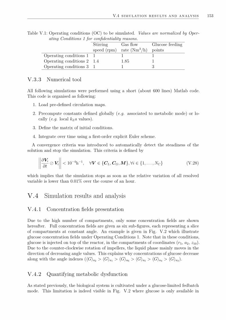
V.4 simulation results and analysis 153
Table V.1: Operating conditions (OC) to be simulated. Values are normalized by Oper-ating Conditions 1 for confidentiality reasons.
Stirringspeed (rpm)
Gas flowrate (Nm3/h)
Glucose feedingpoints
Operating conditions 1 1 1 1Operating conditions 2 1.4 1.85 1Operating conditions 3 1 1 3
V.3.3 Numerical tool
All following simulations were performed using a short (about 600 lines) Matlab code.This code is organised as following:
1. Load pre-defined circulation maps.
2. Precompute constants defined globally (e.g. associated to metabolic mode) or lo-cally (e.g. local kLa values).
3. Define the matrix of initial conditions.
4. Integrate over time using a first-order explicit Euler scheme.
A convergence criteria was introduced to automatically detect the steadiness of thesolution and stop the simulation. This criteria is defined by∣∣∣∣∣
∣∣∣∣∣∂Vi∂t Vi
∣∣∣∣∣∣∣∣∣∣ < 10−4h−1, ∀V ∈ CL,CG,M,∀i ∈ 1, . . . , NC (V.28)
which implies that the simulation stops as soon as the relative variation of all resolvedvariable is lower than 0.01% over the course of an hour.
V.4 Simulation results and analysis
V.4.1 Concentration fields presentation
Due to the high number of compartments, only some concentration fields are shownhereafter. Full concentration fields are given as six sub-figures, each representing a sliceof compartments at constant angle. An example is given in Fig. V.2 which illustrateglucose concentration fields under Operating Conditions 1. Note that in these conditions,glucose is injected on top of the reactor, in the compartments of coordinates (r5, a2, z10).Due to the counter-clockwise rotation of impellers, the liquid phase mainly moves in thedirection of decreasing angle values. This explains why concentrations of glucose decreasealong with the angle indexes (〈G〉a2 > 〈G〉a1 > 〈G〉a6 > 〈G〉a5 > 〈G〉a4 > 〈G〉a3).
V.4.2 Quantifying metabolic dysfunction
As stated previously, the biological system is cultivated under a glucose-limited fedbatchmode. This limitation is indeed visible in Fig. V.2 where glucose is only available in

154 simulation of an industrial fermenter
Figure V.2: Glucose concentration fields in steady fedbatch culture under Operating Con-ditions 1.
the downstream of the feeding point and is depleted in most of the reactor volume. Inthese conditions, the population mean growth-rate is spatially homogeneous: 〈µ(b)
G 〉 =0.0118 h−1 and max
(µ
(b)G
)−min
(µ
(b)G
)< 4.10−6 h−1 which is consistent with predictions
from Chapter III where we decided not to track the diversity of growth-rates as this wouldnot be significant.
The low growth-rate, coupled with the periodic exposure to high glucose concentrationsis expected to induce the short-term Crabtree effect through the increase of the glycolyticstress σ. We recall that this stress is indeed induced by a disequilibrium between the up-take rate (high in glucose-rich regions) and the glucose utilization rate through anabolism(spatially homogeneous). The mean value of this stress is shown in Fig. V.3 and rangesbetween min(σ) = 0.09 and max(σ) = 0.66. This corresponds to a loss of 12% to 50% ofefficiency for oxidative metabolic modes according to Eq. (II.18).
The metabolic dysfunctional can be illustrated by concentration fields of ethanol andacetate, shown in Figs. V.4 and V.5. The presence of ethanol can be partially attributedto its direct injection as a co-substrate in the compartment of coordinates (r5, a4, z9).However, the fact that highest concentrations span the whole top area of the reactorimplies that ethanol is also produced as a by-product of glucose fermentation. Thisfermentation is due to the short-term Crabtree effect, which limits the use of oxidativemetabolisms, and is reinforced by an insufficient gas-liquid mass transfer rate of oxygenwhich causes oxygen depletion in the upper part of the reactor, as shown by low residualoxygen concentrations in Fig. V.6.

V.4 simulation results and analysis 155
Figure V.3: Field of mean glycolytic stress in steady fedbatch culture under OperatingConditions 1.
Figure V.4: Field of ethanol concentration in steady fedbatch culture under OperatingConditions 1.
Figure V.5: Field of acetate concentration in steady fedbatch culture under OperatingConditions 1.
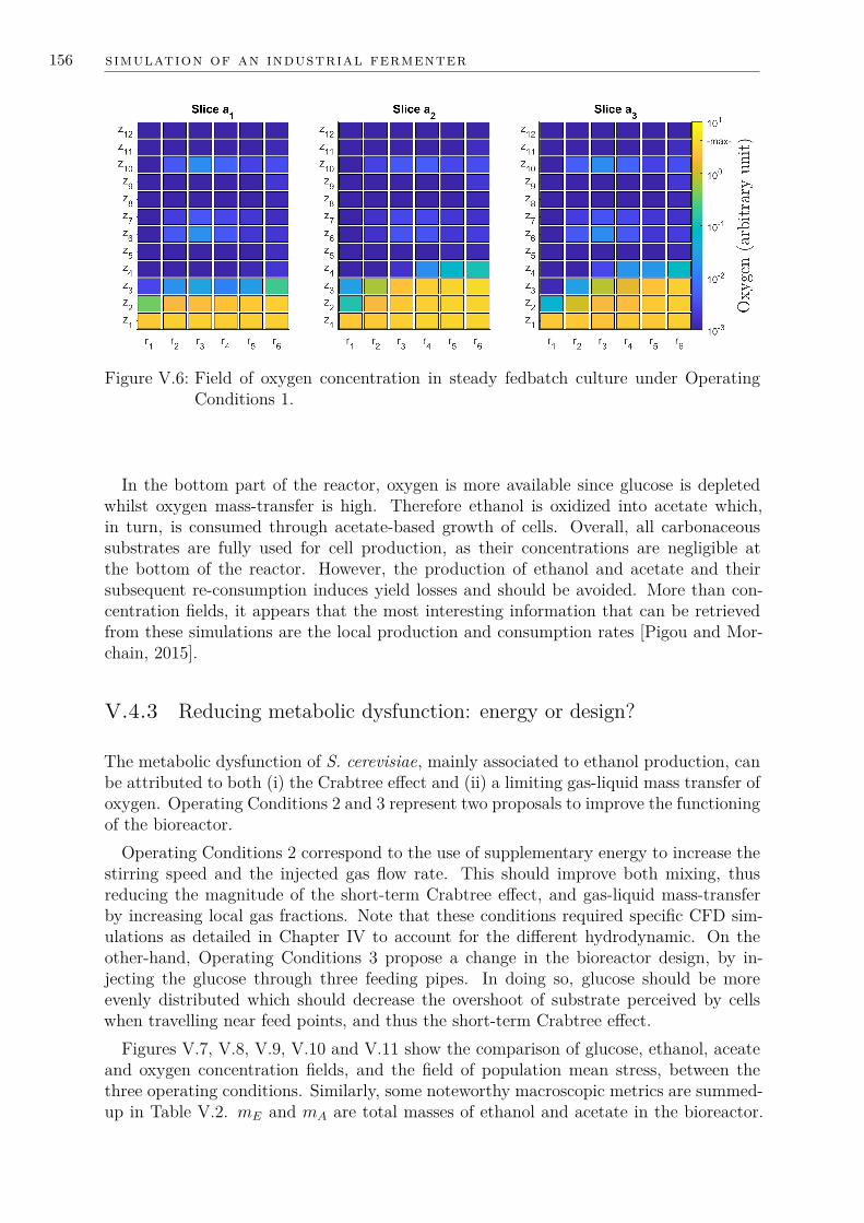
156 simulation of an industrial fermenter
Figure V.6: Field of oxygen concentration in steady fedbatch culture under OperatingConditions 1.
In the bottom part of the reactor, oxygen is more available since glucose is depletedwhilst oxygen mass-transfer is high. Therefore ethanol is oxidized into acetate which,in turn, is consumed through acetate-based growth of cells. Overall, all carbonaceoussubstrates are fully used for cell production, as their concentrations are negligible atthe bottom of the reactor. However, the production of ethanol and acetate and theirsubsequent re-consumption induces yield losses and should be avoided. More than con-centration fields, it appears that the most interesting information that can be retrievedfrom these simulations are the local production and consumption rates [Pigou and Mor-chain, 2015].
V.4.3 Reducing metabolic dysfunction: energy or design?
The metabolic dysfunction of S. cerevisiae, mainly associated to ethanol production, canbe attributed to both (i) the Crabtree effect and (ii) a limiting gas-liquid mass transfer ofoxygen. Operating Conditions 2 and 3 represent two proposals to improve the functioningof the bioreactor.
Operating Conditions 2 correspond to the use of supplementary energy to increase thestirring speed and the injected gas flow rate. This should improve both mixing, thusreducing the magnitude of the short-term Crabtree effect, and gas-liquid mass-transferby increasing local gas fractions. Note that these conditions required specific CFD sim-ulations as detailed in Chapter IV to account for the different hydrodynamic. On theother-hand, Operating Conditions 3 propose a change in the bioreactor design, by in-jecting the glucose through three feeding pipes. In doing so, glucose should be moreevenly distributed which should decrease the overshoot of substrate perceived by cellswhen travelling near feed points, and thus the short-term Crabtree effect.
Figures V.7, V.8, V.9, V.10 and V.11 show the comparison of glucose, ethanol, aceateand oxygen concentration fields, and the field of population mean stress, between thethree operating conditions. Similarly, some noteworthy macroscopic metrics are summed-up in Table V.2. mE and mA are total masses of ethanol and acetate in the bioreactor.

V.4 simulation results and analysis 157
Figure V.7: Comparison of glucose concentration fields between simulated operating con-ditions on compartment slice a2.
Figure V.8: Comparison of ethanol concentration fields between simulated operating con-ditions on compartment slice a2.
mσ is expressed in terms of mass of biomass but no physical meaning should be lookedfor this variable. It is defined as
mσ =∫∫∫
V
∫Ωσσn(σ)dσdV, with n(σ) =
∫ΩµG
∫ΩµE
∫ΩµA
∫ΩΦO
n(p)dΦOdµAdµEdµG
(V.29)
which is the volumic integral of m0,0,0,0,1. σ was defined as an adimensional quantitymeasuring the stress level of cell between 0 and 1. By its definition, mσ is expressed asa mass of biomass, but should be interpreted as a “quantity of stress” in the reactor.
By simply looking at ethanol and acetate concentration fields, Operating Conditions 2which correspond to higher stirring and gas-flow rates are the more favourable in terms ofperformances and reduction of metabolic dysfunctions. The explanation for this mainlylies in the elevated oxygen concentrations. These are the consequence of an enhancedgas-liquid mass transfer of oxygen thanks to (i) higher local gas fractions and inter-facialarea, and (ii) increased turbulence which favourably affects the mass transfer coefficientkL.
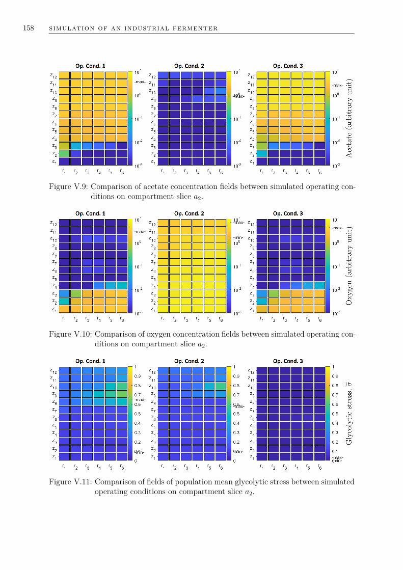
158 simulation of an industrial fermenter
Figure V.9: Comparison of acetate concentration fields between simulated operating con-ditions on compartment slice a2.
Figure V.10: Comparison of oxygen concentration fields between simulated operating con-ditions on compartment slice a2.
Figure V.11: Comparison of fields of population mean glycolytic stress between simulatedoperating conditions on compartment slice a2.

V.4 simulation results and analysis 159
Table V.2: Macroscopic metrics comparing performances of the three simulated operatingconditions. Values normalized by Operating Conditions 1 results (except formin(σ) and max(σ)). Units are those of raw (not normalized) values.
Op. Cond. 1 Op. Cond. 2 Op. Cond. 3max(GL) (gG/L) 1.00 1.13 0.47mE (kgE) 1.00 0.02 0.52mA (kgA) 1.00 0.03 1.44〈OL〉 (mgO/L) 1.00 16.7 1.03min(σ) 0.09 0.10 0.00max(σ) 0.65 0.57 0.04mσ (kgX) 1.00 0.76 0.04
Under Operating Conditions 2, the stress level is slightly lower than in the referencecase (Op. Cond. 1). Indeed the higher stirring rate induces a shorter residence time inthe feeding zones where the maximum glucose concentration is also smaller. Both effectsdecrease cell exposure to stressing conditions. However, this decrease in stress levels isnot especially significant compared to the reference case. Coupling this observation withthe low amount of ethanol observed under Op. Cond. 2 allows inferring that the ethanolproduced in reference conditions is mainly attributed to the limiting oxygenation of theliquid phase. This conclusion is reinforced by results of simulations under Op. Cond. 3.
When changing the reference case by injecting glucose through three different feedingpoints (located in compartments of heights z2, z6 and z10, radius r5 and angle a2), itbecomes visible in Fig. V.11 that the stress level has fallen down to zero everywhere in thereactor. This can be explained by the fact that a significant part of the bioreactor volumenow contains glucose (Fig. V.7) in noticeable amounts, and that over-concentrations atfeeding points are less stressing (see max(G) in Tab. V.2). Therefore, maximum stresslevels under Op. Cond. 3 are lower than minimum stress levels in the two other conditions.Resolving the stress issue and the occurrence of the Crabtree effect partially resolves theethanol production issue by decreasing its quantity by 48% (see mE in Tab. V.2).
A surprising result from these simulations is the slight increase of acetate quantitiesdue to the multiple point injection of glucose. This can be explained by subtleties of themetabolic models from Chapter II: the presence of a significant amount of glucose in alarger fraction of the bioreactor volume, under Op. Cond. 3, strongly inhibits growth onethanol. However, the currently proposed metabolic model assumes a constant ethanoluptake rate unless the environment is limiting. By inhibiting growth on ethanol while notvarying the uptake rate of this substrate, the metabolic model predicts that this substratewill be diverted toward ethanol oxidation into acetate (metabolic mode E2). Whether thisbehaviour is consistent with experimental data is yet to be checked. If it is not, this showsthat the metabolic model could still be improved, in particular by considering varyingbiological limits on uptake rates as currently considered by Quedeville et al. [2018].
Overall, these simulations show the interest of a modelling framework for bioreactorswhich allows for fast simulations. Here, we could identify the cause for ethanol productionin an industrial fermenter, and therefore a way to decrease these negative effects, i.e. theincrease of oxygen mass-transfer rate. We could also quantify the effect of a better reactordesign by showing a reduction of ethanol concentrations by 50% simply by distributingthe glucose feeding over three points instead of a single one. Operating conditions athigher stirring and gas-flow rates have shown to significantly decrease ethanol produc-

160 simulation of an industrial fermenter
tion, but the study could be pushed further by identifying the optimal trade-off betweenthis undesired ethanol production, and the energetic cost of the process. In particular,energetic expense is known to increase as the cube of the stirring speed, therefore onecould use the proposed simulation framework to identify the lowest stirring speed whichstill prevents ethanol production. It is easy to see how this tool can find its place intechnical studies offices as an engineering or decision-assisting tool.
V.4.4 Numerical cost
Presented simulations ran in almost real-time using a simple Matlab code. Matlab is aprogramming language known for its ease-of-use and the accessibility of advanced routinesfor scientific computing, but this is an interpreted language, which consequently does notmake an efficient use of computing resources. This is in particular true when one usesmultiple routines, each defining its own variables, as this has been the case with themetabolic model and the EQMOM moment-inversion procedure in previously describedsimulations. For this reason, it might be beneficial to estimate the gain that would beprovided by switching simulations toward a compiled language.
First, we estimate the numerical cost (in floating-point operations, flop) associated tocomputations performed at each time-step and in each compartment. This correspondsto following operations:
• 1 call to a 2-nodes EQMOM moment-inversion procedure ≈ 800 flop [Pigou et al.,2018a],
• 5 calls to the metabolic model for S. cerevisiae ≈ 5× 140 = 700 flop,
• time-advancement of variables, computation of stopping criteria, computation ofgas-liquid mass-transfer rate, . . .≈ 50 flop
. To simulate one hour of culture, using timesteps δt = 1.10−5 h, the number of operationrequired is then Nflop ≈ 105×432×(800+700+50) ≈ 1010 flop. This number of operationsis not high even for mid-range CPUs present on current desktop computers. The actualcomputing throughput of a CPU is always hard to predict, as different codes will nothave the same vectorizability, especially when iterative algorithms such as the EQMOMmoment-inversion procedure are involved. However, any current CPU should be ableto process 1010 flop within a few seconds with a tight memory management. Over thecourse of this PhD thesis, an engineer wrote a C++ code that reproduced simulationsfrom Pigou and Morchain [2015]. Our Matlab code needed one day to perform associatedsimulations while the C++ code obtained the same results within only ten seconds.
Therefore, the coupling of compartment, population balance and mode-based metabolicmodels does allow for fast simulations on industrial bioreactors. A “slow” Matlab codewas able to perform these simulations in real-time, but translating this interpreted codeinto a compiled language could allow for much faster than real-time simulations. Thisopens the door for many engineering applications, from parametric optimization of theprocess to real-time simulation-based control of an industrial installation.

V.5 conclusion 161
V.5 Conclusion
The modelling of industrial bioreactors is a challenging topic as one must account forlarge-scale hydrodynamics as well as the peculiarities of the biological phase which ismade of dynamic living systems and therefore tends to become heterogeneous. To per-form predictive simulations while using limited computational resources, we choose tocouple a metabolic designed in Chapter II, a population balance model tackled by a nu-merical method improved in Chapter III and compartment models deduced from CFDsimulations in Chapter IV. Numerical methods and procedures associated to these modelswere designed, improved or selected for their efficiency in order to reach fast simulationtimes.
One aspect that was missing from previous Chapters developments is the limitation ofsubstrate uptake by cells due to limiting environments. This aspects has been introducedin the modelling by following preliminary developments detailed in Morchain et al. [2016]based on micro-mixing considerations and classical chemical engineering approaches. Clo-sure laws have been suggested to simultaneously account for environmental and biologicallimits on uptake rates.
By applying these developments to an industrial example, we could show the capa-bilities of this modelling framework. Using a simple MATLAB [2016] implementation,we could simulate in real-time an industrial bioreactor to quantitatively assess the effectof some operating conditions, namely the stirring speed and the gas-flow rate, and toillustrate the use of this tool for bioreactor design purposes. This shows the feasibility ofsimulating large-scale bioreactors while accounting for both physical and biological het-erogeneities, on standard computing resources, and opens the door to the developmentof engineering software.


VIO U T L O O K S A N D C O N C L U S I O N S
VI.1 Introduction
The simulation of industrial biological systems form a vast topic encompassing a varietyof strikingly different aspects, from the comprehension of the living organisms chemistryand of advanced numerical methods, to high-performance computing and chemical engi-neering. Many of these aspects were, at least partially, considered over the course of thisPhD thesis as demonstrated in previous Chapters.
To cover both metabolic modelling, advanced numerical methods for population bal-ance, the mastering of Computational Fluid Dynamics (CFD) software and the develop-ment of numerous processing and simulation tools, over the course of three years, choicehad to be made about what could, and could not, be reasonably done. Therefore, for eachaspect developed in previous Chapters, there is still room left for numerous improvementsand supplementary studies and developments. Though not being exhaustive, section VI.2details some of these outlooks.
Research is an “activity undertaken in order to increase the stock on knowledge [...]and the use of this knowledge to devise new applications” [OECD, 2008]. On this regard,section VI.3 serves as a general conclusion to this report with an overview of majorachievements of this work.
VI.2 Outlooks
The major goal of this thesis was to develop a model framework or structure that al-lows fast, yet accurate, simulations of bioreactors. On that regard, we mainly aimed atperforming proof-of-concept simulations coupling developed models structures, numericalmethods and tools, rather than focusing on obtaining an over-parametrized model andfit it to few experimental data. Now that these proof-of-concept simulations have beenobtained as presented in Chapter V, it will be interesting to improve the accuracy of pro-posed models to enhance their predictive capabilities, or to slightly modify the modellingframework to expand its capabilities. These aspects are discussed hereafter, by keepinga structure close to this thesis: prospect considerations for Chapter II to V are discussedone-by-one in dedicated sections.
VI.2.1 Metabolic modelling
The metabolic model structure developed in Chapter II is satisfactory on multiple regards.In particular, it allows describing dynamic cultures, including switches between multiple
163

164 outlooks and conclusions
elementary modes, while keeping a strikingly low numerical cost. This is mainly done byoutsourcing dynamic aspects to the biological heterogeneity part of the overall modelling,which track the evolution and diversity of biological properties. If the metabolic modelstructure was to be improved, the most crucial improvement might be to reduce theconstraint on the sorting of metabolic modes. A comparison with cybernetic models witha view of tracking the origin of metabolic mode shifts would be profitable. If done, theproposed solution should not significantly increase the model numerical cost, for instanceby not relying on iterative optimization methods.
Apart from the metabolic model structure definition, two main aspects should be con-sider to build upon developments presented in Chapter II. The first one is in the directcontinuation of the modelling of Saccharomyces cerevisiae. Chapter II describes a modelfor this yeasts which has been fitted against multiple experimental data sets. While be-ing satisfactory, this fitting was performed by-hand through a manual iterative procedure.The goal was to demonstrate capabilities of the model structure under dynamic perturba-tions but we did not search for the highest possible accuracy. On top of accuracy, an otheraspect is that of parameter identifiability. While designing the model, we attempted tokeep the number of parameters as low as possible to limit the risk of over-parametrizationand prevent in-identifiability of parameters. We did manage to limit the number of pa-rameters to 35 where other models required more parameters for a final model with lesscapabilities to predict the course of dynamic large-scale cultures (e.g. 87 parameters forthe model from Rizzi et al. [1997]). Nevertheless, tools and methods exist to automati-cally improve a model fitting, and to assess the identifiability of parameters [Steuer, 2007;Balsa-Canto et al., 2010; Kravaris et al., 2013; Sanchez et al., 2014]. Applying theseapproaches, using existing tools, to the currently proposed S. cerevisiae model wouldbe easily feasible and could significantly improve its predictive capabilities. Once thesedevelopments are integrated to reinforce the model definition method, one could easilyenrich the wild strain S. cerevisiae model which new elementary modes corresponding tospecific synthetic pathways corresponding to industrial interests.
A large part of this thesis work was dedicated to automating complex tasks. Whenimproving the Extended Quadrature Method of Moments in Chapter III, we automatedthe benchmark of these method implementations. As detailed in Chapter IV, we usedCFD software which, though requiring a certain level of expertise, were designed to be asuser-friendly as possible. To make use of CFD results, we developed a C++ tool whichautomatically integrates scalar and vector fields into a compartment model, and a Matlabtool to clean these models from numerical error. Even though all these automated toolswould need to be interconnected under a single platform –which has been started underthe ADENON project briefly detailed hereafter– one aspect has not been automated atall: the design of elementary-mode based metabolic models. For now, designing metabolicmodels for E. coli and S. cerevisiae required analysing experimental data from lab-scalecultures [van Dijken and Scheffers, 1986; Flikweert et al., 1999; Sweere et al., 1988],reading analysis of their metabolism dysfunctional [Pronk et al., 1996; Xu et al., 1999]and browsing databases of metabolic reactions [Heavner et al., 2013; Orth et al., 2011]to define a minimal set of required elementary modes. This work is time-consuming andwidely depends on the availability of detailed resources about a specific micro-organism.
To improve on this aspect, and possibly reach an almost fully automated modellingand simulation platform for bioreactors, tools will be required to simplify the design ofmetabolic models. One approach would be to rely on detailed metabolic network to

VI.2 outlooks 165
determine simplified networks [Gerdtzen et al., 2004] from which elementary modes canbe extracted [Trinh et al., 2008].
VI.2.2 Biological heterogeneity
The idea of tracking dynamics properties of micro-organisms is not new [Sweere et al.,1988] but coupling this description to the transport of a biological phase in an non-homogeneous system is a more demanding problem. Some attempts used Lagrangianapproaches [Lapin et al., 2006] but did not provide a reverse coupling between thesedynamic cell properties and local consumptions rates which influence gradients. Otherattempts were limited to a rough description of spatial heterogeneity by consideringsimple two-compartments set-up [Heins et al., 2015]. Our current Population Balance-based modelling results from work by Morchain [2000]; Morchain et al. [2013] who appliedPopulation Balance Model (PBM) approaches to biological systems, thus enabling a fullcoupling between a fine treatment of the biological phase and the description of time-evolving gradients [Pigou and Morchain, 2015].
In this context, we did not diverge from these ideas and, as shown in Chapter III,we kept a Population Balance treatment of the biological phase. We shifted from class-approach toward less expensive moment methods but we restricted ourselves to monovari-ate numerical methods. This is partially due to results from Pigou and Morchain [2015]where a single biological property was deemed sufficient on some regards, and to discus-sion with Lebaz et al. [2016] who, in a different context, also dealt with dynamic systemsusing monovariate Population Balance Equations (PBEs). This has shown some limits asthe metabolic model designed for S. cerevisiae happened to require at least five dynamicbiological properties. Consequently, a significant improvement of the modelling frame-work for industrial fermenters would be the ability to handle multi-variate description ofbiological heterogeneity. Two approaches could be suggested to do so while keeping thenumerical cost reasonable.
Multi-variate population balance models
Numerical methods to treat multivariate population balance models do exist. For ob-vious reasons of numerical costs, discretization methods (finite-volume, finite-element)will not be considered. However, multi-variate moment methods are available such asthe multidimensional moment-constrained maximum-entropy method [Abramov, 2007],the Conditional Quadrature Method of Moments [Yuan and Fox, 2011] or a multivariateversion of the Gauss-EQMOM approach [Pollack et al., 2016; Chalons et al., 2017]. Wecould attempt to implement and apply them to the modelling of biological systems, butfor multiples reasons, this choice might not be the most advisable.
The choice of moment-methods in place of class method for mono-variate PBMs wasmotivated in Chapter III by their extensive comparison. In particular, we could use theclass-method as a reference to ensure the accuracy for mono-variate moment methods.However, such a reference is not available for multi-variate PBMs unless one implementsfinite-volume scheme to obtain a reference resolution of the PBE under controlled accu-racy.
If a metabolic model happens to require multiple dynamic variables evolving with shorttime-scales and whose evolutions are tightly coupled, accuracy in the resolution of cou-pled moments, and on the computation of quadrature rules, will be critical. However,

166 outlooks and conclusions
it is known that increasing the number of moments does not necessarily improves sig-nificantly the accuracy of the method [Tagliani, 2001; Gzyl and Tagliani, 2010]. Thiscould already be observed in comparisons performed in Chapter III (see also Pigou et al.[2017], Appendix B) between numerical methods, where results from MaxEnt and EQ-MOM methods were only slightly sensitive to the number of resolved moments. Thecapability of multi-variate moment methods to handle any set of biological propertieswhose evolution may or may not be tightly coupled can therefore be questioned. At least,this aspect can hardly be assessed in a rational manner.
A final aspect is that of stability. Numerical methods tested in Chapter III are ap-plicable only if resolved moments remain within the realisable moment space, i.e. acomplex-geometry convex space in which moment sets correspond to actual –realisable–probability distributions. In Chapter V, we already faced instability issues when resolv-ing more than 5 moments over the distribution of glycolytic stress σ. These were dueto a time-integration scheme which did not ensure moment realisability. Some possibledevelopment could then be to derive such a realisability-preserving scheme to performtime-integration of moment sets in a Compartment Model framework, or to identifyone if this already exists. Note that while the geometry and mathematical propertiesof the realisable mono-variate moment space are well understood [Dette and Studden,1997; Gautschi, 2004], as much cannot be said for the multi-variate realisable momentspace. Therefore, deriving a realisability-preserving scheme for multi-variate problems isexpected to be a more challenging task.
Pseudo-Lagrangian/Monte-Carlo approaches
Though suited for mono-variate problems, the application of moment methods is morechallenging for multi-variate models. Class methods have also been considered for multi-variate situations, but they basically consist in a N + 3-dimensions finite volume schemeto solve the Population Balance Equation with N the number of biological propertiesand 3 the number of geometrical dimensions. This would turn to be expensive, both interms of meshing due to the extra dimensions, and in terms of global numerical cost asthis has been discussed in previous chapters.
A solution to tackle multi-variate problems for the simulation of large-scale bioreac-tors might lies in an approach that was discarded in Chapter I to consider biologicalheterogeneity: the Lagrangian approach. We oriented developments toward PopulationBalances and moment-methods following a lineage other works [Morchain and Fonade,2009; Morchain et al., 2013; Pigou and Morchain, 2015] and due to a synergy betweenmultiple projects with this thesis [Lebaz, 2015; Quedeville et al., 2018]. The Lagrangianframework solves issues associated to class and moment methods: its cost does not in-crease with the number of biological properties, its accuracy is easily controlled by thenumber of considered particles and is assessed through convergence studies. Moreover,only relevant parts of the phase-space are explored by particles which removes the draw-backs of class-methods where numerous classes happen to be empty most of the time.Finally, computations over a large-number of particles constitutes an embarrassingly par-allel problem which can strongly benefit from current advances in parallel computations.
The reason why we did not consider Lagrangian approaches sooner is because, for now,Euler-Lagrange simulations of bioreactors were limited to using the Lagrange phase as anon-reactive phase which would only record the events occurring along the trajectoriesof each particles [Lapin et al., 2004, 2006; Haringa et al., 2016]. The main difficulty is to

VI.2 outlooks 167
allow a reverse coupling: having access to the biological heterogeneity is useful only if itseffect on local uptake rates and on concentration gradients can be accounted for. Doingso within a CFD framework, which is the natural framework for Lagrangian simulations,is a major challenge.
So could we overcome these remaining difficulties? An approach that seems to resolveall issues is to couple the principle of particle-tracking along with Compartment Modelling.Under this idea, the “location” of a particle, or micro-organism, is no longer a vectorof spatial coordinates ~x, but the index of a compartment. The location of the micro-organism within the compartment is not resolved, hence the pseudo-Lagrangian approach.
The “tracking” of particles in a compartmental framework has been suggested by De-lafosse et al. [2015] which compared “trajectories” of particles with stochastic motionin a compartment model against experimental trajectories obtained through optical tra-jectography. Note that in their work, the compartment model was deduced from CFDsimulations. A particle located in the i-th compartment would leave this compartmentafter a time δt taken randomly out of the Residential Time Distribution (RTD) of anhomogeneous volume:
δt ∼ λe−λt, with λ =∑NCj=1Qij
Vi(VI.1)
Once a particle reaches its local residence time, the probability that it enters the j-thcompartment is given by
pj = Qij∑NCj=1Qij
(VI.2)
Delafosse et al. [2015] have shown the interest of this method to effectively track the roughlocations and trajectories of particles in a stirred-tank reactor under a CompartmentModel framework. Note however that they used between 19000 to 35000 compartmentsin their zonal model which is significantly high compared to the 432 compartments modelfrom Chapters IV and V. We may question the relevancy of previous closures for δt andpj if the number of compartments is significantly lowered.
To improve upon previous developments, we propose to deduce laws for δt and pjusing actual Lagrangian tracking in CFD software. It is quite simple to perform particletracking in ANSYS Fluent [2015] and to export trajectories in an Ensight Gold formatdatafile. Therefore, an easily feasible development is to improve the tool presented inChapter IV that converts CFD results into a compartment model. The goal would beto detect all events of a particle moving from one compartment i to another j, and torecord both the time of the event t, the source and destinations compartments i and j.From this information, on numerous events, it would be possible to construct probabilitydistributions from which one can randomly pick the time δt during which a particlethat entered compartment j while coming from compartment i will remain in j beforejumping into the compartment k. By extracting these easily accessible distributions fromCFD results, it should be possible to accurately mimic trajectories of particles, within acompartment model, without requiring as many compartments as Delafosse et al. [2015].This also opens the door to Monte-Carlo simulations where one does not actually solvethe trajectories of particles.
168 outlooks and conclusions
Once pseudo-Lagrangian simulations are shown to be feasible within compartmentmodel framework, it remains to explain how they actually solve previously met problems.In Chapter V, moments of the distribution of biological properties were used to createquadrature rules that allow integrating the biological behaviour over the population (seeEq. (V.27)):
ΦBL =Q∑i=1
wiϕ(a)(CL,ϕ
(e), pi) (VI.3)
Using pseudo-Lagrangian approaches, this quadrature is simply replaced by:
ΦBL = XL
Np
Np∑i=1ϕ(a)(CL,ϕ
(e), pi) (VI.4)
with Np the number of particles in the considered compartment, XL the local biomassconcentration (gX/L) and pi the vector of biological properties of the i-th particle. Theseproperties simply evolve over time as described by the following Ordinary DifferentialEquation:
∂pi∂t
= ζ(pi,CL) (VI.5)
Overall, this Lagrangian approach easily replaces the quadrature methods of moment toaccount for biological heterogeneity. However, they have the advantage of being directlycompatible with multi-variate descriptions of the biological phase, and they only spanparts of the phase-space that are relevant for the described system, thus tackling draw-backs of both the class and moment approaches. Moreover, as stated previously, theaccuracy of the method can easily be assessed through convergence studies by varyingthe total number of particles.
The main drawback of this approach will be its numerical cost that increases linearlywith the number of particles. In particular, the metabolic model (computation of ϕ(a)and ζ) must be called for each particle individually. On that regard, the low-cost of themodel structure proposed in Chapter II is beneficial, but does not prevent the fact that,to reach convergence, the number of particle per compartment Np will be higher than thenumber of quadrature nodes in moment method approaches. This is the cost for enablingmulti-variate biological models. Note however that this can be balanced by the use ofparallelisation programming techniques which are easily applicable here as the metabolicmodel can be computed in parallel between multiple particles.
VI.2.3 Large-scale hydrodynamics
This thesis was not about improving the current state-of-the-art in terms of hydrody-namics modelling for bioreactors. There is still many aspects to improve upon in termsof modelling of rheology, of gas-liquid interactions, of turbulence, . . . Improving thismodelling can be done in parallel of its coupling with biological heterogeneity and be-haviour as this will only impact the obtained compartment model. Nevertheless, thework presented in Chapter IV can be improved on two aspects. The first one is specificto the application case of the industrial fermenter, and the second one is a long-termimprovement of the proposed modelling framework.

VI.2 outlooks 169
For the CFD simulations of the industrial fermenter presented in Chapter IV, the choiceof turbulent model and of closures for momentum exchange between gas and liquid phaseshas been somehow overlooked: we did not try to choose the most recent models on thatregard. Moreover, we imposed a mono-dispersed bubble size distribution onto the gasphase, which is clearly a disputable choice considering the high gas flow rate and thelarge role of coalescence and breakage in large-scale aerated reactors [Laakkonen et al.,2006, 2007]. Therefore, to improve coupled simulations from Chapter V, a first step couldbe to improve the hydrodynamic modelling that yields the used compartment model inChapter IV. On that regard, a critical aspect would be to enable models for interfacialarea transport which would significantly improve gas-liquid interaction description, aswell as the prediction of gas-liquid oxygen mass transfer in coupled simulations [Hibikiand Ishii, 2000].
In coupled simulations of an industrial fermenter shown in Chapter V, most of thenumerical cost is associated to the treatment of the biological phase, to account for itsheterogeneity and to compute its metabolic behaviour. It would make sense to alsodedicate part of the computational power toward an improvement of the hydrodynamicdescription. In particular, for now, we presented simulations using a steady compartmentmodel, with circulation maps and local phase-fractions that were constant over time. Asalready briefly suggested in Chapter IV, it should be possible to obtain dynamic com-partment models from time-resolved CFD simulations. Doing so could improve the de-scription of interactions between the biological phase and its environment, in particularin stressing zones, by improving the prediction of exposure time of cells to these stressingsituations. Over the course of this thesis, a significant time has been spent on obtain-ing time-resolved CFD simulations using NEPTUNE CFD [2016], the development ofdynamic compartment models could rely upon these available results.
VI.2.4 Simulation of industrial fermenters
The simulation of industrial fermenters has been the core topic of this thesis. Beyondmodelling considerations that have been thoroughly explored previously, the future ofbioreactor simulation can be summed-up to two questions: why perform such simulations?and how to perform these simulations? We already started answering the first question,by illustrating the use of the proposed modelling framework for design and engineeringpurposes, the second question is far from being tackled.
Engineer toolboxes lack an integrated solution to easily perform simulations of large-scale bioreactors and most developments from this thesis could be integrated into such asoftware tool-suite. Since the prototype work that led to this PhD thesis [Pigou and Mor-chain, 2015], we have been developing the ADENON software which is a MATLAB [2016]based solution for the dynamic simulation of large-scale bioreactors. This tool providesa user-friendly graphical interface to set-up simulations coupling compartment models,metabolic modelling and population balance models solved through class or momentmethods. It was designed with modularity in mind allowing for new models (compart-ment, metabolism, . . . ) to be easily added to the database of already available models.This tools has been used to perform simulations presented in multiple published articles[Pigou and Morchain, 2015; Morchain et al., 2016; Pigou et al., 2017].
We could build upon this first software by (i) converting it into a compiled languagethus improving significantly its performances and (ii) by adding developments from Chap-

170 outlooks and conclusions
ter IV to help integrating compartment models based on CFD results. Moreover, assuggested previously, this tool-suite could integrate a tool formulating elementary-modebased metabolic model using detailed metabolic networks.
Such tools already exist in the Chemical Engineering community to assist the designand the operation of chemical processes (Aspen HYSYS, ProSim, . . . ). It is easy to seehow the biochemical engineering community could also benefit from similar software.
VI.3 General conclusion
The modelling and simulation of industrial bioreactors is a challenging topic. This lastsentence has been a leitmotiv scattered throughout this thesis. To explain these chal-lenges, our main postulate is that micro-organisms may face both internal (i.e. bio-logical) and external (i.e. environmental) limitations and that due to the scale of in-dustrial fermenters, these limitations will be at disequilibrium, inducing the well-knownmetabolic dysfunctions in large-scale cultures. To address these challenges, we proposeto model bioreactors using three distinct yet complementary modelling-blocks. These areillustrated in the graphical abstract of an introductory article reproduced in Fig. VI.1[Pigou and Morchain, 2015]. We proposed a modelling for E. coli cultures based on (i)a simplified metabolic model, (ii) a mono-variate population balance model and (iii) anhydrodynamic compartmental model. By using Population Balance modelling to trackthe biological state, we could apply the same metabolic model to the simulation of lab-scale and industrial-scale cultures while correctly predicting the metabolic disequilibriumbetween cells and their environment. This PhD thesis was a direct continuation of thispreliminary work and aimed at improving the proposed framework to expend its capabili-ties while preserving a numerical cost sufficiently low to allow for fast simulations. To doso, we compared and improved existing numerical methods, used engineering CFD tools,developed methodologies to obtain compartment models from CFD results, defined alow-cost architecture for metabolic model, and illustrated the capabilities of the obtainedmodelling framework on an industrial application case.
Chapters II to V show multiple developments improving the modelling of bioreactorbut also what could be a generic methodology to model these systems:
1. Identify metabolic features of the micro-organism and develop a low-cost dynamicmetabolic model.
2. Select a suited approach and numerical method to account for the heterogeneity ofdynamic biological properties between micro-organisms.
3. Use CFD software to describe the hydrodynamic and deduce a compartment modelfrom resulting fields.
4. Couple previously obtained models to gain insight in the bioreactor functioning.
Of course, these developments are still on-going works and do no yet fully address themodelling of bioreactors. This thesis still does not change the statement from Takors[2012] according to which we are still not able to “accurately predict – a priori — large-scale process performance”. In particular, future modellings will require experimentaladvances to fully analyse core mechanisms that need to be accounted for. Overall, thisthesis was at the junction of multiple disciplines and we attempted to cover all of these,
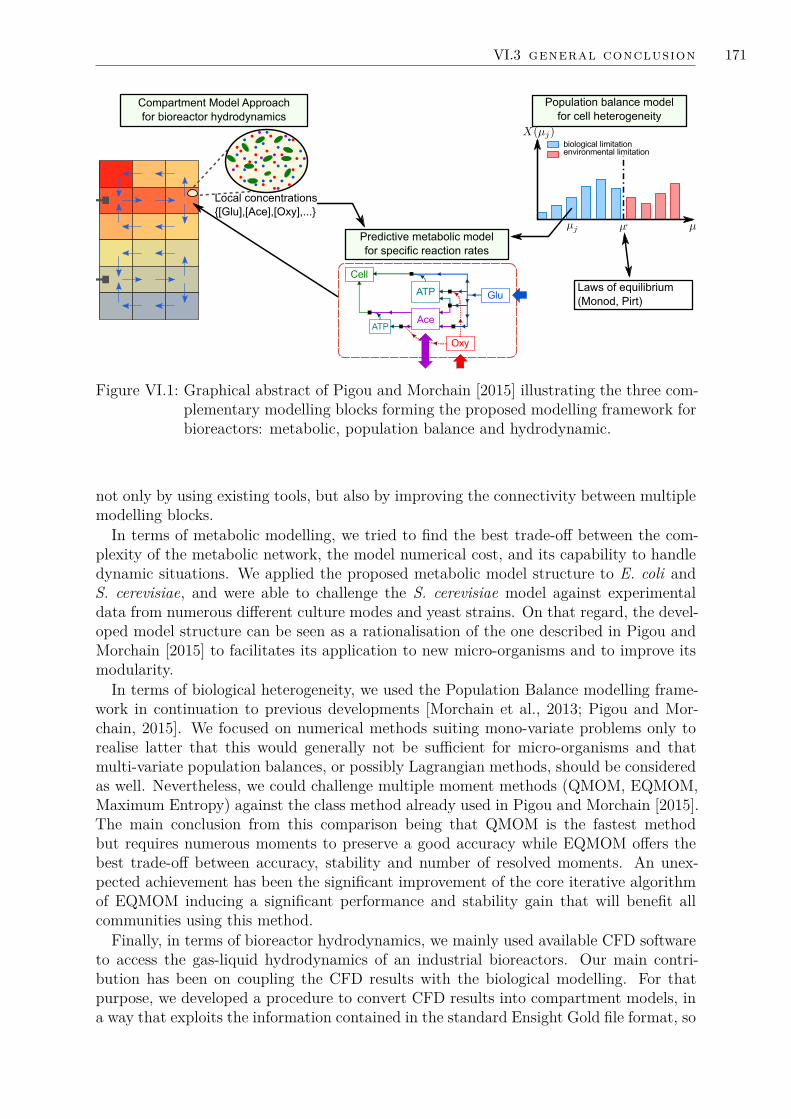
VI.3 general conclusion 171
Figure VI.1: Graphical abstract of Pigou and Morchain [2015] illustrating the three com-plementary modelling blocks forming the proposed modelling framework forbioreactors: metabolic, population balance and hydrodynamic.
not only by using existing tools, but also by improving the connectivity between multiplemodelling blocks.
In terms of metabolic modelling, we tried to find the best trade-off between the com-plexity of the metabolic network, the model numerical cost, and its capability to handledynamic situations. We applied the proposed metabolic model structure to E. coli andS. cerevisiae, and were able to challenge the S. cerevisiae model against experimentaldata from numerous different culture modes and yeast strains. On that regard, the devel-oped model structure can be seen as a rationalisation of the one described in Pigou andMorchain [2015] to facilitates its application to new micro-organisms and to improve itsmodularity.
In terms of biological heterogeneity, we used the Population Balance modelling frame-work in continuation to previous developments [Morchain et al., 2013; Pigou and Mor-chain, 2015]. We focused on numerical methods suiting mono-variate problems only torealise latter that this would generally not be sufficient for micro-organisms and thatmulti-variate population balances, or possibly Lagrangian methods, should be consideredas well. Nevertheless, we could challenge multiple moment methods (QMOM, EQMOM,Maximum Entropy) against the class method already used in Pigou and Morchain [2015].The main conclusion from this comparison being that QMOM is the fastest methodbut requires numerous moments to preserve a good accuracy while EQMOM offers thebest trade-off between accuracy, stability and number of resolved moments. An unex-pected achievement has been the significant improvement of the core iterative algorithmof EQMOM inducing a significant performance and stability gain that will benefit allcommunities using this method.
Finally, in terms of bioreactor hydrodynamics, we mainly used available CFD softwareto access the gas-liquid hydrodynamics of an industrial bioreactors. Our main contri-bution has been on coupling the CFD results with the biological modelling. For thatpurpose, we developed a procedure to convert CFD results into compartment models, ina way that exploits the information contained in the standard Ensight Gold file format, so

172 outlooks and conclusions
that a single software implementation of that procedure can be used for the compartmen-talization of results from ANSYS Fluent [2015], NEPTUNE CFD [2016], OpenFOAM,and other CFD software.
The final aspect in this work has been the development of a bioreactor simulationtool-suite, ADENON, whose purpose is to integrate and couple metabolic models andnumerical methods to solve population balances along with compartmental approachesto enable engineering studies using the proposed modelling framework. The relevancyof this tool has been demonstrated on scale-up issues and on actual industrial systemsfor design and optimisation purposes. For now, a MATLAB version of ADENON allowsfor real-time simulations but future versions based on compiled languages shall enablesignificantly faster simulations along with new capabilities such as parametric studies oranticipated process control.

B I B L I O G R A P H Y
Abramov, R.V., 2007. An improved algorithm for the multidimensional moment-constrained maximumentropy problem. Journal of Computational Physics 226, 621–644. doi:10.1016/j.jcp.2007.04.026.
Abulesz, E.M., Lyberatos, G., 1989. Periodic operation of a continuous culture of baker’s yeast. Biotech-nology and Bioengineering 34, 741–749. doi:10.1002/bit.260340603.
Adamberg, K., Lahtvee, P.J., Valgepea, K., Abner, K., Vilu, R., 2009. Quasi steady state growth ofLactococcus lactis in glucose-limited acceleration stat (a-stat) cultures. Antonie van Leeuwenhoek 95,219–226. doi:10.1007/s10482-009-9305-z.
Alopaeus, V., Laakkonen, M., Aittamaa, J., 2006. Solution of population balances with breakage andagglomeration by high-order moment-conserving method of classes. Chemical Engineering Science 61,6732–6752. doi:10.1016/j.ces.2006.07.010.
Alopaeus, V., Laakkonen, M., Aittamaa, J., 2007. Solution of population balances with growth andnucleation by high order moment-conserving method of classes. Chemical Engineering Science 62,2277–2289. doi:10.1016/j.ces.2006.12.070.
Alopaeus, V., Laakkonen, M., Aittamaa, J., 2008. Solution of population balances by high order moment-conserving method of classes: reconstruction of a non-negative density distribution. Chemical Engi-neering Science 63, 2741–2751. doi:10.1016/j.ces.2008.02.027.
Alves, S., Maia, C., Vasconcelos, J., Serralheiro, A., 2002. Bubble size in aerated stirred tanks. ChemicalEngineering Journal 89, 109–117. doi:10.1016/s1385-8947(02)00008-6.
Anane, E., Lopez C, D.C., Neubauer, P., Bournazou, M.N.C., 2017. Modelling overflow metabolism inEscherichia coli by acetate cycling. Biochemical Engineering Journal 125, 23–30. doi:10.1016/j.bej.2017.05.013.
ANSYS Fluent, 2015. User’s Guide, release 16.2. ANSYS, Inc., Southpointe, 2600 ANSYS Drive,Canonsburg, PA 15317.
Askari, E., Proulx, P., Passalacqua, A., 2018. Modelling of bubbly flow using CFD-PBM solver inOpenFOAM: Study of local population balance models and extended quadrature method of momentsapplications. ChemEngineering 2, 8. doi:10.3390/chemengineering2010008.
Athanassoulis, G., Gavriliadis, P., 2002. The truncated Hausdorff moment problem solved by using kerneldensity functions. Probabilistic Engineering Mechanics 17, 273–291. doi:10.1016/S0266-8920(02)00012-7.
Bailey, J., 1998. Mathematical modeling and analysis in biochemical engineering: Past accomplishmentsand future opportunities. Biotechnology Progress 14, 8–20. doi:10.1021/bp9701269.
Baldyga, J., Bourne, J.R., 1999. Turbulent Mixing and Chemical Reactions. John Wiley and Sons.Balsa-Canto, E., Alonso, A.A., Banga, J.R., 2010. An iterative identification procedure for dynamic
modeling of biochemical networks. BMC Systems Biology 4, 11. doi:10.1186/1752-0509-4-11.Barford, J.P., Hall, R.J., 1979. An examination of the crabtree effect in Saccharomyces cerevisiae:
the role of respiratory adaptation. Journal of General Microbiology 114, 267–275. doi:10.1099/00221287-114-2-267.
Barigou, M., Greaves, M., 1992. Bubble-size distributions in a mechanically agitated gas-liquid contactor.Chemical Engineering Science 47, 2009 – 2025. doi:10.1016/0009-2509(92)80318-7.
Bellgardt, K.H., 1994. Analysis of synchronous growth of baker's yeast. part II: Comparison of modelprediction and experimental data. Journal of Biotechnology 35, 35–49. doi:10.1016/0168-1656(94)90188-0.
Bergmann, M., 2004. Optimisation aerodynamique par reduction de modele POD et controle optimal :application au sillage laminaire d’un cylindre circulaire. Ph.D. thesis. Institut National Polytechniquede Lorraine.
Bezzo, F., Macchietto, S., Pantelides, C.C., 2003. General hybrid multizonal/CFD approach for bioreac-tor modeling. AIChE Journal 49, 2133–2148. doi:10.1002/aic.690490821.
Blattner, F.R., Plunkett, G., Bloch, C.A., Perna, N.T., Burland, V., Riley, M., Collado-Vides, J., Glasner,J.D., Rode, C.K., Mayhew, G.F., Gregor, J., Davis, N.W., Kirkpatrick, H.A., Goeden, M.A., Rose,D.J., Mau, B., Shao, Y., 1997. The complete genome sequence of Escherichia coli K-12. Science 277,1453–1462. doi:10.1126/science.277.5331.1453.
173

174 BIBLIOGRAPHY
Bolotin, A., Quinquis, B., Sorokin, A., dusko Ehrlich, S., 2005. Clustered regularly interspaced shortpalindrome repeats (CRISPRs) have spacers of extrachromosomal origin. Microbiology 151, 2551–2561.doi:10.1099/mic.0.28048-0.
Brand, E., Junne, S., Anane, E., Cruz-Bournazou, M.N., Neubauer, P., 2018. Importance of the cultiva-tion history for the response of Escherichia coli to oscillations in scale-down experiments. Bioprocessand Biosystems Engineering doi:10.1007/s00449-018-1958-4.
Brognaux, A., Han, S., Sørensen, S.J., Lebeau, F., Thonart, P., Delvigne, F., 2013. A low-cost, multi-plexable, automated flow cytometry procedure for the characterization of microbial stress dynamicsin bioreactors. Microbial Cell Factories 12, 100. doi:10.1186/1475-2859-12-100.
Buffo, A., Vanni, M., Marchisio, D., 2012. Multidimensional population balance model for the simulationof turbulent gas–liquid systems in stirred tank reactors. Chemical Engineering Science 70, 31–44.doi:10.1016/j.ces.2011.04.042.
Camarasa, C., Chiron, H., Daboussi, F., Valle, G.D., Dumas, C., Farines, V., Floury, J., Gagnaire, V.,Gorret, N., Leonil, J., Mouret, J.R., O’Donohue, M.J., Sablayrolles, J.M., Salmon, J.M., Saulnier, L.,Truan, G., 2018. INRA’s research in industrial biotechnology: for food, chemicals, materials and fuels.Innovative Food Science & Emerging Technologies 46, 140–152. doi:10.1016/j.ifset.2017.11.008.
Caudal, J., Fiorina, B., Massot, M., Labegorre, B., Darabiha, N., Gicquel, O., 2013. Characteristicchemical time scales identification in reactive flows. Proceedings of the Combustion Institute 34, 1357– 1364. doi:doi.org/10.1016/j.proci.2012.06.178.
Chalons, C., Fox, R., Laurent, F., Massot, M., Vie, A., 2017. Multivariate gaussian extended quadraturemethod of moments for turbulent disperse multiphase flow. Multiscale Modeling & Simulation 15,1553–1583. doi:10.1137/16M109209X.
Chalons, C., Fox, R.O., Massot, M., 2010. A multi-gaussian quadrature method of moments for gas-particle flows in a LES framework, in: Proceedings of the 2010 Summer Program, Center for turbulenceResearch. Stanford University. pp. 347–358.
Chassagnole, C., Noisommit-Rizzi, N., Schmid, J.W., Mauch, K., Reuss, M., 2002. Dynamic modelingof the central carbon metabolism of Escherichia coli. Biotechnology and Bioengineering 79, 53–73.doi:10.1002/bit.10288.
Chihara, T., 1978. An introduction to orthogonal polynomials. Number vol. 13 in Mathematics and itsapplications, Gordon and Breach.
Coste, P., 2013. A large interface model for two-phase CFD. Nuclear Engineering and Design 255, 38–50.doi:10.1016/j.nucengdes.2012.10.008.
Couderc, J.P., Gourdon, C., Line, A., 2008. Phenomenes de transfert en genie des procedes. Lavoisier.Courant, R., Friedrichs, K., Lewy, H., 1928. Uber die partiellen differenzengleichungen der mathematis-
chen physik. Mathematische Annalen 100, 32–74. doi:10.1007/BF01448839.Delafosse, A., 2008. Analyse et Etude Numerique des Effets de Melange dans un Bioreacteur. Ph.D.
thesis. INSA de Toulouse.Delafosse, A., Calvo, S., Collignon, M.L., Delvigne, F., Crine, M., Toye, D., 2015. Euler–Lagrange
approach to model heterogeneities in stirred tank bioreactors – Comparison to experimental flowcharacterization and particle tracking. Chemical Engineering Science 134, 457–466. doi:10.1016/j.ces.2015.05.045.
Delafosse, A., Collignon, M.L., Calvo, S., Delvigne, F., Crine, M., Thonart, P., Toye, D., 2014. CFD-based compartment model for description of mixing in bioreactors. Chemical Engineering Science 106,76–85. doi:10.1016/j.ces.2013.11.033.
Delafosse, A., Delvigne, F., Collignon, M.L., Crine, M., Thonart, P., Toye, D., 2010. Development of acompartment model based on CFD simulations for description of mixing in bioreactors. Biotechnology,Agronomy, Society and Environment 14, 517–522.
Delvigne, F., Goffin, P., 2014. Microbial heterogeneity affects bioprocess robustness: Dynamic single-cell analysis contributes to understanding of microbial populations. Biotechnology Journal 9, 61–72.doi:10.1002/biot.201300119.
Delvigne, F., Zune, Q., Lara, A.R., Al-Soud, W., Sørensen, S.J., 2014. Metabolic variability in bio-processing: implications of microbial phenotypic heterogeneity. Trends in Biotechnology 32, 608–616.doi:10.1016/j.tibtech.2014.10.002.
Dette, H., Studden, W.J., 1997. The theory of canonical moments with applications in statistics, proba-bility, and analysis. John Wiley & Sons, New York; Chichester.
van Dijken, J., Bauer, J., Brambilla, L., Duboc, P., Francois, J., Gancedo, C., Giuseppin, M., Heijnen,J., Hoare, M., Lange, H., Madden, E., Niederberger, P., Nielsen, J., Parrou, J., Petit, T., Porro, D.,Reuss, M., van Riel, N., Rizzi, M., Steensma, H., Verrips, C., Vindeløv, J., Pronk, J., 2000. An

BIBLIOGRAPHY 175
interlaboratory comparison of physiological and genetic properties of four Saccharomyces cerevisiaestrains. Enzyme and Microbial Technology 26, 706–714. doi:10.1016/S0141-0229(00)00162-9.
van Dijken, J.P., Scheffers, W., 1986. Redox balances in the metabolism of sugars by yeasts. FEMSMicrobiology Letters 32, 199–224. doi:10.1111/j.1574-6968.1986.tb01194.x.
Elqotbi, M., Vlaev, S., Montastruc, L., Nikov, I., 2013. CFD modelling of two-phase stirred bioreactionsystems by segregated solution of the euler-euler model. Computers & Chemical Engineering 48,113–120. doi:10.1016/j.compchemeng.2012.08.005.
Enfors, S.O., Jahic, M., Rozkov, A., Xu, B., Hecker, M., Jurgen, B., Kruger, E., Schweder, T., Hamer,G., O’Beirne, D., Noisommit-Rizzi, N., Reuss, M., Boone, L., Hewitt, C., McFarlane, C., Nienow, A.,Kovacs, T., Tragardh, C., Fuchs, L., Revstedt, J., Friberg, P., Hjertager, B., Blomsten, G., Skogman,H., Hjort, S., Hoeks, F., Lin, H.Y., Neubauer, P., van der Lans, R., Luyben, K., Vrabel, P., A.Manelius, 2001. Physiological responses to mixing in large scale bioreactors. Journal of Biotechnology85, 175–185. doi:10.1016/S0168-1656(00)00365-5. twenty years of the European Federation ofBiotechnology.
Ensight, 2016. version 10.2. Computational Engineering International, Inc., 2166 N. Salem Street, Suite101, Apex, NC 27523 USA. URL: http://www3.ensight.com/EnSight10_Docs/UserManual.pdf.
Escudie, R., Line, A., 2004. Experimental analysis of hydrodynamics in a radially agitated tank. AIChEJournal 49, 585–603. doi:10.1002/aic.690490306.
Farzan, P., Lerapetritou, M.G., 2017. Integrated modeling to capture the interaction of physiology andfluid dynamics in biopharmaceutical bioreactors. Computers & Chemical Engineering 97, 271–282.doi:10.1016/j.compchemeng.2016.11.037.
Favard, J., 1935. Sur les polynomes de Tchebicheff. C. r. hebd. seances Acad. sci. 200, 2052–2053.Ferenci, T., 1996. Adaptation to life at micromolar nutrient levels: the regulation of Escherichia coli
glucose transport by endoinduction and cAMP. FEMS Microbiology Reviews 18, 301–317. doi:10.1111/j.1574-6976.1996.tb00246.x.
Ferenci, T., 1999. Regulation by nutrient limitation. Current Opinion in Microbiology 2, 208–213.doi:10.1016/S1369-5274(99)80036-8.
Ferenci, T., 2001. Hungry bacteria - definition and properties of a nutritional state. EnvironmentalMicrobiology 3, 605–611. doi:10.1046/j.1462-2920.2001.00238.x.
Flikweert, M.T., Kuyper, M., Maris, A.J.A.v., Kotter, P., Dijken, J.P.v., Pronk, J.T., 1999. Steady-state and transient-state analysis of growth and metabolite production in a Saccharomyces cerevisiaestrain with reduced pyruvate-decarboxylase activity. Biotechnology and Bioengineering 66, 42–50.doi:10.1002/(SICI)1097-0290(1999)66:1<42::AID-BIT4>3.0.CO;2-L.
Ford, W., 2015. Chapter 19 - the symmetric eigenvalue problem, in: Numerical Linear Algebra withApplications. Academic Press, Boston, pp. 439–468. doi:10.1016/B978-0-12-394435-1.00019-3.
Frank, T., Shi, J.M., Burns, A.D., 2004. Vaalidation of eulerian multiphase flow models for nuclear safetyapplications., in: 3rd International Symposium on two-phase flow modelling and experimentations.
Fredrickson, A.G., Tsuchiya, H.M., 1963. Continuous propagation of microorganisms. AIChE Journal 9,459–468. doi:10.1002/aic.690090410.
Gautschi, W., 2004. Orthogonal Polynomials: Computation and Approximation. Numerical mathematicsand scientific computation, Oxford University Press.
Gerdtzen, Z.P., Daoutidis, P., Hu, W.S., 2004. Non-linear reduction for kinetic models of metabolicreaction networks. Metabolic Engineering 6, 140–154. doi:10.1016/j.ymben.2003.11.003.
Goldrick, S., Stefan, A., Lovett, D., Montague, G., Lennox, B., 2015. The development of an industrial-scale fed-batch fermentation simulation. Journal of Biotechnology 193, 70–82. doi:10.1016/j.jbiotec.2014.10.029.
Gosset, G., 2005. Improvement of Escherichia coli production strains by modification of the phos-phoenolpyruvate: sugar phosphotransferase system. Microbial Cell Factories 4, 14. doi:10.1186/1475-2859-4-14.
Guillou, V., Plourde-Owobi, L., Parrou, J.L., Goma, G., Francois, J., 2004. Role of reserve carbohydratesin the growth dynamics of saccharomyces cerevisiae. FEMS Yeast Research 4, 773–787. doi:10.1016/j.femsyr.2004.05.005.
Gzyl, H., Tagliani, A., 2010. Hausdorff moment problem and fractional moments. Applied Mathematicsand Computation 216, 3319–3328. doi:10.1016/j.amc.2010.04.059.
Haringa, C., Tang, W., Deshmukh, A.T., Xia, J., Reuss, M., Heijnen, J.J., Mudde, R.F., Noorman,H.J., 2016. Euler-Lagrange computational fluid dynamics for (bio)reactor scale down: An analysis oforganism lifelines. Engineering in Life Sciences doi:10.1002/elsc.201600061.

176 BIBLIOGRAPHY
Hatzis, C., Srienc, F., Fredrickson, A., 1995. Multistaged corpuscular models of microbial growth: MonteCarlo simulations. Biosystems 36, 19–35. doi:10.1016/0303-2647(95)01524-o.
Heavner, B.D., Smallbone, K., Barker, B., Mendes, P., Walker, L.P., 2012. Yeast 5 - an expandedreconstruction of the Saccharomyces cerevisiae metabolic network. BMC Systems Biology 6. doi:10.1186/1752-0509-6-55.
Heavner, B.D., Smallbone, K., Price, N.D., Walker, L.P., 2013. Version 6 of the consensus yeast metabolicnetwork refines biochemical coverage and improves model performance. Database 2013. doi:10.1093/database/bat059.
Heins, A.L., Fernandes, R.L., Gernaey, K.V., Lantz, A.E., 2015. Experimental and in silico investigationof population heterogeneity in continuous Sachharomyces cerevisiae scale-down fermentation in a two-compartment setup. Journal of Chemical Technology and Biotechnology 90, 324–340. doi:10.1002/jctb.4532.
Hempfling, W.P., Mainzer, S.E., 1975. Effects of varying the carbon source limiting growth on yieldand maintenance characteristics of Escherichia coli in continuous culture. Journal of bacteriology 123,1076–1087.
Hibiki, T., Ishii, M., 2000. One-group interfacial area transport of bubbly flows in vertical round tubes. In-ternational Journal of Heat and Mass Transfer 43, 2711–2726. doi:10.1016/s0017-9310(99)00325-7.
Hjersted, J.L., Henson, M.A., 2006. Optimization of fed-batch Saccharomyces cerevisiae fermentationusing dynamic flux balance models. Biotechnology Progress 22, 1239–1248. doi:10.1021/bp060059v.
Hristov, H., Mann, R., Lossev, V., Vlaev, S., 2004. A simplified CFD for three-dimensional analysisof fluid mixing, mass transfer and bioreaction in a fermenter equipped with triple novel geometryimpellers. Food and Bioproducts Processing 82, 21–34. doi:10.1205/096030804322985281.
John, V., Angelov, I., Oncul, A., Thevenin, D., 2007. Techniques for the reconstruction of a distributionfrom a finite number of its moments. Chemical Engineering Science 62, 2890–2904. doi:10.1016/j.ces.2007.02.041.
Jung, W.M., Kang, S.H., Kim, W.S., Choi, C.K., 2000. Particle morphology of calcium carbonateprecipitated by gas-liquid reaction in a Couette-Taylor reactor. Chemical Engineering Science 55, 733– 747. doi:10.1016/S0009-2509(99)00395-4.
Kafarski, P., 2012. Rainbow code of biotechnology. CHEMIK 66, 811–816.Kajihata, S., Matsuda, F., Yoshimi, M., Hayakawa, K., Furusawa, C., Kanda, A., Shimizu, H., 2015.
13c-based metabolic flux analysis of saccharomyces cerevisiae with a reduced crabtree effect. Journalof Bioscience and Bioengineering 120, 140–144. doi:10.1016/j.jbiosc.2014.12.014.
Katterer, L., Allemann, H., Kappeli, O., Fiechter, A., 1986. Transient responses of continuously growingyeast cultures to dilution rate shifts: A sensitive means to analyze biology and the performance ofequipment. Biotechnology and Bioengineering 28, 146–150. doi:10.1002/bit.260280126.
Kawase, Y., Halard, B., Moo-Young, M., 1992. Liquid-phase mass transfer coefficients in bioreactors.Biotechnology and Bioengineering 39, 1133–1140. doi:10.1002/bit.260391109.
Kim, S.R., Park, Y.C., Jin, Y.S., Seo, J.H., 2013. Strain engineering of Saccharomyces cerevisiae forenhanced xylose metabolism. Biotechnology Advances 31, 851–861. doi:10.1016/j.biotechadv.2013.03.004.
Klumpp, S., Scott, M., Pedersen, S., Hwa, T., 2013. Molecular crowding limits translation and cell growth.Proceedings of the National Academy of Sciences 110, 16754–16759. doi:10.1073/pnas.1310377110.
Kolev, N.I., 2007. Multiphase Flow Dynamics 2. Springer Berlin Heidelberg. doi:10.1007/3-540-69835-3.
Kravaris, C., Hahn, J., Chu, Y., 2013. Advances and selected recent developments in state and parameterestimation. Computers & Chemical Engineering 51, 111–123. doi:10.1016/j.compchemeng.2012.06.001.
Kumar, S., Ramkrishna, D., 1996a. On the solution of population balance equations by discretization - I.a fixed pivot technique. Chemical Engineering Science 51, 1311 – 1332. doi:10.1016/0009-2509(96)88489-2.
Kumar, S., Ramkrishna, D., 1996b. On the solution of population balance equations by discretization - II.a moving pivot technique. Chemical Engineering Science 51, 1333–1342. doi:10.1016/0009-2509(95)00355-X.
Kumar, S., Ramkrishna, D., 1997. On the solution of population balance equations by discretization- III. nucleation, growth and aggregation of particles. Chemical Engineering Science 52, 4659–4679.doi:10.1016/S0009-2509(97)00307-2. festshrift for Professor M. M. Sharma.
Kuschel, M., Siebler, F., Takors, R., 2017. Lagrangian trajectories to predict the formation of populationheterogeneity in large-scale bioreactors. Bioengineering 4, 27. doi:10.3390/bioengineering4020027.
BIBLIOGRAPHY 177
Laakkonen, M., Moilanen, P., Alopaeus, V., Aittamaa, J., 2006. Dynamic modeling of local reactionconditions in an agitated aerobic fermenter. AIChE Journal 52, 1673–1689. doi:10.1002/aic.10782.
Laakkonen, M., Moilanen, P., Alopaeus, V., Aittamaa, J., 2007. Modelling local bubble size distributionsin agitated vessels. Chemical Engineering Science 62, 721 – 740. doi:10.1016/j.ces.2006.10.006.
Lapin, A., Muller, D., Reuss, M., 2004. Dynamic behavior of microbial populations in stirred bioreactorssimulated with Euler–Lagrange methods: Traveling along the lifelines of single cells. Industrial &Engineering Chemistry Research 43, 4647–4656. doi:10.1021/ie030786k.
Lapin, A., Schmid, J., Reuss, M., 2006. Modeling the dynamics of E. coli populations in the three-dimensional turbulent field of a stirred-tank bioreactor—a structured–segregated approach. ChemicalEngineering Science 61, 4783 – 4797. doi:10.1016/j.ces.2006.03.003.
Launder, B., Spalding, D.B., 1972. Lectures in Mathematical Models of Turbulence. Academic PressInc, London, England.
Laupsien, D., 2017. Hydrodynamics, Mass Transfer and Mixing induced by Bubble Plumes in ViscousFluids. Ph.D. thesis. INSA de Toulouse.
Le Moullec, Y.and Gentric, C., Potier, O., Leclerc, J.P., 2010. Comparison of systemic, compartmentaland CFD modelling approaches: application to the simulation of a biological reactor of wastewatertreatment. Chemical Engineering Science 65, 343–350. doi:10.1016/j.ces.2009.06.035.
Lebaz, N., 2015. Modelisation de l’hydrolyse enzymatique de substrats lignocellulosiques par bilan depopulation. Ph.D. thesis. INSA de Toulouse. URL: http://www.theses.fr/2015ISAT0030.
Lebaz, N., Cockx, A., Sperandio, M., Morchain, J., 2016. Reconstruction of a distribution from a finitenumber of its moments: A comparative study in the case of depolymerization process. Computers &Chemical Engineering 84, 326–337. doi:10.1016/j.compchemeng.2015.09.008.
Leegwater, M.P.M., Neijssel, O.M., Tempest, D.W., 1982. Aspects of microbial physiology in relationto process control. Journal of Chemical Technology and Biotechnology 32, 92–99. doi:10.1002/jctb.5030320113.
Lei, F., Rotbøll, M., Jørgensen, S.B., 2001. A biochemically structured model for Saccharomyces cere-visiae. Journal of Biotechnology 88, 205–221. doi:10.1016/S0168-1656(01)00269-3.
Lencastre Fernandes, R., Carlquist, M., Lundin, L., Heins, A.L., Dutta, A., Sørensen, S.J., Jensen, A.D.,Nopens, I., Lantz, A.E., Gernaey, K.V., 2012. Cell mass and cell cycle dynamics of an asynchronousbudding yeast population: Experimental observations, flow cytometry data analysis, and multi-scalemodeling. Biotechnology and Bioengineering 110, 812–826. doi:10.1002/bit.24749.
Li, L., Chen, N., Xiang, K., Xiang, B., 2018. A comparative CFD study on gas-liquid dispersion in astirred tank with low and high gas loadings. International Journal of Chemical Reactor Engineeringdoi:10.1515/ijcre-2017-0147.
Line, A., Gabelle, J.C., Morchain, J., Anne-Archard, D., Augier, F., 2013. On POD analysis of PIVmeasurements applied to mixing in a stirred vessel with a shear thinning fluid. Chemical EngineeringResearch and Design 91, 2073 – 2083. doi:10.1016/j.cherd.2013.05.002. mixing.
Linkes, M., Fede, P., Morchain, J., Schmitz, P., 2014. Numerical investigation of subgrid mixing effectson the calculation of biological reaction rates. Chemical Engineering Science 116, 473–485. doi:10.1016/j.ces.2014.05.005.
Loffler, M., Simen, J.D., Muller, J., Jager, G., Laghrami, S., Schaferhoff, K., Freund, A., Takors, R.,2017. Switching between nitrogen and glucose limitation: Unraveling transcriptional dynamics inEscherichia coli. Journal of Biotechnology 258, 2–12. doi:10.1016/j.jbiotec.2017.04.011.
Machon, V., Pacek, A., Nienow, A., 1997. Bubble sizes in electrolyte and alcohol solutions in aturbulent stirred vessel. Chemical Engineering Research and Design 75, 339–348. doi:10.1205/026387697523651.
Madadi-Kandjani, E., Passalacqua, A., 2015. An extended quadrature-based moment method with log-normal kernel density functions. Chemical Engineering Science 131, 323–339. doi:10.1016/j.ces.2015.04.005.
Mantzaris, N.V., Daoutidis, P., Srienc, F., 2001. Numerical solution of multi-variable cell populationbalance models: I. Finite difference methods. Computers & Chemical Engineering 25, 1411–1440.doi:10.1016/S0098-1354(01)00709-8.
Mantzaris, N.V., Daoutidis, P., Srienc, F., Fredrickson, A.G., 1999. Growth processes in a cascade ofbioreactors: Mathematical models. AIChE Journal 45, 164–176. doi:10.1002/aic.690450114.
Marchisio, D., Fox, R., 2013. Computational Models for Polydisperse Particulate and Multiphase Systems.Cambridge Series in Chemical Engineering, Cambridge University Press.
Marchisio, D.L., Pikturna, J.T., Fox, R.O., Vigil, R.D., Barresi, A.A., 2003a. Quadrature method of mo-ments for population-balance equations. AIChE Journal 49, 1266–1276. doi:10.1002/aic.690490517.
178 BIBLIOGRAPHY
Marchisio, D.L., Vigil, R.D., Fox, R.O., 2003b. Implementation of the quadrature method of moments inCFD codes for aggregation-breakage problems. Chemical Engineering Science 58, 3337–3351. doi:10.1016/S0009-2509(03)00211-2.
MATLAB, 2016. version 9.0 (R2016a). The MathWorks, Inc., Natick, Massachusetts, United States.Matsuoka, Y., Shimizu, K., 2013. Catabolite regulation analysis of Escherichia coli for acetate overflow
mechanism and co-consumption of multiple sugars based on systems biology approach using computersimulation. Journal of Biotechnology 168, 155 – 173. doi:10.1016/j.jbiotec.2013.06.023. specialissue: Biotechnology for a healthy and green world.
Mayr, B., Horvat, P., Nagy, E., Moser, A., 1993. Mixing-models applied to industrial batch bioreactors.Bioprocess Engineering 9, 1–12. doi:10.1007/BF00389534.
McGraw, R., 1997. Description of aerosol dynamics by the quadrature method of moments. AerosolScience and Technology 27, 255–265. doi:10.1080/02786829708965471.
Mead, L.R., Papanicolaou, N., 1984. Maximum entropy in the problem of moments. Journal of Mathe-matical Physics 25, 2404–2417.
Meadows, A.L., Karnik, R., Lam, H., Forestell, S., Snedecor, B., 2010. Application of dynamic fluxbalance analysis to an industrial Escherichia coli fermentation. Metabolic Engineering 12, 150–160.doi:10.1016/j.ymben.2009.07.006.
Mer, S., Praud, O., Neau, H., Merigoux, N., Magnaudet, J., Roig, V., 2018. The emptying of a bottleas a test case for assessing interfacial momentum exchange models for euler–euler simulations ofmulti-scale gas-liquid flows. International Journal of Multiphase Flow 106, 109–124. doi:10.1016/j.ijmultiphaseflow.2018.05.002.
Merigoux, N., Lavieville, J., Mimouni, S., Guingo, M., Baudry, C., 2016. A generalized large interfaceto dispersed bubbly flow approach to model two-phase flows in nuclear power plant, in: MA-USA, C.(Ed.), CFD4NRS-6, pp. 1–20. Paper 11-1.
Moilanen, P., Laakkonen, M., Visuri, O., Aittamaa, J., 2007. Modeling local gas-liquid mass transfer inagitated viscous shear-thinning dispersions with CFD. Industrial & Engineering Chemistry Research46, 7289–7299. doi:10.1021/ie070566x.
Moilanen, P., Laakkonen, M., Visuri, O., Alopaeus, V., Aittamaa, J., 2008. Modelling mass transfer inan aerated 0.2 m3 vessel agitated by rushton, phasejet and combijet impellers. Chemical EngineeringJournal 142, 95–108. doi:10.1016/j.cej.2008.01.033.
Monod, J., 1952. Theory and Application of the Technique of Continuous Culture. Defense TechnicalInformation Center.
Morchain, J., 2000. Etude et modelisation des couplages entre cinetiques physiques et biologiques dansles reacteurs de grand volume. Ph.D. thesis. INSA de Toulouse.
Morchain, J., 2017. Bioreactor Modeling. Elsevier. doi:10.1016/c2015-0-05985-8.Morchain, J., Fonade, C., 2009. A structured model for the simulation of bioreactors under transient
conditions. AIChE Journal 55, 2973–2984. doi:10.1002/aic.11906.Morchain, J., Gabelle, J.C., Cockx, A., 2013. Coupling of biokinetic and population balance models to
account for biological heterogeneity in bioreactors. AIChE Journal 59, 369–379. doi:10.1002/aic.13820.
Morchain, J., Gabelle, J.C., Cockx, A., 2014. A coupled population balance model and CFD approachfor the simulation of mixing issues in lab-scale and industrial bioreactors. AIChE Journal 60, 27–40.doi:10.1002/aic.14238.
Morchain, J., Pigou, M., Lebaz, N., 2016. A population balance model for bioreactors combininginterdivision time distributions and micromixing concepts. Biochemical Engineering Journal , –doi:10.1016/j.bej.2016.09.005.
Muller, L., Klar, A., Schneider, F., 2017. A numerical comparison of the method of moments for thepopulation balance equation. arXiv:arXiv:1706.05854.
Natarajan, A., Srienc, F., 2000. Glucose uptake rates of single E. coli cells grown in glucose-limitedchemostat cultures. Journal of Microbiological Methods 42, 87–96. doi:10.1016/S0167-7012(00)00180-9. microbial Analysis at the Single Cell Level.
Nauha, E.K., Kalal, Z., Ali, J.M., Alopaeus, V., 2018. Compartmental modeling of large stirred tankbioreactors with high gas volume fractions. Chemical Engineering Journal 334, 2319 – 2334. doi:/10.1016/j.cej.2017.11.182.
NEPTUNE CFD, 2016. version 3.2.0 user guide. EDF SA, 6 quai Watier, 78401 Chatou, France.Neubauer, P., Haggstrom, L., Enfors, S.O., 1995. Influence of substrate oscillations on acetate forma-
tion and growth yield in escherichia coli glucose limited fed-batch cultivations. Biotechnology andBioengineering 47, 139–146. doi:10.1002/bit.260470204.
BIBLIOGRAPHY 179
Nguyen, T., Laurent, F., Fox, R., Massot, M., 2016. Solution of population balance equations in applica-tions with fine particles: Mathematical modeling and numerical schemes. Journal of ComputationalPhysics 325, 129–156. doi:10.1016/j.jcp.2016.08.017.
Nielsen, J., Villadsen, J., 1992. Modelling of microbial kinetics. Chemical Engineering Science 47,4225–4270. doi:10.1016/0009-2509(92)85104-J.
Nobs, J.B., Maerkl, S.J., 2014. Long-term single cell analysis of S. pombe on a microfluidic microchemo-stat arraynobs. PLoS ONE 9. doi:10.1371/journal.pone.0093466.
Noh, K., Gronke, K., Luo, B., Takors, R., Oldiges, M., Wiechert, W., 2007. Metabolic flux analysis atultra short time scale: Isotopically non-stationary 13c labeling experiments. Journal of Biotechnology129, 249–267. doi:10.1016/j.jbiotec.2006.11.015.
Noorman, H.J., Heijnen, J.J., 2017. Biochemical engineering´s grand adventure. Chemical EngineeringScience 170, 677 – 693. doi:10.1016/j.ces.2016.12.065. 13th International Conference on Gas-Liquid and Gas-Liquid-Solid Reactor Engineering.
OECD, 2008. OECD Glossary of Statistical Terms. OECD Publishing.Ordonez, M.C., Raftery, J.P., Jaladi, T., Chen, X., Kao, K., Karim, M.N., 2016. Modelling of batch
kinetics of aerobic carotenoid production using saccharomyces cerevisiae. Biochemical EngineeringJournal 114, 226–236. doi:10.1016/j.bej.2016.07.004.
Orth, J.D., Conrad, T.M., Na, J., Lerman, J.A., Nam, H., Feist, A.M., Palsson, B.O., 2011. A com-prehensive genome-scale reconstruction of Escherichia coli metabolism – 2011. Molecular SystemsBiology 7. doi:10.1186/1752-0509-6-55.
Paddon, C.J., Keasling, J.D., 2014. Semi-synthetic artemisinin: a model for the use of synthetic biology inpharmaceutical development. Nature Reviews Microbiology 12, 355–366. doi:10.1038/nrmicro3240.
Pagliolico, S., Marchisio, D., Battesi, A.A., 1999. Influence of operating conditions on BaSO4 crystal sizeand morphology in a continuous couette precipitator. Journal of Thermal Analysis and Colorimetry56, 1423–1433.
Passalacqua, A., Laurent, F., Madadi-Kandjani, E., Heylmun, J., Fox, R., 2017. An open-sourcequadrature-based population balance solver for OpenFOAM. Chem. Eng. Sci. doi:10.1016/j.ces.2017.10.043.
Petrik, M., Kappeli, O., Fiechter, A., 1983. An expanded concept for the glucose effect in the yeast Sac-charomyces uvarum: Involvement of short- and long-term regulation. Journal of General Microbiology129, 43–49. doi:10.1099/00221287-129-1-43.
Pigou, M., Morchain, J., 2015. Investigating the interactions between physical and biological hetero-geneities in bioreactors using compartment, population balance and metabolic models. ChemicalEngineering Science 126, 267–282. doi:10.1016/j.ces.2014.11.035.
Pigou, M., Morchain, J., Fede, P., Penet, M.I., Laronze, G., 2017. An assessment of methods of momentsfor the simulation of population dynamics in large-scale bioreactors. Chemical Engineering Science171, 218–232. doi:10.1016/j.ces.2017.05.026.
Pigou, M., Morchain, J., Fede, P., Penet, M.I., Laronze, G., 2018a. New developments of the extendedquadrature method of moments to solve population balance equations. Journal of ComputationalPhysics 365C, 243–268. doi:10.1016/j.jcp.2018.03.027.
Pigou, M., Morchain, J., Fede, P., Penet, M.I., Laronze, G., 2018b. A new moment-inversion procedurefor the extended quadrature method of moments, in: 6th Population Balance Modelling Conference.
Pirt, S.J., 1965. The maintenance energy of bacteria in growing cultures. Royal Society of LondonProceedings Series B 163, 224–231. doi:10.1098/rspb.1965.0069.
Pollack, M., Salenbauch, S., Marchisio, D., Hasse, C., 2016. Bivariate extensions of the extended quadra-ture method of moments (EQMOM) to describe coupled droplet evaporation and heat-up. Journal ofAerosol Science 92, 53–69. doi:10.1016/j.jaerosci.2015.10.008.
Postma, E., Verduyn, C., Scheffers, W.A., Dijken, J.P.V., 1989. Enzymatic analysis of the crabtreeeffect in glucose-limited chemostat cultures of Saccharomyces cerevisiae. Applied and EnvironmentalMicrobiology 55, 468–477. URL: https://www.ncbi.nlm.nih.gov/pmc/articles/PMC184133/.
Pronk, J.T., Yde Steensma, H., Van Dijken, J.P., 1996. Pyruvate Metabolism in Saccharomyces cere-visiae. Yeast 12, 1607–1633. doi:10.1002/(SICI)1097-0061(199612)12:16<1607::AID-YEA70>3.0.CO;2-4.
Quedeville, V., Ouazaite, H., Polizzi, B., Fox, R., Villedieu, P., Fede, P., Letisse, F., Morchain, J.,2018. A two-dimensional population balance model for cell growth including multiple uptake systems.Chemical Engineering Research and Design 132, 966 – 981. doi:10.1016/j.cherd.2018.02.025.
Reuss, M., 1991. Structured modeling of bioreactors. Annals of the New York Academy of Sciences 646,284–299. doi:10.1111/j.1749-6632.1991.tb18591.x.

180 BIBLIOGRAPHY
Ribeiro, C.P., Lage, P.L., 2004. Population balance modeling of bubble size distributions in a direct-contact evaporator using a sparger model. Chemical Engineering Science 59, 2363–2377. doi:10.1016/j.ces.2004.01.060.
Rieger, M., Kappeli, O., Fiechter, A., 1983. The role of limited respiration in the incomplete oxidation ofglucose by Saccharomyces Cerevisiae. Microbiology 129, 653–661. doi:10.1099/00221287-129-3-653.
Rizzi, M., Baltes, M., Theobald, U., Reuss, M., 1997. In vivo analysis of metabolic dynamics inSaccharomyces cerevisiae: II. mathematical model. Biotechnology and Bioengineering 55, 592–608.doi:10.1002/(SICI)1097-0290(19970820)55:4<592::AID-BIT2>3.0.CO;2-C.
Robert, L., Hoffmann, M., Krell, N., Aymerich, S., Robert, J., Doumic, M., 2014. Division in Escherichiacoli is triggered by a size-sensing rather than a timing mechanism. BMC Biology 12, 17. doi:10.1186/1741-7007-12-17.
Rodrıguez, J., Perner, I., Schmidt, K., Posten, C., 2004. Simple metabolic model of Saccharomycescerevisiae in fed-batch culture to study the cellular nitrogen uptake, in: Pons, M.N., Van Impe, J.(Eds.), Computer Applications in Biotechnology 2004, International Federation of Automatic Control.Elsevier Science Ltd.
Rosas-Lemus, M., Uribe-Alvarez, C., Chiquete-Felix, N., Uribe-Carvajal, S., 2014. In Saccharomycescerevisiae fructose-1,6-bisphosphate contributes to the crabtree effect through closure of the mitochon-drial unspecific channel. Archives of Biochemistry and Biophysics 555-556, 66–70. doi:10.1016/j.abb.2014.05.027.
Sanchez, B.J., Perez-Correa, J.R., Agosin, E., 2014. Construction of robust dynamic genome-scale metabolic model structures of Saccharomyces cerevisiae through iterative re-parameterization.Metabolic Engineering 25, 159–173. doi:10.1016/j.ymben.2014.07.004.
Sander, R., 2015. Compilation of Henry’s law constants (version 4.0) for water as solvent. AtmosphericChemistry and Physics 15, 4399–4981. doi:10.5194/acp-15-4399-2015.
Schlegel, A., Bohm, A., Lee, S., Peist, R., Decker, K., Boos, W., 2002. Network regulation of theEscherichia coli maltose system. Journal of Molecular Microbiology and Biotechnology 4, 301–307.
Schmideder, A., Severin, T.S., Cremer, J.H., Weuster-Botz, D., 2015. A novel milliliter-scale chemostatsystem for parallel cultivation of microorganisms in stirred-tank bioreactors. Journal of Biotechnology210, 19 – 24. doi:10.1016/j.jbiotec.2015.06.402.
Schutze, J., Hengstler, J., 2006. Assessing aerated bioreactor performance using CFD, in: 12th EuropeanConference on Mixing, Bologna, Italy.
Shohat, J., Tamarkin, J., 1943. The Problem of Moments. Mathematical Surveys and Monographs. 4ed., American Mathematical Society.
Silveston, P., Budman, H., Jervis, E., 2008. Forced modulation of biological processes: A review. Chem-ical Engineering Science 63, 5089–5105. doi:10.1016/j.ces.2008.06.017. 5TH Unsteady-State Pro-cesses in Catalysis: a Special Issue of Chemical Engineering Science.
Simen, J.D., Loffler, M., Jager, G., Schaferhoff, K., Freund, A., Matthes, J., Muller, J., Takors, R.,2017. Transcriptional response of Escherichia coli to ammonia and glucose fluctuations. MicrobialBiotechnology 10, 858–872. doi:10.1111/1751-7915.12713.
Steuer, R., 2007. Computational approaches to the topology, stability and dynamics of metabolic net-works. Phytochemistry 68, 2139–2151. doi:10.1016/j.phytochem.2007.04.041.
Sunya, S., Delvigne, F., Uribelarrea, J.L., Molina-Jouve, C., Gorret, N., 2012. Comparison of thetransient responses of Escherichia coli to a glucose pulse of various intensities. Applied Microbiologyand Biotechnology 95, 1021–1034. doi:10.1007/s00253-012-3938-y.
Sweere, A.P.J., Giesselbach, J., Barendse, R., de Krieger, R., Honderd, G., Luyben, K.C.A.M., 1988.Modelling the dynamic behaviour of Saccharomyces cerevisiae and its application in control experi-ments. Applied Microbiology and Biotechnology 28, 116–127. doi:10.1007/BF00694298.
Tagliani, A., 1999. Hausdorff moment problem and maximum entropy: A unified approach. AppliedMathematics and Computation 105, 291–305. doi:10.1016/S0096-3003(98)10084-X.
Tagliani, A., 2001. Numerical aspects of finite Hausdorff moment problem by maximum entropy approach.Applied Mathematics and Computation 118, 133 –149. doi:10.1016/S0096-3003(99)00210-6.
Takors, R., 2012. Scale-up of microbial processes: Impacts, tools and open questions. Journal ofBiotechnology 160, 3–9. doi:10.1016/j.jbiotec.2011.12.010.
Tartakovsky, B., Sheintuch, M., Hilmer, J.M., Scheper, T., 1997. Modelling of E.coli fermentations:comparison of multicompartment and variable structure models. Bioprocess Engineering 16, 323–329.doi:10.1007/pl00008947.
Theisen, M., Liao, J.C., 2016. Industrial Biotechnology: Escherichia coli as a Host. Wiley-Blackwell.chapter 5. pp. 149–181. doi:10.1002/9783527807796.ch5.

BIBLIOGRAPHY 181
Theobald, U., Mailinger, W., Baltes, M., Rizzi, M., Reuss, M., 1997. In vivo analysis of metabolic dy-namics in Saccharomyces cerevisiae: I. experimental observations. Biotechnology and Bioengineering55, 305–316. doi:10.1002/(SICI)1097-0290(19970720)55:2<305::AID-BIT8>3.0.CO;2-M.
Tomiyama, A., 1998. Struggle with computational bubble dynamics. Proc. Int. Conf. Multiphase FlowURL: https://ci.nii.ac.jp/naid/10010263641/en/.
Trinh, C.T., Wlaschin, A., Srienc, F., 2008. Elementary mode analysis: a useful metabolic pathwayanalysis tool for characterizing cellular metabolism. Applied Microbiology and Biotechnology 81, 813.doi:10.1007/s00253-008-1770-1.
United Nations, 1992. Convention on biological diversity. URL: https://www.cbd.int/doc/legal/cbd-en.pdf.
Varma, A., Palsson, B.O., 1994. Stoichiometric flux balance models quantitatively predict growth andmetabolic by-product secretion in wild-type Escherichia coli w3110. Applied and environmental mi-crobiology 60, 3724–3731.
Vie, A., Laurent, F., Massot, M., 2013. Size-velocity correlations in hybrid high order moment/multi-fluidmethods for polydisperse evaporating sprays: Modeling and numerical issues. Journal of Computa-tional Physics 237, 177–210. doi:10.1016/j.jcp.2012.11.043.
Vikas, V., Wang, Z., Passalacqua, A., Fox, R., 2011. Realizable high-order finite-volume schemes forquadrature-based moment methods. Journal of Computational Physics 230, 5328–5352. doi:10.1016/j.jcp.2011.03.038.
Vrabel, P., van der Lans, R.G., van der Schot, F.N., Luyben, K.C., Xu, B., Enfors, S.O., 2001. CMA:integration of fluid dynamics and microbial kinetics in modelling of large-scale fermentations. ChemicalEngineering Journal 84, 463–474. doi:10.1016/S1385-8947(00)00271-0.
Vrabel, P., der Lans, R.V., Cui, Y., Luyben, K., 1999. Compartment model approach: Mixing in largescale aerated reactors with multiple impellers. Chemical Engineering Research and Design 77, 291–302.doi:10.1205/026387699526223.
Wheeler, J.C., 1974. Modified moments and gaussian quadratures. Rocky Mountain J. Math. 4, 287–296.doi:10.1216/RMJ-1974-4-2-287.
Winter, G., Kromer, J.O., 2013. Fluxomics - connecting `omics analysis and phenotypes. EnvironmentalMicrobiology 15, 1901–1916. doi:10.1111/1462-2920.12064.
Xu, B., Jahic, M., Enfors, S.O., 1999. Modeling of overflow metabolism in batch and fed-batch culturesof Escherichia coli. Biotechnology Progress 15, 81–90. doi:10.1021/bp9801087.
Yamane, T., Shimizu, S., 1984. Fed-batch techniques in microbial processes, in: Bioprocess ParameterControl, Springer Berlin Heidelberg. pp. 147–194.
Yang, N., Xiao, Q., 2017. A mesoscale approach for population balance modeling of bubble size distri-bution in bubble column reactors. Chemical Engineering Science 170, 241–250. doi:10.1016/j.ces.2017.01.026.
Yasuda, K., 2011. Algebraic and geometric understanding of cells: Epigenetic inheritance of phenotypesbetween generations, in: Muller, S., Bley, T. (Eds.), High Resolution Microbial Single Cell Analytics.Springer Berlin Heidelberg. volume 124 of Advances in Biochemical Engineering / Biotechnology, pp.55–81. doi:10.1007/10_2010_97.
Young, T.B., Bruley, D.F., Bungay, H.R., 1970. A dynamic mathematical model of the chemostat.Biotechnology and Bioengineering 12, 747–769. doi:10.1002/bit.260120506.
Yuan, C., Fox, R., 2011. Conditional quadrature method of moments for kinetic equations. Journal ofComputational Physics 230, 8216–8246. doi:10.1016/j.jcp.2011.07.020.
Yuan, C., Laurent, F., Fox, R., 2012. An extended quadrature method of moments for population balanceequations. Journal of Aerosol Science 51, 1–23. doi:10.1016/j.jaerosci.2012.04.003.
Zahradnık, J., Mann, R., Fialova, M., Vlaev, D., Vlaev, S., Lossev, V., Seichter, P., 2001. A networks-of-zones analysis of mixing and mass transfer in three industrial bioreactors. Chemical EngineeringScience 56, 485–492. doi:10.1016/s0009-2509(00)00252-9.
Zhang, H., Zhang, K., Fan, S., 2009. CFD simulation coupled with population balance equations foraerated stirred bioreactors. Engineering in Life Sciences 9, 421–430. doi:10.1002/elsc.200800074.
Zhao, W., Buffo, A., Alopaeus, V., Han, B., Louhi-Kultanen, M., 2016. Application of the compartmentalmodel to the gas-liquid precipitation of CO2-ca(OH)2aqueous system in a stirred tank. AIChE Journal63, 378–386. doi:10.1002/aic.15567.
Zieringer, J., Takors, R., 2018. In silico prediction of large-scale microbial production performance:Constraints for getting proper data-driven models. Computational and Structural BiotechnologyJournal 16, 246–256. doi:10.1016/j.csbj.2018.06.002.


AI N V E S T I G AT I N G T H E I N T E R AC T I O N B E T W E E N P H Y S I C A LA N D B I O L O G I C A L H E T E RO G E N E I T I E S I N B I O R E AC T O R SU S I N G C O M PA RT M E N T , P O P U L AT I O N B A L A N C E A N DM E TA B O L I C M O D E L S
183

Investigating the interactions between physical and biologicalheterogeneities in bioreactors using compartment, populationbalance and metabolic models
Maxime Pigou, Jérôme Morchain n
Université de Toulouse, Laboratoire d'Ingénierie des Systèmes Biologiques et des Procédés, INSA/CNRS/INRA, 135 Avenue de Rangueil, 31077 Toulouse Cedex,France
H I G H L I G H T S
Population balance, metabolic andcompartment models are coupled.
The disequilibrium between substrateuptake and utilization rate is intro-duced.
Simulations at lab and large scales com-pare favorably to E. coli culture data.
Mixing limitation induces substrate gra-dients affecting metabolism.
Through scale-up, yield loss and by-product formation are predicted.
G R A P H I C A L A B S T R A C T
a r t i c l e i n f o
Article history:Received 21 July 2014Received in revised form3 November 2014Accepted 14 November 2014Available online 26 November 2014
Keywords:Two-way couplingPopulation balanceMetabolic modelCompartment modelBioreactor scale-up
a b s t r a c t
A generic model for the description of biological population dynamics in industrial bioreactors isdetailed. Hydrodynamics, mass transfer between the cell and the surrounding fluid, populationheterogeneity, metabolism and biological adaptation have to be considered with equal interest and, ifpossible, simultaneously. This model couples a hydrodynamic model, a population balance model for thegrowth rate adaptation and a metabolic model predicting the reaction rates depending on the state ofthe individuals. This approach dissociates the growth rate from local concentrations leading to a goodunderstanding of the effects of a changing environment on a microbial population. Our model is appliedto Escherichia coli for which experimental data exist in the literature for batch and fed-batch cultures.The considered strain is known for producing acetate when exposed to heterogeneities. Whensimulating a large bioreactor using a compartment model approach for hydrodynamics, our coupledmodel could predict that, under certain conditions, acetate is simultaneously produced and consumed indifferent areas of the reactor.
& 2014 Elsevier Ltd. All rights reserved.
1. Introduction
The modeling of intensified bioreactors is a current challenge forboth the academic and industrial communities. This is principally dueto the complexity of such processes that combine mixing, transfer andreaction over a very large range of time and length scales. Compared
to other chemical processes, the case of bioprocesses is even morecomplex because of the dynamic response of biosystems (Enfors et al.,2001). The chemical composition of the liquid phase constraints thecell potential, the biological uptakes modify the concentration fieldsand microorganisms adapt to the concentration changes experiencedalong their trajectories. Aiming at higher productivities always pushesthe bioreactor towards a more severe competition between mixingand substrate uptake (Linkès et al., 2014). The main consequence isthe formation of large scale concentration gradients which in turnexpose cells to fluctuating concentration signals further triggering cell
Contents lists available at ScienceDirect
journal homepage: www.elsevier.com/locate/ces
Chemical Engineering Science
http://dx.doi.org/10.1016/j.ces.2014.11.0350009-2509/& 2014 Elsevier Ltd. All rights reserved.
n Corresponding author. Tel.: þ33 561559774; fax: þ33 561559400.E-mail address: [email protected] (J. Morchain).
Chemical Engineering Science 126 (2015) 267–282

adaptation and metabolic dysfunctioning. It has been shown thatperiodic exposure to excessive substrate concentration induces somemodifications of the cell metabolism and leads to: (i) the overassimilation of substrates, (ii) the formation of by-products, and (iii)a decrease in the overall reactor performance. As a result, themodeling and simulation of industrial bioreactors leads to a strongtwo-way coupling issue illustrated in Fig. 1. Indeed, in biologicalreactors, the reaction rates co-evolve with concentration fields due toa permanent adaptation of the physiological state of cells.
Comparing the characteristic times of the various processesinvolved is of great help to identify the potential issues. In a previouswork, mixing, substrate uptake and biological adaptation times wereconsidered (Morchain et al., 2014). An important result concerns theconcept of local equilibrium between the biophase and the liquidphase. A cell may adapt to any change in its environment (Ferenci,1996, 1999) through a large variety of response systems havingdifferent characteristic times (Wick et al., 2001, 2002; Franchini andEgli, 2006; Ryall et al., 2012). As an illustration, growth rateadaptation is a slow process whereas the change of biovolume dueto an osmotic shock is very fast. In between, the characteristic time ofsubstrate uptake regulation is in the range of a few seconds. In most,if not all, studies coupling hydrodynamics and bioreactions, it isassumed that the microorganisms are at an equilibrium with theirenvironment: the reaction rates are calculated from the local con-centrations in the liquid phase via a kinetic (Altintas et al., 2006;Peskov et al., 2012) or a metabolic model (Xu et al., 1999; Meadowset al., 2010; Matsuoka and Shimizu, 2013). The consequence is thatthe actual history of cells is not considered: all cells are supposed tobehave as if they were adapted to that local environment. In otherwords, instantaneous adaptation of the cell functioning is postulated.In order to account for the cell diversity and the ability to be out ofequilibrium, the outgoing approach is to consider population balancemodeling. Cells are segregated according to one or more internalproperties. They are presumably different from one another. Thevector of internal properties can be used to define the behavior ofany cell in terms of reaction rates. This approach is very powerful toaddress the issues related to bioreactor dynamics. Unfortunately, cellensembles (Henson et al., 2002; Mantzaris, 2005, 2006, 2007) andclass methods (Lencastre Fernandes et al., 2012) are not easy toimplement in the framework of Computational Fluid Dynamicssoftwares and would lead to prohibitively large computational times(Lapin et al., 2006).
Nevertheless, hydrodynamics, mass transfer between the cell andthe surrounding fluid, population heterogeneity, metabolism andbiological adaptation have to be considered with equal interest and,if possible, simultaneously. One possibility to combine all these asp-ects into a tractable model is to reduce the size of the problem thro-ugh the use of a simplified hydrodynamic model named compart-ment approach (Vrábel et al., 1999, 2000; Lencastre Fernandes et al.,2013). Bezzo et al. (2003), Moullec et al. (2010) and Delafosse et al.
(2014) have proposed different techniques to transpose the 3D-CFDresults into a reduced compartment model.
In this paper, we propose to combine a compartment modelapproach for the hydrodynamics, a population balance model forthe population dynamics and a metabolic model for the descriptionof bioreactions. The problem formulation is closed by setting themass transfer law between cells and the liquid phase. The first partof the paper deals with the model presentation with a minimumdetails since most aspects have already been published elsewhere(Morchain and Fonade, 2009; Morchain et al., 2013, 2014). Then themetabolic part of the model (adapted from Xu et al., 1999) isvalidated against experimental results obtained in a small scale(15 L) batch cultivation of Escherichia coli. In the third part the wholemodel combining the aforementioned aspects is compared to someexperimental results from a 20 m3 fed-batch cultivation of the samestrain (Xu et al., 1999a; Vrábel et al., 2001). In that case, we will relyupon the reactor compartimentation proposed by the authors. Asignificant improvement of the predictive capacities is obtained withour two-way coupled approach, without parameter adjustmentbetween the two scales. Namely, the occurrence of a disequilibriumbetween the cell and the environment allow the formation of largeamount of by-products when assimilation rates exceed the internalutilization rates for growth and energy production. On the opposite,by-products are uptaken and used as secondary substrate in zoneswhere the main substrate is depleted. Owing to the populationbalance approach the threshold between substrate excess andsubstrate limiting conditions is relative to the physiological state ofeach microorganism. The actual behavior of each subgroup of cellsresults from the disequilibrium between its own potential and thatoffered by the local environment.
2. Materials and methods
2.1. Hydrodynamic model
The principle of the Compartment Model Approach (CMA) isbriefly recalled hereafter. More details can be found in the originalpapers of Hristov et al. (2004) and Zahradník et al. (2001). In such amodel, the reactor's volume is split into N sub-volumes, referred as“compartments” and considered as perfectly homogeneous. We thenneed to define a “circulation map” representing the flow pattern cir-culating between those compartments. This circulation map may bededuced from CFD simulations (Delafosse et al., 2010, 2014) or exp-erimental observations (Vrábel et al., 1999).
To mathematically implement such a model, we define a matrixof volume flow rates, M f, which is a N-by-N matrix such as theMf
m;n entry of this matrix is the value of the flow, expressed inm3:h1, going from the m-th compartment to the n-th one with mand nAf1;…;Ng.
Let Cin be the mass concentration of any species, referred as i, inthe compartment nAf1;…;Ng. Then, the mass conservation equa-tion for this species in the n-th compartment is given in the foll-owing equation:
∂Cni
∂t¼ RiþTiþ ∑
N
m ¼ 1ðMf
m;nCmi ÞCn
i ∑N
m ¼ 1ðMf
n;mÞ ð1Þ
The term Ti is a gas–liquid transfer rate and Ri an overallreaction rate, both expressed in gi L
1 h1. The calculation pro-cedure for the bioreaction rates will be detailed in following partsthrough a population balance model and a metabolic model.
The mass balances, for each species and over each compartment,lead to a set of Ordinary Differential Equations. The ODEs sets weresolved using a program written with MATLABs 7.9 (R2009b) usingthe ODE solver ode23with relative and absolute error tolerances setrespectively to 103 and 106.
Fig. 1. Illustration of (a) the one-way coupling (as in chemical reactors) and (b) thetwo-way coupling in biochemical reactors: concentration gradients impact the cellstate and induce biological heterogeneity.
M. Pigou, J. Morchain / Chemical Engineering Science 126 (2015) 267–282268

2.2. Population balance
The population balance model, detailed in previous papers(Morchain et al., 2013, 2014), discriminates individuals dependingon their growth capabilities represented by a biological growth rateμ. The application of the general formulation of a Population BalanceEquation (PBE) proposed by Ramkrishna (2000), adapted to our casein a homogeneous volume, is given by the following equation:
∂Xðμ; tÞ∂t
¼ ∂∂μ
ðXðμ; tÞζÞþhðμ; tÞ ð2Þ
In this formulation, ζ represents the rate of variation of the internalvariable μ and h is the rate of production of cell with a given value of μ.
We consider that the cell division will lead to the formation ofdaughter cells which inherit of their mother's growth rate. Underthat assumption, the PBE given in Eq. (2) becomes
∂Xðμ; tÞ∂t
¼ ∂∂μ
ðXðμ; tÞζðμÞÞþμXðμ; tÞ ð3Þ
The first term on the right hand side of Eq. (3) is the net flux ofbiomass moving in μ-space. ζ represents the velocity in that space.
The model actually distinguishes an upward velocity, ζu com-puted using a time constant Tu characterizing the upward adapta-tion, and a downward velocity ζd computed with a similar timeconstant Td.
ζuðμÞ Tu1þμ
μnμ ð4Þ
ζdðμÞ Td1þμ
μnμ ð5Þ
This formulation implies that the population will tend to reacha balanced growth rate μn representing the optimal growth rateconsidering local concentrations. We can assume that the relation-ship between μn and those local concentrations is known.
In order to solve this PBE, we use a discretizationmethod. Previousequations have then been discretized and their exact formulations aregiven in previous work (Morchain et al., 2013). The biological popu-lation is segregated within J classes referred by jAf1;…; Jg. Each classis characterized by its biological growth rate μj:
μj ¼ μmaxj1J1
ð6Þ
The biomass concentration within the class j is noted Xj, thetotal biomass concentration XT is then given by
XT ¼ ∑J
j ¼ 1Xj ð7Þ
Each concentration Xj is transported by the liquid phase asdissolved species, which allow applying Eq. (1) to those J conc-entrations.
The migration of biomass between classes is presented in Fig. 2.A change in the environment results in a modification of theoptimal growth rate, μn, represented by the double-arrow in Fig. 2.The population does not adapt immediately to the new environ-ment, but migrates toward the two classes surrounding μn at a ratecontrolled by the time constants Tu and Td.
The second term of Eq. (3) represents the formation of new cellswith a growth rate equal to μ. After discretizing this term, weintroduce the actual growth rate μj
a. Indeed, if the environmentalconditions are favorable, cells will be able to achieve the growthrate μj corresponding to their class. If the environment is limiting,cells will not be able to grow at their potential growth rate μj andwill be limited to the maximum growth rate possible in that env-ironment, μn. Thus, the actual growth rate in each class is calculatedas the minimum of the two: μa
j ¼min μj;μn
. In the discretized
version of Eq. (3), the rate of cell production is therefore defined asμaj Xj. See also Appendix A for further details.It is noteworthy that cells with a specific growth rate smaller
than μn are limited by their own biological capabilities whereasthose having a specific growth rate higher than μn will be limitedby the environment. Although the environment is the same for allcells, their metabolic behaviors are therefore expected to be diff-erent. The population balance model thus introduces inertia, ortime delay, in the dynamic response of the cell population to achanging environment. It decouples the actual growth rate of thepopulation from local concentrations.
2.3. Metabolic model
2.3.1. General descriptionThe metabolic model is invoked for each class of individuals
described in the population balance model. It allows the calcula-tion of the specific reaction rates for each group of individuals.This step only requires the knowledge of the concentrations in theliquid phase and the specific growth rate of individuals (related totheir class index).
Our metabolic model for E. coli is based on the one described by Xuet al. (1999): their model details the growth of E. coli in aerobicconditions in the presence of glucose or acetate. They considered ametabolism, called “overflow metabolism”, leading to acetate forma-tionwhen the oxidative pathway for energy productionwas saturated.
Based on their work, we added a fermentative pathway for energyproduction triggered in anaerobic conditions, or when the oxidativepathway is saturated. We also dissociated the overflow metabolismfrom energy or biomass production, which was not the case in Xu etal.'s model. Now, this metabolism is triggered when there is a dise-quilibrium between glucose assimilation and needs. Finally, we usedthe Pirt's formulation (Pirt, 1965) to estimate the conversion yield ofglucose in biomass as explained in Appendix A.
Then, our metabolic model is based on four categories of bio-logical reactions:
Anabolism ðanaÞ: biomass production through glucose (or ace-tate) and energy consumption.
Oxidative catabolism ðoxyÞ: energy production through oxida-tive pathway.
Fermentative catabolism ðfermÞ: energy production through fer-mentative pathway (mixed-acid fermentation).
Metabolism ðoverÞ: production of acetate through glucose over-consumption.
The oxidative and fermentative catabolism pathways allow toproduce the energy needed for biomass growth. In presence ofoxygen, the oxidative pathway will be preferably used for its betterenergetic yield. The fermentative pathway is triggered only when
Fig. 2. Schematic representation of mechanisms affecting the specific growth ratedistribution.
M. Pigou, J. Morchain / Chemical Engineering Science 126 (2015) 267–282 269

the energetic need for growth is not fulfilled by the oxidativepathway, it leads to acetate formation.
It is known that E. coli is able to grow using glucose (G), or acetate(A) if glucose is depleted, as carbon source. If a cell consumes moreglucose than what it is able to use, the amount in excess will beconverted in acetate through the overflow metabolism (Matsuokaand Shimizu, 2013). In our work, we assimilated the energy to mol-ecules of Adenosine TriPhosphate (ATP, noted E) which is the mainenergy source used for cellular functions.
Those considerations lead to the following set of reactions,represented in Fig. 3:
GþYEGE⟶qGana YXGX ðR1Þ
AþYEAE⟶qAana YXAX ðR10Þ
GþYOGO⟶qGoxy
YoEGE ðR2Þ
AþYOAO⟶qAoxy
YoEAE ðR20Þ
G⟶qGferm
YfEGEþYAGA ðR3Þ
G⟶qGover YAGA ðR4ÞWith YBA being stoichiometric molar coefficients in molB mol1
Awhile qGα and qAα are the specific reaction rates on G and A res-pectively expressed in molG g1
X h1 and molA g1X h1.
2.3.2. Solution procedureThe improvements made between Xu et al.'s model and ours do
not rely only on the new fermentative reaction, but mainly on itsstrong coupling with the population balance model. Our goal ishere to estimate the reaction rates for individuals in each class.When solving the ODEs set, the following procedure will be calledfor each class of the population balance model in each compart-ment of the hydrodynamic model. Although modern metabolicflux calculations now refer to time-consuming optimization meth-ods, our procedure is a hierarchic method, consisting in a set oftests, similar to the method used by Xu et al. (1999). The advantageof the simple method adopted here is to allow a direct and rapidcalculation of the reaction rates.
First, let us dissociate the overflow reaction (R4) from “usefulreactions”. By useful reaction, we mean the reactions whose goal isthe production of new cells, through direct production (anabolism:R1 and R0
1) or energy production (catabolism: R2, R02 and R3).
Our main hypothesis is that there is an energetic balancewithin a cell: the rate of ATP production through catabolism rea-ctions must be equal to the rate of ATP consumption by anabolism.Under that assumption, we will be able to define a method toestimate the useful reaction rates of a cell, just by knowing itsspecific growth rate μj, and liquid-phase concentrations (G, A, O).This method is represented by the hereunder function f, and isdetailed in Appendix A.
f : ½0; μmax R3þ⟶R5ðμj;G;A;OÞ↦ðqGana; qAana; qGoxy; qAoxy; qGfermÞ ð8Þ
With this method defined, the overflow reaction rate is theonly one missing. In our model, this metabolism is triggered whena cell consumes (or uptakes) more glucose than what is needed forits growth.
Let us note that ΦGu the useful glucose uptake rate, i.e. the
amount of glucose which is used by anabolism and catabolism rea-ctions. This rate is then defined as
ΦuG;j ¼ qGana;jþqGoxy;jþqGferm;j ð9Þ
The reaction rate of the overflow metabolism, will simply bethe difference between the total glucose uptake rate ΦG;j and theuseful part of this rate Φu
G;j:
qGover;j ¼ΦG;jΦuG;j ð10Þ
Closing this problem finally requires an estimation of the totalglucose uptake rateΦG;j. It has been observed that the glucose uptakerate, in continuous cultures of E. coli, is not correlated to the growthrate (Leegwater et al., 1982; Natarajan and Srienc, 2000). In otherwords, the glucose uptake rate will be the same for all cells, no mattertheir class-index.
As cells dynamically adapt their uptake capacity in response tosubstrate fluctuations (Ferenci, 1996), our proposal is to considerthat the regulation of the uptake system is fast compared to thecharacteristic time of concentration fluctuations. This adaptationof the uptake system will be made in order to uptake the amountof glucose that would be needed for internal reactions if the cellwere at equilibrium with the environment.
By definition, cells at equilibrium do not produce overflowmetabolites and therefore ΦG;j can be expressed as
8 jAf1;…; Jg;ΦG;j ¼Φn
G ¼ΦuGðμnÞ ð11Þ
In other words, the glucose uptake rate equals the sum ofglucose internal utilization rates of a cell whose biological growthrate is μj ¼ μn.
The last requirement in this procedure is an expression for μn.This equilibrium growth rate represents the mean growth rate ofa biological population adapted to its environment. Usually, this
Fig. 3. Representation of the internal reactions considered in the metabolic model.
M. Pigou, J. Morchain / Chemical Engineering Science 126 (2015) 267–282270

growth rate is modelized using an empirical law such as a Monodformulation which we used here.
We consider growth on two different substrates: glucose andacetate. The presence of glucose strongly inhibits the use of acetate(Xu et al., 1999). Moreover, acetate is known for its inhibition pro-perties. This leads to the following formulation for μn :
μGn ¼ μGmax
GGþKG
OOþKO
Ki;A
AþKi;Að12Þ
μAn ¼ μAmax
AAþKA
OOþKO
Ki;G
GþKi;G:ð13Þ
μn ¼ μGnþμAn ð14ÞSumming up, the calculation process requires the following steps:
(i) Estimate the equilibrium growth rate from local concentra-tions:
G;A;O↦μn
(ii) Estimate the glucose consumption rate of a virtual cell atequilibrium with its environment:
ðqGnα ; qAnα Þ ¼ f ðμn;G;A;OÞ; α stands for any reaction ðanabolism;
catabolism; etc:Þ
(iii) Deduce the population glucose uptake rate from thisbalanced state:
ΦG ¼ΦuGðμnÞ ¼ qGnanaþqGnoxyþqGnferm
(iv) In each class jAf1;…; Jg, estimate the internal reaction ratesfor anabolism and catabolism:
ðqGα;j; qAα;jÞ ¼ f ðμj;G;A;OÞ
(v) In each class, deduce from precedent results the overflowreaction rate:
qGover;j ¼ΦGqGana;jqGoxy;jqGferm;j
It must be understood that all these reaction rates will stronglydepend on the class-index of the considered cell. In the sameenvironment, two cells of different classes will exhibit very diff-erent behaviors. An illustration of the variety of behaviors encoun-tered in a same population, for a particular environment, is givenin Appendix A after the presentation of the method f.
2.3.3. Overall reaction ratesKnowing the reaction rates for each reaction, the specific con-
sumption or production rates ri;j in gi g1Xj
h1 are calculated:
rX;j ¼ qGana;jYXGþqAana;jYXA
MX ¼ μa
j ð15Þ
rG;j ¼ qGana;jþqGoxy;jþqGferm;jþqGover;j
MG ð16Þ
rA;j ¼ qGferm;jYAGþqGover;jYAGqAoxy;jqAana;j
MA ð17Þ
rO;j ¼ qGoxy;jYOGþqAoxy;jYOA
MO ð18Þ
The volumetric reaction rates needed in the mass conservationequation (Eq. (1)), Ri in gi L
1 h1 with iAfX;G;A;Og, are easilyobtained from a summation of the specific rates over the entire
population:
Ri ¼ ∑J
j ¼ 1ri;jXj ð19Þ
For all specific variables, i.e. variables expressed per gram ofbiomass (subscript j), we define a mean variable over the popula-tion using the notation . Thus, the population growth rate, noted~μa , is given by
~μa ¼ 1XT
∑J
j ¼ 1ðμa
j XjÞ ð20Þ
Note that ~μa is the growth rate experimentally observed.Model parameters used in our simulations of E. coli cultivations
are given in Tables 1 and 2.
3. Results
3.1. Batch culture
First, our biological model has been challenged by a set ofexperimental data coming from a batch culture conducted in a15 liters stirred tank reactor. This culture and related measure-ment methods have been described by Xu et al. (1999). From thesedata, it can be assumed that mixing and oxygen mass transferwere not limiting, so that the reactor is treated as perfectly mixed.Thus, the associated Compartment Model consisted in a singlecompartment (Mf¼0). In the experiment, the oxygen concentra-tion was regulated around a value corresponding to 30% of sat-uration. Accordingly it was decided to discard the conservationequation for oxygen in the liquid phase and to impose a constantvalue in the simulations.
During a 12 h culture, measurements of glucose, biomass andacetate concentrations were carried out each hour. Plus, a respiro-metric monitoring allowed to determine the Oxygen ConsumptionRate (OCR in mmolO L1 h1). In that paper the authors proposeda metabolic model for aerobic cultivation of E. coli in which over-flow metabolism resulted from the saturation of the oxidative cap-acity of cells. Our formulation is slightly different: overflow resultsfrom an extra assimilation of substrate compared to the cell needs.The latter may include energy production by fermentation if theoxidative capacity is saturated. Therefore it was essential to check
Table 1Model constants for E. coli.
Symbol Value Unit Source
Molar massesMX 113.1 gX mol1
Xa
MG 180.2 gG mol1G
MO 32.0 gO mol1O
MA 59.0 gA mol1A
Affinity and inhibition constantsKG 0.05 gG L1 0:05b
0:095c
(
KA 0.05 gA L1 0.05b
KO 0.1 mgO L1 0:0768c
0:1d
(
Ki;G 0.2 gG L1
Ki;A 3.0e gA L1 4.0–5.0b
Koi;A 4.0 gA L1 4.0b
a The biomass is represented by the typical chemical formula C5H7NO2.b Xu et al. (1999).c Meadows et al. (2010).dMorchain et al. (2013).e Curve fitting.
M. Pigou, J. Morchain / Chemical Engineering Science 126 (2015) 267–282 271

that our modification constitutes a real improvement while pre-serving the original model capacities.
Results for batch culture simulations with both models, as wellas experimental data, are shown in Fig. 4a,b,e,f. The initial conc-entrations used for simulations are detailed in Table 3. The initialbiomass concentration, X0, was not reported by Xu et al. (1999).After implementing the original model described by these auth-ors, the initial biomass concentration could be identified through acurve fitting of the data. The value obtained was also used as theinitial condition for our simulations.
We decided to initialize the population in the class correspond-ing to μj ¼ 0:4 h1. This value is chosen as it gives the best fittingof experimental data. The reason for this choice is further detailedat the beginning of the discussion section.
The results presented in Fig. 4 were obtained using 100 classesin our population balance model. Unpublished data show that thesimulation results are independent from the number of classes aslong as this number is higher than 60.
Fig. 4a and b represents the concentrations of glucose andacetate over time. The substrate consumption is perfectly repre-sented by both models, however those models differ in the waythis substrate is used, leading to a difference in acetate product-ion. When glucose is depleted, the acetate is re-consumed at a rateconsistent with experimental observation. Our model provides amuch better fit of the experimental data which is not the result ofa parameter adjustment as will be discussed later on. Fig. 4e and fshows a good prediction of oxygen consumption as long as glucoseis present. This prediction becomes less accurate as soon as this
substrate is entirely consumed. In such a situation, some phenom-ena like endogenous metabolisms are known to participate in theoxygen consumption. Yet, such details are not implemented in ourmodel, leading to those prediction errors.
The experimental concentrations have been post-processed todetermine the experimental apparent growth rate ~μa and acetatevariation rate ~rA as detailed in the following equations:
~μa tiþtiþ1
2
¼ Xiþ1Xi
tiþ1ti
XiþXiþ1
2
1
ð21Þ
~rAtiþtiþ1
2
¼ Aiþ1Ai
tiþ1ti
XiþXiþ1
2
1
ð22Þ
With A and X being the experimental concentrations of Acetate(in gA L1) and Biomass (in gX L1). The subscripts i and iþ1 referto two consecutive samples and analysis.
As shown in Fig. 4b, our model predicts acetate formationalmost perfectly compared to Xu et al's model. This is mainly exp-lained by the way our model differentiates the two acetate origins:the fermentation, and the overflow metabolism.
At initial conditions, glucose and oxygen concentrations arehigh compared to their affinity constants, meaning that cultureconditions are optimal (here, μn
0 0:64 h1). Meanwhile, it is obs-erved experimentally that the specific rate of acetate production ishigh too. However, Xu et al.'s model is not able to predict that highinitial acetate production (Fig. 4d): only a constant production rateis predicted, and is correlated to an oxygen deficiency caused by alow value of the maximum oxygen uptake rate. On the opposite,our own model differentiate two phases in the acetate production.In our model the glucose uptake rate is correlated to μn, whichhappens to be high initially. However, we initialized the biologicalpopulation in a unique class such as ~μ ¼ 0:4 h1. Then, for the first2 h of the culture, a disequilibrium exists between the populationand its environment ( ~μoμn) leading to acetate formation throughthe overflow metabolism (see ~rAover in Fig. 5b). This productiondecreases along with the progressive adaptation of the populationto the environment.
Around 2 h, a switch between the two acetate origins occurs:the high value of ~μa leads to high energetic needs, saturating theoxidative catabolism pathway. Then, a fraction of the energy isproduced through fermentation.
It may be observed that the curve of acetate produced by thefermentation pathway (Aferm in Fig. 5a) looks alike the curve ofacetate predicted by Xu et al.'s model (Fig. 4b). This tends to showthat the so-called overflow metabolism used in their model con-sists in a fermentative metabolism. Indeed, their model links ace-tate production with energy and cell production as does our ferm-entation reaction (R3).
Here, we chose to initialize the population with a Dirac distribu-tion by concentrating all biomass in a unique class. However, manyother distributions could have led to similar results such as, maybe,a Gaussian distribution centered around μ¼ 0:45 h1 or even amultimodal distribution. Here, we want to point out that there is alack of experimental data about the state of the population in theinoculum used in biological cultures. As measurements are usuallycarried out at the population scale, hardly no data exists about thedistribution of biological parameters even though such data appearmore and more mandatory for the good comprehension of biologi-cal behaviors observed in bio-reactors (Dhar and McKinney, 2007).
The inhibition of respiration by acetate is underlined in Fig. 4eas the specific oxygen consumption rate ~ΦO decreases significantlybetween 2 and 8 h. This inhibition strengthens the acetate produ-ction through fermentation by limiting the use of the oxidativepathway.
Those results allow to validate our biological model in a reactorin which hydrodynamics has no visible effect on the biological
Table 2Model constants for E. coli
Symbol Value Unit Source
Molar yieldsYEG 12.05 molE mol1
G
YmaxXG 1.32 molX mol1
G1.2570.05
a
m 250 μmolG g1X :h1 310b
220c
350740d
8>><>>:
YOG 6.0 molO mol1G
6.0c,d
YoEG 20.0 molE mol1
G18.7d
YfEG
3.0 molE mol1G
3.0e
YAG 2.0 molA mol1G
2.0c
YEA 4.0 molE mol1A
YXA 0.40f molX mol1A
0.21c
YOA 2.0 molO mol1A
2.0c,d
YoEA 4.67 molE mol1
A4.67d
Biological limitationsμGmax 0.663 gX :g
1X h1 0:67670:038
g
μAmax 0.032 gX g1X h1 0:05270:028
g
ΦmaxO 15.6 mmolO g1
X h1 15:3719c
20d;h
(
Growth rate adaptationTu 1.9 h 1.9i
Td 6.7f h 1.9i
a Values extracted from Xu's overall yield YX=S;of and YX=S;ov (Xu et al., 1999)coupled with our Y∅=f =o
EG values.b Russell and Cook (1995).c Xu et al. (1999).d Varma et al. (1993).e Wang et al. (2010).f Curve fitting.g Extracted from Xu's qAc;max, qSmax, YX=A and YX=S;ox (Xu et al., 1999).h Meadows et al. (2010).i Morchain and Fonade (2009).
M. Pigou, J. Morchain / Chemical Engineering Science 126 (2015) 267–282272

population. However, in large bioreactors, heterogeneities mayappear under certain conditions depending on the quality ofmixing and the intensity of biological reactions. Thus, the abilityof our model to predict the complex transition between homo-geneous and heterogeneous concentration fields has to be chal-lenged against experimental data.
3.2. Fedbatch culture
The validation of our model in large bioreactors was performedusing data provided by Xu et al. (1999a) on a fed-batch cultureconducted in a 30 m3 reactor stirred with four impellers (Rushtonturbines). This reactor has been described previously (Xu et al.,1999a; Larsson et al., 1996) and its matrix of volume flow rates, Mf,was computed using the compartment model proposed by Vrábelet al. (1999, 2000, 2001) with 70 compartments. The Appendix Bdetails the calculation of Mf for this reactor.
The validation of our implementation of this compartmentmodel was performed through the simulation of a tracer pulse-response. Fig. 6 details the predicted relative concentration of thetracer on top, middle and bottom positions of the reactor byinjecting the tracer in the top-stirrer compartment. These curvesare very similar to those presented by Vrábel et al. (1999) whichvalidates our implementation of the flow map at the reactor scale.
Fig. 4. Comparison of experimental data with simulation results in a batch reactor.
Table 3Initial concentrations for batch culture.
Symbol Value Unit
X0 0.077 gX L1
A0 0.00 gA L1
G0 13.86 gG L1
O0 2.70 mgO L1
M. Pigou, J. Morchain / Chemical Engineering Science 126 (2015) 267–282 273

We also deduce from this tracer experiment that the overallmixing time in this reactor is about tmix 250 s.
In the following, the notation ⟨⟩ describes the volumetric ave-rage of variables. By default, the volumetric average is taken overthe entire reactor volume, but a subscript may be used to specify asub-part of the reactor (top, middle or bottom). The Fig. 7compares the results from our simulation, the experimental data(Xu et al., 1999a) and the curves coming from Xu et al.'s simula-tions using Xu et al.'s model (Vrábel et al., 2001). Initial conditionsare reported in Table 4. The biomass was initially put in the classcorresponding to μj ¼ 0:63 h1 as this choice leads to the bestcurve fitting. As for the batch culture, consequences of this choiceare detailed at the beginning of the discussion.
It is important to note that the simulation of the fedbatchculture was carried out without further adjustments of our modelparameters compared to the batch culture simulation.
Fig. 7a details the evolution of glucose concentrations on top,middle and bottom positions. It should be noticed that the wayVrábel et al. (2001) modeled the feed leads to an overestimation ofglucose concentration during the first hours of culture (Fig. 7a)which is not consistent with experimental measurements. Never-theless, the same sudden shift of the feed flow rate at t¼0.8 h wasimposed in our simulation in order to allow the assessment of theresults. Both models give very similar results regarding the glucose
concentration. It is likely that a modification of the affinityconstant for glucose could produce better agreement betweenthe experimental data and the simulation results. However thisdoes not constitute an objective for this work which is morefocused on the minimal structure of a two-way coupling approachfor the simulation of heterogeneous bioreactors. It will appearclearly in the next paragraphs that the benefits of the coupledapproach is more related to the structure of the model than to theaccuracy of the parameter identification procedure.
The first observation of interest is on the total biomass concen-tration XTh i given in Fig. 7b. The mixing-time, tmix 250 s, isnegligible compared to the characteristic time of biological growth(Morchain et al., 2014), then the total biomass concentration isindependent of the position within the reactor. Vrábel et al.'s sim-ulation over-predicted the biomass production and an unjustifiedadjustment of the conversion yield YXG by a factor as large as 0.76was necessary to fit experimental data. Meanwhile, our modelcorrectly predicts this production by taking into account the knownphenomena of yield decrease at low growth rate using the Pirt'sformulation (Pirt, 1965) as explained in Appendix A.
The next remarkable point is related to the acetate production.The acetate concentration is presented in Fig. 7c and its specificvariation rate is given in Fig. 7d. In that case a noticeabledifference between the model predictions appears. Whereas themodel of Xu et al. predicted no residual acetate, our coupledmodel qualitatively predicts the transient accumulation before10 h and the formation of a spatial gradient as the biomass con-centration increases.
As shown in Fig. 7d, the acetate is produced everywhere in thereactor before 7 h. After that, it appears that acetate is produced inthe upper part of the reactor and is consumed in the lower part ofthe reactor where the glucose concentration is very low. Moreoverthe data in Fig. 7d also allow the identification of the mechanismsinvolved. The thick dotted-dashed line corresponds to the
Fig. 5. Differentiation of acetate production pathway throughout the culture. Aferm: acetate produced through fermentative catabolism, Aover: acetate produced by overflowmetabolism.
Fig. 6. Pulse-response monitoring after tracer injection in the feeding compartment.
Table 4Fed-batch culture—initial conditions.
Value Unit
Volume V0 22 m3
Biomass X0 0.10 gX L1
Glucose G0 0.029 gG L1
Acetate A0 0.05 gA L1
M. Pigou, J. Morchain / Chemical Engineering Science 126 (2015) 267–282274

production through fermentation. The fermentation metabolism isonly triggered between 4 and 7 h leading to the acetate peakobservable at the same time in Fig. 7c. This demonstrates that,apart from that period of time, acetate is produced throughoverflow metabolism.
4. Discussion
Our modeling approach, based on population balance model, isclearly dependent on the initial conditions, obviously X and Gconcentrations, but also the initial growth rate distribution whosechoice may have a real impact on the simulation results. This is acommon feature of biological systems which has been discarded inmost previous modeling approaches. From that initial distributionwill depend the global kinetic of the culture, but also the initialdisequilibrium between the population and its environment whichleads to different metabolic behaviors.
In batch and fedbatch cultures, we decided to concentrate allthe biological population in one class. The choice of that class wasmade in order to fit the results with experimental data.
For the batch culture, the initial population growth rateimposed in the simulation (μj ¼ 0:4 h1) is different from the exp-erimental one reported by Xu et al. (1999). Based on their exp-erimental measurements, Xu et al. (1999) estimated the initial
growth rate around μ¼ 0:56 h1. However, since initial biomassconcentrations are negligible, this estimation of the initial growthrate may be flawed and we estimate, by an error analysis, that theactual growth rate is lies between 0:3 h1 and 0:8 h1.
With our model, the choice of the initial distribution has twomain consequences: the first one is about the initial disequilibriumbetween the biological population and the environment. Actually,the value of μ returned by Xu et al.'s model is very similar to whatwe call the equilibrium growth rate, μn. Then, by initializing theentire population at μj ¼ 0:4 h1, we artificially create the initialdisequilibrium that explains, with our model, the high value of ~rA .Many different initial distributions could produce similar results interms of ~rA . The fact is that the experimental information on theactual distribution of growth rate at t¼0 is not available.
The second consequence is about the global kinetic of the culture.If we initialized the biomass at μj ¼ 0:2 h1, we would have inc-reased the disequilibrium, leading to an higher production of acetate,but we also would have add a lag in the biomass growth (glucoseconsumption would have been slower). We choose the value of μj ¼0:4 h1 as it was the best compromise between the global kineticand the acetate production.
The same comment applies to the initial distribution of fedbatchculture. Moreover, in continuous culture (e.g. fedbatch or chemostat),the medium is continuously renewed and the duration of the cultureexceeds the time scale of biological growth-rate adaptation. Then, after
Fig. 7. Experimental data and simulation results in the 30 m3 fedbatch reactor.
M. Pigou, J. Morchain / Chemical Engineering Science 126 (2015) 267–282 275

a few hours, the population tends to “forget” its initial state. Forexample, in our fedbatch simulation, the choice of the initial distribu-tion only has an effect for the first hours of the simulation: it is foundthat the initial conditions are forgotten when the culture enters the“mixing/reaction competition zone” after 7 h. So it has no fundamentalimpact on the observations made when the reactor becomes spatiallyheterogeneous.
On the results of the models, the main difference betweenours and Xu et al.'s one is shown on fedbatch acetate curves.Indeed, their model was not able to predict the acetate residualconcentration that is experimentally observed after 10 h offedbatch culture while ours predicts the apparition of an acetategradient over the reactor.
To understand this capability of our model, one must distinguishtwo different phases in the culture. For the 7 first hours of culture,the reactor appears homogeneous while, after 10 h, vertical gradi-ents appear for glucose and acetate. It is worth investigating morespecifically what happens during the transitional phase between7 h and 10 h. This can be done through the time scale analysis of thevarious processes involved.
In a previous paper (Morchain et al., 2014), we introduced thetime scale of the substrate assimilation, tS:
tG ¼ ⟨G⟩⟨RG⟩
MXYXG⟨G⟩MGμmax⟨XT ⟩
ð23Þ
Fig. 8 shows the evolution of this assimilation time-scale com-pared to the mixing time. It can be seen that a switch occurs around7 h with the assimilation time becoming smaller than the mixingtime. This means that at the beginning of the culture, the glucosepoured into the reactor is quickly mixed compared to the reactionrate, leading to an homogeneous reactor. Then a regime switchoccurs, the substrate consumption gets faster (due to an increasingbiomass concentration) and substrate is now consumed beforereaching the bottom of the reactor, leading to the observed gradients.
A gradient on acetate concentration appears around 2 h after theglucose gradient. This delay of 2 h results from the dynamic ada-ptation of the population (Eq. (4)). This clearly illustrates the of dyn-amic responses at the reactor scale: the acetate gradient is a cons-equence of the biomass adaptation to the heterogeneous glucoseconcentration field induced by a mixing limitation.
Those different situations may be visualized and understood inFigs. 9 and 10. It is shown that around 8 h the reactor changes froma homogeneous to a heterogeneous state. After the transitionalphase, glucose is mainly present around the feeding point while a
major fraction of the reactor has little or no substrate as shown inFig. 9 top. This leads to the strong spatial variation of the equi-librium growth rate (Fig. 9 bottom). In our model, the uptake rateis closely related to local concentrations whereas the utiliza-tion rate for growth is determined by the volume average concen-tration. This is consistent with the fact that the adaptation ofuptake systems is rather fast compared to that of the growth rate.This difference in the response dynamics is thought to be respon-sible for the cell disequilibrium.
As explained previously, the overflow metabolism is triggeredwhen the biomass is in a rich-in-substrate environment whilebeing adapted to a limiting environment. This is what happensduring the heterogeneous phase: the biomass is accustomed to amean concentration but happens to be in a high concentrationzone around the feeding point, and in low concentration zoneselsewhere, leading to a permanent disequilibrium (Fig. 10 top).This unbalanced population reacts by producing acetate throughoverflow in the feeding area. This acetate is afterward transportedin the areas with low glucose concentrations and is consumedthere by the starving biomass, leading to the acetate gradient asunderlined in Fig. 10 bottom.
Furthermore, it is interesting to observe that, the time constantof growth rate adaptation being larger than the circulation time,the mean biological growth rate ~μ is related to the volume averageconcentration of glucose ⟨G⟩. Thus, as already demonstrated in aprevious work, the population distribution in the μ-space is ind-ependent of the location in the reactor, but the difference betweenthe population state and the local environment is spatially dep-endent (Morchain et al., 2014). Although the time constant relatedto the specific growth rate adaptation is much larger than the mix-ing time, the repeated exposure to high and low concentrationsover hours has a significant effect on the width of specific growthrate distribution of the population. Indeed, Fig. 11 shows theevolution of the population distribution over classes comparedwith the equilibrium growth rate in different areas of the reactor.The width of the distribution is related to the width of the coloredzone around the volumetric mean. In this figure β is defined by
βðt;μjÞ ¼XjðtÞ
maxJj ¼ 1ðXjðtÞÞð24Þ
It is indicative of the population growth rate distribution width(note that only values higher than 5% are shown). Thus it is visiblethat the population is always distributed (and almost centered)around the mean volumetric growth rate.
It may be seen that after 10 h, when a major volumetric fractionof this reactor has low glucose concentrations, the population getsused to these low concentrations by moving to lowest classes. Then,this population is no longer capable to use the glucose efficientlywhen being in the feeding area, leading to these high local acetateproductions.
Such phenomena may only be predicted by considering thedisequilibrium between the substrate consumption and the cellneeds. The quantification of this disequilibrium relies upon the useof a population balance model to describe the dynamic adaptationof the growth rate.
In the present work, we considered in our modeling thatbiological heterogeneity in terms of growth rate distribution isinduced by the environment (exogenous heterogeneity). In achemostat, this characteristic of the model ensures that thepopulation growth rate will tend, in the long term, to the dilutionrate. In a constant environment, all cells will be distributed in thetwo classes surrounding μn as shown in Morchain et al. (2013).However, recent experimental data indicate that an interdivisiontime distribution exists in a chemostat (Nobs and Maerkl, 2014). Itimplies that endogenous source of heterogeneity is also present.
Fig. 8. Comparison of mixing and substrate assimilation time scales during thefedbatch culture.
M. Pigou, J. Morchain / Chemical Engineering Science 126 (2015) 267–282276

Taking this fact into account in the modeling constitutes apotential way for future improvements. Still, the current formula-tion proposed in this work remains meaningful in a large scalebioreactor in which concentration gradients are present and play adominant role in the production of heterogeneity within thepopulation.
5. Conclusions
In this work, we focused on the dynamic simulation of bior-eactors. Due to the strong two-way coupling between the biologicalbehavior and the spatial and temporal variations of concentrationfields, we introduced a modeling using a metabolic and a popula-tion balance models. It leads to the description of a possible dis-equilibrium between the biomass and its environment, interpretedas an imbalance between a cell needs and its actual glucose cons-umption. This modelization has been applied to the well knownbacteria Escherichia coli in order to challenge our model with dataextracted from the literature.
We integrated this biological model with a compartment modeldescribing the hydrodynamics of two reactors of different scales:(i) a 15 L homogeneous reactor and (ii) a 30 m3 stirred reactor. Ourmodel was consistent enough to allow good predictions ofexperimental measurements at two reactor scales without
modifying its parameters. Thus, we shown that the coupling of ametabolic and a population balance models strongly improves theprediction of acetate production, as well as the overall biologicalbehavior, compared to the standalone metabolic model. In parti-cular, we observed that the formation of a glucose gradientnecessarily induces the production and the consumption ofacetate in different zones of the reactor. Such phenomena couldnot be predicted without introducing an unbalanced biomass inour modeling. So it is believed that these concepts leading to atwo-way coupled approach is a promising way to address the issueof simulating industrial bioreactors.
Notation
RomanA acetateE energy, molecule of ATPG glucoseJ number of classesK affinity or inhibition biological constant (g L1)M molar mass (g mol1)m maintenance rate (molG g1
X :h1)
Mf matrix of volume flow rates
Fig. 9. Glucose concentration field (top) and related equilibrium growth rates (bottom) in the 30 m3 reactor during the cultivation. The grid corresponds to the 70compartments of the hydrodynamic model. The numerical data are local instantaneous values.
M. Pigou, J. Morchain / Chemical Engineering Science 126 (2015) 267–282 277

N number of compartmentsO oxygenq specific reaction rate (mol g1
X h1)R volumetric reaction rate (g L1 h1)r specific reaction rate (g g1
X h1)T volumetric transfer rate (g L1 h1)
Td time constant for downward transfer between classes (h)
Tu time constant for upward transfer between classes (h)t time (h)X cells, biomassY stoichiometric molar coefficient (mol mol1)
Subscript and superscript
n variable describing a cell at equilibrium with itsenvironment
0 initial conditionsa actual or achievedf fermentative reactioni generic notation for any species (A, E, G, O or X)j class indexm compartment indexmax maximum value of a biological constantn compartment indexo oxidative reactionT total over the biological population
Greek
α generic notation for any biological reactionΦ biological uptake rate ðmol g1
X h1Þμ specific growth rate of a cell (h1)ζ rate of change of specific growth rate (h2)
Fig. 10. Overall population disequilibrium expressed as μn ~μ (top) and acetate production/consumption rates (bottom). The grid corresponds to the 70 compartments of thehydrodynamic model. The numerical data are local instantaneous values.
Fig. 11. Evolution of biological population width, and equilibrium growth rates atdifferent locations in the reactor.
M. Pigou, J. Morchain / Chemical Engineering Science 126 (2015) 267–282278

Acknowledgments
The authors would like to thank Toulouse White BiotechnologyUMS INRA 1337, UMS CNRS 3582 for its financial support. Theauthors declare no conflict of interest.
Appendix A. Metabolic reaction rates calculation
This appendix details explicitly the calculation procedure ofbiological reaction rates. It presents a method to calculate thesereactions rates, starting from the cell biological growth rate μj andthe liquid-phase concentrations (in glucose (G), acetate (A) andoxygen (O)). In its principle, this method is similar to that pro-posed by Xu et al. (1999): it consists in a set of tests (hierarchicmethod). This procedure defines the rates of the following reactions:
GþYEGE⟶qGana YXGX ðR1Þ
AþYEAE⟶qAana YXAX ðR10Þ
GþYOGO⟶qGoxy
YoEGE ðR2Þ
AþYOAO⟶qAoxy
YoEAE ðR20Þ
G⟶qGferm
YfEGEþYAGA ðR3Þ
This estimation is here possible by assuming an energeticbalance within a cell: the rate of ATP production, through cata-bolism pathways, is strictly equal to the rate of ATP consumptionthrough anabolism:
YoEGq
GoxyþYf
EGqGferm ¼ YEGqGana ðA:1Þ
YoEAq
Aoxy ¼ YEAqAana ðA:2Þ
First, we must evaluate the actual growth rate of the conside-red cell. We consider that growth may be limited either by thebiological growth rate (internal limitation), or by the environmentconcentrations (external limitation). Those concentrations allow tocompute an environment permitted (or equilibrium) growth-rate μn :
μGn ¼ μGmax
GGþKG
OOþKO
Ki;A
AþKi;AðA:3Þ
μAn ¼ μAmax
AAþKA
OOþKO
Ki;G
GþKi;GðA:4Þ
μn ¼ μGnþμAn ðA:5ÞThen, the actual growth rate is defined as the minimum between
the biological, and the equilibrium, growth rates. We define anactual growth rate for glucose-based growth (μa;G
j ), and an otherone for acetate-based growth (μa;A
j ). The sum of them leads to theactual growth rate of the cell:
μa;Gj ¼min μj;μ
Gn
ðA:6Þ
μa;Aj ¼min μjμa;G
j ;μAn
ðA:7Þ
μaj ¼ μa;G
j þμa;Aj ¼min μj;μ
n
ðA:8Þ
Anabolism
The anabolism reaction rates are directly deduced from the actualgrowth rates, on G (Eq. (A.10)) and A (Eq. (A.11)), of the j-th class. The
conversion yield of glucose in biomass, YXG, is computed using thePirt's formulation (Pirt, 1965). This formulation, given in Eq. (A.9),reflects the fact that maintenance operations take a major role insubstrate consumption at low growth rate while having a negligibleeffect at high growth rate (Russell and Cook, 1995):
1YXG
¼mMX
μaj
þ 1YmaxXG
ðA:9Þ
m (in molG g1X h1) is the maintenance rate, representing the
amount of substrate needed for maintenance. In the present work,m was kept constant at 250 μmolG g1
X h1, but for a more detailedmodel it has been suggested that this rate is partially linked to thegrowth rate (Holms, 1996; Meadows et al., 2010).
qGana;j ¼μa;Gj
YXGMXðA:10Þ
qAana;j ¼μa;Aj
YXAMXðA:11Þ
Those rates represent a cell-production rate that will effectivelybe achieved. But to allow this cell production, energy must beproduced as well. We then must estimate the rate of energy pro-duction through the oxidative pathway, and if needed, through thefermentative pathway.
Catabolism
As the oxidative pathway provides a better energetic yield, wemake the assumption that the energy needed for anabolism willbe only produced through that pathway if possible. The fermenta-tive pathway will only be triggered if there is an oxygen deficiency.
First, lets estimate the amount of oxygen that would be needed(upper-script n) to produce all the energy needed. In that case, theoxidative catabolism reaction rates would be
qG;noxy;j ¼YEGqGana;j
YoEG
ðA:12Þ
qA;noxy;j ¼YEAqAana;j
YoEA
ðA:13Þ
This leads to a needed oxygen consumption rate, expressed inmolO g1
X h1, in Eq. (A.16).
ΦG;nO;j ¼ YOGq
G;noxy;j ðA:14Þ
ΦA;nO;j ¼ YOAq
A;noxy;j ðA:15Þ
ΦnO;j ¼ΦG;n
O;j þΦA;nO;j ðA:16Þ
Beside of the oxygen need, we estimate the oxygen availabilitywhich does not depend on the considered class and relies on liquidphase concentrations. This maximum possible oxygen consump-tion rate (upper-script p) is assumed to follow a Monod model.This model implements an inhibition of oxygen uptake rate byacetate as observed by Xu et al. (1999):
ΦpO ¼Φmax
OO
OþKO
KOi;A
AþKOi;A
ðA:17Þ
If the oxygen availability excess the cell needs (ΦpOZΦn
O;j), thenall energy is produced by oxidative pathway:
qGoxy;j ¼ qG;noxy;j ðA:18Þ
qAoxy;j ¼ qA;noxy;j ðA:19Þ
qGferm;j ¼ 0 ðA:20Þ
M. Pigou, J. Morchain / Chemical Engineering Science 126 (2015) 267–282 279

Otherwise, if oxygen is a limiting factor (ΦpOoΦn
O;j), thefermentative catabolism is triggered to fulfill energetic needs.Then, the fermentation reaction rate is deduced from the energybalance (Eq. (A.1):
qGoxy;j ¼ qG;noxy;j
ΦpO
ΦnO;j
ðA:180Þ
qAoxy;j ¼ qA;noxy;j
ΦpO
ΦnO;j
ðA:190Þ
qGferm;j ¼YEGqGana;jYo
EGqGoxy;j
YfEG
ðA:200Þ
Using Eqs. (A.1)–(A.20)0, we define the function f introduced inSection 2.3.2:
f : ½0; μmax R3þ⟶R5
ðμj;G;A;OÞ↦ qGana; qAana; q
Goxy; q
Aoxy; q
Gferm
ðA:21Þ
By using both this function and the calculation procedure of theoverflow reaction rate, we may plot all the reaction rates throughout apopulation in a given environment as done in Fig. A1. This figure hasbeen computed with the following concentrations: G¼ 0:2 gG L1,
O¼ 3:6 mgO L1 and A¼ 0:06 gA L1. Some constants were alsomodified to make the figure more readable: μG
max ¼ 0:6 h1, μAmax ¼
0:3 h1 and ΦmaxO ¼ 8 mmolO g1
X h1.In this figure, each abscissa corresponds to the behavior of a
particular class.Fig. A1a shows the evolution of the actual growth rates both on
glucose and acetate following Eqs. (A.6)–(A.8). Thus, three differ-ent regimes may be observed:
μjA ½0;μGn: only glucose in consumed due to strong internallimitations.
μjA ½μGn;μn: both glucose and acetate are consumed, butgrowth is still limited by internal capabilities.
μjA ½μn;μmax: availabilities of glucose and acetate limit growth.
Fig. A1b shows the evolution of the needed oxygen consump-tion rateΦO
n , expressed in Eq. (A.16). When the oxygen needs (ΦOn)
exceed the oxygen availability (ΦOp , Eq. (A.17)), the oxygen con-
sumption is saturated and a part of the energy is produced thr-ough fermentation. It leads to the following regimes:
μjA ½0;μferm: Energy produced only through the oxidativepathway.
μjA ½μferm;μmax: Energy produced with both oxidative andfermentative pathways.
These two first sub-figures allow to identify, for each value ofμj, what is (or are) the factor(s) limiting growth. From that, we candeduce the actual reaction rates, presented in Fig. A1c and d. Inparticular, these inter-correlations may be observed:
1. The anabolism rates, qGana and qAana, are directly proportional toμa;G (Eq. (A.10)) and μa;A (Eq. (A.11)).
2. The energy used for growth on acetate is always producedthrough acetate oxidation, then, qAoxy is directly proportional toqAana.
3. The rate of energy production for growth on glucose are cal-culated such as the maximum part of this energy in producedthrough the oxidative pathway, in the limit of oxygen avai-labilities.
4. The useful part of glucose uptake, ΦGu is the sum of qGana, q
Goxy
and qGferm.5. The overflow reaction rate, qGover , is defined as the difference
between ΦuGðμnÞ and Φu
GðμÞ
Again, each abscissa represents the behavior of a particularclass. It is important to note that depending on the state of thepopulation, not all these behaviors will be exhibited. Our biologicalmodel couples the population balance with this metabolic model,leading to a wide variety of different possible behaviors at thescale of the population. In usual models, an instantaneous adapta-tion of bacteria to their environments is postulated. When usingour metabolic model, such an hypothesis would constrain theobserved behaviors to the one described in Fig. A1 at the μn
abscissa.
Appendix B. Computation of the matrix of volume flow ratesfor the fedbatch reactor
Vrábel et al. (1999, 2000, 2001) designed, challenged and useda compartment model to run simulations compared with thebehaviors observed within their large bioreactor (30 m3). We usedthe description of their compartment model to compute thematrix of volume flow rates, Mf, needed to run our own
Fig. A1. Evolution of (a) growth rates, (b) oxygen uptake rates, (c) glucose uptakeand reactions rates and (d) acetate reaction rates, throughout the population. Lefthand side: legends of variables depending only on the environment (independentfrom individuals). Right hand side: legends for corresponding curves. Legends alsodetail the equations in which are given expressions of corresponding variables.
M. Pigou, J. Morchain / Chemical Engineering Science 126 (2015) 267–282280

simulations. This model is based on the definition of three flowsinduced either by the use of Rushton turbines, or by the aeration.
Vrábel et al. observed that each of the four stirrers induces twocirculation loops plus a supplementary loop on the top of thereactor as shown in Fig. B1 left. The flow in those loops is namedCirculation Flow (CF). The presence of bubble for the aerationcreates a flow that connects the circulation loops on their middles.This aeration Induced Flow (IF) also increases the velocity of theliquid within the circulation loops. Finally, the mixing and theaeration leads to the apparition of vertical turbulence flow (EF).
With these observations, Vrábel et al. modelized this hydro-dynamics by splitting the reactor's volume in 14 rows (3 per stirrerplus 2 for the top-loop), and each row in 5 columns, as shown inthe right of Fig. B1. The last figure shows a numeration ofcompartments as well as the flows going through each of them.
By definition, the matrix of volume flow rates is here a 70-by-70 matrix. Its value on the m-th row and n-th column representsthe flow going from the compartment m to the compartment n.For example Mf
18;19 ¼ CFþ2IF as shown in Fig. B1.Once Mf has been designed based on values of CF, IF and EF, an
estimation of these flows is needed. The calculation method usedin estimating those flows has already been detailed by Vrábel et al.(1999, 2000). However, their procedure needs the knowledge ofthe stirrer speed and the gas-holdup throughout the culture. Wethen considered a constant stirrer speed of 1 s1, a gas flow of1=60 m3 s1 and an overall gas-holdup of 8%. Those values areconsistent with the range of values used by Vrábel et al. (1999,2000, 2001).
These values lead to the following flows:
CF ¼ 0:32 m3 s1
IF ¼ 0:04 m3 s1
EF ¼ 0:28 m3 s1
References
Altintas, M.M., Eddy, C.K., Zhang, M., McMillan, J.D., Kompala, D.S., 2006. Kineticmodeling to optimize pentose fermentation in Zymomonas mobilis. Biotechnol.Bioeng. 94 (2), 273–295.
Bezzo, F., Macchietto, S., Pantelides, C.C., 2003. General hybrid multizonal CFDapproach for bioreactor modeling. AIChE J. 49 (8), 2133–2148.
Delafosse, A., Collignon, M.-L., Calvo, S., Delvigne, F., Crine, M., Thonart, P., Toye, D.,2014. CFD-based compartment model for description of mixing in bioreactors.Chem. Eng. Sci. 106 (0), 76–85.
Delafosse, A., Delvigne, F., Collignon, M.-L., Crine, M., Thonart, P., Toye, D., et al.,2010. Development of a compartment model based on CFD simulations for
description of mixing in bioreactors. Biotechnol. Agron. Soc. Environ. 14 (2),517–522.
Dhar, N., McKinney, J.D., 2007. Microbial phenotypic heterogeneity and antibiotictolerance. Curr. Opin. Microbiol. 10 (1), 30–38.
Enfors, S.-O., Jahic, M., Rozkov, A., Xu, B., Hecker, M., Jürgen, B., Krüger, E., Schweder, T.,Hamer, G., O'Beirne, D., Noisommit-Rizzi, N., Reuss, M., Boone, L., Hewitt, C.,McFarlane, C., Nienow, A., Kovacs, T., Trägårdh, C., Fuchs, L., Revstedt, J., Friberg, P.,Hjertager, B., Blomsten, G., Skogman, H., Hjort, S., Hoeks, F., Lin, H.-Y., Neubauer, P.,van der Lans, R., Luyben, K., Vrábel, P., Manelius, Å., 2001. Physiological responsesto mixing in large scale bioreactors. J. Biotechnol. 85 (2), 175–185 (Twenty years ofthe European Federation of Biotechnology).
Ferenci, T., 1996. Adaptation to life at micromolar nutrient levels: the regulation ofEscherichia coli glucose transport by endoinduction and cAMP. FEMS Microbiol.Rev. 18 (4), 301–317.
Ferenci, T., 1999. Regulation by nutrient limitation. Curr. Opin. Microbiol. 2 (2),208–213.
Franchini, A.G., Egli, T., 2006. Global gene expression in Escherichia coli K-12 duringshort-term and long-term adaptation to glucose-limited continuous cultureconditions. Microbiology 152 (7), 2111–2127.
Henson, M.A., Müller, D., Reuss, M., 2002. Cell population modelling of yeastglycolytic oscillations. Biochem. J. 368 (2), 433–446.
Holms, H., 1996. Flux analysis and control of the central metabolic pathways inEscherichia coli. FEMS Microbiol. Rev. 19 (2), 85–116.
Hristov, H., Mann, R., Lossev, V., Vlaev, S., 2004. A simplified CFD for three-dimensional analysis of fluid mixing, mass transfer and bioreaction in afermenter equipped with triple novel geometry impellers. Food Bioprod.Process. 82 (1), 21–34 (Mixing, Heat and Mass Transfer).
Lapin, A., Schmid, J., Reuss, M., 2006. Modeling the dynamics of E. coli populationsin the three-dimensional turbulent field of a stirred-tank bioreactor—a struc-tured—segregated approach. Chem. Eng. Sci. 61 (14), 4783–4797.
Larsson, G., Törnkvist, M., Wernersson, E., Trägårdh, C., Noorman, H., Enfors, S.-O.,1996. Substrate gradients in bioreactors: origin and consequences. Bioprocess.Biosyst. Eng. 14 (6), 281–289.
Leegwater, M.P.M., Neijssel, O.M., Tempest, D.W., 1982. Aspects of microbialphysiology in relation to process control. J. Chem. Technol. Biotechnol. 32 (1),92–99.
Lencastre Fernandes, R., Jensen, A.D., Nopens, I., Gernaey, K. V., 2013. The effect ofbioreactor compartmentalization on yeast population dynamics during con-tinuous cultivation. In: Proceedings of 5th International Conference on Popula-tion Balance Modelling, p. 5.
Lencastre Fernandes, R., Nierychlo, M., Lundin, L., Pedersen, A.E., Puentes Tellez, P.E.,Dutta, A., Carlquist, M., Bolic, A., Schäpper, D., Brunetti, A.C., Helmark, S., Heins,A.L., Jensen, A.D., Nopens, I., Rottwitt, K., Szita, N., van Elsas, J.D., Nielsen, P.H.,Martinussen, J., Sorensen, S.J., Lantz, A.E., Gernaey, K.V., 2012. Experimentalmethods and modeling techniques for description of cell population hetero-geneity. Biotech. Adv. 29 (6), 575–599.
Linkès, M., Fede, P., Morchain, J., Schmitz, P., 2014. Numerical investigation ofsubgrid mixing effects on the calculation of biological reaction rates. Chem.Eng. Sci. 116, 473–485.
Mantzaris, N.V., 2005. A cell population balance model describing positive feedbackloop expression dynamics. Comput. Chem. Eng. 29 (4), 897–909 (Control ofMultiscale and Distributed Process Systems).
Mantzaris, N.V., 2006. Stochastic and deterministic simulations of heterogeneouscell population dynamics. J. Theor. Biol. 241 (3), 690–706.
Mantzaris, N.V., 2007. From single-cell genetic architecture to cell populationdynamics: quantitatively decomposing the effects of different populationheterogeneity sources for a genetic network with positive feedback architec-ture. Biophys. J. 92 (12), 4271–4288.
Fig. B1. Representation of the macroscopic flow patterns in the fedbatch reactor (left) and detail of its compartimentation and specific flows on the top of the reactor (right).
M. Pigou, J. Morchain / Chemical Engineering Science 126 (2015) 267–282 281

Matsuoka, Y., Shimizu, K., 2013. Catabolite regulation analysis of Escherichia coli foracetate overflow mechanism and co-consumption of multiple sugars based onsystems biology approach using computer simulation. J. Biotechnol. 168 (2),155–173 (Special Issue: Biotechnology for a healthy and green world).
Meadows, A.L., Karnik, R., Lam, H., Forestell, S., Snedecor, B., 2010. Application ofdynamic flux balance analysis to an industrial Escherichia coli fermentation.Metab. Eng. 12 (2), 150–160 (Metabolic Flux Analysis for PharmaceuticalProduction Special Issue).
Morchain, J., Fonade, C., 2009. A structured model for the simulation of bioreactorsunder transient conditions. AIChE J. 55 (11), 2973–2984.
Morchain, J., Gabelle, J.-C., Cockx, A., 2013. Coupling of biokinetic and populationbalance models to account for biological heterogeneity in bioreactors. AIChEJ. 59 (2), 369–379.
Morchain, J., Gabelle, J.-C., Cockx, A., 2014. A coupled population balance model andCFD approach for the simulation of mixing issues in lab-scale and industrialbioreactors. AIChE J. 60 (1), 27–40.
Moullec, Y.L., Gentric, C., Potier, O., Leclerc, J., 2010. Comparison of systemic,compartmental and CFD modelling approaches: application to the simulationof a biological reactor of wastewater treatment. Chem. Eng. Sci. 65 (1), 343–350(20th International Symposium in Chemical Reaction Engineering–GreenChemical Reaction Engineering for a Sustainable Future).
Natarajan, A., Srienc, F., 2000. Glucose uptake rates of single E. coli cells grown inglucose-limited chemostat cultures. J. Microbiol. Methods 42 (1), 87–96.
Nobs, J.-B., Maerkl, S.J., 2014. Long-term single cell analysis of S. pombe on amicrofluidic microchemostat array. PLoS ONE 9 (April (4)), e93466.
Peskov, K., Mogilevskaya, E., Demin, O., 2012. Kinetic modelling of central carbonmetabolism in Escherichia coli. FEBS J. 279 (18), 3374–3385.
Pirt, S.J., 1965. The maintenance energy of bacteria in growing cultures. Proc. R. Soc.B 163 (October), 224–231.
Ramkrishna, D., 2000. Population Balances: Theory and Applications to ParticulateSystems in Engineering. Academic Press.
Russell, J.B., Cook, G.M., 1995. Energetics of bacterial growth: balance of anabolicand catabolic reactions. Microbiol. Rev. 59 (1), 48–62.
Ryall, B., Eydallin, G., Ferenci, T., 2012. Culture history and population heterogeneityas determinants of bacterial adaptation: the adaptomics of a single environ-mental transition. Microbiol. Mol. Biol. Rev. 76 (3), 597–625.
Varma, A., Boesch, B.W., Palsson, B.O., 1993. Stoichiometric interpretation ofEscherichia coli glucose catabolism under various oxygenation rates. Appl.Environ. Microbiol. 59 (8), 2465–2473.
Vrábel, P., van der Lans, R., Cui, Y., Luyben, K., 1999. Compartment model approach:mixing in large scale aerated reactors with multiple impellers. Chem. Eng. Res.Des. 77 (4), 291–302.
Vrábel, P., vanderLans, R.G., Luyben, K.C., Boon, L., Nienow, A.W., 2000. Mixing inlarge-scale vessels stirred with multiple radial or radial and axial up-pumpingimpellers: modelling and measurements. Chem. Eng. Sci. 55 (23), 5881–5896.
Vrábel, P., vanderLans, R.G., vanderSchot, F.N., Luyben, K.C., Xu, B., Enfors, S.-O.,2001. CMA: integration of fluid dynamics and microbial kinetics in modelling oflarge-scale fermentations. Chem. Eng. J. 84 (3), 463–474.
Wang, Q., Ou, M.S., Kim, Y., Ingram, L., Shanmugam, K., 2010. Metabolic flux controlat the pyruvate node in an anaerobic Escherichia coli strain with an activepyruvate dehydrogenase. Appl. Environ. Microbiol. 76 (7), 2107–2114.
Wick, L.M., Quadroni, M., Egli, T., 2001. Short- and long-term changes in proteomecomposition and kinetic properties in a culture of Escherichia coli duringtransition from glucose-excess to glucose-limited growth conditions in con-tinuous culture and vice versa. Environ. Microbiol. 3 (9), 588–599.
Wick, L.M., Weilenmann, H., Egli, T., 2002. The apparent clock-like evolution ofEscherichia coli in glucose-limited chemostats is reproducible at large but not atsmall population sizes and can be explained with monod kinetics. Microbiology148 (9), 2889–2902.
Xu, B., Jahic, M., Blomsten, G., Enfors, S.-O., 1999a. Glucose overflow metabolismand mixed-acid fermentation in aerobic large-scale fed-batch processes withEscherichia coli. Appl. Microbiol. Biotechnol. 51 (5), 564–571.
Xu, B., Jahic, M., Enfors, S.-O., 1999. Modeling of overflow metabolism in batch andfed-batch cultures of Escherichia coli. Biotechnol. Progr. 15 (1), 81–90.
Zahradník, J., Mann, R., Fialová, M., Vlaev, D., Vlaev, S., Lossev, V., Seichter, P., 2001.A networks-of-zones analysis of mixing and mass transfer in three industrialbioreactors. Chem. Eng. Sci. 56 (2), 485–492 (16th International Conference onChemical Reactor Engineering).
M. Pigou, J. Morchain / Chemical Engineering Science 126 (2015) 267–282282


BA N A S S E S S M E N T O F M E T H O D S O F M O M E N T S FO R T H ES I M U L AT I O N O F P O P U L AT I O N DY N A M I C S I N L A RG E - S C A L EB I O R E AC T O R S
201

An assessment of methods of moments for the simulation of populationdynamics in large-scale bioreactors
Maxime Pigou a,b,⇑, Jérôme Morchain a, Pascal Fede b, Marie-Isabelle Penet c, Geoffrey Laronze c
a LISBP, Université de Toulouse, CNRS, INRA, INSA, Toulouse, Franceb Institut de Mécanique des Fluides de Toulouse, Université de Toulouse, CNRS-INPT-UPS, Toulouse, Francec Sanofi Chimie, C&BD Biochemistry Vitry, 9 quai Jules Guesde, 94400 Vitry-sur-Seine, France
h i g h l i g h t s
A biological population balance model is solved using class and moment methods. Homogeneous chemostat and heterogeneous fedbatch cultures are simulated. Methods are compared through accuracy, stability and computation time. The Maximum Entropy method is found to be unstable in the present test-cases. QMOM and EQMOM are well suited and have major advantages against class method.
a r t i c l e i n f o
Article history:Received 13 February 2017Received in revised form 27 April 2017Accepted 15 May 2017Available online 20 May 2017
Keywords:Biological dynamicsPopulation balance modelMethod of classesMethod of moments(E)QMOMMaximum Entropy
a b s t r a c t
A predictive modelling for the simulation of bioreactors must account for both the biological and hydro-dynamics complexities. Population balance models (PBM) are the best approach to conjointly describethese complexities, by accounting for the adaptation of inner metabolism for microorganisms that travelin a large-scale heterogeneous bioreactor. While being accurate for solving the PBM, the Class and Monte-Carlo methods are expensive in terms of calculation and memory use. Here, we apply Methods ofMoments to solve a population balance equation describing the dynamic adaptation of a biological pop-ulation to its environment. The use of quadrature methods (Maximum Entropy, QMOM or EQMOM) isrequired for a good integration of the metabolic behavior over the population. We then compare the accu-racy provided by these methods against the class method which serves as a reference. We found that theuse of 5 moments to describe a distribution of growth-rate over the population gives satisfactory accu-racy against a simulation with a hundred classes. Thus, all methods of moments allow a significantdecrease of memory usage in simulations. In terms of stability, QMOM and EQMOM performed far betterthan the Maximum Entropy method. The much lower memory impact of the methods of moments offerspromising perspectives for the coupling of biological models with a fine hydrodynamics depiction.
2017 Elsevier Ltd. All rights reserved.
1. Introduction
The large-scale simulation of bioreactors is currently a challeng-ing issue. Such simulations must account for both (i) the (multi-phase) hydrodynamics and (ii) the metabolic behaviour of thebiological population carried by the fluid. The first can be achievedthrough the use of widespread CFD softwares which require signif-icant computational power. The second can be addressed withadvanced cell models which result from community efforts to inte-grate genome-scale reconstructions of a strain metabolic networkand depict thousands of intracellular reactions and metabolite con-
centrations. Examples are the iJO1366 model for Escherichia coli(Orth et al., 2011) and the consensus YEAST model for Saccha-romyces cerevisiae (Heavner et al., 2012; Heavner et al., 2013).These models describe state of the art knowledge of a cellmetabolism, however their implementations require to solveeither cumbersome optimization problems to access a steady-state cell-functioning, or to solve dynamically the metabolite con-centrations in a cell that experiences exogeneous perturbations.
Even though the computational power increased significantlyover the past few decades, it is still not possible to couple theCFD approach with a biological modelling that fully embraces thebiological complexity. Such an approach is numerically untractableas it requires to solve dynamically the intracellular concentrationsfor each cell in a bioreactor with an Euler-Lagrange framework.
http://dx.doi.org/10.1016/j.ces.2017.05.0260009-2509/ 2017 Elsevier Ltd. All rights reserved.
⇑ Corresponding author.E-mail address: [email protected] (M. Pigou).
Chemical Engineering Science 171 (2017) 218–232
Contents lists available at ScienceDirect
Chemical Engineering Science
journal homepage: www.elsevier .com/ locate /ces

Therefore, two simplified approaches are usually applied. On theone hand, one can neglect the spatial heterogeneity and solve acomplex metabolic model in homogeneous batch or chemostat cul-tures (Meadows et al., 2010; Matsuoka and Shimizu, 2013). On theother hand, one will describe the hydrodynamic complexity jointlywith a simplified biological approach such as either structured orunstructured kinetic models (Bezzo et al., 2003; Elqotbi et al.,2013; Lu et al., 2015).
Concentration gradients are known to be responsible for meta-bolic dysfunctions in large-scale reactors (Enfors et al., 2001),therefore we should avoid the first approach and describe the spa-tial heterogeneities. However, the use of kinetic models should bediscarded too. Indeed, from the point of view of a cell travelling inthese heterogeneous concentrations fields, the concentration sig-nal is fluctuating (Linkès et al., 2014; Haringa et al., 2016). Thismake kinetic models inappropriate as they are usually based onthe Monod kinetics law which reflects a steady-state equilibriumbetween a population and its environment. By making use of aMonod law, the kinetic models have ‘‘been over simplified byallowing instantaneous adaptation of the cell to the abiotic envi-ronment” (Silveston et al., 2008).
In previous work (Pigou and Morchain, 2015), we stepped backin both the hydrodynamic description by using a CompartmentModel Approach (Cui et al., 1996; Mayr et al., 1993; Vrábel et al.,2000; Vrábel et al., 2001) and in the metabolic description ofE. coli by simplifying the key reactions of the central carbon meta-bolism into a 6 reactions model inspired by the model proposed byXu et al. (1999). More importantly, we introduced the use of a Pop-ulation Balance Model (PBM) as a key modelling tool that allowsdescribing simultaneously both (i) the concentration gradients,(ii) a dynamic adaptation of cells to the fluctuating conditions theyexperience along their trajectories and (iii) the metabolic impact ofa disequilibrium between a cell and its local environment. Thisapproach has been successfully challenged against experimentaldata in lab-scale batch culture and industrial-scale heterogeneousfedbatch culture. More recently, we improved the PBM to accountfor an experimentally observed stochastic diversity related to cell-division (Morchain et al., in press).
Until now, we solved the PBM using a class method (also knownas fixed pivot method, Kumar and Ramkrishna (1996a, 2001)) withat least 60 classes to span the entire range of possible values for thechosen variable (i.e. the maximum growth-rate achievable by a cellprovided enough nutrients are available). Each class represents ascalar that must be transported by the hydrodynamic framework.While transporting a hundred classes within a 70 compartmentsmodel (Pigou and Morchain, 2015) was perfectly feasible, doingthe same in a CFD simulation would be prohibitively expensive.
The current paper thus makes the focus on improving thenumerical tractability of the PBM, through the use of the Methodof Moments (MOM), in order to increase the allowed level of spa-tial accuracy. Instead of performing a direct resolution of the pop-ulation balance equation, the MOM describes the evolution of thefirst moments of a Number Density Function (NDF). However, itwill be of interest to perform a reverse operation and to recoveran approximation of the NDF from a finite set of its moments; thisis known as a truncated moment problem (Abramov, 2007).
Many methods are available to tackle this problem. A review ofsuch methods is available (John et al., 2007) though new methodsor improvements are available since its publication. More recently,Lebaz et al. (2016) compared the most common approaches whichare Kernel Density Element Method (KDEM), Spline-based method,and the Maximum Entropy (MaxEnt) method applied to the case ofa depolymerization process. The KDEM approximates the unknownNDF as the sum of weighted Kernel Density Functions (KDF). Theidentification of the weights is performed through a constrainedminimization procedure, which requires a high number ofmoments to prevent an underdetermined problem and the multi-plicity of solutions. The spline method (John et al., 2007) leads toa piece-wise polynomial reconstruction, but the resulting recon-struction is highly dependent on numerical parameters, and canlead to negative values of the reconstructed NDF. For these reasons,the KDEM and spline methods will be discarded in the currentwork.
The MaxEnt method (Mead and Papanicolaou, 1984; Tagliani,1999) was point out as efficient and accurate, even with a lownumber of moments, by Lebaz et al. (2016). It is however
Notation
RomanC concentration (kg.m3)H Shannon entropyK biological affinity constant (kg.m3)L quadrature node abscissae (h1)m moment of distribution n (kg.m3.hk)n number density function (h.kgX.m3)N number of resolved momentsNC number of classesNc number of compartmentsP order of moment methodsq specific reaction rate (mol.kg1
X .h1)Q flow rate (m3.h1)R reaction rate (kg.m3.h1)T time constant of adaptation (h)V compartment volume (m3)w quadrature node weight (kgX.m3)Y stoichiometric molar coefficient (mol.mol1)
Subscript and superscript~x population mean valuex equilibrium value
xa achieved valuexA acetatexG glucosexi inhibitionxk moment orderxm compartment indexxn compartment indexxO oxygenxT threshold value
Greek symbolse turbulent energy dissipation rate (W.kg1)j PDF kernell growth rate ðgX :g1
X :h1Þm kinematic viscosity ðm2:s1Þu polynomial coefficientU specific uptake rate ðg:g1
X :h1ÞW environmental limitation coefficientr standard deviation (h1)f rate of change of specific growth rate (h2)
M. Pigou et al. / Chemical Engineering Science 171 (2017) 218–232 219

ill-conditioned at the boundaries of moment space (Massot et al.,2010), but this can be handled by providing some adjustments ofthe method (Vié et al., 2013). Finally, we consider the recentEQMOM method (Chalons et al., 2010; Yuan et al., 2012;Marchisio and Fox, 2013) which constitutes an interesting fusionof KDEM with the QMOM approach (Marchisio et al., 2003a;Marchisio et al., 2003b; Marchisio et al., 2003c). This method hasproven to be stable and efficient –in particular near the frontierof the realizable moment space where MaxEnt is ill-conditioned–but requires to make assumptions on the shape of thereconstruction.
The current work is focused on assessing the methods QMOM,EQMOM and MaxEnt against the already used classes method, inthe perspective of running predictive and numerically tractablebioreactor simulations.All thesemethodshavebeenused toperformthe simulation of a homogeneous chemostat culture stressedwith adilution rate shift (Kätterer et al., 1986). After, themethods are com-pared in terms of their numerical efficiency, their accuracy and theirstability in this peculiar configuration. Finally, the moment andclasses methods are compared on the configuration investigatedby Pigou and Morchain (2015) of a heterogeneous fedbatch culturedescribed by Vrábel et al. (1999, 2000). For this last, the heterogene-ity is taken into account by a compartment model approach.
2. Models and methods
2.1. Local mass balance
The basis in the modelling of bioreactors is the formulation oflocal mass balances. They describe the evolution of local concen-trations as a consequence of (i) transport by the carrying fluidand (ii) consumption or production by the biological phase. As inprevious work (Pigou and Morchain, 2015), we will hereafterdescribe the hydrodynamics using Compartment Model Approach(CMA). Let Cn (kg.m3) be the vector of mass concentrations withinthe n-th compartment, Vn the volume (m3) of that compartment,and Qn;m (m3.h1) the volume flow rate going from the n-th tothe m-th compartment. The total number of compartments is Nc .Then, the mass balance equation in compartment n is given as:
@VnCn
@tþ Cn
XNc
m¼1
ðQn;mÞ XNc
m¼1
ðQm;nCmÞ ¼ VnRðCnÞ ð1Þ
Our contribution is to express the vector of biological reactionrates RðCÞ (kg.m3.h1) as the sum of the substrate uptake rates,or product production rates, due to all cells considering their indi-vidual physiological states. Let l (h1) be the biological growthcapability of a cell (i.e. the growth rate they can achieve if permit-ted by the nutrient availability), we will distinguish each individualupon this value. Different cells, having different values of l in asimilar environment, will exhibit different metabolic behaviours.Then, in order to express the bioreaction rates at the scale of thebiological population, one must know the statistical distributionof the property l over that population, and integrate the uptakeor production rates over that distribution:
RiðCnÞ ¼Z þ1
0nðlÞUiðl;CnÞdl ð2Þ
where nðlÞ is the NDF defining the fraction of the biological phasewhose specific growth rate is l. The first two moments of this NDFare defined as following:Z þ1
0nðlÞdl ¼ X ð3ÞZ þ1
0lnðlÞdl ¼ ~lX ð4Þ
with X the total biomass concentration (kg.m3) and ~l the popula-tion mean growth rate (h1). In the current work, we consider themetabolic behaviour of Escherichia coli and the vector C actuallyconsists in a vector of Glucose (G), Acetate (A) and Oxygen (O)concentrations.
C ¼CG
CA
CO
264
375 ð5Þ
We will also consider scalar variables to transport informationabout the distribution nðlÞ as explained afterwards.
Therefore, the glucose uptake rate UGðl;CÞ, the oxygen uptakerate UOðl;CÞ and the acetate uptake/production rate UAðl;CÞ willbe outcomes of the metabolic model calculation procedure. Thelater uses as inputs (i) the specific potential growth rate of individ-ual, l; (ii) the vector of concentrations in the liquid phase C, and(iii) the equilibrium law l ¼ f ðCÞ. The growth rate at equilibriuml is the growth rate that cells would exhibit at steady state in anenvironment defined by the vector of concentrations C. Suchexpressions are known from chemostat experiments and typicallytake the form of a multi-component Monod-Law, taking here intoaccount the inhibitory effect of acetate:
l ¼ lmaxCG
CG þ KG
CO
CO þ KO
K i;A
CA þ K i;Að6Þ
with KG and KO the affinity constants (kg.m3) of the biomasstoward glucose and oxygen, and K i;A the inhibitory constant ofgrowth by acetate.
A noticeable point is that the substrate uptake rate is not alge-braically related to the specific growth rate as it cannot be assumedin general that cells are at equilibrium with their environment(Ferenci, 1996). Therefore, our approach is consistent with theoret-ical considerations (Perret, 1960) and experimental observations(Abulesz and Lyberatos, 1989; Li, 1982; Silveston et al., 2008) indi-cating that the growth and uptake rates are decoupled in thedynamic regime whilst an algebraic relation exists between themat steady state.
The second point in terms of modelling resides in the calcula-tion of the NDF nðlÞ that defines the concentration of biomasswhose potential growth rate is l. This calculation will beaddressed in a dedicated paragraph.
2.2. Calculation procedure for the metabolic reaction rates
The procedure is almost identical to that presented in a previ-ous paper (Pigou and Morchain, 2015), therefore, only the key fea-tures of the metabolic model, and the few differences of thecalculation procedure are detailed here.
The first step of that procedure is to compute the actual growthrate of each cell, by taking into account its growth capabilities (seeSection 2.3), and a potential limitation related to nutrient availabil-ity. In the previous work, we defined this actual growth rate of acell, la, as the minimum between its biological growth capability,l, and the environment equilibrium growth rate l (given by theMonod law, Eq. (6)): la ¼ minðl;lÞ. However, we recently shiftedthis formulation toward a more meaningful and physical one,based on a limitation by the micromixing, which proved to be con-sistent with experimental studies of membrane transporters atlimiting nutrient concentrations (Ferenci, 1996; Ferenci, 1999).The detailed explanation for this change is given in Morchainet al. (in press).
We then defined a threshold glucose concentration, CGT , aroundwhich micromixing will start to be a limiting factor. As long as thebulk substrate concentration is significantly higher than this
220 M. Pigou et al. / Chemical Engineering Science 171 (2017) 218–232

threshold concentration, cells will be fed enough by micromixingto be able to achieve their potential growth rate.
CGT ¼ RG 17me
0:5ð7Þ
The term 17ffiffiffiffiffiffiffiffim=e
pis proposed by Baldyga and Bourne (1999) to
evaluate the micro-mixing time-scale, and depends on the fluidviscosity, m (m2/s), and the turbulent energy dissipation rate, e,whose value usually ranges from 0:5 to 10 W/kg depending onthe bioreactor stirring.
As RG is an output of the metabolic calculation procedure (Eq.(2)), which itself depends on la, and considering that we only needthe order of magnitude of the limiting concentration, we providethe following rough approximation of RG for the estimation of CGT :
RG MG
YXGMX
Z þ1
0lnðlÞdl ð8Þ
With YXG the molar yield of glucose to cell conversion
(molX :mol1G ), MX the molar mass of biomass (MX ¼ 113:1 gX :
mol1X considering the typical chemical formula C5H7NO2) and MG
the molar mass of glucose (MG ¼ 180:2 gG:mol1G ).
Now, following Morchain et al. (in press), the actual growth rateis given by:
la ¼ Wl ð9Þwhere the coefficient W reads:
W ¼ 1 eCG=CGT ð10Þ
As a recall, the estimation of la along with the calculation of l
is the very first step of the calculation procedure of the metabolicmodel, as detailed in Pigou and Morchain (2015) which explainswhy the choice of la formulation is of importance. After estimatingthe actual -effectively achieved- growth rate of a cell, the calcula-tion procedure of the metabolic model is exactly the one describedin the previous work.
This metabolic model roughly describes the central metabolismof Escherichia coli, it accounts for:
Anabolism based on either glucose or acetate as a carbonsource, leading to the formation of new cells,
Oxidative catabolism on both substrates for energy production, Fermentative catabolism of glucose, leading to the productionof energy, and acetate as a by-product,
Overflow metabolism, leading to production of acetate whenglucose is over-consumed.
Each pathway is simplified into the following set of reactions:
Gþ YEGE !qGana YXGX ðR1Þ
Aþ YEAE !qAana YXAX ðR10 Þ
Gþ YOGO !qGoxyYo
EGE ðR2Þ
Aþ YOAO !qAoxyYo
EAE ðR20 Þ
G !qGferm
Y fEGEþ YAGA ðR3Þ
G !qGover YAGA ðR4Þ
G: Glucose, E: Energy, A: Acetate, O: Oxygen, X: Biomass. YBA isthe stoichiometric molar coefficient in molB=molA. qG
a and qAa are
the specific reaction rates for reactions respectively based on glu-
cose (molG:g1X :h1) and on acetate (molA:g1
X :h1).The calculation procedure gives access to the specific reaction
rates, and is based on:
The growth capability of a cell (l), whose evolution is describedby the Population Balance Model (see Section 2.3),
The environmental conditions (G, A and O concentrations) andthe W coefficient,
An assumption of non-accumulation within the cytoplasm. Inparticular, the rate of energy production is balanced by the rateof energy consumption.
2.3. Population balance model
External and intrinsic perturbations are known to produceheterogeneity among the cell population. In order to track thisdiversity, the usual mathematical approach is to refer to a popula-tion balance model. The originality of our approach resides in thatthe discriminating factor is the specific growth rate of individuals.Recent observations have proved that this variable is actually dis-tributed in a cell population (Yasuda, 2011). This formulation isadvantageous since the relationship between the growth rate andthe metabolic reaction rates is much more natural than when thesize or mass of the cell is chosen as the discriminating parameter(Pigou and Morchain, 2015; Morchain et al., in press). The Popula-tion Balance Equation (PBE) for the specific growth rate distribu-tion nðlÞ is here given for a homogeneous case; termsaccounting for the transport might be added on the left hand sidedepending on the hydrodynamic framework:
@nðlÞ@t
¼ @
@lnðlÞfðlÞ½ þ
Z þ1
0bðl;l0Þnðl0ÞWl0dl0 ð11Þ
The first term in the right-hand side of Eq. (11) is a convectionterm in the l-space instead of the physical space. It describes thefact that individuals are able to adapt their specific growth ratein response to insufficient or excessive substrate concentrations.We refer to this term as the adaptation term. In the adaptationterm, fðlÞ refers to a velocity in the l-space or equivalently tothe rate of change of l over time. This velocity can be either posi-tive or negative depending on whether the environment is respec-tively rich or poor in nutrients, compared to what a cell is used to.In previous work, a general form for fðlÞ was proposed and vali-dated against experimental data sets:
fðlÞ ¼ 1Tþ l
l lð Þ ð12Þ
The second term of Eq. (11) is often referred to as the birth anddeath term in PBM. bðl;l0Þ is a Probability Density function (PDF)which defines the probability that a mother cell having a specificgrowth rate l0 produces a daughter cell whose specific growthrate is l. The analysis of recent experimental data revealed thatb can be modeled using a skew-normal distribution (Yasuda,2011; Morchain et al., in press) whose parameters are given inAppendix A.
Instead of looking for an analytic solution for the PBE (Eq. (11)),we will try to solve that equation numerically. The moststraightforward method simply consists in a discretization of thel-space using either fixed (Kumar and Ramkrishna, 1996a) ormoving (Kumar and Ramkrishna, 1996b) meshes. These methodstend to be expensive as soon as heterogeneous systems are consid-ered. However, they accurately describe the solution distributionof the PBE and allow an easy coupling with the transport and
M. Pigou et al. / Chemical Engineering Science 171 (2017) 218–232 221

reaction parts of the modelling (Eq. (1)). We used to apply thesefixed mesh (also known as Methods Of Classes, MOC), as detailedin previous papers (Morchain et al., 2013; Pigou and Morchain,2015). We will here focus on applying methods of moments andchallenging their results against the already validated MOC. Know-ing the law for the evolution of the distribution (Eq. (11)), the firststep to apply moment methods is to transform the PBE so that itexpresses the evolution of the distribution’s moments. The k-thorder moment of the distribution nðlÞ is defined as:
mk ¼Z þ1
0lknðlÞdl ð13Þ
The Appendix A details how this definition and the PBE lead tothe following law of moments evolution:
@mk
@t¼ k
l
Tmk1 þ l 1
T
mk mkþ1
þWm1Bkð~lÞ ð14Þ
Bk is the k-th order moment of the PDF bðl;l0Þ whose formula-tion is also given in Appendix A.
~l is the population mean growth rate, defined in terms ofmoments by:
~l ¼R þ10 lnðlÞdlRþ10 nðlÞdl ¼ m1
m0ð15Þ
@mk@t depends on mkþ1 which leads to an unclosed formulation. To
tackle this issue, McGraw (1997) introduced the QuadratureMethod of Moments (QMOM) which is based on a Gaussianquadrature whose nodes and weights are chosen so that the N firstmoments of the PDF are well computed by the quadrature:
mk ¼XPi¼1
wiLki 8k 2 f0; . . . ;N 1g ð16Þ
P is here the order of the method, which deals with N ¼ 2 Pnumber of moments. The core of the method lies in the identifica-tion of weights wi and abscissas Li of the Gaussian quadrature.These parameters allow an exact computation of moments of orderranging from 0 to N 1 and usually give satisfactory approxima-tion of higher order moments. This method then allows closingthe formulation given by Eq. (14).
We introduce here one refinement of the PBE compared to theone described in Pigou and Morchain (2015). The moment formu-lation of the PBE (Eq. (14)) is correct only if the time constant T isnot dependent on l. However, we used in Pigou and Morchain(2015) one time constant Tu ¼ 1:9h for individuals that are movingupward in the l-space, and a different time constant Td ¼ 6:7h forindividuals moving downward. This formulation implies that thedecrease of growth capabilities in poor environments is slowerthan the increase of these capabilities in rich environments, andthis fact is required to allow a good fitting of experimental data.In the current work, and in order to make use the moment formu-lation of the PBE given in Eq. (14), we define the time constant Tm
as the mean value of the functional TðlÞ that we used previously:
TðlÞ ¼ Tu if l < l
Td otherwise
ð17Þ
Tm ¼ m10
ZXl
TðlÞnðlÞdl ð18Þ
¼ aTu þ ð1 aÞTd with a ¼ m10
Z l
0nðlÞdl ð19Þ
We then actually make use of the PBE given in Eq. (20) todescribe the evolution of moments. Similarly, we use the time
constant Tm to describe the evolution of the distribution in theclass method in order to have consistent formulations betweenmethods.
@mk
@t¼ k
l
Tmmk1 þ l 1
Tm
mk mkþ1
þWm1Bkð~lÞ ð20Þ
2.4. Reconstruction methods
In the present case, and it seems very likely that this wouldextend to many biological applications, the calculation of the inte-gral reaction term in Eq. (2) cannot be expressed in terms ofmoments of nðlÞ, at least because the uptake rates Uiðl;CÞ arenot continuously differentiable with respect to l. To tackle thisissue, we must construct a suited quadrature rule that will be usedto approximate all integrals of the following form:ZXl
f ðlÞnðlÞdl Xi
wif ðLiÞ ð21Þ
wherew and L are the weights and abscissas of the quadrature rule.Different methods exist to provide a quadrature rule with the
constraint that this rule does compute accurately the known Nmoments of the distribution:ZXllknðlÞdl ¼
Xi
wiLki k 2 f0; . . . ;N 1g ð22Þ
Each method formulates some assumptions about the proper-ties of the NDF nðlÞ, and identify a unique NDF nðlÞ that matchesthe set of known moments and the formulated assumptions. Wewill refer to nðlÞ as a reconstruction – or approximation – ofnðlÞ. Knowing the properties of nðlÞ, obtaining the quadrature rulew and L will be quite straightforward.
We will then use this rule to perform the estimation of higherorder unknown moments (Eq. (14)) as well as the numerical com-putation of unclosed integral terms (Eq. (2) and (19)).
2.4.1. The QMOM methodTheQMOMmethod is the easiestmethod to implement. Itmakes
the assumption that the moment set is at the frontier of the realiz-able moment space. This implies that the distribution nðlÞ is a dis-crete distribution, written as the sum of P ¼ N=2 weighted Diracdistributions. The reconstructed NDF is then given by:
nðlÞ ¼XPi¼1
widðl LiÞ ð23Þ
Thus the reaction term (Eq. (2)) can be approximated by:
RðCÞ XPi¼1
wiUðLi;CÞ ð24Þ
Due to the complexity of the function Uðl;CÞ, a high orderquadrature will be required, which implies the need of a high num-ber of resolved moments to correctly approximate the integralterm in Eq. (2).
The computation of the weights wi and abscissas Li of thequadrature nodes is performed using either the Product-Difference Algorithm (PDA) or the Wheeler Algorithm (WA) asimplemented by Marchisio and Fox (2013), with some code tuningto improve efficiency.
With this method, a generic quadrature is given by:ZXl
f ðlÞnðlÞdl XPi¼1
wif ðLiÞ ð25Þ
2.4.2. The EQMOM methodYuan et al. (2012) introduced the Extended Quadrature Method
of Moments (EQMOM) which consists in coupling QMOM with the
222 M. Pigou et al. / Chemical Engineering Science 171 (2017) 218–232

Kernel Density Element Method (KDEM) in which the NDF isreconstructed as the weighted sum of Kernel Density Functions.
The reconstructed NDF, using a P-nodes EQMOM reconstruc-tion, has the following expression:
nðlÞ ¼XPi¼1
wijðl; Li;rÞ ð26Þ
This method then requires the first N ¼ 2P þ 1 moments of theNDF, in order to identify uniquely the value of wi; Li and r. The fol-lowing kernels are known to be compatible with the EQMOM pro-cedure: Gaussian jG (Chalons et al., 2010), Log-Normal jL (Madadi-Kandjani and Passalacqua, 2015), Beta jb and Gamma jC
(Athanassoulis and Gavriliadis, 2002; Yuan et al., 2012) kernels.We tested each of these kernels but we will only focus on the Gaus-sian kernel in this paper. Its expression is given hereafter:
jGðl; L;rÞ ¼ 1rffiffiffiffiffiffiffi2p
p eðlLÞ22r2 ð27Þ
This method relies on the Wheeler algorithm (Marchisio andFox, 2013), in order to identify the values ofw and L. On top of that,a non-linear solver must identify the unique value of rwhich leadsto a reconstructed distribution whose moments match theexpected values. We implemented a bisection method to findnumerically the root of the objective function that quantify thegood agreement of the reconstruction with the set of knownmoments. We also implemented analytical solutions for P ¼ 1and P ¼ 2 as described by Marchisio and Fox (2013).
The integration of the metabolic behaviour over the population(Eq. (2)) is performed by using a 10-nodes Gauss-Hermite quadra-ture for each node of the Gaussian EQMOM reconstruction as sug-gested by Yuan et al. (2012).
With this method, a generic quadrature is given by:
ZXlf ðlÞnðlÞdl
XPi¼1
wi
XP0j¼1
bjffiffiffiffip
p f Li þ ajrffiffiffi2
p ð28Þ
wi and Li and r are the weights and nodes returned by the EQMOMprocedure. aj and bj are the nodes and weights of a Gauss-Hermitequadrature of order P0.
2.4.3. The Maximum Entropy methodGiven a finite realizable set of N moments, there exists an infi-
nite set of NDF with the same set of first N moments (Mead andPapanicolaou, 1984). Therefore, the goal of any reconstructionmethod is to choose one plausible NDF out of this infinite set ofpossibilities. While the EQMOM method enforces the expectedshape of the reconstruction by choosing arbitrarily a specific ker-nel, the Maximum Entropy method aims to find, out of all possiblereconstructions, the one that maximizes the Shannon Entropydefined for any PDF f as:
H½f ¼ Z þ1
1f ðxÞ lnðf ðxÞÞdx ð29Þ
Tagliani (1999) describes the application of this method for thespecific case of a positive PDF defined on the closed supportx 2 ½0;1. This method can be extended to any finite support ½a; bwithout loss of generality by a mere linear change of variable.
The reconstructed distribution whose Shannon entropy is thehighest takes the following form (Mead and Papanicolaou, 1984;Tagliani, 1999):
nðlÞ ¼ exp XPi¼0
uili
!ð30Þ
With P ¼ N 1 the highest order of known moments.
The key issue is to identify the values of the polynomial coeffi-cients ui, which is achieved through the minimization of the fol-lowing function (Kapur, 1989; Mead and Papanicolaou, 1984):
Cðu1; . . .uPÞ ¼XPk¼1
ukmk
m0þ ln
Z 1
0exp
XPk¼1
uklk
!dl
!ð31Þ
The C function is both convex and smooth which makes its min-imization possible through an iterative Newton-Raphson proce-dure, with the necessary and sufficient condition that themoment sequence is realizable and not too close from the frontierof the realizable moment space, otherwise the Hessian matrix willbe ill-conditioned.
The Jacobian and Hessian matrices of this function are easilyexpressed, but they require the numerical computation of the fol-lowing integrals:
mk ¼Z 1
0lk exp
XPi¼0
uili
!dl k 2 f0; . . . ;2Pg ð32Þ
These integrals must be evaluated numerically as no analyticform exists as soon as P > 2, which is done using the adaptativesupport quadrature proposed by Vié et al. (2013). The fact thatsuch integrals must be numerically computed, at each step ofthe Newton-Raphson procedure, which itself is called at eachtime-step, explains why we marked that method as computa-tionally intensive on Fig. 1. However as moments evolve in acontinuous way over time, the ui will also evolve continuously,and the initial guess of the Newton-Raphson procedure is setas the solution of the previous time-step, leading to a fastconvergence.
The number of nodes for the resulting quadrature rule actuallydepends on the results of the procedure described by Vié et al.(2013). We used a 15 nodes Gauss-Legendre quadrature for eachsub-intervals identified by their procedure. The number of sub-interval, s, is variable depending on the ui values: s 2 f1; . . . ;Ng.Thus, a generic quadrature is given by:
ZXl
f ðlÞnðlÞdlXsi¼1
XP0j¼1
bjxmax;ixmin;i
2f
ajþ12
ðxmax;ixmin;iÞþxmin;i
ð33Þ
with
s the number of sub-intervals returned by the proceduredescribed by Vié et al. (2013) (s 6 N),
xmin;i and xmax;i the minimum and maximum limits of the i-thsub-interval,
aj and bj the nodes and weights of a Gauss-Legendre quadratureof order P0.
Finally, in our following simulations, we did encounter caseswhere the moment set was too close from the frontier of themoment space which led to ill-conditioned Hessian matrices. Wefirst performed the reconstruction on the support ½0;K lmax withK ¼ 1:5, however we observed that our distributions only span atiny fraction of this interval at each time. This often led to momentsets whose last moment were close to their upper or lower boundin the moment space (we underlined this by calculating the canon-ical moments using the QD algorithm from Dette and Studden(1997)). We then decided to adapt dynamically the value of Kbetween 0 and 2 in order to stretch the support of the reconstruc-tion so that the moments of the distribution are always far enoughfrom the frontier of the moment space, which then allows a fastand accurate convergence of the MaxEnt method.
M. Pigou et al. / Chemical Engineering Science 171 (2017) 218–232 223

The rules for the evolution of K, from time step ðnÞ to timestepðnþ 1Þ are based on the value of the last canonical momentspP 2 ½0;1 computed from the set of known moments m0; . . . ;mP:
If pðnÞP < 0:4 : Kðnþ1Þ ¼ 0:96 KðnÞ.
If pðnÞP > 0:6 : Kðnþ1Þ ¼ 1:04 KðnÞ.
This proposition is most probably not universal and might onlywork in our specific application cases.
2.5. Simulation software
All following simulations are performed using ADENON, a user-friendly simulation software we developed using the environmentprovided by MATLAB R2016a. This software is mainly focused onthe simulation of bioreactors, by applying our PBM/Metabolic bio-logical models within a hydrodynamic framework (compartmentmodels, plug-flow reactors, batch or fedbatch cultures as well asaccelerostat cultures). Population balances can be solved usingeither class ormomentmethods,with all core routines –formomentquadrature or distribution reconstruction– built into this software.
Following the case configuration provided by the user, this toolformulates the corresponding ODE in terms of mass and volumebalances. This set of ODE is then solved using an explicit schemefor time integration, either the Runge-Kutta 2,3 pair of Bogackiand Shampine (1989) or a simple first-order Euler scheme. Thespecificities of our solver compared to the built-in ‘‘ode23” func-tion are (i) its capability of running in parallel (multi-core) modeby distributing the resolved variables and the reconstruction com-puting across CPU cores, and (ii) the fact that it enforces the consis-tency of resolved variables (mainly their non-negativity) in a morestringent way.
We used the simple explicit Euler scheme for all simulations,and choose a timestep dt tiny enough to make the solution inde-pendent from this timestep.
3. Results
3.1. Stressed chemostat culture
In a first attempt of applying the method of moments withreconstruction of the NDF, we chose to reproduce numericallythe experimental results from Kätterer et al. (1986). We simulatea homogeneous chemostat culture with a constant initial dilution
rate D ¼ 0:1 h1 for 30 h in order to reach a steady-state, we then
apply a sudden shift in dilution rate toward D0 ¼ 0:42 h1 in orderto analyse 15 h of the transient-state.
As the original experiments were conducted using Candida trop-icalis instead of E. coli, we adjusted the parameters of our metabolicmodel to fit quantitatively the biomass and substrate curves pro-vided by Kätterer et al. (1986). It is however obvious that the meta-bolic behaviours of the yeast C. tropicalis and the bacteria E. coli arequite different and a mere parameter adjustment of a E. coli meta-bolic model will not produce a model exhibiting the metabolicbehaviour of C. tropicalis. Here, we are only interested in the anal-ysis of the population balance part of the model. We shall investi-gate each reconstruction method in terms of stability, computationtime, and accuracy of the reconstruction. The shape of the recon-struction will have a metabolic impact in terms of acetate produc-tion, and we will only compare these productions between classand moment methods, not against experimental results.
The Fig. 2 shows simulation results for each method, with dif-ferent orders or resolution. We applied QMOM with order rangingfrom P ¼ 2 to P ¼ 5 (N ¼ 2P), EQMOM with order ranging fromP ¼ 1 to P ¼ 3 (N ¼ 2P þ 1) and MaxEnt with P ranging from 2 to6 (N ¼ P þ 1).
The overall dynamics are well reproduced by each method, evenwith as few as two nodes with QMOM, even though that lastmethod gives noticeably different results depending on its order.As explained before, the overall dynamics does not depend directlyon the redistribution term of the PBE (Eq. (11)) but mainly on the
Fig. 1. Summary of applied methods to couple the population balance with transport and reaction. Numerically expensive methods. P: Order of moment method (positiveinteger). P0 : Order of nested quadrature (we use P0 ¼ 10 (EQMOM) or P0 ¼ 15 (MaxEnt)).
224 M. Pigou et al. / Chemical Engineering Science 171 (2017) 218–232
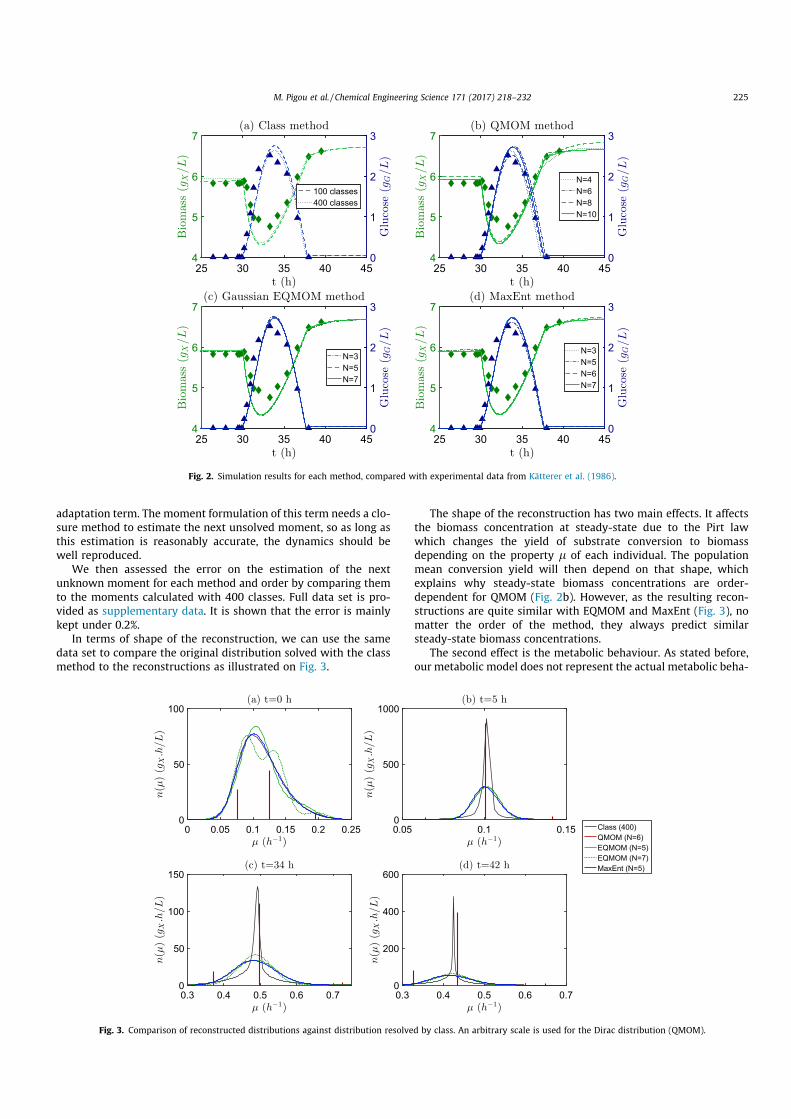
adaptation term. The moment formulation of this term needs a clo-sure method to estimate the next unsolved moment, so as long asthis estimation is reasonably accurate, the dynamics should bewell reproduced.
We then assessed the error on the estimation of the nextunknown moment for each method and order by comparing themto the moments calculated with 400 classes. Full data set is pro-vided as supplementary data. It is shown that the error is mainlykept under 0.2%.
In terms of shape of the reconstruction, we can use the samedata set to compare the original distribution solved with the classmethod to the reconstructions as illustrated on Fig. 3.
The shape of the reconstruction has two main effects. It affectsthe biomass concentration at steady-state due to the Pirt lawwhich changes the yield of substrate conversion to biomassdepending on the property l of each individual. The populationmean conversion yield will then depend on that shape, whichexplains why steady-state biomass concentrations are order-dependent for QMOM (Fig. 2b). However, as the resulting recon-structions are quite similar with EQMOM and MaxEnt (Fig. 3), nomatter the order of the method, they always predict similarsteady-state biomass concentrations.
The second effect is the metabolic behaviour. As stated before,our metabolic model does not represent the actual metabolic beha-
Fig. 2. Simulation results for each method, compared with experimental data from Kätterer et al. (1986).
Fig. 3. Comparison of reconstructed distributions against distribution resolved by class. An arbitrary scale is used for the Dirac distribution (QMOM).
M. Pigou et al. / Chemical Engineering Science 171 (2017) 218–232 225

viour of Candida tropicalis, however, it describe the overflow meta-bolism existing in E. coliwhich leads to acetate production in a waythat depends on the shape of the distribution. Fig. 4 illustratesthese different acetate productions depending on the chosenmethod. Once again, QMOM exhibits different behaviours depend-ing on the order of the method, while EQMOM and MaxEnt lead topredictions close to the class method.
Acetate production is slightly overestimated by all momentmethods (Fig. 4), due to the fact that they do not account for thenarrow peak of the distribution (Fig. 3b,c,d). This slightly overesti-mates the disequilibrium between the individuals and their envi-ronment, which is a key point in our modelling: thedisequilibrium between the cell uptake of substrate and itsrequirements for growth determines the intensity of the overflowmetabolism (i.e. the production of by-products, here the acetate).
In terms of simulation performances, the Fig. 5 details the meancomputation time spent on each time-step of the simulation. Ablank simulation –ran without computing the terms related to
bioreaction or population balance– is shown in order to estimateand distinguish the actual models computation time from the timespent on other tasks in the software.
The class method is a direct one, the computation time ismainly spent on (i) computing the metabolic model from Pigouand Morchain (2015) for each class and (ii) computing the redistri-bution term of the PBE as detailed in Morchain et al. (in press) foreach class, which implies computing NC þ 1 values of the Owen’s Tfunction using 10-nodes Gauss-Legendre quadratures (with NC thenumber of classes).
All method of moments must compute the first N moments ofthe skewnormal distribution which is not expensive consideringthat their expressions are available. The major computational costthen comes from (i) establishing the quadrature rule and (ii) com-puting the metabolic model for each node of the quadrature.
In this regard, QMOM is the least expensivemethod: the quadra-ture rule is computed using directly either the Product-DifferenceAlgorithm (PDA) or the Wheeler Algorithm (WA), both consistingin computing the eigenvalues and eigenvectors of a particularN=2 N=2 matrix, and computing the metabolic model for N=2nodes. The WA seems to be slightly faster than the PDA.
In order to establish a quadrature rule with the EQMOMmethod, Marchisio and Fox (2013) detail the analytical solutionfor N ¼ 3 and a solution whose cost is hardly higher than a 2 nodesQMOM for N ¼ 5, which explains the low computation times forthese two orders of resolution. The case N ¼ 7 needs an iterativealgorithm to find the suited quadrature rule, based on a dichotomicmethod. We speed-up that method by making use of the resultfrom the previous timestep, the dichotomic algorithm then con-verges most of the time in 3 to 6 evaluation of the objective func-tion, each of which requiring a single call to the WA.
Finally,MaxEnt is themost expensivemethod. It is actually as fastas QMOMand EQMOMwhen themoment set is far from the frontierof the moment space, but our model often produces moment setsnear the frontier. Then,we slowdown themethod by using differenttweaks in order to stabilise it: (i) the adaptive quadrature proposedby (Vié et al., 2013), (ii) the dynamic adaptation of the distribution’ssupport and (iii) the computation of canonical moments to checkrealizability of the moment set. The underlying Newton-Raphsonprocedure often converges in a single iteration, but this numberincreases up to 10 for many time-steps after the dilution rate shift,so simulating the next few hours following this shift is actually aslong as computing the rest of the time range.
Fig. 4. Evolution of acetate concentrations as predicted by the E. coli metabolicmodel. Black dash-dotted line: results from class method.
Fig. 5. Mean run-time per timestep for each method and different orders (ms/ts)( standard deviation measured on 20 simulations per method and order).
226 M. Pigou et al. / Chemical Engineering Science 171 (2017) 218–232

3.2. Fedbatch culture - Vrabel et al.
We simulated the very same fedbatch culture described with a70 compartments hydrodynamic model by Vrábel et al. (2001) butusing our own biological modelling as detailed in Pigou and
Morchain (2015). Here, we reproduce these simulations, by usingthe methods of moments to solve the population balance model.The QMOMmethod is applied with 5 nodes (N = 10) as this seemedto be required to produce the same results than the EQMOM andMaxEnt methods (Figs. 2 and 4). The MaxEnt method is used with
Fig. 6. Representation of the macroscopic flow patterns in the fedbatch reactor (left) and details of its compartmentalization and specific flows for the top of the reactor(right). Values for the flow rates CF, IF and EF are given in the appendix B of Pigou and Morchain (2015).
Fig. 7. Simulation results for the different population balance methods in the heterogeneous fedbatch culture. (a) Glucose concentration, (b) Total biomass concentration, (c)Acetate concentration and (d) Acetate specific production rate.
M. Pigou et al. / Chemical Engineering Science 171 (2017) 218–232 227

N = 5 moments as we did not manage to increase the number ofmoments up to 7 is this setup due to stability issues and alsobecause, surprisingly, the prediction of acetate production wasactually better with 5 moments than with 7 moments (seeFig. 4c). Finally, EQMOM was also applied with N = 5 moments asgoing up to 7 moments did not increase the precision drastically(Fig. 4b) but did increase significantly the computation time(Fig. 5). This will also make the comparison between MaxEnt andEQMOM more relevant.
In order to enforce the consistency of numerical results, welimit the maximum value of the time-step to the minimum com-partment mean-residence-time:
dtmax ¼ minNc
n¼1
VnPNcm¼1Qn;m
!ð34Þ
The value of the maximum time-step for the compartmentmodel shown in Fig. 6 is dtmax ¼ 1:47105 h.
The Fig. 7 gathers the results in term of glucose, total biomassand acetate concentrations as well as mean population reactionrates. The plotted values are mean values at different heights(volumetric mean value over compartments of the same row).The three heights (top, middle and bottom) correspond to thefollowing compartments (see Fig. 6 for numbering):
top: compartments 11–15, middle: compartments 36–40, bottom: compartments 61–65.
The good agreements between the methods is related tothe fact that, in the heterogeneous large-scale reactor, thedistribution is continuously perturbed by external fluctuationswhich prevent the apparition of the narrow distribution seenpreviously (Fig. 3). The expected distribution has a smoothershape which is well reconstructed by MaxEnt and EQMOM asshown in Fig. 8.
Finally, we ran 5 times the first hour of simulation in order togather statistics about simulation runtimes in the heterogeneouscase with different orders of resolution. The results are shown inFig. 9.
Each CPU core had to perform calculations for 14 compartmentsin Fig. 9 while a single compartment was considered in Fig. 5 whichexplains the overall higher computation times. However, the previ-ous analysis about the comparison of the complexity of eachmethod remains the same, and the observations on the heteroge-neous case are the same than in the homogeneous case: QMOMmaintains a constant computation time, EQMOM is as fast as
QMOM as long as N 5 and MaxEnt is slower than other methodsdue to the stabilisation of the method.
4. Discussion
Dealing with a biological phase naturally leads to the use of the‘‘population” semantic field due to the individual nature of cells,each of which having its own set of properties and its own ‘‘mem-ory”. Hence, the use of a Population Balance Model to describe abiological population seems to be obvious, almost axiomatic.
The most natural way to solve a PBM is the class method, whichconstitutes a direct resolution of the equations. However, its accu-racy comes with the price of a high memory cost. Unpublished datashow that for simple batch and chemostat simulations, the resultsare dependent on the number of classes up to 60 classes, and wecan even notice differences between 100 and 400 classes inFig. 2a. This number of classes is needed to span the entire prop-erty space with sufficient accuracy, however simulations clearlyshow that most of the time a large fraction of classes are nearlyempty. This means that we allocate memory for variables thatmost of the time carry almost no information, but still happensometime to be used, depending on the state of the population.
This explains why we are shifting toward methods of moments.They resolve basic properties of the distribution (total number,mean, variance, skewness, flatness, . . .) which all contain usefulinformation no matter the state of the population. Moments gatherhigher entropy about the distribution than classes, in the sense of
Fig. 8. Comparison of distribution shapes as resolved by the class method and reconstructed by the EQMOM and MaxEnt methods both with N ¼ 5 moments.
Fig. 9. Comparison of simulation runtimes for each method (ms=ts) ( standarddeviation measured on 5 simulations per method and order). Simulationsperformed using 5 CPU cores.
228 M. Pigou et al. / Chemical Engineering Science 171 (2017) 218–232

information theory. This significantly reduces the required numberof resolved variables, from more than 60, to half a dozen.
For some applications, each equation of the model can be for-mulated in terms of moments (Hulburt and Katz, 1964; McGraw,1997) leading to closed formulations or easy closure through theused of quadrature based methods. In these cases, the accuracyof the methods of moments poses no question –and is even betterthan a class method considering that the latter induces numericaldiffusion in the parameter space– for a smaller memory and com-putational cost.
Unfortunately, we deal here with a metabolic complexity thatoffers no model formulation in terms of moments. We tackle thisissue by using reconstruction methods, namely QMOM, EQMOMand MaxEnt methods; but these methods introduce quadratureinaccuracy as well as extra computational cost, which we tried toquantify in our simulations.
The results in terms of concentration fields are really promising,as the biomass, glucose and acetate concentrations were wellreproduced both in the homogeneous and the heterogeneouscases. We mainly noticed slight errors consisting in an over-production of acetate with moment methods in the Katterer case(see Fig. 4) due to difficulties in reconstructing a narrow distribu-tion with a wide base (similar to a Laplace distribution). However,we are shifting toward moment methods only to perform large-scale simulations at low memory cost: the class method performsjust fine enough for homogeneous cases. The crucial comparisonmust then be made on the large-scale simulation.
In Fig. 7, we observe a surprisingly good agreement between theclass method and the moment methods. The only noticeable differ-ence is seen on acetate curves for the moment methods whichslightly underestimate the acetate production for t 10 h whichinduces a persistent shift along time when compared to the classmethod. On this regard, the accuracy for variables whose value isof importance (substrate and product concentrations) is satisfac-tory for all methods.
In terms of computational cost, which we evaluate through thesimulation time, Yuan et al. (2012) already performed a compar-ison of EQMOM and the MaxEnt methods. They observed thatEQMOM was a hundred times faster than MaxEnt for the recon-struction of two NDF. However, we do not feel that their compar-ison is fair: the slow convergence of MaxEnt is only due to a badinitialization of the Newton-Raphson procedure, similar to whatwe observe in our simulations for the very first time-step. We wantto supplement their observations by pointing out that when usedin time resolved simulations, which happens to be our specificapplication for these methods, the MaxEnt method performs onlyslightly slower than EQMOM (see Figs. 5 and 9) due to differentadjustments made in order to improve stability.
We do not develop nor try to promote a specific reconstructionmethod, but only want to draw general guidelines about whichmethod should be used for the simulation of large-scale bioreac-tors. We then did our best to keep the comparison of the methodsas fair as possible. On the basis of our results, here are the keyobservations we made about the different methods.
EQMOM is a stable method: it behaves well near the momentspace frontier and we did not notice any particular difficulty whenincreasing the number of resolved moments. When used on mono-modal distribution, it can be applied at a low computational costwith 3 or 5 moments, thanks to analytical solutions (Marchisioand Fox, 2013). The possibility to increase the number of resolvedmoments, without loss of stability, means that this method is alsowell suited to reconstruct multi-modal distributions, this will beuseful when tracking fast population dynamics in heterogeneoussystems. Moreover, the method naturally embeds the feature ofnested quadratures: a relevant Gauss-Hermite quadrature can beconstructed on each Gaussian node of the EQMOM reconstruction,
which helps performing efficiently the integration of Eq. (2), com-pared to MaxEnt. This can be an important advantage of thismethod if the metabolic model (computation ofU) is computation-ally expensive. Here, the metabolic model was easy enough tocompute, which hide this salient feature of EQMOMreconstructions.
The same level of accuracy than EQMOMwith 5 moments couldbe reached with QMOM using 10 moments with a similar compu-tation time, but with less calls to the metabolic model. Both meth-ods can then be used based on whether we try to reduce thememory usage or the number of calls to a potentially complexmetabolic model. Similarly, as shown in A, if the redistributionlaw bðl;l0Þ did not allow such a simple moment formulation(Eq. (20)), the computational cost of EQMOM or MaxEnt to com-pute the redistribution term would be significantly higher thanQMOM. This is directly related to the number of nodes returnedby each method for a generic integral approximation (see Fig. 1,Eqs. (25), (28) and (33)).
MaxEnt is known to be ill-conditioned near the boundaries ofthe moment space (Massot et al., 2010) or when the number ofresolved moments increases (Gzyl and Tagliani, 2010), in particularwe did not manage to perform simulations using this method andmore than 7 resolved moments, or even 5 moments in the hetero-geneous case. This comes from the fact that we describe quite nar-row distributions on a large support, which naturally correspond tomoments near the frontier of the moment space. When the methodis working, it might give a better reconstruction with 5 momentsthan EQMOMwith 7 moments (Fig. 3a), however, using this recon-struction to construct a relevant quadrature rule is more difficultthan for EQMOM.We then recommend its use when assessing slowdynamics (preserving mono-modal distribution in heterogeneoussystems) for simulations where the time-step is negligible com-pared to the characteristic time of moment evolution (to ensurea good initialization), and only if a method can be designed to forma set of moment far enough from the frontier of the moment space.These are quite restrictive conditions which do not make thismethod the more advisable.
Finally, in terms of memory footprint, we managed to reducethe number of resolved variables to describe the population fromabout a hundred (class method) to about only 5 variables whichwill be significant when moving toward CFD simulations of biore-actors. However, it should be noted that for MaxEnt, memory reg-isters must be allocated both for the transported moments and forthe vector of polynomial coefficientsuwhich serves as initial valuefor the Newton-Raphson procedure. MaxEnt then requires twice asmuch memory space than QMOM and EQMOM methods for equiv-alent number of resolved moments.
The significant improvements in terms of memory usage will beeven more significant when we will shift toward multivariate pop-ulation balance models. For a bivariate distribution, the number ofclasses or moments will roughly be squared leading to about 104
classes opposed to 25 moments in each geometrical node.
5. Conclusions
The point of applying population balance based modelling forthe predictive simulation of heterogeneous bioreactors is now wellestablished (Morchain et al., 2014; Morchain et al., in press; Pigouand Morchain, 2015; Heins et al., 2015; Bertucco et al., 2015;Fredrickson and Mantzaris, 2002). This paper is more focused onnumerical methods to solve the population balance model, in orderto shift from a class method to moment based methods. In ourmodelling, the reconstruction methods of a NDF from a finite setof moments is required for the computation of the populationmetabolic behaviour. We then implemented QMOM, EQMOM and
M. Pigou et al. / Chemical Engineering Science 171 (2017) 218–232 229

Maximum Entropy methods, and challenged them in terms of sta-bility, memory footprint, computational cost and accuracy againstclass method results.
At equivalent number of resolved moments, QMOM is notice-ably less accurate than EQMOM and MaxEnt. However, increasingthe number of moments for QMOM does not increase significantlythe computation time, which make this method competitive withthe others when looking only at accuracy and simulation runtime.
If reducing the memory footprint is the main concern, EQMOMactually reaches the same accuracy than QMOM with half thenumber of resolved moments. However, its computational costincreases significantly between 5 and 7 resolved moments, dueto the need of an iterative procedure rather than an analytical ordirect solution.
Depending on the use case, MaxEnt has often been reported asan interesting method (Massot et al., 2010; Vié et al., 2013; Lebazet al., 2016), however, we will tend to discard it for our futureworks. Indeed, even when the method is well-conditioned, it isnot particularly competitive with EQMOM in terms of computationtime and accuracy, but comes with twice the memory usage ofEQMOM. Moreover, the method tends to be quickly unstable ifmoments are near the limit of realizability. This poses problemfor our modelling as the lack of experimental data about thedynamics of internal biological properties will make us formulatemodels which tend toward narrow distributions until data areavailable. An example of that is the PBM from Pigou andMorchain (2015) which led to a Dirac distribution in steady-statehomogeneous systems until experimental data from Nobs andMaerkl (2014, 2011) allowed us to improve the PBM and add anexperimentally justified redistribution term as explained inMorchain et al. (in press).
Overall, the QMOM and EQMOM methods have shown to beaccurate and stable enough for the simulation of a large scalebioreactor with a significantly reduced memory impact and a sim-ulation time of the same order of magnitude than the class method.
Acknowledgments
The authors thank Sanofi Chimie - C&BD Biochemistry Vitry forits financial support. The authors declare no conflict of interest.
Appendix A. Moment formulation of the PBE
As a recall, the population balance equation is defined as
@nðlÞ@t
¼ @
@lnðlÞfðlÞ½ þ
Z þ1
0bðl;l0Þnðl0ÞWl0dl0 ðA:1Þ
and the k-th order moment of the distribution nðlÞ is defined by
mk ¼Z þ1
0lknðlÞdl ðA:2Þ
We want to formulate the law of moments evolution, as the
sum of contributions from an adaptation term @ma;kðtÞ@t
, and a
growth term @mg;kðtÞ@t
:
@mkðtÞ@t
¼ @ma;kðtÞ@t
þ @mg;kðtÞ@t
ðA:3Þ
The formulation of @ma;kðtÞ@t comes by multiplying the first RHS
term of Eq. (A.1) by lk and integrating by part with respect to l:
@ma;kðtÞ@t
¼ ZXllk @
@lnðl; tÞ fðlÞð Þdl ðA:4Þ
¼ZXl
klk1nðl; tÞfðlÞdl lknðl; tÞfðlÞ @Xl ðA:5Þ
Considering that the adaptation will not allow individuals tocross the frontier of the l-space (@Xl), the second term of Eq.(A.5) is necessarily null. By expanding the formulation of
fðlÞ ¼ T1 þ l
ðl lÞ, the formulation of @ma;kðtÞ@t in terms of
moments of the distribution is trivial:
@ma;kðtÞ@t
¼ kl
Tmk1ðtÞ þ l 1
T
mkðtÞ mkþ1ðtÞ
ðA:6Þ
The contribution of the growth term to the moment evolutiondepends both on the used quadrature method and on the propra-bility function modeling the redistribution phenomena related tocell division. We have
@mg;kðtÞ@t
¼ZXllk
ZXl
bðl; ~lÞWl0nðl0Þdl0" #
dl ðA:7Þ
The approximations of nðlÞ by the methods of moments lead toZXl
f ðlÞnðlÞdl XI
i¼1
wi f ðLiÞ ðA:8Þ
where I;wi and Li depend on the methods used to perform thequadrature of moments (Eqs. (25), (28) and (33)).
Using these quadratures, we reach the following expression:
@mg;kðtÞ@t
WZXllk
XI
i¼1
wiLibðl; LiÞ !
dl ðA:9Þ
WXI
i¼1
wiLi
ZXllkbðl; LiÞdl ðA:10Þ
This last formulation is generic and can be used for any redistri-bution law bðl;l0Þ. In the case of current simulations, we base thisterm on the previous work from Morchain et al. (in press) were weidentified the following probability density function as a goodmodel for experimental data from the literature (Nobs andMaerkl, 2014; Yasuda, 2011):
bðl;l0Þ ¼ 2r/
l lr
U a l l
r
ðA:11Þ
with:
/ðxÞ ¼ 1ffiffiffiffi2p
p ex22 ,
UðxÞ ¼ 12 1þ erf xffiffi
2p
.
The redistribution law is a skew-normal distribution whoseparameters depend on the population mean growth rate ~l butnot on the growth rate of the mother cell (hence, l0 is not usedin the expression):
~l ¼ m1ðtÞm0ðtÞ ðA:12Þ
l ¼ kl ~l ðA:13Þr ¼ kr ~l ðA:14Þa ¼ 3:65 ðA:15Þ
The constants kl and kr were chosen so that the PDF bðl;l0Þ fitsexperimental data, but also with the constraint that the firstmoment of this PDF is equal to ~l so that the redistribution termwill have no impact on the population mean growth rate. The usedvalues are:
Then, the growth related evolution of the distribution momentsis easily expressed in terms of moments of bðl;l0Þ ¼ bðlÞ and doesnot require the moment quadrature:
230 M. Pigou et al. / Chemical Engineering Science 171 (2017) 218–232

@mg;kðtÞ@t
¼ZXl
lkZXl
bðlÞWl0nðl0Þdl0" #
dl ðA:16Þ
¼ WZXllkbðlÞ
ZXll0nðl0Þdl0
" #dl ðA:17Þ
¼ WZXllkbðlÞm1ðtÞdl ðA:18Þ
¼ Wm1ðtÞBk ðA:19ÞBk is the k-th order moment of the PDF bðlÞ which happens to
only depend on ~l whose value is accessible using the first twomoments of the distribution (Eq. (A.12)). The moments Bk can bedetermined analytically using the Moment Generating Functionof the skew-normal distribution:
Bk ¼ @kM@tk
ð0Þ ðA:23Þ
MðtÞ ¼ exp lt þ r2t2
2
1þ erf
ratffiffiffiffiffiffiffiffiffiffiffiffiffiffiffiffiffiffiffiffiffi2ð1þ a2Þp
! !ðA:24Þ
We used the MATLAB Symbolic Toolbox to pre-compute theexpressions of Bk;8k 2 f0; . . . ;9g.
Note that in order to respect the constraint B1 ¼ ~l; kr and klmust satisfy the following relationship:
kl þffiffiffiffiffiffiffiffiffiffiffiffiffiffiffiffiffiffiffiffiffi
2a2
pð1þ a2Þ
skr ¼ 1 ðA:25Þ
Appendix B. Supplementary material
Supplementary data associated with this article can be found, inthe online version, at http://dx.doi.org/10.1016/j.ces.2017.05.026.
References
Abramov, R.V., 2007. An improved algorithm for the multidimensional moment-constrained maximum entropy problem. J. Comput. Phys. 226, 621–644. http://dx.doi.org/10.1016/j.jcp.2007.04.026.
Abulesz, E.M., Lyberatos, G., 1989. Periodic operation of a continuous culture ofbaker’s yeast. Biotechnol. Bioeng. 34, 741–749. http://dx.doi.org/10.1002/bit.260340603.
Athanassoulis, G., Gavriliadis, P., 2002. The truncated hausdorff moment problemsolved by using kernel density functions. Probab. Eng. Mech. 17, 273–291.http://dx.doi.org/10.1016/S0266-8920(02)00012-7.
Baldyga, J., Bourne, J.R., 1999. Turbulent Mixing and Chemical Reactions. John Wileyand Sons.
Bertucco, A., Sforza, E., Fiorenzato, V., Strumendo, M., 2015. Population balancemodeling of a microalgal culture in photobioreactors: comparison betweenexperiments and simulations. AIChE J. 61, 2702–2710. http://dx.doi.org/10.1002/aic.14893.
Bezzo, F., Macchietto, S., Pantelides, C.C., 2003. General hybrid multizonal/CFDapproach for bioreactor modeling. AIChE J. 49, 2133–2148. http://dx.doi.org/10.1002/aic.690490821.
Bogacki, P., Shampine, L., 1989. A 3(2) pair of Runge-Kutta formulas. Appl. Math.Lett. 2, 321–325. http://dx.doi.org/10.1016/0893-9659(89)90079-7.
Chalons, C., Fox, R.O., Massot, M., 2010. A multi-Gaussian quadrature method ofmoments for gas-particle flows in a LES framework. In: Proceedings of the 2010Summer Program, Center for turbulence Research. Stanford University, pp. 347–358.
Cui, Y.Q., van der Lans, R.G., Noorman, H.J., Luyben, K.C.A.M., 1996. Compartmentmixing model for stirred reactors with multiple impellers. Chem. Eng. Res. Des.74, 261–271.
Dette, H., Studden, W.J., 1997. The Theory of Canonical Moments with Applicationsin Statistics, Probability, and Analysis. JohnWiley & Sons, New York; Chichester.
Elqotbi, M., Vlaev, S., Montastruc, L., Nikov, I., 2013. CFD modelling of two-phasestirred bioreaction systems by segregated solution of the euler-euler model.Comput. Chem. Eng. 48, 113–120. http://dx.doi.org/10.1016/j.compchemeng.2012.08.005.
Enfors, S.O., Jahic, M., Rozkov, A., Xu, B., Hecker, M., Jürgen, B., Krüger, E., Schweder,T., Hamer, G., O’Beirne, D., Noisommit-Rizzi, N., Reuss, M., Boone, L., Hewitt, C.,McFarlane, C., Nienow, A., Kovacs, T., Trägardh, C., Fuchs, L., Revstedt, J., Friberg,P., Hjertager, B., Blomsten, G., Skogman, H., Hjort, S., Hoeks, F., Lin, H.Y.,Neubauer, P., van der Lans, R., Luyben, K., Vrábel, P., Manelius, A., 2001.Physiological responses to mixing in large scale bioreactors. J. Biotechnol. 85,
175–185. http://dx.doi.org/10.1016/S0168-1656(00)00365-5. twenty years ofthe European Federation of Biotechnology.
Ferenci, T., 1996. Adaptation to life at micromolar nutrient levels: the regulation ofEscherichia coli glucose transport by endoinduction and cAMP. FEMS Microbiol.Rev. 18, 301–317. http://dx.doi.org/10.1111/j.1574-6976.1996.tb00246.x.
Ferenci, T., 1999. Regulation by nutrient limitation. Curr. Opin. Microbiol. 2, 208–213. http://dx.doi.org/10.1016/S1369-5274(99)80036-8.
Fredrickson, A., Mantzaris, N.V., 2002. A new set of population balance equations formicrobial and cell cultures. Chem. Eng. Sci. 57, 2265–2278. http://dx.doi.org/10.1016/S0009-2509(02)00116-1.
Gzyl, H., Tagliani, A., 2010. Hausdorff moment problem and fractional moments.Appl. Math. Comput. 216, 3319–3328. http://dx.doi.org/10.1016/j.amc.2010.04.059.
Haringa, C., Tang, W., Deshmukh, A.T., Xia, J., Reuss, M., Heijnen, J.J., Mudde, R.F.,Noorman, H.J., 2016. Euler-Lagrange computational fluid dynamics for (bio)reactor scale down: an analysis of organism lifelines. Eng. Life Sci. http://dx.doi.org/10.1002/elsc.201600061.
Heavner, B.D., Smallbone, K., Barker, B., Mendes, P., Walker, L.P., 2012. Yeast 5 – anexpanded reconstruction of the Saccharomyces cerevisiae metabolic network.BMC Syst. Biol. 6. http://dx.doi.org/10.1186/1752-0509-6-55.
Heavner, B.D., Smallbone, K., Price, N.D., Walker, L.P., 2013. Version 6 of theconsensus yeast metabolic network refines biochemical coverage and improvesmodel performance. Database, 2013. http://dx.doi.org/10.1093/database/bat059.
Heins, A.L., Fernandes, R.L., Gernaey, K.V., Lantz, A.E., 2015. Experimental and insilico investigation of population heterogeneity in continuous Saccharomycescerevisiae scale-down fermentation in a two-compartment setup. J. Chem.Technol. Biotechnol. 90, 324–340. http://dx.doi.org/10.1002/jctb.4532.
Hulburt, H., Katz, S., 1964. Some problems in particle technology: a statisticalmechanical formulation. Chem. Eng. Sci. 19, 555–574. http://dx.doi.org/10.1016/0009-2509(64)85047-8.
John, V., Angelov, I., Öncül, A., Thévenin, D., 2007. Techniques for the reconstructionof a distribution from a finite number of its moments. Chem. Eng. Sci. 62, 2890–2904. http://dx.doi.org/10.1016/j.ces.2007.02.041.
Kapur, J., 1989. Maximum-entropy Models in Science and Engineering. Wiley.Kätterer, L., Allemann, H., Käppeli, O., Fiechter, A., 1986. Transient responses of
continuously growing yeast cultures to dilution rate shifts: a sensitive means toanalyze biology and the performance of equipment. Biotechnol. Bioeng. 28,146–150. http://dx.doi.org/10.1002/bit.260280126.
Kumar, S., Ramkrishna, D., 1996a. On the solution of population balance equationsby discretization – I. A fixed pivot technique. Chem. Eng. Sci. 51, 1311–1332.http://dx.doi.org/10.1016/0009-2509(96)88489-2.
Kumar, S., Ramkrishna, D., 1996b. On the solution of population balance equationsby discretization – II. A moving pivot technique. Chem. Eng. Sci. 51, 1333–1342.http://dx.doi.org/10.1016/0009-2509(95)00355-X.
Lebaz, N., Cockx, A., Spérandio, M., Morchain, J., 2016. Reconstruction of adistribution from a finite number of its moments: a comparative study in thecase of depolymerization process. Comput. Chem. Eng. 84, 326–337. http://dx.doi.org/10.1016/j.compchemeng.2015.09.008.
Li, W., 1982. Estimating heterotrophic bacterial productivity by inorganicradiocarbon uptake: importance of establishing time courses of uptake. DeepSea Res. Part B. Oceanogr. Literature Rev. 29, 167–172. http://dx.doi.org/10.1016/0198-0254(82)90325-9.
Linkès, M., Fede, P., Morchain, J., Schmitz, P., 2014. Numerical investigation ofsubgrid mixing effects on the calculation of biological reaction rates. Chem. Eng.Sci. 116, 473–485. http://dx.doi.org/10.1016/j.ces.2014.05.005.
Lu, H., Li, C., Tang, W., Wang, Z., Xia, J., Zhang, S., Zhuang, Y., Chu, J., Noorman, H.,2015. Dependence of fungal characteristics on seed morphology and shearstress in bioreactors. Bioprocess Biosyst. Eng. 38, 917–928. http://dx.doi.org/10.1007/s00449-014-1337-8.
Madadi-Kandjani, E., Passalacqua, A., 2015. An extended quadrature-based momentmethod with log-normal kernel density functions. Chem. Eng. Sci. 131, 323–339. http://dx.doi.org/10.1016/j.ces.2015.04.005.
Mantzaris, N.V., Daoutidis, P., Srienc, F., 2001. Numerical solution of multi-variablecell population balance models: I. Finite difference methods. Comput. Chem.Eng. 25, 1411–1440. http://dx.doi.org/10.1016/S0098-1354(01)00709-8.
Marchisio, D., Fox, R., 2013. Computational Models for Polydisperse Particulate andMultiphase Systems. Cambridge Series in Chemical Engineering. CambridgeUniversity Press.
Marchisio, D.L., Pikturna, J.T., Fox, R.O., Vigil, R.D., Barresi, A.A., 2003a. Quadraturemethod of moments for population-balance equations. AIChE J. 49, 1266–1276.http://dx.doi.org/10.1002/aic.690490517.
Marchisio, D.L., Vigil, R., Fox, R.O., 2003b. Quadrature method of moments foraggregation-breakage processes. J. Colloid Interface Sci. 258, 322–334. http://dx.doi.org/10.1016/S0021-9797(02)00054-1.
Marchisio, D.L., Vigil, R.D., Fox, R.O., 2003c. Implementation of the quadraturemethod of moments in CFD codes for aggregation-breakage problems. Chem.Eng. Sci. 58, 3337–3351. http://dx.doi.org/10.1016/S0009-2509(03)00211-2.
Massot, M., Laurent, F., Kah, D., De Chaisemartin, S., 2010. A robust moment methodfor evaluation of the disappearance rate of evaporating sprays. SIAM J. Appl.Math. 70, 3203–3234. http://dx.doi.org/10.1137/080740027.
Matsuoka, Y., Shimizu, K., 2013. Catabolite regulation analysis of Escherichia coli foracetate overflow mechanism and co-consumption of multiple sugars basedon systems biology approach using computer simulation. J. Biotechnol. 168,155–173. http://dx.doi.org/10.1016/j.jbiotec.2013.06.023. special issue:Biotechnology for a healthy and green world.
M. Pigou et al. / Chemical Engineering Science 171 (2017) 218–232 231

Mayr, B., Horvat, P., Nagy, E., Moser, A., 1993. Mixing-models applied to industrialbatch bioreactors. Bioprocess Eng. 9, 1–12. http://dx.doi.org/10.1007/BF00389534.
McGraw, R., 1997. Description of aerosol dynamics by the quadrature method ofmoments. Aerosol Sci. Technol. 27, 255–265. http://dx.doi.org/10.1080/02786829708965471.
Mead, L.R., Papanicolaou, N., 1984. Maximum entropy in the problem of moments. J.Math. Phys. 25, 2404–2417.
Meadows, A.L., Karnik, R., Lam, H., Forestell, S., Snedecor, B., 2010. Application ofdynamic flux balance analysis to an industrial Escherichia coli fermentation.Metabolic Eng. 12, 150–160. http://dx.doi.org/10.1016/j.ymben.2009.07.006.metabolic Flux Analysis for Pharmaceutical Production Special Issue.
Morchain, J., Gabelle, J.C., Cockx, A., 2013. Coupling of biokinetic and populationbalance models to account for biological heterogeneity in bioreactors. AIChE J.59, 369–379. http://dx.doi.org/10.1002/aic.13820.
Morchain, J., Gabelle, J.C., Cockx, A., 2014. A coupled population balance model andCFD approach for the simulation of mixing issues in lab-scale and industrialbioreactors. AIChE J. 60, 27–40. http://dx.doi.org/10.1002/aic.14238.
Morchain, J., Pigou, M., Lebaz, N., in press. A population balance model forbioreactors combining interdivision time distributions and micromixingconcepts. Biochem. Eng. J. http://dx.doi.org/10.1016/j.bej.2016.09.005. in press.
Nobs, J.B., Maerkl, S.J., 2014. Long-term single cell analysis of S. pombe on amicrofluidic microchemostat array. PLoS ONE 9. http://dx.doi.org/10.1371/journal.pone.0093466.
Orth, J.D., Conrad, T.M., Na, J., Lerman, J.A., Nam, H., Feist, A.M., Palsson, B.O., 2011. Acomprehensive genome-scale reconstruction of Escherichia coli metabolism.Molec. Syst. Biol. 7. http://dx.doi.org/10.1186/1752-0509-6-55.
Perret, C.J., 1960. A new kinetic model of a growing bacterial population.Microbiology 22, 589–617. http://dx.doi.org/10.1099/00221287-22-3-589.
Pigou, M., Morchain, J., 2015. Investigating the interactions between physical andbiological heterogeneities in bioreactors using compartment, populationbalance and metabolic models. Chem. Eng. Sci. 126, 267–282. http://dx.doi.org/10.1016/j.ces.2014.11.035.
Silveston, P., Budman, H., Jervis, E., 2008. Forced modulation of biological processes:a review. Chem. Eng. Sci. 63, 5089–5105. http://dx.doi.org/10.1016/j.ces.2008.06.017. 5TH Unsteady-State Processes in Catalysis: a Special Issue ofChemical Engineering Science.
Tagliani, A., 1999. Hausdorff moment problem and maximum entropy: a unifiedapproach. Appl. Math. Comput. 105, 291–305. http://dx.doi.org/10.1016/S0096-3003(98)10084-X.
Vié, A., Laurent, F., Massot, M., 2013. Size-velocity correlations in hybrid high ordermoment/multi-fluid methods for polydisperse evaporating sprays: modelingand numerical issues. J. Comput. Phys. 237, 177–210. http://dx.doi.org/10.1016/j.jcp.2012.11.043.
Vrábel, P., van der Lans, R.G., Cui, Y., Luyben, K., 1999. Compartment modelapproach: mixing in large scale aerated reactors with multiple impellers. Chem.Eng. Res. Des. 77, 291–302. http://dx.doi.org/10.1205/026387699526223.
Vrábel, P., van der Lans, R.G., Luyben, K.C., Boon, L., Nienow, A.W., 2000. Mixing inlarge-scale vessels stirred with multiple radial or radial and axial up-pumpingimpellers: modelling and measurements. Chem. Eng. Sci. 55, 5881–5896. http://dx.doi.org/10.1016/S0009-2509(00)00175-5.
Vrábel, P., van der Lans, R.G., van der Schot, F.N., Luyben, K.C., Xu, B., Enfors, S.O.,2001. CMA: integration of fluid dynamics and microbial kinetics in modelling oflarge-scale fermentations. Chem. Eng. J. 84, 463–474. http://dx.doi.org/10.1016/S1385-8947(00)00271-0.
Xu, B., Jahic, M., Enfors, S.O., 1999. Modeling of overflow metabolism in batch andfed-batch cultures of Escherichia coli. Biotechnol. Prog. 15, 81–90. http://dx.doi.org/10.1021/bp9801087.
Yasuda, K., 2011. Algebraic and geometric understanding of cells: epigeneticinheritance of phenotypes between generations. In: Müller, S., Bley, T. (Eds.),High Resolution Microbial Single Cell Analytics, Advances in BiochemicalEngineering/Biotechnology, vol. 124. Springer, Berlin, Heidelberg, pp. 55–81.http://dx.doi.org/10.1007/10_2010_97.
Yuan, C., Laurent, F., Fox, R., 2012. An extended quadrature method of moments forpopulation balance equations. J. Aerosol Sci. 51, 1–23. http://dx.doi.org/10.1016/j.jaerosci.2012.04.003.
232 M. Pigou et al. / Chemical Engineering Science 171 (2017) 218–232

CN E W D E V E L O P M E N T S O F T H E E X T E N D E D Q U A D R AT U R EM E T H O D O F M O M E N T S T O S O LV E P O P U L AT I O N B A L A N C EE Q U AT I O N S
217

Journal of Computational Physics 365 (2018) 243–268
Contents lists available at ScienceDirect
Journal of Computational Physics
www.elsevier.com/locate/jcp
New developments of the Extended Quadrature Method of
Moments to solve Population Balance Equations
Maxime Pigou a,b,∗, Jérôme Morchain a, Pascal Fede b, Marie-Isabelle Penet c, Geoffrey Laronze c
a LISBP, Université de Toulouse, CNRS, INRA, INSA, Toulouse, Franceb Institut de Mécanique des Fluides de Toulouse – Université de Toulouse, CNRS-INPT-UPS, Toulouse, Francec Sanofi Chimie – C&BD Biochemistry Vitry - 9 quai Jules Guesde, 94400 Vitry-sur-Seine, France
a r t i c l e i n f o a b s t r a c t
Article history:Received 17 October 2017Received in revised form 15 February 2018Accepted 16 March 2018Available online 21 March 2018
Keywords:Extended Quadrature Method of Moments (EQMOM)Quadrature Based Method of Moments (QBMM)Population BalanceMathematical modellingGauss quadrature
Population Balance Models have a wide range of applications in many industrial fields as they allow accounting for heterogeneity among properties which are crucial for some system modelling. They actually describe the evolution of a Number Density Function (NDF) using a Population Balance Equation (PBE). For instance, they are applied to gas–liquid columns or stirred reactors, aerosol technology, crystallisation processes, fine particles or biological systems. There is a significant interest for fast, stable and accurate numerical methods in order to solve for PBEs, a class of such methods actually does not solve directly the NDF but resolves their moments. These methods of moments, and in particular quadrature-based methods of moments, have been successfully applied to a variety of systems. Point-wise values of the NDF are sometimes required but are not directly accessible from the moments. To address these issues, the Extended Quadrature Method of Moments (EQMOM) has been developed in the past few years and approximates the NDF, from its moments, as a convex mixture of Kernel Density Functions (KDFs) of the same parametric family. In the present work EQMOM is further developed on two aspects. The main one is a significant improvement of the core iterative procedure of that method, the corresponding reduction of its computational cost is estimated to range from 60% up to 95%. The second aspect is an extension of EQMOM to two new KDFs used for the approximation, the Weibull and the Laplace kernels. All MATLAB source codes used for this article are provided with this article.
© 2018 Elsevier Inc. All rights reserved.
1. Introduction
Population Balance Equations (PBEs) are particular formalisms that allows describing the evolution of properties among heterogeneous populations. They are used to track the size distribution of fine particles [1]; the bubble size distribution in gas–liquid stirred-tank reactors or bubble columns [2,3]; the crystal-size distribution in crystallizers; the distribution of biological cell properties in bioreactors [4,5]; the volume and/or surface distribution of soot particles in flames [6,7] or the formation of nano-particles [8], among other examples.
* Corresponding author at: LISBP-INSA Toulouse, 135 Avenue de Rangueil, 31077 Toulouse, France.E-mail address: maxime .pigou @insa -toulouse .fr (M. Pigou).
https://doi.org/10.1016/j.jcp.2018.03.0270021-9991/© 2018 Elsevier Inc. All rights reserved.

244 M. Pigou et al. / Journal of Computational Physics 365 (2018) 243–268
Nomenclature
Greek symbols
ε relative tolerance
λ j j-th nested quadrature node
μ positive measure
ω j j-th nested quadrature weight
ξ NDF support
πk k order orthogonal polynomial
σ shape parameter
ξ random variable
ξi i-th main quadrature node
ζ realisability criteria on ]0,+∞[
Roman
a orthogonal polynomials recurrence coefficient
A transition matrix to degenerated moments
b orthogonal polynomials recurrence coefficient
H Hankel determinant
J n n order Jacobi matrix
mk moment of order kM realisable moment space
n number density function
n approximation of nN order of moment set
N order of realisability
pk canonical moment of order kP number of main quadrature nodes
Q number of nested quadrature nodes
wi i-th main quadrature weight
A PBE describes the evolution and transport of a Number Density Function (NDF), under the influence of multiple processes which modify the tracked property distribution (e.g. erosion, dissolution, aggregation, breakage, coalescence, nu-cleation, adaptation, etc.).
One often requires low-cost numerical methods to solve PBEs, for instance when coupling with a flow solver (e.g. Computational Fluid Dynamics software). Monte-Carlo methods constitute a stochastic resolution of the popula-tion balance and can be applied to such PBE–CFD simulations [9]. Similarly, sectional methods allow direct numeri-cal resolutions of the PBE through the discretisation of the property space [10,11]. They respectively require a high number of parcels or sections in order to reach high accuracy and are thus often discarded for large-scale simula-tions.
An interesting alternative approach lies in the field of methods of moments. A PBE, which describes the evolution of a NDF, is transformed in a set of equations which describes the evolution of the moments of that distribution. Moments are integral properties of NDFs, the first low order integer moments are related to the mean, variance, skewness and flatness of the statistical distributions described by NDFs. This approach then reduces the number of resolved variables to a finite set of NDF moments. It also comes with some difficulties when one must compute non-moment integral properties, or point-wise evaluations, of the distribution [12].
To tackle these issues, one can try to recover a NDF from a finite set of its moments. In most cases, this reverse problem has an infinite number of solutions and different approaches exist to identify one or an other out of them. The simplest is probably to assume that the NDF is a standard distribution (Gaussian, Log-normal, . . . ) whose parameters will be deduced from its first few moments. Other methods that lead to continuous approximations, and which preserve a higher number of moments, are the Spline method [13], the Maximum-Entropy approach [12,14,15] or the Kernel Density Element Method (KDEM) [16].
More recently, the Extended Quadrature Method of Moments (EQMOM) was proposed as a new approach which is more stable than the previous ones, and yields either continuous or discrete NDFs depending on the moments [1,17,18]. EQMOM has been implemented in OpenFOAM [19] for the purpose of PBE–CFD coupling. The core of this method relies on an iterative procedure that is a computational bottleneck.
The current work focuses on EQMOM and develops a new core procedure whose computational cost is significantly lower than previous implementations by reducing both (i) the cost of each iteration and (ii) the total number of required iterations.
The previous core procedure [1] will be recalled before describing how it can be shifted toward the new – cheaper – approach. Both implementations will be compared in terms of computational cost (number of required floating-point operations) and run-time.
Multiple variations of EQMOM exist, the Gauss EQMOM [17,20], Log-normal EQMOM [21] as well as Gamma and Beta EQMOM [18]. Two new variations, namely Laplace EQMOM and Weibull EQMOM, are proposed along with a unified formal-ism among all six variations.
The whole source code used to write this article (figures and data generation) is provided as supplementary data, as well as our implementations of EQMOM in the form of a MATLAB functions library [22].

M. Pigou et al. / Journal of Computational Physics 365 (2018) 243–268 245
2. Quadrature Based Methods of Moments: QMOM and EQMOM
2.1. Definitions
Let dμ(ξ) be a positive measure, induced by a non-decreasing function μ(ξ) defined on a support ξ . This measure is associated to a Number Density Function n(ξ) such that dμ(ξ) = n(ξ)dξ . Let mN be the vector of the first N + 1 integer moments of this measure:
mN =
⎡⎢⎢⎢⎣m0m1...
mN
⎤⎥⎥⎥⎦ , mk =∫ξ
ξkn(ξ)dξ (1)
Three actual supports will be considered: (i) ξ = ]−∞,+∞[, (ii) ξ = ]0,+∞[ and (iii) ξ = ]0,1[. For each support, one can define the associated realisable moment space, MN (ξ ), as the set of all vectors of finite moments mN induced by all possible positive measures defined on ξ .
A moment set is said to be “weakly realisable” if located on the boundary of the realisable moment space (mN ∈∂MN (ξ )). Otherwise, if located within the realisable moment space, mN is said to be “strictly realisable”.
2.2. Quadrature method of moments
EQMOM is based on the Quadrature Method of Moments (QMOM) that was first introduced by McGraw [23]. It is used to approximate integral properties of a distribution where only a finite number of its moments is known. By making use of an even number of moments 2P , one can compute a Gauss quadrature rule characterised by its weights w P = [w1, . . . , w P ]T
and nodes ξ P = [ξ1, . . . , ξP ]T such that:∫ξ
f (ξ)dμ(ξ) =P∑
i=1
wi f (ξi) (2)
holds true if f (ξ) = ξk, ∀k ∈ 0, . . . , 2P − 1. Otherwise, this quadrature rule will produce an approximation of the integral property. The computation of the quadrature rule (i.e. the vectors w P and ξ P ) is of special interest for following develop-ments, which is why its two main steps will be detailed.
Any positive measure dμ(ξ) is associated with a sequence of monic polynomials (i.e. polynomial whose leading coeffi-cient equals 1) denoted πk – with k the order of the polynomial – such that:∫
ξ
πi(ξ)π j(ξ)dμ(ξ) = 0, for i = j (3)
These polynomials are said orthogonal with respect to the measure dμ(ξ) and are defined by:
πk(ξ) = 1
ck
∣∣∣∣∣∣∣∣∣∣∣
m0 m1 · · · mk−1 mkm1 m2 · · · mk mk+1...
.... . .
......
mk−1 mk · · · m2k−2 m2k−1
1 ξ · · · ξk−1 ξk
∣∣∣∣∣∣∣∣∣∣∣(4)
with ck a constant chosen so that the leading coefficient (of order k) of πk equals 1, hence making πk a monic polynomial.It is known that monic orthogonal polynomials satisfy a three-term recurrence relation [24]:
πk+1(ξ) = (ξ − ak)πk(ξ) − bkπk−1(ξ) (5)
with ak and bk being the recurrence coefficients specific to the measure dμ(ξ), π−1(ξ) = 0 and π0(ξ) = 1.Let J n(dμ) be the n × n Jacobi matrix associated to the measure dμ. This is a tridiagonal symmetric matrix defined as:
J n(dμ) =
⎛⎜⎜⎜⎜⎝a0
√b1 0
√b1 a1
. . .
. . .. . .
√bn−1
0√
bn−1 an−1
⎞⎟⎟⎟⎟⎠ (6)

246 M. Pigou et al. / Journal of Computational Physics 365 (2018) 243–268
The weights and nodes of the quadrature rule from Eq. (2) are given by spectral properties of J P (dμ). The nodes ξ P of the rule are the eigenvalues of J P (dμ). The weights of the rule are given by:
wi = m0 v21,i (7)
where v1,i is the first component of the normalised eigenvector belonging to the eigenvalue ξi . The computation of the quadrature rule (Eq. (2)) then relies on two steps:
1. The computation of the recurrence coefficients aP−1 = [a0, . . . , aP−1]T and bP−1 = [b1, . . . , bP−1]T .2. The computation of the eigenvalues and the normalised eigenvectors of J P (dμ).
Multiple algorithms are available in the literature to compute the recurrence coefficients:
• The Quotient-Difference algorithm [25,26]• The Product-Difference algorithm [27]• The Chebyshev algorithm [28]
The Chebyshev algorithm was found to be the stablest one of the three [1,28], its description is given in Appendix A.
2.3. Extended Quadrature Method of Moments
The QMOM method is well suited for the approximation of integral properties of the NDF, which is actually the main purpose of Gauss quadratures. However, in many applications such as evaporation [12] or dissolution [29] processes, point-wise values of the NDF n(ξ) are required but not directly accessible from the moments. For that purpose, a method is needed to produce an approximation n(ξ) of the original distribution n(ξ), by knowing only a finite set of its moments.
In a sense, one can consider that the Gaussian quadrature computed with QMOM approximates n(ξ) as a weighted sum of Dirac distributions:
n(ξ) =P∑
i=1
wiδ(ξ, ξi) (8)
with the Dirac δ distribution defined by its sifting property
+∞∫−∞
f (ξ) δ(ξ, ξm)dξ = f (ξm) (9)
For most applications, n(ξ) is expected to be a continuous distribution whilst QMOM yields monodisperse or discrete polydisperse reconstructions of n(ξ), with n(ξ) = 0 for all values of ξ except some finite number of these values.
Many methods were suggested to tackle this problem and to propose a continuous reconstruction n(ξ) from a finite number of moments mN . Some of them are the Spline method [13], the Maximum-Entropy approach [14,15,12] or the Kernel Density Element Method [16]. Their properties will not be discussed here but one only underlines that they tend to be unstable, ill-conditioned, or have a high sensitivity to numerical parameters [13,29,30]. In particular, none of them can handle the case of a weakly realisable moment set. Such a moment set is associated to a discrete (or degenerated) distribution and, in this specific case, the distribution provided by QMOM is the only possible reconstruction (see Eq. (8)).
Note that a failure – or instabilities – in a numerical method can compromise the integrity of large-scale simulations. For this reason, Chalons et al. [17], Yuan et al. [18] and Nguyen et al. [1] proposed a robust and stable method to tackle this reconstruction problem by handling both continuous approximations and discrete solutions. Their approach, the Extended Quadrature Method of Moments, approximates n(ξ) as a convex mixture of Kernel Density Functions (KDFs) of the same parametric family:
n(μ) =P∑
i=1
wiδσ (ξ, ξi) (10)
with
• wi : the weight of the i-th node, wi ≥ 0, ∀i ∈ 1, . . . , P • ξi : the location parameter of the i-th node, ξi ∈ ξ , ∀i ∈ 1, . . . , P • δσ : a KDF chosen to perform the approximation, referred later to as the reconstruction kernel. σ is the shape parameter
of the approximation.

M. Pigou et al. / Journal of Computational Physics 365 (2018) 243–268 247
The computation of the weights w P = [w1, . . . , w P ]T , the nodes ξ P = [ξ1, . . . , ξP ]T and the shape parameter σ from the moment set m2P is performed by the EQMOM moment-inversion procedure. The improvement of this procedure constitutes the core of this article and is detailed in section 3.
Multiple standard normalized distribution functions can be used as the reconstruction kernel δσ (e.g. Gaussian, Log-normal, etc.). A list of them is given in Appendix B. All of these kernels degenerate into Dirac distribution if their shape parameters are sufficiently small:
limσ→0
δσ (ξ, ξm) = δ(ξ, ξm) (11)
This allows EQMOM to be numerically stable in the case of a moment set m2P being on the boundary of the realisable moment space ∂M2P (ξ ). Indeed, in such cases, the EQMOM approximation simply degenerates in a weighted sum of Dirac distribution and the definition given in Eq. (10) still holds true, with σ = 0.
EQMOM can also be used to compute integral properties of the NDF with high accuracy. This comes with the introduction of nested quadratures. The main quadrature proposes the following approximation of integral terms:
∫ξ
f (ξ)n(ξ)dξ ≈P∑
i=1
wi
⎡⎢⎣∫ξ
f (ξ)δσ (ξ, ξi)dξ
⎤⎥⎦ (12)
Moreover, a quadrature rule can be used to approximate the bracketed integral in Eq. (12). This will be the nested quadra-ture that actually depends on the kernel δσ (ξ, ξm). For instance, Gauss–Hermite quadratures can be used to approximate integrals over a Gaussian kernel (see Appendix B.1). Nested quadratures then give the following approximation:∫
ξ
f (ξ)n(ξ)dξ ≈P∑
i=1
wi
Q∑j=1
ω j f(
g(σ , ξi, λ j))
(13)
with Q the order, ωQ = [ω1, . . . , ωQ ]T the weights and λQ = [λ1, . . . , λQ ]T the nodes of the sub-quadrature. g defines the nodes of the nested quadrature from σ , ξi and λ j . These nested quadratures are detailed for all KDFs in Appendix B and Appendix C.
3. Moment inversion procedure
The EQMOM moment-inversion procedure comes with analytical solutions for some kernels in the case of low-order quadratures. The one-node analytical solutions are detailed for all kernels in Appendix B. When they exist, the two-nodes analytical solutions are implemented in MATLAB code (see supplementary data) but are not detailed in this article. The current section is focusing on the numerical procedure used to compute the reconstruction parameters in absence of an analytical solution.
The procedure proposed by Yuan et al. [18] and Nguyen et al. [1] is first recalled in section 3.1. The section 3.2 details how their approach can be shifted toward a new convergence criteria that will be applied to the specific cases of
• the Hamburger moment problem (section 3.3): NDF defined on the whole phase space ξ = ]−∞,+∞[• the Stieltjes moment problem (section 3.4): NDF defined on the positive phase space ξ = ]0,+∞[• the Hausdorff moment problem (section 3.5): NDF defined on the closed support ξ = ]0,1[
Some moment sets lead to ill-conditioned situations that need to be specifically handled by EQMOM implementations. These are addressed in section 3.6.
3.1. Standard procedure
Let mN be the vector of the first N + 1 integer moments of the measure dμ(ξ) = n(ξ)dξ , with N = 2P an even integer:
mN =
⎡⎢⎢⎢⎣m0m1...
mN
⎤⎥⎥⎥⎦ , mk =∫ξ
ξkn(ξ)dξ (14)
The EQMOM moment-inversion procedure aims to identify the parameters σ , w P = [w1, . . . , w P ]T and ξ P = [ξ1, . . . , ξP ]T
such that mN = mN with:
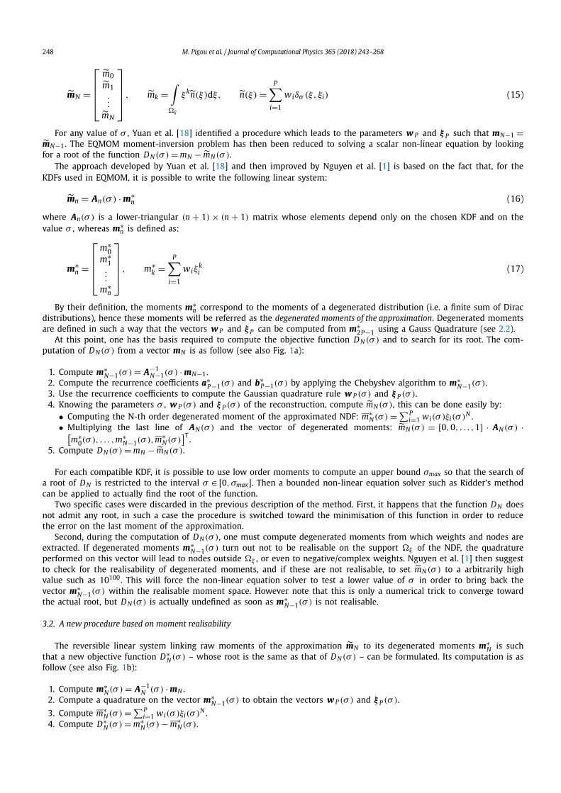
248 M. Pigou et al. / Journal of Computational Physics 365 (2018) 243–268
mN =
⎡⎢⎢⎢⎣m0m1...
mN
⎤⎥⎥⎥⎦ , mk =∫ξ
ξkn(ξ)dξ, n(ξ) =P∑
i=1
wiδσ (ξ, ξi) (15)
For any value of σ , Yuan et al. [18] identified a procedure which leads to the parameters w P and ξ P such that mN−1 =mN−1. The EQMOM moment-inversion problem has then been reduced to solving a scalar non-linear equation by looking for a root of the function D N (σ ) = mN − mN(σ ).
The approach developed by Yuan et al. [18] and then improved by Nguyen et al. [1] is based on the fact that, for the KDFs used in EQMOM, it is possible to write the following linear system:
mn = An(σ ) · m∗n (16)
where An(σ ) is a lower-triangular (n + 1) × (n + 1) matrix whose elements depend only on the chosen KDF and on the value σ , whereas m∗
n is defined as:
m∗n =
⎡⎢⎢⎢⎣m∗
0m∗
1...
m∗n
⎤⎥⎥⎥⎦ , m∗k =
P∑i=1
wiξki (17)
By their definition, the moments m∗n correspond to the moments of a degenerated distribution (i.e. a finite sum of Dirac
distributions), hence these moments will be referred as the degenerated moments of the approximation. Degenerated moments are defined in such a way that the vectors w P and ξ P can be computed from m∗
2P−1 using a Gauss Quadrature (see 2.2).At this point, one has the basis required to compute the objective function D N (σ ) and to search for its root. The com-
putation of D N (σ ) from a vector mN is as follow (see also Fig. 1a):
1. Compute m∗N−1(σ ) = A−1
N−1(σ ) · mN−1.2. Compute the recurrence coefficients a∗
P−1(σ ) and b∗P−1(σ ) by applying the Chebyshev algorithm to m∗
N−1(σ ).3. Use the recurrence coefficients to compute the Gaussian quadrature rule w P (σ ) and ξ P (σ ).4. Knowing the parameters σ , w P (σ ) and ξ P (σ ) of the reconstruction, compute mN (σ ), this can be done easily by:
• Computing the N-th order degenerated moment of the approximated NDF: m∗N (σ ) =∑P
i=1 wi(σ )ξi(σ )N .• Multiplying the last line of AN (σ ) and the vector of degenerated moments: mN(σ ) = [0, 0, . . . , 1] · AN(σ ) ·[
m∗0(σ ), . . . ,m∗
N−1(σ ),m∗N (σ )
]T .5. Compute D N(σ ) = mN − mN(σ ).
For each compatible KDF, it is possible to use low order moments to compute an upper bound σmax so that the search of a root of D N is restricted to the interval σ ∈ [0, σmax]. Then a bounded non-linear equation solver such as Ridder’s method can be applied to actually find the root of the function.
Two specific cases were discarded in the previous description of the method. First, it happens that the function D N does not admit any root, in such a case the procedure is switched toward the minimisation of this function in order to reduce the error on the last moment of the approximation.
Second, during the computation of D N (σ ), one must compute degenerated moments from which weights and nodes are extracted. If degenerated moments m∗
N−1(σ ) turn out not to be realisable on the support ξ of the NDF, the quadrature performed on this vector will lead to nodes outside ξ , or even to negative/complex weights. Nguyen et al. [1] then suggest to check for the realisability of degenerated moments, and if these are not realisable, to set mN (σ ) to a arbitrarily high value such as 10100. This will force the non-linear equation solver to test a lower value of σ in order to bring back the vector m∗
N−1(σ ) within the realisable moment space. However note that this is only a numerical trick to converge toward the actual root, but D N (σ ) is actually undefined as soon as m∗
N−1(σ ) is not realisable.
3.2. A new procedure based on moment realisability
The reversible linear system linking raw moments of the approximation mN to its degenerated moments m∗N is such
that a new objective function D∗N (σ ) – whose root is the same as that of D N (σ ) – can be formulated. Its computation is as
follow (see also Fig. 1b):
1. Compute m∗N(σ ) = A−1
N (σ ) · mN .2. Compute a quadrature on the vector m∗
N−1(σ ) to obtain the vectors w P (σ ) and ξ P (σ ).
3. Compute m∗N(σ ) =∑P
i=1 wi(σ )ξi(σ )N .4. Compute D∗
N(σ ) = m∗N(σ ) − m∗
N (σ ).

M. Pigou et al. / Journal of Computational Physics 365 (2018) 243–268 249
Fig. 1. Comparison of the computation of convergence criteria based on (a) DN(σ ), (b) D∗N (σ ) and (c) the realisability criteria of the support ξ . CA:
Chebyshev Algorithm. QC: Quadrature Computation. The convergence criteria are highlighted in light blue. Inspired by Fig. 1 from Nguyen et al. [1]. (For interpretation of the colours in the figure(s), the reader is referred to the web version of this article.)
Note that D N (σ ) = D∗N(σ ) × AN,N(σ ). As shown in Appendix B for all kernels, diagonal elements of An(σ ) are always
strictly positive, therefore the two objective functions do share the same roots.The benefit of this new objective function is that it only requires the matrix A−1
N (σ ) instead of both the matrix A−1N−1(σ )
and the last line of AN(σ ). This only increases the clarity of the method, but has hardly no effect on its numerical cost.The point of this alternative approach is however to underline a crucial element for the new EQMOM implementation:
we actually look for a value of σ for which m∗2P (σ ) = m∗
2P (σ ). This implies that, for this specific searched σ value, the vector m∗
2P (σ ) reads
m∗2P (σ ) =
⎡⎢⎢⎢⎢⎢⎣∑P
i=1 wiξ0i∑P
i=1 wiξ1i
...∑Pi=1 wiξ
2Pi
⎤⎥⎥⎥⎥⎥⎦ (18)
which is, by construction, the vector of the first 2P + 1 moments of the sum of P Dirac distributions.Under the condition that a P -node EQMOM reconstruction exists for the moment set m2P with σ > 0, wi > 0, ξi =
0, i ∈ 1, . . . , P , the vector m∗2P (σ ) will have the following specific properties:
1. The vector m∗2P−1(σ ) must be strictly within the realisable moment space MN−1(ξ ).
2. The vector m∗2P (σ ) must be on the boundary of the realisable moment space MN (ξ ).
EQMOM procedure will then rely on the realisability of the vector m∗2P (σ ) instead of the computation of the error on
the last moment, this will be a cheaper approach.Situations were the EQMOM reconstruction exist but with σ = 0, or ∃i ∈ 1, . . . , P , wi = 0 or ξi = 0 are tackled in
section 3.6 but are always based on checking the realisability of m∗2P (σ ).
The actual definition of the realisable moment space of order n, Mn , depends on the support ξ of the NDF. The three classical supports, corresponding to the Hamburger, Stieltjes and Hausdorff moment problems, come with different constraints on a moment set to ensure its realisability. The realisability criteria for each of these supports will then be detailed.
Fig. 1 sums up the “standard approach” based on D N (σ ), the shifted approach, based on D∗N (σ ), as well as the new
approach based on the realisability criteria of m∗2P (σ ) for all three supports.
3.3. Application to the Hamburger problem
As stated in 2.2, it is known that monic polynomials which are orthogonal to a measure dμ(ξ) = n(ξ)dξ satisfy a three-term recurrence relation (Eq. (5)) with ak and bk, k ∈ N, the recurrence coefficients specific to the measure dμ(ξ). The Favard’s theorem [31] and its converse [32] imply that the measure dμ(ξ) is realisable on ξ = ]−∞,+∞[ if and only if ak ∈ R and bk > 0, ∀k ∈ N.

250 M. Pigou et al. / Journal of Computational Physics 365 (2018) 243–268
Fig. 2. Evolution of the different convergence criteria for both Gaussian (a and b) and Laplace (c and d) kernels depending on σ value. The two initial moment sets are m(1)
6 = [1 1 2 5 12 42 133]T and m(2)6 = [1 2 7 17 58 149 493]T .
One looks for a value of σ such that the associated degenerated moments m∗2P−1(σ ) are strictly realisable (i.e. within the
moment space), and the moments m∗2P (σ ) are weakly realisable (i.e. on the frontier of realisability). Then, if the Chebyshev
algorithm is used to compute the recurrence coefficients a∗P−1(σ ) = [a∗
0(σ ), . . . , a∗P−1(σ )]T and b∗
P (σ ) = [b∗1(σ ), . . . , b∗
P (σ )]T
from the vector m∗2P (σ ), the condition of realisability can be written in terms of values of b∗
P (σ ): looking for the EQMOM reconstruction parameters with the Gaussian and Laplace kernels is equivalent to looking for a value of σ such as:
• b∗k (σ ) > 0, ∀k ∈ 1, . . . , P − 1
• b∗P (σ ) = 0
Fig. 2 makes use of the developments from Appendix B.1 and Appendix B.2, about the Gaussian and Laplace kernels respectively, to show the evolution of D6(σ ), D∗
6(σ ) and b∗k (σ ), k ∈ 1, 2, 3 for two sets of 7 moments (P = 3). This figure
illustrates the fact that indeed the approaches based on D N (σ ), D∗N(σ ) and b∗
P (σ ) are equivalent as they share the same circled root.
Let denote σk the root of bk(σ ). One can notice that the root σk lies within the interval [0, σk−1]. We actually observed the existence of all roots σk, k ∈ 1, . . . , P on numerous (about 106) randomly selected moment sets of N + 1 = 13 mo-ments, and never observed an undefined root. The generality of this observation has not been mathematically proved, but it seems that indeed σk is always defined and always lies in σk ∈ [0, σk−1] , k ∈ 2, . . . , P . σ1 is defined analytically.
The previous observations were used to design a simple algorithm which allows identifying the root σP . This algorithm is based on the fact that it is possible to check whether a value σt is higher or lower than σP at low cost and with no prior knowledge of σP value:
• If b∗k (σt) > 0, ∀k ∈ 1, . . . , P , then σt < σP .
• Otherwise, that is if ∃k ∈ 1, . . . , P , b∗k (σt) < 0, then σt > σP .
One can then use an iterative approach that will
1. Check the realisability of the raw moments m2P = m∗2P (0) by computing b∗
P (0) and checking the positivity of all elements.
2. Initialise an interval [σ
(0)
l , σ(0)r
]such that σ (0)
l < σP and σ (0)r > σP , and then update these bounds to shrink the search
interval. These initial values will be σ (0)
l = 0 and σ (0)r = σ1 with σ1 the analytical solution of b∗
1(σ ) = 0.3. Iterate over k
(a) Choose σt ∈[σ
(k−1)
l , σ(k−1)r
].
(b) Compute b∗P (σt).
(c) If all elements of b∗P (σt) are positive, set σ (k)
l = σt and σ (k)r = σ
(k−1)r .
(d) Otherwise, set σ (k)
l = σ(k−1)
l and σ (k)r = σt .
The choice of σt at step 3a will be made by trying to locate the root σ j of b∗j (σ ) with j the index of the first negative
element of b∗P
(σ
(k)r
). Following Nguyen et al. [1] developments, the use of Ridder’s method is advised to select σt . This
method actually tests two σ values per iteration. Consequently, the step 3 of the previous algorithm becomes:

M. Pigou et al. / Journal of Computational Physics 365 (2018) 243–268 251
3. Iterate over k(a) Identify j the index of the first negative element of b∗
P
(σ
(k−1)r
).
(b) Compute σt1 = 12
(σ
(k−1)
l + σ(k−1)r
)and b∗
P (σt1 ).
(c) Compute σt2 = σt1 +(σt1 − σ
(k−1)
l
) b∗j
(σt1
)√b∗
j
(σt1
)2−b∗j
(σ
(k−1)
l
)∗b∗
j
(σ
(k−1)r
) and b∗P (σt2 ).
(d) Set σ (k)
l as the highest value between σ (k−1)
l , σt1 and σt2 such that the corresponding vector b∗P contains only
positive values.(e) Set σ (k)
r as the lowest value between σ (k−1)r , σt1 and σt2 such that the corresponding vector b∗
P contains at least one negative value.
Stop the computation if σ (k)r − σ
(k)
l < ε σ1 or if b∗P
(σ
(k)
l
)< ε b∗
P (0), with ε a relative tolerance (e.g. ε = 10−10). Then compute the weights w P and nodes ξ P of the EQMOM reconstruction by computing a Gauss quadrature based on the recurrence coefficients a∗
P−1
(σ
(k)
l
)and b∗
P−1
(σ
(k)
l
).
Actual implementations of this algorithm for both kernels are provided as supplementary data.
3.4. Application to the Stieltjes problem
It is well known that the realisability of a moment set mN on the support ξ = ]0,+∞[ is strictly equivalent to the positivity of the Hankel determinants H2n+d [33] defined as:
H2n+d =
∣∣∣∣∣∣∣md · · · mn+d...
. . ....
mn+d · · · m2n+d
∣∣∣∣∣∣∣ (19)
with d ∈ 0, 1 and n ∈ N, 2n + d ≤ N .This condition on the positivity of Hankel determinants can be translated into a condition on the positivity of the
numbers ζk [32] defined by:
ζk = Hk−3Hk
Hk−2Hk−1, H j = 1 if j < 0 (20)
These numbers can be directly computed from the recurrence coefficients aP and bP defined in 2.2 through the following relations:
ζ2k = bk
ζ2k−1, ζ2k+1 = ak − ζ2k (21)
with ζ1 = a0 = m1/m0.The goal here is to use these realisability criteria to compute the parameters of EQMOM quadrature with either the
Log-normal, the Gamma or the Weibull kernel (see Appendix B.3, Appendix B.4 and Appendix B.5 respectively). In these cases, one must
1. Compute m∗N(σ ) = A−1
N (σ ) · mN with AN (σ ) the matrix associated to the chosen kernel (see Appendix B.3, Ap-pendix B.4, Appendix B.5).
2. Apply the Chebyshev algorithm to m∗N(σ ) to access the recurrence coefficients a∗
P (σ ) and b∗P (σ ).
3. Compute ζ ∗N (σ ) = [ζ ∗
1 (σ ), . . . , ζ ∗N (σ )]T using relations in Eq. (21).
One actually looks for σ such that
• ζ ∗k (σ ) > 0, ∀k ∈ 1, . . . , N − 1
• ζ ∗N (σ ) = 0
Let σk be the root of ζ ∗k (σ ). In all cases, the root σ2 is defined, analytically for the Log-normal and Gamma kernels, and
numerically for the Weibull kernel. Fig. 3 shows the evolution of D6(σ ), D∗6(σ ) and ζ ∗
6(σ ) for three moment sets when the developments relative to the Weibull (see Appendix B.5) kernel are used. Three situations can be observed on that figure:
1. All roots σk , k ∈ 2, . . . , N are defined (Fig. 3a).2. Some intermediary roots σk , k ∈ 3, . . . , N − 1, are not defined but the root σN still exists (Fig. 3b).3. The root σN is not defined (Fig. 3c).

252 M. Pigou et al. / Journal of Computational Physics 365 (2018) 243–268
Fig. 3. Evolution of the different convergence criteria for the Weibull kernel depending on σ value. The initial moment sets are m(a)6 =
[1 1.5 12 131 15200 18033 2.16e5]T , m(b)6 = [1 5.5 78 1285 22225 4.05e5 7.88e6]T and m(c)
6 = [1 1 2 5 14 42 133]T .
These three cases can be observed for the Gamma and Log-normal kernels too.In the first two cases, when σN exists, the EQMOM approximation is well defined. The last case – where ζ ∗
N (σ ) admits no root in [0, σN−1] – actually corresponds to the case described by Nguyen et al. [1] where D N(σ ) did not admit any root either. In this case, it was suggested to minimise D N (σ ) in order to reduce the difference between mN and mN (σ ) as much as possible.
DN (σ ) tends to be a decreasing function, but is undefined as soon as any element of ζ ∗N−1(σ ) is negative. The minimum
of D N(σ ) is then usually located at the highest order defined root. For instance, in the case shown in Fig. 3c, the minimum of D6(σ ) is located at the root σ5 of ζ ∗
5 (σ ).The moment-inversion procedure for reconstruction kernels defined on ξ = ]0,+∞[ is then reduced to the identifica-
tion of the defined root σk, k ∈ 2, . . . , N, of highest index. The algorithm proposed in section 3.3 already converges toward this root and only requires little adjustments:
1. Check the realisability of the raw moments m2P = m∗2P (0) by computing ζ ∗
N (0) and checking the positivity of all elements.
2. Initialise an interval [σ
(0)
l , σ(0)r
]with σ (0)
l = 0 and σ (0)r = σ2 with σ2 the solution of ζ ∗
2 (σ ) = 0.
3. Iterate over k(a) Identify j the index of the first negative element of ζ ∗
N
(σ
(k−1)r
).
(b) Compute σt1 = 12
(σ
(k−1)
l + σ(k−1)r
)and ζ ∗
N(σt1 ).
(c) Compute σt2 = σt1 +(σt1 − σ
(k−1)
l
)ζ ∗
j
(σt1
)√ζ ∗
j
(σt1
)2−ζ ∗j
(σ
(k−1)
l
)∗ζ ∗
j
(σ
(k−1)r
) and ζ ∗N(σt2 ).
(d) Set σ (k)
l as the highest value between σ (k−1)
l , σt1 and σt2 such that the corresponding vector ζ ∗N contains only
positive values.(e) Set σ (k)
r as the lowest value between σ (k−1)r , σt1 and σt2 such that the corresponding vector ζ ∗
N contains at least one negative value.
Stop the computation if σ (k)r −σ
(k)
l < εσ1 or if ζ ∗N
(σ
(k)
l
)< εζ ∗
N (0), with ε a relative tolerance (e.g. ε = 10−10). Then compute the weights w P and nodes ξ P of the EQMOM reconstruction by computing a Gaussian-quadrature based on recurrence coefficients a∗
P−1
(σ
(k)
l
)and b∗
P−1
(σ
(k)
l
).
3.5. Application to the Hausdorff problem
Moments of a distribution defined on the closed support ξ = ]0,1[ must obey two sets of conditions in order to be within the realisable moment space [15,26]. The moment set mN is interior to the realisable moment space associated to the support ξ = ]0,1[ if and only if:
• Hk > 0, ∀k ∈ 0, . . . , N• Hk > 0, ∀k ∈ 1, . . . , N

M. Pigou et al. / Journal of Computational Physics 365 (2018) 243–268 253
Fig. 4. Evolution of the different convergence criteria for the Beta reconstruction kernel and four initial moment sets. These sets can be found in the figure source code provided as supplementary data.
with Hk defined in Eq. (19) and Hk defined by
H2n+d =
∣∣∣∣∣∣∣md−1 − md · · · mn+d−1 − mn+d
.... . .
...
mn+d−1 − mn+d · · · m2n+d−1 − m2n+d
∣∣∣∣∣∣∣ (22)
Leaving aside the obvious condition H0 = m0 > 0, the conditions Hk > 0 and Hk > 0 induce a lower bound m−k and an
upper bound m+k for the values of mk , k ∈ 1, . . . , N. Consequently, one can define the canonical moments of the distribution
pN = [p1, . . . , pN ]T as
pk = mk − m−k
m+k − m−
k
(23)
A moment set mN is strictly realisable if and only if the associated canonical moment set pN lies in the hypercube ]0,1[N . Canonical moments can be computed through the recurrence relation [34]:
pk = ζk
1 − pk−1(24)
with ζk defined in Eq. (20) and p1 = m1.In the case of the Beta kernel (see B.6), one is looking for a value of σ such that the vector p∗
N (σ ) has the following properties:
• p∗k (σ ) ∈ ]0,1[ , ∀k ∈ 1, . . . , N − 1
• p∗N (σ ) = 0
p∗N(σ ) is computed from the vector ζ ∗
N(σ ) which is deduced from the recurrence coefficients a∗P−1(σ ) and b∗
P (σ ). These are computed –like previously– through the Chebyshev algorithm applied to the vector m∗
N(σ ) = A−1N (σ ) · mN .
Fig. 4 shows the evolution of the canonical moments and the convergence criteria D6(σ ) and D∗6(σ ) for four different
sets of 7 moments with the developments relative to the Beta kernel (see Appendix B.6). Each of these sets corresponds to one of the four situations encountered when dealing with Beta EQMOM:
• Fig. 4a: the root σN of D N (σ ), D∗N(σ ) and p∗
N (σ ) exists and can be identified through a similar procedure than that described in sections 3.3 and 3.4.
• Fig. 4b: the root σN is not defined but the minimum of D N (σ ) is located at the σ value for which p∗N−1(σ ) is on the
boundary of the hypercube ]0,1[N−1.• Fig. 4c: D N(σ ), D∗
N(σ ) and p∗N (σ ) admit multiple roots.
• Fig. 4d: the root σN is defined, but there is a range ]σv1 , σv2 [ with σv2 < σN , highlighted in light grey, such that in this interval the convergence criteria are undefined because ∀σ ∈]σv1 , σv2 [, p∗
N−1(σ ) /∈ ]0,1[N−1.
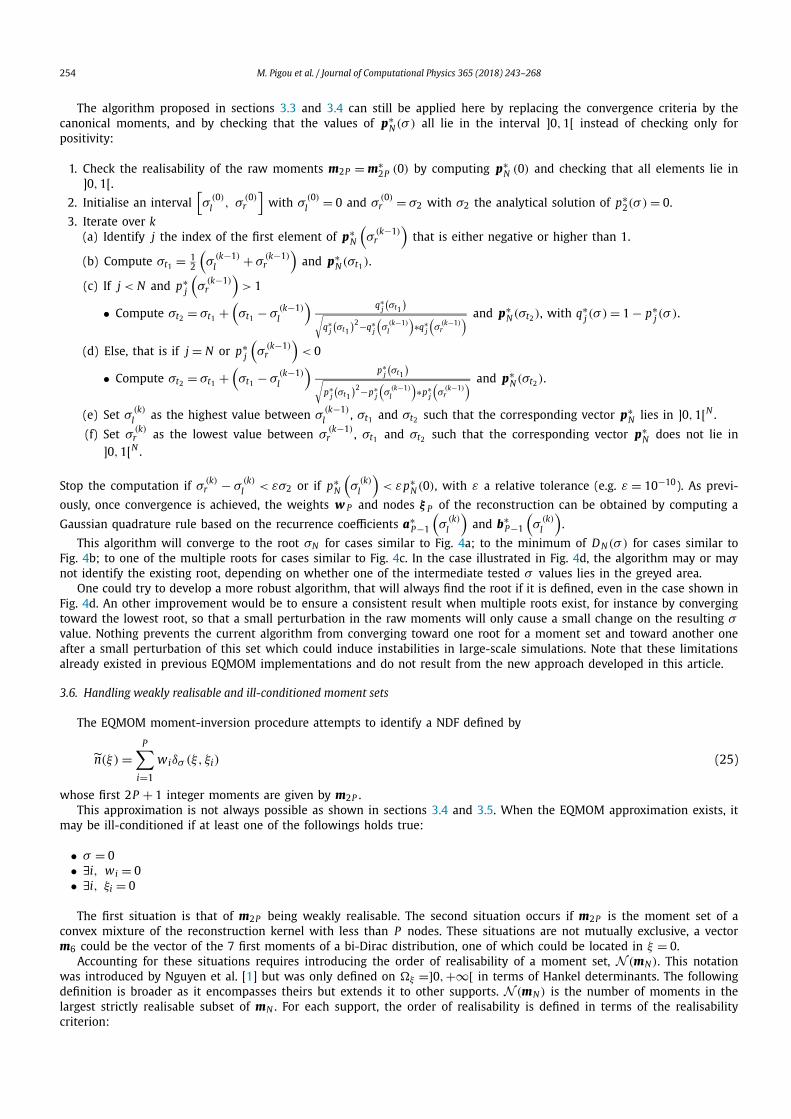
254 M. Pigou et al. / Journal of Computational Physics 365 (2018) 243–268
The algorithm proposed in sections 3.3 and 3.4 can still be applied here by replacing the convergence criteria by the canonical moments, and by checking that the values of p∗
N (σ ) all lie in the interval ]0,1[ instead of checking only for positivity:
1. Check the realisability of the raw moments m2P = m∗2P (0) by computing p∗
N (0) and checking that all elements lie in ]0,1[.
2. Initialise an interval [σ
(0)
l , σ(0)r
]with σ (0)
l = 0 and σ (0)r = σ2 with σ2 the analytical solution of p∗
2(σ ) = 0.
3. Iterate over k(a) Identify j the index of the first element of p∗
N
(σ
(k−1)r
)that is either negative or higher than 1.
(b) Compute σt1 = 12
(σ
(k−1)
l + σ(k−1)r
)and p∗
N(σt1 ).
(c) If j < N and p∗j
(σ
(k−1)r
)> 1
• Compute σt2 = σt1 +(σt1 − σ
(k−1)
l
) q∗j
(σt1
)√q∗
j
(σt1
)2−q∗j
(σ
(k−1)
l
)∗q∗
j
(σ
(k−1)r
) and p∗N (σt2 ), with q∗
j (σ ) = 1 − p∗j (σ ).
(d) Else, that is if j = N or p∗j
(σ
(k−1)r
)< 0
• Compute σt2 = σt1 +(σt1 − σ
(k−1)
l
) p∗j
(σt1
)√p∗
j
(σt1
)2−p∗j
(σ
(k−1)
l
)∗p∗
j
(σ
(k−1)r
) and p∗N(σt2 ).
(e) Set σ (k)
l as the highest value between σ (k−1)
l , σt1 and σt2 such that the corresponding vector p∗N lies in ]0,1[N .
(f) Set σ (k)r as the lowest value between σ (k−1)
r , σt1 and σt2 such that the corresponding vector p∗N does not lie in
]0,1[N .
Stop the computation if σ (k)r − σ
(k)
l < εσ2 or if p∗N
(σ
(k)
l
)< εp∗
N (0), with ε a relative tolerance (e.g. ε = 10−10). As previ-
ously, once convergence is achieved, the weights w P and nodes ξ P of the reconstruction can be obtained by computing a Gaussian quadrature rule based on the recurrence coefficients a∗
P−1
(σ
(k)
l
)and b∗
P−1
(σ
(k)
l
).
This algorithm will converge to the root σN for cases similar to Fig. 4a; to the minimum of D N (σ ) for cases similar to Fig. 4b; to one of the multiple roots for cases similar to Fig. 4c. In the case illustrated in Fig. 4d, the algorithm may or may not identify the existing root, depending on whether one of the intermediate tested σ values lies in the greyed area.
One could try to develop a more robust algorithm, that will always find the root if it is defined, even in the case shown in Fig. 4d. An other improvement would be to ensure a consistent result when multiple roots exist, for instance by converging toward the lowest root, so that a small perturbation in the raw moments will only cause a small change on the resulting σvalue. Nothing prevents the current algorithm from converging toward one root for a moment set and toward another one after a small perturbation of this set which could induce instabilities in large-scale simulations. Note that these limitations already existed in previous EQMOM implementations and do not result from the new approach developed in this article.
3.6. Handling weakly realisable and ill-conditioned moment sets
The EQMOM moment-inversion procedure attempts to identify a NDF defined by
n(ξ) =P∑
i=1
wiδσ (ξ, ξi) (25)
whose first 2P + 1 integer moments are given by m2P .This approximation is not always possible as shown in sections 3.4 and 3.5. When the EQMOM approximation exists, it
may be ill-conditioned if at least one of the followings holds true:
• σ = 0• ∃i, wi = 0• ∃i, ξi = 0
The first situation is that of m2P being weakly realisable. The second situation occurs if m2P is the moment set of a convex mixture of the reconstruction kernel with less than P nodes. These situations are not mutually exclusive, a vector m6 could be the vector of the 7 first moments of a bi-Dirac distribution, one of which could be located in ξ = 0.
Accounting for these situations requires introducing the order of realisability of a moment set, N (mN). This notation was introduced by Nguyen et al. [1] but was only defined on ξ =]0, +∞[ in terms of Hankel determinants. The following definition is broader as it encompasses theirs but extends it to other supports. N (mN ) is the number of moments in the largest strictly realisable subset of mN . For each support, the order of realisability is defined in terms of the realisability criterion:

M. Pigou et al. / Journal of Computational Physics 365 (2018) 243–268 255
• For ξ = ]−∞,+∞[, compute bP from m2P ;– if all elements are positive, N (m2P ) = 2P + 1;– else, if there is n such that bn = 0, N (m2P ) = 2n;– else, if there is n such that bn < 0, N (m2P ) = 2n − 1.
• For ξ = ]0,+∞[, compute ζ 2P from m2P ;– if all elements are positive, N (m2P ) = 2P + 1;– else identify n such that ζn ≤ 0, N (m2P ) = n.
• For ξ = ]0,1[, compute p2P from m2P ;– if all elements are included on ]0, 1[, N (m2P ) = 2P + 1;– else identify n such that pn /∈ ]0, 1[, N (m2P ) = n.
Detecting situations where σ = 0 requires to check the order of realisability of raw moments. If N (m2P ) is even, set σ = 0; otherwise apply the iterative procedure to m2P ′ with N (m2P ) = 2P ′ − 1 to identify σ [1].
The actual number of nodes required by the EQMOM approximation, i.e. the number of non-zero weights P ′′ , is de-termined from N (m∗
2P (σ )). If it is even, P ′′ = N (m∗2P (σ ))/2; otherwise, P ′′ = (N (m∗
2P (σ )) + 1)/2 but one node will be located in ξ = 0 which might be an issue for KDFs defined on ξ = ]0,+∞[ or ξ = ]0,1[. The weights and nodes will be computed from the recurrence coefficients a∗
P ′′−1(σ ) and b∗P ′′−1(σ ). If P ′′ < P , let wk = 0, ξk = 1/2, ∀k ∈ P ′′ + 1, . . . , P .
These adjustments of the first and last steps of algorithms described in sections 3.3, 3.4 and 3.5 give great stability to the moment-inversion procedure at low cost.
In the situation where N (m∗2P (σ )) = 2P , the EQMOM approximation is guaranteed to preserve the whole moment set
m2P . However, if N (m∗2P (σ )) < 2P , the approximation may, or may not, preserve all moments with no simple method to
check for this. One should compute the moments of the EQMOM approximation and measure the relative error from original moments.
4. Comparison of EQMOM approaches
4.1. Method
The new EQMOM moment-inversion procedure only requires computation of the realisability criteria of the vector of degenerated moments m∗
2P (σ ) in order to identify σ . These computations were already performed in the original approach [1] to ensure the realisability of the vector m∗
2P−1(σ ) prior to the quadrature computation and ulterior steps.It is therefore obvious that the new approach will always require a lower number of floating point operations (FLOP). In
order to quantify this reduction on FLOP number, and the actual performance gain, different implementations of EQMOM are compared, they are based either on the realizability criteria, or on a quadrature-based objective function.
4.1.1. Tested EQMOM implementationsComparison are performed for kernels defined on ξ = ]−∞,+∞[ (i.e. Gauss and Laplace kernels), and on ξ = ]0,+∞[
(i.e. Log-Normal, Gamma and Weibull kernels), using MATLAB [22] implementations.Implementations that are based on the realizability criteria of m∗
2P (σ ) use algorithms that were fully described in sec-tions 3.3 and 3.4 and adjustments from section 3.6.
For quadrature-based moment-inversion implementations, we optimized codes from Marchisio and Fox [20] and the OpenQBMM project [19] by implementing optimizations suggested by Nguyen et al. [1] and adjustments from section 3.6. Instead of searching for the root of D2P (σ ) (see Fig. 1a), these implementations directly search the root of D∗
2P (σ ) (Fig. 1b). Doing so, all compared implementations only require the matrix A−1
2P (σ ) and can benefit from the same code optimization when computing m∗
2P (σ ) = A−12P (σ ) · m2P .
For kernels defined on ξ = ]0,+∞[, if Ridder’s method fails to identify a root of D∗2P (σ ), the golden-ratio method
is used to minimize D2P (σ )2 = (D∗
2P (σ ) · A2P ,2P (σ ))2. The golden-ratio minimization method was already used in Open-
QBMM [19].
4.1.2. Performance measurementsThe main element of comparison is the number of floating-point operations required for the whole moment-inversion
procedure. The MATLAB implementations embed a simple FLOP counter that distinguishes each operation (+, −, ∗, /, exp,
√·, (·), . . . ) and counts them for each step of the moment-inversion procedure (linear system, Chebyshev algorithm, quadrature computation and others).
In order to evaluate the number of operations used in the computation of the eigenvalues and eigenvectors of the Jacobi matrix (Eq. (6)), the Jacobi and the Francis algorithms which are suited for symmetric matrices [35] are used in place of the MATLAB built-in “eig” function [22]. The Jacobi algorithm is used for matrices of size up to 3 × 3 and the Francis algorithm for larger matrices in order to always use the fastest method.
Two others metrics are measured for each call to the moment-inversion procedure: the number of tested σ values and the wall-time of function calls.

256 M. Pigou et al. / Journal of Computational Physics 365 (2018) 243–268
Table 1Comparison of Gauss EQMOM implementations corresponding to Fig. 1b and 1c for moment sets far from the frontier of realisability. The count of FLOP details the operations related to (i) the matrix–vector product A−1
2P (σ ) · m2P , (ii) the Chebyshev Algorithm (CA), (iii) the Quadrature Computation (QC) and (iv) a miscellaneous category. Results are given as mean±standard-deviation among 104 moment sets.
P = 2 P = 3 P = 4 P = 5
Newapproach
FLOP A−12P (σ ) 237±59 767±141 1709±253 3201±476
CA 177±40 477±83 979±139 1751±251
QC 52±0 474±42 995±120 1746±188
Misc. 54±12 65±11 75±11 86±12
Total 519±112 1783±242 3759±441 6784±830
Evaluations 12±3 14±2 17±2 19±3
Run-time (ms) 1±0 2±0 3±0 4±1
Former approach
FLOP A−12P (σ ) 295±161 1433±423 4060±869 8516±1870
CA 202±102 853±241 2246±467 4509±967
QC 742±377 9171±2910 24997±9966 52312±14096
Misc. 191±99 430±129 804±156 1298±251
Total 1429±739 11887±3603 32108±10645 66635±16085
Evaluations 14±7 26±7 39±8 50±11
Run-time (ms) 1±1 9±3 17±5 31±7
Gain in FLOP 59.1%±12.3% 84.2%±3.5% 87.9%±2.5% 88.0%±13.1%
Evaluations 8.6%±27.7% 40.9%±17.7% 54.2%±12.8% 53.0%±55.2%
Run-time 53.2%±13.2% 81.9%±4.2% 84.0%±3.6% 83.3%±18.0%
4.1.3. Tested moment setsEach comparison was performed on 104 randomly generated moment sets. These have varying size 2P + 1 ∈ 5, 7, 9, 11
and were either far from, or close to, the boundary of the realisable moment space.Moments sets for kernels defined on ξ = ]−∞,+∞[ were computed from random vectors aP−1 and bP using a re-
versed Chebyshev algorithm. Distribution laws for the elements of these vectors are
• ak ∼ N (0, 25), k ∈ 0, . . . , P − 1.• bk ∼ 1 + Exp(4), k ∈ 1, . . . , P .• bP ∼ Exp(0.5) for moment sets close from the frontier of realisability.
Similarly, moments sets for kernels defined on ξ = ]0,+∞[ were computed from random vectors ζ 2P using a reversed ζ -Chebyshev algorithm [1]. Elements of these vectors are generated using following distribution laws:
• ζk ∼ 1 + Exp(4), k ∈ 1, . . . , 2P .• ζ2P ∼ Exp(0.5) for moment sets close from the frontier of realisability.
4.1.4. ReproducibilityTo allow reproducibility of results described hereafter, every source codes previously described, and randomly generated
data, are available as supplementary data.
4.2. Results
Results of the comparison performed on Gauss-EQMOM for moment sets far from the boundary of the realisable moment space are given in Table 1. Similar tables are available as supplementary data for all kernels and moment sets.
Table 2 underlines a decrease in the number of tested σ values, in particular for high order reconstructions. This decrease is mainly due to the fact that in the former approach, if m∗
N−1(σ ) turns out not to be realisable, the objective function is set to a arbitrarily high negative value. The use of such an arbitrary value slows down the convergence of the non-linear equation solver. Meanwhile, the new approach never makes use of arbitrary values, all the elements of the vectors of realisability criteria (b∗
P (σ ), ζ ∗2P (σ ) or p∗
2P (σ )) are used one after the other which yields a better choice of the next tested σ value.
Moreover, for kernels defined on ξ = ]0,+∞[ and in situations illustrated in Fig. 3c, the former approach may switch from a root search to a minimization process if no root is found. This induces numerous supplementary tested σ values before convergence is reached while this situation never occurs in the new approach.
A significant drop in the total number of FLOP can be observed in Table 3. This was expected and is mainly justified by the fact that the quadrature computation is only called once in the new approach whilst it is called for most tested σvalues in the former moment-inversion procedure. This quadrature, which consists in the computation of the eigenvalues
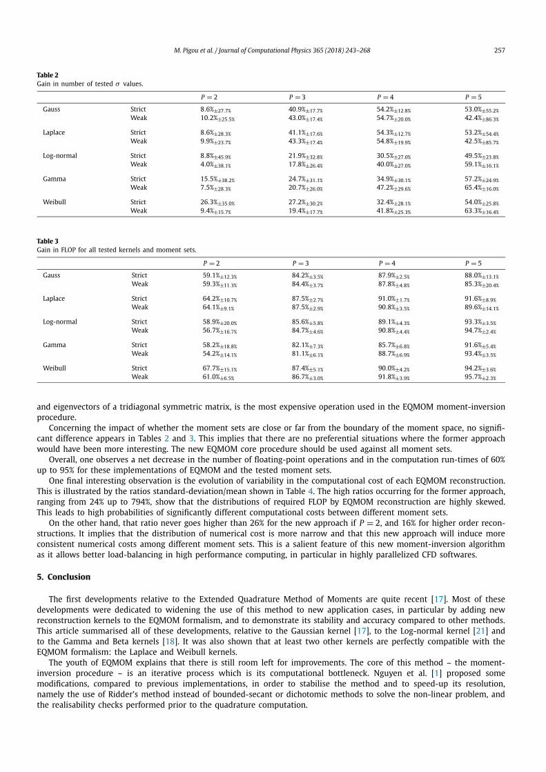
M. Pigou et al. / Journal of Computational Physics 365 (2018) 243–268 257
Table 2Gain in number of tested σ values.
P = 2 P = 3 P = 4 P = 5
Gauss Strict 8.6%±27.7% 40.9%±17.7% 54.2%±12.8% 53.0%±55.2%
Weak 10.2%±25.5% 43.0%±17.4% 54.7%±20.0% 42.4%±86.3%
Laplace Strict 8.6%±28.3% 41.1%±17.6% 54.3%±12.7% 53.2%±54.4%
Weak 9.9%±23.7% 43.3%±17.4% 54.8%±19.9% 42.5%±85.7%
Log-normal Strict 8.8%±45.9% 21.9%±32.8% 30.5%±27.0% 49.5%±23.8%
Weak 4.0%±38.1% 17.8%±26.4% 40.0%±27.0% 59.1%±16.1%
Gamma Strict 15.5%±38.2% 24.7%±31.1% 34.9%±30.1% 57.2%±24.9%
Weak 7.5%±28.3% 20.7%±26.0% 47.2%±29.6% 65.4%±16.0%
Weibull Strict 26.3%±35.0% 27.2%±30.2% 32.4%±28.1% 54.0%±25.8%
Weak 9.4%±15.7% 19.4%±17.7% 41.8%±25.3% 63.3%±16.4%
Table 3Gain in FLOP for all tested kernels and moment sets.
P = 2 P = 3 P = 4 P = 5
Gauss Strict 59.1%±12.3% 84.2%±3.5% 87.9%±2.5% 88.0%±13.1%
Weak 59.3%±11.3% 84.4%±3.7% 87.8%±4.8% 85.3%±20.4%
Laplace Strict 64.2%±10.7% 87.5%±2.7% 91.0%±1.7% 91.6%±8.9%
Weak 64.1%±9.1% 87.5%±2.9% 90.8%±3.5% 89.6%±14.1%
Log-normal Strict 58.9%±20.0% 85.6%±5.8% 89.1%±4.3% 93.3%±3.5%
Weak 56.7%±16.7% 84.7%±4.6% 90.8%±4.4% 94.7%±2.4%
Gamma Strict 58.2%±18.8% 82.1%±7.3% 85.7%±6.8% 91.6%±5.4%
Weak 54.2%±14.1% 81.1%±6.1% 88.7%±6.9% 93.4%±3.5%
Weibull Strict 67.7%±15.1% 87.4%±5.1% 90.0%±4.2% 94.2%±3.6%
Weak 61.0%±6.5% 86.7%±3.0% 91.8%±3.9% 95.7%±2.3%
and eigenvectors of a tridiagonal symmetric matrix, is the most expensive operation used in the EQMOM moment-inversion procedure.
Concerning the impact of whether the moment sets are close or far from the boundary of the moment space, no signifi-cant difference appears in Tables 2 and 3. This implies that there are no preferential situations where the former approach would have been more interesting. The new EQMOM core procedure should be used against all moment sets.
Overall, one observes a net decrease in the number of floating-point operations and in the computation run-times of 60% up to 95% for these implementations of EQMOM and the tested moment sets.
One final interesting observation is the evolution of variability in the computational cost of each EQMOM reconstruction. This is illustrated by the ratios standard-deviation/mean shown in Table 4. The high ratios occurring for the former approach, ranging from 24% up to 794%, show that the distributions of required FLOP by EQMOM reconstruction are highly skewed. This leads to high probabilities of significantly different computational costs between different moment sets.
On the other hand, that ratio never goes higher than 26% for the new approach if P = 2, and 16% for higher order recon-structions. It implies that the distribution of numerical cost is more narrow and that this new approach will induce more consistent numerical costs among different moment sets. This is a salient feature of this new moment-inversion algorithm as it allows better load-balancing in high performance computing, in particular in highly parallelized CFD softwares.
5. Conclusion
The first developments relative to the Extended Quadrature Method of Moments are quite recent [17]. Most of these developments were dedicated to widening the use of this method to new application cases, in particular by adding new reconstruction kernels to the EQMOM formalism, and to demonstrate its stability and accuracy compared to other methods. This article summarised all of these developments, relative to the Gaussian kernel [17], to the Log-normal kernel [21] and to the Gamma and Beta kernels [18]. It was also shown that at least two other kernels are perfectly compatible with the EQMOM formalism: the Laplace and Weibull kernels.
The youth of EQMOM explains that there is still room left for improvements. The core of this method – the moment-inversion procedure – is an iterative process which is its computational bottleneck. Nguyen et al. [1] proposed some modifications, compared to previous implementations, in order to stabilise the method and to speed-up its resolution, namely the use of Ridder’s method instead of bounded-secant or dichotomic methods to solve the non-linear problem, and the realisability checks performed prior to the quadrature computation.

258 M. Pigou et al. / Journal of Computational Physics 365 (2018) 243–268
Table 4Ratio standard-deviation/mean of the distribution of total number of FLOP required by EQMOM reconstructions. Only moment sets generated far from the frontier of realisability are considered.
P = 2 P = 3 P = 4 P = 5
Gauss New approach 0.22 0.14 0.12 0.12Former approach 0.52 0.30 0.33 0.24
Laplace New approach 0.21 0.12 0.11 0.11Former approach 0.67 0.30 0.43 0.43
Log-normal New approach 0.26 0.15 0.12 0.11Former approach 1.10 0.97 7.94 6.48
Gamma New approach 0.25 0.16 0.15 0.15Former approach 1.26 1.14 0.87 3.23
Weibul New approach 0.21 0.13 0.12 0.11Former approach 1.05 1.46 7.21 6.41
Further improvements were proposed by shifting the resolution toward a new paradigm. This results in a significant decrease in computational cost of about 60%–95% in terms of required floating-point operations. This resulted in our MATLAB implementations in a similar gain in terms of computation wall-time. Moreover, the new approach offers more consistent numerical costs which will be beneficial to load-balancing in parallelized software.
In multiple works [1,18,30], EQMOM has been compared to other methods (Maximum Entropy approach or sectional methods) and exhibited (i) similar accuracy even with a lower number of resolved variables, and (ii) faster or comparable computation times. The new improvements of EQMOM will make it even more competitive as its stability and accuracy are kept while reducing the gap in terms of numerical cost between EQMOM and other cheaper methods such as Gauss or Gauss–Radau quadratures.
We strongly believe that transparency about these developments will help further refinements of EQMOM. For that reason, all sources used to generate figures and data in this article are provided as supplementary data. We also release all our EQMOM source codes both with this article and in an open-access GIT repository (url: https://gitlab .com /open -eqmom). It will be updated as well as supplemented with implementations of EQMOM in languages other than MATLAB. In the case of the Beta reconstruction kernel, some suggestions for further improvements in terms of accuracy and stability were listed in section 3.5. These will be tackled in ulterior work.
Acknowledgements
The authors thank Sanofi Chimie – C&BD Biochemistry Vitry for its financial support. The authors would also like to thank Prof. Frédérique Laurent and Prof. Rodney O. Fox for the precious discussions and insights about EQMOM and the developments presented in this paper. The authors declare no conflict of interest.
Appendix A. Chebyshev algorithm
The Chebyshev algorithm allows to compute the three-term recurrence coefficients of the monic polynomials orthog-onal to a measure dμ(ξ) whose moments are given by the vector mN = [m0, . . . , mN ]. This version of the algorithm fills column-wise a N + 1 × N+1
2 matrix denoted S .First, fill the first column with the moments Si,0 = mi , compute a0 = m1/m0 and fill the second column with Si,1 =
Si+1,0 − a0 Si,0, ∀i ∈ 1, . . . , N − 1.Then iterate for j ∈ 2, . . . , N−1
2 :
a j−1 = S j, j−1
S j−1, j−1− S j−1, j−2
S j−2, j−2
b j−1 = S j−1, j−1
S j−2, j−2
Si, j = Si+1, j−1 − a j−1 Si, j−1 − b j−1 Si, j−2, i ∈ j, . . . , N − j
Appendix B. Kernels for EQMOM
There exists multiple variations of the EQMOM method depending on the Kernel Density Function that is used for the reconstruction in Eq. (15). This section details the specificities of multiple KDF that were found to be compatible with the EQMOM procedure. It details for each kernel
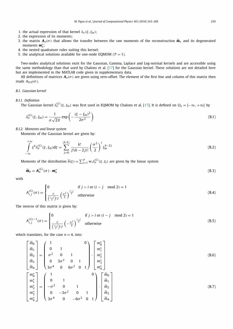
M. Pigou et al. / Journal of Computational Physics 365 (2018) 243–268 259
1. the actual expression of that kernel δσ (ξ, ξm);2. the expression of its moments;3. the matrix An(σ ) that allows the transfer between the raw moments of the reconstruction mn and its degenerated
moments m∗n;
4. the nested quadrature rules suiting this kernel;5. the analytical solutions available for one-node EQMOM (P = 1).
Two-nodes analytical solutions exist for the Gaussian, Gamma, Laplace and Log-normal kernels and are accessible using the same methodology than that used by Chalons et al. [17] for the Gaussian kernel. These solutions are not detailed here but are implemented in the MATLAB code given in supplementary data.
All definitions of matrices An(σ ) are given using zero-offset. The element of the first line and column of this matrix then reads A0,0(σ ).
B.1. Gaussian kernel
B.1.1. DefinitionThe Gaussian kernel δ(G)
σ (ξ, ξm) was first used in EQMOM by Chalons et al. [17]. It is defined on ξ = ]−∞,+∞[ by
δ(G)σ (ξ, ξm) = 1
σ√
2πexp
(− (ξ − ξm)2
2σ 2
)(B.1)
B.1.2. Moments and linear systemMoments of the Gaussian kernel are given by:
+∞∫−∞
ξkδ(G)σ (ξ, ξm)dξ =
k/2∑j=0
k!j!(k − 2 j)!
(σ 2
2
) j
ξk−2 jm (B.2)
Moments of the distribution n(ξ) =∑Pi=1 wiδ
(G)σ (ξ, ξi) are given by the linear system
mn = A(G)n (σ ) · m∗
n (B.3)
with
A(G)i, j (σ ) =
⎧⎪⎨⎪⎩0 if j > i or (i − j mod 2) = 1
i!(i− j
2
)! j!
(σ 2
2
) i− j2
otherwise(B.4)
The inverse of this matrix is given by:
A(G)−1i, j (σ ) =
⎧⎪⎨⎪⎩0 if j > i or (i − j mod 2) = 1
i!(i− j
2
)! j!
(−σ 2
2
) i− j2
otherwise(B.5)
which translates, for the case n = 4, into:⎡⎢⎢⎢⎢⎢⎢⎣m0
m1
m2
m3
m4
⎤⎥⎥⎥⎥⎥⎥⎦=
⎛⎜⎜⎜⎜⎜⎜⎝
1 0
0 1
σ 2 0 1
0 3σ 2 0 1
3σ 4 0 6σ 2 0 1
⎞⎟⎟⎟⎟⎟⎟⎠ ·
⎡⎢⎢⎢⎢⎢⎢⎣m∗
0
m∗1
m∗2
m∗3
m∗4
⎤⎥⎥⎥⎥⎥⎥⎦ (B.6)
⎡⎢⎢⎢⎢⎢⎢⎣m∗
0
m∗1
m∗2
m∗3
m∗4
⎤⎥⎥⎥⎥⎥⎥⎦=
⎛⎜⎜⎜⎜⎜⎜⎝
1 0
0 1
−σ 2 0 1
0 −3σ 2 0 1
3σ 4 0 −6σ 2 0 1
⎞⎟⎟⎟⎟⎟⎟⎠ ·
⎡⎢⎢⎢⎢⎢⎢⎣m0
m1
m2
m3
m4
⎤⎥⎥⎥⎥⎥⎥⎦ (B.7)
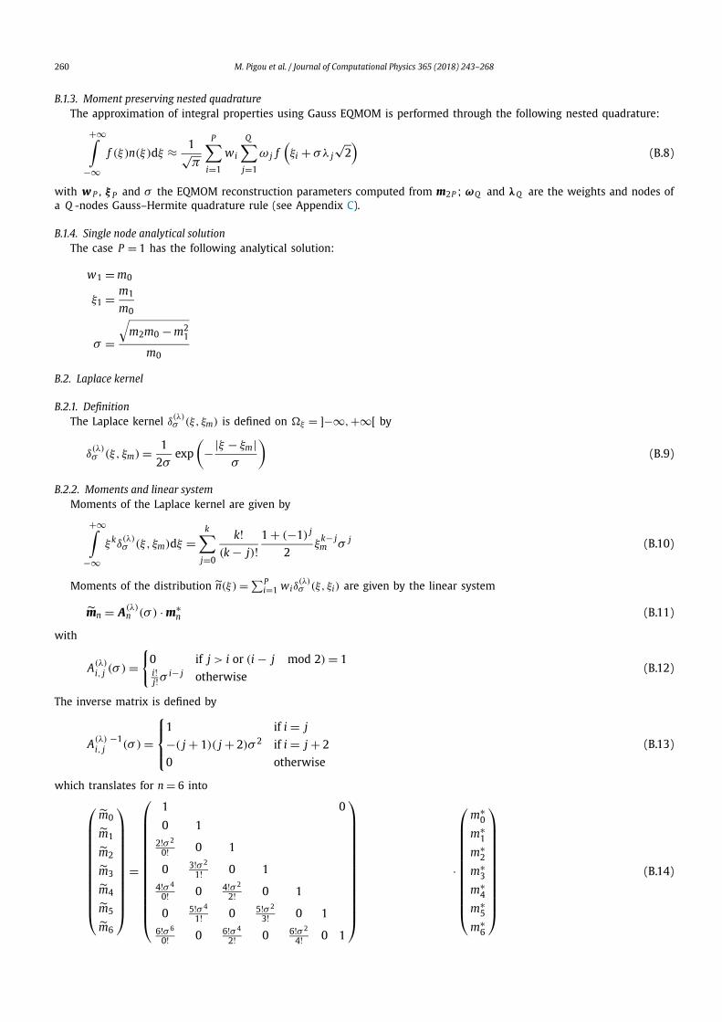
260 M. Pigou et al. / Journal of Computational Physics 365 (2018) 243–268
B.1.3. Moment preserving nested quadratureThe approximation of integral properties using Gauss EQMOM is performed through the following nested quadrature:
+∞∫−∞
f (ξ)n(ξ)dξ ≈ 1√π
P∑i=1
wi
Q∑j=1
ω j f(ξi + σλ j
√2)
(B.8)
with w P , ξ P and σ the EQMOM reconstruction parameters computed from m2P ; ωQ and λQ are the weights and nodes of a Q -nodes Gauss–Hermite quadrature rule (see Appendix C).
B.1.4. Single node analytical solutionThe case P = 1 has the following analytical solution:
w1 = m0
ξ1 = m1
m0
σ =√
m2m0 − m21
m0
B.2. Laplace kernel
B.2.1. DefinitionThe Laplace kernel δ(λ)
σ (ξ, ξm) is defined on ξ = ]−∞,+∞[ by
δ(λ)σ (ξ, ξm) = 1
2σexp
(−|ξ − ξm|
σ
)(B.9)
B.2.2. Moments and linear systemMoments of the Laplace kernel are given by
+∞∫−∞
ξkδ(λ)σ (ξ, ξm)dξ =
k∑j=0
k!(k − j)!
1 + (−1) j
2ξ
k− jm σ j (B.10)
Moments of the distribution n(ξ) =∑Pi=1 wiδ
(λ)σ (ξ, ξi) are given by the linear system
mn = A(λ)n (σ ) · m∗
n (B.11)
with
A(λ)i, j (σ ) =
0 if j > i or (i − j mod 2) = 1i!j!σ
i− j otherwise(B.12)
The inverse matrix is defined by
A(λ) −1i, j (σ ) =
⎧⎪⎨⎪⎩1 if i = j
−( j + 1)( j + 2)σ 2 if i = j + 2
0 otherwise
(B.13)
which translates for n = 6 into⎛⎜⎜⎜⎜⎜⎜⎜⎜⎜⎜⎜⎝
m0
m1
m2
m3
m4
m5
m6
⎞⎟⎟⎟⎟⎟⎟⎟⎟⎟⎟⎟⎠=
⎛⎜⎜⎜⎜⎜⎜⎜⎜⎜⎜⎜⎜⎜⎝
1 0
0 12!σ 2
0! 0 1
0 3!σ 2
1! 0 14!σ 4
0! 0 4!σ 2
2! 0 1
0 5!σ 4
1! 0 5!σ 2
3! 0 16!σ 6
0! 0 6!σ 4
2! 0 6!σ 2
4! 0 1
⎞⎟⎟⎟⎟⎟⎟⎟⎟⎟⎟⎟⎟⎟⎠·
⎛⎜⎜⎜⎜⎜⎜⎜⎜⎜⎜⎜⎝
m∗0
m∗1
m∗2
m∗3
m∗4
m∗5
m∗6
⎞⎟⎟⎟⎟⎟⎟⎟⎟⎟⎟⎟⎠(B.14)

M. Pigou et al. / Journal of Computational Physics 365 (2018) 243–268 261⎛⎜⎜⎜⎜⎜⎜⎜⎜⎜⎜⎜⎝
m∗0
m∗1
m∗2
m∗3
m∗4
m∗5
m∗6
⎞⎟⎟⎟⎟⎟⎟⎟⎟⎟⎟⎟⎠=
⎛⎜⎜⎜⎜⎜⎜⎜⎜⎜⎜⎜⎝
1 0
0 1
−2σ 2 0 1
−6σ 2 0 1
−12σ 2 0 1
−20σ 2 0 1
0 −30σ 2 0 1
⎞⎟⎟⎟⎟⎟⎟⎟⎟⎟⎟⎟⎠·
⎛⎜⎜⎜⎜⎜⎜⎜⎜⎜⎜⎜⎝
m0
m1
m2
m3
m4
m5
m6
⎞⎟⎟⎟⎟⎟⎟⎟⎟⎟⎟⎟⎠(B.15)
B.2.3. Moment preserving nested quadratureThe approximation of integral properties using Laplace EQMOM is performed through the following nested quadrature:
+∞∫−∞
f (ξ)n(ξ)dξ ≈P∑
i=1
wi
Q∑j=1
ω j f(ξi + σλ j
)(B.16)
with w P , ξ P and σ the EQMOM reconstruction parameters computed from m2P ; ωQ and λQ are the weights and nodes of a Q -nodes “Gauss-Laplace” quadrature rule (see Appendix C).
B.2.4. Single node analytical solutionThe case P = 1 has the following analytical solution:
w1 = m0
ξ1 = m1
m0
σ =√
m2m0 − m21
2m20
B.3. Log-normal kernel
B.3.1. DefinitionThe Log-normal kernel δ(L)
σ (ξ, ξm) was first used in EQMOM by Madadi-Kandjani and Passalacqua [21]. It is defined on ξ = ]0,+∞[ by
δ(L)σ (ξ, ξm) = 1
σξ√
2πexp
(− (log(ξ) − log(ξm))2
2σ 2
)(B.17)
B.3.2. Moments and linear systemMoments of the Log-normal kernel are given by
+∞∫0
ξkδ(L)σ (ξ, ξm)dξ = ξk
mzk2with z = eσ 2/2 (B.18)
Moments of the distribution n(ξ) =∑Pi=1 wiδ
(L)σ (ξ, ξi) are given by
mk = m∗k zk2
(B.19)
This can be translated into a linear system
mn = A(L)n (σ ) · m∗
n (B.20)
with A(L)n (σ ) a diagonal matrix:
A(L)i, j (σ ) =
zi2
if i = j
0 otherwise(B.21)
whose inverse matrix is directly given by
A(L)−1i, j (σ ) =
z−i2
if i = j
0 otherwise(B.22)

262 M. Pigou et al. / Journal of Computational Physics 365 (2018) 243–268
B.3.3. Low cost nested quadratureA variable change allows approximating integral properties over a LogN EQMOM reconstruction using Gauss–Hermite
quadratures [21]:
+∞∫0
f (ξ)n(ξ)dξ ≈ 1√π
P∑i=1
wi
Q∑j=1
ω j f(ξi exp
(σλ j
√2))
(B.23)
with w P , ξ P and σ the EQMOM reconstruction parameters computed from m2P ; ωQ and λQ are the weights and nodes of a Q -nodes Gauss–Hermite quadrature rule (see Appendix C).
Parameters of this nested quadrature do not depend on σ of the main quadrature nodes ξ P . Consequently, ωQ and λQonly need to be computed once. It is worth noting that this quadrature does not preserve the moments of the distribution and only yields exact results for f (ξ) = log(ξ)k, k ∈ 0, . . . , 2 min(P , Q ) − 1.
B.3.4. Moment preserving nested quadraturePassalacqua et al. [19] suggested the use of Gauss–Wigert quadratures [36] to preserve the moments of a LogN EQMOM
reconstruction:
+∞∫0
f (ξ)n(ξ)dξ ≈P∑
i=1
wi
Q∑j=1
ω(σ)j f
(ξiλ
(σ )j
)(B.24)
with w P , ξ P and σ the EQMOM reconstruction parameters computed from m2P ; ω(σ )Q and λ(σ )
Q are the weights and nodes of a Q -nodes Gauss–Wigert quadrature rule of parameter σ (see Appendix C). This quadrature rule must be computed for each value of σ , i.e. for each LogN EQMOM reconstruction.
B.3.5. Single node analytical solutionThe case P = 1 has the following analytical solution:
w1 = m0
ξ1 =√
m41
m2m30
σ =√√√√log
(m2m0
m21
)
B.4. Gamma kernel
B.4.1. DefinitionThe Gamma kernel δ()
σ (ξ, ξm) was first used in EQMOM by Yuan et al. [18]. It is defined on ξ = ]0,+∞[ by
δ()σ (ξ, ξm) = ξ (l−1) exp(−ξ/σ )
(l)σ lwith l = ξm
σand (x) =
+∞∫0
tx−1e−tdt (B.25)
B.4.2. Moments and linear systemMoments of the Gamma kernel are given by
+∞∫0
ξkδ()σ (ξ, ξm)dξ = Gk(ξm,σ ) =
1 if k = 0∏k−1
j=0 (ξm + jσ) otherwise(B.26)
Moments of the distribution n(ξ) =∑Pi=1 wiδ
()σ (ξ, ξi) are given by the linear system
mn = A()n (σ ) · m∗
n (B.27)
with
A()i, j (σ ) =
⎧⎪⎨⎪⎩0 if j > i or i = 0 or j = 0
1 if i = 0 and j = 0
A()i−1, j−1(σ ) + (i − 1)σ A()
i−1, j(σ ) otherwise
(B.28)

M. Pigou et al. / Journal of Computational Physics 365 (2018) 243–268 263
The inverse of this matrix is given by
A()−1i, j (σ ) =
⎧⎪⎨⎪⎩0 if j > i or i = 0 or j = 0
1 if i = 0 and j = 0
A()−1i−1, j−1(σ ) − jσ A()−1
i−1, j (σ ) otherwise
(B.29)
which translates, for n = 6 into⎡⎢⎢⎢⎢⎢⎢⎢⎢⎢⎢⎢⎣
m0
m1
m2
m3
m4
m5
m6
⎤⎥⎥⎥⎥⎥⎥⎥⎥⎥⎥⎥⎦=
⎛⎜⎜⎜⎜⎜⎜⎜⎜⎜⎜⎜⎝
1 0
0 1
0 1σ 1
0 2σ 2 3σ 1
0 6σ 3 11σ 2 6σ 1
0 24σ 4 50σ 3 35σ 2 10σ 1
0 120σ 5 274σ 4 225σ 3 85σ 2 15σ 1
⎞⎟⎟⎟⎟⎟⎟⎟⎟⎟⎟⎟⎠·
⎡⎢⎢⎢⎢⎢⎢⎢⎢⎢⎢⎢⎣
m∗0
m∗1
m∗2
m∗3
m∗4
m∗5
m∗6
⎤⎥⎥⎥⎥⎥⎥⎥⎥⎥⎥⎥⎦(B.30)
⎡⎢⎢⎢⎢⎢⎢⎢⎢⎢⎢⎢⎣
m∗0
m∗1
m∗2
m∗3
m∗4
m∗5
m∗6
⎤⎥⎥⎥⎥⎥⎥⎥⎥⎥⎥⎥⎦=
⎛⎜⎜⎜⎜⎜⎜⎜⎜⎜⎜⎜⎝
1 0
0 1
0 −σ 1
0 σ 2 −3σ 1
0 −σ 3 7σ 2 −6σ 1
0 σ 4 −15σ 3 25σ 2 −10σ 1
0 −σ 5 31σ 4 −90σ 3 65σ 2 −15σ 1
⎞⎟⎟⎟⎟⎟⎟⎟⎟⎟⎟⎟⎠·
⎡⎢⎢⎢⎢⎢⎢⎢⎢⎢⎢⎢⎣
m0
m1
m2
m3
m4
m5
m6
⎤⎥⎥⎥⎥⎥⎥⎥⎥⎥⎥⎥⎦(B.31)
B.4.3. Low cost nested quadratureA Gauss–Laguerre quadrature can be used to approximate integral properties over a Gamma EQMOM reconstruction:
+∞∫0
f (ξ)n(ξ)dξ ≈Q∑
j=1
ω j f (σλ j)
P∑i=1
wi
(
ξiσ
)λξiσ −1j (B.32)
with w P , ξ P and σ the EQMOM reconstruction parameters computed from m2P ; ωQ and λQ are the weights and nodes of a Q -nodes Gauss–Laguerre quadrature rule of parameter α = 0 (see Appendix C). The advantage of this quadrature is that it only requires ωQ and λQ to be computed once. However, this quadrature will not preserve the moments of the distribution.
B.4.4. Moment preserving nested quadratureA generalized Gauss–Laguerre quadrature preserves the moments of a Gamma EQMOM reconstruction:
+∞∫0
f (ξ)n(ξ)dξ ≈P∑
i=1
wi
(
ξiσ
) Q∑j=1
ω(αi)
j f(σλ
(αi)
j
)(B.33)
with w P , ξ P and σ the EQMOM reconstruction parameters computed from m2P ; ω(αi)Q and λ(αi)
Q are the weights and nodes of a Q -nodes Gauss–Laguerre quadrature rule of parameter αi = ξi
σ − 1 (see Appendix C).
The accuracy of this quadrature comes with a cost related to the computation of ω(αi)Q and λ(αi)
Q for each value of αi .
B.4.5. Single node analytical solutionThe case P = 1 has the following analytical solution:
w1 = m0
ξ1 = m1
m0
σ = m2
m1− m1
m0

264 M. Pigou et al. / Journal of Computational Physics 365 (2018) 243–268
B.5. Weibull kernel
B.5.1. DefinitionThe Weibull kernel δ(W )
σ (ξ, ξm) is defined on ξ = ]0,+∞[ by
δ(W )σ (ξ, ξm) = 1
σξm
(ξ
ξm
) 1−σσ
exp
(−(
ξ
ξm
)1/σ)
(B.34)
B.5.2. Moments and linear systemMoments of the Weibull kernel are given by
+∞∫0
ξkδ(W )σ (ξ, ξm)dξ = ξk
m(1 + kσ) (B.35)
Moments of the distribution n(ξ) =∑Pi=1 wiδ
(W )σ (ξ, ξi) are given by
mk = m∗k(1 + kσ) (B.36)
This can be translated into a linear system
mn = A(W )n (σ ) · m∗
n (B.37)
with A(W )n (σ ) a diagonal matrix:
A(W )i, j (σ ) =
(1 + iσ) if i = j
0 otherwise(B.38)
whose inverse matrix is directly given by
A(W )−1i, j (σ ) =
1
(1+iσ )if i = j
0 otherwise(B.39)
B.5.3. Low cost nested quadratureA Gauss–Laguerre quadrature can be used to approximate integral properties over a Weibull EQMOM reconstruction:
+∞∫0
f (ξ)n(ξ)dξ ≈P∑
i=1
wi
Q∑j=1
ω j f(ξiλ
σj
)(B.40)
with w P , ξ P and σ the EQMOM reconstruction parameters computed from m2P ; ωQ and λQ are the weights and nodes of a Q -nodes Gauss–Laguerre quadrature rule of parameter α = 0 (see Appendix C). The advantage of this quadrature is that it only requires ωQ and λQ to be computed once. However, this quadrature will not preserve the moments of the distribution and only yields exact results for f (ξ) = ξk/σ , k ∈ 0, . . . , 2 min(P , Q ) − 1
B.5.4. Moment preserving nested quadratureOne can produce a Gauss quadrature that preserves the moments of Weibull EQMOM approximations:
+∞∫0
f (ξ)n(ξ)dξ ≈P∑
i=1
wi
Q∑j=1
ω(σ)j f
(ξiλ
(σ )j
)(B.41)
with w P , ξ P and σ the EQMOM reconstruction parameters computed from m2P ; ω(σ )Q and λ(σ )
Q are the weights and nodes of a Q -nodes “Gauss-Weibull” quadrature rule of parameter σ (see Appendix C). The weights and nodes of the nested quadrature need to be computed for each value of σ , i.e. for each Weibull EQMOM approximation of the NDF.

M. Pigou et al. / Journal of Computational Physics 365 (2018) 243–268 265
B.5.5. Single node numerical solutionThe parameters w1, ξ1 and σ of the one-node Weibull EQMOM must be solution of the following system:
m0 = w1
m1
(1 + σ)= w1ξ1
m2
(1 + 2σ)= w1ξ
21
The first equation gives w1 = m0 but no explicit solution exists for the two other equations. One can however notice that s = σ
1+σ must be a root of
G(s) = m2m0
m21
− ( 1+s1−s )
( 11−s )
2(B.42)
which is monotonous, defined on s ∈ [0, 1[ and has the following limits
G(0) = m2m0
m21
> 0
lims→1− G(s) < 0
G(s) then admits a single root that can be computed numerically with the Ridder’s method. One can also narrow down, at a very low cost, the search interval [0, 1[ by using the property
gn = G
(n
n + 1
)= m2m0
m21
− (2n)!(n!)2
(B.43)
with n an integer, which induces the following recurrence relation:
gn = c − hn (B.44)
hn+1 =(
4 − 2
n + 1
)hn (B.45)
with c = m2m0m2
1and h1 = 2.
The proposed algorithm to identify the root of G(s) is
1. Compute c = m2m0m2
1• if c < 1, cancel the operation as the moments are not realisable;• if c = 1, s = 0 is the root of G(s);• if c < 2, set sl = 0, vl = c − 1, sr = 1
2 and vr = c − 2 and go to step 3.• otherwise, set sl = 0, vl = c − 1 and go to step 2.
2. Initialise i = 1, h = 2 and iterate(a) increment i by 1;
(a) compute h = h ∗(
4 − 2i
)• if h = c, then s = i
i+1 is a root of G(s);
• if h < c, set sl = ii+1 and vl = c − h;
• if h > c, set sr = ii+1 , vr = c − h and go to step 3.
3. Apply the Ridder’s method to G(s) on the interval [sl, sr](a) compute st1 = 1
2 (sl + sr) and vt1 = G(st1 );
(b) compute st2 = st1 + (st1 − sl)vt1√
v2t1
−vl vr
and vt2 = G(st2 );
(c) set sl the highest value between sl , st1 and st2 whose image by G is positive;(d) set sr the lowest value between sr , st1 and st2 whose image by G is negative;(e) stop the computation if vl < ε(c − 1) with ε a relative tolerance (e.g. ε = 10−10) and consider sl as a root of G(s).
Once the root of G(s) is identified, compute
σ = s
1 − s
ξ1 = m1
m0(1 + σ)

266 M. Pigou et al. / Journal of Computational Physics 365 (2018) 243–268
Note that each iteration of the Ridder’s method requires two computations of G(s), that implies four computations of the Gamma function – which is quite expensive – by iteration. This explains the interest of the second step which allows to narrow down the research interval at hardly no cost.
B.6. Beta kernel
B.6.1. DefinitionThe Beta kernel δ(β)
σ (ξ, ξm) was first used in EQMOM by Yuan et al. [18]. It is defined on ξ = ]0,1[ by
δ(β)σ (ξ, ξm) = ξ (l−1)(1 − ξ)(m−1)
B(l,m)with l = ξm
σand m = 1 − ξm
σ(B.46)
with B(l, m) = ∫ 10 x(l−1)(1 − x)(m−1)dx the beta function.
B.6.2. Moments and linear systemMoments of the Beta kernel are given by
1∫0
ξkδ(β)σ (ξ, ξm)dξ = Hk(ξm,σ ) =
1 if k = 0∏k−1
j=0
(ξm+ jσ1+ jσ
)otherwise
(B.47)
Moments of the distribution n(ξ) =∑Pi=1 wiδ
(β)σ (ξ, ξi) are given by the linear system
mn = A(β)n (σ ) · m∗
n (B.48)
with the elements of A(β)n (σ ) being computed from the elements of the matrix relative to Gamma EQMOM, A()
n (σ ):
A(β)
i, j (σ ) = A()i, j (σ )
Fi(σ )(B.49)
Fi(σ ) =
1 if i ≤ 1
(1 + (i − 1)σ )Fi−1(σ ) otherwise(B.50)
The inverse of this matrix is also easily defined from A()−1n (σ ):
A(β)−1i, j (σ ) = A()−1
i, j (σ )F j(σ ) (B.51)
B.6.3. Low cost nested quadratureA Gauss–Legendre quadrature can be used to approximate integral properties over a Beta EQMOM reconstruction:
1∫0
f (ξ)n(ξ)dξ ≈ 1
2
P∑i=1
wi
B (αi+1, βi+1)
Q∑j=1
ω j f
(1 − λ j
2
)(1 − λ j
2
)αi(
1 + λ j
2
)βi
(B.52)
with w P , ξ P and σ the EQMOM reconstruction parameters computed from m2P ; ωQ and λQ are the weights and nodes of a Q -nodes Gauss–Legendre quadrature rule (see Appendix C); αi = ξi−σ
σ and βi = 1−ξi−σσ . This nested quadrature only
requires ωQ and λQ to be computed once, but will not preserve the moments of the distribution.
B.6.4. Moment preserving nested quadratureA Gauss–Jacobi quadrature will preserve the moments of the distribution:
1∫0
f (ξ)n(ξ)dξ ≈ 2σ−1σ
P∑i=1
wi
B (αi+1, βi+1)
Q∑j=1
ω(αi ,βi)
j f
⎛⎝1 − λ(αi ,βi)
j
2
⎞⎠ (B.53)
with w P , ξ P and σ the EQMOM reconstruction parameters computed from m2P ; ω(αi ,βi)Q and λ
(αi ,βi)Q are the weights
and nodes of a Q -nodes Gauss–Jacobi quadrature rule of parameters αi = ξi−σσ and βi = 1−ξi−σ
σ (see Appendix C). The moment-preserving property of this quadrature comes with the need to compute ω(αi ,βi)
Q and λ(αi ,βi)Q for each node of the
main Beta EQMOM quadrature.

M. Pigou et al. / Journal of Computational Physics 365 (2018) 243–268 267
B.6.5. Single node analytical solutionThe case P = 1 has the following analytical solution:
w1 = m0
ξ1 = m1
m0
σ = m21 − m0m2
m0(m2 − m1)
Appendix C. Gaussian quadratures
A Q-node Gaussian quadrature allows to approximate a function integral as a weighted sum of point wise values of this function over an interval I:∫
I
f (x)p(x)dx ≈Q∑
j=1
ω j f(λ j)
(C.1)
p(x) is a weight function, and the quadrature rule yields accurate integral evaluations if f (x) = xk, k ∈ 0, . . . , 2Q − 1. The computation of the weights ωQ and nodes λQ is performed as detailed in 2.2 by considering polynomials that are orthogonal with respect to the weight function p(x).
Table C.1 details for each Gauss quadrature:
• the weight function p(x);• the integration support I;• the computation of recurrence coefficients aQ −1 and bQ −1;• the zero-th order moment P0 of p(x).
The recurrence coefficients are used to construct the Jacobi matrix J Q associated with p(x) on I (see Eq. (6)). The nodes λQ are the eigenvalues of J Q , and the weights ωQ are given by ω j = P0 v2
1, j with v1, j the first component of the normalised eigenvector belonging to the eigenvalue λ j .
Table C.1Specifics of Gauss quadratures used for EQMOM nested quadratures.
Gauss- I p(x) aQ and bQ P0
Hermite R exp(−x2
)ak = 0
bk = k/2
√π
Laplacec R exp (−|x|) /2
Apply Chebyshev algorithm to
P 2Q −1 with Pk =
0 if k odd
k! if k even1
Laguerref R+ xα exp (−x) a0 = 1 + α
ak = 2 + ak−1
bk = k(k + α)
(1 + α)d
Wigerta,f R+ 1γ x
√2π
exp(
log2(x)2γ 2
)ak =
((z2 + 1
)z2k − 1
)z2k−1
bk =(
z2k − 1)
z6k−4
z = exp(γ 2/2)
1
Weibullc,f R+ γ xγ−1 exp(−xγ
) Apply Chebyshev algorithm toP 2Q −1 with Pk = (1 + k/γ )
1
Legendreb ]−1,1[ 1 ak = 0
bk = k2
4k2 − 1
2
Jacobib,f ]−1,1[ (1−x)α (1+x)β ak = β2−α2
δk(δk+2)
bk = 4k(k+α)(k+β)(k+α+β)
δ2k (δ2
k −1)
δk = 2k+α+β
2α+β+1×B (α+1, β+1)e
a Wilck [36].b Shen et al. [37].c Not standard Gauss-quadrature.d (x) = ∫ +∞
0 tx−1e−t dt .e B(x, y) = (x)(y)
(x+y).
f α > −1, β > −1, γ > 0.

268 M. Pigou et al. / Journal of Computational Physics 365 (2018) 243–268
Appendix D. Supplementary material
Supplementary material related to this article can be found online at https://doi .org /10 .1016 /j .jcp .2018 .03 .027.
References
[1] T. Nguyen, F. Laurent, R. Fox, M. Massot, Solution of population balance equations in applications with fine particles: mathematical modeling and numerical schemes, J. Comput. Phys. (ISSN 0021-9991) 325 (2016) 129–156, https://doi .org /10 .1016 /j .jcp .2016 .08 .017.
[2] P. Moilanen, M. Laakkonen, O. Visuri, V. Alopaeus, J. Aittamaa, Modelling mass transfer in an aerated 0.2 m3 vessel agitated by Rushton, Phasejet and Combijet impellers, Chem. Eng. J. (ISSN 1385-8947) 142 (1) (2008) 95–108, https://doi .org /10 .1016 /j .cej .2008 .01.033.
[3] A. Buffo, V. Alopaeus, A novel simplified multivariate PBE solution method for mass transfer problems, Chem. Eng. Sci. (ISSN 0009-2509) 172 (Supple-ment C) (2017) 463–475, https://doi .org /10 .1016 /j .ces .2017.06 .036.
[4] J. Morchain, J. Gabelle, A. Cockx, A coupled population balance model and CFD approach for the simulation of mixing issues in lab-scale and industrial bioreactors, AIChE J. (ISSN 1547-5905) 60 (1) (2014) 27–40, https://doi .org /10 .1002 /aic .14238.
[5] A. Heins, R.L. Fernandes, K.V. Gernaey, A.E. Lantz, Experimental and in silico investigation of population heterogeneity in continuous Sachharomyces cerevisiae scale-down fermentation in a two-compartment setup, J. Chem. Technol. Biotechnol. (ISSN 1097-4660) 90 (2) (2015) 324–340, https://doi .org /10 .1002 /jctb .4532.
[6] S. Salenbauch, A. Cuoci, A. Frassoldati, C. Saggese, T. Faravelli, C. Hasse, Modeling soot formation in premixed flames using an extended conditional quadrature method of moments, Combust. Flame (ISSN 0010-2180) 162 (6) (2015) 2529–2543, https://doi .org /10 .1016 /j .combustflame .2015 .03 .002.
[7] A. Wick, T.-T. Nguyen, F. Laurent, R.O. Fox, H. Pitsch, Modeling soot oxidation with the extended quadrature method of moments, Proc. Combust. Inst. (ISSN 1540-7489) 36 (1) (2017) 789–797, https://doi .org /10 .1016 /j .proci .2016 .08 .004.
[8] J. Akroyd, A.J. Smith, R. Shirley, L.R. McGlashan, M. Kraft, A coupled CFD-population balance approach for nanoparticle synthesis in turbulent reacting flows, Chem. Eng. Sci. (ISSN 0009-2509) 66 (17) (2011) 3792–3805, https://doi .org /10 .1016 /j .ces .2011.05 .006.
[9] P. Fede, O. Simonin, P. Villedieu, Monte-Carlo simulation of colliding particles or coalescing droplets transported by a turbulent flow in the frame-work of a joint fluid–particle pdf approach, Int. J. Multiph. Flow (ISSN 0301-9322) 74 (Supplement C) (2015) 165–183, https://doi .org /10 .1016 /j .ijmultiphaseflow.2015 .04 .006.
[10] S. Kumar, D. Ramkrishna, On the solution of population balance equations by discretization, I: a fixed pivot technique, Chem. Eng. Sci. (ISSN 0009-2509) 51 (8) (1996) 1311–1332, https://doi .org /10 .1016 /0009 -2509(96 )88489 -2.
[11] S. Kumar, D. Ramkrishna, On the solution of population balance equations by discretization, II: moving pivot technique, Chem. Eng. Sci. (ISSN 0009-2509) 51 (8) (1996) 1333–1342, https://doi .org /10 .1016 /0009 -2509(95 )00355 -X.
[12] M. Massot, F. Laurent, D.K.S. de Chaisemartin, A robust moment method for evaluation of the disappearance rate of evaporating sprays, SIAM J. Appl. Math. 70 (8) (2010) 3203–3234, https://doi .org /10 .1137 /080740027.
[13] V. John, I. Angelov, A. Öncül, D. Thévenin, Techniques for the reconstruction of a distribution from a finite number of its moments, Chem. Eng. Sci. (ISSN 0009-2509) 62 (11) (2007) 2890–2904, https://doi .org /10 .1016 /j .ces .2007.02 .041.
[14] L. Mead, N. Papanicolaou, Maximum entropy in the problem of moments, J. Math. Phys. 25 (8) (1984) 2404–2417.[15] A. Tagliani, Hausdorff moment problem and maximum entropy: a unified approach, Appl. Math. Comput. (ISSN 0096-3003) 105 (2–3) (1999) 291–305,
https://doi .org /10 .1016 /S0096 -3003(98 )10084 -X.[16] G. Athanassoulis, P. Gavriliadis, The truncated Hausdorff moment problem solved by using kernel density functions, Probab. Eng. Mech.
(ISSN 0266-8920) 17 (3) (2002) 273–291, https://doi .org /10 .1016 /S0266 -8920(02 )00012 -7.[17] C. Chalons, R. Fox, M. Massot, A multi-Gaussian quadrature method of moments for gas–particle flows in a LES framework, in: Proceedings of the 2010
Summer Program, 2010, pp. 347–358, Center for Turbulence Research, Stanford University.[18] C. Yuan, F. Laurent, R. Fox, An extended quadrature method of moments for population balance equations, J. Aerosol Sci. (ISSN 0021-8502) 51 (2012)
1–23, https://doi .org /10 .1016 /j .jaerosci .2012 .04 .003.[19] A. Passalacqua, F. Laurent, E. Madadi-Kandjani, J. Heylmun, R. Fox, An open-source quadrature-based population balance solver for OpenFOAM, Chem.
Eng. Sci. (ISSN 0009-2509) 176 (2018) 306–3018, https://doi .org /10 .1016 /j .ces .2017.10 .043.[20] D. Marchisio, R. Fox, Computational Models for Polydisperse Particulate and Multiphase Systems, Cambridge Series in Chemical Engineering, Cambridge
University Press, ISBN 9781107328174, 2013.[21] E. Madadi-Kandjani, A. Passalacqua, An extended quadrature-based moment method with log-normal kernel density functions, Chem. Eng. Sci.
(ISSN 0009-2509) 131 (2015) 323–339, https://doi .org /10 .1016 /j .ces .2015 .04 .005.[22] MATLAB, version 9.0 (R2016a), The MathWorks, Inc., Natick, Massachusetts, United States, 2016.[23] R. McGraw, Description of aerosol dynamics by the quadrature method of moments, Aerosol Sci. Technol. 27 (2) (1997) 255–265, https://doi .org /10 .
1080 /02786829708965471.[24] W. Gautschi, Orthogonal Polynomials: Computation and Approximation, Numerical Mathematics and Scientific Computation, Oxford University Press,
ISBN 9780198506720, 2004.[25] P. Henrici, The quotient-difference algorithm, Natl. Bur. Stand., Appl. Math. Ser. 49 (1958) 23–46.[26] H. Dette, W. Studden, The Theory of Canonical Moments with Applications in Statistics, Probability, and Analysis, John Wiley & Sons, New York,
Chichester, 1997.[27] R. Gordon, Error Bounds in Equilibrium Statistical Mechanics, J. Math. Phys. 9 (1968) 655, https://doi .org /10 .1063 /1.1664624.[28] J. Wheeler, Modified moments and Gaussian quadratures, Rocky Mt. J. Math. 4 (2) (1974) 287–296, RMJ-1974-4-2-287.[29] N. Lebaz, A. Cockx, M. Spérandio, J. Morchain, Reconstruction of a distribution from a finite number of its moments: a comparative study in the case
of depolymerization process, Comput. Chem. Eng. (ISSN 0098-1354) 84 (2016) 326–337, https://doi .org /10 .1016 /j .compchemeng .2015 .09 .008.[30] M. Pigou, J. Morchain, P. Fede, M. Penet, G. Laronze, An assessment of methods of moments for the simulation of population dynamics in large-scale
bioreactors, Chem. Eng. Sci. (ISSN 0009-2509) 171 (2017) 218–232, https://doi .org /10 .1016 /j .ces .2017.05 .026.[31] J. Favard, Sur les polynomes de Tchebicheff, C. R. Hebd. Séances Acad. Sci. 200 (1935) 2052–2053.[32] T. Chihara, An Introduction to Orthogonal Polynomials, vol. 13, Mathematics and Its Applications, Gordon and Breach, ISBN 9780677041506, 1978.[33] J. Shohat, J. Tamarkin, The Problem of Moments, Mathematical Surveys and Monographs, vol. 4, American Mathematical Society, 1943.[34] H. Wall, Analytic Theory of Continued Fractions, The University Series in Higher Mathematics, Van Nostrand, 1948.[35] W. Ford, Chapter 19 – The symmetric eigenvalue problem, in: Numerical Linear Algebra with Applications, Academic Press, Boston,
ISBN 978-0-12-394435-1, 2015, pp. 439–468.[36] M. Wilck, A general approximation method for solving integrals containing a lognormal weighting function, J. Aerosol Sci. (ISSN 0021-8502) 32 (9)
(2001) 1111–1116, https://doi .org /10 .1016 /S0021 -8502(01 )00044 -1.[37] J. Shen, T. Tang, L.-L. Wang, Orthogonal Polynomials and Related Approximation Results, Springer, Berlin, Heidelberg, ISBN 978-3-540-71041-7, 2011,
pp. 47–140.


DC O U P L E D S I M U L AT I O N R E S U LT S
This Appendix details all simulations results for coupled simulations described in ChapterV.
For confidentiality reasons, the complete thesis cannot be made fully available. In thecurrent version, this appendix has been edited out.
245

246 coupled simulation results
Copyright © 2022 FDOKUMEN