
Nanoreinforced biocompatible hydrogels from wood hemicelluloses and cellulose whiskers
Upload
khangminh22Category
view
2download
0
HAL Id: tel-01298169https://tel.archives-ouvertes.fr/tel-01298169
Submitted on 5 Apr 2016
HAL is a multi-disciplinary open accessarchive for the deposit and dissemination of sci-entific research documents, whether they are pub-lished or not. The documents may come fromteaching and research institutions in France orabroad, or from public or private research centers.
L’archive ouverte pluridisciplinaire HAL, estdestinée au dépôt et à la diffusion de documentsscientifiques de niveau recherche, publiés ou non,émanant des établissements d’enseignement et derecherche français ou étrangers, des laboratoirespublics ou privés.
Growth of zinc whiskersJuan Manuel Cabrera-Anaya
To cite this version:Juan Manuel Cabrera-Anaya. Growth of zinc whiskers. Materials. Université de Grenoble, 2014.English. �NNT : 2014GRENI039�. �tel-01298169�

THÈSE POUR OBTENIR LE GRADE DE
DOCTEUR DE L’UNIVERSITÉ DE GRENOBLE Spécialité : Matériaux, Mécanique, Génie Civil, Electrochimie Arrêté ministériel : 7 août 2006 PRESENTEE PAR
Juan Manuel CABRERA-ANAYA THÈSE DIRIGÉE PAR M. Yves BRÉCHET, CODIRIGÉE PAR M. Marc VERDIER ET COENCADRÉE PAR M. Patrick FAVARO ET Mme. Agnès LINA PRÉPARÉE AU SEIN du Laboratoire SIMaP DANS l'École Doctorale IMEP2
Growth of zinc whiskers THÈSE SOUTENUE PUBLIQUEMENT LE 8 septembre 2014, DEVANT LE JURY COMPOSÉ DE:
M. Yves BRÉCHET Professeur à Grenoble INP, DIRECTEUR DE THÈSE
M. Yannick CHAMPION Directeur de recherche au CNRS de Paris, RAPPORTEUR
M. Thierry DUFFAR Professeur à Grenoble INP, PRÉSIDENT
M. Marc LEGROS Directeur de recherche au CNRS de Toulouse, RAPPORTEUR
M. Patrick FAVARO Ingénieur chercheur à EDF R&D Les Renardières, INVITÉ
M. Marc VERDIER Directeur de recherche au CNRS de Grenoble, CODIRECTEUR DE THÈSE
M. Daniel WEYGAND Docteur Ingénieur à l’Institut de technologie de Karlsruhe, EXAMINATEUR

ii

iii
Caminante, son tus huellas el camino y nada más;
caminante, no hay camino, se hace camino al andar.
Al andar se hace el camino, y al volver la vista atrás se ve la senda que nunca
se ha de volver a pisar. Caminante no hay camino
sino estelas en la mar.
Antonio Machado, from "Proverbios y cantares" (XXIX) in Campos de Castilla. 1912
Wanderer, your footsteps are the road, and nothing more;
wanderer, there is no road, the road is made by walking.
By walking one makes the road, and upon glancing behind
one sees the path that never will be trod again.
Wanderer, there is no road Only wakes upon the sea.
(Translated by Betty Jean Craige in Selected Poems of Antonio Machado, Louisiana State University Press, 1979)
Voyageur, les traces de tes pas sont le chemin, c’est tout;
il n’y a pas de chemin, le chemin se fait en marchant.
Le chemin se fait en marchant, et quand on tourne les yeux en arrière
on voit le sentier que jamais on ne doit à nouveau fouler
Voyageur, il n’est pas de chemin Rien que sillages sur la mer.
(Traduction de Sylvie Léger et Bernard Sesé in Champs de Castille et autres poèmes, Gallimard, 1981)

iv

v
Abstract
Whiskers, conductive metallic filaments that grow from metallic surfaces, are a very important issue for reliability of electronic components. Through recent years, there has been a renewed industrial interest on whisker growth, mainly due to the miniaturization of electronic devices and the environmental regulations forbidding the use of lead.
While most of the research has been focused on tin whiskers, there is still little reference to zinc whiskers. Electroplated zinc coatings are actually used as anticorrosive protection for low alloy steels in diverse industries such as automotive, aerospace or energy, as well as for support structures or raised-floor tiles in computer data centers. In order to mitigate, prevent and predict the failures caused by the zinc whiskers, the mechanisms of growth must be understood.
By accelerated storage tests and Scanning Electron Microscopy (SEM) observation, kinetics of growth of zinc whiskers was studied on low alloy chromed electroplated carbon steel. Quantitative characterization of both whisker and hillocks (density, volume and growth rate) was related with the parameters temperature, electroplating electrolyte, presence of chrome, steel substrate thickness, zinc coating thickness and residual stress, in order to understand the mechanisms of growth.
Additionally, both microstructure and crystallography of zinc coating, whisker roots and actual whiskers were studied by Electron Backscatter Diffraction (EBSD), Transmission Electron Microscopy (TEM), Energy-dispersive X-ray spectroscopy (EDX) and local grain orientation with ASTAR setup, using Focused Ion Beam (FIB) for samples preparation. Recrystallization as well as dislocations were observed in both whiskers and hillocks; no intermetallic compounds were seen in neither electroplated nor whiskers.
It is found that compressive residual stress relaxation and whiskers growth are two different but strongly interconnected phenomena both thermally activated, an each of them follows a different mechanism; apparent activation energies of the two phenomena are calculated, and grain boundary diffusion is established as the main diffusion mechanism for whiskers growth.
Whiskers growth kinetics, both analytical and phenomenological is proposed. Good estimation of whiskers growth and whiskers growth rate at temperatures close to operation conditions is obtained when compared with experimental data.
Keywords: zinc whiskers, whiskers growth, whisker growth kinetics, recrystallization film Zn, residual stress, Zn electroplated thin film microstructure

vi

vii
Resumé
Les whiskers, filaments métalliques qui poussent sur des surfaces métalliques, sont un problème très important pour la fiabilité des composants électroniques. Depuis ces dernières années, il y a eu un regain d’intérêts industriels dans le domaine de la croissance des whiskers, principalement en raison de la miniaturisation des dispositifs électroniques et des réglementations environnementales interdisant l'utilisation du plomb.
Alors que la plupart des recherches concernent les whiskers d'étain, il y a encore peu de travaux sur les whiskers de zinc. Les revêtements d’électrodéposés de zinc sont utilisés comme protection anticorrosion pour les aciers faiblement alliés dans diverses industries, comme l'automobile, l'aéronautique ou l'énergie, ainsi que dans les structures de soutien ou les planchers faux plafonds dans les centres de données informatiques. Afin d'atténuer, de prévenir et de prédire les défaillances causées par les whiskers de zinc, les mécanismes de sa croissance doivent être compris.
Grâce à des tests de stockage accéléré et à des observations par microscopie électronique à balayage (MEB), la cinétique de croissance des whiskers de zinc a été étudiée sur des tôles d'acier au carbone faiblement allié, galvanisé et chromé. Afin de comprendre les mécanismes de la croissance des whiskers de zinc, la caractérisation quantitative ainsi que les excroissances (densité, volume et vitesse de croissance) ont été reliées aux paramètres suivants: la température, le bain pour l’électrodéposition du zinc, la chromatation, l’épaisseur du substrat d’acier, l’épaisseur du revêtement de zinc ainsi que la contrainte résiduelle.
En outre, la microstructure et la cristallographie du revêtement de zinc, des racines des whiskers ainsi que des whiskers elles-mêmes ont été étudiées par diffraction des électrons rétrodiffusés (EBSD), microscopie électronique à transmission (MET), microanalyse par rayon X (EDX) et le dispositif ASTAR pour l'orientation locale des grains; la préparation des échantillons a été réalisée à l’aide d’un faisceau d'ions focalisés (FIB). La recristallisation ainsi que les dislocations dans les whiskers et les excroissances ont été observés; aucun composé intermétallique n’a été observé que ce soit dans les échantillons issus de différents bains électrolytes ou encore dans les films / whiskers.
Il a été montré que la relaxation de contrainte de compression résiduelle et la croissance des whiskers sont deux phénomènes différents mais fortement reliés et thermiquement activés. Chacun d'entre eux suit un mécanisme différent; les énergies d'activation apparentes des deux phénomènes ont été établies, et la diffusion aux joints de grains est proposée comme le principal mécanisme de diffusion pour la croissance des whiskers.
Des cinétiques de la croissance des whiskers, à la fois analytique et phénoménologique sont proposées. Une bonne estimation de la croissance des whiskers et de leur vitesse de croissance à des températures proches des conditions de fonctionnement est obtenue par comparaison avec les données expérimentales.
Mots-clés: whiskers de zinc, croissance des whiskers, cinétique de croissance de whiskers , recristallisation film Zn, contrainte résiduelle, microstructure de film électrodéposé de Zn

viii

ix
Resumen
Whiskers, filamentos metálicos que crecen en superficies metálicas, son un problema muy importante para la fiabilidad de componentes electrónicos. Durante los últimos años, ha habido un renovado interés industrial en el crecimiento de whiskers, debido principalmente a la miniaturización de dispositivos electrónicos y a las regulaciones ambientales que prohíben la utilización de plomo.
La mayoría de las investigaciones se concentran en los whiskers de estaño y hay todavía pocos trabajos sobre los whiskers de zinc. Los recubrimientos de zinc electrodepositado son utilizados como protección anticorrosión para los aceros de baja aleación en diversas industrias, como automotriz, aeronáutica o energética, así como en la estructuras de soporte o tejas de techos falsos en los centros de datos informáticos. Para atenuar, prevenir y predecir las fallas causadas por los whiskers de zinc, los mecanismos de crecimiento deben ser comprendidos.
Gracias a experimentos de almacenamiento de muestras y a observaciones por microscopía electrónica de barrido (SEM), la cinética de crecimiento de whiskers de zinc ha sido estudiada en aceros de baja aleación recubiertos de zinc y cromados. Para comprender los mecanismos de crecimiento de whiskers de zinc, la caracterización cuantitativa de whiskers y de protuberancias (densidad, volumen y velocidad de crecimiento) fue relacionada con los parámetros siguientes: temperatura, electrolito usado en la electrodeposición de zinc, cromado, espesor del substrato de acero, espesor del recubrimiento de zinc al igual que el estrés residual.
Adicionalmente, microestructura y cristalografía del recubrimiento de zinc, de raíces de whiskers así como de los propios whiskers fueron estudiadas por medio de la difracción de electrones por retrodispersión (EBSD), microscopía electrónica de transmisión (TEM), microanálisis por rayos X (EDX) y el dispositivo ASTAR para la orientación local de granos; la preparación de muestras fue realizada con la ayuda de un haz de iones localizados (FIB). La recristalización así como las dislocaciones en whiskers y protuberancias fueron observadas; ningún compuesto intermetálico ha sido observado en los recubrimientos ni en los whiskers.
Se determinó que la relajación del estrés residual de compresión y el crecimiento de whiskers son dos fenómenos diferentes pero fuertemente interconectados y térmicamente activados. Cada uno de ellos sigue un mecanismo diferente; las energías de activación aparentes de los dos fenómenos han sido establecidas, y la difusión por bordes de grano es propuesta como el principal mecanismo de difusión para el crecimiento de whiskers.
Cinéticas de crecimiento de whiskers, a la vez analíticas y fenomenológicas son propuestas. Una buena estimación del crecimiento de whiskers y su velocidad de crecimiento a temperaturas cercanas a las condiciones de operación es obtenida por comparación con los datos experimentales.
Palabras clave: whiskers de zinc, crecimiento de whiskers, cinética de crecimiento de whiskers, recristalización film Zn, estrés residual, microestructura de film electrodepositado de Zn

x

xi
Acknowledgments
WHY did you want to climb Mount Everest?" This question was asked to George Leigh Mallory, who took part of the first expeditions to the Mount Everest summit in the early 1920’s. He replied: τBECAUSE it’s there”.
Even the fifty thousand words making this manuscript are not enough to show the tortuous path towards this PhD summit, full of ups and downs. At the end, although it is a personal effort, product of persistence and determination, this PhD is at the same time a result of work and help of many persons in different ways.
First of all, I want to thank Tierry Duffar for accepting to be the president of the jury of my doctoral defense. I thank also Marc Legros and Yannick Champion who, as rapporteurs, took the time to read in details this long manuscript, providing interesting comments and remarks. I also thank Daniel Weygand for his participation in the jury and for his questions during the doctoral defense.
My gratitude to Yves Bréchet, doctoral advisor, who offered me the opportunity to work on these exotic whiskers. I thank him and Marc Verdier, coadvisor, for their supervision during these years despite the time and distance constraints.
Thanks to Patrick Favaro and Agnès Lina, industrial coadvisors, who were always there, supporting this research and working on my side; I appreciate their exhaustive revision and correction of the manuscript. I thank also Laurent Cretinon who was part of this project, as industrial coadvisor during the first year.
I learned a lot during these years at both EDF and INP-Grenoble. I want to thank the SIMaP laboratory which hosted this doctoral research. Thanks to EDF R&D at Les Renardières center, particularly to the two departments where I worked during these years: MMC (Materials and Mechanics of Components) and LME (Laboratory of Electrical Materials).
Thanks to the T29 (MMC) group headed by Ellen-Marie Pavageau as well as to M2A (LME) group headed first by Anne-Lise Didierjean and then by Philippe Mathevon. Thanks to the group of Electron Microscopy, mainly Laurent Legras and Dominique Loisnard, for their training, support and advice in the FIB samples preparation and TEM observation.
Thanks to Michel Mahe for patiently showing me the first steps for SEM microscopy, to Philippe Le Bec for his invaluable help in stress measurements by XRD. To Coventya for the electroplating of the samples used in this research, to the XRD laboratories of the École nationale supérieure d'Arts et Métiers for the texture measurements, to the Institut de Chimie et des Matériaux Paris-Est (ICMPE) for ASTAR observation.
Thanks to MAI (Materials Ageing Institute) at EDF where I spent these years of PhD, thanks to all the staff, mainly Veronique as well as the colleagues of the open space: the Japanese researchers (Yuichiro, Kenji and Kimitoshi) and the PhD guys (Bandiougou, Nicolas, Emeric and Ricardo).

xii
I want to thank all the nice people that I had the pleasure to meet during these years at Les Renardières. Antonella and Bego; the PhD candidates: Samuel, José, Kevin, Pierreyves, Gilbert and Jacqueline; the basketball team: Jacopo, Marcelo, Géraud, Thomas, Malik, Marc, Mihai, and all the other players. I remember also Giovanni and André, my friends at the Champagne-sur-Seine. Thanks to all the other researchers, engineers, technicians, PhD candidates and interns with whom I spent time during my doctoral years.
A PhD is undoubtedly a proof of persistence and determination. It is a personal goal, impossible to achieve without the invaluable support of many people who gave that encouraging word when it was needed, often despite the distance. At the end I do believe that achieving goals is worth only if it can be shared, and I am blessed to have lovely people around me with whom I share my achievements and happiness.
Thanks to Silvija and Shrikant who came from Germany to attend my PhD defense, as well as to Diana and Louise also present in the defense. Thanks to les grenobloises Diana, Mickaël and Carlos for their support not only those days before the defense but every time I was in Grenoble during these years of thesis. Thanks particularly to Kelly for her encouraging words, as well as to Annabell and Fabian R. Thanks to Andrea C., Ioanna, Lili, Sergio G. and María I. Thanks to Benjamin (le colloc), Claudia and Benjamin, Jen, Julian (the other temporary flat mates). Thanks to all other friends I don’t name here because space constraints but they deserve all my gratitude, they will excuse me for the omission.
My eternal gratitude to Louise for her lovely energy and contagious smile. Her support and patience during this last year has been invaluable.
This achieved goal does not belong to me but to my family in Bucaramanga (Colombia) because their permanent support during all my life despite the distance. Infinite gratitude to my parents, grandparents (their memory are still with us), aunts, sister, brothers, cousins, nephew, nieces…to all my family. Words are not enough to express my deep and eternal gratefulness...I remember also my family from Villa Rosa, that little village in the Caribbean savannas. Infinitas gracias a todos.
.

xiii
Preface
This doctoral dissertation begins with an introduction to the industrial and scientific problem concerning the growth of zinc whisker, including the general objective of this research.
In the first chapter, the state of art is addressed, including not only information about zinc whiskers but also about tin whiskers. An historical background of the metallurgy of whiskers is presented, as well as a general introduction to whiskers where their morphology, composition and characteristics are described; the chapter continues with the discussion of the influence of different parameters in the whiskers growth and the mechanisms of growth.
Taken in account the information developed in the state of the research, the last part of this first chapter describes the goals and outline of this research, where the specific scientific goals of this thesis are formulated, as well as the strategies to achieve them.
The second chapter describes the investigated material, both materials from industrial site and materials specifically processed. The experimental methods employed in this research and their fundamentals are described as well as the samples preparation. Finally, the preliminary characterization of the material (as received) is addressed, as well as the description of the storage experiments.
The third chapter details the results obtained during this thesis. Morphology observations are described, including some key definitions and phenomenological concepts, followed by the study of the microstructure and crystallographic structure of the zinc coatings and whiskers by Electron microscopy. The storage of samples under controlled conditions is also described as well as the studied growth kinetics of whiskers.
The discussion of results in the fourth chapter will interpret and evaluate the findings of this thesis: the influence of temperature on material growth and on stress relaxation during samples, as well as the kinetic aspects of mass diffusion during the whiskers growth.
Finally, the last chapter will present the different conclusions of this research thesis and it will propose as well some perspectives that could lead to deepen the understanding of the phenomenon of growth of zinc whiskers.

xiv
xv
Table of contents
Introduction: industrial and scientific problem .................................................................................. 1
Chapter 1. State of research of zinc whiskers growth ................................................................... 3
1.1 Historical background ............................................................................................................. 4
1.2 Introduction to the whiskers .................................................................................................. 6
1.2.1 Morphology ...................................................................................................................... 6
1.2.2 Dimensions and growth kinetics ................................................................................... 7
1.2.3 Deposition processes ...................................................................................................... 8
1.2.4 Microstructure of the whiskers and zinc coating ........................................................ 9
1.3 Influencing parameters in the whiskers growth ................................................................ 14
1.3.1 Intrinsic parameters of the material ............................................................................ 14
1.3.2 Environmental parameters........................................................................................... 23
1.3.3 Summary of influencing parameters ........................................................................... 25
1.4 Whiskers growth mechanisms ............................................................................................. 26
1.4.1 Dislocation mechanisms proposing growth from the tip of the whisker ............. 26
1.4.2 Dislocation mechanisms proposing growth from the base of the whisker .......... 26
1.4.3 Recrystallization mechanisms ...................................................................................... 31
1.4.4 Summary of discussed mechanisms ........................................................................... 37
1.5 Summary of state of research of zinc whiskers and objectives ....................................... 38
Chapter 2. Materials and experimental methods .......................................................................... 39
2.1 Investigated material ............................................................................................................. 40
2.1.1 Samples from industrial site (group I) ........................................................................ 40
2.1.2 Materials specifically processed (group II) ................................................................ 41
2.2 Experimental methods .......................................................................................................... 43
2.2.1 Samples preparation ...................................................................................................... 43
2.2.2 Tensile test...................................................................................................................... 44
2.2.3 Determination of the apparent grain size of steel .................................................... 45
2.2.4 Electron microscopy ..................................................................................................... 45
2.2.5 Chemical characterization ............................................................................................ 55
2.2.6 Texture measurement ................................................................................................... 56
2.2.7 Residual stress measurement ....................................................................................... 56
2.3 Characterization of samples as received ............................................................................. 60

Table of contents
xvi
2.3.1 Mechanical characterization of steel ........................................................................... 60
2.3.2 Determination of the apparent grain size of steel .................................................... 60
2.3.3 Electroplates thickness measurement ........................................................................ 62
2.3.4 Chemical composition of electroplates ...................................................................... 63
2.3.5 Texture of steel and electroplates ............................................................................... 67
2.3.6 Residual stress ................................................................................................................ 71
2.3.7 SEM observation of electroplated samples as received ........................................... 76
2.4 Storage of samples ................................................................................................................. 82
2.4.1 Storage and observation conditions ........................................................................... 82
2.4.2 Quantitative analysis of whiskers and related features............................................. 86
2.5 Summary of materials and experimental methods ............................................................ 91
Chapter 3. Effect of aging treatments ........................................................................................... 93
3.1 Morphology observations..................................................................................................... 94
3.1.1 Definition of terms ....................................................................................................... 94
3.1.2 Whiskers characteristics ............................................................................................... 96
3.2 SEM observation of stored samples ................................................................................. 102
3.2.1 Storage of specifically processed samples (group II) in environmental chambers 102
3.2.2 SEM storage of specifically processed samples (group II) .................................... 104
3.2.3 Summary of influencing parameters on zinc growth ............................................. 108
3.3 Kinetics of growth ............................................................................................................... 109
3.3.1 Kinetics of samples from industrial site (group I) .................................................. 109
3.3.2 Kinetics of specifically processed samples (group II) ............................................ 115
3.3.3 Summary of kinetics of growth and its influencing parameters ........................... 134
3.4 Residual stress ...................................................................................................................... 136
3.4.1 Residual stress of samples from industrial site (group I) in environmental chambers 136
3.4.2 Residual stress of specifically processed samples (group II) ................................. 137
3.5 Microstructure of zinc coating and whiskers ................................................................... 142
3.5.1 EBSD observation ...................................................................................................... 142
3.5.2 TEM observation ........................................................................................................ 151
3.5.3 TEM/ASTAR observation ........................................................................................ 154
3.6 Chemical analysis of zinc coating and whiskers .............................................................. 158
3.6.1 First specimen (hillock) analysis ................................................................................ 158

Table of contents
xvii
3.6.2 Second specimen (whisker) analysis ......................................................................... 163
3.7 Summary of effect of aging treatments ............................................................................ 167
Chapter 4. Discussion of results ................................................................................................... 168
4.1 Stress relaxation ................................................................................................................... 169
4.1.1 Material growth and stress relaxation ....................................................................... 169
4.1.2 Apparent activation energy of stress-relaxation ...................................................... 171
4.1.3 Stress relaxation coefficient ....................................................................................... 173
4.2 Material growth .................................................................................................................... 176
4.2.1 Apparent activation energy of material growth ...................................................... 176
4.2.2 Growth rate estimation .............................................................................................. 178
4.3 Kinetic aspects of mass diffusion ...................................................................................... 181
4.4 Whiskers growth model ...................................................................................................... 186
4.4.1 Analytical models ........................................................................................................ 186
4.4.2 Phenomenological model ........................................................................................... 193
4.5 Microstructure ...................................................................................................................... 202
4.6 Summary of discussion of results ...................................................................................... 204
Conclusions and perspectives ........................................................................................................... 206
References ............................................................................................................................................ 210
Appendix 1: Texture of steel and electroplates .............................................................................. 216
Appendix 2: SEM observation of stored samples .......................................................................... 219
Appendix 3: Kinetics of growth of samples stored in SEM ......................................................... 223
Appendix 4: Kinetics of growth of single whiskers from samples stored in SEM ................... 228
Appendix 5: Stress relaxation ............................................................................................................ 236
Appendix 6: Influence of temperature on material growth .......................................................... 240
Appendix 7: Whiskers and hillocks density ..................................................................................... 243
Appendix 8: Summary of whiskers and hillocks growth ............................................................... 245

xviii

xix
List of acronyms
ACOM Automated Crystal Orientation Mapping
ASTAR TEM orientation imaging
BF Bright Field
CTE Coefficient of Thermal Expansion
DF Dark Field
DRX Dynamic recrystallization
EBSD Electron Backscattered Diffraction
EDX Energy-dispersive X-ray spectroscopy
FEG Field Emission Gun
FIB Focused Ion Beam
HR-GDMS High Resolution Glow Discharge Mass Spectrometry
IMC Intermetallic compounds
JEDEC Joint Electron Device Engineering Council
JMAK Johnson-Mehl-Avrami-Kolmogorov (equation)
RoHS Reduction of Hazardous Substances
NASA National Aeronautics and Space Administration
SEM Scanning Electron Microscopy
STEM Scanning Transmission Electron Microscopy
TEM Transmission Electron Microscopy

xx

xxi
List of variables
AH Total hillocks surface in mm2 surface
A Pre-exponential factor for stress relaxation
AΩ Pre-exponential factor for total growth (whiskers and hillocks combined)
whiskers growth
AΩw Pre-exponential factor for whiskers growth
B JMAK equation constant
D0 Pre-exponential coefficient for mass diffusion
dav Average grains diameter
davg W Whiskers average diameter
dW Whisker diameter
Ea Apparent activation energy of the stress relaxation during material growth
EaΩ Apparent activation energy of total growth (whiskers and hillocks
combined)
EaΩw Apparent activation energy of whiskers growth
h Whisker length
h'b Whiskers growth rate for grain boundary diffusion
h'p Whiskers growth rate for dislocation pipes diffusion
h's Whiskers growth rate for lattice diffusion
k Residual stress relaxation coefficient
LW Total whiskers length in mm2 surface
M Equation constant for calculating B
n JMAK equation exponent
navg Average JMAK equation exponent (independent of temperature)
P Equation constant for calculating whiskers growth at saturation
Q Activation energy for mass diffusion
R Universal gas constant
RW Whisker radius (dW = 2RW)
S Equation constant for calculating B
t Time
T Temperature
VH Hillocks volume

xxii
VW Whisker volume
Z Equation constant for calculating whiskers growth at saturation
Grain border thickness
Relaxed residual stress
ρH Hillocks density
ρW Whiskers density
Compressive residual stress (negative values for tensile stress)
time constant for nucleation
ω time constant for stress relaxation
Ω Total growth (in volume) in mm2 surface (Ω= ΩW + ΩH)
ΩH Hillocks growth (in volume) in mm2 surface
ΩW Whiskers growth (in volume) in mm2 surface �a Atomic volume
List of subscripts for a variable X
X0 X at time zero (before storage)
X∞ X at growth saturation
X' Rate of X

1
Introduction: industrial and scientific problem
Introduction
Industrial and scientific problem Zinc electroplating coating is commonly used to protect low alloy steels from oxidation. These
steels are widely used in packaging of electrical devices in diverse industries such as automotive, aeronautic or energy, as well as for support structures or raised floor tiles in computer data centers [1].
Since the 1940’s, when short circuits were reported in military electrical components caused by cadmium whiskers [2], spontaneous growth of whiskers has been a very important issue for reliability of electrical components; because of their high conductivity they can carry tens of milliamperes before melting [1], bridging the gaps between short distances in the electrical components. Cases of failures due to whiskers have been reported in pacemakers, satellites, data rooms, etc. [3]
Intermittent shorts circuits can occur if available current is above tens of milliamperes, and permanent shorts circuits if it is below. Metal vapor arcs can be initiated in vacuum when voltage is above dozens of volts and current above tens of amperes, such arcs are capable of sustaining hundreds of amperes.
Tin whiskers became the most studied whiskers during the 40’s and 50’s of last century; the mitigation of the problem by using a eutectic alloy tin-lead instead of pure tin, reported by Arnold [4] entailed a remarkable decrease of interest on the whiskers growth issue. By the end of the 90’s, the miniaturization of electronic devices reduced the distance between the electrical components and decreased the used electrical current. These two effects brought a considerable increase in the reported failures related to whiskers, and therefore the interest on whiskers growth was renewed [1]. This renewal was reinforced at the beginning of the current century with the environmental regulations, mainly the European Union directive of Reduction of Hazardous Substances (RoHS), effective in July 2006 [5] [6], restricting the use of lead; the eutectic alloy tin-lead as mitigation solution for tin whisker growth became then inapplicable.
Introduction: Industrial and scientific problem
2
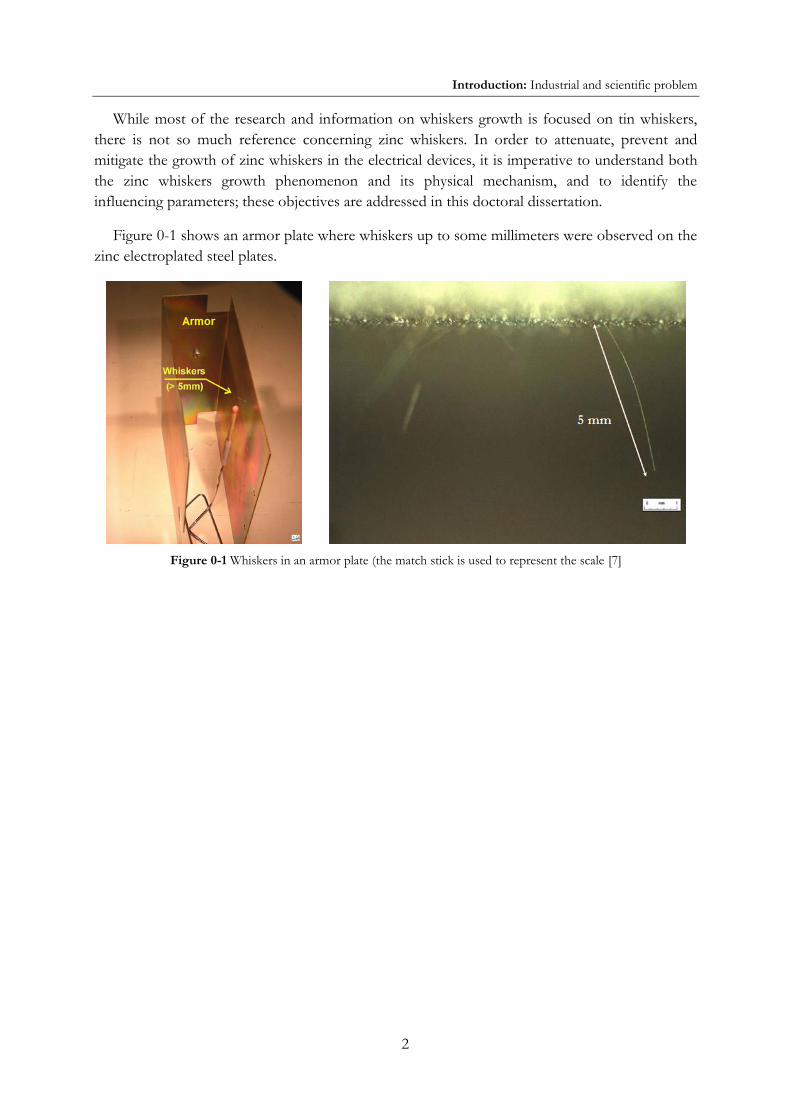
While most of the research and information on whiskers growth is focused on tin whiskers, there is not so much reference concerning zinc whiskers. In order to attenuate, prevent and mitigate the growth of zinc whiskers in the electrical devices, it is imperative to understand both the zinc whiskers growth phenomenon and its physical mechanism, and to identify the influencing parameters; these objectives are addressed in this doctoral dissertation.
Figure 0-1 shows an armor plate where whiskers up to some millimeters were observed on the zinc electroplated steel plates.
Figure 0-1 Whiskers in an armor plate (the match stick is used to represent the scale [7]

3
Chapter 1. State of research of zinc whiskers growth
Chapter 1
State of research of zinc whiskers growth
This first chapter addresses the historical background of the whiskers growth in general,
followed by a description of the general characteristics of zinc whiskers. The influence of various
intrinsic and environmental parameters in the whiskers growth phenomenon is discussed as well
as the different mechanisms proposed in the literature for the whiskers growth. Finally, taken in
account the information developed in the state of the research, the last part of this first chapter
describes the goals and outline of this doctoral research, where the specific scientific goals of this
thesis are formulated, as well as the strategies to achieve them.
Historical background Introduction to the whiskers Influencing parameters in the whiskers growth Whiskers growth mechanisms Summary of state of research of zinc whiskers and objectives

Chapter 1: Historical background
4
1.1 HISTORICAL BACKGROUND
Metallurgic whiskers have been known for long time. Ercker, a German mining inspector, published in 1574 in Prague a treatise on ores and assaying «Beschreibung allerfürnemisten Mineralischen Ertzt, und Bergwercksarten…» where he reported phenomena occurring during the smelting and fire assay processes [8] and described procedures for artificial growth of hair silver from silver matte occurring during the smelting and fire assay processes, one of the first examples of whiskers growth (Figure 1-1).
Figure 1-1 Lazarus Erckers fire assay book from 1574. «Beschreibung allerfürnemisten Mineralischen Ertzt, und Bergwercksarten…» [8]
The translation from German to English by Sisco and Smith states: «as long as I am talking about silver matte, I should for the sake of the eager reader tell something that is characteristic of its nature and behavior. First: When silver matte is cast into an ingot, and while it is still hot, it can be hammered and shaped as you wish, just like lead. And further: It is possible to cast figures or coin medals from it which look like vitreous silver. When you have cast it into funny little decorative figures, lightly cut or scratch them with a knife and hold them over a gentle charcoal fire until they get hot, whereupon silver will sprout or grow out of them very delicately just as it grows in the mineral. This is amusing and very pretty to watch. I am telling this so anybody who would like to do this for fun and play with it some more should know how it is done » [8]. These whiskers, commented in many posterior treatises of chemistry, are not spontaneously produced but only under exceptional environmental conditions [9].
A curious finding of spontaneous whiskers growth is reported by Schmidt in 1927 [10]; he found that when insects with well-developed fat bodies are impaled on tinned bras needles, the tin corrodes; green whiskers, composed of tin and fatty acids and several centimeters long, grow on the needles but not on the insects (Figure 1-2).
During the World War II, cadmium whiskers were found on electroplated cadmium surfaces producing important failures of air condensers in military equipment [2]. Few years later, failures were found on channel filters used for multi-channel transmission lines at Bell Telephones due to

Chapter 1: Historical background
5
zinc whiskers [9]. It was established that not only cadmium, zinc or tin were susceptible to develop whiskers, but also aluminum casting alloys and electroplated silver exposed to an atmosphere of hydrogen sulfide (H2S).
Figure 1-2 Fibers of fat on needle impaling insect in museum collection [10]
In 1954 Compton et al. established that whiskers grow by addition of material to the base of the whiskers and not to the tip of the whisker [11] (§1.4.2); by observing micrographs over several weeks, it was found that the morphology of the top of the whiskers remain unchanged. This fundamental statement was proved for tin whiskers some years later by Key [12] through SEM (Scanning Electron Microscopy) observations, while Lindborg [13] reached the same conclusion for zinc and cadmium whiskers.
Despite whiskers and zinc whiskers in particular are a very old industrial problem, the understanding of the phenomenon remains incipient and a lot of research is yet to be done.

Chapter 1: Introduction to the whiskers
6
1.2 INTRODUCTION TO THE WHISKERS
1.2.1 Morphology
JEDEC (Joint Electron Device Engineering Council) [14] defines whiskers as spontaneous columnar or cylindrical filaments, usually made of monocrystalline metals, emanating from the surface of a finish. JEDEC classified whiskers in three categories: nodular whiskers, rectilinear whiskers and whiskers with abrupt changes of direction (Figure 1-3), being the second type the most problematic for the industry.
10 µm 20 µm
a) nodular whisker b) rectilinear whisker
Figure 1-3 Types of zinc whiskers: a) nodular and b) rectilinear whiskers [15]
Metallurgic whiskers are filamentary features that spontaneously grow from metallic surfaces [5]. Because their high conductivity (they can carry tens of miliamperes before melting [1]), whiskers can bridge gaps between electronic components causing short circuits and consequently failures of the equipment. Also, because they are very fragile, whiskers are easily broken which makes not only difficult to detect them in maintenance testing of equipment, but also it makes possible that whiskers travel around the device bridging gaps somewhere else.
Whiskers made of tin do not look very different than those made of zinc, as can be seen in the Figure 1-4, where longitudinal and annular striations of some of these whiskers are observed.
5 µm 2 µm
a) tin whisker b) zinc whisker
Figure 1-4 Metallurgical whiskers: a) tin whiskers [14] and b) zinc whiskers [15]

Chapter 1: Introduction to the whiskers
7
1.2.2 Dimensions and growth kinetics
When incubation time is considerably long, whiskers growth is often ignored in devices of rapid obsolescence (for example, telephones and personal computers). However, there are many applications where the life time of the devices, expected to reach decades, surpass the incubation time such as in aeronautic or energy industries.
In Table 1-1 Lina [16] summarizes the main characteristics of zinc whiskers (diameter, maximal length, incubation time and growth rate) obtained from experiments and reported in different literature references [1] [9] [12] [13] [17]; tin whiskers information is also included for comparison [5] [12] [13] [18] [19]. There is good agreement among the different authors concerning whiskers dimensions but not regarding the growth rate.
Table 1-1 Main characteristics of zinc and tin whiskers from reported experiments [16]
Metal electroplate Zinc Tin
Diameter 0.5-2 µm [9] [13]
2-5 µm [12]
10 µm [1]
0.05-5 µm [18]
1-5 µm [5] [12]
Maximal length 5 mm [13]
10 mm [9] [12]
30 mm [17]
5 mm [5]
10 mm [12]
Incubation time From months to years [1] Several years [19]
Growth rate at 20°C 0.95 mm/year [1]
0.03-1.3 mm/year [13]
0.3 mm/year [5]
0.03-15.8 mm/year [13]
Growth rate at 50°C 3.2-9.5 mm/year [13] 31.5-315.4 mm/year [13]
According to Brusse and Sampson [1], the zinc whiskers growth phenomenon has two stages: incubation time that can take from few months to several years, followed by a growth of whiskers with 1 mm/year as maximal rate.
Franks describes tin whiskers as three-stage phenomenon: incubation time inversely proportional to stress, fast growth proportional to stress and finally, a strong deceleration or stop of the growth depending only of the whisker length [18]. According to Glazunova and Kudryavtsev [19], incubation time for tin whiskers lasts several years, and whiskers can reach 1 to 5 mm length after 3 to 5 years.
Nagai et al. [20] show that the incubation time for zinc whiskers is inversely proportional to stress (Figure 1-15), as Franks described it for tin whiskers [18].

Chapter 1: Introduction to the whiskers
8
1.2.3 Deposition processes
Zinc is used to protect steel from oxidation by playing a role of sacrificial anode; it actually forms zinc oxide which prevents further zinc corrosion.
The choice of the process for zinc deposition on a steel substrate has a great influence on the formation of whiskers. There are mainly two processes: hot dip galvanizing and electroplating.
In the hot dip galvanization, the metal substrate is immersed into a molten zinc bath. The resulting coating is actually composed of several metallurgical bonded layers. The coatings obtained by this process are not prone to whisker growth, according to WES (World Environment Services) [21]. Nevertheless, Lahtinen et al. [22] [23] found whiskers in zinc coatings deposited by hot dip galvanization.
Electroplated zinc coatings, on the other hand, have been identified to be more prone to whiskers growth. The present research thesis focuses on electroplated zinc coatings rather than on galvanized steel.
1.2.3.1 Electroplating process
Zinc electroplating of steel consists basically of the application of an electrical current to an electrolytic solution coupled to a zinc anode, while the steel acts as cathode. Zinc, the metal to be deposited, comes from either the anode (soluble anode) or from the reduction of the electrolyte with an electrical current.
Preliminary steps are required before the actual deposition: surface preparation (for roughness reduction), degreasing and cleaning. Each of these processes is followed by rinsing in order to eliminate any trace of grease or oxides. These preliminary treatments are defined depending of the metal substrate.
The zinc electroplating has been used since the first decades of the 20th century with the introduction of cyanide-bath electrolytes. By de middle of the century, acid chloride-electrolytes became commonly used but later in the 1980’s cyanide-free electrolytes were introduced.
The bath composition for depositing varies according to the desired deposit quality [24]; in the case of zinc, there are mainly two sort of electroplating electrolytes: alkaline (cyanide, zincates and pyrophosphates) and acid (sulfates, chlorides and fluorites).
Typically, the cyanide electrolytes (alkaline) contain sodium hydroxide (NaOH) and sodium cyanide (NaCN), both used as brighteners. As expected, sodium cyanide is not present in the cyanide-free electrolytes; in these sort of electrolytes, several compounds can be added such as calcium hydroxide (Ca(OH)2), calcium sulfate (CaSO4) and aluminum sulfate (Al(SO4)3) [25]. Concerning the acid electrolytes, they contain typically ammonium chloride (NH4Cl), but also ammonium-based and potassium-based electrolytes

Chapter 1: Introduction to the whiskers
9
1.2.3.2 Chrome finishing treatment
Once the steel is coated with zinc, the metal is often subject to a chroming treatment. Chroming modifies chemically the zinc surface by simple immersion composed usually of an acid bath of hexavalent salts (Cr6+, CrO3, NaCrO4, Na2Cr2O7) and acid activators (sulfates, nitrates, acetates, chlorides, fluorides, phosphates or sulfamates). With this finishing, the aspect of the surface is modified (brightness, iridescence and colors) and the resistance to corrosion is improved. The finishing coating is therefore composed of the metal to be finished (zinc in this case), plus hexavalent (Cr6+) and trivalent (Cr3+) chromium, that play as corrosion inhibiters.
Rinsing after the finishing has to be fast in order to avoid an excessive loss of hexavalent chrome. Drying temperature must not exceed 60°C, in order to avoid the chrome to be cracked.
As in the case of lead, hexavalent chromium is one of the substances restricted by the European Union directive of Reduction of Hazardous Substances (RoHS), effective in July 2006 [6].
1.2.4 Microstructure of the whiskers and zinc coating
By analysis of X-ray diffraction, Compton et al. [9] determined that zinc, cadmium and tin whiskers are not compounds but metallic filaments in the form of single or twinned crystals. Zinc and cadmium have a hexagonal crystalline structure, while tin has body centered tetragonal crystallographic structure. The orthogonal axis (direction c in Figure 1-5) is parallel to the filament.
Both Compton et al. [9] and Takemura et al. [26] isolated whiskers in order to determine their texture by X-ray diffraction. They found out that zinc and cadmium whiskers are composed of a single crystal. It is not clear, however, if tin whiskers can be polycrystalline [9] [27].
Figure 1-5 Hexagonal structure of zinc [28]; unit-cell dimensions: a=266.47 pm, c=494.69 pm
Lindborg et al. [29] observed recrystallized zinc in the coating, with columnar grains extending in a direction perpendicular to the surface. New technologies as the Dual Beam microscope (with both electronic and ionic beam) have favored the observation of the microstructure of whiskers and coatings [16]. EBSD (Electron Backscattered Diffraction) observations by Etienne et al. [30] confirmed Lindborg observations concerning the columnar grains in the zinc electroplate, with an average length of 1.5 µm and an average width of 310 nm (Figure 1-6).

Chapter 1: Introduction to the whiskers
10
Figure 1-6 EBSD Band contrast image of zinc electroplate, showing the grain structure. Steel is visible at the bottom of the sample [30]
Reynolds and Hilty [31] used FIB (Focused Ion Beam) to observe zinc whiskers by SEM, finding that zinc coating has a structure of small grains between the electroplated zinc and the root of a rectilinear whisker. No thinning of the coating was observed, even around the whisker root. These authors compared their results with FIB images of tin whiskers obtained by Xu et al. [32] (Figure 1-7).
1 µm
a) tin whisker b) zinc whisker
Figure 1-7 Comparison of FIB cross sections of whiskers: a) zinc whisker (with a nodule), by Reynolds and Hilty [31]; b) tin whisker by Xu et al. [32]
In the case of tin coating on copper substrate, IMC (intermetallic compounds) Cu6Sn5 are formed not only at the substrate-coating interface, but also at the grain boundaries of the tin coating due to copper diffusion. In contrast, electroplated zinc coatings on a steel substrate do not show intermetallic compounds at the scale of SEM observations. In fact, the phases diagram of Fe-Zn (Figure 1-8) shows that the solubility limit of iron in zinc is very low (<0.03% at 450°C).

Chapter 1: Introduction to the whiskers
11
Figure 1-8 Phases Fe-Zn diagram [31]
Several intermetallic compounds can be formed in the zinc coating, as showed in Table 1-2. Following the phase diagram, Reynolds and Hilty [31] assumed that IMC would form rapidly in hot dip galvanizing processes when temperature is high, but not on electroplating with low temperatures.
Table 1-2 Intermetallic phases Fe-Zn [25]
Phase Zn at.%
-Zn >99.7% (at 450°C)
-FeZn13 92.5 – 94
86.5 – 92
1 78.6 – 81
Baated et al. [33] brought something new in this discussion. When it was somehow agreed that zinc whiskers did not present intermetallic compounds as in the case of tin, this paper claims the presence of a Fe-Zn phase on the structure of the zinc coating by TEM (Transmission Electron Microscopy) observations and EDX (Energy-dispersive X-ray spectroscopy) analysis (Figure 1-9), although the results are not very conclusive.

Chapter 1: Introduction to the whiskers
12
Figure 1-9 Elemental analysis of zinc coating obtained by FIB and TEM-EDX [33]
The same authors stated that zinc oxides and Fe-Zn intermetallic compounds are a key source of compressive stress in the zinc coating. Zinc reacts with the iron diffused from the substrate and with the oxygen diffused from the environment, producing an IMC and oxide layer respectively. The consequent volume expansion of zinc oxide is twice as big as the expansion of tin oxide, while the zinc/iron IMC expansion is at least six times smaller than tin/copper IMC (Table 1-3).
Table 1-3 Molar volume and mass, density and volume expansion of some electroplates [33]
Both oxide and IMC can be source of compressive stress on zinc grains which actually diffuse to surface of coating forming the whiskers (Figure 1-10). This compressive stress would be the driving force of the zinc whisker growth.

Chapter 1: Introduction to the whiskers
13
Figure 1-10 Schema of Zn-Fe intermetallic compounds in the formation of zinc whiskers [33]

Chapter 1: Influencing parameters in the whiskers growth
14
1.3 INFLUENCING PARAMETERS IN THE WHISKERS GROWTH
1.3.1 Intrinsic parameters of the material
1.3.1.1 The deposited metal
Tin, cadmium and zinc, low melting point metals (231, 312 and 420°C respectively [28]), are known to be prone to whiskers growth. Nevertheless more metals can also develop whiskers: silver, gold, aluminum, lead and indium whiskers are reported by NASA (National Aeronautics and Space Administration) website of metallurgical whiskers [3].
Compton [9] studied approximately thousand specimens of different metals, solid and plated, exposed under various environmental conditions. This study shows that zinc, cadmium, tin and silver can develop whiskers under certain conditions. Table 1-4 shows the results for the experiments done through two years. Nickel whiskers were neither observed by the author nor reported by NASA [3].
Table 1-4 Results of experiments by Compton et al. [9] after two years of storage
Coating thickness
[µm] Low relative
humidity High relative
humidity
Without contaminants
1.3 Sn Cd Zn Ag* Cu* Zn Ag* Cu*
Sn Cd Zn Ag* Zn Ag* 2.1
12.7 - -
With organic contaminants
1.3 Sn Cd Zn Ag* Cu* Sn Ag* Cu*
Sn Cd Zn Ag* 2.1 Sn Cd Zn Ag*
12.7 Sn Cd Zn Ag* Cu* *On silver and copper whiskers developed only in presence of sulfur (hard rubber)
1.3.1.2 Electroplating electrolyte and chrome finishing
Lindborg et al. [29] reported that zinc coatings obtained with chloride, sulfate and zincate electrolytes containing significant amount of carbon, are formed of smaller grains and in general have larger stress than the coatings obtained with cyanide electrolytes with or without brighteners.
While grain diameters of samples electroplated with alkaline cyanide electrolytes are between 0.1 and 0.4 µm, grains of samples obtained with acid electrolytes (chloride, sulfate and zincate) have diameters from 0.04 to 0.1 µm.
It was also found that while the cross-section of most of the grains are more or less equiaxial, those with high concentration of cyanide and higher current density tend to be flat, lath-like with straight parallel grain boundaries resembling a martensitic structure.
Sugiarto et al. [17] observed that the current density of the electroplating has an influence on the residual stress of the coating and therefore in the whiskers growth, as can be observed in

Chapter 1: Influencing parameters in the whiskers growth
15
Figure 1-11. A maximal stress of approximately 70 MPa is observed for the employed cyanide electrolyte, with an approximate current density of 40 mA/cm2. The authors also made experiments to conclude that chrome finishing inhibits the onset of whiskers but does not avoid them.
Figure 1-11 Residual tress in zinc coating as function of current density for a cyanide bath containing 10 mL/L
brightener [17]
1.3.1.3 Organic contaminants
Table 1-4 shows that the presence of contaminants favors the zinc whiskers growth (no whiskers in absence of contaminants). Growth of zinc whiskers seems to be favored by the presence of organic contaminants, regardless of humidity.
The impurities in the coating can play a role in the formation of whiskers. The organic elements that can influence the whiskers growth can come either from the electroplating electrolyte or from the finishing chroming bath. Sugiarto et al. [17] observed that local whisker formation increased in areas close to high concentration of organic contaminants (from brighteners) responsible for compressive stress in electroplated metals.
By EDX analysis, Lathinen and Gustafsson [22] observed the presence of sulfur and chlorine in the area close to the whiskers roots; these impurities can come not only from electroplating and chroming processes, but also from the environment contamination.
Lindborg et al. [29] and Sugiarto et al. [17] determined the influence of brighteners and the whiskers growth. More whiskers are found in bright coatings (with brighteners) than in dull zinc coatings (without brighteners). The presence of brighteners in the electrolytes favors the whisker growth by increasing the residual stress in the coating (Figure 1-12). Nevertheless, Key [12] concludes that the absence of brighteners in the electrolyte does not eliminate the risk of whisker formation in zinc, tin and cadmium coatings.
0
20
40
60
80
0 20 40 60 80
Com
pres
sive
res
idua
l str
ess
[MP
a]
Cathode current density [mA/cm²]
Maximal stress

Chapter 1: Influencing parameters in the whiskers growth
16
Figure 1-12 Residual stress in zinc coating as function of coating thickness for different brighteners concentration levels compared with additive free control [17]
The components of electroplating electrolytes and brighteners can remain in the coating, although in low quantities; they can play an important role in the whiskers growth. Etienne et al. [34] observed an inclusion in zinc electroplated steel prone to whiskers growth, visible in the SEM image of Figure 1-13; EDX analysis shows that the inclusion is rich in carbon, calcium, and aluminum (50%, 30%, and 15% of C, Ca and Al respectively, plus some Fe and Zn traces). The authors suggest that impurities could have been trapped during electroplating or during a water rinsing.
Figure 1-13 SEM side view of electroplate sample prone to whiskers growth, glued on the Cu grid and polished with Ga-ions [34]
1.3.1.4 Residual stress in the coatings
Weil [35] introduces five theories to explain the origin of residual stress in the electroplated coatings:

Chapter 1: Influencing parameters in the whiskers growth
17
i) The agglomerations of atoms quasi-amorphous, formed at the beginning of the electroplating, recrystallize in order to reduce the surface energy, leading to a volume decrease that creates tensile stress. However, this theory does not explain the compressive stress observed often in zinc, cadmium and tin electroplated coatings.
ii) The presence of hydrogen in the coating produces tensile stress when the hydrogen diffuses to the exterior or compressive stress when the hydrogen diffuses to the interior creating gas pockets.
iii) The presence of hydrated components, coming from the impurities of the electrolyte and remaining in the coating by water diffusion, decreases the volume leading to tensile stress. The oxidation of the metal when it is in contact with this water can lead to compressive stress.
iv) The excess of energy can generate tensile macro-stress. This effect is similar to the temperature effect: the volume is reduced when cooling.
v) The presence of defects in the crystal (voids) can explain both the macro-stress and the localized stress at both tension and compression. These effects lead to inter-granular tensile stress and intra-granular compressive stress.
Residual macro-stress, or bulk stress, is defined by Lindborg et al. [29] as the long-range, linearly averaged over the whole zinc deposit; it can be measured by dilatometry or by determination of the shifting of X-ray diffraction peaks [36]. From now on, residual stress refers to macro-stress, unless otherwise indicated.
Zinc coatings have compressive residual macro-stress regardless the choice of electroplating electrolyte. If the coating remains immersed in the electrolyte, compressive stress decreases because the zinc re-dissolution in the electrolyte and the hydrogen diffusion out the deposit; this stress decrease is lower if the coating remains in contact of air.
Lindborg states that the residual macro-stress in the coating is the most probable driving force in whiskers growth [13]. Experimental data in Figure 1-14 show the maximal whisker growth rate as function of macro-stress for two different temperatures; three zones are identified in both figures:
Slow or zero whiskers growth below macro-stress threshold (45 MPa at 20°C and 40 MPa at 50°C); the stress threshold decreases with temperature.
Rapid whiskers growth: after 50 MPa at 20°C and 55 MPa.
Mixed region (grey zone in the figure) between slow growth and fast growth zones.
Sugiarto et al. [17] measured the macro-stress on zinc coatings fabricated with the same electrolyte with and without brightener. Unlike Lindborg [13], the authors stated that whiskers growth is related to localized stress at the grains within the electrodeposit rather than the macro-stress (whiskers were also observed in samples with almost zero measured macro-stress); localized stress is associated with the presence of defects in the crystal such as voids and dislocations.

Chapter 1: Influencing parameters in the whiskers growth
18
Figure 1-14 Whisker growth rate for different 10 µm zinc electroplated as function of internal macro-stress at 50°C (left) and 20°C (right); letters denote plating conditions [13]
Since brighteners presence favors residual stress in the zinc coating (§Figure 1-12), local sites of high organic matter concentration derived from brighteners are more prone to whiskers growth. According to Sugiarto et al. [17], the conventional methods for measuring macro-stress, which yield an integrated mean stress value for the whole sample, are not capable of recording localized stress of the zinc coating.
Nagai et al. [20] observed that incubation time (time elapsed between electrodeposition and the growth of the first whiskers) decreases as the electroplate macro-stress increases, as illustrated in Figure 1-15.
Figure 1-15 Macro-stress as function of incubation time [20]
Whiskers were found in samples with stress under 45 MPa (Lindborg’s threshold at 20°C); for these samples the incubation time is longer than 2 years (up to 6 years for 20 MPa). Lindborg’s storage lasted only 2 years, which explains why he did not observe whiskers for samples with stress lower than 45 MPa (the storage time was shorter than the incubation time). Additionally,

Chapter 1: Influencing parameters in the whiskers growth
19
Nagai et al., like Sugiarto et al. [17], do not consider the stress, as the driving force of the whisker growth, in disagreement with Lindborg [13].
Xu et al. [32] applied external stress to electroplated samples; they observed that the applied compressive stress generates more whisker growth than the applied tensile stress does. The authors calculated a whisker index ∑(n∙d∙l∙f(l)) as function of number of whiskers (n), whisker diameter (d), whisker length (l) and a related factor (f(l)). Figure 1-16 shows the calculated whisker index as function of ageing time for tensile, compressive and zero applied stress. Samples under compressive stress are more prone to whisker growth than samples under tensile or zero stress.
Figure 1-16 Whiskers growth as function of aging time for different external stresses; whisker index ∑(n∙d∙l∙f(l)) depends of number of whiskers (n), whisker diameter (d), whisker length (l) and a related factor (f(l)) [32]
According to Lindborg [13] experiments on the zinc whiskers growth, micro-strain has little or no direct influence on the whiskers growth rates or the measured stress (Figure 1-17). For the author, the micro-strain does not constitute the main driving force for whiskers growth like it does for recrystallization. This observation disagrees with other mechanisms proposed by some authors (§1.2.4) where dislocations, producing localized stress, are the driving force of the whiskers formation.
Figure 1-17 Influence of micro-strain in whisker growth and stress [13]

Chapter 1: Influencing parameters in the whiskers growth
20
1.3.1.5 Microstructure of the zinc coating
Concerning the microstructure of the zinc coating, Lindborg [13] observed that specimens with elongated grains tended to have larger whiskers growth rates than specimens with equiaxed columnar grains. Elongated grains, however, were always coupled in his observations with high macro-stress and this factor may explain itself the larger growth rates. Figure 1-18 shows the macro-stress of several samples versus grain size measured by TEM. It is observed that for the studied samples, grain size of the coating does not have an influence on whiskers growth rates.
Grain size is strongly influenced by electroplating electrolyte, as explained above (§1.3.1.2); alkaline electrolytes favors the grain size of the zinc in the coating. While samples electroplated with alkaline electrolyte have grain diameters from 0.1 to 0.4 µm, those obtained with acid electrolyte have grain diameters from 0.04 to 0.1 µm.
Figure 1-18 Influence of grain size in whisker growth and stress [13]
1.3.1.6 Hardness
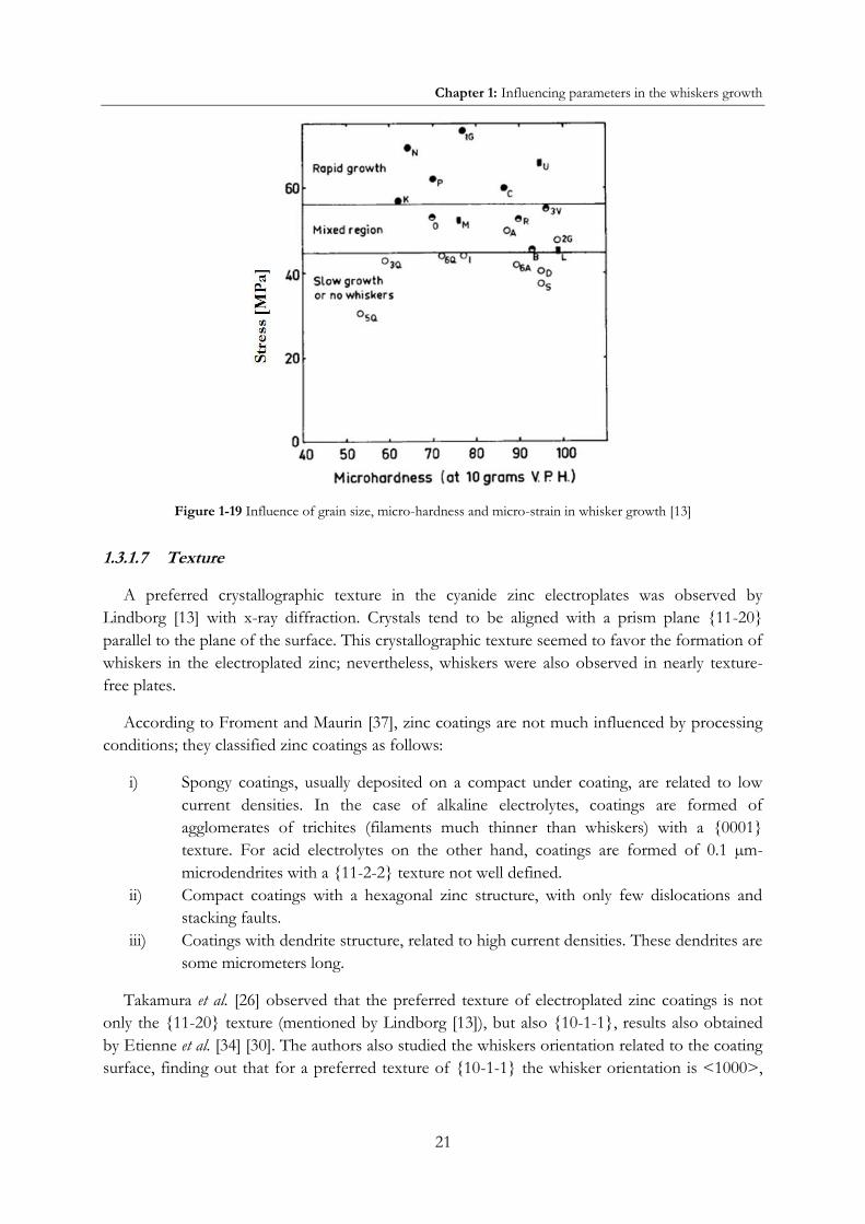
Lindborg [13] observed that the whiskers growth rates are not influenced by micro-hardness (Figure 1-19). However, the author suggested that a study with larger number of samples is necessary to reach more reliable conclusions.
Chapter 1: Influencing parameters in the whiskers growth
21
Figure 1-19 Influence of grain size, micro-hardness and micro-strain in whisker growth [13]
1.3.1.7 Texture
A preferred crystallographic texture in the cyanide zinc electroplates was observed by Lindborg [13] with x-ray diffraction. Crystals tend to be aligned with a prism plane {11-20} parallel to the plane of the surface. This crystallographic texture seemed to favor the formation of whiskers in the electroplated zinc; nevertheless, whiskers were also observed in nearly texture-free plates.
According to Froment and Maurin [37], zinc coatings are not much influenced by processing conditions; they classified zinc coatings as follows:
i) Spongy coatings, usually deposited on a compact under coating, are related to low current densities. In the case of alkaline electrolytes, coatings are formed of agglomerates of trichites (filaments much thinner than whiskers) with a {0001} texture. For acid electrolytes on the other hand, coatings are formed of 0.1 µm-microdendrites with a {11-2-2} texture not well defined.
ii) Compact coatings with a hexagonal zinc structure, with only few dislocations and stacking faults.
iii) Coatings with dendrite structure, related to high current densities. These dendrites are some micrometers long.
Takamura et al. [26] observed that the preferred texture of electroplated zinc coatings is not only the {11-20} texture (mentioned by Lindborg [13]), but also {10-1-1}, results also obtained by Etienne et al. [34] [30]. The authors also studied the whiskers orientation related to the coating surface, finding out that for a preferred texture of {10-1-1} the whisker orientation is <1000>,

Chapter 1: Influencing parameters in the whiskers growth
22
i.e. an angle of 30 to 38° to the normal of the surface. For {11-20}, the angle would correspond to 60°; that is, whiskers can have very different orientations.
Figure 1-20 shows experiments by Lindborg [13] to determine the influence of zinc texture in the whiskers growth. It may be concluded that orientation-index values above 0.45 to 0.7 increase the probability of whisker growth without being a necessary or a sufficient requirement.
Figure 1-20 Influence of znc texture in whisker growth [13]
Lee and Lee [38] proposed that tin whiskers are formed in order to relax stresses between misoriented grains because the mechanical anisotropy of -Sn [39]. Same principle can be extended to zinc whiskers since zinc is also highly anisotropic elastically (even more than tin), considering the stiffness constants reported by Ledbetter in Table 1-5 [40] (the more dissimilar are the constants from each other, the more anisotropic is the material).
Table 1-5 Stiffness constants of zinc [GPa] [40]
C11 C33 C44 C12 C13 C66
163 60.3 39.4 30.6 48.1 65.9
1.3.1.8 Coating thickness
For Compton et al. [9], thinner electroplates are more prone to whiskers growth, as can be seen in the Table 1-4 above. Lindborg [13] explains these results indicating that coating thickness is coupled with texture for at least some substrates; Lindborg observed the largest number of observed whiskers in one of the thickest coatings.

Chapter 1: Influencing parameters in the whiskers growth
23
Sugiarto et al. [17] (§Figure 1-12) show that for thin coatings (thinner than 5µm), the stress is strongly influenced by the coating thickness; in contrast, for thicker electroplates, stress seems to be independent of coating thickness.
1.3.1.9 Substrate thickness
Concerning the substrate, Lindborg [13] experimented with cold-rolled carbon steel substrates with different thicknesses. The results, plotted in Figure 1-20 above, reveals that the thinner the substrate, the more whiskers growth is observed in the zinc coating. In fact, the texture of the thinner steel substrate {110} would favor the development of a {11-20} zinc texture and thus favor whisker growth.
1.3.2 Environmental parameters
1.3.2.1 Temperature
According to Compton et al. [9], temperature increases tin whiskers density as well as whiskers length (Figure 1-21). Lindborg [13] tested 10 µm zinc electroplated samples at 20 and 50°C (§Figure 1-14). The whisker growth rate is significantly increased with temperature; even the macro-stress threshold is slightly decreased when temperature is higher.
Figure 1-21 Influence of temperature on whisker growth [13]
Chapter 1: Influencing parameters in the whiskers growth
24
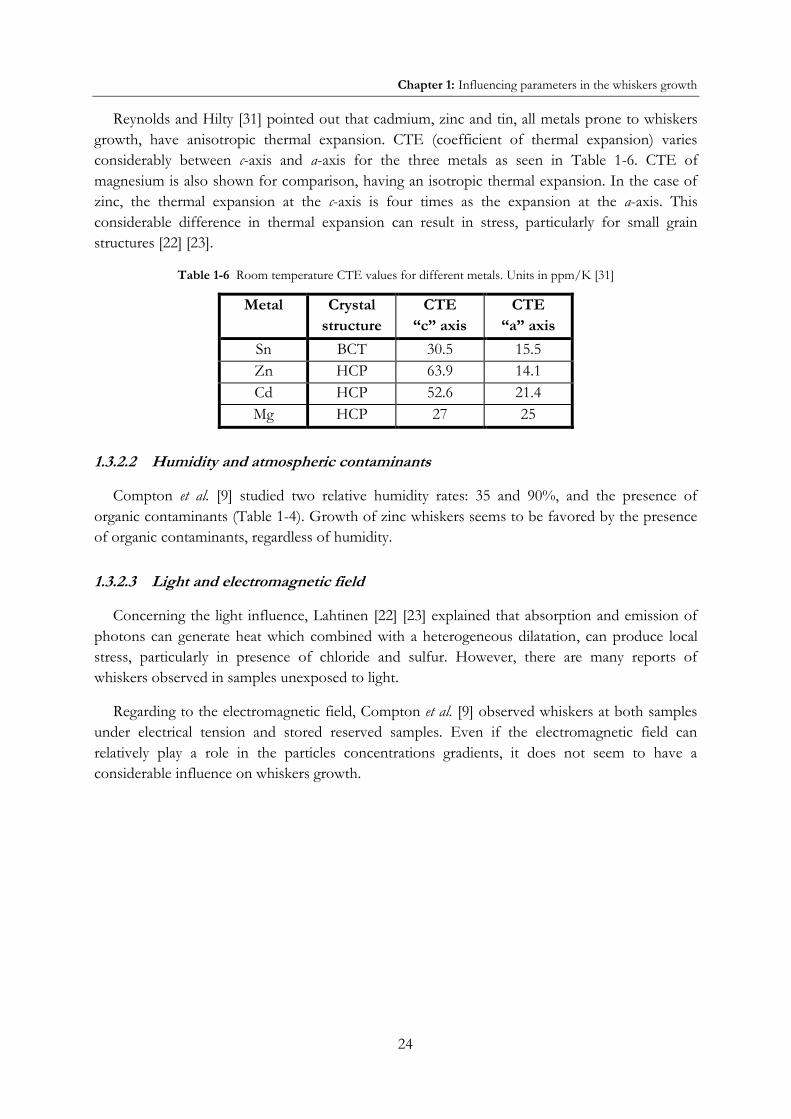
Reynolds and Hilty [31] pointed out that cadmium, zinc and tin, all metals prone to whiskers growth, have anisotropic thermal expansion. CTE (coefficient of thermal expansion) varies considerably between c-axis and a-axis for the three metals as seen in Table 1-6. CTE of magnesium is also shown for comparison, having an isotropic thermal expansion. In the case of zinc, the thermal expansion at the c-axis is four times as the expansion at the a-axis. This considerable difference in thermal expansion can result in stress, particularly for small grain structures [22] [23].
Table 1-6 Room temperature CTE values for different metals. Units in ppm/K [31]
Metal Crystal structure
CTE “c” axis
CTE “a” axis
Sn BCT 30.5 15.5 Zn HCP 63.9 14.1 Cd HCP 52.6 21.4 Mg HCP 27 25
1.3.2.2 Humidity and atmospheric contaminants
Compton et al. [9] studied two relative humidity rates: 35 and 90%, and the presence of organic contaminants (Table 1-4). Growth of zinc whiskers seems to be favored by the presence of organic contaminants, regardless of humidity.
1.3.2.3 Light and electromagnetic field
Concerning the light influence, Lahtinen [22] [23] explained that absorption and emission of photons can generate heat which combined with a heterogeneous dilatation, can produce local stress, particularly in presence of chloride and sulfur. However, there are many reports of whiskers observed in samples unexposed to light.
Regarding to the electromagnetic field, Compton et al. [9] observed whiskers at both samples under electrical tension and stored reserved samples. Even if the electromagnetic field can relatively play a role in the particles concentrations gradients, it does not seem to have a considerable influence on whiskers growth.

Chapter 1: Influencing parameters in the whiskers growth
25
1.3.3 Summary of influencing parameters
As it has been discussed in this section, there are many parameters, both intrinsic and environmental, influencing the whiskers growth; the difficulty consists in the fact that these parameters are somehow already correlated. Table 1-7 summarizes the influencing of the different discussed parameters.
Table 1-7 Summary of influence of parameters on whiskers growth
Parameter Influence
Influencing parameters
Temperature favors whiskers length and density [9] and growth rate [13]
Residual stress in the coating favors whiskers growth rate [13] [29] and decreases incubation
time [20]
Microstructure Elongated grains tend to have larger whiskers growth rates than
specimens with equiaxed columnar grains [13]
Electroplating electrolyte Cyanide electrolytes produce less residual stress [29], and
therefore lower whiskers growth rate
Organic contaminants
(including brighteners)
favors whiskers growth [9] by increasing compressive localized
stress in electroplated metals [17]
Chrome inhibits the onset of whiskers but does not avoid them [17]
Applied external compressive
stress
Compressive applied stress favors growth more than tensile
applied external stress [32]
Texture Planes {11-20}and {10-1-1} favor whiskers growth [13] [26]
Coating thickness
The thinner coating favors whiskers growth [9] by influencing
the coating texture [13] and the residual stress in thin (<5µm)
coatings [17]
Substrate thickness The thinner substrate favors whiskers growth by influencing
the coating texture [13]
Non-influencing parameters
Hardness and micro-strain No influence observed [13]
Light and electromagnetic
field
No influence observed [9] [22] [23]
Humidity No influence observed [9]
Grain size No clear influence observed [13]

Chapter 1: Whiskers growth mechanisms
26
1.4 WHISKERS GROWTH MECHANISMS
The fact that multiple physical phenomena in the material interact during whisker growth (inter-diffusion, phase transformation, stress generation, relaxation, etc.) makes very hard to determine the mechanism behind to understand why and how the whiskers grow. Nevertheless, diverse mechanisms for whisker growth have been proposed trough the time, mostly for tin whiskers, classified by Smetana [41] in three different categories:
i- Dislocation mechanisms with growth from the tip of the whisker: Peach [42] (1952) for tin whiskers.
ii- Dislocation mechanisms with growth from the base of the whisker: Frank [43], Eshelby [44], Franks [18] and Amelinckx et al. [45] for tin whiskers in the 1950’s, and Lindborg [46] in 1976 for zinc, tin and cadmium whiskers.
iii- Recrystallization mechanisms: Smetana [41] and Vianco and Rejent [47], among others, for tin whiskers (2007 and 2009 respectively).
1.4.1 Dislocation mechanisms proposing growth from the tip of the whisker
The first of these mechanisms was proposed by Peach in 1952 [42], stating that «tin whiskers grew from tin atoms migrating through a screw dislocation at the center of the whisker. These migrating tin atoms subsequently deposited themselves at the whisker tip» [41]. It took only two years for Bell Labs, with Koonce and Arnaud [11], to disprove this mechanism theory. They observed electron micrographs of growing tin whiskers during several weeks and observed that the morphology of the tip of the whiskers remain unchanged while the whisker grew. This observation led to a very important conclusion: whiskers grow from their base and not from their tip which remains constant; whiskers grow by addition of material to their base which is then pushed up. This observation was confirmed later on by Key [12] by SEM observation; many subsequent observations have confirmed the growth at the whisker base.
1.4.2 Dislocation mechanisms proposing growth from the base of the whisker
These diffusion-limited mechanisms were first proposed in 1953 by Frank [43] and Eshelby [44]. Frank proposed a rotating edge dislocation pinned to a screw dislocation at right angles to the surface and staying in the same plane after each revolution (Figure 1-22). Each revolution would add an additional layer on tin atoms to the whisker base [41].

Chapter 1: Whiskers growth mechanisms
27
Figure 1-22 Schema of Frank’s whisker dislocation mechanism [43]
Eshelby [10] assumes that a small hump already exists on the surface (Figure 1-23-a), and that, as consequence of oxidation, the interface energy has a negative value - . The surface tractions tend to pull out a whisker, while providing a constraining collar at the root which keeps the diameter constant. The author proposed Frank–Read dislocation sources at the base of the whisker emitting loops that expanded by climb to a boundary (Figure 1-23-b). The dislocation loops glide to the surface and deposit a half plane of atoms at the surface (Figure 1-23-c).
Figure 1-23 Schematic of Eshelby’s whisker dislocation mechanism: a) negative surface tension, b) Frank-Read dislocation, c) deposit of half plane at the surface [44]
In 1958, Franks [18] proposed a mechanism such that dislocations that result in whiskers are pinned due to lattice faults, and thus they act as dislocation sources under the influence of a stress field. These pinned dislocations would to move by glide to grow whiskers [41].
In 1956, Amelinckx et al. [45] proposed a helical dislocation model for whisker formation and growth. These spiral prismatic dislocations are proposed to move to a surface by a climb mechanism. Each complete loop of the spiral that reaches the surface would add a Burgers vector thickness of material [41].

Chapter 1: Whiskers growth mechanisms
28
Based on experimental data [29], Lindborg concluded that to each metal atom leaving the electroplated, there should be a corresponding vacancy formed somewhere below the root of the whisker [13]. As holes in electroplated have never been seen, diffusion has to take place over long distances compared to the diameter of the whisker. Therefore, he proposed a model for zinc whisker growth [46], consisting of a long-distance diffusion stage (where a climbing dislocation loop acts as a vacancy-emitting source) and a glide stage (where dislocations glide to the surface). The diffusion stage is controlled by long-range diffusion while the glide stage is controlled by intersection of glide and forest dislocations in the case of zinc and cadmium, but not for tin (recovery-creep mechanism).
Figure 1-24 is a schematic of Lindborg whisker growth model. At (a) and (b), an extra-plane of atoms expands by climb of the surrounding edge dislocation loop marked 1. At (c), the loop 1 has reached full size starting to glide upwards while a second loop started expanding. At (d), loop 1 has reached the surface and pushed out the whisker one atomic spacing. The subsequent loop 2 is in the gliding stages and a loop 3 is expanding by climb.
Figure 1-24 Lindborg whisker growth model: a, b) expansion of extra-plane marked 1, c) full-sized loop gliding, d) loop reaches the surface [46]
Mechanisms proposed by Eshelby, Franks and Lindborg are based on creep diffusion at the grain boundaries. Two creep mechanisms are considered: bulk or lattice diffusion (Nabarro-Herring creep) and grain boundary diffusion (Coble creep), as well as a combined diffusion (bulk diffusion plus grain boundary diffusion) [48].
Creep-diffusion strain can be calculated when a force is applied to either a single crystal or a polycrystalline system, as described in Equation 1-1 and Equation 1-2. Creep-diffusion strain is proportional to the applied stress and inversely proportional to the square or cube of grain size [16].

Chapter 1: Whiskers growth mechanisms
29
Creep strain, bulk diffusion (Nabarro-Herring creep):
Equation 1-1
Creep strain, grain boundary diffusion (Coble creep):
Equation 1-2
where: creep strain B, C coefficients depending of the geometry of the grain D, D’ diffusion coefficients �a atomic volume applied stress
k Boltzmann constant L grain size grain border thickness
T temperature
According to the mechanism proposed by him and described above, Lindborg applied Nabarro-Herring model for whiskers growth of zinc, cadmium and tin, in order to determine the growth rate for diffusion through the lattice, trough grain boundaries and through dislocation pipes [46] to obtain the following three equations:
Growth rate for diffusion through the lattice (h's):
Equation 1-3
Growth rate for diffusion through grain boundaries (h'b):
Equation 1-4
Growth rate for diffusion through dislocation pipes (h'p):
Equation 1-5
where: DS, Db, Dp diffusion coefficients RW whisker radius � dislocations density dav average diameter of grains b Burgers vector
As expected, from a diffusional process, whiskers growth rate is proportional to the stress. However, it is also inversely proportional to whisker diameter. Based on empirical data, Lindborg concludes that lattice diffusion cannot supply the required flow of atoms to the whisker root. Indeed, he found that grain boundary diffusion agrees better with the experiments.

Chapter 1: Whiskers growth mechanisms
30
In his model, the diffusion contributes with the material to the whisker root, according to Equation 1-3 to Equation 1-5. The second part of this mechanism is the glide, which is strongly dependant of shear stress. Shear stress is commonly assumed as half of the compressive stress, and the growth rate by glide is described as follows:
Growth rate by glide (h'):
Equation 1-6
where: , i stresses
µ shear modulus φw distance to the forest of dislocations n factor independent of dislocation density and temperature but not of stress;
between 7 and 20, for zinc at room temperature [46]
Given the values of the exponential factor (n), the growth rate (h') is strongly stress dependent.
A region in the electroplate with large spacing (φw) will have a very low internal stress ( )and
therefore the deformation will be easy here facilitating the whiskers growth. This term ( )
subtracted from the stress ( ) corresponds to the threshold stress for dislocation glide when they are pinned to dislocation faults.
In this two-stage model, both diffusion and glide are necessary for whisker growth. The slowest one of these two mechanisms will determine the growth rate. The model shows that glide, and therefore whisker growth is possible only for stresses higher than a critical value, this value depends on the mesh size of the dislocation structure near the whisker root.
If stress is slightly higher than this critical value, glide is a very slow process and therefore it controls the whisker growth, i.e., there is a strong stress dependence of the growth, as experimentally observed in Figure 1-25.
For higher stresses, glide is strongly accelerated; dislocation loops expand so fast that they do not control whisker growth anymore. Diffusion is now the rate-determining step implying a stress linear dependence. However, this prediction of the model has not been probed experimentally yet.

Chapter 1: Whiskers growth mechanisms
31
Figure 1-25 Experimental results for zinc whisker growth rates by Lindborg [46]
1.4.3 Recrystallization mechanisms
Spontaneous whiskers growth has been observed mainly in electroplated coatings of low melting point metals, where recrystallization temperature is under room temperature such as cadmium, zinc and tin, as can be seen in the Table 1-8.
Already in 1958 Ellis et al. [49] concluded that dislocations could not explain their experimental observations, so they suggested recrystallization as a mechanism of whisker growth, although they did not propose any mechanism. Later on, Glazunova and Kudryavtsev [19], Kakeshita et al. [50], Lebret et al. [51] and Boguslavsky and Bush [52], among other authors also proposed recrystallization as the mechanism for whisker growth instead of dislocations mechanisms. The two main recrystallization mechanisms, proposed by Smetana [41] and Vianco and Rejent [47], have been elaborated for tin whiskers but they can eventually be correlated to zinc whiskers.
Table 1-8 Melting and recrystallization temperatures for cadmium, zinc and tin [28] [31]
Metal T melting T recrystallization
Cd 321°C ~0°C
Zn 420°C ~10°C
Sn 232°C ~-20°C
1.4.3.1 “The end game” by Smetana
Proposed by Smetana in 2007 [41], in this model the atoms at the grain boundary in the whisker base are averagely at lower energy (compressive stress) level than the surrounding areas, which allows the movement of tin atoms. Grain boundaries are actually sites with lower degree of

Chapter 1: Whiskers growth mechanisms
32
order and atom packing density. This theory considers compressive stress in the tin films as the driving force for the whisker growth.
1.4.3.1.1 Starting conditions
This mechanism is based on the columnar grain boundaries observed at the electroplated tin (also observed in the electroplated zinc §Figure 1-7); they are schematically represented in the Figure 1-26 where the grain boundary interfaces are subjected to biaxial compressive stress ( ) at the plane of the coating, resulted from a force (F).
Figure 1-26 Schema of electroplated tin grains under compressive stress [41]
1.4.3.1.2 Recrystallization and oblique grain boundaries
After recrystallization of new grains, oblique grain boundaries are formed in the tin coating (Figure 1-27); these oblique grain boundaries have been already observed in tin whiskers growth (Figure 1-28). Compressive stress at oblique grain boundaries is lower than at the vertical grain boundaries, although the applied force is equal, as shown in the Figure 1-28, which leads to stress gradients in the grain boundaries, necessary for tin diffusion to the base of the whisker growth.
Figure 1-27 Schematic of electroplated tin grains after recrystallization [41]

Chapter 1: Whiskers growth mechanisms
33
Figure 1-28 Oblique grain boundaries under a tin whisker [41]
Additionally, there is lower atomic packaging density in the grain boundaries, leading to a stress gradient between the grain boundary and the bulk tin grain. In Figure 1-29, closely packed tin atoms are represented by blue circles, while the more loosely packed tin atoms in the grain boundary are represented by grey circles.
Figure 1-29 Representation of vertical grain boundaries (left) and oblique ones (right) [41]
1.4.3.1.3 Whisker growth mechanism
The components of the stress applied to the oblique grain boundaries (Figure 1-30) result in shear stress, parallel and perpendicular to the grain boundary.
Figure 1-30 Representation of applied stress on an oblique grain boundary [41]
On the other hand, because the low melting point of tin (232°C, lower than room temperature), creep mechanisms are likely to occur even at room temperature. Figure 1-31 shows

Chapter 1: Whiskers growth mechanisms
34
a single recrystallized tin grain with oblique grain boundaries; atoms of the grain are close packed, while the atoms in the grain boundary have lower atomic packaging density.
The grain boundary then glides a distance corresponding to the displacement of one atom; atoms originally in the grain (grey in the figure) move upward to form the whisker. This glide produces vacancies in the original grain (yellow) that are occupied by atoms coming from the oblique grain boundary; the resulting vacancies in the oblique grain boundaries (blue) are occupied by atoms coming from vertical grain boundaries by diffusion trough grain boundaries. As result, the grain boundary glide produces one additional single atom layer. The addition of atoms at all the grain boundaries, results in a uniform cross section for the whisker growth.
Figure 1-31 Schematic of a tin whisker growth from a single grain [41]
According to the author, the proposed mechanism would explain the different whisker morphologies: impurities would produce deformed whiskers, while the non-uniform slide of a grain boundary would produce curved whiskers. The model also agrees qualitatively with Fisher’s criteria for whisker model [53]: linear whisker growth rate, incubation time, sudden stop of the growth and production of monocrystalline whiskers.
In the case of tin coating, intermetallic compounds (or IMC) are formed at the grain boundaries (Cu6Sn5). Since the molar volume of the IMC is larger than the tin molar volume, there is an extra source of compressive stress. Since there is more IMC formation at the base of the coating (close to the copper substrate) than close to the surface, there is therefore a gradient of compressive stress, which would favor the whiskers growth. The presence of tin oxides could also contribute to the compressive stress gradient, although in a lesser extent.

Chapter 1: Whiskers growth mechanisms
35
1.4.3.2 Dynamic Recrystallization (DRX), by Vianco & Rejent
In this mechanism, proposed by Vianco and Rejent [47] in 2009, the compressive stress does not explicitly cause whisker growth by the bulk movement of the material. Instead, the compressive stress generates inelastic deformation and thus an increase of strain energy that initiates DRX, which is actually the source of whisker growth from the surface.
«Dynamic recrystallization (DRX) is an enhancement of static recrystallization caused by the simultaneous occurrence of deformation. In contrast, static recrystallization occurs when the strain energy of defects structures is reduced without additional deformation occurring at the same time. The slower the strain rate, the more likely it is for the deformation (strain energy build-up) and recrystallization (strain energy loss) processes to overlap (DRX). » [47]
The DRX begins with accumulation of dislocations in the material under deformation; the dislocations are accumulated typically at the pre-existing grain boundaries. The resulting increase of strain energy provides the added driving force that initiates recrystallization either sooner, or at a lower temperature, than would occur under static recrystallization.
Above certain strain energy, the DRX process continues with the grains refinement: nucleation of new grains, smaller than the original grains. The new small grains grow from the matrix after annihilation of the dislocations which removes strain energy from the material. The grains keep growing and they become, like the pre-existing grains, susceptible to an increased dislocations density at their boundaries under the applied stress. Because the dislocation accumulation, the grain boundaries become nucleation sites for new grains. This cycle, which continues until the relaxation of stress in the material, is called a cyclic DRX; it is favored by low stacking-fault energies, high temperature, low strain rate and small grains.
According to the authors, the DRX model requires two processes: first, the deformation mechanism that initiates DRX and second, the mass transport mechanism that sustains grain (whisker) growth. The steps of DRX model for whisker growth, illustrated in Figure 1-32, are as follows:
The compressive stress leads to the creation of dislocations which pile up at a pre-existing grain boundaries (Figure 1-32-a).
The resulting strain energy increases to the point where new grains are initiated as the DRX grain refinement step described above (Figure 1-32-b). Whisker does not grow from a pre-existing grain, therefore the new grain, and thus the whisker grain orientation, does not need to correlate exactly to the texture of the nearby grains.
The new grain grows by migration of grain boundaries (Figure 1-32-c), although the size of the new grain is limited to the size of the already existent grains, which corresponds to the thickness of the electrodeposited film in the case of coatings.
The strain continues under the action of the compressive stress, producing a driving force in order to reduce the energy of the system; at this point, the whisker growth starts (Figure 1-32-d). Since it is not possible further growth in the coating, the grain has to grow outside, from the surface with a whisker shape.

Chapter 1: Whiskers growth mechanisms
36
Figure 1-32 Schematic of whisker growth by a dynamic recrystallization mechanism [47]
Concerning the mass transport mechanism which warranties the supply of material for the whisker growth, two mechanisms are proposed. Firstly, short-distance diffusion, suggested from the observation of thinned regions around the whiskers [52]. Nevertheless the presence of these zones is not observed in all cases, therefore a long-distance diffusion is also proposed.
While these recrystallization mechanisms are proposed for tin whiskers, recrystallized grains have been also observed in zinc electroplates in recent experiments. Etienne et al. [34] analyzed a whisker root on zinc electroplated steel by EBSD; the zinc coating was found to be formed by columnar grains, while the grains at the root of the whisker were recrystallized (Figure 1-33).
Figure 1-33 Misorientation cartography of the Zn coating superimposed on the EBSD pattern quality map [34]
Surf

Chapter 1: Whiskers growth mechanisms
37
The misorientation cartography in Figure 1-33 illustrates the recrystallization at the whisker root. The average misorientation angle within each grain is calculated. If it is higher than the minimum angle θmin specified by the user (0.9° in this paper), the grain (red in the figure) is defined as a deformed grain. If the average misorientation angle within each sub-grain is under θmin but the misorientation from sub-grain to sub-grain is higher than θmin, these grains (yellow) are called grains composed of sub-grains. All the remaining grains (blue) are classified as recrystallized. Within the columnar region, 80% of the grains are considered as deformed, whereas 15% are sub-grains and only 5% are recrystallized. On the contrary, in the root region, 70% of the grains are classified as recrystallized and 30% are classified as grains composed of sub-grains.
1.4.4 Summary of discussed mechanisms
Table 1-9 summarizes the different kind of discussed whiskers growth mechanisms; although with the exception of Lindborg, all the mechanisms are proposed for tin whiskers, they can eventually be correlated to zinc whiskers.
Table 1-9 Summary of discussed whiskers growth mechanisms
Mechanism Authors Material Comments
Dislocation, growth
from whisker tip
Peach, 1952 [42]
Sn
Disproved by electron micrographs
of growing tin whiskers [11]
Dislocation, growth
from whisker base
Frank, 1953 [43]
Eschelby, 1953 [44]
Amelincks et.al, 1956 [45]
Franks, 1958 [18]
Some observations cannot be
explained by dislocations [49]
Lindborg, 1976 [46] Sn, Cd, Zn
Recrystallization Smetana, 2007 [41], τthe
end game”
Sn
So far, the mechanisms that better
explain experimental observations Vianco and Rejent, 2009
[47], Dynamic
recrystallization (DRX)

Chapter 1: Summary
38
1.5 SUMMARY OF STATE OF RESEARCH OF ZINC WHISKERS AND
OBJECTIVES
The conclusions of this literature review include not only information about zinc whiskers but also about tin whiskers since the latest ones are the most studied concerning the mechanism of formation and growth of metallurgical whiskers.
Some parameters as temperature and residual stress in the coating have a similar effect on the kinetics growth for both tin and zinc whiskers. Nevertheless, there are significant differences which do not allow applying directly to zinc whiskers those mechanisms proposed for tin whiskers. One of the most remarkable differences is the intermetallic compounds (IMC) that play a major role in the residual stress developed in the tin coatings after an elapsed time; on the contrary, the presence of IMC in zinc coatings has not been clearly observed.
The main conclusions obtained in this state of the art of zinc whiskers are as follows:
The influencing parameters on zinc whiskers growth are numerous and interdependent, which makes the problem complex.
Many authors agree on the fact that the temperature and the stress are first order influencing parameters. The stress seems to be the main driving force of the phenomenon; although there is not entire agreement among the authors concerning the order of stress (both micro-stress and macro-stress are mentioned).
The analysis of the microstructure is imperative for understanding the mechanisms of formation and growth of zinc whiskers. Up to now there is no proposed mechanism to explain zinc whiskers formation.
Taken in account these conclusions, the objectives of this doctoral research is to deepen the understanding of zinc whiskers growth mechanisms by studying the kinetics of growth, the influencing parameters and the microstructure of the zinc coating and whiskers.
As the incubation time of whiskers (the onset of the first whiskers) can be relatively long (up to several years), this research is therefore focused on two types of tests:
Long-term storage tests, under conditions recommended by JEDEC [14] for tin whiskers (60°C) which are close to actual operation conditions of the electronic equipment.
Short-term storage tests, at high temperatures (150, 175 and 200°C), in order to accelerate the whiskers growth phenomenon, to study the influence of temperature, and eventually, to determine the conditions of a tests that allow to forecast the growth of whiskers in a given zinc coating.

39
Chapter 2. Materials and experimental methods
Chapter 2
Materials and experimental methods
This second chapter describes the investigated material, both from industrial site and
specifically processed. The experimental methods employed in this research and their
fundamentals are described as well as the samples preparation. Finally, the preliminary
characterization of the material (as received) is addressed, as well as the description of the storage
experiments.
Investigated material Experimental methods Characterization of samples as received Storage of samples Summary of materials and experimental methods

Chapter 2: Investigated material
40
2.1 INVESTIGATED MATERIAL
The investigated material is a substrate of low alloy steel with zinc electroplate of few micrometers. For most of the samples, the zinc coating is passivated with a final chrome conversion coating about 200 nm thick. Two different groups of material were studied; the first group comes from industrial application while the second group corresponds to material specifically processed for this doctoral research.
This steel corresponds to S235JR in the French norm (NF EN 10025 of 1993) [54] [55], which corresponds to failure load between 370 and 440 MPa.
Figure 2-1 Cross section of the investigated electroplated material, SEM image
2.1.1 Samples from industrial site (group I)
The first group of samples consisted of electroplated steel sheets provided by the laboratories of LME (Electrical Materials Laboratory) of EDF R&D, for use in armor plates of electromechanical devices. Samples A, B and C compose this group; while samples A and C were already used in the industrial application for at least twenty years, the sample B was received before use. Conditions of electroplating are unknown (with the exception of the fabrication date of sheets B and C).
In 2008, EDF R&D LME laboratories did some observations of material A and C; in 2009 Lina and Mahe [56], from EDF R&D MMC laboratories studied the three materials in controlled storage in environmental chambers at 30°C (60% relative humidity) and 60°C (87% relative humidity). These observations as well as the summary of the information concerning these materials are included in Table 2-1.
Despite the fabrication conditions are unknown, based on the electroplating date, it can be expected that the chrome of samples A and C includes Cr6+, broadly used until the end of the 20th century. On the other hand, it is very probable that sample B chrome is composed only of trivalent chromium (Cr3+) but not of hexavalent chromium (Cr6+), since the sample was fabricated after 2006, when the European Union directive of Reduction of Hazardous Substances (RoHS) became effective forbidding the use of hexavalent chromium (§1.2.3.2) [6].

Chapter 2: Investigated material
41
Table 2-1 Information concerning the samples from industrial site (group I)
Label Description Fabrication date 2008 observations 2009 observations
A Used in industrial site 1982 Whiskers observed Whiskers observed
in all samples B Not used in situ 2009 n/a
C Used in industrial site Unknown No whiskers observed
2.1.2 Materials specifically processed (group II)
Certain parameters thought to be relevant in whiskers growth phenomenon are unknown in this first group of materials (A, B and C); in order to study these parameters (Table 2-2), specifically processed materials consisted of electroplated steel sheets (10 cm x 10 cm) were specifically electroplated for this research (Figure 2-2).
Table 2-2 Influencing intrinsic parameters to be studied in the specifically processed materials
Parameter Influence according to literature Specifically processed
materials
Steel substrate
thickness
The thinner substrate favors whiskers growth
by influencing the coating texture [13]
Sheets from 0.5 to 1.5 mm
Zinc coating
thickness
The thinner coating favors whiskers growth [9]
by influencing the coating texture [13] and the
residual stress in thin (<5µm) coatings [17]
Electrodeposits from
5 to 15 µm
Presence of
chrome
It can influence the presence of organic
contaminants, which favors whiskers growth [9]
by increasing compressive localized stress in
electroplated metals [17]
Chromed and non-chromed
samples
Electroplating
electrolyte
Samples electroplated with
acid and alkaline electrolytes
Figure 2-2 Electroplated steel sheets specifically electroplated (group II)

Chapter 2: Investigated material
42
2.1.2.1 Electrodeposition and chrome plating
As mentioned above, electroplating conditions of the industrial samples are unknown. As far as the specifically processed samples are concerned, their electroplating was done by an external society (Coventya). The current density for both electrolytes is 15 mA/ cm². The technical details of used electroplating electrolytes, both acid and alkaline, are described as follows:
Acid electrolyte
The ammonium-free acid electrolyte process is commercially named Zetaplus 450. The electrolyte contains zinc chloride ZnCl2 (53 to 63 g/L), potassium chloride KCl (240 to 245 g/L) and boric acid H3BO3 (25 to 28 g/L) as well as some brighteners.
During the electroplating, typical concentrations of the electrolytic solution are 20 to 35 g/L of zinc, 130 to 150 g/L of chlorides and 25 to 28 g/L of boric acid, with a pH of 5.2 to 5.8. The electrolyte is stirred and conserved at temperatures between 30 and 45 °C.
Alkaline electrolyte
The cyanide-free alkaline process is commercially named Oklane. The electrolyte contains sodium oxide NaOH (120 to 150 g/L) and zinc (12 to 8 g/L) as well as some brighteners. The electrolyte is also stirred and conserved at temperatures between 20 and 35 °C.
Since their introduction in 1980’s, cyanide-free electrolytes are the most used in the industry (§1.2.3.1); this research is focused on alkaline electrolytes.
Chrome plating
The chrome plating is commercially named EXCBN 1020; it is used to obtain chrome plating of trivalent chromium (Cr3), without hexavalent chromium (Cr6) (forbidden by the European environmental regulations, RoHS, §1.2.3.2).
The chrome plating consists of an immersion of the samples in the chroming solution during 60 seconds at 25°C. Chroming solution can contain contaminants such zinc (10-15 g/L) and iron (100-150 mg/L). The obtained chrome has from 0.8 to 1.1 mg/dm² of chromium.
.

Chapter 2: Experimental methods
43
2.2 EXPERIMENTAL METHODS
Samples preparation is described in this section, as well as the experimental techniques used for characterization and their fundamentals.
2.2.1 Samples preparation
For storage experiments in environmental chambers, rectangular small samples (10 mm x 20 mm) were cut from the electroplated sheets (10 cm x 10 cm) by wire electric discharge machining (this cutting technique was used in order to avoid the application of extra stress on the samples).
Four indenting marks (Vickers, 2 kg force), were made in each of the small samples in order to define a 25 mm² square observation zone for further SEM (Scanning Electron Microscopy) observation during storage experiments (Figure 2-3).
Figure 2-3 Indentation marks to define 25 mm² square observation zone
Samples were cleaned with alcohol and glued on aluminum studs commonly used to fix the samples on the stage of the SEM. That allows reducing the manipulation of the samples, and therefore favoring conservation of relatively fragile whiskers. Samples were then arranged in supports as seen in Figure 2-4.
a) Sample in an aluminum stud b) Supports for samples
Figure 2-4 Arrangement of samples in a) aluminum studs and b) in supports

Chapter 2: Experimental methods
44
For SEM storage experiments, due to reduced space of the samples heating support, smaller samples (approximately 3 mm x 3 mm) were cut from the former samples (10 mm x 20 mm) by wire saw (Figure 2-5).
Figure 2-5 Rectangular sample (20 mm x 10 mm) for storage in environmental chambers and smaller squared sample (approximately 3 mm x 3 mm) for SEM storage
2.2.2 Tensile test
In the tensile test, a specimen is tested under controlled tensile force until failure of the specimen. From this test, several mechanical properties can be determined such as maximal elongation and ultimate tensile strength. Yield strength, among other mechanical properties, can be indirectly calculated from the measurements of the tensile test.
During the test, elongation of the specimen and applied tensile force are recorded. Stress and strain are calculated and a strain-stress curve can be generated. The norm ASTM E8/E8M-11 defines the Standard Test Methods for Tension Testing of Metallic Materials [57].
Specimens (57 mm x 10 mm) were cut from the three steel sheets before zinc electroplating (Figure 2-6), corresponding each to different thicknesses (0.5, 1.0 and 1.5 mm). Tensile stress tests were applied to these specimens at two different axes: longitudinal and traversal.
Figure 2-6 Sample and dimensions for tensile test

Chapter 2: Experimental methods
45
2.2.3 Determination of the apparent grain size of steel
The norm ISO 643 specifies a micrographic method of determining apparent ferritic or austenitic grain size in steels. It describes the methods of revealing grain boundaries and of estimating the mean grain size of specimens with unimodal size distribution. Although grains are three-dimensional in shape, the metallographic sectioning plane can cut through a grain at any point from a grain corner, to the maximum diameter of the grain, thus producing a range of apparent grain sizes on the two-dimensional plane, even in a sample with a perfectly consistent grain size [58].
Nital solution (4% nitric acid in alcohol) is used to etch polished cross-sections of steel sheets in order to reveal the microstructure of the material. The etched cross-section is then observed with an optical microscope and the grain sizes are calculated by the ISO 643 norm.
2.2.4 Electron microscopy
Several electronic microscopy techniques are available for materials characterization. A brief introduction to the fundamental concepts of electron-matter and ion-matter interactions is introduced, followed by a discussion of the principles of different electron microcopy techniques.
2.2.4.1 Principles of electron-matter and ion-matter interactions
2.2.4.1.1 Electron-matter interaction
Electron-matter interactions are either elastic or inelastic, as can be observed in the Figure 2-7. For samples thin enough, electrons can traverse the material. In elastic interactions, the incident electron does not transfer energy to the atom or to other electrons; therefore the incident electron has the same energy before and after the interaction, that is, same kinetic energy and same wavelength.
Figure 2-7 Electron-matter interactions
Elastic interactions are mainly Coulomb interactions between the incident electron and the nucleus or the electron cloud, as can be seen in the Figure 2-8. If the electron is deflected from

Chapter 2: Experimental methods
46
its path by Coulomb interaction with the nucleus of the electron cloud, an elastic scattering happens resulting in the production of back scattered electrons (Figure 2-8-a). EBSD (Electron Backscattered Diffraction) technique is based on the analysis of these electrons.
Figure 2-8 Elastic interactions of a) electron and electron cloud, b) electron and nucleus
If the electron does not interact with the nucleus but only with the electron cloud, the incident electron is diffused but not scattered, with low angle diffusion (Figure 2-8-b). These electrons are observed in TEM (Transmission Electron Microscopy).
On the other hand, in the inelastic interactions, the incident electron interacts with the atom transferring kinetic energy to the atom or to other electrons (Figure 2-9). The nucleus attracts the electron producing its deceleration and thus a loss of kinetic energy. If the loss of energy is transferred to a low bond electron, this electron is ejected, named secondary electron (Figure 2-9-a).
If the transferred energy is sufficient to move an electron out of its site, a vacancy is created (Figure 2-9-b). To fill this vacancy, an outer electron will move to a lower orbital, producing either an emission of a photon (X-ray) or an energy transfer to another electron which will be ejected (Auger electron). The collection of the mentioned X-rays is studied by X-ray spectroscopy (EDX) technique; secondary and Auger electrons can be detected by SEM.
Figure 2-9 Inelastic interactions of a) electron and electron, b) electron and neutron

Chapter 2: Experimental methods
47
2.2.4.1.2 Ion-matter interaction
Ions-matter interactions depend not only on the sample material but also on the energy and angle of the ion beam. As depicted in Figure 2-10, when the primary incident ion penetrates the studied material, there is a collision between the ion and an atom in the material crystal lattice. This collision can be either elastic (the ion can continue moving either deeper into the material or towards the surface) or inelastic (the ion becomes implanted in an interstice of the material). It can also be observed the so-called collision cascade, where after a collision between the atom and the incident ions, these can reach the surface of the target. The consequent ionization of the surface will produce an emission of secondary ions and secondary electrons.
Figure 2-10 Ion-matter interactions
2.2.4.2 Electron microscopy techniques
SEM, TEM, EBSD and FIB (Focus Ion Beam) techniques are employed for samples characterization and study of the microstructure and crystallography of the material. With the exception of ACOM (automated crystal orientation mapping) and ASTAR (TEM orientation imaging) experiments, all observations concerning Electron Microscopy techniques were done at the laboratory facilities of MAI (Materials Aging Institute) and MMC department, both at Les Renardières site of EDF R&D. ASTAR observation was done at the Institut de Chimie et des Matériaux Paris-Est (ICMPE).
2.2.4.2.1 SEM (Scanning Electron Microscopy)
A scanning electron microscope (SEM) is based on electron-matter interactions, described in the previous section. An electron beam is used for scanning the target sample, and specialized detectors can detect the electrons reflected from the surface (either elastic or inelastic interactions with the solid) to create an image. Detectors can count the secondary electrons (most common), X-rays or backscattered electrons in order to obtain quantitative results of chemical or elemental compositions on the surface of a material. Observation and determination of localized microstructure and chemistry of the grains, as well as segregations and metallographic impurities on the surface of a material can be obtained by SEM.

Chapter 2: Experimental methods
48
2.2.4.2.2 TEM (Transmission Electron Microscopy)
A Transmission Electron Microscope (TEM) is based on the diffraction of incident electrons that traverse the thin target sample (≤200 nm). Elastic scattered electrons are then used to visualize the diffraction pattern projected in the focal plane of the objective lens and an image of the illuminated area (corresponding to a Fast Fourier transform (FFT) of the diffraction pattern) in the image plane of the same lens.
In a conventional TEM, there are mainly two operational modes based on diffraction contrast: Bright Field (BF) and Dark Field (DF), as illustrated in Figure 2-11. Imaging depends on whether or not the un-diffracted beam is selected to create the image. Dark field imaging uses the strongly diffracted regions of the sample to create an image that is brighter than the transmitted beam. While bright field imaging uses the un-diffracted beam to create an image. Those images are used to observe and characterize planar and linear defects. TEM allows for the observation of nanometer sized defects in small areas and can additionally create elemental maps or obtain crystallographic information [59].
Figure 2-11 Schema of BF (on the left) and DF (on the right) imaging techniques (Θ is the Bragg angle)
Objective aperture can be displaced to select the diffracted beam which will result in a poor image since spherical aberration and astigmatism occur when the electron beam is far from the optical axis. DF image is better achieved by tilting the electron beam by electromagnetic lenses. For TEM observations, three different microscopes were used: 80-300 kV FEI TITAN, a 200 kV FEI TECNAI and a 80-200 kV FEI TECNAI Osiris, all equipped with a Field Emission Gun (FEG).

Chapter 2: Experimental methods
49
2.2.4.2.3 Energy Dispersive X-ray analysis (EDX)
Energy-Dispersive X-ray Spectroscopy (EDS or EDX) is a technique for chemical composition analysis of a localized region. The EDX collects the characteristic X-rays emitted from the sample, after an inelastic electron-matter interaction. The technique is based on the principle that for each element there is a particular set of peaks on the X-ray spectrum.
2.2.4.2.4 Electron Backscatter Diffraction
Electron Backscattered Diffraction (EBSD) is a method of crystallographic analysis based on the backscattered electrons diffraction. This technique is usually coupled to a SEM microscope.
The sample is tilted 70° relative to the incident electron beam. This configuration allows a maximal emission of backscattered electrons. Among the electrons diffused by the target material in a long angular range, some are necessary in Bragg condition with the different atomic planes families and therefore they are diffracted. As illustrated in Figure 2-12, the electrons diffracted by a planes family form two diffraction cones. The intersection of these cones with a phosphorescent screen facing the samples produces couples of Kikuchi lines; these lines limit the Kikuchi bands which are actually the diffracting planes footprints of the screen.
Figure 2-12 Schematic of the formation of the diffraction diagram
The electrons diffraction in the region where the electron beam is focused produces several crystalline planes families; therefore several diffraction bands can be seen on the screen in order to have a Kikuchi diagram.
EBSD analysis can define a poly-crystal by both the morphology and the crystallographic orientation of its grains. In other words, using EBSD, it is possible to find the correlation between the microstructure and the texture of materials. On the contrary, it is difficult to recognize two phases if they both have the same crystallographic structure. If this occurs, it is

Chapter 2: Experimental methods
50
necessary to combine the EBSD with EDX in order to recognize this difference in elements and thus in phases.
2.2.4.2.5 Dual Beam
Description
FIB (Focused Ion Beam) is an ion column that ejects gallium (Ga+) ions that hit the samples surface, producing local sputtering of material of the sample which allows an ionic image of the zone.
Electron beam (SEM) coupled with the focused ionic beam (FIB) in the same instrument is called Dual Beam microscope (Figure 2-13). The ion beam is capable of either milling or making platinum or carbon depositions on the surface of the target sample. This coupling allows preparation of thin samples transparent to electron beam for TEM observation and cross section views for EBSD observation. Since the ionic beam is coupled with an electronic beam, the Dual Beam allows having a SEM image during sample ion milling in order to follow the evolution of the sample preparation.
Figure 2-13 FEI- Helios Nanolab 600 (from FEI System User’s Guide)
The ion beam is tilted 52° with respect to the electron beam, as seen in Figure 2-14 . The columns are arranged so that, at eucentric sample height, the focus point of both beams is coincident. When the stage-sample is tilted normal to the ion beam, the face of interest is at a 52° tilt to the electron beam. The sample can be milled and imaged without moving the sample, just by switching imaging modes [60] [61].

Chapter 2: Experimental methods
51
Figure 2-14 Dual Beam Column Arrangement [60] [61]
The microscope used was a Helios Nanolab 600 – FEI dual beam (Figure 2-13); the equipment has a Schottky field emission gun column, Ga ion beam column (acceleration between 0.5 and 30 keV), Pt and C gas injection system, carbon selective etching system, 3D EBSD system, EDX detector as well as an auto probe internal micromanipulator to remove the prepared thin foil and to weld it to a TEM cupper grid.
TEM sample preparation
Obtaining a zinc sample thin enough for TEM observation (at least 50 nm) was difficult to achieve, mainly because the porosity of the zinc coating. It was also found that the milling rate of the zinc and the platinum (protective layer) was higher than the steel substrate. Backside milling was used in order to avoid this effect [62]. This technique includes of a 180° rotation of thin foil sample by a double 180° rotation of the micromanipulator with an intermediate welding (due to geometry reasons). Preparation of thin samples for TEM observation by using the Dual Beam microscope is described in detail by Legras [59].
The whole procedure is described in Figure 2-15. Some of the stages during the samples preparation of a hillock specimen are illustrated from Figure 2-16 to Figure 2-18. Another faced problem was the bending of the thin foil once a given thickness was achieved, probably as a consequence of the residual stress of the sample, as shown in Figure 2-18-d.

Chapter 2: Experimental methods
52
Figure 2-15 TEM samples preparation procedure

Chapter 2: Experimental methods
53
a) Definition of observation zone
b) Electron protective deposition
c) Ion protective deposition
d) Rough cut
e) Cross-section cut
f) Cut-out and extraction of sample
Figure 2-16 TEM samples preparation by FIB, preliminary stages, rough cut and cutout
a) Lift-out of sample
b) Welding sample-grid
c) Welded sample to the grid
Figure 2-17 TEM samples preparation by FIB, lift-out of sample

Chapter 2: Experimental methods
54
a) After first thinning (1 nA)
b) After second thinning (0.5 nA)
c) After third thinning (0.1 nA)
d) After fourth thinning (30 pA)
d) After fifth thinning (30 pA)
d) Bending of thin foil
Figure 2-18 TEM samples preparation by FIB, foil thinning after several stages at different currents
2.2.4.2.6 ASTAR/ACOM simulation
ACOM (automated crystal orientation mapping) and ASTAR (TEM orientation imaging) tools, developed at the SIMaP laboratories of the INP-Grenoble, allow automatic recognition of crystallographic orientations and of phases in a polycrystalline specimen [63] [64].
The system consists of two steps, as illustrated in Figure 2-19:
Acquisition and storage: the specimen is scanned by TEM microscope in diffraction mode; at each step of the scanning, a diffraction pattern is stored by an ultra-scan camera.
Analysis of comparison of diffraction patterns: the acquired patterns are compared with diffraction patterns calculated for known structure by using ACOM software; the identification of the diffraction patterns is done by template matching technique.

Chapter 2: Experimental methods
55
Figure 2-19 Schematic of ASTAR technique [63]
2.2.5 Chemical characterization
Chemical composition of electroplated steel was analyzed by HR-GDMS (High Resolution Glow Discharge Mass Spectrometry). This technique is based on the abrasion of the target sample surface (about 8 mm diameter) by charged plasma, a process called sputtering. The sputtered atoms, which are in gas phase, are detected by Mass Spectroscopy of the searched elements.
The concentration results are originally given as function of sputtering time. It is assumed that the interface electrodeposit-steel corresponds to the intersection of the zinc and iron profiles in the HR-GDMS results, and at the same time it corresponds to the measured zinc coating thicknesses (§ Table 2-3 and 2.5).
The electroplate thickness and the corresponding sputtering time allow calculating an average sputtering rate of the zinc coating; this rate is between 0.21 and 0.29 µm/min for the industrial-origin samples, and between 0.30 and 0.43 µm/min for the specifically processed samples. If the calculated sputtering rate is assumed constant for both electroplate and steel (strong assumption), the axis of sputtering time can be converted into depth of material, having the chemical profile as function of material depth, as seen in Figure 2-20.
Figure 2-20 HD-GDMS results data treatment (from sputtering time to material depth)

Chapter 2: Experimental methods
56
2.2.6 Texture measurement
The texture is the distribution of the grains orientations related to a reference in the target sample. Due to fabrication (as solidification or deposition) or processing of the material (as rolling), grains are not randomly but particularly oriented according to the crystallographic directions. Some references suggest a preferred orientation favorable to whiskers growth.
The measurement principle is to seek a diffraction line, measuring the diffracted intensity for all orientations of the sample. If the irradiated volume is constant for all orientations, the measured intensity is representative of the volume of crystals in diffraction condition for each orientation. The tracking guidance is performed with respect to the diffraction vector.
The texture of steel sheets as well as of electroplated sheets was analyzed by X-ray diffraction in the XRD laboratories of the École nationale supérieure d'Arts et Métiers. Technical details of this measurement are included in the Appendix 1.
2.2.7 Residual stress measurement
Residual stress refers to stress that exists inside the solid material in the absence of external loads or thermal gradients, as consequence of various thermal and mechanical processing of the material, including electroplating and chrome finishing.
A non-destructive technique to measure residual stress is X-ray diffraction (XRD). In this technique, the strain in the crystal lattice produced by the residual stress is measured, and the associated residual stress is determined from the elastic constants, assuming a linear elastic distortion of the appropriate crystal lattice plane.
X-rays impact over an area on the specimen, therefore many grains and crystals are measured, depending on the grain size and beam geometry. The penetration depth of the X-rays into the material depends on the anode, material and angle of incidence; the measured strain is actually the average of a few microns depth under the surface of the sample [65]. The XRD measures indirectly the surface residual stress by measuring the interatomic space of the material. Stress can be determined by measuring the change of lattice spacing of the material due to the stress.
A collimated X-ray beam is focused onto a specimen and the number of X-rays diffracted (diffracted intensity) is counted as the diffraction angle (angle between the X-ray tube and X-ray detector) is changed [66]. The diffracted intensity is plotted versus diffraction angle, as illustrated in Figure 2-21. A typical plot will result in a peak as shown on the left figure, while the right figure shows the plot without a clear peak.
Lattice spacing, which will vary from stressed to non-stressed materials, can be determined from these peaks by using the Bragg equation:
Equation 2-1

Chapter 2: Experimental methods
57
Figure 2-21 Plot of diffracted intensity versus diffraction angle; left, typical curve with clear peak; right, curve without clear peak (results from sample from industrial site, group I)
where: λ wavelength of X-ray beam n integer constant θ diffraction angle d interplanar spacing between crystallographic planes
The angle , defining the orientation of the sample surface, is the angle between the normal of the surface and the incident and diffracted beam bisector, which is also the angle between the normal to the diffracting lattice planes and the sample surface [67]. Figure 2-22 shows the diffraction of a monochromatic beam of X-rays at a high diffraction angle from the surface of a stressed sample, for two different orientations of the sample respect to the x-ray beam (ψ=0 and ψ>0).
At ψ=0, the sample orientated so that the diffracting lattice planes are parallel to the surface; tensile stress in the sample results in a reduction of the lattice space and a slight increase of the diffraction angle.
At ψ>0, when sample is rotated, tensile stress increases the lattice spacing over the stress-free state and decreases diffraction angle.
The change of interplanar spacing can be related with the stress and the diffraction angles, as follows:
Equation 2-2
where: interplanar spacing in the free-stress sample interplanar spacing in the direction defined by ψ
ν Poisson’s ratio E Young modulus tensile residual tress

Chapter 2: Experimental methods
58
Figure 2-22 Schema of XRD stress measurement a) for =0, b) for >0 (sample rotated an angle ) [67]
Equation 2-2 allows calculating the stress in any chosen direction from the interplanar spacing, determined from two measurements (two different values of ψ), made in a plane normal to the surface and containing the direction of the stress to be measured.
The most commonly used method for stress determination is the sin2ψ method. A number of XRD measurements are made at different ψ tilts. The interplanar spacing is then measured and plotted as function of ψ, as illustrated in Figure 2-23. In the plot, dψ is the intercept on the y-axis when sin2ψ = 0. Samples are considered as free of stress if dψ = d0.
Figure 2-23 Plot of interplanar distance d vs. sin²ψ
Thus the stress is given by:
Equation 2-3
where: gradient of the d vs. sin²ψ curve

Chapter 2: Experimental methods
59
This is the basis of stress determination using X-ray diffraction. More complex solutions exist for non-ideal situations where, for example, ψ splitting occurs (caused by the presence of shear stresses) or there is an inhomogeneous stress state within the material [65]; large size crystals and multiphase materials can origin as well non ideal situations; examples of these complex situations are showed in Figure 2-24.
Figure 2-24 Plot of interplanar distance d vs. sin²ψ, for complex situations [65]

Chapter 2: Characterization of samples as received
60
2.3 CHARACTERIZATION OF SAMPLES AS RECEIVED
2.3.1 Mechanical characterization of steel
The steel substrate has an influence on the zinc coating. According to the literature, the substrate thickness favors whiskers growth by influencing the zinc coating texture [13].
Tensile stress tests were applied to specimens of steel substrate (before electroplating) of various thicknesses (0.5, 1.0 and 1.5 mm) at two different axes: longitudinal and traversal.
As result of the tensile stress tests, Figure 2-25 shows the calculated offset yield strength and ultimate strength. It is observed that the strength of the intermediate thickness steel (1 mm) has the lowest strength values, while the thinnest steel (0.5 mm) has the largest strength.
Figure 2-25 Offset yield strength and ultimate strength of steel at three different thicknesses: 0.5, 1 and 1.5 mm
2.3.2 Determination of the apparent grain size of steel
Grain size of steel sheets of different thicknesses (0.5, 1.0 and 1.5 mm) was measured by optical microscope following the ISO-643 norm [58] (§2.2.3). Photos of the microstructure at the axis X (rolling direction) are shown in Figure 2-26 at three different magnifications; the observed microstructure is typical of ferritic steel, and it is homogeneous in thickness of the steel.
Figure 2-27 shows the apparent grain size of the steel with different thicknesses. It can be seen that while the thinnest steel (0.5 mm) has the smallest grains, it is the steel with the intermediate thickness (1 mm) which has the largest grains.
0
100
200
300
400
0.5 mm 1 mm 1.5 mm
Stre
ngt
h [
MP
a]
Offset yield strength Ultimate Strength

Chapter 2: Characterization of samples as received
61
scale 0.5 mm steel 1.0 mm steel 1.5 mm steel
0.5
mm
0.2
mm
0.1
mm
Figure 2-26 Microstructure observations by optical microscope of steel sheets for different thicknesses at different magnifications

Chapter 2: Characterization of samples as received
62
Figure 2-27 Apparent grain size of steel of different steel substrate thicknesses
2.3.3 Electroplates thickness measurement
Thicknesses of zinc coating and steel substrates of the different sheets were measured with optical microscopy in polished cross-section samples. Thickness is not constant trough the different locations of the electroplated sheets from industrial site (group I), which origins the deviations noted in the Table 2-3.
Table 2-3 Thickness of zinc coating and steel substrate; samples from industrial site (group I)
Label Steel thickness [µm] Zinc thickness [µm]
A 622 20±5
B 499 7±2
C 1436 7±1
Concerning the specifically processed material (group II), the electrodeposition was done in order to achieve a defined zinc thickness. The thicknesses of the electrodeposited zinc, measured in order to confirm the wanted thicknesses, are included in italics in Table 2-4; measured thicknesses are very close to nominal thicknesses, most of them remain within 2% deviation while the largest deviation is about 10%.
Table 2-4 Thickness of zinc coating; specifically processed samples (group II)
Electroplating
electrolyte
Nominal
Zn-thickeness
[µm]
Steel thickness
0.5 mm 1.0 mm 1.5 mm
Measured Zn-thickeness
Alkaline
5 4.96 µm 4.95 µm 5.3 µm
10 10 µm 11 µm 9.5 µm
15 15.1 µm 15.1 µm 14.2 µm
Alkaline (no chromed) 10 10 µm 10.2 µm 10.8 µm
Acid 10 10.4 µm 10.2 µm 10.2 µm
0102030405060
0 0,5 1 1,5St
eel g
rain
siz
e [µ
m]
Steel thickness [mm]

Chapter 2: Characterization of samples as received
63
2.3.4 Chemical composition of electroplates
Zinc coating is expected to be almost pure zinc. However, some references have reported the presence of organic elements in the zinc coating which could eventually increase the stress favoring the whiskers growth. In the case of tin whiskers, it has been widely reported the presence of intermetallic compounds in the tin coating, although it seems not to be the case of zinc electroplates. The chemical composition analysis is therefore done in order to detect the presence of different elements in the zinc coating (besides the zinc) that can influence the whiskers growth phenomenon.
Samples from group I (from industrial site) and group II (specifically processed) were analyzed by HR-GDMS (High Resolution Glow Discharge Mass Spectrometry) in order to obtain information of their chemical composition.
2.3.4.1 Chemical analysis of samples from industrial site (group I)
Samples A, B and C were analyzed by HR-GDMS; the electroplating conditions of these samples are unknown. The searched elements were Zn, Fe, Cr, Na, S and Cl. Figure 2-28 corresponds to the HR-GDMS profiles of samples A, B and C of the different selected elements.
Zinc and iron profiles have mainly the same behavior for all three samples, but at the interface the curves look sharper in the sample B (the newest one, about 2 years old) than in the older samples A and C (at least 20 years of use). Concerning the steel, as expected, all three substrates present very similar chemical composition.
Given the small thickness of the layer, the chrome thickness cannot be precisely determined from the chromium profiles, however, a maximal value can be determined following the strong chromium decrease at the beginning of the sputtering. Thus, the chrome thickness would correspond to <0.6 µm for sample A, <1.1 µm for sample B, and <1.6 µm for sample C.
The sulfur and chlorine contents are particularly high in the chrome of sample C, while samples A and B profiles have important peaks of sodium in the chrome. These results indicate the use of sulfur and chlorine in the chroming finishing of sample C, and of sodium in the chroming finishing of samples A and B. Concerning the zinc coating, chlorine is present in all electroplates, particularly in samples B and C, chlorine may have been used in the zinc electroplating electrolyte.
There is also considerable content of chromium in samples A and C compared with sample B. This does not mean the presence of chromium in an electroplating electrolyte; instead, it can be the consequence of chromium diffusion from steel substrate, with significant amount of chrome (common in this type of alloy steel), to the zinc coating. Newest processed sample B has a sharp chromium profile at interfaces chrome-electroplate and electroplate-steel than other two samples.

Chapter 2: Characterization of samples as received
64
a) Sample A
b) Sample B
c) Sample C
Figure 2-28 GDMS analysis of samples from industrial site (group I), samples A, B and C (two different scales); broken lines are interface Zn-steel
0
20
40
60
80
100
0 5 10 15 20 25 30 35
Che
mic
al c
ompo
sitio
n [w
t.%]
Depth [µm]
Zn
Fe
0
0,05
0,1
0,15
0,2
0 5 10 15 20 25 30 35
Che
mic
al c
ompo
sitio
n [w
t.%]
Depth [µm]
Cr
Na
S
Cl
0
20
40
60
80
100
0 5 10 15 20 25 30 35
Che
mic
al c
ompo
sitio
n [w
t.%]
Depth [µm]
Zn
Fe
0
0,02
0,04
0,06
0,08
0,1
0 5 10 15 20 25 30 35
Che
mic
al c
ompo
sitio
n [w
t.%]
Depth [µm]
Cr
Na
S
Cl
0
20
40
60
80
100
0 5 10 15 20 25 30 35
Che
mic
al c
ompo
sitio
n [w
t.%]
Depth [µm]
Zn
Fe
0
0,05
0,1
0,15
0,2
0 5 10 15 20 25 30 35C
hem
ical
com
posi
tion
[wt.%
] Depth [µm]
Cr
Na
S
Cl

Chapter 2: Characterization of samples as received
65
2.3.4.2 Specifically processed electroplated samples (group II)
Samples of specifically processed electroplated steel were also analyzed by HR-GDMS; the searched elements were Zn, Fe, Cr, Na, S, Cl, B, N, Mg, P, K and Mo. Unlike samples from industrial site, the electroplating conditions of the specifically processed samples were already known. Figure 2-29 corresponds to the HR-GDMS profiles of the analyzed samples for the different selected elements (Mg and N profiles are not included in the figure due to the very low content).
Three of the samples were analyzed in order to study the influence of the electroplating electrolyte and of the chrome; the three samples have approximately 10 µm of zinc electroplated on 1.0 mm of steel substrate:
Alkaline electroplating electrolyte (11µm of zinc electroplate)
No chromed, alkaline electroplating electrolyte (10.2 µm of zinc electroplate)
Acid electroplating electrolyte (10.2 µm of zinc electroplate)
Zinc and iron profiles have mainly the same behavior for all three samples, but at the interface, the curves look slightly sharper in the alkaline-electrolyte samples than in the acid-electrolyte samples. Concerning the steel, as expected, the chemical composition of the three samples is almost identical, since the same steel sheet was used for the three different studied samples.
The non-chromed sample has, as expected, negligible content of chromium at both the surface and the zinc coating has two particularities: first, much lower content of sulfur at the surface than the chromed samples; second, low or zero content of molybdenum at the surface and at the zinc coating unlike chromed samples. The sulfur was already related with chroming in the industrial samples (group I).
The sample electroplated with acid electrolyte has a significant content of boron, nitrogen and potassium in the zinc coating, while samples electroplated with alkaline electrolyte present an important amount of nitrogen and sodium
These results are actually related with the chemical composition of the electrolytes (§1.2.3.1). Boron and potassium in the zinc coating of alkaline samples are due to the presence of boric acid and potassium chloride respectively in the alkaline electrolyte. On the other hand, sodium in the zinc coating of acid samples is due to the presence of sodium hydroxide in the acid electrolyte.
Chemical analysis of samples from industrial site shows levels of sodium and particularly of sulfur in the zinc coating similar to those of alkaline samples from group II (specifically processed). This observation suggests the use of alkaline electrolytes for electroplating of the samples from industrial site. Besides, the cyanide-free alkaline electroplating was the most commonly used in the times of the fabrication of the samples A (1982) and B (2009) (unknown date for sample C).

Chapter 2: Characterization of samples as received
66
a) Alkaline electroplating
electrolyte
b) Alkaline electroplating
electrolyte (no chromed)
c) Acid electroplating
electrolyte
Figure 2-29 GDMS analysis of the specifically processed samples (group II); 10 µm Zn coating on 1 mm of steel substrate (two different scales); broken lines are interface Zn-steel
0
20
40
60
80
100
0 5 10 15 20 25 30 35
Che
mic
al c
ompo
sitio
n [w
t.%]
Depth [µm]
Zn
Fe
0
0,01
0,02
0,03
0,04
0,05
0 5 10 15 20 25 30 35
Che
mic
al c
ompo
sitio
n [w
t.%]
Depth [µm]
Cr
Na
S
Cl
B
P
K
Mo
0
20
40
60
80
100
0 5 10 15 20 25 30 35
Che
mic
al c
ompo
sitio
n [w
t.%]
Depth [µm]
Zn
Fe
0
0,01
0,02
0,03
0,04
0,05
0 5 10 15 20 25 30 35
Che
mic
al c
ompo
sitio
n [w
t.%]
Depth [µm]
Cr
Na
S
Cl
B
P
K
Mo
0
20
40
60
80
100
0 5 10 15 20 25 30 35
Che
mic
al c
ompo
sitio
n [w
t.%]
Depth [µm]
Zn
Fe
0
0,01
0,02
0,03
0,04
0,05
0 5 10 15 20 25 30 35C
hem
ical
com
posi
tion
[wt.%
] Depth [µm]
Cr
Na
S
Cl
B
P
K
Mo

Chapter 2: Characterization of samples as received
67
Samples from industrial site and specifically processed were chemically analyzed: each of the three different zones of the sample (chrome, zinc coating and steel) has its particular chemical composition.
While as expected, zinc coating is composed mainly of zinc; traces of some elements can be related to electroplating conditions. Chemical composition is a footprint of the electroplating process; samples from industrial have a typical chemical profile of samples electroplated with alkaline electrolyte.
2.3.5 Texture of steel and electroplates
Steel substrate and zinc coating crystallographic textures seems to influence the formation of whiskers in the electroplated zinc [13]. Therefore, texture of samples was measured by X-ray diffraction, including not only the electroplated samples but also the steel substrate before electroplating.
2.3.5.1 Texture of steel substrates (before electroplating)
Non-electroplated steel sheets with three different thicknesses (0.5, 1 and 1.5 mm) were analyzed in order to analyze the influence of thickness in the texture of the steel samples.
Figure 2-30 shows the pole figures of the thinnest steel sheet (0.5 mm), while the results of the other samples, with different thicknesses, are included in Appendix 1. The three samples have high similitudes at both the level of the maximal intensities (Table 2-5) and the position of these maximal intensities.
Table 2-5 Maximal intensities in the pole figures for {110}, {200} and {211} plane families measured at three different steel thicknesses
Steel thickness
Maximal intensities in the pole figures for each planes family
{110} {200} {211}
0.5 mm 2.62 2.25 1.80
1.0 mm 2.43 3.02 1.69
1.5 mm 2.43 2.78 1.70
The observed texture is actually characteristic of rolling textures. It is important to notice that the penetration depth of the incident beam is relatively low in the test conditions and therefore the information is obtained from very near to the surface.
The pole figure of the thinnest steel sheet (0.5 mm) has well defined contour lines; the 1 mm and 1.5 mm sheets pole figures have less defined contour lines for {110} planes and chaotic lines for {200} planes, which means that the grains in the 0.5 mm sheet are smaller than in the 1 mm 1.5 mm sheets. However, concerning the {110} pole figure, the 1.5 mm sheet presents a little more defined lines than the 1 mm sheet; this would mean that 1.5 mm sheet grain size is larger

Chapter 2: Characterization of samples as received
68
than the 0.5 mm steel but slightly smaller than the 1.0 mm steel; these results perfectly agree with the determination of the apparent grain size of steel (§2.3.2).
a) {110} Pole figure b) {200} Pole figure
c) {211} Pole figure
Figure 2-30 Pole figures of 0.5 mm steel substrate ({110}, {200} and {211} planes)
2.3.5.2 Texture of specifically processed electroplates
In order to study the influence of electroplating electrolyte, zinc electroplates thickness and steel substrate thickness, specifically processed chromed electroplates from both alkaline and acid electrolytes origin were analyzed:
Alkaline-electrolyte samples: (10 µm zinc on 0.5 mm steel), (10 µm zinc on 1.5 mm steel) and (15 µm zinc on 0.5 mm steel)
Acid-electrolyte samples: (10 µm zinc on 0.5 mm steel) and (10 µm zinc on 1.5 mm steel)
2.3.5.2.1 Alkaline-electrolyte electroplates
Pole figures of alkaline-electrolyte sample (15 µm Zn on 0.5 mm steel) are shown in Figure 2-31, while the results of the other samples with different zinc thickness (10 µm) are included in Appendix 1. All three samples have pole figures where rings are observed at 30° angle in {10-10} planes family, and at 50.7° angle in {10-12} planes family, which is a characteristic of fiber texture. The fiber axis for the three samples is {11-20}.
ODF project:E:\...\manips - philips\1776-05-odf.wtxPole figure: 110 Corr.Intensities:
Psi Phi IntensityMin 0.0 112.5 0.302Max 30.0 107.5 3.356Dimension: 2DProjection: SchmidtScale: LinearColour map: DefaultContours: 20
Intensity Colour 1 0.448 6 1.175 11 1.902 16 2.629 20 3.210
Grid settings:Psi Phi
First 0 0Last 90 360Step 30 90
ODF project:
ODF project:E:\...\manips - philips\1776-05-odf.wtxPole figure: 200 Corr.Intensities:
Psi Phi IntensityMin
25.0 267.5 0.160Max
60.0 267.5 2.256
Dimension: 2DProjection: SchmidtScale: LinearColour map: DefaultContours: 20
Intensity Colour 1 0.260 6 0.759 11 1.258 16 1.757 20 2.156
Grid settings:Psi Phi
First 0 0Last 90 360Step 30 90
ODF project:E:\...\manips - philips\1776-05-odf.wtxPole figure: 211 Corr.Intensities:
Psi Phi IntensityMin
75.0 85.0 0.563Max
10.0 5.0 2.159
Dimension: 2DProjection: SchmidtScale: LinearColour map: DefaultContours: 20
Intensity Colour 1 0.639 6 1.019 11 1.399 16 1.779 20 2.083
Grid settings:Psi Phi
First 0 0Last 90 360Step 30 90

Chapter 2: Characterization of samples as received
69
Table 2-6 shows the level of maximal intensities for all alkaline-origin electroplates. While, as expected, substrate thickness does not seem to influence the maximal intensities in the zinc electroplate, zinc thickness has indeed an influence: the fiber texture of the thickest zinc (15 µm) is the most significant given the higher levels of maximal intensities. The coupling of zinc coating thickness and texture was already observed by Lindborg [13].
a) {10-10} Pole figure b) {10-12} Pole figure
Figure 2-31 Pole figures of samples electroplated with alkaline electrolyte (group II, 15 µm Zn on 0.5 mm steel), {10-10} and {10-12} planes)
Table 2-6 Maximal intensities in the pole figures for {10-10} and {10-12} planes for alkaline-electrolyte samples with different steel substrates and zinc coating thicknesses
Zn
thickness
Steel
thickness
Maximal intensities in the pole figures for
each planes family
{10-10} {10-12}
10 µm 0.5 mm 4.31 2.90
10 µm 1.5 mm 4.32 2.89
15 µm 0.5 mm 5.38 3.47
2.3.5.2.2 Acid-electrolyte electroplates
Pole figures of acid-electrolyte sample (10 µm Zn on 0.5 mm steel) are shown in Figure 2-32, while the results of the sample with different zinc thickness (1.5 µm) are included in Appendix 1. Pole figures of acid electrolyte electroplates present a ring at 50.7° angle in {10-12} planes family, like in alkaline-origin electroplates; this is characteristic of a fiber texture; however the maximal intensities at the mentioned ring is lower for acid-origin samples than for alkaline-origin samples, as seen in Table 2-7.
ODF project:E:\...\manips - philips\1776-7-odf.wtxPole figure: 100 Corr.Intensities:
Psi Phi IntensityMin
55.0 85.0 0.087Max
30.0 275.0 5.647
Dimension: 2DProjection: SchmidtScale: ManualColour map: DefaultContours: 20
Intensity Colour 1 0.352 6 1.676 11 3.000 16 4.323 20 5.383
Grid settings:Psi Phi
First 0 0Last 90 360Step 30 90
ODF project:E:\...\manips - philips\1776-7-odf.wtxPole figure: 102 Corr.Intensities:
Psi Phi IntensityMin 5.0 40.0 0.028Max 50.0 225.0 3.647Dimension: 2DProjection: SchmidtScale: ManualColour map: DefaultContours: 20
Intensity Colour 1 0.200 6 1.062 11 1.924 16 2.785 20 3.474
Grid settings:Psi Phi
First 0 0Last 90 360Step 30 90
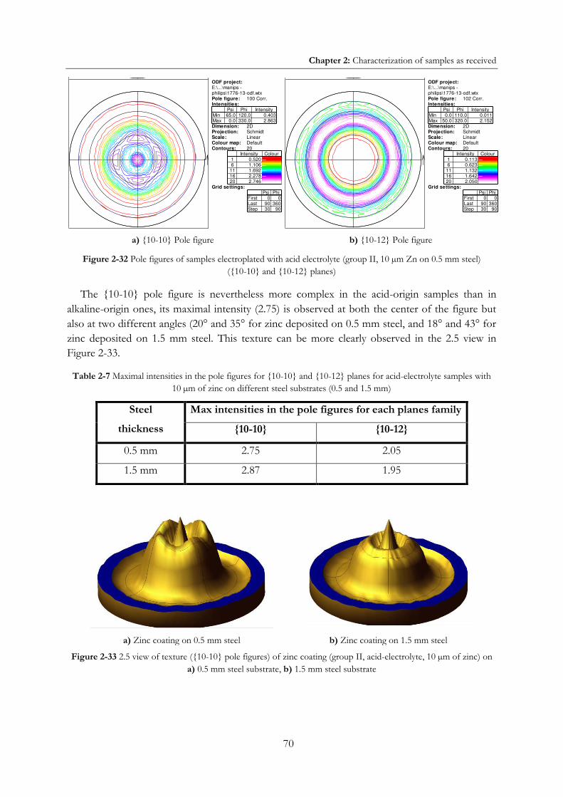
Chapter 2: Characterization of samples as received
70
a) {10-10} Pole figure b) {10-12} Pole figure
Figure 2-32 Pole figures of samples electroplated with acid electrolyte (group II, 10 µm Zn on 0.5 mm steel) ({10-10} and {10-12} planes)
The {10-10} pole figure is nevertheless more complex in the acid-origin samples than in alkaline-origin ones, its maximal intensity (2.75) is observed at both the center of the figure but also at two different angles (20° and 35° for zinc deposited on 0.5 mm steel, and 18° and 43° for zinc deposited on 1.5 mm steel. This texture can be more clearly observed in the 2.5 view in Figure 2-33.
Table 2-7 Maximal intensities in the pole figures for {10-10} and {10-12} planes for acid-electrolyte samples with 10 µm of zinc on different steel substrates (0.5 and 1.5 mm)
Steel
thickness
Max intensities in the pole figures for each planes family
{10-10} {10-12}
0.5 mm 2.75 2.05
1.5 mm 2.87 1.95
a) Zinc coating on 0.5 mm steel b) Zinc coating on 1.5 mm steel
Figure 2-33 2.5 view of texture ({10-10} pole figures) of zinc coating (group II, acid-electrolyte, 10 µm of zinc) on a) 0.5 mm steel substrate, b) 1.5 mm steel substrate
ODF project:E:\...\manips - philips\1776-13-odf.wtxPole figure: 100 Corr.Intensities:
Psi Phi IntensityMin 65.0 120.0 0.403Max 0.0 330.0 2.863Dimension: 2DProjection: SchmidtScale: LinearColour map: DefaultContours: 20
Intensity Colour 1 0.520 6 1.106 11 1.692 16 2.278 20 2.746
Grid settings:Psi Phi
First 0 0Last 90 360Step 30 90
ODF project:E:\...\manips - philips\1776-13-odf.wtxPole figure: 102 Corr.Intensities:
Psi Phi IntensityMin 0.0 110.0 0.011Max 50.0 320.0 2.152Dimension: 2DProjection: SchmidtScale: LinearColour map: DefaultContours: 20
Intensity Colour 1 0.113 6 0.623 11 1.132 16 1.642 20 2.050
Grid settings:Psi Phi
First 0 0Last 90 360Step 30 90

Chapter 2: Characterization of samples as received
71
Acid-origin electroplates have therefore a more complex texture:
A fiber component {10-10} represented by the central spot in the {10-10} pole figure; this texture component induces two additional rings in {10-12} pole figures at 43° and 68.6°.
A fiber component {11-20}; represented in Figure 2-32 by the ring at 30° in the {10-10} pole figure, and the ring at 50.7° angle in {10-12} pole figure.
The superposition in the {10-12} pole figure of the three rings at 43°, 50.7° and 68.6° is observed in single ring in each of the pole figures, much larger than those rings observed in the alkaline-origin samples.
The sheet plates have textures which are characteristic of rolling surfaces. The grain size of the thinnest steel (0.5 mm) is smaller than the other two sheets. The intermediate steel sheet (1.0 mm) however has grain size larger than the thickest sheet (1.5 mm). Same results observed in the microstructure photos of steel substrate (§1.1.2).
Concerning electroplates, they have a fiber texture. Zinc coating thickness has an influence in the electroplate texture; electroplates from acid bath present more complex texture than the alkaline samples.
2.3.6 Residual stress
According to the literature, compressive residual stress in the zinc coatings favors the whiskers growth rate [13] [29] and decreases incubation time [20]. Residual stress of both steel and electroplated samples was therefore measured by X-ray diffraction as preliminary characterization before further experiments for both industrial-origin samples and specifically processed samples. The influence of samples location on residual stress was studied. As a convention, positive values of residual stress are compressive and negative values are tensile.
2.3.6.1 Residual stress of steel
Figure 2-34 shows the residual stress of steel samples with three different thicknesses: 0.5, 1 and 1.5 mm. All samples, no matter the thickness, are almost stress-free. Consequently, residual stress to be measured in the electroplated samples result only from electroplating process. It is remarkable the large confidence intervals of the measured stress.

Chapter 2: Characterization of samples as received
72
Figure 2-34 Compressive residual stress of steel at both longitudinal and transversal axes
2.3.6.2 Residual stress of electroplated samples
2.3.6.2.1 Residual stress of samples from industrial site (group I)
Figure 2-35 shows residual stress of samples A, B and C at both the longitudinal axis (longest one) and the transversal axis (shortest one). Axis of measurement does not influence considerably the measured stress for all three samples.
The residual compressive stress in the sample B is higher than in sample A while sample C is almost free of residual stress. Literature reports that residual compressive stress of at least 45 MPa (stress threshold at 20°C) is required for the growth of whiskers [29] [46]; this condition is reached by both samples A and B, but not by sample C, i.e., only samples A and B would be prone to whiskers growth.
Figure 2-35 Compressive residual stress of industrial samples (group I) at longitudinal and transversal axes
-50-40-30-20-10
01020304050
0 0,5 1 1,5
Com
pres
sive
str
ess
[MP
a]
Steel thickness [mm]
Longitudinalaxis
Transversalaxis
-20
0
20
40
60
80
100
120
Com
pres
sive
str
ess
[MP
a]
Sample A Sample B Sample C
Longitudinal axis
Transversal axis

Chapter 2: Characterization of samples as received
73
2.3.6.2.2 Residual stress of specifically processed samples (group II)
As explained above (§2.2.1) and seen in Figure 2-36, specifically processed samples were cut in rectangles (2 cm x 1 cm) from larger sheets (10 cm x 10 cm) as. It is important to determine if residual stress is influenced by samples location with respect to the original sheet.
Figure 2-36 Labeling system for samples cut from the 10 cm x 10 cm sheet
Figure 2-37 shows that the location of samples in the original sheet does not influence the measured residual stress no matter the used electroplating electrolyte bath or the substrate thickness. Residual stress is found independent of steel thickness.
It is also seen that the electroplating electrolyte has a very strong influence on residual stress; compressive residual stress of samples electroplated with alkaline electrolyte is twice as large as stress of samples electroplated with acid electrolyte. Therefore, alkaline electrolyte would favor the compressive residual stress and consequently, samples electroplated with alkaline electrolyte would be more prone to whiskers growth than samples electroplated with acid electrolyte.
Residual stress was also measured for all the other specifically processed samples (fifteen different samples), and the results are shown in Figure 2-38. Residual stress is not influenced by the presence of chrome in the samples electroplated with alkaline electrolyte.
Concerning the zinc electroplate thickness in the alkaline samples, it does not seem to influence the residual stress, as observed by Sugiarto et.al. [17] for coatings thicker than 5 µm.
Residual-stress threshold proposed by Lindborg (at least 40 MPa), required for the growth of whiskers at 20°C [29] [46]) is only reached by alkaline-electrolyte samples.

Chapter 2: Characterization of samples as received
74
a) 0.5 mm steel substrate, influence of electroplating electrolyte b) Alkaline electroplating electrolyte, influence of steel substrate thickness
a) 0.5 mm steel substrate, influence of electroplating electrolyte b) Alkaline electroplating electrolyte, influence of steel substrate thickness
c) 1.5 mm steel substrate, influence of electroplating electrolyte d) Acid electroplating electrolyte, influence of steel substrate thickness
Figure 2-37 Influence of sample location, steel substrate thickness and electroplating electrolyte in residual stress (10 µm zinc coating, group II)
0
20
40
60
80
100
120
140
0 1 2 3 4 5 6 7 8 9 10
Com
pres
sive
str
ess
[MP
a]
Sample location
Alkaline electrolyte
Acid electrolyte
0
20
40
60
80
100
120
140
0 1 2 3 4 5 6 7 8 9 10
Com
pres
sive
str
ess
[MP
a]
Sample location
0.5 mm steel
1.5 mm steel
0
20
40
60
80
100
120
140
0 1 2 3 4 5 6 7 8 9 10
Com
pres
sive
str
ess
[MP
a]
Sample location
Alkaline electrolyte
Acid electrolyte
0
20
40
60
80
100
120
140
0 1 2 3 4 5 6 7 8 9 10
Com
pres
sive
str
ess
[MP
a]
Sample location
0.5 mm steel
1.5 mm steel

Chapter 2: Characterization of samples as received
75
a) Alkaline electroplating electrolyte; influence of sample size, zinc coating thickness and steel substrate thickness
b) 10 µm zinc coating; influence of sample size, chrome, electroplating electrolyte and steel substrate thickness
Figure 2-38 Influence of sample size, chrome, electroplating electrolyte, zinc coating thickness and steel substrate thickness (group II)
9 mm² samples (3 mm x 3 mm), prepared for SEM storage, were found to have larger residual stress than larger 200 mm² samples (2 cm x 1 cm), prepared for storage in environmental chambers. Figure 2-39 shows a significant growth in the surface close to the border of a 9 mm² sample before SEM storage; this growth may be a consequence of the applied stress during wire saw cutting.
Figure 2-39 Zinc growth observed in the surface close to the border of a 9 mm² sample before SEM storage (group II, acid-electrolyte sample, 10 µm Zn on 1.5 mm steel), SEM image
0
20
40
60
80
100
120
140
0 0,5 1 1,5
Com
pres
sive
str
ess
[MP
a]
Steel substrate thickness [mm]
5 µm Zn (sample 9 mm²)
5 µm Zn (sample 200 mm²)
10 µm Zn (sample 9 mm²)
10 µm Zn (sample 200 mm²)
15 µm Zn (sample 9 mm²)
15 µm Zn (sample 200 mm²)
0
20
40
60
80
100
120
140
0 0,5 1 1,5
Com
pres
sive
str
ess
[MP
a]
Steel substrate thickness [mm]
Alk.,non-chromed (sample 9 mm²)
Alk.,non-chromed (sample 200mm²)Alk.,chromed (sample 9 mm²)
Alk.,chromed (sample 200 mm²)
Acid,chromed (sample 9 mm²)
Acid,chromed (sample 200 mm²)

Chapter 2: Characterization of samples as received
76
Steel substrate is stress-free; therefore the residual stress of electroplated samples results only from electroplating process.
Residual stress is independent of axis measurement, location of sample in the sheet, zinc coating thickness, steel thickness and chrome.
Only electroplating electrolyte seems to influence the residual stress (alkaline samples have more residual compressive stress than acid samples).
2.3.7 SEM observation of electroplated samples as received
Both samples from industrial site and specifically processed were preliminarily observed in SEM microscopy before the storage.
2.3.7.1 SEM observation of samples from industrial site (group I) as received
Each of the three samples of the first group of materials, from industrial site, has a different and particular surface, as seen from Figure 2-40 to Figure 2-42; no whiskers were observed in any of the three samples before storage in environmental chambers.
Figure 2-40 is a SEM image of the surface of sample A, which has a very flat and regular surface, although it has some scratches. A particularly of this plate, when compared with the others, is the presence of significant growth of zinc on the indentation marks. This growth happened during the approximately three weeks between the indentation and the actual preliminary observation.
50 µm
100 µm
a) b)
Figure 2-40 Surface of sample A (group I) before storage: a) scratches, b) zinc growth in indentation mark, SEM images
Concerning the plate B, Figure 2-41 shows different features of plate B, presenting a surface relatively flat with some undulations. Interestingly, the chrome layer is cracked, producing isolated areas of few micrometers length; this cracking could be consequence of the drying of the material when it is manufactured. Besides, there are many surface defects as scratches, holes, and

Chapter 2: Characterization of samples as received
77
hills (much more than in samples A and C). It is not clear, from the SEM images, if the hill grows after of before the cracking of the chrome layer.
50 µm
10 µm
10 µm
a) b) c)
100 µm
100 µm
d) e)
Figure 2-41 Surface of sample B (group I) before storage: a) b) surface cracking, c) hill on the cracked surface, d) undulated surface and e) scratches; SEM images
The surface of plate C presents many small bumps on a much more undulated surface (Figure 2-42), probably as a consequence of drying after the plate is manufactured; bumps certainly increase the surface of the plate, which potentially could favour the stress release.
100 µm
Figure 2-42 Surface of sample C (group I) before storage: bumps and undulations; SEM image

Chapter 2: Characterization of samples as received
78
2.3.7.2 SEM preliminary observation of specifically processed samples (group II) as received
Specifically processed samples were also observed with SEM in order to study how the surface is influenced by different parameters of the samples: zinc electroplates thickness, steel substrate thickness, electroplating electrolyte and chrome. This observation was not done immediately after the electroplating of the samples but nine months later. During this elapsed time, some material grew from the surface of some of the samples. Some whiskers were observed in some samples although in very low quantity (whiskers density lower to 1.5 whiskers/mm²). The contrast between chromium and zinc (dark and light respectively in the SEM images) is used for observation of zinc growth out of the chrome.
2.3.7.2.1 Alkaline-electrolyte samples
SEM images of the surface as received of the samples electroplated with alkaline electrolyte are shown for different zinc coating thicknesses (5 to 15 µm) in Figure 2-43.
200 µm
200 µm
a) 5 µm zinc b) 10 µm zinc
Figure 2-43 Surface of alkaline-electrolyte samples (group II) before storage; 1.0 mm steel substrate with different zinc coating thicknesses: a) 5 µm and b) 10 µm; SEM images
Zinc growth seems to be influenced by:
Zinc thickness: more observed growth in the thickest zinc coating (10 µm) than in the thinnest one (5 µm Zn), as seen in Figure 2-43
Steel substrate thickness: more observed growth in the electroplated with the thinnest steel substrate (0.5 mm) than that one with the thickest substrate (1.5 mm).
Few whiskers were already observed in alkaline-origin samples before storage; these whiskers grew during the nine months passed between the electroplating of samples and the actual observation, all of them with length inferior to 100 µm. Some of these whiskers are illustrated in Figure 2-44.

Chapter 2: Characterization of samples as received
79
50 µm
20 µm
50 µm
a) 0.5 mm steel b) 1 mm steel b) 1.5 mm steel
Figure 2-44 Whiskers observed in alkaline-electrolyte samples (group II) before storage (10 µm Zn), different steel substrate thicknesses: a) 0.5 mm, b) 1 mm and c) 1.0 mm; SEM images
Significant growth of zinc, including whiskers, was detected in the indentation marks done during sample preparation (Figure 2-45). These sites became particularly prone to material growth probably due to stress applied when indenting which also breaks the chrome.
50 µm
20 µm
a) 5 µm zinc b) 15 µm zinc
Figure 2-45 Zinc growth observed in alkaline-electrolyte samples (group II) before storage (1 mm steel), different zinc coating thicknesses: a) 5 µm and b) 15 µm; SEM images
Concerning the influence of chrome in the surface, Figure 2-46 compares the surface of alkaline-electrolyte samples (10 µm Zn on 1.0 mm steel substrate) with and without chrome layer. Due to the absence of chromium, in the case of the non-chromed samples, the contrast between elements (zinc and chromium) cannot be used and the observation of zinc growth becomes more difficult. Nevertheless, despite the lack of contrast in SEM, some whiskers were detected for non-chromed samples, as seen in Figure 2-47.

Chapter 2: Characterization of samples as received
80
200 µm
200 µm
a) Chromed b) Non-chromed
Figure 2-46 Alkaline-electrolyte samples (group II), with and without chrome, before storage (10 µm Zn on 1 mm steel substrate): a) chromed and b) non-chromed; SEM images
50 µm
10 µm
Figure 2-47 Whisker in an non-chromed alkaline-origin sample (group II) before storage (10 µm Zn on 1.0 mm steel); SEM image
2.3.7.2.2 Acid-electrolyte samples
Figure 2-48 is a SEM image of the surface as received of the samples electroplated with acid electrolyte (10 µm Zn) on different steel substrate thicknesses (0.5 to 1.5 mm). There is no clear difference between the samples at different steel substrate thicknesses.
200 µm
200 µm
a) 0.5 mm steel b) 1.5 mm steel
Figure 2-48 Surface of acid-electrolyte samples (group II) before storage; 10 µm Zn on different steel substrate thicknesses: a) 0.5 mm and b) 1.5 mm; SEM images

Chapter 2: Characterization of samples as received
81
Unlike alkaline samples, zinc growth (including the growth of whiskers) is not regular through the surface but concentrated on irregularities such scratches, as observed in Figure 2-49; these whiskers developed slightly longer than in alkaline-origin samples, reaching up to 140 µm in length.
50 µm
10 µm
Figure 2-49 Whiskers and other features in acid-electrolyte samples (group II) before storage (10 µm Zn on 0.5 mm steel substrate), SEM images

Chapter 2: Storage of samples
82
2.4 STORAGE OF SAMPLES
In order to study the kinetics of whiskers growth and the influence of different parameters, storage experiments were done for both groups of samples: from industrial site (group I) and specifically processed samples (group II). The preparation of samples for this experiment is already described in §2.2.1.
2.4.1 Storage and observation conditions
Three different experiments were done in environmental chambers (20 mm x 10 mm samples) and in SEM microscope (3 mm x 3 mm samples):
Samples from industrial site (group I) at 30°C and 60°C at 60% relative humidity in environmental chamber for 7000 hours (42 weeks)
Specifically processed samples (group II) at 60°C at 60% relative humidity in environmental chamber during for 2000 hours (12 weeks)
Specifically processed samples (group II) at 150°C, 175°C and 200°C, in vacuum in SEM microscope for approximately one hour
2.4.1.1 Storage in environmental chambers
Samples from industrial site (group I) and specifically processed samples (group II) were both stored in environmental chambers; Scanning Electron Microscopy (Quanta FEI in the Electron Microscopy Laboratory of EDF R&D, Figure 2-50) was used to observe an already defined 25 mm² zone in the samples in order to determine the presence of whiskers on the samples and to quantify them in terms of density, length and diameter.
Figure 2-50 Sample (marked with a blue arrow) in SEM (Quanta-FEI) microscope for observation during storage

Chapter 2: Storage of samples
83
In SEM images obtained at observation during storage in environmental chambers, the contrast between the chemical elements allows differentiating the zinc (bright on the images) and the chromium (dark in the images). The light zones therefore correspond to growth of zinc from the surface as either whisker or hillocks.
JEDEC (Joint Electronic Device Engineering Council) [14] establishes experimental storage conditions of temperature and relative humidity for study of tin whiskers; these conditions were followed in the experiments developed by MMC department of EDF R&D in 2010 [56]: 30°C with 60% relative humidity, and 60°C with 87% relative humidity. The study found considerable corrosion on the second set of conditions studied (higher humidity).
As temperature is thought to have a great influence on the growth of whiskers, and having to limit the set of conditions given the availability of environmental chambers, relative humidity was fixed at 60% (samples at 87% of humidity developed significant corrosion in former experiment [56]), while two different temperatures were tested (30 and 60°C).
As detailed in §2.2.1, the observation zone was fixed with a 5 mm square. In each observation of the samples, the zone was scanned acquiring SEM images with 20% overlap between images, as seen in Figure 2-51. The size of each image was 1270 x 1097 µm (4096 x 3775 pixels).
Figure 2-51 Schematic of acquisition of SEM images for storage in environmental chambers
2.4.1.1.1 Storage of samples from industrial site (group I) in environmental chambers
Two specimens of each of the samples from industrial site (samples A, B and C) were stored in environmental chambers. The samples were removed from the environmental chambers every two or three weeks for SEM observation, taking approximately 30 hours each stop. After the first 20 weeks of storage, the time lapses between observations were increased to 7-8 weeks since the whisker growth rate was considerably reduced. The observations time are shown in Table 2-8.
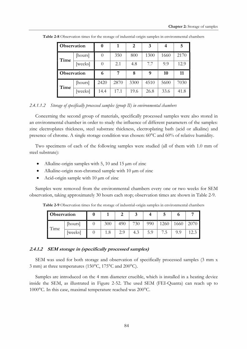
Chapter 2: Storage of samples
84
Table 2-8 Observation times for the storage of industrial-origin samples in environmental chambers
Observation 0 1 2 3 4 5
Time [hours] 0 350 800 1300 1660 2170
[weeks] 0 2.1 4.8 7.7 9.9 12.9
Observation 6 7 8 9 10 11
Time [hours] 2420 2870 3300 4510 5600 7030
[weeks] 14.4 17.1 19.6 26.8 33.6 41.8
2.4.1.1.2 Storage of specifically processed samples (group II) in environmental chambers
Concerning the second group of materials, specifically processed samples were also stored in an environmental chamber in order to study the influence of different parameters of the samples: zinc electroplates thickness, steel substrate thickness, electroplating bath (acid or alkaline) and presence of chrome. A single storage condition was chosen: 60°C and 60% of relative humidity.
Two specimens of each of the following samples were studied (all of them with 1.0 mm of steel substrate):
Alkaline-origin samples with 5, 10 and 15 µm of zinc
Alkaline-origin non-chromed sample with 10 µm of zinc
Acid-origin sample with 10 µm of zinc
Samples were removed from the environmental chambers every one or two weeks for SEM observation, taking approximately 30 hours each stop; observation times are shown in Table 2-9.
Table 2-9 Observation times for the storage of industrial-origin samples in environmental chambers
Observation 0 1 2 3 4 5 6 7
Time [hours] 0 300 490 730 990 1260 1660 2070
[weeks] 0 1.8 2.9 4.3 5.9 7.5 9.9 12.3
2.4.1.2 SEM storage in (specifically processed samples)
SEM was used for both storage and observation of specifically processed samples (3 mm x 3 mm) at three temperatures (150°C, 175°C and 200°C).
Samples are introduced on the 4 mm diameter crucible, which is installed in a heating device inside the SEM, as illustrated in Figure 2-52. The used SEM (FEI-Quanta) can reach up to 1000°C. In this case, maximal temperature reached was 200°C.

Chapter 2: Storage of samples
85
Figure 2-52 Crucible and heating device inside the SEM
As seen in Figure 2-53, a single image of a fixed zone of 0.5 mm x 0.43 mm (2048 x 1887 pixels), corresponding to 0.215 mm², was taken at each observation every two minutes approximately.
Figure 2-53 Schematic of acquisition of SEM images for storage in environmental SEM
Eight samples were analyzed in order to study the influence of temperature, zinc electroplate thickness, steel substrate thickness, chrome and electroplating electrolyte, as seen in Table 2-10. All samples were tested at the three temperatures unless otherwise indicated (with an asterisk in the table).
Table 2-10 Samples stored in environmental SEM (marked with X)
Electroplating electrolyte Zinc
thickness
Steel substrate thickness
0.5 mm 1.0 mm 1.5 mm
Alkaline 5 µm X*
10 µm X*
15 µm X* X** X*
Alkaline non-chromed 10 µm X*
Acid 10 µm X* X*
*tested only at 150°C and 200°C **tested only at 200°C

Chapter 2: Storage of samples
86
2.4.2 Quantitative analysis of whiskers and related features
The goal is to characterize quantitatively (in terms of density and growth) two features: whiskers and hillocks, defined later in §3.1.1 and illustrated in Figure 2-54.
Figure 2-54 Schematic of whisker and hillock
2.4.2.1 Data acquisition
In the SEM observation during storage of samples, the following data are obtained at each time observation: whiskers density total whiskers length in a 1 mm² surface hillocks density total hillocks surface in a 1 mm² surface
2.4.2.1.1 Hillocks
Image-J, a public Java-based image processing program, was used for SEM images processing; Figure 2-55 compares the images before and after treatment.
First, background illumination correction is applied to SEM images. Second, images (originally 8-bits grey-scale) are binarized, that is, they are converted into binary images (1 bit) where pixels are either black or white; black corresponds to chromium, and white to zinc. It is necessary to have a binary image in order to apply further image operations.
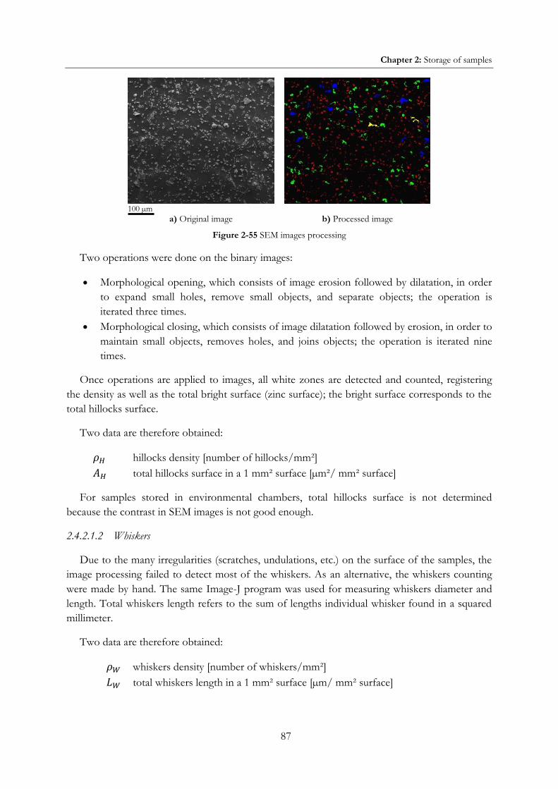
Chapter 2: Storage of samples
87
Figure 2-55 SEM images processing
Two operations were done on the binary images:
Morphological opening, which consists of image erosion followed by dilatation, in order to expand small holes, remove small objects, and separate objects; the operation is iterated three times.
Morphological closing, which consists of image dilatation followed by erosion, in order to maintain small objects, removes holes, and joins objects; the operation is iterated nine times.
Once operations are applied to images, all white zones are detected and counted, registering the density as well as the total bright surface (zinc surface); the bright surface corresponds to the total hillocks surface.
Two data are therefore obtained: hillocks density [number of hillocks/mm²] total hillocks surface in a 1 mm² surface [µm²/ mm² surface]
For samples stored in environmental chambers, total hillocks surface is not determined because the contrast in SEM images is not good enough.
2.4.2.1.2 Whiskers
Due to the many irregularities (scratches, undulations, etc.) on the surface of the samples, the image processing failed to detect most of the whiskers. As an alternative, the whiskers counting were made by hand. The same Image-J program was used for measuring whiskers diameter and length. Total whiskers length refers to the sum of lengths individual whisker found in a squared millimeter.
Two data are therefore obtained: whiskers density [number of whiskers/mm²] total whiskers length in a 1 mm² surface [µm/ mm² surface]
100 µm
a) Original image b) Processed image

Chapter 2: Storage of samples
88
For samples from industrial site (group I), diameter and length of each whisker were measured; for specifically processed samples (group II), length and diameter were measured only for three of the longest observed whiskers:
h length of a single whisker [µm] diameter of a single whisker [µm]
2.4.2.2 Data treatment
The acquired data are treated in order to calculate the following parameters as function of time: whiskers growth [µm³/ mm² surface] hillocks growth [µm³/ mm² surface] total growth (whiskers and hillocks combined) [µm³/ mm² surface]
2.4.2.2.1 Whiskers growth
Whiskers growth corresponds to the volumetric growth of whiskers in a squared millimeter surface. According to literature [26], most of whiskers are inclined from 30° to 60° to the surface (§1.3.1.7), therefore, it is assumed an average of 45°C inclination; consequently whisker length has to be corrected by a √2 factor (Figure 2-54). Whiskers are assumed to be cylindrical, as seen in, and their volume can be calculated from their diameter and length:
Equation 2-4 √
where: volume of a single whisker [µm³] diameter of a single whisker [µm] length of a single whisker [µm]
Adding volumes of all whiskers, the total volume of whiskers is given by the equation:
Equation 2-5 ∑
Replacing Equation 2-4 in Equation 2-5:
Equation 2-6 √ ∑
For samples from industrial site (group I), Equation 2-5 can be applied directly since diameter and length of whiskers are known; in the case of specifically processed samples (group II), diameter of whiskers is averaged based on experimental observations.
Equation 2-7 √ ∑
where: average whiskers diameter
Defining total whiskers length as the sum of lengths of all whiskers:

Chapter 2: Storage of samples
89
Equation 2-8 ∑
where: total whiskers length in a 1 mm² surface
Replacing Equation 2-8 in Equation 2-7:
Equation 2-9 √
It was found that most of the whiskers observed in the specifically processed samples (group II) have approximately 1 µm diameter, therefore this value is taken for the average whisker diameter. From Equation 2-9 whiskers growth ( )can be calculated from total whiskers length
( ).
2.4.2.2.2 Hillocks growth
Hillocks growth corresponds to the volumetric growth of hillocks in a squared millimeter surface; they have more complicated geometry than whiskers due to their branch-like shape. In order to simplify, hillocks shape are assumed to be half-spherical (Figure 2-54). The projected area of each hillock is calculated from dividing the total hillocks surface over hillocks density:
Equation 2-10
where: projected surface of a single hillock [µm²] total hillocks projected surface in a 1 mm² surface [µm²/ mm² surface] hillocks density [number of hillocks/mm²]
Volume of each half-sphere hillock volume is calculated from its projected area1:
Equation 2-11
where: volume of a single hillock [µm³]
Hillocks growth is defined as the sum of all hillocks volumes, and it is calculated by multiplying the hillock volume times the number of hillocks in a squared millimeter surface (hillocks density):
Equation 2-12
Replacing Equation 2-11 in Equation 2-12:
Equation 2-13
Replacing Equation 2-10 in Equation 2-13:
1 Area of a circumference A=π r², from here r= (A/π)0.5
Volume of half a sphere V=2/3 π r³. Replacing r by A: V=2/3 π-0.5 A1.5

Chapter 2: Storage of samples
90
Equation 2-14 √
From Equation 2-14 hillocks growth ( ) can be calculated from total hillocks projected area
( ) and hillocks density ( ).
2.4.2.2.3 Total growth
Finally, the total growth is calculated by adding the two components of growth: whiskers growth and hillocks growth:
Equation 2-15
Since total hillocks projected area is not determined in samples stored in environmental chambers, the value is then replaced by an average obtained for the same sample in SEM storage. The whole discussed protocol for data acquisition and analysis is summarized and illustrated in Figure 2-56.
Figure 2-56 Schematic of data acquisition and analysis

Chapter 2: Summary
91
2.5 SUMMARY OF MATERIALS AND EXPERIMENTAL METHODS
Investigated material was described, including the samples from the industrial site and the specifically processed (groups I and II respectively.
Processing conditions of samples from group I are unknown. Samples from group II were processed in order to study the influencing parameters (steel substrate and zinc coating thicknesses, chrome and electroplating electrolyte).
The material was characterized as received; main observations found are:
Iron grains size in the steel substrate is influenced by the steel substrate thickness.
The grains of the zinc coating have a fiber texture, which is influenced not only by the zinc coating thickness but also by the electroplating electrolyte.
Traces of chemical elements in the zinc coating are a footprint of the electrolyte used for electroplating. Samples from industrial site have a typical chemical profile of samples electroplated with alkaline electrolyte.
Residual stress of electroplated samples results only from electroplating process (steel is free of stress before electroplating). The residual stress is independent of axis measurement, location of sample in the sheet, zinc coating thickness, steel thickness and chrome. Only electroplating electrolyte seems to influence the residual stress
Finally, storage experiments in both environmental chambers and SEM were described as well as the SEM images acquisition and the protocol for quantitative analysis of whiskers and related features.

92
93
Chapter 3. Effect of aging treatments
Chapter 3
Effect of ageing treatments
The third chapter details the experimental results concerning the effect of ageing treatments; it
starts with some key definitions and phenomenological concepts.
In order to have an observation at global scale, the aged material is observed with Electron
microscopy. Afterwards, results of kinetics of growth as well of residual stress measurements
during material ageing are addressed.
The local scale of the phenomenon is discussed including both observations of the
microstructure of the samples and chemical analysis results.
Morphology observations SEM observation of stored samples Kinetics of growth Residual stress Microstructure of zinc coating and whiskers Chemical analysis of zinc coating and whiskers Summary of effect of aging treatments

Chapter 3: Morphology observations
94
3.1 MORPHOLOGY OBSERVATIONS
Key definitions and phenomenological concepts of the whiskers growth are given, followed by a description of the morphological characteristics of whiskers.
3.1.1 Definition of terms
At first, it is necessary to give some definitions concerning the different features involved in the whiskers growth phenomenon. Figure 3-2 schematizes the phenomenon of whisker growth from zinc electroplated steel covered with a chrome layer.
When certain time is elapsed after the electroplating of the steel, the zinc coating under the chrome layer starts pushing up the chrome at some locations, giving origin to elevations of the chrome layer, these protuberances will be called bumps. These bumps are still covered by the chrome without zinc being exposed.
If zinc continues pushing up the chrome, eventually the chrome layer may break; the zinc would then come out to the surface, producing branch-like zinc formations; these zinc features will be called hillocks. Hillocks can have very different shapes and dimensions, as they continue growing. Figure 3-1 shows SEM (Scanning Electron Microscopy) images of the time-evolution of a hillock during storage at 60°C, it can be observed a bump of few micrometers which is broken by the zinc that pushes up; after coming up, the hillock continues growing up.
20 µm 20 µm 20 µm
a) 1300 hours b) 1700 hours c) 2300 hours
Figure 3-1 Growing hillock; SEM images of sample B (group I) stored at 60°C at a) 1300 hours, b) 1700 hours and c) 2300 hours
Whiskers are filament-like zinc formations growing from the zinc electroplate; they can grow from the flat surface, from a bump or from a hillock. Figure 3-3 shows the growth of a whisker from a small hillock developed from a bump.
The ratio length-diameter of whiskers can have a broad range; for this research, only features with length at least five times the diameter will be considered as whiskers.

Chapter 3: Morphology observations
95
Figure 3-2 Schematic of the whisker growth phenomenon

Chapter 3: Morphology observations
96
Both hillocks and whiskers, where zinc is exposed, are identified in SEM images thanks to the contrast between zinc and chrome (bright in SEM images), as seen in the Figure 3-4 (surface of alkaline-sample from group II, 15 µm Zn on 0.5 mm steel, after one hour of storage at 150°C).
200 µm 5 µm
Figure 3-3 Growing whisker from a hillock; SEM image of a whisker in sample B (group I) after 300-hours storage at 60°C (higher magnification on the right image)
100 µm
Figure 3-4 Hillocks and whiskers at the surface; SEM image of alkaline-origin sample from group II (15 µm Zn on 0.5 mm steel) after one hour of storage at 150°C
3.1.2 Whiskers characteristics
As it was shown in Table 1-1, dimensions of zinc whiskers can vary from 0.5 to 10 µm of diameter [1] [9] [12] [13], with length up to 3 cm [17]. In this research, whiskers diameter was found between 0.5 and 4 µm (most of them around 1 µm), with length up to 1 mm.
The angle between the whiskers and the surface can also vary significantly, from 0° (parallel to the coating surface) to 90° (perpendicular to the coating surface), although most typical angles are between 30° and 60°; these angles are actually related with the growth axis of the whisker [26].
Whiskers are not only straight filaments (Figure 3-5-a) but they can also have different shapes, as seen in the same figure. Whiskers can be kinked at different angles and several times; this

Chapter 3: Morphology observations
97
phenomenon is typical of crystal growth where the presence of defects impedes the straight growth (figures b to-e). Several whiskers can grow from the same site, as shown in Figure 3-5-f where two whiskers grow from the same hillock. Figure 3-6 shows in detail direction changes of a whisker.
200 µm 40 µm 100 µm
a) Straight whisker (60°C) b) Kinked whisker (30°C) c) Kinked whisker (60°C)
100 µm 40 µm 40 µm
d) Looped whisker (60°C) e) Looped whisker (30°C) f) Two whiskers from same site (60°C)
Figure 3-5 Different shapes of whiskers; SEM images of different whiskers in sample B (group I) after 1300 hours of storage at 30°C and 60°C
50 µm 10 µm 4µm
Figure 3-6 A kinked whisker; SEM images at different magnifications of a whisker in sample B (group I) after 300 hours of storage at 60°C

Chapter 3: Morphology observations
98
The tip of the whisker can also have different forms; since the whisker grows from the base of the whisker rather than from the tip, the tip remains constant as footprint of the hillock where it comes from. Figure 3-7 shows not only kinked tips but also looped tips of whiskers.
5 µm 10 µm 5 µm
Figure 3-7 Different shapes of whisker tips; SEM images of different whiskers in sample B (group I) after 300 hours of storage at 60°C
As illustrated in Figure 3-8, zinc whiskers have striations, not only the commonly reported longitudinal striations but also regularly-space circumferential striations; both sorts of striations have been observed in tin whiskers.
2 µm
a) Circumferential striations
2 µm
b) Longitudinal striations
Figure 3-8 Striations in a whisker: a) circumferential and b) longitudinal; SEM images of alkalyne-origin sample from group II (15 µm Zn on 1 mm steel) after 1260 hours of storage at 60°C
Figure 3-9 and Figure 3-10 illustrate examples of longitudinal striations. While Figure 3-9 shows how the longitudinal striations remain even after changes of whisker direction, Figure 3-10 illustrates the striations at the base of the whisker.

Chapter 3: Morphology observations
99
50 µm 5 µm
Figure 3-9 Longitudinal striations in a whisker; SEM images at different magnifications of a whisker in alkalyne-origin sample from group II (10 µm Zn on 1 mm steel) after one-year storage at room conditions
50 µm 5 µm
Figure 3-10 Longitudinal striations in a whisker; SEM images at different magnifications of a whisker in acid-origin sample from group II (10 µm Zn on 1 mm steel) after 1000 hours at room conditions
Figure 3-11 and Figure 3-12 show different details of periodical and circumferential striations; typical width of these observed striations is between 80 to 100 nm.

Chapter 3: Morphology observations
100
50 µm 2 µm 1 µm
Figure 3-11 Circumferential and periodical striations in a whisker; SEM images at different magnifications of a whisker in sample B (group I) after 7000-hours storage at 60°C
50 µm 2 µm
Figure 3-12 Circumferential striations in a whisker; SEM images at different magnifications of a whisker in alkalyne-origin sample from group II (10 µm Zn on 0.5 mm steel) after one-year storage at room conditions
Figure 3-13 shows also the striations as well as the steps on the whisker. In Figure 3-14, although corroded, it is visible the hexagonal shape of the cross-section of the whisker.

Chapter 3: Morphology observations
101
50 µm 10 µm 4µm
Figure 3-13 Direction changes and steps in a whisker; SEM images at different magnifications of a whisker in acid-origin sample from group II (10 µm Zn on 1 mm steel) after 1000 hours at room conditions
50 µm 5 µm
Figure 3-14 Hexagonal cross section of a whisker; SEM images at different magnifications of a whisker observed in acid-origin sample from group II (10 µm Zn on 1 mm steel) after 1260 hours at 60°C
The main terminology of whiskers growth features was defined: whiskers, hillocks and bumps.
Among the main characteristics of whiskers are:
Diameter: 0.5 to 4 µm Length: up to 1 mm
All possible angles respect to the surface coating (mainly from 30 to 60°C) Presence of kinks and striations (both longitudinal and circumferential)
Whisker grows from the base of the whisker rather than from the tip

Chapter 3: SEM observation of stored samples
102
3.2 SEM OBSERVATION OF STORED SAMPLES
SEM microscopy is used to follow the evolution of electroplated samples during and after storage at both environmental chambers and SEM. This observation allows a preliminary observation of the influence of several parameters on the whiskers growth.
While the hillocks and whiskers growth in samples from industrial site (group I) is not sufficient to be seen at low magnification SEM images, the growth in specifically processed samples (group II) can be clearly observed in SEM images. All samples are chromed unless otherwise indicated.
3.2.1 Storage of specifically processed samples (group II) in environmental chambers
Figure 3-15 compares the surface of samples electroplated with alkaline electrolyte before and after 2000 hours of storage at 60°C, for different zinc coating thicknesses.
Before storage After 2000 hours (12 weeks) at 60°C
5 µm Zn
15 µm Zn
200 µm 200 µm
Figure 3-15 Samples electroplated with alkaline electrolyte with different zinc coating thicknesses; SEM images of samples surface (1 mm steel, group II) before and after 2000-hours storage at 60°C

Chapter 3: SEM observation of stored samples
103
While there is no clear change during storage in the 5-µm-Zn sample, in the case of the 15-µm-Zn sample there is an evident growth of zinc features on the surface after the storage. The zinc coating thickness, as expected, favors the zinc growth.
Figure 3-16 shows the surface of alkaline-electrolyte samples without chromed. Due to the absence of zinc-chrome contrast, it is difficult to observe the different zinc features on the image. Nevertheless it is clear that there is a growth of material, probably corroded, after the 2000 hours of storage.
Before storage After 2000 hours (12 weeks) at 60°C
200 µm 200 µm
Figure 3-16 Non-chromed samples electroplated with alkaline electrolyte; SEM images of sample surface (1 mm steel, group II) before and after 2000-hours storage at 60°C
In Figure 3-17, it is observed that the growth in chromed samples electroplated with acid electrolyte is concentrated on the irregularities of the surface such as scratches (marked with a blue arrow), that is, the growth is not regular as observed in the alkaline-origin samples (§Figure 3-15). The electroplating electrolyte seems to influence not only the amount of growth but also its distribution on the surface.

Chapter 3: SEM observation of stored samples
104
Before storage After 2000 hours (12 weeks) at 60°C
200 µm 200 µm
Figure 3-17 Samples electroplated with acid electrolyte; SEM images of sample surface (1 mm steel, group II) before and after 2000-hours storage at 60°C
3.2.2 SEM storage of specifically processed samples (group II)
SEM images of the surface of specifically processed samples (group II) before and after one hour of SEM storage were taken in order to compare the different studied parameters. Samples electroplated with alkaline electrolyte (with and without chrome) and with acid electrolyte are compared in the SEM storage for different temperatures (from 150°C to 200°C) at vacuum.
3.2.2.1 Samples electroplated with alkaline electrolyte
Figure 3-18 shows the surface of alkaline-origin samples (group II) before and after one-hour SEM storage (15 µm Zn on 0.5 mm steel) for 150°C, 175°C and 200°C. The growth of zinc is significant in the sample, becoming more important as temperature increases. SEM images of the surfaces of samples with other zinc coating thicknesses (5 µm and 10 µm) and other steel substrate thickness (1.5 mm) are shown from Figure A2-1 to Figure A2-3 (Appendix 2).
Zinc growth is significantly favored by zinc coating thickness: during storage there is very little change of the surface of samples with the thinnest zinc coating (5 µm), or no change at all in the storage at 150°C. On the other hand, the most important growth is observed at 200°C in samples with the thickest coating of zinc (15 µm) no matter the steel substrate thickness.
Figure 3-19 shows the SEM images of the surface of non-chromed samples (10 µm Zn on 0.5 mm steel). There is clearly growth of zinc, particularly at 200°C; the absence of contrast, however, makes difficult the observation of the diverse features.

Chapter 3: SEM observation of stored samples
105
Before storage After one-hour storage
150°C
175°C
200°C
200 µm 200 µm
Figure 3-18 Samples electroplated with alkaline electrolyte stored at different temperatures; SEM images of samples surface (15 µm Zn on 0.5 mm steel) before and after one-hour SEM storage
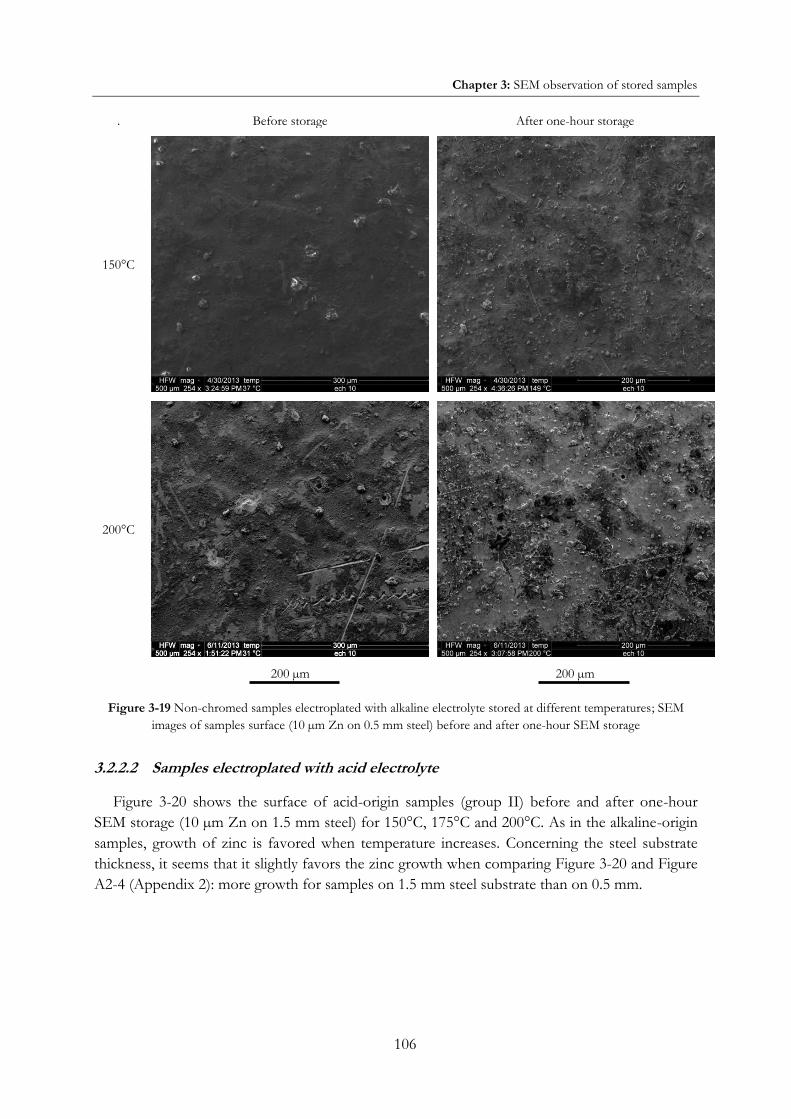
Chapter 3: SEM observation of stored samples
106
. Before storage After one-hour storage
150°C
200°C
200 µm 200 µm
Figure 3-19 Non-chromed samples electroplated with alkaline electrolyte stored at different temperatures; SEM images of samples surface (10 µm Zn on 0.5 mm steel) before and after one-hour SEM storage
3.2.2.2 Samples electroplated with acid electrolyte
Figure 3-20 shows the surface of acid-origin samples (group II) before and after one-hour SEM storage (10 µm Zn on 1.5 mm steel) for 150°C, 175°C and 200°C. As in the alkaline-origin samples, growth of zinc is favored when temperature increases. Concerning the steel substrate thickness, it seems that it slightly favors the zinc growth when comparing Figure 3-20 and Figure A2-4 (Appendix 2): more growth for samples on 1.5 mm steel substrate than on 0.5 mm.

Chapter 3: SEM observation of stored samples
107
. Before storage After one-hour storage
150°C
175°C
200°C
200 µm 200 µm
Figure 3-20 Samples electroplated with acid electrolyte stored at different temperatures; SEM images of samples surface (10 µm Zn on 1.5 mm steel) before and after one-hour SEM storage

Chapter 3: SEM observation of stored samples
108
3.2.3 Summary of influencing parameters on zinc growth
Table 3-1 summarizes the influencing parameters on the zinc growth (both whiskers and hillocks) in SEM observation.
Table 3-1 Summary of influencing parameters zinc growth in SEM observation
Studied
parameter Influence on zinc growth Comments
Temperature
Temperature favors growth
The influence is stronger in alkaline electrolytes
Zinc coating
thickness
Zn thickness favors growth
In alkaline electrolytes (not information for acid)
Steel substrate
thickness
(alkaline)
Steel thickness does not favors growth in alkaline-samples
(acid)
Steel thickness favors growth in acid-samples
Electroplating
electrolyte Uniform hillocks growth for alkaline, concentrated growth (surface irregularities) for acid
From SEM images, it is observed that zinc growth is favored not only by temperature but also by zinc coating.
Steel substrate seems to favor the growth in the case of acid-origin samples but to disfavor the growth in the case of alkaline-origin samples.
Growth in acid-origin samples is localized on some irregularities of the surface, while in alkaline-origin samples the growth is regularly distributed on the surface.

Chapter 3: Kinetics of growth
109
3.3 KINETICS OF GROWTH
As explained in the second chapter (§2.4.2), SEM images were taken in order to follow the evolution of the electroplated samples during and after storage at both environmental chambers and SEM, and to study the influence of temperature and samples parameters in the growth kinetics.
Three different experiments were carried out as follows:
Samples from industrial site (group I) at 30°C and 60°C at 60% relative humidity in environmental chamber for 7000 hours (42 weeks).
Specifically processed samples (group II) at 60°C at 60% relative humidity in environmental chamber during for 2000 hours (12 weeks).
Specifically processed samples (group II) at 150°C, 175°C and 200°C, in SEM microscope (in vacuum) for approximately one hour.
The obtained data are used in order to calculate the following parameters as function of time: hillocks density, whiskers density, whiskers growth and total growth.
3.3.1 Kinetics of samples from industrial site (group I)
The influence of the stored sample (A, B and C) and of temperature (30°C and 60°C) is studied in this section. No change was observed during storage on the surface of sample C at neither 30°C nor 60°C, therefore neither hillocks nor whiskers were observed.
On the other hand, samples A and B did experience a growth of material, at least hillocks, during storage at both temperatures. Concerning whiskers, while sample B grew whiskers at both temperatures, sample A displayed whiskers only at 60°C.
These results agree with the residual stress measured for these samples (larger residual stress in sample B than in sample A, while almost zero stress for sample C, §2.3.6.2.1). That is, compressive residual stress is required for whiskers and hillocks growth, and the more residual stress has the material, the more whiskers and hillocks it grows. This is not surprising since whiskers and hillocks growth is taught to be a stress relaxation phenomenon.
Figure 3-21 shows the kinetics of these industrial-origin samples during storage at 30°C and 60°C, including hillocks density, whiskers density and whiskers growth. The three curves have clearly two stages:
Growth stage: where the parameter (either density or whisker growth) increases with time until reaching a plateau. In the case of hillocks density curve, the slope is not constant but decreasing, having the maximal rate at the beginning of the growth. On the other hand, the whisker density and whisker growth curves seem to have approximately a constant slope in the growth stage, that is, a constant growth rate.
Saturation stage: once the plateau is reached (at saturation time) the growth phenomenon stops and the parameter (either density or whisker growth) remains constant.

Chapter 3: Kinetics of growth
110
It is observed that the mentioned saturation time (the time where the growth stops) is shorter for hillocks growth (hillocks density curve) than for whiskers growth (whiskers density and growth curves). That is, when the hillocks density stops increasing (no more new hillocks), whiskers continue growing for more time. The growth time is favored by temperature and it is larger in sample B than in sample A.
Figure 3-21 Growth kinetics of samples from industrial site (group I) stored at 30°C and 60°C: a) whiskers density ρW, b) hillocks density ρH and c) whiskers growth per mm² surface ΩW (no whiskers observed in sample A at 60°C)
0
0,2
0,4
0,6
0,8
1
1,2
0 1000 2000 3000 4000 5000 6000 7000
ρ W [whis
kers
/mm
²]
Time [h]
a) Whiskers density ρW
A 60°C
B 30°C
B 60°C
0
20
40
60
80
100
120
0 1000 2000 3000 4000 5000 6000 7000
ρ H [hilloc
ks/
mm
²]
Time [h]
b) Hillocks density ρH
A 30°C
A 60°C
B 30°C
B 60°C
0
50
100
150
200
250
300
350
400
0 1000 2000 3000 4000 5000 6000 7000
ΩW
[µm
³ /m
m²
surf
ace]
Time [h]
c) Whiskers growth per mm² surface ΩW
A 60°C
B 30°C
B 60°C

Chapter 3: Kinetics of growth
111
Figure 3-22 shows the influence of the sample and temperature in hillocks density, whiskers density, ratio whiskers-hillocks and maximal whiskers length. Influence of two parameters (sample and temperature) is clearly observed in the hillocks and to a major extent in the whiskers growth. Neither whiskers nor hillocks were observed in sample C at 30°C and 60°C.
Figure 3-22 Samples from industrial site (group I) after 3000 hours storage at 30°C and 60°C: a) hillocks density ρH,
b) whiskers density ρW, c) ratio whiskers-hillocks density ρW/ρH, d) maximal whisker length hmax, e) maximal growth rate h'max and f) saturation time for whiskers growth (whiskers or hillocks not observed in sample C)
0
20
40
60
80
100
120
Sample A Sample B
ρ H [hillock
s/ m
m²s
urfa
ce]
a) Hillocks density ρH
30°C 60°C
0
0,2
0,4
0,6
0,8
1
1,2
Sample A Sample B
ρ W [whis
kers
/ m
m²
surf
ace]
b) Whiskers density ρW
30°C 60°C
0
0,2
0,4
0,6
0,8
1
1,2
Sample A Sample B
ρ W/ρ H [%
]
c) Ratio ρW/ρH
30°C 60°C
0
100
200
300
400
500
600
Sample A Sample B
h max
[µm
]
d) Maximal whisker length hmax
30°C 60°C
0
2
4
6
8
0
0,1
0,2
Sample A Sample B
h'm
ax [m
m/y
r]
h'm
ax [n
m/s
]
e) Maximal growth rate h'max
30°C 60°C
0
10
20
30
40
50
Sample A Sample B
t ∞ [h
]
f) Saturation time t∞ (whiskers growth)
30°C 60°C

Chapter 3: Kinetics of growth
112
Temperature favors both hillocks and whiskers growth; while the increase from 30°C to 60°C of storage approximately doubles the hillocks density in samples A and B, it also multiplies by more than five the whiskers density in sample B. Concerning the sample A, whiskers growth is observed at 60°C but not at 30°C.
Temperatures also increase the maximal whiskers length in sample B (0.57 mm at 60°C and 0.22 mm at 30°C). These observed lengths are under the values reported in literature [13] (at least 5 mm §Table 1-1).
As far as samples is concerned, sample B is more prone not only to hillocks growth but specifically to whiskers growth (both density and growth). While hillocks growth in sample B is around twice as much as in sample A, whiskers growth in sample B is more than three times as much as in sample A. On the other hand, sample B has slightly longer whiskers than sample A.
In the same Figure 3-22, maximal whiskers growth rate and saturation time for whiskers growth are compared for both samples and temperatures. Sample B (the sample with higher initial residual stress) has faster growth rates and longer whiskers growth saturation time than sample A.
It is observed that the saturation time rises considerably when increasing temperature (13 min at 30°C, between 41 and 48 minutes at 60°C). Whiskers growth rate is also favored by temperature although not significantly: 5.3 mm/year at 30°C and 6.9 mm/year at 60°C for sample B (same order of values found by Lindborg [13], §Table 1-1).
For samples from industrial site (group I), each of the observed whiskers were measured individually in terms of length and diameter, and the results are shown in Figure 3-23. Diameter varies from 0.5 to 3.8 µm (most of literature reports values from 0.5 to 2 µm [9] [13], §Table 1-1).
For the storage of sample A at 60°C and B at 30°C, there are not enough data to make conclusions. On the contrary, in the case of sample B at 60°C, it can be seen that most of the whiskers have a diameter around 1 µm; 80% of the whiskers observed in sample B have diameter of 1 ±0.2 µm and length between 0.1 and 0.5 mm.

Chapter 3: Kinetics of growth
113
Figure 3-23 Length and diameter of whiskers after 3000 hours storage at 30°C and 60°C; samples from industrial site (group I)
Figure 3-24 shows SEM images of a 1-µm-diameter whisker observed in sample B during the storage at 30°C. It is observed a change in the direction of the whisker at 300 hours of storage; at 2700 hours the whiskers becomes corroded and at 3000 hours it breaks up in several pieces.
Kinetics of whisker growth is illustrated in Figure 3-25, showing the time-evolution of length and linear growth rate. The curve is typical for all the observed kinetics: namely it starts with a maximal growth rate, followed by a deceleration of the growth rate until 1700 hours (growth time) where the growth stops. At the end, the whisker reached a 121 µm length, which corresponds to 95 µm³ (considering its 1 µm diameter). The maximal growth rate, measured between 0 and 300 hours, is 0.14 µm/h, or 1.2 mm/year.
0
200
400
600
800
0 1 2 3 4
Max
imal
leng
th [µ
m]
Diameter [µm]
a) Sample A at 60°C
0
200
400
600
800
0 1 2 3 4
Max
imal
leng
th [µ
m]
Diameter [µm]
b) Sample B at 30°C
0
200
400
600
800
0 1 2 3 4
Len
gth
Diameter [µm]
c) Sample B at 60°C

Chapter 3: Kinetics of growth
114
a) 300 hours b) 1700 hours c) 2300 hours
50 µm
d) 2700 hours e) 3000 hours
Figure 3-24 Growing whisker; SEM images of sample B (group I) stored at 30°C at a) 300 hours, b) 1700 hours, c) 2300 hours, d) 2700 hours and e) 3000 hours
Figure 3-25 Growing whisker; growth kinetics of a whisker (growth rate and whisker length) in sample B (group I)
stored at 30°C (§ Figure 3-25)
0
20
40
60
80
100
120
140
0
20
40
60
80
100
120
140
160
0 500 1000 1500 2000 2500 3000
Wh
iske
r le
ngh
t [µ
m]
Gro
wth
rat
e [n
m/
h]
time [h]

Chapter 3: Kinetics of growth
115
3.3.2 Kinetics of specifically processed samples (group II)
3.3.2.1 Kinetics of specifically processed samples (group II) at room conditions
Approximately one year passed between the zinc electroplating and the samples preparation for SEM storage and the first SEM observations. During this time, samples were stored at room conditions (approximately 20°C).
Significant hillocks growth is observed through the one year after the samples electroplating. Figure 3-26 shows the density of hillocks in the 9 mm² samples prepared for SEM storage. It is clearly observed that the zinc coating thickness favors the hillocks growth while the steel substrate thickness disfavors the hillocks growth.
This growth was observed only in samples electroplated with alkaline electrolyte but not in those electroplated with acid electrolyte. This can be explained by the compressive residual stress of the samples before storage (§2.3.6.2.2). Acid-origin samples have residual stress between 39±7 and 44±17 MPa, which are slightly under Lindborg’s threshold for whiskers growth at 20°C (§1.3.1.4) which corresponds to 45 MPa. Alkaline-origin samples have values between 52±47 and 157±12 MPa, over Lindborg’s threshold.
Figure 3-26 Hillocks density ρH of samples (group II) before SEM storage
On the other hand, the presence of chrome does not seem to influence the hillocks growth; the non-chromed sample (red bar in the figure) has almost the same hillocks density as the correspondent chromed sample (with the same 10 µm zinc coating thickness, second bar from left in the figure). No hillocks were observed in the acid-origin samples, therefore hillocks growth is also favored by the alkaline electrolyte.
As far as whiskers growth is concerned, all chromed alkaline samples, with exception of the thinnest zinc coating (5 µm), grew one single whisker in the 0.215 mm² observation zone; this single whisker corresponds to a density of 4.7 whiskers/mm2 and reached a maximal length between 9 to 15 µm. No whiskers were observed in non-chromed samples.
0
20
40
60
80
100
120
140
160
180
200
5μm-Zn on 0.5mm-steel
10μm-Zn on 0.5mm-steel
15μm-Zn on 0.5mm-steel
15μm-Zn on 1.0mm-steel
15μm-Zn on 1.5mm-steel
10μm-Zn on 0.5mm-steel
(without chrome)
ρ H [hillock
s /
mm
²]
Wh: observed whiskers
Wh
Wh Wh
Wh
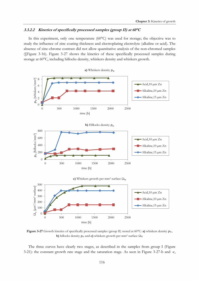
Chapter 3: Kinetics of growth
116
3.3.2.2 Kinetics of specifically processed samples (group II) at 60°C
In this experiment, only one temperature (60°C) was used for storage; the objective was to study the influence of zinc coating thickness and electroplating electrolyte (alkaline or acid). The absence of zinc-chrome contrast did not allow quantitative analysis of the non-chromed samples (§Figure 3-16). Figure 3-27 shows the kinetics of these specifically processed samples during storage at 60°C, including hillocks density, whiskers density and whiskers growth.
Figure 3-27 Growth kinetics of specifically processed samples (group II) stored at 60°C: a) whiskers density ρW,
b) hillocks density ρH and c) whiskers growth per mm² surface ΩW
The three curves have clearly two stages, as described in the samples from group I (Figure 3-21): the constant growth rate stage and the saturation stage. As seen in Figure 3-27-b and -c,
0
2
4
6
8
0 500 1000 1500 2000 2500
ρ W [whis
kers
/mm
²]
time [h]
a) Whiskers density ρW
Acid,10 µm Zn
Alkaline,10 µm Zn
Alkaline,15 µm Zn
0
200
400
600
800
0 500 1000 1500 2000 2500
ρ H [hillock
s/m
m²]
time [h]
b) Hillocks density ρH
Acid,10 µm Zn
Alkaline,10 µm Zn
Alkaline,15 µm Zn
0
100
200
300
400
500
0 500 1000 1500 2000 2500
Ωw [µ
m³/
mm
² su
rfac
e]
time [h]
c) Whiskers growth per mm² surface ΩW
Acid,10 µm Zn
Alkaline,10 µm Zn
Alkaline,15 µm Zn

Chapter 3: Kinetics of growth
117
whiskers density curve stops increasing earlier than whiskers growth curve; that is, while de formation of new whiskers stop, the already formed whiskers continue growing for longer time.
Figure 3-28 shows the influence of zinc coating thickness and electroplating electrolyte in hillocks density, whiskers density, ratio whiskers-hillocks and maximal whiskers length. Maximal whiskers rate and saturation time for whiskers growth are also compared.
Figure 3-28 Specifically processed samples (group II) after 2000 hours storage at 60°C: a) hillocks density ρH,
b) whiskers density ρW, c) ratio whiskers-hillocks density ρW/ρH, d) maximal whisker length hmax, e) maximal growth rate h'max and f) saturation time for whiskers growth (whiskers or hillocks not observed in alkaline-origin sample with
5 µm Zn coating)
0
100
200
300
400
500
600
700
800
Acid, 10 µmZn
Alkaline, 10µm Zn
Alkaline, 15µm Zn
ρ H [hillock
s/ m
m²]
a) Hillocks density ρH
0
1
2
3
4
5
6
7
8
9
Acid, 10 µmZn
Alkaline, 10µm Zn
Alkaline, 15µm Zn
ρ w [whisk
ers/
mm
²]
b) Whiskers density ρW
0
1
2
3
4
5
6
7
8
Acid, 10 µmZn
Alkaline, 10µm Zn
Alkaline, 15µm Zn
ρ W/ρ H [%
]
c) Ratio ρW/ρH
050
100150200250300350400450500
Acid, 10 µmZn
Alkaline, 10µm Zn
Alkaline, 15µm Zn
h max
[µm
]
d) Maximal whisker length hmax
0
0,2
0,4
0,6
0,8
1
1,2
0
0,01
0,02
0,03
0,04
Acid, 10µm Zn
Alkaline,10 µm Zn
Alkaline,15 µm Zn
h'm
ax [m
m/y
r]
h'm
ax [n
m/s
]
e) Maximal growth rate h'max
0
5
10
15
20
Acid, 10 µmZn
Alkaline, 10µm Zn
Alkaline, 15µm Zn
t ∞ [h
]
f) Saturation time t∞ (whiskers growth)

Chapter 3: Kinetics of growth
118
Since the time evolution of whiskers length was measured as total length per squared millimeter rather than for each of the whiskers (as in the samples from industrial site), the reported maximal growth rate (h'max) results from h'max= Lw'/ ρw. Whiskers growth rates varies from 0.7 to 1.2 mm/ year (values under those of literature [13], §Table 1-1).
The zinc coating thickness clearly favors the whisker growth and density, and to a major extent the hillocks density; maximal whiskers length is also favored by zinc coating thickness (five times longer in 15 µm coating than in 10 µm coating). Electroplated thickness also favors the whiskers growth saturation time but it has not strong influence on the whiskers growth rate. Neither whiskers nor hillocks were observed in alkaline-sample with the thinnest zinc coating (5 µm).
Concerning the electroplating electrolyte, it has a different effect on hillocks and whiskers growth. Samples from acid electrolyte have more and longer whiskers (0.4 mm) than samples from alkaline electrolyte (up to 0.2 mm). These observed lengths are under the values reported in literature [13] (at least 5 mm §Table 1-1). Samples from acid electrolyte have also longer whiskers growth saturation time and slowest growth rate than samples from alkaline electrolyte of the same thickness.
On the other hand, samples from alkaline electrolyte have three times more hillocks than samples from acid electrolyte. This was already observed and described in the SEM images (§3.2.2.2); growth in samples from acid electrolyte is localized on the irregularities of the surface, that is, the growth is not regular as observed in samples from alkaline electrolyte (§Figure 3-17).
Figure 3-29 compares samples from group I (from industrial site) and group II (specifically processed) after storage at 60°C during 3000 and 2000 hours respectively (zinc coating thickness: 20 and 7 µm for samples A and B respectively). In general, the behavior of samples from industrial site (group I) is much closer to alkaline-origin samples than to acid-origin samples. This is not surprising since, although the electrolyte used for electroplating of these samples is unknown, some results such as chemical characterization (§2.3.4.2) suggests the use of alkaline electrolyte.
Maximal growth rate is higher for samples from industrial site (A and B) than for specifically processed samples. However, it is important to remark that while data from samples A and B were taken for each of the whiskers, data for specifically processed samples were taken as an average of total whiskers (all whiskers combined) as explained above.

Chapter 3: Kinetics of growth
119
Figure 3-29 Comparison between samples from group I and II after storage at 60°C (3000 and 2000 hours
respectively): a) hillocks density ρH, b) whiskers density ρW, c) ratio whiskers-hillocks density ρW/ρH d) maximal whisker length (hmax) e) maximal growth rate h'max and f) saturation time for whiskers growth (whiskers or hillocks
not observed in neither sample C nor in alkaline-sample with 5 µm Zn coating)
0
100
200
300
400
500
600
700
800
Acid, 10µm Zn
Alkaline,10 µm
Zn
Alkaline,15 µm
Zn
SampleA, 20 µm
Zn
SampleB, 7 µm
Zn
ρ H [hillock
s/ m
m²]
a) Hillocks density ρH
0123456789
Acid, 10µm Zn
Alkaline,10 µm Zn
Alkaline,15 µm Zn
SampleA, 20 µm
Zn
Sample B,7 µm Zn
ρ w [whisk
ers/
mm
²]
b) Whiskers density ρW
0
1
2
3
4
5
6
7
8
Acid, 10µm Zn
Alkaline,10 µm Zn
Alkaline,15 µm Zn
SampleA, 20 µm
Zn
Sample B,7 µm Zn
ρ W/ρ H [%
]
c) Ratio ρW/ρH
0
100
200
300
400
500
600
Acid, 10µm Zn
Alkaline,10 µm
Zn
Alkaline,15 µm
Zn
SampleA, 20 µm
Zn
SampleB, 7 µm
Zn
leng
th
d) Maximal whisker length hmax
01234567
0
0,05
0,1
0,15
0,2
0,25
Acid, 10µm Zn
Alkaline,10 µm
Zn
Alkaline,15 µm
Zn
SampleA, 20 µm
Zn
SampleB, 7 µm
Zn
h'm
ax [m
m/y
r]
h'm
ax [n
m/s
]
e) Maximal growth rate h'max
0
10
20
30
40
50
60
Acid, 10µm Zn
Alkaline,10 µm Zn
Alkaline,15 µm Zn
Sample A,20 µm Zn
Sample B,7 µm Zn
t ∞ [h
]
f) Saturation time t∞ (whiskers growth)

Chapter 3: Kinetics of growth
120
3.3.2.3 Kinetics of specifically processed samples (group II) at 150, 175 and 200°C
In the SEM storage experiments, the influence of five different parameters in the growth kinetics (hillocks density, whiskers density, whiskers growth and total growth) was studied:
Temperature (150°C, 175°C and 200°C)
Zinc thickness (5 µm, 10 µm and 15 µm)
Steel substrate thickness (0.5 mm, 1.0 mm and 1.5 mm)
Chrome finishing (presence/ absence)
Electrolyte used for zinc electroplating (alkaline and acid)
3.3.2.3.1 Influence of temperature
Influence of temperature in the growth of whiskers is studied for both alkaline and acid electroplating electrolytes; non-chromed samples electroplated with alkaline electrolyte are also studied. Growth curves (hillocks density, whiskers density, whiskers growth and total growth) are shown for each sample at three different temperatures (150°C, 175°C and 200°C). All four curves, as in the case of samples stored at 60°C (§Figure 3-27) show two stages: constant growth rate and saturation. Growth curves of single whiskers are included in Appendix 4, three whiskers for each of the studied samples, at three different temperatures (150°C, 175°C and 200°C).
Samples electroplated with alkaline electrolyte
Figure 3-30 shows the kinetics growth curves of specifically processed chromed samples electroplated with alkaline electrolyte (15 μm of chromed Zn on 0.5 mm steel) for three different temperatures (150°C, 175°C and 200°C). The four growth parameters (hillocks density, whiskers density, whiskers growth and total growth) are all favored by temperature, particularly the whiskers density (already observed by Compton et.al. [9]). All four profiles experienced a growth at early stage (around 20 minutes in the figure) followed by a plateau. Most of samples with other zinc thickness and steel thickness (§Figure A3-1 to Figure A3-4 in Appendix 3) have the same behavior.
Non-chromed samples electroplated with alkaline electrolyte
Figure 3-31 shows the kinetics growth curves of specifically processed non-chromed samples electroplated with alkaline electrolyte (10 μm of chromed Zn on 0.5 mm steel) for two different temperatures (150°C and 200°C). As with the chromed samples, four growth parameters (hillocks density, whiskers density, whiskers growth and total growth) are favored by temperature.
While sample at 150°C has a similar behavior compared with chromed samples, in the storage at 200°C, it can be seen a very fast whiskers growth (density and growth) reaching a maximal at around 10 minutes; at this point, the surface as well as the whiskers start being corroded, due to the absence of protective chrome, and the whiskers are broken. Indeed, despite the samples are stored at vacuum in the SEM, it is not possible to avoid the corrosion in the samples without chrome protection. After one hour of storage, there are less than 10% of the original whiskers observed at 10 minutes.

Chapter 3: Kinetics of growth
121
Figure 3-30 Influence of temperature on growth kinetics of specifically processed samples (group II) electroplated
with alkaline electrolyte (15 µm Zn on 0.5 mm steel): a) whiskers density ρW, b) hillocks density ρH, c) whiskers growth per mm² surface ΩW and d) total growth per mm² surface Ω
0200400600800
1 0001 2001 400
0 10 20 30 40 50 60
ρ W [whis
kers
/mm
²]
Time [min]
a) Whiskers density ρW
200°C
175°C
150°C
0
1 000
2 000
3 000
4 000
5 000
0 10 20 30 40 50 60
ρ H [hillock
s/m
m²]
Time [min]
b) Hillocks density ρH
200°C
175°C
150°C
0
2 000
4 000
6 000
8 000
10 000
12 000
0 10 20 30 40 50 60ΩW
[µm
³/m
m²
surf
ace
]
Time [min]
c) Whiskers growth per 1 mm² surface Ωw
200°C
175°C
150°C
0
20 000
40 000
60 000
80 000
100 000
120 000
0 10 20 30 40 50 60
Ω[µ
m³/
mm
² su
rfac
e]
Time [min]
d) Total growth per 1 mm² surface Ω
200°C
175°C
150°C

Chapter 3: Kinetics of growth
122
Figure 3-31 Influence of temperature on growth kinetics of specifically processed non-chromed samples (group II)
electroplated with alkaline electrolyte (10 µm Zn on 0.5 mm steel): a) whiskers density ρW, b) hillocks density ρH, c) whiskers growth per mm² surface ΩW and d) total growth per mm² surface Ω
0
100
200
300
400
0 10 20 30 40 50 60
ρ W [whis
kers
/mm
²]
Time [min]
a) Whiskers density ρW
200°C
150°C
0
1 000
2 000
3 000
4 000
0 10 20 30 40 50 60
ρ H [hillock
s/m
m²]
Time [min]
b) Hillocks density ρH
200°C
150°C
01 0002 0003 0004 0005 0006 000
0 10 20 30 40 50 60Ωw[µ
m³/
mm
² su
rfac
e]
Time [min]
c) Whiskers growth per 1 mm² surface Ωw
200°C
150°C
0
5 000
10 000
15 000
0 10 20 30 40 50 60
Ω[µm³/m
m²
surf
ace]
Time [min]
d) Total growth per 1 mm² surface Ω
200°C
150°C

Chapter 3: Kinetics of growth
123
Samples electroplated with acid electrolyte
Figure 3-32 shows the kinetics growth curves of specifically processed chromed samples electroplated with acid electrolyte (15 μm of chromed Zn on 1.5 mm steel) for three different temperatures (150°C, 175°C and 200°C). As with the alkaline-origin samples, hillocks density and total growth are favored by temperature. However, concerning whiskers growth (density and growth), the temperature influence is not as strong as in the alkaline origin samples.
3.3.2.3.2 Influence of zinc coating thickness
Influence of zinc coating thickness in the growth of whiskers is studied in samples electroplated with alkaline electrolyte. Kinetic growth curves (hillocks density, whiskers density, whiskers growth and total growth) are presented for three different zinc coating thickness (5 µm, 10 µm and 15 µm).
Figure 3-33 shows the kinetics growth curves at 200°C of specifically processed samples electroplated with alkaline electrolyte on 0.5 mm steel, at three different zinc coating thickness (5 µm, 10 µm and 15 µm). Curves at 150°C and 175°C can be obtained from Figure 3-30, Figure A3-1 and Figure A3-2 (Appendix 3).
For the three temperatures, and much more significantly for 200°C, whiskers growth (density and growth) is favored by zinc coating thickness. After one hour of 200°C storage, for instance, the whiskers density of the thickest zinc coating (15µm) is around ten and fifty times the whiskers density of the 10 µm and 5 µm zinc coating respectively.
In the case of 150°C storage, while the thickest zinc coatings (15 and 10 µm) have developed whiskers, the thinnest coating (5 µm) does not present whiskers growth at all.
The same tendency can be observed for hillocks growth, i.e. it is favored by the zinc coating thickness; the influence, however, is not as strong as in the case of whiskers growth. After one hour of 200°C storage, the hillocks density of the thickest zinc coating (15µm) is around twice and fourteen times the hillocks density of the 10 µm and 5 µm coatings respectively.
In the case of alkaline-origin samples, it was observed that the zinc coating thickness increases the electroplate texture (§2.3.5.2). The stronger texture of the thickest zinc coating would therefore favor the growth of whiskers. This observation disagrees with Compton et.al. who suggested that thinner coatings are more prone to whiskers growth [9].
Concerning electroplates, they have a fiber texture. Zinc coating thickness has an influence in the electroplate texture; electroplates from acid electrolyte present more complex texture than those from alkaline one.
3.3.2.3.3 Influence of steel substrate thickness
Influence of the steel substrate thickness in the growth of whiskers is studied in samples electroplated with both alkaline and acid electrolytes. Kinetic growth curves (hillocks density, whiskers density, whiskers growth and total growth) are presented for each sample at two different steel substrate thickness (0.5 mm and 1.5 mm).

Chapter 3: Kinetics of growth
124
Figure 3-32 Influence of temperature on growth kinetics of specifically processed samples (group II) electroplated
with acid electrolyte (10 µm Zn on 1.5 mm steel): a) whiskers density ρW, b) hillocks density ρH, c) whiskers growth per mm² surface ΩW and d) total growth per mm² surface Ω
0
50
100
150
200
0 10 20 30 40 50 60
ρ W [whis
kers
/mm
²]
Time [min]
a) Whiskers density ρW
200°C
175°C
150°C
0
500
1 000
1 500
2 000
0 10 20 30 40 50 60
ρ H [hillock
s/m
m²]
Time [min]
b) Hillocks density ρH
200°C
175°C
150°C
0
500
1 000
1 500
2 000
2 500
0 10 20 30 40 50 60ΩW
[µm
³/m
m²
surf
ace]
Time [min]
c) Whiskers growth per 1 mm² surface ΩW
200°C
175°C
150°C
02 0004 0006 0008 000
10 00012 000
0 10 20 30 40 50 60
Ω[µ
m³/
mm
² su
rfac
e]
Time [min]
d) Total growth per 1 mm² surface Ω
200°C
175°C
150°C

Chapter 3: Kinetics of growth
125
Figure 3-33 Influence of zinc coating thickness on growth kinetics of specifically processed samples (group II)
electroplated with alkaline electrolyte (0.5 mm steel) at 200°C: a) whiskers density ρW, b) hillocks density ρH, c) whiskers growth per mm² surface ΩW and d) total growth per mm² surface Ω
0
500
1 000
1 500
0 10 20 30 40 50 60
ρ W [whis
kers
/mm
²]
Time [min]
a) Whiskers density ρw
15 µm Zn
10 µm Zn
5 µm Zn
0
1 000
2 000
3 000
4 000
5 000
0 10 20 30 40 50 60
ρ H [hillock
s/m
m²]
Time [min]
b) Hillocks density ρH
15 µm Zn
10 µm Zn
5 µm Zn
02 0004 0006 0008 000
10 00012 000
0 10 20 30 40 50 60Ωw[µ
m³/
mm
² su
rfac
e]
Time [min]
c) Whiskers growth per 1 mm² surface ΩW
15 µm Zn
10 µm Zn
5 µm Zn
020 00040 00060 00080 000
100 000120 000
0 10 20 30 40 50 60
Ω[µ
m³/
mm
² su
rfac
e]
Time [min]
d) Total growth per 1 mm² surface Ω
15 µm Zn
10 µm Zn
5 µm Zn

Chapter 3: Kinetics of growth
126
Samples electroplated with alkaline electrolyte
Figure 3-34 shows the kinetics growth curves at 200°C of specifically processed samples electroplated with alkaline electrolyte (15 µm of zinc coating) for two different steel substrate thickness (0.5 mm and 1.5 mm). Curves at 150°C and 175°C can be obtained from Figure 3-30, Figure A3-3 and Figure A3-4 (Appendix 3).
Whiskers growth (density and growth) is disfavored by steel substrate thickness; it can be seen that for the three temperatures (150°C, 175°C and more significantly 200°C), the thinner the steel substrate the more whiskers grow. According to Lindborg, this result is due to the texture of the thinner substrate that would favor the development of a {11-20} zinc texture and thus favor the whiskers growth [13].
After one hour of 200°C storage, for instance, whiskers density of the thinnest steel substrate (0.5 mm) is around three times the whiskers density of the thickest steel substrate (1.5 mm). As in the case of zinc coating thickness, the influence of steel substrate thickness becomes stronger with the temperature.
The same tendency is observed for hillocks growth, but the influence of the steel substrate thickness on the hillocks growth is not as strong as in the whiskers growth. Making the same comparison (after one hour of 200°C storage), the hillocks density of the thinnest steel substrate (0.5 mm) is only around 10% more than in the thickest steel substrate.
Samples electroplated with acid electrolyte
Figure 3-35 shows kinetics growth curves at 175°C of specifically processed samples electroplated with acid electrolyte (10 µm of zinc coating) for two different steel substrate thickness (0.5 mm and 1.5 mm). Curves at 150°C and 200°C can be obtained from Figure 3-30 and Figure A3-5 (Appendix 3).
In the case of samples electroplated with acid electrolyte, the influence of steel substrate thickness is the contrary to that one of alkaline-origin samples. In the acid-origin samples, the whiskers growth (density and growth), the hillocks growth and the total growth are all favored by the steel substrate thickness. After one hour at 200°C storage, for instance, the whiskers density of the thickest steel substrate (1.5 mm) is around 50% more than the whiskers density of the thinnest steel substrate (0.5 mm). As in the case of zinc coating thickness, the influence of steel substrate thickness becomes stronger with the temperature.

Chapter 3: Kinetics of growth
127
Figure 3-34 Influence of steel thickness on growth kinetics of specifically processed samples (group II)
electroplated with alkaline electrolyte (15 µm Zn) at 200°C: a) whiskers density ρW, b) hillocks density ρH, c) whiskers growth per mm² surface ΩW and d) total growth per mm² surface Ω
0
500
1 000
1 500
0 10 20 30 40 50 60
ρ W [whis
kers
/mm
²]
Time [min]
a) Whiskers density ρW
0.5 mm steel
1.5 mm steel
0
1 000
2 000
3 000
4 000
5 000
0 10 20 30 40 50 60
ρ H [hillock
s/m
m²]
Time [min]
b) Hillocks density ρH
0.5 mm steel
1.5 mm steel
02 0004 0006 0008 000
10 00012 000
0 10 20 30 40 50 60Ωw[µ
m³/
mm
² su
rfac
e]
Time [min]
c) Whiskers growth per 1 mm² surface ΩW
0.5 mm steel
1.5 mm steel
020 00040 00060 00080 000
100 000120 000
0 10 20 30 40 50 60
Ω[µ
m³/
mm
² su
rfac
e]
Time [min]
d) Total growth per 1 mm² surface Ω
0.5 mm steel
1.5 mm steel

Chapter 3: Kinetics of growth
128
Figure 3-35 Influence of steel thickness on growth kinetics of specifically processed samples (group II) electroplated
with acid electrolyte (10 µm Zn) at 175°C a) whiskers density ρW, b) hillocks density ρH, c) whiskers growth per mm² surface ΩW and d) total growth per mm² surface Ω
0
50
100
150
0 10 20 30 40 50 60
ρ W [whis
kers
/mm
²]
Time [min]
a) Whiskers density ρW
0.5 mm steel
1.5 mm steel
0
200
400
600
800
0 10 20 30 40 50 60
ρ H [hillock
s/m
m²]
Time [min]
b) Hillocks density ρH
0.5 mm steel
1.5 mm steel
0
500
1 000
1 500
2 000
2 500
0 10 20 30 40 50 60
Ωw[µ
m³/
mm
² su
rfac
e]
Time [min]
c) Whiskers growth per 1 mm² surface ΩW
0.5 mm steel
1.5 mm steel
0
2 000
4 000
6 000
8 000
0 10 20 30 40 50 60
Ω[µ
m³/
mm
² su
rfac
e]
Time [min]
d) Total growth per 1 mm² surface Ω
0.5 mm steel
1.5 mm steel

Chapter 3: Kinetics of growth
129
3.3.2.3.4 Influence of chrome and electroplating electrolyte
Influence of chrome and electroplating electrolyte in the growth of whiskers is studied; kinetic growth curves (hillocks density, whiskers density, whiskers growth and total growth) are presented for samples electroplated with alkaline electrolyte (chromed and non-chromed) and with acid electrolyte (chromed).
Figure 3-36 shows kinetics growth curves at 200°C of specifically processed samples with 10 µm of zinc coating on 0.5 mm of steel substrate; curves at 150°C and 175°C can be obtained from Figure 3-31, Figure A3-2 and Figure A3-5 (Appendix 3).
The absence of chrome favors the growth of whiskers (density and growth); nevertheless in the case of the 200°C storage, as explained before, the non-chromed sample seems to experience corrosion of the whiskers. On the other hand, the hillocks density and the total growth are not clearly influenced by the presence of chrome
Concerning the electroplating electrolyte, it does not seem to influence the whiskers density of the chromed samples, although the whiskers growth is slightly favored by the alkaline electrolyte. Hillocks density and the total growth are significantly larger in the samples electroplated with alkaline electrolyte. This observation was already done above: growth in samples electroplated with acid electrolyte is localized on the irregularities of the surface, that is, the growth is not regular as observed in the alkaline-origin samples (§Figure 3-17).
Compressive residual stress of alkaline-electrolyte samples is larger than acid-electrolyte ones (§2.3.6.2), so it would be expected that the first ones have more total growth (whiskers and hillocks combined) since the more residual stress has the material, the more whiskers and hillocks it grows.

Chapter 3: Kinetics of growth
130
Figure 3-36 Influence of electroplating electrolyte and chrome on growth kinetics of specifically processed samples
(group II) (10 µm Zn on 0.5 mm steel) at 200°C: a) whiskers density ρW, b) hillocks density ρH, c) whiskers growth per mm² surface ΩW and d) total growth per mm² surface Ω
0
100
200
300
400
0 10 20 30 40 50 60
ρ W [whis
kers
/mm
²]
Time [min]
a) Whiskers density ρW
Alk. non-chromed
Alk. chromed
Acid chromed
0
1 000
2 000
3 000
4 000
0 10 20 30 40 50 60
ρ H [hillock
s/m
m²]
Time [min]
b) Hillocks density ρH
Alk. non-chromed
Alk. chromed
Acid chromed
0
1 000
2 000
3 000
4 000
5 000
6 000
0 10 20 30 40 50 60ΩW
[µm
³/m
m²
surf
ace]
Time [min]
c) Whiskers growth per 1 mm² surface ΩW
Alk. non-chromed
Alk. chromed
Acid chromed
0
5 000
10 000
15 000
0 10 20 30 40 50 60
Ω [µ
m³/
mm
² su
rfac
e]
Time [min]
d) Total growth per 1 mm² surface Ω
Alk. non-chromed
Alk. chromed
Acid chromed

Chapter 3: Kinetics of growth
131
3.3.2.3.5 Influencing parameters on growth after saturation
Figure 3-37 shows the influence of zinc coating thickness, steel substrate thickness, chrome, electroplating electrolyte and temperature in the kinetic parameters after growth saturation: whiskers and hillocks density, maximal whiskers length, maximal whiskers growth rate and incubation and saturation time for whiskers growth.
Hillocks density after saturation increases with temperature (strongly), zinc coating thickness, presence of chrome, alkaline electroplating electrolyte (compared with acid) and steel substrate thickness in acid-origin samples; the influence of steel substrate thickness is not clear for alkaline-origin samples.
Concerning whiskers density after saturation, for alkaline-origin samples, it increases with temperature (strongly) and zinc coating thickness; and it is disfavored by steel substrate thickness and presence of chrome. It is not clear the influence of neither temperature in acid-origin samples nor the electroplating electrolyte.
When comparing 150 to 200°C, longest whiskers are found at the lowest temperature (150°C); however, as mentioned above, temperature favors whiskers density, that is, more temperature implies more whiskers but shorter. This observation is important since whiskers length rather than density is the most penalizing parameter from the industrial point of view of the problematic of whiskers growth (higher probability to make bridges inside the electrical components and therefore short circuits).
Longest whiskers were observed in the non-chromed samples; however due to the absence of protecting chrome, whiskers become rapidly corroded. Maximal length is also favored by zinc coating thickness and acid electrolyte when compared with alkaline. No clear influence of steel thickness is observed.
Any clear influence of the different parameters on neither maximal whiskers growth rate2 nor incubation time is observed.
Saturation time, the time before the whiskers growth stops, decrease with temperature in alkaline samples, while in acid samples it seems to be independent of temperature. The presence of chrome also increases the saturation time, while the influence of other parameters remains unclear.
2 Since the time-evolution of length of whiskers was measured as total length per squared
millimeter rather than for each of the whiskers (as in the samples from industrial site), the reported
maximal growth rate (hw') is actually the average of all whiskers that results from hw'= Lw'/ ρw.

Chapter 3: Kinetics of growth
132
Figure 3-37 Influencing parameters on growth data after saturation for specifically processed samples (group II): a) hillocks density ρH, b) whiskers density ρW, c) maximal whisker length hmax, (cont. next page)
0
1000
2000
3000
4000
5μm-Zn on 0.5mm-steel
10μm-Zn on 0.5mm-steel
15μm-Zn on 0.5mm-steel
15μm-Zn on 1.5mm-steel
10μm-Zn on 0.5mm-steel
(without chrome)
10μm-Zn on 0.5mm-steel
(acid)
10μm-Zn on 1.5mm-steel
(acid)
ρ H [hillock
s/ m
m²
surf
ace]
a) Hillocks density (ρH)
150°C 175°C 200°C
no Cr
Acid thicker substrate
Alkaline
0
200
400
600
800
1000
1200
5μm-Zn on 0.5mm-steel
10μm-Zn on 0.5mm-steel
15μm-Zn on 0.5mm-steel
15μm-Zn on 1.5mm-steel
10μm-Zn on 0.5mm-steel
(without chrome)
10μm-Zn on 0.5mm-steel
(acid)
10μm-Zn on 1.5mm-steel
(acid)
ρ w [whisk
ers/
mm
² su
rfac
e]
b) Whiskers density (ρw)
150°C 175°C 200°C
no Cr
Acid
thicker substrate
Alkaline
0
20
40
60
80
100
5μm-Zn on 0.5mm-steel
10μm-Zn on 0.5mm-steel
15μm-Zn on 0.5mm-steel
15μm-Zn on 1.5mm-steel
10μm-Zn on 0.5mm-steel
(without chrome)
10μm-Zn on 0.5mm-steel
(acid)
10μm-Zn on 1.5mm-steel
(acid)
h max
[µm
]
c) Maximal whisker length (hmax)
150°C 175°C 200°C
no Cr
Acid thicker substrate
Alkaline

Chapter 3: Kinetics of growth
133
Figure 3-37 (cont. from last page) Influencing parameters on growth data after saturation for specifically processed samples (group II): d) maximal growth rate h'W, e) incubation time for whiskers growth tinc and f) saturation time for
whiskers growth t∞
0
1 000
2 000
3 000
4 000
5 000
020406080
100120140160
5μm-Zn on 0.5mm-steel
10μm-Zn on 0.5mm-steel
15μm-Zn on 0.5mm-steel
15μm-Zn on 1.5mm-steel
10μm-Zn on 0.5mm-steel
(without chrome)
10μm-Zn on 0.5mm-steel
(acid)
10μm-Zn on 1.5mm-steel
(acid)
Max
. gro
wth
rat
e [m
m/y
r]
h'm
ax [n
m/s
] d) Maximal growth rate h'max
150°C 175°C 200°C
no Cr
Acid
thicker substrate
Alkaline
01234567
5μm-Zn on 0.5mm-steel
10μm-Zn on 0.5mm-steel
15μm-Zn on 0.5mm-steel
15μm-Zn on 1.5mm-steel
10μm-Zn on 0.5mm-steel
(without chrome)
10μm-Zn on 0.5mm-steel
(acid)
10μm-Zn on 1.5mm-steel
(acid)
t inc [
min
]
e) Incubation time tinc (whiskers growth)
150°C 175°C 200°C
no Cr
Acid
thicker substrate
Alkaline
0 0 0 0 0 0
05
10152025303540
5μm-Zn on 0.5mm-steel
10μm-Zn on 0.5mm-steel
15μm-Zn on 0.5mm-steel
15μm-Zn on 1.5mm-steel
10μm-Zn on 0.5mm-steel
(without chrome)
10μm-Zn on 0.5mm-steel
(acid)
10μm-Zn on 1.5mm-steel
(acid)
t ∞ [m
in]
f) Saturation time t∞ (whiskers growth)
150°C 175°C 200°C
no Cr
Acid
thicker substrate
Alkaline
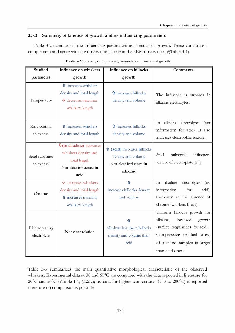
Chapter 3: Kinetics of growth
134
3.3.3 Summary of kinetics of growth and its influencing parameters
Table 3-2 summarizes the influencing parameters on kinetics of growth. These conclusions complement and agree with the observations done in the SEM observation (§Table 3-1).
Table 3-2 Summary of influencing parameters on kinetics of growth
Studied
parameter
Influence on whiskers
growth
Influence on hillocks
growth
Comments
Temperature
increases whiskers
density and total length
decreases maximal
whiskers length
increases hillocks
density and volume
The influence is stronger in
alkaline electrolytes.
Zinc coating
thickness
increases whiskers
density and total length
increases hillocks
density and volume
In alkaline electrolytes (not
information for acid). It also
increases electroplate texture.
Steel substrate
thickness
(in alkaline) decreases
whiskers density and
total length
Not cleat influence in
acid
(acid) increases hillocks
density and volume
Not cleat influence in
alkaline
Steel substrate influences
texture of electroplate [29].
Chrome
decreases whiskers
density and total length
increases maximal
whiskers length
increases hillocks density
and volume
In alkaline electrolytes (no
information for acid).
Corrosion in the absence of
chrome (whiskers break).
Electroplating
electrolyte Not clear relation
Alkalyne has more hillocks
density and volume than
acid
Uniform hillocks growth for
alkaline, localized growth
(surface irregularities) for acid.
Compressive residual stress
of alkaline samples is larger
than acid ones.
Table 3-3 summarizes the main quantitative morphological characteristic of the observed whiskers. Experimental data at 30 and 60°C are compared with the data reported in literature for 20°C and 50°C (§Table 1-1, §1.2.2); no data for higher temperatures (150 to 200°C) is reported therefore no comparison is possible.
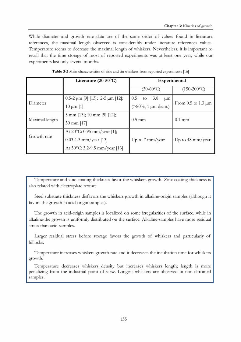
Chapter 3: Kinetics of growth
135
While diameter and growth rate data are of the same order of values found in literature references, the maximal length observed is considerably under literature references values. Temperature seems to decrease the maximal length of whiskers. Nevertheless, it is important to recall that the time storage of most of reported experiments was at least one year, while our experiments last only several months.
Table 3-3 Main characteristics of zinc and tin whiskers from reported experiments [16]
Literature (20-50°C) Experimental
(30-60°C) (150-200°C)
Diameter 0.5-2 µm [9] [13]; 2-5 µm [12];
10 µm [1]
0.5 to 3.8 µm
(>80%, 1 µm diam.) From 0.5 to 1.3 µm
Maximal length 5 mm [13]; 10 mm [9] [12];
30 mm [17] 0.5 mm 0.1 mm
Growth rate At 20°C: 0.95 mm/year [1];
0.03-1.3 mm/year [13]
At 50°C: 3.2-9.5 mm/year [13]
Up to 7 mm/year
Up to 48 mm/year
Temperature and zinc coating thickness favor the whiskers growth. Zinc coating thickness is also related with electroplate texture.
Steel substrate thickness disfavors the whiskers growth in alkaline-origin samples (although it favors the growth in acid-origin samples).
The growth in acid-origin samples is localized on some irregularities of the surface, while in alkaline-the growth is uniformly distributed on the surface. Alkaline-samples have more residual stress than acid-samples.
Larger residual stress before storage favors the growth of whiskers and particularly of hillocks.
Temperature increases whiskers growth rate and it decreases the incubation time for whiskers growth.
Temperature decreases whiskers density but increases whiskers length; length is more penalizing from the industrial point of view. Longest whiskers are observed in non-chromed samples.

Chapter 3: Residual stress
136
3.4 RESIDUAL STRESS
Compressive residual stress in the zinc coatings seems to favor the whiskers growth rate [13] [29] and decreases incubation time [20]. Residual stress was measured on the samples by X-ray diffraction after storage in environmental chambers and in SEM, and compared with the stress measured before storage (§2.3.6); this comparison has to be taken with care, due to large confidence intervals in the measurements. It is assumed positive values of residual stress as compressive.
3.4.1 Residual stress of samples from industrial site (group I) in environmental chambers
Figure 3-38 shows residual stress measured in samples A and B after storage at 30°C and 60°C in environmental chambers, at both the longitudinal axis (longest one) and the transversal axis (shortest one).
No stress after storage was measured for sample C, already stress-free before storage; this sample did not grow whiskers or hillocks at neither 30°C nor 60°C (§3.3.1); an expected result since whiskers growth is taught to be a stress relaxation phenomenon.
Results are compared with stress measured before storage (§Figure 2-35). Storage at both temperatures produces stress stress relaxation in both samples A and B; the values of this stress relaxation are included in Figure 3-38.
Figure 3-38 Compressive residual stress of samples from industrial site (group I) before and after storage (30°C and 60°C) at both longitudinal and transversal axis (values of stress relaxation included)
-20
0
20
40
60
80
100
120
Com
pres
sive
str
ess
[MP
a]
Sample A Sample B Sample C
Long. (before) Long. (after 30°C)Long. (after 60°C) Transv. (before)Transv. (after 30°C) Transv. (after 60°C)
43±29 30°C
13±19 60°C
48±19 30°C
48±23 60°C
29±16 30°C 41±19
60°C
51±27 30°C
64±16 60°C
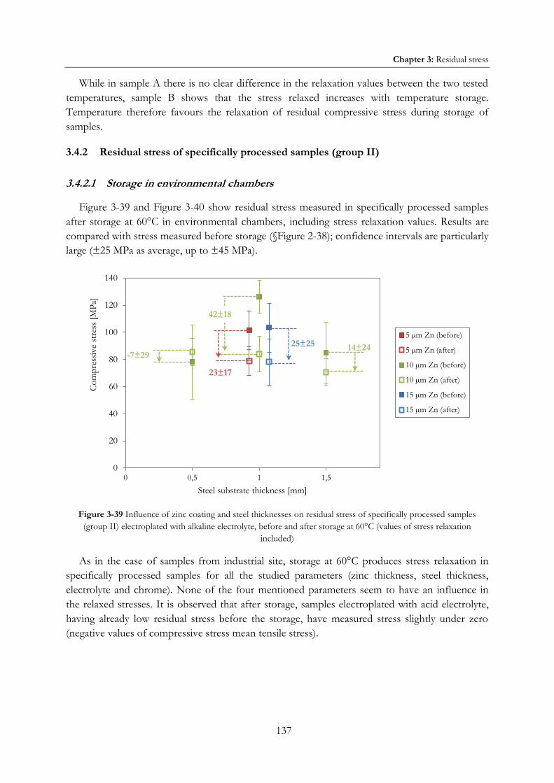
Chapter 3: Residual stress
137
While in sample A there is no clear difference in the relaxation values between the two tested temperatures, sample B shows that the stress relaxed increases with temperature storage. Temperature therefore favours the relaxation of residual compressive stress during storage of samples.
3.4.2 Residual stress of specifically processed samples (group II)
3.4.2.1 Storage in environmental chambers
Figure 3-39 and Figure 3-40 show residual stress measured in specifically processed samples after storage at 60°C in environmental chambers, including stress relaxation values. Results are compared with stress measured before storage (§Figure 2-38); confidence intervals are particularly large (±25 MPa as average, up to ±45 MPa).
Figure 3-39 Influence of zinc coating and steel thicknesses on residual stress of specifically processed samples
(group II) electroplated with alkaline electrolyte, before and after storage at 60°C (values of stress relaxation included)
As in the case of samples from industrial site, storage at 60°C produces stress relaxation in specifically processed samples for all the studied parameters (zinc thickness, steel thickness, electrolyte and chrome). None of the four mentioned parameters seem to have an influence in the relaxed stresses. It is observed that after storage, samples electroplated with acid electrolyte, having already low residual stress before the storage, have measured stress slightly under zero (negative values of compressive stress mean tensile stress).
0
20
40
60
80
100
120
140
0 0,5 1 1,5
Com
pres
sive
str
ess
[MP
a]
Steel substrate thickness [mm]
5 µm Zn (before)
5 µm Zn (after)
10 µm Zn (before)
10 µm Zn (after)
15 µm Zn (before)
15 µm Zn (after)
42±18
14±24
23±17
25±25 -7±29

Chapter 3: Residual stress
138
Figure 3-40 Influence of chrome, electroplating electrolyte and steel thicknesses on residual stress of specifically processed samples (group II, 10 µm Zn), before and after storage at 60°C (values of stress relaxation included)
3.4.2.2 SEM storage
Figure 3-41 and Figure 3-42 show residual stress measured in specifically processed samples after SEM storage at 150°C and 200°C, including stress relaxation values. Results are compared with stress measured before storage (§Figure 2-38); confidence intervals are smaller than in the stress measurements of samples stored in environmental chambers (§Figure 3-40 and Figure 3-41).
As in the storage at 60°C, SEM storage at 150°C and 200°C produces stress relaxation in samples of group II for all the studied parameters (zinc thickness, steel thickness, electrolyte and chrome). This stress relaxation is favored by temperature storage (more or at least same stress relaxation at 200°C than at 150°C).
No clear influence of zinc coating and steel substrate thicknesses on residual stress relaxation is observed in Figure 3-41. On the other hand, Figure 3-42 shows that relaxed stress is influenced by the electroplating electrolyte since acid electrolyte seems to favor stress relaxation. However, as it was also observed in the storage at 60°C, the measured compressive stress after storage of acid-origin samples has negative values, that is, after relaxation, the samples become under tensile residual stress (negative values of compressive stress mean tensile stress).
-20
0
20
40
60
80
100
120
140
0 0,5 1 1,5
Com
pres
sive
str
ess
[MP
a]
Steel substrate thickness [mm]
Alk.,non-chromed(before)
Alk.,non-chromed(after)
Alk.,chromed (before)
Alk.,chromed (after)
Acid,chromed (before)
Acid,chromed (after)
-7±29
42±18
14±24 40±13
23±13
43±9 42±19

Chapter 3: Residual stress
139
Figure 3-41 Influence of zinc coating and steel thicknesses on residual stress of specifically processed samples
(group II) electroplated with alkaline electrolyte, before and after SEM storage (150°C and 200°C) (values of stress relaxation included)
Figure 3-42 Influence of chrome, electroplating electrolyte and steel thicknesses on residual stress of specifically
processed samples (group II, 10 µm Zn), before and after SEM storage (150°C and 200°C) (values of stress relaxation included)
-50
0
50
100
150C
ompr
essi
ve s
tres
s [M
Pa]
0.5 mm steel 1.5 mm steel
5 µm Zn (before)
5 µm Zn (after 150°C)
5 µm Zn (after 200°C)
10 µm Zn (before)
10 µm Zn (after 150°C)
10 µm Zn (after 200°C)
15 µm Zn (before)
15 µm Zn (after 150°C)
15 µm Zn (after 200°C)
-150
-100
-50
0
50
100
Com
pres
sive
str
ess
[MP
a]
0.5 mm steel 1.5 mm steel
Alk.,non-chromed (before)
Alk.,non-chromed (after 200°C)
Alk.,chromed (before)
Alk.,chromed (after 150°C)
Alk.,chromed (after 200°C)
Acid,chromed (before)
Acid,chromed (after 150°C)
Acid,chromed (after 200°C)
84±8 150°C
115±6 200°C
106±7 200°C
78±11 150°C
76±11 200°C
91±8 150°C
101±9 200°C
103±7 150°C
78±11 150°C
76±11 200°C
92±87 150°C
107±7 150°C
159±7 200°C
92±8 150°C
110±7 200°C
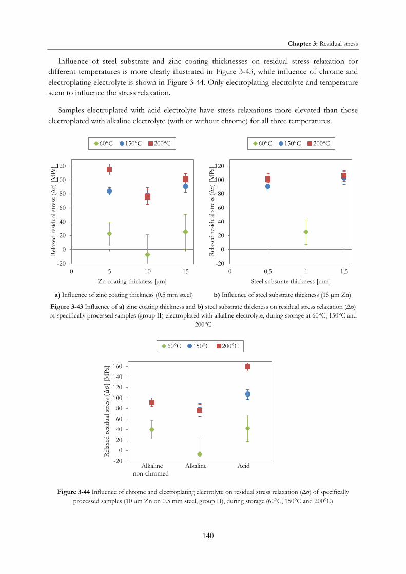
Chapter 3: Residual stress
140
Influence of steel substrate and zinc coating thicknesses on residual stress relaxation for different temperatures is more clearly illustrated in Figure 3-43, while influence of chrome and electroplating electrolyte is shown in Figure 3-44. Only electroplating electrolyte and temperature seem to influence the stress relaxation.
Samples electroplated with acid electrolyte have stress relaxations more elevated than those electroplated with alkaline electrolyte (with or without chrome) for all three temperatures.
a) Influence of zinc coating thickness (0.5 mm steel) b) Influence of steel substrate thickness (15 µm Zn)
Figure 3-43 Influence of a) zinc coating thickness and b) steel substrate thickness on residual stress relaxation ( ) of specifically processed samples (group II) electroplated with alkaline electrolyte, during storage at 60°C, 150°C and
200°C
Figure 3-44 Influence of chrome and electroplating electrolyte on residual stress relaxation ( ) of specifically
processed samples (10 µm Zn on 0.5 mm steel, group II), during storage (60°C, 150°C and 200°C)
-20
0
20
40
60
80
100
120
0 5 10 15
Rel
axed
res
idua
l str
ess
() [
MP
a]
Zn coating thickness [µm]
60°C 150°C 200°C
-20
0
20
40
60
80
100
120
0 0,5 1 1,5
Rel
axed
res
idua
l str
ess
() [
MP
a]
Steel substrate thickness [mm]
60°C 150°C 200°C
-20
0
20
40
60
80
100
120
140
160
Rel
axed
res
idua
l str
ess
(Δσ) [MP
a]
60°C 150°C 200°C
Alkaline Alkaline Acid non-chromed

Chapter 3: Residual stress
141
Temperature has the most important influence on stress relaxation; it is clearly seen that storage at 200°C relaxes more stress (or at least the same) than at 150°C, while storage at 60°C relaxes the least. The influence of temperature is more visible in samples from acid electrolyte. These relaxation stresses are of the order of:
37 to 53 MPa for 60°C storage 67 to 114 MPa for 150°C storage 65 to 166 MPa for 200°C storage
Storage of samples produces stress relaxation for all storage conditions.
Relaxation is strongly favored by:
Temperature (which also favors the whiskers growth) Electroplating electrolyte (larger relaxation in acid samples than in alkaline samples)
On the other hand, relaxation is independent of:
Zinc coating thickness Steel substrate thickness Chrome
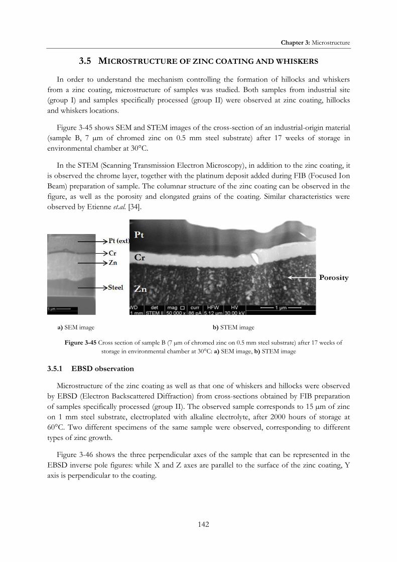
Chapter 3: Microstructure
142
3.5 MICROSTRUCTURE OF ZINC COATING AND WHISKERS
In order to understand the mechanism controlling the formation of hillocks and whiskers from a zinc coating, microstructure of samples was studied. Both samples from industrial site (group I) and samples specifically processed (group II) were observed at zinc coating, hillocks and whiskers locations.
Figure 3-45 shows SEM and STEM images of the cross-section of an industrial-origin material (sample B, 7 µm of chromed zinc on 0.5 mm steel substrate) after 17 weeks of storage in environmental chamber at 30°C.
In the STEM (Scanning Transmission Electron Microscopy), in addition to the zinc coating, it is observed the chrome layer, together with the platinum deposit added during FIB (Focused Ion Beam) preparation of sample. The columnar structure of the zinc coating can be observed in the figure, as well as the porosity and elongated grains of the coating. Similar characteristics were observed by Etienne et.al. [34].
a) SEM image b) STEM image
Figure 3-45 Cross section of sample B (7 µm of chromed zinc on 0.5 mm steel substrate) after 17 weeks of storage in environmental chamber at 30°C: a) SEM image, b) STEM image
3.5.1 EBSD observation
Microstructure of the zinc coating as well as that one of whiskers and hillocks were observed by EBSD (Electron Backscattered Diffraction) from cross-sections obtained by FIB preparation of samples specifically processed (group II). The observed sample corresponds to 15 µm of zinc on 1 mm steel substrate, electroplated with alkaline electrolyte, after 2000 hours of storage at 60°C. Two different specimens of the same sample were observed, corresponding to different types of zinc growth.
Figure 3-46 shows the three perpendicular axes of the sample that can be represented in the EBSD inverse pole figures: while X and Z axes are parallel to the surface of the zinc coating, Y axis is perpendicular to the coating.

Chapter 3: Microstructure
143
Figure 3-46 Schema of axes represented in EBSD inverse pole figures
The reference triangle of the inverse pole figures corresponds to the directions <0001>, <10-10> and <2-1-10>, represented in the triangle by red, blue and green respectively. Figure 3-47-a shows the hexagonal structure of zinc as well as the main represented directions. Figure 3-47-b shows the hexagonal structure from above, while Figure 3-47-c depicts the reference triangle.
a) b)
c)
Figure 3-47 a) Hexagonal structure and main represented directions, b) from above, c) reference triangle
3.5.1.1 First specimen
The first specimen corresponds to a hillock that grew from the surface, breaking the chrome of the surface (zinc looks bright on the SEM image). Figure 3-48 shows a schema of the growth and a SEM image of the observed zone.

Chapter 3: Microstructure
144
a) b)
Figure 3-48 First specimen observed by EBSD: a) schema, b) SEM image. 15 µm of zinc on 1 mm steel substrate, after 2000 hours of storage at 60°C of specifically processed sample (group II) electroplated with alkaline electrolyte
Resulting inverse pole figures with respect to axes Y (perpendicular to the coating) and Z (parallel to the coating) are shown in Figure 3-49, as well as a SEM image of the observed zone. Three different regions are clearly distinguished, as follows:
The columnar grain-structure of the zinc coating composed of needle-like grains, already observed in Figure 3-45. These grains are approximately 0.13 µm wide and 0.55 µm long, with an aspect ratio from 2 to 4. Grains are orientated with directions between <0001> and <1-100> with respect to the Z axis (red to blue in the figure) and mostly with <2-1-10> direction respect to the Y axis (green in the figure).
A mixed zone, where most of the grains become equiaxial, (mainly at the upper part of the zone, at the border with the recrystallized zone), although some of grains remains elongated but in a less measure than the grains of the rest of the zinc coating. Grains are orientated with directions between <2-1-10> and <1-100> with respect to the Y axis (green to blue in the figure), while there is not clear orientation with respect to the Z axis. This mixed zone is developed under the hillock, up to 3 µm deeper into the coating.
The hillock (around 4 µm wide) composed of equiaxial recrystallized grains of larger size (0.4 to 0.6 µm of diameter). This zone corresponds to the zinc growth during storage. Grains of this zone are clearly visible and they not have clear orientation at neither of the Y and Z axes.
In the inverse pole figures, pores in the zinc coating are clearly visible and they correspond to the black areas (they are black because they are not indexed in EBSD). Porosity, along to the very small size of the grains of the zinc coating, make difficult the indexation of the grains in the zinc coating.

Chapter 3: Microstructure
145
a)
b)
c)
d)

Chapter 3: Microstructure
146
Figure 3-49 First specimen observed by EBSD: a) SEM image, b) inverse pole figure with respect axis Z (parallel to the coating), d) inverse pole figure with respect axis Y (perpendicular to the coating), c) schema of the observed feature, reference axes and stereographic triangle that relates the EBSD colors to the crystallographic orientation; 15 µm of
zinc on 1 mm steel substrate, after 2000 hours of storage at 60°C of specifically processed sample (group II) electroplated with alkaline electrolyte

Chapter 3: Microstructure
147
Figure 3-50 shows the misorientation cartography of the first specimen. The average misorientation angle within each grain is calculated. A minimum angle Θmin is defined (5° in this case), and the grains are classified according to the misorientation angle, as follows:
«deformed grains» (red in the figure): those with misorientation angle higher than the minimum angle
«substructured grains» (yellow in the figure): those grains, composed of sub-grains, whose average misorientation angle within each sub-grain is under the minimum angle Θmin but the misorientation angle from sub-grain to sub-grain is higher than Θmin
«recrystallized grains» (blue in the figure): all remaining grains
a)
b)
Figure 3-50 a) Misorientation cartography of the first specimen observed by EBSD, b) distribution of crystallographic directions of indexed grains 15 µm of zinc on 1 mm steel substrate, after 2000 hours of storage at
60°C (alkaline electroplating electrolyte, specifically processed sample, group II)
Within the columnar region, most of the grains (85%) are considered as deformed, while 11% are substructured grains and only 4% are recrystallized. On the hillock itself, grains are mainly substructured or recrystallized. In Figure 3-50-b it is seen that most of deformed grains are orientated between <0001> and <10-10>, while the substructured grains do not have a preferred orientation.

Chapter 3: Microstructure
148
3.5.1.2 Second specimen
The second specimen observed with EBSD corresponds to a bump that grows from the surface without breaking the chrome at the top of the feature; nevertheless, the chrome is broken at the sides of the bump by the growing zinc (zinc looks bright on the SEM image).
Figure 3-51 shows a schema of the growth and a SEM image of the observed zone, as well as a SEM image of the cross section of the studied sample, obtained during FIB preparation; the small blue frames in the SEM images specifies the zone analyzed by EBSD.
a)
b) c)
Figure 3-51 Second specimen observed by EBSD: a) schema, b) SEM image, c) cross-section SEM image (FIB sample preparation); 15 µm of zinc on 1 mm steel substrate, after 2000 hours of storage at 60°C (alkaline
electroplating electrolyte, specifically processed sample, group II)
Figure 3-52 shows the resulting inverse pole figures with respect to axes Y (perpendicular to the coating) and Z (parallel to the coating), as well as a SEM image of the observed zone. As in the first observed zone, three different regions are clearly distinguished:
The columnar grain-structure of the zinc coating, with needle-like grains.
The recrystallized zone, a 2.5 µm wide strip developed under the bump, composed of larger grains, wider and less elongated than grains of the coating, including even some equiaxial grains (up to 0.5 µm of diameter). Grains of this zone are clearly visible and they not have clear orientation at neither of Y and Z axes.
A mixed zone, where, as already explained above, most of the grains become equiaxial. Grains of this zone are clearly visible and they not have clear orientation at neither of Y and Z axes. This mixed zone is actually a bump (1.2 µm height, 2.2 µm width) and its located above the recrystallized zone.

Chapter 3: Microstructure
149
a)
b)
c)
d) Figure 3-52 Second specimen observed by EBSD: a) SEM image, b) inverse pole figure with respect axis Z (parallel to the coating), d) inverse pole figure with respect axis Y
(perpendicular to the coating), c) schema of the observed feature, reference axes and stereographic triangle that relates the EBSD colors to the crystallographic orientation; 15 µm of zinc on 1 mm steel substrate, after 2000 hours of storage at 60°C (alkaline electroplating electrolyte, specifically processed sample, group II).

Chapter 3: Microstructure
150
Figure 3-53 shows the misorientation cartography of the second observed specimen. The results are very similar to the first observed specimen; within the columnar region, most of the grains (86%) are considered as deformed, while 10% are substructured grains and only 4% are recrystallized. On the recrystallized zone itself, grains are mainly substructured or recrystallized. In Figure 3-53-b, it is seen that most of deformed grains are orientated between <0001> and <10-10>, while the substructured and recrystallized grains do not have a preferred orientation.
a)
b)
Figure 3-53 a) Misorientation cartography of the second specimen observed by EBSD, b) distribution of crystallographic directions of indexed grains; 15 µm of zinc on 1 mm steel substrate, after 2000 hours of storage at
60°C (alkaline electroplating electrolyte, specifically processed sample, group II)
Two regions are clearly present in both samples:
The columnar-grain zone in the zinc coating.
The zone with larger and more equiaxial grains, located at particular features such as hillocks or bumps; these larger grains are actually recrystallized and substructured grains.
As explained above, the preferred orientations of the columnar grains of the zinc coating are between <0001> and <1-100> along to the Z axis (red to blue in the figures), and <2-1-10> direction respect to the Y axis (green in the figures). These directions correspond to planes

Chapter 3: Microstructure
151
perpendicular to these preferred orientations, that is, planes between {-12-10} and {10-10}, as shown in the Figure 3-47.
3.5.2 TEM observation
In order to observe with higher detail the microstructure of the samples, TEM observation was done at samples corresponding to 15 µm of chromed zinc on 1 mm steel substrate, electroplated using alkaline electrolyte, after 2000 hours of storage at 60°C. Two different specimens were obtained by TEM-samples preparation using Dual Beam microscope (FIB and SEM).
3.5.2.1 First specimen (hillock)
The first specimen corresponds to a hillock which includes a small whisker of around 1.2 µm width and 5 µm length, as seen in the Figure 3-54.
Figure 3-54 First specimen for TEM analysis (a hillock); 15 µm of zinc on 1 mm steel substrate, after 2000 hours of storage at 60°C (alkaline electroplating electrolyte, specifically processed sample, group II)
Figure 3-55 is a HAADF image of the hillock, the first observed specimen, where the 0.2-µm chrome can be easily observed (black strip on the left figure). On the right figure, the interface between the hillock and the zinc coating can be observed in detail.
Two different regions are clearly distinguished (same regions observed in the samples analyzed with EBSD (§3.5.1).
The poly crystalline zinc coating where the columnar grains can be slightly observed; many cavities are also observed, most of them with less than 40 nm diameter.
The mono-crystalline hillock around 1.6 µm wide and 2 µm high; there is also cavities but much less than in the coating.

Chapter 3: Microstructure
152
Figure 3-55 HAADF image of first specimen (hillock), detail of the interface coating/hillock (at the right); 15 µm of zinc on 1 mm steel substrate, after 2000 hours of storage at 60°C (alkaline electroplating electrolyte, specifically
processed sample, group II)
Concerning the zinc coating, its microstructure presents an interesting aspect combining chevron-pattern zones and vertical-line-patter zones, as shown in the HAADD image and the schema of the Figure 3-56.
Figure 3-56 Chevron-pattern and vertical-lines-pattern in the zinc coating (HAADF image on the left, schema on
the right), §Figure 3-55
3.5.2.2 Second specimen (whisker)
The second specimen corresponds to a 30-µm-long whisker parallel to the surface growing from a cauliflower-like hillock. The specimen was obtained from a section including both the hillock and the whisker (Figure 3-57). Figure 3-58 is a HAADF image of the sample, where the triple interface hillock-whisker-coating is observed.

Chapter 3: Microstructure
153
Figure 3-57 Second specimen for TEM analysis (a hillock); 15 µm of zinc on 1 mm steel substrate, after 2000 hours of storage at 60°C (alkaline electroplating electrolyte, specifically processed sample, group II)
Besides the zinc coating, also observed in the first specimen, two other regions are distinguished:
Recrystallized zone, observed at the upper left part of the figure, which it is likely a fragment of the hillock.
The mono-crystalline whisker with a diameter around 1 µm, around 3.5 µm of the whiskers is observed from a total length of the whisker (30 µm). The whisker starts almost normal to the surface (70° inclination) before kinking to the right getting a direction almost parallel to the surface as it is also observed in the Figure 3-58. Some dark zones are observed at the center of the whisker.
Figure 3-58 HAADF image of second specimen (whisker), detail of the triple interface coating/ hillock / whisker (at
the right); 15 µm of zinc on 1 mm steel substrate, after 2000 hours of storage at 60°C (alkaline electroplating electrolyte, specifically processed sample, group II)

Chapter 3: Microstructure
154
A high-magnification with enhanced contrast from a HAADF image is shown in the Figure 3-59 to illustrate the dislocations are observed in the whisker and particularly in the hillock (up to 300 nm long are clearly observed).
Figure 3-59 High magnification of the Figure 3-58 with enhanced contrast to show dislocations
According to Sugiarto et al. [17], dislocations are associated with localized stress at the electroplate grains; whiskers growth is related with localized stress rather than with the macro-stress of the coating (§1.3.1.4). Dislocations mechanisms for whiskers growth have been proposed by Frank [43] in 1953, Eshelby [44] in 1953, Amelinckx et al. [45] in 1956, Franks [18] in 1958 and Lindborg [46] in 1976. However, until now no experimental evidence of dislocations in whiskers had been reported before our observations.
3.5.3 TEM/ASTAR observation
Due to the small size of the zinc coating grains, the EBSD resolution is not high enough to study the microstructure of the material. ACOM (automated crystal orientation mapping) and ASTAR (TEM orientation imaging) tools were used in order to obtain more details of the crystallographic orientations of the samples.
The second of the specimens observed with TEM was also analyzed by ASTAR (§3.5.2.2). Figure 3-60 depicts an ASTAR crystal orientation image (with respect to Z axis) combined with reliability images. Here, a triple interface between the whisker, the recrystallized grain (at the left of the whisker) and the zinc coating is observed.

Chapter 3: Microstructure
155
Figure 3-60 ASTAR crystal orientation image of interface coating/ whisker/ recrystallized grain (§Figure 3-58); 15 µm of zinc on 1 mm steel substrate, after 2000 hours of storage at 60°C (alkaline electroplating electrolyte,
specifically processed sample, group II)
Figure 3-61 is the ASTAR crystal orientation of the three different zones depicted in Figure 3-60 corresponding to interfaces coating/ whisker/ recrystallized grain.
The orientation images show the preferred orientation directions in the zinc coating: mainly <10-10> (in blue) respect to the X axis, <2-1-10> (in green) respect to the Y axis (same orientation observed in the EBSD observation above) and <0001> (in red) respect to the Z axis; same orientation observed in the EBSD observation above (§Figure 3-49 and Figure 3-52) and coherent with the texture measured by XRD by Lindborg [29] and EBSD observations by Etienne et. al. [25].
As far as the whiskers is concerned, their orientation direction is clearly <10-10> (in blue) respect to the Z axis (Figure 3-61). The recrystallized grain at the left to the whiskers presents an orientation not very different to the orientation of the whisker.
.
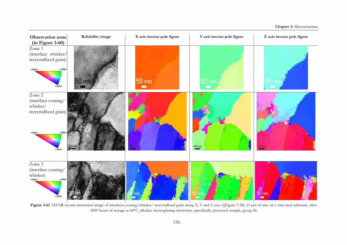
Chapter 3: Microstructure
156
Observation zone (in Figure 3-60)
Reliability image X axis inverse pole figure Y axis inverse pole figure Z axis inverse pole figure
Zone 1 (interface whisker/ recrystallized grain)
Zone 2 (interface coating/ whisker/ recrystallized grain)
Zone 3 (interface coating/ whisker)
Figure 3-61 ASTAR crystal orientation image of interfaces coating/whisker/ recrystallized grain along X, Y and Z axes (§Figure 3-58); 15 µm of zinc on 1 mm steel substrate, after
2000 hours of storage at 60°C (alkaline electroplating electrolyte, specifically processed sample, group II)

Chapter 3: Microstructure of zinc coating and whiskers
157
The results obtained by EBSD and ASTAR in this section show the microstructure of the samples:
There is high porosity in the zinc coating, which is composed of columnar-grain structure with needle-like grains (0.1-0.2 µm wide and 0.5-0.6 µm long), most of them deformed, with a preferred orientation between <2-1-10> and <10-10>, corresponding to planes between {-12-10} and {10-10} respectively, parallel to the coating surface (Figure 3-62). Results correspond to observation done by X-ray Diffraction (§2.3.5.2).
Recrystallized single-crystal whiskers with <10-10> orientation respect to the Z-axis, parallel to the coating surface (Figure 3-63).
Recrystallized grains are found in the regions close to hillocks and whiskers.
Dislocations are observed in both hillocks and whiskers. Until now, no experimental evidence of dislocations in whiskers had been reported before our observations. They can be a key feature in understanding the mechanism of whiskers growth.
Figure 3-62 Preferred orientation of crystallographic planes in the zinc coating
Figure 3-63 Whisker orientation <0001> respect to Z axis

Chapter 3: Chemical analysis
158
3.6 CHEMICAL ANALYSIS OF ZINC COATING AND WHISKERS
While IMC (Intermetallic compounds) of Cu/Sn have been observed and identified as an influence on the tin whiskers growth (§1.2.4), no clear observation of IMC has been reported in the case of zinc whiskers. As complement of the microstructure study, a chemical analysis of the zinc coating, hillocks and whiskers in specifically processed samples (group II) was done in order to detect the presence of IMC or other elements besides the zinc in the coating, hillocks and whiskers.
The same two specimens prepared for TEM observations (§3.5.2) were studied with EDX (Energy-dispersive X-ray spectroscopy) for chemical analysis, both from a sample corresponding to 15 µm of chromed zinc on 1 mm steel substrate, electroplated using alkaline electrolyte, after 2000 hours of storage at 60°C. Particular regions of the samples as well as determined linear profiles were analyzed by EDX for two different specimens, as follows:
A hillock which includes a small whisker of around 1.2 µm width and 5 µm length (§Figure 3-54)
A whisker parallel to the surface growing from a cauliflower-like hillock (§Figure 3-57)
3.6.1 First specimen (hillock) analysis
Figure 3-64 shows the three different zones analyzed by EDX, depicted with red circles in the image, as follows:
A small iron-rich zone between the chrome and the platinum (on the left of the image)
The chrome (black strip on the left of the image)
The zinc hillock (on the right)
Figure 3-64 Zones analyzed by EDX on the first specimen (hillock); 15 µm of zinc on 1 mm steel substrate, after 2000 hours of storage at 60°C (alkaline electroplating electrolyte, specifically processed sample, group II)

Chapter 3: Chemical analysis
159
Resulting chemical composition of the three analyzed zones is shown in Figure 3-65, with some remarkable observations as follows:
The iron-rich zone has up to 35% iron; the origin of this iron accumulation is unknown, but since it is placed between the chrome and the platinum (no contact with the zinc coating), it is assumed that it is a contamination not related to the electroplating processing.
The chrome has, as expected, a significant amount of chromium; however, there is also considerable content of zinc and oxygen. The zinc can be consequence of the coating roughness (some part of the zinc coating can be unintentionally included in the analyzed region) but also of the zinc contamination of the solution used for chrome plating (§2.1.2.1); the oxygen might come from superficial oxidation of the chrome. Traces of molybdenum, calcium, potassium and chlorine (in descending order, each of them with less than 2%) are also present; these elements were detected also in the HR-GDMS (High Resolution Glow Discharge Mass Spectrometry) chemical analysis of the same sort of samples (§2.3.4.2).
The hillock is, as expected, almost pure zinc, with some traces of iron and oxygen.
Figure 3-65 EDX analysis results of the hillock specimen (§Figure 3-64); 15 µm of zinc on 1 mm steel substrate, after 2000 hours of storage at 60°C (alkaline electroplating electrolyte, specifically processed sample, group II)
The following four different profiles, depicted in Figure 3-66 were analyzed by EDX in the hillock sample:
Profile 1: vertical 5-µm profile crossing the chrome
Profile 2: vertical 5-µm profile crossing the hillock
Profile 4: vertical 0.9-µm profile in zinc coating and hillock
Profile 3: horizontal 0.9-µm profile inside the zinc coating
0
10
20
30
40
50
60
70
80
90
100
Whisker root Cr layer Fe-rich zone
Ch
emic
al c
omp
osit
ion
[w
t.%
]
Zn
Fe
O
Cr
Hillock specimen

Chapter 3: Chemical analysis
160
Figure 3-66 Profiles analyzed by EDX on the first specimen (hillock); 15 µm of zinc on 1 mm steel substrate, after 2000 hours of storage at 60°C (alkaline electroplating electrolyte, specifically processed sample, group II)
Both 5-µm vertical profiles 1 and 2 (Figure 3-67 and Figure 3-68 respectively) show some interesting features:
An apparent oxidation of porosities in the zinc coating; this increase of oxygen concentration might be taken with care since the local thickness of the sample decreases in these zones, and thus the absortion of oxygen irradiation is significantly lowered, producing the high contents of oxygen in the EDX profiles.
The chrome (profile 1) is, as expected, rich in chromium; an iron-rich zone is observed over the chromes layer. Chemical composition of both chrome and iron-rich zone were already shown in Figure 3-65.
The porosity of the zinc coating, represented by the noise of the zinc profile is due to the cavities present in the coating, composed of very small grains. On the other hand, the hillock, composed of larger grains, has a very flat zinc profile due to the less quantity of cavities.
Concerning profiles 3 and 4 (Figure 3-69 and Figure 3-70) show the same features observed above in the profiles 1 and 2 but with higher resolution: cavities and porosity of the zinc coating as well as the non-porosity of the hillock.
In the profile 4 of the hillock specimen, the pattern of the microstructure of the zinc coating is schemed, combining chevron-pattern zones and vertical-line-patter zones (§Figure 3-56).

Chapter 3: Chemical analysis
161
Figure 3-67 EDX profile 1 on the hillock specimen (§Figure 3-66): vertical profile crossing the chrome
Figure 3-68 EDX profile 2 on the hillock specimen (§Figure 3-66: vertical profile crossing the hillock
0
20
40
60
80
100
0 1 2 3 4 5
Ch
emic
al c
omp
osit
ion
[w
t.%
]
µm
Profile 1 of hillock specimen
Zn
Fe
O
Cr
Pt
0
10
20
30
40
0 1 2 3 4 5Ch
emic
al c
omp
. [w
t.%
]
µm
Fe
O
Cr
0
20
40
60
80
100
0 1 2 3 4 5
Ch
emic
al c
omp
osit
ion
[w
t.%
]
µm
Profile 2 of hillock specimen
Zn
Fe
O
Cr
Pt
0
10
20
30
40
0 1 2 3 4 5Ch
emic
al c
omp
. [w
t.%
] µm
Fe
O
Cr
Fe-rich
Cavity
Zn porosity
Fe-rich Chrome
Zn porosity hillock (flat profile)

Chapter 3: Chemical analysis of zinc coating and whiskers
162
Figure 3-69 EDX profile 3 on the hillock specimen (§Figure 3-66): vertical profile in zinc coating and hillock (traces of Cu and Fe under 0.5 %)
Figure 3-70 EDX profile 3 on the hillock specimen (§Figure 3-66): horizontal profile inside the zinc coating (traces of Cu and Fe under 0.5 %)
0
20
40
60
80
100
0 200 400 600 800
Ch
emic
al c
omp
osit
ion
[w
t.%
]
nm
Profile 3 of hillock specimen
Zn
O
Zn porosity hillock (flat profile)
Cavity
0
20
40
60
80
100
0 200 400 600 800
Ch
emic
al c
omp
osit
ion
[w
t.%
]
nm
Profile 4 of hillock specimen
Zn
O
Zn porosity
Cavity

Chapter 3: Chemical analysis of zinc coating and whiskers
163
3.6.2 Second specimen (whisker) analysis
Figure 3-71 shows the four different zones analyzed by EDX, depicted with red frames in the image, as follows:
A hillock (on the left of the image)
A whisker (square on the center of the image)
The zinc coating (on the lower part of the image)
A small iron-rich zone between the zinc coating and the whisker (a magnified image is shown as well as its image map, where the accumulation of iron is marked as blue)
a)
b)
c)
Figure 3-71 a) Zones analyzed by EDX on the whisker specimen, b) magnified HAADF image, c) map data
Resulting chemical composition of the four analyzed zones is shown in Figure 3-72:
The iron-rich zone has less than 2% iron (very low compared to the iron-rich zone of the hillock specimen, §Figure 3-65); in the whisker specimen, the iron-rich zone is placed

Chapter 3: Chemical analysis of zinc coating and whiskers
164
between the whisker and the zinc coating. The origin of this iron accumulation is unknown but it can be related to dilution effect of iron signal in EDX analysis due to variation of thickness of the specimen.
The hillock, the zinc coating and the whisker are all almost pure zinc with few traces of iron; the observed oxygen content can be due to superficial oxidation of the thin foil specimen.
Figure 3-72 EDX analysis results of the whisker specimen (§Figure 3-71); 15 µm of zinc on 1 mm steel substrate, after 2000 hours of storage at 60°C (alkaline electroplating electrolyte, specifically processed sample, group II)
The following two different profiles, depicted in Figure 3-73 were analyzed by EDX in the whisker specimen:
Profile 1: vertical 3-µm profile in zinc coating, whisker and hillock
Profile 2: horizontal 1.8- µm profile in the zinc coating
Figure 3-74 shows the profile 1 which includes the zinc coating, the whisker and the hillock. Two iron-rich zones are observed. The first one (blue in the center of the EDX map data (Figure 3-74-b) is located between the coating and the whisker; it was already analyzed in Figure 3-72 with less than 2% of iron.
0
10
20
30
40
50
60
70
80
90
100
Hillock Whisker Zn coating Fe-rich zone
Ch
emic
al c
omp
osit
ion
[w
t.%
]
Zn
Fe
O
Whisker specimen
0
1
2
3
Hillock Whisker Zn coating Fe-rich zone
Ch
emic
al c
omp
. [w
t.%
]
Zn
Fe
O

Chapter 3: Chemical analysis of zinc coating and whiskers
165
Figure 3-73 Profiles analyzed by EDX on the whisker specimen a) HAADF picture b) EDX Map data
Figure 3-74 EDX profile 1 on the whisker sample (Figure 3-73): vertical profile in zinc coating, whisker and hillock
0
20
40
60
80
100
0 0,5 1 1,5 2 2,5 3
Che
mic
al c
ompo
sitio
n [w
t.%]
µm
Profile 1 of whisker specimen
Zn
Fe
O
Cr
Pt
Zn coating Whisker Hillock
Fe-high-rich zone
0
1
2
3
4
0 0,5 1 1,5 2 2,5 3
Che
mic
al c
omp.
[wt.%
]
µm
Zn
Fe
O
Cr
Pt
Fe-rich zone

Chapter 3: Chemical analysis of zinc coating and whiskers
166
The second zone is highly rich in iron (20%) and located at the top of the profile 1, the iron content is comparable to the zone observed between the chrome and the coating in the first specimen (hillock) (30%, §Figure 3-65).
The profile 2 is illustrated in the Figure 3-75, showing the characteristic porosity of the zinc coating, already observed in the hillock specimen (§Figure 3-72).
Figure 3-75 EDX profile 2 on the whisker specimen (Figure 3-73): horizontal profile in zinc coating (traces of Fe under 0.5 %)
Iron-rich zones are found but they are found in the interface of the sample with the platinum added during FIB preparation or between the whisker and the zinc coating but not inside the coating itself. The origin of this iron accumulation is unknown.
The results obtained by chemical analyses do not show intermetallic compounds in the zinc coating, the recrystallized grains, the hillocks nor the whiskers; nevertheless, some iron-rich zones were observed.
The chemical profiles also show the porosity of the coating represented in the noise of the zinc profile.
0
20
40
60
80
100
0 0,2 0,4 0,6 0,8 1 1,2 1,4 1,6 1,8
Che
mic
al c
ompo
sitio
n [w
t.%]
µm
Profile 2 of whisker specimen
Zn
Fe
O
Zn porosity

Chapter 3: Summary
167
3.7 SUMMARY OF EFFECT OF AGING TREATMENTS
The main terminology of whiskers growth features was defined: whiskers, hillocks and bumps.
Among the main characteristics of whiskers are:
Diameter: 0.5 to 4 µm
Length: up to 1 mm
All possible angles respect to the surface coating (mainly from 30 to 60°C)
Presence of kinks and striations (both longitudinal and circumferential)
Whisker grows from the base of the whisker rather than from the tip
Concerning the influencing parameters on whiskers growth, it was observed:
Temperature and zinc coating thickness favor the whiskers growth.
Steel substrate thickness disfavors the whiskers growth in alkaline-origin samples (although it favors the growth in acid-origin samples).
The growth in acid-origin samples is concentrated on some irregularities of the surface, while in alkaline- is uniformly distributed on the surface.
Temperature decreases whiskers density but increases whiskers length. Temperature also increases whiskers growth rate and it seems to decrease the incubation time for whiskers growth.
TEM observations show dislocations in whiskers and hillocks. Until now, no experimental evidence of dislocations in whiskers had been reported before our observations.
The results obtained by EBSD and ASTAR in this section show the microstructure of the samples, particularly two different features
Columnar-grain structure of the zinc coating with needle-like grains with a preferred orientation between <2-1-10> and <10-10>, corresponding to planes between {-12-10} and {10-10} respectively, parallel to the coating surface. Results correspond to observation done by X-ray Diffraction.
Single-crystal whiskers with <10-10> orientation respect to the Z-axis, parallel to the coating surface.
On the other hand, the results obtained by chemical analyses do not show intermetallic compounds in the zinc coating, the recrystallized grains, the hillocks nor the whiskers; nevertheless; porosity of the zinc coating was observed as well as some iron-rich zones from unknown origin.
Dislocations, recrystallization and the absence of intermetallic compounds are important features for understanding the mechanism of whiskers growth.

168
Chapter 4. Discussion of results
Chapter 4
Discussion of results
The fourth chapter discusses the results presented in the third chapter, to evaluate quantitatively some
parameters that influence whiskers growth.
First, influence of temperature on material growth and on stress relaxation during samples storage is addressed.
Afterwards, kinetic aspects of mass diffusion during the whiskers growth are also discussed and maximal whiskers
growth rates are estimated; whiskers growth models are proposed both analytical and phenomenological, in order to
predict the growth of whiskers during samples storage. Finally, a short discussion of the microstructure observations
is addressed.
Stress relaxation Material growth Kinetic aspects of mass diffusion Whiskers growth model Microstructure Summary of discussion of results

Chapter 4: Stress relaxation
169
4.1 STRESS RELAXATION
Relation of material growth and stress relaxation is studied; apparent activation energy of the stress relaxation phenomenon is calculated as well as stress relaxation coefficients.
4.1.1 Material growth and stress relaxation
Compressive residual stress was measured only before and after storage of samples at different temperatures. Stress is relaxed during storage of samples by growth of material out of the surface, through both whiskers and hillocks (§3.4); Figure 4-1 plots the relaxed stress values (Δ ∞) versus both whiskers growth (Ωw-∞) and total growth (Ω∞, whiskers and hillocks combined), for all specifically processed samples.
Figure 4-2 shows the influence of different parameters (zinc coating and steel susbtrate thicknesses) in the curves of relaxed stress versus whiskers growth (Ωw-∞) and total growth (Ω∞), for samples electroplated with alkaline electrolyte (curves for acid electrolyte are illustrated in Figure A5-1 of Appendix 5).
Both figures show that stress relaxation seems to be favored by both total and whiskers growth, particularly at low material growth values. At high values of material growth, the influence of growth in the relaxed stress becomes almost negligible. That is, at a first stage, part of the residual stress is relaxed by material growth, followed by a stage where stress remains constant.
Figure 4-1 Influence of growth in relaxed stress (Δ ∞) for specifically processed samples (all samples combined), a) total growth (Ω∞), b) whiskers growth (Ωw-∞)
0
20
40
60
80
100
120
140
160
180
100 1 000 10 000 100 000
Stre
ss r
elie
f (
∞) [
MP
a]
a) Total growth (Ω∞) [µm³/mm2 surface]
0
20
40
60
80
100
120
140
160
180
10 100 1 000 10 000
Stre
ss r
elie
f (
∞) [
MP
a]
b) Whiskers growth (Ωw-∞) [µm³/mm2 surface]
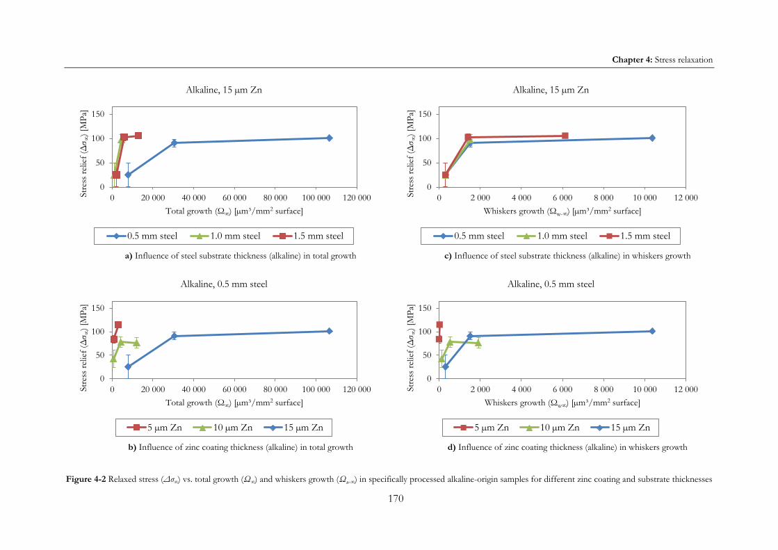
Chapter 4: Stress relaxation
170
a) Influence of steel substrate thickness (alkaline) in total growth
c) Influence of steel substrate thickness (alkaline) in whiskers growth
b) Influence of zinc coating thickness (alkaline) in total growth
d) Influence of zinc coating thickness (alkaline) in whiskers growth
Figure 4-2 Relaxed stress (Δ ∞) vs. total growth (Ω∞) and whiskers growth (Ωw-∞) in specifically processed alkaline-origin samples for different zinc coating and substrate thicknesses
0
50
100
150
0 20 000 40 000 60 000 80 000 100 000 120 000Stre
ss r
elie
f (
∞) [
MP
a]
Total growth (Ω∞) [µm³/mm2 surface]
Alkaline, 15 µm Zn
0.5 mm steel 1.0 mm steel 1.5 mm steel
0
50
100
150
0 2 000 4 000 6 000 8 000 10 000 12 000Stre
ss r
elie
f (
∞) [
MP
a]
Whiskers growth (Ωw-∞) [µm³/mm2 surface]
Alkaline, 15 µm Zn
0.5 mm steel 1.0 mm steel 1.5 mm steel
0
50
100
150
0 20 000 40 000 60 000 80 000 100 000 120 000Stre
ss r
elie
f (
∞) [
MP
a]
Total growth (Ω∞) [µm³/mm2 surface]
Alkaline, 0.5 mm steel
5 µm Zn 10 µm Zn 15 µm Zn
0
50
100
150
0 2 000 4 000 6 000 8 000 10 000 12 000Stre
ss r
elie
f (
∞) [
MP
a]
Whiskers growth (Ωw∞) [µm³/mm2 surface]
Alkaline, 0.5 mm steel
5 µm Zn 10 µm Zn 15 µm Zn

Chapter 4: Stress relaxation
171
4.1.2 Apparent activation energy of stress-relaxation
Compressive residual stress relaxation is strongly influenced by temperature of samples storage, as illustrated in Figure 4-3, for the different samples and influencing parameters.
Storage at 60°C was done only for samples with 1 mm steel substrate, while storage at 150 to 200°C was done for samples with 0.5 and 1.5 mm steel substrate; in order to correlate the stress relaxation and temperature, we assume that the stress relaxation at 60°C does not change with the steel substrate thickness.
Stress relaxation is therefore a thermally activated phenomenon and the relaxed stress can be correlated with temperature by an Arrhenius-type equation, as follows:
Equation 4-1
where: Δ ∞ relaxed compressive residual stress A pre-exponential factor for stress relaxation Ea apparent activation energy of the stress relaxation during the material growth R universal gas constant T temperature
The slopes of curves from Figure 4-3 allow determining apparent activation energies of stress relaxation (Ea ) for each sample; pre-exponential factors for stress relaxation (A ) are also calculated. Both Ea and A values are included in Table A5-1 (Appendix 5) for all studied samples, while apparent activation energies are illustrated in Figure 4-4.
Good fit is obtained (R²> 0.92) for all correlations of diverse samples. Apparent activation energy values varies from 6.7 to 24.1 kJ/mol in all samples; for alkaline-electrolyte chromed samples in particular, the range of apparent activation energy goes from 13.7 to 24.1 kJ/mol. These values correspond only to a fraction (maximum 26%) of the bulk diffusion for zinc (92kJ/mol) [68], which suggests surface diffusion mechanism for the stress relaxation.
Figure 4-4 shows that the apparent activation energy of stress relaxation is strongly favored by the presence of chrome; apparent activation energy is higher for samples electroplated with alkaline electrolyte than for those electroplated with acid electrolyte. On the other hand, it is not clear how the other parameters (zinc coating thickness and steel substrate thickness) influence this apparent activation energy.
)

Chapter 4: Stress relaxation
172
a) Influence of steel thickness (alkaline)
b) Influence of steel thickness (acid)
c) Influence of zinc coating thickness (alkaline)
d) Influence electrolyte and chrome
Figure 4-3 Relaxed stress (Δ ∞) vs. temperature (1/RT) in specifically processed samples for different influencing parameters (samples at 60°C correspond to 1 mm steel substrate)
0
1
2
3
4
5
In
1/RT [1/°K]
Alkaline, 15 µm Zn
0.5 mm steel 1.5 mm steel200°C 150°C 60°C
0
1
2
3
4
5
In
1/RT [1/°K]
Acid, 10 µm Zn
0.5 mm steel 1.5 mm steel
200°C 150°C 60°C
0
1
2
3
4
5
Ln
1/RT [1/°K]
Alkaline, 0.5 mm steel
5 µm Zn 10 µm Zn 15 µm Zn
0
1
2
3
4
5
In
1/RT [1/°K]
10 µm Zn, 0.5 mm steel
Acid chromed Alkaline, chromed Alkaline, non-chromed
200°C 150°C 60°C 60°C 150°C 200°C

Chapter 4: Stress relaxation
173
Figure 4-4 Apparent activation energy (Ea ) of stress relaxation in samples storage
4.1.3 Stress relaxation coefficient
Figure 4-5 shows the measured stress of a specifically processed sample (15 µm on 0.5 mm steel) at both 150°C and 200°C. The corresponding figures of all other samples are included in the appendix 5 (Figure A5-2 to Figure A5-5).
Since residual stress was measured only before and after storage, there is not experimental data describing the stress behavior during the storage time. We make therefore two assumptions:
i) Stress is relaxed only through materials growth; despite storage temperature, no further stress is relaxed after growth saturation is reached, therefore stress remains constant ( (t) = ∞).
ii) Stress is relaxed linearly with time until growth saturation time is reached (t∞). Stress relaxation coefficients (k ) are determined from stress-time curves slopes, and they are shown in Figure 4-6.
Consequently, time-behavior of residual stress until growth saturation can be described by the following equation:
Equation 4-2 for
where:
t storage time t∞ whiskers growth saturation time (t) compressive residual stress as function of time
0
5
10
15
20
25
30
5µm
Zn,
0.5
mm
ste
el
10µm
Zn,
0.5
mm
ste
el
15µm
Zn,
0.5
mm
ste
el
15µm
Zn,
1.5
mm
ste
el
10µm
Zn,
0.5
mm
ste
el
10µm
Zn,
0.5
mm
ste
el
10µm
Zn,
1.5
mm
ste
el
7 µm
Zn,
0.5
mm
ste
el
Act
ivat
ion
ener
gy [k
J/m
ol]
Alkaline without Cr
Alkaline with Cr
Acid with Cr
Sam
ple
B
(fro
m in
du
stri
al s
ite)

Chapter 4: Stress relaxation
174
0 compressive residual stress before storage
∞ compressive residual stress after stress relaxation k stress relaxation coefficient
Figure 4-5 Time-behavior of compressive residual stress (relaxation) of samples (specifically processed sample
(15 µm on 0.5 mm steel substrate)
Figure 4-6 Calculated stress relaxation coefficients (k )
As shown in Figure 4-6, stress relaxation coefficients vary considerably from temperatures close to room conditions (30°C and 60°C) to high temperatures (150°C and 200°C), that is, stress is relaxed faster as temperature increases. The influence of other parameters in the stress relaxation coefficient is not clear, such as zinc coating thickness, steel substrate thickness and
0
20
40
60
80
100
120
140
0 20 40 60 80 100 120 140
Com
pres
sive
str
ess
[MP
a]
Time [min]
200°C
150°C
saturation
1E-5
1E-4
1E-3
1E-2
1E-1
1E+0
1E+1
1E+2
1E+3
Alk
alin
e, 5
µm
Zn
(0.5
mm
ste
el)
Alk
alin
e, 1
0 µm
Zn
(0.5
mm
ste
el)
Alk
alin
e, 1
5 µm
Zn
(0.5
mm
ste
el)
Alk
alin
e, 1
5µm
Zn
(1m
m s
teel
)
Alk
alin
e, 1
5 µm
Zn
(1.5
mm
ste
el)
Alk
alin
e, 1
0 µm
Zn
(0.5
mm
ste
el)
non-
chro
med
Aci
d 10
µm
Zn
(
0.5m
m s
teel
)
Aci
d, 1
0µm
Zn
(1m
m s
teel
)
Aci
d 10
µm
Zn
(
1.5m
m s
teel
)
Sam
ple
B, 7
µm Z
n (0
.6m
m s
teel
)
K [k
Pa/
s] 30°C
60°C
150°C
200°C

Chapter 4: Stress relaxation
175
electroplating electrolyte. Nevertheless, these values must be taken cautiously due to both large confidence intervals of the measured stress and considerable difference in storage time of samples (approximately one hour for 150°C and 200°C, and more than 2000 hours for 30°C and 60°C).
Stress relaxation seems to be sligthly favored by both total and whiskers growth, particularly at low material growth values. At high values of material growth, the influence of growth in the relaxed stress becomes almost negligible.
It was found that surface diffusion is the most plausible mechanism controlling stress relaxation, based on calculated apparent activation energies: from 6.7 to 24.1 kJ/mol (in chromed alkaline-samples, 13.7 to 24.1 kJ/mol.)
Residual stress is relaxed faster as temperature increases. The influence of other parameters in the stress relaxation coefficient is not clear, such as zinc coating thickness, steel substrate thickness and electroplating electrolyte.

Chapter 4: Influence of temperature on material growth
176
4.2 MATERIAL GROWTH
4.2.1 Apparent activation energy of material growth
Figure 4-7 shows the influence of temperature on whiskers growth (Ωw-∞) and total growth (Ω∞) after saturation for different zinc coating thicknesses in samples electroplated with alkaline electrolyte; influence of other parameters (steel susbtrate thickness, electroplating electrolyte and presence of chrome) is illustrated in Figure A6-1 and Figure A6-2 (Appendix 6).
As explained in 4.1.2, storage at 60°C was done only for samples with 1 mm steel substrate, while storage at 150 to 200°C was done for samples with 0.5 and 1.5 mm steel substrate; in order to correlate the growth and temperature, we assume that the growth at 60°C does not change with the steel substrate thickness.
a) Total growth (Ω∞)
b) Whiskers growth (Ωw-∞)
Figure 4-7 a) Total growth (Ω∞) and b) whiskers growth (Ωw-∞) vs. temperature in specifically processed samples electroplated with alkaline electrolyte for different zinc coating thicknesses on 0.5 mm steel substrate (samples at
60°C correspond to 1 mm steel substrate)
In all cases, the growth increases exponentially with temperature; it is also observed that the growth is favored by zinc coating thickness and disfavored by steel substrate thickness. On the
0
20 000
40 000
60 000
80 000
100 000
120 000
50 75 100 125 150 175 200
Tot
al g
row
th (
Ω∞)
[µm
³/m
m2
surf
ace]
Temperature [°C]
5 µm Zn 10 µm Zn 15 µm Zn
0
2 000
4 000
6 000
8 000
10 000
12 000
50 75 100 125 150 175 200
Whi
sker
s gr
owth
(Ω
w-∞
) [µ
m³/
mm
2 su
rfac
e]
Temperature [°C]
5 µm Zn 10 µm Zn 15 µm Zn

Chapter 4: Influence of temperature on material growth
177
other hand, while very small influence of electroplating eletrolyte is observed, no influence of chrome presence is detected.
Since material growth is thermally activated, data of total growth rate (whiskers and hillocks combined) and whiskers growth rate at 150°C, 175°C and 200°C (temperatures of SEM storage) were fit to an Arrhenius-type equation, as follows:
Equation 4-3
Equation 4-4
where:
Ω' total growth rate (calculated from growth vs. time data) Ωw' whiskers growth rate (calculated from growth vs. time data) AΩ pre-exponential factor for total growth AΩw pre-exponential factor for whiskers growth EaΩ apparent activation energy of total growth EaΩw apparent activation energy of whiskers growth
Equation 4-3 and Equation 4-4 are used to estimate the apparent activation energy of both total growth and whisker growth, as well as the pre-exponential factors; these energies are shown in Figure 4-8 for all studied samples (values are included in Table A6-1, Appendix 6). In general, apparent activation energy of whiskers growth is larger than one of total growth (whiskers and hillocks combined): while apparent activation energy of the whiskers growth varies from 24 to 96 kJ/mol, in the case of the total growth it varies from 30 to 76 kJ/mol.
Figure 4-8 Apparent activation energy of whiskers growth (EaΩw) and total growth (EaΩ) (whiskers and hillocks
combined)
0
20
40
60
80
100
5µm
Zn,
0.5
mm
ste
el
15µm
Zn,
0.5
mm
ste
el
15µm
Zn,
1.5
mm
ste
el
10µm
Zn,
0.5
mm
ste
el
10µm
Zn,
1.5
mm
ste
el
Act
ivat
ion
ener
gy [k
J/m
ol]
Total growth
Whiskers growth
Alkaline without Cr
Alkaline with Cr
Acid with Cr

Chapter 4: Influence of temperature on material growth
178
Both apparent activation energies (for total growth and whiskers growth) seem to be favored by zinc coating thickness and slighly disfavored by steel substrate thickness. The alkaline electrolyte and the chrome seems to favor the activation energy.
4.2.2 Growth rate estimation
The data fitting was done only with samples from SEM storage (150 to 200°C) since there is not enough data before growth saturation for storage at 60°C. Equation 4-3 and Equation 4-4, used for calculating apparent activation energies from growth rates data at 150, 175 and 200°C, are used to estimate growth rates at 60°C; these estimated values are compared with maximal experimental growth rates, as illustrated in Figure 4-9 (specifically processed sample electroplated with alkaline electrolyte, 15 µm zinc coating on 0.5 mm steel). In the figure, apparent activation energy corresponds to the slope of the curves.
Figure 4-9 Total growth rate (Ω') and whiskers growth rate (Ωw') vs. temperature (specifically processed sample electroplated with alkaline electrolyte, 15 µm zinc coating on 0.5 mm steel susbtrate); experimental values at 60°C
correspond to samples with 1 mm steel substrate
Table 4-1 shows this comparison between experimental and calculated rates for all studied samples. Growth rates are expressed not only in terms of volume (Ω' and Ωw') but also in terms of length (Lw') in the case of whiskers.
-10
-8
-6
-4
-2
0
2
4
6
LnΩ
'
1/RT [1/°K]
Whiskers growth rate (Ωw) [µm³]
Total growth (Ω) [µm³]
Experimental
Calculated
Experimental
Calculated
200°C 60°C 150°C

Chapter 4: Influence of temperature on material growth
179
Table 4-1 Comparison of calculated and experimental total and whiskers growth at 60°C (calculated from Equation 4-3 and Equation 4-4); experimental data for 60°C storage correspond to samples with 1 mm steel susbtrate
Electrolyte
Zinc coating thickness
Steel substrate thickness
Total growth rate (Ω')
at 60°C [µm³/s]
Whiskers growth rate (Ωw')
at 60°C [µm³/s]
Whiskers growth rate (Lw')
at 60°C [nm/s]
Calc..
Exp. (1 mm steel)
Ratio Exp./ Calc.
Calc. Exp. (1 mm steel).
Ratio Exp./ Calc.
Calc. Exp. (1 mm steel).
Alkaline 5µm 0.5mm 2.3∙10-3 0 - 0 0 - 0 0
Alkaline 15µm 0.5mm 3.3∙10-1 7.1∙10-3 47 9.0∙10-4 2.0∙10-4 5 1.1 0.2
Alkaline 15µm 1.5mm 1.1∙10-1 1.8∙10-3 63 1.2∙10-4 2.0∙10-4 6 1.6 0.2
Alkaline (no chromed)
10µm 0.5mm 4.9∙10-1 - - 1.3∙10-1 - - 161 -
Acid 10µm 1.5mm 5.3∙10-1 8.4∙10-4 621 1.4∙10-1 2.1∙10-4 675 179 0.1

Chapter 4: Influence of temperature on material growth
180
For chromed samples electroplated with alkaline electrolyte, the estimated whiskers growth rates at 60°C are between 5 and 6 times the corresponding experimental data, that is, they are in the overestimation range. In the case of samples electroplated with acid electrolytes, the experimental and estimated data do not fit so well as in the case of alkaline samples (between two and three orders of magnitude of difference).
This difference can be result of the precision of the growth kinetics data in storage at 60°C (in environmental chambers), which is not as good as at 150 to 200°C in the SEM storage. Besides, the storage conditions environmental chambers are not the same as in the SEM, mainly concerning humidity (60% of relative humidity in environmental chambers and vacuum in SEM storage).
Both apparent activation energies (for total growth and whiskers growth) are favored by zinc coating thickness, alkaline electrolyte (compared with acid) and chrome, and slighly disfavored by steel substrate thickness.
Whiskers growth rate estimation for samples electroplated with alkaline electrolyte can be obtained (5 to 6 times the corresponding experimental data).

Chapter 4: Mass diffusion
181
4.3 KINETIC ASPECTS OF MASS DIFFUSION
Lindborg proposed equations to calcul growth rate for both lattice diffussion and grain boundary diffusion [28]. Table 4-2 includes the values used for Equation 1-3 and Equation 1-4 (§1.4.2).
Growth rate for diffusion through the lattice:
Equation 4-5
Growth rate for diffusion through the grain boundaries:
Equation 4-6 � Diffusion coefficients D in Equation 4-5 and Equation 4-6 are calculated from the following
equation:
Equation 4-7
Table 4-2 Values used for Equation 4-5 and Equation 4-6 in order to calculate whisker growth rates
Variable Value Reference �a atomic volume 9.2∙10-6 m3/mol [28]
RW whisker radius 0.5 µm Experimental§2.4.2.2.1
grain border thickness 0.5 nm [46]
dav average grains diameter 0.2 µm Experimental§3.5.1
D0 pre-exponential for lattice diffusion 7.6∙10-6 m2/s
[46] [68]
for grain boundary diffusion
2.2∙10-5 m2/s
Q activation energy
for lattice diffusion 92 kJ/mol
for grain boundary diffusion
60 kJ/mol
Figure 4-10 shows the whiskers growth rate calculated by Equation 4-5 and Equation 4-6 from experimental data for both grain boundary and lattice diffusion if compressive stress is assumed to be 100 MPa (value close to the mean measured stress of samples before storage).
Grain boundary diffusion is faster than lattice diffusion, this difference is increased as temperature is higher. While at 20°C, grain boundary diffusion is more than 2000 times faster than lattice diffusion, at 200°C it is only 25 times faster.

Chapter 4: Mass diffusion
182
Figure 4-10 Growth rate for both lattice diffussion and grain boundary diffusion ( =100 MPa)
Whiskers growth rate is calculated, using stress ( 0) measured before storage, for all samples stored at different temperatures and compared with the maximal observed growth rate. Figure 4-11 compares the experimental data with calculated growth values for grain boundary and lattice diffusion.
As explained in 4.1.2, storage at 60°C was done only for samples with 1 mm steel substrate, while storage at 150 to 200°C was done for samples with 0.5 and 1.5 mm steel substrate; in order to correlate the growth and temperature, we assume that the growth rate at 60°C does not change with the steel substrate thickness.
Two different growth rates are calculated, for two different sort of activation energy values:
Activation energy values from literature (Table 4-2): 60 and 92 kJ/mol for grain boundary and lattice diffusion respectively (broken lines in Figure 4-11).
Activation energy values 10% smaller than values from literature: 54 and 83 kJ/mol for grain boundary and lattice diffusion respectively (solid lines in Figure 4-11).
Calculated growth rates for lattice diffusion are several orders of magnitude larger than experimental growth values, particulary at low temperatures (30 and 60°C).
For grain boundary diffusion on the other hand, data fit is better, since almost all experimental data (exception of the only data at 30°C) are found within (or almost) the band limited by the two activation energy values (54 and 60 kJ/mol).
1E-9
1E-8
1E-7
1E-6
1E-5
1E-4
1E-3
1E-2
1E-1
1E+0
30 60 90 120 150 180
Whi
sker
gro
wth
rat
e (µ
m/s
)
Temperature [°C]
hb: grain boundary diffusion hs: lattice diffussion

Chapter 4: Mass diffusion
183
Sam
ple
A
(20
µm Z
n, 0
.5 m
m s
teel
)
Sam
ple
B
(7 µ
m Z
n, 0
.5 m
m s
teel
)
Alk
alin
e el
ectr
olyt
e (5
µm
Zn,
0.5
mm
ste
el)
Alk
alin
e el
ectr
olyt
e (1
0 µm
Zn,
0.5
mm
ste
el)
Alk
alin
e el
ectr
olyt
e (1
5 µm
Zn,
0.5
mm
ste
el)
Alk
alin
e el
ectr
olyt
e (1
5 µm
Zn,
1.5
mm
ste
el)
Alk
.ele
ctro
lyte
, no-
chro
med
(1
0 µm
Zn,
0.5
mm
ste
el)
Aci
d el
ectr
olyt
e (1
0 µm
Zn,
0.5
mm
ste
el)
Aci
d el
ectr
olyt
e (1
0 µm
Zn,
1.5
mm
ste
el)
Sam
ple
A
(20
µm Z
n, 0
.5 m
m s
teel
)
Sam
ple
B
(7 µ
m Z
n, 0
.5 m
m s
teel
)
Alk
alin
e el
ectr
olyt
e (5
µm
Zn,
0.5
mm
ste
el)
Alk
alin
e el
ectr
olyt
e (1
0 µm
Zn,
0.5
mm
ste
el)
Alk
alin
e el
ectr
olyt
e (1
5 µm
Zn,
0.5
mm
ste
el)
Alk
alin
e el
ectr
olyt
e (1
5 µm
Zn,
1.5
mm
ste
el)
Alk
.ele
ctro
lyte
, no-
chro
med
(1
0 µm
Zn,
0.5
mm
ste
el)
Aci
d el
ectr
olyt
e (1
0 µm
Zn,
0.5
mm
ste
el)
Aci
d el
ectr
olyt
e (1
0 µm
Zn,
1.5
mm
ste
el)
Figure 4-11 Comparison of experimental and calculated growth rate for a) grain boundary diffusion (Ea: 54 and 60 kJ/mol) and b) lattice diffusion (Ea: 83 and 92 kJ/mol)
1E-8
1E-7
1E-6
1E-5
1E-4
1E-3
1E-2
1E-1
1E+0
Whi
sker
s gr
owth
rat
e (h
s) [µ
m/s
]
b) Lattice diffusion (hs); solid line for Ea=83 kJ/mol and broken line for Ea=90 kJ/mol)
1E-8
1E-7
1E-6
1E-5
1E-4
1E-3
1E-2
1E-1
1E+0
Whi
sker
s gr
owth
rat
e (h
b) [µ
m/s
] a) Grain boundary diffusion (hb); solid line for Ea=54 kJ/mol and broken line for
Ea=60 kJ/mol)
200°C exp.
175°C exp.
150°C exp.
60°C exp.
30°C exp.
200°C calc. 54 kJ/mol
175°C calc. 54 kJ/mol
150°C calc. 54 kJ/mol
60°C calc. 54 kJ/mol
30°C calc. 54 kJ/mol
200°C calc. 60 kJ/mol
175°C calc. 60 kJ/mol
150°C calc. 60 kJ/mol
30°C calc. 60 kJ/mol
60°C calc. 60 kJ/mol
Chapter 4: Mass diffusion
184
Figure 4-12 and Figure 4-13 show the ratio of experimental and calculated growth for grain boundary diffusion with activation energy values of 54 and 60 kJ/mol respecively.
For calculated rates using 54 kJ/mol as activation energy (Figure 4-12), growth rates are overestimated (ratio>1) for high temperatures (150 to 200°C). Data fit for high temperatures is good (ratio<100) particulary at 200°C (ratio<3); however for rates at 60°C, growth rates are understimated (ratio<1) for almost one order of magnitude.
On the other hand, for calculated rates using 60 kJ/mol as activation energy (Figure 4-12), while data fit for high temperatures is not as good as with 54 kJ/mol, while for 60°C the data fit gets better. With this activation energy, growth rates are overestimated (ratio>1) for almost all samples not matter the storage temperature, which is convenient for eventual growth rates forecast in industrial applications at room temperature.
Calculated growth rates are influenced by several sources or errors such as the calculation of the diffusion constants, the large confidence intervals of the measured stress on the samples, as well as the grain size.
In general, it is observed that experimental data fits better with calculated values from grain boundary diffusion than with values from lattice diffusion. Therefore, it is reasonable to conclude that the whiskers growth is a grain boundary diffusion mechanism; this results agrees with Lindborg experiments, who found that the lattice diffusion cannot suply the required flow of atoms to the whisker root [46].
Good estimation of maximal whiskers growth rate of single whiskers can be obtained.
Whiskers growth is controlled by grain boundary diffusion mechanism since experimental data fits better with calculated values from grain boundary diffusion than with values from lattice diffusion
Apparent activation energy for whiskers growth rate of single whiskers is estimated between 54 and 60 kJ/mol.

Chapter 4: Mass diffusion
185
Sam
ple
A
(20
µm Z
n, 0
.5 m
m s
teel
)
Sam
ple
B
(7 µ
m Z
n, 0
.5 m
m s
teel
)
Alk
alin
e el
ectr
olyt
e (5
µm
Zn,
0.5
mm
ste
el)
Alk
alin
e el
ectr
olyt
e (1
0 µm
Zn,
0.5
mm
ste
el)
Alk
alin
e el
ectr
olyt
e (1
5 µm
Zn,
0.5
mm
ste
el)
Alk
alin
e el
ectr
olyt
e (1
5 µm
Zn,
1.5
mm
ste
el)
Alk
. ele
ctro
lyte
, no-
chro
med
(1
0 µm
Zn,
0.5
mm
ste
el)
Aci
d el
ectr
olyt
e (1
0 µm
Zn,
0.5
mm
ste
el)
Aci
d el
ectr
olyt
e (1
0 µm
Zn,
1.5
mm
ste
el)
Figure 4-12 Ratio of experimental and calculated growth rate (grain boundary diffusion), Ea=54 kJ/mol
Sam
ple
A
(20
µm Z
n, 0
.5 m
m s
teel
)
Sam
ple
B
(7 µ
m Z
n, 0
.5 m
m s
teel
)
Alk
alin
e el
ectr
olyt
e (5
µm
Zn,
0.5
mm
ste
el)
Alk
alin
e el
ectr
olyt
e (1
0 µm
Zn,
0.5
mm
ste
el)
Alk
alin
e el
ectr
olyt
e (1
5 µm
Zn,
0.5
mm
ste
el)
Alk
alin
e el
ectr
olyt
e (1
5 µm
Zn,
1.5
mm
ste
el)
Alk
. ele
ctro
lyte
, no-
chro
med
(1
0 µm
Zn,
0.5
mm
ste
el)
Aci
d el
ectr
olyt
e (1
0 µm
Zn,
0.5
mm
ste
el)
Aci
d el
ectr
olyt
e (1
0 µm
Zn,
1.5
mm
ste
el)
Figure 4-13 Ratio of experimental and calculated growth rate (grain boundary diffusion), Ea=60 kJ/mol
0,1
1
10
100
1000E
xper
imen
tal/
cal
cula
ted
grow
th
200°C
175°C
150°C
60°C
30°C
0,1
1
10
100
1000
Exp
erim
enta
l/ c
alcu
late
d gr
owth
200°C
175°C
150°C
60°C
30°C

Chapter 4: Kinetics of whiskers growth
186
4.4 WHISKERS GROWTH MODEL
In order to predict the whiskers growth, two different sorts of models are studied. First, analytical models based in mass diffusion equations that takes in account nucleation and growth of whiskers but not the growth saturation. Second, a phenomenological model based in JMAK (Johnson, Mehl, Avrami and Kolmogorov) equation that includes the growth saturation.
In all models, specifically processed samples electroplated with alkaline electroplating (chromed, 15 µm) at different steel substrate thicknesses are studied.
Models are calculated from SEM storage experiments (150, 175 and 200°C) of samples with 0.5 and 1.5 mm steel substrate. The calculated models allows extrapolating values for 60°C which are compared with experimental data from 60°C storage of sample with 1.0 mm steel substrate in environmental chambers (the available data of 60°C storage before saturation was not sufficient). As explained in 4.1.2, we assume that the growth at 60°C does not change with the steel substrate thickness.
4.4.1 Analytical models
This proposed model takes in account nucleation of grains and their growth into whiskers. This model uses both whiskers density experimental data and single whisker growth rate calculated from Lindborg [46] equations. Since the first analytical approach does not predict growth saturation, a modified model is also presented.
4.4.1.1 First analytical model (without growth saturation)
4.4.1.1.1 Experimental whiskers density data
Time-evolution of whiskers density follows the behaviour described with the following equation:
Equation 4-8
where: whiskers density time whiskers density at saturation time constant for nucleation
Figure 4-14 compares experimental whiskers densities with data fitting from Equation 4-8, for a specifically processed sample (0.5 mm steel substrate) at 150°C. In the figure, ratio of whisker density and whiskers density at saturation is plotted versus time.

Chapter 4: Kinetics of whiskers growth
187
Figure 4-14 Whiskers density data fitting (Equation 4-8); specifically processed sample (alkaline, 15 µm zinc coating
on 0.5 mm steel susbtrate) at 150°C
Time constant for nucleation ( ) is determined for two different steel substrate thicknesses at three temperatures (150, 175 and 200°C). Results, illustrated in Figure 4-15, indicate a very fast kinetics for the whiskers nucleation at high temperatures (from 150 to 200°C), beween 4.3 and 10 minutes (225 to 602 seconds).
Time constant is decreased by temperature, up to 3∙105 seconds (88 hours) at 60°C (not included in Figure 4-15), between two and three orders of magnitude larger than at high temperatures. As far as steel substrate thickness is concerned, it does not seem to influence considerably the time constants at a given temperature.
Figure 4-15 Time constant for nucleation ( ) determined for specifically processed samples (alkaline, 15 µm zinc
coating) on two different steel substrate thicknesses at three temperatures (150, 175 and 200°C)
4.4.1.1.2 Whiskers growth rate from Lindborg equations
As described above (§4.3), whiskers growth seems to have a grain boundary diffusion mechanism; linear growth rate, described by Equation 4-6, depends linearly of the residual stress.
Equation 4-6 that describes linear growth rate of a single whisker for grain boundary diffusion (h's) and depends linearly of the residual stress, can be rewritten as function of time in the form of Equation 4-9; the factor is independent of time but dependant of temperature because it includes Db (diffusion coefficient) and T, all data for calculating factor are taken from Table 4-2.
0
0,2
0,4
0,6
0,8
1
0 1000 2000 3000 4000
ρ(t)/ρ∞
time [min]
calculated
experimental
0
100
200
300
400
500
600
700
150°C 175°C 200°C
time
cons
tant
() [
s]
temperature
0.5 mm steel substrate
1.5 mm steel substrate
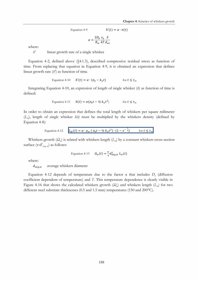
Chapter 4: Kinetics of whiskers growth
188
Equation 4-9
�
where: h' linear growth rate of a single whisker
Equation 4-2, defined above (§4.1.3), described compressive residual stress as function of time. From replacing that equation in Equation 4-9, it is obtained an expression that defines linear growth rate (h') as function of time.
Equation 4-10 for
Integrating Equation 4-10, an expression of length of single whisker (h) as function of time is defined:
Equation 4-11 ) for
In order to obtain an expression that defines the total length of whiskers per square milimeter (Lw), length of single whisker h(t) must be multiplied by the whiskers density (defined by Equation 4-8):
Equation 4-12 for
Whiskers growth (Ωw) is related with whiskers length (Lw) by a constant whiskers cross-section surface (π∙d2
avg, w) as follows:
Equation 4-13
where: average whiskers diameter
Equation 4-12 depends of temperature due to the factor that includes Db (diffusion coefficient dependent of temperature) and T. This temperature dependence is clearly visible in Figure 4-16 that shows the calculated whiskers growth (Ωw) and whiskers length (Lw) for two different steel substrate thicknesses (0.5 and 1.5 mm) temperatures (150 and 200°C).

Chapter 4: Kinetics of whiskers growth
189
Figure 4-16 Whisker growth (Ωw) and whiskers length (Lw) calculated from Equation 4-12 for different steel
susbtrate thicknesses at 150 and 200°C (specifically processed samples electroplated with alkaline electrolyte, 15 µm Zn coating)
Figure 4-17 and Figure 4-18 compare whisker growth (Ωw) and whiskers length (Lw) experimetal data at 150 and 200°C respectively, with values calculated from Equation 4-12 for different steel susbtrate thicknesses (0.5 and 1.5 mm). The expression is valid until growth saturation ( ) and it and fits well with experimental data for both temperatures; once growth is saturated, Equation 4-12 fails to predict the growth behaviour (the calculated values start decreasing).
Figure 4-17 Whisker growth (Ωw) and whiskers length (Lw), comparison of experimetal data and values calculated from Equation 4-12 for different steel susbtrate thicknesses at 150°C(specifically processed samples electroplated
with alkaline electrolyte, 15 µm Zn coating)
0
2 000
4 000
6 000
8 000
10 000
12 000
14 000
0
2 000
4 000
6 000
8 000
10 000
12 000
0 20 40 60
Whi
sker
s le
nght
(L
w)
[µm
]
Whi
sker
s gr
owth
(Ω
w)
[µ
m³/
mm
2 su
rfac
e]
time [min]
200°C 0.5 mm steel
200°C 1.5 mm steel
150°C 0.5 mm steel
150°C 1.5 mm steel
0
500
1 000
1 500
2 000
0
200
400
600
800
1 000
1 200
1 400
1 600
0 10 20 30 40 50 60
Len
gth
Whi
sker
s gr
owth
(Ω
w)
[µ
m³/
mm
2 su
rfac
e]
time [min]
exp.(0.5 mm steel)
calc.(0.5 mm steel)
exp.(1.5 mm steel)
calc.(1.5 mm steel)

Chapter 4: Kinetics of whiskers growth
190
Figure 4-18 Whisker growth (Ωw) and whiskers length (Lw), comparison of experimetal data and values calculated from Equation 4-12 for different steel susbtrate thicknesses at 200°C(specifically processed samples electroplated
with alkaline electrolyte, 15 µm Zn coating)
The cause of this decrease is found on the the term of Equation 4-12. Once growth saturation is reached, the second part of the term increases faster than the first term and therefore the whole term decreases as well as calculated whiskers growth and length. This inflexion point of the curves correspond to the saturation time and it is calculated as follows:
Equation 4-14
That is, saturation time increases as initial compressive residual stress increases and stress relaxation coefficient decreases, as it is observed in Figure 4-19 also for experimental data. A good correspondance between experimental and calculated data for saturation time is found. As comparison, the observed stauration time for the sample (1 mm steel susbtrate, not included in the figure) stored at 60°C is around 296 hours.
Figure 4-19 Whisker growth saturation time (t∞) from Equation 4-14 for different steel susbtrate thicknesses at 150,
175 and 200°C (specifically processed samples electroplated with alkaline electrolyte, 15 µm Zn coating)
0
2 000
4 000
6 000
8 000
10 000
12 000
14 000
0
2 000
4 000
6 000
8 000
10 000
12 000
0 10 20 30 40 50 60
Len
gth
Whi
sker
s gr
owth
(Ω
w)
[µ
m³/
mm
2 su
rfac
e]
time [min]
exp.(0.5 mm steel)
calc.(0.5 mm steel)
exp.(1.5 mm steel)
calc.(1.5 mm steel)
0
5
10
15
20
25
30
35
150°C 175°C 200°C
satu
ratio
n tim
e [m
in]
temperature
0.5 mm steel (exp.)
1.5 mm steel (exp.)
0.5 mm steel (calc.)
1.5 mm steel (calc.)

Chapter 4: Kinetics of whiskers growth
191
This model takes in account nucleation and growth of whiskers but it fails to predict the growth saturation; this approach needs also good knowledge of several factors, mainly two:
Time constant for nucleation ( ) from whiskers density curves, which requires having very short lapses between observations, in order to have enough data before growth saturation.
Time-evolution of residual stress. In this work, only data before and after storage were known, and some hypotheses were assumed (§4.1.3). Equation 4-2 assumes a linear stress relaxation with time during whiskers growth and it not describes the stress after growth saturation. It is therefore necessary to have experimental data of stress during whiskers growth in order to define an equation that describes the time-evolution of stress relaxation.
4.4.1.2 Second analytical model (with growth saturation)
As explained above, the former model fails in predicting the growth saturation; this is due to the hypothesis that assumed a linear stress relaxation with time during whiskers growth (§Equation 4-2); this equation however did not describe the stress after growth saturation In order to correct this failure, stress relaxation will be considered subject to an exponential decay, with ω as characteristic time according to the following equation:
Equation 4-15 ⁄ where:
Δ (t) relaxable stress as function of time → Δ 0 relaxable stress at time zero → ω time constant
In contrast to Equation 4-2, Equation 4-15 takes in account the residual stress after growth saturation, where for .
The following equation is a modified version of Equation 4-9 which includes residual stress as function of time:
Equation 4-16
�
Replacing Equation 4-15 in Equation 4-16:
Equation 4-17 ⁄
The factor is independent of time but dependent of temperature because it includes Db (diffusion coefficient) and T, all data for calculating factor are taken from Table 4-2.
In order to calculate the total whiskers length in a squared millimeter surface Lw(t) that defines the whiskers growth, we integrate Equation 4-8 and Equation 4-17 in the following equation:

Chapter 4: Kinetics of whiskers growth
192
∫ ( )
[ ] [ ⁄ ⁄ ] ∫ ⁄ ⁄ ⁄
[ ⁄ ⁄ ( ( ⁄ ⁄ ) ⁄ ⁄ )] Equation 4-18
[ ⁄ ⁄ ( ( ⁄ ⁄ ) ⁄ ⁄ )] Equation 4-18 expresses total whiskers length (LW) per squared millimeter. Whiskers growth
per squared millimeter (ΩW) can be determined from Equation 4-13. This equation predicts growth saturation: for t→∞, LW = LW∞. For t=0, LW=0.
Nevertheless, this equation requires the time constant for stress relaxation (ω) that comes from Equation 4-15; we do not have experimental information concerning the stress exponentially relaxed.
Figure 4-20 shows the calculated whiskers length (LW) and whiskers growth (ΩW) calculated from Equation 4-18 for a specifically processed sample electroplated with alkaline electrolyte (15 µm zinc coating on 1.5 mm steel) at 200°C. In this case, three different values of time constant (ω): ω= , ω=5 and ω→∞.
It is observed that the calculated growth is in the same order of magnitude than the experimental values. For the extreme case with infinite time constant (ω→∞), the calculated growth at saturation corresponds to 86% of the experimental values, while for ω= and ω=5 , the calculated values correspond to 43% and 71% respectively.
Figure 4-20 shows a maximal value reached by the whiskers growth before decreasing to saturation; this bump does not correspond to the physical phenomenon and it becomes stronger for low time constant (ω); this feature is due to the first term inside the brackets of Equation 4-18. The inflexion point of this maximal growth corresponds to approximately 1400 seconds (23 minutes).
As mentioned above, this model requires the time constant for stress relaxation (ω) that comes from Equation 4-17; we do not have this information since stress was measured only before and after storage.

Chapter 4: Kinetics of whiskers growth
193
Figure 4-20 Whisker length (LW) and growth (ΩW) calculated from Equation 4-18 for for a specifically processed sample electroplated with alkaline electrolyte (15 µm zinc coating on 1.5 mm steel) at 200°C ( =375 s)
4.4.2 Phenomenological model
An alternative approach is followed, based on JMAK equation3: Figure 4-21 shows the typical kinetics of whisker growth, which includes three stages:
i) Incubation: no growth is observed between the electroplating and the incubation time. ii) Growth: at the incubation time, the growth phenomenon starts; at first the growth rate is
increasing reaching a maximal growth rate (inflexion point), followed by a decreasing growth rate.
iii) Saturation: the growth rate reaches zero, while the no further whiskers growth is observed.
The following equation, inspired from the JMAK equation, describes the whiskers growth (Ωw):
Equation 4-19 ( ) where:
B JMAK equation constant n JMAK equation exponent ̇ ̇ where ̇ is the grains nucleation rate and ̇ is the linear growth rate of the
grains. Concerning JMAK equation exponent, according to Humphreys and Hatherly [69], it depends of the dimensionality of the grains growth during recrystallization. Ideal JMAK equation exponents are shown in Table 4-3. Sample geometry or internal microstructural constraints can
3 Also known as Avrami equation, based in the work of Johnson, Mehl, Avrami and Kolmogorov in
the 1930's, first proposed to describe recrystallization kinetic in polycrystals. Recrystallization has been observed in whiskers and coatings in the present work (§3.5.1).
0
2 000
4 000
6 000
8 000
10 000
12 000
0
2 000
4 000
6 000
8 000
10 000
0 5 000 10 000 15 000
Whi
sker
s gr
owth
(Ω
w)
[µm
³/ m
m²
surf
ace]
Whi
sker
s le
nght
(L
w)
[µm
/ m
m²
surf
ace]
time [s]
exp
Calc ( →∞)
Calc ( =5 )
Calc ( = )

Chapter 4: Kinetics of whiskers growth
194
make the grains growing in one or two dimensions, instead of a isotropical growth in three dimensions.
Figure 4-21 Typical kinetics of whiskers growth (whiskers growth and whiskers growth rate), specifically processed
sample (alkaline, 15 µm zinc coating on 0.5 mm steel substrate) at 150°C
Table 4-3 Ideal JMAK exponents [69]
Growth dimensionality Constant nucleation rate
Site saturation
3-D 4 3
2-D 3 2
1-D 2 1
Nucleation rate can be either constant or time-depending, which has an influence on JMAK exponents:
Nucleation and growth rates can be assumed constant during recrystallization (constant nucleation rate), and the JMAK exponents varies from 2 to 4.
If nucleation rate is not constant but time-decreasing during recrystallization, and the rate declines so fast that all nucleation events happen at the start of the recrystallization (site staturation). Here, JMAK exponents varies from 1 to 3.
Equation 4-19 can be rewritten in the following form:
Equation 4-20
Equation 4-20 can be expressed as follows:
Equation 4-21 [ ]
0
2000
4000
6000
8000
10000
12000
0
5
10
15
20
25
30
0 1000 2000 3000 4000 5000 6000 7000 8000
Wh
iske
rs g
row
th (
Ωw
)
[µm
³/ m
m2
surf
ace]
Wh
iske
rs g
row
th r
ate
(Ωw
')
[µm
³/s∙
mm
2 su
rfac
e]
time [s]
Growth saturation
Maximal growth rate
Growth initiation

Chapter 4: Kinetics of whiskers growth
195
This equation is used to fit experimental data, as shown in Figure 4-22 for an specifically processed sample stored at 175°C. Parameters B and n can be obtained from the equation data fitting; in this particular case, with the coefficient of determination (R²) over 0.97: ln(B)=-2.99 and n =0.44
Figure 4-22 Data fitting using Equation 4-21; specifically processed sample electroplated with alkaline electrolyte
(15 µm zinc coating on 0.5 mm steel)
Experimental rates are compared with calculated rates for 0.5 and 1.5 mm steel susbtrate in Figure 4-23 and Figure 4-24 respectively, at three temperatures (150, 175 and 200°C).
Figure 4-23 Kinetics data fitting with Equation 4-19 (JMAK) of specifically processed sample electroplated with
alkaline electrolyte (15 µm zinc coating on 0.5 mm steel)
y = 0.44x - 2.99 R² = 0.9745
-0,5
0
0,5
1
5 6 7 8 9
Ln(
-Ln(
1-Ω
w(t
)/Ω
w*)
)
Ln(t)
0
2 000
4 000
6 000
8 000
10 000
12 000
14 000
0
2 000
4 000
6 000
8 000
10 000
0 20 40 60 80 100 120 140 160
Whi
sker
s le
nght
(L
w)
[µm
/ m
m²
surf
ace]
Whi
sker
s gr
owth
(Ω
w)
[µm
³/ m
m²
surf
ace]
time [min]
200°C exp
200°C calc
175°C exp
175°C calc
150°C exp
150°C calc

Chapter 4: Kinetics of whiskers growth
196
Figure 4-24 Kinetics data fitting with Equation 4-19 (JMAK) of specifically processed sample electroplated with
alkaline electrolyte (15 µm zinc coating on 1.5 mm steel)
Figure 4-25 shows the determined JMAK equation constant B and exponent n for different temperatures and steel substrate thicknesses. While n decreases with temperature, B is considerably favored with temperature. Concerning the steel substrate thickness, samples with thickest substrate have the largest parameter n and the smallest B.
The whiskers growth is an unidimensional growth, which ideally corresponds to n=1 in the site saturation case, according to Table 4-3. Our calculated exponents n, between 0.44 and 1.64, fall well in this case (one-dimension growth, site saturation). Average n corresponds to 0.57 and 1.08 for samples with 0.5 and 1.5 mm stel substrate respectively.
a) JMAK equation constant (B) b) JMAK equation exponent (n)
Figure 4-25 JMAK equation parameters: a) JMAK equation constant (B), b) JMAK equation exponent (n) for whiskers growth in specifically processed sample electroplated with alkaline electrolyte (15 µm zinc coating)
0
2 000
4 000
6 000
8 000
10 000
12 000
14 000
0
2 000
4 000
6 000
8 000
10 000
0 20 40 60 80 100 120 140 160
Whi
sker
s le
nght
(L
w)
[µm
/ m
m²
surf
ace]
Whi
sker
s gr
owth
(Ω
w)
[µm
³/ m
m²
surf
ace]
time [min]
200°C exp
200°C calc
175°C exp
175°C calc
150°C exp
150°C calc
1E-6
1E-5
1E-4
1E-3
1E-2
1E-1
1E+0
150 175 200
JMA
K e
quat
ion
cons
tant
Temperature [°C]
B for 0.5 mmB for 1.5 mm
0
0,5
1
1,5
2
150°C 175°C 200°C
JMA
K e
quat
ion
expo
nent
n for 0.5 mmn for 1.5 mmavg n for 0.5 mm

Chapter 4: Kinetics of whiskers growth
197
For further analysis, we make two assumptions concerning both JMAK exponent (n) and constant (B):
Ideal JMAK equation exponent (n=1)
JMAK equation constant as function of temperature
We will take the ideal JMAK equation exponent (n) for site saturation unidimensional growth that corresponds to 1. With n=1, we determined the constants B that fit the better the experimental data. Recalculated growth with n=1 is shown in Figure 4-26 and Figure 4-27 for samples with 0.5 and 1.5 mm steel substrate respectively and compared with experimental data.
Figure 4-26 Kinetics data fitting with Equation 4-19 (JMAK), n=1 (fixed and independent of temperature), for specifically processed sample electroplated with alkaline electrolyte (15 µm zinc coating on 0.5 mm steel)
Figure 4-27 Kinetics data fitting with Equation 4-19 (JMAK), n=1 (fixed and independent of temperature), for
specifically processed sample electroplated with alkaline electrolyte (15 µm zinc coating on 1.5 mm steel)
0
2 000
4 000
6 000
8 000
10 000
12 000
14 000
0
2 000
4 000
6 000
8 000
10 000
0 20 40 60 80 100 120 140 160
Whi
sker
s le
nght
(L
w)
[µm
/ m
m²
surf
ace]
Whi
sker
s gr
owth
(Ω
w)
[µm
³/ m
m²
surf
ace]
time [min]
200°C exp
200°C calc
175°C exp
175°C calc
150°C exp
150°C calc
0
2 000
4 000
6 000
8 000
10 000
12 000
14 000
0
2 000
4 000
6 000
8 000
10 000
0 20 40 60 80 100 120 140 160
Whi
sker
s le
nght
(L
w)
[µm
/ m
m²
surf
ace]
Whi
sker
s gr
owth
(Ω
w)
[µm
³/ m
m²
surf
ace]
time [min]
200°C exp
200°C calc
175°C exp
175°C calc
150°C exp
150°C calc

Chapter 4: Kinetics of whiskers growth
198
Here we introduce the second assumption, considering JMAK equation constant (B) as exponentially dependent of temperature:
Equation 4-22
M and S are equation constants (independents of temperature) that slighly vary for each sample):
M corresponds to 1.41∙10-4 and 1.34∙10-4 for 0.5 and 1.5 mm steel respectively
S corresponds to 1.35∙10-2 and 1.44∙10-2 for 0.5 and 1.5 mm steel respectively
This equation allows determination of JMAK equation constant (B) as function of temperature.
Figure 4-28 JMAK equation constant (B) for whiskers growth in specifically processed sample electroplated with
alkaline electrolyte (15 µm zinc coating); n=1
Figure 4-29 compares the calculated growth at 60°C of samples with 0.5 and 1.5 mm steel with experimental data of sample with an intermediare steel thickness (1 mm).
Figure 4-29 Kinetics data fitting at 60°C with Equation 4-19 (JMAK), n=1, for specifically processed sample
electroplated with alkaline electrolyte (15 µm zinc coating on 0.5 to 1.5 mm steel)
0E+0
1E-3
2E-3
3E-3
50 100 150 200
JMA
K e
quat
ion
cons
tant
temperature [°C]
0.5 mm steel
1.5 mm steel
050100150200250300350400
0
50
100
150
200
250
300
350
0 200 400 600 800 1000 Whi
sker
s le
nght
(L
w)
[µm
/ m
m²
surf
ace]
Whi
sker
s gr
owth
(Ω
w)
[µm
³/
mm
² su
rfac
e]
time [hours]
exp (1 mm steel)
calc. (0.5 mm steel)
calc. (1.5 mm steel)

Chapter 4: Kinetics of whiskers growth
199
The calculated data do not vary considerably with steel thickness; both calculated growth curves are above the experimental data and saturates faster. However we have only single data for 60°C, more information before saturation is required.
If replacing Equation 4-22 in Equation 4-19, we can obtain the following JMAK-type expression that describes the time behaviour of the growth (Ωw/ Ωw∞) as function of temperature, for n=1, which is plotted in Figure 4-30:
Equation 4-23 ( )
Figure 4-30 Kinetics of growth for several temperatures (Equation 4-23), specifically processed sample electroplated
with alkaline electrolyte (15 µm zinc coating on 1.5 mm steel (n=1)
However, Equation 4-23 still depends of saturation growth (Ωw∞); this term can be correlated with temperature from experimental data as shown in Figure 4-31, and expressed in the following equation:
Equation 4-24
Figure 4-31 Saturation whiskers growth (Ωw∞) as function of temperature for specifically processed sample electroplated with alkaline electrolyte (15 µm zinc coating on 1 and 1.5 mm steel)
0
0,2
0,4
0,6
0,8
1
0 30 60 90 120 150 180
Ω/Ω
∞ o
r L/L
∞
time [min]
calc 200°C
calc 175°C
calc 150°C
calc 100°C
calc 60°C
calc 30°C
exp 200°C
exp 175°C
exp 150°C
exp 60°C
y = 101,12e0,0213x R² = 0,9727
0
2000
4000
6000
8000
50 100 150 200
Whi
sker
s gr
owth
(Ω
w)
[µm
³/
mm
² su
rfac
e]
Temperature [°C]
1 mm steel 1.5 mm steel

Chapter 4: Kinetics of whiskers growth
200
Where P and Z are equation constants (independents of temperature) for each sample. In our sample (1.5 mm steel), P and Z corresponds to 101 and 2.1∙10-2 respectively (we assumed that at 60°C the saturation growth does not vary from 1 to 1.5 mm steel thickness).
Finally, replacing Equation 4-24 in Equation 4-23, we obtain the following JMAK-type expression that describes the time behaviour of the growth (Ωw) as function of temperature, for n=1, which is plotted in Figure 4-32:
Equation 4-25 ( )
where the constants P, Z, M and Q are particular for a given sample. In the case of our sample (1.5 mm steel), these values are summarized in Table 4-4.
Table 4-4 Values used for Equation 4-25 in order to calculate whisker growth (Ωw) for specifically processed sample electroplated with alkaline electrolyte (15 µm zinc coating on 1.5 mm steel
Variable Value
P 101 µm3/mm2 surface
Z 2.1∙10-2 /°C
M 1.34∙10-4
S 1.44∙10-2 /°C
n (JMAK equation exponent) 1 (ideal)
Figure 4-32 Kinetics of growth for several temperatures (Equation 4-25) for a specifically processed sample electroplated with alkaline electrolyte (15 µm zinc coating on 1.5 mm steel), n=1
Equation 4-25 allows a good prediction of whiskers growth, althought it requires several parameters for the studied sample (P, Z, M and S) that define the temperature behaviour of both
1
10
100
1 000
10 000
1
10
100
1 000
10 000
1E+
2
1E+
3
1E+
4
1E+
5
1E+
6
1E+
7
Whi
sker
s le
nght
(L
w)
[µm
/ m
m²
surf
ace]
Whi
sker
s gr
owth
(Ω
w)
[µm
³/ m
m²
surf
ace]
time [s]
calc 200°C
calc 150°C
calc 100°C
calc 60°C
calc 30°C
calc 175°C
exp 200°C
exp 175°C
exp 150°C
exp 60°C
1 hour 1 day

Chapter 4: Kinetics of whiskers growth
201
saturation whiskers growth and the JMAK equation constant (B). For most of temperatures, the calculated values overestimate the experimental data.
Following the data concerning total whiskers length (LW) at saturation in Figure 4-32, if one assumes one whisker per squared milimeter, the length of this whisker would be 0.3 mm at 60°C. These values agree with maximal lengths observed in industrial-origin samples A and B, (between 0.4 and 0.6 mm), although the zinc coating and steel thicknesses are different to the model sample.
If we look at the high temperatures, the assumed whiskers per squared millimeter would have length of 5.6 mm at 200°C, 3.3 mm at 175°C and 1.9 mm at 150°C. These values are in the same order of magnitude of maximal length reported in literature (§Table 1-1), although the temperature conditions are not necessary the same.
Three different models are studied for predicting whiskers growth kinetics:
The first model is an analytical one that takes in account nucleation of grains and their growth into whiskers. The model is valid until growth saturation and it and fits well with experimental data for both temperatures; however, the model fails to predict the growth staturation, mainly due to the the lack of information of time-behaviour of residual stress. The second model corrects this failure of the first model, although it also fails to describe properly the phenomenon; besides, information concerning the time behaviour of stress relaxation is required.
A third model is more phenomenological, based on JMAK equation that includes the growth saturation. This model allows the estimation of whiskers growth kinetics at different temperatures for a given samples; the parameters required for this model are obtained by imposing n=1 (ideal for one-dimensional growth).

Chapter 4: Microstructure
202
4.5 MICROSTRUCTURE
Microstructure observations show that grains of hillocks, whiskers roots and whiskers are recrystallized. Recrystallization therefore has to be considered in the mechanism of whiskers growth. Mechanisms proposed by Vianco and Smetana take recrystallization in account, since they are based on observations of tin coating where columnar grains are under compressive stress.
In Smetana model [41], whiskers growth starts with the formation of oblique grain boundaries during recrystallization. Since the coating is under compressive stress, oblique grain boundaries are under a force that makes them slide. Whisker formation is actually the result of the grain boundary sliding. In addition, there is a diffusion process, driven by the stress gradient from vertical grain boundaries to whisker grain. Consequence of this diffusion, atoms move from the coating to the base of the whiskers, and thus, the whiskers continues growing.
On the other hand, Vianco [47] recently demonstrated a cyclic dynamic recrystallization (DRX) mechanism for tin whiskers growth. The compressive stress produces dislocations that are piled up at the vertical gran boundary. Energy is stored, as consequence of the piling up of dislocations, and results in the formation of a new grain free of defects at the vertical grain boundary. This new grain continues growing; when it reaches a maximum size in the coating, the new grain grows out of the coating, at the surface in the form of a whisker.
Some of our microstructure observations support this mechanism for zinc whiskers growth:
Zinc coating is composed of columnar grains.
Grains close to either hillocks or whiskers are recrystallized, and they are actually larger than most of the grains of the zinc coating.
According to Vianco, a condition for having a cyclic DRX is that the final grain has to be more than twice as large as the initial grain. In our case, this condition is fulfilled since the grains of the coating are 0.13 wide and 0.55 long, while the recrystallized and equiaxial grains of a hillock are around 0.5 µm diameter.
Dislocations were observed in both hillocks and whiskers. Until now no experimental evidence of dislocations in whiskers had been reported before our observations.
Circumferential striations were observed in some whiskers during storage of samples.
The periodic patter of circumferential striations indicates a dynamic process which could be a consequence of cyclic DRX. In Figure 3-8-a (§3.1.2) one of these striations is observed in a whiskers in specifically processed sample electroplated with alkaline electrolyte (15 µm zinc coating on 1 mm steel) at 60°C storage; these striations are separated by a distance between 80 and 100 nm.
Growth data for this sample at 60°C are:
Average whiskers growth rate per squared millimeter is L'w= 2.5∙10-4 µm/s
Whiskers density is ρw=7 whiskers/mm2

Chapter 4: Microstructure
203
From these data, average single whisker growth (L'w / ρw) is hw=3.6∙10-5 µm/s. Considering the striation length (from 80 and 100 nm), it is calculated the time required for growing the length corresponding to one striation; this time is between 37.5 and 46.9 minutes.
Stress relaxation coefficient k (§4.1.3) refers to the rate of compressive residual stress relaxation, and it corresponds to 8.7∙10-4 MPa/s for this samples. Therefore, in the time lapse of striation growth (37.5 to 46.9 minutes), between 1.9 and 2.4 MPa would be relaxed.
Columnar grains, dislocations, circumferential striations and recrystallization are the main observed features that support DRX as mechanism of whiskers growth.

Chapter 4: Summary
204
4.6 SUMMARY OF DISCUSSION OF RESULTS
The alkaline electroplating electrolyte favors the activation energy of both stress relaxation and whiskers growth, when compared to acid-electrolyte. On the other hand, whiskers growth activation energy is favored by zinc coating thickness and disfavored by steel susbtrate thickness.
Residual stress is relaxed faster as temperature increases. The influence of other parameters in the stress relaxation coefficient is not clear, such as zinc coating thickness, steel substrate thickness and electroplating electrolyte. Whiskers growth rate estimation for samples electroplated with alkaline electrolyte can be obtained (5 to 6 times the corresponding experimental data).
An analysis of the mass diffusion in the whiskers growth suggested that whiskers growth is controlled by grain boundary diffusion rather than by lattice diffusion. Calculated whiskers growth rate is compared with experimental data, using activation energy from literature. Apparent activation energy for whiskers growth rate of single whiskers is estimated between 54 and 60 kJ/mol.
Two different model approaches are studied for predicting whiskers growth kinetics. The first approach is analytical and it takes in account nucleation of grains and their growth into whiskers. The first analytical model is valid until growth saturation and it and fits well with experimental data for both temperatures; however, the model fails to predict the growth staturation, mainly due to the the lack of information of time-behaviour of residual stress relaxation. A second analytical model corrects this failure of the first model, although it also fails to describe properly the phenomenon; besides, information concerning the time behaviour of stress relaxation is required.
A phenomenological approach is based on JMAK equation that includes the growth saturation. This model allows the estimation of whiskers growth kinetics at different temperatures for a given samples; the parameters required for this model are obtained by imposing n=1 (ideal for one-dimensional growth).
Concerning microstructure, columnar grains, dislocations, circumferential striations and recrystallization are main observed features that support DRX as mechanism of whiskers growth.

205

Conclusions and perspectives
206
Conclusions and perspectives
Conclusions and perspectives
This work concerns spontaneous growth of zinc whiskers in electroplated coatings, a serious problem for reliability of electrical devices in the most diverse industrial applications. Although it is an old industrial issue, there is little research done on the subject.
The attenuation, prevention and/or mitigation of failures related zinc whiskers require a deep understanding of the zinc whiskers growth phenomenon and its physical mechanism by studying the kinetics of growth, the influencing parameters and the microstructure of the zinc coating and whiskers.
The influencing parameters on zinc whiskers growth, numerous and interdependent, were studied:
Temperature and zinc coating thickness favor the whiskers growth.
Steel substrate thickness disfavors the whiskers growth in alkaline-origin samples (although it favors the growth in acid-origin samples).
Growth in acid-origin samples is localized on some irregularities of the surface, while in alkaline- is uniformly distributed on the surface.
At least, residual compressive stress is a major parameter in whiskers growth
On the other hand, microstructure observations evidence a porous, columnar-grain structure of the zinc coating grains with a preferred orientation between <2-1-10> and <10-10>. Recrystallized grains were observed in regions close to hillocks and whiskers; whiskers are single crystalline features result of recrystallization mechanism of the columnar grains with <10-10> orientation.
In the frame of our observations, basic mechanism of Zn whisker growth seem to be analogous to dynamic recrystallization, i.e. stress driven crystallization. This look similar to recent observations and experiments led on tin whiskers growth.
Longitudinal and circumferential striations as well as kinks and direction changes are observed. It was also confirmed the growth of whisker from the base rather than from the tip.
As far as for the presence of intermetallic compounds (important in the development of residual stress in tin whiskers), they were not observed neither in zinc whiskers nor in zinc coating or hillocks. Dislocations were observed for first time in whiskers and hillocks.

Conclusions and perspectives
207
On the other hand, the results obtained by local chemical analyses do not show intermetallic compounds in the zinc coating, the recrystallized grains, the hillocks nor the whiskers; nevertheless, porosity of the zinc coating was observed as well as some iron-rich zones from unknown origin.
Compressive residual stress relaxation and whiskers growth are two different but strongly interconnected phenomena, both thermally activated, each of them follows a different mechanism. From experimental data, apparent activation energies of the two phenomena are calculated, and gran boundary diffusion is established as the main diffusion mechanism for whiskers growth.
The experimental data of this work was based on accelerated storage experiments at high temperature, while the actual whiskers growth can last decades at room conditions. The goal of these accelerated tests was to determine some mechanism parameters in order to extrapolate whisker growth and growth rates at room temperature.
Whiskers growth mechanisms, both analytical and phenomenological are proposed. Good estimation of whiskers growth and whiskers growth rate at temperatures close to operation conditions is obtained when compared with experimental data, which allows a forecast of whiskers growth in industrial applications.
On the other hand, during samples storage, the most important SEM observations to be done are at the growth stage in order to have sufficient data for a study of growth kinetics. The time lapse between observations must be reduced enough to have enough data before the growth is saturated. Based on the saturation time we observed for 60°C, it is possible to design an experiment that focuses on the growth stage; in our experiments it was observed that 300 hours (12.5 days) was not short enough.
This observation was the reason why we ran SEM storage experiments that allow SEM observation without stopping the storage and with the shortest lapse between observations (live-observation). We recommend SEM storage as the most appropriate technique to study growth kinetics.
One of the issues was the scarcity of literature references about zinc whiskers, since almost all the research concerning metallurgical whiskers were focused on tin whiskers. This dissertation therefore developed an initial work that must be deepened to understand the mechanism behind and to determine the industrial application conditions to prevent whiskers growth. Exploring the following as future approaches will help achieving these objectives:
A study of microstructure and the influence of diverse parameters are required to deepen the understanding of the phenomena, and it is imperative in order to propose a mechanism of growth. EBSD, TEM and ASTAR observations should be done as function of parameters such as electroplating electrolyte and zinc coating thickness. An observation of time-evolution of the microstructure (before storage, during growth and after saturation) would help understanding the whiskers growth mechanism.

Conclusions and perspectives
208
A deeper study of the diverse parameters is necessary to understanding the influence of such parameters in whiskers growth. For instance, like recently conducted for Sn films [70], model Zn films on various substrate could be conducted, varying film thickness, grain size, roughness of substrate for example.
Moreover, a detailed understanding of the role of oxygen and humidity could be carried out on model films/substrate systems.
In our work, residual stress was measured only before and after samples storage. A more detailed study of residual stress relaxation must be done, with several stress measurement at different stages of the whiskers growth, particularly before saturation. That will allow understanding the mechanism of stress relaxation.
A study of applied stress to samples must be done in order to correlate the growth of whiskers in the sample as function of the applied stress. Such study can be done with a device that allows applying stress on the sample inside a SEM microscope for permanent samples observation.

209

References
210
References
References
[1] J. Brusse and M. Sampson, "Zinc whiskers: hidden cause of equipment failure," IEEE IT Pro, vol. 6, no. 6, pp. 43-47, 2004.
[2] H. L. Cobb, "Cadmium whiskers," Monthly Rev. Am. Electroplaters Soc, vol. 33, no. 28, pp. 28-30, 1946.
[3] NASA, "NASA website: Tin Whisker (and Other Metal Whisker)," 8 May 2012. [Online]. Available: nepp.nasa.gov/whisker.
[4] S. M. Arnold, "The growth of metal whiskers on electrical components," in Proceedings. IEEE Electronic Component Conference, Philadelphia, PA, 1959.
[5] G. T. Gaylon, "A history of Tin whiskers theory: 1946 to 2004," in SMTA International Conference Proceedings, Chicago-IL, 2004.
[6] European Union, "Directive 2002/95/EC of the Parlament and the Council of 27 January 2003 on the restriction of the use of certain hazardous substances in electrical and electronic equipment," Official Journal of the European Union, 2003.
[7] E. Pernot, "Compte rendu d'expertise des relais de protection électrique (...)," EDF R&D, Moret sur Loing, France, 2007.
[8] M. Schamel, C. Schopf, D. Linsler , S. T. Haag, L. Hofacker, C. Kappel and et al. , "The filamentary growth of metals," International Journal of Materials Research (formerly Z. Metallkd.), vol. 102, no. 7, pp. 828-836, 2011.
[9] K. G. Compton, A. Mendizza and S. M. Arnold, "Filamentary growths on metal surfaces-whiskers," Corrosion, vol. 7, no. 10, pp. 327-334, 1951.
[10] F. R. Nabarro and P. J. Jackson, "Growth of crystal whiskers," in Growth and perfection of crystals, R. H. Doremus, B. W. Roberts and D. Turnbull, Eds., New York, NY: John Wiley & Sons, 1958, pp. 13-101.
[11] S. E. Koonce and S. M. Arnold, "Growth of metal whiskers," Journal of Applied Physics (letters to the editor), vol. 24, no. 3, pp. 365-366, 1953.
[12] P. L. Key, "Surface morphology of whiskers crystals of tin, zinc, and cadmium," Washington, DC, 1970.
[13] U. Lindborg, "Observations on the growth of whisker crystals from zinc electroplate,"
References
211
Metallurgical transactions A, no. 6A, pp. 1581-1586, 1975.
[14] JEDEC, Test method for measuring whisker growth on tin and tin alloy surface finishes, Technical document JEDEC (Ref:JESD22A121.01), 2005.
[15] F. Arnoldi and C. Cossange, "Caractérisation des whiskers sur un relais ITG143," EDF R&D, Moret sur Loing, France, 2008.
[16] A. Lina, «Etude bibliographique de la formation des whiskers de zinc,» EDF R&D, Moret sur Loing, France, 2009.
[17] H. Sugiarto, I. R. Christie and B. P. Richards, "Studies of zinc whiskers formation and growth from bright zinc electrodeposits," Transactions of the Institute of Metal Finishing, vol. 62, no. 3, pp. 92-97, 1984.
[18] J. Franks, "Growth of whiskers in the solid phase," Acta Metallurgica, vol. 6, no. 2, p. 103–109, 1958.
[19] V. K. Glazunova and N. T. Kudryavtsev, "An investigation of the conditions of spontaneous growth of filiform crystals on electrolytic coatings," Russian J. Appl. Chem. (Zhurnal Prikladnoi Khimii), vol. 36, no. 3, pp. 543-550, 1963.
[20] T. Nagai, K. Natori and T. Furasama, "Rate of short-circuit caused by whiskers growth on Zn electroplated steels in electronic appliance," Journal Japan Institut Metals, vol. 53, no. 3, pp. 303-307, 1989.
[21] WES Worldwide Environmental ServiceS, "Metallic whisker sources," www.wes.net, 2004.
[22] R. Lahtinen and T. E. Gustafsson, "The driving force behind whisker growth, an investigation on what triggers this phenomenon in hot-dip galvanized zinc coating, Part 1," Metal finishing, vol. Nov., p. 25, 2005.
[23] R. Lahtinen and T. E. Gustafsson, "The driving force behind whisker growth, an investigation on what triggers this phenomenon in hot-dip galvanized zinc coating, Part 2," Metal finishing , vol. Dec., p. 33, 2005.
[24] L. Lacourcelle, Traité de Galvanotechnique, Paris: Galva-conseils, 1997.
[25] A. Etienne, "Microstructure et nanostructure des whiskers et des revêtements de Zn," EDF R&D, Moret sur Loing, France, 2012.
[26] T. Takemura, M. Kobayashi, M. Okutani, T. Kakoshita and K. Shimizu, "Relation between the direction of whiskers growth and the crystallographic texture of zinc electroplate," Japanese journal of applied physics, vol. 1, no. 25, p. 1948, 1986.

References
212
[27] K. J. Courey, S. S. Asfour, J. A. Bayliss, L. L. Ludwig and M. C. Zapata, "Tin whisker electrical short circuit characteristics - Part I," IEEE transactions on electronics packaging manufacturing, vol. 31, no. 1, p. 32, 2008.
[28] E. Generalic, "EniG. Periodic Table of the Elements," 28 September 2013. [Online]. Available: http://www.periodni.com/zn.html. [Accessed 30 January 2014].
[29] U. Lindborg, S. Ramsin, L. Lind and L. Revay, "Microstructure and metallurgical properties of some zinc electroplates," Plating, no. 61, pp. 1111-1116, , 1974.
[30] A. Etienne, E. Cadel, A. Lina, L. Cretinon and P. Pareige, "Micro- and nanostructure of Zn whiskers and their coating," Journal of Electronic Materials, vol. 42, no. 2, pp. 272-279, 2013.
[31] H. L. Reynolds and R. Hilty, "Investigations of zinc whiskers using FIB technology," in IPC/JEDEC Lead Free North America Conference, Boston-MA, 2004.
[32] C. Xu , Y. Zhang, C. Fan and J. A. Abys , "Understanding whisker phenomenon: the driving force for whisker formation," www.circuitree.com, 2002.
[33] A. Baated, K. Kim and K. Suganuma , "Whisker growth from an electroplated zinc coating," J. Mater. Res., vol. 25, no. 11, pp. 2175-2182, 2010.
[34] A. Etienne, E. Cadel, A. Lina, L. Cretinon and P. Pareige, "Crystallographic characterization of an electroplated Zinc coating prone to whiskers," IEEE Transactions on Components, Packaging, and Manufacturing Technology, vol. 2, no. 11, pp. 1928-1932, 2012.
[35] R. Weil, "Origins of stress in electrodeposits, Part III," Plating, p. 131, 1971.
[36] A. Dvořák and L. Vrobel, "A new method for the measurement of internal stress in electrodeposits," Transactions of the Institute of Metal Finishing, no. 49, p. 153, 1971.
[37] M. Froment and G. Maurin, "Etude en microscopie électronique de la morphologie des dépôts électrolytiques de zinc," Electrodeposition and Surface treatment, no. 3, p. 245, 1975.
[38] B. Lee and D. Lee, "Spontaneous growth mechanism of tin," Acta Mater., vol. 46, no. 10, pp. 3701-, 1998.
[39] W. Chen, P. Sarobol, J. Holaday, C. Handwerker and J. Blendell, "Effect of crystallographic texture, anisotropic elasticity, and thermal expansion on whisker formation in -Sn thin films," J. Mater. Res, vol. 29, no. 2, p. 197, 2014.
[40] H. Ledbetter, "Elastic properties of zinc: a compilation an review," J. Phys. Chem. Ref. Data, vol. 6, no. 4, pp. 1181-1203, 1977.
[41] J. Smetana, "The end game," IEEE Transactions on Electronics Packaging Manufacturing, no. 30,
References
213
pp. 11-22, 2007.
[42] M. O. Peach, "Mechanism of growth of whiskers on cadmium," Journal of Applied Physics, vol. 23, no. 12, pp. 1401-1403, 1952.
[43] F. C. Frank, "On tin whiskers," Philosophical Magazine, vol. XLIV, no. 7, p. 854–860, 1953.
[44] J. D. Eshelby, "A tentative theory of metallic whisker growth," Physical Review Letters, no. 91, pp. 755-756, 1953.
[45] S. Amelinckx, W. Bontinck, W. Dekeyser and F. Seitz, "On the formation and properties of helical dislocations," Philosophical. Magazine 8th Series, vol. 2, no. 15, pp. 355-378, 1957.
[46] U. Lindborg, "A model for the spontaneous growth of zinc, cadmium, and tin whiskers," Acta Metallurgica, no. 24, pp. 181-186, 1976.
[47] P. T. Vianco and J. A. Rejent, "Dynamic recrystallization (DRX) as the mechanism for Sn whisker," Journal of Electronic Materials, vol. 38, no. 9, pp. 1815-1825, 2009.
[48] J. Philibert;, Diffusion et transport de matière dans les solides, Paris: Les Editions de Physique, 1985.
[49] W. C. Ellis, D. F. Gibbons and R. C. Treuting, "Growth of metal whiskers from the solid," in Growth and perfection of crystals, R. H. Doremus, B. W. Roberts and D. Turnbull, Eds., New York, NY: John Wiley & Sons, 1958, pp. 102-120.
[50] T. Kakeshita, K. Shimizu, R. Kawanaka and T. Hasegawa, "Grain size effect on electroplated tin coatings on whisker growth," Journal of Materials Science, vol. 17, no. 9, pp. 2560-2566, 1982.
[51] B. Le-Bret and M. G. Norton, "Electron microscopy study of tin whisker growth," Journal of Materials Research, vol. 18, no. 3, pp. 585-593, 2003.
[52] I. Boguslavsky and P. Bush, "Recrystallization principles applied to whisker growth in tin," in Proc. APEX Conf, Anaheim-CA, 2003.
[53] R. M. Fisher, L. S. Darken and K. G. Carroll, "Accelerated growth of tin whiskers," Acta Metallurgica, no. 2, pp. 368-373, 1954.
[54] J. Pescatore, "Les aciers de construction de la norme NF en 10025, historique de leur designation," Revue Construction Metalique, vol. 3, pp. 1-10, 2003.
[55] AFNOR, NF EN 10027-2, système de désignation des aciers, AFNOR, 1992.
[56] A. Lina et M. Mahe, «Essais en enceinte climatique pour l'étude de la formation et de la

References
214
croissance,» EDF R&D, Moret sur Loing, France, 2010.
[57] ASTM, ASTM E8/E8M-11; Standard Test Methods for Tension Testing of Metallic Materials, ASTM.
[58] ISO, ISO 643:2012; Steels - Micrographic determination of the apparent grain size, ISO, 2012.
[59] L. Legras, "Préparation d’échantillons par microscopie double faisceau pour observations par MEB équipé d’un detecteur STEM ou pour MET," in Préparation des échantillons pour MEB et Microanalyses, P. Jonnard and F. Brisset, Eds., EDP Sciences, 2011.
[60] B. Holdford, "The uses of dual beam FIB in microelectronic failure analysis," in Introduction to Focused Ion Beams. Instrumentation, Theory, Techniques and Practice, Boston, Springer Science + Business Media, Inc, 2005, pp. 107-132.
[61] P. Gnauck, P. Hoffrogge and M. Schumann, "High resolution live imaging of FIB milling processes for optimum accuracy," in Introduction to Focused Ion Beams. Instrumentation, Theory, Techniques and Practice, Boston, Springer Science + Business Media, Inc., 2005, pp. 133-142.
[62] R. Soulas, Effet de la cristallographie sur les premiers stades de l’oxydation des aciers austénitiques 316L, Grenoble: Université de Grenoble, 2012.
[63] M. Veron and E. Rauch, "EBSD in TEM : Introduction to ASTAR system," in ALEMI, Avignon, 2010.
[64] E. Rauch, M. Veron, J. Portillo, D. Bultreys, Y. Maniette and S. Nicolopoulos, "Automatic Crystal Orientation and Phase Mapping in TEM by Precession Diffraction," Microscopy and Analysis, no. 93, pp. 5-8, 2008.
[65] M. Fitzpatrick, A. Fry, P. Holdway, F. Kandil, J. Shackleton and L. Suominen, Measurement Good Practice Guide No. 52: Determination of Residual Stresses by X-ray Diffraction – Issue 2, Teddington, UK: National Physical Laboratory, 2005.
[66] D. Tanner, "Residual stress determination - X-ray Diffraction," [Online]. Available: https://sites.google.com/site/temfemguy/research/residual-stress-in-aluminium-forgings/residual-stress-determination---x-ray-diffraction. [Accessed 07 12 2013].
[67] P. Prevéy, "X-ray diffraction residual stress techniques," Lambda Research, Inc, 1986.
[68] H. Frost and M. Ashby, "Web version of "Deformation-Mechanism Maps, The Plasticity and Creep of Metals and Ceramics"," [Online]. Available: http://engineering.dartmouth.edu/defmech/. [Accessed 29 5 2014].
[69] F. Humphreys and M. Hatherly, "Recrystallization of single-phase alloys," in Recrystallization and Related Annealing Phenomena, Oxford, Elsevier, 2004, pp. 215-253.

References
215
[70] E. R. Crandall, Factors Governing Tin Whisker Growth, Auburn, Alabama : Auburn University, 2012.

Appendix 1: Texture of steel and electroplates
216
Appendix 1: Texture of steel and electroplates
A1.1 Experimental conditions
Texture of steel sheets as well as of electroplated sheets was analyzed by X-ray diffraction using Panalytical X’Pert as a Materials Research Diffractometer in the XRD laboratories of the École nationale supérieure d'Arts et Métiers in Paris.
This diffractometer includes a X-ray source (2000 W) and a four-circle goniometer which data are analyzed by a Panalytical software.
The diffraction conditions
Radiation: K of Cu at 40 kV, 40 mA (cu=0.15418nm)
Incident beam size 2mm x 2mm
Observed angular ranges: 0 to 75° (5° step) for ψ, 0 to 360° (5° step) for φ
Acquisition step time: 8 seconds
Diffraction conditions for steel samples and electroplated steel samples are shown in Table A1-1
Table A1-1 Diffraction conditions for texture measurement of steel and electroplated steel
Sample Steel Electroplated steel
Phase body-centered cubic phase hexagonal close-packed phase
Studied planes families {110}, {200}, {211} {100}, {102}
Diffraction angle
2η44.7°,
2η65.05°
2η82.40°
2η39,03°,
2η54,37°
Penetration depth (I90%) 0.7 m to 3m 4.3 m to 13m
A1.1 Results
Pole figures of steel samples without electroplate are shown in Figure A1-1 for 1 mm thickness and Figure A1-2 for 1.5 mm thickness.
Pole figures of specifically processed samples electroplated (10 µm zinc coating thickness) with alkaline electrolyte are shown in Figure A1-3 for 0.5 mm steel substrate thickness and Figure A1-4 for 1.5 mm thickness.
Finally pole figures of specifically processed samples electroplated (10 µm zinc coating thickness) with acid electrolyte on 1.5 mm thick steel substrate are shown in Figure A1-5.

Appendix 1: Texture of steel and electroplates
217
a) {110} Pole figure b) {200} Pole figure
c) {211} Pole figure
Figure A1-1 Pole figures of 1.0 mm steel substrate ({110}, {200} and {211} planes)
a) {110} Pole figure b) {200} Pole figure
c) {211} Pole figure
Figure A1-2 Pole figures of 1.5 mm steel substrate ({110}, {200} and {211} planes)
ODF project:E:\...\manips - philips\1776-1-odf.wtxPole figure: 110 Corr.Intensities:
Psi Phi IntensityMin 0.0 7.5 0.273Max 35.0 237.5 3.072Dimension: 2DProjection: SchmidtScale: ManualColour map: DefaultContours: 20
Intensity Colour 1 0.406 6 1.073 11 1.739 16 2.406 20 2.939
Grid settings:Psi Phi
First 0 0Last 90 360Step 30 90
ODF project:
ODF project:E:\...\manips - philips\1776-1-odf.wtxPole figure: 200 Corr.Intensities:
Psi Phi IntensityMin 30.0 270.0 0.264Max 55.0 195.0 3.563Dimension: 2DProjection: SchmidtScale: ManualColour map: DefaultContours: 20
Intensity Colour 1 0.421 6 1.206 11 1.992 16 2.777 20 3.406
Grid settings:Psi Phi
First 0 0Last 90 360Step 30 90
ODF project:E:\...\manips - philips\1776-1-odf.wtxPole figure: 211 Corr.Intensities:
Psi Phi IntensityMin 70.0 105.0 0.548Max 20.0 190.0 2.498Dimension: 2DProjection: SchmidtScale: LinearColour map: DefaultContours: 20
Intensity Colour 1 0.641 6 1.105 11 1.570 16 2.034 20 2.405
Grid settings:Psi Phi
First 0 0Last 90 360Step 30 90
ODF project:E:\...\manips - philips\1776-1-5-odf.wtxPole figure: 110 Corr.Intensities:
Psi Phi IntensityMin 5.0 230.0 0.359Max 30.0 250.0 2.532Dimension: 2DProjection: SchmidtScale: LinearColour map: DefaultContours: 20
Intensity Colour 1 0.463 6 0.980 11 1.497 16 2.015 20 2.428
ODF project:
ODF project:E:\...\manips - philips\1776-1-5-odf.wtxPole figure: 200 Corr.Intensities:
Psi Phi IntensityMin 20.0 265.0 0.310Max 55.0 0.0 1.856Dimension: 2DProjection: SchmidtScale: LinearColour map: DefaultContours: 20
Intensity Colour 1 0.383 6 0.751 11 1.119 16 1.488 20 1.782
ODF project:E:\...\manips - philips\1776-1-5-odf.wtxPole figure: 211 Corr.Intensities:
Psi Phi IntensityMin 75.0 90.0 0.666Max 5.0 180.0 1.759Dimension: 2DProjection: SchmidtScale: LinearColour map: DefaultContours: 20
Intensity Colour 1 0.718 6 0.978 11 1.238 16 1.499 20 1.707
Grid settings:Psi Phi
First 0 0Last 90 360Step 30 90

Appendix 1: Texture of steel and electroplates
218
a) {10-10} Pole figure b) {10-12} Pole figure
Figure A1-3 Pole figures of samples electroplated with alkaline electrolyte (group II, 10 µm Zn on 0.5 mm steel) ({10-10} and {10-12} planes)
a) {10-10} Pole figure b) {10-12} Pole figure
Figure A1-4 Pole figures of samples electroplated with alkaline electrolyte (group II, 10 µm Zn on 1.5 mm steel) ({10-10} and {10-12} planes)
a) {10-10} Pole figure b) {10-12} Pole figure
Figure A1-5 Pole figures of samples electroplated with acid electrolyte (group II, 10 µm Zn on 0.5 mm steel) ({10-10} and {10-12} planes)
ODF project:E:\...\manips - philips\1776-4-odf.wtxPole figure: 100 RawIntensities:
Psi Phi IntensityMin
70.0 45.0 0.065Max
25.0 90.0 4.901
Dimension: 2DProjection: SchmidtScale: LinearColour map: DefaultContours: 20
Intensity Colour 1 0.295 6 1.447 11 2.598 16 3.749 20 4.670
Grid settings:Psi Phi
First 0 0Last 90 360Step 30 90
ODF project:E:\...\manips - philips\1776-4-odf.wtxPole figure: 102 RawIntensities:
Psi Phi IntensityMin 75.0 255.0 0.137Max 50.0 110.0 2.855Dimension: 2DProjection: SchmidtScale: LinearColour map: DefaultContours: 20
Intensity Colour 1 0.266 6 0.913 11 1.561 16 2.208 20 2.725
Grid settings:Psi Phi
First 0 0Last 90 360Step 30 90
ODF project: ODF project:
ODF project:E:\...\manips - philips\1776-6-odf.wtxPole figure: 100 RawIntensities:
Psi Phi IntensityMin 70.0 165.0 0.056Max 30.0 355.0 4.803Dimension: 2DProjection: SchmidtScale: LinearColour map: DefaultContours: 20
Intensity Colour 1 0.282 6 1.412 11 2.543 16 3.673 20 4.577
Grid settings:Psi Phi
First 0 0Last 90 360Step 30 90
ODF project:E:\...\manips - philips\1776-6-odf.wtxPole figure: 102 RawIntensities:
Psi Phi IntensityMin 75.0 15.0 0.129Max 50.0 10.0 2.854Dimension: 2DProjection: SchmidtScale: LinearColour map: DefaultContours: 20
Intensity Colour 1 0.259 6 0.908 11 1.556 16 2.205 20 2.724
Grid settings:Psi Phi
First 0 0Last 90 360Step 30 90
ODF project: ODF project:
ODF project:E:\...\manips - philips\1776-15-odf.wtxPole figure: 100 RawIntensities:
Psi Phi IntensityMin 75.0 15.0 0.147Max 0.0 315.0 5.455Dimension: 2DProjection: SchmidtScale: ManualColour map: DefaultContours: 20
Intensity Colour 1 0.400 6 1.664 11 2.928 16 4.191 20 5.202
Grid settings:Psi Phi
First 0 0Last 90 360Step 30 90
ODF project:E:\...\manips - philips\1776-15-odf.wtxPole figure: 102 RawIntensities:
Psi Phi IntensityMin 0.0 55.0 0.160Max 45.0 165.0 2.410Dimension: 2DProjection: SchmidtScale: ManualColour map: DefaultContours: 20
Intensity Colour 1 0.267 6 0.803 11 1.339 16 1.874 20 2.303
Grid settings:Psi Phi
First 0 0Last 90 360Step 30 90
ODF project: ODF project:

Appendix 2: SEM observation of stored samples
219
Appendix 2: SEM observation of stored samples
Before storage After one-hour storage
150°C
175°C
200°C
200 µm 200 µm
Figure A2-1 Samples electroplated with alkaline electrolyte stored at different temperatures; SEM images of samples surface (5 µm Zn on 0.5 mm steel) before and after one-hour SEM storage

Appendix 2: SEM observation of stored samples
220
Before storage After one-hour storage
150°C
200°C
200 µm 200 µm
Figure A2-2 Samples electroplated with alkaline electrolyte stored at different temperatures; SEM images of samples surface (10 µm Zn on 0.5 mm steel) before and after one-hour SEM storage

Appendix 2: SEM observation of stored samples
221
Before storage After one-hour storage
150°C
175°C
200°C
200 µm 200 µm
Figure A2-3 Samples electroplated with alkaline electrolyte stored at different temperatures; SEM images of samples surface (15 µm Zn on 1.5 mm steel) before and after one-hour SEM storage

Appendix 2: SEM observation of stored samples
222
Before storage After one-hour storage
150°C
175°C
200°C
200 µm 200 µm
Figure A2-4 Samples electroplated with acid electrolyte stored at different temperatures; SEM images of samples surface (10 µm Zn on 0.5 mm steel) before and after one-hour SEM storage

Appendix 3: Kinetics of growth of samples stored in SEM
223
Appendix 3: Kinetics of growth of samples stored in SEM
Figure A3-1 Influence of temperature on growth kinetics of specifically processed samples (group II) electroplated
with alkaline electrolyte (5 µm Zn on 0.5 mm steel): a) whiskers density ρW, b) hillocks density ρH, c) whiskers growth per mm² surface ΩW and d) total growth per mm² surface Ω
0
5
10
15
20
0 10 20 30 40 50 60
ρ w [whisk
ers/
mm
²]
Time [min]
a) Whiskers density ρW
200°C
175°C
150°C
0
100
200
300
400
0 10 20 30 40 50 60
ρ H [hillock
s/m
m²]
Time [min]
b) Hillocks density ρH
200°C
175°C
150°C
0
100
200
300
0 10 20 30 40 50 60ΩW
[µm
³/m
m²
surf
ace]
Time [min]
c) Whiskers growth per 1 mm² surface ΩW
200°C
175°C
150°C
0
1 000
2 000
3 000
0 10 20 30 40 50 60
Ω[µ
m³/
mm
² su
rfac
e]
Time [min]
d) Total growth per 1 mm² surface Ω
200°C
175°C
150°C

Appendix 3: Kinetics of growth of samples stored in SEM
224
Figure A3-2 Influence of temperature on growth kinetics of specifically processed samples (group II) electroplated
with alkaline electrolyte (10 µm Zn on 0.5 mm steel): a) whiskers density ρW, b) hillocks density ρH, c) whiskers growth per mm² surface ΩW and d) total growth per mm² surface Ω
0
50
100
150
0 10 20 30 40 50 60
ρ W [whis
kers
/mm
²]
Time [min]
a) Whiskers density ρW
200°C
150°C
0
1000
2000
3000
4000
0 10 20 30 40 50 60
ρ H [hillock
s/m
m²]
Time [min]
b) Hillocks density ρH
200°C
150°C
0
500
1 000
1 500
2 000
0 10 20 30 40 50 60
ΩW
[µm
³/m
m²
surf
ace]
Time [min]
c) Whiskers growth per 1 mm² surface ΩW
200°C
150°C
0
5 000
10 000
15 000
0 10 20 30 40 50 60
Ω[µ
m³/
mm
² su
rfac
e]
Time [min]
d) Total growth per 1 mm² surface Ω
200°C
150°C

Appendix 3: Kinetics of growth of samples stored in SEM
225
Figure A3-3 Influence of temperature on growth kinetics of specifically processed samples (group II) electroplated
with alkaline electrolyte (15 µm Zn on 1 mm steel): a) whiskers density ρW, b) hillocks density ρH, c) whiskers growth per mm² surface ΩW and d) total growth per mm² surface Ω
0
20
40
60
80
100
120
0 10 20 30 40 50 60
ρ W [whis
kers
/mm
²]
Time [min]
a) Whiskers density ρW
150°C
0
1 000
2 000
3 000
0 10 20 30 40 50 60
ρ H [hillock
s/m
m²]
Time [min]
b) Hillocks density ρH
150°C
0
500
1 000
1 500
0 10 20 30 40 50 60
Ωw[µ
m³/
mm
² su
rfac
e]
Time [min]
c) Whiskers growth per 1 mm² surface ΩW
150°C
0
1 000
2 000
3 000
4 000
5 000
0 10 20 30 40 50 60
Ω[µ
m³/
mm
² su
rfac
e]
Time [min]
d) Total growth per 1 mm² surface Ω
150°C

Appendix 3: Kinetics of growth of samples stored in SEM
226
Figure A3-4 Influence of temperature on growth kinetics of specifically processed samples (group II) electroplated
with alkaline electrolyte (15 µm Zn on 1.5 mm steel): a) whiskers density ρW, b) hillocks density ρH, c) whiskers growth per mm² surface ΩW and d) total growth per mm² surface Ω
0
100
200
300
400
0 10 20 30 40 50 60
ρ W [whis
kers
/mm
²]
Time [min]
a) Whiskers density ρW
200°C
175°C
150°C
0
1 000
2 000
3 000
4 000
0 10 20 30 40 50 60
ρ H [hillock
s/m
m²]
Time [min]
b) Hillocks density ρH
200°C
175°C
150°C
0
1 000
2 000
3 000
4 000
5 000
6 000
0 10 20 30 40 50 60ΩW
[µm
³/m
m²
surf
ace]
Time [min]
c) Whiskers growth per 1 mm² surface ΩW
200°C
175°C
150°C
0
5 000
10 000
15 000
0 10 20 30 40 50 60
Ω[µ
m³/
mm
² su
rfac
e]
Time [min]
d) Total growth per 1 mm² surface Ω
200°C
175°C
150°C

Appendix 3: Kinetics of growth of samples stored in SEM
227
Figure A3-5 Influence of temperature on growth kinetics of specifically processed samples (group II) electroplated
with acid electrolyte (10 µm Zn on 0.5 mm steel): a) whiskers density ρW, b) hillocks density ρH, c) whiskers growth per mm² surface ΩW and d) total growth per mm² surface Ω
0
50
100
150
0 10 20 30 40 50 60
ρ W [whis
kers
/mm
²]
Time [min]
a) Whiskers density ρW
200°C
175°C
150°C
0
200
400
600
800
0 10 20 30 40 50 60
ρ H [hillock
s/m
m²]
Time [min]
b) Hillocks density ρH
200°C
175°C
150°C
0
1 000
2 000
3 000
0 10 20 30 40 50 60
ΩW
[µm
³/m
m²
surf
ace]
Time [min]
c) Whiskers growth per 1 mm² surface ΩW
200°C
175°C
150°C
0
1 000
2 000
3 000
4 000
5 000
6 000
0 10 20 30 40 50 60
Ω[µ
m³/
mm
² su
rfac
e]
Time [min]
d) Total growth per 1 mm² surface Ω
200°C
175°C
150°C

Appendix 4: Kinetics of growth of single whiskers from samples stored in SEM
228
Appendix 4: Kinetics of growth of single whiskers from samples stored in SEM
Figure A4-1 Growth kinetics of single whiskers observed in samples from industrial site (group I); a) sample A at 60°C, b) sample B at 30°C and c) sample B at 60°C
0
20
40
60
80
100
120
140
0 500 1000 1500 2000 2500 3000
Ωw [
µm³]
Time [h]
a) sample A, 60°C
whisker 1
whisker 2
whisker 3
0
20
40
60
80
100
120
140
160
0 500 1000 1500 2000 2500 3000
Ωw [
µm³]
Time [h]
b) sample B, 30°C
whisker 4
whisker 5
0
100
200
300
400
500
600
0 500 1000 1500 2000 2500 3000
Ωw [
µm³]
Time [h]
c) sample B, 60°C
whisker 6
whisker 7
whisker 8

Appendix 4: Kinetics of growth of single whiskers from samples stored in SEM
229
Figure A4-2 Growth kinetics of single whiskers observed in specifically processed samples (group II) electroplated with alkaline electrolyte (5 µm Zn on 0.5 mm steel); a) 175°C and b) 200°C (only whisker observed) (no whiskers
observed for 150°C)
0
2
4
6
8
10
12
0 20 40 60 80 100
Ωw [
µm³]
Time [min]
a) 175°C
whisker 4
whisker 5
whisker 6
0
0,5
1
1,5
2
0 20 40 60 80 100
Ωw [
µm³]
Time [min]
b) 200°C
whisker 7

Appendix 4: Kinetics of growth of single whiskers from samples stored in SEM
230
Figure A4-3 Growth kinetics of single whiskers observed in specifically processed samples (group II) electroplated with alkaline electrolyte (10 µm Zn on 0.5 mm steel); a) 150°C and b) 200°C
0
2
4
6
8
10
12
14
0 20 40 60 80 100
Ωw [
µm³]
Time [min]
a) 150°C
whisker 1
whisker 2
whisker 3
0
5
10
15
20
25
0 20 40 60 80 100
Ωw [
µm³]
Time [min]
b) 200°C
whisker 7
whisker 8
whisker 9
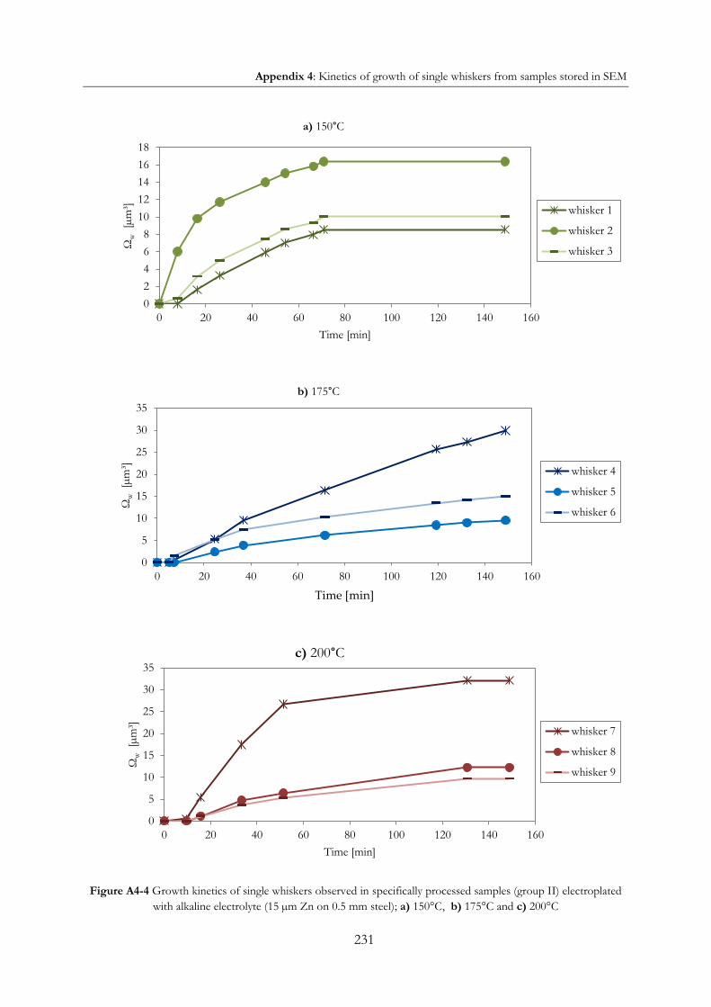
Appendix 4: Kinetics of growth of single whiskers from samples stored in SEM
231
Figure A4-4 Growth kinetics of single whiskers observed in specifically processed samples (group II) electroplated with alkaline electrolyte (15 µm Zn on 0.5 mm steel); a) 150°C, b) 175°C and c) 200°C
0
2
4
6
8
10
12
14
16
18
0 20 40 60 80 100 120 140 160
Ωw [
µm³]
Time [min]
a) 150°C
whisker 1
whisker 2
whisker 3
0
5
10
15
20
25
30
35
0 20 40 60 80 100 120 140 160
Ωw [
µm³]
Time [min]
b) 175°C
whisker 4
whisker 5
whisker 6
0
5
10
15
20
25
30
35
0 20 40 60 80 100 120 140 160
Ωw [
µm³]
Time [min]
c) 200°C
whisker 7
whisker 8
whisker 9

Appendix 4: Kinetics of growth of single whiskers from samples stored in SEM
232
Figure A4-5 Growth kinetics of single whiskers observed in specifically processed samples (group II) electroplated with alkaline electrolyte (15 µm Zn on 1 mm steel); a) 150°C
0
1
2
3
4
5
6
7
0 10 20 30 40 50 60
Ωw [
µm³]
Time [min]
a) 150°C
whisker 1
whisker 2
whisker 3

Appendix 4: Kinetics of growth of single whiskers from samples stored in SEM
233
Figure A4-6 Growth kinetics of single whiskers observed in specifically processed samples (group II) electroplated with alkaline electrolyte (15 µm Zn on 1.5 mm steel); a) 150°C, b) 175°C and c) 200°C
0
1
2
3
4
5
6
7
8
0 20 40 60 80 100
Ωw [
µm³]
Time [min]
a) 150°C
whisker 1
whisker 2
whisker 3
0
2
4
6
8
10
12
14
16
0 20 40 60 80 100
Ωw [
µm³]
Time [min]
b) 175°C
whisker 4
whisker 5
whisker 6
0
2
4
6
8
10
12
0 20 40 60 80 100
Ωw [
µm³/
s]
Time [min]
c) 200°C
whisker 7
whisker 8
whisker 9

Appendix 4: Kinetics of growth of single whiskers from samples stored in SEM
234
Figure A4-7 Growth kinetics of single whiskers observed in specifically processed samples (group II) electroplated with acid electrolyte (10 µm Zn on 0.5 mm steel); a) 150°C, b) 175°C and c) 200°C
0
2
4
6
8
10
12
14
16
0 20 40 60 80
Ωw [
µm³]
Time [min]
a) 150°C
whisker 1
whisker 2
whisker 3
0
1
2
3
4
5
6
7
0 20 40 60 80
Ωw [
µm³]
Time [min]
b) 175°C
whisker 4
whisker 5
whisker 6
0123456789
10
0 20 40 60 80
Ωw [
µm³]
Time [min]
c) 200°C
whisker 7
whisker 8
whisker 9

Appendix 4: Kinetics of growth of single whiskers from samples stored in SEM
235
Figure A4-8 Growth kinetics of single whiskers observed in specifically processed samples (group II) electroplated with acid electrolyte (10 µm Zn on 1.5 mm steel); a) 150°C, b) 175°C and c) 200°C
0
5
10
15
20
25
30
35
40
0 20 40 60 80 100 120 140
Ωw [
µm³]
Time [min]
a) 150°C
whisker 1
whisker 2
whisker 3
0
5
10
15
20
25
30
35
40
45
0 20 40 60 80 100 120 140
Ωw [
µm³]
Time [min]
b) 175°C
whisker 4
whisker 5
whisker 6
0
2
4
6
8
10
12
14
16
18
0 20 40 60 80 100 120 140
Ωw [
µm³]
Time [min]
c) 200°C
whisker 7
whisker 8
whisker 9

Appendix 5: Stress relaxation
236
Appendix 5: Stress relaxation
a) Influence of steel substrate thickness (acid) in total growth
c) Influence of steel substrate thickness (acid) in whiskers growth
b) Influence of electroplating electrolyte in total growth
d) Influence of electroplating electrolyte in whiskers growth
Figure A5-1 Relaxed stress ( ) vs. total growth (Ω) and whiskers growth (Ωw) in specifically processed alkaline-origin samples for different zinc coating and substrate thicknesses
0
50
100
150
0 2 000 4 000 6 000 8 000 10 000 12 000 14 000Stre
ss r
elie
f (
) [M
Pa]
Total growth (Ω) [µm³/ mm² surface]
Acid, 10 µm Zn
1.5 mm steel 0.5 mm steel
0
50
100
150
0 2 000 4 000 6 000 8 000Stre
ss r
elie
f (
) [M
Pa]
Whiskers growth (Ωw) [µm³/ mm² surface]
Acid, 10 µm Zn
1.5 mm steel 0.5 mm steel
0
50
100
150
0 2 000 4 000 6 000 8 000 10 000 12 000 14 000Stre
ss r
elie
f (
) [M
Pa]
Total growth (Ω) [µm³/ mm² surface]
10 µm Zn, 0.5 mm steel
Acid Alkaline
0
50
100
150
0 2 000 4 000 6 000 8 000Stre
ss r
elie
f (
) [M
Pa]
Whiskers growth (Ωw) [µm³/ mm² surface]
10 µm Zn, 0.5 mm steel
Acid Alkaline

Appendix 5: Stress relaxation
237
Table A5-1 Activation energy of stress relaxation (Ea ), pre-exponential factor (a) and coefficient of determination
(R²) (Equation 4-1)
Electrolyte Zinc coating thickness steel thickness a [MPa]
Eaσ [kJ/mol]
R²
Alkaline chromed 5µm 0.5mm 6418 15.6 0.9914
Alkaline chromed 10µm 0.5mm 47763 24.1 0.9207
Alkaline chromed 15µm 0.5mm 3715 13.7 0.9572
Alkaline chromed 15µm 1.5mm 4826 14.4 0.9346
Alkaline non-chromed 10µm 0.5mm 688 7.9 1*
Acid chromed 10µm 0.5mm 3712 12.4 0.9997
Acid chromed 10µm 1.5mm 1137 9.0 0.9907
Sample B (from industrial site)
7µm 0.6 mm 7612 6.7 1**
*From only two data (60°C and 150°C) **from only two data (30°C and 60°C)
a) 0.5 mm steel substrate
b) 1.5 mm steel substrate
Figure A5-2 Stress relaxation of samples with time (specifically processed samples,10 µm Zn coating, acid electrolyte, at 150 and 200°C)
-140
-120
-100
-80
-60
-40
-20
0
20
40
0 50 100 150 200 250
Com
pres
sive
str
ess
[MP
a]
Time [min]
200°C 150°C
-140
-120
-100
-80
-60
-40
-20
0
20
40
0 50 100 150 200
Com
pres
sive
str
ess
[MP
a]
Time [min]
200°C 150°C

Appendix 5: Stress relaxation
238
a) 5 µm Zn on 0.5 mm steel substrate
b) 10 µm Zn on 0.5 mm steel substrate
c) 15 µm Zn on 0.5 mm steel substrate
d) 15 µm Zn on 1.5 mm steel substrate
Figure A5-3 Stress relaxation of samples with time (specifically processed samples, alkaline electrolyte, at 150 and 200°C)
-20
0
20
40
60
80
100
120
0 20 40 60 80 100 120 140
Com
pres
sive
str
ess
[MP
a]
Time [min]
200°C
0
20
40
60
80
100
120
0 20 40 60 80 100 120 140
Com
pres
sive
str
ess
[MP
a]
Time [min]
200°C 150°C
0
20
40
60
80
100
120
140
0 20 40 60 80 100 120 140
Com
pres
sive
str
ess
[MP
a]
Time [min]
200°C 150°C
0
20
40
60
80
100
120
140
0 50 100
Com
pres
sive
str
ess
[MP
a]
Time [min]
200°C 150°C

Appendix 5: Stress relaxation
239
a) chromed
b) non chromed
Figure A5-4 Stress relaxation of samples with time (specifically processed samples, alkaline electrolyte, at 150 and 200°C)
Figure A5-5 Stress relaxation of samples with time (specifically processed samples and samples from industrial site)
at 30 and 60°C)
0
20
40
60
80
100
120
0 20 40 60 80 100
Com
pres
sive
str
ess
[MP
a]
Time [min]
200°C 150°C
0
20
40
60
80
100
120
0 20 40 60 80 100
Com
pres
sive
str
ess
[MP
a]
Time [min]
200°C
0
20
40
60
80
100
120
0 2 000 4 000 6 000
Com
pres
sive
str
ess
[MP
a]
Time [h]
Sample B (7 µm Zn, 0.6 mmsteel), 30°C
Sample B (7 µm Zn, 0.6 mmsteel), 60°C
Alkaline, 15 µm Zn (1 mmsteel), 60°C
Acid, 10 µm Zn (1 mmsteel), 60°C

Appendix 6: Influence of temperature on material growth
240
Appendix 6: Influence of temperature on material growth
a) Influence of zinc coating thickness (alkaline)
b) Influence of steel thickness (alkaline)
c) Influence of chrome (alkaline)
d) Influence of electrolyte
Figure A6-1 Total growth per mm² surface (Ω) vs. temperature in specifically processed samples for diverse influencing parameters
0,1
10
1000
100000
50 75 100 125 150 175 200
Tot
al g
row
th (
Ω) [
µm³/
mm
² su
rf.]
Temperature [°C]
Alkaline, 0.5 mm steel
5 µm Zn 10 µm Zn 15 µm Zn
1
10
100
1 000
10 000
100 000
50 75 100 125 150 175 200
Tot
al g
row
th (
Ω) [
µm³/
mm
² su
rf.]
Temperature [°C]
Alkaline, 15 µm Zn
0.5 mm steel 1 mm steel 1.5 mm steel
1
10
100
1 000
10 000
100 000
50 75 100 125 150 175 200
Tot
al g
row
th (
Ω) [
µm³/
mm
² su
rf]
Temperature [°C]
Alkaline, 10 µm Zn on 0.5 mm steel
Non-chromed Chromed
1
10
100
1 000
10 000
100 000
50 75 100 125 150 175 200T
otal
gro
wth
(Ω
) [µm
³/ m
m²
surf
] Temperature [°C]
10 µm Zn, 1.5 mm steel
Acid Alkaline

Appendix 6: Influence of temperature on material growth
241
a) Influence of zinc coating thickness (alkaline)
b) Influence of steel thickness (alkaline)
c) Influence of chrome (alkaline) d) Influence of electrolyte
Figure A6-2 Whiskers growth per mm² surface (Ωw) vs. temperature in specifically processed samples, for diverse influencing parameters
1
10
100
1 000
10 000
100 000
50 75 100 125 150 175 200 Ωw
[µm
³/ m
m²
surf
ace]
Temperature [°C]
Alkaline, 0.5 mm steel
5 µm Zn 10 µm Zn 15 µm Zn
1
10
100
1 000
10 000
100 000
50 75 100 125 150 175 200 Ωw
[µm
³/ m
m²
surf
ace]
Temperature [°C]
Alkaline, 15 µm Zn
0.5 mm steel 1 mm steel 1.5 mm steel
1
10
100
1 000
10 000
100 000
50 75 100 125 150 175 200 Ωw
[µm
³/ m
m²
surf
ace]
Temperature [°C]
Alkaline, 10 µm Zn on 0.5 mm steel
Non-chromed Chromed
1
10
100
1 000
10 000
100 000
50 75 100 125 150 175 200 Ωw
[µm
³/ m
m²
surf
ace]
Temperature [°C]
10 µm Zn, 1.5 mm steel
Acid Alkaline

Appendix 6: Influence of temperature on material growth
242
Table A6-1 Activation energy (Ea) of total growth and whiskers growth, pre-exponential factor (b) and coefficient of determination (R²) (for Equation 4-3)
Electrolyte Zinc coating thickness
Steel substrate thickness
For whiskers growth For total growth
b [µm³/s]
Ea [kJ/mol]
R² b [µm³/s]
Ea [kJ/mol]
R²
Alkaline chromed 5µm 0.5mm - - - 21.2 76.0 0.8926
Alkaline chromed 15µm 0.5mm 27.8 96.3 0.9606 18.1 53.2 0.99
Alkaline chromed 15µm 1.5mm 23.9 84.8 0.9139 14.0 44.7 0.8035
Alkaline non-chromed 10µm 0.5mm 14.5 45.8 1* 14.1 41.0 1*
Acid chromed 10µm 1.5mm 6.7 24.1 0.9361 10.3 30.4 0.7826
*From only two data (150°C and 200°C)

Appendix 7: Whiskers and hillocks density
243
Appendix 7: Whiskers and hillocks density
Average distance between hillocks (dh) and between whiskers (dw) are plotted in Figure A7-1, assuming an uniform and square-pattern distribution of both hillocks and whiskers, as shown in Figure A7-2.
Distance between whiskers can be as short as 29 µm (alkaline 15 µm Zn on 0.5 mm steel at 200°C) and as long as 2 mm (sample A at 60°C).
As far as hillocks it is concerned, distance between hillocks goes from 5 µm (alkaline 15 µm Zn on 0.5 mm steel at 200°C) to 177 µm (sample A at 30°C). The ratio is dw/dh is also calculated and plotted in Figure A7-3, it is seen that this ratio is in most of the cases lower to 10.
Sam
ple
A
(20
µm Z
n, 0
.5 m
m s
teel
)
Sam
ple
B
(7 µ
m Z
n, 0
.5 m
m s
teel
)
Alk
alin
e el
ectr
olyt
e (5
µm
Zn,
0.5
mm
ste
el)
Alk
alin
e el
ectr
olyt
e (1
0 µm
Zn,
0.5
mm
ste
el)
Alk
alin
e el
ectr
olyt
e (1
5 µm
Zn,
0.5
mm
ste
el)
Alk
alin
e el
ectr
olyt
e (1
5 µm
Zn,
0.5
mm
ste
el)
Alk
alin
e el
ectr
olyt
e (1
5 µm
Zn,
1 m
m s
teel
)
Alk
alin
e el
ectr
olyt
e, n
o-ch
rom
ed
(10
µm Z
n, 0
.5 m
m s
teel
)
Aci
d el
ectr
olyt
e (1
0 µm
Zn,
0.5
mm
ste
el)
Aci
d el
ectr
olyt
e (1
0 µm
Zn,
1.5
mm
ste
el)
Figure A7-1 Average distance between whiskers (dw) and between hillocks (dh)
10
100
1000
10000
Avg
. dis
tanc
e be
twee
n w
hisk
ers
[µm
] 200°C
175°C
150°C
60°C
30°C
10
100
1000
Avg
. dis
tanc
e be
twee
n hi
llock
s [µ
m]
200°C
175°C
150°C
60°C
30°C

Appendix 7: Whiskers and hillocks density
244
Figure A7-2 Square pattern of whiskers and hillocks distribution
Figure A7-3 Ratio dw/ dh
10
100
1000
10000
0 20 40 60 80 100 120
d w/
d h
distance between hillocks [µm]
200°C
175°C
150°C
60°C
30°C
dw=dh
dw=10dh

Appendix 8: Summary of whiskers and hillocks growth
245
Appendix 8: Summary of whiskers and hillocks growth
Figure A8-1 summarizes the influence of temperature on whiskers growth and total growth. Both hillocks and whiskers growth are strongly influenced by temperature.
Sam
ple
A
(20
µm Z
n, 0
.5 m
m s
teel
)
Sam
ple
B
(7 µ
m Z
n, 0
.5 m
m s
teel
)
Alk
alin
e el
ectr
olyt
e (5
µm
Zn,
0.5
mm
ste
el)
Alk
alin
e el
ectr
olyt
e (1
0 µm
Zn,
0.5
mm
ste
el)
Alk
alin
e el
ectr
olyt
e (1
5 µm
Zn,
0.5
mm
ste
el)
Alk
alin
e el
ectr
olyt
e (1
5 µm
Zn,
0.5
mm
ste
el)
Alk
alin
e el
ectr
olyt
e (1
5 µm
Zn,
1 m
m s
teel
)
Alk
alin
e el
ectr
olyt
e, n
o-ch
rom
ed
(10
µm Z
n, 0
.5 m
m s
teel
)
Aci
d el
ectr
olyt
e (1
0 µm
Zn,
0.5
mm
ste
el)
Aci
d el
ectr
olyt
e (1
0 µm
Zn,
1.5
mm
ste
el)
Figure A8-1 Whiskers growth per mm² surface ΩW and total growth per mm² surface Ω
The ratio of whiskers growth and total growth is shown in Figure A8-2; up to 60% of the total growth can correspond to whiskers growth (non-chromed alkaline-origin sample at 150°C and 200°C).
Figure A8-2 also shows the ratio of total growth respect to the coating volume; this ratio corresponds to the fraction of the zinc material that grows outside the coating in hillocks or whiskers features. The maximal determined fraction corresponds to 0.7% (alkaline 15 µm Zn on 0.5 mm steel at 200°C), that is, up to 0.7% of the material of the coating grows out of the surface trough hillocks or whiskers growth.
10
100
1 000
10 000
100 000
Ωw[µ
m³/
mm
² su
rfac
e ]
200°C
175°C
150°C
60°C
30°C
100
1 000
10 000
100 000
Ω[µ
m³/
mm
² su
rfac
e ]
200°C
175°C
150°C
60°C
30°C
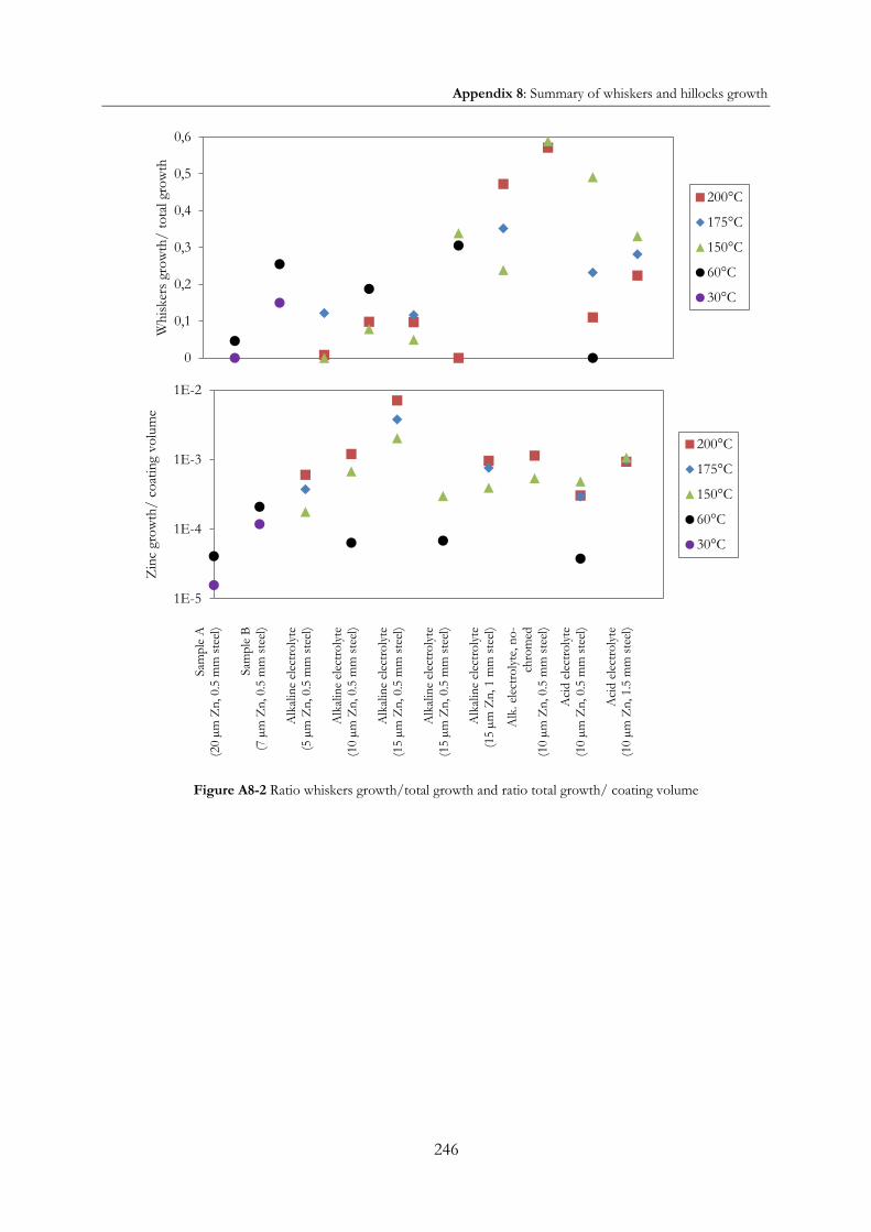
Appendix 8: Summary of whiskers and hillocks growth
246
Sam
ple
A
(20
µm Z
n, 0
.5 m
m s
teel
)
Sam
ple
B
(7 µ
m Z
n, 0
.5 m
m s
teel
)
Alk
alin
e el
ectr
olyt
e (5
µm
Zn,
0.5
mm
ste
el)
Alk
alin
e el
ectr
olyt
e (1
0 µm
Zn,
0.5
mm
ste
el)
Alk
alin
e el
ectr
olyt
e (1
5 µm
Zn,
0.5
mm
ste
el)
Alk
alin
e el
ectr
olyt
e (1
5 µm
Zn,
0.5
mm
ste
el)
Alk
alin
e el
ectr
olyt
e (1
5 µm
Zn,
1 m
m s
teel
)
Alk
. ele
ctro
lyte
, no-
chro
med
(1
0 µm
Zn,
0.5
mm
ste
el)
Aci
d el
ectr
olyt
e (1
0 µm
Zn,
0.5
mm
ste
el)
Aci
d el
ectr
olyt
e (1
0 µm
Zn,
1.5
mm
ste
el)
Figure A8-2 Ratio whiskers growth/total growth and ratio total growth/ coating volume
0
0,1
0,2
0,3
0,4
0,5
0,6
Whi
sker
s gr
owth
/ to
tal g
row
th
200°C
175°C
150°C
60°C
30°C
1E-5
1E-4
1E-3
1E-2
Zin
c gr
owth
/ co
atin
g vo
lum
e
200°C
175°C
150°C
60°C
30°C
Copyright © 2022 FDOKUMEN