processes

Article

Effects of Different Wall Shapes on Thermal-HydraulicCharacteristics of Different Channels Filled with Water BasedGraphite-SiO2 Hybrid Nanofluid

Yacine Khetib 1,2,*, Ahmad Alahmadi 3, Ali Alzaed 4, Ahamd Tahmasebi 5 , Mohsen Sharifpur 6,7,*and Goshtasp Cheraghian 8,*

�����������������

Citation: Khetib, Y.; Alahmadi, A.;

Alzaed, A.; Tahmasebi, A.;

Sharifpur, M.; Cheraghian, G. Effects

of Different Wall Shapes on

Thermal-Hydraulic Characteristics of

Different Channels Filled with Water

Based Graphite-SiO2 Hybrid

Nanofluid. Processes 2021, 9, 1253.

https://doi.org/10.3390/pr9071253

Academic Editor: Hussein

A. Mohammed

Received: 12 June 2021

Accepted: 16 July 2021

Published: 20 July 2021

Publisher’s Note: MDPI stays neutral

with regard to jurisdictional claims in

published maps and institutional affil-

iations.

Copyright: © 2021 by the authors.

Licensee MDPI, Basel, Switzerland.

This article is an open access article

distributed under the terms and

conditions of the Creative Commons

Attribution (CC BY) license (https://

creativecommons.org/licenses/by/

4.0/).

1 Mechanical Engineering Department, Faculty of Engineering, King Abdulaziz University,Jeddah 80204, Saudi Arabia

2 Center Excellence of Renewable Energy and Power, King Abdulaziz University, Jeddah 80204, Saudi Arabia3 Department of Electrical Engineering, College of Engineering, Taif University, Taif 21944, Saudi Arabia;

aziz@tu.edu.sa4 Architectural Engineering Department, Faculty of Engineering, Taif University, Taif 21944, Saudi Arabia;

alzaed@tu.edu.sa5 Independent Researcher, Dubai 999041, United Arab Emirates; tahmaseby.ahmad@gmail.com6 Department of Mechanical and Aeronautical Engineering, University of Pretoria, Hatfield 0028, South Africa7 Department of Medical Research, China Medical University Hospital, China Medical University,

Taichung 404, Taiwan8 Technische Universität Braunschweig, 38106 Braunschweig, Germany* Correspondence: ykhetib@yahoo.com (Y.K.); mohsen.sharifpur@up.ac.za (M.S.);

g.cheraghian@tu-braunschweig.de (G.C.)

Abstract: In the current numerical study, various wall shape effects are investigated on the thermal-hydraulic characteristics of different channels filled with water-based graphite-SiO2 hybrid nanofluid.In this work, the performance evaluation criteria (PEC) index is employed as the target parameter toattain optimum geometry. Six different cases are studied in this research, and each case has differentgeometrical dimensions. The inlet temperature for the fluids in the channel is 300 K, over a rangeof different flow velocities. According to the obtained results, an increase in the volume fraction ofnanoparticles results in higher PEC values. In addition, an increase in Reynolds number to Re = leadsto an increase in the PEC index. The results clearly show that increasing the Reynolds number hastwo consequences: on the one hand, it increases the pressure drop penalty; on the other hand, itimproves heat transfer. Therefore, the maximum value of the PEC index occurs at Re = 15,000.

Keywords: hybrid nanofluid; PEC; graphite-SiO2; channel; different wall

1. Introduction

The use of different surfaces and nanofluids have always been recognized as twovery effective solutions to improving heat exchanger performance [1–5]. However, theshape of the wall of the channel affects the hydraulic performance of the system, so ge-ometries that have the smallest pressure drops are used. On the other hand, nanofluidshave been widely used in recent years due to their unique properties [6–10]. Nanofluidscan increase the heat transfer in heat devices [11–15]. Some researchers have used nu-merical methods to study nanofluids [16–20]. Nakharintr and Naphon [21] studied thethermal hydraulic characteristics of TiO2 nanofluid magnetohydrodynamic (MHD) flowexperimentally through a mini-channel heat sink with a confined jet impingement. Theeffects of different magnetic fields (B = 0.084 and 0.28 µT) were investigated in their work.Ashorynejad and Zarghami [22] used the lattice Boltzmann method to investigate thethermal characteristics of partially porous wavy channels using Cu nanofluid MHD (waterbased nanofluid) flow. Important parameters including Nusselt number, Hartmann num-ber, pressure drop, friction factor, and Darcy number were investigated in their research.

Processes 2021, 9, 1253. https://doi.org/10.3390/pr9071253 https://www.mdpi.com/journal/processes

Processes 2021, 9, 1253 2 of 34

Dormohammadi et al. [23] studied the thermal entropy generation and characteristics of asinusoidal wavy wall channel with a water based Cu nanofluid flow. The results show thatthe entropy generation values increase when increasing the Richardson numbers. Saeedand Kim [24] studied the thermal characteristics of a mini-channel heat sink using Al2O3water based nanofluid. They analyzed the different influences of geometrical parameters,nanofluid flow velocities, and nanoparticle volume fractions on outlet temperatures andheat transfer improvements.

Dalkılıç et al. [25] investigated the thermal enhancement of different quad channel(horizontal tube) inserts filled with water based graphite-SiO2 hybrid nanofluid. In thatstudy, convection heat transfer and the nanofluid flow were simulated in the turbulentflow regime (3400 < Re < 11,000). The results illustrated that the nanofluid can significantlyimprove heat transfer parameters. Saba et al. [26] investigated the usage of hybrid SWCNT-Fe3O4 water based nanofluid for thermal efficiency improvement of an asymmetric channelwith dilating or squeezing walls. They realized that the SWCNTs nanoparticles have asuperior influence on thermal characteristics. Ajeel et al. [27] numerically and experimen-tally studied convective heat transfer and turbulent flow inside a different channel filledwith Al2O3 water based nanofluid in the turbulent flow regime (10,000 < Re < 30,000).Based on the results, the utilization of nanofluid and corrugated geometry increases systemenergy efficiency. Gholami et al. [28] studied natural convection heat transfer in a verticalchannel wall equipped with dimple fins filled with different nanofluids (water based Al2O3,TiO2, Cu and CNT nanofluids) by the finite volume method (FVM). In addition, they usedthe SIMPLE algorithm for pressure-velocity system coupling and governing equationsdiscretization. They found that TiO2 nanofluid at a volume fraction of 6% had the highestthermal performance among all studied models.

Shah et al. [29] numerically studied nanofluid flow and radiative heat transfer betweenpermeable channels. Different effects of non-dimensional parameters like Darcys Number,micropolar parameter, injection/suction fractional factor, flow velocity, radiation parameter,and Prandtl number, were analyzed in detail in their paper. Ajeel et al. [30,31] experimen-tally and numerically studied heat transfer in different channels by SiO2 water nanofluid.Their goal was to analyze different nanoparticle volume fractions (1 < ϕ < 4%) and flowvelocities (10,000 < Re < 30,000). The results showed that numerical and experimental datahad fine convergence and supported each other. In another study, geometrical parametereffects investigated thermal-hydraulic performance (friction factor and average Nusseltnumber) in a trapezoidal channel filled with SiO2 water based nanofluid [32]. In that study,the nanofluid flow (SiO2–graphite water based nanofluid) was simulated in a turbulentregime (10,000 < Re < 30,000) and also a house shaped-different channel. Their resultsindicated that the nanofluid and different geometries enhanced the energy efficiency ofthe system.

Our literature review indicates that the effects of different wall shapes on thermal-hydraulic characteristics of different channels filled with water based graphite-SiO2 hy-brid nanofluid have not yet been analyzed by researchers. In this work, the perfor-mance evaluation criteria (PEC) index is employed as a target parameter to ascertainthe optimum geometry.

2. Numerical Model2.1. Physical Model

A schematic diagram of the heat exchangers studied is shown in Figure 1. It canbe seen that six different cases are studied in this paper with different wall shapes andboundary conditions. Each case has different geometrical dimensions, which are inves-tigated numerically to achieve the most efficient configuration. The channel is under aconstant temperature of Ts = 450 K. The heat transfer fluid (HTF) is hybrid graphite-SiO2water based nanofluid, which enters the channel at 330 K and at different flow velocities ofRe = 11,000, 15,000, 19,000, and 23,000 (Table 1).

Processes 2021, 9, 1253 3 of 34

Processes 2021, 9, x FOR PEER REVIEW 3 of 37

boundary conditions. Each case has different geometrical dimensions, which are investi-gated numerically to achieve the most efficient configuration. The channel is under a con-stant temperature of Ts = 450 K. The heat transfer fluid (HTF) is hybrid graphite-SiO2 water based nanofluid, which enters the channel at 330 K and at different flow velocities of Re = 11,000, 15,000, 19,000, and 23,000 (Table 1).

inT

outTsT

A1A2

RR JJ L

D

Case A

inT

outTsT

D

RR JJ L

B1B2

Case B

inT

outTsT

2R2R JJ L

C1C2

D

Case C

inT

outTsT

2R2R JJ L

D1D2

D

Case D

Processes 2021, 9, x FOR PEER REVIEW 4 of 37

inT

outTsT

E1E2

2R2R JJ L

D

Case E

inT

outTsT

2F2F JJ L

D

Case F

Figure 1. Schematic of heat exchangers with different wall shapes and boundary conditions.

Table 1. Boundary conditions and geometrical data.

Parameters Values Parameters Values D 60 mm J 17 mm L 180 − 4𝑅 − 2𝐽 R 11, 13 and 15 mm

A1 12 mm A2 22, 24 and 26 mm B1 12 mm B2 22, 24 and 26 mm C1 12 mm C2 22, 24 and 26 mm D1 12 mm D2 22, 24 and 26 mm E1 12 mm E2 10, 12 and 14 mm F 11, 13 and 15 mm 𝛿 2 mm

Tin 330 K Ts 450 K

Pout 0 (gage) Re 11,000, 15,000, 19,000, and 23,000

Table 2 presents the thermophysical properties of the base fluid and nanoparticles.

Table 2. Thermophysical properties of base fluid and nanoparticles [25].

Thermophysical Proper-ties k (W/m·K) cp (J/kg·K) ρ (kg/m3)

Mean Diam-eter of Parti-

cle (nm) Graphite 25 720 2060 8

SiO2 1.4 765 2200 7 water 0.613 4179 997.1 -

The hybrid nanoparticle volume fraction based on the proportion of SiO2 and graph-ite nanoparticle portions is calculated using the following equation [25]:

Figure 1. Schematic of heat exchangers with different wall shapes and boundary conditions.

Processes 2021, 9, 1253 4 of 34

Table 1. Boundary conditions and geometrical data.

Parameters Values Parameters Values

D 60 mm J 17 mmL 180− 4R− 2J R 11, 13 and 15 mm

A1 12 mm A2 22, 24 and 26 mmB1 12 mm B2 22, 24 and 26 mmC1 12 mm C2 22, 24 and 26 mmD1 12 mm D2 22, 24 and 26 mmE1 12 mm E2 10, 12 and 14 mmF 11, 13 and 15 mm δ 2 mm

Tin 330 K Ts 450 K

Pout 0 (gage) Re 11,000, 15,000, 19,000,and 23,000

Table 2 presents the thermophysical properties of the base fluid and nanoparticles.

Table 2. Thermophysical properties of base fluid and nanoparticles [25].

ThermophysicalProperties k (W/m·K) cp (J/kg·K) ρ (kg/m3)

Mean Diameterof Particle (nm)

Graphite 25 720 2060 8SiO2 1.4 765 2200 7water 0.613 4179 997.1 -

The hybrid nanoparticle volume fraction based on the proportion of SiO2 and graphitenanoparticle portions is calculated using the following equation [25]:

ϕ =

(

mnp1ρnp1

)+(

mnp2ρnp2

)(

mnp1ρnp1

)+(

mnp2ρnp2

)+(mb f

ρb f

) (1)

where m is the mass portion of used materialsThe hybrid nanofluid density can be written as followss [5]:

ρn f = ϕnp1ρnp1 + ϕnp2ρnp2 +(1− ϕnp1 − ϕnp2

)ρb f (2)

where ϕnp1 and ϕnp2 are the nanoparticle volume fractions of SiO2 and Graphite, respectively [25].The hybrid nanofluid specific heat capacity is calculated using the following Equation [25]:

(ρn f × cp,n f ) = ϕnp1ρnp1cp,np1 + ϕnp2ρnp2cp,np2 +(1− ϕnp1ρnp1 − ϕnp2ρnp2

)cp,b f (3)

The hybrid nanofluid relative dynamic viscosity can be written as follows [25]:

µn f

µb f= 1.00527× T0.00035 × (1 + ϕ)9.36265 ×

(mnp1

mnp2

)−0.028935(4)

where T is the average temperature.The hybrid nanofluid relative thermal conductivity is determined as follows [25]:

kn f

kb f= 0.852870218× T0.052797513 × (1 + ϕ)6.591412917 ×

(mnp2

mnp1

)0.022254808

(5)

2.2. Governing Equations

In this work, the Eulerian–Eulerian (two-phase technique) was used to simulatethe nanofluid in channel. The continuity equation and momentum are also reported

Processes 2021, 9, 1253 5 of 34

using the following equations [33–36], where the mixture dynamic viscosity is µm, the

pressure is→P , the density of the two-phase mixture is ρm, the base fluid velocity is

→Ub f , the

nanoparticle velocity is→Us, and the base fluid and nanoparticles velocities are

→Udr,b f and

→Udr,s, respectively [36].

Continuity equation:

∇

ρn f (ρsφs

→Us + ρb f φb f

→Ub f

ρsφs + ρb f φb f)

= 0 (6)

Momentum equation:

ρn f (→Um∇

→Um) = −∇

→P + µm(∇

→Um + (∇

→Um)

T) +∇(ρb f φb f

→Udr,b f

→Udr,b f + ρsφs

→Udr,s

→Udr,s) + ρm

→g

→Udr,b f =

→Ub f −

→Um

→Udr,s =

→Us −

→Um

(7)

The energy equation is reported here, where the enthalpy of solid particles and thebase fluid are hs and hb f , respectively. The equation of volume fraction for slip velocity andtwo-phase mixture are defined by Refs. [37,38]. These equations are suitable to calculatethe relation between drift velocity and relative velocity [39,40]. The nanoparticle Reynoldsnumber (Res) is also offered, where dp is the mean particle diameter. The relative velocity iscalculated from Schiller and Naumann’s formulation, where the gravitational accelerationof the fluid and the nanoparticle are

→g and

→α , respectively [41].

Energy equation:

∇(ρb f φb f→Ub f hb f + ρsφs

→Ushs) = ∇((φb f kb f + φsks)∇

→T)

∇(ρsφs→Um) = −∇(ρsφs

→Udr,s)

→Ub f ,s =

→Ub f −

→Us

→Udr,s =

→Us,b f −

ρsφsρm

→Ub f ,s

→Ub f ,s =

d2p

18µb f fd

ρs−ρmρs

→α fd = 1 + 0.15Re0.687

s

→α =

→g − (

→Um∇

→Um) Res =

→Umdpρm

µm

(8)

Equation (9) presents the descriptive equations of the k-ε model, where µt,m is theturbulent dynamic viscosity and k, G are production rates [37–39]. Additionally, Nur and frare the ratios between the reference system and the novel configurations. The referenceconfiguration (RC) is the empty test section (without twisted tape) filled with nanofluid at0.2% volume concentration. The standard constants are employed, Cµ = 0.09, c1 = 1.44,c2 = 1.92, σk = 1.00, σε = 1.30, and σt = 0.85. The Nusselt number and Rayleigh numberof the nanofluid are also reported in [33–37].

Turbulence equations:

∇(ρm→Umk) = ∇

[(µm +

µt,mσk

)∇k]+ Gk,m − ρmε

∇(ρm→Umε) = ∇

[(µm +

µt,mσε

)∇ε]+ ε

k (c1Gk,m − c2ρmε)

µt,m = Cµρmk2

ε Gk,m = µt,m(∇→Um + (∇

→Um)

T)

(9)

Average Nusselt number:

Nu =kn f

k f

∫∂T∂x

(10)

Nusselt number ratio:Nur =

NuNu0

(11)

Processes 2021, 9, 1253 6 of 34

Mean friction factor:f =

2DhL

∆Pρn f V2

in(12)

Friction factor ratio:fr =

ff0

(13)

Performance evaluation criteria index:

PEC = Nur· f− 1

3r (14)

2.3. Grid Mesh Independence Test

The grid mesh independence test was done in this research to achieve the mostefficient grid mesh layout with the minimum error (4%) and calculating time (see Figure 2).Different grid meshes were analyzed, and error values were achieved in Nusselt numberterms. Finally, the grid mesh with 2478 nodes was adopted as the valuable grid mesh fornumerical simulation.

Processes 2021, 9, x FOR PEER REVIEW 7 of 37

Figure 2. The grid mesh independence test in different Reynolds numbers.

2.4. Validation Figure 3 shows the code validation between the numerical data of Yang and Ordonez

[42] and the obtained numerical results from the current study in the case of the PEC in-dex. The PEC numbers were compared at similar geometries and boundary conditions. As can be seen in Figure 3, there is remarkable uniformity between the numerical data of Yang and Ordonez [42] and the numerical results obtained from the current study.

Figure 3. Code validation between numerical data of Yang and Ordonez [42] and obtained numer-ical results from the current study in case of PEC index.

Mass flow rate (kg/s)

PEC

1 2 3 4 5 6 7 8 9 10

0.4

0.5

0.6

0.7Yang and Ordonez (2019) Num.Present study

Figure 2. The grid mesh independence test in different Reynolds numbers.

2.4. Validation

Figure 3 shows the code validation between the numerical data of Yang and Or-donez [42] and the obtained numerical results from the current study in the case of the PECindex. The PEC numbers were compared at similar geometries and boundary conditions.As can be seen in Figure 3, there is remarkable uniformity between the numerical data ofYang and Ordonez [42] and the numerical results obtained from the current study.

Processes 2021, 9, 1253 7 of 34

Processes 2021, 9, x FOR PEER REVIEW 7 of 37

Figure 2. The grid mesh independence test in different Reynolds numbers.

2.4. Validation Figure 3 shows the code validation between the numerical data of Yang and Ordonez

[42] and the obtained numerical results from the current study in the case of the PEC in-dex. The PEC numbers were compared at similar geometries and boundary conditions. As can be seen in Figure 3, there is remarkable uniformity between the numerical data of Yang and Ordonez [42] and the numerical results obtained from the current study.

Figure 3. Code validation between numerical data of Yang and Ordonez [42] and obtained numer-ical results from the current study in case of PEC index.

Mass flow rate (kg/s)

PEC

1 2 3 4 5 6 7 8 9 10

0.4

0.5

0.6

0.7Yang and Ordonez (2019) Num.Present study

Figure 3. Code validation between numerical data of Yang and Ordonez [42] and obtained numericalresults from the current study in case of PEC index.

3. Results and Discussion

In this section, the results of the numerical simulations for different configurations withdifferent geometric parameters are examined. The numerical results of the temperaturecontour, velocity contour, streamlines, kinetic energy contour, Nusselt number variation,friction factor, and PEC index are presented. In the end, different configurations arecompared and arranged in terms of PEC.

3.1. Case A

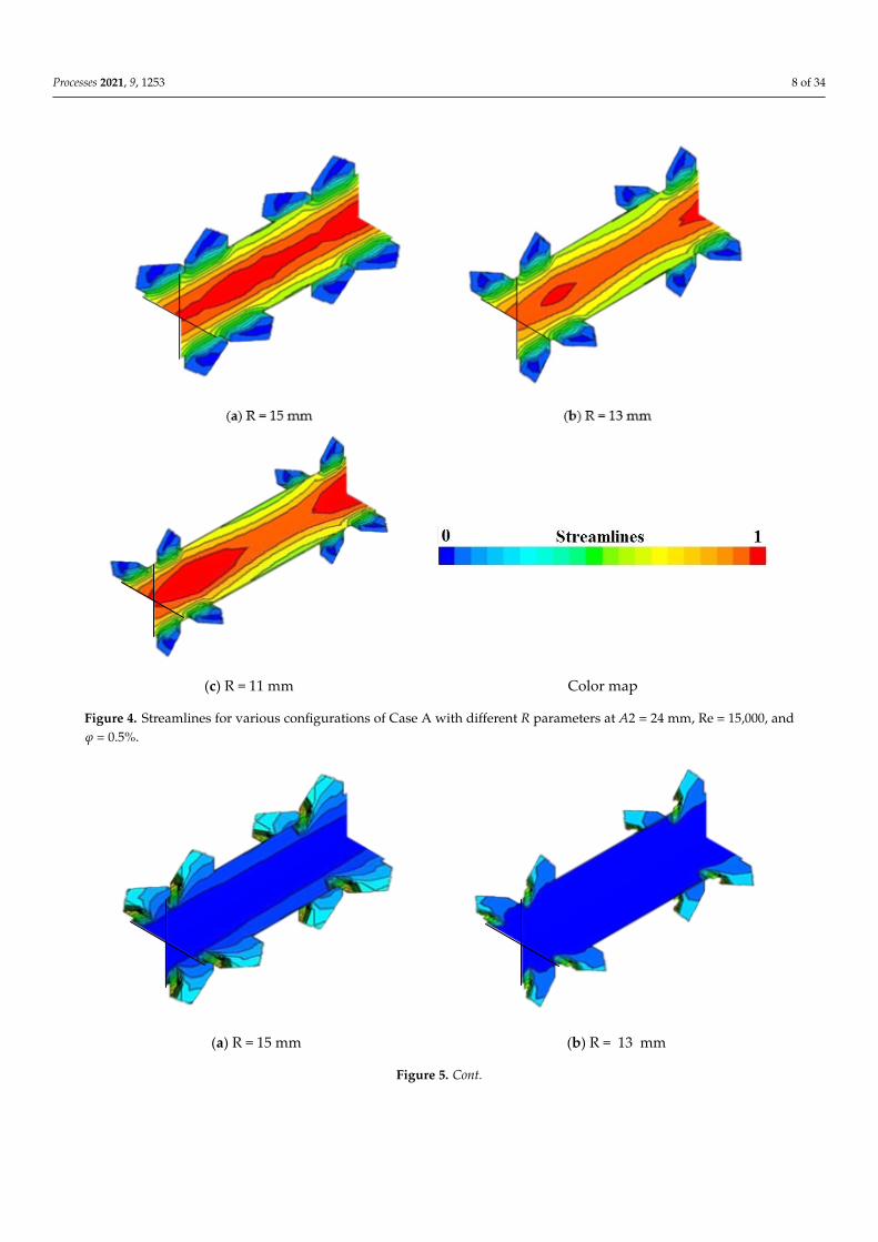
In Case A, two parameters are variable, which are R and A2. First, the variationsin the R parameter are examined and then parameter A2 is analyzed. Therefore, herestreamlines, velocity, kinetic energy contours, and temperature are used. Figure 4 showsstreamlines for various configurations of Case A with different R parameters at A2 = 24 mm,Re = 15,000, and ϕ = 0.5%. As can be seen, by changing parameter R, the streamlines areaffected and change. As parameter R becomes smaller, the formation of vortices and localturbulence in the pipe increases and the flow mixing rate increases. This, on the one hand,increases the heat transfer coefficient, and on the other hand, leads to a greater pressuredrop penalty. This can clearly be seen by the reduction in the dark blue color in this sectionof the tube. Figure 5 illustrates temperature contours for various configurations of Case Awith different R parameters at A2 = 24 mm, Re = 15,000, and ϕ = 0.5%. As can be seen, bychanging parameter R, the temperature contours are affected and change. As parameter Rbecomes smaller, a reduction in the dark blue color in this section of the tube can be seen.The presence of sharp edges in this geometry causes the separation and reversal of theflow, which decreases parameter R and increases parameter A2. The main reason for theformation of the vortex is exactly these sharp edges.

Processes 2021, 9, 1253 8 of 34

1

Processes 2021, 9, x FOR PEER REVIEW 9 of 37

(c) R = 11 mm Color map

Figure 4. Streamlines for various configurations of Case A with different R parameters at A2 = 24 mm, Re = 15,000, and 𝜑

= 0.5%.

Figure 6 presents kinetic energy contours for various configurations of Case A with

different R parameters at A2 = 24 mm, Re = 15,000, and 𝜑 = 0.5%. A reduction in light

green and blue colors with a reduction of parameter R is observed in these figures. Figure

7 demonstrates velocity magnitude contours for various configurations of Case A with

different R parameters at A2 = 24 mm, Re = 15,000, and 𝜑 = 0.5%. This can clearly be seen

in the reduction in the dark blue color in this section of the tube with a reduction in pa-

rameter R.

However, in order to reduce the volume of the article, contours related to different

Reynolds numbers have been omitted. As can be seen, increasing the Reynolds number

intensifies the turbulence, increases the flow mixing rate, and increases the vortices. This

leads to an increase in heat transfer coefficient as well as an increase in the pressure drop

penalty.

(a) R = 15 mm (b) R = 13 mm

Figure 4. Streamlines for various configurations of Case A with different R parameters at A2 = 24 mm, Re = 15,000, andϕ = 0.5%.

Processes 2021, 9, x FOR PEER REVIEW 9 of 37

(c) R = 11 mm Color map

Figure 4. Streamlines for various configurations of Case A with different R parameters at A2 = 24 mm, Re = 15,000, and 𝜑

= 0.5%.

Figure 6 presents kinetic energy contours for various configurations of Case A with

different R parameters at A2 = 24 mm, Re = 15,000, and 𝜑 = 0.5%. A reduction in light

green and blue colors with a reduction of parameter R is observed in these figures. Figure

7 demonstrates velocity magnitude contours for various configurations of Case A with

different R parameters at A2 = 24 mm, Re = 15,000, and 𝜑 = 0.5%. This can clearly be seen

in the reduction in the dark blue color in this section of the tube with a reduction in pa-

rameter R.

However, in order to reduce the volume of the article, contours related to different

Reynolds numbers have been omitted. As can be seen, increasing the Reynolds number

intensifies the turbulence, increases the flow mixing rate, and increases the vortices. This

leads to an increase in heat transfer coefficient as well as an increase in the pressure drop

penalty.

(a) R = 15 mm (b) R = 13 mm

Figure 5. Cont.

Processes 2021, 9, 1253 9 of 34Processes 2021, 9, x FOR PEER REVIEW 10 of 37

(c) R = 11 mm Color map

Figure 5. Temperature contours for various configurations of Case A with different R parameters at A2 = 24 mm, Re =

15,000, and 𝜑 = 0.5%.

(a) R = 15 mm (b) R = 13 mm

(c) R = 11 mm Color map

Figure 6. Kinetic energy contours for various configurations of Case A with different R parameters at A2 = 24 mm, Re =

15,000, and 𝜑 = 0.5%.

Figure 5. Temperature contours for various configurations of Case A with different R parameters at A2 = 24 mm, Re = 15,000,and ϕ = 0.5%.

Figure 6 presents kinetic energy contours for various configurations of Case A withdifferent R parameters at A2 = 24 mm, Re = 15,000, and ϕ = 0.5%. A reduction in lightgreen and blue colors with a reduction of parameter R is observed in these figures. Figure 7demonstrates velocity magnitude contours for various configurations of Case A withdifferent R parameters at A2 = 24 mm, Re = 15,000, and ϕ = 0.5%. This can clearly beseen in the reduction in the dark blue color in this section of the tube with a reduction inparameter R.

Processes 2021, 9, x FOR PEER REVIEW 10 of 37

(c) R = 11 mm Color map

Figure 5. Temperature contours for various configurations of Case A with different R parameters at A2 = 24 mm, Re = 15,000, and 𝜑 = 0.5%.

(a) R = 15 mm (b) R = 13 mm

(c) R = 11 mm Color map

Figure 6. Kinetic energy contours for various configurations of Case A with different R parameters at A2 = 24 mm, Re = 15,000, and 𝜑 = 0.5%. Figure 6. Kinetic energy contours for various configurations of Case A with different R parameters at A2 = 24 mm,

Re = 15,000, and ϕ = 0.5%.

Processes 2021, 9, 1253 10 of 34Processes 2021, 9, x FOR PEER REVIEW 11 of 37

(a) R = 15 mm (b) R = 13 mm

(c) R = 11 mm Color map

Figure 7. Velocity magnitude contours for various configurations of Case A with different R parameters at A2 = 24 mm,

Re = 15,000, and 𝜑 = 0.5%.

Figure 8 shows streamlines for various configurations of Case A with different A2

parameters at R = 15 mm, Re = 15,000, and 𝜑 = 0.5%. As can be seen, by changing param-

eter A2, the streamlines are affected and change. As parameter A2 becomes longer, the

formation of vortices and local turbulence in the pipe increases and the flow mixing rate

increases. This, on the one hand, increases the heat transfer coefficient, and on the other

hand, leads to a greater pressure drop penalty. This can clearly be seen by the reduction

in the dark blue color in this section of the tube.

Figure 7. Velocity magnitude contours for various configurations of Case A with different R parameters at A2 = 24 mm,Re = 15,000, and ϕ = 0.5%.

However, in order to reduce the volume of the article, contours related to differentReynolds numbers have been omitted. As can be seen, increasing the Reynolds numberintensifies the turbulence, increases the flow mixing rate, and increases the vortices. Thisleads to an increase in heat transfer coefficient as well as an increase in the pressuredrop penalty.

Figure 8 shows streamlines for various configurations of Case A with different A2parameters at R = 15 mm, Re = 15,000, and ϕ = 0.5%. As can be seen, by changing parameterA2, the streamlines are affected and change. As parameter A2 becomes longer, the formationof vortices and local turbulence in the pipe increases and the flow mixing rate increases.This, on the one hand, increases the heat transfer coefficient, and on the other hand, leadsto a greater pressure drop penalty. This can clearly be seen by the reduction in the darkblue color in this section of the tube.

Processes 2021, 9, 1253 11 of 34Processes 2021, 9, x FOR PEER REVIEW 12 of 37

(a) A2 = 26 mm (b) A2 = 24 mm

(c) A2 = 22 mm Color map

Figure 8. Streamlines for various configurations of Case A with different A2 parameters at R = 15 mm, Re = 15,000, and 𝜑

= 0.5%.

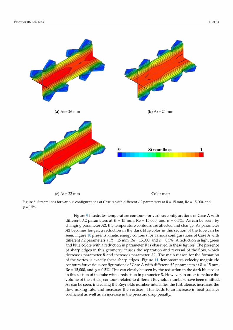
Figure 9 illustrates temperature contours for various configurations of Case A with

different A2 parameters at R = 15 mm, Re = 15,000, and 𝜑 = 0.5%. As can be seen, by

changing parameter A2, the temperature contours are affected and change. As parameter

A2 becomes longer, a reduction in the dark blue color in this section of the tube can be

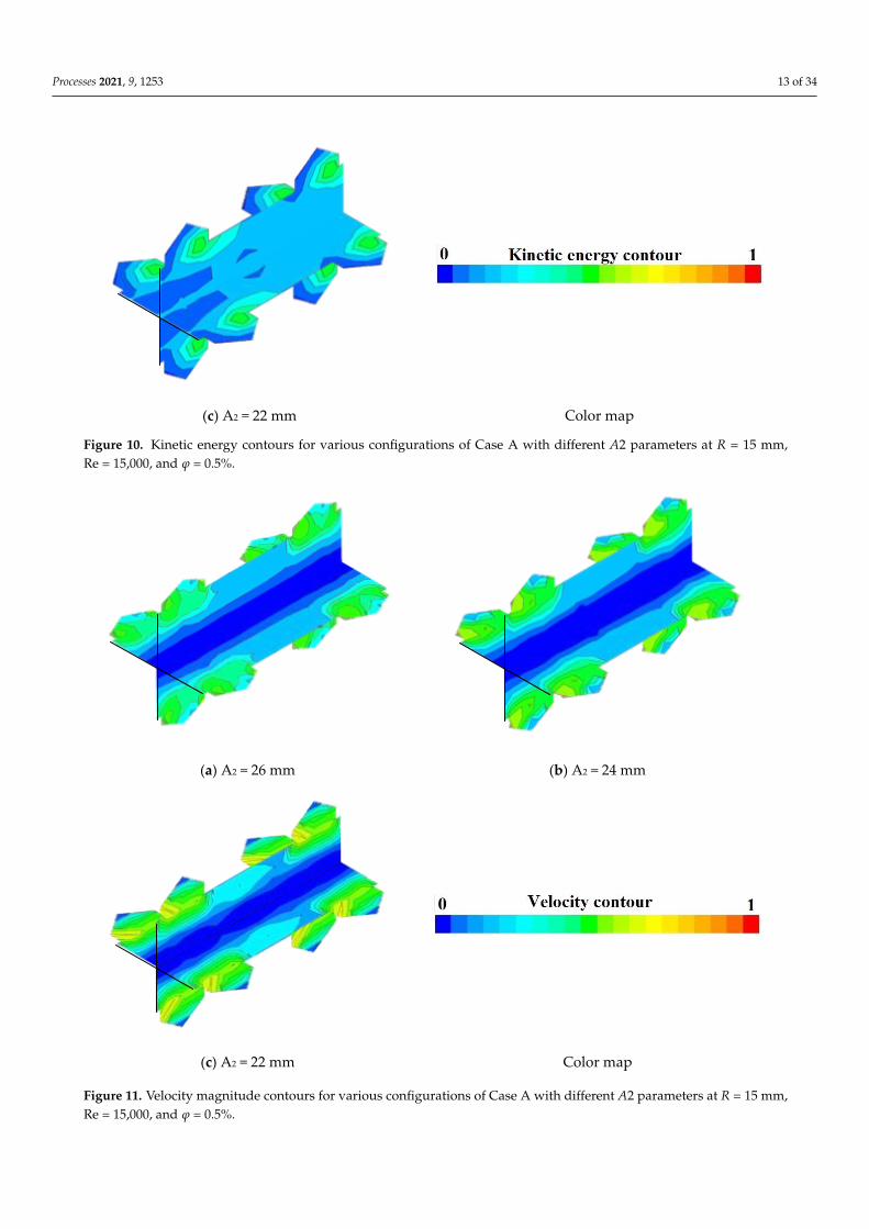
seen. Figure 10 presents kinetic energy contours for various configurations of Case A with

different A2 parameters at R = 15 mm, Re = 15,000, and 𝜑 = 0.5%. A reduction in light

green and blue colors with a reduction in parameter R is observed in these figures. The

presence of sharp edges in this geometry causes the separation and reversal of the flow,

which decreases parameter R and increases parameter A2. The main reason for the for-

mation of the vortex is exactly these sharp edges. Figure 11 demonstrates velocity magni-

tude contours for various configurations of Case A with different A2 parameters at R = 15

mm, Re = 15,000, and 𝜑 = 0.5%. This can clearly be seen by the reduction in the dark blue

color in this section of the tube with a reduction in parameter R. However, in order to

reduce the volume of the article, contours related to different Reynolds numbers have

been omitted. As can be seen, increasing the Reynolds number intensifies the turbulence,

increases the flow mixing rate, and increases the vortices. This leads to an increase in heat

transfer coefficient as well as an increase in the pressure drop penalty.

Figure 8. Streamlines for various configurations of Case A with different A2 parameters at R = 15 mm, Re = 15,000, andϕ = 0.5%.

Figure 9 illustrates temperature contours for various configurations of Case A withdifferent A2 parameters at R = 15 mm, Re = 15,000, and ϕ = 0.5%. As can be seen, bychanging parameter A2, the temperature contours are affected and change. As parameterA2 becomes longer, a reduction in the dark blue color in this section of the tube can beseen. Figure 10 presents kinetic energy contours for various configurations of Case A withdifferent A2 parameters at R = 15 mm, Re = 15,000, and ϕ = 0.5%. A reduction in light greenand blue colors with a reduction in parameter R is observed in these figures. The presenceof sharp edges in this geometry causes the separation and reversal of the flow, whichdecreases parameter R and increases parameter A2. The main reason for the formationof the vortex is exactly these sharp edges. Figure 11 demonstrates velocity magnitudecontours for various configurations of Case A with different A2 parameters at R = 15 mm,Re = 15,000, and ϕ = 0.5%. This can clearly be seen by the reduction in the dark blue colorin this section of the tube with a reduction in parameter R. However, in order to reduce thevolume of the article, contours related to different Reynolds numbers have been omitted.As can be seen, increasing the Reynolds number intensifies the turbulence, increases theflow mixing rate, and increases the vortices. This leads to an increase in heat transfercoefficient as well as an increase in the pressure drop penalty.

Processes 2021, 9, 1253 12 of 34Processes 2021, 9, x FOR PEER REVIEW 13 of 37

(a) A2 = 26 mm (b) A2 = 24 mm

(c) A2 = 22 mm Color map

Figure 9. Temperature contours for various configurations of Case A with different A2 parameters at R = 15 mm, Re =

15,000, and 𝜑 = 0.5%.

(a) A2 = 26 mm (b) A2 = 24 mm

Figure 9. Temperature contours for various configurations of Case A with different A2 parameters at R = 15 mm, Re = 15,000,and ϕ = 0.5%.

Processes 2021, 9, x FOR PEER REVIEW 13 of 37

(a) A2 = 26 mm (b) A2 = 24 mm

(c) A2 = 22 mm Color map

Figure 9. Temperature contours for various configurations of Case A with different A2 parameters at R = 15 mm, Re =

15,000, and 𝜑 = 0.5%.

(a) A2 = 26 mm (b) A2 = 24 mm

Figure 10. Cont.

Processes 2021, 9, 1253 13 of 34Processes 2021, 9, x FOR PEER REVIEW 14 of 37

(c) A2 = 22 mm Color map

Figure 10. Kinetic energy contours for various configurations of Case A with different A2 parameters at R = 15 mm, Re =

15,000, and 𝜑 = 0.5%.

(a) A2 = 26 mm (b) A2 = 24 mm

(c) A2 = 22 mm Color map

Figure 11. Velocity magnitude contours for various configurations of Case A with different A2 parameters at R = 15 mm,

Re = 15,000, and 𝜑 = 0.5%.

Figure 10. Kinetic energy contours for various configurations of Case A with different A2 parameters at R = 15 mm,Re = 15,000, and ϕ = 0.5%.

Processes 2021, 9, x FOR PEER REVIEW 14 of 37

(c) A2 = 22 mm Color map

Figure 10. Kinetic energy contours for various configurations of Case A with different A2 parameters at R = 15 mm, Re =

15,000, and 𝜑 = 0.5%.

(a) A2 = 26 mm (b) A2 = 24 mm

(c) A2 = 22 mm Color map

Figure 11. Velocity magnitude contours for various configurations of Case A with different A2 parameters at R = 15 mm,

Re = 15,000, and 𝜑 = 0.5%. Figure 11. Velocity magnitude contours for various configurations of Case A with different A2 parameters at R = 15 mm,Re = 15,000, and ϕ = 0.5%.

Processes 2021, 9, 1253 14 of 34

3.2. Case B

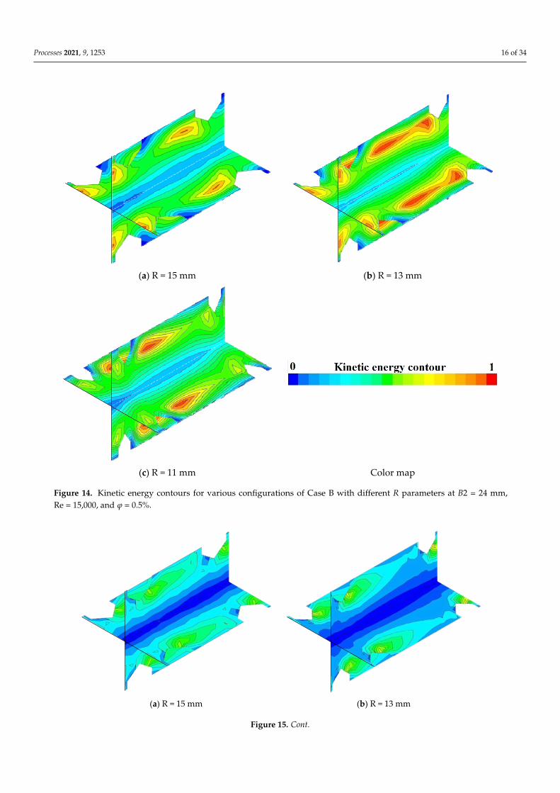
In Case B, two parameters are variable, which are R and B2. First, the variations in theR parameter are examined and then parameter B2 is analyzed. Figure 12 shows streamlinesfor various configurations of Case B with different R parameters at B2 = 24 mm, Re = 15,000,and ϕ = 0.5%. As can be seen, when changing parameter R, the streamlines are affectedand thus also change. As parameter R becomes smaller, the formation of vortices and localturbulence in the pipe increases and the flow mixing rate increases. This, on the one hand,increases the heat transfer coefficient, and on the other hand, leads to a greater pressuredrop penalty. This can clearly be seen by the reduction in the dark blue color in this sectionof the tube. Figure 13 illustrates temperature contours for various configurations of Case Bwith different R parameters at B2 = 24 mm, Re = 15,000, and ϕ = 0.5%. As can be seen, bychanging parameter R, the temperature contours are affected and change. As parameterR becomes smaller, a reduction in the dark blue color in this section of the tube can beseen. The presence of sharp edges in this geometry causes the separation and reversal ofthe flow, which decreases parameter R and increases parameter B2. The main reason forthe formation of the vortex is exactly these sharp edges. Figure 14 presents kinetic energycontours for various configurations of Case B with different R parameters at B2 = 24 mm,Re = 15,000, and ϕ = 0.5%. A reduction in light green and blue colors alongside a reductionin parameter R is observed in these figures. Figure 15 demonstrates velocity magnitudecontours for various configurations of Case A with different R parameters at B2 = 24 mm,Re = 15,000, and ϕ = 0.5%. This can clearly be seen by the reduction in the dark bluecolor in this section of the tube alongside a reduction in parameter R. However, in orderto reduce the volume of the article, contours related to different Reynolds numbers havebeen omitted. As can be seen, increasing the Reynolds number intensifies the turbulence,increases the flow mixing rate, and increases the vortices. This leads to an increase in heattransfer coefficient as well as an increase in the pressure drop penalty.

1

Figure 12. Cont.

Processes 2021, 9, 1253 15 of 34

1

Figure 12. Streamlines for various configurations of Case B with different R parameters at B2 = 24 mm, Re = 15,000, andϕ = 0.5%.

1

Figure 13. Temperature contours for various configurations of Case B with different R parameters at B2 = 24 mm, Re = 15,000,and ϕ = 0.5%.

Processes 2021, 9, 1253 16 of 34

Processes 2021, 9, x FOR PEER REVIEW 17 of 37

Figure 13. Temperature contours for various configurations of Case B with different R parameters at B2 = 24 mm, Re = 15,000, and 𝜑 = 0.5%.

(a) R = 15 mm (b) R = 13 mm

(c) R = 11 mm Color map

Figure 14. Kinetic energy contours for various configurations of Case B with different R parameters at B2 = 24 mm, Re = 15,000, and 𝜑 = 0.5%.

Figure 14. Kinetic energy contours for various configurations of Case B with different R parameters at B2 = 24 mm,Re = 15,000, and ϕ = 0.5%.

Processes 2021, 9, x FOR PEER REVIEW 17 of 37

(a) R = 15 mm (b) R = 13 mm

(c) R = 11 mm Color map

Figure 14. Kinetic energy contours for various configurations of Case B with different R parameters at B2 = 24 mm, Re =

15,000, and 𝜑 = 0.5%.

(a) R = 15 mm (b) R = 13 mm

Figure 15. Cont.

Processes 2021, 9, 1253 17 of 34Processes 2021, 9, x FOR PEER REVIEW 18 of 37

(c) R = 11 mm Color map

Figure 15. Velocity magnitude contours for various configurations of Case B with different R parameters at B2 = 24 mm,

Re = 15,000, and 𝜑 = 0.5%.

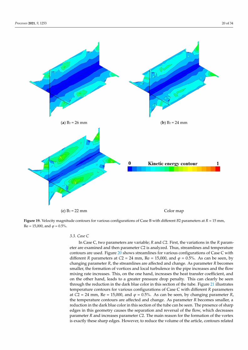
Figure 16 shows streamlines for various configurations of Case B with different B2

parameters at R = 15 mm, Re = 15,000, and 𝜑 = 0.5%. As can be seen, by changing param-

eter B2, the streamlines are affected and change. As parameter B2 becomes longer, the

formation of vortices and local turbulence in the pipe increases and the flow mixing rate

increases. This, on the one hand, increases the heat transfer coefficient, and on the other

hand, leads to a greater pressure drop penalty. This can clearly be seen through the re-

duction in the dark blue color in this section of the tube. Figure 17 illustrates temperature

contours for various configurations of Case B with different B2 parameters at R = 15 mm,

Re = 15,000, and 𝜑 = 0.5%. As can be seen, by changing parameter B2, the temperature

contours are affected and change. As parameter B2 becomes longer, a reduction in the

dark blue color in this section of the tube can be seen. Figure 18 presents kinetic energy

contours for various configurations of Case B with different B2 parameters at R = 15 mm,

Re = 15,000, and 𝜑 = 0.5%. A reduction in the light green and blue colors alongside a re-

duction in parameter R is observed in these figures. The presence of sharp edges in this

geometry causes the separation and reversal of the flow, which decreases parameter R

and increases parameter B2. The main reason for the formation of the vortex is exactly

these sharp edges. Figure 19 demonstrates velocity magnitude contours for various con-

figurations of Case B with different B2 parameters at R = 15 mm, Re = 15,000, and 𝜑 =

0.5%. This can clearly be seen by the reduction in the dark blue color in this section of the

tube alongside a reduction in parameter R. However, in order to reduce the volume of the

article, contours related to different Reynolds numbers have been omitted. As can be seen,

increasing the Reynolds number intensifies the turbulence, increases the flow mixing rate,

and increases the vortices. This leads to an increase in heat transfer coefficient as well as

an increase in the pressure drop penalty.

Figure 15. Velocity magnitude contours for various configurations of Case B with different R parameters at B2 = 24 mm,Re = 15,000, and ϕ = 0.5%.

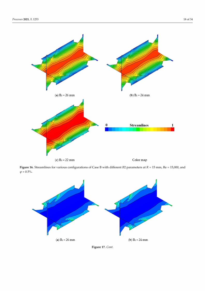
Figure 16 shows streamlines for various configurations of Case B with different B2parameters at R = 15 mm, Re = 15,000, and ϕ = 0.5%. As can be seen, by changing parameterB2, the streamlines are affected and change. As parameter B2 becomes longer, the formationof vortices and local turbulence in the pipe increases and the flow mixing rate increases.This, on the one hand, increases the heat transfer coefficient, and on the other hand, leadsto a greater pressure drop penalty. This can clearly be seen through the reduction in thedark blue color in this section of the tube. Figure 17 illustrates temperature contours forvarious configurations of Case B with different B2 parameters at R = 15 mm, Re = 15,000,and ϕ = 0.5%. As can be seen, by changing parameter B2, the temperature contours areaffected and change. As parameter B2 becomes longer, a reduction in the dark blue colorin this section of the tube can be seen. Figure 18 presents kinetic energy contours forvarious configurations of Case B with different B2 parameters at R = 15 mm, Re = 15,000,and ϕ = 0.5%. A reduction in the light green and blue colors alongside a reduction inparameter R is observed in these figures. The presence of sharp edges in this geometrycauses the separation and reversal of the flow, which decreases parameter R and increasesparameter B2. The main reason for the formation of the vortex is exactly these sharp edges.Figure 19 demonstrates velocity magnitude contours for various configurations of Case Bwith different B2 parameters at R = 15 mm, Re = 15,000, and ϕ = 0.5%. This can clearly beseen by the reduction in the dark blue color in this section of the tube alongside a reductionin parameter R. However, in order to reduce the volume of the article, contours related todifferent Reynolds numbers have been omitted. As can be seen, increasing the Reynoldsnumber intensifies the turbulence, increases the flow mixing rate, and increases the vortices.This leads to an increase in heat transfer coefficient as well as an increase in the pressuredrop penalty.

Processes 2021, 9, 1253 18 of 34

1

Figure 16. Streamlines for various configurations of Case B with different B2 parameters at R = 15 mm, Re = 15,000, andϕ = 0.5%.

1

Figure 17. Cont.

Processes 2021, 9, 1253 19 of 34

2

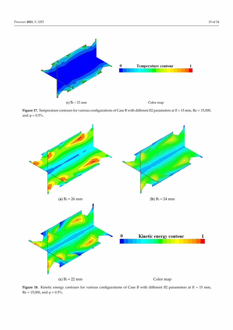
Figure 17. Temperature contours for various configurations of Case B with different B2 parameters at R = 15 mm, Re = 15,000,and ϕ = 0.5%.

Processes 2021, 9, x FOR PEER REVIEW 20 of 37

(c) B2 = 22 mm Color map

Figure 17. Temperature contours for various configurations of Case B with different B2 parameters at R = 15 mm, Re =

15,000, and 𝜑 = 0.5%.

(a) B2 = 26 mm (b) B2 = 24 mm

(c) B2 = 22 mm Color map

Figure 18. Kinetic energy contours for various configurations of Case B with different B2 parameters at R = 15 mm, Re =

15,000, and 𝜑 = 0.5%. Figure 18. Kinetic energy contours for various configurations of Case B with different B2 parameters at R = 15 mm,Re = 15,000, and ϕ = 0.5%.

Processes 2021, 9, 1253 20 of 34Processes 2021, 9, x FOR PEER REVIEW 21 of 37

(a) B2 = 26 mm (b) B2 = 24 mm

(c) B2 = 22 mm Color map

Figure 19. Velocity magnitude contours for various configurations of Case B with different B2 parameters at R = 15 mm,

Re = 15,000, and 𝜑 = 0.5%.

3.3. Case C

In Case C, two parameters are variable; R and C2. First, the variations in the R pa-

rameter are examined and then parameter C2 is analyzed. Thus, streamlines and temper-

ature contours are used. Figure 20 shows streamlines for various configurations of Case

C with different R parameters at C2 = 24 mm, Re = 15,000, and 𝜑 = 0.5%. As can be seen,

by changing parameter R, the streamlines are affected and change. As parameter R be-

comes smaller, the formation of vortices and local turbulence in the pipe increases and the

flow mixing rate increases. This, on the one hand, increases the heat transfer coefficient,

and on the other hand, leads to a greater pressure drop penalty. This can clearly be seen

through the reduction in the dark blue color in this section of the tube. Figure 21 illustrates

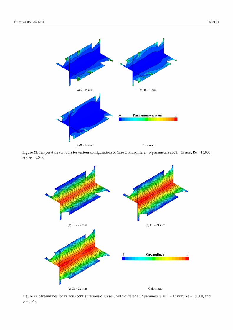
temperature contours for various configurations of Case C with different R parameters at

C2 = 24 mm, Re = 15,000, and 𝜑 = 0.5%. As can be seen, by changing parameter R, the

temperature contours are affected and change. As parameter R becomes smaller, a reduc-

tion in the dark blue color in this section of the tube can be seen. The presence of sharp

edges in this geometry causes the separation and reversal of the flow, which decreases

parameter R and increases parameter C2. The main reason for the formation of the vortex

is exactly these sharp edges. However, to reduce the volume of the article, contours related

to different Reynolds numbers have been omitted. As can be seen, increasing the Reynolds

Figure 19. Velocity magnitude contours for various configurations of Case B with different B2 parameters at R = 15 mm,Re = 15,000, and ϕ = 0.5%.

3.3. Case C

In Case C, two parameters are variable; R and C2. First, the variations in the R param-eter are examined and then parameter C2 is analyzed. Thus, streamlines and temperaturecontours are used. Figure 20 shows streamlines for various configurations of Case C withdifferent R parameters at C2 = 24 mm, Re = 15,000, and ϕ = 0.5%. As can be seen, bychanging parameter R, the streamlines are affected and change. As parameter R becomessmaller, the formation of vortices and local turbulence in the pipe increases and the flowmixing rate increases. This, on the one hand, increases the heat transfer coefficient, andon the other hand, leads to a greater pressure drop penalty. This can clearly be seenthrough the reduction in the dark blue color in this section of the tube. Figure 21 illustratestemperature contours for various configurations of Case C with different R parametersat C2 = 24 mm, Re = 15,000, and ϕ = 0.5%. As can be seen, by changing parameter R,the temperature contours are affected and change. As parameter R becomes smaller, areduction in the dark blue color in this section of the tube can be seen. The presence of sharpedges in this geometry causes the separation and reversal of the flow, which decreasesparameter R and increases parameter C2. The main reason for the formation of the vortexis exactly these sharp edges. However, to reduce the volume of the article, contours related

Processes 2021, 9, 1253 21 of 34

to different Reynolds numbers have been omitted. As can be seen, increasing the Reynoldsnumber intensifies the turbulence, increases the flow mixing rate, and increases the vortices.This leads to an increase in heat transfer coefficient as well as an increase in the pressuredrop penalty.

Processes 2021, 9, x FOR PEER REVIEW 22 of 37

number intensifies the turbulence, increases the flow mixing rate, and increases the vorti-ces. This leads to an increase in heat transfer coefficient as well as an increase in the pres-sure drop penalty.

(a) R = 15 mm (b) R = 13 mm

(c) R = 11 mm Color map

Figure 20. Streamlines for various configurations of Case C with different R parameters at C2 = 24 mm, Re = 15,000, and 𝜑 = 0.5%. Figure 20. Streamlines for various configurations of Case C with different R parameters at C2 = 24 mm, Re = 15,000, andϕ = 0.5%.

Figure 22 shows streamlines for various configurations of Case C with different C2parameters at R = 15 mm, Re = 15,000, and ϕ = 0.5%. As can be seen, by changing parameterC2, the streamlines are affected and change. As parameter C2 becomes longer, the formationof vortices and local turbulence in the pipe increases and the flow mixing rate increases.This, on the one hand, increases the heat transfer coefficient, and on the other hand, leadsto a greater pressure drop penalty. This can clearly be seen by the reduction in the darkblue color in this section of the tube.

Figure 23 illustrates temperature contours for various configurations of Case C withdifferent C2 parameters at R = 15 mm, Re = 15,000, and ϕ = 0.5%. As can be seen, bychanging parameter C2, the temperature contours are affected and change. As parameterC2 becomes longer, a reduction in the dark blue color in this section of the tube can be seen.

Processes 2021, 9, 1253 22 of 34

1

Figure 21. Temperature contours for various configurations of Case C with different R parameters at C2 = 24 mm, Re = 15,000,and ϕ = 0.5%.

Processes 2021, 9, x FOR PEER REVIEW 24 of 37

(a) C2 = 26 mm (b) C2 = 24 mm

(c) C2 = 22 mm Color map

Figure 22. Streamlines for various configurations of Case C with different C2 parameters at R = 15 mm, Re = 15,000, and 𝜑 = 0.5%.

Figure 23 illustrates temperature contours for various configurations of Case C with different C2 parameters at R = 15 mm, Re = 15,000, and 𝜑 = 0.5%. As can be seen, by changing parameter C2, the temperature contours are affected and change. As parameter C2 becomes longer, a reduction in the dark blue color in this section of the tube can be seen.

Figure 22. Streamlines for various configurations of Case C with different C2 parameters at R = 15 mm, Re = 15,000, andϕ = 0.5%.

Processes 2021, 9, 1253 23 of 34

1

Figure 23. Temperature contours for various configurations of Case C with different C2 parameters at R = 15 mm, Re = 15,000,and ϕ = 0.5%.

However, in order to reduce the volume of the article, contours related to differentReynolds numbers have been omitted. As can be seen, increasing the Reynolds numberintensifies the turbulence, increases the flow mixing rate, and increases the vortices. Thisleads to an increase in heat transfer coefficient as well as an increase in the pressuredrop penalty.

3.4. Case D

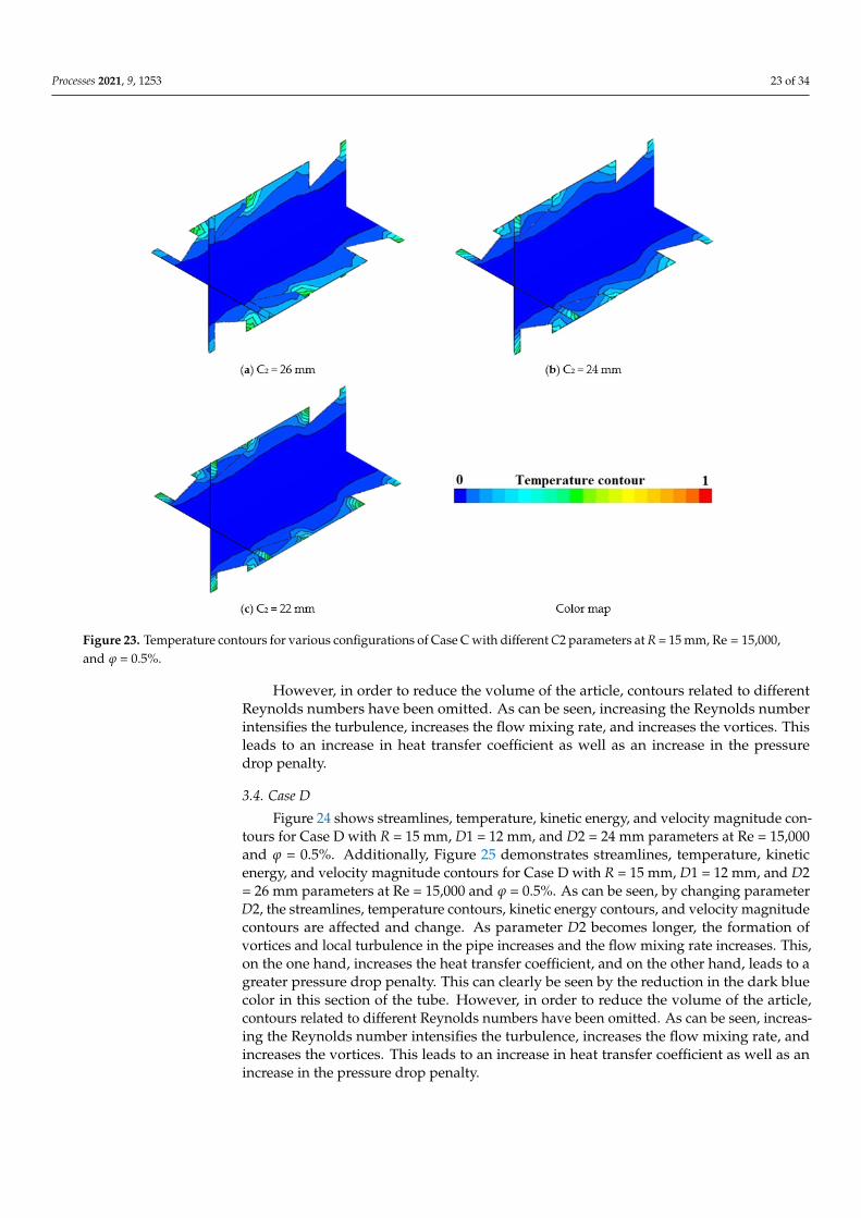
Figure 24 shows streamlines, temperature, kinetic energy, and velocity magnitude con-tours for Case D with R = 15 mm, D1 = 12 mm, and D2 = 24 mm parameters at Re = 15,000and ϕ = 0.5%. Additionally, Figure 25 demonstrates streamlines, temperature, kineticenergy, and velocity magnitude contours for Case D with R = 15 mm, D1 = 12 mm, and D2= 26 mm parameters at Re = 15,000 and ϕ = 0.5%. As can be seen, by changing parameterD2, the streamlines, temperature contours, kinetic energy contours, and velocity magnitudecontours are affected and change. As parameter D2 becomes longer, the formation ofvortices and local turbulence in the pipe increases and the flow mixing rate increases. This,on the one hand, increases the heat transfer coefficient, and on the other hand, leads to agreater pressure drop penalty. This can clearly be seen by the reduction in the dark bluecolor in this section of the tube. However, in order to reduce the volume of the article,contours related to different Reynolds numbers have been omitted. As can be seen, increas-ing the Reynolds number intensifies the turbulence, increases the flow mixing rate, andincreases the vortices. This leads to an increase in heat transfer coefficient as well as anincrease in the pressure drop penalty.

Processes 2021, 9, 1253 24 of 34

2

Figure 24. Streamlines, temperature, kinetic energy and velocity magnitude contours for Case D with R = 15 mm,D1 = 12 mm, and D2 = 24 mm parameters at Re = 15,000, and ϕ = 0.5%.

3

Figure 25. Streamlines, temperature, kinetic energy and velocity magnitude contours for Case D with R = 15 mm,D1 = 12 mm, and D2 = 26 mm parameters at Re = 15,000, and ϕ = 0.5%.

Processes 2021, 9, 1253 25 of 34

3.5. Case E

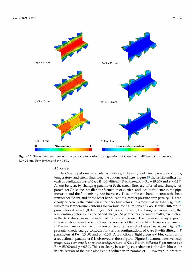
In Case E two parameters are variable; R and E2. First, the variations in the Rparameter are examined and then parameter E2 is analyzed. In that manner, temperaturecontours and streamlines are used. Figure 26 shows streamlines and temperature contoursfor various configurations of Case E with different R parameters at E2 = 24 mm, Re = 15,000,and ϕ = 0.5%. As can be seen, when we change parameter R, the streamlines are affectedand change. As parameter R becomes smaller, the formation of vortices and local turbulencein the pipe increases and the flow mixing rate increases. This, on the one hand, increasesthe heat transfer coefficient, and on the other hand, leads to a greater pressure drop penalty.This can clearly be seen through the reduction in the dark blue color in this section of thetube. Figure 27 shows streamlines and temperature contours for various configurations ofCase E with different R parameters at E2 = 24 mm, Re = 19,000, and ϕ = 0.5%. As can beseen, by changing parameter R, the streamlines are affected and change. As parameter Rbecomes smaller, the formation of vortices and local turbulence in the pipe increases andthe flow mixing rate increases. This, on the one hand, increases the heat transfer coefficient,and on the other hand, leads to a greater pressure drop penalty. This can clearly be seen bythe reduction in the dark blue color in this section of the tube. It is seen that increasing theReynolds number intensifies the turbulence, increases the flow mixing rate, and increasesthe vortices. This leads to an increase in heat transfer coefficient as well as an increasein the pressure drop penalty. There is always an optimum Reynolds number, where themaximum PEC value is occurred.

4

Figure 26. Streamlines and temperature contours for various configurations of Case E with different R parameters atE2 = 24 mm, Re = 15,000, and ϕ = 0.5%.

Processes 2021, 9, 1253 26 of 34

5

Figure 27. Streamlines and temperature contours for various configurations of Case E with different R parameters atE2 = 24 mm, Re = 19,000, and ϕ = 0.5%.

3.6. Case F

In Case F, just one parameter is variable; F. Velocity and kinetic energy contours,temperature, and streamlines were the options used here. Figure 28 shows streamlines forvarious configurations of Case E with different F parameters at Re = 15,000 and ϕ = 0.5%.As can be seen, by changing parameter F, the streamlines are affected and change. Asparameter F becomes smaller, the formation of vortices and local turbulence in the pipeincreases and the flow mixing rate increases. This, on the one hand, increases the heattransfer coefficient, and on the other hand, leads to a greater pressure drop penalty. This canclearly be seen by the reduction in the dark blue color in this section of the tube. Figure 29illustrates temperature contours for various configurations of Case F with different Fparameters at Re = 15,000 and ϕ = 0.5%. As can be seen, by changing parameter F, thetemperature contours are affected and change. As parameter F becomes smaller, a reductionin the dark blue color in this section of the tube can be seen. The presence of sharp edges inthis geometry causes the separation and reversal of the flow, which decreases parameterF. The main reason for the formation of the vortex is exactly these sharp edges. Figure 30presents kinetic energy contours for various configurations of Case F with different Fparameters at Re = 15,000 and ϕ = 0.5%. A reduction in light green and blue colors witha reduction in parameter R is observed in these figures. Figure 31 demonstrates velocitymagnitude contours for various configurations of Case F with different F parameters atRe = 15,000 and ϕ = 0.5%. This can clearly be seen by the reduction in the dark blue colorin this section of the tube alongside a reduction in parameter F. However, in order to

Processes 2021, 9, 1253 27 of 34

reduce the volume of the article, contours related to different Reynolds numbers havebeen omitted. As can be seen, increasing the Reynolds number intensifies the turbulence,increases the flow mixing rate, and increases the vortices. This leads to an increase in heattransfer coefficient as well as an increase in the pressure drop penalty.

Processes 2021, 9, x FOR PEER REVIEW 30 of 37

edges in this geometry causes the separation and reversal of the flow, which decreases parameter F. The main reason for the formation of the vortex is exactly these sharp edges. Figure 30 presents kinetic energy contours for various configurations of Case F with dif-ferent F parameters at Re = 15,000 and 𝜑 = 0.5%. A reduction in light green and blue colors with a reduction in parameter R is observed in these figures. Figure 31 demonstrates ve-locity magnitude contours for various configurations of Case F with different F parame-ters at Re = 15,000 and 𝜑 = 0.5%. This can clearly be seen by the reduction in the dark blue color in this section of the tube alongside a reduction in parameter F. However, in order to reduce the volume of the article, contours related to different Reynolds numbers have been omitted. As can be seen, increasing the Reynolds number intensifies the turbulence, increases the flow mixing rate, and increases the vortices. This leads to an increase in heat transfer coefficient as well as an increase in the pressure drop penalty.

(a) F = 15 mm (b) F = 13 mm

(c) F = 11 mm Color map

Figure 28. Streamlines for various configurations of Case F with different F parameters at Re = 15,000, and 𝜑 = 0.5%. Figure 28. Streamlines for various configurations of Case F with different F parameters at Re = 15,000, and ϕ = 0.5%.

Processes 2021, 9, 1253 28 of 34

6

Figure 29. Temperature contours for various configurations of Case F with different F parameters at Re = 15,000, andϕ = 0.5%.

Processes 2021, 9, x FOR PEER REVIEW 31 of 37

(a) F = 15 mm (b) F = 13 mm

(c) F = 11 mm Color map

Figure 29. Temperature contours for various configurations of Case F with different F parameters at Re = 15,000, and 𝜑 = 0.5%.

(a) F = 15 mm (b) F = 13 mm

Figure 30. Cont.

Processes 2021, 9, 1253 29 of 34Processes 2021, 9, x FOR PEER REVIEW 32 of 37

(c) F = 11 mm Color map

Figure 30. Kinetic energy contours for various configurations of Case F with different F parameters at Re = 15,000, and 𝜑 = 0.5%.

(a) F = 15 mm (b) F = 13 mm

(c) F = 11 mm Color map

Figure 31. Velocity magnitude contours for various configurations of Case F with different F parameters at Re = 15,000, and 𝜑 = 0.5%.

3.7. Comparison

Figure 30. Kinetic energy contours for various configurations of Case F with different F parameters at Re = 15,000, andϕ = 0.5%.

7

Figure 31. Velocity magnitude contours for various configurations of Case F with different F parameters at Re = 15,000, andϕ = 0.5%.

Processes 2021, 9, 1253 30 of 34

3.7. Comparison

According to the results and the calculation of the PEC index, the optimum configura-tions for the different cases are as followss:

Case A: R = 15 mm and A2 = 24 mmCase B: R = 15 mm and B2 = 26 mmCase C: R = 13 mm and B2 = 22 mmCase D: R = 13 mm and B2 = 24 mmCase E: R = 15 mm and B2 = 24 mmCase F: F = 15 mm

To achieve the optimum case, a comparison of these optimum configurations is madeusing the PEC index. Figure 32 shows the PEC variation for optimum configurations ofdifferent cases at Re = 11,000. It can be seen that Case D has the most optimum PEC valuesand is followed by Cases B, F, C, A, and E, respectively. Additionally, it is seen that an in-crease in nanoparticle volume fraction leads to higher PEC values. Additionally, Figure 33illustrates PEC variation versus different Reynolds numbers for optimum configurations ofCase D. As can be seen, increasing the Reynolds number to Re = 15,000 leads to an increasein PEC index and then a decreasing trend. In other words, increasing the Reynolds numberhas two consequences: on the one hand, it improves heat transfer, and on the other hand, itincreases the pressure drop penalty. Thus, the compromise point for the maximum valueof the PEC index occurs at Re = 15,000.

Processes 2021, 9, x FOR PEER REVIEW 33 of 37

According to the results and the calculation of the PEC index, the optimum configu-rations for the different cases are as followss:

Case A: R = 15 mm and A2 = 24 mm Case B: R = 15 mm and B2 = 26 mm Case C: R = 13 mm and B2 = 22 mm Case D: R = 13 mm and B2 = 24 mm Case E: R = 15 mm and B2 = 24 mm Case F: F = 15 mm To achieve the optimum case, a comparison of these optimum configurations is made

using the PEC index. Figure 32 shows the PEC variation for optimum configurations of different cases at Re = 11,000. It can be seen that Case D has the most optimum PEC values and is followed by Cases B, F, C, A, and E, respectively. Additionally, it is seen that an increase in nanoparticle volume fraction leads to higher PEC values. Additionally, Figure 33 illustrates PEC variation versus different Reynolds numbers for optimum configura-tions of Case D. As can be seen, increasing the Reynolds number to Re = 15,000 leads to an increase in PEC index and then a decreasing trend. In other words, increasing the Reyn-olds number has two consequences: on the one hand, it improves heat transfer, and on the other hand, it increases the pressure drop penalty. Thus, the compromise point for the maximum value of the PEC index occurs at Re = 15,000.

Figure 32. PEC variation for optimum configurations of different cases at Re = 11,000.

1.0

1.1

1.2

1.3

1.4

1.5

1.6

Case A Case B Case C Case D Case E Case F

PEC

Configuration

φ = 0.5%

φ = 1.0%

Figure 32. PEC variation for optimum configurations of different cases at Re = 11,000.

Processes 2021, 9, 1253 31 of 34Processes 2021, 9, x FOR PEER REVIEW 34 of 37

Figure 33. PEC variation versus different Reynolds numbers for optimum configurations of Case D.

4. Conclusions The present study studies the effects of different wall shapes on the thermal-hydrau-

lic characteristics of different channels filled with water based graphite-SiO2 hybrid nanofluid. The effects of different wall shapes on the thermalhydraulic characteristic of different channels filled with water based Graphite-SiO2 hybrid nanofluid is a challeng-ing topic that, accordig to the literature review, is an area that needs to be worked on. In this study, performance evaluation criteria (PEC) index is employed as the goal parameter to attain the optimum geometry. Six different cases were studied in this paper. Each case has different geometric dimensions, which were investigated numerically to achieve the most efficient configuration. The length of the channel is 180 mm, which is under a con-stant temperature of Ts = 450 K. The heat transfer fluid (HTF) is water based graphite-SiO2 hybrid nanofluid, which enters the channel at 330 K at different flow velocities related to Re = 11,000, 15,000, 19,000, and 23,000. The grid mesh independence test was done in this research to achieve the most efficient grid mesh layout with the minimum error (4%) and calculating time. Additionally, PEC index code validation was conducted, and it was found that there is a remarkable coincidence between the numerical data in the literature and the obtained numerical results from the current study. According to the obtained re-sults, by changing geometrical parameters, the streamlines, temperature contours, kinetic energy contours, and velocity magnitude contours are affected significantly. As parame-ter R or F becomes smaller or as parameter X2 becomes longer (X = A, B, C, D, E and F), the formation of vortices and local turbulence in the pipe increases and the flow mixing rate increases. On the one hand, this increases the heat transfer coefficient, and on the other hand leads to a greater pressure drop penalty. According to the results and calcula-tion of the PEC index, the optimum configurations for different cases are: Case A: R = 15 mm and A2 = 24 mm, Case B: R = 15 mm and B2 = 26 mm, Case C: R = 13 mm and B2 = 22 mm, Case D: R = 13 mm and B2 = 24 mm, Case E: R = 15 mm and B2 = 24 mm, and Case F: F = 15 mm. It was seen that Case D had the greatest PEC values, followed by Cases B, F, C, A, and E, respectively. Additionally, it can be seen that an increase in nanoparticle vol-ume fraction leads to higher PEC values. Additionally, increasing the Reynolds number to Re = 15,000 leads to an increase in PEC index and then a decreasing trend. In other

1.40

1.45

1.50

1.55

1.60

1.65

11000 15000 19000 23000

PEC

Re

φ = 0.5%

φ = 1.0%

Figure 33. PEC variation versus different Reynolds numbers for optimum configurations of Case D.

4. Conclusions

The present study studies the effects of different wall shapes on the thermal-hydrauliccharacteristics of different channels filled with water based graphite-SiO2 hybrid nanofluid.The effects of different wall shapes on the thermalhydraulic characteristic of differentchannels filled with water based Graphite-SiO2 hybrid nanofluid is a challenging topicthat, accordig to the literature review, is an area that needs to be worked on. In this study,performance evaluation criteria (PEC) index is employed as the goal parameter to attain theoptimum geometry. Six different cases were studied in this paper. Each case has differentgeometric dimensions, which were investigated numerically to achieve the most efficientconfiguration. The length of the channel is 180 mm, which is under a constant temperatureof Ts = 450 K. The heat transfer fluid (HTF) is water based graphite-SiO2 hybrid nanofluid,which enters the channel at 330 K at different flow velocities related to Re = 11,000, 15,000,19,000, and 23,000. The grid mesh independence test was done in this research to achievethe most efficient grid mesh layout with the minimum error (4%) and calculating time.Additionally, PEC index code validation was conducted, and it was found that there isa remarkable coincidence between the numerical data in the literature and the obtainednumerical results from the current study. According to the obtained results, by changinggeometrical parameters, the streamlines, temperature contours, kinetic energy contours,and velocity magnitude contours are affected significantly. As parameter R or F becomessmaller or as parameter X2 becomes longer (X = A, B, C, D, E and F), the formation ofvortices and local turbulence in the pipe increases and the flow mixing rate increases. Onthe one hand, this increases the heat transfer coefficient, and on the other hand leads to agreater pressure drop penalty. According to the results and calculation of the PEC index,the optimum configurations for different cases are: Case A: R = 15 mm and A2 = 24 mm,Case B: R = 15 mm and B2 = 26 mm, Case C: R = 13 mm and B2 = 22 mm, Case D: R = 13 mmand B2 = 24 mm, Case E: R = 15 mm and B2 = 24 mm, and Case F: F = 15 mm. It was seenthat Case D had the greatest PEC values, followed by Cases B, F, C, A, and E, respectively.Additionally, it can be seen that an increase in nanoparticle volume fraction leads to higherPEC values. Additionally, increasing the Reynolds number to Re = 15,000 leads to anincrease in PEC index and then a decreasing trend. In other words, increasing the Reynoldsnumber has two consequences: on the one hand, it improves heat transfer; on the otherhand, it increases the pressure drop penalty. Therefore, the maximum value of the PECindex occurs at Re = 15,000.

Processes 2021, 9, 1253 32 of 34

Author Contributions: Conceptualization, Y.K.; Data curation, Y.K. and A.T.; Formal analysis, Y.K.and A.T.; Investigation, Y.K., A.A. (Ahmad Alahmadi) and A.A. (Ali Alzaed); Methodology, Y.K.,A.A. (Ahmad Alahmadi) and A.A. (Ali Alzaed); Supervision, Y.K., M.S. and G.C.; Writing—Originaldraft, Y.K., A.A. (Ahmad Alahmadi), A.A. (Ali Alzaed) and A.T.; Writing—Review & editing, A.A.(Ahmad Alahmadi), M.S. and G.C. All authors have read and agreed to the published version ofthe manuscript.

Funding: This research received no external funding.

Acknowledgments: This work was supported by the Taif University Researchers Supporting Project,Taif University, Taif, Saudi Arabia, under Project TURSP-2020/121.

Conflicts of Interest: The authors declare no conflict of interest.

Nomenclature

cp Specific heat capacity (J/kg.K)f Friction coefficient (-)g Gravitational acceleration (m/s2)ϕ Volume fractionk Thermal conductivity (W/m.K)Nu Nusselt number (-)Um Mass-averaged velocity (m/s)Us Velocity of solid particles (m/s)Ub f Velocity of the base fluid (m/s)Udr Drift velocity (m/s)Greek Symbolsε Turbulent dissipation (m2/s3)η Efficiency (-)µ Viscosity (N·s/m2)µt,m Turbulent viscosity (N·s/m2)P Pressure (Pa)Re Reynolds number (-)Subscriptsn f Nanofluidnp Nanoparticles Solid

References1. Parsa, S.M.; Yazdani, A.; Dhahad, H.; Alawee, W.H.; Hesabi, S.; Norozpour, F.; Ali, H.M.; Afrand, M. Effect of Ag, Au, TiO2

metallic/metal oxide nanoparticles in double-slope solar stills via thermodynamic and environmental analysis. J. Clean. Prod.2021, 311, 127689. [CrossRef]

2. Eshgarf, H.; Kalbasi, R.; Maleki, A.; Shadloo, M.S.; Karimipour, A. A review on the properties, preparation, models and stabilityof hybrid nanofluids to optimize energy consumption. J. Therm. Anal. Calorim. 2021, 144, 1959–1983. [CrossRef]

3. Parsa, S.M.; Rahbar, A.; Koleini, M.; Aberoumand, S.; Afrand, M.; Amidpour, M. A renewable energy-driven thermoelectric-utilized solar still with external condenser loaded by silver/nanofluid for simultaneously water disinfection and desalination.Desalination 2020, 480, 114354. [CrossRef]

4. Keepaiboon, C.; Dalkilic, A.S.; Mahian, O.; Ahn, H.S.; Wongwises, S.; Mondal, P.K.; Shadloo, M.S. Two-phase flow boiling in amicrofluidic channel at high mass flux. Phys. Fluids 2020, 32, 093309. [CrossRef]

5. Wang, N.; Maleki, A.; Nazari, M.A.; Tlili, I.; Shadloo, M.S. Thermal Conductivity Modeling of Nanofluids Contain MgO Particlesby Employing Different Approaches. Symmetry 2020, 12, 206. [CrossRef]

6. Garbadeen, I.; Sharifpur, M.; Slabber, J.; Meyer, J. Experimental study on natural convection of MWCNT-water nanofluids in asquare enclosure. Int. Commun. Heat Mass Transf. 2017, 88, 1–8. [CrossRef]

7. Rostami, S.; Kalbasi, R.; Talebkeikhah, M.; Goldanlou, A.S. Improving the thermal conductivity of ethylene glycol by additionof hybrid nano-materials containing multi-walled carbon nanotubes and titanium dioxide: Applicable for cooling and heating.J. Therm. Anal. Calorimetry 2021, 143, 1701–1712. [CrossRef]

8. Yan, S.R.; Golzar, A.; Sharifpur, M.; Meyer, J.P.; Liu, D.H.; Afrand, M. Effect of U-shaped absorber tube on thermal-hydraulicperformance and efficiency of two-fluid parabolic solar collector containing two-phase hybrid non-Newtonian nanofluids. Int. J.Mech. Sci. 2020, 185, 105832. [CrossRef]

Processes 2021, 9, 1253 33 of 34

9. Aghakhani, S.; Ghasemi, B.; Pordanjani, A.H.; Wongwises, S.; Afrand, M. Effect of replacing nanofluid instead of water on heattransfer in a channel with extended surfaces under a magnetic field. Int. J. Numer. Methods Heat Fluid Flow 2019, 29, 1249–1271.[CrossRef]

10. Giwa, S.; Sharifpur, M.; Goodarzi, M.; Alsulami, H.; Meyer, J.P. Influence of base fluid, temperature, and concentration on thethermophysical properties of hybrid nanofluids of alumina–ferrofluid: Experimental data, modeling through enhanced ANN,ANFIS, and curve fitting. J. Therm. Anal. Calorim. 2021, 143, 4149–4167. [CrossRef]

11. Aghakhani, S.; Pordanjani, A.H.; Afrand, M.; Sharifpur, M.; Meyer, J.P. Natural convective heat transfer and entropy generationof alumina/water nanofluid in a tilted enclosure with an elliptic constant temperature: Applying magnetic field and radiationeffects. Int. J. Mech. Sci. 2020, 174, 105470. [CrossRef]

12. Ibrahim, M.; Saeed, T.; Chu, Y.-M.; Ali, H.M.; Cheraghian, G.; Kalbasi, R. Comprehensive study concerned graphene nano-sheetsdispersed in ethylene glycol: Experimental study and theoretical prediction of thermal conductivity. Powder Technol. 2021, 386,51–59. [CrossRef]

13. Pordanjani, A.H.; Aghakhani, S.; Afrand, M.; Mahmoudi, B.; Mahian, O.; Wongwises, S. An updated review on application ofnanofluids in heat exchangers for saving energy. Energy Convers. Manag. 2019, 198, 111886. [CrossRef]

14. Komeilibirjandi, A.; Raffiee, A.H.; Maleki, A.; Nazari, M.A.; Shadloo, M.S. Thermal conductivity prediction of nanofluidscontaining CuO nanoparticles by using correlation and artificial neural network. J. Therm. Anal. Calorim. 2020, 139, 2679–2689.[CrossRef]

15. Pordanjani, A.H.; Aghakhani, S. Numerical Investigation of Natural Convection and Irreversibilities between Two InclinedConcentric Cylinders in Presence of Uniform Magnetic Field and Radiation. Heat Transf. Eng. 2021, 1–21. [CrossRef]

16. Yan, S.-R.; Aghakhani, S.; Karimipour, A. Influence of a membrane on nanofluid heat transfer and irreversibilities inside a cavitywith two constant-temperature semicircular sources on the lower wall: Applicable to solar collectors. Phys. Scr. 2020, 95, 085702.[CrossRef]

17. Ghalandari, M.; Maleki, A.; Haghighi, A.; Shadloo, M.S.; Nazari, M.A.; Tlili, I. Applications of nanofluids containing carbonnanotubes in solar energy systems: A review. J. Mol. Liq. 2020, 313, 113476. [CrossRef]

18. Parsa, S.M. Reliability of thermal desalination (solar stills) for water/wastewater treatment in light of COVID-19 (novel coron-avirus “SARS-CoV-2”) pandemic: What should consider? Desalination 2021, 512, 115106. [CrossRef]

19. Rostami, S.; Aghakhani, S.; Pordanjani, A.H.; Afrand, M.; Cheraghian, G.; Oztop, H.F.; Shadloo, M.S. A Review on the ControlParameters of Natural Convection in Different Shaped Cavities with and Without Nanofluid. Processes 2020, 8, 1011. [CrossRef]

20. Parsa, S.M.; Rahbar, A.; Koleini, M.; Javadi, Y.D.; Afrand, M.; Rostami, S.; Amidpour, M. First approach on nanofluid-based solarstill in high altitude for water desalination and solar water disinfection (SODIS). Desalination 2020, 491, 114592. [CrossRef]

21. Nakharintr, L.; Naphon, P. Magnetic field effect on the enhancement of nanofluids heat transfer of a confined jet impingement inmini-channel heat sink. Int. J. Heat Mass Transf. 2017, 110, 753–759. [CrossRef]

22. Ashorynejad, H.R.; Zarghami, A. Magnetohydrodynamics flow and heat transfer of Cu-water nanofluid through a partiallyporous wavy channel. Int. J. Heat Mass Transf. 2018, 119, 247–258. [CrossRef]

23. Dormohammadi, R.; Farzaneh-Gord, M.; Ebrahimi-Moghadam, A.; Ahmadi, M.H. Heat transfer and entropy generation of thenanofluid flow inside sinusoidal wavy channels. J. Mol. Liq. 2018, 269, 229–240. [CrossRef]

24. Saeed, M.; Kim, M.-H. Heat transfer enhancement using nanofluids (Al2O3-H2O) in mini-channel heatsinks. Int. J. Heat MassTransf. 2018, 120, 671–682. [CrossRef]

25. Dalkılıç, A.S.; Türk, O.A.; Mercan, H.; Nakkaew, S.; Wongwises, S. An experimental investigation on heat transfer characteristicsof graphite-SiO2/water hybrid nanofluid flow in horizontal tube with various quad-channel twisted tape inserts. Int. Commun.Heat Mass Transf. 2019, 107, 1–13. [CrossRef]

26. Saba, F.; Ahmed, N.; Khan, U.; Mohyud-Din, S.T. A novel coupling of (CNT-Fe3O4/H2O) hybrid nanofluid for improvementsin heat transfer for flow in an asymmetric channel with dilating/squeezing walls. Int. J. Heat Mass Transf. 2019, 136, 186–195.[CrossRef]

27. Ajeel, R.K.; Salim, W.I.; Hasnan, K. Experimental and numerical investigations of convection heat transfer in different channelsusing alumina nanofluid under a turbulent flow regime. Chem. Eng. Res. Des. 2019, 148, 202–217. [CrossRef]

28. Gholami, M.; Nazari, M.R.; Talebi, M.H.; Pourfattah, F.; Akbari, O.A.; Toghraie, D. Natural convection heat transfer enhancementof different nanofluids by adding dimple fins on a vertical channel wall. Chin. J. Chem. Eng. 2020, 28, 643–659. [CrossRef]

29. Shah, Z.; Khan, A.; Khan, W.; Alam, M.K.; Islam, S.; Kumam, P.; Thounthong, P. Micropolar gold blood nanofluid flow andradiative heat transfer between permeable channels. Comput. Methods Programs Biomed. 2020, 186, 105197. [CrossRef]

30. Ajeel, R.K.; Salim, W.I.; Sopian, K.; Yusoff, M.Z.; Hasnan, K.; Ibrahim, A.; Al-Waeli, A.H. Turbulent convective heat transferof silica oxide nanofluid through different channels: An experimental and numerical study. Int. J. Heat Mass Transf. 2019, 145,118806. [CrossRef]

31. Ajeel, R.K.; Salim, W.S.I.W.; Hasnan, K. Influences of geometrical parameters on the heat transfer characteristics through symmetrytrapezoidal-different channel using SiO2-water nanofluid. Int. Commun. Heat Mass Transf. 2019, 101, 1–9. [CrossRef]

32. Ajeel, R.K.; Salim, W.I.; Hasnan, K. Numerical investigations of heat transfer enhancement in a house shaped-different channel:Combination of nanofluid and geometrical parameters. Therm. Sci. Eng. Prog. 2020, 17, 100376. [CrossRef]

33. Salimpour, M.R.; Kalbasi, R.; Lorenzini, G. Constructal multi-scale structure of PCM-based heat sinks. Contin. Mech.Thermodynamics 2017, 29, 477–494. [CrossRef]

Processes 2021, 9, 1253 34 of 34

34. Salari, A.; Kazemian, A.; Ma, T.; Hakkaki-Fard, A.; Peng, J. Nanofluid based photovoltaic thermal systems integrated with phasechange materials: Numerical simulation and thermodynamic analysis. Energy Convers. Manag. 2020, 205, 112384. [CrossRef]

35. Al-Ansary, H.; Zeitoun, O. Numerical study of conduction and convection heat losses from a half-insulated air-filled annulus ofthe receiver of a parabolic trough collector. Sol. Energy 2011, 85, 3036–3045. [CrossRef]

36. Arani, A.A.A.; Sadripour, S.; Kermani, S. Nanoparticle shape effects on thermal-hydraulic performance of boehmite aluminananofluids in a sinusoidal–wavy mini-channel with phase shift and variable wavelength. Int. J. Mech. Sci. 2017, 128–129, 550–563.[CrossRef]

37. Sadripour, S. 3D numerical analysis of atmospheric-aerosol/carbon-black nanofluid flow within a solar air heater located inShiraz, Iran. Int. J. Numer. Methods Heat Fluid Flow 2018, 29, 1378–1402. [CrossRef]

38. Sadripour, S.; Chamkha, A.J. The effect of nanoparticle morphology on heat transfer and entropy generation of supportednanofluids in a heat sink solar collector. Therm. Sci. Eng. Prog. 2019, 9, 266–280. [CrossRef]

39. Kim, D.; Kwon, Y.; Cho, Y.; Li, C.; Cheong, S.; Hwang, Y.; Lee, J.; Hong, D.; Moon, S. Convective heat transfer characteristics ofnanofluids under laminar and turbulent flow conditions. Curr. Appl. Phys. 2009, 9, e119–e123. [CrossRef]

40. Giwa, S.; Sharifpur, M.; Meyer, J. Experimental study of thermo-convection performance of hybrid nanofluids of Al2O3-MWCNT/water in a differentially heated square cavity. Int. J. Heat Mass Transf. 2020, 148, 119072. [CrossRef]

41. Leong, W.; Hollands, K.; Brunger, A. Experimental Nusselt numbers for a cubical-cavity benchmark problem in natural convection.Int. J. Heat Mass Transf. 1999, 42, 1979–1989. [CrossRef]

42. Yang, S.; Ordonez, J. 3D thermal-hydraulic analysis of a symmetric wavy parabolic trough absorber pipe. Energy 2019, 189,116320. [CrossRef]