Effect of the variance of pore size distribution on the transport properties of heterogeneous...

JOURNAL OF GEOPHYSICAL RESE•CH, VOL 103, NO. B1, PAGES 513-525, JANUARY 10, t998

Effect of the variance of pore size distribution on the transport properties of heterogeneous networks

Yves Bernab6 and C61ine Bruderer

!nstitut •e Physique du Globe de Strasbourg, Universit6 Louis Pasteur - CNRS, Strasbourg, France

Abstract. The goal of this paper is to evaluate the effect of the variance of pore size distribution on the transport properties of rocks. Several heterogeneous network realizations with very broad, uniform, or log uniform pore size distributions were constructed. A series of networks were then derived deterministically from these initial networks by repeatedly applying a shrinking operator to the pores of the original realizations. This operator was devised in such a way as to maintain the mean pore size constant while changing the variance of the pore size distribution, therefore allowing its effect on the transport properties to be isolated. We thus assessed the validity of several permeability models from the literature as a function of the variance of the pore size distribution. We found that the product of the permeability by the electrical formation factor was proportional to the square of the critical radius as proposed in the Katz-Thompson model [Katz and Thompson, 1986]. However, we observed that the dramatic flow localization occurring at high pore size variance was not restricted to the backbone of the critical subnetwork (or critical path) as assumed in the Katz-Thompson model. We propose that a better justification of the relation mentioned above arises from the underlying percolation problem of the viscous-inertial transition observed in harmonic flow as a function of frequency. In addition, we appraised the stochastic Bemab6-Revil model [Bemabd ar• Revil, 1995]. We found that this model was more and more difficult to implement as the pore size variance was increased. A possible interpretation could be that at high levels of pore-scale heterogeneity, very large pore size fluctuations occur and the flow pattern is so strongly and deterministically related to these extreme fluctuations that a stochastic description becomes inadequate.

1. Introduction

One of the most revealing tools to investigate the physical properties of rocks is the direct observation of their microstructure (the new techniques of laser confocal microscopy and X ray microtomography can now provide high- resolution, three-dimensional images [Fredrich et al., ! 995; Auzerais et al., 1996]). Browsing through the microstructure literature, one can only be struck by the great complexity of the pore structure of rocks [e.g., Simmons et al., 1982]. In any given rock, pores widely vary in size and shape. Furthermore, when the images cover a large enough area, several scales of heterogeneity can usually be observed [e.g., Prince et at., 1995]. The implications of such a high level of pore-scale heterogeneity are far reaching. The physical properties of rocks are all affected to some degree, and some of them, such as hydrodynamic dispersion, are direct consequences of the heterogeneous nature of rocks [e.g., Sahimi, 1995; GeIhar, 1993]. However, rocks are not all equally heterogeneous. For instance, clayish sandstones are notoriously more difficult to mbdel than "clean" ones, largely owing to t-heir much broader pore size distribution. It is therefore important to improve our understanding of how variable levels of pore-scale heterogeneity affect the physical properties of rocks.

As a step in this direction, this paper is an attempt to assess the effect of the variance of the pore size distribution on the transport properties of rocks. Network simulation is an ideally

Copyright 1998 by the American Geophysical Union.

Paper number 97JB02486. 0148-0227/98/97JB-02486509.00

suited approach for this pu. rpose [e.g., Adler, 1992; Bernabd, 1995, and references therein]. Heterogeneous networks with arbitrary pore size distributions are easy to construct, and their transport properties are easy to calculate. Usually, in this approach, the interpretation relies on the statistical analysis of the results obtained from a large number of realizations. This can be highly time consuming, and, more important, some ambiguity remains because several factors may vary simultaneously from one realization to another. One alternative strategy is to study a series of networks constructed deterministically by repeatedly applying a shrinking or enlarging operator to the pores of a single realization. This operator can be devised in such a way as to maintain the mean pore size constant while changing the variance of the pore size distribution. Note that the rank by size and the spatial position of the pores in these networks are also kept unchanged. This last feature is very important if, as expected from percolation theory, the spatial arrangement of the largest pores is the principal factor controlling the transport properties of rocks [Katz and Thompson, I986]. Thus the variance of the pore size distribution is the only parameter allowed to vary, and its effect on the transport properties can be isolated (a similar procedure was used by Moreno and Tsang [1994]). In this study, we used only four initial realizations, and from each one we constructed four additional networks for a total number of 4 x 5 x 2 = 40 flow simulations (they were

performed in two mutually perpendicular directions for each network). Despite such small numbers the procedure depicted above allowed us to assess the validity of several permeability models from the literature as a function of the variance of the

pore size distribution. These models, namely, the mean field Kozeny-Carman model [Kozeny, !927; Carman, 1956]

513

514 BERNABE AND BRUDERER: PORE SIZE VARIANCE AND PERMEABILITY

(hereafter referred to as KC), the weighted averaging Johnson- Schwartz model [Johnson and Schwartz, 1989] (hereafter referred to as JS), the percolation Katz-Thompson model [Katz and Thompson, 1986] (hereafter referred to as KT), and the stochastic Bernab6-Revil model [Bernabd and Revil, 1995] (hereafter referred to as BR) are reviewed in section 2.

2. Permeability Models 2.1. Kozeny-Carman Model

The KC model is a zeroth-order, mean field model. Many variations exist in the literature. A very good example is the so-called "equivalent channel" model (EC) by Paterson [ 1983] and Walsh and Brace [1984]. Like all KC models, EC can be summarized by

2

(1)

where k denotes the perm6abi!ity, F is the electrical formation factor (i.e., the ratio of the fluid bulk conductivity to the rock conductivity in absence of surface conduction effects), and r H is the hydraulic radius. As a consequence of Poiseui!!e and Ohm's laws, the constant c is equal to 8 for cylindrical pores with a circular cross section and 12 for fiat microcracks. The

hydraulic radius is a characteristic length scale defined by r•)=2<Vi>/<A,.>, where Vi is the local pore volume, A,. is the local pore surface are/t, and the brackets refer to volume averaging. The following notations are used hereafter: (1) the index i always denotes local or microscopic quantities, whereas its absence indicates global or macroscopic parameters and functions, and (2) when necessary, we distinguish the observed and theoretical values of a given quantity by denoting the former with lower case letters and the latter with capital letters (•br instance, the experimental mean radius is noted <ri> and its theoretical value is <R>). One reason why r H was and still is so widely used in practice is that it can be calculated from macroscopic measurements of the porosity and the pore specific surface area. Note that in the case of self-affine roughness of the pore walls, the measurements of the pore specific surface area depend on the scale of the measuring yardstick. Deciding what is the appropriate scale remains a controversial question that often obscures the issue of the validity of KC. Notice that in the KC averaging procedure all pores are given the same weight, which is implicitly equivalent to assuming very small fluctuations of the pore geometrical properties (i.e., pore size, connectivity, and so forth).

2.2. Johnson-Schwartz Model

The JS model is based on an earlier model of the electrical

conductivity of saturated rock [e.g., Johnson and Sen, 1988]. In the limit of high salinities of the saturating electrolyte, the rock conductivity o asymptotically approaches a linear function of the electrolyte bulk conductivity o s as follows:

I 2Os) 2 O' =--(Of +----- +O(o s ) F A (2)

where F is the formation factor, c h. is the surface conductivity of the pore/solid interface (% depends on the chemistry of the electrolyte, in particular, the pH, and the mineralogy of the rock; at high salinities it is much smaller than os), and A is a characteristic length scale defined by A=2IE•dV/IE[dAi. Thus A is the ratio of the weighted average pore volume by the weighted average pore surface. The weighting function E• is the square of the local electric field. This ensures that highly conducting pores receive larger weights than poorly conducting ones.

An important breakthrough occurred when Johnson et al. [1987] realized that the high-salinity electrical conduction problem was analogous to that of the high-frequency harmonic fluid flow. They could thus relate the electrical parameters F and A to the "dynamic" permeability k(co). They derived the asymptotic form of the complex-valued k(co) in the limit of high frequencies and made an educated guess at low frequencies. They obtained, respectively,

3

pto- i a(co) = . (•) +--(PCø + o(PCø) -2 (3)

2Fk pco k(co) = k + iFk 2 (1 + ). + O(P'm) 2 (4)

11

where p and x ! are the density and the viscosity of the fluid, respectively; and k denotes the usual, "static" permeability [see Johnson et aI., 1987]. It was theoretically and experimentally shown that this model produces satisfactory results [e.g., Banavar and Johnson, 1987; Bernabe, 1997, and references therein]. Furthermore, since A was the only length scale naturally arising in their model, Johnson and Schwartz [1989] had the intuition that in the case of heterogeneous rocks, ̂ could be a more appropriate length scale than rH to incorporate into (1). The following equation was therefore added to the JS model:

• - (5) cF

where c was specifically assumed to be equal to 8 (i.e., a generalization of Poiseui!le and Ohm's laws).

2.3. Katz-Thompson Model

It has often been observed in numerical simulations of flow

through porous media that the flow pattern becomes more and more localized as the heterogeneity of the simulated medium is increased [e.g., David, 1993; Moreno and Dang, 1994]. In order to analyze the flow localization, Katz and Thompson [1986] proposed using the so-called critical path analysis (CPA) devised in previous studies of hopping conduction [e.g., Ambegaokar et at., 1971; Shante, 1977]. The first step of CPA is to reconstruct the pore space of a porous medium by adding individual pores, one by one, in descending size order. In this way a series of subnetworks including more and more pores is derived from the initial network. The first such subnetwork containing a cluster of pores connected throughout the entire network is called the first sample spanning or "critical" subnetwork. The main idea now is to assume that flow

BERNABE AND BRUDERER: PORE SIZE VARIANCE AND PERMEABILITY 515

localization occurs on the backbone of the critical subnetwork, therefore called the "critical path".

Let us call r,. the pore radius characterizing the critical subnetwork. For any r*>r,. the subset of pores with radii greater than or equal to r* is disconnected and its permeability k* and electrical conductivity (•* are zero. For any r*<r,., lower bounds of k* and (5' (or, equivalently, I/F*) can be calculated by applying percolation theory to the subsidiary networks obtained by replacing the pores with radii greater than or equal to r* by pores of radius r* and by removing all the other ones. Thus k* and I/F* can be approximated by gh(r*)•(r*) and ge(r*)•(r*), respectively, where g,,(r*) and ge(r*) are the permeability and inverse tbrmation tactor, respectively, of a homogeneous medium with a single pore radius equal to r* and g(r*) is a function describing the connectivity of the actual subsidiary pore network constructed as explained above. The following theoretical expression is obtained from percolation theory (according to our convention, the theoretical function •(r*) is here noted E(r*)):

(p(r*) - Pc)t E(r*) = (6)

(1 - pc)t

where p(r*) is the probability of finding a pore with a radius greater than or equal to r*, p,. is the percolation threshold, and t is the critical exponent. Percolation theory yields p,.=0.5 and 0.25 and t=l.2 and 1.9 for two-dimensional square and three- dimensional simple cubic networks, respectively [Stauffer and Aharony, 1992]. Values of 1.3 and 2.0, respectively, were recently obtained for t [Sahimi, 1993]. Both sets of t were tested in this study, yielding nearly identical results. Note that the old set produced slightly better results visually and is used in the rest of this paper. It is clear that E(r*), and therefore •(r*) must increase from 0 at r*=r,. to 1 when r* reaches its minimum value rmi,,, whereas g•,(r*) and &(r*) decrease continuously with decreasing r*, reaching 0 for r*=0. Therefore k* and I/F* must reach maxima somewhere between

r,. and r*=0. Note that the absolute maxima may sometimes occur for values lower than r,,,i,, (i.e., outside the definition interval). The maxima of k* and I/F* do not necessarily occur for identical values of r*. Let us denote these two points, rh* and re*, in the hydraulic and electrical case, respectively (as explained above, we may sometimes find rh* and/or r,.*=rm,). The KT model assumes that r•,* and r,,* are only slightly smaller than r,. and that the corresponding maxima of k* and I/F* provide good approximations (i.e., slight underestimations) of the original transport properties k and 1/F. It is furthermore expected that the above approximations should be better when the flow pattern is more localized (i.e., when the pore size distribution is broader). Finally, to first order in (r,.-rj,*) and (r,: re*), approximate expressions for the maxima of k* and I/F*, or, consequently, for k and I/F themselves, were derived by Katz and Thompson [1986]. However, this derivation is not convincing since the resulting estimates of (r,.-r•*)and (r,.-r,.*) turned out to be rather large, 0.4r,. and 0.7r,., respectively. Combining these final expressions yielded

2

k- rc (7) cF

where c is 56.5, but this large value stemmed partially from the additional assumption that the pore lengths were equal to the

diameters and from a derivation error as pointed out by Banavar and Johnson [1987] and Le Doussal [1989] who obtained values close to 32 and 21, respectively. As we can see, (7) is identical to (1), except r,. replaces r•. One goal of this work is to provide evidence to decide which among r n A, and r,. is the most appropriate length scale to use in (1).

Finally, although rarely stressed in the literature, it is very useful to note that r,. is theoretically given by R,., the quantile of the pore radius distribution corresponding to p,.. For example, R,. is equal to the median in the case of a two-dimensional square lattice and to the upper quartile for a three-dimensional cubic one.

2.4. Bernab6-Revil Model

The BR model is an attempt to derive an effective averaging procedure, capable of predicting the transport properties of rocks from the geometrical characteristics of the individual pores. This is done by comparing global and local determinations of the energy dissipated in the porous rock during hydraulic flow. The result is summarized by

V..3 2 k =< •" VPi -> (8) , ,

cVTA • V, 2 where V r is the total volume of porous rock, Vpi is the local pressure gradient along an individual pore, and VP is the macroscopically applied pressure gradient. The constant c equals 2 in the case of tubular pores and 3 for fiat cracks. Therefore k is calculated as the weighted average of V,'•/.4, :. The weighting function is proportional to the square of the local pressure gradient. This again ensures that more weight is given to highly conducting pores than to poorly conducting ones. The inverse formation factor I/F can be similarly estimated, and, in this case, the weighting function is identical to that of the JS model.

Equation (8) is exact for networks of tubular pores and/or fiat cracks. The BR model assumes that it remains valid in the case

of real rocks, but its practical usefulness is apparently limited because the local pressure gradients cannot be experimentally measured. One possibility is to consider Vpi 2, V, and A: as stochastic variables. Since these three variables are not

independent, it may be possible to derive the statistics of Vp, '2 from the experimental statistics of V, and &. This last problem is very difficult in practice and is not included in the scope of this work. If, however, the statistics of Vp• 2 are somehow known, BR proposes constructing Monte Carlo realizations of the Vp, 2 field with the appropriate statistics and evaluating k from (8) and the experimental V, and A, fields. Note that, unlike the previous models, BR attempts to estimate k directly.

3. Numerical Procedures

As explained eloquently by Bear [!972, pp. 92 and 93], the enormously complex pore space of rocks can be conceptually viewed as an irregular network of pores with idealized shapes. Since the hydraulic and electrical conductances of the pores depend much more on their lateral dimensions than on their length, the pore length heterogeneity may be neglected. In


this case, it is convenient to use regular networks. Note, however, that variations of the local coordination number (i.e., number of pores connected to a node) can still be included by leaving some of the network bonds unfilled. Since the energy dissipation occurs predominantly along the walls of the pores, the fluid preszure and electrical potential are assumed to be constant over the volume of each node (that is, the pore intersections are neglected). The resolution of hydraulic and electric flow problems on such networks has been discussed extensively [e.g., Adler, 1992; Sahimi, 1995] •d does not need to be described again here. Since our goal was to isolate the effect of the variance of the pore size distribution, we further simplified the pore structure by considering only cylindrical pores with circular cross section and by assuming a constant coordination number (that is, all bonds were filled). Because of limited computational power, this study was limited to two-dimensional square lattices, but percolation theory allowed us to extrapolate our important results to three dimensions. The two lattice directions were rotated by 45 ø with respect to the nominal flow direction, so there was no preferred direction with respect to the macroscopic flow [see Bernab& 1995]. The network heterogeneity was generated by choosing the radius of each pore randomly. Two types of pore radius distributions were used, namely, the truncated uniform and log uniform distributions (the truncation interval [rm,, r, ..... ] was, of course, not kept constant in this paper). It is easy to demonstrate that because the pore radius is a positive quantity (that is, the smallest possible •;,•,, is zero), a uniform distribution cannot have a normalized standard deviation greater than 0.58. Although quite large, this value is often considered insufficient to produce realistic pore-scale heterogeneity (D.L. Johnson, personal communication, 1995). In order to generate a larger %/<•;>, a skewed distribution such as the log uniform distribution must be used. It is also worth noting that the local hydraulic and electrical conductances are proportional to ri 4 and r• •, respectively. Theretbre the resulting conductance distributions are always broader and more skewed than the pore radius distributions.

In the case of the uniform distribution a suite of networks

with differing pore radius variance can be constructed from a single network realization by applying the following operator to each pore of the original network:

,i'= (q- < R >)c•+ < R > (9)

where o• is an arbitrary factor (o•<1 produces a decrease of o/<r•>) and q' indicate the radius of the pore at the same spatial position in the new network. Equation (9) cannot be applied in the case of the log uniform distribution because it does not preserve the log uniform character. The lollowing operator was used instead:

q'= (q/[•)• • (•0) where in order to maintain the rnean radius constant, 13 and n must be related by (r•"-r,,,•)=n(r•-r,,,)[•" (in this last expression, r,,, and • refer to the range [r,,•,,, r ...... ] of the initial realization). Notice that <R>, the theoretical value of <r?, was used (9) and implicitly in (10). Consequently, <q> was not kept perfectly constant for each network but was allowed to fluctuate slightly.

We solved the steady state hydraulic flow and electrical conduction problems with periodic boundary conditions on each of these networks: that is, we computed the local hydraulic fluxes q•, electrical currents j;, pressure gradients Vp• and potential gradients V•;=E;. As explained in section 4, these

four fields were normalized to the values they would have in a homogeneous network with a single pore radius equal to <R> and across which the same macroscopic pressure gradient VP was applied. As a consequence, the normalized fields all have unit mean values. From these four fields and • we determined the porosity qb, the transport properties /, and F, and the other relevant parameters ru, A, and t;.. In order to test the KC, J S, and KT models, these three length scales were compared to r,=(8kF)

4. Results and Discussion

4.1. Transport Properties

We constructed four initial 30 x 30 network realizations.

Two had uniform pore radius distributions with rrJ<r,>=0.58 (that is, the range was [0, 2<R>]) and the other two had log uniform distributions with crJ<r•>=l.58 (that is, the range was [0.06<R>, 71<R>]). The corresponding normalized standard deviations of the hydraulic conductance distributions (i.e., [2

4 4 4 4 112) • In(r, ..... /r,,,•,,)(r, ..... +r,,•,, )/(r, ..... -r,,,•n )] were 1.3 and 3.6 respectively. This last value is enormously large. For comparison with Moreno and Tsang's [1994] work, we calculated the corresponding standard deviation of the logarithms of the conductances (i.e., ln(rm.,x4/r ...... 4)/2'/3) and found 8.2, which is greater than Moreno and Tsang's maximum

qi VPi

b)

c)

Figure 1. Maps of the pore radius t;., flux ,-7, and pressure gradient fields Vp• for various values of o/<r•>in the case of the uniform pore radius distribution; •/<•> of (a) 0.58, (b) 0.29, and tc) 0.06. Thicker segments indicate greater values. Dotted and/or shaded lines represent negative fluxes and pressure gradients. For comparison purposes the same line thickness scales were used in Figures la - lc. Note that the thickness scales are distorted for the low values because of the minimurn

thickness imposed by the printer.


value of 6. The operators of (9) and (10) were then applied to these /'our initial realizations, yielding 16 additional networks with decreasing values of (Xr/<r•>, namely, 0.41, 0.29, 0.15, and 0.06 for the uniform distribution and 1.01, 0.65, 0.22, and 0.06 for the log uniform distribution.

Figure 1 shows an example of the evolution of the •;, eli and V Pi fields in the case of the uniform distribution as decreases from 0.58 to 0.29 and, finally, to 0.06. Figure 2 illustrates the evolution of the same fields for the log uniform distribution with (Sr/<r,> equal to 1.58, 0.65, and 0.00. Clearly, the three fields become more and more uniform as %/<•.;> decreases. Furthermore, the flow and pressure gradient fields both appear strongly localized for the highest values of CYr/<•;.>. Since <R> is an arbitrary constant in this study, it is convenient to normalize our results for any quantity (i.e., q), k, F, r n, •;., A, q, qi, Vpi, and so forth) to the value obtained for the •ame parameter on a homogeneous network with a single pore radius equal to <R> (notice that in order to simplify the text, no new notations are introduced: the same symbols hereafter denote normalized quantities). We can see in Figure 3a that, as planned, the experimental mean radius <t3.> remained nearly constant around I. Figure 3a also shows that the porosity was an approximately quadratic function of cyJ<r•>, which was expected since q) proportional to <ri2> and <•3> is nearly constant. Figure 3b is more interesting m•d shows that in the case of the log uniform distribution, /,. strongly decreased with increasing (Sr/<•;.>, and therefore with increasing porosity, whereas F did the opposite. On the other hand, in the case of the uniform distribution, k and F remained essentially constant

ri qi Vpi

a)

b)

Figure 2. Same as Figure !, but for the case of the log uniform pore radius distribution; cy,/<•;> of (a) 1.58, (b) 0.65, and • c) 0.06.

A

a)

m

...

m

. I

F

1.0

/<ri>

i

2.O

100 '"

10 -

0ol -

0.01 -

0.001

0 F

k

I i i

0.0 0.5 1.0 1.5 2.0

b) 6r/<ri> Figure 3 (a) Normalized porosity and mean pore radius as a function of {J,/<q>. !,b) Normalized permeability and formation factor as a function of %/<r>. U refers to the uniform distribution, and LU refers to the log uniform distribution.

near 1. This peculiar behavior is, in fact, quite normal as will be explained in section 4.2.

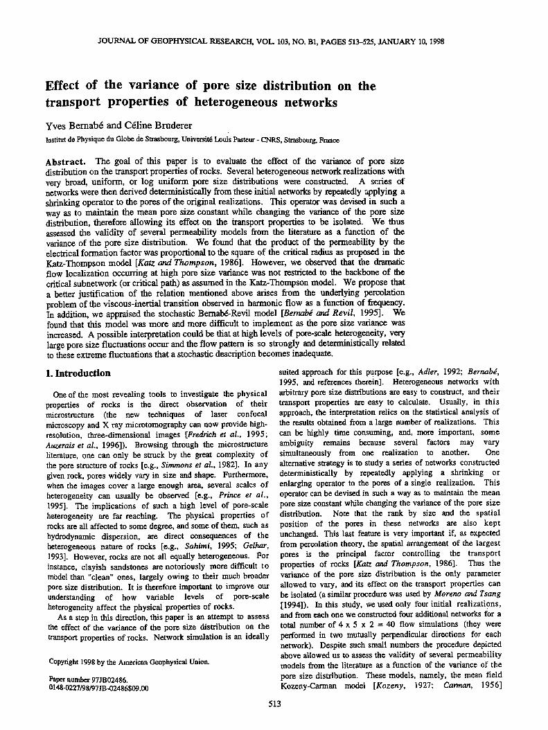
4.2. Comparison of Length Scales

Figure 4 shows the three length scales r•, A and q. versus (Sr/<•;> and compares thein to r,,=[SkF) m (the values of r• are indicated by the thick, shaded lines). First, note that all these parameters appro:tch I for the small values of %/<t;>. Thus the three models ,tre found equally valid in the limit of homogeneous networks, and tiffs conclusion can reasonably be extended to real holnogeneous por(•us ntcdia. Not surprisingly, the situation is quite ditferent at high levels of heterogeneity.


10

x rH7 , r e

A

re LU • !

0.5 0.1 •

o.o 1.5 2.0

Or/<ri>

Figure 4. Comparison of the hydraulic radius r u, the JS model [Johnson and Schwartz, 1989] length scale A, and the KT model [Katz and Thompson, 1986] critical radius •;. with r,,=(SkF) m. Hem r, is indicated by the thick, shaded lines, whose thickness corresponds to the fluctuation range of r,,. The two thin lines represent the theoretical values of R,. for three- dimensional cubic networks (see text for more details).

Recall that the validity of the various models is assessed by compari•g the characteristic length scales to r,,, which appears nearly constant in the case of the uniform distribution and strongly decreases with Or/<r•> for the log uniform distribution. We can see immediately that in all cases, KC becomes rapidly inadequate as o,/<r•> increases. Indeed, being equal to <q.2>/<r•>, r• increases with o,/<r,> (note that this result is specific to the tubular geometry but independent of the lattice dimensionality). Therefore our results suggest that KC should be valid only for very homogeneous rocks. It is worth emphasizing that this conclusion does not depend at all on porosity. In practice, however, KC is often claimed to work satisfactorily in high-porosity rocks and to fail only in low- porosity materials [e.g., v,n Genttb•ek and Rothman, 1996, and references therein]. If true, this might indicate a correlation between pore-scale heterogeneity and porosity in rocks. We are not in a position to discuss this statement here but can only point out that it seems to be contradicted by past experimental observations of one of the authors (Y.B.).

In contrast to the hydraulic radius, A and t;. are both in good agreement with r,,. Within the expected statistical fluctuations, r, is always nearly equal to r,,. The behavior of A is less simple; it is, of course, equal to r,, at low o,/<r•> but then slowly diverges, to finally stabilize and remain proportional to r, at very high values of oJ<r•> (notice that A is systematically lower than r,,). This behavior is consistent with the predictions of Banavar and Johnson [1987], although the observed ratio A/r,, for high %/<r•> is about a factor of 2 larger than the theoretical value of 1/(t+2)=0.3. We can conclude that both models appear valid for any degree of pore-scale hete• ogeneity, with a slight advantage to KT [see also Bernabd, 1995, 1997].

We can now understand why k was observed to decrease with o,]<t;> in the case of the log uniform distribution. Recall that for a two-dimensional square lattice, R,., the theoretical value of r,.. is equal to the median of the pore radius distribution M,•(r, ..... r,,h•) m. Indeed, we observed in all cases that within the expected statistical 'fluctuations, t;. was equal to Furthermore, we found that 5 was always closer to the

experimental median m a rather than to the theoretical value M,t. This observation suggests that r,. in a ,qven rock sample should be approximated accurately by the observed p,. quantile of the experimental pore size distribution (i.e., t¾om image analysis or mercury injection). Recall now that in the log uniform distribution the median is lower than the mean and that their

difference increases with increasing variance. We can see that R, and therefore r,. must become smaller and smaller with respect to <R> as %/<r•> increases. As a consequence, k must also decrease and F increase with %/<r/>. In the case of the uniform distribution, median and mean are identical nnd, within the statistical fluctuations, k and F should therefore remain

constant. We can easily extrapolate these results to three- dimensional cubic networks for which R,. is given by the upper quartile (i.e., (3r, ..... +rm,)/4 tbr the uniform distribution and (r, .... 3r,,•,,)•4 lbr the log uniform distribution). In the three- dimensional, unitbrm distribution case the permeability can thus be shown to increase linearly with Or/<r-,> with a slope of 3m/2. In the three-dimensional, log uniform case, R. has a

1.0

0.8

0.6

0.2

rmin

0.58 rc

0.5

rmax

1.0 1.5 2.0 r ß

1.0

0.8

0.6

0.4

0.2

a)

rmin • r c '•, 1.01

R c rmax •

0.2 0.4 0.6 0.8 1.0 r*

b)

Figure 5. Two examples oI the observed connectivity function •(r*)(note the position of r,,i,, r,. and r, ..... ). The corresponding theoretical curves E(r*) are represented by thin shaded lines (note that the position of R. does not coincide with that oi: r,.). (a) Uniform distributit•n with Or/<r•>=0.58 and (b) log uniform distribution with o',/<r•>=l.01.


more complex behavior, first increasing with c•r/<ri> then decreasing (the maximum corresponds to •r/<ri>=l ). This behavior, represented by the thin lines in Figure 4, is consistent with the observations of Moreno and Tsang [1994], who used a three-dimensional, cubic lattice and a range of conductance variance roughly corresponding in Figure 4 to a region from the origin to slightly beyond the maximum. Interestingly, this suggests that the KC model might have a greater range of validity in three dimensions than in two.

Since KT appears to be the best model, (7) implies that the product kF is approximately proportional to rfi. It would be interesting to know how k and F depend separately on r,.. Considering that our networks only contain tubular pores, it seems reasonable that k should be proportional to r,. 4 and 1/F be proportional to %2. As a matter of fact, our results agreed very well with this statement. We found that k and 1/F were well

approximated by gh(r,) and g,(r,.), respectively. However, this result strongly depends on the specific pore geometry considered here and is unlikely to have general validity. On the other hand, (7) is probably quite robust and general because, in real rocks, k and 1/F should be similarly affected by the other important factors such as pore length heterogeneity or variations of local coordination number. Therefore these

various effects cancel out in (7), leaving it unaffected. Another important question concerns the value of the constant c in (7). Again, the value found here, c=8, is not a general result but a direct consequence of Poiseuille law and the specific pore geometry used in this work. Remarkably, image analysis and experimental studies often yield the same value c--8 (F.D. Morgan, personal communication, 1996).

1.0

.o6

[•] 0'6 trmin" N•-58 • • 0.4

0.2

1.0

a)

0.8

0.6

0.4

0.2

b)

0.25 0.5 0.75 1.0 1.25 1-q 1.75 2.0

r ß

0.06

0.2 0.4 0.6 0.8 !.0 1.2

Figure 6. Comparison of the theoretical connectivity curves E(r*) for three-dimensional cubic networks (solid lines) and two-dimensional square networks (shaded lines) for several values of cxJ<r,>. (a) Uniform distribution and (b) log uniform distribution.

1.0

0.8

0.6

0.4

0.2

rmin

0.2 0.4 0.6 0.8 1.0

a) r* 1.0

0.6

0.4i /••//rg i•• f o.s

0.2 0.4 0.6 0.8 1.0 r*

b)

Figure 7. Examples of the observed function k*(r*) normalized to k for various values of c•r/<ri> (solid, segmented lines). For comparison the corresponding theoretical curves are plotted (shaded lines). (a) Uniform distribution and (b) log uniform distribution.

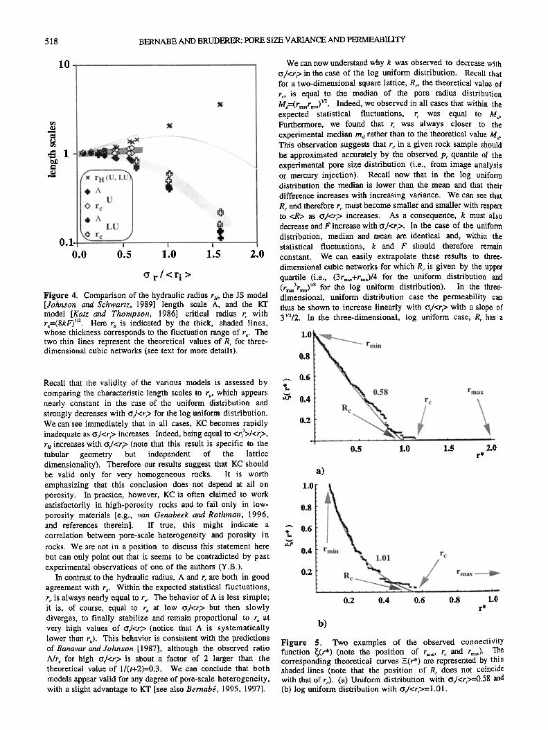
4.3. Critical Path Analysis

The most important result so far is that the length scale controlling fluid flow in heterogeneous porous rocks is best estimated by r,.. We would like now to understand why and, in particular, to check if this is indeed a consequence of CPA. The first task is to calculate the connectivity function •(r*) for each one of the four initial realizations (the same functions will apply to the derived networks, provided the appropriate change of variable is implemented according to (9) or (10)). In order to evaluate •(r*), we proceeded in a way similar to CPA. For r* decreasing from rma x to rm, ,, we constructed a suite of subsidiary networks by replacing r• with r'i=l (i.e., a constant) for r?_r* and with r'?0 for ri<r*. The permeability of each such subnetwork was computed and normalized to the value obtained when the entire network was recovered (i.e., r*=rm, n). Note that the periodic boundary conditions are not consistent with our definition of connectivity (i.e., across the network, from one side to the opposite one). Therefore different boundary conditions had to be used here, namely, constant fluid pressures on the fight and left sides of the network and no flow through the top and bottom sides. Figure 5 shows examples of •(r*) for both the uniform and log uniform distributions. For comparison the theoretical functions E(r*) are also indicated (that is, from (6), E(r*)=[2(rmax-r*)/(r.,ax-rnx•n)-l] •2 for the uniform distribution and E(r*)={ 2[ln(rraax)-!n(r*)]/[ln(rmax)- ln(r:n•n)]-I }t'2 for the log uniform distribution; the medians are (truax+tmOn)/2 and (rmaxrm.,) m. respectively). The agreement is


excellent, with the largest fluctuations in the vicinity of R,.

(note, in particular, how much These fluctuations with their shape of irregular steps make the •(r*) curves appear strikingly similar to the "devil staircase" conductivity curves measured by Thompson et at. [1987] during mercury injection experiments. In three-dimensional cubic networks, E(r*) is given by [4/3(;-, ..... -r*)/(r. .... -rm•,)-l/3] TM for the

uniform distribution and by {4/311n(r, )-ln(r*)]/[ln(r, )- In(r,,,,,)]-1/3}'"' for the log uniform distribution (the upper quartiles are (3;-, ..... +rm,)/4 and ' .-• tr, ..... 'r,mI , respectively). The

theoretical, two-and three-dimensional connectivity functions E(r*) are coinpared in Figure 6 for various values of o,/<r,>. Interestingly, both types are asymptotically coincident for the lowest r*, and since the three-dimensional E.(r*)are stretched

over a wider ran,,e than the two-dimensional ones, the5 have a slower connectivity buildup near R,.. In order to calculate k* and l/F*, we only need to multiply •(r*) by gt,(r*) and g,.(r*), respectively proportional to ;"4 and r '2. The calculated curves k*/1, versus r* are compared to the theoretical ones (i.e., =(r*)gt,(r*)) in Figure 7, where. for visibility, the theoretical curves are also plotted outside their definition intervals. The agreement between the calculated and theoretical curves was, again, very good, except in the vicinity of R,. where large fluctuations occurred. More important, the maximum of k*/l, appeared usually much lower than I and decreased rapidly with

increasing oJ<r•> (Figure 8). These low values around 0.1-0.2 are consistent with the results reported by Bernabe' [1995]. Also shown in Figure 8 is the maximum of F/F* which had a similar evolution with oJ<r•> but was generally higher than the maximum of k*/k. The positions of the maxima. rt,* and r,.*, did not usually coincide; rt,* and q.* did not evolve smoothly with oJ<•;> but were strongly sensitive to the statistical fluctuations of the observed k* and I/F* curves.

Therefore the CPA estimates of k and 1/F became worse and

worse as the flow was more and more localized. This behavior

totally contradicts CPA and the KT model. This can only mean that even when highly localized, the flow is not truly restricted

1.00

0.7s -

0.50 -

0.25 -

ß k

0 U

L o 1/F

0.00 , 0.0 1.5 2.0 0.5 1.0

Or/<ri> Figure 8. Critical Path Analysis estimates of the transport properties (i.e., the maxima of k* and l/F*)as a function of oJ<r,>. In each cdse, k* and l/F* were normalized to the original values of k and 1/F.

a) b)

Figure 9. (a) Example of the critical subnetwork (log uniform distribution, o,/<r,>=1.58). The backbone is represented by solid segments, and the isolated and dead-end branches are denoted by shaded segments. The position of the main shortcut is indicated by arrows. (b) Corresponding flow field. Note that flow boundary conditions differ froin those of Figure 2 (see text).

to the critical path as defined by CPA. Indeed, percolation theory shows that the backbone of the critical subnetwork is highly tortuous [Staujfer and Aharony, 1992; Sahimi, 1995] and that the critical subnetwork contains a large number of nearly touching dead-end branches. This geometry offers a very large number of possible shortcuts (that is, the main flow actually occurring through pores narrower than r,., and therelore not included in the critical subnetwork, but connecting nearly touching dead-end branches). Consequently, the probability of existence of such shortcuts should be nearly 1, except maybe in very sinall networks. Indeed, we observed these shortcuts in our flow simulations as illustrated in Figure 9. The shortcuts are energetically favorable over wider but more tortuous paths because the established flow must minimize the viscous energy dissipation [l_ztndau and Lifvhitz., 1987]. This is achieved by following not only the largest possible channels, as assumed by CPA, but also the straightest possible path.

Since, as explained earlier, k is well approximated by g,,0;.), a discussion of k*/gt,(r,.)=(r*/r,.)4•(r *) (or its theoretical form, •(r*)=(r*/R,.)4E(r*)) should be equivalent to that of k*/k. Clearly, •(r*)is equal to zero for r*=R,., and the increase of •(r*) with decreasing r* in the vicinity of R, is always less steep than that of E(r*) because (r*/Rc) 4 is a decreasing function. The maximum of •(r*) in the definition interval [rm. ,, r. ..... ] and, consequently, that of k* must therefore be lower than 1 (but note that outside the definition interval the absolute

maximum may be greater than 1) and take higher values if it occurs closer to R,.. In our simulations we verified that the maximum of k* occurred when the connectivity buildup was sufficient (i.e., for low enough r*) to include all the most important shortcuts. In the low oJ<r•> cases this happened for rt,*=rm, (i.e., when the entire network was recovered), but because •;m was almost equal to r,., the CPA estimate of k was not bad at all. On the other hand, in the high oJ<r•> cases, r** was greater than rm• n but was also so much lower than •;. that the CPA estimate had to be unacceptably low. We can extrapolate this result to three-dimensional cubic networks using the functions E(r*) shown in Figure 6. Their very slou connectivity buildup suggests that CPA should also greatly underestimate the transport properties of very heterogeneous three-dimensional cubic networks. This is consistent with the

results of Friedman and Seaton [ 1997], who studied the wdidity

BERNABE AND BRUDERER: PORE SIZE VARIANCE AND PERMI:•.ABILrrY 521

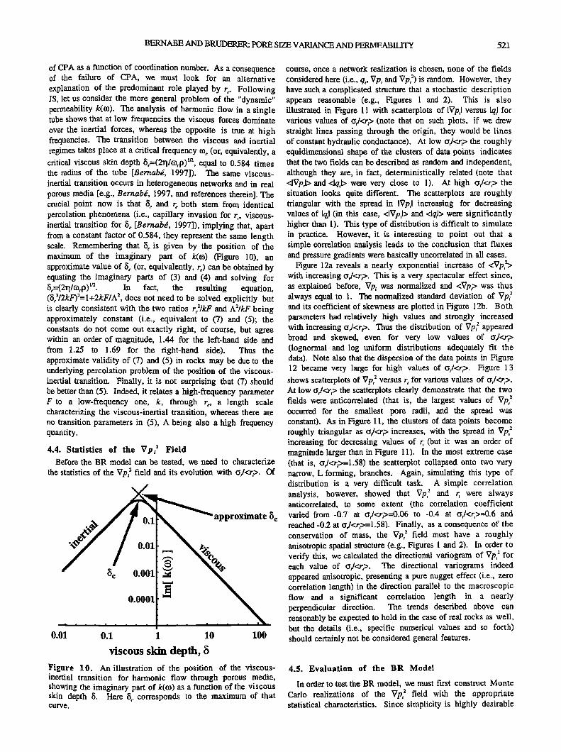
of CPA as a function of coordination number. As a consequence of the failure of CPA, we must look for an alternative explanation of the predominant role played by r,.. Following JS, let us consider the more general problem of the "dynamic" permeability k(to). The analysis of harmonic flow in a single tube shows that at low frequencies the viscous forces dominate over the inertial forces, whereas the opposite is true at high frequencies. The transition between the viscous and inertial regimes takes place at a critical frequency o3• (or, equivalently, a critical viscous skin depth 5,.--(2rl/to,.p) m, equal to 0.584 times the radius of the tube [Sernabd, 1997]). The same viscous- inertial transition occurs in heterogeneous networks and in real porous media [e.g., Bernabd, 1997, and references therein]. The crucial point now is that 8,. and 5. both stem from identical percolation phenomena (i.e., capillary invasion for r,., viscous- inertial transition for •5• [Bernabd, 1997]), implying that, apart from a constant factor of 0.584, they represent the same length scale. Remembering that õ,. is given by the position of the maximum of the imaginary part of k(to) (Figure 10), an approximate value of 5,. (or, equivalently, r,.) can be obtained by equating the imaginary parts of (3) and (4) and solving for 8•=(2ri/o)•p) TM. In fact, the resulting equation, (õ•:/2kF)•=l +2kF/A •, does not need to be solved explicitly but is clearly consistent with the two ratios r,)/kF and A•-/kF being approximately constant (i.e., equivalent to (7) and (5); the constants do not come out exactly right, of course, but agree within an order of magnitude, 1.44 for the left-hand side and from 1.25 to 1.69 for the fight-hand side). Thus the approximate validity of (7) and (5) in rocks may be due to the underlying percolation problem of the position of the viscous- inertial transition. Finally, it is not surprising that (7) should be better than (5). Indeed, it relates a high-frequency parameter F to a low-frequency one, k, through r,., a length scale characterizing the viscous-inertial transition, whereas there are no transition parameters in (5), A being also a high frequency quantity.

4.4. Statistics of the Vpl z Field Before the BR model can be tested, we need to characterize

the statistics of the Vp• field and its evolution with (•,/<r,>. Of

approximate 5 c

8c 0.001 •

0.0001 •

0.01 0.1 1 10 100

viscous skin depth, 5 Figure 10. An illustration of the position of the viscous- inertial transition •br harmonic flow through porous media, showing the imaginary part of k(ro) as a function of the viscous skin depth 8. Here 5,. corresponds to the maximum of that curve.

course, once a network realization is chosen, none of the fields

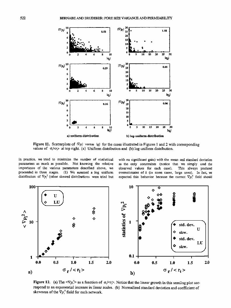
considered here (i.e., qi, Vpi and Vpi") is random. However, they have such a complicated structure that a stochastic description appears reasonable (e.g., Figures 1 and 2). This is also illustrated in Figure 11 with scatterplots of IVpJ versus Iq, I ['or various values of (•J<r,> (note that on such plots, if we drew straight lines passing through the origin, they would be lines of constant hydraulic conductance). At low c•]<ri> the roughly equidimensional shape of the clusters of data points indicates that the two fields can be described as random and independent, although they are, in fact, deterministically related (note that <lVpJ> and <lqJ> were very close to 1). At high (•J<ri> the situation looks quite different. The scatterplots are roughly triangular with the spread in [Vpi[ increasing for decreasing values of IqJ (in this case, <lVpil> and <lqJ> were significantly higher than 1). This type of distribution is difficult to simulate in practice. However, it is interesting to point out that a simple correlation analysis leads to the conclusion that fluxes and pressure gradients were basically uncorrelated in all cases.

Figure 12a reveals a nearly exponential increase of <Vp?> with increasing (•J<ri>. This is a very spectacular effect since, as explained before, Vpi was normalized and <Vpi> was thus always equal to 1. The normalized standard deviation of Vpfi and its coefficient of skewness are plotted in Figure 12b. Both parameters had relatively high values and strongly increased with increasing (•J<r•>. Thus the distribution of Vp/appeared broad and skewed, even for very low values of oJ<r• (lognormal and log uniform distributions adequately fit the data). Note also that the dispersion of the data points in Figure 12 became very large for high values of C•r/<r,>. Figure 13 shows scatterplots of Vp• • versus r i for various values of (•J<ri>. At low oJ<ri> the scatterplots clearly demonstrate that the two fields were anticorrelated (that is, the largest values of Vp• 2 occurred fbr the smallest pore radii, and the spread was constant). As in Figure 11, the clusters of data points become roughly triangular as (•/<r,> increases, with the spread in Vp• 2 increasing tbr decreasing values of r• (but it was an order of magnitude larger than in Figure 11). In the most extreme case (that is, (•J<r•>=l.58) the scatterplot collapsed onto two very narrow, L forming, branches. Again, simulating this type of distribution is a very difficult task. A simple correlation analysis, however, showed that Vp•: and r,. were always anticorrelated, to some extent (the correlation coefficient varied from-0.7 at (•J<r,>=O.06 to -0.4 at {J/<r•>•-0.6 and reached-0.2 at (•r/<ri>=l.58). Finally, as a consequence of the conservation of mass, the Vp• z field must have a roughly anisotropic spatial structure (e.g., Figures I and 2). In order to verify this, we calculated the directional variogram of Vp,: for each value of (•J<ri>. The directional variograms indeed appeared anisotropic, presenting a pure nugget effect (i.e., zero correlation length) in the direction parallel to the macroscopic flow and a significant correlation length in a nearly perpendicular direction. The trends described above can reasonably be expected to hold in the case of real rocks as well, but the details (i.e., specific numerical values and so forth) should certainly not be considered general features.

4.5. Evaluation of the BR Model

In order to test the BR model, we must first construct Monte

Carlo realizations of the Vp, 2 field with the appropriate statistical characteristics. Since simplicity is highly desirable


IVpil

IVpil

IVpil

lO

8

6

4

2

o

iqil

0.29

10

8

6

4

2

0 2 4 6

2 4 6 8 10

iqil

O.O6

IVpil 2s * L58 2o

15 • ee ß ß lO

5 **

0 5 10 15 20 25 30

lqil

iVpi I 30 25 0.65 20

15

10

0 0 5 10 15 20 25 30

Iqil

0.06

a) uniform distribution

iVpi I 3o 25

20

15

!0

5

8 10 0 5 10 15 •0 •5 30 Iqil Iqil

b) log-uniform distribution

Figure 11. Scatterplots of IVp,I versus Iqil for the cases illustrated in Figures 1 and 2 with corresponding values of oJ<r;> at top right. (a) Uniform distribution and (b) log uniform distribution.

in practice, we tried to minimize the number of statistica! parameters as much as possible. Not knowing the relative importance of the various parameters described above, we proceeded in three stages. (1) We assumed a log uniform distribution of Vp; 2 (other skewed distributions were tried but

with no significant gain) with the mean and standard deviation as the only constraints (notice that we simply used the observed values for each case). This always produced overestimates of k (in some cases, large ones). In fact, we expected this behavior because the correct Vp; 2 field should

100'

A

D 10- v

lO

! i i

0.0 0.5 1.0 1.5 2.0 0.0 0.5

* std. dev.

0 skw.

• std. dev.

• skw.

1.0 1.5

a) cv r / < ri > b) r / < ri > Figure 12. (a) The <Vp,•-> as a function of •x/<r?. Notice that the linear growth in this semilog plot correspond to an exponential increase in linear scales. (b) Normalized standard deviation and coefficient of skewness of the Vp, 2 field for each network.


Vpi2 601 .......... '- ........................ 250 i' 0 8 VpiZ 1.58 40 • ' •#ø '.- l, ß }• '. 150 •.,•.••. ß 50

O0 - 1 2 0 ' - 0 3.5 7

ri r i

Vpi2 16 0.29 Vpi2 '. 0.65

0 0.5 1 1.5

Vpi2 0.06

2 o-..... . ..

0.9 1 1.1


Vpi2

0 'ø' 0.5 1.5 2.5

ri

0.06

2

0.9 1 1.I

ri


Figure 13 Scatterplots of Vp, 2 versus r, for the cases illustrated in figures 1 and 2, with corresponding values of cy,/<r,> at top right. For visibility, different scales were used in each plot. (a) Uniform distribution and (b) log uniform distribution.

minimize the viscous dissipation and therefore k [Betvzabd atwl ReviI, 1995]. (2) Using simulated annealing [Deutsch and Journel, 1992], we spatially redistributed the same values of V p•" of the previously constructed realizations in order to introduce the anticorrelation of Vp; 2 with r• as observed in Figure 13. We implemented the cost function in the simulated annealing procedure in the simplest possible way, namely, by incorporating the absolute values of the correlation coefficients calculated for each •7pi2 versus r• scatterplot. This is, of course, an oversimplified description (see Figure 13 and discussion in section 4.4). This procedure overshot our goal and systematically yielded underestimates of k, a surprising result since it apparently violated the minimization principle mentioned above. One possible explanation is that the Monte Carlo Vpi" fields were unphysical and, in particular, did not verify the law of conservation of mass. We tried stage 3 as a means tbr taking this into account. (3) We again applied simulated annealing to the realizations from stage 1, with a modified cost function, which additionally contained the first three nonzero values of the Vpl 2 variogram in the direction perpendicular to the macroscopic flow. The results were quite good at low c•/<ri>, but the estimates became less and less accurate and, more important, more and more erratic as cL/<r,> was increased (see Figure 14). The values plotted in Figure 14a represent averages, each one taken on 10 Monte Carlo simulations. The error bars correspond to 1 standard deviation (the normalized standard deviations are shown in Figure 14b).

Thus, as implemented here, the BR model could handle only moderate levels of pore-scale heterogeneity. The poor results obtained for high (•J<r,> may be merely due to the insufficiently detailed statistical description used here.

However, we feel that this failure has deeper roots. When c•J<r,> is very high, Vp• 2 may occasionally take enormously large values. Discrepancies in the positioning of these extreme values of Vp• 2 in the network will cause huge errors in the k estimates, which is exactly what we observed. In our opinion this means that the location of these extreme values of Vpf are set deterministically and that a purely stochastic description is not adequate at very high levels of pore-scale heterogeneity. Obviously, this is a manifestation of flow localization. In such cases it is therefore interesting to change our viewpoint and try to characterize the high-flow channels deterministically [see also Moreno and Tsang, 1994]. Figure 15 shows examples of scatterplots of IqJ versus r• for various c•J<r,>. In all cases (even for •J<r,>=l.58) the pores with high values of Iq•l had pore radius distributions with a higher mean and a lower variance than the complete distribution (similar results were reported by Moreno and Dang [1994]). Clearly, Iqil and ri are well correlated at low •JJ<r,>; this was possible because the high-flow channels did not form continuous paths. Instead, we can see in Figures 1 and 2 that their spatial distribution was roughly uniform, the flow field converging into and diverging out of them. At high cU<ri>, when flow localization occurs, the high-flow channels do form continuous paths that must therefore include some narrow pores (also see the discussion of CPA in section 4.3). However, the pore radius distribution along these paths is much less skewed and therefore has a higher mean and a lower variance than the complete distribution (cU<r,>=l.58 case in Figure 15). We suspect that among all the possible paths with the appropriate pore size distribution, those where the flow is localized are the shortest, but we did not check this point yet.


a)

•

,..

,.,,

o u 1.5-

1.0-

0.5-

' • • 0.0 , •

0.0 0.4 0.8 0.0 1.0 1.5 i

0.5

(Y r / < ri > b) cy r / < r i >

Figure 14. (a) Average of 10 Monte Carlo estimations of k following the BR procedure [Bernabe' and Revil, 1995]. Notice the values are normalized to the original k in each case. The error bars correspond to plus or minus 1 standard deviation. (b) Standard deviation of the same Monte Carlo estimates normalized to the mean.

2.0

10

0 1 2

Iqil

*•',,; ß eee ß ß ß 10 I"-.,n,, •,., • •, ' '=' n, ee •e• •e ß •e ß ß

0 3.5 7

ri r i 5 15

0.65 Iqil 4 Iqil .... o ß

3 10 e ß ß eel • ß ß

1

o o• 0.5 1 1.5 0.5 1.5 2.5

Iqil

ri

1

o

0.9 1


1.1

ri

2

0.9 1 1.1

ri


Figure 15. Scatterplots of [q,I versus r, for the cases illustrated in figures 1 ans 2, with corresponding values of cyJ<r• at top right. For visibility, different scales were used in each plot. (a) Uniform distribution and (b) log uniform distribution.


5. Conclusions

In summary, we were able to isolate several interesting aspects of the influence of pore size variance on the transport properties of heterogeneous networks. First, all four models considered here were valid and their predictions converged at low pore-scale heterogeneity levels. This was not true at high o/<•;>. Only the Johnson-Schwartz and Katz-Thompson models remained satisfactory at all heterogeneity levels. This is expressed in the (5) and (7) which are not exact relations but were found to be quite accurate at any tSr/<r;>. Equation (5) is a little less useful than (7) because the constant c in it varies slightly with c•/<ri> (i.e., •¾om 8 at low ts/<ri> to about 3 at high c•/<ri> if we assume c=8 in (7)). A second result was that the effectiveness of (7) and the predominant role played by the critical radius r,. cannot be explained by CPA. We found that the dramatic flow localization occurring at high (5/<ri> was not restricted to the backbone of the critical subnetwork (or critical path) as assumed in CPA. Indeed, the critical path is too tortuous to minimize the viscous energy dissipation. We propose that a better justification of (7) is the underlying percolation problem of the viscous-inertial transition observed in harmonic flow as a function of frequency. Another result that could be useful in practical applications is that 5. is well approximated by the ?,. quantile (i.e., corresponding to the percolation threshold p,.) of the observed pore size distribution. Third, for the purpose of appraising BR, we statistically analyzed the Vp/2 field as a function of ts/<ri>. The Vpi" field had a rather simple random structure at low to moderate •Sr/<ri> and a stochastic description was an attractive option in this case. At high Or/<ri>, owing to flow localization, extreme values of Vp• 2 occurred at deterministic positions. The flow pattern is so strongly controlled by these huge values that a stochastic description becomes inadequate. Finally, our contention is that the results summarized above are general enough to hold reasonably well in real rocks (in particular, they do not seem to depend on the dimensionality of the networks nor on the specific pore radius distributions used here).

Acknowledgments. We are grateful to two anonymous reviewers for their very helpful comments and suggestions.

References

Adler, P.M., Porous Media: Geometry and Tran,•port, 544 pp., Butterworths, London, 1992.

Ambegaokar, V., B.I. Halperin, and J.S. Langer, Hopping conductivity in disordered systems, Phys. Rev. B Solid State, 4, 2612-2620, 1971.

Auzerais, F.M., J. Dunsmuir, B. Ferr6ol, N. Martys, J. Olson, T.S. Rmnakrishnan, D.H. Rothman, and L.M. Schwartz, Transport in sandstone: A study based on three-dimensional microtomography, Geophys. Res. Lett., 23, 705-708, 1996.

Banavar, J.R., and D.L. Johnson, Characteristic pore sizes and transport in porous media, Phys. Rev. B Condens. Matter, 35, 7283-7286, 1987.

Bear, J., Dynamics of Fluids in Porous Media, 764 pp., Dover, Mineola, N.Y., 1972.

Bernab6, Y., The transport properties of networks of cracks and pores, J. Geophys. Res., 100, 4231-4241, 1995.

Bernab6, Y., The frequency dependence of harmonic fluid flow through networks of cracks and pores, Pure App!. Geophys., 149, 489-506, 1997.

Bernabe, Y., and A. Revil, Pore-scale heterogeneity, energy dissipation and the transport properties of rocks, Geophys. Res. Lett., 22, 1529- 1532, 1995.

Carman, P.C., Flow of Gases through Porous Media, Butterworths, London, 1956.

David, C., Geometry of flow paths for fluid transport in rocks, J. Geophys. Res., 98, 12,267-12,278, 1993.

Deutsch, C.V., and A.G. JourneI, GSLiB Geosmtistical Software Librat3' and User's Guide, 340 pp., Oxtbrd Univ. Press, New York, 1992.

Fredrich, J.T., B. Men6ndez, and T-f. Wong, Imaging the pore structure of geomaterials, Science, 268, 276-279, !995.

Friedman, S.P., and N.A. Seaton, Critical path analysis of the relationship between permeability and electrical conductivity of 3-dimensional pore networks, submitted to Wat. Resour. Res., 1997.

Gelhar, L.W., Stoctmstic Subsu,rfitce Hydrology, 390 pp., Prentice-Hall, Englewood Cliffs, N.J., 1993.

Johnson, D.L., and L.M. Schwartz, Unified theory of geometrical effects in transport properties of porous media, paper presented at SPWLA 30th Annual Logging, Symposium, Soc. of Prof. Well Log Anal., Houston, Tex., 1989.

Johnson, D.L., and P.N. Sen, Dependence of the conductivity of a porous medium on electrolytic conductivity, Phys. Rev. B Condens. Matter, 37, 3502-3510, 1988.

Johnson, D.L., J. Koplik, and R. Dashen, Theory of dynamic permeability and tortuosity in fluid-saturated porous media, J. Fluid Mech., 176, 379-402, 1987.

Katz, A.J., and A.H. Thompson, Quantitative prediction of permeability in porous rock, Phys. Rev. B Condens. Matter, 34, 8179-8!81, 1986.

Kozeny, J., Uber Kapillare Leitung des Wassers im Boden, Sitz. ungsber. Akad. Wiss. Wien., 136, 271-306, 1927.

Landau, L.D., and E.M. Lifshitz, Fluid Mechanics, 2nd ed., 539 pp., Pergamon, Tarrytown, N.Y., t987.

Le Doussal, P., Permeability versus conductivity for porous media with wide distribution of pore sizes, Phys. Rev. B Condens. Matter, 39, 4816-4819, 1989.

Moreno, L., and C-F. Tsang, Flow channeling in strongly heterogeneous porous media: A numerical study, Water Resour. Res., 30, 1421-1430, 1994.

Paterson, M.S., The equivalent channel model for permeability and resistivity in fluid-saturated rock: A reappraisal, Mech. Mater., 2, 345-352, 1983.

Prince, C.M., R. Ehrlich, and Y. Anguy, Analysis of spatial order in sandstones Ii: Grain clusters, packing flaws, and the small-scale structure of sandstones, J. Sediment. Res., Sect. A, 65, 13-28, 1995.

Sahimi, M., Flow phenomena in rocks: From continuum models to fractals, percolation, cellular automata and simulated annealing, Rev. Mod. Phys., 65, 1393-1534, 1993.

Sahimi, M., Flow and Transport in Porous Media and Fractured Rock, 482 pp., VCH, New York, 1995.

Shante, V.K.S., Hopping conduction in quasi-one-dimensional disordered compounds, Phys. Rev. B Solid State, 16, 2597-2612, 1977.

Simmons, G., R. Wilkens, L. Caruso, T. Wissler and F. Miller, Physical properties and microstructures of a set of sandstones, Annual report to Schlumberger-Doll Res. Cent., Ridgefield, Conn., 1982.

Stauffer, D., and A. Aharony, Introduction to Percolation Theory, 2nd ed., 180 pp., Taylor and Francis, Bristol, Pa., 1992.

Thompson, A.H., A.J. Katz, and C.E. Krohn, The microgeometry and transport properties of sedimentary rock, Adv. Phys., 36, 625-694, 1987.

van Genabeek, O., and D.H. Rothman, Macroscopic manifestations of microscopic flows through porous media: Phenomenology from simulation, Annu. Rev. Earth Planet. Sci., 24, 63-87, 1996.

Walsh, J.B., and W.F. Brace, The effect of pressure on porosity and the transport properties of rocks, J. Geophys. Res., 89, 9425-9431, 1984.

Y. Bernab6 and C. Bruderer, Institut de Physique du Globe de Strasbourg, Universit6 Louis Pasteur - CNRS, 5 rue Ren6 Descartes, 67084 Strasbourg Cedex, France. (e-mail: yves @climont.u-strasbg2¾)

(Received June 9, 1997; revised August 21, 1997; accepted August 28, !997.)

Effect of the variance of pore size distribution on the transport properties of heterogeneous...

Documents

Transcript of Effect of the variance of pore size distribution on the transport properties of heterogeneous...