Effect of orbital drift and sensor changes on the time series of AVHRR vegetation index data

2584 IEEE TRANSACTIONS ON GEOSCIENCE AND REMOTE SENSING, VOL. 38, NO. 6, NOVEMBER 2000

Effect of Orbital Drift and Sensor Changes on theTime Series of AVHRR Vegetation Index DataRobert K. Kaufmann, Liming Zhou, Yuri Knyazikhin, Nikolay V. Shabanov, Ranga B. Myneni, and

Compton J. Tucker

Abstract—This paper assesses the effect of changes in solarzenith angle (SZA) and sensor changes on reflectances in channel1, channel 2, and normalized difference vegetation index (NDVI)from the advanced very high resolution radiometer (AVHRR)Pathfinder land data set for the period July 1981 throughSeptember 1994. First, the effect of changes in SZA on channelreflectances and NDVI is derived from equations of radiativetransfer in vegetation media. Starting from first principles, itis rigorously shown that the NDVI of a vegetated surface is afunction of the maximum positive eigenvalue of the radiativetransfer equation within the framework of the theory used andits assumptions. A sensitivity analysis of this relation indicatesthat NDVI is minimally sensitive to SZA changes, and thissensitivity decreases as leaf area increases. Second, statisticalmethods are used to analyze the relationship between SZA andchannel reflectances or NDVI. It is shown that the use of ordinaryleast squares can generate spurious regressions because of thenonstationary property of time series. To avoid such a confusion,we use the notion of cointegration to analyze the relation betweenSZA and AVHRR data. Results are consistent with the conclusionof theoretical analysis from equations of radiative transfer. NDVIis not related to SZA in a statistically significant manner exceptfor biomes with relatively low leaf area. From the theoretical andempirical analysis, we conclude that the NDVI data generatedfrom the AVHRR Pathfinder land data set are not contaminatedby trends introduced from changes in solar zenith angle due toorbital decay and changes in satellites (NOAA-7, 9, 11). As such,the NDVI data can be used to analyze interannual variability ofglobal vegetation activity.

Index Terms—AVHRR, interannual variability, NDVI, path-finder data, satellite drift.

I. INTRODUCTION

A data set of normalized difference vegetation index (NDVI)at 8-km resolution (square pixels) has been produced

with data from the advanced very high resolution radiome-ters (AVHRR) onboard the afternoon-viewing NOAA seriessatellites (NOAA-7, 9, and 11) under the joint sponsorship ofNASA and NOAA Earth Observing System (EOS) PathfinderProject [1]. The data processing includes improved navigation,intersatellite calibration, and partial correction for Rayleighscattering. The data are currently available for the periodJuly 1981 to September 1994 and have been used to study

Manuscript received July 27, 1999; revised March 16, 2000. This work wassupported by NOAA grant NA76G90481 and NASA Earth Science Enterprise.

R. K. Kaufmann, L. Zhou, Y. Knyazikhin, N. V. Shabanov, and R. B. Myneniare with the Department of Geography, Boston University, Boston, MA 02215USA (e-mail: [email protected]).

C. J. Tucker is with the Biospheric Sciences Branch, Code 923, NASA God-dard Space Flight Center, Greenbelt, MD 20771 USA.

Publisher Item Identifier S 0196-2892(00)07154-0.

interannual variations in global vegetation dynamics. Analysisof the Pathfinder NDVI data indicates increased photosyntheticactivity of terrestrial vegetation from 1981 to 1991 in a mannersuggestive of an increase in plant growth associated with anincrease in the duration of the active growing season [2]. Theregion of greatest increase lies between 45N and 70N, wheremarked warming has occurred in the spring time due to an earlydisappearance of snow [3]. The satellite data are consistent withan increase in amplitude of the seasonal cycle of atmosphericCO exceeding 20% since the early 1970’s and an advance inthe timing of the drawdown of COin spring and early summerof up to seven days [4].

Conclusions about interannual variability and the biotic ef-fect of climate change are based on a critical assumption: thatthe data collected by AVHRR’s are not contaminated by changesin measurement error over time. If measurement error changesover time, the time series collected by the sensor will contain adeterministic or stochastic trend when none may exist. To avoidconfusing these trends with trends generated by changes in ter-restrial biota, it is important to identify such errors and cor-rect for their effects before analyzing the data. In the case ofthe Pathfinder data set, both sensor calibration and illuminationvariations contribute to measurement error change over time,and the effect of changing illumination, however, can mitigateor enhance the artificial trends caused by calibration instability.The calibration issue has been addressed in numerous scientificstudies, but the illumination issue has not. The illumination ef-fect is a combination of the effects of absorption and scatteringin the atmosphere and surface anisotropy [5]. In general, proper-ties of both surface and atmosphere vary during the year, whichmakes the problem even more complex [5]. Quantitative charac-teristics of atmospheric constituents (aerosol and water vapor)and of the surface are only now becoming available on a globalscale. As discussed by Privetteet al.[6], changes in SZA can af-fect reflectances by modifying the radiation interactions in themedia. Changes in the optical depth of aerosol particles in thetroposphere and stratosphere (AOD) affect reflectances directlyby changing the reflectivity of the atmosphere [7].

In this paper, we assess the effect of changes in solar zenithangle on reflectances in channel 1, channel 2, and NDVI fromthe AVHRR Pathfinder land data set assembled from NOAA-7,9, and 11 sensors (the effect of stratospheric aerosol opticaldepth is explored in a separate paper). Our assumptions are thefollowing.

1) Most of the artificial signals caused by calibration resid-uals have been removed by the calibration methods usedto process this dataset.

0196–2892/00$10.00 © 2000 IEEE

KAUFMANN et al.: EFFECT OF ORBITAL DRIFT AND SENSOR CHANGES ON THE TIME SERIES OF AVHRR VEGETATION INDEX DATA 2585

2) Major AOD variations due to volcanic eruptions onlycause significant measurement errors within two rel-atively short periods compared with our whole studyperiod.

3) Residual atmospheric effects were minimized by an-alyzing the maximum NDVI values within a ten-dayinterval.

Based on such assumptions, the major signals of changes inreflectances and NDVI are related to changes in SZA, if any.This analysis is described in five sections. In Section II, we de-rive the effect of changes in SZA on channel reflectances andNDVI from equations of radiative transfer in vegetation media.Starting from first principles, it is rigorously shown that theNDVI of a vegetated surface is a function of the maximum pos-itive eigenvalue of the radiative transfer equation. A sensitivityanalysis of this relation is performed to determine the effect ofSZA changes on NDVI. It is shown that NDVI is minimally sen-sitive to SZA changes and that this sensitivity decreases as leafarea increases. The third section describes statistical methodsused to analyze the relationship between SZA and channel re-flectances or NDVI. It is shown that the use of ordinary leastsquares (OLS) can generate spurious regressions because thedistribution of test statistics in regression models is based onthe assumption that time series are stationary, that is, they donot contain a stochastic trend. To avoid confusion about the rela-tion between SZA and NDVI that may be implied by a spuriousregression, the notion of cointegration is used to analyze the re-lation between SZA and AVHRR data. The results of this empir-ical analysis are described in Section IV, and they are consistentwith the conclusion of Section II. NDVI is not related to SZAin a statistically significant manner except for biomes with rela-tively low leaf area. From the theoretical and empirical analysis,we conclude in Section V that the time series of NDVI gener-ated from the AVHRR Pathfinder land data set are not contam-inated by trends introduced from changes in solar zenith angledue to orbital decay and changes in satellites (NOAA-7, 9, 11).As such, the NDVI data can be used to analyze interannual vari-ability of global vegetation activity.

II. THEORETICAL ANALYSIS

A. Angular Variation of the NDVI

Data for the spectral reflectance recorded by satellite sensorsusually are compressed into vegetation indices. The literaturedescribes more than a dozen such indices and these correlatewell with vegetation amount [8], the fraction of absorbed pho-tosynthetically active radiation [9], unstressed vegetation con-ductance and photosynthetic capacity [10], and seasonal atmo-spheric carbon dioxide variations [11]. These correlations arealso supported by theoretical investigations [12]–[15]. This sec-tion expands these investigations to analyze the relationship be-tween solar zenith angle (SZA) and NDVI from first principles.

1) Radiative Transfer Problem for VegetationMedia: Consider a vegetation canopy in the layer 0

. The top 0 and bottom surfaces form itsupper and lower boundaries. The position vectordenotesthe Cartesian triplet ( ) with its origin at the top of thecanopy. Assume that photons interact with phytoelements only.

That is, photon interactions with optically active elementsof the atmosphere inside the layer 0 are ignored.The radiation field within the layer can be described by thethree-dimensional (3-D) transport equation [16], [17]

(1)

Here, is the monochromatic radiance which depends onwavelength , location , and direction . The unit vectoris expressed in spherical coordinates with respect toaxis, and and are its polar angle and azimuth.is the total interaction cross section, which does not dependon wavelength, and is the differential scattering crosssection. A precise description of these variables can be foundin [18], [19]. In the follwing, the formulation of Myneni [19]is adopted.

The transfer equation (1) is a statement of energy conserva-tion in the phase space. The physical meaning of the variousterms in (1) is that the first term characterizes the change in ra-diance in at , the other terms show whether the changes takeplace at the expense of absorption and scattering in the medium(second term) and at the expense of the scattering from the otherdirections (third term).

The magnitude of scattering by elements of the vegetationcanopy is described using the hemispherical leaf albedo

(2)

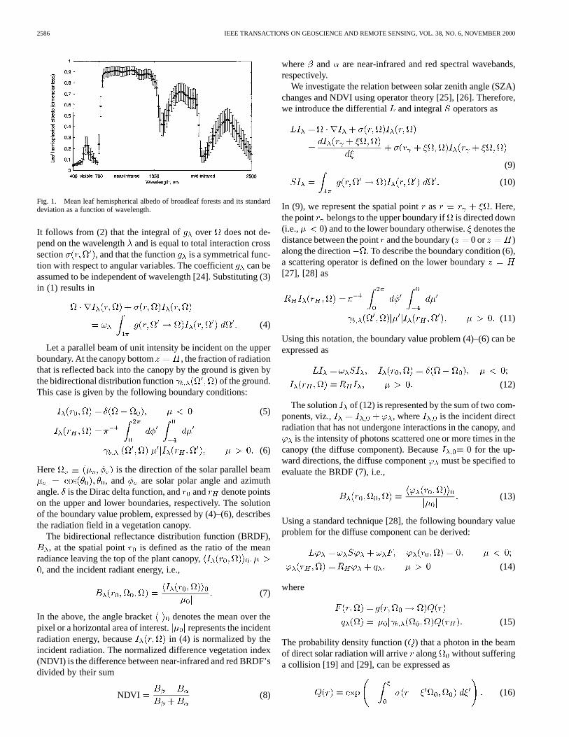
An individual leaf is assumed to reflect and transmit the inter-cepted energy in a cosine distribution about the leaf normal. Inthis case, the leaf albedo does not depend on the angularvariable and the differential scattering cross section isa symmetrical function with respect to angular variables [20].It is assumed that the leaf albedo is independent of the spatialvariable . These assumptions are not essential to the followinganalysis. The typical spectral variation of leaf albedo is definedby three distinct spectral regions [21], i.e., visible (0.4–0.7m),near-infrared (0.7–1.35m), and mid-infrared (1.35–2.5m).In general, a green leaf absorbs 90–95% of solar radiation in thevisible region but only 5–10% in the near-infrared. Leaf albedoin the mid-infrared region is usually smaller than in the near-in-frared and is controlled by internal leaf structure and absorptionby leaf water [22], [23]. Characteristic water absorption bandsare at 1.43, 1.95, and 2.2m. These properties are inferred fromthe spectral behavior of a green, healthy leaf and are quite stablealthough the magnitude of reflectance and transmittance mayvary with leaf age and among species. Fig. 1 demonstrates a typ-ical spectral variation of leaf albedo for broadleaf forests. Leafspectral data were obtained from a variety of sources of filedmeasurements on different broadleaf trees. The mean and vari-ance spectra were calculated from a large number of samples.

In this study, the normalized differential scattering cross sec-tion is used

(3)


Fig. 1. Mean leaf hemispherical albedo of broadleaf forests and its standarddeviation as a function of wavelength.

It follows from (2) that the integral of over does not de-pend on the wavelengthand is equal to total interaction crosssection , and that the function is a symmetrical func-tion with respect to angular variables. The coefficientcan beassumed to be independent of wavelength [24]. Substituting (3)in (1) results in

(4)

Let a parallel beam of unit intensity be incident on the upperboundary. At the canopy bottom , the fraction of radiationthat is reflected back into the canopy by the ground is given bythe bidirectional distribution function of the ground.This case is given by the following boundary conditions:

(5)

(6)

Here is the direction of the solar parallel beam, and are solar polar angle and azimuth

angle. is the Dirac delta function, and and denote pointson the upper and lower boundaries, respectively. The solutionof the boundary value problem, expressed by (4)–(6), describesthe radiation field in a vegetation canopy.

The bidirectional reflectance distribution function (BRDF),, at the spatial point is defined as the ratio of the mean

radiance leaving the top of the plant canopy,, and the incident radiant energy, i.e.,

(7)

In the above, the angle bracket denotes the mean over thepixel or a horizontal area of interest. represents the incidentradiation energy, because in (4) is normalized by theincident radiation. The normalized difference vegetation index(NDVI) is the difference between near-infrared and red BRDF’sdivided by their sum

NDVI (8)

where and are near-infrared and red spectral wavebands,respectively.

We investigate the relation between solar zenith angle (SZA)changes and NDVI using operator theory [25], [26]. Therefore,we introduce the differential and integral operators as

(9)

(10)

In (9), we represent the spatial pointas . Here,the point belongs to the upper boundary ifis directed down(i.e., 0) and to the lower boundary otherwise.denotes thedistance between the pointand the boundary ( 0 or )along the direction . To describe the boundary condition (6),a scattering operator is defined on the lower boundary[27], [28] as

(11)

Using this notation, the boundary value problem (4)–(6) can beexpressed as

(12)

The solution of (12) is represented by the sum of two com-ponents, viz., , where is the incident directradiation that has not undergone interactions in the canopy, and

is the intensity of photons scattered one or more times in thecanopy (the diffuse component). Because 0 for the up-ward directions, the diffuse component must be specified toevaluate the BRDF (7), i.e.,

(13)

Using a standard technique [28], the following boundary valueproblem for the diffuse component can be derived:

(14)

where

(15)

The probability density function () that a photon in the beamof direct solar radiation will arrive along without sufferinga collision [19] and [29], can be expressed as

(16)


The functions and depend on the SZA and determine theeffect of changes in SZA on NDVI.

2) Eigenvalues of the Transport Equation:To determine theeffect of changes in SZA on NDVI, a sensitivity analysis on therelation between NDVI and the maximum positive eigenvalueof the transport equation is performed. By definition, the eigen-value of the transport equation is a numbersuch that thereexists a function that satisfies

(17)

with vacuum boundary conditions

(18)

The function is the eigenvector corresponding to thegiven eigenvalue . The set of eigenvaluesand eigenvectors of the transport equa-tion is a discrete set [26]. The transport equation has a uniquepositive eigenvalue that corresponds to a positive eigenvector[26]. This eigenvalue is greater than the absolute magnitudes ofthe remaining eigenvalues. It provides information intrinsic tothe medium (vegetation canopy) and is independent of illumi-nation geometry.

Methods developed in operator theory can be used to estimatethe maximum positive eigenvalue. In particular, Krasnoselskii’s[30] results on positive operators will be used in the following.Let be a positive operator, and letbe a positive function forwhich the following inequality holds:

(19)

where and are some positive constants. Under some gen-eral conditions [30], the sequences

inf sup (20)

converge to the maximum eigenvalue of the operatorfrom below and above

(21)

Knyazikhin [31] discusses conditions under which this resultis applicable to the transport equation. The next section showsthat the NDVI for a sufficiently dense canopy is a function ofthe maximum eigenvalue of the operator . It fol-lows from (19) and (20) that the maximum positive eigenvalueequation is independent of illumination geometry. Therefore,exploring its relation to NDVI provides the proper analysis toaddress SZA effects.

B. Dependence of NDVI on SZA in the Case of An AbsorbingGround

Consider the simplest case: reflectance of the ground belowthe vegetation is zero, that is, 0 (0). The problem of radiative transfer in this case is termed the

“black soil problem.” Results presented in this subsection are re-quired to extend our analysis to the general case of a reflectingsoil below the vegetation. We use a standard technique devel-oped in mathematical transport theory [26]–[28] as well as theresult mentioned in the previous section.

The solution of the transport equation (14) can be expandedin Neumann series [27], [28] and [32] as

(22)

where , are wavelength independentfunctions. Substituting (22) into (8) and accounting for (13), weobtain

NDVI

(23)

Here is the ratio between leaf albedos at red and near-infraredwavelengths, i.e., . Note that a typical value ofvaries by about 0.1 ( Fig. 1). This allows us to neglectfor

in (23), which means we neglect the multiple scatteringat red spectral band while accounting for multiple scattering ra-diation at near infrared band. Under these conditions, (23) canbe reduced to a rational function whose variation with SZA re-sults from variation of . Therefore, the followinganalysis begins with the justification of this technique.

Consider the following functions:

(24)

(25)

These expressions can be used to represent NDVI as

NDVI (26)

Neglecting the term in (26), the following approximation forNDVI results:

NDVI (27)

The accuracy of this approximation (27) can be investigated bythe difference NDVI = NDVI - NDVI. Because

NDVI

(28)

Thus, the accuracy of the approximation (27) is proportional to.


Fig. 2. Coefficientp, which characterizes canopy structure as a function ofleaf area index (LAI).

The operator is positive [31]. The positivity ofthe operator and equation imply thefollowing inequalities:

(29)

where

(30)

The supremum in (30) is taken over alland , for which0. This involves the validity of the following trans-

formations:

(31)

These inequalities allow estimation of the functionas

(32)

Substituting this inequality in (28) and accounting for the in-equality , one obtains

NDVI (33)

It follows from (19) and (20) that the coefficient is an es-timate of the maximal positive eigenvalue of the operator(spectral radius of the operator ). This spectral radius canbe estimated as [32]. Here, where is awavelength independent constant. Thus,is a coefficient whichdepends on canopy structure only. Fig. 2 shows the coefficient

as a function of leaf area index (LAI). Fig. 3 demonstratesvariation of NDVI with respect to for different values of .

Fig. 3. Difference�NDVI between exactly evaluated NDVI and its approxi-mation as a function of the ratio� between leaf albedos at red and near-infraredwavelengths for� = 0.1, 0.4, and 0.9.

Fig. 4. Range of variation in NDVI caused by variation in canopy structureand sun-view geometry for different values of the ratio� between leaf albedosat red and near-infrared spectral bands.

NDVI is less than 0.02 at the typical value of(about 0.1)even at the largest 0.9. Compared with the range of NDVIvalues in Fig. 4, one can see that (27) approximates NDVI ac-curately. Therefore, (27) is used to evaluate NDVI.

Thus, variations in the NDVI are caused by variation in thefunction , which is the radiance of photons scattered once.Therefore, the range of variation in NDVI depends on the pro-portions of and . To estimate this range, the following func-tion is introduced:

(34)

It follows from (22), (25), and (34) that .The equation 1 allows to beexpressed as . Substituting and in(27), we obtain

NDVI (35)


Fig. 5. Upper and lower bounds of variations of�(r;) as a function ofLAI for different values of (a) SZA= 15 and (b) SZA= 60. Here,� and� are maximum and minimum of�(r;), taken over all possible spatialpoints r and directions. � and � are maximum and minimum of�(r;) over pointsr on the upper canopy boundary and upward directions. ! p is the maximum positive eigenvalue (spectral radius) of the transportequation. Values of�(r;) at the upper canopy boundary and in the zenithview direction are depicted with}.

It follows from (30) that 0 1. That is, therange of all possible variations indoes not exceed the interval[0, 1]. Here

(36)

where infinum is taken over all and , for which0. The relation between NDVI andfor different values of ,shown in Fig. 4, indicates that the range of variation in the NDVIis determined by , which varies about 0.1 (see Fig. 1) and.Note that variations in result from variations in sun-view ge-ometry and canopy structure. From (35), it follows that NDVIcan never be less than in the case of a completelyabsorbing soil. The condition NDVI indicatesthat the case when the ground below the vegetation contributesto the canopy leaving radiation.

Fig. 5 demonstrates the range [ ] of variation of as afunction of LAI for different values of the SZA. It follows from(30) and (36) that the upper and lower bounds result fromvariation in and ; that is, at any spatial pointin the canopyand in any direction the values of will never be out ofthe range . This interval estimates the spectral radius ofthe operator from above and from below [31], [33], [47],

that is, varies about the spectral radius . If one constrainsvariations of and by spatial points on the upper boundaryand view directions (that determines measured NDVI values),the range of variation of becomes essentially nar-rower. Here, and are determined by (30) and (36), re-spectively, in which supremum and infinum are taken over allon the upper canopy boundary and view directions. Fig. 5 alsoshows the upper ( ) and lower ( ) bounds as a function ofLAI for different values of SZA. The upper bound variesabout the spectral radius , being only slightly sensitive toSZA. The sensitivity of the lower boundary to SZA is morediscernable. However, this does not result in significant varia-tion in NDVI. For example, the maximum range [ 0.4,

0.65] of possible variation in, which corresponds tothe low sun position (SZA 60 ) causes NDVI values to varyin the interval [0.88, 0.93] if 0.1, and in [0.78, 0.86] if0.2 (Fig. 4). It should also be noted that values offor the zenithview direction are close to the upper bound . Thus, in thecase of a vegetation canopy with a dark background, variationsin NDVI are caused mainly by, which describes the opticalproperties of an individual leaf, and by the parameter, whichdescribes canopy structure. Both parameters are independent ofSZA and view angle. Therefore, we conclude that changes inSZA have no appreciable effect on NDVI.

C. NDVI Variations in the Case of a Reflective Ground

To parameterize the contribution of the surface underneath thecanopy (soil and/or understory) to the canopy radiation regime,an effective ground reflectance is introduced, namely [15]

(37)

The function w is a wavelength-independent configurable func-tion that will be specified later in this section. Note that the effec-tive ground reflectance depends on the solution of the boundaryvalue problem (4)–(6). However, it follows from the definitionthat the variation of satisfies the following inequality:

(38)

That is, the range of variations depends on the integrated bidirec-tional factor of the ground surface only. Therefore, canbe taken as a parameter that characterizes ground reflectivity.

To account for the anisotropy of the ground surface, an effec-tive ground anisotropy is used

(39)


Consider the case when the bidirectional distribution functioncan be factorized as . Taking

(40)

the following expressions for the effective ground reflectanceand anisotropy result:

(41)

The integral of over 1. One can see thatthe effective ground reflectance and anisotropy do not dependon the solution of the boundary value problem (4)–(6), whichcan be expressed as [15]

(42)

Here, is the solution of the black soil problem discussedin the previous section. is the downwelling flux at thecanopy bottom for the case of the black surface.andare radiance and downward flux at the surface level, respec-tively, generated by the anisotropic source (39) located at thecanopy bottom. The function satisfies the equation

. Here, is the radiance generated by photons inthe anisotropic source (39) located at the canopy bottom thathave not undergone any interactions in the canopy. It satisfiesthe equation 0 and the boundary condition0 ( ); ( ).

Equation (42) includes two extreme situations. The first isthe case of a dense canopy, which transmits a negligible amountof radiation, i.e., 0. The NDVI is evaluated by (35)and is minimally sensitive to variations in the SZA. This isalso the case when the surface underneath the canopy is suf-ficiently dark, i.e., 0. Broadleaf forests are an exampleof such a situation. The second situation is characteristic of asparse canopy, which transmits almost all incident radiation, i.e.,

1, and scattering from green leaves is negligible. Thatis, 0, . In this case, NDVI can becalculated as

NDVI

(43)

i.e., the effect of changes in the SZA on NDVI is totally deter-mined by the anisotropy of bare soils.

In conclusion, this analysis indicates that NDVI is minimallysensitive to changes in SZA when the vegetation canopy is suffi-ciently dense or the surface underneath the canopy is sufficientlydark. This sensitivity is determined by canopy structure only andvaries between 1 and (Fig. 4). The sensitivityof NDVI to SZA may increase with decrease in green leaf areaof the canopy and/or with increase in ground reflectivity. This

process is controlled by the square of canopy transmittance (42),. That is, the greater its value, the higher the con-

tribution of the ground to the canopy leaving radiation and, as aconsequence, the greater the sensitivity of NDVI to SZA.

III. EMPIRICAL ANALYSIS

In this section, the theoretical formulation described above istested with the NOAA-NASA AVHRR Land Pathfinder data set[1]. First, we describe the preprocessing and compilation of thesatellite data. Next, we describe the statistical techniques usedto analyze the data.

A. Data Processing

The Pathfinder AVHRR data set includes channel 1 re-flectances (red band, 580–680 nm), channel 2 reflectances(near-infrared band, 725–1100 nm), and solar zenith angle fromJuly 1981 to September 1994 at 8 km resolution (square pixels).The data processing included improved navigation, intersatel-lite calibration, and partial correction for Rayleigh scattering.Correction for atmospheric effects requires information onatmospheric gases, aerosols, clouds, and surface scatteringproperties. This information is not available, and therefore theNDVI data were composited over a ten-day period. NDVI iscalculated from channel 1 and channel 2 reflectances using(8). NDVI is measured on a scale from1 to 1. For vegetatedsurfaces, near-infrared reflectance is always greater than redreflectance, therefore NDVI always is positive.

The AVHRR sensor covers the global land surface daily. Thequality of these data varies daily due to changes in atmosphericconditions (e.g. clouds and stratospheric aerosols). The dailyNDVI data are composited over a ten-day period. Residual at-mospheric effects were minimized by analyzing only the max-imum NDVI value within each ten-day interval [11] (which gen-erates 474 observations for the sample period). These data gen-erally correspond to observations from near-nadir view direc-tion and clear atmosphere. Compositing the AVHRR data maycause retention of bad scan lines. However, there are very fewbad scan lines. Furthermore, spatially averaging on the data, asdescribed below, also helps to reduce the noise caused by theseeffects.

To reduce the effects of bad scan lines and to compile the datain a way that is consistent with the biophysical parameters bywhich SZA may affect the AVHRR data (leaf area), we processthe Pathfinder AVHRR data (NDVI, Channel 1, Channel 2, andSZA) over the vegetated areas (pixels with positive NDVI) andcompile them by biome using a global landcover map [34]. Thismap identifies 13 biomes (Table I).

The AVHRR data display a significant and relatively con-stant intrannual seasonality. This pattern is not relevant to thefocus of this analysis (the effect of changes in solar zenith angleon interannual variability). Therefore, intrannual variability inthe AVHRR and SZA time series is removed as follows. Thedata are deseasonalized by calculating anomalies from the meanvalue of the composites for each ten-day compositing period.For example, to calculate NDVI anomalies in the first compos-ited period of August for broadleaf evergreen forests, we cal-culated the mean NDVI for broadleaf evergreen forests for the


TABLE IBIOME NO. AND BIOME TYPE OF A GLOBAL LANDCOVER MAP

BY DEFRIESet al. [34]

first ten days of August from 1981 through August 1994, sub-tract this mean from each of the ten-day composited values.Monthly-averaged anomalies are generated from the ten-daycomposite anomalies (which generates 157 observations for thesample period). Both the ten-day composite and monthly-av-eraged anomalies are used in the statistical analysis describedbelow.

B. Statistical Methodology

To validate the sensitivity of NDVI to changes in SZA im-plied by the physics of radiative transfer described in Section II,the AVHRR data anomalies are used to estimate the followingmodels:

Channel SZA (44)

Channel SZA (45)

NDVI SZA (46)

in which Channel 1, Channel 2, and NDVI are derived from theAVHRR Pathfinder data sets [1], SZA is the corresponding solarzenith angle, and are regression coefficients, and , and

are normally distributed random error terms. These modelscan be estimated using a variety of statistical techniques, in-cluding ordinary least squares (OLS). When using OLS, the ef-fect of changes in solar zenith angle on AVHRR data can beevaluated with a statistic to test the null hypothesis that0. Rejecting the null hypothesis would indicate that there is astatistically meaningful relation between solar zenith angle andthe AVHRR data. Such a result would indicate that changes insolar zenith angle introduce a trend into the AVHRR data.

We use OLS to estimate (44)–(46) to evaluate the relation be-tween SZA and the ten-day composite AVHRR data describedin the previous subsection. Estimating the relation between SZAand channel 1 reflectance (model 1), SZA and channel 2 re-flectance (model 2) from this data set indicates that we rejectthe null hypothesis that 0 for nearly every biome (Table II).These results imply that the data for channel 1 and channel 2reflectances are influenced by changes in SZA. There is less ev-idence for a relation between SZA and NDVI (model 3). Wecannot reject the null hypothesis that 0 for about half of

TABLE IIORDINARY LEAST SQUARES (OLS) REGRESSIONRESULTS FOR

(44)–(46)—t TEST� = 0

the biomes (Table II). These results imply that there may be arelation between SZA and NDVI.

Using OLS to estimate (44)–(46) is appealing because of itssimplicity. But using OLS to estimate relations between timeseries carries a significant danger. The distribution of test statis-tics generated by OLS is based on the assumption that the dataare stationary. That is, they do not contain a stochastic trend. Ifthe independent and/or dependent variables in an OLS regres-sion contain a stochastic trend, the regression residual () oftenwill contain a stochastic trend. This violates the assumptionsthat underline OLS. Such a regression is known as a spuriousregression [35]. When evaluated against standard distributions,the correlation coefficients andstatistics for a spurious regres-sion are likely to show that there is a significant relation betweenthe variables when in fact none exists. The possibility for a spu-rious regression clouds the interpretation of results generated byOLS.

To avoid spurious regressions, we use the notion of cointe-gration to analyze the relation between solar zenith angle andthe AVHRR data. If the data for solar zenith angle contain astochastic trend, and if this trend “contaminates” channel 1 re-flectances, channel 2 reflectances, or NDVI, then SZA will coin-tegrate with the AVHRR data if the AVHRR data do not con-tain a separate stochastic trend(s) generated by the terrestrialbiota. Cointegration implies that there exists a linear combina-tion of the variables that eliminates the stochastic trend in thedata [36]. The linear function(s) that eliminates the stochastictrend is termed a cointegrating vector (CV). For variables thatcointegrate, standard inference theory can be used for furtherhypothesis tests using distributions for cointegrating variables.

The methodology used to examine the relation among SZAand the AVHRR data is carried out in two steps. In the firststep, we use statistical tests developed by Dickey and Fuller [37]to determine whether the data for solar zenith angle, channelreflectances, and NDVI contain a stochastic trend. In the secondstep, we use the full information likelihood procedure developedby Johansen [38], [39] to examine the relation between SZAand channel 1 reflectances, SZA and channel 2 reflectances, andSZA and NDVI. We test two aspects of this relation. First, weask if there a statistically meaningful relation between SZA and


Fig. 6. Globally averaged anomalies of deseasonalized solar zenith angle,channel 1 reflectance, channel 2 reflectance, and NDVI for vegetated areas(where NDVI is positive) from the Pathfinder data set. There are total of 474samples from July 1981 to September 1994.

the AVHRR data. Second, if there is one present, we ask what isthe statistical ordering of this relation (do changes in SZA causechanges in the AVHRR data or vice-versa).

A cursory glance at the time series for SZA indicates thatthese data are not stationary (Fig. 6). Furthermore, this non-stationarity does not appear to be caused by a deterministictrend. Rather, the data increase fairly steadily over three periods,which are defined by two sharp drops. These drops correspondto changes in satellites (NOAA-7 to NOAA-9, and NOAA-9 toNOAA-11). As such, these changes have a permanent effect onsubsequent values for SZA. This persistence implies that thedata for SZA contain a stochastic trend.

A stochastic trend is an integrated series of random variables.A random walk in discrete time, which corresponds to Brownianmotion in continuous time, is a simple example of a stochastictrend. Stochastic trends are said to be integrated of order one,symbolized as(1). This terminology indicates that differencingthe series once yields a nonintegrated series(0). An (0) seriesis stationary, that is, it does not contain a stochastic or determin-istic trend. A deterministic trend is an increase or decrease in atime series that is generated by the passage of time.

We use the augmented Dickey-Fuller (ADF) test [37] to clas-sify the time series for SZA, channel 1 reflectances, channel

TABLE IIIVALUES FOR THEDICKEY-FULLER TESTSTATISTIC USED TODETERMINE THE

TIME SERIESPROPERTIES OF THEAVHRR AND SZA DATA

2 reflectances, and NDVI as(0) or (1). The model for theDickey-Fuller test is

(47)

where is the variable under investigation, is the first dif-ference operator, is a linear time trend (which represents thepossible presence of a deterministic trend), , and areregression coefficients, and is a random error term. The ADFtest evaluates the t-statistic for(which is equal to the first orderautoregressive coefficient minus one) against a nonstandard dis-tribution. The null hypothesis is that the series is at least(1).Under this null, 0. If we can reject this null hypothesis forthe undifferenced series, then that series is(0). If we can onlyreject the null hypothesis for the differenced series, then that se-ries is (1). The number of augmenting lagged dependent vari-ables ( ) is selected using the Akaike information criterion [40].

The results of the ADF tests for the ten-day data set indicatethat the time series properties of SZA, channel 1 reflectancesand channel 2 reflectances, and NDVI differ (Table III). TheADF test statistic generated from the levels of SZA fail to rejectthe null hypothesis (except for biome 13, lichens and mosses),which indicates that the SZA data contain a stochastic trend.Tests on the first difference of the SZA data reject the null hy-pothesis, which indicate that the SZA data are(1). The resultsfor the AVHRR data are mixed. The ADF test statistic generatedfrom the levels of channel 1 reflectances reject the null hypoth-esis (except for biome 6, woodlands), which indicates that thesedata are (0). Similarly, the ADF test statistic generated fromthe levels of channel 2 reflectances reject the null hypothesis(except for biome 2, evergreen broadleaf forests), which indi-cates that these data are(0). The ADF test statistic generatedfrom the levels of NDVI are mixed. The test statistic rejects thenull hypothesis for seven of the biomes, and fails to reject thenull hypothesis for the remaining seven biomes.

The results in Table III undermine conclusions about the re-lation between SZA and the AVHRR data that are obtained byusing OLS. The NDVI data for about half of the biomes have astochastic trend. For these biomes, it is not possible to determinewhether the relation between NDVI and SZA indicated by OLS(Table II) is spurious. For example, OLS indicates that there isa relation between SZA and NDVI in grasslands (biome 10).


But the time series for both SZA and NDVI contain a stochastictrend and therefore, it is not possible to determine whether therelation between these variables for grasslands introduced byOLS is statistically meaningful or is spurious.

For other biomes, the data for SZA contain a stochastic trendwhile the AVHRR data for NDVI (and channel 1 and channel2 reflectances) do not. For example, the NDVI time series forbiome 7 (wooded grasslands and shrubs) are(0), while theSZA time series is (1). These differences are critical because itis not possible for an(1) variable (SZA) to be related directlyto an (0) variable (most of the channel 1 reflectances, channel2 reflectances and about half of the NDVI data). Conclusionsabout the lack of a statistically meaningful relation may be pre-mature because the augmented Dickey-Fuller and other tests forstochastic trends lack power. These tests tend to reject the nulltoo often when the true data generating process is a random walkwith noise, and the noise is large compared to the signal [41],[42]. The lower the SNR, the higher the probability of a type Ierror (i.e., incorrect rejection of the null of a stochastic trend).In a finite sample, reducing the SNR increases the probabilitythat the test will indicate that a variable is trend stationary (thatis, a type error [41]). This conclusion is confirmed by MonteCarlo simulations [43]–[45].

Cursory examination of the data indicate that the signal tonoise ratio is low (Fig. 6). Fluctuations in channel 1 reflectances,channel 2 reflectances, and NDVI are large relative to whateversignal may exist. This noise is damped in the monthly-averageddata set (results not shown). Nonetheless, the results of the ADFchange only slightly. Reflectances for channel 1 and channel 2generally are (0), while the NDVI for about half of the biomesis (1).

To evaluate whether the AVHRR data cointegrate (share astochastic trend) with SZA, we use the full information like-lihood procedure developed by Johansen [38] and Johansen andJuselius [39] to examine the relation between SZA and channel1 reflectances, SZA and channel 2 reflectances, and SZA andNDVI. The procedures to estimate cointegrating vectors are de-rived from a vector autoregression (VAR) in levels, which canbe represented as

(48)

in which is a vector of variables whose behavior is beingmodeled, is the number of lags, the’s and are matrices ofregression coefficients, and are a vector of constants, arenonintegrated exogenous variables, andis a vector of errorterms, each of which is normally independently and identicallydistributed [46]. is a subset of , so that (48) can be a part ofa larger system of equations.

To test for cointegrating relations among variables inand toestimate the coefficients of the cointegrating vectors, the VARis reformulated as a vector error correction model (VECM)

(49)

where is the first difference operator. Equation (49) speci-fies the first difference of the(1) variables, which is stationary,as a function of linear lagged values of the first difference of

the nonstationary variables, which also are stationary, and sta-tionary linear combinations of the nonstationary variables, thatis, the cointegrating relations.

If there are one or more cointegrating relations, the ECM canbe reformulated as follows:

(50)

The term [ ] indicates that a constant and/or deter-ministic trend may be included in the cointegrating relation.is the matrix of cointegrating vectors, andis a matrix of co-efficients that indicates how each cointegrating relation affectseach dependent variable. The significance of coefficients in the( matrix can be used to infer the statistical ordering in the rela-tion between variables in the cointegrating relation. The numberof cointegrating vectors, the variables that make-up a cointe-grating vector, the coefficients associated with these variables,and the relation between an ECM and the dependent variables,all can be evaluated using statistics generated by the estimationprocess.

We specify the VECM (49) to estimate the relation betweenSZA and channel 1 reflectances (model 1), SZA and channel2 reflectances (model 2), and SZA and NDVI (model 3). Weuse no lags ( 1) on the assumption that measurement er-rors caused by changes in SZA appear in the current measureof channel 1 reflectances, channel 2 reflectances, and NDVI. AVECM is estimated for each of the 13 biomes and global data(biome 14). This implies a total of 42 VECM’s.

For each VECM, we determine the number of cointegratingvectors, that is, the number of columns inusing theand statistics [38], [39]. The statistic tests the nullhypothesis that the number of cointegrating vectors is less thanor equal to against a general alternative that the number ofcointegrating vectors is greater than. The statistic teststhe null hypothesis that the number of cointegrating vectors isagainst the specific alternative of+ 1 cointegrating vectors.

The number of cointegrating vectors is used to determine inpart the presence of a relation between SZA and channel 1,channel 2, or NDVI. If there is no relation between SZA andthe AVHRR data, the and statistics will not allowus to reject the null hypothesis that there are zero cointegratingvectors. Alternatively, the lack of at least one cointegrating re-lation could indicate that SZA and the AVHRR data share a sto-chastic trend, but no cointegrating relation is present because theAVHRR data contain a stochastic trend that originates from theterrestrial biota that is not present in the data for SZA. Rejectingthis null hypothesis would indicate that there are one or morecointegrating vectors. This result also signals two possibilities:1) there are one (or more) linear combinations of SZA and theAVHRR data that are stationary, or 2) the AVHRR and/or SZAdata are (0). The first possibility implies that there is a statis-tically meaningful relation between SZA and the AVHRR data.The second possibility may imply that there is no relation. Bydefinition, there is one cointegrating vector for each stationaryvariable in . So if either the SZA or AVHRR data are(0), thattime series alone could make up a cointegrating relation.

To distinguish between these two possibilities, we use exclu-sion tests to evaluate restrictions onthat eliminate SZA or the


AVHRRvariable from the cointegrating vector. If there is a singlecointegrating vector, and the exclusion tests allow us to reject re-strictions that eliminate the SZA and the AVHRR variable fromthe cointegrating relation, both variables are needed to form thecointegrating relation. This result would imply that there is a sta-tistically meaningful (at a specified threshold for statistic signif-icance, 0.05) relation between SZA and the AVHRR vari-able. On the other hand, if there is a single cointegrating rela-tion and we cannot reject restriction that eliminates either SZA orthe AVHRR variable from the cointegrating relation, this wouldindicate that the cointegrating relation consists of a single(0)variable—the variable that cannot be eliminated from the coin-tegrating relation. In this case, there is no statistically significantrelation between SZA and the AVHRR variable.

If there is a relation between SZA and the AVHRR variable,we can determine the statistical ordering of this relation from thestatistical significance of the elements of. The elements ofindicate whether a cointegrating relation affects (loads into) theequation for the first difference of SZA or the AVHRR variable.A statistically significant value for the element of( 0.05)indicates that disequilibrium in the long run relation betweenvariables in the cointegrating relation affects the first differenceequation. If there is a cointegrating relation between SZA andNDVI, we would expect that the element of that loads thiscointegrating relation into the equation for the first difference ofNDVI would be significant. That is, disequilibrium in the longrun relation between SZA and NDVI should affect the first dif-ference of the NDVI time series. On the other hand, we wouldexpect that the element of that loads the cointegrating rela-tion between SZA and NDVI into the first difference of the SZAequation would be insignificant. Disequilibrium in the long runrelation between SZA and NDVI should not affect the first dif-ference of the SZA time series.

IV. RESULTS

Conclusions about the number of cointegrating relations inmodels 1–3 are similar. Both the and statisticsindicate that assigning a rank of zero are rejected strongly forall biomes and all models (Table IV). This allows us to reject thepossibility that SZA and the AVHRR variable share a stochastictrend, but this cointegration cannot be detected because theAVHRR data also contain a stochastic trend that is introducedby the terrestrial biota (and therefore is not shared by the SZAdata). Nearly all models have only one cointegrating relation.Both the and statistics indicate that assigningarank of 1 cannot be rejected for all models and biomes exceptbiome 13 (mosses and lichens). For this biome, the results ofthe and statistics indicate that assigninga rankof less than 2 can be rejected. Together, these results imply thatthe variables in model 1, model 2, and model 3 for biomes otherthan mosses and lichens contain one cointegrating relation.

Restrictions that eliminate channel 1 reflectances from thesingle cointegrating relation are rejected strongly in all biomes(Table V). There are ten biomes for which we can reject therestriction that eliminates SZA from the cointegrating relation(Table V). For these ten biomes, there is a statistically mean-ingful relation between SZA and channel 1 reflectances. This

TABLE IVLAMBDA STATISTICS FORCHOOSING THERANK OF �

TABLE VTESTS� (1) OF EXCLUSION RESTRICTIONS ON THECOINTEGRATING

RELATIONS

relation is consistent with the analysis in Section II, which indi-cates that channel 1 reflectances are functions of view and illu-mination geometry.

For these ten biomes, the nature of the relation between SZAand channel 1 reflectances is indicated by the statistical signif-icance of the elements of. The statistical significance of theelement of indicates that the cointegrating relations that in-clude SZA and channel 1 reflectances generally load into theequation for the first difference for channel 1 reflectances andgenerally do not load into the equation for the first differencefor SZA (Table VI). This result is consistent with the physicalnotion that changes in SZA should affect channel 1 reflectances,but changes in channel 1 reflectances do not affect SZA.

The results of model 2 indicate a relation between SZAand channel 2 reflectances, but this relation is present infewer biomes than the relation between SZA and channel 1reflectances. For model 2, restrictions that eliminate channel 2reflectances from the cointegrating relation are rejected stronglyin all biomes (Table V). Restrictions that eliminate SZA from


TABLE VIELEMENTS OF� USED TODETERMINE THE STATISTICAL ORDERING OFCOINTEGRATING RELATIONS

the cointegrating relation are rejected in seven biomes. Forthese seven biomes, there is a statistically meaningful relationbetween SZA and channel 2 reflectances. Again, this relation isconsistent with the analysis in Section II, which indicates thatchannel 2 reflectances are functions of view and illuminationgeometry. Consistent with this result, the statistical significanceof the elements of indicate that changes in SZA affect channel2 reflectances, but changes in channel 2 reflectances generallydo not affect SZA (Table VI).

The results for model 3 indicate that the relation between SZAand NDVI is less prevalent than the relation between SZA andthe channel reflectances. Exclusion tests indicate that we can re-ject the restriction that eliminates NDVI from the cointegratingrelation for each of the individual biomes and the global data.Tests indicate that we can reject restrictions that eliminate SZAfrom only four of the individual biomes. For the remaining ninebiomes and the global data, we cannot reject restrictions thateliminate SZA from the cointegrating relation. Together, theseresults indicate that there is no statistically meaningful relationbetween SZA and NDVI for nine of the biomes and the globaldata. Conversely, there is a statistically meaningful relation be-tween SZA and NDVI for four biomes. The four biomes inwhich there is a statistically meaningful relation between SZAand NDVI is slightly less than the six biomes indicated by themodels estimated using OLS. This implies that the relation be-tween SZA and NDVI indicated by OLS for two biomes, ever-green broadleaf forests and bare ground, is spurious as definedby [35].

The four biomes for which there is a statistically meaningfulrelation between SZA and NDVI are consistent with the theo-retical analysis described in Section II. The cointegration anal-ysis indicates that there is a statistically meaningful relation

between SZA and NDVI in wooded grassland/shrub, closedbushlands, open shrublands, and bushes. None of these biomesare present in the northern latitudes to invalidate the result pub-lished in Myneniet al.[2]. Each of these biomes has a relativelysparse canopy. A sparse canopy is one of the conditions underwhich the theoretical analysis indicates that there may be a re-lation between SZA and NDVI. Thus, the empirical analysissupports the potential for a relation between SZA and NDVI inbiomes with spares canopies indicated by the analysis of radia-tive transfer.

The statistical significance of the elements ofis consistentwith the causal order between SZA and NDVI implied bytheory. For the four biomes in which there is a relation betweenSZA and NDVI, the elements of that represent the effectsof disequilibrium in the relation between SZA and NDVI onthe first difference of NDVI is statistically significant. Thisindicates that changes in the long run relation between SZAand NDVI affects NDVI. Conversely, the elements ofthatrepresent the effect of this disequilibrium on the first differenceof SZA are insignificant. This indicates that changes in SZA‘cause’ changes in NDVI, but changes in NDVI do not causechanges in SZA.

We obtain similar results when we analyze the relationbetween SZA and monthly averaged AVHRR data (results notshown for brevity). The same four biomes have a statisticallymeaningful relation between SZA and NDVI: wooded grass-land/shrub, closed bushlands, open shrublands, and bushes.Similarly, the statistical significance of the elements ofindicate that changes in SZA cause changes in NDVI butchanges in NDVI do cause changes in SZA. Together, theseresults indicate that data frequency do not affect conclusionsabout the relation between SZA and NDVI.


V. CONCLUSIONS

The results of the empirical analysis of the AVHRR data areconsistent with the relation between SZA and the AVHRR dataindicated by theory. Equations that describe the physics of radia-tive transfer in a plant canopy imply that SZA will affect channel1 and channel 2 reflectances measured by the AVHRR. Consis-tent with this result, using OLS to estimate model 1 and model2 indicate a strong relation between reflectances and SZA, re-gardless of frequency and geographic region. These relations areonly slightly weaker when the variables in model 1 and model 2are examined for cointegration using the full information max-imum likelihood procedure developed by Johansen [39].

A physical interpretation of our results is that the NDVI dif-ferences with changes in SZA are primarily a soil-induced effectsince they become greater with lighter colored soils and they areminimal with very dark soils [47]. In case of dense vegetationcanopies, which have high NDVI values, the influence of thesoil-induced effect is minimal.

Equations that describe the physics of radiative transfer in aplant canopy imply that the relation between SZA and NDVIshould be relative weak. The strength depends on the reflectingsurface such that the effect of SZA on NDVI will decreaseas leaf area in the canopy increases and the ground under thecanopy darkens. The empirical analysis indicates that theseconditions are satisfied in a limited number of biomes suchthat there is a statistically meaningful relation between SZAand NDVI in wooded grassland/shrub, closed bushlands, openshrublands, and bushes. In other biomes, there is no statisticallymeaningful evidence for a relation between SZA and NDVI.For these biomes, our results imply that the data for NDVIare not contaminated by trends introduced by changes in SZAdue to orbital drift and changes in satellite. As such, data forNDVI can be used to analyze interannual variability in theproductivity of terrestrial ecosystems.

The presence of a cointegrating relation that includes NDVIonly seems to contradict arguments [2] regarding changes inpeak greenness and the length of the growing season. A cointe-grating relation that includes NDVI only implies that these datado not contain a stochastic trend. Without a stochastic trend,there may be no signal for an elongation in the growing seasonand an increase in peak greenness. But this seeming contradic-tion can be resolved by looking at the data examined by [2].They argue for changes during the growing season only, butthis analysis looks for a stochastic trend shared by NDVI andSZA during the entire year. As such, this analysis cannot de-tect a shared stochastic trend that carries over from one growingseason to the next. If such changes are real, such innovationsmay persist by affecting the amount of biomass that is availableat the next growing season. The stochastic trend that would re-sult from such a relation could be detected with the estimationtechniques used in this analysis, but would require a differentspecification. This specification is the focus of future efforts.

REFERENCES

[1] M. E. James and S. N. V. Kalluri, “The pathfinder AVHRR land data set:An improved coarse resolution data set for terrestrial monitoring,”Int.J. Remote Sensing, vol. 15, pp. 3347–3364, 1994.

[2] R. Myneni, C. D. Keeling, C. J. Tucker, G. Asrar, and R. R. Nemani, “In-creased plant growth in the northern high latitudes from 1981 to 1991,”Nature, vol. 386, pp. 698–702, 1997.

[3] P. Y. Groisman, T. R. Karl, and R. W. Knight, “Changes of snow cover,temperature, and radiative heat balance over the northern hemisphere,”J. Climate, vol. 7, pp. 1633–1656, 1994.

[4] C. D. Keeling, J. F. S. Chin, and T. P. Whorf, “Increased activity ofnorthern vegetation inferred from atmospheric COmeasurements,”Na-ture, vol. 3104, pp. 6241–6255, 1996.

[5] G. G. Gutman, “On the use of long-time global data of land reflectancesand vegetation indices derived from the advanced very high resolutionradiometer,”J. Geophys. Res., 1998.

[6] J. L. Privette, C. Fowler, G. A. Wick, D. Baldwin, and W. J. Emery, “Ef-fects of orbital drift on advanced very high resolution radiometer pro-duces: Normalized difference vegetation index and sea surface temper-ature,”Remote Sens. Environ., vol. 53, pp. 164–171, 1995.

[7] E. Vermote, E. L. Saleous, N. Holben, and B. N. Holben,Advancesin the Use of NOAA AVHRR Data for Land Applications, G. D’Souza,Ed. Brussels, Belgium, 1995, pp. 93–121.

[8] C. J. Tucker, “Red and photographic infrared linear combination formonitoring vegetation,”Remote Sens. Environ., vol. 8, pp. 127–150,1979.

[9] G. Asrar, M. Fuchs, E. T. Kanemasu, and J. L. Hatfield, “Estimatingabsorbed photosynthetic radiation and leaf area index from spectral re-flectance in wheat,”J. Agron., vol. 76, pp. 300–306, 1984.

[10] P. J. Sellers, J. A. Berry, G. J. Collatz, C. B. Field, and F. G. Hall,“Canopy reflectance, photosynthesis and transpiration, III, a reanalysisusing improved leaf models and a new canopy integration scheme,”Re-mote Sens. Environ., vol. 42, pp. 187–216, 1992.

[11] C. J. Tucker, Y. Fung, C. D. Keeling, and R. H. Gammon, “Relationshipbetween atmospheric COvariations and a satellite-derived vegetationindex,” Nature, vol. 319, pp. 195–199, 1986.

[12] N. N. Vygodskaya and I. I. Gorshkova,Theory and Experiment in Vege-tation Remote Sensing (in Russian, with English abstract). St. Peters-burg, Russia: Gidrometeoizdat, 1987, p. 248.

[13] R. B. Myneni, F. G. Hall, P. J. Sellers, and A. L. Marshak, “The inter-pretation of spectral vegetation indexes,”IEEE Trans. Geosci. RemoteSensing, vol. 33, pp. 481–486, Mar. 1995.

[14] M. M. Verstraete and B. Pinty, “Designing spectral indexes for remotesensing applications,”IEEE Trans. Geosci. Remote Sensing, vol. 34, pp.1254–1265, Sept. 1996.

[15] Y. Knyazikhin, J. V. Martonchik, R. B. Myneni, D. J. Diner, and S.W. Running, “Synergistic algorithm for estimating vegetation canopyleaf area index and fraction of absorbed photosynthetically active ra-diation from MODIS and MISR data,”J. Geophys. Res., vol. 103, pp.32 257–32 275, 1998.

[16] Y. Knyazikhin, J. Kranigk, R. B. Myneni, O. Panfyorov, and G.Gravenhorst, “Influencee of small-scale structure on radiative transferand photosynthesis in vegetation cover,”J. Geophys. Res., vol. 103, pp.6133–6144, 1998.

[17] N. V. Shabanov, Y. Knyazikhin, F. Baret, and R. B. Myneni, “Stochasticmodeling of radiation regime in discontinuous vegetation canopies,”Re-mote Sens. Environ., 2000, to be published.

[18] J. Ross,The Radiation Regime and Architecture of Plant Stands, W.Junk, Ed. Norwell, MA, 1981, p. 391.

[19] R. B. Myneni, “Modeling radiative transfer and photosynthesis in three-dimensional vegetion canopies,”Agric. Forestry Meteorol., vol. 55, pp.323–344, 1991.

[20] J. K. Shultis and R. B. Myneni, “Radiative transfer in vegetationcanopies with anisotropic scattering,”J. Quant. Spectrosc. Radiat.Transf., vol. 39, no. 2, pp. 115–129, 1988.

[21] E. A. Walter-Shea and J. M. Norman,Leaf Optical Properties, inPhoton-Vegetation Interactions: Applications in Plant Physiology andOptical Remote Sensing, R. B. Myneni and J. Ross, Eds. New York:Springer-Verlag, 1991, pp. 229–251.

[22] E. B. Knipling, “Physical and physiological basis for the reflectanct ofvisible and near-infrared radiation from vegetation,”Remote Sens. Env-iron., vol. 1, pp. 155–159, 1970.

[23] J. T. Woolley, “Reflectance and transmittance of light by leaves,”PlantPhysiol., vol. 47, pp. 656–662, 1971.

[24] O. Panferov, Y. Knyazikhin, R. B. Myneni, J. Szarzynski, S. Engwald,K. G. Schnitzler, and G. Gravenhorst, “The role of canopy structure inthe spectral variation of transmission and absorption of solar radiation invegetation canopies,”IEEE Trans. Geosci. Remote Sensing, to be pub-lished.

[25] R. D. Richtmyer,Principles of Advanced Mathematical Physics. NewYork: Springer-Verlag, 1978, p. 422.

[26] V. S. Vladimirov, “Mathematical problems in the one-velocity theory ofparticle transport,” Tech. Rep. AECL-1661, At. Energy Can. Ltd., ChalkRiver, ON, Canada, 1963.

[27] T. A. Germogenova,The Local Properties of the Solution of the Trans-port Equation (in Russian). Moscow, Russia: Nauka, 1986, p. 272.


[28] J. Y. Ross, Y. Knyazikhin, A. Kuusk, A. Marshak, and T. Nilson,Math-ematical Modeling of the Solar Radiation Transfer in Plant Canopies(in Russian, with English abstract). St. Peterburg, Russia: Gidrome-teoizdat, 1992, p. 195.

[29] Y. Knyazikhin, G. Miessen, O. Panfyorov, and G. Gravenhorst,“Small-scale study of three-dimensional distribution of photosynthet-ically active radiation in a forest,”Agric. Forestry Meteorol., vol. 88,pp. 215–239, 1997.

[30] M. A. Krasnoselskii, Positive Solutions of Operator Equa-tions. Groningen: P. Noordhof, 1964, p. 378.

[31] Y. V. Knyazikhin, “On the solvability of plane-prallel problems in thetheory of radciation transport,”U.S.S.R. Comput. Math. Phys., vol. 30,no. 2, pp. 145–154, 1990.

[32] Y. Knyazikhin and A. Marshak,Fundamental Equations of RadiativeTransfer in Leaf Canopies and Iterative Methods for Their Solution inPhoton-Vegetation Interactions: Applications in Plant Physiology andOptical Remote Sensing, R. B. Myneni and J. Ross, Eds. New York:Springer-Verlag, 1991, pp. 9–43.

[33] S. G. Krein,Functional Analysis, S. G. Krein, Ed. Moscow, Russia:Naukapp, 1972, p. 544.

[34] R. S. DeFries, M. Hansen, J. Townshend, and R. Sohlberg, “Global landcover classifications at 8 km spatial resolution: The use of training dataderived from Landsat imagery in decision tree classifiers,”Int. J. RemoteSensing, vol. 19, no. 16, pp. 3141–3168, 1998.

[35] C. W. J. Granger and P. Newbold, “Spurious regressions in economet-rics,” J. Econometrics, vol. 35, pp. 143–159, 1974.

[36] R. E. Engle and C. W. J. Granger, “Cointegration and error-correction:Representation, estimation, and testing,”Econometrica, vol. 55, pp.251–276, 1987.

[37] D. A. Dickey and W. A. Fuller, “Distribution of the estimators for au-toregressive time series with a unit root,”J. Amer. Statist. Assoc., vol.74, pp. 427–431, 1979.

[38] S. Johansen, “Statistical analysis of cointegration vectors,”J. Econ.Dynam. Contr., vol. 12, pp. 231–254, 1988.

[39] S. Johansen and K. Juselius, “Maximum likelihood estimation and infer-ence on cointegration with application to the demand for money,”OxfordBull. Econ. Statist., vol. 52, pp. 169–209, 1990.

[40] H. Akaike, “Information theory and an extension of the maximum like-lihood principle,” in2nd Int. Symp. Information Theory, B. N. Petrovand F. Csaki, Eds. Budapest: Akademini Kiado, 1973, pp. 267–281.

[41] W. Enders,Applied Econometric Time Series. New York: Wiley, 1995.[42] J. D. Hamilton,Time Series Analysis. Princeton, NJ: Princeton Univ.

Press, 1994.[43] G. W. Schwert, “Tests for unit roots: A Monte Carlo investigation,”J.

Bus. Econ. Statist., vol. 7, pp. 147–159, 1989.[44] P. C. B. Phillips and P. Perron, “Testing for a unit root in time series

regression,”Biometrika, vol. 75, pp. 335–346, 1988.[45] K. Kim and P. Schwert, “Some evidence on the accuracy of the Phillips-

Perron tests using alternative estimates of nuisance parameters,”Econ.Lett., vol. 34, pp. 345–350, 1990.

[46] H. Hansen and K. Juselius,CATS in RATS: Cointegration Analysis ofTime Series. Evanston, IL: Estima, 1995.

[47] G. Asrar,Theory and Applications of Optical Remote Sensing. NewYork: Wiley, 1989, ch. 4, pp. 125–125.

Robert K. Kaufmann received the B.S. degree in ecology and systematics fromCornell University, Ithaca, NY, in 1979, the M.A. degree in economics from theUniversity of New Hampshire, Durham, NH, in 1984, and the Ph.D. degree inenergy management and policy from the University of Pennsylvania, Philadel-phia, in 1988.

Currently, he is an Associate Professor with the Department of Geographyand the Center for Energy and Environmental Studies, Boston University,Boston, MA. His research focuses on the attribution of climate change tohuman activity, the impacts of global climate change, world energy markets,and land use change in the Pearl River Delta in China.

Liming Zhou received the B.S. and M.S. degrees in meteorology from NanjingInstitute of Meteorology, Nanjing, China, in 1991 and 1994, respectively. He iscurrently pursuing the Ph.D. degree in the Department of Geography, BostonUniversity, Boston, MA, where he is working on the relation between inter-annual variability in climate change and global vegetation dynamics observedfrom satellite sensed dataset.

Yuri Knyazikhin received the M.S. degree in applied mathematics from TartuUniversity, Tartu, Estonia, in 1978, and the Ph.D. degree in numerical analysisfrom the N.I. Muskhelishvilli Institute of Computing Mathematics, the GeorgianAcademy of Sciences, Tbilisi, Georgia, in 1985.

From 1978 to 1990, he was a Research Scientist with the Institute of As-trophysics and Atmospheric Physics and the Computer Center of the SiberianBranch of the Russian Academy of Sciences, Tartu University. He was with theUniversity of Göttingen, Göttingen, Germany, from 1990 to 1996. He is cur-rently a Research Associate Professor, Department of Geography, Boston Uni-versity, Boston, MA. He has worked and published in areas of numerical integraland differential equations, theory of radiation transfer in atmospheres and plantcanopies, remote sensing of the atmosphere and plant canopies, ground-basedradiation measurements, forest ecosystem dynamics, and modeling sustainablemultifunctional forest management.

Dr. Knyazikhin was an Alexander von Humboldt Fellow from 1992 to 1993.

Nikolay V. Shabanovreceived the M.A degree in physics from Moscow StateUniversity, Moscow, Russia, in 1996, and the M.A. degree in geography fromBoston University, Boston, MA, in 1999. He is currently pursuing the Ph.D.degree in the Department of Geography, Boston University, Boston, MA, wherehe is working on the analysis of satellite vegetation index data for ecosystemstructure changes.

Ranga B. Myneni received the Ph.D. degree in biology from the University ofAntwerp, Antwerp, Belgium, in 1985.

Since 1985, he has been with Kansas State University, Manhattan, the Uni-versity of Göttingen, Göttingen, Germany, and NASA Goddard Space FlightCenter, Greenbelt, MD. He is currently on the Faculty of the Department of Ge-ography, Boston University, Boston, MA. His research interests are in radiativetransfer, remote sensing of vegetation, and climate-vegetation dynamics.

Dr. Myneni is a MODIS and MISR science team member.

Compton J. Tucker received the B.S. degree in biology and the M.S. and Ph.D.degrees in forestry from Colorado State University, Fort Collins, in 1969, 1973,and 1975, respectively.

He has been with NASA Goddard Space Flight Center, Greenbelt, MD, forover 20 years, planning and conducting research on deforestation and the Earth’sclimate and biogeochemical cycles.

Effect of orbital drift and sensor changes on the time series of AVHRR vegetation index data

Documents

Transcript of Effect of orbital drift and sensor changes on the time series of AVHRR vegetation index data