Effect of mean and fluctuating pressure gradients on boundary layer turbulence
49
J. Fluid Mech. (2014), vol. 748, pp. 36–84. c Cambridge University Press 2014 doi:10.1017/jfm.2014.147 36 Effect of mean and fluctuating pressure gradients on boundary layer turbulence Pranav Joshi, Xiaofeng Liu and Joseph Katz† Department of Mechanical Engineering, Johns Hopkins University, Baltimore, MD 21218, USA (Received 15 April 2013; revised 31 January 2014; accepted 12 March 2014) This study focuses on the effects of mean (favourable) and large-scale fluctuating pressure gradients on boundary layer turbulence. Two-dimensional (2D) particle image velocimetry (PIV) measurements, some of which are time-resolved, have been performed upstream of and within a sink flow for two inlet Reynolds numbers, Re θ (x 1 ) = 3360 and 5285. The corresponding acceleration parameters, K, are 1.3 × 10 -6 and 0.6 × 10 -6 . The time-resolved data at Re θ (x 1 ) = 3360 enables us to calculate the instantaneous pressure distributions by integrating the planar projection of the fluid material acceleration. As expected, all the locally normalized Reynolds stresses in the favourable pressure gradient (FPG) boundary layer are lower than those in the zero pressure gradient (ZPG) domain. However, the un-scaled stresses in the FPG region increase close to the wall and decay in the outer layer, indicating slow diffusion of near-wall turbulence into the outer region. Indeed, newly generated vortical structures remain confined to the near-wall region. An approximate analysis shows that this trend is caused by higher values of the streamwise and wall-normal gradients of mean streamwise velocity, combined with a slightly weaker strength of vortices in the FPG region. In both boundary layers, adverse pressure gradient fluctuations are mostly associated with sweeps, as the fluid approaching the wall decelerates. Conversely, FPG fluctuations are more likely to accompany ejections. In the ZPG boundary layer, loss of momentum near the wall during periods of strong large-scale adverse pressure gradient fluctuations and sweeps causes a phenomenon resembling local 3D flow separation. It is followed by a growing region of ejection. The flow deceleration before separation causes elevated near-wall small-scale turbulence, while high wall-normal momentum transfer occurs in the ejection region underneath the sweeps. In the FPG boundary layer, the instantaneous near-wall large-scale pressure gradient rarely becomes positive, as the pressure gradient fluctuations are weaker than the mean FPG. As a result, the separation-like phenomenon is markedly less pronounced and the sweeps do not show elevated small-scale turbulence and momentum transfer underneath them. In both boundary layers, periods of acceleration accompanying large-scale ejections involve near-wall spanwise contraction, and a high wall-normal momentum flux at all elevations. In the ZPG boundary layer, although some of the ejections are preceded, and presumably initiated, by regions of adverse pressure gradients and sweeps upstream, others are not. Conversely, in the FPG boundary layer, there is no evidence of sweeps or adverse pressure gradients immediately upstream of ejections. Apparently, the mechanisms initiating these ejections are either different from those involving large-scale sweeps or occur far upstream of the peak in FPG fluctuations. Key words: boundary layers, boundary layer structure, turbulent boundary layers † Email address for correspondence: [email protected]
Transcript of Effect of mean and fluctuating pressure gradients on boundary layer turbulence

J. Fluid Mech. (2014), vol. 748, pp. 36–84. c© Cambridge University Press 2014doi:10.1017/jfm.2014.147
36
Effect of mean and fluctuating pressuregradients on boundary layer turbulence
Pranav Joshi, Xiaofeng Liu and Joseph Katz†
Department of Mechanical Engineering, Johns Hopkins University, Baltimore, MD 21218, USA
(Received 15 April 2013; revised 31 January 2014; accepted 12 March 2014)
This study focuses on the effects of mean (favourable) and large-scale fluctuatingpressure gradients on boundary layer turbulence. Two-dimensional (2D) particleimage velocimetry (PIV) measurements, some of which are time-resolved, havebeen performed upstream of and within a sink flow for two inlet Reynoldsnumbers, Reθ(x1) = 3360 and 5285. The corresponding acceleration parameters,K, are 1.3× 10⁻⁶ and 0.6× 10⁻⁶. The time-resolved data at Reθ(x1) = 3360 enablesus to calculate the instantaneous pressure distributions by integrating the planarprojection of the fluid material acceleration. As expected, all the locally normalizedReynolds stresses in the favourable pressure gradient (FPG) boundary layer are lowerthan those in the zero pressure gradient (ZPG) domain. However, the un-scaledstresses in the FPG region increase close to the wall and decay in the outer layer,indicating slow diffusion of near-wall turbulence into the outer region. Indeed, newlygenerated vortical structures remain confined to the near-wall region. An approximateanalysis shows that this trend is caused by higher values of the streamwise andwall-normal gradients of mean streamwise velocity, combined with a slightly weakerstrength of vortices in the FPG region. In both boundary layers, adverse pressuregradient fluctuations are mostly associated with sweeps, as the fluid approachingthe wall decelerates. Conversely, FPG fluctuations are more likely to accompanyejections. In the ZPG boundary layer, loss of momentum near the wall duringperiods of strong large-scale adverse pressure gradient fluctuations and sweeps causesa phenomenon resembling local 3D flow separation. It is followed by a growingregion of ejection. The flow deceleration before separation causes elevated near-wallsmall-scale turbulence, while high wall-normal momentum transfer occurs in theejection region underneath the sweeps. In the FPG boundary layer, the instantaneousnear-wall large-scale pressure gradient rarely becomes positive, as the pressuregradient fluctuations are weaker than the mean FPG. As a result, the separation-likephenomenon is markedly less pronounced and the sweeps do not show elevatedsmall-scale turbulence and momentum transfer underneath them. In both boundarylayers, periods of acceleration accompanying large-scale ejections involve near-wallspanwise contraction, and a high wall-normal momentum flux at all elevations. In theZPG boundary layer, although some of the ejections are preceded, and presumablyinitiated, by regions of adverse pressure gradients and sweeps upstream, others arenot. Conversely, in the FPG boundary layer, there is no evidence of sweeps or adversepressure gradients immediately upstream of ejections. Apparently, the mechanismsinitiating these ejections are either different from those involving large-scale sweepsor occur far upstream of the peak in FPG fluctuations.
Key words: boundary layers, boundary layer structure, turbulent boundary layers
† Email address for correspondence: [email protected]

Effect of pressure gradients on boundary layer turbulence 37
1. IntroductionTurbulent boundary layers are subjected to mean favourable pressure gradients
(FPG) in numerous applications, and hence have been studied extensively. However,some aspects of their physics, especially the interaction between the large-scalestructures and the near-wall turbulence, have rarely been investigated. Such interactionshave been shown to become increasingly important in zero pressure gradient (ZPG)boundary layers with increasing Reynolds numbers (Marusic et al. 2010). Amongthe many potential contributors, the role played by large-scale pressure gradientfluctuations in modulating the near-wall turbulence has hardly been explored. Inaddition to possibly modifying near-wall turbulence production, pressure gradientfluctuations also play an important role in the transfer of energy among differentcomponents of the Reynolds stress through the so-called pressure strain correlations.Until recently, experimental studies involving the pressure away from boundarieshave been very limited (details follow), primarily due to the difficulty in performingnon-intrusive free-stream pressure measurements. To this end, we perform particleimage velocimetry (PIV)-based, simultaneous measurements of pressure and velocityin both ZPG and FPG boundary layers. The analysis that follows investigates theeffect of large-scale pressure gradient fluctuations on the structure of turbulence ofboth boundary layers.
Various coherent structures intimately connected with the production of near-wallturbulence and its transport into the outer layer, such as hairpin and streamwisevortices, and low-speed streaks have been described in numerous previous studies,too many to summarize here (e.g. Robinson 1991; Panton 2001; Adrian 2007).Several mechanisms for the generation of these structures have been proposed. Forexample, Zhou et al. (1999) describe the generation of secondary and tertiary hairpinvortices from the primary vortex by formation of self-induced kinks and subsequentreconnection of vortex elements. Smith et al. (1991) show that ‘offspring’ vorticescan be generated as a result of the ‘viscous-inviscid’ interaction of the parent vortexwith the wall, and that low-speed streaks do not play an active role in this process.Conversely, Jiménez & Pinelli (1999) and Schoppa & Hussain (2002) show, usingdirect numerical simulation (DNS) data, that the instability of the low-speed streaksis the dominant mechanism for the generation of streamwise vortices in the near-wallregion. Although the details in these two studies differ, both suggest that the formationof streamwise vortices is largely independent of the outer flow. Using high-resolutiondigital holographic PIV, Sheng, Malkiel & Katz (2009) show that hairpin vorticesand the associated low-speed streaks are formed by abrupt lifting of vortex lines veryclose to the wall. The cause of this lifting, however, is not known.
Although the evidence for self-sustained near-wall turbulence generation independentof the outer flow is strong, it has also been established that the large-scale outerlayer structures modulate the near-wall turbulence (Hutchins & Marusic 2007).Indeed, Mathis, Hutchins & Marusic (2009) show that the small-scale turbulencein the buffer layer is higher underneath high-momentum regions in the outer layer.Chung & McKeon (2010) and Hutchins et al. (2011) demonstrate that there is aphase delay between the large- and small-scale velocity fluctuations, and that thelatter tend to be higher in regions of adverse streamwise gradients of large-scalefluctuations. Ganapathisubramani et al. (2012) suggest that this phase differencecould be caused by differences in convection velocities of the large- and small-scalestructures. For very-high-Reynolds-number boundary layers, Hunt & Morrison (2000)propose a ‘top-down’ model, in which outer layer, large-scale eddies impinge on thewall, generating high Reynolds shear stress and small-scale turbulence. The DNS

38 P. Joshi, X. Liu and J. Katz
results of Toh & Itano (2005) also suggest that large-scale outer layer structures playan active role in the near-wall generation and dynamics of small-scale turbulence.Numerous studies have focused on very large structures, also called ‘superstructures’(Hutchins & Marusic 2007), in the logarithmic and wake regions of boundary layers(e.g. Tomkins & Adrian 2003; Ganapathisubramani et al. 2005; Hutchins & Marusic2007; Hutchins et al. 2011) and pipe flows (Kim & Adrian 1999; Bailey & Smits2010). These superstructures involve regions of momentum deficit or surplus withsubstantial streamwise extent. Some studies suggest that these structures are formedby streamwise alignment of hairpin packets (e.g. Kim & Adrian 1999; Balakumar& Adrian 2007). Others suggest that they are the most amplified instability modesof the mean velocity profile (Del Álamo & Jiménez 2006), or observe that they areformed by the collective behaviour of the small-scale structures (Toh & Itano 2005).
Systematic studies of the impact of large-scale pressure gradient fluctuations havebeen rare. Using large eddy simulations (LES) for a channel flow, Kim (1983,1985) shows that streamwise adverse pressure gradients occurring within sweepingevents, with scales of several hundred wall units, cause ejections downstream, ina phenomenon resembling flow separation. As will be discussed later, the presentresults, although at significantly larger scales, are in agreement with these findings. Atsmaller scales, DNS of Johansson, Alfredsson & Kim (1991) and LES of Lo, Voke& Rockliff (2000) show that the pressure fluctuations peak in the vicinity of inclinedinternal shear layers in the buffer layer. Moin & Kim (1982) and Lenaers et al. (2012)observe regions of elevated pressure around high-momentum fluid in the inner layer,which they attribute to ‘quasi-stagnation’ regions formed by splatting fluid. UsingDNS, Kim (1989) reports that while the instantaneous ∂p/∂y and ∂p/∂z contoursat the wall are elongated in the streamwise direction, those of ∂p/∂x are not. Here,p is the pressure and x, y and z are, respectively, the streamwise, wall-normal andspanwise directions. Furthermore, two-point pressure correlation contours are alignednormal to the wall, unlike those of the velocity, which are inclined to the wall.Space–time correlations are used by Choi & Moin (1990) to show that large-scalepressure fluctuation events travel faster than small-scale events. Moin & Kim (1982)and Spalart (1988) compute the contribution of pressure terms in the Reynolds stressbudgets, and pressure fluctuations spectra are discussed in Choi & Moin (1990) andJiménez & Hoyas (2008).
Until recently, experimental studies of pressure fluctuations in boundary layers havebeen limited to intrusive point measurements away from the wall (e.g. Elliott 1972;Schols & Wartena 1986; Tsuji et al. 2007), and to applications of surface-mountedprobes (e.g. Willmarth & Wooldridge 1962; Bull 1967; Wills 1970; Thomas &Bull 1983; Morrison & Bradshaw 1991). Bull (1967) and Wills (1970) report aconvection velocity increasing with scale, in agreement with Choi & Moin (1990).According to Tsuji et al. (2007), there is a positive two-point correlation between thepressure at the wall and at other elevations, but for regions with limited streamwiseextent. Elliott (1972) finds that large-scale velocity and pressure fluctuations in thelogarithmic region of the atmospheric boundary layer are approximately in phase.Estimating the streamwise pressure gradients based on a single point measurementin the log layer and invoking Taylor’s hypothesis, Schols & Wartena (1986) reportthat the fluctuating pressure gradients are positive (adverse) during periods of highmomentum. Following the same approach, but relying on wall measurements, Thomas& Bull (1983), Kobashi & Ichijo (1986) and Morrison & Bradshaw (1991) show thatsweeps are accompanied by adverse pressure gradients and are followed downstreamby ejections and FPG. Furthermore, Thomas & Bull (1983) report that the small-scale

Effect of pressure gradients on boundary layer turbulence 39
pressure fluctuations are relatively high during periods of large-scale adverse pressuregradients. Recently, several studies have examined the fluid acceleration in boundarylayers based on PIV data. Christensen & Adrian (2002) use time-resolved PIV ina turbulent channel flow to show that the temporal acceleration term dominates theso-called ‘bulk convective acceleration’, i.e. ∂ui/∂t+Ub∂ui/∂x. Here, ui is the velocitycomponent in the ‘ith’ direction, t is time, and Ub is the wall-normal averaged meanstreamwise velocity. This observation implies that small vortices remain nearly frozenin time. Employing tomographic PIV data to calculate the instantaneous pressurefields in a turbulent boundary layer by integrating the Poisson equation, Ghaemi,Ragni & Scarano (2012) report good agreement between their results and point wallpressure measurement.
The effects of favourable mean pressure gradients on the structure of turbulentboundary layers, one of the present foci, have been studied extensively (e.g.Blackwelder & Kovasznay 1972; Escudier et al. 1998; Fernholz & Warnack 1998;Bourassa & Thomas 2009). The strength of the imposed FPG is typically expressedin terms of the acceleration parameter, K, or the pressure gradient parameter, Kp,defined as,
K = ν
U20
dU0
dx, Kp = ν
ρu3τ
dPdx. (1.1a,b)
Here U0(x) is the mean freestream velocity, uτ (x) is the friction velocity, P(x) isthe mean pressure, ρ is the density and ν is the kinematic viscosity of the fluid. Assummarized by Sreenivasan (1982), relaminarization may occur if K > ∼3 × 10⁻⁶
(Spalart 1986) is maintained over a sufficient streamwise distance. Even undermoderate acceleration (K < ∼2.5 × 10⁻⁶), the Reynolds stress distribution in theso-called ‘laminarescent’ boundary layer is altered significantly. If K is constant,e.g. in a sink flow, or changes gradually, laminarescent boundary layers can attainan equilibrium state, i.e. the appropriately non-dimensionalized mean velocity andReynolds stress profiles are invariant in the streamwise direction (Townsend 1976).For such moderate K, the shape factor decreases, the skin friction coefficient increases,and the mean velocity profile has a logarithmic region, but κ , the Kármán constant,increases with K (Dixit & Ramesh 2008; Bourassa & Thomas 2009). As the flowaccelerates, but before reaching equilibrium, the absolute magnitudes of all Reynoldsstress components increase axially close to the wall. However, they decrease whenscaled with the local freestream velocity. As for the outer region, published trendsdiffer, with some reporting little change or an increase (Jones & Launder 1972;Piomelli, Balaras & Pascarelli 2000), while others observe a decrease (Escudier et al.1998; Fernholz & Warnack 1998) in stresses.
Unlike the wealth of information about coherent structures in ZPG boundary layers,relatively few studies have investigated them in FPG boundary layers. Piomelliet al. (2000) use LES to show that the low-speed streaks in the buffer and loglayers become more elongated with fewer ‘wiggles’. The vortical structures extendto smaller distances away from the wall and their inclination angles decrease. Jang,Sung & Krogstad (2011) use DNS to reveal that the streamwise velocity correlationcontours are aligned at shallower angles with the wall, while measurements of Dixit& Ramesh (2010) show that these inclination angles decrease systematically as Kincreases. For very mild FPG (K ∼ 0.08 × 10⁻⁶), Harun et al. (2013) find that theouter-layer large-scale structures are weaker than those in ZPG boundary layers. InDNS results at K = 2.5 × 10⁻⁶, Spalart (1986) observes large patches of quiescentfluid, accompanied locally by low wall shear stress and wide normalized (in wallunits) spacing of the buffer layer low-speed streaks. These patches are not observed

40 P. Joshi, X. Liu and J. Katz
at K = 1.5× 10⁻⁶. The increase in the streak spacing only for large K is consistentwith other studies (Kline et al. 1967; Talamelli et al. 2002; Pearce, Denissenko &Lockerby 2013). The normalized frequency of bursting, believed to be intimatelyconnected with turbulence production, also decreases under strong FPG (Kline et al.1967; Ichimiya, Nakamura & Yamashita 1998).
In all of the above-mentioned studies, very little information is provided aboutthe possible role played by large-scale pressure gradient fluctuation events on theflow structure and turbulence in ZPG and FPG boundary layers. To address thisquestion, we use time-resolved PIV data to calculate the in-plane distribution ofmaterial acceleration, and then spatially integrate it to calculate the instantaneouspressure distributions (Liu & Katz 2006). The effect of the missing out-of-planecomponent is also evaluated. Section 2 describes the experimental set-up, as well asmeasurement and data analysis procedures. Mean flow and turbulence statistics arediscussed in § 3. The greatly reduced wall-normal transport of coherent structuresin the FPG boundary layer is discussed in § 4, and two-point correlations involvingpressure and velocity are presented in § 5. In § 6, we show that the separation-likephenomenon caused by the adverse pressure gradient fluctuations accompanyinglarge-scale sweeps in the ZPG boundary layer is greatly suppressed in the FPGdomain. Furthermore, we demonstrate that, in both boundary layers, the impact oflarge-scale pressure gradient fluctuations on the flow structure is very different fromthat of mean pressure gradients.
2. Experimental set-up and measurement procedures2.1. Facility and data acquisition
Experiments have been performed in a rectangular channel, which is a part of theoptically index-matched flow facility at Johns Hopkins University described in Hong,Katz & Schultz (2011), Wu, Miorini & Katz (2011), Hong et al. (2012) and Talapatra& Katz (2012, 2013). Figure 1 shows the schematic of the relevant section of thefacility. The channel walls are made of acrylic and the liquid is a solution of NaI inwater (62 % by weight, ρ = 1800 kg m−3, ν = 1.1 × 10⁻⁶ m2 s−1), whose refractiveindex is very close to that of acrylic. The index matching minimizes reflectionat the surfaces, and enables near-wall optical measurements. The settling chamberbefore the channel entrance contains a honeycomb (A) and two screens as flowstraighteners. It is followed by a 4:1, 2D contraction. A second honeycomb (B) with3.4 mm cells is introduced at the entrance and a 2 mm thick mesh is attached to thelower wall to improve the spanwise uniformity of the flow. The channel is 51 mmhigh and 203 mm wide. To generate a sink flow, the top wall transitions smoothlyto an inclined surface starting from 775 mm downstream of honeycomb B, whichdecreases the channel height to 27 mm over a streamwise distance of l = 313 mm.The origin of the coordinate system is located on the lower wall, at the beginning ofthe accelerating region. In the following discussion, u, v, w represent instantaneousvelocities, while U, V , and W are the corresponding mean values along the x, y andz directions, respectively. Fluctuations are indicated by ( )′, and ensemble averagedquantities by 〈 〉. Measurements are performed in the boundary layers on the lowerwall and the first site (x1/l=−0.04) is located 762 mm downstream of honeycomb B.
We perform PIV measurements at inlet Reynolds numbers, Reθ(x1)= θ(x1)U0(x1)/ν= 5285 and 3360, where θ is the momentum thickness of the boundary layer (Pope2000). The ZPG conditions are represented by results obtained at x1. Althoughthe flow there begins to accelerate, K is still very low. For Reθ(x1) = 5285,

Effect of pressure gradients on boundary layer turbulence 41
Honeycomb AHoneycomb B
Mesh to improvespanwise uniformity
27 mm
51 mm
876 mm
775 mm
Flow
Sand paper toimprove spanwiseuniformity 626 mm
Screens
y
x
FIGURE 1. Schematic of the experimental set-up.
statistically independent x–y plane data is recorded at eight locations, xk, aslisted in table 1, with the last site representing the FPG boundary layer. Theflow is seeded with 1–6 µm diameter silver-coated glass spheres (mean diameterdp ∼ 2 µm, density ρp = 2600 kg m−3), and illuminated with a ∼1 mm thickNd:YAG (532 nm) laser sheet. The difference between particle and fluid densitieshas negligible effect on the measurements, as the Stokes number, St = τp/τf , is lessthan 0.04, where τp = ρpd2
p/18ρν is the particle relaxation time, and τf = ν/u2τ is
the characteristic smallest flow time scale (Raffel et al. 2007). Images are recordedusing a 4864× 3248 pixels2 CCD camera (pixel pitch 7.4 µm). They are enhanced byusing a modified histogram equalization procedure, and velocity is calculated using anin-house-developed correlation-based program (Roth & Katz 2001). The interrogationwindow size (∆) is 32× 32 pixels2, with 50 % overlap between windows. At least5000 velocity distributions are used to obtain flow statistics. In order to cover theentire boundary layer, four different magnifications are used, as summarized in table 1.
For Reθ(x1)=3360, time-resolved measurements are performed in x–y planes aroundx/l = −0.04 and 0.86, and in x–z planes at y = 1.5 mm and 4 mm, i.e. y/δ = 0.06and 0.15 at x/l=−0.04, and y/δ= 0.08 and 0.22 at x/l= 0.86, respectively, where δis the boundary layer thickness. In terms of inner variables, corresponding values arey+= 73 and 193 and y+= 125 and 335, where y+= y/δν and δν = ν/uτ . The lower yis the nearest wall-parallel plane that could be conveniently accessed using a ∼1 mmthick laser sheet. A 527 nm Nd:YLF laser sheet and 13 µm silver-coated hollow glassspheres (ρp = 1600 kg m−3, St < 0.06) are used for these measurements. Images arerecorded by a pco.dimax CMOS high-speed camera, which has a pixel pitch of 11 µmand a maximum sensor size of 2016× 2016 pixels2. To achieve adequate spatial andtemporal resolutions, data are recorded at 5000 fps using sensor configurations of1296× 720 pixels2 and 816× 1012 pixels2 for the x–y and x–z planes, respectively.During analysis, these images are enhanced using modified histogram equalization,and the velocity fields are calculated using the LaVision DaVis R© software. The final∆ is 32× 32 pixels2 (740 × 740 µm2), with 75 % overlap between windows. Tostudy the effect of resolution, we also calculate the velocity fields using the in-houseprogram, as it allows use of rectangular correlation windows. Results for 32× 32and 32× 16 pixels2 windows are then compared, where the shorter dimension isaligned with the wall-normal direction. More than 13 000 velocity fields, obtainedover a period of 2.74 s, are used to obtain flow statistics. For these measurements,the field of view does not cover the entire boundary layer. Consequently, we havealso recorded lower resolution, time-resolved data at 3500 fps, and analysed it using

42 P. Joshi, X. Liu and J. Katz
Loc
atio
nx 1/l=−0.0
4x 2/l=
0.14
x 3/l=
0.29
x 4/l=
0.4
x 5/l=
0.52
x 6/l=
0.63
x 7/l=
0.75
x 8/l=
0.88
∆(µ
m)
383
383
344
344
300
300
249
249
Vec
tor
spac
ing(µ
m)
191.
519
1.5
172
172
150
150
124.
512
4.5
∆/δ ν
38.6
37.6
33.8
36.3
35.7
41.2
38.0
43.7
U0(
x)(m
s−1 )
2.97
3.1
3.31
3.52
3.75
4.06
4.4
4.88
δ(x)
(mm
)22
.55
22.7
323
.84
22.3
20.0
419
.41
18.1
517
.49
θ(x)
(mm
)1.
961.
761.
511.
261.
070.
880.
770.
65R
e θ(x)
5285
4946
4547
4026
3643
3241
3079
2900
K(x)×
106
0.02
0.43
0.51
0.57
0.54
0.62
0.57
0.65
u τ(x)(m
s−1 )
0.11
10.
108
0.10
80.
116
0.13
10.
151
0.16
80.
193
u τ(x)/
U0(
x)0.
037
0.03
50.
033
0.03
30.
035
0.03
70.
038
0.04
0δ+
2276
2232
2341
2352
2387
2664
2772
3069
κ(x),
assu
med
0.41
0.42
0.42
20.
422
0.42
20.
422
0.42
20.
422
1U+ m
ax2.
021.
81.
140.
35−0
.9−1
.71
−2.1
6−2
.62
∫ 1 0(∂
U/∂
x)δ/U
0d(y/δ)
0.00
60.
033
0.04
20.
044
0.04
20.
045
0.04
50.
045
TAB
LE
1.M
easu
rem
ent
reso
lutio
nsan
dbo
unda
ryla
yer
glob
alpa
ram
eter
sat
diff
eren
tst
ream
wis
elo
catio
nsfo
rR
e θ(x
1)=
5285
.
Effect of pressure gradients on boundary layer turbulence 43
Location x/l=−0.04 x/l= 0.86
∆ (µm), high-resolution 740 740Vector spacing (µm), high-resolution 185 185∆/δν , high-resolution 35.8 61.9∆ (µm), low-resolution 1068 1068Vector spacing (µm), low-resolution 267 267∆/δν , low-resolution 51.7 89.3U0(x) (m s−1) 1.37 2.16δ(x) (mm) 26.76 17.8θ(x) (mm) 2.698 0.814Reθ (x) 3360 1598K(x) 0.05× 10⁻⁶ 1.28× 10⁻⁶
uτ (x) (m s−1) 0.053 0.092uτ (x)/U0(x) 0.039 0.043δ+ 1294 1489κ(x) 0.41 (assumed) 0.681U+max 2.55 −0.21∫ 1
0 (∂U/∂x)δ/U0d(y/δ) 0.006 0.04(∂U/∂y)δ/U0|wall 50.3 63.4
TABLE 2. Measurement resolutions and boundary layer global parameters for thetime-resolved PIV measurements in ZPG and FPG boundary layers for Reθ (x1)= 3360.
∆ = 32 × 32 pixels2 (1068 × 1068 µm2) and 75 % overlap between windows. Theresults are used for calculating the global flow parameters, such as U0(x), K(x),δ(x), θ(x) and Reθ(x), as summarized in table 2. After calculating the local velocitydistributions, to present profiles of mean velocity and turbulence parameters, weaverage the data over 21 streamwise grid points centred at the specified x/l.
In-line digital holographic microscopy (DHM) is performed to measure the wallshear stress in the Reθ(x1) = 3360 FPG boundary layer, at a magnification thatresolves the viscous sublayer. Details of the optical set-up, image processing andparticle tracking methods can be found in Sheng, Malkiel & Katz (2008) and Shenget al. (2009), and the methodology involved with implementation in the present facilityis discussed in Talapatra & Katz (2012, 2013). A schematic of the optical set-up isshown in figure 2. A spatially filtered and collimated Nd:YAG laser beam illuminatesthe flow. Light scattered by the tracer particles interferes with the undisturbed part ofthe original beam to produce a hologram. The holograms are magnified by 10×, andrecorded on the 4864× 3248 pixels2 CCD camera at a resolution of 0.73 µm pixel−1.The flow is seeded with 1–6 µm diameter silver-coated glass spheres, which areinjected at a velocity of 0.05 U0 from sixteen 200 µm diameter holes, located 40 mm,i.e. 200 hole diameters, upstream of the sample volume. Holograms are numericallyreconstructed in wall-normal steps of 4 µm, followed by 3D segmentation to obtainthe particle coordinates. Particle tracking is used to obtain 3D velocity vectors onan unstructured grid. Data are analysed only in the viscous sublayer and part of thebuffer layer (y < 350 µm, y+ < 29). The mean velocity profile obtained from 107statistically independent realizations, each containing 800–2200 matched particle pairs,is used to calculate the mean wall shear stress, τw.
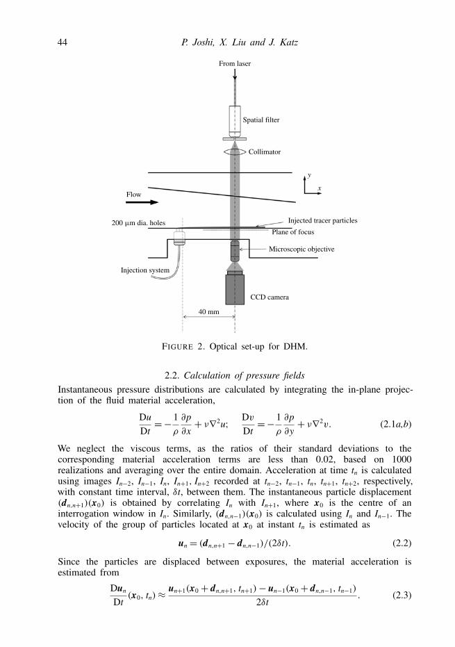
44 P. Joshi, X. Liu and J. Katz
From laser
Spatial filter
Collimator
Injected tracer particles
Plane of focus
Microscopic objective
CCD camera
40 mm
Injection system
Flow
y
x
FIGURE 2. Optical set-up for DHM.
2.2. Calculation of pressure fieldsInstantaneous pressure distributions are calculated by integrating the in-plane projec-tion of the fluid material acceleration,
DuDt=− 1
ρ
∂p∂x+ ν∇2u; Dv
Dt=− 1
ρ
∂p∂y+ ν∇2v. (2.1a,b)
We neglect the viscous terms, as the ratios of their standard deviations to thecorresponding material acceleration terms are less than 0.02, based on 1000realizations and averaging over the entire domain. Acceleration at time tn is calculatedusing images In−2, In−1, In, In+1, In+2 recorded at tn−2, tn−1, tn, tn+1, tn+2, respectively,with constant time interval, δt, between them. The instantaneous particle displacement(dn,n+1)(x0) is obtained by correlating In with In+1, where x0 is the centre of aninterrogation window in In. Similarly, (dn,n−1)(x0) is calculated using In and In−1. Thevelocity of the group of particles located at x0 at instant tn is estimated as
un = (dn,n+1 − dn,n−1)/(2δt). (2.2)
Since the particles are displaced between exposures, the material acceleration isestimated from
Dun
Dt(x0, tn)≈ un+1(x0 + dn,n+1, tn+1)− un−1(x0 + dn,n−1, tn−1)
2δt. (2.3)
Effect of pressure gradients on boundary layer turbulence 45
0.5
(a) (b)
0
–0.5
–3 –2 –1 –1.0 –0.5 0 0.5 1.00 1 2 3
0.05
0
–0.05
0.02900.02100.01300.00500.0001 PDF 0.02900.02100.01300.00500.0001
0.001
0.0001 0.0001
0.001
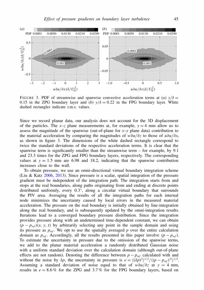
FIGURE 3. PDF of streamwise and spanwise convective acceleration terms at (a) y/δ =0.15 in the ZPG boundary layer and (b) y/δ = 0.22 in the FPG boundary layer. Whitedashed rectangles indicate r.m.s. values.
Since we record planar data, our analysis does not account for the 3D displacementof the particles. The x–z plane measurements at, for example, y= 4 mm allow us toassess the magnitude of the spanwise (out-of-plane for x–y plane data) contribution tothe material acceleration by comparing the magnitudes of w∂u/∂z to those of u∂u/∂x,as shown in figure 3. The dimensions of the white dashed rectangle correspond totwice the standard deviations of the respective acceleration terms. It is clear that thespanwise term is significantly smaller than the streamwise term – for example, by 9.1and 23.3 times for the ZPG and FPG boundary layers, respectively. The correspondingvalues at y = 1.5 mm are 6.98 and 18.2, indicating that the spanwise contributionincreases close to the wall.
To obtain pressure, we use an omni-directional virtual boundary integration scheme(Liu & Katz 2006, 2013). Since pressure is a scalar, spatial integration of the pressuregradient must be independent of the integration path. The integration starts from andstops at the real boundaries, along paths originating from and ending at discrete pointsdistributed uniformly, every 0.3◦, along a circular virtual boundary that surroundsthe PIV area. Averaging the results of all the integration paths for each internalnode minimizes the uncertainty caused by local errors in the measured materialacceleration. The pressure on the real boundary is initially obtained by line-integrationalong the real boundary, and is subsequently updated by the omni-integration results.Iterations lead to a converged boundary pressure distribution. Since the integrationprovides pressure along with an undetermined time-dependent constant, we can obtain(p − pref )(x, y, t) by arbitrarily selecting any point in the sample domain and usingits pressure as pref . We opt to use the spatially averaged p over the entire calculationdomain as pref . Accordingly, all the results presented in this paper involve (p− pref ).To estimate the uncertainty in pressure due to the omission of the spanwise terms,we add to the planar material acceleration a randomly distributed Gaussian noisewith a uniform standard deviation over the calculation domain (although out-of-planeeffects are not random). Denoting the difference between p− pref calculated with andwithout the noise by δp, the uncertainty in pressure is e= 〈(δp)2〉1/2/〈(p− pref )
′2〉1/2.Assuming a standard deviation of noise equal to that of w∂u/∂z at y = 4 mm,results in e = 8.6 % for the ZPG and 3.7 % for the FPG boundary layers, based on

46 P. Joshi, X. Liu and J. Katz
1000 realizations and averaging over the entire domain. When the noise r.m.s. isincreased to that of w∂u/∂z at y = 1.5 mm, the corresponding values of e increaseto 11.5 % and 6.8 %. These estimates agree with the impact of out-of-plane termsmeasured by Ghaemi et al. (2012). They report a correlation of 0.6 between the wallpressure measured by a transducer and that calculated from 3D acceleration, whilethe corresponding correlation for planar calculations is 0.48.
3. Results: Mean flow and turbulence statistics3.1. Mean velocity and Reynolds stresses
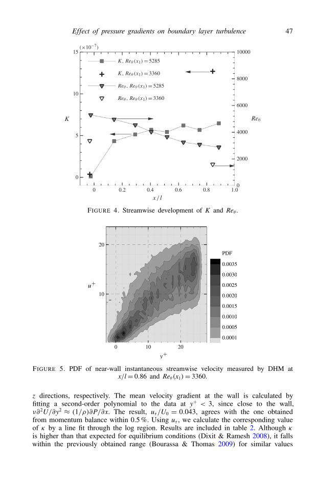
At x/l=−0.04, there is a narrow ‘freestream’ region, which is approximately 7 mmand 12 mm wide for Reθ(x1) = 3360 and 5285, respectively, between the top andbottom wall boundary layers. However, following Tsuji et al. (2012), due to theproximity between the top and bottom boundary layers, the pressure fluctuations inone might affect those in the other. Such effects are more consistent with channelflows. Due to the asymmetry in boundary conditions, ∂U/∂y in the freestream is notzero, but is very small, less than 0.3 % of ∂U/∂ymax. Hence, the boundary layer edge,where U0 is determined, is defined as the point where ∂U/∂y drops below a thresholdof 0.015 U0(x1)/h for Reθ(x1)= 5285 and 0.04 U0(x1)/h for Reθ(x1)= 3360, where his the half channel height at x1. The different thresholds reflect variations in minimaattained by ∂U/∂y. Figure 4 shows the streamwise evolution of the accelerationparameter and the Reynolds number. To calculate K, dU0/dx is obtained by linearleast-square fits to U0(x) over 0.55-0.7δ long domains centred at each x/l. For bothReynolds numbers, K is very small at x/l = −0.04, allowing us to use it as thereference ZPG site. For Reθ(x1)= 5285, the acceleration parameter rises to a plateauof ∼0.6 × 10⁻⁶ at x/l > 0.3, while for Reθ(x1) = 3360, Kx/l=0.86 = 1.3 × 10⁻⁶. Bothvalues are only 9 % higher than those based on potential flow calculations and, byconstruction, are well below the relaminarization level. For both Reynolds numbers,Reθ decreases with increasing x/l, but it does not reach the corresponding equilibriumvalues of 1600 and 840, predicted by Jones, Marusic & Perry (2001). In spite ofthe plateau in K, the sink flow is not long enough for the boundary layers to reachequilibrium.
To estimate the friction velocity from the log region data at x/l=−0.04, we assumeκ = 0.41. In the FPG region, for Reθ(x1)= 3360, we calculate uτ using two methods:by direct measurement of ∂U/∂y at the wall from the DHM data, and by performinga 2D momentum analysis,
τwlCV ={∫ 0.88δ
0
[(P− Pref )+ ρU2 + ρ〈u′2〉] dy
}
x=xU
−{∫ 0.88δ
0
[(P− Pref )+ ρU2 + ρ〈u′2〉] dy
}
x=xD
−{∫ xD
xU
[ρUV + ρ〈u′v′〉] dx
}
y=0.88δ
. (3.1)
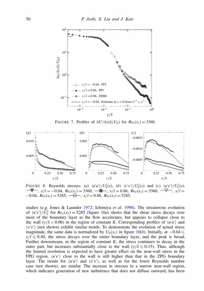
Here xU, xD are the upstream and downstream boundaries, respectively, of a controlvolume of length lCV = 0.88δ. This balance accounts for the variation of ∂P/∂xacross the boundary layer, which, as shown later, is ±12 %. Figure 5 showsthe probability distribution function (PDF) of u obtained from DHM data over avolume of 3.51 mm× 0.34 mm× 2.34 mm (293δν × 28δν × 195δν) in the x, y and
Effect of pressure gradients on boundary layer turbulence 47
15
10
5
0
01.00.80.60.40.20
2000
4000
6000
8000
10000
FIGURE 4. Streamwise development of K and Reθ .
20
10
10 20
0.0001
0.0005
0.0010
0.0015
0.0020
0.0025
0.0030
0.0035
0
FIGURE 5. PDF of near-wall instantaneous streamwise velocity measured by DHM atx/l= 0.86 and Reθ (x1)= 3360.
z directions, respectively. The mean velocity gradient at the wall is calculated byfitting a second-order polynomial to the data at y+ < 3, since close to the wall,ν∂2U/∂y2 ≈ (1/ρ)∂P/∂x. The result, uτ/U0 = 0.043, agrees with the one obtainedfrom momentum balance within 0.5 %. Using uτ , we calculate the corresponding valueof κ by a line fit through the log region. Results are included in table 2. Although κis higher than that expected for equilibrium conditions (Dixit & Ramesh 2008), it fallswithin the previously obtained range (Bourassa & Thomas 2009) for similar values

48 P. Joshi, X. Liu and J. Katz
of K without equilibrium. Since we do not have DHM data for Reθ(x1) = 5285,we estimate uτ/U0 by assuming equilibrium values of κ for the correspondingacceleration parameters, following Dixit & Ramesh (2008). As is evident from theresult for Reθ(x1) = 3360, this assumption might lead to underestimation of uτ fornon-equilibrium FPG boundary layers. Consequently, these estimates are used only forpresenting mean velocity profiles, and subsequent Reθ(x1)= 5285 data are normalizedonly by δ and U0.
A comparison between velocity profiles is presented in figure 6(a).In the log region,the ZPG profiles fall slightly above the universal law U+ = (1/0.41) ln y+ + B (B =5.3, Pope 2000), giving B = 6.1. For the Reθ(x1) = 3360 FPG boundary layer, theplot includes both DHM and PIV results. As expected, in the viscous sublayer theprofile lies below the U+= y+ curve, since ∂U/∂y decreases with increasing elevation.For both Reynolds numbers, the FPG profiles have log regions, and dip below thelog fits away from the wall, in agreement with previous studies for non-equilibriumboundary layers (e.g. Patel & Head 1968; Badri Narayanan & Ramjee 1969; Escudieret al. 1998). Streamwise variations in velocity profiles for Reθ(x1)= 5285 are shownin figure 6(b). As the flow accelerates, the profiles initially shift upward, peakingat x/l ∼ 0.4, and then reverse trend further downstream. However, the log regionsremain above that of the ZPG boundary layer. These trends may occur in part as aresult of the assumed values of κ , but are consistent with trends of Reynolds shearstresses, discussed later. Values of the wake parameter, defined as 1U+max=max{U+−[(1/κ) ln y+ + B]}, are provided in tables 1 and 2. In using the term ‘max’, werefer to the magnitude, but keep the sign of the term in the bracket. In the ZPGarea, for both Reynolds numbers, the distribution of the wake function agrees withthe classical relation 1U+=1U+max sin2(πy/2δ) (Gad-el-hak & Bandyopadhyay 1994;Pope 2000), and 1U+max falls within the expected range (Fernholz & Finley 1996).The profiles increasingly deviate from this relation with increasing x/l, where 1U+maxdecreases monotonically, becoming negative for x/l > 0.4. For a later discussion ofmean velocity gradient effects on alignment of turbulent structures, figure 7 shows∂U/∂y(δ/U0) for Reθ(x1)= 3360, assuming U+= y+ at the wall in the ZPG boundarylayer. Results for the higher Reynolds number display similar trends (not shown). Asis evident, when normalized by U0(x)/δ(x), the near-wall shear in the FPG region isonly slightly higher than that in the ZPG boundary layer (table 2). The ratio of theactual magnitudes at the wall is 2.99. The values of ∂U/∂x(δ/U0), which representsstreamwise stretching, are largely constant across the boundary layers (not shown), andare significantly higher in the FPG domain (∼0.04) than those in the ZPG boundarylayer (∼0.006).
Figure 8 compares profiles of Reynolds stresses. Trends in the ZPG domain aresimilar to those observed in previous studies (e.g. Spalart 1988; Fernholz & Finley1996). However, the profiles do not collapse when normalized either with U0 (exceptfor the outer layer 〈u′u′〉) or with uτ (results not shown). These trends might beaffected by the limited spatial resolution of measurements. As an example, figure 9compares 〈u′v′〉 obtained using the regular 740× 740 µm2 windows to that obtainedusing 740× 370 µm2 windows. Results are indistinguishable in the outer layer.However, doubling the wall-normal resolution increases 〈u′v′〉 by 6 % at y/δ∼ 0.04 inthe ZPG boundary layer. The change is significantly higher (20 %) near the wall of theFPG region, presumably since the normalized resolution there is lower. The limitedresolution affects the near-wall trends, but not those in the outer layer, consistentwith prior studies (e.g. Ligrani & Moffat 1986; Shah, Agelinchaab & Tachie 2008).
Figures 8 and 9 indicate that all the locally normalized stresses in the FPG boundarylayer are much weaker than those in ZPG conditions, in agreement with previous

Effect of pressure gradients on boundary layer turbulence 49
30(a)
(b)
30
20
20
10
010–1 100 101 102 103
102 103
FIGURE 6. Mean velocity profiles (a) in the ZPG and FPG boundary layers and (b) atdifferent streamwise locations for Reθ (x1) = 5285. In (b), , x/l = −0.04; ,x/l= 0.14; , x/l= 0.29; , x/l= 0.4; , x/l= 0.52; , x/l= 0.63;
, x/l= 0.75; , x/l= 0.88; , U+ = (1/0.41) ln y+ + 5.3. In (b), only afraction of the data points are shown to make trends discernible.
50 P. Joshi, X. Liu and J. Katz
10–3 10–2 10–1
10–1
100
101
102
100
FIGURE 7. Profiles of ∂U/∂y(δ/U0) for Reθ (x1)= 3360.
0.010
(a) (b) (c)
0.005
0 0.25 0.50 0.75
0.002
0.001
0 0.25 0.50 0.75
–0.0015
–0.0010
–0.0005
0 0.25 0.50 0.75
FIGURE 8. Reynolds stresses: (a) 〈u′u′〉/U20(x), (b) 〈v′v′〉/U2
0(x) and (c) 〈u′v′〉/U20(x).
, x/l = −0.04, Reθ (x1) = 3360; , x/l = 0.86, Reθ (x1) = 3360; , x/l =−0.04, Reθ (x1)= 5285; , x/l= 0.88, Reθ (x1)= 5285.
studies (e.g. Jones & Launder 1972; Ichimiya et al. 1998). The streamwise evolutionof 〈u′v′〉/U2
0 for Reθ(x1)= 5285 (figure 10a) shows that the shear stress decays overmost of the boundary layer as the flow accelerates, but appears to collapse close tothe wall (y/δ < 0.06) in the region of constant K. Corresponding profiles of 〈u′u′〉 and〈v′v′〉 (not shown) exhibit similar trends. To demonstrate the evolution of actual stressmagnitude, the same data is normalized by U0(x1) in figure 10(b). Initially, at −0.046x/l 6 0.40, the stress decays over the entire boundary layer, and the peak is broad.Further downstream, in the region of constant K, the stress continues to decay in theouter part, but increases substantially close to the wall (y/δ 6 0.15). Thus, althoughthe limited resolution is expected to have greater effect on the near-wall stress in theFPG region, 〈u′v′〉 close to the wall is still higher than that in the ZPG boundarylayer. The trends for 〈u′u′〉 and 〈v′v′〉, as well as for the lower Reynolds numbercase (not shown), are similar. The increase in stresses in a narrow near-wall region,which indicates generation of new turbulence that does not diffuse outward, has been

Effect of pressure gradients on boundary layer turbulence 51
0 0.25 0.50 0.75
–0.0015
–0.0005
FIGURE 9. Effect of interrogation window size on profiles of Reynolds shear stress;Reθ (x1) = 3360. , ZPG, ∆ = 32 × 32 pixels2; , ZPG, ∆ = 32 × 16 pixels2;
, FPG, ∆= 32× 32 pixels2; , FPG, ∆= 32× 16 pixels2.
0 0.5 1.0
–0.0015
(a) (b)
–0.0005
–0.0010
–0.001
0 0.1 0.2
0 0.5 1.0
–0.0015
–0.0005
–0.0010
FIGURE 10. Reynolds shear stresses for Reθ (x1) = 5285 normalized by: (a) localfreestream velocity and (b) freestream velocity at the inlet to the sink flow region. ,x/l=−0.04; , x/l= 0.14; , x/l= 0.29; , x/l= 0.4; , x/l= 0.52;
, x/l= 0.63; , x/l= 0.75; , x/l= 0.88. Only alternate data points areshown. Inset in (a) shows a magnified view of the near-wall region.
observed in several previous studies (e.g. Escudier et al. 1998; Bourassa & Thomas2009). Finally, for both Reynolds numbers, u2
τ is higher than the peak |〈u′v′〉| by lessthan 5 % at x/l = −0.04 (tables 1 and 2). Further downstream, |〈u′v′〉|max/u2
τ decaysto below 0.4 in the FPG boundary layers, consistent, for example, with Bourassa &Thomas (2009).
3.2. Statistics for pressure and pressure gradientFigure 11 presents profiles of mean pressure and pressure gradient, and compares dataobtained by integrating the instantaneous material acceleration, P, to that obtained by

52 P. Joshi, X. Liu and J. Katz
0.003
0.002
0.001
–0.001
–0.002
0 0.25 0.50 0 0.25 0.750.50
0
0.002
0
–0.05
–0.10
–0.15
0.001
–0.001
–0.002
0
0
–0.05
–0.15
–0.20
–0.10
(a) (b)
FIGURE 11. Mean pressure (left ordinate) and mean pressure gradient (right ordinate) inthe (a) ZPG and (b) FPG boundary layers for Reθ (x1)= 3360. , (∂P/∂x)(δ/ρU2
0);, (∂P/∂x)(δ/ρU2
0); , (P − Pwall)/(ρU20); , (P − Pwall)/(ρU2
0); ,−〈v′v′〉/U2
0 ; ,∫ y
0 [(1/U20)U∂V/∂x]dy; ,
∫ y0 [(1/U2
0)V∂V/∂y]dy; ,∫ y0 [(1/U2
0)∂〈u′v′〉/∂x]dy. Only alternate data points are shown.
integrating the Reynolds-averaged Navier–Stokes equation,
P(y)= Pwall − ρ〈v′v′〉(y)− ρ∫ y
0
[U∂V∂x+ V
∂V∂y+ ∂〈u
′v′〉∂x
]dy, (3.2)
where viscous terms are neglected, and Pwall is averaged over the lowest interrogationwindow (10 6 y+ 6 45 and 15 6 y+ 6 77 for the ZPG and FPG flows, respectively).In both cases, P − Pwall and P − Pwall, as well as ∂P/∂x and ∂P/∂x, follow eachother closely, but the omni-directional results are smoother, presumably since they areless sensitive to uncertainties in the small v close to the wall (0.01 pixel in the ZPG,and < 0.1 pixel in the FPG boundary layer). According to the 2D boundary layerapproximation, P−Pwall∼−ρ〈v′v′〉. However, in the present results, P−Pwall follows−ρ〈v′v′〉 closely only near the wall. In the outer layer, U∂V/∂x becomes significantin the ZPG flow, and both convective terms contribute in the FPG boundary layer. Thecontribution of the shear stress is negligible in both cases. Yet, in the FPG domain,∂P/∂y (not shown) is still an order of magnitude smaller than ∂P/∂x, except close tothe wall (y/δ < 0.08), where it increases to ∼22 % of ∂P/∂x.
Figure 12(a) shows that σ∂p/∂x = 〈(∂p′/∂x)2〉1/2 normalized by ρU20(x)/δ(x) in the
ZPG region is substantially higher than that in the FPG boundary layer, and that,in both cases, σ∂p/∂x increases rapidly with decreasing y. However, when normalizedby ρ〈u′u′〉(x,y)/δ(x), profiles of both boundary layers collapse onto each other(figure 12b), and the magnitudes increase with distance from the wall. They do notcollapse if we replace δ with δν as the normalizing length scale (not shown). Similarto the behaviour of Reynolds stresses, un-scaled σ∂p/∂x in the FPG boundary layeris higher close to the wall and lower away from the wall in comparison to that inthe ZPG region (also not shown). The profiles of σp = 〈(p′ − p′ref )
2〉1/2, shown infigures 13(a)–(c), inherently account only for fluctuations at scales smaller than ourfield of view. The rapid near-wall increase in σp for both boundary layers agrees withtrends reported by Spalart (1988) and Tsuji et al. (2007). Very near the wall, σp is
Effect of pressure gradients on boundary layer turbulence 53
0.4
(a) (b)
0.2
0 0.25 0.50 0.75 0.25 0.50 0.75
150ZPGFPG
100
50
0
FIGURE 12. R.m.s. values of: (a) (∂p/∂x)[δ(x)/ρU20(x)] and
(b) (∂p/∂x)[δ(x)/ρ〈u′u′〉(x, y)].
expected to decrease (Spalart 1988; Jiménez & Hoyas 2008). Consequently, our σpat the lowest elevation for the ZPG case, which represents a spatial average over thelowest interrogation window, is higher than published wall pressure fluctuation results(e.g. Tsuji et al. 2007). However, in figure 13(b), the present values of σp/ρu2
τ arecompared to those provided in previous studies for the log region. Our values arehigher than the DNS results of Spalart (1988) for Reθ = 1410, but fall within therange measured by Tsuji et al. (2007) for 7420 < Reθ < 15 200. The ZPG pressurefluctuations are much higher than those of the FPG boundary layer, when scaledwith ρU2
0(x) or ρu2τ (x) (figures 13a,b). Unlike the pressure gradients, the profiles do
not collapse when scaled by ρ〈u′u′〉 (figure 13c), but the difference between them isgreatly reduced. At 06 y/δ6 0.5, σp/ρ〈u′u′〉∼ 1 for the ZPG case, in agreement withTsuji et al. (2007). Spectra and PDFs of p′ − p′ref at different elevations in the ZPGboundary layer are presented in figures 13(d) and 13(e), respectively. The spectrashow a power law exponent of −1.6 in the outer layer. The wavenumber range forthis behaviour (0.016 < k1ν/uτ < 0.06) is smaller than, and roughly coincident with,that of Tsuji et al. (2007) at Reθ > 5870. Also in agreement with previous studies(e.g. Kim 1989; Tsuji et al. 2007), PDFs of p′− p′ref (figure 13e) exhibit higher peaksnear zero, and larger tails than a Gaussian distribution. The skewness and flatnessvalues are approximately −0.1 and 4, except at y/δ= 0.05, where they are −0.07 and5.6, respectively. The skewness values are lower in magnitude than the log regionvalue of −0.3 reported by Tsuji et al. (2007). However, the flatness values are closeto the value of 4.6 reported by them. The present FPG spectra and PDFs (not shown)exhibit similar trends.
4. Effect of mean FPG on instantaneous flow structuresNumerous studies have discussed the dynamics of packets of hairpin vortices
in ZPG boundary layers, which appear as inclined trains of vortices in the x–yplane. These structures migrate away from the wall by self-induction, and play adominant role in wall-normal momentum transport (Adrian, Meinhart & Tomkins2000; Hutchins, Hambleton & Marusic 2005). Figure 14(a) shows an example ofsuch a vortex train evident in the present ZPG boundary layer. Instantaneous dataalso confirms that hairpin packets often form in the FPG boundary layer, but remain

54 P. Joshi, X. Liu and J. Katz
0.015
0.010
6
4
2
0101
104
103
102
101
10–1
10–3 10–2 10–1
100
102 103
0.005
10
5
0
00.25 0.50 0.75
0.25 0.50 0.75
(a)
(c)
(b)
(d)
100
10–2
10–4
–10 0 10
10–6
(e)
FIGURE 13. R.m.s. values of: (a) (p − pref )/ρU20(x), (b) (p − pref )/ρu2
τ (x) and (c) (p −pref )/ρ〈u′u′〉(x, y). , ZPG boundary layer; , FPG boundary layer; , Spalart(1988), Reθ = 1410; , Tsuji et al. (2007), Reθ = 7420–15 200. Spectra and PDFs forp − pref at different elevations in the ZPG boundary layer are shown in (d) and (e),respectively. , y/δ = 0.05; , y/δ = 0.18; , y/δ = 0.36; ,y/δ = 0.44; , y/δ = 0.53. In (e), , Gaussian distribution.
Effect of pressure gradients on boundary layer turbulence 55
confined to the near-wall region and are inclined at shallow angles to the wall(figure 14c). Consequently, the outer layer frequently consists of extended regionsof low turbulence. The shallow inclinations are in line with previous studies (e.g.Piomelli et al. 2000; Dixit & Ramesh 2010) and, as discussed later, are predominantlycaused by the larger ∂U/∂y and ∂U/∂x relative to the vortex self-induction. Asexpected, the minima in the corresponding p′ − p′ref distributions (figures 14b, 14d)coincide with the vortical structures, while the maxima show a preference for regionsof elevated normal strain. Furthermore, p′ − p′ref decays rapidly away from the wallin the FPG boundary layer, in agreement with figure 14(c).
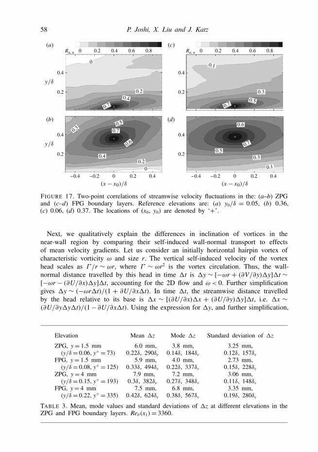
A consistent picture is observed in the x–z planes. Figure 15(a) presents a sampleof ω′y and streamlines at y/δ = 0.06 in the ZPG domain. Here, low-speed regionsseem to be bounded by ‘legs’ of large-scale vortices, which appear as swirlingstreamline patterns, as reported in previous studies (e.g. Tomkins & Adrian 2003;Ganapathisubramani, Longmire & Marusic 2003). Figure 15(b) is a characteristicsample for the FPG case, at y/δ = 0.08. It shows parallel, nearly continuous,streamwise-elongated regions with opposite sign ωz, and low-speed streaks betweenthem. This pattern suggests that the visualized plane dissects structures inclined atshallow angles. These elongated vortices are not observed at y/δ = 0.22 (not shown),consistent with the x–y plane observations. In figure 15(b), it is much harder toidentify the legs of large-scale structures, although broad regions of roughly circularstreamlines cross the sample area frequently, e.g. at 14.55 < x/δ < 15.25. In theZPG domain, small-scale structures are found everywhere, but more frequently insidelow-speed regions. Conversely, in the FPG boundary layer, they are nearly absentin high-momentum regions, as sweeps (u′ > 0, v′ < 0) force outer layer fluid withlow small-scale turbulence towards the wall. To calculate the width of the low-speedregions, 1z, u′ is filtered by 1D moving box filters of width TB = 1.5δ/U0 in time,and WB = 0.25δ along x, to obtain large-scale fluctuations, u′. The spatial filter sizeis limited by the overall extent of the measurement domain, while TB is chosen toextract large-scale motions, which are discussed in § 6.1. Boundaries of low-speedregions are defined by u′ = 0 and require u′ < −0.5σu within them, where σu is thestandard deviation of u′. Our analysis indicates that this threshold, as well as thefilter sizes, have little impact on the reported trends. The PDFs of 1z at y= 1.5 mm(figure 16) show that un-scaled 1z values for both boundary layers are similar. Sincethe ZPG site is located 10.5δ(x1) upstream of the FPG region, it is possible that someof the FPG low-speed regions are formed in the ZPG area. Mean values, modes andr.m.s. of 1z are summarized in table 3, including data for y = 4 mm. Here again,1z is not significantly different between the two flows, suggesting causality, but itincreases with increasing elevation, consistent with reported trends for ZPG flows(Tomkins & Adrian 2003; Hutchins & Marusic 2007).
5. Two-point correlations of velocity and pressure fluctuationsWe analyse two-point correlations among variables ϕ and ψ ,
Rϕ,ψ(x0, y0, x, y)= 〈ϕ′(x0, y0) ·ψ ′(x, y)〉/[σϕ(x0, y0) · σψ(x, y)], (5.1)
to further ascertain the impact of FPG on the flowstructure. Here, σϕ and σψ are thestandard deviations of ϕ and ψ , respectively, and (x0, y0) is the reference location. TheZPG results for Ru,u (figures 17a,b) show the inclined eddy structure observed beforenumerous times (e.g. Tutkun et al. 2009), and has been attributed to hairpin packets

56 P. Joshi, X. Liu and J. Katz
0.5
(a)
(b)
(c)
(d)
–9.0 –6.0 –3.0 0 3.0 6.0 9.0
0.4
0.3
0.2
0.5
–0.015
–2.8
–0.012 –0.004 0 0.004 0.012
2.8–1.4 1.40
–0.007 0.007 0.0150
0.4
0.3
0.2
0.1
0.8
0.6
0.4
0.2
14.4 14.8 15.2
0.8
0.6
0.4
0.2
14.4 14.8 15.2
0.1
–0.8 –0.6 –0.4 –0.2 0
–0.8 –0.6 –0.4 –0.2 0
FIGURE 14. Sample instantaneous distributions of (a and c) ω′zδ/U0 and vectors of (u′/U0,v′/U0); (b and d) (p′ − p′ref )/ρU2
0 . Distributions are taken in the (a and b) ZPG and(c and d) FPG boundary layers. Only alternate vectors are shown.

Effect of pressure gradients on boundary layer turbulence 57
–0.4
(a) (b)–12.0 –7.2 –2.4 0 0–4.0 –2.4 2.4 4.0–0.8 0.82.4 7.2 12.0
15.4
15.0
14.6
–0.6
–0.8
–1.0 –1.6 –1.2 –0.8–0.8 –0.6 –0.4
FIGURE 15. Sample snapshots of wall-normal vorticity and streamlines in x–z planes, for(a) ZPG boundary layer at y/δ= 0.06 (y+= 73) and (b) FPG boundary layer at y/δ= 0.08(y+ = 125).
0.020.01
0.050
0.025PDF
0
FIGURE 16. PDFs of the width of low-speed regions at y= 1.5 mm.
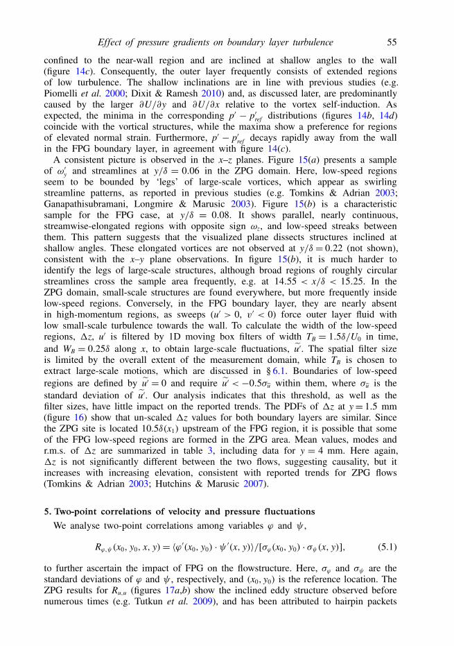
(Guala, Metzger & McKeon 2011). A similar structure in figure 17(c) suggests thatthese packets also contribute significantly to Ru,u near the wall of the FPG region.However, the inclination angle is shallower than that for the ZPG case, consistentwith the orientation of near-wall vortex trains, the reasons for which are discussedbelow. The angle increases with y0 in the ZPG domain, but decreases with increasingelevation in the FPG boundary layer. This trend is likely a result of the near-wallconfinement of the hairpin packets (figure 14c), which essentially eliminates theprimary mechanism of wall-normal momentum transport, in agreement with low outerlayer 〈u′v′〉. Furthermore, as the outer region is left with only large-scale turbulence,the correlation lengths increase more rapidly with increasing y0 in comparison to theZPG case.
58 P. Joshi, X. Liu and J. Katz
0.4
(a)
(b)
(c)
(d)
0Ru, u 0.2 0.4 0.6 0.8
0.2
0.4
0.2
0.4
0.7 0.7
0.7
0.4 0.5
0.50.2
–0.4 –0.2 0 0.2 0.4
0.4
0.2
–0.4 –0.2 0 0.2 0.4
0 0.2 0.4 0.6 0.8
0.2 0.30.3
0.6
0 0.1
0.3
0.1
0.30.5
0.6
0.7
0.40.2
0
Ru, u
FIGURE 17. Two-point correlations of streamwise velocity fluctuations in the: (a–b) ZPGand (c–d) FPG boundary layers. Reference elevations are: (a) y0/δ = 0.05, (b) 0.36,(c) 0.06, (d) 0.37. The locations of (x0, y0) are denoted by ‘+’.
Next, we qualitatively explain the differences in inclination of vortices in thenear-wall region by comparing their self-induced wall-normal transport to effectsof mean velocity gradients. Let us consider an initially horizontal hairpin vortex ofcharacteristic vorticity ω and size r. The vertical self-induced velocity of the vortexhead scales as Γ /r ∼ ωr, where Γ ∼ ωr2 is the vortex circulation. Thus, the wall-normal distance travelled by this head in time 1t is 1y∼ [−ωr + (∂V/∂y)1y]1t ∼[−ωr− (∂U/∂x)1y]1t, accounting for the 2D flow and ω< 0. Further simplificationgives 1y ∼ (−ωr1t)/(1 + ∂U/∂x1t). In time 1t, the streamwise distance travelledby the head relative to its base is 1x ∼ [(∂U/∂x)1x + (∂U/∂y)1y]1t, i.e. 1x ∼(∂U/∂y1y1t)/(1− ∂U/∂x1t). Using the expression for 1y, and further simplification,
Elevation Mean 1z Mode 1z Standard deviation of 1z
ZPG, y= 1.5 mm 6.0 mm, 3.8 mm, 3.25 mm,(y/δ = 0.06, y+ = 73) 0.22δ, 290δv 0.14δ, 184δv 0.12δ, 157δv
FPG, y= 1.5 mm 5.9 mm, 4.0 mm, 2.73 mm,(y/δ = 0.08, y+ = 125) 0.33δ, 494δv 0.22δ, 337δv 0.15δ, 228δv
ZPG, y= 4 mm 7.9 mm, 7.2 mm, 3.06 mm,(y/δ = 0.15, y+ = 193) 0.3δ, 382δv 0.27δ, 348δv 0.11δ, 148δv
FPG, y= 4 mm 7.5 mm, 6.8 mm, 3.35 mm,(y/δ = 0.22, y+ = 335) 0.42δ, 624δv 0.38δ, 567δv 0.19δ, 280δv
TABLE 3. Mean, mode values and standard deviations of 1z at different elevations in theZPG and FPG boundary layers. Reθ (x1)= 3360.

Effect of pressure gradients on boundary layer turbulence 59
the tangent of the vortex inclination angle, β, can be expressed as
tan β ≈ 1− (∂U/∂x)1t(∂U/∂y)1t
. (5.2)
Since, as will be discussed shortly, |ωr| � (∂U/∂x)1y for y/δ 6 0.2, 1t ∼−1y/ωr.Then, using 1y∼ 0.2δ we obtain,
tan β ≈[ −ωr
0.2δ(∂U/∂y)
] [1− (∂U/∂x)
(0.2δ−ωr
)]. (5.3)
In this equation, the terms in the first and second square brackets compare the effectsof ∂U/∂y and ∂U/∂x, respectively, to the vortex self-induced velocity, indicatingthat both have an impact on structure inclination. Using procedures described below,for prograde vortices (ω < 0), the mean values of |ωr| at y/δ 6 0.2 are 0.12 and0.15 in the ZPG and FPG boundary layers, respectively. Using vertically averagedvalues of ∂U/∂y for y/δ 6 0.2, one obtains (∂U/∂y)ZPG/(∂U/∂y)FPG ∼ 0.54, and(tan β)ZPG/(tan β)FPG ∼ 1.7. Thus, the shallower inclination angles in FPG boundarylayers should be expected. Experimentally, we obtain a ratio of ∼1.5, by visuallyfitting straight lines to Ru,u contours in figures 17(a) and 17(c). While progradevortices are likely the heads of hairpin structures (Adrian 2007), retrograde vortices(ω > 0) observed in proximity to prograde ones are presumed to be the signaturesof dissecting the same hairpin structures at different locations, or of vortex ring-likestructures (Natrajan, Wu & Christensen 2007). They could also result from theinteraction of prograde vortices with the wall (Panton 2001). If the analysis isrepeated based on the retrograde vortices, the values of |ωr| at y/δ 6 0.2 are 0.056and 0.061, and (tan β)ZPG/(tan β)FPG∼ 2.3. The substantially lower values of |ωr| forω > 0 in comparison to those for ω < 0, consistent with previous observations forswirling strengths (Wu & Christensen 2006), suggest that at least a fraction of theretrograde vortices is not part of hairpin structures.
To obtain ωr, following Wu et al. (2011), we identify vortex centres by the localmaxima of swirling strength (Zhou et al. 1999) within crests of |ω|. The boundary ofthe vortex is selected as the location where |ω| decreases to 1/e of its centre value,or the crest edge, if the magnitude does not fall below this threshold. Then, takingω as the spatially averaged vorticity, and r = (area/π)0.5, figure 18 shows PDFs ofωr at y/δ 6 0.2. For both positive and negative vortices, the un-scaled |ωr| in theFPG boundary layer is higher than that in the ZPG domain (figure 18a). However,when scaled by U0(x), the ZPG values are higher. The results also confirm that |ωr|�(∂U/∂x)1y (table 2).
Contours of Rp,p, shown in figure 19, are oriented almost vertically, with inclinationsthat are intermediate to those of Ru,u and Rv,v. Contours for the latter (not shown)appear to be nearly circular, similar to previously published results (e.g. Liu, Adrian& Hanratty 2001). Values of Rp,p decrease faster upstream of the reference point,especially for the near-wall y0, similar to the results of Kim (1989) and Tsuji et al.(2007). The Rp,p length scales are in general closer to those of Rv,v than those ofRu,u, consistent with the fact that Rp,v peaks (figure 20) are significantly higher thanthose of Rp,u (not shown). These observations, along with trends depicted in figure 19,suggest that like Rv,v, Rp,p is predominantly affected by characteristic boundary layervortical structures of size ∼0.1 δ. In general, the normalized Rp,p length scales in theZPG boundary layer are shorter than those in the FPG domain. The present ZPG

60 P. Joshi, X. Liu and J. Katz
0.10
0.05
FPG
ZPG
(a) (b)
0
0.10
0.05
0–0.8 0.8–0.4 0.40 –0.4 –0.2 0.40.20
FIGURE 18. PDFs of ωr for y/δ 6 0.2.
0.4
(a)
(b)
(c)
(d)
0.2
0.4
0.2
0.4
–0.2
0.6
0.2
–0.4 –0.2 0 0.2 0.4
0.4
0.2
–0.4 –0.2 0 0.2 0.4
0.30.5
0.1
0.1
0.4
0.2
0.5
0.2
0.3
0.1
–0.1
–0.1
–0.1
0.4
0.3
0.6
0.2
0
0
–0.
1
0
0
0
Rp, p 0 0.2–0.2 0.4 0.6 0.8 Rp, p 0 0.2–0.2 0.4 0.6 0.8
FIGURE 19. Two-point correlations of p′− p′ref in the (a–b) ZPG and (c–d) FPG boundarylayers. Reference elevations are: (a) y0/δ = 0.05, (b) 0.36, (c) 0.06, (d) 0.37.
length scale for Rp,p = 0 and y0/δ = 0.05, ∼0.2 δ, is smaller than previous results(∼0.5 δ) based on wall pressure (e.g. Bull 1967; Choi & Moin 1990). However, thedifferences are smaller for Rp,p = 0.5, for which the corresponding values are 0.05 δand 0.05–0.2 δ. It is likely that the present Rp,p close to the sample area edges isaffected by the spatial high-pass filtering caused by subtracting p′ref from p′.
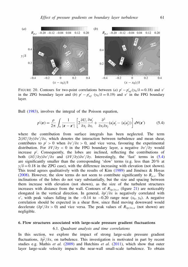
Sample distributions of Rp,v (figure 20) indicate that the peaks of p′ and v′ aredisplaced. In the ZPG boundary layer (figure 20a), the ‘lobes’ are aligned horizontally,in agreement with prior data based on wall pressure in, e.g. Panton et al. (1980) andKobashi & Ichijo (1986). A possible explanation for this trend, following Thomas &
Effect of pressure gradients on boundary layer turbulence 61
0.4
0.2
–0.4 –0.2 0 0.2 0.4
0.4
0.2
–0.4 –0.2 0 0.2 0.4
0.1
0.02
0.080.04–0.1
0.12
–0.0
8
–0.14
–0.12 –0.1
6
–0.0
4
0 0
–0.1
0.04
–0.20 –0.12 –0.04 0.04 0.12 0.20 –0.20 –0.12 –0.04 0.04 0.12 0.20(a) (b)
FIGURE 20. Contours for two-point correlations between (a) p′− p′ref (y0/δ= 0.18) and v′
in the ZPG boundary layer and (b) p′ − p′ref (y0/δ = 0.19) and v′ in the FPG boundarylayer.
Bull (1983), involves the integral of the Poisson equation,
p′(x)= ρ
2π
∫
∀
1|x− x′|
[2∂Ui
∂xj
∂u′j∂xi+ ∂2
∂xi∂xj(u′iu
′j − 〈u′iu′j〉)
]d∀(x′) (5.4)
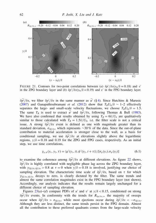
where the contribution from surface integrals has been neglected. The term2(∂U/∂y)∂v′/∂x, which denotes the interaction between turbulence and mean shear,contributes to p′ > 0 when ∂v′/∂x > 0, and vice versa, favouring the experimentaldistribution. For ∂V/∂y < 0 in the FPG boundary layer, a negative ∂v′/∂y wouldincrease p′. Consequently, the lobes are inclined, reflecting the contributions ofboth (∂U/∂y)∂v′/∂x and (∂V/∂y)∂v′/∂y. Interestingly, the ‘fast’ terms in (5.4)are significantly smaller than the corresponding ‘slow’ terms (e.g. less than 20 % aty/δ= 0.18 in the ZPG case), with the difference increasing with elevation (not shown).This trend agrees qualitatively with the results of Kim (1989) and Jiménez & Hoyas(2008). However, the slow terms do not seem to contribute significantly to Rp,v. Theinclinations of the lobes do not vary substantially, but the size and spacing betweenthem increase with elevation (not shown), as the size of the turbulent structuresincreases with distance from the wall. Contours of R∂p/∂x,v (figure 21) are noticeablyelongated in the vertical direction. In general, ∂p′/∂x is negatively correlated withv′, with peak values falling in the −0.14 to −0.20 range near (x0, y0). A negativecorrelation should be expected in a shear flow, since fluid moving downward woulddecelerate (∂p′/∂x > 0) and vice versa. The peak values of R∂p/∂x,u (not shown) arenegligible.
6. Flow structures associated with large-scale pressure gradient fluctuations6.1. Quadrant analysis and time correlations
In this section, we explore the impact of strong large-scale pressure gradientfluctuations, ∂ p′/∂x, on turbulence. This investigation is motivated in part by recentstudies e.g. Mathis et al. (2009) and Hutchins et al. (2011), which show that outerlayer large-scale velocity impacts the near-wall small-scale turbulence. To obtain
62 P. Joshi, X. Liu and J. Katz
–0.2 0 0.2
0.2
0.4
–0.06
–0.20 –0.12 –0.04 0.04 0.12 0.20 –0.20 –0.12 –0.04 0.04 0.12 0.20
–0.2 0 0.2
0.2
0.4
0
0
–0.04
–0.0
2
–0.04
–0.1
–0.06
0
(a) (b)
FIGURE 21. Contours for two-point correlations between (a) ∂p′/∂x(y0/δ = 0.18) and v′in the ZPG boundary layer and (b) ∂p′/∂x(y0/δ= 0.19) and v′ in the FPG boundary layer.
∂ p′/∂x, we filter ∂p′/∂x in the same manner as u′ (§ 4). Since Hutchins & Marusic(2007) and Ganapathisubramani et al. (2012) show that TBU0/δ ∼ 1–2 effectivelyseparates the large- and small-scale velocity fluctuations, we choose TBU0/δ = 1.5.The same TB is used to extract u′ and ∂ p′/∂x, following Thomas & Bull (1983).We have also confirmed that results obtained by using TB = 6δ/U0 are qualitativelysimilar to those calculated with TB = 1.5δ/U0, i.e. the filter scale is not a criticalissue. A strong ∂ p′/∂x event is defined as one with magnitude greater than itsstandard deviation, σ∂ p/∂x, which represents ∼30 % of the data. Since the out-of-planecontribution to material acceleration is stronger close to the wall, as a basis forconditional sampling, we use ∂ p′/∂x at elevations slightly above the logarithmicregions, y/δ = 0.18 and 0.19 for the ZPG and FPG cases, respectively. As an initialstep, we use time correlations,
γϕ,ψ(y1, y2, τ )= 〈ϕ′(y1, t).ψ ′(y2, t+ τ)〉/[σϕ(y1).σψ(y2)] (6.1)
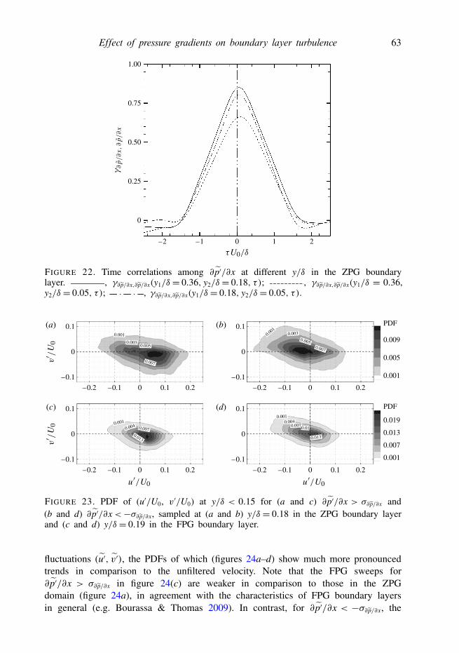
to examine the coherence among ∂ p′/∂x at different elevations. As figure 22 shows,∂ p′/∂x is highly correlated with negligible phase lag across the ZPG boundary layer,with γ∂ p/∂x,∂ p/∂x > 0.8 at τ = 0 when y/δ = 0.18 is involved, justifying our choice ofsampling elevation. The characteristic time scale of ∂ p′/∂x, based on τ for whichγ∂ p/∂x,∂ p/∂x decays to zero, is clearly dictated by the filter. The same trends andalmost the same correlation magnitudes exist in the FPG boundary layer (not shown).Accordingly, our analysis indicates that the results remain largely unchanged for adifferent choice of sampling elevation.
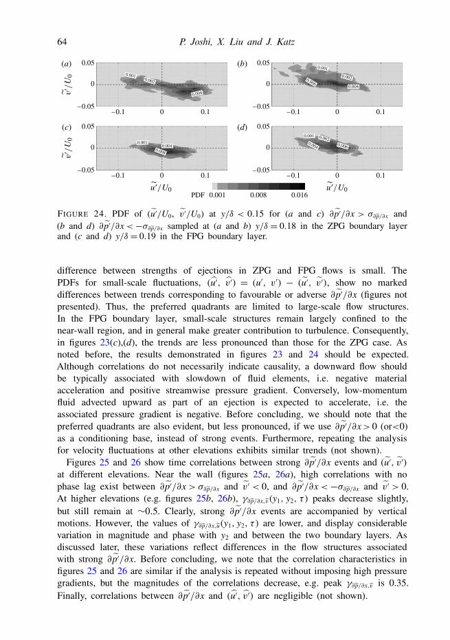
Figures 23(a)–(d) compare PDFs of u′ and v′ at y/δ < 0.15, conditioned on strong∂ p′/∂x events. In conformity with the trends for R∂p/∂x,v, the majority of sweepsoccur when ∂ p′/∂x > σ∂ p/∂x, while most ejections occur during ∂ p′/∂x < −σ∂ p/∂x.Although they are less distinct, the same trends persist in the FPG domain. Almostall the contribution to these preferred quadrants comes from the large-scale velocity
Effect of pressure gradients on boundary layer turbulence 63
1.00
0.75
0.50
0.25
0
–2 –1 20 1
FIGURE 22. Time correlations among ∂ p′/∂x at different y/δ in the ZPG boundarylayer. , γ∂ p/∂x,∂ p/∂x(y1/δ = 0.36, y2/δ = 0.18, τ ); , γ∂ p/∂x,∂ p/∂x(y1/δ = 0.36,y2/δ = 0.05, τ ); , γ∂ p/∂x,∂ p/∂x(y1/δ = 0.18, y2/δ = 0.05, τ ).
0.1(a)
0
–0.1
–0.1 0 0.1 0.2–0.2
0.1(c)
0
–0.1
–0.1 0 0.1 0.2–0.2
0.1(b)
0
–0.1
–0.1 0 0.1 0.2–0.2
0.1(d)
0
–0.1
–0.1 0 0.1 0.2
0.001
0.001
0.005
0.009
0.007
0.013
0.019
–0.2
0.001
0.0030.005
0.007
0.007
0.005
0.003
0.0070.004
0.013
0.001
0.001
0.0010.004
0.007
0.013
0.01
FIGURE 23. PDF of (u′/U0, v′/U0) at y/δ < 0.15 for (a and c) ∂ p′/∂x > σ∂ p/∂x and(b and d) ∂ p′/∂x<−σ∂ p/∂x, sampled at (a and b) y/δ = 0.18 in the ZPG boundary layerand (c and d) y/δ = 0.19 in the FPG boundary layer.
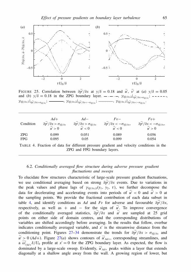
fluctuations (u′, v′), the PDFs of which (figures 24a–d) show much more pronouncedtrends in comparison to the unfiltered velocity. Note that the FPG sweeps for∂ p′/∂x > σ∂ p/∂x in figure 24(c) are weaker in comparison to those in the ZPGdomain (figure 24a), in agreement with the characteristics of FPG boundary layersin general (e.g. Bourassa & Thomas 2009). In contrast, for ∂ p′/∂x < −σ∂ p/∂x, the
64 P. Joshi, X. Liu and J. Katz
0.001PDF 0.008 0.016
0.05
–0.05
(a)
(c)
(b)
(d)
–0.1 0 0.1
0
0.05
–0.05–0.1 0 0.1
0
0.05
–0.05–0.1 0 0.1
0
0.05
–0.05–0.1 0 0.1
0
0.0010.002
0.004
0.0010.004
0.008
0.004
0.001 0.0020.006
0.004
0.002
0.001
0.006
FIGURE 24. PDF of (u′/U0, v′/U0) at y/δ < 0.15 for (a and c) ∂ p′/∂x > σ∂ p/∂x and(b and d) ∂ p′/∂x<−σ∂ p/∂x sampled at (a and b) y/δ = 0.18 in the ZPG boundary layerand (c and d) y/δ = 0.19 in the FPG boundary layer.
difference between strengths of ejections in ZPG and FPG flows is small. ThePDFs for small-scale fluctuations, (u′, v′) = (u′, v′) − (u′, v′), show no markeddifferences between trends corresponding to favourable or adverse ∂ p′/∂x (figures notpresented). Thus, the preferred quadrants are limited to large-scale flow structures.In the FPG boundary layer, small-scale structures remain largely confined to thenear-wall region, and in general make greater contribution to turbulence. Consequently,in figures 23(c),(d), the trends are less pronounced than those for the ZPG case. Asnoted before, the results demonstrated in figures 23 and 24 should be expected.Although correlations do not necessarily indicate causality, a downward flow shouldbe typically associated with slowdown of fluid elements, i.e. negative materialacceleration and positive streamwise pressure gradient. Conversely, low-momentumfluid advected upward as part of an ejection is expected to accelerate, i.e. theassociated pressure gradient is negative. Before concluding, we should note that thepreferred quadrants are also evident, but less pronounced, if we use ∂ p′/∂x> 0 (or<0)as a conditioning base, instead of strong events. Furthermore, repeating the analysisfor velocity fluctuations at other elevations exhibits similar trends (not shown).
Figures 25 and 26 show time correlations between strong ∂ p′/∂x events and (u′, v′)at different elevations. Near the wall (figures 25a, 26a), high correlations with nophase lag exist between ∂ p′/∂x> σ∂ p/∂x and v′ < 0, and ∂ p′/∂x<−σ∂ p/∂x and v′ > 0.At higher elevations (e.g. figures 25b, 26b), γ∂ p/∂x,v(y1, y2, τ ) peaks decrease slightly,but still remain at ∼0.5. Clearly, strong ∂ p′/∂x events are accompanied by verticalmotions. However, the values of γ∂ p/∂x,u(y1, y2, τ ) are lower, and display considerablevariation in magnitude and phase with y2 and between the two boundary layers. Asdiscussed later, these variations reflect differences in the flow structures associatedwith strong ∂ p′/∂x. Before concluding, we note that the correlation characteristics infigures 25 and 26 are similar if the analysis is repeated without imposing high pressuregradients, but the magnitudes of the correlations decrease, e.g. peak γ∂ p/∂x,v is 0.35.Finally, correlations between ∂ p′/∂x and (u′, v′) are negligible (not shown).
Effect of pressure gradients on boundary layer turbulence 65
0.5
0
–0.5
(a) (b)
–2 0 2 –2 0 2
0.5
0
–0.5
FIGURE 25. Correlation between ∂ p′/∂x at y/δ = 0.18 and u′, v′ at (a) y/δ = 0.05and (b) y/δ = 0.18 in the ZPG boundary layer. , γ∂ p/∂x,u|∂ p′/∂x>σ∂ p/∂x
; ,γ∂ p/∂x,v|∂ p′/∂x>σ∂ p/∂x
; , γ∂ p/∂x,u|∂ p′/∂x<−σ∂ p/∂x; , γ∂ p/∂x,v|∂ p′/∂x<−σ∂ p/∂x
.
Ad+ Ad− Fv− Fv+Condition ∂ p′/∂x>σ∂ p/∂x ∂ p′/∂x>σ∂ p/∂x ∂ p′/∂x<−σ∂ p/∂x, ∂ p′/∂x<−σ∂ p/∂x,
u′ > 0 u′ < 0 u′ < 0 u′ > 0
ZPG 0.099 0.051 0.089 0.056FPG 0.095 0.05 0.099 0.054
TABLE 4. Fraction of data for different pressure gradient and velocity conditions in theZPG and FPG boundary layers.
6.2. Conditionally averaged flow structure during adverse pressure gradientfluctuations and sweeps
To elucidate flow structures characteristic of large-scale pressure gradient fluctuations,we use conditional averaging based on strong ∂ p′/∂x events. Due to variations inthe peak values and phase lags of γ∂ p/∂x,u(y1, y2, τ ), we further decompose thedata for decelerating and accelerating events into periods of u′ < 0 and u′ > 0 atthe sampling points. We provide the fractional contribution of each data subset intable 4, and identify conditions as Ad and Fv for adverse and favourable ∂ p′/∂x,respectively, as well as + and − for the sign of u′. To improve convergenceof the conditionally averaged statistics, ∂ p′/∂x and u′ are sampled at 25 gridpoints on either side of domain centres, and the corresponding distributions ofvariables are shifted accordingly before averaging. In the results that follow, overbarindicates conditionally averaged variable, and x′ is the streamwise distance from theconditioning point. Figures 27–34 demonstrate the trends for ∂ p′/∂x > σ∂ p/∂x andu′ > 0 (Ad+). Figure 27(a) shows contours of u′Ad+, corresponding streamlines, anda ω′zAd+δ/U0 profile at x′ = 0 for the ZPG boundary layer. As expected, the flow isdominated by a large-scale sweep. Evidently, u′Ad+ peaks within a layer that extendsdiagonally at a shallow angle away from the wall. A growing region of lower, but

66 P. Joshi, X. Liu and J. Katz
0.5
0
–0.5
(a) (b)
–2 0 2 –2 0 2
0.5
0
–0.5
FIGURE 26. Correlation between ∂ p′/∂x at y/δ = 0.19 and u′, v′ at (a) y/δ = 0.06and (b) y/δ = 0.19 in the FPG boundary layer. , γ∂ p/∂x,u|∂ p′/∂x>σ∂ p/∂x
; ,γ∂ p/∂x,v|∂ p′/∂x>σ∂ p/∂x
; , γ∂ p/∂x,u|∂ p′/∂x<−σ∂ p/∂x; , γ∂ p/∂x,v|∂ p′/∂x<−σ∂ p/∂x
.
still positive, u′Ad+ develops below this layer, where ∂u′/∂xAd+ < 0. Close to thewall, ω′zAd+ becomes positive, presumably due to secondary interaction of the shearlayer underneath the peak u′Ad+ with the wall. Consistent features appear in thecorresponding sample instantaneous velocity and vorticity distributions (figure 27b),where very few vortices appear away from the wall, presumably since the sweepingflow suppresses the outward migration of structures. Figure 27(c) shows the ∂w′/∂zAd+profile at x′ = 0, calculated using the continuity equation. Its magnitude is negligibleat y/δ > 0.075, but becomes positive close to the wall. Thus, as shown in the y–zplane schematic (figure 27c, inset), the conditional mean flow is largely 2D in theouter region, but involves near-wall spanwise stretching as the fluid rushing towardsthe wall decelerates and migrates out of the x–y plane. Examination of the datashows that the instantaneous large-scale flow is also more 2D in the outer layer. Forexample, the mean and r.m.s. of (∂w′/∂z)Ad+(δ/U0) at y/δ > 0.2 are ∼0 and ∼0.15,respectively, while the corresponding values at y/δ∼ 0.03 are 0.4 and 0.55. Note thatflow symmetry in the schematic is only for illustration.
To examine motions at scales larger than ∼δ, we invoke Taylor’s hypothesis andstudy the evolution of variables in time at the sampling location, with conditionsimposed at t = 0. Figure 28(a) shows ∂ p′/∂xAd+ contours and ∂w′/∂zAd+ profiles,
while u′Ad+ contours and associated streamlines are presented in figure 28(b). Thegeneral features of unfiltered velocity, i.e. u′Ad+, and pressure gradient fluctuationsare similar, but noisier, as demonstrated in figure 28(c), indicating that the observedphenomena persist whether we filter the sampled data or not. Caution should beexercised while interpreting these plots, since the advection velocity varies withelevation, and the y axis is stretched relative to U0t. To assist in interpreting theobserved phenomena, figure 29 shows a schematic of the structure inferred from∂w′/∂zAd+ and in-plane velocity. Several trends are clearly evident. First, the featuresaround t = 0 are consistent with the spatial structures depicted in figure 27. Second,the scales of the educed pressure gradient field are consistent with the filter scale and,in agreement with figure 22, values of ∂ p′/∂x at all elevations are in phase. Their

Effect of pressure gradients on boundary layer turbulence 67
0.5
(a)
(b)
(c) 0.6
0 0.015
–0.5 0 0.5
0.035 0.055
0.4
0.2
–0.4 0 0.4 0.80
0.4
0.3
0.2
0.1
–0.4 –0.2 0 0.2 0.4
0.5
0.4
0.3
0.2
0.1
–0.4 –0.2 0 0.2 0.4
0.2
yz
0.1
0.015
0.025
0.0250.035
0.065 0.035
0.0450.055
FIGURE 27. Conditionally sampled flow structure in the ZPG boundary layer for ∂ p′/∂x>σ∂ p/∂x and u′ > 0 (Ad+): (a) contours of u′Ad+/U0, streamlines and ω′zAd+(δ/U0) profileat x′/δ = 0; (b) sample snapshot of ω′zδ/U0 and (u′/U0, v′/U0) vectors; (c) profile of∂w′/∂zAd+(δ/U0) at x′/δ= 0, with the inset showing the inferred flow structure in the y–zplane. In (b), only alternate vectors are shown; dark grey contours, ω′zδ/U0 < −2; lightgrey contours, ω′zδ/U0 > 2; contour lines, −11, −8, −5, −2, 2, 5, 8, 11.
magnitudes, however, decrease with increasing y, in agreement with the LES resultsof Kim (1983). Third, a broad inclined region of sweeping flow coincides with thatof ∂ p′/∂x > σ∂ p/∂x. This domain is preceded in time by an ejection and ∂ p′/∂x < 0,which appear ‘downstream’ of the sampling point. This ejection region expands with‘distance’ from its origin near the wall. Slightly downstream of the sweep–ejectiontransition, at tU0/δ∼−1.1, the near-wall ∂w′/∂zAd+ changes from positive to negative,i.e. the flow changes from splatting to anti-splatting.
The results in figures 27–29 indicate that as the outer layer, high-momentumfluid approaches the wall, it loses momentum. Near the wall, around t = 0,
∂ u′/∂tAd+> 0 (figure 28b). Of all the convective terms, the dominant one, ˜v′∂U/∂yAd+is approximately equal to −∂ u′/∂tAd+, and the adverse pressure gradient is balanced
by ˜u′∂u′/∂xAd+ < 0, consistent with figure 27(a). Eventually u′Ad+ becomes negative,and ejection starts as part of a phenomenon resembling flow separation. Note that,
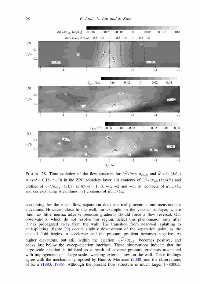
68 P. Joshi, X. Liu and J. Katz
6
–0.003 –0.003
–0.030.
009
0.012
0
00.4
(a)
(b)
(c)
0.2
–0.5
–0.06 –0.04 –0.02 0.02 0.04 0.060
–0.04 –0.02 0 0.02 0.04
–0.50.5 0 –0.50.5 0.50
–0.018 –0.012 0.0060–0.006 0.012 0.018
4 2 0 –2 –4 –6
6
0.4
0.2
4 2 0 –2 –4 –6
6
0.4
0.2
4 2 0 –2 –4 –6
0
0.01 0.04
0.02
0
–0.01
–0.02–0.04
00
0.01
0.02
0.04
0.02
0
FIGURE 28. Time evolution of the flow structure for ∂ p′/∂x > σ∂ p/∂x and u′ > 0 (Ad+)
at (y/δ = 0.18, t= 0) in the ZPG boundary layer: (a) contours of ∂ p′/∂xAd+(δ/ρU20) and
profiles of ∂w′/∂zAd+(δ/U0) at tU0/δ = 1, 0, −1, −2 and −3; (b) contours of u′Ad+/U0
and corresponding streamlines; (c) contours of u′Ad+/U0.
accounting for the mean flow, separation does not really occur at our measurementelevations. However, close to the wall, for example, in the viscous sublayer, wherefluid has little inertia, adverse pressure gradients should force a flow reversal. Ourobservations, which do not resolve this region, detect this phenomenon only afterit has propagated away from the wall. The transition from near-wall splatting toanti-splatting (figure 29) occurs slightly downstream of the separation point, as theejected fluid begins to accelerate and the pressure gradient becomes negative. Athigher elevations, but still within the ejection, ∂w′/∂zAd+ becomes positive, andpeaks just below the sweep–ejection interface. These observations indicate that thelarge-scale ejection is initiated as a result of adverse pressure gradients associatedwith impingement of a large-scale sweeping external flow on the wall. These findingsagree with the mechanism proposed by Hunt & Morrison (2000) and the observationsof Kim (1983, 1985). Although the present flow structure is much larger (∼8000δν
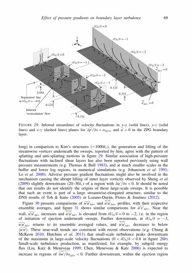
Effect of pressure gradients on boundary layer turbulence 69
Inferred‘recirculation’ flow
xz
y
FIGURE 29. Inferred streamlines of velocity fluctuations in x–y (solid lines), y–z (solidlines) and x–z (dashed lines) planes for ∂ p′/∂x> σ∂ p/∂x and u′ > 0 in the ZPG boundarylayer.
long) in comparison to Kim’s structures (∼1000δν), the generation and lifting of thestreamwise vortices underneath the sweeps, reported by him, agree with the pattern ofsplatting and anti-splatting motions in figure 29. Similar association of high-pressurefluctuations with inclined shear layers has also been reported previously using wallpressure measurements (e.g. Thomas & Bull 1983), and at much smaller scales in thebuffer and lower log regions, in numerical simulations (e.g. Johansson et al. 1991;Lo et al. 2000). Adverse pressure gradient fluctuations might also be involved in themechanism causing the abrupt lifting of inner layer vorticity observed by Sheng et al.(2009) slightly downstream (20–30δν) of a region with ∂u′/∂x< 0. It should be notedthat our results do not identify the origins of these large-scale sweeps. It is possiblethat such an event is part of a large streamwise-elongated structure, similar to theDNS results of Toh & Itano (2005) or Lozano-Durán, Flores & Jiménez (2012).
Figure 30 presents comparisons of u′u′Ad+ and u′u′Ad+ profiles, with their respectiveensemble averages, and figure 31 shows similar comparisons for u′v′Ad+. Near thewall, u′u′Ad+ increases and u′u′Ad+ is elevated from tU0/δ= 0 to −2, i.e. in the regionof initiation of ejection underneath sweeps. Further downstream, at tU0/δ = −3,u′u′Ad+ returns to its ensemble averaged values, and u′u′Ad+ decreases to below〈u′u′〉. These near-wall trends are consistent with recent observations (e.g. Chung &McKeon 2010; Hutchins et al. 2011) that small-scale turbulence peaks downstreamof the maximum in large-scale velocity fluctuations (0 < tU0/δ < 0.8 in figure 28b).Small-scale turbulence production, as manifested, for example, by subgrid energyflux (Liu, Katz & Meneveau 1999; Chen, Meneveau & Katz 2006) is expected toincrease in regions of ∂ u′/∂xAd+ < 0. Further downstream, within the ejection region

70 P. Joshi, X. Liu and J. Katz
0.4
(a) (b) (c)
0.2
0 10–2 10–2 10–2
0.4
0.2
0
0.4
0.2
0
FIGURE 30. Comparisons of the conditionally averaged streamwise velocity fluctuations,u′u′Ad+/U2
0 ( ), and their small-scale part, u′u′Ad+/U20 ( ), to their ensemble
averaged values, 〈u′u′〉/U20 ( ) and 〈u′u′〉/U2
0 ( ), respectively, at(a) tU0/δ = 0, (b) −2 and (c) −3 in the ZPG boundary layer.
0.4
(a) (b) (c)
0.2
0
0.4
0.2
0
0.4
0.2
0 –0.001 –0.002–0.001 –0.002–0.001 –0.002
FIGURE 31. Comparison between profiles of u′v′Ad+/U20 ( ) and 〈u′v′〉/U2
0 ( )at (a) tU0/δ = 0, (b) −2 and (c) −3 in the ZPG boundary layer.
(e.g. tU0/δ = −3), u′u′Ad+ decreases, presumably since ∂ u′/∂xAd+ > 0 suppressessmall-scale turbulence production. As for u′v′Ad+ (figure 31), at tU0/δ = 0, the broadsweeping flow imposes a nearly uniform wall-normal momentum flux all the way tothe lowest elevation, where it exceeds 〈u′v′〉. Further downstream, at tU0/δ=−2 and−3, u′v′Ad+ peaks within the growing ejection region.
Spatial contours of u′Ad+ and profiles of ω′zAd+ and ∂w′/∂zAd+ in the FPG boundarylayer are presented in figure 32. Corresponding instantaneous distributions are similarto those of the ZPG case (not shown). The broad sweeping region, as well as
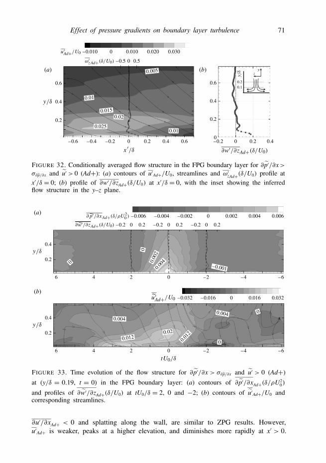
Effect of pressure gradients on boundary layer turbulence 71
0.6
(a) (b)
–0.5
–0.010 0 0.010 0.020 0.030
0.50
0.4
0.6
0.2
–0.2 0 0.2 0.40
0.4
0.2
–0.4 –0.2 0 0.2 0.4 0.6–0.6
0.2
yz
0.1
0.025
0.015
0.005
0.01
0.02
0.01
FIGURE 32. Conditionally averaged flow structure in the FPG boundary layer for ∂ p′/∂x>σ∂ p/∂x and u′ > 0 (Ad+): (a) contours of u′Ad+/U0, streamlines and ω′zAd+(δ/U0) profile atx′/δ = 0; (b) profile of ∂w′/∂zAd+(δ/U0) at x′/δ = 0, with the inset showing the inferredflow structure in the y–z plane.
0.4
(a)
(b)
0.2
6 4 2
–0.2
–0.032 –0.016 0 0.016 0.032
–0.006 –0.004 –0.002 0.002 0.004 0.0060
0 0.2 –0.2 0 0.2 –0.2 0 0.2
0 –2 –4 –6
0.4
0.2
6 4 2 0 –2 –4 –6
0.00
20.0
04 –0.001
0
0.0040.004
0.012
0.012
0.02
0
0
0
FIGURE 33. Time evolution of the flow structure for ∂ p′/∂x > σ∂ p/∂x and u′ > 0 (Ad+)
at (y/δ = 0.19, t = 0) in the FPG boundary layer: (a) contours of ∂ p′/∂xAd+(δ/ρU20)
and profiles of ∂w′/∂zAd+(δ/U0) at tU0/δ = 2, 0 and −2; (b) contours of u′Ad+/U0 andcorresponding streamlines.
∂u′/∂xAd+ < 0 and splatting along the wall, are similar to ZPG results. However,u′Ad+ is weaker, peaks at a higher elevation, and diminishes more rapidly at x′ > 0.
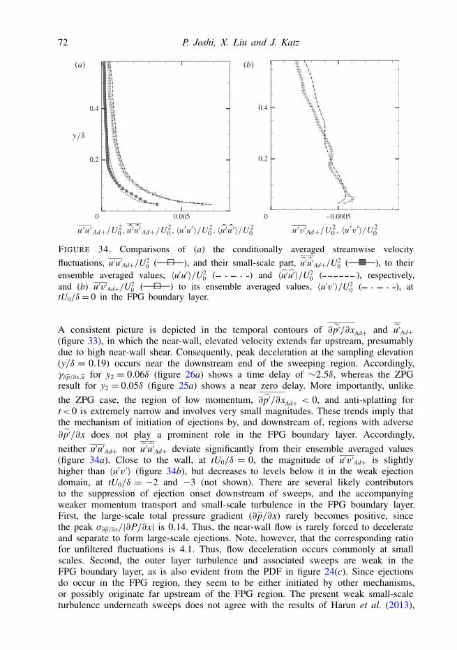
72 P. Joshi, X. Liu and J. Katz
0.4
(a) (b)
0.2
0.4
0.2
0.005 –0.00050 0
FIGURE 34. Comparisons of (a) the conditionally averaged streamwise velocityfluctuations, u′u′Ad+/U2
0 ( ), and their small-scale part, u′u′Ad+/U20 ( ), to their
ensemble averaged values, 〈u′u′〉/U20 ( ) and 〈u′u′〉/U2
0 ( ), respectively,and (b) u′v′Ad+/U2
0 ( ) to its ensemble averaged values, 〈u′v′〉/U20 ( ), at
tU0/δ = 0 in the FPG boundary layer.
A consistent picture is depicted in the temporal contours of ∂ p′/∂xAd+ and u′Ad+(figure 33), in which the near-wall, elevated velocity extends far upstream, presumablydue to high near-wall shear. Consequently, peak deceleration at the sampling elevation(y/δ = 0.19) occurs near the downstream end of the sweeping region. Accordingly,γ∂ p/∂x,u for y2 = 0.06δ (figure 26a) shows a time delay of ∼2.5δ, whereas the ZPGresult for y2 = 0.05δ (figure 25a) shows a near zero delay. More importantly, unlikethe ZPG case, the region of low momentum, ∂ p′/∂xAd+ < 0, and anti-splatting fort< 0 is extremely narrow and involves very small magnitudes. These trends imply thatthe mechanism of initiation of ejections by, and downstream of, regions with adverse∂ p′/∂x does not play a prominent role in the FPG boundary layer. Accordingly,neither u′u′Ad+ nor u′u′Ad+ deviate significantly from their ensemble averaged values(figure 34a). Close to the wall, at tU0/δ = 0, the magnitude of u′v′Ad+ is slightlyhigher than 〈u′v′〉 (figure 34b), but decreases to levels below it in the weak ejectiondomain, at tU0/δ = −2 and −3 (not shown). There are several likely contributorsto the suppression of ejection onset downstream of sweeps, and the accompanyingweaker momentum transport and small-scale turbulence in the FPG boundary layer.First, the large-scale total pressure gradient (∂ p/∂x) rarely becomes positive, sincethe peak σ∂ p/∂x/|∂P/∂x| is 0.14. Thus, the near-wall flow is rarely forced to decelerateand separate to form large-scale ejections. Note, however, that the corresponding ratiofor unfiltered fluctuations is 4.1. Thus, flow deceleration occurs commonly at smallscales. Second, the outer layer turbulence and associated sweeps are weak in theFPG boundary layer, as is also evident from the PDF in figure 24(c). Since ejectionsdo occur in the FPG region, they seem to be either initiated by other mechanisms,or possibly originate far upstream of the FPG region. The present weak small-scaleturbulence underneath sweeps does not agree with the results of Harun et al. (2013),

Effect of pressure gradients on boundary layer turbulence 73
0.5
(a)
(b)
(c) 0.6
0.4
0.2
–0.8 –0.4 0 0.40
0.4
0.3
0.2
0.1
–0.4 –0.2 0 0.2 0.4
0.5
0.4
0.3
0.2
0.1
–0.4 –0.2 0 0.2 0.4
0.2
yz
0.1
–0.035
–0.035
–0.055
–0.055
–0.045
–0.045
0–0.015–0.035–0.055
FIGURE 35. Conditionally sampled flow structure in the ZPG boundary layer for ∂ p′/∂x<−σ∂ p/∂x and u′ < 0 (Fv−): (a) contours of u′Fv−/U0 and streamlines; (b) sample snapshotof ω′zδ/U0 and (u′/U0, v′/U0) vectors; (c) profile of ∂w′/∂zFv−(δ/U0) at x′/δ= 0, with theinset showing the inferred flow structure in the y–z plane. In (b), only alternative vectorsare shown; dark grey contours, ω′zδ/U0 < −2; light grey contours, ω′zδ/U0 > 2; contourlines, −11, −8, −5, −2, 2, 5, 8, 11.
presumably since their K is very small (∼0.08× 10⁻⁶), allowing near-wall ∂ p/∂x tobecome positive more often.
6.3. Conditionally averaged flow structure during FPG fluctuations and ejections
Results for ∂ p′/∂x<−σ∂ p/∂x and u′ < 0 (Fv−) events are presented in figures 35–40.As expected, the spatial u′Fv− contours and corresponding streamlines in the ZPGboundary layer (figure 35a) show a large-scale ejection. In contrast to the effects ofmean FPG, which suppresses the wall-normal transport of coherent structures, thesample snapshot (figure 35b) displays trains of vortices propagating away from thewall, transporting small-scale turbulence into the outer layer. As is evident from the∂w′/∂zFv− profile (figure 35c), and consistent with trends shown in figure 29, ejectionsinvolve near-wall anti splatting, but the conditionally averaged (and the instantaneous)flow becomes more two-dimensional in the outer layer. The temporal contours of∂ p′/∂xFv− and u′Fv− (figures 36a, 36b) show that the ∂ p′/∂xFv−< 0 region spans ∼6 δ,and that the fluctuations peak at the wall. Upstream of this region, around tU0/δ∼ 4,
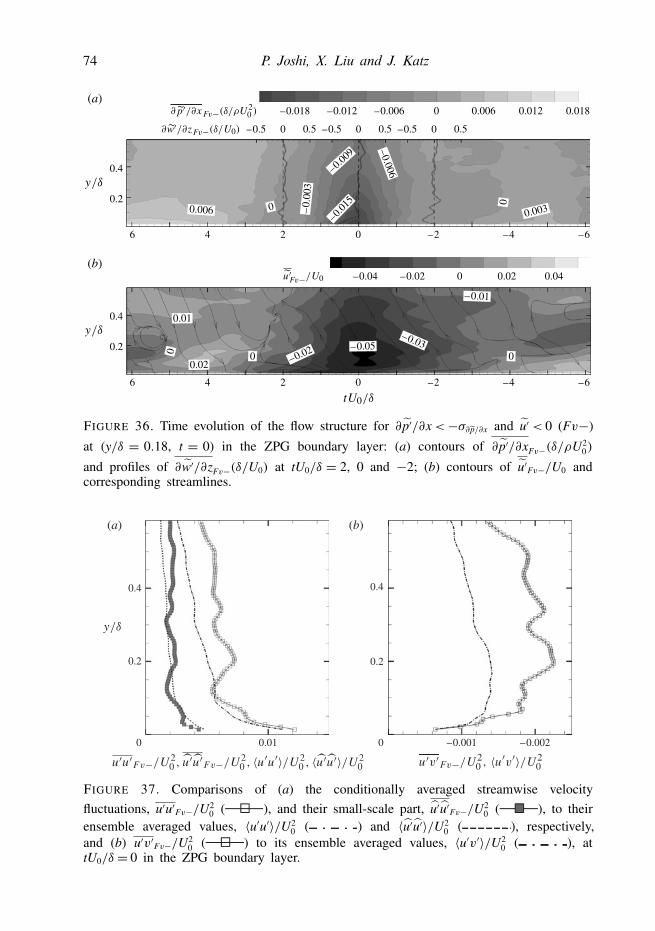
74 P. Joshi, X. Liu and J. Katz
0.4
(a)
(b)
0.2
6 4 2
–0.5
–0.04 –0.02 0 0.02 0.04
–0.018 –0.012 –0.006 0.006 0.012 0.0180
0 0.5 –0.5 0 0.5 –0.5 0 0.5
0 –2 –4 –6
0.4
0.2
6 4 2 0 –2 –4 –6
0.0030.006
–0.015
–0.006–0.009
–0.
003
0 0
–0.01
–0.03–0.05
0.02
0.01
–0.02 000
FIGURE 36. Time evolution of the flow structure for ∂ p′/∂x<−σ∂ p/∂x and u′ < 0 (Fv−)
at (y/δ = 0.18, t = 0) in the ZPG boundary layer: (a) contours of ∂ p′/∂xFv−(δ/ρU20)
and profiles of ∂w′/∂zFv−(δ/U0) at tU0/δ = 2, 0 and −2; (b) contours of u′Fv−/U0 andcorresponding streamlines.
0.4
(a) (b)
0.2
0.4
0.2
0.01 –0.002–0.0010 0
FIGURE 37. Comparisons of (a) the conditionally averaged streamwise velocityfluctuations, u′u′Fv−/U2
0 ( ), and their small-scale part, u′u′Fv−/U20 ( ), to their
ensemble averaged values, 〈u′u′〉/U20 ( ) and 〈u′u′〉/U2
0 ( ), respectively,and (b) u′v′Fv−/U2
0 ( ) to its ensemble averaged values, 〈u′v′〉/U20 ( ), at
tU0/δ = 0 in the ZPG boundary layer.
Effect of pressure gradients on boundary layer turbulence 75
0.6
(a) (b)
0.4
0.6
0.2
–0.4 –0.2 0 0.20
0.4
0.2
–0.4 –0.2 0 0.2 0.4 0.6–0.6
0.2
yz
0.1
–0.04
–0.01–0.01
–0.025
–0.015
–0.005
–0.045 –0.035 –0.025 –0.015 –0.005
–0.02
–0.02
FIGURE 38. Conditionally averaged flow structure in the FPG boundary layer for ∂ p′/∂x<−σ∂ p/∂x and u′ < 0 (Fv−): (a) contours of u′Fv−/U0 and streamlines; (b) profile of∂w′/∂zFv−(δ/U0) at x′/δ = 0, with the inset showing the inferred flow structure in they–z plane.
0.4
(a)
(b)
0.2
6 4 2
–0.2
–0.032 –0.016 0 0.016 0.032
–0.006 –0.004 –0.002 0.002 0.004 0.0060
0 0.2 –0.2 0 0.2 –0.2 0 0.2
0 –2 –4 –6
0.4
0.2
6 4 2 0 –2 –4 –6
–0.0
02
–0.004
–0.001
0
0
–0.004
–0.016 –0.024
–0.008
–0.004
–0.008
FIGURE 39. Time evolution of the flow structure for ∂ p′/∂x<−σ∂ p/∂x and u′ < 0 (Fv−)
at (y/δ = 0.19, t = 0) in the FPG boundary layer: (a) contours of ∂ p′/∂xFv−(δ/ρU20)
and profiles of ∂w′/∂zFv−(δ/U0) at tU0/δ = 2, 0 and −2; (b) contours of u′Fv−/U0 andcorresponding streamlines.
there is a weak, but clear, signature of a sweeping flow with ∂ p′/∂xFv−> 0, indicatingthat at least some of the ejections are preceded by large-scale sweeps, consistent withresults in § 6.2. However, the sweep–ejection interface is not as distinct, and does

76 P. Joshi, X. Liu and J. Katz
0.4
(a) (b)
0.2
0.4
0.2
0.005 –0.0010–0.00050 0
FIGURE 40. Comparisons of (a) the conditionally averaged streamwise velocity fluctua-tions, u′u′Fv−/U2
0 ( ), and their small-scale part, u′u′Fv−/U20 ( ), to their
ensemble averaged values, 〈u′u′〉/U20 ( ) and 〈u′u′〉/U2
0 ( ), respectively, and(b) u′v′Fv−/U2
0 ( ) to its ensemble averaged values, 〈u′v′〉/U20 ( ), at tU0/δ=0
in the FPG boundary layer.
not have the previously shown low inclination angle. This difference might be aconditional sampling artefact or, more likely, occurs because not all ejections arepreceded by sweeps, as is indeed revealed by instantaneous data. Sample profiles ofu′u′Fv−, u′u′Fv− and u′v′Fv− at t= 0 (figure 37) show that u′u′Fv− is close to 〈u′u′〉 nearthe wall, but is significantly higher in the outer region. On the other hand, u′u′Fv− isslightly lower than 〈u′u′〉 near the wall, and slightly higher away from the wall. Thelatter trends are consistent with those reported in, for example, Hutchins et al. (2011).The differences between u′u′Fv−, and u′u′Fv− indicate that the increase in outer layerturbulence during ejections is mostly associated with large-scale motions. Except forvery close to the wall, the wall-normal momentum transport (figure 37b) during Fv−events is much higher than 〈u′v′〉, consistent with figure 31.
Some of the trends for Fv− events in the FPG boundary layer (figures 38–40)are consistent with ZPG results, e.g. the near-wall anti-splatting (figure 38b), as wellas high u′u′Fv− and u′v′Fv− relative to their ensemble averaged values (figures 40a,40b). There are, however, obvious differences. First, near the wall, ejection extends farupstream (∼4δ) of t= 0 and the peak in favourable ∂ p′/∂xFv− (figure 39), consistent
with γ∂ p/∂x,u (figure 26a). Thus, the ∂ p′/∂xFv− < 0 peak occurs well after the ejectionis initiated, i.e. the pressure field is not the cause of the ejection, but might be anoutcome of it. Second, the FPG ejections decay rapidly away from the wall, and arequite weak at y/δ > 0.3. Third, in agreement with quadrant analysis, the strength ofejections is much greater than that of sweeps (figures 33b, 39b). Finally, there is nosign of any sweep upstream of the ejection, which also agrees with instantaneousmovies. As the samples in figures 14(c) and 15(b) show, the streamwise-elongatedejections are directly associated with very long, nearly horizontal trains of vortices,
Effect of pressure gradients on boundary layer turbulence 77
0.4
(a)
(b)
0.2
6 4 2
–0.5
–0.04 –0.02 0 0.02 0.04
–0.018 –0.012 –0.006 0.006 0.012 0.0180
0 0.5 –0.5 0 0.5 –0.5 0 0.5
0 –2 –4 –6
0.4
0.2
6 4 2 0 –2 –4 –6
0.006 0.0030.003 0.
012–0.003
0 0
–0.01
–0.04–0.01
0.01
–0.020
0
–0.003
0.2
yz
0.1
FIGURE 41. Time evolution of the flow structure for ∂ p′/∂x > σ∂ p/∂x and u′ < 0 (Ad−)
at (y/δ = 0.18, t= 0) in the ZPG boundary layer: (a) contours of ∂ p′/∂xAd−(δ/ρU20) and
profiles of ∂w′/∂zAd−(δ/U0) at tU0/δ = 2, 0 and −2, with the inset showing the inferred
flow structure in the y–z plane at t = 0; (b) contours of u′Ad−/U0 and correspondingstreamlines.
which frequently extend axially beyond our field of view, and rarely appear to belinked to sweeping events immediately upstream. As discussed before, ejections arelikely to be initiated in the FPG boundary layer by mechanisms other than thoseinvolving sweeps and adverse ∂ p′/∂x. It is also possible that many of the ejectionsoriginate far upstream, and then sustain themselves, e.g. through autogeneration (Zhou,Adrian & Balachandar 1996; Zhou et al. 1999) for a long distance. Such a possibilityis also suggested by similar un-scaled widths of the low-speed regions in the ZPGand FPG domains, as discussed in § 4.
6.4. Conditionally averaged flow structure for the infrequent Ad− and Fv+ eventsResults for the less likely events, Ad− and Fv+, are briefly summarized in figures 41and 42, respectively. We do not show spatially averaged contours since they areconsistent with temporal averages. In the ZPG boundary layer, ∂ p′/∂xAd− (figure 41a)
is significantly weaker than ∂ p′/∂xAd+ (figure 28a). The u′Ad− contours for t > 0 are
similar to those of u′Ad+ for t< 0 (figure 28b), with the sweep–ejection transition andproper signs of ∂ p′/∂x. However, around t = 0, growth of the ejection region seemsto be suppressed by ∂ p′/∂x > 0. Below the ejection peak, v′Ad− < 0, ∂u′/∂xAd− < 0
(not shown) and ∂w′/∂zAd− > 0, as expected for ∂ p′/∂x> 0. Further away from wall,
∂w′/∂zAd− changes sign twice, indicating spanwise contraction between extension

78 P. Joshi, X. Liu and J. Katz
0.4
(a)
(b)
0.2
6 4 2
–0.5
–0.04 –0.02 0 0.02 0.04
0 0.5 –0.5 0 0.5 –0.5 0 0.5
0 –2 –4 –6
0.4
0.2
6 4 2 0 –2 –4 –6
0.003
–0.0
03
–0.00
6 –0.009
–0.01
8
0
0
–0.01
–0.01
–0.01
–0.010.03
0.01
00
0.2
yz
0.1
–0.018–0.024 –0.012 –0.006 0.006 0.012 0.0180
0
0.02
FIGURE 42. Time evolution of the flow structure for ∂ p′/∂x<−σ∂ p/∂x and u′ > 0 (Fv+)
at (y/δ = 0.18, t= 0) in the ZPG boundary layer: (a) contours of ∂ p′/∂xFv+(δ/ρU20) and
profiles of ∂w′/∂zFv+(δ/U0) at tU0/δ = 2, 0 and −2, with the inset showing the inferred
flow structure in the y–z plane at t = 0; (b) contours of u′Fv+/U0 and correspondingstreamlines.
domains (figure 41a, inset). The results for the FPG case (not presented) are similararound t = 0, but, as expected, the ejection is not preceded by a sweep. Figure 42shows that peak ∂ p′/∂xFv+ in the ZPG boundary layer is markedly stronger than that
of ∂ p′/∂xFv−. Around t = 0, the narrow ejection region at y/δ < 0.1 seems to beconfined under a sweep. The flow structure away from t = 0 is quite complex anddoes not lend itself to a straightforward interpretation. To explore this flow structurefurther, 3D measurements would be required. The ∂w′/∂zFv+ profile at t = 0 showsthat, consistent with our observations so far, ∂ p′/∂x< 0 is associated with near-wallanti-splatting as the fluid there accelerates. Spanwise extension at the sweep–ejectioninterface, and contraction above it, are illustrated in the schematic in figure 42(a),which is consistent with the flow pattern observed for Ad+ events. The flow structurenear t= 0 for the FPG case (not shown) is very similar, except, as expected, that thestructure is markedly stretched in the streamwise direction.
7. Summary and concluding remarksWe study the effects of mean (favourable) and large-scale fluctuating pressure
gradients on boundary layer turbulence. Two-dimensional (2D) PIV measurementshave been performed upstream of and within a sink flow, at two inlet Reynoldsnumbers, Reθ(x1) = 3360 and 5285. The corresponding values of K – 1.3× 10⁻⁶
and 0.6× 10⁻⁶ – are well below the relaminarization level. Time-resolved data
Effect of pressure gradients on boundary layer turbulence 79
for Reθ(x1) = 3360 enable calculation of instantaneous pressure by integrating theplanar projection of material acceleration. The effects of out-of-plane motion on themeasurement accuracy are assessed. For this case, we also determine the wall shearstress in the FPG boundary layer using digital holography to measure the velocityprofile in the viscous sublayer and buffer layer.
Locally normalized Reynolds stresses in the FPG domain are weaker than thoseunder ZPG conditions. For the higher Reynolds number case, all stresses show anear-wall collapse in the constant K region. However, for both Reynolds numbers,un-scaled stresses in the FPG boundary layer are higher close to the wall andlower away from the wall in comparison to the ZPG domain. This trend is causedby suppression of outward diffusion of newly produced near-wall turbulence. Anapproximate analysis comparing the self-induced rise velocity of vortical structures tostraining by the mean flow shows that this confinement is caused by higher ∂U/∂yand ∂U/∂x, as well as the slightly weaker strength of vortical structures in the FPGregion. The resulting shallower structure inclinations are also evident in two-pointcorrelations for u′. Consistent with the low outer layer turbulence, x–z plane datawithin the logarithmic region show that small-scale structures are almost absent inhigh-speed regions of the FPG boundary layer, as sweeps force outer layer fluidtowards the wall.
In both boundary layers, pressure and pressure gradient fluctuations decreasewith increasing distance from the wall. The locally normalized σp and σ∂p/∂x aresignificantly weaker in the FPG boundary layer than those in the ZPG region.However, when scaled by 〈u′u′〉(x, y), profiles of σ∂p/∂x collapse, and the differencebetween σp profiles is greatly reduced. Two-point correlations of pressure showonly slight inclination from the vertical direction, consistent with previous findings.Correlations between p′ and v′ show that p′ > 0 is likely to be associated with∂v′/∂x > 0 and vice versa in the ZPG boundary layer, resulting in two horizontallyoriented lobes in the Rp,v distributions. This trend presumably results from thecontribution of 2(∂U/∂y)∂v′/∂x in the integral of the Poisson equation for p′.Significant contribution of (∂V/∂y)∂v′/∂y results in inclined lobes of Rp,v in the FPGcase. In both boundary layers, although the ‘slow’ terms in the Poisson equation aresignificantly stronger than the ‘fast’ terms, they do not contribute substantially to Rp,v.
In both boundary layers, large-scale (>1.5δ) pressure gradient fluctuations atdifferent elevations are highly correlated and have the same phase. Large-scalesweeps are mostly associated with ∂ p′/∂x> 0, as downward moving fluid decelerates.Conversely, a fluid element is more likely to accelerate as it moves away from thewall. As a result, ∂ p′/∂x < 0 is preferentially associated with large-scale ejections.Similar trends have been reported before, based on experimental wall pressuremeasurements (e.g. Morrison & Bradshaw 1991) and numerical simulations (e.g.Kim 1983). The observed correlations between ∂ p′/∂x and (u′, v′) hold only atcorresponding scales of motion. Accordingly, (u′, v′) do not show preferred quadrantswhen ∂ p′/∂x is positive or negative.
Conditional sampling shows that the sweeping flow structure during periods of∂ p′/∂x> σ∂ p/∂x and u′ > 0 is nearly two-dimensional at y/δ > 0.1. However, close tothe wall, the flow becomes three-dimensional as the near-wall fluid loses momentumand is stretched in the spanwise direction (splatting flow). In the ZPG boundarylayer, the near-wall deceleration causes flow ‘separation’ (not accounting for themean flow), which initiates a growing region of ejection and high wall-normalmomentum transport underneath the sweep. An inclined, large-scale (3–4δ) shear
80 P. Joshi, X. Liu and J. Katz
layer forms at the sweep–ejection interface. Our measurement resolution allowsus to detect this phenomenon only after it has grown beyond the buffer layer.Downstream of the ‘separation’ point, the near-wall flow changes from splatting toanti-splatting, the ejected fluid accelerates as it migrates upward and, accordingly,∂ p′/∂x becomes favourable. Even before separation, the near-wall small-scaleturbulence increases underneath the sweeps, as the fluid decelerates, and decreaseswithin the ejection region further downstream, as the flow accelerates. The existenceof elevated small-scale turbulence underneath regions of high large-scale streamwisevelocity fluctuations is consistent with several recent studies (e.g. Hutchins et al.2011). Although significantly weaker than the ZPG case, the correlation betweenlarge-scale sweeps and ∂ p′/∂x> 0 persists in the FPG boundary layer. However, sinceσ∂ p/∂x < |∂P/∂x|, the instantaneous large-scale pressure gradient close to the wallrarely becomes positive. As a result, the separation-like phenomenon is weak, and isconfined to a very small near-wall domain. The associated small-scale turbulence andmomentum transfer do not show elevated levels underneath the sweeps.
In both boundary layers, the flow structure during periods of large-scale ejectionsand acceleration is again mostly 2D at y/δ > 0.2, but involves near-wall spanwisecontraction. The wall-normal momentum flux is substantially higher than 〈u′v′〉 overa broad area, except very near the wall. In the ZPG boundary layer, the ejectionscontain numerous familiar trains of rising vortical structures. Conditional sampling andinstantaneous realizations confirm that some of the ejections are preceded by regionswith sweeps and ∂ p′/∂x> 0, which presumably initiate the ejections. However, someof the ejections are not preceded by sweeps, at least within ∼6δ upstream of the∂ p′/∂x < 0 peak, i.e. other mechanisms must be involved. In the FPG boundarylayer, large-scale ejections containing multiple, nearly horizontal trains of vorticesare evident during periods of ∂ p′/∂x < 0. Conditional sampling and instantaneousrealizations do not show evidence of sweeps or ∂ p′/∂x > 0 within 6δ upstream ofthe ejections. Evidently, the mechanism involving adverse pressure gradients does notplay a significant role in initiation of ejections, implying again that others are moreimportant. The similar un-scaled widths of low-speed regions in the ZPG and FPGboundary layers might indicate that some of these structures propagate all the wayfrom the ZPG domain. Thus, it is still possible that adverse pressure gradients areinvolved in the initiation of ejections, but the process occurs far upstream of the FPGregion.
AcknowledgementsThe authors acknowledge the financial support from the National Science Foundation
(NSF), initially under grant no. CTS 0625571, and continuing under grant no. CBET0932941. The pressure measurement technique has been developed with support fromthe Office of Naval Research (ONR), Ki-Han Kim is the Program Officer. Fundingfor the high-speed PIV system was provided in part by an ONR DURIP Grant, andin part by an NSF MRI grant. The authors also thank Dr Rinaldo Miorini for helpwith the time-resolved PIV measurements.
REFERENCES
ADRIAN, R. J. 2007 Hairpin vortex organization in wall turbulence. Phys. Fluids 19, 041301.ADRIAN, R. J., MEINHART, C. D. & TOMKINS, C. D. 2000 Vortex organization in the outer region
of the turbulent boundary layer. J. Fluid Mech. 422, 1–54.

Effect of pressure gradients on boundary layer turbulence 81
BADRI NARAYANAN, M. A. & RAMJEE, V. 1969 On the criteria for reverse transition in a two-dimensional boundary layer flow. J. Fluid Mech. 35 (part 2), 225–241.
BAILEY, S. C. C. & SMITS, A. J. 2010 Experimental investigation of the structure of large- andvery-large-scale motions in turbulent pipe flow. J. Fluid Mech. 651, 339–356.
BALAKUMAR, B. J. & ADRIAN, R. J. 2007 Large- and very-large-scale motions in channel andboundary-layer flows. Phil. Trans. R. Soc. A 365 (1852), 665–681.
BLACKWELDER, R. F. & KOVASZNAY, L. S. G. 1972 Large-scale motion of a turbulent boundarylayer during relaminarization. J. Fluid Mech. 53 (part 1), 61–83.
BOURASSA, C. & THOMAS, F. O. 2009 An experimental investigation of a highly accelerated turbulentboundary layer. J. Fluid Mech. 634, 359–404.
BULL, M. K. 1967 Wall-pressure fluctuations associated with subsonic turbulent boundary layer flow.J. Fluid Mech. 28 (part 4), 719–754.
CHEN, J., MENEVEAU, C. & KATZ, J. 2006 Scale interactions of turbulence subjected to a straining–relaxation–destraining cycle. J. Fluid Mech. 562, 123–150.
CHOI, H. & MOIN, P. 1990 On the space–time characteristics of wall-pressure fluctuations. Phys.Fluids A 2, 1450–1460.
CHRISTENSEN, K. T. & ADRIAN, R. J. 2002 The velocity and acceleration signatures of small-scalevortices in turbulent channel flow. J. Turbul. 3, N23, 1–28.
CHUNG, D. & MCKEON, B. J. 2010 Large-eddy simulation of large-scale structures in long channelflow. J. Fluid Mech. 661, 341–364.
DE KAT, R. & VAN OUDHEUSDEN, B. W. 2012 Instantaneous planar pressure determination fromPIV in turbulent flow. Exp. Fluids 52, 1089–1106.
DEL ÁLAMO, J. C. & JIMÉNEZ, J. 2006 Linear energy amplification in turbulent channels. J. FluidMech. 559, 205–213.
DIXIT, S. A. & RAMESH, O. N. 2008 Pressure-gradient-dependent logarithmic laws in sink flowturbulent boundary layers. J. Fluid Mech. 615, 445–475.
DIXIT, S. A. & RAMESH, O. N. 2010 Large-scale structures in turbulent and reverse-transitionalsink flow boundary layers. J. Fluid Mech. 649, 233–273.
ELLIOTT, J. A. 1972 Microscale pressure fluctuations measured within the lower atmospheric boundarylayer. J. Fluid Mech. 53 (part 2), 351–383.
ESCUDIER, M. P., ABDEL-HAMEED, A., JOHNSON, M. W. & SUTCLIFFE, C. J. 1998 Laminarisationand re-transition of a turbulent boundary layer subjected to favourable pressure gradient. Exp.Fluids 25, 491–502.
FERNHOLZ, H. H. & FINLEY, P. J. 1996 The incompressible zero-pressure-gradient turbulent boundarylayer: an assessment of the data. Prog. Aerosp. Sci. 32, 245–311.
FERNHOLZ, H. H. & WARNACK, D. 1998 The effects of a favourable pressure gradient and of theReynolds number on an incompressible axisymmetric turbulent boundary layer. Part 1. Theturbulent boundary layer. J. Fluid Mech. 359, 329–356.
GAD-EL-HAK, M. & BANDYOPADHYAY, P. R. 1994 Reynolds number effects in wall-bounded turbulentflows. Appl. Mech. Rev. 47 (8), 307–365.
GANAPATHISUBRAMANI, B., HUTCHINS, N., HAMBLETON, W. T., LONGMIRE, E. K. & MARUSIC, I.2005 Investigation of large-scale coherence in a turbulent boundary layer using two-pointcorrelations. J. Fluid Mech. 524, 57–80.
GANAPATHISUBRAMANI, B., HUTCHINS, N., MONTY, J. P., CHUNG, D. & MARUSIC, I. 2012Amplitude and frequency modulation in wall turbulence. J. Fluid Mech. 712, 61–91.
GANAPATHISUBRAMANI, B., LONGMIRE, E. K. & MARUSIC, I. 2003 Characteristics of vortexpackets in turbulent boundary layers. J. Fluid Mech. 478, 35–46.
GHAEMI, S., RAGNI, D. & SCARANO, F. 2012 PIV-based pressure fluctuations in the turbulentboundary layer. Exp. Fluids 53, 1823–1840.
GUALA, M., METZGER, M. & MCKEON, B. J. 2011 Interactions within the turbulent boundary layerat high Reynolds number. J. Fluid Mech. 666, 573–604.
HARUN, Z., MONTY, J. P., MATHIS, R. & MARUSIC, I. 2013 Pressure gradient effects on thelarge-scale structure of turbulent boundary layers. J. Fluid Mech. 715, 477–498.

82 P. Joshi, X. Liu and J. Katz
HONG, J., KATZ, J., MENEVEAU, C. & SCHULTZ, M. P. 2012 Coherent structures and associatedsubgrid-scale energy transfer in a rough-wall turbulent channel flow. J. Fluid Mech. 712,92–128.
HONG, J., KATZ, J. & SCHULTZ, M. P. 2011 Near-wall turbulence statistics and flow structures overthree-dimensional roughness in a turbulent channel flow. J. Fluid Mech. 667, 1–37.
HUNT, J. C. R. & MORRISON, J. F. 2000 Eddy structure in turbulent boundary layers. Eur. J. Mech.(B/Fluids) 19, 673–694.
HUTCHINS, N., HAMBLETON, W. T. & MARUSIC, I. 2005 Inclined cross-stream stereo particle imagevelocimetry measurements in turbulent boundary layers. J. Fluid Mech. 541, 21–54.
HUTCHINS, N. & MARUSIC, I. 2007 Evidence of very long meandering features in the logarithmicregion of turbulent boundary layers. J. Fluid Mech. 579, 1–28.
HUTCHINS, N., MONTY, J. P., GANAPATHISUBRAMANI, B., NG, H. C. H. & MARUSIC, I. 2011Three-dimensional conditional structure of a high-Reynolds-number turbulent boundary layer.J. Fluid Mech. 673, 255–285.
ICHIMIYA, M., NAKAMURA, I. & YAMASHITA, S. 1998 Properties of a relaminarizing turbulentboundary layer under a favourable pressure gradient. Exp. Therm. Fluid Sci. 17, 37–48.
JANG, S. J., SUNG, H. J. & KROGSTAD, P. 2011 Effects of an axisymmetric contraction on aturbulent pipe flow. J. Fluid Mech. 687, 376–403.
JIMÉNEZ, J. & HOYAS, S. 2008 Turbulent fluctuations above the buffer layer of wall-bounded flows.J. Fluid Mech. 611, 215–236.
JIMÉNEZ, J. & PINELLI, A. 1999 The autonomous cycle of near-wall turbulence. J. Fluid Mech. 389,335–359.
JOHANSSON, A. V., ALFREDSSON, P. H. & KIM, J. 1991 Evolution and dynamics of shear-layerstructures in near-wall turbulence. J. Fluid Mech. 224, 579–599.
JONES, W. P. & LAUNDER, B. E. 1972 Some properties of sink-flow turbulent boundary layers.J. Fluid Mech. 56 (part 2), 337–351.
JONES, M. B., MARUSIC, I. & PERRY, A. E. 2001 Evolution and structure of sink-flow turbulentboundary layers. J. Fluid Mech. 428, 1–27.
KATZ, J. & SHENG, J. 2010 Applications of holography in fluid mechanics and particle dynamics.Annu. Rev. Fluid Mech. 42, 531–555.
KIM, J. 1983 On the structure of wall-bounded turbulent flows. Phys. Fluids 26, 2088–2097.KIM, J. 1985 Turbulence structures associated with the bursting event. Phys. Fluids 28, 52–58.KIM, J. 1989 On the structure of pressure fluctuations in simulated turbulent channel flow. J. Fluid
Mech. 205, 421–451.KIM, K. C. & ADRIAN, R. J. 1999 Very large-scale motion in the outer layer. Phys. Fluids 11,
417–422.KLINE, S. J., REYNOLDS, W. C., SCHRAUB, F. A. & RUNSTADLER, P. W. 1967 The structure of
turbulent boundary layers. J. Fluid Mech. 30 (part 4), 741–773.KOBASHI, Y. & ICHIJO, M. 1986 Wall pressure and its relation to turbulent structure of a boundary
layer. Exp. Fluids 4, 49–55.LENAERS, P., LI, Q., BRETHOUWER, G., SCHLATTER, P. & ÖRLÜ, R. 2012 Rare backflow and
extreme wall-normal velocity fluctuations in near-wall turbulence. Phys. Fluids 24, 035110.LIGRANI, P. M. & MOFFAT, R. J. 1986 Structure of transitionally rough and fully rough turbulent
boundary layers. J. Fluid Mech. 162, 69–98.LIU, Z., ADRIAN, R. J. & HANRATTY, T. J. 2001 Large-scale modes of turbulent channel flow:
transport and structure. J. Fluid Mech. 448, 53–80.LIU, X. & KATZ, J. 2006 Instantaneous pressure and material acceleration measurements using a
four-exposure PIV system. Exp. Fluids 41, 227–240.LIU, X. & KATZ, J. 2013 Vortex–corner interactions in a cavity shear layer elucidated by time-resolved
measurements of the pressure field. J. Fluid Mech. 728, 417–457.LIU, S., KATZ, J. & MENEVEAU, C. 1999 Evolution and modelling of subgrid scales during rapid
straining of turbulence. J. Fluid Mech. 387, 281–320.LO, S. H., VOKE, P. R. & ROCKLIFF, N. J. 2000 Eddy structures in a simulated low Reynolds
number turbulent boundary layer. Flow Turbul. Combust. 64, 1–28.

Effect of pressure gradients on boundary layer turbulence 83
LOZANO-DURÁN, A., FLORES, O. & JIMÉNEZ, J. 2012 The three-dimensional structure of momentumtransfer in turbulent channels. J. Fluid Mech. 694, 100–130.
MARUSIC, I., MCKEON, B. J., MONKEWITZ, P. A., NAGIB, H. M., SMITS, A. J. & SREENIVASAN,K. R. 2010 Wall-bounded turbulent flows at high Reynolds numbers: recent advances and keyissues. Phys. Fluids 22, 065103.
MATHIS, R., HUTCHINS, N. & MARUSIC, I. 2009 Large-scale amplitude modulation of the small-scalestructures in turbulent boundary layers. J. Fluid Mech. 628, 311–337.
MOIN, P. & KIM, J. 1982 Numerical investigation of turbulent channel flow. J. Fluid Mech. 118,341–377.
MORRISON, J. F. & BRADSHAW, P. 1991 Bursts and sources of pressure fluctuation in turbulentboundary layers. Eighth Symposium on Turbulent Shear Flows, Technical University of Munich,September 9–11, 1991 Paper 2-1.
NATRAJAN, V. K., WU, Y. & CHRISTENSEN, K. T. 2007 Spatial signatures of retrograde spanwisevortices in wall turbulence. J. Fluid Mech. 574, 155–167.
PANTON, R. L. 2001 Overview of the self-sustaining mechanisms of wall turbulence. Prog. Aerosp.Sci. 37, 341–383.
PANTON, R. L., GOLDMAN, A. L., LOWERY, R. L. & REISCHMAN, M. M. 1980 Low-frequencypressure fluctuations in axisymmetric turbulent boundary layers. J. Fluid Mech. 97 (part 2),299–319.
PATEL, V. C. & HEAD, M. R. 1968 Reversion of turbulent to laminar flow. J. Fluid Mech. 34(part 2), 371–392.
PEARCE, N. F., DENISSENKO, P. & LOCKERBY, D. A. 2013 An experimental study into the effectsof streamwise and spanwise acceleration in a turbulent boundary layer. Exp. Fluids 54 (1),1–17.
PIOMELLI, U., BALARAS, E. & PASCARELLI, A. 2000 Turbulent structures in accelerating boundarylayers. J. Turbul. 1, N1, 1–16.
POPE, S. B. 2000 Turbulent Flows. Cambridge University Press.RAFFEL, M., WILLERT, C. E., WERELEY, S. T. & KOMPENHANS, J. 2007 Particle Image Velocimetry:
A Practical Guide. Springer.ROBINSON, S. K. 1991 Coherent motions in the turbulent boundary layer. Annu. Rev. Fluid Mech.
23, 601–639.ROTH, G. I. & KATZ, J. 2001 Five techniques for increasing the speed and accuracy of PIV
interrogation. Meas. Sci. Technol. 12, 238–245.SCHOLS, J. L. J. & WARTENA, L. 1986 A dynamical description of turbulent structures in the
near neutral atmospheric surface layer: the role of static pressure fluctuations. Boundary-LayerMeteorol. 34, 1–15.
SCHOPPA, W. & HUSSAIN, F. 2002 Coherent structure generation in near-wall turbulence. J. FluidMech. 453, 57–108.
SHAH, M. K., AGELINCHAAB, M. & TACHIE, M. F. 2008 Influence of PIV interrogation area onturbulent statistics up to 4th order moments in smooth and rough wall turbulent flows. Exp.Therm. Fluid Sci. 32 (3), 725–747.
SHENG, J., MALKIEL, E. & KATZ, J. 2008 Using digital holographic microscopy for simultaneousmeasurements of 3D near wall velocity and wall shear stress in a turbulent boundary layer.Exp. Fluids 45, 1023–1035.
SHENG, J., MALKIEL, E. & KATZ, J. 2009 Buffer layer structures associated with extreme wallstress events in a smooth wall turbulent boundary layer. J. Fluid Mech. 633, 17–60.
SMITH, C. R., WALKER, J. D. A., HAIDARI, A. H. & SOBRUN, U. 1991 On the dynamics ofnear-wall turbulence. Phil. Trans. 336 (1641), 131–175.
SPALART, P. R. 1986 Numerical study of sink-flow boundary layers. J. Fluid Mech. 172, 307–328.SPALART, P. R. 1988 Direct simulation of a turbulent boundary layer up to Rθ = 1410. J. Fluid
Mech. 187, 61–98.SREENIVASAN, K. R. 1982 Laminarescent, relaminarizing and retransitional flows. Acta Mechanica
44, 1–48.
84 P. Joshi, X. Liu and J. Katz
TALAMELLI, A., FORNACIARI, N., JOHAN, K., WESTIN, K. J. A. & ALFREDSSON, P. H. 2002Experimental investigation of streaky structures in a relaminarizing boundary layer. J. Turbul.3, N18, 1–13.
TALAPATRA, S. & KATZ, J. 2012 Coherent structures in the inner part of a rough-wall channel flowresolved using holographic PIV. J. Fluid Mech. 711, 161–170.
TALAPATRA, S. & KATZ, J. 2013 Three-dimensional velocity measurements in a roughness sublayerusing microscopic digital in-line holography and optical index matching. Meas. Sci. Technol.24, 024004.
THOMAS, A. S. W. & BULL, M. K. 1983 On the role of wall-pressure fluctuations in deterministicmotions in the turbulent boundary layer. J. Fluid Mech. 128, 283–322.
TOH, S. & ITANO, T. 2005 Interaction between a large-scale structure and near-wall structures inchannel flow. J. Fluid Mech. 524, 249–262.
TOMKINS, C. D. & ADRIAN, R. J. 2003 Spanwise structure and scale growth in turbulent boundarylayers. J. Fluid Mech. 490, 37–74.
TOWNSEND, A. A. 1976 The Structure of Turbulent Shear Flow. Cambridge University Press.TSUJI, Y., FRANSSON, J. H. M., ALFREDSSON, P. H. & JOHANSSON, A. V. 2007 Pressure
statistics and their scaling in high-Reynolds-number turbulent boundary layers. J. Fluid Mech.585, 1–40.
TSUJI, Y., IMAYAMA, S., SCHLATTER, P., ALFREDSSON, P. H., JOHANSSON, A. V., MARUSIC, I.,HUTCHINS, N. & MONTY, J. 2012 Pressure fluctuation in high-Reynolds-number turbulentboundary layer: results from experiments and DNS. J. Turbul. 13, N50, 1–19.
TUTKUN, M., GEORGE, W. K., DELVILLE, J., STANISLAS, M., JOHANSSON, P. B. V.,FOUCAUT, J. -M. & COUDERT, S. 2009 Two-point correlations in high Reynolds number flatplate turbulent boundary layers. J. Turbul. 10, N21, 1–23.
WILLMARTH, W. W. & WOOLDRIDGE, C. E. 1962 Measurements of the fluctuating pressure at thewall beneath a thick turbulent boundary layer. J. Fluid Mech. 14 (2), 187–210.
WILLS, J. A. B. 1970 Measurements of the wavenumber/phase velocity spectrum of wall pressurebeneath a turbulent boundary layer. J. Fluid Mech. 45 (part 1), 65–90.
WU, Y. & CHRISTENSEN, K. T. 2006 Population trends of spanwise vortices in wall turbulence.J. Fluid Mech. 568, 55–76.
WU, H., MIORINI, R. L. & KATZ, J. 2011 Measurements of the tip leakage vortex structures andturbulence in the meridional plane of an axial water-jet pump. Exp. Fluids 50, 989–1003.
ZHOU, J., ADRIAN, R. J. & BALACHANDAR, S. 1996 Autogeneration of near-wall vortical structuresin channel flow. Phys. Fluids 8, 288–290.
ZHOU, J., ADRIAN, R. J., BALACHANDAR, S. & KENDALL, T. M. 1999 Mechanisms for generatingcoherent packets of hairpin vortices in channel flow. J. Fluid Mech. 387, 353–396.