Effect of a weak polar misalignment of the magnetic field on the stabilization of the Hadley flow
34
J. Fluid Mech. (1997), vol. 333, pp. 23–56 Copyright c 1997 Cambridge University Press 23 Numerical study of convection in the horizontal Bridgman configuration under the action of a constant magnetic field. Part 1. Two-dimensional flow By HAMDA BEN HADID, DANIEL HENRY AND SLIM KADDECHE Laboratoire de M´ ecanique des Fluides et d’Acoustique-UMR CNRS 5509, Ecole Centrale de Lyon/Universit´ e Claude Bernard-Lyon 1, ECL, BP 163, 69131 Ecully Cedex, France (Received 6 December 1994 and in revised form 20 September 1996) Studies of convection in the horizontal Bridgman configuration were performed to investigate the flow structures and the nature of the convective regimes in a rectangular cavity filled with an electrically conducting liquid metal when it is subjected to a constant vertical magnetic field. Under some assumptions analytical solutions were obtained for the central region and for the turning flow region. The validity of the solutions was checked by comparison with the solutions obtained by direct numerical simulations. The main effects of the magnetic field are first to decrease the strength of the convective flow and then to cause a progressive modification of the flow structure followed by the appearance of Hartmann layers in the vicinity of the rigid walls. When the Hartmann number is large enough, Ha > 10, the decrease in the velocity asymptotically approaches a power-law dependence on Hartmann number. All these features are dependent on the dynamic boundary conditions, e.g. confined cavity or cavity with a free upper surface, and on the type of driving force, e.g. buoyancy and/or thermocapillary forces. From this study we generate scaling laws that govern the influence of applied magnetic fields on convection. Thus, the influence of various flow parameters are isolated, and succinct relationships for the influence of magnetic field on convection are obtained. A linear stability analysis was carried out in the case of an infinite horizontal layer with upper free surface. The results show essentially that the vertical magnetic field stabilizes the flow by increasing the values of the critical Grashof number at which the system becomes unstable and modifies the nature of the instability. In fact, the range of Prandtl number over which transverse oscillatory modes prevail shrinks progressively as the Hartmann number is increased from zero to 5. Therefore, longitudinal oscillatory modes become the preferred modes over a large range of Prandtl number. 1. Introduction In this paper we focus on the flow of an electrically conducting liquid metal con- tained in a differentially heated cavity subjected to a constant magnetic field. The flow which develops is of both buoyancy and thermocapillary origin. Buoyancy convec- tion arises from the thermally induced density gradients and thermocapillary-driven flows from the thermally induced surface tension gradients at the free-liquid surface.
-
Upload
independent -
Category
Documents
-
view
0 -
download
0
Transcript of Effect of a weak polar misalignment of the magnetic field on the stabilization of the Hadley flow
J. Fluid Mech. (1997), vol. 333, pp. 23–56
Copyright c© 1997 Cambridge University Press
23
Numerical study of convection in the horizontalBridgman configuration under the action of a
constant magnetic field. Part 1.Two-dimensional flow
By H A M D A B E N H A D I D, D A N I E L H E N R YAND S L I M K A D D E C H E
Laboratoire de Mecanique des Fluides et d’Acoustique-UMR CNRS 5509, Ecole Centrale deLyon/Universite Claude Bernard-Lyon 1, ECL, BP 163, 69131 Ecully Cedex, France
(Received 6 December 1994 and in revised form 20 September 1996)
Studies of convection in the horizontal Bridgman configuration were performed toinvestigate the flow structures and the nature of the convective regimes in a rectangularcavity filled with an electrically conducting liquid metal when it is subjected to aconstant vertical magnetic field. Under some assumptions analytical solutions wereobtained for the central region and for the turning flow region. The validity of thesolutions was checked by comparison with the solutions obtained by direct numericalsimulations. The main effects of the magnetic field are first to decrease the strength ofthe convective flow and then to cause a progressive modification of the flow structurefollowed by the appearance of Hartmann layers in the vicinity of the rigid walls.When the Hartmann number is large enough, Ha > 10, the decrease in the velocityasymptotically approaches a power-law dependence on Hartmann number. All thesefeatures are dependent on the dynamic boundary conditions, e.g. confined cavity orcavity with a free upper surface, and on the type of driving force, e.g. buoyancyand/or thermocapillary forces. From this study we generate scaling laws that governthe influence of applied magnetic fields on convection. Thus, the influence of variousflow parameters are isolated, and succinct relationships for the influence of magneticfield on convection are obtained. A linear stability analysis was carried out in the caseof an infinite horizontal layer with upper free surface. The results show essentially thatthe vertical magnetic field stabilizes the flow by increasing the values of the criticalGrashof number at which the system becomes unstable and modifies the nature ofthe instability. In fact, the range of Prandtl number over which transverse oscillatorymodes prevail shrinks progressively as the Hartmann number is increased from zeroto 5. Therefore, longitudinal oscillatory modes become the preferred modes over alarge range of Prandtl number.
1. IntroductionIn this paper we focus on the flow of an electrically conducting liquid metal con-
tained in a differentially heated cavity subjected to a constant magnetic field. The flowwhich develops is of both buoyancy and thermocapillary origin. Buoyancy convec-tion arises from the thermally induced density gradients and thermocapillary-drivenflows from the thermally induced surface tension gradients at the free-liquid surface.
24 H. Ben Hadid, D. Henry and S. Kaddeche
The flow field in such a configuration is of interest in a number of technologicalapplications such as, for example, the production of crystals.
It has been recognized for many years that beyond a certain temperature differencebetween the vertical walls of the container a time-dependent flow (oscillatory thenturbulent) appears. See for example Hurle, Jakeman & Johnson (1974), Carruthers(1977), Ben Hadid & Roux (1992), Pratte & Hart (1990), Hung & Andereck (1988,1990). These time-dependent flows give rise to a fluctuating temperature field whichin turn produces oscillatory crystal growth responsible for the microscopically non-uniform distribution of dopant in the crystal. When a magnetic field is imposed on anelectrically conducting liquid, the liquid motion is reduced because of the interactionbetween the imposed magnetic field and the induced electric current. Therefore,the use of a magnetic field is considered to be an effective means for reducing oreliminating these undesired effects in electrically conducting liquids (see the reviewpaper by Series & Hurle 1991), and thereby represents a promising method to improvecrystal quality.
There are a number of modelling results on the effect of a constant magneticfield. Oreper & Szekely (1983, 1984), Motakef (1990) and Kim, Adornato & Brown(1988) used numerical simulation in a vertical Bridgman–Stockbarger configurationand demonstrated the dissipative influence of the applied magnetic field on theintensity of convection in the melt. More recently, Alboussiere, Garandet & Moreau(1993) investigated analytically the influence of the cylinder cross-section shape onthe core flow structure at large Hartmann number and concluded that with electricinsulating walls, the magnetically damped convective velocity varies as Ha−2 whenthe cross-section has a horizontal plane of symmetry, while it varies as Ha−1 fornon-symmetrical shapes. In the electrically conducting boundary case the trend ofthe velocity is of order Ha−2 and does not depend on the cross-section shape. Aquantitative analysis of how an externally imposed magnetic field affects the impuritiesdistribution was presented by Kaddeche, Ben Hadid & Henry (1994). Baumgartl& Muller (1992) investigated numerically the three-dimensional buoyancy-drivenconvection in a cylindrical geometry subjected to a constant magnetic field. Ozoe &Okada (1989) give numerical results for a differentially heated cubic box under theaction of external magnetic fields.
The general equations governing the magnetohydrodynamic (MHD) flow are de-veloped in §2 where particular mention is made of the Lorentz force term. In order tounderstand the full two-dimensional MHD flow behaviour a numerical model basedupon the solution of the two-dimensional Navier–Stokes equations is adopted. Thefull set of MHD equations are nonlinear and prevent any sort of analytical progressbeing made on them. However, if certain simplifying assumptions are made, then itshould be possible to find solutions which will exhibit realistic flow behaviour. Theanalytical model presented in §3 does serve to elucidate the likely behaviour of afully developed flow in the case of an extended cavity A�1 (A = length/height). Ananalytical treatment for the turning flow region is also proposed. A scaling analysisis presented in §4. In §5 the dependence of the velocity on the governing parameters(i.e. Grashof number Gr, Hartmann number Ha, and Reynolds number Re) is exam-ined by use of direct numerical simulation and comparisons are made with derivedanalytical results. Finally, a resume of the results obtained from the stability analysisof the extended cavity approximation is provided in §6.
Convection under constant magnetic field. Part 1. Two-dimensional flow 25
2. Mathematical model and boundary conditions2.1. Governing equations
A brief summary of the relevant equations used to describe laminar magnetohy-drodynamic flow in a Bridgman configuration is now presented. The motion of anelectrically conducting liquid in the presence of a magnetic field will give rise to aLorentz force which acts on the fluid so that an extra body force term F appearsin the Navier–Stokes equation. The Lorentz force term F in such a flow is given asfollows:
F = ρeE + J × B, (2.1)
where ρe is the electric charge density of the fluid, E = −∇φ the electric field intensity,φ the electric field potential, J the electric current density and B the magnetic field.On the other hand, the electric current density is described by Ohm’s law for a movingmedium:
J = ρev + σe(−∇φ+ v × B), (2.2)
where σe is the electric conductivity and v the fluid velocity vector. In addition tothe applied magnetic field B0, there is an induced magnetic field produced by theelectric currents in the liquid metal. We assume in the following that the walls of thecavity are electric insulators and that the magnetic Reynolds number Rem = PrmRedis sufficiently small that the induced magnetic field is negligible with respect tothe imposed constant magnetic field B0. Red is the dynamic Reynolds number,Prm = µσeν the magnetic Prandtl number, µ the magnetic permeability and ν thekinematic viscosity. As ρe is very small in liquid metal, we can neglect the terms ρeEand ρev. For a Newtonian fluid the equations of motion and heat transport assumingthe Boussinesq approximation may be written as:
∇ · v = 0, (2.3)
∂v
∂t+ (v · ∇)v = − 1
ρ0
∇p+ ν∇2v − [1− β(T − T0)]gez +1
ρ0
J × B0, (2.4)
∂T
∂t+ (v · ∇)T = κ∇2T , (2.5)
where p denotes the pressure, β is the coefficient of thermal volumetric expansion, κthe thermal diffusivity and T0 a reference temperature. Note that in equation (2.5) theviscous dissipation and Joule heating are neglected. Finally, from the conservation ofelectric current it follows that
∇ · J = 0. (2.6)
Equations (2.2) and (2.6) give an equation for φ:
∇2φ = ∇ · (v × B0). (2.7)
2.2. The two-dimensional model
We consider a rectangular finite cavity of height H and length L (figure 1) filled witha low-Prandtl-number fluid of high conductivity. The upper horizontal boundarycan be rigid, free or subject to a surface tension gradient. The flow developed inthe fluid due to the horizontal thermal gradient resulting from differentially heatedsidewalls is laminar. The surface tension on the free surface is a linear function oftemperature and is given by σ = σ0[1− γ(T − T0)] where γ = −(1/σ0)(∂σ/∂T ). In atwo-dimensional formulation, if B0 is parallel to the plane of the cavity, (2.7) gives
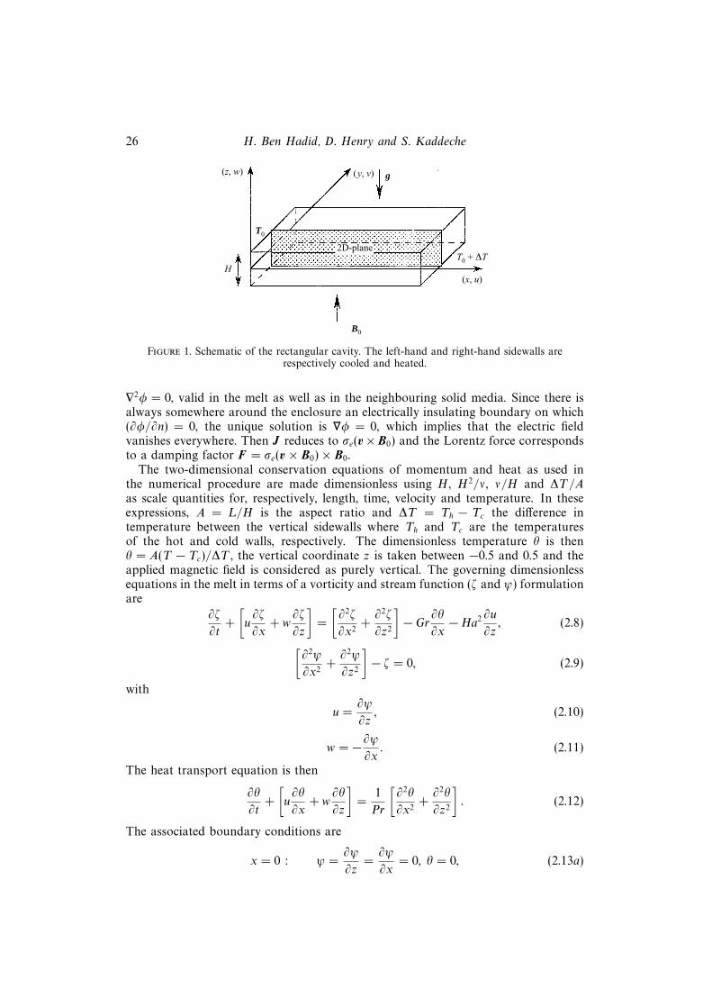
26 H. Ben Hadid, D. Henry and S. Kaddeche
(z, w) (y, v)
H(x, u)
2D-plane
T0
T0 + DT
B0
g
Figure 1. Schematic of the rectangular cavity. The left-hand and right-hand sidewalls arerespectively cooled and heated.
∇2φ = 0, valid in the melt as well as in the neighbouring solid media. Since there isalways somewhere around the enclosure an electrically insulating boundary on which(∂φ/∂n) = 0, the unique solution is ∇φ = 0, which implies that the electric fieldvanishes everywhere. Then J reduces to σe(v×B0) and the Lorentz force correspondsto a damping factor F = σe(v × B0)× B0.
The two-dimensional conservation equations of momentum and heat as used inthe numerical procedure are made dimensionless using H , H2/ν, ν/H and ∆T/Aas scale quantities for, respectively, length, time, velocity and temperature. In theseexpressions, A = L/H is the aspect ratio and ∆T = Th − Tc the difference intemperature between the vertical sidewalls where Th and Tc are the temperaturesof the hot and cold walls, respectively. The dimensionless temperature θ is thenθ = A(T − Tc)/∆T , the vertical coordinate z is taken between −0.5 and 0.5 and theapplied magnetic field is considered as purely vertical. The governing dimensionlessequations in the melt in terms of a vorticity and stream function (ζ and ψ) formulationare
∂ζ
∂t+
[u∂ζ
∂x+ w
∂ζ
∂z
]=
[∂2ζ
∂x2+∂2ζ
∂z2
]− Gr
∂θ
∂x−Ha2 ∂u
∂z, (2.8)[
∂2ψ
∂x2+∂2ψ
∂z2
]− ζ = 0, (2.9)
with
u =∂ψ
∂z, (2.10)
w = −∂ψ∂x. (2.11)
The heat transport equation is then
∂θ
∂t+
[u∂θ
∂x+ w
∂θ
∂z
]=
1
Pr
[∂2θ
∂x2+∂2θ
∂z2
]. (2.12)
The associated boundary conditions are
x = 0 : ψ =∂ψ
∂z=∂ψ
∂x= 0, θ = 0, (2.13a)
Convection under constant magnetic field. Part 1. Two-dimensional flow 27
x = A : ψ =∂ψ
∂z=∂ψ
∂x= 0, θ = A, (2.13b)
z = −0.5 : ψ =∂ψ
∂z=∂ψ
∂x= 0, (2.13c)
and, for the rigid-rigid case,
z = 0.5 : ψ =∂ψ
∂z=∂ψ
∂x= 0, (2.13d)
whereas for the free surface case with surface tension effects,
z = 0.5 : ψ =∂ψ
∂x= 0, ζ =
∂2ψ
∂z2= −Re
∂θ
∂x. (2.13e)
On the horizontal boundaries we consider two kinds of thermal conditions, eitherθ = x (conducting) or (∂θ/∂z) = 0 (insulating).
The dimensionless parameters appearing in equations (2.8)–(2.13) are the Grashofnumber Gr = gβ∆TH4/Lν2, the Reynolds–Marangoni number (called Reynoldsnumber in the following) Re = (−∂σ/∂T )∆TH2/Lρν2, the Prandlt number Pr = ν/κand the Hartmann number Ha = |B0|H(σe/ρν)
1/2.
3. Theoretical solutionsTheoretical solutions will be found for an infinite horizontal layer subjected to a
horizontal temperature gradient. In such a two-dimensional layer the flow can bedivided into three horizontal adjacent regions: the central region where the flowis horizontal and invariant, and the two end regions at ± infinity where the flowturns around. This simple model is a first tool for studying the interaction betweenthe Lorentz force and the different driving forces of convection, i.e. buoyancy andthermocapillarity. A considerable simplification of the governing equations (2.8)–(2.12) is obtained. The rigid–rigid case has been treated by Garandet, Alboussiere &Moreau (1992). We focus our study on the case with a free surface which can also besubjected to a surface tension force.
3.1. One-dimensional mathematical model for the central region
The dimensionless horizontal temperature gradient (∂θ/∂x) can be considered asconstant and equal to one. The temperature is then taken as θ(x, z) = x+ θp(z). Withthese assumptions and in a one-dimensional approximation, (2.8)–(2.12) reduce to
∂3u
∂z3−Ha2 ∂u
∂z− Gr = 0, (3.1)
∂2θp
∂z2= Pr u. (3.2)
The solution of equation (3.1) for the velocity is of the form
u(z) =C1
Hasinh(Ha(z + 0.5)) +
C2
Hacosh(Ha(z + 0.5))− Gr
Ha2(z + 0.5) + C3. (3.3)
The coefficients C1, C2 and C3 are determined by using the boundary conditions(u(z = −0.5) = 0 and (∂u/∂z) = −Re on the upper free surface, i.e. z = 0.5)and the conservation of mass flow across any vertical plane in the liquid layer
28 H. Ben Hadid, D. Henry and S. Kaddeche
(∫ 0.5
−0.5u(z)dz = 0). We obtain the following three equations:
C2
Ha+ C3 = 0, (3.4a)
C1 cosh(Ha) + C2 sinh(Ha)− Gr
Ha2= −Re, (3.4b)
C1
Ha2(cosh(Ha)− 1) +
C2
Ha2sinh(Ha)− Gr
2Ha2+ C3 = 0, (3.4c)
which give
C1 =−HaK1 +K2S
S −HaC, C2 =
K1 −K2C
S −HaC, C3 =
−C2
Ha,
with K1 = −Re +Gr
Ha2, K2 = K1 − 1
2Gr, C = cosh(Ha) and S = sinh(Ha).
Concerning the temperature, the solution θp to equation (3.2) is obtained by twosuccessive integrations with respect to z: θp(z) = A+ Bz + Pr f(z), with
f(z) =1
Ha2
(C1
Hasinh(Ha(z + 0.5)) +
C2
Hacosh(Ha(z + 0.5))− C2
Ha
)−(C1
Ha2(z + 0.5) +
Gr
6Ha2(z + 0.5)3 +
C2
2Ha(z + 0.5)2
), (3.5)
where A and B are integration constants. Depending on the thermal boundaryconditions, different solutions can be obtained:conducting conditions: θp(z) = Pr[f(z)− (z + 0.5)f(0.5)],
insulating conditions: θp(z) = Pr[f(z)−∫ 0.5
−0.5f(z)dz].
In the low-Ha limit, power series expansions of these expressions for the velocityand the temperature give the characteristic profiles obtained in the absence of amagnetic field. In the high-Ha range an asymptotic expression, valid in the wholecavity, can be found for the velocity:
u(z) = − Gr
Ha2z − K1
Ha2+K1
Hae−Ha(−z+0.5) +
K2
Ha2e−Ha(z+0.5). (3.6)
This gives the following simplified expressions:in the core,
u(z) = − Gr
Ha2z +
Re
Ha2+ O(Ha−4), (3.7a)
and at the upper surface,
u(0.5) = −Re
Ha− Gr
2Ha2+
Re
Ha2+ O(Ha−3). (3.7b)
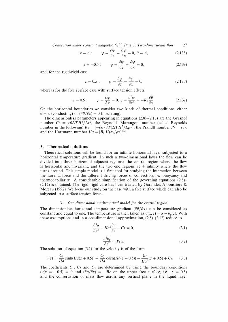
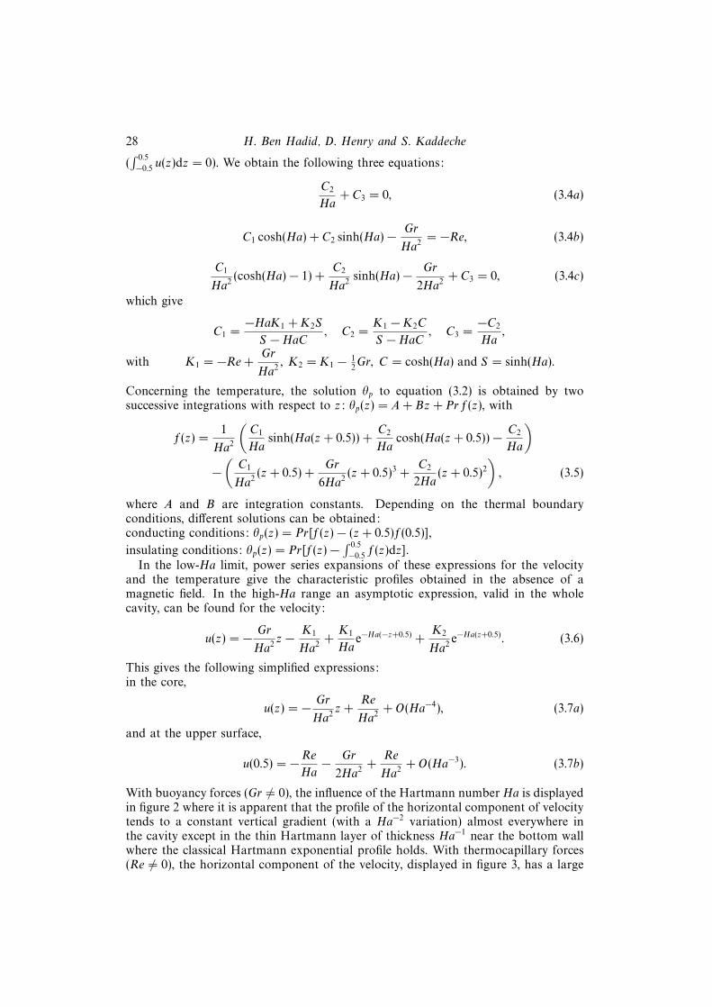
With buoyancy forces (Gr 6= 0), the influence of the Hartmann number Ha is displayedin figure 2 where it is apparent that the profile of the horizontal component of velocitytends to a constant vertical gradient (with a Ha−2 variation) almost everywhere inthe cavity except in the thin Hartmann layer of thickness Ha−1 near the bottom wallwhere the classical Hartmann exponential profile holds. With thermocapillary forces(Re 6= 0), the horizontal component of the velocity, displayed in figure 3, has a large
Convection under constant magnetic field. Part 1. Two-dimensional flow 29
–0.5
–0.3
–0.1
0.1
0.3
0.5
Ver
tica
l coo
rdin
ate
–2.0 –1.0 0 1.0 2.0
Ha = 50
Ha = 70
Ha = 100
Horizontal velocity
Figure 2. Vertical profiles of the horizontal velocity. Analytical solution (3.3) in the rigid–free casefor pure buoyancy effect (Gr = 104, Re = 0) for three values of the Hartmann number (Ha = 50,70 and 100).
–0.5
–0.3
–0.1
0.1
0.3
0.5
Ver
tica
l coo
rdin
ate
–198 –157 –116 –75 7
Ha = 50
Ha = 70
Ha = 100
Horizontal velocity–34
Figure 3. As figure 2 but for pure thermocapillary effect (Gr = 0, Re = 104).
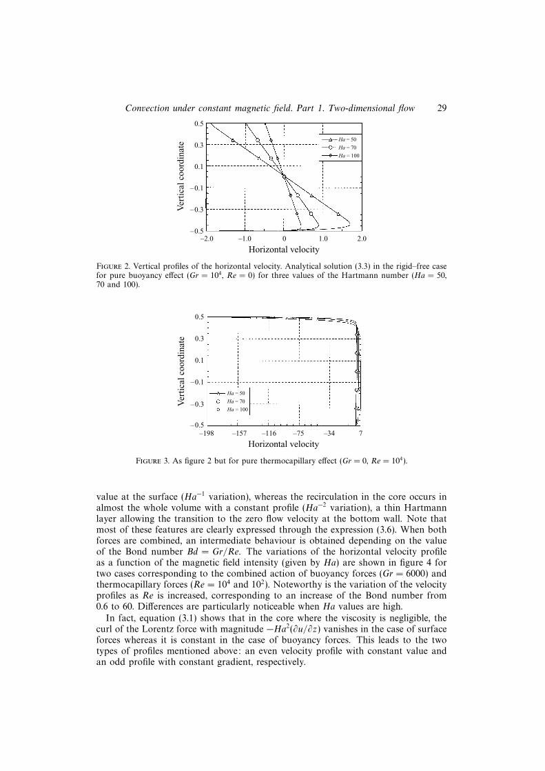
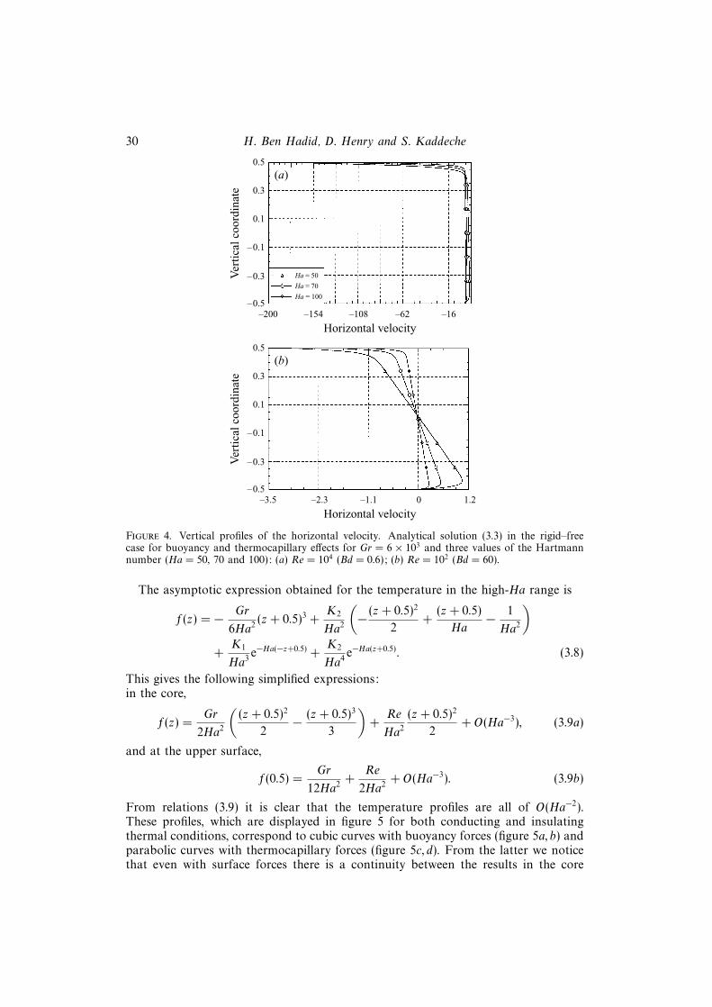
value at the surface (Ha−1 variation), whereas the recirculation in the core occurs inalmost the whole volume with a constant profile (Ha−2 variation), a thin Hartmannlayer allowing the transition to the zero flow velocity at the bottom wall. Note thatmost of these features are clearly expressed through the expression (3.6). When bothforces are combined, an intermediate behaviour is obtained depending on the valueof the Bond number Bd = Gr/Re. The variations of the horizontal velocity profileas a function of the magnetic field intensity (given by Ha) are shown in figure 4 fortwo cases corresponding to the combined action of buoyancy forces (Gr = 6000) andthermocapillary forces (Re = 104 and 102). Noteworthy is the variation of the velocityprofiles as Re is increased, corresponding to an increase of the Bond number from0.6 to 60. Differences are particularly noticeable when Ha values are high.
In fact, equation (3.1) shows that in the core where the viscosity is negligible, thecurl of the Lorentz force with magnitude −Ha2(∂u/∂z) vanishes in the case of surfaceforces whereas it is constant in the case of buoyancy forces. This leads to the twotypes of profiles mentioned above: an even velocity profile with constant value andan odd profile with constant gradient, respectively.
30 H. Ben Hadid, D. Henry and S. Kaddeche
–0.5
–0.3
–0.1
0.1
0.3
0.5
Ver
tica
l coo
rdin
ate
–200 –154 –108 –62
Ha = 50
Ha = 70
Ha = 100
Horizontal velocity–16
(a)
–0.5
–0.3
–0.1
0.1
0.3
0.5
Ver
tica
l coo
rdin
ate
–3.5 –2.3 –1.1 0
Horizontal velocity1.2
(b)
Figure 4. Vertical profiles of the horizontal velocity. Analytical solution (3.3) in the rigid–freecase for buoyancy and thermocapillary effects for Gr = 6× 10³ and three values of the Hartmannnumber (Ha = 50, 70 and 100): (a) Re = 104 (Bd = 0.6); (b) Re = 102 (Bd = 60).
The asymptotic expression obtained for the temperature in the high-Ha range is
f(z) = − Gr
6Ha2(z + 0.5)3 +
K2
Ha2
(− (z + 0.5)2
2+
(z + 0.5)
Ha− 1
Ha2
)+
K1
Ha3e−Ha(−z+0.5) +
K2
Ha4e−Ha(z+0.5). (3.8)
This gives the following simplified expressions:in the core,
f(z) =Gr
2Ha2
((z + 0.5)2
2− (z + 0.5)3
3
)+
Re
Ha2
(z + 0.5)2
2+ O(Ha−3), (3.9a)
and at the upper surface,
f(0.5) =Gr
12Ha2+
Re
2Ha2+ O(Ha−3). (3.9b)
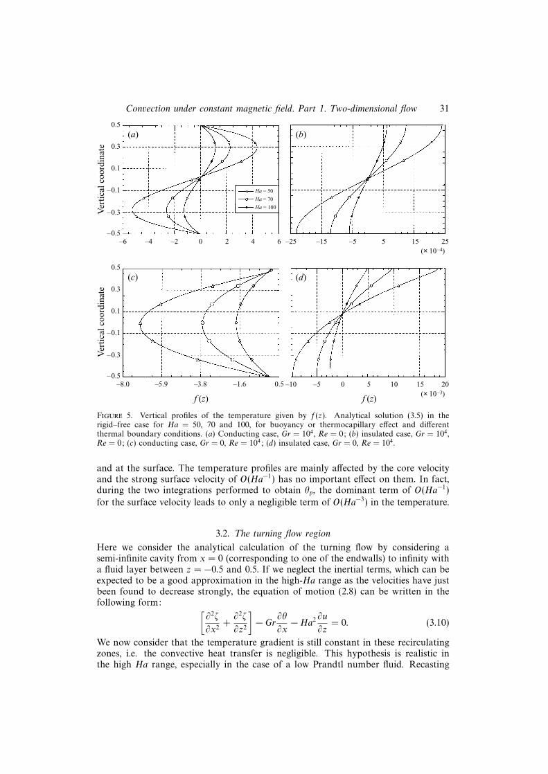
From relations (3.9) it is clear that the temperature profiles are all of O(Ha−2).These profiles, which are displayed in figure 5 for both conducting and insulatingthermal conditions, correspond to cubic curves with buoyancy forces (figure 5a, b) andparabolic curves with thermocapillary forces (figure 5c, d). From the latter we noticethat even with surface forces there is a continuity between the results in the core
Convection under constant magnetic field. Part 1. Two-dimensional flow 31
–0.5
–0.3
–0.1
0.1
0.3
0.5
Ver
tica
l coo
rdin
ate
–6 –4 –2 2
Ha = 50
Ha = 70
Ha = 100
4
(a)
–0.5
–0.3
–0.1
0.1
0.3
0.5
Ver
tica
l coo
rdin
ate
–8.0 –5.9 –3.8 –1.6
f (z)
0.5
(c)
0 6 –25 –15 –5 15
(b)
5 25(× 10–4)
–10 –5 0 15
(d)
5 20(× 10–3)
10
f (z)
Figure 5. Vertical profiles of the temperature given by f(z). Analytical solution (3.5) in therigid–free case for Ha = 50, 70 and 100, for buoyancy or thermocapillary effect and differentthermal boundary conditions. (a) Conducting case, Gr = 104, Re = 0; (b) insulated case, Gr = 104,Re = 0; (c) conducting case, Gr = 0, Re = 104; (d) insulated case, Gr = 0, Re = 104.
and at the surface. The temperature profiles are mainly affected by the core velocityand the strong surface velocity of O(Ha−1) has no important effect on them. In fact,during the two integrations performed to obtain θp, the dominant term of O(Ha−1)
for the surface velocity leads to only a negligible term of O(Ha−3) in the temperature.
3.2. The turning flow region
Here we consider the analytical calculation of the turning flow by considering asemi-infinite cavity from x = 0 (corresponding to one of the endwalls) to infinity witha fluid layer between z = −0.5 and 0.5. If we neglect the inertial terms, which can beexpected to be a good approximation in the high-Ha range as the velocities have justbeen found to decrease strongly, the equation of motion (2.8) can be written in thefollowing form: [
∂2ζ
∂x2+∂2ζ
∂z2
]− Gr
∂θ
∂x−Ha2 ∂u
∂z= 0. (3.10)
We now consider that the temperature gradient is still constant in these recirculatingzones, i.e. the convective heat transfer is negligible. This hypothesis is realistic inthe high Ha range, especially in the case of a low Prandtl number fluid. Recasting
32 H. Ben Hadid, D. Henry and S. Kaddeche
equation (3.10) using the definition of the vorticity (2.9), we obtain the followingequation for ψ:
∇4ψ −Ha2 ∂2ψ
∂z2= Gr. (3.11)
The associated boundary conditions are those defined in (2.13) for x = 0, z = −0.5and z = 0.5. Moreover the different variables must be finite as z tends towardsinfinity.
We can seek a solution in the form of a Fourier series expansion in z. In order tosatisfy the boundary condition for the thermocapillary case, we must add a polynomialexpansion in z. The expansion is then taken as follows:
ψ =
∞∑j=0
Vj(x) cos(αjz) +
∞∑k=0
Wk(x) sin(γkz)− 16Re((z2 − 1
4)(z + 3
2)), (3.12)
with αj = (2j + 1)π, j = 0,∞ and γk = 2(k + 1)π, k = 0,∞.Equation (3.12) satisfies all the conditions at the horizontal boundaries, except theno-slip condition at z = −0.5, i.e. the Hartmann layer near the bottom wall is notconsidered. This approximation is not too drastic as the Hartmann layer has here apassive nature (the electric current in the core is not forced to close in this layer).Moreover, the classical exponential variation of the velocity distribution within theHartmann layers (see (3.6)) could be used to satisfy the realistic no-slip condition, atleast when Ha is large.
If we put this expansion into equation (3.11), expand the polynomial in the sineand cosine bases, and use the orthogonality of the sine and cosine functions, weobtain equations for Vj and Wk that have to be solved with the appropriate boundaryconditions. After some tedious calculations which are presented in Appendix, weobtain the solutions for ψ, u and w, given for ψ by (3.12), and for u and w by thefollowing expressions:
u =∂ψ
∂z= −
∞∑j=0
Vj(x)αj sin(αjz) +
∞∑k=0
Wk(x)γk cos(γkz)− 16Re((z2 − 1
4) + 2z(z + 3
2)),
(3.13)
w = −∂ψ∂x
= −∞∑j=0
V ′j (x) cos(αjz)−∞∑k=0
W ′k(x) sin(γkz). (3.14)
with
Vj(x) = λje−ajx cos(bjx) + µje
−ajx sin(bjx) +gj
(α4j + Ha2α2
j ),
V ′j (x) = −e−ajx(bjλj + ajµj) sin(bjx),
and
Wk(x) = νke−ckx cos(dkx) + πke
−ckx sin(dkx) +hk
(γ4k + Ha2γ2
k ),
W ′k(x) = −e−ckx(dkνk + ckπk) sin(dkx),
where
λj = Vj0 −gj
(α4j + Ha2α2
j ), µj =
aj
bjλj ,
Convection under constant magnetic field. Part 1. Two-dimensional flow 33
and
νk = Wk0 −hk
(γ4k + Ha2γ2
k ), πk =
ck
dkνk.
We have also
Vj0 = −Re2(−1)j
α3j
and Wk0 = −Re2(−1)k
γ3k
,
with
gj = (−Ha2 12Re + Gr)
4(−1)j
αjand hk = −Ha2Re
2(−1)k
γk.
Finally,
aj =1√2
(α2j + αj(Ha2 + α2
j )1/2)1/2
and bj =1√2
(−α2
j + αj(Ha2 + α2j )
1/2)1/2
,
ck =1√2
(γ2k + γk(Ha2 + γ2
k )1/2)1/2
and dk =1√2
(−γ2
k + γk(Ha2 + γ2k )
1/2)1/2
.
We can derive the expressions valid in the high-Ha range. If we suppose that Ha�αjand Ha� γk , that is, more precisely, that Ha is greater than each αj and γk whichplays a significant role in the expansion, we can write
aj ∼ bj ∼ ( 12Haαj)
1/2 and ck ∼ dk ∼ ( 12Haγk)
1/2.
Moreover
Vj∞ =gj
α4j + Ha2α2
j
= −Re2(−1)j
α3j
+ Gr4(−1)j
α3jHa2
+ Re2(−1)j
αjHa2+ O(Ha−4),
Wk∞ =hk
γ4k + Ha2γ2
k
= −Re2(−1)k
γ3k
+ Re2(−1)k
γkHa2+ O(Ha−4),
and
µj ∼ λj = Vj0 − Vj∞, πk ∼ νk = Wk0 −Wk∞.
In order to check the consistency of our approach with respect to the solution in thecentral region calculated in §3.1, we can express the results as x tends towards infinityin the high-Ha range. Since Vj(x)→ Vj∞ and Wk(x)→Wk∞, we have
ψ =
∞∑j=0
(−Re
2(−1)j
α3j
+ Gr4(−1)j
α3jHa2
+ Re2(−1)j
αjHa2
)cos(αjz)
+
∞∑k=0
(−Re
2(−1)k
γ3k
+ Re2(−1)k
γkHa2
)sin(γkz)− 1
6Re((z2 − 1
4)(z + 3
2)) + O(Ha−4).
By using the expansions of the polynomials given in the Appendix, we can find theexpressions corresponding to the above expansions:
ψ∞ ∼−Gr
2Ha2(z2 − 1
4) +
Re
Ha2(z + 1
2),
and
v∞ ∼ −zGr
Ha2+
Re
Ha2. (3.15)
34 H. Ben Hadid, D. Henry and S. Kaddeche
(a) (b) (c)
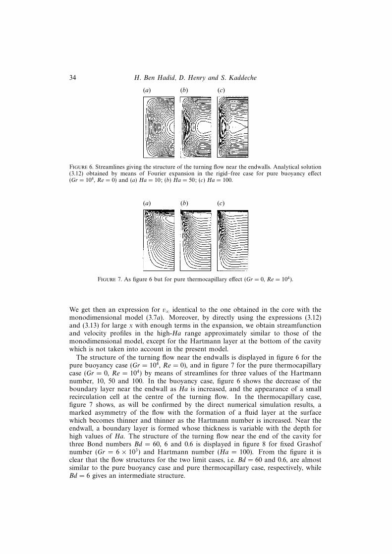
Figure 6. Streamlines giving the structure of the turning flow near the endwalls. Analytical solution(3.12) obtained by means of Fourier expansion in the rigid–free case for pure buoyancy effect(Gr = 104, Re = 0) and (a) Ha = 10; (b) Ha = 50; (c) Ha = 100.
(a) (b) (c)
Figure 7. As figure 6 but for pure thermocapillary effect (Gr = 0, Re = 104).
We get then an expression for v∞ identical to the one obtained in the core with themonodimensional model (3.7a). Moreover, by directly using the expressions (3.12)and (3.13) for large x with enough terms in the expansion, we obtain streamfunctionand velocity profiles in the high-Ha range approximately similar to those of themonodimensional model, except for the Hartmann layer at the bottom of the cavitywhich is not taken into account in the present model.
The structure of the turning flow near the endwalls is displayed in figure 6 for thepure buoyancy case (Gr = 104, Re = 0), and in figure 7 for the pure thermocapillarycase (Gr = 0, Re = 104) by means of streamlines for three values of the Hartmannnumber, 10, 50 and 100. In the buoyancy case, figure 6 shows the decrease of theboundary layer near the endwall as Ha is increased, and the appearance of a smallrecirculation cell at the centre of the turning flow. In the thermocapillary case,figure 7 shows, as will be confirmed by the direct numerical simulation results, amarked asymmetry of the flow with the formation of a fluid layer at the surfacewhich becomes thinner and thinner as the Hartmann number is increased. Near theendwall, a boundary layer is formed whose thickness is variable with the depth forhigh values of Ha. The structure of the turning flow near the end of the cavity forthree Bond numbers Bd = 60, 6 and 0.6 is displayed in figure 8 for fixed Grashofnumber (Gr = 6 × 10³) and Hartmann number (Ha = 100). From the figure it isclear that the flow structures for the two limit cases, i.e. Bd = 60 and 0.6, are almostsimilar to the pure buoyancy case and pure thermocapillary case, respectively, whileBd = 6 gives an intermediate structure.
Convection under constant magnetic field. Part 1. Two-dimensional flow 35
(a) (b) (c)
Figure 8. As figure 6 but for Ha = 100,Gr = 6× 10³ with buoyancy and thermocapillary effects:(a) Re = 102 (Bd = 60); (b) Re = 103 (Bd = 6); (c) Re = 104 (Bd = 0.6).
4. Scaling analysisThe characteristic behaviours for large Ha can also be obtained by a scaling
analysis. We can make use of the vorticity equation (3.10) with (∂θ/∂x) = 1 orof the equation of ψ (3.11). For a shallow cavity, in the central region the flow isunidirectional (w = 0) and independent of x.
4.1. Boundary layers
We can derive the characteristic lengths corresponding to the Hartmann layer (δHa)and to the parallel layer (δ‖). For that, we use (3.11) and, as the term on the right-handside does not depend on boundary layer thickness, we make the two terms of theleft-hand side equal.
For the Hartmann layers along the horizontal boundaries, the relevant length scalefor both viscous and magnetic terms is δz = δHa, δx being of order unity. We get then(1/δ4
Ha) ∼ (Ha2/δ2Ha), and so
δHa ∼ Ha−1. (4.1)
For the parallel layers along the vertical boundaries, the relevant length scale forthe viscous term is δx = δ‖ and that for the magnetic term is δz of order unity. We
get then (1/δ4‖) ∼ (Ha2/1), and so
δ‖ ∼ Ha−1/2. (4.2)
4.2. Rigid–rigid cavity
In the central region, the motion is driven by buoyancy-induced pressure gradient andthe velocity profile, u, has a Z-like shape (Garandet et al. 1992). Outside the boundarylayers of size δz = δHa (i.e. −0.5 + δz 6 z 6 0.5 − δz), the viscous effects are smalland the dominant balance occurs between the Lorentz term and the buoyancy term,which leads (with (∂u/∂z) ∼ (u/1)) in (3.10) to a horizontal velocity scale u ∼ GrHa−2.
Near the endwalls, the fluid flows with a mean vertical velocity w throughout alayer of thickness δx = δ‖. Since there is only one global circulation roll, this heatedfluid will travel horizontally along the top wall of the cavity in a layer of thickness1/2 (or H/2 in dimensional form). The continuity between the vertical and horizontal
circulations gives w δx ∼ u, and so w ∼ GrHa−3/2.From the above analyses, we can state that for large Hartmann numbers Ha > 10,
the maximum values of u and w are
umax ∼ GrHa−2 (4.3)
36 H. Ben Hadid, D. Henry and S. Kaddeche
and
wmax ∼ GrHa−3/2, (4.4)
and the associated length scales on z and x are, respectively, 1 and Ha−1/2. Consideringthe equation in primitive variables, the Lorentz force (Ha2u) is then of order Gr, andthe leading contribution to the inertial term (v · ∇)v varies like Gr2Ha−3. A conditionfor inertia term to be negligible thus is
Ha3�Gr. (4.5)
4.3. Rigid–free cavity
In the pure buoyancy case, the characteristic variations are similar to those ofthe rigid–rigid cavity and can be obtained by analogous considerations. The onlydifference is the absence of a real Hartmann layer at the upper free boundary.
In the pure thermocapillary case, the entire flow is driven by temperature-inducedsurface tension gradients at the upper surface. Large velocities are then created atthis upper surface and drive the subsurface layer of thickness δz . The scaling law atthis upper surface is determined by the balance between shear and thermocapillaryforces as expressed by the thermocapillary boundary condition (2.13e). Thus, weobtain u ∼ Re δz .
In the subsurface layer, for large Hartmann numbers the correct balance is betweenviscous and magnetic forces. Inserting Gr = 0, (∂2ζ/∂x2) = 0 and ζ ∼ u/δz in (3.10),gives δz ∼ Ha−1 and so u ∼ ReHa−1, establishing that the upper circulation will occurinside the Hartmann layer.
The scaling law for the constant returning core velocity which applies on almostthe whole height of the cavity (except the boundary layers) can be obtained from themass conservation equation. We find uret ∼ ReHa−2.
Near the endwalls, the fluid flows with a mean vertical velocity w throughouta layer of thickness δx = δ‖. The continuity with the horizontal circulations give
w ∼ ReHa−3/2.Finally, for large Hartmann numbers, the maximum values of the horizontal and
vertical velocities are, respectively,
umax ∼ ReHa−1 (4.6)
and
wmax ∼ ReHa−3/2, (4.7)
and the associated length scales on z and x are, respectively, Ha−1 and Ha−1/2. TheLorentz force is then of order ReHa, and the leading contributions to the inertialterms vary like Re2Ha−3/2. The condition for inertial terms to be negligible thusbecomes
Ha5/2�Re. (4.8)
5. Numerical resultsThe numerical scheme employed is based upon a highly accurate method which has
proven effective for classical hydrodynamical problems. The technique employed tosolve the system of non-dimensionalized equations (2.8)–(2.13) was the culminationof earlier work on accurate numerical representations of Navier–Stokes and energyequations (Roux et al. 1979 and Ben Hadid 1989). The main features of this numericaltechnique are:
Convection under constant magnetic field. Part 1. Two-dimensional flow 37
(a)
(b)
(c)
(d)
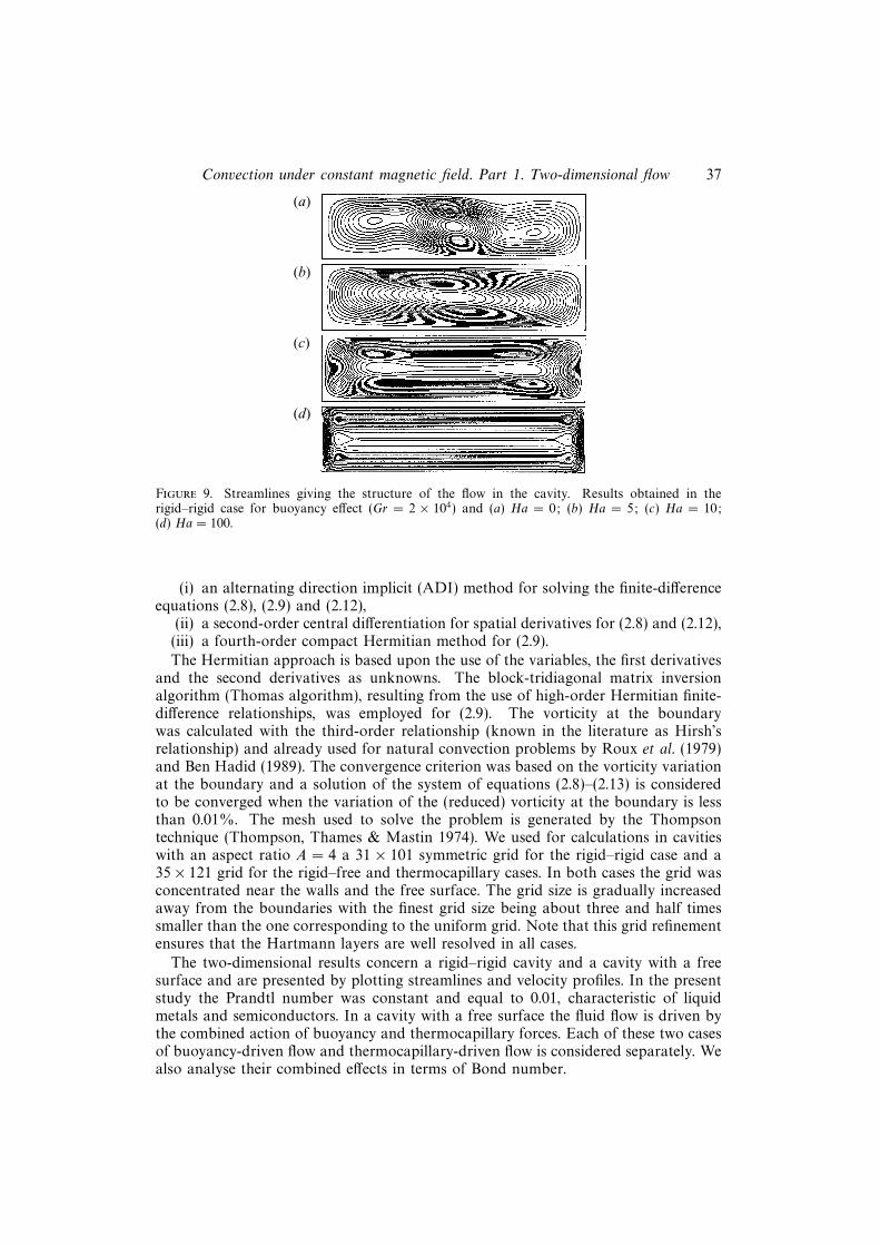
Figure 9. Streamlines giving the structure of the flow in the cavity. Results obtained in therigid–rigid case for buoyancy effect (Gr = 2 × 10⁴) and (a) Ha = 0; (b) Ha = 5; (c) Ha = 10;(d) Ha = 100.
(i) an alternating direction implicit (ADI) method for solving the finite-differenceequations (2.8), (2.9) and (2.12),
(ii) a second-order central differentiation for spatial derivatives for (2.8) and (2.12),(iii) a fourth-order compact Hermitian method for (2.9).
The Hermitian approach is based upon the use of the variables, the first derivativesand the second derivatives as unknowns. The block-tridiagonal matrix inversionalgorithm (Thomas algorithm), resulting from the use of high-order Hermitian finite-difference relationships, was employed for (2.9). The vorticity at the boundarywas calculated with the third-order relationship (known in the literature as Hirsh’srelationship) and already used for natural convection problems by Roux et al. (1979)and Ben Hadid (1989). The convergence criterion was based on the vorticity variationat the boundary and a solution of the system of equations (2.8)–(2.13) is consideredto be converged when the variation of the (reduced) vorticity at the boundary is lessthan 0.01%. The mesh used to solve the problem is generated by the Thompsontechnique (Thompson, Thames & Mastin 1974). We used for calculations in cavitieswith an aspect ratio A = 4 a 31 × 101 symmetric grid for the rigid–rigid case and a35× 121 grid for the rigid–free and thermocapillary cases. In both cases the grid wasconcentrated near the walls and the free surface. The grid size is gradually increasedaway from the boundaries with the finest grid size being about three and half timessmaller than the one corresponding to the uniform grid. Note that this grid refinementensures that the Hartmann layers are well resolved in all cases.
The two-dimensional results concern a rigid–rigid cavity and a cavity with a freesurface and are presented by plotting streamlines and velocity profiles. In the presentstudy the Prandtl number was constant and equal to 0.01, characteristic of liquidmetals and semiconductors. In a cavity with a free surface the fluid flow is driven bythe combined action of buoyancy and thermocapillary forces. Each of these two casesof buoyancy-driven flow and thermocapillary-driven flow is considered separately. Wealso analyse their combined effects in terms of Bond number.

38 H. Ben Hadid, D. Henry and S. Kaddeche
–0.5
–0.3
–0.1
0.1
0.3
0.5
Ver
tica
l coo
rdin
ate
–1.10 –0.55 0 0.55 1.10
Ha = 5
Ha = 50
Ha = 100
Normalized horizontal velocity
Ha = 0
Figure 10. Vertical profiles of the normalized horizontal velocity at mid-length of the cavity. Resultsobtained by numerical simulation in the rigid–rigid case for buoyancy effect (Gr = 2 × 10⁴) andHa = 0, 5, 50 and 100.
–1.10
–0.55
0
0.55
1.10
Nor
mal
ized
ver
tica
l vel
ocit
y
0 1 2 3 4
Horizontal coordinate
Ha = 5
Ha = 50
Ha = 200
Ha = 0
Figure 11. Horizontal profiles of the normalized vertical velocity at mid-height of the cavity.Results obtained by numerical simulation in the rigid–rigid case for buoyancy effect (Gr = 2× 10⁴)and Ha = 0, 5, 50 and 200.
5.1. Rigid-rigid cavity
In this case, the fluid flow is generated by buoyancy forces due to the temperaturegradients in the liquid resulting from the lateral heating. The calculations were carriedout for Grashof numbers ranging from 104 to 2.0 × 10⁴, and various values of theHartmann number, 0 6 Ha 6 200. In this range of Grashof numbers the flow forHa = 0 is expected to be steady with intense convective rolls (see Roux 1990; BenHadid & Roux 1990). Figure 9(a–d) shows the streamlines patterns at Hartmannnumbers of 0, 5, 10 and 100, respectively. For a zero Hartmann number (figure 9a),there is an intense circulation loop in the central region and two smaller ones nearthe endwalls. As the Hartmann number is increased to 5, the small rolls disappearand the central circulation is seen to spread gradually over the whole cavity. On afurther increase in Hartmann number, the streamlines in the central region becomemore and more horizontal whereas they accumulate near the endwalls indicating theexistence of a boundary layer at these walls (figure 9d). Boundary layers are alsoformed adjacent to the horizontal walls of the cavity.
The horizontal and vertical normalized velocity profiles are shown, respectively,
Convection under constant magnetic field. Part 1. Two-dimensional flow 39
Max
imum
of
the
hori
zont
alve
loci
ty
10–2
1 10 100 1000
Ha
Gr = 3.0 × 10³
10–3
10–4
10–5
10–6
Ha–2
(a)
Gr = 6.0 × 10³
Gr = 104
Gr = 1.5 × 10⁴
Gr = 2.0 × 10⁴
Max
imum
of
the
vert
ical
velo
city
10–2
100 101 102 103
Ha
10–3
10–4
10–5
Ha–3/2
(b)
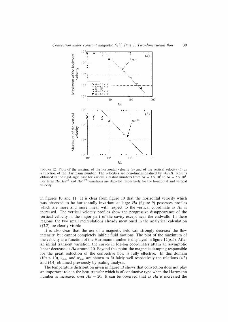
Figure 12. Plots of the maxima of the horizontal velocity (a) and of the vertical velocity (b) asa function of the Hartmann number. The velocities are non-dimensionalized by νGr/H . Resultsobtained in the rigid–rigid case for various Grashof numbers from Gr = 3 × 10³ to Gr = 2 × 10⁴.
For large Ha, Ha−2 and Ha−3/2 variations are depicted respectively for the horizontal and verticalvelocity.
in figures 10 and 11. It is clear from figure 10 that the horizontal velocity whichwas observed to be horizontally invariant at large Ha (figure 9) possesses profileswhich are more and more linear with respect to the vertical coordinate as Ha isincreased. The vertical velocity profiles show the progressive disappearance of thevertical velocity in the major part of the cavity except near the endwalls. In theseregions, the two small recirculations already mentioned in the analytical calculation(§3.2) are clearly visible.
It is also clear that the use of a magnetic field can strongly decrease the flowintensity, but cannot completely inhibit fluid motions. The plot of the maximum ofthe velocity as a function of the Hartmann number is displayed in figure 12(a, b). Afteran initial transient variation, the curves in log-log coordinates attain an asymptoticlinear decrease at Ha around 10. Beyond this point the magnetic damping responsiblefor the great reduction of the convective flow is fully effective. In this domain(Ha > 10), umax and wmax are shown to fit fairly well respectively the relations (4.3)and (4.4) obtained previously by scaling analysis.
The temperature distribution given in figure 13 shows that convection does not playan important role in the heat transfer which is of conductive type when the Hartmannnumber is increased over Ha = 20. It can be observed that as Ha is increased the
40 H. Ben Hadid, D. Henry and S. Kaddeche
(a)
(b)
(c)
Figure 13. Isotherm lines giving the temperature distribution in the cavity. Results obtained in therigid–rigid case for buoyancy effect (Gr = 2× 10⁴) and (a) Ha = 0; (b) Ha = 10; (c) Ha = 20.
(a)
(b)
(c)
Figure 14. Streamlines giving the structure of the flow in the cavity. Results obtained in therigid–free case for pure buoyancy effect (Gr = 104, Re = 0) and (a) Ha = 0; (b) Ha = 10;(c) Ha = 100.
isotherm-lines which are distorted in the absence of magnetic field (figure 13a) becomegradually straightlines (see figure 13c).
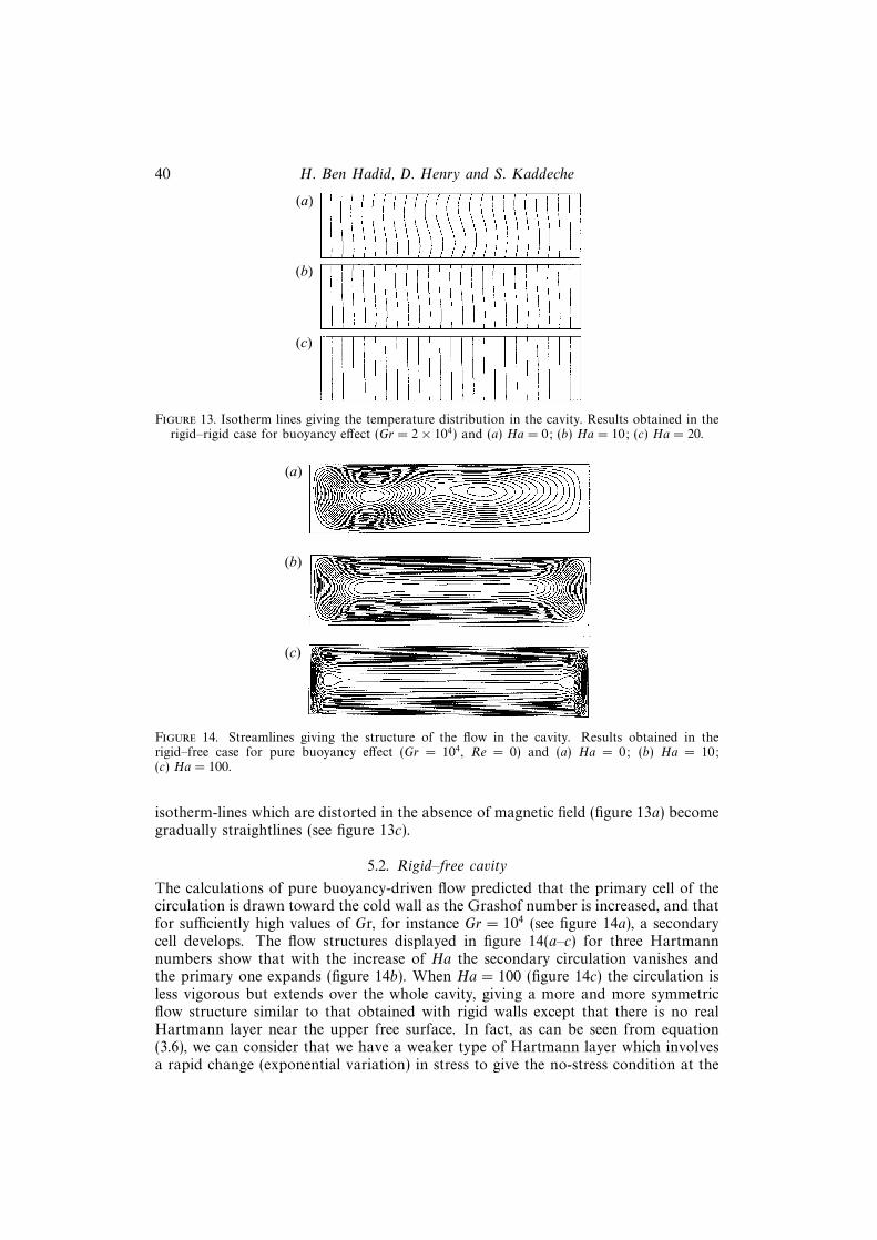
5.2. Rigid–free cavity
The calculations of pure buoyancy-driven flow predicted that the primary cell of thecirculation is drawn toward the cold wall as the Grashof number is increased, and thatfor sufficiently high values of Gr, for instance Gr = 104 (see figure 14a), a secondarycell develops. The flow structures displayed in figure 14(a–c) for three Hartmannnumbers show that with the increase of Ha the secondary circulation vanishes andthe primary one expands (figure 14b). When Ha = 100 (figure 14c) the circulation isless vigorous but extends over the whole cavity, giving a more and more symmetricflow structure similar to that obtained with rigid walls except that there is no realHartmann layer near the upper free surface. In fact, as can be seen from equation(3.6), we can consider that we have a weaker type of Hartmann layer which involvesa rapid change (exponential variation) in stress to give the no-stress condition at the

Convection under constant magnetic field. Part 1. Two-dimensional flow 41
(a)
(b)
(c)
Figure 15. As figure 14 but for pure thermocapillary effect (Gr = 0, Re = 104).
free surface. Furthermore, the characteristic behaviour of the two components of thevelocity for large values of Ha are similar to those obtained in the rigid–rigid case.
In the pure thermocapillary case the flow structure at Re = 104 is shown in figure15(a–c) for Ha = 0, 10 and 100. In the absence of a magnetic field (figure 15a) theflow corresponds to a strong counterclockwise cell with the centre located near thecold wall. At Ha = 10 (figure 15b), the strength of the flow decreases but the cellularstructure persists. Large Hartmann numbers (Ha = 100) decrease the flow strengthto the point that a single cell stretches to fill the whole cavity so that most of theflow is perpendicular to the field and hence affected by it. The flow becomes moreand more antisymmetric with respect to the centre vertical line, and unidirectionalover most of the cavity except in the close vicinity of the vertical walls (figure 15c).The most vigorous flow is limited to a small region near the free surface (subsurfacelayer), whereas the returning flow occurs with a constant velocity over almost thewhole height of the cavity.
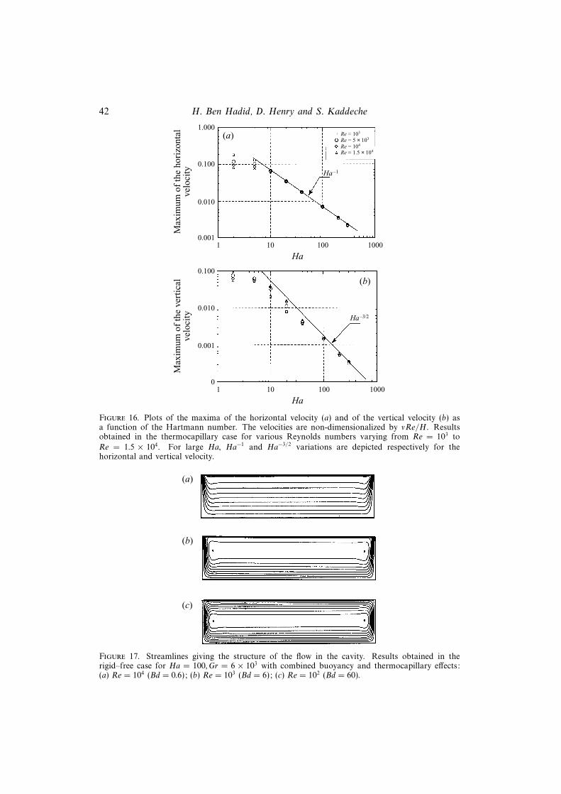
The maximum of the velocity as a function of the Hartmann number is plottedin figure 16 where we can observe that for large values of Ha the maximum of thehorizontal velocity, umax, and the maximum of the vertical velocity, wmax, satisfy therelations given by scaling analysis, respectively (4.6) and (4.7).
The effect of increasing the strength of the magnetic field in the case of a combinedbuoyancy and thermocapillary-driven flow is evident in the flow structures shown infigure 17(a–c) for three Bond numbers, Bd = 0.6, 6 and 60 for a fixed Hartmannnumber, Ha = 100. Examination of these figures shows that the characteristics ofthe final flow structures depend strongly on Bd. For Bd = 0.6 (figure 17a) the flowpattern is in a qualitative sense similar to that of the pure thermocapillary case (figure15c), while for Bd = 60 (figure 17c) the flow pattern compares favourably with thatof pure buoyancy-driven flow (figure 14c).
5.3. Comparison with the analytical results
The previous sections clearly show the large modifications of the flow structurewhich occur under the action of a strong magnetic field. To illustrate further thecharacteristics of these flows and verify the analytical approach, we will compare
42 H. Ben Hadid, D. Henry and S. Kaddeche
Max
imum
of
the
hori
zont
alve
loci
ty
1.000
1 10 100 1000
Ha
Re = 103
0.100
0.010
0.001
Ha–1
(a)Re = 5 × 10³
Re = 104
Re = 1.5 × 10⁴
Max
imum
of
the
vert
ical
velo
city
0.100
1 10 100 1000
Ha
0.010
0.001
0
Ha–3/2
(b)
Figure 16. Plots of the maxima of the horizontal velocity (a) and of the vertical velocity (b) asa function of the Hartmann number. The velocities are non-dimensionalized by νRe/H . Resultsobtained in the thermocapillary case for various Reynolds numbers varying from Re = 103 to
Re = 1.5 × 10⁴. For large Ha, Ha−1 and Ha−3/2 variations are depicted respectively for thehorizontal and vertical velocity.
(a)
(b)
(c)
Figure 17. Streamlines giving the structure of the flow in the cavity. Results obtained in therigid–free case for Ha = 100,Gr = 6 × 10³ with combined buoyancy and thermocapillary effects:(a) Re = 104 (Bd = 0.6); (b) Re = 103 (Bd = 6); (c) Re = 102 (Bd = 60).
Convection under constant magnetic field. Part 1. Two-dimensional flow 43
0.5
0.3
0.1
–0.1
–0.3
–0.5–1.0 –0.5 0.5
Horizontal velocity
Ver
tica
l coo
rdin
ate
Ha = 50; numeri.
Ha = 20; numeri.
Ha = 10; numeri.
Ha = 5; numeri.
Ha = 50; analy.
Ha = 20; analy.
Ha = 10; analy.
Ha = 5; analy.
0 (¬102)
Figure 18. Vertical profiles of the horizontal velocity at mid-length of the cavity. Comparison withanalytical solutions (3.3) in the rigid–free case for pure buoyancy effect (Gr = 104, Re = 0) andHa = 5, 10, 20 and 50.
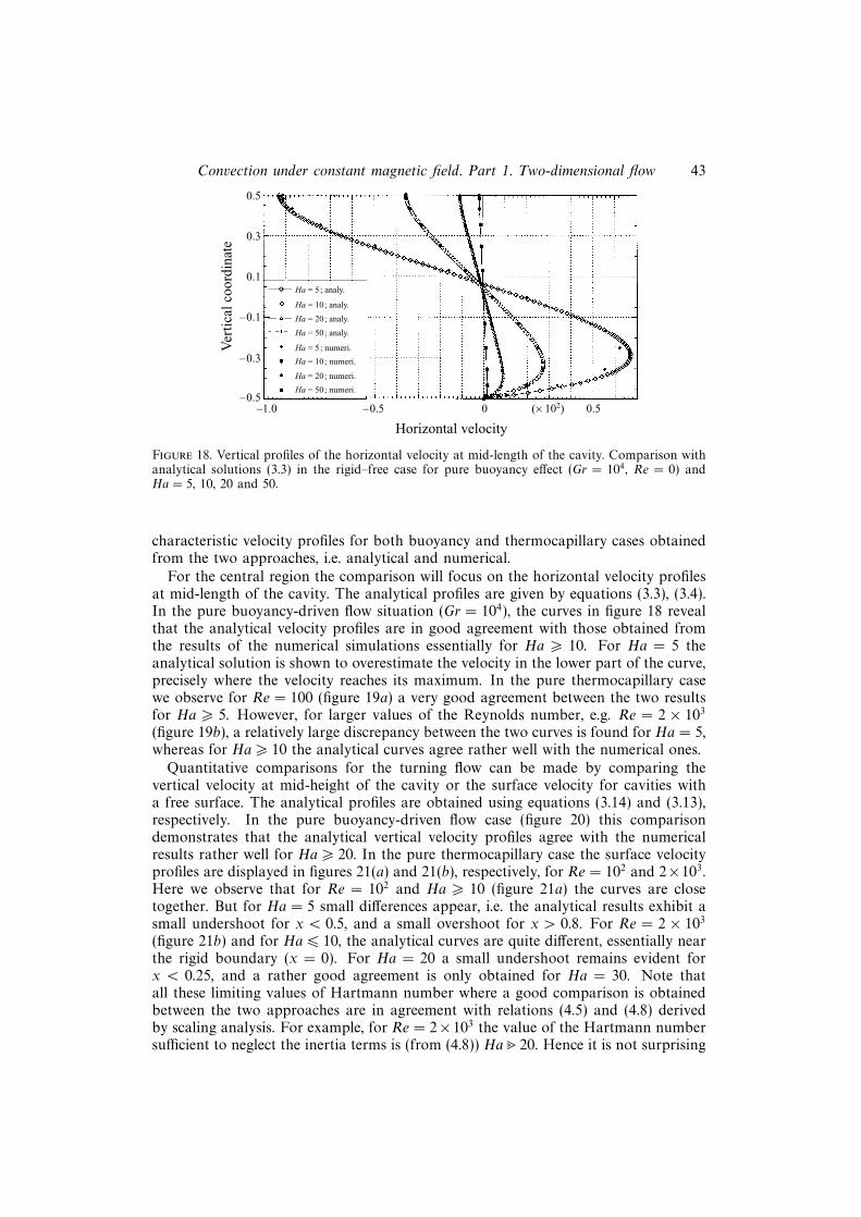
characteristic velocity profiles for both buoyancy and thermocapillary cases obtainedfrom the two approaches, i.e. analytical and numerical.
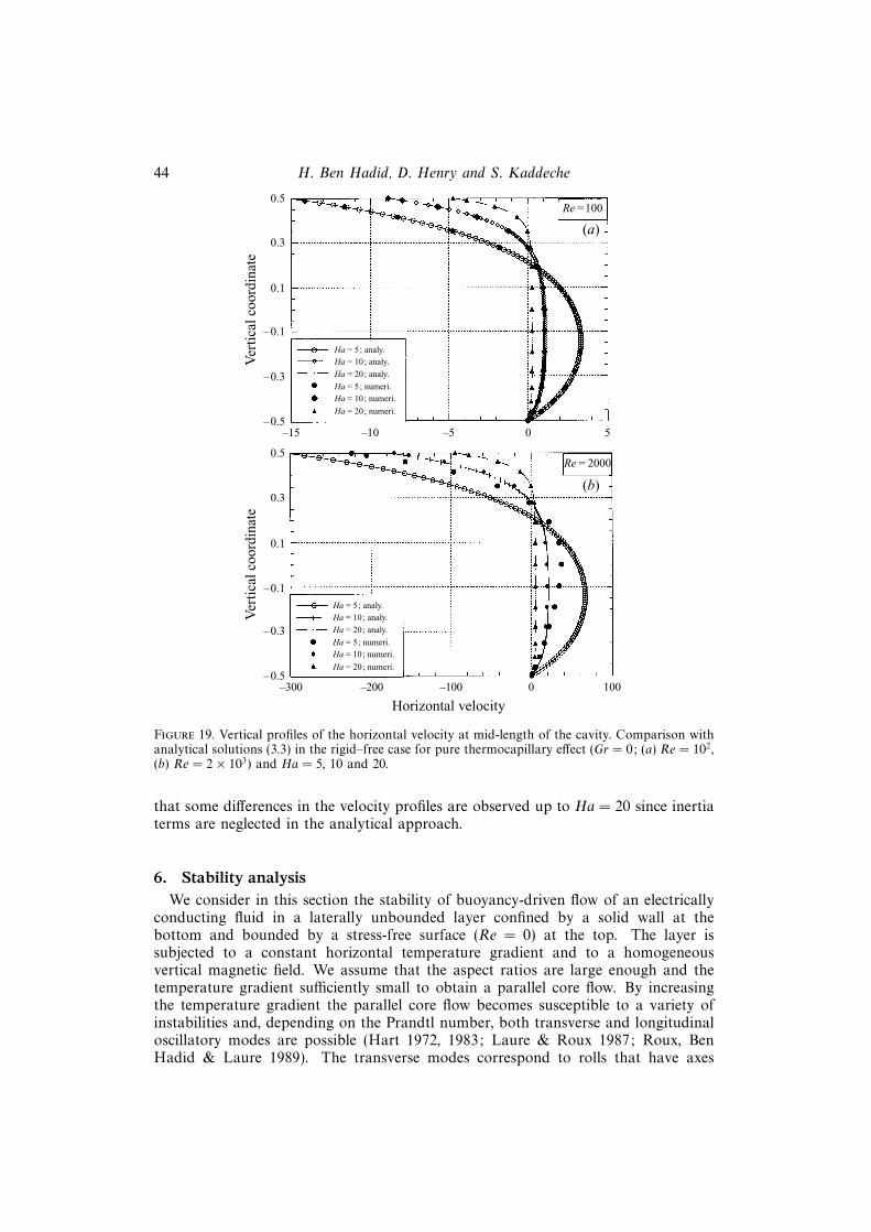
For the central region the comparison will focus on the horizontal velocity profilesat mid-length of the cavity. The analytical profiles are given by equations (3.3), (3.4).In the pure buoyancy-driven flow situation (Gr = 104), the curves in figure 18 revealthat the analytical velocity profiles are in good agreement with those obtained fromthe results of the numerical simulations essentially for Ha > 10. For Ha = 5 theanalytical solution is shown to overestimate the velocity in the lower part of the curve,precisely where the velocity reaches its maximum. In the pure thermocapillary casewe observe for Re = 100 (figure 19a) a very good agreement between the two resultsfor Ha > 5. However, for larger values of the Reynolds number, e.g. Re = 2 × 10³
(figure 19b), a relatively large discrepancy between the two curves is found for Ha = 5,whereas for Ha > 10 the analytical curves agree rather well with the numerical ones.
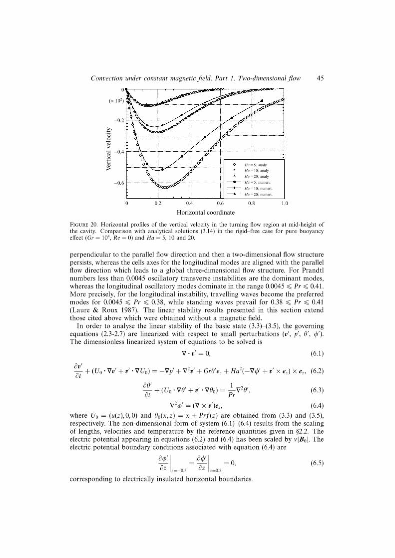
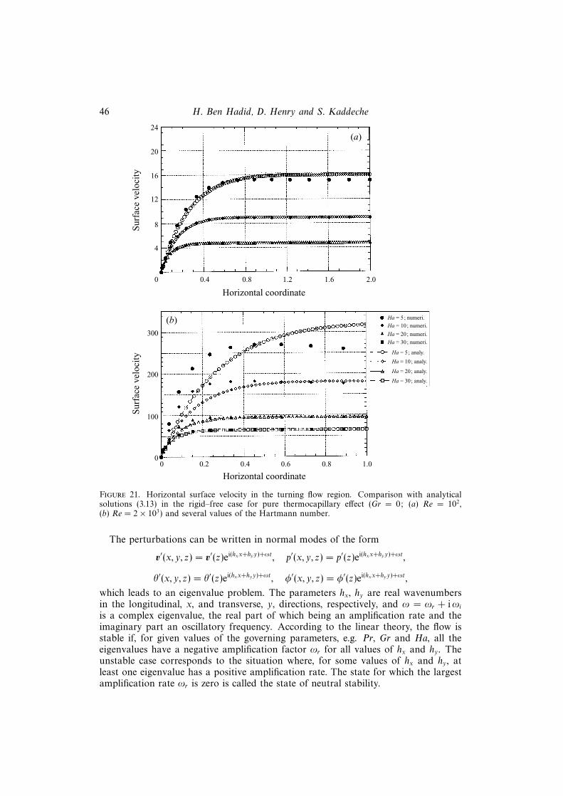
Quantitative comparisons for the turning flow can be made by comparing thevertical velocity at mid-height of the cavity or the surface velocity for cavities witha free surface. The analytical profiles are obtained using equations (3.14) and (3.13),respectively. In the pure buoyancy-driven flow case (figure 20) this comparisondemonstrates that the analytical vertical velocity profiles agree with the numericalresults rather well for Ha > 20. In the pure thermocapillary case the surface velocityprofiles are displayed in figures 21(a) and 21(b), respectively, for Re = 102 and 2×10³.Here we observe that for Re = 102 and Ha > 10 (figure 21a) the curves are closetogether. But for Ha = 5 small differences appear, i.e. the analytical results exhibit asmall undershoot for x < 0.5, and a small overshoot for x > 0.8. For Re = 2 × 10³
(figure 21b) and for Ha 6 10, the analytical curves are quite different, essentially nearthe rigid boundary (x = 0). For Ha = 20 a small undershoot remains evident forx < 0.25, and a rather good agreement is only obtained for Ha = 30. Note thatall these limiting values of Hartmann number where a good comparison is obtainedbetween the two approaches are in agreement with relations (4.5) and (4.8) derivedby scaling analysis. For example, for Re = 2×10³ the value of the Hartmann numbersufficient to neglect the inertia terms is (from (4.8)) Ha�20. Hence it is not surprising
44 H. Ben Hadid, D. Henry and S. Kaddeche
0.5
0.3
0.1
–0.1
–0.3
–0.5–15 –10 0 5
Ver
tica
l coo
rdin
ate
Ha = 20; numeri.
Ha = 10; numeri.Ha = 5; numeri.
Ha = 20; analy.
Ha = 10; analy.Ha = 5; analy.
(a)
–5
0.5
0.3
0.1
–0.1
–0.3
–0.5–300 –200 0 100
Ver
tica
l coo
rdin
ate
(b)
–100
Horizontal velocity
Ha = 20; numeri.
Ha = 10; numeri.Ha = 5; numeri.
Ha = 20; analy.
Ha = 10; analy.Ha = 5; analy.
Re =100
Re = 2000
Figure 19. Vertical profiles of the horizontal velocity at mid-length of the cavity. Comparison withanalytical solutions (3.3) in the rigid–free case for pure thermocapillary effect (Gr = 0; (a) Re = 102,(b) Re = 2× 10³) and Ha = 5, 10 and 20.
that some differences in the velocity profiles are observed up to Ha = 20 since inertiaterms are neglected in the analytical approach.
6. Stability analysisWe consider in this section the stability of buoyancy-driven flow of an electrically
conducting fluid in a laterally unbounded layer confined by a solid wall at thebottom and bounded by a stress-free surface (Re = 0) at the top. The layer issubjected to a constant horizontal temperature gradient and to a homogeneousvertical magnetic field. We assume that the aspect ratios are large enough and thetemperature gradient sufficiently small to obtain a parallel core flow. By increasingthe temperature gradient the parallel core flow becomes susceptible to a variety ofinstabilities and, depending on the Prandtl number, both transverse and longitudinaloscillatory modes are possible (Hart 1972, 1983; Laure & Roux 1987; Roux, BenHadid & Laure 1989). The transverse modes correspond to rolls that have axes
Convection under constant magnetic field. Part 1. Two-dimensional flow 45
0
–0.2
–0.4
–0.6
0 0.2 0.6 0.8
Horizontal coordinate
Ver
tica
l vel
ocit
y
Ha = 20; numeri.
Ha = 10; numeri.
Ha = 5; numeri.
Ha = 20; analy.
Ha = 10; analy.
Ha = 5; analy.
0.4 1.0
(¬102)
Figure 20. Horizontal profiles of the vertical velocity in the turning flow region at mid-height ofthe cavity. Comparison with analytical solutions (3.14) in the rigid–free case for pure buoyancyeffect (Gr = 104, Re = 0) and Ha = 5, 10 and 20.
perpendicular to the parallel flow direction and then a two-dimensional flow structurepersists, whereas the cells axes for the longitudinal modes are aligned with the parallelflow direction which leads to a global three-dimensional flow structure. For Prandtlnumbers less than 0.0045 oscillatory transverse instabilities are the dominant modes,whereas the longitudinal oscillatory modes dominate in the range 0.0045 6 Pr 6 0.41.More precisely, for the longitudinal instability, travelling waves become the preferredmodes for 0.0045 6 Pr 6 0.38, while standing waves prevail for 0.38 6 Pr 6 0.41(Laure & Roux 1987). The linear stability results presented in this section extendthose cited above which were obtained without a magnetic field.
In order to analyse the linear stability of the basic state (3.3)–(3.5), the governingequations (2.3-2.7) are linearized with respect to small perturbations (v′, p′, θ′, φ′).The dimensionless linearized system of equations to be solved is
∇ · v′ = 0, (6.1)
∂v′
∂t+ (U0 · ∇v′ + v′ · ∇U0) = −∇p′ + ∇2v′ + Grθ′ez + Ha2(−∇φ′ + v′ × ez)× ez, (6.2)
∂θ′
∂t+ (U0 · ∇θ′ + v′ · ∇θ0) =
1
Pr∇2θ′, (6.3)
∇2φ′ = (∇× v′)ez, (6.4)
where U0 = (u(z), 0, 0) and θ0(x, z) = x + Prf(z) are obtained from (3.3) and (3.5),respectively. The non-dimensional form of system (6.1)–(6.4) results from the scalingof lengths, velocities and temperature by the reference quantities given in §2.2. Theelectric potential appearing in equations (6.2) and (6.4) has been scaled by ν|B0|. Theelectric potential boundary conditions associated with equation (6.4) are
∂φ′
∂z
∣∣∣∣z=−0.5
=∂φ′
∂z
∣∣∣∣z=0.5
= 0, (6.5)
corresponding to electrically insulated horizontal boundaries.
46 H. Ben Hadid, D. Henry and S. Kaddeche
24
16
12
8
4
0 0.4 1.2 2.0
Horizontal coordinate
Sur
face
vel
ocit
y(a)
0.8
300
200
100
00 0.2 0.8 1.0
Sur
face
vel
ocit
y
(b)
0.4
Horizontal coordinate
20
1.6
0.6
Ha = 20; numeri.
Ha = 10; numeri.
Ha = 5; numeri.
Ha = 20; analy.
Ha = 10; analy.
Ha = 5; analy.
Ha = 30; numeri.
Ha = 30; analy.
Figure 21. Horizontal surface velocity in the turning flow region. Comparison with analyticalsolutions (3.13) in the rigid–free case for pure thermocapillary effect (Gr = 0; (a) Re = 102,(b) Re = 2× 10³) and several values of the Hartmann number.
The perturbations can be written in normal modes of the form
v′(x, y, z) = v′(z)ei(hxx+hyy)+ωt, p′(x, y, z) = p′(z)ei(hxx+hyy)+ωt,
θ′(x, y, z) = θ′(z)ei(hxx+hyy)+ωt, φ′(x, y, z) = φ′(z)ei(hxx+hyy)+ωt,
which leads to an eigenvalue problem. The parameters hx, hy are real wavenumbersin the longitudinal, x, and transverse, y, directions, respectively, and ω = ωr + iωiis a complex eigenvalue, the real part of which being an amplification rate and theimaginary part an oscillatory frequency. According to the linear theory, the flow isstable if, for given values of the governing parameters, e.g. Pr, Gr and Ha, all theeigenvalues have a negative amplification factor ωr for all values of hx and hy . Theunstable case corresponds to the situation where, for some values of hx and hy , atleast one eigenvalue has a positive amplification rate. The state for which the largestamplification rate ωr is zero is called the state of neutral stability.
Convection under constant magnetic field. Part 1. Two-dimensional flow 47
106
0.001 0.01 0.1
Pr
Grc
Ha = 0; 2D
105
104
103
Ha = 1; 2D
Ha = 2; 2D
Ha = 3; 2D
Ha = 4; 2D
Ha = 5; 2D
Ha = 0; 3D
Ha = 1; 3D
Ha = 2; 3D
Ha = 3; 3D
Ha = 4; 3D
Ha = 5; 3D
Figure 22. Neutral stability curves in the pure buoyancy case with magnetic effect. The criticalGrashof number Grc is given as a function of Prandtl number Pr for several values of theHartmann number Ha (from 0 to 5). Two types of curves are obtained corresponding respectivelyto transverse oscillating modes (two-dimensional structures) and to longitudinal oscillating modes(three-dimensional structures).
The numerical procedure is based on a Tau-method which uses Chebyshev polyno-mials as trial functions. In the present study we used 20 polynomials which are foundsufficient to give grid-free results. The discretized system results in a generalizedalgebraic eigenvalue problem AW = λBW , where A and B are complex matrices.The problem is then solved using the EIGZC routine from the IMSL library. In thisroutine the eigenvectors are normalized so that the largest component has absolutevalue 1. The details of the method may be found in Laure (1987).
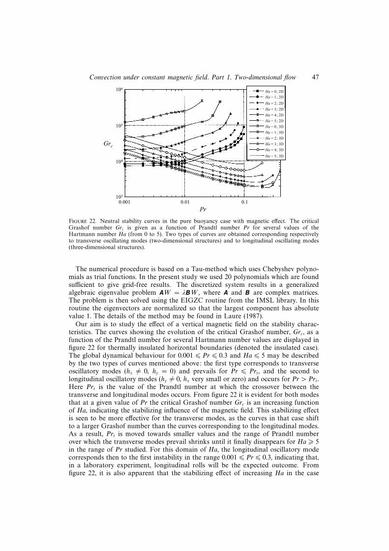
Our aim is to study the effect of a vertical magnetic field on the stability charac-teristics. The curves showing the evolution of the critical Grashof number, Grc, as afunction of the Prandtl number for several Hartmann number values are displayed infigure 22 for thermally insulated horizontal boundaries (denoted the insulated case).The global dynamical behaviour for 0.001 6 Pr 6 0.3 and Ha 6 5 may be describedby the two types of curves mentioned above: the first type corresponds to transverseoscillatory modes (hx 6= 0, hy = 0) and prevails for Pr 6 Prt, and the second tolongitudinal oscillatory modes (hy 6= 0, hx very small or zero) and occurs for Pr > Prt.Here Prt is the value of the Prandtl number at which the crossover between thetransverse and longitudinal modes occurs. From figure 22 it is evident for both modesthat at a given value of Pr the critical Grashof number Grc is an increasing functionof Ha, indicating the stabilizing influence of the magnetic field. This stabilizing effectis seen to be more effective for the transverse modes, as the curves in that case shiftto a larger Grashof number than the curves corresponding to the longitudinal modes.As a result, Prt is moved towards smaller values and the range of Prandtl numberover which the transverse modes prevail shrinks until it finally disappears for Ha > 5in the range of Pr studied. For this domain of Ha, the longitudinal oscillatory modecorresponds then to the first instability in the range 0.001 6 Pr 6 0.3, indicating that,in a laboratory experiment, longitudinal rolls will be the expected outcome. Fromfigure 22, it is also apparent that the stabilizing effect of increasing Ha in the case
48 H. Ben Hadid, D. Henry and S. Kaddeche
10–1
0 3
Ha
Prt
10–3
10–4
10–2
21 4 5
Insulating case
Conducting case
Figure 23. Variation with Ha of Prt which is the value of the Prandtl number corresponding to thetransition between transverse and longitudinal modes. Buoyancy-driven flow case in the rigid–freecavity and for two thermal boundary conditions.
0 15
Ha2
Grc
4
105 20 25
Longitudinal modes
8
12 Transverse modes
(× 104) ~ Ha2
~ exp (Ha2/9)
Figure 24. Neutral stability curves in the pure buoyancy case with magnetic effect. The criticalGrashof number Grc is given as a function of Ha2 for Pr = 0.001. The evolution is in Ha2 for thetransverse modes and in exp(Ha2/9) for the longitudinal modes.
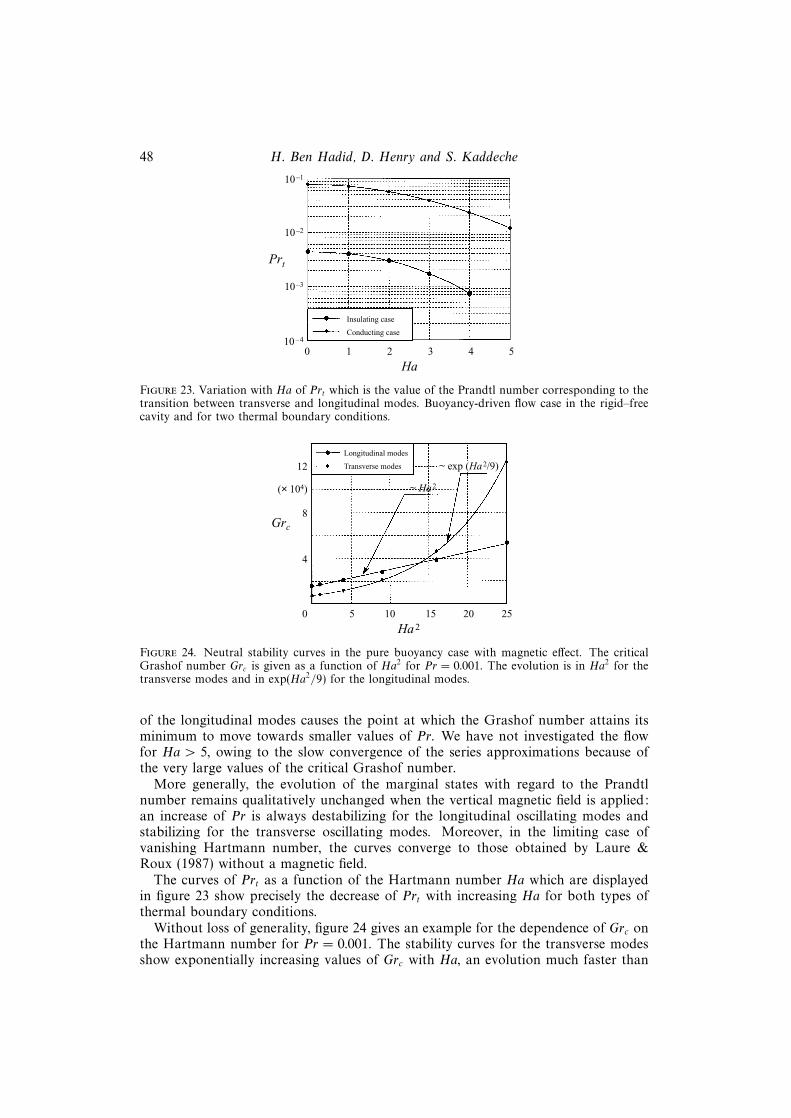
of the longitudinal modes causes the point at which the Grashof number attains itsminimum to move towards smaller values of Pr. We have not investigated the flowfor Ha > 5, owing to the slow convergence of the series approximations because ofthe very large values of the critical Grashof number.
More generally, the evolution of the marginal states with regard to the Prandtlnumber remains qualitatively unchanged when the vertical magnetic field is applied:an increase of Pr is always destabilizing for the longitudinal oscillating modes andstabilizing for the transverse oscillating modes. Moreover, in the limiting case ofvanishing Hartmann number, the curves converge to those obtained by Laure &Roux (1987) without a magnetic field.
The curves of Prt as a function of the Hartmann number Ha which are displayedin figure 23 show precisely the decrease of Prt with increasing Ha for both types ofthermal boundary conditions.
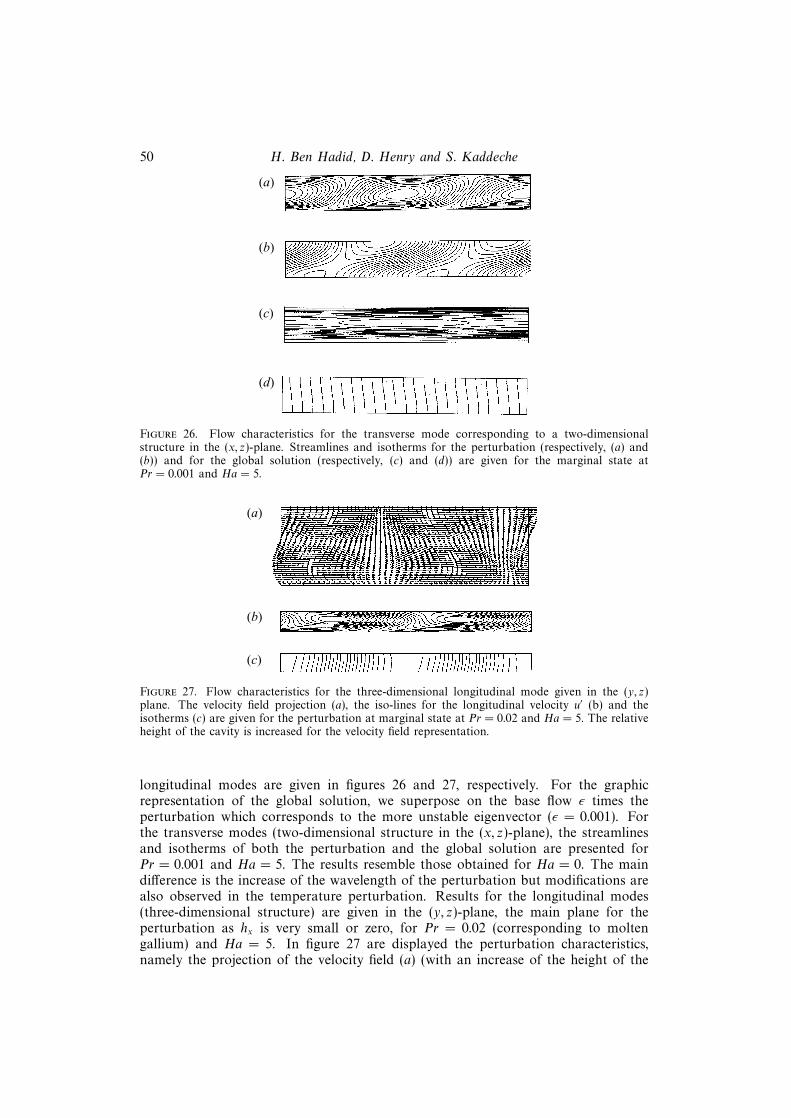
Without loss of generality, figure 24 gives an example for the dependence of Grc onthe Hartmann number for Pr = 0.001. The stability curves for the transverse modesshow exponentially increasing values of Grc with Ha, an evolution much faster than

Convection under constant magnetic field. Part 1. Two-dimensional flow 49
12
10
6
40.001 0.01 0.1
Pr
kx
14
Ha = 2Ha = 1Ha = 0
Ha = 3
8
Ha = 4Ha = 5
(a)
60
20
00.001 0.01 0.1
Pr
ky
80
40
(b)
Figure 25. Variation with Pr of the wavelength of the neutral modes for several values of theHartmann number: (a) transverse modes (λx); (b) longitudinal modes (λy).
for the longitudinal modes. In fact, from the results it is possible to derive for eachmode a simple relationship giving the dependence of Grc on Ha. This relationshipmay be written in the form Grc ∼ exp(Ha2/9) for the transverse modes and Grc ∼ Ha2
for the longitudinal modes. More general relationships may be found by including theeffect of Pr: Grc ∼ Ha2Pr−1/2 for the longitudinal modes, valid for 0.001 6 Pr 6 0.1,and again Grc ∼ exp(Ha2/9) for the transverse modes, valid in the limit of very smallPr. Note that the Ha2 dependence of the critical Grashof number was pointed out inthe experimental investigations of Hurle et al. (1974).
We display in figure 25 the curves of critical wavelength as a function of the Prandtlnumber for the transverse (λx = 2π/hx) and longitudinal (λy = 2π/hy) oscillatorymodes. Examination of these curves reveals that for Pr < 0.02, the variation of λxwith Pr is relatively small, but it becomes more important for Pr > 0.02. For λy arapid decrease is observed in the range Pr < 0.1. For the longitudinal modes, anincrease of Ha up to 5 produces relatively moderate effects on λy which goes downas Ha is increased. In contrast, for the transverse modes, the curves for λx are shiftedup and appear to be more sensitive to the effect of the magnetic field. This featurecorresponds to an increase of the size of the secondary transverse cells as Ha increases.It is qualitatively contrary to what is observed in the Rayleigh–Benard problem (seeChandrasekhar 1961), where the cells tend to become more narrow as the strength ofthe magnetic field is increased.
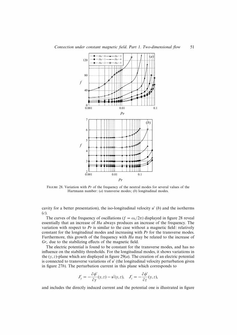
Typical characteristics of the flow at the marginal state for the transverse and
50 H. Ben Hadid, D. Henry and S. Kaddeche
(a)
(b)
(c)
(d)
Figure 26. Flow characteristics for the transverse mode corresponding to a two-dimensionalstructure in the (x, z)-plane. Streamlines and isotherms for the perturbation (respectively, (a) and(b)) and for the global solution (respectively, (c) and (d)) are given for the marginal state atPr = 0.001 and Ha = 5.
(a)
(b)
(c)
Figure 27. Flow characteristics for the three-dimensional longitudinal mode given in the (y, z)plane. The velocity field projection (a), the iso-lines for the longitudinal velocity u′ (b) and theisotherms (c) are given for the perturbation at marginal state at Pr = 0.02 and Ha = 5. The relativeheight of the cavity is increased for the velocity field representation.
longitudinal modes are given in figures 26 and 27, respectively. For the graphicrepresentation of the global solution, we superpose on the base flow ε times theperturbation which corresponds to the more unstable eigenvector (ε = 0.001). Forthe transverse modes (two-dimensional structure in the (x, z)-plane), the streamlinesand isotherms of both the perturbation and the global solution are presented forPr = 0.001 and Ha = 5. The results resemble those obtained for Ha = 0. The maindifference is the increase of the wavelength of the perturbation but modifications arealso observed in the temperature perturbation. Results for the longitudinal modes(three-dimensional structure) are given in the (y, z)-plane, the main plane for theperturbation as hx is very small or zero, for Pr = 0.02 (corresponding to moltengallium) and Ha = 5. In figure 27 are displayed the perturbation characteristics,namely the projection of the velocity field (a) (with an increase of the height of the
Convection under constant magnetic field. Part 1. Two-dimensional flow 51
120
80
00.001 0.01 0.1
Pr
f
Ha = 2
Ha = 1Ha = 0
40
(a)
5
3
20.001 0.01 0.1
Pr
f
6
4
(b)
Ha = 5
Ha = 4Ha = 3
7
Figure 28. Variation with Pr of the frequency of the neutral modes for several values of theHartmann number: (a) transverse modes; (b) longitudinal modes.
cavity for a better presentation), the iso-longitudinal velocity u′ (b) and the isotherms(c).
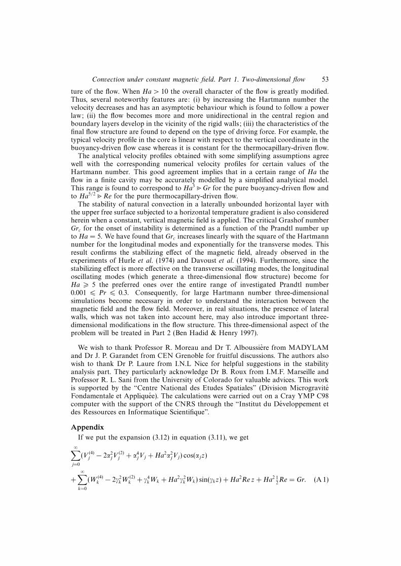
The curves of the frequency of oscillations (f = ωi/2π) displayed in figure 28 revealessentially that an increase of Ha always produces an increase of the frequency. Thevariation with respect to Pr is similar to the case without a magnetic field: relativelyconstant for the longitudinal modes and increasing with Pr for the transverse modes.Furthermore, this growth of the frequency with Ha may be related to the increase ofGrc due to the stabilizing effects of the magnetic field.
The electric potential is found to be constant for the transverse modes, and has noinfluence on the stability thresholds. For the longitudinal modes, it shows variations inthe (y, z)-plane which are displayed in figure 29(a). The creation of an electric potentialis connected to transverse variations of u′ (the longitudinal velocity perturbation givenin figure 27b). The perturbation current in this plane which corresponds to
J ′y = −∂φ′
∂y(y, z)− u′(y, z), J ′z = −∂φ
′
∂z(y, z),
and includes the directly induced current and the potential one is illustrated in figure

52 H. Ben Hadid, D. Henry and S. Kaddeche
(a)
(b)
Figure 29. Electric characteristics for the three-dimensional longitudinal mode given in the(y, z)-plane. The iso-lines for the electric potential (a) and the electric current projection (b)are given for the perturbation at marginal state at Pr = 0.02 and Ha = 5.
29(b). The global current in the cavity is in fact given by
J ′x = v′(y, z), J ′y = −∂φ′
∂y(y, z)− (u′(y, z) + u(z)), J ′z = −∂φ
′
∂z(y, z),
but the two new terms are conservative. The effect of the electric potential, as seenin the (y, z)-plane, is thus to slow down the directly induced current and to allowcounter circulation along the boundaries (mainly the no-slip bottom boundary) forthe conservation of the current. The potential will then decrease the stabilizing effectgenerated by the directly induced current. This is confirmed by the fact that for thelongitudinal modes the instability thresholds increase if we neglect the potential effect.
The results obtained with thermally conducting horizontal boundaries reveal thesame qualitative influence of the Hartmann number on the main characteristics ofthe transverse and longitudinal oscillatory modes. The main differences are connectedwith the influence of Pr and were already observed without a magnetic field: first thevalue of Prt is larger (see figure 23) and then the variation with Pr of the wavelengthand of the frequency of the longitudinal modes are changed.
Some general comments on the stability analyses can be made. The action of themagnetic field on the stability characteristics is twofold: it appears in the analyticalvelocity and temperature equations for the basic state as well as in the linearizedgoverning equation (6.2) in the Lorentz force term. It is established from the foregoingresults (see §5) that the asymptotic behaviour of the velocity (with a Ha−2 dependence)occurs only for Ha > 10. As all our results in the stability analysis are obtained forHa 6 5, this may suggest that the stabilizing effect is more effective in the Lorentzforce which is directly proportional to Ha2. Concerning the different variation withHa of the transverse and longitudinal modes, it may be noted that the transversemodes are of dynamical origin (asymptotic behaviour for Pr = 0 and increase ofthe thresholds as Pr increases) whereas the longitudinal modes are of thermal origin(increase of the thresholds as Pr decreases). Moreover, the decrease of wavelength asHa is increased is observed for our longitudinal modes as well as in the Rayleigh–Benard situation, both corresponding to instabilities of thermal origin.
7. ConclusionsWe investigated the effect of a constant magnetic field on the flow states in a dif-
ferentially heated horizontal Bridgman cavity. We derived analytical solutions for thehorizontal velocity in the central region and for the two components of the velocity inthe turning flow region. We also performed numerical simulations for a cavity with amoderate aspect ratio A = 4. One obvious finding is that for increasing values of theHartmann number, i.e. for increasing strength of the magnetic field, the intensity of theconvective flow decreases and is followed by a progressive change of the overall struc-
Convection under constant magnetic field. Part 1. Two-dimensional flow 53
ture of the flow. When Ha > 10 the overall character of the flow is greatly modified.Thus, several noteworthy features are: (i) by increasing the Hartmann number thevelocity decreases and has an asymptotic behaviour which is found to follow a powerlaw; (ii) the flow becomes more and more unidirectional in the central region andboundary layers develop in the vicinity of the rigid walls; (iii) the characteristics of thefinal flow structure are found to depend on the type of driving force. For example, thetypical velocity profile in the core is linear with respect to the vertical coordinate in thebuoyancy-driven flow case whereas it is constant for the thermocapillary-driven flow.
The analytical velocity profiles obtained with some simplifying assumptions agreewell with the corresponding numerical velocity profiles for certain values of theHartmann number. This good agreement implies that in a certain range of Ha theflow in a finite cavity may be accurately modelled by a simplified analytical model.This range is found to correspond to Ha3�Gr for the pure buoyancy-driven flow andto Ha5/2�Re for the pure thermocapillary-driven flow.
The stability of natural convection in a laterally unbounded horizontal layer withthe upper free surface subjected to a horizontal temperature gradient is also consideredherein when a constant, vertical magnetic field is applied. The critical Grashof numberGrc for the onset of instability is determined as a function of the Prandtl number upto Ha = 5. We have found that Grc increases linearly with the square of the Hartmannnumber for the longitudinal modes and exponentially for the transverse modes. Thisresult confirms the stabilizing effect of the magnetic field, already observed in theexperiments of Hurle et al. (1974) and Davoust et al. (1994). Furthermore, since thestabilizing effect is more effective on the transverse oscillating modes, the longitudinaloscillating modes (which generate a three-dimensional flow structure) become forHa > 5 the preferred ones over the entire range of investigated Prandtl number0.001 6 Pr 6 0.3. Consequently, for large Hartmann number three-dimensionalsimulations become necessary in order to understand the interaction between themagnetic field and the flow field. Moreover, in real situations, the presence of lateralwalls, which was not taken into account here, may also introduce important three-dimensional modifications in the flow structure. This three-dimensional aspect of theproblem will be treated in Part 2 (Ben Hadid & Henry 1997).
We wish to thank Professor R. Moreau and Dr T. Alboussiere from MADYLAMand Dr J. P. Garandet from CEN Grenoble for fruitful discussions. The authors alsowish to thank Dr P. Laure from I.N.L Nice for helpful suggestions in the stabilityanalysis part. They particularly acknowledge Dr B. Roux from I.M.F. Marseille andProfessor R. L. Sani from the University of Colorado for valuable advices. This workis supported by the “Centre National des Etudes Spatiales” (Division MicrograviteFondamentale et Appliquee). The calculations were carried out on a Cray YMP C98computer with the support of the CNRS through the “Institut du Developpement etdes Ressources en Informatique Scientifique”.
AppendixIf we put the expansion (3.12) in equation (3.11), we get
∞∑j=0
(V (4)j − 2α2
jV(2)j + α4
jVj + Ha2α2jVj) cos(αjz)
+
∞∑k=0
(W (4)k − 2γ2
kW(2)k + γ4
kWk + Ha2γ2kWk) sin(γkz) + Ha2Re z + Ha2 1
2Re = Gr. (A 1)
54 H. Ben Hadid, D. Henry and S. Kaddeche
We need then to express the functions 1, z, z2 and z3 in the orthogonal basis of thesine and cosine functions. We get
1 =
∞∑j=0
4(−1)j
αjcos(αjz), (z2 − 4) =
∞∑j=0
−8(−1)j
α3j
cos(αjz), (A 2)
z =
∞∑k=0
2(−1)k
γksin(γkz), (z3 − 1
4z) =
∞∑k=0
−12(−1)k
γ3k
sin(γkz). (A 3)
By replacing Ha2Re z and (Ha2 Re/2−Gr) by their expansions and taking into accountthe orthogonality of the sine and cosine functions, we obtain
∀j, V(4)j − 2α2
jV(2)j + (α4
j + Ha2α2j )Vj = gj, (A 4)
and
∀k, W(4)k − 2γ2
kW(2)k + (γ4
k + Ha2γ2k )Wk = hk, (A 5)
with
gj = (−Ha2 12Re + Gr)
4(−1)j
αjand hk = −Ha2Re
2(−1)k
γk.
These two equations have the same form. Let us consider the first one. Its character-istic equation is
m4 − 2α2jm
2 + (α4j + Ha2α2
j ) = 0
and the solution is of the form m = ±aj ± ibj with
aj =1√2
(α2j + αj(Ha2 + α2
j )1/2)1/2
and bj =1√2
(−α2
j + αj(Ha2 + α2j )
1/2)1/2
.
A particular solution of the global equation is gj/(α4j + Ha2α2
j ). We can then write theglobal solution as
Vj(x) = λje−ajx cos(bjx) + µje
−ajx sin(bjx) + λ′jeajx cos(bjx) + µ′je
ajx sin(bjx)
+gj
α4j + Ha2α2
j
.
As Vj must be finite as x tends towards infinity, λ′j and µ′j must be zero. We havethen for Vj and Wk
Vj(x) = λje−ajx cos(bjx) + µje
−ajx sin(bjx) +gj
α4j + Ha2α2
j
, (A 6)
and
Wk(x) = νke−ckx cos(dkx) + πke
−ckx sin(dkx) +hk
γ4k + Ha2γ2
k
, (A 7)
with ck and dk defined as aj and bj . The solution is then obtained from (3.12) withthe expressions for Vj and Wk given above.
We must then verify the boundary conditions at x = 0: ψ = 0 and (∂ψ/∂x) = 0.For that, we need to know the expansion of the polynome P on the basis. By usingexpressions (A 2)–(A 3), we can write
ψ =
∞∑j=0
(Vj(x)− Vj0) cos(αjz) +
∞∑k=0
(Wk(x)−Wk0) sin(γkz),
Convection under constant magnetic field. Part 1. Two-dimensional flow 55
with
Vj0 = −Re2(−1)j
α3j
and Wk0 = −Re2(−1)k
γ3k
.
The boundary conditions are then
∀j, Vj(x = 0) = Vj0 and V ′j (x = 0) = 0,
and
∀k, Wk(x = 0) = Wk0 and W ′k(x = 0) = 0,
which gives
λj = Vj0 −gj
α4j + Ha2α2
j
, µj =aj
bjλj ,
and
νk = Wk0 −hk
γ4k + Ha2γ2
k
, πk =ck
dkνk.
REFERENCES
Alboussiere, T., Garandet, J. P. & Moreau, R. 1993 Buoyancy-driven convection with a uniformmagnetic field. Part 1. Asymptotic analysis. J. Fluid Mech. 253, 545–563.
Baumgartl, J. & Muller, G. 1992 Calculation of the effects of magnetic field damping onfluid flow – Comparison of magnetohydrodynamic models of different complexity. In Proc.VIIIth European Symposium on Materials and Fluid Sciences in Microgravity (ESA SP-333),pp. 161–164. ESA Publ. Division c/o ESTEC, Noordwijk, The Netherlands.
Ben Hadid, H. 1989 Etude numerique des mouvements convectifs au sein des fluides de faiblenombre de Prandtl. These de Doctorat d’Etat, University of Aix-Marseille II, France.
Ben Hadid, H. & Henry, D. 1997 Numerical study of convection in the horizontal Bridgmanconfiguration under the action of a constant magnetic field. Part 2. Three-dimensional flow. J.Fluid Mech. 333, 57–83.
Ben Hadid, H. & Roux, B. 1990 Thermocapillary convection in long horizontal layers of low-Prandtl-number melts subject to a horizontal temperature gradient. J. Fluid Mech. 221, 77–103.
Ben Hadid, H. & Roux, B. 1992 Buoyancy- and thermocapillary-driven flows in differentiallyheated cavities for low-Prandtl-number fluids. J. Fluid Mech. 235, 1–36.
Carruthers, J. R. 1977 Thermal convection instabilities relevant to crystal growth from liquids. InPreparation and Properties of Solid state Materials (ed. W. R. Wilcox & R. A. Lefever), Vol. 3.M. Dekker.
Chandrasekhar, S. 1961 Hydrodynamic and Hydromagnetic Stability. Clarendon Press.
Davoust, L., Moreau, R., Bolcato, R., Alboussiere, T., Neubrand, A. C. & Garandet, J. P.
1994 Influence of a vertical magnetic field on convection in the horizontal Bridgman crystalgrowth configuration. In Proc. 2nd Intl Conf. on Energy Transfer in Magnetohydrodynamicflows, Aussois, France, Vol. 1, pp. 15–26.
Garandet, J. P., Alboussiere, T. & Moreau, R. 1992 Buoyancy driven convection in a rectangularenclosure with a transverse magnetic field. Intl J. Heat Mass Transfer 35, 741–748.
Hart, J. E. 1972 Stability of thin non-rotating Hadley circulations. J. Atmos. Sci. 29, 687–697.
Hart, J. E. 1983 A note on the stability of low-Prandtl-number Hadley circulations. J. Fluid Mech.132, 271–281.
Hung, M.C. & Andereck, C.D. 1988 Transitions in convection driven by a horizontal temperaturegradient. Phys. Lett. A 132, 253–258.
Hung, M.C. & Andereck, C.D. 1990 Subharmonic transitions in convection in a moderatelyshallow cavity. In Numerical Simulation of Oscillatory Convection in low-Pr Fluids (ed. B.Roux). Notes on Numerical Fluid Mechanics, vol. 27, pp. 338–343. Vieweg.
Hurle, D. T. J., Jakeman, E. & Johnson, C. P. 1974 Convective temperature oscillations in moltengallium. J. Fluid Mech. 64, 565–576.
56 H. Ben Hadid, D. Henry and S. Kaddeche
Kaddeche, S., Ben Hadid, H. & Henry, D. 1994 Macrosegregation and convection in the horizontalBridgman configuration. I. Dilute alloys. J. Cryst. Growth 135, 341–353.
Kim, D.H., Adornato, P.M. & Brown, R.A. 1988 Effect of vertical magnetic field on convectionand segregation in vertical Bridgman crystal growth. J. Cryst. Growth 89, 339–356.
Laure, P. 1987 Etude des mouvements de convection dans une cavite rectangulaire soumise a ungradient de temperature horizontal. J. Mec. Theor. Appl. 6, 351–382.
Laure, P. & Roux, B. 1987 Synthese des resultats obtenus par l’etude de stabilite des mouvementsde convection dans une cavite horizontale de grande extension. C. R. Acad. Sci. Paris 305,1137–1143.
Motakef, S. 1990 Magnetic field elimination of convective interference with segregation duringvertical-Bridgman growth of doped semiconductors. J. Cryst. Growth 104, 833–850.
Oreper, G.M. & Szekely, J. 1983 The effect of an externally imposed magnetic field on buoyancydriven flow in a rectangular cavity. J. Cryst. Growth 64, 505–515.
Oreper, G.M. & Szekely, J. 1984 The effect of a magnetic field on transport phenomena in aBridgman-Stockbarger crystal growth. J. Cryst. Growth 67, 405–419.
Ozoe, H. & Okada, K. 1989 The effect of the direction of the external magnetic field on thethree-dimensional natural convection in a cubical enclosure. Intl J. Heat Mass Transfer 32,1939–1954.
Pratte, J.M. & Hart, J. E. 1990 Endwall driven, low Prandtl number convection in a shallowrectangular cavity. J. Cryst. Growth 102, 54–68.
Roux, B. (Ed.) 1990 GAMM Workshop : Numerical Simulation of Oscillatory Convection in low-PrFluids. Notes on Numerical Fluid Mechanics, vol. 27. Vieweg.
Roux, B., Bontoux, P., Loc, T. P. & Daube, O. 1979 Optimisation of Hermitian Methods for N. S.Equations in Vorticity and Stream Function Formulation. Lecture Notes in Mathematics, vol.771, pp. 450–468. Springer.
Roux, B., Ben Hadid, H. & Laure, P. 1989 Hydrodynamical regimes in metallic melts subject to ahorizontal temperature gradient. Eur. J. Mech. B/Fluids 8, 375–396.
Series, R.W. & Hurle, D. T. J. 1991 The use of magnetic fields in semiconductor crystal growth.J. Cryst. Growth 113, 305–328.
Thompson, J. F., Thames, F. C. & Mastin, C.W. 1974 Automatic numerical generation of a body-fitted curvilinear system. J. Comput. Phys. 15, 299–319.