Fluid Dynamics Research 31 (2002) 275–287

Edge wave scattering by a coastal structure

A. Baquerizoa ;∗, M.A. Losadaa, I.J. Losadab

aGrupo de Puertos y Costas de la Universidad de Granada, Edif. Fray Luis de Granada, Ram�on y Cajal 4, 18071,Granada, Spain

bGrupo de Ingenier�%a Oceanogr�a(ca y de Costas, Universidad de Cantabria, Spain

Received 19 September 2001; received in revised form 1 August 2002; accepted 2 August 2002Communicated by K. Nadaoka

Abstract

The propagation of an incident edge wave on a straight beach with a coastal structure perpendicular to thecoastline is analyzed. A simple idealized beach pro6le with a steep foreshore, a plane slope and a horizontalshelf on an in6nitely long straight shoreline is considered. The edge wave is re7ected and transmitted at thestructure and, by assuming that its width is much smaller than the alongshore wave length, the solution to theproblem is obtained by a mode matching method including the head loss at the structure. The existence of thesteep foreshore and the shelf modi6es the dispersion equation of the trapped modes obtained by Eckart (WaveReport 100, Ref. 51-12, Scripps Institute of Oceanography, University of California, La Jolla, 1951, 99pp).The re7ection coe=cient, de6ned by the ratio of the incident and re7ected edge wave amplitudes, depends onthe friction coe=cient at the coastal structure.c© 2002 Published by The Japan Society of Fluid Mechanics and Elsevier Science B.V. All rights reserved.

MSC: 92.10.H; 47.35

Keywords: Edge waves; Wave re7ection; Head loss; Friction coe=cient

1. Introduction

Edge waves exist near the shore and are often said to be trapped to the coast in the sense that waveenergy propagates parallel to the shoreline and cannot escape from it. They can occur in a variety ofdiBerent scales: high-frequency waves resonated by the incident wind waves (Guza and Davis, 1974),forced by incident wave groups (SchEaBer, 1990) and very low-frequency waves of oceanographicscale (Munk et al., 1956). Edge waves may play an important role in coastal dynamics, as they are

∗ Corresponding author. Tel.: +34-958-248315; fax: +34-958-248314.E-mail address: abaqueri@ugr.es (A. Baquerizo).

0169-5983/01/$22.00 c© 2002 Published by The Japan Society of Fluid Mechanics and Elsevier Science B.V.All rights reserved.PII: S0169-5983(02)00119-3

276 A. Baquerizo et al. / Fluid Dynamics Research 31 (2002) 275–287

linked to the formation of rip currents (Bowen and Inman, 1969) or beach cusps (Guza and Inman,1975). Recently, Ciriano et al. (2000) have shown that edge waves may induce resonant oscillationsinside harbors with the mouth being opened to the beach. The phenomenon of topographically trappedwaves in headlands and estuaries has been studied theoretically by Stoker and Johnson (1991), whoseresults agree with 6eld observations by Schwing (1989).

Edge wave theory dates back to Stokes’ (1846) solution for a wave trapped on a plane slopingbeach. Eckart (1951) applied the linear shallow water theory and showed that Stokes’ solutionrepresented only the 6rst of other possible modes. Ursell (1952) obtained the exact solution tothe linearized boundary problem. Green (1986) outlined the solution of the problem of an edgewave propagating along a seawall. Neu and Oh (1987) presented a method to solve the type ofedge wave problems where the nearshore topography is represented by a series of linearly varyingdepth segments. They wrote the solution in terms of Kummer’s functions and considered two beachpro6les: a constant beach slope terminated with a constant depth region and the case of an oBshorebar.

A classical solution in coastal engineering to prevent the erosion of a beach or to have thecontrol of the alongshore sediment transport is to build a groin perpendicular to the coastline. Thesestructures, built with stones or as platform piles, are permeable. Moreover, some beaches have apier perpendicular to the coastline in order to have access to deeper waters.

In this paper, the propagation and transformation of an incident edge wave through a permeablecoastal structure is explored in a fashion that resembles the one addressed by Stoker and Johnson(1991). The edge wave problem is formulated following Neu and Oh’s solution. A beach pro6le witha steep foreshore and a plane slope ending with a horizontal shelf with a perpendicular permeablestructure extending from the shoreline up to far oBshore is considered. Because the width of thegroins compared to the edge wave length is very small, usually less than 1/50, dissipation inside thestructure is mainly due to the sudden contraction and expansion of the 7ow and depends mainly onthe Keulegan–Carpenter number de6ned as UT=a, where U is a representative velocity at the gaps,T is the wave period and a is a characteristic dimension of the holes. For groins, UT=a is a largenumber and therefore head loss can be satisfactorily calculated with a formula quadratic to the localvelocity (Mei et al., 1974).

As the edge wave propagates through the coastal structure, part of its alongshore energy is re-7ected, part is transmitted and part is dissipated on the structure. The re7ected part interferes withthe incoming wave, building up a partial standing wave pattern which may help to develop ripcurrents, crescentic bars or other beach morphologic features. The transmitted part propagates down-wards as an edge wave with the same mode as the incident wave. In this research, the re7ectionand transmission coe=cients, which depend on the friction loss occurring at the coastal structure,are evaluated.

The paper is organized as follows. First, the problem of an edge wave propagating on an in-6nitely long, straight coastline, with a steep foreshore and a shelf is formulated. Next, the theoreti-cal closed-form solution is evaluated numerically; the dispersion equation is solved and results aregraphically presented for the propagating modes as well as for the evanescent modes that are neededto solve properly the matching conditions at the structure. Then, the scattering of the edge wavewhile impinging the coastal structure is analyzed. For that purpose, a mixed boundary condition atthe structure is established (Sneddon, 1966). Finally, the re7ection and the transmission coe=cientsand the water surface elevation around the structure are obtained.

A. Baquerizo et al. / Fluid Dynamics Research 31 (2002) 275–287 277

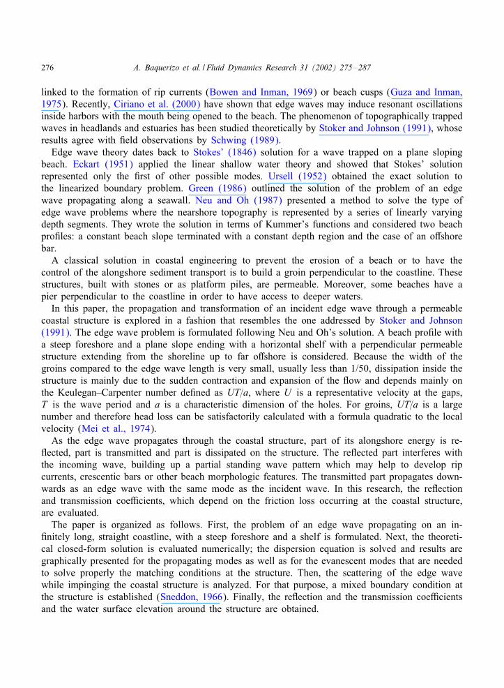
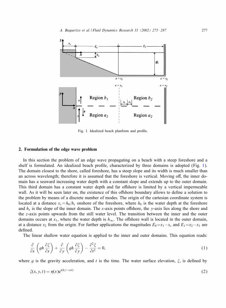
Fig. 1. Idealized beach planform and pro6le.

2. Formulation of the edge wave problem

In this section the problem of an edge wave propagating on a beach with a steep foreshore and ashelf is formulated. An idealized beach pro6le, characterized by three domains is adopted (Fig. 1).The domain closest to the shore, called foreshore, has a steep slope and its width is much smaller thanan across wavelength; therefore it is assumed that the foreshore is vertical. Moving oB, the inner do-main has a seaward increasing water depth with a constant slope and extends up to the outer domain.This third domain has a constant water depth and far oBshore is limited by a vertical impermeablewall. As it will be seen later on, the existence of this oBshore boundary allows to de6ne a solution tothe problem by means of a discrete number of modes. The origin of the cartesian coordinate system islocated at a distance xs=h0=hx onshore of the foreshore, where h0 is the water depth at the foreshoreand hx is the slope of the inner domain. The x-axis points oBshore, the y-axis lies along the shore andthe z-axis points upwards from the still water level. The transition between the inner and the outerdomains occurs at x1, where the water depth is h∞. The oBshore wall is located in the outer domain,at a distance x2 from the origin. For further applications the magnitudes E0=x1−xs and E1=x2−x1 arede6ned.

The linear shallow water equation is applied to the inner and outer domains. This equation reads:

@@x

(gh@�@x

)+

@@y

(gh@�@y

)− @2�@t2

= 0; (1)

where g is the gravity acceleration, and t is the time. The water surface elevation, �, is de6ned by

�(x; y; t) = �(x)ei(ky−!t) (2)

278 A. Baquerizo et al. / Fluid Dynamics Research 31 (2002) 275–287

! is the angular frequency and k is the alongshore wave number. The governing shallow waterequation is re-formulated in terms of the function �:

ddx

(gh

d�dx

)+ (!2 − ghk2)�= 0: (3)

The problem is solved in each region and the following boundary and matching conditions areimposed:

1. The across-shore velocities at the foreshore and at the oBshore wall must be zero.2. Surface elevations must be equal at x1.3. The across-shore velocities must be equal at x1.

2.1. Solution to the edge wave problem

In this section a solution to the shallow water equation for the inner and the outer domains isobtained. At the constant depth region the surface elevation depends on the parameter � = 1 −!2=gh∞k2,

�=

{Ce−

√�kx + De

√�kx if � �= 0;

Cx + D if �= 0:(4)

For k real, k ¿ 0 (propagating modes in the alongshore direction) and �¿ 0, Eq. (4) correspondsto trapped wave solutions. Values of �¡ 0 give oscillatory motions and, therefore, correspond tonon-trapped waves. On the other hand, if k is purely imaginary, k = ike; ke real, Eq. (4) correspondsto evanescent modes in the alongshore direction that, because �¿ 0, are oscillatory on the shelf.

For the plane slope domain, introducing a new independent variable, r=2kx, and a new dependentvariable, �(r), related to the amplitude of the surface elevation, �, as follows:

�= er=2�(r) (5)

Eq. (3) transforms into,

rd2�dr2

+ (1− r)d�dr

− a� = 0; (6)

where, a = −1=2(!2=ghxk − 1). The solution to this equation (Green, 1986), is written as a linearcombination of Kummer’s functions (con7uent hypergeometric functions) of 6rst and second kind,denoted by M (a; r) =M (a; b= 1; r) and U (a; r) = U (a; b= 1; r)

�(r) = AM (a; r) + BU (a; r); (7)

where A and B are constants. For a beach without a foreshore, that is, for h0 = 0, the U functionmust be excluded since it has a logarithmic singularity at r = 0.Applying the boundary condition at the foreshore and at the oBshore wall and matching the surface

elevations and their derivatives at x1, a system of two linear homogeneous equations governing theamplitudes A and C, is obtained. Equating to zero the determinant of the matrix to guarantee theexistence of a non-trivial solution, the dispersion relationship results. For a given r1=2kx1, the valueof a that satis6es the dispersion equation can be obtained numerically.

A. Baquerizo et al. / Fluid Dynamics Research 31 (2002) 275–287 279

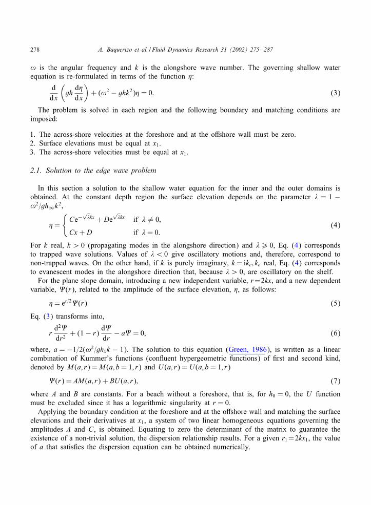
Fig. 2. Dispersion relation curves of edge wave propagating modes in terms of the parameter a of the con7uent hyper-geometric equation for the values of the parameters h0 = 1 (m), hx = 0:03; E0 = 500 (m) and E1 = 200 (m).

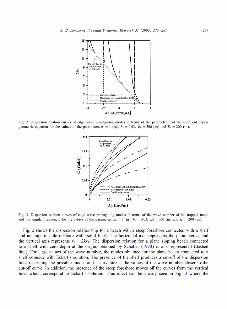
Fig. 3. Dispersion relation curves of edge wave propagating modes in terms of the wave number of the trapped modeand the angular frequency, for the values of the parameters h0 = 1 (m), hx = 0:03; E0 = 500 (m) and E1 = 200 (m).

Fig. 2 shows the dispersion relationship for a beach with a steep foreshore connected with a shelfand an impermeable oBshore wall (solid line). The horizontal axis represents the parameter a, andthe vertical axis represents r1 = 2kx1. The dispersion relation for a plane sloping beach connectedto a shelf with zero depth at the origin, obtained by SchEaBer (1990) is also represented (dashedline). For large values of the wave number, the modes obtained for the plane beach connected to ashelf coincide with Eckart’s solution. The presence of the shelf produces a cut-oB of the dispersionlines restricting the possible modes and a curvature at the values of the wave number closer to thecut-oB curve. In addition, the presence of the steep foreshore moves oB the curves from the verticallines which correspond to Eckart’s solution. This eBect can be clearly seen in Fig. 3 where the

280 A. Baquerizo et al. / Fluid Dynamics Research 31 (2002) 275–287

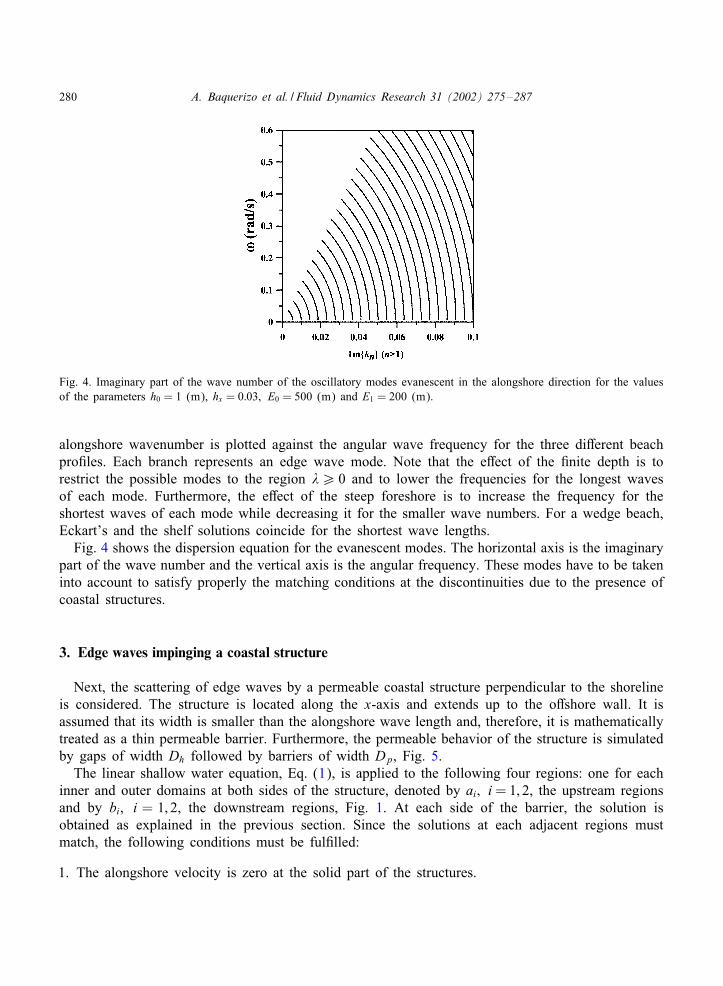
Fig. 4. Imaginary part of the wave number of the oscillatory modes evanescent in the alongshore direction for the valuesof the parameters h0 = 1 (m), hx = 0:03; E0 = 500 (m) and E1 = 200 (m).

alongshore wavenumber is plotted against the angular wave frequency for the three diBerent beachpro6les. Each branch represents an edge wave mode. Note that the eBect of the 6nite depth is torestrict the possible modes to the region �¿ 0 and to lower the frequencies for the longest wavesof each mode. Furthermore, the eBect of the steep foreshore is to increase the frequency for theshortest waves of each mode while decreasing it for the smaller wave numbers. For a wedge beach,Eckart’s and the shelf solutions coincide for the shortest wave lengths.

Fig. 4 shows the dispersion equation for the evanescent modes. The horizontal axis is the imaginarypart of the wave number and the vertical axis is the angular frequency. These modes have to be takeninto account to satisfy properly the matching conditions at the discontinuities due to the presence ofcoastal structures.

3. Edge waves impinging a coastal structure

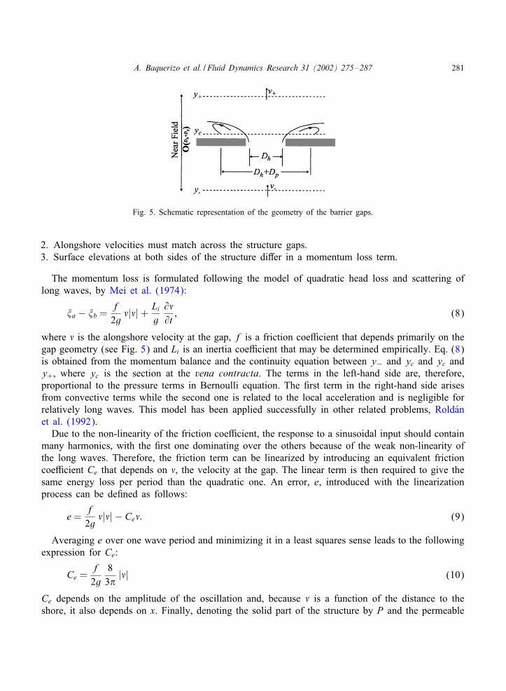
Next, the scattering of edge waves by a permeable coastal structure perpendicular to the shorelineis considered. The structure is located along the x-axis and extends up to the oBshore wall. It isassumed that its width is smaller than the alongshore wave length and, therefore, it is mathematicallytreated as a thin permeable barrier. Furthermore, the permeable behavior of the structure is simulatedby gaps of width Dh followed by barriers of width Dp, Fig. 5.

The linear shallow water equation, Eq. (1), is applied to the following four regions: one for eachinner and outer domains at both sides of the structure, denoted by ai; i= 1; 2, the upstream regionsand by bi; i = 1; 2, the downstream regions, Fig. 1. At each side of the barrier, the solution isobtained as explained in the previous section. Since the solutions at each adjacent regions mustmatch, the following conditions must be ful6lled:

1. The alongshore velocity is zero at the solid part of the structures.

A. Baquerizo et al. / Fluid Dynamics Research 31 (2002) 275–287 281

Fig. 5. Schematic representation of the geometry of the barrier gaps.

2. Alongshore velocities must match across the structure gaps.3. Surface elevations at both sides of the structure diBer in a momentum loss term.

The momentum loss is formulated following the model of quadratic head loss and scattering oflong waves, by Mei et al. (1974):

�a − �b =f2g#|#|+ Li

g@#@t; (8)

where # is the alongshore velocity at the gap, f is a friction coe=cient that depends primarily on thegap geometry (see Fig. 5) and Li is an inertia coe=cient that may be determined empirically. Eq. (8)is obtained from the momentum balance and the continuity equation between y− and yc and yc andy+, where yc is the section at the vena contracta. The terms in the left-hand side are, therefore,proportional to the pressure terms in Bernoulli equation. The 6rst term in the right-hand side arisesfrom convective terms while the second one is related to the local acceleration and is negligible forrelatively long waves. This model has been applied successfully in other related problems, RoldNanet al. (1992).

Due to the non-linearity of the friction coe=cient, the response to a sinusoidal input should containmany harmonics, with the 6rst one dominating over the others because of the weak non-linearity ofthe long waves. Therefore, the friction term can be linearized by introducing an equivalent frictioncoe=cient Ce that depends on #, the velocity at the gap. The linear term is then required to give thesame energy loss per period than the quadratic one. An error, e, introduced with the linearizationprocess can be de6ned as follows:

e =f2g#|#| − Ce#: (9)

Averaging e over one wave period and minimizing it in a least squares sense leads to the followingexpression for Ce:

Ce =f2g

83&

|#| (10)

Ce depends on the amplitude of the oscillation and, because # is a function of the distance to theshore, it also depends on x. Finally, denoting the solid part of the structure by P and the permeable

282 A. Baquerizo et al. / Fluid Dynamics Research 31 (2002) 275–287

part or gaps by H , the matching conditions at the coastal structure, y = 0, are

@�a@y

∣∣∣∣y=0

= 0 x∈P

@�a@y

∣∣∣∣y=0

=@�b@y

∣∣∣∣y=0

x∈H

�a(x; y = 0)− �b(x; y = 0) = Ce(x)#(x; y = 0) x∈H: (11)

3.1. Solution to the scattering problem

The solutions in the upstream domain, y¡ 0, and downstream, y¿ 0, of the barrier are

�a(x; y; t) =

[Aa�0(x)eik0y +

N∑n=0

Rn�n(x)e−ikny

]e−i!t; (12)

�b(x; y; t) =

[Aa�0(x)eik0y −

N∑n=0

Tn�n(x)eikny]e−i!t; (13)

where k0 is the wave number of a propagating mode and kn; n = 1; 2; : : : ; N are the evanescent(imaginary) wave numbers. The 6rst term in Eqs. (12) and (13) represents the incoming edgewave and Aa its amplitude; the second term in Eq. (12) contains the re7ected edge wave, n = 0,with unknown amplitude, R0, and the N evanescent modes with unknown amplitudes, Rn; n¿ 0.Eq. (13) contains the transmitted edge wave mode with unknown amplitude, A0−T0, and a set of Nevanescent modes with unknown amplitudes Tn; n¿ 0. The evanescent modes decay rapidly awayfrom the barrier in the alongshore direction.

Following previous work (Losada et al., 1992), making use of the fact that {�n(x)}∞n=1 is a set oforthogonal functions, it is shown that the condition of equal upstream and downstream velocities atthe gaps is ful6lled if Rn = Tn; n¿ 0. The other two matching conditions related to the 7ow at thesolid wall and the surface displacement at the gaps can be expressed as

k0Aa�0 −N∑n=0

knRn�n(x) = 0 x∈P; (14)

N∑n=0

(2 + Ce

g!kn)Rn�n(x)− Ce

gk0!Aa�0 = 0 x∈H: (15)

These two conditions, Eqs. (14) and (15), need to be solved simultaneously to determine thevalues of the coe=cients Rn. The conditions can be combined into a mixed boundary conditionalong the x-axis written as follows:

G(x) = 0; xs6 x6 x2; (16)

A. Baquerizo et al. / Fluid Dynamics Research 31 (2002) 275–287 283

where

G(x) =

k0Aa�0 −N∑n=0

knRn�n(x) x∈P;

N∑n=0

(2 + Ce

g!kn)Rn�n(x)− Ce

gk0!Aa�0 x∈H:

(17)

To determine the coe=cients Rn, the least-squares method that requires∫ x2

xs

|G(x)|2 dx; (18)

to be minimum, is applied.The minimization of this integral with respect to the coe=cients Rn; n= 0; 1; : : : ; N , leads to the

following equations,∫ x2

xs

[G(x)]∗@G(x)@Rn

dx = 0 n= 1; : : : ; N; (19)

where

@G(x)@Rn

=

−kn�n(x) x∈P(2 + Ce

g!kn)�n(x) x∈H (20)

and [G(x)]∗ represents the complex conjugate of the function G(x). The solution of (19) for the N+1values of Rn results in a complex linear system of N + 1 equations. Because the equivalent frictioncoe=cient depends on the alongshore velocity, #(x), to solve the problem an iterative approximationhas to be used.

4. Results

A beach pro6le de6ned by the following values of the parameters, T = 30 (s), f = 100; h0 = 1(m), hx = 0:03; E0 = 500 (m) and E1 = 200 (m), has been chosen as a basis. The case of a seriesof gaps and barriers of the same size, Dh = Dp = 10 (m) is analyzed with N = 252 evanescentmodes.

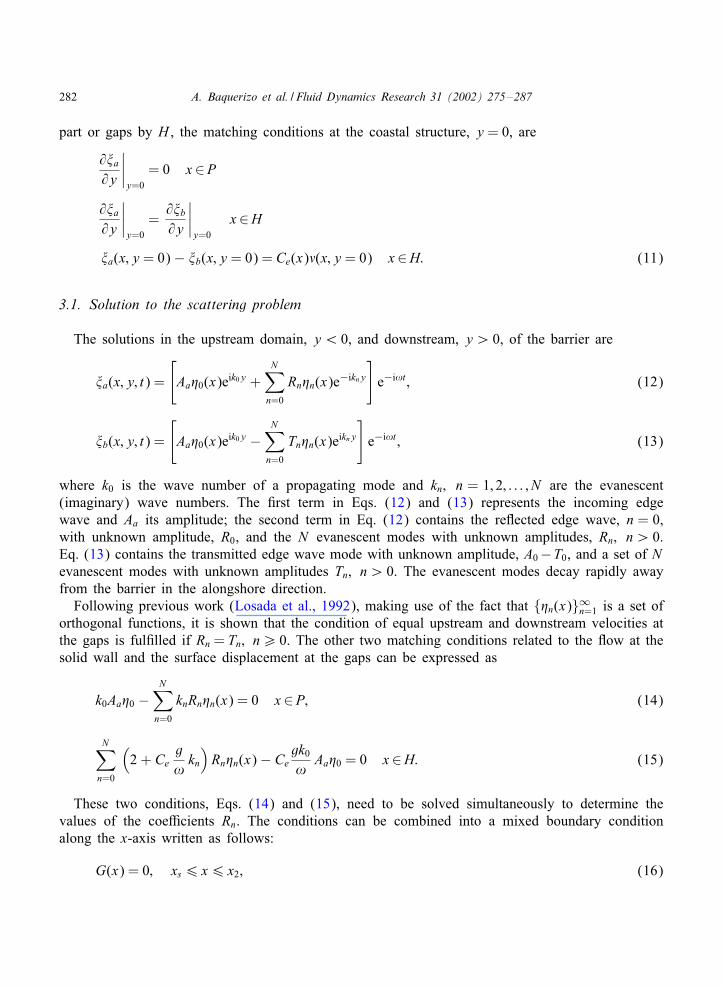
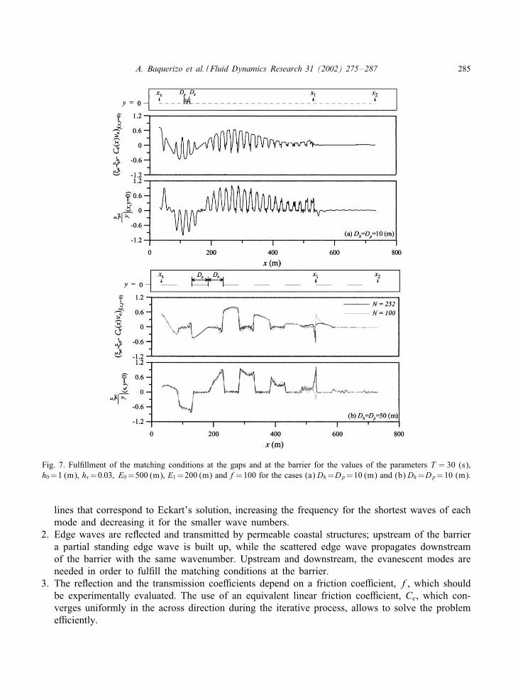
Fig. 6 shows the head loss terms functions, Cne (x); n=1; 15; 30 and 35, obtained during the iterativeprocess for the zero edge wave mode. It can be appreciated that the functions Cne (x); n= 1; 2; 3; : : :converge moderately fast to Ce(x). In Fig. 7(a) and (b), the time independent factor of the functionsg1(x) = @�a=@y|y=0 and g2(x) = �a(x; y = 0) − �b(x; y = 0) − Ce(x)#(x; y = 0) are plotted againstthe distance to the shoreline. The function g1(x), proportional to the alongshore component of thevelocity at y = 0, varies from almost negligible values at the barriers to non-zero values at thegaps. The ful6llment of the matching condition at the gaps, represented by g2(x), is also quite good.Both conditions are best ful6lled on the shelf where the matching results in a conventional series

284 A. Baquerizo et al. / Fluid Dynamics Research 31 (2002) 275–287

Fig. 6. Convergence of the head loss term for the values of the parameters T = 30 (s), h0 = 1 (m), hx = 0:03; E0 = 500(m), E1 = 200 (m), Dh = Dp = 10 (m), and f = 100.

of sines and cosines. For a barrier con6guration with Dh=Dp=50 (m), the match is even better andneeds a smaller number of evanescent modes, see Fig. 7(b) where N =100 and N =252 have beentried.

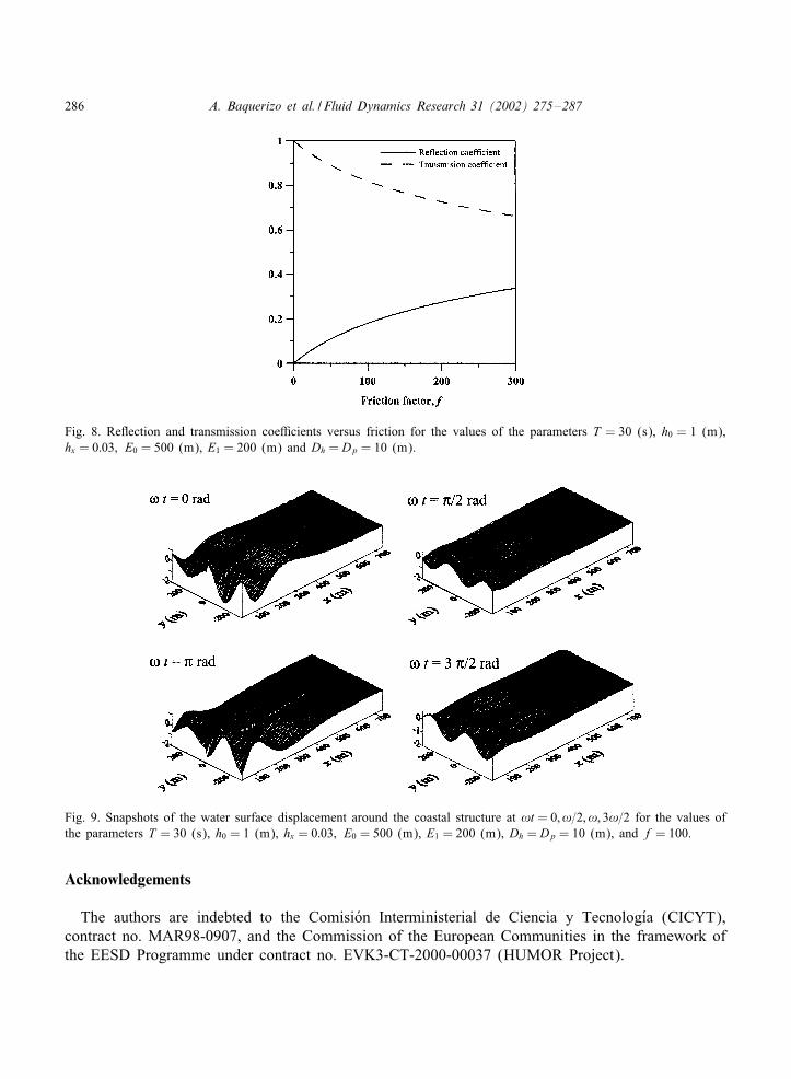
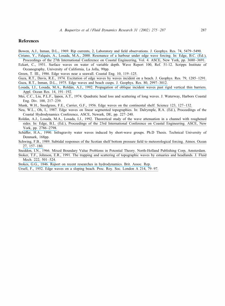
Fig. 8 shows the re7ection and transmission coe=cients versus the friction coe=cient, f, at thegaps for a zero mode edge wave. Increasing f, the re7ection coe=cient, R= R0=Aa increases whiledecreasing the transmission at the structure given by T=1−R0=Aa. Fig. 9 is a sequence of snapshotsof the water surface displacement around the coastal structure at !t=0; &=2; &; 3&=2. Upstream ofthe barrier, the oscillation is built up by the interference of the incident and re7ected edge waves;the transmitted edge wave propagates downstream of the barrier.

5. Conclusions

The scattering of an edge wave propagating on an in6nitely long, straight coastline with a steepforeshore and a shelf, impinging on a permeable coastal structure, like a groin or a jetty, is con-sidered. On the sloping region, the edge wave solution is written in terms of the Kummer’s func-tions and matched with the exponential solution on the shelf. A mode matching method includingthe head loss at the gaps is used. After de6ning an equivalent friction coe=cient, the solutionis obtained by an iterative approximation. From this research the following conclusions may bedrawn:

1. The presence of the shelf produces a curvature and a cut-oB of the dispersion curves (a; 2k0x1),restricting the possible modes to the region �¿ 0 and lowering the frequencies for the longestwaves of each mode. The presence of the steep foreshore moves oB the curves from the vertical

A. Baquerizo et al. / Fluid Dynamics Research 31 (2002) 275–287 285

Fig. 7. Ful6llment of the matching conditions at the gaps and at the barrier for the values of the parameters T = 30 (s),h0 =1 (m), hx=0:03; E0 =500 (m), E1 =200 (m) and f=100 for the cases (a)Dh=Dp=10 (m) and (b)Dh=Dp=10 (m).

lines that correspond to Eckart’s solution, increasing the frequency for the shortest waves of eachmode and decreasing it for the smaller wave numbers.

2. Edge waves are re7ected and transmitted by permeable coastal structures; upstream of the barriera partial standing edge wave is built up, while the scattered edge wave propagates downstreamof the barrier with the same wavenumber. Upstream and downstream, the evanescent modes areneeded in order to ful6ll the matching conditions at the barrier.

3. The re7ection and the transmission coe=cients depend on a friction coe=cient, f, which shouldbe experimentally evaluated. The use of an equivalent linear friction coe=cient, Ce, which con-verges uniformly in the across direction during the iterative process, allows to solve the probleme=ciently.

286 A. Baquerizo et al. / Fluid Dynamics Research 31 (2002) 275–287

Fig. 8. Re7ection and transmission coe=cients versus friction for the values of the parameters T = 30 (s), h0 = 1 (m),hx = 0:03; E0 = 500 (m), E1 = 200 (m) and Dh = Dp = 10 (m).

Fig. 9. Snapshots of the water surface displacement around the coastal structure at !t = 0; !=2; !; 3!=2 for the values ofthe parameters T = 30 (s), h0 = 1 (m), hx = 0:03; E0 = 500 (m), E1 = 200 (m), Dh = Dp = 10 (m), and f = 100.

Acknowledgements

The authors are indebted to the ComisiNon Interministerial de Ciencia y TecnologNQa (CICYT),contract no. MAR98-0907, and the Commission of the European Communities in the framework ofthe EESD Programme under contract no. EVK3-CT-2000-00037 (HUMOR Project).

A. Baquerizo et al. / Fluid Dynamics Research 31 (2002) 275–287 287

References

Bowen, A.J., Inman, D.L., 1969. Rip currents, 2, Laboratory and 6eld observations. J. Geophys. Res. 74, 5479–5490.Ciriano, Y., FalquNes, A., Losada, M.A., 2000. Resonance of a harbour under edge wave forcing. In: Edge, B.C. (Ed.),

Proceedings of the 27th International Conference on Coastal Engineering, Vol. 4. ASCE, New York, pp. 3680–3691.Eckart, C., 1951. Surface waves on water of variable depth. Wave Report 100, Ref. 51-12. Scripps Institute of

Oceanography, University of California, La Jolla, 99pp.Green, T. III., 1986. Edge waves near a seawall. Coastal Eng. 10, 119–125.Guza, R.T., Davis, R.E., 1974. Excitation of edge waves by waves incident on a beach. J. Geophys. Res. 79, 1285–1291.Guza, R.T., Inman, D.L., 1975. Edge waves and beach cusps. J. Geophys. Res. 80, 2997–3012.Losada, I.J., Losada, M.A., RoldNan, A.J., 1992. Propagation of oblique incident waves past rigid vertical thin barriers.

Appl. Ocean Res. 14, 191–192.Mei, C.C., Liu, P.L.F., Ippen, A.T., 1974. Quadratic head loss and scattering of long waves. J. Waterway, Harbors Coastal

Eng. Div. 100, 217–239.Munk, W.H., Snodgrass, F.E., Carrier, G.F., 1956. Edge waves on the continental shelf. Science 123, 127–132.Neu, W.L., Oh, I., 1987. Edge waves on linear segmented topographies. In: Dalrymple, R.A. (Ed.), Proceedings of the

Coastal Hydrodynamics Conference, ASCE, Newark, DE, pp. 227–240.RoldNan, A.J., Losada, M.A., Losada, I.J., 1992. Theoretical study of the wave attenuation in a channel with roughened

sides. In: Edge, B.L. (Ed.), Proceedings of the 23rd International Conference on Coastal Engineering. ASCE, NewYork, pp. 2786–2798.

SchEaBer, H.A., 1990. Infragravity water waves induced by short-wave groups. Ph.D Thesis. Technical University ofDenmark, 168pp.

Schwing, F.B., 1989. Subtidal responses of the Scotian shelf bottom pressure 6eld to meteorological forcing. Atmos. Ocean27, 157–180.

Sneddon, I.N., 1966. Mixed Boundary Value Problems in Potential Theory. North-Holland Publishing Corp, Amsterdam.Stoker, T.F., Johnson, E.R., 1991. The trapping and scattering of topographic waves by estuaries and headlands. J. Fluid

Mech. 222, 501–524.Stokes, G.G., 1846. Report on recent researches in hydrodynamics. Brit. Assoc. Rep.Ursell, F., 1952. Edge waves on a sloping beach. Proc. Roy. Soc. London A 214, 79–97.