Edge and corner identification for tracking the line of sight

Ingenierıa y Ciencia, ISSN 1794-9165

Volumen 1, numero 2, paginas 5-23, septiembre de 2005

Edge and corner identification for tracking

the line of sight

Ursula Kretschmer1, Marıa S. Orozco2,Oscar E. Ruiz3 and Uwe Jasnoch4

Recepcion: 21 de mayo de 2004 — Aceptacion: 30 de julio de 2004

Se aceptan comentarios y/o discusiones al artıculo

Resumen

Este artıculo presenta un detector de aristas y esquinas, implementado en el dominio delproyecto GEIST (un Sistema de Informacion Turıstica Asistido por Computador) para ex-traer la informacion de aristas rectas y sus intersecciones (esquinas en la imagen) a partirde imagenes de camara (del mundo real) contrastadas con imagenes generadas por compu-tador (de la Base de Datos de Monumentos Historicos a partir de posicion y orientacionde un observador virtual). Las imagenes de la camara y las generadas por computador sonprocesadas para reducir detalle, hallar el esqueleto de la imagen y detectar aristas y esqui-nas. Las esquinas sobrevivientes del proceso de deteccion y hallazgo del esqueleto de lasimagenes son tratados como puntos referentes y alimentados a un algoritmo de puesta encorrespondencia, el cual estima los errores de muestreo que usualmente contaminan los da-tos de GPS y orientacion (alimentados al generador de imagenes por computador). De estamanera, un ciclo de control de lazo cerrado se implementa, por medio del cual el sistemaconverge a la determinacion exacta de posicion y orientacion de un observador atravesandoun escenario historico (en este caso, la ciudad de Heidelberg). Con esta posicion y orienta-cion exactas, en el proyecto GEIST otros modulos son capaces de proyectar re-creacioneshistoricas en el campo de vision del observador, las cuales tienen el escenario exacto (laimagen real vista por el observador). Ası, el turista “ve” las escenas desarrollandose ensitios historicos materiales y reales de la ciudad. Para ello, este artıculo presenta la modi-ficacion y articulacion de algoritmos tales como el Canny Edge Detector, “SUSAN Cornerdetector”, filtros 1- y 2-dimensionales, etcetera.

Palabras claves: metodos de sintetizacion de imagenes, vision por computador,deteccionde aristas, deteccion de esquinas.

AbstractThis article presents an edge-corner detector, implemented in the realm of the GEIST

1 Diplomada ingeniera, [email protected], investigadora, Fraunhofer Institute forComputer Graphics, Abteilung 5 (Geographic Information Systems).2 Ingeniera de Sistemas, [email protected], investigadora, Grupo I+D=I Enxeneria e Desenho Univer-sidade de Vigo.3 Doctor en ingenierıa, [email protected], associate professor, EAFIT University.4 Doctor en ingenierıa, [email protected], marketing director, GIStec.

Universidad EAFIT 5|

mailto:[email protected]

http://www.igd.fhg.de/

http://www.igd.fhg.de/


http://www.uvigo.es

http://www.uvigo.es


http://www.eafit.edu.co


http://www.gistec-online.de/splash/index.html

Edge and corner identification for tracking the line of sight

project (an Computer Aided Touristic Information System) to extract the information ofstraight edges and their intersections (image corners) from camera-captured (real world)and computer-generated images (from the database of Historical Monuments, using ob-server position and orientation data). Camera and computer-generated images are processedfor reduction of detail, skeletonization and corner-edge detection. The corners surviving thedetection and skeletonization process from both images are treated as landmarks and fedto a matching algorithm, which estimates the sampling errors which usually contaminateGPS and pose tracking data (fed to the computer-image generatator). In this manner, aclosed loop control is implemented, by which the system converges to exact determinationof position and orientation of an observer traversing a historical scenario (in this case thecity of Heidelberg). With this exact position and orientation, in the GEIST project othermodules are able to project history tales on the view field of the observer, which have theexact intended scenario (the real image seen by the observer). In this way, the tourist “sees”tales developing in actual, material historical sites of the city. To achieve these goals thisarticle presents the modification and articulation of algorithms such as the Canny EdgeDetector, SUSAN Corner Detector, 1-D and 2-D filters, etcetera.

Key words: image synthesis techniques, computer vision, edge detection, feature detec-

tion.

1 Introduction

1.1 Goal of this work

The goal of this work is the extraction of edges and cornes from an image. In general,corner identification is successful only if a high level of detail is allowed by filtering stages.However, this level of detail is undesirable because of data size considerations. On theother hand, if the level of detail is reduced, only important landmarks survive (whichnaturally reduces the data size) but the cornes are lost. In this work, the second strategywas adopted, and complemented with a post-processing which infers the corners from thesurviving landmarks (edges).

1.2 Context

The GEIST project1 [1] is an educational game that aims to transmit historical factsboth to youngsters and adults by means of Augmented Reality (AR). The aim of thegame is by means of AR the player is immersed in ancient times: the times of the thirtyyears war in Heidelberg.

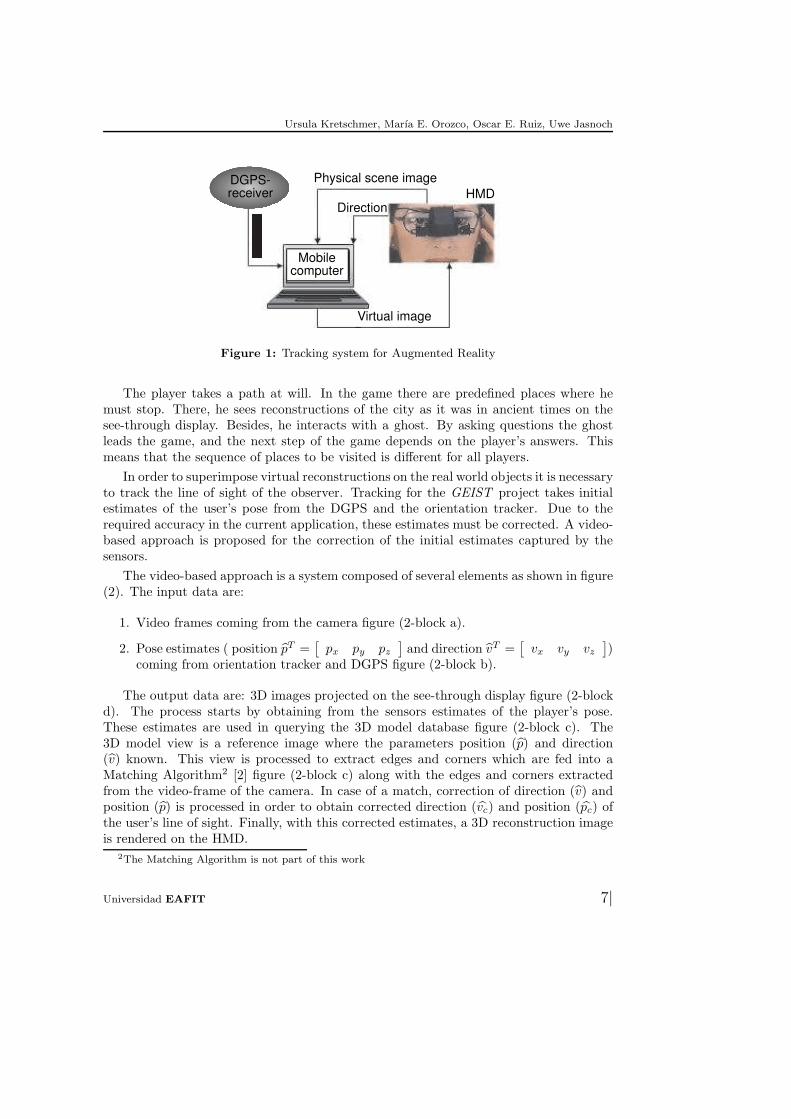
AR requires devices such as a mobile computer, sensors (Differential Global Position-ing System (DGPS) and orientation tracker), a see-through display and a video camera asshown in figure (1). These devices are used as a system for displaying three dimensional(3D) images in the player’s line of sight. Such images are superimposed on real worldobjects seen by the observer through the display. For a correct superposition of virtualand real images a video-based approach is pursued.

1The term geist is the German expression for the English word ghost

|6 Ingenierıa y Ciencia, volumen 1, numero 2

Ursula Kretschmer, Marıa E. Orozco, Oscar E. Ruiz, Uwe Jasnoch

Physical scene image

DirectionHMD

Virtual image

Mobilecomputer

DGPS-receiver

Figure 1: Tracking system for Augmented Reality

The player takes a path at will. In the game there are predefined places where hemust stop. There, he sees reconstructions of the city as it was in ancient times on thesee-through display. Besides, he interacts with a ghost. By asking questions the ghostleads the game, and the next step of the game depends on the player’s answers. Thismeans that the sequence of places to be visited is different for all players.

In order to superimpose virtual reconstructions on the real world objects it is necessaryto track the line of sight of the observer. Tracking for the GEIST project takes initialestimates of the user’s pose from the DGPS and the orientation tracker. Due to therequired accuracy in the current application, these estimates must be corrected. A video-based approach is proposed for the correction of the initial estimates captured by thesensors.

The video-based approach is a system composed of several elements as shown in figure(2). The input data are:

1. Video frames coming from the camera figure (2-block a).

2. Pose estimates ( position pT =[

px py pz

]and direction vT =

[vx vy vz

])

coming from orientation tracker and DGPS figure (2-block b).

The output data are: 3D images projected on the see-through display figure (2-blockd). The process starts by obtaining from the sensors estimates of the player’s pose.These estimates are used in querying the 3D model database figure (2-block c). The3D model view is a reference image where the parameters position (p) and direction(v) known. This view is processed to extract edges and corners which are fed into aMatching Algorithm2 [2] figure (2-block c) along with the edges and corners extractedfrom the video-frame of the camera. In case of a match, correction of direction (v) andposition (p) is processed in order to obtain corrected direction (vc) and position (pc) ofthe user’s line of sight. Finally, with this corrected estimates, a 3D reconstruction imageis rendered on the HMD.

2The Matching Algorithm is not part of this work



Figure 2: Block diagram of the tracking workflow of the GEIST project

2 State of the art

Image processing is required to transform data into analytical representation. Researchin the field of human vision has shown that edges are the features that leads to objectrecognition by the brain: “Edges characterize object boundaries and are therefore usefulfor segmentation, registration and identification of objects in scenes”[3]. Edge identifi-cation can be done by different methods: the earliest methods used small convolutionmasks to approximate the first derivative [4, 5]. The use of zero crossings of the Lapla-cian of Gaussian (LoG) was proposed by Marr and Hildreth [6]. The first derivative ofa Gaussian was proposed by Canny [7]. Directional second-derivative zero crossings wasproposed by Haralick [8]. Morphology was proposed by Noble [9]. Venkatesch [10] uses“local energy” in the frequency domain to find edges.

Corners as well as edges are required for a full image description. In real time ap-plications, such as the current one, corners are basic in object identification from frameto frame. Methods using binary edge maps to find corners have been suggested, asin [11, 12]. The edges are detected and then edge curvature is calculated in order tofind corner locations. Beaudet [13] enhanced high curvature edges by calculating imageGaussian curvature. “Points of interest” were developed by Moravec [14]. These aredefined as occurring when there are large intensity variations in every direction. Kitchenand Rosenfeld [15] used a local quadratic fit to find corners. Their work included meth-ods based on change of direction along the edge, angle between most similar neighbors,turning of the fitted surface and gradient magnitude of gradient direction. Harris and



Stephens [16] described what has become know as the Plessey feature point detector.This is built on similar ideas to the Moravec interest operator, but the measurementof local autocorrelation is estimated from first order image derivatives. Rangarajan etal. [17] proposed a detector which tries to find an analytical expression for an optimalfunction whose convolution with the windows of an image has significant values at cornerpoints. Arrebola et al. introduced different corner detectors based on local [18] andcircular [19] histogram contour chain code. Quddus and Fahmy [20] presented a wavelet-based scheme for detection of corners on 2D planar curves. Zheng et al. [21] proposedgradient-direction corner detector that was developed from the popular Plessey cornerdetector. Smith and Brady [22] proposed the Smallest Univalue Segment AssimilatingNucleus (SUSAN) corner detector: given a circular mask delimiting a circular region ofthe image, the Univalue Segment Assimilating Nucleus (USAN) area is the area of thecircular mask made up of pixels similar in intensity to the intensity of the central pixel(nucleus) of the mask. In a digital image, the USAN area reaches a minimum when thenucleus lies at a corner point. SUSAN is not sensitive to noise and is very fast for itonly uses very simple operations. The SUSAN corner detector was chosen in this workbecause it detects corners at more than 2 adjacent regions, say junctions. Besides, it hasa characteristic that makes it very attractive: no image derivatives are used, hence nonoise reduction is needed.

3 Methodology

The Canny edge detector was already developed for the GEIST project. It had 2 de-ficiencies: (i) resultant edges were fragmented in little pieces, and (ii) corners were notdetected. In the beginning a corner detector was developed to overcome the second.Though corner data improved, the large amount of fragmented edges remained as aproblem. Therefore, the matching algorithm that processed the edges and corners wastoo slow or did not give any results at all. It was decided to build the Canny edge detec-tor at new. In this section it is explained the methodology followed in the developmentof the edge-corner detectors.

3.1 Identification of edges in pixel domain

It is the process of locating pixels corresponding to edges in a given image. This processuses the Canny edge detector [7].

The identification of edges in pixel domain process is composed of four steps as shownin figure (3). The first step, the Gaussian Convolution (see definitions 3 and 9) aims atnoise reduction and fine detail elimination. The First Derivative Convolution (definitions7 and 8) step finds the big changes in the image intensity function. The Non-maximaSuppression step reduces edges to a single pixel width (or “path”, see definition 4).The Hysteresis Thresholding step eliminates weak edges. As a result, edges in rasterrepresentation are obtained.



Figure 3: Block diagram of Identification of Edges in Pixel Domain

3.2 Vectorized edge synthesis

Consists on the transformation from a data structure, in the present case “raster” intovector representation. This process uses the Douglas-Peucker algorithm [23]. The amountof data that describes an edge based image is reduced by this process. Edges are trans-formed into straight segments as shown in figure (4). Two steps are followed in thisprocess as explained below.

1. Generalized edges construction. The arrangement of lists of pixels related by 8-neighborhood (see definition 2) among them. Besides, pixels in such lists mustcomply with the Generalized Edge definition (see definition 5).

2. Vectorized edge synthesis. The straight edges are constructed in this step, basedon the edge pixels of an E() list constructed in the previous step. The process is



(a) Rough Approxima-tion between v1 and v2

(b) Creation of astraight edge betweenv2 and v3

(c) Creation of astraight edge betweenv3 and v5

(d) Creation of astraight edge betweenv5 and v1

Figure 4: Approximation by straight lines

shown in figure (4). It can be seen how a raster represented edge is transformed tovectorial representation. Initial data is a matrix of n×n pixels, this data is reducedto three vectors represented by three pairs of points, i.e. (v1, v5), (v3, v5), (v3, v2).It can be seen how the amount of data is siginificantly reduced.

3.3 Direct corner extraction from images

It is the identification of corners directly from an image. The corner detector implementedis the SUSAN algorithm proposed by Smith and Brady [22].

A circular area is delimited around a central pixel -called the nucleus (v0). Theprocedure consists on deciding whether or not the nucleus is a corner. Four steps composethis algorithm as shown in figure (5).



Figure 5: Block diagram of Direct Corner Extraction from a given Image

1. Univalue Segment Assimilating Nucleus (USAN) area calculation. The USAN areais the area of the circular mask made up of pixels similar in intensity to the intensityof the nucleus (v0) of the mask.

Pixels whose intensity value is similar to the nucleus of the circular mask are foundand counted in this step. The delta intensity function (see definition 12) appliesthe intensity difference threshold ∆It (see definition 11) to the pixels of the maskin order to find the USAN area.

2. Corner response calculation. The corner response R(v0) (see definition 14) is thecapacity of the nucleus to be considered a corner. It is calculated based on thegeometrical threshold gt (see definition 13) and the size of the USAN area. Largervalues mean grater possibility for the nucleus to be considered a corner.

3. False positives elimination. False positives are points wrongly reported as corners.Cases like noise, lines across the circular mask may be reported as corners. Hencethe aim of the false positives elimination is to detect and eliminate such points.

4. Non-maxima suppression. This step finds a maximum value of corner response in asubwindow of 5 x 5 pixels. Once the previous three steps are finished for all pixelsof the image, the non-maxima suppression is applied to the set of pixels representedby their corner response.

The subwindow is placed on each pixel and is moved from left to right and fromtop to bottom of the corner response array. A maximum value is found for thesubwindow. In case that more than one maxima value were found in the subwindow,the current pixel (the subwindow central pixel) is suppressed i.e. its corner responseis turned to zero.



3.4 Edge-corner alignment

This process aims at putting together the detected corners and edges. The guidingprinciple is the relationship of collinearity between an edge and its neighboring corners.The parametric equation of the line [24, page 118] was used in this step.

In order to find a collinear corner, the distance between the corner and each of thevertices of the current edge must be calculated. This step helps to ensure that neighboringcorners are chosen for the edge-corner alignment. In case a corner is along the samestraight line of an edge, then the edge is extended to meet the corner.

The same procedure must be repeated for all edges obtained in the vectorized edgesynthesis.

3.5 Indirect corner extraction

The results obtained in the edge-corner alignment process were insufficient, because manypairs of edges remained without a common corner after a lengthy edge-corner alignmentprocess. Therefore, an alternative algorithm was developed, using indirect corner calcu-lation based on the existent edges. Its description follows:

Indirect corner calculation. Corners are calculated by finding the intersection point(pi()) between two non-parallel edges. For a given pair of edges to be related through acommon corner they must be closer than a user defined threshold. The threshold is aninteger number in the range of [0 - 10]. Two edges being far away from each other arenot sought to be related by a corner. The calculation of the intersection point (pixel)follows:

Intersection point pi (e1, e2). The intersection point is the pixel where two edges (e())meet. Let two edges be: e1 ((x1, y1) , (x2, y2)) and e2 ((x3, y3) , (x4, y4)). The parametert of the intersection point is [24, page 113]:

t =(x4 − x3)(y1 − y3) − (y4 − y3)(x1 − x3)

(y4 − y3)(x2 − x1) − (x4 − x3)(y2 − y1).

And so, the intersection point is defined as :

x = x1 + t(x2 − x1) ,

y = y1 + t(y2 − y1) .

In addition to the indirect corner calculation, 1-D filters were used to improve the timeresponse in the process of identification of edges in pixel domain (see definition 15).

4 Results

The results of the implemented algorithms is discussed in this section. They are basedon the photo of one of the buildings of the University of Heidelberg as shown in figure(6).



Figure 6: Original image

This section is composed of 3 cases of study:

1. Edge Vectorization (EV).

2. Edge Vectorization and Direct Corner Extraction (DCE).

3. Edge Vectorization and Indirect Corner Extraction (ICE).

Parameter values for these cases of study are described in table (1).

Table 1: Parametrization values for the experiments

σ T1 T2 st filter ∆It gt dist Process(pix.) (pix.) (pix.)

EdgeFig 6a 0,0 250 200 2 2D - - - Vect.

EdgeFig 6b 0,0 80 60 2 1D - - - Vect.

EdgeFig 6c 2,0 400 300 2 2D - - - Vect.

EdgeFig 6d 2,0 100 80 2 1D - - - Vect.

Dir. CornerFig 7b - - - - - 20 25 - Calc.

Dir. CornerFig 7c 2,0 400 300 2 2D 20 25 - and Edge Vect.

Ind. Corner Calc.Fig 8b 2,0 400 300 2 2D - - 7 and Edge Vect.

The EV case consists on edge detection based on 1D and 2D filters. Results of thisprocesses are seen in figure (7). The figure shows the contrast in the use of 2D filtersvs 1D filters for edge detection and how different levels of smoothing (σ = 0,0 and σ

= 2,0) affect the resulting edges. It can be seen in figure (7-d) that edge detection



based on 1D filters is best at keeping corners, but too much fine detail is present in finaledges. Conversely, edges obtained by the application of 2D filters have less fine detail,but corners are lost in the process of smoothing.

(a) Edge vectorization based on 2D filters.No gaussian convolution was applied to im-age (σ = 0)

(b) Edge vectorization based on 1D filters.No gaussian convolution was applied to im-age (σ = 0)

(c) Edge vectorization based on 2D filters.Gaussian convolution with σ = 2.0

(d) Edge vectorization based on 1D filters.Gaussian convolution with σ = 2.0

Figure 7: Edge Vectorization (EV) with varying filters. No corner generation applied

Results shown in figure (7-c) are the edges that best fit the needs of this work, becausethey characterize the important features of the original building and they are free of finedetail. Therefore these have been used as input for the remaining two cases of study, i.e.DCE an ICE. Quantitative results of the EV process shown in table (2) are also takenfrom figure (7-c).

Table 2: Quantitative results for the cases of study

False False Goodpositives (%) negatives (%) localization (%)

Edges EV (fig 7c) 8,33 21 79Corners DCE (fig 8c) 1,30 71 29Corners ICE (fig 9) 1,30 40 60

Figure (8) shows results of the DCE case. In this case two additional processes areimplemented: Corner extraction and edge-corner alignment. In (8-a) the edges conveythe most important information of the building, i.e. the straight lines. The missing



corners of this figure are going to be obtained by aligning the corners found in (8-b) tothe edges. Figure (8-c) shows results of the Edge-corner Alignment process. It can beseen that even though many edges appear joined by a common corner there are still manymissing corners. In order to improve the results the following method was implemented.

(a) Edge vectorization

(b) Direct corner extraction

(c) Edge-corner alignment from datashown in (8a) and (8b)

Figure 8: Edge-corner Generation process using the Direct Corner Extraction algorithm (DCE)

Localization is one of the parameters to measure good quality in feature detectors.Good localization means that the reported corner or edge position is as close as possibleto the correct position [22, page 5]. Results of the ICE case figure (9) are superimposedon original image as shown in figure (10). Note the good localization of edges and corners.In table (2) results of the detection show that 79% of the edges were localized correctly,60% of the reported corners have good localization in the ICE case, whereas 29% of thecorners have good localization in the DCE case.

Figure 9: Edge-corner generation process using Indirect Corner Extraction algorithm (ICE)



Figure 10: Original image with superimposed edges and calculated corners

Another parameter that measures quality in feature detectors is good detection. Gooddetection is measured by the number of false negatives and false positives reported [22,page 4]. The arrows on the left side of figure (10) are pointing to two cases of falsepositives. These are edges that are incorrect and should not have been reported. Thepercentage of false positives for all cases of study is low. For edges 8, 33% and for corners1, 30%. False negatives are features that should have been reported. Elimination of finedetail causes false negatives. False negatives in the EV case is 21%, corner false negativesin the DCE case is 71%, whereas corner false negatives for DCE is 40%.

5 Discussion and conclusions

This article has addressed the detection of straight edges and corners present in archi-tectural images. Applications are discussed in the sub-sequent matching of computer-generated vs. camera sampled pictures of historical buildings for Computer AssistedTourist Information Systems (specifically, the GEIST project).

1. In this work the straight lines are defined as principal features because they con-vey the most important information about urban buildings. Directional derivativefilters were used in order to maximize the detection of straight lines in the originalimage. Besides the use of Gaussian convolution favored the fine detail absence fromfinal edges.

2. The smoothing achieved by the gaussian convolution gives as a result the lost offine detail, noise and corners. Even though the first two are good consequences,the lack of corners is an undesired consequence, because corners are indispensablein the workflow in order to obtain the user’s pose. This situation gave rise to theneed to implement an additional process: the corner generation.



3. Two methods of corner generation were developed: DCE and ICE. The methodICE improved the amount of edges joined by a common corner respect to the DCEalgorithm. Time response was also improved by corner generation based on ICE.

Advantages of ICE:

(a) More efficient.

(b) More edges related to a common corner.

Disadvantages of ICE:

(a) Localization of corners may not be correct. Two neighboring edges should notbe joined through a corner. But, because of their proximity, the algorithmdoes join them. Therefore a false positive is obtained.

(b) In the presence of fine detail, results of ICE are very poor. Edges becomemisshaped after applying the corner generation process.

4. The results of the corner generation processes may be improved by finding a directlyextracted corner (DCE) in the neighborhood of an indirectly calculated corner(ICE).

5. Results of this work show that a video based approach for the Detection of theLine of Sight problem is feasible. The processes implemented in this work extractprincipal features from video images. Through these features it is possible thecalculation of the line of sight in a unexpensive and accurate way.

5.1 Future work

Continuation of this work is possible in several ways: (i) to produce, from the urbanisticdata base for a particular landmark, not raster images but vectorized information. Inthis way, the raster image of the tourist camera would be matched against a vectorizedimage, therefore improving the efficiency of the process. (ii) once a landmark has beenidentified as visited by the tourist, and the positions and trajectory of his/hers havebeen indentified, only neighboring landmarks need to be displayed and searched through.Remote ones are not accessible to the viewer, as a non-continuous trajectory would berequired to approach them. (iii) curved lines are to be identified, for the case in whicharchitectural landmarks present circular or elliptical features.

A Definitions

In this section basic terms for the comprehension of this article are detailed.



1. Image I()Given I : Z × Z −→ N

Domain [0, Xc] × [0, Yr], where Xc : Column pixels, usually 639; Yr : Row pixels,usually 479.Range of I( ) function is [BL, WL], where BL : Black level (usually 0); WL : Whitelevel (usually 255).

2. 8-Neighborhood of a pixel (i, j) N8 (i, j)The relationship between pairs of pixels (i, j) and (m, n) that share one or twoend-points.

N8 (i, j) = {(m, n)| (|m − i| = 1) ∨ (|n − j| = 1)} .

3. ConvolutionConvolution is a linear operation that calculates a resulting value as a linear com-bination of the neighborhood of the input pixel and a convolution mask [25, page68-69]. In equation (1) the output pixel -Final(i,j)- is calculated as a linear com-bination of the neighborhood of the input pixel -Inital(i,j)- and the coefficients ofthe two dimensional (2D) convolution filter M.

Final(i, j) = Initial(i, j) ∗ M =

+1∑

k=−1

+1∑

l=−1

Initial(i + k, j + l)M(k, l) . (1)

Final(i,j) in equation (1) is the sum of the products of pixels in the neighborhood of(i, j) and filter M . In the present work two steps apply filters, they are: Gaussianand First derivative convolution.

4. Path p (v0, vf )A path is a non-selfintersecting, unit-width sequence of vertices, starting at v0 andending at vf , made up of orthogonal or diagonal steps. No assumptions are madeon I(vi)

p (v0, vf ) = [v0, v1, ..., vf ] s.t.

(vi ∈ [0, Xc] × [0, Yr]) ∧ (D8 (vi, vi+1) ≤ 1) ∧ (|N8 (vi) | ≤ 2) .

5. Generalized edge E (v0, vf )A generalized edge between v0 and vf , E (v0, vf ), is a path p (v0, vf ) between them,built with high gradient pixels. All pixels of the path have gradient larger than T2,and at least one pixel in the path has gradient larger than T1. A generalized edgeE() does not have to be straight.Given T1, T2 ∈ N , where T1 > T2,

E (v0, vf ) = [v0, v1, ...., vf ]s.t.(p (v0, vf ))∧

(∀vi ∈ p(v0, vf ),∇I(v)v=vi> T2)∧

(∃vj ∈ p(v0, vf ),∇I(v)v=vj> T1) .



6. Straight edge (or simply, edge) e (v0, vf )An edge is an approximately straight generalized edge, in which the perpendiculardistance from each pixel to the straight segment, v0vf , joining the extremes isbounded by an ǫ value.

e (v0, vf ) = [v0, v1, ..., vf ] s.t.

E(v0, vf ) ∧ ∀vi ∈ E(v0, vf ), d (vi, v0vf ) < ǫ .

Typical values for ǫ: [0, 10].

7. Orthogonal differences, ∆iI, ∆jI

The orthogonal differences ∆iI and ∆jI approximate the first directional deriva-tives of I() in the X and Y directions respectively [25, page 80]. They are appliedon functions, and return a scalar value:∆i() : I() → R

∆j() : I() → R

calculated as:∆iI (i, j) = I (i + 1, j) − I (i − 1, j)∆jI (i, j) = I (i, j + 1) − I (i, j − 1) .Notation simplification:if v = (i, j) ⇒ ∆iI (i, j) = ∆iI(v) .

8. Gradient operator ∇I(i, j)A gradient operator is the vector formed by the directional derivatives or orthogonaldifferences (see definitions A7). The gradient operator is applied on functions, andreturns a vector:∇() : I() → R2

∇() : I() = ∇I(i, j) = (∆iI(i, j), ∆jI(i, j)).Collaterally, its direction and magnitude are defined:

(a) Gradient direction, θ(I(i, j)), is the angle (in radians) from the x axis to thepoint (i, j):

θ(I(i, j)) = arg(∇I(i, j)) = arctan(

∆jI(i,j)∆iI(i,j)

).

(b) Gradient magnitude, |∇(i, j)|, is the norm of the Gradient operator:

|∇I(i, j)| = |(∆iI(i, j), ∆jI(i, j))| =√

(∆iI (i, j))2

+ (∆jI (i, j))2.

9. Gaussian operator G∆x,∆y,σ (i, j)Gaussian operator is a function that reduces the possible number of frequencies atwhich image intensity function changes take place.G∆x,∆y,σ (i, j) : Z2 → R

G∆x,∆y,σ (i, j) =

12πσ2 e

−

“

i2+j2

2σ2

”

, if −∆x ≤ i ≤ ∆x ,

−∆y ≤ j ≤ ∆y .

0, otherwise.



Usually ∆x = ∆y = 3σ. Typical values for σ are in [0, 10].

10. Circular mask M (x, y, R)Set of pixels (usually 37) that make up the interior and boundary of a circularsubwindow of an I()[22].

M (x, y, R) ={(i, j) | (x − i)2 + (y − j)2 ≤ R2

}.

With nucleus v0 the center of the circle: v0 = (x, y).And vi any other point in the circle: vi = (i, j).

11. Intensity difference threshold ∆It

A threshold of the intensity function of an image. It is used in order to definesimilarity in intensity among the nucleus v0 and all other pixels of the circularmask M( )[22].Typical values for ∆It are in [10, 60].

12. Delta intensity function δv0,∆It(vi)

Difference in intensity between pixels vi and v0 [22].

δv0,∆It(vi) =

{1, if |I(vi) − I(v0)| ≤ ∆It .

0, otherwise.

Given an intensity difference threshold ∆It, δv0,∆It(vi) measures the similarity in

pixel intensity with respect to a reference pixel v0.

13. Geometrical threshold gt

Geometric threshold is the maximum size allowed for |USAN()|. The maximumvalue of this threshold is bounded by the size of the circular mask M(). Corner

sharpness is determined by this threshold [22].Domain[0, |M( )|]Typical values for gt: [15, 28].

14. Corner response R(v0)Corner response is a number, that determines the capacity of the nucleus (v0) tobe detected as a corner. The higher the value of R(v0) the greater the possibilityfor v0 to be a corner [22].

R(v0) =

{gt − |USAN()| if |USAN()| < gt .

0 otherwise.

15. 1D Gaussian operator G∆x,σ (i)G∆x,σ (i) : Z → R

G∆x,σ (i) =

{1

2πσ2 e−

“

i2

2σ2

”

, if −∆x ≤ i ≤ ∆x .

0, otherwise.



References

[1] D. Holweg, A. Schilling and U. Jasnoch. Mobile tourism new gis-based applicationsat the cebit fair, Computer Graphik Topics, 15(1), 17–19 (2003).

[2] P. Gros, O. Bournez and E. Bouyer. Using geometric quasi-invariants to match andmodel images of line segments, Technical Report, RR-2608, INRIA, July 1995.

[3] Anil K. Jain. Fundamentals of Digital Image Processing, Prentice Hall, 1989.

[4] J. M. S. Prewitt. Object enhancement and extraction, Picture Processing and Psy-chopictorics, Academic Press, 1970.

[5] I. Sobel. An isotropic 3 × 3 image gradient operator, Machine Vision for Three-dimensional Scenes, Academic Press, 1990.

[6] D. Marr and E. C. Hildreth. Theory of edge detection, Proc. Roy. Soc. London,B-207:187–217 (nov 1980).

[7] J.F. Canny. A computational approach to edge detection, IEEE Transactions onPattern Analysis and Machine Inteligence, 8(6), 679–698 (nov 1986).

[8] R. M. Haralick. Digital step edges from zero crossing of second directional derivatives,IEEE Transactions on Pattern Analysis and Machine Inteligence, 6(1), 58–68 (jan1984).

[9] J. A. Noble. Descriptions of Image Surfaces, PhD thesis, Robotics Research Group,Department of Engineering Science, Oxford University, 1989.

[10] S. Venkatesch. A study of Energy Based Models for the Detection and Classificationof Image Features, PhD thesis, Department of Computer Science, The University ofWestern Australia, 1990.

[11] H. Asada and M. Brady. The curvature primal sketch, IEEE Transactions on PatternAnalysis and Machine Inteligence, 8(1), 2–14 (1986).

[12] H. Freeman and L. S. Davis. A corner finding algorithm for chain code curves, IEEETransactions on Computers, 26, 297–303 (1977).

[13] P. R. Beaudet. Rotational invariant image operators, Int. Conference on PatternRecognition, 579–583 (1978).

[14] H. P. Moravec. Visual mapping by a robot rover, Joint Conference on ArtificialIntelligence, 598–600 (1979).

[15] L. Kitchen and A. Rosenfeld. Gray-level corner detection, Pattern RecognitionLetters, 1, 95–102 (1982).



[16] C. G. Harris and M. Stephens. A combined corner and edge detector, 4th AlveyVision Conference, 147–151 (1988).

[17] K. Rangarajan, M. Shah and D. V. Brackle. Optimal corner detector, ComputerVision, Graphics and Image Processing, 48, 230–245 (1989).

[18] F. Arrebola, A. Bandera, P. Camacho and F. Sandoval. Corner detection by localhistograms of contour chain code, Electronic Letters, 33(21), 1769–1771 (1997).

[19] F. Arrebola, P. Camacho, A. Bandera, and F. Sandoval. Corner detection andcurve representation by circular histograms of contour chain code, Electronic Letters,35(13), 1065–1067 (1999).

[20] A. Quddus and M. Fahmy. Fast wavelet-based corner detection technique, ElectronicLetters, 35(4), 287–288 (1999).

[21] Z. Zheng, H. Wang, and E. Teoh. Analysis of gray level corner detection, PatternRecognition Letters, 20, 149–162 (1999).

[22] S. M. SMITH and J. M. BRADY. Susan - a new approach to low level imageprocessing, International Journal of Computer Vision, 23(1), 45–78 (1997).

[23] D. Douglas and T. Peucker. Algorithms for the reduction of the number of pointsrequired to represent a digitized line or its caricature, The Canadian Cartographer,10(2), 112–122 (1973).

[24] James D. Foley, Andries van Dam, Steven K. Feiner and John F. Hughes. ComputerGraphics, Principles and Practice, Addison-Wesley Publishing Co., 2 edition, 1990.

[25] Milan Sonka, Vaclav Hlavac and Roger Boyle. Image Processing, Analysis and Ma-chine Vision, Brooks/Cole Publishing Co., Pacific Grove, 1999.


Edge and corner identification for tracking the line of sight

Documents

Transcript of Edge and corner identification for tracking the line of sight