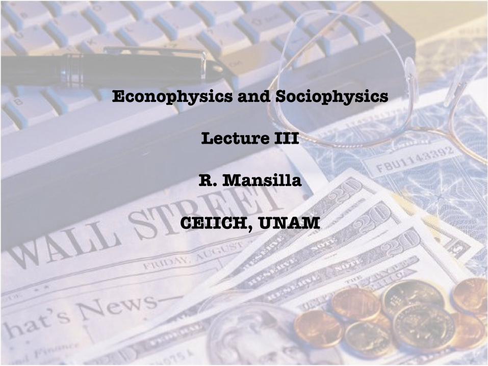
Econophysics and Sociophysics

Lecture III

R. Mansilla

CEIICH, UNAM

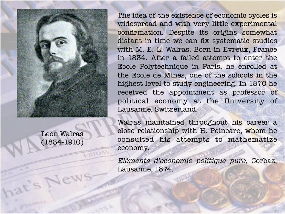
The idea of the existence of economic cycles is widespread and with very little experimental confirmation. Despite its origins somewhat distant in time we can fix systematic studies with M. E. L. Walras. Born in Evreux, France in 1834. After a failed attempt to enter the Ecole Polytechnique in Paris, he enrolled at the Ecole de Mines, one of the schools in the highest level to study engineering. In 1870 he received the appointment as professor of political economy at the University of Lausanne, Switzerland.

Walras maintained throughout his career a close relationship with H. Poincare, whom he consulted his attempts to mathematize economy.

Eléments d’economie politique pure, Corbaz, Lausanne, 1874.

Leon Walras (1834-1910)

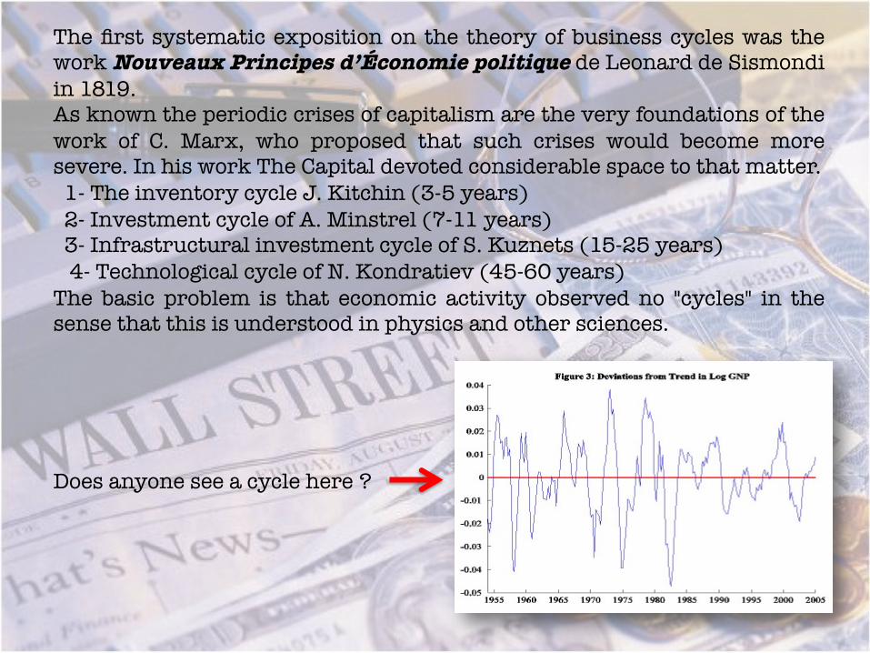
The first systematic exposition on the theory of business cycles was the work Nouveaux Principes d’Économie politique de Leonard de Sismondi in 1819. As known the periodic crises of capitalism are the very foundations of the work of C. Marx, who proposed that such crises would become more severe. In his work The Capital devoted considerable space to that matter.   1- The inventory cycle J. Kitchin (3-5 years)   2- Investment cycle of A. Minstrel (7-11 years)   3- Infrastructural investment cycle of S. Kuznets (15-25 years)    4- Technological cycle of N. Kondratiev (45-60 years) The basic problem is that economic activity observed no "cycles" in the sense that this is understood in physics and other sciences.

Does anyone see a cycle here ?

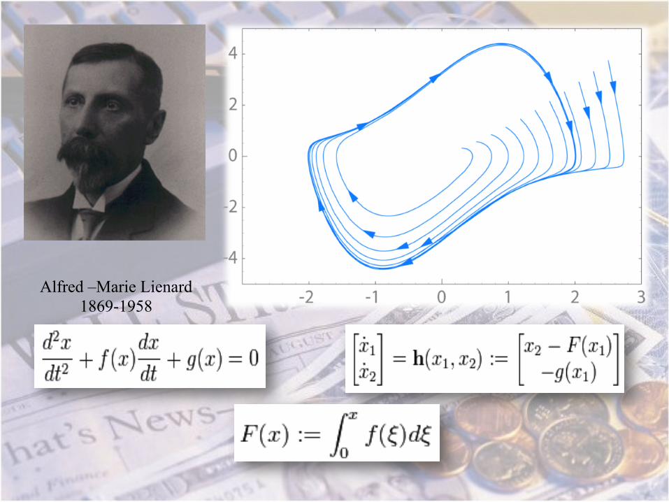
Alfred –Marie Lienard 1869-1958

There are other methods to study the financial time series. These are based on the assumption (quite reasonable) that the markets are dynamic systems from which we receive incomplete information. It is therefore very reasonable to use the methods of nonlinear time series based on the immersion theorem of F. Takens.

F. Takens, “Detecting strange attractors in turbulence”, Springer Lectures Notes in Mathematics, 898, 1981.

Otto E. Rossler, “Continuous chaos-four prototype equations”, Annals of N.Y. Academy of Sciences vol. 316, pags. 376-392, 1979.

42398.0

)(=

=

=

⎪⎪⎪

⎩

⎪⎪⎪

⎨

⎧

−+=

+=

−−=

cba

cxzbdtdz

ayxdtdy

zydtdx

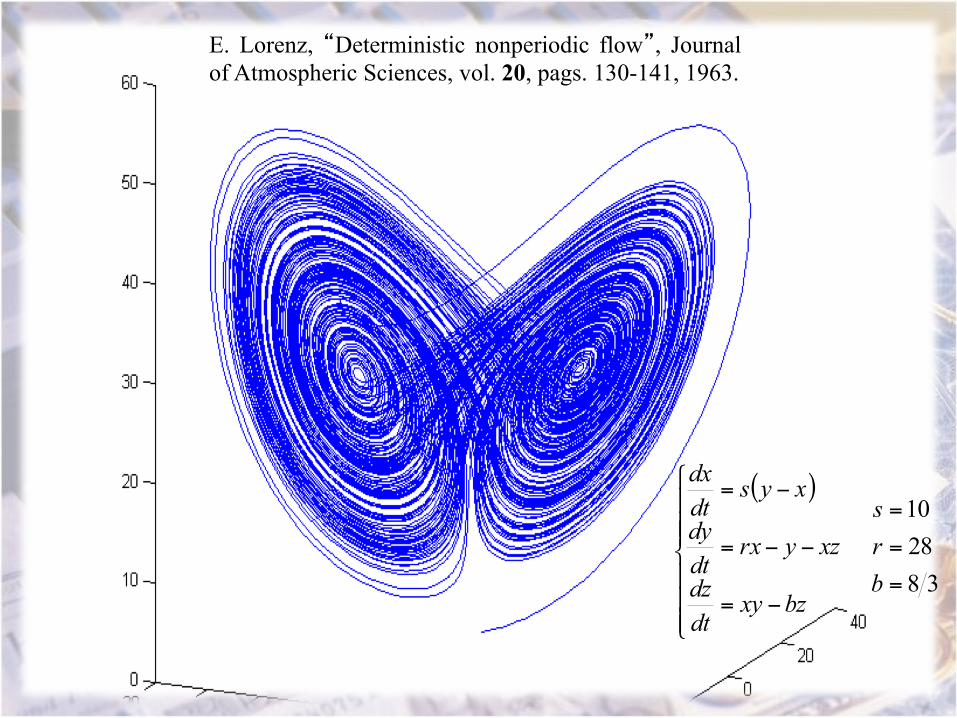
E. Lorenz, “Deterministic nonperiodic flow”, Journal of Atmospheric Sciences, vol. 20, pags. 130-141, 1963.

( )

382810

=

=

=

⎪⎪⎪

⎩

⎪⎪⎪

⎨

⎧

−=

−−=

−=

brs

bzxydtdz

xzyrxdtdy

xysdtdx

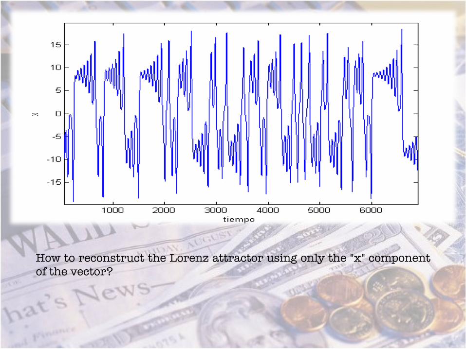
How to reconstruct the Lorenz attractor using only the "x" component of the vector?

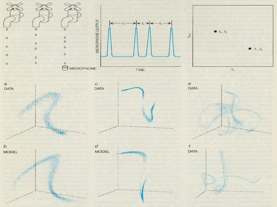
The dripping faucet problem

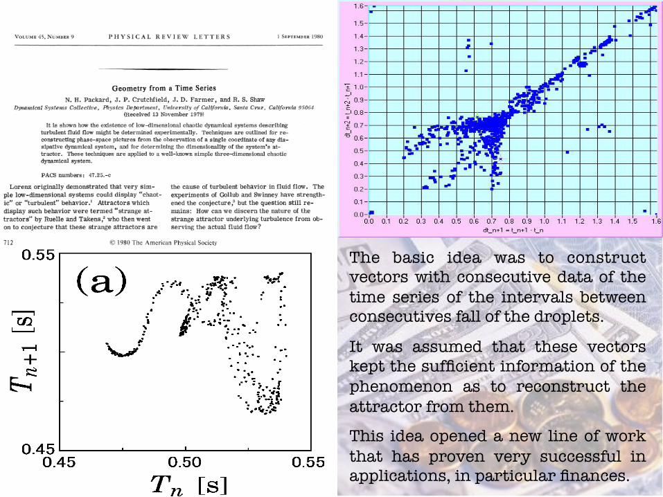
The basic idea was to construct vectors with consecutive data of the time series of the intervals between consecutives fall of the droplets.

It was assumed that these vectors kept the sufficient information of the phenomenon as to reconstruct the attractor from them.

This idea opened a new line of work that has proven very successful in applications, in particular finances.

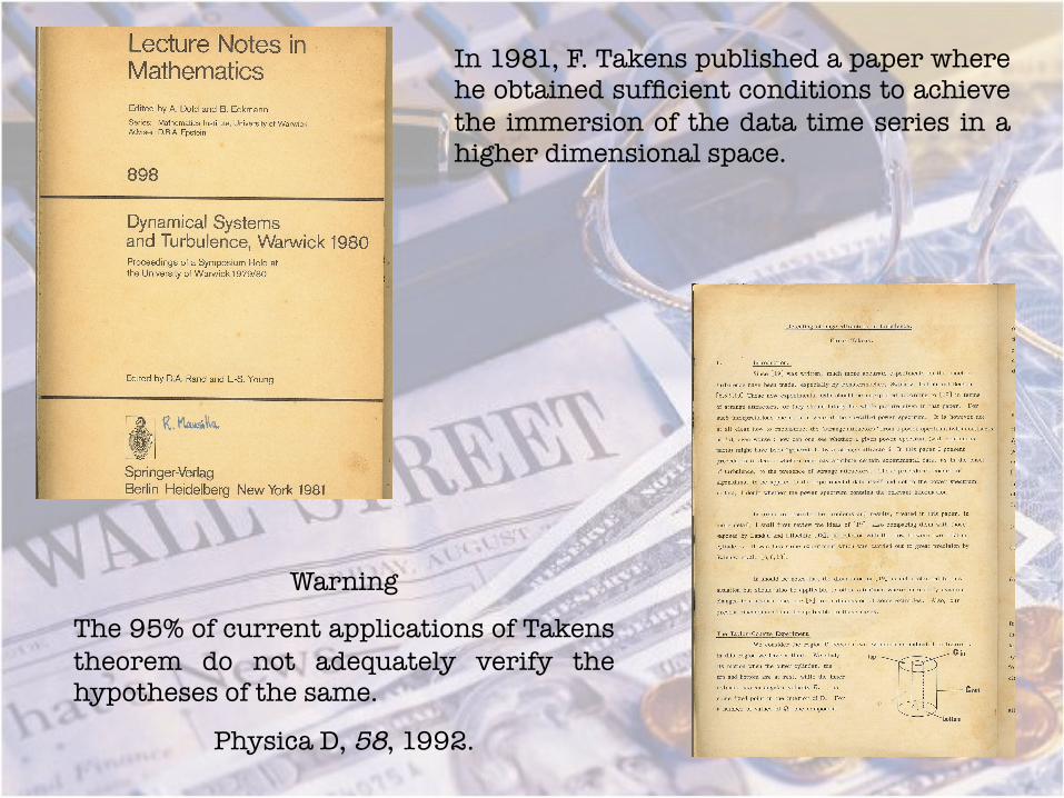
In 1981, F. Takens published a paper where he obtained sufficient conditions to achieve the immersion of the data time series in a higher dimensional space.

Warning

The 95% of current applications of Takens theorem do not adequately verify the hypotheses of the same.

Physica D, 58, 1992.

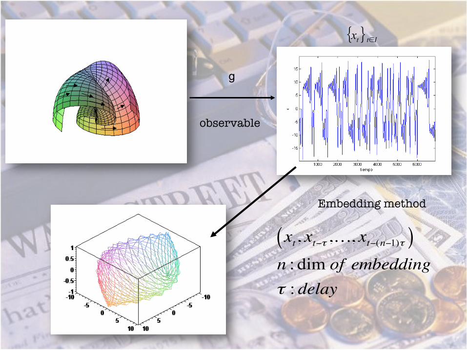
g

Embedding method

{ } Ittx ∈

xt, xt−τ ,…, xt−(n−1)τ( )n : dim of embeddingτ : delay

observable

The basic problem with the application of Takens theorem is that one postulates the existence of the parameters and ,but provides no method for calculating them.

Then we will discuss the most common procedures that are used to estimate these parameters.

There are two theoretical concepts associated with this quest, is the concept of mutual information and correlation integral.

n τ

Mutual information

The concept of mutual information was introduced by C. Shannon in 1948.

C. Shannon, “ A mathematical theory of communication”, The Bell Systems Technical Journal, vol. 27, pags. 379-423, 1948.

Let the time series

{ } { }nn yyYxxX ,,,,, 11 …… ==

Their mutual information represents the average number of bits of the series that can be predicted by measuring

( )YXI ,XY

∑∑= =

⎥⎦

⎤⎢⎣

⎡=

n

i

n

j YX

YXYX jPiP

jiPjiPYXI

1 1

,2, )()(

),(log),(),(

)(

),(,

iP

jiP

X

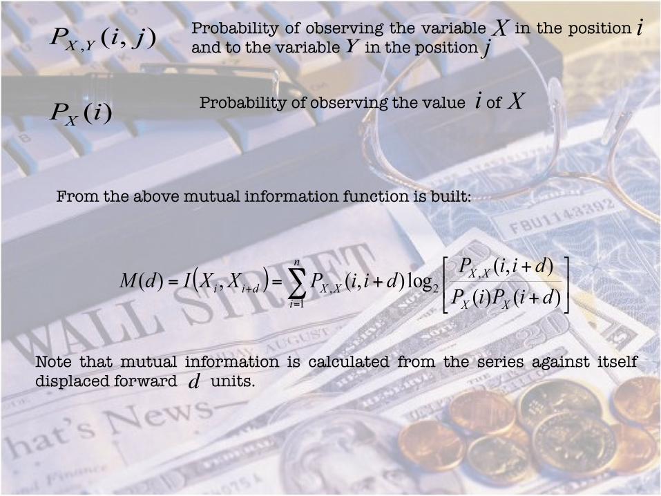
YXProbability of observing the variable in the position and to the variable in the position

X iY j

Probability of observing the value of Xi

From the above mutual information function is built:

( ) ∑=

+ ⎥⎦

⎤⎢⎣

⎡

+

++==

n

i XX

XXXXdii diPiP

diiPdiiPXXIdM

1

,2, )()(

),(log),(,)(

Note that mutual information is calculated from the series against itself displaced forward units. d

The correct value of is the first minimum of mutual information function.

A. M. Fraser, H. L. Swinney, “Independent coordinates for strange attractors from mutual information”, Physical Review A, vol. 33, pag. 1134, 1986.

C. J. Celluci, et al., “Statistical validation of mutual information calculations: comparison of alternative numerical methods”, Physical Review E, vol. 71, 066208, 2005.

M. Small, “Applied nonlinear time series analysis”, World Scientific, 2005.

τ

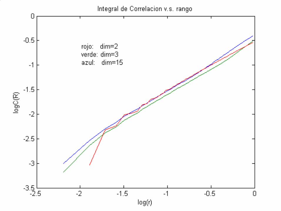
The search for the appropriate dimension

In the search for adequate emdedding dimension there are only heuristic criteria. The most used is related to the so-called correlation integral:

( )∑≤<≤

−

<−⎟⎟⎠

⎞⎜⎜⎝

⎛=

njijin XXH

nC

1

1

2)( εε

With this, the dimension of correlation is defined as:

)log()(loglimlim

0 εε

ε

nnc

Cd∞→→

=

Basically, the correlation dimension is the slope of the correlation integral at the origin.

The criterion for selecting a dimension of embedding is as follows:

"Choose increasing embedding dimensions and in each case, calculate the correlation integral. When no changes in behavior of the integral of correlation with respect to the increase of the dimension of embedding, then it will have found a suitable embedding dimension ".

M. Small, “Applied nonlinear time series analysis”, World Scientific, pag. 8, 2005.

Grassberger P., Procaccia I., Characterization of strange attractors. Physical Review Letters vol. 50, pags. 346-349, 1983.

Theiler J., Spurious dimension from correlation algorithms applied to limited time-series data. Physical Review A vol. 34 pags. 2427-2432, 1986.

Albano A. M., Muench J., Schwartz C., Mees A. I., Rapp P. E., Singular-value decomposition and the Grassberger-Procaccia algorithm, Physical Review A vol. 38: pags. 3017-3026, 1988.

Some application to finance M. Small. Applied Nonlinear Time Series Analysis: Applications in Physics, Physiology and Finance. Nonlinear Science Series A, vol. 52. World Scientific, 2005. T. Nakamura and M. Small. “Tests of the random walk hypothesis for financial data.” Physica A 377, pp. 599-615, 2007. T. Nakamura and M. Small. “Testing for dynamics in the irregular fluctuations of financial data.” Physica A 366, pp. 377-386, 2006. M. Small and C.K. Tse. “Determinism in financial time series.” Studies in Nonlinear Dynamics and Econometrics, 7, no. 3, art. 5, 2003.

FIN